effect of modified moisture barriers on slopes stabilized with

EFFECT OF MODIFIED MOISTURE BARRIERS ON SLOPES STABILIZED WITH

RECYCLED PLASTIC PINS

by

ANUJA SAPKOTA

Presented to the Faculty of the Graduate School of

The University of Texas at Arlington in Partial Fulfillment

of the Requirements

for the Degree of

DOCTOR OF PHILOSOPHY IN CIVIL ENGINEERING

THE UNIVERSITY OF TEXAS AT ARLINGTON

August 2019

ii

Copyright © by Anuja Sapkota 2019

All Rights Reserved

iii

ACKNOWLEDGMENTS

I would like to express my sincere gratitude to my supervising professor, Dr. MD.

Sahadat Hossain, for his unconditional support, encouragement, guidance, and valuable

suggestions throughout this research. This research would not have been possible without

his supervision, and I am grateful for the opportunity he has provided me.

I would also like to give my special thanks to Dr. Xinbao Yu, Dr. Nur Yazdani, and

Dr. Ashfaq Adnan for spending their valuable time serving on my Ph.D. supervising

committee, and for their valuable insights.

I also wish to acknowledge the Texas Department of Transportation for providing

the funding for this research. Special thanks to TxDOT officials Boon Thain and Dr. Nicasio

Lozano for providing their valuable time and suggestions during the study period.

I would also like to acknowledge all the SWIS members for their support and

assistance during this research. Special thanks to Dr. Asif Ahmed for his continuous

encouragement, support, and assistance during this research. I am also very thankful to

Pratibha, Sachini, Dola, Prabesh, Cory, and Maddie for their constant help during the field

monitoring work. Thanks also to fellow lab mates Rakib Ahmed, Dr. Naima Rahman, Dr.

Jobair Bin Alam, and Dr. Nur Basit Zaman.

Last but not least, I would like to extend my deepest gratitude to my family: my

parents and my brothers for constant encouragement and my life in general. Finally, I wish

to acknowledge my beloved husband Binaya Pudasaini for his continuous support,

nagging, patience, and unconditional love throughout my studies.

July 26, 2019

iv

ABSTRACT

EFFECT OF MODIFIED MOISTURE BARRIERS ON SLOPES STABILIZED WITH

RECYCLED PLASTIC PINS

Anuja Sapkota, PHD

The University of Texas at Arlington, 2019

Supervising Professor: MD. Sahadat Hossain

High plasticity expansive clayey soils are prone to repeated swelling and shrinkage

due to cyclic climatic variations. These variations lead to desiccation cracks that act as

pathways for rainfall intrusion into the slope, and lead to increased moisture content. The

increase in the moisture content of the soil generates considerable hydrostatic pressure,

which can cause pavement distress and shallow slope failure. Previously, failed slopes in

North Texas were repaired by the UTA research team using only recycled plastic pins,

which increase the stability of the slope but do not improve the performance of the

pavement shoulder or limit the intrusion of moisture into the slope. Since these types of

distresses and failures are frequently observed in many parts of North Texas, an approach

for minimizing the rainfall intrusion into the desiccation cracks and increasing the lateral

stability of the slope was developed, combining the use of modified moisture barriers and

recycled plastic pins. The developed method was applied to stabilize a failed slope along

US Highway 287 located near Midlothian, Texas. The failed highway segment was divided

into three test sections: a pin-plus barrier section, pin-only section, and control section. The

pin-plus barrier section was stabilized with both a modified moisture barrier and recycled

plastic pins, the pin-only section was stabilized using only the recycled plastic pins, and

the control section was left unstabilized. The stabilized and unstabilized sections were

instrumented with integrated temperature and moisture sensors, rain gauges, and

inclinometers to monitor real-time moisture and temperature variations, rainfall events, and

v

lateral deformation of slopes, respectively. A topographic survey was conducted to monitor

the vertical settlement and edge drops of stabilized and unstabilized slopes, and resistivity

imaging was performed on a monthly basis to monitor the continuous subsurface profile

and to determine the depth of active moisture fluctuations. The sections were monitored

periodically to evaluate the effectiveness of the proposed stabilization method as compared

to other sections.

Measuring the volumetric moisture content in the control and pin-only sections revealed an

instantaneous response to rainfall events, while measuring the volumetric water content

measured in the pin-plus barrier section showed insignificant variations, even with the

rainfall events. The maximum moisture variation of the control and pin-only sections was

32.81%, while the maximum moisture variation of the pin-plus barrier was 3.89%.

Therefore, it can be concluded that the use of a modified moisture barrier significantly

reduced moisture intrusion into the slope. The variations in the moisture content directly

reflected the measured lateral movement and vertical settlement of the slopes. Maximum

lateral movements of 1.5 inches and 0.8 inches were observed in the control section and

pin-only section, respectively, while only 0.38 inches lateral movement was observed in

the pin-plus barrier section. The average vertical settlements observed in the control and

pin-only sections were 2.65 inches and 1.61 inches, respectively, while only 0.59 inches

vertical settlement was observed in the pin-plus barrier section. The performances of the

test sections were evaluated using the finite element program PLAXIS 2D, and the results

of the finite element model were in good agreement with the field performance results. The

numerical study also showed an improvement in the stability of the slope with an increase

in the length of the modified moisture barrier along the slope. In summary, the combined

use of modified moisture barriers and recycled plastic pins is effective in increasing the

vi

stability of highway slopes by limiting the rainfall-induced moisture variations, lateral

deformation, and vertical settlement.

vii

TABLE OF CONTENTS

ACKNOWLEDGMENTS......................................................................................................iii

ABSTRACT ........................................................................................................................ iv

LIST OF FIGURES ............................................................................................................xiv

LIST OF TABLES .............................................................................................................xxv

CHAPTER 1. INTRODUCTION....................................................................................... 1

1.1 Background ........................................................................................................ 1

1.2 Problem Statement ............................................................................................ 3

1.3 Research Objective ........................................................................................... 5

1.4 Thesis Organization ........................................................................................... 6

CHAPTER 2. LITERATURE REVIEW ............................................................................ 8

2.1 Introduction ........................................................................................................ 8

2.2 Expansive soils .................................................................................................. 8

2.2.1 Cyclic Swelling and Shrinkage Mechanism ................................................. 10

2.2.2 Softening Mechanism of Expansive Soil ..................................................... 11

2.3 Damages due to Expansive Clay .................................................................... 12

2.3.1 Longitudinal Edge Cracks ........................................................................... 13

2.3.2 Edge Drops.................................................................................................. 13

2.3.3 Shallow Slope Failure .................................................................................. 14

2.4 Various Techniques for Repair of Shallow Slope Failure ................................ 16

2.4.1 Slope Rebuilding ......................................................................................... 17

2.4.2 Retaining Wall ............................................................................................. 18

2.4.2.1 Low Masonry or Concrete Walls ......................................................... 18

2.4.2.2 Gabion Walls ...................................................................................... 19

2.4.2.3 Mechanically Stabilized Earth Walls ................................................... 20

viii

2.4.3 Wood Lagging and Pipe Pile ....................................................................... 21

2.4.4 Geogrids ...................................................................................................... 22

2.4.5 Soil Cement Repair ..................................................................................... 23

2.4.6 Soil Nails ...................................................................................................... 24

2.4.7 Earth Anchors .............................................................................................. 24

2.4.8 Geofoam ...................................................................................................... 25

2.4.9 Wick Drains ................................................................................................. 27

2.4.10 Anchored Geosynthetic Systems (AGS) ..................................................... 28

2.4.11 Soil Reinforcement ...................................................................................... 30

2.4.11.1 Pin Piles (Micropiles) .......................................................................... 30

2.4.11.2 Slender Piles ....................................................................................... 30

2.4.11.3 Plate Piles ........................................................................................... 31

2.4.11.4 Recycled Plastic Pins ......................................................................... 33

2.5 Slope Stabilization Using Recycled Plastic Pins ............................................. 33

2.5.1 Stability of Reinforced Slopes ..................................................................... 33

2.5.2 Design Method for RPP Reinforced Slope .................................................. 34

2.6 Field Performance of Slope Stabilized with Recycled Plastic Pins ................. 39

2.6.1 US Highway 287 Slope Site (Khan, 2014, Hossain et al. 2017, Tamrakar,

2015 and Rauss, 2019) ............................................................................................ 40

2.6.2 I 35 Slope Site (Hossain et.al. 2017, Tamrakar, 2015 and Rauss, 2019) ... 44

2.6.3 SH 183 Slope Site- Dallas, Texas (Hossain et.al. 2017, Tamrakar, 2015 and

Rauss, 2019) ............................................................................................................ 47

2.6.4 I-70 Slope Site – Emma Field Test Site in Columbia, Missouri (Loehr and

Bowders, 2007 and Parra et al., 2003)..................................................................... 49

2.6.5 I-435 - Wornall Road Field Test Site (Loehr and Bowders, 2007) .............. 53

ix

2.7 Limitation of Recycled Plastic Pins .................................................................. 57

2.8 Controlling Rainwater Intrusion in Pavement Subgrade ................................. 60

2.8.1 Horizontal Moisture Barrier .......................................................................... 61

2.8.2 Vertical Moisture Barriers ............................................................................ 61

2.8.3 Case Studies of using Geosynthetics in Roadway Subgrade ..................... 62

2.8.4 Modified Moisture Barrier ............................................................................ 69

2.9 Slope Stabilization using Moisture Control System ......................................... 70

2.9.1 Horizontal Drains ......................................................................................... 70

2.9.2 Capillary Barrier System (CBS) ................................................................... 70

2.9.2.1 CBS using Fine Sand and Granite Chips Layer ................................. 71

2.9.2.2 CBS using Fine Sand and Recycled Crushed Concrete Aggregate .. 73

2.9.2.3 CBD using Fine Sand and Geosynthetics (Secudrain) ...................... 75

2.10 Limitation of Previous Studies ......................................................................... 77

CHAPTER 3. SITE INVESTIGATION AND SLOPE STABILIZATION PLAN ............... 79

3.1 Introduction ...................................................................................................... 79

3.2 Project Background and Visual Inspection ...................................................... 79

3.3 Site Investigation ............................................................................................. 80

3.3.1 Geotechnical Drilling ................................................................................... 81

3.3.1.1 Gravimetric Moisture Content Tests ................................................... 82

3.3.1.2 Grain Size Distribution Samples ......................................................... 83

3.3.1.3 Atterberg Limit Test ............................................................................ 84

3.3.1.4 Specific Gravity Test ........................................................................... 86

3.3.1.5 Shear Strength Test............................................................................ 86

3.3.2 Geophysical Testing .................................................................................... 87

3.4 Analyses of Site Investigation Results ............................................................ 89

x

3.5 Slope Stability Analysis for Unstabilized Slope ............................................... 90

3.6 Slope Stability Analysis for Slope Reinforced with RPPs ................................ 90

3.7 Controlling Rainwater Intrusion through Slope Stabilized with RPPs ............. 91

3.8 Slope Stabilization Plan ................................................................................... 93

3.8.1 Mechanism of Slope Stabilization using RPPs and MMB ........................... 93

3.8.2 Material Selection ........................................................................................ 94

3.8.2.1 Recycled Plastic Pins ......................................................................... 95

3.8.2.2 Modified Moisture Barrier ................................................................... 96

3.8.3 Design of Slope Stabilization Plan .............................................................. 98

CHAPTER 4. FIELD INSTALLATION AND INSTRUMENTATION ............................. 101

4.1 Introduction .................................................................................................... 101

4.2 Field Installation ............................................................................................. 101

4.2.1 Installation of Recycled Plastic Pins .......................................................... 101

4.2.2 Installation of Modified Moisture Barrier .................................................... 105

4.3 Field Instrumentation ..................................................................................... 108

4.3.1 Monitoring Instruments .............................................................................. 108

4.3.2 Calibration of Sensors ............................................................................... 110

4.3.3 Installation of Sensors ............................................................................... 110

4.3.4 Installation of Inclinometer ......................................................................... 113

4.3.5 Data Collection and Field Monitoring ........................................................ 114

CHAPTER 5. RESULTS AND DISCUSSIONS ........................................................... 116

5.1 Introduction .................................................................................................... 116

5.2 Moisture Variation .......................................................................................... 116

5.2.1 Moisture Variation in Control Section ........................................................ 117

5.2.1.1 Moisture Variation in Barrier Section ................................................ 118

xi

5.2.1.2 Moisture Variation in Pin only section ............................................... 120

5.2.1.3 Comparison of Moisture Variations .................................................. 122

5.2.2 Comparison with Previous Studies ........................................................... 123

5.3 Lateral Deformation by Inclinometer.............................................................. 124

5.3.1 Lateral Deformation of Control Section ..................................................... 125

5.3.2 Lateral Deformation of Pin-plus Barrier Section ........................................ 127

5.3.3 Lateral Deformation of Pin-only Section .................................................... 129

5.3.4 Change in Lateral Deformation with respect to Moisture Variation ........... 132

5.3.4.1 Control Section ................................................................................. 132

5.3.4.2 Pin-only Section ................................................................................ 134

5.3.4.3 Pin-plus Barrier Section .................................................................... 136

5.3.5 Comparison of Lateral Deformation of Control Section, Pin-only Section, and

Pin- plus Barrier Section ......................................................................................... 138

5.3.6 Comparison with Previous Literature ........................................................ 140

5.4 Topographic Survey ...................................................................................... 146

5.4.1 Vertical Settlement at Survey Line-1 ( Pavement Deformation at Edge) .. 148

5.4.2 Vertical Settlement at Survey Line-2 (Edge Drop-off) ............................... 149

5.4.3 Vertical Settlement at Survey Line S-3 ..................................................... 150

5.4.4 Comparison with Previous Literature ........................................................ 151

5.5 Resistivity Variation and Active Zone Determination by Resistivity Imaging 152

5.5.1 Resistivity Variation and Active Zone in Control section ........................... 155

5.5.2 Resistivity Variation and Active Zone in Pin plus Barrier Section ............. 156

5.6 Visual Survey Results .................................................................................... 158

5.6.1 Pin-plus Barrier Section ............................................................................. 158

5.6.2 Pin-only Section ........................................................................................ 159

xii

5.6.3 Control Section .......................................................................................... 160

5.7 Effectiveness of Current Stabilization Method ............................................... 163

CHAPTER 6. NUMERICAL STUDY ............................................................................ 165

6.1 Background .................................................................................................... 165

6.2 Finite Element Based Numerical Model ........................................................ 165

6.3 Model Calibration ........................................................................................... 167

6.3.1 Model Calibration of Control Section ......................................................... 167

6.4 Numerical Modelling of Pin-only Section ....................................................... 171

6.4.1 Vertical Settlement of Slope and Comparison with Field Result ............... 172

6.4.2 Horizontal Deformation of Slope and Comparison with Field Results ...... 174

6.4.3 Horizontal Deformation of RPP ................................................................. 177

6.4.4 Bending Moment and Moment Transfer of RPP ....................................... 178

6.4.5 Slope Stability Analysis ............................................................................. 181

6.5 Numerical Modelling of Pin-plus Barrier Section ........................................... 181

6.5.1 Vertical Settlement of Slope and Comparison with Field Result ............... 183

6.5.2 Horizontal Deformation of Slope and Comparison with Field Results ...... 186

6.5.3 Horizontal Deformation of RPPs ............................................................... 188

6.5.4 Bending Moment and Moment Transfer of RPPs ..................................... 189

6.5.5 Slope Stability Analysis ............................................................................. 191

6.6 Comparison of Test Sections ........................................................................ 192

6.7 Calculation of Factor of Safety using Ordinary Method of Slices .................. 195

6.7.1 Control Section .......................................................................................... 195

6.7.2 Pin-only Section ........................................................................................ 202

6.7.2.1 Determination of Load Carrying Capacity of RPPs .......................... 205

6.7.2.2 Calculation of Factor of Safety ......................................................... 214

xiii

6.7.3 Pin-plus Barrier Section ............................................................................. 219

6.8 Effect of Modified Moisture Barrier on Slope Stability ................................... 226

6.8.1 Simple Linear Regression Model .............................................................. 229

6.9 Design Steps for the Slope Stabilized with both RPPs and MMB. ................ 231

CHAPTER 7. SUMMARY AND CONCLUSIONS ........................................................ 234

7.1 Introduction .................................................................................................... 234

7.1.1 Site Investigation ....................................................................................... 235

7.1.2 Moisture Variations .................................................................................... 235

7.1.3 Lateral Deformation ................................................................................... 236

7.1.4 Vertical Deformation .................................................................................. 237

7.1.5 Numerical Study ........................................................................................ 237

7.2 Recommendations for Future Study .............................................................. 238

REFERENCES ................................................................................................................ 240

APPENDIX A ................................................................................................................... 256

BIOGRAPHICAL INFORMATION ................................................................................... 261

xiv

LIST OF FIGURES

Figure 1-1. (a) Rainwater Intrusion through cracks in (a) unreinforced slope (Redrawn after

(Hossain and Hossain 2012)), and (b) slope stabilized with recycled plastic pins. ............ 4

Figure 2-1. Expansive clay map of the United States of America (Image Source:

www.geology.com). ............................................................................................................. 9

Figure 2-2. Infiltration of water molecules between clay sheets (Hensen and Smit, 2002).

.......................................................................................................................................... 11

Figure 2-3. Comparisons of peak, fully softened, and residual shear strength (Skempton,

1970). ................................................................................................................................ 12

Figure 2-4. Longitudinal edge cracks observed in (a) US Highway 287 (Sapkota et.al, 2019)

and (b) SH 342 (Hedayati 2014). ...................................................................................... 13

Figure 2-5. Edge drop observed in: (a) US Highway 287 (Khan, 2014), and (b) FM 2557

(Hedayati, 2014). ............................................................................................................... 14

Figure 2-6. Surficial slope failure (Day and Axten, 1989; and Khan, 2014). ..................... 16

Figure 2-7. Low wall cross-section with planted vegetation for stabilization (USDA, 1992).

.......................................................................................................................................... 19

Figure 2-8. Schematic representation of shallow MSE wall (Berg et al., 2009)................ 21

Figure 2-9. Graphical representation of wood lagging and pipe pile system (Day, 1996).

.......................................................................................................................................... 22

Figure 2-10. Repair of slope failure using geogrid (Day, 1996). ....................................... 23

Figure 2-11. Repair of failed slope using soil-cement (Day, 1996). .................................. 23

Figure 2-12. Schematic of slope repair using launched soil nails (redrawn after Titi and

Helwany, 2007). ................................................................................................................ 24

Figure 2-13. Slope stabilized with earth anchors (Titi and Helwany, 2007). ..................... 25

Figure 2-14. Stabilization scheme using geofoam. ........................................................... 26

xv

Figure 2-15. Graphic representation of AGS (Vitton et al., 1998). .................................... 29

Figure 2-16. Schematic representation of slope stabilization using plate piles (Short and

Collins, 2006). ................................................................................................................... 32

Figure 2-17. Equilibrium of an individual slice in the method of slice (Khan, 2014). ........ 34

Figure 2-18. Mechanism of failure for failure mode 1 and a typical limit resistance curve

based on this failure mode (Loehr and Bowders, 2007). .................................................. 36


based on this failure mode (Loehr and Bowders, 2007). .................................................. 37

Figure 2-20. Mechanism of failure mode 3-a and corresponding limit resistance curve

(Khan, 2014). .................................................................................................................... 38

Figure 2-21. Mechanism of failure mode 3-b and corresponding limit resistance curve

(Khan 2013). ..................................................................................................................... 38

Figure 2-22. Limit resistance envelope considering all four failure modes (Loehr and

Bowders, 2007). ................................................................................................................ 39

Figure 2-23. Cracks observed in US Highway 287 (Khan, 2014). .................................... 40

Figure 2-24. Slope stabilization plan using RPPs (Khan, 2014). ...................................... 41

Figure 2-25. Vertical settlement at the crest of US 287 slope site (Rauss, 2019). ........... 42

Figure 2-26. Displacement in inclinometer I-1 at US-287. ................................................ 43

Figure 2-27. Displacement in inclinometer I-3 at US-287. ................................................ 43

Figure 2-28. Slope stabilization plan using RPP at I-35 slope (Tamrakar, 2015). ............ 45

Figure 2-29. Settlement at the crest of I-35 slope. ............................................................ 46

Figure 2-30. Cumulative lateral deformation at the crest of I-35 slope. ............................ 46

Figure 2-31. Slope stabilization plan, using RPP at State Highway 183 slope (Tamrakar,

2015). ................................................................................................................................ 48

Figure 2-32. Settlement at the crest of State Highway 183 slope .................................... 49

xvi

Figure 2-33. Layout of RPP at the slide area of I-70 site: (a) Slide areas S1 and S2 and (b)

Slide area S3 (Loehr and Bowders, 2007 and Parra et al., 2003). ................................... 50

Figure 2-34. Instrumentation plan of I-70 slope site: (a) Slide areas S1 and S2 and (b) Slide

area S3 (Loehr and Bowders, 2007 and Parra et al., 2003). ............................................ 51

Figure 2-35. Result of inclinometer I-2 installed at slide area S2 (Parra et al., 2003). ..... 52

Figure 2-36. Displacement profile at slide section S3: (a) Section A, (b) Section B, (c)

Section C, and (d) Section D (Loehr and Bowders, 2007). ............................................... 53

Figure 2-37. Layout of RPP at the I-435 slope site: (a) Cross-sectional view, and (b) Plan

view (Loehr and Bowders, 2007). .................................................................................... 54

Figure 2-38. Field instrumentation plan for I-435 - Wornall Road slope site (Loehr and

Bowders, 2007). ................................................................................................................ 55

Figure 2-39. Cumulative lateral displacement versus time for inclinometer I-2 located at I-

435 site (Parra et al., 2003). ............................................................................................. 56

Figure 2-40. (a) Rainwater intrusion through cracks in: (a) Unreinforced slope (Redrawn

after (Hossain and Hossain 2012)), and (b) Slope stabilized with recycled plastic pins. . 57

Figure 2-41. Resistivity imaging result, showing moisture intrusion from the edge toward

the center of pavement and toward the side slopes. ........................................................ 58

Figure 2-42. FE model on the slope stabilized with RPPs: (a) Deformed mesh, (b)

Deformation contour. ......................................................................................................... 59

Figure 2-43. Propagation of shoulder crack on the slope stabilized with RPPs: (a) Initial

condition of slope during stabilization with RPPs, and (b) Current condition of slope (Year

2019) (Khan, 2014; Rauss, 2019). .................................................................................... 60

Figure 2-44. Installation of plastic sheeting as moisture barrier.( Evans and McManus,

1999). ................................................................................................................................ 62

Figure 2-45. Vertical moisture barrier in Interstate Highway 410. (Steinberg, 1989). ...... 63

xvii

Figure 2-46. Observed edge cracks over pavement stabilized with vertical moisture barrier

(Steinberg, 1989). ............................................................................................................. 64

Figure 2-47. Cross-section for moisture barrier system (Al-Qadi et al., 2004). ................ 67

Figure 2-48. Base layer moisture content variation under moisture barrier (Al-Qadi et al,

2004). ................................................................................................................................ 67

Figure 2-49. Geocomposite drainage layers applications (Christopher et al. 2000). ....... 68

Figure 2-50. Moisture content comparison (a) for the section with modified moisture barrier,

(b) the section without modified moisture barrier, and (c) at 3 ft. depth near the edge of

pavement. ......................................................................................................................... 69

Figure 2-51. (a) Schematic diagram of stabilized slope and (b) Cross-section of CBS with

fine sand as fine-grained layer and granite chips as coarse-grained layer (Rahardjo et al.

2012). ................................................................................................................................ 72

Figure 2-52. Pore-water pressure variations with rainfall and time near the crest of the

slope: (a) with capillary barrier system, and (b) without capillary barrier system. ............ 73

Figure 2-53. (a) Schematic diagram of stabilized slope and (b) Cross section of CBS with

fine sand as fine grained layer and RCA as coarse-grained layer. .................................. 74

Figure 2-54. Pore-water pressure variation with time at the middle of the slope: (a) with

capillary barrier system (b) without capillary barrier system, and (c) Rainfall intensity with

respect to time. .................................................................................................................. 75


fine sand as fine-grained layer and Secudrain/geosynthetics as coarse-grained layer. .. 76

Figure 2-56. Porewater pressure variations with time at the middle of the slope: (a) with

capillary barrier system (b) without capillary barrier system, and (c) rainfall intensity with

respect to time. .................................................................................................................. 77

xviii

Figure 3-1. (a) Site location, (b) Shallow slope failure, (c) Shoulder cracks, and (d)

Maximum edge drop of 20 inches at the middle of the failure section (US Highway 287).

.......................................................................................................................................... 80

Figure 3-2. Location of soil borings and resistivity imaging inspection lines. ................... 81

Figure 3-3. Moisture profile with respect to depth. ............................................................ 83

Figure 3-4. Grain size distribution curve. .......................................................................... 84

Figure 3-5. Plasticity chart for collected soil samples. ...................................................... 86

Figure 3-6. (a) RI Line_1 and (b) RI Line_2. ..................................................................... 88

Figure 3-7. Resistivity imaging of (a) RI Line_1 and (b) RI Line_2. .................................. 89

Figure 3-8. (a) Prevention of rainwater intrusion into pavement subgrades, (b) Detailed

mechanism of modified moisture barrier in Section A. ..................................................... 92

Figure 3-9. Schematic diagram of slope stabilized with both RPPs and MMB. ................ 94

Figure 3-10. Illustration of test sections. ........................................................................... 99

Figure 3-11. Plan view of test sections: control, pin-only, and pin-plus barrier. ............. 100

Figure 4-1. RPP installation process: (a) Excavator equipped with a hydraulic hammer, (b)

RPP layout using flags, (c) Excavator equipped hydraulic hammer using steel pin to make

1.5 feet deep holes at flag location, (d) RPP placement. ................................................ 103

Figure 4-2. RPP installation process: (a) Alignment of hydraulic hammer, (b) Driving of RPP

(2 feet depth), (c) Driving of RPP (7 feet depth), and (d) Completion of driving. ............ 104

Figure 4-3. Modified Moisture Barrier installation process: (a) Saw cutting tool, (b) Cutting

shoulder portion of pavement using saw cutting tool, (c) Removal of wearing coarse using

backhoe, (d) compaction of excavated trench, (e) Removal of loose and bulky aggregate

(f) Placement of geomembrane, (g) Placement of geocomposite, (h) Refilling of trench with

soil in side slope, (i) Refilling of shoulder portion of trench with limestone rock asphalt, and

(j) Repaving the shoulder portion of pavement. .............................................................. 107

xix

Figure 4-4. Field instrumentation. ................................................................................... 108

Figure 4-5. (a) Integrated moisture and temperature sensors, (b) Tipping bucket rain

gauge, (c) Data logger. ................................................................................................... 109

Figure 4-6. Slope indicator (vertical inclinometer). ......................................................... 110

Figure 4-7. Location of moisture sensors and data logger for pin-plus barrier section. . 111

Figure 4-8. Installation of sensors: (a) Marking and alignment of borehole location, (b)

Drilling of boreholes, (c) Installation of sensors, (d) Filling and compaction after each depth

of sensor installation, (e) Recording the sensors location in data logger, (f) Digging of

trench to bury insulated sensor’s wire. ............................................................................ 112

Figure 4-9. Installation of inclinometer: (a) Drilling of boreholes, (b) Placement of

inclinometer casing in borehole, (c) Inclinometer casing after placement in borehole, (d)

Placement of bentonite, (e) Completely inserted inclinometer casing and bentonite, (f)

Pouring of water in bentonite (g) Placement of sandbags on top of inclinometer casing to

prevent lifting due to groundwater. .................................................................................. 114

Figure 5-1. Change in volumetric moisture content with rainfall and time for control section.

........................................................................................................................................ 118

Figure 5-2. Change in volumetric moisture content with time and rainfall for barrier section

at location TM_2 .............................................................................................................. 119

Figure 5-3. Change in volumetric moisture content with time and rainfall for barrier section

at location TM_3. ............................................................................................................. 120

Figure 5-4. Change in volumetric moisture content with rainfall and time for pin-only

section. ............................................................................................................................ 121

Figure 5-5. Comparison of moisture variation in control, pin-only, and pin-plus barrier

section at 3 ft. depth. ....................................................................................................... 122

xx

Figure 5-6. Pore-water pressure variation with rainfall and time near the crest of the slope:

(a) with capillary barrier system, and (b) without capillary barrier system. ..................... 123

Figure 5-7. Location of inclinometer casings. ................................................................. 124

Figure 5-8. Lateral deformation of control section (Inclinometer 1). ............................... 125

Figure 5-9. Lateral deformation for rainfall and time for control section. ........................ 127

Figure 5-10. Lateral deformation of pin plus barrier (Inclinometer 2). ............................ 128

Figure 5-11. Lateral Deformation for rainfall and time for pin-plus barrier section. ........ 129

Figure 5-12. Lateral deformation of pin-only section (Inclinometer 3). ........................... 130

Figure 5-13. Lateral deformation for rainfall and time for pin-only section. .................... 131

Figure 5-14. Comparison of lateral deformation with moisture variation of control section at

3 ft. depth from ground surface. ...................................................................................... 133

Figure 5-15. Comparison of lateral deformation with moisture variation of pin-only section

at 3 ft. depth from ground surface. .................................................................................. 135

Figure 5-16. Comparison of lateral deformation with moisture variation of pin-plus section

at 3 ft. depth from ground surface. .................................................................................. 137

Figure 5-17. Comparison of lateral deformation of control, pin-only, and pin-plus barrier

sections at (a) 3 ft. depth, and (b) 10 ft. depth. ............................................................... 138

Figure 5-18. Slope stabilization plan using RPPs (Khan, 2014). .................................... 141

Figure 5-19. Displacement in inclinometer I-1 at US-287. .............................................. 141

Figure 5-20. Displacement in inclinometer I-3 at US-287. .............................................. 142

Figure 5-21. Cumulative lateral deformation at the crest of I-35 slope. .......................... 143

Figure 5-22. Inclinometer data from I-2 at I-70 site (Parra et al., 2003). ........................ 144

Figure 5-23. Cumulative displacement plot of inclinometer I-2 at I-435 site (Parra et al.,

2003). .............................................................................................................................. 145

xxi

Figure 5-24. Comparison of lateral deformation of pin-only and pin-plus barrier section with

previous literature for 1 year, 8 months period. .............................................................. 146

Figure 5-25. Location of survey lines. ............................................................................. 147

Figure 5-26. Vertical settlement at survey line S-1. ........................................................ 148

Figure 5-27. Vertical settlement at survey line S-2 (Crack survey). ............................... 149

Figure 5-28. Vertical settlement at survey line S-3 ......................................................... 150

Figure 5-29. Vertical settlement at the crest of US 287 slope site (Rauss, 2019). ......... 151

Figure 5-30. Location of resistivity lines. ......................................................................... 153

Figure 5-31. 2D Resistivity imaging line. ......................................................................... 154

Figure 5-32. Typical 2D resistivity imaging plot (a) Wet season (February 2018) and (b) Dry

season (June 2018). ....................................................................................................... 155

Figure 5-33. Resistivity versus depth at the middle of the control section. ..................... 156

Figure 5-34. Typical 2D resistivity imaging plot (a) Wet season (February 2018) and (b) Dry

season (June 2018). ....................................................................................................... 157

Figure 5-35. Resistivity versus depth at the middle of pin-plus barrier section. ............. 158

Figure 5-36. Pictures of pin-only section taken on: (a) Sep 5, 2017, (b) May 26, 2018, (c)

September 5, 2018, and (d) June 16, 2019. ................................................................... 159

Figure 5-37. Pictures of pin-only section taken on: (a) Sept. 5, 2017, (b) May 26, 2018, (c)


Figure 5-38. Pictures of control section taken on: (a) Sept. 5, 2017, (b) May 26, 2018, (c)


Figure 5-39. (a) Location of failed slope, (b) Failed slope adjacent to control section. .. 162

Figure 6-1: (a) Shallow slope failure, (b) Edge cracks, and (c) Edge drop of 20 inches in

year 2017. ....................................................................................................................... 168

Figure 6-2. Soil geometry of control section. .................................................................. 169

xxii

Figure 6-3 Back analysis showing: (a) vertical settlement of 20 inches at crest of slope and

(b) factor of safety of 1.04 for control section. ................................................................ 171

Figure 6-4. Model geometry for pin-only section. ........................................................... 171

Figure 6-5. Plastic deformation analysis of pin-only section showing vertical settlement (Uy)

contour at every FE node. ............................................................................................... 173

Figure 6-6. (a) Vertical settlement (Uy) at the crest of the slope (at the same location as

survey line S2) using numerical model, (b) Comparison of vertical settlement observed

from numerical model with field monitoring value. .......................................................... 174

Figure 6-7. Plastic deformation analysis of pin-only section showing lateral deformation

(Ux) contour at every FE node. ....................................................................................... 175

Figure 6-8. (a) Lateral deformation (Ux) at the inclinometer location using numerical model,

(b) Comparison of lateral deformation observed from numerical model with field monitoring

value. ............................................................................................................................... 176

Figure 6-9. Horizontal displacement of first 8 rows of RPPs in pin-only section. ........... 178

Figure 6-10. Bending moment of first 8 rows of RPPs in pin-only section. ..................... 179

Figure 6-11. Percentage of moment transfer of first 8 rows of RPPs in pin-only section.

........................................................................................................................................ 180

Figure 6-12. Slope stability analysis for pin-only section with factor of safety of 1.594. . 181

Figure 6-13. (a) Model geometry with MMB and (b) Simplified model geometry without

MMB for pin-plus barrier section. .................................................................................... 183

Figure 6-14. Plastic deformation analysis of pin-plus section showing vertical settlement

(Uy) contour at every FE node. ....................................................................................... 184

Figure 6-15. (a) Vertical settlement (Uy) just below MMB (at the same location as survey

line S3) using numerical model, (b) Comparison of vertical settlement observed from

numerical model with field monitoring value. .................................................................. 185

xxiii

Figure 6-16. Plastic deformation analysis of pin-plus barrier section showing lateral

deformation (Ux) contour at every FE node. ................................................................... 186

Figure 6-17. (a) Lateral deformation (Ux) at the inclinometer location using numerical

model, (b) Comparison of lateral deformation observed from numerical model with field

monitoring value. ............................................................................................................. 187

Figure 6-18. Horizontal displacement of first 8 rows of RPPs in pin-plus barrier section.

........................................................................................................................................ 188

Figure 6-19. Bending moment of the first 8 rows of RPPs in the pin-plus barrier section.

........................................................................................................................................ 189

Figure 6-20. Percentage of moment transfer of first 8 rows of RPPs at pin-plus barrier

section. ............................................................................................................................ 190

Figure 6-21. Slope stability analysis for pin-plus barrier section with factor of safety 1.632.

........................................................................................................................................ 191

Figure 6-22. Comparison of (a) Maximum horizontal deformation and maximum vertical

deformation, and (b) Factor of safety for control section, pin-only section, and pin-plus

barrier section. ................................................................................................................ 193

Figure 6-23. Comparison of factor of safety for (a) Control section (FOS = 1.04), (b) Pin-

only section (FOS = 1.594), and (c) Pin-plus barrier section (FOS = 1.632). ................. 195

Figure 6-24. Critical slip surface for control section using Geo-Studio. .......................... 196

Figure 6-25. Critical slip surface for control section for determining FS. ........................ 197

Figure 6-26. Schematic diagram of pin-only section using ordinary method of slice. .... 203

Figure 6-27. Plastic deformation around stabilizing piles (From Ito and Matsui, 1975). . 205

Figure 6-28. Illustration of failure mode - 1 (Khan 2014). ............................................... 207

Figure 6-29. Illustration of failure mode - 2 (Khan 2014). ............................................... 207

xxiv

Figure 6-30. Limit soil resistance due to lateral deformation/ flow of soil between the RPP.

........................................................................................................................................ 209

Figure 6-31. Flowchart for developing design chart to determine limit horizontal deformation

and maximum bending moment. ..................................................................................... 211

Figure 6-32. Soil model for determining lateral load capacity of RPPs. ......................... 212

Figure 6-33. Lateral load versus maximum horizontal displacement curve at various depths

of slip surface. ................................................................................................................. 213

Figure 6-34. Lateral load versus maximum bending moment curve at various depths of

failure............................................................................................................................... 213

Figure 6-35. Final limit resistance curve for RPPs. ......................................................... 214

Figure 6-36. Critical slip surface of pin plus barrier section using ordinary method of slices.

........................................................................................................................................ 220

Figure 6-37. Results of safety analysis for (a) 0 feet, (b) 4 feet, (c) 8 feet, (d) 12 feet, and

(e) 16 feet of MMB along the slope. ................................................................................ 227

Figure 6-38. Maximum horizontal deformation and vertical settlement versus length of

MMB. ............................................................................................................................... 228

Figure 6-39. Relationship with barrier factor ‘B’ and length of MMB ‘Lb’......................... 230

xxv

LIST OF TABLES

Table 2-1. Global-wide damages of expansive soils (Adem and Vanapalli, 2013)........... 10

Table 2-2. Failure modes considered to create the limit resistance curve (Loehr and

Bowders, 2007). ................................................................................................................ 35

Table 3-1. Atterberg Limits of collected soil samples. ...................................................... 85

Table 3-2. Summary of shear strength test....................................................................... 87

Table 3-3. Properties of Recycled Plastic Pins. ................................................................ 95

Table 3-4. Properties of selected geocomposite. ............................................................. 97

Table 3-5. Properties of selected geomembrane. ............................................................. 98

Table 4-1. Driving time for Recycled Plastic Pins. .......................................................... 105

Table 4-2. Monitoring schedule. ...................................................................................... 115

Table 5-1. Comparison of moisture variation and lateral deformation for pin-plus barrier

section, pin-only section, and control section at 3 ft. depth. ........................................... 139

Table 5-2. Summary of performance monitoring results. ................................................ 164

Table 6-1. Parameter from finite element analysis. ........................................................ 170

Table 6-2. Properties of RPPs used in numerical model. ............................................... 172

Table 6-3. Summary table for calculating factor of safety using ordinary method of slices

for control section. ........................................................................................................... 200

Table 6-4. Parameters for calculation of limit soil pressure. ........................................... 209


for pin-only section. ......................................................................................................... 216

Table 6-6. Load carrying capacity of RPPs (P). .............................................................. 218


for pin-plus barrier section. ............................................................................................. 223

Table 6-8. Load capacity of installed RPP in pin-plus barrier section. ........................... 225

xxvi

Table 6-9. Summary table showing the effect of length of MMB on factor of safety. ..... 230

1

CHAPTER 1. INTRODUCTION

1.1 Background

Expansive soil covers one-fourth of the US. Annually, about 9 billion US dollars

are spent in the US for the maintenance and rehabilitation of structures that have been

damaged due to expansive clay (Nelson and Miller 1992; Steinberg 1989; Zhao et al.

2014). More than half of the annual spending is allocated for maintenance of highways

and roads (Steinberg 1989); hence highway slopes constructed over expansive clay can

be huge economic liabilities. Highway subgrades and slopes constructed on high-plasticity

expansive clay are subjected to cyclic changes in moisture that significantly reduce their

strength by softening effect and ultimately leading to failure (Rogers and Wright 1986;

Skempton 1997). The cyclic changes in moisture in highway subgrades also induce cyclic

swelling and shrinkage, which lead to various pavement distresses, such as longitudinal

cracks, edge cracks, and edge drops. These types of distresses are localized at the edge

of the pavement and offer suitable entryways for rainwater intrusion. The stability of

highway slopes and long-term performance of highways decrease significantly due to the

intrusion of rainwater into pavement subgrades. Furthermore, such distresses, if left

unmitigated, can potentially cause shallow slope failures (Hedayati and Hossain 2015;

Hossain et al. 2017). Therefore, effective methods to prevent both pavement distresses

and rainfall-induced shallow slope failures of highway slopes should be identified.

Rainfall-induced shallow slope failures are conventionally prevented by using

various methods, such as the installation of a drilled shaft, replacement of part of the slope

with a retaining wall, installation of soil nails, and reinforcing the slope with geogrids.

Alternatively, the Recycled Plastic Pins(RPPs) have been successfully used as a

sustainable, practical, and cost-effective solution for stabilizing shallow slope failures in the

2

last decades (Hossain et al. 2017; Khan et al. 2016; Loehr et al. 2000). For instance, RPPs

were successfully used in Missouri, Iowa, and Texas to stabilize a rainfall-induced shallow

slope failure (Hossain et al. 2017; Khan et al. 2016). RPP is mainly a polymeric material,

fabricated from recycled plastics waste (Chen et al., 2007, Bowders et al., 2003). It is

constitute of high density polyethylene, HDPE (55% – 70%); low density polyethylene,

LDPE (5% -10%); polystyrene, PS (2% – 10%); polypropylene, PP (2% -7%); polyethylene-

terephthalate, PET (1%-5%), and various additives, i.e., sawdust and fly ash (0%-5%)

(Chen et al., 2007, McLaren, M. G., 1995; Lampo and Nosker, 1997). In addition, the

modulus of elasticity for plastic lumber has been reported to significantly improve, by

addition of glass and wood fiber (Breslin et al., 1998).

The intrusion of moisture through desiccation cracks can be controlled by using

moisture control barriers. The moisture control barriers, such as vertical barriers, horizontal

barriers, capillary barriers, and modified moisture barriers are used to control moisture

fluctuations in subgrade soil by enhancing the drainage (Christopher et al. 2000; Elseifi et

al. 2001a; Henry et al. 2002) and preventing moisture intrusion in roadways (Ahmed et al.

2018; Elseifi et al. 2001a). The capillary barrier systems are also used in slope stabilization

to limit rainwater intrusion to underlying layers (Rahardjo et al., 2011, 2012, 2013). The

capillary barrier is comprised of fine-grained soil with an underlying layer of coarse-grained

soil or a geocomposite layer. The difference between the permeability of these two layers

limits the downward movement of water due to the capillary barrier effect (Rahardjo et al.

2012, 2013); however, the capillary barrier system is not able to completely stop the

intrusion of water to the underlying soil and allows some percolation (break-through)

(Rahardjo et al. 2012). To reduce the chances of such percolation, the modified moisture

barrier, which was used in this study, was initially proposed by adding a geomembrane

layer at the bottom of the capillary barrier system (Ahmed et al. 2018).

3

The modified moisture barrier is a layer of geocomposite (interconnected

geotextile-geonet-geotextile layer) underlain by a geomembrane layer (Ahmed et al. 2018).

The primary use of the geocomposite layer is to properly drain infiltrated rainwater; the

geomembrane layer prevents the further infiltration of rainwater. The modified moisture

barrier is considered an economical and effective solution for controlling moisture intrusion

in pavement subgrades. Moreover, it is easier to construct, even with traffic movement,

because only part of the shoulder is involved. The modified moisture barrier system used

in this study was placed horizontally underneath the shoulder portion of pavement and

inclined towards the grassy side slope. It is defined as a “modified moisture” barrier

because of its “modified” geometry (Ahmed et al. 2018). This is a novel application of a

moisture barrier, as previous studies either used the barrier system horizontally throughout

the pavement, or vertically at the edge of the shoulder (Browning 1999; Elseifi et al. 2001a).

1.2 Problem Statement

Recycled plastic pins have been successfully used as a sustainable, practical, and

cost-effective solution for stabilizing shallow slope failures in the past decades (Hossain et

al. 2017; Khan et al. 2016; Loehr et al. 2000; Loehr et al. 2007). However, they cannot

prevent the intrusion of moisture through desiccation cracks and are not effective in

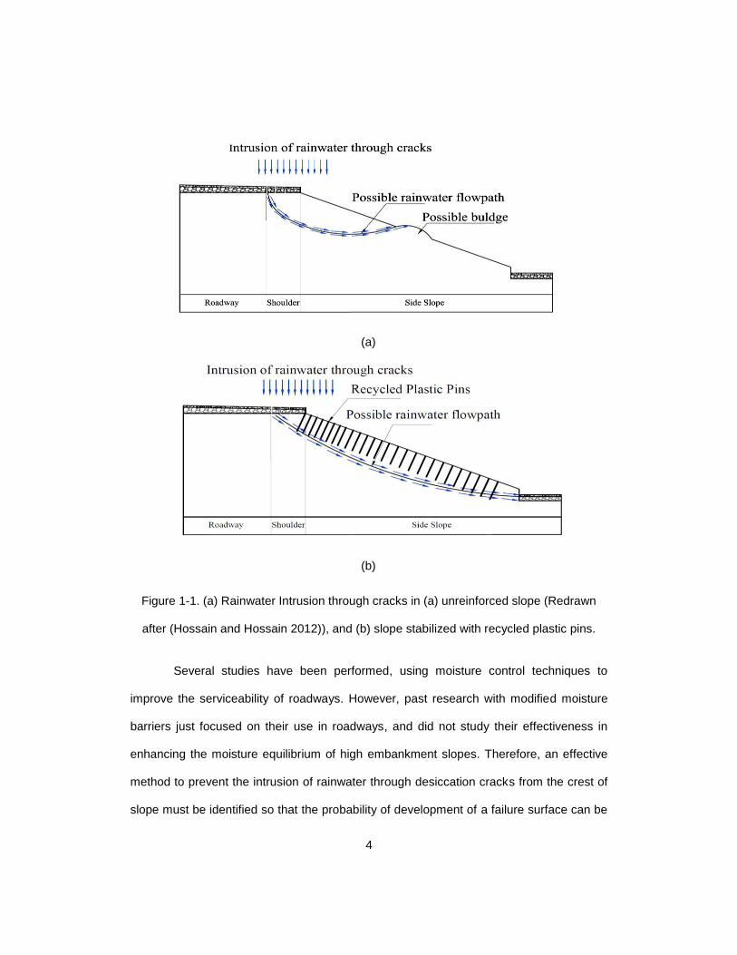
reducing moisture fluctuations in pavement subgrades. Figure 1-1(a) shows a possible

failure mechanism in an unreinforced highway slope, and Figure 1-1(b) shows the same

mechanism for a highway slope stabilized with recycled plastic pins. From these figures, it

is evident that the use of recycled plastic pin prevents the development of a slip surface at

shallow depths and only allows failure through a deeper slip surface. In both of these

scenarios, however, rainwater intrusion is possible from the edge of the pavement through

desiccation cracks into these potential failure planes, which increases the probability of

failure of the slope along these planes.

4

(a)

(b)

Figure 1-1. (a) Rainwater Intrusion through cracks in (a) unreinforced slope (Redrawn

after (Hossain and Hossain 2012)), and (b) slope stabilized with recycled plastic pins.

Several studies have been performed, using moisture control techniques to

improve the serviceability of roadways. However, past research with modified moisture

barriers just focused on their use in roadways, and did not study their effectiveness in

enhancing the moisture equilibrium of high embankment slopes. Therefore, an effective

method to prevent the intrusion of rainwater through desiccation cracks from the crest of

slope must be identified so that the probability of development of a failure surface can be

5

reduced. Additionally, no research has been done to study the performance improvement

of slopes by the combined use of recycled plastic pins and moisture control techniques.

The current study combines RPPs and modified moisture barriers to stabilize rainfall-

induced shallow slope failures.

1.3 Research Objective

The objective of the current study was to overcome the limitations of the current

knowledge database and practice by developing a sustainable slope stabilization

technique for preventing shallow slope failures, using both recycled plastic pins and

modified moisture barriers. The specific tasks performed to fulfill the objective of the study

were:

• Site Investigation and selection of the full-scale study area;

• Development of a preliminary slope stabilization scheme, using recycled plastic

pins and a modified moisture barrier, based on the previous literature and Finite

Element Method (FEM) analysis;

• Field installation of recycled plastic pins and modified moisture barriers;

• Field Instrumentation of the stabilized and unstabilized slope to evaluate the

performance;

• Performance monitoring of the stabilized and unstabilized slope

• Determining the effectiveness of modified moisture barriers in controlling

longitudinal edge cracks, edge drops, and slope failures;

• Finite element (FE) modeling of a slope stabilized with recycled plastic pins and a

modified moisture barrier, using PLAXIS 2D;

• Comparison of the results of FE modeling with hand calculations, using an ordinary

method of slices and field monitoring data; and

6

• Determination of the effect of the length of modified moisture barriers on slopes

stabilized with recycled plastic pins, using FEM analysis.

1.4 Thesis Organization

The dissertation is organized into the following chapters:

Chapter 1 provides the problem statement, objectives, and a summary of the

overall insights of the current research.

Chapter 2 presents the damages that are due to expansive clay in highway

shoulders and embankments, along with their preventive measures. Different types of

mechanical, earthwork, and moisture control slope stabilization techniques that have been

used in previous studies are also provided, as well as the details and limitations of using

RPPs for slope stabilization. Finally, the limitations of previous studies are highlighted, and

the need for this research is established.

Chapter 3 mainly focuses on the site investigation plan conducted for this study,

including the details of selected highway sections; laboratory testing; and geophysical

testing, using resistivity imaging. The shear strength parameter was back calculated at

failure condition, using FEM modeling. The site investigation results were utilized for

conducting FEM modeling, and the results were utilized to formulate a slope stabilization

plan, using MMB and RPPs.

Chapter 4 includes the field installation, field instrumentation, field monitoring, and

data acquisition procedures. The field installation plan includes procedures for the selection

and installation of materials (RPPs and MMBs). The field instrumentation plan includes the

selection and instrumentation procedures for performance monitoring of stabilized slopes.

The field monitoring plan evaluates the effectiveness of the proposed slope stabilization

method.

7

Chapter 5 focuses on the performance monitoring results obtained from the field.

The performance of the current stabilization method, using both RPPs and MMBs, was

monitored, using integrated temperature and moisture sensors, 2D-resistivity Imaging, rain

gauge, inclinometers, and a topographic survey. The results obtained from the field

instrumentation are presented and discussed, along with its comparison to existing

literature.

Chapter 6 includes the results and analysis of a numerical study conducted using

2D finite element software PLAXIS 2D. The finite element analysis was performed to

evaluate the effectiveness of the proposed slope stabilization method by the combined use

of RPPs and MMBs. The model calibration, numerical analysis of both pin-only sections

and pin-plus barrier sections, along with the factor of safety calculation using an ordinary

method of slices, are explained in this chapter. Additionally, the effects of increasing the

length of MMBs on slopes stabilized with RPPs are explained in this chapter.

Chapter 7 presents a summary of the current research and makes

recommendations for future studies.

8

CHAPTER 2. LITERATURE REVIEW

2.1 Introduction

Infrastructure systems including highways, electrical grid, communication network,

and water pipe systems are vital for the functioning of modern cities and communities.

Despite their immense importance, current state of US infrastructure is not satisfactory.

This is supported by D+ grade assigned by the American Society of Civil Engineers to the

current infrastructure state of the United States (ASCE, 2017). This highlights the critical

importance of the research into the infrastructure maintenance, rehabilitation, and

resilience enhancement. Numerous such studies dealing with electrical grid infrastructure

(Gholami, Aminifar, & Shahidehpour, 2016; Shahidehpour, Liu, Li, & Cao, 2016; Ton &

Wang, 2015), communication network (Çetinkaya, Broyles, Dandekar, Srinivasan, &

Sterbenz, 2011; Sterbenz et al., 2010)), and water pipe network (Pudasaini &

Shahandashti, 2018; Pudasaini, Shahandashti, & Razavi, 2017; Shahandashti &

Pudasaini, 2019) attest to the importance of such research. Due to its huge significance,

highway systems too demand lots of research focus. Due to their spatial distribution,

topological complexities, and exposure to numerous vulnerabilities, highway maintenance

and rehabilitation studies present a unique challenge to researchers. One of the major

sources of vulnerabilities to highway system arises from the presence of expansive soil in

the highway embankments and slope. Hence, studies dealing with expansive soil in the

highway embankments and slope is discussed in the following sections.

2.2 Expansive soils

Expansive soils, which cover one-fourth of the United States, exhibit a high

potential for volume change behavior when the volume of soil moisture changes. An

9

expansive clay map of the United States, based on the soil’s swelling and shrinkage

properties, is shown in

Figure 2-1.

LEGEND

>50% areas are underlain with clays with high swelling potential

<50% areas are underlain with clays with high swelling potential

>50% areas are underlain with clays of slight to moderate swelling potential

>50% areas are underlain with clays of slight to moderate swelling potential

Areas are underlain with little or no clay swelling potential

Data insufficient to indicate clay content or swelling potential

Figure 2-1. Expansive clay map of the United States of America (Image Source:

www.geology.com).

Expansive soils swell when they are exposed to moisture, and shrink when they

lose moisture, resulting in their undergoing appreciable volume and strength changes that

can cause serious damage to infrastructures such as foundation slabs, bridges, roadways,

slopes, and residential homes. US property owners incur more financial losses annually

from expansive soils than from earthquakes, floods, hurricanes, and tornadoes combined

(Jones and Jefferson, 2012). It has been estimated that the annual cost of the infrastructure

10

damages due to expansive soils in the US can be as high as 15 billion dollars (Table 2-1).

Therefore, it is important to understand the swelling-shrinkage behavior, changes in

strength, and the softening mechanism of expansive soils so that infrastructures

constructed thereon can be effectively maintained and rehabilitated.

Table 2-1. Global-wide damages of expansive soils (Adem and Vanapalli, 2013).

2.2.1 Cyclic Swelling and Shrinkage Mechanism

Expansive soil swells when it absorbs moisture, and shrinks when it loses moisture

(Ahmed et al., 2017; Ahmed et al., 2018; Pandey et al., 2019). Swelling is mostly observed

in clays from the smectite family, including vermiculite and montmorillonite (Young, 2012;

Hossain et al., 2016). Factors controlling the pattern and extent of volumetric deformation

include the type of clay mineral, overburden and confining pressure, initial moisture

content, initial dry density, and the presence of free water content (Chen, 2012). Although

all of the factors contribute to volumetric deformation, water content is considered to be the

most critical. In the micro-scale, swelling occurs as water molecules infiltrate between clay

sheets and interact with the clay mineral surface via hydrogen bonding. As illustrated in

Figure 2-2, hydration increases the interlayer distance and causes swelling in the macro

11

scale (Hensen and Smit, 2002). On the other hand, exfiltration of water molecules from the

matrix brings clay sheets closer together, and results in the overall shrinkage of the soil.

Possible sources of water dynamics include precipitation, thawing, irrigation, pumping, load

application, and evapotranspiration. Reaching full saturation from a relatively dry state can

cause swelling up to 20%.

Figure 2-2. Infiltration of water molecules between clay sheets (Hensen and Smit, 2002).

2.2.2 Softening Mechanism of Expansive Soil

The cyclic change in strength over a long time due to the wetting and drying cycles

is known as softening of expansive soil (Wright, 2005). The expansive soil is said to be

fully softened when its strength is equal to fully softened shear strength. The fully softened

shear strength refers to the shear strength of clay with high plasticity which seems to

develop over time, due to the cyclic shrinkage and swelling (Wright, 2005). The

embankments constructed on high plasticity clay are prone to the softening. The concept

of fully softened behavior was first proposed by Skempton (1977) for natural and excavated

slopes in the London clays. Skempton (1977) explained that the strength of the high plastic

London clay reduced over time and eventually reached to “fully-softened” strength. Khan

12

(2014) considered top 7 feet of the soil in fully softened state while performing slope stability

analysis. The fully softened strength lies between peak, and residual strength, as

presented in Figure 2-3. Skempton (1977) also reported that the fully softened strength is

comparable to the shear strength of the soil at normally consolidated state.

Figure 2-3. Comparisons of peak, fully softened, and residual shear strength (Skempton,

1970).

2.3 Damages due to Expansive Clay

Expansive clay exhibits cyclic swelling and shrinkage behavior that leads to

damage to the properties constructed over it. The cyclic swelling and shrinkage behavior

in expansive clay result in differential movement and reduction of soil shear strength, and

cause damages to infrastructures such as pavements, buildings, embankment slopes,

canals, and conduits. The damages due to expansive clay on pavements, roadways, and

13

embankments include, but are not limited to, longitudinal edge cracks, edge drops, and

shallow slope failures.

2.3.1 Longitudinal Edge Cracks

Longitudinal cracks are very common in North Texas. They are widely seen near

the edge of the pavements as a result of the differential movement of the expansive

subgrade soil. Typical longitudinal cracks observed in highways are shown in Figure 2-4.

These types of cracks initiate as small cracks that extend over time. They usually start to

appear during the dry season, when the expansive soil dries out following the maximum

heave (Gupta et al., 2008; Sebesta, 2002).

(a) (b)

Figure 2-4. Longitudinal edge cracks observed in (a) US Highway 287 (Sapkota et.al,

2019) and (b) SH 342 (Hedayati 2014).

2.3.2 Edge Drops

Edge drops occur due to longitudinal edge cracks, which are localized within 0.3

to 0.6 m of the outer edge of the pavement (Figure 2-5). These cracks are formed mainly

14

due to excessive differential movement, lack of support from the sides (shoulders), base

weakness frost action, inadequate drainage, groundwater, soil moisture variations in soils

(Hearn, et al., 2008), weak cohesive soils (Heath et al., 1990), and lateral movement of

side slopes. The cracks usually developed when there is cyclic moisture intrusion in

pavement subgrade, and where there is maximum moisture penetration (Zornberg and

Gupta, 2009).

(a) (b)

Figure 2-5. Edge drop observed in: (a) US Highway 287 (Khan, 2014), and (b) FM 2557

(Hedayati, 2014).

2.3.3 Shallow Slope Failure

Shallow slope failure generally refers to the instability that occurs in highway fill or

cut slopes and embankments. These instabilities are common in slopes constructed on

high plastic expansive clay after prolonged rainfalls. The depth and extent of these

instabilities vary with factors such as soil type, slope geometry, seepage, degree of

saturation, and climatic conditions (Titi and Helwany, 2007). The shallow slope failures

generally occur after a prolonged rainfall saturates a slope up to a certain depth, and when

15

the intensity of rainfall is greater than the rate of infiltration of the soil (Abramson et al.,

2001). According to Day and Axten (1989), the usual depth of shallow slope failure is 4 ft.

or less; however, various depths of surficial failures have been reported in previous

literature. The study conducted by Loehr et al. (2000) reported the depth of shallow slope

failure at less than 10 ft.; Titi and Helwany (2007) reported the shallow failure depth ranging

from 2 to 4 ft. In general, the depth of shallow slope failures varies between 3 to 6 ft. The

typical shallow slope failure is shown in Figure 2-6.

Shallow slope failures are quite common in the United States, where annual

losses due to landslides have been estimated at one billion dollars or more (Schuster and

Fleming, 1986). The costs associated with the repair of shallow slope failures are estimated

to be greater than or equal to costs associated with major landslides across the United

States (Turner and Schuster 1996). Shallow slope failures do not constitute direct damages

to human life; however, they damage infrastructures such as road surfaces, guardrails,

drainage facilities, utilities, shoulders, etc. that surround the failure area (Titi and Helwany,

2007). Moreover, shallow slope failures can interrupt traffic flow if the debris flows onto the

highway carriageway. Surficial failures can also have an economic impact on highway

agencies at the district/local levels.

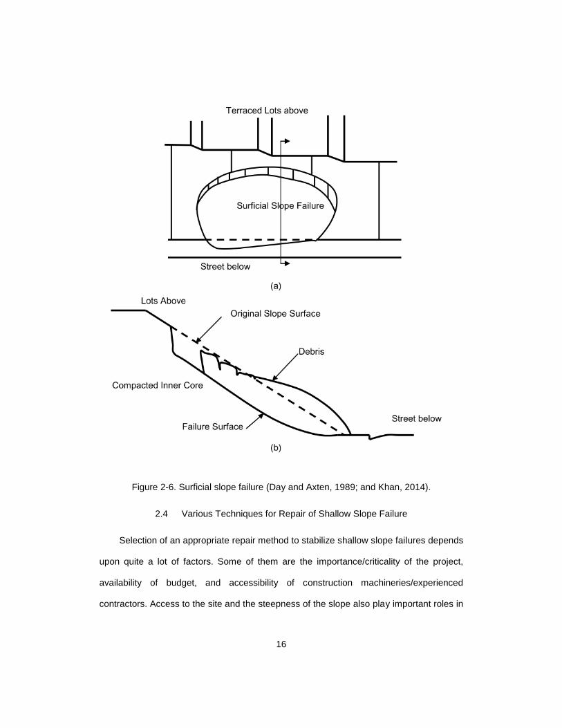
16

Figure 2-6. Surficial slope failure (Day and Axten, 1989; and Khan, 2014).

2.4 Various Techniques for Repair of Shallow Slope Failure

Selection of an appropriate repair method to stabilize shallow slope failures depends

upon quite a lot of factors. Some of them are the importance/criticality of the project,

availability of budget, and accessibility of construction machineries/experienced

contractors. Access to the site and the steepness of the slope also play important roles in

17

the selection of a repair method. Among the various methods, pushing the failed soil mass

back and re-compacting it has been regarded as the most common method for repairing

surficial failures.

The physical movement of soil and vegetation to stabilize a slope failure, while

controlling erosion, falls under earthwork techniques. The surficial slopes are reshaped by

making terraces or benches to break the steep slopes into small portions, or even flattening

over-steepened slopes, in addition to soil roughening or land forming.

The slopes can also be repaired with mechanical stabilization methods, which involve using

some additional materials. Fay et al. (2012) reported that both cut and fill slopes can be

stabilized using materials such as concrete, geosynthetics, rock, and gabion baskets.

Mechanical methods are applied to retaining walls; slopes reinforced with geosynthetics;

and mechanically stabilized earth walls, including other in-situ reinforcement methods.

Earth supports and recycled plastic pins have been used to affix shallow soils (Pearlman

et al. 1992; Loehr et al. 2000). A list of repair methods for stabilizing shallow slope failures

was compiled from previous literatures and is presented in the following sections.

2.4.1 Slope Rebuilding

Slope rebuilding is the most common and economical method of shallow slope repair.

The failed zone is first air-dried, then the soil is pushed back to the failure area and re-

compacted to the required density. Even though this method is economical and is usually

carried out as routine maintenance work on failed slopes, it is not very effective. The shear

strength of the recompacted soil does not improve considerably, especially in clays, when

the soil saturates again (Titi and Helwany, 2007).

18

2.4.2 Retaining Wall

The main function of retaining walls is to retain slopes at a steep angle. They are

most useful when the right of way, or space, is limited. The USDA (1992) stated that steep

slopes can be graded back to stable angles with the use of low retaining structures at the

base of the slope. It also makes revegetation possible without any loss of land at the top

of the slope. Such low retaining structures protect the scouring and undermining of the

slopes (Gray and Sotir, 1996). Short retaining structures, if built at the top of a fill slope,

provide a more stable road bench, along with extra width for road shoulders. Retaining

walls can be built with completely external materials, such as concrete or masonry, or the

soil itself can be reinforced to make the slope stable (Fay et al., 2012). An MSE wall is an

example of a retaining wall that can also be utilized to stabilize large deep-seated failures,

as well as slopes with shallow failure planes. Several types of retaining structures are

discussed in the following sections.

2.4.2.1 Low Masonry or Concrete Walls

These types of walls are rigid and cannot withstand differential settlement. Gravity

walls support themselves with their weight and can be built with plain or reinforced

concrete. They can also be constructed using stone masonry. Fay et al. (2012) stated that

masonry walls built with mortar and stone are easier to construct and are stronger than dry

stone masonry walls. Nonetheless, the porewater does not drain very well.

Cantilever walls are built with reinforced concrete and have a base slab connecting

a stem, as shown in Figure 2-7. Fay et al. (2012) stated that a drainage system should be

put behind a retaining wall so that the water can flow easily and prevent the formation of a

19

perched water zone behind the wall. It is to be noted that free-draining compacted backfill

is more efficient than cohesive backfill soils.

Figure 2-7. Low wall cross-section with planted vegetation for stabilization (USDA, 1992).

2.4.2.2 Gabion Walls

Gabion walls are specifically used in places where significant differential

settlement is expected, as they are adjustable to a range of slope geometries. Gabion

baskets, made of heavy wire mesh, are assembled on-site, put in the designated place,

and then packed with rocks. After this, the required strength is attained by the use of

horizontal and vertical wire support ties. Since the gabion baskets are stacked atop each

other, gabion walls are considered unbound structures. Their strength is from the

mechanical interlock between the stones (Fay et al., 2012). These types of walls can be

20

constructed both at the toe of a cut slope and the crest of a fill slope. Gabion walls also

provide free drainage through the wall (Kandaris, P. M., 2007).

2.4.2.3 Mechanically Stabilized Earth Walls

Mechanically stabilized earth (MSE) walls are built with reinforced soil, with or

without a facing. (Figure 2-8 shows a schematic representation of the MSE wall.) The

reinforced soil is strengthened using metal strips, welded wire steel grids, or geogrids,

among others. The main advantages of MSE walls over other types of walls are that they

are simpler and faster to construct, require less site preparation, are more economical,

have better tolerance for differential settlement, and have a reduced right of way

acquirement (Elias et al., 2001). They can be built to heights greater than 80 feet and can

adapt to complex geometries.

MSE walls greater than 10 ft. in height have proven to be more economical than

conventional concrete retaining walls of the same height. Nonetheless, shorter MSE walls

can also be constructed cost-effectively (Fay et al., 2012). They can be constructed with a

wide range of facing types, such as modular block facing, precast concrete, or metal

sheets. Fay et al. (2012) recommended using high-quality backfill materials for high walls

to aid in drainage, while poor-quality soils can be used in shorter walls.

21

Figure 2-8. Schematic representation of shallow MSE wall (Berg et al., 2009).

2.4.3 Wood Lagging and Pipe Pile

This technique uses galvanized steel pipe piles and a wood logging system to

stabilize failed slopes. The debris from the failed zone is disposed of, and benches are built

below the slip surface into the natural ground. Then, galvanized steel pipe piles are placed

or driven into pre-drilled holes, and the holes are filled with concrete. A pressure-treated

wood lagging system is then installed behind the pipe piles, and a drainage system is

constructed behind the lagging system. Finally, the fill materials are compacted in layers

over the whole system, and the slope is protected with an erosion control system and

landscaping (Day, 1996). A drawback of this method is that the lateral soil pressure is

transferred from the wood lagging directly to the pipe piles. The piles, being small in

diameter with low flexural capacity, have a low resistance to lateral force, thus eventually

failing the piles in bending (Titi and Helwany, 2007). Figure 2-9 shows a graphical

presentation of the repair system.

22

Figure 2-9. Graphical representation of wood lagging and pipe pile system (Day, 1996).

2.4.4 Geogrids

Geogrids are geosynthetic materials commonly made of polymeric materials such

as high-density polyethylene resins. They are strong in tension and support the soil by

interlocking with the granular materials. The failed slope is first cleared of the surficial

debris, after which benches are made on the slope below the slip surface (Day, 1996).

Vertical and horizontal drains are installed, and the collected water is disposed of off-site.

The slope is then built-in pre-specified layers of geogrids and compacted granular material,

and is protected with erosion control measures. Figure 2-10 shows the schematic of a slope

repair using geogrids.

23

Figure 2-10. Repair of slope failure using geogrid (Day, 1996).

2.4.5 Soil Cement Repair

The process of soil-cement repair is similar to geogrid repair for the first few steps.

The failed slope is cleared of debris, then the slope is excavated into benches reaching

below the slip surface to the undisturbed soil zone. Vertical and horizontal drains are also

placed to collect water and dispose of it off-site. According to Day (1996), granular material,

mixed with approximately 6% cement, is placed on the slope and compacted to at least

90% of modified Proctor maximum unit weight. The purpose of mixing the cement is that it

increases the overall shear strength of the granular material mixture and improves the

factor of safety of the slope. Figure 2-11 presents a schematic of the soil-cement repair.

Figure 2-11. Repair of failed slope using soil-cement (Day, 1996).

24

2.4.6 Soil Nails

Solid or hollow steel bars are utilized as soil nails to stabilize shallow slope failures.

A typical hollow non-galvanized bar is 20 ft. long and has an outer diameter of 1.5 in. (0.12

in. wall thickness). Galvanized steel bars can also be used in highly abrasive environments,

due to their resistant against corrosion. They are used as soil nails, and are driven into the

slopes at high speeds, using high-pressure compressed air. The principle behind the

resistance is that the soil nails go beyond the slip surface and provide resistance along the

slipping plane, eventually increasing the factor of safety of the slope. Titi and Helwany

(2007) suggested that the minimum yield strength of the steel bars is 36 ksi. Finally, after

the installation, the surface of the slope is treated with an erosion mat, steel mesh, and

shotcrete. Figure 2-12 shows a schematic diagram of the launched soil nails.

Figure 2-12. Schematic of slope repair using launched soil nails (redrawn after Titi and

Helwany, 2007).

2.4.7 Earth Anchors

An earth anchoring system, comprised of a mechanical earth anchor, wire

rope/rod, and end plate with accessories, is used to repair shallow slope failures. Figure

25

2-13 shows a cross-section of a slope stabilized with earth anchors. The anchors are first

pushed into the ground below the failure surface, then a wire tendon, which is attached to

the anchor, is used to pull the anchors to their full working position. The wire tendon is then

locked against an end plastic cap/end-plate on the slope surface to tighten the whole

system.

Figure 2-13. Slope stabilized with earth anchors (Titi and Helwany, 2007).

2.4.8 Geofoam

Rigid cellular polystyrene, commonly known as geofoam, is widely used in

geotechnical applications. The most easily available forms of geofoam are expanded

polystyrene (EPS) and extruded polystyrene (XPS). EPS is manufactured with low-density

cellular plastic solids, which have been expanded to be lightweight, chemically stable,

environmentally stable blocks. With unit weights ranging from 0.7 to 1.8 pcf, they have

compressive strength between 13 to 18 psi.

A case study was conducted by Jukofsky et al. (2000) to stabilize a problematic

highway slope over route 23A in New York, using EPS geofoam. The authors evaluated

26

various repair techniques, such as the construction of a berm, decreasing the steepness

of the slope, and using lightweight aggregates and stone columns, but they were all found

to be unfeasible, environmentally incompatible, and/or cost-prohibitive. The authors then

analyzed the slope by replacing the top 9 ft. of soil with EPS geofoam. It was found, using

the Bishop method, that the factor of safety increased to 1.25. The performance monitoring

of the stabilized slope was carried out by using inclinometers, extensometers, thermistors’

and piezometers’ lateral displacement, subsurface slope movements, temperature

changes, and seepage pressure. Figure 2-14 shows the stabilization scheme and the

sensors.

Figure 2-14. Stabilization scheme using geofoam.

The monitoring results of the piezometer showed no change in the water table and

porewater pressure, while the inclinometer recorded a 4.3-inch movement during

installation due to vibration. There was no lateral displacement after construction, but the

insignificant movement was detected during the geofoam post-construction, as shown by

the extensometer data. The thermistor results showed nearly constant ground

temperatures at different locations near the bottom of the subbase layer during the

27

monitoring period. The temperatures were not affected by the changes in the air

temperature, and no differential icing was observed. The typical pavement surface,

however, presented substantial differences in temperature with time, along with differential

icing problems. Based on the results, the authors established that geofoam can be used to

stabilize slopes, as it reduces the lateral driving force and increases the factor of safety.

The differential icing problem was also dealt with, and the slope over New York State Route

23A has exhibited no movement since the treatment was completed.

2.4.9 Wick Drains

Wick drains are used as conduits or drainage paths for porewater in soft

compressible soils. Horizontal wick drains are cheap, withstand clogging, and are so

flexible that they can be deformed without rupture, thus proving that they are better than

conventional horizontal drains. An innovative installation technique of horizontal

geosynthetic wick drains was evaluated by Santi et al. (2001) in order to formulate an

effective method to stabilize landslides. Santi et al. (2001) conducted a study by installing

100 drains throughout eight locations in Missouri, Colorado, and Indiana, using backhoes,

bulldozers and standard wick drain driving cranes. They stated that wick drains could be

driven 100 ft. through the soil, where SPT values could reach as high as 28. It has been

shown that drains should be driven in clusters, fanning outward, with an average spacing

of 25 ft. in normal clayey soils.

A study was conducted by Santi et al. (2001) during 1998 in an embankment in

Rolla, Missouri, where one-half of the 1:1 slope embankment was stabilized with 6 wick

drains, while the other half was left unstabilized as a control section. The embankment was

instrumented using 6 piezometers, 16 moisture sensors, and 20 survey markers. A

sprinkler system was utilized to simulate 100-year 24-hour rainfall to evaluate the

28

effectiveness of the wick drains. The wick drains performed very appropriately, and a

significant amount of water was drained from the slope, thus lowering the groundwater

level by 1 ft. This resulted in substantially less movement in the stabilized section as

compared to the control section. Following the success of this project, several other sites

with different geologies were stabilized by the author, using wick drains. No clogging by

dirt and algae was found in the installed sections, thus enhancing the performance of the

stabilization design.

Santi et al. (2001) recommended that wick drains should extend 10 ft. to 18 ft.

beyond the existing or potential failure plane. During installation, a smear zone was formed

that reduced the flow of water. This zone could be reduced by pushing the drain through a

pipe, instead of using the pounding or vibration method. Experience has shown that wick

drains have a few drawbacks. For successful driving of them, the recommended SPT value

of the soil is 20 or less, and in harder soils, the maximum drain length is expected to be

100 ft., while it is 150 ft. to 200 ft. for soft soils. Some scenarios might also experience a

large number of dry drains.

2.4.10 Anchored Geosynthetic Systems (AGS)

As a means for developing a new cost-effective and efficient method for slope

stabilization, Vitton et al. (1998) performed a study, using the anchored geosynthetics

system (AGS). The main principle behind this technique is the tensioning of a geosynthetic

layer placed over the soil, using ground anchors to increase the factor of safety. When the

soil beneath the geosynthetic deforms, membrane stresses start developing in the

tensioned geosynthetics, thus imparting a compressive load over the slope. Small-

diameter, ribbed steel rebars are driven into the soil in a grid pattern through the

geosynthetics, perpendicular to the surface of the slope, to provide the anchorage action.

29

After fastening the geosynthetic to the anchor, it is driven further, thus, tensioning the

geosynthetics and forming a curved geosynthetic-soil interface. This imparts compressive

stress over the soil and stabilizes the slope. Figure 2-15 shows a graphic representation of

the AGS.

Figure 2-15. Graphic representation of AGS (Vitton et al., 1998).

A field study was conducted by Vitton et al. (1998) to assess the efficiency and

implications of AGS by remediating an abandoned mine landslide in eastern Kentucky. The

field installation, which began in March 1994 with four installation workforces, took about

2.5 weeks to complete, but due to inclement weather and soil conditions, four months were

required to complete the whole project. Even though a high-strength geotextile was

selected for the study, stress relaxation and UV radiation stability led to mobilization of only

60% of the strength to regulate the strength loss. Load cells and soil pressure cells, along

with temperature sensors and rain gauges, were used to monitor the AGS. The load cells

showed an increase in the load, which continued only for 20 days after the installation. The

authors reasoned that the decrease in load was due to the consolidation of the soil just

below the anchor geotextile connection, and also due to stress relaxation in the geotextiles.

30

Thus, it was indicated that the geotextiles need to be constantly re-tensioned, even if

sufficient deformation has developed.

Although, the monitoring period was very limited, the authors concluded that AGS should

be used as a passive stabilization system, rather than an active one. The system might

prove to be effective for certain types of slopes, such as those prone to creep; however,

additional study was recommended before making any firm conclusions.

2.4.11 Soil Reinforcement

Soil reinforcement are the process of reinforcing the slopes with geosynthetics,

which deliver tensile reinforcement that allows the slopes to be stable at steeper

inclinations. The design techniques for RSS are more conservative, as they are more

stable than flatter slopes with the same factor of safety (Elias et al., 2001). RSS are more

beneficial than MSE walls, as the backfill soil requirement is less restrictive, they are more

tolerant of differential settlement, and no facing is required, thereby reducing the cost.

Furthermore, the face of the slope can be protected against erosion with proper vegetation.

2.4.11.1 Pin Piles (Micropiles)

Although pin piles, or micro piles, are used mostly for foundations, rather than for

slope stabilization, they have great potential for use in reinforcing slopes as well (Taquinio

and Pearlman, 1999; Fay et al., 2012).

2.4.11.2 Slender Piles

Slender piles, both flexible and rigid, are currently being used for slope

stabilization. The lateral loads applied on the piles due to slope soil movements are

distributed along the piles, varying with the p-y response, pile stiffness, and section

31

capacity of the piles. The piles provide passive resistance to the applied lateral loads by

conveying the loads to a stable foundation. The two methodologies for designing piles are

the pressure-based and displacement-based methods. In the pressure-based method, the

piles are designed as passive piles. The ultimate pressure from the soil is calculated and

applied to the piles directly, or by utilizing a corresponding loading condition. Relative

displacement between the soil and piles can be used to determine the pile-soil reaction

and passive pile response. The evaluation of pile displacement depends on the soil

displacement near the pile, making the estimation of relative displacement between the

soil and piles complex.

2.4.11.3 Plate Piles

Similar to pile slope installation, plate piles are installed vertically into the slope

and help in stabilizing the slope by reducing the shear stresses. Typically, the plate piles

are 6 - 6.5 ft. long, with 2.5 in. by 2.5 in. steel angle iron sections that have a 2 ft. by 1 ft.

wide rectangular steel plate welded to one end (Mccormick and Short, 2006). Plate piles

are generally used to stabilize shallow slopes. As shown in Figure 2-16, they are driven

into an existing failed slope or potential failure slope with 2-3 ft. of soft or degraded clay fill

over stiffer bedrock. The plates transfer the load from the upper slope to the stiffer

subsurface, hence reducing the driving force of the upper unstable portion.

32

Figure 2-16. Schematic representation of slope stabilization using plate piles (Short and

Collins, 2006).

Short and Collins (2006) stated that the angle iron resistance plays a major role in

determining the initial pile spacing. An investigation was carried out by installing plate piles

in a staggered grid pattern at 4 ft. c/c. The plate piles, depending on the stiffness of the

underlying soil, were driven by either direct push, using an excavator bucket, or by using a

hoe-ram or “head-shaker” compactor at a rate of 20-25 blows per hour.

Short and Collins (2006) investigated the use of plate piles to stabilize a failed

shallow slope in California. The study was presented as a promising alternative technique

for shallow slope remediation. The study concluded that this method could increase the

factor of safety against sliding by 20% or more. It also could reduce the cost for slope repair

by 6 to 10 times compared to traditional slope repair methods. However, one major

limitation is that the method is applicable only for shallow slope failures with depths of the

failure plane up to 3 ft.

33

2.4.11.4 Recycled Plastic Pins

Recycled plastic pins (RPPs) are manufactured using recycled plastics and waste

materials such as sawdust, polymers, and fly ash (Chen et al., 2007). Since the major

component is plastic, it is more resistant to biological and chemical degradation than other

conventional structural materials. The study conducted by Sapkota (2017) showed that the

plastic waste composed of approximately 19% of the total waste stream. It is the second-

largest component of municipal solid waste. Therefore, the use of RPPs as slope

stabilization reduces the waste volume and is considered as a sustainable and

environment-friendly solution for slope stabilization. The main principle behind slope

stabilization using RPP is that once driven into the slope, it intercepts the potential failure

plane and resists the lateral force, thereby increasing the stability of the slope.

2.5 Slope Stabilization Using Recycled Plastic Pins

2.5.1 Stability of Reinforced Slopes

In the limit equilibrium method of calculating the slope stability of reinforced slopes,

a potential sliding surface is considered, then the factor of safety is calculated based on

the following equation (Equation 2-1)

𝐹 =∫ 𝑆

∫ 𝜏 (2-1)

where F is the factor of safety against sliding along the considered failure surface,

𝑆 is the maximum shear strength of soil and reinforcement along the potential failure

surface, and 𝜏 is currently mobilized shear stress. The integration can be approximated by

using the method of slices, which is equivalent to numerical integration. The method of

slices involves dividing the slope continuum into many vertical slices (Figure 2-17) and

analyzing each slice, using equations of equilibrium. The strength parameters of soil and

34

reinforcement are calculated using Mohr column failure criterion and limiting strength of

reinforcement, respectively, while the mobilized shear stress is calculated by applying the

principle of equilibrium to each slice. Such calculation is carried out for all of the slices to

get the factor of safety against sliding. This process is then repeated for many potential

and unique failure surfaces to identify the failure surface with the minimum factor of safety.

The minimum factor of safety is then considered as the factor of safety of the reinforced

slope against sliding.

Figure 2-17. Equilibrium of an individual slice in the method of slice (Khan, 2014).

2.5.2 Design Method for RPP Reinforced Slope

The resistance offered by reinforcement against sliding was thoroughly studied by

Loehr and Bowders (2007), who demonstrated that resisting force provided by

35

reinforcement is a function of the depth of failure surface through the creation of limit

resistance curves of RPP. To create these curves, they considered two modes of failure of

the surrounding soil, and two modes of failure of RPP itself, which are summarized in Table

2-2.

Table 2-2. Failure modes considered to create the limit resistance curve (Loehr and

Bowders, 2007).

Failure Mode Description

Mode 1 Failure of soil above the sliding surface

Mode 2 Failure of soil below the sliding surface due to Insufficient

anchorage length

Mode 3 Bending failure of RPP

Mode 4 Shear failure of RPP

Failure mode 1 pertains to failure of the soil above the sliding surface, in which the

soil flows between the reinforcing members, as shown in Figure 2-18. The reinforcing

members need to have enough anchorage length for the soil to fail by this failure mode.

Figure 2-18 also shows a typical limit resistance curve created by Loehr and Bowders

(2007), based on this failure mode.

36

Figure 2-18. Mechanism of failure for failure mode 1 and a typical limit resistance

curve based on this failure mode (Loehr and Bowders, 2007).

Failure mode 2 corresponds to failure of soil below the sliding surface, which

occurs due to insufficient anchorage of the reinforcing members. The mechanism of failure

mode 2 and a typical limit resistance curve created by Loehr and Bowders (2007) are

shown in Figure 2-19.

37


based on this failure mode (Loehr and Bowders, 2007).

For failure mode 3, two cases should be considered. The first case is when the soil

above the failure exerts a soil pressure that is strong enough to generate limit bending

stresses in reinforcing members, causing bending-induced failure. In the second case, the

soil below the failure surface leads to similar failure-inducing bending stresses. These are

illustrated in Figure 2-20 and Figure 2-21. Likewise, failure mode 4 corresponds to a

phenomenon very similar to failure mode 3 except for the fact that the failure causing

stresses are induced by shear rather than bending.

38

Figure 2-20. Mechanism of failure mode 3-a and corresponding limit resistance

curve (Khan, 2014).

Figure 2-21. Mechanism of failure mode 3-b and corresponding limit resistance

curve (Khan 2013).

After the consideration of all of these failure modes, Loehr and Bowders (2007)

proposed the creation of a composite curve that provides an envelope of limiting resistance

39

provided by reinforcing members which can be used for further calculation. A typical limit

resistance curve created by Loehr and Bowders (2007) is shown in Figure 2-22.

Figure 2-22. Limit resistance envelope considering all four failure modes (Loehr

and Bowders, 2007).

As such, the design methodology proposed by Loehr and Bowders (2007) could be

used to estimate the limiting resistance provided by each reinforcing member by creating

a curve similar to that depicted in Figure 2-22. The limiting resistance of the reinforcing

members could then be used to perform the slope stability analysis of a reinforced slope,

using the method of slices or other similar methods.

2.6 Field Performance of Slope Stabilized with Recycled Plastic Pins

Because utilizing RPPs to stabilize slopes is more cost-effective than traditional

methods (Loehr and Bowders, 2007; Hossain et. al. 2017), various studies have been

conducted in Missouri, Kansas, and Texas, using RPPs to stabilize shallow slope failures.

40

Parra et al. (2003) conducted a study to stabilize the shallow slope failure of 3 to 5-foot-

deep using RPPs, which had a history of reoccurring failure. Other researchers, such as

Khan (2014) and Hossain et.al. (2017) also used RPPs to stabilize shallow slope failures.

A few of the case studies that used RPPs as a slope stabilization technique are described

below.

2.6.1 US Highway 287 Slope Site (Khan, 2014, Hossain et al. 2017, Tamrakar, 2015

and Rauss, 2019)

The highway slope located in US highway 287, near the St. Paul overpass in

Midlothian, Texas was stabilized with RPPs in 2011, when massive cracks were observed

near the crest of the slope or edge of the shoulder, as shown in Figure 2-23. The slope is

about 30 to 35 ft. high, with a slope geometry of 3 H: 1 V.

Figure 2-23. Cracks observed in US Highway 287 (Khan, 2014).

The site investigation study conducted at this site to identify the root cause of the

failure indicated the presence of highly plastic expansive clay. There was also a high

41

moisture zone between 5 and 14 ft. depth. Khan (2014) explained that the root cause of

the high moisture zone was the intrusion of rainwater into the slope. He further explained

that the shoulder cracks present in the crest of the slope provided easy passage for the

rainwater, which eventually led to the saturation of the soil, increased the driving force,

and reduced the factor of safety of the slope. Based on the analysis of the site investigation

and the finite element modeling results, Khan (2014) designed the slope stabilization plan,

using RPPs, as shown in Figure 2-24.

Figure 2-24. Slope stabilization plan using RPPs (Khan, 2014).

The slope stabilization plan proposed by Khan (2014) included five sections of 50

ft. width. Three sections were stabilized with recycled plastic pins, and two sections were

left unstabilized. The performance of the slopes was monitored, using inclinometers and

topographic surveys. Details of the topographic survey conducted at the crest of the slope

are shown in Figure 2-25.

42

Figure 2-25. Vertical settlement at the crest of US 287 slope site (Rauss, 2019).

The results of the topographic survey conducted on the crest of slope showed

maximum total settlements of 4.99 inches, 7.02 inches, and 6.3 inches in reinforced

sections 1, 2, and 3, respectively, while the control sections 1 and 2 showed maximum total

settlement of 15 inches and 11 inches, respectively (Rauss, 2019). This result indicates

that RPPs are effective at controlling the vertical settlement at the crest of the slope.

The lateral deformation of the stabilized slope was also monitored with

inclinometers. The results of inclinometers 1 and 3 installed in reinforced sections 1 and

section 3, respectively, are shown in Figure 2-26 and Figure 2-27. The results showed that

maximum cumulative displacements of 2.22 inches and 2.503 inches occurred near the

surface of the slope at a depth of 2.5 ft. in reinforced sections 1 and 2, respectively.

43

Figure 2-26. Displacement in inclinometer I-1 at US-287.


44

2.6.2 I 35 Slope Site (Hossain et.al. 2017, Tamrakar, 2015 and Rauss, 2019)

After observing cracks on the shoulder of the I-35 slope that resulted from the

shallow movement of the slope situated along northbound I-35E, south of the Mockingbird

Lane overpass, a study was conducted to investigate the effectiveness of RPPs at

stabilizing shallow slope failures. Laboratory tests conducted on the soil revealed that the

slope was constructed of high plastic clayey soil, which is susceptible to swelling and

shrinkage. It was found that the repeated swelling and shrinkage decreased the shear

strength of the soil, and caused the formation of cracks which were infiltrated by rainfall

and saturated the crest of the slope (Tamrakar, 2015). This eventually led to the failure of

the slope.

Finite element modeling was performed to design a stabilization scheme for the 3

H: 1 V I-35 slope, as shown in Figure 2-28. In 2014, an 85 ft. section of the failed slope

was stabilized, using 10 ft. length RPPs with rectangular cross-sections of 4 in. x 4 in. The

pins were driven in a staggered pattern, with the top 6 rows spaced at 3 ft. c/c, while the

remaining pins were spaced at 5 ft. c/c. The cracks were left unsealed at the shoulder of

the pavement to evaluate the performance of the RPPs.

45

Figure 2-28. Slope stabilization plan using RPP at I-35 slope (Tamrakar, 2015).

The slope was monitored regularly, using topographic and inclinometer surveys.

The results of the topographic survey conducted on the crest of the slope are presented in

Figure 2-29. The maximum settlement, as of December 2018, was 2.63 inches (Rauss,

2019), and the maximum incremental settlement seemed to decrease with time after the

pin stabilization. Rauss (2019) mentions that there were major rainfall events in 2018 in

the Dallas area. The egregious cracks left unsealed, along with the heavy rainfall, produced

some settlement and enlargement of cracks; nonetheless, the slope performed well and

did not fail (Rauss, 2019).

Inclinometer 1 was installed at the crest of the slope for monitoring the lateral displacement

of the slope. The maximum cumulative lateral displacement at 2.5 ft. below the crest of

slope was recorded as 2.80 in., as depicted in Figure 2-30. Most of the displacements were

in the top 4.5 ft. of the soil; the displacement was insignificant below that. Rauss (2019)

reported an average yearly increase in lateral movement of just 0.6 in. The results clearly

show that RPPs are effective at stabilizing shallow slope failures.

46

Figure 2-29. Settlement at the crest of I-35 slope.

Figure 2-30. Cumulative lateral deformation at the crest of I-35 slope.

47

2.6.3 SH 183 Slope Site- Dallas, Texas (Hossain et.al. 2017, Tamrakar, 2015 and

Rauss, 2019)

A type of failure similar to that seen in the I-35 slope was observed in SH 183, at

the northeast corner of TxDOT’s Fort Worth District, east of the exit ramp from eastbound

SH 183, heading toward northbound SH 360. A surficial failure, along with bulging, was

observed near the crest of the slope. After detailed laboratory and geophysical testing, it

was found that due to repeated shrinkage of the surface soil, cracks had formed, which led

to the infiltration of rainwater. Since clay is not very permeable, the water remained there

for some time, saturating the crest of the slope (Tamrakar, 2015). This ultimately decreased

the shear strength of the soil, and the slope moved, causing a shallow failure.

In September 2014, following the results of finite element modeling, a 60 ft. section

of the 2.5 H: 1 V slope was stabilized, using 4 in. x 4 in. cross-section RPPs that were 10

ft. in length. The pins were installed in a staggered pattern, with the top 30 ft. of the slope

consisting of 3 ft. c/c spaced pins, while the remaining 60 ft. had pins in 4 ft. c/c, as shown

in Figure 2-31.

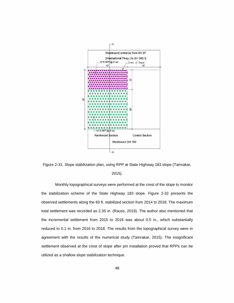
48

Figure 2-31. Slope stabilization plan, using RPP at State Highway 183 slope (Tamrakar,

2015).

Monthly topographical surveys were performed at the crest of the slope to monitor

the stabilization scheme of the State Highway 183 slope. Figure 2-32 presents the

observed settlements along the 60 ft. stabilized section from 2014 to 2018. The maximum

total settlement was recorded as 2.35 in. (Rauss, 2019). The author also mentioned that

the incremental settlement from 2015 to 2016 was about 0.5 in., which substantially

reduced to 0.1 in. from 2016 to 2018. The results from the topographical survey were in

agreement with the results of the numerical study (Tamrakar, 2015). The insignificant

settlement observed at the crest of slope after pin installation proved that RPPs can be

utilized as a shallow slope stabilization technique.

49

Figure 2-32. Settlement at the crest of State Highway 183 slope

2.6.4 I-70 Slope Site – Emma Field Test Site in Columbia, Missouri (Loehr and

Bowders, 2007 and Parra et al., 2003)

The I-70 Emma slope site is located approximately 65 miles west of Columbia,

Missouri. The slope height is 22 feet, with a slope geometry of 2.5 H: 1 V. The site

investigation results showed the presence of a mixture of lean (CL) and fat clay (CH), with

scattered cobbles and construction rubble. The four different areas of the slopes (S1, S2,

S3, and S4) experienced reoccurring slope failures over the few past decades. The slide

areas (S1 and S2) were stabilized initially, using RPPs, and the remaining slide areas were

utilized as the control section for monitoring the effectiveness of the stabilized slopes. After

50

multiple slides occurred in slide area S3, the slide area S3 was also stabilized with RPPs.

The plan and layout of RPPs used to stabilize slide areas S1, S2, and S3 are shown in

Figure 2-33.

Figure 2-33. Layout of RPP at the slide area of I-70 site: (a) Slide areas S1 and S2 and

(b) Slide area S3 (Loehr and Bowders, 2007 and Parra et al., 2003).

The stabilized slope areas S1, S2, and S3 were monitored, using inclinometers to

monitor the lateral deformation, strain gauges to monitor loads on the reinforcing members,

jet-filled tensiometers to monitor the soil suction, and piezometers to monitor the

groundwater table. The instrumentation plan for the stabilized slopes, S1, S2, and S3, are


51

(a)

(b)

Figure 2-34. Instrumentation plan of I-70 slope site: (a) Slide areas S1 and S2 and (b)

Slide area S3 (Loehr and Bowders, 2007 and Parra et al., 2003).

The results of installed Inclinometer I-2 installed at the slide area S2, shown in

Figure 2-35, revealed a maximum lateral deformation of 0.8 inches at 2 ft. depth.

Additionally, the results showed that the lateral deformation decreased as the depth

increased.

52

(a)

(b)

Figure 2-35. Result of inclinometer I-2 installed at slide area S2 (Parra et al., 2003).

The results of the inclinometers I-6, I-7, I-8, and I-9 installed in Section A, Section

B, Section C, and Section D of slide area S-3 are shown in Figure 2-36 (a), Figure 2-36

(b), Figure 2-36 (c), and Figure 2-36 (d), respectively. The results showed the increments

in the value of horizontal displacement with respect to RPP spacing. The section with

smaller spacing (Section A) deformed less than the other sections. The maximum

53

deformation observed in Section A, Section B, Section C, and Section D was 1.6 inches,

4.8 inches, 2.5 inches, and 3 inches, respectively.

Figure 2-36. Displacement profile at slide section S3: (a) Section A, (b) Section B, (c)

Section C, and (d) Section D (Loehr and Bowders, 2007).

2.6.5 I-435 - Wornall Road Field Test Site (Loehr and Bowders, 2007)

The I-435 - Wornall Road field test slope site was stabilized with 4 rows of RPPs

with 3 ft. c/c spacing in a transverse direction, and 6 ft. c/c spacing in a longitudinal

direction, followed by 15 rows of RPPs with 3 ft. c/c spacing in both directions. Altogether,

54

643 RPPs were installed to stabilize the failed slope area. The layout of the RPPs at the I-

435 Wornall Site is shown in Figure 2-37.

Figure 2-37. Layout of RPP at the I-435 slope site: (a) Cross-sectional view, and (b) Plan

view (Loehr and Bowders, 2007).

The slopes stabilized with RPPs were instrumented with four inclinometers, four

strain gauges, two standpipe piezometers, and an array of moisture sensors (Loehr and

Bowders, 2007). The field instrumental layout is shown in Figure 2-38.

55

Figure 2-38. Field instrumentation plan for I-435 - Wornall Road slope site (Loehr and

Bowders, 2007).

The depths of installed inclinometers I-1, I-2, I-3, and I-4 were 19 ft., 26 ft., 14.5 ft.,

and 19.5 ft., respectively. The results of inclinometer I-2, presented in Figure 2-39, showed

negligible displacement for several months after installation, and then the increment in the

value of cumulative displacement was observed after the spring season. The maximum

cumulative displacement observed by Parra et.al. (2003) in inclinometer I-2 was

approximately 1.2 inches.

56

(a)

(b)

Figure 2-39. Cumulative lateral displacement versus time for inclinometer I-2 located at I-

435 site (Parra et al., 2003).

57

2.7 Limitation of Recycled Plastic Pins

Recycled plastic pins were successfully used in past decades as a sustainable,

practical, and cost-effective solution for stabilizing shallow slope failures (Hossain et al.

2017; Khan et al. 2016; Khan et al. 2017; Loehr et al. 2000). However, they cannot prevent

the intrusion of moisture through desiccation cracks, and are not effective in reducing

moisture fluctuations in pavement subgrades. Figure 2-40 (a) shows a possible failure

mechanism in an unreinforced highway slope. Figure 2-40 (b) shows the same for a

highway slope stabilized with recycled plastic pins. From these figures, it is evident that the

use of recycled plastic pins prevents the development of a slip surface at shallow depths,

and only allows failure through a deeper slip surface.

(a) (b)

Figure 2-40. (a) Rainwater intrusion through cracks in: (a) Unreinforced slope (Redrawn

after (Hossain and Hossain 2012)), and (b) Slope stabilized with recycled plastic pins.

In both scenarios, rainwater intrusion is possible from the edge of the pavement

towards the center of the pavement and the side slopes through desiccation cracks.

Moisture intrusion through these cracks leads to various types of pavement distress, and

ultimately increases the probability of failure of the slopes along these planes.

For instance, the study conducted by Hedayati (2014) showed the intrusion of moisture

from the edge toward the center of the pavement and the side slope. Figure 2-41 depicts

the results of resistivity imaging, showing the intrusion of moisture from the edge toward

58

the center of pavement and towards the side slope. The resistivity imaging was conducted

on pavement, using 56 electrodes at 3 ft. c/c, as shown in Figure 2-41.

Figure 2-41. Resistivity imaging result, showing moisture intrusion from the edge toward

the center of pavement and toward the side slopes.

Hedayati (2014) explained that the intrusion of rainwater in an expansive clay roadway

subgrade potentially leads to longitudinal edge cracks and edge drops, due to cyclic

swelling and shrinkage behavior. These longitudinal edge cracks and drops create a

passageway for rainwater intrusion which leads to increased moisture content that

eventually saturates the side slope. This leads to an increase in the value of driving forces,

causing the failure of the side slope.

Hossain and Hossain (2012) conducted finite element modeling on a slope

stabilized with recycled plastic pins. The results showed the highest deformation at the

crest of the slope stabilized with RPPs. This was probably due to intrusion of rainwater

from the crest of slope; however, the study did not utilize any techniques to control the

intrusion of rainwater into the slope.

59

Figure 2-42. FE model on the slope stabilized with RPPs: (a) Deformed mesh, (b)

Deformation contour.

The initial condition of the slope on I-35 was compared with the condition of the

slope after it was stabilized with RPPs, and it was observed that a significant number of

cracks had propagated (Figure 2-43). This was due to continuous intrusion of rainwater

through shoulder cracks on the slope. The use of moisture control strategies can prevent

the formation of longitudinal edge cracks by preventing the intrusion of rainwater.

60

(a)

(b)

Figure 2-43. Propagation of shoulder crack on the slope stabilized with RPPs: (a) Initial

condition of slope during stabilization with RPPs, and (b) Current condition of slope (Year

2019) (Khan, 2014; Rauss, 2019).

2.8 Controlling Rainwater Intrusion in Pavement Subgrade

The intrusion of rainwater into pavement subgrades can be controlled by using

moisture barrier systems. The use of moisture barrier systems in highway subgrades not

only improves the pavement differential settlement, but also controls the formation of

longitudinal edge cracks and edge drops. Horizontal, vertical, capillary, and modified

61

moisture barriers were typically used in previous studies to control moisture intrusion in

pavement subgrades. The details and types of moisture barrier systems used in previous

studies are described below.

2.8.1 Horizontal Moisture Barrier

Horizontal moisture barriers are laid over the subgrade soil to stop the water from

entering into the pavement system. Consequently, less fluctuation in moisture occurs in

the subgrade soil. This leads to less swelling, ultimately reducing the road roughness.

However, Browning (1999) reported that the horizontal moisture barriers did not seem to

reduce the moisture fluctuation under the pavement subgrade or roughness of the

pavement surface in his study.

2.8.2 Vertical Moisture Barriers

Vertical moisture barriers are widely used in the United States to control the

expansive nature of pavement subgrade soil. It was first used in San Antonio, Texas on

IH-40 in 1978 (Steinberg, 1992). Vertical moisture barriers prevent the vertical movement

of pavement by controlling moisture intrusion in pavement subgrade, which controls the

swelling and shrinkage of the expansive soil at different times of the year (Picornell and

Lytton, 1987).

Vertical moisture barriers are more useful in wet and semi-arid climates with

cracked soil and shallow root depths (Jayatilaka et al, 1993). The deeper barriers, which

can range up to 8 ft., perform better than shallow barriers, as they can effectively prevent

the lateral movement of the moisture; however, they are more expensive (Gay and Lytton,

1988). This has limited the use of vertical moisture barriers to projects involving major

highways.

62

Evans and McManus (1999) proposed a method for low volume roads in Australia, utilizing

a spray-on seal surface for subgrades, after discovering the disadvantages of expensive

moisture barriers for low volume roads in the United States. The pavement stabilized with

moisture barrier system in Texas utilize soil to backfill the deep trenches excavated to

install a moisture barrier at the edge of the pavement. The deep swelling was observed

because of the high PI backfill soil, and the pavement with moisture barrier also acts as a

reservoir in flat terrain with inadequate drainage. While the method proposed by Evans and

McManus (1999 was economical and utilized the cementitious backfill in deep trenches

with plastic sheeting instead of soil backfill.

Figure 2-44. Installation of plastic sheeting as moisture barrier.( Evans and McManus,

1999).

2.8.3 Case Studies of using Geosynthetics in Roadway Subgrade

Horizontal and vertical geomembranes were utilized by the Texas State

Department of Highways and Public Transportation as a moisture barrier in twelve test

63

sections. One of the sections was laid with horizontal geomembranes, and eleven other

test sections were installed with vertical geomembranes (Steinberg, 1989). Continuous

monitoring of the twelve sites revealed that the vertical moisture barriers were effective in

improving pavement serviceability; however, cracks were observed in the outer lanes,

compromising the serviceability of the pavement with time. The maintenance cost was low

for the test sections. The past studies showed that the use of deep vertical moisture barriers

can effectively minimize the cyclic swelling and shrinkage behavior on the pavement;

however, their cost and difficulty in construction limit their use.

In 1979 and 1980, vertical moisture barriers were installed in Highway Loop 410

and Highway 37 in 1979 (Steinberg 1981), and the pavement exhibited less roughness

than the sections with no vertical moisture barrier (Steinberg 1985). Figure 2-45 shows

the section of I-410 that was installed with the vertical moisture barrier during the study.

Figure 2-45. Vertical moisture barrier in Interstate Highway 410. (Steinberg, 1989).

The successful use of vertical moisture barriers to improve the condition of the

pavements at these two sites led to proposals that they be installed in many other

64

pavements exhibiting distresses (Steinberg, 1980; 1985; 1989; 1992); however, edge

cracks appeared over time, as shown in Figure 2-46. The backfilling of the trench was

identified as the crucial factor, as improper backfilling can provide a pathway for moisture

to intrude into the system.

Figure 2-46. Observed edge cracks over pavement stabilized with vertical moisture

barrier (Steinberg, 1989).

Picomell et al. (1984) studied variations of moisture on the subgrade of Highway

37 where moisture barriers were installed, and measured the roughness of the pavement

over time. The study showed constant moisture inside the moisture barrier, and concluded

that moisture barriers are effective enough to control the pavement roughness.

Gay (1994) reported that the use of moisture barrier systems can effectively reduce the

development of roughness over pavements. Conversely, Jayatilaka et al (1993) reported

that moisture barriers are only effective to prevent moisture intrusion where medium-sized

cracks are present.

Picomell and Lytton (1987) proposed a procedure for determining the required

depth of vertical moisture barriers for specific soil characteristics and climatic conditions.

65

Two criteria were considered: the barrier would prevent water from flowing to the shrinkage

crack fabric when the soil was very desiccated, and it would prevent excessive drying under

the edges of the pavement when the soil was very wet. Generally, a depth of 2.4 meters

was used for the moisture barriers.

Pavement is designed for the potentially worst drought condition for the location,

which is determined by using meteorological data. The return period of the event is

assumed to be equal to the design life of the pavement. The depth of the moisture barrier

can be determined using edge distortion, along with maximum crack depth criterion. The

minimum depth at which the angular distortion is less than or equal to zero at the edge of

the pavement, and the maximum depth of the crack governs the depth of the moisture

barrier under these criteria, respectively. The edge distortion criteria can be used in

conditions of equilibrium, while the crack depth criteria can be used in conditions less than

equilibrium (Picornell and Lytton, 1987). The barrier should go 25% deeper than the depth

of the roots to prevent roughness in the pavement, and the longitudinal cracks can be

controlled if the barrier reaches a depth equal to the root depth. (Picornell and Lytton,

1987).

A computer program that predicts the performance of various barrier types was

introduced by Abd Rahim and Picornell in 1989. Their assumptions were that the subsoil

is divided into different sized parallelepipeds, and moisture movement only occurs between

various soil layers, through cracks in the interface of the soil blocks. Water balance was

performed in the program for the soils located on the side and underneath the pavement.

It was seen from initial runs of the program that if there were cracks that allowed the

intrusion of moisture into the soil, the moisture barrier caused more rapid swelling of the

soil under the pavement. The program required sizing the soil blocks to generate shrinkage

crack fabrics, which is not easily available for typical subsoil conditions in Texas.

66

A similar study was conducted by Chen and Bulut (2015) on areas where the

cracks beyond the vertical moisture barrier resulted in moisture intrusion into the subgrade

soil. The study was made through numerical simulation, using Abaqus software. The

cracks initially localized outside the barrier, and were slowly witnessed in the pavement as

well. Consequently, the performance of the vertical moisture barrier was compromised due

to cracks in the unprotected area, and it was suggested that a horizontal moisture barrier

be used.

The vertical moisture barriers were brought into practice in the mid-1990s by the

Texas Department of Transportation, after witnessing the detrimental effects of expansive

soil (Jayatilaka and Lytton 1997). Their study showed that deeper moisture barriers are

more effective at controlling pavement roughness; however, there are associated

difficulties and higher costs.

Al-Qadi et al. (2004) investigated the performance of a horizontal moisture barrier

underneath the Virginia Smart Road. In this study, 2 mm thick low modulus polyvinyl

chloride (PVC), covered by a nonwoven polyester geotextile on both sides, was utilized as

a barrier and put into place during the construction of the road. The performance of the

moisture barrier in controlling the pavement distresses was evaluated, using ground-

penetrating radar (GPR) and time-domain reflectometry. Figure 2-47 shows the typical

cross-section for the moisture barrier.

67

Figure 2-47. Cross-section for moisture barrier system (Al-Qadi et al., 2004).

From the study, it was evident that the moisture variations were significantly

reduced with the use of moisture barriers. The moisture was reduced by 30%, which was

witnessed after some days of rainfall events. Figure 2-48 shows the variations in moisture

content value with precipitation. The rainfall does not seem to have much effect below the

moisture barrier.

Figure 2-48. Base layer moisture content variation under moisture barrier (Al-Qadi et al,

2004).

68

Christopher et al. (2000) analyzed the performance of horizontal moisture barriers

at controlling drainage in various kinds of pavements in Maine. A special geocomposite

made up of geotextiles and geonets (Figure 2-49) was used and found to be effective at

draining the water away from the pavement system. The moisture infiltration into the

subgrade soil was controlled; however it was difficult to install the required perforated pipe

into the system to enhance drainage.

Figure 2-49. Geocomposite drainage layers applications (Christopher et al. 2000).

Henry et al. (2002) studied geocomposite capillary barrier drains (GCBD) installed

in pavement systems, and revealed that moisture variations can be controlled effectively

in the subgrade soil with the use of GCBD. However, their use was not practical because

the study was not economical because of the use of expensive materials.

69

2.8.4 Modified Moisture Barrier

The modified moisture barrier system is a layer of geocomposites underlain by a

layer of geomembranes. It is a modification of the geocomposite capillary barrier system

proposed by Henry and Stormont (2000) and utilized by Ahmed (2018) to prevent edge

cracks and edge drops on the farm road located along FM 987 in Post Oak, Bend County,

Kaufman, TX. Two sections were built: one with a modified moisture barrier, and one

without one. The preliminary results from this study showed insignificant variations of

volumetric moisture content in the section with a modified moisture barrier, while a

significant change in the value of moisture content was observed in the section without a

modified moisture barrier, as shown in Figure 2-50.

Figure 2-50. Moisture content comparison (a) for the section with modified moisture

barrier, (b) the section without modified moisture barrier, and (c) at 3 ft. depth near the

edge of pavement.

70

2.9 Slope Stabilization using Moisture Control System

The shear strength of a slope is an important factor for accessing the stability of a

slope with a deep groundwater table, particularly a fill embankment slope. These slopes

have a substantial, thick, and unsaturated soil layer, which provides an apparent shear

strength due to matric suction or negative porewater pressure. The infiltration of rainwater

decreases the matric suction, consequently reducing the apparent shear strength. The

reduction in apparent shear strength due to rainwater intrusion is one of the main reasons

for shallow slope failures.

In order to preserve the matric suction, horizontal drains, capillary barrier systems,

geotextiles, and geobarriers have been used to prevent the infiltration of rainfall into

highway embankments. The details of above-mentioned preventive measure techniques

are described in the following topics.

2.9.1 Horizontal Drains

Horizontal drains are holes drilled in the cut of fill slopes and encased with a

perforated metal or slotted plastic liner (Royster, 1980). The main purpose of using a

horizontal drain as a part of slope stabilization is to drain away groundwater and keep the

soil dry in order to control landslides. The effectiveness of horizontal drains can be

observed in terms of factor of safety. The factor of safety of a slope with a horizontal drain

was found to be higher than that of a slope without a horizontal drain (Royster, 1980, Lau

and Kenney, 1984, Martin et.al., 1994).

2.9.2 Capillary Barrier System (CBS)

The capillary barrier system is used as a cover system, and consists of two

different layers: a fine-grained soil layer overlying a coarse-grained soil layer. These soil

71

layers have different hydraulic properties which prevent the intrusion of rainwater into the

underlying soil by utilizing the unsaturated soil mechanics principles (Nicholson et al. 1989;

Steenhuis et al. 1991; Ross 1990; Stormont 1996; and Rowlett and Barbour 2000).

Different types of materials are used for the fine-grained and coarse-grained layers that

form the capillary barrier system. A few examples of capillary barrier systems used in

previous studies to stabilize slope failures are explained below.

2.9.2.1 CBS using Fine Sand and Granite Chips Layer

The study conducted by (Rahardjo et al. 2012) used a capillary barrier system to

stabilize a shallow slope failure. It was comprised of a 20 cm thick layer of fine sand for the

fine-grained layer, and a 20 cm thick layer of granite chips as the coarse-grained layer, as

shown in Figure 2-51. The construction sequence for this methodology includes laying the

geodrain on top of the slope after trimming it to the correct depth. The geodrain is secured

by steel wires to prevent slippage, then the geocells are laid on top of the geodrain and are

filled with granite chips to form an underlying coarse-grained layer. A layer of geotextiles

is then placed on top of the coarse-grained layer. After placing a geotextile layer as a

separator layer, a second layer of geocell is laid and filled with fine sand to form the fine-

grained layer.

72


fine sand as fine-grained layer and granite chips as coarse-grained layer (Rahardjo et al.

2012).

The results of tensiometers being installed at the crest of the slope stabilized with

and without a capillary barrier system are presented in Figure 2-52. The results showed

that the slope with a capillary barrier system more effectively maintained negative

porewater pressure than the slope without a capillary barrier system. Additionally, this

system showed a rise in the value of porewater pressure with respect to rainfall events,

indicating the percolation of rainwater into the slope.

73

(a) (b)

Figure 2-52. Pore-water pressure variations with rainfall and time near the crest of the

slope: (a) with capillary barrier system, and (b) without capillary barrier system.

2.9.2.2 CBS using Fine Sand and Recycled Crushed Concrete Aggregate

The fine sand layer and recycled crushed concrete aggregate layer were utilized

as fine-grained and coarse-grained layers, respectively, in the capillary barrier system

installed by Rahardjo et al.(2013) to stabilize the rainfall-induced slope failure (See Figure

2-53). The construction sequence for this CBS includes laying a 6.5mm thick geosynthetics

drainage layer as a separator on top of the slope, after trimming it to 540 mm depth. Then,

the geocells are laid on top of it for the placement of recycled crushed concrete aggregate

as a coarse-grained layer, and are secured with steel J pins of 75 cm length. After placing

the recycled crushed concrete aggregate, a layer of geotextiles is placed as a separator

layer, and a second layer of geocells is laid and filled with fine sand to form the fine-grained

layer.

74

Figure 2-53. (a) Schematic diagram of stabilized slope and (b) Cross section of CBS with

fine sand as fine grained layer and RCA as coarse-grained layer.

The results of the tensiometer installed at the middle of the slope stabilized with

and without a capillary barrier system are presented in Figure 2-54. The results showed

that the slope with a capillary barrier system more effectively maintained negative

porewater pressure than the slope without a capillary barrier system. Additionally, this

system showed a rise in the value of porewater pressure with respect to rainfall events,


75

Figure 2-54. Pore-water pressure variation with time at the middle of the slope: (a) with

capillary barrier system (b) without capillary barrier system, and (c) Rainfall intensity with

respect to time.

2.9.2.3 CBD using Fine Sand and Geosynthetics (Secudrain)

The fine sand and geosynthetics (Secudrain) layers were utilized as a fine-grained

and coarse-grained layer, respectively, as a capillary barrier system in the study conducted

by Rahardjo et al.(2013) to stabilize the rainfall-induced slope failure (Figure 2-55). The

construction sequence for this CBS includes putting down a 6.5 mm thick geosynthetics

drainage layer, to serve as a separator layer on top of the slope, after trimming it to 360

76

mm depth. Then, another layer of geosynthetics drainage/Secudrain is placed as a coarse-

grained layer. Geocells are then laid over the Secudrain, and are secured with steel J pins

of 75 cm length, penetrating 54 cm in the ground. Finally, the entire geocells area is filled

with fine sand, to form the fine-grained layer.


fine sand as fine-grained layer and Secudrain/geosynthetics as coarse-grained layer.

The results of tensiometer installed at the middle of the slope stabilized with and

without a capillary barrier system are presented in Figure 2-56. The results showed that

slopes with a capillary barrier system more effectively maintained the negative porewater

pressure than slopes without a capillary barrier system. Additionally, this system showed

a rise in the value of porewater pressure with respect to rainfall events, indicating the

percolation of rainwater into the slope.

77

Figure 2-56. Porewater pressure variations with time at the middle of the slope: (a) with

capillary barrier system (b) without capillary barrier system, and (c) rainfall intensity with

respect to time.

2.10 Limitation of Previous Studies

Soil reinforcement, using recycled plastic pins, and soil moisture control techniques

using a modified moisture barrier, have been separately used to enhance the performance

of highway slopes constructed over high plasticity clay and to mitigate pavement

distresses, respectively. However, no research has been done to study the performance

78

improvement of slopes with the combined use of recycled plastic pins and moisture control

techniques. Furthermore, past research with modified moisture barriers did not study its

effectiveness in enhancing moisture equilibrium of high embankment slopes, and was just

focused on its use in roadways and shoulders with lower side slopes. This study proposes

stabilizing rainfall-induced shallow slope failures and pavement distresses with the

combined use of recycled plastic pins and modified moisture barriers. As such, the main

objective of this study is to determine the effectiveness of stabilizing rainfall-induced

shallow slope failures and pavement distresses by the combined use of recycled plastic

pins and modified moisture barriers in high embankment slopes constructed over high

plasticity clay. In the following chapters, a site investigation plan and slope stabilization

plan, along with the field installation and instrumentation adopted, are discussed.

Subsequently, results are presented and analyzed, and the conclusions drawn from this

research are presented.

79

CHAPTER 3. SITE INVESTIGATION AND SLOPE STABILIZATION PLAN

3.1 Introduction

This chapter includes the site investigation and slope stabilization plan formulated

to fulfill the research objective. The objective of this study is to stabilize shallow slope

failures and to mitigate pavement distresses, using recycled plastic pins and modified

moisture barriers. Pavements constructed on highly plastic expansive clay subgrades with

fill embankment slopes are prone to cyclic swelling and shrinkage behavior, which results

in pavement distresses and shallow slope failures. Therefore, an actual highway pavement

section with visible signs of pavement distress and potential shallow slope failure was

selected for this study. The details of the selected highway section; site investigation

results; and design of the slope stabilization plan, using Modified Moisture Barriers (MMBs)

and Recycled Plastic Pins (RPPs) are discussed in this chapter.

3.2 Project Background and Visual Inspection

In 2017, a section of a highway slope along Texas highway US 287 near Midlothian,

with visible signs of pavement distress and potential shallow slope failure, was selected for

the experiment. The location of the slope is presented in Figure 3-1(a). The selected

highway section’s shoulder was closed to traffic by TxDOT due to the visible distresses

and failure potential at that time. This section of the highway was constructed over an

embankment with a slope of 1V: 3.3 H. The pavement supported a two-lane roadway with

an 11 ft. wide shoulder. The existing report indicated the presence of Eagle Ford clay

deposits. During the preliminary site reconnaissance, massive longitudinal visual cracks

were observed over the pavement shoulder, along with edge drops as large as 20 inches

at the edge of the shoulder. The aerial view of the slope showed signs indicating shallow

slope failure. The longitudinal massive shoulder cracks, along with edge drop and shallow

80

slope failure observed during preliminary reconnaissance of US Highway 287, are shown

in Figure 3-1.

(a) (b)

(c) (d)

Figure 3-1. (a) Site location, (b) Shallow slope failure, (c) Shoulder cracks, and (d)

Maximum edge drop of 20 inches at the middle of the failure section (US Highway 287).

3.3 Site Investigation

The site investigations were carried out according to the recommendations of the

TxDOT Geotechnical Manual, Section 1 – “Soil Survey”. The main objective of the soil

investigation was to understand the subsurface soil condition and to identify the reasons

behind the massive longitudinal cracks, shoulder drop, and shallow slope failure. The site

Site Location 32°29'23.6"N 97°01'58.7"W

81

investigation was conducted in March 2017. The preliminary site investigation program

included subsurface exploration by geotechnical drilling and geophysical testing. The

location of the geotechnical drilling and geophysical testing, using resistivity imaging, is


Figure 3-2. Location of soil borings and resistivity imaging inspection lines.

3.3.1 Geotechnical Drilling

Four soil test boreholes of 30 ft. depth were drilled for the sub-surface sample

collection. Three soil test boreholes (BH1, BH2, and BH3) were located at the crest of the

slope, while one soil test borehole (BH4) was located at the toe of the slope, as shown in

Figure 3-3. Hollow-stem augers with a 5-inch outer diameter were used for the drilling, and

were powered by truck-mounted drilling rigs. Each auger was 5 ft. in length, and each of

the subsequent sections was added as the drilling depth progressed. Disturbed and

undisturbed samples were collected for laboratory testing. Undisturbed samples were

collected from each borehole at intervals of 5 ft. depth, using a thin-walled Shelby tube

sampler with an outer diameter of 3 inches, while the disturbed samples were collected

82

from each borehole at intervals of 2 ft. depth. The standard penetration tests (SPT) were

performed at intervals of 5 ft. depth.

Based on in-situ observations, the predominant soil strata was dark brown high plasticity

clay. The bore logs from the geotechnical drilling are presented in Appendix A.

The ASTM standards were followed to conduct the laboratory tests on the collected

soil samples to determine the physical properties. The physical properties of the collected

soil samples were determined, based on the following tests.

3.3.1.1 Gravimetric Moisture Content Tests

Moisture content tests were performed to observe the variations of moisture

content with depth. The gravimetric moisture content test followed ASTM D2216 Standard

Test Methods for Laboratory Determination of Water (Moisture) Content of Soil and Rock

by Mass. The moisture content profiles, with respect to depth of collected soil samples from

four boreholes, are presented in Figure 3-3. The results showed that the gravimetric

moisture content varied from 22% to 42%. Additionally, high moisture variations were

observed in the top 8 ft.

83

Figure 3-3. Moisture profile with respect to depth.

3.3.1.2 Grain Size Distribution Samples

The grain size distribution test was performed, using a wash sieve and following the ASTM

D 422-63 Standard Test Procedure for Particle-Size Analysis of Soils. Both sieve and

hydrometer analyses were performed to obtain the full-range grain size distribution curve.

First, the soil was oven-dried at a temperature of 120 F, then it was crushed and washed

with flowing water through sieve #200. The soil retained on the #200 sieve after the wash

sieve analysis was again kept in the oven for drying. Then, the sieve analysis was

performed, using #4, #10, #30, #40, #60, #100, and #200 US standard sieves. Additionally,

High Moisture Zone

84

the hydrometer test was performed according to ASTM D 422-63, using the soil passing

through a #200 sieve during the wet sieve analysis. The grain size distribution curves for

the samples collected at different depths are shown in Figure 3-4.

Figure 3-4. Grain size distribution curve.

The results of the grain size distribution test showed that the fine fraction of the

collected soil samples passing through a #200 sieve ranged from 75 to 95%, indicating

fine-grained soils.

3.3.1.3 Atterberg Limit Test

The Atterberg limit test was conducted on collected soil samples, using the ASTM

D 4318 Standard Test Methods for liquid limit, plastic limit, and plasticity index of soils. The

results of the Atterberg limit test on collected soil samples are presented in Table 3-1. The

liquid limit for collected samples ranged from 47 to 80%, while the plastic limit ranged from

30 to 55%. The plasticity chart of the soil samples is presented in Figure 3-5. The results

85

of the Atterberg limit tests and grain size distribution tests showed that the collected soil

samples were high plasticity clay, based on the Unified Soil Classification System (USCS).

Table 3-1. Atterberg Limits of collected soil samples.

Borehole ID

Depth (ft.) Liquid

Limit (%) Plastic

Limit (%) Plasticity Index (%)

BH-1 3 47 25 22

BH-1 7 60 28 32

BH-1 12 62 25 37

BH-1 18 80 27 53

BH-1 25 75 30 45

BH-2 3 63 20 43

BH-2 7 67 30 37

BH-2 12 70 33 37

BH-2 18 80 27 53

BH-2 25 80 32 48

BH-3 3 65 29 36

BH-3 7 62 28 34

BH-3 12 70 33 37

BH-3 18 72 30 42

BH-3 25 75 33 42

BH-4 3 63 21 42

BH-4 7 67 30 37

BH-4 12 71 32 39

BH-4 18 74 32 42

BH-4 25 75 30 45

86

Figure 3-5. Plasticity chart for collected soil samples.

3.3.1.4 Specific Gravity Test

The specific gravity test was performed, using the water pycnometer method and

following ASTM D845 Standard Test Methods for Specific Gravity of Soil Solids. The soil

passing from a #4 sieve was utilized for the test. The value of specific gravity was found to

range between 2.712 to 2.746. The average value of the specific gravity was found to be

approximately 2.73.

3.3.1.5 Shear Strength Test

The soil samples from different depths within each borehole were further

investigated to evaluate the peak and fully softened shear strength of the soil. The peak

shear strength of the undisturbed samples is summarized in Table 3-2. The shear strength

87

tests were further utilized to conduct a slope stability analysis and design of the slope

stabilization scheme, which are shown in the following section.

Table 3-2. Summary of shear strength test.

Bore

Hole ID

Sample

Depth (ft.)

Specimen

Type Test Type

Cohesion

(psf)

Friction

Angle

(°)

BH-3 3 Fully Softened DS/ UCS* 50 12

BH-2 10 Undisturbed DS/ UCS* 350 15

BH-2 14 Undisturbed DS/ UCS* 1000 25

*Note: DS = Direct Shear Test

UCS = Unconfined Compressive Strength Test

3.3.2 Geophysical Testing

Geophysical testing was performed, using 2D electrical resistivity imaging (ERI),

which provides a continuous image of a subsurface, using a multi-electrode array system

and inversion modeling. 2D ERI is increasingly used for geotechnical investigations, and

for this research, it was used to examine the subsurface soil condition of the slope. The 2D

ERI lines were performed along two alignments: the RI Line_1 and RI Line_2 at the slope.

The lines along which the resistivity imaging was conducted are shown in Figure 3-3. RI

Line_1 was at the crest of the slope, while RI Line_2 was at the middle of the slope, as

shown in

Figure 3-6.

88

Figure 3-6. (a) RI Line_1 and (b) RI Line_2.

The 2D ERI was conducted, using 8-channel SuperSting equipment, which is faster than

the conventional single-channel unit. It was performed, using 28 electrodes where the

length of the ERI line was 162 ft., and the spacing between electrodes was 6 ft. c/c. The

RI Line-1 and RI Line-2 are presented in Figure 3-7 (a) and Figure 3-7 (b), respectively. An

inverse relationship exists between resistivity and moisture content. The blue zone in

Figure 3-7(a) represents the lower resistivity value, while the red zone represents the

higher resistivity value. Figure 3-7 (a) shows that more blue zones exist in the top 5 to 8 ft.,

indicating a higher moisture zone that is due to the presence of shoulder cracks. The

shoulder cracking allows rainwater water to infiltrate the adjacent soil layer, reducing the

resistivity value and increasing the moisture content of the underlying soil layer. Results

obtained from RI-Line_2 indicate that even at the mid-depth of the slope, water intruded to

a depth of 5 to 8 ft. through a high resistive zone that was observed near the surface of the

(a) (b)

89

slope. Perched water zones were observed at the top and middle of the slope, which might

be an indication that water was seeping through the top layer and the direction of seepage

was parallel to the slope surface.

(a)

(b)

Figure 3-7. Resistivity imaging of (a) RI Line_1 and (b) RI Line_2.

3.4 Analyses of Site Investigation Results

The site investigation results performed on the failed section of US Highway 287

showed the presence of highly plastic expansive clay with liquid and plastic limits ranging

from 47 to 80%, and 30 to 55%, respectively. Highly plastic expansive clay undergoes

swelling and shrinkage behavior in the presence and absence of moisture. The cyclic

swelling and shrinkage nature of expansive clay causes a reduction of its strength with

time, and it will eventually reach a fully softened state (Saleh and Wright, 1997). In the fully

softened state, the value of cohesion almost reaches 0, while the change in the angle of

friction is not significant (Saleh and Wright, 1997). Due to this behavior in expansive clay,

highway embankments constructed with expansive clay eventually show various types of

pavement distresses, such as edge cracks, edge drops, etc., and shallow slope failure.

The site investigation results of the current study also showed the presence of massive

90

longitudinal edge cracks, and edge drops up to 20 inches. The initiation of slope failure

was observed. The cyclic drying and wetting of expansive clay in US 287 slope may have

reduced its strength to fully softened state, which led to the start of movement of the slope

and caused the cracks over the shoulder. These cracks provided an easy passageway for

rainwater entering the slope, which eventually led to saturation of the soil near the crest.

The moisture content and 2D resistivity imaging showed a high moisture zone in the top 8

feet. The results and observations of the site investigation conducted on US Highway 287

were used to perform numerical modeling to formulate a suitable slope stabilization plan

for the failed portion of the highway.

3.5 Slope Stability Analysis for Unstabilized Slope

The stability analysis of the unstabilized slope was performed using finite element

software PLAXIS 2D. The Mohr-Coulomb soil model was used for this analysis. The top 8

feet of the soil was considered to be at fully softened strength, based on the site

investigation results. The details of the safety analysis for the unstabilized slope are

presented in Chapter 6. The factor of safety of the unstabilized slope was found to be

1.055.

3.6 Slope Stability Analysis for Slope Reinforced with RPPs

A slope stabilization plan was designed, using 4 inch by 4 inch, and 10 ft. long

recycled plastic pins (RPPs). The section and type of RPPs were selected based on the

study conducted by Khan (2014). The performance monitoring results of the US 287 slope

stabilized with RPPs in 2011 showed significant improvement in the stability of the slope

as compared to other stabilization methods (Khan, 2014); therefore, RPPs were used to

stabilize the slope. Several trials were run, using different spacing of RPPs. The optimum

91

spacing, which provided an adequate factor of safety, was selected. The details of the

procedure used for selecting this layout can be found in Hossain et al. (2017).

Based on several iterations in PLAXIS 2D, a 3 ft. c/c spacing of the RPPs was

selected near the crest of the slope, followed by a 4 ft. c/c spacing at the middle portion of

the slope, and 5 ft. c/c spacing for the rest of the slope. The spacing of the RPPs was the

same in both horizontal and longitudinal directions. The details and outputs of the slope

stability analyses of the reinforced areas of the slope are presented in Chapter 6. The factor

of safety of the slope stabilized with RPPs was found to be 1.594, which is greater than 1.5

and suitable for slope stabilization design. The value of factor of safety increased from

1.055 to 1.594 because the use of RPPs provided additional resistance towards the

stability of the slope. Even though the use of RPPs improves the factor of safety of the

slope, the recycled plastic pins cannot prevent the intrusion of moisture through desiccation

cracks and are not effective in reducing moisture fluctuations in the pavement subgrade.

Therefore, to prevent pavement distress, moisture control techniques, along with RPPs,

should be utilized for the slope stabilization plan.

3.7 Controlling Rainwater Intrusion through Slope Stabilized with RPPs

The recycled plastic pins were successfully used as a sustainable, practical, and

cost-effective solution for stabilizing shallow slope failures in past decades (Hossain et al.

2017; Khan et al. 2016; Loehr et al. 2000). However, the recycled plastic pins cannot

prevent the intrusion of moisture through desiccation cracks and are not effective in

reducing moisture fluctuations in the pavement subgrade.

The intrusion of moisture through desiccation cracks can be controlled by using moisture

control barriers. Moisture control barriers (such as vertical barriers, horizontal barriers,

capillary barriers, and modified moisture barriers) are used to control moisture fluctuations

in subgrade soil by enhancing drainage and preventing moisture intrusion (Ahmed et al.

92

2018; Elseifi et al. 2001a). Among these moisture control barriers, the modified moisture

barrier has high potential to prevent rainwater intrusion in pavement subgrades and to drain

infiltrated rainwater. The modified moisture barrier is a layer of geocomposites

(interconnected geotextile-geonet-geotextile layer) underlain by geomembrane layer

(Ahmed et al. 2018). The primary use of a geocomposite layer is to properly drain infiltrated

rainwater, while the geomembrane layer prevents the further infiltration of rainwater.

Figure 3-8 shows the detailed mechanism of preventing of rainwater intrusion with

geomembranes, and promoting drainage by using geotextiles and a geonet layer.

(a)

(b)

Figure 3-8. (a) Prevention of rainwater intrusion into pavement subgrades, (b) Detailed

mechanism of modified moisture barrier in Section A.

93

Considering the effectiveness of MMBs in controlling moisture intrusion and

pavement deformation in the previous studies conducted by (Ahmed et al. 2018; Sapkota

et al. 2019b), the combined use of RPPs and MMB was selected to stabilize rainfall-

induced shallow slope failures and pavement distresses in the current study.

3.8 Slope Stabilization Plan

The slope stabilization plan was designed, using both RPPs and MMB to combat

rainfall-induced shallow slope failures and pavement distresses at the US Highway 287

site located in Midlothian, Texas. It included the use of RPPs for lateral stabilization of the

slope, and the installation of MMB for preventing the intrusion of rainwater through

desiccation cracks. The mechanism of slope stabilization, materials selections, and design

of the slope stabilization plan are described in the following sections.

3.8.1 Mechanism of Slope Stabilization using RPPs and MMB

The utilization of RPPs in slope stabilization provides additional shear strength

along critical failure surfaces. The addition of MMB prevents the intrusion of rainwater from

the crest of slope. Also, it doesn’t allow the initiation of failure from the area where MMB is

not provided, which reduces the radius of the critical slip surface, resulting in an increased

value of factor of safety. The schematic diagram of a slope stabilized with both RPPs and

MMBs is shown in Figure 3-9.

94

Figure 3-9. Schematic diagram of slope stabilized with both RPPs and MMB.

The factor of safety of the slope stabilized with RPPs and MMB (FSR+B) can be

determined by taking the ratio of the total resisting moment to the total driving moment

(MD), as shown in Equation 3-1. The total resisting moment is the summation of the

resisting moment due to the shear strength of the soil (MR) and due to the installed RPPs

(ΔMR).

FSR+B = 𝑀𝑅+ ΔM𝑅

𝑀𝐷 (3-1)

3.8.2 Material Selection

Commercially available RPPs, geocomposites, and geomembranes were selected

for the slope stabilization plan. The properties of the selected RPPs and MMB for stabilizing

and mitigating slope failure and pavement distresses, respectively, are described in the

section below.

95

3.8.2.1 Recycled Plastic Pins

Commercially available recycled plastic pins were selected for this study. Different

lengths, sizes, and shapes (i.e., rectangular, circular, square) of RPPs are available

commercially. A typical RPP is composed of high density polyethylene, HDPE (55% –

70%); low density polyethylene, LDPE (5% -10%); polystyrene, PS (2% – 10%);

polypropylene, PP (2% -7%); polyethylene- terephthalate, PET (1%-5%); and varying

amounts of additives, i.e., sawdust and fly ash (0%-5%) (McLaren, 1995). However, the

composition of recycled plastic pins varies, as they are manufactured by different

companies. Based on available options, fiber-reinforced recycled plastic pins were

selected for the current study due to their improved elastic modulus and creep resistant

behavior (Hossain et al., 2017). The rectangular cross-sectioned recycled plastic pins of

size 4 in. x 4 in. and depth of 10 ft. were selected based on the previous study (Khan et al.,

2016; Hossain et. al., 2017).

The flexural strength and elastic modulus of the RPP samples were determined by

the three-point bending test. Nine samples were tested in accordance with ASTM D790.

The flexural strength and elastic modulus of the RPPs ranged between 3.1 to 4.7 ksi and

190 to 200 ksi, respectively (Khan, 2014). The properties of RPP used in this current study

are summarized in Table 3-3.

Table 3-3. Properties of Recycled Plastic Pins.

Property Test Method Value Unit

Length - 4 inch

Breadth - 4 inch

Height - 10 feet

Flexural strength ASTM D790 3.1 to 4.7 ksi

Elastic modulus ASTM D790 190 to 200 ksi

96

3.8.2.2 Modified Moisture Barrier

The modified moisture barrier, which has been shown to effectively prevent the

intrusion of rainwater (Ahmed et al. 2018), was selected for the pin-plus barrier section.

The modified moisture barrier is a layer of geocomposites underlain by a layer of

geomembranes (Ahmed et al. 2018). The modified moisture barrier used in this study is a

combination of a 40 mil LLDPE geomembrane (Linear Low Density Polyethylene) and 8

oz. HDPE geocomposite (High-Density Polyethylene). The selection criteria and the

properties of the geocomposites and geomembranes are described in the following

sections.

3.8.2.2.1 Geocomposite Selection

The geocomposite with an interconnected layer of geotextiles, geonets, and,

geotextiles was selected for this study. The size of geocomposite was 50 ft. long by 12 ft.

wide. The geocomposite was used to provide adequate drainage and to prevent separation

from the subbase layer. The commercially available 8 oz. HDPE (High-Density

Polyethylene) was selected after checking both strength and flow properties. The strength

capacity of geocomposite is required to sustain continuous traffic movement without

showing considerable deformation and the flow capacity is required to effectively drain

percolated rainwater (Christopher et al., 2000). Both the flow and strength properties were

tested in accordance with AASHTO (M 288). Based on the ASTM standards, geotextiles

can be used for pavement subsurface drainage when its Apparent Opening Size (AOS) is

less than 0.22 m, permittivity is greater than 0.1 sec -1, and grab tensile strength is greater

than 700 N. Additionally, the geocomposite was selected to use 2 feet below the pavement

surface, just below the base layer, it should have the drainage capacity similar to 4-inch

(Open Graded Base Layer) OGBL. In order to have drainage capability similar to OBGL,

97

the transmissivity of geocomposite should be greater than 0.00035 to 0.001 m2/sec

(Christopher et al., 2000). The geocomposite used in this study had a transmissivity value

of 0.0007 m2/sec. Therefore, the commercially available gecomposite with 8 oz. high-

density polyethylene geonet resin with nonwoven polypropylene geotextile fabric heat

bonded on both sides of geonet, was selected based on ASTM standards (Table 3-4). The

properties of the geocomposite used in this study are summarized in Table 3-4.

Table 3-4. Properties of selected geocomposite.

Component Property Value Units Test Method

Geotextile

AOS 0.18 mm ASTM D4751

Permittivity 1.26 sec-1 ASTM D4491

Permeability 0.3 cm/sec ASTM D4491

Grab Tensile Strength 1001 N ASTM D4632

Geonet

Thickness 178 mm ASTM D5199

Tensile Strength 7×10-4 kN/m ASTM D7179

Transmissivity 6.98 m2/sec ASTM D4716

Geocomposite Ply Adhesion 11.35 g/sec ASTM D7005

Transmissivity 6×10-3 m2/sec ASTM D4716

3.8.2.2.2 Geomembrane Selection

The geomembrane used in this study was 50 ft. long by 12 ft. wide, with thickness

of 40 mil. The geomembrane is an impermeable layer and can be used for various

purposes, but the primary use of the selected geomembrane in this study was to prevent

rainwater intrusion underneath the subgrade of the pavement. The selected geomembrane

was similar to a bottom liner used in a landfill. The 40 mil commercially available

impermeable LLDPE geomembrane manufactured by Brawler Industries was selected for

this study. The properties of the geomembrane used in this study are summarized in Table

3-5.

98

Table 3-5. Properties of selected geomembrane.

Component Property Value Units Test Method

Geomembrane

Thickness 40 mil

Tensile Strength 270 N ASTM D6693

Puncture Resistance 267 N ASTM D4833

3.8.3 Design of Slope Stabilization Plan

Previously, the failed slopes in North Texas were repaired, using only RPPs

(Hossain et.al. 2017). Although the RPPs increase the stability of slope, they do not

improve the performance of the pavement shoulder or limit the intrusion of moisture into

the slope. The intrusion of rainwater from the edge and shoulder of pavements leads to

pavement distress and failures. Since these types of failures are frequently observed in

many parts of North Texas, minimizing the rainfall intrusion into the desiccation cracks and

increasing the lateral stability of the slope are important factors to consider in designing a

slope stabilization plan that combines the use of MMB and RPPs.

The three test sections, the pin-plus barrier, pin-only, and control section, were

designed to stabilize the failed portion of US Highway 287. Each of them was 50 ft. long

(Figure 3-10).

99

Figure 3-10. Illustration of test sections.

The pin-only section was stabilized with RPPs only. The layout was a staggered

pattern, with 3 ft. center-to-center spacing for the crest portion of the slope, 4 ft. center-to-

center spacing for the middle portion of the slope, and 5 ft. center-to-center spacing for toe

portion of slope. Since the crest of the slope was found to be critical due to the potential

maximum lateral movement (Khan, 2014) and subsequent initiation of rainwater-induced

slope failure (Hossain and Hossain, 2012), the smaller RPP spacing was provided at the

crest of the slope. The placement for the RPPs was fixed, based on the numerical modeling

that was performed, using the finite element program, PLAXIS 2D. The details of the

numerical study are described in Chapter 6.

The pin-plus barrier section was stabilized by using both RPPs and MMB. The

layout of the RPPs was kept identical to the pin-only section to compare the effectiveness

of the pin-plus barrier section and the pin-only section. The size of the MMB in the pin-plus

barrier section was 50 ft. long by 12 ft. wide. Four feet (33.33%) of the barrier width was

installed in the shoulder, while the remaining width of the barrier was in the slope. The

modified moisture barrier was installed at a depth of 2 ft.

100

The control section was left unsterilized. The layouts of the control, pin-only, and

pin-plus barrier sections are illustrated in Figure 3-10.

Figure 3-11. Plan view of test sections: control, pin-only, and pin-plus barrier.

101

CHAPTER 4. FIELD INSTALLATION AND INSTRUMENTATION

4.1 Introduction

The field installation and field instrumentation process are presented in this

chapter. The installation was based on the slope stabilization plan. The Recycled Plastic

Pins (RPPs) and Modified Moisture Barrier (MMB) were installed for slope stabilization,

and the integrated temperature and moisture sensors, rain gauges, and inclinometers were

installed in each of the sections for evaluating the performance of the proposed stabilization

method.

4.2 Field Installation

The field installation included the installation of the RPPs and the MMB, and was

implemented based on the slope stabilization plan described in Chapter 3. Both RPPs and

MMB were installed in the pin-plus barrier section. The RPPs were installed in the pin-only

section, and the control section was left unstabilized. The details of the installation

procedure for the RPPs and MMB are described below.

4.2.1 Installation of Recycled Plastic Pins

A series of experiments, reduced-scaled laboratory and field tests were conducted

by Sommers et.al. (2000) to assess the processes and equipment for installing RPPs into

the slopes. The most economical, reliable, and cost-effective system reported in the

previous studies was a mast-mounted vibratory hammer system, which maintains the

alignment of the hammers and restricts the additional lateral loads imported while driving

the RPPs (Bowders et al., 2003). A crawler-mounted drilling rig was reported in previous

studies as the most suitable and cost-effective equipment for driving the RPPs into slopes.

A crawler-type drilling rig with a mast-mounted vibratory hammer (Klemm 802 drill rig and

102

KD 1011 percussion head drifter) was utilized by Khan (2014) while stabilizing a slope with

RPPs on US 287. He found that the crawler-type rig performed well for the installation

process, as no additional anchorage was required to the maintain the stability of the

equipment, which significantly reduced the labor, cost, and time required for the installation

process. Tamrakar (2015) reported that a crawler-mounted rig with pseudo vibratory

hammer (Casagrande M9-1) was not suitable due to the steepness of the slope at the

crest. Further installation work was carried out with an excavator equipped with a hydraulic

breaker (Deer 200D with FRD, F22 hydraulic hammer). Therefore, a similar excavator,

equipped with a hydraulic hammer, was utilized for installation of RPPs in the current study.

It took four days (July 26 to July 31, 2017), to install 534 recycled plastic pins as

per the layout shown in Figure 3-11. The slope had to be cleared of vegetation, and then

flags were used to mark where the RPPs should be installed, based on the slope

stabilization plan. Steel pins were used to make a 1.5 ft. deep hole at each marked location,

and the RPPs were placed in those holes and driven into the slope. Photographs of the

RPP installation process at the US 287 slope are presented in Figure 4-1 and Figure 4-2.

103

Figure 4-1. RPP installation process: (a) Excavator equipped with a hydraulic hammer,

(b) RPP layout using flags, (c) Excavator equipped hydraulic hammer using steel pin to

make 1.5 feet deep holes at flag location, (d) RPP placement.

104

Figure 4-2. RPP installation process: (a) Alignment of hydraulic hammer, (b) Driving of

RPP (2 feet depth), (c) Driving of RPP (7 feet depth), and (d) Completion of driving.

One major aspect of evaluating the effectiveness of using RPPs is the time

required for installing the pins at the site. The driving times for the pins were measured

simultaneously during the installation process. The installation time per RPP is the

summation of the time required to install it and to maneuver the drilling equipment to the

next location (Khan, 2014). The driving times of the recycled plastic pins in the crest,

middle, and toe portions of the slope are summarized in Table 4-1.

105

It can be seen that the driving rate for recycled plastic pins ranged from 8 ft./min

to 5.71 ft./min. The higher driving time signifies stiffer soil, while the lower driving time

signifies relatively soft soil. Since the pins were stacked nearer to the crest of slope, it was

quicker for the operators to maneuver the RPPs to the crest portion of the slope than to

the middle and toe portions; therefore, the driving time was less at the crest of the slope.

Table 4-1. Driving time for Recycled Plastic Pins.

Section Location RPPs

Spacing (ft.) RPPs

Length (ft.) Driving

Time (min) Driving Rate

(ft./min)

Pin only Section

Crest 3 10 1.25 8

1.31 7.63

Middle 4 10 1.52 6.58

1.59 6.29

Toe 5 10 1.63 6.13

1.69 5.91

Pin plus barrier section

Crest 3 10 1.29 7.75

1.30 7.69

Middle 4 10 1.48 6.76

1.58 6.33

Toe 5 10 1.75 5.71

1.73 5.78

4.2.2 Installation of Modified Moisture Barrier

The modified moisture barrier was installed in the pin-plus barrier section. A trench

50 ft. long, 12 ft. wide, and 2 ft. deep was dug, and the asphalt layer on the pavement

shoulder was cut, using a saw cutting tool. Of the 12 ft. width of the trench, 4 ft. were

towards the pavement shoulder, and 3 ft. were towards the side slope. After the excavation,

bulky and loose aggregates were removed, the trench was swept and compacted properly,

and a thin layer of sand was put down before the geomembrane was placed in the trench.

The geocomposite layer was placed on top of the geomembrane layer, and the trench was

refilled with limestone rock asphalt (LRA) aggregate in the shoulder portion and with

106

excavated soil along the slope portion. Finally, the surface was leveled and repaved.

Photos of the installation of the modified moisture barrier are shown in Figure 4-3.

(a) (b)

(c) (d)

(e) (f)

107

(g) (h)

(i) (j)

Figure 4-3. Modified Moisture Barrier installation process: (a) Saw cutting tool, (b) Cutting

shoulder portion of pavement using saw cutting tool, (c) Removal of wearing coarse using

backhoe, (d) compaction of excavated trench, (e) Removal of loose and bulky aggregate

(f) Placement of geomembrane, (g) Placement of geocomposite, (h) Refilling of trench

with soil in side slope, (i) Refilling of shoulder portion of trench with limestone rock

asphalt, and (j) Repaving the shoulder portion of pavement.

108

4.3 Field Instrumentation

The test slope sections were instrumented with moisture sensors, temperature

sensors, rain gauges, and inclinometers. The 5TM sensors (moisture-temperature

sensors), 100ECRN tipping bucket rain gauge, and a Digitilt inclinometer probe were

installed at the locations shown in Figure 4-4.

Figure 4-4. Field instrumentation.

4.3.1 Monitoring Instruments

Commercially available integrated moisture-temperature sensors and rain gauges

were selected to measure the hourly moisture- temperature and rainfall data, respectively.

109

Decagon (currently Meter Group) 5TM integrated moisture and temperature sensors were

used because they are designed to measure volumetric moisture content and temperature

by measuring the dielectric constant of surrounding soil media. A high-resolution rain

gauge was used to measure the precipitation events, and the data loggers were used to

record, collect, and store the data. The selected data logger can record the data

continuously and can store up to 36800 scans. The sensors and logger are shown in Figure

4-5.

Figure 4-5. (a) Integrated moisture and temperature sensors, (b) Tipping bucket rain

gauge, (c) Data logger.

In order to measure the lateral deflections of the pavement in US 287, a Digitilt

inclinometer probe was used (Figure 4-6). The inclinometer, developed by Slope Indicator

Inc., measures the tilting angle of the device from a vertical line and determines the vertical

settlement by conducting a topographic survey, using total station.

110

Figure 4-6. Slope indicator (vertical inclinometer).

4.3.2 Calibration of Sensors

Integrated moisture and temperature sensors were calibrated and tested before

field instrumentation to ensure that they were performing properly. According to Cobos and

Chambers (2010), the calibration of sensors can be performed by manually measuring the

moisture content of several samples and comparing them with the values recorded by the

sensors. In this study, the volumetric moisture content of each soil sample was measured

both manually and by the moisture sensors, and the values were compared. The sensor-

recorded moisture content values were in good agreement with the data for those

measured manually.

4.3.3 Installation of Sensors

After the RPPs were installed, the 5TM integrated moisture and temperature

sensors, which record volumetric water content by measuring the dielectric constant of

surrounding soil media, were installed at varying depths to monitor the changes in moisture

111

at various depths. Boreholes were drilled 10 ft. deep at each 5TM location, as shown in

Figure 4-4, and four moisture temperature sensors were installed (one at 3 ft., 5 ft., 7ft.,

and 10 ft. depth). A total of 16 integrated moisture and temperature sensors were installed.

Proper care was taken while compacting the soil after each sensor was installed.

In addition, one rain gauge was installed to record the rainfall events. Both the rain

gauge and moisture-temperature sensors were set to provide hourly readings. The

moisture-temperature sensors and rain gauge were connected to a Meter EM-50G data

logger, which was used to store the recorded hourly data from both the rain gauge and

moisture-temperature sensors. Figure 4-7 depicts the typical cross-section elevation of the

pin-plus barrier section, and shows the locations of the moisture-temperature sensors. The

installation of the sensors is shown in Figure 4-8.

Figure 4-7. Location of moisture sensors and data logger for pin-plus barrier section.

3 ft 5 ft 7 ft 10 ft

112

(a) (b)

(c) (d)

(e) (f)

Figure 4-8. Installation of sensors: (a) Marking and alignment of borehole location, (b)

Drilling of boreholes, (c) Installation of sensors, (d) Filling and compaction after each

depth of sensor installation, (e) Recording the sensors location in data logger, (f) Digging

of trench to bury insulated sensor’s wire.

113

4.3.4 Installation of Inclinometer

An inclinometer is a device that is typically used to measure incremental lateral

displacement by passing a probe into a casing installed at a point of interest (Dunnicliff and

Green 1993). Three inclinometer casings (I1, I2, and I3) were installed 30 ft. deep, one in

each of the test sections, to monitor the lateral deformation. The locations of the

inclinometer casings are shown in Figure 4-4.

First, a 30 ft. borehole was drilled with a hollow-stem auger with an inside diameter

of 4 inches. The commercially available inclinometer casing usually comes in 10 ft. in

lengths; therefore, three inclinometer casings, each 10 ft. long (total of 30 ft.), were

connected and taped at the joint. Then, the bottom of the casing was sealed with a bottom

cap, and the 30 ft. long inclinometer casing was placed in the previously drilled 30 ft. deep

borehole. The grooves of the inclinometer were aligned parallel to the slope, and the area

surrounding the inclinometer casing was filled with bentonite. Then, the water was poured

on top of the bentonite and inside of the inclinometer casing. And, sandbags were placed

on the top of the casing to prevent the inclinometer casing from rising, due to the perched

groundwater table. Figure 4-9 shows the installation of the inclinometer.

114

(a) (b) (c)

(d) (e) (f) (g)

Figure 4-9. Installation of inclinometer: (a) Drilling of boreholes, (b) Placement of

inclinometer casing in borehole, (c) Inclinometer casing after placement in borehole, (d)

Placement of bentonite, (e) Completely inserted inclinometer casing and bentonite, (f)

Pouring of water in bentonite (g) Placement of sandbags on top of inclinometer casing to

prevent lifting due to groundwater.

4.3.5 Data Collection and Field Monitoring

The moisture content, temperature, and rainfall data were collected from the site

monthly. The lateral deformation of the highway slope was determined by using a vertical

inclinometer. The lateral deformation profile was recorded by passing the vertical

inclinometer through the installed casing and recording the measured values. Monthly

115

surveying was also performed to monitor the vertical deformation of the pavement, and

monthly resistivity imaging was performed to determine the moisture fluctuation zone

beyond the MMB. The monitoring schedule is shown in Table 4-2. The collected data were

analyzed further analyzed to determine the effects of using modified moisture barriers to

stabilize slopes.

Table 4-2. Monitoring schedule.

Instrumentations Monitoring Frequency

Inclinometer Monthly

Moisture Sensor Continuous

Rain Gauge Continuous

Temperature Sensor Continuous

Resistivity Imaging Monthly

Topographic Survey Monthly

116

CHAPTER 5. RESULTS AND DISCUSSIONS

5.1 Introduction

The performance monitoring results obtained from the slope stabilized with Recycled

Plastic Pins (RPPs) only, the slope stabilized with both RPPs and a Modified Moisture

Barrier (MMB), and the slope without RPPs or a MMB are presented in this chapter. The

performance of each of these sections was monitored, using integrated temperature and

moisture sensors; 2D-resistivity imaging; rain gauges; inclinometers; and topographic

surveys, using total station. The results obtained from the field instrumentation are

presented and discussed in this chapter. The field performance of the current method is

also compared with those described in the existing literature.

5.2 Moisture Variation

The hourly data recorded by moisture sensors was averaged to obtain the daily

volumetric moisture content values. The variation of the volumetric moisture content was

determined from the analysis of the recorded moisture content data. The two-year

monitoring data, from August 2017 to June 2019, are presented in this chapter. The initial

ten days of moisture content data were considered the moisture sensors’ adjustment

period, and were discarded. The variations of moisture content at 3 ft., 5 ft., 7 ft., and 10 ft.

depth were plotted with rainfall and time for the control, pin-plus barrier, and pin-only

sections, as shown in Figure 5-1 to Figure 5-4. A total of 16 integrated moisture and

temperature sensors were installed as per the field instrumentation layout shown in Figure

4-4. Of the 16 installed sensors, 2 sensors recorded negative or above-saturation values.

The survivable rate of such sensors is about 70%, as reported by (Hedayati 2014; Hedayati

et al. 2014); hence, a few sensors were non-functional, as was expected.

117

5.2.1 Moisture Variation in Control Section

The moisture content values from the four sensors located at 3 ft., 5 ft., 7 ft., and

10 ft. are shown in Figure 5-1. The initial moisture content values for the control section at

depths of 3 ft., 5 ft., 7 ft., and 10 ft. were 37.8%, 74.57%, 76.75%, and 72.35% respectively.

The sensors showed that the values of the volumetric moisture content were higher at

shallow depths than at deeper depths. There were also significant variations in the moisture

content values. Several peaks and drops in the value of the volumetric water content was

observed to occur with rainfall events. For instance, the moisture content increased from

40.1% to 70.3% at 3 ft. depth immediately after precipitation events of 17.6 mm and

16.2mm on November 27, 2017 and November 28, 2017, respectively, and then gradually

decreased, as shown in Figure 5-1. These peaks in the value of volumetric moisture

content were observed immediately after rainfall events. The observed peaks in the value

of volumetric water content were most likely due to the intrusion of rainwater in the

subgrade soil. The fluctuations of moisture content ranged from 4% to 32.81% with

precipitation events during the monitoring period. Additionally, the fluctuations in volumetric

water content were more pronounced for the moisture sensors installed at 3 ft. (shallower

depth) than for those installed at 5 ft., 7 ft., and 10 ft. depths (deeper depths). Such high

fluctuations of moisture content can significantly reduce the serviceability of highways by

affecting the bearing capacity (Cedergren 1974) and shear strength of subgrade soil, thus

triggering shallow slope failures.

118

Figure 5-1. Change in volumetric moisture content with rainfall and time for control

section.

5.2.1.1 Moisture Variation in Barrier Section

The measurements of moisture content values from sensors located in the pin-

plus barrier section are shown in Figure 5-2 and Figure 5-3. The moisture sensors were

installed in two locations in the pin-plus barrier section: 12.5 ft. away from the control

section (designated as TM_2), and 12.5 ft. away from the pin-only section (designated as

TM_3). The moisture content variations in the TM_2 and TM_3 locations are shown in

Figure 5-2 and Figure 5-3, respectively. The volumetric moisture content was plotted with

rainfall and time to observe the effect of precipitation on the value of moisture content. The

119

initial moisture content values for the pin-plus barrier section recorded from the installed

sensors at depths of 3 ft., 5 ft., 7 ft., and 10 ft. were 46.4%, 58.2%, 70.2%, and 70.4%,

respectively. Similar to the control section, the volumetric moisture content was lower in

the shallow depths than in the deeper depth. The moisture variation for the pin-plus barrier

section showed a nearly constant value. It was not affected by precipitation events, and

the fluctuations in moisture content values were notably low (<4%) during the monitoring

period of one year and eight months. Since the placement of the modified moisture barrier

in the pin-plus barrier section resulted in insignificant variations in subgrade moisture

content values, it showed potential for mitigating the pavement distress caused by rainfall-

induced volumetric changes in expansive subgrade soils.

Figure 5-2. Change in volumetric moisture content with time and rainfall for barrier

section at location TM_2

120

Figure 5-3. Change in volumetric moisture content with time and rainfall for barrier

section at location TM_3.

5.2.1.2 Moisture Variation in Pin only section

The measurements of the moisture content values from four sensors located at 3

ft., 5 ft., 7 ft., and 10 ft. depths are shown in Figure 5-4. The volumetric moisture content

was plotted with rainfall and time to observe the effect of precipitation on the value of

moisture content. The initial moisture content for the pin-only section was 39.79%, 51.17%,

and 54.58% at depths of 3 ft., 5 ft., and 7 ft., respectively. The plot showed several peaks

and drops in the values of the volumetric water content, which were probably due to the

intrusion of rainwater into the subgrade soil, which significantly reduced the apparent shear

strength of the soil due to the reduction in the matric suction. The cyclic moisture

fluctuations reduced the overall shear strength to fully softened strength, triggering shallow

121

slope failure. The pin-only section was stabilized with RPPs which provided additional

shear strength and increased the stability of slope; however, they did not prevent the

intrusion of rainwater into the slope and highway subgrade, which resulted in pavement

distresses, such as longitudinal edge cracks and edge drop-offs, and ultimately reduced

the stability of the slope.

Additionally, the fluctuations in volumetric water content were greater for the

moisture sensors installed at 3 ft. than for those installed at 5 ft., 7 ft., and 10 ft. Seventy

percent (70%) of sensors are still operational after one or two years of use, but the sensors

installed at 10 ft. stopped working after eight months.

Figure 5-4. Change in volumetric moisture content with rainfall and time for pin-only

section.

122

5.2.1.3 Comparison of Moisture Variations

The moisture variation results from sensors installed at 3 ft. in the control section,

pin-only section, and pin-plus barrier section were compared and are shown in Figure 5-5.

Several peaks and drops were observed in the control and pin-only sections, while the

volumetric moisture content in the barrier section was almost constant, even with the

rainfall events. The observed peaks and drops in the value of volumetric water content in

the control and pin-only sections were probably due to the rainwater intrusion into the

subgrade soil. The value of volumetric water content in the pin-plus barrier section was

lower than that of the control section at 3 ft. depth. These observations led to a conclusion

that the proposed approach is effective in controlling rainfall-induced cyclic wetting and

drying of soil that leads to various pavement distresses.

Figure 5-5. Comparison of moisture variation in control, pin-only, and pin-plus barrier

section at 3 ft. depth.

123

5.2.2 Comparison with Previous Studies

Even though the moisture barrier systems are widely used to control moisture

fluctuations in the pavement subgrades, very few studies have been conducted to stabilize

shallow slope failures, using the moisture barrier system (Rahardjo et al. 2013, Rahardjo

et al. 2012 ). The study conducted by Rahardjo et al. (2012) used a capillary barrier system

to stabilize the shallow slope failure. The capillary barrier system is comprised of a layer of

fine sand (the fine-grained layer) and granite chips (the coarse-grained layer). The results

from the of tensiometer installed at the crest of the slopes stabilized with and without a

capillary barrier system are presented in the Figure 5-6, and show that the slope with a

capillary barrier system was able to maintain negative porewater pressure more effectively

than the slope without a capillary barrier system. However, the value of the porewater

pressure rose after rainfall events in the slope stabilized with a capillary barrier system,


(a) (b)

Figure 5-6. Pore-water pressure variation with rainfall and time near the crest of the

slope: (a) with capillary barrier system, and (b) without capillary barrier system.

124

Meanwhile, the current study utilized a modified moisture barrier, and showed

insignificant variations of volumetric moisture content after rainfall events (Figure 5-5). The

insignificant variation of moisture corresponds to the insignificant variation of porewater

pressure i.e minimal percolation of rainwater into the slope as opposed to the observation

of Rahardjo et al. (2012). Therefore, we can conclude the use of modified moisture barrier

is more effective in controlling moisture intrusion in the slope as compared to the capillary

barrier system proposed by Rahardjo et al. (2012).

5.3 Lateral Deformation by Inclinometer

The lateral deformation of a stabilized slope was monitored, using an inclinometer.

Three inclinometer casings (I1, I2, and I3) were installed at a depth of 30 ft., perpendicular

to the slope surface. Inclinometer I1 was installed in the control section, I2 was installed in

the pin-plus barrier section, and I3 was installed in the pin-only section (Figure 5-7).

Figure 5-7. Location of inclinometer casings.

The spatial orientation of the inclinometer casings was monitored on a monthly

basis. The reading from the inclinometer was normalized in reference to the vertical axis

to determine the lateral deformation of the slope. The lateral deformation observed with

125

time for the control section, pin-plus barrier section, and pin-only are presented and

discussed in the following section.

5.3.1 Lateral Deformation of Control Section

The field monitoring results from inclinometer I1 installed in the control section is

presented in Figure 5-8. The maximum lateral deformation of 1.5 inches occurred on June

2019. The lateral movement of the slope was observed maximum near the ground surface,

and decreased gradually as the depth from the ground surface increases. The lateral

movement of the slope was found to be minimum at the depth of 28 ft.

Figure 5-8. Lateral deformation of control section (Inclinometer 1).

126

The lateral deformation was also plotted with time and rainfall, as shown in Figure

5-9. From the lateral deformation versus rainfall and time plot, it was observed that the

increase in lateral deformation was more sensitive to the series of persistent rainfall events,

which increased lateral deformation of the slope significantly. For instance, the series of

rainfall events that occurred in the months of September and October, 2018 caused the

lateral deformation to increase from 0.3096 inches on September 5, 2018 to 1.12 inches

on November 11, 2018. From these results, we can conclude that the lateral stability of a

slope is more vulnerable to a series of persistent rainfall events.

The inclinometer reading also showed the cyclic behavior, which can be due to

cyclic shrinkage and swelling behavior of expansive clay that is caused by climatic loading,

such as precipitation. The lateral movement of the slope increased gradually during the

rainy season, and then decreased gradually and became stable during the dry season.

The cyclic fluctuations in the lateral deformation of the slope were synchronous with cyclic

variations in the intensity of the precipitation of events. For instance, increasing horizontal

displacement was observed immediately after installation (from October 5 to 23rd, 2017);

however, after the 23rd, the movement of the slope dropped. The slope had similar cyclic

behavior between November and December 2017, indicating that precipitation events can

significantly affect the lateral stability of slopes.

127

Figure 5-9. Lateral deformation for rainfall and time for control section.

5.3.2 Lateral Deformation of Pin-plus Barrier Section

The field monitoring results from the inclinometer installed in the pin-plus barrier

section are presented in Figure 5-10. The lateral deformation was maximum near the

surface of the slope, and decreased as the depth increased. The maximum lateral

deformation observed in the pin-plus barrier section was 0.384 inches on June 2019, which

was comparatively less than in the control and pin-only sections.

128

Figure 5-10. Lateral deformation of pin plus barrier (Inclinometer 2).


5-11. The inclinometer reading showed an almost constant value, even with the rainfall

events, which was due to the fact that the use of a modified moisture barrier prevented the

intrusion of rainwater into the slope and controlled the lateral deformation of the stabilized

slope.

129

Figure 5-11. Lateral Deformation for rainfall and time for pin-plus barrier section.

5.3.3 Lateral Deformation of Pin-only Section

The field monitoring results from the inclinometer installed in the pin-only section

are presented in Figure 5-12. The maximum lateral deformation of 0.8 inches occurred in

June, 2019. The lateral movement of the slope was observed maximum near the ground

surface, and decreased gradually as the depth from the ground surface increases. The

lateral movement of the slope was found to be minimum at the depth of 28 ft.

Maximum Deformation = 0.38 inches

130

Figure 5-12. Lateral deformation of pin-only section (Inclinometer 3).


5-13, and demonstrated an increasing trend with the series of persistent rainfall events that

occurred from March to May, 2019. The lateral deformation increased to 0.71 inches on

June 4, 2019 from 0.53 inches on March 8, 2019; however, the increment in lateral

deformation with respect to moisture variation was lower than that of the control section.

The inclinometer reading of the pin-only section also showed cyclic behavior which

could be due to the cyclic shrinkage and swelling behavior of the expansive clay caused

131

by climatic loading, such as precipitation. The lateral movement of the slope increased

gradually during the rainy season, and then decreased gradually and became stable during

the dry season. The cyclic fluctuations in the lateral deformation of the slope were

synchronous with the cyclic variations in the intensity of the precipitation of event. For

instance, the increasing horizontal displacement was observed immediately after

installation, from October 5 to October 23, 2017. After the 23rd, however, the movement

of the slope dropped. The slope had similar cyclic behavior between April and June 2018.

This indicates that precipitation events affected the lateral stability of the pin-only section.

Figure 5-13. Lateral deformation for rainfall and time for pin-only section.

Maximum Deformation = 0.823 inches

132

5.3.4 Change in Lateral Deformation with respect to Moisture Variation

The lateral deformations of the control section, pin-only section, and pin-plus

barrier section were compared with the average monthly/daily moisture variations, and are

presented in the following topic. In addition, the average monthly and daily rainfall data

were also plotted.

5.3.4.1 Control Section

The lateral deformation of the control section was compared with moisture

variations and rainfall events over a period of time for 3 ft. depth, as shown in Figure 5-14.

The results showed that the lateral deformation increased with an increase in

moisture content and precipitation; however, there was a time lag in the change in the value

of lateral deformation following rainfall events. For instance, the volumetric moisture

content increased to 55.2% from 45.85% on November 9, 2017, after the cumulative daily

rainfall of 1.65 inches on November 8, 2017; however, the increase in lateral deformation

wasn’t reflected for one month (December 12, 2017). The value of the lateral deformation

increased from 0.0156 inches to 0.2712 inches approximately one month after the rainfall

event, indicating a time lag in the change of the value of lateral deformation.

The increase in lateral deformation is more sensitive to the series of persistent

rainfall events. The series of rainfall events increased the soil moisture content, which

ultimately reflected the increment in the lateral deformation of the slope. For instance, the

series of rainfall events occurred during the months of September and October 2018,

causing an increase in the average daily soil moisture content from 38.84% in September

to 57% in October, 2018. The change in the soil moisture content caused the lateral

deformation to increase from 0.3096 inches on September 5, 2018 to 1.12 inches on

133

November 11, 2018. Therefore, from these results, we can conclude that the lateral stability

of slopes is more vulnerable to increases in soil moisture content and series of persistent

rainfall events.

(a)

(b)

Figure 5-14. Comparison of lateral deformation with moisture variation of control section

at 3 ft. depth from ground surface.

134

5.3.4.2 Pin-only Section

The lateral deformation of the pin-only section was also compared with moisture

variation and rainfall events over a period of time, which are shown in Figure 5-15. The

results also showed that the lateral deformation increased with an increase in moisture

content and precipitation; however, the increase in lateral deformation was lower in the pin-

only section than in the control section.

The lateral deformation of the pin-only section also showed an increasing trend

with the series of persistent rainfall events. The series of rainfall events occurred from

March to May, 2019, causing the soil moisture content to increase from 47.22% on March

8 to 58% on May 8, 2019. These changes in moisture content caused an increase in the

lateral deformation of the pin-only section from 0.53 inches on March 8 to 0.71 inches on

June 4, 2019; however, the increment in lateral deformation was comparatively lower than

that of the control section. The use of RPPs as a slope stabilization component controlled

the lateral deformation of the slope even with the changes in moisture content.

135

(a)

(b)

Figure 5-15. Comparison of lateral deformation with moisture variation of pin-only section


136

5.3.4.3 Pin-plus Barrier Section

The lateral deformation of the pin-plus barrier section was also compared with the

moisture variations and rainfall events over a period of time (Figure 5-16). The results

showed that the soil moisture content remained almost constant even with the rainfall

events, and that the variations of the lateral deformation with rainfall events were

insignificant. The use of a modified moisture barrier prevented the intrusion of moisture,

resulting in insignificant variations in moisture content, even with the series of rainfall

events which in turn controlled the lateral deformation of the slope. Therefore, in

conclusion, the use of a modified moisture barrier was effective in controlling the lateral

deformation of the slope.

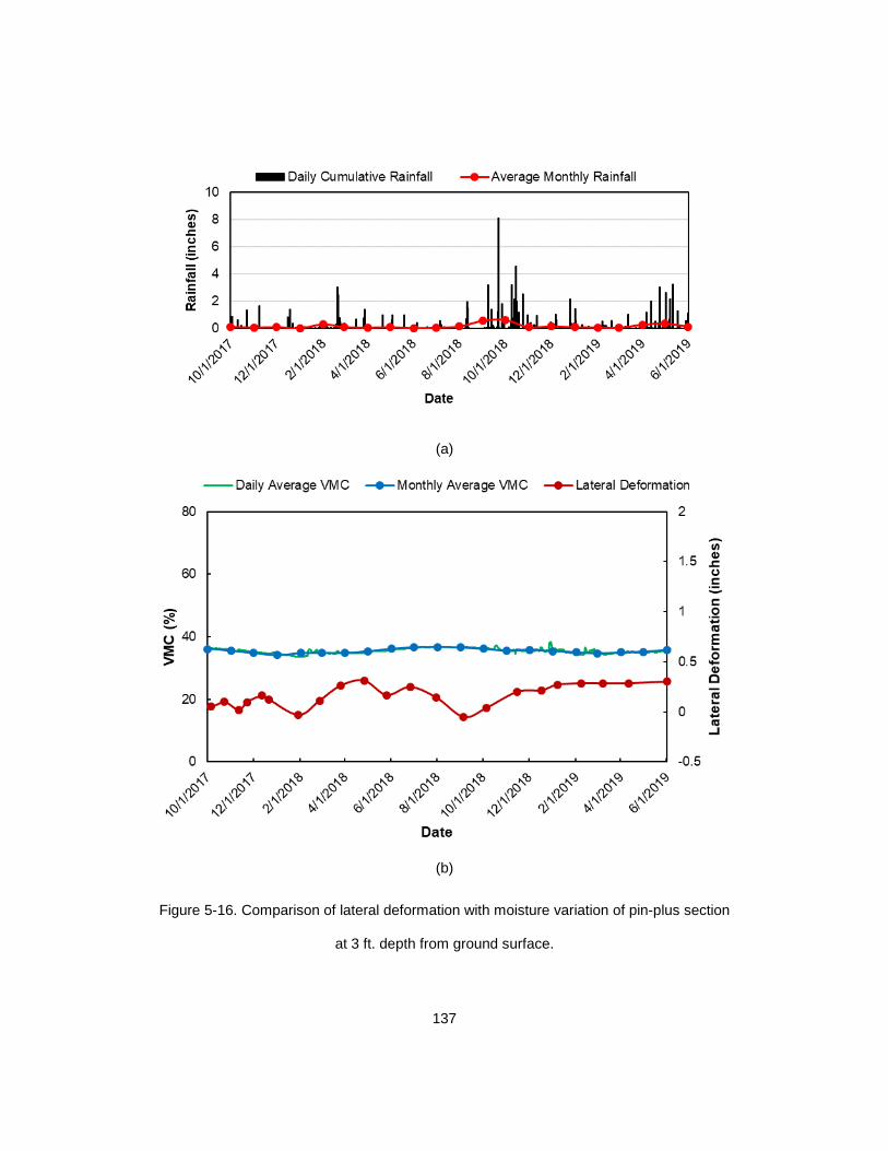
137

(a)

(b)

Figure 5-16. Comparison of lateral deformation with moisture variation of pin-plus section


138

5.3.5 Comparison of Lateral Deformation of Control Section, Pin-only Section, and Pin-

plus Barrier Section

The lateral deformation results from the inclinometers installed at 3 ft. and 10 ft.

depths in the control section, pin-only section, and pin-plus barrier section were compared

and are shown in Figure 5-17.

(a)

(b)

Figure 5-17. Comparison of lateral deformation of control, pin-only, and pin-plus barrier

sections at (a) 3 ft. depth, and (b) 10 ft. depth.

139

Figure 5-17 shows that the lateral deformation of the control section was higher

than that of the pin-only and pin-plus barrier sections at both 3 ft. and 10 ft. depths.

Additionally, the lateral deformation was synchronous with rainfall events in the control and

pin-only sections, while the pin-plus barrier section showed minimal change in lateral

deformation, even with the rainfall events. The observed changes in the values of lateral

deformation for the control and pin-only sections were probably due to the infiltration of

rainwater. The modified moisture barrier in the pin-plus barrier section prevented the

intrusion of rainwater from the crest portion of the slope, controlling the lateral deformation

of the slope by two times as compared to the pin-only section and three times as compared

to the control section.

The maximum lateral deformation of the control section, pin-only section, and pin-

plus barrier section was compared with the maximum moisture variation in subgrade soil

at 3 ft. depth, and is shown in Table 5-1.

Table 5-1. Comparison of moisture variation and lateral deformation for pin-plus barrier

section, pin-only section, and control section at 3 ft. depth.

Section Maximum Lateral

Deformation (inches)

Maximum Moisture

Variation (%)

Control Section 1.28 32.81

Pin only section 0.71 31.17

Pin plus Barrier Section 0.3024 3.89

The observed moisture content variations for the control and pin-only sections

were 32.81% and 31.17%, respectively, while the moisture variation in the pin-plus barrier

section was relatively insignificant (3.89%). This insignificant variation in moisture content

values was directly reflected in the maximum lateral deformation of the slope. Even though

the pin-only section of the slope was stabilized with recycled plastic pins, its lateral

deformation was more than twice as large as that of the pin-plus barrier section. Based on

140

these preliminary results, the combined use of a modified moisture barrier and RPPs

showed better performance in terms of lateral deformation and moisture variations when

compared to the unreinforced section and section reinforced with RPP alone. Therefore,

the combined use of recycled plastic pins and a modified moisture barrier can significantly

reduce the lateral deformation and moisture variations in subgrade soil, and can be used

as an effective solution for stabilizing slopes.

5.3.6 Comparison with Previous Literature

Even though no prior research has been performed that combines the use of a

modified moisture barrier and RPPs to stabilize rainfall-induced shallow slope failures, the

RPPs are widely used to stabilize shallow slope failures in Missouri, Kansas, and Texas.

The study conducted by Khan (2014) utilized RPPs only to stabilize a slope section

with visible distresses, such as longitudinal edge cracks and edge drops. Three test

sections were reinforced with RPPs, and two were left unreinforced in his study (Figure

5-18). The result of installed Inclinometer 1 and Inclinometer 3 in reinforced sections 1 and

2, respectively, are shown in Figure 5-19 and Figure 5-20, respectively.

141

Figure 5-18. Slope stabilization plan using RPPs (Khan, 2014).


Maximum Lateral Deformation of 1.9 inches after 1 year and 8 months

142


The results showed maximum cumulative displacements of 2.22 inches and 2.503

inches near the surface of the slope at a depth of 2.5 ft. in reinforced section 1 and

reinforced section 2, respectively. Additionally, maximum cumulative displacements of 1.9

and 2 inches were observed one year and eight months after installation, which were higher

than those of the pin-only section.

Other studies conducted by Tamraker (2015) and Hossain et al. (2017) utilized the

RPPs to stabilize the slope located on Interstate Highway 35. Cracks up to 42 feet long

were observed over the shoulder due to surficial movement of the slope. The 85 ft. by 50

ft. slope section was stabilized with 6 rows of RPPs with 3 ft. c/c spacing followed by 6

rows of RPPs with 5 ft. c/c spacing. The results of the inclinometer installed at the crest of

the slope are shown in Figure 5-21.

Maximum Lateral Deformation of 2 inches after 1 year and 8 months

143

Figure 5-21. Cumulative lateral deformation at the crest of I-35 slope.

The results showed a maximum cumulative displacement of 2.80 inches near the

surface of the slope stabilized with RPPs at a depth of 2.5. A maximum cumulative

displacement of 2.3 inches was observed one year and eight months after installation,

which was higher than that of the pin-only section in this study.

The study conducted by Parra et al. (2003) and Loehr and Bowders (2007) on the

Interstate Highway 70 slope site showed a maximum lateral deformation of 0.8 inches

(Figure 5-22). The slope was stabilized with 14 rows of RPPs with 3ft c/c spacing. A total

of 199 RPPs were installed to stabilize the failed slope area. A maximum cumulative

displacement of 0.68 inches was observed one year and eight months after installation,

which was similar to the lateral deformation observed in the pin-only section of this study.


144

Figure 5-22. Inclinometer data from I-2 at I-70 site (Parra et al., 2003).

Another study conducted by Parra et al. (2003) and Loehr and Bowders (2007) on

the Interstate Highway 435 slope site showed a maximum lateral deformation of 1.2 inches

(Figure 5-23). The slope was stabilized with 4 rows of RPPs with 3 ft. c/c spacing in a

transverse direction and 6 ft. c/c spacing in a longitudinal direction, followed by 15 rows of

RPPs with 3 ft. c/c spacing in both directions. A total of 643 RPPs were installed to stabilize

the failed slope area. A maximum cumulative displacement of 1.15 inches was observed

one year and eight months after installation, which is higher as compared to this study.


145

Figure 5-23. Cumulative displacement plot of inclinometer I-2 at I-435 site (Parra et al.,

2003).

This study, utilizing RPPs only, showed a maximum lateral deformation of 0.76

inches at a depth of 2 ft. one year and eight months after installation, which is similar to the

study conducted by Parra et al., (2003) and Loehr and Bowders (2007) on the Interstate

Highway 435 slope site, and is comparatively lower as compared to the study conducted

by Khan (2014) on US Highway 287, Tamrakar (2015) on Interstate Highway 1-35, and

Parra et al., (2003) on Interstate Highway I-70. The study conducted by Khan (2014) on

US Highway 287 and Tamrakar (2015) on Interstate Highway 1-35 did not fix the shoulder

cracks after stabilizing the slope with RPPs. The presence of the shoulder cracks allowed

a passageway for rainwater intrusion, and might have caused the higher value of lateral

deformation as compared to our pin-only section. The study conducted by Parra et al.,

(2003) on Interstate Highway I-70 utilized higher spacing than our pin-only section, which

might be one of the reasons for higher lateral deformation. However, as compared to all of

the previous studies with RPPs, the pin-plus barrier section, i.e., the slope stabilized with

both RPPs and MMB, showed even lower lateral deformation (Figure 5-24). Therefore, we


146

can conclude that using a modified moisture barrier and RPPs is more effective in

controlling lateral deformation in the slope than using only RPPs.

Figure 5-24. Comparison of lateral deformation of pin-only and pin-plus barrier section

with previous literature for 1 year, 8 months period.

5.4 Topographic Survey

The vertical deformation of control, pin-plus barrier, and pin-only sections was

monitored using topographic survey. The survey over the stabilized and unstabilized slopes

were conducted in January 2018 for the first time, after the repaving/ asphalt patching of

the pin-plus barrier section. The survey was continued on a monthly basis to assess the

settlement of the control, pin-plus barrier, and pin-only sections. During the survey, the

cracked zones over the shoulder were monitored; however, for more comprehensive

understanding of the settlement, two additional survey lines were established across the

slope. The survey lines are designated as S-1, S-2, and S-3, and are presented in Figure

147

5-25. During the survey, 3 permanent points were utilized to align the periodically

monitored data. Among the permanent points, 2 of them were located on the base of pole,

while the third point was located on the top of drainage ditch. The survey points were

observed each month during the field survey, which were then aligned during analysis to

capture the actual incremental movement of the slope. The result of survey line S-1, S-2,

and S-3 are presented in the subsequent topic.

Figure 5-25. Location of survey lines.

S-1

S-2

S-3

148

5.4.1 Vertical Settlement at Survey Line-1 ( Pavement Deformation at Edge)

The results of survey line S-1 is presented in Figure 5-26. The survey line was

located parallel to the highway, 4 ft. from the edge of shoulder, as shown in Figure 5-25.

It can be noted that during a period of almost two years, the average settlement along the

survey line S-1 in the control and pin-only sections was found to be 0.6 and 0.34 inches,

respectively, while the settlement in the pin-plus barrier section was found to be 0.192

inches. It is evident from the results and from comparison with the pin-only and control

sections, that the combination of modified moisture barrier and recycled plastic pins is more

effective at controlling pavement deformation at the edge.

Figure 5-26. Vertical settlement at survey line S-1.

149

5.4.2 Vertical Settlement at Survey Line-2 (Edge Drop-off)

The result of survey line S-2 is presented in Figure 5-27. The survey line was

located parallel to the highway near the edge of shoulder, as shown in Figure 5-25. It can

be noted that during a period of almost two years, the average settlement along survey line

S-2 in the control and pin-only sections was 2.65 and 1.61 inches, respectively, while the

settlement in the pin-plus barrier section was 0.6068 inches. It is evident from the results

and from comparisons with the pin-only and control sections, that the combination of a

modified moisture barrier and recycled plastic pins is more effective at controlling the edge

drop off at the crest of slope.

Figure 5-27. Vertical settlement at survey line S-2 (Crack survey).

150

5.4.3 Vertical Settlement at Survey Line S-3

The result of survey line S-3 is presented in Figure 5-28. The survey line was

located parallel to the highway, 10 ft. away from the edge of the shoulder, along the slope

shown in Figure 5-25. It can be noted that during a period of almost two years, the average

settlement along the survey line S-3 in the control and pin-only sections was 3.53 and 1.29

inches, respectively, while the settlement in the pin-plus barrier section was 0.69 inches. It

is evident from the results and in comparison with the pin-only and control sections, that

the combination of a modified moisture barrier and recycled plastic pins is more effective

at controlling the vertical deformation of slopes.

Figure 5-28. Vertical settlement at survey line S-3

151

5.4.4 Comparison with Previous Literature

The study conducted by Khan (2014) utilized RPPs only on a highway section with

visible distresses, such as longitudinal edge cracks and edge drops. Three test sections

were reinforced with RPPs, and two were left unreinforced in his study (Figure 5-18). The

performance of these slopes was monitored, using inclinometers and topographic surveys.

The results of topographic survey conducted at the crest of the slope are shown in Figure

5-29.

Figure 5-29. Vertical settlement at the crest of US 287 slope site (Rauss, 2019).

The result of the topographic survey conducted on the crest of the slope showed

maximum total settlements of 4.99 inches, 7.02 inches, and 6.3 inches in reinforced

sections 1, 2, and 3, respectively, while the control sections 1 and 2 showed maximum total

settlement of 15 inches and 11 inches, respectively, during a 7-year monitoring period

(Rauss, 2019). The maximum settlements observed after a 1 year and 8 month monitoring

period were 4.93 inches, 5.12 inches, and 4.39 inches for reinforced sections 1, 2, and 3,

152

respectively, while control sections 1 and 2 showed vertical settlements of 14.10 inches

and 10.09 inches, respectively.

The values observed by Khan (2014) were comparatively higher than those of the

pin-plus barrier section (1.74 inches), pin-only section (2.83 inches), and control section

(5.07 inches). This is due to the fact that the cracks observed over the shoulder portion

during the site investigation were not fixed during the slope stabilization. These cracks

created a passageway for rainwater intrusion, increasing the vertical settlement of slope.

Our section with both MMB and RPPs minimizes the intrusion of rainwater, thereby

reducing the vertical settlement of the slope.

5.5 Resistivity Variation and Active Zone Determination by Resistivity Imaging

The 2D resistivity imaging was conducted to monitor the subsurface profile of the

side slopes. Moisture sensors installed at the crest of the slope showed moisture variations

only at that particular location. However, the moisture sensors did not give any direct

information regarding the moisture variation at the middle or toe of the slope. Hence, 2D

resistivity imaging was performed monthly along two different lines (RI_1 and RI_2), as

shown in Figure 5-30. One line of resistivity was conducted on the pin-plus barrier section,

and one line was conducted on the control section.

153

Figure 5-30. Location of resistivity lines.

The first line of resistivity imaging in the pin-plus barrier section (RI_1) was parallel

to the roadway, just downstream of the modified moisture barrier. The second line (RI_2)

was in the control section, along the roadway, as an extension of the first resistivity

line(RI_1). The 2D resistivity imaging setup is shown in Figure 5-31.

R-1 R-2

154

Figure 5-31. 2D Resistivity imaging line.

The reasons for choosing these locations for 2D resistivity imaging were two-fold.

First, 2D resistivity imaging could not be performed immediately above the modified

moisture barrier because the hammering of the resistivity electrode might puncture the

geomembrane layer, compromising the overall performance of the modified moisture

barrier. Otherwise, subsurface moisture immediately beneath the modified moisture barrier

would directly correlate with the effectiveness of the modified moisture barrier. Second,

monitoring the moisture variations downstream of the moisture barrier would also allow us

to monitor the effect of the modified moisture barrier on moisture variations at the location

where resistivity was conducted. Hence, these 2D resistivity imaging plots provide a more

comprehensive picture of moisture movement in the test slope. The 2D resistivity imaging

was conducted with the main objective of observing the moisture movement in the slope

and determining the active zones, which were more prominently affected by rainfall events.

The results of the 2D resistivity imaging conducted from November 2017 to March 2019

are presented in this section.

155

For interpretation of the qualitative data presented, an inverse relationship ewas

utilized between resistivity and moisture. The high resistivity value represents lower

moisture content, while low value of resistivity represents higher moisture content. The

scale from red to blue indicates the levels of high and low resistivity values, respectively.

5.5.1 Resistivity Variation and Active Zone in Control section

Resistivity imaging was conducted on a monthly basis in the control section. The

resistivity imaging plots showed a lower resistivity zone from November to April, indicating

the wet season, while higher resistivity zones were observed during the dry season, from

May to October. It can be noticed in the resistivity imaging plots of May 2018, June 2018,

and July 2018 that the values of resistivity were higher than during the other months. This

is because the cumulative monthly rainfall for these months was higher than that of the

other months. A typical resistivity plot for the control section is shown in Figure 5-32.

(a)

(b)

Figure 5-32. Typical 2D resistivity imaging plot (a) Wet season (February 2018) and (b)

Dry season (June 2018).

Further analysis was conducted to determine the active zone and to understand

the seasonal variations. The data was extracted from the resistivity log at the middle of

control section to observe the variations of resistivity with depth. The resistivity data were

156

extracted along the depth of the slope at the middle of control section, as shown in Figure

5-33. It can be seen that a change in the resistivity values followed a narrow band (1-1.5

Ohm) after a 8 ft. depth. Hence, it can be concluded that changes in the moisture are not

significant after 8 ft., meaning that it is an active zone, after which changes in the moisture

are not significant. The resistivity values ranged from 3.8 to 6.7 Ohm-m in the active zone

during the wet season, and reached 11 Ohm-m in the dry season.

Figure 5-33. Resistivity versus depth at the middle of the control section.

5.5.2 Resistivity Variation and Active Zone in Pin plus Barrier Section

Resistivity imaging was also conducted each month in the pin-plus barrier section,

and showed a pattern similar to that of the control section. A typical resistivity plot for the

pin-plus barrier section is shown in Figure 5-34.

157

(a)

(b)

Figure 5-34. Typical 2D resistivity imaging plot (a) Wet season (February 2018) and (b)

Dry season (June 2018).

Similar to the control section, the resistivity imaging plots showed lower resistivity

zones from November to April, indicating the wet season, while higher resistivity zones

were observed from May to October. Further analysis was conducted to determine the

active zone and to understand the seasonal variations. The data was extracted from the

resistivity log at the middle of the pin-plus barrier section to observe the variations of

resistivity with depth. The resistivity data were extracted along the depth of the slope at the

middle of the pin-plus barrier section, as shown in Figure 5-35. . It can be seen from Figure

5-35 that the changes in resistivity values followed a narrow band (1-1.5 Ohm) after a 7 ft.

depth. Hence, it can be concluded that change of moisture is not that prominent after this

depth. This depth can be considered an active zone, after which change of moisture is not

significant. This finding also supports the data obtained from the sensors. The resistivity

values ranged from 3.3 to 6.7 Ohm-m in the active zone during the wet season, and

reached 9.8 Ohm-m in the dry season.

158

Figure 5-35. Resistivity versus depth at the middle of pin-plus barrier section.

5.6 Visual Survey Results

The visual surveys were performed monthly on the control section, pin-plus barrier

section, and pin-only section, and the results are described in the following section.

5.6.1 Pin-plus Barrier Section

Figure 5-36 shows pictures taken at four different times to monitor the condition of

the pin-plus barrier section. No cracks or edge drop-offs were observed during the

monitoring period of 1 year and 8 months (Figure 5-36). This was probably due to the use

of the modified moisture barrier, which prevented the rainwater from intruding the slope,

providing additional resistance against the stability of slope, and controlling the formation

of edge drop-offs and edge cracks.

159

(a) (b)

(c) (d)

Figure 5-36. Pictures of pin-only section taken on: (a) Sep 5, 2017, (b) May 26, 2018, (c)

September 5, 2018, and (d) June 16, 2019.

5.6.2 Pin-only Section

Figure 5-37 shows pictures taken at four different times to monitor the condition of

the pin-only section. The pin-only section was stabilized in August, 2017, and edge cracks

started to appear during the dry season, in May 2018. While comparing the pictures taken

in May, June, and September, the propagation of edge cracks, which were probably

caused by the intrusion of rainwater from the crest of the slope, can be observed. Moreover,

160

the cracks located at the edge of the slope allowed an easy passageway for the water to

enter the highway subgrade, reducing the stability of the slope.

(a) (b)

(c) (d)

Figure 5-37. Pictures of pin-only section taken on: (a) Sept. 5, 2017, (b) May 26, 2018,

(c) September 5, 2018, and (d) June 16, 2019.

5.6.3 Control Section

Figure 5-38 shows pictures taken at four different times to monitor the conditions

of the highway slope and shoulder of the control section. The development of edge cracks

and edge drops can be seen, and when comparing the May, June, and September pictures,

further deterioration is obvious. This deterioration was probably due to the rainwater

161

intrusion at the crest of slope. The cracks located at the edge of the slope allow easy

passageway for the intrusion of rainwater saturating the crest of slope, i.e., increasing the

driving force and reducing the stability of the slope. Actually, the slope near the vicinity of

control section failed after prolonged rainfall events on November 2018 (Figure 5-39 (b)).

The location of the failure was just beyond the control section, as shown in Figure 5-39 (a).

(a) (b)

(c) (d)

Figure 5-38. Pictures of control section taken on: (a) Sept. 5, 2017, (b) May 26, 2018, (c)

September 5, 2018, and (d) June 16, 2019.

162

(a)

(b)

Figure 5-39. (a) Location of failed slope, (b) Failed slope adjacent to control section.

Figure 5-39 shows the failed slope, as well as the pin-only section and the pin-

plus barrier section, which is clear empirical evidence that our method was effective in

controlling an imminent shallow slope failure. The visual survey results clearly depict the

effectiveness of the pin-plus barrier section at controlling longitudinal edge cracks, edge

drops, and shallow slope failures.

163

5.7 Effectiveness of Current Stabilization Method

The effectiveness of the current stabilization method can be evaluated in terms of

moisture variations, lateral deformations, vertical settlements, active zones, and visible

distresses. The results of the performance monitoring are summarized in Table 5-2. . The

volumetric moisture content measured in the control and pin-only sections showed

instantaneous response to rainfall events, while the volumetric water content measured in

the pin-plus barrier section showed insignificant variations, even with the rainfall events.

The maximum moisture variation of the control and pin-only sections was 32.81%, while

the pin-plus barrier showed a maximum moisture variation of 3.89%. This variation in

moisture content directly reflected the slopes’ values of lateral deformation and vertical

settlement. Maximum lateral deformations of 1.5 inches and 0.8 inches were observed in

the control and pin-only sections, while only 0.38 inches of lateral deformation was

observed in the pin-plus barrier section, which is 4 and 2.1 times lower than the control and

pin-only sections, respectively.

Additionally, the average vertical settlement in the control section was 2.65 inches,

and 1.61 inches in the pin-only section. Only 0.59 of vertical settlement was observed in

the pin-plus barrier section, which is 4.5 lower than the control section and 2.7 times lower

than the pin-only section.

The use of a modified moisture barrier helped to reduce the moisture

fluctuation zone by 1 ft. Therefore, after summarizing all of the results, it can be concluded

that the pin-plus barrier section is more effective at controlling moisture intrusion, lateral

deformation, vertical settlements, and active zones than the pin-only and control sections.

164

Table 5-2. Summary of performance monitoring results.

Section

Maximum

Moisture

Content

(%)

Maximum

Lateral

Deformation

(In)

Average

Vertical

Settlement

(In)

Active

Depth

(ft)

Current Slope

Condition/Remarks

Control 32..81 1.5 2.65 8

• Edge drop-off up to

2.65 inches and edge

cracks of width 1 to 1.5

inches were observed

in control section

Pin-only 31.17 0.8 1.61 8

• Edge cracks of width

0.2 to 0.3 inches were

observed in pin-only

section

Pin-plus

barrier 3.89 0.38 0.59 7

• No cracks were

observed in pin plus

barrier section

165

CHAPTER 6. NUMERICAL STUDY

6.1 Background

The results and analysis of a numerical study conducted, using 2D finite element

software, PLAXIS 2D are presented in this chapter. Since the current study stabilized a

failed highway embankment with an edge drop-off of 20 inches, the numerical model was

calibrated using initial slope condition observed during preliminary site investigation

conducted on 2017. Both deformation analysis and safety analysis were performed, using

the calibrated model for the pin-only and pin-plus barrier sections, and the results of the

deformation analysis were compared with the results of the performance monitoring over

a period of one year and eight months. In addition, the numerical model was used to

evaluate the performance of the pin-only and pin-plus barrier sections in terms of maximum

horizontal deformation, vertical deformation, bending moment, moment transfer, and factor

of safety. The factor of safety calculated from the numerical model was also compared with

hand calculations, using the ordinary method of slices. Finally, the numerical model was

used to determine the effect that the length of the Modified Moisture Barrier (MMB) has on

the stability of slopes and design steps.

The detailed procedures of the numerical analysis performed to evaluate the

effectiveness of the slope stabilized with both Recycled Plastic Pins (RPPs) and MMB are

explained in the following sections.

6.2 Finite Element Based Numerical Model

The numerical modeling was performed, using the two-dimensional finite element

program, PLAXIS 2D, which was developed for the purpose of analyzing slope stability

problems, plastic deformations, and groundwater flow problems in various geotechnical

engineering applications (PLAXIS 2019). The plain strain model was utilized to create 2D

166

model geometry in the PLAXIS 2D platform, using the X-axis and Y-axis. The plain strain

model is generally used when the geometry is infinitely long in the z-direction, with uniform

cross sections, stress states, and loading schemes. The displacements and strains are

assumed to be zero in the z-direction, and the normal stresses in the z-direction are fully

considered.

Several soil models can be utilized in the PLAXIS 2D platform, such as the linear

elastic model (LE), Mohr-Coulomb model (MC), hardening soil model (HS), soft soil model

(SS), soft soil creep model (SSC), jointed rock model (JR), modified cam-clay model

(MCC), NGI-ADP model, Hoek-Brown model, Sekiguchi-Ohta model, and user-defined

model (UD) (PLAXIS 2019). The elastic perfectly plastic Mohr-Coulomb soil model with 15-

node triangle element was utilized to perform both stability and deformation analysis,

because it provides the first order approximation of real soil behavior. The 15-node triangle

element was utilized since it provides a fourth-order interpolation for displacements, and

the numerical integration involves twelve Gauss points (stress points), making it a very

accurate element for producing high-stress results for difficult problems (PLAXIS 2019).

Five parameters are required to perform the elastic perfectly plastic Mohr-Coulomb

soil model: unit weight (γ), Young’s modulus (E), Poisson’s ratio (ν), cohesion (c), and

friction angle (φ)). The parameters for each soil layer were determined from collected soil

samples, by performing laboratory tests.

The FE model was created by drawing the 2D model geometry, using the actual

dimensions of the slope utilized for the field study, and the geotechnical drilling and soil

test results were utilized to create soil layers and to specify the material properties,

respectively. After creating the model geometry and specifying the material properties, the

boundary conditions were applied to the upper, lower, and side boundaries. The bottom

boundary (y-minimum) was fully fixed, the top boundary (y-maximum) was fully free, and

167

the side boundaries (x-minimum and x-maximum) were fixed horizontally. Once the

boundary conditions were applied, very fine mesh (033 ft.) was used to generate the finite

element mesh. Then, the initial phase was calculated, using gravity loading before

conducting plastic deformation and stability analyses. The plastic deformation analysis was

performed to determine the horizontal and vertical deformation on stabilized and

unstabilized slopes, and the slope stability analysis was performed, using the shear

reduction method (phi-C reduction analysis), to determine factor of safety of stabilized and

unstabilized slopes.

The finite element model was generated to simulate stabilized (pin-only and pin-plus

barrier sections) and unstabilized slopes (control section). To simulate the numerical model

similar to the initial field condition, the model calibration was done for unstabilized slopes.

The model calibration procedure is explained in the following topic.

6.3 Model Calibration

Model calibration is considered as an important step before performing any FE

modelling. The FE model calibration was performed for the control section, using the initial

field condition (failed slope with 20-inch edge drop-off). The model calibration procedure

for simulating the initial slope condition is explained in following topic.

6.3.1 Model Calibration of Control Section

The model calibration of the control section was performed by utilizing the initial

condition of the slope, back in 2017, when the initiation of shallow slope failure was first

observed. The selected highway slope for the current study had massive longitudinal edge

cracks and a maximum edge drop of 20 inches at the crest of the slope. The longitudinal

edge cracks, edge drops, and shallow slope failure in 2017 are shown in Figure 6-1.

168

(a)

(b) (c)

Figure 6-1: (a) Shallow slope failure, (b) Edge cracks, and (c) Edge drop of 20 inches in

year 2017.

Back analysis was performed in two steps, using PLAXIS 2D to simulate the initial

failure condition in 2017 in the FE model. A safety analysis was performed to simulate the

shallow slope failure, and a deformation analysis was performed to simulate the edge drop

of 20 inches.

The modelling was performed, considering three layers of soils. The top 8 feet of

soil was modeled with fully softened strength, because the moisture fluctuation zone, i.e.,

169

active zone, observed from the installed moisture sensors and resistivity imaging, extended

up to 8 feet. Due to the repeated wetting and drying cycles in the active zone, the first 8

feet of the soil was subjected weathering action, thereby reducing the strength of the soil

to fully softened strength. The numerical study conducted by Khan (2014) considered the

top 7 feet of soil with fully softened strength as the failure zone. All of the other soil layers

(Soil 2 and Soil 3) were modeled, based on the soil test results performed on the collected

soil samples. The slope geometry used in the PLAXIS 2D modeling is shown in Figure 6-2.

Figure 6-2. Soil geometry of control section.

The numerical model was calibrated in two steps, using back analysis. First, the

back analysis was performed to determine the critical soil parameters corresponding to

limiting factor of safety equals to 1. Second, the model was further recalibrated, using

plastic deformation analysis to determine the soil parameter corresponding to the

anticipated vertical deformation of 20 inches at the crest, which was observed in the field

in 2017. Several iterations were performed in both steps during the numerical analysis to

evaluate the soil parameters at the failure stage, which is equivalent to the initial field

condition. The calibrated soil parameters at failure, derived from the numerical modeling,

are shown in Table 6-1.

SOIL 2

SOIL 1

SOIL 3

170

Table 6-1. Parameter from finite element analysis.

Soil Layers

-

Unit Weight

γ (pcf)

Cohesion c

(psf)

Angle of friction

φ (degree)

Poisson Ratio

ν -

Modulus of Elasticity

E (psf)

Soil 1 110 50 12 0.35 1150

Soil 2 115 350 15 0.3 100000

Soil 3 120 1000 25 0.25 200000

The deformation and factor of safety, using the calibrated soil parameter, were

found to be 20 inches and 1.04, respectively, which was very close to the field condition in

2017. The results of the back analysis are shown in Figure 6-3.

(a)

171

(b)

Figure 6-3 Back analysis showing: (a) vertical settlement of 20 inches at crest of slope

and (b) factor of safety of 1.04 for control section.

6.4 Numerical Modelling of Pin-only Section

The numerical modeling of the pin-only section was performed by utilizing soil

parameters identical to those of the control section. Since no methods were utilized to

control moisture intrusion. and the moisture fluctuation extended up to 8 feet in the pin-only

section, the top 8 feet of the soil layer was modeled with fully softened strength. All other

soil layer (Soil 2 and Soil 3) properties were based on the laboratory testing shown in Table

6-1. The model geometry for the pin-only section is shown in Figure 6-4.

Figure 6-4. Model geometry for pin-only section.

The RPPs used in the pin-only section were modeled, using a plate element with

the properties listed in Table 6-2. The properties of RPPs listed in Table 6-2 were based

RPPs SOIL 2

SOIL 1

SOIL 3

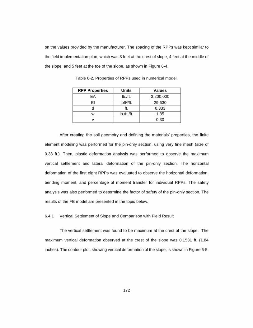
172

on the values provided by the manufacturer. The spacing of the RPPs was kept similar to

the field implementation plan, which was 3 feet at the crest of slope, 4 feet at the middle of

the slope, and 5 feet at the toe of the slope, as shown in Figure 6-4.

Table 6-2. Properties of RPPs used in numerical model.

RPP Properties Units Values

EA lb./ft. 3,200,000

EI lbft2/ft. 29,630

d ft. 0.333

w lb./ft./ft. 1.85

ν 0.30

After creating the soil geometry and defining the materials’ properties, the finite

element modeling was performed for the pin-only section, using very fine mesh (size of

0.33 ft.). Then, plastic deformation analysis was performed to observe the maximum

vertical settlement and lateral deformation of the pin-only section. The horizontal

deformation of the first eight RPPs was evaluated to observe the horizontal deformation,

bending moment, and percentage of moment transfer for individual RPPs. The safety

analysis was also performed to determine the factor of safety of the pin-only section. The

results of the FE model are presented in the topic below.

6.4.1 Vertical Settlement of Slope and Comparison with Field Result

The vertical settlement was found to be maximum at the crest of the slope. The

maximum vertical deformation observed at the crest of the slope was 0.1531 ft. (1.84

inches). The contour plot, showing vertical deformation of the slope, is shown in Figure 6-5.

173

Figure 6-5. Plastic deformation analysis of pin-only section showing vertical settlement

(Uy) contour at every FE node.

The vertical settlement observed from the FE model was compared with that of the

field monitoring results. The vertical settlement at the same location as the survey line (S2)

was 0.1341 ft. (1.6092 inches), as determined by the FE modeling shown in Figure 6-6(a).

The observed value of vertical settlement was found to be 1.6050 inches, which was

identical to that of the field monitoring value, as shown in Figure 6-6(b).

Maximum Settlement observed at crest of

slope

174

(a)

(b)

Figure 6-6. (a) Vertical settlement (Uy) at the crest of the slope (at the same location as

survey line S2) using numerical model, (b) Comparison of vertical settlement observed

from numerical model with field monitoring value.

6.4.2 Horizontal Deformation of Slope and Comparison with Field Results

A plastic deformation analysis was performed to determine the lateral deformation

of the pin-only section. The maximum lateral deformation was found to be 0.1153 ft. (1.384

inches). The contour plot, showing the lateral deformation of the slope, is shown in Figure

6-7.

175

Figure 6-7. Plastic deformation analysis of pin-only section showing lateral deformation

(Ux) contour at every FE node.

The maximum lateral deformation at the inclinometer location (I-2) of the pin-only

section was determined as 0.07124 ft. (0.8548 inches) by the FE modeling shown in Figure

6-8 (a), which was similar to that of the field monitoring value of 0.8238 inches. The lateral

deformation measured during the field monitoring from inclinometer I2 located in the pin-

only section was compared with the FE modeling result and is shown in Figure 6-8 (b).

Maximum lateral deformation observed at crest of slope

176

(a)

(b)



monitoring value.

177

6.4.3 Horizontal Deformation of RPP

The study conducted by Khan (2014) showed that the RPPs located at the crest

of the slope deformed more horizontally than those at the middle and toe of the slope.

Hence, the horizontal deformation of the first eight RPPs was evaluated to observe the

horizontal deformation of RPPs located at the crest of the slope, which is the most probable

location for the initiation of slope failure.

The horizontal deformation of the first eight rows of RPPs near the crest of the

slope is shown in Figure 6-9. Based on the horizontal deformation versus depth plot (Figure

6-9), the maximum horizontal deformation observed in the second and third rows of RPPs

was 1.03 and 0.89 inches, respectively. The horizontal deformation of RPPs decreases

with the increase of RPP depth. Rotational movement was also observed in the second

row of RPPs, which was generally due to the short pile action that takes place due to

insufficient anchorage beneath the foundation soil. In the current study, the RPPs had only

2 ft. of anchorage from the foundation soil, which resulted in short pile action. The RPP

length can be increased to reduce the rotational movement of RPPs at the crest of slope.

178

Figure 6-9. Horizontal displacement of first 8 rows of RPPs in pin-only section.

6.4.4 Bending Moment and Moment Transfer of RPP

The bending moment distribution along the length of RPPs in the first eight rows

located at the crest of the pin-only section were analyzed, using the FE model in PLAXIS

2D. The results of the analysis are presented in Figure 6-10.

179

Figure 6-10. Bending moment of first 8 rows of RPPs in pin-only section.

The maximum bending moment versus depth of the RPP plot showed that the maximum

bending moment of 642.81 lbf-ft was observed in second row of the RPPs, which was three

3 feet away from the edge of pavement, near the interface of the foundation soil and topsoil.

The percentage of moment transfer along the length of the RPPs was calculated, using

Equation 6-1, and is shown in Figure 6-11. The maximum moment capacity of the RPP

(𝑀𝑚𝑎𝑥) in Equation 6-1 was calculated as 3555.56 lbf-ft., using the ultimate flexural strength

of 4 ksi (Khan 2014) and section modulus of 10.67 in3.

𝑃𝑒𝑟𝑐𝑒𝑛𝑡𝑎𝑔𝑒 𝑜𝑓 𝑀𝑜𝑚𝑒𝑛𝑡 𝑇𝑟𝑎𝑛𝑠𝑓𝑒𝑟 (%) = 𝐵𝑒𝑛𝑑𝑖𝑛𝑔 𝑀𝑜𝑚𝑒𝑛𝑡 𝑜𝑓 𝑅𝑃𝑃, 𝑀

𝑀𝑎𝑥𝑖𝑚𝑢𝑚 𝑀𝑜𝑚𝑒𝑛𝑡 𝐶𝑎𝑝𝑎𝑐𝑖𝑡𝑦, 𝑀𝑚𝑎𝑥 (6-1)

180

Figure 6-11. Percentage of moment transfer of first 8 rows of RPPs in pin-only section.

As shown in Figure 6-11, the maximum moment transfer of 18.08% occurred in the

second row of the RPPs. Chen et al. (2007) studied the creep behavior of the RPPs used

in soli stabilization, and concluded that RPPs subjected to moment transfer less than 35%

have a service life of at least 100 years. Hence, under current loading conditions, the RPPs

in the pin-only section can be expected to have a service life of at least 100 years.

181

6.4.5 Slope Stability Analysis

The safety analysis for the pin-only section was performed, using the shear

reduction method (phi-C reduction analysis) to determine the factor of safety and to

observe the critical failure slip surface. The factor of safety for the pin-only section was

found, from the FE model, using PLAXIS 2D, to be 1.594 (Figure 6-12). The utilization of

RPPs in slope stabilization provides additional shear strength along critical failure surfaces,

increasing the factor of safety from 1.04 (control section) to 1.594 (pin-only section).

Figure 6-12. Slope stability analysis for pin-only section with factor of safety of 1.594.

6.5 Numerical Modelling of Pin-plus Barrier Section

The FE model was used to evaluate the performance of the pin-plus barrier

section, which was stabilized with RPPs and MMB. The studies conducted by Sapkota et

al. (2019a and 2019b) showed that MMBs significantly reduce the percentage of moisture

fluctuation at the crest of slope, and are more effective at reducing the horizontal

deformation of slopes than RPPs only. The MMB was 50 feet long and 12 feet wide, and

was located at the crest of the slope. The spacing and layout of the RPPs were identical to

those in the pin-only section to compare the effect of the MMB on the slope stability with

that of RPPs alone.

The numerical modeling of the pin-plus barrier section was performed by utilizing

the soil parameters shown in Table 6-1. The pin-plus barrier section was designed with

182

both RPPs and a modified moisture barrier. The RPPs in the pin-plus barrier section were

modelled as a plate element, with properties identical to those in the pin-only section shown

in Table 6-2. The performance monitoring results showed the effectiveness of MMBs at

preventing rainwater intrusion from the crest of the slope. The two-year real-time moisture

fluctuation data from the installed moisture sensors showed less than 4% of moisture

variation underneath the MMB. Based on these results, it can be concluded that the soil

beneath the MMB is not subjected to cyclic swelling and shrinkage behavior. Therefore,

the effect of the MMB in the numerical model was considered by modeling the soil below

the MMB with peak soil strength, similar to that of Soil 1 shown in Figure 6-13. The soil

above the MMB was modeled with fully softened strength, and the top 8 ft. of the soil, where

there was not MMB, was modelled with fully softened strength. All of the other soil layer

(Soil 2 and Soil 3) properties were based on laboratory testing shown in Table 6-1. The

model details for the pin-plus barrier section are shown in Figure 6-13.

(a)

MMB

SOIL 2

SOIL 3

SOIL 1

RPPs

183

(b)

Figure 6-13. (a) Model geometry with MMB and (b) Simplified model geometry without

MMB for pin-plus barrier section.

After creating the soil geometry and defining the materials’ properties, finite

element modeling was performed for the pin-plus barrier section, using very fine mesh size

of 0.33 ft. Plastic deformation analysis was performed to observe the maximum vertical

settlement and lateral deformation of the pin-plus barrier section. The horizontal

deformation of the first eight RPPs was evaluated to observe the horizontal deformation,

bending moment, and percentage of moment transfer of each RPP located at the crest of

the slope. Safety analysis was also performed to determine the factor of safety. The results

of the FE model are presented in the topic below.

6.5.1 Vertical Settlement of Slope and Comparison with Field Result

The vertical settlement was found to be maximum just beyond the MMB, as shown

in Figure 6-14. The maximum vertical settlement in the pin-plus barrier section was 0.05940

ft. (0.7128 inches).

RPPs SOIL 2

SOIL 1

SOIL 3

184

Figure 6-14. Plastic deformation analysis of pin-plus section showing vertical settlement

(Uy) contour at every FE node.

The vertical settlement at the crest of the slope, observed from the FE model, was

found to be less than 0.1 inches, which was less than the field monitoring results. This is

probably due to improper compaction of the subgrade layer during the MMB installation.

The current numerical model did not consider reduction in the strength parameter due to

improper compaction of the subbase layer/subgrade layer in the trench after the MMB was

placed. Hence, the results of survey lines S1 and S2 were not compared with the results

of the FE modeling; instead, the results of the FE model were compared with the vertical

Maximum vertical settlement observed just below MMB

185

survey results from the topographic survey line S3. From the FE modeling shown in Figure

6-15 (a), the observed vertical settlement at survey line S3 was found to be 0.05839 ft.

(0.70068 inches), which was similar to that of the field monitoring value (0.69 inches)

shown in Figure 6-15 (b).

(a)

(b)

Figure 6-15. (a) Vertical settlement (Uy) just below MMB (at the same location as survey

line S3) using numerical model, (b) Comparison of vertical settlement observed from

numerical model with field monitoring value.

186

6.5.2 Horizontal Deformation of Slope and Comparison with Field Results

Plastic deformation analysis was performed to observe the lateral deformation of

the pin-plus barrier section. The maximum lateral deformation was found to be 0.05371 ft.

(0.6445 inches). The contour plot showing the lateral deformation of the slope is shown in

Figure 6-16.

Figure 6-16. Plastic deformation analysis of pin-plus barrier section showing lateral

deformation (Ux) contour at every FE node.

The maximum lateral deformation at inclinometer location I-2 for of the pin-plus

barrier section was determined, using the FE model. The maximum lateral deformation at

inclinometer location I-2 was found, from the FE modeling shown in Figure 6-17 (a), to be

0.02948 ft. (0.3537 inches). The observed value of maximum lateral deformation at

Maximum lateral deformation observed just beyond MMB

187

inclinometer location I-2 was found to be similar to that of the field monitoring value (0.384

inches). The lateral deformation measured during field monitoring from Inclinometer I-2

was compared with the FE modeling result and is shown in Figure 6-17 (b).

(a)

(b)



monitoring value.

188

6.5.3 Horizontal Deformation of RPPs

The horizontal deformation of the first eight rows of RPPs in the pin-plus barrier

section is shown in Figure 6-18. Based on the horizontal deformation versus depth plot

(Figure 6-18), the maximum horizontal deformation observed in the fifth and sixth rows of

RPPs was 0.5 inches and 0.39 inches, respectively. Insignificant horizontal deformation

was observed for the first four rows of RPPs, where MMB was provided. Therefore, it can

be concluded that the use of MMBs significantly reduces the horizontal deformation of

RPPs/slopes underneath it, since it prevents the intrusion of moisture.

Figure 6-18. Horizontal displacement of first 8 rows of RPPs in pin-plus barrier section.

189

6.5.4 Bending Moment and Moment Transfer of RPPs

The bending moment distribution along the length of RPPs for the first eight rows

located at the crest of the pin-plus barrier was analyzed, using the FE model in PLAXIS

2D. The results of the analysis are presented in Figure 6-19.

Figure 6-19. Bending moment of the first 8 rows of RPPs in the pin-plus barrier section.

The maximum bending moment versus depth of the RPPs plot showed that the

maximum bending moment of 604.75 lbf-ft. was observed in the eighth row of RPPs, near

190

the interface of the foundation soil and topsoil. The percentage of moment transfer along

the length of RPPs was calculated using Equation 6-1, and is shown in Figure 6-20. The

maximum moment capacity of the RPP (𝑀𝑚𝑎𝑥) in Equation 6-1 was calculated as 3555.56

lbf-ft., using ultimate flexural strength of 4 ksi (Khan 2014) and section modulus of 10.67

in3.

Figure 6-20. Percentage of moment transfer of first 8 rows of RPPs at pin-plus barrier

section.

191

As shown in Figure 6-20, the maximum moment transfer of 17.01% resulted in the

eighth row of RPPs. Chen et al. (2007) studied the creep behavior of the RPPs used in soil

stabilization, and concluded that RPPs subjected to moment transfer less than 35% have

a service life of at least 100 years. Hence, under current loading conditions, the RPPs in

the pin-plus barrier section can be expected to have a service life of at least 100 years.

6.5.5 Slope Stability Analysis

The safety analysis for the pin-plus barrier section was performed, using the shear

reduction method (phi-C reduction analysis) to determine the factor of safety of the pin-

plus barrier section and critical failure depth of the slip surface. The factor of safety was

found to be 1.632 from the FE model, using PLAXIS 2D, and is shown in Figure 6-21.

Figure 6-21. Slope stability analysis for pin-plus barrier section with factor of safety 1.632.

The pin-plus barrier section was stabilized with both RPPs and MMB. The

utilization of RPPs in slope stabilization provides additional shear strength along critical

failure surfaces, and the addition of MMB to RPP-stabilized slopes further increases

resistance to failure by preventing the intrusion of rainwater from the crest of slope along

the critical slip surface. The use of MMB reduced the moisture fluctuation to less than 4%

at the crest of slope. Hence, the soil below the MMB was modeled based on laboratory soil

test results, while the top 8 feet of soil, which was exposed to moisture fluctuations, was

192

modelled using the fully softened shear strength parameter. The soil in fully softened state

has relatively lower shear strength, resulting in less resistance against slope failure.

Moreover, the installation of MMB prevents moisture intrusion, thereby preserving its

original strength and improving the stability of the slope. The results from the stability

analysis showed that the utilization of MMB, in addition to RPPs, increased the shear

strength along the critical failure surface, thereby increasing the factor of safety from 1.594

(pin-only section) to 1.632 (pin-plus barrier section).

6.6 Comparison of Test Sections

The maximum horizontal deformation, maximum vertical deformation, and factor

of safety results, along with the critical failure slip surface results from FE modeling for the

control section, pin-only section, and pin-plus barrier section were compared to evaluate

their performance (Figure 6-22 and Figure 6-23). Based on the results of the FE modeling,

shown in Figure 6-22 (a), the maximum horizontal deformation and maximum vertical

deformation were found to be 0.64 inches and 0.71 inches, respectively, for the pin-plus

barrier section; 1.38 inches and 1.84 inches, respectively, for the pin-only section; and

20.57 inches and 20.00 inches, respectively, for the control section. The results showed

that the use of MMB in the pin-plus barrier section reduced the maximum horizontal and

vertical deformation of the slope by 0.7 inches and 1.13 inches, respectively, as compared

to the pin-only section, and 19.93 inches and 19.29 inches as compared to the control

section. Hence, we can conclude that the pin-plus barrier section more effectively

controlled the lateral and horizontal deformation of the slopes than either the pin-only

section or the control section.

The results from the safety analysis of the control section, pin-only section, and

pin-plus barrier section (Figure 6-22 (b)) showed factors of safety of 1.632, 1.594, and 1.04,

respectively. These results showed that the pin-plus barrier section was more effective at

193

increasing the factor of safety, by providing more resistance to slope failure, than either the

pin-only section or control section.

(a)

(b)

Figure 6-22. Comparison of (a) Maximum horizontal deformation and maximum vertical

deformation, and (b) Factor of safety for control section, pin-only section, and pin-plus

barrier section.

The critical slip surfaces of the control, pin-only, and pin-plus barrier sections were

also compared and are shown in Figure 6-23 (a), Figure 6-23 (b), and Figure 6-23 (c),

194

respectively. The FE modeling results showed the beginning and end of the critical slip

surface from the crest to the toe of the slopes for the control and pin-only sections. The

beginning and end of the critical slope surface for the pin-plus barrier section was observed

just beneath the MMB to the toe of slope since the use of MMB at the crest of the slope

prevents the intrusion of moisture in the slope and soil-moisture fluctuation. Eliminating

moisture fluctuation in high plastic expansive clay prevents the cyclic swelling and

shrinkage behavior, which preserves the original shear strength of expansive clay, avoiding

fully softened soil. Consequently, the critical slope surface of the pin-plus barrier section

begins just beneath the MMB, as shown in Figure 6-23 (c).

(a)

(b)

195

(c)

Figure 6-23. Comparison of factor of safety for (a) Control section (FOS = 1.04), (b) Pin-

only section (FOS = 1.594), and (c) Pin-plus barrier section (FOS = 1.632).

6.7 Calculation of Factor of Safety using Ordinary Method of Slices

The ordinary method of slices was used to determine the factor of safety of the

control section, pin-only section, and pin-plus barrier section, and the results were

compared with the results of the FE modeling. The calculation procedure for the ordinary

method of slices, as well as the results and comparisons, are explained in following

sections.

6.7.1 Control Section

The ordinary/conventional method of slices was used to determine the factor of

safety of the control section. The first step in the ordinary method of slices is to determine

the critical failure surface, using several industry-standard software packages, such a Geo-

Studio, GStable, etc., or by performing several trials. The critical failure surface for the

control section was determined in this study by using Geo-Studio software, and is shown

in Figure 6-24.

196

Figure 6-24. Critical slip surface for control section using Geo-Studio.

The ABC arc shown in Figure 6-25 is the circular failure surface with a center of

109.81, 113.77 and radius (r) equal to 92.37 ft. The critical slip surface (ABCA) is divided

into 30 vertical slices with equal widths of 2.36 ft. Considering out-of-plane width of unity,

the force acting on the slice ‘n’ is shown in Figure 6-25 , where ‘W’ is the weight of slice,

N is the normal component of the reaction force, T is the tangential component of the

reaction force, Fn and Fn+1 are normal components of interslice forces acting on the side of

slice, and Tn and Tn+1 are the shearing forces/ tangential components of interslice forces

acting on the sides of the slice. During this analysis, the normal and tangential components

of the interslice forces acting on the two sides of the slice are assumed equal, and opposite

in direction, and are considered to act on the same line of action. The porewater pressure

during this analysis was assumed to be zero.

197

Figure 6-25. Critical slip surface for control section for determining FS.

Here,

Normal component of reaction (N)= W * Cos α

Tangential component of reaction/ Driving Force = W * Sin α

Td = 𝜏𝑑ΔL = 𝜏𝑓

FSΔL =

1

FS∗ (c′ + σ′tanϕ′) ∗ ΔL

where,

W = Weight of slice

𝛼 = Angle between normal component of reaction and vertical axis

𝜏𝑑 = Allowable/design shear stress

𝜏𝑓 = Shear stress at failure

Δ𝐿 = Base width of slice

198

FS = Factor of safety

𝜎′ = Effective stress

𝑐′ = Effective cohesion

𝜙 = Effective angle of internal friction

The normal stress (𝜎′) = 𝑁

Δ𝐿=

𝑊𝑐𝑜𝑠𝛼

Δ𝐿

Now, considering the equilibrium of the trial slip surface (ABC) at the center of slip

circle (o), the resisting moment at the center of slip circle ‘o’ equals the driving moment at

the center of slip circle ‘o’.

Driving Moment at the center of slip circle ‘o’ ( Md )= ∑ 𝑊 ∗ 𝑟 ∗ 𝑆𝑖𝑛𝛼 𝑛=𝑝𝑛=1

Md = ∑ 𝑊 ∗ 𝑟 ∗ 𝑆𝑖𝑛𝛼 𝑛1 (6-2)

Resisting Moment at the center of slip circle ‘o’ Mr = ∑1

FS∗ (c′ + σ′tanϕ′) ∗ ΔL ∗ r

𝑛=𝑝𝑛=1

Mr =∑1

FS∗ (c′ +


Δ𝐿∗ tanϕ′) ∗ ΔL ∗ r

𝑛=𝑝𝑛=1 (6-3)

Equating equation Eq: 6-1 and Eq: 6-2, we get

∑ 𝑊 ∗ 𝑟 ∗ 𝑆𝑖𝑛𝛼

𝑛=𝑝

𝑛=1

= ∑1

FS∗ (c′ +


Δ𝐿∗ tanϕ′) ∗ ΔL ∗ r

𝑛=𝑝

𝑛=1

Or, FS = ∑ (c′∗ΔL+𝑊𝐶𝑜𝑠𝛼∗tanϕ′)

𝑛=𝑝𝑛=1

∑ 𝑊∗𝑆𝑖𝑛𝛼 𝑛=𝑝𝑛=1

(6-4)

199

The factor of safety of the control section/unreinforced section can be determined

using Equation 6-5,

Factor of Safety, FS = ∑ (c′∗ΔL+𝑊𝐶𝑜𝑠𝛼∗tanϕ′)

𝑛=𝑝𝑛=1


(6-5)

The details for each vertical slice are presented in Table 6-3. The soil properties

used in this calculation were derived from the soil test results conducted on the collected

soil samples during the site investigation. Only the soil properties of the top layer were

utilized to perform the calculation, since only the top-soil was prone to failure, based on the

observations of the FE modeling. The values of cohesion, angle of friction, and unit weight

of soil were 50 psf, 12°, and 110 pcf, respectively.

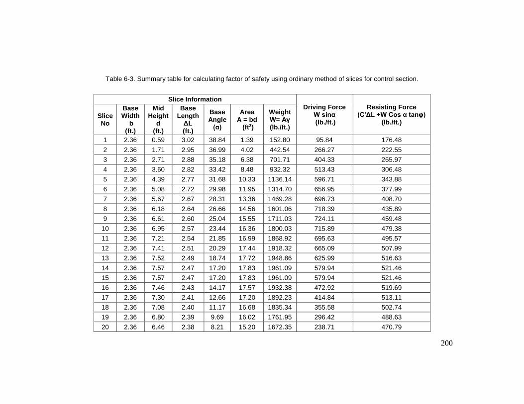
200

Table 6-3. Summary table for calculating factor of safety using ordinary method of slices for control section.

Slice Information

Driving Force W sinα (lb./ft.)

Resisting Force (C'ΔL +W Cos α tanφ)

(lb./ft.) Slice No

Base Width

b (ft.)

Mid Height

d (ft.)

Base Length

ΔL (ft.)

Base Angle

(α)

Area A = bd

(ft2)

Weight W= Aγ (lb./ft.)

1 2.36 0.59 3.02 38.84 1.39 152.80 95.84 176.48

2 2.36 1.71 2.95 36.99 4.02 442.54 266.27 222.55

3 2.36 2.71 2.88 35.18 6.38 701.71 404.33 265.97

4 2.36 3.60 2.82 33.42 8.48 932.32 513.43 306.48

5 2.36 4.39 2.77 31.68 10.33 1136.14 596.71 343.88

6 2.36 5.08 2.72 29.98 11.95 1314.70 656.95 377.99

7 2.36 5.67 2.67 28.31 13.36 1469.28 696.73 408.70

8 2.36 6.18 2.64 26.66 14.56 1601.06 718.39 435.89

9 2.36 6.61 2.60 25.04 15.55 1711.03 724.11 459.48

10 2.36 6.95 2.57 23.44 16.36 1800.03 715.89 479.38

11 2.36 7.21 2.54 21.85 16.99 1868.92 695.63 495.57

12 2.36 7.41 2.51 20.29 17.44 1918.32 665.09 507.99

13 2.36 7.52 2.49 18.74 17.72 1948.86 625.99 516.63

14 2.36 7.57 2.47 17.20 17.83 1961.09 579.94 521.46

15 2.36 7.57 2.47 17.20 17.83 1961.09 579.94 521.46

16 2.36 7.46 2.43 14.17 17.57 1932.38 472.92 519.69

17 2.36 7.30 2.41 12.66 17.20 1892.23 414.84 513.11

18 2.36 7.08 2.40 11.17 16.68 1835.34 355.58 502.74

19 2.36 6.80 2.39 9.69 16.02 1761.95 296.42 488.63

20 2.36 6.46 2.38 8.21 15.20 1672.35 238.71 470.79

201

Slice Information

Driving Force W sinα (lb./ft.)


(lb./ft.) Slice No

Base Width

b (ft.)

Mid Height

d (ft.)

Base Length

ΔL (ft.)

Base Angle

(α)

Area A = bd

(ft2)

Weight W= Aγ (lb./ft.)

21 2.36 6.05 2.37 6.73 14.24 1566.68 183.68 449.28

22 2.36 5.58 2.36 5.26 13.14 1445.11 132.58 424.12

23 2.36 5.05 2.36 3.80 11.89 1307.81 86.64 395.38

24 2.36 4.46 2.36 2.34 10.50 1154.84 47.06 363.11

25 2.36 3.81 2.36 0.87 8.97 986.26 15.05 327.37

26 2.36 3.10 2.36 0.59 7.29 802.12 8.21 288.24

27 2.36 2.33 2.36 2.05 5.48 602.42 21.53 245.79

28 2.36 1.49 2.36 3.51 3.52 387.15 23.71 200.11

29 2.36 0.60 2.36 4.98 1.42 156.20 13.55 151.27

30 1.33 0.07 1.33 6.12 0.09 10.36 1.10 68.82

Total 10846.82 11448.35

From the Table 6-3, the total driving force, ∑ 𝑊 ∗ 𝑆𝑖𝑛𝛼

𝑛=𝑝𝑛=1 = 10846 lbf/ft.

And, the total resisting force, ∑ (c′ ∗ ΔL + 𝑊𝐶𝑜𝑠𝛼 ∗ tanϕ′)𝑛=𝑝𝑛=1 = 11448.35 lbf/ft.

Factor of Safety for Control Section, FS =∑ (c′∗ΔL+𝑊𝐶𝑜𝑠𝛼∗tanϕ′)

𝑛=𝑝𝑛=1


= 11448.35

10846.82= 1.055

The factor of safety, using ordinary method of slices, was found to be 1.055, which was similar to the value obtained from

the FE modeling (FS= 1.04).

202

6.7.2 Pin-only Section


safety of the pin-only section. The critical failure surface was determined. The ABC arc

shown in Figure 6-26 is the critical failure of the pin-only section surface, with a center of

109.81, 113.77, and radius (r) equal to 92.37 ft. The critical slip surface (ABCA) was divided

into 30 vertical slices, with equal widths of 2.36 ft. Considering the out-of-plane width of

unity, the active force acting on the slice ‘n’ is shown in Figure 6-26, where W is the weight

of slice, N is the normal component of the reaction force, T is the tangential component of

the reaction force, P is the limiting resistance due to RPPs, Fn and Fn+1 are normal

components of the interslice forces acting on the sides of the slice, and Tn and Tn+1 are

the shearing forces/ tangential components of interslice forces acting on the sides of the

slice. During this analysis, the normal and tangential components of the interslice forces

acting on two sides of the slice were assumed equal and opposite in direction, and were

considered to act on same line. The porewater pressure during this analysis was assumed

to be zero.

From the Figure 6-26,


Tangential component of reaction/Driving Force = W * Sin α

Total shear strength = Td + Pu

= 𝜏𝑑ΔL + Pu = 1

FS(ΔL ∗ 𝜏𝑓 + 𝑃) =

1

FS∗ ((c′ + σ′tanϕ′) ∗ ΔL + P)

where,


𝜏𝑑 = Allowable shear stress


203

P = Limiting resistance due to RPP

𝜎 = Normal stress


𝑐′ = Cohesion

𝜙 = Angle of internal friction

Δ𝐿 = Angular width of slice

Figure 6-26. Schematic diagram of pin-only section using ordinary method of slice.


Δ𝐿=


Δ𝐿

Now, considering the equilibrium of slip surface (ABC) at the center of slip circle

(o), the resisting moment at the center of slip circle ‘o’ equals the driving moment at the

center of slip circle ‘o’.

204


Md = ∑ 𝑊 ∗ 𝑟 ∗ 𝑆𝑖𝑛𝛼 𝑛1 (6-6)

Resisting Moment at the center of slip circle ‘o’ ( Mr )

= 1

FS[∑ ((c′ + σ′tanϕ′)ΔL) ∗ r

𝑛=𝑝𝑛=1 + ∑ 𝑃

𝑛=𝑞𝑛=1 ∗ r]

Mr =1


𝑛=𝑝𝑛=1 + ∑ 𝑃

𝑛=𝑞𝑛=1 ∗ r] (6-7)

Equating Equation 6-6 and Equation 6-7, we get


𝑛=𝑝

𝑛=1

=1

FS[∑∗ ((c′ +


Δ𝐿∗ tanϕ′) ∗ ΔL) ∗ r

𝑛=𝑝

𝑛=1

+ ∑ 𝑃

𝑛=𝑞

𝑛=1

∗ r]

Or, FS = ∑ (c′∗ΔL+𝑊𝐶𝑜𝑠𝛼∗tanϕ′+∑ 𝑃

𝑛=𝑞𝑛=1 )

𝑛=𝑝𝑛=1


(6-8)

The factor of safety of the pin-only section can be determined by using Equation

6-9,

Factor of Safety, FS = ∑ (c′∗ΔL+𝑊𝐶𝑜𝑠𝛼∗tanϕ′)+∑ 𝑃

𝑛=𝑞𝑛=1

𝑛=𝑝𝑛=1


(6-9)

The additional resistance from the RPPs (P) in Equation 6-9 can be determined by

calculating the load carrying capacity of an individual RPP. Details of the procedure for

calculating the load-carrying capacity of RPPs are provided in the following topic.

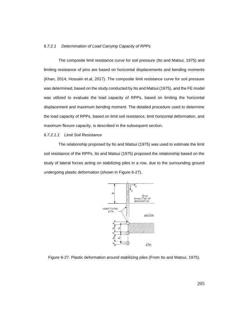
205

6.7.2.1 Determination of Load Carrying Capacity of RPPs

The composite limit resistance curve for soil pressure (Ito and Matsui, 1975) and

limiting resistance of pins are based on horizontal displacements and bending moments

(Khan, 2014; Hossain et.al, 2017). The composite limit resistance curve for soil pressure

was determined, based on the study conducted by Ito and Matsui (1975), and the FE model

was utilized to evaluate the load capacity of RPPs, based on limiting the horizontal

displacement and maximum bending moment. The detailed procedure used to determine

the load capacity of RPPs, based on limit soil resistance, limit horizontal deformation, and

maximum flexure capacity, is described in the subsequent section.

6.7.2.1.1 Limit Soil Resistance

The relationship proposed by Ito and Matsui (1975) was used to estimate the limit

soil resistance of the RPPs. Ito and Matsui (1975) proposed the relationship based on the

study of lateral forces acting on stabilizing piles in a row, due to the surrounding ground

undergoing plastic deformation (shown in Figure 6-27).

Figure 6-27. Plastic deformation around stabilizing piles (From Ito and Matsui, 1975).

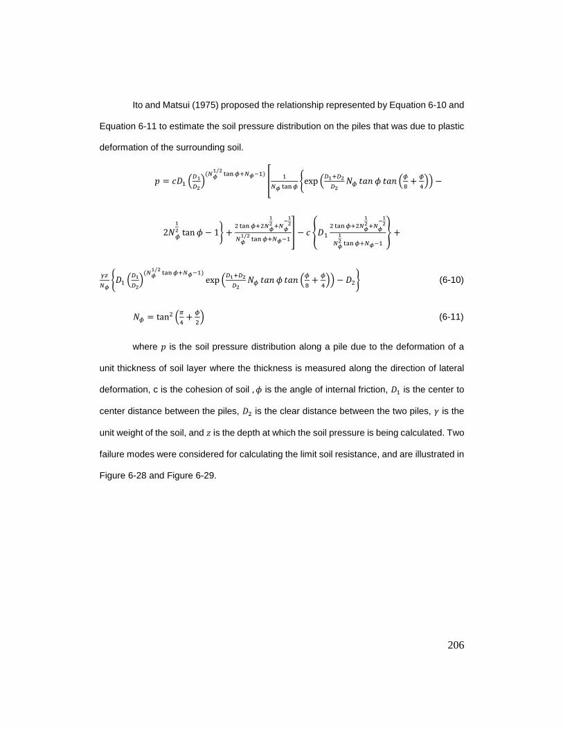
206

Ito and Matsui (1975) proposed the relationship represented by Equation 6-10 and

Equation 6-11 to estimate the soil pressure distribution on the piles that was due to plastic

deformation of the surrounding soil.

𝑝 = 𝑐𝐷1 (𝐷1

𝐷2)

(𝑁𝜙1/2

tan 𝜙+𝑁𝜙−1)

[1

𝑁𝜙 tan 𝜙{exp (

𝐷1+𝐷2

𝐷2𝑁𝜙 𝑡𝑎𝑛 𝜙 𝑡𝑎𝑛 (

𝜙

8+

𝜙

4)) −

2𝑁𝜙

1

2 tan 𝜙 − 1} +2 tan 𝜙+2𝑁

𝜙

12 +𝑁

𝜙

−12

𝑁𝜙1/2

tan 𝜙+𝑁𝜙−1] − 𝑐 {𝐷1

2 tan 𝜙+2𝑁𝜙

12 +𝑁

𝜙

−12

𝑁𝜙

12 tan 𝜙+𝑁𝜙−1

} +

𝛾𝑧

𝑁𝜙{𝐷1 (

𝐷1

𝐷2)

(𝑁𝜙1/2

tan 𝜙+𝑁𝜙−1)

exp (𝐷1+𝐷2

𝐷2𝑁𝜙 𝑡𝑎𝑛 𝜙 𝑡𝑎𝑛 (

𝜙

8+

𝜙

4)) − 𝐷2} (6-10)

𝑁𝜙 = tan2 (𝜋

4+

𝜙

2) (6-11)

where 𝑝 is the soil pressure distribution along a pile due to the deformation of a

unit thickness of soil layer where the thickness is measured along the direction of lateral

deformation, c is the cohesion of soil , 𝜙 is the angle of internal friction, 𝐷1 is the center to

center distance between the piles, 𝐷2 is the clear distance between the two piles, 𝛾 is the

unit weight of the soil, and 𝑧 is the depth at which the soil pressure is being calculated. Two

failure modes were considered for calculating the limit soil resistance, and are illustrated in

Figure 6-28 and Figure 6-29.

207

Figure 6-28. Illustration of failure mode - 1 (Khan 2014).

Figure 6-29. Illustration of failure mode - 2 (Khan 2014).

208

Failure mode-1 is the failure of the soil above the failure surface and subsequent

flow of soil around the RPP above the failure surface (shown in Figure 6-28). In this case,

the soil above the failure surface exerts limiting soil pressure on the RPP. This soil pressure

is given by Equation 6-10 and Equation 6-11. For a fixed 𝑐, 𝜙, 𝛾 and depth of a failure

surface (𝑑𝑓), the limiting resistance offered by the unit thickness of soil layer along the

direction of deformation based on this failure mode-1 is given by Equation 6-12.

𝑃(𝑑𝑓) = ∫ 𝑝𝑑𝑓

𝑧=0𝑑𝑧 (6-12)

Similarly, failure mode-2 is the failure of soil below a plane and subsequent flow of

soil around the RPP below the plane (shown in Figure 6-29). In this case, the soil below

the plane exerts limiting soil pressure on the RPP. This soil pressure is given by Equation

6-10 and Equation 6-11. For a fixed 𝑐, 𝜙, 𝛾, depth of failure surface (𝑑𝑓) and maximum

embedment of RPP (𝐷𝑝) the limiting resistance offered by the unit thickness of soil layer

along the direction of deformation for failure mode-2 is given by Equation 6-13.

𝑃(𝑑𝑓) = ∫ 𝑝𝐷𝑝

𝑧=𝑑𝑓𝑑𝑧 (6-13)

Using the Equations 6-10 to Equation 6-13, the limiting resistance offered by the

soil to the RPPs was calculated for the slope studied in this research. The parameters

utilized are tabulated in Table 6-4. The resulting composite limit resistance curve is shown

in Figure 6-30.

209

Table 6-4. Parameters for calculation of limit soil pressure.

Parameters Value

Cohesion (𝑐) 50 psf

Angle of Internal Friction (𝜙) 12°

Unit Weight (𝛾) 110 pcf

Centre to Centre Spacing of RPP (𝐷1) 3 ft.

Clear Spacing of RPP (𝐷2) 2.667 ft.

Depth of RPP (𝐷𝑝) 9.563 ft.

Thickness of Deforming Soil (t) 3 ft. ( i.e. 𝐷1)

Figure 6-30. Limit soil resistance due to lateral deformation/ flow of soil between the RPP.

210

6.7.2.1.2 Limit Horizontal Displacement and Maximum Flexure Capacity of RPPs

The studies conducted by Wei and Cheng (2009), Khan (2014), Hossain et. al.

(2017), and Cai and Ugai, (2003) showed that the FE method is an accurate, simple, and

robust method for evaluating the stability and deformation of slopes reinforced with anchors

and pile. Therefore, for the current study, the load-carrying capacity of RPPs was

determined, using 2D FE software PLAXIS 2D. The limit horizontal displacement and limit

flexure capacity of individual RPPs were determined, based on the procedure proposed by

Khan (2014). In the current study, the load-carrying capacity of individual RPPs was

determined by applying a series of lateral loads (10, 20, 30, 40, 50, 60, 70, 80, 90, 100,

200, 300, 400, and 500 psf) on RPPS at various depths of slip surface (1, 2, 3, 4, 5, 6, 7,

and 8 ft.). Then, the corresponding maximum lateral deformation and maximum bending

moment were observed.

The design chart developed by Khan (2014) cannot be utilized in the current study

because it doesn’t consider the depth of the slip surface below 7 ft. or above 3 ft. Nor does

it consider cohesion values below 100 psf. The current analysis requires a load-carrying

capacity of RPPs below 3 ft. and above 7 ft. depth, and soil with a cohesion value of 50

psf. Therefore, it was necessary to conduct FE modeling to determine the load-carrying

capacity of the RPPs for site-specific conditions, using the procedure described by Khan

(2014).

The current study considered a wide range of failure depths and lateral loads,

using the soil parameters of the current slope. The flowchart shown in Figure 6-31 includes

the step-by-step procedure for developing the design chart for determining the limit

horizontal displacement and maximum flexure capacity curve for various lateral loadings

on RPPs.

211

Figure 6-31. Flowchart for developing design chart to determine limit horizontal

deformation and maximum bending moment.

Topsoil c= 50 psf

𝜙 = 12

Current Slope

Depth of Slip Surface

1 ft 2 ft 3 ft 4 ft 5 ft 6 ft 7 ft

10 p

sf

20 p

sf

30 p

sf

40 p

sf

50 p

sf

60 p

sf

70 p

sf

80 p

sf

90 p

sf

100 p

sf

200 p

sf

300 p

sf

400 p

sf

500 p

sf

Lateral Pressure on RPP

Response Maximum Flexure

on RPP

Maximum Horizontal

Displacement

Soil 2 c= 350 psf

𝜙 = 15

Soil 3 c= 1000 psf

𝜙 = 25

212

The 2D geometry in the PLAXIS 2D platform, using the X-axis and Y-axis, was

created identical to the field slope geometry, using a plain strain model. Then, the elastic

perfectly plastic Mohr-Coulomb soil model with a 15-node triangle element was utilized to

perform the deformation analysis. The three layers of soil were modelled, using the soil

properties shown in Table 6-1. In addition, the RPPs were modeled as a plate element,

using the properties shown in Table 6-2. The model geometry for determining the load-

carrying capacity of the RPPs is shown in Figure 6-32.

Figure 6-32. Soil model for determining lateral load capacity of RPPs.

The analyzed depths of the topsoil were 2 ft., 3 ft., 4 ft., 5 ft., 6 ft., and 7 ft. The

deformation analysis was performed by applying uniform lateral loads of 10, 20, 30, 40, 50,

60, 70, 80, 90, 100, 200, 300, 400 and 500 psf to every depth, and the corresponding

maximum horizontal deformations and bending moments were observed. The maximum

horizontal displacement and maximum moment bending were then plotted with the applied

lateral load for each sliding depth of slope, and are shown in Figure 6-33 and Figure 6-34,

respectively.

Soil 1

Soil 2

Soil 3

213

Figure 6-33. Lateral load versus maximum horizontal displacement curve at various

depths of slip surface.

Figure 6-34. Lateral load versus maximum bending moment curve at various depths of

failure.

214

6.7.2.1.3 Final Limit Resistance Curve of RPP

The final limit resistance curve was generated to calculate the load-carrying

capacity of RPPs for our study. The soil resistance curve for failure mode 1, soil resistance

curve for failure mode 2, maximum horizontal displacement curve, and maximum flexure

capacity curve were used to determine the load-carrying capacity of RPPs at each failure

depth. The limiting maximum horizontal displacement and bending moment were 1 inch

and 1.4 ksi, respectively. The smallest value of load-carrying capacity of RPPs at each

depth was determined, plotted as the final limit resistance curve, and is shown in Figure

6-35.

Figure 6-35. Final limit resistance curve for RPPs.

6.7.2.2 Calculation of Factor of Safety

The factor of safety for the pin-only section was determined, using Equation 6-9.

The resisting force (c′ ∗ ΔL + 𝑊𝐶𝑜𝑠𝛼 ∗ tanϕ′) and driving force (𝑊 ∗ 𝑆𝑖𝑛𝛼) acting on all

215

vertical slices were calculated by taking the topsoil properties (Table 6-5). Only the soil

properties of the top layer were utilized to perform the calculations, since only the top-soil

was prone to failure, based on observations of the FE modeling. The value of cohesion,

angle of friction, and unit weight of the top layer of soil were 50 psf, 12°, and 110 pcf,

respectively. The value of P (additional resisting force due to RPPs) in Equation 6-9 was

determined, using final resistance curve shown in Figure 6-35. The resisting force (P) due

to RPPs are tabulated in Table 6-6.

216

Table 6-5. Summary table for calculating factor of safety using ordinary method of slices for pin-only section.

Slice Information

Driving Force W sinα (lbf/ft.)


(lbf/ft.) Slice No

Base Width

b (ft.)

Mid Height

d (ft.)

Base Length

ΔL (ft.)

Base Angle

(α)

Area A = bd

(ft2)

Weight W= Aγ (lbf/ft.)

1 2.36 0.59 3.02 38.84 1.39 152.80 95.84 176.48

2 2.36 1.71 2.95 36.99 4.02 442.54 266.27 222.55

3 2.36 2.71 2.88 35.18 6.38 701.71 404.33 265.97

4 2.36 3.60 2.82 33.42 8.48 932.32 513.43 306.48

5 2.36 4.39 2.77 31.68 10.33 1136.14 596.71 343.88

6 2.36 5.08 2.72 29.98 11.95 1314.70 656.95 377.99

7 2.36 5.67 2.67 28.31 13.36 1469.28 696.73 408.70

8 2.36 6.18 2.64 26.66 14.56 1601.06 718.39 435.89

9 2.36 6.61 2.60 25.04 15.55 1711.03 724.11 459.48

10 2.36 6.95 2.57 23.44 16.36 1800.03 715.89 479.38

11 2.36 7.21 2.54 21.85 16.99 1868.92 695.63 495.57

12 2.36 7.41 2.51 20.29 17.44 1918.32 665.09 507.99

13 2.36 7.52 2.49 18.74 17.72 1948.86 625.99 516.63

14 2.36 7.57 2.47 17.20 17.83 1961.09 579.94 521.46

15 2.36 7.57 2.47 17.20 17.83 1961.09 579.94 521.46

16 2.36 7.46 2.43 14.17 17.57 1932.38 472.92 519.69

17 2.36 7.30 2.41 12.66 17.20 1892.23 414.84 513.11

18 2.36 7.08 2.40 11.17 16.68 1835.34 355.58 502.74

19 2.36 6.80 2.39 9.69 16.02 1761.95 296.42 488.63

20 2.36 6.46 2.38 8.21 15.20 1672.35 238.71 470.79

217

Slice Information



(lbf/ft.) Slice No

Base Width

b (ft.)

Mid Height

d (ft.)

Base Length

ΔL (ft.)

Base Angle

(α)

Area A = bd

(ft2)


21 2.36 6.05 2.37 6.73 14.24 1566.68 183.68 449.28

22 2.36 5.58 2.36 5.26 13.14 1445.11 132.58 424.12

23 2.36 5.05 2.36 3.80 11.89 1307.81 86.64 395.38

24 2.36 4.46 2.36 2.34 10.50 1154.84 47.06 363.11

25 2.36 3.81 2.36 0.87 8.97 986.26 15.05 327.37

26 2.36 3.10 2.36 0.59 7.29 802.12 8.21 288.24

27 2.36 2.33 2.36 2.05 5.48 602.42 21.53 245.79

28 2.36 1.49 2.36 3.51 3.52 387.15 23.71 200.11

29 2.36 0.60 2.36 4.98 1.42 156.20 13.55 151.27

30 1.33 0.07 1.33 6.12 0.09 10.36 1.10 68.82

Total 10846.82 11448.35

218

Table 6-6. Load carrying capacity of RPPs (P).

RPP Row

RPP Depth at critical

failure surface

P (lbf/ft.)

1 NA

2 0.88 139.2415

3 1.95 450.2144

4 2.9 627.3351

5 3.75 544.8703

6 4.49 438.7836

7 5.13 349.0845

8 5.67 290.3987

9 6.24 228.4051

10 6.64 184.8549

11 6.87 159.8135

12 6.94 152.1922

13 6.84 163.0798

14 6.58 191.3874

15 6.01 253.4464

16 5.17 344.7374

17 4.06 502.5005

18 2.66 584.201

Total 5604.546

From the Equation 6-9, Table 6-5, and Table 6-6,

Total driving force, ∑ 𝑊 ∗ 𝑆𝑖𝑛𝛼 𝑛=𝑝𝑛=1 = 10846.82 lbf/ft.

Resisting force due to soil shear strength, ∑ (c′ ∗ ΔL + 𝑊𝐶𝑜𝑠𝛼 ∗ tanϕ′)𝑛=𝑝𝑛=1

=11448.35 lbf/ft.

Additional resisting force due to Installed RPPs, P = ∑ 𝑃𝑛=𝑞𝑛=1 =5604.546 lbf/ft.

Factor of Safety for control section, FS =∑ (c′∗ΔL+𝑊𝐶𝑜𝑠𝛼∗tanϕ′)+∑ 𝑃

𝑛=𝑞𝑛=1

𝑛=𝑝𝑛=1


= 11448.35 +5604.546

10846.82 = 1.572

The factor of safety, using the ordinary method of slices for the pin-only section,

was 1.572, which is similar to the results obtained from the FE model (1.594).

219

6.7.3 Pin-plus Barrier Section


safety of the pin-plus barrier section. First, the critical failure surface was determined, as

shown in Figure 6-36. The ABC arc shown in Figure 6-36 was the critical failure surface

with center (109.22, 106.15) and radius (r) equal to 84.39 ft. The critical slip surface (ABCA)

was divided into 30 vertical slices with equal widths of 2.1059 ft. Considering out-of-plane

width of unity, the active force acting on slice ‘n’ is shown in Figure 6-36, where W is the

weight of slice, N is the normal component of the reaction force, T is the tangential

component of the reaction force, P is the limiting resistance due to RPPs, Fn and Fn+1

are normal components of the interslice forces acting on the sides of the slice, and Tn and

Tn+1 are the shearing forces/tangential components of the interslice forces acting on the

sides of the slice. During this analysis, the normal and tangential components of interslice

forces acting on two sides of the slice were assumed equal and opposite in direction, and

were considered to act on same line of action. The porewater pressure during this analysis

was assumed to be zero.

220

Figure 6-36. Critical slip surface of pin plus barrier section using ordinary method of

slices.

Here,


Tangential component of reaction/Driving Force = W * Sin α

Total shear strength = Td + Pu

= 𝜏𝑑ΔL + Pu = 1

FS(ΔL ∗ 𝜏𝑓 + 𝑃) =

1

FS∗ ((c′ + σ′tanϕ′) ∗ ΔL + P)

where,


𝜏𝑑 = Allowable shear stress


P = Limiting Resistance due to RPP

221

𝜎 = Normal stress


𝑐′ = Cohesion

𝜙 = Angle of internal friction

Δ𝐿 = Angular width of slice


Δ𝐿=


Δ𝐿

Now, considering the equilibrium of the slip surface (ABC) at the center of the slip

circle (o), the resisting moment at the center of the slip circle ‘o’ equals the driving moment

at the center of slip circle ‘o’.


Md = ∑ 𝑊 ∗ 𝑟 ∗ 𝑆𝑖𝑛𝛼 𝑛1 (6-10)

Resisting moment at the center of slip circle ‘o’ ( Mr )

= 1


𝑛=𝑝𝑛=1 + ∑ 𝑃

𝑛=𝑞𝑛=1 ∗ r]

Mr =1


𝑛=𝑝𝑛=1 + ∑ 𝑃

𝑛=𝑞𝑛=1 ∗ r] (6-11)

Equating equation Eq: 6-5 and Eq: 6-6, we get


𝑛=𝑝

𝑛=1

=1

FS[∑∗ ((c′ +


Δ𝐿∗ tanϕ′) ∗ ΔL) ∗ r

𝑛=𝑝

𝑛=1

+ ∑ 𝑃

𝑛=𝑞

𝑛=1

∗ r]

Or, FS = ∑ (c′∗ΔL+𝑊𝐶𝑜𝑠𝛼∗tanϕ′+∑ 𝑃

𝑛=𝑞𝑛=1 )

𝑛=𝑝𝑛=1


(6-12)

222

The factor of safety of pin-plus barrier section can be determined, using Equation

6-13.


𝑛=𝑞𝑛=1

𝑛=𝑝𝑛=1


(6-13)

The factor of safety for the pin-plus barrier section was determined, using Equation

6-13. The resisting force (c′ ∗ ΔL + 𝑊𝐶𝑜𝑠𝛼 ∗ tanϕ′) and driving force (𝑊 ∗ 𝑆𝑖𝑛𝛼) acting on

all of the vertical slices were calculated and are presented in Table 6-7. Only the soil

properties of the top layer were utilized to perform the calculations, since only the top soil

was prone to failure, based on observations of the FE modeling. The value of cohesion,

angle of friction, and unit weight of the top layer of soil were 50 psf, 12°, and 110 pcf,

respectively. The value of P (additional resisting force due to RPPs) in Equation 6-13 was

determined, using Figure 6-35. The resisting force (P) due to RPPs is tabulated in Table

6-8.

223

Table 6-7. Summary table for calculating factor of safety using ordinary method of slices for pin-plus barrier section.

Slice Information



(lbf/ft.) Slice No

Base Width

b (ft.)

Mid Height

d (ft.)

Base Length

ΔL (ft.)

Base Angle

(α)

Area A = bd

(ft2)


1 2.11 0.53 2.71 39.04 1.12 123.57 77.84 155.97

2 2.11 1.55 2.64 37.22 3.26 358.20 216.68 192.86

3 2.11 2.45 2.59 35.45 5.17 568.68 329.80 227.73

4 2.11 3.27 2.53 33.71 6.88 756.59 419.90 260.36

5 2.11 3.99 2.48 32.01 8.39 923.31 489.37 290.60

6 2.11 4.62 2.44 30.34 9.73 1070.03 540.44 318.30

7 2.11 5.17 2.40 28.69 10.89 1197.81 575.09 343.37

8 2.11 5.64 2.37 27.08 11.89 1307.52 595.13 365.72

9 2.11 6.04 2.33 25.48 12.73 1399.97 602.26 385.27

10 2.11 6.37 2.30 23.91 13.42 1475.86 598.07 401.97

11 2.11 6.63 2.28 22.35 13.96 1535.79 584.03 415.77

12 2.11 6.82 2.25 20.81 14.37 1580.33 561.52 426.64

13 2.11 6.95 2.23 19.29 14.64 1609.96 531.88 434.55

14 2.11 7.02 2.21 17.78 14.77 1625.09 496.32 439.50

15 2.11 7.02 2.19 16.29 14.78 1626.11 456.04 441.47

16 2.11 6.96 2.18 14.80 14.67 1613.37 412.21 440.46

17 2.11 6.85 2.16 13.33 14.43 1587.14 365.90 436.48

18 2.11 6.68 2.15 11.86 14.07 1547.69 318.16 429.54

19 2.11 6.45 2.14 10.41 13.59 1495.27 270.08 419.66

20 2.11 6.17 2.13 8.96 13.00 1430.02 222.60 406.85

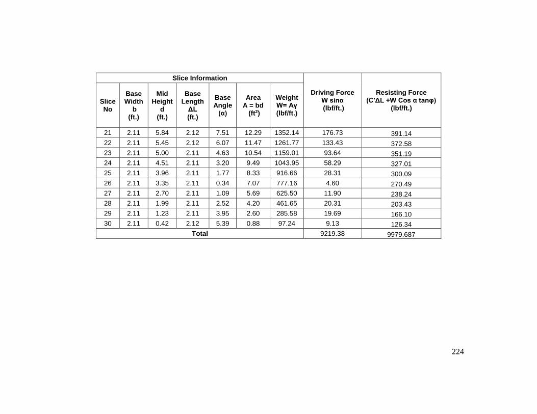
224

Slice Information



(lbf/ft.) Slice No

Base Width

b (ft.)

Mid Height

d (ft.)

Base Length

ΔL (ft.)

Base Angle

(α)

Area A = bd

(ft2)


21 2.11 5.84 2.12 7.51 12.29 1352.14 176.73 391.14

22 2.11 5.45 2.12 6.07 11.47 1261.77 133.43 372.58

23 2.11 5.00 2.11 4.63 10.54 1159.01 93.64 351.19

24 2.11 4.51 2.11 3.20 9.49 1043.95 58.29 327.01

25 2.11 3.96 2.11 1.77 8.33 916.66 28.31 300.09

26 2.11 3.35 2.11 0.34 7.07 777.16 4.60 270.49

27 2.11 2.70 2.11 1.09 5.69 625.50 11.90 238.24

28 2.11 1.99 2.11 2.52 4.20 461.65 20.31 203.43

29 2.11 1.23 2.11 3.95 2.60 285.58 19.69 166.10

30 2.11 0.42 2.12 5.39 0.88 97.24 9.13 126.34

Total 9219.38 9979.687

225

Table 6-8. Load capacity of installed RPP in pin-plus barrier section.

RPP Row

RPP Depth at critical failure surface

(Ft.)

P (lbf/ft.)

1.00 NA NA

2.00 NA NA

3.00 NA NA

4.00 1.63 351.86

5.00 2.61 575.22

6.00 3.47 582.37

7.00 4.21 480.27

8.00 4.85 385.44

9.00 5.52 306.70

10.00 6.01 253.45

11.00 6.32 219.70

12.00 6.44 206.63

13.00 6.38 213.17

14.00 6.14 239.30

15.00 5.58 300.18

16.00 4.72 404.70

17.00 3.57 568.98

18.00 2.10 483.55

Total 5071.51

From the Equation 6-13, Table 6-7 and Table 6-8:

Total driving force, ∑ 𝑊 ∗ 𝑆𝑖𝑛𝛼 𝑛=𝑝𝑛=1 = 9219.38 lbf/ft.

Resisting force due to soil shear strength, ∑ (c′ ∗ ΔL + 𝑊𝐶𝑜𝑠𝛼 ∗ tanϕ′)𝑛=𝑝𝑛=1 = 9979.69 lbf/ft.

Additional resisting force for due of Installed RPPs, P = ∑ 𝑃 𝑛=𝑞𝑛=1 = 5071.51 lbf/ft.

Factor of Safety for control section, FS =∑ (c′∗ΔL+𝑊𝐶𝑜𝑠𝛼∗tanϕ′)+∑ 𝑃

𝑛=𝑞𝑛=1

𝑛=𝑝𝑛=1


= 9979.69+5071.51

9219.38 = 1.633

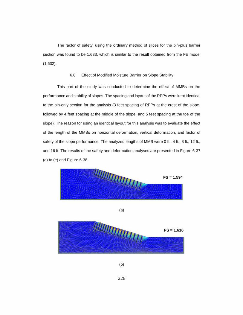
226

The factor of safety, using the ordinary method of slices for the pin-plus barrier

section was found to be 1.633, which is similar to the result obtained from the FE model

(1.632).

6.8 Effect of Modified Moisture Barrier on Slope Stability

This part of the study was conducted to determine the effect of MMBs on the

performance and stability of slopes. The spacing and layout of the RPPs were kept identical

to the pin-only section for the analysis (3 feet spacing of RPPs at the crest of the slope,

followed by 4 feet spacing at the middle of the slope, and 5 feet spacing at the toe of the

slope). The reason for using an identical layout for this analysis was to evaluate the effect

of the length of the MMBs on horizontal deformation, vertical deformation, and factor of

safety of the slope performance. The analyzed lengths of MMB were 0 ft., 4 ft., 8 ft., 12 ft.,

and 16 ft. The results of the safety and deformation analyses are presented in Figure 6-37

(a) to (e) and Figure 6-38.

(a)

(b)

FS = 1.594

FS = 1.616

227

(c)

(d)

(e)

Figure 6-37. Results of safety analysis for (a) 0 feet, (b) 4 feet, (c) 8 feet, (d) 12 feet, and

(e) 16 feet of MMB along the slope.

FS = 1.632

FS = 1.639

FS = 1.673

228

Figure 6-38. Maximum horizontal deformation and vertical settlement versus length of

MMB.

Figure 6-37 showed that the use of MMB shifts the formation of the critical slip

surface almost equal to its length. The increase in the length of MMB along the slope

reduces the radius of the critical slip surface, thereby increasing the factor of safety. The

value of the factor of safety increases with an increase in MMB length along the slope.

Additionally, the results showed that the increase in the length of MMB reduces

the horizontal deformation and vertical settlement of slopes. For instance, the use of a 4

ft., length of MMB along the slope deformed up to 0.99 Inches laterally and 1.102 inches

vertically, while a 12 ft. length of MMB along the slope deformed 0.251 inches laterally and

0.136 inches vertically. The increase in the length of the MMB by 8 ft., from 4 to 12 ft.,

reduced the lateral deformation up to 74.9% and the vertical settlement up to 87.8%.

However, the result also showed that an increase in length of MMB from 12 ft. to 16 ft. also

increased the maximum horizontal displacement and vertical displacement of the slope.

229

This might be due to the increased spacing of RPPs, from 3 to 4 ft. at the middle portion of

the slope. The 4 ft. spacing of RPPs was provided 21 ft. below the crest, which might have

affected the horizontal and vertical deformations of the slope. Therefore, further analysis

should be conducted to identify the best possible layout of RPPs when used in combination

with MMB.

A linear regression model was developed to further explore the relationship

between the increase of the factor of safety due to the use of a modified moisture barrier

in a slope reinforced with RPPs. The details of the simple linear regression model are

explained in the following topic.

6.8.1 Simple Linear Regression Model

Simple linear regression was performed to determine the increase in the value of

the factor of safety due to the use of a modified moisture barrier in a slope stabilized with

RPPs. A linear regression model was developed with the inclined length of MMBs along

the slope as the independent variable (𝐿𝑏), and the ratio of the factor safety of the slope

with RPPs and an MBB to the factor of the safety of slope stabilized with RPPs (Table 6-9).

The results of the safety analysis from FE modeling for various lengths of MMBs are

tabulated in Table 6-9.

230

Table 6-9. Summary table showing the effect of length of MMB on factor of safety.

Length of MMB along the slope

Factor of Safety of slope with both RPPs

and MMB (FSB+R)

Factor due to MMB, B

0 1.594 1.000

2 1.606 1.008

4 1.616 1.014

6 1.624 1.019

8 1.632 1.024

10 1.641 1.029

12 1.639 1.028

14 1.659 1.041

16 1.673 1.050

Figure 6-39. Relationship with barrier factor ‘B’ and length of MMB ‘Lb’.

From the simple linear regression model, the factor due to the installed MMB for

the slope stabilized with both RPPs and MMB “B” can be expressed in terms of the function

of the length of the MMB.

231

B(Lb) = ( 0.0028 𝐿𝑏2

+ 1.0011 ) (6-14)

The factor of safety of the slope stabilized with RPPs only (FSR) can be

determined, using Equation (6-9),

FSR = ∑ (c′∗ΔL+𝑊𝐶𝑜𝑠𝛼∗tanϕ′)+∑ 𝑃

𝑛=𝑞𝑛=1

𝑛=𝑝𝑛=1


Now, combining Equation (6-14) and Equation (6-9), the factor of safety of slopes

stabilized with recycled plastic pins and a modified moisture barrier can be determined by

Equation (6-15),

FSR+B = ∑ (c′∗ΔL+𝑊𝐶𝑜𝑠𝛼∗tanϕ′)+∑ 𝑃

𝑛=𝑞𝑛=1

𝑛=𝑝𝑛=1


B(Lb) (6-15)

The use of MMBs on slopes stabilized with RPPs increases the factor of safety of

slope by factor B(Lb), which depends on the length of the MMB provided along the slope

to prevent the intrusion of moisture in the slope.

6.9 Design Steps for the Slope Stabilized with both RPPs and MMB.

The current stabilization method utilizes both RPPs and MMB to stabilize shallow

slope failures. The design chart developed by Hossain et al. (2017) and Khan et al. (2016)

can be utilized to determine the limit resistance of RPPs, and the effect of MMB can be

incorporated into the design by simply utilizing the peak shear strength parameters of the

soil underneath the MMB instead of fully softened shear strength. The use of MMB at the

crest of the slope prevents the moisture fluctuations underneath the MMB. The prevention

of moisture fluctuations at the crest potentially prevents the cyclic wetting and drying

cycles, keeping the soil from reaching a fully softened state. Therefore, the soil underneath

the MMB can be modeled, using the peak shear strength parameter instead of the fully

softened strength parameter.

The slope, using both RPPs and MMB, can be designed using an ordinary method

of slices by the procedure explained below.

232

• Step 1: The shear strength parameter, such as c’ and 𝜙′ at different depths of

slope, should be determined by performing laboratory tests. The fully softened

shear strength parameter should also be determined.

• Step 2: The critical slip surface for the slope, considering the effect of MMB, should

be determined. The critical slope surface can be determined by using any

commercially available software for slope stability, such as Geo-Studio, Geostase,

and Slide.

• Step 3: The critical failure slip surface is then divided into small segments of equal

widths.

• Step 4: The spacing and depth of the RPPs should be fixed, after which the RPPs

should be plotted along the critical slip surface.

• Step 5: After plotting the RPPs, the depth, ‘d,’ where each RPP crosses the critical

slip surface, should be determined.

• Step 6: The depth of the critical slip surface ‘d’ can be utilized to determine the

limit resistance of the RPPs. The design charts proposed by Khan (2014) and

Hossain et al. (2017) can be utilized to determine the limit resistance of individual

RPPs. If the soil geometry, soil type, depth of slip surface, and RPP size are not

the same, then the load-carrying capacity the of RPPs should be determined prior

to determining the factor of safety, based on the limit soil resistance, limit horizontal

displacement, and maximum flexure criteria, based on the methodology proposed

by Ito and Matsui (1975), Khan, (2014), and Hossain et.al, (2017).

• Step 7: Then, the factor of safety of the slope, utilizing both RPPs and MMB, can

be determined, using Equation (7-1):


𝑛=𝑞𝑛=1

𝑛=𝑝𝑛=1


(7-1)

233

• Step 8: Finally, the calculated factor of safety should be compared with the

targeted factor of safety. If the calculated factor of safety is less than the targeted

factor of safety, it is suggested to increase the length of MMB, reduce the spacing

of the RPPs, and recalculate the factor of safety following Step 2 to Step 7. The

critical slip surface should be determined prior to determing factor of safety if the

length of MMB is increased. If the calculated factor of safety is greater than the

targeted factor of safety, then the design is considered safe for field

implementation.

234

CHAPTER 7. SUMMARY AND CONCLUSIONS

7.1 Introduction

The current study mainly focused on the stabilization of highway embankments

constructed on highly plastic expansive clay. Highly plasticity expansive clayey soils are

prone to repeated swelling and shrinkage, due to cyclic climatic variations. These variations

lead to desiccation cracks that act as passageways for rainfall intrusion into the soil, which

leads to increased moisture content. The increase in the moisture content of the soil

generates large hydrostatic pressures, which can lead to pavement distresses and shallow

slope failures. These types of distresses and failures are frequently observed in many parts

of North Texas. Therefore, an approach for inhibiting the rainfall intrusion into the

desiccation cracks and increasing the lateral stability of the slope was developed by the

combined use of a modified moisture barrier and recycled plastic pins.

The main objective of the study was to determine the effect of Modified Moisture

Barriers (MMB) on slopes stabilized with Recycled Plastic Pins (RPPs). To achieve that

goal, an actual highway pavement section with visible signs of pavement distresses and

potential shallow slope failure was selected for this study. The failed highway segment was

divided into three test sections: pin-plus barrier section, pin-only section, and control

section. The pin-plus barrier section was stabilized with both a modified moisture barrier

and recycled plastic pins; the pin-only section was stabilized using just the recycled plastic

pins; and the control section was left unstabilized. The stabilized and unstabilized sections

were instrumented with integrated temperature and moisture sensors, rain gauges, and

inclinometers, to monitor real-time moisture and temperature variations, rainfall events,

and lateral deformation of the slope, respectively. Additionally, the topographic survey was

conducted every month to monitor the vertical settlement and edge drop of stabilized and

unstabilized slopes. Resistivity imaging was performed on a monthly basis to monitor the

235

continuous subsurface profile and to determine the active moisture fluctuation depth. The

sections were monitored periodically to evaluate the effectiveness of the proposed

stabilization method as compared to other sections. The results obtained from the current

study are summarized as follows.

7.1.1 Site Investigation

• The site investigation was performed prior to the slope stabilization, using

geotechnical drilling and geophysical testing. Both disturbed and undisturbed

samples were collected, and the laboratory soil test was performed on the

collected soil samples.

• The results of the grain-size distribution test showed that the fine fraction passing

from #200 sieve for collected soil samples ranged from 75 to 95%, with the liquid

limit and plastic limit ranging from 47 to 80% and 30 to 55%, respectively. The soil

was classified as highly plastic expansive clay (USCS Classification), and the

specific gravity of the collected soil samples was found to range between 2.712

and 2.746, with an average value of 2.73.

• The result of the moisture content test on collected samples and geophysical

testing via 2D resistivity imaging showed the presence of a high moisture zone up

to 8 ft. deep.

7.1.2 Moisture Variations

• The volumetric moisture content measured in the control and pin-only sections

showed instantaneous response to rainfall events, while the volumetric water

content measured in the pin-plus barrier section showed insignificant variations,

even with the rainfall events.

236

• The maximum moisture variation in the control section and pin-only section was

32.81% and 31.17%, respectively, while pin-plus barrier showed a maximum

moisture variation up to 3.89%.

• The results of resistivity imaging conducted on the pin-plus barrier section and

control section showed an active moisture fluctuation depth up to 7 ft. and 8 ft.,

respectively. Moreover, the use of a modified moisture barrier helped to reduce the

moisture fluctuation zone by 1 ft.

• Based on all of these results, it can be concluded that the pin-plus barrier section

is more effective at controlling moisture intrusion than either the pin only or control

section.

7.1.3 Lateral Deformation

• Maximum lateral deformations of 1.5 inches and 0.8 inches were observed in the

control and pin-only sections, while only 0.38 inches of lateral deformation was

observed in the pin-plus barrier section.

• The maximum lateral deformation of the pin-plus barrier section was 4 and 2.1

times lower than control and pin-only sections, respectively.

• The cyclic horizontal movements of the slope were observed due to seasonal

variations. The lateral movement of the slope increased gradually in the rainy

season, then decreased gradually and became stable in the dry season. The cyclic

fluctuations in the lateral deformation of the slope were synchronous with cyclic

variations in the intensity of precipitation events, indicating that precipitation events

can significantly affect the lateral stability of slopes. These cyclic fluctuations in

lateral deformation were highest in the control section, followed by the pin-only

section and pin-plus barrier section.

237

• Based on all of these results, it can be concluded that the pin-plus barrier section

is more effective at controlling lateral deformation than either the pin-only or control

section.

7.1.4 Vertical Deformation

• Average vertical settlements of 2.65 inches and 1.61 inches were observed in the

control section and pin-only section, respectively, while only 0.59 inches of vertical

settlement was observed in the pin-plus barrier section.

• The average vertical settlement of the pin-plus barrier section was 4.5 and 2.7

times lower than the control and pin-only sections, respectively.

• Based on all of these results, we can say the pin-plus barrier section is more

effective at controlling vertical settlement than either the pin-only or control section.

7.1.5 Numerical Study

• The initial slope condition was utilized to calibrate a numerical model, and the

calibrated model was used to perform deformation and safety analyses for the pin-

only and pin-plus barrier sections. The results of the plastic deformation analysis

from PLAXIS 2D was in good agreement with the field monitoring results for both

the pin-only and pin-plus barrier sections.

• The maximum horizontal and vertical deformation were found to be 0.64 inches

and 0.71 inches, respectively, for the pin-plus barrier section; 1.38 inches and 1.84

inches, respectively, for the pin-only section; and 20.57 inches and 20.00 inches,

respectively, for the control section.

• The results of the plastic deformation analysis showed that the use of MMB in the

pin-plus barrier section reduced the maximum horizontal and vertical deformation

238

of the slope by 0.7 inches and 1.13 inches, respectively, as compared to the pin-

only section.

• The factors of safety for the control section, pin-only section, and pin-plus barrier

section were found to be 1.04, 1.594, and 1.632, respectively.

• The factor of safety was also calculated using the ordinary method of slices for the

pin-plus barrier section, control section, and pin-only section, and was found to be

1.055, 1.572, and 1.633, respectively. The values were in good agreement with

values calculated by PLAXIS 2D.

• An increase in the length of the MMB along the slope reduces the radius of the

critical slip surface, thereby increasing the factor of safety. The value of the factor

of safety increases with an increase in the MMB length along the slope.

Additionally, the results showed that an increase in the length of MMB reduces the

horizontal deformation and vertical settlement of slopes.

Based on the performance monitoring results, the current stabilization method,

using RPPs and modified moisture barriers, was proven effective in controlling the lateral

and vertical deformation of highway slopes and rainfall-induced cycling wetting and drying

in subgrade soil. Therefore, the combined use of RPPs and modified moisture barriers can

be used by DOTs around the US for minimizing rainfall-induced pavement distresses and

shallow slope failures in high embankment slopes constructed over high plasticity clay

7.2 Recommendations for Future Study

Based on the findings of this study and literature review, the following

recommendations are suggested for further research:

• The performance results included in this study were based on the results of a one

year and eight-month monitoring period. It is recommended that the performance

239

of slopes stabilized with a modified moisture barrier and recycled plastic pins be

monitored for a longer period of time.

• The proposed slope stabilization method should be tested in a different location,

with different slope geometries. Additionally, the test section was only 50 feet long,

and it is recommended that large-scale studies be performed, using this

stabilization method.

• Further studies should be conducted by using different types of geocomposites

and geomembranes as part of the modified moisture barriers. Additionally, the

current study utilized square shape RPPs; therefore it is recommended that

various shapes of RPPs be employed, such as H-shaped and circular RPPs.

• A combined seepage and slope stability analysis should be performed to

determine the time-dependent factor of safety of slopes stabilized with both RPPs

and MMBs.

240

REFERENCES

Abramson, L. W., Lee, T. S., Sharma, S., & Boyce, G. M. (2001). Slope Stability and

Stabilization Methods. John Wiley & Sons, New York, 712 p.

Adem, H. H., & Vanapalli, S. K. (2013). "Constitutive Modeling Approach for Estimating 1-

D Heave with Respect to Time for Expansive Soils." International Journal of

Geotechnical Engineering, 7(2), 199-204.

Ahmed, A., Hossain, M. S., Khan, M. S., and Greenwood, K. (2018). “Use of Modified

Moisture Barrier to Reduce Subsurface Moisture in Flexible Pavement in North

Texas.” 97th Annual Meeting of Transportation Research Board, Transportation

Research Board, Washington D.C.

Ahmed, A., Hossain, M. S., Khan, M. S., Greenwood, K., & Shishani, A. (2017).” Moisture

Variation in Expansive Subgrade Through Field Instrumentation and Geophysical

Testing”. In International Congress and Exhibition" Sustainable Civil

Infrastructures: Innovative Infrastructure Geotechnology"(pp. 45-58). Springer,

Cham.

Ahmed, A., Hossain, S., Khan, M. S., & Shishani, A. (2018). “Data-Based Real-Time

Moisture Modeling in Unsaturated Expansive Subgrade in Texas”. Transportation

Research Record, 2672(52), 86-95.

Al-Qadi, I. L., Lahouar, S., Loulizi, A., Elseifi, M. A., & Wilkes, J. A. (2004). “Effective

Approach to Improve Pavement Drainage Layers.” Journal of Transportation

Engineering, 130(5), 658-664.

241

ASCE. (2017). America’s Infrastructure Scores a D+. Retrieved August 7, 2019, from

https://www.infrastructurereportcard.org/

Berg, R. R., Christopher, B. R., & Samtani, N. C. (2009). Design of Mechanically Stabilized

Earth Walls and Reinforced Soil Slopes–Volume II (No. FHWA-NHI- 10-025).

Bowders, J. J., Loehr, J. E., Salim, H., & Chen, C. W. (2003). Engineering properties of

recycled plastic pins for slope stabilization. Transportation Research Record:

Journal of the Transportation Research Board, 1849(1), 39-46.

Breslin, V.T., Senturk, U., Berndt, C.C. (1998) “Long-term engineering properties of

recycled plastic lumber in pier construction”. Resources, Conservation and

Recycling 23 (1998), 243– 258.

Browning, G. (1999). Evaluation of Soil Moisture Barrier Report No. FHWA/MS-DOT-RD-

99-21 & 23). Jackson, MS.

Cai, F., and Ugai, K., (2003). “Reinforcing mechanism of anchors in slopes: a numerical

comparison of results of LEM and FEM”, Int. J. Numer. Anal. Meth. Geomech., 27

(2003), 549-564.

Cedergren, H. R. (1974). Drainage of Highway and Airfield Pavements. Wiley, New York.

Çetinkaya, E. K., Broyles, D., Dandekar, A., Srinivasan, S., & Sterbenz, J. P. G. (2011).

Modelling communication network challenges for Future Internet resilience,

survivability, and disruption tolerance: a simulation-based approach.

Telecommunication Systems, 52(2), 751–766. http://doi.org/10.1007/s11235-011-

9575-4

242

Chen, C. W., Salim, H., Bowders, J., Loehr, E., and Owen, J. (2007). “Creep Behavior of

Recycled Plastic Lumber in Slope Stabilization Applications.” J. Mater. Civ. Eng.,

19(2), 130-138.

Chen, F. H. (2012). Foundations on expansive soils (Vol. 12). Elsevier.

Chen, L., & Bulut, R. (2015). Numerical Analysis of Vertical Moisture Barriers in Controlling

Expansive Soils in Presence of Soil Cracks. In IFCEE 2015 (pp. 2102-2111).

Christopher, B., Hayden, S., and Zhao, A. (2000). “Roadway Base and Subgrade

Geocomposite Drainage Layers.” Testing and Performance of Geosynthetics in

Subsurface Drainage, ASTM International, 100 Barr Harbor Drive, PO Box C700,

West Conshohocken, PA 19428-2959, 35-35–17.

Cobos, D R, and C Chambers. Calibrating ECH2O Soil Moisture Sensors . Pullman, WA :

Decagon Devices, 2010.

Day, R. W. (1996). Design and Repair for Surficial Slope Failures. Practice Periodical on

Structural Design and Construction, 1(3), 83-87.

Day, R. W., & Axten, G. W. (1989). Surficial stability of compacted clay slopes. Journal of

Geotechnical Engineering, 115(4), 577-580.

Dunnicliff, J., and Green, G. E. (1993). Geotechnical Instrumentation for Monitoring Field

Performance. John Wiley & Sons.

Elias, V., Christopher, B. R., & Berg, R. R. (2001). Mechanically Stabilized Earth Walls and

Reinforced Soil Slopes Design and Construction Guidelines, Publication No.

FHWA-NHI-00-043, Federal Highway Administration, Washington, D.C., USA.

243

Elseifi, M., Al-Qadi, I., Loulizi, A., and Wilkes, J. (2001a). “Performance of Geocomposite

Membrane as Pavement Moisture Barrier.” Transportation Research Record:

Journal of the Transportation Research Board, 1772, 168–173.

Evans, R. P.; McManus, K. J. (1999). “Construction of Vertical Moisture Barriers to Reduce

Expansive Soil Subgrade Movement.” Transportation Research Record 1652, 7th

International Conference on Low-Volume Roads, pp.108-112.

Fay, L., Akin, M., & Shi, X. (2012). Cost-Effective and Sustainable Road Slope Stabilization

and Erosion Control (Vol. 430). Transportation Research Board.

Gay, D. A.(1994). Development of a Predictive Model for Pavement Roughness on

Expansive Soils (Doctoral dissertation, Doctoral Dissertation, Texas A&M

University).

Gay, D. A., & Lytton, R. L. (1988). Moisture Barrier Effects on Pavement Roughness.

Measured Performance of Shallow Foundations, Geotechnical Special

Publication, (15).

Gholami, A., Aminifar, F., & Shahidehpour, M. (2016). Front Lines Against the Darkness:

Enhancing the Resilience of the Electricity Grid Through Microgrid Facilities. IEEE

Electrification Magazine, 4(1), 18–24. http://doi.org/10.1109/MELE.2015.2509879

Gray, D. H., and Sotir, R. B. (1996). “Biotechnical and Soil Bioengineering Slope

Stabilization: A Practical Guide for Erosion Control.” John Wiley & Sons, New York,

N.Y.

244

Gupta, R., McCartney, J. S., Nogueira, C. D. L., & Zornberg, J. G. (2008). Moisture

Migration in Geogrid Reinforced Expansive Subgrades.

Hearn, G J, T Hunt, J Aubert, and J Howell. (2008). "Landslide Impacts on the Road

Network of Lao PDR and the Feasibility of Implementing a Slope Management

Program." International Conference on Management of Landslide Hazards in Asia.

Heath, W, B S Saros, and J W F Dowling. (1990). Highway Slope Problems in Indonesia.

London, UK: Transport & Road Research Laboratory.

Hedayati, M. (2014). “Real-Time Modeling of Moisture Distribution in Subgrade Soils.”

Ph.D. Dissertation, The University of Texas at Arlington.

Hedayati, M., and Hossain, S. (2015). “Data-based Model to Estimate Subgrade Moisture

Variation Case Study: Low Volume Pavement in North Texas.” Transportation

Geotechnics, Elsevier Ltd, 3, 48–57.

Henry, K. S., Stormont, J. C., Barna, L. A., and RAMOS, R. D. (2002). “Geocomposite

Capillary Barrier Drain for Unsaturated Drainage of Pavement.” Geosynthetics:

State of the Art-Recent Developments. Proceedings of the Seventh International

Conference on Geosynthetics, 7-ICG, AA Balkema, Nice, France, 877–80.

Henry, Karen S., and John C. Stormont. (2000) "Geocomposite capillary barrier drain."

U.S. Patent No. 6,152,653. 28 Nov.

Hensen, E. J., & Smit, B. (2002). Why clays swell. The Journal of Physical Chemistry

B, 106(49), 12664-12667.

245

Hossain, J., and Hossain, M. S. (2012). “Numerical Modeling for Remedial Measures of

Shallow Slope Failure Using Recycled Plastic Pins.” GeoCongress 2012,

American Society of Civil Engineers, Reston, VA, 3739–3746.

Hossain, S., Ahmed, A., Khan, M. S., Aramoon, A., & Thian, B. (2016). “Expansive

subgrade behavior on a state highway in North Texas”. In Geotechnical and

Structural Engineering Congress 2016Structural Engineering Institute.

Hossain, S., Khan, S., & Kibria, G. (2017). Sustainable Slope Stabilization using Recycled

Plastic Pins. CRC Press.

Ito, T., and T. Matsui (1975), “Methods to estimate lateral force acting on stabilizing piles,”

Soils and Foundations, Vol. 15, No. 4, 43-59.

Jayatilaka, R., & Lytton, R. L. (1997). Prediction of Expansive Clay Roughness in

Pavements with Vertical Moisture Barriers (No. FHWA/TX-98/187-28F).

Jayatilaka, R., Gay, D. A., Lytton, R. L., and Wray, W. K. (1993). "Effectiveness of

Controlling Pavement Roughness Due to Expansive Clays with Vertical Moisture

Barriers." Research Report 1165-2F, Texas Transportation Institute, Texas A&M

University, College Station, Texas.

Jones, L. D., and I. Jefferson (2012). Expansive Soils. In ICE Manual of Geotechnical

Engineering, Volume 1: Geotechnical Engineering Principles, Problematic Soils

and Site Investigation, ICE Publishing, London, UK, pp. 413-441.

246

Kandaris, P.M., “Use of Gabions for Localized Slope Stabilization in Difficult Terrain.” In

Proceedings of the 37th U.S. Symposium on Rock Mechanics, Vail, Colo., June

7–9, 2007.

Khan, M. S. (2014). “Sustainable Slope Stabilization using Recycled Plastic Pin in Texas.”

The University of Texas at Arlington. (Doctoral dissertation).

Khan, M. S., Hossain, M. S., and Kibria, G. (2016). “Slope Stabilization Using Recycled

Plastic Pins.” Journal of Performance of Constructed Facilities, 30(3), 04015054.

Khan, M. S., Hossain, S., Ahmed, A., & Faysal, M. (2017). “Investigation of a shallow slope

failure on expansive clay in Texas”. Engineering geology, 219, 118-129.

Lampo, R., & Nosker, T. J. (1997). Development and testing of plastic lumber materials for

construction applications. US Army Corps of Engineers, Construction Engineering

Research Laboratories, USACERL Technical Report 97/95.

Lau, K.C., Kenney, T.C., 1984. “Horizontal Drains to Stabilise Clay Slopes.” Canadian

Geotechnical Journal 21 (2), 241–249.

Loehr, J. E., and Bowders, J. J. (2007). “Slope Stabilization using Recycled Plastic Pins –

Phase III.” Final Report: RI98-007D, Missouri Department of Transportation,

Jefferson City, Missouri.

Loehr, J. E., Bowders, J. J., Owen, J. W., Sommers, L., Liew, W., Loehr, J. E., Bowders,

J. J., Owen, J. W., Sommers, L., and Liew, W. (2000). “Stabilization of Slopes

Using Recycled Plastic Pins.” A paper presented at the 79th Annual Meeting of the

Transportation Research Board. 6380.

247

Loehr, J. E., Bowders, J., Owen, J., Sommers, L., & Liew, L. (2000). “Stabilization of slopes

using recycled plastic pins.” Journal of the Transportation Research Board, 1-8.

Loehr, J. E., Fennessey, T. W., & Bowders, J. J. (2007). “Stabilization of Surficial Slides

using Recycled Plastic Reinforcement.” Transportation Research Record: Journal

of the Transportation Research Board, 1989(1), 79-87.

Martin, R.P., Siu, K.L., Premchitt, J., 1994. Review of the performance of horizontal drains

in Hong Kong. Special Project Report, SPR 11/94, Geotechnical Engineering

Office, Civil Engineering Department, Hong Kong, p. 106.

McCormick, W., and Short, R. (2006). “Cost Effective Stabilization of Clay Slopes and

Failures using Plate Piles.” Proc., IAEG2006, The Geological Society of London,

London, United Kingdom, 1-7.

McLaren, M. G. (1995). Recycled Plastic Lumber & Shapes Design and Specifications. In

Restructuring: America and Beyond (pp. 819-833). ASCE.

Nelson, J. D., and Miller, D. J. (1992). Expansive Soils Problems and Practice in

Foundation and Pavement Engineering. Courier Companies Inc.

Nicholson, R. V., Gillham, R. W., Cherry, J. A., and Reardon, E. J. (1989). “Reduction of

Acid Generation in Mine Tailings through the use of Moisture-Retaining Cover

Layers as Oxygen Barriers.” Can. Geotech. J., 26(1), 1–8.

Pandey, P., Ahmed, A., Sapkota, A., Hossain, M. S., & Thian, B. (2019). “Performance

Evaluation of Pavement Subgrade by In Situ Moisture and Matric Suction

Measurements”. In Eighth International Conference on Case Histories in

248

Geotechnical Engineering (Geo-Congress 2019), American Society of Civil

Engineers.

Parra, J. R., Loehr, J. E., Hagemeyer, D. J., & Bowders, J. J. (2003). “Field Performance

of Embankments Stabilized with Recycled Plastic Reinforcement.” Transportation

Research Record: Journal of the Transportation Research Board, 1849(1), 31-38.

Pearlman, S.L., B.D. Campbell, and J.L. Withiam, “Slope Stabilization Using In Situ Earth

Reinforcements.” In Proceedings of the Conference on Stability and Performance

of Slopes and Embankment II (GSP 31), 1992, pp. 1333–1348.

Picomell, M. and Lytton, R. L. (1987). "Behavior and Design of Vertical Moisture Barriers."

Transportation Research Record 1137, TRB, National Research Council,

Washington, D.C., 71-81.

Picornell, M., Lytton, R. L., & Steinberg, M. L. (1984). Assessment of the effectiveness of

a vertical moisture barrier. In Fifth International Conference on Expansive Soils

1984: Preprints of Papers (p. 354). Institution of Engineers, Australia.

PLAXIS. (2019). PLAXIS 2D Reference Manual 2019.

Pudasaini, B., & Shahandashti, S. M. (2018). “Identification of Critical Pipes for Proactive

Resource-Constrained Seismic Rehabilitation of Water Pipe Networks”. Journal of

Infrastructure Systems, 24(4), 04018024. http://doi.org/10.1061/(ASCE)IS.1943-

555X.0000439

Pudasaini, B., Shahandashti, S. M., & Razavi, M. (2017). “Identifying Critical Links in Water

Supply Systems Subject to Various Earthquakes to Support Inspection and Renewal

249

Decision Making”. In Computing in Civil Engineering 2017 (pp. 231–238). Reston,

VA: American Society of Civil Engineers. http://doi.org/10.1061/9780784480847.029

Rahardjo, H., Santoso, V. A., Leong, E. C., Ng, Y. S., & Hua, C. J. (2011). “Performance

of an Instrumented Slope Covered by a Capillary Barrier System.” Journal of

Geotechnical and Geoenvironmental Engineering, 138(4), 481-490.

Rahardjo, H., Santoso, V. A., Leong, E. C., Ng, Y. S., and Hua, C. J. (2012). “Performance

of an Instrumented Slope Covered by a Capillary Barrier System.” Journal of

Geotechnical and Geoenvironmental Engineering, 138(4), 481–490.

Rahardjo, H., Santoso, V. A., Leong, E. C., Ng, Y. S., Tam, C. P. H., and Satyanaga, A.

(2013). “Use of Recycled Crushed Concrete and Secudrain in Capillary Barriers

for Slope Stabilization.” Canadian Geotechnical Journal, 50(6), 662–673.

Rahim, M. A. B. A., & Picornell, M. (1989). "Moisture Movement under the Pavement

Structure." Research Report 1165-1, Center for Geotechnical and Highway

Research, University of Texas at El Paso, El Paso, Texas.

Rauss, C. A. (2019). “Long Term Performance Monitoring of Shallow Slope Stabilization

Utilizing Recycled Plastic Pins.” MS Thesis, The University of Texas at Arlington,

Spring, 2019.

Rogers, L. E., and Wright, S. G. (1986). The effect of Wetting and Drying on the Long-Term

Shear Strength Parameters for Compacted Beaumont Clay. Final Report.

Research.

250

Ross, B. (1990). “The Diversion Capacity of Capillary Barriers.” Water Resour. Res.,

26(10), 2625–2629.

Rowlett, D. K., and Barbour, S. L. (2000). “Development of a stand-pipe lysimeter to

measure suction and collect a porewater sample in waste rock piles.” Icard:

Proceedings of the 5th International Conference on Acid Rock Drainage, Society

for Mining, Metallurgy & Exploration, Englewood, CO, Littleton, 235–246.

Royster, D.L., 1980. “Horizontal Drains and Horizontal Drilling: An Overview.”

Transportation Research Record 783, 16–25.

Saleh, A. A., & Wright, S. G. (1997). Shear Strength Correlations and Remedial Measure

Guidelines for Long-Term Stability of Slopes Constructed of Highly Plastic Clay

Soils (No. FHWA/TX-98/1435-2F).

Santi, P. M., Elifrits, C. D., & Liljegren, J. A. (2001). “Design and Installation of Horizontal

Wick Drains for Landslide Stabilization.” Transportation Research Record: Journal

of the Transportation Research, 1757(1), 58-66.

Sapkota, A. (2017). “Effect of Manure and Enzyme on the Degradation of Organic Fraction

of Municipal Solid Waste in Biocell.” MS Thesis, The University of Texas at

Arlington, Spring, 2017.

Sapkota, A., Ahmed, A., Pandey, P., Hossain, M. S., and Lozano, N. (2019a). “Stabilization

of Rainfall-Induced Slope Failure and Pavement Distresses Using Recycled

Plastic Pins and Modified Moisture Barrier.” In Eighth International Conference on

Case Histories in Geotechnical Engineering (Geo-Congress 2019), American

Society of Civil Engineers, Reston, VA, 237–246.

251

Sapkota, A., Hossain, S., Ahmed, A., and Pandey, P. (2019b). “Effect of Modified Moisture

Barrier on the Slope Stabilized with Recycled Plastic Pins.” 98th Annual Meeting

of Transportation Research Board, Transportation Research Board, Washington

D.C.

Schuster, R. L., & Fleming, R. W. (1986). Economic losses and fatalities due to landslides.

Bulletin of the Association of Engineering Geologists, 23(1), 11-28.

Sebesta, S. (2002). “Investigation of Maintenance Base Repairs over Expansive Soils:

Year 1 Report.” Report No. FHWA/TX-03/0-4395-1, Texas Transportation Institute,

Texas A&M University, College Station, TX.

Shahandashti, S. M., & Pudasaini, B. (2019). “Proactive Seismic Rehabilitation Decision-

Making for Water Pipe Networks Using Simulated Annealing”. Natural Hazards

Review, 20(2), 04019003. http://doi.org/10.1061/(ASCE)NH.1527-6996.0000328

Shahidehpour, M., Liu, X., Li, Z., & Cao, Y. (2016). “Microgrids for Enhancing the Power

Grid Resilience in Extreme Conditions”. IEEE Transactions on Smart Grid, 8(2),

1–1. http://doi.org/10.1109/TSG.2016.2579999

Short, R. and Collins, B.D., (2006), “Testing and Evaluation of Driven Plate Piles in Full-

Size Test Slope: New Method for Stabilizing Shallow Landslides.” TRB 85th Annual

Meeting Compendium of Papers CD-ROM, January 22-26, Washington D.C.

Skempton, A. W. (1970). First-time slides in over-consolidated clays. Geotechnique, 20(3),

320- 324.

252

Skempton, A.W. (1977). “Slope Stability of Cuttings in Brown London Clay”. In Proceedings

of Ninth International Conference on Soil Mechanics and Foundation Engineering,

Tokyo, Vol. 3, 261-270.

Sommers, L., Loehr, J. E., & Bowders, J. J. (2000). Construction Methods for Slope

Stabilization with Recycled Plastic Pins. Proc. Mid-Continent Transportation

Symposium 2000. Iowa State University, Ames, Iowa, May 15-16, 2000.

Steenhuis, T. S., Parlange, J.-Y., and Kung, K.-J. S. (1991). “Comment on the Diversion

Capacity of Capillary Barriers.” Benjamin Ross. Water Resour. Res., 27(8), 2155–

2156.

Steinberg, M. L. (1980). "Deep Vertical Fabric Moisture Seals." Proc., Fourth International

Conference on Expansive Soils, Denver, Colorado, 1, 383-400.

Steinberg, M. L. (1981). "Deep-Vertical-Fabric Moisture Barriers in Swelling Soils.”

Transportation Research Record 790, TRB, National Research Council,

Washington, D.C., 87-94.

Steinberg, M. L. (1985). "Controlling Expansive Soil Destructiveness by Deep Vertical

Geomembranes on Four Highways." Transportation Research Record 1032, TRB,

National Research Council, Washington, D.C., 48-53.

Steinberg, M. L. (1989). Further Monitoring of Twelve Geomembrane Sites in Texas DHT-

18. Austin, TX.

253

Steinberg, M. L. (1992). "Controlling Expansive Soils: Twenty Texas Highway Projects."

Proc., Seventh International Conference on Expansive Soils, Dallas, Texas, 1,

392-397.

Sterbenz, J. P. G., Hutchison, D., Çetinkaya, E. K., Jabbar, A., Rohrer, J. P., Schöller, M.,

& Smith, P. (2010). Resilience and survivability in communication networks:

Strategies, principles, and survey of disciplines. Computer Networks, 54(8), 1245–

1265. http://doi.org/10.1016/j.comnet.2010.03.005

Stormont, J. C. (1996). “The Effectiveness of Two Capillary Barriers on a 10% slope.”

Geotech. and Geol. Eng., 14(4), 243–267.

Tamrakar, S. (2015). Slope Stabilization and Performance Monitoring of I-35 and SH-183

Slopes Using Recycled plastic pins (Master’s Thesis).

Taquinio, F. and Pearlman, S.L. (1999). “Pin Piles for Building Foundations.” Presented at

the 7th Annual Great Lakes Geotechnical and Geoenvironmental Conference,

Kent, Ohio, May 10.

Titi, H., & Helwany, S. (2007). Investigation of Vertical Members to Resist Surficial Slope

Instabilities (No. WHRP 07-03). Wisconsin Department of Transportation,

Madison, WI.

Ton, D. T., & Wang, W.-T. P. (2015). A More Resilient Grid: The U.S. Department of Energy

Joins with Stakeholders in an R&D Plan. IEEE Power and Energy

Magazine, 13(3), 26–34. http://doi.org/10.1109/MPE.2015.2397337

254

Turner, A. K., & Schuster, R. L. (1996). Landslides: Investigation and Mitigation:

Transportation Research Board Special Report 247. National Research Council,

Washington, DC, 673.

U.S. Department of Agriculture (USDA), (1992). Natural Resources Conservation Service,

National Engineering Handbook, Part 650, Engineering Field Handbook, Chapter

18, “Soil Bioengineering for Upland Slope Protection and Erosion Reduction.”

USDA, Washington, D.C.

U.S. Department of the Interior | U.S. Geological Survey, “Texas geologic map data.”

http://mrdata.usgs.gov/geology/state/state.php?state=TX, Accessed July 25,

2013.

Vitton, S. J., Harris, W. W., Whitman, M. F., & Liang, R. Y. (1998). “Application of Anchored

Geosynthetic Systems for In-situ Slope Stabilization of Fine-Grained Soils.”

Transportation Research Record: Journal of the Transportation Research Board,

1633(1), 94-101.

Wei, W. B., & Cheng, Y. M. (2009). Strength reduction analysis for slope reinforced with

one row of piles. Computers and Geotechnics, 36(7), 1176-1185.

Wright, S. G. (2005). “Evaluation of Soil Shear Strengths for Slope and Retaining Wall

Stability Analyses with Emphasis on High Plasticity Clays.” FHWA/TX-06/5-1874-

01-1, Federal Highway Administration, Washington, D.C.

Young, R. (2012). Soil properties and behaviour (Vol. 5). Elsevier.

255

Zhao, H., Ge, L., Petry, T. M., and Sun, Y.-Z. (2014). “Effects of Chemical Stabilizers on

an Expansive Clay.” KSCE Journal of Civil Engineering, 18(4), 1009–1017.

Zornberg, J. G., & Gupta, R. (2009, October). “Reinforcement of pavements over

expansive clay subgrades”. In Proceedings of the 17th International Conference

on Soil Mechanics and Geotechnical Engineering (Vol. 1, pp. 765-768).

256

APPENDIX A

Borehole Logs

261

BIOGRAPHICAL INFORMATION

Anuja Sapkota completed a bachelor’s degree in Civil Engineering from

Kathmandu Engineering College (KEC) in Kathmandu, Nepal in December 2013. After

graduation, she worked as a civil engineer for Himalayan Engineering Associates Pvt. Ltd.

(HEALP) for one year, from November 2013 to November 2014. From November 2014 to

July 2015, she worked as a civil engineer in a governmental organization, Kathmandu

Valley Development Authority (KVDA) during the occasion of the SAARC Summit for

Kathmandu Valley Beautification Project. In August 2015, she was admitted to the Master

of Science program in Civil Engineering at The University of Texas at Arlington (UTA).

After completing a Master of Science in Civil Engineering in May 2017, she began her

studies as a Ph.D. student in June 2017. She worked as a graduate research assistant/

teaching assistant during her graduate studies under the supervision of Dr. MD. Sahadat

Hossain. Her research interests include slope stabilization, application of geosynthetics,

pavement maintenance, unsaturated soil mechanics, soil dynamics, sustainable waste

management, landfill design, bioreactor landfill, biocell landfill, and anaerobic digester.

effect of modified moisture barriers on slopes stabilized with

Documents

Transcript of effect of modified moisture barriers on slopes stabilized with