S-LIME: Stabilized-LIME for Model ExplanationZhengze ZhouCornell University

Ithaca, New York, USAzz433@cornell.edu

Giles HookerCornell University

Ithaca, New York, USAgjh27@cornell.edu

Fei WangWeill Cornell Medicine

New York City, New York, USAfew2001@med.cornell.edu

ABSTRACTAn increasing number of machine learning models have been de-ployed in domains with high stakes such as finance and healthcare.Despite their superior performances, many models are black boxesin nature which are hard to explain. There are growing efforts forresearchers to develop methods to interpret these black-box models.Post hoc explanations based on perturbations, such as LIME [39],are widely used approaches to interpret a machine learning modelafter it has been built. This class of methods has been shown toexhibit large instability, posing serious challenges to the effective-ness of the method itself and harming user trust. In this paper, wepropose S-LIME, which utilizes a hypothesis testing frameworkbased on central limit theorem for determining the number ofperturbation points needed to guarantee stability of the resultingexplanation. Experiments on both simulated and real world datasets are provided to demonstrate the effectiveness of our method.

CCS CONCEPTS• Computing methodologies → Feature selection; Supervisedlearning by classification; • Mathematics of computing → Hy-pothesis testing and confidence interval computation.

KEYWORDSinterpretability; stability; LIME; hypothesis testing

ACM Reference Format:Zhengze Zhou, Giles Hooker, and Fei Wang. 2021. S-LIME: Stabilized-LIMEfor Model Explanation. In Proceedings of the 27th ACM SIGKDD Conferenceon Knowledge Discovery and Data Mining (KDD ’21), August 14–18, 2021,Virtual Event, Singapore. ACM, New York, NY, USA, 10 pages. https://doi.org/10.1145/3447548.3467274

1 INTRODUCTIONData Mining and machine learning models have been widely de-ployed for decisionmaking inmany fields, including criminal justice[54] and healthcare [35, 37]. However, many models act as “blackboxes" in that they only provide predictions but with little guidancefor humans to understand the process. It has been a desideratato develop approaches for understanding these complex models,

Permission to make digital or hard copies of all or part of this work for personal orclassroom use is granted without fee provided that copies are not made or distributedfor profit or commercial advantage and that copies bear this notice and the full citationon the first page. Copyrights for components of this work owned by others than ACMmust be honored. Abstracting with credit is permitted. To copy otherwise, or republish,to post on servers or to redistribute to lists, requires prior specific permission and/or afee. Request permissions from permissions@acm.org.KDD ’21, August 14–18, 2021, Virtual Event, Singapore© 2021 Association for Computing Machinery.ACM ISBN 978-1-4503-8332-5/21/08. . . $15.00https://doi.org/10.1145/3447548.3467274

which can help increase user trust [39], assess fairness and privacy[4, 11], debug models [28] and even for regulation purposes [19].

Model explanation methods can be roughly divided into two cat-egories [12, 52]: intrinsic explanations and post hoc explanations.Models with intrinsically explainable structures include linear mod-els, decision trees [6], generalized additive models [20], to namea few. Due to complexity constraints, these models are usuallynot powerful enough for modern tasks involving heterogeneousfeatures and enormous numbers of samples.

Post hoc explanations, on the other hand, provide insights aftera model is trained. These explanations can be either model-specific,which are typically limited to specific model classes, such as splitimprovement for tree-based methods [57] and saliency maps forconvolutional networks [42]; or model-agnostic that do not requireany knowledge of the internal structure of the model being exam-ined, where the analysis is often conducted by evaluating modelpredictions on a set of perturbed input data. LIME [39] and SHAP[31] are two of the most popular model-agnostic explanation meth-ods.

Researchers have been aware of some drawbacks for post hocmodel explanation. [25] showed that widely used permutation im-portance can produce diagnostics that are highly misleading dueto extrapolation. [17] demonstrated how to generate adversarialperturbations that produce perceptively indistinguishable inputswith the same predicted label, yet have very different interpreta-tions. [1] showed that explanation algorithms can be exploited tosystematically rationalize decisions taken by an unfair black-boxmodel. [40] argued against using post hoc explanations as thesemethods can provide explanations that are not faithful to what theoriginal model computes.

In this paper, we focus on post hoc explanations based on per-turbations [39]: one of the most popular paradigm for designingmodel explanation methods. We argue that the most importantproperty of any explanation technique is stability or reproducibility:repeated runs of the explanation algorithm under the same condi-tions should ideally yield the same results. Unstable explanationsprovide little insight to users as how the model actually works andare considered unreliable. Unfortunately, LIME is not always stable.[55] separated and investigated sources of instability in LIME. [51]highlighted a trade-off between explanation’s stability and adher-ence and propose a framework to maximise stability. [30] improvedthe sensitivity of LIME by averaging multiple output weights forindividual images.

We propose a hypothesis testing framework based on a centrallimit theorem for determining the number of perturbation samplesrequired to guarantee stability of the resulting explanation. Briefly,LIME works by generating perturbations of a given instance andlearning a sparse linear explanation, where the sparsity is usuallyachieved by selecting top features via LASSO [49]. LASSO is known

arX

iv:2

106.

0787

5v1

[st

at.M

L]

15

Jun

2021

to exhibit early occurrence of false discoveries [33, 47] which, com-bined with the randomness introduced in the sampling procedure,results in practically-significant levels of instability. We carefullyanalyze the Least Angle Regression (LARS) [13] for generating theLASSO path and quantify the aymptotics for the statistics involvedin selecting the next variable. Based on a hypothesis testing pro-cedure, we design a new algorithm call S-LIME (Stabilized-LIME)which can automatically and adaptively determine the number ofperturbations needed to guarantee a stable explanation.

In the following, we review relevant background on LIME andLASSO along with their instability in Section 2. Section 3 statisti-cally analyzes the asymptotic distribution of the statistics which isat the heart of variable selection in LASSO. Our algorithm S-LIMEis introduced in Section 4. Section 5 presents empirical studies onboth simulated and real world data sets. We conclude in Section 6with some discussions.

2 BACKGROUNDIn this section, we review the general framework for constructingpost hoc explanations based on perturbations using Local Inter-pretable Model-agnostic Explanations (LIME) [39]. We then brieflydiscuss LARS and LASSO, which are the internal solvers for LIMEto achieve the purpose of feature selection. We illustrate LIME’sinstability with toy experiments.

2.1 LIMEGiven a black box model 𝑓 and a target point 𝒙 of interest, wewould like to understand the behavior of the model locally around𝒙 . No knowledge of 𝑓 ’s internal structure is available but we areable to query 𝑓 many times. LIME first samples around the neigh-borhood of 𝒙 , query the black box model 𝑓 to get its predictionsand form a pseudo data sets D = {(𝒙1, 𝑦1), (𝒙2, 𝑦2), . . . , (𝒙𝑛, 𝑦𝑛)}with 𝑦𝑖 = 𝑓 (𝒙𝑖 ) and a hyperparameter 𝑛 specifying the numberof perturbations. The model 𝑓 can be quite general as regression(𝑦𝑖 ∈ R) or classification (𝑦𝑖 ∈ {0, 1} or 𝑦𝑖 ∈ [0, 1] if 𝑓 returns aprobability). A model 𝑔 from some interpretable function spaces 𝐺is chosen by solving the following optimization

argmin𝑔∈𝐺

𝐿(𝑓 , 𝑔, 𝜋𝒙 ) + Ω(𝑔) (1)

where• 𝜋𝒙 (𝒛) is a proximity measure between a perturbed instance𝒛 to 𝒙 , which is usually chosen to be a Gaussian kernel.

• Ω(𝑔) measures complexity of the explanation 𝑔 ∈ 𝐺 . Forexample, for decision trees Ω(𝑔) can be the depth of the tree,while for linear models we can use the number of non-zeroweights.

• 𝐿(𝑓 , 𝑔, 𝜋𝒙 ) is a measure of how unfaithful 𝑔 is in approximat-ing 𝑓 in the locality defined by 𝜋𝒙 .

[39] suggests a procedure called k-LASSO for selecting top 𝑘 fea-tures using LASSO. In this case, 𝐺 is the class of linear modelswith 𝑔 = 𝝎𝑔 · 𝒙 , 𝐿(𝑓 , 𝑔, 𝜋𝒙 ) =

∑𝑛𝑖=1 𝜋𝒙 (𝒙𝑖 ) (𝑦𝑖 − 𝑔(𝒙𝑖 ))2 and Ω =

∞1[| |𝜔𝑔 | |0 > 𝑘]. Under this setting, (1) can be approximatelysolved by first selecting K features with LASSO (using the reg-ularization path) and then learning the weights via least square[39].

We point out here the resemblance between post hoc explana-tions and knowledge distillation [7, 22]; both involve obtainingpredictions from the original model, usually on synthetic examples,and using these to train a new model. Differences lie in both thescope and intention in the procedure. Whereas LIME produces in-terpretable models that apply closely to the point of interest, modeldistillation is generally used to provide a global compression ofthe model representation in order to improve both computationaland predictive performance [18, 34]. Nonetheless, we might expectthat distillation methods to also exhibit the instability describedhere; see [56] which documents instability of decision trees used toprovide global interpretation.

2.2 LASSO and LARSEven models that are “interpretable by design" can be difficult tounderstand, such as a deep decision tree containing hundreds ofleaves, or a linear model that employs many features with non-zeroweights. For this reason LASSO [49], which automatically producessparse models, is often the default solver for LIME.

Formally, suppose D = {(𝒙1, 𝑦1), (𝒙2, 𝑦2), . . . , (𝒙𝑛, 𝑦𝑛)} with𝒙𝑖 = (𝑥𝑖1, 𝑥𝑖2, . . . , 𝑥𝑖𝑝 ) for 1 ≤ 𝑖 ≤ 𝑛, LASSO solves the followingoptimization problem:

𝛽𝐿𝐴𝑆𝑆𝑂 = argmin𝛽

𝑛∑𝑖=1

(𝑦𝑖 − 𝛽0 −𝑝∑𝑗=1

𝑥𝑖 𝑗 𝛽 𝑗 )2 + _

𝑝∑𝑗=1

|𝛽 𝑗 | (2)

where _ is the multiplier for 𝑙1 penalty. (2) can be efficiently solvedvia a slight modification of the LARS algorithm [13], which givesthe entire LASSO path as _ varies. This procedure is described inAlgorithm 1 and 2 below [14], where we denote𝒚 = (𝑦1, 𝑦2, . . . , 𝑦𝑛)and assume 𝑛 > 𝑝 .

Algorithm 1: Least Angle Regression (LARS)(1) Standardize the predictors to have zero mean and unit norm.

Start with residual 𝒓 = 𝒚 −𝒚, 𝛽1, 𝛽2, . . . , 𝛽𝑝 = 0.(2) Find the predictor 𝒙 · 𝑗 most correlated with 𝒓 , and move 𝛽 𝑗

from 0 towards its least-squares coefficient ⟨𝒙 · 𝑗 , 𝒓⟩, untilsome other competitors 𝒙 ·𝑘 has as much correlation withthe current residual as does 𝒙 · 𝑗 .

(3) Move 𝛽 𝑗 and 𝛽𝑘 in the direction defined by their joint leastsquares coefficient of the current residual on (𝒙 · 𝑗 , 𝒙 ·𝑘 ),until some other competitors 𝒙 ·𝑙 has as much correlationwith the current residual.

(4) Repeat step 2 and 3 until all 𝑝 predictors have been entered,at which point we arrive at the full least squares solution.

Algorithm 2: LASSO: Modification of LARS3a. In step 3 of Algorithm 1, if a non-zero coefficient hits zero,

drop the corresponding variable from the active set ofvariables and recompute the current joint least squaresdirection.

Both Algorithm 1 and 2 can be easily modified to incorporate aweight vector𝝎 = (𝜔1, 𝜔2, . . . , 𝜔𝑛) on the data setD, by transform-ing it toD = {(√𝜔1𝒙1,

√𝜔1𝑦1), (

√𝜔2𝒙2,

√𝜔2𝑦2), . . . , (

√𝜔𝑛𝒙𝑛,

√𝜔𝑛𝑦𝑛)}.

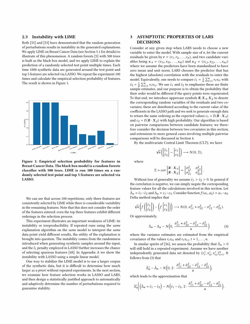
2.3 Instability with LIMEBoth [55] and [53] have demonstrated that the random generationof perturbations results in instability in the generated explanations.We apply LIME on Breast Cancer Data (see Section 5.1 for details) toillustrate of this phenomenon. A random forests [5] with 500 treesis built as the black box model, and we apply LIME to explain theprediction of a randomly selected test point multiple times. Eachtime 1000 synthetic data are generated around the test point andtop 5 features are selected via LASSO.We repeat the experiment 100times and calculate the empirical selection probability of features.The result is shown in Figure 1.

Figure 1: Empirical selection probability for features inBreast Cancer Data. The black boxmodel is a random forestsclassifier with 500 trees. LIME is run 100 times on a ran-domly selected test point and top 5 features are selected viaLASSO.

We can see that across 100 repetitions, only three features areconsistently selected by LIME while there is considerable variabilityin the remaining features. Note that this does not consider the orderof the features entered: even the top three features exhibit differentorderings in the selection process.

This experiment illustrates an important weakness of LIME: itsinstability or irreproducibility. If repeated runs using the sameexplanation algorithm on the same model to interpret the samedata point yield different results, the utility of the explanation isbrought into question. The instability comes from the randomnessintroduced when generating synthetic samples around the input,and the 𝑙1 penalty employed in LASSO further increases the chanceof selecting spurious features [48]. In Appendix A we show theinstability with LASSO using a simple linear model.

One way to stabilize the LIME model is to use a larger corpusof the synthetic data, but it is difficult to determine how muchlarger as a priori without repeated experiments. In the next section,we examine how feature selection works in LASSO and LARS,and then design a statistically justified approach to automaticallyand adaptively determine the number of perturbations required toguarantee stability.

3 ASYMPTOTIC PROPERTIES OF LARSDECISIONS

Consider at any given step when LARS needs to choose a newvariable to enter the model. With sample size of 𝑛, let the currentresiduals be given by 𝒓 = (𝑟1, 𝑟2, . . . , 𝑟𝑛), and two candidate vari-ables being 𝒙 ·𝒊 = (𝑥1𝑖 , 𝑥2𝑖 , . . . , 𝑥𝑛𝑖 ) and 𝒙 ·𝒋 = (𝑥1𝑗 , 𝑥2𝑗 , . . . , 𝑥𝑛𝑗 )where we assume the predictors have been standardized to havezero mean and unit norm. LARS chooses the predictor that hasthe highest (absolute) correlation with the residuals to enter themodel. Equivalently, one needs to compare 𝑐1 = 1

𝑛

∑𝑛𝑡=1 𝑟𝑡𝑥𝑡𝑖 with

𝑐2 = 1𝑛

∑𝑛𝑡=1 𝑟𝑡𝑥𝑡 𝑗 . We use 𝑐1 and 𝑐2 to emphasize these are finite

sample estimates, and our purpose is to obtain the probability thattheir order would be different if the query points were regenerated.To that end, we introduce uppercase symbols 𝑹,𝑿 ·𝒊,𝑿 ·𝒋 to denotethe corresponding random variables of the residuals and two co-variates; these are distributed according to the current value of thecoefficients in the LASSO path and we seek to generate enough datato return the same ordering as the expected values 𝑐1 = 𝐸 (𝑹 · 𝑿 ·𝒊)and 𝑐2 = 𝐸 (𝑹 · 𝑿 ·𝒋) with high probability. Our algorithm is basedon pairwise comparisons between candidate features; we there-fore consider the decision between two covariates in this section,and extensions to more general cases involving multiple pairwisecomparisons will be discussed in Section 4.

By the multivariate Central Limit Theorem (CLT), we have

√𝑛

( [𝑐1𝑐2

]−[𝑐1𝑐2

] )−→ 𝑁 (0, Σ),

where

Σ = cov[𝑹 · 𝑿 ·𝒊

𝑹 · 𝑿 ·𝒋

]=

[𝜎211 𝜎212𝜎221 𝜎222

].

Without loss of generality we assume 𝑐1 > 𝑐2 > 0. In general ifthe correlation is negative, we can simply negate the correspondingfeature values for all the calculations involved in this section. LetΔ𝑛 = 𝑐1−𝑐2 andΔ𝑛 = 𝑐1−𝑐2. Consider function 𝑓 (𝑎1, 𝑎2) = 𝑎1−𝑎2.Delta method implies that

√𝑛

(𝑓

( [𝑐1𝑐2

] )−(𝑓

[𝑐1𝑐2

] ))−→ 𝑁 (0, 𝜎211 + 𝜎222 − 𝜎212 − 𝜎221).

Or approximately,

Δ𝑛 − Δ𝑛 ∼ 𝑁

(0,

𝜎211 + 𝜎222 − 𝜎212 − 𝜎221

𝑛

)(3)

where the variance estimates are estimated from the empiricalcovariance of the values 𝑟𝑡𝑥𝑡𝑖 and 𝑟𝑡𝑥𝑡 𝑗 , 𝑡 = 1, . . . , 𝑛.

In similar spirits of [56], we assess the probability that Δ𝑛 > 0will still hold in a repeated experiment. Assume we have anotherindependently generated data set denoted by {𝑟∗𝑡 , 𝑥∗𝑡𝑖 , 𝑥

∗𝑡 𝑗}𝑛𝑡=1. It

follows from (3) that

Δ∗𝑛 − Δ𝑛 ∼ 𝑁

(0, 2 ·

𝜎211 + 𝜎222 − 𝜎212 − 𝜎221

𝑛

),

which leads to the approximation that

Δ∗𝑛

���� (Δ𝑛 = 𝑐1 − 𝑐2

)∼ 𝑁

(𝑐1 − 𝑐2, 2 ·

𝜎211 + 𝜎222 − 𝜎212 − 𝜎221

𝑛

).

In order to control 𝑃 (Δ∗𝑛 > 0) at a confidence level 1 − 𝛼 , we need

𝑐1 − 𝑐2 > 𝑍𝛼

√2𝜎211 + 𝜎222 − 𝜎212 − 𝜎221

𝑛, (4)

where 𝑍𝛼 is the (1 − 𝛼)-quantile of a standard normal distribution.For a fixed confidence level 𝛼 and 𝑛, suppose we get the corre-

sponding 𝑝-value 𝑝𝑛 > 𝛼 . From (4) we have√𝑛

𝑐1 − 𝑐2√2(𝜎211 + 𝜎222 − 𝜎212 − 𝜎221)

= 𝑍𝑝𝑛 .

This implied we would need approximately 𝑛′ samples to get asignificant result where √

𝑛

𝑛′=𝑍𝑝𝑛

𝑍𝛼. (5)

4 STABILIZED-LIMEBased on the theoretical analysis developed in Section 3, we can runLIME equipped with hypothesis testing at each step when a newvariable enters. If the testing result is significant, we continue tothe next step; otherwise it indicates that the current sample size ofperturbations is not large enough. We thus generate more syntheticdata according to Equation (5) and restart the whole process. Notethat we view any intermediate step as conditioned on previousobtained estimates of 𝛽 . A high level sketch of the algorithm ispresented below in Algorithm 3.

In practice, we may need to set an upper bound on the number ofsynthetic samples generated (denoted by𝑛𝑚𝑎𝑥 ), such that wheneverthe new 𝑛′ is greater than 𝑛𝑚𝑎𝑥 , we’ll simply set 𝑛 = 𝑛𝑚𝑎𝑥 andgo though the outer while loop one last time without testing ateach step. This can prevent the algorithm from running too longand wasting computation resources in cases where two competingfeatures are equally important in a local neighborhood; for example,if the black box model is indeed locally linear with equal coefficientsfor two predictors.

We note several other possible variations of the Algorithm 3.Multiple testing. So far we’ve only considered comparing a pair

of competing features (the top two). But when choosing the nextpredictor to enter the model at step𝑚 (with𝑚 − 1 active features),there are 𝑝−𝑚+1 candidate features. We can modify the procedureto select the best feature among all the remaining candidates, byconducting pairwise comparisons between the feature with largestcorrelation (𝑐1) against the rest (𝑐2, . . . , 𝑐𝑝−𝑚+1). This is a multi-ple comparisons problem, and one can use an idea analogous toBonferroni correction. Mathematically:

• Test the hypothesis𝐻𝑖,0 : 𝑐1 ≤ 𝑐𝑖 , 𝑖 = 2, . . . , 𝑝−𝑚+1. Obtain𝑝-values 𝑝2, . . . , 𝑝𝑝−𝑚+1.

• Reject the null hypothesis if∑𝑝−𝑚+1𝑖=2 𝑝𝑖 < 𝛼 .

Although straightforward, this Bonferroni-like correction ignoresmuch of the correlation among these statistics and will result ina conservative estimate. In the experiments, we only conduct hy-pothesis testing for top two features without resorting to multipletesting, as it is more efficient and empirically we do not observeany performance degradation.

Efficiency. Several modifications can be made to improve theefficiency of Algorithm 3. At each step when 𝑛 is increased to 𝑛′,

Algorithm 3: S-LIMEInput :A black box model 𝑓 , data sample to explain 𝒙 ,

initial size for perturbation samples 𝑛0,significance level 𝛼 , number of features to select 𝑘 ,proximity measure 𝜋𝒙 .

Output :Top 𝑘 features selected for interpretation.Generate D = {𝑛0 synthetic samples around 𝒙} andcalculate weight vector 𝝎 using 𝜋𝒙 ;Set 𝑛 = 𝑛0;while True do

Run Algorithm 2 on D with weight 𝝎 along withhypothesis testing at each step:

while active features less than 𝑘 doSelect top two predictors most correlated with thecurrent residual from remaining covariates, withcovariance 𝑐1 and 𝑐2;Calculate test statistic:

𝑡 = 𝑐1 − 𝑐2 − 𝑍𝛼

√2𝜎211 + 𝜎222 − 𝜎212 − 𝜎221

𝑛

if 𝑡 >= 0 thenContinue with this selection;

else

Calculate 𝑛′ = 𝑛 ∗(𝑍𝛼

𝑍𝑝𝑛

)2and set 𝑛 = 𝑛′;

Break;end

endif active features less than 𝑘 then

Generate D = {𝑛′ synthetic samples around 𝒙} andcalculate weight vector 𝝎 using 𝜋𝒙 ;

elseReturn 𝑘 selected features;

endend

we can reuse the existing synthetic samples and only generate addi-tional 𝑛′ −𝑛 perturbation points. One may also note that wheneverthe outer while loop restarts, we conduct repetitive testings for thefirst several variables entering the model. To achieve better effi-ciency, each new run can condition on previous runs: if a variableenters the LASSO path in the same order as before and has beentested with significant statistics, no additional testing is needed.Hypothesis testing is only invoked when we select more featuresthan previous runs, or in some rare cases, the current iterationdisagrees with previous results. In our experiments, we do not im-plement the conditioning step for implementation simplicity, as wefind the efficiency gain is marginal when selecting a moderate sizeof features.

5 EMPIRICAL STUDIESRather than performing a broad-scale analysis, we look at severalspecific cases as illustrations to show the effectiveness of S-LIME ingenerating stabilized model explanations. Scikit-learn [36] is used

for building black box models. Code for replicating our experimentsis available at https://github.com/ZhengzeZhou/slime.

5.1 Breast Cancer DataWe use the widely adopted Breast Cancer Wisconsin (Diagnostic)Data Set [32], which contains 569 samples and 30 features1. A ran-dom forests with 500 trees is trained on 80% of the data as the blackbox model to predict whether an instance is benign or malignant.It achieves around 95% accuracy on the remaining 20% test data.Since our focus is on producing stabilized explanations for a spe-cific instance, we do not spend additional efforts in hyperparametertuning to further improve model performance.

Figure 1 in Section 2.3 has already demonstrated the inconsis-tency of the selected feature returned by original LIME. In Figure 2below, we show a graphical illustration of four LIME replicationson a randomly selected test instance, where the left column of eachsub figure shows selected features along with learned linear param-eters, and the right column is the corresponding feature value forthe sample. These repetitions of LIME applied on the same instancehave different orderings for the top two features, and also disagreeon the fourth and fifth features.

(a) Iteration 1 of LIME (b) Iteration 2 of LIME

(c) Iteration 3 of LIME (d) Iteration 4 of LIME

Figure 2: Four iterations of LIME on Breast Cancer Data. Theblack boxmodel is a random forests classifier with 500 trees.LIME explanations are generatedwith 1000 synthetic pertur-bations.

To quantify the stability of the generated explanations, we mea-sure the Jaccard index, which is a statistic used for gauging thesimilarity and diversity of sample sets. Given two sets 𝐴 and 𝐵

(in our case, the sets are selected features from LIME), the Jaccardcoefficient is defined as the size of the intersection divided by thesize of the union:

𝐽 (𝐴, 𝐵) = |𝐴 ∩ 𝐵 ||𝐴 ∪ 𝐵 | .

One disadvantage of the Jaccard index is that it ignores order-ingwithin each feature set. For example, if top two features returnedfrom two iterations of LIME are𝐴 = {𝑤𝑜𝑟𝑠𝑡 𝑝𝑒𝑟𝑖𝑚𝑒𝑡𝑒𝑟, 𝑤𝑜𝑟𝑠𝑡 𝑎𝑟𝑒𝑎}and 𝐵 = {𝑤𝑜𝑟𝑠𝑡 𝑎𝑟𝑒𝑎, 𝑤𝑜𝑟𝑠𝑡 𝑝𝑒𝑟𝑖𝑚𝑒𝑡𝑒𝑟 }, we have 𝐽 (𝐴, 𝐵) = 1 but1https://scikit-learn.org/stable/modules/generated/sklearn.datasets.load_breast_cancer.html

it does not imply LIME explanations are stable. To better quantifystability, we look at the Jaccard index for the top 𝑘 features for𝑘 = 1, . . . , 5. Table 1 shows the average Jaccard across all pairsfor 20 repetitions of both LIME and S-LIME on the selected testinstance. We set 𝑛𝑚𝑎𝑥 = 10000 for S-LIME.

Table 1: Average Jaccard index for 20 repetitions for LIMEand S-LIME. The black box model is a random forests with500 trees.

Position LIME S-LIME1 0.61 1.02 1.0 1.03 1.0 1.04 0.66 1.05 0.59 0.85

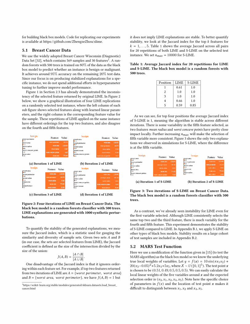
As we can see, for top four positions the average Jaccard indexof S-LIME is 1, meaning the algorithm is stable across differentiterations. There is some variability in the fifth feature selected, astwo featuresmean radius and worst concave points have pretty closeimpact locally. Further increasing 𝑛𝑚𝑎𝑥 will make the selection offifth variable more consistent. Figure 3 shows the only two explana-tions we observed in simulations for S-LIME, where the differenceis at the fifth variable.

(a) Iteration 1 of S-LIME (b) Iteration 2 of S-LIME

Figure 3: Two iterations of S-LIME on Breast Cancer Data.The black box model is a random forests classifier with 500trees.

As a contrast, we’ve already seen instability for LIME even forthe first variable selected. Although LIME consistently selects thesame top two and the third feature, there is much variably for thefourth and fifth feature. This experiment demonstrates the stabilityof S-LIME compared to LIME. In Appendix B.1, we apply S-LIME onother types of black box models. Stability results on a large cohortof test samples are included in Appendix B.2.

5.2 MARS Test FunctionHere we use a modification of the function given in [15] (to test theMARS algorithm) as the black boxmodel sowe know the underlyingtrue local weights of variables. Let 𝑦 = 𝑓 (𝒙) = 10 sin(𝜋𝑥1𝑥2) +20(𝑥3−0.05)2+5.2𝑥4+5𝑥5, whereX ∼ 𝑈 ( [0, 1]5). The test point 𝒙is chosen to be (0.51, 0.49, 0.5, 0.5, 0.5). We can easily calculate thelocal linear weights of the five variables around 𝒙 and the expectedselection order is (𝑥3, 𝑥1, 𝑥2, 𝑥4, 𝑥5). Note here the specific choiceof parameters in 𝑓 (𝑥) and the location of test point 𝒙 makes itdifficult to distinguish between 𝑥1, 𝑥2 and 𝑥4, 𝑥5.

Table 2 presents the average Jaccard index for the selected featuresets by LIME and S-LIME, where LIME is generated with 1000synthetic samples and we set 𝑛0 = 1000 and 𝑛𝑚𝑎𝑥 = 10000 forS-LIME. The close local weights between 𝑥1, 𝑥2 and 𝑥4, 𝑥5 causessome instability in LIME, as can be seen from the drop in the indexat position 2 and 4. S-LIME outputs consistent explanations in thiscase.

Table 2: Average Jaccard index for 20 repetitions for LIMEand S-LIME on test point (0.51, 0.49, 0.5, 0.5, 0.5). The blackbox model is MARS.

Position LIME S-LIME1 1.0 1.02 0.82 1.03 1.0 1.04 0.79 1.05 1.0 1.0

5.3 Early Prediction of Sepsis From ElectronicHealth Records

Sepsis is a major public health concern which is a leading causeof death in the United States [3]. Early detection and treatmentof a sepsis incidence is a crucial factor for patient outcomes [38].Electronic health records (EHR) store data associated with eachindividual’s health journey and have seen an increasing use re-cently in clinical informatics and epidemiology [46, 50]. There havebeen several work to predict sepsis based on EHR [16, 21, 29]. In-terpretability of these models are essential for them to be deployedin clinical settings.

We collect data from MIMIC-III [26], which is a freely accessiblecritical care database. After pre-processing, there are 15309 patientsin the cohort for analysis, out of which 1221 developed sepsis basedon Sepsis-3 clinical criteria for sepsis onset [43]. For each patient,the record consists of a combination of hourly vital sign summaries,laboratory values, and static patient descriptions. We provide thelist of all variables involved in Appendix C. ICULOS is a timestampwhich denotes the hours since ICU admission for each patient, andthus is not used directly for training the model.

For each patient’s records, missing values are filled with the mostrecent value if available, otherwise a global average. Negative sam-ples are down sampled to achieve a class ratio of 1:1. We randomlyselect 90% of the data for training and leave the remaining 10%for testing. A simple recurrent neural network based on LSTM [23]module is built with Keras [9] for demonstration. Each sample fedinto the network has 25 features with 24 timestamps, then goesthrough a LSTM with 32 internal units with dropout rate 0.2, andfinally a dense layer with softmax activation to output a probability.The network is optimized by Adam [27] with an initial learningrate of 0.0001 and we train it for 500 epochs on a batch size of 50.

The model achieves around 0.75 AUC score on the test set. Notethat we do not fine tune the architecture of the network throughcross validation. The purpose of this study is not on achieving a su-perior performance as it usually requires more advanced modelingtechniques for temporal data [16, 29] or exploiting missing value

patterns [8]. Instead, we would like to demonstrate the effectivenessof our proposed method in reliably explaining a relatively largescale machine learning model applied to medical data.

To deal with temporal data where each sample in the trainingset is of shape (𝑛_𝑡𝑖𝑚𝑒𝑠𝑡𝑒𝑝𝑠, 𝑛_𝑓 𝑒𝑎𝑡𝑢𝑟𝑒𝑠), LIME reshapes the datasuch that it becomes a long vector of size𝑛_𝑡𝑖𝑚𝑒𝑠𝑡𝑒𝑝𝑠 × 𝑛_𝑓 𝑒𝑎𝑡𝑢𝑟𝑒𝑠 .Essentially it transforms the temporal data to the regular tabularshape while increasing the number of features by a multiple ofavailable timestamps. Table 3 presents the average Jaccard indexfor the selected feature sets by LIME and S-LIME on two randomlyselected test samples, where LIME is generated with 1000 syntheticsamples and we set 𝑛0 = 1000 and 𝑛𝑚𝑎𝑥 = 100000 for S-LIME.

LIME exhibits undesirable instability in this example, potentiallydue to the complex black box model applied and the large numberof features (24 × 25 = 600). S-LIME achieves much better stabilitycompared to LIME, although we can still observe some uncertaintyin choosing the fifth feature in the second test sample.

Table 3: Average Jaccard index for 20 repetitions for LIMEand S-LIME on two randomly selected test samples. Theblack box model is a recurrent neural network.

Position LIME S-LIME1 0.37 1.02 0.29 1.03 0.33 1.04 0.25 0.895 0.26 1.0(a) test sample 1

Position LIME S-LIME1 0.31 1.02 0.24 1.03 0.19 1.04 0.17 0.965 0.18 0.78(b) test sample 2

Figure 4 below shows the output of S-LIME on two different testsamples. We can see that for sample 1, most recent temperaturesplay an important role, along with the latest pH and potassiumvalues. While for sample 2, latest pH values are the most importantones.

We want to emphasize that extra caution must be taken by prac-titioners in applying LIME, especially for some complex problems.The local linear model with a few features might not be suitableto approximate a recurrent neural network built on temporal data.How to apply perturbation based explanation algorithms to tempo-ral data is still an open problem, and we leave it for future work.That being said, the experiment in this section demonstrates theeffectiveness of S-LIME in producing stabilized explanations.

6 DISCUSSIONSAn important property for model explanation methods is stability:repeated runs of the algorithm on the same object should outputconsistent results. In this paper, we show that post hoc explana-tions based on perturbations, such as LIME, are not stable due to therandomness introduced in generating synthetic samples. Our pro-posed algorithm S-LIME is based on a hypothesis testing frameworkand can automatically and adaptively determine the appropriatenumber of perturbations required to guarantee stability.

The idea behind S-LIME is similar to [56] which tackles theproblem of building stable approximation trees in model distillation.In the area of online learning, [10] uses Hoeffding bounds [24] to

(a) test sample 1

(b) test sample 2

Figure 4: Output of S-LIME for two randomly selected testsamples. The black boxmodel is a recurrent neural network.

guarantee correct choice of splits in a decision tree by comparingtwo best attributes. We should mention that S-LIME is not restrictedto LASSO as its feature selection mechanism. In fact, to producea ranking of explanatory variables, one can use any sequentialprocedures which build a model by sequentially adding or removingvariables based upon some criterion, such as forward-stepwise orbackward-stepwise selection [14]. All of these methods can bestabilized by a similar hypothesis testing framework like S-LIME.

There are several works closely related to ours. [55] identifiesthree sources of uncertainty in LIME: sampling variance, sensitivityto choice of parameters and variability in the black box model.We aim to control the first source of variability as the other twodepend on specific design choices of the practitioners. [51] highlighta trade-off between explanation’s stability and adherence. Theirapproach is to select a suitable kernel width for the proximitymeasure, but it does not improve stability given any kernel width.In [53], the authors design a deterministic version of LIME by onlylooking at existing training data through hierarchical clusteringwithout resorting to synthetic samples. However, the number ofsamples in a dataset will affect the quality of clusters and a lackof nearby points poses additional challenges; this strategy alsorelies of having access to the training data. Most recently, [45]develop a set of tools for analyzing explanation uncertainty ina Bayesian framework for LIME. Our method can be viewed asa frequentist counterpart without the need to choose priors andevaluate a posterior distribution.

Another line of work concerns adversarial attacks to LIME. [44]propose a scaffolding technique to hide the biases of any givenclassifier by building adversarial classifiers to detect perturbedinstances. Later, [41] utilize a generative adversarial network tosample more realistic synthetic data for making LIME more robust

to adversarial attacks. The technique we developed in this work isorthogonal to these directions, as . We also plan to explore otherdata generating procedures which can help with stability.

ACKNOWLEDGMENTSGiles Hooker is supported by NSF DMS-1712554. Fei Wang is sup-ported by NSF 1750326, 2027970, ONR N00014-18-1-2585, AmazonWeb Service (AWS) Machine Learning for Research Award andGoogle Faculty Research Award.

REFERENCES[1] Ulrich Aïvodji, Hiromi Arai, Olivier Fortineau, Sébastien Gambs, Satoshi Hara,

and Alain Tapp. 2019. Fairwashing: the risk of rationalization. arXiv preprintarXiv:1901.09749 (2019).

[2] Zeyuan Allen-Zhu and Yuanzhi Li. 2020. Towards Understanding Ensemble,Knowledge Distillation and Self-Distillation in Deep Learning. arXiv preprintarXiv:2012.09816 (2020).

[3] Derek C Angus, Walter T Linde-Zwirble, Jeffrey Lidicker, Gilles Clermont, JosephCarcillo, and Michael R Pinsky. 2001. Epidemiology of severe sepsis in the UnitedStates: analysis of incidence, outcome, and associated costs of care. Read Online:Critical Care Medicine| Society of Critical Care Medicine 29, 7 (2001), 1303–1310.

[4] Julia Angwin, Jeff Larson, Surya Mattu, and Lauren Kirchner. 2016. Machine bias.ProPublica. See https://www. propublica. org/article/machine-bias-risk-assessments-in-criminal-sentencing (2016).

[5] Leo Breiman. 2001. Random forests. Machine learning 45, 1 (2001), 5–32.[6] Leo Breiman, Jerome Friedman, Charles J Stone, and Richard A Olshen. 1984.

Classification and regression trees. CRC press.[7] Cristian Bucilua, Rich Caruana, and Alexandru Niculescu-Mizil. 2006. Model

compression. In Proceedings of the 12th ACM SIGKDD international conference onKnowledge discovery and data mining. 535–541.

[8] Zhengping Che, Sanjay Purushotham, Kyunghyun Cho, David Sontag, and YanLiu. 2018. Recurrent neural networks for multivariate time series with missingvalues. Scientific reports 8, 1 (2018), 1–12.

[9] François Chollet et al. 2015. Keras. https://keras.io.[10] Pedro Domingos and Geoff Hulten. 2000. Mining high-speed data streams. In

Proceedings of the sixth ACM SIGKDD international conference on Knowledgediscovery and data mining. 71–80.

[11] Finale Doshi-Velez and Been Kim. 2017. Towards a rigorous science of inter-pretable machine learning. arXiv preprint arXiv:1702.08608 (2017).

[12] Mengnan Du, Ninghao Liu, and Xia Hu. 2019. Techniques for interpretablemachine learning. Commun. ACM 63, 1 (2019), 68–77.

[13] Bradley Efron, Trevor Hastie, Iain Johnstone, Robert Tibshirani, et al. 2004. Leastangle regression. The Annals of statistics 32, 2 (2004), 407–499.

[14] Jerome Friedman, Trevor Hastie, and Robert Tibshirani. 2001. The elements ofstatistical learning. Vol. 1. Springer series in statistics New York.

[15] Jerome H Friedman. 1991. Multivariate adaptive regression splines. The annalsof statistics (1991), 1–67.

[16] Joseph Futoma, Sanjay Hariharan, Katherine Heller, Mark Sendak, Nathan Brajer,Meredith Clement, Armando Bedoya, and Cara O’Brien. 2017. An improvedmulti-output gaussian process rnn with real-time validation for early sepsisdetection. In Machine Learning for Healthcare Conference. PMLR, 243–254.

[17] Amirata Ghorbani, Abubakar Abid, and James Zou. 2019. Interpretation of neuralnetworks is fragile. In Proceedings of the AAAI Conference on Artificial Intelligence,Vol. 33. 3681–3688.

[18] Robert D Gibbons, Giles Hooker, Matthew D Finkelman, David J Weiss, Paul APilkonis, Ellen Frank, Tara Moore, and David J Kupfer. 2013. The computerizedadaptive diagnostic test for major depressive disorder (CAD-MDD): a screeningtool for depression. The Journal of clinical psychiatry 74, 7 (2013), 1–478.

[19] Bryce Goodman and Seth Flaxman. 2017. European Union regulations on algo-rithmic decision-making and a “right to explanation”. AI magazine 38, 3 (2017),50–57.

[20] Trevor J Hastie and Robert J Tibshirani. 1990. Generalized additive models. Vol. 43.CRC press.

[21] Katharine E Henry, David N Hager, Peter J Pronovost, and Suchi Saria. 2015. Atargeted real-time early warning score (TREWScore) for septic shock. Sciencetranslational medicine 7, 299 (2015), 299ra122–299ra122.

[22] Geoffrey Hinton, Oriol Vinyals, and Jeff Dean. 2015. Distilling the knowledge ina neural network. arXiv preprint arXiv:1503.02531 (2015).

[23] Sepp Hochreiter and Jürgen Schmidhuber. 1997. Long short-termmemory. Neuralcomputation 9, 8 (1997), 1735–1780.

[24] Wassily Hoeffding. 1994. Probability inequalities for sums of bounded randomvariables. In The Collected Works of Wassily Hoeffding. Springer, 409–426.

[25] Giles Hooker and Lucas Mentch. 2019. Please stop permuting features: Anexplanation and alternatives. arXiv preprint arXiv:1905.03151 (2019).

[26] Alistair EW Johnson, Tom J Pollard, Lu Shen, H Lehman Li-Wei, Mengling Feng,Mohammad Ghassemi, Benjamin Moody, Peter Szolovits, Leo Anthony Celi, andRoger GMark. 2016. MIMIC-III, a freely accessible critical care database. Scientificdata 3, 1 (2016), 1–9.

[27] Diederik P Kingma and Jimmy Ba. 2014. Adam: A method for stochastic opti-mization. arXiv preprint arXiv:1412.6980 (2014).

[28] Pang Wei Koh and Percy Liang. 2017. Understanding black-box predictions viainfluence functions. arXiv preprint arXiv:1703.04730 (2017).

[29] Simon Meyer Lauritsen, Mads Ellersgaard Kalør, Emil Lund Kongsgaard, Ka-trine Meyer Lauritsen, Marianne Johansson Jørgensen, Jeppe Lange, and BoThiesson. 2020. Early detection of sepsis utilizing deep learning on electronichealth record event sequences. Artificial Intelligence in Medicine 104 (2020),101820.

[30] Eunjin Lee, David Braines, Mitchell Stiffler, Adam Hudler, and Daniel Harborne.2019. Developing the sensitivity of LIME for better machine learning explana-tion. In Artificial Intelligence and Machine Learning for Multi-Domain OperationsApplications, Vol. 11006. International Society for Optics and Photonics, 1100610.

[31] Scott M Lundberg and Su-In Lee. 2017. A unified approach to interpreting modelpredictions. In Advances in neural information processing systems. 4765–4774.

[32] Olvi L Mangasarian, W Nick Street, and William H Wolberg. 1995. Breast cancerdiagnosis and prognosis via linear programming. Operations Research 43, 4 (1995),570–577.

[33] Nicolai Meinshausen and Peter Bühlmann. 2010. Stability selection. Journal of theRoyal Statistical Society: Series B (Statistical Methodology) 72, 4 (2010), 417–473.

[34] Aditya Krishna Menon, Ankit Singh Rawat, Sashank J Reddi, Seungyeon Kim,and Sanjiv Kumar. 2020. Why distillation helps: a statistical perspective. arXivpreprint arXiv:2005.10419 (2020).

[35] RiccardoMiotto, FeiWang, ShuangWang, Xiaoqian Jiang, and Joel T Dudley. 2018.Deep learning for healthcare: review, opportunities and challenges. Briefings inbioinformatics 19, 6 (2018), 1236–1246.

[36] F. Pedregosa, G. Varoquaux, A. Gramfort, V. Michel, B. Thirion, O. Grisel, M.Blondel, P. Prettenhofer, R. Weiss, V. Dubourg, J. Vanderplas, A. Passos, D. Cour-napeau, M. Brucher, M. Perrot, and E. Duchesnay. 2011. Scikit-learn: MachineLearning in Python. Journal of Machine Learning Research 12 (2011), 2825–2830.

[37] Alvin Rajkomar, Eyal Oren, Kai Chen, Andrew M Dai, Nissan Hajaj, MichaelaHardt, Peter J Liu, Xiaobing Liu, Jake Marcus, Mimi Sun, et al. 2018. Scalable andaccurate deep learning with electronic health records. NPJ Digital Medicine 1, 1(2018), 18.

[38] Matthew A Reyna, Chris Josef, Salman Seyedi, Russell Jeter, Supreeth P Shashiku-mar, M Brandon Westover, Ashish Sharma, Shamim Nemati, and Gari D Clifford.2019. Early prediction of sepsis from clinical data: the PhysioNet/Computingin Cardiology Challenge 2019. In 2019 Computing in Cardiology (CinC). IEEE,Page–1.

[39] Marco Tulio Ribeiro, Sameer Singh, and Carlos Guestrin. 2016. " Why should Itrust you?" Explaining the predictions of any classifier. In Proceedings of the 22ndACM SIGKDD international conference on knowledge discovery and data mining.1135–1144.

[40] Cynthia Rudin. 2019. Stop explaining black box machine learning models forhigh stakes decisions and use interpretable models instead. Nature MachineIntelligence 1, 5 (2019), 206–215.

[41] Sean Saito, Eugene Chua, Nicholas Capel, and Rocco Hu. 2020. Improving LIMERobustness with Smarter Locality Sampling. arXiv preprint arXiv:2006.12302(2020).

[42] Karen Simonyan, Andrea Vedaldi, and Andrew Zisserman. 2013. Deep insideconvolutional networks: Visualising image classification models and saliencymaps. arXiv preprint arXiv:1312.6034 (2013).

[43] Mervyn Singer, Clifford S Deutschman, Christopher Warren Seymour, ManuShankar-Hari, Djillali Annane, Michael Bauer, Rinaldo Bellomo, Gordon RBernard, Jean-Daniel Chiche, Craig M Coopersmith, et al. 2016. The third inter-national consensus definitions for sepsis and septic shock (Sepsis-3). Jama 315, 8(2016), 801–810.

[44] Dylan Slack, Sophie Hilgard, Emily Jia, Sameer Singh, and Himabindu Lakkaraju.2020. Fooling lime and shap: Adversarial attacks on post hoc explanationmethods.In Proceedings of the AAAI/ACM Conference on AI, Ethics, and Society. 180–186.

[45] Dylan Slack, Sophie Hilgard, Sameer Singh, and Himabindu Lakkaraju. 2020.How Much Should I Trust You? Modeling Uncertainty of Black Box Explanations.arXiv preprint arXiv:2008.05030 (2020).

[46] Jose Roberto Ayala Solares, Francesca Elisa Diletta Raimondi, Yajie Zhu, Fate-meh Rahimian, Dexter Canoy, Jenny Tran, Ana Catarina Pinho Gomes, Amir HPayberah, Mariagrazia Zottoli, Milad Nazarzadeh, et al. 2020. Deep learningfor electronic health records: A comparative review of multiple deep neuralarchitectures. Journal of biomedical informatics 101 (2020), 103337.

[47] Weijie Su, Małgorzata Bogdan, Emmanuel Candes, et al. 2017. False discoveriesoccur early on the lasso path. The Annals of statistics 45, 5 (2017), 2133–2150.

[48] Weijie J Su. 2018. When is the first spurious variable selected by sequentialregression procedures? Biometrika 105, 3 (2018), 517–527.

[49] Robert Tibshirani. 1996. Regression shrinkage and selection via the lasso. Journalof the Royal Statistical Society: Series B (Methodological) 58, 1 (1996), 267–288.

[50] Akhil Vaid, Suraj K Jaladanki, Jie Xu, Shelly Teng, Arvind Kumar, Samuel Lee,Sulaiman Somani, Ishan Paranjpe, Jessica K De Freitas, TingyiWanyan, et al. 2020.Federated learning of electronic health records improves mortality prediction inpatients hospitalized with covid-19. medRxiv (2020).

[51] Giorgio Visani, Enrico Bagli, and Federico Chesani. 2020. OptiLIME: Opti-mized LIME Explanations for Diagnostic Computer Algorithms. arXiv preprintarXiv:2006.05714 (2020).

[52] Fei Wang, Rainu Kaushal, and Dhruv Khullar. 2020. Should Health Care DemandInterpretable Artificial Intelligence or Accept" Black Box" Medicine? Annals ofinternal medicine 172, 1 (2020), 59–60.

[53] Muhammad Rehman Zafar and Naimul Mefraz Khan. 2019. DLIME: A determinis-tic local interpretable model-agnostic explanations approach for computer-aideddiagnosis systems. arXiv preprint arXiv:1906.10263 (2019).

[54] Jiaming Zeng, Berk Ustun, and Cynthia Rudin. 2015. Interpretable classificationmodels for recidivism prediction. arXiv preprint arXiv:1503.07810 (2015).

[55] Yujia Zhang, Kuangyan Song, Yiming Sun, Sarah Tan, and Madeleine Udell. 2019." Why Should You Trust My Explanation?" Understanding Uncertainty in LIMEExplanations. arXiv preprint arXiv:1904.12991 (2019).

[56] Yichen Zhou, Zhengze Zhou, and Giles Hooker. 2018. Approximation trees:Statistical stability in model distillation. arXiv preprint arXiv:1808.07573 (2018).

[57] Zhengze Zhou and Giles Hooker. 2019. Unbiased measurement of feature impor-tance in tree-based methods. arXiv preprint arXiv:1903.05179 (2019).

A INSTABILITY WITH LASSOInstability with LASSO has been studied previously by severalresearchers. [33] introduce stability selection based on subsamplingwhich provides finite sample control for some error rates of falsediscoveries. [48] find that sequential regression procedures selectthe first spurious variable unexpectedly early, even in settings oflow correlations between variables and strong true effect sizes. [47]further develop a sharp asymptotic trade-off between false and truepositive rates along the LASSO path.

We demonstrate this phenomenon using a simple linear case.Suppose 𝑡 = 𝜌1𝑥1 + 𝜌2𝑥2 + 𝜌3𝑥3, where 𝑥1, 𝑥2 and 𝑥3 are indepen-dent and generated from a standard normal distribution N(0, 1).Note that we do not impose any additional noise in generating theresponse 𝑦. We choose 𝜌1 = 1, 𝜌2 = 0.75 and 𝜌3 = 0.7, such thatwhen one uses LARS to solve LASSO, 𝑥1 always enter the modelfirst, while 𝑥2 and 𝑥3 have closer coefficients and will be morechallenging to distinguish.

We focus on the ordering of the three covariates entering themodel. The “correct" ordering should be (𝑥1, 𝑥2, 𝑥3). For multipleruns of LASSO with 𝑛 = 1000, we observe roughly 20% of theresults have order (𝑥1, 𝑥3, 𝑥2) instead. Figure 5 below shows tworepresentative LASSO paths.

(a) Variable ordering in LASSOpath: (𝑥1, 𝑥2, 𝑥3) .

(b) Variable ordering in LASSOpath: (𝑥1, 𝑥3, 𝑥2) .

Figure 5: Two cases of variable ordering in LASSO path.

This toy experiment demonstrates the instability of LASSO itself.Even in this ideal noise-free setting where we have an indepen-dent design with Gaussian distribution for the variables, 20% ofthe time LASSO exhibits different paths due to random sampling.Intuitively, the solutions at the beginning of the LASSO path isoverwhelmingly biased and the residual vector contains many ofthe true effects. Thus some less relevant or irrelevant variable couldexhibit high correlations with the residual and gets selected early.𝑛 = 1000 seems to be a reasonable large number of samples toachieve consistency results, but when applying the idea of S-LIME,the hypothesis testing is always inconclusive at the second stepwhen it needs to choose between 𝑥2 and 𝑥3. Increasing 𝑛 in thiscase can indeed yield significant testing results and stabilize theLASSO paths.

B ADDITIONAL EXPERIMENTSB.1 S-LIME on other model typesBesides the randomness introduced in generating synthetic per-turbations, the output of model explanation algorithms is also de-pendent on several other factors, including the black box modelitself. There may not be a universal truth to the explanations of agiven instance, as it depends on how the underlying model capturesthe relationship between covariates and responses. Distinct modeltypes, or even the same model structure trained with random ini-tialization, can utilize different correlations between features andresponses [2], and thus result in different model explanations.

We apply S-LIME on other model types to illustrate two points:• Compared to LIME, S-LIME can generate stabilized explana-tions, though for some model types more synthetic pertur-bations are required.

• Different model types can have different explanations for thesame instance. This does not imply that S-LIME is unstableor not reproducible, but practitioners need to be aware ofthis dependency on the underlying black box model whenapply any model explanation methods.

We use support-vector machines (SVM) and neural networks(NN) as the underlying black box models and apply LIME andS-LIME. Basic setups is similar to Section 5.1. For SVM training,we use default parameters2 where rbf kernel is applied. The NN isconstructed with two hidden layers, each with 12 and 8 hidden units.ReLU activations are used between hidden layers while the lastlayer use sigmoid functions to output a probability. The network isimplemented in Keras [9]. Both models achieve over 90% accuracyon the test set.

Table 4 lists the average Jaccard index across 20 repetitions foreach setting on a randomly selected test instance. LIME is generatedwith 1000 synthetic samples, while for S-LIME we set 𝑛𝑚𝑎𝑥 =

100000 for SVM and 𝑛𝑚𝑎𝑥 = 10000 for NN. Compared with LIME,S-LIME achieves better stability at each position.

Figure 6 shows the graphical exhibition of the explanations gen-erated by S-LIME for both SVM and NN being the black box models.We can see that they differ in the features selected.

One important observation is that the underlying black boxmodel also affects the stability of local explanations. For example,

2https://scikit-learn.org/stable/modules/svm.html#svm-classification

Table 4: Average Jaccard index for 20 repetitions for LIMEand S-LIME. The black box models are SVM and NN.

Position SVM NNLIME S-LIME LIME S-LIME

1 1 1.0 0.73 1.02 0.35 0.87 0.87 1.03 0.23 0.83 0.71 0.744 0.19 1.0 0.66 1.05 0.18 0.67 0.55 1.0

(a) S-LIME on SVM.

(b) S-LIME on NN.

Figure 6: S-LIME on Breast Cancer Data with SVM and NNas black box models.

the original LIME is extremely unstable for SVM. S-LIME needs alarger 𝑛𝑚𝑎𝑥 to produce consistent results.

B.2 A large cohort of test samplesMost of the experiments in this paper are targeted at a randomlyselected test sample, which allows us to examine specific featureseasily. That being said, one can expect the instability of LIME andthe improvement of S-LIME to be universal. In this part we conductexperiments on a large cohort of test samples for both Breast Cancer(Section 5.1) and Sepsis (Section 5.3) data.

In each application, we randomly select 50 test samples. For eachtest instance, LIME and S-LIME are applied for 20 repetitions andwe calculate average Jaccard index across all pairs out of 20 asbefore. Finally, we report the overall average Jaccard index for 50test samples. The results are shown in Table 5. LIME explanationsare generated with 1000 synthetic samples.

For Breast Cancer Data, we pick 𝑛𝑚𝑎𝑥 = 10000 as in Section5.1. We can see that in general there is some instability from thefeatures selected by LIME, while S-LIME can improve stability. By

further increasing 𝑛𝑚𝑎𝑥 we may get better stability metrics, but atthe cost of computational costs.

For the sepsis prediction task, LIME performs much worse ex-hibiting undesirable instability across 50 test samples at all 5 po-sitions. S-LIME with 𝑛𝑚𝑎𝑥 = 100000 achieves obviously stabilityimprovement. The reason for invoking a larger value of 𝑛𝑚𝑎𝑥 isdue to the fact that there are 600 features to select from. It is aninteresting future direction to see how one can use LIME to explaintemporal models more efficiently.

Table 5: Overall average Jaccard index for 20 repetitions forLIME and S-LIME across 50 randomly chosen test samples.

Position LIME S-LIME1 0.90 0.982 0.85 0.963 0.82 0.924 0.81 0.965 0.80 0.84

(a) Breast Cancer Data

Position LIME S-LIME1 0.54 1.02 0.43 1.03 0.37 0.784 0.35 0.905 0.34 0.99

(b) Sepsis Data

C VARIABLES LIST FOR SEPSIS DETECTION

Table 6: Variables list and description for data used in sepsisprediction.

# Variables Description1 Age age(years)2 Gender male (1) or female (0)3 ICULOS ICU length of stay (hours since ICU admission)4 HR hea1t rate5 Potassium potassium6 Temp temperature7 pH pH8 PaCO2 partial pressure of carbon dioxide from arterial blood9 SBP systolic blood pressure10 FiO2 fraction of inspired oxygen11 SaO2 oxygen saturation from arterial blood12 AST aspartate transaminase13 BUN blood urea nitrogen14 MAP mean arterial pressure15 Calcium calcium16 Chloride chloride17 Creatinine creatinine18 Bilirubin bilirubin19 Glucose glucose20 Lactate lactic acid21 DBP diastolic blood pressure22 Troponin troponin I23 Resp respiration rate24 PTT partial thromboplastin time25 WBC white blood cells count26 Platelets platelet count