Mechanically Stabilized Earth (MSE) Wall Fills - Federal ...
293
MECHANICALLY STABILIZED EARTH (MSE) WALL FILLS A Framework for Use of Local Available Sustainable Resources (LASR) Publication No. FHWA-HIN-21-002 May 2021
-
Upload
khangminh22 -
Category
Documents
-
view
1 -
download
0
Transcript of Mechanically Stabilized Earth (MSE) Wall Fills - Federal ...
MECHANICALLY STABILIZED EARTH (MSE) WALL FILLS A Framework for Use of Local Available Sustainable Resources (LASR)
Publication No. FHWA-HIN-21-002 May 2021

Mechanically Stabilized Earth (MSE) Wall Fills A Framework for Use of Local Available Sustainable Resources (LASR)
May 2021
U.S. Department of Transportation Federal Highway Administration
COORDINATED TECHNOLOGY IMPLEMENTATION PROGRAM

NOTICE
This document is disseminated under the sponsorship of the U.S. Department of Transportation in the interest of information exchange. The U.S. Government assumes no liability for the use of the information contained in this document. The U.S. Government does not endorse products or manufacturers. Trademarks or manufacturers’ names appear in the document only because they are considered essential to the objective of the document.
QUALITY ASSURANCE STATEMENT
The Federal Highway Administration (FHWA) provides high-quality information to serve government, industry, and the public in a manner that promotes public understanding. Standards and policies are used to ensure and maximize the quality, objectivity, utility, and integrity of its information. The FHWA periodically reviews quality issues and adjusts its programs and processes to ensure continuous quality improvement. Cover Photo Credits: Naresh C. Samtani

i
TECHNICAL REPORT DOCUMENTATION PAGE
1. Report No. FHWA-HIN-21-002
2. Government Accession No.
3. Recipient's Catalog No.
4. Title and Subtitle Mechanically Stabilized Earth (MSE) Wall Fills A Framework for Use of Local Available Sustainable
Resources (LASR)
5. Report Date May 2021 6. Performing Organization Code J2013-13
7. Author(s) *Naresh C. Samtani, PE, PhD *Edward A Nowatzki, PE, PhD
8. Performing Organization Report No.
9. Performing Organization Name and Address *NCS GeoResources, LLC Under Contract to: 640 West Paseo Rio Grande CH2M Hill Tucson, AZ 85737 9193 South Jamaica Street www.ncsgeoresources.com Englewood, CO 80112
10. Work Unit No. (TRAIS) 11. Contract or Grant No. DTFH68-09-D-00002/T-13-054
12. Sponsoring Agency Name and Address Federal Highway Administration (FHWA) Central Federal Lands Highway Division (CFLHD) 12300 W. Dakota Avenue, Suite 210B Lakewood, CO 80228
13. Type of Report and Period Covered First Phase: November 2013 – April 2015 Second Phase: March 2020 – May 2021 14. Sponsoring Agency Code HFTS-16.4
15. Supplementary Notes This project was funded under the FHWA Federal Lands Highway Coordinated Technology Implementation Program (CTIP). Contracting Officer’s Representative (COR): Marilyn Dodson, PE (FHWA-CFLHD). Team Lead: Braden Peters, PE (FHWA-CFLHD), Technical Working Group (TWG): Mounir Abouzakhm, PE (FHWA-EFLHD); Daniel Alzamora, PE (FHWA-RC); Scott A. Anderson, PE, PhD (FHWA-RC); Brian Collins, PE (FHWA-WFLHD); Marilyn Dodson, PE (FHWA-CFLHD); Robert Kraig, PE (FHWA-WFLHD); and Roger Surdahl, PE (FHWA-CFLHD). Affiliations noted are from the time of the first phase of the study in 2013-2015.
16. Abstract Mechanically Stabilized Earth (MSE) walls have been used in the United States as earth retention systems
since the 1970s. Select fills are commonly specified for the reinforced soil zone. Typically, transportation agencies use select fills that limit the fines to 15% and plasticity index (PI) to 6 along with other limitations on particle sizes and electrochemical properties. Often such select fill materials are not available locally and their import to a jobsite, environmental impacts, and associated disposal of local native soils increases project costs leading to consideration of alternative earth retention systems. The intent of this report is to establish a risk-based framework for the use of local available sustainable resources (LASR) in the reinforced zone of MSE walls. MSE walls using LASR are herein termed MSE-LASR walls. The ultimate goal for establishing this framework is the development of design and construction guidelines for Federal Lands projects in the context of AASHTO’s Load and Resistance Factor Design (LRFD) approach. The framework presented herein allows for the performance of future studies as appropriate to ensure the guidelines are applicable to the specific needs of an agency based on the range of possible LASR materials that the agency encounters within its jurisdiction.
This report presents a summary of a comprehensive literature review on the use of LASR fills in MSE walls. Several issues were identified, e.g., drainage, post-construction deformations, maintenance, etc. The report has been organized in the context of risks associated with various aspects of using LASR fills. Based on an understanding of the risks associated with the use of LASR materials, a framework is presented for the development of guidelines in the context of AASHTO-LRFD for use in the design and construction of MSE-LASR walls. Considerations related to design criteria, constructability, practical deployment of framework, future studies etc. are presented. User tools and an example calculation are presented.
17. Key Words MSE, Fills, Risk, Drainage, Design, Constructability, Testing, Select Fills, Sustainable Resources, LASR
18. Distribution Statement No restriction. This document is available to the public from the sponsoring agency at the website https://www.fhwa.dot.gov/clas/ctip/.
19. Security Classif. (of this report) Unclassified
20. Security Classif. (of this page) Unclassified
21. No. of Pages 292
22. Price
Form DOT F 1700.7 (8-72) Reproduction of completed page authorized

ii
SI (MODERN METRIC) CONVERSION FACTORS
APPROXIMATE CONVERSIONS TO SI UNITS
Symbol When You Know Multiply By To Find Symbol LENGTH
in inches 25.4 millimeters mm ft feet 0.305 meters m yd yards 0.914 meters m mi miles 1.61 kilometers km
AREA in2 square inches 645.2 square millimeters mm2 ft2 square feet 0.093 square meters m2 yd2 square yard 0.836 square meters m2 ac acres 0.405 hectares ha mi2 square miles 2.59 square kilometers km2
VOLUME fl oz fluid ounces 29.57 milliliters ml gal gallons 3.785 liters l ft3 cubic feet 0.028 cubic meters m3 yd3 cubic yards 0.765 cubic meters m3
NOTE: volumes greater than 1000 L shall be shown in m3 MASS
oz ounces 28.35 grams g lb pounds 0.454 kilograms kg T short tons (2000 lb) 0.907 megagrams (or "metric ton") Mg (or "t")
TEMPERATURE (exact degrees) °F Fahrenheit 5 (F-32)/9 Celsius °C
or (F-32)/1.8 ILLUMINATION
fc foot-candles 10.76 Lux lx fl foot-Lamberts 3.426 candela/m2 cd/m2
FORCE and PRESSURE or STRESS lbf Pound force 4.45 newtons N lbf/in2 Pound force per square inch 6.89 kilopascals kPa
APPROXIMATE CONVERSIONS FROM SI UNITS Symbol When You Know Multiply By To Find Symbol
LENGTH mm millimeters 0.039 inches in m meters 3.28 Feet ft m meters 1.09 yards yd km kilometers 0.621 miles mi
AREA mm2 square millimeters 0.0016 square inches in2 m2 square meters 10.764 square feet ft2 m2 square meters 1.195 square yards yd2 ha hectares 2.47 acres ac km2 square kilometers 0.386 square miles mi2
VOLUME ml milliliters 0.034 fluid ounces fl oz L liters 0.264 gallons gal m3 cubic meters 35.314 cubic feet ft3 m3 cubic meters 1.307 cubic yards yd3
MASS g grams 0.035 ounces oz kg kilograms 2.202 pounds lb Mg (or "t") megagrams (or "metric ton") 1.103 short tons (2000 lb) T
TEMPERATURE (exact degrees) °C Celsius 1.8C+32 Fahrenheit °F
ILLUMINATION lx lux 0.0929 foot-candles fc cd/m2 candela/m2 0.2919 foot-Lamberts fl
FORCE and PRESSURE or STRESS N newtons 0.225 Pound force lbf kPa kilopascals 0.145 Pound force per square inch lbf/in2
*SI is the symbol for the International System of Units. Appropriate rounding should be made to comply with Section 4 of ASTM E380.(Revised March 2003)
EXECUTIVE SUMMARY
iii
EXECUTIVE SUMMARY
Mechanically Stabilized Earth (MSE) walls have been successfully used in the United States (US) since the 1970s. The Federal Highway Administration (FHWA) and the American Association of State Highway and Transportation Officials (AASHTO) have established guidelines for the design and construction of MSE walls in transportation works. FHWA and AASHTO specify select fills for the reinforced soil zone. Use of select fill materials for MSE walls, while preferable, is not always practical because often such select fill materials are not available locally and must be imported to the jobsite. In that case the disposal of unsuitable local native soils may be required with an associated cost that may significantly increase the total project cost and have an intangible adverse impact on the environment. The issue of increased project costs is particularly true in the case of Federal Land Management Agencies (FLMAs) such as the Federal Lands Highway Division (FLHD) of the FHWA, United States Forest Service (USFS), National Park Service (NPS), and Fish and Wildlife Service (FWS), which are often involved in the design and construction of MSE walls at locations that are far from borrow sources suitable for select fill and disposal areas for local native soils. In fact, the availability of cost-effective select fills has also become a concern for urban areas wherein demands of multiple projects with select fill requirements and dwindling sources of borrow material for such select fill result in increased project costs. Indeed, the same situation is true for many parts of the world, e.g., Japan, India, New Zealand, Brazil, etc. In such cases consideration is often given to alternative earth retention systems. Alternative earth retention systems such as cast-in-place reinforced concrete walls generally have a larger carbon footprint, which is environmentally undesirable. To address these issues, the FLHD-FHWA commissioned this report to develop a framework for using materials that do not meet select fill criteria in support of the unique performance-based management needs of FLHD and other agencies such as local and state Departments of Transportation (DOTs). The intent of this report is to establish a risk-based framework for the use of local available sustainable resources (LASR) in the reinforced zone of MSE walls. MSE walls using LASR are herein termed MSE-LASR walls. The ultimate goal for establishing this framework is the development of design and construction guidelines for MSE-LASR walls in the context of AASHTO’s Load and Resistance Factor Design (LRFD) approach. This report presents a summary of a comprehensive literature review on the use of LASR fills in MSE walls. Several issues were identified, e.g., drainage, post-construction deformations, maintenance, etc. The report has been organized in the context of risks associated with various aspects of using LASR fills. Based on an understanding of the risks associated with the use of LASR materials, a framework is presented for the development of guidelines in the context of AASHTO-LRFD for use in the design and construction of MSE-LASR walls. Considerations related to design criteria, constructability, practical deployment of developed guidelines, future studies, etc. are presented. Several appendices are provided that include detailed information to supplement some of the discussions in various chapters. To assist the end-user with

EXECUTIVE SUMMARY
iv
implementation of the MSE-LASR technology the appendices also include an example calculation for MSE-LASR wall and example user tools for inspection, maintenance, and inventory of MSE-LASR walls. In order to control risks associated with the use of MSE-LASR walls, the design process must be based on some decisions about construction that must be established prior to the start of the design. Therefore, an integrated design and construction framework is necessary for the proper design and construction of MSE-LASR wall systems. This report provides such an integrated risk-based framework for MSE-LASR systems. The framework is intended to provide the general thought process to aid in the development of an agency specific formal framework. The framework provided herein is intended to allow immediate application of the MSE-LASR walls using local agency specific experiences based on local geologic conditions. Each agency considering the use of MSE-LASR systems must formalize the framework based on its specific needs and the types of LASR materials encountered within its jurisdiction. In this regard, the following considerations are important: 1. An understanding of the fundamental properties of fill materials is essential to understand the
selection and use of LASR materials for MSE-LASR systems. 2. Each MSE-LASR system must be treated on a project- and site-specific basis with particular
emphasis on appropriate laboratory testing and field compaction control criteria. 3. The owner must mandate development of a project-specific risk assessment document that
forces all project stakeholders to explicitly acknowledge the potential risks associated with the use of a MSE-LASR system for the given project.
4. Each MSE-LASR wall is unique and requires individual attention. 5. Significantly more testing and evaluations will be required with deployment of the MSE-
LASR system. Project-specific plans and specifications and procurement processes will be required.
Finally, nothing is this report is to be construed as an endorsement to replace the guidance provided by FHWA and AASHTO for MSE walls with select fills. Rather, the MSE-LASR framework has been built on the guidance provided by FHWA and AASHTO with appropriate additional requirements. Depending on the quality of the LASR materials the additional requirements can be significant. Therefore, the framework presented in this report must be evaluated as part of the early decision-making process to pursue MSE-LASR walls because a significant commitment will be required from all stakeholders for a given project.

INTRODUCTORY WEBINAR
v
INTRODUCTORY WEBINAR
To facilitate the transfer and implementation of the MSE-LASR technology an introductory webinar was developed. It is available at https://connectdot.connectsolutions.com/p21ey7rddi4/. This webinar is approximately 1 hour long and provides a succinct background that will be helpful in following the content of this report. The webinar is particularly recommended for the first-time user of this report to develop a better understanding of the work included herein. See additional information about the webinar in Section 1.4.1 of the report before viewing it.

TABLE OF CONTENTS
vi
TABLE OF CONTENTS
TECHNICAL REPORT DOCUMENTATION PAGE ................................................................... i SI (MODERN METRIC) CONVERSION FACTORS .................................................................. ii EXECUTIVE SUMMARY ........................................................................................................... iii INTRODUCTORY WEBINAR ......................................................................................................v
TABLE OF CONTENTS ............................................................................................................... vi LIST OF ACRONYMS, ABBREVIATIONS, AND SYMBOLS .............................................. xvi
CHAPTER 1 – INTRODUCTION ..................................................................................................1
1.1 GOAL ......................................................................................................................4
1.2 SCOPE OF THE WORK .........................................................................................4
1.3 PAST STUDIES AND THE CURRENT REPORT ................................................5
1.4 ORGANIZATION OF THE REPORT ....................................................................5
1.4.1 Introductory Webinar ...................................................................................6
1.4.2 Units .............................................................................................................6
1.4.3 Terminology .................................................................................................6
1.5 A FRAME OF REFERENCE ..................................................................................7
1.6 LIMITATIONS OF THE REPORT.........................................................................8
1.7 CHAPTER KEY POINTS .......................................................................................8
CHAPTER 2 – CURRENT PRACTICE AND LITERATURE REVIEW .....................................9
2.1 DEFINITIONS AND CURRENT PRACTICE .....................................................10
2.1.1 Select Reinforced Fill ................................................................................13
2.1.1.1 Select Granular Material for the Reinforced Fill Zone ..................14
2.1.1.2 Design Strength of Select Granular Reinforced Fill ......................17
2.1.1.3 NCMA Fill Requirements ..............................................................17
2.1.2 Non-select Reinforced Fills .......................................................................19
2.2 LITERATURE REVIEW FOR MSE-LASR STUDIES AND APPLICATIONS ...................................................................................................19
2.2.1 NCHRP and NCMA Studies ......................................................................19
2.2.2 Other Sources of Information for MSE-LASR Applications ....................21
2.3 GENERAL OBSERVATIONS BASED ON LITERATURE REVIEW ..............35
2.4 CHAPTER KEY POINTS .....................................................................................36
CHAPTER 3 – FACTORS AFFECTING SELECTION OF MSE WALL FILLS .......................37
3.1 INDEX PROPERTIES AND WEIGHT-VOLUME RELATIONSHIPS ..............37
3.1.1 Specific Gravity of Solids ..........................................................................39
3.1.2 Gradation....................................................................................................40
3.1.2.1 Criteria for Identifying Coarse and Fine Fractions ........................44
3.1.2.2 Evaluation of Gradation from Drainage and Compaction

TABLE OF CONTENTS
vii
Perspectives....................................................................................45
3.1.2.3 Clay Fraction (Percent Clay) .........................................................48
3.1.2.4 Relevance of Gradation Evaluation ...............................................50
3.1.3 Atterberg (Consistency) Limits ..................................................................51
3.2 GEOLOGIC ORIGIN AND MINERALOGY .......................................................52
3.3 ELECTROCHEMICAL PROPERTIES ................................................................55
3.3.1 Steel Reinforcements .................................................................................55
3.3.2 Geosynthetic Reinforcements ....................................................................56
3.3.3 Quality of Water for Compaction of Soils .................................................56
3.4 COMPACTION OF FILLS FOR MSE WALLS...................................................57
3.5 SHEAR STRENGTH OF COMPACTED SOILS .................................................58
3.5.1 Consideration of Cohesion Component of Shear Strength ........................61
3.5.1.1 Concepts of Shear Strength and Nomenclature for MSE-LASR Applications ........................................................................61
3.5.1.2 Concept of True and Apparent Cohesion .......................................63
3.5.2 Effect of Organic Content on Shear Strength ............................................65
3.5.3 Site-Specific Estimation of Shear Strength for MSE-LASR Walls ...........65
3.6 VOLUME CHANGE OF COMPACTED SOILS .................................................66
3.6.1 Collapse of Compacted Soil .......................................................................66
3.6.2 Swell and Shrink of Compacted Expansive Soils ......................................68
3.7 MECHANISM OF SOIL-REINFORCEMENT INTERACTION ........................70
3.7.1 Categories of Soil Reinforcements ............................................................70
3.7.1.1 Reinforcement Geometry ...............................................................70
3.7.1.2 Reinforcement Material .................................................................71
3.7.1.3 Reinforcement Extensibility ..........................................................71
3.7.2 Reinforcement Types .................................................................................71
3.7.3 Soil-Reinforcement Interaction ..................................................................72
3.7.4 Choice of Type of Soil Reinforcement for MSE-LASR ............................74
3.7.5 Geosynthetic Reinforcement with Built-In Drainage ................................76
3.7.6 Soil-Reinforcement Interaction for MSE-LASR Walls .............................77
3.8 NON-FILL ELEMENTS .......................................................................................77
3.8.1 Facing .........................................................................................................77
3.8.2 Drainage .....................................................................................................80
3.8.3 Pavement Base Course ...............................................................................81
3.8.4 Surcharges ..................................................................................................82
3.9 CONSTRUCTABILITY ........................................................................................83
3.9.1 Compaction Effort for MSE-LASR Systems .............................................83
3.9.2 Alternative Compaction Specifications .....................................................87
3.9.2.1 The SAV Method of Field Compaction Control............................87
3.9.2.2 The SAV&S Method of Field Compaction Control ......................94
3.9.2.3 Compaction of Granular and Nonplastic Soils ..............................98
3.9.2.4 Choice of Compaction Control Method for MSE-LASR Systems ........................................................................................101
3.9.3 Zoning of Materials ..................................................................................101

TABLE OF CONTENTS
viii
3.10 DESIGN METHODS........................................................................................102
3.10.1 LRFD Limit States and Stability Modes for MSE Walls ........................102
3.10.2 Resistance Factors ....................................................................................104
3.11 MAINTENANCE .............................................................................................106
3.11.1 Periodic inspections .................................................................................106
3.11.2 Site Grading .............................................................................................106
3.11.3 Drainage ...................................................................................................106
3.11.4 Vegetation and Landscaping ....................................................................107
3.11.5 Subsurface Drainage Additions ...............................................................107
3.11.6 Fences/Barriers ........................................................................................107
3.11.7 Adjacent Structures and Excavations .......................................................108
3.11.8 Stockpiling or Increasing Wall Height ....................................................108
3.12 CHAPTER KEY POINTS ................................................................................108
CHAPTER 4 – RISKS WITH USE OF LOCAL AVAILABLE SUSTAINABLE RESOURCES (LASR) .....................................................................................109
4.1 POOR DRAINAGE .............................................................................................109
4.2 INCREASED DEFORMATIONS .......................................................................110
4.3 CONSTRUCTABILITY PROBLEMS ................................................................111
4.4 INCREASED MAINTENANCE .........................................................................111
4.5 POOR LONG-TERM AESTHETICS .................................................................112
4.6 DEFINING DESIGN LIFE ..................................................................................113
4.7 DEFINING SHEAR STRENGTH .......................................................................114
4.8 INCORRECT ASSESSMENT OF RISKS ..........................................................116
4.9 CONSIDERATION OF RISKS IN DESIGN AND CONSTRUCTION OF MSE- LASR WALLS ..........................................................................................117
4.10 CHAPTER KEY POINTS ................................................................................118
CHAPTER 5 – A FRAMEWORK ..............................................................................................119
5.1 CRITERIA FOR SELECTION OF MSE-LASR SYSTEM ................................119
5.1.1 Consideration of Risks and Costs in Selection of MSE-LASR System ......................................................................................................121
5.2 MATERIALS .......................................................................................................121
5.2.1 Properties of Materials within the Reinforced and Retained Fill Zones ........................................................................................................121
5.2.2 Properties of the Materials within the Permeable Zones .........................122
5.2.3 Types and Quantities of Samples for Testing ..........................................122
5.3 DESIGN ...............................................................................................................125
5.3.1 Selection of Design Shear Strength Parameters .......................................125
5.3.1.1 Verification by Field Testing .......................................................125
5.3.2 External Stability .....................................................................................125
5.3.2.1 Earth Pressure Theory ..................................................................126
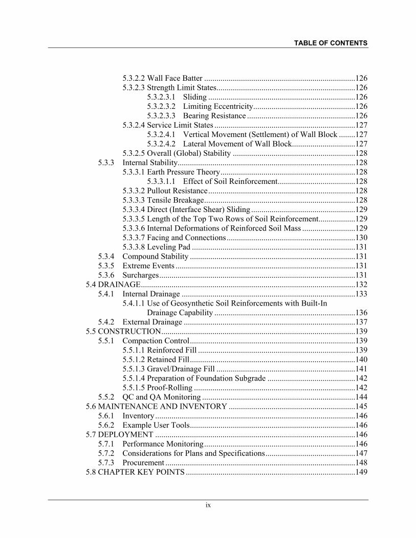
TABLE OF CONTENTS
ix
5.3.2.2 Wall Face Batter ..........................................................................126
5.3.2.3 Strength Limit States ....................................................................126
5.3.2.3.1 Sliding ........................................................................126
5.3.2.3.2 Limiting Eccentricity ..................................................126
5.3.2.3.3 Bearing Resistance .....................................................126
5.3.2.4 Service Limit States .....................................................................127
5.3.2.4.1 Vertical Movement (Settlement) of Wall Block ........127
5.3.2.4.2 Lateral Movement of Wall Block ...............................127
5.3.2.5 Overall (Global) Stability ............................................................128
5.3.3 Internal Stability .......................................................................................128
5.3.3.1 Earth Pressure Theory ..................................................................128
5.3.3.1.1 Effect of Soil Reinforcement ......................................128
5.3.3.2 Pullout Resistance ........................................................................128
5.3.3.3 Tensile Breakage ..........................................................................128
5.3.3.4 Direct (Interface Shear) Sliding ...................................................129
5.3.3.5 Length of the Top Two Rows of Soil Reinforcement..................129
5.3.3.6 Internal Deformations of Reinforced Soil Mass ..........................129
5.3.3.7 Facing and Connections ...............................................................130
5.3.3.8 Leveling Pad ................................................................................131
5.3.4 Compound Stability .................................................................................131
5.3.5 Extreme Events ........................................................................................131
5.3.6 Surcharges ................................................................................................131
5.4 DRAINAGE .........................................................................................................132
5.4.1 Internal Drainage .....................................................................................133
5.4.1.1 Use of Geosynthetic Soil Reinforcements with Built-In Drainage Capability .....................................................................136
5.4.2 External Drainage ....................................................................................137
5.5 CONSTRUCTION ...............................................................................................139
5.5.1 Compaction Control .................................................................................139
5.5.1.1 Reinforced Fill .............................................................................139
5.5.1.2 Retained Fill .................................................................................140
5.5.1.3 Gravel/Drainage Fill ....................................................................141
5.5.1.4 Preparation of Foundation Subgrade ...........................................142
5.5.1.5 Proof-Rolling ...............................................................................142
5.5.2 QC and QA Monitoring ...........................................................................144
5.6 MAINTENANCE AND INVENTORY ..............................................................145
5.6.1 Inventory ..................................................................................................146
5.6.2 Example User Tools .................................................................................146
5.7 DEPLOYMENT ..................................................................................................146
5.7.1 Performance Monitoring ..........................................................................146
5.7.2 Considerations for Plans and Specifications ............................................147
5.7.3 Procurement .............................................................................................148
5.8 CHAPTER KEY POINTS ...................................................................................149
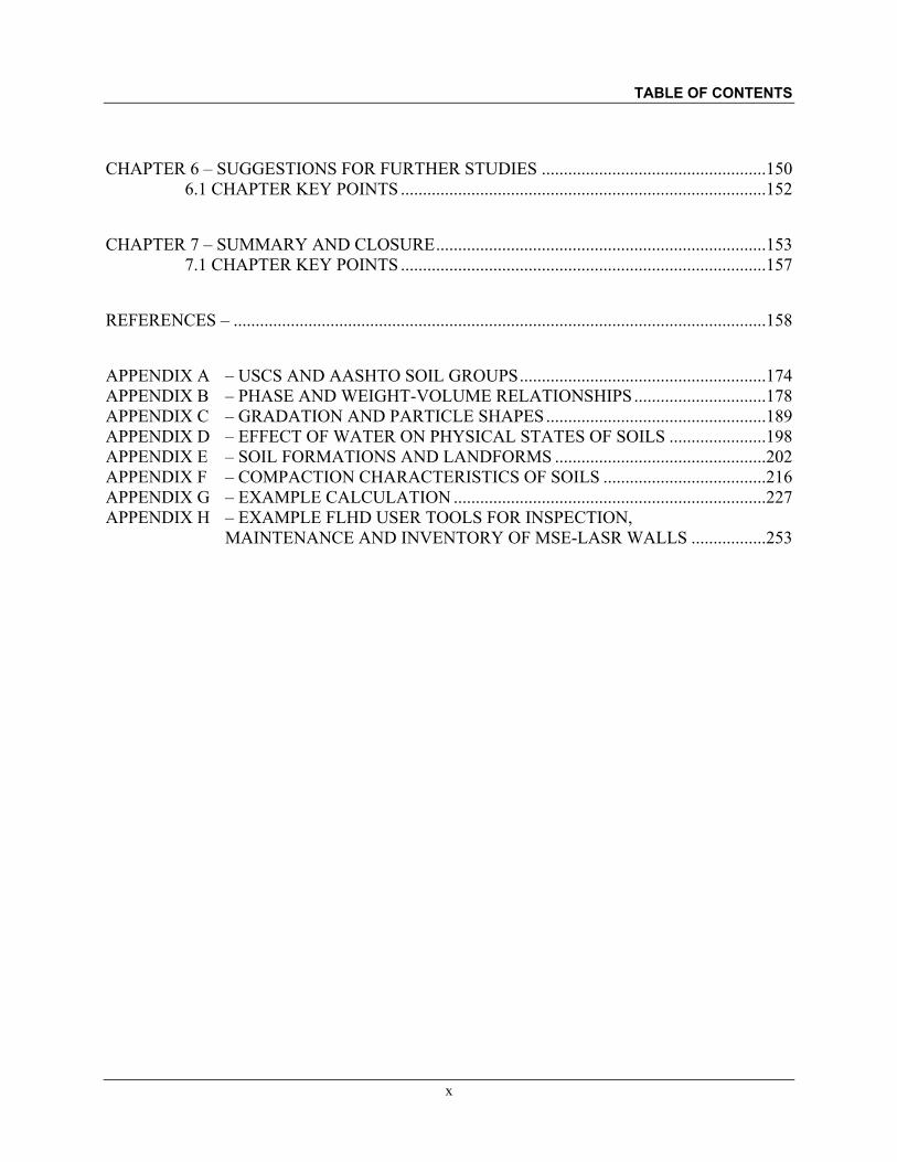
TABLE OF CONTENTS
x
CHAPTER 6 – SUGGESTIONS FOR FURTHER STUDIES ...................................................150
6.1 CHAPTER KEY POINTS ...................................................................................152
CHAPTER 7 – SUMMARY AND CLOSURE ...........................................................................153
7.1 CHAPTER KEY POINTS ...................................................................................157
REFERENCES – .........................................................................................................................158
APPENDIX A – USCS AND AASHTO SOIL GROUPS ........................................................174
APPENDIX B – PHASE AND WEIGHT-VOLUME RELATIONSHIPS ..............................178
APPENDIX C – GRADATION AND PARTICLE SHAPES ..................................................189
APPENDIX D – EFFECT OF WATER ON PHYSICAL STATES OF SOILS ......................198
APPENDIX E – SOIL FORMATIONS AND LANDFORMS ................................................202
APPENDIX F – COMPACTION CHARACTERISTICS OF SOILS .....................................216
APPENDIX G – EXAMPLE CALCULATION .......................................................................227
APPENDIX H – EXAMPLE FLHD USER TOOLS FOR INSPECTION, MAINTENANCE AND INVENTORY OF MSE-LASR WALLS .................253

TABLE OF CONTENTS
xi
LIST OF FIGURES
Figure 2.1. Schematic. Basic Nomenclature for MSE Walls (Modified from Samtani, 2014b). ...................................................................................................................... 10
Figure 2.2. Schematic. Basic Geometry and Forces for MSE Walls (Modified from Samtani, 2014b). ........................................................................................................ 12
Figure 2.3. Schematic. Computation of Active Earth Pressure Coefficient for MSE Walls (Modified from Samtani, 2014b). .............................................................................. 13
Figure 3.1. Graph. Sample Format for Gradation Curve with Select Fill Limits for MSE Walls. ......................................................................................................................... 42
Figure 3.2. Graph. Evaluation of Select Fill Criteria from Drainage Viewpoint Using Limits of Drainage Characteristics from NAVFAC (1986a) and After Powers (1992). ....................................................................................................................... 46
Figure 3.3. Graph. Effect of Fines on Permeability (Modified after Barber and Sawyer, 1952, and NAVFAC, 1986a) [1 cm/sec ≈ 2,835 ft/day]. .......................................... 47
Figure 3.4. Graph. (a) Relationship Between Water Content and Percent Clay by Weight Needed to Fill Voids in a Granular Soil (Based on Mitchell, 1993, and Mitchell and Soga, 2005), (b) Effect of Percent Clay (Clay Fraction) by Weight on R-value of Compacted Subgrade (After Hveem, 1953), (c) Effect of Various Fine Materials on the Sand Equivalent (After Hveem, 1953), (d) Sand Equivalent versus Resistance (R) Value (After Hveem, 1953). ....................... 49
Figure 3.5. Chart. USCS Plasticity Chart as per ASTM D2487 with PI Limit for Select Fill for MSE Walls. ................................................................................................... 51
Figure 3.6. Chart. USCS Plasticity Chart with Location of Clay Minerals and Activity Index Values (After FHWA, 2006, and Based on Data from Skempton, 1953; Mitchell, 1993; and Holtz and Kovacs, 1981). .......................................................... 54
Figure 3.7. Schematic. (a) USBR (1960) Definition of Shear Strength Parameters Based on Straight Line Mohr-Coulomb Failure Envelope for Data in Table 3.4, (b) Concept of Curved Failure Envelope and Choice of Shear Strength Parameters Based on Range of Interest for Normal Stress. ...................................... 60
Figure 3.8. Chart. Potential Contributions of Several Bonding Mechanisms to Soil Strength (After Ingles, 1962, and Mitchell, 1993). ................................................... 64
Figure 3.9. Graph. Volume Change for Compacted Silty Clay (After Handy and Spangler, 2007, Based on Data from Lawton et al, 1992). ........................................................ 67
Figure 3.10. Graph. Controlling the Volume Change of Expansive Clay by Adjusting the Compaction Moisture Content (After Seed and Chan, 1959). .................................. 68
Figure 3.11. Schematic. Stress Transfer Mechanisms for Soil Reinforcement (FHWA, 2009), (a) Frictional Stress Transfer Between Soil and Reinforcement Surfaces, and (b) Soil Passive (Bearing) and Frictional Resistance on Reinforcement Surfaces. ........................................................................................... 73
Figure 3.12. Schematic. Coverage Ratio (After FHWA, 2009).................................................... 75
Figure 3.13. Schematic. Interaction of Facing with Soil Reinforcement (After NCS, 2014). ......................................................................................................................... 78

TABLE OF CONTENTS
xii
Figure 3.14. Schematic. Potential Sources and Flow Paths of Water (Modified from Samtani, 2014b and NCS, 2014). .............................................................................. 80
Figure 3.15. Schematic. Example of Undesirable Water Seepage Through Pavement Because of Deficient Grades (FHWA, 2009). ........................................................... 81
Figure 3.16. Schematic. Example of Some Surcharges on MSE Wall (After Samtani, 2014b). ....................................................................................................................... 82
Figure 3.17. Graph. Illustration of Compaction Characteristics of Variable Fill Materials at a Given Site (After Pickens, 1980). ....................................................................... 85
Figure 3.18. Graph. Standard Proctor Compaction Test Results on an Allophane Clay (After Wesley, 2010b). .............................................................................................. 86
Figure 3.19. Graph. Example of the 10% SAV Evaluation Method, Gs = 2.70 (After Mokwa and Fridleifsson, 2005, and Procedure MT 229 of MDT, 2013). ................ 87
Figure 3.20. Graph. Example Chart from Procedure MT 229-04 of MDT (2013) for 16% SAV based on Gs = 2.65. .......................................................................................... 88
Figure 3.21. Graph. Evaluation of Sensitivity of SAV Method to Variation in Specific Gravity (After Jones, 1973 and Mokwa and Fridleifsson, 2005). ............................. 90
Figure 3.22. Graph. Scenarios Illustrating Possible Limitations of SAV Method (After Mokwa and Fridleifsson, 2005). ................................................................................ 92
Figure 3.23. Graph. Standard Proctor Compaction Test on Clay Including Measurements of Undrained Shear Strength (After Wesley, 2010a). ............................................... 95
Figure 3.24. Schematic. Compaction Control Using SAV&S Method (After Wesley, 2010a, Pickens, 1980). .............................................................................................. 96
Figure 3.25. Schematic. Compaction Control Chart Using SAV&S Method. ............................. 97
Figure 3.26. Graph. (a) Gradation of Concrete Sand (b) Compaction Results for Concrete Sand (After Drnevich et al., 2007). ........................................................................... 99
Figure 3.27. Schematic. Hand Penetrometers that can be Used to Control Compaction (After Wesley, 2010a). ............................................................................................ 100
Figure 5.1. Graph. Resistance Factor for Sliding Resistance Between MSE-LASR Soil and Foundation Geomaterial. .................................................................................. 127
Figure 5.2. Schematic. Potential Drainage Features (Modified from Samtani, 2014b, and NCS, 2014). ............................................................................................................. 134
Figure 7.1. Flow chart. Activities for Implementation of MSE-LASR Technology. ................. 156
Figure A.1. Chart. Comparison of the USCS with the AASHTO Soil Classification System (After Utah DOT – Pavement Design and Management Manual, 2005). ....................................................................................................................... 175
Figure B.1. Schematic. A Unit of Soil Mass and its Idealization (FHWA, 2006). ..................... 179
Figure B.2. Weight-Volume Relations (After FHWA, 2006 and Jumikis, 1962) ...................... 185
Figure B.3. Weight-Volume relations for Gs, n and e for Saturated Soils (based on Jumikis, 1962). ........................................................................................................ 186
Figure B.4. Useful Equations in Terms of γw, γd, and w .......................................................... 186
Figure B.5. Schematic. Weight-Volume Relationships for a Saturated Clay-Granular Soil Mixture (After Mitchell and Soga, 2005). ............................................................... 187
Figure C.1. Schematic. Sample Particle Size Distribution Curves (After FHWA 2006). .......... 191
Figure C.2. Schematic. Evaluation of Type of Gradation for Coarse-Grained Soils. ................. 194

TABLE OF CONTENTS
xiii
Figure C.3. Schematic. Criteria for Particle Shape (After ASTM D2488). ................................ 195
Figure C.4. Photo. Typical Angularity of Bulky Particles (After ASTM D2488). ..................... 197
Figure D.1. Schematic. Conceptual Changes in Soil Phases as a Function of Water Content (FHWA 2006). ........................................................................................... 198
Figure D.2. Chart. Plasticity Chart and Significance of Atterberg Limits (NAVFAC, 1986a). ..................................................................................................................... 201
Figure E.1. Schematic. Typical Weathering Profile for Metamorphic and Igneous Rocks (After Deere and Patton, 1971). .............................................................................. 205
Figure E.2. Map. Soil Deposits of the United States and Canada (After Belcher, et al., 1946 and Peck, et al., 1974). ................................................................................... 209
Figure E.3. Map. Soil Deposits of the United States (NAVFAC, 1971). ................................... 210
Figure E.4. Map. Physiographic Map of the United States (http://www.bing.com). .................. 211
Figure F.1. Photo. Hammer and Mold for Laboratory Compaction Test; Tape Measure is for Scale Purpose Only (FHWA 2006). .................................................................. 217
Figure F.2. Graph. Example Compaction Curves (After Holtz and Kovacs, 1981). .................. 218
Figure F.3. Graph. Soil Air Voids Curve in Relation to Degree of Saturation Curves. ............. 220
Figure F.4. Chart. Compactors Recommended for Various Types of Soil and Rock (Schroeder, 1980). ................................................................................................... 221
Figure F.5. Graph. Relative Density, Relative Compaction and Void Ratio Concepts (FHWA, 2006). ........................................................................................................ 223
Figure F.6. Chart. Correlation Between Relative Density, Material Classification and Angle of Internal Friction for Coarse-Grained Soils (After NAVFAC, 1986a). ..... 224
Figure F.7. Schematic. Example Evaluation of Economical Field Compaction Conditions (After Bowles, 1979). .............................................................................................. 226
Figure G.1. Schematic. Configuration Showing Various Parameters for Analysis of a MSE-LASR Wall with Level Fill and Live Load Surcharge (Not-To-Scale). ........ 227
Figure G.2. Schematic. Legend for Computation of Forces and Moments (Not-To-Scale) (After FHWA, 2009). .............................................................................................. 231
Figure G.3. Schematic. Geometry Definition, Location of Critical Failure Surface and Variation of Kr and F* Parameters for Geogrid Reinforcements............................ 238
Figure H.1. Data. Listing of Codes for Wall Function, Wall Type, Architectural Facing Type and Surface Treatments (FHWA, 2010). ....................................................... 254
Figure H.2. Data. Field Inspection Form – Front Page (FHWA, 2010). .................................... 255
Figure H.3. Data. Guide to Complete Field Inspection Form – Page 1 of 4 (FHWA, 2010) ..... 257

TABLE OF CONTENTS
xiv
LIST OF TABLES
Table 2.1. MSE Wall Select Granular Reinforced Fill Gradation Requirements – Test Method: AASHTO T 27 (After FHWA Table 3-1) ................................................... 14
Table 2.2. Additional MSE Wall Select Granular Reinforced Fill Requirements (After FHWA Table 3-1) ...................................................................................................... 14
Table 2.3. Recommended Limits of Electrochemical Properties for Reinforced Fills with Steel Reinforcement (After FHWA Table 3-3). ........................................................ 15
Table 2.4. Recommended Limits of Electrochemical Properties for Reinforced Fills with Geosynthetic Reinforcements (After FHWA Table 3-4). .......................................... 15
Table 2.5. SRW Suggested Reinforced Fill Requirements (After NCMA 2010). ....................... 18
Table 2.6. Additional SRW Suggested Reinforced Fill Requirements (After NCMA 2010). ......................................................................................................................... 18
Table 3.1. Methods of Index Testing of Soils (After FHWA, 2006). .......................................... 38
Table 3.2. Typical Values of Gs for Various Soil Components (After Bowles, 1979). .............. 41
Table 3.3. Typical Values of Gs for Various Soil Minerals (After Jumikis, 1962). .................... 41
Table 3.4. Average Engineering Properties of Compacted Inorganic Soils (After USBR, 1960 and FHWA, 2006). ............................................................................................ 59
Table 3.5. Limit States and Stability Modes for MSE Wall Systems (After FHWA, 2009, Samtani and Sabatini, 2010, and Samtani, 2014b). ................................................. 104
Table 3.6. Resistance Factors or Criteria for External Stability Limit States Based on AASHTO (2020) ...................................................................................................... 105
Table 3.7. Resistance Factors or Criteria for Internal Stability Limit States Table 11.5.7-1 and Article 11.5.8 of AASHTO (2020) and Simplified Method ............................. 105
Table 3.8. Resistance Factors or Criteria for Overall and Compound Stability Limit States (After Article 11.6.3.7 of AASHTO, 2020) ............................................................. 105
Table 5.1. Limiting Criteria for MSE-LASR Wall Fills. ........................................................... 120
Table 5.2. Procedure for the Determination of Properties of LASR Materials Within the Reinforced and Retained Fill Zones. ....................................................................... 123
Table 5.3. Sampling Frequency for Reinforced Fill Material. ................................................... 144
Table 5.4. Sampling Frequency for Retained Fill Material. ...................................................... 145
Table A.1. Comparable Soil Groups in AASHTO System based on Soil Groups in USCS (After Liu, 1970 and Holtz and Kovacs, 1981). ...................................................... 176
Table A.2. Comparable Soil Groups in USCS based on Soil Groups in AASHTO System (After Liu, 1970 and Holtz and Kovacs, 1981). ...................................................... 177
Table B.1. Summary of Index Properties and Their Application (After FHWA, 2006). .......... 185
Table C.1. U.S. Standard Sieve Sizes and Corresponding Opening Dimension (FHWA 2006). ....................................................................................................................... 190
Table C.2. Gradation Based on Cu and Cc Parameters ............................................................. 193
Table D.1. Concept of Soil Phase, Soil Strength and Soil Deformation Based on Liquidity Index for Remolded Soils (FHWA 2006). ............................................................... 200
Table E.1. Common Landforms of Water Transported Soils and Their Engineering Significance (FHWA, 2006). ................................................................................... 206

TABLE OF CONTENTS
xv
Table E.2. Common Landforms of Ice (Glacier) Transported Soils and Their Engineering Significance (FHWA, 2006). ................................................................................... 207
Table E.3. Common Landforms of Wind Transported (Aeolian) Soils and Their Engineering Significance (FHWA, 2006). ............................................................... 208
Table E.4. Common Landforms of Gravity Transported Soils and Their Engineering Significance (FHWA, 2006). ................................................................................... 208
Table E.5. Distribution of Non-Soil Deposits in the United States (After NAVFAC, 1971 and Hunt, 2005). ...................................................................................................... 212
Table E.6. Distribution of Alluvial Soil Deposits in the United States (After NAVFAC, 1971 and Hunt, 2005). ............................................................................................. 212
Table E.7. Distribution of Residual Soil Deposits in the United States (After NAVFAC, 1971 and Hunt, 2005). ............................................................................................. 213
Table E.8. Distribution of Loessial Soil Deposits in the United States (After NAVFAC, 1971 and Hunt, 2005). ............................................................................................. 214
Table E.9. Distribution of Glacial Soil Deposits in the United States (After NAVFAC, 1971 and Hunt, 2005). ............................................................................................. 215
Table F.1. Characteristics of Laboratory Compaction Tests (After FHWA 2006). .................. 216
Table F.2. Some Values of Dr as a Function of RC Based on Modified and Standard Proctor Compaction Test (FHWA, 2006) ................................................................ 224
Table G.1. Summary of Steps in Analysis of MSE-LASR Wall with Level Fill and Live Load Surcharge. ....................................................................................................... 228
Table G.2. Equations for Computing Unfactored (Nominal) Vertical Forces and Moments. ................................................................................................................. 230
Table G.3. Equations for Computing Unfactored (Nominal) Horizontal Forces and Moments. ................................................................................................................. 230
Table G.4. Unfactored (Nominal) Vertical Forces and Moments. ............................................ 232
Table G.5. Unfactored (Nominal) Horizontal Forces and Moments. ........................................ 232
Table G.6. Summary of Applicable Load Factors. .................................................................... 233
Table G.7. Summary of Applicable Resistance Factors. ........................................................... 233
Table G.8. Computations for Evaluation of Sliding Resistance of MSE-LASR Wall. ............. 234
Table G.9. Computations for Evaluation of Limiting Eccentricity for MSE-LASR Wall. ....... 235
Table G.10. Computations for Evaluation of Bearing Resistance for MSE-LASR Wall. ......... 237
Table G.11. Summary of Computations for Svt and Atrib. ....................................................... 240
Table G.12. Summary of Load Components Leading to Horizontal Stress. ............................. 240
Table G.13. Geogrid Grades (Strengths) and Scale Correction Factors. ................................... 242
Table G.14. Geogrid Nominal and Factored Resistances. ......................................................... 243
Table G.15. Summary of Internal Stability Computationsfor Strength I (max) Load Combination. ............................................................................................................ 246
Table G.16. Summary of Internal Stability Computations forDirect (Interface Shear) Sliding. ..................................................................................................................... 248
Table G.17. Connection Strength Check. .................................................................................. 249

LIST OF ACRONYMS, ABBREVIATIONS, AND SYMBOLS
xvi
LIST OF ACRONYMS, ABBREVIATIONS, AND SYMBOLS
a Location of the resultant force on base of MSE-LASR wall from Point A A Activity Index AASHTO American Association of State Highway and Transportation Officials AC Asphaltic Concrete Aceff Effective cross-sectional after corrosion loss (computed) Aeff Effective cross-sectional after corrosion loss (computed) AMSE Association of Metallically Stabilized Earth API Asset Priority Index ASTM American Society for Testing and Materials AQL Acceptable Quality Level ASD Allowable Stress Design Atrib Tributary area b Width of reinforcement B Base width of MSE wall B' Effective width of base of MSE-LASR wall BS British Standard C Percent of clay by weight co Cohesion of as-compacted specimen as defined by USBR (1960) csat Cohesion of compacted-saturated specimen as defined by USBR (1960) c Cohesion of compacted-saturated specimen based on straight line Mohr-
Coulomb failure envelope over the stress range of interest c Cohesion of as-compacted specimen based on straight line Mohr-Coulomb
failure envelope over the stress range of interest CALTRANS California Department of Transportation Cc Coefficient of Curvature (Coefficient of Concavity or Coefficient of Gradation) CDR Capacity Demand Ratio CDRDS Capacity Demand Ratio for direct (interface shear) sliding CDRPullout Capacity Demand Ratio for pullout CDRTensile Breakage Capacity Demand Ratio for tensile breakage CF Clay Fraction (Percent Clay by weight) CFLHD Central Federal Lands Highway Division CGR Cone Index Gradient

LIST OF ACRONYMS, ABBREVIATIONS, AND SYMBOLS
xvii
CI Cone Index CMAR Construction Manager at Risk COR Contracting Officer’s Representative COV Coefficient of Variation CTIP Coordinated Technology Implementation Program Cu Coefficient of Uniformity (Uniformity Coefficient) CU Consolidated-Undrained CY Cubic yards d Minimum embedment depth at front face of wall D10 Particle size for which 10% of weight is finer D30 Particle size for which 30% of weight is finer D60 Particle size for which 60% of weight is finer DCP Dynamic Cone Penetrometer DOT Department of Transportation DO Distance of the exit point of the outlet pipe from the front of wall facing Dr Relative Density e Void ratio or Eccentricity eG Void ratio of granular phase eL Limiting eccentricity eo In-situ void ratio E Modulus of elasticity (or elastic modulus) EFLHD Eastern Federal Lands Highway Division EH Horizontal earth pressure load EN Euronorm, European Standard ES Earth surcharge load ESALs Equivalent Single Axle Loads EV Vertical pressure from dead load of earth fill F Amount of fines in % F1 Horizontal force due to retained fill (external stability) F2 Horizontal force due to surcharge on retained fill (external stability) FCI Facility Condition Index FHWA Federal Highway Administration FLH Federal Land Highway
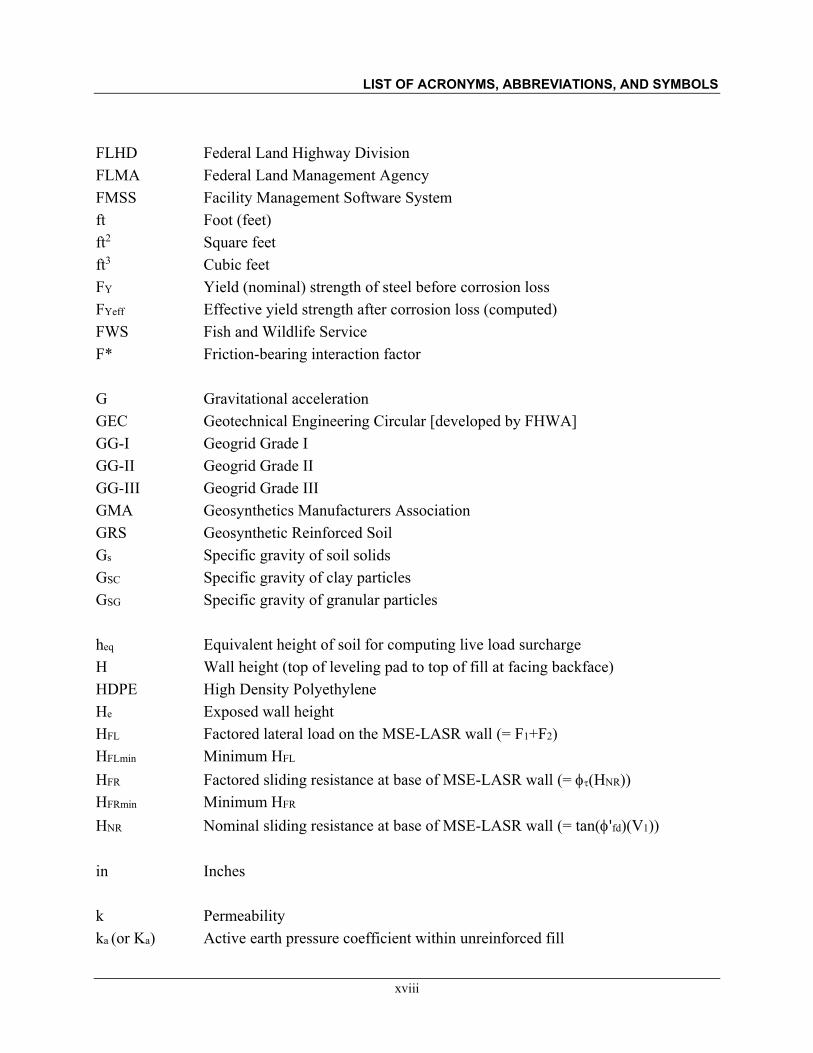
LIST OF ACRONYMS, ABBREVIATIONS, AND SYMBOLS
xviii
FLHD Federal Land Highway Division FLMA Federal Land Management Agency FMSS Facility Management Software System ft Foot (feet) ft2 Square feet ft3 Cubic feet FY Yield (nominal) strength of steel before corrosion loss FYeff Effective yield strength after corrosion loss (computed) FWS Fish and Wildlife Service F* Friction-bearing interaction factor G Gravitational acceleration GEC Geotechnical Engineering Circular [developed by FHWA] GG-I Geogrid Grade I GG-II Geogrid Grade II GG-III Geogrid Grade III GMA Geosynthetics Manufacturers Association GRS Geosynthetic Reinforced Soil Gs Specific gravity of soil solids GSC Specific gravity of clay particles
GSG Specific gravity of granular particles heq Equivalent height of soil for computing live load surcharge H Wall height (top of leveling pad to top of fill at facing backface) HDPE High Density Polyethylene He Exposed wall height HFL Factored lateral load on the MSE-LASR wall (= F1+F2) HFLmin Minimum HFL HFR Factored sliding resistance at base of MSE-LASR wall (= (HNR)) HFRmin Minimum HFR HNR Nominal sliding resistance at base of MSE-LASR wall (= tan('fd)(V1)) in Inches k Permeability ka (or Ka) Active earth pressure coefficient within unreinforced fill
LIST OF ACRONYMS, ABBREVIATIONS, AND SYMBOLS
xix
karein (or Karein) Active earth pressure coefficient based on reinforced fill friction angle karet (or Karet) Active earth pressure coefficient based on retained fill friction angle Kr Earth pressure coefficient within reinforced fill ksi Kips per square inch kPa Kilopascal kN Kilonewton L Length of soil reinforcement La Length of soil reinforcement in active zone LASR Local Available Sustainable Resources Le Length of soil reinforcement in resistance zone LI Liquidity Index LL Liquid Limit (or vehicular live load) LS Live load surcharge LRFD Load and Resistance Factor Design m Meter m2 Square meters MA Net factored moment about Point A (MA = MRA – MOA) MBW Modular Block Wall MCP Mobility Cone Penetrometer MDD Maximum Dry Density – compaction mils Milli inches (= 0.001 inch) MPa Megapascal MOA Overturning factored moments about Point A (MOA = MF1+MF2) MOA-C Maximum overturning factored moments about Point A MRA Resisting factored moments about Point A without LL surcharge (MRA = MV1) MRA-C Minimum resisting overturning factored moments about Point A Ms Mass of soil solids MSE Mechanically Stabilized Earth MSE-LASR MSE wall built with Local Available Sustainable Resources MSS Minimum shear strength MUTCD Manual on Uniform Traffic Control Devices n Porosity N Number of tests required

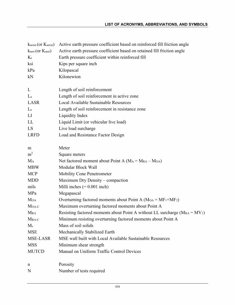
LIST OF ACRONYMS, ABBREVIATIONS, AND SYMBOLS
xx
Na Percent air voids NCHRP National Cooperative Highway Research Program NCMA National Concrete Masonry Association NPS National Park Service NTP Notice to Proceed OMC Optimum Moisture Content – compaction oz Ounce (ounces) Pap Probability of Adverse Performance Pf Probability of unsatisfactory performance (or failure) Pr Nominal pullout resistance Prr Factored pullout resistance Ps Probability of satisfactory performance (or success) pc Confining pressure PCCP Portland Concrete Cement Pavement pcf Pounds per cubic foot PE Polyester PET PVC coated polyester PI Plasticity Index PL Plastic Limit PPM Parts Per Million psi Pounds per square inch psf Pounds per square foot pt Total vertical stress PVC Polyvinyl Chloride q Pressure due to live load surcharge QA Quality Assurance QC Quality Control qnf-ser Factored bearing resistance for settlement evaluation at service limit state qnf-str Factored bearing resistance for bearing evaluation at strength limit state RC Relative Compaction Rc Reinforcement Coverage Ratio (=b/Sh) RECo Reinforced Earth Company
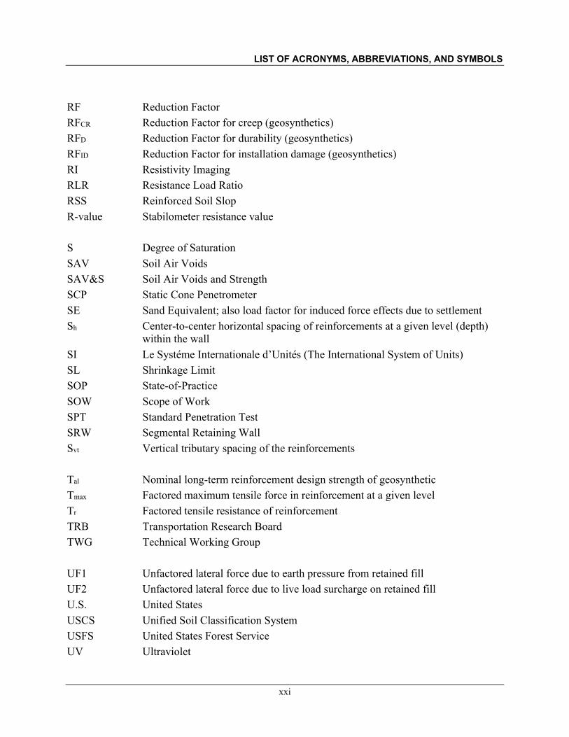
LIST OF ACRONYMS, ABBREVIATIONS, AND SYMBOLS
xxi
RF Reduction Factor RFCR Reduction Factor for creep (geosynthetics) RFD Reduction Factor for durability (geosynthetics) RFID Reduction Factor for installation damage (geosynthetics) RI Resistivity Imaging RLR Resistance Load Ratio RSS Reinforced Soil Slop R-value Stabilometer resistance value S Degree of Saturation SAV Soil Air Voids SAV&S Soil Air Voids and Strength SCP Static Cone Penetrometer SE Sand Equivalent; also load factor for induced force effects due to settlement Sh Center-to-center horizontal spacing of reinforcements at a given level (depth)
within the wall SI Le Systéme Internationale d’Unités (The International System of Units) SL Shrinkage Limit SOP State-of-Practice SOW Scope of Work SPT Standard Penetration Test SRW Segmental Retaining Wall Svt Vertical tributary spacing of the reinforcements Tal Nominal long-term reinforcement design strength of geosynthetic Tmax Factored maximum tensile force in reinforcement at a given level Tr Factored tensile resistance of reinforcement TRB Transportation Research Board TWG Technical Working Group UF1 Unfactored lateral force due to earth pressure from retained fill UF2 Unfactored lateral force due to live load surcharge on retained fill U.S. United States USCS Unified Soil Classification System USFS United States Forest Service UV Ultraviolet

LIST OF ACRONYMS, ABBREVIATIONS, AND SYMBOLS
xxii
V Total volume of soil VH Vibrating Hammer VR Total volume within the reinforced and retained fill zones Va Volume of air VA Total factored vertical load at base of MSE-LASR wall without LL (VA = V1) VA-C Vertical factored force VC Volume of air VGS Volume of granular solids VS or Vs Volume of soil solids VS Vertical force due to surcharge (external stability) Vv Total volume of voids Vw Volume of water V1 Vertical force due to reinforced soil mass (external stability) w Water content W Total weight of soil Wa Weight of air Ww Weight of water Ws Weight of soil solids WES U.S. Army Waterways Experiment Station WFLHD Western Federal Lands Highway Division WIP Wall Inventory Program wopt Optimum moisture content – compaction wp Width of face panel yd3 Cubic yards Z Depth below top of reinforced soil mass ZAV Zero Air Voids % Percent # Number ≈ Approximately equal to
Scale correction factor for geosynthetic reinforcement

LIST OF ACRONYMS, ABBREVIATIONS, AND SYMBOLS
xxiii
Slope of ground above and behind wall face T Target reliability index
Load factor d Dry density dmax Maximum dry density dfield Maximum dry density measured in the field EV Load factor for EV load type EH Load factor for EH load type fd Total unit weight of foundation soil LL Load factor for LL load type LS Load factor for LS load type P-EV Load factor for EV load type for pullout resistance evaluation where live load is
not included (internal stability) rein Total unit weight of reinforced fill ret Total unit weight of retained fill s Unit weight of solid particles w Unit weight of water
Wall interface friction angle (in degrees) r Relative displacement ratio rm Modified relative displacement ratio max Maximum estimated lateral displacement Front face batter of wall (in degrees) w Volumetric water content Mean value m Microns
Interface shear friction angle between geogrid and reinforced fill soil d Mass density of water dry Dry density s Mass density of solid particles t Total density Standard deviation Effective normal stress - USBR (1960) notation σH Total horizontal stress at a reinforcement level for internal stability σH-soil Horizontal stress due to soil at a reinforcement level for internal stability σH-surcharge Horizontal stress due to surcharge at a reinforcement level for internal stability

LIST OF ACRONYMS, ABBREVIATIONS, AND SYMBOLS
xxiv
v Equivalent uniform (“Meyerhof”) bearing stress at the base of the MSE-LASR wall
v-c Factored bearing stress v-soil Vertical stress due to soil at a reinforcement level for internal stability V Resultant of vertical forces at base of wall (or Total factored vertical load at
base of MSE-LASR wall including LL on top, ΣV = R = V1 + VS) Shear strength Effective friction angle of as-compacted and compacted-saturated soil - USBR
(1960) notation Total friction angle – general notation used in this report. Effective friction angle – general notation used in this report. b Resistance factor for bearing evaluation (external stability) c Resistance factor for connection strength (internal stability) DS Resistance factor for direct (interface shear) sliding (internal stability) fd Effective friction angle of foundation soil p Resistance factor for pullout resistance of reinforcement rein Effective friction angle of reinforced fill ret Effective friction angle of retained fill t Resistance factor for tensile resistance of reinforcement Resistance factor for shear resistance in sliding stability analysis

ACKNOWLEDGMENTS
xxv
ACKNOWLEDGMENTS (Unless otherwise noted, all affiliations are from
the time of the first phase of the study in 2013-2015) This project is funded by Federal Highway Administration (FHWA) Federal Lands Highway (FLH) Coordinated Technology Implementation Program (CTIP), a premier national model for evaluating, developing, and implementing leading edge technology. The contributions and cooperation of the Technical Working Group (TWG), which included the following members, is gratefully acknowledged: • Mounir Abouzakhm, PE (FHWA – Eastern Federal Lands Highway Division), • Daniel Alzamora, PE (FHWA – Resource Center), • Dr. Scott Anderson, PE (FHWA – Resource Center), • Brian Collins, PE (FHWA – Western Federal Lands Highway Division), • Marilyn Dodson, PE (FHWA – Central Federal Lands Highway Division), • Robert Kraig, PE (FHWA – Western Federal Lands Highway Division), • Braden Peters, PE (FHWA – Central Federal Lands Highway Division), and • Roger Surdahl, PE (FHWA – Central Federal Lands Highway Division). In the second phase of the study in 2020-2021, Rebecca Borst, EIT (FHWA – Central Federal Lands Highway Division) performed the work for 508 compliance in coordination with FHWA – Federal Lands Highways Division Public Relations Department (Sterling, VA) and their collective efforts towards making the final version of the report 508 compliant are appreciated. The efforts of William Lang, PE, and Danielle Yearsley of CH2M Hill in administering the contractual aspects with FHWA-CFLHD are appreciated. In addition to the TWG, numerous other individuals contributed to the study in the form of providing useful literature, discussions, and/or office support. Of noteworthy mention is Jim Scott, PE (AECOM, Denver) who provided the most literature. Additional literature was provided by Ryan Berg, PE (Ryan R. Berg and Associates, Inc.), Dr. Barry Christopher, PE (Christopher Consultants), Kathryn Griswell, PE (Caltrans), Dr. Dov Leshchinsky (University of Delaware), Dr. Robert Koerner, PE (Drexel University and Geosynthetic Institute), Tony Allen, PE (Washington State Department of Transportation and AASHTO T-15 Committee Vice-Chair), Dr. Richard Bathurst (Royal Military College of Canada), Willie Liew, PE (Tensar, United States), Michael Dobie, CEng (Tensar International, Jakarta, Indonesia), Dr. Laurence Wesley (University of Auckland, New Zealand), Dr. Jorge Zornberg, PE (University of Texas, Austin), Dr. Kenneth Fishman, PE (Earth Reinforcement Testing, Inc.), Franciscus Hardianto, PE (Reinforced Earth Company, San Diego), Gabriela Mariscal, PE (National Concrete Masonry Association), Dr. Jonathan Wu (University of Colorado, Denver), Craig Moritz, PE (Keystone Systems), and Alexander Kidd (Consultant, London, United Kingdom).
ACKNOWLEDGMENTS
xxvi
In addition to the above list the following individuals were contacted for information and provided support in form of phone discussions and/or e-mail communications: Jawdat Siddiqi, PE (Ohio Department of Transportation and AASHTO T-15 Committee Chair), Robert Meyers, PE (New Mexico Department of Transportation), Jeff Sizemore, PE (South Carolina Department of Transportation), Jerry DiMaggio, PE (ARA, Inc.), Dr. W. Allen Marr, PE (Geocomp Corporation/Geotesting Express), Richard Stulgis, PE (Geocomp Corporation), Dr. James Collin, PE (The Collin Group), Dr. Robert Bachus, PE (Geosyntec Consultants), Robert Gladstone, PE (Association of Metallically Stabilized Earth, AMSE), Michael Bernardi (Geosynthetic Manufacturers Association, GMA, and TENCATE), Thomas Taylor, PE (Vist-A-Wall Systems), Dr. William Neely, PE (Flatiron Construction Corporation), and Dr. Brian Simpson (ARUP, London, United Kingdom). Joseph Harris, PE, and Kenton Watts, EIT of NCS Consultants, LLC provided support by checking computations and drafting some figures. Sagar Samtani (Graduate Student, University of Arizona) provided support by collecting numerous publications through library search and interlibrary loan requests. Finally, the efforts of the following individuals in providing review comments on various parts of the draft manuscripts are acknowledged: Jim Scott, PE (AECOM, Denver), Ryan Berg, PE (Ryan R. Berg and Associates, Inc.), Dr. Barry Christopher, PE (Christopher Consultants), Kathryn Griswell, PE (Caltrans), Jerry DiMaggio, PE (ARA, Inc.), Dr. Laurence Wesley (University of Auckland, New Zealand), and Joseph Harris, PE (NCS Consultants, LLC).

CHAPTER 1 – INTRODUCTION
1
CHAPTER 1 – INTRODUCTION
Mechanically Stabilized Earth (MSE) walls have been successfully used in the United States (U.S.) since the 1970s. The Federal Highway Administration (FHWA) and the American Association of State Highway and Transportation Officials (AASHTO) have established guidelines for the design and construction of MSE walls in transportation works. MSE walls have been also used extensively internationally with other guidelines, e.g., British, Japanese, etc. A common thread through all the MSE wall guidelines is the desire to use “select” fills which are primarily frictional and permit gravity drainage within the reinforced soil zone, i.e., the zone of the wall within which soil reinforcement is used. FHWA and AASHTO require that select fill materials limit the fines (material finer than 0.075 mm as measured with the U.S. Standard Sieve No. 200) to 15% by weight, the plasticity index (PI) to 6 along with limitations on the electrochemical properties such as resistivity, pH, and soluble salts (sulfates and chlorides) to control corrosion and/or degradation of the soil reinforcements. The general guidelines noted above have been developed based on collective industry experiences with observed and/or measured performance of MSE walls since the 1970s. The goal of these guidelines, although not clearly quantified in the literature, was to minimize deformations and maintenance issues, which, if not controlled, would lead to a condition that could have an adverse effect on the wall and the facilities supported by the wall or in the vicinity of the wall. The deformations can be due to a number of underlying issues such as poor drainage, inadequate shear strength, poor soil-structure interaction, excess pore water pressures, increased corrosion/degradation, difficulty of moisture conditioning and compaction, etc. The effects of all these issues will be discussed in this report. While small deformations may be troublesome from an aesthetic perspective, large deformations may be construed as adverse performance from the perspective of wall serviceability and, if taken to their limit, may lead to total collapse. Use of select fill materials for MSE walls, while preferable, is not always practical because often such select fill materials are not available locally and must be imported to the jobsite. In that case the disposal of unsuitable local native soils may be required with an associated cost that may significantly increase the total project cost and have an intangible impact on the environment. This situation is particularly true in the case of Federal Land Management Agencies (FLMAs) such as the Federal Lands Highway Division (FLHD) of the FHWA, United States Forest Service (USFS), National Park Service (NPS), and Fish and Wildlife Service (FWS), which are often involved in the design and construction of MSE walls at locations that are far from borrow sources suitable for select fill and disposal areas for local native soils. The availability of cost-effective select fills has also become a concern for urban areas wherein demands of multiple projects with select fill requirements and dwindling sources of borrow material for such select fill result in increased project costs. Indeed, the same situation is true for many parts of the world, e.g., Japan, India, New Zealand, Brazil, etc. In such cases consideration is often given to alternative earth retention systems. Alternative earth retention systems such as cast-in-place reinforced concrete walls generally have a larger carbon footprint, which is environmentally undesirable. To address these issues, the FLHD-FHWA commissioned this report to develop a
CHAPTER 1 – INTRODUCTION
2
framework for using materials that do not meet select fill criteria in support of the unique performance-based management needs of FLHD and other agencies such as local and state Departments of Transportation (DOTs). As will be seen in Chapter 2, several past studies attempted to define and address this problem. Often these studies termed non-select lower quality fills as “marginal” fills where the word “marginal” was generally associated with a fines content larger than 15%. Therefore, those studies do not encompass the full range of the meaning of the word “marginal” in the sense that a fill with any property that does not meet the specifications for select fill can be considered marginal, e.g., large PI, low resistivity, etc. In other words, from an engineering viewpoint there is a need to define the word “marginal” in terms of the specific properties of select fill that are not satisfied. From a legal viewpoint, the word “marginal” could have a negative connotation in the sense that one could construe that the wall was intentionally constructed with inferior fills. Therefore, the project team decided that if the effects of the required properties of the select fill were correctly understood and if one or more of the existing criteria for select fill were not met by a candidate fill, then MSE walls could be constructed with local available sustainable resources (LASR) provided an appropriate level of testing and analysis was performed to define the effects of the relevant properties on design and construction. In such cases, the MSE walls can be the preferred earth retention system because of the advantages of rapid construction in virtually all seasons. MSE walls using LASR are herein called MSE-LASR walls. For correct application of MSE-LASR walls, it is important to understand the meaning of each of the four words in “LASR” as defined below: • The word “local” is intended to signify geographical limits around the MSE-LASR wall
location within which the haul distances would be considered economically and environmentally reasonable.
• The word “available” is intended to signify readily available resources that do not require an unusual (or inordinate) amount of permitting, cultural monitoring and/or environmental clearances.
• A cursory internet search for the meaning of the word “sustainable” with reference to infrastructure development will lead to a number of different interpretations, most of which deal with the effect of human activities on natural systems and the environment. Herein, the word “sustainable” means that use of LASR minimizes the consumption of resources required to obtaining them in fuel and transportation hauling distances. Sustainability can be realized on construction projects by (1) reduction in greenhouse gas emissions from elimination of hauling imported materials, (2) reduction in construction waste (recycling in-situ materials); (3) traffic noise reduction; and (4) reduced congestion.
• The word “resources” has been used herein to acknowledge suitably durable, non-select geomaterials. Thus, the words “sustainable resources” are meant to imply suitably durable non-select geomaterials which will permit construction and maintenance of a MSE-LASR wall that will meet the expected performance criteria, e.g., design life and acceptable
CHAPTER 1 – INTRODUCTION
3
deformations. In this context, the performance criteria themselves can be configured to fit the properties of the sustainable resources.
As discussed previously, the use of non-select fill materials could increase the risks for adverse wall performance such as increased deformations and maintenance issues leading to implementation of costly remedial measures in some cases. Therefore, an understanding of risks (or conversely, reliability) needs to be developed to comprehend the rationale behind the current specifications for various materials used in the construction of MSE walls to be able to understand the potential consequences of overriding existing criteria by the use of LASR. Other than out-of-tolerance placement issues, the simplest manifestation of an adverse performance may be in the form of cracking of an engineered component or structure during its design life. In the context of MSE walls, that component may be a cracked facing panel or a crack in the pavement above the MSE wall. Other manifestations may include loss of intended serviceability (functional or aesthetic), excessive maintenance costs, economic losses, total collapse and/or loss of life. Serviceability of MSE walls has not been explicitly quantified for MSE walls with select fills because the select fills have historically provided satisfactory performance with respect to deformations. However, for MSE-LASR systems the issue of serviceability must be explicitly assessed and quantified. In general, it is more appropriate to understand adverse performance as an unacceptable difference between expected and observed performance. Thus, if the expectations associated with the use of LASR materials in lieu of select fill materials are properly expressed and managed and the observed performance meets the expectations established during the feasibility and design stages of the project, then a project can be considered successful. The issue then becomes one of establishing expectations in terms of risks. Establishing risk criteria entails an evaluation of the probability of adverse performance (Pap) and its impact (i.e., consequences). Since the design for the case of absolutely no adverse performance is theoretically impossible within the context of stochastic processes and the design for a very small probability of adverse performance will be very expensive, a certain acceptable value of Pap needs to be defined. It is difficult, if not impossible, to define a probability of adverse performance for an entire MSE wall system. Thus, from practical considerations, an acceptable level of risk should be determined for a given limit state, e.g., sliding. In the context of Load and Resistance Factor Design (LRFD) as included in AASHTO (2020), this determination is achieved by evaluating discrete limit states as part of different stability modes. For example, limit states such as sliding, limiting eccentricity, settlement, etc. are considered for external stability, while limit states such as pullout and tensile breakage of reinforcement elements are considered for internal stability. Within these stability modes further distinction is made based on ultimate strength (Strength limit state), serviceability (Service limit state) and extreme events (Extreme Event limit state). The load and resistance factors for the various limit states have been calibrated to a certain probability of adverse performance, i.e., level of risk. This
CHAPTER 1 – INTRODUCTION
4
formal framework of limit states as defined within the AASHTO-LRFD1 procedures allows for an evaluation of risks for MSE-LASR walls based on the variation in properties of the LASR within the reinforced zone. The application of this framework to MSE-LASR walls is discussed in Section 4.9 and Chapter 5.
1.1 GOAL
The primary goal of this report is to develop a general risk-based framework in the context of AASHTO-LRFD for the use of MSE-LASR walls. A framework is presented herein that can be used to perform future studies as appropriate that will lead to the development of guidelines for the design and construction of MSE-LASR walls. Although thousands of MSE walls with non-select fill materials have been designed and built in the United States and abroad for private and commercial applications, in the large majority of such cases the design and construction have not been in accordance with FHWA guidelines as contained in FHWA (2009) nor has their performance in all cases been acceptable from the viewpoint of FHWA requirements, e.g., deformations. In addition, the serviceability failure rate of 5 to 10% and a structural failure rate on the order of 1% of such structures is unacceptable for transportation applications. Therefore, the underlying goal of this report is to develop a general risk-based framework for the development of guidelines in the context of AASHTO-LRFD for the use of MSE-LASR walls directed specifically to transportation applications.
1.2 SCOPE OF THE WORK
The scope of the work for the present study to attain the stated goal for transportation applications is as follows: • Perform a literature review to gather information on the use of non-select fills in MSE walls, • Identify and define the factors that influence the selection of MSE wall fills, • Develop a general framework for the use of LASR that is based on an understanding of the
underlying risks associated with the use of such non-select fills, • Provide a framework and example user tools for the development of guidelines for the
implementation of MSE-LASR technology for transportation applications, and • Provide recommendations for future studies to aid in the development of refined guidelines
for the design and construction of MSE-LASR walls in the context of AASHTO-LRFD. This report was developed in two phases: 2013-2015 and 2020-2021. The first phase of the work included reference to provisions AASHTO (2014). The second phase work involved updating the
1 Similar frameworks based on limit states are in place internationally, e.g., Eurocode, Austroads, etc. Thus, any
discussions herein with respect to AASHTO-LRFD generally also apply to international codes based on limit states.
CHAPTER 1 – INTRODUCTION
5
report from the first phase to: (a) comply with requirements of Section 508 of the Rehabilitation Act of 1973, and (b) ensure consistency with the latest provisions in AASHTO (2020). The authors assume that the reader has a basic understanding and knowledge of the analysis, design, and construction of MSE walls as well as LRFD methodology. The reader is referred to the References that contains an extensive list of references for additional information on those topics. In particular, it is assumed that the reader has access to and is familiar with the guidelines in FHWA (2009) and AASHTO (2020) for MSE walls using select fills.
1.3 PAST STUDIES AND THE CURRENT REPORT
The use of non-select fills for MSE walls is not a new topic and neither is the subject matter of this report. Several studies have been sponsored by various entities such as the Transportation Research Board (TRB) through their National Cooperative Highway Research Program (NCHRP), the Departments of Transportation (DOT) of various states (e.g., Virginia, Louisiana, California, etc.), Universities (e.g., Purdue, Missouri-Columbia), and industry associations (e.g., National Concrete Masonry Association (NCMA)). Internationally, there are other similar studies, e.g., in Japan MSE walls are commonly built with fills having fines much larger than the maximum 15% allowed by FHWA because most of the locally available soils have large amounts of fines. A list of the studies relevant to the current report is provided in the References of this report, which is organized according to primary and secondary sources. Primary sources include publications of government agencies such as the FHWA, TRB, NCHRP, AASHTO, DOTs and various university transportation research organizations. Secondary sources include articles published in peer-reviewed technical journals or in conference proceedings. This effort differs from past studies in that it (a) attempts to provide a framework for use of LASR for fills that is based on an understanding of the underlying risks associated with the use of such non-select materials, and (b) provides quantifiable guidelines in the context of the LRFD (or limit states) methodology, which is now mandatory for the design of highway bridge structures that are built with Federal funds. The framework will permit an avenue for immediate and practical application of the recommendations in this report by the owner agency. With experience from such applications, the framework presented herein can be refined to achieve more cost efficiencies. Thus, the differentiating aspect of this report with respect to past studies is the ability to apply the recommendations using the current LRFD procedures with an understanding of the underlying risks.
1.4 ORGANIZATION OF THE REPORT
Chapter 2 provides the basic definitions so that the reader can understand the context of various discussions in the report. The results of the literature review conducted as part of this investigation and general observations based on the reviewed literature are also provided. Chapter 3 provides a discussion of the various factors that can affect the selection of MSE wall fills. The intent is to make sure the reader understands the rationale behind the current criteria for
CHAPTER 1 – INTRODUCTION
6
select fills. Chapter 4 identifies the risks associated with the use of LASR that do not meet the criteria for select fills. Chapter 5 provides a framework based on various considerations associated with the use of LASR (e.g., design procedures, specifications, construction, etc.). Chapter 6 provides suggestions for further studies that will be helpful in refining the framework in Chapter 5. Chapter 7 provides a summary and the conclusions based on the results of this investigation. The discussions in the chapters are intentionally brief to maintain the flow of thought rather than getting bogged down by details. Several appendices are provided that include detailed information to supplement some of the discussions in various chapters. Thus, the information in the appendices permits the reader to obtain a detailed understanding of the discussions in the various chapters.
1.4.1 Introductory Webinar
To facilitate the transfer and implementation of the MSE-LASR technology an introductory webinar was developed. It is available at https://connectdot.connectsolutions.com/p21ey7rddi4/. This webinar is approximately 1 hour long and provides a succinct background that will be helpful in following the content of this report. The webinar is particularly recommended for the first-time user of this report to develop a better understanding of the work included herein. The introductory webinar was recorded in 2015 after completion of the first phase of the study. Thus, it shows the cover page of the report dated April 2015. As noted earlier, the work in the first phase referenced provisions in AASHTO (2014) while the work in the second phase (current report) included update to provisions in AASHTO (2020). Therefore, while viewing the webinar, references to the cover page of 2015 report and AASHTO (2014) should be considered with respect to the cover page of this report and AASHTO (2020). Except for these considerations, the content of the introductory webinar is still applicable with respect to the current report.
1.4.2 Units
English units are the primary units in this report. Where SI units are reported in referenced material they are maintained as primary units, e.g., sieve opening sizes. In this case, as appropriate, the English units are included in the parenthesis. All unit conversions are “hard,” resulting in rounded and rationalized values.
1.4.3 Terminology
While preparing Chapter 2 on the review of current practice and literature, it was observed, as expected, that different terminology is used for same elements by various publications. Following is a list of items that are specifically referenced in a certain way in this report: • Fill: In the literature, the word “backfill” is commonly used. However, the term “fill” is used
in this report because a MSE wall is a “fill wall” and not a “backfill wall.” The fills in the reinforced and retained zones are distinguished by using the terms “reinforced fill” and “retained fill.” Furthermore, the subscripts “rein” and “ret” are used to distinguish the soil parameters, e.g., rein and ret refer to the unit weight of the reinforced fill and retained fill,

CHAPTER 1 – INTRODUCTION
7
respectively. The term backfill is used only in quoted text so as not to alter the original text; directly quoted text is italicized and/or included within quotation marks.
• Gradation: The FHWA and AASHTO references cite the Unified Soil Classification System (USCS) and AASHTO soil classification system. The soil groups in these systems are not directly equivalent and often create confusion in terms of soil types. For example, AASHTO A-2-4 soil group may mean a variety of designations in terms of USCS such as GM, SM, GC, or SC. In the report the soil designations are included as per the original reference. For example, the references based on NCMA (2009) cited in Section 2.2.2 use AASHTO designations which are then cited in this report. Appendix A provides a comparison of soil groups in the USCS and AASHTO soil classification systems so that the reader can develop a good feel for soil designations according to USCS. Appendix A will permit use of the information in this report to compare with other classification systems, e.g., Eurocode 7.
• MSE-LASR: The term MSE-LASR is used in different ways as follows: MSE-LASR
materials, MSE-LASR fill materials, MSE-LASR wall system, MSE-LASR system, and MSE-LASR technology. When used with the words “materials” or “fill materials” the discussions are in the context of properties of the materials. When used with the words “wall system” or “system,” the discussions are in the context of the overall wall. Finally, the word “technology” is intended to distinguish the technology that considers the factors that are unique to MSE-LASR from the technology currently used with conventional MSE wall systems with select fills.
1.5 A FRAME OF REFERENCE
It is expected that this report will generate significant interest from many different segments of the MSE wall industry ranging from owners, agencies, designers, researchers, vendors, trade associations, and contractors. Based on their specific vested interest different groups will provide narrow viewpoints which when looked at collectively may be contradictory in some aspects. For example, researchers will argue that some theories work better than others while vendors may tout their specific products as superior to others. While it is inevitable that such activities will occur, it would be good for all concerned to remember the following quote by Terzaghi (1936) which is still applicable, particularly to the subject matter of this report:
“As soon as we pass from steel and concrete to earth, the omnipotence of theory ceases to exist.”
Thus, while theories will continue to abound and researchers will continue to argue about the merits of various methods, it is of utmost importance to realize that the true essence of a successful design process includes construction control according to project- and site-specific plans and specifications developed during the design process. Often the finer points of theory that various researchers argue about are offset by the variability in the construction processes. Therefore, this report emphasizes the importance of understanding the properties of fills and the

CHAPTER 1 – INTRODUCTION
8
processes associated with their construction. It is essential that the users of this report devote significant attention to the construction processes required for MSE-LASR systems.
1.6 LIMITATIONS OF THE REPORT
As noted earlier, this report is intended to develop a risk-based framework for using LASR in lieu of select fills in support of the unique performance-based management needs of FLHD and other agencies such as local and state Departments of Transportation (DOTs). The framework provided herein is intended to allow immediate consideration of the MSE-LASR wall technology. It is expected that agencies may vary on how they adopt and use the framework. The experiences of those agencies may augment the suggestions for further studies presented in Chapter 6 so that eventually the framework presented in Chapter 5 may be modified and/or expanded. The decision to use the framework in this report shall be based on the performance criteria for the structure being designed, e.g., permissible deformations, maintenance cycles, etc. None of the recommendations in this report shall be construed as an endorsement to replace the recommendations in FHWA (2009) and AASHTO (2020) without the approval of the owner of the facility and consideration of the various factors discussed in this report. Finally, the implementation of MSE-LASR technology will require a binding commitment from the owner and designer to implement the framework in this report. Among other things, this implementation will involve more laboratory and field testing than is currently performed for conventional MSE wall systems with select fills.
1.7 CHAPTER KEY POINTS
Chapter 1 provides the background for the report. It states that a risk-based approach will be taken in the report. The organization of the report is discussed so that the reader has a road map for understanding the presentation of the information in this report. The contrast of the expected results of this report with respect to past similar studies is presented. The key points in this regard are as follows: (a) By understanding the underlying risks, an owner will be able to make informed decisions
regarding the use of LASR in lieu of select fills.
(b) The reader will be able to build on his/her knowledge of the current design procedures based on the use of select fill and develop a platform for evaluating the potential for using LASR as MSE wall fills.

CHAPTER 2 – CURRENT PRACTICE AND LITERATURE REVIEW
9
CHAPTER 2 – CURRENT PRACTICE AND LITERATURE REVIEW
The purpose of this chapter is to summarize the current practice as outlined in FHWA (2009), which is also used by AASHTO (2020) and to present summaries of other available publications that could be considered applicable to MSE-LASR walls as defined herein. FHWA (2009) and AASHTO (2020) are the primary references for MSE wall practice in the United States. They are cited frequently in this report rather than repeating the material in those two documents. FHWA (2009) is organized as a series of chapters and sections within a chapter. AASHTO (2020) is organized as a series of sections and articles within a section with some articles having a commentary. The text in AASHTO (2020) appears in two columns, one for the articles which provide design specifications and an adjacent column for the corresponding commentaries. The commentary is labeled with article number with a prefix C and does not have a title but is located in the column adjacent to the titled article and generally starts on the same line as the article. However, the commentary may not be continuous for a given article since separate commentaries can be made that pertain to various paragraphs in the article. In this report, for brevity, the following convention is used for citing the information in these two documents: • “FHWA Chapter 3” refers to chapter titled “Soil Reinforcement Principles and System
Design Properties” of FHWA (2009). A section, table, figure, and equation in FHWA (2009) will be referenced as “FHWA Section x.y.z,” “FHWA Table x-y,” “FHWA Figure x-y,” and “FHWA Equation x-y,” respectively. Examples are as follows: o “FHWA Section 3.2.1” refers to the topic of “Reinforced Fill Soil” in Section 2 of
Chapter 3 in FHWA (2009), o “FHWA Table 3-1” refers to the table titled “MSE Wall Select Granular Reinforced Fill
Requirements” in FHWA (2009), o “FHWA Figure 3-3” refers to the figure captioned “Coverage ratio” in FHWA (2009),
and o “FHWA Equation 3-1” refers to the equation Rc = b/Sh in FHWA (2009).
• “AASHTO Section 11” refers to the section titled “Walls, Abutments, and Piers” of AASHTO (2020). An article, table, figure, and equation in AASHTO (2020) will be referenced as “AASHTO Article …….,” “AASHTO Table …..,” “AASHTO Figure ……,” and “AASHTO Equation …..,” respectively. Examples are as follows: o “AASHTO Article 11.10.6.4.2a” refers to the topic of “Steel Reinforcements” in Article
10 of Section 11 in AASHTO (2020). As indicated previously, a commentary is often provided in AASHTO (2020) for a given article, e.g., “AASHTO Article C11.10.6.4.2a” refers to the commentary for Article 11.10.6.4.2a.
o “AASHTO Table C11.10.2.2-1” refers to the table titled “Guide for Minimum Front Face Embedment Depth” in AASHTO (2020),
o “AASHTO Figure C11.10.1-1” refers to figure captioned “Typical Mechanically Stabilized Earth Walls” in AASHTO (2020), and
o “AASHTO Equation B11.2-1” refers to equation Tmax = Svkr(γrZ + γfS) in AASHTO (2020).

CHAPTER 2 – CURRENT PRACTICE AND LITERATURE REVIEW
10
Since frequent references to FHWA (2009) and AASHTO (2020) will be made in the format described above, it is important that the reader have access to these documents. Such references and the summary of the current practice in this chapter are intended to provide a benchmark for understanding the differences and risks associated with the use of MSE-LASR systems. This chapter also provides a review of available publications that describe studies and applications, which could be considered applicable to MSE-LASR walls. General observations based on the summary of current practice and literature review of MSE-LASR systems are provided.
2.1 DEFINITIONS AND CURRENT PRACTICE
Figure 2.1 shows the schematic of a typical MSE wall system that has two major components: facing and reinforced fill. Reinforced fill refers to a compacted soil mass that is reinforced by mechanical inclusions, also known as reinforcing elements or soil reinforcements, which are commonly placed in a horizontal direction perpendicular to the facing. The retained fill refers to the material, placed or in-situ, directly adjacent to the reinforced fill zone. The retained fill within the triangular active wedge as shown in Figure 2.1 is the source of lateral pressures that the reinforced soil zone must resist. The soils within the active wedge may be different than the soils behind the active wedge in that the soils in the active wedge may be the same as those used for reinforced fill. The reinforced soil along with the facing, when designed and constructed correctly, behave as a composite mass, which then acts like a gravity block resting on a competent foundation soil that resists the lateral forces from the retained fill. The leveling pad is not a structural foundation and is intended solely to create a level surface for placement of facing elements; in this sense the leveling pad serves an important purpose.
Figure 2.1. Schematic. Basic Nomenclature for MSE Walls (Modified from Samtani, 2014b).
Note: Horizontal lines within reinforced fill represent reinforcing elements

CHAPTER 2 – CURRENT PRACTICE AND LITERATURE REVIEW
11
In Figure 2.1, the subscripted symbols denote total unit weight and the subscripted symbols denote effective angle of internal friction for the fill and soil types they represent. To distinguish these symbols from load factor () and resistance factor (), the symbols are subscripted as shown with subscript “rein” for reinforced fill, “ret” for retained fill, and “fd” for foundation soil. Within the reinforced soil mass there can be a variety of reinforcing elements. Reinforcing elements may be classified by stress/strain behavior and geometry. In terms of stress/strain behavior, reinforcing elements may be considered inextensible (metallic) or extensible (polymeric). This division is not strictly correct because some newer glass-fiber reinforced composites and ultra-high-modulus polymers have moduli that approach that of mild steel. Likewise, certain metallic woven wire mesh reinforcements, such as hexagon gabion material, have a structure that will deform more than the soil at failure and are thus considered extensible. Based on their geometric shapes, reinforcements can be categorized as strips, grids, or sheets. Facing elements can be precast concrete panels, dry-cast modular blocks, large precast concrete units, gabions, welded wire mesh, cast-in-place concrete, timber, shotcrete, vegetation, or geosynthetic wrap-around. A drainage system below and behind the reinforced fill is also an important component, especially when poorly draining materials are used as fill. Figure 2.2 presents the basic geometry and forces for on a typical reinforced mass (gravity block) without any applied loads at the surface. The dimension “d” is the minimum embedment depth that is a function of the slope in front of the MSE wall and considerations of global stability, bearing resistance and frost effects. The depth d is measured from finished ground surface at the wall face to the top of the leveling pad. Guidance for dimension d is given in FHWA Table 2-2 and AASHTO Article 11.10.2.2 and Table C11.10.2.2-1. In the case of a slope in front of the wall, a minimum 4-feet wide bench is recommended based on the consideration of resistance against general bearing failure, allowance for erosion and provision of space for inspection and maintenance. In cases where weak and/or compressible foundation soils exist and/or where the slope grade beyond the horizontal bench is judged to be steep, site-specific bearing and global stability analysis should be performed to determine the minimum bench width. The wall height “H” is defined as the vertical distance from the top of leveling pad to top of the reinforced fill at the backface of the facing. The dimension “L” denotes the length of the reinforcement behind the facing backface. The dimension “B” denotes the base width of the wall and includes the thickness of the facing. Thus, the difference between L and B is the facing thickness. Both dimensions are measured to the back end of the reinforcement. Guidance for minimum reinforcement length is given in FHWA Table 2-1 and AASHTO Article 11.10.2.1. The 1-foot length beyond the back end of the reinforcement is to show that the reinforced soil should extend beyond the reinforcement to ensure that the reinforcement is fully encapsulated within the reinforced soil with select corrosion properties (discussed later). Figure 2.2 also shows the load types in LRFD terminology. Thus, the lateral earth load is assigned a load type “EH” while the weight of the reinforced soil mass is assigned a load type “EV” because most of the weight is due to earth. For external and internal stability analyses, the weight and dimensions of the facing elements are typically ignored. However, it is acceptable to include the facing dimensions and weight in sliding and bearing resistance calculations. For internal stability calculations, the wall dimensions are considered to begin at the back of the

CHAPTER 2 – CURRENT PRACTICE AND LITERATURE REVIEW
12
facing elements, i.e., dimension L is used. The lateral earth load is calculated as shown in the pressure diagram on the right side in Figure 2.2. The parameter karet is the coefficient of active earth pressure that is computed by using the equations shown in Figure 2.3 based on the configuration of the wall and the soil properties of the retained fill.
Figure 2.2. Schematic. Basic Geometry and Forces for MSE Walls (Modified from Samtani, 2014b).
In MSE walls, karet is generally (not always) based on Rankine (1857) lateral earth pressure theory. However, FHWA (2009) and AASHTO (2020) present equations for the Coulomb (1776) theory to calculate the active earth pressure coefficient because the Coulomb theory is more general than Rankine’s theory. The Rankine coefficients can be derived from Coulomb’s theory as a special sub-set as indicated in Note 2 in Figure 2.3. Figure 2.3 defines the various angles that appear in the equations, such as the wall backface angle, θ, the fill angle, β, and the angle of wall friction, δ. All the angles are expressed in degrees. Since in FHWA (2009) the design of MSE walls is based on Rankine theory, which assumes a vertical wall with a smooth backface, the value of karet is computed by using a value of zero for the angle of wall friction (δ) and 90 degrees for the wall backface angle (θ). For sloping fills, the angle of lateral thrust is measured from the horizontal for Rankine’s theory and is assumed to be equal to the fill slope angle. Within the MSE wall industry, any wall with a batter of 10 degrees or less from the vertical is designed as if the wall face is vertical; this is noted in Figure 2.3 where it is stated that 90° < < 100°.

CHAPTER 2 – CURRENT PRACTICE AND LITERATURE REVIEW
13
Figure 2.3. Schematic. Computation of Active Earth Pressure Coefficient for MSE Walls (Modified from Samtani, 2014b).
2.1.1 Select Reinforced Fill
The selection criteria for reinforced soil should consider long-term performance of the completed structure, construction phase stability, and the degradation environment created for the reinforcements. Much of the engineering community’s knowledge and experience with MSE wall structures to date has been with select, cohesionless fill. Hence, assumptions made in analysis and design about internal stress distribution, pullout resistance, and failure surface shape are strongly influenced by the unique engineering properties of the select cohesionless fill. Because of their engineering properties, granular soils are ideally suited for MSE wall structures. However, because of uncertainties related to construction techniques and the properties of the actual granular soils used in construction of reinforced fill, many agencies have adopted conservative requirements for reinforced fill for both walls and slopes. These conservative properties are suitable for inclusion in standard specifications or special provisions when project-specific testing is not feasible and when the quality of construction control and inspection may be in question. It should be recognized, however, that using conservative reinforced fill property criteria cannot completely replace a reasonable degree of construction control and inspection. In general, select reinforced fill materials will be more expensive than lower quality materials. The specification criteria for each application (walls and slopes) differ somewhat primarily based on performance requirements of the completed structure, e.g., allowable deformations, and the design approach. Detailed project-specific reinforced fill specifications, which uniformly apply to all MSE wall systems, should be provided by the contracting agency. Requirements for reinforced fill that are consistent with current practice are presented in the following sections.
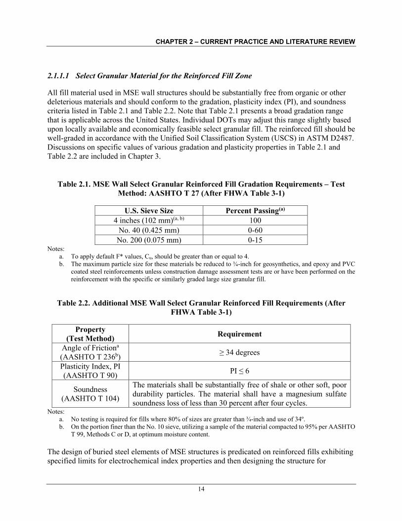
CHAPTER 2 – CURRENT PRACTICE AND LITERATURE REVIEW
14
2.1.1.1 Select Granular Material for the Reinforced Fill Zone
All fill material used in MSE wall structures should be substantially free from organic or other deleterious materials and should conform to the gradation, plasticity index (PI), and soundness criteria listed in Table 2.1 and Table 2.2. Note that Table 2.1 presents a broad gradation range that is applicable across the United States. Individual DOTs may adjust this range slightly based upon locally available and economically feasible select granular fill. The reinforced fill should be well-graded in accordance with the Unified Soil Classification System (USCS) in ASTM D2487. Discussions on specific values of various gradation and plasticity properties in Table 2.1 and Table 2.2 are included in Chapter 3.
Table 2.1. MSE Wall Select Granular Reinforced Fill Gradation Requirements – Test Method: AASHTO T 27 (After FHWA Table 3-1)
U.S. Sieve Size Percent Passing(a)
4 inches (102 mm)(a, b) 100 No. 40 (0.425 mm) 0-60 No. 200 (0.075 mm) 0-15
Notes: a. To apply default F* values, Cu, should be greater than or equal to 4. b. The maximum particle size for these materials be reduced to ¾-inch for geosynthetics, and epoxy and PVC
coated steel reinforcements unless construction damage assessment tests are or have been performed on the reinforcement with the specific or similarly graded large size granular fill.
Table 2.2. Additional MSE Wall Select Granular Reinforced Fill Requirements (After FHWA Table 3-1)
Property (Test Method) Requirement
Angle of Frictiona (AASHTO T 236b) ≥ 34 degrees
Plasticity Index, PI (AASHTO T 90) PI ≤ 6
Soundness (AASHTO T 104)
The materials shall be substantially free of shale or other soft, poor durability particles. The material shall have a magnesium sulfate soundness loss of less than 30 percent after four cycles.
Notes: a. No testing is required for fills where 80% of sizes are greater than ¾-inch and use of 34º. b. On the portion finer than the No. 10 sieve, utilizing a sample of the material compacted to 95% per AASHTO
T 99, Methods C or D, at optimum moisture content. The design of buried steel elements of MSE structures is predicated on reinforced fills exhibiting specified limits for electrochemical index properties and then designing the structure for

CHAPTER 2 – CURRENT PRACTICE AND LITERATURE REVIEW
15
maximum corrosion rates associated with those specified limits. These recommended index properties and their corresponding limits are shown in Table 2.3. Fills with properties that meet the requirements in Table 2.3 are considered to be moderately corrosive fills. Reinforced fill soils must meet the indicated criteria to qualify for use in MSE construction where steel reinforcements are used. For geosynthetic reinforcements, the limits for electrochemical criteria will vary depending on the polymer. Limits, based on current research, are shown in Table 2.4. Discussions on specific values of the various properties listed in Tables 2.3 and 2.4 are included in Chapter 3.
Table 2.3. Recommended Limits of Electrochemical Properties for Reinforced Fills with Steel Reinforcement (After FHWA Table 3-3).
Property Criteria Test Method Resistivity > 3000 ohm-cm AASHTO T 288
pH > 5 and < 10 AASHTO T 289 Chlorides < 100 PPM ASTM D4327 Sulfates < 200 PPM ASTM D4327
Organic Content 1% maximum AASHTO T 267
Table 2.4. Recommended Limits of Electrochemical Properties for Reinforced Fills with Geosynthetic Reinforcements (After FHWA Table 3-4).
Base Polymer Property Criteria Test Method Polyester (PET) pH 3 < pH < 9 AASHTO T 289 Polyolefin (PP & HDPE) pH pH > 3 AASHTO T 289
In addition to the requirements noted in Tables 2.1 to 2.4, FHWA (2009) provides the following guidelines: • Other Properties: The fill material must be free of organic matter and other deleterious
substances, as these materials generally result in poor performance of the structure and enhance degradation of the reinforcements. Other materials such as soils containing mica, gypsum, smectite, montmorillonite, chemically unstable particles, or other low durability particles should be carefully evaluated as large strains are typically required to reach peak strength and pullout capacity, resulting in larger lateral and vertical deformation than with higher quality granular fills. Use of salvaged materials such as asphaltic concrete millings or Portland Cement Concrete rubble is not allowed. Recycled asphalt is prone to creep resulting in both wall deformation and reinforcement pullout. Recycled concrete has a potential to produce tufa precipitate from unhydrated cement, which can clog drains and exude a white pasty substance onto the wall face creating aesthetic problems. Recycled concrete typically does not meet electrochemical properties and its corrosion potential has also not been fully evaluated, especially if residual wire reinforcement and rebar are present that could create problems with dissimilar metals.

CHAPTER 2 – CURRENT PRACTICE AND LITERATURE REVIEW
16
• Compaction: The compaction specifications should include a specified lift thickness and allowable range of moisture content with reference to the optimum moisture content. Compaction moisture control should be ±2% of optimum moisture content (wopt). The compaction requirements of reinforced fill are different within 3 feet of the wall facing. Lighter compaction equipment, e.g., walk-behind vibratory plate or roller compactors, and thinner lifts are used near the wall face to prevent buildup of excessive lateral pressures from the compaction equipment and to prevent facing panel movement. Because of the use of this lighter equipment, a reinforced fill material of good quality in terms of both friction and drainage, such as crushed stone may be used close to the face of the wall to provide adequate strength and minimize settlement in this zone. If an open graded fill is used adjacent to the face, filtration requirements with the reinforced wall fill must be addressed as discussed in FHWA Section 5.3.3. Granular fill containing even a few percent fines may not be free draining since coarse-grained particles and soil clods may breakdown during compaction thereby adding to the percentage of fines. Therefore, drainage requirements should always be carefully evaluated.
• Reinforced Rock Fill Structures. Material that is composed primarily of rock fragments,
i.e., material having less than 25 percent passing a ¾-inch (20 mm) sieve, should be considered to be a rock fill. The maximum particle size should not exceed the limits listed in Table 2.1. Such material should also meet all the other non-gradation requirements such as soundness in Table 2.2 and electrochemical properties in Tables 2.3 and 2.4. When such material is used, a very high survivability geotextile filter should encapsulate the rock fill to within 3 feet below the wall coping. For example, a Type 1 geotextile used in accordance with AASHTO M 288 can be designed for filtration performance following the guidelines in FHWA (2008). Adjoining sections of separation fabric should be overlapped by a minimum of 12 inches. Additionally, the upper 3 feet of fill should contain no stones whose maximum dimension is greater than 3 inches and should be composed of material not considered to be rock fill, as defined herein. Where density testing is not possible, trial fill sections should be constructed with agency supervisory personnel and a qualified geotechnical engineer present to determine appropriate watering, in-situ modification requirements, e.g., grading, lift thickness, and number of passes to achieve adequate compaction. Compaction can be determined by measuring the settlement of the trial section at several points after each pass. For example, a minimum of 5 points measured at the center of a 1-foot square plate is typically required. Several lifts should be constructed to determine the appropriate number of passes that will maximize compaction without excessively crushing the rock at the surface. The number of passes to achieve at least 80 percent of the maximum settlement should be required.
• Limits of Reinforced Fill. For MSE walls, except back-to-back walls, and RSS, many agencies extend the reinforced fill beyond the free end of the reinforcement. Some agencies extend the reinforced fill 1-foot beyond the reinforcement length; others extend the fill in a wedge behind the reinforced zone, as illustrated in Figure 2.2. For back-to-back walls where the free ends of the reinforcement of the two walls are spaced apart less than or equal to one-

CHAPTER 2 – CURRENT PRACTICE AND LITERATURE REVIEW
17
half the design height of the taller wall, reinforced fill should be used for the space between the free ends of the reinforcements as well.
2.1.1.2 Design Strength of Select Granular Reinforced Fill
The reinforced fill criteria outlined previously represent materials that have been successfully used throughout the United States and elsewhere to construct MSE wall structures that have performed excellently. Peak shear strength parameters are used in the wall and slope analyses. In accordance with AASHTO Article 11.10.6.2, for MSE walls using fill meeting the gradation requirements in Table 2.1, a maximum effective friction angle (rein) of 34 degrees is usually assumed (see Table 2.2) unless project-specific fill is tested by triaxial (AASHTO T 297) or direct shear tests (AASHTO T 236). However, some nearly uniform fine sands meeting the specifications limits may exhibit friction angles of 30 to 32 degrees. When contractor-furnished sources are used, the specification may also require testing of the source material to verify that its friction angle meets specification requirements, e.g., 34 degrees. Greater values may be used if substantiated by laboratory direct shear or triaxial test results for the site-specific material used or proposed. The angle of friction used for design shall not exceed 40 degrees (AASHTO Article 11.10.6.2) even if the measured friction angle is greater than 40 degrees. In all cases, the cohesion of the reinforced fill is assumed to be zero.
2.1.1.3 NCMA Fill Requirements
Within the U.S. other organizations such as the National Concrete Masonry Association (NCMA) have also published guidelines. The NCMA guidelines are specifically for MSE wall faced with modular blocks and reinforced with geosynthetic soil reinforcements. This wall type is also referred to as segmental retaining wall (SRW) or modular block walls (MBW). The 1st edition of NCMA Design Manual for Segmental Retaining Walls was published in 1993 (NCMA, 1993), followed by a 2nd edition in 1997 (NCMA, 1997) and the current 3rd edition in 2010 (NCMA, 2010). These guidelines are generally used for design of MSE walls for private and commercial works, and not for highway works. The NCMA design guidelines vary significantly from the FHWA and AASHTO guidelines in the quality of reinforced fill material specified. The NCMA criteria for reinforced fill material have evolved over the years and the latest criteria based on 3rd edition of NCMA manual (NCMA, 2010) are presented in Table 2.5. For comparison and a historical perspective, in the 1st Edition (NCMA, 1993), the reinforced fill specification required a soil with a USCS designation of GP, GW, SW, SP, SM, ML, CL with the following characteristics: • less than 20% by weight of particles greater than 1½ inches, • maximum of 60% by weight passing the #200 sieve, and • PI < 20. In the 2nd Edition (NCMA, 1997) the reinforced fill specification was revised to require a soil with a USCS designation of GP, GW, SW, SP, SM with following characteristics:

CHAPTER 2 – CURRENT PRACTICE AND LITERATURE REVIEW
18
• maximum particle size of ¾ inches, • maximum of 35% by weight passing the #200 sieve, • PI < 20, and • pH between 3 and 9.
As can be seen from Table 2.5 and Table 2.6, which are based on the 3rd Edition (NCMA, 2010), the reinforced fill requirements are the same as in the 2nd edition (NCMA, 1997) except that the maximum particle size of 1 inch is used. All three editions of the NCMA manuals include guidance in Notes for Table 2.5 and Table 2.6. Unlike the FHWA criteria presented in Table 2.2, NCMA does not provide soundness requirements. NCMA (2010) indicates that some of the typical strategies employed by design professionals to address performance issues for taller walls include the following: (i) limit PI to less than 5 to 10 for taller walls, and/or (ii) require select granular fill with less than 5 to 15% fines. The definition of tall is left up to the design professional.
Table 2.5. SRW Suggested Reinforced Fill Requirements (After NCMA 2010).
U.S. Sieve Size Percent Passing (a, b) (AASHTO T 27) 1 inch (25 mm) (a, b) 100 No. 4 (4.75 mm) 100 – 20
No. 40 (0.425 mm) 0-60 No. 200 (0.075 mm) 0-15
Notes: a. The maximum size should be limited to 1 inch for reinforced soil SRW unless tests have been or will be
performed to evaluate potential strength reduction in the geosynthetic due to installation damage. b. Cohesionless, coarse-grained soils are recommended with a USCS designation of GP, GW, SW, SP, SM.
Table 2.6. Additional SRW Suggested Reinforced Fill Requirements (After NCMA 2010).
Property (Test Method) Requirement Plasticity Index, PI(a) (AASHTO T 90) PI < 20
pH (AASHTO T 289) 3 – 9 Notes:
a. Fine-grained soils (i.e., > 50% fines) with PI < 20 may be used provided the following four additional design criteria are implemented:
1. Sufficient internal drainage is installed. 2. Only soils with low to moderate frost potential are utilized. 3. The internal cohesive shear strength parameter, c, is ignored for stability analysis. 4. The final design is checked by a qualified geotechnical engineer to ensure that the use of cohesive
soils does not result in unacceptable time-dependent movement of the SRW system.

CHAPTER 2 – CURRENT PRACTICE AND LITERATURE REVIEW
19
2.1.2 Non-select Reinforced Fills
MSE wall reinforced fill materials that do not meet the requirements in Tables 2.1 to 2.4 have been used successfully. However, in many such cases problems including significant distortion and structural failure have been observed with fills having finer grained and/or more plastic soils than specified in Table 2.1. Within the context of the current report the non-select reinforced fill used in these applications is considered to be a local available sustainable resource (LASR). Section 2.2 presents a literature review for MSE-LASR studies and applications.
2.2 LITERATURE REVIEW FOR MSE-LASR STUDIES AND APPLICATIONS
As noted in Chapter 1, the subject of using LASR for MSE wall construction has attracted attention worldwide. There have been several publications that have documented the use of non-select fills. Additionally, there have been some formal studies related to the use of reinforced soils with more than 15% fines and little or no plasticity, e.g., by NCHRP Project 24-22 (NCHRP, 2013) and NCMA (2009). The NCHRP and NCMA studies are summarized first followed by a summary of other available publications that could be considered applicable to MSE-LASR walls as defined herein.
2.2.1 NCHRP and NCMA Studies
During the performance of the NCHRP Project 24-22 work, the NCHRP investigators published several papers based on the results of their study. These papers, e.g., Stulgis (2005a), Stulgis (2005b), and Marr and Stulgis (2009) will be used here to present a summary of the work performed for NCHRP. As part of NCHRP Project 24-22, four full-scale wall sections were constructed: one with AASHTO A-1-a soils, one with AASHTO A-2-4 soils and two with AASHTO A-4 soils. The NCHRP team chose to employ a flexible, welded wire facing system and polyester geogrid reinforcement for three of the test sections, and needle-punched nonwoven geotextile reinforcement for the fourth. The purpose of the NCHRP full-scale field test was to establish properties for “high fines” reinforced soils and associated design control that give acceptable performance. The field test included provisions to demonstrate the role of pore water pressure in the reinforced fill and the importance of including a positive drainage system behind the reinforced fill zone for obtaining good wall performance. The NCMA (2009) study was similar to the NCHRP study and was performed by the same primary entity, Geocomp Corporation and its subsidiary GeoTesting Express, Inc. The NCMA (2009) study involved construction of two full-scale Segmental Retaining Wall (SRW) test sections with reinforced fill consisting of A-1-a and A-4 soils, which were also selected for the NCHRP project. The use of the same type fills would allow direct comparison of the performance of the NCMA SRW test walls to the NCHRP sections. The two NCMA walls were constructed with modular block face elements and polyester geogrid reinforcement. The NCHRP and NCMA studies included provisions to demonstrate the role of pore water pressure in the reinforced fill and the importance of including a positive drainage system for

CHAPTER 2 – CURRENT PRACTICE AND LITERATURE REVIEW
20
obtaining good wall performance. In both studies, each test section was fully instrumented to record data to evaluate a number of technical questions. Instrumentation consisting of strain gages mounted on geosynthetic reinforcement, piezometers, thermistors, multiple position horizontal extensometer and vertical extensometers were positioned throughout the reinforced fill. An array of high precision prisms was mounted on the face of the test walls to allow optical survey readings to be taken by using Automatic Robotic Total Station technology. The following points are based on information in Stulgis (2005a), Stulgis (2005b), and Marr and Stulgis (2009) related to the NCHRP 24-12 study: • MSE structures can be successfully built with soils having not more than 25% fines and PI
not greater than 6% provided that: o All potential sources of water that might cause increases in pore pressure in the
reinforcing zone are addressed by the design. o Good practices are used to measure the engineering properties of the reinforced fill for
design, project specifications include requirements for reinforced fill selection and placement, and good practice construction with focused QC/QA is employed.
• The performance of MSE walls with a percentage of fines greater than 6% is more dependent on as-placed density and moisture content than free draining materials. The use of soils with a percentage of fines greater than 6% requires a greater level of engineering for design and monitoring. Also, additional testing is required to determine the shear strength parameters and case-specific requirements for as-placed conditions (i.e., default values should not be used). A greater level of construction monitoring and focused Quality Control (QC) and Quality Assurance (QA) effort is necessary to ensure that the wall is constructed in compliance with the plans and specifications.
The NCMA (2009) study provides the following evaluation:
“The field test clearly demonstrates that SRW structures with marginal soils in the reinforced fills soils will provide excellent performance subject to the following considerations: • Soils with less than 25% fines and a Plasticity Index not greater than 6% are used.
Soils with up to 50% fines and a Plasticity Index not greater than 12% may be used where design and construction is monitored by a qualified Professional Engineer.
• The design is based on soil parameters measured on representative samples compacted to the field conditions, consolidated to field stress levels, and sheared to measure drained strength parameters. Presumptive values of soil shear strength should not be used.
• All potential sources of pore pressure build up in the reinforcing zone should be considered in the design. Where potential sources exist, or may develop during the life of the facility, the design should include specific measures to prevent flow of water into the reinforced fill in the form of a water barrier, a drain or both.

CHAPTER 2 – CURRENT PRACTICE AND LITERATURE REVIEW
21
• Good practice is used to control the quality of material selection and placement, as the performance of marginal soils is more susceptible to as-placed density and moisture content than free draining materials.”
Additionally, the NCMA (2009) report states the following:
“In summary, the two field tests demonstrate that SRWs constructed with marginal reinforced fills (i.e., up to 50% fines and 12% plasticity) can perform well with no obvious indications of distress. This statement remains true even with significant positive pore pressures in the reinforced fill, provided that the design accounts for the presence of these pressures. However, for the best long-term performance, we recommend that the reinforced fill for SRWs be designed with measures to prevent flow of water into the reinforced fill by using water barriers, drains or both. These measures will also help reduced the potential for damage by freezing of the fine-grained reinforced fill soils.”
In general, the findings of NCHRP and NCMA studies are similar and appear to indicate that use of MSE-LASR walls is feasible provided that guidelines for various design issues are developed. Design issues include drainage, corrosion, deformations, reinforcement pullout, constructability, and performance expectations. While there may be a significant savings in using local available sustainable resources (LASR) for reinforced fill, the effect of such LASR materials on the overall performance of the MSE structure must be carefully evaluated. The development of a framework for this purpose is the focus and goal of the current report.
2.2.2 Other Sources of Information for MSE-LASR Applications
Summaries of various works published from the early 1970s to present are presented chronologically in this section. As can be seen from the citations, the MSE industry has been quite active in trying to evaluate the factors that might influence the use of LASR materials as fills for MSE walls. The published works cited here are meant to provide the reader with background only and are not intended to imply that these are the only works for MSE-LASR systems. The interested reader should consult the references in the various publications cited here for sources having more extensive information related to the use of LASR for MSE walls. The requirement of less than 15% fines can be traced back to the work by Schlosser and co-workers in the 1970s at Laboratore des Ponts et Chausses (LCPC) in France. Schlosser and Long (1974) evaluated the effect of the fines fraction on the angle of internal friction. They noted that an important parameter in reinforced soil is the relative volume of the fine-grained portion to the granular portion in that the friction developed decreases with increasing fine-grained portion. Schlosser and Elias (1978) and Elias (1979) evaluated the effect of fines on the friction between smooth and ribbed steel strip reinforcements. Based on a laboratory experimental study Elias (1979) notes the trend of decreasing friction with increased normal pressures for fine-grained soils. Citing the work by Schlosser and Long (1974), Elias (1979) notes that the critical grain size that separates purely frictional behavior is the 15 m size, which is identified as “medium silt” by Eurocode 7 and falls close to the lower bound of the range of silt particle sizes (6 m to

CHAPTER 2 – CURRENT PRACTICE AND LITERATURE REVIEW
22
75 m) according to the Unified Soil Classification System (USCS). These works led to the original criterion that MSE wall fills should be limited to cohesionless soils having no more than 15% by weight finer than the #200 mesh sieve (75 m). The effect of the fines fraction on the shear strength of soils has also been studied by others, e.g., Mitchell and Soga (2005), and their findings are similar to those by Schlosser and co-workers. Elias (1979) notes that significant additional work is necessary prior to the unrestricted use of fine-grained soils in MSE walls along with study of the effects of saturation compaction water content. Elias and Swanson (1983) describe a case history of a reinforced earth wall constructed in Virginia in 1978-1979. The wall had a maximum height of about 23 feet, reinforcing elements consisted of ribbed galvanized steel strips, and specifications that restricted fill to less than 15 % fines. No drainage system was installed. Before construction was complete, several days of above normal precipitation resulted in excessive movements of the wall of up to 10 to12 inches out of plumb at the tallest section. Subsurface investigation revealed that in areas of severe wall distress, the fill contained 30 to 50 percent fines, with more than 15 percent finer than 15 m size, and a plasticity index (PI) exceeding project specifications. For mitigation, areas with more than 25 percent fines were identified, excavated, and replaced with fill limited to less than 25 percent fines since no movement was originally noted in areas with less than 25 percent fines. The results of this study indicate the following: • Fines content and moisture content are important factors in the construction of reinforced
earth with residual soils. • When fill soils contain more than 10 to 20 percent finer than 15 m, significant reduction in
pullout capacity and decrease internal stability can occur. • Reduction in frictional strength is more pronounced in saturated soils. Fines content of
residual soil can vary greatly over small distances. • Highly micaceous sands of the Piedmont physiographic province are extremely sensitive to
moisture variations, as significant strength reduction was observed with increased compaction water content.
Hannon and Forsyth (1984) discuss four MSE walls with metallic reinforcements that were constructed for the widening of Interstate 80 near Baxter, California. Two of the walls, with a maximum height of 16 feet, were instrumented to monitor the performance of a sandy silt fill having up to 50 percent fines. Moisture content control and implementation of an appropriate drainage system resulted in good performance. A subsurface drainage system was constructed, and construction was stopped several times to allow saturated material to dry out. Monitoring through heavy rainfall the following year showed no significant vertical or lateral wall movements. Bressette and Chang (1986) present the results of a three-year evaluation of a mechanically stabilized embankment (MSE) constructed by the California Department of Transportation (CALTRANS) using low quality fill (greater than 32% passing the #200 sieve). Until recently CALTRANS commonly allowed the use of 25% fines for MSE walls. Four MSE walls were constructed in the mid-1982 along Interstate 80 near Baxter, California utilizing the clayey silt

CHAPTER 2 – CURRENT PRACTICE AND LITERATURE REVIEW
23
and clayey sand embankment materials available within the project limits. Two walls were instrumented to monitor stresses in the reinforcement, both horizontal and vertical movements, and lateral earth pressures on the wall backface. The bid price for the MSE alternative was 12% lower than that for reinforced earth walls constructed according to the standard fill criteria and 15% lower than concrete crib walls. The lower cost is attributed to reduced excavation and on-site availability of fill. Dummy bar-mats were buried in the fill at various depths and pulled out a year later to determine pullout resistance for various configurations. Laboratory pullout tests on bar-mats with the same configurations were also conducted in a direct shear device. The laboratory and field pullout test results were compared. No definitive relationship was found to exist between field, laboratory, or theoretical results; number of transverse bars and resistance; or resistance and overburden. The authors report that the walls performed well. Stresses measured in the reinforcement were distributed in a manner similar to the expected distribution. Christopher and Berg (1990) presented procedures for pullout evaluation of geosynthetics in cohesive soils and results from a test program on five geogrids and four cohesive soils. They present a comparative summary of the results of both long-term (drained) and short-term (undrained) pullout tests. Geosynthetic and soil creep are evaluated as part of the long-term tests. As the authors note in their paper, the significance of this study is not in the comparison of the results, but in reporting the results based on data which is very difficult and time consuming to obtain. A test procedure is proposed for future similar work. Anderson et al. (1991) presents a case history of a project in Atlanta and describes the design and construction of two MBW-faced, geogrid reinforced walls constructed with a silty clayey sand wall fill. One wall is 26 feet high and supports a building founded on spread footings, and the other wall is 40 feet high and supports a parking lot. The walls were founded on 8 to 28 feet of random fill of fine sands and silts, with blow counts of 6 to 20, and some pockets of organic and of construction debris. The permanent walls also support a surcharge load to compress the foundation soils and minimize future settlements. Detailing included back drains and cushioning material between rows of MBW units. The walls demonstrated a tolerance for differential settlement, with up to 6 inches of settlement without apparent damage. The walls costs saved 45% over the alternate MSE steel reinforced, panel faced system with select granular fill. In companion papers Bergado et al. (1991a) and Bergado (1991b) describe the behavior of a welded wire wall with steel grid reinforcements embedded in poor quality cohesive-friction fills on soft Bangkok clay. Three different locally available fills were used. These were clayey sand, lateritic residual soil, and weathered clay. Instrumentation was placed both in the wall and the foundation soil, which is referred to as “subsoil” by the authors. Increases in total and excess pore-water pressures were noted during construction. As expected, both decreased after the construction activities were concluded. The authors report that the amount of subsoil movement greatly influenced the variation in the vertical pressure beneath the wall, as well as the tension in the reinforcements. Pullout resistances were also found to be affected by the arching effect due to the presence of inextensible reinforcements in combination with the subsoil movements. The wall showed no signs of instability both during construction and post-construction phases, despite the large settlements and lateral movements. The authors found that the location of the maximum tension line was severely affected by the foundation compressibility, arching effects,

CHAPTER 2 – CURRENT PRACTICE AND LITERATURE REVIEW
24
and effects of compaction-induced stresses. These features caused the overall behavior of the wall to depart from the behavior of reinforced walls with granular fill constructed on relatively rigid foundations. However, the authors deemed the overall performance of the wall to be satisfactory and concluded that the steel grid reinforcement can be used effectively to reinforce poor to marginal quality fill in walls and embankments on soft clay foundations. Brockbank et al. (1992) report on the use of oil sands for construction of a test wire-faced reinforced earth dump wall at the Syncrude Canada Ltd. oil sand mine site located in Mildred Lake, just north of Fort McMurray, Alberta, Canada. The oil sands had an average of 45% fines and plasticity index of 5. The structure was monitored by surveying and instrumentation. The authors conclude that lean oil sands can be used as an acceptable source of fill for a MSE wall, provided careful consideration is given to both design and construction QC/QA. Testing found a reduced friction value between the oil sands and the reinforcement when compared to clean sand. They report that alignment of the facing was improved by the use of a granular chimney immediately behind the wall panels. Bergado et al. (1993a, b) performed full-scale tests on a 5.7-m (18.7 feet) high wall/embankment MSE system. The wall consisted of three different sections each containing a different fill material (clayey sand, lateritic soil, and weathered clay). The fill was compacted to 95% of standard Proctor maximum dry density. The reinforcements used for the wall were two types of steel grids: grids with only longitudinal ribbed bars and grids with both longitudinal and transverse bars. The purpose of these tests was to study the interaction between steel grid reinforcements and fill soils through pullout tests on selected reinforcements. From the results of these tests the authors concluded that most of the pullout resistance was obtained from the transverse members of the grid, and that larger pullout displacements were needed to mobilize pullout resistance for grids with both longitudinal and transverse bars as compared to grids with only longitudinal ribbed bars. The authors also observed that the pullout resistance for a fill compacted on the dry side of optimum was greater than the pullout resistance for fill compacted on the wet side. Zornberg and Mitchell (1994) and Mitchell and Zornberg (1995) in companion papers present an evaluation of the use and performance of reinforced soil structures with poorly draining and/or cohesive fills. Their evaluation shows that proper design and construction can result in stable, durable, and economical earth structures. The authors propose that permeable geosynthetic reinforcements may be especially useful for soil structures with poorly draining fills because the drainage capabilities of the geosynthetic can dissipate excess pore water pressures, thus enhancing stability. Consequently, the design of a safe and economical structure should address two aspects specific to poorly draining fills: • the use of cohesive soil-reinforcement interaction, and • reinforcement drainage characteristics. The authors present results of experimental and
analytical studies undertaken to evaluate these issues.

CHAPTER 2 – CURRENT PRACTICE AND LITERATURE REVIEW
25
Keller (1995) describes U.S. Forest Service practice with MSE walls. Hundreds of walls utilizing various reinforcing and facing materials have been successfully constructed with native fill soils on Forest Service and rural roads since the mid-1980s. Reinforcements have included geotextiles, geogrids, and welded wire mesh. Facing materials have included timbers, gabions, tires, geocells, and segmental concrete blocks. Fills typically include soils with up to 50 percent fines, a PI of less than 20, and a peak friction angle between 25 and 30 degrees. The greatest potential for cost savings is in material supply, disposal, and transportation. For example, for Forest Service walls the average cost of local fill material was $8 per cubic yard including procurement, placement, compaction, and haulage. In comparison, the average cost of imported select fill was $18 per cubic yard including procurement, placement, compaction, and haulage. For a wall with 1,500 square feet of wall face, and 750 cubic yards of fill, the average cost was estimated to be $4 per square foot of wall face for local material versus $9 per square foot of wall face for imported material. These costs do not include the cost of the soil reinforcements and the wall facing system. Building on the work of Zornberg and Mitchell (1994), Christopher et al. (1998) provide a review of issues associated with use of non-select fills with an emphasis on the use of permeable inclusions as a design alternative to provide internal drainage of the reinforced soil zone. Case histories demonstrating successful use of permeable inclusions for addressing both internal and external seepage problems are presented. Adverse conditions of excess moisture and pore water pressures within poorly draining fills are identified. Use of reinforcements with in-plane drainage capabilities is proposed as part of a two-phase analysis to account for both short- and long-term conditions. Abrahams and Sankey (2000) discuss the design and construction of reinforced earth (RE) walls on marginal lands. Their focus is on marginal foundations and improvement techniques. They recommend the use of vertical joints and staged construction to increase the flexibility and stability of RE walls. The authors also discuss 2-stage MSE walls and provide a summary of design and construction practices that will improve the aesthetics, cost, safety, and durability of RE walls. Alzamora et al. (2000) present the case history of a segmental retaining wall (SRW) wherein the reinforced zone included low plasticity fine-grained soil with an effective friction angle of 26 degrees and a unit weight of 19 kN/m3 (≈121 pcf). Although the paper concentrates on a discussion of the use of a load transfer platform on jet grouted columns, it does demonstrate the use of LASR type soils for MSE wall fills. Bobet (2002) performed laboratory-scale experiments and numerical studies to evaluate the effect of drained and undrained conditions on the pullout resistance of steel reinforcement embedded in fill soil types ranging from clean sand to silty sands with 5%, 15% and 35% silt content and for overburden pressures of 30, 100 and 200 kPa (626, 2,088, and 4,176 psf). Numerical studies were performed to determine scale and permeability effects for dissipation of excess pore pressures. The results of the pullout tests show that both drained and undrained pullout capacities change as silt content changes since the pullout capacity increases as the

CHAPTER 2 – CURRENT PRACTICE AND LITERATURE REVIEW
26
internal friction angle of the soil increases. It was also observed that the pullout capacity increases as the overburden pressure increases. Undrained conditions significantly reduce the pullout capacity by as much as 50%. This decrease is caused by the generation of excess pore water pressures in the soil under rapid loading that decrease the effective stress at the soil reinforcement interface. The magnitude of the pullout reduction is related to the permeability of the soil since for large permeabilities the dissipation of excess pore pressures is very rapid and no reduction in pullout is produced. In contrast, for low permeabilities the dissipation of excess pore pressures is slower than the rate of pullout and thus a reduction in pullout resistance occurs. This condition is confirmed by the experiments that show no reduction in pullout capacity for clean sand, and a large reduction for silty sands. The ratio of undrained to drained pullout capacity changes with silt content and overburden pressure; for 100 and 200 kPa (2,088 and 4,176 psf) magnitudes of overburden pressure, the ratio is 1.0 for clean sand, 0.67~0.69 for 5% silty sand, 0.77~0.78 for 10% silty sand, 0.72~0.73 for 15% silty sand, and 0.57~0.59 for 35% silty sand. For an overburden pressure of 30 kPa (626 psf), the ratio is 1.0 for clean sand, 0.5 for 5 % silty sand, 0.67 for 10 % silty sand, 0.78 for 15 % silty sand, and 0.72 for 35 % silty sand. In the numerical analyses the dissipation of pore pressures was very rapid for permeabilities larger than 10-2 cm/sec, and significantly slower for permeabilities smaller than 10-3 cm/sec. Scale effects are extremely important since the time for pore pressures to dissipate increases as the length of the reinforcement increases. Farrag and Morvant (2004) present the construction and performance evaluation of a 20-feet tall, 160-feet long reinforced-soil test wall sponsored by the Louisiana Transportation Research Center (LTRC). The wall was constructed with low-quality fill. Its vertical facing was constructed with modular blocks. The wall consisted of three sections reinforced with various types of geogrid reinforcement placed at various spacings. The backside of the wall was a one-to-one slope reinforced with woven and non-woven geotextiles. The test wall was constructed to evaluate the design procedure and performance of geosynthetic-reinforced structures constructed with silty-clay fill founded on a soft clay foundation. The instrumentation program consisted of monitoring wall deformation, foundation settlement, strains in the reinforcement, vertical and horizontal stresses in the soil, and pore water pressure under the wall. Results of the monitoring program from construction through four months after completion of the wall are detailed. The results of the instrumentation program showed relatively high deformations because of the low factors of safety used in design of the wall and the large settlement of the foundation soil. These deformations, however, occurred mostly during construction. The results of strain measurements in the reinforcement were used to evaluate the effect of reinforcement stiffness and spacing on the distribution and magnitude of stresses in reinforcement layers and the shape of the potential failure surface. According to the authors, the results show promising performance of silty-clay soils as a fill material in reinforced-soil walls provided proper design is performed and control of soil compaction and moisture are implemented. However, as noted by the authors, long-term performance of the wall needs to be monitored for a complete evaluation of these types of walls. Christopher and Stulgis (2005) present the results of a survey of state agencies and private sector groups and a literature review as the basis for a state-of-the-practice report on the use of low permeability, marginal soils as reinforced fill in geosynthetic reinforced soil walls. The authors suggest that a greater quantity of fines could be safely allowed in the reinforced fill provided the

CHAPTER 2 – CURRENT PRACTICE AND LITERATURE REVIEW
27
properties of the materials are well defined and controls are established to address the design issues. They raise concern about the deleterious effects of excess pore water pressures and recommend that either that the water be kept out of the reinforced zone by collecting and discharging it away from the reinforced zone, or that excess pore pressures be considered in the analysis and design. They also caution about the anticipated increase in vertical and horizontal deformation both during and after construction and note that the compressibility characteristics of marginal soils may have to be evaluated depending upon the nature of the reinforced soil structure. Finally, they note that environmental effects may play an important role in the form of shrink/swell potential, frost susceptibility, hydro-compaction potential, and susceptibility to surface tension cracks. Sandri (2005) discusses drainage recommendations for MSE walls constructed with fills having greater than 35% fines and plasticity index greater than 20. He identifies three general areas of concern: (1) generation of pore water pressure from within the reinforced fill, (2) wetting front advancing into the reinforced fill, and (3) seepage configuration established within the reinforced fill. He emphasizes the importance of having focused QC/QA for walls constructed with poorly draining fills and recommends moisture control during the soil placement process be maintained at relatively tight tolerances such as 1% of optimum. He also recommends that sheeps-foot or similar kneading type compaction equipment should be used instead of rubber-tired equipment, plate compactors, or large vibratory equipment. He concludes by advocating careful attention to design and contractual aspects of such construction. Lawson (2005) presents an international perspective on the use of fine-grained fills in geosynthetic reinforced soil walls and slopes. He notes that internationally, a wide range of reinforced fill types are used in MSE walls and slopes. These fill types range from wholly granular materials to materials with significant quantities of clays. In general, the warmer and drier the climate, the more fine-grained fills are used in MSE structures. The author notes that like frictional fills, so-called fine-frictional fills also provide good shear resistance at relatively small deformations, but when such fills are well-compacted, they have reduced hydraulic conductivity. Consequently, when fine-frictional fills are used importance should be given to drainage design as well as structural design. Much of the economics of MSE fill slopes rely on the use of the in-situ, or locally available, soils as the reinforced fill. Consequently, a wide range of fill types are used for MSE fill slopes and these may be categorized as being fine-frictional, cohesive-frictional, and fine-cohesive in nature. When dealing with this range of fills, good and consistent compaction quality is essential. Also, the provision of good drainage measures becomes just as important as the reinforcement in ensuring a long-term stable structure, especially in environments subject to heavy rainfall. The use of durable and inert frictional fills for reinforced soil structures provides an efficient and risk-free solution. The impetus to use fine-grained reinforced fills is normally driven by cost considerations, for which there is an added element of risk. This risk must be alleviated by quality placement and compaction of the fine-grained fill and attention to the effects of the external environment in which the fine-grained fill will be placed, e.g., climatic conditions, groundwater effects, etc. In many instances, reported problems with the use of fine-grained fills have been over-emphasized. Other than the possible problem of fill degradation with time, problems normally arise as a result of design faults, poor construction quality, and the neglect of water ingress. It is true that fine-grained fills may be

CHAPTER 2 – CURRENT PRACTICE AND LITERATURE REVIEW
28
more susceptible to water ingress, than other granular-fill types, they perform just as well as granular fills in MSE walls and slopes provided these potential susceptibilities are dealt with properly. Dove and Darden (2005) performed a study for the Virginia Department of Transportation (VDOT) for the use of LASR for MSE walls. The authors first make a distinction between critical and non-critical walls as follows:
“Unless otherwise noted, non-critical walls include those walls that are 15 feet or less in height (H) and do not have a structure or traveled way on the retained soil within a horizontal distance of 2H behind the face of the wall. Non-critical walls also include structures used to retain cut slopes adjacent to a highway. MSE walls associated with bridge abutments, approach embankments, or high walls adjacent to the traveled way are considered critical walls, and the use of alternative backfills is not permitted at present.”
The results of this study by Dove and Darden (2005) indicate that the use of alternative fill soils is feasible for non-critical wall applications. The study recommends that soils for use with metallic reinforcement should be well-graded with a maximum size of 3 inches and less than 20 percent fines with a plasticity index less than 6. Fill for polymer-reinforced walls is recommended to be well-graded with a maximum size of ¾-inch and less than 30 percent fines with a plasticity index less than 9. The use of wall systems such as geosynthetic reinforced modular block walls should be considered when alternative fills are used. It is emphasized that all walls constructed with alternative fill soils should have an internal drainage system installed during construction. Drainage systems should include continuous freely draining aggregate for a minimum distance of 12 inches behind the wall face, beneath the reinforced zone of the fill, and behind the reinforced zone of the fill. Positive drainage at the surface should be directed away from the reinforced zone and should be maintained at all times during and after construction. An impermeable boundary, such as a high-density polyethylene geomembrane, should be installed above the first layer of reinforcement to prevent saturation of the fill after construction. The drainage system should be monitored to ensure functionality after precipitation events. Masonry block wall (MBW) masonry unit fill, where required, should also be a free-draining material. Finally, the study notes that additional costs might be incurred for quality control testing and material placement. Guidance for testing a soil with more than 15 percent fines for suitability as a LASR for MSE walls is provided as follows: • Compact soils in the direct shear apparatus on the wet side of optimum to 95 percent of
maximum dry density as determined by the Standard Proctor test (AASHTO T 99). • Inundate samples and allow full consolidation under the applied normal stress. Monitor the
vertical deformation of the sample over time under the applied normal stress. • Assumed or typical strain rates for granular soils should not be used. If a well-defined time
deformation curve is not obtained, use as slow of a strain rate as is practicable. In their study the authors used a strain rate of 0.005 mm per minute.

CHAPTER 2 – CURRENT PRACTICE AND LITERATURE REVIEW
29
• Check the measured friction angle against commonly accepted values for the material being tested. If the results are questionable, use triaxial compression tests such as the isotropically consolidated undrained (CU) or the consolidated drained (CD) test for verification.
Hatami and Bathurst (2005) present the results of a parametric analysis of MSE walls with fills having different properties. Based on data obtained from tests on four full-scale, 3.6 m (11.8 feet) tall MSE walls with different configurations of grids performed at the Royal Military College of Canada, they developed a numerical model that can evaluate the effects of the different fills. They note that cohesion of 10 kPa (209 psf) can lead to a significant reduction in lateral displacement. The authors indicate that fine-grained soils can be used efficiently if adequate drainage is included along with a performance monitoring system. Bueno et al. (2006) report that in spite of the significant caution against the use of marginal quality soils in the United States, reinforced soil structures in Brazil have often been built with soils having a large percentage of fines. The authors note that based on the results of field instrumentation, many of such structures have shown a very good long-term performance. An overview of case histories for walls with marginal quality soils is presented. Some of the structures built by using poorly draining soils were over 20 years old (in 2006) and showed no signs of distress. The authors attribute this observed good performance to the significantly different characteristics of fine-grained soils in the U.S. and Brazil. Specifically, most of the fine-grained soils used as fill material in Brazil are residual soils, and often lateritic soils, which have shown excellent performance in engineered embankments. Based on this observation, the authors opine that existing guidelines for reinforced soil construction should be refined since the use of grain size distributions to define the adequacy of fill soils may be an oversimplification. Rathje et al. (2006) present the results of an experimental program aimed at evaluating the use of crushed concrete (CC) and recycled asphalt pavement (RAP) for MSE wall fills. Various properties of RAP and CC such as strength, hydraulic conductivity, pullout resistance, creep potential, and corrosivity were investigated. CC was judged to be an adequate fill for MSE walls, although its marginal hydraulic conductivity requires additional drainage to be provided behind walls. RAP displayed a significant potential for deviatoric creep, making this material unsuitable for MSE wall fills. Parrish (2006) describes the case where an existing concrete retaining wall was constructed at a residence in Rocheport, Missouri and exhibited unsatisfactory performance. A geotextile wrap-face wall, located behind the existing wall, was designed and constructed to carry the lateral load from the fill, while the concrete wall remained in place. The wrap-face wall was designed using on-site cohesive fill. Laboratory testing was performed to establish the design parameters of the geotextile reinforcement and fill soil. Incorporating the marginal material as the wall fill, resulted in an approximate 55 percent savings when compared to conventional granular fill. Laboratory testing of the construction materials established the design parameters for the wrap-face wall. Index tests indicated that the on-site fill is a low-plasticity clay, with a maximum dry unit weight of 105 pcf and an optimum moisture content of 16 percent. Interface friction tests between the marginal fill soil and the geotextile reinforcement indicated that the cohesion ranged from 1.0 to

CHAPTER 2 – CURRENT PRACTICE AND LITERATURE REVIEW
30
2.5 psi (144 to 360 psf) and the angle of interface friction from 30 to 50 degrees. The monitoring data showed that little movement of the concrete wall had occurred since construction of the geotextile wall. The performance of the geotextile wall was satisfactory approximately three months after construction. The concrete wall movements were minimal, indicating that the majority of the lateral load induced by the fill soil was being carried by the geotextile wrap-face wall. The author concludes that marginal soil utilized as MSE wall fill can provide satisfactory performance if properly designed. A design using marginal fill must incorporate aggressive drainage on all sides of the wall. Increased pore pressures because of the fills low permeability drastically increased the lateral load on the wall. The author recommended that instrumentation and monitoring of the wall and drainage system should always be implemented when marginal materials are used as fills to serve as indicators for loading of the structure. A properly designed MSE wall using marginal fill, as compared to high quality fill, is more economical, while matching the same level of satisfactory performance. Miyata and Bathurst (2007) performed an evaluation of case histories of walls with fills containing 6 to 91 percent fines and a range of cohesion. The authors note that the “… predicted reinforcement loads using the current AASHTO simplified method excessively overestimated measured reinforcement loads for walls constructed with cohesive and noncohesive backfill soils…” They present a modification of the K-stiffness method originally proposed by Allen et al. (2003). The approach in this paper allows for consideration of cohesion that may exist in fills with large fines content. Bathurst et al. (2008) provide more details with additional case histories. Garcia, et al. (2007) performed laboratory tests and experiments using scale models to study the hydraulic behavior of permeable geosynthetics within unsaturated embankments subjected to rainfall infiltration. Water retention curves were measured in the laboratory in order to evaluate the unsaturated hydraulic characteristics of soil and geosynthetics. Model embankments were built using two layers of permeable geosynthetics; rainfall was simulated using an irrigation pipe. Embankments were subjected to wetting and drying processes; negative and positive pore water pressure and water contents within the model were measured. Comparison between Tempe pressure cell and hanging column test results showed that geosynthetics embedded within the soil approached saturation only when the pore water pressures of the surrounding soil were close to zero or positive. This behavior was also observed in the model tests. Local failure during the wetting processes was observed while pore water pressure increased immediately above the geosynthetic layers. In the models where strips of geotextile were used, water could not accumulate above the geotextile, and instead drained down between strips. Strips of geotextile prevented the capillary barrier effect and allowed the free drainage of water through the embankment. Wu and Brockbank (2009) discuss the sustainable use of alternative “non-soil” fills for MSE walls. They comment on various fill types such as recycled concrete, recycled asphalt, soil cement incompressible fill, lean or roller compacted concrete, lightweight foam concrete, lightweight kiln dried clay, fly ash, bottom ash, steel slag, light processed blast furnace slag, mine waste (e.g., lean oil sand), and pumice. The authors provide a color-coded matrix of

CHAPTER 2 – CURRENT PRACTICE AND LITERATURE REVIEW
31
alternative fill type versus the general properties of these fills in which qualitative rankings such as “positive,” “warning or neutral,” or “undesirable” are given for each element in the matrix. The conventional sand and gravel fill is provided for comparison. They note that any of the mentioned alternative “non-soil” fills have one or more undesirable properties and that their use should be allowed only after careful consideration of the material properties and their interaction with the soil reinforcement both physically and electrochemically. They highly recommend consultation with experts experienced in such construction before such alternate “non-soil” fills are used. Ropret (2009) provides a case history where a reinforced earth wall with steel strip reinforcement was constructed by using locally re-cycled concrete as fill. The author notes that (a) extensive research and testing was conducted to examine the suitability of re-cycled concrete as fill, and (b) by using the re-cycled concrete as fill, savings were realized by eliminating the need to remove waste fill and import new fill. Dobie (2010) discusses the practical use of clay fills in reinforced soil structures. He postulates that clay fill compacted to a normal earthwork specification is likely to be in a state of suction (negative pore water pressure) up to considerable heights. This suction, which is generally ignored in design, can provide an additional margin against failure or poor performance of the reinforced soil structure. It is desirable to maintain the suction in the long-term by addressing the issue of access of free water into the reinforced mass from the fill surface because the moisture ingress will reduce or destroy the matric suction and exacerbate any swelling and softening that might take place. The author recommends that drainage measures of various types should be implemented such that external free water has little chance to come in contact with the outer surfaces of the compaction mass of the clay fill. Portelinha et al. (2012) evaluate the performance of a full-scale model of a nonwoven geotextile reinforced wall constructed with fine-grained local soils as fill. They focused on the beneficial effect of matric suctions generated by the unsaturated conditions in fine-grained soils. They report that because of the effect of matric suction only small forces are transmitted to the reinforcements and therefore low strength materials can be used. However, they caution on restricting the wetting front by means of a drainage system and/or water barriers to ensure maintenance of the unsaturated conditions and matric suction. They suggest that these restrictions can lead to an economical alternative for use of fine-grained fills. Hossain et al. (2012) present a case study of a MSE wall located at State Highway 342 in Lancaster, Texas. The top of the MSE wall had moved as much as 300 to 450 mm (12 to 16 inches) only 5 years after construction. Steel wire meshes were used as soil reinforcement. An extensive site and laboratory investigation testing program were conducted to determine the possible causes of the MSE wall movement. The site investigation included soil test borings and resistivity imaging (RI). Perched water zones were identified at a few locations in the fill area using RI. The bulging of the MSE wall facings was observed where the perched water zones were located. Laboratory testing of the collected soil samples was conducted to determine the characteristics of the fill soil. The test results indicated the fill soil was clayey sand (SC) according to the Unified Soil Classification System. Based on the test results and analyses, it was

CHAPTER 2 – CURRENT PRACTICE AND LITERATURE REVIEW
32
determined that the high fines content of the fill may have caused the excessive movement of the MSE wall. The movement of the MSE wall was also modeled by using the finite-element program PLAXIS. The actual movement of the MSE wall and the movement obtained from the model were in good agreement. Raja et al. (2012) note that well-compacted fine-grained fills placed close to optimum moisture content often generate suctions that result in a relatively large strength interaction between the fill and the geosynthetic reinforcement. In cases where a fine-grained fill with high moisture content is used, geosynthetic reinforcement that provides in-plane drainage may be beneficial. Ling et al. (2012) report on the seismic performance of three geosynthetic-reinforced segmental retaining wall systems filled with a silty sand mixture, tested on a shaking table simulating the 1995 Kobe earthquake loadings. The preparation of the fill mixture and its properties, the tested wall configurations, the reinforcement layouts and instrumentations, and the observed wall performance are described. Visual observations and test results indicate that walls having 0.4-m (1.3 feet) spacing of the vertical reinforcement, filled with soil containing a large percentage of fines, performed better than those having good-quality sandy soil under otherwise identical conditions. Vertical spacing of 0.8 m (2.6 feet) with removal of interlocking facing blocks in one of the walls did not lead to global collapse under repeated applications of the Kobe earthquake loadings. Only localized shear failure behind the top block layer was observed as the top facing blocks tended to topple. Under strict conditions where seepage of ground and surface water into the fill soil was prevented, the reinforced soil retaining walls with low-quality fill soil showed better performance compared with an equivalent wall with sandy fill subjected to the same earthquake shakings. The good performance was attributable to apparent cohesion in the soil mixture stemming from soil matrix suction and true cohesion. Because this apparent cohesion is affected by the moisture content, its existence must be ensured by providing sufficient drainage to prevent seepage into the fill. Considering the risk associated with the use of apparent cohesion, its exclusion from design is recommended by the authors. Kandolkar and Mandal (2013) present the results of a study where mine waste was used as an alternative fill material for reinforced soil walls because of the remoteness of the site. Model tests were performed on reinforced mine waste walls to examine the horizontal displacement of fascia and the failure mechanism under uniformly distributed loading. Steel grids in the form of L-shaped discrete units were used to prepare the wall fascia and bamboo strips were used as reinforcement material. The length of reinforcement was 0.3H, 0.5H and 0.7H, where H is height of wall. The results show that bamboo strips are effective in reducing the horizontal displacement of the wall fascia. The displacements are reduced with increasing length of reinforcement and the uniformly distributed loading at failure increased with increasing length of reinforcement. Kim and Borden (2013) present the results of a series of numerical analyses with unsaturated soil properties that were performed to better understand a 5.4-m (15.9-feet) high MSE wall in North Carolina that experienced a localized collapse during a rainy season. They found that large increases can occur in lateral wall face, vertical soil deformation, and reinforcement tension

CHAPTER 2 – CURRENT PRACTICE AND LITERATURE REVIEW
33
during surface-water infiltration. The authors attribute these increases to a decrease of shear strength from the loss of initial suction following water infiltration and settlements behind the wall face that were caused by larger compression of the low-density soils because of the moisture infiltration. Koerner and Koerner (2013) present 171 cases of MSE wall failures resulting in either excessive deformation or actual collapse. Based on their evaluation of the failures they identify the following critical issues: • use of fine-grained silt and clay soils for the reinforced zone fill, • poor placement and compaction of the fine-grained fill soils, • drainage systems and utilities being located within the reinforced soil zone, • non-existing water control behind, beneath or above the reinforced soil zone, and • incorrectly determined and/or assessed design details. Of the 171 cases, the authors identify 164 (96%) of the cases as occurring in the private sector where “... it appears that liberties are being taken for MSE walls at shopping centers, industrial parks, housing developments, private facility infrastructure projects and the like, that are not being taken by public sector (federal, state and local) regulatory agencies.” The authors note that major construction inadequacy involves the use of fine-grained silt and clay fill soils coupled with inadequate placement and compaction of those soils. This practice leads to hydraulic pressures being mobilized behind or within the reinforced soil zone. Therefore, the back and base drains are required to dissipate the pressures and remove the water at the front of the wall. The authors state that there are no cases involving inadequate or improperly manufactured geotextile or geogrid products. The authors state, “Clearly, authoritative (and regularly updated) codes, guides and practice documents are critical to have and to be implemented accordingly.” Santos and Palmeira (2013) evaluated the use of recycled construction and demolition waste (RCDW) in reinforced soil structures. They report on their research program where two instrumented full-scale wrapped face geosynthetic reinforced walls were constructed with recycled construction and demolition waste used as backfill material. The instrumentation plan consisted of more than 400 instruments and required the adoption of a careful installation process because of the presence of coarse particles of RCDW. The results of their testing program show that RCDW has excellent mechanical properties, with low variation, which suggest that it could be used as a backfill material for MSE-LASR walls. Based on their evaluation of the construction process, the authors present some recommendations that they feel would result in better performance of reinforced walls built with RCWD materials. Santos et al. (2013) in a companion paper to the previous citation (Santos and Palmeira, 2013 provide details of the construction of a 3.6-m high wrapped-face geosynthetic reinforced soil over a collapsible foundation soil where recycled construction and demolition waste (RCDW) material was used as backfill. The wall was instrumented and then monitored though dry and wet rainy seasons. The influence of cumulative rainfall on foundation compressibility was detectable and seasonal wetting and drying was shown to influence wall deformations, settlement, horizontal earth pressures and reinforcement strains. Nevertheless, wall performance was judged

CHAPTER 2 – CURRENT PRACTICE AND LITERATURE REVIEW
34
to be satisfactory when compared to the performance of other walls of similar size constructed with traditional select granular soils over non-collapsible foundation soils. The authors conclude that significant cost savings may be possible by using RCDW as a backfill material without compromising wall performance. Societal and environmental economic savings may also be realized by diverting RCDW waste streams from landfills. Valentine (2013) presented an assessment of the factors that contribute to the poor performance of geosynthetic reinforced earth retaining walls. He based his assessment on an investigation of 45 geosynthetic reinforced soil structures that performed poorly. He notes that not all of the walls completely failed, but the performance of each was sufficiently degraded to the point that it no longer satisfied the requirements of the owner. Valentine indicates that in most cases the poor performance was not the result of a single cause but rather a combination of adverse factors. The author evaluates these adverse factors and assigns them to one of ten categories. He makes the following conclusions and recommendations: • Water in the form of surface runoff, subsurface seepage or discharge from a broken utility is
the single most recurring factor in poor wall performance. As with pavement design, one might argue that the three principles of MSE wall design are “drainage, drainage, and drainage.”
• Wet utilities at or near a MSE wall are significant risk factors. Consideration should be given to the consequences of utility failure. If the consequences are unacceptable to the Owner, then the utilities should be located elsewhere.
• Clay and silt are not suitable fill materials with which to build MSE retaining walls. • Walls in which the reinforced fill comprises more than 15% finer than 75 m (No. 200 sieve)
should be designed with internal drainage systems such as a drainage blanket, a chimney drain or both, regardless of whether or not there is an indication of a subsurface water course.
• Mechanically stabilized earth walls are structures that behave largely in accordance with established geotechnical principles. Competent design requires that the engineer understand these geotechnical principles as well as the mechanics associated with compound and global modes of failure.
• The Owner should specify minimum experience requirements for both the design engineer and the wall contractor for each project on which a MSE wall is planned.
• Inspection of all aspects of MSE wall construction should be required. The conclusions and recommendations by Valentine echo similar comments made by Koerner and Koerner (2013). Although the two works are not specific to the use of LASR they do indeed provide valuable comments that should be considered for all MSE walls and in particular for MSE-LASR systems. Tatsuoka et al. (2014) present a summary of 25 years of experience in building geosynthetic-reinforced soil retaining walls (GRS-RWs) for railways in Japan. They report that GRS-RWs have been constructed for a total length of more than 135 km mainly for railways, including high-speed train lines. These structures often utilize soils that have a large amount of fines. For the GRS-RW, a full-height rigid (FHR) facing is constructed, firmly connected to the

CHAPTER 2 – CURRENT PRACTICE AND LITERATURE REVIEW
35
reinforcement layers, after a full-height wrapped-around GRS has been constructed and the major residual deformation of the fill and supporting ground has taken place. The authors report that these walls have shown good performance during earthquakes. This paper is essentially a summary of the work by the lead author (Fumio Tatsuoka) over the past 25 years in developing the GRS-RW system for the railways in Japan. As noted in Section 1.2, this report was developed in two phases: 2013-2015 and 2020-2021. The literature review provided above is based on the relevant information collected during the first phase in 2013-2015. Since the first phase, some additional documents (reports, papers, etc.) noting the use of non-select fills have been published. In general, the underlying theme of the additional documents is similar to those noted above and serve to underscore the need for guidance for MSE-LASR walls that is provided in this report.
2.3 GENERAL OBSERVATIONS BASED ON LITERATURE REVIEW
Based on the information presented in Section 2.1 and 2.2, some general observations are as follows: 1. While there may be a significant savings in using LASR for reinforced fill, the effect on
performance must be carefully evaluated. Design issues including drainage, corrosion, deformations, reinforcement pullout, constructability, and performance expectations must be addressed with greater attention.
2. For MSE walls constructed with reinforced fill containing more than 15% passing a No. 200 (0.075 mm) sieve and/or a PI exceeding 6, both total and effective shear strength parameters should be determined by appropriate tests in order to obtain an accurate assessment of horizontal stresses, sliding, and failure behind and through the reinforced zone, i.e., compound failure.
3. It is essential that the influence of drainage on the performance of the wall be assessed. For
example, drainage requirements at the back, face, and beneath the reinforced zone must be carefully evaluated. Flow nets should be used to evaluate the influence of seepage forces and hydrostatic pressure. In all cases where LASR materials are used for fill, the surface of the wall should be positively sloped such that water drains away from the wall. In addition, a geomembrane is recommended above the wall to preclude infiltration of seepage water into the fill. These drainage features are good practice for all MSE walls as discussed in FHWA Chapter 5. They are more important if LASR is used as fill.
4. Both long-term and short-term reinforcement pullout tests as well as soil/reinforcement
interface friction tests should be performed using candidate LASR materials.

CHAPTER 2 – CURRENT PRACTICE AND LITERATURE REVIEW
36
5. Settlement characteristics must be carefully evaluated, especially in relation to drag loads imposed on connections at the face as a consequence of the relative settlement between the facing and the fill.
6. The length of the upper 2 layers of reinforcement should be extended at least 3 to 5 feet
beyond the lower reinforcement layers to reduce the potential for tension cracks to develop directly behind the reinforced zone. If the soil reinforcement is steel, the extended layers must be contained within select granular fill to avoid potential differential corrosion conditions. This is similar to the recommendations in the Shored MSE (SMSE) systems (FHWA-CFL, 2006a).
7. Electrochemical tests should be performed on the LASR materials to obtain information for
evaluating degradation of reinforcements and facing connections.
8. Moisture and density control during construction must be carefully controlled in order to obtain strength and interaction values assumed in design. This implies the performance of compaction tests on all LASR material.
9. Deformation during construction must be carefully monitored and maintained within defined
design limits.
10. Performance monitoring is recommended for reinforced fills constructed of LASR materials. Monitoring is good practice for all MSE walls as described in FHWA Chapter 11.
It is clear from the discussions regarding current practice and the results of various studies performed since the 1970s that there are many factors affecting the selection of MSE fills. Those factors are identified and discussed in the next section from a fundamental perspective so that their influence with regard to the selection LASR fills can be better understood.
2.4 CHAPTER KEY POINTS
Chapter 2 provides information on current practice regarding the design and construction of MSE walls in general including nomenclature and the system of forces typically acting on the basic geometry of MSE walls. A comprehensive review of literature is presented. The key points based on the literature review are as follows: (a) MSE walls have been successfully constructed with soils not meeting the select fill criteria in
Table 2.1.
(b) The limitations and risks associated with the use of LASR materials for MSE wall fills should be clearly understood by all stakeholders in terms of the consequences of the variation from the select fill criteria on the overall performance of the MSE-LASR wall system.
CHAPTER 3 – FACTORS AFFECTING SELECTION OF MSE WALL FILLS
37
CHAPTER 3 – FACTORS AFFECTING SELECTION OF MSE WALL FILLS
The focus of this chapter is to understand the factors that affect the selection of reinforced and retained fills for MSE walls. The index properties that are used to develop a general idea of the geomaterials, such as USCS or AASHTO groupings, are discussed first. Then, the performance properties that are used for design and construction purposes, such as shear strength, volume change, and soil reinforcement interaction, are discussed. Finally, applicable features of LRFD are discussed. The intent of the discussions in this chapter is to establish a baseline for understanding the design and construction considerations associated with the use of LASR materials for MSE wall fills.
3.1 INDEX PROPERTIES AND WEIGHT-VOLUME RELATIONSHIPS
Table 3.1 provides a list of the index properties of soils along with the applicable AASHTO and ASTM standards for laboratory tests, applicable soil types, applicable soil properties and limitations/remarks. Index properties are generally determined from the results of laboratory tests performed on disturbed samples and when considered together are characteristic of a specific type of soil. Specific gravity, gradation (mechanical sieve, wash sieve, hydrometer and sand equivalent tests) and Atterberg (consistency) limits can be considered to be basic index properties in the sense that they are invariant for a given soil, meaning that they are not affected by variable factors such as moisture, applied stress, etc. The other three properties in Table 3.1, i.e., moisture content, unit weight and density, and organic content are environment-specific properties that are variant, meaning that they can be affected by factors such as temperature, applied stress, etc. These index properties can have a significant influence on performance characteristics such as shear strength, volume change characteristics, compaction, and drainage (infiltration) behavior at the source (borrow location) as well as destination (wall location). Information generated from laboratory index tests provides an inexpensive way to assess soil consistency and variability among samples collected from a site. Information obtained from index tests is used to select samples for engineering property testing as well as to provide an indicator of general engineering behavior. For example, a soil with a high plasticity index (PI) can generally be expected to have high compressibility, low hydraulic conductivity, and high swell potential. Index testing should be conducted on every project for each type of soil material encountered at the potential borrow sites and the construction site. Information from basic index tests for invariant properties should be assessed prior to a final decision regarding the LASR samples selected for subsequent testing for variant index properties and performance properties. Sections 3.1.1 to 3.1.3 discuss the basic invariant index properties. The invariant properties must always be evaluated first. Once the invariant properties are evaluated then the frequency of determination of the variant properties must be evaluated on a site-specific basis. After the invariant and variant index properties are determined on a site-specific basis then based on phase relationships, they can be used to develop weight-volume relationships as noted in Appendix B. The site-specific weight-volume relationships are then used to develop the parameters for design as well as compaction control during construction.

CHAPTER 3 – FACTORS AFFECTING SELECTION OF MSE WALL FILLS
38
Table 3.1. Methods of Index Testing of Soils (After FHWA, 2006).
Test [Category] Procedure ASTM;
[AASHTO] Applicable Soil Types Applicable Soil Properties Limitations / Remarks
Specific gravity of solids, Gs [Invariant]
The volume of a known mass of soil is compared to the known volume of water in a calibrated pycnometer
D854, D5550 [T 100]
Sand, silt, clay, peat Used in calculation of eo Particularly helpful in cases where unusual solid minerals are encountered.
Mechanical sieve [Invariant]
Place air dry material on a series of successively smaller screens of known opening size and vibrate to separate particles of a specific equivalent diameter
D422 [T 88]
Gravel, sand, silt Soil classification Not appropriate for clay soils. Useful, particularly in clean and dirty granular materials.
Wash sieve [Invariant]
Wash fine particles through a U.S. No. 200 (0.075 mm) sieve with water.
C 117, D1140 [T 88]
Sand, silt, clay Soil classification Needed to assess fines content in dirty granular materials.
Hydrometer [Invariant]
Allow particles to settle and measure specific gravity of the solution with time.
D422, D1140 [T 88]
Fine sand, silt, clay Soil classification Helpful to assess relative quantity of silt and clay.
Sand Equivalent [Invariant]
Sample passing No. 4 (4.75 mm) sieve is separated into sand and clay size particles
D2419 [T 176]
Gravel, Sand, silt, clay Aggregate classification Compaction
Useful for aggregates.
Atterberg (Consistency) limits, LL, PL, PI, SL [Invariant]
LL – Moisture content associated with closure of the groove at 25 blows of specimen in Casagrande cup PL – Moisture content associated with crumbling of rolled soil at 1/8-inch (3 mm)
D4318 [T 89, T 90]
Clays, silts, peat; silty and clayey sands to determine whether SM or SC
Soil classification and used in consolidation parameters
Not appropriate in non-plastic granular soil. Recommended for all plastic materials.
Moisture content, w [Variant]
Dry soil in oven at 100 + 5 oC D2216 [T 265]
Gravel, sand, silt, clay, peat
eo, unit weights Simple index test for all materials.
Unit weight and density [Variant]
Extract a tube sample; measure dimensions and weight;
D2216 [T 265]
Soils where undisturbed samples can be taken, i.e., silt, clay, peat
t, dry, tot, dry, pt Not appropriate for clean granular materials where undisturbed sampling is not possible. Useful index test.
Organic content [Variant]
After performing a moisture content test at 110 oC (230 ºF), the sample is ignited in a muffle furnace at 440 oC (824 ºF) to measure the ash content.
D2974 [T 267]
All soil types where organic matter is suspected to be a concern
Not related to any specific performance parameters, but samples high in organic content will likely have high compressibility.
Recommended on all soils suspected to contain organic materials.
Symbols used in Table 3.1 eo: in-situ void ratio dry: dry density
dry: dry unit weight tot: total density
t: total unit weight pt: total vertical stress

CHAPTER 3 – FACTORS AFFECTING SELECTION OF MSE WALL FILLS
39
3.1.1 Specific Gravity of Solids
The specific gravity of solids (Gs) is a measure of solid particle density and is referenced to an equivalent volume of water. Specific gravity of solids is defined as Gs = (Ms/Vs)/ d where Ms is the mass of the soil solids, Vs is the volume of the soil solids and d is the mass density of water = 62.4 pcf or 1 g/cc or 1,000 kg/m3 or 1 Mg/m3. This formulation represents the theoretically correct definition of specific gravity and can be rewritten as Gs = s / d, where s is the mass density of solid particles. However, since γ = ρg, the gravitational constant appears in both the numerator and denominator of the expression so that the equation for Gs can also be given as Gs = γs/γw where γs = unit weight of solid particles in the soil mass and γw = unit weight of water in consistent units. From Figure B.2 in Appendix B it is clear that the specific gravity of the solids, Gs, is a key parameter in most of the weight-volume relationships. Specific gravity of the solids, Gs, must not be confused with the bulk specific gravity of the soil mass (Gm), which is expressed as the ratio of the unit weight of the soil mass to the unit weight of water, Gm = γt/γw. Because Gm varies depending upon the amount of moisture in the soil, it is not a reliable index property and is never used in geotechnical computations. The specific gravity is relatively unimportant as far as its effect on the qualitative behavior of soil is concerned. However, it is an important consideration in the determination of properties such as unit weight, void ratio, and degree of saturation, each of which can have a significant influence on the performance characteristics of MSE-LASR walls. The specific gravity is also a good indicator of the durability, e.g., Gs 2.6 indicates good durability. LASR materials used for MSE wall fills may contain geomaterials having numerous minerals not typically found in conventional select fills. These minerals may have specific gravities very different from the minerals found in conventional fills, which can lead to performance issues. For example, in a LASR material consisting of a fine-grained soil with gravels and other coarse particles, the specific gravity of the fine-grained particles may differ appreciably from that of the coarse-grained particles. Unless otherwise mentioned, the average value of the specific gravities of all particles is understood to be the specific gravity of the solids in a given soil mass. For MSE walls with conventional select fill, the most common mineral is quartz and the specific gravity is reasonably constant because of the general uniformity of the fill materials, but for LASR applications the relative proportions of various particle sizes may vary significantly with resultant variations in average specific gravity. Not accounting for such atypical variations may lead to errors in compaction control since, as shown in Figure B.2 in Appendix B, the specific gravity of the solids directly affects dry unit weight, d, which is one of the commonly used compaction control parameters, the other being water content. The zero air-voids (ZAV) curve in standard (and modified) Proctor tests is also directly affected by the value of specific gravity. Therefore, the choice of an incorrect value of specific gravity can lead to misleading passing or failing compaction control tests, which may lead to contractual problems and construction claims. The choice of the value of specific gravity also affects the analysis and design since unit

CHAPTER 3 – FACTORS AFFECTING SELECTION OF MSE WALL FILLS
40
weight is a key parameter that affects the evaluation of various limit states, e.g., sliding, limiting eccentricity, pullout, etc. Thus, the determination of the specific gravity of the solids is of particular importance for MSE-LASR applications. For most natural soils Gs does not vary widely, having a maximum value of 3.0 and a minimum value of 2.3 depending upon the soil type. A value of Gs = 2.65 is typically assumed for coarse-grained soils such as sands and gravels. A value of Gs = 2.70 is typically assumed for fine-grained soils such as silts and clays. These assumptions are based on an average value of Gs = 2.65 for the mineral quartz and an average value of Gs = 2.70 for the mineral feldspar, which is the parent mineral that weathers chemically to form many clay soils. Table 3.2 presents typical ranges of values of Gs for various soil components commonly encountered in practice. Exceptions include soils with appreciable organics (e.g., peat), ores (e.g., mine tailings), or calcareous (high calcium carbonate content) constituents (e.g., caliche). It is common to assume a reasonable Gs value within the ranges listed in Table 3.2 for preliminary calculations. Laboratory testing by AASHTO T 100 or ASTM D854 (water pycnometer) can be used to confirm the magnitude of Gs, particularly on projects where little previous experience exists, and unusually low or high unit weights are measured. The method in ASTM D5550 (gas pycnometer) is sometimes more expeditious than AASHTO T 100 or ASTM D854. Since natural soils can contain particles composed of a variety of different minerals the average values of Gs for some soils can fall outside of the range of Gs commonly encountered in practice. Table 3.3 presents a table showing ranges of Gs for various minerals from which soil particles are typically composed. These values can be used as a guideline for estimating Gs for soils having a significant percentage of particles composed of one or more of those minerals. For example, such a condition could be encountered if a LASR material such as mine spoils is used for MSE wall fill.
3.1.2 Gradation
Among the major factors that affect the behavior of the soil mass is the size and distribution of the solid particles or grains. The size of the particles may range from the coarsest (e.g., boulders, which can have an effective diameter of 12 or more inches [300 mm]) to the finest (e.g., colloids, which can be smaller than 0.0002 inches [0.005 mm]). Since soil particles come in a variety of different shapes, the size of the particles is defined in terms of an effective particle diameter. A gradation chart is used to depict the results of the index tests for particle size distribution. The distribution of particle sizes for coarse-grained soils is obtained by performing a sieve (mechanical) analysis where each sieve corresponds to a specific effective particle size. The distribution of particle sizes for fine-grained soils is obtained by performing a hydrometer analysis. For the gradation chart an arithmetic scale is used on the ordinate (Y-axis) to plot the percent finer by weight passing a given sieve size and the percent smaller than a given particle size as determined by the hydrometer analysis. A logarithmic scale is used on the abscissa (X-axis) for plotting particle size, which is typically expressed in millimeters. Figure 3.1 shows the general format for plotting gradation curves. The curves shown in the figure correspond to the select fill limits for MSE walls presented in Table 2.1. Note that the results of hydrometer
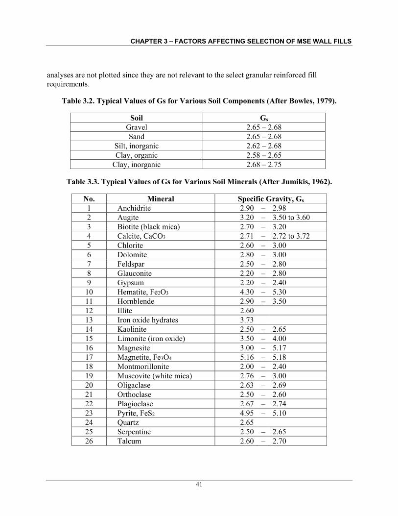
CHAPTER 3 – FACTORS AFFECTING SELECTION OF MSE WALL FILLS
41
analyses are not plotted since they are not relevant to the select granular reinforced fill requirements.
Table 3.2. Typical Values of Gs for Various Soil Components (After Bowles, 1979).
Soil Gs Gravel 2.65 – 2.68 Sand 2.65 – 2.68
Silt, inorganic 2.62 – 2.68 Clay, organic 2.58 – 2.65
Clay, inorganic 2.68 – 2.75
Table 3.3. Typical Values of Gs for Various Soil Minerals (After Jumikis, 1962).
No. Mineral Specific Gravity, Gs 1 Anchidrite 2.90 – 2.98 2 Augite 3.20 – 3.50 to 3.60 3 Biotite (black mica) 2.70 – 3.20 4 Calcite, CaCO3 2.71 – 2.72 to 3.72 5 Chlorite 2.60 – 3.00 6 Dolomite 2.80 – 3.00 7 Feldspar 2.50 – 2.80 8 Glauconite 2.20 – 2.80 9 Gypsum 2.20 – 2.40 10 Hematite, Fe2O3 4.30 – 5.30 11 Hornblende 2.90 – 3.50 12 Illite 2.60 13 Iron oxide hydrates 3.73 14 Kaolinite 2.50 – 2.65 15 Limonite (iron oxide) 3.50 – 4.00 16 Magnesite 3.00 – 5.17 17 Magnetite, Fe3O4 5.16 – 5.18 18 Montmorillonite 2.00 – 2.40 19 Muscovite (white mica) 2.76 – 3.00 20 Oligaclase 2.63 – 2.69 21 Orthoclase 2.50 – 2.60 22 Plagioclase 2.67 – 2.74 23 Pyrite, FeS2 4.95 – 5.10 24 Quartz 2.65 25 Serpentine 2.50 – 2.65 26 Talcum 2.60 – 2.70

CHAPTER 3 – FACTORS AFFECTING SELECTION OF MSE WALL FILLS
42
Figure 3.1. Graph. Sample Format for Gradation Curve with Select Fill Limits for MSE Walls.
Legend: Limits of Select Fill U
W Upper limit for metallic reinforcement V W Upper limit geosynthetic reinforcement X Y Lower limit for all reinforcements
Cu Coefficient of uniformity

CHAPTER 3 – FACTORS AFFECTING SELECTION OF MSE WALL FILLS
43
Much can be learned about a soil’s behavior from the shape and location of the gradation curve. The shape of the grain-size distribution (GSD) curve or “gradation curve” as it is frequently called, is one of the more important aspects in a soil classification system for coarse-grained soils. The shape of the gradation curve can be characterized by a pair of “shape” parameters called the coefficient of uniformity, Cu, and the coefficient of curvature, Cc, to which numerical values may be assigned. Both of these parameters are a function of specific particle sizes as defined in Appendix C, which provides a detailed discussion on the various aspects of gradation and shape parameters. Gradation is evaluated here in the context of the use of select fill for MSE walls and possible implications for the use of LASR instead of select fill. As indicated previously, Figure 3.1 shows the limits of the select fill criteria listed in Table 2.1 as plotted on a gradation chart. The value of Cu is noted on the left side of each of the limiting curves. As noted in the legend the limits are characterized as “upper” and “lower,” which mean larger and smaller particles sizes, respectively. The range of the Cu for the lower limit is intended to signify the potential practical range of approximately 0.04 mm to 0.06 mm of D10 sizes since the criteria in Table 2.1 is limited to Point Y which represents a D15 size while a D10 size is needed to quantify a Cu as explained in Appendix C. The smaller value of 0.04 is based on judgment in that the fines will be likely in the silt particle size based on the limiting PI value of 6 noted in Table 2.2. The value of Cc is approximately 0.7 for any of the limiting curves. For Cc < 1, it is not possible to assign a Group Symbol, e.g., SW, etc., to the limiting curves because a Cc value between 1 and 3 is necessary to classify soils according to the USCS as discussed in Appendix C. The AASHTO soil classification system does not use the shape parameters, Cu and Cc, but even so the limits do not fit any specific group classifications, e.g., A-1-a, etc. The following are the two important goals of the limiting curves: • The horizontal distance between the limiting curves is intended to force the use of granular
and non-plastic to low-plasticity soils, and • The left to right inclination of the curves is intended to force a range of soil particles to
promote dense packing during compaction that will help in promoting shear strength and reducing compressibility.
Gradation curves between the limits shown in Figure 2.1, can be of many different shapes and associated uniformity coefficients. To illustrate the probable range of uniformity coefficients for soil gradations that fall within the upper and lower limits, assume that the range of D10 sizes from approximately 0.04 to 0.06 mm is valid for the lower limit. In that case, the Cu values of soil gradations that fall within the upper and lower limits can range from approximately 190 to 300 based on Curve UW for metallic reinforcements and from approximately 70 to 110 based on curve VW for geosynthetic reinforcements considering their respective D60 sizes. For this reason, the potential use of Cu as a criterion for MSE wall fills should be approached cautiously, especially for LASR materials whose percent fines could be larger than 15%.

CHAPTER 3 – FACTORS AFFECTING SELECTION OF MSE WALL FILLS
44
Based on the above discussion, the key point to realize is that the limiting curves for select fill as shown in Figure 3.1 are not based on a specific soil type according to USCS or AASHTO. A variety of soil types can be acceptable as long as their gradation curves are constrained within the limiting curves shown in Figure 3.1 and the soils meet the other limiting criteria noted in Table 2.1. Based on the limiting curves UW and XY and the criterion of PI 6, the select fill soils within the limiting curves likely belong to the following USCS soil groups: SW, SP, SM, SC, SW-SM, SW-SC, SP-SM, or SP-SC. Appendix A can be used to determine the likely corresponding AASHTO soil groups. Rather than relying on the USCS (or AASHTO) soil group designations, it is important to evaluate the gradation curves of the soils proposed for MSE fills carefully because curves for gap-graded soils can also fit between the limiting curves while meeting the criteria for select fill. Gap-graded soils are undesirable as discussed in Appendix C. Curves I, II and III in Figure C.2 and the associated discussion in Appendix C demonstrate the importance of carefully evaluating the gradation curves rather than simply relying on the soil group designations. Given the long history of successful use of the limiting criteria shown in Figure 3.1 based on Table 2.1, and use of conservative design parameters, the considerations noted above have not received enough attention in the literature. The intention of this observation is not to comment on the conservatism or potential inconsistencies of the current procedures, but rather to ensure that the designer fully understands the basic concepts of soil gradation and the meaning of the associated index properties before using LASR materials for MSE wall fills. The use of LASR materials for MSE wall fills requires attention to these considerations from other aspects, including criteria for identifying coarse and fines fractions, drainage, compaction, specifications, QC/QA, etc.
3.1.2.1 Criteria for Identifying Coarse and Fine Fractions
The gradation curve is instructive in evaluating the relative proportions of the coarse and fine fractions within a given soil sample. Both the USCS and AASHTO systems separate the coarse-grained particles and the fine-grained particles based on the No. 200 sieve which has a square opening size of 0.075 mm). However, the criteria used by the two systems to classify fine-grained soils are as follows: • AASHTO: more than 35 percent passing the No. 200 sieve • USCS: more than 50 percent passing the No. 200 sieve Liu (1970) notes that the amount of fines required to fill all the voids of a coarse-grained material so as to hold the coarse particles apart from each other is approximately 35 percent. Such a mixture behaves more like a fine-grained soil since coarse particles are not in contact with each other. Therefore, the AASHTO criterion of classifying fine-grained soils appears to be more appropriate. However, the 50 percent criterion used by the USCS system is a much simpler criterion, particularly for field identification and classification. Both systems use their own plasticity charts to further group fine-grained soils, e.g., CL, A-7-6, etc.

CHAPTER 3 – FACTORS AFFECTING SELECTION OF MSE WALL FILLS
45
Within the context of MSE walls, as with any other fill wall structure, it is important to realize that the AASHTO or USCS criteria for identifying the coarse and fine fractions is largely redundant in the sense that further limiting criteria such as those in Tables 2.1 and 2.4 are imposed. Those additional criteria do not necessarily match any particular soil group or classification criteria such as coefficient of uniformity, Cu, and coefficient of curvature, Cc. The relative proportions of the coarse and fine fractions can have differing impacts on different aspects of designs, e.g., shear strength, compaction, drainage, etc. Furthermore, the geologic origin and the mineralogy can have a significant impact on the performance of compacted fills in MSE walls. The following sections of the report are intended to discuss the effect of these considerations in the context of MSE-LASR wall system.
3.1.2.2 Evaluation of Gradation from Drainage and Compaction Perspectives
Based on information in NAVFAC (1986a) and Powers (1992), Figure 3.2 presents general particle size limits in terms of drainage superimposed on the MSE wall select granular reinforced fill requirements as expressed in Figure 3.1. The purpose of Figure 3.2 is to qualitatively evaluate the drainage characteristics of soils within the limiting curves. Zone A includes coarse sands, gravels and cobbles, which are free-draining in the sense that water can flow easily through such materials. Zone B encompasses soils that can drain by gravity over time. Zones C and D are subsets of Zone B. Zone C comprises medium to fine sands and Zone D comprises fine sands and silts. The rate of drainage of soils in Zone D is much slower than that of soils in Zone C. Soils in Zones E and F are in the silt and clay ranges; they require external forces such as well points with vacuum and electro-osmosis to extract water. FHWA (1998) presents additional information for drainage in terms of filtration criteria between adjacent zones of different gradations. The following observations can be made based on Figure 3.2: • Depending on the source of the fill and the gradation characteristics the drainage
characteristics can vary widely from free-draining to slow gravity drainage. • The maximum limit of 15% fines, represented by Point Y, constrains drainage of the select
fill which may lead to a build-up of pore water pressures with associated performance problems such as increased deformations and a failure in its limiting condition.
• The limits of select fill material allow for a variety of soil types ranging from well-graded, poorly graded, and gap-graded soils. In fact, Curves I, II and III shown in Figure C.2 of Appendix C are within the prescribed limits of select fill shown in Figure 3.1, but the soils represented by each of those curves will have a significantly different behavior from a drainage perspective.
• Since the general drainage patterns shown in Figure 3.2 by the various zones affect the moisture retention characteristics of the soils, it is apparent that the compaction characteristics of the soils in different zones and possibly within a given zone can vary significantly. This observation is particularly important with respect to use of LASR materials because the normal earthwork compaction criteria based on control of moisture content and dry density may not be suitable when a wide range of soils are involved in fill sources.

CHAPTER 3 – FACTORS AFFECTING SELECTION OF MSE WALL FILLS
46
Figure 3.2. Graph. Evaluation of Select Fill Criteria from Drainage Viewpoint Using Limits of Drainage Characteristics from NAVFAC (1986a) and After Powers (1992).
Zone Method of Drainage Legend: Limits of Select Fill A Free-draining U
W Metallic reinforcement B Theoretical limit of gravity drainage V W Geosynthetic reinforcement C Gravity drainage X Y Lower limit D Gravity drainage too slow E Wells and/or well points with vacuum Cu Coefficient of uniformity F Electro-osmosis

CHAPTER 3 – FACTORS AFFECTING SELECTION OF MSE WALL FILLS
47
A wide range of uniformity coefficients are possible within the limits of the select fill criteria. The key is to realize that the uniformity coefficients of the soil gradations within the limits can exceed those noted at the upper and lower limits provided the requirement that particle uniformity as expressed by the uniformity coefficient pertains only to coarse-grained soils is not violated, i.e., D10 must correspond to a coarse-grained soil particle size > 0.075 mm. Unstable broadly graded soils (i.e., uniformity coefficient Cu > 20 with concave upward particle size distributions) and gap-graded soils should be avoided. Procedures to identify unstable soils are provided by Kenney and Lau (1985, 1986) and should be used when uniformity coefficient values are large. Such soils tend to pipe and erode internally, creating problems with both loss of materials and clogging of drainage systems. Figure 3.3 presents approximate values of coefficient of permeability as a function of increasing fines content. It is clear that there is a drastic reduction in permeability with increasing fines content. The type of fines, silt or clay, has a significant influence. At 15% fines, the range of coefficient of permeability varies over 2 orders of magnitude depending on the type of fines. Practically, for free-draining fills, the fines content should be limited to less than 3 to 5% based on Figure 3.3. Even within the 3 to 5% range, the permeability can vary by several orders of magnitude depending on the type of fines. Similar discussions on the effect of the fines fraction on permeability are also found in Cedergren (1989) and Terzaghi et al. (1996). Use of LASR materials for MSE fills will likely contain more than 15% fines and it is clear that drainage of the soil will be significantly impeded.
Figure 3.3. Graph. Effect of Fines on Permeability (Modified after Barber and Sawyer, 1952, and NAVFAC, 1986a) [1 cm/sec ≈ 2,835 ft/day].
CHAPTER 3 – FACTORS AFFECTING SELECTION OF MSE WALL FILLS
48
3.1.2.3 Clay Fraction (Percent Clay)
Clay fraction (or percent clay) is commonly defined as the percentage by weight of a sample that is finer than 0.002 mm (or 2 m). Section B.1.5 in Appendix B presents the weight-volume relationships for saturated clay-granular soil mixes. Figure 3.4a presents a plot based on Equation B.16 in Appendix B. With respect to Figure 3.4a, Mitchell (1993) notes that,
“… for water contents usually encountered in practice, say 15 to 40 percent, only a maximum of about one third of the soil solids need to be clay in order to dominate the behavior by preventing direct interparticle contact of the granular particles. In fact, since there is a tendency for clay particles to coat granular particles in most soils, the clay will significantly influence properties even when present in quantities much less than shown by Figure 10.4 (reproduced as Figure 3.4a below). For example, just 1 or 2 percent of a highly plastic clay present in a gravel used as fill or aggregate may be sufficient to clog handling and batching equipment.”
Figure 3.4b shows the influence of percent clay (clay fraction) on stabilometer resistance value (R-value). As demonstrated by Chua and Tension (2003), the R-value can be correlated with elastic modulus, E, and therefore can be considered to be a representation of the compressibility of compacted subgrade. Since MSE walls involve compacted subgrade layers the data in Figure 3.4b are of particular significance. Figure 3.4b shows characteristic curves illustrating loss in stability or internal resistance plotted from stabilometer R-value data on a crushed sandy gravel to which plastic clay was added (Hveem, 1953). The data in Figure 3.4b show that it is not only the percent clay (clay fraction) that is important but also the type of clay mineral. Bentonite, which belongs to the smectite mineral group, is much finer and more reactive to water compared to kaolinite and it is clear that presence of bentonite will affect the R-value more than that for the case of kaolinite. Based on the above discussions, consideration of the effects of clay fraction and mineralogy is paramount in the evaluation of LASR materials that contain large percentages of fine-grained soils. Thus, it is not only the amount of fines that is of interest in assessing the suitability of a LASR material for MSE wall fills, but it is also the amount and type of clay in the fines fraction that together are an equally important consideration. Hence, when the use of a LASR material is contemplated for MSE wall fill, determination of clay fraction and type of clay mineral is necessary. Clay fraction can be determined by a hydrometer test. The hydrometer test is based on particle weight consideration. Clay particles often occur as coating on larger particles in a soil sample. This can skew the actual gradation of sizes in the sample and thereby affect the clay fraction. For LASR fills which can have large fines content, evaluation on volume basis is important. This is because the quantity of one component of larger density may not provide sufficient volume to completely fill the voids between larger particles which would affect the frictional resistance between the larger particles. In contrast, the same weight of a lighter density material can occupy more volume within a sample and possibly change the performance characteristics of the soil, e.g., shear strength, compaction, etc.

CHAPTER 3 – FACTORS AFFECTING SELECTION OF MSE WALL FILLS
49
Figure 3.4. Graph. (a) Relationship Between Water Content and Percent Clay by Weight Needed to Fill Voids in a Granular Soil (Based on Mitchell, 1993, and Mitchell and Soga,
2005), (b) Effect of Percent Clay (Clay Fraction) by Weight on R-value of Compacted Subgrade (After Hveem, 1953), (c) Effect of Various Fine Materials on the Sand Equivalent
(After Hveem, 1953), (d) Sand Equivalent versus Resistance (R) Value (After Hveem, 1953).
(a) (b)
(c) (d)

CHAPTER 3 – FACTORS AFFECTING SELECTION OF MSE WALL FILLS
50
For LASR fills with large fines content it is important to reliably estimate clay fraction by volume to understand the behavior of the fills during placement and their long-term performance. The volume of clay fraction based on hydrometer tests can be calculated by determining the specific gravity of the various particle sizes in a soil sample. Determination of clay fraction based on volume consideration can also be performed by sand equivalent (SE) tests. The sand equivalent test permits a more rapid determination of clay fraction compared to hydrometer tests and is therefore useful as a field correlation (construction control) test. For LASR fills, it is recommended that both hydrometer and sand equivalent tests be performed to confirm and correlate the clay fraction from each test. Figure 3.4c shows a correlation between sand equivalent (SE) and percent clay for various fine materials that can be used as a preliminary guide. The data in Figure 3.6c also show the effect of the clay mineral type on SE value. Figure 3.4d presents data for sand equivalent in terms of resistance (R) value for a variety of soil mixtures and applications (e.g., gravel base). Caltrans experience (Griswell, 2015) indicates that SE values greater than 30 generally define a mixture where the clay fraction is too small in volume to significantly affect the behavior of compacted fill. In contrast, the soil resistance (R-value) reduces significantly below SE value of 30 with the clay component having a large influence on the overall behavior of the soil mixture. Most agencies today specify SE > 30 for unmodified fill soils and 20 < SE < 30 for reinforced or contained fill soils such as in MSE walls or crib walls. LASR soils may have SE < 20 which indicates smaller resistance values and hence a need for greater care in design and construction. In general, the greater the content of a medium to high plasticity clay in a soil, the greater the potential for shrinkage/swell, the less the permeability, the greater the compressibility, and the more the shear strength properties become altered with larger true cohesion and smaller true angle of internal friction (Mitchell and Soga, 2005). Therefore, the importance of clay content and mineralogy cannot be overemphasized in view of the dominating influence of the clay fraction on soil behavior as shown in Figure 3.4. Mineralogy is discussed in Section 3.2.
3.1.2.4 Relevance of Gradation Evaluation
Although evaluation of gradation is important, the size of the particles and their distribution in a soil mass are just two of the factors that influence the behavior of the soil under stress and seepage. The discussions in Section 3.1.2.1 to 3.1.2.3, and Appendix C, Section C.1, serve to emphasize this aspect. Important characteristics such as the shape of the particles, their mineralogical composition, their in-situ structure, and the relative density of the soil mass cannot be represented by an evaluation of gradation. To do so can result in misleading conclusions, particularly when LASR materials are used. The effect of specific gravity of the solids was discussed in Section 3.1.1. Other factors such as Atterberg limits (Section 3.1.3), geologic origin and mineralogy (Section 3.2) and electrochemical properties (Section 3.3) must also be considered in conjunction with gradation. These factors are discussed in the following sections.

CHAPTER 3 – FACTORS AFFECTING SELECTION OF MSE WALL FILLS
51
3.1.3 Atterberg (Consistency) Limits
Water has a significant influence on the behavior of soils. In general, increasing water content changes the consistency of soils, which results in reduced shear strength and increased compressibility. The change in the physical states of soils with changes in water content is discussed in Appendix D where the Atterberg limits are shown conceptually in Figure D.1 and their physical significance is shown in the form of a plasticity chart in Figure D.2. The plasticity chart is used to classify fine-grained cohesive soils. As shown in Figure A.1 in Appendix A, the plasticity chart is different in the USCS and AASHTO systems. The MSE wall industry generally uses the USCS version of the plasticity chart shown in Figure 3.5. Table 2.2 indicates that the plasticity index (PI) of select fill for MSE walls shall be less than or equal to 6. This limit is shown by a dashed line at PI=6 in Figure 3.5. As a frame of reference, the upper and lower bound values of PI for the CL-ML zone are 7 and 4, respectively, as shown in Figure 3.5 and Figure D.2 in Appendix D. While dealing with low PI values it must be realized that the determination of PI is operator dependent and the variability between tests can be so great that the difference between test results by different testers can be the difference of being within specification or out of specification while the results themselves are still considered to be within the realm of acceptance (Quire and Kowalski, 2004).
Figure 3.5. Chart. USCS Plasticity Chart as per ASTM D2487 with PI Limit for Select Fill for MSE Walls.

CHAPTER 3 – FACTORS AFFECTING SELECTION OF MSE WALL FILLS
52
Table 2.2 does not provide guidance on the upper bound value of the liquid limit (LL) on the x-axis of the plasticity chart. However, some general observations can be made based on the significance of A- and U-lines on the plasticity chart as follows: • The A-line on the chart separates soils with clay characteristics (above the A-line) from soils
with silt characteristics (below the A-line). The A-line also separates inorganic (above the A-line) from organic (below the A-line) soils.
• The LL = 50 line generally represents the dividing line between silt, clay, and organic fractions of the soil that exhibit low to medium plasticity (LL < 50) and high plasticity (LL > 50). Furthermore, in general, clayey soils with LL < 30 are considered to be low plasticity soils while soils with 30 < LL< 50 are considered to be medium plasticity soils (Mitchell and Soga, 2005).
• The U-line represents the upper range of PI and LL coordinates that have been found for soils. When a data point plots above the U-line, the test results should be considered spurious, and the tests for Atterberg limits should be rerun. As per ASTM D2487, the U-line is vertical at LL = 16 for 0 PI 7. Thus, it would appear that a limiting value of LL = 16 should be considered along with the criterion of PI 6 based on the USCS as per ASTM D2487.
Given the constraints of the U-line, the A-line, and PI 6, it can be deduced that the select fill criterion PI 6 attempts to limit the fine-grained fraction of soils within the select fill to soils having silty characteristics with low plasticity. Based on the literature review in Chapter 2, there have been several successful applications of MSE walls with PI values in the range of 20 to 30 that had fines contents > 15%. Based on the USCS plasticity chart, those soils appear to have been CL soils. Because these applications were successful, the use of LASR materials for MSE wall fills would likely mean use of soils in the CL and possibly CH zones of the USCS plasticity chart. Behavior of such soils is significantly affected by the geologic origin and mineralogy as discussed in Section 3.2.
3.2 GEOLOGIC ORIGIN AND MINERALOGY
The effects of the geologic origin and mineralogy of soils used in LASR-MSE wall fills is important to understand. Unfortunately, this consideration also happens to be the most overlooked aspect in current design procedures for MSE walls. This deficiency is likely due to the fact that fill soils have been assigned limiting criteria that do not take the geologic origin and mineralogy into account, e.g., Table 2.1, Table 2.2, Figure 3.1, and Figure 3.5, are indexed to USCS or AASHTO designations. It is generally assumed that a soil classified within a certain group, e.g., SW (USCS) or A-1-a (AASHTO) will behave the same regardless of their geographical location and geomorphology. The reality is that soils within a given USCS or

CHAPTER 3 – FACTORS AFFECTING SELECTION OF MSE WALL FILLS
53
AASHTO group could have significantly differing performance characteristics depending on the geographical locations and the geologic processes that occurred at those locations. Appendix E presents a brief discussion on soil formations and landforms. With respect to excavation at the borrow source and subsequent placement as fills, the behavior of residual soils and transported soils can be significantly different. Residual soils remain in the place of their formation where they are usually formed from chemical and physical weathering of native rocks. Their characteristics depend on the mineralogy of the parent rocks. As their name suggests, transported soils consist of weathered pieces of rocks that have been carried by wind and/or water to locations where they may continue to weather. Consequently, transported soils can consist of minerals from a variety of rock types not native to the area where they were deposited. Such soils are frequently called sediments or sedimentary soils. As noted by Wesley (2010a, 2010b), some residual soils are not strictly particulate, i.e., they do not consist of discrete particles. They may appear to consist of individual particles, but when disturbed or subjected to shear stress, these particles disintegrate and form an array of much smaller particles. They may not meet the soundness criteria listed in Table 2.2. The mineralogy of residual and transported soils can be significantly different. Figure 3.6 can be used as a first step to identify the mineral type based on where the soil’s Atterberg limits plot on the plasticity chart. The mineral type can also be identified based on the Activity Index, A, noted in the Figure 3.6. The symbol for Activity Index (A) should not be confused with the “A-line” also shown in the figure. The Activity Index, A, is defined as PI/CF where CF the clay fraction as defined in Section 3.1.2.3 and both PI and CF are expressed in the same units (decimal or percentage). The greater the value of A, the greater the influence of the clay fraction on the properties of the soil. Clays with A < 0.75 are considered to be “inactive” while clays with 0.75 < A < 1.25 are classified as “normal” clays and those with A > 1.25 are “active,” all in the sense of significant volume change potential. Thus, if the soil plots just below the U-line, it probably contains a significant amount of the clay mineral montmorillonite that expands in the presence of water. The value of activity index, A, for soils plotting in this area near the U-line can be used to cross-check the estimation of the clay mineral. The table in Figure 3.6 provides the values of Activity Index, A, for other minerals. A more accurate identification of clay mineralogy is commonly determined by x-ray diffraction analyses and/or differential thermal analysis. These analyses are economical to perform and are widely used in practice. Details are described in Mitchell and Soga (2005). Once the clay mineral has been identified based on the USCS plasticity chart then the designer should use more detailed references such as Mitchell and Soga (2005) to evaluate the performance characteristics of the soil such as strength and volume change characteristics. In addition to the performance characteristics the effect of clay mineralogy on corrosion should be evaluated. For example, Jones (1996) notes that some clay minerals, such as illite, accelerate metal corrosion. While the limiting criteria noted in Table 2.1, Table 2.2, Figure 3.1, and Figure 3.3 effectively ruled out the possibility of deleterious clay minerals, consideration of LASR materials as fill for MSE walls will need careful evaluation with respect to mineralogy.

CHAPTER 3 – FACTORS AFFECTING SELECTION OF MSE WALL FILLS
In addition to the values of Activity Index, A, for the minerals shown in the chart, the values of other minerals are as follows:
Mineral Activity Index, A Attapulgite 0.5 – 1.2 Allophane 0.5 – 1.2
Calcite 0.2 Mica (muscovite) 0.2
Quartz 0.0
Figure 3.6. Chart. USCS Plasticity Chart with Location of Clay Minerals and Activity Index Values (After FHWA, 2006, and Based on Data from Skempton, 1953; Mitchell,
1993; and Holtz and Kovacs, 1981).
54

CHAPTER 3 – FACTORS AFFECTING SELECTION OF MSE WALL FILLS
55
3.3 ELECTROCHEMICAL PROPERTIES
The required electrochemical properties for select fill depend on whether steel or geosynthetic reinforcement is used as noted in Table 2.3 and Table 2.4, respectively. The goal of limiting electrochemical properties is to mitigate the corrosion of steel reinforcements and the degradation of geosynthetic reinforcements. The recommendations in Tables 2.3 and 2.4 do not preclude corrosion of steel or degradation of geosynthetics. Rather, the required properties are such that the rate of corrosion of steel or degradation of geosynthetics can be reasonably quantified for design purposes based on measured data. These rates are included in FHWA (2009) and AASHTO (2020). FHWA (2009a) provides detailed background information for consideration of corrosion/degradation of soil reinforcements for MSE walls.
3.3.1 Steel Reinforcements
In some areas of the United States, it is becoming more and more difficult to locate fill that meets the FHWA/AASHTO requirements for steel reinforcements listed in Table 2.3. In the context of the current study to evaluate the suitability of LASR materials for MSE wall fills, it becomes imperative to evaluate the possibility of using more relaxed electrochemical criteria, e.g., resistivity less than 3,000 ohm-cm. There are very little data available in the publishedliterature to document performance and formulate appropriate metal loss models for design in thecase of potential LASR fill materials.
Based on the results of limited field studies performed for Caltrans, Jackura et al. (1987) proposed greater rates of metal loss when fills are more aggressive, i.e., fills having resistivity less than 3,000 ohm-cm. Specifically, Caltrans’ current specification (Caltrans, 2012) allows for fills with a resistivity greater than 2,000 ohm-cm, a pH between 5.5 and 10, and maximum chloride and sulfate concentrations of 250 ppm and 500 ppm, respectively. Caltrans allows these conditions by using a greater rate of metal loss in determining sacrificial steel. Caltrans also assumes that the zinc coating on the reinforcing elements provides 10 years of additional service life for the specified minimum coating thickness of 85 m per side. This value of additional service life is less than the 16 years of zinc life assumed by FHWA (2009) and AASHTO (2020) for soils with minimum resistivity of 3,000 ohm-cm. A corrosion rate of 1.10 mils/year (28 m/year) is considered to affect the base metal after the zinc has been consumed. This corrosion rate is used to compute the sacrificial steel requirements. These corrosion rates account for the potential of localized corrosion and pitting, i.e., a factor of two relating the loss of tensile strength to idealized uniform corrosion rates is included. Presently, LASR materials are subject to these types of corrosion specifications.
Report 675 of NCHRP (2011) presents guidelines for LRFD metal loss and service-life strength reduction factors for metal-reinforced systems. For the case of MSE-LASR wall with metallic reinforcements, an instrumentation and monitoring program that includes steel coupons is recommended. Such a program will permit early intervention in the event that the actual corrosion loss rates are larger than those assumed in design. Typical monitoring programs are discussed in FHWA (2009a).

CHAPTER 3 – FACTORS AFFECTING SELECTION OF MSE WALL FILLS
56
3.3.2 Geosynthetic Reinforcements
For geosynthetic reinforcements, the electrochemical criteria are expressed in terms of pH that varies depending on the polymer as per Table 2.4. The range of 3 < pH < 9 for PET geosynthetics in Table 2.4 was developed for a 100-year design life in the absence of long-term product specific testing. It is possible that some LASR materials may have a pH value larger than 9. In such a case PET may be used if product specific testing for PET geosynthetic with site-specific LASR material is performed in accordance with procedures in FHWA (2009). Once the specific base polymer has been selected for a given project, the estimation of long-term allowable strength of geosynthetic reinforcements is based on consideration of installation damage, creep, and durability (aging). Each of these considerations is addressed by a corresponding reduction factor, RF, as follows: • The reduction factor of installation damage, RFID, is dependent on the fill soil gradation
characteristics and its angularity, especially for lighter weight geosynthetics. Damage during reinforced fill placement and compaction operations is a function of the severity of loading imposed on the geosynthetic during construction operations and the size and angularity of the reinforced fill. For MSE-LASR walls lightweight, low strength geotextiles and geogrids should be avoided to minimize damage with ensuing loss of strength. Protocols for field testing for this reduction factor are detailed in FHWA (2009a) and in ASTM D5818. Typical values of RFID are given in FHWA (2009).
• The creep reduction factor, RFCR, is required to limit the load in the reinforcement to a level known as the creep limit that will preclude excessive elongation and creep rupture over the life of the structure. Creep is essentially a long-term deformation process. The creep limit strength is thus analogous to yield strength in steel. The creep reduction factor is obtained from long-term laboratory creep testing as detailed in FHWA Appendix D. Typical values of RFCR are given in FHWA (2009).
• The durability (aging) reduction factor, RFD, is dependent on the susceptibility of the geosynthetic to attack by chemicals, thermal oxidation, hydrolysis, environmental stress cracking, and microorganisms. Protocols for development of this reduction factor are discussed in FHWA (2009a).
The reduction factors RFID, RFCR, and RFD, are determined in accordance with AASHTO R 69. Detailed discussions for each of the above reduction factors can be found in FHWA (2009), AASHTO (2020) and FHWA (2009a).
3.3.3 Quality of Water for Compaction of Soils
The quality of water used for molding and compacting soils in the reinforced zones can affect the electrochemical properties of the as-constructed environment for the soil reinforcements. The water used for molding and compacting soils should not be salty or brackish and should be free from injurious amounts of oil, acid, alkali, clay, vegetable matter, silt, or other harmful matter.

CHAPTER 3 – FACTORS AFFECTING SELECTION OF MSE WALL FILLS
57
Water quality can be sampled and tested in accordance with the requirements of AASHTO T 26. Potable water obtained from public utility distribution lines is acceptable and, generally, not subjected to quality testing. In general water used for Portland cement concrete mixes will be suitable for use in compaction of reinforced fill soils. Local agencies generally have stipulations for water chemistry (e.g., limits on Cl, SO4, pH, etc.) depending on the source and its use. The designer should consider the local water chemistry stipulations with respect to their effect on the specific type of reinforcements considered for MSE-LASR walls. Electrochemical tests (resistivity, pH, organic content, chlorides, and sulfates) on soil samples compacted to optimum moisture content using local water proposed for use on a project should be performed to verify that the as-constructed environment will be compatible with the design assumptions for corrosion of metallic reinforcements and degradation of geosynthetic reinforcements. Electrochemical tests should be repeated at the frequency of 1 per 1,000 yd3 of fill with new tests at every instance of change in borrow source of soil and/or water.
3.4 COMPACTION OF FILLS FOR MSE WALLS
All fills for MSE walls composed of either select or LASR materials need to be compacted. Compaction is the process of densifying soil under controlled moisture conditions by application of a given amount and type of energy. Appendix F discusses the compaction characteristics of soils including the concept of compaction, ASTM and AASHTO test procedures (standard Proctor and modified Proctor), interpretation of test results (maximum dry density and optimum moisture content), relationship between relative compaction and relative density, and typical field compaction specifications. The select fill material as specified in Table 2.1 is primarily a coarse-grained soil that likely has uniform invariant index properties. The concepts of compaction discussed in Appendix F are readily applicable to such materials. Common practice for compaction control of select fill is to specify water content limits within several percentage points on each side of the optimum moisture content and minimum dry density not less than 90 or 95 percent of the maximum dry density. Compaction control is achieved by so-called performance based or end-product specifications wherein a certain relative compaction, RC, also known as percent compaction, is specified. The RC is simply the ratio of the desired field dry unit weight, dfield, to the maximum dry density measured in the laboratory, dmax, expressed as a percentage. The value of RC is chosen carefully based on the site-specific needs of the project. Depending on the type of soil every 1% change in the RC can change the shear strength of the compacted soil. For example, as discussed in Appendix F, for SW soils, there is a 3.3% increase in the coefficient of friction, tan' for every 1% increase in RC. The coefficient of friction is directly related to the shear strength of the soil. Taken in reverse, this means that if compaction is not done properly in the field, there can be a rapid decrease in the coefficient of friction of the compacted soils and a consequent reduction of shear strength. This example underscores the importance of achieving the specified levels of compaction in the field.

CHAPTER 3 – FACTORS AFFECTING SELECTION OF MSE WALL FILLS
58
In contrast to select fills where the concept of relative compaction has been used successfully, LASR materials could include a wide range of geomaterials that may have non-uniform invariant index properties. Therefore, the compaction characteristics and resulting engineering properties, such as shear strength and volume change, may be variable within MSE-LASR wall fills. Consequently, more stringent and/or alternative compaction control procedures may be required for MSE wall fills constructed with LASR materials. These aspects are discussed in more detail in Section 3.9. To comprehend the need for appropriate compaction control procedures it is first important to understand the shear strength and volume change characteristics of compacted soils; these aspects are discussed in Section 3.5 and 3.6, respectively.
3.5 SHEAR STRENGTH OF COMPACTED SOILS
The design shear strength parameters of select fill for the reinforced zone are discussed in Section 2.1.1.2. The effective friction angle is assumed to be 34 degrees unless project-specific fill is tested to justify larger values. Regardless, the maximum friction angle is limited to 40 degrees. In all cases, the cohesion of the select fill is assumed to be zero. Thus, for select fill only the frictional component of shear strength is assumed to contribute to the design shear strength. When LASR materials are used for MSE fills, the percent fines will likely be larger than 15% and the PI will likely be greater than 6 as specified in Table 2.1. The USCS designations for such soils include soil groups such as SC, CL, etc. Since the fill will be compacted, the shear strength of the compacted soils is of primary interest. Therefore, the in-situ shear strength at the borrow source has little or no relevance to MSE wall designs. Appendix F provides a discussion on compaction characteristics of soils that should be reviewed to understand the nuances of the discussions presented in this section. Table 3.4 lists typical values for the engineering properties of compacted soils for 14 different USCS designations. The soils are numbered 1 to 14 in the first column of the table. In general, soils 1 through 6 can meet the requirements of select fill while soils 7 through 14 may not; therefore soils 7 through 14 are of more interest in the context of LASR materials. The values of the engineering properties refer to soils compacted to maximum dry density by the standard Proctor test. The data in Table 3.4 are based on more than 1,500 soil tests performed by the Bureau of Reclamation as reported in USBR (1960). Different versions of this table are included in later USBR publications, but for the purpose of this report the data presented in Table 3.4 are instructive and useful because they include valuable information on the shear strength properties of saturated compacted soils. The majority of the soils were from 17 western states in the United States. The data also contain the results of tests performed on some foreign soils. The background information for the values in Table 3.4 is given in the notes section of the table with Note h being of particular importance.

CHAPTER 3 – FACTORS AFFECTING SELECTION OF MSE WALL FILLS
59
Table 3.4. Average Engineering Properties of Compacted Inorganic Soils (After USBR, 1960 and FHWA, 2006).
Soil
No.
USCS
Standard Proctor Maximum Dry
Density (MDD or dmax), pcf (kN/m3)
Standard Proctor Optimum Moisture
Content, wopt (%)
As Compacted
Effective Cohesion,
co psi (kPa)
Compacted-Saturated Effective
Cohesion, csat psi (kPa)
Friction Angle,
(deg)
Void Ratio, e [Permeability,
k (ft/yr)]
1 GW >119 (>18.7) <13.3 * * >38 *
[27,000 13,000]
2 GP >110 (>17.3) <12.4 * * >37 *
[64,000 34,000]
3 GM >114 (>17.9) <14.5 * * >34 *
[> 0.3]
4 GC >115 (>18.1) <14.7 * * >31 *
[> 0.3]
5 SW 119 5 (18.7 0.8) 13.3 2.5 5.7 0.6
(39 4) * 38 1 0.37 * [*]
6 SP 110 2 (17.3 0.3) 12.4 1.0 3.3 0.9
(23 6) * 37 1 0.50 0.03 [>15.0]
7 SM 114 1 (17.9 0.2) 14.5 0.4 7.4 0.9
(51 6) 2.9 1.0 (20 7) 34 1 0.48 0.02
[7.5 4.8]
8 SM-SC 119 1 (18.7 0.2) 12.8 0.5 7.3 3.1
(50 21) 2.1 0.8 (14 6) 33 4 0.41 0.02
[0.8 0.6]
9 SC 115 1 (18.1 0.2) 14.7 0.4 10.9 2.2
(75 15) 1.6 0.9 (11 6) 31 4 0.48 0.01
[0.3 0.2]
10 ML 103 1 (16.2 0.2) 19.2 0.7 9.7 1.5
(67 10) 1.3 * (9 *) 32 2 0.63 0.02
[0.59 0.23]
11 ML-CL 109 2 (17.1 0.3) 16.8 0.7 9.2 2.4
(63 17) 3.2 * (22 *) 32 3 0.54 0.03
[0.13 0.07]
12 CL 108 1 (17.0 0.2) 17.3 0.3 12.6 1.5
(87 10) 1.9 0.3 (13 2) 28 2 0.56 0.01
[0.08 0.03]
13 MH 82 4 (12.9 0.6) 36.3 3.2 10.5 4.3
(72 30) 2.9 1.3 (20 9) 25 3 1.15 0.12
[0.16 0.10]
14 CH 94 2 (14.8 0.3) 25.5 1.2 14.9 4.9
(103 34) 1.6 0.86 (11 6) 19 5 0.80 0.04
[0.05 0.05] Notes: (a) The entry indicates 90 percent confidence limits of the average value; * denotes insufficient data. (b) For permeability, 1 ft/yr ≈ 10-6 cm/sec and 1 cm/sec ≈ 2835 ft/day. (c) All shear strengths, void ratios and permeabilities were determined on samples prepared at Standard Proctor maximum dry
density and optimum moisture content. (d) The values of cohesion, co and csat, and friction angle, , are based on a straight-line Mohr strength envelope on effective stress
axes as shown in Figure 3.7a (USBR, 1960). The value of csat, for the compacted-saturated condition was obtained by assuming that the frictional component of shear strength is not affected by saturation. Therefore, the friction angle, , also applies to the compacted-saturated condition. Consolidated-undrained (CU) triaxial tests with pore water pressure measurements were used to determine all the shear strengths.
(e) Since all laboratory tests, except large-sized permeability tests, were performed on the minus No. 4 (4.75 mm) fraction of soil, data on average values for gravels are not available for most properties. However, an indication as to whether these average values will be greater than or less than the average values for the corresponding sand group are given in the table (note entries with > or < symbol).
(f) Void ratio was derived from the maximum dry density and specific gravity of the soil grains. (g) In USCS, there are no upper boundaries of liquid limit of MH and CH soils. The maximum limits for MH and CH soils tested
by USBR (1960) were 81% and 88%, respectively. Soils with higher liquid limits than these will have inferior engineering properties.
(h) The data in this table must not be used for design purposes. Design parameters must be developed based on project-specific testing.

CHAPTER 3 – FACTORS AFFECTING SELECTION OF MSE WALL FILLS
60
Figure 3.7. Schematic. (a) USBR (1960) Definition of Shear Strength Parameters Based on Straight Line Mohr-Coulomb Failure Envelope for Data in Table 3.4, (b) Concept of
Curved Failure Envelope and Choice of Shear Strength Parameters Based on Range of Interest for Normal Stress.
(a)
(b)

CHAPTER 3 – FACTORS AFFECTING SELECTION OF MSE WALL FILLS
61
3.5.1 Consideration of Cohesion Component of Shear Strength
Table 3.4 indicates that when compacted to maximum dry density according to the standard Proctor tests, soils can exhibit notable cohesive strength, co. The concept of cohesive strength is often misunderstood. The designer must develop a good understanding of this concept otherwise there will be a disconnect between reality and the design of earth structures, e.g., compacted soils in fill slopes of low heights. It is important to understand the basis for the development of shear strength parameters reported in any publication. Figure 3.7a defines the shear strength components, co, csat and that are noted in Table 3.4. This nomenclature is specific to USBR (1960). For clarity, the specimens shown in Figure 3.7a as “placed at Proctor density” are referred to in this discussion as being in an “as-compacted” condition while the specimen shown in the figure as “placed at Proctor density then saturated” is referred to as being in a “compacted-saturated” condition. As shown in Figure 3.7a, the tangent to the Mohr circles for the as-compacted specimens is labeled “Mohr Strength Envelope.” This straight-line approximation is used to determine co and . USBR (1960) assumed that the frictional component of shear strength is not affected significantly by saturation. Hence, USBR (1960) used a straight-line approximation parallel to the “Mohr Strength Envelope” for the compacted-saturated condition to determine a value of csat. Therefore, in this case the loss of shear strength because of saturation is attributed to a reduction in the cohesion component of shear strength as represented by the value of csat, which is less than the value of co. The values of cohesion and friction angle in Table 3.4 must be interpreted in the context of how they were developed by the USBR. In addition to this significant observation about reduction in the cohesion component, the data in Table 3.4 provides a relative comparison of the values of various items identified in the table header for different soil types identified in Column 1 of the table. Beyond these two observations, i.e., reduction in cohesion component following saturation and the relative values of the shear strength parameters for different soil types, the actual values in Table 3.4 must not be used for design. Project-specific testing must be performed to develop the design shear strength parameters.
3.5.1.1 Concepts of Shear Strength and Nomenclature for MSE-LASR Applications
Concurrent with the publication of USBR (1960), ASCE published the proceedings of a research conference on the shear strength of cohesive soils (ASCE, 1960). In this conference, Seed et al. (1960) provided a paper on shear strength of compacted cohesive soils. Starting with the papers presented at that conference, a greater understanding of shear strength has been developed by the geotechnical community as reported in numerous journal papers since then. This is particularly true for the shear strength of partially saturated (unsaturated) soils, which is the case for soils at the as-compacted condition discussed earlier. Hilf (1975) and Fredlund and Rahardjo (1993) discuss the effect of partial saturation on shear strength of compacted soils. Unfortunately, the nomenclature for shear strength and the shear strength parameters has not been standardized and their symbols often vary in different publications. Figure 3.7b presents the nomenclature that has been adopted in this report.

CHAPTER 3 – FACTORS AFFECTING SELECTION OF MSE WALL FILLS
62
For comparison with Figure 3.7a, the failure envelope AB in Figure 3.7b is the same as the “Mohr Strength Envelope” in Figure 3.7a that is drawn tangent to the Mohr circles for the as-compacted condition. The equation of the failure envelope AB is as noted in Figure 3.7b for the as-compacted condition and the notation cac is used for the cohesion component. Since the soils are partially saturated at this condition, the shear strength represented by failure envelope AB is influenced by matric suction, which is the result of capillary stresses generated by surface tension in the pore water. The matric suction is reflected in the value of cohesion designated by cac in Figure 3.7b. The contribution of matric suction to the value of cac is significant as discussed in Section 3.5.1.2. The level of matric suction depends on a number of parameters including, but not limited to, the gradation of the soil, mineralogy, and level of compaction. Thus, even for soils with same USCS designation, the value of cac can vary as evidenced by the values noted in Table 3.4. The effect of matric suction is overcome by saturation, which reduces the value of the cohesion as discussed earlier. When the soils are saturated, the failure envelope is curved as shown in Figure 3.7b. The curved failure envelope, often referred to as the "Mohr Failure Envelope," is obtained by drawing tangents to a series of Mohr circles at failure obtained from shear tests on saturated samples with accurate pore water pressure measurements. Most retaining walls involve a relatively narrow range of normal pressures. Therefore, it is often possible to fit a straight-line approximation over this range of interest as shown in Figure 3.7b, unless the range of normal pressures includes a portion of the Mohr failure envelope that is sharply curved as is often the case near the origin. This straight-line approximation is commonly referred to as the "Mohr-Coulomb Failure Criterion" and is represented by the equation for envelope XY noted in Figure 3.7b for the compacted-saturated condition. For purposes of comparison with failure envelope AB, the cohesion component for failure envelope XY is labeled as ccs. The value of ccs can be significantly less than cac due to the reduction in matric suction as discussed previously. In this report, the notations c and are used for effective cohesion and effective friction angle, respectively. They are based on the concept of a linear failure envelope defined over the range of interest of normal stresses as discussed above. The values of these two parameters will vary depending upon whether peak, fully softened, or residual conditions as defined in FHWA (2002) are selected for design. Regardless of the approach taken to determine and quantify the cohesion and friction angle for the straight-line Mohr-Coulomb failure envelope, the component referred to as “cohesion” is the intercept of the straight line with the shear strength axis. Similarly, the friction angle is also a function of the straight line fitted over the range of interest of normal stresses. Thus, in view of the actual curved failure envelope, it must be understood that the value of “cohesion” and “friction angle” are artifacts of the straight-line Mohr-Coulomb failure envelope that is used to model the approximate shear strength over the range of interest based on the level of saturation that exists in the soil and the level of strain that could be experienced. In other words, the value of cohesion and friction angle are not fundamental properties of the soil but are parameters for a straight-line failure envelope model used to represent the approximate shear strength over the normal stress range of interest.

CHAPTER 3 – FACTORS AFFECTING SELECTION OF MSE WALL FILLS
63
In addition to the effect of the interpretation of the test data, the straight-line model chosen to represent the shear strength must be carefully evaluated in the context of the phenomenon that is being evaluated, e.g., bearing capacity, slope stability, etc. The implications of using the straight-line approximation may be different depending on the problem under consideration and the range of normal pressures of interest. For example, Baker (2004) quantitatively demonstrates the effect of cohesion resulting from the straight-line approximation on slope stability. Similarly, Vahedifard et al. (2014) demonstrate the impact of cohesion on the seismic design of geosynthetic-reinforced soil structures. Therefore, it is very important to understand the concept of the phenomenon called “cohesion” and its effect on design.
3.5.1.2 Concept of True and Apparent Cohesion
There are two types of cohesion in soils: true cohesion and apparent cohesion. A summary based on Mitchell and Soga (2005) and FHWA (2006) follows: A. True cohesion may result from chemical cementation (just like in rocks) and/or forces of
attraction (e.g., electrostatic and electromagnetic attractions) between colloidal (10-3 mm to 10-6 mm) clay particles. True cohesion is stress-independent unlike frictional resistance that is a function of normal stress.
B. Apparent cohesion may develop because of capillary stresses and mechanical interlocking as follows:
• Capillary stresses develop between particles in a partially saturated soil because of
surface tension in the water. The surface tension (negative pressure or matric suction) in the water produces an equal and opposite effective stress between the soil particles, which results in an apparent cohesion since it too is stress-independent. The magnitude of this type of apparent cohesion can be extremely large, especially in fine-grained soils. Such capillary stresses can be overcome by an increase in the degree of saturation.
• Apparent mechanical forces are often exhibited by the interlocking of rough (angular) soil particles. The interlock between the soil particles can offer some resistance to shear stresses even in the absence of a normal stress. This type of apparent cohesion is often the cause of cohesion measured in compacted soils. However, such apparent mechanical forces are susceptible to significant reduction by vibrations and other types of mechanical disturbance.
Figure 3.8 illustrates these concepts by showing the potential contributions of the various mechanisms discussed above as a function of particle size. It is evident from the figure that tensile strength (apparent cohesion) from capillary adhesion can be significant, especially for clay soils. The cohesion values, c (as-compacted) and csat (compacted-saturated) listed in Table 3.4 are instructive in the context of the apparent cohesion concept. In the soil’s compacted state at

CHAPTER 3 – FACTORS AFFECTING SELECTION OF MSE WALL FILLS
64
optimum moisture content (OMC), the capillary stresses and the apparent mechanical forces assume their peak values at that particular compaction energy. Capillary stress, as noted above, is caused by surface tension in the pore water between individual soil grains. The magnitude of capillary stress is larger in fine-grained soils than coarse-grained soils as demonstrated by the increasing values of csat in Table 3.4 as the soil type changes from coarse-grained to fine-grained.
Figure 3.8. Chart. Potential Contributions of Several Bonding Mechanisms to Soil Strength (After Ingles, 1962, and Mitchell, 1993).
The same trend is observed with the csat values in Table 3.4. However, the values of csat are approximately 10% (for CH soils) to 40% (for SM soils) of the corresponding co values. This drastic reduction in cohesive strength is attributable to the effect of capillary stresses being significantly reduced by the increase in moisture content required to reach saturation resulting in much lower apparent cohesive strengths. The reduction may also represent loss of apparent mechanical forces due to reduction in the interlocking of the particles because of the lubricating effect of water. The following guidelines are based on the above discussions: • Since cohesion cannot be defined with confidence, its contribution to long-term shear
strength in c- soils is often disregarded or greatly minimized by using only a small value such as 50 to 100 psf. For purely cohesive soils, the designer should be careful in evaluating the cohesion for long-term design purposes. The value selected should be based on whether peak, fully softened or residual conditions are appropriate for the feature being designed, e.g., slope, wall, etc.
• It is important to ensure that compacted soils are protected against increases in moisture content because the strength of such soils will decrease with associated detrimental effects on the facilities they support.

CHAPTER 3 – FACTORS AFFECTING SELECTION OF MSE WALL FILLS
65
3.5.2 Effect of Organic Content on Shear Strength
As per Table 2.3, the organic content of select fill is limited to a maximum of 1%. However, organic content may pose a problem for certain types of LASR materials. Franklin et al. (1973) observed that increasing organic content reduced maximum dry density and increased optimum moisture content of samples compacted with the Harvard miniature compaction apparatus. They found that there was no appreciable reduction in maximum dry density until the organic content of the natural soil reached 7 to 10% by mass. At organic contents greater than 7 to 10% the maximum dry density decreased significantly. This conclusion regarding the effect of organic content on compacted maximum dry density was also made for unconfined compressive strength. Franklin et al. (1973) conclude that compaction of soils with organic content differs appreciably from that of inorganic soils. They offer the following explanation:
“The organic particles are generally larger than clay particles and have the ability to absorb water. They also attract clay particles which become bound to their surfaces. The organic particles are stiff when compressed and act as rigid particles when dry, but when they absorb water they become sponge-like and soft. All this implies that at low water contents much of the water added to the sample becomes in effect a part of the organic matter. This reduces the efficiency of adjusting the water content to optimize the compaction behavior, and in soils with very high organic content … the optimum dry density becomes very hard to define.”
It is important to understand the long-term (decomposition) and short-term (moisture absorption/desorption) effects of organic content on the compaction characteristics and shear strength of compacted soils. For soils that are not “substantially free” of organics, the organic content should be determined by tests. For engineering purposes, the ignition test (ASTM D2974, is the most commonly used laboratory method for measurement of soil organic co
AASHTO T 267) ntent. However, depending upon the mineralogy of the clay fraction of the soil, the
results of this test can be in error by up to 15% because of a loss of surface hydration water from the clay. For MSE walls, the organic content is also relevant from the viewpoint of electrochemical properties because deleterious acids may be generated from decomposition of organic matter. From this consideration, it is prudent to limit the organic content to 1% for metallic reinforcements.
3.5.3 Site-Specific Estimation of Shear Strength for MSE-LASR Walls
The shear strength soil is influenced by many factors including the effective stress state, mineralogy, packing arrangement of the soil particles, organic content, soil hydraulic conductivity, rate of loading, stress history, sensitivity, and other variables. As a result, the shear strength of soil is not a unique property. There is no satisfactory substitute for actual testing to determine the important engineering properties of a particular soil. Therefore, the data in Table 3.4 should not be used for design purposes. Project-specific testing must be performed to determine the appropriate shear strength parameters of the LASR material that is under consideration. At a minimum, consolidated-undrained (CU) triaxial tests with accurate pore

CHAPTER 3 – FACTORS AFFECTING SELECTION OF MSE WALL FILLS
66
water pressure measurements or consolidated-drained (CD) direct shear tests at a strain rate that does not cause generation of excess pore water pressures is recommended on compacted LASR materials to determine the shear strength parameters. The values of cohesion at the as-compacted and compacted-saturated conditions must be carefully evaluated using fully softened or residual conditions at strains well beyond those corresponding to the peak shear strength. If cohesion is considered in design, then it must be a conservative fraction of the cohesive strength based on compacted saturated conditions and consideration of fully softened or residual conditions as appropriate. The level of compaction for shear strength tests should be consistent with the project-specific compaction specifications. FHWA (2006) provides discussions on shear strength testing of soils. Further discussion on selection of site-specific shear strength parameters for MSE-LASR walls is included in Chapter 5.
3.6 VOLUME CHANGE OF COMPACTED SOILS
Consideration of volume change in the form of collapse or swell is often thought of as being peculiar to the behavior of in-situ natural soils under loading and moisture changes. However, it is important to realize that such volume change phenomena can happen in both natural and compacted soils. Every year millions of dollars are spent dealing with the consequences of swelling (expanding) and collapsing compacted soils. Where LASR materials are considered for MSE wall fills, careful evaluation must be made to evaluate the potential for such volume change when the LASR materials are compacted. This section illustrates the important concepts in this regard. As noted earlier, Appendix F provides information on the compaction characteristics of soils that should be reviewed to fully understand the nuances of the following discussions.
3.6.1 Collapse of Compacted Soil
Compacted soils can experience wetting-induced volume change. Wetting-induced compression has been described by several different terms in geotechnical literature, e.g., “collapse,” “hydrocollapse,” “hydrocompression,” “hydroconsolidation,” and “hydrocompaction.” Depending on the mineralogy, compacted soils may also exhibit swell when wetted as discussed in Section 3.6.2. Figure 3.9 illustrates the effect of wetting on volume change in a compacted soil. The axes in the figure are essentially the same as those of a conventional compaction plot except that the ordinate is expressed in terms of percent maximum dry density instead of dry unit weight. The contours shown in the figure represent the percent volume change that occurred after the wetting of a compacted silty clay. Compaction within common earthwork specification limits (shown by heavy arrows) results in negligible volume change if the soil is not highly expansive. The area of zero volume change under the compaction curve is shown shaded, and, for the most part, falls within a box drawn for the specification limits of OMC 2 percent, and a compacted unit weight between 95 and 100 percent of modified Proctor density. Thus, compaction within these specifications normally will result in a soil that is relatively stable against future volume changes. An exception is expansive clays as will be discussed in Section 3.6.2.

CHAPTER 3 – FACTORS AFFECTING SELECTION OF MSE WALL FILLS
67
Figure 3.9. Graph. Volume Change for Compacted Silty Clay (After Handy and Spangler, 2007, Based on Data from Lawton et al, 1992).
Where even a small amount of collapse cannot be tolerated, as in the case of MSE walls supporting structures or MSE walls with rigid facings, the specification limits for moisture content often are increased to between OMC and the OMC plus 2 percent to as high as 4 percent. However, compaction on the wet side of optimum weakens the soil and makes it more susceptible to overcompaction in the field and the development of excess pore water pressure, i.e., pumping conditions. Following are some characteristics related to the phenomena of wetting-induced volume change in compacted soils: 1. The wetting-induced volume change in compacted soils is a function of as-compacted dry
unit weight, compaction water content (degree of saturation), clay content, and vertical pressure (i.e., depth) at which wetting occurs
2. The wetting-induced volume change in compacted soils develops over time as a function of the rate of advance of wetting front.
3. The wetting-induced compression increases with increase in vertical stress and at some critical stress reaches maximum value and beyond that critical stresses the volume change decreases. The maximum wetting-induced compression occurs at a vertical stress that is approximately the compactive prestress of the compacted soil specimen
4. At low vertical stresses (i.e., shallow depths) wetting-induced expansion can occur. 5. Wetting-induced compression decreases with increasing water content and increasing as-
compacted dry unit weight (i.e., increasing compactive effort). 6. Risk of wetting-induced compression increases when the degree of saturation is less than
approximately 80% to 85% or air voids are more than approximately 5% to 6%. This concern is enhanced in deeper fills.
7. To reduce risk of wetting-induced compression compact using higher energy and on the wet side of optimum water content (line of optimums).

CHAPTER 3 – FACTORS AFFECTING SELECTION OF MSE WALL FILLS
68
3.6.2 Swell and Shrink of Compacted Expansive Soils
Figure 3.10 shows the effects of compaction on the dry and wet side of optimum for the case of a sandy clay. From the upper graph, it may be seen that expansion (swell) is over 2 percent if the soil is compacted to maximum density at the OMC which is reduced by approximately half if the soil is compacted at 2 percent above optimum. The potential for expansion on wetting becomes zero if the soil is compacted at a moisture content 4 percent above optimum. However, such a soil will be significantly weakened by dispersion and possible overconsolidation, and if it dries out it will shrink excessively. On the other hand, if the soil is compacted at 2 percent below the OMC, shrinkage is reduced by approximately half compared to that which will occur if the soil is compacted at the OMC, but shrinkage is not completely eliminated (<1%).
Figure 3.10. Graph. Controlling the Volume Change of Expansive Clay by Adjusting the Compaction Moisture Content (After Seed and Chan, 1959).
The above example illustrates the difficulties associated with compaction of expansive soils. As discussed in Section 3.2, the plasticity chart can be used for preliminary screening of clay minerals that could indicate whether or not the soils will be expansive (swelling). While montmorillonite (smectite) exhibits a high degree of swell potential, illite has no-to-moderate swell potential, and kaolinite exhibits almost none. Savage (2007) presents a relatively simple system for the assessment of swell potential based only on Atterberg Limits that provides guidance as to whether a given soil should or should not be compacted or should or should not be used in a fill. The system accounts for clay mineralogy through consideration of the Activity Index. The percentage of volumetric swell of a soil depends on the amount and type of clay, the compaction moisture content and dry density, permeability, location of the groundwater table,

CHAPTER 3 – FACTORS AFFECTING SELECTION OF MSE WALL FILLS
69
the presence of vegetation and trees, overburden pressure, etc. Expansive soils are found throughout the U.S., however, damage caused by expansive clays is most prevalent in certain parts of California, Wyoming, Colorado, and Texas where the climate is considered to be semi-arid, and periods of intense rainfall are followed by long periods of dry weather. This pattern of wet and dry cycles results in periods of extensive near-surface drying and the formation of desiccation cracks. During intense precipitation, water enters the deep cracks causing the soil to swell; upon drying, the soil will shrink. This weather pattern results in cycles of swelling and shrinking that can be detrimental to the performance of pavements, slabs on-grade, and retaining walls built on or in such soils. For situations where a LASR material involves expansive soils, it will be necessary to estimate the magnitude of swell, i.e., surface heave, and the corresponding swelling pressures that may occur if the compacted soil becomes wetted. The swelling pressure represents the magnitude of pressure that would be necessary to resist the tendency of the soil to swell. A one-dimensional swell potential test can be performed in an oedometer on compacted samples according to AASHTO T 258 or ASTM D4546. In this test, the swell potential is evaluated by observing and measuring the swell of a laterally confined specimen when it is lightly surcharged and flooded with water. Alternatively, if the swelling pressure is to be measured, the height of the specimen is kept constant by adding vertical load after the specimen is inundated. The swelling pressure is then defined as the vertical pressure necessary to maintain zero volume change. Swelling pressures in some expansive soils may be so large that the loads imposed by lightweight structures or pavements do little to counteract the swelling. The use of the one-dimensional swell potential test to evaluate in-situ swell potential of compacted clay soils has limitations including: • Lateral swell and lateral confining pressure are not simulated in the laboratory. The
calculated magnitude of swell in the vertical direction may not be a reliable estimate of soil expansion for structures that are not confined laterally (e.g., bridge abutments).
• The rate of swell calculated in the laboratory will not likely be indicative of the rate of swell
experienced in the field. Laboratory tests cannot simulate the actual availability of water in the field.
As noted by Nelson and Miller (1992) there is lack of a standard definition of swell potential in the technical literature based in part on variations in the test procedures and environmental factors, e.g., the condition of the test specimen (remolded or undisturbed), the magnitude of the surcharge, etc. Therefore, the geotechnical specialist must be sure that the conditions used in the laboratory swell test simulate those expected in the field. In general, soils classified as CL or CH according to the USCS and A-6 or A-7 according to the AASHTO classification system should be considered potentially expansive. A limiting value of PI should be considered for LASR materials to control swell potential. The criteria for PI for MSE-LASR walls is included in Chapter 5.

CHAPTER 3 – FACTORS AFFECTING SELECTION OF MSE WALL FILLS
70
3.7 MECHANISM OF SOIL-REINFORCEMENT INTERACTION
A correctly designed reinforced soil structure supports itself as a coherent body. The inclusion of reinforcement within the soil tends to restrain the soil deformation which, in turn, increases the strength of the soil and the stability of the composite material. The stability of a reinforced soil mass is dependent on three fundamental characteristics: • The soil-reinforcement interaction (expressed through pullout resistance) • The tensile strength of the reinforcement • The durability of the reinforcing material All of the above characteristics are discussed in FHWA (2009) and the details and governing equations will not be discussed here. Rather the intent here is to discuss the mechanism of soil reinforcement interaction because it is a direct function of the soil type and the type and configuration of the reinforcement. Unlike conventional select fills, LASR materials used as fills will be more variable. Therefore, it is important to understand the salient points of soil reinforcement interaction so that the effect of soil type can be properly judged when a LASR material is used for MSE wall fills. Categories of soil reinforcements are first noted in Section 3.7.1 followed by general discussions of reinforcement types and soil reinforcement interaction in Section 3.7.2 and Section 3.7.3, respectively. The remainder of discussion is focused on the choice of the type of soil reinforcement for MSE-LASR in Section 3.7.4, including a discussion of permeable geosynthetic reinforcements with built-in drainage in Section 3.7.5. Finally, a discussion of soil-reinforcement interaction specifically for MSE-LASR walls is presented in Section 3.7.6.
3.7.1 Categories of Soil Reinforcements
There are many different types of materials that can be used as reinforcement for soils. These materials are categorized based on geometry, material, and extensibility as follows:
3.7.1.1 Reinforcement Geometry
Three types of reinforcement geometry can be considered:
• Linear unidirectional: Strips, including smooth or ribbed steel strips, or coated geosynthetic strips over a load-carrying fiber.
• Composite unidirectional: Grids or bar mats characterized by grid spacing greater than 6 inches (150 mm).
• Planar bidirectional: Continuous sheets of geosynthetics, welded wire mesh, and woven wire mesh. The mesh is characterized by element spacing of less than 6 inches (150 mm).

CHAPTER 3 – FACTORS AFFECTING SELECTION OF MSE WALL FILLS
71
3.7.1.2 Reinforcement Material
Distinction can be made between the characteristics of metallic and nonmetallic reinforcements:
• Metallic reinforcements: Typically made of mild steel. The steel is usually galvanized or may be epoxy coated.
• Nonmetallic reinforcements: Generally, polymeric materials consisting of polypropylene, polyethylene, or polyester.
The performance and durability considerations for these two classes of reinforcement vary considerably and are detailed in FHWA (2009a).
3.7.1.3 Reinforcement Extensibility
Based on extensibility the reinforcements are categorized as follows:
• Inextensible: The deformation of the reinforcement at failure is much less than the deformation of the soil. Steel strip and bar mat reinforcements are inextensible.
• Extensible: The deformation of the reinforcement at failure is comparable to or even greater than the deformation of the soil. Geogrid, geotextile, and woven steel wire mesh reinforcements are extensible.
3.7.2 Reinforcement Types
Most, although not all, MSE wall systems with precast concrete panels use steel reinforcements that are typically galvanized. The two types of steel reinforcements currently in use with segmental panel faced MSE walls are: 1. Steel strips. The currently commercially available strips are ribbed top and bottom, 2 inches
(50 mm) wide and 5/32 inches (4 mm) thick. Smooth strips 2 to 4¾ inches (60 to 120 mm) wide, 1/8 to 5/32 inches (3 to 4 mm) thick have also been used.
2. Steel grids. Welded wire grid using two to six W7.5 to W24 longitudinal wire spaced at
either 6 or 8 inches (150 or 200 mm). The transverse wire may vary from W11 to W20 and are spaced based on design requirements from 9 to 24 inches (230 to 600 mm). Welded steel wire mesh spaced at 2 by 2-inch (50 by 50 mm) of thinner wire has been used in conjunction with a welded wire facing. Some modular block wall (MBW) systems use steel grids with two longitudinal wires.
Most segmental retaining wall (SRW) systems use geosynthetic reinforcement, predominantly geogrids. The following soil reinforcement types are widely used and available:

CHAPTER 3 – FACTORS AFFECTING SELECTION OF MSE WALL FILLS
72
1. High Density Polyethylene (HDPE) geogrid. These are uniaxial geogrids and are available in up to 6 grades of strength. This type of reinforcement is also used with segmental panel facing.
2. PVC coated polyester (PET) geogrid. Available from a number of manufacturers. These
geogrids are characterized by bundled high tenacity PET fibers in the longitudinal load carrying direction. For longevity, the PET is supplied as a high molecular weight fiber and is further characterized by a low carboxyl end group number. In general, PET stands for polyethylene terephthalate polyester
Other types of soil reinforcements, and their applications, include: 1. Geotextiles. High strength geotextiles can be used principally in connection with reinforced
soil slope (RSS) construction. Both polyester (PET) and polypropylene (PP) geotextiles have been used. Nonwoven geotextiles can provide in-plane drainage that can be helpful in mitigating build-up of excess pore pressures.
2. Double twisted steel mesh. The Terramesh® system by Maccaferri, Inc. uses a metallic, soft-
temper, double twisted mesh soil reinforcement that is galvanized and then coated with poly vinyl chloride (PVC). This reinforcement is used for RSS and gabion faced MSE wall construction. Note that this reinforcement is classified as an extensible type of reinforcement even though it is metallic because the connections within the mesh allow for larger movements compared to strip or welded grids.
3. Geosynthetic strap. Although not currently widely used, a geosynthetic strap type
reinforcement has been used with segmental panel faced MSE walls. The strap consists of PET fibers encased in a polyethylene (PE) sheath.
3.7.3 Soil-Reinforcement Interaction
A reinforced soil mass is somewhat analogous to reinforced concrete in that the mechanical properties of the mass are improved by reinforcement placed parallel to the principal strain direction to compensate for soil's lack of tensile resistance. The improved tensile properties are a result of the interaction between the reinforcement and the soil. The composite material has the following characteristics: • Stress transfer between the soil and reinforcement takes place continuously along the
reinforcement.
• Reinforcements are distributed throughout the soil zone with a predetermined degree of regularity.
The stress transfer between the soil and the reinforcement takes place through two mechanisms: (1) friction along the soil-reinforcement interface (Figure 3.11a), and (2) passive soil resistance

CHAPTER 3 – FACTORS AFFECTING SELECTION OF MSE WALL FILLS
73
or lateral bearing capacity developed along the transverse sections of the reinforcement (Figure 3.11b). A summary of these two mechanisms of stress transfer follows: • Frictional resistance: This mechanism is based on friction that develops at locations where
there is a relative displacement between the soil and the reinforcement surface that generates a corresponding resisting stress because of interface friction. To optimize the frictional resistance, reinforcing elements should be aligned with the direction of the soil reinforcement’s relative movement. Examples of such reinforcing elements are steel strips, longitudinal bars in grids, geotextile, geosynthetic straps, and some geogrid layers.
• Passive resistance: This mechanism is based on passive resistance that is developed by bearing type stresses on "transverse" reinforcement surfaces normal to the direction of the reinforcement’s longitudinal movement. Passive resistance is generally considered to be the primary interaction component for bar mat and wire mesh reinforcements, and for geogrids with relatively stiff cross machine direction ribs. The transverse ridges on "ribbed" strip reinforcements also provide some passive resistance.
Figure 3.11. Schematic. Stress Transfer Mechanisms for Soil Reinforcement (FHWA, 2009), (a) Frictional Stress Transfer Between Soil and Reinforcement Surfaces, and (b) Soil
Passive (Bearing) and Frictional Resistance on Reinforcement Surfaces.
(a)
(b)

CHAPTER 3 – FACTORS AFFECTING SELECTION OF MSE WALL FILLS
74
The contribution of each transfer mechanism for a particular reinforcement depends on the roughness of the surface, normal effective stress, grid opening dimensions, thickness of the transverse members, and elongation characteristics of the reinforcement. Equally important for the development of soil-reinforcement interactions are the soil characteristics, including particle size and distribution, particle shape, density, water content, cohesion, and stiffness. The primary function of reinforcements is to restrain soil deformations. In so doing, stresses are transferred from the soil to the reinforcement. These stresses are carried by the reinforcement through tension and/or shear and bending. The design of the soil reinforcement system requires an evaluation of the long-term pullout performance of the reinforcement with respect to three basic criteria:
• Pullout capacity, i.e., the pullout resistance of each reinforcement should be adequate to resist the design working tensile force in that reinforcement with a specified factor of safety.
• Allowable displacement, i.e., the relative soil-to-reinforcement displacement required to mobilize the design tensile force should be smaller than the allowable displacement.
• Long-term displacement, i.e., the pullout load should be smaller than the critical creep load.
FHWA (2009) and AASHTO (2020) present a normalized approach to quantify the frictional and passive resistance of strip and grid reinforcement configurations in granular soils and low plasticity cohesive soils. For details on the normalized approach the reader should consult FHWA Chapter 3.
3.7.4 Choice of Type of Soil Reinforcement for MSE-LASR
The soil reinforcement is placed at a certain vertical spacing along the height of the wall. At any given level, the area covered by the soil reinforcement is a function of the internal stability which includes consideration of pullout resistance, tensile breakage and facing connection limit states. FHWA (2009) uses the concept of coverage ratio, Rc, as shown in Figure 3.12, to relate the force per unit width of discrete reinforcement to the force per unit width required across the entire structure. For walls with metallic strip reinforcement, a value of Rc = 0.066 is typical based on b (gross width of reinforcement) = 2 inches and typical Sh (center-to-center horizontal spacing) = 2.5 feet. In contrast, for geosynthetic reinforcement a value of Rc = 1 is commonly used because each reinforcement layer covers the entire horizontal surface of the reinforced fill zone. Other reinforcements such as metallic grids can have intermediate values. Often the wide range of coverage ratio is interpreted as being necessary from the viewpoint of the long-term design strength of the soil reinforcement. For example, since geosynthetic materials have less tensile strength than steel, the conventional wisdom has been that steel reinforcement can be spaced farther apart than geosynthetic reinforcements. This is generally true if one considers both reinforcement types in the same select fill.

CHAPTER 3 – FACTORS AFFECTING SELECTION OF MSE WALL FILLS
75
The select fill is a frictional material and the configuration of the traditionally used 2-inch wide ribbed steel strip was designed to maximize the frictional contact between the soil and the strip with as low a coverage ratio as possible to achieve maximum economy. Based on the typical coverage ratios of 0.066 and 1.0 for steel strips and geosynthetics, respectively, the area of soil to reinforcement contact is approximately 15 (= 1.0/0.066) times larger for geosynthetic reinforcement. Because of the much larger contact area, adequate frictional resistance can be achieved with fills having lesser friction angles compared to select fills. Use of geosynthetic reinforcement also has an added advantage because the requirements for resistivity and soluble salts based on Table 2.3 are not applicable. Based on these considerations, it appears that geosynthetics may be more suitable for MSE-LASR applications. However, the decision to use geosynthetics for LASR materials should also be balanced by the fact that LASR materials can have other issues, e.g., compaction difficulties, possible development of pore pressures during construction, more deformations of the MSE walls, more drag loads on the facing elements, etc. These considerations are discussed more in Chapter 5.
Figure 3.12. Schematic. Coverage Ratio (After FHWA, 2009).
Coverage Ratio, Rc = b/Sh
b the gross width of the strip, sheet, or grid. For grids, b is measured from the center to
center of the outside longitudinal bars as shown Sh center-to-center horizontal spacing between strips, sheets, or grids
CHAPTER 3 – FACTORS AFFECTING SELECTION OF MSE WALL FILLS
76
3.7.5 Geosynthetic Reinforcement with Built-In Drainage
The soil-reinforcement interaction for select fill assumes no build-up of pore water pressure. If a LASR material with a large amount of fines is used, then it is possible that pore water pressure build up can occur during construction. Slowing the rate of construction to prevent development of excessive pore water pressures is a possibility, but this would cost additional time and money possibly offsetting the potential cost savings associated with the use of LASR materials. In Chapter 2 it was noted that companion papers by Zornberg and Mitchell (1994) and Mitchell and Zornberg (1995) proposed that permeable geosynthetic reinforcements may be especially useful for soil structures with poorly draining fills because the drainage capabilities of the geosynthetic can dissipate excess pore water pressures, thus enhancing stability. Nonwoven geotextiles may be considered as permeable geosynthetic reinforcement because their porosity is generally larger than most soils. Thus, nonwoven geotextiles offer in-plane hydraulic conductivity that can accommodate the desired drainage capacity both during construction and after rainfall events. In this case, the permeable reinforcements act as horizontal wick drains that mitigate the build-up of pore water pressure. Obviously, metallic reinforcements are not good candidates for poorly draining MSE-LASR systems. Based on a study of the unsaturated flow through soil and geosynthetic drains, Zornberg, et al. (2010) note that nonwoven geotextiles drains will conduct water only after the soil has become nearly saturated. This conclusion is supported by numerical studies performed by Iryo and Rowe (2005) showing that nonwoven geotextiles may retard water flow in situations where the pore pressure is negative (unsaturated conditions), whereas they act as a drainage material in situations where the pore water pressure is positive. Garcia et al. (2007) performed an experimental study in which they built model embankments consisting of two layers of permeable geosynthetics. The following summarizes their findings: • The geosynthetics embedded within the soil approached saturation only when the pore water
pressure within the surrounding soil approached zero.
• Local failure was observed during infiltration caused by water accumulated above the geosynthetics. Failure occurred because of pore water pressure increases within the soil immediately above the geosynthetic layers.
Based on the above considerations and as noted in Chapter 2, water ingress into the reinforced fill will reduce or destroy the matric suction within the fill and exacerbate any swelling and softening that might take place. Therefore, great care must be taken when combining the materials that provide the reinforcement and drainage functions to make sure the geosynthetic material is compatible with the LASR material. The design should be performed to evaluate the geosynthetic drainage requirements. This compatibility would be a particularly important issue if there is a significant source of external water such as a creek or a lake in which case such applications are not recommended.

CHAPTER 3 – FACTORS AFFECTING SELECTION OF MSE WALL FILLS
77
Thus, it is important to realize that the concept of using permeable geosynthetics for poorly draining fills needs to be carefully evaluated based on project-specific conditions rather than blindly mandating their use. These considerations are also discussed more fully in Chapter 5.
3.7.6 Soil-Reinforcement Interaction for MSE-LASR Walls
The mechanism of soil-reinforcement interaction discussed previously is presented in FHWA (2009) and AASHTO (2020) for select fill materials, which are primarily granular. Use of LASR materials may entail a larger amount of fines (>15%) and larger plasticity index values (PI > 6). If that is the case, it will have the effect of reducing the frictional mechanism because of a reduction in the friction angle of the fill. On the other hand, additional resistance may be realized from the adhesion component resulting from cohesion. As noted in Chapter 2, Section 2.2, Hatami and Bathurst (2005) present the results of a parametric analysis of MSE walls with fills having different properties. Based on data obtained from tests on four full-scale, 3.6 m (11.8 feet) tall MSE walls with different configurations of grids performed at the Royal Military College of Canada, they developed a numerical model that can evaluate the effects of the different fills. They note that a cohesion of 10 kPa (209 psf or 1.45 psi) can lead to a significant reduction in lateral displacement. As indicated in Figure 3.8, such a value of cohesion is easily attainable in fine-grained soils from capillary adhesion. Hatami and Bathurst (2005) suggest that fine-grained soils can be used efficiently if adequate drainage is included along with a performance monitoring system.
3.8 NON-FILL ELEMENTS
A MSE wall constructed as part of a transportation facility has several non-fill elements that can affect the performance of the wall based on their interaction with the MSE wall fill. These include the facing, drainage, pavement base course, and surcharges. Each of these elements has detailed considerations of its own. Although these are non-fill elements and not the primary focus of this study, it is important to recognize the effects that these elements may have with respect to the topic of this study, i.e., use of non-select fill materials. Therefore, these elements are briefly discussed below.
3.8.1 Facing
As shown in Figure 2.1, the soil reinforcements are connected to a facing. The facing can be constructed from rigid or flexible elements. A 5 feet x 5 feet precast reinforced concrete panel facing element can be considered to be a rigid element while a 5 feet wide x 2.5 feet tall welded wire mesh facing element may be considered to be a flexible element. There are many other types of facing elements, e.g., dry cast modular block facing, large wet cast concrete block facing, gabion facing, geosynthetic facing, shotcrete facing, and full height precast reinforced concrete facing. More information on type of facings can be found in FHWA Section 2.4.3. Aesthetics frequently control the type of facing elements used in different MSE systems because the facing elements are the only visible parts of the completed structure. Regardless of the

CHAPTER 3 – FACTORS AFFECTING SELECTION OF MSE WALL FILLS
78
aesthetics, the facing serves to provide protection against fill sloughing and erosion, and provides, in certain cases, drainage paths. In addition, the facing serves an important function in providing structural stability and stiffness within the active zone. Figure 3.13 shows the case where the soil reinforcements are not connected to the facing and the case where they are firmly connected to the facing. In the case where the soil reinforcements are not connected to the facing (e.g., wrap around geosynthetic facing) the active zone is similar to that in an unsupported vertical reinforced slope. In contrast, when the soil reinforcements are firmly connected to the facing (e.g., steel reinforcement connected to rigid precast reinforced concrete facing), the stability of the active zone is enhanced because of the increased stiffness provided by the confining effect and structural stiffness of the facing. The term “firm” connection means a connection that is capable of sustaining part or full value of the maximum tension, Tmax, in the soil reinforcement without causing any structural distress to the facing element. This condition is similar to the effect of the structural shotcrete facing for soil nailed structures where the facing is designed based on considerations of flexure and punching shear. The size and shape of the active zone is a function of the facing batter (vertical or sloped), type of facing (rigid or flexible, segmental or full-height, etc.), type of facing connection (shear, moment, partial rotational, etc.) and density of the soil reinforcement (vertical and horizontal spacing). The shape and size of the active zones shown in Figure 3.13 are schematics for the purpose of discussion.
Figure 3.13. Schematic. Interaction of Facing with Soil Reinforcement (After NCS, 2014).
Legend: Active Active zone Resistant Resistance zone where reinforcement is effective in providing pullout
resistance La Length of reinforcement within Active zone Le Length of reinforcement within Resistant zone which is effective in providing
pullout resistance Tmax Maximum tension in the reinforcement Sv Vertical spacing between soil reinforcement layers

CHAPTER 3 – FACTORS AFFECTING SELECTION OF MSE WALL FILLS
79
Since the reinforced fill is a flexible composite mass, its deformation imposes a lateral pressure on the facing. Additionally, the interaction of the reinforced fill with the foundation soil can cause relative movement between the facing and the reinforced fill. Larger settlement of the fill relative to the facing induces drag loads at the backface of the facing elements. The combination of lateral and drag loads can lead to distress in the facing, which is often manifested by cracks in rigid facing elements or excessive deformations of flexible facing elements. Since the facing is the only visible part of the completed MSE wall, such distress patterns are construed as a sign of impending failure of the wall system leading to costly repairs. Therefore, to mitigate such distress the wall facing should be axially compressible. This is achieved by providing compressible materials between rigid elements, e.g., bearing pads, or allowing the flexible elements to deform a certain amount, e.g., permissible bend in the facing element between reinforcing layers. Based on these considerations, a facing is designed as a structural element that is subjected to lateral stresses from the fill and drag loads from the relative settlement between the fill and the facing. Therefore, a facing should not be considered as just an aesthetic fascia but must be designed as a structural member. The vertical and horizontal joint openings between the facing elements and the characteristics of the compressible joint materials must be designed to accommodate the expected deformation patterns associated with the lateral and drag loads. Similarly, the connections between the facing and the soil reinforcements must be structurally designed to prevent damage at these critical locations. The magnitudes of the lateral and drag loads on the facing elements are a function of the type of the fill. Select fill materials as specified in Table 2.1 are “elastic” in the sense that once the structure is completed, they are not expected to experience long-term relative deformation between the facing and the fill. If any long-term settlements of the foundation soil are anticipated, then a MSE wall with 2-stage facing is used. In a MSE wall with 2-stage facing, the primary MSE wall is constructed with flexible facing elements such as a wire mesh or geosynthetic. After the primary flexible face wall has been constructed, it is left in place for a pre-determined amount of time to induce the settlements in the foundation soil. Once the settlements are within acceptable limits, the facing units are installed in the second (final) stage. The second stage facing units are often of the rigid type ranging from segmental precast reinforced concrete units to full height units that can accommodate a variety of aesthetic patterns. For MSE-LASR systems, the type of the soil will dictate the type (rigid versus flexible) and configuration (height and length) of the facing elements. Of primary consideration are the deformation and wetting-sensitive characteristics of the compacted soils with and without the soil reinforcements. These characteristics will be a function of the placement moisture content and the variations in moisture content that may be experienced after construction. The drag loads at the connections can be estimated based on consideration of deformations during construction and post construction. An estimate of such deformations could be obtained from performing a series of pseudo consolidation tests as per ASTM D5333 (or ASTM D2435) on compacted soil specimens where moisture is introduced at predetermined normal stress levels and deformations are monitored to estimate the collapse potential of soil in event of moisture ingress. This will permit an evaluation of the potential settlements within the reinforced soil fill as well as estimation of the relative settlement between the reinforced soil fill and the foundation soil.

CHAPTER 3 – FACTORS AFFECTING SELECTION OF MSE WALL FILLS
80
Unless extensive site-specific tests and evaluations are performed for a given project, it may be prudent to use facings that can tolerate significant movements. Thus, either flexible facing elements or 2-stage facing should be considered for MSE-LASR systems. These aspects of facing will be discussed in Chapter 5.
3.8.2 Drainage
Good drainage is essential to the proper performance of a MSE wall. Figure 3.14 shows potential sources and flow paths for water for the case of a long continuous slope behind a MSE wall. There are two types of drainage considerations for a MSE wall, internal and external. Internal drainage considerations are related to control of surface or subgrade water that may infiltrate the reinforced soil mass and fluid that may migrate from a pressurized or non-pressurized wet utility such as a water or sewer pipe placed within the reinforced fill. Landscape irrigation systems installed to maintain vegetation above the top of the wall can be a significant source of water migrating towards the MSE wall in the event that they leak or are ruptured by accident. The internal drainage of a MSE wall depends on the characteristics of the reinforced fill. External drainage considerations deal with water that may flow externally over and/or around the wall that has the potential to infiltrate the reinforced soil mass thereby taxing the internal drainage and/or create external erosion issues. The external drainage depends on the location of the MSE wall with respect to local hydrogeological factors and generally deals with diverting water flow away from the reinforced soil structure.
Figure 3.14. Schematic. Potential Sources and Flow Paths of Water (Modified from Samtani, 2014b and NCS, 2014).
Regardless of the source of the water, i.e., internal or external, the cardinal rule in the design of MSE walls, as with any other wall type, is to allow unimpeded flow of water through the wall and/or collect and remove water before it enters the zone of influence of the wall to prevent the following: • build-up of hydrostatic forces that increase lateral pressures, • piping, i.e., erosion of one soil into another, which creates paths for additional water flow or
clogging of drainage aggregate, and • external soil erosion from the toe, around the edges or at the top of the wall.

CHAPTER 3 – FACTORS AFFECTING SELECTION OF MSE WALL FILLS
81
FHWA (2009) recommends that adequate drainage features be required for all walls unless the engineer determines that such features are not needed for a specific project. However, in the case of MSE-LASR systems the option of not including drainage features is discouraged because of the deleterious effect of fines on drainage as discussed in Section 3.1.2. Thus, for MSE-LASR systems the engineer must consider the control of both subsurface (e.g., ground water, perched water, flooding, and tidal action) and surface infiltration water (e.g., rain, runoff, and snow melt). Drainage must be provided in MSE-LASR systems regardless of whether or not there is an indication of a moisture source. Good design of drainage features requires proper consideration of the filtration properties of various geomaterials within and external to the MSE wall as well as drains (e.g., pipes) that are adequately sized to effectively remove any seepage water. Internal and external drainage details, which represent good drainage for MSE-LASR systems, are presented in Chapter 5.
3.8.3 Pavement Base Course
Pavements are porous structures. Surface water flows through asphalt pavement cracks and concrete joints and cracks into the pavement base material(s). The flow into the base aggregates can be significant, with up to 50% of the water falling on the pavement finding its way to the base course, and much more if there are cracks in the pavement, e.g., upwards of 97% will flow through a ⅛-inch (3 mm) crack according to AASHTO (1986). This water then saturates the subgrade because the relatively high permeability base aggregate ponds the water above the MSE wall. The situation is compounded if the site and/or pavement grades toward a low spot behind the wall as shown in Figure 3.15. The MSE wall designer should interact with the project civil engineer to ensure that such a condition is avoided altogether or mitigated by providing positive drainage measures to capture the pavement drainage in the form of edge drains and sufficient grading away from the wall. Such steps are particularly important for MSE-LASR systems with large amount of fines since such soils will effectively result in ponding of water that will gradually seep into the fill leading to increasing problems with the performance of the structure over time. FHWA (2009) presents good details in this regard, e.g., sloping the roadway towards a ditch, the use of geomembranes, etc. These details are discussed in Chapter 5.
Figure 3.15. Schematic. Example of Undesirable Water Seepage Through Pavement Because of Deficient Grades (FHWA, 2009).
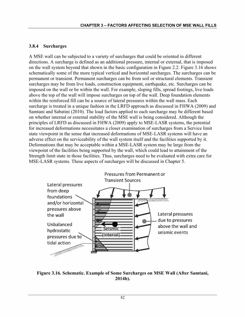
CHAPTER 3 – FACTORS AFFECTING SELECTION OF MSE WALL FILLS
82
3.8.4 Surcharges
A MSE wall can be subjected to a variety of surcharges that could be oriented in different directions. A surcharge is defined as an additional pressure, internal or external, that is imposed on the wall system beyond that shown in the basic configuration in Figure 2.2. Figure 3.16 shows schematically some of the more typical vertical and horizontal surcharges. The surcharges can be permanent or transient. Permanent surcharges can be from soil or structural elements. Transient surcharges may be from live loads, construction equipment, earthquake, etc. Surcharges can be imposed on the wall or be within the wall. For example, sloping fills, spread footings, live loads above the top of the wall will impose surcharges on top of the wall. Deep foundation elements within the reinforced fill can be a source of lateral pressures within the wall mass. Each surcharge is treated in a unique fashion in the LRFD approach as discussed in FHWA (2009) and Samtani and Sabatini (2010). The load factors applied to each surcharge may be different based on whether internal or external stability of the MSE wall is being considered. Although the principles of LRFD as discussed in FHWA (2009) apply to MSE-LASR systems, the potential for increased deformations necessitates a closer examination of surcharges from a Service limit state viewpoint in the sense that increased deformations of MSE-LASR systems will have an adverse effect on the serviceability of the wall system itself and the facilities supported by it. Deformations that may be acceptable within a MSE-LASR system may be large from the viewpoint of the facilities being supported by the wall, which could lead to attainment of the Strength limit state in those facilities. Thus, surcharges need to be evaluated with extra care for MSE-LASR systems. These aspects of surcharges will be discussed in Chapter 5.
Figure 3.16. Schematic. Example of Some Surcharges on MSE Wall (After Samtani, 2014b).

CHAPTER 3 – FACTORS AFFECTING SELECTION OF MSE WALL FILLS
83
3.9 CONSTRUCTABILITY
The design of any facility must consider the possible construction procedures that may be used by the contractor. Although earthwork operations are the major component of the construction of a MSE wall, unlike earthwork operations in embankments there are additional features that need to be closely coordinated, e.g., facing and various zones of different materials such as reinforced fill and retained fill. Within the reinforced fill there are at least two distinct zones of compaction, one within the 3 feet behind the wall face where less compaction energy is used and the other extending to at least 1 foot behind the free end of the reinforcement where more compaction energy is used. The various levels of compaction effort are discussed in Section 2.1.1.1, which provides information included in FHWA (2009). The compaction criteria noted in Section 2.1.1.1, Section 3.4, and Appendix F, which are based on the concept of relative compaction (RC) will be referred to as the RC control method. Even with the use of select fill, it is a well-known fact in the MSE wall industry that the horizontal and vertical alignment of the wall face is affected by the compaction characteristics of the project-specific soil that is approved as select fill. The facing alignment tolerances noted in FHWA (2009) are indexed to the use of select fill. For MSE-LASR walls, which may be constructed with a variety of soils that will likely have larger amount of fines, conformance to the facing alignment tolerances may be difficult if the compaction characteristics of the soils are not correctly evaluated and controlled during construction. This factor is probably the single most important consideration for constructability of MSE-LASR systems. This section discusses the issues that may be encountered during compaction during construction of MSE-LASR systems.
3.9.1 Compaction Effort for MSE-LASR Systems
The principles of compaction and common methods to control compaction in the field are discussed in Appendix F. The principal objectives in compacting soil are normally to create a fill of high strength and low compressibility, and, in the case of water-retaining fills, of low permeability. It is also desirable that the fill will not significantly soften with time as a result of exposure to rainfall or infiltration. As noted in Section 3.4, in contrast to select fills where the RC compaction control method has been successfully used, LASR materials could include a wide range of geomaterials that may have non-uniform invariant index properties. Therefore, the compaction characteristics and resulting engineering properties, such as shear strength and volume change, may be variable within MSE-LASR wall fills. Consequently, more stringent and/or alternative compaction control procedures may be required for MSE wall fills constructed with LASR materials. For the designer and owner considering a MSE-LASR system, the first item to acknowledge and fully comprehend is the fact that there are two major categories of landforms. As discussed in Appendix E, these are transported (sedimentary) landforms and residual landforms. Wesley (2010a) states that, “at least half of the earth’s surface is covered by residual soils, and in today’s world the most rapid growth and development is occurring in countries that contain a very high proportion of these soils.” As shown in Figure E.2 in Appendix E, residual soils cover significant portions of the United States. For example, the Piedmont province in eastern United

CHAPTER 3 – FACTORS AFFECTING SELECTION OF MSE WALL FILLS
84
States consists locally of thick residual soils developed from many different kinds of igneous and metamorphic rocks (FHWA, 1976). The Piedmont is a plateau region located in the eastern United States between the Atlantic Coastal Plain and the main Appalachian Mountains, stretching from New Jersey in the north to central Alabama in the south. The Piedmont's area is approximately 80,000 square miles. Some of the more densely populated areas in the eastern United States, are located within the Piedmont province. Residual soils are prevalent in geographical regions with volcanic activity, mesas, plateaus, and plains. Depending on the parent rock type and the stage of weathering, the residual soils contain a variety of mineral types. Mitchell and Soga (2005) note that allophane is clay mineral often associated with residual soils and is found in Pacific areas of the United States. Hawaii is another geographical region where the soils are of volcanic origin. The tropical weathering of volcanic ash and rock leads to formation of allophane and halloysite. Smectites (montmorillonites) may also form in the early stages of weathering of volcanic materials. Ultimately, kaolinite and gibbsite may form. The position of some of these various clay minerals on the plasticity chart is shown in Figure 3.6 and a discussion on the effect of mineralogy is in Section 3.2. Further discussion on residual soils can be found in Appendix E, Terzaghi et al. (1996), Mitchell and Soga (2005) and Wesley (2010b). The point to be recognized is that the soils from transported or residual landforms may have the same soil group classification based on USCS or AASHTO, e.g., SW, A-1-a, etc., but their compaction and performance characteristics (e.g., shear strength and volume change) may be very different. Even within a given landform, the type of the mineral may be a function of the stage of weathering as noted above for the case of residual soils. This variability is a critically important aspect to evaluate for the appropriate design and construction of a successful MSE-LASR system. This discussion re-emphasizes the need to follow all of the evaluation procedures for determination of soil characteristics for MSE-LASR systems as noted in Section 3.1, 3.2, and 3.3. Marinho et al. (2013) present the results of a study to determine the shear strength behavior of a compacted residual soil from São Paulo, Brazil. Several series of experiments were conducted under both saturated and unsaturated conditions. A total of 57 unconfined compression tests and 57 constant water content triaxial tests were conducted on specimens compacted at three different initial water content conditions to study the shear strength behavior. One of the key objectives of the study was to examine the influence of soil structure associated with different water contents and also the initial stress state on the shear strength. The matric suction in the soil specimens was precisely measured during the tests by using high capacity tensiometers. The experimental results suggest that the shear strength behavior is significantly influenced by the different initial compaction water contents. An empirical model is proposed in which the results of the study are used to estimate the three-dimensional failure envelope of the tested compacted residual soil for any condition of the initial stress state. Such a model may be useful for practicing engineers to estimate the shear strength behavior of residual soil for different loading and initial compaction water content conditions. Each site for MSE-LASR system application will be unique. Some sites or portions of sites may have essentially uniform fill material with consistent maximum dry density and optimum moisture content as determined by appropriate compaction tests. In such cases, use of the RC

CHAPTER 3 – FACTORS AFFECTING SELECTION OF MSE WALL FILLS
85
compaction control method as noted in Section 2.1.1.1 may be acceptable. However, there can be sites that may contain variable soils such that earth moving equipment may inadvertently or indiscriminately mix one type of soil with another resulting in soil mixtures for which compaction characteristics may be significantly different than those determined from the control tests run on specific portions of the site. Figure 3.17 shows an example of the order of variation that can be encountered at a given site. Note that the left figure shows soils that have varying specific gravities within the same site which emphasizes the earlier discussion in Section 3.1.1. The left figure is for a site where the soil consisted of relatively recent transported (sedimentary) soil of Pleistocene origin. The right figure is for a site where the soils were much older and had weathered from a range of volcanic deposits, including basaltic lava flows and ash layers. Both sites were relatively small, and the soil involved was of the same geologic origin. Despite this similarity, there is a large variation in the type of soil, as reflected in the compaction curves.
Figure 3.17. Graph. Illustration of Compaction Characteristics of Variable Fill Materials at a Given Site (After Pickens, 1980).
A further complication arising with some soils, particularly those of volcanic origin containing allophane, is that their compaction properties vary depending on the history of wetting and drying and any manipulation prior to final compaction (Pickens, 1980, Wesley, 2010b). The compaction curves for such soils do not show clear peaks of dry density and thus do not indicate optimum values of water content. One of the distinctive characteristics is the very flat nature of their compaction curves. Figure 3.18 shows typical results of compaction tests on two samples of allophane clay. As can be seen the compaction characteristics are a function of how the tests were performed, i.e., natural, air dried, or oven dried, and the peaks were not well defined. For such soils, the concept of relative compaction discussed in Section 3.4 and Appendix F has little meaning unless the laboratory tests model the field sequence of water content adjustment and soil manipulation. Such modeling of field sequence can be counter-productive in the sense that mistakes can be made easily in the field by inspectors who may not fully comprehend the procedures for application of the laboratory test standards for variable fill soils.

CHAPTER 3 – FACTORS AFFECTING SELECTION OF MSE WALL FILLS
86
Figure 3.18. Graph. Standard Proctor Compaction Test Results on an Allophane Clay (After Wesley, 2010b).
Based on the above considerations, the field compaction control criteria for MSE-LASR system must be evaluated on a site-specific basis. Depending on the geologic source and the type of landform (transported versus residual) the conventional approach of relative compaction discussed in Sections 2.1.1.1 and 3.4 and Appendix F may not be appropriate. This issue is further compounded where the fill source is variable for which alternative specifications that reduce the problems of controlling variable fills are particularly valuable. Given that compaction is a critical component for the success of any MSE system whether MSE-LASR or not, it is important to explore and understand alternative compaction control methods. Two such methods (SAV and SAV&S) are discussed herein. Mokwa and Fridleifsson (2005, 2007) evaluate the soil air voids method as an alternate approach to the traditional Proctor method of field compaction control; this method is herein referred to as the SAV (soil air voids) method. This method, while being expeditious, has several limitations as discussed in Section 3.9.2.1. Another method that incorporates the measurement of shear strength of compacted soil with the determination of the soil air voids, as proposed by Pickens (1980) and Wesley (2010a, b), is discussed in Section 3.9.2.2. This method is herein referred to as the SAV&S (soil air voids and strength). Both of these methods are discussed below. Either one can be considered as an alternative specification method to the conventional RC compaction control method on a site-specific basis.

CHAPTER 3 – FACTORS AFFECTING SELECTION OF MSE WALL FILLS
87
3.9.2 Alternative Compaction Specifications
The SAV method was developed as part of a study by Mokwa and Fridleifsson (2005, 2007) at Montana State University of Montana sponsored by the Montana Department of Transportation (MDT). The SAV&S method was developed by Pickens (1980) in New Zealand. While the SAV method is based solely on air voids criterion, the SAV&S method considers the shear strength of the compacted soil in addition to the air voids criterion.
3.9.2.1 The SAV Method of Field Compaction Control
The SAV method can be traced back to the work by Allen (1942) and is based on the premise that the future performance of a compacted layer of soil can be evaluated by comparing the measured air voids with a predetermined limiting value. In theory, a field inspector can rapidly determine if a soil layer meets the specified compaction criterion without obtaining a soil sample for laboratory Proctor compaction testing. Figure 3.19 shows a typical case for application of this method. The SAV of a compacted layer is determined by measuring the compaction state of a soil layer in the field (dry unit weight, d, and water content, w) and examining the relative position of this data point with respect to the location of the zero air voids (ZAV) line and the SAV line on a plot of d and w as shown in Figure 3.19. Theoretically, the ZAV curve represents a boundary beyond which a data point should not occur.
Figure 3.19. Graph. Example of the 10% SAV Evaluation Method, Gs = 2.70 (After Mokwa and Fridleifsson, 2005, and Procedure MT 229 of MDT, 2013).
The horizontal and vertical axes of the plot shown in Figure 3.19 are the same as those of the conventional compaction curve shown in Figure F.2. The zero air voids (ZAV) curve shown in Figure 3.19 is identical to the 100% saturation curve shown in Figure F.2 or Figure F.3 in Appendix F. However, as demonstrated in Figure F.3 the 10% air voids line is not the same as 90% saturation curve. This difference, which is discussed in Appendix F, is extremely important
The percentage of air voids, Na, can be determined as follows where the various parameters are as defined in Section 3.1:
%1001
1 xwG
Nsw
da

CHAPTER 3 – FACTORS AFFECTING SELECTION OF MSE WALL FILLS
88
to understand because it can lead to significant errors if charts such as those shown in Figure 3.19 are indiscriminately used for field compaction control.
As shown in Figure 3.19, field compaction test results are plotted on a graph containing the ZAV and predetermined SAV lines. According to SAV method, the field compaction test is considered to be passing if the field compaction test results for d and w plot between the SAV and ZAV lines. A data point that plots below (i.e., to the left) of the SAV line indicates a failing test. As noted earlier, theoretically a point should not plot above (i.e., to the right) the ZAV line. However, given the uncertainty in the measurements of the basic (invariant) properties, there is a possibility that some data points may plot above the ZAV line (Schmertmann, 1989). When this occurs, it may be an indication of a mistake made with the application of this method, e.g., an operator error, a bad reading by a density gage, a bad gage, or that an incorrect value of specific gravity, Gs, was assumed. The importance of the correct determination of the site-specific value of Gs was discussed in Section 3.1.1. Procedure MT 229-04 of MDT (2013) provides charts for SAV ranging from 10% to 16% for Gs values ranging from 2.60 to 2.80. A typical chart from Procedure MT 299-04 is shown in Figure 3.20. Other charts for any value of SAV and Gs can be easily developed by using the equation shown in Figure 3.19.
Figure 3.20. Graph. Example Chart from Procedure MT 229-04 of MDT (2013) for 16% SAV based on Gs = 2.65.
CHAPTER 3 – FACTORS AFFECTING SELECTION OF MSE WALL FILLS
89
Procedure MT 229-04 cautions that the SAV method “usually applies to north central, eastern and southeastern areas of Montana but may apply to other areas of the state. It will be the responsibility of the District Materials Supervisor to monitor the applicability of this method” and “The zero-air voids method will usually apply to soils classified from A-4 to A-7.” Based on the information in Appendix A, soils in AASHTO soil groups A-4 to A-7 are primarily fine-grained soils with equivalent USCS soil groups of ML, MH, CL, CH, OL, and OH, all of which are in the realm of possible MSE-LASR materials. Furthermore, Procedure MT 229-04 states the following:
“In order for this method to be accurate, it is necessary to find the specific gravity for the soils proposed for use. The most logical time to determine the specific gravity is during the preconstruction soil survey. However, due to the excavation process, which may result in a mixture of various soil strata, it may become necessary to perform additional specific gravity tests once the project is under contract. The specific gravity of soils is determined in accordance with MT 220, (AASHTO Designation T 100). (An average specific gravity is determined for the soil samples secured within any individual project.)”
The note about the importance of specific gravity re-emphasizes the discussion in Section 3.1.1. Mokwa and Fridleifsson (2005, 2007) indicate that a premise of the SAV method is that the specific gravity for a project will vary less than the maximum dry density, if the soils along a given project alignment are derived from the same geologic source and evaluate this premise as shown in Figure 3.21. Based on the discussion in Section 3.1.1 and the formula shown in Figure 3.19, it is clear that the SAV is a direct function of the specific gravity, Gs. Figure 3.21a contains a hypothetical graph in which the zero air voids and 10% SAV lines are plotted for two values of Gs, 2.6 and 2.7. This diagram illustrates that the dry unit weight will change by about 3 pcf for a change of 0.1 in specific gravity. For a variation in Gs of 0.06, the change in dry density would be less than 2 pcf.

CHAPTER 3 – FACTORS AFFECTING SELECTION OF MSE WALL FILLS
90
Figure 3.21. Graph. Evaluation of Sensitivity of SAV Method to Variation in Specific Gravity (After Jones, 1973 and Mokwa and Fridleifsson, 2005).
Another approach for examining the sensitivity of Na to changes in Gs is shown in Figure 3.21b, in which the variation of Na is computed over a range of Gs values for three sets of dry densities and water contents. The slopes of the lines shown in this plot represent the sensitivity of Na to changes in Gs; or, in equation form, slope = Na/Gs as shown in the figure. Any combination of d and w will result in a different value of Na and thus a different value of the slope. There are many possible values of d and w. Mokwa and Fridleifsson (2005) selected the three sets of the values of d and w shown in Figure 3.21b as being representative of the typical range of compaction data that could be encountered for a subgrade or fill soil. The computed slopes from these three sets of compaction parameters range from 17.9 to 29.2. The slopes of lines drawn in this plot can be used to examine the sensitivity of Na to errors or deviations in the measured value of Gs. For example, the largest value of slope, 29.2, corresponds to the compaction parameters d
= 130 pcf and w = 6%. For this set of parameters, a change in Gs of 0.06 will result in a change to Na of 1.75%. Using the smallest value of slope, 17.9, which corresponds to the compaction parameters d = 105 pcf and w = 16%, results in a change of Na of only 1.1% for a 0.06 change in

CHAPTER 3 – FACTORS AFFECTING SELECTION OF MSE WALL FILLS
91
Gs. This evaluation validates the observation by Lewis (1954), who suggested that an error of ±0.05 in Gs would result in an error of only ±1 to 1.5% in the calculation of air voids. Mokwa and Fridleifsson (2005) discuss the limitations of the SAV method. Three particular limitations are demonstrated by use of Figure 3.22a, 3.22b, and 3.22c and are discussed below: • Figure 3.22a: As shown in Table 3.4, depending on the soil type, the maximum dry density
always has a certain range, e.g., for Soil No. 6, which has a USCS designation of SP, the range of maximum dry density (MDD or dmax) is 1102 pcf and the optimum moisture content (wopt) is 12.41 percent. High-plasticity soils such as those in the AASHTO A-7 or USCS CH soil groups are sensitive to small changes in water content. Figure 3.22a shows results of laboratory compaction tests for AASHTO A-7-6(20) soil from an MDT project. Clearly, there is a large scatter of the results and selection of accurate combination of dmax and wopt to develop appropriate field control criteria is difficult unless numerous (say 8 to 10) compaction points are generated at closely spaced intervals of water content. In such cases, (a) it is important to allow sufficient soak time for these samples to absorb added water prior to testing, and (b) controlling the compaction water content in the field is more critical than obtaining a specific dry density of SAV content. Therefore, the SAV method is not recommended for these soils because of lack of control on water content.
• Figure 3.22b: For most soils, the 10% SAV lines will likely cross the compaction curve on
the dry (or left) side of the optimum moisture content as shown in Figure 3.22b; in this figure the data are based on compaction tests on an AASHTO A-7-5(10) soil. In such cases, a field-measured data point that plots in the “acceptable region” would be evaluated as a passing test for both the SAV method as well as the RC compaction control method noted in Section 2.1.1.1, Section 3.4, and Appendix F. Such a situation can be considered to be an ideal scenario in regard to achieving the desired density and SAV content. However, it is possible to reduce the soil air voids to relatively low values simply by increasing the soil water content (Parsons 1992, Johnson and Sallberg 1960, Lewis 1954). The cross-hatched zone in Figure 3.22b identified as the “problematic region” exemplifies this primary shortcoming in the SAV method. A field-measured data point that plots in the problematic region would indicate the material is poorly compacted and excessively wet. Obviously, this would be an unfavorable condition for a subgrade or fill. The field test would clearly fail if the Proctor relative compaction (RC) test was used to evaluate the material; however, a passing result would be obtained if the air voids criterion was used. Therefore, the applicability of the SAV method should be carefully evaluated in such cases.

CHAPTER 3 – FACTORS AFFECTING SELECTION OF MSE WALL FILLS
92
Figure 3.22. Graph. Scenarios Illustrating Possible Limitations of SAV Method (After Mokwa and Fridleifsson, 2005).
• Figure 3.22c: Another potential problem with the relationship between the compaction curve and the air voids line is illustrated in Figure 3.22c; in this figure the data are based on compaction test on an AASHTO A-7-5(10) soil. The typical acceptable region based on Proctor criteria is shown in the figure. For this material, which was compacted using a higher energy for this example (modified Proctor), the entire acceptable Proctor region is located on the left side of the 10% air voids line. In this case, there is a definite discontinuity between the air voids and Proctor methods. A sample that passed the air voids test would contain excessive water based on the conventional Proctor approach. This is an example of a material that would not be suitable for the 10% SAV method because of the potential for problems if the soil is compacted at an excessively high water content. The example demonstrates the limitation of the SAV method. The soil in this example would experience a decrease in bearing resistance, increase in the potential for excessive settlement and shrink/swell and stability problems because of large excess pore water pressures. This issue can only be handled in a controlled manner by placing an upper allowable limit on the compaction water
(a) (b)
(c)

CHAPTER 3 – FACTORS AFFECTING SELECTION OF MSE WALL FILLS
93
content. For these types of soils, reliance upon inherent controls of moisture during construction is too subjective of an approach on MSE-LASR projects or large earthwork projects, particularly if the designer, owner, and inspector are not highly trained and experienced in handling such nuances and anticipating such situations in design and specifications before construction starts.
In summary, the primary advantages of the SAV method for evaluating field compaction are simplicity, economy, and efficiency, which can be attractive qualities for busy, congested, and earthwork projects involving accelerated delivery. However, in addition to the potential problem related to a difference in basic definitions described previously, the SAV method also has the following limitations as described by Mokwa and Fridleifsson (2005, 2007): 1. Air voids can be reduced by simply increasing the water content for most soils. This is
obviously counter-productive from the viewpoint of performance characteristics such as shear strength and volume change properties. Inherent field water content limitations may be effective for many soil types, but such an approach is subjective and requires specific enforcement language in the earthwork specifications to minimize potential conflicts in the field. If the SAV method is used, it is suggested that provisions be provided in the specifications for the inspector to order a Proctor compaction test on any questionable material (e.g., excessively wet or pumping soils) and to use these results to make a proper assessment of the situation.
2. Some materials may pass the SAV test but fail the conventional Proctor compaction test
criteria. These soils can be identified in the laboratory if Proctor compaction and specific gravity tests are conducted and analyzed as discussed herein.
3. The SAV method should not be used on poorly graded granular soils (USCS soil groups of
SP and GP) because these soils contain large void spaces and, consequently, they may not provide consistent results using the SAV method.
4. Incorrect conclusions could be made in the field if the in-place specific gravity is
substantially different than the specific gravity used to develop the air voids line.
5. Not all materials can readily be compacted to 10% or less air voids.
6. A limiting range of acceptable compaction water contents should be specified if the SAV method is to be used for construction control.
7. Plastic clayey soils require tight controls on compaction moisture content to minimize future
problems with settlement, shrinkage upon drying, and swell during periods of hydration. The SAV method of compaction control is not suitable for these soil types (USCS classification CH and MH).

CHAPTER 3 – FACTORS AFFECTING SELECTION OF MSE WALL FILLS
94
8. Silty soil and soil with high contents of fine sand can be frost susceptible. The potential for frost heave and thaw weakening problems is greatly increased if these soils are not adequately compacted. High compaction water contents and low densities (as could theoretically be achieved with improper use of the SAV method) should be avoided when working with frost susceptible soils, which generally fall in the USCS classification of ML or SM.
Based on the above discussions, the SAV method is most suitable for the following circumstances (Mokwa and Fridleifsson, 2007): 1. Projects in which the material types and Proctor densities change considerably or
unpredictably, but the specific gravity values are relatively stable. This might be the case if the geomaterials used on the project are obtained from a variety of excavation cuts or borrow areas, but overall, the materials originated from the same geologic source.
2. Projects in which there is not sufficient time available to perform a Proctor laboratory compaction test to verify the Proctor maximum dry density at every corresponding field location.
3. Any project in which alternative compaction control method is desired for quality control or
quality assurance purposes. For the right project conditions determined during the investigation and design phase of the project the SAV method may have merit. If determined to be usable, the frequency of the testing depends on project-specific conditions, including number of material sources, variability of geomaterial properties, earthwork quantities, and relative importance or complexity of the project. In any case, for the successful application of the SAV method, specific gravity tests must be conducted at the same frequency as the Proctor compaction tests during the design stage of the project. The contract earthwork specifications should also provide a means for controlling and monitoring the compaction water content.
3.9.2.2 The SAV&S Method of Field Compaction Control
Many of the limitations of the SAV method can be traced back to the use of only one discriminating parameter for compaction control, that being the soil’s percentage of air voids. Although the computation for soil’s percent air voids by use of the equation in Figure 3.19 includes both d and w, only the SAV line is used to evaluate the field compaction control. Consideration of the density of packing of the soil particles and the actual compacted strength of the soil can result in a better field compaction control method. Specifications in terms of the soil’s percent air voids and shear strength do exactly that and can thereby cope satisfactorily with variable soils ranging from clays to sands without involving extensive reference testing (Pickens, 1980, Wesley, 2010a, b). Vane shear testing is a simple and convenient way to determine the shear strength for materials that behave as clays after compaction and cone penetrometer testing is suitable for such determinations for sandy fills. The method that uses both the soil’s percent air

CHAPTER 3 – FACTORS AFFECTING SELECTION OF MSE WALL FILLS
95
voids and shear strength is referred to here as the SAV&S Method. The following description of this method is based on Wesley (2010a) and Pickens (1980). In the SAV&S method the undrained shear strength of compacted cohesive soils is used. Figure 3.23 illustrates the basis for using the undrained shear strength. The figure shows the results of a standard Proctor compaction test on clay. During the test measurements of undrained shear strength were made in addition to dry density and water content. The measurements were made by performing both hand vane shear and unconfined compressive tests on samples of the compacted soil. As expected, the two strength measurements gave significantly different results. From Figure 3.23 it is seen that at optimum water content the undrained shear strength is about 150 kPa (≈ 3,100 psf) from the unconfined tests and about 230 kPa (≈ 4,800 psf) from the vane shear tests. The conventional RC compaction control method may allow for water contents 2 to 3 percent greater than optimum, in which case the comparable shear strength values would be about 120 kPa (≈ 2,500 psf) and 180 kPa (≈ 3,750 psf). Thus, to obtain a fill with properties comparable to those obtained by the conventional RC control method, specifying a minimum undrained shear strength in the range of 150 to 200 kPa (≈ 3,100 to 4,150 psf) would be appropriate. Such a specification would put an upper limit on the water content at which the soil could be compacted. Since the undrained shear strength steadily increases with decreasing water content, the required shear strength could be achieved by compacting the soil in a very dry state, which would be generally undesirable, since dry fills may soften and swell excessively when exposed to moisture. To prevent the soil’s being too dry, a second parameter is specified, namely the percent soil air voids (SAV).
Figure 3.23. Graph. Standard Proctor Compaction Test on Clay Including Measurements of Undrained Shear Strength (After Wesley, 2010a).
In general, at optimum water content the soil air voids are about 5 percent. If the soil is compacted 2 to 3 percent drier than the optimum moisture content corresponding to the compaction effort being used, the soil air voids may be as much as 8 to 10 percent. Thus, to

CHAPTER 3 – FACTORS AFFECTING SELECTION OF MSE WALL FILLS
96
prevent the soil from being compacted too dry an upper limit is placed on the percent soil air voids, normally in the range of 8 to 10 percent. Figure 3.24 illustrates how the SAV&S Method of controlling compaction relates to the conventional RC control method. The zero air-voids (ZAV) line is always the upper limit of the dry density for any water content regardless of the compaction control method (RC, SAV or SAV&S). The conventional RC method involves an upper and lower limit on water content and a lower limit on the dry density and thus encloses the shaded area shown in Figure 3.24. The SAV method is based on the predetermined limiting percent air voids line only as discussed in Section 3.9.2.1. The SAV&S method involves an upper limit on water content corresponding to a predetermined shear strength limit and the predetermined SAV line. Thus, as shown in Figure 3.24, the SAV&S Method encloses the area defined by the ZAV line, the vertical line corresponding to the water content limit from the minimum shear strength criterion, and the SAV line. There is no specific lower limit on water content, but the SAV line prevents the soil from being too dry. Just as with the SAV method of compaction control, the SAV&S method does not actually require compaction tests at all. However, it is still useful to perform the compaction tests to determine the degree of drying or wetting needed to bring the soil to a state appropriate for compaction.
Figure 3.24. Schematic. Compaction Control Using SAV&S Method (After Wesley, 2010a, Pickens, 1980).
Figure 3.25 shows a typical compaction control chart based on the SAV&S method. As shown in Figure 3.25, field compaction test and shear strength results are plotted on a graph containing the ZAV and predetermined SAV and shear strength lines. According to the method, the field compaction test is considered to be passing if the field compaction test (d and w) plots between the SAV and ZAV lines and the field shear strength plots above the shear strength limit. Hypothetical examples of tests at two locations, A and B are shown. At each location, a pair of data points is obtained based on measured water content, dry density, and shear strength. Based on the location of the data points with respect to the SAV line and the minimum shear strength

CHAPTER 3 – FACTORS AFFECTING SELECTION OF MSE WALL FILLS
97
line an evaluation is made whether or not the location tested is acceptable or not. For a location to be acceptable, both the data points must pass the acceptance criteria. Based on the hypothetical examples, location A is acceptable while location B is not acceptable. At location B, the data point Bwd based on measured water content and dry density is acceptable while the data point Bws based on measured water content and shear strength is not acceptable. Since one of the two data points at location B is not acceptable, location B is not considered to be acceptable and the contractor must implement remedial measures, e.g., recompaction, additional compaction effort, etc., after an assessment of the possibilities that might have led to the unacceptable test. In this context, as noted earlier, a data point based on measured dry unit weight, d, and water content, w, should not plot above (i.e., to the right) the ZAV line. When this occurs, it may be an indication of a mistake made with the application of this method, e.g., an operator error, a bad reading by a density gage, a bad gage, or that an incorrect value of specific gravity, Gs, was assumed. The importance of correctly determining the value of Gs was discussed in Section 3.1.1.
Figure 3.25. Schematic. Compaction Control Chart Using SAV&S Method.
Point Data Based on Field Measurement Pass/Fail Awd Water content and dry density at test location A Pass based on SAV and ZAV Aws Water content and shear strength at test location A Pass based on MSS Bwd Water content and dry density at test location B Pass based on SAV and ZAV Bws Water content and shear strength at test location B Fail based on MSS

CHAPTER 3 – FACTORS AFFECTING SELECTION OF MSE WALL FILLS
98
Based on experience with many projects in New Zealand, Pickens (1980) and Wesley (2010a, b) suggest the following limits for the two control parameters for the SAV&S method: • Undrained shear strength based on hand vane shear tests: > 150 kPa (≈ 3,100 psf) based on
an average of 10 tests with no value being less than 120 kPa (≈ 2,500 psf) • Maximum soil air-voids (SAV): 8 percent. The SAV&S criteria can be adjusted to meet the needs of a given project, e.g., for volcanic ash containing allophane clays the maximum SAV of 12 percent is suggested by Wesley (2006). The hand-held vane shear testing device as per ASTM D2573 is recommended because tests performed with this device are simpler than the unconfined compression tests and more expeditious in the field. As noted in Section 3.9.2.1, conventional nuclear gage equipment is the most expeditious way to determine the dry density and water content in the field as they would normally be done in a conventional RC control method. These measurements could then be used in the equation shown in Figure 3.19 to calculate the percent air voids in the field. In summary, the advantages of the SAV&S method for cohesive soils are as follows (Wesley, 2010a, b): 1. The method is ideally suited for compacted fills with large variations in soil properties
because the same specification limits apply regardless of the variations. 2. Field control is more direct as the value of the undrained shear strength is known as soon as
the measurements are made. 3. The specification is easily varied to produce fills with particular properties needed in special
situations.
3.9.2.3 Compaction of Granular and Nonplastic Soils
The SAV&S method described above is useful as an alternative compaction control method for cohesive soils that exhibit plasticity. For granular and nonplastic soils the conventional RC control method can be used. However, for uniform granular soils, the use of the Proctor test itself may be misleading. Consider the case of concrete sand that has the gradation shown in Figure 3.26a. In this case, almost all particle sizes are within the sand range of particle sizes, i.e., between No.4 and No. 200 sieves. This gradation is within the upper and lower limits shown in Figure 3.1 with a uniformity coefficient of approximately 6. Thus, the gradation meets the requirements of select fill in Table 2.1. Figure 3.26b shows the compaction curves for this material. The conventional RC control method for such soils is risky because the results from standard or modified Proctor compaction tests do not provide the characteristic “parabolic” shape shown in Figure F.2 in Appendix F that allows for determining the maximum dry density and the optimum water content. Instead, as shown in Figure 3.26b, the compaction curves are relatively flat with poorly defined peaks that may be due more to “bulking action” than a truly dense state for the soil (Drnevich et al., 2007).

CHAPTER 3 – FACTORS AFFECTING SELECTION OF MSE WALL FILLS
99
Figure 3.26. Graph. (a) Gradation of Concrete Sand (b) Compaction Results for Concrete Sand (After Drnevich et al., 2007).
Based on a study performed for the Indiana Department of Transportation (INDOT), Drnevich et al. (2007) recommend that instead of the Proctor tests, the Vibrating Hammer (VH) test method of compaction (ASTM D7382) be considered as an alternative method for specifying maximum dry unit weights for granular soils. The VH test also establishes a water content range for field compaction. Drnevich et al. (2007) indicate that the VH test is also sufficient for use for fills
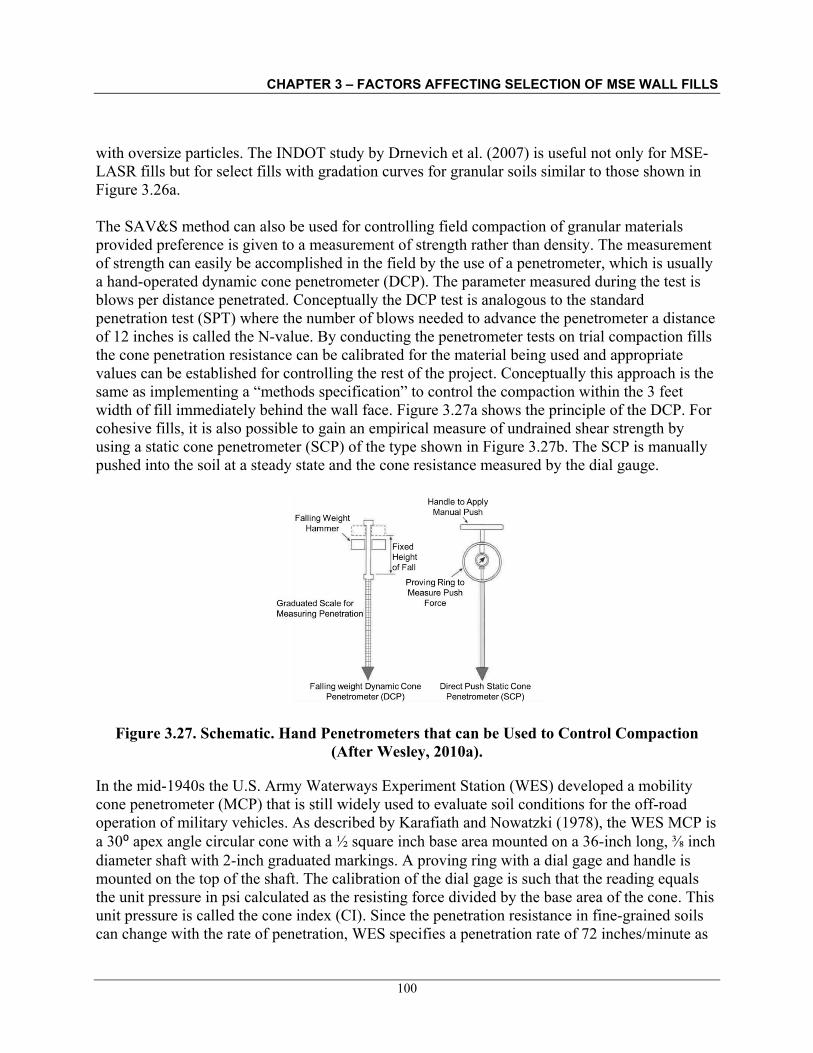
CHAPTER 3 – FACTORS AFFECTING SELECTION OF MSE WALL FILLS
100
with oversize particles. The INDOT study by Drnevich et al. (2007) is useful not only for MSE-LASR fills but for select fills with gradation curves for granular soils similar to those shown in Figure 3.26a. The SAV&S method can also be used for controlling field compaction of granular materials provided preference is given to a measurement of strength rather than density. The measurement of strength can easily be accomplished in the field by the use of a penetrometer, which is usually a hand-operated dynamic cone penetrometer (DCP). The parameter measured during the test is blows per distance penetrated. Conceptually the DCP test is analogous to the standard penetration test (SPT) where the number of blows needed to advance the penetrometer a distance of 12 inches is called the N-value. By conducting the penetrometer tests on trial compaction fills the cone penetration resistance can be calibrated for the material being used and appropriate values can be established for controlling the rest of the project. Conceptually this approach is the same as implementing a “methods specification” to control the compaction within the 3 feet width of fill immediately behind the wall face. Figure 3.27a shows the principle of the DCP. For cohesive fills, it is also possible to gain an empirical measure of undrained shear strength by using a static cone penetrometer (SCP) of the type shown in Figure 3.27b. The SCP is manually pushed into the soil at a steady state and the cone resistance measured by the dial gauge.
Figure 3.27. Schematic. Hand Penetrometers that can be Used to Control Compaction (After Wesley, 2010a).
In the mid-1940s the U.S. Army Waterways Experiment Station (WES) developed a mobility cone penetrometer (MCP) that is still widely used to evaluate soil conditions for the off-road operation of military vehicles. As described by Karafiath and Nowatzki (1978), the WES MCP is a 30⁰ apex angle circular cone with a ½ square inch base area mounted on a 36-inch long, ⅜ inch diameter shaft with 2-inch graduated markings. A proving ring with a dial gage and handle is mounted on the top of the shaft. The calibration of the dial gage is such that the reading equals the unit pressure in psi calculated as the resisting force divided by the base area of the cone. This unit pressure is called the cone index (CI). Since the penetration resistance in fine-grained soils can change with the rate of penetration, WES specifies a penetration rate of 72 inches/minute as

CHAPTER 3 – FACTORS AFFECTING SELECTION OF MSE WALL FILLS
101
the standard rate for vehicle mobility evaluations. In frictional soils the rate of increase of cone penetration resistance with depth is called the cone index gradient (CGR). The CGR is a measure of soil density. Karafiath and Nowatzki (1978) present empirical relationships between CI and cohesion and friction angle for cohesive soils and between CGR and relative density and internal friction angle for non-cohesive soils. The reported correlations are approximately valid for other types of soils that are either purely cohesive or purely frictional. An excellent review of the methods of analysis of cone penetration resistance is presented by Yu and Mitchell (1998). It is clear from the works cited here that a “methods specification” is best suited for the control of compaction of granular and nonplastic soils in the field if the DCP, SCP or MCP test is to be used.
3.9.2.4 Choice of Compaction Control Method for MSE-LASR Systems
Perhaps the biggest takeaway from the above discussions is that there is no perfect compaction control method. The conventional RC control method has been used routinely in earthwork specifications and agencies have trained their inspectors based on this method. Use of select fill masks most of the deficiencies related to the RC procedures. The deficiencies of the RC control method can lead to significant problems for cohesive soils with high plasticity as well as uniform granular soils. The MSE-LASR systems will likely have cohesive soils based on the allowance of large percentage of fines which may be plastic or more uniform granular soils having Cu less than 4. The use of alternative compaction control methods such as SAV and SAV&S should be proactively considered for MSE-LASR systems. The SAV&S method includes the SAV method as a subset and therefore could be considered to be the better method of the two. However, some agencies such as MDT have successfully used the SAV method and preference can be given to continued use of such methods where they have a good track record. Regardless of the choice of method, it is clear from the foregoing discussions, that it is critically important to perform specific gravity tests in addition to the Proctor tests for every type of LASR fill source anticipated to be used. The compaction characteristics of the soils will vary based on whether the soils are transported (sedimentary) or residual. In this regard, the AASHTO and USCS soil groups are of little relevance and consideration of the local geomorphology becomes crucial in the selection of the appropriate compaction control process. Finally, a qualified and experienced local geotechnical engineer should be consulted to discuss local compaction experiences and the designer of the MSE-LASR system should ensure that the field personnel are properly trained and adept at adjusting to the needs of the project on a site-specific basis.
3.9.3 Zoning of Materials
In a MSE wall there are different zones of materials to control drainage and deformation of the wall (refer to Figure 2.1). For example, to control the distortion of the wall facing units, the fill within the 3 feet immediately behind the wall face is compacted by using less energy compared to the balance of the reinforced fill zone. In certain wall systems, such as modular block walls, this zone also contains gravel fills as a compaction aid and since they are more permeable materials, they tend to also facilitate drainage near the wall face. A similar permeable zone is
CHAPTER 3 – FACTORS AFFECTING SELECTION OF MSE WALL FILLS
102
also provided between the reinforced and retained fill or at the back of the retained fill zone to intercept groundwater if present. The retained fill behind the reinforced fill is often of less quality compared to the fill in the reinforced zone. In the case of a MSE-LASR system it is likely that the soils within the reinforced fill and the retained fill zones will be the same but compacted to different standards. For example, the retained fill will be compacted by using larger energy so that the stiffness of the retained fill zone approximates that of the reinforced fill zone, thereby mitigating differential settlement between the reinforced and retained fill zones. The constructability of the various zones will involve proper evaluation of the compaction characteristics of the soils in those zones. Evaluation of the compaction characteristics is of particular importance in the context of internal and external drainage of the wall system. All the discussions in Section 3.9.2 about compaction control procedures are equally applicable to the various zones of the materials within the MSE walls, particularly for those designed for and constructed with LASR materials. Different compaction control procedures will likely be required in different zones. For example, the RC procedure may be more applicable to the permeable fill materials provided to promote internal and external drainage while alternative compaction control procedures such as SAV or SAV&S may be more appropriate for reinforced and retained fill materials depending on the amount of fines and plasticity.
3.10 DESIGN METHODS
The two primary design methods for MSE walls are the Allowable Stress Design (ASD) and the Load and Resistance Factor Design (LRFD). FHWA (2001) and AASHTO (2002) present design guidelines for MSE walls based on the ASD method while FHWA (2009) and AASHTO (2020) present design guidelines for MSE walls based on the LRFD method. Samtani and Sabatini (2010) and Samtani (2014b) provide in-depth discussion and guidance on the use of the LRFD method for MSE walls that is presented in FHWA (2009) and AASHTO (2020). The procedure for design of MSE walls by using LRFD methodology is very similar to that of using ASD methodology. Recognizing the history of successful designs of MSE walls based on the ASD method, the LRFD method for MSE walls has been calibrated to provide virtually the same results as those based on the ASD method. However, by separating the uncertainty in loads and resistances through the use of load factors and resistance factors, respectively, the LRFD method offers an opportunity to address the geotechnical resistances separately for each external and internal limit state that is identified in Section 3.10.1. This feature of the LRFD method can be significant for the design of MSE-LASR systems because each project where a MSE-LASR system is contemplated can be conceivably tailored to fit the properties of the LASR materials. Chapter 5 provides a framework for the design of MSE-LASR systems based on the LRFD method.
3.10.1 LRFD Limit States and Stability Modes for MSE Walls
AASHTO (2020) defines a limit state as, “A condition beyond which the bridge or component ceases to satisfy the provisions for which it was designed.” In the AASHTO-LRFD framework,
CHAPTER 3 – FACTORS AFFECTING SELECTION OF MSE WALL FILLS
103
there are four distinct limit states: (1) strength (or ultimate) limit states; (2) service limit states; (3) extreme event limit states; and (4) fatigue limit states. The design of a wall or wall component is usually governed by either the strength or the service limit state and then checked for extreme event limit states. Fatigue limit states are generally not applicable for walls and will not be discussed here. The Strength, Service, and Extreme Event limit states are briefly described below (Samtani and Sabatini, 2010):
• Strength (or ultimate) limit states pertain to structural safety and the loss of load-carrying capability. Strength limit states may be reached through either geotechnical or structural failure. Evaluation of Strength limit states is based on inelastic behavior of the structure, which is accomplished by using increased or factored loads, and on modification of soil behavior, which is accomplished by using reduced or factored strengths. From a geotechnical viewpoint, Strength limit states are reached when they involve the partial or total collapse of the structure by sliding, bearing failure, etc. For well-designed structures, Strength limit states have a very small probability of failure.
• Service limit states are the limiting conditions affecting the function of the structure under expected service conditions. Thus, Service limit states address serviceability and include conditions short of the complete loss of load-carrying capability that may restrict the intended use of the structure, e.g., excessive total or differential settlements, cracking, local damage, poor ride quality, etc. Evaluation of Service limit states is usually performed by using expected service loads, nominal strengths, and elastic analyses. Compared to Strength limit states, the Service limit states have a greater probability of failure, but, if exceeded, involve less significant consequences. Serviceability of MSE walls has not been explicitly quantified for MSE walls with select fills because the select fills have historically provided satisfactory performance with respect to deformations. However, for MSE-LASR systems the issue of serviceability must be explicitly assessed and quantified.
• An Extreme Event is considered to be an event whose return period exceeds the design life of the structure. Examples include earthquakes, scour at super flood events, ice loads, and vehicle or vessel collisions. Once a wall has been designed based on Strength and Service limit states, it is then examined for its adequacy to withstand Extreme Events with the expectation to preserve life and not necessarily the serviceability of the structure. Based on these considerations, an earth retaining structure whose design has considered all appropriate failure modes based on Strength limit states will likely be adequate when checked against an Extreme Event limit state, except perhaps high seismic zones.
Design of a MSE wall (or any earth retaining structure) must provide adequate resistance against geotechnical and structural limit states. The limit states and stability modes for MSE walls are shown in Table 3.5. During the design process, all applicable limit states and load combinations within a limit state are analyzed. Usually, for a given structure, one stability mode within a limit state will control the design. Details of the design procedures based on LRFD methodology can be found in FHWA (2009). Chapter 5 provides a framework for the evaluation of the limit states noted in Table 3.5 for MSE-LASR systems.

CHAPTER 3 – FACTORS AFFECTING SELECTION OF MSE WALL FILLS
104
Table 3.5. Limit States and Stability Modes for MSE Wall Systems (After FHWA, 2009, Samtani and Sabatini, 2010, and Samtani, 2014b).
Limit State Stability Mode Strength and Extreme Event
A. External Stability 1. Limiting Eccentricity 2. Sliding 3. Bearing Resistance
B. Internal Stability 1. Geotechnical
a. Pullout Resistance of Reinforcement 2. Structural
a. Tensile resistance of reinforcement b. Structural resistance of face elements c. Structural resistance of face element connections
Service A. External Stability 1. Excessive vertical wall movement (settlement) 2. Excessive lateral wall movement (including rotation)
B. Component deterioration from corrosion and/or degradation C. Internal Deformations within Reinforced Soil
1. Excessive internal vertical deformation (Note 3) 2. Excessive internal horizontal deformation (Note 4)
Notes: 1. Global and compound stability are evaluated by using Strength limit state as per AASHTO (2020). 2. Fatigue limit states are not applicable to MSE walls. 3. Need to evaluate rigid versus flexible facing requirement, cushion thickness requirements between rigid
facings units, and downdrag on facing connections. 4. Need to evaluate bulging and face movement potential.
3.10.2 Resistance Factors
For the Strength and Extreme Event limit states in LRFD the goal is to have the factored resistance greater than the factored load. The term capacity to demand ratio, CDR, is used to quantify the ratio of the factored resistance to the factored load. Alternatively, the more appropriate term is resistance to load ratio, RLR, in which the factored values of load and resistance are used (Samtani, 2014b). Regardless of whether the term CDR or RLR is used the critical value of this ratio is 1.0. If CDR (or RLR) is greater than or equal to 1.0 then the limit state being evaluated is considered to be satisfied. In case of a value less than 1.0, appropriate changes must be made, and the design procedure repeated until a value 1.0 is achieved. The resistance factors that are used as part of the CDR (or RLR) evaluation are summarized in Tables 3.6 and 3.7. Chapter 5 provides a framework for the use of the resistance factors noted in Figure 3.26 for MSE-LASR systems.

CHAPTER 3 – FACTORS AFFECTING SELECTION OF MSE WALL FILLS
105
Table 3.6. Resistance Factors or Criteria for External Stability Limit States Based on AASHTO (2020)
Limit State Resistance Factor or Criteria Bearing resistance [AASHTO Table 11.5.7-1] BR = 0.65 Sliding resistance [AASHTO Table 11.5.7-1] SR = 1.00 Limiting eccentricity, emax [AASHTO Article 11.6.3.3] L/3 (soils); 0.45L (rocks)
Table 3.7. Resistance Factors or Criteria for Internal Stability Limit States Table 11.5.7-1 and Article 11.5.8 of AASHTO (2020) and Simplified Method
Limit State Condition Resistance Factor Tensile resistance of steel strip reinforcement and connectors(1) Static loading 0.75
Combined state/earthquake loading 1.00
Tensile resistance of steel grid reinforcement and connectors(1,2)
Static loading 0.65 Combined state/earthquake loading 0.85
Tensile resistance of geosynthetic reinforcement and connectors
Static loading – Geotextiles and geogrids 0.80 Static loading – Geostrips 0.55 Combined static/earthquake loading 1.00
Pullout resistance of steel strip and steel grid reinforcements
Static loading 0.90 Combined state/earthquake loading 1.20
Pullout resistance of geotextiles, geogrids and geostrips reinforcements
Static loading 0.70
Combined state/earthquake loading 1.00 Notes:
(1) Apply to gross cross-section less sacrificial area. For sections with holes, reduced gross area in accordance with AASHTO Article 6.8.3 and apply to net section less sacrificial area.
(2) Applies to grid reinforcement connected to a rigid face element, e.g., concrete panel or block. For grid reinforcements connected to a flexible facing mat or which are continuous with the facing mat, use the resistance factor for strip reinforcements.
Table 3.8. Resistance Factors or Criteria for Overall and Compound Stability Limit States (After Article 11.6.3.7 of AASHTO, 2020)
Condition Resistance Factor Geotechnical parameters and subsurface stratigraphy are highly variable or based on limited information 0.65
Geotechnical parameters and subsurface stratigraphy are well defined 0.75

CHAPTER 3 – FACTORS AFFECTING SELECTION OF MSE WALL FILLS
106
3.11 MAINTENANCE
The performance of any MSE wall (or any wall) depends not only on proper design and construction, but also on proper maintenance by the owner of the wall. Regularly scheduled maintenance is necessary because a correctly designed and constructed wall may still experience distress from surcharge loads resulting from modifications of the surrounding grades and/or installation of adjacent structures, landscaping and vegetation, excavations, or underground utility lines. This section provides information for various elements that should be considered as part of proper maintenance of MSE walls, particularly MSE-LASR systems.
3.11.1 Periodic inspections
Periodically inspect walls for evidence of fill loss, loss of joint seals, or movement. Reseal joints, particularly those that may allow surface water to enter the wall fill. If evidence of fill loss is observed, backfill the affected area with compacted select fill if the area is accessible, or flowable fill if access is restricted. Water infiltration into voids in walls can cause excessive pressures within the wall and result in displaced wall facing units and wall failures. Treat voided areas when they are small and manageable since they will tend to increase in size with time.
3.11.2 Site Grading
It is quite common for fills to experience post-construction settlement. Often such settlement is associated with hydrocompaction resulting from moisture ingress into compacted fills. Moisture ingress is promoted by settlement behind the wall that creates low areas in which water ponds. If a low spot is neglected, water will collect at that spot following rainfall or sheetflow from adjacent facilities and infiltrate into the wall. Such moisture ingress will increase the total unit weight and reduce the shear strength of compacted soils. If the wall is not designed to account for excess pore water pressures a blow-out of a portion of the wall may occur. Preventing this problem is easy by scheduling periodic inspections such that the site grades are inspected prior to and after periods of heavy rainfall. If any low spots that promote adverse drainage are found, then they must be filled and graded immediately to restore favorable drainage profiles.
3.11.3 Drainage
Features that minimize water flow into a MSE wall and features that preserve MSE wall drainage should be maintained over the life of the structure. For example, cracks in pavements above MSE walls should be sealed. Differential settlements and pavement cracks around catch basins should be corrected to minimize potential inflow into the reinforced soil or retained soil mass. These maintenance items are for non-wall features and the wall designer may have little influence on these items. However, in interacting with designers of other project features, the need to maintain items that potentially could affect the performance of the wall should be discussed. One of the maintenance items that the wall designer has control over is the drain outlet(s). Screens should be installed and maintained on drainpipe outlets. Screening is used to prevent

CHAPTER 3 – FACTORS AFFECTING SELECTION OF MSE WALL FILLS
107
small animals from nesting in and clogging the pipe. Outlet screens and cleanouts to provide access to clogged drainage features should be detailed on the retaining wall construction drawings. Additional items should be detailed when outlets are located in a soil embankment beneath the MSE wall. Drains are not effective unless the outlets are maintained, i.e., not clogged. Outlets in soil embankments should drain onto a concrete apron (usually precast) and should be marked with a permanent metal fence post. The apron and post minimize the chance of the outlet being run over and crushed by mowers or covered in subsequent construction activities. The apron and post should be detailed on the wall construction drawings.
3.11.4 Vegetation and Landscaping
Once the wall construction is complete, the surface areas surrounding the wall that were disturbed during construction are typically finished with some type of landscaped treatment. This might include paving (hardscape), plantings, mulch, sod or seed for turf, or some other type of ground cover. Sometimes large shrubs and trees are planted. Irrigation systems are often located within a few feet of the wall face and within the reinforced fill zone. If the vegetated and irrigated areas are close to the wall face, then infiltrating water from leaking pipes may create serious problems as discussed in Section 3.8.2. Root growth from large shrubs and trees can create significant pressures on the wall face. These adverse situations can be easily avoided by addressing such issues during design. If such situations cannot be avoided then they must be accounted for in the design, e.g., large shrubs/trees may be planted in lined containers, the irrigation systems must have leak detection mechanisms, the main sprinkler trunk lines must not be placed next to the wall face, etc. In general, xeriscape should be considered if any vegetation must be used, including the use of native plants that require minimal to no irrigation.
3.11.5 Subsurface Drainage Additions
No subsurface drainage or below-grade water utilities should be allowed to be installed behind the retaining wall unless its design has been reviewed and approved by the wall engineer-of-record. All drainage behind the high side of the wall must be specified to be surface drainage only. All through-face and behind-wall drainage pipes should be sleeved to allow unobstructed maintenance for these pipes. If at all possible, passage of utilities of any kind (gas, electric, cable, fiber optic, etc.) beneath or through the wall should be avoided because of the difficulty of access in case of rupture.
3.11.6 Fences/Barriers
The structural condition of fences/barriers must be evaluated carefully as part of the periodic inspections. If these elements show signs of vehicle collisions the condition of the wall in the immediate vicinity should be examined and any changes from the design should be addressed as soon as possible. Repair of damaged elements should ensure that the wall has the strength to resist similar events in the future.
CHAPTER 3 – FACTORS AFFECTING SELECTION OF MSE WALL FILLS
108
3.11.7 Adjacent Structures and Excavations
The engineer-of-record of the wall must be contacted prior to construction of any structures or excavations, which are not explicitly shown on the wall design drawings that occur within a horizontal distance of less than the height of the MSE wall (including embedment).
3.11.8 Stockpiling or Increasing Wall Height
Stockpiling of soil within the limits of the reinforced and retained fills must not be allowed unless approved by the engineer-of-record of the wall. Similarly, any adjustment of wall height by vertically extending the top of the wall, by placing fences/barriers on top of it, or by removing soil from the base of the wall must be strictly prohibited. All such cases must be evaluated carefully by the engineer-of-record of the wall. The proper design and detailing of the wall system in the first place, although not a substitute for periodic maintenance, will certainly reduce the chances of major repair during the design life of the wall. For MSE-LASR systems the proper design and detailing begins by a detailed evaluation of the LASR materials that are being proposed for the wall. All the factors discussed in this chapter must be considered carefully by the wall designer. The maintenance items listed above can be included in the design specifications to ensure that the owner is aware of the maintenance needs for the wall system and can plan and budget for such activities.
3.12 CHAPTER KEY POINTS
Chapter 3 provides information on factors affecting selection of MSE wall fills. The key points in this regard are as follows: (a) A full understanding of the fundamental properties of fill materials is essential for the
selection and use of LASR materials for MSE-LASR wall systems.
(b) Each MSE-LASR wall system must be treated on a project- and site-specific basis with particular emphasis on appropriate laboratory testing and field compaction control methods.

CHAPTER 4– RISKS WITH USE OF LOCAL AVAILABLE SUSTAINABLE RESOURCES (LASR)
109
CHAPTER 4 – RISKS WITH USE OF LOCAL AVAILABLE SUSTAINABLE RESOURCES (LASR)
The focus of this chapter is to identify and discuss the risks associated with the use of LASR materials in MSE walls. The discussions in Chapter 3 regarding factors affecting the selection of MSE wall fills were meant to provide the reader with a better understanding of the implications of each parameter that can influence the design and/or construction aspects of MSE walls. The discussions in Chapter 3 are re-framed in this chapter in the context of risk so that the owner of the facility and the designer are able to communicate better regarding the design and construction considerations associated with the use of MSE-LASR systems.
4.1 POOR DRAINAGE
Sections 3.1.2, 3.8.2 and 3.8.3 discussed the drainage aspects related to the selection of the fills for MSE walls. Based on the discussions in those sections, it is clear that the amount of fines is the single most dominant factor that controls the drainage aspects, a situation that is compounded by increasing plasticity of the fines. Poor drainage can lead to an increase in excess pore water pressures leading to increased deformation, reduced stability, and an increase in corrosion and/or degradation of the soil reinforcements. Figures 3.2 and 3.3 demonstrate that if the amount of fines in the fill exceeds 3 to 5 percent, then the flow of water through such a fill will be impeded. The select fill criterion for fines content in Table 2.1 allows for 15 percent fines. Clearly, even a select fill material with a fines content larger than 3 to 5 percent will not drain freely according to Figures 3.2 and 3.3. However, fills meeting the fines criterion in Table 2.1 have been used extensively in the construction of many MSE walls that have performed successfully. Among the reasons for such acceptable performance is that adequate surface and subsurface drainage measures were provided, e.g., appropriate surface grades to lead the water away from the wall and an appropriate combination of open joints in the facing elements with filter fabric and/or chimney drains immediately behind the facing leading to base drains. For Segmental Retaining Walls (SRW), a gravel zone is provided immediately behind the modular block facing. Often this gravel zone is misinterpreted to represent a chimney drain. In reality, this material is provided as a compaction aid to minimize deformation of the facing units. Gravel behind a rigid facing may help in transition from the rigid facing to a more flexible LASR fill. There is a risk that such gravel fill will become a potential conduit for the flow of surface water into the wall. Failures can occur if a large volume of surface runoff enters into this column of gravel leading to the build-up of water pressure because the configuration of the gravel is not adequate to handle such volumes of water. The use of gravel leveling pads for SRW can also compound the issue of drainage if the water from the gravel column and/or other sources (e.g., artesian pressure from foundation soils) is trapped there as would be the case if the gravel leveling pad is surrounded by soils of low permeability. Such water entrapment at the base of the facing units causes softening of the foundation and adverse settlements.

CHAPTER 4– RISKS WITH USE OF LOCAL AVAILABLE SUSTAINABLE RESOURCES (LASR)
110
Risk: MSE-LASR systems will likely have larger amount of fines compared to the 15 percent limit for select fills. Fills with a fines content larger than 15 percent should be considered virtually impermeable based on the information in Figure 3.3. Thus, the risk associated with a MSE-LASR system constructed with compacted fills having a fines content larger than 15 percent is that the fill will act like a dam that will slowly saturate over time leading to a build-up of external water pressure behind the reinforced fill zone and in the resistant zone of the reinforced fill. The shear strength of the compacted soils and the pullout resistance of the soil reinforcements will be progressively reduced due to softening leading to increased deformations. Increased moisture contents over time will also promote corrosion of metallic elements and/or degradation of geosynthetic elements in the MSE-LASR system. Use of a gravel zone behind the modular block facing in SRW can lead to performance problems if it starts conveying large amounts of water to the base of the wall or if it cannot handle large flows and causes buildup of hydrostatic pressures behind the wall. Similarly, use of gravel leveling pads can create performance issues if it starts trapping water without letting it drain external to the wall.
4.2 INCREASED DEFORMATIONS
For the same level of compaction energy, compacted fine-grained soils will have less stiffness than compacted granular soils. Thus, under the same pressure the compacted fine-grained soils will experience more deformation compared to compacted granular soils. While this is clear in the case of vertical loads on level ground, within the wall height the deformations are a function of the stiffness of the wall facing, tensile modulus of soil reinforcements, and the stiffness of the connections between the soil reinforcements and the facing. The lateral deformation of a wall built with fine-grained soils is expected to be larger leading to the increased risk of facing misalignment and bulging. Although such deformations may lead to aesthetic issues, they generally are not structurally significant unless they occur in combination with vertical deformations, in which case overstresses of the connections between the soil reinforcements and the facing may occur. Such combined deformations can occur due to the generation of the drag loads if the compacted fills settle more than the facing elements. The drag loads can overstress the connections as well as compress the facing elements themselves leading to serious problems such as facing elements breaking off from the reinforced fill. These deformations can occur during construction and afterwards, i.e., post-construction or during service life of the structure. The post-construction deformations may be compounded by adverse drainage conditions that lead water into the compacted fill. The presence of such water could result in softening and associated deformations. Risk: MSE-LASR systems will likely experience larger magnitudes of deformations than MSE walls built with select fills. These deformations can occur during and/or after construction. Post-construction deformations may be compounded by softening effects from moisture ingress because of poor drainage measures. These larger deformations can create aesthetic and structural issues leading to increased maintenance demands.

CHAPTER 4– RISKS WITH USE OF LOCAL AVAILABLE SUSTAINABLE RESOURCES (LASR)
111
4.3 CONSTRUCTABILITY PROBLEMS
Compaction of fine-grained soils, particularly clays, is usually more difficult than compaction of granular soils. The latter can be compacted in almost any weather while clayey soils can be compacted only during reasonably dry weather. Although in cases where only visual inspection and judgment are used as control measures, it may be possible to compact clays to a satisfactory state, however it is desirable that compaction control be done in a more scientific manner by evaluating specific soil parameters. The conventional RC control method can be difficult to apply when the soil is fine-grained and variable or if the soil is granular with a very uniform gradation. These types of materials can create significant constructability problems in the sense of misleading field compaction control test data. Section 3.9 discusses these constructability issues in detail. Moisture control during compaction is of paramount importance. Compaction too dry of OMC can lead to excessive long-term movement and significant loss of strength over time because of moisture ingress. Compaction too wet of the OMC can lead to large deformations during construction. Improper compaction control can lead to the generation of excess pore pressures and variable shear strength properties, which, if not addressed and/or controlled, can potentially lead to failures during construction thus creating another set of constructability problems. Additionally, improper compaction control, particularly with variable fills, will lead to variable zones of permeability leading to preferential internal seepage paths and erosion with associated variable zones of excess pore water pressure. Of particular concern is the level of compaction at the bottom of the lift where the compaction is less compared to the top. Considering that the reinforcements are placed on top of a compacted lift, which also happens to be the location that corresponds to the bottom of the overlying lift, improper compaction control can lead to a preferential flow path along the top of the reinforcement with increased potential for sliding and/or reduced pullout resistance. To lessen the potential of construction problems, the design engineer should be actively involved in the construction of all MSE walls and, in particular, MSE-LASR walls. Risk: Poor compaction control in the field will lead to increased maintenance because of increased deformations. These deformations in turn, may lead to the generation of adverse site grades, which can cause drainage issues that can lead to further deformations. Differential deformations may cause increased drag loads on the backface of the facing that will lead to structural problems at the connections of the soil reinforcements to the facing.
4.4 INCREASED MAINTENANCE
A retaining wall is a significant asset within a transportation system or otherwise. Failure of a retaining wall can significantly impair a portion of the facility it is a part of thereby creating a great deal of inconvenience to the users of the facility, e.g., traveling public in transportation facility. Therefore, a retaining wall, just like any other manufactured product, must be maintained over its service life so that the design assumptions remain valid. Based on
CHAPTER 4– RISKS WITH USE OF LOCAL AVAILABLE SUSTAINABLE RESOURCES (LASR)
112
experiences with the use of MSE walls with select fill since 1970s, the transportation agencies are generally accustomed to a certain level of maintenance. Often, the maintenance is limited to infrequent inspections, restoration of grades that may have eroded at the toe of the walls or above the walls, restoration of drainage ditches, landscaping, removal of adverse vegetation, etc. In all such maintenance activities, the wall itself, once successfully constructed, rarely requires any attention if select granular fill is used in accordance with Table 2.1. This aspect of minimal maintenance of the wall itself occurs because compacted select granular fill will not experience time-dependent deformations. For MSE-LASR systems, where fills will likely have a larger amount of fines that may also be plastic, deformations with time can be expected. Such deformations may create cosmetic or structural problems for the walls necessitating frequent repairs (sometime referred to as “casualty maintenance”). The frequency of the periodic inspections will likely need to be increased to allow early intervention and implementation of preventative maintenance, e.g., simple site regrading may help mitigate adverse drainage patterns and lead water away from the wall in a safe manner or the use of xeriscape type of landscaping within the limits of the walls can prevent growth of undesirable vegetation that can attract and retain water and at the same time generate significant pressures on the wall from root growth. Additionally, sealing of pavement cracks, joints between curb and gutter and measures to prevent surface flow into the gravel zone behind the facing must be part of any maintenance program. Risk: MSE-LASR systems will definitely need to be inspected and maintained more frequently compared to MSE systems with select fill. Different types of LASR materials used for different walls may result in different inspection cycles. A formal inspection and maintenance protocol may need to be established on a project-specific basis. This will require a commitment from the owner agency in terms of resources such as qualified inspection personnel and budget. Such a commitment must be sought and obtained prior to design and construction of the MSE-LASR system.
4.5 POOR LONG-TERM AESTHETICS
Retaining walls are strong visual elements since they are vertical (or near vertical) and often quite tall. Because walls are vertical elements, they can dominate the field of view. Where the walls are visible to the traveling public, the color, texture, and pattern of walls have a commanding influence on driver perception of the highway landscape. Depending on the color and texture they will tend to blend in or contrast with the background. There are indeed hundreds of examples of different types of aesthetics on the front face of the MSE walls. When MSE walls are constructed with select fill, most if not all of the deformations are concluded shortly after the construction is completed. However, as discussed previously, long-term deformations can occur for MSE-LASR systems particularly if the fill is poorly compacted and/or water enters the fill. Even if the effect of the increased deformations on the structural performance of the wall may not be serious, the aesthetics of the wall may suffer greatly. Seepage through the wall face can lead to discoloration depending on the chemical characteristics of the LASR materials used in the MSE walls. Such non-structural situations can create a visual nuisance and public dissatisfaction leading to costly repairs and maintenance.

CHAPTER 4– RISKS WITH USE OF LOCAL AVAILABLE SUSTAINABLE RESOURCES (LASR)
113
Risk: Use of MSE-LASR systems can lead to situations where the aesthetics may deteriorate over time resulting in costly repairs and maintenance in addition to problems from a public perception and political viewpoint.
4.6 DEFINING DESIGN LIFE
All MSE walls include some form of soil reinforcement. The types of soil reinforcements commonly used in MSE walls are presented in Section 3.7. Over time metallic reinforcements corrode while geosynthetic reinforcements degrade. This is true for any engineered material in the sense that such engineered (man-made) materials will inevitably revert back to the original compounds from which they were formed with the rate of reversion being dependent on the type of engineered material and the environment in which it is placed, e.g., geosynthetics will generally take a longer time to degrade compared to corrosion of metallic reinforcements. From this perspective, the design life of an engineered structure such as a MSE wall is a function of the rate of reversion of the primary load carrying elements, which in the case of MSE walls are the soil reinforcements. For select fill meeting the requirements of Tables 2.1 to 2.4, FHWA (2009) and AASHTO (2020) provide guidelines for evaluating the rate of corrosion and/or degradation of soil reinforcements. FHWA (2009a) provides detailed background information for consideration of corrosion/degradation of reinforcements for MSE walls. Using guidelines published in these documents, the MSE wall industry has been able to design walls that provide a desired service life ranging from 50 to 100 years from the viewpoint of soil reinforcements performing as designed. In this regard the early MSE structures constructed in 1970s are barely reaching the service life of 50 years. However, the MSE wall industry has been able to develop guidelines based on accelerated testing methods as described in FHWA (2009, 2009a) to allow development of MSE wall designs for a desired service life of up to 100 years. For MSE-LASR systems there is no formal guidance on the rate of corrosion and/or degradation for soil reinforcements. Based on Table 2.3 and Table 2.4, the general consensus in the MSE wall industry appears to be that if protected against initial damage (e.g., ultraviolet [UV] exposure, installation effects, etc.), the performance of the geosynthetic reinforcements will be a function of the pH of the fill material. Some guidance developed by Caltrans for metallic reinforcements in marginal fills is discussed in Section 3.3. There are very little data available in the published literature to document performance and formulate appropriate metal loss models for design in the case of potential LASR fill materials. For MSE-LASR systems, the design life of the structure will be a function of not only the electrochemical properties but also other properties such as moisture content, mechanical properties, type of minerals, bacterial corrosion, etc. FHWA (2009a) and Jones (1996) provide a good discussion in this regard. The key point to recognize is that with no definite guidelines for the rate of corrosion and/or degradation of LASR materials it is difficult to predict the design life of a MSE-LASR system accurately if the properties of the fills are significantly different from those noted in Tables 2.1 to 2.4. It is not possible to define what “significantly different” means because the term could be a combination of several parameters being slightly out of acceptable

CHAPTER 4– RISKS WITH USE OF LOCAL AVAILABLE SUSTAINABLE RESOURCES (LASR)
114
ranges in Tables 2.1 to 2.4 or a single parameter being a fraction or multiples of the values noted in Table 2.3 and Table 2.4. Based on the above discussions, it is clear that depending on the type of fill material, it may be difficult to identifying the design life of a MSE-LASR system. The implications in terms of risk may range from premature failure of the system or unanticipated increased demands on the maintenance budget. Such risks can probably be mitigated by detailed testing of the properties of the fill materials, choice of appropriate shear strength parameters for design, and choice of appropriate type and quantity (density) of the soil reinforcements. In this context, it appears that geosynthetic reinforcements would be a better choice since their long-term degradation is a function of pH values based on Tables 2.2 and 2.3. However, even with geosynthetics one must be careful to evaluate the effect of other deleterious materials within non-select fills, e.g., type of minerals, homogeneity of fills, presence of organic matter, microbial activity, etc. Such considerations can only be evaluated based on detailed testing of the fills. Once the results of the detailed testing of the proposed LASR materials is obtained, then FHWA (2009a) can be used to evaluate the effect on the design life of the MSE-LASR wall. Risk: It may be difficult to predict the design life of a MSE-LASR system after it has been designed. During the design process, certain assumptions will have to be made regarding the inevitable deterioration of the structure over time. Enhanced maintenance protocols may be needed to ensure the assumed design life of the structure is being realized. Otherwise, the owner may have to accept the possibility of major repairs and/or replacement of the structure before the assumed design life is reached. This risk could be mitigated by requiring that the electrochemical properties of the LASR materials be in accordance with the limits noted in Tables 2.3 and 2.4 in which case the design life can be estimated using the guidance in FHWA (2009) and AASHTO (2020).
4.7 DEFINING SHEAR STRENGTH
Section 2.1.1.2 provides the conservative design strength of select granular reinforced fill. The typical friction angle of 34 degrees that is advocated by FHWA (2009) and AASHTO (2020) is generally conservative except for the case of uniform rounded sands where the friction angle may be in the range of 30 to 32 degrees. Cohesion of the reinforced fill is assumed to be zero for MSE walls with select fill. The presence of mica in the fill material can also reduce the friction angle of granular soils. As noted in Section 2.1.1.1, the typical design strength can be superseded by performing triaxial or direct shear tests on project-specific fill materials. For MSE-LASR systems with a larger amount of fines compared to select fill, it is intuitive that the friction angle will be less than that for select fill. While such an intuition could be questioned, the larger issue is the selection of the appropriate value of the shear strength for such fills based on the concept of peak, fully softened, residual, or critical state shear strength. There are differing opinions among geotechnical engineers as to whether peak, fully softened, residual, or critical state shear strength should be used for the design of reinforced soil walls and slopes.

CHAPTER 4– RISKS WITH USE OF LOCAL AVAILABLE SUSTAINABLE RESOURCES (LASR)
115
For example, Zornberg et al. (1998) describe model tests which show that failure is clearly governed by the peak value, and they argue (Zornberg, et al., 2000) for its use in design. Leshchinsky (2000, 2001) proposes a hybrid design procedure in which the peak value is used to determine the critical slip surface, but the residual value is used to determine the length of the reinforcement beyond the failure surface, i.e., length Le in Figure 3.13. Wesley (2006) presents data from triaxial tests and argues that the use of residual strength seems to be a grossly over-conservative approach, without any theoretical justification, and that the use of peak shear strength is more appropriate because safety factors, which are included in the design process, in effect limit the deformations. Once the deformations are limited, there is little chance that residual strength conditions will be realized. In addition to peak, critical state, and residual shear strength, FHWA (2002) makes another distinction in terms of fully softened shear strength, which is intermediate between peak and residual shear strength and is a value that is determined by the designer based on acceptable strains. In some cases, long-term wetting of plastic soils or deleterious materials such as shale will lead to significant loss of strength over time in which case use of residual strength is more prudent. Clearly, the issue of which value of shear strength parameters should be used for design evokes significant discussions. While the question of design shear strength parameters can probably be resolved based on the magnitude of permissible deformations, it is not easy to define a value of permissible deformation for the overall structure because a permissible deformation for one element of the structure may be different than that of another. Therefore, perhaps the question in the context of MSE-LASR systems may be considered based on the consequences of failure and the associated risks. In other words, the decision on choice of shear strength parameters should probably be made in a pragmatic way rather than in a purely theoretical and academic manner. In this context, it is important to realize that the use of larger (e.g., peak) shear strength values will lead to less soil reinforcement. However, in view of the potentially significant cost savings that may be realized with the use of LASR materials, seeking additional economies based on perhaps unwarrantedly optimistic values of shear strength may not be prudent or wise. Given that for MSE-LASR systems the properties of the fills may be variable coupled with difficulties in construction control and possible changes in shear strength properties over time, it might be prudent to consider conservative design parameters compared to peak values. Such conservatism may lead to the selection of shear strength parameters based a specified (i.e., acceptable) design deformation. In this case, the stress-deformation response of the LASR material could be determined by advanced high quality triaxial tests and pullout tests on the specific soil and reinforcement combinations selected for the proposed MSE-LASR system. However, use of such high-quality tests may not be routinely possible and may therefore be impractical, e.g., the equipment and trained personnel may not be readily available and even if they are the tests may not be conducted properly and/or the results may not be interpreted correctly. In such cases, conservatively, the use of fully softened or residual shear strength values may be considered. While the use of fully softened or residual shear strength may lead to an increased size of the MSE reinforced fill zone and an increase in the number and/or length of the soil reinforcements, these consequences may offset some of the other risks identified in this chapter, e.g., reduced design life, increased maintenance, etc. Such an approach will also likely lead to less global and compound stability issues. In general, deformations of MSE-LASR walls are expected to be

CHAPTER 4– RISKS WITH USE OF LOCAL AVAILABLE SUSTAINABLE RESOURCES (LASR)
116
much larger than those of MSE walls with select fills. Thus, while the use of peak values may be appropriate for MSE walls with select fill, the use of fully softened or residual shear strength values may be more appropriate for MSE-LASR walls, unless demonstrated otherwise by data from instrumented MSE-LASR walls in the future. Based on the above discussions, the owner and designer of MSE-LASR systems must undertake a very careful review of the shear strength properties of the project-specific compacted fills with and without reinforcements. Careful review of the retained fill and foundation soils is also prudent to mitigate global and compound stability problems. If an appropriate testing protocol is not implemented to determine the stress-deformation (stiffness) response of the project-specific foundation soils and compacted fills, then the risk of performance problems with such systems will increase. The risk for a specific performance problem may be identified based on the controlling limit state and failure mode, e.g., sliding failure mode in the Strength Limit state, compound stability using Service I limit state, pullout resistance at the Strength limit state, etc. Generally, once the critical (controlling) failure mode is identified then the remainder of the failure modes will likely have larger safety margins. Therefore, by identifying the critical (controlling) failure mode and providing an adequate safety margin by studying the effect of shear strength parameters on that failure mode, it may be possible to manage the risk associated with the choice of design shear strength parameters. Risk: The choice of shear strength parameters for compacted fills in MSE-LASR systems should be made based on considerations of the risks associated with adverse performance of the structure in the event that the chosen shear strength parameters are not satisfied during construction. Recognizing that significant cost savings may already be realized simply by using LASR materials, the designer and owner would be prudent to minimize the risk associated with choice of conservative design shear strength parameters as appropriate. Owners should not set guidelines for conservatism, e.g., reduced the friction angle by a certain amount or neglect cohesion. Such guidelines can be counter-productive when some designer chooses to use published data bases (e.g., Table 3.4) or correlations between measured and unmeasured parameters and then apply the guidelines for conservatism prescribed by an agency. Such an approach would enhance the risk. The owner and designer must determine the appropriate shear strength parameters based on project-specific considerations.
4.8 INCORRECT ASSESSMENT OF RISKS
Several potential risks have been discussed in this chapter. Perhaps the biggest risk is an incorrect assessment of the risks themselves. An incorrect assessment of risk can occur for a variety of reasons including missing specific risks, such as not considering the effect of adjacent facilities, not having a proper understanding of the various factors involved in MSE wall design, e.g., the potentially dangerous effect of the presence of wet utilities beneath and/or within the wall with respect to the possible infiltration of water, etc. For any project where a MSE-LASR system is being contemplated, the project team must prepare a risk assessment document to mitigate the chances of missing any risks associated with the use of the MSE-LASR system.

CHAPTER 4– RISKS WITH USE OF LOCAL AVAILABLE SUSTAINABLE RESOURCES (LASR)
117
Risk: Use of MSE-LASR system involves several risks. Incorrect assessment of these risks is a risk by itself that must be mitigated by the preparation and implementation of a risk assessment document for each project where a MSE-LASR system is contemplated.
4.9 CONSIDERATION OF RISKS IN DESIGN AND CONSTRUCTION OF MSE- LASR WALLS
There are many design platforms. Three of the major design platforms are Allowable Stress Design (ASD), Ultimate Strength Design (USD), and Load and Resistance Factor Design (LRFD). Regardless of the design platform the common goal is construction of a safe structure that maintains its serviceability and stability over the design life. Safety is a key consideration in any design process. Consideration of safety involves an acknowledgment of risk. Incorporation of risk into the design process involves quantification of the uncertainty in loads and resistances. Once uncertainty is identified then the risk is controlled by controlling the level of uncertainty. The difference between the three design platforms is the way in which uncertainty in loads and resistances is expressed. For example, the ASD platform uses the concept of factor of safety while the LRFD platform uses the concept of limit states, load factors and resistance factors to consider uncertainty. The concepts of limit states, load factors, resistance factors, and risk (or reliability) are discussed in NCS (2007a) and NCS (2007b). In this report, the LRFD specifications based on limit states as found in AASHTO (2020) are used and are referred to as AASHTO-LRFD. Section 3.10 discusses the use of AASHTO-LRFD for MSE walls. Even though this report is based on AASHTO-LRFD, the discussions and concepts herein are applicable to other design specifications based on limit states (e.g., Eurocode). In AASHTO-LRFD the concept of target reliability index, T, is used to express the level of desired reliability based on a combined consideration of uncertainties in loads and resistances. Reliability is a term used to express the probability of satisfactory performance (or probability of success, Ps). Risk is a term used to express the probability of unsatisfactory performance (or probability of failure, Pf). Since Ps = 1 - Pf, reliability and risk are complementary terms. As noted in Chapter 1, establishing risk criteria entails a quantification of the probability of adverse performance (Pap). In AASHTO-LRFD, this is achieved through the process of calibrating an acceptable Pap with the uncertainty expressed in terms of the coefficient of variation, COV. For a normal distribution, the COV is defined as the standard deviation () divided by the mean value (). Indeed, the concept of target reliability index, T, that is used by AASHTO-LRFD or other specifications based on limit states, such as Eurocode, is an indirect representation of the COV (Samtani, 2014a). In essence, as the COV decreases the levels of uncertainty and risk also decrease or, in other words, the level of reliability increases. Thus, the level of risk can be controlled by selecting the appropriate value of COV for the parameters of interest during evaluation of a given limit state. This approach to control risk is taken in Chapter 5 wherein the COV of parameters used in the evaluation of various limit states is selected based on the desire to consider the risks discussed in this chapter. While the concept of COV can be used in the design process, appropriate construction control procedures must be implemented to ensure that the assumed COV values are valid thereby assuring that the goal of controlling risks is realized.
CHAPTER 4– RISKS WITH USE OF LOCAL AVAILABLE SUSTAINABLE RESOURCES (LASR)
118
Thus, Chapter 5 presents an integrated design and construction framework that is necessary to control risks for MSE-LASR wall systems.
4.10 CHAPTER KEY POINTS
Chapter 4 provides information on risks associated with the use of LASR materials for MSE walls. The key points in this regard are as follows: (a) MSE-LASR systems entail more risks compared to MSE walls built with select fills.
While the concept of COV can be used in the design process, appropriate construction control procedures must be implemented to ensure that the assumed COV values are valid, thereby assuring that the goal of controlling risks is realized.
(b) The owner must mandate joint development of a project-specific risk assessment document with the designer that would force explicit acknowledgement of all the potential risks associated with the use of MSE-LASR systems as well as the proposed solution to mitigate the risk and expected performance.
CHAPTER 5– A FRAMEWORK
119
CHAPTER 5 – A FRAMEWORK
In order to control risks associated with the use of MSE-LASR walls, the design process has to be based on some decisions about construction that must be established prior to the start of the design. Therefore, as discussed in Section 4.9, an integrated design and construction framework is necessary for the proper design and construction of MSE-LASR wall systems. This chapter provides such an integrated framework for MSE-LASR systems based on the discussions in previous chapters. Each agency considering the use of MSE-LASR systems must formalize the framework based on its specific needs and the types of LASR materials encountered within its jurisdiction. The framework in this chapter is intended to provide the general thought process to aid in the development of an agency specific formal framework. The framework in this chapter must be evaluated as part of the early decision-making process to pursue MSE-LASR walls because a significant commitment will be required from all stakeholders for a given project.
5.1 CRITERIA FOR SELECTION OF MSE-LASR SYSTEM
Consideration of a MSE-LASR wall system for a given project should be based on the wall’s effect on the project if it were to fail. This consideration is no different from the selection of any other wall type for a project. However, such a consideration takes on added meaning for a MSE-LASR system because the properties of the LASR materials will likely be different and more variable compared to the properties of select fills that are used in MSE walls designed according to guidance in FHWA (2009) and AASHTO (2020). Therefore, the first step is to identify whether the MSE-LASR wall is a critical element of the project or not. From this perspective, the MSE-LASR wall can be classified as critical based on the following criteria and for these conditions MSE-LASR wall should not be used: 1. If the wall supports another structure, which, based on an applicable design code or
specification for the supported structure, must be designed for loadings that can cause deformations within the wall structure leading to poor performance of the wall. This criterion is most critical if the wall’s poor performance impacts the performance of the supported structure.
2. If the structural failure (i.e., collapse) of the wall will affect any facility behind or in front of it, e.g., traveled roadways or pressurized utilities within a lateral distance of 2 times the height of the wall.
3. If the wall requires seismic analysis as per AASHTO Article 11.5.4.2. 4. If the wall has the potential of being subjected to inundation, e.g., waterfront walls. If the wall meets any of the above criteria it is then considered to be a critical wall and the use of a MSE-LASR system is not recommended. Additionally, the limiting criteria in Table 5.1 are recommended if the use of a MSE-LASR wall is contemplated.

CHAPTER 5– A FRAMEWORK
120
Table 5.1. Limiting Criteria for MSE-LASR Wall Fills.
Feature Property Criteria Test Method Fines Percent passing U.S. No. 200 sieve < 50% ASTM D1140 Maximum particle size For steel reinforcements 4 inches ASTM D1140 Maximum particle size For geosynthetic reinforcements ¾ inch (Note 1) ASTM D1140 Plasticity Plasticity Index, PI < 20 ASTM D4318 Plasticity Liquid Limit, LL < 50% ASTM D4318 Durability Soundness Note 2 AASHTO T 104 Organics For steel reinforcements < 1% ASTM D2974 Organics For geosynthetic reinforcements < 7% ASTM D2974 Steel Reinforcement Resistivity > 3000 ohm-cm AASHTO T 288 Steel Reinforcement pH 5 < pH < 10 AASHTO T 289 Steel Reinforcement Chlorides < 100 PPM ASTM D4327 Steel Reinforcement Sulfates < 200 PPM ASTM D4327 Geosynthetic Rein pH for polyester (PET) 3 < pH < 9 AASHTO T 289 Geosynthetic Rein pH for polyolefin (PP & HDPE) > 3 AASHTO T 289 Notes:
1. The maximum size should be limited to ¾ inch unless acceptable construction damage tests to determine the reduction factor for installation damage (RFID) are performed on the reinforcement combination with the specific LASR material containing the larger particle size.
2. The materials shall be substantially free of shale or other soft, poor durability particles. The material shall have a magnesium sulfate soundness loss of less than 30 percent after four cycles (or a sodium sulfate value less than 15 percent after five cycles).
3. The corrosion rates for steel reinforcements and reduction factors for geosynthetics shall be in accordance with recommendations in FHWA (2009) and AASHTO (2020). The range of 3 < pH < 9 for PET geosynthetics and the reduction factor of durability (RFD) for PET aging listed in Table 3-11 of FHWA (2009) were developed for a 100-year design life in the absence of long-term product specific testing. Larger values of pH can be used if product specific testing for PET geosynthetic with site-specific LASR material is performed in accordance with procedures in FHWA (2009).
4. MSE-LASR walls are not recommended to be constructed with fills that are considered to be unsuitable for common embankment conditions. In this context, the general rule for the evaluation of the suitability of fills for MSE-LASR walls should be that a candidate LASR fill must be an acceptable fill for embankments with notes on additional restrictions for wet regions of the country and freeze-thaw conditions. In general, if agencies have had problems with embankment construction and performance with specific types of fills, then such fills should not be used for MSE-LASR walls.
5. Use of recycled asphaltic concrete or Portland cement concrete is not recommended.
6. The water used for molding and compacting soils should not be salty or brackish and should be free from injurious amounts of oil, acid, alkali, clay, vegetable matter, silt, or other harmful matter. Water quality can be sampled and tested in accordance with the requirements of AASHTO T 26. Potable water obtained from public utility distribution lines is acceptable and, generally, not subjected to quality testing.

CHAPTER 5– A FRAMEWORK
121
The framework for the development of guidelines in this chapter is provided based on the assumption that the minimum level of site investigations has been conducted in accordance with FHWA Section 2.6 and AASHTO Article 10.4 including appropriate investigations for the in-situ retained and foundation soils. The requirements for testing in the present chapter are considered to be in addition to the requirements noted in FHWA (2009) and AASHTO (2020).
5.1.1 Consideration of Risks and Costs in Selection of MSE-LASR System
Use of MSE-LASR system entails acceptance of larger risks as discussed in Chapter 4. As noted in Section 4.10, the owner must mandate joint development of a project-specific risk assessment document with the designer that would force explicit acknowledgement of all the potential risks associated with the use of MSE-LASR systems as well as the proposed solution to mitigate the risk and expected performance. As part of risk mitigation extra effort will be necessary for design and construction as discussed in the remainder of this chapter. In general, the following trends could be expected during application of MSE-LASR systems as the fill quality diminishes, e.g., as the amount of fines and/or plasticity increases: • Increased design costs • Increased amount of soil reinforcements • Increased construction inspection effort Each of the above trends are likely not linear because they are a function of the fill quality which in turn is a function of many parameters, e.g., amount of fines, plasticity, clay mineral, compaction effort, etc. The cumulative effect on costs will likely be outweighed by the savings realized by using LASR materials through consideration of factors such as material supply, disposal, and transportation.
5.2 MATERIALS
For a MSE-LASR system to be implemented successfully it is imperative to understand the properties of the materials that will be used. From this viewpoint there are two major categories of materials that will be needed for the MSE-LASR system (a) materials in the reinforced and retained fill zone, and (b) materials in the drainage (permeable) zones. A framework for the development of guidelines for selection of these materials is discussed below.
5.2.1 Properties of Materials within the Reinforced and Retained Fill Zones
Chapter 3 provides a detailed discussion on the relevant properties of materials within the reinforced fill zone. If LASR materials are used, then it is recommended that the same materials be used in the retained fill zone as those used in the reinforced fill zone. This uniformity of materials will ensure consistency of soils in these two zones, which can be beneficial from the viewpoints of construction control and drainage analysis. All the parameters identified in Table 3.1 should be determined during the design phase so that the design is consistent with the final placement procedures for the LASR materials. This recommendation means that the borrow

CHAPTER 5– A FRAMEWORK
122
source for LASR materials must be identified early during the design phase of the project and appropriate tests on those materials must be performed concurrently with the design as indicated below. Once the borrow source is identified then the step-by-step procedure in Table 5.2 is recommended.
5.2.2 Properties of the Materials within the Permeable Zones
The permeability characteristics of compacted soils as determined from the tests noted in Table 5.2, can be used to design the internal and external drainage features according to the concepts presented in Section 5.4. As part of this design process, the properties of the granular free draining materials in the permeable zones will be identified to mitigate build-up of excess pore pressures. These materials will likely be in Zone A of Figure 3.2 and will typically be similar to gradation of No. 57 stone as per AASHTO M 43 or ASTM C33. The borrow source(s) for the permeable materials must be identified during the design phase and the gradation determined so that they can be evaluated for conformance with filtration criteria discussed in Section 5.4 based on the permeability characteristics of LASR materials determined in Step 4a.e.iii and Step 4b.d.ii of Table 5.2. A suitable geotextile fabric between the drainage fill and the adjacent material, e.g., reinforced fill, retained fill or foundation soil, shall be used to meet the filtration requirements if the drainage fill does not meet the filtration criteria. The selection of a suitable geotextile fabric for filtration and survivability purposes shall be supported by design computations taking in to account the actual gradations of the drainage fill and the adjacent soils. The behavior of the permeable materials will be significantly different than those in the reinforced fill from a construction viewpoint. For example, compaction procedures for such materials will likely be “performance-based” rather than “method based,” e.g., minimum number of passes using specific compaction equipment as discussed in Section 5.5.1.
5.2.3 Types and Quantities of Samples for Testing
The tests noted in Table 5.2 will require large bulk samples, disturbed split-spoon samples, and undisturbed samples. The requirements of local jurisdictions regarding sampling frequency, type and quantities should be satisfied.

CHAPTER 5– A FRAMEWORK
123
Table 5.2. Procedure for the Determination of Properties of LASR Materials Within the Reinforced and Retained Fill Zones.
Step Procedure Step 1 Compute the total volume required, VR, for the reinforced and retained fill zones of the wall
to be constructed. For computational purposes, assume that the retained fill zone extends a lateral distance of 0.5H behind the reinforced zone, where H is the height of the proposed wall as measured by the difference in elevation between the top of the fill behind the wall face and the top of the leveling pad. As a first approximation use the preliminary sizing guidelines from FHWA Section 4.4.
Step 2 Express the volume VR in cubic yards and divide it by 500. Let this result be denoted by N. The value of N represents the number of each invariant and variant tests (e.g., gradation, hydrometer, sand equivalent, Atterberg limits, etc.) identified in Table 3.1 that must be performed. The value of N is rounded-up to the next integer value. These tests must be spread throughout the borrow source at different locations as determined by a qualified geotechnical specialist. The minimum value of N =10 is recommended. Example: Assume a wall with level fill that is 500 feet long with an average height, H = 20 feet. Assume the reinforced fill zone to be 0.7H = 14 feet wide. As per Step 1, assume retained fill to be 0.5H = 10 feet wide. For this configuration, VR = (500 feet) (20 feet) (14 feet + 10 feet) = 240,000 ft3 ≈ 8,900 yd3. Thus, N = 8,900/500 = 17.8 which is rounded-up to 18. Since this value of N is greater than 10, it governs. Therefore, use N = 18 different locations.
Step 3 Once the test results from Step 2 are available, then analyze the variability of the soils from the borrow sources. Identify areas that show consistent soil properties in terms of the properties listed in Table 3.1. Perform and report statistical analyses as appropriate to justify demarcation of consistent areas. A coefficient of variation (COV) of less than 0.20 is recommended for considering an area to be consistent in terms of properties. The coefficient of variation is defined as the ratio of the standard deviation to mean value for a property of interest. Subdivide the borrow source into smaller areas until the required COV is achieved within a given area. Example: Consider a site where N = 11 based on Step 2 with the following values of plasticity index, PI: 8, 9, 6, 11, 7, 8, 9, 8, 7, 11 and 10. The mean value of PI is 8.50 and the standard deviation is 1.63. The COV is 0.19 which is less than 0.20 and the site can be considered to be consistent in terms of PI.
Step 4a For each area of the borrow source that has soils with plastic fines and is determined to be consistent according to the criteria in Step 3, perform the following tests: a. Electrochemical tests as noted in Table 5.1 using samples as noted in Section 3.3.3. b. Soundness tests as noted in Table 5.1. c. Standard Proctor tests (ASTM D698 or AASHTO T 99). d. Modified Proctor tests (ASTM D1557 or AASHTO T 180). e. Use the results from the Standard and Modified Proctor tests to prepare samples at
100% and 90% maximum dry density and perform the following tests at full saturation: i. Consolidated-undrained (CU) triaxial (ASTM D4767 or AASHTO T 297) with
accurate measurement of pore water pressures or consolidated-drained (CD) direct shear (ASTM D3080 or AASHTO T 236) tests at a strain rate which does not cause generation of excess pore water pressures. The confining pressures used for testing should be 10%, 50%, 100% and 150% of the maximum vertical stress at the bottom of the wall.
ii. Expansion (swell) potential tests according to ASTM D4546 or AASHTO T 256. If swell is not indicated, perform collapse potential tests according to ASTM D5333 as appropriate within the range of interest of normal stresses.

CHAPTER 5– A FRAMEWORK
124
Table 5.2 (continued). Procedure for the Determination of Properties of LASR Materials Within the Reinforced and Retained Fill Zones.
Step Procedure Step 4a (cont.)
iii. Rigid wall permeability tests according to ASTM D2434 or AASHTO T 215. The results of these tests will be used for internal and external stability and deformation
analysis of the wall and for designing appropriate properties of permeable zones to meet the filtration criteria.
f. Use the results from the Standard and Modified Proctor compaction tests to prepare samples at moisture contents 1%, 2% and 3% of optimum moisture contents and determine the undrained shear strength by using hand vane shear testing equipment. Superimpose the results of the hand vane shear tests on the compaction curve to develop a relationship for field control of compaction once a minimum value of hand vane shear strength has been selected. The hand vane shear equipment used in the laboratory must be the same as the model/manufacturer of the hand vane shear equipment used by the field inspectors.
Step 4b For each area of the borrow source that contains granular and non-plastic soils and that is determined to be consistent according to the criteria in Step 3, perform the following tests: a. Electrochemical tests as noted in Table 5.1 using samples as noted in Section 3.3.3. b. Soundness tests as noted in Table 5.1. c. Vibrating Hammer tests (ASTM D7382 – Method B). d. Use the results from the Vibrating Hammer tests to prepare samples at 100% and 90%
maximum dry density and perform the following tests at full saturation: i. Consolidated-undrained (CU) triaxial (ASTM D4767 or AASHTO T 297) with
accurate measurement of pore water pressures or consolidated-drained (CD) direct shear (ASTM D3080 or AASHTO T 236) tests at a strain rate which does not cause generation of excess pore water pressures. The confining pressures used for testing should be 10%, 50%, 100% and 150% of the maximum vertical stress at the bottom of the wall.
ii. Appropriate permeability tests depending on the material type. iii. Collapse potential tests according to ASTM D5333 as appropriate within the
range of interest of normal stresses. The results of these tests will be used for internal and external stability and deformation
analysis of the wall and for designing appropriate properties of permeable zones to meet the filtration criteria.
e. After recording the results of each Vibrating Hammer test (moisture content and total unit weight) perform a cone penetration test directly in the 11-inch diameter compaction mold to a depth of 6 inches. Use available correlations to estimate shear strength from the measured values of cone penetration resistance.
f. Perform a sufficient number of Vibrating Hammer tests to plot a compaction curve. Superimpose the results of the cone penetration tests on the compaction curve to develop a relationship that can be used for field control of compaction once a minimum value of cone resistance has been selected. The cone penetrometer equipment used in the laboratory must be the same as the model/manufacturer of the cone penetrometer used by the field inspectors.
CHAPTER 5– A FRAMEWORK
125
5.3 DESIGN
5.3.1 Selection of Design Shear Strength Parameters
Based on the tests performed as recommended in Table 5.2, the following steps are recommended for selection and verification of the design shear strength parameters: 1. Develop the effective residual shear strength parameters based on the results of the shear
strength tests performed as discussed in Step 4a.e.i and Step 4b.d.i of Table 5.2.
2. Determine the COV of the effective residual shear strength parameters. If the COV is more than 0.10 then for design use the minimum values of effective residual shear strength parameters otherwise use the mean values. For the value of adhesion use 50% of the value of the effective design cohesion, c, determined based on effective residual shear strength.
On some projects, the designer may elect to use fully softened condition as a basis for selection of shear strength. As discussed in Section 3.5.1.1 and FHWA (2002), a fully softened condition is intermediate between peak and residual condition. In this case, the designer must ensure that the stiffness of the MSE-LASR system is consistent with the strains corresponding to the fully softened condition.
5.3.1.1 Verification by Field Testing
The verification of the design parameters in the field is recommended by the use of the SAV&S method which shall be implemented in addition to the RC method of compaction control. The acceptable minimum value of the undrained shear strength by hand vane shear equipment shall be based on the minimum value determined from the results from Step 4a.f of Table 5.2. The acceptable minimum value of cone resistance by hand-held static penetrometer shall be based on the minimum value determined from the results from Step 4b.f of Table 5.2. The undrained shear strength for field verification is not to be confused with the design shear strength. The undrained shear strength is simply for the purpose of field compaction control by the use of SAV&S method and will be much larger than the design shear strength based on the residual condition at large strains.
5.3.2 External Stability
This section provides guidance for evaluation of external stability. The guidance is indexed to FHWA (2009) and AASHTO (2020) using the referencing convention system as described at the start of Chapter 2. Where guidance is indexed to a specific section of FHWA (2009), e.g., FHWA Section 4.4.6.c, and that section references AASHTO then the information in AASHTO (2020) should be used particularly with respect to the values of load and resistance factors.

CHAPTER 5– A FRAMEWORK
126
5.3.2.1 Earth Pressure Theory
The active earth pressure shall be computed by using the definitions in Figure 2.3 with a value of angle of wall friction, = 0.
5.3.2.2 Wall Face Batter
For MSE-LASR systems an agency could consider implementing a battered wall face to compensate for the effect of increased deformations on aesthetics that might result from the use of fine-grained soils for fills. However, as noted in Figure 2.3, for lateral earth pressure evaluation for walls with 90 < < 100, use = 90 degrees.
5.3.2.3 Strength Limit States
As noted in Section 3.10.1, the failure modes for external stability that need to be analyzed at the Strength limit state are sliding, limiting eccentricity, and bearing resistance. Guidance on each of these failure modes is provided below:
5.3.2.3.1 Sliding
The procedures in FHWA Section 4.4.6.a or AASHTO Article 11.10.5.3 should be used with the resistance factor, , expressed in terms of percent fines as shown in Figure 5.1. The fines are defined as the particle sizes finer than the No. 200 sieve (0.075 mm). The recommended reduction in resistance factor with an increase in the amount of fines is based on the discussion of the influence of the fines and plastic clay-size fraction (particle sizes < 0.002 mm) on the engineering properties of soil presented in Sections 3.1 and 3.2. In practice, the clay fraction of the material passing the No. 200 sieve (0.075 mm) is generally not known accurately. Therefore, as noted in Figure 5.1, the computed resistance factor for amount of fines, F, between 15% and 50% is recommended to be rounded to the lower 0.05. For walls that rest on clay soils, the procedures in AASHTO Article 10.6.3.4 should be used.
5.3.2.3.2 Limiting Eccentricity
The procedures in FHWA Section 4.4.6.b should be used, except with the limiting eccentricity criteria as noted in Table 3.6 in this report or AASHTO Article 11.6.3.3.
5.3.2.3.3 Bearing Resistance
The procedures in FHWA Section 4.4.6.c should be used. The bearing resistance chart approach described in FHWA (2010) can also be used.

Notes: The resistance factor for amount of fines, F between 15% and 50% shall be rounded to the lower 0.05. Example: For F = 35%, φτ = 1.214 – 0.014 (35) = 0.724 Use φτ = 0.70
CHAPTER 5– A FRAMEWORK
Figure 5.1. Graph. Resistance Factor for Sliding Resistance Between MSE-LASR Soil and
Foundation Geomaterial.
5.3.2.4 Service Limit States
As noted in Section 3.10.1, the vertical movement (settlement) and lateral movement of MSE walls are evaluated using the Service I limit state. Based on AASHTO Table 3.4.1-5, the value of SE load factor consistent with the type of movement and movement estimation method should be used to determine the relevant factored movement value(s). Guidance on these movement modes is provided below:
5.3.2.4.1 Vertical Movement (Settlement) of Wall Block
The procedure in FHWA Section 4.4.6.d, which refers to guidance in FHWA (2006), should be used. The bearing resistance chart approach described in FHWA (2010) can also be used to evaluate settlements.
5.3.2.4.2 Lateral Movement of Wall Block
The procedures in FHWA Section 4.4.7.j should be used. These procedures are also included in AASHTO Article 11.10.4.2. In addition, vendors of MSE walls have experience in estimating lateral movements during construction as a function of the type of fill they use. They typically use these estimates to adjust the batter of the wall facing units such that when construction is complete the wall will be within specified facing tolerances. Vendors for the possible MSE- LASR system should be contacted for information in this regard.
For geosynthetic reinforcements, the profile of lateral movement at wall face over the height of the wall can be estimated using the baseline solution approach in the Limit Equilibrium Analysis
127

CHAPTER 5– A FRAMEWORK
128
(LEA) method as presented in Leshchinsky et al. (2016, 2017), Leshchinsky (2020), and AASHTO Article 11.10.5.6.
5.3.2.5 Overall (Global) Stability
The procedures in AASHTO Article 11.6.3.7 should be used with the residual shear strength parameters determined in Section 5.3.1 of this chapter.
5.3.3 Internal Stability
This section provides guidance for evaluation of internal stability. The guidance is indexed to FHWA (2009) and AASHTO (2020) using the referencing convention system as described at the start of Chapter 2. Where guidance is indexed to a specific section of FHWA (2009), e.g., FHWA Section 4.4.7.b, and that section references AASHTO then the information in AASHTO (2020) should be used particularly with respect to the values of load and resistance factors. For MSE-LASR walls, the Simplified method as presented in FHWA Section 4.4.7 is recommended. The Simplified method is also included in AASHTO Appendix B11.
5.3.3.1 Earth Pressure Theory
The Rankine method based on coefficient of active earth pressure, Karein, is recommended as noted in FHWA Section 4.4.7a. This coefficient is modified based on the type of soil reinforcement as shown in FHWA Figure 4-10 or AASHTO Figure B11.2-1.
5.3.3.1.1 Effect of Soil Reinforcement
The type of soil reinforcement, e.g., metallic, geosynthetic, etc., has an influence on the shape of the critical slip surface and the internal coefficient of earth pressure, Kr, within the reinforced fill. Determine the critical slip surface in accordance with FHWA Section 4.4.7.b or AASHTO Article 11.10.6.3.1. The variation of Kr within the height of the wall is obtained in terms of Karein through the Kr/Ka relationships shown in FHWA Figure 4-10 or AASHTO Figure B11.2-1 and using Ka=Karein in these figures.
5.3.3.2 Pullout Resistance
The procedures in FHWA Section 4.4.7.h or AASHTO Article 11.10.6.3.2 should be used with the design residual shear strength parameters as determined in Section 5.3.1 of this chapter.
5.3.3.3 Tensile Breakage
The procedures in FHWA Sections 4.4.7.f and 4.4.7.g or AASHTO Article 11.10.6.4 should be used. If metallic reinforcements are used, then implement the corrosion loss rates and an instrumentation and monitoring program as discussed in Section 3.3.1.

CHAPTER 5– A FRAMEWORK
129
5.3.3.4 Direct (Interface Shear) Sliding
The procedures in FHWA Section 4.4.6.a used to check sliding for external stability should be used to check the potential for direct (interface) shear sliding along the reinforcement interface with the reinforced fill at each level of interface. The interface friction angle, , must be determined from soil-reinforcement direct shear tests in accordance with ASTM D5321. For LASR fills, use of default interface friction angle in accordance with FHWA Section 3.4.3 is not recommended. A resistance factor DS = 1.0 is recommended for direct (interface shear) sliding evaluation.
5.3.3.5 Length of the Top Two Rows of Soil Reinforcement
To mitigate the potential of tension cracks near the end of the reinforced fill zone, the length of the upper 2 layers of reinforcement should be extended at least 3 to 5 feet beyond the lower reinforcement layers. If the soil reinforcement is steel, the extended layers must be contained within select granular fill to avoid differential corrosion conditions.
5.3.3.6 Internal Deformations of Reinforced Soil Mass
As discussed in Section 3.6, compacted soils can experience volume change. For MSE-LASR walls this will lead to internal deformations (vertical and lateral) within the reinforced soil mass. Internal deformations can occur during and after construction and will be a function of the characteristics of LASR materials, e.g., gradation, plasticity, clay mineral, level of compaction, amount of moisture ingress during service life of structure, etc. Estimation of internal deformation is critical for selection of appropriate facing type and the design of connections of soil reinforcement to the facing which is discussed in Section 5.3.3.7. The tests in Steps 4a and 4b of Table 5.2 can be used as the basis to estimate the internal deformation of reinforced soil mass. In this regard, the results of the volume change tests for expansion (swell) potential and collapse potential tests noted in Step 4a.e.ii and Step 4b.d.iii, respectively, of Table 5.2 are particularly useful in providing a first order of magnitude estimates for internal deformations. These volume change tests must be performed within the range of interest of normal stresses within the reinforced soil mass. Refined estimates can be obtained from appropriate level of analysis by developing parameters such as deformation modulus using data from results of various tests noted in Step 4a and 4b of Figure 5.2. The choice of analytical methods can range from those used for conventional settlement analysis as presented in FHWA (2006) to advanced numerical analysis using finite element methods with the latter being used in case of complex wall configurations with surcharges. Volume change due to moisture ingress will be the source of the majority of the post-construction internal deformations. Such internal deformations will be differential within the reinforced soil prism depending on the direction and rate of advance of the wetting front and are difficult to predict with accuracy. Thus, it is prudent to implement mechanisms to prevent the moisture ingress in the first place using drainage features discussed in Section 5.4

CHAPTER 5– A FRAMEWORK
130
5.3.3.7 Facing and Connections
The procedures in FHWA Section 4.4.7.i should be used. Drag loads imposed by settlement of reinforced fill with respect to the facing elements shall be included in the structural analysis. The drag loads should be based on the estimated internal deformation of reinforced soil mass as discussed in Section 5.3.3.6 in conjunction with the foundation settlements estimated in Section 5.3.2.4.1. Full drag loads are mobilized at relative settlement values of less than 0.4 to 0.5 inch. The connections should be designed using Strength limit state with factored vertical shear load that incorporates the drag load in addition to the factored horizontal tensile load from the internal stability analyses. For the case of facings with a compressible material (cushion) between the horizontal joints of the facings, e.g., the segmental precast concrete panel, the compressible material shall be capable of resisting 3 times the weight of the facing at less than 5% vertical strain. If no compressible material is used, e.g., in modular block wall facing, the blocks shall be capable of resisting vertical loads corresponding to 3 times the weight of the facing as measured at the leveling pad elevation. For MSE-LASR systems, the type of the fill material will dictate the type (rigid versus flexible) and configuration (height and length) of the facing elements. Of primary consideration are the deformation characteristics of the compacted soils with and without the soil reinforcements. The estimation of internal deformations within the reinforced soil mass is discussed in Section 5.3.3.6. For MSE-LASR walls it may be prudent to use facings that can tolerate significant movements. If rigid facing elements such as precast panels are desired, then they should be placed as part of a 2-stage facing wherein they are attached to the primary flexible facing and the space between the first and second stage facing is filled with uncompacted gravel. For SRW systems the deformation of the facing can be controlled by use of the gravel zone with an appropriate level of compaction behind the facing units. The use of a gravel zone (minimum 2 feet wide) is recommended for any type of facing for MSE-LASR walls including wire-faced facing. Infiltration of surface flows into the gravel zone must be prevented. To prevent migration of fines into the gravel zone, an appropriate geotextile separation fabric must be installed between the gravel zone and adjacent geomaterials as discussed in Section 5.4.1. For setback blocks, the reinforcement should not be installed over an offset between the face and the fill below. Finally, the back of the facing blocks at the location of the reinforcements should have rounded edges. Some other methods that the wall designer can consider to mitigate facing and connection distress are closer vertical spacing of soil reinforcements, secondary soil reinforcement between primary levels of soil reinforcements, open graded fill near the wall face, and increased wall face batter. Use of closer vertical spacing of soil reinforcements and/or secondary reinforcement can also lead to better compaction control.
CHAPTER 5– A FRAMEWORK
131
5.3.3.8 Leveling Pad
As noted in FHWA Section 5.2, the leveling pad should be constructed from lean (e.g., 2,500 psi) unreinforced concrete. Gravel leveling pads should not be allowed.
5.3.4 Compound Stability
The procedures in AASHTO Article 11.10.5.6 should be used with the residual shear strength parameters determined in Section 5.3.1 of this chapter. Compound stability can govern the density and layout of soil reinforcements depending on the shear strength of the foundation and/or the retained fills relative to the shear strength of the reinforced soil. Compound stability must always be checked for all walls including walls with level backfill and on level ground.
5.3.5 Extreme Events
In Section 5.1 it was mentioned that MSE-LASR walls are not recommended for conditions that require seismic analysis according to AASHTO Article 11.5.4.2. This stipulation restricts the use of MSE-LASR system for the “No Analysis” criteria described in Article 11.5.4.2, which states that seismic design is not mandatory for walls located in Seismic Zones 1 through 3, or sites where the site-adjusted peak ground acceleration, As, is less than 0.4g unless one or more of the following conditions is true: • Subsurface can experience liquefaction-induced lateral spreading or slope failure, and • The wall supports another structure whose seismic stability could be impacted by the poor
seismic performance of the wall AASHTO Article 11.5.4.2 provides other exclusions for the “No Analysis” criteria that should be carefully reviewed. For MSE-LASR walls that meet the requirements of the “No Analysis” criteria the analysis should be performed by using the guidance in FHWA Section 7.1 (Seismic Events). The Generalized Limit Equilibrium (GLE) slope stability method as described in FHWA Chapter 7 is recommended. The Mononobe-Okabe method, as presented in FHWA Chapter 7 and AASHTO Appendix A11 shall not be used for MSE-LASR walls. Seismic events are considered as part of the Extreme Event I limit state. The Extreme Event II limit state includes consideration of vehicular and vessel collision, ice loads, blast loads, and scour during check flood events. The procedures described in FHWA Chapter 7 should be followed for MSE-LASR walls.
5.3.6 Surcharges
Figure 3.16 in Section 3.8.4 shows a variety of surcharges loads that may be imposed on a MSE wall regardless of whether it is built with select or LASR fills. In the LRFD approach, each of these surcharges is assigned a different load factor. For MSE walls, the load factors for the same surcharge may be different for external and internal stability analyses. The procedures discussed in Chapter 4, Chapter 6, and FHWA Appendix F are recommended for MSE-LASR walls. The
CHAPTER 5– A FRAMEWORK
132
extra care that is needed with respect to surcharges relates to the consideration of swell pressures if the soil within the reinforced zone is potentially expansive. Such conditions may require advanced numerical analyses.
5.4 DRAINAGE
The major concern with the use of low permeability reinforced fill is related to drainage. Koerner and Koerner (2013) present a large number of case histories of walls with significant serviceability issues (e.g., large deformations) and failures (actual collapse) associated with lack of drainage features and/or inadequately designed drainage features when low permeability fills were used. The serviceability issues can occur in the form of large deformations at any location within the wall height. Localized or global rotational deformations can also occur. Serviceability issues tend to involve cracks that provide avenues for water to enter into the reinforced and/or retained zones, which can create additional problems in the form of pore water pressures approaching hydrostatic conditions. Frost action and ice formation within the reinforced and/or retained zones can also create undesirable additional lateral pressures. Generation of the excess lateral pressures tends to lead to wall failures in the long run. As noted in Section 3.5.1, in compacted soils (particularly fine-grained soils), capillary stresses develop between particles in a partially saturated soil because of surface tension in the water. The surface tension (negative pressure or matric suction) in the water produces an equal and opposite effective stress between the soil particles, which results in an apparent cohesion. The magnitude of this type of apparent cohesion can be extremely large, especially in fine-grained soils as shown in Figure 3.8. As noted in Section 3.5 and by Leshchinsky and Tatsuoka (2013), this apparent cohesion is conservatively disregarded in design. Nevertheless, the reality is that it is present in some form and its magnitude gives an additional safety margin that can be valuable. Indeed, this aspect may be contributing to the successful performance of MSE walls with non-select fill reported in Chapter 2. The primary reason that this added safety margin is not explicitly relied upon in design is that the shear strength attributed to such capillary stresses can be diminished significantly by an increase in the degree of saturation. From this perspective, it is vitally important to protect the compacted reinforced fill from moisture ingress that can lead to a reduction of matric suction and reduce the unquantifiable hidden safety margin that is disregarded in design but is intangibly important for the successful performance of MSE-LASR walls. As noted in Section 3.8.2, FHWA (2009) recommends that adequate drainage features be required for all walls unless the engineer determines that such features are not needed for a specific project. However, in the case of MSE-LASR systems the option of not including drainage features is extremely risky and not recommended, mainly because of the effect of fines on drainage as discussed in Section 3.1.2. Thus, for MSE-LASR systems the engineer must include consideration for both subsurface water (e.g., ground water, perched water, flooding, and tidal action) and surface infiltration water (e.g., rain, runoff, and snow melt). Any water, whether internal (gravity or artesian behind and/or underneath the wall) or external (surface water) must
CHAPTER 5– A FRAMEWORK
133
be collected, channelized and discharged beyond the limits of the wall. Drainage must be provided in MSE-LASR systems regardless of whether there is an indication of source of moisture. Drainage features should be designed in accordance with guidance in FHWA Section 5.3 and the minimum requirements noted herein. Figure 5.2 shows a scenario of a MSE-LASR wall along a highway on a hillside. As is evident from the figure there are numerous potential sources of water. The reinforced fill, denoted by A, which has low permeability, must be protected against infiltration of water into it over the service life of the wall because moisture ingress into the reinforced fill will lead to its softening. Softening is a sign of loss of strength that invariably leads to undesirable events such as increased deformation, reduced stability, etc. that may cause serviceability issues and possible failures (collapse). The legend in Figure 5.2 defines the significant drainage elements for the particular setting of the MSE-LASR wall shown in the figure. In general, features denoted by letters B, C, D, E, and the symbol represent elements of internal drainage. Features F, G, and H can be considered elements of external drainage. Depending on its design and configuration, feature G can conceivably be considered a hybrid feature in that it serves as an internal and external drainage feature. The distance Do is based on external drainage consideration of the slope below the toe of the wall. FHWA Section 5.3 provides information that can be used for the design of each of these features. Koerner et al. (2005) present useful information on back drainage design and geocomposite drainage materials for MSE walls. The connections for all pipes for drainage must be watertight in contrast to water resistant or waterproof. The discussion below on the internal and external drainage features is intended to supplement the information provided in FHWA (2009) and serves to emphasize the need for implementing properly designed drainage measures.
5.4.1 Internal Drainage
1. As shown in Figure 5.2, the two primary sources of internal water that can generate adverse water pressures are from the retained fill side and/or the foundation soil when water under artesian pressure is present. Additional sources of water may occur on a site-specific basis, e.g., infiltrating water from a number of surface sources as shown in Figure 5.2 and flow through high-permeability sand lenses and fractured rock. Internal drainage should be designed to intercept internal groundwater flows from all possible sources.

CHAPTER 5– A FRAMEWORK
134
Figure 5.2. Schematic. Potential Drainage Features (Modified from Samtani, 2014b, and NCS, 2014).

CHAPTER 5– A FRAMEWORK
135
For precast panel walls with horizontal and vertical joints, Feature B in Figure 5.2 is generally a geotextile filter fabric with a width of 18 inches that is placed over every joint while for modular block units Feature B typically consists of a 12- to 18-inch wide gravel zone placed in the configuration shown in Figure 5.2. For modular blocks, the column of gravel fill is provided as a compaction aid to control the facing alignment. Since the gravel is free-draining it is sometimes specified as a drain fill in DOT specifications. This column of gravel fill can create serious problems as discussed in Section 4.1 in Chapter 4. Regardless of the type of facing for MSE-LASR walls, Feature B is not adequate for drainage from the retained fill zone if water cannot pass through the reinforced fill. Therefore, reliance on Feature B to provide drainage will lead to serious performance issues for the wall. For the case of a MSE-LASR system, or for that matter any MSE wall containing reinforced fill with more than 3 to 5% fines, additional drains such as the back drain (Feature C) and base drain (Feature D) with an appropriate daylighted outlet pipe system (Feature E) are necessary to mitigate the various adverse effects of water discussed earlier. Note that the Feature B is still a valuable feature since it will serve to provide drainage for fluids from leaking wet utilities or any other localized and limited ingress of moisture; therefore, it should not be eliminated. However, the column of gravel fill must not extend to the surface of the reinforced fill because it can then be overwhelmed by surface drainage. To mitigate this possibility, a drainage swale (Feature F) to collect surface runoff should be provided. Additionally, an impermeable barrier must be provided at the top of the column of gravel fill. To prevent migration of fines into the gravel fill, an appropriate geotextile separation fabric must be installed between the gravel fill and adjacent geomaterials as discussed in Item 9 below.
2. The back drain (Feature C) and base drain (Feature D) should be connected at the heel of the
wall to ensure a pathway for water to exit the wall. The base drain should be protected from migration of fines from the reinforced fill to prevent it from becoming clogged. An additional system of outlet pipes should be considered as shown in Figure 5.2. This system should also integrate the drainage from Feature B.
3. The exit point of the outlet pipe system (Feature E) is an important feature in that (a) the exit point is where all the internal drainage is released from the wall, and (b) its distance, Do, from the wall face must be carefully designed to mitigate erosion of the ground in front of the wall. Erosion in front of the wall can lead to undermining of the wall with consequent loss of material from behind the wall face that could lead to wall failures. The exit point E must be inspected and properly maintained to ensure that it is not blocked. Blockage of the outlet pipe would lead to a build-up of water pressures within the wall system. As noted in Section 3.11.3, screens should be installed and maintained on drainpipe outlets. Screening is used to minimize the chance of small animals nesting in and clogging the pipe. Additionally, depending on the location of the exit point E with respect to the downslope, consideration should be given to a concrete splash pad in the area designated by “P” in Figure 5.2 to mitigate localized erosion that can migrate back towards the wall leading to wall undermining. The extent of the area “P” should be based on a site-specific evaluation.

CHAPTER 5– A FRAMEWORK
136
4. To prevent piping and erosion of soils at the toe of the wall, the outlet drain (Feature E) must be sized to (a) handle the combined flows that are accumulated from all possible subsurface sources, and (b) ensure that there is no free water anywhere in the system. In this regard as much redundancy and flow rate factor of safety as possible is encouraged for the internal drainage system. The flow rate factor of safety is defined as the ratio of the design flow rate of the drainage system to the required flow rate based on site-specific design.
5. Vertical down drainpipes (e.g., corrugated metal or plastic pipes) in lieu of the 12- to 18-inch
wide freely draining gravel front drain configuration discussed previously should not be allowed. There have been many case histories where such pipes have cracked because of differential settlements over service life of the structure leading to uncontrolled discharge of water into the wall system that eventually led to failures.
6. The top elevation of the back drain (Feature C in Figure 5.2) should be selected such that is it
several feet below the finished grade above the wall to prevent the possibility of surface flow finding its way into the drain. Surface flow entering the back drain could overwhelm the capacity of the internal drainage system and generate adverse hydrostatic pressures. Note that in Figure 5.2 the ground behind the wall is sloping and there is significant elevation difference between the top of back drain and the ground surface. Where the ground is level behind the wall face, the top elevation of the back drain is typically H/3 below the finished ground surface, where H is the height of the wall.
7. The base drain (Feature D) must have sufficient downslope to allow water to experience
gravity flow. The downslope must be designed to accommodate the possible differential settlement scenarios between toe and heel where the presence of large embankments or surcharges behind the wall may lead to grades sloping towards the heel rather than the toe. As indicated previously, the base drain should be designed to prevent the migration of fines from the reinforced fill into the drain and the possibility for the drain to become clogged.
8. For features B, C, and D, a suitable geotextile fabric between the gravel/drainage fill and
adjacent soil shall be used to meet the filtration requirements if the gravel/drainage fill itself does not meet the filtration criteria. The selection of a suitable geotextile fabric for filtration purposes shall be supported by design computations taking in to account the actual gradations of the drainage fill and the adjacent soil to be used on the project. The use of a filtration fabric should also be considered in the design of the outlet pipe system. FHWA Section 5.3 provides guidance in this regard.
5.4.1.1 Use of Geosynthetic Soil Reinforcements with Built-In Drainage Capability
There are several geosynthetics manufacturers that market geosynthetic soil reinforcements with a built-in drainage capability. Koerner et al. (2005) present useful information for geocomposite drainage materials for MSE walls. Geosynthetic soil reinforcement with built-in drainage capability is a composite geogrid/geotextile element with the geogrid providing the reinforcing capability and the geotextile providing in-plane drainage. The geotextile is of the needle-punched
CHAPTER 5– A FRAMEWORK
137
nonwoven variety whose mass per unit area depends upon the site-specific drainage requirements. Conceptually, such geosynthetic soil reinforcements act as wick drains and provide internal drainage within the reinforced fill. In wet fills, such products with permeability much larger than that of the surrounding soils may serve to relieve the excess pore water pressures during construction. In order to avoid the problems noted in Section 3.7.5, care must be taken to avoid the potential for external water to enter the fill though the geosynthetic. To that end, appropriate materials must be selected based on the hydraulic conductivity of the reinforced fill. To avoid ingress of water into the wall, the geosynthetic should be placed to maintain positive drainage (e.g., either at slight downward grade to drain through the face or at a downward grade to a back drain if used). Based on the work by Bathurst et al. (2009) it would be prudent to use geosynthetics with a permeability of at least an order of magnitude greater than that of the soil to mitigate water ponding above the geosynthetic. The transmissivity of the geosynthetic should also be sufficient to remove all anticipated infiltration water. Computer programs such as SEEP/W can be used to determine the transmissivity requirements or the adequacy of a specific geosynthetic. Soil-geosynthetic column test could also be performed in the laboratory to evaluate the adequacy of the geosynthetic’s transmissivity. Alternatively, hydrofilic geosynthetics that develop suction potential (i.e., true wicking action) could be considered. As noted in Section 3.7.5, it is important to realize that the concept of using geosynthetics with built-in drainage capability for poorly draining fills needs to be carefully evaluated based on project-specific conditions rather than blindly mandating its use.
5.4.2 External Drainage
1. The external drainage system must be designed to handle all possible surface water resulting from a 100-year storm event unless otherwise approved by the Owner.
2. A concrete lined drainage swale (Feature F) must be provided in the ground surface behind the wall face to intercept surface water and direct it in a controlled manner to an outlet way from the wall. While a single swale shown in Figure 5.2 may be adequate for the specific scenario of a finite broken-back slope shown in the figure, multiple swales at different elevations may be required for long and steep slopes.
3. If the size (e.g., depth and width) and geometry (site grades) of the drainage swale becomes
impractical to handle the design surface flows, then consideration should be given to overflow sills at the top of the wall with associated spillways at the bottom of the wall so that the water overtopping the wall does not cause erosion at the toe of the wall, which can lead to the wall being undermined. Vertical down-drain pipes through the reinforced fill at these locations should be avoided for the reasons noted earlier. Vertical down drainpipes external to the wall face could be used, but they may be considered undesirable from an aesthetics viewpoint.
4. There must be no connection between the surface and subsurface drainage systems. In this
regard, if Feature B includes a permeable material zone the point of particular concern is the top elevation of permeable zone. The top of the permeable zone in Feature B should be a

CHAPTER 5– A FRAMEWORK
138
sufficient distance below the bottom of the concrete lined drainage swale to avoid the possibility of any connection between the surface and subsurface drainage systems.
5. Vegetated swales constructed with low permeability high plasticity clayey soils, which may
be considered aesthetically pleasing, should be avoided. Shrinkage cracks formed in such soils during periods of extended dry weather will act as channels for surface water to infiltrate into the subsurface where it will tax the subsurface drainage system leading to the associated problems discussed earlier.
6. The top of the reinforced fill should be graded towards the back drain (Feature G in Figure
5.2). Since the reinforced fill for MSE-LASR system will be relatively impermeable a 1 to 2% downslope towards the back drain should suffice. The magnitude of the downslope should include adjustments to offset any differential settlements perpendicular to the wall face that may reverse the downslope and lead to the ponding of water. If there is potential for the infiltration of water from surface sources as shown in Figure 5.2, then consideration should be given to placing a geomembrane on the sloped top of the reinforced fill zone and extending it a short distance vertically behind the reinforced fill. Depending on the volume of the infiltrating water anticipated a collector pipe may be installed at the junction of the end of the geomembrane and the top of back drain. Design requirements for geomembrane approach are discussed in FHWA Section 5.3.3.
7. The toe and ends of walls must be adequately protected by riprap or other similar measures
that serve to reduce the water velocity and mitigate erosion and loss of ground in these areas, which can ultimately lead to undermining of portions of the wall and associated stability problems. Drainage swales are often routed towards the ends of the wall or to an intermediate system of sills and spillways along the wall. These locations are particularly vulnerable during short-term extreme events, e.g., short heavy rainfall events, and should be carefully considered during the design of the external drainage system.
8. If possible, all the elements that can contribute surface water, such as landscaping irrigation
systems or pavement aggregate base courses, should be designed such that any leakages are immediately captured, e.g., safety check valves in irrigation systems.
9. Feature H is to mitigate water infiltration from the pavement base course as discussed in
Section 3.8.3. The bottom of the pavement base course can be sloped parallel to pavement surface to direct the water towards the pavement edge where edge drains can collect water and drain it beyond the limits of the wall. Additional discussion about effect of pavement base courses is provided in Section 3.8.3.
The maintenance measures discussed in Sections 3.11, 4.4, and 5.6 must ensure that all drainage features for a given wall are performing adequately.

CHAPTER 5– A FRAMEWORK
139
5.5 CONSTRUCTION
The issues peculiar to the construction of MSE-LASR walls were discussed in detail in Section 3.9. Unlike earthwork operations in embankments, for MSE walls there are additional features that need to be closely coordinated, e.g., facing and various zones of different materials such as reinforced fill, drainage zones, retained fill, and foundation subgrade. Each of these zones needs specific attention as discussed below.
5.5.1 Compaction Control
The reinforced fill, retained fill, and drainage fill will need to be compacted as part of the construction of the MSE-LASR system. Additionally, the foundation soil will need to be scarified, compacted and proof-rolled to provide a stable subgrade to construct the wall. The compaction control will vary based on the location under consideration and the LASR material being used. The quality of water used for molding and compaction process must be in accordance with Note 6 of Table 5.1. The following framework for the development of guidelines is recommended:
5.5.1.1 Reinforced Fill
The RC control procedure using the criteria in Section 2.1.1.1 is recommended at a minimum. In view of the case histories reported in Section 2.2, for fills with a fines content larger than approximately 25%, use of the SAV&S compaction control procedure discussed in Section 3.9.2.2 is recommended in addition to the RC procedure to avoid problems with LASR fills containing large amount of fines, which may have variable plasticity and compaction properties. The following framework for the development of additional guidelines is recommended: 1. The maximum loose lift thickness shall be 10 inches.
2. For the RC control procedure, the reinforced fill shall be compacted to 95 percent of the
maximum dry density as determined in accordance with the standard Proctor test method (ASTM D698 or AASHTO T 99).
3. The moisture content of the fill material prior to and during compaction shall be uniformly dispersed throughout each layer. Fill materials shall have a placement moisture content three (3) percent less than or equal to optimum moisture content, as determined in accordance with the requirements of the standard Proctor test method (ASTM D698 or AASHTO T 99) for the reinforced fill. Fill material with a placement moisture content in excess of optimum shall be removed and reworked until the moisture content is uniform and acceptable throughout the entire lift.
4. For the SAV&S method, the test results from Step 4a.f of Table 5.2 should be used to setup acceptance guidelines for cohesive fills. At a minimum, the guidelines should include the following for each compacted lift (the values shown are placeholders for this report; actual values must be based on site-specific conditions):

CHAPTER 5– A FRAMEWORK
140
a. Undrained shear strength measured by hand vane shear tests (ASTM D2573): > 3,000 psf based on an average of 10 tests with no value less than 2,500 psf
b. Maximum air-voids: 8 percent.
5. For the SAV&S method, the test results from Step 4b.f of Table 5.2 should be used to setup acceptance guidelines for uniform granular fills or fills with non-plastic fines. At a minimum, the guidelines should include the following for each compacted lift (the values shown are placeholders for this report; the actual values must be based on site-specific conditions): a. Cone resistance measured by a hand-held cone penetrometer tests: > a predetermined
minimum value based on the base area of the cone. The reported value should be an average of 10 tests with no value less than 80% of the predetermined minimum value.
b. Maximum air-voids: 8 percent.
6. Fill shall be compacted by using a static-weighted or vibratory roller. Sheep-foot or grid-type rollers shall not be used for compacting material within the limits of the soil reinforcement. The contractor shall take soil density tests, in accordance with agency approved methods (e.g., sand cone, nuclear gage) to ensure compliance with the specified compaction requirements. Soil density tests shall be taken at intervals of not less than one for every 250 cubic yards, with a minimum of three tests per lift. The tests should be staggered from the face of the wall to the back of the fill. Compaction tests shall be taken at locations selected by the Engineer.
7. The elevation of the reinforced fill shall not differ by more than 6 inches in comparison with the adjacent retained fill and drainage fill zones.
5.5.1.2 Retained Fill
Fill behind the limits of the reinforced fill shall be considered as retained fill for a distance equal to 50 percent of the design height of the MSE wall or as shown on the plans. The RC control procedure using the criteria in Section 2.1.1.1 is recommended at a minimum. For fills with amount of fines larger than approximately 25%, use the SAV&S compaction control procedure as discussed in Section 3.9.2.2 is recommended in addition to the RC procedure to avoid problems with fills containing large amount of fines which may have variable plasticity and compaction properties. The following additional framework for the development of guidelines is recommended: 1. The maximum loose lift thickness shall be 10 inches.
2. For the RC control procedure, the reinforced fill shall be compacted to 95 percent of the
maximum dry density as determined in accordance with the modified Proctor test method (ASTM D1557 or AASHTO T 180).
3. The moisture content of the fill material prior to and during compaction shall be uniformly dispersed throughout each layer. Fill materials shall have a placement moisture content three (3) percent less than or equal to optimum moisture content, as determined in accordance with

CHAPTER 5– A FRAMEWORK
141
the requirements of the modified Proctor test method (ASTM D1557 or AASHTO T 180) for the retained fill. Fill material with a placement moisture content in excess of optimum shall be removed and reworked until the moisture content is uniform and acceptable throughout the entire lift.
4. For the SAV&S method, use the test results from Step 4.a.f of Table 5.2 to setup acceptance guidelines for cohesive fills. At a minimum, the guidelines should include the following for each compacted lift (the values shown are placeholders for this report; actual values must be based on site-specific conditions): a. Undrained shear strength based on hand vane shear tests (ASTM D2573): > 3,000 psf
based on an average of 10 tests with no value being less than 2,500 psf b. Maximum air-voids: 8 percent.
5. For the SAV&S method, the test results from Step 4b.f of Table 5.2 should be used to setup acceptance guidelines for uniform granular fills or fills with non-plastic fines. At a minimum, the guidelines should include the following for each compacted lift (the values shown are placeholders for this report; actual values must be based on site-specific conditions): a. Cone resistance measured by a hand-held cone penetrometer tests: > a predetermined
minimum value based on the base area of the cone. The reported value should be an average of 10 tests with no value less than 80% of the predetermined minimum value.
b. Maximum air-voids: 8 percent. 6. Fill shall be compacted using a static-weighted or vibratory roller. The contractor shall take
soil density tests, in accordance with agency approved methods (e.g., sand cone, nuclear gage), to ensure compliance with the specified compaction requirements. Soil density tests shall be taken at intervals of not less than one for every 250 cubic yards, with a minimum of three tests per lift. Compaction tests shall be taken at locations selected by the Engineer.
7. The elevation of the retained fill shall not differ by more than 6 inches in comparison with the adjacent reinforced fill and drainage fill zones.
5.5.1.3 Gravel/Drainage Fill
The compaction of gravel/drainage fill immediately behind the wall facing and at other locations as shown on the plans shall be 90 percent of maximum dry density as determined by the standard Proctor test (ASTM D698 or AASHTO T 99, with Method C or D as applicable based on the gradation of the drainage fill). No compaction testing within the gravel/drainage fill zones of the wall will be required. Compaction shall be achieved by a minimum number of passes of a lightweight mechanical tamper or roller system. The minimum number of passes and rolling pattern shall be determined prior to construction of the wall by constructing a test pad section. The minimum dimensions of the test pad shall be 5 feet wide, 15 feet long, and 3 feet depth. Compaction in the test pad section shall be performed as follows:
• Maximum loose lift thickness shall be 10 inches.

CHAPTER 5– A FRAMEWORK
142
• Minimum of one density test per lift.
Only those methods used to establish compaction compliance in the test pad section shall be used for production work. Any change in the drainage fill material or the approved equipment shall require the contractor to conduct a new test pad section and obtain re-approval by the Engineer of the minimum number of passes and rolling pattern. The following additional requirements are recommended:
1. The maximum loose lift thickness of the drainage fill shall be 10 inches.
2. The elevation of the drainage fill shall not differ by more than 6 inches in comparison with the adjacent reinforced fill and/or retained fill zones.
If the material in the gravel/drainage fill meets the criteria for rock fill, then the compaction process as described in Section 2.1.1.1 can be implemented.
5.5.1.4 Preparation of Foundation Subgrade
In the absence of specific ground improvement requirements in the plans and special provisions, the following is recommended as a minimum for preparation of the foundation subgrade: 1. The foundation for the reinforced and retained fills shall be graded level for the entire area of
the base of such fills, plus an additional 12 inches on all sides, or to the limits shown in the plans.
2. If the wall is to be positioned on a native rock mass, the rock mass shall be classified as being at least Class II rock mass in accordance with AASHTO Section 10. Otherwise, the top foot of native rock mass on which the MSE structure is to be constructed shall be scarified and compacted to a dry density not less than 100 percent of maximum dry density as determined in accordance with the standard Proctor test (ASTM D698 or AASHTO T 99).
3. Proof-roll the prepared foundation subgrade as recommended in Section 5.5.1.5.
5.5.1.5 Proof-Rolling
The contractor shall perform proof-rolling to evaluate the stability and uniformity of the subgrades on which the MSE-LASR wall will be constructed. Proof-rolling shall be performed on the entire areas at the following locations: 1. At the bottom of overexcavation and recompaction zones, if specified on the plans. 2. At the bottom of overexcavation and replacement zones, if specified on the plans. 3. At the base of all walls.

CHAPTER 5– A FRAMEWORK
143
4. At the top of native soil layers that have been scarified, moisture conditioned, and recompacted (if different from the bottom of the overexcavation and recompaction zones, or overexcavation and replacement zones).
Proof-rolling shall be done immediately after subgrade compaction while the moisture content of the subgrade soil is near optimum, or at the moisture content that was used to achieve the required compaction. If proof-rolling is performed after installation of pipe underdrains, the proof-roller shall not be used within 1½ feet of the underdrains. Proof-rolling shall be performed with a pneumatic-tired tandem axle roller with at least three wheels on each axle, a gross weight of 25 tons (50 kips), a minimum tire pressure of 75 pounds per square inch, and a minimum rolling width of 75 inches. A Caterpillar PS-300B (or PF-300B), Ingersoll-Rand PT-240R, BOMAG BW24R, Dynapac CP271, or equipment with equivalent capabilities shall be used for proof-rolling. The values of gross weight and tire pressures noted above are provided as examples and should be carefully evaluated based on the configuration of the wall and chosen such that they do not cause an inadvertent failure of subgrade. Proof-rolling equipment shall be operated at a speed between 1.5 and 3 miles per hour, or slower as required by the Engineer to permit measurements of the deformations, ruts and/or pumping. Proof-rolling shall be carried out in two directions at right angles to each other with no more than 24 inches between tire tracks of adjacent passes. The contractor shall operate the proof-roller in a pattern that readily allows for the recording of deformation data and complete coverage of the subgrade. The following actions shall be taken based on the results of the proof-rolling activity: 1. Rutting less than ¼-inch – The subgrade is acceptable.
2. Rutting greater than ¼-inch and less than 1½ inches – The grade shall be scarified and re-
compacted.
3. Rutting greater than 1½ inches – The compacted area shall be removed and reconstructed.
4. Pumping greater than 1 inch, where pumping is considered to occur when deformation rebounds, or when materials are squeezed out of a wheel’s path. The area shall be remediated as directed by the Engineer.
The contractor shall be responsible for maintaining the condition of the approved proof-rolled soils throughout the duration of the retaining wall construction. Wall construction shall not commence until the foundation has been approved by the Engineer.
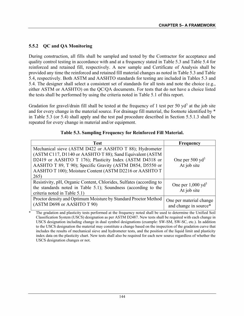
CHAPTER 5– A FRAMEWORK
144
5.5.2 QC and QA Monitoring
During construction, all fills shall be sampled and tested by the Contractor for acceptance and quality control testing in accordance with and at a frequency stated in Table 5.3 and Table 5.4 for reinforced and retained fill, respectively. A new sample and Certificate of Analysis shall be provided any time the reinforced and retained fill material changes as noted in Table 5.3 and Table 5.4, respectively. Both ASTM and AASHTO standards for testing are included in Tables 5.3 and 5.4. The designer shall select a consistent set of standards for all tests and note the choice (e.g., either ASTM or AASHTO) on the QC/QA documents. For tests that do not have a choice listed the tests shall be performed by using the criteria noted in Table 5.1 of this report. Gradation for gravel/drain fill shall be tested at the frequency of 1 test per 50 yd3 at the job site and for every change in the material source. For drainage fill material, the footnote identified by * in Table 5.3 (or 5.4) shall apply and the test pad procedure described in Section 5.5.1.3 shall be repeated for every change in material and/or equipment.
Table 5.3. Sampling Frequency for Reinforced Fill Material.
Test Frequency Mechanical sieve (ASTM D422 or AASHTO T 88); Hydrometer (ASTM C117, D1140 or AASHTO T 88); Sand Equivalent (ASTM D2419 or AASHTO T 176); Plasticity Index (ASTM D4318 or AASHTO T 89, T 90); Specific Gravity (ASTM D854, D5550 or AASHTO T 100); Moisture Content (ASTM D2216 or AASHTO T 265)
One per 500 yd3 At job site
Resistivity, pH, Organic Content, Chlorides, Sulfates (according to the standards noted in Table 5.1); Soundness (according to the criteria noted in Table 5.1)
One per 1,000 yd3 At job site
Proctor density and Optimum Moisture by Standard Proctor Method (ASTM D698 or AASHTO T 90)
One per material change and change in source*
* The gradation and plasticity tests performed at the frequency noted shall be used to determine the Unified Soil Classification System (USCS) designation as per ASTM D2487. New tests shall be required with each change in USCS designation including change in dual symbol designations (example: SW-SM, SW-SC, etc.). In addition to the USCS designation the material may constitute a change based on the inspection of the gradation curve that includes the results of mechanical sieve and hydrometer tests, and the position of the liquid limit and plasticity index data on the plasticity chart. New tests shall also be required for each new source regardless of whether the USCS designation changes or not.
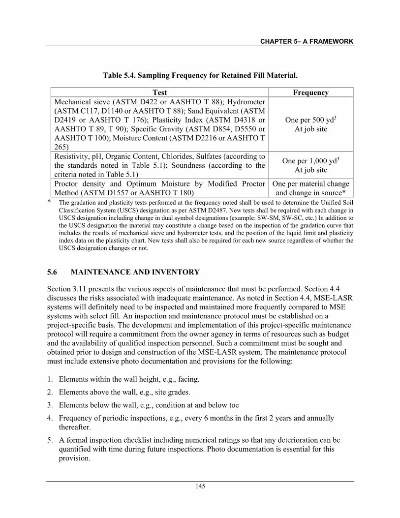
CHAPTER 5– A FRAMEWORK
145
Table 5.4. Sampling Frequency for Retained Fill Material.
Test Frequency Mechanical sieve (ASTM D422 or AASHTO T 88); Hydrometer (ASTM C117, D1140 or AASHTO T 88); Sand Equivalent (ASTM D2419 or AASHTO T 176); Plasticity Index (ASTM D4318 or AASHTO T 89, T 90); Specific Gravity (ASTM D854, D5550 or AASHTO T 100); Moisture Content (ASTM D2216 or AASHTO T 265)
One per 500 yd3 At job site
Resistivity, pH, Organic Content, Chlorides, Sulfates (according to the standards noted in Table 5.1); Soundness (according to the criteria noted in Table 5.1)
One per 1,000 yd3 At job site
Proctor density and Optimum Moisture by Modified Proctor Method (ASTM D1557 or AASHTO T 180)
One per material change and change in source*
* The gradation and plasticity tests performed at the frequency noted shall be used to determine the Unified Soil Classification System (USCS) designation as per ASTM D2487. New tests shall be required with each change in USCS designation including change in dual symbol designations (example: SW-SM, SW-SC, etc.) In addition to the USCS designation the material may constitute a change based on the inspection of the gradation curve that includes the results of mechanical sieve and hydrometer tests, and the position of the liquid limit and plasticity index data on the plasticity chart. New tests shall also be required for each new source regardless of whether the USCS designation changes or not.
5.6 MAINTENANCE AND INVENTORY
Section 3.11 presents the various aspects of maintenance that must be performed. Section 4.4 discusses the risks associated with inadequate maintenance. As noted in Section 4.4, MSE-LASR systems will definitely need to be inspected and maintained more frequently compared to MSE systems with select fill. An inspection and maintenance protocol must be established on a project-specific basis. The development and implementation of this project-specific maintenance protocol will require a commitment from the owner agency in terms of resources such as budget and the availability of qualified inspection personnel. Such a commitment must be sought and obtained prior to design and construction of the MSE-LASR system. The maintenance protocol must include extensive photo documentation and provisions for the following: 1. Elements within the wall height, e.g., facing. 2. Elements above the wall, e.g., site grades. 3. Elements below the wall, e.g., condition at and below toe 4. Frequency of periodic inspections, e.g., every 6 months in the first 2 years and annually
thereafter. 5. A formal inspection checklist including numerical ratings so that any deterioration can be
quantified with time during future inspections. Photo documentation is essential for this provision.

CHAPTER 5– A FRAMEWORK
146
6. Safety protocol during maintenance and inspection, e.g., fall protection and site stability. 7. Prioritization of repairs based on findings of inspection 8. Immediate spot repairs, e.g., cleaning clogged drainage pipes, removing adverse vegetation,
etc. 9. Reporting format for maintenance and inspection. 10. After each inspection, a report stamped by the original engineer of record certifying that the
entity has reviewed the maintenance and inspection report. The report must provide recommendations for any corrections that are needed including the time frame for corrective measures.
5.6.1 Inventory
Once the maintenance protocol is established, an inventory of the MSE-LASR assets should be developed. An inventory will help streamline the maintenance and asset management while creating a valuable database for future studies. The inventory can be modeled after the work performed by the National Park Service Procedures Manual (FHWA, 2010a).
5.6.2 Example User Tools
Appendix H provides example some user tools for maintenance and inventory that can be considered by an agency that is considering use of MSE-LASR technology.
5.7 DEPLOYMENT
The deployment of MSE-LASR systems will require a change in the thinking about MSE walls. While the basic principles of MSE wall design and construction remain intact, e.g., formation of a coherent soil mass by inclusion of mechanical reinforcement, the considerations for the primary component of the MSE wall, i.e., the type of fill in the reinforced zone, are drastically different. The first step in the deployment of the MSE-LASR system is the education of the owner, designer, contractor, and maintenance personnel. This step requires that all stakeholders have a basic understanding of the fundamental characteristics of the geomaterials proposed to be used in the MSE-LASR system. Significantly more testing and evaluations will be required with deployment of the MSE-LASR system. This section presents general recommendations for deployment of MSE-LASR systems.
5.7.1 Performance Monitoring
FHWA Section 11.4 presents guidelines for performance monitoring of MSE walls. Every MSE-LASR system must include a performance monitoring program consistent with the criticality of the structure. For example, if the MSE-LASR wall is in a remote area that is lightly traveled and the implications of wall deformations and/or failure are not serious in that human life will not be threatened in the event of a failure and that the wall can be repaired in an economical manner,

CHAPTER 5– A FRAMEWORK
147
then the recommendations of FHWA Section 11.4.2 (Limited Monitoring Program) may be implemented. In contrast, if the wall is considered to be critical, e.g., if its failure can result in injury or the loss of human life or affect a number of other facilities, then the recommendations of FHWA Section 11.4.3 (Comprehensive Monitoring Program) may be implemented. FHWA Table 11-6 presents possible instruments for various parameters that may be considered for monitoring. The key aspect of monitoring includes actual interpretation of the data that is generated. Monitoring instruments are often installed, but for some reason the data generated are never interpreted, or if the interpretations are performed, they are not recorded and stored. FHWA Section 11.4.5 provides a discussion regarding data interpretation. For MSE-LASR systems, it is imperative that qualified and experienced personnel be retained to interpret the data. In this regard, the FHWA should consider establishment of a database that future designers of MSE-LASR systems can use to develop specific guidelines within the framework presented in this chapter.
5.7.2 Considerations for Plans and Specifications
Plans and specifications are necessary for any engineered facility to convey the thought process of the designer/owner to the contractor. In this regard, plans and specifications refer to an explicit set of requirements to be satisfied by a material, design, product, or service. Unlike MSE walls constructed with select fills, each MSE-LASR system will likely have unique conditions whose consideration will have to be addressed by unique plans and specifications. The generic example specifications included in FHWA Section 10.9 will need to be modified on a project-specific basis. A primary element in the specifications for MSE-LASR wall will be the testing requirements for the LASR materials and the method of compaction control during construction. The recommendations in Section 5.2 to Section 5.5 should be included in the specifications. Since many MSE wall systems are proprietary, the specifications should clearly communicate the design requirements. For the design requirements, the recommendations in Section 5.3 must be included in the specifications. Design responsibilities, e.g., external and internal stability, must be clearly identified. For example, global (overall) and compound stability analyses are expected to be key components of the design process. The entity responsible for each and every element of the design process must be clearly identified in the specifications. Finally, surface and subsurface drainage details must be clearly expressed in the plans and specifications. Section 5.4 provides some recommendations in this regard. The minimum drainage requirements must be shown by drawings on plans so that there is no ambiguity. Since specifications are commonly in a written narrative format, it is often difficult to convey all the thought processes. Therefore, details of every design element must be shown in drawings on the plans and supported by appropriate notes. The plans and specifications can be “methods-based” or “performance-based.” For MSE-LASR system a hybrid approach that combines methods and performance specifications may be necessary. For example, the field compaction control method may be “methods-based,” such as by specifying the SAV&S method, but additional performance criteria may also be required e.g., by specifying facing tolerances. As noted earlier, each MSE-LASR project will be unique, and

CHAPTER 5– A FRAMEWORK
148
the type of plans and specifications will need to be tailored to meet the needs and expectations for the project.
5.7.3 Procurement
Every owner is familiar with a variety of procurement processes, e.g., design-bid-build, design-build, construction manager at risk (CMAR), etc. Within these processes, the procurement for walls may be different, e.g., lump sum or measurement and payment for various discrete elements of wall. Furthermore, the procurement on government contracts is commonly on a low-bid basis from a list of pre-qualified vendors. Such an approach may not be appropriate for MSE-LASR systems because it is likely that many of the pre-qualified vendors are those who supply MSE walls that use metallic reinforcements, which may not be suitable based on the various considerations discussed in this report. Vendors of systems that use geosynthetic reinforcements may not be equally qualified because of their lack of engineering and testing capabilities. Since each MSE-LASR wall will be unique, the procurement process for each wall must be looked at on a project-specific basis. Therefore, an active discussion within the project team must take place, including personnel from the procurement department, and a detailed evaluation must be made of “what-if” scenarios to mitigate construction issues and claims. In this regard, it would be beneficial for the owner to consider a two-step procurement process as follows: Step 1: Prepare pre-qualification criteria and minimum performance requirements on a project-
specific basis including a list of questions that would help screen qualified teams of MSE wall vendors and general contractors. Clearly specify the minimum requirements for screening, e.g., 90th percentile, based on ranking of answers. The ranking system must be clearly communicated as part of the procurement process.
Step 2: Based on the results from Step 1, prepare a short-list of the pre-qualified teams of MSE
wall vendors and general contractors. The mixing and matching of MSE wall vendor and general contractors between different teams should not be allowed. The pre-qualified teams on this short-list may then be invited to bid the project. The owner may choose to make the final selection according to specific pre-advertised criteria, e.g., lowest bid, mid-bid, weighted bid, etc.
There can be many variations of the 2-step procurement process described above. The bottom line is that the procurement process for MSE-LASR system must be well thought out in the early stages of consideration for using such a system on a given project. The procurement process must be conducted fairly and without the possibility of conflicts of interest.

CHAPTER 5– A FRAMEWORK
149
5.8 CHAPTER KEY POINTS
Chapter 5 provides a framework for the development of guidelines for implementation of MSE-LASR systems. The key points in this regard are as follows: (a) Each MSE-LASR application will be unique and will therefore require individual
attention.
(b) Significantly more testing and evaluations during design and construction will be required with deployment of the MSE-LASR system. Project-specific plans and specifications and procurement processes will be required.

CHAPTER 6– SUGGESTIONS FOR FURTHER STUDIES
150
CHAPTER 6 – SUGGESTIONS FOR FURTHER STUDIES
MSE walls with non-select fills have been built successfully and are performing adequately within the United States and elsewhere. The major impetus for this study is the need for guidelines to design and construct such MSE-LASR systems for transportation applications. This report presents a detailed review of the literature and a framework for the development of guidelines in this regard. The development of such guidelines will undoubtedly require further studies. A list of recommendations for further evaluation and study follows. This list should be taken in the context of the frame of reference identified in Section 1.5. 1. Perform parametric studies and develop example problems that will serve as a benchmark for
vendors and engineers to use for design of MSE-LASR walls. An example calculation is presented in Appendix G.
2. Develop agency specific formal protocol for maintenance and inventory of MSE-LASR walls. An example is presented in Appendix H.
3. Develop agency specific formal checklist for inspection of MSE-LASR walls that can be
used as part of the wall maintenance protocol. An example is presented in Appendix H.
4. Prepare a formal specification to be used exclusively for MSE-LASR walls.
5. Develop a sample risk assessment form that could be used by the owner and stakeholders to assess risks associated with the use of MSE-LASR walls.
6. Develop a set of generic standard details for inclusion in the plan set for MSE-LASR walls.
7. Based on the implementation of the SAV&S Method for field control of compaction in
addition to the RC construction compaction control procedure, develop guidelines for the use of the SAV&S method.
8. Identify specific hand-held cone penetration equipment for laboratory and field use to
determine the strength of uniform granular fills. Develop correlations between cone resistance and strength parameters for use with the SAV&S Method for field control of compaction.
9. Develop a database of MSE-LASR walls that would enable others who contemplate using
such systems to learn from experiences. Included in this database would be information on soil properties, soil-reinforcement interaction data, results of instrumentation on actual walls, drag loads on facing and connections, construction compaction control experiences, etc.
10. Develop charts of vertical and horizontal deformations of walls based on measured data from
performance monitoring in terms soil type, wall height, type and density of reinforcement, facing type, etc.

CHAPTER 6– SUGGESTIONS FOR FURTHER STUDIES
151
11. Develop numerical models for the evaluation of drag loads on the wall face and connections. Verify the results of the numerical models by comparing them to measured data from performance monitoring. Refine load and/or resistance factors for connection strength design.
12. Refine the current soil-structure interaction models based on measured field and laboratory
data specific to MSE-LASR walls.
13. Develop models to predict the useful service life of MSE-LASR walls. Development of such models will likely entail evaluation of the current corrosion models for metallic reinforcements and degradation models for geosynthetic reinforcements including creep behavior.
14. Develop models to incorporate the effect of cohesion into pullout loads and/or resistances.
15. Study the long-term effect of load transfer (“load shedding”) due to the differential in creep
of soil and creep of geosynthetic reinforcement.
16. Refine Figure 5.1 as more data become available. Conceivably the chart can include data based on landforms, e.g., residual and transported geomaterials.
17. Develop minimum criteria for field personnel to monitor and document the construction.
18. Develop a formal educational program to disseminate the information for proper design and
construction of MSE-LASR walls.
19. Develop a list of pre-qualified vendors for MSE-LASR systems.
20. Develop guidelines for procurement of MSE-LASR walls.
Finally, it would behoove the industry to think of the MSE-LASR system as a specialized MSE wall because the success of this technology is heavily dependent on the correct understanding of the fundamental properties of LASR materials and construction compaction control procedures. Although the construction processes are relatively straightforward it is important that qualified construction and inspection personnel are involved in the construction of the MSE-LASR walls. Thus, while the studies suggested above are being performed, FHWA should consider immediate development of a course for inspector qualification for MSE-LASR systems similar to the FHWA courses for inspector qualification for drilled shafts, driven piles, MSE walls, and subsurface investigations.

CHAPTER 6– SUGGESTIONS FOR FURTHER STUDIES
152
6.1 CHAPTER KEY POINTS
Chapter 6 provides recommendations for further studies. The key points in this regard are: (a) The further studies must concentrate on practical aspects such as better definition of
material properties and field control of fill compaction and wall construction.
(b) A formal education program must be developed to disseminate the information for proper design and construction of MSE-LASR walls.

CHAPTER 7– SUMMARY AND CLOSURE
153
CHAPTER 7 – SUMMARY AND CLOSURE
The primary goal of this report is to develop a framework for using local available sustainable resources (LASR) in lieu of select material as MSE wall fills in support of the unique performance-based management needs of FLHD and other agencies such as local and state Departments of Transportation (DOTs). The use of select fill materials for MSE walls, while preferable, is not always practical because often such select fill materials are not available locally and must be imported to the jobsite. In that case the disposal of unsuitable local native soils may be required with an associated cost that may significantly increase the total project cost and have an intangible impact on the environment. This situation is particularly true in the case of Federal Land Management Agencies (FLMAs) such as the Federal Lands Highway Division (FLHD) of the FHWA, United States Forest Service (USFS), National Park Service (NPS), and Fish and Wildlife Service (FWS), which are often involved in the design and construction of MSE walls at locations that are far from borrow sources suitable for select fill. The availability of cost-effective select fills has also become a concern for urban areas wherein demands of multiple projects with select fill requirements and dwindling sources of borrow material for such select fill materials result in increased project costs. Indeed, the same situation is true in many parts of the world, e.g., Japan, India, New Zealand, Brazil, etc. In such cases consideration is often given to alternative earth retention systems. Alternative earth retention systems such as cast-in-place reinforced concrete walls (CIP) are often more costly than MSE walls and generally have a larger carbon footprint, which is environmentally undesirable. The following approach was taken to attain the goal of the project: 1. Perform a literature review to gather information on the use of non-select fills in MSE walls,
2. Identify and define the factors that influence the selection of MSE wall fills,
3. Develop a general framework for the use of LASR materials as fills that is based on an
understanding of the underlying risks associated with the use of such non-select fills,
4. Provide a framework for the development of guidelines for the implementation of the use of local available sustainable resources (LASR) in lieu of select material as MSE wall fills and
5. Provide recommendations for future studies to establish guidelines for the design and construction of MSE-LASR walls for transportation applications. The term MSE-LASR is proposed in this report for MSE walls built with non-select fills wherein LASR stands for Local, Available, Sustainable, Resources; each of these four words is defined in Chapter 1.
Use of select fills in MSE walls has provided a certain sense of complacency in the MSE wall industry in the sense that nothing much can go wrong since the procedures for the design and construction of walls with select fill are well established and documented in FHWA (2009) and AASHTO (2020). Often lost in the applications of MSE walls with select fill is the fundamental

CHAPTER 7– SUMMARY AND CLOSURE
154
understanding of the material properties and their effect on design and construction. Furthermore, often problems associated with the use of LASR materials for MSE wall fills can be traced back to a poor understanding of the material properties and construction control methods, e.g., compaction. Therefore, as a first step it was considered necessary to distinguish between the use of MSE-LASR walls and those based on FHWA (2009) and AASHTO (2020) standards. Any information in this report related to MSE-LASR walls must be first screened to ensure compliance with the definition of these words used in the acronym LASR as noted in Chapter 1. If the proposed fills do not meet the definitions of these words, then this report shall not be considered applicable, and the proposed wall system cannot be categorized as a MSE-LASR wall. Chapter 2 provides basic definitions so that the reader is able to understand the context of various discussions in the report. The results of the literature review conducted as part of this investigation and general observations based on the reviewed literature are also provided. A brief discussion is devoted to NCMA requirements for select fills. Finally, a summary of the results of the work performed as part of NCHRP Project 24-12 and the parallel NCMA study conducted in 2009 is provided. The results of more than 40 additional studies related to various aspects of MSE-LASR walls are summarized and referenced. Chapter 3 provides a discussion of the various factors that can affect the selection of MSE wall fills. The intent is to clarify the rationale behind the current criteria for select fills while also helping understand the consequences of using MSE-LASR materials. Chapter 4 identifies the risks associated with the use of LASR materials in lieu of materials that meet the current criteria for select fills. Chapter 5 establishes guidance based on the risks identified in Chapter 4 for various considerations associated with the use of LASR materials (e.g., design procedures, specifications, construction, etc.). Chapter 6 provides suggestions for further studies that will be helpful in developing guidelines for the various considerations associated with the use of LASR materials discussed in Chapter 5. The discussions are intentionally brief to maintain the flow of thought and to avoid getting bogged down by details. Several appendices are provided that include detailed information to supplement some of the discussions in various chapters. Thus, the information in the appendices permits the reader to obtain an understanding of the discussions in the various chapters. The authors assume that the reader has a basic understanding and knowledge of the analysis, design, and construction of MSE walls as well as LRFD methodology. The reader is referred to the References section of the report that contains an extensive list of references for additional information on those topics. In particular, it is assumed that the reader has access to and is familiar with the guidelines in FHWA (2009) and AASHTO (2020) for MSE walls designed and built with select fills. The framework for the development of guidelines provided herein is intended to ultimately allow application of the MSE-LASR wall technology to design and construction. It is expected that agencies may vary on how they adopt and use this framework. The experiences of those agencies may augment the suggestions for further studies presented in Chapter 6 so that eventually a comprehensive set of guidelines and standards will be developed to address all the considerations presented in Chapter 5.
CHAPTER 7– SUMMARY AND CLOSURE
155
The decision to use the framework for the development of guidelines in this report shall be based on the performance criteria for the structure being designed, e.g., permissible deformations, maintenance cycles, etc. None of the recommendations in this report shall be construed as an endorsement to replace the recommendations in FHWA (2009) and AASHTO (2020) without the approval of the owner of the facility and consideration of the various factors discussed in this report. Figure 7.1 presents a flow chart to guide the owner and designer through the process of implementation of the MSE-LASR technology. The flow chart identifies the activities during each of the 6 primary blocks, e.g., Block 1 relates to project planning. The typical sub-activities corresponding to each block are identified by a numbered list in the text box immediately to the right of each block. The list of sub-activities is self-evident based on the discussions in Chapters 1 to 5. Based on the study the following closing comments are provided: 1. MSE walls with soils not meeting the select fill criteria in Table 2.1 have been
successfully designed and constructed. 2. The limitations and risks associated with the use of MSE-LASR systems should be clearly
understood by the agency and the designers 3. An understanding of the fundamental properties of fill materials is essential to understand
the selection and use of LASR materials for MSE-LASR systems. 4. Each MSE-LASR system must be evaluated on a project- and site-specific basis with
particular emphasis on appropriate laboratory testing and field compaction control criteria. 5. Compared to MSE walls built with select fills, MSE-LASR systems entail more risks. 6. The owner must mandate development of a project-specific risk assessment document that
forces all project stakeholders to explicitly acknowledge the potential risks associated with the use of a MSE-LASR system for the given project.
7. Each MSE-LASR wall is unique and requires individual attention. 8. Significantly more testing and evaluations will be required with deployment of the MSE-
LASR system. Project-specific plans and specifications and procurement processes will be required.
9. Further studies should concentrate on practical aspects such as better definition of material properties and field construction control. In this regard, a project-specific MSE-LASR system may require project-specific studies not covered in this report.
10. A formal education program must be developed to disseminate the information for proper design and construction of MSE-LASR wall systems.
11. Remember and understand the frame of reference identified in Section 1.5.

CHAPTER 7– SUMMARY AND CLOSURE
156
Figure 7.1. Flow chart. Activities for Implementation of MSE-LASR Technology.

CHAPTER 7– SUMMARY AND CLOSURE
157
In conclusion, this report has attempted to address a major consideration in the field of MSE walls related to the fill materials used in the reinforced zone. Documented case histories demonstrate that MSE-LASR systems have already been used successfully within and outside the United States. The report provides insight into the fundamental aspects of fill material selection, compaction control, and issues related to drainage of the constructed wall.
7.1 CHAPTER KEY POINTS
Chapter 7 provides summary and closure. The key points in this regard are: (a) The implementation of MSE-LASR technology must be systematic and performed
according to the activities outlined in the flow chart in Figure 7.1.
(b) A formal education program must be developed to disseminate the information to the project stakeholders in order to ensure proper design and construction of MSE-LASR walls.

REFERENCES
158
REFERENCES –
The references are organized according to primary and secondary sources. Primary sources are considered to be publications of transportation agencies (e.g., FHWA, NCHRP, state DOTs, etc.) and codes and standards (e.g., AASHTO, ASTM, etc.). Secondary sources are journal articles, books, and all other publications that do not classify as primary sources. The references presented herein focus on Mechanically Stabilized Earth (MSE) retaining walls and material directly relevant to this report. It is acknowledged that the literature is replete with many more references related to MSE and MSE-LASR type walls.
PRIMARY SOURCES
Federal Highway Administration (FHWA)
FHWA (1976). An Occurrence and Distribution Survey of Expansive Materials in the United States by Physiographic Areas. Report No. FHWA RD-76-82, Authors: Patrick, D. M. and Snethen, D. R., Federal Highway Administration, U.S. Department of Transportation, Washington, DC.
FHWA (2001). Mechanically Stabilized Earth Walls and Reinforced Soil Slopes, Design and Construction Guidelines, Report No. FHWA-NHI-00-043, Authors: Elias, V, Christopher, B.R. and Berg, R.R., Federal Highway Administration, U.S. Department of Transportation, Washington, DC.
FHWA (2002). Evaluation of Soil and Rock Properties, Report No. FHWA-IF-02-034, Authors: Sabatini, P. J., Bachus, R. C., Mayne, P. W., Schneider, J. A. and Zettler, T. E., Federal Highway Administration, U.S. Department of Transportation, Washington, DC.
FHWA (2006). Soils and Foundations. Volumes I and II, Report No. FHWA-NHI-06-088 and FHWA-NHI-06-089, Authors: Samtani, N. C. and Nowatzki, E. A., Federal Highway Administration, U.S. Department of Transportation, Washington, DC.
FHWA-CFL (2006a). Shored Mechanically Stabilized Earth (SMSE) Wall Systems Design Guidelines. Report No. FHWA-CFL/TD-06-001, Authors: Morrison, K. F., Harrison, F. E, Collin, J. G.; Dodds, A., and Arndt, B., Central Federal Lands Highway Division, Federal Highway Administration, Lakewood, CO.
FHWA (2008). Geosynthetic Design and Construction Guidelines, Report No. FHWA NHI-07-092, Authors: Holtz, R. D., Christopher, B. R., and Berg, R. R., Federal Highway Administration, U.S. Department of Transportation, Washington, DC.
FHWA (2009). Design and Construction of Mechanically Stabilized Earth Walls and Reinforced Soil Slopes, Report No. FHWA NHI-09-083, Authors: Berg, R. R.,
REFERENCES
159
Christopher, B. R. and Samtani, N. C., Federal Highway Administration, U.S. Department of Transportation, Washington, DC.
FHWA (2009a). Corrosion/Degradation of Soil Reinforcements for Mechanically Stabilized
Earth Walls and Reinforced Soil Slopes, FHWA NHI-09-087, Authors, Elias, V., Fishman, K. L., Christopher, B. R. and Berg, R. R., Federal Highway Administration, U.S. Department of Transportation, Washington, DC.
FHWA (2010). Selection of Spread Footings on Soils to Support Highway Bridge Structures.
Authors: Samtani, N. C., Nowatzki, E. A. and Mertz, D. R. Publication No. FHWA RC/TD-10-001, U.S. Department of Transportation, Federal Highway Administration – Resource Center, Matteson, IL.
FHWA (2010a). Retaining Wall Inventory and Assessment Program (WIP) – National Park
Services Procedures Manual. Authors: DeMarco, M., Keough, D. and Lewis, S., Publication No. FHWA-CFL/TD-10-003, Transportation Management Program, National Park Service, Department of the Interior, Washington, D.C.
Transportation Research Board (TRB) and National Cooperative Highway Research Program (NCHRP)
NCHRP (2011). LRFD Metal Loss and Service-Life Strength Reduction Factors for Metal-Reinforced Systems, Final Report for National Cooperative Highway Research Project 24-28. Authors: Fishman, K.L. and Withiam, J.L., Transportation Research Board of the National Academies, Washington, DC, 116 p.
NCHRP (2013). Selecting Backfill Materials for MSE Retaining Walls, Final Report for
National Cooperative Highway Research Project 24-22. Authors: Marr, W.A. and Stulgis, R.P., Transportation Research Board of the National Academies, Washington, DC, 353 p.
United States, State DOTs and University Transportation Research Organizations Belcher, D.J., Gregg, L.E., Woods, K.B., and Jenkins, D.S., 1946, Origin and Distribution of
United States Soils: Washington, U.S. Dept. of Commerce. Civil Aeronautics Administration.
Bobet, A. (2002). Design of MSE Walls for Fully Saturated Conditions, Report No.
FHWA/IN/JTRP-2002/13, performed by Purdue University for the Indiana Department of Transportation, Indianapolis, IN.
Bressette, T., and Chang, G. (1986). Mechanically Stabilized Embankment Constructed with
Low Quality Backfill, Report No. FHWA/CA/TL-86/06, California Department of Transportation, Sacramento, CA.

REFERENCES
160
Caltrans (2012). Corrosion Guidelines – Version 2.0, California Department of Transportation, Division of Engineering Services, Materials Engineering and Testing Services, Corrosion and Structural Concrete, Field Investigation Branch, Sacramento, CA.
Dove, J. E., and Darden, J. N. (2005). Native Backfill Materials for Mechanically Stabilized
Earth Walls, Report No. VTRC 05-CR12, Virginia Department of Transportation, Richmond, VA.
Drnevich, V. P., Evans, A. C., and Prochaska, A. B. (2007). A Study of Effective Soil
Compaction Control of Granular Soils, FHWA/IN/JTRP-2007/12, Joint Transportation Research Program, Indiana Department of Transportation and Purdue University, West Lafayette, Indiana.
Farrag, K., and Morvant, M. (2004). Evaluation of Interaction Properties of Geosynthetics in
Cohesive Soils: LTRC Reinforced-Soil Test Wall. Report No. FHWA/LA.03/379, Louisiana Department of Transportation and Development, Baton Rouge, LA.
MDT (2013). Method for Sampling and Testing MT 229-04, Procedure for Solids-Water-Voids
Relations of Soil Masses (Zero-Air Voids), The State of Montana Department of Transportation.
Mokwa, R.L. and Fridleifsson, S. (2007). Soil Air Voids Method for Compaction Control, Final
Report prepared for The State of Montana Department of Transportation in cooperation with The U.S. Department of Transportation Federal Highway Administration, Bozeman, MT, 94 p.
NAVFAC (1971). Design Manual - Soil Mechanics, Foundations, and Earth Structures.
Department of the Navy, Naval Facilities Engineering Command, Washington, DC. NAVFAC (1986a). Design Manual 7.01 - Soil Mechanics. Department of the Navy, Naval
Facilities Engineering Command, Alexandria, VA. NAVFAC (1986b). Design Manual 7.02 - Foundations and Earth Structures. Department of
the Navy, Naval Facilities Engineering Command, Alexandria, VA. Parrish, B.R. (2006). Geotextile Wrap-Face Wall Using Marginal Backfill, a Thesis presented
to the Faculty of the Graduate School, University of Missouri-Columbia in partial fulfillment of the requirements for the degree of Master of Science in Civil and Environmental Engineering.
Rathje, E. M., Rauch, A. F., Trejo, D., Folliard K. J., Viyanant, C., Esfellar, M., Jain, A., and
Ogalla, M. (2006). Evaluation of Crushed Concrete and Recycled Asphalt Pavement as Backfill for Mechanically Stabilized Earth Walls, Report No. FHWA/TX-06/0-4177-3,

REFERENCES
161
Center for Transportation Research, University of Texas at Austin. Prepared for Texas Department of Transportation, Austin, TX.
Codes and Standards
AASHTO (1986). AASHTO Guide for Design of Pavement Structures, American Association of State Highway and Transportation Officials, Washington, DC.
AASHTO (2002). Standard Specifications for Highway Bridges, 17th Edition, American Association of State Highway and Transportation Officials, Washington, DC.
AASHTO (2014). AASHTO LRFD Bridge Design Specifications, 7th Edition. American
Association of State Highway and Transportation Officials, Washington, DC. AASHTO (2019). Standard Specifications for Transportation Materials and Methods of
Sampling and Testing, American Association of State Highway and Transportation Officials, Washington, DC.
AASHTO (2020). AASHTO LRFD Bridge Design Specifications, 9th Edition. American
Association of State Highway and Transportation Officials, Washington, DC. ASTM (2019a). Annual Book of ASTM Standards, Volume 4.08, Soil and Rock (I), American
Society for Testing and Materials, West Conshohocken, PA. ASTM (2019b). Annual Book of ASTM Standards, Volume 4.09, Soil and Rock (II), American
Society for Testing and Materials, West Conshohocken, PA. NCMA (1993). Design Manual for Segmental Retaining Walls, 1st Edition, Editors: Simac,
M.R., Bathurst, R.J., Berg, R.R., and Lothspiech, S.E., National Concrete Masonry Association, Herndon, Virginia, 336 p.
NCMA (1997). Design Manual for Segmental Retaining Walls, 2nd Edition, Editor: J.G. Collin,
National Concrete Masonry Association, Herndon, Virginia, 289 p. NCMA (2002). Segmental Retaining Walls Drainage Manual, Authors: J.G. Collin, Berg, R.R.
and Meyers, M., National Concrete Masonry Association, Herndon, Virginia, 104 p. NCMA (2010). Design Manual for Segmental Retaining Walls, 3rd Edition, Editor: Bernardi,
M. National Concrete Masonry Association, Herndon, Virginia, 282 p.

REFERENCES
162
SECONDARY SOURCES
Journal and Conference Papers
Abrahams, A., and Sankey, J. E. (2000). “Design and Construction of Reinforced Earth Walls on Marginal Lands,” Geotechnics of High Water Content Materials, ASTM STP 1374, eds: T. B. Edil and P. J. Fox, American Society for Testing and Materials, West Conshohocken, PA, pp 334-350.
Allen, H. (1942). “Classification of soils and control procedures used in construction of
embankments,” Public Roads, Vol. 22, No. 12, pp. 263-282. Allen, T.M., Bathurst, R.J., Holtz, R.D., Walters, D. L., and Lee, W.F. (2003). “A New Working
Stress Method for Prediction of Reinforcement Loads in Geosynthetic Walls,” Canadian Geotechnical Journal, Vol. 40, No. 5, pp. 976-994.
Alzamora, D., Wayne, M., and Han, J. (2000). “Performance of SRW Supported by Geogrids
and Jet Grout Columns,” Proceedings of ASCE on Performance Confirmation of Constructed Geotechnical Facilities, Amherst, Massachusetts, USA, pp. 456-466
Anderson, R. B., Boyd, F.N. and Shaw, L. (1991). Modular Block Faced Polymer Geogrid
Reinforced Soil Walls U.S. Postal Service Combined Carrier Facility, Proceedings of Geosynthetics '91 Conference, Atlanta, GA, pp. 889-902.
Atterberg, A. (1911) “Lerornas Forhallande till Vatten, deras Plasticitetsgranser och
Plasticitetsgrader,” (The Behavior of Clays with Water, their Limits of Plasticity and their Degrees of Plasticity,”) Kungliga Lantbruksakademiens Handlingar och Tidskrift, Vol. 50, No.2, pp. 132-158; also in Internationale Mitteilungen fur Bodenkunde, Vol 1., pp. 10-43 (“Uber die Physikalische Bodenuntersuchung und uber die Plastuxitat der Tone”).
Baker, R. (2004). “Nonlinear Mohr Envelopes Based on Triaxial Data,” Journal of
Geotechnical and Geoenvironmental Engineering, Vol. 130, No. 5, pp. 498–506, American Society of Civil Engineers, Reston, VA.
Barber, E. S. and Sawyer, C. L. (1952). “Highway Subdrainage,” Proceedings, Highway
Research Board, Vol. 31, pp. 643-666, Washington, DC. Bathurst, R. J., Miyata, Y, Nernheim, A, and Allen, A. M. (2008), “Refinement of K-Stiffness
Method for Geosynthetic Reinforced Soil Walls”, Geosynthetics International, Vol. 15, No. 4, pp. 269-295.
Bathurst, R.J., Siemens, G. and Ho, F. (2009), “Experimental Investigation of Infiltration
Ponding in One-Dimensional Sand-Geotextile columns”, Geosynthetics International, Vol. 16, No. 3, pp. 158-172.

REFERENCES
163
Bergado, D. T., Sampaco, C. L., Shivashankar, R., Alfaro, M. C., Anderson, L. R. and Balasubramaniam, A. S. (1991a). “Performance of Welded Wire Wall with Poor Quality Backfills on Soft Clay”. Proceedings of ASCE Geotechnical Engineering Congress, Boulder, Colorado, U.S.A. 909-922.
Bergado, D. T., Shivashankar, R., Sampaco, C. L., Alfaro, M. C. and Anderson, L. R. (1991b).
“Behavior of Welded-Wire Wall with Poor Quality Cohesive-Frictional Backfills on Soft Bangkok Clay,” Canadian Geotechnical Journal, Vol. 28, No. 6, pp. 860-880.
Bergado, D.T., Lo, K-H, Chai, J-C, Shivashankar, R, Alfaro, M. C., and Anderson, L. R. (1992).
“Pullout Tests Using Steel Grid Reinforcements with Low-Quality Backfill,” Journal of Geotechnical Engineering, Vol. 118, No. 7, pp. 1047-1063, American Society of Civil Engineers, Reston, VA.
Bergado, D.T., Hardiyatimo, H.C., Cisneros, C.B., Chai, J-C., Alfaro, M.C., Balasubramaniam,
A.S., and Anderson, L.R. (1992). “Pullout Resistance of Steel Geogrids with Weathered Clay as Backfill Material,” Geotechnical Testing Journal, Vol. 15, No. 1, pp. 33-46.
Bergado, D.T., Shivashankar, R., Alfaro, M.C., Chai, J-C. and Balasubramaniam, A.S. (1993a).
“Interaction Behavior of Steel Grid Reinforcements in a Clayey Sand,” Geotechnique, Vol. 43. No.4, pp. 589-603.
Bergado, D.T., Chai, J. C., Abiera, H. O., Alfaro, M. C., and Balasubramaniam, A.S. (1993b).
“Interaction between Cohesive-Frictional Soil and Various Grid Reinforcements,” Geotextiles and Geomembranes, Vol. 12, Elsevier Science Publishers Ltd., pp. 327-349.
Brockbank, B., Kalynchuk, G., and Scherger, B. (1992), “Use of Oil Sand for Construction of a Reinforced Earth Dump Wall,” Innovation Conservation and Renovation - 45th Canadian Geotechnical Conference, Toronto, The Canadian Geotechnical Society, Richmond, British Columbia, pp. 1-10.
Bueno, B., Patias, J., and Zornberg, J. G. (2006). “Use of Poor Draining Soils in Reinforced Soil Structures in Brazil,” Proceedings of Annual Meeting 2006 (CD-ROM), Transportation Research Board, Washington, DC. 15 pp.
Burwash, W. J., and Frost, J. D. (1991). “Case History of a 9 m High Geogrid Reinforced Retaining Wall Backfilled with Cohesive Soil,” Proceedings of the Geosynthetics '91 Conference, Atlanta, GA, Vol. 2, pp. 485-493.
Casagrande (1959). “Discussion of Requirements for the Practice of Applied Soil Mechanics,” Proceedings of the 1st Panamerican Conference on Soil Mechanics and Foundation Engineering, Vol III, pp. 1029-1037.

REFERENCES
164
Christopher, B.R. and Berg, R.R. (1990). "Pullout Evaluation of Geosynthetics in Cohesive Soils," Proceedings of the 4th International Conference on Geotextiles, Geomembranes, and Related Products, The Hague, Netherlands, pp. 731-736.
Christopher, B. R., Zornberg, J. G., Mitchell, J. K. (1998), “Design Guidance for Reinforced Soil
Structures with Marginal Soil Backfills,” Proceedings of the 6th International Conference on Geosynthetics, Boston, MA, USA, pp. 797-804.
Christopher, B. R., and Stulgis, R. P. (2005), "Low Permeable Backfill Soils in Geosynthetic
Reinforced Soil Walls: State of the Practice in North America,” Proceedings of North American Geosynthetics Conference (GRI-19), Las Vegas, NV, USA, 12 p.
Chua, K-M, and Tenison, J. (2003). “Explaining the Hveem Stabilometer Tests: Relating R-
value, S-value, and the Elastic Modulus,” Proceedings of Journal of Testing and Evaluation, Vol. 31, No. 4, ASTM International, West Conshohocken, PA, USA, 10 pp.
Deere, D. U., and Patton, F. D. (1971). "Slope Stability in Residual Soils,” Proceedings 4th
Panamerican Conference on Soil Mechanics and Foundation Engineering, San Juan, PR, pp. 87-170.
Dobie, M., (2010). “Practical Use of Clay Fills in Reinforced Soil Structures,” Development of
Geotechnical Engineering in Civil Works and Geo-Environment, Yogyakarta, Indonesia, 11 p.
Elias, V. and Swanson, P. (1983). “Cautions of Reinforced Earth with Residual Soils,”
Transportation Research Record 919, Transportation Research Board, Washington, DC, pp. 21-26.
Franklin, A.G., Orozco, L.F., and Semrau, R. (1973), “Compaction and Strength of Slightly
Organic Soils,” Journal of the Soil Mechanics and Foundations Division, Vol. 99, No. SM7, pp. 541-557, American Society of Civil Engineers, Reston, VA.
Garcia, E. F., Gallage, C.P.K. and Uchimura, T. (2007). “Function of Permeable Geosynthetics
in Unsaturated Embankments Subjected to Rainfall Infiltration”, Geosynthetics International, Vol. 14, No. 2, pp. 89-99.
Hannon, J.B., and Forsyth, R.A. (1984), “Performance of an Earth Reinforcement System
Constructed with Low Quality Backfill,” Transportation Research Record 975, Transportation Research Board, Washington, DC, pp. 55-66.
Hatami, K. and Bathurst, R. J. (2005). “Parametric Analysis of Reinforced Soil Walls with
Different Backfill Material Properties,” Proceedings of North American Geosynthetics Conference (GRI-19), Las Vegas, NV, USA, 13 p.

REFERENCES
165
Hazen, A. (1892). “Some Physical Properties of Sands and Gravels, with Special Reference to their Use in Filtration,” Public Roads of Massachusetts, Annual Reports, Vol V., Nos 34 to 46, Boston, Wright and Potter Printing Co., pp. 541-556.
Hazen, A. (1911). “Discussion of “Dams on Sand Foundations,” By A. C. Koenig, Transactions,
ASCE, Vol. 73, pp. 199-203. Hossain, M., Kibria, G., Khan, M., Hossain, J., and Taufiq, T. (2012). “Effects of Backfill Soil
on Excessive Movement of MSE Wall,” Journal of Performance of Constructed Facilities, Vol. 26, Issue 6, pp. 793–802, American Society of Civil Engineers, Reston, VA.
Houlsby, G.T. and Hitchman, R. (1988). “Calibration Chamber Tests of Cone Penetrometer in
Sand,” Geotechnique, Vol. 38, No. 1, pp. 39-44. Hveem, F. N. (1953). “The Sand Equivalent Test for Control of Materials During Construction,”
Proceedings, Highway Research Board, Washington, DC. Ingles, O. G. (1962). "Bonding Forces in Soils, Part 3: A Theory of Tensile Strength for Stabilised
and Naturally Coherent Soils,” Proceedings of the 1st Conference of the Australian Road Research Board, Victoria, Australia, pp. 1025-1047.
Iryo, T. and Rowe, R. K. (2005). “Infiltration into an Embankment Reinforced with Nonwoven
Geotextiles,” Canadian Geotechnical Journal, Vol. 42, No. 4, pp. 1145-1159. Johnson, A. W. and Sallberg, J. R. (1960). “Fundamentals of Soil Compaction,” U. S. National
Research Council Publication, Vol. 272, National Academy of Science, pp. 4-19. Jones, W. (1973). “Earthwork Compaction Control by Percent Air Voids,” Proceedings of the
11th Symposium on Engineering Geology and Geotechnical Engineering, Sponsored by Idaho Department of Transportation, University of Idaho, and Idaho State University, Pocatello, Idaho, April 4-6, 1973, pp. 251-263.
Kandolkar, S.S. and Mandal, J.N. (2013). “Behaviour of Reinforced Mine Waste Model Walls
under Uniformly Distributed Loading,” Electronic Journal of Geotechnical Engineering, Vol. 1, Bund. G, pp. 1351-1365
Keller, G.R. (1995). “Experiences with Mechanically Stabilized Structures and Native Soil
Backfill,” Transportation Research Record 1474, pp. 30-38, Transportation Research Board, National Research Council, Washington, DC.
Kenney, T.C. and Lau, D. (1985). “Internal Stability of Granular Filters,” Canadian Geotechnical
Journal, Vol. 22, No. 2, 1985, pp. 215-225.

REFERENCES
166
Kenney, T.C. and Lau, D. (1986). Canadian Geotechnical Journal, Vol. 23, No. 3, pp. 420-423, Reply to discussions on, “Internal Stability of Granular Filters,” Canadian Geotechnical Journal, Vol. 22, No. 2, 1985, pp. 215-225.
Kim, W.S. and Borden, R.H. (2013), “Numerical Simulation of MSE Wall Behavior Induced by
Surface-Water Infiltration,” Journal of Geotechnical and Environmental Engineering, Vol. 139, No. 12, pp. 2110-2124, American Society of Civil Engineers, Reston, VA.
Koerner, R.M., Soong, T-Y, and Koerner, G.R. (2005), "Back Drainage Design and
Geocomposite Drainage Materials,” Proceedings of North American Geosynthetics Conference (GRI-19), Las Vegas, NV, USA, 36 p.
Koerner, R.M. and Koerner, G.R. (2013). “A Data Base, Statistics and Recommendations
Regarding 171 Failed Geosynthetic Reinforced Mechanically Stabilized Earth (MSE) Walls,” Geotextiles and Geomembranes, Vol. 40, pp. 20-27.
Lambe, P. C. (1996). "Residual Soils,” Landslides Investigation and Mitigation, Special Report
No. 247, pp. 507-524, Transportation Research Board, National Research Council, Washington, DC.
Lawson, C. (2005). “Geosynthetic Reinforced MSE Walls And Slopes with Fine-grained Fills:
International Perspectives,” Proceedings of North American Geosynthetics Conference (GRI-19), Las Vegas, NV, USA, 16 p.
Lawton, E. C., Fragasky, R. J., and Hetherington, M. D. (1992), “Review of Wetting-Induced
Collapse in Compacted Soils,” Journal of Geotechnical and Environmental Engineering, Vol. 118, No. 9, pp. 1376-1394, American Society of Civil Engineers, Reston, VA.
Lee, K. L., and Singh, A. (1971). "Compaction of Granular Soils,” Proceedings of the 9th
Annual Engineering Geology and Soils Engineering Symposium, Idaho Department of Highways, Boise, ID, 161-174.
Leshchinsky, D. (2000). Discussion on “Performance of Geosynthetic Reinforced Slopes at
Failure,” Journal of Geotechnical and Environmental Engineering, Vol. 126, No. 3, pp. 281 to 283, American Society of Civil Engineers, Reston, VA.
Leshchinsky, D. (2001). “Design Dilemma: Use of Peak or Residual Strength of Soil,”
Geotextiles and Geomembranes, Vol. 19, pp 111-125. Leshchinsky, D. and Tatsuoka, F. (2013). “Geosynthetic Reinforced Walls in the Public Sector –
Performance, Design, and Redundancy,” Geosynthetics, June-July, pp 12-21.
REFERENCES
167
Leshchinsky, D., O. Leshchinsky, B. Zelenko, and J. Horne. (2016). Limit Equilibrium Design Framework for MSE Structures with Extensible Reinforcement, FHWA-HIF-17-004, Federal Highway Administration, Office of Bridge Technology, Washington, DC. https://www.fhwa.dot.gov/engineering/geotech/pubs/hif17004.pdf.
Leshchinsky, D., B. Leshchinsky, and O. Leshchinsky. (2017). “Limit State Design Framework
for Geosynthetic Reinforced Soil Structures,” Geotextiles and Geomembranes, No. 45, pp. 642-652, DOI: http://dx.doi.org/10.1016/j.geotexmem.2017.08.005.
Leshchinsky, D. 2020. Limit Equilibrium Design Framework for Geosynthetic Reinforced
Structures, The Donald M. Burmister Lecture, April 28, 2020. https://spaces.hightail.com/receive/e150ZodYNC or https://www.geoprograms.com/
Lewis, W.A. (1954). “Further Studies in the Compaction of Soil and the Performance of
Compaction Plant,” Road Research Technical Paper No. 33, Department of Scientific and Industrial Research, Road Research Laboratory, Crowthorne, Berkshire, UK, pp. 1-36.
Ling, H.I., Leshchinsky, D., Mohri, Y., and Wang, J-P. (2012). “Earthquake Response of
Reinforced Segmental Retaining Walls Backfilled with Substantial Percentage of Fines,” Journal of Geotechnical and Environmental Engineering, Vol. 138, No. 8, pp. 934-944, American Society of Civil Engineers, Reston, VA.
Liu, T. K. (1970). “A Review of Engineering Soil Classification Systems,” Special Procedures
for Testing Soil and Rock for Engineering Purposes, 5th Edition, ASTM Special Technical Publication 479, pp. 361-382, Philadelphia, PA.
Marinho, F.A.M., Oliveira, O.M., Adem, H., and Vanapalli, S. (2013). “Shear strength behavior
of compacted unsaturated residual soil,” International Journal of Geotechnical Engineering, Vol. 7, No 1, pp. 1-9.
Marr, W.A. and Stulgis, R.P. (2009), “Selecting Backfill Materials for MSE Walls,”
Geosynthetics, Salt Lake City, UT, USA, pp. 318-328. Mitchell, J.K. and Zornberg, J.G., 1995, “Reinforced Soil Structures with Poorly Draining
Backfills. Part II: Case Histories and Applications”, Geosynthetics International, Vol. 2, No. 1, pp. 265-307.
Miyata, Y. and Bathurst, R.J. (2007) “Development of the k-Stiffness Method for Geosynthetic
Reinforced Soil Walls Constructed with c-φ Soils,” Canadian Geotechnical Journal, Vol. 44, No. 12, pp. 1391-1416.
Mokwa, R.L. and Fridleifsson, S. (2007). “Earthwork compaction evaluation using soil air
voids,” Canadian Geotechnical Journal, Vol. 44, pp. 151- 159.

REFERENCES
168
NCS (2007a). “LRFD for Substructures – Limit States and Interaction between Structural and Geotechnical Specialists,” Article # 01-0507-R0, pdf-file downloadable from www.ncsgeoresources.com.
NCS (2007b). “LRFD for Substructures – Concept of Failure and Reliability Index,” Article # 01-0607-R0, pdf-file downloadable from www.ncsgeoresources.com.
Parsons, A. W. (1992). Compaction of Soils and Granular Materials: A Review of Research
Performed at The Transport Research Laboratory – Chapter 2 Basics Principles of Compaction, pp. 3 -11, HMSO Publishing Centre, London.
Pickens, G. A. (1980). “Alternative Compaction Specifications for Non-uniform Fill Materials,” Proceedings of the Third Australia-New Zealand Conference on Geomechanics, Volume 1, Wellington, New Zealand, May 12-16, pp. 231-235.
Portelinha, F.H.M., de Souza Bueno, B., Zornberg, J.G. and Pimentel, V. (2012), “Field
Performance of Steep Walls of Nonwoven and Woven Geotextiles Reinforcing Poorly Draining Soils,” Proceedings 2nd Pan American Geosynthetics Conference & Exhibition GeoAmericas 2012, Lima, Perú, pp. 136-144
Quire, D. and Kowalski, T. (2004). "Variability of Plasticity Index Testing," Proceedings 12th
Annual Symposium of International Center for Aggregates Research (ICAR), Denver, CO, 8 p.
Raja, J., Dixon, N., Frost, M., Fraser, I. and Fowmes, G. (2012). “Designing with Marginal Fills:
Understanding and Practice,” Proceedings of the 5th European Geosynthetics Congress. Valencia 2012, Vol. 5, pp. 460-465.
Ropret, M. (2009), “Innovative Backfill for MSE Wall,” Proceedings of the Annual
Conference, Canadian Society for Civil Engineering, St. John’s, Newfoundland and Labrador, Canada, Vol. 2, pp. 892-898
Samtani, N. C. and Sabatini, P. J. (2010). “LRFD for Earth Retaining Structures in U.S.
Transportation Practice,” Proceedings of ASCE’s 2010 Earth Retention Conference 3, Geotechnical Special Publication No. 208, pp. 826-843, American Society of Civil Engineers, Reston, VA.
Samtani, N. C. (2014a). “Fundamentals of LRFD – Part I,” Practical Implementation of Load
and Resistance Factor (LRFD) for Geotechnical Engineering Features, ASCE Webinar, January 7, American Society of Civil Engineers, Reston, VA.
Samtani, N. C. (2014b). “Earth Retaining Structures – Mechanically Stabilized Earth (MSE)
Walls,” Practical Implementation of Load and Resistance Factor (LRFD) for

REFERENCES
169
Geotechnical Engineering Features, ASCE Webinar, July 14, American Society of Civil Engineers, Reston, VA.
Sandri, D. (2005), “Drainage Recommendations for MSE Walls Constructed with Marginal
Fills,” Proceedings of North American Geosynthetics Conference GRI-19, December 14–16, Las Vegas NV, 13 p.
Savage, P.F. (2007), “Evaluation of Possible Swelling Potential of Soil,” Proceedings of the
26th Southern African Transport Conference (SATC 2007), Pretoria, South Africa, pp. 277-283.
Schlosser, F. and Long, N. T. (1974), “Recent Results in French Research in Reinforced Earth,”
Journal of Construction Engineering, Vol. 100, No. CO-3, pp 223-237, American Society of Civil Engineers, Reston, VA.
Schlosser, F. and Elias, V. (1978), “Friction in Reinforced Earth,” Proceedings of ASCE
Symposium on Earth Reinforcement, Pittsburg, PA, pp. 735-763, American Society of Civil Engineers, Reston, VA.
Schmertmann, J. H. (1989), “Density Tests Above Zero Air Voids Line,” Journal of
Geotechnical Engineering, Vol. 115, No. 7, pp. 1003-1018, American Society of Civil Engineers, Reston, VA.
Seed, H. B. and Chan, C. K. (1959), “Structure and Strength of Compacted Clays,” Journal of
Geotechnical Engineering, Vol. 8, No. SM5, Part I, pp. 87-128, American Society of Civil Engineers, Reston, VA.
Seed, H. B., Mitchell, J. K., and Chan, C. K. (1959), “The Strength of Compacted Cohesive
Soils,” Research Conference on Shear Strength of Cohesive Soils, pp. 877-964, held at the University of Colorado, Boulder, CO, sponsored by the Soil Mechanics and Foundation Division of the American Society of Civil Engineers, Reston VA.
Stulgis, R. P. (2005a), “Full-Scale MSE Test Walls Proceedings of North American
Geosynthetics Conference GRI-19, December 14–16, Las Vegas NV, 22 p. Stulgis, R. (2005b), “Selecting Reinforced Fill Materials for MSE Retaining Walls,”
Geosynthetics Research and Development in Progress: Proceedings of the 18th GRI Conference , eds: Koerner, R.M., Koerner, G.R., Hsuan, Y.G., and Ashley, M.V., pp. 1-6, American Society of Civil Engineers, Reston, VA.
Tatsuoka, F., Tateyama, M., Koseki, J., and Yonezawa, T. (2014). “Geosynthetic-Reinforced
Soil Structures for Railways: Twenty-Five Year Experiences in Japan,” Geotechnical Engineering Journal of the SEAGS & AGSSEA, Vol. 45, No. 1, 6 p.

REFERENCES
170
Terzaghi, K. (1936). “The Relationship between Soil Mechanics and Foundation Engineering,” Proceedings of the 1st International Conference on Soil Mechanics and Foundation Engineering, Vol. 3, pp. 13-18, Cambridge, MA.
Vahedifard, F., Leshchinsky, B.A., Sehat, S, and Leshchinsky, D. (2014), “Impact of Cohesion
on Seismic Design of Geosynthetic-Reinforced Earth Structures,” Journal of Geotechnical and Environmental Engineering, Vol. 140, No. 6, pp. 04014016-1 to 04014016-12, American Society of Civil Engineers, Reston, VA.
Valentine, R. (2013), “An Assessment of the Factors that Contribute to the Poor Performance of
Geosynthetic – Reinforced Earth Retaining Walls,” Proceedings of Design and Practice of Geosynthetic-Reinforced Soil Structures, eds: Ling, H. I., Gottardi, Cazzuffi, D, Han, J., and Tatsuoka, F., pp. 318-327, DEStech Publications, Inc., Lancaster, PA.
Vaughan, P. R., Maccarini, M., and Mokhtar, S. M. (1988). "Indexing the Engineering Properties
of Residual Soil," Quarterly Journal of Engineering Geology & Hydrogeology, Vol. 21, No. 1, pp. 69-84.
Wesley, L. D., (2006), “Comments on the Use of Clay in Geosynthetic Reinforced Retaining
Walls,” Proceedings of INA-IGS Technical Meeting, Indonesian Chapter of International Geosynthetics Society, 15 p.
Wright, S. G., Arcement, B., and Benson, C. H. (2003). “Comparison of Maximum Density of
Cohesionless Soils Determined Using Vibratory and Impact Compaction Methods,” Soil and Rock America 2003, Proceeding of the 12th Panamercian Conference on Soil Mechanics and Geotechnical Engineering, Cambridge, MA, pp. 1709-1715.
Wu, P. and Brockbank, P. (2009), “Sustainable Use of Alternative Non-soil Backfills for MSE
Walls,” Proceedings of Canadian Geotechnical Society Conference, Geo-Halifax 2009, The Canadian Geotechnical Society, Richmond, British Columbia, 6 p.
Yu, H.S. and Mitchell, J.K. (1998). “Analysis of cone resistance: review of methods,” Journal of
Geotechnical and Environmental Engineering, Vol. 124, No. 2, pp. 140-149, American Society of Civil Engineers, Reston, VA.
Zornberg, J.G. and Mitchell, J.K. (1994), “Reinforced Soil Structures with Poorly Draining
Backfills. Part I: Reinforcement Interactions and Functions,” Geosynthetics International, Vol. 1, No. 2, pp. 103-148.
Zornberg, J. G., Sitar, N., and Mitchell, J. K. (1998), “Performance of Geosynthetic Reinforced
Slopes at Failure,” Journal of Geotechnical and Environmental Engineering, Vol. 124, No. 8, pp. 670-683, American Society of Civil Engineers, Reston, VA.

REFERENCES
171
Zornberg, J. G., Sitar, N., and Mitchell, J. K. (2000), Closure to Discussion on “Performance of Geosynthetic Reinforced Slopes at Failure,” Journal of Geotechnical and Environmental Engineering, Vol. 126, No. 3, pp. 281-286, American Society of Civil Engineers, Reston, VA.
Zornberg, J.G., Bouazza, A. and McCartney, J.S., (2010), “Geosynthetic Capillary Barriers:
Current State of Knowledge,” Geosynthetics International, Vol. 17, No. 5, pp. 273-300. Books, Book Chapters, and Miscellaneous Reports ASCE (1960). Research Conference on Shear Strength of Cohesive Soils, held at the
University of Colorado, Boulder, CO, sponsored by the Soil Mechanics and Foundation Division of the American Society of Civil Engineers, Reston VA.
Belcher, D. J., Gregg, L.E, Jenkins, D.S., and Woods, K. B. (1946), Origin and Distribution of
United States Soils, Map included in Prelinear Technical Development Report 52, Civil Aero. Admin, Washington, D.C.
Bowles, J. E. (1979). Physical and Geotechnical Properties of Soils. The McGraw Hill
Companies Inc., New York, NY. Cedergren, H. R. (1989). Seepage, Drainage, and Flow Nets, 3rd Edition, John Wiley & Sons,
New York, NY. Fredlund. D. G. and Rahardjo, H. (1993). Soil Mechanics for Unsaturated Soils, John Wiley &
Sons, New York, NY. Goodman, R. E. (1993). Engineering Geology: Rock in Engineering Construction, John Wiley
& Sons, New York, NY. Handy, R. L. and Spangler, M. G. (2007). Geotechnical Engineering – Soil and Foundation
Principles and Practice, 5th Edition, The McGraw Hill Companies Inc., New York, NY. Hilf, J. W. (1975). Compacted Fill, Chapter 7, Foundation Engineering Handbook, Editors:
Winterkorn, H. F. and Fang, H-Y, Van Nostrand Reinhold Company, Inc., New York, NY.
Holtz, R. D. and Kovacs, W. D. (1981). An Introduction to Geotechnical Engineering. Prentice-
Hall, Englewood Cliffs, N.J. Jones, C. J. F. P. (1996). Earth Reinforcement and Soil Structures. Thomas Telford Publishing,
London, UK Jumikis, A. R. (1962). Soil Mechanics, D. Van Nostrand Company, Inc., Princeton, NJ.
REFERENCES
172
Karafiath, L. L. and Nowatzki, E. A. (1978). Soil Mechanics for Off-Road Vehicle Engineering, Trans Tech Publications, Clausthal, Germany.
Mitchell, J. K. (1993). Fundamentals of Soil Behavior, 2nd Edition, John Wiley & Sons, New
York, NY. Mitchell, J. K. and Soga, K. (2005). Fundamentals of Soil Behavior, 3rd Edition, John Wiley &
Sons, New York, NY. Leonards, G. A. (1962). Foundation Engineering. McGraw-Hill Book Company, New York, NY. Levin, H.L. (2006). Earth Through Time, 8th Edition, John Wiley & Sons, Inc., New York, NY NCMA (2009). Report on Full-Scale SRW Test Walls, Leominster, Massachusetts, prepared by
Geocomp Consulting as part of Project No. 20056 for the National Concrete Masonry Association, Herndon, VA.
Nelson, J. D. and Miller, D. J. (1992). Expansive Soils, John Wiley & Sons, Inc. New York, NY. Peck, R. B., Hanson, W. E., and Thornburn, T. H. (1974). Foundation Engineering. 2nd Edition,
John Wiley & Sons, New York, NY. Powers, J. P. (1992). Construction Dewatering – New Methods and Applications, 2nd Edition.
John Wiley & Sons, New York, NY. Schroeder, W. L. (1980). Soils in Construction, 2nd Edition, John Wiley & Sons, New York, NY. Terzaghi, K., Peck, R. B. and Mesri, G. (1996). Soil Mechanics in Engineering Practice, 3rd
Edition, John Wiley & Sons, New York, NY. USBR (1960). Design of Small Dams. 1st Edition. U.S. Department of the Interior, Bureau of
Reclamation, Washington, DC. Wesley, L. D. (2010a). Fundamentals of Soil Mechanics for Sedimentary and Residual Soils,
John Wiley & Sons, New York, NY. Wesley, L. D., (2010b). Geotechnical Engineering in Residual Soils, John Wiley & Sons Ltd.,
New York, NY.

REFERENCES
173
Other
Griswell, K. (2015). Personal Communication. NCS (2014). In-House Files and Training Materials, NCS Consultants, LLC, Tucson, AZ.

APPENDIX A – SOIL GROUPS AS PER USCS AND AASHTO
174
APPENDIX A – USCS AND AASHTO SOIL GROUPS
Soil description/identification is the systematic naming of individual soils in both written and spoken forms (ASTM D2488, AASHTO M 145). Soil classification is the grouping of soils with similar engineering properties into a category by using the results of laboratory-based index tests, e.g., group name and symbol (ASTM D2487, AASHTO M 145). The Unified Soil Classification System, USCS, (ASTM D2487), which is the most commonly used system in geotechnical work, is based on grain size, gradation, and plasticity. The AASHTO system (AASHTO M 145), which is commonly used for highway projects, groups soils into categories having similar load carrying capacity and service characteristics for pavement subgrade design. Chapter 4 of FHWA (2006) discusses these two systems in detail and presents a comparison of the USCS and AASHTO system as shown in Figure A.1 and Tables A.1, and A.2.

APPENDIX A – SOIL GROUPS AS PER USCS AND AASHTO
175
Figure A.1. Chart. Comparison of the USCS with the AASHTO Soil Classification System (After Utah DOT – Pavement Design and Management Manual, 2005).
, % , %

APPENDIX A – SOIL GROUPS AS PER USCS AND AASHTO
176
Table A.1. Comparable Soil Groups in AASHTO System based on Soil Groups in USCS (After Liu, 1970 and Holtz and Kovacs, 1981).
Soil Group in USCS Most Probable Possible Possible but Improbable
GW A-1-a -- A-2-4, A-2-5, A-2-6, A-2-7 GP A-1-a A-1-b A-3,
A-2-4, A-2-5, A-2-6, A-2-7 GM A-1-b,
A-2-4, A-2-5, A-2-7 A-2-6 A-1-a,
A-4, A-5, A-6,
A-7-5, A-7-6, GC A-2-6, A-2-7 A-2-4, A-6 A-4,
A-7-6, A-7-5 SW A-1-b A-1-a A-3,
A-2-4, A-2-5, A-2-6, A-2-7 SP A-3,
A-1-b A-1-a A-2-4, A-2-5, A-2-6, A-2-7
SM A-1-b, A-2-4, A-2-5, A-2-7
A-2-6, A-4, A-5
A-1-a A-6,
A-7-5, A-7-6 SC A-2-6, A-2-7 A-2-4,
A-4, A-6,
A-7-6
A-7-5
ML A-4, A-5
A-6, A-7-5
--
CL A-6, A-7-6
A-4 --
OL A-4, A-5
A-6, A-7-5, A-7-6
--
MH A-5, A-7-5
-- A-7-6
CH A-7-6 A-7-5 -- OH A-5,
A-7-5 -- A-7-6
Pt -- -- --

APPENDIX A – SOIL GROUPS AS PER USCS AND AASHTO
177
Table A.2. Comparable Soil Groups in USCS based on Soil Groups in AASHTO System (After Liu, 1970 and Holtz and Kovacs, 1981).
Soil Group in AASHTO System Most Probable Possible Possible but Improbable
A-1-a GW, GP SW, SP GM, SM
A-1-b SW, SP, SM, GM
GP --
A-3 SP -- SW, GP A-2-4 GM,
SM GC, SC
GW, GP, SW, SP
A-2-5 GM, SM
-- GW, GP, SW, SP
A-2-6 GC, SC
GM, SM
GW, GP, SW, SP
A-2-7 GM, GC, SM, SC
-- GW, GP, SW, SP
A-4 ML, OL
CL, SM, SC
GM, GC
A-5 OH, OL MH, ML
-- SM, GM
A-6 CL ML, OL, SC
GC, GM, SM
A-7-5 OH, MH
ML, OL, CH
GM, GC, SM, SC
A-7-6 CH, CL ML, OL, SC
OH, MH,
GC, GM, SM
APPENDIX B – PHASE AND WEIGHT-VOLUME RELATIONHIPS
178
APPENDIX B – PHASE AND WEIGHT-VOLUME RELATIONSHIPS
Soil mass is generally a three-phase system that consists of solid particles, liquid and gas. The liquid and gas phases occupy the voids between the solid particles as shown in Figure B.1a. For practical purposes, the liquid may be considered to be water (although in some cases the water may contain some dissolved salts or pollutants) and the gas as air. Soil behavior is controlled by the interaction of these three phases. Because of the three-phase composition of soils, complex states of stresses and strains may exist in a soil mass. Quantification of these states of stress, and their corresponding strains, is a key factor in the design and construction of transportation facilities.
The first step in quantification of the stresses and strains in soils is to characterize the distribution of the three phases of the soil mass and determine their inter-relationships. The inter-relationships of the weights and volumes of the different phases are important since they not only help define the physical make-up of a soil but also help determine the in-situ geostatic stresses, i.e., the states of stress in the soil mass due only to the soil’s self-weight. The volumes and weights of the different phases of matter in a soil mass shown in Figure B.1a can be represented by the block diagram shown in Figure B.1b. Such a diagram is also known as a phase diagram. A block of unit cross sectional area is considered. The symbols for the volumes and weights of the different phases are shown on the left and right sides of the block, respectively. The symbols for the volumes and weights of the three phases are defined as follows:
Va, Wa : volume, weight of air phase. For practical purposes, Wa = 0. Vw, Ww: volume, weight of water phase.
Vv, Wv : volume, weight of total voids. For practical purposes, Wv = Ww as Wa = 0. Vs, Ws : volume, weight of solid phase. V, W : volume, weight of the total soil mass .
Although Wa = 0 so that Wv = Ww, Va is generally > 0 and must always be taken into account. Since the relationship between Va and Vw usually changes with groundwater conditions as well as under imposed loads, it is convenient to designate all the volume not occupied by the solid phase as void space, Vv. Thus, Vv = Va + Vw. Use of the terms illustrated in Figure B.1b, allows a number of basic phase relationships to be defined and/or derived as discussed next.

APPENDIX B – PHASE AND WEIGHT-VOLUME RELATIONHIPS
179
Figure B.1. Schematic. A Unit of Soil Mass and its Idealization (FHWA, 2006).
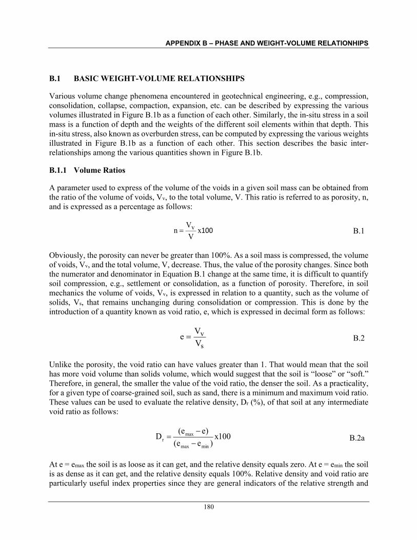
APPENDIX B – PHASE AND WEIGHT-VOLUME RELATIONHIPS
180
B.1 BASIC WEIGHT-VOLUME RELATIONSHIPS
Various volume change phenomena encountered in geotechnical engineering, e.g., compression, consolidation, collapse, compaction, expansion, etc. can be described by expressing the various volumes illustrated in Figure B.1b as a function of each other. Similarly, the in-situ stress in a soil mass is a function of depth and the weights of the different soil elements within that depth. This in-situ stress, also known as overburden stress, can be computed by expressing the various weights illustrated in Figure B.1b as a function of each other. This section describes the basic inter-relationships among the various quantities shown in Figure B.1b.
B.1.1 Volume Ratios
A parameter used to express of the volume of the voids in a given soil mass can be obtained from the ratio of the volume of voids, Vv, to the total volume, V. This ratio is referred to as porosity, n, and is expressed as a percentage as follows:
100xV
Vn v B.1
Obviously, the porosity can never be greater than 100%. As a soil mass is compressed, the volume of voids, Vv, and the total volume, V, decrease. Thus, the value of the porosity changes. Since both the numerator and denominator in Equation B.1 change at the same time, it is difficult to quantify soil compression, e.g., settlement or consolidation, as a function of porosity. Therefore, in soil mechanics the volume of voids, Vv, is expressed in relation to a quantity, such as the volume of solids, Vs, that remains unchanging during consolidation or compression. This is done by the introduction of a quantity known as void ratio, e, which is expressed in decimal form as follows:
s
vVVe B.2
Unlike the porosity, the void ratio can have values greater than 1. That would mean that the soil has more void volume than solids volume, which would suggest that the soil is “loose” or “soft.” Therefore, in general, the smaller the value of the void ratio, the denser the soil. As a practicality, for a given type of coarse-grained soil, such as sand, there is a minimum and maximum void ratio. These values can be used to evaluate the relative density, Dr (%), of that soil at any intermediate void ratio as follows:
100x)ee(
)ee(Dminmax
maxr
B.2a
At e = emax the soil is as loose as it can get, and the relative density equals zero. At e = emin the soil is as dense as it can get, and the relative density equals 100%. Relative density and void ratio are particularly useful index properties since they are general indicators of the relative strength and

APPENDIX B – PHASE AND WEIGHT-VOLUME RELATIONHIPS
181
compressibility of the soil sample, i.e., large relative densities and small void ratios generally indicate strong or incompressible soils; small relative densities and large void ratios may indicate weak or compressible soils. While the expressions for porosity and void ratio indicate the relative volume of voids, they do not indicate how much of the void space, Vv, is occupied by air or water. In the case of a saturated soil, all the voids (i.e., all the soil pore spaces) are filled with water, Vv = Vw. While this condition is true for many soils below the ground water table or below standing bodies of water such as rivers, lakes, or oceans, and for some fine-grained soils above the ground water table because of capillary action, the condition of most soils above the ground water table is better represented by consideration of all three phases where voids are occupied by both air and water. To express the amount of void space occupied by water as a percentage of the total volume of voids, the term degree of saturation, S, is used as follows:
v
wVVS x100 B.3
Obviously, the degree of saturation can theoretically never be greater than 100%. When S = 100%, all the void space is filled with water and the soil is considered to be saturated. When S = 0%, there is no water in the voids and the soil is considered to be dry.
B.1.2 Weight Ratios
While the expressions of the distribution of voids in terms of volumes are convenient for theoretical expressions, it is difficult to measure these volumes accurately on a routine basis. Therefore, in soil mechanics it is convenient to express the void space in gravimetric, i.e., weight, terms. Since, for practical purposes, the weight of air, Wa, is zero, a measure of the void space in a soil mass occupied by water can be obtained through an index property known as the gravimetric water or moisture content, w, expressed as a percentage as follows:
s
wWWw x100 B.4
The word “gravimetric” denotes the use of weight as the basis of the ratio to compute water content as opposed to volume, which is often used in hydrology and the environmental sciences to express water content. Since water content is understood to be a weight ratio in geotechnical engineering practice, the word “gravimetric” is generally omitted. Obviously, the water content can be greater than 100% on a gravimetric basis. This occurs when the weight of the water in the soil mass is greater than the weight of the solids. In such cases the void ratio of the soil is generally greater than 1 since there must be enough void volume available for the water so that its weight is greater than the weight of the solids because the unit weight of water is much less than the unit weight of the solids. However, even if the water content is greater than 100%, the degree of saturation may not be 100% because the water content is a weight ratio while saturation is a volume ratio.

APPENDIX B – PHASE AND WEIGHT-VOLUME RELATIONHIPS
182
For a given amount of soil, the total weight of soil, W, is equal to Ws + Ww, since the weight of air, Wa, is practically zero. The water content, w, can be easily measured by oven-drying a given quantity of soil to a high enough temperature so that the amount of water evaporates and only the solids remain. By measuring the weight of a soil sample before and after it has been oven dried, both W and Ws, can be determined. The water content, w, can be determined as follows since Wa = 0:
s
w
s
sWW
WWWw
x100 B.4a
Most soil moisture is released at a temperature between 220 and 230oF (105 and 110oC). Therefore, to compare reported water contents on an equal basis between various soils and projects, this range of temperature is considered to be a standard range.
B.1.3 Weight-Volume Ratios (Unit Weights) and Specific Gravity
The simplest relationship between the weight and volume of a soil mass (refer to Figure B.1b) is known as the total unit weight, t, and is expressed as follows:
VWW
VW sw
t
B.5
The total unit weight of a soil mass is a useful quantity for computations of vertical in-situ stresses. For a constant volume of soil, the total unit weight can vary since it does not account for the distribution of the three phases in the soil mass. Therefore, the value of the total unit weight for a given soil can vary from its maximum value when all of the voids are filled with water (S=100%) to its minimum value when there is no water in the voids (S=0%). The former value is called the saturated unit weight, sat; the latter value is referred to as the dry unit weight, d. In terms of the basic quantities shown in Figure B.1b and with reference to Equation B.5, when Ww = 0 the dry unit weight, d, can be expressed as follows:
VWs
d B.6
For computations involving soils below the water table, the buoyant unit weight is frequently used where:
wsatb B.7
where, w equals the unit weight of water and is defined as follows:

APPENDIX B – PHASE AND WEIGHT-VOLUME RELATIONHIPS
183
w
ww V
W B.8
In the geotechnical literature, the buoyant unit weight, b, is also known as the effective unit weight, ', or the submerged unit weight, sub. Unless there is a high concentration of dissolved salts, e.g., in sea water, the unit weight of water, w, can be reasonably assumed to be 62.4 pcf (9.81 kN/m3). To compare the properties of various soils, it is often instructive and preferable to index the various weights and volumes to unchanging quantities, which are the volume of solids, Vs, and the weight of solids, Ws. A ratio of Ws to Vs, is known as the unit weight of the solid phase, s, and is expressed as follows:
S
SS V
W B.9
The unit weight of the solid phase, s, should not be confused with the dry unit weight of the soil mass, d, which is defined in Equation B.6 as the total unit weight of the soil mass when there is no water in the voids, i.e., at S = 0%. The distinction between s and d is very subtle, but it is very important and should not be overlooked. For example, for a solid piece of rock (i.e., no voids) the total unit weight is s while the total unit weight of the same rock, if crushed, is d provided the voids are dry. In geotechnical engineering, d is more commonly of interest than s. Since the value of w is reasonably well known, the unit weight of solids, s, can be expressed in terms of w. The concept of Specific Gravity, G, is used to achieve this goal. In physics textbooks, G is defined as the ratio between the mass density of a substance and the mass density of some reference substance. Since unit weight is equal to mass density times the gravitational constant, G can also be expressed as the ratio between the unit weight of a substance and the unit weight of some reference substance. In the case of soils, the most convenient reference substance is water since it is one of the three phases of the soil and its unit weight is reasonably constant. Using this logic, the specific gravity of the soil solids, Gs, can be expressed as follows:
w
SSG
B.10
The bulk specific gravity of a soil is equal to t / w. The “bulk specific gravity” is not the same as Gs and is not very useful in practice since the t of a soil can change easily with changes in void ratio and/or degree of saturation. Therefore, the bulk specific gravity is almost never used in geotechnical engineering computations.

APPENDIX B – PHASE AND WEIGHT-VOLUME RELATIONHIPS
184
The value of Gs can be determined in the laboratory, but it can usually be estimated with sufficient accuracy for various types of soil solids. For routine computations, the value of Gs for sands composed primarily of quartz particles may be taken as 2.65. Tests on a large number of clay soils indicate that the value of Gs for clays usually ranges from 2.5 to 2.9 with an average value of 2.7.
B.1.4 Determination and Use of Basic Weight-Volume Relations
The five relationships, n, e, w, t and Gs, represent the basic weight-volume properties of soils and are used in the classification of soils and for the development of other soil properties. These properties and how they are obtained and applied in geotechnical engineering are summarized in Table B.1. A summary of commonly used weight-volume (unit weight) relations that incorporate these terms is presented in Figure B.2 and Figure B.3. In the field, the commonly measured parameters are dry unit weight, d, and water content, w. Figure B.4 presents equations based on these two parameters and unit weight of water, w. In addition to the relationships presented in Figure B.2 and Figure B.3, Equation B.11a and B.11b present relationships that can be used to quantify the percent air voids, Na, in the soil.
%100xVVN a
a B.11a
%1001
1 xwG
Nsw
da
B.11b
The relationship given by Equation B.11a is similar to that for porosity, n, given by Equation B.1, except that the numerator includes the volume of air, Va, instead of the total volume of voids, Vv. Equation B.11b is expressed in terms of the various quantities noted in Tables B.1 and B.2 and is more useful in practice. The relationship given by Equation B.11 is used in alternate compaction control specifications as discussed in Chapter 3 and shown in Figure 3.19. The percent air voids can be correlated to the degree of saturation as per Equation B.12.
ss
a wGSwGSN 1
1 B.12
Similar to the percent air voids, the water content can be expressed in volumetric terms. The volumetric water content, w, in percent can be expressed as shown in Equation B.12.
%100%100 xnSxV
Vww B.13
In seepage analysis, volumetric water content, w, is typically used instead of the gravimetric water content, w, given by Equation B.4.

APPENDIX B – PHASE AND WEIGHT-VOLUME RELATIONHIPS
185
Table B.1. Summary of Index Properties and Their Application (After FHWA, 2006).
Property Symbol Units1 How Obtained (AASHTO/ASTM)
Comments and Direct Applications
Porosity n Dim From weight-volume relations
Defines relative volume of voids to total volume of soil
Void Ratio e Dim From weight-volume relations
Volume change computations
Moisture Content w Dim By measurement
(T 265/ D4959) Classification and in weight-volume relations
Total unit weight2 γt FL-3
By measurement or from weight-volume
relations
Classification and for pressure computations
Specific Gravity Gs Dim By measurement
(T 100/D854) Volume computations Notes: 1 F=Force or weight; L = Length; Dim = Dimensionless. Although by definition, moisture content is a dimensionless
decimal (ratio of weight of water to weight of solids) and used as such in most geotechnical computations, it is commonly reported in percent by multiplying the decimal by 100.
2 Total unit weight for the same soil can vary from “saturated” (S=100%) to “dry” (S=0%).
Figure B.2. Weight-Volume Relations (After FHWA, 2006 and Jumikis, 1962)
Total Unit Weight, t Dry Unit Weight, d (No Water)
Saturated Unit Weight, sat (No Air)
w)+ n)(1 - (1G =S
wG + 1
G w)+ (1 =
e + 1Se) + G( =
e + 1G w)+ (1
=
wst
sws
t
wst
wst
wsatd
wsatd
wd
sws
d
wsd
wsd
td
e + 1e - =
n - = we) + (1
eS =
SwG + 1
G =
n) - (1G = e + 1
G =
w+ 1 =
wdsat
wdsat
wsat
wss
sat
wssat
wssat
e + 1e + =
n + = e + 1
w+ 1we =
GG w+ 1
w+ 1 =
n] + Gn) - [(1 = e + 1e) + G( =

APPENDIX B – PHASE AND WEIGHT-VOLUME RELATIONHIPS
186
Figure B.3. Weight-Volume relations for Gs, n and e for Saturated Soils (based on Jumikis, 1962).
Figure B.4. Useful Equations in Terms of 𝛄𝐰, 𝛄𝐝, and w
Figure B.5 shows the weight-volume relationships for different phases of saturated soil. Mitchell and Soga (2005) present the following equations: The volume of voids in the granular phase, eGVGS, is given as follows:
GewSGG
SWCFGSVGe
1001 B.14
The volume of water plus volume of clay is given by
wSCGSWCF
wSWw
CVWV
100100
B.15
Specific Gravity, GS Porosity, n Void Ratio, e
dw
ds
satdw
ds
wG
G
=
+ =
wd
dsat
wsd
wn
nG
n
1
1
s
dwd
dws
wGe
wwe
Ge
1
Specific Gravity, GS Porosity, n Void Ratio, e Total Unit Weight, t
dw
ds w
G
= w
dwn
dw
dw
we
)1( wdt

APPENDIX B – PHASE AND WEIGHT-VOLUME RELATIONHIPS
187
Figure B.5. Schematic. Weight-Volume Relationships for a Saturated Clay-Granular Soil Mixture (After Mitchell and Soga, 2005).
wSWw
WV
100
wSGGSWCF
GSV
1001
wSGGSWCF
CV
100
100SwW
WW
SWCFGSW
1001
SW)CF(CW
100
V Total volume of saturated soil W Total weight of saturated soil CF Clay Fraction (Percent of clay by weight) GSC Specific gravity of clay particles GSG Specific gravity of granular particles eG Void ratio of the granular phase VGS Volume of granular solids eGVGS Volume of voids in granular phase w Water content in percent w Unit weight of water
Volume
Vw
Vs V
Ve
-------------------------------------:::::::::::::::l Water F:::::::::::::::
-----------------------mm~~m~m~m~@@@@@j~m ~~~~~~ on Clay $~$~ mm (G ranular olids) mf mmmmmmmmmmmmmmmi •
--1~>---- l unit
Weight
Ww
w
w
\1/,

APPENDIX B – PHASE AND WEIGHT-VOLUME RELATIONHIPS
188
If clay and water completely fill the voids in the granular phase, then
GewSGG
SWCF
wSCGSWCF
wSWw
1001
100100 B.16
which simplifies to
SGGGeCF
SCGCFw
1001
100100 B.17
The void ratio of a granular material composed of bulky particles is of the order of 0.9 in its loosest possible state. The specific gravity of the nonclay fraction in most soils is about 2.67, and that of the clay fraction is about 2.75. Inserting these values in Eq. B.17 gives
w..CF 421448 B.18 Mitchell and Soga (2005) note that the relationship given by Equation B.18 indicates that for water contents usually encountered in practice, say 15 to 40 percent, only a maximum of about one third of the soil solids needs to be clay in order to dominate the behavior by preventing direct interparticle contact of the granular particles. In fact, since there is a tendency for clay particles to coat granular particles in most soils, the clay will significantly influence properties. For example, just 1 or 2 percent of a highly plastic clay present in a gravel used as fill or aggregate may be sufficient to clog handling and batching equipment.
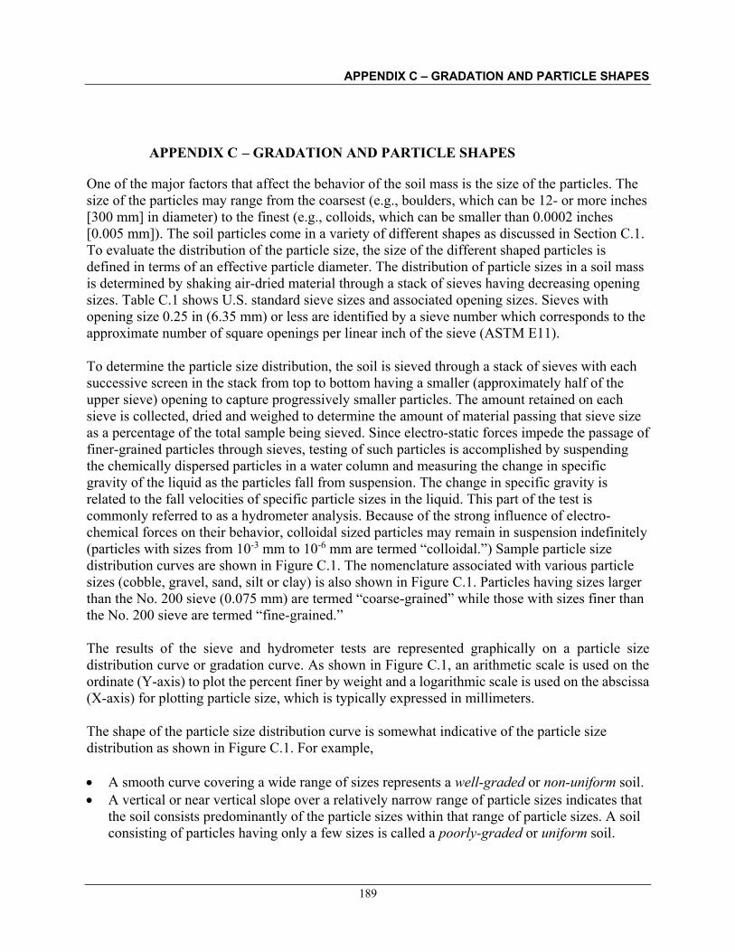
APPENDIX C – GRADATION AND PARTICLE SHAPES
189
APPENDIX C – GRADATION AND PARTICLE SHAPES
One of the major factors that affect the behavior of the soil mass is the size of the particles. The size of the particles may range from the coarsest (e.g., boulders, which can be 12- or more inches [300 mm] in diameter) to the finest (e.g., colloids, which can be smaller than 0.0002 inches [0.005 mm]). The soil particles come in a variety of different shapes as discussed in Section C.1. To evaluate the distribution of the particle size, the size of the different shaped particles is defined in terms of an effective particle diameter. The distribution of particle sizes in a soil mass is determined by shaking air-dried material through a stack of sieves having decreasing opening sizes. Table C.1 shows U.S. standard sieve sizes and associated opening sizes. Sieves with opening size 0.25 in (6.35 mm) or less are identified by a sieve number which corresponds to the approximate number of square openings per linear inch of the sieve (ASTM E11). To determine the particle size distribution, the soil is sieved through a stack of sieves with each successive screen in the stack from top to bottom having a smaller (approximately half of the upper sieve) opening to capture progressively smaller particles. The amount retained on each sieve is collected, dried and weighed to determine the amount of material passing that sieve size as a percentage of the total sample being sieved. Since electro-static forces impede the passage of finer-grained particles through sieves, testing of such particles is accomplished by suspending the chemically dispersed particles in a water column and measuring the change in specific gravity of the liquid as the particles fall from suspension. The change in specific gravity is related to the fall velocities of specific particle sizes in the liquid. This part of the test is commonly referred to as a hydrometer analysis. Because of the strong influence of electro-chemical forces on their behavior, colloidal sized particles may remain in suspension indefinitely (particles with sizes from 10-3 mm to 10-6 mm are termed “colloidal.”) Sample particle size distribution curves are shown in Figure C.1. The nomenclature associated with various particle sizes (cobble, gravel, sand, silt or clay) is also shown in Figure C.1. Particles having sizes larger than the No. 200 sieve (0.075 mm) are termed “coarse-grained” while those with sizes finer than the No. 200 sieve are termed “fine-grained.” The results of the sieve and hydrometer tests are represented graphically on a particle size distribution curve or gradation curve. As shown in Figure C.1, an arithmetic scale is used on the ordinate (Y-axis) to plot the percent finer by weight and a logarithmic scale is used on the abscissa (X-axis) for plotting particle size, which is typically expressed in millimeters.
The shape of the particle size distribution curve is somewhat indicative of the particle size distribution as shown in Figure C.1. For example, • A smooth curve covering a wide range of sizes represents a well-graded or non-uniform soil. • A vertical or near vertical slope over a relatively narrow range of particle sizes indicates that
the soil consists predominantly of the particle sizes within that range of particle sizes. A soil consisting of particles having only a few sizes is called a poorly-graded or uniform soil.

APPENDIX C – GRADATION AND PARTICLE SHAPES
190
• A curve that contains a horizontal or nearly horizontal portion indicates that the soil is deficient in the particle sizes in the region of the horizontal slope. Such a soil is called a gap-graded soil.
Table C.1. U.S. Standard Sieve Sizes and Corresponding Opening Dimension (FHWA 2006).
U.S. Standard Sieve No.1
Sieve Opening
(in)
Sieve Opening
(mm)
Comment (Based on the Unified Soil Classification System
(USCS)) 3 0.2500 6.35
4 0.1870 4.75 • Breakpoint between fine gravels and coarse sands • Soil passing this sieve is used for compaction test
6 0.1320 3.35 8 0.0937 2.36
10 0.0787 2.00 • Breakpoint between coarse and medium sands • Soil passing this sieve is used for hydrometer analysis
12 0.0661 1.70 16 0.0469 1.18 20 0.0331 0.850 30 0.0234 0.600
40 0.0165 0.425 • Breakpoint between medium and fine sands • Soil passing this sieve is used for Atterberg limits
50 0.0117 0.300 60 0.0098 0.250 70 0.0083 0.212
100 0.0059 0.150 140 0.0041 0.106 200 0.0029 0.075 • Breakpoint between fine sand and silt or clay 270 0.0021 0.053 400 0.0015 0.038
Note: 1. The sieve opening sizes for various sieve numbers listed above are based on Table 1 from ASTM E 11. Sieves
with opening size greater than No. 3 are identified by their opening size. The 3 in (76.1 mm) sieve size differentiates between cobbles and coarse gravels. The ¾ in (19 mm) sieve differentiates between coarse and fine gravels.

APPENDIX C – GRADATION AND PARTICLE SHAPES
191
Figure C.1. Schematic. Sample Particle Size Distribution Curves (After FHWA 2006).
Well-graded soils are generally produced by bulk transport processes (e.g., glacial till). Poorly graded soils are usually sorted by the transporting medium e.g., beach sands by water; loess by wind. Gap-graded soils are also generally sorted by water, but certain sizes were not transported. Particle size distribution is the single most important element in the design of structures on, in, or composed of granular soils. Much can be learned about a soil’s behavior from the shape and location of the curve. The shape of the particle-size distribution (GSD) curve or “gradation curve” as it is frequently called, is one of the more important aspects in a soil classification system for coarse-grained soils. The shape of the gradation curve can be characterized by a pair of “shape” parameters called the coefficient of uniformity, Cu, and the coefficient of curvature, Cc, to which numerical values may be assigned. By assigning numerical values to such shape

APPENDIX C – GRADATION AND PARTICLE SHAPES
192
parameters it becomes possible to compare particle-size distribution curves for different soils without having to plot them on the same diagram. In order to define shape parameters certain characteristic particle sizes must be identified that are common to all soils. Since the openings of a sieve are square, particles of many different shapes are able to pass through a sieve of given size even though the abscissa on the gradation curve is expressed in terms of particle “diameter,” which implies a spherical-shaped particle. Therefore, the “diameter” shown on the gradation curve is an effective diameter so that the characteristic particle sizes that must be identified to define the shape parameters are in reality effective grain sizes (EGS). A useful EGS for the characterizing the shape of the gradation curve is the particle size for which 10 percent of the soil by weight is finer. This EGS is labeled D10. This size is convenient because Hazen (1892, 1911) found that the ease with which water flows through a soil is a function of the D10. In other words, Hazen found that the sizes smaller than the D10 affected the permeability more than the remaining 90 percent of the sizes. Therefore, the D10 is a logical choice as a characteristic particle size. Other convenient sizes were found to be the D30 and the D60, which pertain to the particle size for which thirty and sixty percent, respectively, of the soil by weight is finer. These EGSs are used as follows in the Unified Soil Classification System (USCS) for the classification of coarse-grained soils. • Slope of the gradation curve: The shape of the curve could be defined relative to an
arbitrary slope of a portion of the gradation curve. Since one EGS has already been identified as the D10, the slope of the gradation curve could be described by identifying another convenient point (EGS) that is “higher” on the curve. Hazen selected this other convenient size as the D60 that indicates the particle size for which 60 percent of the soil by weight is finer. The slope between the D60 and the D10 can then be related to the degree of uniformity of the sample through a parameter called the “Coefficient of Uniformity” or the “Uniformity Coefficient,” Cu, which is expressed as follows:
10
60u D
DC C.1
A uniformity coefficient of unity usually means a soil in which the particles are all of
practically the same size. A large coefficient corresponds to a large range in sizes. Thus, the uniformity coefficient is large when the degree of uniformity is low.
• Curvature of the gradation curve: The second “shape” parameter is used to evaluate the
curvature of the gradation curve between the two arbitrary points, D60 and D10. A third EGS, D30, that indicates the particle size for which 30 percent of the soil by weight is finer, is chosen for this purpose. The curvature of the slope between the D60 and the D10 can then be related to the three EGS’ through a parameter called the “Coefficient of Curvature” or the “Coefficient of Concavity” or the “Coefficient of Gradation,” Cc, which is expressed as follows:
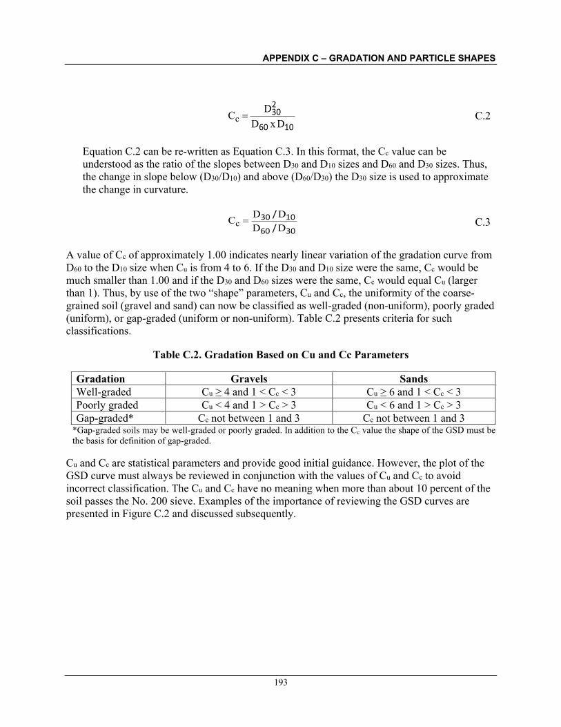
APPENDIX C – GRADATION AND PARTICLE SHAPES
193
1060
230
DxDDCc C.2
Equation C.2 can be re-written as Equation C.3. In this format, the Cc value can be
understood as the ratio of the slopes between D30 and D10 sizes and D60 and D30 sizes. Thus, the change in slope below (D30/D10) and above (D60/D30) the D30 size is used to approximate the change in curvature.
3060
1030
/
/
DDDDCc
C.3
A value of Cc of approximately 1.00 indicates nearly linear variation of the gradation curve from D60 to the D10 size when Cu is from 4 to 6. If the D30 and D10 size were the same, Cc would be much smaller than 1.00 and if the D30 and D60 sizes were the same, Cc would equal Cu (larger than 1). Thus, by use of the two “shape” parameters, Cu and Cc, the uniformity of the coarse-grained soil (gravel and sand) can now be classified as well-graded (non-uniform), poorly graded (uniform), or gap-graded (uniform or non-uniform). Table C.2 presents criteria for such classifications.
Table C.2. Gradation Based on Cu and Cc Parameters
Gradation Gravels Sands Well-graded Cu ≥ 4 and 1 < Cc < 3 Cu ≥ 6 and 1 < Cc < 3 Poorly graded Cu < 4 and 1 > Cc > 3 Cu < 6 and 1 > Cc > 3 Gap-graded* Cc not between 1 and 3 Cc not between 1 and 3
*Gap-graded soils may be well-graded or poorly graded. In addition to the Cc value the shape of the GSD must be the basis for definition of gap-graded.
Cu and Cc are statistical parameters and provide good initial guidance. However, the plot of the GSD curve must always be reviewed in conjunction with the values of Cu and Cc to avoid incorrect classification. The Cu and Cc have no meaning when more than about 10 percent of the soil passes the No. 200 sieve. Examples of the importance of reviewing the GSD curves are presented in Figure C.2 and discussed subsequently.

APPENDIX C – GRADATION AND PARTICLE SHAPES
Curve D10 (mm)
D30 (mm)
D60 (mm) Cu Cc Gradation
I 0.075 0.2 0.6 8.0 0.90 Well-graded (1) II 0.600 1.5 2 3.3 1.88 Poorly graded; Gap-graded (2) III 0.425 0.45 0.47 1.1 1.01 Poorly graded
(1) Soil does not meet Cu and Cc criteria for well-graded soil but GSD curve clearly indicates a well-graded soil
(2) The Cu and Cc parameters indicate a uniform (or poorly) graded material, but the GSD curve clearly indicates a gap-graded soil.
Note: For clarity only the D10, D30, and D60 sizes for Curve I are shown on the figure.
Figure C.2. Schematic. Evaluation of Type of Gradation for Coarse-Grained Soils.
194
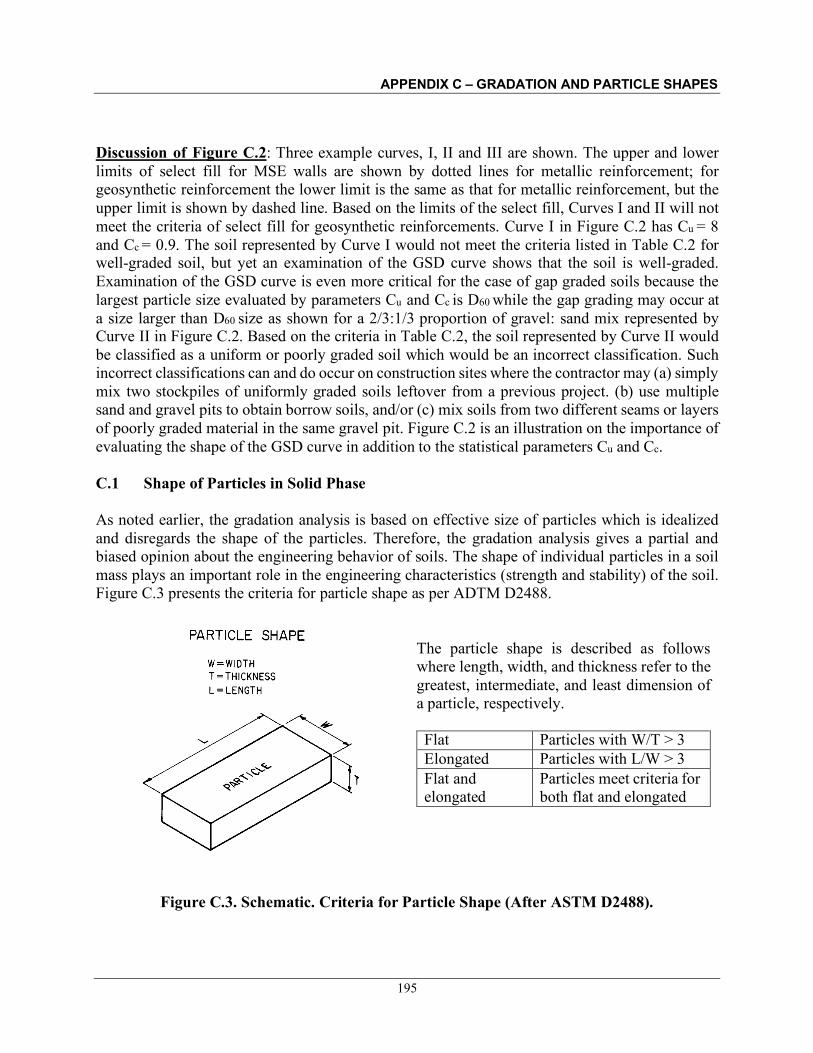
APPENDIX C – GRADATION AND PARTICLE SHAPES
Discussion of Figure C.2: Three example curves, I, II and III are shown. The upper and lower limits of select fill for MSE walls are shown by dotted lines for metallic reinforcement; for geosynthetic reinforcement the lower limit is the same as that for metallic reinforcement, but the upper limit is shown by dashed line. Based on the limits of the select fill, Curves I and II will not meet the criteria of select fill for geosynthetic reinforcements. Curve I in Figure C.2 has Cu = 8 and Cc = 0.9. The soil represented by Curve I would not meet the criteria listed in Table C.2 for well-graded soil, but yet an examination of the GSD curve shows that the soil is well-graded. Examination of the GSD curve is even more critical for the case of gap graded soils because the largest particle size evaluated by parameters Cu and Cc is D60 while the gap grading may occur at a size larger than D60 size as shown for a 2/3:1/3 proportion of gravel: sand mix represented by Curve II in Figure C.2. Based on the criteria in Table C.2, the soil represented by Curve II would be classified as a uniform or poorly graded soil which would be an incorrect classification. Such incorrect classifications can and do occur on construction sites where the contractor may (a) simply mix two stockpiles of uniformly graded soils leftover from a previous project. (b) use multiple sand and gravel pits to obtain borrow soils, and/or (c) mix soils from two different seams or layers of poorly graded material in the same gravel pit. Figure C.2 is an illustration on the importance of evaluating the shape of the GSD curve in addition to the statistical parameters Cu and Cc.
C.1 Shape of Particles in Solid Phase
As noted earlier, the gradation analysis is based on effective size of particles which is idealized and disregards the shape of the particles. Therefore, the gradation analysis gives a partial and biased opinion about the engineering behavior of soils. The shape of individual particles in a soil mass plays an important role in the engineering characteristics (strength and stability) of the soil. Figure C.3 presents the criteria for particle shape as per ADTM D2488.
The particle shape is described as follows where length, width, and thickness refer to the greatest, intermediate, and least dimension of a particle, respectively.
Flat Particles with W/T > 3 Elongated Particles with L/W > 3 Flat and elongated
Particles meet criteria for both flat and elongated
Figure C.3. Schematic. Criteria for Particle Shape (After ASTM D2488).
195
APPENDIX C – GRADATION AND PARTICLE SHAPES
196
C.1.1 Bulky Shape
Cobbles, gravel, sand and some silt particles cover a large range of sizes as shown on the x-axis of Figure C.1. In general, they are all bulky in shape. The term bulky is confined to particles that are relatively large in all three dimensions, as contrasted to platy particles, in which one dimension is small as compared to the other two, see Figure C.4. The bulky shape has four subdivisions listed in descending order of desirability for construction • Angular: As per ASTM D2488 angular particles have sharp edges and relatively plane sides
with unpolished surfaces; see Figure C.4a. These are particles are those that have been freshly broken up and are characterized by jagged projections, sharp ridges, and flat surfaces. Angular gravels and sands are generally the best materials for construction because of their interlocking characteristics. Such particles are seldom found in nature, however, because physical and chemical weathering processes usually wear off the sharp ridges in a relatively short period time. Angular material is usually produced artificially, by crushing.
• Subangular: As per ASTM D2488 subangular particles that are similar to angular description
but have rounded edges; see Figure C.4b. These are particles are those that have been weathered to the extent that the sharper points and ridges have been worn off.
• Subrounded: As per ASTM D2488 subrounded particles that have nearly plane sides but have
well-rounded corners and edges; see Figure C.4c. These particles are those that have been weathered to a further degree than subangular particles. They are still somewhat irregular in shape but have no sharp corners and few flat areas. Materials with this shape are frequently found in stream beds. If composed of hard, durable particles, subrounded material is adequate for most construction needs.
• Rounded: As per ASTM D2488 rounded particles have smoothly curved sides and no edges;
see Figure C.4d. These are particles are those on which all projections have been removed, with few irregularities in shape remaining. The particles resemble spheres and are of varying sizes. Rounded particles are usually found in or near stream beds or beaches. The rounded shape can be considered to be “Well rounded” if the few remaining irregularities have been removed. Like rounded particles, well rounded particles are also usually found in or near stream beds or beaches.
C.1.2 Platy particles
Platy, or flaky, particles are those that have flat, plate like particles. Clay and some silts are platy particles. Because of their shape, flaky particles have a greater surface area than bulky particles, assuming that the weights and volumes of the two are the same. For example, 1 gram of bentonite (commercial name for montmorillonite clay) has a surface area of approximately 950 yd2 (800 m2) compared to a surface area of approximately 0.035 yd2 (0.03 m2) of 1 gram of sand. Because of their mineralogical composition and greater specific surface area, most flaky particles also have a greater affinity for water than bulky particles. Due to the high affinity of such soils for water, the

APPENDIX C – GRADATION AND PARTICLE SHAPES
197
physical states of such fine-grained soils change with the amount of water in these soils. The effect of water on the physical states of fine-grained soils is discussed in Appendix D.
Figure C.4. Photo. Typical Angularity of Bulky Particles (After ASTM D2488).
(a) Angular (b) Subangular
(c) Subrounded (d) Rounded

APPENDIX D – EFFECT OF WATER ON PHYSICAL STATES OF SOILS
198
APPENDIX D – EFFECT OF WATER ON PHYSICAL STATES OF SOILS
For practical purposes, the two most dominant phases are the solid phase and the water phase. It is intuitive that as the water content increases, the contacts between the particles comprising the solid phase will be “lubricated.” If the solid phase is comprised of coarse particles, e.g. coarse sand or gravels, then water will start flowing between the particles of the solid phase. If the solid phase is comprised of fine-grained particles, e.g., clay or silt, then water cannot flow as freely as in the coarse-grained solid phase because pore spaces are smaller, and solids react with water. However, as the water content increases even the fine-grained solid phase will conduct water and under certain conditions the solid phase itself will start deforming like a viscous fluid, e.g., like a milk shake or a lava flow. The mechanical transformation of the fine-grained soils from a solid phase into a viscous phase is a very important concept in geotechnical engineering since it is directly related to the load carrying capacity of soils. It is obvious that the load carrying capacity of a solid is greater than that of water. Since water is contained in the void space, the effect of water on the physical states of fine-grained soils is important. Some of the basic index properties related to the effect of water are described next. The physical and mechanical behavior of fine-grained-soils is linked to four distinct states: solid, semi-solid, plastic and viscous liquid in order of increasing water content. Consider a soil initially in a viscous liquid state that is allowed to dry uniformly. This state is shown as Point A in Figure D.1, which shows a plot of total volume versus water content. As the soil dries, its water content reduces and consequently so does its total volume as the solid particles move closer to each other. As the water content reduces, the soil can no longer flow like a viscous liquid. Let us identify this state by Point B in Figure D.1. The water content at Point B is known as the “Liquid Limit” in geotechnical engineering and is denoted by LL. As the water content continues to reduce due to drying, there is a range of water content at which the soil can be molded into any desired shape without rupture. In this range of water content, the soil is considered to be “plastic.”
Figure D.1. Schematic. Conceptual Changes in Soil Phases as a Function of Water Content (FHWA 2006).

APPENDIX D – EFFECT OF WATER ON PHYSICAL STATES OF SOILS
199
If the soil is allowed to dry beyond the plastic state, the soil cannot be molded into any shape without showing cracks, i.e., signs of rupture. The soil is then in a semi-solid state. The water content at which cracks start appearing when the soil is molded is known as the “Plastic Limit.” This moisture content is shown at Point C in Figure D.1 and is denoted by PL. The difference in water content between the Liquid Limit and Plastic Limit, is known as the Plasticity Index, PI, and is expressed as follows:
PI = LL – PL D.1 Since PI is the difference between the LL and PL, it denotes the range in water content over which the soil acts as a plastic material as shown in Figure D.1. As the soil continues to dry, it will be reduced to its basic solid phase. The water content at which the soil changes from a semi-solid state to a solid state is called the Shrinkage Limit, SL. No significant change in volume will occur with additional drying below the shrinkage limit. The shrinkage limit is useful for the determination of the swelling and shrinkage characteristics of soils. The liquid limit, plastic limit and shrinkage limit are called Atterberg limits after A. Atterberg (1911), the Swedish soil scientist who first proposed them for agricultural applications. For foundation design, engineers are most interested in the load carrying capacity, i.e., strength, of the soil and its associated deformation. The soil has virtually no strength at the LL, while at water contents lower than the PL (and certainly below the SL) the soil may have considerable strength. Correspondingly, soil strength increases, and soil deformation decreases as the water content of the soil reduces from the LL to the SL. Since the Atterberg limits are determined for a soil that is remolded, a connection needs to be made between these limits and the in-situ moisture content, w, of the soil for the limits to be useful in practical applications in foundation design. One way to quantify this connection is through the Liquidity Index, LI, that is given by:
PIPLwLI
D.2
The liquidity index is the ratio of the difference between the soil’s in-situ water content and plastic limit to the soil’s plasticity index. The various phases shown in Figure D.1 and anticipated deformation behavior for remolded soils can now be conveniently expressed in terms of LI as shown in Table D.1.

APPENDIX D – EFFECT OF WATER ON PHYSICAL STATES OF SOILS
200
Table D.1. Concept of Soil Phase, Soil Strength and Soil Deformation Based on Liquidity Index for Remolded Soils (FHWA 2006).
Liquidity Index, LI Soil Phase Soil Strength
(Soil Deformation)
LI ≥ 1 Liquid Low strength (Soil deforms like a viscous fluid)
0 < LI < 1 Plastic
Intermediate strength • at w ≈ LL, the soil is considered soft and very compressible • at w ≈ PL, the soil is considered stiff (Soil deforms like a plastic material)
LI ≤ 0 Semi-solid to Solid
High strength (Soil deforms as a brittle material, i.e., sudden, fracture of material)
Another valuable tool in assessing the characteristics of a fine-grained soil is to compare the LL and PI of various soils. Each fine-grained soil has a relatively unique value of LL and PI. A plot of PI versus LL is known as the Plasticity Chart shown in Figure D.2. Arthur Casagrande, who developed the concept of the Plasticity Chart, had noted the following during the First Pan American Conference on Soil Mechanics and Foundation Engineering (Casagrande, 1959).
“I consider it essential that an experienced soils engineer should be able to judge
the position of soils, from his territory, on a plasticity chart merely on the basis of his visual and manual examination of the soils. And more than that, the plasticity chart should be for him like a map of the world. At least for certain areas of the chart, that are significant for his activities, he should be well familiar. The position of soils within these areas should quickly convey to him a picture of the significant engineering properties that he should expect.”
Casagrande proposed the inclusion of the A-line on the plasticity chart as a boundary between clay (above the A-line) and silt (below the A-line) to help assess the engineering characteristics of fine-grained soils. Once PI and LL are determined for a fine-grained soil at a specific site, a point can be plotted on the plasticity chart that will allow the engineer to develop a feel for the general engineering characteristics of that particular soil. The plasticity chart also permits the engineer to compare different soils across the project site and even between different project sites. The plasticity chart, including the laboratory determination of the various limits (LL, PL and SL), are discussed further in Chapters 4 and 5 of FHWA (2006).

APPENDIX D – EFFECT OF WATER ON PHYSICAL STATES OF SOILS
201
Figure D.2. Chart. Plasticity Chart and Significance of Atterberg Limits (NAVFAC, 1986a).

APPENDIX E – SOIL FORMATIONS AND LANDFORMS
202
APPENDIX E – SOIL FORMATIONS AND LANDFORMS
Soils are a result of the weathering of rocks. In general, rocks are classified as igneous, sedimentary, and metamorphic. Igneous rocks are products of melts (magma) generated an unknown distance below the earth’s surface. Sedimentary rocks are cemented and/or compressed materials derived from pre-existing sediments deposited in layers by water or by air. A metamorphic rock originates by a process of change from what it was previously. Any former igneous, sedimentary, or metamorphic rock can be metamorphosed (changed) into a new metamorphic rock by an increase in temperature and/or pressure and/or by reaction with surrounding hot fluids and gases. Regardless of the type of rock, most weathering generally takes place near the ground surface. Rock weathering can occur due to mechanical (physical) and/or chemical processes as follows: • Mechanical or physical process refers to the process whereby the intact rock breaks into
smaller fragments. Physical weathering may be caused by expansion resulting from unloading (e.g., exfoliation or spalling off of the exterior surface of the exposed rock), abrasion, temperature changes (e.g., freeze/thaw), erosion by wind or rain, crystal growth (e.g., ice and other crystals such as salt crystals that form as the result of the capillary action of water containing salts in solution), and organic activity (e.g., forces exerted by growing plants and roots in voids and crevasses of rock).
• Chemical process refers to the process whereby the minerals in the rock are altered into new
compounds. Chemical weathering is usually preceded by hydration and hydrolysis and may be caused by, oxidation (e.g., chemical reaction with rainwater), solution (e.g., dissolution of limestone) and/or leaching (e.g., dissolution of the cementing agent in the rock). Chemical weathering commonly occurs by fluids seeping into the fractures caused by mechanical (physical) weathering processes. These fluids are chiefly acids created as rainwater dissolves carbon dioxide from the atmosphere and more carbon dioxide and organic acids from the soil. Most chemical weathering processes result in an increase in volume (that causes an increase in stress within the rock mass), lower density materials (e.g., soils), smaller particle sizes (e.g., clay sizes), and more stable minerals (that may decrease the rate of chemical weathering).
The combined effects of the mechanical and chemical weathering processes vary considerably with climate and the mineralogy of the parent rock. The chemical reactions proceed most rapidly and completely in humid tropics and subtropics and least effectively in cold or arid climates (Goodman, 1993). Thus, in the Arctic regions and deserts, the mechanical processes of physical weathering act virtually alone to gradually breakup the rock into a fractured or rubbled mass whereas, in the tropics, the two weathering processes work together rapidly first to break up the rock and then to alter newly exposed rock surfaces during a project’s life. Once the intact rock is broken into fragments, the rate of weathering depends on the particle size and the climate. In general, small particles weather at a faster rate than large ones due to their larger surface area. The weathering processes can result in particle sizes that are not distinguishable

APPENDIX E – SOIL FORMATIONS AND LANDFORMS
203
by the naked eye (e.g., colloidal particle size) and can be identified only by equipment such as electron microscopes. Based on particle size, the principal terms used by civil engineers to describe soils are gravel, sand, silt and clay. These terms were discussed in Appendix A as a function of the particle sizes they represent and some of their physical characteristics. For example, silt and clay particles are finer than the No. 200 sieve (0.075 mm) and exhibit varying properties in the presence of water. Soils created by a particular geologic process assume characteristic topographic features, called landforms, which can be readily identified by the geotechnical specialist. A landform contains soils with generally similar engineering properties and typically extends irregularly over wide areas of a project alignment. Early identification of landforms can be used to optimize the subsurface exploration program. Landforms may be described according to the method of formation as residual soil landforms or transported (sedimentary) soil landforms. Soils commonly associated with these two types of landforms are briefly described as follows:
E.1 Residual Soils
A residual soil landform is one that was formed in its present location through weathering of the parent (or bed) rock. Residual soils tend to be characterized by angular to subangular particles, mineralogy similar to parent rock, and the presence of large angular fragments within the overall soil mass. Because residual soil weathers from parent bedrock, its profile with depth represents a history of the weathering process. Figure E.1 shows a typical weathering profile for metamorphic and igneous rocks. In Figure E.1, the weathering profile is divided into three zones: residual soil, weathered rock, and unweathered rock. Deere and Patton (1971) present 12 other weathering-profile classification systems proposed by workers from around the world. Regardless of the weathering-profile classification, the following are some of the properties for such profiles: • The permeability and shear strength gradually change with depth. These two parameters
control both the amount of rainfall infiltration and the location of the shear surface when external loads are applied on or in these soils.
• Soil profile thickness and properties depend upon parent bedrock, discontinuities, topography, and climate. Because these factors vary horizontally, the profile can vary significantly over relatively short horizontal distances.
• Deep profiles form in tropical regions where weathering agents are especially strong and advanced stages of chemical weathering form cemented soils called laterites. The technical literature often refers to residual soils as tropical soils.
• The material in the transitory zone between residual soil and unweathered rock is called saprolite. Saprolites are generally unsaturated, weakly bonded and heterogeneous soils with relict joint systems (Lambe, 1996). Saprolites have widely varying void ratios and widely varying mineralogy and shear strength (Vaughn, et al., 1988).
More information on residual soils can be found in Wesley (2010a, b).

APPENDIX E – SOIL FORMATIONS AND LANDFORMS
204
E.2 Transported (Sedimentary) Soils
A transported soil is one that was formed from rock weathering at one location and transported by some exterior agent to another location. The transporting agent may be water (principal agent), a glacier, wind, and/or gravity. Often the deposits of transported soils are given names indicative of the mode of transportation causing the deposit, e.g., alluvial deposits, glacial till, etc. Transported soils are characterized by subrounded to rounded particles and a wide variety of particle sizes. Tables E.1 to E.4 summarize commonly encountered landforms composed of transported soils, their primary formational process, and their engineering significance.
E.3 Distribution of Soil Deposits in United States
Figure E.2 shows the distribution of soil deposits in continental United States. It can be seen that approximately half of the United States has residual soils. Figure E.3 shows a similar map that provides more detail in terms of identification of specific nomenclature for soils based on their origin, e.g., A1, R2, G3, etc. The nomenclature for Figure E.3 is given in Tables E.5.to E.9. Some of the source data for Figures E.2 and E.3 are from Belcher et al. (1946) with interpretation by the authors cited in the captions of those figures. While the maps in the two figures are generally consistent, there are some significant differences. For example, the broad clay belts in southeastern Texas shown in Figure E.2 are not included in Figure E.3 where the symbol A1 appears, which signifies coastal plain alluvial soil deposits. Upon review of the characteristic soil deposits corresponding to A1 in Table E.6 it is found that the broad clay belts west of the Mississippi River shown in Figure E.2 are acknowledged. Thus, the maps in Figures E.2 and E.3 should be considered complementary. More detailed maps can be found in Leonards (1962) and Hunt (2005). Figure E.4 shows the physiographic map of United States with major cities and highways. This map can be used with the maps in Figures E.2 and E.3 and Tables E.5 to E.9 to identify features such as the Appalachian Mountains, Great Plains, etc. Based on these figures it can be seen that the area covered by residual soils (R1, R2 and R3 in Figure E.3) includes some of the major urban areas in the southeastern United States. The information in Figures E.2, E.3, and E.4 and Tables E.5 to E.9 should be used for general information and not for final design. The intent here is to show that there are many different types of soils throughout the United States and that consequently the types of LASR materials may also vary accordingly.

APPENDIX E – SOIL FORMATIONS AND LANDFORMS
205
Figure E.1. Schematic. Typical Weathering Profile for Metamorphic and Igneous Rocks (After Deere and Patton, 1971).

APPENDIX E – SOIL FORMATIONS AND LANDFORMS
206
Table E.1. Common Landforms of Water Transported Soils and Their Engineering Significance (FHWA, 2006).
Landform Formational Process and General Engineering Significance for Study Flood Plain • Formed in valleys that are nearly flat and near the high-water level of streams. At flood stage the valley is essentially a “flood
plain” that is susceptible to widespread shallow flooding. • Generally poor construction site with fine-grained soils and water problems. Potential scour area. Spread footing design below
ground will probably require undercut, low foundation pressure and scour protection. Pile foundations probable. Additional shallow explorations required along footing length to determine buried meandering channels. Historic high-water levels should be used in design.
Coastal Plain
• Formed similar to flood plain but in coastal areas. • Consider spread footings for moderate loads except for high water areas. Potential scour area. Soil “set-up” possible for
friction piles (see Chapter 9). Terraces • Formed when a stream or water body cuts into a previously deposited sediment or as the stream bed is lowered over geological
periods due to normal erosion or to crustal deformations. Terraces are also known as bajadas. • Consider spread footings for lightly loaded foundations.
Lakebed (Lacustrine,Varves)
• Formed by sedimentation in lake (fresh water) environments. Varves are a particular type of lake deposit formed during glacial periods from seasonal ice melting, which temporarily increased the runoff velocity so that precipitated sand layers alternate with layers of precipitates such as silt or silt-clay made at low velocities.
• Suitable only for spread footings to support light loads and even then settlement may be expected. Pile foundation probable and often deep. Obtain undisturbed tube samples for laboratory testing. Consider drilling with "mud" rather than casing. Long-term water observations necessary to determine static water level due to impervious soil. Potential scour area.
Deltas • Formed by sediments precipitated at the mouths of rivers or streams into bays, oceans, or lakes. • The use of spread footings must be carefully studied as poor soils often underlie deltaic sands and gravels. The parent material
is capable of sustaining high spread footing loads. Piles may be required to penetrate delta material and poor soil. Use casing of adequate size to obtain undisturbed samples of poor soil. Potential scour area.
Alluvial Fans. Filled Valleys (Basin Deposits)
• Formed similar to delta deposits, but typically found in arid areas where mountain stream runoff flows into wide valleys or on to the plains at the mouths of streams. In arid climates, alluvial fans can become cemented by salts left in the ground by evaporating water or by dropping groundwater. Cemented soils can be loose to dense (e.g., caliche) or open-graded (collapsible-susceptible).
• Consider spread footings for low to moderate loads except at lower elevation of alluvial fans where high water table is possible. In case of collapsible soils, either treat the soils such that collapse potential is mitigated or use deep foundations to bypass such soils. If the caliche is firm to hard, spread foundations can be used.

APPENDIX E – SOIL FORMATIONS AND LANDFORMS
207
Table E.2. Common Landforms of Ice (Glacier) Transported Soils and Their Engineering Significance (FHWA, 2006).
Landform Formation and General Engineering Significance for Study Moraines (Terminal, lateral)
• Formed by soil deposits pushed into ridges around the periphery of a glacier. Terminal moraines are ridges of material scraped or bulldozed to the front of a glacier; lateral moraines develop along the sides of a glacier. The moraine may not be a single nicely rolled ridge, but rather a highly serrated, above ground level, earth mass.
• Advisable to use spread footings for all foundation loads. Piles should not be used due to very difficult driving and boulders. Core all rock to 10 ft (3.0 m) in case boulders are encountered.
Glacial Till (ground moraine)
• Glacial Till (also termed ground moraine or simply till) is the deposit of ice-suspended material through the bottom of the glacier. As glaciers melted, materials suspended in the ice precipitated onto the underlying soil or rock to form glacial till. Till deposits are characterized by all sizes of particles with no obvious arrangement. Much of northern U.S. has glacial till.
• Where till is unsorted, dense and contains considerable sand and gravel, it is advisable to use spread footings for all foundation loads. Piles should not be used due to difficult driving conditions and boulders. Core all rock encountered to depth of 10 ft (3.0 m) as large boulders may be encountered. Long-term water observations necessary to determine static water level due to soil density.
Outwash • Sediments precipitated from glacial melts in the discontinuities between ridges in moraines. Small lakes may temporarily form in depressions behind ridges, producing lacustrine (fresh water) sediments.
• Spread footing normally used to support moderate to heavy foundation loads. Piles, if required, will be short. Use large diameter sample spoon to permit representative sample to be obtained as average particle size may jam 1-⅜ in (35.3 mm) sample spoon. Standard penetration test may be erratically high due to large particle sizes. Commercial value as sand and gravel sources since the material often contains very little amount of fines, i.e., particle size less than No. 200 (0.075 mm) sieve.
Eskers • Eskers are deposits (usually as ridges) formed by precipitation of water-suspended material flowing in ice tunnels. • Advisable to use spread footings for all loads as soil contains much gravel and is dense. Piles not recommended. Large diameter
sample spoon recommended as above for outwash. Commercial value as sand and gravel sources since the material often contains very little amount of fines, i.e., particle size less than No. 200 (0.075 mm) sieve.
Drumlins • Drumlins are isolated mounds of glacial debris varying from about 35 (10 m) ft to 230 ft (70 m) high and 650 ft (200 m) to 2600 ft (800 m) long. Most drumlins are of the order of 100 ft (30 m) or less in height and 1000 ft (300 m) or less in length. They often occur in groups called drumlin fields (several).
• Suitable for spread footing design with moderate to heavy loads. Piles seldom used due to dense coarse nature of subsoil. Commercial value as sand and gravel sources since the material often contains very little amount of fines, i.e., particle size less than No. 200 (0.075 mm) sieve.

APPENDIX E – SOIL FORMATIONS AND LANDFORMS
208
Table E.3. Common Landforms of Wind Transported (Aeolian) Soils and Their Engineering Significance (FHWA, 2006).
Landform Formation and General Engineering Significance for Study Loess • Formed by wind blowing silt and clay with the deposit held together by a montmorillonite binder. Generally derived from glacial
outwash in the US. Low density (often less than 90 pcf (14 kN/m3)), low wet strength (i.e., collapsible upon water ingress), has the ability to stand on vertical cuts due to cementing agents between particles.
• Consider spread footings for low to moderate loads. Heavy loads should be pile supported with the bearing resistance obtained below the loess deposit. Accurate ground water level determination important.
Sand Dune • Formed by wind action blowing the sand. Transport occurs mainly along the ground until an obstruction is met, whereupon a dune (or mound) forms. Later winds may demolish the dune and redeposit the material at a new location further downwind. Dune sands tend to be well rounded from abrasion.
• Consider spread footings for small foundations not subject to vibratory loading. Heavy structural loads should be supported on friction piles.
Table E.4. Common Landforms of Gravity Transported Soils and Their Engineering Significance (FHWA, 2006).
Landform Formation and General Engineering Significance for Study Colluvium • Formed by physical and chemical weathering of bedrock. The fragmented particles, given sufficient topographic relief, tend to
move down slopes under gravitational forces and accumulate as distinctive deposits along the lower portions of slopes, in topographic depressions, and especially at the base of cliffs.
• The characteristics of colluvial materials vary according to the characteristics of the bedrock sources and the climate under which the weathering and transport occur. From an engineering viewpoint, colluvium is weakly stratified and consists of a heterogeneous mixture of soil and rock fragments ranging in size from clay particles to rock more than 3 ft (1 m) in diameter. Because they are found along the lowest portions of valley sides, such deposits frequently need to be partially excavated to allow passage of transportation facilities. The resulting cut slopes are commonly unstable and require constant monitoring and maintenance. Colluvial soils are prone to creep (slow movement with time) and landslides are common in such soils.
Talus (Scree)
• Talus is colluvium composed of predominantly large fragments. Talus fragments can be huge boulders tens of feet across; however, a lower size limit has not been well defined. With time, the coarse fragments may degrade, or finer materials may be added by wind or water transport so that these deposits slowly become infilled with a matrix of fine-grained materials. The degree of infilling of these talus deposits may vary horizontally and vertically.
• Rock-supported talus is often inherently unstable and may be hazardous to even walk across. Furthermore, the open structure is porous. Talus deposits are not suitable for engineering structures. Talus deposits could be used to make riprap.

APPENDIX E – SOIL FORMATIONS AND LANDFORMS
209
Figure E.2. Map. Soil Deposits of the United States and Canada (After Belcher, et al., 1946 and Peck, et al., 1974).

APPENDIX E – SOIL FORMATIONS AND LANDFORMS
210
Figure E.3. Map. Soil Deposits of the United States (NAVFAC, 1971).

APPENDIX E – SOIL FORMATIONS AND LANDFORMS
211
Figure E.4. Map. Physiographic Map of the United States (http://www.bing.com).

APPENDIX E – SOIL FORMATIONS AND LANDFORMS
212
Table E.5. Distribution of Non-Soil Deposits in the United States (After NAVFAC, 1971 and Hunt, 2005).
Principal Soil
Deposits (Figure E.3)
Physiographic Province
Physiographic Features Characteristic Soil Deposits
Non-Soil Areas
Principal mountain masses
Mountains, canyons, scablands, badlands
• Locations in which soil cover is very thin or has little engineering significance because of rough topography or exposed rock.
Table E.6. Distribution of Alluvial Soil Deposits in the United States (After NAVFAC, 1971 and Hunt, 2005).
Symbol for Area in Figure E.3
Physiographic Province
Physiographic Features Characteristic Soil Deposits
A1 Coastal Plain Terraced or belted coastal plan with submerged border on Atlantic. Marine plain with sinks, swamps, and sand hills in Florida
• Marine and continental alluvium thickening seaward. • Broad clay belts west of Mississippi. • Calcareous sediments on soft and cavitated limestone in Florida.
A2 Mississippi Alluvial Plain
River floodplain and delta • Recent alluvium, fine-grained and organic in low areas, overlying clays of Coastal Plain.
A3 High Plains Section of Great Plains Province
Broad intervalley remnants of smooth fluvial plains
• Outwash mantle of silt, sand, silty clay, lesser gravels, underlain by soft shale, sandstone, and marls.
A4 Basin and Range Province
Isolated ranges of dissected block mountains separated by desert plains
• Desert plains formed principally of alluvial fans of coarse-grained soils merging to playa like deposits. Numerous non soil areas.
A5 Major Lakes of Basin and Range Province
Intermontane Pleistocene lakes in Utah and Nevada, Salton Basin in California
• Lacustrine silts and clays with beach sands on periphery. • Widespread sand areas in Salton Basin.
A6 Valleys and Basins of Pacific Border Province
Intermontane lowlands, Central Valley, Los Angeles Basin, Williamette Valley
• Valley fills of various gradations, fine-grained and sometimes organic in lowest areas near drainage system.

APPENDIX E – SOIL FORMATIONS AND LANDFORMS
213
Table E.7. Distribution of Residual Soil Deposits in the United States (After NAVFAC, 1971 and Hunt, 2005).
Symbol for Area in
Figure E.3
Physiographic Province Physiographic Features • Characteristic Soil Deposits
R1 Piedmont Province Dissected peneplain with moderate relief. Ridges on stronger rocks.
• Soils weathered in place from metamorphic and intrusive rocks (except red shale and sandstone in New Jersey).
• Generally more clayey at surface. R2 Valley and Ridge Province Folded strong and weak strata
forming successive ridges and valleys
• Soils in valleys weathered from shale, sandstone, and limestone. • Soil thin or absent on ridges.
R3 Interior low plateaus and Appalachian plateaus
Mature, desiccated plateaus or moderate relief
• Soils weathered in place from shale, sandstone and limestone.
R4 Ozark Plateau, Ouachita Province, Portions of Great Plains and Central Lowland, Wisconsin Driftless Section
Plateaus and plains of moderate relief, folded strong and weak strata in Arkansas
• Soils weathered in place from sandstone and limestone predominantly, and shales secondarily.
• Numerous non soil areas in Arkansas.
R5 Northern and Western Sections of Great Plains Province
Old plateau, terrace lands, and Rocky Mountain Piedmont
• Soils weathered in place from shale, sandstone and limestone including areas of clay-shales in Montana, South Dakota, Colorado.
R6 Wyoming Basin Elevated plains • Soils weathered in place from shale, sandstone and limestone. R7 Colorado Plateaus Dissected plateau of strong relief • Soils weathered in place from sandstone and limestone
predominantly, and shale and limestone secondarily. R8 Columbia Plateaus and
Pacific Border Province High plateaus and piedmont • Soils weathered from extrusive rocks in Columbia Plateaus and
from shale and sandstone on Pacific Border. Includes area of volcanic ash and pumice in Central Oregon.

APPENDIX E – SOIL FORMATIONS AND LANDFORMS
214
Table E.8. Distribution of Loessial Soil Deposits in the United States (After NAVFAC, 1971 and Hunt, 2005).
Symbol for Area in
Figure E.3
Physiographic Province
Physiographic Features Characteristic Soil Deposits
L1 Portion of Coastal Plain Steep bluffs on west limit with incised drainage
• 30 to 100 feet of loessial silt and sand overlying Coastal plain alluvium. Loess cover thins eastward.
L2 Southwest Section of Central Lowland. Portions of Great Plains
Broad intervalley remnants of smooth plains
• Loessial silty clay, silt, silty fine sand and clayey binder in western areas, calcareous binder in eastern areas.
L3 Snake River Plain in Columbia Plateaus
Young lava plateau • Relatively thin cover of loessial silty fine sand overlying fresh lava flows.
L4 Walla Walla Plateau of Columbia Plateaus
Rolling plateau with young incised valleys
• Loessial silt as thick as 75 feet overlying basalt. • Incised valleys floored with coarse grained alluvium.

APPENDIX E – SOIL FORMATIONS AND LANDFORMS
215
Table E.9. Distribution of Glacial Soil Deposits in the United States (After NAVFAC, 1971 and Hunt, 2005).
Symbol for Area in Figure E.3
Physiographic Province
Physiographic Features Characteristic Soil Deposits
G1 New England Province Low peneplain maturely eroded and glaciated
• Generally glacial till overlying metamorphic and intrusive rocks, frequent and irregular outcrops. Coarse, stratified drift in upper drainage systems. Varved silt and clay deposits at Portland, Boston, New York, Connecticut River Valley, Hackensack area.
G2 North Section of Appalachian Plateau, Northern Section of Central Lowland
Mature glaciated plateau in northeast, young till plains in western areas
• Generally glacial till overlying sedimentary rocks. Coarse stratified drift in drainage system. Numerous swamps and marshes in north central section. Varved silt and clay deposits at Cleveland, Toledo, Detroit, Chicago, northwest Minnesota.
G3 Areas in Southern Central Lowland
Dissected old till plains • Old glacial drift, sorted and unsorted, deeply weathered, overlying sedimentary rocks.
G4 Western area of Northern Rocky Mountains
Deeply dissected mountain uplands with intermontane basins extensively glaciated
• Varved clay, silt, and sand in intermontane basins, overlain in part by coarse grained glacial outwash.
G5 Puget Trough on Pacific Border Province
River valley system, drowned and glaciated
• Variety of glacial deposits, generally stratified, ranging from clayey silt to very coarse outwash.
G6 Alaska Peninsula Folded mountain chains or great relief with intermontane basins extensively glaciated
• In valleys and coastal area widespread deposits of stratified outwash, moraines and till.
• Numerous non soil areas. G6 Hawaiian Island Group Coral islands on the west, volcanic
islands on the east • Coral islands generally have sand cover. Volcanic ash, pumice, and
tuff overlie lava flows and cones on volcanic islands. In some areas volcanic deposits are deeply weathered.

APPENDIX F – COMPACTION CHARACTERISTICS OF SOILS
216
APPENDIX F – COMPACTION CHARACTERISTICS OF SOILS
F.1 Concept of Compaction
In the construction of highway embankments, earth dams, retaining walls, structural foundations and many other facilities, loose soils must be compacted to increase their densities. Compaction is the process of densifying soil under controlled moisture conditions by application of a given amount and type of energy. Compaction increases the density of the soil, which leads to: • an increase in the strength and stiffness characteristics of the soil, • a decrease in the amount of undesirable settlement of structures under both static and dynamic
loads, • a reduction in soil permeability, and • an increase in the stability of slopes and embankments. The density of compacted soils is measured in terms of the dry unit weight, γd, of the soil. The dry unit weight is a measure of the amount of solid materials present in a unit volume of soil. The greater the amount of solid materials, the stronger and more stable the soil will be. Pertinent parameters for evaluating the results of laboratory and field compaction tests are: • dry “density” or dry “unit weight.” • compaction water content. • type of energy input, e.g., impact, static, vibratory, kneading. • amount of energy input expressed in ft-lbs/ft3. Table F.1 presents a summary of the characteristics of the most commonly used laboratory compaction tests. Figure F.1 shows a typical hammer and a mold which is used for performing compaction tests in the laboratory. A comparison of the various values in Table F.1 reveals that the energy level in the Modified Proctor compaction (MPC) test is approximately 4.5 times that for the Standard Proctor compaction (SPC) test.
Table F.1. Characteristics of Laboratory Compaction Tests (After FHWA 2006).
Common Name
ASTM (AASHTO) Designation
Mold Diam.
(in)
Mold Height
(in)
Mold Vol. (ft3)
Hammer Wt. (lbs)
Hammer Drop Ht.
(in)
No. of Layers
Blows/ Layer
Energy (ft-lbs/ft3)
Standard Proctor
D698 (T 99) 4 4½ 1/30 5.5 12 3 25 12,375
Modified Proctor
D1557 (T 180) 4 4½ 1/30 10 18 5 25 56,250
Note: ASTM has Method A, B, and C depending on the percent passing No. 4, ⅜-in, and ¾ -in sieves, respectively. A 4-in diameter mold and 25 blows/layer are used for Methods A and B while a 6-in diameter mold and 56 blows/layer is used for Method C. AASHTO has Method A, B, C, and D. Methods A and B use materials passing No. 4 sieve while Methods C and D use materials passing the ¾ -in sieve. Methods A and C use a 4-in diameter mold and 25 blows/layer. Methods B and D while a 6-in diameter mold and 56 blows/layer.

APPENDIX F – COMPACTION CHARACTERISTICS OF SOILS
217
Figure F.1. Photo. Hammer and Mold for Laboratory Compaction Test; Tape Measure is for Scale Purpose Only (FHWA 2006).
F.2 Test Procedures
At least 3 (preferably 5) samples of the same type of soil are prepared at various water contents and compacted according to the requirements listed in Table F.1. Following compaction, the moist unit weight of the compacted soil (γt) in the mold is easily calculated as the weight of the soil (measured) divided by the volume of the mold (constant = 1/30 ft3). The water content (w) is determined as per ASTM D2216 and the dry unit weight is then calculated as (see Figure B.2 in Appendix B):
)w1(t
d
F.1
The dry unit weight (pcf (kN/m3)) for each compacted sample is plotted versus its compaction moisture content (%). The resulting curve is called a compaction curve. Figure F.2 shows compaction curves for the same soil using Standard Proctor compaction (SPC) test parameters and Modified Proctor compaction (MPC) test parameters as listed in Table 5-13. The typical compaction curves as presented in Figure F.2 have the following characteristics:
• Maximum dry density (γdmax) is the dry density corresponding to the peak of the compaction curve for a given type and amount of input energy. Note from Figure F.2, that the SPC γdmax is less than the MPC γdmax. Note from Table F.1 that although the type of energy (impact) is the same for both SPC and MPC, the amount of energy in the MPC test is 4.5 times that of the SPC test.

APPENDIX F – COMPACTION CHARACTERISTICS OF SOILS
218
• Optimum moisture content (wopt) is the compaction water content at which the soil attains its maximum dry density for a given input energy. Note from Figure F.2, that the SPC wopt is greater than the MPC wopt.
Figure F.2. Graph. Example Compaction Curves (After Holtz and Kovacs, 1981).
• Zero air voids curve is the curve that corresponds to S=100% regardless of the amount or
type of energy input. The importance of the zero-air-voids curve is that it denotes the limits of compaction, i.e., if the moisture content of a fill is too high for a given amount of input energy, the compacted fill may begin to “pump” as its voids become fully saturated with moisture. This can happen even at low moisture contents if the input energy is very large as may be the case with too many passes of a too heavy a piece of compaction equipment. Points on the zero air voids curve are calculated from the basic equation for dry unit weight given by Equation F.2 by setting S=1 and choosing arbitrary values of compaction moisture content within the range of the compaction curve.
SwG1
G)e1(
Gs
wswsd
F.2

APPENDIX F – COMPACTION CHARACTERISTICS OF SOILS
219
where: Gs = specific gravity of solid particles γw = unit weight of water e = void ratio w = water content expressed as a decimal S = degree of saturation expressed as a decimal.
Note that the S=100% (zero air voids) curve is calculated for a specific value of Gs. Curves corresponding to other degrees of saturation can be calculated in the same way by setting S=80 for the 80% saturation curve, S=60 for the 60% saturation curve and so forth. The saturation curve for a degree of saturation less than 100% is often useful for developing compaction specifications for silty soils since such soils frequently have sharply peaked compaction curves. Therefore, they can begin to “pump” even though the degree of saturation is less than 100%.
• Line of optimums - As its name suggests the “line of optimums” is obtained by passing a
curve through the peaks of the compaction curves that were developed for a certain type of soil compacted at various energy input levels. Testing laboratories frequently develop such curves for various types of soil based on information in their job files. The line of optimums can be used as a guide for developing compaction specifications where no laboratory test data are available.
• Relationship between soil air voids and degree of saturation – Figure F.3 shows the relative positions of the soil air voids (Na) line with respect to the degree of saturation lines. The zero air voids (ZAV) curve is identical to the 100% saturation curve shown in Figure F.2. However, the 10% air voids line in Figure F.3 is not the same as 90% saturation curve in Figure F.2. This is because of a difference in the fundamental definitions of percent air voids, Na, as noted in Equation B.11a in Appendix B and percent saturation as used in Equation F.2. As per Equation B.11a, the percent air voids, Na, is expressed in terms of total volume of the soil, V, while the percent saturation in Equation F.2 is expressed in terms of volume of voids, Vv as discussed in Equation B.3 in Appendix B. As shown in Figure F.3, for the case of Gs = 2.70, the 10% air voids line can correspond to a degree of saturation ranging from 60 to 80% depending on the value of the water content, w, for the range of the dry densities shown.

APPENDIX F – COMPACTION CHARACTERISTICS OF SOILS
220
Figure F.3. Graph. Soil Air Voids Curve in Relation to Degree of Saturation Curves.
Regardless of the air voids line or the degree of saturation lines, the most important concept about compaction curves as discussed above is that an increase in the amount of compaction (more energy) results in an increase in the maximum dry density and a corresponding decrease in the optimum moisture content. Therefore, this concept should be recognized when the geotechnical specialist is required to develop specifications for field compaction of soils.
F.3 Implication of Laboratory Tests on Field Compaction Specifications
With reference to Figure F.2 it is obvious that except at the peak of a given compaction curve the same dry unit weight can be obtained at two different compaction moisture contents, one below optimum and the other above optimum. For fine-grained soils this difference in moisture contents relates to a difference in soil structure that may affect engineering properties such as shear strength and permeability. It is very important that compaction specifications be given in terms of three parameters: the compaction energy (Standard or Modified Proctor), the desired dry density expressed as a percentage of the maximum dry density, and the compaction moisture content expressed as a range (+ or -) with respect to the optimum moisture content. For example, since the input energy of Modified Proctor is greater than the input energy of Standard Proctor (see Table F.1) the Modified Proctor curve plots above the Standard Proctor curve so that 95% of MPC γdmax may be greater than 100% of SPC γdmax. Likewise, a compaction moisture content of 1 or 2% above optimum for modified Proctor compaction may be below the standard Proctor optimum moisture content. Unfortunately, laboratory compaction curves mainly serve as guidelines for field compaction. This approach is inconsistent because the impact type of energy input in the laboratory is not the

APPENDIX F – COMPACTION CHARACTERISTICS OF SOILS
221
same as the type of energy delivered by the equipment commonly used in construction. Figure F.4 illustrates this point by presenting the types of compactive effort (static, vibratory, kneading) corresponding to the equipment typically used in practice. Note that none of the compaction processes in Figure F.3 involves impact type of energy that is used to determine the compaction characteristics of the soils in a laboratory SPC or MPC test. Due to the obvious disconnect between the types of energy in the laboratory and the field, some method is needed to express the laboratory-measured compaction parameters, i.e., maximum dry unit weight (γdmax) and optimum moisture content (wopt), in terms of field compaction. Most commonly, this relationship is achieved by so-called performance based or end-product specifications wherein a certain relative compaction, RC, also known as percent compaction, is specified. The RC is simply the ratio of the desired field dry unit weight, dfield, to the maximum dry density measured in the laboratory, d max, expressed in percent as follows:
%100xRCmaxd
fieldd
F.3
Figure F.4. Chart. Compactors Recommended for Various Types of Soil and Rock (Schroeder, 1980).
The relative compaction, RC, is not the same as relative density, Dr. Relative density applies only to granular soils with fines less than 12% (ASTM D2049), while relative compaction is used across a wide variety of soils. Lee and Singh (1971) published the following relationship between RC and Dr based on a statistical evaluation of 47 different granular soils compacted by using Modified Proctor energy (Wright, et al., 2003).
APPENDIX F – COMPACTION CHARACTERISTICS OF SOILS
222
Dr = 0% for RC = 80% Dr = 100% for RC = 100% Assuming a linear interpolation, the above relationship can be expressed as follows:
80]%)([RC5(%)Dr F.4 or
5(%)D80(%)RC r F.5
In terms of Standard Proctor, Equations F.4 and F.5 are approximately as follows:
85]%)([RC5(%)Dr F.6 or
5(%)D85(%)RC r F.7
Figure F.5 presents the above equations in a graphical format. Table F.2 presents the values of Dr for values of RC values ranging from 85 to 100% for MPC and from 90 to 105% for SPC.
Figure F.5 and Table F.2 indicates that for every 1% increase in RC, the increase in Dr is 5% regardless of compaction energy. This is rather significant when it is realized that the effective angle of friction (shear strength parameter), ', of granular soils is a direct function of relative density as shown in Figure F.6 and as illustrated by the following simple computations: • Based on Figure F.6, the angle of internal friction for well-graded sands (SW soils) for values
of Dr between 50% and 100% varies from 33º to 41º. From Table F.2, values of Dr between 50% and 100% correspond to RC values of 90 and 100%, respectively for Modified Proctor and 95 and 105%, respectively for Standard Proctor. In other words, for SW soils, for every 1% increase in RC, the angle of internal friction, ', increases by 0.8º.
• Alternatively, the increase in the coefficient of friction, tan' would be tan (41º)/ tan (33º) =
1.33 or a 33% increase over a 10% change in RC. In other words, there is a 3.3% increase in shear strength for every 1% increase in RC.
Select materials are often specified in the construction of transportation facilities such as embankments, foundations, and pavement sub-bases and bases. The select materials are granular
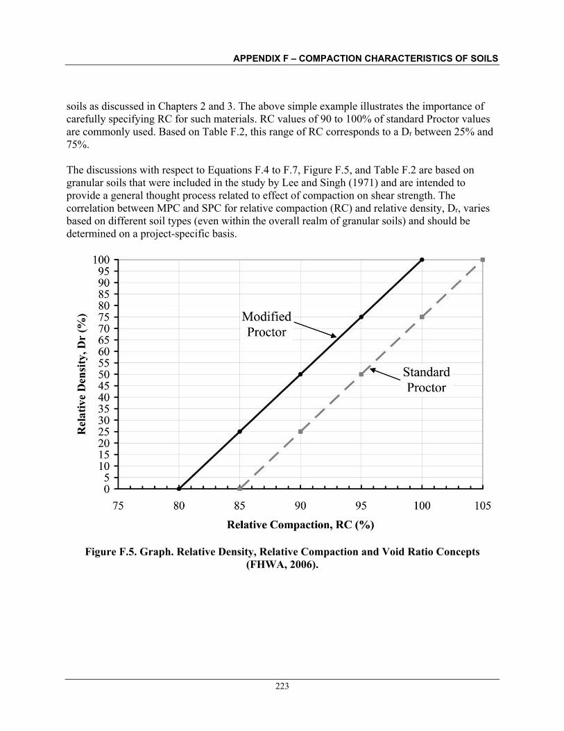
APPENDIX F – COMPACTION CHARACTERISTICS OF SOILS
223
soils as discussed in Chapters 2 and 3. The above simple example illustrates the importance of carefully specifying RC for such materials. RC values of 90 to 100% of standard Proctor values are commonly used. Based on Table F.2, this range of RC corresponds to a Dr between 25% and 75%. The discussions with respect to Equations F.4 to F.7, Figure F.5, and Table F.2 are based on granular soils that were included in the study by Lee and Singh (1971) and are intended to provide a general thought process related to effect of compaction on shear strength. The correlation between MPC and SPC for relative compaction (RC) and relative density, Dr, varies based on different soil types (even within the overall realm of granular soils) and should be determined on a project-specific basis.
Figure F.5. Graph. Relative Density, Relative Compaction and Void Ratio Concepts (FHWA, 2006).

APPENDIX F – COMPACTION CHARACTERISTICS OF SOILS
224
Table F.2. Some Values of Dr as a Function of RC Based on Modified and Standard Proctor Compaction Test (FHWA, 2006)
RC (%) MPC (SPC)*
Dr (%) RC (%) MPC (SPC)*
Dr (%) RC (%) MPC (SPC)*
Dr (%)
85 (90) 25 90 (95) 50 95 (100) 75 86 (91) 30 91 (96) 55 96 (101) 80 87 (92) 35 92 (97) 60 97 (102) 85 88 (93) 40 93 (98) 65 98 (103) 90 89 (94) 45 94 (99) 70 99 (104) 95
100 (105) 100 * MPC: Modified Proctor; SPC: Standard Proctor
Figure F.6. Chart. Correlation Between Relative Density, Material Classification and Angle of Internal Friction for Coarse-Grained Soils (After NAVFAC, 1986a).
For most transportation applications, the RC value is prescribed in performance-based specifications. In this case, it does not matter which equipment or type of compaction energy the contractor chooses to use as long as the end-product meets the specified RC. The prudent contractor would choose the equipment according to the type of soil. Often the contractor

APPENDIX F – COMPACTION CHARACTERISTICS OF SOILS
225
chooses to use the equipment he/she owns or is cheapest to lease or rent. Unfortunately, this equipment may not always be the most efficient equipment for the work. Figure F.3 can be used as a preliminary guide in selecting the type of equipment and mode of compaction energy as a function of soil type. In Figure F.3 the “100%” above the word clay on the left and the word sand on the right indicates boundaries for the range of soils types in between, e.g. 100% clay means that the soil to be compacted is all fine-grained, therefore use of a sheep-foot roller is recommended. The figure also suggests that a sheep-foot roller can be used for various soil mixtures consisting of up to approximately 35% fine-grained soils and 70 % coarse grained soils. An example of the influence of the choice of compaction equipment and energy is shown in Figure F.7. Assume that Curve 1 is obtained from laboratory tests to develop the compaction curve for a borrow material that the contractor has identified for a given project. Further assume that the specification for the project requires that RC = 90%. If M represents the point of maximum dry density, dmax, then RC=90% would mean that Points P and Y represent the limits of Curve 1 within which the contractor has to operate. In other words, the contractor cannot use compaction moisture contents less than a or c on the compaction moisture content axis. To evaluate the choice of the compaction equipment, the contractor should perform compaction tests at various RC values in the laboratory to develop a line of optimums and a family of curves similar to Curve 2 and 3 shown in Figure F.7. Once these data are developed, then it can be observed from Figure F.7, that the most economical water content would be that corresponding to point R along the line of optimums, i.e., the moisture content given by Point b on the X-axis. Point R represents the minimum compactive effort to attain RC=90%. To avoid inadequate compaction and risk failed field quality control tests, a prudent contractor usually aims to achieve somewhat higher dry density. Thus, the contractor often chooses to select a target curve similar to Curve 2 and aim to maintain moisture content in Zone B.
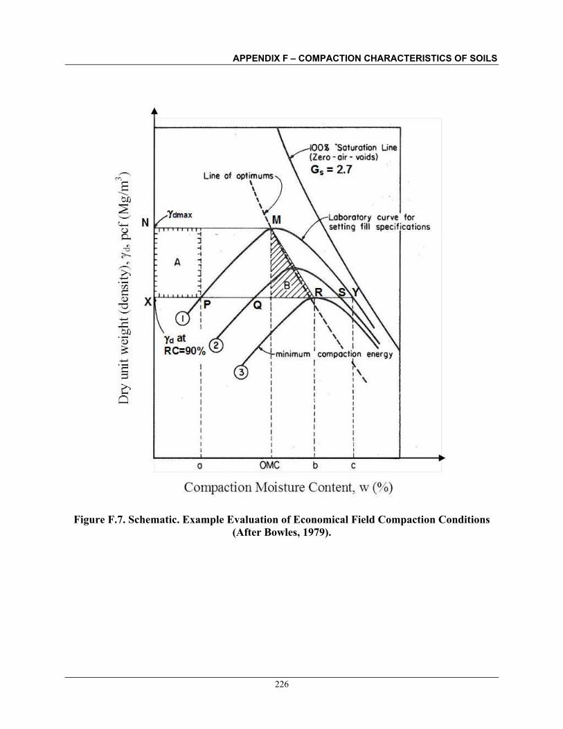
APPENDIX F – COMPACTION CHARACTERISTICS OF SOILS
226
Figure F.7. Schematic. Example Evaluation of Economical Field Compaction Conditions (After Bowles, 1979).

APPENDIX G – EXAMPLE CALCULATION
227
APPENDIX G – EXAMPLE CALCULATION
G.1 Introduction
In this appendix an example calculation is presented to demonstrate the analysis of a MSE-LASR wall with a level fill and live load surcharge. The MSE-LASR wall is assumed to include a modular block wall (MBW) unit face with extensible geogrid (geosynthetic) reinforcements. The MSE-LASR wall configuration to be analyzed is shown in Figure G.1.
Figure G.1. Schematic. Configuration Showing Various Parameters for Analysis of a MSE-LASR Wall with Level Fill and Live Load Surcharge (Not-To-Scale).
The analysis is based on various principles that are discussed in Chapter 5 in this manual and FHWA Chapter 4. Table G.1 presents a summary of steps involved in the analysis. Each of the steps and sub-steps is sequential and if the design is revised at any step or sub-step then all the previous computations need to be re-visited. Each of the steps and the sub-steps in Table G.1 is explained in detail herein. Note, that the internal stability analysis in Step 7 is based on the Simplified method. Practical considerations are presented in Section G.2 after the illustration of the step-by-step procedures. This example calculation is comparable to the example calculation E4 in FHWA Appendix E in that the same exposed wall height of 23.64 ft has been used. This was done intentionally so that the readers of this manual can have a direct comparison between a MSE-LASR system and MSE system with select fill, precast concrete facing elements and metallic reinforcements. Herein the MSE-LASR system has been analyzed using LASR fill, modular block facing elements and geogrid reinforcements.

APPENDIX G – EXAMPLE CALCULATION
228
Table G.1. Summary of Steps in Analysis of MSE-LASR Wall with Level Fill and Live Load Surcharge.
Step Item 1 Establish project requirements. 2 Establish project parameters. 3 Estimate wall embedment depth and length of reinforcements. 4 Estimate unfactored (nominal) loads. 5 Summarize applicable load and resistance factors. 6 Evaluate external stability of MSE-LASR wall.
6.1 Evaluation of sliding resistance. 6.2 Evaluation of limiting eccentricity. 6.3 Evaluation of bearing resistance. 6.4 Settlement analysis.
7 Evaluate internal stability of MSE-LASR wall using the Simplified method. 7.1 Estimate critical failure surface and variation of Kr and F* for internal stability. 7.2 Establish vertical layout of soil reinforcements. 7.3 Calculate horizontal stress and maximum tension at each level of reinforcement. 7.4 Establish nominal and factored long-term tensile resistance of soil reinforcement. 7.5 Establish nominal and factored pullout resistance of soil reinforcement. 7.6 Evaluate CDRs (Capacity:Demand Ratio) and establish geogrid grade (strength) at
each level of reinforcement. 7.7 Check direct (interface shear) sliding.
8 Evaluate facing connections. 9 Check overall (global) and compound stability at the service limit state. 10 Design wall drainage system.
Note to users: Tables G.4, G.5, G.8 through G.11, and G.15 through G.17 were generated using a spreadsheet in which numbers at all calculation steps were not rounded. Thus, the end results in these tables may be somewhat different when compared to long-form hand calculations. However, the difference should be less than 0.2 in most cases. All the long-form step-by-step calculations illustrated in Step 7 were based on hand-calculations in which numbers were rounded to the third or fourth significant digit as appropriate in each step.

APPENDIX G – EXAMPLE CALCULATION
229
STEP 1. ESTABLISH PROJECT REQUIREMENTS • Exposed wall height, He = 23.64 ft. • Length of wall = 850 ft. • Design life = 75 years. • Level backslope. • Level toe slope. • Facing: MBW units 8-in tall x 12-in deep x 18-in long. • Wall face batter: 2 degrees; assume 0 degrees (i.e., vertical face) for design. • 100% coverage ratio (Rc) of geogrid reinforcement at each level of reinforcement. Therefore,
perform analysis on per foot basis. Thus, width of facing element, wp = 1.00 ft. • Traffic surcharge. • No traffic barrier impact. • No seismic loads. • All drainage provisions as per Section 5.4 are implemented to ensure no adverse positive
pore water pressures within the wall system STEP 2. EVALUATE PROJECT PARAMETERS • Based on site-specific investigations in accordance with Table 5.2 and Section 5.3.1 of
Chapter 5, the project team has selected the following geotechnical parameters: o Reinforced fill, 'rein = 28°, rein = 125 pcf, Amount of Fines, F = 35%; pH = 7.3,
maximum particle size ¾-inch, Plasticity Index (PI) = 20, Liquid Limit (LL) = 40% o Retained fill, 'ret = 28°, ret = 125 pcf, Amount of Fines, F = 35%; pH = 7.3, maximum
particle size 3-inch, Plasticity Index (PI) = 20, Liquid Limit (LL) = 40% o Foundation soil 'fd = 30°, fd = 130 pcf; no ground water
• Interface shear friction angle between geogrid and reinforced fill soil, = 21.0°, based on
soil-geogrid direct shear tests in accordance with ASTM D5321. Note that for MSE-LASR system it is strongly recommended that interface shear friction angle be determined from soil-geogrid direct shear tests rather than using default values in FHWA (2009).
• Data for connection strength between facing blocks and geogrids based on data from past project (see Table G.17).
• Factored bearing resistance of foundation soil
o For service limit consideration, the factored bearing resistance, qnf-ser = 4.50 ksf for 1-inch of total settlement assuming length of reinforcements to be 0.85H or larger. No long-term settlement is anticipated.
o For strength limit consideration, the factored bearing resistance, qnf-str = 7.00 ksf (includes bearing resistance factor, b = 0.65) assuming length of reinforcements to be 0.85H or larger.
• Since H > 20 ft, live load surcharge, heq = 2 ft of soil per AASHTO Table 3.11.6.4-2.

APPENDIX G – EXAMPLE CALCULATION
230
STEP 3. ESTIMATE DEPTH OF EMBEDMENT AND LENGTH OF REINFORCEMENT
Based on AASHTO Table C.11.10.2.2-1, the minimum embedment depth = He/20 for walls with horizontal ground in front of wall, i.e., 1.2 ft for exposed wall height of 23.64 ft. For this design, assume embedment, d = 1.7 ft. Thus, design height of the wall, H = He + d = 23.64 ft + 1.7 ft = 25.34 ft. The choice of d = 1.7 ft is based on the consideration of the modular block height of 8-in (= 0.667 ft) so that full height blocks can be used over the entire wall height. Due to the level fill and consideration of use of LASR material, the minimum initial length of reinforcement is assumed to be 0.85H or 22 ft (rounded up to the nearest foot). This length will be verified as part of the design process. The length of the reinforcement is assumed to be constant throughout the height.
STEP 4. ESTIMATE UNFACTORED (NOMINAL) LOADS
Tables G.2 and G.3 present the equations for unfactored loads and moment arms about Point A shown in Figure G.2. The moments are a product of the respective forces and moment arms. Each force is assigned a designation representing the applicable load type as per AASHTO Tables 3.4.1-1 and 3.4.1-2.
Table G.2. Equations for Computing Unfactored (Nominal) Vertical Forces and Moments.
Vertical Force (Force/length units)
LRFD Load Type
Moment arm (Length units) @ Point A
V1 = (γrein)(H)(L) EV L/2 VS = (γrein)(heq)(L) = (q)L LL L/2
Note: heq is the equivalent height of soil such that q = (γrein)(heq).
Table G.3. Equations for Computing Unfactored (Nominal) Horizontal Forces and Moments.
Horizontal Force (Force/length)
LRFD Load Type
Moment arm (Length units)
@ Point A F1 = ½(Karet)[(γret)H2 EH H/3 F2 = (Karet)[(γret)(heq)](H) LL H/2

APPENDIX G – EXAMPLE CALCULATION
231
Figure G.2. Schematic. Legend for Computation of Forces and Moments (Not-To-Scale) (After FHWA, 2009).
(a)
(b)
A
A
VS = qL
Retained fill 'ret, γret
Reinforced fill 'rein, γrein
Karet
½ retH2Karet
Retained fill 'ret, γret
rein H L
rein Z L
Reinforced fill 'rein, γrein
Max Stress: v = rein Z + q + v Pullout: v = rein Z + v
A

APPENDIX G – EXAMPLE CALCULATION
232
To compute the numerical values of various forces and moments, the parameters provided in Step 1 and Step 2 are used. As per FHWA (2009) walls with face batter of up to 10o are considered to be vertical for evaluation of the lateral active earth pressure coefficients. Using the values of the various friction angles, the coefficients of lateral active earth pressure are as follows: • Karein = (1 – sin28°)/(1 + sin28°) = 0.361
• Karet = (1 – sin28°)/(1 + sin28°) = 0.361 For the example calculation, Tables G.4 and G.5 summarize the numerical values unfactored (nominal) forces and moments, respectively, based on the equations, various dimensions and values of lateral earth pressure coefficients presented above. Refer to Figure G.2 for notations of various forces. The unfactored (nominal) forces and moments in Tables G.4 and G.5 form the basis of all computations in this example calculation. The unfactored (nominal) forces and moments should be multiplied by the appropriate load factors based on the load types identified in the second column of the Tables G.2 and G.3 to perform the analysis for various load combinations such as Strength I, Service I, etc. The load factors for various load types relevant to this example calculation are discussed in Step 5.
Table G.4. Unfactored (Nominal) Vertical Forces and Moments.
Vertical Force
Value k/ft
Moment Arm @
Point A, ft Moment
Moment at Point A, k-ft/ft
V1 = 69.69 11.00 MV1 = 766.54 VS = 5.50 11.00 MVs = 60.50
Note: VS is based on heq of 2 ft per AASHTO Table 3.11.6.4-1.
Table G.5. Unfactored (Nominal) Horizontal Forces and Moments.
Horizontal Force
Value k/ft
Moment Arm @
Point A, ft Moment
Moment at Point A,
k-ft/ft F1 = 14.49 8.45 MF1 = 122.37 F2 = 2.29 12.67 MF2 = 28.98

APPENDIX G – EXAMPLE CALCULATION
233
STEP 5. SUMMARIZE APPLICABLE LOAD AND RESISTANCE FACTORS Table G.6 summarizes the load factors for the various LRFD load type shown in second column of Tables G.2 and G.3. Throughout the computations in this example calculation, the forces and moments in Tables G.4 and G.5 should be multiplied by appropriate load factors. For example, if computations are being done for Strength I (maximum) load combination, the forces and moments corresponding to load V1 should be multiplied by 1.35 which is associated with load type EV assigned to load V1.
Table G.6. Summary of Applicable Load Factors.
Load Combination Load Factors
(After AASHTO, 2014 Tables 3.4.1-1 and 3.4.1-2) EV EH LS (due to LL)
Strength I (maximum) 1.35 1.50 1.75 Strength I (minimum) 1.00 0.90 1.75 Service I 1.00 1.00 1.00
For computation of factored resistances during evaluation of strength limits states, appropriate resistance factors have to be used. Table G.7 summarizes the applicable resistance factors. For service limit state, all resistance factors are equal to 1.0.
Table G.7. Summary of Applicable Resistance Factors.
Item Resistance Factors
Reference: AASHTO
Reference: This
Manual Sliding of MSE-LASR wall on foundation soil = 0.70 See Note 1 Figure 5.1 Bearing resistance b = 0.65 Table 11.5.7-1 Table 3.6 Limiting eccentricity (for walls on soils) See Note 2 Table 11.5.7-1 Table 3.6 Tensile resistance (for geogrids) t = 0.80 Table 11.5.7-1 Table 3.7 Pullout resistance (for geogrids) p = 0.90 Table 11.5.7-1 Table 3.7 Connection resistance (for geogrids) c = 0.80 Table 11.5.7-1 Table 3.7 Direct (interface shear) sliding at reinforcement-soil interface DS = 1.00 See Note 3 Section
5.3.3.5 Notes: 1. AASHTO (2020) does not address MSE-LASR walls and therefore the sliding resistance factor provided in
AASHTO Table 11.5.7-1 is not applicable. Based on Figure 5.1 in this report, = 1.214 – 0.014(F) = 1.214 – 0.014(35) = 0.724; use = 0.70.
2. For limiting eccentricity (external stability) of walls on soils, the computed eccentricity, e, shall be less that the value of e/L < 0.33 as per AASHTO Article 11.6.3.3 or Table 3.6 of this report.
3. AASHTO (2020) does not provide a resistance factor for direct (interface shear) sliding at reinforcement-soil interface. AASHTO Table 11.5.7-1 provides a value of 1.00 for sliding for external stability. A value of 1.00 is recommended in Section 5.3.3.5 of this report.

APPENDIX G – EXAMPLE CALCULATION
234
STEP 6. EVALUATE EXTERNAL STABILITY OF MSE-LASR WALL
The external stability of MSE-LASR wall is a function of the various forces and moments shown in Figure G.2. In the LRFD context the forces and moments need to be categorized into various load types. The primary load types for this example calculation are soil loads (EV, EH) and live load (LL) which is represented as live load surcharge (LS).
6.1 Sliding Resistance at Base of MSE-LASR Wall
The purpose of these computations is to evaluate the sliding resistance at the base of the MSE-LASR wall. Since the computations are related to sliding resistance, the beneficial contribution of live load to resisting forces and moments is neglected. The computations for sliding resistance at the base of the MSE-LASR wall are illustrated in Table G.8 and Table G.8-1. Note that sliding resistance is a strength limit state check and therefore service limit state calculations are not performed. Since the friction angle of foundation soil, 'fd, is larger than the friction angle for reinforced soil, 'rein, the sliding check will be performed using 'rein = 28º . The critical values based on max/min result in the extreme force effect govern the sliding mode of failure and are shown in Table G.8-1. The value of CDR based on the critical max/min combination is 1.01 which is larger than the acceptable value of 1.0. Thus, the MSE-LASR wall can be considered to be safe against the sliding limit state (failure mode).
Table G.8. Computations for Evaluation of Sliding Resistance of MSE-LASR Wall.
Item Unit Str I (max)
Str I (min) Ser I
Factored lateral load on the MSE-LASR wall, HFL = F1+F2 k/ft 25.73 17.04 NA
Factored vertical load at base of MSE-LASR wall without LL surcharge = V1 k/ft 94.07 69.69 NA
Nominal sliding resistance at base of MSE-LASR wall, HNR = tan(28º)(V1) k/ft 50.02 37.05 NA
Factored sliding resistance at base of MSE-LASR wall, HFR= (HNR) k/ft 35.01 25.94 NA
Is HFR > HFL? - Yes Yes NA Capacity:Demand Ratio (CDR) = HFR:HFL dim 1.36 1.52 NA
Table G.8-1. Critical Values for Sliding Resistance Based on Max/Min in Table G.8
Item Unit Critical Value Minimum HFR (HFRmin) k/ft 25.94 Maximum HFL (HFLmax) k/ft 25.73 Is HFRmin > HFLmax? - Yes Capacity:Demand Ratio (CDR) = HFRmin:HFLmax dim 1.01

APPENDIX G – EXAMPLE CALCULATION
235
6.2 Limiting Eccentricity at Base of MSE-LASR Wall
The purpose of these computations is to evaluate the limiting eccentricity at the base of the MSE-LASR wall. Since the computations are related to limiting eccentricity, the beneficial contribution of live load to resisting forces and moments is neglected. The computations for limiting eccentricity at the base of the MSE-LASR wall are illustrated in Table G.9 and Table G.9-1. Limiting eccentricity is a strength limit state check and therefore service limit state calculations are not performed. The critical values based on max/min result in the extreme force effect and govern the limiting eccentricity mode of failure and are shown in Table G.9-1. For the critical values based on max/min, the value of eL/L is 0.15 which is less than 0.33 required by Note 1 in Table G.7 and hence the MSE-LASR wall can be considered to be safe against the overturning limit state (failure mode).
Table G.9. Computations for Evaluation of Limiting Eccentricity for MSE-LASR Wall.
Item Unit Str I (max)
Str I (min) Ser I
Total factored vertical load at base of MSE-LASR wall without LL, VA = V1 k/ft 94.07 69.69 N/A
Resisting factored moments about Point A without LL surcharge= MRA = MV1 k-ft/ft 1034.82 766.54 N/A
Overturning factored moments about Point A = MOA = MF1+MF2 k-ft/ft 234.27 160.84 N/A
Net factored moment about Point A = MA = MRA – MOA k-ft/ft 800.56 605.69 N/A Location of the resultant force on base of MSE-LASR wall from Point A, a = MA/VA ft 8.51 8.69 N/A
Eccentricity at base of MSE-LASR wall, eL = L/2 – a ft 2.49 2.31 N/A Limiting eccentricity, e = L/3 for strength limit state ft 7.33 7.33 N/A Is the resultant within limiting value of e? - Yes Yes N/A Calculated eL/L - 0.11 0.10 N/A
Table G.9-1. Critical Values for Limiting Eccentricity Based on Max/Min in Table G.9
Item Unit Critical Value Max overturning factored moments about Point A, MOA-C k-ft/ft 234.27 Min resisting factored moments about Point A, MRA-C k-ft/ft 766.54* Net factored moment about Point A, MA-C = MRA-C - MOA-C k-ft/ft 532.27 Vertical factored force, VA-C k/ft 69.69* Location of resultant from Point A, anl = MA-C/VA-C ft 7.64 Eccentricity from center of wall base, eL=0.5(L) - anl ft 3.36 Limiting eccentricity, e = L/3 ft 7.33 Is the limiting eccentricity criterion satisfied? - Yes Effective width of base of MSE-LASR wall, B' = L-2eL ft 15.28 Calculated eL/L - 0.15
Note: *766.54 and 69.69 are consistent values based on the mass of reinforced soil block.

APPENDIX G – EXAMPLE CALCULATION
236
6.3 Bearing Resistance at Base of MSE-LASR Wall
For bearing resistance computations, the effect of live load is included since it creates larger bearing stresses. The equivalent uniform (“Meyerhof”) bearing stress at the base of the MSE-LASR wall, v, can be computed as follows:
Lv e2L
V
where ΣV = R = V1 + VS is the resultant of vertical forces and the load eccentricity eL is calculated by principles of statics using appropriate loads and moments with the applicable load factors. In LRFD, σv is compared with the factored bearing resistance when computed for strength limit state and used for settlement analysis when computed for service limit state. The various computations for evaluation of bearing resistance are presented in Table G.10 and Table G.10-1. The Strength I (max) load combination results in the extreme force effect in terms of maximum bearing stress and therefore governs the bearing resistance mode of failure. This is confirmed by the computations in Table G.10-1 where the CDR value is 1.42 which is larger than CDR=1.18 for the Strength I (max) load combination. The Service I load combination is evaluated to compute the bearing stress for settlement analysis. The CDR based on Strength I (max) load combination is 1.18 which is larger than the minimum acceptable value of 1.0. Thus, the MSE-LASR wall can be considered to be safe against the bearing resistance limit state (failure mode).
6.4 Settlement Analysis
Settlement is evaluated at Service I Limit State. From Step 2, the estimated relevant factored settlement under a bearing stress of 4.50 ksf is 1.00 in. From Table G.10, the bearing stress for Service I limit state is 4.18 ksf. Therefore, the relevant factored settlement will be less than 1.00 in and hence acceptable.

APPENDIX G – EXAMPLE CALCULATION
237
Table G.10. Computations for Evaluation of Bearing Resistance for MSE-LASR Wall.
Item Unit Str I (max)
Str I (min) Ser I
Total factored vertical load at base of MSE-LASR wall including LL on top, ΣV = R = V1 + VS k/ft 103.70 79.31 75.19
Resisting factored moments @ Point A on the MSE-LASR wall, MRA = MV1+MVS k-ft/ft 1140.70 872.41 827.04
Overturning factored moments @ Point A on the MSE-LASR wall, MOA = MF1+MF2 k-ft/ft 234.27 160.84 151.35
Net factored moment at Point A, MA = MRA - MOA k-ft/ft 906.43 711.57 675.69 Location of Resultant from Point A, a = MA/ΣV ft 8.74 8.97 8.99 Eccentricity from center of wall base, eL = 0.5(L) – a ft 2.26 2.03 2.01 Limiting eccentricity, e = L/3 for strength limit states and e= L/6 for service limit state ft 7.33 7.33 3.67
Is the resultant within limiting value of eL? - Yes Yes Yes Effective width of base of MSE-LASR wall, B' = L-2eL ft 17.48 17.94 17.97 Bearing stress due to MSE-LASR wall =ΣV/(L-2eL)=v ksf 5.93 4.42 4.18 Bearing resistance, (qnf-str for strength) or (qnf-ser for service) (given) ksf 7.00 7.00 4.50
Is bearing stress less than the bearing resistance? - Yes Yes Yes Capacity:Demand Ratio (CDR) = qnf:σv dim 1.18 1.58 1.08
Table G.10-1. Critical Values for Bearing Resistance Based on Max/Min in Table G.10
Item Unit Critical Value Min resisting factored moments about Point A, MRA-C k-ft/ft 872.41* Max overturning factored moments about Point A, MOA-C k-ft/ft 234.27 Net factored moment about Point A, MA-C = MRA-C - MOA-C k-ft/ft 638.14 Vertical factored force, ΣVC k/ft 79.31* Location of resultant from Point A, a = MA-C/ΣVC ft 8.05 Eccentricity from center of wall base, eL = 0.5(L) – a ft 2.95 Limiting eccentricity, e = L/3 ft 7.33 Is the limiting eccentricity criterion satisfied? - Yes Effective width of base of MSE-LASR wall, B' = L-2eL ft 16.09 Factored bearing stress, ΣVC / (L-2eL) = v-c ksf 4.93 Factored bearing resistance, qnf-str (given) ksf 7.00 Is factored bearing stress < factored bearing resistance? dim Yes Capacity:Demand Ratio (CDR) = qnf-str:σv-c dim 1.42
Note: *872.41 and 79.31 are consistent values based on the mass of reinforced soil block.

APPENDIX G – EXAMPLE CALCULATION
238
STEP 7: EVALUATE INTERNAL STABILITY ANALYSIS OF MSE-LASR WALL
7.1 Estimate Critical Failure Surface, Variation of Kr and F* for Internal Stability
For the case of extensible geogrid (geosynthetic) reinforcements, the profile of the critical failure surface, the variation of internal lateral horizontal stress coefficient, Kr, and the variation of the pullout resistance factor, F*, are as shown in Figure G.3 wherein other definitions such as measurement of depth, Z, and height, H, are also shown. It should be noted that the variation of Kr and F* are with respect to depth Z that for this example is measured from top of the reinforced soil zone. The value of Karein is based on the angle of internal friction of the reinforced fill, 'rein, and is equal to Karein = 0.361 calculated in Step 4. Thus, the value of Kr varies from 1.0(0.361) = 0.361 at Z=0 to 1.0(0.361) = 0.361 at Z =20 ft, i.e., the value of Kr is constant with depth, Z. The value of F* is equal to 0.67(tan 'rein) = 0.67(tan ) = 0.356 and is constant with depth as shown in Figure G.3.
Figure G.3. Schematic. Geometry Definition, Location of Critical Failure Surface and Variation of Kr and F* Parameters for Geogrid Reinforcements.
z
Z=20 ft
Kr Z=0 Z=0
1.0 Ka
0.356
0 ft
z
0.356
F* 1.0 Ka
Z=2
Notes: 1. In this example calculation, the backfill is level, i.e., =0. 2. The Kr and F* profiles start at Z = 0 where Z is the depth below the top of the reinforced soil zone
as shown in the figure.
Z

APPENDIX G – EXAMPLE CALCULATION
239
7.2 Establish Vertical Layout of Soil Reinforcements
The MBW face units are 8 inches tall. The vertical layout of the soil reinforcements should be in multiples of 8 inches. The upper layer of geogrid will be 8 inches below the top of wall, and the bottom layer of geogrid will be 8 inches above the leveling pad. The vertical spacing was chosen based on a vertical spacing, Sv, of approximately 16 inches (1.333 ft) or two times 8 inches so that the reinforcement levels are in multiple of the MBW unit height. Using the definition of depth Z as shown in Figure G.3 the vertical layout of the soil reinforcements chosen is shown in the second column of Table G.11. This layout leads to 19 levels of reinforcement. The vertical spacing near the top and bottom of the walls are locally adjusted as necessary to fit the height of the wall.
For internal stability computations, each layer of reinforcement is assigned a tributary area, Atrib as follows
Atrib = (wp)(Svt)
where wp is a unit-width or the width of the facing element and Svt is the vertical tributary spacing of the reinforcements based on the location of the reinforcements above and below the level of the reinforcement under consideration. The computation of Svt is summarized in Table G.11 wherein Svt = Z+ – Z-. Since a 100% coverage of reinforcement at each level will be used,the analysis is performed on a per foot (unit-width) basis which leads to wp = 1.00 ft per Step 1.An example computation of Z- and Z+ in Table G.11 is shown below for Level 8.
Z- = 10.00 ft – 0.5(10.00 ft - 8.67 ft) = 9.33 ftZ+ = 10.00 ft + 0.5(11.34 ft – 10.00 ft) = 10.67 ft
7.3 Calculate Horizontal Stress and Maximum Tension at Each Level of Reinforcement
The horizontal spacing of the reinforcements is based on the maximum tension, Tmax, at each level of reinforcements which requires computation of the horizontal stress, σH, at each reinforcement level. The reinforcement tensile and pullout resistances are then compared with Tmax and an appropriate reinforcement pattern is adopted. This section demonstrates the calculation of horizontal stress, σH, and maximum tension, Tmax.
The total horizontal stress, σH, at any depth within the MSE-LASR wall is based on only the soil load as noted in the equation below and summarized in Table G.12.
σH = σH-soil + σH-surcharge

APPENDIX G – EXAMPLE CALCULATION
240
Table G.11. Summary of Computations for Svt and Atrib.
Level Z (ft) Z (ft) Z (ft) Svt (ft) Atrib (ft2)
1 0.67 0.00 1.33 1.334 1.334 2 2.00 1.33 2.67 1.333 1.333 3 3.33 2.67 4.00 1.333 1.333 4 4.67 4.00 5.33 1.333 1.333 5 6.00 5.33 6.67 1.333 1.333 6 7.33 6.67 8.00 1.333 1.333 7 8.67 8.00 9.33 1.333 1.333 8 10.00 9.33 10.67 1.333 1.333 9 11.33 10.67 12.00 1.333 1.333 10 12.67 12.00 13.33 1.333 1.333 11 14.00 13.33 14.67 1.333 1.333 12 15.33 14.67 16.00 1.333 1.333 13 16.67 16.00 17.33 1.333 1.333 14 18.00 17.33 18.67 1.333 1.333 15 19.33 18.67 20.00 1.333 1.333 16 20.67 20.00 21.33 1.333 1.333 17 22.00 21.33 22.67 1.333 1.333 18 23.33 22.67 24.00 1.333 1.333 19 24.67 24.00 25.34 1.340 1.340
Table G.12. Summary of Load Components Leading to Horizontal Stress.
Load Component Load Type Horizontal Stress Soil load from reinforced mass, σv-soil EV σH-soil = [Kreinσv-soil]γP-EV Surcharge traffic live load, q EV σH-surcharge = [Kreinq]γP-EV
Using the unit weight of the reinforced soil mass and heights Z and heq, the equation for total horizontal stress at any depth Z within the MSE-LASR wall can be written as follows (also see FHWA Chapter 4): σH = Kr (rein Z) γP-EV + Kr (rein heq) γP-EV = Kr [rein (Z + heq) γP-EV] In the above equation the maximum value of γP-EV is used. Once the total horizontal stress is computed at any given level of reinforcement, the maximum tension, Tmax, is computed as follows:
APPENDIX G – EXAMPLE CALCULATION
241
Tmax = (σH)(Atrib) where Atrib is the tributary area for the soil reinforcement at a given level as discussed in Section 7.2 and given in Table G.11. The computations for Tmax are illustrated at Z = 10.00 ft which is Level 8 in the assumed vertical layout of reinforcement shown in Table G.11. Assume Strength I (max) load combination for illustration purposes and use appropriate load factors from Table G.6.
• At Z = 10.00 ft, the following depths are computed: Z = 9.33 ft (from Table G.11) Z = 10.67 ft (from Table G.11)
• The value of Kr = 0.361 is constant with depth as shown in Figure G.3.
• Compute σH-soil = [Kr σv-soil]γP-EV as follows:
γP-EV = 1.35 from Table G.6. At Z = 9.33 ft,
v-soil(Z-) = (0.125 kcf)(9.33 ft) = 1.17 ksf σH-soil(Z-) = [Kr(z-)σv-soil(z-)]γP-EV = (0.361)(1.17 ksf)(1.35) = 0.57 ksf At Z = 10.67 ft,
v-soil(Z+) = (0.125 kcf)(10.67 ft) = 1.33 ksf σH-soil(Z+) = [Kr(z+)σv-soil(z+)]γP-EV = (0.361)(1.33 ksf)(1.35) = 0.65 ksf σH-soil = 0.5(0.57 ksf + 0.65 ksf) = 0.61 ksf
• Compute σH-surcharge = [Kr q] γP-EV as follows: γP-EV = 1.35 from Table G.6 q = (γrein)(heq) = (0.125 kcf)(2.00 ft) = 0.25 ksf At Z = 9.33 ft, σH-surcharge(Z-) = [Kr(Z-) q] γP-EV = (0.361)(0.25 ksf)(1.35) = 0.12 ksf
At Z = 10.67 ft, σH-surcharge(Z+) = [Kr(Z+) q] γP-EV = (0.361)(0.25 ksf)(1.35) = 0.12 ksf
σH-surcharge = 0.5(0.12 ksf + 0.12 ksf) = 0.12 ksf
• Compute σH = σH-soil + σH-surcharge as follows: σH = 0.61 ksf + 0.12 ksf = 0.73 ksf
• Based on Table G.11, the vertical tributary spacing at Level 8 is Svt = 1.333 ft

APPENDIX G – EXAMPLE CALCULATION
242
• The unit-width, wp, is 1.00 ft (use per foot basis since there will be 100% reinforcement coverage ratio)
• The tributary area, Atrib, is computed as follows: Atrib = (1.333 ft)(1.00 ft) = 1.333 ft2
• The maximum tension at Level 8 is computed as follows: Tmax = (σH)(Atrib) = (0.73 ksf)(1.333 ft2) = 0.97 k/ft width of wall face
Using similar computations, the various quantities can be developed at other levels of reinforcements and load combinations.
7.4 Establish Nominal and Factored Long-term Tensile Resistance of Soil Reinforcement
Geogrid soil reinforcement will be used. Three grades, or strengths, of geogrid may be used. The grades, ultimate tensile strengths, and pullout scale correction factors for these geogrids are summarized in Table G.13.
Table G.13. Geogrid Grades (Strengths) and Scale Correction Factors.
Name (Grade): GG-I GG-II GG-III Ultimate Tensile Strength (lbs/ft): 3,000 6,000 9,000 Pullout scale correction factor, (based on laboratory data) 0.80 0.80 0.80
The nominal long-term geosynthetic reinforcement strength, Tal, per FHWA Equation 3-12, is given as follows:
DCRID
ultultal RFRFRF
TRFTT
Where RFID is the reduction factor for installation damage, RFCR is the reduction factor for creep, RFD is the reduction factor for durability and RF is the total reduction factor which is numerically the product of the three reduction factors are shown in the equation. The procedure and discussion on definition of nominal long-term reinforcement design strength (Tal), for geosynthetic reinforcements, are presented in FHWA Section 3.5. The factored tensile resistance is the product of the nominal long-term strength and applicable resistance factor, t. The resistance factors for tensile rupture of MSE-LASR wall soil reinforcements are summarized in Table G.7. The resistance factor for tensile resistance of geosynthetic reinforcement is t = 0.90. As per FHWA Equation 4-33 the factored tensile resistance of reinforcement, Tr, is as follows: Tr = t (Tal)

APPENDIX G – EXAMPLE CALCULATION
243
The strength reduction factors, nominal resistance, and factored resistance for the three grades of geogrids are summarized in Table G.14.
Table G.14. Geogrid Nominal and Factored Resistances.
Parameter Geogrid GG-I Geogrid GG-II Geogrid GG-III Tult (lbs/ft) 3,000 6,000 9,000 Durability, RFD 1.15 1.15 1.15 Installation, RFID 1.30 1.30 1.20 Creep, RFCR 1.85 1.85 1.85 Tal (lbs/ft) 1,085 2,169 3,525 Tr = t (Tal) [lb/ft] 868 1,735 2,820 Tr = t (Tal) [k/ft] 0.868 1.735 2.820
Note: The values of RFD, RFID and RFCR are assumed for this example. For actual projects use project-specific values.
7.5 Establish Nominal and Factored Pullout Resistance of Soil Reinforcement
The nominal pullout resistance, Pr, of geogrid reinforcement is based on various parameters in the following equation: Pr = (F*)(2b)(Le)[(σv-soil)(γP-EV)] In the above equation, the contribution of live load is not included as per Figure G.2b. The computations for Pr are illustrated at Z = 10.00 ft which is Level 8 as measured from top of the wall. Assume Strength I (max) load combination for illustration purposes and use appropriate load factors from Table G.6.
• The value of F*= 0.356 remains constant with depth as shown in Figure G.3. Thus, at Z = 10.00 ft, F* = 0.356.
• Compute effective length Le as follows:
Le = L – [(H-Z)/(tan(45o + 'rein/2))] Le = 22 ft – [(25.34 ft – 10.00 ft)/(1.664)] = 12.78 ft
• Compute (σv-soil)(γP-EV) Per AASHTO Article 11.10.6.3.2, use unfactored vertical stress for pullout resistance. Thus, γP-EV = 1.00 (σv-soil)(γP-EV) = (0.125 kcf)(10.00 ft)(1.00) = 1.250 ksf

APPENDIX G – EXAMPLE CALCULATION
244
• Compute nominal pullout resistance as follows: Pr = (F*)(2b)(Le)[(σv-soil)(γP-EV)] Pr = (0.80)(0.356)(2)(1.00 ft)(12.78 ft)[1.250 ksf] = 9.10 k/ft
• Compute factored pullout resistance as follows using a resistance factor, p = 0.90 based on Table G.7: Prr = p Pr = (0.90)(9.10 k/ft) = 8.19 k/ft
Using similar computations, the various quantities can be developed at other levels of reinforcements and load combinations.
7.6 Evaluate CDRs and Establish the Geogrid Grade at Each Level of Reinforcement
Based on Tmax, Tr and Prr, the determination of CDRs for pullout and tensile breakage and the required geogrid grade at any given level of reinforcements can be computed as follows by using the example of Level 8 at depth Z = 10.00 ft:
• At Z = 10.00 ft, Tmax = 0.97 k/ft width of wall face (see computation in Step 7.3 above). Note that the Tmax value represented a factored load.
• To evaluate safety for pullout limit state, compare Tmax value with factored pullout resistance, Prr, and express it in the form of Capacity Demand Ratio, CDR, as follows: CDRPullout = Prr /Tmax = (8.19 k/ft)/(0.97 k/ft) = 8.44 > 1.0 Acceptable. Since the value of CDRPullout > 1.0, the reinforcement at Level 8 is safe against pullout limit state (failure mode). For pullout, another necessary condition is that the value of Le > 3 ft as per FHWA (2009). From Section 7.5, Le = 12.78 ft at Level 8. Thus, the condition of Le > 3 ft is satisfied.
• To evaluate safety for tensile breakage limit state, compare Tmax value with factored tensile resistance, Tr, and express it in the form of Capacity Demand Ratio, CDR, as follows: CDRTensile Breakage = Tr /Tmax To ensure safety against tensile breakage, CDRTensile Breakage ≥ 1.0 Select geogrid grade from Table G.14 that has Tr value larger than Tmax value at a given level of reinforcement. For the case of Level 8, Tmax = 0.97 k/ft. The Tr value for GG-I geogrid is 0.868 k/ft that is less than the Tmax value and hence not acceptable. The Tr value of GG-II geogrid is 1.735 k/ft which is larger than the value of Tmax = 0.97 k/ft and therefore acceptable. For GG-II geogrid, the value of CDRTensile Breakage is as follows:

APPENDIX G – EXAMPLE CALCULATION
245
CDRTensile Breakage = Tr /Tmax = (1.735 k/ft)/(0.97 k/ft) = 1.78 > 1.0 Acceptable. Since the value of CDRTensile Breakage > 1.0, the reinforcement at Level 8 is safe against tensile breakage limit state (failure mode).
Using similar computations, the geogrid grade can be selected at other levels of reinforcements and load combinations. The computations in Steps 7.4 to 7.6 are repeated at each level of reinforcement. Table G.15 presents the computations at all levels of reinforcement for Strength I (max) load combination. Similar computations can be performed for Strength I (min) and Service I load combination, but they will not govern the design because the load factors for these two load combinations are less than those for Strength I (max) load combination. As noted in Section 5.3.3.4 of Chapter 5, to mitigate the potential of tension cracks near the end of the reinforced fill zone, the length of the upper 2 layers of reinforcement should be extended at least 3 to 5 feet beyond the lower reinforcement layers design length. Based on the CDR values for pullout and tensile breakage for the top two rows as shown in Table G.15, a 3 feet extension of the reinforcements in the top two rows may be acceptable. If the CDR for pullout would have been in the less than 1.10 then longer extensions may be warranted. In Table G.15, note that the Tmax value at levels 7 and 15 are such that GG-I and GG-II geogrids may work because the Tr values for these geogrids are approximately equal to Tmax values. However, it should be recognized that the Tmax value is directly affected by the as-compacted unit weight of the soil and if the characteristics of the soils at the site are such that the as-compacted unit weight is larger than 125 pcf assumed for reinforced soil then the value of Tmax will be larger in direct proportion to the ratio of the as-compacted soil to 125 pcf. In such cases, the Tmax value could be larger than those noted in Table G.15. Thus, in such cases, it is prudent to select the geogrid that has a larger Tr value.
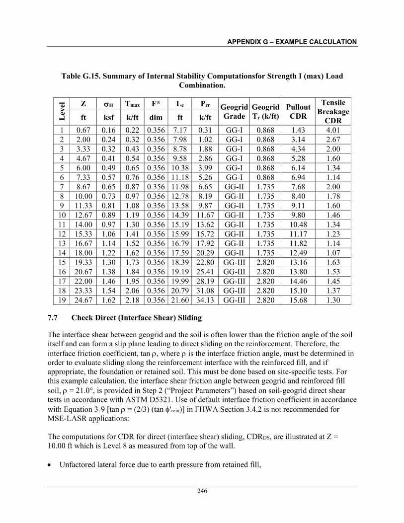
APPENDIX G – EXAMPLE CALCULATION
246
Table G.15. Summary of Internal Stability Computationsfor Strength I (max) Load Combination.
Lev
el Z H Tmax F* Le Prr Geogrid
Grade Geogrid Tr (k/ft)
Pullout CDR
Tensile Breakage
CDR ft ksf k/ft dim ft k/ft 1 0.67 0.16 0.22 0.356 7.17 0.31 GG-I 0.868 1.43 4.01 2 2.00 0.24 0.32 0.356 7.98 1.02 GG-I 0.868 3.14 2.67 3 3.33 0.32 0.43 0.356 8.78 1.88 GG-I 0.868 4.34 2.00 4 4.67 0.41 0.54 0.356 9.58 2.86 GG-I 0.868 5.28 1.60 5 6.00 0.49 0.65 0.356 10.38 3.99 GG-I 0.868 6.14 1.34 6 7.33 0.57 0.76 0.356 11.18 5.26 GG-I 0.868 6.94 1.14 7 8.67 0.65 0.87 0.356 11.98 6.65 GG-II 1.735 7.68 2.00 8 10.00 0.73 0.97 0.356 12.78 8.19 GG-II 1.735 8.40 1.78 9 11.33 0.81 1.08 0.356 13.58 9.87 GG-II 1.735 9.11 1.60 10 12.67 0.89 1.19 0.356 14.39 11.67 GG-II 1.735 9.80 1.46 11 14.00 0.97 1.30 0.356 15.19 13.62 GG-II 1.735 10.48 1.34 12 15.33 1.06 1.41 0.356 15.99 15.72 GG-II 1.735 11.17 1.23 13 16.67 1.14 1.52 0.356 16.79 17.92 GG-II 1.735 11.82 1.14 14 18.00 1.22 1.62 0.356 17.59 20.29 GG-II 1.735 12.49 1.07 15 19.33 1.30 1.73 0.356 18.39 22.80 GG-III 2.820 13.16 1.63 16 20.67 1.38 1.84 0.356 19.19 25.41 GG-III 2.820 13.80 1.53 17 22.00 1.46 1.95 0.356 19.99 28.19 GG-III 2.820 14.46 1.45 18 23.33 1.54 2.06 0.356 20.79 31.08 GG-III 2.820 15.10 1.37 19 24.67 1.62 2.18 0.356 21.60 34.13 GG-III 2.820 15.68 1.30
7.7 Check Direct (Interface Shear) Sliding
The interface shear between geogrid and the soil is often lower than the friction angle of the soil itself and can form a slip plane leading to direct sliding on the reinforcement. Therefore, the interface friction coefficient, tan , where is the interface friction angle, must be determined in order to evaluate sliding along the reinforcement interface with the reinforced fill, and if appropriate, the foundation or retained soil. This must be done based on site-specific tests. For this example calculation, the interface shear friction angle between geogrid and reinforced fill soil, = 21.0°, is provided in Step 2 (“Project Parameters”) based on soil-geogrid direct shear tests in accordance with ASTM D5321. Use of default interface friction coefficient in accordance with Equation 3-9 [tan = (2/3) (tan 'rein)] in FHWA Section 3.4.2 is not recommended for MSE-LASR applications: The computations for CDR for direct (interface shear) sliding, CDRDS, are illustrated at Z = 10.00 ft which is Level 8 as measured from top of the wall. • Unfactored lateral force due to earth pressure from retained fill,
APPENDIX G – EXAMPLE CALCULATION
247
UF1 = ½(Karet)(γret)Z2 For Z = 10.00 ft, UF1 = [½(0.361)(125 pcf)(10.00 ft)2]/1,000 = 2.26 k/ft. Load factor for lateral force due to earth pressure, EH (max) = 1.50. Factored lateral force due to earth pressure from retained fill, F1 = 1.50 (2.26 k/ft) = 3.38 k/ft.
• Unfactored lateral force due to live load surcharge on retained fill,
UF2 = (Karet)[(γret)(heq)](Z) For Z = 10.00 ft, UF2 = [(0.361)(125 pcf)(2.00 ft)(10.00 ft)]/1,000 = 0.903 k/ft. Load factor for lateral force due to live load surcharge on retained fill, LS = 1.75. Factored lateral force due to live load surcharge on retained fill, F2 = 1.75 (0.903 k/ft) = 1.58 k/ft.
• Total factored lateral load at Z = 10.00 ft, HL = F1 + F2 = 3.38 k/ft + 1.58 k/ft = 4.96 k/ft. • Unfactored vertical load at depth Z,
VNm = (L)(γrein)Z For Z = 10.00 ft, VNm = [(22 ft)(125 pcf)(10.00 ft)]/1,000 = 27.50 k/ft.
• Factored sliding resistance at depth Z,
HR = (DS) (tan) VNm As per Table G.7, the resistance factor for direct sliding mode is DS= 1.00. For Z = 10.00 ft, HR = (1.00)(tan 21.0°) (27.50 k/ft) = 10.56 k/ft.
• Compute CDR for direct (interface shear) sliding, CDRDS,
CDRDS = HR / HL = (10.56 k/ft) / (4.96 k/ft) = 2.13. Since the value of CDRDS > 1.0, the MSE-LASR wall at Level 8 of the reinforcements is safe against direct (interface shear) sliding limit state (failure mode). Using similar computations, the CDR for direct (interface shear) sliding can be obtained at other levels of reinforcements. Table G.16 presents the computations for the CDR for direct (interface shear) sliding at all levels of reinforcement. All the CDRDS values in Table G.16 are greater than 1.00. Thus, the MSE-LASR structure is safe against direct (interface shear) sliding at each reinforcement level.

APPENDIX G – EXAMPLE CALCULATION
248
Table G.16. Summary of Internal Stability Computations forDirect (Interface Shear) Sliding.
Level Z Geogrid F1 F2 HL VNm HR CDRDS # ft Grade k/ft k/ft k/ft k/ft k/ft dim 1 0.67 GG-I 0.02 0.11 0.12 1.83 0.70 5.85 2 2.00 GG-I 0.14 0.32 0.45 5.50 2.11 4.68 3 3.33 GG-I 0.38 0.53 0.90 9.17 3.52 3.90 4 4.67 GG-I 0.74 0.74 1.47 12.83 4.93 3.34 5 6.00 GG-I 1.22 0.95 2.17 16.50 6.33 2.92 6 7.33 GG-I 1.82 1.16 2.98 20.17 7.74 2.60 7 8.67 GG-II 2.54 1.37 3.91 23.83 9.15 2.34 8 10.00 GG-II 3.38 1.58 4.96 27.50 10.56 2.13 9 11.33 GG-II 4.35 1.79 6.14 31.17 11.96 1.95 10 12.67 GG-II 5.43 2.00 7.43 34.83 13.37 1.80 11 14.00 GG-II 6.63 2.21 8.85 38.50 14.78 1.67 12 15.33 GG-II 7.96 2.42 10.38 42.17 16.19 1.56 13 16.67 GG-II 9.40 2.63 12.03 45.83 17.59 1.46 14 18.00 GG-II 10.97 2.84 13.81 49.50 19.00 1.38 15 19.33 GG-III 12.65 3.05 15.71 53.17 20.41 1.30 16 20.67 GG-III 14.46 3.26 17.72 56.83 21.82 1.23 17 22.00 GG-III 16.38 3.47 19.86 60.50 23.22 1.17 18 23.33 GG-III 18.43 3.69 22.11 64.17 24.63 1.11 19 24.67 GG-III 20.59 3.90 24.49 67.83 26.04 1.06
STEP 8: EVALUATE FACING CONNECTIONS
The connection of the reinforcements with the facing, should be designed for Tmax for all limit states. The nominal long-term connection strengths, Talc, based upon laboratory connection tests between these MBW units and geogrids, as a function of geogrid grade and normal pressure, are summarized in Column 6 of Table G.17. The computations for CDR for connection strength, CDRCS, are illustrated at Z = 10.00 ft which is Level 8 as measured from top of the wall. • From Table G.15, the following information is obtained at Z = 10.00 ft,
Tmax = 0.97 k/ft; Geogrid Grade: GG-II; Tr = 1.95 k/ft
• Compute factored long-term connection strengths, c(Talc), From Table G.7, c = 0.80; From Table G.17, Talc = 1.45 k/ft Thus, c(Talc), = (0.80)(1.45 k/ft) = 1.16 k/ft
• Based on above value c(Talc) < Tr
• Thus, governing value of factored Talc, Talcg= 1.16 k/ft

APPENDIX G – EXAMPLE CALCULATION
249
• Compute CDR for connection strength, CDRCS, CDRCS = Talcg / Tmax = (1.16 k/ft) / (0.97 k/ft) = 1.19.
Since the value of CDRCS > 1.0, the connection strength at Level 8 of the reinforcements is safe. Using similar computations, the values of CDRCS can be obtained at other levels of reinforcements. Table G.17 presents the computations for the CDRCS at all levels of reinforcement. All the CDRDS values in Table G.16 are greater than 1.00. Thus, the MSE-LASR structure has safe connection strength at each reinforcement level.
Table G.17. Connection Strength Check.
Lev
el
Z Tmax Geogrid Tr Talc (Note 1) c(Talc)
Is Tr < (c.Talc)?
Talcg (Governing
Factored Talc) (Note 2)
CDRCS
# ft k/ft Grade (k/ft) (k/ft) (k/ft) (Yes/No) (k/ft) -- 1 0.67 0.22 GG-I 0.98 0.53 0.43 No 0.43 1.94 2 2.00 0.32 GG-I 0.98 0.67 0.53 No 0.53 1.67 3 3.33 0.43 GG-I 0.98 0.80 0.64 No 0.64 1.49 4 4.67 0.54 GG-I 0.98 0.93 0.75 No 0.75 1.38 5 6.00 0.65 GG-I 0.98 1.07 0.85 No 0.85 1.31 6 7.33 0.76 GG-I 0.98 1.20 0.96 No 0.96 1.26 7 8.67 0.87 GG-II 0.98 1.33 1.07 Yes 0.98 1.13 8 10.00 0.97 GG-II 1.95 1.45 1.16 No 1.16 1.19 9 11.33 1.08 GG-II 1.95 1.60 1.28 No 1.28 1.18 10 12.67 1.19 GG-II 1.95 1.75 1.40 No 1.40 1.18 11 14.00 1.30 GG-II 1.95 1.90 1.52 No 1.52 1.17 12 15.33 1.41 GG-II 1.95 2.05 1.64 No 1.64 1.16 13 16.67 1.52 GG-II 1.95 2.20 1.76 No 1.76 1.16 14 18.00 1.62 GG-II 1.95 2.35 1.88 No 1.88 1.16 15 19.33 1.73 GG-III 1.95 2.50 2.00 Yes 1.95 1.13 16 20.67 1.84 GG-III 3.17 2.65 2.12 No 2.12 1.15 17 22.00 1.95 GG-III 3.17 2.80 2.24 No 2.24 1.15 18 23.33 2.06 GG-III 3.17 2.95 2.36 No 2.36 1.15 19 24.67 2.18 GG-III 3.17 3.11 2.48 No 2.48 1.14
Notes: 1. Talc values are assumed in this example calculation using connection test data from a past successful project that
use a typical geogrid and MBW combination assumed in this example calculation. For actual projects use project-specific connection strength data at applicable normal load, on specific geogrid-block combination.
2. The Tr value limits factored connection strength.
APPENDIX G – EXAMPLE CALCULATION
250
STEP 9: CHECK OVERALL (GLOBAL) AND COMPOUND STABILITY AT SERVICE LIMIT STATE
The ground in front of the wall is horizontal and the foundation soil has no water table. The width of the wall base is 22 ft. Therefore, based on observation and experience, overall (global) stability is adequate. For actual projects the overall (global) stability should be investigated at the Strength I load combination as per AASHTO Article 11.6.3.7 with an appropriate resistance factor as shown in Table 3.8. Similar considerations apply for compound stability as noted in AASHTO Article 11.10.5.6 and Section 5.3.4.
STEP 10: DESIGN WALL DRAINAGE SYSTEMS
This step is of paramount importance. The design of the wall is based on the assumption that there is no generation of adverse positive pore water pressures within the wall system. All the necessary internal and external drainage measures as shown in Figure 5.2 must be implemented. Section 5.4 provides detailed information for wall drainage considerations. Considerations for seepage from pavement base course, as discussed in Section 3.8.3 of Chapter 3 must also be considered for this particular example calculation since the will be a pavement structure on top of the wall to accommodate the traffic surcharge. As noted in Section 5.4.2, the external drainage system must be designed to handle all possible surface water resulting from a 100-year storm event unless otherwise approved by the Owner.
G.2 PRACTICAL CONSIDERATIONS
Following is a general list of practical considerations from a geotechnical and structural viewpoint: • The magnitude of lateral displacement depends on fill placement techniques, compaction
techniques and effects, reinforcement extensibility, reinforcement length, reinforcement-to-facing connection details, and details of the wall facing. A rough estimate of probable lateral displacements of simple MSE walls that may occur during construction can be estimated based on empirical correlations shown in FHWA Figure 2-15 (also shown in AASHTO Figure C11.10.4.2-1). The computation is as follows:
o For L= 0.85H, the relative displacement ratio, r, is approximately 0.80 for 20 feet high wall.
o As per the note in FHWA Figure 2-15, the relative displacement increases approximately 25% for every 400 psf surcharge.
o Since H = 25.34 ft, the surcharge could be considered to be as follows: ▪ (25.34 ft – 20.00 ft)(125 pcf) = 667.50 psf; traffic surcharge is not included
since it is a transient load.
o Due to the surcharge, the modified lateral displacement ratio, rm, can be estimated as follows:

APPENDIX G – EXAMPLE CALCULATION
251
▪ rm = r + (0.25)(667.50 psf)/(400 psf) = 0.80 + 0.42 = 1.22.
o Thus, maximum estimated lateral displacement max, at the top of the wall can be computed as follows:
▪ max = rm [(20 ft)/75] using the equation for extensible reinforcements noted in Figure 2-15.
▪ max = 1.22 [(20 ft)/75] = 0.33 feet ≈ 4.0 inches. The designer should carefully evaluate the estimated value of lateral displacement. As noted in FHWA Figure 2-15, “Actual displacement will depend, in addition to the parameters addressed in the figure, on soil characteristics, compaction effort, and contractor.” Furthermore, it should be recognized that the estimate is based on a chart which assumes select fill. Fills used in MSE-LASR wall may experience larger lateral movements depending on the stiffness properties of the LASR fill. Using an inward batter of the wall facing is helpful in offsetting some of the lateral displacement. Flexible wire face may also be considered. For geosynthetic reinforcements, the profile of lateral movement at wall face over the height of the wall can be estimated using the baseline solution approach in the Limit Equilibrium Analysis (LEA) method as presented in Leshchinsky et al. (2016, 2017), Leshchinsky (2020), and AASHTO Article 11.10.5.6.
• Bearing pads are generally not used with MBW unit facings and are not used with this example calculation. The wall height is 25.34 ft and is below the recommended maximum height of 32 ft without bearing pads (see FHWA Section 3.6.1). However, as noted in Section 5.3.3.5 of Chapter 5, the compressive strength of modular block units shall be such that they can safely (with appropriate resistance factor) sustain a vertical load corresponding to 3 times the weight of the facing as measured at the leveling pad elevation.
• Calculation of the external settlement was reviewed in Step 6.4. However, given that LASR material is used, it should be expected that some additional vertical deformation due to internal compression of the reinforced soil mass may occur. The internal deformations can occur during and after construction and will be a function of the characteristics of the LASR materials, e.g., gradation, plasticity, clay mineral, level of compaction, moisture control during compaction, amount of moisture ingress during service life of structure, etc. Refer to Section 5.3.3.5 for estimation of internal deformations of reinforced soil mass.
• To control the deformation of the modular block facing use of a 2-ft wide gravel zone is
recommended as noted in Section 5.3.3.6 of Chapter 5. Infiltration of surface flows into the gravel zone must be prevented. To prevent migration of fines into the gravel zone, an appropriate geotextile separation fabric must be installed between the gravel zone and adjacent geomaterials as discussed in Section 5.4.1 of Chapter 5. For setback blocks, the reinforcement should not be installed over an offset between the face and the fill below. Finally, the back of the facing blocks at the location of the reinforcements should have rounded edges.

APPENDIX G – EXAMPLE CALCULATION
252
• As noted in Section 5.3.3.7, the leveling pad shall be constructed from lean concrete (e.g.,
2,500 psi) unreinforced concrete. Gravel leveling pads shall not be allowed. Finally, it is important that project-specific details are developed and included in the project plans and specifications. These should also include detailed construction control procedures e.g., type of compaction control, frequency of materials testing etc., and detailed construction inspection, inventory and maintenance requirements. Appendix H presents some user tools for construction inspection, maintenance, and inventory for MSE-LASR walls.

APPENDIX H – EXAMPLE FLHD USER TOOLS FOR INSPECTION, MAINTENANCE, AND INVENTORY OF MSE-LASR WALLS
253
APPENDIX H– EXAMPLE FLHD USER TOOLS FOR INSPECTION, MAINTENANCE AND INVENTORY OF MSE-LASR WALLS
Owner or management agencies may choose to establish an inspection and maintenance protocol to be used on a project-specific basis according to Section 5.6. The adoption of an inspection and maintenance protocol helps in development of an inventory of the MSE-LASR assets which would help in streamlining the maintenance and asset management while creating a valuable database for future studies. The development and implementation of project-specific inspection, maintenance and inventory protocol for MSE-LASR walls will require a commitment from the owner agency in terms of resources such as budget and the availability of qualified inspection personnel. This appendix is intended to provide an agency with an example of user tools for inspection, maintenance and inventory protocol for MSE-LASR walls.
H.1 User Tools for Maintenance and Inventory
FHWA (2010) presents a comprehensive procedures manual for developing a retaining wall inventory and condition assessment program. The Federal Lands Highway Division (FLHD) of the Federal Highway Administration (FHWA), in partnership with the National Park Service (NPS), developed the manual as part of the NPS Wall Inventory Program (WIP). The purpose of the WIP program was to define, quantify, and assess wall assets associated with park roadways in terms of their location, geometry, construction attributes, geotechnical and structural condition, failure consequence, cultural aspects, apparent design criteria, and cost of structure maintenance, repair or replacement. Ultimately, condition assessments for retaining wall structures are expressed as deferred maintenance costs, which are then divided by current year replacement costs to arrive at a “Facility Condition Index” (FCI). Coupling this condition prioritization index with an “Asset Priority Index” (API), which measures the feature’s importance to the mission of the park, capital asset investments are made more efficiently. This approach appropriately focuses maintenance and construction priorities on value, rather than solely on cost. The FHWA (2010) manual documents the data collection and management processes, wall attribute and element definitions, and team member responsibilities for conducting retaining wall inventories and condition assessments based on nearly 3,500 wall assessments within 32 national parks across the U.S. Additionally, the FHWA (2010) is supported by several features, including a comprehensive training program for field inspectors, an database, unique data collection forms, a supporting field guide, and a wall repair/replace cost estimation guide. The FHWA (2010) manual has been written to cover a wide variety of retaining walls for a variety of functions and with different architectural facings and surface treatments. Each of these elements is assigned a code as shown in Figure H.1. The wall type codes “MG,” “MP,” “MS,” and “MW” are applicable to MSE walls and cover the potential range of MSE-LASR
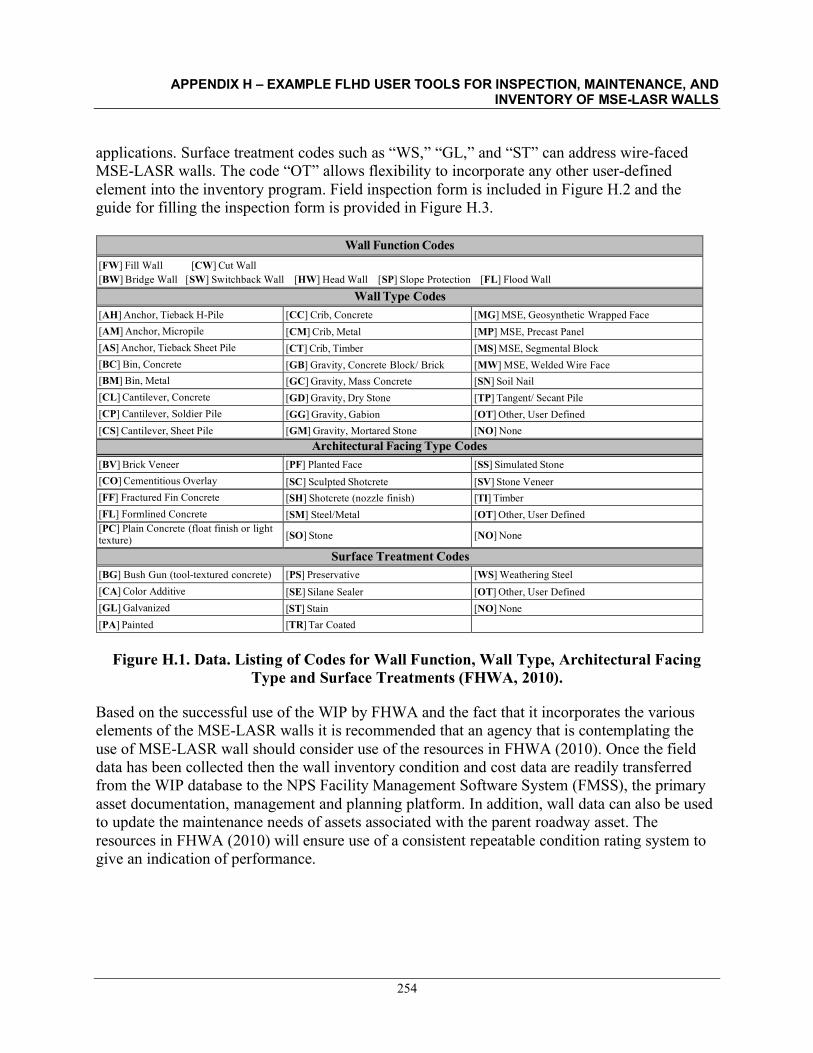
APPENDIX H – EXAMPLE FLHD USER TOOLS FOR INSPECTION, MAINTENANCE, AND INVENTORY OF MSE-LASR WALLS
254
applications. Surface treatment codes such as “WS,” “GL,” and “ST” can address wire-faced MSE-LASR walls. The code “OT” allows flexibility to incorporate any other user-defined element into the inventory program. Field inspection form is included in Figure H.2 and the guide for filling the inspection form is provided in Figure H.3.
Wall Function Codes
[FW] Fill Wall [CW] Cut Wall [BW] Bridge Wall [SW] Switchback Wall [HW] Head Wall [SP] Slope Protection [FL] Flood Wall
Wall Type Codes [AH] Anchor, Tieback H-Pile [CC] Crib, Concrete [MG] MSE, Geosynthetic Wrapped Face [AM] Anchor, Micropile [CM] Crib, Metal [MP] MSE, Precast Panel [AS] Anchor, Tieback Sheet Pile [CT] Crib, Timber [MS] MSE, Segmental Block [BC] Bin, Concrete [GB] Gravity, Concrete Block/ Brick [MW] MSE, Welded Wire Face [BM] Bin, Metal [GC] Gravity, Mass Concrete [SN] Soil Nail [CL] Cantilever, Concrete [GD] Gravity, Dry Stone [TP] Tangent/ Secant Pile [CP] Cantilever, Soldier Pile [GG] Gravity, Gabion [OT] Other, User Defined [CS] Cantilever, Sheet Pile [GM] Gravity, Mortared Stone [NO] None
Architectural Facing Type Codes [BV] Brick Veneer [PF] Planted Face [SS] Simulated Stone [CO] Cementitious Overlay [SC] Sculpted Shotcrete [SV] Stone Veneer [FF] Fractured Fin Concrete [SH] Shotcrete (nozzle finish) [TI] Timber [FL] Formlined Concrete [SM] Steel/Metal [OT] Other, User Defined [PC] Plain Concrete (float finish or light texture) [SO] Stone [NO] None
Surface Treatment Codes [BG] Bush Gun (tool-textured concrete) [PS] Preservative [WS] Weathering Steel [CA] Color Additive [SE] Silane Sealer [OT] Other, User Defined [GL] Galvanized [ST] Stain [NO] None [PA] Painted [TR] Tar Coated
Figure H.1. Data. Listing of Codes for Wall Function, Wall Type, Architectural Facing
Type and Surface Treatments (FHWA, 2010). Based on the successful use of the WIP by FHWA and the fact that it incorporates the various elements of the MSE-LASR walls it is recommended that an agency that is contemplating the use of MSE-LASR wall should consider use of the resources in FHWA (2010). Once the field data has been collected then the wall inventory condition and cost data are readily transferred from the WIP database to the NPS Facility Management Software System (FMSS), the primary asset documentation, management and planning platform. In addition, wall data can also be used to update the maintenance needs of assets associated with the parent roadway asset. The resources in FHWA (2010) will ensure use of a consistent repeatable condition rating system to give an indication of performance.

- NPS RETAINING WALL INVENTORY PROGRAM (WIP) FIEW FORM-NPSParkName Route/Parking No. Wall Start Milepoint
Inspected By Route/Parking Name Wall EndMilepoint
Inspection Date Side of Centerline (R/UP##) Visidata E,ent Milepoint
WALL FUNCTION, DIMENSIONS, and DESCRIPTION
Wall Ftmcti on Primary Wall Type Architectural Facings
Approx. Year Built Secondary Wall Types Surface Treatments
Wall General Description Notes: (e.g., wall pwpose, setting, construction, consequence of failure, special design, etc.)
Wall Length (ft) Wall Face Area (ft2) Wall Start Offset (ft)
Max. Wall Height (ft) Ve11ical Offset ( +/-ft) Wall End Offset (ft)
Photo Description/No.(e.g., approach, elevation, wall top, alignment.face derail, deficiencies, ere.) Face Angle (deg)
REPAIR/REPLACE RECOMMENDATIONS AND WORK ORDER
Wall Condi ti on Rating Design Criteria Failure Consequence
Imestigation Req'd? (Yf.\) Cultural Concern? (Y/'.\) Action
Brief Work Order Description (5-10 word maximum, key work elements)
Repair/Reµace Reconunendations (itemized description of wall repairs, methods, estimated quantities, and costs per repair item, including consideration of constrnctability issues such as access, traffic control, staging, safety hazards, etc.)
Repair/Re place COST:
Re,: 07-10-2007
APPENDIX H – EXAMPLE FLHD USER TOOLS FOR INSPECTION, MAINTENANCE, AND INVENTORY OF MSE-LASR WALLS
Figure H.2. Data. Field Inspection Form – Front Page (FHWA, 2010).
255

APPENDIX H – EXAMPLE FLHD USER TOOLS FOR INSPECTION, MAINTENANCE, AND INVENTORY OF MSE-LASR WALLS
256
Figure H-3 (Cont.). Data. Field Inspection Form – Front Page (FHWA, 2010).
Element Condition Nat't'ative Condition Wf:ighti.ng: Condition Dau Rating: Factor Score Reliability
Prlmarv Wall Elements
Piles and Shafts 8 1-10 1-3
Lagging 8 1-10 1-3
Anchor Heads 8 1-10 1-3
Wire/Geosynthetic 8
Facing EJements 1-10 1-3
Bin or Crib 8 1-10 1-3
Concrete 8 1-10 1-3
Shotcrete 8 1-10 1-3
Mo1tar 8 1-10 1-3
Manufactured 8
Block/Brick 1-10 1-3
Placed Stone 8 1-10 1-3
Stone Masonry 8 1-10 1-3
all Foundation 8
Material 1-10 1-3
Other Primaty 8
Wall Element 1-10 1-3
W
Secondarv Wall Elements (WF=O.S for CR=S-10/ WF=l.O for CR=4-7/\VF=5 for CR=l-3)
Wall Drains 1-10 0.5-5 1-3
Architectural Facing 1-10 0.5-5 1-3
Traffic Bata-ier/Fence 1-10 0.5-5 1-3
Road/Sidewalk/ Shoulder 1-10 0.5-5 1-3
Upslope 1-10 0.5-5 1-3
Do.,.-nslope 1-10 0.5-5 1-3
Lateral Slope 1-10 0.5-5 1-3
Vegetation 1-10 0.5-5 1-3
Cuhert 1-10 0.5-5 1-3
Curb/Benn/Ditch 1-10 0.5-5 1-3
Other Seconda1y Wall Elements 1-10 0.5-5 1-3
Wall Performance
Perfonnat1ce 1-10 8
WALL RATING Weighting Factor (xi 0) and Condition Score Totals
Wall Condition Rating (- [Condition Score Total/Weighting Factor Total (xi 0)] X 100)

APPENDIX H – EXAMPLE FLHD USER TOOLS FOR INSPECTION, MAINTENANCE, AND INVENTORY OF MSE-LASR WALLS
Figure H.3. Data. Guide to Complete Field Inspection Form – Page 1 of 4 (FHWA, 2010)
257
- NPS Retaining Wall Inventory Program Field Guide (WIFG)-Retaining WaU Acceptance Criteria
* All classes of paved roadways and parking areas included in the RIP Route Investigation Report and/or identified by Park staff. *\Valls must reside ,vithin the constructed roadway/parking are.a prism.
*i\.faximwn wall height, including only that portion actively retaining soil and/orrock, must be;:: 4 ft (e:: 6 ft for culvert headwalls). *Considerkno,vnlverifiable wall embedment in detennining maximwn retainmgwall height Include fully bwied retainmg structures. *Walls have an internal wall face angle;:: 45' (e:: lH:lV face slope ratio).
*Include all walls where the intent is to support/protect the travelway, and where failure would require replacement ,vith a retaining wall
Definitions ~ie.asureofhowwell cWTent design criteria are satisfied: None. - Does not meet any kno,vn standards.
Non-AASHTO - Does not meet AASHTO, but is consistent'vith other structures ofits type/period ,vith good perfonnance. AASHTO - Apparently meets current AASHTO Geometric, Design, Materials, and Construction Standards.
Design Criteria
Consequenc-.eof Failure
Low - No loss of roadway, no to low public risk. no impact to traffic dwing wall repair/replacement Afoderate- Howiy to short-tenn closure of roadway, low-to-moderate public risk, multiple alternate routes available
High- Seasonal to long-tenn loss of roadway, substantial loss-of-life risk, no alternate routes available
Action Select from: No Action, Monitor, Maintenanc.e,, Repair Elements, Replac.e Elements, andReplac.e \Vall
Weighting Fae.tor
Weighting Factor to be applied to the Condition Rating (CR). When indicated on the Condition Assessment Input Fonn: WF=0.S for CR=S-10; WF=l.0 for CR=4-7; and WF=S for CR=l -3.
Estimate of how well observed conditions represent wall petfonnance, and if additional investigations maybe warranted.
I-Poor Conditions cannot be sufficiently observed to rate element(s), warranting additional investigations to better define element petfonnance and/or to detennine the cause(s) or poor petfonnance. 1Good Observed conditions are sufficient to rate the conditions of wall element(s); however, additional investigations would be
useful to better understand element petfonnance.
3 Very Good Observed conditions clearly describe wall petfonnance. Additional investigations are not needed.
Data Reliability
WaU Fnnction Codes
(FW) Fill Wall (CW) Cut Wall (BW) Bridge Wall (SW) S" itchback Wall (HW) Head Wall (SP) Slope Protection (FL) Flood Wall
WaU Type Codes (AH) Anchor, Tieback H-Pile (CC) Crib, Concrete
(Cllf) Crib, Metal
(CT) Crib, Timber
(GB) Gravity, Concrete Block/ Brick
JGC) Gravity, Mass Concrete
(GD) Gravity, Dry Stone
(GG) Gravity, Gabion
(GM) Gravity, Mortared Stone
(MG) MSE, Geosynthetic Wrapped Face
(MP) MSE, Precast Panel
(MS) MSE, Segmental Block
(MW) MSE, Welded Wire Face
(SN) Soil Nail
(TP) Tangent/ SecantPile
(OT) Other, User Defined
[NO) None
(Allf) Anchor, Micropile
(AS) Anchor, Tieback Sheet Pile
(BC) Bin, Concrete
(BM) Bin, Metal
(CL) Cantilever, Concrete
(CP) Cantilever, Soldier Pile
(CS) Cantilever, Sheet Pile
Architectnral Facing Type Codes (BV] Brick Veneer (PF) Planted Face
(SC) Sculpted Shotcrete
(SH) Shotcrete (nozzle finish)
(SM) Steel/i\•l etal
(SO) Stone
(SS) Simulated Stone
(CO) Cementitious Overlay
FF) Fractured Fin Concrete
FL) Formlined Concrete l'l.. J c ldlI1 L-oncrete tnoat 1uusn or u~ut ex1ure)
(SV) Stone Veneer
(TI) Timber
(OT) Other, User Defined
[NO) None
(
( l
t
Snrface Treatment Codes (BG) Bush Gun (tool-tex1ured concrete)
[CA) Color Additive
(GL) Galvanized
(PA) Painted
(PS) Preservative (WS) WeatheringSteel
(OT) Other, User Defined
[NO) None
(SI) Silane Sealer
(ST) Stain
(TR) Tar Coated

APPENDIX H – EXAMPLE FLHD USER TOOLS FOR INSPECTION, MAINTENANCE, AND INVENTORY OF MSE-LASR WALLS
258
wan Start Milepoinl ),
wan End ,, Milepoint
H.,.
H,,. ..
L
Maximum exposed -II height, ft
Average vert.Cal distance from pavement to out wal toe or grO<mlne et top of fill wan ( + obove/- belCNV roaawer,,), ft
Horizontal clstence to wall faioe from edge of roadlvay, ft
Wal face angle me8$Ured from tho hori%ontel, degrees
Maximum earth relar,ing length of the wall (e,o;IUdi"IJ guardwalls). w .. length is the aot""I length of the stn.cture, not simpy the projected le<9h along the roadway, ft
Figure H.3 (Cont.). Data. Guide to Complete Field Inspection Form – Page 2 of 4 (FHWA, 2010)
Condition Ratin2s Condition Ratings apply to all Primary and Sec,ondary \Vall Elements., and are intended to assist in c,onsistendy defining element severity,
extent. and rep;1ir/ replilc.e urg,ency of wall element distresses.
9-10 -Any defects are minor and are \vithin nonnal range for newlyconjfructedor fabricated elements.
(Ixr.ellent) -Defects may include those typically caused from fabrication or c,onsauc.tion. -Low-to-moderate extent onow seventy distress.
7-8 -Distress present does not significantlyc,omprom.ise the element function, nor is there significantly severe distress to major sauc.tural (Good) c,omponents ofan element.
-High extent oflow severity distress andlorlow-to-mediwn extent of mediwn to high severity distress. 5-6 -Distress present does not c,omprom.ise element function, but lack of treatment may lead to impaired function/elevated risk of
(Foir) element failure in the near tenn.
-Medium-to-rugh extent of medium-to-rugh severity distress. 3-4
-Distress present threatens element func.tion. and strength is obviouslyc,ompromisedandlor structural analy sis is warranted. (Poor)
-The element conditiondoesnotposean immediate threat to wall stabilitv and road closure is notnecessarv. -Medium-to-rugh extent of rugh severity distress.
1-2 -Element is no longer servingintendedfunc.tion.Element perfonnanc.e threatening overall stability of the wall at the time of (Critkol) inspection.
WaU Performance Condition Ratin2s Good to Ixcellent -No observationofdistressesnotalreadycapturedby individual
Evaluation of overall wall element c,onditionassessment. No c,ombination of element distresses indicating W1seen
perfonnance as indicated by problems or creating sign.ificantperfonnance problems. No history of remediation or
observations not necessarily repair to wall or adjacent elements.
captured by observed distresses F:air - Some obsetVedglobal distressisnotassociated\vithspecillc elements. Some
for specific elements, including observation of element distress combinations that indicate wall c,omponent problems. global wall distresses (rotation, Perfonnmc-e ri.+finor \vork on primary elements or major \vork on secondary elements has occurred settlement, translation.
improving overall wall function. displacement, etc.) andlor
Poor to Criric.:11 - Global wall rotation. settlement, and/or overtu.m.i.ngis readily apparent. evidence of prior repairs that
Combined element distresses clearly indicate serious stability problems \\tith c,omponents may further indicate component
or global wall stability. ri.+fajor repairs have occurred to wall struc.tural elements, though problems.
functionality has not improved significantly.
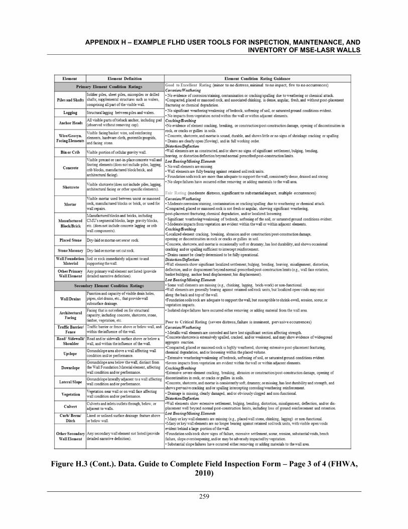
Element Definition Element Condition Rating Guidance
Primary Il~m~n, Condition Ratini:;s Good to Excellent Rating (minor to no distress . minimal to no impact,. few to no occurrences) Con-oSUJ1vJr;ad1n i-11C • No evidence of corrosion/staining, contamination or crackin~spalling due to weathering or chemical attack. •Compacted, placed or masoned rod, and associated chinking, is dense, angular, fre,h,and "ithout post-,ia<ement fracturing or chemical degradation. • No significant weathering.\,•eakening of bedrod, softening of soil, or saturated gro\1'1d conditions e.ident. • No impacts from ,·e:getation noted \Vi.thin the wall or \'\<i.thin adjacent elements.. Cracku,g/Br,aku,g •No es,dence of element cracking_, breaking, or construction/post-ronslructiondamage, opening of discontinuities in rod, or cracks or gullies in soils. • Concrete, shotcrote,and mortar is SOU'1d, durable, and shows httle or no signs of shrink.age cracking or spalling. • Drains are clearlyopen (flo"ing), and in full working order. Disw1tw1o/D,ft,ctw11 •Wall elements are as constructed,and1or show no signs of significant s.ettlement, bulging, bending, hea,ing, or distortion/def!e<:tion beyond normal prescribed post-ronstruction limits. Lost Bttui11gl/lli.m,og El,nwll> • No wall elements are missing. • Wall elements are fully bearing against retained soil/rock units. • Foundation soib/rock are more than adequate to support the \Yall, consistently dens.e, drained and strong. • No slope failures h.a,·e occurred either removing or adding materials to the wall area.
Fall' luting (moderate distress, significant to substantial impact,. multiple occwren ces)
CorroSUJ111JJ ; ad1.ffU1g • Moderate corrosion/staining, contamination or cracking/spalling due to weathering or chemical attack. -Compacted, placed or masoned rock is not fresh or angular, sho-.ing significant weathering, post-placement fracturing,chemical degradation, and/or localized loosening. • Significant weathering/weakening of bedtod, softening of the soil, or saturatedgroll'1d conditions -.ident. • Moderate impacts from\·e:getation are evi.dent \vi.thin the wall or \Vithin adjacent elements. Cntcki,,g!Brtaku,g •Localized element cracking, breaking, abrasion and/or constructionlpo,t-conslructiondamage, opening or discontinuities in rock or cracks or gullies in soil. •Concrete, shotcrete, and mortar is occasionally soft or drummy, has lost durability, and shows occasional cracking and/or ,palling sufficient to intercept reinforcement. • Drains cannot be clearly determined to be fully operational. Disw1tw1o/D,fl,ctw11 •Wall elements show significant loc-alized s.ettlement, bulging, bendin_g_, heaving, misalignment, distortion, defle<:tion, and/or dispacernent beyond normal prescribed post-ronstruction limits (e.g., wall face rotation, basket buldging, anchor head displacement, bin displacement). Lost B#tuiJ1CIAJissi11g El-1n1~11ts • Some \Vall elements are missing (e.g., chinking, lagging, bricL::.work) or non-functional. •Wall elernentsar. generally bearing against retained soil/rock units, but localized open ,·oids maywst along the back and top of the wall. •Foundation soils/rock are adequate to support the\vall, but susceptible to shrink.swell., erosion, scour, or vegetation impacts. • Isolated slope failures hav• occurred either reroosing or adding material from the wall area.
Poor to Critic-al Rating (se\·ere distress , failure is imminen t,. p ervasive occurrences) CorroSUm/JJ ; adr.ffU'K • M•tallic wall elements are corroded and have lost significant se<:tion affe<:ting strength. •Concreteishotcrete is u tensiv,ly spalled, cracked, and'or weakened, and may showe,,dence of "'despread ag__u;regate reaction. •Compacted, placed or masoned rock is highly weathered, shO\sing extensiYe post -placement fracturing, chemical degradation, and/or loosening "ithin the placed ,,olume. • utensi,·e weathering/weakening of bedtock, softening of soil, or saturated groll'1d conditions .,,dent. •Se,·ere impacts from ,·egetation are e\-i.de:nt within the wall or \Vi.thin adjacent elements. Cracku,g/Br,aku,g •Extensive s.e\·ere element cracking, breaking, .abrasion or construction/post-eonstructiondamage, opening of discontinuities in rod, or cracks or gullies in soils. •Concrete, shotcrete, and mortar is consistently soft, drummy, or missing, has lost durability and strength, and shows pen--asi\·ecracking and1or spalling intercepting corroding,'\"\·eathering reinforcement.
• Drainage is. missing, clearly damaged, and/or ob\-i.ously clogged and non-functional. Diswttio1o/D,ft,ctw11 •Wall elements shu.v utensive settlement, bulging, bending, distortion, misalignment, deflection, and/or dis-placement well beyond normal post-construction limits, including loss of gro\1'1d reinforcement and retention Lost B, tuiJ1CIAlissi-11g El-11u~11ts • Manyorkeywallelernents ar• missing (e.g., placed wall stone, chinking, lagging) or non-functional. •Many or key wall tlernents are no longer bearing against retained soillrock units, "'th sisible open voids e\-i.de:nt be.hind a large portion of the wall. •Foundation soils/rock show signs of failure, exces.s-ive settlement, scour, erosion, substantial voids, bench failure, slope oversteepening, andlor may be adversely impacted by vegetation. • Substantial slope failures have occurred either rerno.ing or adding materials to the wall area.
Soldier piles, sheet piles, micropiles or drilled shafts; sq:,plemental st:ruchl"es mch. as \valers, compruing .Wpart of the sisible wall.
Structural lagging between piles and waters.
All visible parts of tieback anchor, including pad (ob,er,·ed "ithout removing cap).
Piles ad Sbafu
Lagging
A.ncborHr:rids.
Visible facing. basket wire, soil reinforcing elements, hardware cloth, geotutileigeogrids, and facing stone.
Visible portion of cellular gravity wall.
Visible precast or cast.in.place concrete wall.and footing elements (does not include piles, lag_,;ing, crib blocks, manufactured blocklbrick, and architectural facing).
Visible shotcret• (does not include piles, lag_,;ing, architectural facing or other specific.lements).
Visible mortar used beh-,;een unCli or masoned rod, manufactured blocks or brick, or used for wall repairs.
Manufactured blocks and bricks, including CMU' s segmental blocks, large gra.ity blocks, etc. (does not include concret• lagging or crib wall components).
Dry-laid or mortar.set w1c-u1 rod..
Dry-laid or mortar-set cut rock.
Soil or rock immediately adjacent to and supporting the wall.
Any primary wall element not listed (prO\,de detailed narrau,·e definition).
WireJGeosYn. faciogEl•m·••"
Bin or Crib
Concrete
Shotcrete
Mortar
Maouf'actu.red Block/Brick
Placed Stone
Stone Masonry
" ;dlFou.ndation Mattrial
Other Prima.ry WallEl•m•nt
Secondal)· II-~nt Condition Ratinss
f ll'1ctionand capacityof\,sible drain holes, Wall Drains pipes, slot drains, etc., that provide wall
subsurface drain.age.
Ar<hite<t11nl facing that is not relied on for structural
fociog capacity, including concrete, shotcrete. stone, timber, \·eget.ation, etc.
T raffk Barri tr/ Traffic barrier or fenoe above or below wall, and Ftnce \vi.thin the influ...--nce of the wall.
Road/ Sidenlld Road and1or s-ide\valk surface .abo,·e or below .a Sbo11lder ·wall, and \"\-i.thin the influence of the wall.
Grounds lope area .above a wall affecting wall Upslope condition andlor performance.
Oro\1'1dslope area below the wall, distinct from Down.slope the Wall foU'1dation Material element, affecting
wall condition and1or performanoe.
Oro\1'1dslope laterally adjacent to a wall affe<:ting Lateral Slope wall condition and1or perform.a.nee.
Vegetation near wall or on \Vall faoe affecting , ·egetation
wall condition and1or performance.
C11lnrt CulYertsand inlet•'outlets through, below, or .adj.ace:nt to \"\--alls.
C11rb/ B,nn/ Lined or unlined surfaoe drain.age feature abo\·e Ditch or below wall.
Other Set'ondary Anysecondary wallelement not li.sted(pro,,de WallEl•m•nt detailed narrati,·e definition).
APPENDIX H – EXAMPLE FLHD USER TOOLS FOR INSPECTION, MAINTENANCE, AND INVENTORY OF MSE-LASR WALLS
Figure H.3 (Cont.). Data. Guide to Complete Field Inspection Form – Page 3 of 4 (FHWA, 2010)
259

APPENDIX H – EXAMPLE FLHD USER TOOLS FOR INSPECTION, MAINTENANCE, AND INVENTORY OF MSE-LASR WALLS
Figure H.3 (Cont.). Data. Guide to Complete Field Inspection Form – Page 4 of 4 (FHWA, 2010)
260
WALL TYPE
[AH] Anchor, Tieback H-Pile 0 0 0 •
• • • • 0 0 0 [AM] Anchor Micropile e • [AS] Anchor, Tieback Sheet Pile • • • • 0 0 0 e • [BC] Bin, Concrete • • • 0 0 0 e • [BM] Bin, Metal • • • 0 0 0 e • [CL] Cantilever, Concrete • • • 0 0 0 • • [CPJ Cantilever, Soldier Pile • • • • 0 0 0 e •
0 0 0 [CS] Cantilever, Sheet Pile • • • e • • • • 0 0 0 [CC] Crib, Concrete e •
[CM] Crib, Metal • • • 0 0 0 e • [CT] Crib, Timber • • • 0 • [GB] Gravity, Concrete Block/Brick •
0 0 •
• • • 0 0 0 e • • • • 0 0 0 [GCJ Gravity, Mass Concrete e •
[GD] Gravity, Dry Stone • • [GGJ Gravity •
0 0
, Gabion • • 0 0 0 •
• 0 0 0 e • [GM] Gravity, Mortared Stone •
• 0 0 • • 0 • •
[MG] MSE Geosyn. Wrapped Face • • 0 0
, 0 0 0 e • [MP] MSE, Precast Panel • • • 0 0 0 • • [MS] MSE, Segmental Block • • • 0 0 0 • • [MW] MSE, Welded Wire Face • • • 0 0 0 e • [SN] Soil Nail • • • 0 0 0 • • [TPJ Tangent/Secant Pile • • • 0 0 0 e • [OT] Other, User Defined • • 0 0 0 • •
• • • • • •
• Wall elements that should always be rated for the given wall type (others may also app~).
o 1 of 2 primary wall elements reQuired depending on material observed. 2 of 3 secondary wall elements reQuired depending on wall location relative to roadway.
Road/Sidewalk/Shoulder: Rate only when these elements lie within the influence of the wall. The shoulder is generally defined as extending no greater than 5 n horizontal~ from the roadway/sidewalk, and less than -5 n vertical ottset.
Upslope: Rate the upslope condition for all walls above roadway grade, regardless of slope ratio. Rate the upslope condition for all walls below roadway grade, regardless of slope ratio, when the vertical ottset to the wall from the roadway/shoulder is greater than 5 n (otherwise evaluate the condition of the upslope under the 'Road/Sidewalk/Shoulder' element).
Downslope: Rate the downslope condition for all walls below roadway grade, regardless of slope ratio. Rate the downslope cond1t1on for all walls above roadway grade, regardless of slope ratio, when the vertical ottset to the wall from the roadway/shoulder is greater than 5 n (otherwise evaluate the condition of the downslope under the 'Road/Sidewalk/Shoulder' element).

APPENDIX H – EXAMPLE FLHD USER TOOLS FOR INSPECTION, MAINTENANCE, AND INVENTORY OF MSE-LASR WALLS
261
H.2 User Tools for Construction Inspection
Construction of MSE systems is relatively simple and rapid. The construction sequence consists mainly of preparing the subgrade, placing and compacting fill in normal lift operations, laying the reinforcing layer into position, and installing the facing elements (tensioning of the reinforcement may also be required). Special skills or equipment are usually not required, and locally available labor can be used, however, experienced crews can provide higher production rates. Most material suppliers provide training for construction of their systems. The outline of a checklist showing general requirements for monitoring and inspecting MSE systems is provided in Table H.1. The table should be expanded by the agency to include detailed requirements based on the agency’s specifications and the specific project plans and specification requirements. Examples of detailed checklists for specific sections are provided in FHWA Chapter 11, and is also provided below.
1. Read the specifications and become familiar with:
- Material requirements
- Construction procedures
- Soil compaction procedures
- Alignment tolerances
- Acceptance/rejection criteria
2. Review the construction plans and become familiar with:
- Construction sequence
- Corrosion protection requirements
- Special placement to reduce damage
- Soil compaction restrictions
- Details for drainage requirements
- Details for utility construction
- Construction of slope face
- Contractor's documents

APPENDIX H – EXAMPLE FLHD USER TOOLS FOR INSPECTION, MAINTENANCE, AND INVENTORY OF MSE-LASR WALLS
262
3. Review material requirements and approval submittals.
- Review construction sequence for the reinforcement system.
4. Check site conditions and foundation requirements. Observe:
- Preparation of foundations
- Leveling pad construction (check level and alignment)
- Site accessibility
- Limits of excavation
- Construction dewatering
- Drainage features; seeps, adjacent streams, lakes, etc.
5. On site, check reinforcements and prefabricated units. Perform inspection of prefabricated elements (i.e. casting yard) as required. Reject precast facing elements if:
- Compressive strength < specification requirements
- Molding defects (e.g., bent molds)
- Honeycombing
- Severe cracking, chipping or spalling
- Color of finish variation
- Tolerance control
- Misaligned connections
6. Check reinforcement labels to verify whether they match certification documents.
7. Observe materials in batch of reinforcements to make sure they are the same. Observe
reinforcements for flaws and nonuniformity.
8. Obtain test samples according to specification requirements from randomly selected reinforcements.
9. Observe construction to see that the contractor complies with specification requirements for installation.

APPENDIX H – EXAMPLE FLHD USER TOOLS FOR INSPECTION, MAINTENANCE, AND INVENTORY OF MSE-LASR WALLS
263
10. If possible, check reinforcements after aggregate or riprap placement for possible damage. This can be done either by constructing a trial installation, or by removing a small section of aggregate or riprap and observing the reinforcement after placement and compaction of the aggregate, at the beginning of the project. If damage has occurred, contact the design engineer.
11. Check all reinforcement and prefabricated facing units against the initial approved shipment and collect additional test samples.
12. Monitor facing alignment:
- Adjacent facing panel joints
- Precast face panels
- Modular block walls
- Wrapped face walls
- Line and grade

APPENDIX I
Note: This text-equivalent version of the Figure 7.1 flow chart (page 156) is provided for accessibility conformance.
Figure 7.1 Flow Chart: Activities for Implementation of MSE-LASR Technology.
Block 1: Project Planning
1. Site reconnaissance. 2. Evaluate sources of select fill and haul distances. 3. Perform cost-benefit analysis for use of MSE-LASR. 4. Secure commitment from decision makers. 5. Set up qualified project team.
Block 2: Site Investigation and Testing/Evaluation of LASR Materials
1. Perform site investigations 2. Identify borrow sources for LASR materials and evaluate consistency and haul distances. 3. Perform testing of LASR materials. 4. Confirm the cost-benefit analysis performed as part of item 3 of block 1. Perform re-evaluation as
necessary and make adjustments, e.g., budgets, approach, etc.
Block 3: Design, Plans, & Specifications
1. Develop design parameters based on data from Block 2. 2. Perform appropriate analyses to allow development of plans and specifications. 3. Ensure plans and specifications are consistent with the procurement processes. 4. Develop a submittal review checklist that has been reviewed and approved by responsible parties.
Block 4: Procurement and Inspector Training
1. Develop appropriate bid documents, e.g. 2-step process. 2. Short-list qualified teams. 3. Provide project-specific training that includes field inspectors and representatives of contractor
and design team. 4. Develop an inspection checklist that is agreed upon by project personnel.
Block 5: Construction
1. Review contractor submittals for conformance with specifications 2. Pre-construction meeting with Resident Engineer, engineer of record, MSE vendor and
contractor. 3. Ensure materials used in construction are consistent with those assumed in design process. 4. Review daily reports. 5. Make adjustments as necessary to meet design assumptions.
Block 6: Data Collection and Maintenance
1. Collect data from any performance monitoring systems installed during and after construction. 2. Implement a formal maintenance protocol and provide reports from each inspection to engineer
of record.