HAL Id: hal-00555552https://hal.archives-ouvertes.fr/hal-00555552

Preprint submitted on 13 Jan 2011

HAL is a multi-disciplinary open accessarchive for the deposit and dissemination of sci-entific research documents, whether they are pub-lished or not. The documents may come fromteaching and research institutions in France orabroad, or from public or private research centers.

L’archive ouverte pluridisciplinaire HAL, estdestinée au dépôt et à la diffusion de documentsscientifiques de niveau recherche, publiés ou non,émanant des établissements d’enseignement et derecherche français ou étrangers, des laboratoirespublics ou privés.

Effect of Loading Induced Anisotropy on the ShearBehavior of Rough Interfaces

Anil Misra, Shiping Huang

To cite this version:Anil Misra, Shiping Huang. Effect of Loading Induced Anisotropy on the Shear Behavior of RoughInterfaces. 2011. �hal-00555552�

Effect of Loading Induced Anisotropy on the Shear Behavior of

Rough Interfaces

Anil Misra and Shiping Huang

Department of Civil, Environmental and Architectural Engineering, the University of

Kansas

Corresponding Author:

Dr. Anil Misra

Professor, Civil, Environmental and Architectural Engineering Department

The University of Kansas

Learned Hall

1530 W. 15th Street

Lawrence, KS 66045-7609

Ph: (785) 864-1750

Fax: (785) 864-5631

Email: amisra@ku.edu

Tribology International (in print)

Effect of Loading Induced Anisotropy on the Shear Behavior of

Rough Interfaces

Anil Misra and Shiping Huang

Department of Civil, Environmental and Architectural Engineering, the University of

Kansas

Abstract: We have utilized a statistical method to model the shear behavior of

rough contacts. In contrast to the traditional statistical methods, which only describe

the asperity height and curvature distributions, we have introduced a contact

orientation distribution in our analysis. We have also incorporated asperity contact

sliding and developed an incremental scheme for computing the stress-displacement

relationship. Using this enhanced model, we can demarcate the boundary between

elastically deforming and sliding asperity contact orientations under given loading.

Consequently, we can describe the shear-normal coupling as well as the effects of

inherent anisotropy and the induced anisotropy of the sheared interfaces.

Keywords: contact mechanics; sliding; elastic; roughness

1. Introduction

Stress-displacement behavior of contact between solid bodies has been one of the

most widely researched problems with contributions spanning more than a

century[1-4]. It has been widely recognized that surface roughness has a significant

role in determining the contact behavior under loading that is in the direction normal

and tangential to the nominal contact surface. A clear consequence of surface

roughness is that the actual contact area at the interface is smaller than the area of

contacting surfaces because the contact occurs via asperities. Moreover, when the

surfaces come into contact, the asperity heights and their relative locations are

uncertain, consequently, the resulting asperity contacts are oblique to the nominal

contact directions and of random orientations. A large number of models have been

proposed to simulate the interface behavior of contacting solids. The recent

approaches of rough contact modeling can be considered in three categories based

upon how the surface roughness is incorporated in the calculations: (1) direct

simulation using the finite element method, (2) fractal representation, and (3)

statistical methods.

Direct simulation of rough contact is useful for providing perceptual intuition and

showing details of the local behavior at the interfaces [4-9]. Furthermore, it is able

to consider the elasto-plastic behavior of material as well as larger deformation.

However, direct simulation can entail prohibitive computational expense for modeling

surfaces with numerous asperities of irregular geometry. Consequently, this

approach is seldom used to model the whole contact surface, although it could be

useful in micro-macro approaches for determining the relationships between local and

global properties. Along the lines of fractal representation, a number of authors have

shown that the rough interface demonstrates the self-affine feature which indicates the

geometry of the interface are scale dependent [7, 10-13]. The fractal model was

proposed to account for such feature. However, the fractal model typically does not

incorporate the local asperity behavior which is important when considering the shear

behavior. Furthermore, many materials like thin-film disks, magnetic tapes and

geotechnical materials have been shown to have little scale dependency and can be

adequately described by the statistical approach [14]. In contrast to the fractal

approach, the statistical approach is an asperity based model, in which the interface

behavior is described as a group effect of numerous local asperity contacts [15-31].

Scale dependent parameters have also been considered within the ambit of statistical

approaches to address the fractal or resolution dependent nature of rough surfaces [32,

33]. The pioneering work on the statistical approach was done by Greenwood and

Williams[15], who assumed that the surface is formed by a large number of spherical

shaped asperities with equivalent radius but different heights that follow Gaussian

distribution. Nayak [18, 34] introduced the techniques of random process theory

into the analysis of Gaussian roughness. In order to account for anisotropic interface,

McCool and Gassel [22] introduced the elliptic paraboloid asperities instead of

spherical shape asperities. However, the basic solution for elliptic paraboloid

asperities is much more complicated than that for spherical asperities, which has been

found to adequately describe the asperity contact behavior. The advantage of the

statistical method is that it not only considers the local behavior of contacting surface,

but also describes the interface geometry in a simple way. Therefore, this method

continues to be attractive for describing rough surface contact behavior.

In this paper, we introduce an orientation function to consider the anisotropic surface

while retaining the spherical shape of the asperities in the context of the statistical

approach. The orientation function models the random asperity contact obliquity

which results in the coupling of the shear and normal directions which is commonly

ignored in other models. Furthermore, we incorporate Hertz-Mindlin fundamental

solutions and sliding at the asperity contact in our model. This work extends the

previous micromechanical approach developed by the authors [28, 35, 36]. A

numerical procedure is implemented to evaluate the derived expressions for the

overall contact behavior. We then obtain the contact behavior under normal-shear

combined loading. In particular, we investigate (1) how the stress-displacement

relationship evolves as the interface is subjected to shear loading whose direction is

varied, and (2) the coupling between the normal and shear behavior under shear

loading.

In the subsequent discussion, we first briefly present our approach for modeling

contact behavior, including the statistical modeling of contact surface and the essence

of the micromechanical approach. We then utilize the micromechanical model to

investigate the sliding behavior of asperity contacts and the overall

stress-displacement behavior of the interface. We find that under certain applied

loading, existing asperity contacts can unload in the normal direction and separate.

Similarly, contacts that are sliding can unload in the shear direction and such that they

are no longer sliding. We also find that the overall behavior of the interface exhibits

significant coupling between the normal-shear and shear-shear directions depending

upon the loading sequence.

2. Modeling Method

2.1. Statistical Description of Contact Interface

The contact surface geometry determines the orientations and the number of asperity

contacts under a given loading condition. The composite topography of contacting

surfaces, described via statistics of asperity contact heights, orientations, and

curvatures may be utilized for this purpose [9, 18, 21, 28]. In this paper, the

statistics of asperity contact heights is described via gamma distributions, asperity

contact orientations via spherical harmonic expansions, and asperity curvatures are

assumed to be constant for simplicity. It is usual to define the asperity contact height

with reference to the highest peak of the composite topography such that, asperity

contact height, r, represents the overlap of the interacting surfaces. The density

function for asperity contact heights, H(r), is given by a gamma distribution [21, 26,

27] expressed as:

/

0 , , 01

rr eH r r

(1)

where and are parameters related to the mean and variance of the asperity contact

heights as follows

22 )1(:

)1(:

rariancev

rmean m

(2)

Parameter is unit less while parameter takes the unit of asperity contact height.

Surfaces that have smaller average asperity contact height and narrow distributions of

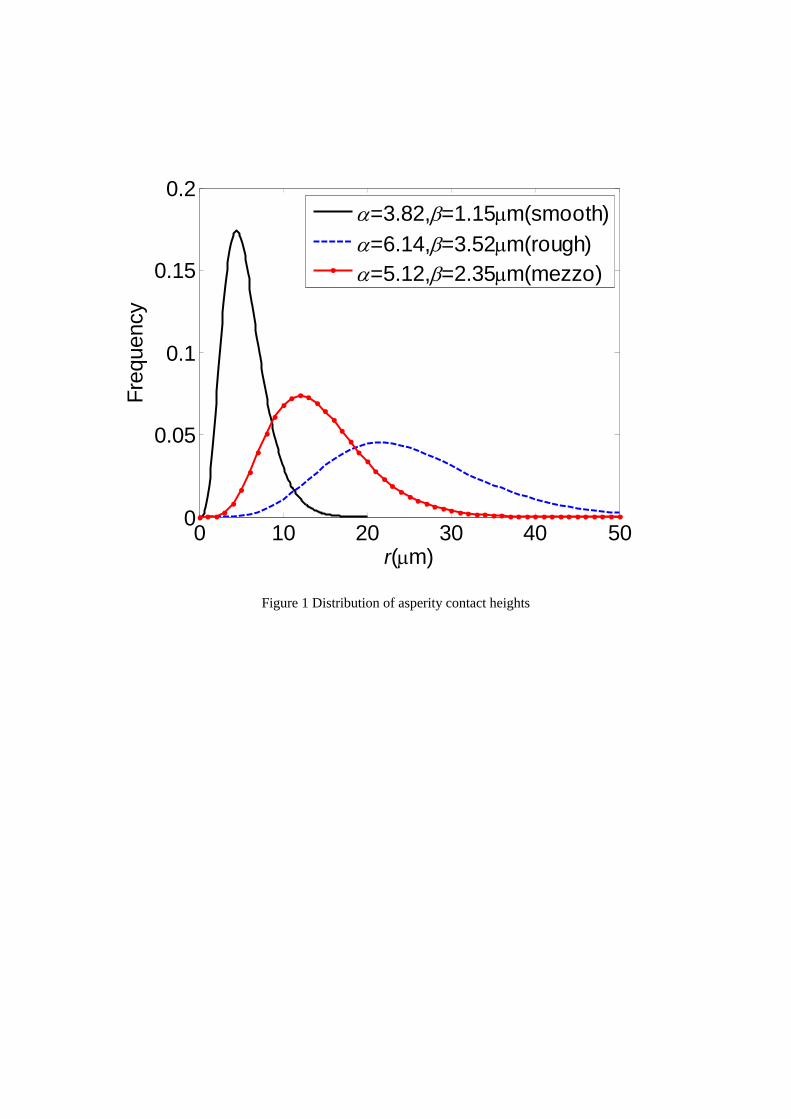
asperity contact heights are considered to be smoother. Fig. 1 gives examples of

asperity contact height distributions for two interfaces that can be described as smooth

and rough in comparison with each other. For an interface with N asperity contacts

per unit area, NH(r)dr denotes that number of asperity contacts in the interval

represented by r and r + dr. Thus, the total number of asperity contacts, under a given

closure, is given by

N N H r drr

r

0 (3)

In order to describe the orientation distribution, we introduce a local Cartesian

coordinate system as shown in Fig. 2. The local coordinate system consists of three

vectors n, s and t, among which n is the vector normal to the asperity contact surface,

and s and t are on the plane tangential to the asperity contact surface. The

relationship between the local coordinate system and the global Cartesian system is

given by:

cos,sin,0

sincos,coscos,sin

sinsin,cossin,cos

t

s

n

(4)

The asperity contact orientation is defined by considering the inclination of the

asperity contact normal with respect to that of the interface normal direction. As

shown in Fig. 2, the orientation of an oblique asperity contact is defined by the

azimuthal angle, , and the meridional angle, , measured with respect to a Cartesian

coordinate system in which direction 1 is normal to the interface. A 3-dimensional

density function utilizing shifted spherical harmonics expansion in spherical polar

coordinates that describes the concentrations of asperity contact orientations was

introduced by Misra [28, 35]. For an interface with isotropic distribution of asperity

contact orientations, the density function, (,) is given by

2sin( , ) 1 (3cos 1) 3 (sin ) cos 2

2 sin 4

a a ba c a

1;20;

20 a

a

(5)

where angles and are defined in Fig 2, and parameters a, b and c determine the

shape of the density function (,). Further, to ensure that the density function is

positive semi-definite, i.e. (,) 0, the values of parameters b and c are bounded as

follows:1 1

1 2 and -3 6 3 6

b bb c . Thus, the product Nr(,)sindd

denotes the number of asperity contacts N in the interval represented by sindd,

that is

, sinrN N d d (6)

The density function in Eq.(6) has the ability to model surfaces with varying

roughness. As discussed in Misra [35] for smooth surfaces the asperity contact

directions have a greater tendency to be aligned in the direction normal to the

interface in contrast to that for rough surfaces. It is noteworthy that, as parameter, a,

increases, the contact distribution concentrates towards the direction normal to the

interface. In particular, the density function, (,), behaves like a delta function in

the limit a and yields an expectation E[] =0, which represents a concentrated

contact orientation, normal to a perfectly smooth interface. The parameter, a,

describes the extent of the asperity contacts in the meridional direction as well as the

mean asperity contact orientation. The extent of asperity contact inclination in

meridional direction is /2 for a=1 and /4 for a=2. The shapes of contact

distributions vary with the values of parameter b, within the meridional extent of

asperity contacts. The lower bound of parameter b=-1, represents an interface on

which the asperity contacts tend to orient closer to the horizon. On the other hand,

the upper bound of parameter b=2, represents an interface on which preferred

orientation is closer to the interface normal. The asperity contacts are equally

distributed in the meridional direction for parameter b=0. Parameter, c, describes the

shape of the contact distributions in the azimuthal direction and, therefore models the

inherent anisotropy in the interface tangential direction. Fig. 3 shows the

3-dimensional distribution density under different combination of parameters a, b and

c.

2.2. Micromechanical Stress-Displacement Relationship

In the kinematically driven approach, we assume that the asperity contact

displacement, j, at a given asperity contact height is the same and directly related to

the overall displacement of the interface, j. The subscripts in this paper follow the

established tensor convention unless specified otherwise. Thus, the asperity contact

displacement in the local coordinate system can be written in terms of the overall

interface displacements as follows:

1 2 3 1

1 2 3 2

1 2 3 3

n

s

t

n n n r

s s s

t t t

(7)

Note that we assume the asperities to have spherical shape with the same radius but

different heights. Therefore, for a normal interface displacement 1, the

displacement of the asperity contact at height r is 1-r as depicted in Fig. 4. In local

coordinate system, considering the Hertz-Mindlin contact theory of perfectly smooth

elastic interfaces as well as other theories of smooth elastic-plastic interfaces[3], it is

reasonable to assume that normal asperity contact stiffness Kn depends on the normal

asperity contact displacement n according to the following power law:

nn KK (8)

Where K, and are constants. The asperity contact stiffness, Kn given by

Eq.(8),becomes identical with the Hertz stiffness for contact of perfectly smooth

elastic spheres when[3]

2 1 8; ;

2(1 ) 2 3(2 )

v G RK

v v

(9)

where G is the shear modulus, v is Poisson's ratio and R is asperity radius of curvature.

It is noteworthy that the exponent can vary from 0 for perfectly plastic to ½ for

perfectly elastic behavior at contact of perfectly smooth spherical asperities[3].

Since this paper focuses on monotonic loading of interfaces, we consider the case of

constant normal asperity contact force and monotonically increasing asperity contact

shear force. Mindlin and Deresiewicz [37] have derived the following asperity

contact force-displacement relationship for this loading condition, considering partial

slip at contact edge with increasing contact shear displacement:

2

3

)1(1n

stnnst Kf

(10)

Where fst is the asperity contact shear force and st is the asperity contact shear

displacement given by,

22

tsst (11)

Thus, in s- and t-direction, we have the following force displacement relationship:

3

21 (1 ) est ss n n st s

n st

f K K

(12)

3

21 (1 ) est tt n n st t

n st

f K K

(13)

where Kst is the stiffness in the tangential direction, and the superscript e denotes

asperity contacts that are not sliding. We note Eqs. (12) and (13) are valid when

|n|>st. When this condition is violated, sliding occurs at the contact per the

Amonton–Coulomb’s friction law. In this case Eqs. (12) and (13) can be rewritten

as:

pss n n st s

st

f K K

(14)

ptt n n st t

st

f K K

(15)

where the superscript p denotes asperity contacts that are sliding. In Eqs. (12)

through (15) the ratios s/st and t/st give the projection of the asperity contact shear

force, fst, in the s- and the t-directions and the stiffness, Kst, has been introduced for

convenience. Thus, for a single asperity contact the force-displacement can be

written in the following matrix form in the local coordinate system, where the

superscript has been dropped:

0 0

0 0

0 0

n n n

s st s

t st t

f K

f K

f K

(16)

Or in the global coordinate system, the asperity contact forces, fi, and displacements,

j, are related as follows:

1 11 12 13 1

2 12 22 23 2

3 13 23 33 3

f K K K r

f K K K

f K K K

(17)

Where the asperity contact stiffnesses, Kij, given by：

ij n i j st i j i jK K n n K s s t t (18)

where Kn, and Kst denote asperity contact stiffness along the normal and tangential

direction of the asperity contact.

At a rough interface, numerous asperity contacts of varying height overlap and

orientations occur under a given loading condition. These asperity contacts can be

classified into three groups: (1) those in contact but without sliding, (2) those in

contact but with sliding, and (3) those not in contact. The overall interface stress can

be obtained as the sum of the asperity contact forces contributed by groups (1) and (2).

Utilizing the orientation distribution and height distribution introduced in section 2,

we obtain the following expression for the overall interface stress, Fi, given in terms

of force per unit area since N is the areal asperity contact density

( ( , )sin ( ) ( , )sin ( ) )e e e p p p

e p

i i ir r

F N f d d H r dr f d d H r dr

(19)

In Eq. 19, the superscript e denotes the domain and forces of asperity contacts that are

not sliding, and the superscript p denotes the domain and forces of asperity contacts

experiencing sliding.

3. Results

3.1. Sliding behavior of asperity contacts at different orientations

Here we discuss the sliding behavior of asperity contacts subjected to a combined

normal and shear displacement. We consider asperity contacts with different

orientations at the same asperity contact height, r. We note that the asperity contact

orientation are defined by and and forms a hemi-spherical surface. As we

discussed before, asperity contacts with the same height r experience the same global

displacements Δ1-r, Δ2 and Δ3. However, the local displacements n, s and t which

determine the sliding behavior of asperity contacts are different since these are

functions of contact orientations. For simplicity but without loss of generality, let us

consider the asperity contacts subjected to the exterior displacement that lies on the

1-3 plane of the global coordinate system and makes an oblique loading angle, ,

with 1-axis as shown in Fig. 5. In this case, the asperity contacts of height, r, will

experience a displacement of (Δ1-r) =d, in the direction of 1-axis and a displacement

of Δ2=0 and Δ3=d tan () in the directions of 2- and 3-axis, respectively, as depicted

in Fig. 5. The asperity contact displacement in the local coordinate system can then

be written as follows based on Eq. (7):

)sin()sin()tan()cos( ddn

)sin()sin()tan()sin( dds (20)

)cos()tan( rt

Using these expressions for asperity contact displacement, we can determine whether

a contact is in sliding condition. To this end, we discretize the asperity contact

orientation domain into various asperity contact directions denoted by the pair (i, i).

For each asperity contact direction, we evaluate the local displacement using Eq. (20).

When the normal displacement, n(i, i) < 0, no contact exists; when the normal

displacement, n(i, i) > 0, and the shear displacement, st(i, i) < n(i, i),

contact exists, however is not sliding. Finally when the normal displacement, n(i,

i) > 0, and the shear displacement, st(i, i) n(i, i), contact experiences

sliding. An extensive numerical search is performed using these criteria to define

the asperity contact orientation groups as no-contact area, no-sliding area, or sliding

area. In Figs. 6 and 7, we illustrate how the three areas evolve for different and

respectively. The three areas are plotted on =0 plane looking down along the

1-axis. The resultant polar diagram represents a projection of the asperity contact

directions onto the interface (=0 ) plane. In these figures, the polar direction is ,

while the radial direction is sin, where and are defined in Figs. 2 and 3. The

points lying in the three domains then represent asperity contact directions (,) that

are experiencing no-sliding, sliding or separation. The area designated as no-sliding,

given by the closed interior loop, represents the asperity contact orientations that

satisfy the no-sliding criterion. The area designated as sliding, given by the space

between the no-sliding area and no-contact area, represents the asperity contact

orientations that satisfy the sliding criterion. The remaining directions represent

asperity contacts that satisfy no-contact criterion. Under normal loading, shown in

Fig. 6(a), all asperity contacts at that height r are in contact, the no-sliding area is

centered at =0o direction and the sliding areas is given by 45

o for the product

=1. In Fig. 6, we observe that the no-sliding area shifts towards =90o and is

centered at >0o as the interface is subjected to shear along the 3-axis. We find that as

we increase the loading angle, , the no-sliding domain moves closer to the horizon

accompanied by an expanding no-contact area. We also find that the extent of

sliding area depends upon the contact parameter given by the product, ., as shown

in Fig. 7.

3.2 Stress-Displacement Behavior under Combined Normal-Shear Loading

To investigate the stress-displacement behavior of rough interface under combined

normal-shear loading for both isotropic and anisotropic interface, we design the

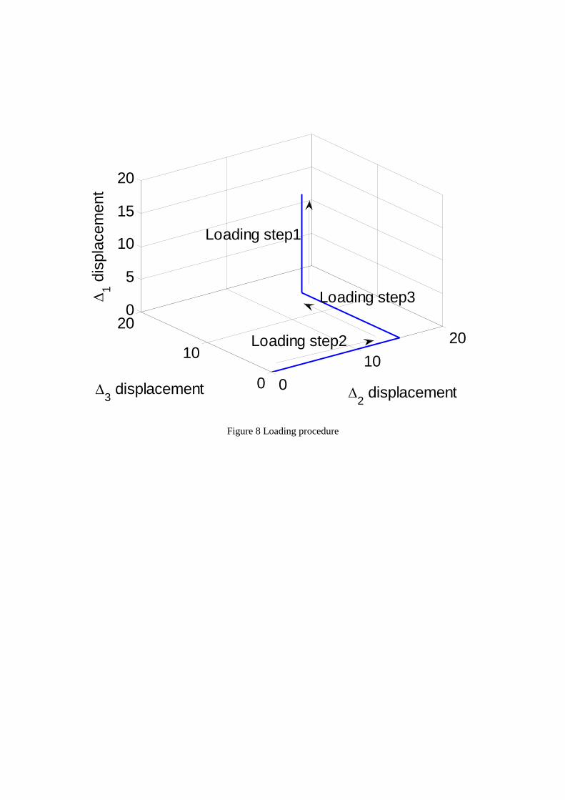
following loading procedure. As illustrated in Fig. 8, we first apply a normal

displacement, 1, subsequently, we apply a shear displacement in the 2-direction, 2,

followed by shear displacement in the 3-direction, 3. For this loading sequence, we

numerically evaluate the discretized Eq. (19) as described in the previous section.

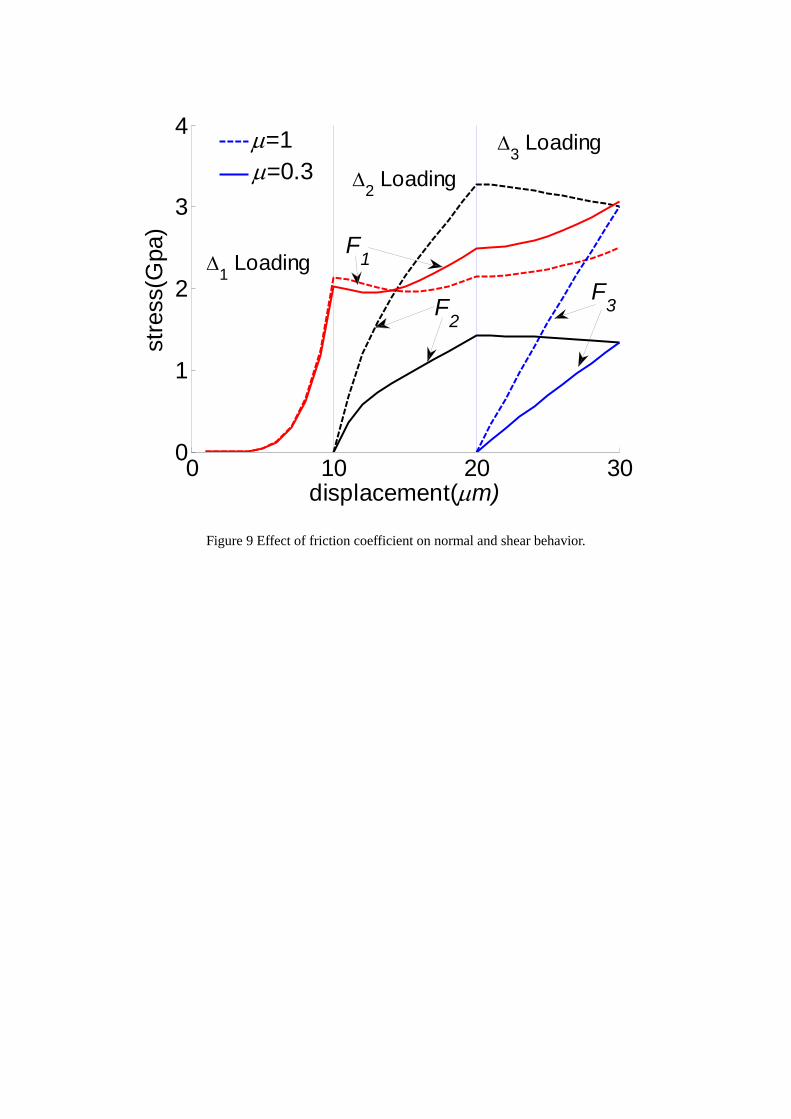
The interface properties used for our example computations are tabulated in Table 1.

Fig. 9 shows the resultant stress-displacement curves. During loading step 1, stress,

F1, increases as interface undergoes closure. Under shear loading in step 2, the

normal stress, F1, increases although the normal displacement, 1, is kept constant.

The increase in normal stress shows the coupling between the normal and shear

behavior induced by the shear loading and is indicative of the fact that the interface is

constrained from dilating. As we now apply the shear loading in step 3 while

keeping the normal displacement, 1, and the shear displacement, 2, we see further

coupling develop between the normal-shear and shear directions. During this

loading step, we find a significant difference between the shear stresses, F1 and F2,

although the corresponding shear displacements may be the same, showing a clear

manifestation of the loading induced anisotropy. At the asperity contact-level, the

no-contact, no-sliding and sliding areas evolve in response to the applied load-path.

The result, of course, is a highly load path dependent overall behavior. To further

illustrate how the stress-displacement behavior changes as a function of the surface

characteristics, we plot the stress-displacement curves for asperity contact friction

coefficient, =0.3, in Fig. 9, for two different asperity contact orientation distributions

in Fig. 10, for two different asperity contact height distributions in Fig. 11, and for

anisotropic asperity contact distributions in Fig. 12. As expected, the overall shear

behavior is softer for the lower asperity contact friction coefficient; however, the

normal behavior becomes more dilatant as seen from a crossover of the normal stress,

F1, as the shear displacement is increased.

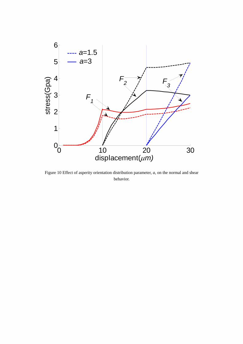
In Fig. 10, the stress-displacement curves are compared for asperity contact

orientation distribution parameter a=1.5 and 3. We observe that the normal behavior

of the two interfaces is similar while the shear behavior shows significant differences.

Since the meridional extent of asperity contact orientation for a=1.5 is much greater

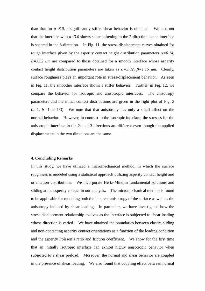
than that for a=3.0, a significantly stiffer shear behavior is obtained. We also not

that the interface with a=3.0 shows shear softening in the 2-direction as the interface

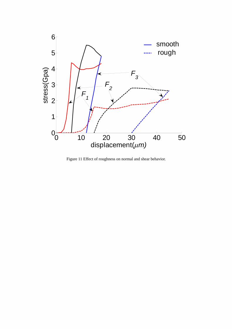
is sheared in the 3-direction. In Fig. 11, the stress-displacement curves obtained for

rough interface given by the asperity contact height distribution parameters =6.14,

=3.52 m are compared to those obtained for a smooth interface whose asperity

contact height distribution parameters are taken as =3.82, =1.15 m. Clearly,

surface roughness plays an important role in stress-displacement behavior. As seen

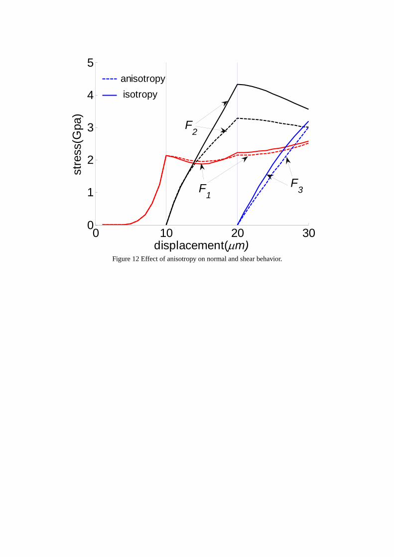
in Fig. 11, the smoother interface shows a stiffer behavior. Further, in Fig. 12, we

compare the behavior for isotropic and anisotropic interfaces. The anisotropy

parameters and the initial contact distributions are given in the right plot of Fig. 3

(a=1, b=-1, c=1/3). We note that that anisotropy has only a small affect on the

normal behavior. However, in contrast to the isotropic interface, the stresses for the

anisotropic interface in the 2- and 3-directions are different even though the applied

displacements in the two directions are the same.

4. Concluding Remarks

In this study, we have utilized a micromechanical method, in which the surface

roughness is modeled using a statistical approach utilizing asperity contact height and

orientation distributions. We incorporate Hertz-Mindlin fundamental solutions and

sliding at the asperity contact in our analysis. The micromechanical method is found

to be applicable for modeling both the inherent anisotropy of the surface as well as the

anisotropy induced by shear loading. In particular, we have investigated how the

stress-displacement relationship evolves as the interface is subjected to shear loading

whose direction is varied. We have obtained the boundaries between elastic, sliding

and non-contacting asperity contact orientations as a function of the loading condition

and the asperity Poisson’s ratio and friction coefficient. We show for the first time

that an initially isotropic interface can exhibit highly anisotropic behavior when

subjected to a shear preload. Moreover, the normal and shear behavior are coupled

in the presence of shear loading. We also found that coupling effect between normal

and shear direction is much stronger in rough interface than that in smooth interface.

References

[1] Hertz H, On the contact of elastic solids. Journal fur de reine und angewandte

Mathematik 1881; 92: 156-71.

[2] Hertz H, On the contact of rigid elastic solids and on hardness. Verhandlungen

des Vereins zur Befoderung des Gewerbefleisses 1882.

[3] Johnson KL, Contact mechanics. Cambridge: Cambridge University Press;

1985.

[4] Wriggers P, Computational contact mechanics. 2nd ed. Berlin ; New York:

Springer; 2006.

[5] Wriggers P, Laursen TA, Computational Contact Mechanics. Vienna: CISM;

2008.

[6] Shankar S, Mayuram MM, A finite element based study on the elastic-plastic

transition behavior in a hemisphere in contact with a rigid flat. Journal of

Tribology-Transactions of the Asme 2008; 130(4): 044502-1-6.

[7] Hyun S, Pei L, Molinari JF, Robbins MO, Finite-element analysis of contact

between elastic self-affine surfaces. Physical Review E 2004; 70(2):

026117-1-12.

[8] Laursen TA, Computational Contact and Impact Mechanics. New York:

Springer; 2002.

[9] Yoshioka N, Elastic Behavior of Contacting Surfaces under Normal Loads - a

Computer-Simulation Using 3-Dimensional Surface Topographies. Journal of

Geophysical Research-Solid Earth 1994; 99(B8): 15549-60.

[10] Majumdar A, Bhushan B, Role of Fractal Geometry in Roughness

Characterization and Contact Mechanics of Surfaces. Journal of

Tribology-Transactions of the Asme 1990; 112(2): 205-16.

[11] Persson BNJ, Albohr O, Tartaglino U, Volokitin AI, Tosatti E, On the nature of

surface roughness with application to contact mechanics, sealing, rubber

friction and adhesion. Journal of Physics-Condensed Matter 2005; 17(1):

R1-R62.

[12] Yang J, Komvopoulos K, A mechanics approach to static friction of

elastic-plastic fractal surfaces. Journal of Tribology-Transactions of the Asme

2005; 127(2): 315-24.

[13] Ciavarella M, Delfine V, Demelio V, A new 2D asperity model with interaction

for studying the contact of multiscale rough random profiles. Wear 2006;

261(5-6): 556-67.

[14] Buczkowski R, Kleiber M, Statistical Models of Rough Surfaces for Finite

Element 3D-Contact Analysis. Archives of Computational Methods in

Engineering 2009; 16(4): 399-424.

[15] Greenwood JA, Williams JB, Contact of Nominally Flat Surfaces. Proceedings

of the Royal Society of London Series a-Mathematical and Physical Sciences

1966; 295(1442): 300-19.

[16] Whitehouse DJ, Archard JF, Properties of Random Surfaces of Significance in

Their Contact. Proceedings of the Royal Society of London Series

a-Mathematical and Physical Sciences 1970; 316(1524): 97-121.

[17] Greenwood JA, Tripp JH, The contact of two nominally flat rough surfaces.

Proceedings of the Institution of Mechanical Engineers 1971; 185: 625-33.

[18] Nayak PR, Random Process Model of Rough Surfaces. Journal of Lubrication

Technology 1971; 93(3): 398-407.

[19] Bush AW, Gibson RD, Thomas TR, Elastic Contact of a Rough Surface. Wear

1975; 35(1): 87-111.

[20] Bush AW, Gibson RD, Keogh GP, Strongly Anisotropic Rough Surfaces.

Journal of Lubrication Technology-Transactions of the Asme 1979; 101(1):

15-20.

[21] Adler RJ, Firman D, A Non-Gaussian Model for Random Surfaces.

Philosophical Transactions of the Royal Society of London Series

a-Mathematical Physical and Engineering Sciences 1981; 303(1479): 433-62.

[22] Mccool JI, S.S.Gassel, The contact of two surfaces having anisotropic

roughness geometry, in Energy technology, Special Publication. 1981,

American Society of Lubrication Engineers: New York. 29-38.

[23] Brown SR, Scholz CH, Closure of Random Elastic Surfaces in Contact.

Journal of Geophysical Research-Solid Earth and Planets 1985; 90(Nb7):

5531-45.

[24] Brown SR, Scholz CH, Closure of Rock Joints. Journal of Geophysical

Research-Solid Earth and Planets 1986; 91(B5): 4939-48.

[25] Chang WR, Etsion I, Bogy DB, An Elastic-Plastic Model for the Contact of

Rough Surfaces. Journal of Tribology-Transactions of the Asme 1987; 109(2):

257-63.

[26] Yoshioka N, Scholz CH, Elastic Properties of Contacting Surfaces under

Normal and Shear Loads .1. Theory. Journal of Geophysical Research-Solid

Earth and Planets 1989; 94(B12): 17681-90.

[27] Yoshioka N, Scholz CH, Elastic Properties of Contacting Surfaces under

Normal and Shear Loads .2. Comparison of Theory with Experiment. Journal

of Geophysical Research-Solid Earth and Planets 1989; 94(B12): 17691-700.

[28] Misra A, Mechanistic model for contact between rough surfaces. Journal of

Engineering Mechanics-Asce 1997; 123(5): 475-84.

[29] Archard JF, Elastic Deformation and the Laws of Friction. Proceedings of the

Royal Society of London Series a-Mathematical and Physical Sciences 1957;

243(1233): 190-205.

[30] Cooper MG, Mikic BB, Yovanovich MM, Thermal Contact Conductance.

International Journal of Heat and Mass Transfer 1969; 12(3): 279-300.

[31] Tabor D, Friction - the Present State of Our Understanding. Journal of

Lubrication Technology-Transactions of the Asme 1981; 103(2): 169-79.

[32] Zavarise G, Borri-Brunetto M, Paggi M, On the reliability of microscopical

contact models. Wear 2004; 257(3-4): 229-45.

[33] Zavarise G, Borri-Brunetto M, Paggi M, On the resolution dependence of

micromechanical contact models. Wear 2007; 262(1-2): 42-54.

[34] Nayak PR, Random Process Model of Rough Surfaces in Plastic Contact.

Wear 1973; 26(3): 305-33.

[35] Misra A, Micromechanical model for anisotropic rock joints. Journal of

Geophysical Research-Solid Earth 1999; 104(B10): 23175-87.

[36] Misra A, Huang S, Micromechanics based stress-displacement relationships of

rough contacts: Numerical implementation under combined normal and shear

loading. Cmes-Computer Modeling in Engineering & Sciences 2009; 52(2):

197-215.

[37] Mindlin RD, Deresiewicz H, Elastic Spheres in Contact under Varying

Oblique Forces. Journal of Applied Mechanics-Transactions of the Asme 1953;

20(3): 327-44.

List of nomenclature

a, b and c= orientation distribution parameters

d= asperity contact displacement in normal direction

e= non-sliding asperity contact

fi = asperity contact forces

Fi = overall interface stress

G= shear modulus

H= asperity contact height distribution

Kij= asperity contact stiffnesses

Kn, Kst = asperity contact stiffness along the normal and the tangential directions

n, s and t = spherical coordinate direction vector

N =asperity contact density given as number of asperity contact per unit area

p= sliding asperity contact

r= composite topography height or asperity contact height

R= radius of asperity

, = height distribution parameters

j= asperity contact displacement

i= interface displacement

and = spherical coordinates

= plasticity parameter

= material constant

= asperity contact friction

= Poisson’s ratio

= angle between the asperity contact normal and the 1-axis in the 1-3 plane

= density function of asperity contact orientations,

List of Figures

Figure 1 Distribution of asperity contact heights

Figure 1 Schematic depiction of the micromechanical modeling methodology for rough interfaces.

Figure 3: Asperity contact orientation distribution, (,): left frame is for isotropic interface

(a=1,b=1/3,c=0) and right frame is for anisotropic interface (a=1,b=-1,c=1/3). Grayscales

indicate the probability density of finding asperity contact in a given orientation defined by the

coordinate system given in the inset. The plots are in spherical coordinates where the radius is

(,).

Figure 4 Asperity contact displacement, d, at height r for a normal interface displacement of 1.

Figure 5 Oblique loading angle ω.

Figure 6 ω effect on sliding and no sliding distribution (μλ=1).

Figure 7 μλ effect on sliding and no sliding distribution (ω=π/4).

Figure 8 Loading procedure.

Figure 9 Effect of friction coefficient on normal and shear behavior.

Figure 10 Effect of asperity orientation distribution parameter, a, on the normal and shear

behavior.

Figure 11 Effect of roughness on normal and shear behavior.

Figure 12 Effect of anisotropy on normal and shear behavior.

List of Tables

Table 1 Interface property.

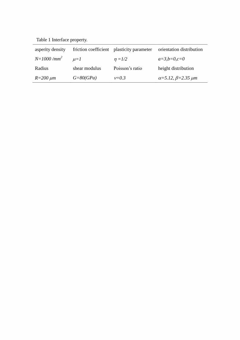
Table 1 Interface property.

asperity density friction coefficient plasticity parameter orientation distribution

N=1000 /mm2 =1 =1/2 a=3,b=0,c=0

Radius shear modulus Poisson’s ratio height distribution

R=200 m G=80(GPa) =0.3 =5.12, =2.35 m

0 10 20 30 40 500

0.05

0.1

0.15

0.2

r(m)

Fre

quency

=3.82,=1.15m(smooth)

=6.14,=3.52m(rough)

=5.12,=2.35m(mezzo)

Figure 1 Distribution of asperity contact heights

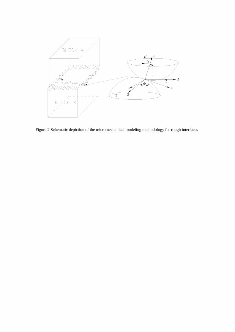
Figure 2 Schematic depiction of the micromechanical modeling methodology for rough interfaces

2

3

θ

φ

1

2

3

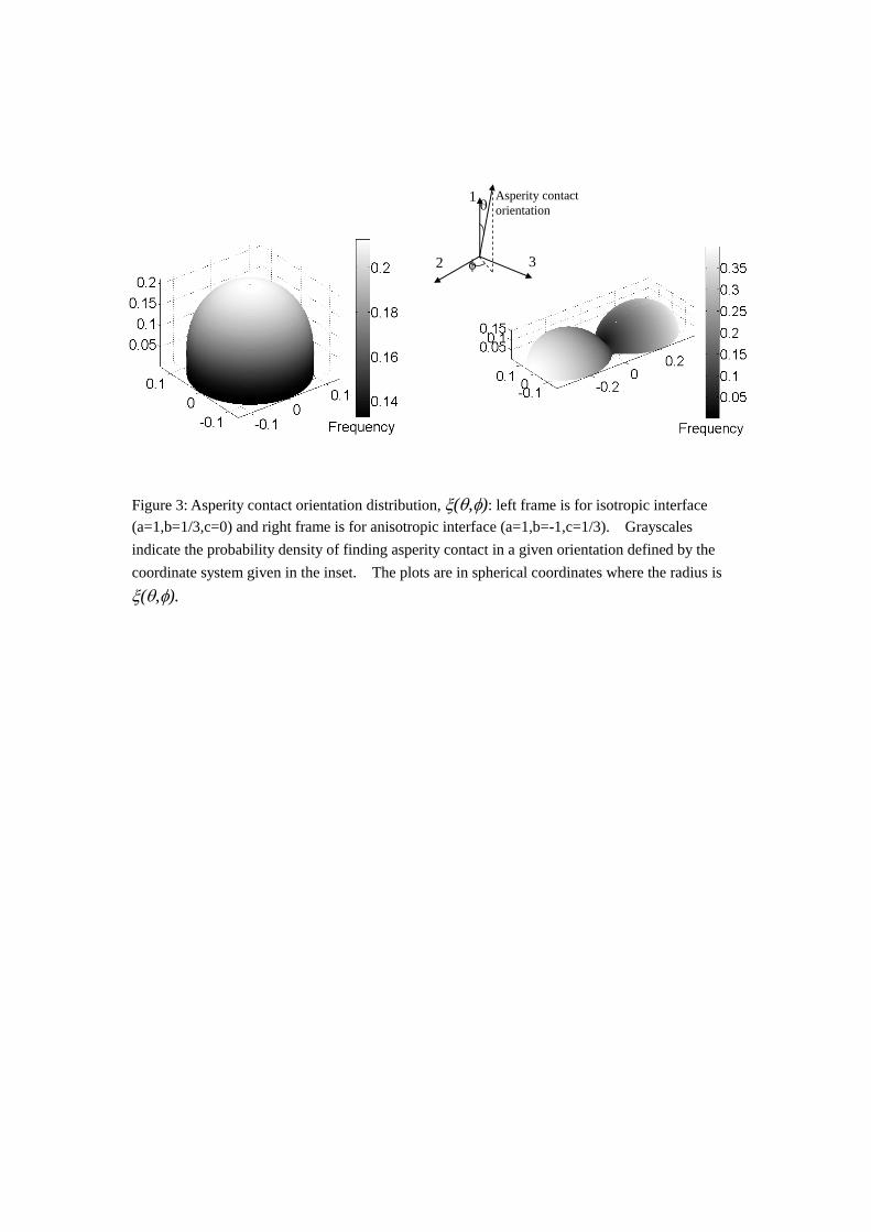
Figure 3: Asperity contact orientation distribution, (,): left frame is for isotropic interface

(a=1,b=1/3,c=0) and right frame is for anisotropic interface (a=1,b=-1,c=1/3). Grayscales

indicate the probability density of finding asperity contact in a given orientation defined by the

coordinate system given in the inset. The plots are in spherical coordinates where the radius is

(,).

1

2 3

Asperity contact

orientation

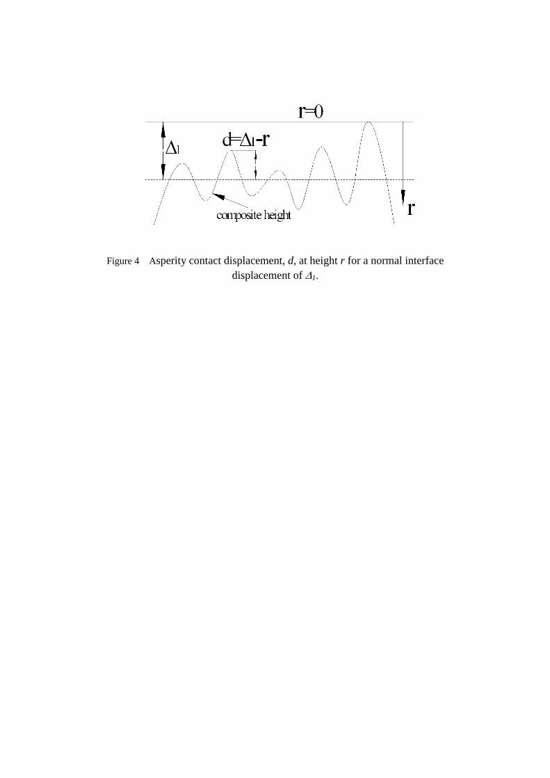
Figure 4 Asperity contact displacement, d, at height r for a normal interface

displacement of 1.

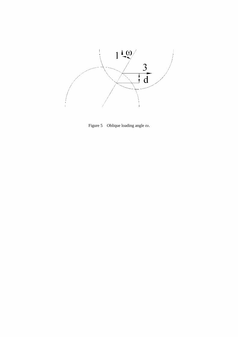
Figure 5 Oblique loading angle ω.

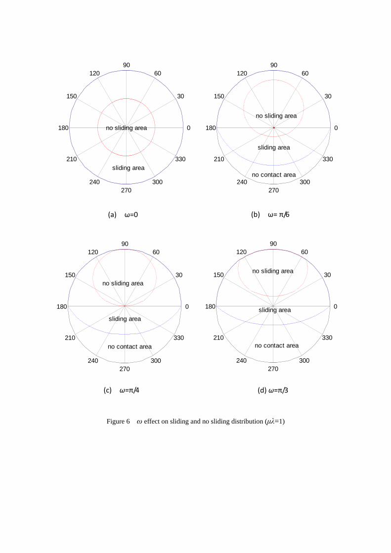
Figure 6 ω effect on sliding and no sliding distribution (μλ=1)

30

210

60

240

90

270

120

300

150

330

180 0no sliding area

sliding area

30

210

60

240

90

270

120

300

150

330

180 0

no sliding area

sliding area

no contact area

30

210

60

240

90

270

120

300

150

330

180 0

no sliding area

sliding area

no contact area

30

210

60

240

90

270

120

300

150

330

180 0

no sliding area

sliding area

no contact area

(d) ω=π/3 (c) ω=π/4

(a) ω=0 (b) ω= π/6

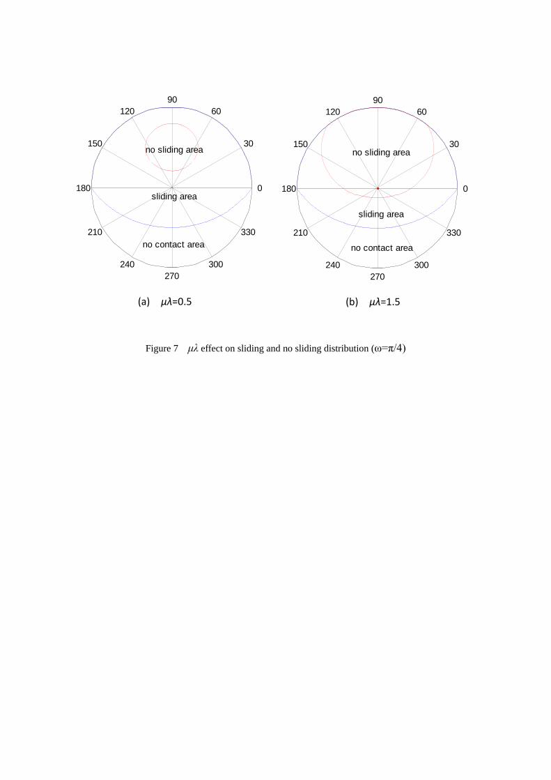
Figure 7 μλ effect on sliding and no sliding distribution (ω=π/4)

30

210

60

240

90

270

120

300

150

330

180 0

no sliding area

sliding area

no contact area

30

210

60

240

90

270

120

300

150

330

180 0

no sliding area

sliding area

no contact area

(a) μλ=0.5 (b) μλ=1.5

0

10

20

0

10

200

5

10

15

20

Loading step3

2 displacement

Loading step2

Loading step1

3 displacement

1 d

ispla

cem

ent

Figure 8 Loading procedure

0 10 20 300

1

2

3

4

displacement(m)

str

ess(G

pa)

1 Loading

2 Loading

3 Loading

F1

F2

F3

=1

=0.3

Figure 9 Effect of friction coefficient on normal and shear behavior.

0 10 20 300

1

2

3

4

5

6

displacement(m)

str

ess(G

pa)

F1

F2 F

3

a=3

a=1.5

Figure 10 Effect of asperity orientation distribution parameter, a, on the normal and shear

behavior.

0 10 20 30 40 500

1

2

3

4

5

6

displacement(m)

str

ess(G

pa)

F1

F2

F3

rough

smooth

Figure 11 Effect of roughness on normal and shear behavior.

0 10 20 300

1

2

3

4

5

displacement(m)

str

ess(G

pa)

F1

F2

F3

isotropy

anisotropy

Figure 12 Effect of anisotropy on normal and shear behavior.