Effect of field-line chaos on Plasma Filament Dynamics and Turbulence in theScrape-Off Layer

D. Meyerson‡, C. Michoski? , F. Waelbroeck‡, W. Horton‡

Institute for Fusion Studies (IFS)‡, Department of Physics‡

Institute for Computational Engineering and Sciences (ICES)?,Department of Aerospace Engineering and Engineering Mechanics?

University of Texas at Austin, Austin, TX 78712(Dated: April 16, 2014)

Naturally occurring error fields as well as resonant magnetic perturbations applied for stabilitycontrol are known to cause magnetic field-line chaos in the scrape-off layer (SOL) region of tokamaks.Here, 2D simulations are used to investigate the effect of the field-line chaos on the SOL and inparticular on its width and peak particle flux. The chaos enters the SOL dynamics through theconnection length, which is evaluated using a Poincare map. The variation of experimentally relevantquantities, such as the SOL gradient length scale and the intermittency of the particle flux in theSOL, is described as a function of the strength of the magnetic perturbation. It is found that theeffect of the chaos is to broaden the profile of the sheath-loss coefficient, which is proportional tothe inverse connection length. That is, the SOL transport in a chaotic field is equivalent to that in amodel where the sheath-loss coefficient is replaced by its average over the unperturbed flux surfaces.

2

I. INTRODUCTION

In diverted tokamaks, the separatrix defines the boundary between open and closed flux surfaces and acts as ariverbed for the scrape-off layer (SOL). In the SOL, the flow across the magnetic field balances the parallel streamingalong the field towards the plasma-facing components (PFC). A picture of how tokamak turbulence and transport inthe SOL scale with experimentally controllable parameters is necessary to minimize peak heat and particle flux loadson the PFC,[1] to minimize introduction of impurities, and to simultaneously maintain conditions that are consistentwith global plasma confinement.[2–5] In the presence of edge-resonant non-axisymmetric perturbations, however, theseparatrix is readily shattered and replaced by a region exhibiting field-line chaos, or magnetic stochasticity, whichmanifests its presence by the splitting of the separatrix footprints.[6] Field-line chaos can be introduced by deliber-ately applied resonant Magnetic Perturbations (RMPs) [7], ergodic magnetic limiters [8, 9] and naturally-occurringinstabilities. RMPs have been the subject of intense recent interest for their use in controlling edge localized modes bykeeping the edge pedestal conditions below some critical threshold and by effectively replacing impulsive intermittentELM transport with a series of smaller less disruptive transport events, or even by achieving full suppression.[10]

While the turbulent SOL has a complex three dimensional geometry, its physics is dominated by curvature-driveninterchange instabilities characterized by a short extension across but a long extension along the field lines.[5] Followingstandard practice, we average vorticity and density equations along the field-aligned dimension and work in theresulting 2D plane normal to the field-lines. Excluding regimes where full drift-wave physics has a strong influenceon the dynamics [11–13], this dimensionally-reduced approach has provided experimentally validated descriptions ofturbulent transport, interplay between zonal flows and turbulence,[14–16] creation of coherent structures, and SOLdensity length scales, among other results.[14, 17–21] End-losses along the field appear as a damping term in thedensity equation characterized by a coefficient α that is inversely proportional to the connection length L‖:

α = 2ρs/L‖ (1)

In this paper we specify L‖ by a map that describes chaotic connection lengths in the region spanning the outerportions of the core and the SOL. To maintain the density in the presence of the end-losses, we include a particlesource at the core-facing edge of the simulation domain. The resulting turbulence is thus flux-driven. The particlesource can be thought of as modeling the injection of particles by gas feed, neutral beams, pellets and recycling.

It is generally accepted that cross field transport in the region between the plasma edge and the vessel wall isdominated by intermittent transport [17, 22, 23] mediated by coherent, radially propagating plasma filaments calledblobs.[18, 24–27] Typically the magnetic-curvature drift combined with the usual E×B convection will drive a blobradially outward (Fig. 1). Continuity and charge conservation equations govern their dynamics. Blobs provide amechanism for radial transport of heat and momentum that greatly exceeds neoclassical predictions. The usefulnessof blobs, as a concept, depends on their ability to survive long enough to affect transport and demonstrate a cleardependence of their properties on model plasma parameters. Blob lifetimes have been examined theoretically byKrasheninnikov [18] and other authors [23, 28] and experimentally in tokamaks[24, 25] and other devices.[29–31]These studies have shown the existence of a most-stable blob size. The mechanisms underlying the interplay betweenparallel transport, diffusion, convective processes, and spontaneous formation of blobs affects the width of the SOLlayer and the intermittency of transport. These mechanisms have been studied in some detail.[5, 12, 15, 21, 32]

In this paper we examine how magnetic chaos, modeled with a chaotic map that mimics the application of staticRMPs, changes statistical characterization of blobs and the scaling of their properties with plasma parameters. Asan example of how our current understanding of blob behavior may be challenged by the presence of chaos, considerthe simplest analytic prediction of radial blob velocity:Vx ∝ L‖/(Rδ

2y), where δy is the blob size (Fig. 1). With

the addition of a chaotic field, there will be large variations in the L‖ value over the spatial footprint of the blob -possibly affecting its coherence and thus the mean particle transport and intermittency of density fluctuations. Fromprevious work we also know that for a constant sheath-loss coefficient α there is a strong selection for a specific blobsize.[18, 32] It is natural to ask whether magnetic chaos might seed blobs of different sizes, or favor hole creation overblob creation. Such effects on blob dynamics would clearly affect the observed density scaling distance in the SOLdensity profile. The aim of the present paper is to answer these questions within the framework of the 2D model ofSOL transport.

The remainder of this paper is organized as follows. In Sec. II, we describe the formulation of the problem andsome simple analytic considerations. In Sec. III, we review the results for unperturbed SOL dynamics and use thisreview to verify our code. We then examine the effect of the field-line chaos in Sec. IV, with particular attention tothe scaling of the density length-scale and the selection of the dominant blob size. We conclude by summarizing anddiscussing our results in Sec. V .

3

FIG. 1. A simple blob with key forces, length scales and directions

II. FORMULATION AND ANALYTIC CONSIDERATIONS

A. Formulation

We use a simple two fluid interchange model that nonetheless contains many of the most important features:curvature and density gradient drifts, convective nonlinearities, blob formation, and a parallel closure scheme thatis able to model both closed and open field lines. Similar models have a been used by many authors to study SOLturbulence, zonal flows and transport in both mirror machines and tokamaks edge plasmas.[5, 12, 32, 33]

The equations used here have been normalized by the gyro-radius ρs = cs/Ωi , ion gyro-frequency Ωi, and ion-

acoustic speed cs =√kTe/mi. They are

∂tn+ VE · ∇n−Dn∇2n + αn = Sn, (2a)

∂t$ + VE · ∇$ −D$∇2$ − αφ− β (b · ∇x×∇n)

n= S$, (2b)

$ = ∇2φ, (2c)

VE = b×∇φ, (2d)

β =2ρsR0

and α =2ρsL‖

. (2e)

The loss terms containing the coefficient α come from averaging the parallel current and velocities given by elementarysheath theory. Notice that we assume no scale-separation between some background and a perturbed portion. Thisis consistent with the observed character of the SOL layer. External density and momentum sources can be specifiedwith Sn and S$ respectively. In this work we set S$ = 0. We will discuss the choice of Sn in section II D.

In arriving at equation (2), the full three dimensional geometry is reduced to two dimensions by averaging alongthe field lines, where we take the flute approximation [34] and assume that all introduced quantities vary weaklyalong uniform magnetic field lines (i.e. the blobs are interchange-like). The influence of RMPs is then reflected in theparallel connection length to the divertor that enters into the α parameter of equation (2).

B. Geometry

While BOUT++ is designed primarily for field-aligned, non-orthogonal coordinates, it also allows for simulationsin slab geometry. A shortcoming of the 2D slab model is that it is unable to account for the variation of the curvaturealong the field lines or for the resulting variation in the mode structure. Various estimates of the parallel wavenumber

4

can be made.[33] Resolving the parallel mode structure requires a full three dimensional simulation.[11] Recent work[12] indicates substantial qualitative changes in the behavior of this system when the full three dimensional picture istaken into account. The simplifying nature of the 2D model, by contrast, enables a greater focus on properties thatare independent of the 3D geometry of the SOL.

C. RMPs and the Ullmann Map

Magnetic fields have a field-line structure governed by Hamilton‘s equations, with the toroidal angle playing therole of time. The field lines of axisymmetric equilibria lie on nested toroidal surfaces, constituting integrable Hamil-tonian systems, and perturbations of such axisymmetric equilibria are naturally described by Poincare sections, theintersection of field lines with a poloidal section. The Ullmann map [35, 36] is a Poincare magnetic field line mapthat was created to study the effects of an ergodic divertor on toroidal plasmas. Repeated application allows us toassign a parallel connection length value based on the number of applications necessary for a given field line to hit thedivertor. One advantage of this map over some others is that it is characterized in terms of experimental quantitiessuch as major and minor radius, Iext/Ip and some safety factor, q(r).

The connection lengths are said to exhibit chaos when two neighboring points are traversed by field lines that followvery different trajectories. For example, one field line may quickly terminate on the divertor or the wall while anothermay stay trapped. A sheath-loss coefficient α may be assigned based on Eq. (1) and this computed chaotic parallelconnection length.

The Ullmann map [35] is a composition of a map with good flux surfaces, where

rn+1 =rn

1− a1sinθn, (3a)

θn+1 = θn +2π

qeq(rn+1)+ a1cosθn, (3b)

and a perturbation map, given by

rn = rn+1 +mCεb

m− 1

(rn+1

b

)m−1

sin (mθn) , (4a)

θn+1 = θn − Cε(rn+1

b

)m−2

cos (mθn) . (4b)

where q is the safety factor, C is a geometric factor, and ε is current in the external coil normalized by the plasmacurrent

C =2mla2

R0b2qa, (5a)

ε =IlIp, (5b)

with m = 2, 3, .... Given some effective minor radius a we can approximate the field-line length once we know howmany applications of the map connect a given point to the divertor:

L‖ ≈ q(a)2πaNturns (6)

Ultimately what enters equation (2) is the inverse of this parallel connection length, α = 2ρs/L‖.To fix the parameters used in this study we adopt an NSTX-like geometry, with minor radius = 68 cm, plasma

radius = 60 cm, external coil size =10 cm, R0 = 85 cm, a1 =-.01, and consider Iext/Ip = ε = 0, .1, .2, .3. We use themap to fix α(x, y) for the duration of the run. The resulting distribution of α values is shown in Fig. 2.

From a macroscopic point of view, one of the effects of the magnetic field chaos is to broaden the transition betweenclosed field lines and open field lines, which appears in an axisymmetric system as a jump in the connection lengthL‖. In order to distinguish the effect of the spatial fluctuations of L‖ in a chaotic SOL field from the effect of thebroadening of the transition, it is interesting to consider a model in which the chaotic inverse connection length isaveraged over an unperturbed flux-surface. We will refer to this case, illustrated in Fig. 3, as the “smooth alpha”case.

5

FIG. 2. Contour plot of the inverse connection length, α, associated with magnetic chaos generated by the Ullmann map.Escape basins appear as darker regions, whereas trapped regions appear white and have α = 0. Note that the contour valueschange discretely.

FIG. 3. The flux-surface averaged α as a function of the radial position with the full range of α superimposed.

D. Reference state

We are interested in characterizing intermittency and the SOL profile as a function of the RMP amplitude. Sincewe will be driving turbulence by introducing a particle source Sn on the core-side edge of the simulation, it is usefulto consider how to select Sn in our model.

The primary density sink in our system is loss through the divertor sheaths (the αn term). If we account for thenonlinear terms through an anomalous diffusivity Da and assume a source localized at the boundary of the simulationand of the form Sn = S0 Θ(x? − x), the profile of the average density will take the form

n(x) = n0e−x√

αDa for x > x?, (7)

where S0 = 2n0. This simple result reflects the fact that the source must roughly balance the dominant sink,represented by the αn term in the density equation.

Note that without a particle source the equations are invariant under a change in the global background density,n→ n+ n0. The source strength thus has the effect of setting the background density for given Da.

6

III. UNPERTURBED SOL DYNAMICS

We use the BOUT++([37–39]) framework to discretize and evolve equation (2). The framework uses a local poly-nomial approximation to compute derivatives along the x coordinate, pseudo-spectral methods to compute derivativesalong the y coordinate, and a CVODE([40]) solver to advance the fields in time. To assess the reliability of our numer-ical tools we verify the linear dispersion relation in section(III A) as well as verify that nonlinear analytic predictionsfavorably compare to the single blob dynamics of two other codes ([41], [21]) in section (III B), and finally matchpublished SOL width values [32] in section (III C).

A. Linear Verification

We compare the growth rate of the SOL interchange mode as deduced from a simulation of a linearized versionof equation (2) with the analytically derived growth rate γ. Expanding equation (2) to the lowest order in φ, u, n,setting D$ = Dn, and dropping parallel dissipation in the density equation yields the analytic result

γ = −(α+ 2Dk4

⊥)

2k2⊥

+

√(α

2k2⊥

)2

+β

`n. (8)

The above expression for the growth rate shows that the mode is driven by the interchange term β/`n and is stabilizedby dissipation for short wavelengths. The growth rate peaks for wavelengths of a few times the Larmor radius ρs.

For the numerical calculation, several γ−1 time increments may be required to converge on the solution, unless onesets the initial condition such that u, φ correspond to an eigenvector of the linearized version of equation (2). Fig. 4shows that the simulations are in satisfactory agreement with the analytic dispersion relation.

0.2 0.4 0.6 0.8 1.0kyρs

−1.0

−0.8

−0.6

−0.4

−0.2

0.0

0.2

0.4

γωci

1e−2 γlinearBOUT++

analytic

0.5 1.0 1.5 2.0 2.5kyρs

−3

−2

−1

0

1

2

3

4

5

γωci

1e−3 γlinearBOUT++

analytic

FIG. 4. Growth rate γ as a function of the poloidal wavenumber ky, where D = µ = 1× 10−2 and 1× 10−3 on left and rightcharts respectively, β = 6× 10−4, α = 3× 10−5. Good agreement between analytic theory and BOUT++ results is observed.

B. Single-blob dynamics

In their insightful paper, Garcia et al. (2006) ([21]) have shown how to characterize the motion of individualblobs by their center of mass. We have repeated some of their simulations using the initial and boundary conditionsshown in Table (I). We chose a simulation domain large enough to keep the blob far away from the boundaries forthe duration of the run. In particular, the size of the domain is such that changing boundary conditions betweenDirichlet (nx boundary = 0), and Neumann (∂xnx boundary = 0), only weakly affects the history of the leading momentsdescribing the blob.

Fig. 5 compares the evolution of the velocity of the center of mass as well as the maximum amplitude of the densityin the blob. We find consistent agreement between the results of BOUT++ and those presented by Garcia et al.(2006) as well as with recent work by Michoski [41] and Hakim [42] using discontinuous Galerkin algorithms (notshown in the figure).

7

Parameter Value

Nx 1056

Ny 1024

Lx 60

Ly 40

n(t = 0) e(x2+y2)

2

u(t = 0) 0

BCx ∂xu = ∂xn = 0

BCy periodic

Ra 102,4,6

TABLE I. Numerical Blob Parameters

0 5 10 15 20 25

t/τcs

0

2

4

6

8

10

12

14

xρcs

Center of mass

Garcia ref., Ra=106

Garcia ref., Ra=104

BOUT++, Ra=104

BOUT++, Ra=106

0 5 10 15 20 25 30

t/τci

0.0

0.2

0.4

0.6

0.8

Vx

ωciρcs

Center of mass velocity

Garcia ref., Ra=106

Garcia ref., Ra=104BOUT++, Ra=104

BOUT++, Ra=106

FIG. 5. Comparison of blob trajectories calculated with BOUT++ to the results of E. Garcia [21], Two cases are comparedcorresponding to Rayleigh number 104 and 106.

C. Saturated turbulence

As an additional verification we examined flux-driven, many-blob interchange turbulence as described by Aydemir.[32]We used equation (2) as for single blob simulations, but with a nonzero density source term, Sn, and with radialboundary conditions that allow the profile to relax. Except for having a constant value of α, the simulation setuphere is similar to ones described in section IV B of the present paper. Using β/α = 5, we see excellent agreement ofλSOL with the results present by Aydemir [32] across a wide range of parameters. Here as in [32], λSOL is determinedby fitting a profile of the form n = n0 exp(−x/λSOL), to observed flux-surface averaged density values.

IV. NUMERICAL STUDIES OF CHAOTIC SOL

We now examine the effects of field-line chaos on SOL dynamics. We begin in Sec. IV A by describing the propagationof an isolated blob in a chaotic region. This motivates the investigation in Sec. IV B of the effect of chaos on saturatedSOL turbulence. We then examine the modifications of the density profile in the SOL in Sec. IV C and the statisticsof the associated fluxtuations in IV D.

A. Effect of field-line chaos on an isolated blob

In contrast to cases where α is a constant value or is simplified by averaging over flux-surfaces, blobs quickly losecoherence when propagating through a region with chaotic α as pictured in Fig. (6). This suggests that magneticchaos may bring about significant changes in the properties of the SOL. The fine fractal structures of the Poincare

8

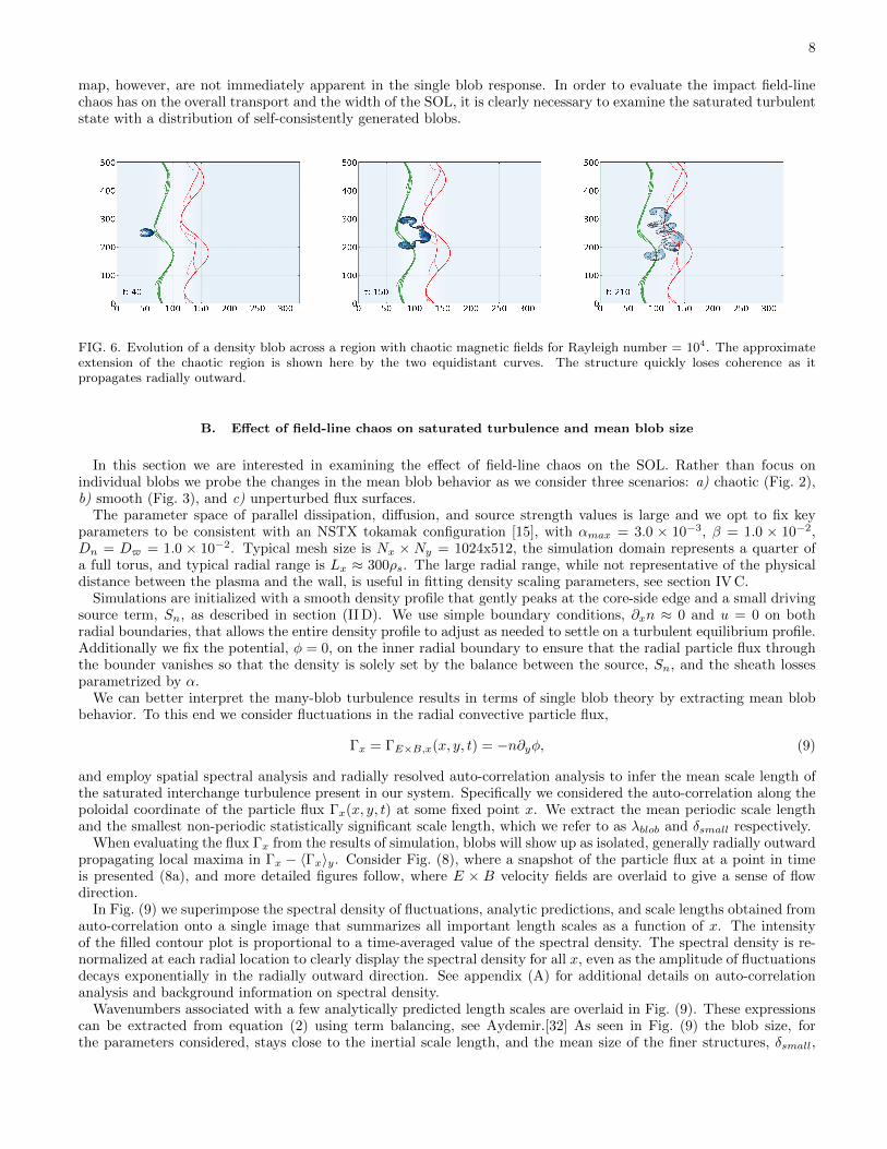
map, however, are not immediately apparent in the single blob response. In order to evaluate the impact field-linechaos has on the overall transport and the width of the SOL, it is clearly necessary to examine the saturated turbulentstate with a distribution of self-consistently generated blobs.

FIG. 6. Evolution of a density blob across a region with chaotic magnetic fields for Rayleigh number = 104. The approximateextension of the chaotic region is shown here by the two equidistant curves. The structure quickly loses coherence as itpropagates radially outward.

B. Effect of field-line chaos on saturated turbulence and mean blob size

In this section we are interested in examining the effect of field-line chaos on the SOL. Rather than focus onindividual blobs we probe the changes in the mean blob behavior as we consider three scenarios: a) chaotic (Fig. 2),b) smooth (Fig. 3), and c) unperturbed flux surfaces.

The parameter space of parallel dissipation, diffusion, and source strength values is large and we opt to fix keyparameters to be consistent with an NSTX tokamak configuration [15], with αmax = 3.0 × 10−3, β = 1.0 × 10−2,Dn = D$ = 1.0 × 10−2. Typical mesh size is Nx × Ny = 1024x512, the simulation domain represents a quarter ofa full torus, and typical radial range is Lx ≈ 300ρs. The large radial range, while not representative of the physicaldistance between the plasma and the wall, is useful in fitting density scaling parameters, see section IV C.

Simulations are initialized with a smooth density profile that gently peaks at the core-side edge and a small drivingsource term, Sn, as described in section (II D). We use simple boundary conditions, ∂xn ≈ 0 and u = 0 on bothradial boundaries, that allows the entire density profile to adjust as needed to settle on a turbulent equilibrium profile.Additionally we fix the potential, φ = 0, on the inner radial boundary to ensure that the radial particle flux throughthe bounder vanishes so that the density is solely set by the balance between the source, Sn, and the sheath lossesparametrized by α.

We can better interpret the many-blob turbulence results in terms of single blob theory by extracting mean blobbehavior. To this end we consider fluctuations in the radial convective particle flux,

Γx = ΓE×B,x(x, y, t) = −n∂yφ, (9)

and employ spatial spectral analysis and radially resolved auto-correlation analysis to infer the mean scale length ofthe saturated interchange turbulence present in our system. Specifically we considered the auto-correlation along thepoloidal coordinate of the particle flux Γx(x, y, t) at some fixed point x. We extract the mean periodic scale lengthand the smallest non-periodic statistically significant scale length, which we refer to as λblob and δsmall respectively.

When evaluating the flux Γx from the results of simulation, blobs will show up as isolated, generally radially outwardpropagating local maxima in Γx − 〈Γx〉y. Consider Fig. (8), where a snapshot of the particle flux at a point in timeis presented (8a), and more detailed figures follow, where E × B velocity fields are overlaid to give a sense of flowdirection.

In Fig. (9) we superimpose the spectral density of fluctuations, analytic predictions, and scale lengths obtained fromauto-correlation onto a single image that summarizes all important length scales as a function of x. The intensityof the filled contour plot is proportional to a time-averaged value of the spectral density. The spectral density is re-normalized at each radial location to clearly display the spectral density for all x, even as the amplitude of fluctuationsdecays exponentially in the radially outward direction. See appendix (A) for additional details on auto-correlationanalysis and background information on spectral density.

Wavenumbers associated with a few analytically predicted length scales are overlaid in Fig. (9). These expressionscan be extracted from equation (2) using term balancing, see Aydemir.[32] As seen in Fig. (9) the blob size, forthe parameters considered, stays close to the inertial scale length, and the mean size of the finer structures, δsmall,

9

5 10

0.1

0.2

0.3

0.4

(a) A hypothetical Γx(y) at a fixed x

5 10 15

0.2

0.4

0.6

0.8

1.0

(b) Autocorrelation reveals the relevant length scales

FIG. 7. The mean size of the smallest reoccurring feature in y can be shown to be 〈δsmall〉y ≈√

2σ, where σ is determined by

a least-squares fit of a Gaussian, e− y2

2σ2 , around the central peak of R(y)

0 50 100 150 200 250x/ρs

0

20

40

60

80

100

120

yρs

Γx⟨δsmall

⟩y⟨

λblob

⟩y

Region 1

Region 2

(a) snapshot of Γx

30 40 50 60x/ρs

0

10

20

30

40

yρs

Γx in Region 1⟨δsmall

⟩y

(b) Region 1 with VE×B flow detail

210 215 220 225 230 235 240 245 250x/ρs

0

5

10

15

20

yρs

Γx in Region 2⟨δsmall

⟩y

(c) Region 2 with VE×B flow detail

FIG. 8. Details of radially outward particle flux Γx with average blob size 〈δblob〉y. The difference in the values of the αparameter is reflected in the size of the blobs in the two closeups images.

Parameter Value

inertial lower limit: km =√

2

(β/α2)1/5

diffusive upper limit: kDn =√

2(αDn)β

parallel upper limit: kα =√

2

(β/α2)1/3

viscous lower limit: kD$ =√

2

(D$/α)1/4

linear scale: klin(γmax) ≈(αDn

)1/4

mean detected blob size: kλblob ≈2πλblob

width of central peak of RΓx : kσ =√

2δsmall

TABLE II. Wavenumber definitions

stays close to the most unstable linear scale. The inertial scale is the length scale at which both inertia and parallelmomentum losses are comparable with the curvature drive. Relating operators in the momentum equation (2a) tosome typical blob size a we may write the various terms of this equation symbolically as(

φ

a2

)2

+β

a− αφ+

D$φ

a4= 0, (10)

the desired length scale am follows by balancing the curvature term against the inertia and the sheet-loss:(φ

a2m

)2

≈ β

am, αφ ≈ β

am. (11)

10

It follows easily that equation (11) is satisfied when

a5m = β/α2. (12)

Examining Fig. (9) further, we observe that the spectral density appears to taper off below the parallel upper limitkα. Modes below this value are dominated by end-losses, and typically lose mass and lose coherence quickly. We canderive this length scale similarly to the preceding example. Rewriting operators in the continuity equation in termsof the scale length a yields

Dn

a2+

φ

a2+ α = 0. (13)

When parallel particle losses roughly balance particle flux in equation (13), and curvature drive is comparable toparallel momentum losses in equation (10) the implied length scale aα must satisfy

φ

a2α

+ α ≈ 0 αφ ≈ β

aα, (14)

from which it follows that

a3α = β/α2. (15)

We also note that the curvature-drive term gets bigger as a gets smaller, therefore aα must be the smallest lengthscale at which parallel dissipation can be comparable to curvature drive. In k-space this will correspond to someupper wavenumber limit, where kα =

√2/aα, when we correctly relate periodic and spatially localized/non-periodic

length scales. As an aside, we observe that in order to correctly associate a non-periodic or spatially localized lengthscale with a wavenumber we use the auto-correlation function of the two signal types. Consider an auto-correlationfunction of a sine wave, and an auto-correlation function of some non-periodic signal, call them Rsine and Rnoperiodrespectively. As reviewed in figure(7) the central peak of the auto-correlation function Rnoperiod will have a standard

deviation of√

2σx, where 2σx can be equated with a diameter a. The auto-correlation of a periodic signal will beanother periodic signal with the same period as the input signal. Using least-squares we can fit a Gaussian around thecentral peak of Rsine to see that it has a standard deviation of 1/k. It follows that 1/k =

√2σx =

√2a/2⇒ k =

√2/a.

0 50 100 150 200 2500.0

0.2

0.4

0.6

0.8

Characteristic wavenumbers

(a) unperturbed α

0 50 100 150 200 2500.0

0.2

0.4

0.6

0.8

Characteristic wavenumbers

(b) chaotic α

0 50 100 150 200 2500.0

0.2

0.4

0.6

0.8

Characteristic wavenumbers

(c) smooth α

FIG. 9. Wavenumbers or length scales present in Γx fluctuations indicate that the inertial scale length, with a correspondingwavenumber km, provides a good estimate of the mean blob size. Additionally we observe that the smallest significant scalelength corresponds to a length scale for which we expect the linear growth rate γ to peak, where k = klin ≈ (α/Dn)1/4. Thenature of the abrupt jump in α field is clear in Fig. (a). The differences between smooth (Fig. 3) and chaotic (Fig. 2) cases,however, is more modest. As indicated by the black curve, significant blob break-up is observed in all three cases.

Fig. 9(a) shows that in the unperturbed equilibrium, the SOL turbulence is well-localized outside the separatrix,whereas Fig. 9(b) shows that in the presence of chaos the turbulent spectrum spreads smoothly as one traverses thechaotic layer. In the laminar region outside of the chaotic layer, x/ρs > 160, the spectra for the unperturbed, chaotic,and smoothed-α cases are indistinguishable: the dominant blob size adjusts rapidly to the prevailing α. Comparisonof the chaotic and smoothed spectra in the region 75 < x/ρs < 160 in Figs. 9 (b) and (c) shows that the mean blob sizedoes not seem to be strongly affected by the fractal character of the α field but does seem to respond quickly to thelocal-in-x variations in the y-averaged parallel connection length, as indicated by the curve labeled kλ. We expect the

11

smallest observed, δsmall-sized, fluctuation and its corresponding wavenumber kσ to be most sensitive to the chaoticnature of the field-lines. While generally kσ closely tracks the most unstable linear wavenumber, klin ≈ (α/Dn)(1/4),in the region where α transitions from 0 to αmax the kσ wavenumber seems to be consistently smaller in the casewith chaotic field-lines than in the case with the smooth simplification pictured in Fig. 9(c). The simplest explanationfor this observed difference is that highly spatially localized variations in α are essentially ignored by the smallestcoherent flux structures, lowering the effective average value of α which determines the unstable linear scale length.In relation to the Poincare magnetic field-line map this observation implies that highly localized escape basins, whileallowing individual particles to escape toroidal confinement quickly, do not qualitatively change the character of theaverage radially propagating coherent structure.

We have seen that the mean blob size does not seem to be strongly affected by the fractal character of the α fieldbut does seem to respond quickly to the local-in-x variations in the y-averaged parallel connection length. For manymachines inertial blobs can be expected to be several multiples of the ion-acoustic gyro-radius,

am = ((2πq(R))2R

ρs)1/5ρs ≈ (2− 3)ρs. (16)

Note that the simple approach taken above to arrive at a set of characteristic length scales on the non-vanishing αend of the simulation domain neglects zonal flows which are seen to dominate the α = 0 end of the simulation domain,and are in fact present throughout. Zonal flows are important in setting the blob creation rate and have a non-trivialinteraction with radial electric field shear.[15]

One expects the above differences between unperturbed and chaotic SOL dynamics to have an influence on theprofile of density in the SOL. To characterize this influence, we next examine ways of modeling this profile that enablethe effect of the chaos to be quantified.

C. Profile characterization

In order to describe the effect of chaos on the density profile, we fit a simple profile to our simulation results wherethe gradient of log(nfit) along x smoothly changes from some λcore to another λSOL with some transition region ofwidth wn linking inner and outer regions,

∂x log(n) = A+B arctan

(x− x0

∆x

)= 0, (17a)

A =λcore + λSOL

2, (17b)

B =λSOL − λcore

π. (17c)

Integrating equation(17) yields a longer analytic expression and introduces a constant of integration. We minimizethe difference of the squares to compute ∆x, λSOL, λcore and the constant of integration. We find a region of widthwn where the derivative of nave is within one standard deviation of maximum value. This wn is the value reportedon the y-axis in Figure(11).

The width of the density shoulder, wn, appears to scale linearly with the width of the α-transition, wα, irrespectiveof whether chaotic (Fig. 2) or smooth (Fig. 3). The density scale length λSOL in the far SOL, by contrast,displaysno clear dependence on the character of the α transition. This observation, combined with blob size measurements insection (IV B), indicates that both globally averaged profiles and the mean blob-size are consistently insensitive to thefiner details of how α transitions from 0 to some maximum αmax. In the next section, rather than simply computethe average profiles and blobs sizes, we examine the distribution of fluctuations in greater detail. Aydemir [32] hasproposed modeling transport in the SOL with a collection of blobs, sized at roughly the most unstable linear scalelength at birth that propagate radially outward. Our observations are consistent with this approach and explicitlyverify that inertial blobs dominate convective particle flux fluctuations.

D. Statistics of density and convective flux fluctuations in the SOL

Single point measurements of density fluctuations are possibly the most common way to detect large bursty eventsin the SOL and a large body of experimental and theoretical work surrounds this diagnostic in the context of blobs and

12

0 50 100 150 200 250 300 350 40010

8

6

4

2

0

2

FIG. 10. Typical nave profile (solid) with the detected shoulder region shaded, along with a fit of a smoothly connected two-λprofile model (dashed).

FIG. 11. Dependence of the transition width in the density profile (‘shoulder’) on the width of the transition in the α profile.While for the chaotic cases we see a greater number of large deviations from a simple linear relationship between the width ofthe α mixing length and the width of the nave shoulder, the linear relationship seems to lie within the same scaling range asthe smooth α set of values.

many-blob turbulence.[26, 27, 43] One difference between data-gathering permitted by numerical work over experimentis that rather than being limited to several locations where probe data is available we can consider fluctuations acrossthe entire computational domain. Additionally we can consider fluctuations in the radial component of the particleflux, Γx. This is a simple way to limit our attention to density fluctuations that have a nonzero radial velocitycomponent. To examine how different distributions deviate from an idealized Gaussian we can normalize the binsenumerating the number of counts of a particular flux amplitude with the Γrms specific to that numerical experiment.With this approach all Gaussian distributions, regardless of their individual Γrms values would sit on a single curve.

13

FIG. 12. The width of the far SOL, λ, does not show any clear dependence on the chaotic properties of the α profile

−6 −4 −2 0 2 4 6 8δΓx⟨δΓx

⟩10-8

10-7

10-6

10-5

10-4

10-3

10-2

10-1

100

P(

δΓx⟨δΓx

⟩)

Probability density function, ǫ :0.2

jump @ 73.ρschaos @ 117ρs

smooth @ 116ρs

-102 -101 -100 0 100 101 102

δΓx

n0Cs

10-8

10-7

10-6

10-5

10-4

10-3

10-2

10-1

100

P(δΓx )

Probability density function, ǫ :0.2

jump @ 73.ρschaos @ 117ρs

smooth @ 116ρs

FIG. 13. Histogram of (a) normalized and (b) unnormalized fluctuations in the convective particle flux Γx near the maximumin the density gradient (in practice this is usually just outside the separatrix). The chaotic and smoothed cases correspond toa magnetic perturbation with Iext/Ip = .2. As seen in panel (b), the precise distribution of the of the chaotic α has little effecton the frequency of high flux events as compared to the smooth case.

Figure 13 shows two histograms for normalized and unnormalized fluctuations in the convective particle flux Γxnear the maximum in the density gradient, i.e. at the separatrix for the unperturbed case and in the chaotic regionfor the perturbed case (Fig. 2) and the smoothed-α model (Fig. 3). Fig. 13(a) shows that the manner in which chaoticand smooth α distributions deviate from a Gaussian is similar. Fig. 13(b) confirms the similarity of the smoothed-αmodel with the chaotic case, and further reveals that the unperturbed case has a strongly bimodal distribution andthe largest absolute deviations from its mean value.

Looking beyond the shoulder region to the laminar region where the field-line length (and thus the sheath-losscoefficient α) is independent of the presence of a perturbation, Fig. 14(a) shows that all three cases appear tohave a very similar distribution of fluctuations. In Fig. 14(b), the significantly lower values of flux fluctuation for theunperturbed case (abruptly changing α) can be understood by noticing that for a given position outside the separatix,the density field has experienced more parallel dissipation as it moved radially outward, due to lack of intermediatevalues of α between 0 and αmax.

14

−10 −5 0 5 10 15 20δΓx⟨δΓx

⟩10-7

10-6

10-5

10-4

10-3

10-2

10-1

100

P(

δΓx⟨δΓx

⟩)

Probability density function, ǫ :0.2

jump @ 243ρschaos @ 243ρs

smooth @ 243ρs

-100 -10-1 -10-2 0 10-2 10-1 100

δΓx

n0Cs

0

10-5

10-4

10-3

10-2

10-1

100

101

102

103

P(δΓx )

Probability density function, ǫ :0.2

jump @ 243.ρschaos @ 243.ρs

smooth @ 243.ρs

FIG. 14. Histogram of (a) normalized and (b) unnormalized fluctuations in the convective particle flux Γx far from theseparatrix.

The histograms of density fluctuations shown in Fig. 15 tell a similar story, with little difference in either the overallshape of the fluctuation distribution or maximum values of particle flux between the chaotic α case and the smoothed-α model. The unperturbed case, by contrast, (abruptly changing α), displays a significantly different distributionthat is strongly bi-modal and exhibits a greater number of high intensity events. This observation is qualitativelyconsistent with section (IV B) where we note that immediately outside the separatrix for the unperturbed case, theobserved blobs, as inferred from auto-correlation of Γx, are smaller and therefore can be expected to travel fasterand generate sharper wave-fronts [44] relative to larger blobs. Whatever initial differences may have been observedbetween the three distributions immediately outside the separatrix mostly disappear when the point of observationmoves 1/2 of the total radial domain size away from the separatrix, as pictured in Fig. (14).

−6 −4 −2 0 2 4 6 8δne⟨δne

⟩10-7

10-6

10-5

10-4

10-3

10-2

10-1

100

P(δne⟨δne

⟩ )

probabality density function, ǫ :0.2

jump @ 73.ρschaos @ 117ρs

smooth @ 116ρs

−5 0 5 10 15 20δne⟨δne

⟩10-7

10-6

10-5

10-4

10-3

10-2

10-1

100

P(

δne⟨δne

⟩)

probabality density function, ǫ :0.2

jump @ 243.ρschaos @ 243.ρs

smooth @ 243.ρs

FIG. 15. (a) Probability density function (PDF) of density fluctuations near the peak density gradient. The case with anunperturbed α, in red, shows the highest relative number of high density events, and has the most clearly bimodal (two-peak)distribution among the considered cases, indicating a region where blobs and holes tend to have a relatively narrow range oftypical respective values, as compared to the perturbed cases. When fluctuation counts are normalized, the differences betweensmoothly varying and chaotic α fields are small and subtle. Only the ε = .2 case is illustrated here, however other valuesof ε yield qualitatively similar results. (b) Probability density function (PDF) of density fluctuations outside of the chaoticregion. Here the probability distributions collapse onto a single curve characterized by some positive skewness, indicative ofintermittent positive density events.

A quantitative treatment examining skewness and kurtosis, the leading moments of the density PDF beyond thesimple mean and standard deviation, can be used to further quantify intermittency and identify the blob birth zones.This analysis, however, reveals little systematic difference between chaotic and smooth α fields. Moreover one could

15

argue that reducing the maximum particle flux is the most important feature we are interested in and this is wellquantified by the observed range in the histograms presented in figures (13) and (14).

V. CONCLUSION

Using a simple, 2D edge-turbulence model applicable to a broad range of devices, we have shown that magneticchaos created by RMP broadens the steady-state density profiles in turbulent SOL. In the far scrape-off layer (outsideof the chaotic region), the characterization of the SOL density by the common metric of an e-folding length remainslargely unchanged. Closer to the separatrix, however, in the region where chaos causes the sheath-loss parameter αto transition between α = 0 and αmax, the mean density profile has a local maximum in the density gradient. Thewidth wn of the peak in the density gradient is proportional to the width of the chaotic region, wα. The broadening isinsensitive to the details of the field-line chaos and we observe almost identical properties when replacing the chaoticsheath-loss parameter by its average along the unperturbed magnetic surfaces.

We observe that radial transport in this SOL model is dominated by blobs of a specific size, regardless of the natureof the interface between the closed flux surfaces and the far SOL. Furthermore, the observed density scale-length isonly weakly affected by the state of the plasma at the interface where blob birth takes place, once a sheath-connectedblob is established. While the introduction of a chaotic interface, where externally introduced magnetic field deformsor even breaks the last closed flux surface, does encourage blob and hole formation over a wider radial region, thesame effect can be achieved by running the numerical experiment with smoothly varying connection lengths lackingany chaotic features.

Our calculations of probability density functions (PDFs) for the observed density and convective radial flux fluctua-tions show that a chaotic magnetic field will generally produce fluctuation statistics that differ little from the smoothlyvarying case. This again suggest that assuming a smoothly varying parallel connection length between just insideseparatrix and the far SOL is a sufficient description when dealing with physics that is otherwise well characterizedby a simple 2D electrostatic model. Additionally, as seen in Fig. 13, the application of chaotic magnetic fields does infact lower the maximum particle flux that can be expected, suggesting that RMPs may be helpful in limiting divertordamage and impurity contamination.

Our results are consistent with experiments on MAST in double-null L-mode discharges.[45] These experimentsshowed only a small reduction in SOL particle-transport during application of the error-field correction coil (ECC) ofamplitude such as to create magnetic chaos in the absence of plasma response. The MAST observations and our ownresults, however, differ from observations on TORE-Supra [46] and TEXTOR [47] that found large reductions in thesize and velocity of blobs and thus in the turbulent radial flux in the SOL. A possible explanation for this is that inthese two machines, neither of which had an X-point, the application of resonant perturbations led to a significantdecrease in the electron temperature in the SOL.[45] This explanation is undermined, however, by the 3D simulationsof Reiser showing that a constant temperature model can reproduce the stabilizing effect of an RMP.[11] Thosesimulations displayed flattening around the X-points of the RMP-induced islands, suggesting that parallel transportmay be responsible for the changes to the SOL turbulence. In particular, parallel transport caused by RMPs reducesthe flux that has to be carried by blob filaments. In the 2D model used here, however, reducing the driving flux doesnot affect the size or velocity of the blobs, so that we cannot account for the observations in the circular machines byinvoking the diversion of flux by parallel transport. More work experimental and theoretical work is clearly neededto clarify the circumstances when RMP reduce intermittency in the SOL.

Appendix A: autocorrelation

We consider the auto-correlation along the poloidal coordinate of the particle flux Γx(x, y, t), at some fixed pointx. We define the auto-correlation as the usual measure of similarity of a signal with itself shifted by some poloidaldisplacement,

As shown in Fig. (7) at least two characteristic length scales can be extracted: the width of the central peak ofR, refered to as 〈δ〉y and some primary period 〈λblob〉y, or in shorthand notation δsmall and λblob. We anticipatethat λblob is a wavelength that can be related to mean blob size, and δsmall is simply the smallest observed coherentconvective density flux structure that is statistically significant. In the subsequent discussion we show that δsmall andλblob agree well with simple analytic predictions of dominant linear instability scale length and blob size, respectively.

In addition to computing the auto-correlations of Γx, we can consider a discrete Fourier transform of Γx, specifically

Γx = Γx(x, ky, t) =

∫ Ly

0

dy e−i2πkyy Γx. (A1)

16

We can go on to compute a time average of the spectral density P (x, ky, t), where

P (x, ky) = P (x, ky, t) =1

(t1 − t0)

∫ t1

t0

dt ΓxΓ?x. (A2)

Note that this is simply the absolute value of the Fourier transform Γx, squared and time averaged, or equivalentlya Fourier transform of the auto-correlation R(x, ky) time averaged. Local maxima of P (x, ky) along ky indicatedominant wavenumbers; important periodic features along the poloidal direction.

[1] M. Kotschenreuther, T. Rognlien, and P. Valanju, Fusion Engineering and Design 72, 169 (2004), ¡ce:title¿Special Issueon Innovative High-Power Density Concepts for Fusion Plasma Chambers¡/ce:title¿.

[2] O. E. GARCIA, Plasma and Fusion Research 4, 019 (2009).[3] B. LaBombard, R. L. Boivin, M. Greenwald, J. Hughes, B. Lipschultz, D. Mossessian, C. S. Pitcher, J. L. Terry, and S. J.

Z. A. Group, Physics of Plasmas 8, 2107 (2001).[4] S. I. KRASHENINNIKOV, D. A. D’IPPOLITO, and J. R. MYRA, Journal of Plasma Physics 74, 679 (2008).[5] D. A. D’Ippolito, J. R. Myra, and S. J. Zweben, Physics of Plasmas 18, 060501 (2011).[6] J. Watkins, T. Evans, C. Lasnier, R. Moyer, and D. Rudakov, Journal of Nuclear Materials 363-365, 708 (2007).[7] T. C. Hender, R. Fitzpatrick, A. W. Morris, P. G. Carolan, R. D. Durst, T. Edlington, J. Ferreira, S. J. Fielding, P. S.

Haynes, J. Hugill, I. J. Jenkins, R. J. L. Haye, B. J. Parham, D. C. Robinson, T. N. Todd, M. Valovic, and G. Vayakis,Nucl. Fusion 32, 2091 (1992).

[8] S. McCool, J. Y. Chen, A. J. Wooton, et al., J. Nucl. Mater. 176-177, 716 (1990).[9] P. Ghendrih, A. Grosman, and H. Capes, Plasma Physics and Controlled Fusion 38, 1653 (1996).

[10] T. Evans, R. Moyer, P. Thomas, J. Watkins, T. Osborne, J. Boedo, E. Doyle, M. Fenstermacher, K. Finken, R. Groebner,M. Groth, J. Harris, R. La Haye, C. Lasnier, S. Masuzaki, N. Ohyabu, D. Pretty, T. Rhodes, H. Reimerdes, D. Rudakov,M. Schaffer, G. Wang, and L. Zeng, Physical Review Letters 92, 235003 (2004).

[11] D. Reiser, Physics of Plasmas 14, 082314 (2007).[12] J. R. Angus, M. V. Umansky, and S. I. Krasheninnikov, Physical Review Letters 108, 215002 (2012).[13] J. R. Angus, S. I. Krasheninnikov, and M. V. Umansky, Physics of Plasmas 19, 082312 (2012).[14] J. R. Myra, D. A. Russell, and D. A. D’Ippolito, Physics of Plasmas 15, 032304 (2008).[15] D. A. Russell, J. R. Myra, and D. A. D’Ippolito, Physics of Plasmas 16, 122304 (2009).[16] G. Xu, V. Naulin, W. Fundamenski, C. Hidalgo, J. Alonso, C. Silva, B. Goncalves, A. Nielsen, J. J. Rasmussen,

S. Krasheninnikov, B. Wan, M. Stamp, and J. E. Contributors, Nuclear Fusion 49, 092002 (2009).[17] Y. Sarazin and P. Ghendrih, Physics of Plasmas 5, 4214 (1998).[18] S. Krasheninnikov, Physics Letters A 283, 368 (2001).[19] G. Q. Yu and S. I. Krasheninnikov, Physics of Plasmas 10, 4413 (2003).[20] D. A. D’Ippolito, J. R. Myra, S. I. Krasheninnikov, G. Q. Yu, and A. Y. Pigarov, Contrib. Plasma Phys. 44, 205 (2004).[21] O. E. Garcia, N. H. Bian, and W. Fundamenski, Physics of Plasmas 13, 082309 (2006).[22] S. Benkadda, T. D. de Wit, A. Verga, A. Sen, ASDEX team, and X. Garbet, Phys. Rev. Lett. 73, 3403 (1994).[23] O. E. Garcia, V. Naulin, A. H. Nielsen, and J. J. Rasmussen, Phys. Rev. Lett. 92, 165003 (2004).[24] J. A. Boedo, D. Rudakov, R. Moyer, S. Krasheninnikov, D. Whyte, G. McKee, G. Tynan, M. Schaffer, P. Stangeby, P. West,

S. Allen, T. Evans, R. Fonck, E. Hollmann, A. Leonard, A. Mahdavi, G. Porter, M. Tillack, and G. Antar, Physics ofPlasmas 8, 4826 (2001).

[25] R. Maqueda, D. Stotler, and the NSTX Team, Nuclear Fusion 50, 075002 (2010).[26] O. E. Garcia, Phys. Rev. Lett. 108, 265001 (2012).[27] N. Yan, A. H. Nielsen, G. S. Xu, V. Naulin, J. Rasmussen, and J. Madsen, 40th EPS Conference on Plasma Physics 37D,

8028 (2013).[28] J. R. Myra, D. A. D’ippolito, S. I. Krasheninnikov, and G. O. Yu, Physics of Plasmas 11, 4267 (2004).[29] R. Barni and C. Riccardi, Plasma Physics and Controlled Fusion 51, 085010 (2009).[30] C. Theiler, I. Furno, P. Ricci, A. Fasoli, B. Labit, S. H. Muller, and G. Plyushchev, Phys. Rev. Lett. 103, 065001 (2009).[31] C. Theiler, I. Furno, A. Fasoli, P. Ricci, B. Labit, and D. Iraji, Physics of Plasmas 18, 055901 (2011).[32] A. Y. Aydemir, Physics of Plasmas 12, 062503 (2005).[33] G. Q. Yu, S. I. Krasheninnikov, and P. N. Guzdar, Physics of Plasmas 13, 042508 (2006).[34] M. N. Rosenbluth and A. Simon, Physics of Fluids 8, 1300 (1965).[35] K. Ullmann and I. L. Caldas, Chaos Solitons and Fractals 11, 2129 (2000).[36] J. S. E. Portela, E. Iber, I. D. F, R. L. Viana, U. Rey, and J. Carlos, Int. J. Bifurcation Chaos 17, 4067 (2007).[37] B. D. Dudson, M. V. Umansky, X. Q. Xu, P. B. Snyder, and H. R. Wilson, Computer Physics Communications 180, 1467

(2009).[38] M. Umansky, X. Xu, B. Dudson, L. LoDestro, and J. Myra, Computer Physics Communications 180, 887 (2009).[39] B. Dudson, Options , 1 (2007).[40] S. Cohen and C. Hindmarsh, Computers in Physics 10, 138 (1996).

17

[41] C. Michoski, D. Meyerson, T. Isaac, and F. Waelbroeck, Journal of Computational Physics (submitted).[42] A. Hakim, G. Hammet, and E. Shi, High-order discontinuous galerkin solver for (drift/gyro) kinetic simulations of edge

plasmas, APS-DPP 2013, 2013.[43] B. Labit, A. Diallo, A. Fasoli, I. Furno, D. Iraji, S. H. Muller, G. Plyushchev, M. Podesta, F. M. Poli, P. Ricci, C. Theiler,

and J. Horacek, Plasma Physics and Controlled Fusion 49, B281 (2007).[44] N. Bian, S. Benkadda, J.-V. Paulsen, and O. E. Garcia, Physics of Plasmas 10, 671 (2003).[45] P. Tamain, A. Kirk, E. Nardon, B. Dudson, B. Hnat, and the MAST team, Plasma Physics and Controlled Fusion 52,

075017 (2010).[46] P. Devynck, X. Garbet, P. Ghendrih, J. Gunn, C. Honore, B. Pegourie, G. Antar, A. Azeroual, P. Beyer, C. Boucher,

V. Budaev, H. Capes, F. Gervais, P. Hennequin, T. Loarer, A. Quemeneur, A. Truc, and J. Vallet, Nuclear Fusion 42, 697(2002).

[47] Y. Xu, R. Weynants, M. V. Schoor, M. Vergote, S. Jachmich, M. Jakubowski, M. Mitri, O. Schmitz, B. Unterberg, P. Beyer,D. Reiser, K. Finken, M. Lehnen, and the TEXTOR Team, Nuclear Fusion 49, 035005 (2009).