Tsallis non-extensive statistics, intermittent turbulence, SOC and chaos in the solar plasma. Part...
33
Physica A 391 (2012) 6287–6319 Contents lists available at SciVerse ScienceDirect Physica A journal homepage: www.elsevier.com/locate/physa Tsallis non-extensive statistics, intermittent turbulence, SOC and chaos in the solar plasma, Part one: Sunspot dynamics G.P. Pavlos a,∗ , L.P. Karakatsanis a , M.N. Xenakis b a Department of Electrical and Computer Engineering, Democritus University of Thrace, 67100 Xanthi, Greece b German Research School for Simulation Sciences, Aachen, Germany article info Article history: Received 8 February 2012 Received in revised form 10 July 2012 Available online 4 August 2012 Keywords: Tsallis non-extensive statistics Non-Gaussian solar process Low dimensional chaos Self organized criticality (SOC) Non-equilibrium phase transition Intermittent turbulence Sunspot dynamics Solar activity abstract In this study, the non-linear analysis of the sunspot index is embedded in the non-extensive statistical theory of Tsallis (1988, 2004, 2009) [7,9,10]. The q-triplet of Tsallis, as well as the correlation dimension and the Lyapunov exponent spectrum were estimated for the SVD components of the sunspot index timeseries. Also the multifractal scaling exponent spectrum f (a), the generalized Renyi dimension spectrum D(q) and the spectrum J (p) of the structure function exponents were estimated experimentally and theoretically by using the q-entropy principle included in Tsallis non-extensive statistical theory, following Arimitsu and Arimitsu (2001, 2000) [76,77]. Our analysis showed clearly the following: (a) a phase transition process in the solar dynamics from high dimensional non-Gaussian SOC state to a low dimensional non-Gaussian chaotic state, (b) strong intermittent solar turbulence and anomalous (multifractal) diffusion solar process, which is strengthened as the solar dynamics makes a phase transition to low dimensional chaos in accordance to Ruzmaikin, Zeleny and Milovanov’s studies (Zelenyi and Milovanov (1991) [21]); Milovanov and Zelenyi (1993) [22]; Ruzmakin et al. (1996) [26]) (c) faithful agreement of Tsallis non-equilibrium statistical theory with the experimental estimations of (i) non- Gaussian probability distribution function P (x), (ii) multifractal scaling exponent spectrum f (a) and generalized Renyi dimension spectrum D q , (iii) exponent spectrum J (p) of the structure functions estimated for the sunspot index and its underlying non equilibrium solar dynamics. © 2012 Elsevier B.V. All rights reserved. 1. Introduction Randomness can be the primary mechanism for the appearance of structures in random media [1]. Already in this direction, Zeldovich et al. [2] use a novel theory of random medium (random field) to explain the generation of a self- exciting magnetic field and its correlation properties in the turbulent hydrodynamic motion of a conducting fluid. From this point of view the study of solar magnetic field is one of the most interested theme in the science of space plasmas. Also the solar plasma dynamics is a prototype of non-linearity and non-integrability. According to Nikolis et al. [3–6] it is known that far from equilibrium the non-linear and non integrable dynamical systems can reveal novel characteristics such as: Self organized macroscopic dynamics with long range spatiotemporal correlations, anomalous and multifractal diffusion (intermittent turbulence), phase transitions and critical dynamics, as well as non-Boltzmann–Gibbs non-Gaussian statistical processes [7–10]. Thermodynamical theory is the fundamental theory of macroscopic physics. As macroscopic phenomena must be related to the microscopic dynamics, the Boltzmann–Gibbs (BG) extensive statistical theory is a faithful theory for the state of ∗ Corresponding author. E-mail address: [email protected] (G.P. Pavlos). 0378-4371/$ – see front matter © 2012 Elsevier B.V. All rights reserved. doi:10.1016/j.physa.2012.07.066
Transcript of Tsallis non-extensive statistics, intermittent turbulence, SOC and chaos in the solar plasma. Part...
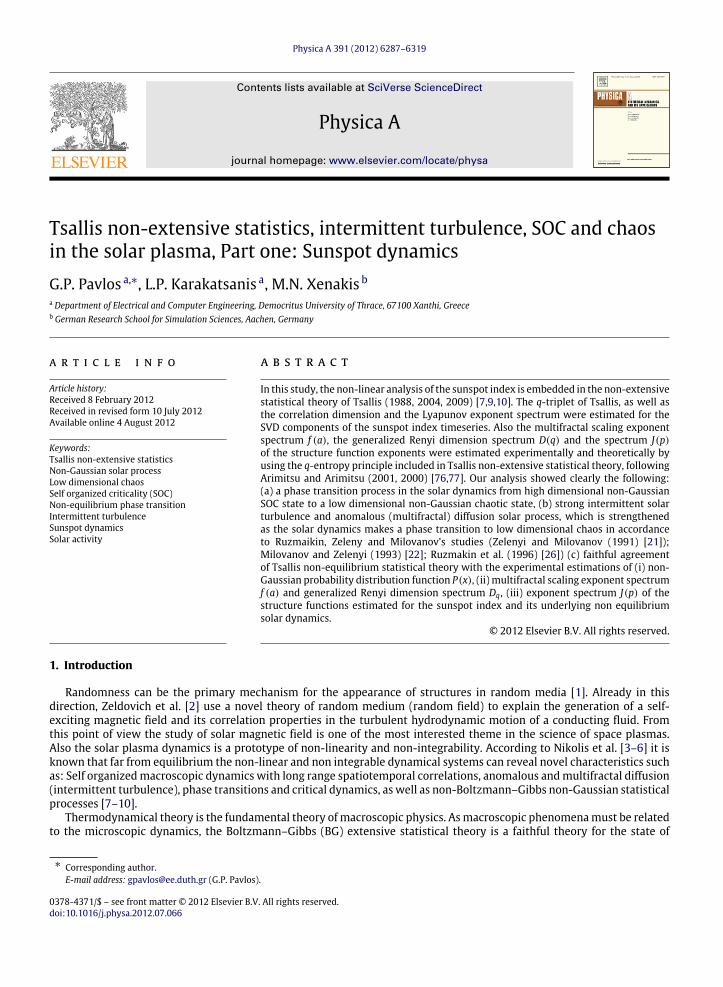
Physica A 391 (2012) 6287–6319
Contents lists available at SciVerse ScienceDirect
Physica A
journal homepage: www.elsevier.com/locate/physa
Tsallis non-extensive statistics, intermittent turbulence, SOC and chaosin the solar plasma, Part one: Sunspot dynamicsG.P. Pavlos a,∗, L.P. Karakatsanis a, M.N. Xenakis b
a Department of Electrical and Computer Engineering, Democritus University of Thrace, 67100 Xanthi, Greeceb German Research School for Simulation Sciences, Aachen, Germany
a r t i c l e i n f o
Article history:Received 8 February 2012Received in revised form 10 July 2012Available online 4 August 2012
Keywords:Tsallis non-extensive statisticsNon-Gaussian solar processLow dimensional chaosSelf organized criticality (SOC)Non-equilibrium phase transitionIntermittent turbulenceSunspot dynamicsSolar activity
a b s t r a c t
In this study, the non-linear analysis of the sunspot index is embedded in the non-extensivestatistical theory of Tsallis (1988, 2004, 2009) [7,9,10]. The q-triplet of Tsallis, as well asthe correlation dimension and the Lyapunov exponent spectrum were estimated for theSVD components of the sunspot index timeseries. Also the multifractal scaling exponentspectrum f (a), the generalized Renyi dimension spectrum D(q) and the spectrum J(p)of the structure function exponents were estimated experimentally and theoretically byusing the q-entropy principle included in Tsallis non-extensive statistical theory, followingArimitsu and Arimitsu (2001, 2000) [76,77]. Our analysis showed clearly the following:(a) a phase transition process in the solar dynamics from high dimensional non-GaussianSOC state to a low dimensional non-Gaussian chaotic state, (b) strong intermittent solarturbulence and anomalous (multifractal) diffusion solar process, which is strengthenedas the solar dynamics makes a phase transition to low dimensional chaos in accordanceto Ruzmaikin, Zeleny and Milovanov’s studies (Zelenyi and Milovanov (1991) [21]);Milovanov and Zelenyi (1993) [22]; Ruzmakin et al. (1996) [26]) (c) faithful agreementof Tsallis non-equilibrium statistical theory with the experimental estimations of (i) non-Gaussian probability distribution function P(x), (ii) multifractal scaling exponent spectrumf (a) and generalized Renyi dimension spectrum Dq, (iii) exponent spectrum J(p) of thestructure functions estimated for the sunspot index and its underlying non equilibriumsolar dynamics.
© 2012 Elsevier B.V. All rights reserved.
1. Introduction
Randomness can be the primary mechanism for the appearance of structures in random media [1]. Already in thisdirection, Zeldovich et al. [2] use a novel theory of random medium (random field) to explain the generation of a self-exciting magnetic field and its correlation properties in the turbulent hydrodynamic motion of a conducting fluid. Fromthis point of view the study of solar magnetic field is one of the most interested theme in the science of space plasmas.Also the solar plasma dynamics is a prototype of non-linearity and non-integrability. According to Nikolis et al. [3–6] it isknown that far from equilibrium the non-linear and non integrable dynamical systems can reveal novel characteristics suchas: Self organizedmacroscopic dynamics with long range spatiotemporal correlations, anomalous andmultifractal diffusion(intermittent turbulence), phase transitions and critical dynamics, as well as non-Boltzmann–Gibbs non-Gaussian statisticalprocesses [7–10].
Thermodynamical theory is the fundamental theory ofmacroscopic physics. Asmacroscopic phenomenamust be relatedto the microscopic dynamics, the Boltzmann–Gibbs (BG) extensive statistical theory is a faithful theory for the state of
∗ Corresponding author.E-mail address: [email protected] (G.P. Pavlos).
0378-4371/$ – see front matter© 2012 Elsevier B.V. All rights reserved.doi:10.1016/j.physa.2012.07.066
6288 G.P. Pavlos et al. / Physica A 391 (2012) 6287–6319
thermodynamic equilibrium and the Gaussian dynamics. Moreover, the Tsallis non-extensive statistical theory [8–10] isa novel faithful extension of the thermodynamics and its statistical interpretation for the far from equilibrium dynamics,where non-Gaussian and long range correlation processes are developed. Tsallis non-extensive statistical theory is used inthis study for the analysis/study of the solar plasma dynamics. Tsallis theory was already used by Kaniadakis et al. [11] andLavagno and Quarati [12] concerning the description of the solar core dynamics for the microscopic diffusion of electronsand ions, as well as the mechanics of the neutrino fluxes. For the outer regions of the sun, sunspots and flare dynamics aretwo distinct but closely related topics of the solarmagnetic activity. The stochasticity of the sunspot process has been relatedtheoretically with low dimensional chaos, by Weiss et al. [13] and Ruzmaikin [14]. Preliminary experimental evidence ofsolar chaos was given by Kurhts and Herzel [15] and Pavlos et al. [16] by using non-linear timeseries analysis. The solarlow dimensional chaos has also been supported by many scientists [17–20]. The fractal properties of sunspots and theirformation by fractal aggregates and clustering phenomena were studied by Zelenyi and Milovanov [21,22].
In a series of papers, Lawrence et al. [23–25] showed the non-Gaussian turbulent and chaotic dynamics underlying solarmagnetic activity as well as the spatial multifractal topology of the solar magnetic field.
More than that, the anomalous diffusion and intermittent turbulence of the solar convection and photospheric motionwas studied by Ruzmakin et al. [26] and Cadavid et al. [27] after using timeseries of solar Doppler images. In this directionZimbatolo et al. [28] studied numerically themagneto-hydrodynamic turbulence showing percolation, Levy flights and non-Gaussian dynamics. A modeling of the solar magnetic field at the photosphere and below, as a diffusion process in a non-Euclidean fractal environment, was introduced by Lawrence and Schrijver [29], and Petroway [30]. The magnetic turbulentcharacter of solar plasma has been also related to self-organized critical process according to the theory of Bak [31] bymanyscientists [32–36]. The coexistence of SOC and low dimensional chaos as well as a phase transition process was supportedby Karakatsanis and Pavlos [37] for the solar dynamics. The solar intermittent turbulence related with Tsallis non-extensivestatistics was also supported by Karakatsanis et al. [38].
Zelenyi and Milovanov [39] used modern concepts of fractal topology and strange kinetics for the theoreticalinterpretation of the formation and dynamical evolution of sun spots and group of spots in the solar photosphere.
After all in this study we present novel results after the application of the Tsallis non-extensive statistical theory andthe intermittent turbulence theory at the solar magnetic activity. For this we use the singular value decomposition (SVD)method applied at the sunspot index timeseries in order to discriminate distinct dynamical components in the solar activity.Complementary to this we apply the method of chaotic algorithm for the estimation of Lyapunov exponents, correlationdimensions and the dynamical degrees of freedom as well as for the discrimination between low dimensional chaoticattractor and high dimensional self-organized critical (SOC) attractor and colored noise stochasticity.
In the first part of our study we present results concerning the analysis of sunspot index timeseries. In the second part(under preparation) we shall present similar results for the solar flare process. In the following sections, we summarizeuseful concepts of Tsallis theory (Section 2). In Section 3 we present the methodology of data analysis. In Section 4 we showthe results of sunspot index data analysis. Finally, in Section 5 we summarize the highlights of our data analysis and discusstheir physical meaning.
2. Theoretical presuppositions for data analysis
In this section we summarize useful theoretical concepts underlying themethodology of data analysis. The Tsallis theoryand the inner relation of this theory with solar turbulence are also presented. Next and according to these theoreticalconcepts, we describe the methodology of data analysis and the algorithm that was used for producing novel results, whichare discussed in Section 3.
2.1. Tsallis theory, turbulence and chaos
The statistical theory of Boltzmann and Gibbs (BG) is based on molecular chaos hypothesis known as ‘‘stosszahlansatz’’,which means the possibility of ergodic motion of the system in the microscopical phase space. That is the system candynamically visit with equal probability all the allowed microscopic states. The dynamical attractor of the (BG) systemdynamics can be a finite or an infinite dimensional chaotic object relatedwith thermodynamical equilibrium. The probabilitydistributions are Gaussians and the observed magnitudes (timeseries) reveal fluctuations in accordance with normaldiffusion processes [10]. The equilibrium Gaussian random dynamics corresponds to physical states of uncorrelated orlocally correlated noise. Timeseries signals related with this kind of dynamics, even if they are subjected to non-lineardistortion [40–42] revealing non-Gaussian and correlated profile, they can identified as Gaussian processes [43–45]. On theother side the far from equilibrium non-linear dynamics can reveal strong self-organization and development of bifurcationprocesses causing long range correlations and strange attractors. Now the Gaussian statistics is unable to describe thefluctuations as these phenomena obey non-Gaussian statistics, with break-down of the conditions of validity of the standardcentral limit theorem and the theorem of large numbers [3,7,10,46,47].
2.1.1. Tsallis entropyThe non-extensive generalization of the classical Gaussian Boltzmann–Gibbs statistical theory as it was done by Tsallis
[7,9,10], showed the road for a deep unification of the microscopic and macroscopic physical theory, as well as for the
G.P. Pavlos et al. / Physica A 391 (2012) 6287–6319 6289
physical interpretation of the non-Gaussian chaotic dynamics. Also, the Tsallis non-extensive statistical mechanics unifiesthe thermodynamical theory at equilibrium, with the non-equilibrium thermodynamics by extending the Boltzmann–Gibbsentropy to what is known, the last two-decades as Tsallis q-entropy described by the relations:
Sq = k1 −
Ni=1
pqi
q − 1
= k1 −
+∞
−∞[p(x)]qdx
q − 1(2.1)
where p(i), (p(x)) is the probability of occupation of state (i) for discrete state space or (x) for continuous state space and qis a real number. This definition is based on q-algebra:
exq = [1 + (1 − q)x]1
1−q , (2.2)
where exq is the q-exponential function with inverse the q-logarithmic function:
lnq x =x1−q
− 11 − q
, (2.3)
the q-logarithmic function satisfies the non-extensive relation:
lnq(xAxB) = lnq xA + lnq xB + (1 − q) lnq xA lnq xB. (2.4)
Tending to the limit q → 1 the Tsallis entropy Sq reproduces the Boltzmann–Gibbs entropy SBG = −k
pi ln pi limx→∞.The optimal probability distribution p(x) which optimizes the Sq[p] function under appropriate constraints is given by therelation:
Gq(β; x) =
√β
Cqe−βx2q (2.5)
where β is the Lagrange parameter associatedwith the constraintx2
q =
x2 [P (x)]q dx = σ 2 < ∞, while the normalizing
constant Cq is given as follows:
Cq =
2
√1 − q
π/2
0(cos t)
3−q1−q dt =
2√
πΓ
1
1 − q
(3 − q)
1 − qΓ
3 − q
2(1 − q)
, −∞ < q < 1,
√π, q = 1,2
√q − 1
∞
0(1 + y2)
−1q−1 dy =
√
πΓ
3 − q
2(q − 1)
q − 1Γ
1
q − 1
, 1 < q < 3.
(2.6)
The function (2.5) maximizes (minimizes) for q > 0 (q < 0) the functional Sq[p] under appropriate constraints [10,47].The above solutions known as q-Gaussians are solutions also of equations corresponding to anomalous diffusion processesincluding: Levy anomalous diffusion, correlated anomalous diffusion and generalized fractal Fokker–Planck equations[10,48–50].
2.1.2. Anomalous diffusionGenerally the fluctuations of observedmagnitudes in the formof timeseries x(t) can be explained as caused by diffusion
processes in the physical or the phase space of the system. Chaotic motion in the physical or the phase space (state) causesexponential or other kinds of growing distances between initially close orbits. When the orbit distance grows exponentiallywith time as:
w(t) = w(0) expLt , (2.7)
where L is a positive Lyapunov exponent, we observe a rapid mixing of orbits within the time interval τ = 1/L. Thenkinetic equations arise as coarse graining and averaging at timescales greater than the mixing time τ = 1/L. The well-knownGaussian and Poissonian chaotic dynamicswith space and temporal diffusion can be produced fromchaotic dynamics[51–55]. Anomalous diffusion processes include long range correlations with mean-squared jump distances:
x2(t)∼ tγ , (2.8)
with γ = 1, (γ = 1 corresponds to normal Gaussian diffusion processes) while γ > 1 (γ < 1) corresponds to superdiffusion (sub-diffusion). Anomalous diffusion processes are caused by chaotic motions on multifractal and multiscale self-similar set of states in physical or state space [54,56,57]. Moreover, anomalous diffusion can be caused by strong non-linearand chaotic dynamics, which creates multifractal attracting structures in state spaces or multifractal material structures inwhich the diffusion process happens by the fractality of space and time by themselves, [58–60].
6290 G.P. Pavlos et al. / Physica A 391 (2012) 6287–6319
Generally the anomalous diffusion processes described by fractional Fokker–Planck equations include Levy distributions,which asymptotically are related to q-Gaussians of Tsallis statistics as follows:
Lγ (x) ∼1
|x|1+γ, |x| → ∞ 0 < γ < 2 (2.9a)
Pq(x) ∼1
|x|2
q−1, |x| → ∞ 1 < q < 3 (2.9b)
where Lγ (x), Pq(x) correspond to Levy and q-Gaussian distributions.These relations indicate that:
γ =
2, if q ≤
53
3 − qq − 1
, if53
< q < 3.(2.10)
2.1.3. Long range correlationsAccording to Ref. [9] the q-statistics for q = 1 indicates the existence of long range correlations as we can conclude by
the relation:
Sq(A + B) = Sq(A) + Sq(B/A) + (1 − q)Sq(A)Sq(B/A) = Sq(B) + Sq(A/B) + (1 − q)Sq(B)Sq(A/B), (2.11)
where A, B are subsystems of the system A + B and Sq(A/B), Sq(B/A) correspond to intercorrelations of subsystems A and Bwhen they are statistically dependent and statistically correlated according to the relation:
PA+Bij = PA
i PBj . (2.12)
When the probabilities PA+Bij = PA
i PBj , indicate that the subsystems are statistically independent and uncorrelated and the
relation (2.11) is transformed to:
Sq(A + B) = Sq(A) + Sq(B) + (1 − q)Sq(A)Sq(B). (2.13)
The first part of Sq(A+ B) is additive Sq(A) + Sq(B) while the second part is multiplicative including long-range correlationssupporting the macroscopic ordering phenomena. Milovanov and Zelenyi [61] showed that the Tsallis definition of entropycoincides with the so-called ‘‘kappa’’ distribution which appears in space plasmas and other physical realizations. Also theyindicate that the application of Tsallis entropy formalism corresponds to physical systems whose the statistical weights arerelatively small, while for large statistical weights the standard statisticalmechanism of Boltzmann–Gibbs is advocated. Thisresult means that when the dynamics of the system is attracted in a confided subset of the phase space, then long-rangecorrelations can be developed. Also according to Tsallis [10] if the correlations are either strictly or asymptotically inexistentthe Boltzmann–Gibbs entropy is extensive whereas Sq for q = 1 is non-extensive.
2.1.4. Chaotic attractors and self-organizationWhen the dynamics is strongly non-linear then for the far from equilibrium processes it is possible to be created strong
self-organization and intensive reduction of dimensionality of the state space, by an attracting low dimensional set withparallel development of long range correlations in space and time. The attractor can be periodic (limit cycle, limitm-torus),simply chaotic (mono-fractal) or strongly chaotic with multiscale and multifractal profile as well as attractors with weakchaotic profile known as SOC states. This spectrum of distinct dynamical profiles can be obtained as distinct critical points(critical states) of the non-linear dynamics, after successive bifurcations as the control parameters change. The fixed pointscan be estimated by using a far from equilibrium renormalization process as it was indicated by Chang [62,63].
From this point of view phase transition processes can be developed by between different critical states, when the orderparameters of the system are changing. The far from equilibrium development of chaotic (weak or strong) critical statesincludes long range correlations and multiscale internal self organization. Now, these far from equilibrium self organizedstates, the equilibrium BG statistics and BG entropy, are transformed and replaced by the Tsallis extension of q-statisticsand Tsallis entropy. The extension of renormalization group theory and critical dynamics, under the q-extension of partitionfunction, free energy and path integral approach has been also indicated [64–67]. The multifractal structure of the chaoticattractors can be described by the generalized Rényi fractal dimensions:
Dq =1
q − 1limλ→0
logNλi=1
pqi
log L, (2.14)
where pi ∼ Lα(i) is the local probability at the location (i) of the phase space, λ is the local size of phase space and a (i) is thelocal scaling (singularity) index or the pointwise (local mass) dimension. The Rényi q numbers (different from the q-index
G.P. Pavlos et al. / Physica A 391 (2012) 6287–6319 6291
of Tsallis statistics) take values in the entire region (−∞, +∞) of real numbers. The spectrum of distinct local pointwisedimensions α(i) is given by the estimation of the function f (α) defined by the scaling of the density n (a, λ) ∼ λ−f (a), wheren (a, λ) da is the number of local regions that have a scaling index between a and a + da. They reveal f (a) as the fractaldimension of points with scaling index a. The fractal dimension f (a) which varies with a shows the multifractal characterof the phase space dynamics which includes interwoven sets of singularity of strength a, by their own fractal measure f (a)of dimension [68,69]. The multifractal spectrum Dq of the Renyi dimensions can be related with the spectrum f (a) of localsingularities by using the following relations:
pqi =
da′p(a′)λ−f (α′)da′ (2.15)
τ(q) ≡ (q − 1)Dq = min[qa − f (a)] (2.16)
a(q) =d[τ(q)]
dq(2.17)
f (a) = minq
[qa − T (q)] . (2.18)
The physical meaning of these magnitudes included in relations (2.15)–(2.18) can be obtained if we identify themultifractalattractor as a thermodynamical object, where its temperature (T ), free energy (F ), entropy (S) and internal energy (U) arerelated to the properties of the multifractal attractor as follows:
q ⇒1T
, τ (q) = (q − 1)Dq ⇒ Fα ⇒ U, f (α) ⇒ S
. (2.19)
This correspondence presents the relations (2.17)–(2.19) as a thermodynamical Legendre transform [70]. When q increasesto infinite (+∞), which means, that we freeze the system (T(q=+∞) → 0), then the trajectories (fluid lines) are closingon the attractor set, causing large probability values at regions of low fractal dimension, where α = αmin and Dq = D−∞.Oppositely, when q decreases to infinite (−∞), that is we warm up the system (T(q=−∞) → 0) then the trajectories arespread out at regions of high fractal dimension (α ⇒ αmax). Also for q′ > q we have Dq′ < Dq and Dq ⇒ D+∞(D−∞)for α ⇒ αmin(αmax) correspondingly. However, the above description presents only a weak or limited analogy betweenmultifractal and thermodynamical objects. Renyi’s generalization of entropy according to the relation is also known:Sq =
1q−1 log
i P
qi . However the real thermodynamical character of the multifractal objects and multiscale dynamics was
discovered after the definition by Tsallis [7] of the q-entropy related with the q-statistics as it was summarized previouslyin relations (2.1)–(2.13). As Tsallis has shown, Renyi’s entropy as well as other generalizations of entropy cannot be used asthe base of the non-extensive generalization of thermodynamics [9].
2.1.5. Intermittent turbulenceAccording to previous description, dissipative non-linear dynamics can produce self-organization and long range
correlations in space and time. In this case we can imagine the mirroring relationship between the phase space multifractalattractor and the corresponding multifractal turbulence dissipation process of the dynamical system in the physical space.Multifractality and multiscaling interaction, chaoticity and mixing or diffusion (normal or anomalous), all of them can bemanifested in both the state (phase) space and the physical (natural) space as themirroring of the same complex underlyingdynamics. We could say that turbulence is for complexity theory, what the blackbody radiation was for quantum theory, asall previous characteristics of strange dynamics can be observed in turbulent states.
The multifractal character of turbulence can be characterized: (a) in terms of local velocity increments δulrand the
structure function Sp (l) ≡δup
l
first introduced by Kolmogorov [71], (b) in terms of local dissipation and local scale
invariance of HD or MHD equations upon scale transformations r ′= λr, u′
= λa/3u, t ′ = λ1− a3 t [72–74]. The turbulent
flow is assumed to process a range of scaling exponent, hmin ≤ h ≤ hmax while for each h there is a subset of point of R3 offractal dimension D (h) such that:
δulr
∼ lh as l → 0. (2.20)
The multifractal assumption can be used to derive the structure function of order P by the relation:
Sp (l) ∼
dµ (h)
lph
l3−D(h) (2.21)
where dµ (h) gives the probability weight of the different scaling exponents, while the factor l3−D(h) is the probability ofbeing with a distance l in the fractal subset of R3 with dimension D (h). By using the method of steepest descent [75] we canderive the power-law
Sp (l) ≡δuP
l
∼ lJ(P), l → 0 (2.22a)
6292 G.P. Pavlos et al. / Physica A 391 (2012) 6287–6319
where:
J (p) = minh
[ph + 3 − D (h)] . (2.22b)
The above relation is the Legendre transformation between J (P) and D (h) as D (h) can be derived by the relation:
D (h) = minp
[ph + 3 − J (p)] . (2.23)
Themultifractal character of the turbulent state can be apparent at the spectrum of the structure function scaling exponentsJ (p) by the relation:
dJ (p) /dp = h∗ (p) +p − D′ (h∗ (p))
dh∗ (p)dp
= h∗ (p) (2.24)
as the minimum value of the relation (2.23) corresponds the maximum of 3 − J (p) function for which:
d (3 − J (p)) /dp =ddp
(D − ph) = 0∞ (2.25)
and
D′ (h∗ (p)) = p. (2.26)
According to Frisch [75] the dissipation is said to bemultifractal if there is a function F (a)whichmaps real scaling exponentsa to scaling dimensions F (a) ≤ 3 such that:
εlr
∼ la−1 as l → 0 (2.27)
for a subset of pointsr of R3 with dimension F (a).
In correspondence with the structure function theory presented above in the case of multifractal energy dissipation themoments ε
ql follow the power laws:
εql
∼ lq (2.28)
where the scaling exponents σ (q) are given by the relation:
σ (q) = mina
[q (a − 1) + 3 − F (a)] . (2.29)
In the case of one dimensional dissipation process the multifractal character is described by the function f (a) instead ofF (a)where f (a) = F (a)−2 [75]. In the language of Renyi’s generalized dimensions andmultifractal theory the dissipationmultifractal turbulence process corresponds to the Renyi’s dimensions Dq according to the relation Dq =
σ0(q)q−1 +3 [75]. Also,
according to Frisch [75] the relation between the dissipation multifractal formalism and the multifractal turbulent velocityincrements formalism is given by the following relations:
h =a3, D (h) = F (a) = f (a) + 2, J (p) =
p3
+ σp3
. (2.30)
The theoretical description of turbulence in the physical space is based upon the concept of the invariance of the HD orMHD equations upon scaling transformations to the space–time variables (σ , t) and velocity (u) and corresponding similarscaling relations for other physical variables [72–74].
In the next part of this section we follow Arimitsu and Arimitsu [76,77] connecting the Tsallis non-extensive statisticsand intermittent turbulence process. Under the scale transformation:
εn ∼ ε0(ln \ l0)α−1 (2.31)
the original eddie of size l0 can be transformed to constituting eddies of different size ln = l0δn, n = 0, 1, 2, 3, . . . after nsteps of the cascade. If we assume that at each step of the cascade eddies break into δ pieces with 1/δ diameter then the sizeln = l0δ−n. If δun = δu (ln) represents the velocity difference across a distance r ∼ ln and εn represents the rate of energytransfer from eddies of size ln to eddies of size ln+1 then we have:
δun = δu (ln/l0)a/3 and εn = ε (ln/l0)a−1 (2.32)
where a is the scaling exponent under the scale transformation (2.31).The scaling exponent a describes the degree singularity in the velocity gradient
∂u(x)∂x = limln→0 (δun/ln)
as the firstequation in (2.32) reveals. The singularities a in velocity gradient fill the physical space of dimension d, (a < d) with afractal dimension F (a). Similar to the velocity singularity, other frozen fields can reveal singularities in the d-dimensionalnatural space. After this, the multifractal (intermittency) character of the HD or the MHD dynamics consists in supposing
G.P. Pavlos et al. / Physica A 391 (2012) 6287–6319 6293
that the scaling exponent α included in relations (2.31) takes on different values at different interwoven fractal subsets ofthe d-dimensional physical space in which the dissipation field is embedded. The exponent α and for values a < d is relatedwith the degree of singularity in the field’s gradient ( ∂A(x)
∂x ) in the d-dimensional natural space [76]. Generally, the gradientsingularities cause the anomalous diffusion in physical or in phase space of the dynamics. The total dissipation occurring ina d-dimensional space of size ln scales also with a global dimension Dq for powers of different order q as follows:
n
εqnl
dn ∼ l
(q−1)Dqn = lτ(q)
n . (2.33)
Supposing that the local fractal dimension of the set dn(a) which corresponds to the density of the scaling exponents in theregion (α, α + dα) is a function fd(a) according to the relation:
dn(a) ∼ ln−fd(a) da (2.34)
where d indicates the dimension of the embedding space, then we can conclude the Legendre transformation between themass exponent τ(q) and the multifractal spectrum fd(a):
fd(a) = aq − (q − 1)(Dq − d + 1) + d − 1
a =ddq
[(q − 1)(Dq − d + 1)]
. (2.35)
For linear intersections of the dissipation field, that is d = 1 the Legendre transformation is given as follows:
f (a) = aq − τ(q), a =ddq
[(q − 1)Dq] =ddq
τ(q), q =df (a)da
. (2.36)
The relations (2.34)–(2.35) describe the multifractal and multiscale turbulent process in the physical state. The relations(2.14)–(2.19) describe the multifractal and multiscale process on the attracting set of the phase space. From this physicalpoint of view, we suppose the physical identification of the magnitudes Dq, a, f (a) and τ(q) estimates in the physical andthe corresponding phase space of the dynamics. By using experimental timeseries we can construct the function Dq of thegeneralized Rényi d-dimensional space dimensions, while the relations (2.24) allow the calculation of the fractal exponent(a) and the corresponding multifractal spectrum fd(a). For homogeneous fractals of the turbulent dynamics the generalizeddimension spectrum Dq is constant and equal to the fractal dimension, of the support [72]. Kolmogorov [71] supposed thatDq does not depend on q as the dimension of the fractal support is Dq = 3. In this case the multifractal spectrum consistsof the single point (a = 1 and f (1) = 3). The singularities of degree (a) of the dissipated fields fill the physical space ofdimension d with a fractal dimension F(a), while the probability P(a)da, to find a point of singularity (a) is specified bythe probability density P(a)da ∼ ld−F(a)
n . The filling space fractal dimension F(a) is related with the multifractal spectrumfunction fd(a) = F(a) − (d − 1), while according to the distribution function Πdis(εn) of the energy transfer rate associatedwith the singularity a it corresponds to the singularity probability as Πdis(εn)dεn = P(a)da [76].
Moreover the partition function
i Pqi of the Rényi fractal dimensions estimated by the experimental timeseries includes
information for the local and global dissipation process of the turbulent dynamics aswell as for the local and global dynamicsof the attractor set, as it is transformed to the partition function
i P
qi = Zq of the Tsallis q-statistical theory.
In the following,wepresent for the theoretical estimation of significant quantitative relationswhich can also be estimatedexperimentally as the probability singularity distribution P(a) can be estimated by extremizing the Tsallis entropy functionalSq [76,77]. According to Arimitsu and Arimitsu [76] the extremizing probability density function P(a) is given as a q-exponential function:
P(a) = Z−1q
1 − (1 − q)
(a − a0)2
2X/ ln 2
11−q
(2.37)
where the partition function Zq is given by the relation:
Zq =2X/[(1 − q) ln 2]B(1/2, 2/1 − q), (2.38)
and B(a, b) is the Beta function. The partition function Zq as well as the quantities X and q can be estimated by using thefollowing equations:
√2X =
a20 + (1 − q)2 − (1 − q)
√b
b = (1 − 2−(1−q))/[(1 − q) ln2]
. (2.39)
We can conclude for the exponent’s spectrum f (a) by using the relation P(a) ≈ lnd−F(a) as follows:
f (a) = D0 + log2
1 − (1 − q)
(a − ao)2
2X/ ln 2
(1 − q)−1 (2.40)
6294 G.P. Pavlos et al. / Physica A 391 (2012) 6287–6319
where a0 corresponds to the q-expectation (mean) value of a through the relation:
⟨(a − a0)2⟩q =
daP(a)q(a − a0)q
daP(a)q (2.41)
while the q-expectation value a0 corresponds to the maximum of the function f (a) as df (a)/da|a0 = 0. For the Gaussiandynamics (q → 1) we have mono-fractal spectrum f (a0) = D0. The mass exponent τ(q) can be also estimated by using theinverse Legendre transformation: τ(q) = aq − f (a) (relations (2.35)–(2.36)) and the relation (2.40) as follows:
τ(q) = qa0 − 1 −2Xq2
1 +Cq
−1
1 − q[1 − log2(1 +
Cq)] (2.42)
where Cq = 1 + 2q2(1 − q)X ln 2.The relation between a and q can be found by solving the Legendre transformation equation q = df (a)/da. Also if we
use the Eq. (2.40) we can obtain the relation:
aq − a0 = (1 −Cq)/[q(1 − q) ln 2]. (2.43)
The q-index is related to the scaling transformations of the multifractal nature of turbulence according to the relationq = 1 − a. Arimitsu and Arimitsu [77] estimated the q-index by analyzing the fully developed turbulence state in terms ofTsallis statistics as follows:
11 − q
=1a−
−1a+
(2.44)
where a± satisfy the equation f (a±) = 0 of the multifractal exponents spectrum f (a). This relation can be used for theestimation of qsen-index included in the Tsallis q-triplet (see next section).
The above analysis based at the extremization of Tsallis entropy can be also used for the theoretical estimation of thestructure functions scaling exponent spectrum J(p), where p = 1, 2, 3, 4, . . . . The structure functions were first introducedby Kolmogorov [71] defined as statistical moments of the field increments:
Sp(−→r) = ⟨|u(r + d) − u(r)|p⟩ = ⟨|δun|
p⟩ (2.45)
Sp(r) = ⟨|u(r + 1r) − u(r)|p⟩. (2.46)
After discretization of 1r displacement, the above relation can be identified to:
Sp(ln) = ⟨|δun|p⟩. (2.47)
The field values u(−→x ) can be related with the energy dissipation values εn by the general relation εn = (δun)3/ln in order
to obtain the structure functions as follows:
Sp(ln) = ⟨(εn/ε0)p⟩ = ⟨δp(a−1)
n ⟩ = δJ(p)n (2.48)
where the averaging processes ⟨· · · ⟩ is defined by using the probability function P(a)da as ⟨· · · ⟩ =da(. . .)P(a). By this,
the scaling exponent J(p) of the structure functions is given by the relation:
J(p) = 1 + τq =
p3
. (2.49)
By following Arimitsu [76,77] the relation (2.30) leads to the theoretical prediction of J(p) after extremization of Tsallisentropy as follows:
J(p) =a0p3
−2Xp2
q(1 +Cp/3)
−1
1 − q[1 − log2(1 +
Cp/3)]. (2.50)
The first term a0p/3 corresponds to the original of known Kolmogorov theory (K41) according to which the dissipationof field energy εn is identified with the mean value ε0 according to the Gaussian self-similar homogeneous turbulencedissipation concept, while a0 = 1 according to the previous analysis for homogeneous turbulence. According to this conceptthe multifractal spectrum consists of a single point. The next terms after the first in the relation (2.50) correspond to themultifractal structure of intermittence turbulence indicating that the turbulent state is not homogeneous across spatialscales. That is, there is a greater spatial concentration of turbulent activity at smaller than at larger scales. According toAbramenko [78] the intermittent multifractal (inhomogeneous) turbulence is indicated by the general scaling exponentJ(p) of the structure functions according to the relation:
J(p) =p3
+ T (u)(p) + T (F)(p), (2.51)
G.P. Pavlos et al. / Physica A 391 (2012) 6287–6319 6295
where the T (u)(p) term is related with the dissipation of kinetic energy and the T (F)(p) term is related to other forms offield’s energy dissipation as the magnetic energy at MHD turbulence [78,79].
The scaling exponent spectrum J(p) can be also used for the estimation of the intermittency exponentµ according to therelation:
S(p = 2) ≡ ⟨ε2/ε⟩ ∼ δµn = δJ(2)
n (2.52)
from which we conclude that µ = J(2). The intermittency turbulence correction to the law P(f ) ∼ f −5/3 of the energyspectrum of Kolmogorov’s theory is given by using the intermittency exponent:
P(f ) ∼ f −(5/3+µ). (2.53)
The previous theoretical description can be used for the theoretical interpretation of the experimentally estimated structurefunction, as well as for relating physically the results of data analysis with Tsallis statistical theory, as it is described in thenext sections.
2.1.6. The q-triplet of Tsallis theoryThe non-extensive statistical theory is based mathematically on the non-linear equation:
dydx
= yq, (y(0) = 1, q ∈ ℜ) (2.54)
with solution the q-exponential function defined previously in Eq. (2.2). The solution of this equation can be realized inthree distinctways included in the q-triplet of Tsallis: (qsen, qstat, qrel). These quantities characterize three physical processeswhich are summarized here, while the q-triplet values characterize the attractor set of the dynamics in the phase space ofthe dynamics and they can change when the dynamics of the system is attracted to another attractor set of the phase space.The Eq. (2.47) for q = 1 corresponds to the case of equilibrium Gaussian Boltzmann–Gibbs (BG) world [9,10]. In this case ofequilibrium BG world the q-triplet of Tsallis is simplified to (qsen = 1, qstat = 1, qrel = 1).a. The qstat index and the non-extensive physical states
According to Refs. [9,10] the long range correlated metaequilibrium non-extensive physical process can be described bythe non-linear differential equation:
d(piZstat)dEi
= −βqstat(piZstat)qstat . (2.55)
The solution of this equation corresponds to the probability distribution:
pi = e−βstatEiqstat /Zqstat (2.56)
where βqstat =1
KTstat, Zstat =
j e
−βqstatEjqstat .
Then the probability distribution function is given by the relations:
pi ∝1 − (1 − q)βqstatEi
1/1−qstat (2.57)
for discrete energy states Ei by the relation:
p(x) ∝1 − (1 − q)βqstatx
21/1−qstat (2.58)
for continuous X states X, where the values of the magnitude X correspond to the state points of the phase space.The above distribution functions (2.57) and (2.58) correspond to the attracting stationary solution of the extended
(anomalous) diffusion equation related with the non-linear dynamics of system [10]. The stationary solutions P(x) describethe probabilistic character of the dynamics on the attractor set of the phase space. The non-equilibrium dynamics can beevolved on distinct attractor sets depending upon the control parameters values, while the qstat exponent can change as theattractor set of the dynamics changes.b. The qsen index and the entropy production process
The entropy production process is related to the general profile of the attractor set of the dynamics. The profile of theattractor can be described by its multifractality as well as by its sensitivity to initial conditions. The sensitivity to initialconditions can be described as follows:
dξdτ
= λ1ξ + (λq − λ1)ξq (2.59)
where ξ describes the deviation of trajectories in the phase space by the relation: ξ ≡ lim∆(x)→01x(t) \ 1x(0) and 1x(t)is the distance of neighboring trajectories [80]. The solution of Eq. (2.41) is given by:
ξ =
1 −
λqsenλ1
+λqsenλ1
e(1−qsen)λ1t 1
1−q
. (2.60)
6296 G.P. Pavlos et al. / Physica A 391 (2012) 6287–6319
The qsen exponent can be also related with the multifractal profile of the attractor set by the relation:
1qsen
=1
amin−
1amax
(2.61)
where amin(amax) corresponds to the zero points of the multifractal exponent spectrum f (a) [10,76,80]. That is f (amin) =
f (amax) = 0.The deviations of neighboring trajectories as well as the multifractal character of the dynamical attractor set in the
system phase space are related to the chaotic phenomenon of entropy production according to Kolmogorov–Sinai entropyproduction theory and the Pesin theorem [10]. The q-entropy production is summarized in the equation:
Kq ≡ limt→∞
limW→∞
limN→∞
⟨Sq⟩(t)t
. (2.62)
The entropy production (dSq/t) is identified with Kq, asW are the number of non-overlapping little windows in phase spaceandN the state points in thewindows according to the relation
Wi=1 Ni = N . The Sq entropy is estimated by the probabilities
Pi(t) ≡ Ni(t)/N . According to Tsallis the entropy production Kq is finite only for q = qsen [10,80].c. The qrel index and the relaxation process
The thermodynamical fluctuation–dissipation theory [81] is based on the Einstein original diffusion theory (Brownianmotion theory). The diffusion process is the physical mechanism for extremization of entropy. If 1S denote the deviation ofentropy from its equilibrium value S0, then the probability of the proposed fluctuation that may occur is given by:
P ∼ exp(1s/k). (2.63)
The Einstein–Smoluchowski theory of Brownianmotionwas extended to the general Fokker–Planck diffusion theory of non-equilibrium processes. The potential of Fokker–Planck equation may include many metaequilibrium stationary states nearor far away from the basic thermodynamical equilibrium state. Macroscopically, the relaxation to the equilibrium stationarystate of some dynamical observable O(t) related to the evolution of the system in phase space can be described by the formof general equation as follows:
dΩ
dτ≃ −
1τ
Ω, (2.64)
where Ω(t) ≡ [O(t) − O(∞)]/[O(0) − O(∞)] is the relaxing relevant quantity of O(t) and describes the relaxationof the macroscopic observable O(t) relaxing towards its stationary state value. The non-extensive generalization offluctuation–dissipation theory is related to the general correlated anomalous diffusion processes [10]. Now, the equilibriumrelaxation process (2.52) is transformed to the metaequilibrium non-extensive relaxation process:
dΩ
dt= −
1Tqrel
Ωqrel (2.65)
the solution of this equation is given by:
Ω(t) ≃ e−t/τrelqrel . (2.66)
The autocorrelation function C(t) or the mutual information I(t) can be used as candidate observables Ω(t) for theestimation of qrel. However, in contrast to the linear profile of the correlation function, the mutual information includesthe non-linearity of the underlying dynamics and it is proposed as a more faithful index of the relaxation process and theestimation of the Tsallis exponent qrel.
2.1.7. Dynamics and mutual informationChaotic or stochastic dynamical systems can be described by using the concept of information. For this scopewe suppose
that the random behaviour of the system is a realization of Shannon’s concept of an ergodic information source. If S is someproperty of the dynamical system and si, i = 1, 2, . . . possible values of S then the average amount of information gainedfrom a measurement that specifies S is given by the entropy H(S)
H(S) = −
ι
P(si) log P(si) (2.67)
where P(si) is the probability that S equals to si and the logarithm is takenwith respect to base 2. An estimate of P(si) is givenby n(si)/nT , where n(si) is the number of times that the value si is observed and nT is the total number of measurements. Thesame concept can be used to identify how much information we obtain about a measurement of an observable S quantityfrom measurement of another observable Q quantity. This concept is the base for the definition of mutual information. Fortimeseries, we consider a general coupled system (S,Q )with Q = x(i) and S = x(i+τ), where x(i), x(i+τ) correspondto scalar samples from a dynamical system at discrete times ti and ti+τ .
G.P. Pavlos et al. / Physica A 391 (2012) 6287–6319 6297
The conditional uncertainty of S given that Q = qi is defined as
H(S/Q = qi) = −
j
P(sj/qi) log P(sj/qi) (2.68)
where P(sj/qi) is the conditional probability of S = sj given that Q = qi. Thus we define the conditional uncertainty of Sgiven Q as a weighted average of the uncertainties H(S/Q = qi), that is
H(S/Q ) = −
qj
P(qi)H(S/Q = qi). (2.69)
Using the fact that P(qi, sj) = P(qi)P(sj/qi) we have
H(S/Q ) = −
qi
sj
P(qi, sj) log P(sj/qi) = H(Q , S) − H(Q ). (2.70)
The amount, which a measurement of Q reduces the uncertainty of S (average mutual information) is given by the relationISQ = H(S) − H(S/Q ) = H(S) + H(Q ) − H(Q , S). (2.71)
If this relation is applied to timeseries leads to:
I(τ ) = −
x(i)
P(x(i)) log2 P(x(i)) −
x(i−τ)
P(x(i − τ)) log2 P(x(i − τ))
+
x(i)
x(i−τ)
P(x(i), x(i − τ)) log2 P(x(i), x(i − τ)). (2.72)
The mutual information between the two samples x(i), x(i + τ) takes values in the range (0, Imax), where Imax = I(0)is equal to the entropy H(x). If the samples Q ≡ x(i) and S ≡ x(i + τ) are statistically independent then the mutualinformation will vanish for this value of τ . That is knowledge for the second sample cannot be gained by knowing the first.On the other hand, if the first sample uniquely determines the second sample then I(τ ) = Imax, which is most likely to betrue when τ = 0.
In this study, we follow the work of Fraser and Swinney [82] for the estimation of the mutual information (according to(2.71)).
2.2. Methodology of data analysis
In this study we use the method of singular value decomposition (SVD) in order to uncover the hidden solar dynamics,underlying the sunspot index timeseries. Moreover the non-extensivity of the solar dynamics is studied in relation to theturbulence and chaotic profiles of the solar plasma convection.
2.2.1. Singular value decomposition (SVD) AnalysisNon-linear dynamics can lead to self organization, which can give rise to asymptotic dynamics and low-dimensional
attracting sets in the phase space. According to embedding theory, experimental timeseries can be used for the embeddingof dynamics in the reconstructed phase space by using the method of delays. The SVDmethod can be used in distinguishingchaotic dynamics as well as to discriminate distinct dynamical components included in the experimental signal.
In this study the embedding theory of Takens [83] and the theory of SVD [84] analysis can be used for the discriminationof deterministic and noisy (stochastic) components included in the observed signals, as well as for the discrimination ofdistinct dynamical components [45,84–86].
Let x(t) = f (t)(x(0)) denote the dynamical flow underlying an experimental timeseries x(ti) = h(x(ti)) where hdescribes the measurement function. When there is a noisy component w(ti) then the observed timeseries must be givenby x(ti) = h(x(ti), w(ti)). On the other hand Takens [83] showed that for autonomous and purely deterministic systems thedelay reconstruction map Φ, which maps the states x into m-dimensional delay vectors
Φ(x) = [h(x), h(f τ (x)), h(f 2τ (x)), . . . , h(f (m−1)τ (x))]= x (ti) = [x (ti) , x (ti + τ) , . . . , x (ti + (m − 1) τ )] . (2.73)
Φ(x) is an embeddingwhenm ≥ 2n+1, where n is the dimension of themanifoldM of the phase space inwhich evolves thedynamics of the system. This means that interested geometrical and dynamical characteristics of the underlying dynamicsin the original phase space are preserved invariable in the reconstructed space as well.
Let Xr = Φ(ι)(X) be the reconstructed phase space and xr(ti) = Φ(x(ti)) the reconstructed trajectory for the embeddingΦ. Then the dynamics evolved in the original phase space is topologically equivalent to its mirror dynamical flow in thereconstructed phase space according to
f tr (xr) = Φ(x) f t(x) Φ−1(xr) (2.74)of the reconstructed phase space Xr . In other words the embedding Φ is a diffeomorphism which takes the orbits f t(x) ofthe original phase space to the orbits f tr (xr) in the reconstructed phase in such a way of preserving their orientation andother topological characteristics as eigenvalues, Lyapunov exponents or dimensions of the attractors.
6298 G.P. Pavlos et al. / Physica A 391 (2012) 6287–6319
Singular value analysis is applied to the trajectory matrix which is constructed by an experimental timeseries as follows:
X =
x(t1), (t1 + τ), . . . , x(t1 + (n − 1)τ )x(t2), x(t2 + τ), . . . , x(t2 + (n − 1)τ )
· · ·
x(tN), x(tN + τ), . . . , x(tN + (n − 1)τ )
=
xT1xT2·
xTN
(2.75)
where x(ti) is the observed timeseries and τ is the delay time for the phase space reconstruction. The rows of the trajectorymatrix constitute the state vectors xTi on the reconstructed trajectory in the embedding space Rn. As we have constructed Nstate vectors in embedding space Rn the problem is how to use them in order to find a set of linearly independent vectorsin Rn which can describe efficiently the attracting manifold within the phase space according to the theoretical concepts ofSection 2.1. These vectors constitute part of a complete orthonormal basis ei, i = 1, 2, . . . , n in Rn and can be constructedas a linear combination of vectors on the reconstructed trajectory in Rn by using the relation
sTi X = σicTi . (2.76)
According to singular value decomposition (SVD) theorem it can be proved that the vectors si and ci are eigenvectors of thestructure matrix XX T and the covariance matrix X TX of the trajectory according to the relations
XX T si = σ 2i si, X TX ci = σ 2
i c′
i . (2.77)
The vectors si, ci are the singular vectors of X and σi are its singular values, while the SVD analysis of X can be written as
X = SΣC T (2.78)
where S = [s1, s2, . . . , sn], C = [c1, c2, . . . , cn] and Σ = diag[σ1, σ2, . . . , σn]. The ordering σ1 ≥ σ2 ≥ · · · ≥ σn ≥ 0 isassumed. Moreover according to the SVD theorem the non-zero eigenvalues of the structure matrix are equal to non-zeroeigenvalues of the covariance matrix. This means that if n′ (where n′
≤ n) is the number of the non-zero eigenvalues, thenrankXX T
= rankX TX = n′. It is obvious that the n′-dimensional subspace of RN spanned by si, i = 1, 2, . . . , n′ ismirrored
to the basis vector ci which can be found as the linear combination of the delay vectors by using the eigenvectors si accordingto (2.75). The complementary subspace spanned by the set si, i = n′
+1, . . . ,N is mirrored to the origin of the embeddingspace Rn according to the same relation. That is according to SVD analysis the number of the independent eigenvectors cithat are efficient for the description of the underlying dynamics is equal to the number n′ of the non-zero eigenvalues σiof the trajectory matrix. The same number n′ corresponds to the dimensionality of the subspace containing the attractingmanifold. The trajectory can be described in the new basis ci, i = 1, 2, . . . , n by the trajectory matrix projected on thebasis ci given by the product XC of the old trajectory matrix and the matrix C of the eigenvectors ci. The new trajectorymatrix XC is described by the relation
(XC)T (XC) = Σ2. (2.79)
This relation corresponds to the diagonalization of the new covariance matrix so that in the basis ci the components ofthe trajectory are uncorrelated. Also, from the same relation (2.79) we conclude that each eigenvalue σ 2
i is the mean squareprojection of the trajectory on the corresponding ci, so that the spectrum σ 2
i includes information about the extending ofthe trajectory in the directions ci as it evolves in the reconstructed phase space. The area explored by the trajectory phasespace corresponds on average to an n-dimensional ellipsoid for which ci give the directions and σi the lengths of itsprincipal evolving in the subspace spanned by eigenvectors ci corresponding to non-zero eigenvalues. However whenthe system is perturbed by external noise or deterministic external input then the trajectory begins to be diffused alsoin directions corresponding to zero eigenvalues where the external perturbation dominates. As we show in the followingthe replacement of the old trajectory matrix X with the new XC works as a linear low pass filter for the entire trajectory.Moreover the SVD analysis permits to reconstruct the original trajectory matrix by using the XC matrix as follows
X =
ni=1
(Xc i)cTi . (2.80)
The part of the trajectorymatrix which contains all the information about the deterministic trajectory, as it can be extractedby observations corresponds to the reduced matrix:
Xd =
n′i=1
(Xc i)cTi (2.81)
which is obtained by summing only for the eigenvectors ci with non-zero eigenvalues. From the relation (2.81) we canreconstruct the original timeseries x(t) by using n new timeseries V (ti) according to relation
x(t) =
ni=1
Vi(t) (2.82)
G.P. Pavlos et al. / Physica A 391 (2012) 6287–6319 6299
where every Vi(t) is given by the first column of the matrix (Xc i)cTi . The Vi(t) timeseries are known as SVD reconstructedcomponents. This is a kind of n-dimensional spectral analysis of a timeseries. The new timeseries Vi(t) constitute thereconstructed timeseries components of the SVD spectrum, corresponding to the spectrum of the singular vectors ci. Thedependence of SVD analysis upon the existence of external noise is described by Broomhead and King [84] for white noiseand by Elsner and Tsonis [87] for colored noise. In the case of white noise the singular values σi of X are shifted uniformlyaccording to the relation
σ 2i = σ 2
i +ξ 2 (2.83)
where σi are the eigenvalues of the unperturbed signal and ⟨ξ 2⟩ is the perturbation of the covariance matrix X TX . Relation
(2.15) indicates that in a simple case of white noise the existence of a non-zero constant background or noise floor inthe spectrum σi can be used to distinguish the deterministic component. In this way we can obtain the deterministiccomponent of the observed timeseries
Xd =
σi>noise
(Xci)cTi (2.84)
where σi corresponds to singular values above the noise background. Also the above relation (2.83) shows that in the caseof white noise the perturbation of the singular values σi is independent of them. In contrast, as we show in the following, inthe case of colored noise the perturbation of the singular values is much stronger for the first singular value σ1 than theothers. This result could be expected as the colored noise includes finite dimensional determinism while the white noiseis an infinite dimensional signal. The above difference between white and colored noise is significant because it makes theSVD analysis efficient to discriminate between different dynamical components of the original signal.
The SVD components Vi corresponding to the non-zero (higher than the noise level) singular values σi describesignificant dynamical components underlying the experimental timeseries. According to Arimitsu and Arimitsu [88] theprobability distribution function of experimental signals of turbulent process can be divided into two parts at every scalelevel ln = l0δn, Π (n)(Xn) = Π
(n)N (Xn) + Πn
S (Xn). The normal part Π(n)N (Xn) stems from thermal Gaussian dissipation and the
singular part Π(n)S (Xn) stems from non-Gaussian multifractal distribution of the singularities (α) corresponding at different
interwoven fractal subsets of the turbulent state. The normal part can be related with the noise level singular values andSVD components,while the singular part corresponds to the dynamical SVD components corresponding to non-zero singularvalues.
As we conclude by the analysis of experimental signals in the next sections of this study, the SVD method can revealdistinct singular parts corresponding to distinct multifractal structures underlying the sunspot signal, caused by a phasetransition process of the solar system, as we explain in the last section of this study.
2.2.2. Flatness coefficient FThe intermittent nature of the magnetospheric plasma dynamics can be investigated through the Probability Density
Functions (PDF) of a set of two-point differenced timeseries of an original timeseries δBτ (t) = B (t + τ) − B (t) which canbe any physical quantity. The coefficient F corresponding to the flatness values of the two-point difference for the observedtimeseries is defined as:
F =⟨δBτ (t)4⟩⟨δBτ (t)2⟩2
. (2.85)
The coefficient F for a Gaussian process is equal to 3. Deviation from Gaussian distributions may imply intermittency, whilethe parameter τ represents the spatial size of the plasma eddies, which contribute to the energy cascade process.
According to general theory of turbulence, intermittency appears in the heavy tails of the distribution functions as thedynamics in the vortex is non-random, but deterministic.
The flatness coefficient reveals the non-Gaussian character of the statistics but it cannot give more information for thehigher than 4 moments of the distribution. In contrast to the flatness coefficient the Tsallis q-statistics and the structurefunction scaling exponents spectrum includemuch stronger information about the non-Gaussian character of the turbulentstate than the flatness coefficient. That is the application of Tsallis theory can generate the non-Gaussian distribution itself.Moreover, Tsallis theory can be used for the quantative prediction of themultifractal character of the turbulent statemakingefficient the comparison of theoretical predictions and experimental estimations.
2.2.3. The q-triplet estimationAccording to previous analysis concerning the q-triplet of Tsallis, we estimate the (qsen, qstat, qrel) as follows:The qsen index is given by the relation:
qsen = 1 +amaxamin
amax − amin. (2.86)
6300 G.P. Pavlos et al. / Physica A 391 (2012) 6287–6319
The amax, amin values correspond to the zeros of multifractal spectrum function f (a), which is estimated by the Legendretransformation f (a) = qa − (q − 1)Dq, where Dq describes the Rényi generalized dimension of the sunspot signals inaccordance to relation:
Dq =1
q − 1· lim
log
pqi / log r
for r → 0. (2.87)
The f (a) and D(q) functions can be estimated experimentally by using the relations (2.14)–(2.18) and the underlying theoryaccording to March and Tu [79] and Consolini [89]. The same functions can be also estimated theoretically by using theTsallis q-entropy principle according to the relations (2.35), (2.36) and (2.40), (2.42) of Section 2.1.5.
The qstat values are derived from the observed Probability Distribution Functions (PDF) according to the Tsallis q-exponential distribution:
PDF [1Z] ≡ Aq1 + (q − 1) βq (1Z)2
11−q , (2.88)
where the coefficients Aq, βq denote the normalization constants and q ≡ qstat is the entropic or non-extensivity factor(qstat ≤ 3) related to the size of the tail in the distributions. Our statistical analysis is based on the algorithm as describedin Ref. [90]. We construct the PDF [1Z] which is associated to the first difference 1Z = Zn+1 − Zn of the experimentalsunspot timeseries, while the 1Z range is subdivided into little ‘‘cells’’ (data binning process) of width δz, centered at ziso that one can assess the frequency of 1z-values that fall within each cell/bin. The selection of the cell-size δz is a crucialstep of the algorithmic process and is equivalent to solving the binning problem: a proper initialization of the bins/cellscan speed up the statistical analysis of the data set and lead to a convergence of the algorithmic process towards the exactsolution. The resultant histogram is being properly normalized and the estimated q-value corresponds to the best linearfitting to the graph lnq(p(zi)) vs. z2i , where lnq is the so-called q-logarithm: lnq(x) = (x1−q
− 1)/(1 − q). Our algorithmestimates for each δq = 0, 01 step the linear adjustment on the graph under scrutiny (in this case the lnq(p(zi)) vs. z2i graph)by evaluating the associated correlation coefficient (CC), while the best linear fit is considered to be the onemaximizing thecorrelation coefficient. The obtained qstat, corresponding to the best linear adjustment is then being used to compute theGq(stat)(β; z) normal Gaussian distribution at zi values for different β-values. Moreover, we select the β-value minimizingthe
i[Gqstat(β, zi) − p(zi)]2, as proposed again in Ref. [90], for the estimation of the q-Gaussian best fitting.
Finally the qrel index is given according to the previous theoretical description (Section 2.1.6) by the relation: qrel =
(s − 1)/s, where s is the slope of the log–log plotting of the autocorrelation function of the sunspot index, according to therelaxation process:
log C(τ ) = a + s log(τ ), (2.89)
where C(τ ) = ⟨[Z(ti + τ) − ⟨Z(ti)⟩] − [Z(ti) − ⟨Z(ti)⟩]/[⟨Z(ti)⟩ − ⟨Z(ti)⟩]2⟩. (2.90)
According to the description of Section 2.1.6(c), instead of C(τ ) we can use the relaxation of mutual information I(τ )according to the description of Section 2.1.7.
2.2.4. Structure functions scaling exponent spectrumThe pth order structure function of the observed signal timeseries is given by the relation:
Sp(τ ) ≡ ⟨|V (t + τ) − V (t)|p⟩ = τ J(p), (2.91)
where in our analysis p may range from 1–20. When the experimental signal can be related to a characteristic (Vts) flowspeed phenomenon, then the length time lag τ corresponds to the flow speed of eddies of size l = τVfs. In the case ofsolar plasma the magnetic field frozen condition can be used for extracting also spatial characteristics of the turbulentsolar magnetic field dissipations. For turbulence with Gaussian statistics a universal scaling law was established at first byKolmogorov [71], according to the relation:
Sp(τ ) ∼ τ J(p) (2.92)
where J(p) = p/3. According to previous description of intermittent turbulence, the turbulent eddies are not homogeneousbut they occupy at every scale only a fraction with dimension DF , of the volume element given by the factor 2(DF−3). In thiscase as intermittency prevails there is a departure from the simple low J = p/3.While, the scaling exponent is given [79,91]by:
J(p) = 3 − DF + p(DF − 2)/3. (2.93)
In this study the scaling exponent spectrum S(p) is estimated experimentally by log–log plotting of the structure functionSp(τ ), p = 2–16, as well as by using the Tsallis statistical theory as it was described in Section 2.1.
G.P. Pavlos et al. / Physica A 391 (2012) 6287–6319 6301
2.2.5. Correlation dimensionIn order to provide information for the dynamical degrees of freedom of the dynamics underlying the experimental
timeseries we estimate the correlation dimension (D) defined as:
D = limr→0
d[ln C(r)]d[ln(r)]
(2.94)
where C(r) is the so-called correlation integral for a radius r in the reconstructed phase space. When an attracting set existsthen C(r) reveals a scaling profile
C(r) ∼ rd for r → 0. (2.95)
The correlation integral depends on the embedding dimension m of the reconstructed phase space and is given by thefollowing relation:
C(r,m) =2
N(N − 1)
Ni=1
Nj=1+1
Θ (r − ∥x(i) − x(j)∥) (2.96)
where Θ(a) = 1 if a > 0 and Θ(a) = 0 if a ≤ 1, and N is the length of the timeseries. The low value saturation of the slopesof the correlation integrals is related to the number (d) of fundamental degrees of freedom of the internal dynamics. For theestimation of the correlation integral we used the method of Theiler [92] in order to exclude time correlated states in thecorrelation integral estimation, thus discriminating between the dynamical character of the correlation integral scaling andthe low value saturation of slopes characterizing self-affinity (or crinkliness) of trajectories in a Brownian process.When thedynamics possesses a finite (small) number of degrees of freedom, we can observe saturation to low values D of the slopesDm for a sufficiently large embeddingm. The dimension of the attractor of the dynamics is then at least the smallest integer(D0) larger than D or at most 2D0 + 1, according to Taken’s theorem [83].
2.2.6. Lyapunov exponent spectrumThe spectrum of the Lyapunov exponents (λj) can be found by following the evolution of small perturbations of the
dynamical orbit in the reconstructed state space according to the relations:
dWdt
= AW (2.97)
and
W (t) =
Cjej exp
λjt
, (2.98)
where Cj are coefficients determined by the initial conditions and ej are the eigenvectors of the evolution matrix (A)corresponding to different eigenvalues (λj). For the estimation of the entire Lyapunov spectrum we follow Sano andSawada [93] correspondingly.
2.2.7. Surrogate dataAccording to Theiler the method of surrogate data is used to distinguish between linearity and non-linearity as well as
between chaoticity and pure stochasticity, since a linear stochastic signal can mimic a non-linear chaotic process after astatic non-linear distortion [40,41]. Surrogate data are constructed according to Schreiber and Schmitz [94]to mimic theoriginal data, regarding their autocorrelation and amplitude distribution. In particular, the procedure starts with a whitenoise signal, inwhich the Fourier amplitudes are replaced by the corresponding amplitudes of the original data. In the secondstep, the rank order of the derived stochastic signal is used to reorder the original timeseries. By doing this, the amplitudedistribution is preserved, but the matching of the two power spectra achieved at the first step is altered. The two steps aresubsequently repeated several times until the change in the matching of the power spectra is sufficiently small. Surrogatedata thus provide the most general type of non-linear stochastic (white noise) signals that can approach the geometrical ordynamical characteristics of the original data. They can be used for the rejection of every null hypothesis that identifies theobserved low dimensional chaotic profile as a purely non-chaotic stochastic linear process. For an extensive description ofthe non-linear analysis algorithm [43,44].
In order to distinguish a non-linear deterministic process from a linear stochastic one, we use as discriminating statistic aquantityQ derived fromamethod sensitive to non-linearity, for example the correlationdimension, themaximumLyapunovexponent, themutual information etc. The discriminating statisticQ is then calculated for the original and the surrogate dataand the null hypothesis is verified or rejected depending on the ‘‘number of sigmas’’.
6302 G.P. Pavlos et al. / Physica A 391 (2012) 6287–6319
3. Results of data analysis
Sunspots are temporary phenomena on the photospheric surface of the convection zone of the sun. The sunspots arethe visible counterparts of magnetic flux-tubes rising in the sun’s convective zone. The intense magnetic activity at thesunspot regions inhibits plasma convection forming areas of reduced surface temperature. As they move across the surfaceof the sun, the sunspots expand and contrast in a diameter of ∼8.000 km. The Wolf number, known as the internationalsunspot numbermeasures the number of sunspots and group of sunspots on the surface of the sun computed by the formula:R = k(10g + s) where: s is the number of individual spots, g is the number of sunspot groups and k is a factor that varieswith location known as the observatory factor.
In this section we present results concerning the analysis of data included in the sunspot index by following physical andthe methodology included in the previous section of this study.
In the following we used for the original Sunspot Index timeseries the symbol SI.
3.1. Timeseries and flatness coefficient F
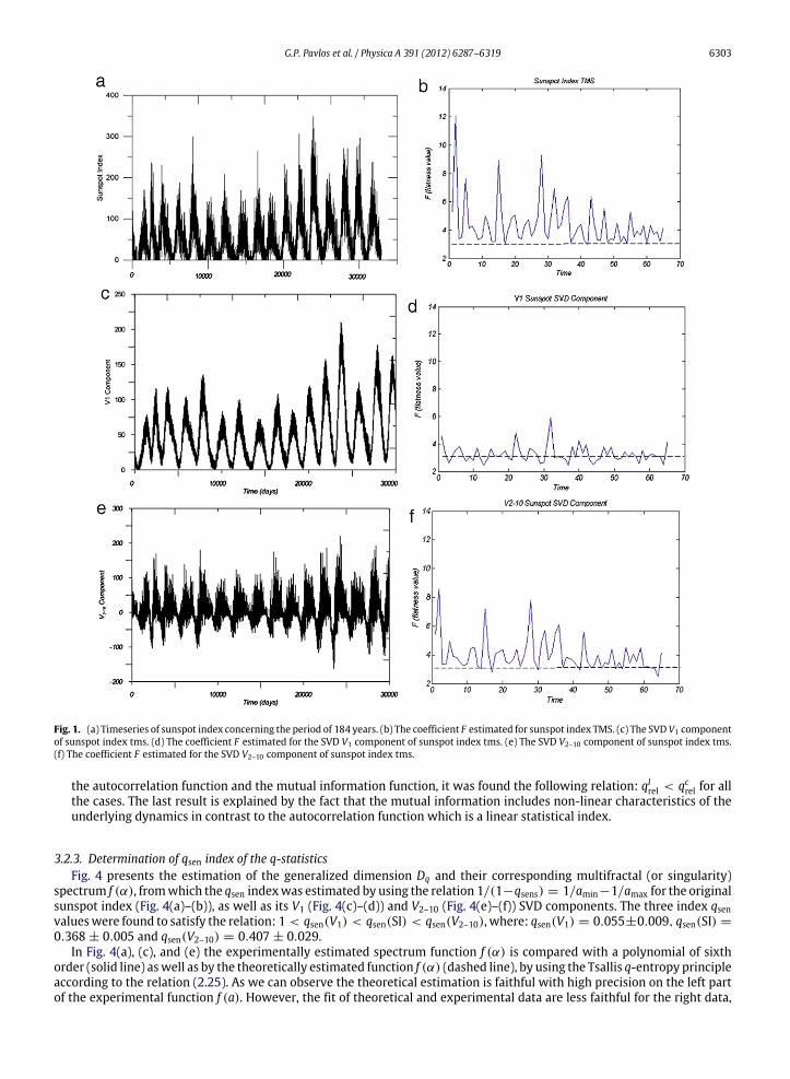
Fig. 1(a) represents the Sunspot Index Timeseries that was constructed during a period of 184 years. As it can be seenfrom this figure the signal has a strong periodic component, almost every 4300 days that corresponds to the well knownphenomenon of the Solar Cycle. Fig. 1(b) presents the flatness coefficient F estimated for the sunspot data (SI) during thesame period. The F values reveal continuous variation of the sunspot statistics between Gaussian profile (F ∼ 3) to strongnon-Gaussian profile (F ∼ 4–12). Fig. 1(c) presents the first (V1) SVD component and Fig. 1(d) the sum V2–10 =
10i=2 Vi
of the next SVD components estimated for the sunspot index timeseries. The estimation of the flatness coefficient F(V1)and F(V2–10) is shown in Fig. 1(e) and Fig. 1(f), correspondingly. As we can notice in these figures the statistics of the V1component is clearly discriminated from the statistics of the V2–10 component, as the F(V1) flatness coefficient obtainedalmost every where low values (∼3–4) while the F(V2–10) obtained higher values (∼4–9). The low values (∼3–4) of theF(V1) coefficient indicates for the solar activity a near Gaussian dynamical process, underlying the V1 SVD component.Oppositely, the high values of the F(V2–10) coefficient indicate a strongly non-Gaussian solar dynamical process underlyingthe V2–10 SVD component. According to the physical meaning of the SVD analysis (Section 2.2.1), the V1 SVD component canbe related to the solar dynamics extended at large spatio-temporal regions of the photospheric system, while the V2–10 SVDcomponent of the sunspot index is related to the spatio-temporal confined photospheric dynamics.
3.2. The Tsallis q-statistics
In this section we present results concerning the computation of the Tsallis q-triplet, including the three-index set(qstat, qsen, qrel) estimated for the original sunspot index timeseries, aswell as for itsV1 andV2–10 SVD components (presentedin Fig. 1(a)–(c) and (e)).
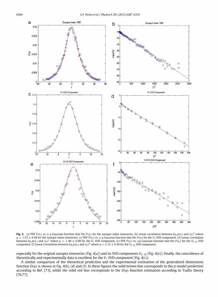
3.2.1. Determination of qstat index of the q-statisticsIn Fig. 2(a) we present (by open circles) the experimental probability distribution function (PDF) p(z) vs. z, where z
corresponds to the Zn+1 − Zn, (n = 1, 2, . . . ,N) timeseries difference values. In Fig. 2(b) we present the best linearcorrelation between lnq[p(z)] and z2. The best fitting was found for the value of qstat = 1.53 ± 0.04. This value was used toestimate the q-Gaussian distribution presented in Fig. 2(a) by the solid black line. Fig. 2(c)–(f) are similar to Fig. 2(a) and (b)but for the V1 and V2–10 SVD components correspondingly. Now the qstat values were for the SVD components estimated tobe: qstat(V1) = 1.40 ± 0.08 and qstat(V2–10) = 2.12 ± 0.20. As we can observe from these results the following relation issatisfied:
1 < qstat(V1) < qstat(SI) < qstat(V2–10), where qstat(SI) corresponds to the original sunspot index timeseries.
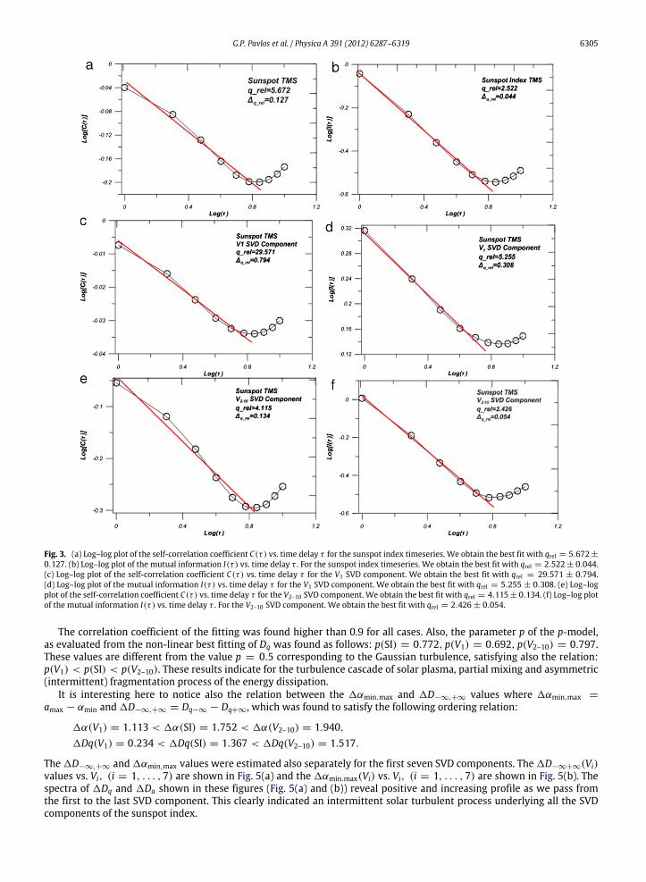
3.2.2. Determination of qrel index of the q-statistics(a) Relaxation of autocorrelation functions
Fig. 3 presents the best log plot fitting of the autocorrelation function C(τ ) estimated for the original sunspot index signal(Fig. 3(a)) its V1 SVD component (Fig. 3(b)), as well as its V2–10 SVD component (Fig. 3(c)). The three qrel values were foundto satisfy the relation: 1 < qcrel(V2–10) < qcrel(SI) < qcrel(V1) as:
qcrel(V2–10) = 4.115 ± 0.134, qcrel(SI) = 5.672 ± 0.127, qcrel(V1) = 29.571 ± 0.794.
(b) Relaxation of mutual information.Fig. 3(b), (d) and (f) is similar with Fig. 3(a), (c), (e) but it corresponds to the relaxation time of the mutual information
I(τ ). For the top of the bottom we see the log–log plot of I(τ ) for the sunspot index timeseries, its V1 SVD component andits V2–10 SVD component. The best log–log (linear) fitting showed the values:
qIrel(V2–10) = 2.426 ± 0.054, qIrel(SI) = 2.522 ± 0.044, qIrel(V1) = 5.255 ± 0.308. Among the three values the followingrelation is satisfied: 1 < qIrel(V2–10) < qIrel(SI) < qIrel(V1). Also comparing the qrel indices, as they were estimated for
G.P. Pavlos et al. / Physica A 391 (2012) 6287–6319 6303
Fig. 1. (a) Timeseries of sunspot index concerning the period of 184 years. (b) The coefficient F estimated for sunspot index TMS. (c) The SVD V1 componentof sunspot index tms. (d) The coefficient F estimated for the SVD V1 component of sunspot index tms. (e) The SVD V2–10 component of sunspot index tms.(f) The coefficient F estimated for the SVD V2–10 component of sunspot index tms.
the autocorrelation function and the mutual information function, it was found the following relation: qIrel < qcrel for allthe cases. The last result is explained by the fact that the mutual information includes non-linear characteristics of theunderlying dynamics in contrast to the autocorrelation function which is a linear statistical index.
3.2.3. Determination of qsen index of the q-statisticsFig. 4 presents the estimation of the generalized dimension Dq and their corresponding multifractal (or singularity)
spectrum f (α), fromwhich the qsen indexwas estimated by using the relation 1/(1−qsens) = 1/amin−1/amax for the originalsunspot index (Fig. 4(a)–(b)), as well as its V1 (Fig. 4(c)–(d)) and V2–10 (Fig. 4(e)–(f)) SVD components. The three index qsenvalueswere found to satisfy the relation: 1 < qsen(V1) < qsen(SI) < qsen(V2–10), where: qsen(V1) = 0.055±0.009, qsen(SI) =
0.368 ± 0.005 and qsen(V2–10) = 0.407 ± 0.029.In Fig. 4(a), (c), and (e) the experimentally estimated spectrum function f (α) is compared with a polynomial of sixth
order (solid line) aswell as by the theoretically estimated function f (α) (dashed line), by using the Tsallis q-entropy principleaccording to the relation (2.25). As we can observe the theoretical estimation is faithful with high precision on the left partof the experimental function f (a). However, the fit of theoretical and experimental data are less faithful for the right data,
6304 G.P. Pavlos et al. / Physica A 391 (2012) 6287–6319
Fig. 2. (a) PDF P(zi) vs. zi q Gaussian function that fits P(zi) for the sunspot index timeseries. (b) Linear correlation between lnq p(zi) and (zi)2 whereq = 1.53 ± 0.04 for the sunspot index timeseries. (c) PDF P(zi) vs. zi q Gaussian function that fits P(zi) for the V1 SVD component. (d) Linear correlationbetween lnq p(zi) and (zi)2 where q = 1.40 ± 0.08 for the V1 SVD component. (e) PDF P(zi) vs. ziq Gaussian function that fits P(zi) for the V2–10 SVDcomponent. (f) Linear Correlation between lnq p(zi) and (zi)2 where q = 2.12 ± 0.20 for the V2–10 SVD component.
especially for the original sunspot timeseries (Fig. 4(a)) and its SVD components V2–10 (Fig. 4(e)). Finally, the coincidence oftheoretically and experimentally data is excellent for the V1 SVD component (Fig. 4(c)).
A similar comparison of the theoretical prediction and the experimental estimation of the generalized dimensionsfunction D(q) is shown in Fig. 4(b), (d) and (f). In these figures the solid brown line corresponds to the p-model predictionaccording to Ref. [73], while the solid red line corresponds to the D(q) function estimation according to Tsallis theory[76,77].
G.P. Pavlos et al. / Physica A 391 (2012) 6287–6319 6305
Fig. 3. (a) Log–log plot of the self-correlation coefficient C(τ ) vs. time delay τ for the sunspot index timeseries. We obtain the best fit with qrel = 5.672±
0.127. (b) Log–log plot of the mutual information I(τ ) vs. time delay τ . For the sunspot index timeseries. We obtain the best fit with qrel = 2.522± 0.044.(c) Log–log plot of the self-correlation coefficient C(τ ) vs. time delay τ for the V1 SVD component. We obtain the best fit with qrel = 29.571 ± 0.794.(d) Log–log plot of the mutual information I(τ ) vs. time delay τ for the V1 SVD component. We obtain the best fit with qrel = 5.255 ± 0.308. (e) Log–logplot of the self-correlation coefficient C(τ ) vs. time delay τ for the V2–10 SVD component. We obtain the best fit with qrel = 4.115± 0.134. (f) Log–log plotof the mutual information I(τ ) vs. time delay τ . For the V2–10 SVD component. We obtain the best fit with qrel = 2.426 ± 0.054.
The correlation coefficient of the fitting was found higher than 0.9 for all cases. Also, the parameter p of the p-model,as evaluated from the non-linear best fitting of Dq was found as follows: p(SI) = 0.772, p(V1) = 0.692, p(V2–10) = 0.797.These values are different from the value p = 0.5 corresponding to the Gaussian turbulence, satisfying also the relation:p(V1) < p(SI) < p(V2–10). These results indicate for the turbulence cascade of solar plasma, partial mixing and asymmetric(intermittent) fragmentation process of the energy dissipation.
It is interesting here to notice also the relation between the 1αmin,max and 1D−∞,+∞ values where 1αmin,max =
amax − αmin and 1D−∞,+∞ = Dq−∞ − Dq+∞, which was found to satisfy the following ordering relation:
1α(V1) = 1.113 < 1α(SI) = 1.752 < 1α(V2–10) = 1.940,1Dq(V1) = 0.234 < 1Dq(SI) = 1.367 < 1Dq(V2–10) = 1.517.
The 1D−∞,+∞ and 1αmin,max values were estimated also separately for the first seven SVD components. The 1D−∞+∞(Vi)values vs. Vi, (i = 1, . . . , 7) are shown in Fig. 5(a) and the 1αmin.max(Vi) vs. Vi, (i = 1, . . . , 7) are shown in Fig. 5(b). Thespectra of 1Dq and 1Da shown in these figures (Fig. 5(a) and (b)) reveal positive and increasing profile as we pass fromthe first to the last SVD component. This clearly indicated an intermittent solar turbulent process underlying all the SVDcomponents of the sunspot index.
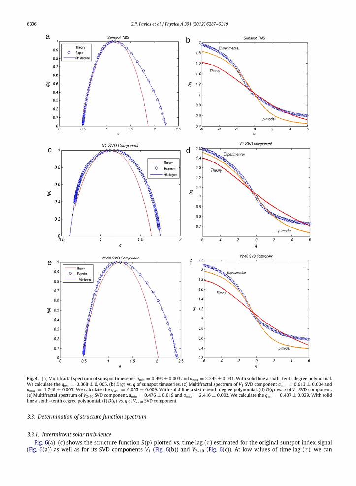
6306 G.P. Pavlos et al. / Physica A 391 (2012) 6287–6319
Fig. 4. (a) Multifractal spectrum of sunspot timeseries amin = 0.493± 0.003 and amax = 2.245± 0.031. With solid line a sixth–tenth degree polynomial.We calculate the qsen = 0.368 ± 0, 005. (b) D(q) vs. q of sunspot timeseries. (c) Multifractal spectrum of V1 SVD component amin = 0.613 ± 0.004 andamax = 1.746 ± 0.003. We calculate the qsen = 0.055 ± 0.009. With solid line a sixth–tenth degree polynomial. (d) D(q) vs. q of V1 SVD component.(e) Multifractal spectrum of V2–10 SVD component. amin = 0.476 ± 0.019 and amax = 2.416 ± 0.002. We calculate the qsen = 0.407 ± 0.029. With solidline a sixth–tenth degree polynomial. (f) D(q) vs. q of V2–10 SVD component.
3.3. Determination of structure function spectrum
3.3.1. Intermittent solar turbulenceFig. 6(a)–(c) shows the structure function S(p) plotted vs. time lag (τ ) estimated for the original sunspot index signal
(Fig. 6(a)) as well as for its SVD components V1 (Fig. 6(b)) and V2–10 (Fig. 6(c)). At low values of time lag (τ ), we can
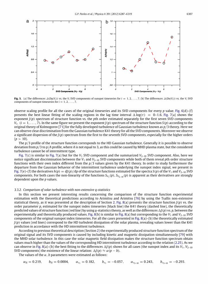
G.P. Pavlos et al. / Physica A 391 (2012) 6287–6319 6307
Fig. 5. (a) The differences ∆(Dq(Vi)) vs. the Vi SVD components of sunspot timeseries for i = 1, 2, . . . , 7. (b) The differences ∆(Da(Vi)) vs. the Vi SVDcomponents of sunspot timeseries for i = 1, 2, . . . , 7.
observe scaling profile for all the cases of the original timeseries and its SVD components for every p value. Fig. 6(d)–(f)presents the best linear fitting of the scaling regions in the lag time interval 1 log(τ ) = 0–1.6. Fig. 7(a) shows theexponent J(p) spectrum of structure function vs. the pth order estimated separately for the first seven SVD componentsVi, (i = 1, . . . , 7). In the same figure we present the exponent J(p) spectrum of the structure function S(p) according to theoriginal theory of Kolmogorov [71] for the fully developed turbulence of Gaussian turbulence known as p/3 theory. Here wecan observe clear discrimination from theGaussian turbulence K41 theory for all the SVD components.Moreoverwe observea significant dispersion of the J(p) spectrum from the first to the seventh SVD components, especially for the higher orders(p > 10).
The p/3 profile of the structure function corresponds to the HD Gaussian turbulence. Generally it is possible to observedeviation from p/3 to p/A profile, where A is not equal to 3, as this could be caused byMHD plasma state, but the consideredturbulence cannot be of intermittent type.
Fig. 7(c) is similar to Fig. 7(a) but for the V1 SVD component and the summarized V2–10 SVD component. Also, here wenotice significant discrimination between the V1 and V2–10 SVD components while both of them reveal pth order structurefunctions with their own index different from the p/3 values given by the K41 theory. In order to study furthermore thedeparture from the Gaussian behavior of the intermittent turbulence underlying the sunspot index signal, we present inFig. 7(e)–(f) the derivatives h(p) = dJ(p)/dp of the structure functions estimated for the spectra S(p) of the V1 and V2–10 SVDcomponents. For both cases the non-linearity of the functions SV1(p), SV2–10(p) is apparent as their derivatives are stronglydependent upon the p values.
3.3.2. Comparison of solar turbulence with non-extensive q-statisticsIn this section we present interesting results concerning the comparison of the structure function experimental
estimation with the theoretical predictions according to Arimitsu and Arimitsu [76] by using the Tsallis non-extensivestatistical theory, as it was presented at the description of Section 2. Fig. 8(a) presents the structure function J(p) vs. theorder parameter p, estimated for the sunspot index timeseries (black line) the K41 theory (dashed line), the theoreticallypredicted values of structure function (red line) byusing q-statistics theory, aswell as the differences1J(p) vs. p, between theexperimentally and theoretically produced values. Fig. 8(b) is similar to Fig. 8(a) but corresponding to the V1 and V2–10 SVDcomponents of the original sunspot index timeseries. For all the cases presented in Fig. 8(a)–(b) the theoretically estimatedJ(p) values (red lines) correspond to the HD turbulent dissipation of the solar plasma, revealing values lower than the K41prediction in accordance with the HD intermittent turbulence.
According to previous theoretical description (Section 2) the experimentally produced structure function spectrumof theoriginal signal and its SVD components is caused by including kinetic and magnetic dissipation simultaneously [79] withthe MHD solar turbulence. In this case the solar magnetic field dissipation makes the structure function spectrum obtainvalues much higher than the values of the corresponding HD intermittent turbulence according to the relation (2.25). As wecan observe in Fig. 8(a)–(b) the best fitting to the differences 1J(p) shows for all cases (the sunspot index and its V1, V2–10SVD components) the existence of the linear relation: 1J(p) ≈ α(p − b).
The values of the α, b parameters were estimated as follows:
αSI = 0.219, bSI = 0.0004, αv1 = 0.182, bv1 = −0.057, αv2–10 = 0.243, bv2–10 = −0.293.
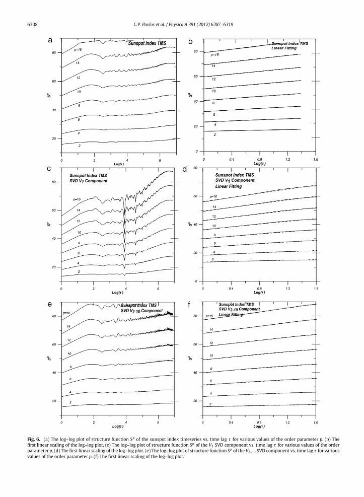
6308 G.P. Pavlos et al. / Physica A 391 (2012) 6287–6319
Fig. 6. (a) The log–log plot of structure function Sp of the sunspot index timeseries vs. time lag τ for various values of the order parameter p. (b) Thefirst linear scaling of the log–log plot. (c) The log–log plot of structure function Sp of the V1 SVD component vs. time lag τ for various values of the orderparameter p. (d) The first linear scaling of the log–log plot. (e) The log–log plot of structure function Sp of the V2–10 SVD component vs. time lag τ for variousvalues of the order parameter p. (f) The first linear scaling of the log–log plot.
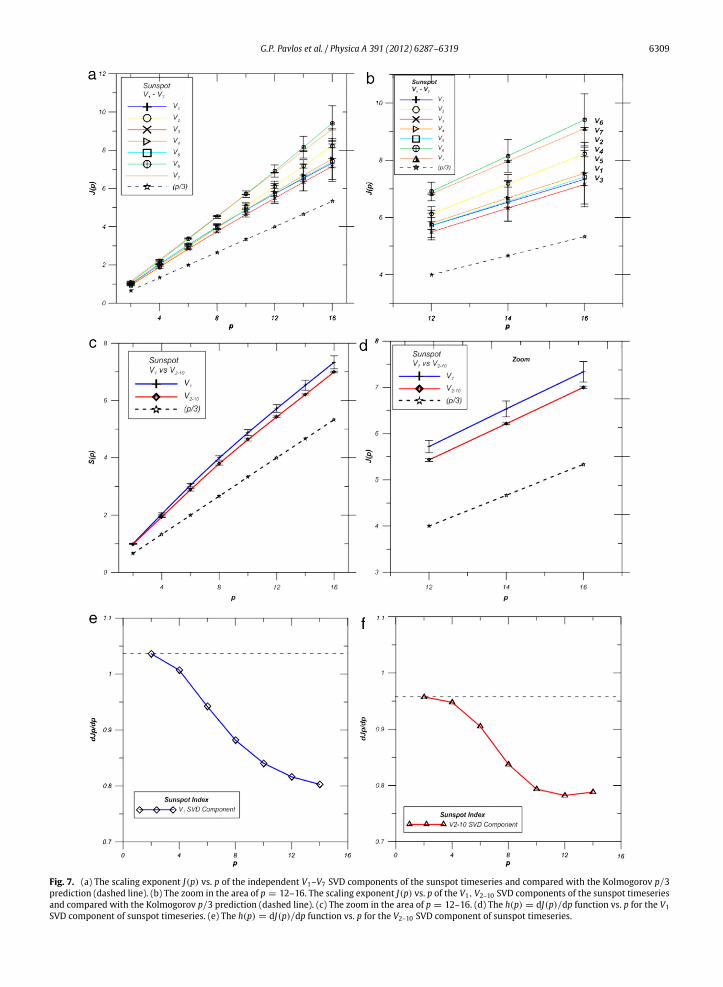
G.P. Pavlos et al. / Physica A 391 (2012) 6287–6319 6309
Fig. 7. (a) The scaling exponent J(p) vs. p of the independent V1–V7 SVD components of the sunspot timeseries and compared with the Kolmogorov p/3prediction (dashed line). (b) The zoom in the area of p = 12–16. The scaling exponent J(p) vs. p of the V1, V2–10 SVD components of the sunspot timeseriesand compared with the Kolmogorov p/3 prediction (dashed line). (c) The zoom in the area of p = 12–16. (d) The h(p) = dJ(p)/dp function vs. p for the V1SVD component of sunspot timeseries. (e) The h(p) = dJ(p)/dp function vs. p for the V2–10 SVD component of sunspot timeseries.
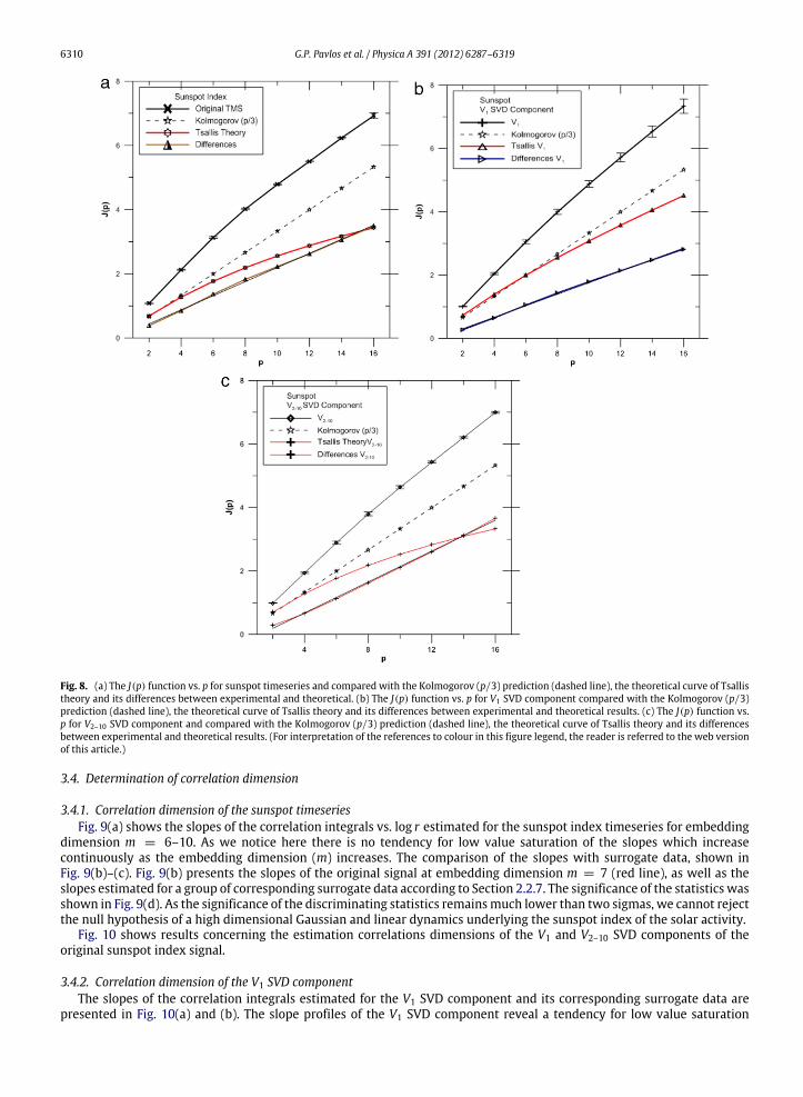
6310 G.P. Pavlos et al. / Physica A 391 (2012) 6287–6319
Fig. 8. (a) The J(p) function vs. p for sunspot timeseries and compared with the Kolmogorov (p/3) prediction (dashed line), the theoretical curve of Tsallistheory and its differences between experimental and theoretical. (b) The J(p) function vs. p for V1 SVD component compared with the Kolmogorov (p/3)prediction (dashed line), the theoretical curve of Tsallis theory and its differences between experimental and theoretical results. (c) The J(p) function vs.p for V2–10 SVD component and compared with the Kolmogorov (p/3) prediction (dashed line), the theoretical curve of Tsallis theory and its differencesbetween experimental and theoretical results. (For interpretation of the references to colour in this figure legend, the reader is referred to the web versionof this article.)
3.4. Determination of correlation dimension
3.4.1. Correlation dimension of the sunspot timeseriesFig. 9(a) shows the slopes of the correlation integrals vs. log r estimated for the sunspot index timeseries for embedding
dimension m = 6–10. As we notice here there is no tendency for low value saturation of the slopes which increasecontinuously as the embedding dimension (m) increases. The comparison of the slopes with surrogate data, shown inFig. 9(b)–(c). Fig. 9(b) presents the slopes of the original signal at embedding dimension m = 7 (red line), as well as theslopes estimated for a group of corresponding surrogate data according to Section 2.2.7. The significance of the statistics wasshown in Fig. 9(d). As the significance of the discriminating statistics remainsmuch lower than two sigmas, we cannot rejectthe null hypothesis of a high dimensional Gaussian and linear dynamics underlying the sunspot index of the solar activity.
Fig. 10 shows results concerning the estimation correlations dimensions of the V1 and V2–10 SVD components of theoriginal sunspot index signal.
3.4.2. Correlation dimension of the V1 SVD componentThe slopes of the correlation integrals estimated for the V1 SVD component and its corresponding surrogate data are
presented in Fig. 10(a) and (b). The slope profiles of the V1 SVD component reveal a tendency for low value saturation
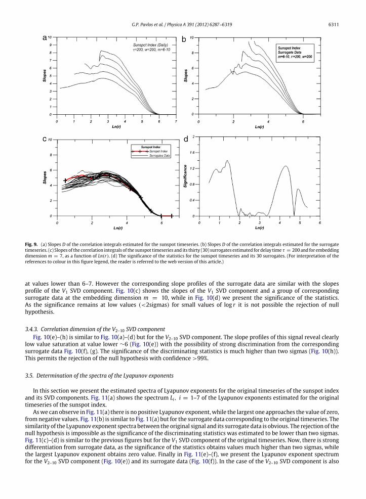
G.P. Pavlos et al. / Physica A 391 (2012) 6287–6319 6311
Fig. 9. (a) Slopes D of the correlation integrals estimated for the sunspot timeseries. (b) Slopes D of the correlation integrals estimated for the surrogatetimeseries. (c) Slopes of the correlation integrals of the sunspot timeseries and its thirty (30) surrogates estimated for delay time τ = 200 and for embeddingdimension m = 7, as a function of Ln(r). (d) The significance of the statistics for the sunspot timeseries and its 30 surrogates. (For interpretation of thereferences to colour in this figure legend, the reader is referred to the web version of this article.)
at values lower than 6–7. However the corresponding slope profiles of the surrogate data are similar with the slopesprofile of the V1 SVD component. Fig. 10(c) shows the slopes of the V1 SVD component and a group of correspondingsurrogate data at the embedding dimension m = 10, while in Fig. 10(d) we present the significance of the statistics.As the significance remains at low values (<2sigmas) for small values of log r it is not possible the rejection of nullhypothesis.
3.4.3. Correlation dimension of the V2–10 SVD componentFig. 10(e)–(h) is similar to Fig. 10(a)–(d) but for the V2–10 SVD component. The slope profiles of this signal reveal clearly
low value saturation at value lower ∼6 (Fig. 10(e)) with the possibility of strong discrimination from the correspondingsurrogate data Fig. 10(f), (g). The significance of the discriminating statistics is much higher than two sigmas (Fig. 10(h)).This permits the rejection of the null hypothesis with confidence >99%.
3.5. Determination of the spectra of the Lyapunov exponents
In this section we present the estimated spectra of Lyapunov exponents for the original timeseries of the sunspot indexand its SVD components. Fig. 11(a) shows the spectrum Li, i = 1–7 of the Lyapunov exponents estimated for the originaltimeseries of the sunspot index.
Aswe can observe in Fig. 11(a) there is no positive Lyapunov exponent, while the largest one approaches the value of zero,fromnegative values. Fig. 11(b) is similar to Fig. 11(a) but for the surrogate data corresponding to the original timeseries. Thesimilarity of the Lyapunov exponent spectra between the original signal and its surrogate data is obvious. The rejection of thenull hypothesis is impossible as the significance of the discriminating statistics was estimated to be lower than two sigmas.Fig. 11(c)–(d) is similar to the previous figures but for the V1 SVD component of the original timeseries. Now, there is strongdifferentiation from surrogate data, as the significance of the statistics obtains values much higher than two sigmas, whilethe largest Lyapunov exponent obtains zero value. Finally in Fig. 11(e)–(f), we present the Lyapunov exponent spectrumfor the V2–10 SVD component (Fig. 10(e)) and its surrogate data (Fig. 10(f)). In the case of the V2–10 SVD component is also
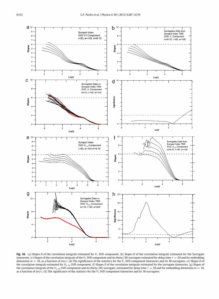
6312 G.P. Pavlos et al. / Physica A 391 (2012) 6287–6319
Fig. 10. (a) Slopes D of the correlation integrals estimated for V1 SVD component. (b) Slopes D of the correlation integrals estimated for the Surrogatetimeseries. (c) Slopes of the correlation integrals of the V1 SVD component and its thirty (30) surrogate estimated for delay time τ = 50 and for embeddingdimension m = 10, as a function of Ln(r). (d) The significance of the statistics for the V1 SVD component timeseries and its 30 surrogates. (e) Slopes D ofthe correlation integrals estimated for V2–10 SVD component. (f) Slopes D of the correlation integrals estimated for the surrogate timeseries. (g) Slopes ofthe correlation integrals of the V2–10 SVD component and its thirty (30) surrogate, estimated for delay time τ = 50 and for embedding dimensionm = 10,as a function of Ln(r). (h) The significance of the statistics for the V1 SVD component timeseries and its 30 surrogates.
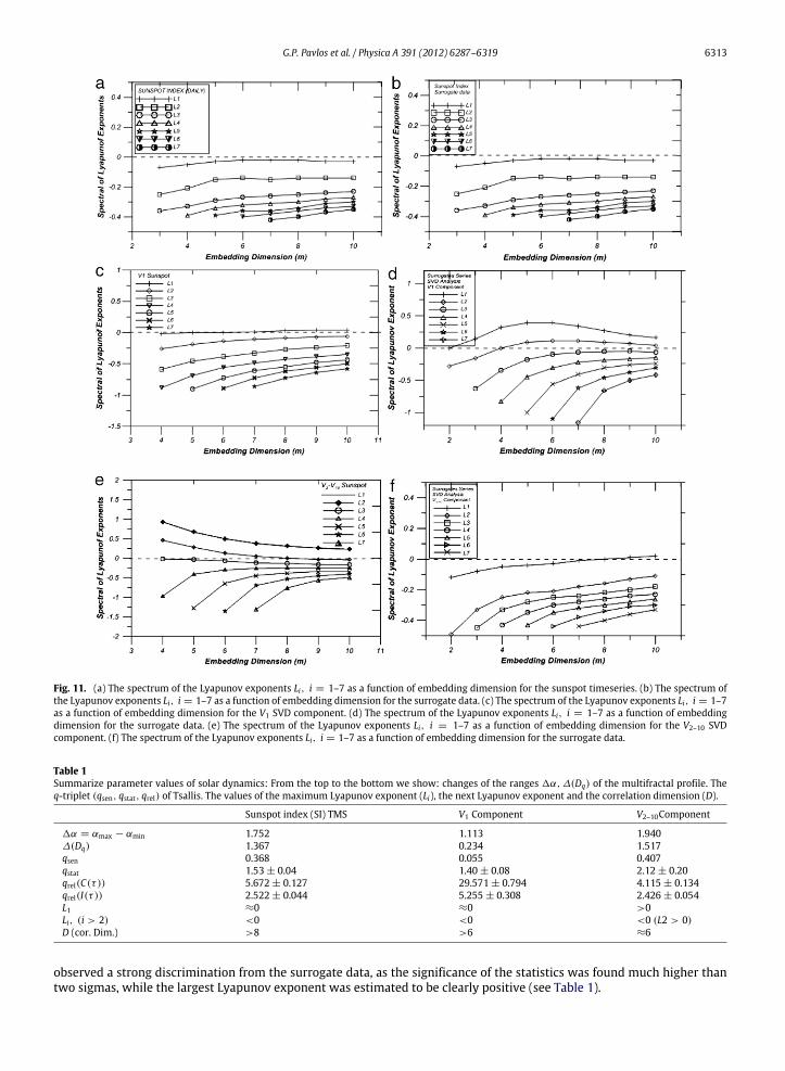
G.P. Pavlos et al. / Physica A 391 (2012) 6287–6319 6313
Fig. 11. (a) The spectrum of the Lyapunov exponents Li, i = 1–7 as a function of embedding dimension for the sunspot timeseries. (b) The spectrum ofthe Lyapunov exponents Li, i = 1–7 as a function of embedding dimension for the surrogate data. (c) The spectrum of the Lyapunov exponents Li, i = 1–7as a function of embedding dimension for the V1 SVD component. (d) The spectrum of the Lyapunov exponents Li, i = 1–7 as a function of embeddingdimension for the surrogate data. (e) The spectrum of the Lyapunov exponents Li, i = 1–7 as a function of embedding dimension for the V2–10 SVDcomponent. (f) The spectrum of the Lyapunov exponents Li, i = 1–7 as a function of embedding dimension for the surrogate data.
Table 1Summarize parameter values of solar dynamics: From the top to the bottom we show: changes of the ranges 1α, ∆(Dq) of the multifractal profile. Theq-triplet (qsen, qstat, qrel) of Tsallis. The values of the maximum Lyapunov exponent (Li), the next Lyapunov exponent and the correlation dimension (D).
Sunspot index (SI) TMS V1 Component V2–10Component
1α = αmax − αmin 1.752 1.113 1.940∆(Dq) 1.367 0.234 1.517qsen 0.368 0.055 0.407qstat 1.53 ± 0.04 1.40 ± 0.08 2.12 ± 0.20qrel(C(τ )) 5.672 ± 0.127 29.571 ± 0.794 4.115 ± 0.134qrel(I(τ )) 2.522 ± 0.044 5.255 ± 0.308 2.426 ± 0.054L1 ≈0 ≈0 >0Li, (i > 2) <0 <0 <0 (L2 > 0)D (cor. Dim.) >8 >6 ≈6
observed a strong discrimination from the surrogate data, as the significance of the statistics was found much higher thantwo sigmas, while the largest Lyapunov exponent was estimated to be clearly positive (see Table 1).
6314 G.P. Pavlos et al. / Physica A 391 (2012) 6287–6319
4. Summary of data analysis
In this study we used the SVD analysis in order to discriminate the dynamical components, underlying the sunspot indextimeseries. After this we applied an extended algorithm for the non-linear analysis of the original sunspot index timeseries,its V1 (first) SVD component and the signal V2–10 composed from the sum of the higher SVD components. The analysis wasexpanded to the estimation of: (a) Flatness coefficients as a measure of Gaussian, non-Gaussian dynamics. (b) The q-tripletof Tsallis non-extensive statistics. (c) The correlation dimension. (d) The Lyapunov exponent spectrum. (e) The spectrum ofthe structure function scaling exponent. (f) The power spectra of the signals.
The results of data analysis presented in Section 3 are summarized as follows:
• A clear distinctionwas observed everywhere between two dynamics: (a) the solar dynamics underlying the first (V1) and(b) the dynamics underlying the (V2–10) SVD component of the sunspot index timeseries.
• The non-Gaussian and non-extensive statistics were found to be effective for the original sunspot index as well as its SVDcomponents V1, V2–10 of the sunspot, indicating non-extensive solar dynamics.
• The Tsallis q-triplet (qsen, qstat, qrel) was found to verify according to the expected scheme qsen ≤ 1 ≤ qstat ≤ qrel.Moreover the Tsallis q-triplet estimation showed clear distinction between the dynamics underlying the SVD analyzedsunspot signal as follows: qk(V1) < qk(SI) < qk(V2–10), for all the k ≡ (sen, stat, rel).
• Themultifractal character was verified for the original signal and its SVD components. Also, themultifractality was foundto be intensified as we pass from the V1 to the V2–10 SVD component in accordance to the relation: 0 < 1a(V1) <1a(V2–10), 0 < 1Dq(V1) < 1Dq(V2–10), where 1a = amax − amin, and 1Dq = Dq=−∞ − Dq=+∞.
• Efficient agreement between Dq and p-model was discovered indicating intermittent (multifractal) solar turbulencewhich is intensified for the solar dynamics underlying the V2–10 SVD component of the sunspot index.
• Generally the differences1a(Vi) and1Dq(Vi) increase passing from lower to higher SVD components Vi, i = 1, 2, . . . , 7.• The qrel index was estimated for two distinct relaxation magnitudes, the autocorrelation function C(τ ) and the mutual
information I(τ ), indicating a good agreement taking into account the linear–non-linear character of the C(τ ) and I(τ )respectively.
• The correlation dimension was estimated at low values DCD = 4–5 for the V2–10 SVD component. For the V1 SVDcomponent of the original signal the correlation dimension was found to be higher than the value ∼10.
• Also the null hypothesis of non-chaotic dynamics and non-linear distortion of white-noise was rejected only for the V2–10SVD component. For the original signal and its V1 SVD component the rejection was insignificant (s < 2). These resultsindicate low dimensional deterministic solar dynamics underlying the V2–10 SVD component and high dimensional SOCsolar dynamics for the V1 SVD component.
• The estimation of Lyapunov exponent spectrum showed for the V2–10 SVD component one positive Lyapunov exponent(λ1 > 0) discriminated from the signal of surrogate data. For the original sunspot signal and its V1 SVD componentthe discrimination with surrogate data was inefficient. These results indicate low-dimensional and chaotic deterministicsolar dynamics underlying theV2–10 SVD component andweak chaos solar dynamics underlying to theV1 SVD componentrelated to a SOC process at the edge of chaos.
• The structure function scaling exponents spectrum J(p)was estimated to values higher than the corresponding p/3 valuesof the K41 theory, for both the V1 and the V2–10 SVD components, as well as for the original signal of the sunspot index.
• The slopes dJ(p)/dp of the scaling exponent function were found to be decreasing as the order p increases. This resultconfirms the intermittent and multifractal character of the solar turbulence dissipation process.
• The SVD analysis of the solar dynamics in relation with the structure functions exponent spectrum J(p) estimated for theSVD components showed clearly distinction of the dynamics underlying the first and the last SVD components.
• The difference 1J(p) between the experimental and theoretical values of the scaling exponent spectrum of the structurefunctions was found to follow a linear profile: 1J(p) = ap+ b for the original sunspot index and its V1 and the V2–10 SVDcomponents.
• Adding the 1J(p) = ap + b function to the theoretically estimated J(p) values by using Tsallis theory we obtain anexcellent agreement of the theoretically predicted and the experimentally estimated exponent spectrum values J(p).
• Noticeable agreement of Tsallis theory and the experimental estimation of the functions f (a),D(q), and J(p) was found.
5. Discussion and theoretical interpretation of data analysis results
The hydromagnetic dynamo model [95,96] can produce partly the chaotic character of the dynamics of the solarconvective zone as the original MHD equations are truncated and transformed to a system of coupled non-linear differentialequations. However, the complexity of the sunspot phenomenology as it is presented in this study cannot be describedfaithfully by this approximation. As we have presented in previous sections the results of data analysis showed clearly:
I. The non-Gaussian and non-extensive statistical character of the solar dynamics underlying the sunspot index timeseries.II. The intermittent and multifractal turbulent character of the solar plasma convection at the photosphere and the
underlying convection zone.III. The phase transition process between different dynamical profiles of the outer solar plasma (convective zone and
photospheric region of the sun).
G.P. Pavlos et al. / Physica A 391 (2012) 6287–6319 6315
IV. Clear discrimination between the high dimensional self organized critical (SOC) solar state dynamical and the lowdimensional dynamical chaotic solar state.
V. Novel agreement of the Tsallis theory predictions concerning the q-entropy principle and the experimental estimationof solar intermittent turbulence indices corresponding: (a) to the multifractal scaling exponents spectrum f (a), (b)the generalized dimension spectrum Dq and (c) the structure function scaling exponents spectrum J(p). However thenoticeable differentiation of the theoretically predicted spectra f (a),Dq, Jp can be explained by the fact that for thetheoretical estimation the HD part of the turbulencewas used. The theoretical prediction can be improved if calculationsbased at Tsallis theory are extended to include the magnetic part of the plasma turbulence.
Purely these results are in agreement with previous studies by Ruzmakin [7,21–25,28,29,96–101].Moreover, significant and novel results included in this study concern the following characteristic of the solar activity:
(a) Intermittent turbulence of the solar convection zone.(b) Solar dynamics and q-extensive statistics of Tsallis theory.(c) Solar plasma self organized criticality (SOC) process.(d) Solar plasma low dimensional chaotic dynamics.(e) Solar plasma phase transition process in the convection zone.
These results can be used:(a) For the theoretical understanding of solar plasma dynamics by developing modern theoretical concepts as the fractal
generalization of dynamics and non equilibrium thermodynamics.(b) The creation of a universal modern theoretical framework of understanding space and cosmic plasma dynamics.
In the next section we attempt an introductory plan for the theoretical interpretation of the results included in theanalysis of the previous sections and their summarized description.
5.1. Solar phase transition process
The critical dynamics of distributed systems includes the possibility of first or second order phase transitionprocesses [102]. From this point of view Pavlos et al. [67,87] showed the existence of two distinct critical states of themagnetospheric plasma. The first critical state corresponds to second order phase transition relatedwith a high dimensionalSOC process, while the second state corresponds to first order phase transition process related with the low dimensionalchaotic process. The results of this study reveal similar results for the case of the solar magnetic activity caused by thesolar convection zone dynamics. The term ‘‘phase transition process’’ included in this studymust be understood as a ‘‘meta-phase transition’’ process and it is used in order to characterize the change of the metaequilibrium critical state of the solarconvection zone dynamics from the high dimensional solar SOC state to the low dimensional solar chaos state.
The first component (V1) of the SVD analysis of the sunspot index including the main power of sunspot timeseries as it isrelated to the higher singular value (σ1) can be related to the solar dynamics at quiet periods. At this critical state the solarconvection zone lives at the edge of the chaos as it was indicated by the zero value of the largest Lyapunov exponent, whilethe dimensionality of the dynamical degrees of freedom was found to be higher than m = 6 without any low saturationprofile of the slopes of the correlation integrals. The sum V2–10 of the next SVD components corresponds to solar activeperiods, where the critical state corresponds clearly to low dimensional chaos with positive Lyapunov exponent and lowdimensional non-linear deterministic dynamics. As the solar system passes from quiet to active periods the critical statechanges its profile. Also according to Arimitsu [88] the singular part of the PDF can be discriminated in two distinct partsΠs(V1), Πs(V2–10). The Πs(V1) PDF describes the solar SOC state, while the Πs(V2–10) describes the solar chaos state. Similarto the magnetospheric plasma the solar SOC state corresponds to second order phase transition, while the solar chaos statecorresponds to first order phase transition.
5.2. Non-extensive statistics and phase transition of the solar dynamics
The estimated values of Tsallis q-triplet corresponding to the solar activity showed clearly non-extensive statisticalcharacter for both critical states SOC and chaos of the solar system. However the distinct profile of the q-triplet valueswas shown clearly as the solar system changes its critical states. At the quiet period of SOC state the values of q-tripletwere found to be: qsen = 0.055, qstat = 1.4, qrel = 5.2, while the q-triplet values at the solar active period were foundto be qsen = 0.4, qstat = 2.12, qrel = 2.46. The quiet state is clearly of non-Gaussian profile (qstat = 1.4 > 1) butit clearly increases to higher values (qstat = 2.12) as the solar system passes to active periods. The corresponding andsimultaneous increase of qsen from the value 0.055 to the value of 0.4 and the decrease of qrel from the value 5.2 to the lowervalue qrel = 2.46 are both in agreement with the change from SOC to the low dimensional chaos as the largest Lyapunovexponent changes from zero to positive values. This implies a decrease of the relaxation time while the attractive set ofthe phase space obtains a strange and strong multifractal topological character causing the increase of the qsen and thelargest Lyapunov exponent values. Also as the low dimensional chaotic state corresponds to a first order phase transitionprocess, the change from a quiet to active profile of the solar dynamics is accompanied with the development of long rangecorrelations. This is in accordance with the observed strengthen of the non-Gaussian profile of dynamics and an increasingof the qstat value.
6316 G.P. Pavlos et al. / Physica A 391 (2012) 6287–6319
5.3. Renormalization group (RNG) theory and solar phase transition
The multifractal and multiscale intermittent turbulent character of the solar dynamics in the solar convection zone wasverified in this study after the estimation of the structure function scaling exponents spectrum J(p) and the spectrum f (a)of the point wise dimensions or singularities (α). This justifies the application of RNG theory for the description of the scaleinvariance and the development of long-range correlation of the solar intermittent turbulence state. Generally the solarplasma can be described by generalized Langevin stochastic equations of the general type:
∂ϕi
∂t= fi (ϕ, x, t) + ni (x, t) i = 1, 2, . . . (5.1)
where fi corresponds to the deterministic process as concerns the plasma dynamical variablesφ(x, t) and ni to the stochasticcomponents (fluctuations). Generally, fi are non-random forces corresponding to the functional derivative of the free energyfunctional of the system.
According to Chang [62,63] and Chang et al. [103] the behavior of a non-linear stochastic system far from equilibriumcan be described by the density functional P , defined by
P (ϕ (x, t)) =
D (x) exp
−i ·
L (ϕ, ϕ, x) dx
dt (5.2)
where L (ϕ, ϕ, x) is the stochastic Lagrangian of the system, which describes the full dynamics of the stochastic system.Moreover, the far from equilibrium renormalization group theory applied to the stochastic Lagrangian L generates thesingular points (fixed points) in the affine space of the stochastic distributed system. At fixed points the system reveals thecharacter of criticality, as near criticality the correlations among the fluctuations of the random dynamic field are extremelylong-ranged and there exist many correlation scales. Also, close to dynamic criticality certain linear combinations of theparameters, characterizing the stochastic Lagrangian of the system, correlate with each other in the form of power laws andthe stochastic system can be described by a small number of relevant parameters characterizing the truncated system ofequations with low or high dimensionality.
According to these theoretical results, the stochastic solar plasma system can exhibit low dimensional chaotic or highdimensional SOC like behavior, including fractal or multifractal structures with power law profiles. The power laws areconnected to the near criticality phase transition process which creates spatial and temporal correlations as well as strongor weak reduction (self-organization) of the infinite dimensionality corresponding to a spatially distributed system. Firstand second phase transition processes can be related to discrete fixed points in the affine dynamical (Lagrangian) space ofthe stochastic dynamics. The SOC like behavior of plasma dynamics corresponds to the second phase transition process asa high dimensional process at the edge of chaos. The process of strong and low dimensional chaos can be related to a firstorder phase transition process. The probabilistic solution (Eq. (5.2)) of the generalized magnetospheric Langevin equationsmay include Gaussian or non-Gaussian processes as well as normal or anomalous diffusion processes depending upon thecritical state of the system.
From this point of view, a SOC or low dimensional chaos interpretation or distinct q-statistical stateswith different valuesof the Tsallis q-triplet depends upon the type of the critical fixed (singular) point in the functional solution space of thesystem. When the stochastic system is externally driven or perturbed, it can be moved from a particular state of criticalityto another characterized by a different fixed point and different dimensionality or scaling laws. Thus, the old SOC theorycould be a special kind of critical dynamics of an externally driven stochastic system. After all SOC and lowdimensional chaoscan coexist in the same dynamical system as a process manifested by different kinds of fixed (critical) points in its solutionspace. Due to this fact, the solar convection zone dynamics may include high dimensional SOC process or low dimensionalchaos or other more general dynamical process corresponding to various q-statistical states.
5.4. q-extension and fractal extension of dynamics
The well known Boltzmann’s formula S = k logW where S is the entropy of the system and W is the number of themicroscopic states corresponding to amacroscopic state indicates the priority of statistics over dynamics. However, Einsteinpreferred to put dynamics in priority of statistics [87,104,105], using the inverse relation i.e.W = eS/k where entropy is nota statistical but a dynamical magnitude. Already, Boltzmann himself was using the relation WR = limT→∞
tRT =
ΩRΩ
wheretR is the total amount of time that the system spends during the time T in its phase space trajectory in the region Rwhile ΩRis the phase space volume of region R and Ω is the total volume of phase space [106]. The above concepts of Boltzmann andEinstein were innovative as concerns modern q-extension of statistics which is internally related to the fractal extension ofdynamics. According to Zaslavsky [107–110] the fractal extension of dynamics includes simultaneously the q-extension ofstatistics as well as the fractal extension RNG theory in the Fraction at Fokker–Planck–Kolmogorov Equation (FFPK):
∂βP (x, t)∂β t
=∂α
∂ (−x)a[A(x)P(x, t)] +
∂a+1
∂ (−x)a+1 [B(x)P(x, t)] . (5.3)
G.P. Pavlos et al. / Physica A 391 (2012) 6287–6319 6317
As concerns the space plasma dynamics, the plasma particle and field’s magnitude correspond to the (x) variablein Eq. (5.3), while P(x, t) describes the probability distribution of the particle-fields variables. The variables A(x), B(x)correspond to the first and second moments of probability transfer and describe the wandering process in the fractal space(phase space) and time. The fractional space and time derivatives ∂β/∂tβ , ∂α/∂xα are caused by the multifractal (strange)topology of phase space which can be described by the anomalous phase space Renormalization Transform [107]. We mustnotice here that the multifractal character of phase space is the mirroring of the phase space strange topology in the spatialmultifractal distribution of the dynamical variables.
The q-statistics of Tsallis corresponds to the meta-equilibrium solutions of the FFPK equation [9,10,111]. Also, themetaequilibrium states of FFPK equation correspond to the fixed points of Chang non-equilibrium RNG theory for spaceplasmas [62,63]. The anomalous topology of phase space dynamics includes inherently the statistics as a consequence of itsmultiscale and multifractal character. From this point of view the non-extensive character of thermodynamics constitute akind of unification between statistics and dynamics. From a wider point of view the FFPK equation is a partial manifestationof a general fractal extension of dynamics. According to Tarasov [112], Zaslavsky’s equation can be derived from a fractionalgeneralization of the Liouville and BBGKI equations. According also to Tarasov [106–108,113,114] the fractal extension ofdynamics including the dynamics of particles or fields is based on the fact that the fractal structure ofmatter (particles, fluids,fields) can be replaced by a fractional continuous model. In this generalization the fractional integrals can be consideredas approximations of integrals on fractals. Also, the fractional derivatives are related with the development of long rangecorrelations and localized fractal structures. In this direction the solar dynamo theory must be based at the extended fractalplasma theory including anomalous magnetic transport and diffusion, magnetic percolation and magnetic Levy randomwalk [39]. Also from a more extreme point of view, the fractal environment for the anomalous turbulence dissipation ofmagnetic field and plasma flows is the fractality of the space–time itself according to Shlesinger [54], Nottale [59], Chen [58].Finally we must explain that the solar phase transition process corresponds to the topological phase transition process ofthe attracting set in the phase space of the solar dynamics.
References
[1] A.A. Tsonis, RANDOMNICITY: Rules and Randomness in the Realm of the Infinite, Imperial College Press, 2008.[2] Ya B. Zeldovich, S.A. Molchanov, A.A. Ruzmaikin, D.D. Sokolov, Intermittency in randommedia, Sov. Phys. Usp. 30 (1987) 353.[3] G. Nikolis, Irreversible thermodynamics, Rep. Progr. Phys. 42 (1979) 227–267.[4] I. Prigozine, Time, structure and fluctuations, Nobel Lecture (1977).[5] V.V. Yankov, Three rules of nonlinear physics, Phys. Rep. 283 (1997) 147–160.[6] J.L. McCauley, Nonintegrability, chaos and complexity, Physica A 237 (1997) 387–404.[7] C. Tsallis, Possible generalization of Boltzmann–Gibbs statistics, J. Stat. Phys. 52 (1–2) (1988) 479–487.[8] C. Tsallis, in: S. Abe, Y. Okamoto (Eds.), Nonextensive Statistical Mechanics and Thermodynamics: Historical Background and Present Status, in: LNP,
vol. 560, Springer, 2001, pp. 3–98.[9] C. Tsallis, Nonextensive statistical mechanics: construction and physical interpretation, in: G.M. Murray, C. Tsallis (Eds.), Nonextensive Entropy—
Interdisciplinary Applications, Oxford Univ. Press, 2004, pp. 1–53.[10] C. Tsallis, Introduction to Non-Extensive Statistical Mechanics, Springer, 2009.[11] G. Kaniadakis, A. Lavagno, M. Lissia, P. Quarati, Anomalous diffusion modifies solar neutrino fluxes, Physica A 261 (1998) 359–373.[12] A. Lavagno, P. Quarati, Nonextensive statistics in stellar plasma and solar neutrinos, Nuclear Phys. B Proc. Suppl. 87 (2000) 209–211.[13] N.O. Weiss, et al., Periodic and aperiodic dynamo waves, Geophys. Astrophys. Fluid Dyn. 30 (1984) 305–345.[14] A.A. Ruzmaikin, Sol. Phys. 100 (1985) 125–140.[15] J. Kurths, H. Herzel, Can a solar pulsation event be characterized by a low-dimensional chaotic attractor? Sol. Phys. 107 (1986) 39–45.[16] G.P. Pavlos, et al., Evidence for strange attractor structures in space plasmas, Ann. Geophys. 10 (5) (1992) 309–322.[17] M. Palus, D. Novotha, Sunspot cycle: a driven nonlinear oscillator, Phys. Rev. Lett. 83 (17) (1999) 3406.[18] J.M. Polygiannakis, X. Moussas, C.P. Sonett, A nonlinear RLC solar cycle model, Sol. Phys. 163 (1996) 193–203.[19] J. Feynman, S.B. Gabriel, Period and phase of the 88-year solar cycle and the maunder minimum: evidence for a chaotic sun, Sol. Phys. 127 (1990)
393–403.[20] C. Letellier, Luis A. Aguirre, Jean Maquet, Relation between observability and differential embeddings for nonlinear dynamics, Phys. Rev. E 71 (2005)
066213.[21] L.M. Zelenyi, A.V. Milovanov, Fractal properties of sunspots, Sov. Astron. Lett. 17 (6) (1991) 425.[22] A.V. Milovanov, L.M. Zelenyi, Applications of fractal geometry to dynamical evolution of sunspots, Phys. Fluids B 5 (7) (1993) 2609.[23] J.K. Lawrenece, A.A. Ruzmaikin, A.C. Cadavid, Multifractal measure of the solar magnetic field, Astrophys. J. 417 (1993) 805–811.[24] J.K. Lawrenece, A.C. Cadavid, A.A. Ruzmaikin, Multiplicative cascade models of multifractal solar magnetic fields, Phys. Rev. E 51 (1) (1995) 316.[25] J.K. Lawrenece, A.C. Cadavid, A.A. Ruzmaikin, Turbulent and chaotic dynamics underlying solarmagnetic variability, Astrophys. J. 455 (1995) 366–375.[26] A.A. Ruzmakin, et al., Spectral properties of solar convection and diffusion, Astrophys. J. 471 (1996) 1022.[27] A.C. Cadavid, J.K. Lawrence, A.A. Ruzmaikin, Anomalous diffusion of solar magnetic elements, Astrophys. J. 521 (1999) 844–850.[28] G. Zimbardo, P. Veltri, G. Basile, S. Principato, Anomalous diffusion and Levy random walk of magnetic field lines in three dimensional turbulence,
Phys. Plasmas 2 (7) (1995) 2653.[29] J.K. Lawrence, C.J. Schrijver, Anomalous diffusion of magnetic elements across the solar surface, Astrophys. J. 411 (1993) 402–405.[30] K. Petroway, The sun as a laboratory for turbulence theory: the problem of anomalous diffusion, Padeu 15 (2005) 53–57.[31] P. Bak, et al., Self organized criticality, Phys. Rev. A V38 (1) (1988) 364–374.[32] E.T. Lu, R.J. Hamilton, Avalanches and the distribution of solar flares, Astrophys. J. 380 (1991) 89–92.[33] E.T. Lu, R.J. Hamilton, J.M. McTiernan, K.R. Bromund, Solar flares and avalanches in driven dissipative systems, Astrophys. J. (ISSN: 0004-637X) 412
(2) (1993) 841–852. Part 1.[34] D. Vassiliadis, A. Anastasiadis, M. Georgoulis, L. Vlahos, Derivation of solar flare cellular automatamodels from a subset of themagnetohydrodynamic
equations, Astrophys. J. 509 (1998) L53. http://dx.doi.org/10.1086/311750.[35] L. de Archangelis, C. Godano, E. Lippiello, M. Nicodemi, Phys. Rev. Lett. 96 (2006) 51102.[36] L. Vlahos, M. Georgoulis, R. Kluiving, P. Paschos, Astron. Astrophys. 299 (1995) 897.[37] L.P. Karakatsanis, G.P. Pavlos, Self organized criticality and chaos into the solar activity, Nonlinear Phenom. Complex Syst. 11 (2) (2008) 280–284.
6318 G.P. Pavlos et al. / Physica A 391 (2012) 6287–6319
[38] L.P. Karakatsanis, G.P. Pavlos, A.C. Iliopoulos, V.G. Tsoutsouras, E.G. Pavlos, Evidence for coexistence of SOC, intermittent turbulence and low-dimensional chaos processes in solar flare dynamics, in:Modern Challenges in Nonlinear Plasma Physics: A Festschrift Honoring the Career of DennisPapadopoulos, in: AIP, vol. 1320, 2011, pp. 55–64.
[39] L.M. Zelenyi, A.V. Milovanov, Fractal topology and strange kinetics: from percolation theory to problems in cosmic electrodynamics, Phys. Usp. 47(8) (2004) 749–788.
[40] J. Theiler, et al., Using surrogate data to detect nonlinearity in time series, in: M. Casdagli, S. Eubank (Eds.), Nonlinear Modeling and Forecasting,in: SFI Studies in the Sciences of Complexity, vol. XII, Addison-Wesley, Reading, Mass, 1992, pp. 163–188.
[41] J. Theiler, et al., Testing for nonlinearity in time series: the method of surrogate data, Physica D 58 (1992) 77–94.[42] T. Schreiber, A. Schmitz, Improved surrogate data for nonlinearity test, Phys. Rev. Lett. 77 (1996) 635–638.[43] G.P. Pavlos, et al., Nonlinear analysis of magnetospheric data, Part I. Geometric characteristics of the AE index time series and comparison with
nonlinear surrogate data, Nonlinear Processes Geophys. 6 (1999) 51–65.[44] G.P. Pavlos, et al., Nonlinear analysis of magnetospheric data, Part II. Dynamical characteristics of the AE index time series and comparison with
nonlinear surrogate data, Nonlinear Processes Geophys. 6 (1999) 79–98.[45] M.A. Athanasiu, G.P. Pavlos, SVD analysis of the magnetospheric AE index time series and comparison with low-dimensional chaotic dynamics,
Nonlinear Processes Geophys. 8 (2001) 95–125.[46] C. Beck, From the Perron–Frobenius equation to the Fokker–Planck equation, J. Stat. Phys. 79 (5–6) (1994) 875–894;
C. Beck, F. Schlogl, Thermodynamics of Chaotic Systems an Introduction, Cambridge University Press, 1993.[47] S. Umarov, et al. A generalization of the central limit theorem concistentwith non-extensive statisticalmechanics, 2007. arxiv:cond-mat/0603593v4.[48] C. Tsallis, S.V.F. Levy, A.M.C. Souza, R. Maynard, Statistical-mechanical foundation of the ubiquity of Lévy distributions in nature, Phys. Rev. Lett. 75
(1995) 3589–3593.[49] P.A. Alemany, D.H. Zanete, Fractal random walks from a variational formalism for Tsallis entropies, Phys. Rev. E 49 (1994) R956–R958.[50] D.H. Zanette, P.A. Alemany, Thermodynamics of anomalous diffusion, Phys. Rev. Lett. 75 (1995) 366–369.[51] M.C. Mackey, Time’s Arrow: The Origins of Thermodynamic Behaviour, Springer-Verlag, 1992.[52] I. Prigozine, El fin de las Certitumbres, Editions Odile Jakob, 1996.[53] C. Beck, From the Perron–Frobenious equation to the Fokker–Planck equation, J. Stat. Phys. 79 (5–6) (1995) 875–893.[54] M.F. Shlesinger, Strange kinetics, Nature 363 (1993) 31–37.[55] G.M. Zaslavsky, Chaos, fractional kinetics, and anomalous transport, Phys. Rep. 371 (2002) 461–580.[56] M.F. Shlesinger, et al., Phys. Rev. Lett. 58 (1987) 1100–1104.[57] J.P. Bouchaud, A. Georges, Anomalous diffusion in disordered media: statistical mechanics, models and physical applications, Phys. Rep. 195 (4–5)
(1989) 127–293.[58] W. Chen, Time–space fabric underlying anomalous diffusion, Chaos Solitons Fractals 28 (4) (2006) 923–929.[59] L. Nottale, Fractal space–time, non–differentiable and scale relativity, in: Invited Contribution for the Jubilee of Benoit Mandelbrot, 2006.[60] I. Antoniadis, Fractal geometry of quantum spacetime at large scales, Phys. Lett. B 444 (1998) 284–292.[61] A.V. Milovanov, L.M. Zelenyi, Functional background of the Tsallis entropy: ‘‘coarse-grained’’ systems and ‘‘lappa’’ distribution functions, Nonlinear
Processes Geophys. 7 (2000) 211–221.[62] T. Chang, Low-dimensional behavior and symmetry braking of stochastic systems near criticality can these effects be observed in space and in the
laboratory, IEEE 20 (6) (1992) 691–694.[63] T. Chang, Self-organized criticality, multi-fractal spectra, sporadic localized reconnections and intermittent turbulence in the magnetotail, Phys.
Plasmas 6 (1999) 4137.[64] R.S. Mendes, C. Tsallis, Renormalization group approach to nonextensive statistical mechanics, Phys. Lett. A 285 (2001) 273–278.[65] Lenzi, et al., Statistical mechanics based on Renyi entropy, Physica A 280 (3–4) (2000) 337–345.[66] A. Robledo, Unifying laws inmultidisciplinary power-law phenomena: fixed-point universality and nonextensive entropy, in: G.M. Murray, C. Tsallis
(Eds.), Nonextensive Entropy—Interdisciplinary Applications, Oxford Univ. Press, 2004, pp. 63–77.[67] G.P. Pavlos, et al., First and second order non-equilibrium phase transition and evidence for non-extensive Tsallis statistics in Earth’s magnetosphere,
Physica A 390 (2011) 2819–2839.[68] Halsey, et al., Fractal measures and their singularities: the characterization of strange sets, Phys. Rev. A 33 (2) (1986) 1141–1151.[69] J. Theiler, Estimating fractal dimension, JOSA 7 (6) (1990) 1055–1073.[70] G. Paladin, A. Vulpiani, Anomalous scaling laws in multifractal objects, Phys. Rep. 156 (4) (1987) 147–225.[71] A. Kolmogorov, The local structure of turbulence in incompressible viscous fluid for very large Reynolds’ numbers, Dokl. Akad. Nauk SSSR 30 (1941)
301–305.[72] C. Meneveau, K.R. Sreenivasan, The multifractal spectrum of the dissipation field in turbulent flows, Nuclear Phys. B Proc. Suppl. 2 (1987) 49–76.[73] C. Meneveau, K.R. Sreenivasan, The multifractal spectrum of the dissipation field in turbulent flows, Nuclear Phys. B 2 (1991) 49–76.[74] J.A. Krommes, Systematic statistical theories of plasma turbulence and intermittency: current status and future prospects, Phys. Rep. 283 (1997)
5–48.[75] U. Frisch, Turbulence, Cambridge University Press, Cambridge, UK, ISBN: 0521457130, 1996, p. 310.[76] T. Arimitsu, A. Arimitsu, Analysis of turbulence by statistics based on generalized entropies, Physica A 295 (2001) 177–194.[77] T. Arimitsu, N. Arimitsu, Tsallis statistics and fully developed turbulence, J. Phys. A: Math. Gen. 33 (2000) L235. http://dx.doi.org/10.1088/0305-
4470/33/27/101.[78] V.I. Abramenko, Solar MHD turbulence in regions with various levels of flare activity, Astron. Rep. 46 (2) (2002) 161–171.[79] E. Marsch, C.Y. Tu, Intermittency, non-Gaussian statistics and fractal scaling of MHD fluctuations in the solar wind, Nonlinear Processes Geophys. 4
(2) (1997) 101–124.[80] C. Tsallis, Entropic nonextensivity a possible measure of complexity, Chaos Solitons Fractals 13 (2002) 371–391.[81] A. Chame, E.V.L. de Mello, The fluctuation–dissipation theorem in the framework of the Tsallis statistics, J. Phys. A: Math. Gen. 27 (11) (1994)
3663–3670.[82] A.M. Fraser, H.L. Swinney, Independent coordinates for strange attractors from mutual information, Phys. Rev. A 33 (1986) 1134–1140.[83] F. Takens, Detecting strange attractors in turbulence, Lecture Notes in Math. 898 (1981) 366–381.[84] D.S. Broomhead, G.P. King, Extracting qualitative dynamics from experimental data, Physica D 20 (1986) 217–236.[85] G.P. Pavlos, M. Athanasiou, D. Diamantidis, A.G. Rigas, E.T. Sarris, Comments and new results about the magnetospheric chaos hypothesis, Nonlinear
Processes Geophys. 6 (1999) 99–127.[86] M.A. Athanasiu, et al., Dynamical characteristics of magnetospheric ion time series: evidence for low dimensional chaos, Ann. Geophys. 21 (2003)
1995–2010.[87] J.B. Elsner, A.A. Tsonis, Spectrum Analysis, Plenum Press, NY, 1996.[88] T. Arimitsu, N. Arimitsu, Analysis of velocity fluctuation in turbulence based on generalized statistics, J. Phys.: Condens. Matter 14 (2002) 2237–2246.[89] G. Consolini, et al., Multifractal structure of auroral electrojet index data, Phys. Rev. Lett. 76 (1996) 4082–4085.[90] G.L. Ferri, M.F. Reynoso Savio, A. Plastino, Tsallis q-triplet and the ozone layer, Physica A 389 (2010) 1829–1833.[91] E. Marsch, Analysisof MHD turbulence: spectra of ideal invariants, structure functions and intermittency scalings, in: Proc. of Clust. Work. on Data
An., ESA, Germany, 1995, pp. 107–118.[92] J. Theiler, Some comments on the correlations dimensions of 1/f a noise, Phys. Lett. A 155 (1991) 480–493.[93] M. Sano, Y. Sawada, Measurement of the Lyapunov spectrum from a chaotic time series, Phys. Rev. Lett. 55 (1985) 1082–1085.[94] T. Schreiber, A. Schmitz, Improved surrogate data for nonlinearity test, Phys. Rev. Lett. 77 (1996) 635–638.
G.P. Pavlos et al. / Physica A 391 (2012) 6287–6319 6319
[95] N.O. Weiss, Chaotic behavior in Stellar dynamos, J. Stat. Phys. 39 (1985) 477.[96] A.A. Ruzmaikin, Order and chaos in the solar cycle, in: J.O. Stenflo (Ed.), Solar Photosphere: Structure, Convection and Magnetic Fields, 1990,
pp. 343–353.[97] A.A. Ruzmaikin, The solar dynamo, Sol. Phys. 100 (1985) 125–140.[98] A.A. Ruzmaikin, S.A. Molchanov, A model of diffusion produced by a cellular surface flow, Sol. Phys. 173 (1997) 223–231.[99] G. Zimbardo, P. Veltri, Field-line transport in stochastic magnetic fields: percolation, Levy flights, and non-Gaussian dynamics, Phys. Rev. E 51 (2)
(1995) 1412.[100] L.M. Zelenyi, A.V. Milovanov, Applications of Lie groups to the equilibrium theory of cylindrically symmetric magnetic flux tubes, Sov. Astron. Lett.
36 (1) (1993) 74.[101] A.V. Milovanov, L.M. Zelenyi, ‘‘Strange’’ Fermi processes and power-law nonthermal tails from a self-consistent fractional kinetic equation, Phys.
Rev. E 64 (2001) 052101.[102] J.J. Binney, N.J. Dowrick, A.J. Fischer, M. Newman, The Theory of Critical Phenomena: An Introduction to Renormalization Group Theory, Oxford
University Press, New York, 1992.[103] T. Chang, et al., A closed-form differential renormalization group generator for critical dynamics, Phys. Lett. A 67 (4) (1978) 287–290.[104] E.G.D. Cohen, Statistics and dynamics, Physica A 305 (2002) 19–26.[105] E.G.D. Cohen, Boltzmann and Einstein: statistics and dynamics—an unsolved problem, Pramana J. Phys. 64 (5) (2005) 635–643.[106] G.P. Pavlos, et al., Tsallis statistics and magnetospheric self-organization, J. Phys. A: Math. Gen. 391 (11) (2012) 3069–3080.[107] V.E. Tarasov, Fractional variations for dynamical systems: Hamilton and Lagrange approaches, J. Phys. A: Math. Gen. 39 (2006) 8409–8425.[108] V.E. Tarasov, Fractional vector calculus and fractional Maxwell’s equations, Ann. Physics 323 (2008) 2756–2778.[109] M.F. Shlesinger, G.M. Zaslavsky, J. Klafter, Strange kinetics, Nature (ISSN: 0028-0836) 363 (6424) (1993) 31–37.[110] G.M. Zaslavsky, Renormalization group theory of anomalous transport in systems with Hamiltonian chaos, Chaos 4 (1) (1993) 25.[111] C. Tsallis, Nonextensive statistical mechanics, anomalous diffusion and central limit theorems, Milan J. Math. 73 (2005) 145–176.[112] V.E. Tarasov, Continuous medium model for fractal media, Phys. Lett. A 366 (2005) 167–174.[113] V.E. Tarasov, Electromagnetic fields on fractals, Modern Phys. Lett. A 21 (2006) 1587–1600.[114] V.E. Tarasov, Fractional systems and fraction Bogoliubov hierarchy equations, Phys. Rev. E 71 (2005) 011102.