Effect of disorder on the electronic properties of graphene: A theoretical approach

Aftab Alam∗

Division of Materials Science and Engineering, Ames Laboratory, Ames, Iowa 50011, USA

Biplab SanyalDepartment of Physics and Astronomy, Uppsala University, Box-516, 75120 Uppsala, Sweden

Abhijit MookerjeeDepartment of Condensed Matter Physics and Materials Sciences,

S.N.Bose National Centre for Basic Science, JD-III, Salt Lake City, Kolkata 700098, India

(Dated: July 3, 2012)

In order to manipulate the properties of graphene, its very important to understand the electronicstructure in presence of disorder. We investigate, within a tight-binding description, the effects ofdisorder in the on-site (diagonal disorder) term in the Hamiltonian as well as in the hopping integral(off-diagonal disorder) on the electronic dispersion and density of states by the augmented spacerecursion method. Extrinsic off-diagonal disorder is shown to have dramatic effects on the two-dimensional Dirac-cone, including asymmetries in the band structures as well as the presence ofdiscontinuous bands (because of resonances) in certain limits. Disorder-induced broadening, relatedto the scattering length (or life-time) of Bloch electrons, is modified significantly with increasingstrength of disorder. We propose that our methodology is suitable for the study of the effects ofdisorder in other 2D materials, such as a boron nitride mono layer.

PACS numbers: 73.22.Pr, 61.48.Gh

I. INTRODUCTION

Graphene, a two-dimensional allotrope of carbon, playsa central role in providing a basis for understanding theelectronic properties of other carbon allotropes. Beingone of the thinnest and the strongest material ever mea-sured, graphene has attracted the attention of the ma-terials research community1 in the recent past. One ofthe most interesting aspects of graphene is that its lowenergy dispersion closely resembles the Dirac spectrumof massless fermions. This particular type of dispersionprovides a bridge between condensed matter physics andquantum electrodynamics (QED) for massless fermions.Of course in graphene, the Dirac fermions move with amuch smaller speed.

Because of its unusual electronic and structural flexi-bility, properties of graphene can be controlled chemicallyor structurally in many different ways. For example, de-position of metal atoms2 on top of the graphene sheet,incorporating other elements like boron and nitrogen3

randomly in the parent structure, either interstitially orsubstitutionally and using different substrates.4 Becausedisorder is unavoidable in any material, there has beenan increasing interest in understanding how disorder af-fects the physics of electrons in graphene.5 Disorderedgraphene based derivatives can probably be referred toas functionalized graphene suitable for specific applica-tions. “Graphene paper”6 is a spectacular example ofhow important such functionalization could be.

There can be many different sources of disorder ingraphene including both intrinsic as well as extrinsic.

Intrinsic sources may include surface ripples and topo-logical defects. Extrinsic disorder comes in the form ofvacancies, adatoms, quenched substitutional atoms andextended defects such as edges and cracks. Another wayof introducing disorder is by ion-irradiation that pro-duces complex defect structures in the graphene lattice.7

Graphene in an amorphous form may increase the metal-licity too.8

To have a theoretical description of graphene’s elec-tronic structure, one may begin with the Kohn-Shamequation and a tight-binding representation whose ba-sis is labeled by the sites of the underlying Bravais lat-tice. Disorder may enter the matrix representation ofthe Hamiltonian in two ways : vacancies, dopants andadatoms predominantly cause a random change in thelocal single-site energy (disorder in the diagonal terms)but through the overlap such defects modify the hop-ping integrals between different sites (disorder in the off-diagonal terms) causing an effective random change inthe distance or angle between the bonding orbitals. Thusdiagonal and off-diagonal disorders simultaneously occurand are correlated. Model calculations which take themto be independent are qualitatively in error. As far asdiagonal disorder is concerned, it acts as a simple chem-ical potential shift of the Dirac fermion i.e. shifts theDirac point locally. Theoretical study of such disorderis rather simple and has indeed received attention andsuccess, reported in literature.5−9 A proper inclusion ofoff-diagonal disorder, on the other hand, is non-trivialand requires more sophisticated approaches.

Till date there have been numerous attempts at study-ing the effects of disorder in graphene.5−9 Among others,

arX

iv:1

204.

6139

v3 [

cond

-mat

.mes

-hal

l] 1

Jul

201

2

2

xx

xx

xx

xx

xx

xx

xx

xx

xx

xx

xx

xx

x

x

x

x

x

x

x

x

x

x

x

x

x

x

x

x

x

Lattice structure with a single (unit) basisLattice structure with a paired basis

03

4

2

1I II

FIG. 1: (Color online) (Left) The standard honeycomb latticewith a basis of two atoms per unit cell. (Right) The under-lying rhombic Bravais lattice which becomes the honeycomblattice when a pair of atoms decorate each site.

the methods used to study effects of disorder includedthe averaged t-matrix approximation (ATA)9 and the co-herent potential approximation(CPA).10 The first one isnot self-consistent and hence inaccurate. The latter isa single-site mean field approximation with all its atten-dant problems.10 Several others have used exact diago-nalization of huge clusters and the real-space recursionof Haydock et al.9,11 Both these techniques actually cal-culate the density of states (DOS) for specific configura-tions of the system followed by direct averaging over alarge number of configurations. Since each of the con-figurations has periodic boundary conditions, the aver-aged spectral function is always a collection of delta func-tions and the disorder induced life-time effects cannot beprobed. The recursion on the lattice probes mainly thereal-space effects of disorder.

From the theoretical perspective, dealing with disor-der has had a long history. As mentioned earlier, oneof the most successful and frequently used approaches isthe single-site, mean field CPA.10 However, as the nameitself suggests, it is a single site approximation and can-not adequately take into account the effects of correlatedconfiguration fluctuations. In particular the CPA is in-

t

t

t

t’t’

12

t’2

t1

t’0V=

= 1

2

tt

FIG. 2: (Color Online) Nearest neighbor overlaps on therhombic lattice

accurate at low dimensions. In one dimension it is shownto be inadequate by Dean12 some time ago. Among thehierarchy of the generalizations of CPA, only a few ap-proaches have maintained the necessary Herglotz ana-lytic properties and lattice translation symmetry of theconfiguration averaged Green’s function. These includethe non-local CPA,13 the special quasi-random structures(SQS),14 the locally self-consistent multiple scatteringapproach (LSMS),15 and the three methods based on theaugmented space formalism proposed by one of us16 :the traveling cluster approximation (TCA),17 the itiner-ant coherent potential approximation (ICPA),18 and theaugmented space recursion (ASR).19 Over the years ASRhas proved to be one of the most powerful techniques,which can accurately take into account the effects of cor-related fluctuations arising out of the disorder in the lo-cal environment. This is reflected in a series of studiesin the past e.g. the effects of local lattice distortion asin CuBe,20 short-range ordering due to local chemistry,21

the phonon problem22 with essential off-diagonal disor-der in the dynamical matrices, and electrical and thermaltransport properties23 in disordered alloys.

In this communication, we present a theoretical tight-binding model to study the effects of disorder ingraphene. Disorders studied were mainly of two forms: substitutional disorder24,25−26 and vacancies.9,27 Un-like earlier models, both the diagonal and off-diagonaldisorders are included on the same footing. The presentformalism is based on the augmented space recursion.19

Although recursion has been used to study graphene be-fore, we want to emphasize that in all those applicationsrecursion was carried out on a Hilbert space H spannedby the tight-binding basis representing the Hamiltonian.In augmented space recursion, we recurse in the space ofall possible configurations which the Hamiltonian may as-sume in the disordered system. For a homogeneously dis-ordered binary alloy, this configuration space is isomor-phic to that of a spin-half Ising model. The augmentedspace theorem16 then connects configuration averages toa specific matrix element in that space of configurations.

The novel approach in this work is that we shall makeuse of the translation symmetries in augmented space (forhomogeneous disorder) to carry out recursion in recipro-cal space. This will directly give us the spectral functionfrom which we extract the ’fuzzy’ band structure. Theinclusion of the effects of configuration fluctuations of theimmediate environment gives us self-energies which arestrongly k dependent, unlike the CPA. In order to makea systematic study, we present results for combinationsof both strong and weak diagonal and off-diagonal disor-der. The combined effects show dramatic changes in thelocation and topology of the Dirac-like dispersion and theDOS. Special emphasis has been given to the non-trivialinclusion of off-diagonal disorder, in which case the aver-aged Bloch spectral function comes out to be significantlybroadened, multiply peaked, and asymmetric in certainlimits where the presence of resonances leads to discon-

3

tinuous dispersion. The interesting interplay of the twokinds of disorder on full-widths at half maxima (FWHM)(related to the life-time of Bloch electrons in a disorderedsystem) is also shown.

The rest of the paper is organized as follows. In Sec. II,we introduce the basic formalism. Sec. III is devoted toresults and discussions. Concluding remarks are presentin Sec. IV.

II. FORMALISM

The most general tight-binding Hamiltonian for elec-trons in graphene can be represented as,

H =∑Rαs

∑R′αs′

εαs

R δRR′δss′Pαs

R + Vαsαs′RR′ T

αsαs′RR′

, (1)

where R,R′ denotes the position of the unit cell of thelattice, αs denotes the α-th atom on the s-th sublattice.The actual atomic position is R + ζαs , where ζαs is theposition of the α-th atom on the s-th sublattice. εαs

Ris the on-site energy describing the scattering propertiesof the atomic potential at R + ζαs , and V

αsαs′RR′ is the

hopping integral between R+ ζα and R′ + ζα′. P and T

are the projection and transfer operators in the Hilbertspace spanned by the tight-binding basis |Rαs〉.

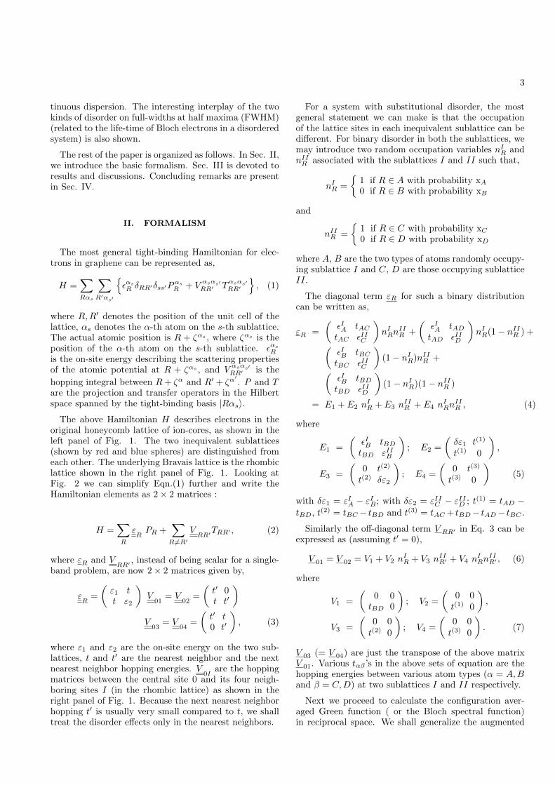
The above Hamiltonian H describes electrons in theoriginal honeycomb lattice of ion-cores, as shown in theleft panel of Fig. 1. The two inequivalent sublattices(shown by red and blue spheres) are distinguished fromeach other. The underlying Bravais lattice is the rhombiclattice shown in the right panel of Fig. 1. Looking atFig. 2 we can simplify Eqn.(1) further and write theHamiltonian elements as 2× 2 matrices :

H =∑R

εRPR +

∑R 6=R′

VRR′TRR′ , (2)

where εR and VRR′ , instead of being scalar for a single-

band problem, are now 2× 2 matrices given by,

εR

=

(ε1 tt ε2

)V

01= V

02=

(t′ 0t t′

)V

03= V

04=

(t′ t0 t′

), (3)

where ε1 and ε2 are the on-site energy on the two sub-lattices, t and t′ are the nearest neighbor and the nextnearest neighbor hopping energies. V

0Iare the hopping

matrices between the central site 0 and its four neigh-boring sites I (in the rhombic lattice) as shown in theright panel of Fig. 1. Because the next nearest neighborhopping t′ is usually very small compared to t, we shalltreat the disorder effects only in the nearest neighbors.

For a system with substitutional disorder, the mostgeneral statement we can make is that the occupationof the lattice sites in each inequivalent sublattice can bedifferent. For binary disorder in both the sublattices, wemay introduce two random occupation variables nIR andnIIR associated with the sublattices I and II such that,

nIR =

1 if R ∈ A with probability xA0 if R ∈ B with probability xB

and

nIIR =

1 if R ∈ C with probability xC0 if R ∈ D with probability xD

where A, B are the two types of atoms randomly occupy-ing sublattice I and C, D are those occupying sublatticeII.

The diagonal term εR for such a binary distributioncan be written as,

εR =

(εIA tACtAC εIIC

)nIRn

IIR +

(εIA tADtAD εIID

)nIR(1− nIIR ) +(

εIB tBCtBC εIIC

)(1− nIR)nIIR +(

εIB tBDtBD εIID

)(1− nIR)(1− nIIR )

= E1 + E2 nIR + E3 n

IIR + E4 n

IRn

IIR , (4)

where

E1 =

(εIB tBDtBD εIIB

); E2 =

(δε1 t(1)

t(1) 0

),

E3 =

(0 t(2)

t(2) δε2

); E4 =

(0 t(3)

t(3) 0

)(5)

with δε1 = εIA − εIB ; with δε2 = εIIC − εIID ; t(1) = tAD −tBD, t(2) = tBC− tBD and t(3) = tAC + tBD− tAD− tBC .

Similarly the off-diagonal term V RR′ in Eq. 3 can beexpressed as (assuming t′ = 0),

V 01 = V 02 = V1 + V2 nIR + V3 n

IIR′ + V4 n

IRn

IIR′ , (6)

where

V1 =

(0 0tBD 0

); V2 =

(0 0t(1) 0

),

V3 =

(0 0t(2) 0

); V4 =

(0 0t(3) 0

). (7)

V 03 (= V 04) are just the transpose of the above matrixV 01. Various tαβ ’s in the above sets of equation are thehopping energies between various atom types (α = A,Band β = C,D) at two sublattices I and II respectively.

Next we proceed to calculate the configuration aver-aged Green function ( or the Bloch spectral function)in reciprocal space. We shall generalize the augmented

4

space formalism (ASF) developed earlier in reciprocalspace.28 The ASF has been described in great detailearlier.29 We shall indicate the main operational resultshere and refer the reader to the above monograph forfurther details. The first step is to associate with nIR andnIIR two operators N I

R and N IIR such that their spectral

density is the probability density of the random variables.For binary random variables, we have :

N IR =

(xB

√xAxB√

xAxB xA

)

Finally, according to augmented space theorem,16 theconfiguration average of any function of nIR,nIIR can bewritten as the matrix element, in configuration space, ofan operator which is the same functional of N I

R,N IIR .

The augmented space Hamiltonian is built up from Eqns.(4) and (6).

H =∑R

E1I + E2N

IR + E3N

IIR + E4N

IR ⊗ N II

R

⊗ PR

+∑R

∑R′

V1I + V2N

IR + V3N

IIR′ + V4N

IR ⊗ N II

R′

⊗ TRR′

with

NXR = xα p

X↑R + xβ p

X,↓R +

√xαxβ(τX,↑↓R + τX,↓↑R ), (8)

(X = I or II)

The configuration averaged Green’s function in the re-ciprocal space is thus a matrix element of an augmentedresolvent given by,

G(k, z)= 〈∅ ⊗ k|(zI− H)−1| k⊗ ∅〉, (9)

| k ⊗ ∅〉 is an augmented space state in the reciprocalspace given by,

| k⊗ ∅〉 =1√N

∑R

e−ik.R| R⊗ ∅〉, (10)

| R⊗∅〉 is an enlarged basis which is a direct product ofthe Hilbert space basis R and the configuration space

basis φR. The configuration space Φ =∏⊗R φR, takes

care of the statistical average, is of rank 2M for a systemof M -lattice sites with binary distribution.

The recursion follows as a three step generation of anew basis |n > :

|1〉 = |k⊗ ∅〉 |0〉 = 0

|n+ 1〉 = H|n〉 − αn|n〉 − β2n−1|n− 1〉

αn(k) =〈n|H|n〉〈n|n〉

and β2n(k) =

〈n|n〉〈n− 1|n− 1〉

The ASR gives the configuration averaged spectralfunction as a continued fraction :

G(k, z) =1

z − α1(k)− β21(k)

z − α2(k)− β21(k)

z − α3(k)−. . .

T (z,k)

=1

z − E0(k)− Σ(z,k)(11)

T (z,k) is a continued fraction terminator as proposedby Beer and Pettifor.30 The spectral function peaks aredecided by <eΣ(E,k) and the imaginary part of Σgives the width related to the disorder induced lifetimes.

The configuration averaged Bloch spectral function isgiven by,

A(k, E)= − 1

πlimδ→0+

=m G(k, E + iδ) (12)

The configuration averaged density of states (DOS) is,

n(E)=1

ΩBZ

∫BZ

dk A(k, E) (13)

The electronic dispersion curves are obtained by nu-merically calculating the peak E-position of the spectralfunction. The full-widths at half maxima (FWHM) arealso calculated from the disorder broadened Bloch spec-tral function.

5

00.10.20.30.40.50.6

00.10.20.30.40.5

-4 -2 0 2 4Energy (E)

00.10.20.30.40.5

Sublatt ’I’ or ’II’E - E =0.4imp host

E - E =0.7

imp host

imp host

E - E =1.0

Sublatt ’I’ or ’II’

Sublatt ’I’ or ’II’LDOS

(Stat

es/E

/atom

)

00.10.20.30.40.50.6

00.10.20.30.40.5

-4 -2 0 2 4Energy (E)

00.10.20.30.40.5

Sublatt I & IIE - E =0.4imp host

E - E =0.7

E - E =1.0

Sublatt I & II

Sublatt I & II

imp

imp

host

host

-4 -2 0 2 4Energy (E)

00.10.20.30.40.50.6

DOS

(Sta

tes/

E/at

om)

Pure

FIG. 3: Local density of states for pure graphene and graphene with a single impurity. The top panel in the middle is the DOSfor pure graphene. Left and right panels show the local DOS with single impurity only on sublattice I or II and both I & IIrespectively. The panel from top to bottom are the results with increasing strength of the impurity potential δE=εimp-εhost

III. RESULTS AND DISCUSSION

In the following subsections, we shall present our re-sults for graphene with impurities, vacancies, diagonaldisorder alone, and with the simultaneous presence ofdiagonal and off-diagonal disorder. The effects of var-ious strengths of impurity potentials on two inequiva-lent sublattices will be shown via changes in the shapeof the DOS. The changes in the topology of Dirac-conedispersion, disorder-induced FWHM and the DOS willbe shown for various strengths of diagonal disorder. Inthe most general case of diagonal and off-diagonal dis-order, we consider three interesting limiting cases: (i)strong diagonal and weak off-diagonal disorder (ii) strongoff-diagonal and weak diagonal disorder and (iii) strongdiagonal as well as off-diagonal disorder. The interest-ing interplay between these different kinds of disorder ingraphene reveals a discontinuous type of band near theΓ-point in the third limiting case.

A. Impurities in Graphene

In Fig. 3, we display the DOS with different strengthsof the single impurity potentials on different inequivalentsublattices. The top figure in the middle panel is theDOS for pure graphene. The left and right panels showlocal DOS with a single impurity put on the sublattice Ior II and both respectively. The strength of the impuritypotential (relative to the host lattice) increases from topto bottom panels (i.e. δE = εimp - εhost = 0.4, 0.7 and1.0). All these calculations are done with a fixed hop-ping parameter t=1. We notice changes in the shape ofthe hump and the van-Hove singularities as the strengthof the impurity potential increases. Although the effectsare small, but are clearly visible for the case of δE=1.0,where the local environment around the impurity sitefeels the strongest scattering. With the introduction ofthe impurity, the symmetry of the DOS around the Diracpoint is lost. At these impurity levels, both the left andright panels show the formation of an impurity peak nearthe upper band edge. With increasing disorder this im-purity peak moves into the band and disappears. Again,at these strengths there is no perceptible changes to thelinear structure of the Dirac point. Similar results have

6

00.20.40.6

00.20.4

00.20.4

00.20.4

00.20.4

00.20.4

00.20.4

-4 -2 0 2 4Energy (E)

0

0.5

LDO

S (s

tate

s/E/

atom

)

t =0 ij

bE=1

b

b

b

b

b

b

for all

E=2

E=3

E=4

E=6

E=8

E=10

b(j = vac)

=1(otherwise)E

t =1

t =1

t =1

t =1

t =1

t =1

t =1

ij

ij

ij

ij

ij

ij

ij

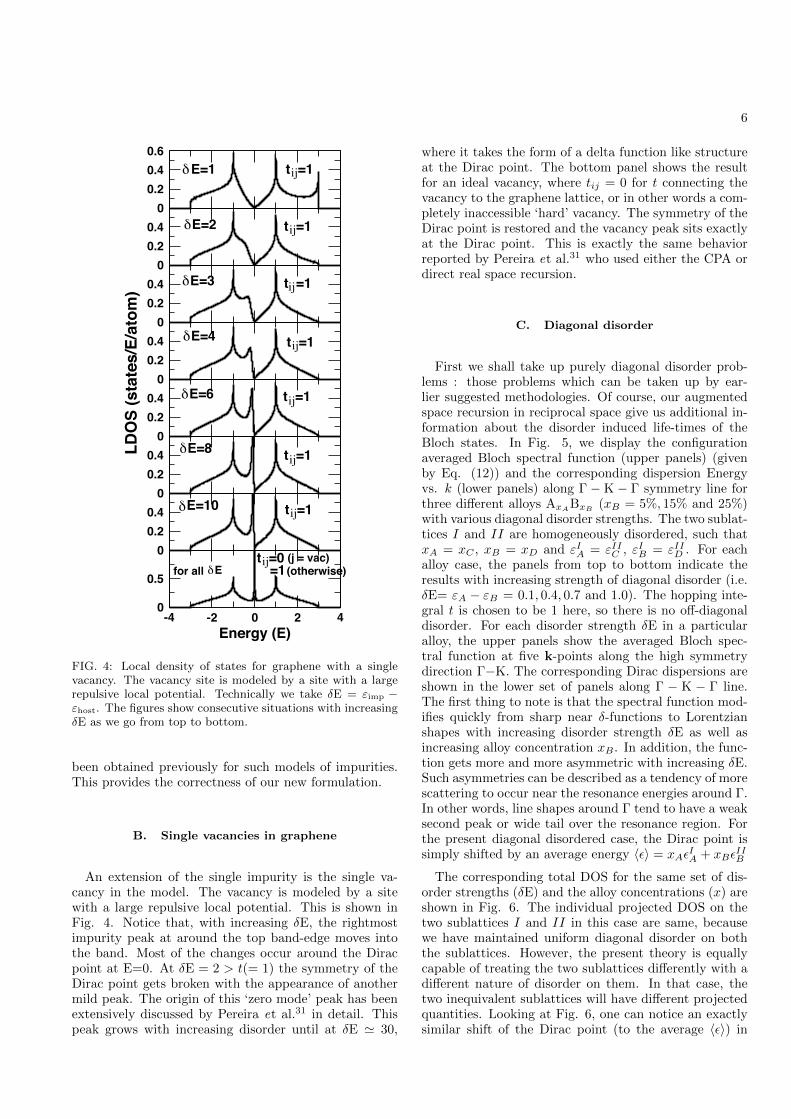
FIG. 4: Local density of states for graphene with a singlevacancy. The vacancy site is modeled by a site with a largerepulsive local potential. Technically we take δE = εimp −εhost. The figures show consecutive situations with increasingδE as we go from top to bottom.

been obtained previously for such models of impurities.This provides the correctness of our new formulation.

B. Single vacancies in graphene

An extension of the single impurity is the single va-cancy in the model. The vacancy is modeled by a sitewith a large repulsive local potential. This is shown inFig. 4. Notice that, with increasing δE, the rightmostimpurity peak at around the top band-edge moves intothe band. Most of the changes occur around the Diracpoint at E=0. At δE = 2 > t(= 1) the symmetry of theDirac point gets broken with the appearance of anothermild peak. The origin of this ‘zero mode’ peak has beenextensively discussed by Pereira et al.31 in detail. Thispeak grows with increasing disorder until at δE ' 30,

where it takes the form of a delta function like structureat the Dirac point. The bottom panel shows the resultfor an ideal vacancy, where tij = 0 for t connecting thevacancy to the graphene lattice, or in other words a com-pletely inaccessible ‘hard’ vacancy. The symmetry of theDirac point is restored and the vacancy peak sits exactlyat the Dirac point. This is exactly the same behaviorreported by Pereira et al.31 who used either the CPA ordirect real space recursion.

C. Diagonal disorder

First we shall take up purely diagonal disorder prob-lems : those problems which can be taken up by ear-lier suggested methodologies. Of course, our augmentedspace recursion in reciprocal space give us additional in-formation about the disorder induced life-times of theBloch states. In Fig. 5, we display the configurationaveraged Bloch spectral function (upper panels) (givenby Eq. (12)) and the corresponding dispersion Energyvs. k (lower panels) along Γ − K − Γ symmetry line forthree different alloys AxA

BxB(xB = 5%, 15% and 25%)

with various diagonal disorder strengths. The two sublat-tices I and II are homogeneously disordered, such thatxA = xC , xB = xD and εIA = εIIC , εIB = εIID . For eachalloy case, the panels from top to bottom indicate theresults with increasing strength of diagonal disorder (i.e.δE= εA − εB = 0.1, 0.4, 0.7 and 1.0). The hopping inte-gral t is chosen to be 1 here, so there is no off-diagonaldisorder. For each disorder strength δE in a particularalloy, the upper panels show the averaged Bloch spec-tral function at five k-points along the high symmetrydirection Γ−K. The corresponding Dirac dispersions areshown in the lower set of panels along Γ − K − Γ line.The first thing to note is that the spectral function mod-ifies quickly from sharp near δ-functions to Lorentzianshapes with increasing disorder strength δE as well asincreasing alloy concentration xB . In addition, the func-tion gets more and more asymmetric with increasing δE.Such asymmetries can be described as a tendency of morescattering to occur near the resonance energies around Γ.In other words, line shapes around Γ tend to have a weaksecond peak or wide tail over the resonance region. Forthe present diagonal disordered case, the Dirac point issimply shifted by an average energy 〈ε〉 = xAε

IA + xBε

IIB

The corresponding total DOS for the same set of dis-order strengths (δE) and the alloy concentrations (x) areshown in Fig. 6. The individual projected DOS on thetwo sublattices I and II in this case are same, becausewe have maintained uniform diagonal disorder on boththe sublattices. However, the present theory is equallycapable of treating the two sublattices differently with adifferent nature of disorder on them. In that case, thetwo inequivalent sublattices will have different projectedquantities. Looking at Fig. 6, one can notice an exactlysimilar shift of the Dirac point (to the average 〈ε〉) in

7

-4 -2 0 2 4

-4 -2 0 2 4

-4 -2 0 2 4

-4 -2 0 2 4Energy (E)

-4 -2 0 2 4

-4 -2 0 2 4

-4 -2 0 2 4

-4 -2 0 2 4Energy (E)

-4 -2 0 2 4

-4 -2 0 2 4

-4 -2 0 2 4

-4 -2 0 2 4Energy (E)

A(k

,E)

(A

rbit

rary

un

its)

E=0.1

A B 85 15A B95E=0.1 E=0.1

E=0.4 E=0.4 E=0.4

E=0.7 E=0.7 E=0.7

E=1.0 E=1.0 E=1.0

05 A B75 25

KK

KK

K KK

KKK

KK

-3-2-101234

Ener

gy

-3-2-101234

-3-2-101234

-3-2-101234

Ener

gy

-3-2-101234

-3-2-101234

-3-2-101234

Ener

gy

-3-2-101234

-3-2-101234

-3-2-101234

Ener

gy

-3-2-101234

-3-2-101234

A B95

K

K

K K

KK

KK

K K K

K

05 A B A B

E=0.1

85 15 75

E=0.1 E=0.1

E=0.4 E=0.4 E=0.4

E=0.7 E=0.7 E=0.7

E=1.0 E=1.0 E=1.0

25

Bloch Spectral Function

Band Dispersion

FIG. 5: (Color online) The averaged spectral functions (upper set of panels) and the complex bands (lower set of panels) nearthe Dirac point. These are all for pure diagonal disorder at three different alloy compositions (left to right) and four disorderstrengths δE (top to bottom). The (red) error bars show how the disorder induced lifetimes vary across the samples.

8

00.20.40.60.8

00.20.40.60.8

00.20.40.60.8

-2 0 2 4Energy (E)

00.20.40.60.8 b = E - E =1.0E A B

b =0.7

b =0.4

b =0.1

E

E

E

A B2575

00.20.40.60.8

00.20.40.60.8

00.20.40.60.8

-2 0 2 4Energy (E)

00.20.40.60.8 b = E - E =1.0E A B

b =0.7

b =0.4

b =0.1

E

E

E

A B1585

00.20.40.60.8

00.20.40.60.8

00.20.40.60.8

-2 0 2 4Energy (E)

00.20.40.60.8 b = E - E =1.0E A B

b =0.4

b =0.7

b =0.1

E

E

E

A B595

DO

S (S

tate

s/E

/ato

m)

FIG. 6: Total DOS for the same set of disorder strengths δE for three alloys AxABxB as in Fig. 5. Due to homogeneousdiagonal disorder on both the sublattices I and II, the individual projected DOS on them are same in this case.

the DOS as shown in the dispersion. The disorder effectsare pronounced around the Dirac-point energy 〈ε〉 andget milder around the hump below δE = 0.7. Above thisdisorder strength, the left band edge starts to show upextra features with a dip at around E = −2, (as shown inthe bottom panel for all the three alloy concentration).The results are qualitatively similar to the CPA worksdone earlier31 but differ in quantitative details.

D. Off-diagonal disorder

We now turn to the cases with off-diagonal disorder.Such problems cannot be dealt with within the CPA.Also, direct calculation of the averaged spectral functionsand disorder induced lifetimes is also not feasible withother techniques and the strength of the ASR comes tothe fore. In addition we should note that in our model,diagonal and off-diagonal disorders are correlated : e.g.if the atom A occupies the site i with probability xA andatom B occupies the site j with probability xB , then tijhas to be tAB with probability 1. Although the presenttheory is equally capable of investigating other interest-ing cases (e.g. inhomogeneous disorder, pseudo-binarytype disorder etc.), here we have chosen to explore threecases which should reflect the behavior of a variety of therealistic materials. The three cases are:

• Strong diagonal and weak off-diagonal disorder;with parameters δE = εIA − εIB = εIIC − εIID = 1.0,

tAC = 1.0, tBD = 0.9 and tAD = tBC = 0.95.

• Weak diagonal and strong off-diagonal disorder;with parameters δE = 0.1, tAC = 1.0, tBD = 0.5and tAD = tBC = 0.75.

• Strong diagonal as well as strong off-diagonal dis-order; with parameters δE = 1.0, tAC = 1.0, tBD =0.5 and tAD = tBC = 0.75.

The results for these three cases are shown in the top,middle and bottom panels of Fig. 7 respectively, for thesame three alloys AxA

BxBas before. Other details are

same as in Fig. 5. Notice that unlike the diagonal dis-ordered case, effects of both diagonal and off-diagonaldisorder are much more dramatic. In addition to highlyasymmetric nature, the Bloch spectral function is foundto have a double peaked structure in the extreme caseof strong diagonal and off-diagonal disorder (shown inthe bottom panels). Such doubly peaked line shapeintroduces extra discontinuous bands in the dispersioncurve. Such a structure had been seen before in phononproblems22 which also have intrinsic off-diagonal disor-der in the dynamical matrices. There it arose because ofresonant modes. Here too we shall give a similar explana-tion. These dispersion at resonance have relatively largeFWHM’s and it will be interesting to choose a realisticmaterial of similar disorder properties and investigate theexperimental outcome.

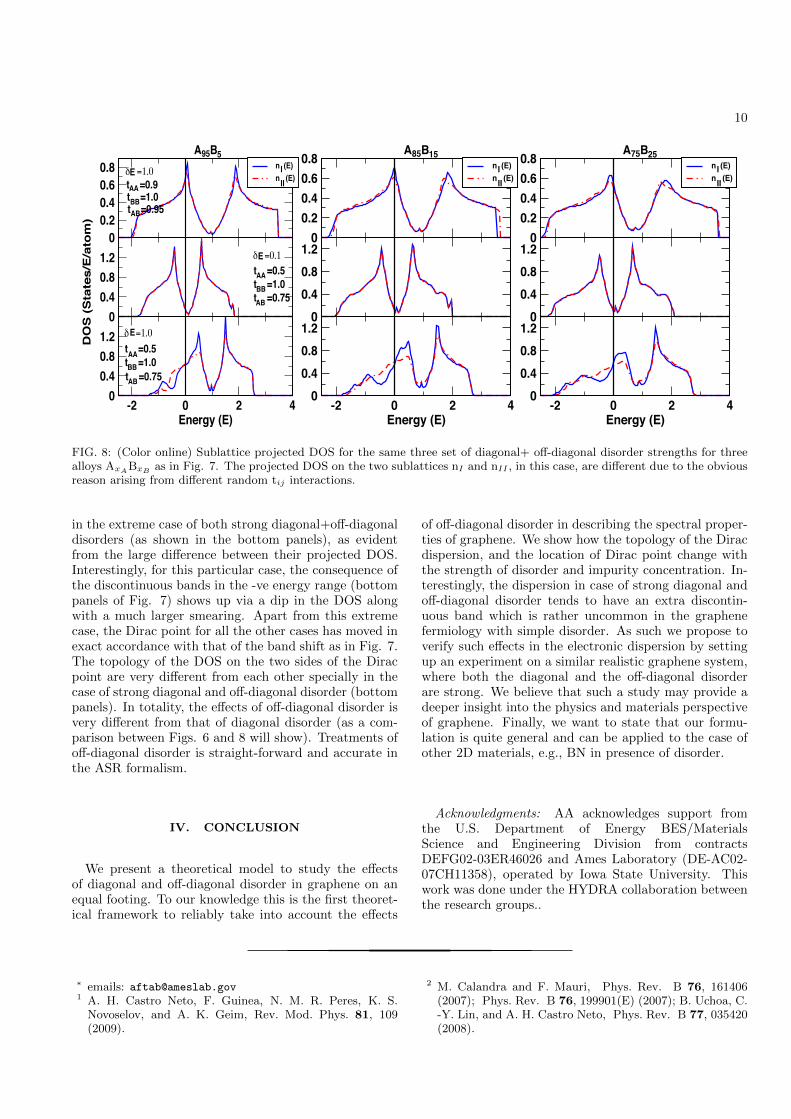
Figure 8 shows the sublattice projected DOS for thesame three limiting cases for the three alloys as above.

9

-4 -2 0 2 4

-4 -2 0 2 4

-4 -2 0 2 4Energy

-4 -2 0 2 4

-4 -2 0 2 4

-4 -2 0 2 4Energy

-4 -2 0 2 4

-4 -2 0 2 4

-4 -2 0 2 4Energy

A(k

,E)

(A

rbit

rary

un

its)

A B A BA B95 05 85 15 75 25

KK

K K KK

KKK

-2-101234

En

erg

y

-2-101234

-2-101234

-2

-1

0

1

2

En

erg

y

-2

-1

0

1

2

-2

-1

0

1

2

-1012

3

En

erg

y

-1012

3

-1012

3

A B95

K

K

K K

KK

KK K

05 A B A B85 15 75 25

Bloch Spectral Function

Band Dispersion

FIG. 7: (Color online) Same as Fig. 5, but with the inclusion of both diagonal and off-diagonal disorder. The three panels foreach alloy indicate the results with coupled diagonal and off diagonal disorders as described in the text.

The solid blue and the dashed red lines indicate the pro-jected DOS on the sublattices I and II respectively. Be-cause of the random hopping (off-diagonal) interactionin this case, the two sublattices acquire different envi-

ronment around it, and hence possess different projectedquantities on them. As expected, the DOS in these caseshave large smearing. The effective environment aroundthe two sublattices is maximally different from each other

10

00.20.40.60.8 n (E)

n (E)

00.40.81.2

-2 0 2 4Energy (E)

00.40.81.2

t =0.5

IIIAA

t =1.0

b =1.0

b =0.1

b =1.0

E

E

E

A B595

DO

S (

Sta

tes/

E/a

tom

)

t =0.95BBAB

t =1.0t =0.75

AABBAB

t =0.5t =1.0t =0.75

AABB

AB

t =0.9

00.20.40.60.8 n (E)

n (E)

00.40.81.2

-2 0 2 4Energy (E)

00.40.81.2

III

A B1585

00.20.40.60.8 n (E)

n (E)

00.40.81.2

-2 0 2 4Energy (E)

00.40.81.2

III

A B2575

FIG. 8: (Color online) Sublattice projected DOS for the same three set of diagonal+ off-diagonal disorder strengths for threealloys AxABxB as in Fig. 7. The projected DOS on the two sublattices nI and nII , in this case, are different due to the obviousreason arising from different random tij interactions.

in the extreme case of both strong diagonal+off-diagonaldisorders (as shown in the bottom panels), as evidentfrom the large difference between their projected DOS.Interestingly, for this particular case, the consequence ofthe discontinuous bands in the -ve energy range (bottompanels of Fig. 7) shows up via a dip in the DOS alongwith a much larger smearing. Apart from this extremecase, the Dirac point for all the other cases has moved inexact accordance with that of the band shift as in Fig. 7.The topology of the DOS on the two sides of the Diracpoint are very different from each other specially in thecase of strong diagonal and off-diagonal disorder (bottompanels). In totality, the effects of off-diagonal disorder isvery different from that of diagonal disorder (as a com-parison between Figs. 6 and 8 will show). Treatments ofoff-diagonal disorder is straight-forward and accurate inthe ASR formalism.

IV. CONCLUSION

We present a theoretical model to study the effectsof diagonal and off-diagonal disorder in graphene on anequal footing. To our knowledge this is the first theoret-ical framework to reliably take into account the effects

of off-diagonal disorder in describing the spectral proper-ties of graphene. We show how the topology of the Diracdispersion, and the location of Dirac point change withthe strength of disorder and impurity concentration. In-terestingly, the dispersion in case of strong diagonal andoff-diagonal disorder tends to have an extra discontin-uous band which is rather uncommon in the graphenefermiology with simple disorder. As such we propose toverify such effects in the electronic dispersion by settingup an experiment on a similar realistic graphene system,where both the diagonal and the off-diagonal disorderare strong. We believe that such a study may provide adeeper insight into the physics and materials perspectiveof graphene. Finally, we want to state that our formu-lation is quite general and can be applied to the case ofother 2D materials, e.g., BN in presence of disorder.

Acknowledgments: AA acknowledges support fromthe U.S. Department of Energy BES/MaterialsScience and Engineering Division from contractsDEFG02-03ER46026 and Ames Laboratory (DE-AC02-07CH11358), operated by Iowa State University. Thiswork was done under the HYDRA collaboration betweenthe research groups..

∗ emails: aftab@ameslab.gov1 A. H. Castro Neto, F. Guinea, N. M. R. Peres, K. S.

Novoselov, and A. K. Geim, Rev. Mod. Phys. 81, 109(2009).

2 M. Calandra and F. Mauri, Phys. Rev. B 76, 161406(2007); Phys. Rev. B 76, 199901(E) (2007); B. Uchoa, C.-Y. Lin, and A. H. Castro Neto, Phys. Rev. B 77, 035420(2008).

11

3 T. B. Martins, R. H. Miwa, A J. R. da Silva, and A. Fazzio,Phys. Rev. Lett. 98, 196803 (2007).

4 I. Calizo, W. Bao, F. Miao, C. N. Lau, and A. A. BalandinAppl. Phys. Lett 91, 201904 (2007); G. Giovannetti, P. A.Khomyakov, G. Brocks, P. J. Kelly, and J. van den Brink,Phys. Rev. B 76, 073103 (2007).

5 V. A. Coleman, R. Knut, O. Karis, H. Grennberg,U.Jansson, R. Quinlan and B. C. Holloway, B. Sanyal andO. Eriksson, J. Phys. D: Appl. Phys. 41, 062001(2008); S.H. M. Jafri, K. Carva, E. Widenkvist, T. Blom, B. Sanyal,J. Fransson, O. Eriksson, U. Jansson, H. Grennberg, O.Karis, R. A. Quinlan, B. C. Holloway, and K. Leifer, J.Phys. D: Appl. Phys. 43, 045404 (2010); K. Carva, B.Sanyal, J. Fransson, and O. Eriksson, Phys. Rev. B 81,245405 (2010).

6 D. A. Dikin et al., Nature 448, 457 (2007); J. T. Robinsonet al., Nano Lett 8, 3441 (2008).

7 F. Banhart, J. Kotakoski and A. V. Krasheninnikov, ACSNano 5, 26 (2011).

8 E. Holmstrom, J. Fransson, O. Eriksson, R. Lizarraga, B.Sanyal, S. Bhandary, and M. I. Katsnelson, Phys. Rev. B84, 205414 (2011).

9 Shangduan Wu, Lei Jing, Qunxiang Li, Q. W. Shi, JieChen, Haibin Su, Xiaoping Wang, and Jinlong Yang,Phys. Rev. B 77, 195411 (2008)

10 P. Soven, Phys. Rev. 156, 809 (1967); G. M. Stocks, W.M. Temmerman, and B. L. Gyorffy, Phys. Rev. Lett. 41,339 (1978).

11 R. Haydock, V. Heine and M. J. Kelly, J. Phys. C: SolidState Phys 5, 2845 (1975).

12 P. Dean, Rev. Mod. Phys. 44, 127-168 (1972).13 D. A. Biava1, Subhradip Ghosh, D. D. Johnson, W. A.

Shelton, and A. V. Smirnov, Phys. Rev. B 72, 113105(2005); Derwyn A. Rowlands, Julie B. Staunton, BalazsL. Gyrffy, Ezio Bruno, and Beniamino Ginatempo, Phys.Rev. B 72, 045101 (2005).

14 A. Zunger, S. -H. Wei, L. G. Ferreira and J. E. Bernard,Phys. Rev. Lett. 65, 353 (1990).

15 Y. Wang, G. M. Stocks, W. A. Shelton, D. M. C. Nicholson,Z. Szotek, and W. M. Temmerman, Phys. Rev. Lett. 75,2867 (1995).

16 Abhijit Mookerjee, J. Phys. C: Solid State Phys 6, L205(1973).

17 R. Mills and P. Ratanavararaksa, Phys. Rev. B 18, 5291(1978); T. Kaplan, P. L. Leath, L. J. Gray, and H. W.Diehl, Phys. Rev. B 21, 4230 (1980).

18 S. Ghosh, P. L. Leath and M. H. Cohen, Phys. Rev. B66, 214206 (2002).

19 T. Saha, I. Dasgupta, and A. Mookerjee, J. Phys.: Con-dens. Matter 6, L245 (1994).

20 T. Saha and A. Mookerjee, J. Phys.: Condens. Matter 8,2915 (1996).

21 A. Alam and A. Mookerjee, J. Phys.: Condens. Matter21, 195503 (2009); T.Saha, I. Dasgupta, and A. Mookerjee,Phys. Rev. B 50, 13267 (1994).

22 A. Alam, S. Ghosh, and A. Mookerjee, Phys. Rev. B 75,134202 (2007); A. Alam and A. Mookerjee, Phys. Rev. B69, 024205 (2004).

23 A. Alam and A. Mookerjee, Phys. Rev. B 72, 214207(2005); K. Tarafder, A. Chakrabarti, K. K. Saha and A.Mookerjee, Phys. Rev. B 74, 144204 (2006).

24 K. Nomura and A. H. MacDonald, Phys. Rev. Lett. 98,076602 (2007)

25 Y. V. Skrypnyk and V. M. Loktev, Phys. Rev. B 75,245401 (2007)

26 T. O. Wehling, A. V. Balatsky, M. I. Katsnelson, A. I.Lichtenstein, K. Scharnberg and R. Wiesendanger, Phys.Rev. B 75, 125425 (2007)

27 N. M. R. Peres, F. Guinea and A. H. Castro Neto, Phys.Rev. B 73, 125411 (2006)

28 P. Biswas, B. Sanyal, M. Fakhruddin, A. Halder, A. Mook-erjee and M. Ahmed, J. Phys.:Condens. Mat. 7, 8569(1995).

29 A. Mookerjee, Electronic Structure of Alloys, Surfaces andClusters (ed. D.D. Sarma and A. Mookerjee) (Taylor Fran-cis, London) (2003).

30 N. Beer and D.G. Pettifor, Electronic Structure of Com-plex Systems ed. P. Phariseau and W. M. Temmerman(Plenum, New York, 1984) p 769.

31 Vitor M. Pereira, F. Guinea, J. M. B. Lopes dos Santos,N. M. R. Peres and A. H. Castro Neto, Phys. Rev. Lett.96, 036801 (2006); Vitor M. Pereira, J. M. B. Lopes dosSantos and A. H. Castro Neto, Phys. Rev. B 77, 115109(2008).