Department of Exploration Geophysics

Effect of capillarity on the acoustics of

partially saturated porous rocks

Qiaomu Qi

This thesis is presented for the Degree of

Doctor of Philosophy

of

Curtin University

August 2015

To the best of my knowledge and belief this thesis contains no material

previously published by any other person except where due acknowledgement

has been made. This thesis contains no material which has been accepted for

the award of any other degree or diploma in any university.

“I think and think for months and years. Ninety-nine times, the conclusion is

false. The hundredth time I am right.”

- Albert Einstein

Acknowledgements

I would like to express my sincere gratitude to my supervisors, Professor. Boris

Gurevich and Dr. Tobias Muller. Without their guidance and input, this journey

would be much more difficult. Thank you Boris for providing me scholarship and

funds from your consortium. I feel extraordinary lucky for being able to work

with you and nourished by your vast experience. I am much obliged to Tobias,

for being a tremendous mentor to me. I am grateful for your years of training

which helps me grow as a research scientist.

A big thank you to Dr. Sofia Lopes and Dr. Maxim Lebedev, for sharing

me your state-of-the-art laboratory data at the beginning of my PhD. It greatly

helps me form my research motivation.

I would like to express my appreciation to Dr. German Rubino and Dr. Pratap

Sahay for multiple simulating discussions which greatly improve my understand-

ing of poroelasticity.

I want to say thank you to our reservoir geophysicists, Eva, Mateus and

Hosni, for sharing me your practical insights of rock physics and commenting on

my work.

A special shout-out to my Curtin friends and colleagues, Shahadat, Javad,

Andrew, Sinem, Olivia, Felix, Michael, Stephanie and Tongcheng for years of

companion which allows me to fulfil my dream without being so lonely. Also

thank Deirdre and Robert for administrative and technical support, I have been

taken good care of because of your hard work.

My final acknowledgement goes to my parents, to whom I owe so much in life.

Thank you for being visionary and putting so much effort on my education since

I was a teenager. This thesis is dedicated to you.

Abstract

It is well known that capillary forces control the fluid distribution in partially

saturated rocks. However, the role of capillarity on acoustic signatures such as

attenuation remains poorly understood. This thesis is dedicated to investigate the

effect of capillarity on acoustic signatures within the framework of Biot’s theory of

wave propagation in a poroelastic medium and to explore its implications for rock

physics modelling. The macroscopic manifestation of capillarity can be captured

by replacing the pressure continuity boundary condition in Biot’s theory by a

pressure jump boundary condition with a non-vanishing interfacial impedance

and involving the concept of membrane stiffness.

This interfacial impedance is incorporated into the classical White’s model for

seismic attenuation and dispersion due to wave-induced fluid flow in layered sed-

imentary structures by solving a boundary value problem for Biot’s quasi-static

poroelasticity equations. The membrane stiffness is also incorporated into mod-

els for 1D and 3D random patchy saturation. These generalized models predict

that the P-wave velocity at low frequency limit increases, thereby decreasing the

amount of dispersion and attenuation and change the velocity- and attenuation-

saturation relations accordingly. The 3D capillarity-extended random patchy

saturation model is applied to interpret ultrasonic data acquired during a forced

imbibition experiment where capillarity is thought to be of importance. Fur-

thermore, the poroelastic P-wave reflectivity is generalized to take into account

the interfacial impedance. Two scenarios where interfacial impedance can arise in

seismic investigations are analyzed, namely the P-wave reflection from a gas-water

contact and from a fluid/gas-saturated-rock contact. For the fluid/gas-saturated-

rock scenario the presence of capillarity substantially influences the frequency-

and angle-dependence of the reflected P-wave amplitude.

Patchy saturation is inherently associated with a characteristic length scale

of the fluid patches. Due to the interplay of capillary and viscous forces during

the course of fluid injection into a reservoir this saturation scale varies and thus

further complicates the interpretation of time-lapse seismic data. The developed

patchy saturation model is used to study the influence of variable saturation scales

on velocity (time-shifts) and seismic amplitude (time-lapse attenuation). For a

brine-saturated reservoir undergoing gas injection it is found that an assessment of

the saturation scale variation can be important for reliable discrimination between

saturation and pressure changes.

Contents

1 Introduction 1

1.1 Background and Motivation . . . . . . . . . . . . . . . . . . . . . 3

1.2 Thesis outline . . . . . . . . . . . . . . . . . . . . . . . . . . . . . 14

2 Theoretical background 15

2.1 Acoustics in saturated porous media— Biot’s theory of poroelasticity . . . . . . . . . . . . . . . . . . 15

2.1.1 Potential energy and stress strain relation . . . . . . . . . 16

2.1.2 Poroelastic constants . . . . . . . . . . . . . . . . . . . . . 18

2.1.3 Kinetic energy . . . . . . . . . . . . . . . . . . . . . . . . . 22

2.1.4 Dissipation function . . . . . . . . . . . . . . . . . . . . . 23

2.1.5 Equations of motion . . . . . . . . . . . . . . . . . . . . . 24

2.1.6 Solutions of wave equations . . . . . . . . . . . . . . . . . 26

2.2 Viscosity-extended Biot framework . . . . . . . . . . . . . . . . . 28

2.3 Alternative formulation of Biot’s theory . . . . . . . . . . . . . . . 30

2.4 Quasi-static approximation of Biot’s theory . . . . . . . . . . . . . 30

2.5 Poroelastic boundary conditions . . . . . . . . . . . . . . . . . . . 31

2.5.1 Open-pore boundary condition . . . . . . . . . . . . . . . 31

2.5.2 Partially open boundary condition . . . . . . . . . . . . . 32

2.6 Acoustics in partially saturated porous media . . . . . . . . . . . 34

vi

2.6.1 Periodic model . . . . . . . . . . . . . . . . . . . . . . . . 35

2.6.2 Random model . . . . . . . . . . . . . . . . . . . . . . . . 41

2.7 Seismic reflection in porous media . . . . . . . . . . . . . . . . . . 45

2.7.1 Elastic reflection coefficient . . . . . . . . . . . . . . . . . 46

2.7.2 Viscoelastic reflection coefficient . . . . . . . . . . . . . . . 49

2.7.3 Poroelastic reflection coefficient . . . . . . . . . . . . . . . 52

2.8 Effect of capillarity on acoustics . . . . . . . . . . . . . . . . . . . 53

2.8.1 Concept of membrane stiffness . . . . . . . . . . . . . . . . 53

2.8.2 Macroscopic capillarity in poroelasticity . . . . . . . . . . 55

2.9 Other attenuation mechanisms . . . . . . . . . . . . . . . . . . . . 57

3 Effects of interfacial impedance on wave-induced pressure diffu-sion 59

3.1 Summary . . . . . . . . . . . . . . . . . . . . . . . . . . . . . . . 59

3.2 Introduction . . . . . . . . . . . . . . . . . . . . . . . . . . . . . . 60

3.3 Theory . . . . . . . . . . . . . . . . . . . . . . . . . . . . . . . . . 62

3.3.1 Background: White’s model and interfacial impedance . . 62

3.3.2 Effective strain for finite interfacial impedance . . . . . . . 64

3.3.3 Generalized White’s model . . . . . . . . . . . . . . . . . . 67

3.4 Attenuation and dispersion . . . . . . . . . . . . . . . . . . . . . . 67

3.5 Poroelastic fields . . . . . . . . . . . . . . . . . . . . . . . . . . . 71

3.5.1 Full Biot’s solution . . . . . . . . . . . . . . . . . . . . . . 71

3.5.2 Numerical results . . . . . . . . . . . . . . . . . . . . . . . 74

3.6 Chapter conclusions . . . . . . . . . . . . . . . . . . . . . . . . . . 79

4 Quantifying the effect of capillarity on attenuation and disper-sion in patchy-saturated rocks 81

4.1 Summary . . . . . . . . . . . . . . . . . . . . . . . . . . . . . . . 81

vii

4.2 Introduction . . . . . . . . . . . . . . . . . . . . . . . . . . . . . . 82

4.3 Model for random patchy saturation including capillary pressure . 85

4.3.1 Static limit . . . . . . . . . . . . . . . . . . . . . . . . . . 85

4.3.2 No-flow limit . . . . . . . . . . . . . . . . . . . . . . . . . 88

4.3.3 Mesoscopic wave-induced pressure diffusion . . . . . . . . . 89

4.3.4 Joint effect of capillarity and fluid distribution . . . . . . . 94

4.4 Modelling the saturation-dependent velocity and attenuation . . . 98

4.4.1 Simultaneous acquisition of X-ray CT and acoustics duringwater imbibition . . . . . . . . . . . . . . . . . . . . . . . 98

4.4.2 Extraction of correlation function, specific surface area andvariance . . . . . . . . . . . . . . . . . . . . . . . . . . . . 102

4.4.3 Modelling the experimental data . . . . . . . . . . . . . . 105

4.5 Discussion . . . . . . . . . . . . . . . . . . . . . . . . . . . . . . . 112

4.6 Chapter conclusions . . . . . . . . . . . . . . . . . . . . . . . . . . 114

5 The role of interfacial impedance on seismic reflectivity 117

5.1 Summary . . . . . . . . . . . . . . . . . . . . . . . . . . . . . . . 117

5.2 Introduction . . . . . . . . . . . . . . . . . . . . . . . . . . . . . . 118

5.3 Quasi-static Biot’s theory . . . . . . . . . . . . . . . . . . . . . . 119

5.4 Reflection between two saturated porous media . . . . . . . . . . 121

5.5 Reflection between fluid and porous medium . . . . . . . . . . . . 122

5.6 Reflectivity at normal incidence . . . . . . . . . . . . . . . . . . . 123

5.7 Numerical analysis . . . . . . . . . . . . . . . . . . . . . . . . . . 124

5.8 Chapter conclusions . . . . . . . . . . . . . . . . . . . . . . . . . . 129

6 The effects of saturation scale on time-lapse seismic signatures 130

6.1 Summary . . . . . . . . . . . . . . . . . . . . . . . . . . . . . . . 130

viii

6.2 Introduction . . . . . . . . . . . . . . . . . . . . . . . . . . . . . . 131

6.3 Scale effect in Partially Saturated Reservoir . . . . . . . . . . . . 134

6.3.1 Characteristic saturation scales . . . . . . . . . . . . . . . 134

6.3.2 Bounds-extended Patchy Saturation Model . . . . . . . . . 136

6.3.3 Characteristic frequency . . . . . . . . . . . . . . . . . . . 137

6.3.4 Attenuation and Acoustic impedance . . . . . . . . . . . . 139

6.3.5 Seismic reflection amplitude . . . . . . . . . . . . . . . . . 141

6.3.6 Seismic characteristics in an attenuative reservoir . . . . . 145

6.4 Implications for the interpretation of time-lapse data . . . . . . . 150

6.4.1 Scale effect on saturation estimation . . . . . . . . . . . . 150

6.4.2 Scale effect on pressure estimation . . . . . . . . . . . . . . 152

6.4.3 Effects of capillary pressure and residual saturation . . . . 155

6.4.4 Effect of lithology . . . . . . . . . . . . . . . . . . . . . . . 157

6.4.5 Effect of in-situ fluid property . . . . . . . . . . . . . . . . 159

6.4.6 Effect of geological complexity . . . . . . . . . . . . . . . . 160

6.5 Identification of saturation scale . . . . . . . . . . . . . . . . . . . 160

6.6 Chapter conclusions . . . . . . . . . . . . . . . . . . . . . . . . . . 161

7 Conclusions and outlook 164

A Static undrained bulk modulus including capillary action 176

B Procedure of constructing saturation maps 180

C Extracting statistical properties from saturation maps 181

D Viscoelastic reflection coefficient for isotropic media 184

ix

E Slow shear waves and the concept of dynamic permeability 185

E.1 Abstract . . . . . . . . . . . . . . . . . . . . . . . . . . . . . . . . 185

E.2 Introduction . . . . . . . . . . . . . . . . . . . . . . . . . . . . . . 186

E.3 A stochastic model for dynamic permeability . . . . . . . . . . . . 187

E.4 Dynamic permeability estimation using digitized rock . . . . . . . 188

E.5 Conclusion . . . . . . . . . . . . . . . . . . . . . . . . . . . . . . . 193

F Copyright consent 194

References 201

x

Chapter 1

Introduction

The seismic method, as one of the most important geophysical prospecting meth-

ods, is powerful in delineating subsurface geological structures of interest. Beyond

the conventional usage of seismic reflection data for imaging stratigraphic pat-

terns, quantitative seismic interpretation (QSI) reduces the exploration risk by

characterizing and forecasting hydrocarbon reservoir properties (Avseth et al.,

2005; Bacon et al., 2007; Bjørlykke, 2010). QSI heavily relies on seismic rock

physics models, that is idealized descriptions of seismic responses from reservoir

rocks. These rock physics models aim at providing a link between geological and

petrophysical parameters with (an-)elastic properties relevant for wave propaga-

tion. Wave measurements such as ultrasonic, sonic-log, crosswell, VSP (Vertical

Seismic Profile) and surface seismic entail characteristic frequencies and conse-

quently encode geological information of various scales, i.e., from a fraction of

core sample at 1 MHz ultrasonic frequency up to geological facies scale at 100

Hz seismic frequency. Maximizing the value of these data for successful QSI re-

quires to integrate the measured or modelled results from one frequency band

to another. Thus, in order to achieve this up- or down-scaling a rock physics

model has to take both frequency and scale effects into account. This requires a

good understanding of the relation between frequency-dependent wave velocity

and attenuation with petrophysical quantities, such as saturation and transport

properties.

It is believed that a major source of fluid-related velocity dispersion and atten-

uation is due to wave-induced fluid flow (WIFF), i.e., that is the oscillatory fluid

1

motion relative to the porous rock frame (Pride et al., 2004; Muller et al., 2010;

Liner, 2012). Particularly, in a partially saturated reservoir WIFF is thought to

be prominent, as it can occur not only across fluid patches at the millimetre- and

centimetre-scale (Lee and Collet, 2009; Morgan et al., 2012) but also at gas-water,

gas-oil contacts at the metre-scale (Rutherford and Williams, 1989; Zhao et al.,

2015). This shows that WIFF in partially saturated rocks is inherently associ-

ated with a characteristic length scale. In the following we refer to this length

scale as the saturation scale. An intriguing feature of this saturation scale is that

it can change with time. This saturation scale variation is more prevalent dur-

ing the course of dynamic fluid injection as evidenced in laboratory experiments

(Lebedev et al., 2009). It is very likely that dynamic fluid injection in reservoir

stimulation operations also leads to a variation of the saturation scale. Then, the

saturation scale might affect time-lapse seismic data interpretation which, in turn,

requires time-lapse QSI methods to be developed. For example, it is not fully

understood how a change of the saturation scale complicates the discrimination

between saturation and pressure effects from time-lapse seismic data.

WIFF in partially saturated rocks is inherently connected with two- or multi-

phase flow phenomena at the pore scale. One phenomenon is capillarity. It is

important since there always exist pore spaces in form of thin capillarities. Cap-

illarity is an old subject in petroleum engineering and is known as an important

control of two-phase flow (Homsy, 1987; Leonormand, 1990). Despite the ubiq-

uitous nature of capillarity in porous rocks saturated with immiscible fluids, its

effect is neglected in the classical treatments of wave-induced fluid flow (White

et al, 1975; Dutta and Ode, 1979; Dutta and Ode, 1983). More recently, studies

on the basis of modified Biot theories point out the potential impact of capillar-

ity on acoustic properties and attenuation (Tserkovnyak and Johnson, 2003; Lo

and Sposito, 2005; Markov and Levin, 2007). However, these predictions have

never been tested against laboratory data and therefore lack validation. Given

the potential importance of WIFF in partially saturated rocks for QSI, it is the

main objective of this thesis to establish a rock physics model that accounts for

the combined effects of wave-induced fluid flow and capillarity. This model will

be applied to better understand the acoustic signatures observed in a dynamic

fluid injection experiment at the core sample scale. Finally, this rock physics

model is also at the core of a workflow devised to interpret time-lapse changes in

a simplified reservoir production scenario.

2

1.1 Background and Motivation

Why partially saturated rocks?

A rock whose pore space is occupied by two or more types of immiscible fluids is

referred as partially saturated rock. There are plenty of geological settings where

partially saturated rocks occur. To name a few, underground aquifers infiltrated

by contaminating fluids, salt-water intrusions induced by earthquakes and oil

and gas reservoirs. In the hydrocarbon reservoir environment, partially saturated

rocks are likely to be encountered in following scenarios (White, 1975):

• at the gas-oil or gas-water contact in a homogeneous reservoir rock, capillary

pressure is responsible for a transition zone in which the gas saturation

varies through a wide range;

• when the reservoir rock is spatially heterogeneous, it seems plausible that

gas saturation may vary accordingly;

• shale stringers may seal off local pockets of gas creating a multitude of

gas-liquid contacts;

• during production of a field, gas exsolution can create distributed pockets

of free gas.

Moreover, during hydrocarbon production there will be changes in saturation.

This time-dependency renders the study of partially saturated rocks particularly

challenging and important from a reservoir surveillance point of view.

This explains why partially saturated rocks are of primary interest in petro-

physical investigations and petroleum engineering. Saturation and its time evolu-

tion provides vital information for petroleum engineers to plan the field produc-

tion. This also explains why the effective seismic properties of partially saturated

rocks is a topic of continued interest. From a rock physics perspective, it means

that there is a need for models that provide the link between the static and

dynamic properties of partially saturated rocks. This motivates further study

of the relation between wave velocities and saturation, velocity dispersion and

attenuation in partially saturated rocks.

3

Wave-induced fluid flow (WIFF)

For an elastic wave travelling through a permeable porous rock, a wavelength

scale pressure gradient always exists regardless of rock and fluid heterogeneities.

WIFF occurring at wavelength scale, or macroscopic scale is the so-called Biot

global flow (Biot, 1956; Geertsma and Smit, 1961; Dutta and Ode, 1983). The

relative fluid-solid movement induced by wavelength scale pressure gradient is

generally small at seismic frequencies so that resulting attenuation and dispersion

are negligible for rocks with porosities less than 35%. However, recent numerical

calculation of Dennemean et al. (2002), Gurevich et al. (2004) show that, in

case of P-wave reflection at contact between liquid and gas-saturated rocks, Biot

global flow can result in significant deviation of reflection coefficient from its

elastic value at low frequencies. Therefore, it is motivated to investigate the joint

role of capillarity and Biot global flow on seismic reflection coefficient.

At the pore scale, a wave can induce pressure gradients between regions of

differing compliances, for instance, between compliant grain contacts and stiff

surrounding pores in a granular sandstone (Murphy et al., 1986; Gurevich et al.,

2009) or between clay or hydrate cements and grains in a shaly sandstone (Best

et al., 2013) or gas-hydrate bearing rock (Priest et al., 2006). WIFF associated

with pore scale is sometimes referred to as squirt flow. Squirt flow is generally

considered to be significant at ultrasonic frequencies plus when the effective stress

is low (Gurevich et al., 2009). Squirt flow may be enhanced by other attenuation

mechanism and play a role in seismic and logging frequencies (Johnston et al.,

1979; Rubino and Holliger, 2013).

In between wavelength- and pore-scale, there exists an intermediate scale,

named mesoscopic scale and it is associated with mesoscopic flow (Pride et al.,

2004; Muller et al., 2010). For elastic waves propagating through a partially sat-

urated rock the mechanism of WIFF can be qualitatively described as follows.

Due to the compressibility contrast of the two fluid phases the wave generates os-

cillating pressure gradients. These pressure gradients tend to equilibrate through

pressure diffusion and therefore cause internal friction. This gives rise to attenu-

ation and velocity dispersion. This process of wave-induced pressure diffusion is

loosely called WIFF. It is, however, important to note that WIFF does not imply

any net flow through the porous medium. WIFF can take place across various

scales as illustrated in Figure 1.1. In typical sedimentary rocks, mesoscopic WIFF

4

can occur within a wide range of scales, from the largest pore size to the smallest

wavelength, and therefore can cause attenuation for a broad range of frequen-

cies. Particular in partially saturated rocks, centimeter to meter saturation scale

give rise to significant velocity dispersion and attenuation at seismic frequencies

(Kirstetter et al., 2006; Rubino et al., 2011).

Figure 1.1: Scales of heterogeneities which are relevant for wave-induced fluid flow.

Reported examples of WIFF in partially saturated reservoir

A free gas zone beneath gas-hydrate charged marine sediments is believed to cause

seismic attenuation through WIFF (Carcione and Picotti, 2006; Gerner et al.,

2007). Morgan et al. (2012) estimate attenuation from seismic reflection data of

a gas-saturated zone under methane hydrates at Blake Ridge (Figure 1.2a). They

use a mesoscopic P-wave attenuation model (White et al., 1975) to invert for the

gas saturation and that also matches with the observed attenuation. The inferred

gas saturation agrees with log data estimates collected from the same site. Lee

and Collett (2009) also report P-wave velocity dispersion between surface seismic

and logging frequencies on the order of 25% in gas-hydrate-bearing sediments

containing free gas. They find that the dispersion can be explained by patchy

saturation model (White, 1975) assuming centimetre scale gas-pocket size.

Another field observation that could be explained by mesoscopic WIFF is

the presence of gas chimneys that is often recorded in offshore seismic sections.

5

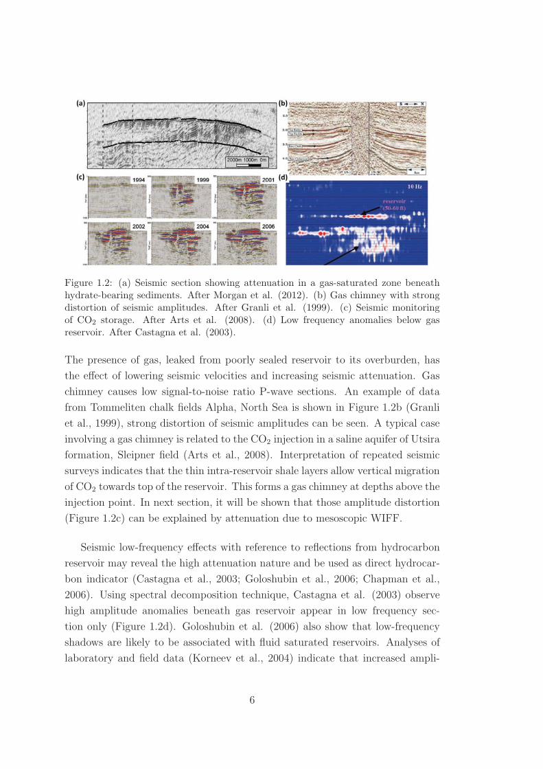
Figure 1.2: (a) Seismic section showing attenuation in a gas-saturated zone beneathhydrate-bearing sediments. After Morgan et al. (2012). (b) Gas chimney with strongdistortion of seismic amplitudes. After Granli et al. (1999). (c) Seismic monitoringof CO2 storage. After Arts et al. (2008). (d) Low frequency anomalies below gasreservoir. After Castagna et al. (2003).

The presence of gas, leaked from poorly sealed reservoir to its overburden, has

the effect of lowering seismic velocities and increasing seismic attenuation. Gas

chimney causes low signal-to-noise ratio P-wave sections. An example of data

from Tommeliten chalk fields Alpha, North Sea is shown in Figure 1.2b (Granli

et al., 1999), strong distortion of seismic amplitudes can be seen. A typical case

involving a gas chimney is related to the CO2 injection in a saline aquifer of Utsira

formation, Sleipner field (Arts et al., 2008). Interpretation of repeated seismic

surveys indicates that the thin intra-reservoir shale layers allow vertical migration

of CO2 towards top of the reservoir. This forms a gas chimney at depths above the

injection point. In next section, it will be shown that those amplitude distortion

(Figure 1.2c) can be explained by attenuation due to mesoscopic WIFF.

Seismic low-frequency effects with reference to reflections from hydrocarbon

reservoir may reveal the high attenuation nature and be used as direct hydrocar-

bon indicator (Castagna et al., 2003; Goloshubin et al., 2006; Chapman et al.,

2006). Using spectral decomposition technique, Castagna et al. (2003) observe

high amplitude anomalies beneath gas reservoir appear in low frequency sec-

tion only (Figure 1.2d). Goloshubin et al. (2006) also show that low-frequency

shadows are likely to be associated with fluid saturated reservoirs. Analyses of

laboratory and field data (Korneev et al., 2004) indicate that increased ampli-

6

tude and travel time at low frequency can be associated with wave propagating

in a fluid-saturated thin-layer exhibiting high attenuation. Attenuation caus-

ing low-frequency shadow can be attributed to WIFF resulting from partial gas

saturations at mesoscopic scale (Quintal et al., 2009).

WIFF in time-lapse seismic monitoring

4D seismic, that is based on analysis of repeated 3D seismic data, opens new

horizons for monitoring changes of reservoir properties such as temperature, sat-

uration and fluid pressure during the productive life of a field (Aronsen et al.,

2004). The detection of areas with significant changes helps reservoir engineers

to determine new drilling sites (Johnston, 2013). Quantitative estimation of sat-

uration and pressure changes can be obtained using time-lapse P- and S- wave

information derived from elastic inversion or from AVO analysis (Tura and Lum-

ley, 1999; Cole et al., 2002; Davolio et al., 2011).

Figure 1.3: Estimated fluid saturation changes (left) and pore pressure changes (right)based on 4D AVO analysis for the top Cook interface at Gullfaks. Yellow color repre-sents significant change, red line shows original oil-water contact. After Landrø (2001).

Landrø (2001) presents a rock-physics-based inversion scheme that directly

solves for pressure and saturation changes from AVO intercept and gradient at-

tributes. Landrø’s approach assumes that the elastic properties associated with

saturation change is given by Gassmann equation whereas pressure changes is

governed by effective stress law obtained from ultrasonic core measurement. The

validity of Gassmann equation restricts to homogeneous fluid distribution (Mavko

7

and Mukerji, 1998). Thus, employing Gassmann’s equation as saturation law ex-

cludes the possible attenuation effect arising from a patchy fluid distribution. On

top of that, the change of reservoir forces during dynamic fluid injection can give

rise to time-dependent saturation scale. This means that there is yet another

variable controlling the time-lapse seismic signal on top of the saturation and

fluid pressure change. Therefore, it seems to be prudent to understand the effect

of saturation scale changes on WIFF.

(a) (b)

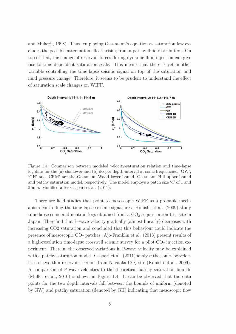
Figure 1.4: Comparison between modeled velocity-saturation relation and time-lapselog data for the (a) shallower and (b) deeper depth interval at sonic frequencies. ‘GW’,‘GH’ and ‘CRM’ are the Gassmann-Wood lower bound, Gassmann-Hill upper boundand patchy saturation model, respectively. The model employs a patch size ‘d’ of 1 and5 mm. Modified after Caspari et al. (2011).

There are field studies that point to mesoscopic WIFF as a probable mech-

anism controlling the time-lapse seismic signatures. Konishi et al. (2009) study

time-lapse sonic and neutron logs obtained from a CO2 sequestration test site in

Japan. They find that P-wave velocity gradually (almost linearly) decreases with

increasing CO2 saturation and concluded that this behaviour could indicate the

presence of mesoscopic CO2 patches. Ajo-Franklin et al. (2013) present results of

a high-resolution time-lapse crosswell seismic survey for a pilot CO2 injection ex-

periment. Therein, the observed variations in P-wave velocity may be explained

with a patchy saturation model. Caspari et al. (2011) analyse the sonic-log veloc-

ities of two thin reservoir sections from Nagaoka CO2 site (Konishi et al., 2009).

A comparison of P-wave velocities to the theoretical patchy saturation bounds

(Muller et al., 2010) is shown in Figure 1.4. It can be observed that the data

points for the two depth intervals fall between the bounds of uniform (denoted

by GW) and patchy saturation (denoted by GH) indicating that mesoscopic flow

8

might play a role. To test this assumption, Caspari et al. (2011) model the

velocity-saturation relation using the random patchy saturation model (denoted

by CRM 1D, 3D) with varying patch sizes. The velocity-saturation trend of the

smoothed data can be explained by the patchy saturation model for a range of

patch sizes.

Figure 1.5: (a) Scheme of the geological model for the Sleipner field. The black thinareas indicate the main CO2 component. The narrow gray shaded areas indicate thepresence of a diffuse CO2 component. (b) Seismic response considering WIFF effectsdue to the presence of CO2 patches. (c) Seismic response for an equivalent elasticmodel with P-wave velocity given by Gassmanns formula. Modified after Rubino et al.(2011).

Rubino et al. (2011) explore the potential implications for mesoscopic flow

on surface seismic data. Their study is inspired by the Sleipner field CO2 storage

project (Arts et al., 2008). Rubino et al. (2011) simulate the propagation of seis-

mic waves through a Utsira like reservoir containing centimetre-scale CO2 patches

(Figure 1.5a). Two modelling methods are employed, one is elastic modeling with

velocity calculated from Gassmann equation (which implies homogeneous satu-

ration) and the other one is viscoelastic modelling which accounts the effect of

WIFF (in this case due to patchy saturation). By comparing the resulting zero-

offset synthetic seismic sections they observe that when velocity dispersion is

considered, velocity push-down caused by the presence of CO2 becomes less pro-

nounced whereas amplitudes around CO2 plumes diminish (Figure 1.5b,c,) Their

9

results indicate that WIFF due to the presence of centimetre-scale fluid patches

may produce noticeable changes in the observed surface seismic data.

Core-flooding combined with ultrasound and CT-imaging

The most detailed insights into the fluid distribution and accompanying evolu-

tions of velocity- and attenuation- saturation relations can be gained from lab-

oratory core-flooding monitored by both ultrasonic transducers and X-ray CT

imaging (Lei and Xue, 2009; Alemu et al., 2013; Lopes et al., 2014). As an exam-

Figure 1.6: Velocity-saturation relation determined from numerical simulations of wavepropagation in a poroelastic solid with randomly distributed patches that cluster forlarger saturation values (see inset). Experimentally determined velocities for the quasi-static injection experiment are also shown. After Lebedev et al. (2009).

ple, in the experiment of Lebedev et al. (2009), the P-wave velocity-saturation

relation resulting from an imbibition exhibits a transition between Gassmann-

Wood and Gassmann-Hill predictions as shown in Figure 1.6. They model the

data by performing numerical simulation, that is based on Biot’s wave equations.

The varying degree of saturation is characterized by increasing the size of the

randomly distributed fluid clusters. Despite the simplified numerical set-up, the

simulation results reproduce the overall behavior of the measured VSR as seen

in Figure 1.6. The modelling indicates that the behaviour of velocity-saturation

relation can be attributed to mesoscopic WIFF. Moreover, from a modelling view-

10

point, it is important to know that the saturation scale, i.e., water patch size,

increases with increasing water saturation during imbibition.

Figure 1.7: (a) Measurement set up and raw CT scan of the sample: the red circleindicates the acoustic monitoring field; (b) The ultrasonic waveforms at various sat-urations. The black waveforms correspond to an injection rate of 2 mL/h while thered waveforms correspond to a reduced injection rate of 0.2 mL/h.(c) Water saturationmap (average Sw=68%) derived from the CT images. Mesoscopic fluid patches appear.

The fluid distribution information inferred from the measurement of Lebedev

et al. (2009) however remains qualitative. More recently, Lopes et al. (2014) per-

form simultaneous acquisition of high-resolution CT scans and ultrasonic wave-

forms during forced water imbibition on a Savonnieres limestone sample (Figure

1.7a). The CT image reveals minimum one-tenth millimetre feature of the sample

that is a good candidate for studying wave-induced fluid flow due to partial satu-

rations at mesoscopic scale. Let us take a closer look at the data by modelling the

measured P-wave velocities and attenuation. First, consecutive CT imaging dur-

ing core-flooding (Lopes et al., 2014) allows for obtaining statistical information,

such as autocorrelation function, from the saturation maps (Figure 1.7c). Toms

et al. (2007a) propose a so-called continuous random patchy saturation model

(CRM) which quantifies the fluid distribution by statistical measures. Therefore,

this model is employed here to give estimates of the velocity and attenuation. Me-

chanical properties of the rock and fluids as well as the frequency in the modelling

are set to be consistent with the measurement. The results are presented in Fig-

ure 1.8. The measured velocities fall in between patchy saturation bounds which

confirms mesoscopic flow to be the driving mechanism. However, the modelled

velocity underestimates the overall measured velocities whereas the modelled at-

tenuation overestimates the overall measured attenuation. It appears that there

is a discrepancy that cannot be satisfactorily explained by CRM model and hence

11

(a) (b)

Figure 1.8: Modeling ultrasonic data obtained during a capillary-force-dominated im-bibition: (a) velocity- and (b) attenuation- saturation relations.

by the mechanism of WIFF alone. A possible explanation for this mismatch is

related to the capillary effect.

Capillarity effects on the acoustics of partially saturated rocks

Theoretical and experimental works of two-phase flow associated with imbibition

suggest that the fluid distribution for immiscible flows is controlled by the inter-

play between viscous and capillary forces. Specifically, in petrophysical experi-

ments the relative importance of the capillary effect is quantified by the capillary

number (e.g., Riaz et al., 2007):

Ca =μfU

γ, U =

4q

πD2(1.1)

where μf is the shear viscosity of the injected fluid and γ is the interfacial ten-

sion between the two fluids. U is the injection velocity which depends on the

injection rate q and the diameter of the sample D. In the experiments of Lopes

et al. (2014), the capillary number is on the order of 10−9. In the context of

reservoir flow simulations, the ratio of viscous force to capillary force is expressed

as (Sengupta and Mavko, 2003)

Rcv = Calr

κ, (1.2)

where l is the length of the core sample and r is a representative pore-throat

radius. The flow permeability is denoted as κ. Rcv in the Lopes et al. (2014)

12

experiment is on the order of 10−3. Therefore, both the capillary number Ca and

the critical flow ratio Rcv indicate that the flow regime is dominated by capillary

forces.

Figure 1.9: Microscopic capillary forces (left) produce a net effect at macroscopic scale(right). The macroscopic capillary pressure may change the overall stiffness of thesaturated rock and consequently affects the wave responses. Arrows denote micro- andmacro- capillary pressure gradients.

It is, however, not clear how this capillarity affects the acoustics of partially

saturated rocks. There is experimental evidence that capillarity can lead to

changes in elastic stiffnesses and hence to changes in wave velocities and at-

tenuation (Moerig et al., 1996; Averbakh et al., 2010). This also involves the

questions how capillary forces affect the velocity-saturation relation and WIFF.

This becomes a particular important problem in the presence of mesoscopic fluid

patches. While capillary forces only exist at fluid-fluid interfaces at the pore-scale,

one can expect that they produce a net effect up in scale (De la Cruz et al., 1995;

Tserkovnyak and Johnson, 2003), thereby creating a new attribute across meso-

scopic patches, or between macroscopic gas-water, gas-oil contacts. Given that

the mesoscopic WIFF is often applied to interpret seismic attenuation (Morgan

et al., 2012; Blanchard and Delommot, 2015), any significant changes induced by

capillarity may possibly entail important implications. This is one of the primary

motivations for including the capillarity effect into models for mesoscopic WIFF.

It is the aim of this thesis to incorporate the mesoscopic manifestation of cap-

illarity in the framework of Biot’s poroelasticity theory. This, in turn, enables us

to extend existing models for patchy-saturation that are based on Biot’s poroe-

lasticity theory. It further allows us to study how capillarity affects WIFF and

what implications for the interpretation of seismic (time-lapse) signatures arise.

13

1.2 Thesis outline

Chapter 2: A mathematical review of relevant theories for acoustics in partially

saturated porous media is given.

Chapter 3: Capillarity effect is incorporated in White’s layered model for study-

ing acoustic responses, i.e., velocity, attenuation and poroelastic fields resulting

from mesoscopic fluid flow.

Related publication: Qiaomu Qi, Tobias M. Muller, German Rubino, 2014. Seis-

mic attenuation: Effect of interfacial impedance on wave-induced pressure diffu-

sion: Geophysical Journal International, 199, 1677-1681. doi: 10.1093/gji/ggu327

Chapter 4: Random patchy saturation theory is generalized to include capillar-

ity effect. The theory is validated by comparing with laboratory data.

Related publication: Qiaomu Qi, Tobias M. Muller, Boris Gurevich, Sofia C.

Lopes, Maxim Lebedev, Eva Caspari, 2014. Quantifying the effect of capillarity on

dispersion and attenuation in patchy-saturated rocks: Geophysics, 79(5), WB35-

WB50. doi: 10.1190/geo2013-0425.1

Chapter 5: Reflection coefficients for contact between saturated porous media

and liquid/porous-medium contact are generalized to include capillarity.

Related publication: Qiaomu Qi, Tobias M. Muller, Boris Gurevich, 2015. The

role of interfacial impedance on poroelastic reflection coefficient. EAGE Technical

Program Expanded Abstract. doi:10.3997/2214-4609.201412626

Chapter 6: A workflow on application of developed theory for quantitative

analysis of time-lapse seismic signatures is established.

Related publication: Qiaomu Qi, Tobias M. Muller, Boris Gurevich, 2015. Sat-

uration scale effect on time-lapse seismic signatures: submitted to Geophysical

Prospecting.

Chapter 7: The thesis is finalized by concluding remarks and future recommen-

dations.

14

Chapter 2

Theoretical background

2.1 Acoustics in saturated porous media

— Biot’s theory of poroelasticity

The theory of wave propagation in a poroelastic solid containing a viscous

compressible fluid has been established by Biot (Biot, 1956a, b; Biot, 1962). It

not only forms the theoretical foundation of seismic wave propagation in fluid-

saturated rocks but also is used in many other disciplines related with porous

media. Biot’s equations of poroelasticity will be frequently referred in this thesis.

Therefore, it is of primary importance here to review its basic concepts. As with

any physical theories, the work of Biot (1956) is based on certain assumptions:

• Porous medium is elastic and statistically isotropic.

• Pore fluid is continuous and does not support shear stress.

• Wave motion induces small deformations only and no thermal variation.

• Seismic wavelength is substantially larger than the pore sizes.

In subsequent sections, the definitions of potential, kinetic and dissipated energies

in Biot’s theory will be introduced. The physical meaning of Biot’s elastic coeffi-

cients will be elaborated. These are followed by the derivation of wave equation

from solving the corresponding Lagrange equation.

15

2.1.1 Potential energy and stress strain relation

Consider a unit cubic aggregate of fluid and solid, the stress tensor of such

elementary volume is given by⎧⎪⎨⎪⎩σxx + σ σxy σxz

σyx σyy + σ σyz

σzx σzy σzz + σ

⎫⎪⎬⎪⎭︸ ︷︷ ︸Total τij

=

⎧⎪⎨⎪⎩σxx σxy σxz

σyx σyy σyz

σzx σzy σzz

⎫⎪⎬⎪⎭︸ ︷︷ ︸Solid σij

+

⎧⎪⎨⎪⎩σ 0 0

0 σ 0

0 0 σ

⎫⎪⎬⎪⎭︸ ︷︷ ︸F luid δijσ

. (2.1)

The total stress components τij equal the sum of solid and fluid force acting on

each face of the two-phase cube. σij represent the force components acting on the

solid portion of the cube face. On the other hand, σ represents the total normal

tension force applied to the fluid portion of the cube face. The fluid stress relates

the hydrostatic fluid pressure in the pores via

−σ = φpf . (2.2)

σ is taken negative when the force acting on the fluid is pressure whereas σij

is positive if the force in the solid is tension. The porosity φ of the skeleton is

defined as

φ =VpVb, (2.3)

where Vp is the volume of the pores contained in the bulk volume Vb. The average

displacement components of the solid are designated by ux, uy, uz whereas for

the fluid they are Ux, Uy, Uz. The strain tensor of the solid is represented by

eij =

⎧⎪⎨⎪⎩exx exy exz

eyx eyy eyz

ezx ezy ezz

⎫⎪⎬⎪⎭ (2.4)

with

exx =∂ux∂x

, exy =1

2

(∂ux∂y

+∂uy∂x

), etc. (2.5)

The strain tensor in the fluid is given by

ε =∂Ux

∂x+∂Uy

∂y+∂Uz

∂z. (2.6)

16

It is sometimes more convenient to define the relative average displacement of

fluid relative to the solid frame as

w = φ(U− u). (2.7)

The associated strain for the relative displacement is the incremental fluid content

which is defined as

ξ = −∇ ·w = φ(e− ε), (2.8)

where e = exx + eyy + ezz is the compressive strain. With a generalization of

elasticity theory (Love, 1944), the potential (strain) energy of the poroelastic

elementary volume is expressed as (Biot, 1962)

V = τxxexx + τyyeyy + τzzezz + τxyexy + τyzeyz + τxzexz + pfξ. (2.9)

The stress components are given by the partial derivatives of the potential energy

τxx =∂V

∂exx, τxy =

∂V

∂exy, ... , pf =

∂V

∂ξ. (2.10)

According to equations 2.10, the stress-strain relation in a general anisotropic

poroelastic medium is characterized by 7 independent equations⎛⎜⎜⎜⎜⎜⎜⎜⎜⎜⎜⎜⎝

τxx

τyy

τzz

τxy

τyz

τxz

pf

⎞⎟⎟⎟⎟⎟⎟⎟⎟⎟⎟⎟⎠=

⎛⎜⎜⎜⎜⎜⎜⎜⎜⎜⎜⎜⎝

c11 c12 c13 c14 c15 c16 c17

c22 c23 c24 c25 c26 c27

c33 c34 c35 c36 c37

c44 c45 c46 c47

c55 c56 c57

c66 c67

c77

⎞⎟⎟⎟⎟⎟⎟⎟⎟⎟⎟⎟⎠

⎛⎜⎜⎜⎜⎜⎜⎜⎜⎜⎜⎜⎝

exx

eyy

ezz

exy

eyz

exz

ξ

⎞⎟⎟⎟⎟⎟⎟⎟⎟⎟⎟⎟⎠(2.11)

The requirement of the symmetry of the stress and strain tensors lead to 28

independent poroelastic coefficients in equations 2.11. For an isotropic material,

the potential energy 2.9 takes the simplified form as

2V = (λ+ 2μ)e2 − μI − 2αMeξ +Mξ2, (2.12)

where the invariant I is given by

I = e2xy + e2yz + e2xz − 4exxeyy − 4eyyezz − 4exxezz. (2.13)

17

From equations 2.2, 2.10 and 2.12, we obtain the stress strain relation for an

isotropic poroelastic medium

τij = (λe− αMξ)δij + 2μeij , (2.14)

pf = −αMe+Mξ , (2.15)

where δij denotes the Kronecker Delta. In either case of φ = 0 or w = 0 ,

the potential energy 2.12 reduces to the case analogous to isotropic elasticity.

Accordingly, the stress strain relations 2.14, 2.15 become analogous to elastic

Hooke’s law.

2.1.2 Poroelastic constants

Four poroelastic coefficients, namely λ, α, M, μ appeared in the stress strain

relations 2.14, 2.15 of Biot’s theory. They incorporate the solid, fluid properties

as well as micro-structural information of the porous medium. The determination

of the meaning and internal relation of these poroelastic coefficients require four

Gedanken experiments (Biot and Willis, 1957; Gassmann, 1951).

Pure shear deformation

First, assuming the porous medium is subjected to a pure shear deformation such

that

e = ξ = 0 → τ sij = τij − 1

3τllδij = μ

(∂ui∂xj

+∂uj∂xi

), (2.16)

where Einstein summation with repeated indices is applied. Since the fluid does

not sustain shear force, it is clear that the parameter μ which relates the shear

stress and strain is the shear modulus of the dry matrix.

Jacketed compressibility test

In this experiment, the porous medium is enclosed in a thin impermeable jacket

and then subjected to an external hydrostatic pressure Pe. To ensure constant

internal fluid pressure, the interior of the jacket is made to communicate with the

18

atmosphere through a tube, therefore

pf = 0 → ξ = αe . (2.17)

With the dilation of the sample e being measured, the jacketed bulk modulus can

be given by

K0 = −Pe

e=

1

3

τlle. (2.18)

Because the entire external pressure is transmitted to the frame, K0 is identical

to the bulk modulus of the dry matrix. Equations 2.14, 2.15, 2.17, 2.18 together

yields the following relation

λ = K0 − 2

3μ+ α2M . (2.19)

This also indicates that a new parameter λc = λ − α2M is equivalent to Lame

coefficient of the dry matrix.

Unjacketed compressibility test

In this experiment, the sample remains unjacketed and is immersed in the fluid

where a pressure −Pe is applied. Since the fluid will completely penetrate the

sample, one has

pf = Pe . (2.20)

With the dilatation of the sample e being measured, the unjacketed bulk modulus

is given by

Ks = −Pe

e=

1

3

τlle. (2.21)

Because the applied pressure is transmitted to the solid skeleton, Ks is equivalent

to the bulk modulus of the solid grain. Equations 2.14, 2.15, 2.20,2.21 together

yields another Biot’s parameter

α = 1− λ− α2M + 23μ

Ks

. (2.22)

19

Using obtained result 2.19, parameter α can be expressed in terms of two mea-

sured quantities, namely the jacked and unjacketed bulk modulus

α = 1− K0

Ks

. (2.23)

Assuming that the fluid strain ε has also been measured during the unjacketed

test, the bulk modulus of the pore fluid can be expressed as

Kf = −Pe

ε. (2.24)

The incremental fluid content under unjacketed test can be now written as

ξ = φPe

(1

Kf

− 1

Ks

)(2.25)

Equations 2.15, 2.20 and 2.25 together gives the expression of the last Biot’s

parameter

M =

(α− φ

Ks

+φ

Kf

)−1

. (2.26)

The first parameter α (2.23) derived from unjacketed test is the so-called Biot-

Willis coefficient (Biot and Willis, 1957), also known as Biot’s effective stress

coefficient (Nur and Byerlee, 1971). It dominates the proportion of fluid pressure

which produces the same strains as the total stress. The second parameter M

(2.26) is fluid storage modulus which is a measure of constrained storage capacity

(Wang, 2000).

Undrained compressibility test

Let us now explore the physical meaning of Biot’s parameter λ, though it has

already been expressed in terms of other defined quantities (eq. 2.19). This

requires one more so-called undrained compressibility test (Gassmann, 1951). In

this experiment, a saturated sample is jacketed and no fluid is allowed to escape

from the medium. This implies zero incremental fluid content

ξ = 0 . (2.27)

The sample is subjected to static compression Pe such that the induced pore

20

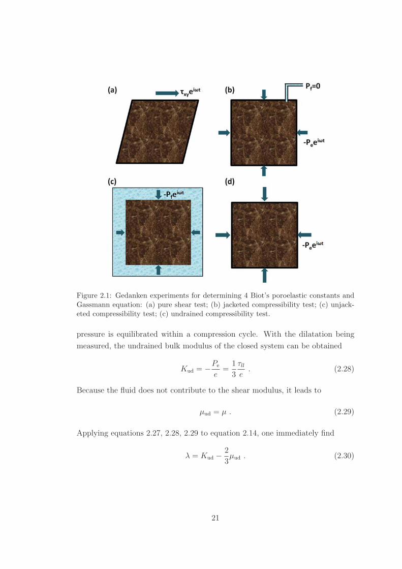
Figure 2.1: Gedanken experiments for determining 4 Biot’s poroelastic constants andGassmann equation: (a) pure shear test; (b) jacketed compressibility test; (c) unjack-eted compressibility test; (c) undrained compressibility test.

pressure is equilibrated within a compression cycle. With the dilatation being

measured, the undrained bulk modulus of the closed system can be obtained

Kud = −Pe

e=

1

3

τlle. (2.28)

Because the fluid does not contribute to the shear modulus, it leads to

μud = μ . (2.29)

Applying equations 2.27, 2.28, 2.29 to equation 2.14, one immediately find

λ = Kud − 2

3μud . (2.30)

21

It is clear now that parameter λ is identical to the undrained Lame coefficient.

Lastly, equations 2.19 and 2.30 together yields the Gassmann’s equation

Kud = K0 + α2M , (2.31)

which is expressed in terms of Biot’s parameters. Gassmann obtained his results

directly by considering elementary elasticity without employing α and M . Alter-

native forms and extensions of Gassmann’s equation can be found in Mavko et

al., (2009). Now with all Biot’s parameters being defined and expressed in terms

of measurable rock physics quantities, namely⎧⎪⎪⎪⎨⎪⎪⎪⎩λ = K0 + α2M − 2

3μ , Undrained Lame coefficient

α = 1− K0

Ks, Biot-Willis coefficient

M =(

α−φKs

+ φKf

)−1

. Fluid storage modulus

(2.32)

one can proceed with the derivation of Biot’s dynamic equations.

2.1.3 Kinetic energy

The assumption of isotropy implies that all directions are equivalent and dy-

namically uncoupled. Then, the kinetic energy per unit volume is expressed as

2E = ρ11uiui + 2ρ12uiUi + ρ22UiUi , (2.33)

where ρ11, ρ12, ρ22 are the mass coefficients. They render the fact that the relative

fluid flow can be non-uniform and satisfy the following relations

ρ11 + ρ12 = (1− φ)ρs ,

ρ12 + ρ22 = φρf ,

ρ12 = −(S∞ − 1)φρf , (2.34)

where ρs is the grain density and S∞ the tortuosity. The mass coefficients must

obey the following inequalities to give a positive kinetic energy

ρ11 > 0, ρ22 > 0 , ρ11ρ22 − ρ212 > 0 . (2.35)

22

2.1.4 Dissipation function

Steady-state permeability

When the viscous fluid flow under an oscillatory pressure gradient ∇Peiωt is of

Poiseuille type (i.e. the Reynolds number of the flow which equals the ratio

of inertial force to viscous force is less than a critical Reynolds number), the

dissipation function D is defined by

D =1

2

η

κ0(w2

x + w2y + w2

z) , (2.36)

where the dot operator denotes the time derivative and η, κ0 are the fluid shear

viscosity and steady-state permeability. Equation 2.36 assumes that the dissipa-

tion due to relative fluid-solid motion is governed by Darcy’s law. The fluid force

is obtained by taking the derivative of the dissipation function with respect to

the relative fluid-solid displacement

−∇pf =∂D

∂w=

η

κ0(wx + wy + wz) . (2.37)

The result is equivalent to the steady-state Darcy’s law.

Dynamic permeability

The assumption of Poiseuille flow breaks down when frequency of the oscillatory

fluid flow exceed the characteristic frequency

ωd =2η

δ2ρf, (2.38)

where ρf is the fluid density, δ is the viscous skin depth. In this regime, the

viscous skin depth δ is small compared to the characteristic pore size and the

flow follows a potential flow pattern (Johnson et al., 1987). This fluid transport

phenomenon can be captured by postulating a dynamic-equivalent Darcy’s law

which renders the permeability a frequency-dependent quantity. To account for

this effect, the dynamic permeability model has been suggested by Johnson et al.

23

(1987)

κ(ω) = κ0

(√1 + i

J

2

ω

ωc

+ iω

ωc

)−1

, (2.39)

where J is a shape factor which is often set to unity. The crossover frequency ωc

which separates the viscosity and inertia-dominated regimes is

ωc =φη

κ0ρfS∞ , (2.40)

where ρf is the fluid density. The replacement of the steady-state permeability κ0

in equations 2.36 and 2.37 with formula 2.39 yield respectively the high-frequency-

corrected dissipation function

D =1

2

η

κ(ω)w2 , (2.41)

and dynamic-equivalent Darcy’s law

−∇pf =η

κ(ω)w . (2.42)

Alternatively, equation 2.42 can be represented by

−∇pf = S(ω)ρfφw , (2.43)

where S(ω) is the so-called dynamic tortuosity. The relation between dynamic

permeability and dynamic tortuosity is clear from equations 2.42, 2.44 that

S(ω) = − iηφ

κ(ω)ωρf. (2.44)

Depending on the circumstances, it is convenient to describe the linear responses

of the system in terms of either κ(ω) or S(ω) (Johnston et al., 1994). More details

of dynamic permeability and its application can be found in Appendix E. The

inertial effect when the viscous skin depth decreases is also considered by Biot

(1956b) who modelled porous media as an ensemble of cylindrical ducts.

2.1.5 Equations of motion

Upon the establishment of potential energy 2.12, kinetic energy 2.33 and dissi-

pated energy 2.41, the equations of motion can now be obtained from the Euler-

24

Lagrange equation which is derived from Hamilton’s principle of least action

(Achenbach, 1984)

∂

∂t

(∂L

∂q

)+∂D

∂q=∂L

∂q, (2.45)

where the volumetric Lagrangian density is defined as

L ≡ E − V. (2.46)

The generalized coordinate q is characterized by the displacements associated

with solid u and fluid U . Treating the solid and fluid on an equal footing by

executing equation 2.45 with respect to q = u and q = U lead

ρ11u+ ρ12U = P∇(∇ · u) +Q∇(∇ ·U)− μ∇×∇× u ,

ρ12u+ ρ22U = Q∇(∇ · u) +R∇(∇ ·U) , (2.47)

which are coupled equations of motion. The definition of the notations are as

follows

P = λ+ 2μ+ (φ2 − 2αφ)M ,

Q = (α− φ)φM ,

R = φ2M . (2.48)

Dynamic mass coefficients are introduced in equations 2.47. They incorporate

the dissipation terms and satisfy the following relations

ρ11 + ρ12 = (1− φ)ρs ,

ρ12 + ρ22 = φρf ,

ρ12 = −(S(ω)− 1)φρf , (2.49)

Applying the dynamic tortuosity 2.44 in conjunction with dynamic permeability

2.39 in above mass coefficients results in their explicit forms

ρ11 = ρ11 − iβF

ω,

ρ12 = ρ12 +iβF

ω,

ρ22 = ρ22 − iβF

ω. (2.50)

25

The steady-state Darcy’s coefficient β and frequency correction factor F are de-

fined as

β =ηφ2

κ0, F =

√1 + i

J

2

ω

ωc

. (2.51)

2.1.6 Solutions of wave equations

In the case of isotropy, dilatational waves are uncoupled from the rotational

waves. In order to obtain the independent wave equations, scalar and vector

valued displacement potentials are introduced in following fashion(u

U

)=

(∇Φ1

∇Φ2

)+

(∇×Ψ1

∇×Ψ2

). (2.52)

Decomposition of dilatational wave and shear wave can be carried out by intro-

ducing the irrotational ∇Φ and isovolumetric ∇×Ψ fields into the coupled wave

equations 2.47, respectively.

Dilatational waves

Introducing the scalar potential Φ = (Φ1,Φ2)T in the motion equation 2.47 yields

a set of differential equations as the following(P Q

Q R

)∇2Φ =

(ρ11 ρ12

ρ12 ρ22

)Φ. (2.53)

Considering plane wave solutions for P-wave propagating along x direction

Φj = Φj exp(i(ωt− kx)) , j = 1, 2 , (2.54)

where Φj are the amplitudes, k is the complex wavenumber and ω is the angular

frequency. Substituting 2.54 into 2.53 lead(Pk2 − ρ11ω

2 Qk2 − ρ12ω2

Qk2 − ρ12ω2 Rk2 − ρ22ω

2

)(Φ1

Φ2

)= 0. (2.55)

For the above homogeneous linear system having non-trivial solution, the deter-

minant of the coefficient matrix must be zero. This results in a dispersion relation

26

which is a quadratic equation of ζ = ω2/k2

(ρ11ρ22 − ρ211)ζ2 − (P ρ22 +Rρ11 − 2Qρ12)ζ + (PR−Q2). (2.56)

Two physical solutions can be obtained for the complex velocity square

V 2 = ζ =Δ±√Δ2 − 4(ρ11ρ22 − ρ211)(PR−Q2)

2(ρ11ρ22 − ρ211), (2.57)

where Δ = P ρ22+Rρ11− 2Qρ12. In accordance with the plane wave ansatz 2.54,

a positive attenuation coefficient requires Im{k} < 0. This further shows that

only two solutions for the complex wavenumber exist. They correspond to two

dilatational wave modes in saturated porous media. It is easy to show from 2.55

that the amplitudes of the solid and fluid are coupled in following fashion

Φ2

Φ1

=ρ11ω

2 − Pk2

Qk2 − ρ12ω2=ρ12ω

2 −Qk2

Rk2 − ρ22ω2. (2.58)

The orthogonality relation (Biot, 1956a) for the wave amplitudes shows that the

amplitudes for one wave mode is in phase whereas for another is out of phase.

The former corresponds to the fast P-wave mode and the latter is the slow P-

wave mode. The terminology fast/slow derives from their corresponding phase

velocities. The phase velocities and attenuation coefficients for the two P-wave

modes can be calculated via

Vfast,slow =ω

Re{kfast,slow} , γ = Im{kfast,slow}. (2.59)

An numerical example is given in Figure 2.2 for a unconsolidated sandstone,

the fast wave exhibits little dispersion and attenuation over several decades of

frequency. On the other hand, the slow wave is highly dispersive at low frequency

and only becomes propagatory at high frequency. The phase velocity of the latter

is much slower than the former. Beyond theoretical prediction of Biot (1956a,b,

1962), Plona (1980) experimentally confirmed the existence of the two P-wave

modes in saturated porous solids.

27

Rotational wave

Introducing the vector potential Ψ = (Ψ1,Ψ2)T in the motion equations 2.47

yields a set of differential equations of the form(μ 0

0 0

)∇2Ψ =

(ρ11 ρ12

ρ12 ρ22

)Ψ (2.60)

A plane wave ansatz for the rotational wave mode leads(μk2 − ρ11ω

2 −ρ12ω2

−ρ12ω2 −ρ22ω2

)(Ψ1

Ψ2

)= 0. (2.61)

The dispersion relation for the rotational mode is therefore

(ρ11ρ22 − ρ211)V2s − μρ22 = 0. (2.62)

Only one physical solution to the dispersion relation exists. It corresponds to

the only rotational wave mode in Biot’s theory. Appying the dynamic mass

coefficients 2.49 in equation 2.62, the resulting shear velocity reads

Vshear =

(μ

((1− φ)ρs + (1− 1S(ω)

))φρf

) 12

. (2.63)

According to equation 2.61, the fluid to solid amplitude ratio for rotational mode

is given byΨ2

Ψ1

= − ρ12ρ22

. (2.64)

Because the acceleration of the fluid must be opposed to that of solid (Biot,

1956a), the coupling mass coefficient ρ12 is always negative. Accordingly from

equation 2.49, ρ22 is obvious positive. Therefore, the shear motion of the solid

and fluid is in phase as pointed out from equation 2.64. Sahay (2008) showed

that on top of the in-phase shear mode, there exists another out-of-phase shear

mode in porous media saturated by a Newtonian fluid.

2.2 Viscosity-extended Biot framework

The viscosity-extended Biot (VEB) framework (Sahay, 2008) refers to a mod-

ification of Biot’s original theory. The modification consists of incorporating the

28

(a)

10-4

10-2

100

102

104

100

101

102

103

104

f/fBiot

V [m

/s]

Vfast

Vslow

Vshear

(b)

10-4

10-2

100

102

104

10-10

10-5

100

105

f/fBiot

γ [m

- 1]

γfast

γslow

γshear

Figure 2.2: An example of (a) dispersion and (b) attenuation coefficient for three wavemodes in a water-saturated unconsolidated sandstone.

viscous stress terms in the fluid stress tensor, i.e., equation 2.1. This means that

the strain rate terms and thus the fluid bulk and shear viscosities enter the con-

stitutive relations. A feature of VEB framework is that it renders the constitutive

relation of a Newtonian fluid if the porosity is unity. A further consequence is

that the VEB framework entails a slow shear wave in addition to the fast shear

wave appearing in Biot’s theory. This slow shear wave can be thought of as the

out-of-phase shearing motion. It plays therefore a similar role as the Biot slow

compressional wave that represents the out-of-phase compressional motion. The

nature of the out-of-phase shear motion is characterized by the Biot’s relaxation

frequency 2.38. When ω � ωc , the slow shear wave is governed by following

diffusion operator with a damping term

∂

∂t+

ωc

dfS∞ =Dν

S∞∇2 (2.65)

where the kinematic viscosity is Dν = η/ρf . The damping term is ωc/(dfS∞)

with df = (S∞ − mf)−1 and mf the fluid mass fraction. In the regime ω � ωc

the damping term vanishes and the slow shear wave is an ordinary diffusion wave

with diffusivity Dν/S∞. Mode conversion into slow shear wave in certain case

represents an efficient dissipation mechanism. For example, when shear wave

propagating through an air-water interface, neglecting the slow shear mode (i.e.,

using the classical Biot’s theory) can result in underestimation of the reflected

S-wave amplitude (Sahay, 2008). Moreover, the dynamic permeability 2.39 can

be modelled as conversion scattering process from Biot slow P-wave into slow

shear wave (Muller and Sahay, 2011a,b). An application of VEB framework in

29

modelling dynamic permeability is given in Appendix E.

2.3 Alternative formulation of Biot’s theory

In certain cases, it is more convenient to express the relative fluid-solid dis-

placement w instead of the fluid displacement U in Biot’s equations. To refor-

mulate the equations of motion, we now redefine the kinetic energy as (Bourbie

et al., 1987)

2C = ρbuiui + 2ρf uiwi +ρfS

∞

φwiwi , (2.66)

where the bulk density ρb is given by

ρb = (1− φ)ρs + φρf . (2.67)

Execution of the Lagrange equation 2.45 with the newly defined kinetic energy

2.66 lead to following equation of motion

τij,j = ρbui + ρf wi , (2.68)

−pf,i = ρf ui +ρfS

∞

φwi +

η

κ(ω)wi . (2.69)

2.4 Quasi-static approximation of Biot’s theory

Considering low frequency regime where

ω � ωc =φη

κ0ρfS∞ , (2.70)

the acceleration terms u, w are negligibly small in comparison with the velocity

term wi. Meanwhile, the dynamic permeability is taken on a character of steady-

state permeability. Dropping the acceleration terms and replacing κ(ω) with κ0

in 2.68 yields the quasi-static formulation of Biot’s poroelasticity

τij,j = 0 , (2.71)

−pf,i = η

κ0wi . (2.72)

Formulae 2.71, 2.72 represent the equation of equilibrium and Darcy’s law, respec-

tively. The combined sets are also known as the Biot’s consolidation equations

30

(Biot, 1941). In conjunction with the stress strain relation 2.14, 2.15, one can

derive a diffusion equation from the consolidation equations

Dp∇2pf = pf , (2.73)

where Dp is the hydraulic diffusivity (Chandler and Johnson, 1981)

Dp =k0ηφ2

PR−Q2

P + 2Q+R. (2.74)

The diffusion equation can also be formulated in terms of the relative fluid-solid

displacement w. This indicates that the out-of-phase movement (w �= 0) which

is associated with Biot slow wave obeys diffusion (Chandler and Johnson, 1981;

Bourbie et al., 1987).

2.5 Poroelastic boundary conditions

2.5.1 Open-pore boundary condition

Based on the assumption of the existence of perfect contact between the con-

tiguous media, the standard boundary condition of Deresiewicz and Skalak (1963)

or so-called open pore boundary condition can be established. Such boundary

condition is derived based on conservation of total energy and proved by Bour-

bie et al (1987) using Hamilton’s principle. In the space-frequency domain, the

continuity of energy flux at the interface of two porous media requires

〈iω(σijui + σδijUi)nj〉 = 0, (2.75)

where σδij = −φpfδij is the fluid stress, σij = τij − σδij is the solid stress,

nj denotes the unit normal of the interface between the two dissimilar porous

media, the angle bracket calculates the difference of the quantity between the

two media. The individual continuity for each term in equation 2.75 is implicitly

assumed (Sahay, 2012)

〈Tiui〉 = 0, (2.76)

〈σUn〉 = 0, (2.77)

31

where Ti = σijnj is the traction of the solid phase, Un = Uinjδij is the normal

component of the fluid displacement. Therefore, conditions 2.76, 2.77 correspond

to the energy flux continuity of the solid phase and fluid phase respectively.

Accordingly, each of the constituents in 2.76, 2.77 is required to be continuous

across the interface

〈T si 〉 = 0, (2.78)

〈ui〉 = 0, (2.79)

〈Un〉 = 0, (2.80)

〈σ〉 = 0. (2.81)

By considering conservation of fluid mass at the interface, the quantity of iωwn =

iωφ(Un−un) is required to be continuous. In order to be compatible with 2.78, it

demands the contintuity of porosity φ or no flow (Ui−ui)ni = 0 at the interface as

subjoined condition. Therefore, by replacing the fluid component Ui withwi

φ+ui,

equation 2.75 can be rewritten as

〈iω(Tiun − pfwn)〉 = 0, (2.82)

where Ti = τijnj is the total traction. Similarly, the continuity of each quantity

requires

〈Ti〉 = 0, (2.83)

〈ui〉 = 0, (2.84)

〈wn〉 = 0, (2.85)

〈pf〉 = 0. (2.86)

The last boundary condition is so-called open-pore boundary condition which

indicates a perfect hydraulic contact across poroelastic interface.

2.5.2 Partially open boundary condition

The physical model depicted by the open pore boundary condition assumes

that the pores of the two media are completely connected. However, this situation

is by no means unique. Non-alignment of a portion of the pores can produce an

interfacial flow area which is smaller than that in either medium adjacent to the

interface. This effect might be accomplished physically by inserting a porous

32

Figure 2.3: Simplified diagram of an interface between two porous media (after Bourbieet al, 1987).

membrane between the two media. Thus, flow through such an interface would

result in a pressure drop across the interface (Deresiewicz and Skalak, 1963)

pfa − pfb = ZIwn, (2.87)

where ZI is interfacial impedance and wn = wini is the normal component of

relative velocity. For perfect hydraulic contact, β equals zero and the boundary

condition 2.87 recovers the standard open-pore boundary condition 2.86. When

ZI goes to infinite large, it is equivalent of inserting an impermeable membrane

between the two saturated media. This situation refers to the no-flow boundary,

or closed pore boundary condition. In order to apply the partially open or closed

interface condition in the context of Biot’s theory, the physical meaning of the

resistance coefficient should be determined. The initial interpretation of the re-

sistance coefficient is given by Deresiewicz and Skalak (1963) as a proxy for pore

mis-alignment. For example, the interfacial impedance can be applied in simu-

lating mud-cake effect for acoustic wave travelling inside borehole (Rosenbaum,

1974). An end-member value of ZI = ∞ indicates a total blockage of borehole

surface whereas ZI = 0 represents open-pore borehole condition.

33

2.6 Acoustics in partially saturated porous me-

dia

The velocity dispersion and attenuation in rock fully saturated with a single

fluid can be satisfactorily described by Biot’s theory. However, it is generally

accepted that Biot’s theory cannot adequately interpret observed magnitudes of

attenuation and dispersion in the low frequency regime (Johnston et al., 1979;

Winkler, 1985; Gist, 1994). On the other hand, for partially saturated rocks,

depending on the compressibility contrast and distribution of the pore fluids, it

can result in significant attenuation and velocity dispersion across a wide range

of frequency. There are number of different approaches for modelling attenuation

and dispersion due to presence of multiphase pore fluids. Each approach empha-

sizes a particular physical aspect and can be summarized into the following five

categories (Johnston et al., 1979; Mavko et al.,2009; Muller et al., 2010):

1. Mesoscale distribution of immiscible fluids

These models consider fluid heterogeneities scale greater than the pore scale

but less than wavelength. An elastic wave induces pressure relaxation be-

tween mesoscopic fluid heterogeneities and gives rise to attenuation and

dispersion. The fluid inhomogeneities are often modeled in fashion of pe-

riodic or random distribution (White et al., 1975; Johnson, 2001; Pride et

al., 2004; Muller et al., 2004; Toms et al., 2007a). Mesoscopic fluid flow also

known as patchy saturation provides explanation for acoustic signatures in

exploration frequency band (Muller et al., 2010).

2. Porescale distribution of immiscible fluids

These models are often referred as local or squirt flow models. Attenuation

and velocity dispersion arise due to wave-induced pressure relaxation be-

tween liquid-filled compliant cracks and surrounding stiff pores which can

be partially saturated (Murphy et al., 1986; Mavko and Nolen-Hoeksema,

1994; Gurevich et al., 2009). Squirt flow mechanism is often important for

encountered attenuation at ultrasoinc frequencies (Mavko et al., 2009).

3. Gas bubble oscillation

This class of models consider presence of gas bubbles at pore or larger scale.

Attenuation rises when wave-induced bubble oscillations occur and result

in viscous and thermal damping (Bedford and Stern, 1983; Lopatnikov and

34

Gorbachev, 1987; Smeulders and van Dongen, 1997). On the other hand,

porescale gas bubble effectively reduce the fluid bulk modulus and further

enhance other dissipation mechanisms (Johnston et al., 1979).

4. Multi-fluid-phase Biot models

There exists a class of models describing the acoustics in porous rocks satu-

rated with two immiscible fluids wherein capillary pressure is incorporated

using a three phase (two fluids and one solid phase) extension of the Biot’s

poroelasticity framework (Santos et al., 1990; Tuncay and Corapcioglu,

1997; Lo et al., 2005). Therein a second slow P-wave is reported and atten-

uation is caused by joint effects of capillary pressure and inertial coupling

(Lo et al., 2005).

5. Models based on viscoelastic rheology

These models intend to capture the attenuation and dispersion resulting

from wave-induced pressure relaxation phenomenon with relaxation be-

haviour of viscoelastic material (Mavko et al., 2009; Picotti et al., 2010).

The fluid-related attenuation is thought to obey Standard linear solid (SLS)

model and the dynamic undrained moduli is bounded by physics-based re-

laxed and unrelaxed moduli (Dvorkin and Mavko, 2009). These models are

useful in applications of seismic modelling.

Beyond the listed mechanisms which focus on the fluid effects, there also exists

a class of models which emphasize the effects of the fractures on velocity and

attenuation (Hudson et al., 1996, 2001; Chapman, 2003). Among all the mecha-

nisms, this thesis particularly focuses on mesoscopic flow with respect to partial

saturation. Two types of patchy saturation models which are frequently applied

for interpreting acoustic signatures in partially saturated rocks will be reviewed.

2.6.1 Periodic model

Four decades ago, J. E. White and co-authors published two important pa-

pers (White, 1975; White et al., 1975) on two theoretical models which provide

predictions for the attenuation and dispersion of compressional seismic waves in

brine saturated rocks containing mesoscopic gas heterogeneities. The first model

of White (White, 1975) considers periodic, gas-filled regions in brine saturated

porous rock. The second model (White et al., 1975) considers a stack of sed-

imentary layers alternatively saturated by water and gas. The representative

35

elementary volume (REV) of both models are considered larger than the pores

but smaller than the wavelength. Therefore, the fluid heterogeneities are consid-

ered as mesoscopic. It is discovered that for certain sizes of the gas pocket and

layering, the resulting P-wave attenuation and dispersion can be significant at

seismic frequencies. Since then, wave-induced pressure diffusion at mesoscale is

considered as one important candidate for seismic attenuation under the earth. A

thorough review of White’s layered model with my extension will be introduced

in Chapter 3. Here, the review of the White’s spherical patchy saturation model

is given.

The original patchy saturation theory of White (White, 1975) includes a

number of approximations such as ignoring the motion of the solid and assum-

ing a frequency-independent pressure discontinuity across the liquid-gas interface

(Dutta and Seriff, 1979). Dutta and Ode (1979) carried out a more systematic

derivation based on Biot’s equations and correct the approximated solutions of

White (1975). However, the approach of Dutta and Ode can lead to significant

loss of numerical accuracy due to the ill-conditioned nature of the coefficient ma-

trix. Johnson (2001) showed that the boundary value problem of White (1975)

and Dutta and Ode (1979) can be solved within the context of quasi-static Biot’s

poroelasticity (see eqs 2.71, 2.72) as long as the frequency of interest is below the

Biot’s relaxation frequency (see eq 2.40). More recently, Vogelaar et al. (2009)

obtained the exact analytical solutions for the spherical White’s model using

quasi-static Biot’s equations.

The set-up of the problem is essentially an upscaling procedure of Biot’s dy-

namic equations with respect to a mesoscopic geometry configuration. Consider-

ing a partially saturated rock, the gas filled regions are spherical and all of the

same radius a. The gas pockets are positioned periodically in an uniform cubic

lattice. A unit cell of this configuration consists of a single sphere at the centre of

a cube of half side-length b′. The cubic cell is further approximated by a sphere

with radius b such that the new unit sphere has the same volume with the unit

cube. This approximation ensures the unchanged gas saturation Sg = (a/b)3 and

further facilitates the mathematical treatment. Further assumptions are made as

follows:

• Radius of gas pocket a is larger than typical pore sizes.

36

Figure 2.4: White’s model of regularly distributed spherical gas pockets of uniformsize. A spherical unit cell is equivalent in volume to a cubical unit cell containing a gaspocket.

• Unit cell is subjected to periodic or sealed boundary condition such that no

exchange of fluid pressure between the cells.

• Wavelength is much longer than the dimension b′ so that the partially sat-

urated rock appears to be macroscopically isotropic and homogeneous.

• External pressure field Pe exp (iωt) which applies on the unit cell is consid-

ered as spatially homogeneous.

Under all above assumptions, the resulting complex bulk modulus of the entire

medium coincides with the effective bulk modulus of mesoscopic unit cell. The

effective undrained bulk modulus is defined by the ratio between the applied

stress and the fractional volume change ΔV/V of the unit cell, thereby

Kud(ω) = − −Pe

ΔV/V= −1

3

b

ub(b)Pe, (2.88)

where ub(b) is the resulting solid displacement at the outer surface of the unit

sphere. To highlight the fluid effect, the rock frame can be considered as homo-

geneous. Thus, the undrained shear modulus is the same with the drained shear

modulus μud = μ0. However, the assumption of a homogeneous rock frame is not

essential in the mathematical formulation.

The starting equations for describing coupled motion of solid and fluid in the

37

unit cell follows quasi-static Biot’s poroelasticity. In conjunction with a set of

well-defined boundary conditions, solution of interest 2.88 can be obtained. The

quasi-static Biot’s equations under symmetrically spherical coordinate is given

by (Johnson, 2001)

∂

∂r

[(P +Q)

(∂u

∂r+

2u

r

)+ (Q+R)

(∂U

∂r+

2U

r

)]= 0 ,

iωφ(U − u) =κ0ηφ

∂

∂r

[Q

(∂u

∂r+

2u

r

)+R

(∂U

∂r+

2U

r

)], (2.89)

where r denotes the radial distance and u, U are the radial displacements of

the solid and fluid, respectively. The general solutions to equations 2.89 can be

written as (Johnson, 2001)

u(r) = Ar +BR−2 + (Q+R)[Fj1(k2r) +Gn1(k2r)] , (2.90)

U(r) = Ar +BR−2 − (P +Q)[Fj1(k2r) +Gn1(k2r)] , (2.91)

pf (r) = −3(Q+R)

φA+

(PR−Q2)

φk2[Fj0(k2r) +Gn0(k2r)] , (2.92)

τ(r) = 3KBGA− 4μr−3B − 4μ(Q+R)

r[Fj1(k2r) +Gn1(k2r)] , (2.93)

where ji, ni are the spherical Bessel functions of order i. The slow P-wavenumber

is k2 =√iω/Dp, where the hydraulic diffusivity is shown in equation 2.74.

A, B, F, G are arbitrary constants yet to be determined from the following

boundary conditions

ua(a) = ub(a) , (2.94)

Ua(a) = Ub(a) , (2.95)

pfa(a) = pfb(a) , (2.96)

τa(a) = τb(a) , (2.97)

ub(b) = Ub(b) , (2.98)

τb(b) = −Pe . (2.99)

The first four boundary conditions (BC) designate the open-pore interface con-

ditions of Deresiewicz and Skalak (1963), see section 2.5. The fifth and sixth

BCs refer to the no-flow condition and continuity of stress at the outer surface

of the unit cell, respectively. The requirement that the particular solution be

finite at r = 0 implies Ba = Ga = 0. The remaining six unknown constants,

38

namely Aa, Ab, Bb, Fa, Fb, Gb can be solved from the six boundary conditions

analytically (Vogelaar et al., 2009). The resulting expression for the undrained

P-wave modulus, after a lot of algebra, can be written as (Vogelaar et al., 2009)

Hud(ω) =KBGb +

43μ

1− g,

g = sa

(1− Ha

Hb

+3X2

PbRb −Q2b

f1f0

1

k2ba

1

1− h

),

fl = jl(k2ba)− nl(k2ba)j1(k2bb)

n1(k2bb), l = 1, 2.,

X = (Rb +Qb)− (Ra +Qa)Hb

Ha

. (2.100)

The P-wave phase velocity and attenuation can be calculated by (Carcione et al.,

2006)

vp =

[Re

(1

v

)]−1

, (2.101)

Q =Im(v2)

Re(v2). (2.102)

The complex velocity is defined by the relation ρv2 = Hud. The averaged density

is ρ = (1−φ)ρs+φSwρfw+φSgρfg, where ρfw, ρfg are the densities of liquid and

gas, respectively. The White’s spherical model given by equation 2.100 is based

on effective medium theory 2.88 and quasi-static Biot’s equations 2.89. Therefore,

two assumptions must be made before its application:

• Angular frequency ω of propagating wave must be much smaller than res-

onant frequency of scattering ωs = 2π√HBG/ρb2 such that the effective

medium theory is applicable.

• Angular frequency ω of propagating wave must be much smaller than Biot’s

relaxation frequency ωb =ηφ

κ0ρfS∞ such that quasi-static assumption is valid.

The characteristic frequency of any mesoscopic attenuation model is defined as the

frequency when the Biot slow wavelength equals the characteristic length of the

inhomogeneity (Gurevich and Lopatnikov, 1995). In terms of White’s spherical

39

model, this transition frequency is approximated by (Carcione et al., 2003)

fc =Dp

(b− a)2, (2.103)

where Dp is the hydraulic diffusivity (eq 2.74). The characteristic length is con-

sider as b− a instead of b. This is because the resulting fluid pressure is different

between the inner sphere and the outer shell. Hence, the relaxation distance

should be the difference between the two radii (Gist, 1994; Carcione et al., 2003).

There are two ways of increasing the gas saturation according to the concentric

sphere configuration. The gas saturation can be either increased by increasing the

radius of the inner sphere or by increasing the radius of the outer shell. Following

the first approach by setting a constant radius b of the outer sphere, a critical

water saturation Swc corresponding to the maximum attenuation can be deduced

from equation 2.103 (Carcione et al., 2003)

Swc = 1−(1−√

Dp

πfb2

)3

. (2.104)

On the other hand, for constant radius of inner sphere a, the critical water satu-

ration is given by

Swc = 1−(1−√

Dp

πfa2

)3

. (2.105)

Within the consideration of White’s model, there exists two scenarios associated

with mesoscopic loss: first, presence of fluid heterogeneities at mesoscale, i.e.,

patchy saturation, which is the main focus. Secondly, presence of frame hetero-

geneities of different porosities and permeabilities. Though the numerical results

of White et al. (1975) indicate that no significant attenuation and dispersion is

associated with mesoscopic flow due to frame heterogeneities. It has later been

pointed out that permeability fluctuation at mesoscale can indeed lead to ap-

preciable attenuation for a wide range of frequency (Shapiro and Muller, 1999;

Carcione and Picotti, 2006; Muller et al., 2007). White’s spherical model has re-

cently been extended to include Biot global flow with a so-called Biot equivalent

medium approach (Kudarova et al., 2014).

40

2.6.2 Random model

In contrast to the patchy saturation model dealing with idealistic fluid distri-

bution, i.e., periodic distribution, there exists a category of models considering

arbitrary fluid inclusions (Johnson, 2001; Pride et al., 2004; Muller and Gurevich,

2004). Models of Johnson (2001) and Pride et al. (2004) rely on a branching func-

tion which ensures causality of the solution and convergence to low- and high-

frequency limits. However, evaluation of these models for arbitrary fluid inclu-

sions require numerical methods (Toms et al., 2007b; Masson and Pride, 2007).

On the other hand, the model of Muller and Gurevich (2004) is based on statis-

tical approach and provides explicit analytical results.

(a)

Dep

th [m

]

Sedimentary Sequence0

200

400

600

(b)

0 20 40

0

0.5

1

r [m]

X(r

)

Correlation Function

Figure 2.5: (a) An example of random sequence of partially saturated sedimentarylayers. Spatial distribution of the saturation follows a exponential correlation functionas shown in (b).

The patchy saturation model of Muller and Gurevich (2004) is based on the

more general results of Gurevich and Lopatnikov (1995). The latter considers

wave propagation in a randomly inhomogeneous porous medium whose material

coefficients are random functions of position. The starting formulae of Gurevich

and Lopatnikov (1995) model is low frequency Biot’s equations with P-wave and

1D consideration

d

dz

(Hdu

dz+ C

dw

dz

)+ ω2(ρu+ ρfw) = 0 ,

d

dz

(Cdu

dz+M

dw

dz

)+ ω2(ρfu+ qw) = 0 , (2.106)

where a time harmonic dependence e−iωt is implicitly assumed and q = iη/κ0ω is

the friction coefficient. By introducing vector V = {u, w, τzz, pf}, where τzz is

41

the normal component of the total stress, the equations 2.106 can be reformulated

as following first-order system

dV

dz+PV = 0. (2.107)

The matrix P is defined as

P =

(0 E

F 0

), (2.108)

where E and F are 2× 2 matrices

E =

(−L−1 −αL−1

αL−1 N−1

), (2.109)

F = ω2

(ρ ρf

−ρf −q

), (2.110)

L = K0 + 4/3μ is the drained P-wave modulus and N = ML/H where H =

L+ 4/3μ is the undrained P-wave modulus. Further assumptions are made that

the parameters of the porous medium, namely each element in the matrix P,

fluctuate around their averaged value. If 〈H(z)〉 denotes an average value of

H(z) and H ′(z) = H(z) − 〈H(z)〉, the coefficient matrix P can be decomposed

as

P(z) = 〈P(z)〉+P′(z). (2.111)

Thus, the differential system 2.107 can be written as

dV

dz+ 〈P(z)〉V +P′(z)V = 0. (2.112)

First, considering a homogeneous medium such that

P′(z) ≡ 0, 〈P(z)〉 ≡ P(z). (2.113)

In this situation, the eigenvalues of the matrix P yields the wavenumbers of fast

and slow P-waves for a saturated homogeneous rock. Secondly, considering a

inhomogeneous medium and low frequency limit such that

P′(z) �= 0, P(z) ≡ 〈P(z)〉. (2.114)

In this case, the eigenvalues of the matrix P yields wavenumbers for a effective

42

homogeneous medium. This is equivalent to the analysis of poroelastic Backus

averaging (Gelinsky and Shapiro, 1997). Thirdly, for a inhomogeneous medium

with variable coefficients under dynamic wave propagation, the corresponding

wavenumbers must be solved from the ordinary differential equations 2.107. By

considering the fluctuation termP′(z) is a stationary and ergodic random function

of z, this can be achieved using so-called Bourret approximation (Karal and

Keller, 1964). The latter method, which is based on perturbation theory, is an

efficient tool for obtaining the effective wavenumber associated with a stochastic

wave equation. Due to low frequency consideration, Gurevich and Lopatnikov

(1995) further restricted their analysis to conversion scattering from fast P-wave

to slow P-wave and neglected elastic scattering. The resulting effective P-wave

modulus for wave travelling along z-direction of a inhomogeneous medium is given

by (Gurevich and Lopatnikov, 1995; Muller and Gurevich, 2004)

Hud(ω) = H0

(1− isk2

∫ ∞

0

ψ(ξ) exp(ik2ξ)dξ

), (2.115)

where the effective slow P-wavenumber is given by

k2 =√iω

⟨√ηκ0N⟩

〈N〉 . (2.116)

The normalized autocorrelation function ψ(ξ) is

ψ(ξ) =〈ε(z)ε(z − ξ)〉

〈ε2(z)〉 , (2.117)

The fluctuating parameter ε(z) is

ε(z) =α(z)M(z)

H(z)−⟨α(z)M(z)

H(z)

⟩, (2.118)

where the angle brackets denote ensemble averaging. The degree of inhomogeneity

of the medium is characterized by

s =

⟨1

H

⟩−1(⟨

α2N

L2

⟩−⟨αL

⟩2⟨ 1

N

⟩−1). (2.119)

Equations 2.115-2.119 provide the general results of Gurevich and Lopatnikov

(1995). Muller and Gurevich (2004) further customized this model to specific

43

case of partial saturation. This is achieved by assuming a homogeneous rock

frame and a heterogeneous fluid distribution. In this sense, the rock is alter-

natively saturated by water and gas layers with their presence and thicknesses

being random function of depth z. Applying averaging operation on fluid related

quantities in equations 2.116, 2.119 result in

k2 =iω

κ0

√ηwNwSw +

√ηgNgSg

NwSw +NgSg

, (2.120)

s = − α2MwMgSwSg

(NgSw +NwSg)(SwHg + SgHw), (2.121)

which are the specialized slow P-wavenumber and inhomogeneity degree for par-

tial saturation. H0 appeared in equation 2.115 is effective modulus of the lay-

ered medium at low frequency limit. It can be calculated by Backus averag-

ing (Gurevich and Lopatnikov, 1995). In case of patchy saturation, H0 be-

comes the Gassmann modulus Hw with the effective fluid bulk modulus provided

by Wood’s mixing law (Muller and Gurevich, 2004). Assuming that the fluid

distribution obeys certain type of correlation function, equation 2.115 can be

evaluated analytically. For example, when an exponential correlation function

ψ(ξ) = exp(−2|ξ|/d) describes the fluid distribution, resulting P-wave modulus

is

Hud(ω) = Hw

(1 + s

(1 +

2i

k2d

)−1). (2.122)

Gurevich and Lopatnikov (1995) and Muller and Gurevich (2004) further analysed

the asymptotic behaviours of the attenuation in their models. In comparison with

the periodic model (see previous section), they obtained two important results:

• In low frequency regime ω < ωc = Dp/d2, attenuation Q−1 is proportional

to ω1/2 for random and to ω for periodic layering (fluid distribution).

• In high frequency regime ω > ωc = Dp/d2, attenuation Q−1 is proportional

to ω−1/2 regardless of particular type of layering (fluid distribution).

Due to particular frequency scaling of the random model, it results in more grad-

ual variation of velocity and width of attenuation over a much wider frequency

range. A comparison of dispersion and attenuation predicted by periodic and

random patchy saturation model is demonstrated in Figure 2.6. This fluid dis-

tribution in the random patchy saturation model is characterized by both the

44

(a)

10-1

100

101

102

103

2900

2950

3000

3050

3100

3150

3200

Frequency [Hz]

V p [m/s

]3D Periodic1D Random

(b)

10-1

100

101

102

103

0.02

0.04

0.06

0.08

Frequency [Hz]

Q-1

3D Periodic1D Random

Figure 2.6: An example of (a) dispersion and (b) attenuation predicted by White’s gaspocket model (3D periodic) and 1D random patchy saturation model for a partiallysaturated sandstone of 15% porosity.

correlation function and correlation d. The correlation length which measures

the randomness and smoothness of the fluid heterogeneities (Muller et al., 2010)

is analogous to the role of patch thickness b− a in White’s spherical model (see

previous section). They both control the location of the peak attenuation and

velocity inflection in frequency domain. The influence of these geometrical quan-

tities, e.g., correlation function, correlation length, patch thickness on velocity

and attenuation is known as fluid distribution effect. Its impact on interpreta-

tion of laboratory and seismic data will be discussed in chapter 4 and chapter 6,

respectively.

2.7 Seismic reflection in porous media

In the previous section, wave propagation in homogeneous and heterogeneous

saturated media has been reviewed. Wave-induced fluid flow at macroscopic and

mesoscopic scales gives rise to velocity dispersion and attenuation, their relative

significance depends on the employed wave frequency. In this section, let us

consider seismic reflection between two unbounded saturated porous media. On

top of wave-induced fluid flow, studying seismic amplitude loss due to reflection

complements the understanding of wave attenuation at reservoir scale. More

importantly, it will be shown that wave-induced fluid flow can affect seismic

reflection via Biot slow P-wave. On the other hand, a solid understanding of

amplitude-versus-angle (AVA) can help seismic interpreter to infer/distinguish

the fluid and lithology information, delineate water-gas, oil-gas contacts from

45

pre-stack seismic data (Ostrander, 1984; Rutherford and Williams, 1989; Avseth

et al., 2005).

2.7.1 Elastic reflection coefficient

At sufficiently low frequencies, the non-dispersive seismic velocity in saturated

porous rock is given by Gassmann’s equations (eqs. 2.29, 2.31). Further calcula-

tion of seismic amplitude is based on elastodynamic theory. The wave equation

for an isotropic linear elastic medium with body force being neglected is given by

λ∇∇ · u+ μ∇2u = −ρω2u. (2.123)

Here, a time dependence of eiωt is implied. λ, μ, u are equivalent to pre-defined

poroelastic quantities with zero porosity. Using the Helmholtz decomposition

u = ∇Φ +∇×Ψ, (2.124)

it is easy to show that the elastic wave equation results in two decoupled P- and

S- wave equations. The corresponding wavenumbers are given by

k2p =ρω2

λ+ 2μ, (2.125)

k2s =ρω2

μ. (2.126)

Assuming a plane interface Γ (y = 0) between two elastic solids Ω and Ω′and a

plane P/SV wave in Ω arriving at Γ with angle θ with respect to the normal of Γ.

Such a perturbation generates a pair of reflected P- and S- waves and another pair

of transmitted waves. The total compressional and shear displacement potentials

in the two half-spaces can be expressed as

Φ = AIei(ωt−(kx+dy)) + ARe

i(ωt−(kx−dy)),

Ψ = BIei(ωt−(kx+hy)) +BRe

i(ωt−(kx−hy)),

Φ′= AT e

i(ωt−(k′x+d

′y)),

Ψ′= BT e

i(ωt−(k′x+h

′y)). (2.127)

46

The wavenumbers are related via

k2 + d2 = k2p , k2 + h2 = k2s ,

k′2 + d

′2 = k′2p , k

′2 + h′2 = k

′2s . (2.128)

The displacements and stresses are then given by

uy =∂Φ

∂z+∂Ψ

∂x,

ux =∂Φ

∂x− ∂Ψ

∂z,

τyy = λ∂2Φ

∂x2+ (λ+ 2μ)

∂2Φ

∂z2+ 2μ

∂2Ψ

∂x∂z,

τxy = μ

(2∂2Φ

∂x∂z− ∂2Ψ

∂z2+∂2Ψ

∂x2

). (2.129)

Considering the plane boundary is in weld contact, the reflection coefficient be-

tween two elastic solids can be established on four boundary conditions (Aki and

Richards, 2002):

(1) ux = u′x continuity of the x-component of solid displacement,

(2) uy = u′y continuity of the y-component of solid displacement,

(3) τyy = τ′yy continuity of the normal stress in the solid,

(4) τxy = τ′xy continuity of the shear stress in the solid. (2.130)

The resulting reflection coefficients for incident P-wave (BI = 0) or SV-wave

(AI = 0) can be solved from following linear systems of equations

ARP = BP , (2.131)

ARS = BS , (2.132)

47

where

A =

⎛⎜⎜⎜⎝k h −k h

′

−d k −d′ −k−2kdμ −(h2 − k2)μ −2kd

′μ

′(h

′2 − k)μ′

(h2 − k2)μ −2khμ −μ′(h

′2 − k2) −2kh′μ

′

⎞⎟⎟⎟⎠ (2.133)

RP =

⎛⎜⎜⎜⎝RPP

RPS

TPP

TPS

⎞⎟⎟⎟⎠BP =

⎛⎜⎜⎜⎝−k−d

−2kdμ

−μ(h2 − k2)

⎞⎟⎟⎟⎠RS =

⎛⎜⎜⎜⎝RSP

RSS

TSP

TSS

⎞⎟⎟⎟⎠BS =

⎛⎜⎜⎜⎝h

−kμ(h2 − k2)

−2khμ

⎞⎟⎟⎟⎠(2.134)

A more compact form of the Zoeppritz equation can be found in Aki and Richards

(2002), where P- ans SV- wave reflection coefficients are combined in one system.

Approximations of Zoeppritz equation sometimes simplify the numerical calcu-

lation and provide more insights on rock and fluid quantities which affect the

seismic amplitudes. An excellent summary of this topic is covered by Castagna

et al. (1993). The formulation of above elastic reflection coefficient lays the

foundation of the following derivation of viscoelastic reflectivity.

Figure 2.7: A diagram illustrating P-wave reflection and transmission between twoelastic solids.

48

2.7.2 Viscoelastic reflection coefficient

When wave frequency no longer resides in the static regime, velocity of the

saturated porous rock exhibits dispersion due to dissipation. In this case, the

attenuating rock can be examined in the light of the viscoelastic solid (Bourbie

et al., 1987; Carcione, 2007). Thus, viscoelastic theory enables us to study the

fluid related frequency-dependent phenomena and their influences on seismic am-

plitudes. Due to correspondence principle of linear viscoelasticity, the wave equa-

tion for attenuating media can be obtained by replacing the real elastic moduli in

elastodynamic equation (eq. 2.123) with complex elastic moduli (Cooper, 1967;

Bourbie and Gonzalez-Serrano, 1983; Aki and Richards, 2002). This results in

λ(ω)∇∇ · u+ μ(ω)∇2u = −ρω2u. (2.135)

With previously introduced decoupling technique, it is easy to find the corre-

sponding wavenumbers of P- and S- waves are

k2p,s =ρω2

M(ω), M(ω) = λ(ω) + 2μ(ω), μ(ω). (2.136)

Note the difference between modulus M here and previously fluid storage modu-

lus. Introducing complex velocities and attenuation

Vp,s =

√M(ω)

ρ, Q−1

p,s =Im[M(ω)]

Re[M(ω)], (2.137)

the corresponding phase velocities and attenuation coefficient are given by (Car-

cione, 2007)

Vp,s =

[Re

(1

Vp,s

)]−1

, Ap,s =ω

Vp,s(√Q2

p,s + 1−Qp,s). (2.138)

The complex wavenumber can be reformulated as function of phase velocity and

attenuation by

kp,s = Pp,s − iAp,s =ω

Vp,s− i

ω

Vp,s(√Q2

p,s + 1−Qp,s). (2.139)

The viscoelastic reflection coefficient can be evaluated analogously to the elasto-

dynamic theory by replacing the real wavenumbers in the plane wave ansatz (eq.

49

2.127) with their complex counterparts (eqs. 2.139). Equation 2.139 facilitates

the application of generalized Snell’s law. However, it is only valid in sense of

homogeneous plane wave, namely, the angle γ between propagation vector Pp,s

and attenuation vector Ap,s is zero. Generally, the angle γ is not zero and results

in inhomogeneous waves. Then, the true propagation angle associated with the

reflection coefficient needs to be re-evaluated using (Aki and Richards, 2002)

sin θtrue =Re(ωkp,s sin θ)

Re(√k2p,s − ω2k2p,s sin

2 θ)(2.140)

for individual plane wave. The formulation of viscoelasticity 2.139 allows one to

Figure 2.8: A diagram illustrating P-wave reflection and transmission between twoviscoelastic solids.

customize the mechanical model for attenuation. Among others, the most popular

candidates are constant Qmodel (Kjartansson, 1979), standard linear solid model

(Zener, 1948; Mavko et al., 2009). In the specific seting of the constant Q model,

Kjartansson (1979) shows that Kramers-Kronig relation (Aki and Richards, 2002)

50

leads to the exact result

Vp,s = Vp,s(ω0)

(f

f0

)ϑp,s

, (2.141)

Q−1p,s = tan(πϑp,s), (2.142)

where Vp,s(f0) is phase velocity measured at reference frequency f0 and ϑp,s is

a constant which parameterizes the attenuation level. The constant Q results

in frequency-independent attenuation and a linear relation between velocity and

frequency under bi-logarithmic scale. There seems to be physical justification of

constant Q in a partially saturated rocks. When the rock contains a distribution

of fluid heterogeneity sizes, the resulting attenuation peaks may smooth out and

remain constant over a broad frequency band (Spencer, 1981; Murphy, 1982).

However, many field measurements (Sams et al., 1997; Gurevich and Pevzner,

2015) indicate that when the saturated sedimentary rocks are dominated by in-

trinsic attenuation, the resulting Q is frequency-dependent. To model the latter

with viscoelasticity, it requires to employ the standard linear solid model (Zener,

1948; Mavko et al., 2009)

Vp,s =

(M0M∞[1 + (f/fc)

2]

ρ[M∞ + (f/fc)2M0]

)− 12

, (2.143)

Q−1p,s =

(M∞ −M0)(f/fc)√M0M∞[1 + (f/fc)2]

. (2.144)

In the model, fc is the characteristic frequency which controls the maximum at-

tenuation; M0 and M∞ are the low- and high- frequency moduli, respectively.

Dvorkin and Mavko (2006) customize standard linear solid (SLS) model to spe-

cific case of partial saturation. Picotti et al. (2010) approximate White’s spherical

model (see previous section) with SLS model and study its feasibility on viscoelas-

tic modelling. A more general theory (Rubino et al., 2009; Rubino et al., 2011)

indicates that the fast (effectve) P-wave modulus resulting from patchy saturation

models (such as eqs. 2.100,2.122) is equivalent to the complex P-wave modulus of

a viscoelastic solid. Thus, viscoelasticity formulation can be fed with the result-

ing velocity and attenuation from poroelastic models to study seismic signatures.

Such an approach is computationally more feasible (Rubino et al., 2009). The ap-

plication of this method for study of seismic amplitude will be discussed in detail

in chapter 6. Viscoelasticity has its advantage on phenomenological modelling,

however, it fails to describe the exact physics of wave propagation in saturated

51

porous media. This is because none of the viscoelastic models supporting the

presence of Biot slow P-wave (Biot, 1962; Plona, 1980). The character of Biot

slow P-wave in seismic reflectivity will be addressed in next section.

2.7.3 Poroelastic reflection coefficient

When P-wave arrives at the gas-water contact of a porous rock, the perturba-

tion generates three converted body waves, namely fast and slow P-waves and one

shear wave in each half space. At seismic frequencies, the slow P-waves are taken

on a diffusion character which decay quickly away from the interface. Therefore,

the slow P-wave will draw energy from the reflected P-wave and affect the seismic

amplitude. To account the effect of slow P-wave on seismic reflectivity, the the-

oretical treatment of plane wave reflection problem needs to be based on Biot’s

equations of poroelasticity (Biot, 1962; Geertsma and Smit, 1961; Dutta and Ode,

1983). Previous plane wave analysis (see section 2.1.6) shows that corresponding

Figure 2.9: A diagram illustrating P-wave reflection and transmission between twoporoelastic media.

52

P- and S- wavenumbers in saturated porous medium are

k2p =2(ρ11ρ22 − ρ211)ω

2

Δ±√Δ2 − 4(ρ11ρ22 − ρ211)(PR−Q2), (2.145)

k2s = ((1− φ)ρs + (1− S(ω)−1))φρfμ−1ω2. (2.146)

The requirement of positive attenuation coefficient results in two P-wavenumbers

and one shear wavenumber from above equations. The displacement potentials

in elastodynamic theory can be extended to include Biot slow wave via

Φ = A1Ie

i(ωt−(k1x+d1y)) + A1Re

i(ωt−(k1x−d1y)) + A2Re

i(ωt−(k2x−d2y)), (2.147)

Ψ = BIei(ωt−(k1x+hy)) +BRe

i(ωt−(k1x−hy)), (2.148)

Φ′= A1

T ei(ωt−(k1

′x+d1

′y)) + A2

T ei(ωt−(k2

′x+d2

′y)), (2.149)

Ψ′= BT e

i(ωt−(k1′x+h

′y)), (2.150)

where superscripts 1, 2 corresponds to fast and slow P-wave potentials, respec-

tively. On top of interface conditions for the solid (eq. 2.130), two additional

interface conditions are needed to account the existence of pore fluid

(5) pf = p′f continuity of the pressure in the fluid,,

(6) wy = w′y continuity of the y-component of the RFS displacement.

Assuming the amplitude of the incident waves are known (where A1I corresponds

to incident fast P-wave, BI corresponds to incident SV-wave), the remaining six

amplitudes of converted waves can be solved from six boundary conditions.

2.8 Effect of capillarity on acoustics

2.8.1 Concept of membrane stiffness

Following Nagy and Blaho (1994), the notion of a membrane stiffness is in-

troduced for the simple pore geometry of a circular pipe (see Figure 2.10). The

membrane stiffness is then defined as the ratio between the pressure discontinuity

across the fluid-fluid boundary and fluid flow relative to the solid. Thus, at the

pore-scale level we have

Wpore =pc

φs(Un − un), (2.151)

53

where pc, φs, Un and un are the wave-induced capillary pressure, volume fraction,

normal component of the pore-scale fluid and solid displacement.

Figure 2.10: Schematic representation of the fluid boundary of a non-wetting andwetting fluid for a cylindrical pipe. The parameters θ, d, R are the contact angle, theradius of the tube and meniscus, respectively. Modified after Nagy and Blaho (1994).

Due to acoustic loading, there is a volume change dV of the wetting fluid

relative to its at rest position. Figure 2.10 illustrates that dV is a function of

the radius R = dcos θ

of the bending meniscus. Following the chain rule of the

differentiation, this volume change induced by pc can be expressed as

dV

dpc=∂V

∂R

∂R

∂pc. (2.152)

The volume dV is approximated by the relative displacement multiplied by the

area of the cross section of the tube

dV = (Un − un)πd2. (2.153)

Hence we have the left hand side of equation 2.152 given by equations 2.151,

2.153dV

dpc=

πd2

Wporeφs

. (2.154)

Assuming a moderate wettability condition that the contact angle θ is relatively

large, we have R � d, then the first derivative on the right hand side of equation

54

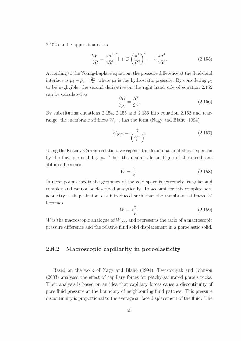
2.152 can be approximated as

∂V

∂R=πd4

4R2

[1 +O

(d2

R2

)]−→ πd4

4R2. (2.155)

According to the Young-Laplace equation, the pressure difference at the fluid-fluid

interface is p0 − pc =2γR, where p0 is the hydrostatic pressure. By considering p0

to be negligible, the second derivative on the right hand side of equation 2.152

can be calculated as∂R

∂pc=R2

2γ. (2.156)

By substituting equations 2.154, 2.155 and 2.156 into equation 2.152 and rear-

range, the membrane stiffness Wpore has the form (Nagy and Blaho, 1994)

Wpore =γ(

φsd2

8

) . (2.157)

Using the Kozeny-Carman relation, we replace the denominator of above equation

by the flow permeability κ. Thus the macroscale analogue of the membrane

stiffness becomes

W =γ

κ. (2.158)

In most porous media the geometry of the void space is extremely irregular and

complex and cannot be described analytically. To account for this complex pore

geometry a shape factor s is introduced such that the membrane stiffness W

becomes

W = sγ

κ. (2.159)

W is the macroscopic analogue ofWpore and represents the ratio of a macroscopic

pressure difference and the relative fluid solid displacement in a poroelastic solid.

2.8.2 Macroscopic capillarity in poroelasticity

Based on the work of Nagy and Blaho (1994), Tserkovnyak and Johnson

(2003) analysed the effect of capillary forces for patchy-saturated porous rocks.

Their analysis is based on an idea that capillary forces cause a discontinuity of

pore fluid pressure at the boundary of neighbouring fluid patches. This pressure

discontinuity is proportional to the average surface displacement of the fluid. The

55

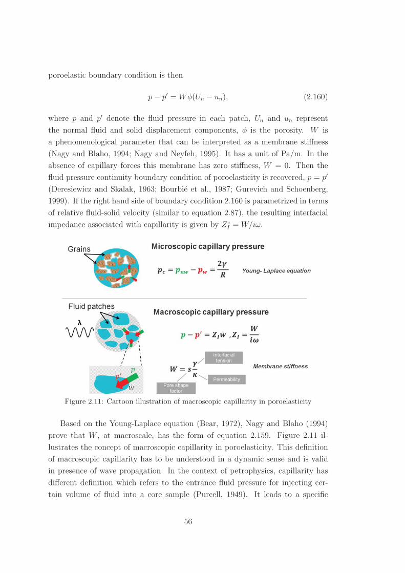
poroelastic boundary condition is then

p− p′ = Wφ(Un − un), (2.160)

where p and p′ denote the fluid pressure in each patch, Un and un represent

the normal fluid and solid displacement components, φ is the porosity. W is

a phenomenological parameter that can be interpreted as a membrane stiffness

(Nagy and Blaho, 1994; Nagy and Neyfeh, 1995). It has a unit of Pa/m. In the

absence of capillary forces this membrane has zero stiffness, W = 0. Then the

fluid pressure continuity boundary condition of poroelasticity is recovered, p = p′

(Deresiewicz and Skalak, 1963; Bourbie et al., 1987; Gurevich and Schoenberg,

1999). If the right hand side of boundary condition 2.160 is parametrized in terms

of relative fluid-solid velocity (similar to equation 2.87), the resulting interfacial

impedance associated with capillarity is given by ZcI = W/iω.

Figure 2.11: Cartoon illustration of macroscopic capillarity in poroelasticity

Based on the Young-Laplace equation (Bear, 1972), Nagy and Blaho (1994)

prove that W , at macroscale, has the form of equation 2.159. Figure 2.11 il-

lustrates the concept of macroscopic capillarity in poroelasticity. This definition

of macroscopic capillarity has to be understood in a dynamic sense and is valid

in presence of wave propagation. In the context of petrophysics, capillarity has

different definition which refers to the entrance fluid pressure for injecting cer-

tain volume of fluid into a core sample (Purcell, 1949). It leads to a specific

56

capillary-pressure-saturation relation (Bear, 1972). However, one must note that

both capillary pressures, namely the dynamic definition and the petrophysical

definition, have the same origin, that is due to the surface tension. The effect of

surface tension is characterized by Young-Laplace equation at microscopic scale,

i.e., pore scale.

The validity of 2.160 is established on theoretical and experimental grounds.

Nagy (1992) successfully use equation 2.160 to analyse his data on surface acous-

tic modes of fully saturated porous media. Tserkovnyak and Johnson (2003)

find that the membrane tension effectively seals the patches into distinct regions

so that fluid communication is impaired. This results in a fluid stiffening effect

yielding higher P-wave velocities. At the same time, WIFF across the patches

is diminished so that attenuation and dispersion become less pronounced. These

results have been also found by Markov and Levin (2007) using equation (2.160)

in a multiple scattering analysis for an assemblage of spherical poroelastic het-

erogeneities. However, none of these predictions has been verified by comparison

with experimental data. It is the purpose of this thesis to investigate the effects of

a non-zero membrane stiffnessW on the acoustic properties of partially saturated

rocks.

2.9 Other attenuation mechanisms

When the seismic waves travelling through the subsurface, it suffers the loss of

amplitude due to attenuation. Attenuation accompanied with velocity dispersion

occurs over a wide range of frequencies and scales from free oscillations of the

entire earth to ultrasound in small rock samples (Aki and Richards, 2002). A clas-

sification of the attenuation mechanism is illustrated in Figure 2.12. The cause

of attenuation and dispersion can be broadly divided into two categories: first,

geometrical effects, where the wavefield energy is conserved (scattering attenua-

tion, geometric spreading); second, absorption where wave energy is transformed

into heat. Absorption also referred as intrinsic attenuation reveals the proper-

ties of rock and pore fluids, therefore, it is of particular interest in the fields of

seismic interpretation and reservoir characterization. Besides wave-induced fluid

flow, intrinsic attenuation in porous media can also be caused by intergranular

friction, thermo-relaxation, change of chemical equilibrium, viscous shear relax-

ation, etc. Thorough reviews of these mechanisms can be found in the papers of

Johnston et al. (1979) and Bourbie et al. (1987). The main focus of this thesis

57

Figure 2.12: Classification of mechanisms responsible for loss of seismic amplitude.Coloured mechanisms are the main focus of this thesis.

is on how capillarity affects the attenuation mechanism due to mesoscopic fluid

flow and how capillarity affects the mode conversion, i.e., seismic reflectivity via

Biot global flow.

58

Chapter 3

Effects of interfacial impedance

on wave-induced pressure

diffusion

3.1 Summary

Seismic attenuation and dispersion in layered sedimentary structures are some-

times interpreted in terms of the classical White’s model for wave-induced pres-

sure diffusion across the layers. However, this inter-layer flow is severely de-

pendent on the properties of the interface separating two layers. This interface

behaviour can be described by a pressure jump boundary condition involving a

non-vanishing interfacial impedance. In this work, we incorporate the interfacial

impedance into the White’s model by solving a boundary value problem in the

framework of quasi-static poroelasticity. We show that White’s predictions for

attenuation and dispersion substantially change. These changes can be attributed

to petrophysically plausible scenarios such as imperfect hydraulic contacts or the

presence of capillarity.

59

3.2 Introduction

Nearly forty years ago White et al. (1975) presented a model for seismic

P-wave attenuation and dispersion for a periodically stratified medium with al-

ternating gas-water layers. The underlying attenuation mechanism is controlled

by pressure diffusion as a consequence of wave-induced pressure gradients across

the layers. Not only because of the relevance of partially saturated sediments for

exploration seismology, but also because of the insightful physical arguments they

used, their work continues to trigger research into wave propagation in porous

media. The White’s model has been reproduced within the framework of Biot’s

theory of poroelasticity (Biot, 1962) using different approaches (Markov and Yu-

matov, 1988; Norris, 1993). It has been subsequently specialized in order to ana-

lyze the effects of random layering (Gurevich and Lopatnikov, 1995; Muller and

Gurevich, 2004), inhomogeneous rock properties (Carcione and Picotti, 2006),

and embedded fractures with variable infill (Brajanovski et al., 2005; Kong et al.,

2013). The White’s model has been generalized to account for dissipation associ-

ated with the pressure diffusion at the wavelength scale (Vogelaar and Smeulders,

2007; Kudarova et al., 2013) and obliquely incident P- and SV-waves (Krzikalla

and Muller, 2011).

Key to the White’s model is the definition of a representative elementary vol-

ume (REV) encompassing the gas-water interface (Figure 3.1). At this interface

the continuity of the fluid pressure is assumed to hold throughout the fluid pres-

sure equilibration process, that is, from the onset of wave-induced fluid pressure

gradients to the final constant pressure once equilibrium is reached. This inter-

face condition is chosen in accordance with the open-pore boundary condition

of Dereciewicz and Skalak (1963). The latter is, however, an end member of a

more general, sometimes called natural boundary condition, wherein the pres-

sure jump across the interface is proportional to the relative fluid solid velocity

(Bourbie et al., 1987). This pressure jump boundary condition can be related

to petrophysically plausible scenarios (Dutta and Ode, 1979; Feng and Johnson,

1983). One is associated with a perturbed hydraulic contact across the inter-

face, as it may arise in the presence of non-load-bearing clay minerals clogging

the pore throats (Figure 3.1). A second scenario is related to the presence of

macroscopic capillarity, thereby creating a permanent pressure jump (Nagy and

Blaho, 1994). Therefore, the question arises how this pressure jump boundary

condition alters the predictions of the White’s model. From analogous problems

60

in thermal diffusion it is known that this kind of jump boundary conditions can

significantly alter the effective conductivity of heterogeneous structures (Cheng

and Torquato, 1997). Given that the White’s model is heavily used to interpret

seismic attenuation estimates (e.g., Morgan et al., 2012), any significant changes

may possibly entail important implications. Indeed, previous works indicate that

the pressure jump boundary condition associated with capillary action reduces

seismic attenuation (Tserkovnyak and Johnson, 2003; Markov and Levin, 2007).

Figure 3.1: Schematic representation of a homogeneous sandstone alternatively satu-rated by water and gas layers. The sketch at pore scale shows two possible interfacescenarios: A) clay minerals are clogging the hydraulic contact and B) meniscus unevenlydistributed due to capillarity.

The aim of this chapter is to incorporate the pressure jump boundary con-

dition into the White’s model in a general fashion so that both aforementioned

scenarios (and possibly other scenarios) can be modelled. To do so, we argue

that the proportionality coefficient of the pressure jump boundary condition can

be interpreted as an interfacial impedance. This interfacial impedance captures

the particular interface properties that cannot be assigned to the gas- or water-

saturated layer. We then solve the modified boundary value problem for the

double layer geometry within the framework of quasi-static poroelasticity. The

result is a generalized White’s model wherein the interfacial impedance appears

explicitly. Depending whether the interfacial impedance is a real- or complex-

valued quantity, new modelling choices arise and the differences with respect to

the original White’s model predictions are worked out.

61

3.3 Theory

3.3.1 Background: White’s model and interfacial impedance

White et al. (1975) determine the effective, frequency-dependent P-wave mod-

ulus H(ω) for a periodically layered system composed of porous layers alternately

saturated with gas and water. Their approach consists in solving a boundary

value problem for the REV with spatial semi-period l = (da + db), as illustrated

in Figure 3.1. Therein the action of the P-wave is simulated through a harmoni-

cally oscillating compression Peeiωt. The resulting ratio of vertical component of

the average strain to stress is (White el al., 1975; their equation 14)

1

H=

1

Hnf+

1

Hff. (3.1)

HereinHnf is the P-wave modulus when fluid exchange between consecutive layers

is not permitted (hence the superscript “nf” for no-flow), as is the case when

there is not enough time for the fluid pressure to equilibrate. Thus, Hnf can

be interpreted as the high-frequency, or unrelaxed, limit. It is obtained from

Backus averaging with the individual, undrained P-wave moduli calculated using

Gassmann’s equation (Gelinsky and Shapiro, 1997)

1

Hnf=

⟨1

H

⟩. (3.2)

The angle brackets denote the volumetric, or saturation-weighted, average 〈x〉 =(daxa + dbxb)/l. According to the Biot-Gassmann theory the undrained P-wave

modulus is given by H = L+ α2M , where L = K0 + 4μ/3 is the drained P-wave

modulus, α = 1 − K0/Ks the Biot-Willis coefficient, and M = ((α − φ)/Ks +

φ/Kf)−1 the fluid storage modulus. Ks and K0 denote the bulk moduli of the

solid grains and of the dry frame. The porosity is φ and the frame shear modulus

is μ.

The second term of the right-hand side (RHS) of equation 3.1 accounts for

fluid pressure diffusion across the layers, thereby reducing the overall stiffness of

the medium. As this is a transient process, Hff turns out to be complex-valued

62

and frequency-dependent,

1

Hff=

1

iωl

(Ba − Bb)2

Za − Zb

≡ 1

iωl

(ΔB)2

ΔZ. (3.3)

This inter-layer flow term has a simple interpretation. The (uni-axial) Skempton

coefficient B quantifies the fluid pressure built-up induced by the external loading

Pe under undrained condition, that is, when the fluid increment ξ is zero

B =∂pnf

f

∂Pe

∣∣∣ξ=0

=αM

H. (3.4)

Only if there is a contrast in the induced fluid pressures, or equivalently ΔB �= 0,

fluid pressure diffusion can take place. This diffusion process is also controlled

by the impedance contrast ΔZ. Herein, the diffusional impedance is defined as

the ratio of the fluid pressure associated with Biot slow P-wave and the normal

component of the relative fluid-solid velocity vn at the interface

Z =pfff

vn

∣∣∣x=0

= ±coth(ksd)

κks. (3.5)

We assume that the unit normal points from layer ‘b’ to layer ‘a’. Thus, the sign

of the diffusional impedance is positive for layer ‘a’ and negative for layer ‘b’.

The impedance entails the pressure diffusion wave number associated with Biot’s

slow P-wave number. In the quasi-static approximation this wave number is ks ≡√iω/Dp with the diffusivity Dp = κN . Herein κ is the hydraulic conductivity

given by the ratio of permeability and fluid shear viscosity and N =M(1−αB).

It is important to notice that equation 3.5 is independent of the properties of the

interface, that is, the condition of fluid pressure continuity across the boundary

is not used to obtain this expression.

From the above considerations it becomes clear that the induced fluid pressure

difference across the interface is central to initiate inter-layer flow. It also means

that interlayer flow is sensitive to the continuity of the pressure at the interface. In

Biot ’s theory of poroelasticity the pressure at the interface is generally described

by (Dereciewicz and Skalak, 1963; Bourbie et al., 1987)

pfa|x=0 − pfb|x=0 = −ZIvn|x=0 . (3.6)

It relates the pressure jump across the interface with the relative fluid-solid veloc-

63

ity. The proportionality coefficient ZI is called the resistance coefficient. If there

is no resistance, ZI = 0, the layers are in perfect hydraulic contact. Then, the

so-called “open-pore boundary condition” is satisfied and the pressure is contin-

uous across the interface. Conversely, for any finite ZI �= 0 there exists a pressure

jump, whereas for ZI → ∞ no pressure equilibration can take place. In general,

ZI can be interpreted as an interfacial impedance assigning a particular property

to the interface. It may even have a reactance term (Im{ZI} �= 0), as discussed

further below. In the next section we show how this interfacial impedance can be

incorporated in the derivation of an effective P-wave modulus.

3.3.2 Effective strain for finite interfacial impedance

We base the derivation on the quasi-static poroelasticity equations (see section

2.4, eqs. 2.71, 2.72). In the space-frequency domain they are given by

∂τxx∂x

= 0, (3.7)

∂pf∂x

= − iωκw , (3.8)

where τxx is the total stress, pf the fluid pressure, and w = v/iω the average

relative fluid displacement per unit volume of bulk material. Equations 3.7 and

3.8 represent stress equilibrium and Darcy’s law, respectively. They are coupled

through the constitutive relations

τxx =H∂u

∂x+BH

∂w

∂x, (3.9)

pf = −BH∂u

∂x−M

∂w

∂x, (3.10)

with u being the average displacement of the solid phase.

For a homogeneous medium, equations 3.7 to 3.10 can be combined such that

the governing equation for w becomes

∂2w

∂ x2=iω

Dp

w. (3.11)

This means that the out-of-phase movement between the fluid and solid phases,

which is associated with the Biot slow P-wave, is governed by diffusion. The

64

solution for the considered REV can be written as

wi =2∑

γ=1

Ai,γ exp{(−1)γksix}, i = a, b, (3.12)

with Ai,γ being complex constants. Since the equation of equilibrium (3.7) im-

plies that the stress is constant throughout the REV and equal to the applied

compression, τxx = −Pe, we write the remaining poroelastic fields as

ui = −Biwi − Pe

Hi

x+ Ei, (3.13)

pfi = BiPe −Ni∂wi

∂x, i = a, b, (3.14)

where Ei are two additional unknowns. For the REV under uni-axial deformation,

the resulting overall strain and the effective plane wave modulus are defined by

exx =(ua|x=da − ub|x=−db)/l , (3.15)

H(ω) = −Pe/exx . (3.16)

To uniquely determine the overall strain, another five equations are needed.

These equations are obtained by choosing appropriate boundary conditions. Due

to symmetry, we impose no-flow conditions at the boundaries of the REV

va|x=da = vb|x=−db = 0 . (3.17)

In addition, we require continuity of solid displacement and relative fluid-solid

velocity at the interface

ua|x=0 = ub|x=0 , (3.18)

va|x=0 = vb|x=0 . (3.19)

The fifth boundary condition is provided by the partially open boundary condition

3.6. It can be written in decomposed form as

pnf

fa+ pff

fa= pnf

fb+ pff

fb− ZIvn , (x = 0) (3.20)

where we interpret the pressure as pf = pnf

f+ pff

f.

65

The first term on the RHS of equation 3.14 quantifies the fluid pressure when

fluid flow across the interface is not permitted, that is, pnffi = BiPe. The sec-

ond term describes the fluid pressure in presence of pressure diffusion, that is,

pfffi = −Ni

∂wi

∂x. The associated diffusional impedance can be computed from the

definition (3.5) by applying boundary condition (3.17).

Next, we compute the overall effective strain by substituting equation 3.13

into 3.15 and making use of boundary conditions 3.18 and 3.19. We obtain

exx = −(daHa

+dbHb

)Pe

l︸ ︷︷ ︸enf

+Ba − Bb

iωlvn|x=0︸ ︷︷ ︸

eff

. (3.21)

Equation (3.21) for the overall strain can be understood if, similarly to the pres-

sure decomposition, the strain is represented as the sum of e = enf + eff . If solid

and fluid phases move in-phase or, equivalently, v = 0, then the second term

on the RHS of equation 3.21 vanishes, and thus the remaining term corresponds

to the effective strain associated with no-flow condition, enf = −〈H−1〉Pe. If

v �= 0, the overall effective strain consists of two terms, wherein the second term

corresponds to the additional strain in presence of pressure diffusion, eff .

Employing equations 3.5, 3.19 in equation 3.20 yields the relative fluid-solid

velocity at the interface

vn|x=0 = − Ba −Bb

Za − Zb + ZI

Pe . (3.22)

This equality shows that the presence of resistance coefficient ZI reduces the rel-

ative fluid-solid velocity. Making use of the extended relative fluid-solid velocity

(3.22) in equation 3.21, we obtain the effective strain associated with the diffusion

process

eff = − (Ba − Bb)2

iωl(Za − Zb + ZI)Pe. (3.23)

The overall effective strain can now be computed via summation of the component

related to no flow across the interface, enf , and the contribution produced by fluid

pressure diffusion between the layers, eff .

66

3.3.3 Generalized White’s model

The undrained P-wave modulus is obtained by substituting the overall effec-

tive strain into equation 3.16. Therefore,

1

H=

⟨1

H

⟩+

1

iωl

(ΔB)2

ΔZ + ZI

. (3.24)

This effective, undrained P-wave modulus is the main result of this chapter. The

interfacial impedance appears in the denominator of the inter-layer flow term

and adds to the impedance contrast ΔZ. If the interfacial impedance vanishes,

ZI = 0, then equation 3.24 reduces to the P-wave modulus given by White et al.

(1975; their equation 14). This shows that the fluid pressure continuity boundary

condition is rooted in White’s model.

This generalized White’s model can be used to characterize P-wave dispersion

and attenuation in partially saturated media wherein the interface separating

the two fluid phases possesses specific properties. As originally envisaged by

Deresiewicz and Skalak (1963) the partially open boundary condition (3.6) models

a perturbed hydraulic contact. Then the interfacial impedance is real-valued,

that is, it has the character of a resistance. It will be denoted as ZmI . Another

scenario is related to the presence of capillary forces. The pressure jump boundary

condition is then (Nagy and Blaho, 1994)

pfa|x=0 − pfb|x=0 = −Wiωvn |x=0, (3.25)

where W (Pa/m) is the so-called membrane stiffness, which controls the capil-

larity reinforcement. In this representation of the pressure jump condition, the

interfacial impedance is an imaginary number, and is given by ZcI = −iW

ω. That

is, it has the character of a reactance. In the following we focus on the implica-

tions on seismic attenuation and dispersion for these two scenarios.

3.4 Attenuation and dispersion

Attenuation and dispersion can be obtained from equation 3.24 via Q−1 =

Im(H)/Re(H) and VP = (Re(1/Vpc))−1, where the complex P-wave velocity is

Vpc =√H/ρ. The effective density ρ is given by the volumetric average of

the grain and fluid densities. Depending on the physical interpretation of the

67

interfacial impedance new predictions for attenuation and dispersion emerge. We

restrict the analysis of the results to the two scenarios mentioned above. In

the first case the interfacial impedance has a resistance term only, while in the

second case it is given by a reactance term. The mechanical properties of the

rock and fluids for calculating the velocity and attenuation are given in Table 3.1.

The corresponding attenuation and dispersion behaviours for a gas saturation of

S = 50% are shown in Figure 3.2. Here the saturation is computed according to

Si = di/l with l = 0.2 m.

Sand FluidsK0 (GPa) 7 Kfa (GPa) 2.25μm (GPa) 9 ρfa (g/cm3) 0.99Ks (GPa) 35 ηfa (Pa s) 1e-3ρs (g/cm

3) 2.65 Kfb (GPa) 0.1φ 0.15 ρfb (g/cm3) 0.1κ0 (m2) 1e-13 ηfb (Pa s) 3e-5

Table 3.1: Mechanical properties of rock and fluids

The red and blue families of curves correspond to the resistance and reac-

tance scenario, respectively, and the original White’s prediction is indicated by

the black curves. We note that in these numerical examples the White’s model

predictions lose their validity at very high frequencies, as then the wavelength be-

comes comparable to the layer thickness. However, to illustrate the asymptotic

characteristics, we show velocity and attenuation up to a frequency of 0.1 MHz.

Two distinct behaviours can be observed. The resistance term causes the dis-

persion curve to shift towards lower frequencies with increasing resistance. The

dispersion window remains unchanged and is bounded by the Gassmann-Wood

(GW) and Gassmann-Hill (GH) predictions. Accordingly, the attenuation peak

is shifted to lower frequencies. This shifting behavior can be understood as a

consequence of the delay the imperfect hydraulic contact imposes on the pressure

equilibration process. In other words, a real-valued interfacial impedance can be

interpreted as the reciprocal of an interface permeability ZmI = 1/κI (Gurevich

and Schoenberg, 1999). Since the characteristic frequency of the White’s model

ωc = κ0N/ηl2 is proportional to the permeability κ0 of the rock. An decreasing

interface permeability κI (increasing interfacial impedance ZmI ) results in a de-

creasing effective permeability κ0 of the rock. Consequently, the characteristic

frequency of the attenuation and dispersion shifts towards the lower frequen-

68

(a)

100

101

102

103

104

105

2900

2950

3000

3050

3100

Frequency [Hz]

V p [m/s

]

WhiteHWMCWMNum

ZIm

4.5 1.5 0.5

GH

GW

CS

W25

10

40

(b)

100

101

102

103

104

105

10−6

10−5

10−4

10−3

10−2

10−1

Frequency [Hz]

Q−1

WhiteHWMCWMNum

50150

350

WZ

Im

4.5 1.5 0.5

Q−1∝ω−1

Q−1∝ω−1/2

Figure 3.2: Phase velocity and inverse quality factor as functions of frequency for ahomogeneous rock alternately saturated with gas and water. “HWM” refers to gener-alised White model with imperfect hydraulic contact, whereas “CWM” indicates thecapillarity extended White model. The values of resistance Zm

I and membrane stiffnessW are given in units of GPa · s/m and GPa/m, respectively.

cies. It is also interesting to note that the high-frequency attenuation asymptote

changes from Q−1 ∝ ω−1/2 for the White’s prediction to Q−1 ∝ ω−1. This change

in asymptotic behaviour is attributed to the fact that, in the presence of im-

perfect hydraulic contacts, the distance over which the pressure gradients are

69

equilibrated has effectively increased (Muller et al., 2010).

(a)

0 0.2 0.4 0.6 0.8 12900

2950

3000

3050

3100

3150

3200

3250

3300

3350

Sw

V p [m/s

]

WhiteHWMCWM

W=150

ZIm=0.3

ZIm=2

GW

W=30

GH

(b)

0 0.2 0.4 0.6 0.8 10

0.01

0.02

0.03

0.04

0.05

0.06

0.07

Sw

Q−1

WhiteHWMCWM Z

Im=0.3

W=30

ZIm=2

W=150

Figure 3.3: Velocity- and attenuation-saturation relations for a frequency of 25 Hz. Thevalues of the resistance Zm

I and membrane stiffness W are given in units of GPa · s/mand GPa/m, respectively.

The reactance term manifests differently. In this case, the pressure jump at

the interface effectively reduces the wave-induced pressure gradient across the

layers. Accordingly, the effects of wave-induce pressure diffusion become less

pronounced so that dispersion and attenuation are reduced. In essence, the sur-

70

face tension between two immiscible fluids perturbs the energy redistribution (or

mode conversion process) across the interface (Markov, 2009), thereby creating

a change of attenuation. In the capillarity interpretation of interface condition

(3.25), an increasing membrane stiffness W increases the low-frequency limiting

velocity above the GW prediction. The new capillarity-extended static (CS) limit

is given by (this will be shown in the next chapter)

H∗1D =

z + Tz

HGW+

T

HGH

, z =

⟨N

S2

⟩, T = Wl . (3.26)

We also validate the capillarity-extended model by numerically solving a bound-

ary value problem. The numerical results displayed by circles coincide with the

model prediction.

As the present modelling refers to partially saturated layered media, it is also

instructive to analyse the velocity- and attenuation-saturation relations. The

velocity-saturation relations (VSRs) at fixed frequency (25 Hz) for both scenar-

ios are shown in Figure 3.3a. It can be observed that both, the resistance and

reactance terms, cause a deviation from the White’s prediction towards the GH

behaviour, thereby increasing the overall stiffness of the layered system. How-

ever, this is due to different reasons. In the resistance scenario, it is the shifting

behaviour that is responsible for an increased velocity at fixed finite frequency.

In the reactance scenario, the imposed pressure jump is permanent and adds

to the overall stiffness. The attenuation-saturation relation (ASR) is shown in

Figure 3.3b. Attenuation first increases with increasing resistance as the chosen

frequency is below the characteristic frequency. For further increased resistance,

the attenuation starts to decline significantly and a broadened peak can be ob-

served.

3.5 Poroelastic fields

3.5.1 Full Biot’s solution

Beyond attenuation and dispersion, it is also meaningful to analyse the re-

sulting poroelastic fields associated with the pressure jump boundary conditions.

In order to analyse the contributions from fast and slow P-wave on the poroe-

lastic fields equivalently, we invoke low frequency Biot’s dynamic equations for

71

compressional waves (see section 2.6.2, eq. 2.106)

d

dz

(Hdu

dz+ C

dw

dz

)+ ω2(ρu+ ρfw) = 0 ,

d

dz

(Cdu

dz+M

dw

dz

)+ ω2(ρfu+ qw) = 0 , (3.27)

where the friction coefficient is

q =ρfS

∞

φ− iη

ωκ0. (3.28)

For a plane wave traveling along x-axis direction, the displacement fields have

the following solutions

ux = Φ1 exp [i(ωt− kx)] , (3.29)

wx = Φ2 exp [i(ωt− kx)] . (3.30)

Introducing the ansatz 3.29 into the wave equations 3.27 and eliminating the

amplitude constants Φ1, Φ2 we obtain the dispersion relation

V 2f,s =

−Δ±√Δ2 − 4(ρq − ρ2f )(HM − C2)

2(ρq − ρ2f ), (3.31)

where Δ = 2ρfC−ρM−qH. The fast and slow P-wavenumbers are calculated via

kf,s =√ω2/V 2

f,s. The amplitude ratio between the relative and solid displacement

reads

λf,s =Φ2

Φ1

=H − ρV 2

f,s

ρfV 2f,s − C

. (3.32)

Alternatively, solutions of solid and relative displacements written in terms of

fast and slow P-wave components are

uxi = A±fi exp (∓ikfix) + A±

si exp (∓iksix), (3.33)

wxi = λfiA±fi exp (∓ikfix) + λsiA

±si exp (∓iksix). (3.34)

The subscript i defines the associated property in the i-th layer of the REV.

Substituting 3.33, 3.34 into the equations 3.13 and 3.14, we obtain the decom-

posed solutions for total stress and fluid pressure. The poroelastic fields consist

of totally eight unknowns A±fi , A

±si (i = 1, 2). On top of previously introduced

five boundary conditions, i.e., equations 3.17-3.20, three addition boundary con-

72

ditions for the stress field are needed

τa|x=0 = τb|x=0 , (3.35)

τa|x=da = −Pe , (3.36)

τb|x=−db = −Pe . (3.37)

Thus, a linear system of eight equations I8×8 × A8×1 = G8×1 can be solved

numerically to yield the resulting dynamic fields under wave propagation. In

the present context, an additional poroelastic field which is dynamic capillary

pressure can be defined as

Pc(ω) = pfa(ω)|x=0 − pfb(ω)|x=0 . (3.38)

Pc(ω) can be interpreted as capillary pressure when it is associated with the cap-

illary boundary condition 3.25. Otherwise, it can be understood as general pres-

sure jump in the presence of discontinuity interface condition such as described by

equation 3.20. To explore the contrasting attenuation behaviour resulting from

different types of pressure jump boundary conditions, we also look into the dis-

sipation. According to Johnson (2001), the dissipated power averaged over one

wave cycle is given by

P = −1

2

∫Re(w∗ · ∇pf)dV , (3.39)

where * indicates the complex conjugate. If we define the average strain energy

over one wave period T as

W =1

2T

∫ ∫(τijeij − pfε)dV dt . (3.40)

Then, the attenuation (within low-loss media assumption) can be calculated via

(Bourbie et al., 1987)

Q−1(ω) =1

2ω

F [P ]

F [W ], (3.41)

where operator F denotes the Fourier transform F (ω) =∫ +∞−∞ f(t) exp(−iωt)dt.

73

3.5.2 Numerical results

It is evident from Figure 3.4 that the existence of pressure jump across the

fluid-fluid interface when capillarity is taken into account. On the other hand,

open-pore interface condition presents a continuous fluid pressure across the in-

terface. The contribution from fast P-wave to the fluid pressure is piecewisely

constant within each fluid phase according to Figure 3.4a,b. Comparing Figure

3.4a,b and Figure 3.4c,d, the fluid pressure due to fast P-wave has no imaginary

component but real component. This confirms that fast P-wave is non-diffusive

at the two considered frequencies, namely 50 Hz and 300 Hz. The imaginary part

of the pressure component is solely caused by slow P-wave. The liquid phase

always supports higher pressure components because of the high Skempton’s co-

efficient. At higher frequencies, the pressure amplitude (Figure 3.4e,f) transits

more sharply from the liquid phase into the gas phase. The net pressure jump be-

comes smaller at higher frequency according to Figure 3.4f and the two scenarios

(open-pore and capillarity) start to merge. The solid displacement field is plotted

in Figure 3.5. Both fast and slow P-wave components are discontinuous across

the interface regardless of the condition of fluid pressure (whether it is open-pore

or capillarity). According to Figure 3.5e,f, the amplitude of displacement field is

continuous across the interface. Also capillarity plays a negligible role on solid

displacement regardless of frequency.

Figure 3.6 shows the profile of relative fluid-solid displacement. The fast P-

wave does not contribute to this field at the two employed frequencies. This

indirectly indicates that relative displacements at the two considered frequencies

obey a diffusion equation. The diffusive character of slow P-wave is reflected by

the net value of the relative displacement. Capillarity results in smaller rela-

tive displacement between fluid and solid comparing to the open-pore situation.

However, this difference becomes smaller at higher frequency. The behaviour of

relative displacement, to a certain degree, explains the attenuation behaviour in

presence of capillarity shown in Figure 3.2.

The dynamic (or wave-induced) capillary pressure is plotted in Figure 3.7a

as function of water saturation for difference frequencies. The capillary pressure

according to our definition 3.38, depends on both frequency ω and amplitude |Pe|of the external loading Pee

iωt. The resulting capillary pressure saturation relation

looks apparently different from what is being typically measured in the lab (see

74

(a)

-0.1 -0.05 0 0.05 0.1-0.4

-0.2

0

0.2

0.4

Position [m]

Re(

p f)/Pe

f=50 Hz

P IP IIP I+P II

(b)

-0.1 -0.05 0 0.05 0.1-0.4

-0.2

0

0.2

0.4

Position [m]

Re(

p f)/Pe

f=300 Hz

P IP IIP I+P II

(c)

-0.1 -0.05 0 0.05 0.1-0.1

-0.05

0

0.05

0.1

0.15

0.2

0.25

Position [m]

Im(p

f)/Pe

f=50 Hz

P IP IIP I+P II

(d)

-0.1 -0.05 0 0.05 0.1-0.04

-0.02

0

0.02

0.04

0.06

0.08

0.1

Position [m]

Im(p

f)/Pe

f=300 Hz

P IP IIP I+P II

(e)

-0.1 -0.05 0 0.05 0.10

0.1

0.2

0.3

0.4

Position [m]

abs(

p f)/Pe

f=50 Hz

Open-poreCapillarity

(f)

-0.1 -0.05 0 0.05 0.10

0.1

0.2

0.3

0.4

Position [m]

abs(

p f)/Pe

f=300 Hz

Open-poreCapillarity

Figure 3.4: The real part (a), imaginary part (c) and amplitude (e) of fluid pressureat 50 Hz while (b),(d),(f) show their high frequency (300 Hz) counterpart. The bluecolour refers to open-pore case whereas red colour refers to capillarity case. The dashedline refers to fast P-wave component whereas the circle corresponds to slow P-wavecomponent. The total component is indicated by solid line.

Brooks and Corey (1964) for example). The latter takes on a petrophysical

meaning and refers to the entrance fluid pressure for injecting certain volume of

fluid into a core sample (Purcell, 1949). Nevertheless, one must note that both

75

(a)

-0.1 -0.05 0 0.05 0.1-60

-40

-20

0

20

40

60

Position [m]

Re(

u) [1

0-13 m

]

f=50 Hz

P IP IIP I+P II

(b)

-0.1 -0.05 0 0.05 0.1-50

0

50

Position [m]

Re(

u) [1

0-13 m

]

f=300 Hz

P IP IIP I+P II

(c)

-0.1 -0.05 0 0.05 0.1-6

-4

-2

0

2

Position [m]

Im(u

) [10

-13 m

]

f=50 Hz

P IP IIP I+P II

(d)

-0.1 -0.05 0 0.05 0.1-2

-1.5

-1

-0.5

0

0.5

1

Position [m]

Im(u

) [10

-13 m

]f=300 Hz

P IP IIP I+P II

(e)

-0.1 -0.05 0 0.05 0.10

10

20

30

40

50

60

Position [m]

abs(

u) [1

0-13 m

]

f=50 Hz

Open-poreCapillarity

(f)

-0.1 -0.05 0 0.05 0.10

10

20

30

40

50

Position [m]

abs(

u) [1

0-13 m

]

f=300 Hz

Open-poreCapillarity

Figure 3.5: The real part (a), imaginary part (c) and amplitude (e) of solid displacementat 50 Hz while (b),(d),(f) show their high frequency (300 Hz) counterpart. The bluecolour refers to open-pore case whereas red colour refers to capillarity case. The dashedline refers to fast P-wave component whereas the circle corresponds to slow P-wavecomponent. The total component is indicated by solid line.

capillary pressure, namely the dynamic definition or the petrophysical definition,

has the same origin which is due to the surface tension.

76

(a)

-0.1 -0.05 0 0.05 0.1-20

-15

-10

-5

0

5

Position [m]

Re(

wn) [

10-1

3 m]

f=50 Hz

P IP IIP I+P II

(b)

-0.1 -0.05 0 0.05 0.1-6

-4

-2

0

2

Position [m]

Re(

wn) [

10-1

3 m]

f=300 Hz

P IP IIP I+P II

(c)

-0.1 -0.05 0 0.05 0.1-5

0

5

10

15

Position [m]

Im(w

n) [10

-13 m

]

f=50 Hz

P I

P II

P I+P

II

(d)

-0.1 -0.05 0 0.05 0.1-1

0

1

2

3

4

5

6

Position [m]

Im(w

n) [10

-13 m

]

f=300 Hz

P I

P II

P I+P

II

(e)

-0.1 -0.05 0 0.05 0.10

5

10

15

20

25

Position [m]

abs(

wn) [

10-1

3 m]

f=50 Hz

Open-poreCapillarity

(f)

-0.1 -0.05 0 0.05 0.10

2

4

6

8

Position [m]

abs(

wn) [

10-1

3 m]

f=300 Hz

Open-poreCapillarity

Figure 3.6: The real part (a), imaginary part (c) and amplitude (e) of relative dis-placement at 50 Hz while (b),(d),(f) show their high frequency (300 Hz) counterpart.The blue colour refers to open-pore case whereas red colour refers to capillarity case.The dashed line refers to fast P-wave component whereas the circle corresponds to slowP-wave component. The total component is indicated by solid line.

The pressure difference associated with capillarity and imperfect hydraulic

contact (IHC) are plotted as function of frequency in Figure 3.7c. The capil-

lary pressure decreases with increasing frequency whereas the pressure difference

77

(a)

0 0.2 0.4 0.6 0.8 10

0.02

0.04

0.06

0.08

0.1

0.12

Sw

abs(

P c)/Pe

f=50 Hzf=300 Hzf=1000 Hz

(b)

-0.1 -0.05 0 0.05 0.1-2

0

2

4

6

8x 10-12

Dis

sipa

tion

f=10 Hz

Open-poreCapillarityIHC

(c)

100 101 102 103 104 1050

0.05

0.1

0.15

0.2

0.25

0.3

0.35

Frequency [Hz]

abs(

P c)/Pe

CapillarityIHC

(d)

-0.1 -0.05 0 0.05 0.1-0.5

0

0.5

1

1.5

2

2.5

3x 10-11

Dis

sipa

tion

f=100 Hz

Open-poreCapillarityIHC

(e)

100 101 102 103 104 1050

1

2

3

4x 10-12

Frequency [Hz]

abs(

wn) a

t x=0

CapillarityIHC

(f)

-0.1 -0.05 0 0.05 0.10

1

2

3

4

5

6x 10-11

Position [m]

Dis

sipa

tion

f=300 Hz

Open-poreCapillarityIHC

Figure 3.7: (a) Capillary pressure is plotted as function of water saturation for differentfrequencies. (c) Pressure difference and relative displacement at interface (e) are plottedas function of frequency. Dissipation at frequency of 10 Hz (a) 100 Hz (b) and 300 Hz.

due to IHC increases. Figure 3.7e shows the corresponding relative displacement

at the interface. As can be seen, both capillarity and IHC result in decreasing

relative displacement with increasing frequency. Last but not the least, the dissi-

pation resulting from capillarity and IHC is examined in Figure 3.7b,d,f for three

78

different frequencies. The dissipation due to capillarity is always smaller than

that for the open-pore scenario. On the other hand, dissipation due to IHC is

highest at low frequency and it decreases with increasing frequency. The charac-

teristics of the dissipation clearly explains the observed attenuation behaviours

in Figure 3.2.

3.6 Chapter conclusions

A pressure jump boundary condition has been incorporated into the expression

for the effective P-wave modulus of a partially saturated porous medium, which

appears in form of an interfacial impedance (equation 3.24). This generalizes the

original White’s model wherein continuity of the fluid pressure at the gas-water

interface is implicitly assumed.

Imperfect hydraulic contacts across fluid patches do not alter attenuation and

dispersion in magnitude, but only decrease the characteristic frequency. It can be

explained by that the imperfect hydraulic contacts give rise to an interface per-

meability which reduces the effective permeability of the rock, and consequently

the characteristic frequency. Therefore, if one infers the size of fluid patches from

attenuation estimates based on the original White’s model, there will be a bias to-

wards overestimating the patch size. Correspondingly, relating a measured wave

velocity to saturation can result in substantial misinterpretation (e.g., in Figure

3.3a the proximity to the GH bound is unrelated to the fluid patch size). This

might have important implications for understanding the role of interlayer flow

in sand-shale sequences. Similarly, these results may have impact in estimations

of permeability from seismic signatures.

The effect of capillarity on inter-layer flow can be modelled by an imaginary

interfacial impedance. This membrane stiffness leads to an elevated low-frequency

velocity and decrease in attenuation. The presence of interfacial impedance signif-

icantly changes the dynamic poroelastic fields, i.e., fluid pressure, relative fluid-

solid displacement. Consequently, it affects the dissipation resulting from the

oscillatory fluid flow and explains the attenuation behaviours.

Since capillary forces control the formation of fluid patches (Zhang et al.,

2014), the generalized White’s model can be useful in the assessment of the

corresponding acoustic signatures in laboratory settings. The developed model

79

can be further extended to the study of inhomogeneous rock formations. This is of

particular interest if, in addition to fluid saturation, aligned fractures complicate

the analysis of attenuation (Amalokwu et al., 2014).

In conclusion, the generalized White’s model for seismic attenuation and dis-

persion generates new modelling choices arising in the presence of an interfacial

impedance. Though the underlying periodic double layer geometry may, in cer-

tain cases, be too simple to resemble real sedimentary records, the generalized

model provides further insight into attenuation and dispersion due to inter-layer

flow.

80

Chapter 4

Quantifying the effect of

capillarity on attenuation and

dispersion in patchy-saturated

rocks

4.1 Summary

Waves in patchy-saturated rocks are attenuated through the mechanism of

wave-induced pressure diffusion. We have shown in the last chapter that the

characteristics of wave-induced pressure diffusion can be affected by the capil-

lary pressure. On the other hand, previous studies revealed that attenuation and

phase velocity dispersion can also depend on the fluid patch size and distribu-

tion. These patch characteristics in turn can be influenced by capillary forces.

In this chapter, we investigate the combined effects of fluid distribution and cap-

illarity on acoustic signatures. To do so we make use of the concept of patch

membrane stiffness as a macroscopic expression of capillarity. We incorporate

the membrane stiffness into the continuous random media model of patchy sat-

uration. The membrane stiffness is associated with a pressure discontinuity at

patch interfaces. This pressure discontinuity impedes wave-induced pressure dif-

fusion and, therefore, reduces wave attenuation. Conversely, the phase velocity

increases due to additional capillarity reinforcement. We apply this capillarity-

81

extended random media model to interpret velocity- and attenuation-saturation

relations retrieved from an ultrasonically monitored core flooding experiment. As

the fluid distribution is approximately known from accompanying computerized

tomographic images, all but one required model input parameters can be inferred.

The elusive input parameter is a shape factor quantifying the geometrical irreg-

ularity of the pore channels. We find, however, that the experimental data can

be consistently modeled only if the capillarity effect is accounted for. The re-

sults suggest that wave-induced fluid pressure diffusion at mesoscopic patches in

conjunction with capillary action can have important implication for interpret-

ing ultrasonic velocity- and attenuation-saturation relations in patchy-saturated

rocks.

4.2 Introduction

Quantification of seismic wave velocities in fluid-saturated, reservoir rocks and

their variations due to production-induced saturation changes are of prime impor-

tance in seismic time-lapse studies (Calvert, 2005). However, seismic velocities

do not only depend on the degree of saturation of each fluid phase but also on

their spatial distribution. This observation is corroborated by laboratory exper-

iments involving different measurement techniques (Murphy et al., 1984; Knight

and Nolen-Hoeksema, 1990; Cadoret et al., 1995; Monsen and Johnstad, 2005;

Alemu, 2012). Two end-member scenarios are typically employed to model the

velocity-saturation relation (VSR). Uniform saturation refers to fluid mixing at

the smallest scale, say pore-scale, whereas patchy saturation assumes the exis-

tence of sub-wavelength-scale fluid pockets. The P-wave velocity in the patchy-

saturated case is larger than for the uniform saturation case (Mavko and Mukerji,

1998). Analysis of experimental data shows that the velocities often are between

these uniform and patchy bounds (Shi et al., 2007; Caspari et al., 2011). One

mechanism that explains the deviation from these bounds is broadly known as

mesoscopic wave-induced fluid flow (WIFF, see Muller et al., 2010 for a review).

It entails an oscillatory, relative fluid-solid movement induced by seismic waves

and results in wave attenuation and dispersion due to dissipation. The magnitude

of attenuation and dispersion in partially saturated rocks depends on the fluid

compressibility contrast. So, one can expect significant attenuation if oil and gas

is heterogeneously distributed, while little attenuation is expected for low com-

pressibility contrast combination, e.g., oil and water. In turn, the characteristic

frequency of WIFF attenuation and dispersion is controlled by the fluid mobility,

82

i.e., the ratio of permeability and fluid viscosity, and the characteristic length

scale of the fluid patches. Modelling and interpretation of VSRs and associated

WIFF attenuation and dispersion due to mesoscopic heterogeneities has been ad-

dressed in several studies (Tserkovnyak and Johnson, 2001; Pride et al., 2004;

Toms et al., 2007a; Muller et al., 2008; Lei and Xue, 2009; Rubino and Holliger

2012; Tisato and Quintal, 2013).

A recent series of laboratory experiments allows us to gain further insights

into the formation of fluid patches during forced water imbibition into air-dry

rock samples and the accompanying evolution of ultrasonic P-wave velocity with

saturation (Lebedev et al., 2009; Lopes and Lebedev, 2012; Lopes et al., 2014).

X-ray computer tomography scans yield saturation images for the ultrasonically

monitored rock volume during the course of water imbibition. These saturation

images suggest that fluid patches are formed at the millimetre-scale. As these

patches extend over the pore spaces in between several grains but are smaller than

the dominant ultrasonic wavelength, we will refer to them as mesoscopic fluid

patches. Theoretical and experimental works of two-phase flow associated with

imbibition suggest that the fluid distribution for immiscible flows is controlled

by the interplay between viscous and capillary forces. Specifically, the relative

importance of the capillary effect can be quantified by either the capillary number

(see equation 1.1) or the critical flow ratio (see equation 1.2). In the experiments

of Lopes et al. (2014), the capillary number and the critical flow ratio are on the

order of 10−9 and 10−3, respectively. Therefore, both the numbers indicate that

flow regime during the forced imbibition is dominated by capillary forces.

The capillary force underpinning saturation distribution has been implemented

by Knight et al. (1998) and Rubino and Holliger (2012) to study the effect of fluid

patches on seismic signatures of WIFF. The direct effect of capillarity on acous-

tic properties itself is neglected in these works. However, there is experimental

evidence that capillarity can lead to changes in elastic stiffnesses and hence to

changes in wave velocities and attenuation (Moerig et al., 1996; Averbakh et al.,

2010). Then, the question arises how capillary forces affect the velocity-saturation

relation. This is a particular interesting problem in the presence of mesoscopic

fluid patches. While capillary forces only exist at fluid-fluid interfaces at the

pore-scale, one might expect that they produce a net effect up in scale (De la

Cruz et al., 1995), thereby creating a new attribute of the mesoscopic patches.

83

Based on the work of Nagy and Blaho (1994), Tserkovnyak and Johnson

(2003) analysed the effect of capillary forces for patchy-saturated porous rocks.

Their analysis is based on an idea that capillary forces cause a discontinuity of

pore fluid pressure at the boundary of neighbouring fluid patches. This pressure

discontinuity is proportional to the average surface displacement of the fluid. The

poroelastic boundary condition is then

p− p′ = Wφ(Un − un), (4.1)

where p and p′ denote the fluid pressure in each patch, Un and un represent

the normal fluid and solid displacement components, φ is the porosity. W is

a phenomenological parameter that can be interpreted as a membrane stiffness

(Nagy and Blaho, 1994). It has a unit of Pa/m. In the absence of capillary forces

this membrane has zero stiffness, W = 0. Then the fluid pressure continuity

boundary condition of poroelasticity is recovered, p = p′ (Deresiewicz and Skalak,

1963; Bourbie et al., 1987; Gurevich and Schoenberg, 1999). Based on the Young-

Laplace equation, Nagy and Blaho (1994) argue that W , at macroscale, has the

form (see section 2.8 for details)

W = sγ

κ. (4.2)

Here s is a shape factor accounting for the irregularity of pore spaces (see also

Nagy and Neyfeh, 1995). In the presence of capillary forces, Tserkovnyak and

Johnson (2003) find that the membrane tension effectively seals the patches into

distinct regions so that fluid communication is impaired. This results in a fluid

stiffening effect yielding higher P-wave velocities. At the same time, WIFF across

the patches is diminished so that attenuation and dispersion become less pro-

nounced. These results have been also found by Markov and Levin (2007) using

equation (4.1) in a multiple scattering analysis for an assemblage of spherical

poroelastic heterogeneities. None of these predictions has been verified by com-

parison with experimental data.

The aim of this chapter is two-fold. First, we extend the random patchy

saturation model of Toms et al. (2007a) so that the effect of capillary forces is

incorporated. In order to do so we draw from the result of Tserkovnyak and John-

son (2003) for the low-frequency approximation of the undrained P-wave modu-

lus. The construction of this capillary-extended random patchy saturation model

84

is motivated by the fact that experimental evidence suggests that mesoscopic

patches are not only randomly distributed but also of random shape (Toms et al.,

2009). Moreover, in core flooding experiments these random patch shapes change

over time and, therefore, with saturation. This dependency can be incorporated

in the random patchy saturation model. Second, the imbibition experiments of

Lopes and Lebedev (2012) and Lopes et al. (2014) provides the opportunity to ap-

ply this model to the experimentally derived velocity- and attenuation-saturation

relations. It also serves as a validation of the above-mentioned predictions with

respect to the fluid stiffening effect and reduction of WIFF attenuation. In fact,

it will be shown that all but one parameter entering the capillarity-extended ran-

dom patchy saturation model can be derived from the experimental data. The

only unconstrained parameter is the shape factor appearing in equation (4.2).

While previous estimations of this shape factor have been obtained for relatively

simple porous media, here the possibility arises to invert for s in a carbonate rock

with rather complicated pore structure.

4.3 Model for random patchy saturation includ-

ing capillary pressure

4.3.1 Static limit

Gassmann-Wood theory

The immiscible fluids can be seen as homogeneously mixed at pore scale when

the frequency of the incident wave is sufficiently low or the characteristic fluid

patch size is much smaller than the diffusion length

λd =

√κN

ωμf

, (4.3)

where κ is the flow permeability, μf the shear viscosity, ω the angular wave

frequency, and N is a combination of poroelastic moduli specified below.

In absence of capillarity, the pore pressure continuity condition p = p′ holds

valid at the fluid patch interfaces. In this case, the static P-wave modulus can be

85

predicted by the Gassmann-Wood equation (Johnson, 2001)

HGW = L+ α2M(KW

f ), (4.4)

with the effective fluid bulk modulus KWf given by Wood’s equation

KW

f =

(n∑

i=1

Si

Kfi

)−1

. (4.5)

The P-wave modulus of the drained frame is given by L = K0 + 4/3μ. The fluid

storage modulus is M = [φ/Kf + (α− φ)/Ks]−1, and α = 1−K0/Ks is the Biot-

Willis coefficient. K0 and μ denote the bulk and shear modulus of the drained

frame. Ks and Kf are the bulk modulus of the solid and fluid phase, respectively.

Si denotes the saturation of the ith fluid.

Static limit including capillary action

When the assumption of vanishing capillary force is relaxed, the Gassmann-Wood

prediction is not valid any more. Generally, capillary forces exist when the porous

rock is saturated with two immiscible fluids. Due to joint action of adhesive and

cohesive intermolecular forces, the edges of the wetting fluid in a pore space

preferentially adhere to the pore wall. It forms a meniscus at the pore fluid

interface. This results in a surface tension and a local pressure difference. At

macroscopic scale, the upscaled effect of the capillary forces leads to a macroscopic

pressure difference across the fluid patch boundary. This is captured by the

boundary condition equation 4.1.

According to Tserkovnyak and Johnson (2003), the introduction of the pres-

sure discontinuity boundary condition 4.1 into macroscopic poroelastictiy frame-

work, results in a rescaled static undrained bulk modulus. Following their ap-

proach, we re-derive the static modulus using Biot constitutive relations for an

isotropic and homogeneous saturated poroelastic solid (Biot, 1962)

τ (m)

ij = [(H (m) − φC (m) − 2μ)e(m)

ii + φC (m)ε(m)]δij + 2μe(m)

ij , (4.6)

p(m)

f = (φ− α(m))M (m)e(m)

ii − φM (m)ε(m), (4.7)

86

where τij is the total stress, pf is the fluid pressure. The undrained P-wave

modulus is H = Kud +43μ. The undraineded bulk modulus is Kud = K0 + α2M

and C = αM . The strains of the solid phase eij and fluid phase ε relate to the

displacement fields via eij = (ui,j + uj,i)/2 and ε = ∇ · U. The superscript m

designates the mth phase. For composites consisting of isotropic and uniform

phases, the overall undrained bulk modulus can be computed by (Hill, 1964)

K∗ud =

1

3

〈τ (m)

ii 〉〈e(m)

ii 〉 . (4.8)

The angle brackets 〈·〉 denote volume average of the poroelastic fields within a

representative elementary volume. Such a representative elementary volume is

subjected to either sealed or periodic boundary condition. By extending the the-

ory of Hill (1964) to account for the boundary condition 4.1, the static undrained

bulk modulus K∗ud involving capillarity can be derived analytically. The de-

tailed derivation is given in Appendix A. Then, we can also compute the static

undrained P-wave modulus H∗ = K∗ud +

43μ. We find

H∗ =z + T

z

HGW+

T

HGH

. (4.9)

The parameter z is defined as

z =L

H1S1

+L

H2S2

. (4.10)

The parameter T is

T =W

sv, (4.11)

where sv is the specific surface area (SSA) of the mesoscopic fluid patches. H∗ is

a monotonically increasing function of T (see Appendix A). A numerical example

of H∗(T ) is given in Figure 4.1 for a limestone sample at 58% water saturation.

The other properties of the limestone can be found in Table 4.1.

As shown Figure 4.1, if T → 0, the static modulus reduces to the Gassmann-

Wood modulus, HGW. This suggests that the fluid pressure is fully equilibrated for

vanishing T . For intermediate values of T (0 < T � HGH

HGWz), H∗ is proportional to

the membrane stiffness W and inversely proportional to the specific surface area

of the fluid patches. The capillary pressure now persists between the fluid patches

87

10-2

10-1

100

101

102

103

0

0.2

0.4

0.6

0.8

1

T [GPa]

The

norm

aliz

ed s

tatic

P-w

ave

mod

ulus

SW= 58%

H*(T)

HGW

HGH

Figure 4.1: Normalised static undrained P -wave modulus is plotted as a function ofcapillarity stiffening T for 58% water saturation (the solid blue line); the black solidline denotes the Gassmann-Wood limit while the dotted line denotes the Gassmann-Hilllimit.

and will affect the pressure diffusion process. As the parameter T controls the

significance of capillarity on wave-induced pressure diffusion, we refer to it as the

capillarity stiffening parameter. When the rock is saturated with a single fluid,

the capillarity vanishes and the capillarity stiffening T becomes zero. Therefore,

the static modulus 4.9 reduces to the Gassmann-Wood modulus (equation 4.4).

4.3.2 No-flow limit

The Gassmann-Hill (GH) theory applies when the frequencies of the passing

wave are sufficiently high or patch size is much larger than the diffusion length.

Then, there is insufficient time for the fluid pressure to equilibrate. Spatially

variable pressure results in a spatially variable bulk modulus while the shear

modulus is uniform. In this limit, Hill’s theorem can be used to determine the

P-wave modulus of the saturated rock via harmonic averaging of the P-wave

moduli:

HGH =

(n∑

i=1

Si

H(Kfi)

)−1

, (4.12)

where H(Kfi) denotes the P-wave modulus of the rock saturated with ith fluid

with bulk modulus Kfi.

88

If the capillarity stiffening T � HGH

HGWz, the static modulus 4.9 results in

the Gassmann-Hill modulus. This implies the fluid pressure becomes piecewisely

constant throughout the porous medium. The undrained medium approaches the

no flow condition as the membrane tension locks the fluid patch and therefore

prevents pressure equilibration. Figure 4.1 illustrates this point by showing that

the P-wave modulus approaches to GH limit when capillarity stiffening becomes

strong. We refer to these conditions (either ω → ∞, or T → ∞) as the no-flow

limits.

4.3.3 Mesoscopic wave-induced pressure diffusion

For intermediate frequencies the uneven deformation of fluid patches caused

by the passing wave results in mesoscopic WIFF. This leads to wave attenuation

and velocity dispersion which can be modeled by the 3D continuous random

model (also known as 3DCRM, Toms et al., 2007a). This model is developed on

the basis of the generalized 3D poroelastic model of Muller and Gurevich (2005).

The basic assumption of the model is that the fluid saturation is a statistically

uniform random function of position. The behaviour of this random function is

quantified by an autocorrelation function.

As discussed above, the presence of the membrane tension gives rise to a

change in the static limit of the saturated bulk modulus. More specifically, the

effect of capillary force rescales the static undrained bulk modulus from KGWud

to K∗ud. The capillarity-extended P-wave modulus H∗ can be incorporated in

the CRM model by renormalizing the effective P-wave modulus with the low-

frequency limit. Then, the capillarity-extended CRM model (CCRM) can be

written as

H∗(ω) = H∗[1 + δ∗(τ ξ2 + (τ − 1)ξ)

], (4.13)

where δ∗ = HGH−H∗H∗ signifies the magnitude of dispersion and ensures that the

model converges to the known low and high frequency limits. The frequency

dependence is contained in the function

ξ(ω) = k2ps

∫ ∞

0

rχ(r) exp(ikpsr)dr , (4.14)

where kps =√

iωμf

κNis the Biot slow P-wavenumber. The factor τ in equation 4.13

89

Table 4.1: Petrophysical properties of rock and fluids

Rock K0 (GPa) a Ks (GPa) b μ (GPa) a

Limestone 10.04 70 9.26ρs (g/cm

3) κ (mD) φ2.65 91 26.5%

Fluids Kf (GPa) ρf (g/cm3) μf (Pa · s)

Water c 2.25 1.04 1e− 3Gas (Air) 1e− 4 1e− 3 1e− 5

Supercritical CO2d 0.046 0.62 7e− 5

a K0 and μ are computed using K0 = ρ0V2p − (4/3)μ, μ = ρ0V

2s , the

velocities Vp, Vs and density ρ0 of the drained frame are experimentally

acquired.b Grain modulus of calcite (Mavko et al, 2009), as it constitutes 98% of

Savonnieres limestone.c The surface tension for water and gas (air/supercritical CO2) is 7.3e−2 (N/m) at 25◦C.

d Lei and Xue (2009).

is given by

τ =α2N

4H· σ2

MM, (4.15)

where N = ML/H. The background P-wave modulus H is obtained from the

background fluid storage modulus M = 〈M(Kfi)〉 via H = L + α2M . The nor-

malized correlation function is χ(r) and the normalized variance (variance of the

fluid storage moduli of the mesoscopic patches normalised by their mean value)

is σ2MM

. The fluid patch geometry-related parameters χM(r) and σ2

MMcan either

be assumed or quantified through CT images. Equation 4.13 converges to the

CRM prediction when the membrane tension is absent, T = 0. The character-

istic frequency of CCRM model can be obtained by equalling the heterogeneity

size a and the diffusion length λd. We have

fc =κN

a2μf

. (4.16)

In order to show how the capillary action affects the acoustic properties, we

study the frequency- and the saturation- dependence of velocity and attenuation

predicted by CRM and CCRM models. Different correlation lengths are chosen to

model various fluid distributions. The correlation function is of the form χM(r) =

exp(− |r|a). The properties of the rock and pore fluids (water and supercritical

CO2) used for the numerical example are specified in Table 4.1.

90

For T = 12 GPa at 58% water saturation, we plot the P-wave velocity and

reciprocal quality factor as a function of normalized frequency using both models.

Figure 4.2a shows that the CCRM model predicts a higher P-wave velocity in

the low frequency limit if compared with the CRM prediction, thereby causing

a reduction of dispersion. This increase in velocity is caused by an increase

of the effective fluid patch stiffness due to the capillarity effect. This results an

overall stiffening of the rock frame. The membrane stiffness strengthens the patch

interface and therefore weakens the relative flow between the fluids and solid. This

results in lower attenuation (Figure 4.2b). Meanwhile, larger correlation lengths

result in a shift of dispersion and attenuation towards lower frequencies.

The saturation-dependent acoustic properties at a frequency of 0.5 MHz with

a constant correlation length a = 1 mm for different T values are presented in

Figure 4.3a, 4.3b. Substantial deviation of the static limit from Gassmann-Wood

limit is observed. The difference in velocity predictions by CRM and CCRM

models reaches maximum at 80% water saturation. When T is increasing from

0 GPa to 7 GPa, the peak of the attenuation reduces by 45%. At full saturation,

W vanishes as this corresponds to the case of a single fluid. Hence, the CRM and

CCRM results coincide. Interestingly, the effect of capillarity on velocity is more

pronounced below the characteristic frequency of mesoscopic flow, as the velocity

difference between two models vanishes at high frequencies. On the other hand,

the discrepancy in attenuation is insensitive to frequency.

Assuming that the fluid distribution is two-phase (e.g., water and gas) and

exponentially-correlated. The specific surface area (SSA) of the fluid patches can

be expressed as function of correlation length via (Blair et al., 1996; Toms et al.,

2007a)

SSA = 4× Sw · Sg

a. (4.17)

Figure 4.4a shows the dependence of SSA on the correlation length for different

water saturations. Rock and fluid properties from Table 3.1 is used to illustrate

the relation here. Applying this relation in the capillarity stiffening 4.11 and

further in the CCRM model, we are now able to study both velocity dispersion

and capillarity-extended static velocity, their dependence on the fluid distribution

(e.g., correlation length) in a joint fashion. Figure 4.4b shows the dependence of

the capillarity-extended static velocity on the correlation length for various sat-

uration. It is interesting to see that the static velocity, despite their dependence

91

(a)

1e−04 1e−3 0.01 0.1 1 10 100 1e3 1e+04

3250

3300

3350

3400

3450

f/fc

V P [m/s

]

Sw= 58%

CRMCCRMGW T=0 GPaStatic T=12 GPaGH limit

a=3 mm

a=3 mm

a=2 mm

a=1 mm

a=2 mm

a=1 mm

(b)

1e−4 1e−3 0.01 0.1 1 10 100 1e3 1e410

−4

10−3

10−2

10−1

f/fc

Q−1

Sw= 58%

CRMCCRM

a=3 mm

a=3 mm

a=2 mm

a=1 mm

a=1 mm

a=2 mm

Figure 4.2: (a) Velocity dispersion and (b) attenuation of the CRM (T = 0 GPa) andCCRM (T = 12 GPa) modelled at 58% water saturation. The correlation lengths are

a = 1, 2, 3 mm (the correlation function if of the form exp(− |r|a )). The frequency f is

normalized by critical frequency fc which is defined by equation 4.16.

on saturation, increases with increasing correlation length. This is because, ac-

cording to Figure 4.4a, the SSA decreases with increasing correlation length. A

decreased SSA according to equation 4.11 corresponds to an increased capillarity

stiffening effect. The velocity dispersion and attenuation after applying relation

92

(a)

0 0.2 0.4 0.6 0.8 13150

3200

3250

3300

3350

3400

3450

3500

3550

3600

3650

Water Saturation

V P [m/s

]

CCRM T=0 GPaCCRM T=7 GPaCCRM T=14 GPaCCRM T=21 GPaGW T=0 GPaStatic T=7 GPaStatic T=14 GPaStatic T=21 GPaGH limit

(b)

0 0.2 0.4 0.6 0.8 10

0.005

0.01

0.015

0.02

0.025

0.03

0.035

0.04

0.045

0.05

Water Saturation

Q-1

CCRM T=0 GPaCCRM T=7 GPaCCRM T=14 GPaCCRM T=21 GPa

Figure 4.3: Velocity- (a) and attenuation- (b) saturation relations predicted by CRM(T = 0 GPa) and CCRM (T = 7, 14, 21 GPa) models at 0.5 MHz. The correlationlength is assumed to be a = 1 mm.

4.17 is given in Figure 4.5. In Figure 4.5a, an increasing correlation length not

only results in a shift of velocities towards lower frequency but also increases the

static velocities. In other words, when the fluid distribution is described by larger

correlation length, stiffening effects from both WIFF and capillarity jointly con-

93

(a)

0.02 0.04 0.06 0.08 0.10

10

20

30

40

50

60

70

80

90

100

Correlation length [m]

SS

A [m

- 1]

Sw

0.1

0.2

0.3

0.4

0.5

0.6

0.7

0.8

0.9

(b)

0.02 0.04 0.06 0.08 0.12900

2950

3000

3050

3100

3150

Correlation length [m]

Sta

tic v

eloc

ity [m

/s]

Sw

0.1

0.2

0.3

0.4

0.5

0.6

0.7

0.8

0.9

Figure 4.4: (a) Specific surface area (SSA) and (b) capillarity-extended static velocityare plotted as function of correlation length for different water saturations.

tribute to a larger velocity at low frequencies. On the other hand, for attenuation

shown in Figure 4.5b, capillarity effect becomes less pronounced for decreasing

correlation length.

4.3.4 Joint effect of capillarity and fluid distribution

In this section, capillarity-extended patchy saturation models with respect to

different fluid distribution consideration are compared. The fluid distribution

94

(a)

100 1022900

2950

3000

3050

3100

Frequency [Hz]

Vp [m

/s]

CRM a=2 cmCRM a=5 cmCRM a=8 cmCCRM a=2 cmCCRM a=5 cmCCRM a=8 cmGW

(b)

100 10210-5

10-4

10-3

10-2

10-1

Frequency [Hz]

Q- 1

CRM a=2 cmCRM a=5 cmCRM a=8 cmCCRM a=2 cmCCRM a=5 cmCCRM a=8 cm

Figure 4.5: (a) Velocities and attenuation predicted by CRM and CCRM model fordifferent correlation lengths. The stiffening effects due to capillarity and WIFF bothdepend on correlation length.

considered here are layered model (chapter 3), random model (this chapter) and

spherical gas-pocket model (details of this model is not included). A membrane

stiffness of W = 300 GPa/m, a gas saturation of 30% are employed in the calcu-

lation. The layering period d for layered model, outer radius Rb for gas-pocket

model and correlation length for random model are set to be the same as 0.2 me-

ter. The specific surface area for the layered model can be calculated as (Johnson,

95

2001)

SSA =2

d. (4.18)

For the gas-porket model, the SSA is given by (Johnson, 2001)

SSA =3R2

a

R3b

, (4.19)

where Ra is the inner radius of the gas pocket. The corresponding SSA for the

random model is calculated using equation 4.17. Therefore, the resulting SSAs

for 30% gas saturation consideration are 6.7 m−1 for the gas-pocket model, 5 m−1

for layered model and 4.2 m−1 for random model. The resulting velocity and

attenuation predicted by these models are given in Figure 4.6. We can see clearly

different levels of capillarity stiffening resulting from models with different fluid

distribution consideration. At seismic frequencies, the attenuation predicted from

capillarity-extended layer model and gas-pocket model are smaller comparing to

the original White’s model. However, the attenuation given by the capillarity-

extended random model overtakes the attenuation given by the original White’s

model at lower frequencies. This observation points out that the dispersion and

attenuation in partially saturated rocks can be jointly controlled by capillarity

and fluid distribution. In addition to the patchy saturation models, there exists

a class of models describing the acoustics in porous rocks saturated with two im-

miscible fluids wherein capillary pressure is incorporated using a three phase (two

fluids and one solid phase) extension of the Biot poroelasticity framework (San-

tos et al., 1990; Tuncay and Corapcioglu, 1997; Lo et al., 2005; also see section

2.6). Therein a second slow P-wave is reported in presence of capillary pressure.

In order to have a comprehensive comparison of the results between our models

and the extended Biot models (EBM), we choose the model of Lo and Spos-

ito (2013). They provide an explicit formula for calculating the undrained fast

P-wave modulus. To model the various hysteresis processes of two phase flow,

different capillary pressure saturation relations are employed in the modelling.

The results are shown by black circles in Figure 4.6a. Interestingly, the fast-wave

velocity predicted by the EBM model shows less sensitivity to the capillary pres-

sure. Moreover, the numerical results coincide with Gassmann-Wood prediction.

Therefore, it seems that the P-wave modulus given by Lo and Sposito (2013) is

a static approximation. Direct comparison with our observation, if one assumes

non-vanishing capillarity, then Gassmann-Wood result can only be achieved via a

presence of large specific surface area. Therefore, it is meaningful to understand

96

(a)

100 101 102 1032900

2950

3000

3050

3100

3150

3200

Frequency [Hz]

Vp [m

/s]

WhiteCWMCGMCCRMLoGWGH

(b)

100 101 102 103

10-3

10-2

10-1

Frequency [Hz]

Q-1

WhiteCWMCGMCCRM

Figure 4.6: Comparison of (a) velocity and (b) attenuation predicted by models ofdifferent fluid distribution consideration. ‘White’ refers to White’s original model;‘CWM’ refers to capillarity-extended White’s model; ‘CGM’ refers extended gas-pocketmodel; ‘CCRM’ refers to extended random model; ‘Lo’ refers to acoustic model of Loand Sposito (2013).

the assumption of the fluid distribution behind EBM model.

In Figure 4.3a, 4.3b, the velocity- and attenuation- saturation relations are

plotted using saturation-independent correlation length and specific surface area.

97

However, in a realistic case the specific surface area and the correlation length

both depend on the saturation in a non-trivial manner. Thus T will also be a

function of saturation. The merit of the capillarity-extended random model is

that the fluid distribution and its related parameters, that is, the specific surface

area (equation 4.11), correlation function (equation 4.14), normalized variance

(equation 4.15) as well as degree of saturation can be estimated from CT images

of the porous rock. In the following sections, we apply capillary-extended random

model to interpret the velocity- and attenuation- saturation relations drawn from

ultrasonic data.

4.4 Modelling the saturation-dependent veloc-

ity and attenuation

4.4.1 Simultaneous acquisition of X-ray CT and acoustics

during water imbibition

Experimental set-up and ultrasonic waveforms

Lopes et al. (2014) perform an experimental study to understand the dependence

of velocity-saturation relations on the injection rate. The main part of the lab-

oratory set-up is illustrated in Figure 4.7a. It involves forced water imbibition

into a Savonnieres limestone cylinder via an injection pump. The mantle surface

of the rock sample was wrapped up by epoxy allowing the flow direction to be

vertical. Two plastic rings were glued to each end of the rock with a hole in the

center. The injection pump was connected to the bottom hole, and distilled water

was imbibed vertically through the hole, displacing air through the top hole. The

direct contact of top hole with the atmospheric pressure minimizes the pressure

build-up. Imbibition was performed at room temperature with an initial rate of

2 mL/h at the first 4 hours, followed by a decrease of injection rate to 0.2 mL/h

for 15 hours, and then restored 2 mL/h for the rest 3 hours.

Ultrasonic measurements are conducted as the water saturation changes. By

using ultrasonic transducers, P-wave and S-wave waveforms at 1 MHz propagat-

ing in the direction perpendicular to the core axis are recorded. The resulting

waveforms are shown in Figure 4.7b. These waveforms reveal a reduction in am-

98

Figure 4.7: (a) Measurement set up and raw CT scan of the sample: the red circleindicates the acoustic monitoring field; (b) The ultrasonic waveforms at various satu-rations. The black waveforms correspond to an injection rate of 2 mL/h while the redwaveforms correspond to a reduced injection rate of 0.2 mL/h.

plitude with increased water imbibition. Velocities are calculated by picking the

first-break of the output waveforms. For more elaborated velcity extraction pro-

cedures we refer to Zhubayev and Ghose (2012). As we assume isotropic samples

with low attenuation, the velocity estimated by this method should be close to

the phase velocity (Cadoret et al, 1995). The central frequency of 0.5 MHz of

the received waveforms, which can be identified from the spectral amplitudes as

shown in Figure 4.8, are only half of the inputs. This is attributed to attenuation

during wave propagation.

Simultaneously, the distribution of fluid phases during the imbibition process

is captured by a medical X-ray scanner. CT images are taken along the axial cross

section and contain information on fluid distribution. This time-space monitor-

ing allows us to link P-wave velocities with its corresponding saturation level and

saturation pattern. By assuming the limestone sample is macroscopically ho-

mogeneous and isotropic, the local saturation of the selected slice is statistically

representative of the local saturation of the sample. For further details of the

experimental set-up, we refer to Lopes et al. (2014).

99

0.2 0.4 0.6 0.8 10

0.005

0.01

0.015

0.02

0.025

0.03

0.035

Frequency (MHz)

Spe

ctra

l am

plitu

de

Figure 4.8: Spectral amplitudes of the ultrasonic waveforms.

CT images and resulting saturation maps

A square section M in Figure 4.7a of pixel size 128 × 128 (30 mm × 30 mm) is

cut out from the original CT scan (512× 512). This section represents the local

saturation of the acoustically monitored volume. The voxel size of the medical

X-ray scanner is 0.2mm× 0.2mm× 1mm, and we filter the image by convolving

it with a 5 × 5 square matrix consisting of unity, as X-ray adsorption is five

times stronger in z-dimension. Though the resolution is limited, the view area

is relatively large and this allows us to quantify fluid patches at the mesoscopic

scale.

Based on the raw CT scans, we create saturation maps. The CT value of

each pixel is converted from intensity to the local saturation level. The details

of saturation map constructing procedure is given in Appendix B. In Figure 4.9,

it can be seen that mesoscopic fluid patches arise. Figure 4.9 illustrates that

the characteristic patch size increases with saturation in the first four saturation

maps when saturation is under 60%. At large saturations, there are no observable

changes in the patch size. Each fluid patch spans a few millimetres.

For our analysis we choose four CT images consecutively scanned at injection

rate q = 2 mL/h (before the rate change) and four at injection rate q = 2 mL/h

(after rate change). The capillary number using equation 1.1 is 2.5× 10−9. The

100

(a) Sw = 46.61%

0

0.2

0.4

0.6

0.8

1(b) Sw = 51.73%

0

0.2

0.4

0.6

0.8

1(c) Sw = 56.52%

0

0.2

0.4

0.6

0.8

1(d) Sw = 58.34%

0

0.2

0.4

0.6

0.8

1

(e) Sw = 63.20%

0

0.2

0.4

0.6

0.8

1(f) Sw = 64.93%

0

0.2

0.4

0.6

0.8

1(g) Sw = 65.44%

0

0.2

0.4

0.6

0.8

1(h) Sw = 68.02%

0

0.2

0.4

0.6

0.8

1

Figure 4.9: Water-saturation maps at different imbibition stages, where dark bluerepresents full water saturation and dark red represents full gas (air) saturation. Thesaturation maps are constructed from the raw CT scans for the monitoring area. Thesize of the maps is 3 cm× 3 cm. The colour-bar indicates water saturation.

Table 4.2: Spatial correlation information for water-saturation maps

Sw aD* RMSsingle a

S* a

L* b

LRMSdouble sv(m

−1)46.61% 2.26 0.1088 0.5783 8.0632 0.3668 0.0316 665.2551.73% 1.38 0.0944 0.6108 8.7186 0.2513 0.0319 744.8456.52% 0.97 0.0652 0.6392 8.3566 0.1591 0.0302 803.6158.34% 0.85 0.0572 0.6510 11.4104 0.1058 0.0308 820.1663.20% 0.70 0.0310 0.6382 10.3231 0.0402 0.0255 837.7264.93% 0.67 0.0253 0.6340 9.9458 0.0266 0.0226 852.8365.44% 0.65 0.0258 0.6135 10.4476 0.0288 0.0223 842.8468.02% 0.58 0.0198 0.5471 9.6817 0.0208 0.0176 840.75* all correlation length is in unit of millimetre.

small capillary number indicates that the capillary forces contribute to the for-

mation of the mesoscopic fluid distribution. The saturation map contains infor-

mation about water saturation in the local pore space. Therefore local saturation

of the acoustically monitored volume can be obtained by averaging value for all

pixels Sw = 1n

∑ni=1 S

iw, where n is the total number of pixels. More impor-

tantly, the saturation map reflects the alteration of the fluid mixture pattern in

3D space. Hence, we can extract the fluid variation information quantitatively

using statistical tools. More precisely, our CCRM model requires information on

the correlation function and length, the specific surface area and the variance of

the fluid storage modulus. Next, we introduce how to extract the morphological

information from the CT images.

101

4.4.2 Extraction of correlation function, specific surface

area and variance

To extract second order statistics from the saturation maps in Figure 4.9,

these maps have to be converted into binary maps. To achieve this, we follow the

statistical processing procedure of Toms et al (2009). Firstly, a global-threshold

segmentation is applied, it segments the map into water and gas domains using

the pixel mean distribution value, while preserving most morphological features

of the water-saturation map. In Appendix C we explain the procedure to extract

the two-point correlation function and autocovariance function. In Figure 4.10a,

the solid blue curve represents the two-point correlation function S2 extracted

from Sw = 58% saturation map. For values of the correlation lag near 0, the

slope of S2 is related to the specific surface area (SSA) sv of the fluid patches

(Blair et al., 1996)

S ′2(0) = −sv

4. (4.20)

The SSA is defined as the ratio of the total surface area of the water-gas interface

to the total volume of the saturated material. The slope S ′2(0) is obtained by

linear fitting ( red line in Figure 4.10a. The SSA values computed from each

saturation map are listed in Table 4.2.

Eight images with medium to large water saturation (46% ∼ 68%) are chosen

to be analysed (Figure 4.9). We exclude maps with low water saturation, because

the water-air interface (saturation front) has not passed the acoustically moni-

tored volume. The normalized autocovariance functions for saturations 46% to

68% are plotted in Figure 4.10b. It can be seen that when the water saturation

is below 60%, the autocovariance functions change as the fluid distribution alters

(Figure 4.9a-4.9d). However, the last four correlation functions for water satura-

tions above 60% show only subtle changes. This observation coincides with the

fluid pattern in Figure 4.9e, 4.9h which becomes stable regardless of increasing

water saturation.

In a next step these autocovariance functions are approximated by a statistical

model to obtain closed form expressions for the P-wave modulus in the CRM and

CCRMmodel. Here we choose the Debye correlation function (Debye and Bueche,

102

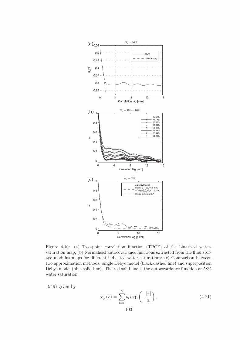
(a)

0 4 8 12 16

0.25

0.3

0.35

0.4

0.45

0.5

0.55

Correlation lag [mm]

S 2(r)

SW= 58%

TPCF

Linear Fitting

(b)

0 4 8 12 160

0.2

0.4

0.6

0.8

1

Correlation lag [mm]

χ

Sw= 46%− 68%

46.61%51.73%56.52%58.34%63.20%64.93%65.44%68.02%

(c)

0 5 10 150

0.2

0.4

0.6

0.8

1

χ

Correlation lag [pixel]

Sw= 58%

AutocovarianceDebye χ

small(a

S=0.6 mm)

+Debye χlarge

(aL=12.5 mm)

Single Debye a=3.7

Figure 4.10: (a) Two-point correlation function (TPCF) of the binarized water-saturation map; (b) Normalised autocovariance functions extracted from the fluid stor-age modulus maps for different indicated water saturations; (c) Comparison betweentwo approximation methods: single Debye model (black dashed line) and superpositionDebye model (blue solid line). The red solid line is the autocovariance function at 58%water saturation.

1949) given by

χN(r) =

N∑i=1

bi exp

(−|r|ai

), (4.21)

103

where aiis the Debye correlation length and the weight coefficient bi satisfies∑N

i=1 bi = 1, the subscript i gives the number of correlation length. However, a

single Debye correlation function χ1(r) = e−|r|/a approximates the autocovariance

function only at small correlation lags (Figure 4.10c). Therefore, it is insufficient

to use a single Debye correlation function to represent the fluid distribution sta-

tistically. To overcome this problem, a superimposed Debye function consisting

of two exponential functions χ2(r) = bSe−|r|/a

S + bLe−|r|/a

L is used. The RMS

errors of the fitting is considerably reduced after employing the latter method

(see Table 4.2). The correlation lengths aS= 0.6 mm characterizes the size of

the smallest patches while the other aL= 12.5 mm indicates the presence of

longer-range disorder, respectively. The correlation information is listed in Table

4.2. The superimposed correlation lengths are in effect equivalent to the average

patch size 0.6 mm observed in Figure 4.9.

(a) Sw = 46.61%

0.00041

0.00058

0.00075

0.00091

0.00108

0.00124(b) Sw = 51.73%

0.00043

0.00068

0.00092

0.00117

0.00142

0.00167(c) Sw = 56.52%

0.00041

0.00086

0.00131

0.00176

0.00221

0.00266(d) Sw = 58.34%

0.00044

0.00123

0.00201

0.00279

0.00357

0.00435

(e) Sw = 63.20%

0.00045

0.00166

0.00287

0.00408

0.00528

0.00649(f) Sw = 64.93%

0.00049

0.00154

0.00259

0.00364

0.00469

0.00574(g) Sw = 65.44%

0.00059

0.00135

0.00212

0.00288

0.00364

0.0044(h) Sw = 68.02%

0.00073

0.00113

0.00154

0.00194

0.00235

0.00276

Figure 4.11: Partitioned fluid modulus maps for different water saturations. The colour-bar indicates the fluid storage modulus of the mesoscopic patch. Dark blue areasindicate a large fluid-modulus (GPa), while dark red areas indicate a small modulus.Note, that the colour-bars have different scalings to better represent the variability ofthe fluid moduli at each saturation.

The normalized variance of the fluid storage modulus σ2MM

is a measure of

the compressibility contrast of the mesoscopic fluid patches. This variance is

computed at the patch-scale level instead of each unit cell in order to preserve the

patch-to-patch contrast. The detailed procedure is given in Appendix C. Figure

4.11 shows the maps constructed at each saturation level. As water saturation

grows from 46.6% to 64.9%, the normalized variance increases from 0.03 to 0.23.

This can be explained by the fact that at higher water saturation, part of the fluid

104

patches reach almost full water saturation (Sw > 90%). The effective fluid bulk

modulus of these particular patches can be 103 ∼ 104 times larger than for patches

below 90% saturation. This water stiffening effect results in a drastic fluctuation

of the fluid storage modulus between the patches. For water saturations over

64.9% the stiffening effect is dominated by the patch-size. As higher saturations

form larger fluid patches, these larger patches average the exceptionally high-

moduli of small patches out. This results in smoothed fluctuations and smaller

normalized variances.

4.4.3 Modelling the experimental data

The saturation Sw, fluid distribution function χ2(r) and fluctuation strength

σ2MM

are now estimated from the CT images. With incorporation of all other

poroelastic parameters into equation 4.13, the frequency-dependent P-wave mod-

ulus H∗(ω) is determined. The phase velocity and attenuation (inverse quality

factor) are then given by

v(ω) =

√�{H∗(ω)}

ρ, Q(ω)−1 =

�{H∗(ω)}�{H∗(ω)} . (4.22)

Here, ρ = (1− φ)ρs + φ(Swρw + Sgρg) is the average density with ρs, ρw, ρg the

density of mineral grain, water and gas, respectively. The angular frequency ω =

2πfEXP, where fEXP = 0.5 MHz is the central frequency of the ultrasonic waves.

The petrophysical properties of Savonnieres limestone and fluids are specified in

Table 4.1.

CRM interpretation

Let us first compare the velocities-saturation relations (VSR) deduced from the

experiment with the predictions of the CRM model. Figure 4.12 shows the exper-

imental VSR (the red squares) and the VSR generated by the CRM model (the

black diamonds). We also extrapolate the CRM prediction to higher saturations

(Sw = 80%, 85%, 90%, 95%, 99%), where no experimental data is available. As

discussed earlier, at high water saturations, the fluid compressibility contrast be-

tween mesoscopic patches is small. This makes the parameter τ given by equation

4.15 negligible. Thus, equation 4.13 reduces to H∗(ω) = H∗(1 − δ∗ξ(ω)). Given

105

that the autocovariance function can be well fitted by a single Debye correlation

function when Sw > 80%, we use a single correlation length inferred from gas

saturation map (Sg = 1%, 5%, 10%, 15%, 20%) of Toms et al (2009) for χM(r)

approximation. The results are plotted in Figure 4.12 (black diamonds). Both

experimental velocities and the CRM simulations show weak saturation depen-

dence. Error bars for the experimentally derived velocities are used to account

for errors in the travel time picking. The velocities at saturations over 80% start

to increase, suggesting that the rock stiffening effect dominates over the den-

sity effect at this saturation. This can be explained as a result of larger fluid

patches (a� λd) forming at higher water saturations. Then the proximity to the

Gassmann-Hill bound is expected.

0 0.1 0.2 0.3 0.4 0.5 0.6 0.7 0.8 0.9 1

3150

3200

3250

3300

3350

3400

3450

3500

3550

3600

Water Saturation

V p [m/s

]

Experimental DataCRM T=0 GPaCCRM T=2.8 GPa s=2.8CCRM T=6.7 GPa s=6.5CCRM T=13 GPa s=13.1CCRM T=18.6 GPa s=18s=18 T=16.5 GPaGassmann-WoodGassmann-HillCRM a=1.4 mm

Figure 4.12: Comparison between experimentally observed and theoretically predictedVSRs at 0.5 MHz. Red squares denote the experimental velocities and black diamondsare the CRM predictions. Dots, triangles, circles and crosses are modelling results ofthe CCRM model for different values of the capillarity stiffening T . The values of Tand the values of the shape factor s are averaged over saturations. The dashed lineindicates the GW bound and the dotted line indicates the GH bound. The solid blackline shows the CRM prediction for a correlation length of a = 1.4 mm. Red asterisksare forward modelled velocities at higher saturations based on an average shape factorst=1.

106

We note that the CRM predictions are on average 80 m/s lower than the

experimental values. The solid black line in Figure 4.12 shows for which char-

acteristic patch size the CRM model would correctly approximate the velocities.

Mesoscopic fluid distribution correlated by a single Debye function χ1(r) with a

constant correlation length of 1.4 mm could explain the experimental data. How-

ever, no evidence of such patch correlation has been found from CT images. As

shown above, the fluid distribution is best described by a double Debye correlation

function with parameters specified in Table 4.2.

0 0.2 0.4 0.6 0.8 10

0.01

0.02

0.03

0.04

0.05

Water Saturation

Q-1

EXP (SRM)

CCRM (T=f(s))

CRM (T=0 GPa)

CRM (a=1.4 mm)

Figure 4.13: Comparison between experimentally observed and theoretically predictedASRs at 0.5 MHz. Red squares show the inverse quality factor obtained from themeasured waveforms (spectral ratio method (SRM)) and the error bars indicate thestandard deviation; black diamonds are the modelling results of the CRM model; bluecircles are the modelling results of the CCRM using the inversely modelled shape factorst=1 = 18 from velocity matching.

The experimentally determined attenuation-saturation relation (ASR) is plot-

ted in Figure 4.13. The inverse quality factor Q−1EXP is obtained by applying the

spectral ratio method (SRM) on the amplitude spectrum of the received wave-

forms. In order to avoid the additional attenuation caused by the initial water

weakening effect (Lopes et al., 2014), we choose the spectral amplitude of the

wetted rock of 3% water saturation as the reference amplitude. The error bars

indicate the possible shifts of the attenuation due to different choice of the ref-

erence amplitude. There is a little ’plunge’ of the ASR curve at 58% water sat-

uration as we exclude the low injection rate period. After the saturation reaches

62% the injection rate is reduced from 2 mL/h to 0.2 mL/h, and it recovers 2

107

mL/h at 63% water saturation. During the low injection rate period, an increase

in wave amplitude is observed (see Figure 4.7b, the red waveforms). Thus, a rel-

ative small attenuation associated with change of injection rate takes place. The

available data over saturation 46% ∼ 68% shows that the quality factor Q given

by CRM model is 38 ∼ 26. This is lower than the experimental quality factor

78 ∼ 51. In other words, the CRM model overestimates the attenuation. Using

the correlation length obtained by fitting the VSR with a single Debye correla-

tion function with a = 1.4 mm, we also estimate the corresponding attenuation,

indicated by solid line in Figure 4.13. Comparing with the attenuation predicted

using image-extracted correlation lengths a ≈ 0.6 mm (as discussed earlier, the

superimposed correlation length is equivalent to the observed fluid patch size),

the attenuation is slightly lower. This is due to the fact that the experimental

frequency is slightly above the characteristic frequency of the mesoscopic flow.

In this particular frequency range, a larger correlation length results in a lower

attenuation, see also Figure 4.2b.

The discrepancy in phase velocities and attenuation reveals that wave-induced

pressure diffusion at mesoscale as described by the CRM model is insufficient for

proper interpretation of the observed ultrasonic signatures. This velocity un-

derestimation is possibly due to the fact that CRM ignores the additional patch

stiffening in the presence of capillary forces. Correspondingly, neglecting the pres-

ence of capillarity-induced membrane stiffness at fluid patch boundaries causes

an overestimation in viscous dissipation. This could explain the discrepancy in

Q.

CCRM interpretation

Using the CCRM model, we predict the superimposed rock stiffening effect due

to membrane tension and mesoscopic flow on acoustic properties. However, to

model velocity and attenuation using equation 4.13, a value for the shape factor

contained in the static undrained P-wave modulus H∗ has to be assigned to

Savonnieres limestone. Based on membrane stiffness measurements, Nagy and

Blaho (1994) calculate the shape factors using equation 4.2 for cylindrical pipes,

synthetic beads and Berea sandstone. We are not aware of any shape factor

estimate for limestones. Due to the lack of data for this parameter, we apply an

inverse modelling procedure to extract the static P-wave modulus. Namely, we

108

choose certain value of the shape factor to fill the discrepancy between CCRM

prediction and the experimental data. The validity of these chosen shape factor

values will be discussed below.

In the CCRMmodel, the dynamic P-wave modulus H∗ is complex and frequency-

dependent, except for the two end-member cases, namely the static limit H∗ and

Gassmann-Hill limit HGH, which are real-valued. Therefore, the velocity term is

contained in the real part of the modulus H∗, while the imaginary part contains

information on attenuation. To obtain the shape factor, we first match the CCRM

velocity prediction term with the target modelling velocity term (subscript m)

�(H∗) = �(Hm) = ρV 2m, (4.23)

where H∗ is obtained from equation 4.13. The velocity prediction is given by

Vm = t(VEXP − VCRM) + VCRM, (4.24)

where VEXP, VCRM are the experimentally observed velocity and the CRM velocity

prediction (the black diamonds in Figure 4.12) respectively. The factor t =Vm−VCRM

VEXP−VCRMwhich varies between 0 and 1 is the normalised velocity discrepancy

and (VEXP − VCRM) × t denotes the absolute velocity discrepancy. The complex

part in the CCRM model (equation 4.13) is only contained in ξ (equation 4.14)

function. Therefore, by setting ξ0 = �(ξ), equation 4.23 can be expressed as

H∗(1 +HGH −H∗

H∗ D) = �(Hm), (4.25)

where D = τξ02 + (τ − 1)ξ0 . The static P-wave modulus can be inverted through

rearranging the above equation,

H∗ =�(Hm)−D ·HGH

1−D. (4.26)

At each saturation level, t is set to be 4%, 18%, 32%, 45%, 59%, 73%, 86%, 100%.

For each t level, we perform H∗ inversion using equation 4.24 and equation 4.26

for each of the eight CT images. Correspondingly, the capillarity stiffening T

can be solved from H∗ using equation 4.9. The computed T at each velocity

and saturation level are plotted in Figure 4.14a. We can see from Figure 4.14a

that the inversely modelled values of T are closely associated with the absolute

109

velocity discrepancy (Figure 4.12) at each water saturation. Figure 4.14) also

demonstrates that, at lower saturations, relatively larger T values are required to

model a certain velocity level.

68 65 64 63 58 56 51 46

418

3245

5973

86100

0

10

20

30

40

50

Sw [%]

σ2t= 0.16

VCCRM−VCRM

VEXP−VCRM[%]

T[G

Pa]

68 65 64 63 58 56 51 46

418

3245

5973

86100

0

10

20

30

40

Sw [%]

σ2t= 0.09

VCCRM−VCRM

VEXP−VCRM[%]

Shapefactors

(a) (b)

Figure 4.14: (a) Parameters of capillarity stiffening T plotted against normalised veloc-ity discrepancy t and water saturation. (b) Shape factors plotted against normalisedvelocity discrepancy t and water saturation. The parameter σ2

t is the average of thenormalised variances of T (shape factor) for each t. The normalised variances are takenover all saturations at each t level.

The velocity prediction for t = 32%, 59%, 86%, 100% are displayed in Figure

4.12. The influence of capillary force on VSR is examined by increasing T from

zero (the CRM modeled velocities T = 0, t = 0) in Figure 4.12. For Vm accounts

for 31%, 58%, 86%, 100% phase velocity discrepancy over Sw = 46% ∼ 68%, the

mean T values are 2.8 GPa, 6.7 GPa, 13 GPa, 18.6 GPa respectively. The T

denotes averaged T value deduced at each saturation. By substituting equation

4.2 into 4.11, we can invert for the shape factor s

s =svκT

γ. (4.27)

Using of the SSA values extracted from the binary saturation maps, we obtain

the associated shape factor at each level plotted in Figure 4.14b. The shape

factors approximately share the characteristic of T in Figure 4.14a. However, the

normalized variance of the shape factors of various saturations (averaged over the

t levels) σ2t = 0.09 is smaller than the normalized variance of T which is 0.16.

This is due to fact that the shape factor is the intrinsic property of rock which

110

is a measure of the complexity of the pore structure (see section 2.8). Therefore,

the shape factor tends to be constant at different saturations, and thus has a

smaller normalized variance. The higher values of the shape factor at 46% water

saturation are due to incorporation of a relatively small SSA into 4.27, as Figure

4.9a is not a strictly isotropic image, it results in a biased lower interfacial contact

area after the segmentation (Table 4.2).

By making use of the mean shape factor s = 18

∑s|t=1 = 18 for which the

CCRM model fully matches the experimental velocities, we predict the undrained

P-wave velocities at higher saturations. The SSA values we used are inferred from

the gas saturation maps (Sg = 1%, 5%, 10%, 15%, 20%) of a limestone (Toms,

2008) which can be regarded as a reasonable approximation for higher water sat-

urations (Sw = 80%, 85%, 90%, 95%, 99%). In Figure 4.12 the modelling results

are plotted by asterisks. Coincidentally, the data reside on the modelling results

of WIFF arising between fluid distribution correlated by a single Debye function

at 1.4 mm. This coincidence reveals that one must be careful when using CRM

to do fluid distribution inversion, as neglecting capillarity can lead to a biased

correlation relation. The larger SSAs value appeared at the end of the imbibition

stages (Sw = 80%, 85%, 90%, 95%, 99%) result in decrease of the parameter T , see

the legend of Figure 4.12. Due to lack of laboratory data at higher saturations,

the modelling results cannot be corroborated.

To check the validity of the deduced shape factor, we compare the acoustic

properties with respect to attenuation. We model the inverse quality factor using

the mean shape factor s = 18 (inverse modelled shape factors averaged over all

saturations at 100% t level, Figure 4.14b). The results are plotted as ASRs against

experimental Q−1EXP in Figure 4.13. The Q−1

CCRM increases with water saturation

from 0.006 to 0.026 and diminishes to zero at full saturation. Apart from a slight

underestimation below 60% water saturation, the attenuation given by CCRM

model overall matches with experimentally derived attenuation of the ultrasonic

waves. The consistency confirms the reliability of the inversely modelled shape

factor for Savonnieres limestone. Therefore, we conclude that for the forced

imbibition experiment where capillary forces are thought to be dominant, the

combined effects of wave-induced pressure diffusion at mesoscopic patches and

membrane stiffening in presence of capillary forces can consistently explain the

velocity- and attenuation- saturation relations.

111

4.5 Discussion

Application of the CCRM model requires knowledge of the shape factor s

appearing in equation 4.2. While all other parameters have been estimated from

the available data set, we do not have a recipe to infer s. That is why s has

been estimated by matching with the ultrasonic velocities (Figure 4.12) and then

checking against the attenuation-saturation relation (Figure 4.13). Thus, s is only

indirectly obtained by this consistency argument. It is interesting to note that our

s estimate is larger than estimates that have been obtained from measurements on

simple porous media (Nagy and Blaho, 1994). Even more, Nagy and Blaho (1994)

argue that s is expected to be smaller than unity for complex porous media. Our

choice of the shape factor can be also understood from the following consideration.

The membrane stiffness for the simple pore geometry of a cylindrical tube can be

written as (2.157)

Ws = γ/(φsd

2

8), (4.28)

where φs is the volume fraction of the tube, d is its radius. According to Kozeny-

Carman relation, φsd2

8equals the permeability of such a simple porous medium.

The shape factor acts as a scaling parameter to account for irregularity of the

pore space (Nagy and Blaho, 1994). By incorporating the shape factor s into

equation 4.28, the membrane stiffness for a rock with complicated pore structure

becomes

W = γ/φ( d√

s)2

8. (4.29)

If we assume that the form of Kozeny-Carman relationφd2eff8

still holds for a porous

medium with complex internal structure then an effective hydraulic radius will

emerge, deff = d√s. This is to say that the shape factor s simply expresses how an

effective hydraulic radius emerges if pore channels are irregular and s > 1 means

that the effective hydraulic radius is reduced. As much as capillary pressure

increases for thin capillaries according to Young-Laplace equation, s > 1 only

means that effect of capillary forces is boosted with respect to the hydraulic

radius dependency. Therefore, if capillary action is significant, a s value larger

than unity is perhaps expected.

The interpretation of the laboratory measurements based on the CCRMmodel

only involves the mechanism of wave-induced pressure diffusion at mesoscopic

fluid patches in conjunction with membrane stiffening. We briefly discuss other

112

mechanisms that could possibly affect the ultrasonic wave propagation in satu-

rated porous rocks. Squirt flow between compliant pores (or micro-cracks) and

stiff pores is a common mechanism of wave attenuation at ultrasonic frequencies

(Muller et al., 2010). However, micro-CT images of Savonnieres limestone show

no such cracks. Furthermore, ultrasonic measurements show that pressure sensi-

tivity of both P- and S-wave velocities is minimal. This indicates that compliant

porosity is negligible and thus squirt flow attenuation can also be neglected. At-

tenuation due to elastic scattering is excluded as well. This is because the resonant

frequency fscat =1

2πa

√Hρ= 0.6 MHz at which the maximum elastic scattering

takes place is slightly greater than the central frequency of the ultrasonic waves

fEXP (0.5 MHz). Apart from that, no evidence from the ultrasonic waveforms

suggests the existence of scattering such as coda waves (Figure 4.7b).

The so-called Biot global flow dissipation mechanism is inherently coupled

with the development of viscous boundary layer flow if the viscous skin depth

becomes smaller than the pore throat thickness. Measurements in fluid saturated

porous rocks with complex pore space structure and pore wall roughness indicate

that dissipation in the viscous boundary layer due to vorticity diffusion results in

an enhanced attenuation of ultrasound. Using the formalism of Muller and Sahay

(2011), we compute the associated dispersion and attenuation with incorporation

of pore-scale heterogeneity correlation information. The latter has been obtained

by Muller et al. (2013) in the context of estimation the dynamic permeability.

In order to quantify the proportion of viscous boundary layer flow effect in the

partially saturated limestone, we firstly compare fEXP with the Biot relaxation

frequency given by

fb =μfφ

2πκρfS∞ , (4.30)

where S∞ is the tortuosity of the pore space. It is the only unknown parameter.

It can be estimated using the relation of Walsh and Brace (1984)

S∞ =√Fφ, (4.31)

where F is the formation factor. According to Archie’s law,

F = φ−m, (4.32)

where m is the cementation factor. For limestone of intergranular rock type we

use m = 2 (Focke and Munn, 1987), so that S∞ = 1.9. For gas saturated pore

113

space, fb (2.6 MHz) is five times greater than fEXP, and thus dispersion and

attenuation is negligible. On the contrary, for the rock saturated with water,

fb (0.27 MHz) is comparable with fEXP, dispersion due to vorticity diffusion is

17 m/s, whilst attenuation is still negligible. For a partially saturated rock, we

take the saturation-weighted dispersion as the contribution to the rock stiffening

effect. The result shows that 6% of velocity difference from the Gassmann-Wood

bound can be attributed to Biot global flow dispersion.

As discussed above, the P-wave velocity difference predicted by CRM and

CCRM models is expected to be significant below the characteristic frequency

of mesoscopic pressure diffusion fc. For the poroelastic parameters assigned to

this Savonnieres limestone sample, fc is contiguous to the center frequency of the

ultrasonic transducer. This explains why we observe that WIFF has a noticeable

effect at ultrasonic frequencies. It is not clear if our findings can be extrapolated

to the seismic frequency range. According to the CCRM model capillarity would

affect seismic attenuation if the fluid patches become large enough, say a few

centimetres. However, for such large fluid patches one can imagine that pore-

scale heterogeneities in form of trapped fluid inclusions (say, air bubbles) affect the

capillarity and possibly reduce the patch membrane stiffness. Moreover, Sengupta

and Mavko (2003) argue that in typical reservoir flow simulations Rcv � 1, i.e.

capillary force is negligible as compared to viscous force. It requires further

research to understand the effect of capillarity on large fluid patches.

In this study, the dispersion and attenuation are closely associated with fluid

patch distribution, i.e. the experimentally-observed millimetre-scale fluid het-

erogeneities. Our data interpretation is sensitive to the results of the statistical

analysis of the CT images. Therefore, the influence of fluid distribution rests on

how much the mesoscopic fluid patch character has been preserved during im-

age processing. The methodology we apply is based on the threshold value of

the segmentation for correlation function extraction and on partitioning size for

normalized variance calculation. The accuracy of the statistical characterization

could be calibrated with improved image resolution.

4.6 Chapter conclusions

The random patchy saturation model is extended to include capillary ac-

tion. The capillarity at the patch-scale involves two new parameters over the

114

random patchy saturation model: the interfacial tension between the two fluids

and a shape factor accounting for irregular pore spaces. By construction, this

capillarity-extended random patchy saturation (CCRM) model has a static limit

which deviates from the Gassmann-Wood prediction. The capillary action leads

to an additional stiffening thereby to higher phase velocities. It also implies a

pressure discontinuity a patch interfaces so that wave-induced pressure diffusion

process is weakened and attenuation is reduced. The joint stiffening effect from

capillarity and wave-induced pressure diffusion becomes stronger when the fluid

distribution is described by larger correlation length. To corroborate these CCRM

predictions we model the experimentally-determined velocity- and attenuation-

saturation relations for a forced imbibition experiment wherein the small capillary

number suggests the presence of capillarity. The conclusions are as follows.

1. The experimentally-determined (ultrasonic) velocity-saturation relation

cannot be modelled with either of the end-member models (theoretical bounds of

the patchy saturation model), but results in velocities which fall in between the

Gassmann-Wood and Gassmann-Hill bounds. Application of the spectral ratio

method to the ultrasonic waveforms results in Q estimates on the order of 50-80

at 70% water saturation.

2. Saturation maps derived from CT scans indicate the presence of water

patches at the millimetre-scale. The fluid patch distribution at consecutive im-

bibition stages is statistically described by autocovariance functions. The auto-

covariance function for medium water saturation 46%-68% can be well approxi-

mated by two superimposed Debye correlation functions.

3. The random patchy saturation model underestimates the ultrasonic ve-

locities for all saturations while it over-estimates the attenuation. The CCRM

model can provide a consistent prediction for the observed saturation relations

for a certain choice of the shape factor. It is argued that the value of the shape

factor s > 1 is expected if the capillarity effect is significant.

Our results suggest that the wave-induced fluid pressure diffusion between

mesoscopic patches in conjunction with capillary action have implications for in-

terpreting ultrasonic data in patchy-saturated rocks in flow regimes characterized

by small capillary numbers. Further research is required in order to understand

the applicability of the CCRMmodel to attenuation and dispersion obtained from

115

seismic low frequency measurements.

116

Chapter 5

The role of interfacial impedance

on seismic reflectivity

5.1 Summary

The characteristics of the P-wave reflectivity can depend on the properties

of the interface separating two dissimilar poroelastic half-spaces. This interface

behaviour can be characterized by an interfacial impedance which is associated

with petrophysical properties such as, imperfect hydraulic contact and capillarity

effect due to presence of membrane stiffness. Using the quasi-static poroelasticity

equations, we obtain a simple expression for the poroelastic P-wave reflectivity

including interfacial impedance at normal incidence. The amplitude versus an-

gle behaviour is obtained by solving the corresponding boundary value problem

numerically. We analyze two seismic scenarios where interfacial impedance can

arise, namely, P-wave reflection at gas-water contact and fluid/porous-medium

contact. The interfacial impedance shows small influence on the P-wave reflec-

tivity for the gas-water contact at seismic frequencies. For contact between fluid

and gas-saturated rock, the reflectivity for different interface scenarios reveals

distinct frequency and angle dependence. With increasing interfacial impedance,

a critical angle starts to appear in the amplitude-versus-angle behaviour. Syn-

thetic seismograms associated with each interface scenarios are compared. We

find that weak hydraulic contact leads to annihilation of amplitudes at small

incident angle, whereas strong capillarity causes a phase reversal at larger angles.

117

5.2 Introduction

The primary mission of amplitude interpretation among other things is to

determine whether a water-saturated rock or a hydrocarbon-saturated rock gen-

erates the reflection of interest (Hilterman, 2001). The Zoeppritz equation in

combination with Gassmann theory (Aki and Richards, 2002; Gassmann, 1951;

also see section 2.7.1) provides the relationship between the seismic reflectivity

and fluid content. However, this elastic-equivalent theory neglects oscillatory

fluid flow across the contact and is only valid at low frequency limit. To ac-

count for the wave frequency-dependence, the calculation of reflectivity needs

to be based on more general theory of Biot’s poroelasticity (Biot, 1962). The

core of the reflection theory based on Biot’s poroelasticity is the generation of

reflected/transmitted slow P-wave upon a body wave striking a poroelastic inter-

face, i.e., gas-water contact. The frequency-dependence of slow P-wave controls

the primary dynamic poroelastic effect on seismic reflectivity (Gurevich, 1996),

as it draws energy from other wave modes, i.e., the reflected fast P-wave, and

consequently reduces their amplitudes.

Dutta and Ode (1983) investigate the P-wave reflection at gas-water contact

in a unconsolidated sandstone. Their numerical results indicate that energy loss

due to converted slow P-waves is proportional to the square root of frequency.

This renders a small difference between poroelastic and elastic P-wave reflectivity

at seismic frequencies. Gurevich (1996) confirm the observation of Dutta and Ode

(1983) by comparing elastic and poroelastic results for contacts between various

types of pore fluids. Therefore, the application of Biot reflection theory is limited

by the fact that the frequency-dependence of amplitude is hard to observe even

with the best quality seismic data. Denneman et al. (2002) and Gurevich et al.

(2004) study the seismic reflection for a completely different context where the

porous rock is in contact with pure fluid. They observe that when the rock is

saturated with gas, there exists a significant difference between poroelastic and

elastic P-wave reflectivity.

The above studies of poroelastic reflectivity are based on so-called open-pore

boundary condition (Deresiewicz and Skalak, 1963; Bourbie et al., 1987), wherein

the fluid pressure across the interface is assumed to be continuous. That implies

a perfect hydraulic connection between the two poroelastic half-spaces. However,

this condition is not always valid (Geertsma and Smit, 1961; Deresiewicz and

118

Skalak, 1963). Especially in presence of capillarity between two immiscible fluids,

the fluid pressure boundary condition needs to be modified to take account of

membrane stiffness (Nagy and Blaho, 1994; Nagy and Nayfeh, 1995). On the

other hand, in presence of imperfect hydraulic contact (i.e., pore mis-alignment;

clay mineral clogging the pore space), the fluid pressure boundary condition needs

to include an interface permeability for describing the proper mechanics of the

interface (Bourbie et al., 1987; Gurevich and Schoenberg, 1999). As shown in

previous chapters, the characteristics of slow P-wave, i.e., oscillatory fluid flow

heavily rely on the poroelastic interface condition. Therefore, an alternative

choice of the interface condition in solving the boundary value problem with

respect to plane wave reflection may further influence the dynamic poroelastic

effect on seismic amplitude.

The aim of this chapter is two-fold: first of all, using quasi-static poroelas-

ticity, an analytical expression for the generalized P-wave reflectivity including

an interfacial impedance is obtained. Depending on the explicit form of the in-

terfacial impedance, it can be interpreted in terms of membrane stiffness due

to capillarity or interface permeability due to imperfect hydraulic contact. Sec-

ondly, we consider two pertinent scenarios where interfacial impedance can play

a role, namely, seismic reflection at gas-water contact (Dutta and Ode, 1983) and

at fluid/porous-medium contact (Denneman et al., 2002; Gurevich et al., 2004).

The resulting frequency- and angle- dependence of seismic reflectivity calculated

via different approaches, i.e., Zoeppritz-Gassmann, poroelastic open-pore and

current theory are compared. The synthetic seismograms for various interface

scenarios are also compared.

5.3 Quasi-static Biot’s theory

Following Biot’s theory, we consider a isotropic and homogeneous rock sat-

urated with a single Newtonian fluid. The grains of the solid are characterized

by the grain bulk modulus Ks and grain density ρs. The rock frame is charac-

terized by its bulk modulus K0 and density ρ, shear modulus μ, porosity φ and

steady-state permeability κ. The pore fluid is characterized by its bulk modulus

Kf , density ρf and steady-state shear viscosity η. With u and U denoting the

average solid and fluid displacements, the relative fluid-solid (RFS) displacement

is defined as

w = φ(U− u). (5.1)

119

Accordingly, the stress tensors in 2D space are defined as

τyy = H∇ · u+BH∇ ·w − 2μ∂ux∂x

, (5.2)

τxy = μ

(∂ux∂y

+∂uy∂x

), (5.3)

whereas the fluid pressure is

pf = −BH∇ · u−M∇ ·w. (5.4)

The definitions of the poroelastic constants H, L, B,M , α can be found in section

3.3.1. According to Biot’s poroelasticity, there exists two types of compressional

waves and one type of shear wave in saturated porous rock. In the low frequency

regime, where the wave angular frequency ω is much smaller than the Biot’s

characteristic frequency

ω � ωb =ηφ

κ0ρfS∞ , (5.5)

the wavenumbers of the fast, slow P-wave and the S-wave can be approximated

as

kα =ω

vα, (5.6)

kβ =

√iωη

κN, (5.7)

ks =ω

vs. (5.8)

The velocities of the fast and slow P-wave are vα =√H/ρ, vs =

√μ/ρ, re-

spectively. The parameter N is given by N = ML/H. Under the quasi-static

assumption 5.5, the RFS displacements of the fast P-wave and shear wave are

negligibly small, namely, w = 0. For the slow P-wave, its solid and RFS displace-

ments are coupled in following manner (Geertsma and Smit, 1961)

w = λu, λ = −(H

C

). (5.9)

The above overview of Biot’s theory provides the basis for deriving the poroelastic

reflection coefficient at seismic frequencies.

120

5.4 Reflection between two saturated porous me-

dia

We consider an incident P-wave striking an interface between two saturated

porous media. The incident wave will generate three reflected waves in the upper

medium 1 and three transmitted waves in the lower medium 2. We assume I, α,

β, s denote the incident, fast, slow and shear waves, respectively. We also denote

the upper and lower medium by 1 and 2, respectively. The solid displacement

potential of the plane wave can be described by

Φl = Alei(ωt−kl·r), l = I, 1α, 1β, 1s, 2α, 2β, 2s, (5.10)

where Al is the amplitude and

kl = (fl, gl) , (5.11)

r = (x, y) , (5.12)

kl · r = flx+ gly . (5.13)

According to Snell’s law, we can assign the x-component of the wave vector as

fl = fI = kI sin θI . (5.14)

The corresponding y-component of the wave vector can be obtained via

gl =

{ √k2l − f 2

I , l = I, 2α, 2β, 2s,

−√k2l − f 2I , l = 1α, 1β, 1s.

(5.15)

Under quasi-static assumption 5.5, for an incident fast P-wave, the solid and RFS

displacements of the upper and lower media can be expressed as

u(1) = ∇ΦI +∇Φ1α +∇Φ1β +∇× Φ1s, (5.16)

w(1) = λ1∇Φ1β, (5.17)

u(2) = ∇Φ2α +∇Φ2β +∇× Φ2s, (5.18)

w(2) = λ2∇Φ2β. (5.19)

The gradient and curl operators are defined as ∇Φ = ∂Φ/∂xi + ∂Φ/∂yj, ∇ ×Φ = −∂Φ/∂yi + ∂Φ/∂xj, respectively. The amplitudes of different displacement

121

potentials relate each other via following six boundary conditions (BC)

u(1)y = u(2)y , (5.20)

u(1)x = u(2)x , (5.21)

w(1)y = w(2)

y , (5.22)

τ (1)yy = τ (2)yy , (5.23)

τ (1)xy = τ (2)xy , (5.24)

p(1)f − p

(2)f = ZIw

(2)y . (5.25)

The first five BCs represent the continuity of normal displacement, shear dis-

placement, normal RFS displacement, normal stress and shear stress. The last

BC represent the natural boundary condition for fluid pressure. It incorporates an

so-called interfacial impedance ZI . Interpreting the interfacial impedance differ-

ently allows us to model different reflection scenarios, such as imperfect hydraulic

contact, capillarity (see more details in chapter 3).

5.5 Reflection between fluid and porous medium

The seismic reflection at fluid/porous-medium contact can be regarded as a

special case of reflection between two porous media with the porosity of one half-

space equalling unity. By setting u = 0 and φ = 1 in equations 5.2, 5.4, we obtain

the stress-strain relation for the fluid

τyy = −pf = Kf∇ ·U. (5.26)

According to Biot’s theory, only P-wave exists in the fluid and its wavenumber is

given by

kfα =ω

vf, vf =

√Kf

ρf. (5.27)

Considering incoming P-wave from the fluid, the displacement potential can be

written as

U1 = ∇ · ΦI +∇ · Φ1α. (5.28)

122

The corresponding boundary conditions for fluid/porous-medium contact is

U (1) = u(2)y + w(2)y , (5.29)

τ (1)yy = τ (2)yy , (5.30)

τ (2)xy = 0, (5.31)

p(1)f − p

(2)f = ZIw

(2)y . (5.32)

The four BCs represent conservation of mass, continuity of normal stress, continu-

ity of shear stress and natural boundary condition for fluid pressure, respectively.

5.6 Reflectivity at normal incidence

Solving the boundary value problem analytically yields simple expressions for

fast P-wave reflection coefficients at normal incidence

Rpp =Z(1) − (1−Xa)Z

(2)

Z(1) + (1 +Xb)Z(2), (5.33)

where the static acoustic impedances are Z(1) = ρ1v1α, Z(2) = ρ2v2α. For reflec-

tion at contact between two saturated porous media

Xa =H1k1α(B1 − B2)

2

k1βN1 + k2βN2︸ ︷︷ ︸+ωZI

k1βN1 + k2βN2

(H1k1αH2k2α

− 1

)︸ ︷︷ ︸, (5.34)

Xb =H1k1α(B1 − B2)

2

k1βN1 + k2βN2︸ ︷︷ ︸poroelastic

+ωZI

k1βN1 + k2βN2

(H1k1αH2k2α

+ 1

)︸ ︷︷ ︸

interfacial impedance

. (5.35)

For reflection at fluid/porous-medium contact

Xa =H1k1α(1− B2)

2

k2βN2︸ ︷︷ ︸+ωZI

k2βN2

(H1k1αH2k2α

− 1

)︸ ︷︷ ︸, (5.36)

Xb =H1k1α(1− B2)

2

k2βN2︸ ︷︷ ︸poroelastic

+ωZI

k2βN2

(H1k1αH2k2α

+ 1

)︸ ︷︷ ︸

interfacial impedance

. (5.37)

Equations 5.33-5.37 are the generalized reflectivities for two often encountered

poroelastic contacts. They can be used to assess the significance of contact-

fluid-flow as well as interfacial impedance on seismic reflection. According to

123

the expressions, if ZI = 0, the reflectivity 5.33 reduces to the open-pore case.

Furthermore, if Xa = Xb = 0, the equation becomes the elastic reflectivity with

velocity calculated via the Gassmann’s equation (see section 2.7.1).

5.7 Numerical analysis

In order to analyse the reflectivity and study the effect of interfacial impedance,

the following two scenarios are chosen: first, we consider seismic reflection at gas-

water contact (Dutta and Ode, 1983); secondly, we consider reflection between

free fluid and gas-saturated porous rock (Denneman et al., 2002; Gurevich et al.,

2004). The mechanical properties of rocks and fluids are given in Table 5.1.

(a) Dutta and Ode (1983)

Sand 1 FluidsKm (GPa) 1.7 Kfa (GPa) 2.4μm (GPa) 1.86 ρfa (g/cm3) 1Ks (GPa) 35 ηfa (Pa s) 1e-3ρs (g/cm

3) 2.65 Kfb (GPa) 0.022φ 0.3 ρfb (g/cm3) 0.1κ0 (m2) 1e-12 ηfb (Pa s) 1.5e-5

(b) Gurevich et al. (2004)

Sand 2 FluidsKm (GPa) 5.8 Kfa (GPa) 2.22μm (GPa) 3.4 ρfa (g/cm3 ) 1Ks (GPa) 40 ηfa (Pa s) 1e-3ρs (g/cm

3) 2.76 Kfb (GPa ) 1e-4φ 0.26 ρfb (g/cm3) 1.2e-3κ0 (m2) 9.5e-13 ηfb (Pa s ) 1.82e-5

Table 5.1: Mechanical properties of rocks and fluids

In the first case, P-wave propagates from the upper gas-saturated poroelastic

half-space through the lower brine-saturated half-space. The reflectivity at nor-

mal incidence is calculated using equations 5.33-5.35. We verify the analytical

reflectivity by comparing with results obtained using Biot’s dynamic equations

of poroelasticity (section 2.1.5, eq. 2.47). Both reflectivities are calculated with

open-pore assumption (ZI = 0). In Figure 5.1a, the resulting amplitudes coincide

up to 104 Hz. This confirms the validity of the expressions at seismic frequen-

124

cies. Next, we consider different interface scenarios by choosing different forms

(a)

100 101 102 103 104 105

0.05

0.1

0.15

0.2

0.25

Frequency [Hz]

|Rpp

(0o )|

Open-pore (full)Open-pore (quasi)IHCCapillarityElastic

(b)

0 15 30 45 60 75 900.2

0.3

0.4

0.5

0.6

0.7

0.8

0.9

1

1.1

Angle [Deg]

|Rpp

(0o )|

Open-pore (full)Open-pore (quasi)IHCCapillarityElastic

Figure 5.1: Seismic reflection between gas and water contact. Amplitude of reflectedP-wave at normal incidence is plotted as function of frequency.

of interfacial impedances, i.e., ZI = 1κI

for modelling the interface permeability

and ZI = Wiω

for modelling the membrane stiffness (capillarity). A range of in-

terface permeabilities κI = 0.3, , 0.5, 1 (10−6m/Pa · s) and membrane stiffness

W = 0.1, 1, 10 (GPa/m) are chosen for modelling the capillarity effect and

125

(a)

10-4 10-3 10-2 10-1 100 101 102 103 1040.2

0.3

0.4

0.5

0.6

0.7

0.8

0.9

1

Frequency [Hz]

|Rpp

(0o )|

Effect of interface permeability

κI=0.3e-5 m/Pa s

κI=0.5e-5 m/Pa s

κI=1e-5 m/Pa s

(b)

10-4 10-3 10-2 10-1 100 101 102 103 1040.2

0.3

0.4

0.5

0.6

0.7

0.8

0.9

1

Frequency [Hz]

|Rpp

(0o )|

Effect of membrane stiffness

W=0.1 GPa/mW=1 GPa/mW=10 GPa/m

Figure 5.2: Seismic reflection between free fluid and gas saturated rock. Amplitude ofreflected P-wave at normal incidence is plotted as function of frequency.

imperfect hydraulic contact (IHC), respectively. The amplitudes resulting from

interface permeability and membrane stiffness are consistent with amplitude as-

sociated with open-pore condition at seismic frequencies. Solving the boundary

value problem numerically, we also obtain reflectivities at different angles. The

amplitude versus angle (AVA) at 100 Hz is shown in Figure 5.1b. Again, we

find negligible effect of interfacial impedance on the amplitude. In Figure 5.1b,

126

(a)

0 15 30 45 60 75 900

0.1

0.2

0.3

0.4

0.5

0.6

0.7

0.8

0.9

1

Angle [Deg]

|Rpp

|

Effect of interface permeability

κI=0.3e-6 m/Pa s

κI=0.5e-6 m/Pa s

κI=1e-6 m/Pa s

Open-pore

Elastic

(b)

0 15 30 45 60 75 900

0.1

0.2

0.3

0.4

0.5

0.6

0.7

0.8

0.9

1

Angle [Deg]

|Rpp

|

Effect of membrane stiffness

W=0.1 GPa/mW=1 GPa/mW=10 GPa/m

Elastic

Open-pore

Figure 5.3: Seismic reflection between free fluid and gas saturated rock. Amplitude ofreflected P-wave at 50 Hz is plotted as function of angle.

the poroelastic AVAs are compared with elastic AVA calculated using Zoeppritz-

Gassmann theory. The comparison indicates that the seismic reflection between

two saturated rocks can be described by elastic theory satisfactorily. This be-

comes more evident when we consider that Biot global flow is relatively significant

for the employed unconsolidated rock at seismic frequencies.

For contact between free fluid and gas-saturated medium, the normal inci-

127

0 30 60 9040

60

80

Elastic

Tim

e [m

s]

0 30 60 9040

60

80

Open-pore

Tim

e [m

s]

0 30 60 9040

60

80

Capillarity W=0.1 GPa/m

Tim

e [m

s]

0 30 60 9040

60

80

IHC κI=0.3e-6 m/Pa s

Tim

e [m

s]0 30 60 90

40

60

80

Capillarity W=1 GPa/m

Tim

e [m

s]

0 30 60 9040

60

80

IHC κI=0.5e-6 m/Pa sTi

me

[ms]

0 30 60 9040

60

80

Capillarity W=10 GPa/m

Tim

e [m

s]

0 30 60 9040

60

80

IHC κI=1e-6 m/Pa s

Tim

e [m

s]

Figure 5.4: Seismic reflection between free fluid and gas-saturated rock, the resultingangle gathers for different interface conditions.

dence reflectivity considering different interface conditions show distinct frequency-

dependence behaviour as shown in Figure 5.2. Considering the exploration fre-

quency range 10 Hz - 10 kHz, there is a significant difference between poroelastic

open-pore (circles) and elastic (solid line) reflection coefficients as originally ob-

served by Denneman et al. (2002). The low frequency limit occurs as low as 10−3

Hz, where the poroelastic open-pore reflectivity reverts to the elastic value. The

strong porolastic effect in this case may allow the effects of capillarity and inter-

face permeability to be noticed. Indeed, as shown in Figure 5.2a, with increasing

interface permeability, the reflection coefficient becomes similar to the open-pore

poroelastic coefficient at seismic frequencies. On the other hand, in Figure 5.2b,

for increasing membrane stiffness, the reflection coefficient becomes similar to

the elastic reflection coefficient at seismic frequencies. The reflectivity associated

with membrane stiffness is bounded by the elastic and poroelastic open-pore re-

flectivity. However, in presence of interface permeability, the reflectivity value

128

can even be lower than elastic and open-pore reflectivity from 10−1 Hz to 10 Hz.

The corresponding AVA signatures at 50 Hz are shown in Figure 5.3. Com-

paring with the poroleastic open-pore case, a critical angle appears due to the

presence of membrane stiffness and interface permeability. The AVA behaviors in

Figure 5.3a,b also confirm that in the case of interface permeability, the resulting

reflectivities may not be bounded by elastic and open-pore reflectivities. The cor-

responding seismograms for Figure 5.3, which also integrate the phase information

are presented in Figure 5.4. The seismograms are computed by convolving the

resulting P-wave reflectivities with the Ricker wavelet. Interestingly, for strong

capillarity, or large membrane stiffness, we observe phase reversal at larger in-

cident angles. When the interface permeability is small, the amplitude can be

very weak at small incident angles. The contrasting AVA behaviors reveals a

potential application of this work. By comparing the theoretical reflectivity with

lab measured reflectivity, we may be able to quantify the poroelastic boundary

conditions, i.e., interface permeability, membrane stiffness.

5.8 Chapter conclusions

We study the influence of interfacial impedance on seismic reflection. Using

quasi-static poroelasticity, we obtain analytical expression for P-wave reflectivity

including interfacial impedance. The interfacial impedance shows negligible ef-

fect on seismic reflection at gas-water contact in the seismic frequency range. For

contact between free fluid and gas-saturated rock, reflectivity considering differ-

ent interface scenarios reveals distinct frequency and angle dependence. Critical

angle starts to appear for increasing interface permeability and membrane stiff-

ness. Comparing the corresponding seismograms, we find weak hydraulic contact

leads to annihilation of amplitudes at small incident angle. Meanwhile, strong

capillarity gives rise to phase reversal at larger incident angle. The results provide

theoretical evidence for examining the poroelastic boundary conditions using lab

measured reflectivity. Furthermore, for gas-saturated sea-floor whose surface is

not perfectly sealed, incorporating interfacial impedance into AVO analysis may

be important for extracting elastic properties from marine seismic data.

129

Chapter 6

The effects of saturation scale on

time-lapse seismic signatures

6.1 Summary

Quantitative interpretation of time-lapse seismic signatures aims at assist-

ing reservoir engineering and management operations. Relevant signatures in-

clude time shifts, reflection amplitude changes and time-lapse attenuation. Time-

lapse signatures are thought to be primarily induced by saturation and pressure

changes. However, core-scale laboratory measurements and reservoir-scale flow

simulations indicate that a change of the driving forces during dynamic fluid injec-

tion gives rise to a varying saturation scale. This saturation scale is yet another

variable controlling the time-lapse seismic signal. In this work, we investigate

the saturation scale effect on time-lapse seismic signatures by analysing simple

modelling scenarios. We consider three characteristic saturation scales – ranging

from few millimetres to metres – which may form during gas injection in an un-

consolidated reservoir. Using the random patchy saturation model, we compare

the acoustic signatures associated with each saturation scale. We further investi-

gate the scale effect on the reflection coefficient for a partially saturated reservoir

encased by high-impedance shale layers. The results show that centimetre and

metre saturation scales may cause significant attenuation and velocity dispersion

at seismic frequencies. The magnitude of the reflection coefficient decreases with

increasing saturation scale. The millimetre saturation scale produces the same

130

seismic signatures as obtained by elastic effective medium modelling, whereas the

centimetre and metre saturation scales lead to highest amplitude decay and ear-

liest arrival for the base reflection. The analysis of the time shift and amplitude

change indicates that ignoring time-dependent saturation scale can result in bi-

ased estimations of saturation and fluid pressure. In the discussion we address the

reservoir parameters which can influence the characteristic role of the saturation

scale.

6.2 Introduction

Quantitative analysis of time-lapse (TL) seismic data is important for mon-

itoring reservoir performance. The key to the time-lapse seismic interpretation

is to understand the relation between the seismic properties such as velocity, at-

tenuation and fluid information such as saturation, pressure. It is known that

seismic velocity and attenuation do not only depend on the type of rock and flu-

ids, amount of saturation but also the fluid distribution, namely the spatial scale

how the fluids are mixed in the pore space. The reservoir fluid distribution is

jointly controlled by multiple forces due to gravity, capillarity, viscosity and iner-

tia (Johnston, 2013). The gravity force plays an important role in separating the

reservoir fluids along the vertical dimension. It has a dominant role with fluids

of large density contrast and in reservoir of shallow depth. The performance of

capillary force and viscous force controls the efficiency of enhanced hydrocarbon

recovery. Their characteristics are determined by the reservoir wettability con-

dition, fluid mobility ratio and injection method. The inertial force reflects the

reservoir flow capacity and is influenced by permeability and lithology variations.

During the process of reservoir production and proceeding recovery, the balance

of these reservoir forces is constantly changing and lead to time-dependent sat-

uration scale. This makes the estimation of the fluid distribution and further

quantifying its effect on 4D seismic exceptionally challenging.

Laboratory rock physicists endeavour to understand the relation between fluid

distribution and elastic properties via core-flooding experiment combining with

acoustic and X-ray computer tomography (CT) monitoring (Cadoret et al., 1995;

Alemu et al., 2013; Nakagawa et al., 2013; Lopes et al., 2014). Cadoret et al

(1995) shows that the fluid distribution induced by different saturation tech-

niques can be different. They report the fluid distribution in a drying experiment

(drainage) is more heterogeneous than during depressurization (imbibition) espe-

131

cially at high water saturation level. The difference in saturation scale leads to

different measured P-wave velocity at the same saturation. Lopes et al. (2014)

study the dependence of P-wave velocity on the injection rate during forced water

imbibition. They observe that, for the same water saturation, P-wave velocity

associated with high injection rate is larger than the velocity associated with

smaller injection rate. This difference is attributed to the injection-rate depen-

dent saturation scale. Alemu et al. (2013) and Nakagawa et al. (2013) conduct

drainage core-flooding with CO2 injection and subsequent imbibition with brine

re-injection. They report the P-wave amplitude and attenuation can be sensitive

to the fluid distribution, which is again strongly influenced by the sub-core frame

heterogeneities. Toms et al. (2009) and chapter 4 apply statistical characteriza-

tion on CT images acquired during core-flooding. They find the saturation scale,

which can be quantified by a correlation length, varies with the saturation itself.

Studies on core-flooding reveal the dependence of fluid distribution on satura-

tion method, injection rate, frame heterogeneities as well as the level of saturation.

On the other hand, the reservoir-scale fluid distribution can be different from the

core-flooding fluid distribution. This is because a change of the dominant forces

of the two phase flow (Sengupta and Mavko, 2003) as well as the presence of

complex geological heterogeneities at larger scale (MacBeth and Stephen, 2008).

At field scale, the fluid distribution can be indirectly identified from the velocity

-saturation relation (VSR). The establishment of field-scale VSR can be based on

well log/VSP data (Caspari et al., 2012; Al Hosni et al., 2015) or saturation profile

from flow simulation (Sengupta and Mavko, 2003). If the VSR follows predic-

tion from Gassmann’s equation, the fluid distribution is identified as uniform and

otherwise patchy. Sengupta and Mavko (2003) perform fine-scale flow simulation

and study the influence of petrophysical parameters (e.g., relative permeability,

wettability, fluid mobility ratio and residual saturation) on the form of saturation

scale. Their results indicate that patchy saturation is encountered in most gas

injection scenarios. This is because the gravitational force induces subseismic-

resolution gas cap, hence resulting patchy saturation at seismic scale. They also

conclude that uniform saturation is commonly associated with water-flooding and

primary production.

Integration of fluid distribution properly into flow simulation and seismic in-

version is crucial for quantifying fluid saturation and pressure from time-lapse seis-

mic data. This requires further understanding the physical mechanism behind the

132

velocity and attenuation -saturation relations in partially saturated rocks. When

an elastic wave propagates in a saturated medium, it will induce local pressure

gradient between rock regions of different compliances. The pressure gradient

tends to equilibrate and gives rise to wave velocity dispersion and attenuation.

Such process is referred as wave-induced fluid flow (Muller et al., 2010). The

wave-induced fluid flow (WIFF) can take place over various scales. Particularly,

for WIFF at mesoscopic scale, which is larger than the pore space but smaller

than the wavelength, the resulting dispersion and attenuation is believed to be

significant at seismic frequencies. When the reservoir fluids uniformly distribute

in the pore space, the wave-induced fluid pressure has enough time to equilibrate

at seismic frequencies. In this case, Gassmann theory can be invoked to predict

the non-dispersive seismic velocity. On the other hand, each fluid phase can oc-

cupy a network of pores and forms as mesoscopic fluid patches. This scenario

becomes more prevalent during dynamic fluid movement induced by injection.

The scale of such fluid patches can differ by orders of magnitude depending on

the reservoir forces.

The patchy saturation models are routinely applied for modeling the velocity

and attenuation due to mesoscopic flow in the field (Morgan et al., 2012; Blan-

chard and Delommot, 2015). Two categories of models are frequently used. One

assumes a periodic presence of gas layers (White et al., 1975; Carcione and Pi-

cotti, 2006; also see chapter 3). The other assumes a random fluid distribution,

which can be quantified by different types of correlation functions (Gurevich et

al., 1995; Gelinsky et al., 1998; Muller and Gurevich, 2004; Toms et al, 2007a).

The saturation scale in the periodic model is given by the size of the representa-

tive elementary volume (REV) whereas in the random model, it is manifested as

the correlation length. The applications of these models are commonly associated

with an assumption of constant saturation scale over time. Namely, a constant

REV size or correlation length is used during the course of fluid injection. Thus,

the change of the velocity and attenuation are solely attributed to the change of

saturation or fluid pressure. However, as evidenced from the studies of laboratory

core-flooding and field-scale flow simulation, the saturation scale can differ over

repeated seismic surveys due to the change of reservoir forces. Therefore, failing

to include time-dependent saturation scale can result in biased saturation and

133

fluid pressure estimation. To overcome this, we propose a new modelling scheme:

Kt+Δtsat (ω) = Patchy[ St+Δt

gas︸ ︷︷ ︸Saturation change

, Kdry(Pt+Δteff ), μdry(P

t+Δteff )︸ ︷︷ ︸

Pressure change

, bt+Δt︸ ︷︷ ︸Scale change

].

(6.1)

Comparing with the conventional Gassmann modelling (Landrø, 2001):

Kt+Δtsat = Gassmann[ St+Δt

gas︸ ︷︷ ︸Saturation change

, Kdry(Pt+Δteff ), μdry(P

t+Δteff )︸ ︷︷ ︸

Pressure change

], (6.2)

patchy saturation model (equation 6.1) operates on change of gas saturation Sgas,

effective pressure Pe and an additional element — saturation scale b. The latter

gives rise to attenuation and velocity dispersion. To illustrate the scale effect, we

consider an initially water-saturated unconsolidated sandstone undergoes gas in-

jection. Three contrastingly different saturation scales are independently assumed

to be formed during the gas injection. They represent three typical attenuation

characteristics at an employed seismic frequency. In the first part, we analyse the

effect of the saturation scale on the acoustic impedance and attenuation using

developed patchy saturation model. Further based on the model, we customize

viscoelastic reflection coefficient for patchy-saturated reservoir and study scale

effect on seismic amplitudes. Viscoelastic seismic modelling is applied to investi-

gate the significance of saturation scale on seismic responses. In the second part,

we illustrate how saturation scale variation affects the estimation of saturation

and fluid pressure from time-lapse seismic signatures. We discuss reservoir pa-

rameters which can influence our analysis of saturation scale effect. Last but not

the least, we address the importance of identifying time-lapse saturation scale for

quantitative 4D study.

6.3 Scale effect in Partially Saturated Reservoir

6.3.1 Characteristic saturation scales

First, we assume a shallow and initially water-saturated reservoir which is

made of unconsolidated sandstone. We further assume that the reservoir has un-

dergone gas injection and therefore, becomes partially saturated. The scenario

where injected gas stays immiscible with the reservoir fluids can be encountered

in CO2 sequestration, enhanced oil recovery using WAG (water alternating with

134

gas) and gas injection for secondary oil recovery as shown in Figure 6.1. We

(a) (b) (c)

Figure 6.1: Three gas injection scenarios which are likely to induce patchy saturation.(a) CO2 sequestration; (b) enhanced oil recovery using WAG (water alternating withgas); (c) gas injection in the gas cap for secondary oil recovery. Modified from Johnston(2013).

assume that one of the following three saturation scales forms during the gas

injection: Patches on the order of 1) of millimetre, 2) centimetre and 3) metre.

The saturation images of the rock containing these representative length scales

are illustrated in Figure 6.2. The images are generated using an exponentially-

correlated random fluid distribution with scales (correlation length) of 5 mm

(left), 15 cm (middle), 2 m (right), respectively. Despite the difference in satura-

tion scale, all images have the same gas saturation of 50%.

(a)

200 400 600 800 1000

Sw

0

0.2

0.4

0.6

0.8

1

(b)

200 400 600 800 1000

Sw

0

0.2

0.4

0.6

0.8

1

(c)

200 400 600 800 1000

Sw

0

0.2

0.4

0.6

0.8

1

Figure 6.2: Synthetic saturation images of a rock with 50% gas saturation. The fluiddistribution is exponentially-correlated with a correlation length of 5 mm for image (a),15 cm for image (b) and 2 m for image (c).

Let us consider a seismic wave with certain frequency passing through rocks

with such different saturation scales. The wave will instantaneously induce dif-

ferent fluid pressure within each fluid phase because of their different compress-

135

ibilities. This wave-induced pressure difference tends to equilibrate and the char-

acteristic time for such equilibration is controlled by the ratio of the saturation

scale b and the diffusion length ld. Intuitively, for rock having small scale fluid

heterogeneities (b � ld) as shown in Figure 6.2a, the induced fluid pressure will

have enough time to equilibrate during one wave cycle. Seismic wave now senses

the rock as if it is saturated by a single, effective fluid. Hence, seismic velocity

can be predicted by Gassmann’s equation with the effective compressibility of

the two-fluid mixture provided by Wood’s mixing law. Meanwhile, in presence of

strong capillarity, the Gassmann’s equation needs to be modified to take the in-

terfacial tension into account (see chapter 3 and 4). On the other hand, for large

scale fluid heterogeneities (b � ld) as shown in Figure 6.2c, the fluid pressure

has no time to equilibrate and will remain piecewisely constant within each fluid

phase. In this scenario, the unrelaxed fluid pressure adds to the overall stiffness of

the rock and seismic velocity can be calculated by Hill’s equation (see 4.3.2). Ad-

ditionally, the Hill’s equation can be modified to include the presence of residual

saturation (Sengupta and Mavko, 2003). Lastly, for rocks having intermediate

saturation scale (b ≈ ld) as shown in Figure 6.2b, wave-induced fluid pressure can

only partially equilibrate during one wave cycle. Such diffusion process results in

frequency-dependent velocity and attenuation.

6.3.2 Bounds-extended Patchy Saturation Model

Here, we extend random patchy saturation model of Toms et al. (2007a)

to take capillarity (see chapter 3, 4) and irreducible saturation (Sengupta and

Mavko, 2003) into account. The resulting effective P-wave modulus simply reads

H(ω) = Hcap + (Hirr −Hcap)Hp(ω) , (6.3)

where Hp(ω) is normalized P-wave modulus and taken on a value between 0

and 1. That is, at low frequency limit, Hp(ω) = 0 and the model converges to

capillarity-extended static limit Hcap. At high frequency limit, Hp(ω) = 1 and

the model reaches irreducible-saturation-modified upper limit Hcap. Here, we give

description for the extended bounds. The detailed expressions for calculating

Hp(ω) can be found in chapter 4. First, the capillarity-extended lower bound is

136

written as (see section 4.3.1)

Hcap =z + T

zHGW

+ THGH

, z =Nw

Sw

+Ng

Sg

, T =bW

4SwSg

, (6.4)

where Gassmann-Wood (GW) HGW, Gassmann-Hill HGH moduli and parameter

N can be found in chapter 4. In equation 6.4, T is a key parameter which

controls the capillarity stiffening effect. It is a function of the saturation scale

b and the membrane stiffness W . When either the saturation scale b or the

membrane stiffnessW is small, capillarity stiffening becomes negligible T = 0. In

this case, the lower bound Hcap reduces to Gassmann-Wood modulus HGW. The

irreducible-saturation modified upper bound is given by (Sengupta and Mavko,

2003)

Hirr =

(Sf1

Hf1

+Sf2

Hf2

)−1

, Sf1 =Sg − Srg

1− Sirrw − Srg

, Sf2 =Sw − Sirrw

1− Sirrw − Srg

, (6.5)

where Hf1 is the GW modulus at the irreducible water saturation Srw, Hf2 is

the GW modulus at the residual gas saturation Srg. When there is no either

irreducible water saturation or residual gas saturation Srw = Srg = 0, the upper

bound Hirr reduces to Gassmann-Hill modulus HGH.

To highlight the saturation scale effect, we first switch off the capillarity and

irreducible saturation effects in our model, namely, we setW = 0, Sirrw = Srg = 0.

Their respective impact will be clearly shown at the end of the result section.

6.3.3 Characteristic frequency

To study the scale effect, it is essential to first look at the characteristic fre-

quency of the model. When the diffusion length equals the saturation scale,

maximum attenuation due to mesoscopic flow takes place. The frequency satisfy-

ing this condition is defined as the characteristic frequency which can be written

as

fc =1

2π

Dp(Sg, Pe)

b2(Sg, Pe), (6.6)

We see that the saturation scale b has an explicit role of controlling the frequency

band where maximum attenuation happens. The diffusivity Dp incorporates the

saturation and the bulk/shear modulus of the frame. Therefore, the characteristic

frequency depends on the saturation and effective pressure. Assuming a given

137

porosity and clay content for the sandstone, the relation between its dry moduli

and effective pressure can be written by the form (Eberhart-Phillips et al., 1989)

K0, μ0 = A+BPe − Ce−DPe . (6.7)

The regression coefficients A,B,C,D can be derived by fitting the lab data. In

light of work of Landrø (2001), we choose the coefficients directly from mea-

surement of Eberhart-Phillips et al. (1989) for an unconsolidated sandstone

(A = 1.41, B = 0.435, C = 0.197, D = 14 for the bulk modulus; A = 0.64,

B = 0.333, C = 0.107, D = 13 for the shear modulus). The resulting pressure-

dependent bulk and shear moduli are shown in Figure 6.3. The petrophysical

0 10 20 30 40 50 600.5

1

1.5

2

2.5

3

3.5

4

4.5

5

Pe [MPa]

Dry

mod

ulus

[MP

a]

BulkShear

Figure 6.3: Relation between bulk and shear frame moduli and effective pressure forthe unconsolidated sandstone.

properties of reservoir rock (at zero effective pressure) and fluids are given in

Table 6.1.

Soft sand Fluids ShaleK0 (GPa) 2.7 Kfa (GPa) 2.4 Vp (m/s ) 2400μ0 (GPa) 0.8 ρfa (g/cm3) 1 Vs (m/s) 800Ks (GPa) 35 ηfa (Pa s) 1e-3 ρ (kg/m3) 2300ρs (g/cm

3) 2.65 Kfb (GPa) 0.01φ 0.3 ρfb (g/cm3) 0.14κ (m2) 1e-12 ηfb (Pa s) 1e-5

Table 6.1: Mechanical properties of rocks and fluids

138

Figure 6.4 shows the characteristic frequency as a function of saturation and

effective pressure for different saturation scales . The common features of fc re-

vealed by Figures 6.4a, b, c are: 1. with increasing gas saturation, fc is shifted

towards higher frequency, then it maximizes at few percent of water saturation

and drops drastically after this critical water saturation; 2. with increasing effec-

tive pressure, fc is shifted towards higher frequency and the pressure dependence

is stronger at lower gas saturation. Most importantly, by comparing Figures

6.4a, b, c, the saturation scales locate the characteristic frequencies (z-axis) in

three rather separated frequency bands for all saturations and effective pressure.

In other words, for the employed rock properties, the millimetre saturation scale

will correspond to a dominant attenuation in kilohertz range; the centimetre satu-

ration scale corresponds to a dominant attenuation in seismic frequencies whereas

the metre-scale is associated with attenuation in millihertz band. These represen-

tative saturation scales will facilitate our discussion on their respect attenuation

characteristics in the following sections.

(a) (b) (c)

Figure 6.4: Characteristic frequency is plotted as function of saturation and effectivepressure. The saturation scales are 5 mm for (a), 15 cm for (b) and 2m for (c).

6.3.4 Attenuation and Acoustic impedance

The attenuation and the acoustic impedance (AI) can be calculated via

Q−1 =Im(H(ω))

Re(H(ω)), Z =

√ρ0Re(H(ω)) , (6.8)

where the effective P-wave modulus H(ω) is given by equation 6.3. The effective

density ρ0 is calculated by taking the volumetric average of the grain and fluid

densities. We discuss the acoustic impedance here instead of velocity, as it not

only incorporates velocity information but also facilitate our further analysis on

139

seismic amplitude.

(a)

10-2 100 102 10410-4

10-3

10-2

10-1

Frequency [Hz]

Atte

nuat

ion

Patchy 5mmPatchy 15cmPatchy 2m

30 Hz

(b)

100 102 1042.5

3

3.5

4

4.5

5

Frequency [Hz]

AI [

106 k

g/m

2 s]

Patchy 5mmPatchy 15cmPatchy 2m

Hill

Shale

Gassmann

Figure 6.5: Attenuation and acoustic impedance are plotted as function of frequency.The saturation and effective pressure 50% and zero, respectively.

The attenuation and acoustic impedance are plotted as function of frequency

in Figure 6.5. The water saturation is 50% whereas the effective pressure is zero.

In Figure 6.5a, the three saturation scales reveals contrasting attenuation levels

140

within seismic frequency range (10 Hz ∼ 150 Hz). Let us consider 30 Hz as

frequency of interest, for millimetre saturation scale, Q is over 1000 indicating

negligible attenuation. For metre saturation scale, attenuation is appreciably

larger with an inverse quality factor of 0.03, whereas for centimetre saturation

scale, an inverse quality factor of 0.08 revealing highest attenuation. The acoustic

impedances in Figure 6.5b are bounded by Gassmann and Hill limits. The metre

saturation scale gives the largest dispersion at seismic frequencies whereas at

centimetre scale, the dispersion is relatively small. The millimetre scale starts to

cause noticeable dispersion above 10 KHz.

The attenuation- and impedance-saturation relations are shown in Figure 6.6.

The frequency is 30 Hz and the effective pressure is zero in this case. The millime-

tre saturation scale produces minimum attenuation and its associated acoustic

impedance is least sensitive with the water saturation. The centimetre satura-

tion scale results in a maximum inverse quality factor of 0.2 (Q = 5) which

is 5 times larger than the attenuation provided by the metre saturation scale.

The associated acoustic impedances of both cases are sensitive with change of

saturation.

The dependence of attenuation and AI on the effective pressure is presented

in Figure 6.7. The frequency and saturation are 30 Hz and 50% respectively

in this case. The centimetre saturation scale yields greatest attenuation and

attenuation sensitivity with the effective pressure. For all cases, the attenuation

and acoustic impedance level off when the effective pressure is above 30 GPa.

The AI -pressure relation for partially saturation (Figure 6.7b) is controlled by

the pressure-dependent dry moduli (Figure 6.3).

6.3.5 Seismic reflection amplitude

In this section, we study the effect of saturation scale on the seismic reflection.

To do so, we employ a simple three-layer model where a low impedance sand layer

is encased between two higher impedance shale layers. This type of reservoir

model is categorized as Class III AVO anomaly (Rutherford and Williams, 1989).

We assume the reservoir sand is partially saturated and attenuating as shown

in previous sections whereas the overburden shale is fully saturated and non-

dissipative at seismic frequencies.

141

(a)

0 0.2 0.4 0.6 0.8 10

0.02

0.04

0.06

0.08

0.1

0.12

0.14

0.16

0.18

0.2

Gas Saturation

1/Q

Patchy 5mmPatchy 15cmPatchy 2m

(b)

0 0.2 0.4 0.6 0.8 12.5

3

3.5

4

4.5

5

5.5

6

Gas saturation

AI [

106 k

g/m

2 s]

Patchy 5mmPatchy 15cmPatchy 2m

Shale

Hill

Gassmann

Figure 6.6: Attenuation and acoustic impedance are plotted as function of saturation.The frequency and effective pressure 30 Hz and zero, respectively.

We are dealing with seismic reflection between two porous media, in which

case, the mode conversion across the interface will generate Biot slow wave. How-

ever, the energy carried away by the latter is negligible at seismic frequencies

(Dutta and Ode, 1983). Therefore, we can simplify the problem to reflection

between two viscoelastic half-spaces which can be solved by the extended Zoep-

pritz equation for attenuative media (Aki and Richards, 1980; Liu et al., 2011).

142

(a)

0 10 20 30 40 50 600

0.01

0.02

0.03

0.04

0.05

0.06

0.07

0.08

0.09

Pe [MPa]

Atte

nuat

ion

Patchy 5mmPatchy 15cmPatchy 2m

(b)

0 10 20 30 40 50 602.5

3

3.5

4

4.5

5

5.5

6

Pe [MPa]

AI [

106 k

g/m

2 s]

Patchy 5mmPatchy 15cmPatchy 2m

Figure 6.7: Attenuation and acoustic impedance are plotted as function of effectivepressure. The frequency and saturation 30 Hz and 50%, respectively.

The resulting reflection coefficient incorporates the frequency-dependent phase

velocities and attenuation of the rocks. The formula for the viscoelastic reflection

coefficient is given in Appendix D.

We further assume the attenuation is negligible for the overburden shale and

consequently constant velocity. We model the attenuation of the reservoir sand

143

(a)

0 20 40 60 800.25

0.26

0.27

0.28

0.29

0.3

0.31

0.32

0.33

0.34

Frequency [Hz]

Am

plitu

de

b [m

]

0

0.1

0.2

0.3

0.4

0.5

0.6

0.7

0.8

0.9

1

Patchy Saturation

Gassmann

(b)

0 10 20 30 40 50 600.25

0.3

0.35

0.4

0.45

0.5

Angle [Degree]

Am

plitu

de

b [m

]

0

0.1

0.2

0.3

0.4

0.5

0.6

0.7

0.8

0.9

1

Patchy Saturation

Gassmann

Figure 6.8: (a) Amplitude of reflection coefficient plotted as function of frequency.Incident angle is 0 degree. (b) Amplitude of reflection coefficient plotted as functionof angle. Frequency is 50 Hz. In both plots, saturation is 50%. Colorbar denotes thesaturation scale.

using the random patchy saturation model. Then, we investigate the amplitude

variation resulting from P-wave reflection between the cap rock and the patchy-

saturated reservoir rock having different characteristic saturation scale.

The velocities and density of the shale are given in Table 1. The resulting

144

acoustic impedance is shown in Figure 6.5b and Figure 6.6b. As can be seen,

despite the dispersion, the impedance contrast between the shale and reservoir

sand is constantly negative suggesting the AVO anomaly is Class III throughout

the frequency and saturation ranges. The amplitude of the reflection coefficient

for normal incident P-wave traveling from the upper shale to the lower sand is

plotted in Figure 6.8a as a function of frequency. The saturation is 50% in this

case. For uniform saturation, the amplitude is predicted by Zoeppritz equation in

combination with Gassmann theory. This is the scenario of the largest impedance

contrast as seen in Figure 6.5b, hence resulting in the highest amplitude-versus-

frequency (AVF) as indicated by the top black line. While for patchy saturation

AVF shows small variation for saturation scale between 0 and 10 centimetres.

AVF decreases gradually with increasing saturation scale from 10 centimetres to

1 metre.

Figure 6.8b demonstrates the angle-dependence with 50% saturation and 30

Hz wave frequency. The amplitudes increase with increasing angle of incidence

as expected from Class III AVO anomaly. Strong angle-dependence is observed

above 20 degree. Larger saturation scale produce overall lower amplitudes. Fig-

ure 6.8a and Figure 6.8b show that, even at the same degree of saturation the

amplitude can depend on the spatial fluid distribution. From uniform fluid mix-

ture to saturation scale of 1m, the amplitude reveals maximum 20% reduction in

both frequency and angle domains. Figure 6.8b also implies that, if we interpret

the AVO signature with a linearised form, i.e, R = R0 + G sin2 θ, it will result

in a saturation scale -dependent AVO intercept R0 and a scale-independent AVO

gradient G. The amplitude of the reflected wave decreases with increasing satu-

ration scale because of velocity dispersion. Thus, it should be noted that this will

be opposite for Class I reservoir where the amplitude will increase with increasing

saturation scale.

6.3.6 Seismic characteristics in an attenuative reservoir

Now let us investigate the significance of the saturation scale on seismic sig-

natures. For P-wave propagating in a porous reservoir containing two fluids, the

cause of attenuation consists of two parts, one is the mode converted Biot slow

wave which diffuses away from the reservoir interface; the second is wave-induced

pressure diffusion across the mesoscopic fluid inhomogeneities inside the reser-

voir. In the seismic frequency range, the former is often negligible whereas the

145

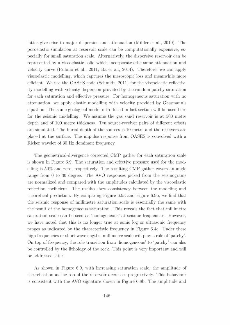
latter gives rise to major dispersion and attenuation (Muller et al., 2010). The

poroelastic simulation at reservoir scale can be computationally expensive, es-

pecially for small saturation scale. Alternatively, the dispersive reservoir can be

represented by a viscoelastic solid which incorporates the same attenuation and

velocity curve (Rubino et al., 2011; Ba et al., 2014). Therefore, we can apply

viscoelastic modelling, which captures the mesoscopic loss and meanwhile more

efficient. We use the OASES code (Schmidt, 2011) for the viscoelastic reflectiv-

ity modelling with velocity dispersion provided by the random patchy saturation

for each saturation and effective pressure. For homogeneous saturation with no

attenuation, we apply elastic modelling with velocity provided by Gassmann’s

equation. The same geological model introduced in last section will be used here

for the seismic modelling. We assume the gas sand reservoir is at 500 metre

depth and of 100 metre thickness. Ten source-receiver pairs of different offsets

are simulated. The burial depth of the sources is 10 metre and the receivers are

placed at the surface. The impulse response from OASES is convolved with a

Ricker wavelet of 30 Hz dominant frequency.

The geometrical-divergence corrected CMP gather for each saturation scale

is shown in Figure 6.9. The saturation and effective pressure used for the mod-

elling is 50% and zero, respectively. The resulting CMP gather covers an angle

range from 0 to 30 degree. The AVO responses picked from the seismograms

are normalized and compared with the amplitudes calculated by the viscoelastic

reflection coefficient. The results show consistency between the modeling and

theoretical prediction. By comparing Figure 6.9a and Figure 6.9b, we find that

the seismic response of millimetre saturation scale is essentially the same with

the result of the homogeneous saturation. This reveals the fact that millimetre

saturation scale can be seen as ‘homogeneous’ at seismic frequencies. However,

we have noted that this is no longer true at sonic log or ultrasonic frequency

ranges as indicated by the characteristic frequency in Figure 6.4c. Under these

high frequencies or short wavelengths, millimetre scale will play a role of ‘patchy’.

On top of frequency, the role transition from ‘homogeneous’ to ‘patchy’ can also

be controlled by the lithology of the rock. This point is very important and will

be addressed later.

As shown in Figure 6.9, with increasing saturation scale, the amplitude of

the reflection at the top of the reservoir decreases progressively. This behaviour

is consistent with the AVO signature shown in Figure 6.8b. The amplitude and

146

1 2 3 4 5 6 7 8 910

400

450

500

550

600

650

Offset number

Tim

e [m

s]

(a) Homogeneous

1 2 3 4 5 6 7 8 910

400

450

500

550

600

650

Offset number

Tim

e [m

s]

(b) 5 mm

1 2 3 4 5 6 7 8 910

400

450

500

550

600

650

Offset number

Tim

e [m

s]

(c) 15 cm

1 2 3 4 5 6 7 8 910

400

450

500

550

600

650

Offset numberTi

me

[ms]

(d) 2 mFigure 6.9: CMP gathers showing the reflections at top and bottom of the reservoir.Ricker wavelet of 30 Hz dominant frequency is used for the modelling. The reservoir isassumed to have 50% saturation and zero effective pressure. The saturation scales are(a) homogeneous; (b) 5 mm; (c) 15 cm; (d) 2m, respectively.

arrival time of the base reflection differs significantly for each saturation scale.

Because the base reflection is not only affected by the reflection coefficient but

also the attenuation due to wave propagation. This contrasting behaviour can

be clearly identified by comparing the zero-offset traces in Figure 6.10a. The

millimetre saturation scale possesses the largest base-reflection amplitude as the

propagation loss is minimum. This is indicated by the negligible attenuation from

Figure 6.5a. The arrival time of the reflected wave from the base is the latest for

the millimetre saturation scale as its corresponding velocity is the lowest, which

is also shown in Figure 6.5b. Then centimetre saturation scale has the smallest

147

(a)

350 400 450 500 550 600-0.5

-0.4

-0.3

-0.2

-0.1

0

0.1

0.2

0.3

0.4

0.5

Time [ms]

Am

plitu

de

GassmannPatchy 5mmPatchy 15cmPatchy 2m

(b)

400 450 500 550 6000

5

10

15

20

25

30

35

40

45

50

Time [ms]

Freq

uenc

y [H

z]

GassmannPatchy 5mmPatchy 15cmPatchy 2m

Figure 6.10: (a) Zero-offset trace extracted from the CMP gather in Figure 6.9; (b)Instantaneous frequency associated with the Zero-offset trace.

amplitude because of high attenuation due to wave-induced pressure diffusion.

Meanwhile, it is associated with an early arrival time due to velocity disper-

sion. The biggest time-shift corresponds to the metre saturation scale whereas

its amplitude resides in between the other two scales.

The instantaneous frequency can be a useful tool to illustrate the attenuation

148

behaviour of a reservoir (Castagna et al., 2003). In Figure 6.10b, we show the

instantaneous frequency attribute of the zero-offset traces extracted from the

CMP gathers. A loss of high frequency content after propagation can be observed

for centimetre and metre saturation scale. Also accompanied with these two cases

is a shifted time location of the dominant frequency. Most interestingly, two low

frequency tails appears for the two attenuative saturation scales. The frequency

content and width of the tails are proportional to the amount of attenuation. This

behaviour is most likely associated with the low frequency shadow of hydrocarbon

reservoir with high attenuation (Castagna et al., 2003).

Generally speaking, Figure 6.10a, 6.10b reveals the typical characteristics of a

frequency-dependent attenuative reservoir. Let us envisage a reservoir dominated

by a bell-shape attenuation curve with characteristic frequency fc, the associated

velocity is a monotonic increasing function of frequency. If the frequency of the

incident wave is f , we have the following three cases

• f � fc −→ small V , small Q−1 ,

• f ≈ fc −→ medium V , high Q−1 ,

• f � fc −→ high V , small Q−1 .

In the realm of patchy-saturation with Class III reservoir assumption, these three

cases are associated with the presence of millimetre, centimetre and metre sat-

uration scale, respectively. For a single 3D seismic survey, one can always use

the patchy saturation model with a reasonable saturation scale or patch size to

fit the observed velocity and attenuation. Accordingly, the saturation or fluid

pressure are inverted. In a 4D seismic survey, the saturation, fluid pressure

and saturation scale will all become a function of time. What commonly being

used for 4D interpretation is to apply the patchy saturation model with a time-

independent saturation scale and attribute the causes for time-lapse attenuation

solely to the change of saturation or fluid pressure. This approach can be prob-

lematic, especially in presence of a drastic change of subsurface fluid distribution

over time. As can be seen from Figures 6.6, 6.7, different scales with different

saturation/pressure can result in the same attenuation and velocity, which cre-

ates an ambiguity for the interpretation. In the next section, we emphasize the

importance of including the saturation scale into quantitative interpretation of

4D seismic signatures.

149

6.4 Implications for the interpretation of time-

lapse data

The reservoir fluid distribution can differ over the repeated seismic surveys

during the time-lapse monitoring. Therefore, integrating the time-dependent sat-

uration scale is important for quantitative interpretation of time-lapse attenua-

tion. Between two surveys, the time shift for the reflected P-wave from the

reservoir base can be written as

Δt = 2

(h

V2(Sg2, Pe2, b2)− h

V1(Sg1, Pe1, b1))

), (6.9)

where h is the thickness of the reservoir. The change of the amplitude (or time-

lapse amplitude) at the top of reservoir can be given by

ΔA = |(A2(Sg2, Pe2, b2)− A1(Sg1, Pe1, b1))| , (6.10)

In an attenuative reservoir, both the time shift and amplitude are frequency-

dependent. For normal incidence, the amplitude between two dispersive half-

spaces can be expressed as (Ren et al., 2009)

A(ω) =

√ω2(Vplρ2 − Vpuρ1)2 + V 2

puV2pl(ρual)

2

ω2(Vplρl + Vpuρu)2 + V 2puV

2pl(ρual)

2, (6.11)

where the superscripts l, u denote the upper and lower half-spaces and a is the

attenuation coefficient (see Appendix D). The amplitude given by equation 6.11

reduces to the elastic case when the attenuation coefficent a becomes zero. Equa-

tions 6.10 and 6.11 can be combined to calculate the time-lapse amplitude at

normal incidence. Based on equations 6.9–6.11 and the reflection coefficient in-

troduced in the previous section, we demonstrate how saturation scale affects the

interpretation of time-lapse data by analysing the time shift, amplitude change

and time-lapse AVA signature.

6.4.1 Scale effect on saturation estimation

The time-shift and amplitude change during gas injection is shown in Figure

6.11. The wave frequency is 30 Hz and the effective pressure here is assumed to be

zero to highlight the saturation effect. In Figure 6.11a, the millimetre saturation

150

(a)

0 0.2 0.4 0.6 0.8 10

10

20

30

40

50

60

Gas saturation

Tim

e sh

ift [m

s]

GassmannPatchy 5 mmPatchy 15 cmPatchy 2 mHill

(b)

0 0.2 0.4 0.6 0.8 10

0.05

0.1

0.15

0.2

0.25

0.3

Gas saturation

Am

plitu

de c

hang

e

GassmannPatchy 5mmPatchy 15cmPatchy 2mHill

Figure 6.11: Time shift and amplitude change are plotted as function of saturation.The frequency and effective pressure are 30 Hz and zero, respectively.

scale presents an increasing time delay when the gas saturation increases from

zero to few percent. When the gas saturation keeps increasing, the amount of time

delay gradually decreases. The centimetre saturation scale presents a gradually

increased time delay with increasing gas saturation. For the metre saturation

scale, the time delay increases quickly and linearly with increasing gas saturation.

In Figure 6.11b, the amplitude change decreases with increasing gas saturation for

151

all scales. In presence of millimetre saturation scale, the time shift and amplitude

change shows less sensitivity with the change of gas saturation. In other words,

with prior knowledge on the change of gas saturation (from well logging data),

if the slopes of the time shift and amplitude change are small, we can deduce

that there is neither larger fluid patches nor a jump in saturation scale during

the repeated surveys. On the other hand, let us assume there is a change of fluid

patch size or a jump in saturation scale (for example from the green curve to the

red curve) with increasing gas saturation. In this case, interpreting an observed

time shift and change in amplitude using Gassmann model or a constant scale

patchy model can result in underestimation in the change of gas saturation.

Whether the reservoir fluids are distributed uniformly or in a patchy manner

will have implications on AVO inversion. To illustrate this point, we compare

time-lapse AVA signatures modelled by Gassmann theory and patchy model. A

correlation length of 1 metre is assumed for the patchy case. In Figure 6.12,

the AVA responses at the end-member saturations are the same for both mod-

els. The gas sand has appreciably stronger reflection than the wet sand. For

uniform saturation, AVA responses for 0% to 95% gas saturations are localized

near the gas bound. In contrast to in patchy saturation, AVAs are evenly dis-

tributed between the bounds. The difference can be explained by invoking the

impedance-saturation relation, see Figure 6.12b. The random patchy saturation

model entails a gradual change of the impedance with saturation which results

in smoothed impedance contrast. Whereas the Gassmann-Wood model implies

a strong ‘gas effect’, this causes a sudden drop of the impedance contrast near

full water saturation. The comparison also indicates that, in presence of ‘seismic

scale’ fluid patches, interpreting time-lapse AVA response with Gassmann model

will overestimate the change in water saturation. Another interesting point we

can draw from Figure 6.12 is that, for homogeneous saturation, the AVA re-

sponses can never reach below 0.2 (except for the wet sand). On the other hand,

for patchy saturation, the minimum AVA response reaches 0.1. Hence, given

the prior knowledge of the rock properties (from well logging data), one can use

time-lapse AVA to deduce the information of fluid distribution.

6.4.2 Scale effect on pressure estimation

Figure 6.13 emphasize the effect of saturation scale on the estimation of pres-

sure change. We consider here that the time-lapse signal variation is mainly

152

(a)

0 10 20 30 40 50 600

0.05

0.1

0.15

0.2

0.25

0.3

0.35

0.4

0.45

0.5

Angle [Degree]

Am

plitu

de

Sw

0

0.1

0.2

0.3

0.4

0.5

0.6

0.7

0.8

0.9

1

Gas saturated

Water saturated

Gassmann

(b)

0 10 20 30 40 50 600

0.05

0.1

0.15

0.2

0.25

0.3

0.35

0.4

0.45

0.5

Angle [Degree]

Am

plitu

de

Sw

0

0.1

0.2

0.3

0.4

0.5

0.6

0.7

0.8

0.9

1

Gas saturated

Water saturated

Patchy Saturation b=1m

Figure 6.12: Time-lapse AVA signature for saturation change. Prediction is made using(a) Gassmann equation and (b) patchy saturation model with 1 m saturation scale. Thefrequency and effective pressure are 30 Hz and zero, respectively.

caused by change of pressure and consequently a constant saturation of 50%.

The frequency is still 30 Hz. Let us also assume that the confining pressure re-

mains constant and an average effective stress coefficient for the reservoir is 1.

Thus, the increment of the effective pressure will be equivalent to the decrement

of the fluid pressure. Here, we only focus on effective pressure varies from 0 to

153

(a)

0 10 20 30 40 50 60-45

-40

-35

-30

-25

-20

-15

-10

-5

0

Tim

e sh

ift [m

s]

Pe [MPa]

GassmannPatchy 5mmPatchy 15cmPatchy 2mHill

(b)

0 10 20 30 40 50 600

0.02

0.04

0.06

0.08

0.1

0.12

0.14

0.16

Pe [MPa]

Am

plitu

de c

hang

e

GassmannPatchy 5mmPatchy 15cmPatchy 2mHill

Figure 6.13: Time shift and amplitude change are plotted as function of effective pres-sure. The frequency and saturation are 30 Hz and 50%, respectively.

10 MPa as the maximum lithostatic pressure with 500 metre overburden shale

is 10 MPa. As shown in Figure 6.13, the time pull-up and amplitude change

increase with increasing effective pressure or decreasing fluid pressure. We see

that saturation scale does not play a significant role on the signal for pressure

changing from 0 to 5 MPa. When pressure change resides between 5 and 10 MPa,

if we assume that the pressure change over repeated surveys is accompanied with

154

an increase in saturation scale (for example, from the blue curve to the green

curve or from the green curve to the red curve). In this situation, interpreting an

observed time shift or amplitude change with the Gassmann model or a constant

scale patchy model will overestimate the decrement of fluid pressure. Also com-

paring with the saturation effect (on the net range of time shift and amplitude

change) in Figure 6.12, we see that pressure effect has a relative small capability

in influencing time-lapse signal.

We compare the time-lapse AVA signatures computed using Gassmann model

and patchy model in Figure 6.14. The patchy model incorporates an correlation

length of 1 metre. In Figure 6.14, from the zero effective pressure line (top blank

line), every following line indicates an increase of 2 MPa effective pressure or

decrease of 2 MPa fluid pressure. The amplitude decreases with increasing effec-

tive pressure (decreasing fluid pressure). On the contrary, the angle dependence

is greater for larger effective pressure. Let us interpret a same time-lapse AVA

decrease, denoted by the white rectangle in the plots, with the two different mod-

els. The patchy model with metre saturation scale predicts a decrease of fluid

pressure from 1 MPa to 8 MPa whereas the Gassmann model predicts a decrease

of fluid pressure from 8 MPa to 40 MPa. Here, we see that if the reservoir has a

patchy fluid distribution, interpreting an observed time-lapse AVA response can

result in both unreasonable change and value of the fluid pressure.

6.4.3 Effects of capillary pressure and residual saturation

Let us now analyse the influence of capillary pressure and irreducible water

saturation on 4D interpretation. To this end, we assume a capillarity stiffening T

of 1.5 GPa and a irreducible water saturation Sirrw of 20%. The modified lower

and upper bounds for the P-wave modulus can be calculated using equation 6.4

and 6.5, accordingly. Then we calculate the corresponding time shift using equa-

tion 6.9 with the calculated velocities. The time shifts at low and high frequency

limits for gas injection is shown in Figure 6.15. We compare the results asso-

ciated with the modified bounds with the results associated with conventional

Gassmann and Hill limits. In Figure 6.15, at low frequencies, the maximum time

delay decreases upon consideration of capillarity (see the change from solid curve

to squares). This is because the stiffening effect from capillarity compensates the

softening effect from density. Time delay now gradually increases with increasing

gas saturation. At high frequencies, due to presence of residual water satura-

155

(a)

0 10 20 30 40 50 600.1

0.15

0.2

0.25

0.3

0.35

0.4

0.45

0.5

Angle [Degree]

Am

plitu

de

Pe [M

Pa]

0

10

20

30

40

50

60Gassmann

(b)

0 10 20 30 40 50 600.1

0.15

0.2

0.25

0.3

0.35

0.4

0.45

0.5

Angle [Degree]

Am

plitu

de

Pe [M

Pa]

0

10

20

30

40

50

60Patchy Saturation b=1m

Figure 6.14: Time-lapse AVA signature for effective pressure change. Prediction is madeusing (a) Gassmann equation and (b) patchy saturation model with 1 m saturationscale. The frequency and saturation are 30 Hz and 50%, respectively.

tion, the time shift yields a stronger dependence on the change of gas saturation

comparing with Hill prediction (see the change from dashed line to triangles).

When both effects are considered, it results a narrower envelope of possible time

shift between saturation limits of 0 and 80% gas saturation. Consequently, the

uncertainty due to scale effect in predicting the saturation change becomes less.

156

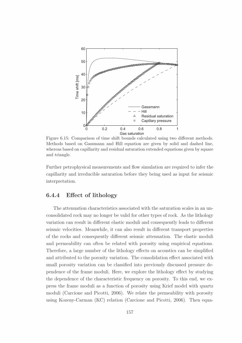
0 0.2 0.4 0.6 0.8 10

10

20

30

40

50

60

Gas saturation

Tim

e sh

ift [m

s]

GassmannHillResidual saturationCapillary pressure

Figure 6.15: Comparison of time shift bounds calculated using two different methods.Methods based on Gassmann and Hill equation are given by solid and dashed line,whereas based on capillarity and residual saturation extended equations given by squareand triangle.

Further petrophysical measurements and flow simulation are required to infer the

capillarity and irreducible saturation before they being used as input for seismic

interpretation.

6.4.4 Effect of lithology

The attenuation characteristics associated with the saturation scales in an un-

consolidated rock may no longer be valid for other types of rock. As the lithology

variation can result in different elastic moduli and consequently leads to different

seismic velocities. Meanwhile, it can also result in different transport properties

of the rocks and consequently different seismic attenuation. The elastic moduli

and permeability can often be related with porosity using empirical equations.

Therefore, a large number of the lithology effects on acoustics can be simplified

and attributed to the porosity variation. The consolidation effect associated with

small porosity variation can be classified into previously discussed pressure de-

pendence of the frame moduli. Here, we explore the lithology effect by studying

the dependence of the characteristic frequency on porosity. To this end, we ex-

press the frame moduli as a function of porosity using Krief model with quartz

moduli (Carcione and Picotti, 2006). We relate the permeability with porosity

using Kozeny-Carman (KC) relation (Carcione and Picotti, 2006). Then equa-

157

0.01 0.05 0.1 0.15 0.2 0.25 0.310-4

10-2

100

102

104

106

Porosity

f c [Hz]

Patchy 5mmPatchy 7cmPatchy 2m

KC, 17 mD, 12 Hz

Eagle Ford shale, 1 uD, 0.001 Hz

Figure 6.16: Effect of lithology on characteristic frequency. Saturation of 50% andeffective pressure of zero are assumed.

tion 6.6 is used to compute the characteristic frequency for different saturation

scales. We see that in Figure 6.16, when the porosity is reduced from 30% to

1%, the characteristic frequency decreases substantially by 3 orders of magni-

tude. For sandstone of large porosity, the millimetre saturation scale results in

an attenuation peak in kilohertz range, thus, it is effectively ‘homogeneous’ scale

at seismic frequencies. For tight sands or shales of small intrinsic porosity, the

millimetre saturation scale gives rise to a attenuation peak in seismic frequency

range. In this case, the millimetre saturation scale will act as ‘patchy’. With

respect to centimetre and metre saturation scales, the attenuation peaks of the

small-porosity rocks (φ <5%) locate below seismic frequency. Therefore, seis-

mic frequency band turns into the high frequency regime. In this case, incident

waves of seismic frequency results in unrelaxed undrained rock, the attenuation

of which becomes negligible whereas the velocity given by Hill theory. Common

thinking is that millimetre saturation scale are only responsible for attenuation

taking place at high frequencies (e.g., ultrasonic, sonic log and crosswell). How-

ever, this is no longer true for rocks with small porosity. This phenomenon has

recently been observed in low frequency laboratory measurement of Eagle Ford

shale (Mikhaltsevitch et al., 2015). In their work, in presence of fluid patches

of 7 centimetres (sample size), no velocity dispersion presents in frequency range

from 0.1 Hz to 500 KHz. The porosity of the Eagle Ford shale sample is 9%.

Using Kozeny-Carman (KC) relation, it results in a permeability of 17 mD and

158

fc of 12 Hz (denoted by circle in Figure 6.16). The measured permeability is

1 μD in the work of Mikhaltsevitch et al. (2015). Apparently Kozeny-Carman

relation fails to predict the right permeability for shale in this case. However, if

we reduce the characteristic frequency (fc ∝ κ) by 4 orders of magnitude as the

exact overestimation in permeability from KC, we will have a fc equal to 0.001

Hz. This indicates that the employed frequency range in the experiment resides

in the non-dispersive regime (high frequency), which is consistent with the lab

observation. Since seismic frequencies become effective ‘high’ frequency for low-

porosity saturated rock, velocity would be close to Hill prediction. Therefore, we

may expect less influence of saturation scale variation on 4D signatures.

6.4.5 Effect of in-situ fluid property

The reservoir fluid properties, such as fluid bulk modulus and density can be

affected by the changes in composition, pressure and temperature during pro-

duction (Johnston, 2013). Our concern here is how the changes of the in-situ

fluid properties affect the attenuation characteristics. Let us further examine

the expression of the characteristic frequency with particular emphasis on fluid

properties. Again fc can be written as

fc =1

2π

D

b2=

1

2π

κ

b2NwSw +NgSg

ηwSw + ηgSg

, (6.12)

with stiff frame approximation Kg � Kf , it further reduces to

fc =1

2π

κ

φb2KfwSw +KfgSg

ηwSw + ηgSg

. (6.13)

Because the gas modulus Kfg and viscosity ηg are much smaller than those of

water, we have

fc =1

2π

κ

φb2Kfw(T, P )

ηw. (6.14)

Therefore, fc essentially relies on the water properties, or precisely the properties

of the stiffer fluid phase. Several important points can be drawn from equa-

tion 6.14. We see that in-situ gas properties do not affect the position of the

attenuation peak and consequently has no influence on the characteristic of the

saturation scale. However, it does affect the amount of attenuation. This is be-

cause when the gas modulus increases with increasing depth, the compressibility

contrast between gas and water saturated region becomes smaller. Consequently,

159

the attenuation due to wave-induced pressure diffusion becomes small. On the

other hand, fc is inversely proportional to the fluid viscosity in equation 6.14. Let

us assume the reservoir contains heavy oil with high viscosity. In this situation,

the attenuation peak (or the characteristic frequency) will shift towards lower

frequency and consequently affect the attenuation characteristic of the discussed

saturation scale. The effect of fluid viscosity on attenuation has been observed

in laboratory by Batzle et al (2006). Same logic with the low porosity rock (last

section) can be applied here: with high viscosity fluids, we may expect less influ-

ence of saturation scale variation on 4D signatures. Despite the complex causes of

in-situ fluid properties, one can always calculate them using equations based on

thermodynamic laws or apply empirical relations obtained from laboratory mea-

surement (Johnston, 2013). These reservoir fluid properties will be used in the

model and the resulting attenuation characteristics can be analyzed accordingly.

6.4.6 Effect of geological complexity

The homogeneous reservoir model employed in this study is of course a simpli-

fication of the realistic reservoir. The natural reservoir and its overburden in sed-

imentary environment may be fractured (lecture by Liu, 2013) and thinly layered

(Gelinsky et al., 1998; MacBeth and Stephen, 2008). Reservoir heterogeneities

can lead to frequency-dependent attenuation, which further complicates the in-

terpretation of time-lapse seismic signatures. Thus, it is important to estimate

the attenuation caused by these frame heterogeneities and correct them from the

observed attenuation or amplitude. The corrected attenuation/amplitude which

is due to fluid heterogeneities, may then be interpreted with the patchy saturation

model. However, the superposition rule (for attenuation) is not valid for veloc-

ity and hence the interpretation of time shift becomes more difficult. Therefore,

further refinement of patchy saturation model is recommended to take geological

heterogeneities into account. The fluid distribution provided by flow simulation

can be used to constrain the development of the saturation model (MacBeth and

Stephen, 2008).

6.5 Identification of saturation scale

Last but not the least, the important question yet to be addressed is where do

we find the saturation scale? From previous discussion, we see that finding the

representative saturation scale for each survey time as input for 4D interpretation

160

can be crucial. As shown in Figures 6.12 and 6.14, the AVO has the potential to

serve as an indicator for the saturation scale. Considering all possible saturations

and pressure, the characteristics and value of AVA signatures between homoge-

neous and patchy saturation are different. This can be used to distinguish the two

scenarios. Laboratory rock physicists also try to study the evolution of the fluid

distribution with change of saturation from core-flooding experiment. However,

the observed fluid distribution is restricted to both the image resolution and size

of the sample. Hence, it is still under debate if it can be used as the representative

fluid distribution at reservoir scale. The accepted fact is that the realistic fluid

distribution and attenuation mechanism are still poorly understood. Nonethe-

less, as a first order approximation, the best way for obtaining the ‘seismic’ fluid

distribution is perhaps using the patchy saturation model to fit the real data.

With the commonly available time-lapse well logs and VSP data (Caspari et al.,

2011; Al Hosni et al., 2015), one has the constrained velocity versus saturation

relation around the well location. The established velocity -saturation relation

can be fitted with the patchy saturation model. The deduced saturation scale

or patch size can be seen as the representative fluid distribution at the survey

moment. It can be used as a constraint at the well location when applying seismic

inversion in combination with the patchy saturation model. With integration of

time-dependent saturation scale from well log and VSP into inversion, we may

be able to achieve the more robust fluid distribution over time and space, and

consequently, more accurate information on the variation of saturation and fluid

pressure. Recent studies also indicate that spectral decomposition (Castagna

et al., 2003; Rubino et al., 2011) and resistivity -saturation relation (Alemu et

al., 2013) can potentially become useful tools for obtaining the fluid distribution

information.

6.6 Chapter conclusions

Dynamic fluid injection in operations such as enhanced oil recovery and CO2

sequestration inevitably leads to the formation of fluid clusters (patches). These

fluid clusters continuously change in shape and size. Despite their spatio-temporal

variability, these clusters have a characteristic length scale at every instant of

time. This saturation scale is a per se unknown variable and induces yet another

uncertainty into quantitative seismic interpretation of time-lapse signatures in

addition the to the saturation and formation pressure changes usually considered.

161

In contrast to empirical models (for example, Brie et al. (1995)), the satura-

tion scale is firmly embedded in the random patchy saturation model including its

extensions for capillarity and residual saturation. Thus, it can be used to analyse

the effect of saturation-scale on time-lapse changes. Both, travel-time shifts and

time-lapse attenuation can be addressed.

In this work, three contrastingly different saturation scales (namely millime-

tre, centimetre and metre sized patches) are used to demonstrate their influence

on time-lapse signatures of a simplistic geological model: The reservoir consists

of an unconsolidated partially saturated sand – modelled as a poroelastic solid

embedded between two shale layers. We find that

• The millimetre saturation scale is associated with dominant attenuation due

to wave-induced pressure diffusion (in the reservoir zone) in the kilohertz

range; the metre scale is responsible for attenuation in the millihertz band.

The centimetre scale leads to significant attenuation at seismic frequencies.

This scale leads to the highest attenuation for all saturations and pressures.

The attenuation levels off at high effective pressure.

• The saturation scale significantly changes the AVF (amplitude versus-frequency)

and AVA (amplitude-versus-angle) responses of the reflected P-wave. For

a class III reservoir, the amplitude of the reflected P-wave decreases with

increasing saturation scale.

• The reflected P-wave from the base of a centimetre-saturation-scale reser-

voir possesses the smallest amplitude. The earliest arrival time of the base

reflection is associated with the metre saturation scale. The seismic signa-

ture of the millimetre saturation scale is the same with elastic modelling

result using homogeneous saturation assumption.

• The time shift and amplitude change of a millimetre saturation-scale reser-

voir is less sensitive to the change of gas saturation compared to the other

two scales. In presence of saturation scale increase/decrease, interpreting

an observed time shift and amplitude change using Gassmann model or a

single scale patchy model will lead to underestimation/overestimation of

gas saturation.

• The saturation scale has less impact on the prediction of fluid pressure

changes. Nevertheless, interpreting an observed time shift or amplitude

162

change with the Gassmann model or a single scale patchy model will under-

estimate/overestimate the fluid pressure if the saturation scale increases/decreases

during the gas injection.

• When the time-lapse signal is dominated by either saturation or pressure

changes, the associated time-lapse AVA signature is different between uni-

form and patchy saturation. This indicates that time-lapse AVA can be

used to infer the subsurface fluid distribution.

• Including the effects of capillarity and residual saturation into the interpre-

tation can potentially reduce the uncertainty from saturation scale effect.

We expect less influence of saturation scale variation on time-lapse seismic

signature either when the porosity of rock is low or the viscosity of fluids

are high.

163

Chapter 7

Conclusions and outlook

Capillarity is a crucial petrophysical parameter which is extensively used by

petroleum engineer for evaluating the reservoir quality and performance. Though

capillarity provides key source of petrophysical information, its role on the mod-

elling of the acoustic signatures has been largely overlooked in rock physics until

this thesis. Through the study of this thesis, we have achieved two major ob-

jectives: one is to investigate the role of capillarity on the wave characteristics

(i.e., velocity, attenuation, reflectivity) in partially saturated porous rocks and

another is to address the implications of the new theory on QSI (quantitative

seismic interpretation) across the hydrocarbon exploration and production life

cycle. The study has been carried out through three primary steps including the

development of the rock physics model, the model calibration via laboratory data

modelling and the practical implementation of the model into QSI. In this final

chapter, I will briefly summarize the obtained results. Based on these results, I

will discuss their application potentials and the associated future aspects.

The presence of the capillarity in response to the dynamic wave propagation can

be represented by a fluid pressure discontinuity boundary condition. Including

this boundary condition in the upscaling procedure of Biot’s dynamic equations

with respect to a mesoscopic geometry configuration enables the study the com-

bined effects of capillarity and mesoscopic fluid flow. Based on this central idea,

the classical White’s model for P-wave attenuation in patchy-saturated layered

media is generalized to account the capillary pressure. The original White’s the-

ory predicts that the low frequency limit of the P-wave velocity is given by the

164

Gassmann’s equation with an effective fluid modulus calculated by the Wood’s

formula. In contrast, the new theory indicates that such static velocity limit can

be further controlled by the capillary pressure. The capillary pressure gives rise

to a membrane stiffness which exerts between the contact area of the immiscible

fluid phases. As a result, the dispersion and attenuation diminishes. These results

lead to an intriguing fact that the Gassmann-Wood theory as well as the original

White’s model are only valid when the capillarity effect is negligibly small. In

other words, it implies that when the reservoir capillarity effect is strong, mod-

elling the velocities obtained from well-log or seismic data with the capillarity-

corrected model will give an increased estimation of the gas saturation (see Figure

3.3 for example). In the current framework of the capillarity-extended White’s

model, the rock frame is required to be homogeneous and isotropic. Given that

the resulting analytical expression (i.e., equation 3.24) for the P-wave modulus

is simple, one possible extension of the model is to further consider the presence

of fractures in the porous host rock. This requires that the generalized White’s

model would to be parametrized within the framework of linear slip theory (Bra-

janovski et al., 2005; Kong et al., 2013). This could be a simple recipe for studying

the capillarity effect in fractured rocks. Frame heterogeneities such as fractures

and permeability fluctuations often lead to an effective anisotropic behaviour of

rocks. If the fractures are aligned, the generalized White’s model can be further

extended to investigate angle-dependence of the attenuation and dispersion using

the recipe suggested by Krzikalla and Muller (2011) and Carcione et al. (2013).

The capillary force controls the two-phase flow behaviour and is inherently cou-

pled with the fluid distribution. The fluid distribution again influences the elastic

properties of the saturated porous rock via mesoscopic fluid flow. To explore the

relationships between the capillarity, fluid distribution and acoustic properties,

the concept of membrane stiffness is incorporated into the framework of the 3D

random patchy saturation model. It is found that not only the membrane stiffness

but also the spatial fluid distribution (i.e., correlation length, specific surface area)

can affect the capillarity stiffening. It is interesting to see that the capillarity-

extended static P-wave velocity increases with increasing correlation length of

the fluid patches. Consequently, the dispersion and attenuation further decreases

with increasing correlation length of the fluid patches at seismic frequencies. The

developed model can be useful for the seismic reservoir monitoring where the

capillarity may play an important role during the dynamic fluid injection. To

validate this idea, the model is applied to interpret the ultrasonic data acquired

165

during a core-flooding experiment where the capillary force dominates the two-

phase flow regime. The predicted velocity- and attenuation- saturation relations

indeed show consistency with the laboratory data. The model has shown its

predictive power at ultrasonic frequencies, however, its applicability at low fre-

quencies still needs to be verified. Therefore, it is recommended as future work

to conduct low-frequency experiments on partially saturated rocks (Batzle et al.,

2006; Tisato and Quintal, 2013) for a thorough examination of the capillarity

phenomenon. The employed frequency of the measurement shall reside in the

low-frequency asymptotic regimes of any attenuation mechanisms. Thus, the ad-

ditional stiffening of the rock (if observed) can be attributed to the capillarity

effect. The experiments shall also be combined with X-ray CT imaging. The

statistical analysis of these CT images will be helpful for quantifying the effect

of the spatial fluid distribution on the capillarity stiffening.

It is shown that the capillary pressure across the mesoscopic fluid heterogeneities

has a strong effect on the velocity and attenuation. On the other hand, in a

large reservoir, the capillary pressure can present between the gas-water contact

and affect the seismic reflectivity. The reflection theory based on Biot’s poroe-

lasticity has been extended to investigate the role of the interfacial impedance

(i.e., capillarity, interface permeability) on the P-wave reflectivity. It is found

that the capillarity effect has a negligible impact on the P-wave reflectivity for

a gas-water contact at seismic frequencies. Because the capillarity effect on the

mesoscopic fluid flow is much more predominant than the capillarity effect on

the P-wave reflectivity, we suggest that the viscoelastic modelling with attenua-

tion estimated from the capillarity-extended patchy saturation model is sufficient

to capture the capillarity effect on seismic signatures at reservoir scale. On the

other hand, we do find that the capillarity has a substantial effect on the P-

wave seismic reflectivity for a fluid/gas-saturated-medium contact. Especially,

the contrasting amplitude-versus-angle behaviour resulting from open-pore, cap-

illarity and imperfect hydraulic contact (see Figure 5.3, 5.3) provide a theoretical

basis for examining these interface scenarios in the laboratory settings. For ex-

ample, by comparing the theoretically calculated reflectivity with the measure

reflectivity in the lab, one may quantify the value of the membrane stiffness, in-

terface permeability in real rocks. These values can be further used in acoustic

models, i.e., extended White’s layered model or extended random patchy satu-

ration model to compute the velocity and attenuation of a specific rock. It is

therefore recommended as future work to devise a laboratory pulse-transmission

166

set-up (Johnson et al., 1994; Bouzidi and Schmitt, 2009) for investigating the

seismic reflectivity associated with a fluid/gas-saturated-medium contact. An-

other possible application of the extended theory is to use AVO technique for

quantifying the sea-floor properties (Amundsen and Reitan, 1995). Particularly,

for a gas-saturated sea-floor whose interface is not perfectly sealed by sediments,

the resulting AVO behaviour is expected to be different from the prediction of

the elastic theory.

A workflow for the interpretation of the time-lapse seismic signatures has been es-

tablished based on the developed patchy saturation model. We find that a chang-

ing saturation scale can be yet another crucial factor which controls the time-lapse

seismic signal. Saturation scales of different orders are associated with contrast-

ing acoustic characteristics of a partially saturated reservoir. A time-dependent

saturation scale further complicates the analysis of the associated time-shifts and

amplitude changes. As a result, ignoring the potential saturation scale variation

over the repeated seismic surveys can result in biased estimation/discrimination

of the saturation and fluid pressure from time-lapse seismic data. It is also found

that including the effects of capillarity and residual saturation into the time-lapse

analysis potentially reduces the uncertainty introduced by the scale effect. The

study implies that integrating the saturation scale and capillarity effect into time-

lapse AVO analysis (Landrø, 2001) can potentially lead to better discrimination

of the saturation and pressure effects. The sub-resolution saturation scale, as

an input for this theory, can be deduced from time-lapse well-log or VSP data

(Konishi et al., 2009; Caspari et al., 2011; Al Hosni et al., 2015). These data is of

high spatial resolution and can provide constraints on the spatial-temporal fluid

distribution. A simple analysis such as comparison of the log- or VSP- derived

velocity-saturation relations with Gassmann modelling results (i.e.,low saturation

scale limit) should determine whether the saturation scale is a first order effect.

If the saturation scale variation is evident, then a patchy saturation model is

suggested to be applied in the time-lapse AVO analysis (Landrø, 2001) to honour

the accompanied attenuation and dispersion effects. Feasibility studies are also

required in the future to examine the sensitivity of the seismic amplitudes on the

log-derived saturation scales.

167

List of Figures

1.1 Scales of heterogeneities which are relevant for wave-induced fluidflow. . . . . . . . . . . . . . . . . . . . . . . . . . . . . . . . . . . 5

1.2 (a) Seismic section showing attenuation in a gas-saturated zonebeneath hydrate-bearing sediments. After Morgan et al. (2012).(b) Gas chimney with strong distortion of seismic amplitudes. Af-ter Granli et al. (1999). (c) Seismic monitoring of CO2 storage.After Arts et al. (2008). (d) Low frequency anomalies below gasreservoir. After Castagna et al. (2003). . . . . . . . . . . . . . . . 6

1.3 Estimated fluid saturation changes (left) and pore pressure changes(right) based on 4D AVO analysis for the top Cook interface atGullfaks. Yellow color represents significant change, red line showsoriginal oil-water contact. After Landrø (2001). . . . . . . . . . . 7

1.4 Comparison between modeled velocity-saturation relation and time-lapse log data for the (a) shallower and (b) deeper depth interval atsonic frequencies. ‘GW’, ‘GH’ and ‘CRM’ are the Gassmann-Woodlower bound, Gassmann-Hill upper bound and patchy saturationmodel, respectively. The model employs a patch size ‘d’ of 1 and5 mm. Modified after Caspari et al. (2011). . . . . . . . . . . . . 8

1.5 (a) Scheme of the geological model for the Sleipner field. The blackthin areas indicate the main CO2 component. The narrow grayshaded areas indicate the presence of a diffuse CO2 component. (b)Seismic response considering WIFF effects due to the presence ofCO2 patches. (c) Seismic response for an equivalent elastic modelwith P-wave velocity given by Gassmanns formula. Modified afterRubino et al. (2011). . . . . . . . . . . . . . . . . . . . . . . . . . 9

1.6 Velocity-saturation relation determined from numerical simulationsof wave propagation in a poroelastic solid with randomly distributedpatches that cluster for larger saturation values (see inset). Exper-imentally determined velocities for the quasi-static injection exper-iment are also shown. After Lebedev et al. (2009). . . . . . . . . . 10

168

1.7 (a) Measurement set up and raw CT scan of the sample: the redcircle indicates the acoustic monitoring field; (b) The ultrasonicwaveforms at various saturations. The black waveforms correspondto an injection rate of 2 mL/h while the red waveforms correspondto a reduced injection rate of 0.2 mL/h.(c) Water saturation map(average Sw=68%) derived from the CT images. Mesoscopic fluidpatches appear. . . . . . . . . . . . . . . . . . . . . . . . . . . . . 11

1.8 Modeling ultrasonic data obtained during a capillary-force-dominatedimbibition: (a) velocity- and (b) attenuation- saturation relations. 12

1.9 Microscopic capillary forces (left) produce a net effect at macro-scopic scale (right). The macroscopic capillary pressure may changethe overall stiffness of the saturated rock and consequently affectsthe wave responses. Arrows denote micro- and macro- capillarypressure gradients. . . . . . . . . . . . . . . . . . . . . . . . . . . 13

2.1 Gedanken experiments for determining 4 Biot’s poroelastic con-stants and Gassmann equation: (a) pure shear test; (b) jack-eted compressibility test; (c) unjacketed compressibility test; (c)undrained compressibility test. . . . . . . . . . . . . . . . . . . . . 21

2.2 An example of (a) dispersion and (b) attenuation coefficient forthree wave modes in a water-saturated unconsolidated sandstone. 29

2.3 Simplified diagram of an interface between two porous media (afterBourbie et al, 1987). . . . . . . . . . . . . . . . . . . . . . . . . . 33

2.4 White’s model of regularly distributed spherical gas pockets of uni-form size. A spherical unit cell is equivalent in volume to a cubicalunit cell containing a gas pocket. . . . . . . . . . . . . . . . . . . 37

2.5 (a) An example of random sequence of partially saturated sedi-mentary layers. Spatial distribution of the saturation follows aexponential correlation function as shown in (b). . . . . . . . . . . 41

2.6 An example of (a) dispersion and (b) attenuation predicted byWhite’s gas pocket model (3D periodic) and 1D random patchysaturation model for a partially saturated sandstone of 15% porosity. 45

2.7 A diagram illustrating P-wave reflection and transmission betweentwo elastic solids. . . . . . . . . . . . . . . . . . . . . . . . . . . . 48

2.8 A diagram illustrating P-wave reflection and transmission betweentwo viscoelastic solids. . . . . . . . . . . . . . . . . . . . . . . . . 50

2.9 A diagram illustrating P-wave reflection and transmission betweentwo poroelastic media. . . . . . . . . . . . . . . . . . . . . . . . . 52

169

2.10 Schematic representation of the fluid boundary of a non-wettingand wetting fluid for a cylindrical pipe. The parameters θ, d, R arethe contact angle, the radius of the tube and meniscus, respectively.Modified after Nagy and Blaho (1994). . . . . . . . . . . . . . . . 54

2.11 Cartoon illustration of macroscopic capillarity in poroelasticity . . 56

2.12 Classification of mechanisms responsible for loss of seismic ampli-tude. Coloured mechanisms are the main focus of this thesis. . . 58

3.1 Schematic representation of a homogeneous sandstone alternativelysaturated by water and gas layers. The sketch at pore scale showstwo possible interface scenarios: A) clay minerals are clogging thehydraulic contact and B) meniscus unevenly distributed due tocapillarity. . . . . . . . . . . . . . . . . . . . . . . . . . . . . . . . 61

3.2 Phase velocity and inverse quality factor as functions of frequencyfor a homogeneous rock alternately saturated with gas and wa-ter. “HWM” refers to generalised White model with imperfecthydraulic contact, whereas “CWM” indicates the capillarity ex-tended White model. The values of resistance Zm

I and membranestiffness W are given in units of GPa · s/m and GPa/m, respectively. 69

3.3 Velocity- and attenuation-saturation relations for a frequency of25 Hz. The values of the resistance Zm

I and membrane stiffness Ware given in units of GPa · s/m and GPa/m, respectively. . . . . . 70

3.4 The real part (a), imaginary part (c) and amplitude (e) of fluidpressure at 50 Hz while (b),(d),(f) show their high frequency (300Hz) counterpart. The blue colour refers to open-pore case whereasred colour refers to capillarity case. The dashed line refers to fastP-wave component whereas the circle corresponds to slow P-wavecomponent. The total component is indicated by solid line. . . . . 75

3.5 The real part (a), imaginary part (c) and amplitude (e) of soliddisplacement at 50 Hz while (b),(d),(f) show their high frequency(300 Hz) counterpart. The blue colour refers to open-pore casewhereas red colour refers to capillarity case. The dashed line refersto fast P-wave component whereas the circle corresponds to slowP-wave component. The total component is indicated by solid line. 76

3.6 The real part (a), imaginary part (c) and amplitude (e) of relativedisplacement at 50 Hz while (b),(d),(f) show their high frequency(300 Hz) counterpart. The blue colour refers to open-pore casewhereas red colour refers to capillarity case. The dashed line refersto fast P-wave component whereas the circle corresponds to slowP-wave component. The total component is indicated by solid line. 77

170

3.7 (a) Capillary pressure is plotted as function of water saturationfor different frequencies. (c) Pressure difference and relative dis-placement at interface (e) are plotted as function of frequency.Dissipation at frequency of 10 Hz (a) 100 Hz (b) and 300 Hz. . . . 78

4.1 Normalised static undrained P -wave modulus is plotted as a func-tion of capillarity stiffening T for 58% water saturation (the solidblue line); the black solid line denotes the Gassmann-Wood limitwhile the dotted line denotes the Gassmann-Hill limit. . . . . . . 88

4.2 (a) Velocity dispersion and (b) attenuation of the CRM (T =0 GPa) and CCRM (T = 12 GPa) modelled at 58% water satura-tion. The correlation lengths are a = 1, 2, 3 mm (the correlation

function if of the form exp(− |r|a)). The frequency f is normalized

by critical frequency fc which is defined by equation 4.16. . . . . . 92

4.3 Velocity- (a) and attenuation- (b) saturation relations predictedby CRM (T = 0 GPa) and CCRM (T = 7, 14, 21 GPa) modelsat 0.5 MHz. The correlation length is assumed to be a = 1 mm. . 93

4.4 (a) Specific surface area (SSA) and (b) capillarity-extended staticvelocity are plotted as function of correlation length for differentwater saturations. . . . . . . . . . . . . . . . . . . . . . . . . . . . 94

4.5 (a) Velocities and attenuation predicted by CRM and CCRMmodelfor different correlation lengths. The stiffening effects due to cap-illarity and WIFF both depend on correlation length. . . . . . . . 95

4.6 Comparison of (a) velocity and (b) attenuation predicted by mod-els of different fluid distribution consideration. ‘White’ refers toWhite’s original model; ‘CWM’ refers to capillarity-extendedWhite’smodel; ‘CGM’ refers extended gas-pocket model; ‘CCRM’ refers toextended random model; ‘Lo’ refers to acoustic model of Lo andSposito (2013). . . . . . . . . . . . . . . . . . . . . . . . . . . . . 97

4.7 (a) Measurement set up and raw CT scan of the sample: the redcircle indicates the acoustic monitoring field; (b) The ultrasonicwaveforms at various saturations. The black waveforms correspondto an injection rate of 2 mL/h while the red waveforms correspondto a reduced injection rate of 0.2 mL/h. . . . . . . . . . . . . . . . 99

4.8 Spectral amplitudes of the ultrasonic waveforms. . . . . . . . . . . 100

4.9 Water-saturation maps at different imbibition stages, where darkblue represents full water saturation and dark red represents fullgas (air) saturation. The saturation maps are constructed fromthe raw CT scans for the monitoring area. The size of the maps is3 cm× 3 cm. The colour-bar indicates water saturation. . . . . . 101

171

4.10 (a) Two-point correlation function (TPCF) of the binarized water-saturation map; (b) Normalised autocovariance functions extractedfrom the fluid storage modulus maps for different indicated watersaturations; (c) Comparison between two approximation methods:single Debye model (black dashed line) and superposition Debyemodel (blue solid line). The red solid line is the autocovariancefunction at 58% water saturation. . . . . . . . . . . . . . . . . . . 103

4.11 Partitioned fluid modulus maps for different water saturations.The colour-bar indicates the fluid storage modulus of the meso-scopic patch. Dark blue areas indicate a large fluid-modulus (GPa),while dark red areas indicate a small modulus. Note, that thecolour-bars have different scalings to better represent the variabil-ity of the fluid moduli at each saturation. . . . . . . . . . . . . . . 104

4.12 Comparison between experimentally observed and theoretically pre-dicted VSRs at 0.5 MHz. Red squares denote the experimental ve-locities and black diamonds are the CRM predictions. Dots, trian-gles, circles and crosses are modelling results of the CCRM modelfor different values of the capillarity stiffening T . The values ofT and the values of the shape factor s are averaged over satura-tions. The dashed line indicates the GW bound and the dottedline indicates the GH bound. The solid black line shows the CRMprediction for a correlation length of a = 1.4 mm. Red asterisksare forward modelled velocities at higher saturations based on anaverage shape factor st=1. . . . . . . . . . . . . . . . . . . . . . . 106

4.13 Comparison between experimentally observed and theoretically pre-dicted ASRs at 0.5 MHz. Red squares show the inverse quality fac-tor obtained from the measured waveforms (spectral ratio method(SRM)) and the error bars indicate the standard deviation; blackdiamonds are the modelling results of the CRM model; blue cir-cles are the modelling results of the CCRM using the inverselymodelled shape factor st=1 = 18 from velocity matching. . . . . . 107

4.14 (a) Parameters of capillarity stiffening T plotted against normalisedvelocity discrepancy t and water saturation. (b) Shape factors plot-ted against normalised velocity discrepancy t and water saturation.The parameter σ2

t is the average of the normalised variances of T(shape factor) for each t. The normalised variances are taken overall saturations at each t level. . . . . . . . . . . . . . . . . . . . . 110

5.1 Seismic reflection between gas and water contact. Amplitude ofreflected P-wave at normal incidence is plotted as function of fre-quency. . . . . . . . . . . . . . . . . . . . . . . . . . . . . . . . . . 125

5.2 Seismic reflection between free fluid and gas saturated rock. Ampli-tude of reflected P-wave at normal incidence is plotted as functionof frequency. . . . . . . . . . . . . . . . . . . . . . . . . . . . . . . 126

172

5.3 Seismic reflection between free fluid and gas saturated rock. Am-plitude of reflected P-wave at 50 Hz is plotted as function of angle. 127

5.4 Seismic reflection between free fluid and gas-saturated rock, theresulting angle gathers for different interface conditions. . . . . . . 128

6.1 Three gas injection scenarios which are likely to induce patchysaturation. (a) CO2 sequestration; (b) enhanced oil recovery usingWAG (water alternating with gas); (c) gas injection in the gas capfor secondary oil recovery. Modified from Johnston (2013). . . . . 135

6.2 Synthetic saturation images of a rock with 50% gas saturation.The fluid distribution is exponentially-correlated with a correlationlength of 5 mm for image (a), 15 cm for image (b) and 2 m forimage (c). . . . . . . . . . . . . . . . . . . . . . . . . . . . . . . . 135

6.3 Relation between bulk and shear frame moduli and effective pres-sure for the unconsolidated sandstone. . . . . . . . . . . . . . . . 138

6.4 Characteristic frequency is plotted as function of saturation andeffective pressure. The saturation scales are 5 mm for (a), 15 cmfor (b) and 2m for (c). . . . . . . . . . . . . . . . . . . . . . . . . 139

6.5 Attenuation and acoustic impedance are plotted as function of fre-quency. The saturation and effective pressure 50% and zero, re-spectively. . . . . . . . . . . . . . . . . . . . . . . . . . . . . . . . 140

6.6 Attenuation and acoustic impedance are plotted as function of sat-uration. The frequency and effective pressure 30 Hz and zero, re-spectively. . . . . . . . . . . . . . . . . . . . . . . . . . . . . . . . 142

6.7 Attenuation and acoustic impedance are plotted as function of ef-fective pressure. The frequency and saturation 30 Hz and 50%,respectively. . . . . . . . . . . . . . . . . . . . . . . . . . . . . . . 143

6.8 (a) Amplitude of reflection coefficient plotted as function of fre-quency. Incident angle is 0 degree. (b) Amplitude of reflectioncoefficient plotted as function of angle. Frequency is 50 Hz. Inboth plots, saturation is 50%. Colorbar denotes the saturation scale.144

6.9 CMP gathers showing the reflections at top and bottom of thereservoir. Ricker wavelet of 30 Hz dominant frequency is used forthe modelling. The reservoir is assumed to have 50% saturationand zero effective pressure. The saturation scales are (a) homoge-neous; (b) 5 mm; (c) 15 cm; (d) 2m, respectively. . . . . . . . . . 147

6.10 (a) Zero-offset trace extracted from the CMP gather in Figure 6.9;(b) Instantaneous frequency associated with the Zero-offset trace. 148

173

6.11 Time shift and amplitude change are plotted as function of satu-ration. The frequency and effective pressure are 30 Hz and zero,respectively. . . . . . . . . . . . . . . . . . . . . . . . . . . . . . . 151

6.12 Time-lapse AVA signature for saturation change. Prediction ismade using (a) Gassmann equation and (b) patchy saturationmodel with 1 m saturation scale. The frequency and effective pres-sure are 30 Hz and zero, respectively. . . . . . . . . . . . . . . . . 153

6.13 Time shift and amplitude change are plotted as function of effec-tive pressure. The frequency and saturation are 30 Hz and 50%,respectively. . . . . . . . . . . . . . . . . . . . . . . . . . . . . . . 154

6.14 Time-lapse AVA signature for effective pressure change. Predictionis made using (a) Gassmann equation and (b) patchy saturationmodel with 1 m saturation scale. The frequency and saturationare 30 Hz and 50%, respectively. . . . . . . . . . . . . . . . . . . . 156

6.15 Comparison of time shift bounds calculated using two differentmethods. Methods based on Gassmann and Hill equation are givenby solid and dashed line, whereas based on capillarity and residualsaturation extended equations given by square and triangle. . . . 157

6.16 Effect of lithology on characteristic frequency. Saturation of 50%and effective pressure of zero are assumed. . . . . . . . . . . . . . 158

E.1 Synchrotron image of a Savonnieres limestone sample (2048 × 2048pixels with a pixel size of 1.5 micro meters). . . . . . . . . . . . . 189

E.2 Two-point correlation function S2 (symbols) inferred from the syn-chrotron images by Monte-Carlo simulations. . . . . . . . . . . . . 190

E.3 Extracted auto-covariance function (circles ) can be well approxi-mation by a double Debye correlation function (dashed line). . . . 192

E.4 Normalized modulus of the dynamic permeability versus frequency.The stochastic dynamic permeability model (SDP) uses the auto-covariance function extracted from the digitized images. The JKDmodel depends on the Λ parameter (given in μm). . . . . . . . . . 192

174

List of Tables

3.1 Mechanical properties of rock and fluids . . . . . . . . . . . . . . 68

4.1 Petrophysical properties of rock and fluids . . . . . . . . . . . . . 90

4.2 Spatial correlation information for water-saturation maps . . . . . 101

5.1 Mechanical properties of rocks and fluids . . . . . . . . . . . . . . 124

6.1 Mechanical properties of rocks and fluids . . . . . . . . . . . . . . 138

E.1 Image-derived properties . . . . . . . . . . . . . . . . . . . . . . . 190

175

Appendix A

Static undrained bulk modulus

including capillary action

We consider a representative poroelastic volume defined in terms of a unit cell

Ω. The displacement field of the solid and fluid u(m)

i , U (m)

i can be decomposed

into a uniform displacement field βx(m)

i and periodic displacement field χ(m)

,i , ψ(m)

,i

(Milton, 2002) such that

u(m)

i = βx(m)

i + χ(m)

,i , U (m)

i = βx(m)

i + ψ(m)

,i . (A.1)

and their associated strain fields are

e(m)

ij = βx(m)

i,j + χ(m)

,ij , ε(m) = 3β + ψ(m)

,ii , (A.2)

where xi (i = 1, 2, 3) are cartesian coordinates. Superscript m denotes the mth

phase and χ, ψ are periodic scalar potentials. β is a constant which can be

regarded as a uniform strain within the unit cell. Substituting equation A.2 into

equation 4.6, the total stress field of the respective saturated patch can be written

as

τ (m)

ij = [(H (m) − φC (m) − 2μ)(3β + χ(m)

,ii ) + φC (m)(3β + ψ(m)

,ii )]δij + 2μ(βx(m)

i,j + χ(m)

,ij ).

(A.3)

176

According to Johnson (2001), the fluid strain ε(m) within each patch can be ex-

pressed through the constitutive equations 4.6 and 4.7

ε(m) =1

3φ

(1

Ks

− 1− φ

K0

)τ (m)

ii +1

φ

(1

Ks

− 1− φ

K0

− φ

Kf

)p(m)

f . (A.4)

In the static limit, the fluid pressure p(m)

f as well as ε(m) are piecewise constant

within each patch. Therefore τ (m)

ii in equation A.4 has a constant solution. Ac-

cording to equation A.3, the dilatational part of the total stress can be expressed

as

τ (m)

ii = 3(3βH (m) − 6βμ(m)) + (3H (m) − 3φC (m) − 4μ(m))χ(m)

,ii + 3φC (m)ψ(m)

,ii . (A.5)

τ (m)

ii has constant solution requires that the Laplacian terms are constant in equa-

tion A.5. That is

χ(m)

,ii = a(m), ψ(m)

,ii = b(m) , (A.6)

where a and b are some constants. The periodicity of displacement potential

contained in equation A.2 implies that the average Laplacian terms 〈χ(m)

,ii 〉, 〈ψ(m)

,ii 〉vanishes within the unit cell. The average solid volumetric strain appearing in

equation 4.8 is therefore obtained

Ω〈χ(m)

,ii 〉 = 〈e(m)

ii 〉 − 3β = 0. (A.7)

Through eqs A.6 and A.7, we obtain the relations for the average dilatational

potential

〈χ(m)

,ii 〉 = 〈a(m)〉 = 0, 〈ψ(m)

,ii 〉 = 〈b(m)〉 = 0. (A.8)

The boundary condition equation 4.1 signifies the marcroscopic pressure discon-

tinuity in presence of membrane stiffness W . It can be integrated over the fluid

interfacial area Af within the unit cell Ω∫Af

(p(1)

f − p(2)

f )dAf = Wφ

∫Af

(Un − un)dAf . (A.9)

In the static limit, the fluid pressure on the left hand side of equation A.9 is

equilibrated, thus piecewise constant and related via constitutive equation 4.7.

We set the outward of the normal displacement component from phase 1 to phase

2. Therefore the volume integration of equation A.9 is taken over phase 1. By

177

application of divergence theorem we obtain

(p(1)

f − p(2)

f )Af = Wφ

∫Ω1

(ε− e)dΩ1 = WφS1Ω(ε(1) − e(1)), (A.10)

where Ω1 = S1Ω is the volume of phase 1, vm is the volume fraction of phase m.

From eqs A.2 and A.6, we have

e(m) = 3β + a(m), ε(m) = 3β + b(m); (A.11)

With the substitution of the strains A.11 into equation A.10 we find

σ(1)

f − σ(2)

f = Tφ2(a(1) − b(1))S1, (A.12)

where the σ(m)

f = −φp(m)

f denotes the fluid stress of phase m and T = W ΩSf

describes the capillarity stiffening effect. The ratio ΩSf

is the reciprocal specific

surface area. The condition of traction continuity across the fluid interface re-

quires that

(τ (1)

ij − τ (2)

ij )nj = 0, (A.13)

where n is an outward normal across the patch interface. Combining equation

A.13 with eqs A.3, A.6 we obtain

{[(H (1) − φC (1) − 2μ)(3β + a(1)) + φC (1)(3β + b(1))]

−[(H (2) − φC (2) − 2μ)(3β + a(2)) + φC (2)(3β + b(2))]}ni

+2μ(χ(1)

,ij − χ(2)

,ij)nj = 0.

(A.14)

According to Hill (1964), the discontinuity in the second derivative of the dis-

placement potential is given by

χ(1)

,ij − χ(2)

,ij = (a(1) − a(2))ninj. (A.15)

Therefore, the last term of equation A.14 can be replaced by 2μ(a(1)−a(2))ni. The

average stress 〈τ (m)

ii 〉 of the undrained solid can be obtained via averaging equation

A.3 over the two phases by their saturations: S1τ(1)

ii + S2τ(2)

ii . Substituting the

above averaged stress and averaged strain given by equation A.7 into relation 4.8,

the effective static undrained bulk modulus becomes

K∗ud =

⟨(K(m)

ud − φC (m))a(m)

3β+ φC (m)

b(m)

3β+K(m)

ud

⟩(A.16)

178

The four unknowns of {a(m), b(m)}/β (m = 1, 2) in the expression can be solved

from the four linear conditions of A.8, A.12, A.14, i.e.,⎧⎪⎪⎪⎪⎪⎪⎪⎪⎪⎪⎪⎨⎪⎪⎪⎪⎪⎪⎪⎪⎪⎪⎪⎩

S1a(1) + S2a

(2) = 0

S1b(1) + S2b

(2) = 0

[φ2M (1)(3β + b(1))− φ(φ− α(1))M (1)(3β + a(1))]− [φ2M (2)(3β + b(2))

−φ(φ− α(2))M (2)(3β + a(2))] = W (a(1) − b(1))S1

{[(H (1) − φC (1) − 2μ)(3β + a(1)) + φC (1)(3β + b(1))]− [(H (2) − φC (2)

−2μ)(3β + a(2)) + φC (2)(3β + b(2))]}+ 2μ(a(1) − a(2)) = 0.

(A.17)

Upon solving the system of equations analytically, the P -wave modulus can be

obtained via H∗ = K∗ud +

43μ, see equation 4.9.

For a finite increment of ΔT , the slope of static modulus (as a function of

parameter T ) can be written as

H∗(T +ΔT )−H∗(T )ΔT

=(z

HGW− z

HGH)

(z

HGW+

T

HGH)(

z

HGW+T +ΔT

HGH). (A.18)

For immiscible fluid saturation HGW < HGH, hencez

HGW− z

HGH> 0 and the

slope is always positive. This shows that the static modulus is a monotonically

increasing function of the parameter T .

179

Appendix B

Procedure of constructing

saturation maps

In order to exclude the influence of the rock frame and determine only the fluid

distribution, we construct water-saturation maps through the raw CT scans. The

pixel value of the CT scan for partially saturated rock linearly relates the CT value

of each constituent (solid, water, gas) weighted by volume fraction (Toms et al.,

2009),

CT = (1− φi)CTs + φiSiwCTw + φiS

igCTg, (B.1)

where φi is the volume fraction of the local pore space represented by the i− th

pixel, Siw is the water saturation of the local pore space and the gas saturation

Sig = 1− Si

w. By subtracting the CT scan of the dry rock,

CTdry = (1− φi)CTs + φiCTg, (B.2)

the high CT value of the rock frame is cancelled and we obtain

Siw =

CT− CTdry

(CTw − CTg)φi

. (B.3)

In equation B.3, CTw is zero HU (Hounsfield Unit) and CTg = −1000 HU.

We assume that porosity is uniform within the monitored area and hence we take

porosity in equation B.3 to be equal to the measured porosity of the whole sample

. The corresponding saturation maps are shown in Figure 4.7.

180

Appendix C

Extracting statistical properties

from saturation maps

From the binary maps, we characterize the morphological structure using spatial

correlation functions. The spatial correlation function can be constructed from

so-called indicator functions I(x) (Torquato, 2002). A value of 1 is assigned to

I(x) if position x resides in the material of the water phase, and 0 if position

x resides in the material of the gas phase. By assuming that the two-phase

medium is statistically homogeneous, the spatial correlation function of S1 and

S2 is defined as

S1 = 〈I(x)〉, (C.1)

S2(r) = 〈I(x)I(x+ r)〉, (C.2)

where the angle brackets denote volume averaging. Function S1 provides an

estimate of the volume fraction of phase 1. For a statistically isotropic material,

the two-point correlation function (TPCF) S2 depends only on the distance |r|,and thus we write S2(r). The TPCF can be understood as the probability of

finding two randomly sampled points residing in the same phase. The statistical

sample size decreases as the scalar distance between points increases. This affects

the accuracy of the correlation function at larger offsets. In order to eliminate

this effect, we apply a random boundary condition (Toms, 2008) to the binary

map and reconstruct its statistically equivalent map. We utilize Monte Carlo

simulations to extract TPCF from the reconstructed binary map.

181

We further analyze the quality of the segmentation method. When r = 0, the

value of the S2 curve provides information on the volume fraction of the ’water’

phase in the filtered image S2(0) = Sw. The saturation deduced from the binary

map deviates from the value obtained from the saturation map. We test the

influence of different segmentation techniques on both the volume fraction of the

’water’ phase and SSA. We find that when the change of the former is 1%, the

change of the latter is only 0.06% which is negligible. Thus, we can assume the

segmentation method does not affect the morphological information.

For the continuous random model, spatial information of the variation of the

fluid modulus is required. A fluid storage modulus map is constructed from the

water saturation map in two steps: First, by assuming that the fluid pressure

achieves equilibrium at pixel scale, we compute an effective fluid bulk modulus

for each pixel using Wood’s mixing law

Mb =

(Mw

Kfw

+Mg

Kfg

)−1

, (C.3)

where Kfw is water bulk modulus, Kfg is air bulk modulus and Mg is the gas-

saturation map given by Mg = 1−Mw. Secondly, Mb is converted into a fluid

storage modulus map using the equation

MM=

[(α− φ)

Ks

+φ

Mb

]−1

. (C.4)

The fluid storage modulus map MM

is converted into a binary map M∗M

by

segmentation using the mean distribution value as a threshold. From this map

we obtain the autocovariance

χM(r) =

S2(r)− S21

S1(1− S1)(C.5)

where S1, S2 are the one- and two-point correlation functions.

To estimate the patch-scale fluid storage modulus, we introduce the charac-

teristic length scale of the patch size λp, which increases with increasing water

saturation (see Figure 4.9). The number of the partitioned patches is

m =

(h

λp

)2

, (C.6)

182

where h is the side length of the map (in number of unit cell). Then the map Mb

is partitioned into m effective patches Kj, (j = 1, ...,m). Each patch Kj consists

of λp unit cells. Assuming pressure equilibration within each rescaled patch, the

bulk modulus of the patch Kj can be calculated with the bulk modulus Kb of

each unit cell via Wood’s law

Kj =

(λp∑n=1

(1

Knb

))−1

(j = 1, ..,m). (C.7)

The patch fluid storage modulus Mj relates Kj via Mj = [(α−φ)/Ks +φ/Kj]−1,

and the normalized variance σ2MM

can be computed using the equation

σ2MM

=

∑mj=1(Mj − 〈Mj〉)2

m〈Mj〉2 (j = 1, ..,m). (C.8)

The steps C.6-C.8 are repeated over the eight CT images. The partitioning works

as an effective approximation for the unrelaxed mesoscopic fluid patches formed

at intermediate saturations.

183

Appendix D

Viscoelastic reflection coefficient

for isotropic media

The P -wave reflection coefficient Rpp can be solved from the following linear

system (Aki and Richards, 2002; Liu et al., 2011)⎡⎢⎢⎢⎢⎣sin θpu cos θsu − sin θpl cos θsl

cos θpu − sin θsu cos θpl sin θslρ1c2sucpu

sin 2θpu ρ1csu cos 2θsuρ2c2slcpl

sin 2θpl −ρ2csl cos 2θsl

ρ1cpu cos 2θsu −ρ1csu sin 2θsu −ρ2cpl cos 2θsl −ρ2csl sin 2θsl

⎤⎥⎥⎥⎥⎦×

⎡⎢⎢⎢⎢⎣Rpp

Rps

Tpp

Tps

⎤⎥⎥⎥⎥⎦ =

⎡⎢⎢⎢⎢⎣− sin θpu

cos θpuρ1c2sucpu

sin 2θpu

−ρ1cpu cos 2θsu

⎤⎥⎥⎥⎥⎦(D.1)

where the superscripts u, l denote the upper and lower media. The complex

velocity c and angles of the converted waves can be calculated via

c =

(1

V− ia

ω

), a = (

√Q2 + 1−Q)

ω

V, (D.2)

θk = arcsinck sin θpucpu

, k = su, pl, sl. (D.3)

The phase velocity V and quality factor Q are provided by the patchy saturation

model.

184

Appendix E

Slow shear waves and the

concept of dynamic permeability

E.1 Abstract

Modelling seismic wave propagation in poroelastic media is based on macro-

scopic equations, such as proposed by Biot. It is clear, however, that some mi-

crostructural information must enter into the computation of the macroscopic

parameters. One example, is the flow permeability in Biot’s theory. Though it is

a macroscopic quantity, it is commonplace to find permeability estimates using

microstructural descriptors. From a wave-propagation point of view, there is also

a temporal upscaling involved. If the wave frequency is high enough then the

flow permeability will loose its meaning. This phenomenon is often captured by

postulating a generalized Darcy law with a frequency-dependent (so-called dy-

namic) permeability. Within the viscosity-extended Biot framework the dynamic

permeability can be modelled as convserion scattering process from the the Biot

slow compressional wave into the slow shear wave. The latter accounts for viscous

dissipation through vorticity diffusion in the fluid phase. This stochastic dynamic

permeability model accounts for pore-scale heterogeneity through the two-point

correlation function. Using digitized images of a limestone sample we extract the

correlation function and predict the dynamic permeability.

185

E.2 Introduction

The physical significance of oscillatory Stokes flow in the context of wave

propagation in porous media has been recognized by Biot (Biot, 1956; Biot,

1962). In many of today’s poroelastic wave propagation numerical simulations

the transition from the viscosity- to inertia dominated regime is captured through

the concept of dynamic permeability (Carcione, 2007; Blanc et al, 2013; Wenzlau

and Muller, 2009) as introduced by Johnson et al. (1987). For quasi-static fluid

flow the dc permeability is a real-valued quantity defined through the macroscopic

Darcy law. At very high frequencies the dc permeability looses its meaning as the

Darcy law is not any longer valid and inertia dominates. The determination of a

dynamic permeability for particular porous media is the scope of many research

papers (Carcione, 2007; Boutin and Geindreau, 2008; Dinariev and Mikhailov,

2011).

There is yet another approach to understand the concept of dynamic permeability.

As originally envisaged by De la Cruz and Spanos (1985), the volume-averaging

theory of dynamic poroelasticity also entails a slow shear wave in addition to the

fast compressional and shear modes and the slow compressional wave (Sahay et

al., 2001). Sahay (2008) showed that the Biot theory also contains a slow shear

mode but the velocity of this mode is zero. This is because the fluid strain-rate

term is absent in the constitutive relation. Using the framework of volume-

averaging, once the missing fluid strain rate term is incorporated into the Biot

constitutive relation, this mode turns out to be, in the inertial regime, a diffusive

process akin to a viscous wave in a Newtonian fluid, and in the viscous regime,

a process governed by a diffusion equation with a damping term. This extension

of the Biot theory we refer to as the viscosity-extended Biot (VEB) framework

(Muller and Sahay, 2009; Muller and Sahay, 2011). The existence of this slow

shear process has been also predicted using the Lagrangian framework to obtain

macroscopic poroelasticity equations (Maximov, 2010).

Within this VEB framework we develop a theory for the dynamic permeability in

deformable porous media. The analysis is based on the momentum flux transfer

from the slow compressional into the slow shear wave in the presence of random

heterogeneities. A first-order statistical smoothing approximation is used to infer

a dynamic permeability in the form of an integral over the covariance function

modulated by the slow shear wave (Muller and Sahay, 2011). This stochastic

186

dynamic permeability (SDP) model opens the possibility to link statistical infor-

mation derived from pore-scale images to the framework of poroelasticity. As an

example, we compute the autocovariance function for a digitized limestone rock

sample and estimate the corresponding dynamic permeability. This appendix

is structured as follows. We briefly review the pertinent equations of the VEB

framework. The analysis of the conversion scattering from the slow compressional

into the slow shear wave entails a model for the dynamic permeability. By ex-

tracting the spatial statistics of a digitized rock sample we show how the SDP

model can be applied.

E.3 A stochastic model for dynamic permeabil-

ity

At high frequencies, say ω ≈ ωc (Biot’s relaxation frequency, eq. 2.38), the

fluid velocity field can be thought of as a superposition of a potential flow field

and a boundary layer flow region attached to the pore walls. The potential flow

field does not depend on the fluid shear viscosity and is controlled by inertia

instead. The flow field within the viscous boundary layer can be interpreted as

viscous wave having wave number kv = (1 + i)/δ wherein the viscous skin depth

is δ =√2η/ρfω. The more the potential flow field is pronounced the less is

the flow permeability. Therefore, the frequency-dependent interaction between

the potential flow field and the viscous wave in the boundary layer can be used

as a proxy for the dynamic permeability behaviour. To quantify this frequency-

dependent interaction we identify the two flow fields with wave processes inherent

to poroelasticity theory. In poroelastic media for ω > ωc the slow compressional

wave of Biot’s theory (Biot, 1962) can be understood as an analog for the poten-

tial flow field. Correspondingly, in VEB framework the slow shear wave can be

interpreted as viscous wave in the boundary layer. Thus a recipe for a dynamic

permeability analysis can be based on the momentum flux transfer from the slow

compressional wave into the slow shear wave. This momentum flux transfer is

modelled as conversion scattering between these two wave fields in the presence

of pore-scale heterogeneities. The latter are assumed to vary randomly, but in

a statistically isotropic fashion. Then the random field is characterized by the

autocovariance function B(r). This conversion scattering approach in a random

medium has also been applied in a different context (Muller and Gurevich, 2005).

The outlined calculations for the dynamic permeability have been presented in

187

Muller and Sahay (2011) and the result is

κ(ω) = κ0

∫∞0rB(r)eik4rdr∫∞

0rB(r)eik

04rdr

, (E.1)

where the slow shear wavenumber can be approximated by k4 = k− + ik+ with

k∓ =

√ωρf2dfη

√√(1 + dfmf)2 +

ω2c

ω2∓ ωc

ω. (E.2)

df = (S∞ −mf)−1 and mf is the fluid mass fraction. The slow shear wavenumber

at zero frequency is

k04 ≡ k4(ω = 0) = i√φ/κ0 . (E.3)

We refer to equation (E.1) as the stochastic dynamic permeability (SDP). If there

was no slow shear wave (k4 = 0) then the dynamic permeability would reduce

to the dc permeability κ0. As soon as viscous boundary layers develop (δ is

on the order of a typical pore-space length scale), equation (E.1) quantifies the

deviation from κ0. This deviation depends on the spatial variability of the pore-

scale heterogeneities as quantified by the autocovariance function B(r). We will

now show how the SDP model can applied using information from digitized rock

images.

E.4 Dynamic permeability estimation using dig-

itized rock

Figure E.1 shows a X-ray tomographic image of a Savonnieres limestone sam-

ple. A millimetre-scale sample was imaged at the 2-BM beamline at the Advanced

Photon Source, Argonne National Laboratory, Chicago. The dataset consists of

a cube of 2048 × 2048 × 2048 pixels with a pixel size of 1.5 micro meters. Such

an image can be interpreted as a two-phase medium consisting of grains (light

gray) and pores (dark gray).

Pore-scale heterogeneity can be mapped with the pore-space indicator function

I(r) assuming a value of unity if r is in the pore space and zero otherwise

(Torquato, 2002). Upon ensemble averaging, 〈I(r)〉 = φ and the two-point cor-

relation function is

S2(r) = 〈I(x)I(x+ r)〉 . (E.4)

188

Figure E.1: Synchrotron image of a Savonnieres limestone sample (2048 × 2048 pixelswith a pixel size of 1.5 micro meters).

In a statistically isotropic medium S2 only depends on the correlation lag r. For

values of correlation lags near 0, a relation between the slope of the two-point

correlation function, S ′2, and specific surface area (SSA) sv of the pore-space

exists, S ′2(0) = −sv/4. The SSA is defined as the ratio of the total surface area

of the pore-grain interface to the total volume of the porous material (Blair et

al., 1996).

Here we use a Monte Carlo simulation to extract the two-point correlation func-

tion (TPCF). The result is shown in Figure E.2. The TPCF decreases monotoni-

cally suggesting that our two-phase porous medium can be interpreted as a Debye

random medium in which one phase consists of different sizes and shapes. The

S2 value at zero correlation lag is the porosity and the linear fit at r ≈ 0 yields

the SSA. The results of image-derived porosity and SSA values for 5 different

synchrotron images are specified in Table 1.

In order to compare the image-derived porosity and permeability with laboratory

measurements for this particular Savonnieres limestone sample we use some em-

pirical relations. Walsh and Brace (1984) developed a Kozeny-Carman relation

by approximating the flow in a porous rock as flow through a bundle of parallel

189

Figure E.2: Two-point correlation function S2 (symbols) inferred from the synchrotronimages by Monte-Carlo simulations.

Table E.1: Image-derived properties

# slice φ sv (μm−1) κ0 (mD)1 0.17 0.06 1242 0.18 0.06 1263 0.19 0.06 1824 0.19 0.07 1555 0.24 0.1 170average 0.194 0.07 151laboratory 0.265 – 91

circular pipes of arbitrary cross section. Their relation is κ0 = φ2/(cFs2v), where

the constant c depends on the tube cross section and F is the formation factor.

Typically, c = 2 for circular tubes and c = 3 for flat cracks. Here we use the

c = 2 for limestone because permeability is more likely controlled by pores rather

than cracks. Due to lack of measurement, the formation factor F is estimated

using Archies law, F = φ−m. Focke and Munn (1987) suggest to use a cementa-

tion exponent of m ≈ 2 for limestone of intergranular type with porosity larger

than 5%. Then the Kozeny-Carman relation yields permeability estimates as

specified in Table 1. For all of the synchrotron images, taken at different posi-

tions, the estimated permeability agrees with the measured permeability within

approximately a factor of 2. It appears that the local porosity fluctuations are

significant and that the average, image-derived porosity is less than the measured

190

value (Table 1). The latter observation indicates that either some pore spaces are

below the image resolution, or that the X-ray imaged millimetre-scale sample is

not fully representative of the centimetre-scale Savonnieres limestone core plug.

We also note that the porosity and permeability measurements were performed

under moderate confining pressure.

The autocovariance function is constructed according to Torquato (2002)

B(r) =S2(r)− φ2

φ(1− φ). (E.5)

and is displayed in Figure E.3. The autocovariance function can be well approx-

imated by a superposition of two Debye exponential correlation functions

B(r) = bse−|r/as| + ble

−|r/al| . (E.6)

where the weighting coefficients satisfy bs + bl = 1. B(r) entails two correlation

lengths, one (as) characterizing the size of the smallest heterogeneities and an-

other one (al) indicating the presence of longer-range disorder. See also Figure

E.3. Though B(r) entails four parameters, it is important to remember that all

these parameters can be derived from the image(s) without invoking empirical

relations.

Having estimated the autocovariance function we are now in the position to pre-

dict the dynamic permeability behaviour when a specific fluid fully saturates the

pore space. By substituting equation (E.6) for B(r) into equation (E.1) we ob-

tain explicit analytical formulas for the dynamic permeability. Assuming water

as pore fluid (shear viscosity η = 0.001 Pa · s and density ρf = 1000 kg/m3) and

S∞ = 2 the modulus of the dynamic permeability is shown in Figure E.4 (solid

line). It is important to understand that all micro-structure related properties in

the SDP model have been extracted from the digitized images. The only param-

eter which needs to be estimated independently is the tortuosity. We verified,

however, that different values of S∞ do not introduce significant changes.

We compare our prediction to the dynamic permeability model of Johnson et al.

(1987) that in the explicit form can be written as

κJKD(ω) = κ0

(√1− 4i

ω

ωc

η

Λ2ρfωc

− iω

ωc

)−1

. (E.7)

191

Figure E.3: Extracted auto-covariance function (circles ) can be well approximation bya double Debye correlation function (dashed line).

Figure E.4: Normalized modulus of the dynamic permeability versus frequency. Thestochastic dynamic permeability model (SDP) uses the auto-covariance function ex-tracted from the digitized images. The JKD model depends on the Λ parameter (givenin μm).

Λ is sometimes referred to as the viscous relaxation length as it can be viewed

as a characteristic length scale governing the viscous fluid flow in the presence

of pore-scale heterogeneities. In Figure E.4 it can be observed that for Λ ≈

192

30 μm both predictions coincide. Choosing a larger Λ value introduces no change

(squares in Figure E.4). In general, the Λ parameter should be determined from

independent measurements. However, estimating Λ by comparison with the SDP

model indicates yet another, digitized image-based way of determining Λ.

E.5 Conclusion

The slow shear wave in the viscosity-extended Biot framework has a distinct

physical meaning. Its importance becomes most apparent if the transition from

the viscosity- to inertia dominated regime is modelled. It is the interplay between

the slow compressional and slow shear wave which governs this transition. The

conversion scattering from the slow compressional into the slow shear wave is a

proxy for the dynamic permeability. An advantage of the stochastic dynamic

permeability model is that it connects micro-structural information, as contained

in digitized rock images, to the macroscopic poroelasticity framework.

193

Appendix F

Copyright consent

194

19/08/2015 Web Content Display

http://www.seg.org/resources/publications/permissions/-/journal_content/56_INSTANCE_1DQw/10161/3869557?p_p_state=pop_up&_56_INSTANCE_1D… 1/1

Print

PermissionsSEG publishes journals, books, and digital works with the primary aim of disseminating research in and theory andapplications of applied geophysics. Consistent with this objective, the Society provides mechanisms for those whoseek to reuse or republish material from SEG publications while protecting the viability of the SEG publicationsprogram. Any further questions about permissions can be sent via email to the SEG publications department atpermissions@seg.org.

Fair useAuthors and publishers may present or republish up to two figures or tables per SEG article or per SEG bookwithout seeking written permission from SEG, provided that full acknowledgment of the source is provided in thenew work. If SEG has cited a publication for which it is not the publisher, rights should be obtained from thatpublisher. SEG considers this fair use. There are no fees associated with this permission. Authors who needdocumentation that SEG is extending this permission are encouraged to print this message and present it to theirpublishers. Those who require further documentation should contact the SEG publications director. Requests touse any portion of "Seismic Data Analysis: Processing, Inversion, and Interpretation of Seismic Data" should bedirected to the SEG publications director.

Permission grantingThose seeking permission to republish more material than described above should contact the SEG publicationsdirector. Such requests should include complete citations of works for which permission to republish is sought. Ifpermission for specific figures or tables is sought, please provide figure and table numbers. Requests shouldinclude a description of the work in which the SEG material would be republished. Information about the audienceand the intended distribution also should be included. The requests should be prepared on institutional letterhead ifthe requesting party is representing an institution. License fees are assessed only when the request is for a largeamount of material or when the proposed usage is commercial in nature or would limit SEG's market. If a licensefee is assessed, it must be paid prior to use or the permission is void.

Purchase redistribution rights onlineThose seeking to redistribute SEG publications or portions thereof in print, by fax, or online may purchasepermission to do so online. SEG publications are registered with the Copyright Clearance Center, and licenses toredistribute SEG articles and portions of books are obtained through this nonprofit agency. Special pricing isavailable for university professors, including license to distribute SEG material through electronic course packs.Licenses also are available for distribution of journal articles and expanded abstracts via email or posting onIntranets and Extranets for limited time periods.

Authors' right to redistributeAuthors of articles in GEOPHYSICS, INTERPRETATION, THE LEADING EDGE, and the Technical Program Expanded Abstractsmay post their own articles on their personal Web sites or the Web sites of their institutions without obtainingfurther permission from SEG. Authors of journal articles and Expanded Abstracts retain similar rights for printredistribution. If an author or an author's institution redistributes an author's article online or in print, the originalpublication venue encompassed in a complete citation and including SEG's status as publisher must be identified.Authors of SEG books, or portions of SEG books, must seek permission from the SEG publications director toredistribute these works in any form. Such permission will not be withheld if SEG's investment in the originalpublication of the works is not threatened. Questions should be directed to the publications director.

195

1

Qiaomu Qi

From: Laura van Kal <lkl@eage.org>Sent: Thursday, 20 August 2015 5:33 PMTo: Qiaomu QiSubject: RE: Copyright permission

Dear Qiaomu Qi,

Hereby EAGE grants permission to use Figure 6 Arts, R. J., Andy Chadwick, Ola Eiken, Sylvain Thibeau, and ScottNooner. "Ten years' experience of monitoring CO2 injection in the Utsira Sand at Sleipner, offshore Norway." FromFirst break 26, no. 1 (2008).Please provide clear references in the thesis.

Kind regards,

Laura van KalPublications CoordinatorEuropean Association of Geoscientists & Engineers (EAGE)PO Box 593990 DB HoutenThe Netherlands

Tel: +31 889955055Fax: +31 30 6343524Email: lkl@eage.org

From: Qiaomu Qi [mailto:qiaomu.qi1@postgrad.curtin.edu.au]Sent: dinsdag 18 augustus 2015 20:35 To: Laura van Kal Subject: Copyright permission

Dear publisher,

I am currently undertaking a PhD at Curtin University, Perth, Western Australia. In my doctoral thesis entitled ‘Effect of capillarity on acoustics of partially saturated rocks’, I would like to reproduce the figure listed below in the thesis:

Figure 6 -- Arts, R. J., Andy Chadwick, Ola Eiken, Sylvain Thibeau, and Scott Nooner. "Ten years' experience of monitoring CO2 injection in the Utsira Sand at Sleipner, offshore Norway." First break 26, no. 1 (2008).

Once completed, the thesis will be made available in hard-copy form in the Curtin Library and in digital form on the website: http://library.curtin.edu.au/find-books-and-resources/theses.cfm . The material will be provided strictly for educational purposes and on a non-commercial basis.

196

2

I would be most grateful for your consent to the copying and republishing of the material as proposed. Full acknowledgement of the ownership of the copyright and the source of the material will be provided in the thesis. I would be willing to use a specific form of acknowledgement that you may require and to communicate any conditions related to the use of this material.

If you are not the copyright owner of the referred material, I would be grateful for any information you can provide as to who is likely to hold the copyright. I look forward to hearing from you and thank you in advance for your consideration of my request.

Best regards,

Qiaomu Qi | PhD StudentDepartment Exploration Geophysics | Western Australian School of Mines Postal Address: GPO Box U1987, Perth, Western Australia, 6845] [Bld 613, Rm 2H15] Street Address: ARRC/CSIRO Building, H Block, Level 2, 26 Dick Perry Avenue, Kensington 6151, Western Australia]Tel | +61 8 9266 3521 Mob | +61 4 69 618 549 Fax | +61 8 9266 3407

Email | qiaomu.qi1@postgrad.curtin.edu.auWeb | www.geophysics.curtin.edu.au

Curtin University is a trademark of Curtin University of Technology. CRICOS Provider Code 00301J (WA), 02637B (NSW)

197

17/02/2016 Author Reuse and Self-Archiving - Oxford University Press

https://global.oup.com/academic/rights/permissions/autperm/?cc=gb&lang=en 1/3

AcademicUnited Kingdom | About Us | Jobs | Contact Us | Help

Sign In | Register | My Account | Basket 0 items

Keyword, Author, ISBN, Title Search

You are here: Home Page > Rights & Permissions > Permissions > Author Reuse and Self-Archiving

Author Reuse and Self-Archiving

Permissions

Author Reuse and Self-ArchivingAs an author of an Oxford University Press title, published by our Academic, Trade, Reference,Science and/or Medical books groups, there are certain rights granted to you in the area ofReuse and Self Archiving. This policy sets out the way in which you, as authors of these titles,may reuse pre and post publication versions of your work for your own teaching, publishingand self-archiving purposes, without the need to obtain written permission from OUP.

Scope of the policyThe specific parameters set out in this policy relate to the following Global Academic Business(GAB) book publishing groups in the UK, US, India and Canada ONLY:

Academic

Trade

Science

Medical

Reference

This does not cover authors of titles published by the following GAB publishing groups:

Higher Education

Law

Education - Schools/K-12 (Canada), or

ELT (Canada)

Requests from these areas will continue to be handled on a case-by-case basis by the book’seditor.

If you are unsure about which division or publishing group is responsible for publishing yourtitle, please contact your Commissioning/Acquiring Editor.

Authors wishing to reuse work that they have published with English Language Teaching(ELT) or Oxford Educational (OE) divisions must contact the respective rights teamsdirectly in order to request permission.

ELTOXED

Our Journals publishing group has its own author reuse guidelines which may be found onthe homepage of each journal.

Rights Granted

Prior to publication

Prior to publication, you retain the right to make a maximum of one chapter (or article whereappropriate) of the original pre-copyedited version of your work available on the following,where necessary:

your personal website

the website of your employer and/or

in pre-print servers (i.e. free public servers of original version articles or other content inyour subject area)

This is permitted provided that you acknowledge that the content has been accepted forpublication by including an acknowledgement as follows:

This is a draft of a chapter/article that has been accepted for publication by Oxford UniversityPress in the forthcoming book [title] by/edited by (Author/editor) due for publication in[year].

After publication Oxford would also ask that you update this record to ensure that the details

Enter your email address

Sign Up for Email

Connect with OUP

We hope you are enjoying our new website. More information about the changes

SPECIAL OFFER View Books in The OUP Winter Book Sale View Offer

Arts & Humanities Dictionaries & Reference Law Medicine & Health Science & Mathematics Social Sciences Journals HigherEducation

198

17/02/2016 Author Reuse and Self-Archiving - Oxford University Press

https://global.oup.com/academic/rights/permissions/autperm/?cc=gb&lang=en 2/3

are accurate, and if possible include links to the OUP catalogue and webpage.

After publication

After publication you may reuse the following portions of your content without obtainingformal permission for the activities expressly listed below:

one chapter or up to 10% of the total of your single author or co-authored book,

a maximum of one chapter/article from your contribution to an edited book or collection(e.g. Oxford Handbooks),

a maximum of one chapter/article of your contribution to an online only, or digital originalpublication, or

three figures/illustrations/tables of your own original work

OUP is pleased to grant this permission for the following uses:

posting on the your own personal website or in an institutional or subject based repositoryafter a 12 month period for Science and Medical titles and a 24 month period forAcademic, Trade and Reference titles;

inclusion in scholarly, not-for-profit derivative reuses, (these can include the extension ofyour contribution to a book-length work, or inclusion in an edited collection of your ownwork, or any work of which you are an author or editor);

reproduction within coursepacks or e-coursepacks for your own teaching purposes, (withthe proviso that the coursepacks are not sold for more than the cost of reproduction);

inclusion within your thesis or dissertation.

Permission for these reuses is granted on the following conditions:

that the material you wish to reuse is your own work and has already been published byOUP;

that the intended reuse is for scholarly purposes, for publication by a not-for-profitpublisher;

that full acknowledgement is made of the original publication stating the specific materialreused [pages, figure numbers, etc.], [Title] by/edited by [Author/editor], [year ofpublication], reproduced by permission of Oxford University Press [link to OUP catalogue ifavailable, or OUP website];

In the case of joint-authored works, it is the responsibility of the authors to obtainpermission from co-authors for the work to be reuse/republished.

that reuse on personal websites and institutional or subject based repositories includes alink to the work as published in an OUP online product (e.g. Oxford Scholarship Online),and/or or to the OUP online catalogue entry; and that the material is not distributed underany kind of Open Access style licences (e.g. Creative Commons) which may affect theLicence between yourself and OUP.

This policy does not cover my intended reuseIf this policy does not cover your intended reuse, either because your material is notpublished by the subject groups listed above, or falls outside the specific parameters set outhere, this does not automatically mean that you will be unable to obtain permission. For alluses not described here, permission may be sought by contacting yourCommissioning/Acquiring Editor or by filling in a Permissions Request Form.

We will aim to process your request within 7-10 working days.

FAQ for authors:

Why do I need permission to reuse my own writing?

Our publishing agreement with you enables OUP to make many investments in your work,including editorial review, copyediting, typesetting, design, printing, coding for electronicpublication, marketing, distribution, and securing copyright against piracy and plagiarism.Reuse permission protects these investments.

Because I am using less than 10% of my chapter or book, I do not need formalwritten permission. How should I word the credit?

We ask that you include this wording: "This material was originally published in [Title] by /edited by [Author / Editor], and has been reproduced by permission of Oxford UniversityPress [link to book within an OUP online product and/or http://global.oup.com/academic].For permission to reuse this material, please visit http://global.oup.com/academic/rights."

I am planning to use a portion of my OUP publication in my thesis or dissertation.Will I be given permission to do so?

Yes. We would appreciate you letting your OUP editor know.

I am planning to use a portion of my OUP publication in a future book. Will I begiven permission to do so?

Generally speaking, yes, permission will be granted without charge. We ask that you requestformal permission here.

199

19/08/2015 Rightslink® by Copyright Clearance Center

https://s100.copyright.com/AppDispatchServlet#formTop 1/1

ConferenceProceeding:

Poromechanics V: Proceedings ofthe Fifth Biot Conference onPoromechanics

ConferenceProceedingPaper:

Slow Shear Waves inPoroelasticity and the Concept ofDynamic Permeability

Author: T. M. Müller, Q. Qi, C. DellePiane, et al

Publisher: American Society of CivilEngineers

Date: 06/18/2013Copyright © 2013, ASCE. All rights reserved.

If you're a copyright.comuser, you can login toRightsLink using yourcopyright.com credentials.Already a RightsLink user orwant to learn more?

Permissions Request

As an ASCE author, you are permitted to reuse you own content for another ASCE or non-ASCEpublication.

Please add the full credit line "With permission from ASCE" to your source citation. Please print thispage for your records.

Type of use: Dissertation/Thesis

Portion: figures/tables/illustrations

Format: electronic

Use of this content will make up more than 25% of the new work: no

Author of this ASCE work or ASCE will publish the new work: yes

Copyright © 2015 Copyright Clearance Center, Inc. All Rights Reserved. Privacy statement. Terms and Conditions. Comments? We would like to hear from you. E-mail us at customercare@copyright.com

200

References

Achenbach, J., 1984, Wave propagation in elastic solids: Elsevier.

Ajo-Franklin, J., J. Peterson, J. Doetsch, and T. Daley, 2013, High-resolution

characterization of a CO2 plume using crosswell seismic tomography: Cran-

field, MS, USA: International Journal of Greenhouse Gas Control, 18, 497–

509.

Aki, K., and P. G. Richards, 2002, Quantitative seismology, Second Edition:

University Science Books.

Alemu, B. L., E. Aker, M. Soldal, Ø. Johnsen, and P. Aagaard, 2013, Effect

of sub-core scale heterogeneities on acoustic and electrical properties of a

reservoir rock: a CO2 flooding experiment of brine saturated sandstone in

a computed tomography scanner: Geophysical Prospecting, 61, 235–250.

Amalokwu, K., A. I. Best, J. Sothcott, M. Chapman, T. Minshull, and X.-Y. Li,

2014, Water saturation effects on elastic wave attenuation in porous rocks

with aligned fractures: Geophysical Journal International, 197, 943–947.

Amundsen, L., and A. Reitan, 1995, Estimation of sea-floor wave velocities and

density from pressure and particle velocity by AVO analysis: Geophysics,

60, 1575–1578.

Aronsen, H. A., B. Osdal, T. Dahl, O. Eiken, R. Goto, J. Khazanehdari, S.

Pickering, and P. Smith, 2004, Time will tell: New insights from time-lapse

seismic data: Oilfield Review, 14, 48–65.

Arts, R., A. Chadwick, O. Eiken, S. Thibeau, and S. Nooner, 2008, Ten years’

experience of monitoring CO2 injection in the Utsira Sand at Sleipner, off-

shore Norway: First break, 26.

Averbakh, V., V. Bredikhin, A. Lebedev, and S. Manakov, 2010, Acoustic spec-

troscopy of fluid saturation effects in carbonate rock: Acoustical Physics,

56, 794–806.

Avseth, P., T. Mukerji, and G. Mavko, 2005, Quantitative seismic interpreta-

tion: Applying rock physics tools to reduce interpretation risk: Cambridge

201

University Press.

Ba, J., J. Carcione, O. Du, H. Zhao, and T. Muller, 2014, Seismic exploration

of hydrocarbons in heterogeneous reservoirs: New theories, methods and

applications–Chapter 3: Acoustics of partially saturated rocks: Theory and

experiments: Elsevier.

Bacon, M., R. Simm, and T. Redshaw, 2007, 3-D seismic interpretation: Cam-

bridge University Press.

Batzle, M. L., D.-H. Han, and R. Hofmann, 2006, Fluid mobility and frequency-

dependent seismic velocity—Direct measurements: Geophysics, 71, N1–N9.

Bear, J., 1972, Dynamics of fluids in porous media.

Bedford, A., and M. Stern, 1983, A model for wave propagation in gassy sedi-

ments: The Journal of the Acoustical Society of America, 73, 409–417.

Best, A. I., T. Han, and J. Sothcott, 2013, Elastic wave attenuation and elec-

trical formation factor of shaly sandstones: Presented at the Second Inter-

national Workshop on Rock Physics.

Biot, M. A., 1941, General theory of three-dimensional consolidation: Journal

of applied physics, 12, 155–164.

——–, 1956a, Theory of propagation of elastic waves in a fluid-saturated porous

solid. i. low-frequency range: the Journal of the Acoustical Society of Amer-

ica, 28, 168–178.

——–, 1956b, Theory of propagation of elastic waves in a fluid-saturated porous

solid. ii. higher frequency range: the Journal of the Acoustical Society of

America, 28, 179–191.

——–, 1962, Mechanics of deformation and acoustic propagation in porous

media: Journal of applied physics, 33, 1482–1498.

Bjørlykke, K., 2010, Petroleum geoscience: From sedimentary environments to

rock physics: Springer Science & Business Media.

Blair, S. C., P. A. Berge, and J. G. Berryman, 1996, Using two-point corre-

lation functions to characterize microgeometry and estimate permeabilities

of sandstones and porous glass: Journal of Geophysical Research, 101,

20359–20.

Blanc, E., G. Chiavassa, and B. Lombard, 2013, Biot-JKD model: simulation

of 1D transient poroelastic waves with fractional derivatives: Journal of

Computational Physics, 237, 1–20.

Blanchard, T. D., and P. Delommot, 2015, An example of the measurement

and practical applications of time-lapse seismic attenuation: Geophysics,

80, WA25–WA34.

202

Bourbie, T., O. Coussy, and B. Zinszner, 1987, Acoustics of porous media:

Editions technip.

Bourbie, T., and A. Gonzalez-Serrano, 1983, Synthetic seismograms in atten-

uating media: Geophysics, 48, 1575–1587.

Boutin, C., and C. Geindreau, 2008, Estimates and bounds of dynamic perme-

ability of granular media: The Journal of the Acoustical Society of America,

124, 3576–3593.

Bouzidi, Y., and D. R. Schmitt, 2009, Measurement of the speed and attenua-

tion of the Biot slow wave using a large ultrasonic transmitter: Journal of

Geophysical Research: Solid Earth (1978–2012), 114.

Brajanovski, M., B. Gurevich, and M. Schoenberg, 2005, A model for P-wave

attenuation and dispersion in a porous medium permeated by aligned frac-

tures: Geophysical Journal International, 163, 372–384.

Brie, A., F. Pampuri, A. Marsala, O. Meazza, et al., 1995, Shear sonic in-

terpretation in gas-bearing sands: Presented at the SPE Annual Technical

Conference and Exhibition, Society of Petroleum Engineers.

Brooks, R. H., and A. T. Corey, 1964, Hydraulic properties of porous media and

their relation to drainage design: Transactions of the ASAE, 7, 26–0028.

Cadoret, T., D. Marion, and B. Zinszner, 1995, Influence of frequency and

fluid distribution on elastic wave velocities in partially saturated limestones:

Journal of Geophysical Research, 100, 9789–9803.

Calvert, R., 2005, Insights and methods for 4D reservoir monitoring and char-

acterization: SEG/EAGE Distinguished Instructor Short Course, 8.

Carcione, J. J. M., 2007, Wave fields in real media: Elsevier Science.

Carcione, J. M., 1998, Viscoelastic effective rheologies for modelling wave prop-

agation in porous media: Geophysical prospecting, 46, 249–270.

Carcione, J. M., B. Gurevich, J. E. Santos, and S. Picotti, 2013, Angular

and frequency-dependent wave velocity and attenuation in fractured porous

media: Pure and Applied Geophysics, 170, 1673–1683.

Carcione, J. M., H. B. Helle, and N. H. Pham, 2003, White’s model for wave

propagation in partially saturated rocks: Comparison with poroelastic nu-

merical experiments: Geophysics, 68, 1389–1398.

Carcione, J. M., and S. Picotti, 2006, P-wave seismic attenuation by slow-

wave diffusion: Effects of inhomogeneous rock properties: Geophysics, 71,

O1–O8.

Carcione, J. M., S. Picotti, D. Gei, and G. Rossi, 2006, Physics and seismic

modeling for monitoring CO2 storage: Pure and Applied Geophysics, 163,

203

175–207.

Caspari, E., T. Muller, and B. Gurevich, 2011, Time-lapse sonic logs reveal

patchy CO2 saturation in-situ: Geophysical Research Letters, 38.

Castagna, J. P., and M. Backus, 1993, AVO analysis–tutorial and review:

Offset-dependent reflectivity: theory and practice of AVO analysis, 3–36.

Castagna, J. P., S. Sun, and R. W. Siegfried, 2003, Instantaneous spectral

analysis: Detection of low-frequency shadows associated with hydrocar-

bons: The Leading Edge, 22, 120–127.

Chandler, R. N., and D. L. Johnson, 1981, The equivalence of quasistatic flow

in fluid-saturated porous media and Biot’s slow wave in the limit of zero

frequency: Journal of Applied Physics, 52, 3391–3395.

Chapman, M., 2003, Frequency-dependent anisotropy due to meso-scale frac-

tures in the presence of equant porosity: Geophysical Prospecting, 51, 369–

379.

Chapman, M., E. Liu, and X.-Y. Li, 2006, The influence of fluid sensitive

dispersion and attenuation on AVO analysis: Geophysical Journal Interna-

tional, 167, 89–105.

Chapman, M., S. V. Zatsepin, and S. Crampin, 2002, Derivation of a mi-

crostructural poroelastic model: Geophysical Journal International, 151,

427–451.

Cheng, H., and S. Torquato, 1997, Effective conductivity of periodic arrays

of spheres with interfacial resistance: Proceedings of the Royal Society of

London. Series A: Mathematical, Physical and Engineering Sciences, 453,

145–161.

Chilingar, G. V., R. W. Mannon, and H. Rieke III, 1972, Oil and gas production

from carbonate rocks.

Cole, S., D. Lumley, M. Meadows, A. Tura, et al., 2002, Pressure and saturation

inversion of 4D seismic data by rock physics forward modeling: Presented

at the 2002 SEG Annual Meeting, Society of Exploration Geophysicists.

Cooper Jr, H. F., 1967, Reflection and transmission of oblique plane waves at

a plane interface between viscoelastic media: The Journal of the Acoustical

Society of America, 42, 1064–1069.

Davolio, A., C. Maschio, D. J. Schiozer, et al., 2011, Incorporating 4D seismic

attributes into history matching process through an inversion scheme: Pre-

sented at the SPE EUROPEC/EAGE Annual Conference and Exhibition,

Society of Petroleum Engineers.

De la Cruz, V., and T. Spanos, 1985, Seismic wave propagation in a porous

204

medium: Geophysics, 50, 1556–1565.

De la Cruz, V., T. Spanos, and D. Yang, 1995, Macroscopic capillary pressure:

Transport in porous media, 19, 67–77.

Debye, P., and A. Bueche, 1949, Scattering by an inhomogeneous solid: Journal

of Applied Physics, 20, 518–525.

Denneman, A. I., G. G. Drijkoningen, D. M. Smeulders, and K. Wapenaar,

2002, Reflection and transmission of waves at a fluid/porous-medium inter-

face: Geophysics, 67, 282–291.

Deresiewicz, H., and J. Rice, 1964, The effect of boundaries on wave propaga-

tion in a liquid-filled porous solid: V. transmission across a plane interface:

Bulletin of the Seismological Society of America, 54, 409–416.

Deresiewicz, H., and R. Skalak, 1963, On uniqueness in dynamic poroelasticity:

Bulletin of the Seismological Society of America, 53, 783–788.

Dinariev, O. Y., and D. Mikhailov, 2011, Simulation of the dynamic (frequency-

dependent) permeability and electrical conductivity in porous materials

based on the concept of an ensemble of pores: Journal of applied mechanics

and technical physics, 52, 82–95.

Dutta, N., and H. Ode, 1979, Attenuation and dispersion of compressional

waves in fluid-filled porous rocks with partial gas saturation (White model)-

Part I: Biot theory: Geophysics, 44, 1777–1788.

——–, 1983, Seismic reflections from a gas-water contact: Geophysics, 48,

148–162.

Dutta, N., and A. Seriff, 1979, On White’s model of attenuation in rocks with

partial gas saturation: Geophysics, 44, 1806–1812.

Dvorkin, J. P., and G. Mavko, 2006, Modeling attenuation in reservoir and

nonreservoir rock: The Leading Edge, 25, 194–197.

Eberhart-Phillips, D., D.-H. Han, and M. D. Zoback, 1989, Empirical relation-

ships among seismic velocity, effective pressure, porosity, and clay content

in sandstone: Geophysics, 54, 82–89.

Feng, S., and D. L. Johnson, 1983, High-frequency acoustic properties of a

fluid/porous solid interface. I. New surface mode: The Journal of the Acous-

tical Society of America, 74, 906–914.

Focke, J., and D. Munn, 1987, Cementation exponents in middle eastern car-

bonate reservoirs: SPE Formation Evaluation, 2, 155–167.

Gassmann, F., 1951, Uber die elastizitat poroser medien: Vierteljahrss-chrift

der naturforschenden gesellschaft in zurich 96, 1-23: Paper translation at

http://sepwww. stanford. edu/sep/berryman/PS/gassmann. pdf.

205

Geertsma, J., and D. Smit, 1961, Some aspects of elastic wave propagation in

fluid-saturated porous solids: Geophysics, 26, 169–181.

Gelinsky, S., S. Shapiro, T. Muller, and B. Gurevich, 1998, Dynamic poroe-

lasticity of thinly layered structures: International Journal of Solids and

Structures, 35, 4739–4751.

Gelinsky, S., and S. A. Shapiro, 1997, Poroelastic Backus averaging for

anisotropic layered fluid-and gas-saturated sediments: Geophysics, 62,

1867–1878.

Gerner, A., E. H. Saenger, and S. A. Shapiro, 2007, Attenuation of P-waves due

to interlayer fluid flow in hydrate-bearing sediments: Journal of Geophysics

and Engineering, 4, 394.

Gist, G. A., 1994, Interpreting laboratory velocity measurements in partially

gas-saturated rocks: Geophysics, 59, 1100–1109.

Goloshubin, G., E. Chabyshova, et al., 2012, A possible explanation of low fre-

quency shadows beneath gas reservoirs: Presented at the 2012 SEG Annual

Meeting, Society of Exploration Geophysicists.

Goloshubin, G., C. Van Schuyver, V. Korneev, D. Silin, and V. Vingalov, 2006,

Reservoir imaging using low frequencies of seismic reflections: The Leading

Edge, 25, 527–531.

Granli, J. R., B. Arntsen, A. Sollid, and E. Hilde, 1999, Imaging through gas-

filled sediments using marine shear-wave data: Geophysics, 64, 668–677.

Gurevich, B., 1996, On:wave propagation in heterogeneous, porous media: A

velocity-stress, finite difference method, by N. Dai, A. Vafidis, and ER

Kanasewich (March-April 1995 Geophysics, p. 327-340): Geophysics, 61,

1230–1231.

Gurevich, B., R. Ciz, and A. I. Denneman, 2004, Simple expressions for normal-

incidence reflection coefficients from an interface between fluid-saturated

porous materials: Geophysics, 69, 1372–1377.

Gurevich, B., and S. Lopatnikov, 1995, Velocity and attenuation of elastic

waves in finely layered porous rocks: Geophysical Journal International,

121, 933–947.

Gurevich, B., D. Makarynska, O. B. de Paula, and M. Pervukhina, 2010, A

simple model for squirt-flow dispersion and attenuation in fluid-saturated

granular rocks: Geophysics, 75, N109–N120.

Gurevich, B., and R. Pevzner, 2015, How frequency dependency of q affects

spectral ratio estimates: Geophysics, 80, A39–A44.

Gurevich, B., and M. Schoenberg, 1999, Interface conditions for biots equations

206

of poroelasticity: The Journal of the Acoustical Society of America, 105,

2585–2589.

Hill, R., 1964, Theory of mechanical properties of fibre-strengthened materials:

I. elastic behaviour: Journal of the Mechanics and Physics of Solids, 12,

199–212.

Hilterman, F. J., 2001, Seismic amplitude interpretation: 2001 Distinguished

Instructor Short Course: SEG Books.

Homsy, G. M., 1987, Viscous fingering in porous media: Annual review of fluid

mechanics, 19, 271–311.

Hudson, J., E. Liu, and S. Crampin, 1996, The mechanical properties of ma-

terials with interconnected cracks and pores: Geophysical Journal Interna-

tional, 124, 105–112.

Hudson, J., T. Pointer, and E. Liu, 2001, Effective-medium theories for fluid-

saturated materials with aligned cracks: Geophysical Prospecting, 49, 509–

522.

Johnson, D. L., 2001, Theory of frequency dependent acoustics in patchy-

saturated porous media: The Journal of the Acoustical Society of America,

110, 682.

Johnson, D. L., D. L. Hemmick, and H. Kojima, 1994, Probing porous media

with first and second sound. I. Dynamic permeability: Journal of Applied

Physics, 76, 104–114.

Johnson, D. L., J. Koplik, and R. Dashen, 1987, Theory of dynamic perme-

ability and tortuosity in fluid-saturated porous media: Journal of fluid me-

chanics, 176, 379–402.

Johnston, D. H., 2013, Practical applications of time-lapse seismic data: Dis-

tinguished Instructor Series, Society of Exploration Geophysicists.

Johnston, D. H., M. Toksoz, and A. Timur, 1979, Attenuation of seismic waves

in dry and saturated rocks: Ii. mechanisms: Geophysics, 44, 691–711.

Karal Jr, F. C., and J. B. Keller, 1964, Elastic, electromagnetic, and other

waves in a random medium: Journal of Mathematical Physics, 5, 537–547.

Kjartansson, E., 1979, Constant Q-wave propagation and attenuation: J. geo-

phys. Res, 84, 4737–4748.

Knight, R., J. Dvorkin, and A. Nur, 1998, Acoustic signatures of partial satu-

ration: Geophysics, 63, 132–138.

Knight, R., and R. Nolen-Hoeksema, 1990, A laboratory study of the depen-

dence of elastic wave velocities on pore scale fluid distribution: Geophysical

Research Letters, 17, 1529–1532.

207

Kong, L., B. Gurevich, T. M. Muller, Y. Wang, and H. Yang, 2013, Effect of

fracture fill on seismic attenuation and dispersion in fractured porous rocks:

Geophysical Journal International, 195, 1679–1688.

Konishi, C., H. Azuma, D. Nobuoka, Z. Xue, and J. Watanabe, 2009, CO2

saturation estimation from P-wave velocity changes by considering patchy

saturation: Presented at the SEG Summer Research Workshop.

Korneev, V. A., G. M. Goloshubin, T. M. Daley, and D. B. Silin, 2004, Seismic

low-frequency effects in monitoring fluid-saturated reservoirs: Geophysics,

69, 522–532.

Krzikalla, F., and T. M. Muller, 2011, Anisotropic P-SV-wave dispersion and

attenuation due to inter-layer flow in thinly layered porous rocks: Geo-

physics, 76, WA135–WA145.

Kudarova, A., K. Karel van Dalen, G. Guy Drijkoningen, et al., 2014, Seismic

wave propagation in porous media with spherical inclusions: Extension

of whites model: Presented at the 2014 SEG Annual Meeting, Society of

Exploration Geophysicists.

Kudarova, A. M., K. N. van Dalen, and G. G. Drijkoningen, 2013, Effective

poroelastic model for one-dimensional wave propagation in periodically lay-

ered media: Geophysical Journal International, 195, 1337–1350.

Lebedev, M., J. Toms-Stewart, B. Clennell, M. Pervukhina, V. Shulakova,

L. Paterson, T. M. Muller, B. Gurevich, and F. Wenzlau, 2009, Direct

laboratory observation of patchy saturation and its effects on ultrasonic

velocities: The Leading Edge, 28, 24–27.

Lei, X., and Z. Xue, 2009, Ultrasonic velocity and attenuation during CO2

injection into water-saturated porous sandstone: Measurements using dif-

ference seismic tomography: Physics of the Earth and Planetary Interiors,

176, 224–234.

Lenormand, R., 1990, Liquids in porous media: Journal of Physics: Condensed

Matter, 2, SA79.

Liner, C. L., 2012, Elements of seismic dispersion: A somewhat practical guide

to frequency-dependent phenomena: Society of Exploration Geophysicists.

Liu, E., and A. Martinez, 2013, Seismic fracture characterization: Concepts

and practical applications: EET Course, EAGE.

Liu, H.-L., and D. L. Johnson, 1997, Effects of an elastic membrane on tube

waves in permeable formations: The Journal of the Acoustical Society of

America, 101, 3322–3329.

Liu, L., S. Cao, and L. Wang, 2011, Poroelastic analysis of frequency-dependent

208

amplitude-versus-offset variations: Geophysics, 76, C31–C40.

Lo, W.-C., and G. Sposito, 2013, Acoustic waves in unsaturated soils: Water

Resources Research, 49, 5674–5684.

Lo, W.-C., G. Sposito, and E. Majer, 2005, Wave propagation through elastic

porous media containing two immiscible fluids: Water Resources Research,

41.

Lopatnikov, S., and P. Y. Gorbachev, 1987, Propagation and attenuation of

longitudinal-waves in a partially gas-saturated porous-medium.

Lopes, S., and M. Lebedev, 2012, Research note: Laboratory study of the

influence of changing the injection rate on the geometry of the fluid front

and on P-wave ultrasonic velocities in sandstone: Geophysical Prospecting,

60, 572–580.

Lopes, S., M. Lebedev, T. M. Muller, M. B. Clennell, and B. Gurevich, 2014,

Forced imbibition into a limestone: measuring P-wave velocity and wa-

ter saturation dependence on injection rate: Geophysical Prospecting, 62,

1126–1142.

Love, A. E. H., 1944, A treatise on the mathematical theory of elasticity:

Courier Corporation.

MacBeth, C., and K. Stephen, 2008, Seismic scale saturation relations in tur-

bidite reservoirs undergoing waterflood: Geophysical Prospecting, 56, 693–

714.

Markov, M., 2009, Reflection of elastic waves at an interfaces between two

porous half-spaces filled with different fluids: Izvestiya, Physics of the Solid

Earth, 45, 769–776.

Markov, M., and V. Levin, 2007, The role of surface tension in elastic wave

scattering in an inhomogeneous poroelastic medium: Waves in Random and

Complex Media, 17, 615–626.

Markov, M., and A. Y. Yumatov, 1988, Acoustic properties of a porous lam-

inated medium: Journal of Applied Mechanics and Technical Physics, 29,

107–111.

Masson, Y. J., and S. R. Pride, 2007, Poroelastic finite difference modeling of

seismic attenuation and dispersion due to mesoscopic-scale heterogeneity:

Journal of Geophysical Research: Solid Earth (1978–2012), 112.

Mavko, G., and T. Mukerji, 1998, Bounds on low-frequency seismic velocities

in partially saturated rocks: Geophysics, 63, 918–924.

Mavko, G., T. Mukerji, and J. Dvorkin, 2009, The rock physics handbook:

Tools for seismic analysis of porous media: Cambridge University Press.

209

Mavko, G., and R. Nolen-Hoeksema, 1994, Estimating seismic velocities at

ultrasonic frequencies in partially saturated rocks: Geophysics, 59, 252–

258.

Maximov, G., 2010, Generalization of Biot’s equations with allowance for shear

relaxation of a fluid: Acoustical Physics, 56, 493–500.

Mikhaltsevitch, V., M. Lebedev, and B. Gurevich, 2015, A laboratory study of

the elastic and anelastic properties of the eagle ford shale: 3rd International

Workshop on Rock Physics, Extended Abstract.

Milton, G. W., 2002, The theory of composites: Cambridge University Press.

Moerig, R., W. Waite, O. Boyd, I. Getting, and H. Spetzler, 1996, Seismic

attenuation in artificial glass cracks: Physical and physicochemical effects

of fluids: Geophysical research letters, 23, 2053–2056.

Monsen, K., and S. Johnstad, 2005, Improved understanding of velocity–

saturation relationships using 4D computer-tomography acoustic measure-

ments: Geophysical Prospecting, 53, 173–181.

Morgan, E. C., M. Vanneste, I. Lecomte, L. G. Baise, O. Longva, and B.

McAdoo, 2012, Estimation of free gas saturation from seismic reflection

surveys by the genetic algorithm inversion of a P-wave attenuation model:

Geophysics, 77, R175–R187.

Muller, T., Q. Qi, C. D. Piane, and P. Sahay, 2013, Slow shear waves in

poroelasticity and the concept of dynamic permeability: Poromechanics

V, Fifth Biot Conference on Poromechanics, ASCE, 316–325.

Muller, T., and P. Sahay, 2009, Compressional wave attenuation and dispersion

due to conversion scattering into slow shear wave: Poro-Mechanics, IV, 673–

678.

Muller, T. M., and B. Gurevich, 2004, One-dimensional random patchy satu-

ration model for velocity and attenuation in porous rocks: Geophysics, 69,

1166–1172.

——–, 2005, A first-order statistical smoothing approximation for the coherent

wave field in random porous media: The Journal of the Acoustical Society

of America, 117, 1796–1805.

Muller, T. M., B. Gurevich, and M. Lebedev, 2010, Seismic wave attenuation

and dispersion resulting from wave-induced flow in porous rocksa review:

Geophysics, 75, 75A147–75A164.

Muller, T. M., G. Lambert, and B. Gurevich, 2007, Dynamic permeability of

porous rocks and its seismic signatures: Geophysics, 72, E149–E158.

Muller, T. M., and P. N. Sahay, 2011a, Fast compressional wave attenuation

210

and dispersion due to conversion scattering into slow shear waves in ran-

domly heterogeneous porous media: The Journal of the Acoustical Society

of America, 129, 2785.

——–, 2011b, Stochastic theory of dynamic permeability in poroelastic media:

Physical Review E, 84, 026329.

Muller, T. M., J. Toms-Stewart, and F. Wenzlau, 2008, Velocity-saturation

relation for partially saturated rocks with fractal pore fluid distribution:

Geophysical Research Letters, 35, L09306.

Murphy, W. F., 1984, Acoustic measures of partial gas saturation in tight

sandstones: Journal of Geophysical Research: Solid Earth (1978–2012),

89, 11549–11559.

Murphy III, W. F., K. W. Winkler, and R. L. Kleinberg, 1986, Acoustic re-

laxation in sedimentary rocks: Dependence on grain contacts and fluid

saturation: Geophysics, 51, 757–766.

Nagy, P. B., 1992, Observation of a new surface mode on a fluid-saturated

permeable solid: Applied physics letters, 60, 2735–2737.

Nagy, P. B., and G. Blaho, 1994, Experimental measurements of surface stiff-

ness on water-saturated porous solids: The Journal of the Acoustical Soci-

ety of America, 95, 828–835.

Nagy, P. B., and A. H. Nayfeh, 1995, Generalized formula for the surface

stiffness of fluid-saturated porous media containing parallel pore channels:

Applied physics letters, 67, 1827–1829.

Nakagawa, S., T. J. Kneafsey, T. M. Daley, B. M. Freifeld, and E. V. Rees, 2013,

Laboratory seismic monitoring of supercritical CO2 flooding in sandstone

cores using the split hopkinson resonant bar technique with concurrent x-

ray computed tomography imaging: Geophysical Prospecting, 61, 254–269.

Norris, A. N., 1993, Low-frequency dispersion and attenuation in partially

saturated rocks: The Journal of the Acoustical Society of America, 94,

359–370.

Nur, A., and J. Byerlee, 1971, An exact effective stress law for elastic deforma-

tion of rock with fluids: Journal of Geophysical Research, 76, 6414–6419.

Ostrander, W., 1984, Plane-wave reflection coefficients for gas sands at non-

normal angles of incidence: Geophysics, 49, 1637–1648.

Picotti, S., J. M. Carcione, J. G. Rubino, J. E. Santos, and F. Cavallini, 2010, A

viscoelastic representation of wave attenuation in porous media: Computers

& Geosciences, 36, 44–53.

Plona, T. J., 1980, Observation of a second bulk compressional wave in a porous

211

medium at ultrasonic frequencies: Applied Physics Letters, 36, 259–261.

Pride, S. R., J. G. Berryman, and J. M. Harris, 2004, Seismic attenuation

due to wave-induced flow: Journal of Geophysical Research: Solid Earth

(1978–2012), 109.

Priest, J. A., A. I. Best, and C. R. Clayton, 2006, Attenuation of seismic waves

in methane gas hydrate-bearing sand: Geophysical Journal International,

164, 149–159.

Purcell, W., et al., 1949, Capillary pressures-their measurement using mer-

cury and the calculation of permeability therefrom: Journal of Petroleum

Technology, 1, 39–48.

Qi, Q., T. M. Muller, B. Gurevich, S. Lopes, M. Lebedev, and E. Caspari,

2014a, Quantifying the effect of capillarity on attenuation and dispersion

in patchy-saturated rocks: Geophysics, 79, WB35–WB50.

Qi, Q., T. M. Muller, and J. G. Rubino, 2014b, Seismic attenuation: effects

of interfacial impedance on wave-induced pressure diffusion: Geophysical

Journal International, 199, 1677–1681.

Quintal, B., S. M. Schmalholz, and Y. Y. Podladchikov, 2009, Low-frequency

reflections from a thin layer with high attenuation caused by interlayer flow:

Geophysics, 74, N15–N23.

Ren, H., G. Goloshubin, and F. J. Hilterman, 2009, Poroelastic analysis of

amplitude-versus-frequency variations: Geophysics, 74, N41–N48.

Riaz, A., G.-Q. Tang, H. A. Tchelepi, and A. R. Kovscek, 2007, Forced im-

bibition in natural porous media: Comparison between experiments and

continuum models: Physical Review E, 75, 036305.

Rosenbaum, J., 1974, Synthetic microseismograms: logging in porous forma-

tions: Geophysics, 39, 14–32.

Rubino, J., and K. Holliger, 2012, Seismic attenuation and velocity dispersion

in heterogeneous partially saturated porous rocks: Geophysical Journal In-

ternational, 188, 1088–1102.

——–, 2013, Research note: Seismic attenuation due to wave-induced fluid

flow at microscopic and mesoscopic scales: Geophysical Prospecting, 61,

882–889.

Rubino, J., D. R. Velis, and M. D. Sacchi, 2011, Numerical analysis of wave-

induced fluid flow effects on seismic data: Application to monitoring of CO2

storage at the sleipner field: Journal of Geophysical Research: Solid Earth

(1978–2012), 116.

Rutherford, S. R., and R. H. Williams, 1989, Amplitude-versus-offset variations

212

in gas sands: Geophysics, 54, 680–688.

Sahay, P. N., 2008, On the Biot slow S-wave: Geophysics, 73, N19–N33.

——–, 2012, Poroelastic seismic boundary conditions: 9th Biennial Interna-

tional Conference and Exposition on Petroleum Geophysics.

Sahay, P. N., T. T. Spanos, and V. De la Cruz, 2001, Seismic wave propaga-

tion in inhomogeneous and anisotropic porous media: Geophysical Journal

International, 145, 209–222.

Sams, M., J. Neep, M. Worthington, and M. King, 1997, The measurement of

velocity dispersion and frequency-dependent intrinsic attenuation in sedi-

mentary rocks: Geophysics, 62, 1456–1464.

Santos, J. E., J. Douglas Jr, J. Corbero, and O. M. Lovera, 1990, A model for

wave propagation in a porous medium saturated by a two-phase fluid: The

Journal of the Acoustical Society of America, 87, 1439–1448.

Schmidt, H., 2004, Oases version 3.1 user guide and reference manual: Depart-

ment of Ocean Engineering, Massachusetts Institute of Technology.

Sengupta, M., and G. Mavko, 2003, Impact of flow-simulation parameters on

saturation scales and seismic velocity: Geophysics, 68, 1267–1280.

Shapiro, S. A., and T. M. Muller, 1999, Seismic signatures of permeability in

heterogeneous porous media: Geophysics, 64, 99–103.

Shi, J.-Q., Z. Xue, and S. Durucan, 2007, Seismic monitoring and modelling of

supercritical CO2 injection into a water-saturated sandstone: Interpretation

of P-wave velocity data: International Journal of Greenhouse Gas Control,

1, 473–480.

Smeulders, D., and M. Van Dongen, 1997, Wave propagation in porous media

containing a dilute gas–liquid mixture: theory and experiments: Journal of

Fluid mechanics, 343, 351–373.

Spencer, J. W., 1981, Stress relaxations at low frequencies in fluid-saturated

rocks: Attenuation and modulus dispersion: Journal of Geophysical Re-

search: Solid Earth (1978–2012), 86, 1803–1812.

Tisato, N., and B. Quintal, 2013, Measurements of seismic attenuation and

transient fluid pressure in partially saturated Berea sandstone: evidence of

fluid flow on the mesoscopic scale: Geophysical Journal International, 195,

342–351.

Toms, J., 2008, Effect of fluid distribution on compressional wave propagation

in partially saturated rocks: PhD thesis, Curtin University of Technology.

Toms, J., B. Gurevich, T. Mueller, and D. Johnson, 2007a, Acoustics of random

patchy saturation: Presented at the 69th EAGE Conference & Exhibition.

213

Toms, J., T. M. Muller, and B. Gurevich, 2007b, Seismic attenuation in porous

rocks with random patchy saturation: Geophysical Prospecting, 55, 671–

678.

Toms, J., T. M. Muller, B. Gurevich, and L. Paterson, 2009, Statistical char-

acterization of gas-patch distributions in partially saturated rocks: Geo-

physics, 74, WA51–WA64.

Torquato, S., 2002, Random heterogeneous materials: microstructure and

macroscopic properties: Springer, 16.

Tserkovnyak, Y., and D. L. Johnson, 2002, Can one hear the shape of a satu-

ration patch?: Geophysical Research Letters, 29, 12–1.

——–, 2003, Capillary forces in the acoustics of patchy-saturated porous media:

The Journal of the Acoustical Society of America, 114, 2596.

Tuncay, K., and M. Corapcioglu, 1997, Wave propagation in poroelastic media

saturated by two fluids: Journal of applied mechanics, 64, 313–320.

Tura, A., and D. Lumley, 1999, Estimating pressure and saturation changes

from time-lapse AVO data, SEG 69th Annual Meeting: Expanded Ab-

stracts, SRC, 4.

Vogelaar, B., and D. Smeulders, 2007, Extension of White’s layered model to

the full frequency range: Geophysical prospecting, 55, 685–695.

Vogelaar, B., D. Smeulders, and J. Harris, 2010, Exact expression for the

effective acoustics of patchy-saturated rocks: Geophysics, 75, N87–N96.

Walsh, J., and W. Brace, 1984, The effect of pressure on porosity and the

transport properties of rock: Journal of Geophysical Research: Solid Earth

(1978–2012), 89, 9425–9431.

Wang, H. F., 2000, Theory of linear poroelasticity: Princeton Series in Geo-

physics, Princeton University Press, Princeton, NJ.

Wenzlau, F., and T. M. Muller, 2009, Finite-difference modeling of wave prop-

agation and diffusion in poroelastic media: Geophysics, 74, T55–T66.

White, J., 1975, Computed seismic speeds and attenuation in rocks with partial

gas saturation: Geophysics, 40, 224–232.

White, J. E., N. Mikhaylova, and F. Lyakhovitskiy, 1975, Low-frequency seis-

mic waves in fluid-saturated layered rocks: Physics of the Solid Earth, 11,

654–659.

Winkler, K. W., 1985, Dispersion analysis of velocity and attenuation in Berea

sandstone: Journal of Geophysical Research: Solid Earth (1978–2012), 90,

6793–6800.

Zener, C., 1948, Elasticity and anelasticity of metals: University of Chicago

214

press.

Zhang, Y., O. Nishizawa, T. Kiyama, S. Chiyonobu, and Z. Xue, 2014, Flow be-

haviour of supercritical CO2 and brine in Berea sandstone during drainage

and imbibition revealed by medical X-ray CT images: Geophysical Journal

International, 197, 1789–1807.

Zhao, L., D.-h. Han, Q. Yao, R. Zhou, and F. Yan, 2015, Seismic reflection

dispersion due to wave-induced fluid flow in heterogeneous reservoir rocks:

Geophysics, 80, D221–D235.

Zhubayev, A., and R. Ghose, 2012, Contrasting behavior between dispersive

seismic velocity and attenuation: Advantages in subsoil characterization:

The Journal of the Acoustical Society of America, 131, EL170–EL176.

Every reasonable effort has been made to acknowledge the owners of copyright

material. I would be pleased to hear from any copyright owner who has been

omitted or incorrectly acknowledged.

215