Editorial - La Granja
138
Editorial Dear reader: After a collaborative and uninterrupted work, the UPS has continued to improve one more year as a Re- search University, and has gone from the position 6,611 in the world and 13 in Ecuador (Webometrics, 2013) to the position 2627 (Webometrics, 2020) worldwide, it is the 170 on the continent and 7 in Ecuador. The continuous impro- vement of all teams and the strategic vision have made progress in the World Ranking, allowing to go to 3984 positions in 7 years and 366 new positions compared to 2019. Within this global strategy of improvement of the UPS as a Research University, LA GRANJA, belonging to the area of Life Sciences, was the first university pu- blication of Ecuador to be included in SCOPUS, Elsevier publishing house and indexed in the Emerging Source Citation Index of the Web of Science (WOS). This edition presents articles by authors from 5 coun- tries and 16 Universities and Research Centers. We star- ted this number 31 with the topic of weather monitoring, in an effort between the Sciences Department of Envi- ronmental Systems of Switzerland and Universidad de Cuenca, led by Dr. Ryan Padrón and his excellent team. In addition, researchers from Universidad de las Fuerzas Armadas, led by Teófilos Toulkeridis, analyze the pro- blem of perceptions in the important and current topic of Climate Change. From Mexico, Nayeli Martínez and Erick de la Barre- ra, researchers from Benemérita Universidad Autónoma de Puebla and Universidad Nacional Autónoma de Méxi- co, present studies of urban weeds. While Salomé Araujo and the joint team from Universidad Nacional de Loja, Universidad de las Américas and Universidad Técnica Particular de Loja, analyze cadmium contamination on cocoa almonds with spectroscopic techniques. In the field of conservation and biotechnology, Paola Jiménez and her interdisciplinary team from Universidad Politécnica Salesiana and the National Institute of Agri- cultural Research present effective techniques for the in vitro propagation of Quishuar. Also, addressing the topic of livestock systems, specifically goats, Araceli Solís and her team from Universidad Estatal de la Península de Santa Elena present a comprehensive study of the classi- fication of these mammals. Additionally, an important area of La Granja is that of Veterinary Sciences, Jimmy Quisirumbay, from Univer- sidad Central, presents a meta-analysis of the effects of glutamine on piglet feeding. Meanwhile from Peru, Vic- tor Carhuarpoma De la Cruz and his team of researchers from Universidad de Huancavelica, present studies of antibiotic resistance on alpacas. Finally, with the topic agricultural production, Rosa Per- tierra and Jimmy Quispe, of Universidad Estatal de la Península de Santa Elena, present an economic analysis of the production system of hydroponic lettuces. And Carlos Abad and his team from Universidad Técnica Par- ticular de Loja, analyze the mircro-tunnel technique in the productivity of strawberry crops. We thank all of them for their collaboration and work to continue improving the Journal and contribute to the improvement of society from the dissemination of scien- ce and international research in the field of Environmen- tal and Earth Sciences. Those who are part of La Granja, Revista de Ciencias de la Vida, are confident that this volume will surely be of great use and interest in the scientific community. Sincerely, Ph.D Ignacio de los Ríos Carmedano Ph.D(c) Sheila Serrano Vincenti Universidad Politécnica de Madrid Universidad Politécnica Salesiana EDITOR IN CHIEF EDITOR IN CHIEF 6 LA GRANJA:Revista de Ciencias de la Vida 31(1) 2020: 6 ©2020, Universidad Politécnica Salesiana, Ecuador.
-
Upload
khangminh22 -
Category
Documents
-
view
1 -
download
0
Transcript of Editorial - La Granja
Editorial
Dear reader:
After a collaborative and uninterrupted work, theUPS has continued to improve one more year as a Re-search University, and has gone from the position 6,611in the world and 13 in Ecuador (Webometrics, 2013) to theposition 2627 (Webometrics, 2020) worldwide, it is the 170on the continent and 7 in Ecuador. The continuous impro-vement of all teams and the strategic vision have madeprogress in the World Ranking, allowing to go to 3984positions in 7 years and 366 new positions compared to2019. Within this global strategy of improvement of theUPS as a Research University, LA GRANJA, belongingto the area of Life Sciences, was the first university pu-blication of Ecuador to be included in SCOPUS, Elsevierpublishing house and indexed in the Emerging SourceCitation Index of the Web of Science (WOS).
This edition presents articles by authors from 5 coun-tries and 16 Universities and Research Centers. We star-ted this number 31 with the topic of weather monitoring,in an effort between the Sciences Department of Envi-ronmental Systems of Switzerland and Universidad deCuenca, led by Dr. Ryan Padrón and his excellent team.In addition, researchers from Universidad de las FuerzasArmadas, led by Teófilos Toulkeridis, analyze the pro-blem of perceptions in the important and current topic ofClimate Change.
From Mexico, Nayeli Martínez and Erick de la Barre-ra, researchers from Benemérita Universidad Autónomade Puebla and Universidad Nacional Autónoma de Méxi-co, present studies of urban weeds. While Salomé Araujoand the joint team from Universidad Nacional de Loja,Universidad de las Américas and Universidad TécnicaParticular de Loja, analyze cadmium contamination on
cocoa almonds with spectroscopic techniques.
In the field of conservation and biotechnology, PaolaJiménez and her interdisciplinary team from UniversidadPolitécnica Salesiana and the National Institute of Agri-cultural Research present effective techniques for the invitro propagation of Quishuar. Also, addressing the topicof livestock systems, specifically goats, Araceli Solís andher team from Universidad Estatal de la Península deSanta Elena present a comprehensive study of the classi-fication of these mammals.Additionally, an important area of La Granja is that ofVeterinary Sciences, Jimmy Quisirumbay, from Univer-sidad Central, presents a meta-analysis of the effects ofglutamine on piglet feeding. Meanwhile from Peru, Vic-tor Carhuarpoma De la Cruz and his team of researchersfrom Universidad de Huancavelica, present studies ofantibiotic resistance on alpacas.Finally, with the topic agricultural production, Rosa Per-tierra and Jimmy Quispe, of Universidad Estatal de laPenínsula de Santa Elena, present an economic analysisof the production system of hydroponic lettuces. AndCarlos Abad and his team from Universidad Técnica Par-ticular de Loja, analyze the mircro-tunnel technique inthe productivity of strawberry crops.
We thank all of them for their collaboration and workto continue improving the Journal and contribute to theimprovement of society from the dissemination of scien-ce and international research in the field of Environmen-tal and Earth Sciences.Those who are part of La Granja, Revista de Ciencias dela Vida, are confident that this volume will surely be ofgreat use and interest in the scientific community.
Sincerely,
Ph.D Ignacio de los Ríos Carmedano Ph.D(c) Sheila Serrano VincentiUniversidad Politécnica de Madrid Universidad Politécnica Salesiana
EDITOR IN CHIEF EDITOR IN CHIEF
6 LA GRANJA:Revista de Ciencias de la Vida 31(1) 2020: 6©2020, Universidad Politécnica Salesiana, Ecuador.
Scientific paper/ Artículo científico
WEATHER MONITORINGpISSN:1390-3799; eISSN:1390-8596
http://doi.org/10.17163/lgr.n31.2020.01
RAIN GAUGE INTER-COMPARSION QUANTIFIES DIFFERENCES IN
PRECIPITATION MONITORING
COMPARACIÓN ENTRE PLUVIÓMETROS CUANTIFICA DIFERENCIAS EN EL
MONITOREO DE LA PRECIPITACIÓN
Ryan S. Padrón1 , Jan Feyen2 , Mario Córdova2 , Patricio Crespo2 andRolando Célleri*2
1 Department of Environmental Systems Science. ETH Zurich, Switzerland.2 Departamento de Recursos Hídricos y Ciencias Ambientales. Universidad de Cuenca. Av 12 de Abril, Cuenca, 10150, Ecuador.
*Corresponding author: [email protected]
Article received on june 5th, 2019. Accepted, after review, on december 9th, 2019. Published on March 1st, 2020.
Resumen
Por décadas se ha trabajado para corregir las medidas de precipitación, sin embargo estos esfuerzos han sido esca-sos en zonas tropicales montañosas. Cuatro pluviómetros de balancín (TB), con distinta resolución y comúnmenteutilizados en las montañas de los Andes, fueron comparados en este estudio: un DAVIS-RC-II, un HOBO-RG3-M, ydos TE525MM (con y sin una pantalla Alter contra el viento). El desempeño de estos pluviómetros, instalados en elObservatorio Ecohidrológico Zhurucay, sur del Ecuador, a 3780 m s.n.m., fue evaluado en relación al sensor de mejorresolución (0,1 mm), el TE525MM. El efecto de la intensidad de precipitación y condiciones del viento también fueanalizado utilizando 2 años de datos. Los resultados revelan que (i) la precipitación medida por el TB de referencia es5,6% y 7,2% mayor que la de pluviómetros con resolución de 0,2 mm y 0.254 mm, respectivamente; (ii) la subestimaciónde los sensores de menor resolución es mayor durante eventos de baja intensidad—una máxima diferencia de 11%para intensidades ≤1 mm h−1; (iii) intensidades menores a 2 mm h−1, que ocurren el 75% del tiempo, no pueden serdeterminadas con exactitud para escalas menores a 30 minutos debido a la resolución de los pluviómetros, e.g. sesgoabsoluto > 10%; y (iv) el viento tiene un efecto similar en todos los sensores. Este análisis contribuye a mejorar laexactitud y homogeneidad de las medidas de precipitación en los Andes mediante la cuantificación del rol clave de laresolución de los pluviómetros.
Palabras clave: Pluviómetros de balancín, análisis comparativo, exactitud de medición, efectos de intensidad y viento,tropical.
7LA GRANJA: Revista de Ciencias de la Vida 31(1) 2020:7-20.c©2020, Universidad Politécnica Salesiana, Ecuador.
Scientific paper / Artículo científicoWEATHER MONITORING Padrón, R.S., Feyen, J., Córdova, M., Crespo, P. and Célleri, R.
Abstract
Efforts to correct precipitation measurements have been ongoing for decades, but are scarce for tropical highlands.Four tipping-bucket (TB) rain gauges with different resolution that are commonly used in the Andean mountainregion were compared-one DAVIS-RC-II, one HOBO-RG3-M, and two TE525MM TB gauges (with and without anAlter-Type wind screen). The relative performance of these rain gauges, installed side-by-side in the Zhurucay Ecohy-drological Observatory, south Ecuador, at 3780 m a.s.l., was assessed using the TB with the highest resolution (0.1 mm)as reference, i.e. the TE525MM. The effect of rain intensity and wind conditions on gauge performance was estimatedas well. Using 2 years of data, results reveal that (i) the precipitation amount for the reference TB is on average 5.6to 7.2% higher than the rain gauges having a resolution of 0.2 mm and 0.254 mm respectively; (ii) relative underesti-mation of precipitation from the gauges with coarser resolution is higher during low-intensity rainfall mounting to amaximum deviation of 11% was observed for rain intensities ≤1 mm h−1; (iii) precipitation intensities of 2 mm h−1 orless that occur 75% of the time cannot be determined accurately for timescales shorter than 30 minutes because of thegauges’ resolution, e.g. the absolute bias is >10%; and (iv) wind has a similar effect on all sensors. This analysis con-tributes to increase the accuracy and homogeneity of precipitation measurements throughout the Andean highlands,by quantifying the key role of rain-gauge resolution.
Keywords: Tipping-bucket rain gauge; comparative analysis; measurement accuracy; intensity and wind effect; tropi-
cal.
Suggested citation: Padrón, R.S., Feyen, J., Córdova, M., Crespo, P. and Célleri, R. (2020). Rain gauge inter-comparsion quantifies differences in precipitation monitoring. La Granja: Revista deCiencias de la Vida. Vol. 31(1):7-20. http://doi.org/10.17163/lgr.n31.2020.01.
Orcid IDs:Ryan S. Padrón: http://orcid.org/0000-0002-7857-2549Jan Feyen: http://orcid.org/0000-0002-2334-6499Mario Córdova: http://orcid.org/0000-0001-8026-0387Patricio Crespo: http://orcid.org/0000-0001-5126-0687Rolando Célleri: http://orcid.org/0000-0002-7683-3768
8LA GRANJA: Revista de Ciencias de la Vida 31(1) 2020:7-20.
c©2020, Universidad Politécnica Salesiana, Ecuador.

Rain gauge inter-comparsion quantifies differences in precipitation monitoring
1 Introduction
Hydrological studies require precipitation as input(Vuerich et al., 2009; Savina et al., 2012; Seo et al.,2015; Muñoz et al., 2016) and in response to thisseveral rainfall sensors, featuring different opera-tional and technological principles, have been de-veloped. Among point-based recording sensors thetipping bucket, weighing and floating gauges arethe most widely used (Nystuen, 1999; WMO, 2008;Grimaldi et al., 2015). In particular, the tipping buc-ket (TB) gauge is a very popular device, used allover the globe (Humphrey et al., 1997; Habib et al.,2001; Tokay et al., 2003; Molini et al., 2005; Vue-rich et al., 2009; Mekonnen et al., 2014; Chen andChandrasekar, 2015; Dai, 2015; Keller et al., 2015).TBs are in general low-cost, but depending on themanufacturer can have different resolution and ac-curacy for measuring rainfall. According to Savinaet al. (2012) inaccuracies in measurements of TBgauges are primarily due to the precipitation varia-bility and sensitivity to environmental conditions,as well as calibration and mechanical errors. Ac-cording to the World Meteorological Organization(WMO, 2008) the principal sources of inaccuracyof TB gauges are: evaporation and wetting losses,and wind-induced errors. Since errors in rainfallmeasurements can lead to the failure of hydrau-lic infrastructure or wrong conclusions in research(Willems, 2001), considerable international effortswere made to quantify and limit the uncertainty inrainfall measurements (Lanza and Stagi, 2008).
Several comparative studies have been conduc-ted to define differences in the precipitation depthcaptured by rainfall gauges, and to develop guideli-nes for the correction of measurements. Since 1955,the WMO has conducted four international high-quality comparative studies (Sevruk et al., 2009) toassist the multiple users of rain gauges in the co-rrect interpretation of precipitation measurements.In the WMO intercomparison studies (Sevruk andHamon, 1984; Vuerich et al., 2009), data from pitgauges are used as reference for quantifying the de-viations of the measurements of the sensors withrespect to actual rainfall depth. Nonetheless, re-lative inter-comparison studies are also valuable,hence the extensive volume of literature dedicatedto comparing the performance of rain sensors withvarying technology, accuracy and resolution (Kra-
jewski et al., 1998; Nešpor and Sevruk, 1999; Nys-tuen, 1999; Krajewski et al., 2006; Lanzinger et al.,2006; Rollenbeck et al., 2007; Duchon and Biddle,2010). Even though more precise gauges are expec-ted to overall perform better than less precise ones,the effect of rainfall intensity and wind conditionson the sensor measurements is still insufficientlyknown.
Comparative studies of rain gauges in tropicalmountain areas are few. In the Andes, the longestcontinental mountain range in the world, one studyhas analyzed the performance of rain sensors in atropical mountain forest in southeastern Ecuadorlocated at an elevation of 1960 m a.s.l. (Rollenbecket al., 2007), and another study analyzed the per-formance on rain gauges in a high-elevation tus-sock grassland ecosystem, locally called páramo,at 3780 m a.s.l. (Padrón et al., 2015) Both of thesestudies used specialized sensors, such as disdro-meters and micro rain radars, that are rarely avai-lable at standard monitoring stations. Meanwhile,there are several monitoring initiatives in the high-lands above 3000 m a.s.l., such as the Initiative forthe Hydrological Monitoring of Andean Ecosys-tems (Iniciativa para el Monitoreo Hidrológico deEcosistemas Andinos), a Northern Andes networkof Non-Governmental Organizations, Public Insti-tutions and universities that are conducting basichydrological monitoring in small catchments as togain knowledge about their hydrological functio-ning and the impacts of global change, and thatuse a variety of commercial rain gauges with dif-ferent resolutions. Using these heterogeneous datacan affect hydrological applications, highlightingthe need to understand the differences between thegauges under the particular rainfall and climateconditions of the ecosystem.
This study assesses the relative performance bet-ween TB rain gauges in the páramo ecosystemin southeastern Ecuador. This ecosystem is a vitalyear-round water provider (for agricultural, urbanand energy production purposes) for Ecuador, Co-lombia and Venezuela (Buytaert et al., 2006b,a; Cé-lleri and Feyen, 2009; Ochoa-Tocachi et al., 2016), re-gions characterized by low intensity rains throug-hout the year. Specific aspects also studied are theeffect of rainfall intensity and wind on the measure-ments of the tested rain gauges.
LA GRANJA: Revista de Ciencias de la Vida 31(1) 2020:7-20.c©2020, Universidad Politécnica Salesiana, Ecuador. 9
Scientific paper / Artículo científicoWEATHER MONITORING Padrón, R.S., Feyen, J., Córdova, M., Crespo, P. and Célleri, R.
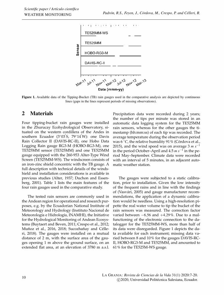
Figure 1. Available data of the Tipping-Bucket (TB) rain gauges used in the comparative analysis are depicted by continuouslines (gaps in the lines represent periods of missing observations).
2 MaterialsFour tipping-bucket rain gauges were installedin the Zhurucay Ecohydrological Observatory, si-tuated on the western cordillera of the Andes insouthern Ecuador (3◦03
′S, 79◦14
′W): one Davis
Rain Collector II (DAVIS-RC-II), one Hobo DataLogging Rain gauge RG3-M (HOBO-RG3-M), oneTE525MM sensor (TE525MM) and one TE525MMgauge equipped with the 260-953 Alter-Type WindScreen (TE525MM-WS). The windscreen consists ofan iron-zinc shield concentric with the TB gauge. Afull description with technical details of the winds-hield and installation considerations is available inprevious studies (Alter, 1937; Duchon and Essen-berg, 2001). Table 1 lists the main features of thefour rain gauges used in the comparative study.
The tested rain sensors are commonly used inthe Andean region for operational and research pur-poses, e.g. by the Ecuadorian National Institute ofMeteorology and Hydrology (Instituto Nacional deMeteorología e Hidrología, INAMHI), the Initiativefor the Hydrological Monitoring of Andean Ecosys-tems (Buytaert and Beven, 2011; Crespo et al., 2012;Muñoz et al., 2016, 2018; Sucozhañay and Célle-ri, 2018). The gauges were installed on a mutualdistance of 2 m, with the surface area of the gau-ges opening 1 m above the ground surface, on anextended flat area, at an elevation of 3780 m a.s.l.
Precipitation data were recorded during 2 years;the number of tips per minute was stored in anautomatic data logging system for the TE525MMrain sensors, whereas for the other gauges the ti-mestamp (hh:mm:ss) of each tip was recorded. Theaverage temperature during the observation periodwas 6 ◦C, the relative humidity 91% (Córdova et al.,2015), and the wind speed was on average 3 m s−1
in the period October–April and 4.5 m s−1 in the pe-riod May–September. Climate data were recordedwith an interval of 5 minutes, in an adjacent auto-matic weather station.
The gauges were subjected to a static calibra-tion, prior to installation. Given the low intensityof the frequent rains and in line with the findingsof (Vasvári, 2005) and gauge manufacturer recom-mendations, the application of a dynamic calibra-tion would be needless. Using a high-resolution pi-pette the real water volume to tip the bucket of therain sensors was measured. The correction factorvaried between −6,56 and +4,29%. Due to a mal-functioning of the electronic connection to the da-talogger for the TE525MM-WS, more than half ofits data were disregarded. Figure 1 depicts the da-ta available for each instrument; missing data va-ried between 8 and 10% for the gauges DAVIS-RC-II, HOBO-RG3-M and TE525MM, and amounted to61% for the TE525M-WS gauge.
10LA GRANJA: Revista de Ciencias de la Vida 31(1) 2020:7-20.
c©2020, Universidad Politécnica Salesiana, Ecuador.
Rain gauge inter-comparsion quantifies differences in precipitation monitoring
Table 1. Manufacturer specifications of the compared Tipping-Bucket (TB) rain gauges.
Sensor Capturing diameter(cm)
Resolution(mm)
Intensity(mm h−1)
Accuracy(%)
DAVIS-RC-II 16.5 0.254 0−50 ± 150−100 ± 5
HOBO-RG3-M 15.4 0.200 0−20 ± 1
TE525MMTE525MM-WS 24.5 0.100
0−10 ± 110−20 +0,−320−30 +0,−5
3 Methods
3.1 Statistical indices for the assessment
For the quantitative assessment of differences inperformance between the rain gauges the followingset of statistical indices, similar to that proposed byTokay et al. (2010), was used: the coefficient of deter-mination
(R2), the Spearman’s non-parametric co-
rrelation (ρ), the standard deviation (σ), the per-cent bias and the percent absolute bias. The statis-tical indices were calculated with respect to the raindata collected by the TE525MM sensor. This sensorwas considered in this study as reference becauseof its better technical features compared to the ot-her rain gauges, and its larger data set compared tothe TE525MM-WS. The percent bias and percent ab-solute bias, Equations (1) and (2) respectively, werecalculated as follows:
percent bias =1y
(1n
n
∑i=1
(xi− yi)
)(1)
percent absolutebias =1y
(1n
n
∑i=1|xi− yi|
)(2)
where x and y are defined as the precipita-tion depth registered by one of the gauges and theTE525MM for any time interval, n is the numberof values or intervals with recorded rainfall, and yis the average precipitation depth measured by theTE525MM for the considered timescale. For ratingthe performance of the gauges the following cate-gories of the percent bias were defined: excellent≤2%, 2% < good ≤5%, 5% < regular ≤10%, andpoor >10%.
3.2 Overall performance
The precipitation records of the different gaugeswere compared to check if they were working pro-perly. The functioning of a sensor was characterizedby R2 and ρ. The latter was calculated to test thevalidity of R2 that normally is affected by the non-normal distribution of rainfall. For the TE525MMdata at an hourly timescale, the non-normal distri-bution was confirmed by finding p-values of lessthan 0.01 for both the Kolmogorov-Smirnov andShapiro-Wilk’s tests. Nonetheless, R2 was calcula-ted to compare our results with those of other stu-dies. To assess the effect of extreme values on R2,the difference between ρ and R2 was considered asindicator. According to Tokay et al. (2003); Rollen-beck et al. (2007); Tokay et al. (2010), R2 values areexpected to be greater than 0.95 for hourly and dailydata from TB gauges located at the same site.
Following this, differences in precipitationdepth were analyzed between each of the rain sen-sors and the reference gauge using the percentbias as indicator (Equation 1). Additionally, giventhe hydrological relevance of precipitation data forshort timescales (Ciach, 2003; Rollenbeck et al.,2007; Buytaert and Beven, 2011), the accuracy of therain gauges was also determined for respectivelythe 5 min, 10 min, 30 min, hourly and daily times-cale. For this, absolute bias (obtained with Equation2) was compared to regular bias, and this informa-tion was complemented with the standard devia-tion of the differences between measurements fromthe sensors (σx−y).
3.3 Rainfall intensity effect
For the assessment of the rainfall intensity effecton the accuracy of the rain gauges, measurementsfrom the sensors corresponding to the following
LA GRANJA: Revista de Ciencias de la Vida 31(1) 2020:7-20.c©2020, Universidad Politécnica Salesiana, Ecuador. 11
Scientific paper / Artículo científicoWEATHER MONITORING Padrón, R.S., Feyen, J., Córdova, M., Crespo, P. and Célleri, R.
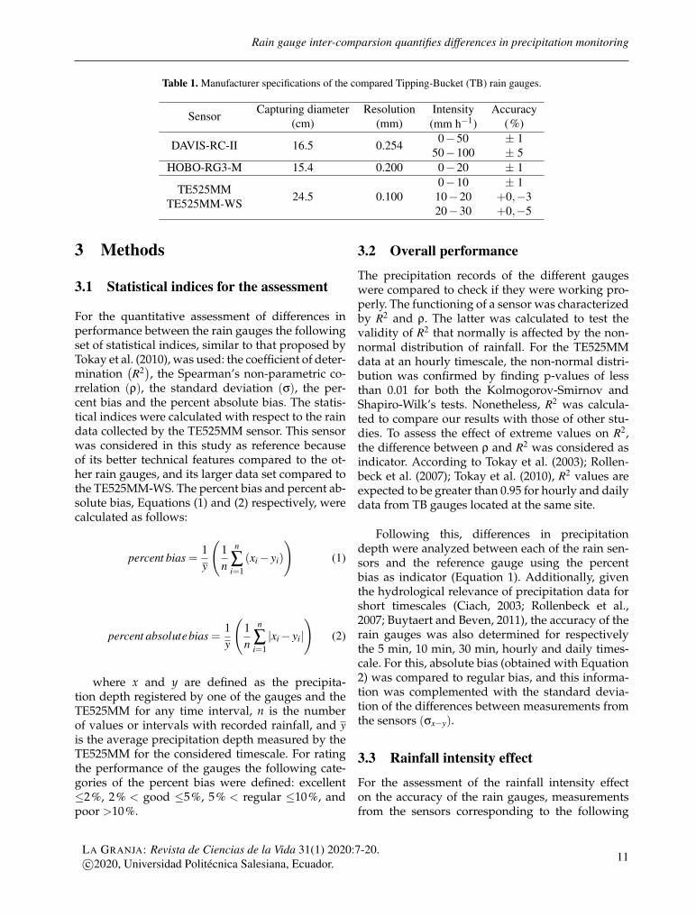
Figure 2. Rainfall intensity exceedance probability curve of the 5-min rainfall data collected by the TE525MM gauge (top), andwind speed exceedance probability curve of the corresponding 5-min intervals (bottom).
categories: 0–1 mm h−1, 1.01–2 mm h−1, 2.01–5 mmh−1, 5.01–10 mm h−1 and >10 mm h−1 were com-pared. These categories were established by tryingto have for each of them a flat distribution, anda representative percentage of the total amount ofdata (Figure 2 top). For the separation of the da-ta per intensity category, the intensities measuredby the TE525MM gauge were within the limits ofeach specific category, whereas the correspondingintensities measured by the other gauges were notnecessarily within these limits. For data belongingto each intensity category and timescales of 5, 10,30, and 60 minutes, the percent absolute bias wascomputed to define the effect of these variables onthe accuracy with which TB gauges estimate actualrainfall intensity. Percent bias was also calculatedfor the different intensity categories to understandand quantify how the deviations between the mea-
surements of the gauges vary as a function of actualrainfall intensity.
The intervals with rain intensities for the compa-rison were between exact hours, without time over-lap and with rain during their entire length. Forexample, for an event that had its first tip at 19:08UTC and its last one at 21:17 UTC of the same day,the used intervals for a 30 minute timescale were:19:30–20:00, 20:00–20:30, and 20:30–21:00 UTC. Theintervals 19:00–19:30 and 21:00–21:30 UTC were dis-carded because it did not rain during the entire in-terval. Although, this approach reduced the volumeof data, the useable dataset was still very represen-tative—e.g. for the 5 min timescale the cumulativerainfall of the used intervals represented 85% of thetotal precipitation volume of the TE525MM databa-se.
12LA GRANJA: Revista de Ciencias de la Vida 31(1) 2020:7-20.
c©2020, Universidad Politécnica Salesiana, Ecuador.
Rain gauge inter-comparsion quantifies differences in precipitation monitoring
3.4 Wind speed effectOnly the effect of wind speed on the accuracy of therain gauges was analyzed because there were notany evident obstacles to suggest an effect of winddirection. Similar criteria as for the rainfall inten-sities were used to classify wind speed (Figure 2bottom), establishing the following categories: 0–2m s−1, 2.01–4 m s−1 and 4 m s−1. The wind speeddata and selected categories are similar to thoseused by Sevruk and Hamon (1984) in their world-wide study. Also, wind speeds registered in othermountain highlands, like the Swiss-Austrian Alpsor the Bolivian Altiplano, did not differ much fromthe recorded wind speeds for the páramo (Vacheret al., 1994; Draxl and Mayr, 2009). Percent bias andpercent absolute bias were used for the data corres-ponding to each category to analyze the effect ofwind speed on the measurements from the sensors.
The selected timescale had to provide good ac-curacy of the precipitation depth captured by eachgauge, while assuring at the same time that a suffi-cient amount of data per wind speed category wasavailable. The accuracy requirement was determi-ned from the overall assessment and intensity ef-fect analyses. To distinguish the individual effect ofwind from the effect of rainfall intensity, the distri-bution of the rainfall intensity data correspondingto each of the wind speed categories was determi-ned. The rain depth intervals for the comparison ofthe sensors with respect to the effect of wind wereselected employing the same criteria used for doingthis when examining the effect of rainfall inten-sity—i.e. intervals between exact hours, without ti-me overlap and with rain during their entire length.
4 Results and Discussion
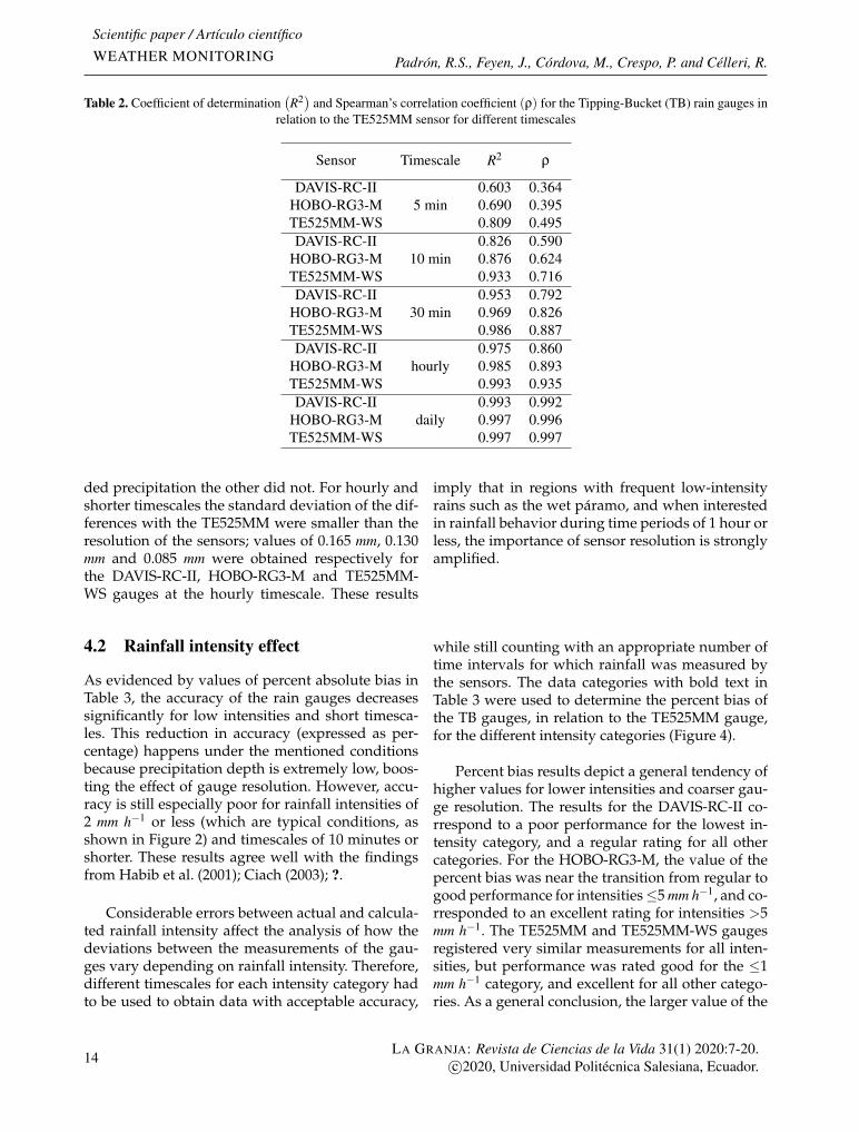
4.1 Overall performanceTable 2 depicts the coefficient of determination
(R2)
and the Spearman’s correlation (ρ) of the DAVIS-
RC-II, HOBO-RG3-M and TE525MM-WS gaugeswith respect to the precipitation recorded by theTE525MM sensor. Both coefficients are presentedfor the timescales 5, 10 and 30 min, hourly anddaily. The data clearly reveal that the value of R2
and ρ increases with timescale, which according toNystuen (1999) is due to the fact that for longerintervals it is less important how it rains. This al-so illustrates that the importance of accuracy andresolution of the rain gauges is more relevant fortime aggregations of 30 minutes or less. Values ofR2 tend to suggest a better agreement between sen-sors than expected, due to the effect that extremevalues have on this index. This effect can be seenclearly for the 5 and 10 minute timescales, whereR2 is much higher than ρ. Correlations between allgauges and the TE525MM were statistically signi-ficant; the probability that measurements from twodifferent gauges were not correlated was alwaysless than 1% (p<0.01). Several other studies (Tokayet al., 2003; Rollenbeck et al., 2007; Tokay et al., 2010)also found high correlations (R2 >0.95) between themeasurements of two side-by-side gauges for res-pectively hourly and daily timescales.
The percent bias of the difference between thetotal precipitation captured by the three gauges re-lative to the TE525MM gauge, which is independentof the used timescale, varied among−7,2% (DAVIS-RC-II), −5,6% (HOBO-RG-3) and −2% (TE525MM-WS). The negative values indicate an underestima-tion of the gauges in relation to rainfall volumecaught by the reference sensor. Based on the afore-mentioned criteria, the performance of the DAVIS-RC-II and HOBO-RG-3 gauges is regular, whereasthat of the TE525MM-WS is excellent. The obtainedresults are in line with the deviation range foundby Rollenbeck et al. (2007) for gauges from differentmanufacturers, and by Tokay et al. (2003, 2010) foridentical gauges.
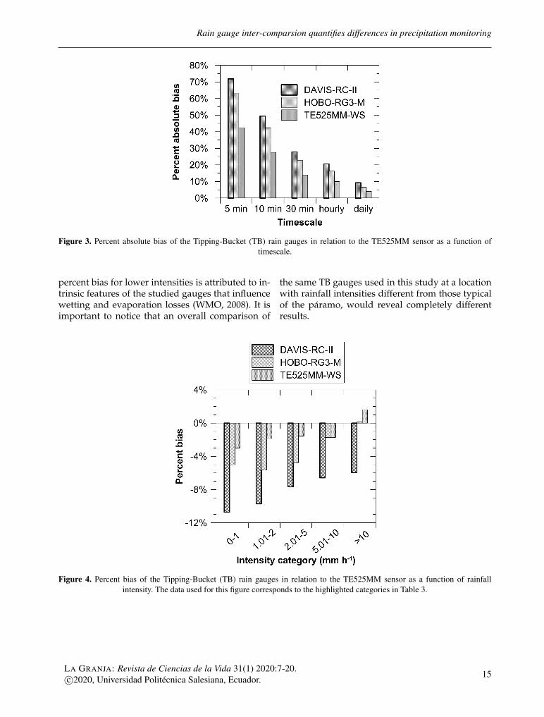
Figure 3 shows the percent absolute bias of theTB gauges as a function of the timescale. Thereis a clear influence of gauge resolution, with theDAVIS-RC-II sensor having the largest percent ab-solute bias and the coarsest resolution. There is alsoan effect of timescale on the gauges’ accuracy that
can be explained by the fact that during short inter-vals, given the overall low rainfall intensity, somesensors do not register rain, while others do, andin the next time interval the opposite often occurs.Indeed, in nearly 50% of all 5 min intervals consi-dered, when one of the compared TB gauges recor-
LA GRANJA: Revista de Ciencias de la Vida 31(1) 2020:7-20.c©2020, Universidad Politécnica Salesiana, Ecuador. 13
Scientific paper / Artículo científicoWEATHER MONITORING Padrón, R.S., Feyen, J., Córdova, M., Crespo, P. and Célleri, R.
Table 2. Coefficient of determination(R2) and Spearman’s correlation coefficient (ρ) for the Tipping-Bucket (TB) rain gauges in
relation to the TE525MM sensor for different timescales
Sensor Timescale R2 ρ
DAVIS-RC-II5 min
0.603 0.364HOBO-RG3-M 0.690 0.395TE525MM-WS 0.809 0.495DAVIS-RC-II
10 min0.826 0.590
HOBO-RG3-M 0.876 0.624TE525MM-WS 0.933 0.716DAVIS-RC-II
30 min0.953 0.792
HOBO-RG3-M 0.969 0.826TE525MM-WS 0.986 0.887DAVIS-RC-II
hourly0.975 0.860
HOBO-RG3-M 0.985 0.893TE525MM-WS 0.993 0.935DAVIS-RC-II
daily0.993 0.992
HOBO-RG3-M 0.997 0.996TE525MM-WS 0.997 0.997
ded precipitation the other did not. For hourly andshorter timescales the standard deviation of the dif-ferences with the TE525MM were smaller than theresolution of the sensors; values of 0.165 mm, 0.130mm and 0.085 mm were obtained respectively forthe DAVIS-RC-II, HOBO-RG3-M and TE525MM-WS gauges at the hourly timescale. These results
imply that in regions with frequent low-intensityrains such as the wet páramo, and when interestedin rainfall behavior during time periods of 1 hour orless, the importance of sensor resolution is stronglyamplified.
4.2 Rainfall intensity effect
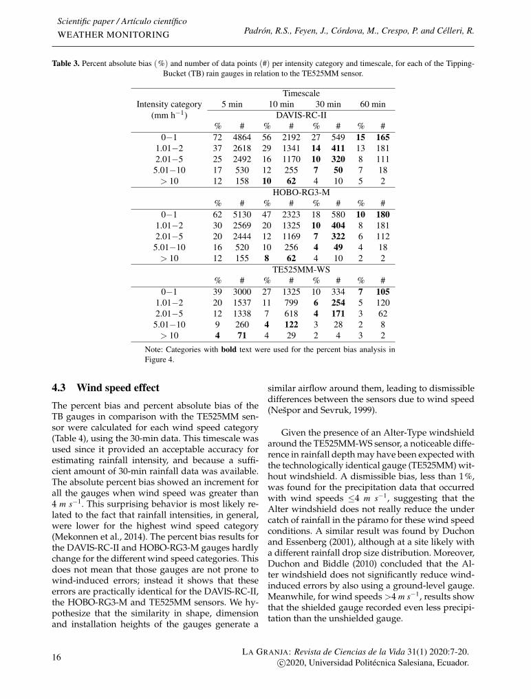
As evidenced by values of percent absolute bias inTable 3, the accuracy of the rain gauges decreasessignificantly for low intensities and short timesca-les. This reduction in accuracy (expressed as per-centage) happens under the mentioned conditionsbecause precipitation depth is extremely low, boos-ting the effect of gauge resolution. However, accu-racy is still especially poor for rainfall intensities of2 mm h−1 or less (which are typical conditions, asshown in Figure 2) and timescales of 10 minutes orshorter. These results agree well with the findingsfrom Habib et al. (2001); Ciach (2003); ?.
Considerable errors between actual and calcula-ted rainfall intensity affect the analysis of how thedeviations between the measurements of the gau-ges vary depending on rainfall intensity. Therefore,different timescales for each intensity category hadto be used to obtain data with acceptable accuracy,
while still counting with an appropriate number oftime intervals for which rainfall was measured bythe sensors. The data categories with bold text inTable 3 were used to determine the percent bias ofthe TB gauges, in relation to the TE525MM gauge,for the different intensity categories (Figure 4).
Percent bias results depict a general tendency ofhigher values for lower intensities and coarser gau-ge resolution. The results for the DAVIS-RC-II co-rrespond to a poor performance for the lowest in-tensity category, and a regular rating for all othercategories. For the HOBO-RG3-M, the value of thepercent bias was near the transition from regular togood performance for intensities≤5 mm h−1, and co-rresponded to an excellent rating for intensities >5mm h−1. The TE525MM and TE525MM-WS gaugesregistered very similar measurements for all inten-sities, but performance was rated good for the ≤1mm h−1 category, and excellent for all other catego-ries. As a general conclusion, the larger value of the
14LA GRANJA: Revista de Ciencias de la Vida 31(1) 2020:7-20.
c©2020, Universidad Politécnica Salesiana, Ecuador.
Rain gauge inter-comparsion quantifies differences in precipitation monitoring
Figure 3. Percent absolute bias of the Tipping-Bucket (TB) rain gauges in relation to the TE525MM sensor as a function oftimescale.
percent bias for lower intensities is attributed to in-trinsic features of the studied gauges that influencewetting and evaporation losses (WMO, 2008). It isimportant to notice that an overall comparison of
the same TB gauges used in this study at a locationwith rainfall intensities different from those typicalof the páramo, would reveal completely differentresults.
Figure 4. Percent bias of the Tipping-Bucket (TB) rain gauges in relation to the TE525MM sensor as a function of rainfallintensity. The data used for this figure corresponds to the highlighted categories in Table 3.
LA GRANJA: Revista de Ciencias de la Vida 31(1) 2020:7-20.c©2020, Universidad Politécnica Salesiana, Ecuador. 15
Scientific paper / Artículo científicoWEATHER MONITORING Padrón, R.S., Feyen, J., Córdova, M., Crespo, P. and Célleri, R.
Table 3. Percent absolute bias (%) and number of data points (#) per intensity category and timescale, for each of the Tipping-Bucket (TB) rain gauges in relation to the TE525MM sensor.
Intensity category(mm h−1)
Timescale5 min 10 min 30 min 60 min
DAVIS-RC-II% # % # % # % #
0−1 72 4864 56 2192 27 549 15 1651.01−2 37 2618 29 1341 14 411 13 1812.01−5 25 2492 16 1170 10 320 8 111
5.01−10 17 530 12 255 7 50 7 18> 10 12 158 10 62 4 10 5 2
HOBO-RG3-M% # % # % # % #
0−1 62 5130 47 2323 18 580 10 1801.01−2 30 2569 20 1325 10 404 8 1812.01−5 20 2444 12 1169 7 322 6 112
5.01−10 16 520 10 256 4 49 4 18> 10 12 155 8 62 4 10 2 2
TE525MM-WS% # % # % # % #
0−1 39 3000 27 1325 10 334 7 1051.01−2 20 1537 11 799 6 254 5 1202.01−5 12 1338 7 618 4 171 3 62
5.01−10 9 260 4 122 3 28 2 8> 10 4 71 4 29 2 4 3 2
Note: Categories with bold text were used for the percent bias analysis inFigure 4.
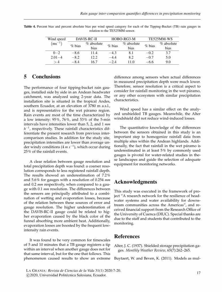
4.3 Wind speed effectThe percent bias and percent absolute bias of theTB gauges in comparison with the TE525MM sen-sor were calculated for each wind speed category(Table 4), using the 30-min data. This timescale wasused since it provided an acceptable accuracy forestimating rainfall intensity, and because a suffi-cient amount of 30-min rainfall data was available.The absolute percent bias showed an increment forall the gauges when wind speed was greater than4 m s−1. This surprising behavior is most likely re-lated to the fact that rainfall intensities, in general,were lower for the highest wind speed category(Mekonnen et al., 2014). The percent bias results forthe DAVIS-RC-II and HOBO-RG3-M gauges hardlychange for the different wind speed categories. Thisdoes not mean that those gauges are not prone towind-induced errors; instead it shows that theseerrors are practically identical for the DAVIS-RC-II,the HOBO-RG3-M and TE525MM sensors. We hy-pothesize that the similarity in shape, dimensionand installation heights of the gauges generate a
similar airflow around them, leading to dismissibledifferences between the sensors due to wind speed(Nešpor and Sevruk, 1999).
Given the presence of an Alter-Type windshieldaround the TE525MM-WS sensor, a noticeable diffe-rence in rainfall depth may have been expected withthe technologically identical gauge (TE525MM) wit-hout windshield. A dismissible bias, less than 1%,was found for the precipitation data that occurredwith wind speeds ≤4 m s−1, suggesting that theAlter windshield does not really reduce the undercatch of rainfall in the páramo for these wind speedconditions. A similar result was found by Duchonand Essenberg (2001), although at a site likely witha different rainfall drop size distribution. Moreover,Duchon and Biddle (2010) concluded that the Al-ter windshield does not significantly reduce wind-induced errors by also using a ground-level gauge.Meanwhile, for wind speeds >4 m s−1, results showthat the shielded gauge recorded even less precipi-tation than the unshielded gauge.
16LA GRANJA: Revista de Ciencias de la Vida 31(1) 2020:7-20.
c©2020, Universidad Politécnica Salesiana, Ecuador.
Rain gauge inter-comparsion quantifies differences in precipitation monitoring
Table 4. Percent bias and percent absolute bias per wind speed category for each of the Tipping-Bucket (TB) rain gauges inrelation to the TE525MM sensor.
Wind speed(ms−1
) DAVIS-RC-II HOBO-RG3-M TE525MM-WS
% bias% absolute
bias % bias% absolute
bias % bias% absolute
bias0−2 −8.6 11.4 −4.3 8.1 −0.2 3.7
2.01−4 −8.2 12.2 −4.4 8.2 −0.7 5.0> 4 −8.4 16.7 −2.4 11.0 −6.6 9.0
5 Conclusions
The performance of four tipping-bucket rain gau-ges, installed side by side in an Andean headwatercatchment, was analyzed using 2-year data. Theinstallation site is situated in the tropical Andes,southern Ecuador, at an elevation of 3780 m a.s.l.,and is representative for the wet páramo region.Rain events are most of the time characterized bya low intensity: 95%, 76%, and 53% of the 5-minintervals have intensities lower than 5, 2, and 1 mmh−1, respectively. These rainfall characteristics dif-ferentiate the present research from previous inter-comparison studies. In addition for the study site,precipitation intensities are lower than average un-der windy conditions (4 m s−1), which occur during25% of the rainfall events.
A clear relation between gauge resolution andtotal precipitation depth was found: a coarser reso-lution corresponds to less registered rainfall depth.The results showed an underestimation of 7.2%and 5.6% for gauges with a resolution of 0.254 mmand 0.2 mm respectively, when compared to a gau-ge with 0.1 mm resolution. The differences betweenthe sensors are principally attributed to a combi-nation of wetting and evaporation losses, becauseof the relation between these sources of error andgauge resolution. The higher underestimation ofthe DAVIS-RC-II gauge could be related to hig-her evaporation caused by the black color of thefunnel absorbing more ambient heat. Additionally,evaporation losses are boosted by the frequent low-intensity rain events.
It was found to be very common for timescalesof 5 and 10 minutes that a TB gauge registers a tipwithin an interval when another gauge does not forthat same interval, but for the one that follows. Thisphenomenon caused results to show an extreme
difference among sensors when actual differencesin measured precipitation depth were much lower.Therefore, sensor resolution is a critical aspect toconsider for rainfall monitoring in the wet páramo,or any other ecosystem with similar precipitationcharacteristics.
Wind speed has a similar effect on the analy-zed unshielded TB gauges. Meanwhile, the Alterwindshield did not reduce wind-induced losses.
The quantitative knowledge of the differencesbetween the sensors obtained in this study is animportant step to homogenize rainfall data frommultiple sites within the Andean highlands. Addi-tionally, the fact that rainfall in the wet páramo isunderestimated in at least 5% by commonly usedgauges is pivotal for water-related studies in the-se landscapes and guide the selection of adequateequipment for monitoring networks.
AcknowledgmentsThis study was executed in the framework of pro-ject “A research network for the resilience of head-water systems and water availability for downs-tream communities across the Americas”, and re-ceived financial support from the Research Office ofthe University of Cuenca (DIUC). Special thanks aredue to the staff and students that contributed to themonitoring.
ReferencesAlter, J. C. (1937). Shielded storage precipitation ga-
ges. Monthly Weather Review, 65(7):262–265.
Buytaert, W. and Beven, K. (2011). Models as mul-
LA GRANJA: Revista de Ciencias de la Vida 31(1) 2020:7-20.c©2020, Universidad Politécnica Salesiana, Ecuador. 17
Scientific paper / Artículo científicoWEATHER MONITORING Padrón, R.S., Feyen, J., Córdova, M., Crespo, P. and Célleri, R.
tiple working hypotheses: hydrological simula-tion of tropical alpine wetlands. Hydrological Pro-cesses, 25(11):1784–1799. Online: https://bit.ly/2OpO62o.
Buytaert, W., Célleri, R., De Bièvre, B., Cisneros, F.,Wyseure, G., Deckers, J., and Hofstede, R. (2006a).Human impact on the hydrology of the andeanpáramos. Earth-Science Reviews, 79:53–72. Onli-ne:http://bit.ly/32yASq6.
Buytaert, W., Célleri, R., Willems, P., De Bièvre, B.,and Wyseure, G. (2006b). Spatial and temporalrainfall variability in mountainous areas: A ca-se study from the south ecuadorian andes. Jour-nal of Hydrology, 329:413–421. Online:http://bit.ly/32yKDoc.
Chen, H. and Chandrasekar, V. (2015). Estimationof light rainfall using ku-band dual-polarizationradar. IEEE Transactions on Geoscience and RemoteSensing, 53(9):5197–5208. Online: https://bit.ly/3974NYe.
Ciach, G. J. (2003). Local random errors in tipping-bucket rain gauge measurements. Journal of At-mospheric and Oceanic Technology, 20:752–759. On-line: https://bit.ly/31mIvza.
Córdova, M., Carrillo-Rojas, G., Crespo, P., Wil-cox, B., and Célleri, R. (2015). Evaluation of thepenman-monteith (fao 56 pm) method for cal-culating reference evapotranspiration using limi-ted data. application to the wet páramo of sout-hern ecuador. Mountain Research and Development,35:230–239. Online: http://bit.ly/2T9sCKb.
Crespo, P., Feyen, J., Buytaert, W., Célleri, R., Fre-de, H., Ramirez, M., and Breuer, L. (2012). De-velopment of a conceptual model of the hydrolo-gic response of tropical andean micro-catchmentsin southern ecuador. Hydrology and Earth SystemSciences Discussions, 9:2475–2510. Online: http://bit.ly/32FIl6D.
Célleri, R. and Feyen, J. (2009). The hydrology oftropical andean ecosystems: Importance, know-ledge status, and perspectives. Mountain Researchand Development, pages 350–355. Online:http://bit.ly/3ce4spn.
Dai, Q. (2015). Probabilistic radar rainfall nowcastsusing empirical and theoretical uncertainty mo-dels. Hydrological Processes, 29(1):66–79. Online:https://bit.ly/2u7p2GN.
Draxl, C. and Mayr, G. (2009). Meteorological windenergy potential of the alps using era40 and windmeasurements of the tyrolean alps. In EuropeanWind Energy Conference & Exhibition, page 6, Mar-seille, France.
Duchon, C. E. and Biddle, C. J. (2010). Under-catch of tipping-bucket gauges in high rain rateevents. Advances in Geosciences, 25:11–15. Online:https://bit.ly/2tmO4RA.
Duchon, C. E. and Essenberg, G. R. (2001).Comparative rainfall observations frompit and aboveground rain gauges withand without wind shields. Water Re-sources Research, 37(12):3253–3263. Online:https://bit.ly/31oV4tU.
Grimaldi, S., Petroselli, A., Baldini, L., and Gorguc-ci, E. (2015). Description and preliminary resultsof a 100 square meter rain gauge. Journal of Hy-drology, page Online: https://bit.ly/3beiNBJ.
Habib, E., Krajewski, W. F., and Kruger, A. (2001).Sampling errors of tipping-bucket rain gaugemeasurements. Journal of Hydrologic Engineering,6(2 (March/April)):159–166. Online: https://bit.ly/3b5CR98.
Humphrey, M. D., Istok, J. D., Lee, J. Y., Hevesi,J. A., and Flint, A. L. (1997). A new method forautomated dynamic calibration of tipping-bucketrain gauges. Journal of Atmospheric and OceanicTechnology, 14(6):1513–1519. Online: https://bit.ly/2UpJI7s.
Keller, V. D. J., Tanguy, M., Prosdocimi, I., Terry,J. A., Hitt, O., Cole, S. J., Fry, M., Morris, D. G.,and Dixon, H. (2015). Ceh-gear: 1 km resolu-tion daily and monthly areal rainfall estimates forthe uk for hydrological and other applications.Earth System Science Data, 7(1):143–155. Online:https://bit.ly/2SQBGC5.
Krajewski, W., Kruger, A., Caracciolo, C., Golé, P.,Barthes, L., Creutin, J., Delahaye, J., Nikolopou-los, E., Ogden, F., and Vinson, J. (2006). Devex-disdrometer evaluation experiment: Basic resultsand implications for hydrologic studies. Advancesin Water Resources, 29(2):311–325. Online: https://bit.ly/396ZyIk.
Krajewski, W. F., Kruger, A., and Nespor, V. (1998).Experimental and numerical studies of small-
18LA GRANJA: Revista de Ciencias de la Vida 31(1) 2020:7-20.
c©2020, Universidad Politécnica Salesiana, Ecuador.
Rain gauge inter-comparsion quantifies differences in precipitation monitoring
scale rainfall measurements and variability. WaterScience and Technology, 37(11):131–138. Online: .
Lanza, L. and Stagi, L. (2008). Certified accu-racy of rainfall data as a standard requirement inscientific investigations. Advances in Geosciences,16:43–48. Online: https://bit.ly/2uatLr6.
Lanzinger, E., Theel, M., and Windolph, H. (2006).Rainfall amount and intensity measured by thethies laser precipitation monitor. page 9, Geneva,Switzerland.
Mekonnen, G. B., Matula, S., Doležal, F., and Fišák,J. (2014). Adjustment to rainfall measurement un-dercatch with a tipping-bucket rain gauge usingground-level manual gauges. Meteorology and At-mospheric Physics, page 241–256. Online: https://bit.ly/38CSCCX.
Molini, A., Lanza, L. G., and La Barbera, P. (2005).Improving the accuracy of tipping-bucket rain re-cords using disaggregation techniques. Atmosphe-ric Research, 77(1-4):203–217. Online: https://bit.ly/2SDcr7E.
Muñoz, P., Célleri, R., and Feyen, J. (2016). Effect ofthe resolution of tipping-bucket rain gauge andcalculation method on rainfall intensities in anandean mountain gradient. Water, 8(11):534. On-line: http://bit.ly/2wi7k3H.
Muñoz, P., Orellana-Alvear, J., Willems, P., and Cé-lleri, R. (2018). Flash-flood forecasting in anandean mountain catchment—development of astep-wise methodology based on the random fo-rest algorithm. Water, 10(11):1519. Online: http://bit.ly/2wRJA6R.
Nešpor, V. and Sevruk, B. (1999). Estimation ofwind-induced error of rainfall gauge measure-ments using a numerical simulation. Journal ofAtmospheric and Oceanic Technology, 16(4):450–464.Online: https://bit.ly/2SClx4c.
Nystuen, J. A. (1999). Relative performance of au-tomatic rain gauges under different rainfall con-ditions. Journal of Atmospheric and Oceanic Tech-nology, 16(8):1025–1043. Online: https://bit.ly/3bI0t3T.
Ochoa-Tocachi, B., Buytaert, W., De Bièvre, B., Célle-ri, R., Crespo, P., Villacis, M., Llerena, C., Acosta,L., Villazon, M., Guallpa, M., Gil-Ríos, J., Fuen-tes, P., Olaya, D., Viñas, P., Rojas, G., and Arias,
S. (2016). Impacts of land use on the hydro-logical response of tropical andean catchments.Hydrological Processes, 30:4074–4089. Online: http://bit.ly/2wjOkSr.
Padrón, R., Wilcox, B., Crespo, P., and Célleri,R. (2015). Rainfall in the andean páramo:New insights from high-resolution monitoring insouthern ecuador. Journal of Hydrometeorology,16(8):985–996. Online: http://bit.ly/2T6nK8v.
Rollenbeck, R., Bendix, J., Fabian, P., Boy, J., Wilcke,W., Dalitz, H., Oesker, M., and Emck, P. (2007).Comparison of different techniques for the mea-surement of precipitation in tropical montanerain forest regions. Journal of Atmospheric andOceanic Technology, 24(2):156–168. Online: https://bit.ly/2uJW3ZV.
Savina, M., Schäppi, B., Molnar, P., Burlando, P.,and Sevruk, B. (2012). Comparison of a tipping-bucket and electronic weighing precipitation ga-ge for snowfall. Atmospheric Research. Elsevier B.V.,103:45–51. Online: https://bit.ly/2UYs4rD.
Seo, B., Dolan, B., Krajewski, W. F., Rutledge, S. A.,and Petersen, W. (2015). Comparison of single-and dual-polarization–based rainfall estimatesusing nexrad data for the nasa iowa flood studiesproject. Journal of Hydrometeorology, page Online:https://bit.ly/3bN3MqL.
Sevruk, B. and Hamon, W. R. (1984). Internationalcomparison of national precipitation gauges witha reference pit gauge. WMO Instrument and Ob-serving Methods Report, No.17, (111):Online: https://bit.ly/323uoPz.
Sevruk, B., Ondrás, M., and Chvíla, B. (2009).The wmo precipitation measurement intercom-parisons. Atmospheric Research. Elsevier B.V.,92(3):376–380. Online: https://bit.ly/37CEyrH.
Sucozhañay, A. and Célleri, R. (2018). Impact of raingauges distribution on the runoff simulation of asmall mountain catchment in southern ecuador.Water, page Online: http://bit.ly/2veA7q1.
Tokay, A., Bashor, P. G., and McDowell, V. L. (2010).Comparison of rain gauge measurements in themid-atlantic region. Journal of Hydrometeorology,11(2):553–565. Online: https://bit.ly/2UYPbCs.
LA GRANJA: Revista de Ciencias de la Vida 31(1) 2020:7-20.c©2020, Universidad Politécnica Salesiana, Ecuador. 19
Scientific paper / Artículo científicoWEATHER MONITORING Padrón, R.S., Feyen, J., Córdova, M., Crespo, P. and Célleri, R.
Tokay, A., Wolff, D., Wolff, K., and Bashor, P.(2003). Rain gauge and disdrometer measure-ments during the keys area microphysics pro-ject (kamp). Journal of Atmospheric and OceanicTechnology, 20:1460–1477. Online: https://bit.ly/38Em5wm.
Vacher, J., Imaña, E., and Canqui, E. (1994). Lascaracteristicas radiativas y la evapotranspira-cion potencial en el altiplano boliviano. Revis-ta de Agricultura, (1):4–12. Online: https://bit.ly/2SBpeYc.
Vasvári, V. (2005). Calibration of tipping bucket raingauges in the graz urban research area. Atmosphe-ric research, 77(1-4):18–28. Online: https://bit.ly/2SUXX1x.
Vuerich, E., Monesi, C., Lanza, L. G., Stagi, L., andLanzinger, E. (2009). Wmo field intercompari-son of rainfall intensity gauges. WMO Instumentsand Observing Methods Report No. 99, (1504):Onli-ne: https://bit.ly/37zqorn.
Willems, P. (2001). Stochastic description of therainfall input errors in lumped hydrological mo-dels. Stochastic Environmental Research and RiskAssessment, 15(2):132–152. Online: https://bit.ly/39GRTAB.
WMO (2008). Guide of meteorological instrumentsand methods of observation. No. 8.
20LA GRANJA: Revista de Ciencias de la Vida 31(1) 2020:7-20.
c©2020, Universidad Politécnica Salesiana, Ecuador.
Scientific paper/ Artículo científico
CLIMATE CHANGEpISSN:1390-3799; eISSN:1390-8596
http://doi.org/10.17163/lgr.n31.2020.02
CLIMATE CHANGE ACCORDING TO ECUADORIAN
ACADEMICS–PERCEPTIONS VERSUS FACTS
CAMBIO CLIMÁTICO SEGÚN LOS ACADÉMICOS ECUATORIANOS -PERCEPCIONES VERSUS HECHOS
Theofilos Toulkeridis*1 , Elizabeth Tamayo2 , Débora Simón-Baile3 , MaríaJ. Merizalde-Mora4 , Diego F. Reyes –Yunga4 , Mauricio Viera-Torres4 and
Marco Heredia3
1 Geología y Geoquímica. Universidad de las Fuerzas Armadas ESPE, Av. General Rumiñahui s/n y Ambato, Sangolquí, Ecua-dor.2 Geología. Universidad de las Fuerzas Armadas ESPE, Av. General Rumiñahui s/n y Ambato, Sangolquí, Ecuador.3 Ciencias Ambientales. Universidad de las Fuerzas Armadas ESPE, Av. General Rumiñahui s/n y Ambato, Sangolquí, Ecuador.4 Geografia y Ciencias Ambientales. Universidad de las Fuerzas Armadas ESPE, Av. General Rumiñahui s/n y Ambato, Sangol-quí, Ecuador.
*Corresponding author: [email protected]
Article received on july 25th, 2019. Accepted, after review, on january 16th, 2019. Published on March 1st, 2020.
Resumen
El cambio climático se ha convertido en uno de los temas principales en las agendas en diferentes países. Los efectosactuales requieren de acciones climáticas efectivas ya establecidas en el Acuerdo de París con el objetivo de reducirlas emisiones de gases de efecto invernadero. Sin embargo, los principales cambios para enfrentar y reducir el cambioclimático dependen de las decisiones de cada país y no sólo de los acuerdos mundiales, ya que los impactos y magni-tudes varían localmente. Uno de los componentes clave para una mejora efectiva es el papel que el comportamiento dela población puede tener sobre la política nacional y las decisiones posteriores. Por esta razón, el nivel de conciencia yconocimiento sobre el cambio climático es vital. El objetivo de la investigación fue comparar la percepción de los aca-démicos ecuatorianos sobre el cambio climático global y nacional con la evidencia científica y los hechos históricos, ycómo su vulnerabilidad puede afectar a los efectos del cambio climático. Los resultados muestran que los académicosecuatorianos están conscientes de los hechos ocurridos mundialmente sobre el cambio climático, como la existencia, lagravedad y la responsabilidad de los seres humanos. Sin embargo, hay un conocimiento limitado sobre el origen delproblema, ya que el 67,2% cree que este es el primer cambio climático en la historia de la humanidad. Los principalesefectos del cambio climático en Ecuador presentan percepciones heterogéneas, como sequías más frecuentes (34,36%)y lluvias escasas pero intensas (21,41%) como sus mayores preocupaciones. En cuanto a las regiones más afectadas enEcuador, las sierra y los valles interandinos representan el 45,6%, mientras que Galápagos sólo alcanza 1,6% a pesarde ser una insignia ecológica con alta vulnerabilidad climática. Parece que los encuestados carecen de conocimiento
21LA GRANJA: Revista de Ciencias de la Vida 31(1) 2020:21-49.c©2020, Universidad Politécnica Salesiana, Ecuador.
Scientific paper / Artículo científicoCLIMATE CHANGE Toulkeridis, T., Tamayo, E., Simón, D., Merizalde, M.J., Reyes, D.F., Viera, M. and Heredia, M.
sobre la situación en otras regiones y creen que su propio entorno se ve más afectado.Palabras clave: cambio climático, calentamiento global, vulnerabilidad, desastres, ecosistemas, paleoclimatología.
Abstract
Climate change has become one of the main issues in the countries government agendas. The current effects demandeffective climate actions which were set out in the Paris Agreement with the global goal of reducing greenhousegas emissions. However, the main changes to face and mitigate climate change depend on each countrys decisionsand not only on global agreements as the impacts and its magnitudes vary locally. One of the key components foran effective adaption and mitigation is the role that the behavior of the population may have over national politicsand subsequent decisions. For this reason, the level of awareness and knowledge about climate change is vital. .The objective of the current study was to compare the perception of Ecuadorian academics regarding global andnational climate change with the scientific evidence and historical facts, and how it may affect their vulnerabilityto the climate change effects. The results show that Ecuadorian academics are well aware of globally known facts ofclimate change such as existence, gravity and responsibility of humans. However, there is limited awareness about theorigin, since 67.2% believes that this is the first climate change in human history. The main effects of climate changein Ecuador exhibit heterogeneous perceptions, with the more frequent droughts (34.36%) and rarer but more intenserains (21.41%) as their greater concerns. Regarding the regions more affected in Ecuador, highlands and Inter-Andeanvalleys sum up 45.6% while Galapagos only reaches 1.6% despite being an ecological flagship with high climatevulnerability. It seems that respondents lack knowledge about the situation in other regions, and believe that theirown environment is more impacted.Keywords: climate change, global warming, vulnerability, disasters, ecosystems, paleoclimatology
Suggested citation: Toulkeridis, T., Tamayo, E., Simón, D., Merizalde, M.J., Reyes, D.F., Viera, M. and He-redia, M. (2020). Climate Change according to Ecuadorian academics–Perceptions ver-sus facts. La Granja: Revista de Ciencias de la Vida. Vol. 31(1):21-49. http://doi.org/10.17163/lgr.n31.2020.02.
Orcid IDs:Theofilos Toulkeridis: http://orcid.org/0000-0003-1903-7914Elizabeth Tamayo: http://orcid.org/0000-0002-7354-9227Débora Simón-Baile: http://orcid.org/0000-0002-8398-9883María J. Merizalde-Mora: http://orcid.org/0000-0001-9686-5436Diego Reyes: http://orcid.org/0000-0002-7792-395XMauricio Viera-Torres: http://orcid.org/0000-0001-8888-1866Marco Heredia: http://orcid.org/0000-0002-6039-3411
22LA GRANJA: Revista de Ciencias de la Vida 31(1) 2020:21-49.
c©2020, Universidad Politécnica Salesiana, Ecuador.
Climate Change according to Ecuadorian academics–Perceptions versus facts
1 Introduction
The occurring and potential impacts that clima-te change has over both nature and societies haveconverted it into a complex topic to approach if tho-rough researches and institutional cooperation arenot linked (Luterbacher et al., 2004). Although thecauses of climate change are globally averaged bythe climatic system (UNDP, 2009), they are actually,local, and highly depend on the level of industria-lization and habits of consumption of each country.Frequently the data of diverse countries are repor-ted considering the highest emitters of cumulativecarbon dioxide. Considering the most recent availa-ble data from 2016 (Agency, 2018), the top emittersof total CO2 are, by far, China with 9056.8 metricmegatons (MT), which almost doubles the follo-wing being the United States with some 4833.1MT.The USA is followed by India, Russian Federationand Japan. However, if the countries are ranked interms of the carbon dioxide emissions per capita,instead of the total emissions, the results changedramatically and China, the major emerging eco-nomy and most populated country, does not leadthe rank any longer. By 2016, the top five countriesin the list of CO2 emitters per capita are Saudi Ara-bia, Australia, USA, Canada and South Korea, withvalues ranging between 16.3 and 11.6 Metric Tons(T). Hereby, China occupies the 12th place in percapita emissions, with approximately 6.4 T, whileIndia ranks 20, with 1.6 T, ten times less than theaverage citizen of Saudi Arabia or Australia and, atonly 40% of the global average.
These uneven current contributions togetherwith differentiated historical responsibilities for cli-mate change have long been discussed (Rajamani,2000; Page, 2008; Müller et al., 2009; Baatz, 2013;Friman and Hjerpe, 2015), and are at the core of thechallenges the world faces in reaching agreementsand achieving commitments in the international cli-mate change negotiations. In a further study it hasbeen discussed the most controversial issue of theBrazilian proposal, which has led to a methodologyof calculating shares of responsibility as opposed tothe shares in causal contribution considering twoconceptions of responsibility being ‘strict’ or ‘limi-ted’ (Müller et al., 2009). Other studies focused onspecific policy options to compensate those vulne-rable to climate change in developing countries,analyzing the applicability of the Beneficiary Pays
Principle rather than the Polluter Pays Principle(Baatz, 2013).
In any case, such commitments need to benationally-tailored, and developing countriesshould endorse meaningful participation and as-sume their share while claiming climate justice andcompensation for climate change loss and damage(Calliari, 2018; Page and Heyward, 2017). In fact, thedeveloping and poorest countries are facing greaterclimate change loss and damage because they areat higher risks (Zenghelis, 2006; Mertz et al., 2009;Hedlund et al., 2018). It has been demonstrated thatthe increase of environmental deterioration throughthe usage of natural resources is indirectly relatedto the culture, education, policy decisions, socialmovements, and economic incomes of each country(Luterbacher et al., 2004). The economic underpri-vileged people tend to live in areas of even higherrisk, re-enforcing the statement that vulnerability iscorrelated to poverty. For this reason, the socioeco-nomic inequality and political instability that LatinAmerica faces, added to a multi-hazard geographiclocation and continuous environmental deteriora-tion in their attempt to reach development, onlyincreases the risks of vulnerability of these regions.Thus, the mitigation of the effects of global andlocal climate change coincides with the reductionof poverty and social inequalities, the applicationof sustainable regulation of natural resources, andan in-depth planning that promotes developmentand reduces risks (Rojas, 2016; Goworek et al., 2018;Furley et al., 2018). Ecuador, in particular, is affec-ted by the regional South American aspects pre-viously mentioned and its specific issues such associo-economic differences among the Coast, High-lands and Amazon regions, and the way in whichenergy and soil are being used. Those aspects hen-ce threat the mitigation and adaptation attemptsthat Ecuador is implementing to face climate chan-ge and reduce its impacts (Reuveny, 2007; Buytaertet al., 2010; Luque et al., 2013; Luterbacher et al.,2004).
Scientists have been informing the society aboutthe impacts that our activities are having over theplanet during the last decades. The monitoring ofdifferent substances started around 32 years agowith the signature of the first protocol after the lea-ders of the main developed countries realized theimpact that humanity had on triggering an irrever-
LA GRANJA: Revista de Ciencias de la Vida 31(1) 2020:21-49.c©2020, Universidad Politécnica Salesiana, Ecuador. 23
Scientific paper / Artículo científicoCLIMATE CHANGE Toulkeridis, T., Tamayo, E., Simón, D., Merizalde, M.J., Reyes, D.F., Viera, M. and Heredia, M.
sible climate change. The first global agreement wasthe Montreal Protocol, signed on 1987, that aimedto protect the ozone layer by reducing and stoppingthe usage of the main gases that deplete the layer(Ibárcena and Scheelje, 2003). These gases includedthe chlorofluorocarbon (CFC) and the hydrochlo-rofluorocarbon (HCFC) (Manzer, 1990; Prather andSpivakovsky, 1990). The second important agree-ment was the Kyoto Protocol, which was adopted in1997 but only entered into force in 2005. It targetedthe reduction of the Green House Gases (GHG) suchas carbon dioxide (CO2), el metano (CH4), nitrousoxideo (N2O), hydrofluorocarbon (HFC), perfluo-rocarbons (PFC), sulphur hexafluoride (SF6) (Prat-her and Spivakovsky, 1990). Lastly, the most recentprotocol is the Paris Agreement, sealed in 2015 andwith 185 state parties to date. The Paris Agreementlooked out for reducing the carbon emissions inorder to keep the upcoming increase of global tem-perature below de 2◦C (Ibárcena and Scheelje, 2003;Enkvist et al., 2007; Van Vuuren et al., 2007; Frielet al., 2009; Hoegh-Guldberg et al., 2018).
As the achievement of a global commitment andsupport requires a trustworthy source of informa-tion about the ongoing changes around the world,the UN Environment Agency and the World Me-teorological Organization created the Intergovern-mental Panel on Climate Change (IPCC) in 1988.The research that the IPCC has been realizing overthe past 25 years has confirmed the severity andundeniable effects of the climate change around theglobe. Some of these effects include: the temperatu-re increase of 0.85◦C between 1880 – 2014, a sea levelrise of 19 cm between 1901 and 2010, the decreaseof 1,07 106 km2 every 10 years of the Arctic ice,the absorption of the thermal energy by the oceans,increase of the greenhouse gases (GHG) in the at-mosphere, the increase of 40% CO2 concentration,the acidification of oceans due to their further absor-ption of CO2, the loss of ecosystems, and the longerdroughts and intense precipitations (Doney, 2006;McNeil and Matear, 2008; Knapp et al., 2008; Franket al., 2015; Hoegh-Guldberg et al., 2018). The latestspecial report presented by the IPCC in 2018 con-firms that the principal driver of the current climatechange is the anthropogenic unsustainable deve-lopment thus they propose an immediate reductionof CO2 emissions to keep the global temperatureincrease below the 1.5◦C (Hoegh-Guldberg et al.,2018).
On the other hand, according to the most recentreport by the World Biodiversity Council (IPBES),one million species will be threatened with extin-ction in the coming years and decades if there areno major changes in land use, environmental pro-tection and mitigation of climate change (on Bio-diversity and Services, 2019). Hereby, as the mostimportant factor in the extinction of species, the re-port names the effects of agriculture. The detailedreport indicates that a) some 85 percent of wetlandsare already destroyed; b) since the late 19th century,around half of all coral reefs have disappeared; c)Nine percent of all livestock breeds are extinct; d)between 1980 and 2000, 100 million hectares of tro-pical rainforest were cut down and another 32 mi-llion hectares between 2010 and 2015 alone; e) 23percent of the planet’s land is considered to be eco-logically degraded and can no longer be used; e)the loss of pollinators threatens food productionworth 235 to 577 billion a year; and f) destructionof coastal areas such as mangrove forests threatensthe livelihoods of up to 300 million people amongother facts (on Biodiversity and Services, 2019).
The local effects of the ongoing climate chan-ge implies that each country has to face them indifferent ways compared to others countries. Therisk that Ecuador has to tackle is not only due tothe hazards linked to its geographic location alongthe equatorial line, but also due to its economic andcultural vulnerability, its preparation towards upco-ming disasters and the importance of climate chan-ge for its society (O’Brien and Wolf, 2010). In or-der to implement effective mitigation and adaptionplans against climate change, cooperation and com-mitment are needed among multiple actors, mainly,the government as law makers and enforcers, in-dustry, corporations, and population as main GHGemitters, and academia as knowledge producers.In the case of Ecuador, its government ratified theParis Agreement in 2017, and, later in March 2019presented its First Nationally determined contri-butions (NDCs) to the United Nations FrameworkConvention on Climate Change (UNFCCC). Whilethe NDCs are not legally binding, they are subject torequired normative expectations of progression Ra-jamani and Brunnée (2017)and to the evaluation oftheir progress by technical experts to assess achie-vement toward the NDC. The NDC is the nationalplan to reduce national emissions and to adapt to
24LA GRANJA: Revista de Ciencias de la Vida 31(1) 2020:21-49.
c©2020, Universidad Politécnica Salesiana, Ecuador.
Climate Change according to Ecuadorian academics–Perceptions versus facts
the impacts of climate change.
In particular, Ecuadors NDC has set the targetto reduce GHG emissions by 9% in the sectors ofenergy, industry, waste and agriculture. Furthermo-re, Ecuador plans to reduce an additional 4% ofGHG emissions in change of land uses, that is, de-forestation and land degradation. Regarding adap-tion to climate change, the Ministry of Environmentwill incorporate actions in seven sectors being natu-ral and water heritage, health, production, humansettlements and agriculture (MAE, 2019). The pe-riod of implementation of the NDC is 2020-2025,hence, has not yet started. Then, in 2025, an evalua-tion will be performed to monitor to what extentthe targets were reached. The Ecuadorian govern-ment considers that, being a developing countrywith many socio-economic needs, its NDC is anambitious yet fair plan to tackle climate change. Ho-wever, the successful implementation of the Ecua-dorian NDC requires the generation of strategicalliances and the financial support, especially fromthe private sector and international cooperation.
Corporation driven lobbied politics of ClimateChange should be rejected and overcome in pursuitof ambtious emission policies. Achieving the com-mitment of the industry in CC plans is arguably oneof the main challenges, yet, these policies should in-corporate the industry as a key pole of enforcementby identifying the economic opportunities and mo-bilizing the co-benefits linked to climate actionssuch as mitigation and adaptation plans, clima-te change risks, incentive types, and incentivizedstakeholders (Huang-Lachmann et al., 2018; Hel-genberger and Jänicke, 2017). In facing the currentclimate crisis, with the active participation of thedifferent actors, there is a need to shift paradigms:from burden-sharing to opportunity-sharing. In allcases, as efficient policies require scientific bases,the different actors need clear and accurate infor-mation from the academics.
Therefore, a survey was performed inquiringEcuadorian academics about their perceptions andknowledge about the climate change processes andits associated vulnerabilities in the Ecuadorian terri-tory with the objective of comparing those with thefacts and evidences about the global climate chan-ge occurrence in Ecuador. The long term aim or in-tention is that the results help to determine the de-
gree of preparation about climate change of a well-educated community of academicis, and how thiscould contribute to the implementation of measu-res for mitigation and adaptation to climate changewhose success would depend on their daily habits.The link between a well-informed community andadequate policies implementation is missing becau-se it’s not necessarily true develop argument andstate of the art literature on this respect. In coun-tries where there is a limited interrelation betweenacademia and governmental institutions the “well-informed community” indicator may be inadequa-te.
2 Methodology and data collection
Considering that there is little research in Ecuadorabout climate change perceptions (Valdivia et al.,2010; Crona et al., 2013) and misconceptions, thefirst reason for conducting this survey (Appendix)was to collect quantitative baseline data from a rela-tively homogeneous population. The second reasonwas to prove or disprove the hypothesis that peoplewith higher education has a more accurate know-ledge about climate change, and are more likely toshare common perceptions about climate change,as proposed by Crona2013. The third reason wasto use the results of this first survey in the futureto monitor changes in the perceptions over time.Furthermore, the survey was conducted along theEcuadorian highlands with the objective of iden-tifying and measuring possible geographical diffe-rences, and asses if they are linked to their degreeof affectation. Taking into account that this studyfocuses on perceptions, the possible methodologi-cal approaches were a survey, a case study throughqualitative interviews with emphasis on openen-ded questions, or a method mixing both.
Qualitative research is often used to explorepoorly known or understood topics or to clarifyissues of meaning which is not the case of clima-te change. It was opted for the survey because thegoal was to pursue a quantitative research whichincludes measurement, comparison and hypothesistesting. Good statistical estimates within quantita-tive research require a big number of samples orsurveyed individuals; hence, in order to reach a lar-ger audience, maximize response rate and still beable to analyze a big amount of data, a simple and
LA GRANJA: Revista de Ciencias de la Vida 31(1) 2020:21-49.c©2020, Universidad Politécnica Salesiana, Ecuador. 25
Scientific paper / Artículo científicoCLIMATE CHANGE Toulkeridis, T., Tamayo, E., Simón, D., Merizalde, M.J., Reyes, D.F., Viera, M. and Heredia, M.
short survey was considered the most adequate ap-proach.
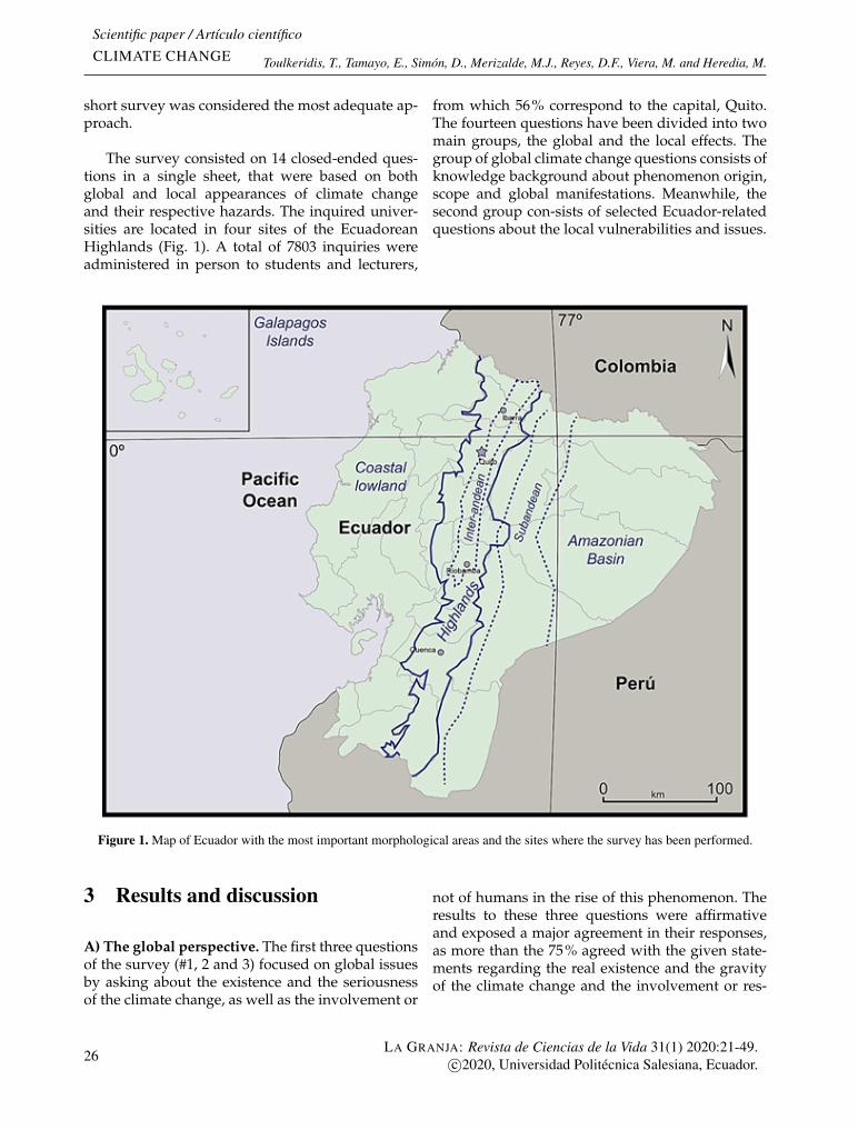
The survey consisted on 14 closed-ended ques-tions in a single sheet, that were based on bothglobal and local appearances of climate changeand their respective hazards. The inquired univer-sities are located in four sites of the EcuadoreanHighlands (Fig. 1). A total of 7803 inquiries wereadministered in person to students and lecturers,
from which 56% correspond to the capital, Quito.The fourteen questions have been divided into twomain groups, the global and the local effects. Thegroup of global climate change questions consists ofknowledge background about phenomenon origin,scope and global manifestations. Meanwhile, thesecond group con-sists of selected Ecuador-relatedquestions about the local vulnerabilities and issues.
Figure 1. Map of Ecuador with the most important morphological areas and the sites where the survey has been performed.
3 Results and discussion
A) The global perspective. The first three questionsof the survey (#1, 2 and 3) focused on global issuesby asking about the existence and the seriousnessof the climate change, as well as the involvement or
not of humans in the rise of this phenomenon. Theresults to these three questions were affirmativeand exposed a major agreement in their responses,as more than the 75% agreed with the given state-ments regarding the real existence and the gravityof the climate change and the involvement or res-
26LA GRANJA: Revista de Ciencias de la Vida 31(1) 2020:21-49.
c©2020, Universidad Politécnica Salesiana, Ecuador.
Climate Change according to Ecuadorian academics–Perceptions versus facts
ponsibility of humans. Those topics are commonlyresearched worldwide and are regularly presentedon the daily news. Therefore, it was assumed thatthe broad and worldwide inputs infer on the com-mon agreement. According to the PNDU2009, thehigh importance of climate change is due to therisks that humanity will face at the current trend ofCO2 concentrations. The risks include: (1) reducedagricultural productivity, (2) increased water stressand insecurity, (3) rising sea levels and exposure toclimate disasters, (4) collapse of ecosystems, (5) in-creased health risks, (6) flooding and (7) hunger.
Although there is still a lack of a reliable quanti-fication of the cumulative impacts of climate changeon the global-scale agricultural productivity, thereis no doubt that there are direct negative effects ofan increase of CO2 on plant physiology and increa-se resource use efficiencies (Olesen and Bindi, 2002;Battisti and Naylor, 2009; Gornall et al., 2010). The-refore, food insecurity will most likely rise due tothe present climate change, especially if societies areunable to cope rapidly with ongoing developments(Lobell et al., 2008; Brown and Funk, 2008). Overall,local biota and human livelihoods are threatened bychanging climates and the associated changes in te-rrestrial ecosystems (Verchot et al., 2007).
Clean water resources are essential for man,society, its life-support system and its industrialdevelop-ment (Sullivan, 2002; Milly et al., 2005;Falkenmark, 2013). However, increasing tempera-tures are stressing the existing water resources andthe ecosystems which provide this important ele-ment. Reduction of glaciers, evaporation of waterdeposits and high-use of subterranean water re-sources have led to the overall reduction of waterin arid and semi-arid areas (Messerli et al., 2004;Greenwood, 2014; Zografos et al., 2014). An increa-se of such vulnerability may cause significant so-cial and territorial problems between societies oreven among countries (Allouche, 2011; Adano et al.,2012; Gleick, 2014).
An increase of the average worldwide tempe-rature results into rising sea levels (Harley et al.,2006). Such climate-induced changes lead to mo-re damaging flood conditions in coastal areasas well as other vulnerable zones close to thesea level (Watson et al., 1998; Berz et al., 2001;Hoegh-Guldberg et al., 2007). Furthermore, hydro-metereological disasters such as hurricanes or cy-
clones tend towards longer duration and greaterintensity being correlated with the rise of tropicalsea surface temperatures in the last decades, evenin regions which have not been affected in theirpast (on Climate Change, 2007; Dasgupta et al.,2011; Brecht et al., 2012). Furthermore, the rise ofthe mean sea-level may also result in the directcollapse of a variety of ecosystems (Worm et al.,2006; MacDougall et al., 2013). Such dramatic effectsare especially reported in island regions or statessuch as those in the Caribbean and southern Paci-fic areas, where the environmental conditions andcoastal communities are alike (Pelling and Uitto,2001; Dolan and Walker, 2006). A consequence ofocean warming is the enhancement of ocean circu-lation driven atmosphere-ocean phenomenon suchas the ENSO and cyclones. Example of this appearsto be the 2015/16 El Niño episode registered as oneof the strongest in the history, although it has beenalso alternatively interpreted (?Mato and Toulkeri-dis, 2017; Brainard et al., 2018). The strong 2015/16El Niño coincides with the global average tempera-ture in 2015, reaching values of 1 ◦C above prein-dustrial level for the first time, labeling this year asthe warmest so far (P. et al., 2016).
Climate change may affect health through a hu-ge range of forms like more intense and more fre-quent heat waves as well as changes in the distribu-tion of vector-borne diseases, among many others(Patz et al., 2005; Haines et al., 2006). The effects ofglobal warming have been observed in the temporalincrease in temperatures that occur more frequentlyand by subsequent enhanced hot waves as well asthe rise of temperatures in the oceans (Meehl andTebaldi, 2004). Thus, long-lasting heat waves whichoccurred in 1995 in Chicago, USA and in 2003 in Pa-ris, France caused 35.000 deaths (Karl and Knight,1997; Luterbacher et al., 2004; Stott et al., 2004). Furt-her heat waves are expected in a variety of regionsall over the planet, based on several modeled sce-narios (Lhotka et al., 2018; Frölicher and Laufkötter,2018; Guo et al., 2018). Additionally, there are manyscientific evidences stating that the climate variabi-lity of the last decades has given rise to vector-bornediseases, as a result of several droughts and or floo-ding as well as fires (Martens et al., 1995; Githekoet al., 2000; Amiro et al., 2001; Flannigan et al., 2009;Moritz et al., 2012; El Universo, 2018).
Changes in climate in different regions allowsthe migration of a high variety of insect and bird
LA GRANJA: Revista de Ciencias de la Vida 31(1) 2020:21-49.c©2020, Universidad Politécnica Salesiana, Ecuador. 27
Scientific paper / Artículo científicoCLIMATE CHANGE Toulkeridis, T., Tamayo, E., Simón, D., Merizalde, M.J., Reyes, D.F., Viera, M. and Heredia, M.
species, who may carry several vector-borne andemerging infectious diseases with them (Patz et al.,1996; Kovats and Hajat, 2008; Tol and Dowlataba-di, 2001; Epstein, 2001; Jones and Mann, 2004; Wuet al., 2016). Based on the compilation by the WorldHealth Organization (WHO), the current global cli-mate change may cause up to 150.000 deaths peryear (Cifuentes Lira, 2008).Additionally, as conse-quences of the current trade of pollution, the globaltemperature is predicted to rise de 1.5 a 4.5 ◦C. Thisrise will cause the melting of many glaciers, resul-ting to a sea level rise of about around 50 cm, im-pacts on the biological systems like the coral reefs,further damage or slower recuperation of the ozo-ne layer, and the spread of tropical diseases such asmalaria and paludism (Ibárcena and Scheelje, 2003).The temperature rise and the heavy rainfall are themain causes for the spread of diseases. For example,the malaria distribution model is based on tempe-ratures (Rogers and Randolph, 2000). The effects onpeople health due to climate change include malnu-trition, undernourishment, and infectious diseases(McMichael and Haines, 1997). Examples of thisare the health impacts such as the epidemics anddiarrhea which occurred after the seasonal varia-bility of the El Niño-Southern Oscillation (ENSO)(Patz et al., 2005).
The responses to question #4, which regard tothe level of agreement that scientists have about theoccurrence or not of climate change, showed a ma-jority of 60% that believe there is agreement in thescientific community. From the research undertakenin several reports and scientific papers, the responseof the survey is supported as most of the scientistsagree in the imminent and mostly dangerous effectsof climate change and global warming. Both pro-cesses have been accelerated by humans and theirindustrial activity. Moreover, they agree on the ef-fects that pollution and global warming have hadand will have over the ecosystem and the atmosp-here, which includes ice poles melting, enhancedENSO, droughts, flooding, coral reef bleaching andthe extinction of some species (Timmermann et al.,1999; Clauer et al., 2000; Walther et al., 2002; Thomaset al., 1999; Cazenave, 2006; Brook et al., 2008; Mar-kus et al., 2009; Ibárcena and Scheelje, 2003; Chenet al., 2013; McClanahan et al., 2018; Cai et al., 2019).
Question #5 of the survey focuses on past clima-te changes during human history, as the idea was
to encounter the knowledge background of clima-te variability by the academics of Ecuador. Basedon scientific studies, there have been several clima-te and temperature changes since the existence ofhumans, and also significant rapid climate chan-ges during the current Holocene (Mayewski et al.,2004). Such climate fluctuations, even the abruptones, seem to have been triggered by changes inearth orbital insolation, volcanic aerosols and as-sociated albedo feedback processes rather than bya significant increase of antrophogenic greenhousegases (Crowley et al., 1993; Rampino and Self, 1993;Overpeck et al., 1997; Crowley, 2000; Atwell, 2001;Bay et al., 2004; Christensen et al., 2019; Guanochan-ga et al., 2018; Fuertes et al., 2019).
In a more detailed approach, it should be re-minded that since the appearance of hominins over2,000,000 years ago, the history of human evolutionhas been intrinsically linked to Earths climate fluc-tuations, which have helped to shape our species.The origins of bipedalism were in a period of clima-tic transition, and Homo erectus emerged in the timeof the colder Pleistocene Epoch and survived va-rious glacial-interglacial cycles (de Menocal, 1995;Rightmire, 2008). Homo sapiens domination initia-ted during the last glacial period and acceleratedover the last glacial-interglacial transition (Grou-cutt et al., 2015; Williams et al., 2016; Asrat et al.,2018; Skillington, 2018). The modern human specieshas successfully experienced nearly two full glacial-interglacial cycles due to its worldwide geographi-cal distribution, extensive population expansion,and global ecological domination together with su-perior technology, and more dynamic social rela-tionships (Shea, 2008; Schramski et al., 2015).
Such climate changes have impacted humanevolution and dispersal, and are believed to havedeter-mined and even stimulated the emergenceof agriculture. Animal domestication seems to ha-ve initiated in western Asia around 11,000 yearsago when goats and sheep were first herded, whileplant domestication started some 2000 years lateras wheat, lentils, and rye were grown by first time(Diamond, 2002; Terrell et al., 2003). This shift froma nomadic hunter-gatherer lifestyle to agrarian-based settlements took place during a phase ofclimatic transition after the last glacial period (Ri-cherson et al., 2001). It seems that, although climatechange affected nomadic societies by causing dras-
28LA GRANJA: Revista de Ciencias de la Vida 31(1) 2020:21-49.
c©2020, Universidad Politécnica Salesiana, Ecuador.
Climate Change according to Ecuadorian academics–Perceptions versus facts
tic decreases in natural resources, it also broughtopportunities as new plants and animals spread orappeared. Although certain civilizations may havecollapsed due to abrupt and intense climatic chan-ges, humans have adapted and survived climatevariations through history. These climate changesrange from decadal to centennial and millennial va-riations, and have been well documented throughhistorical and proxy records, particularly annualgrowth rings in trees, cave stalagmites, corals, coresof lake and deep-sea sediments and ice cores (Mc-Manus et al., 1994; Jones et al., 2009; Esper et al.,2002). Interannual and decadal climate oscillationsinclude El Niño–Southern Oscillation, the NorthAtlantic Oscillation, the Pacific Decadal Oscillationor the Atlantic Multidecadal Oscillation (Henleyet al., 2015; Geng et al., 2017; Kayano et al., 2019).They have also been associated to the collapse of theMaya civilization in Mesoamerica between the 8thand 9th centuries, suggesting that intense droughtsmay have led to social stresses (Hodell et al., 1995;Haug et al., 2003; Douglas et al., 2015; Beach et al.,2016). As for centennial timescales, the Little IceAge (LIA) was a period of relative cooling whichspanned from early 14th through the mid-19th cen-turies (Jones and Mann, 2004; Rubino et al., 2016). Itis characterized by a mountain glaciers expansionin regions such as the European Alps, New Zea-land, and the Patagonian Andes, and a decline of0.6 ◦C in the mean annual temperatures across theNorthern Hemisphere (Svarva et al., 2018). The ef-fects of LIA include bad harvests and famines overmost of Europe due to the increase of rain duringsummers (Appleby, 1980), as well as the collap-se of cod fisheries in the North Atlantic resultingfrom a pronounced decreased of sea temperatures.The LIA began after the Medieval Warm Period(9̃50–1100 CE ) (Cronin et al., 2010), whose warmerwinters and summers led to good crop yields overmost of Europe, with wheat and vineyard beinggrown in colder regions than today. In the NorthernHemisphere, the period around ad 1000 to 1100 fea-tured high temperatures-similar to those recorded
between 1961 and 1990 while minimum temperatu-res about 0.7 ◦C below the average of 1961-90 mayhave occurred around ad 1600 (Moberg et al., 2005).However, neither the Little Ice Age nor the Medie-val Warm Period were climatically homogeneousperiods nor did they exhibit uniform temperatu-res everywhere in the Earth. Instead, they featuredregionally complex spatial rain patterns and asyn-chronous warming, most probably as a result ofcoupled ocean–atmosphere processes (Cronin et al.,2010). For instance, during the LIA, temperatures ofareas like eastern China or the Northern Andes didnot experience a significant reduction. Nonetheless,past climate changes have been different comparedto the recent one, as the climate changes have notbeen recorded worldwide unlike the current (Neu-kom et al., 2019a,b; Brönnimann et al., 2019).
In this respect, and based on the aforementio-ned studies, the perceptions recorded in the surveydoes not match with the facts, since most of the in-quired academics (6̃7.2 %) believe that the currentclimate change is the first climate change humansare experiencing. Hence, there has been no clear re-cognition of earlier climate changes since humansappeared on the earths surface (Fig. 2). The op-tions of totally and mostly agree reach an averageof 39.77% of the results, while the options of totallyand mostly disagree sum up only 32% on average;furthermore, 27.42 % of the answers correspond tothe option probably. However, among the four citiessurveyed, Ibarra and Riobamba are the ones with ahigher percentage (38 %) of totally and mostly di-sagree answers, hence, with a better knowledge ofthe facts, while Quito is the city with the lowest per-centage (20,5 %) in these options, showing a worsecorrespondence with the reality. Independent of thecity, the diverse results clearly indicate that thereis lack of agreement in the perception of this issue,most likely linked to a lack of knowledge or less tono access on facts about paleoclimatology.
B) The Ecuadorian perspective
The second part of the survey aims to evaluatethe knowledge and perceptions of the Ecuadorianacademics about many visible or perceived chan-ges in the climate of their own country. Therefore,
the first question of the second part (#6) has been ifthe inquired people think that Ecuador experiencesa climate change. The answers agreed with about60% to 80%, having a concurrent perception inall four sites of the survey. From past events, it iscommonly known that the geographic location of
LA GRANJA: Revista de Ciencias de la Vida 31(1) 2020:21-49.c©2020, Universidad Politécnica Salesiana, Ecuador. 29

Scientific paper / Artículo científicoCLIMATE CHANGE Toulkeridis, T., Tamayo, E., Simón, D., Merizalde, M.J., Reyes, D.F., Viera, M. and Heredia, M.
Figure 2. Answers with a histogram to the question #5 of the survey with the question-affirmation that since the existence ofhuman history (humanity) it is the first time that there is a climate change impacting the planet.
Ecuador makes it a vulnerable country to climatechange due to the effects that the ENSO has overthe Latin-American coasts but also more inland, inthe Highland and even the Amazonian Lowland,although with opposite effects since thousands ofyears (Rodbell et al., 1999; Riedinger et al., 2002;Terneus and Gioda, 2006). These effects, togetherwith corroborating observations of an increasingtrend in temperature, and increases in intra andinter-annual variations, may be some of the mainreasons to agree that a climate change is occurringin Ecuador.
In Ecuador, the impacts of climate change arehighlighted in a variety of observations. There isfirst the intensification of extreme climatic events,such as those that occurred as a result of the EN-SO phenomenon; specifically, the El Niño extremeevents of 1982-83 and 1997-98, and in later years,causing significant damage to livelihoods, agricul-ture and infrastructure (Rossel and Cadier, 2009;Aceituno et al., 2009; Bendix et al., 2011). Secondly,a certain rise in sea level has been determined du-ring the aforementioned climatic variations (Cuca-lon, 1987; Rodbell et al., 1999). The increase of thesea level threats to coastal flooding of near-coasttowns and further towns as the effect of the ENSOwas also enhanced. Third, the retreat of the glacierswhich is most visible particularly in summer, with
tremendous retreat ranges (Francou et al., 2000; Jor-dan et al., 2005; Francou et al., 2005). Fourth, a de-termined decrease in annual runoff, as indicated ina variety of studies (Yates, 1997; Poulenard et al.,2001; Laraque et al., 2007; Zubieta et al., 2015). Furt-hermore, in Ecuador there has been an increase inthe distribution range of dengue, malaria and ot-her tropical diseases (Gueri et al., 1986; Ruiz andRoeger, 1994; Kovats et al., 2001; Gabastou et al.,2002; Stewart-Ibarra and Lowe, 2013; Stewart-Ibarraet al., 2014; Padilla et al., 2017), as a consequence oftemperature and humidity rise, which create grea-ter areas suitable for the expansion of tropical di-seases (Reguero et al., 2015; Ibárcena and Scheelje,2003). Additionally, the expansion of populationsof invasive species in Galapagos and other sensi-tive ecosystems of continental Ecuador (Schofield,1989; Mauchamp, 1997; Roque Albelo and Caus-ton, 1999; Wikelski et al., 2004; Chaves, 2018; Ruedaet al., 2019; Urquía et al., 2019) and finally even theextinction of several species (Haase, 1997; Batailleet al., 2009; Moret et al., 2016).
Regarding the question #7, about global clima-te change, a few aspects must be mentioned aboutthis issue. The geographic location of Ecuador at theequator allows higher solar radiation, which addedto a rise of the global temperature may also repre-sent a threat for the human health of this region
30LA GRANJA: Revista de Ciencias de la Vida 31(1) 2020:21-49.
c©2020, Universidad Politécnica Salesiana, Ecuador.
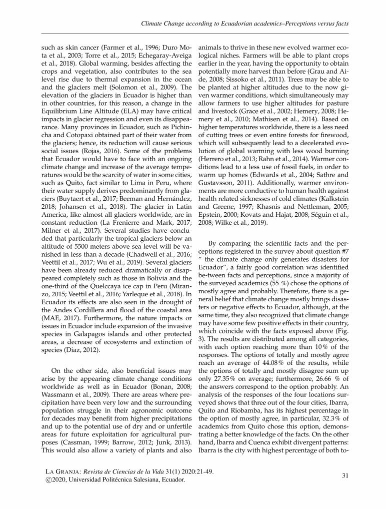
Climate Change according to Ecuadorian academics–Perceptions versus facts
such as skin cancer (Farmer et al., 1996; Duro Mo-ta et al., 2003; Torre et al., 2015; Echegaray-Aveigaet al., 2018). Global warming, besides affecting thecrops and vegetation, also contributes to the sealevel rise due to thermal expansion in the oceanand the glaciers melt (Solomon et al., 2009). Theelevation of the glaciers in Ecuador is higher thanin other countries, for this reason, a change in theEquilibrium Line Altitude (ELA) may have criticalimpacts in glacier regression and even its disappea-rance. Many provinces in Ecuador, such as Pichin-cha and Cotopaxi obtained part of their water fromthe glaciers; hence, its reduction will cause serioussocial issues (Rojas, 2016). Some of the problemsthat Ecuador would have to face with an ongoingclimate change and increase of the average tempe-ratures would be the scarcity of water in some cities,such as Quito, fact similar to Lima in Peru, wheretheir water supply derives predominantly from gla-ciers (Buytaert et al., 2017; Beeman and Hernández,2018; Johansen et al., 2018). The glacier in LatinAmerica, like almost all glaciers worldwide, are inconstant reduction (La Frenierre and Mark, 2017;Milner et al., 2017). Several studies have conclu-ded that particularly the tropical glaciers below analtitude of 5500 meters above sea level will be va-nished in less than a decade (Chadwell et al., 2016;Veettil et al., 2017; Wu et al., 2019). Several glaciershave been already reduced dramatically or disap-peared completely such as those in Bolivia and theone-third of the Quelccaya ice cap in Peru (Miran-zo, 2015; Veettil et al., 2016; Yarleque et al., 2018). InEcuador its effects are also seen in the drought ofthe Andes Cordillera and flood of the coastal area(MAE, 2017). Furthermore, the nature impacts orissues in Ecuador include expansion of the invasivespecies in Galapagos islands and other protectedareas, a decrease of ecosystems and extinction ofspecies (Diaz, 2012).
On the other side, also beneficial issues mayarise by the appearing climate change conditionsworldwide as well as in Ecuador (Bonan, 2008;Wassmann et al., 2009). There are areas where pre-cipitation have been very low and the surroundingpopulation struggle in their agronomic outcomefor decades may benefit from higher precipitationsand up to the potential use of dry and or unfertileareas for future exploitation for agricultural pur-poses (Cassman, 1999; Barrow, 2012; Junk, 2013).This would also allow a variety of plants and also
animals to thrive in these new evolved warmer eco-logical niches. Farmers will be able to plant cropsearlier in the year, having the opportunity to obtainpotentially more harvest than before (Grau and Ai-de, 2008; Sissoko et al., 2011). Trees may be able tobe planted at higher altitudes due to the now gi-ven warmer conditions, which simultaneously mayallow farmers to use higher altitudes for pastureand livestock (Grace et al., 2002; Hemery, 2008; He-mery et al., 2010; Mathisen et al., 2014). Based onhigher temperatures worldwide, there is a less needof cutting trees or even entire forests for firewood,which will subsequently lead to a decelerated evo-lution of global warming with less wood burning(Herrero et al., 2013; Rahn et al., 2014). Warmer con-ditions lead to a less use of fossil fuels, in order towarm up homes (Edwards et al., 2004; Sathre andGustavsson, 2011). Additionally, warmer environ-ments are more conductive to human health againsthealth related sicknesses of cold climates (Kalksteinand Greene, 1997; Khasnis and Nettleman, 2005;Epstein, 2000; Kovats and Hajat, 2008; Séguin et al.,2008; Wilke et al., 2019).
By comparing the scientific facts and the per-ceptions registered in the survey about question #7” the climate change only generates disasters forEcuador”, a fairly good correlation was identifiedbe-tween facts and perceptions, since a majority ofthe surveyed academics (5̃5 %) chose the options ofmostly agree and probably. Therefore, there is a ge-neral belief that climate change mostly brings disas-ters or negative effects to Ecuador, although, at thesame time, they also recognized that climate changemay have some few positive effects in their country,which coincide with the facts exposed above (Fig.3). The results are distributed among all categories,with each option reaching more than 10% of theresponses. The options of totally and mostly agreereach an average of 44.08% of the results, whilethe options of totally and mostly disagree sum uponly 27.35% on average; furthermore, 26.66 % ofthe answers correspond to the option probably. Ananalysis of the responses of the four locations sur-veyed shows that three out of the four cities, Ibarra,Quito and Riobamba, has its highest percentage inthe option of mostly agree, in particular, 32.3% ofacademics from Quito chose this option, demons-trating a better knowledge of the facts. On the otherhand, Ibarra and Cuenca exhibit divergent patterns:Ibarra is the city with highest percentage of both to-
LA GRANJA: Revista de Ciencias de la Vida 31(1) 2020:21-49.c©2020, Universidad Politécnica Salesiana, Ecuador. 31

Scientific paper / Artículo científicoCLIMATE CHANGE Toulkeridis, T., Tamayo, E., Simón, D., Merizalde, M.J., Reyes, D.F., Viera, M. and Heredia, M.
tally agree and totally disagree, revealing more ex-tremist perceptions, whereas Cuenca is the city withlowest percentage of both totally agree and totallydisagree, and highest percentage of probably, indi-cating a conservative approach regarding the issueof effects of climate change in Ecuador. Overall, the
diverse results indicate a lack of consensus in theperception of this issue, hence, a need of more de-tailed knowledge on facts about both negative andpositive effects of climate change in their country.
Figure 3. Histogram with the results based on question #7 of the survey with the question-affirmation if global climate changeonly generates disasters for Ecuador.
The question #8 of the survey pointed out aboutthe features which may demonstrate the most theglobal warming and the climate change in Ecuador.The NOAA in 2015 determined that a new recordin greenhouse gas emissions and global increase intemperatures was reached. As results, impacts onwater and terrestrial ecosystems have been evidentin all regions of the world. Ecuador has suffered se-veral changes over time due to climate change, andit has been evident on the increasingly intense floo-ding, beach erosion, decreased biodiversity in theAndean paramos, retreat of glaciers, reduction ofagricultural productivity and freshwater supplies.The city of Quito has undergone an increase of 1.1◦C from 1880 to 2017. The collateral effects of thisincrease have produced intense winter seasons that
have increased in the last 30 years (García-Garizábalet al., 2017).As for perceptions (Fig. 4), the academics believethat the feature which mostly shows climate chan-ge in Ecuador is more frequent droughts reaching34.36% of the responses, the four cities coincided inchoosing this option as the first. The second featureis the rarer but more intense rainfall with the 21.41%on average. These two options are indeed the extre-me ends of the spectrum, and may seem opposite;however, as Martin2018 explains, when it gets war-mer, water vapor will build up in the atmosphere,so when it does rain it rains a lot, but there will belonger periods between rain events so droughts willbecome worse, and more frequent.
Contrary to expectations, only 18% of the sur-veyed academics chose the option of increase intemperature, which indicates that Ecuadorians donot perceive the temperature as the most affectedvariable; on the contrary, they believe that rainfall
is the main feature. However, this option exhibitsdivergent results among cities, Ibarra and Riobam-ba show high values around 26-27% while Quitoand Cuenca report very low values of 9.6 and 8.4%, respectively. Some 9.98% on average opted for the
32LA GRANJA: Revista de Ciencias de la Vida 31(1) 2020:21-49.
c©2020, Universidad Politécnica Salesiana, Ecuador.
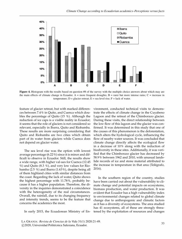
Climate Change according to Ecuadorian academics–Perceptions versus facts
Figure 4. Histogram with the results based on question #8 of the survey with the multiple choice answers about which may arethe main effects of climate change in Ecuador. A = more frequent droughts; B = rarer but more intense rains; C = increase in
temperature; D = glacier retreat; E = sea level rise; F = lack of water.
feature of glacier retreat, but with marked differen-ces between 7.4% in Quito, and Cuenca which dou-bles the percentage of Quito (15 %). Although thereduction of ice caps is a visible reality in Ecuador;it seems that the role of glaciers is not considered sorelevant, especially in Ibarra, Quito and Riobamba.These results are more surprising considering thatQuito and Riobamba are two cities which obtainpart of its water from glaciers while Cuenca doesnot depend on glacier water.
The sea level rise was the option with lowestaverage percentage (6.22%) since it is minor and dif-ficult to observe in Ecuador. Still, the results showa wide range, with higher val-ues for Cuenca (12.45%) and Quito (8.3 %), and very low values for Rio-bamba (2.5 %) and Ibarra (1.63%), despite being allof them highland cities with similar distances fromthe coast. Regarding the lack of water, Quito showsthe highest percentage with 11.78%, probably be-cause it has a higher population. Therefore, the di-versity in the inquiries demonstrated a coincidencewith the heterogeneity of the real circumstances.Overall, the rainfall, due to its changing frequencyand intensity trends, seems to be the feature thatconcerns the academics the most.
In early 2015, the Ecuadorean Ministry of En-
vironment, conducted technical visits to demons-trate the effects of climate change in the CuyabenoLagoon and the retreat of the Chimborazo glacier.During these visits, the direct relationship betweenthe low flow of this lagoon and the glacier was con-firmed. It was determined in this study that one ofthe causes of this phenomenon is the deforestation,which alters the hydrological cycle, influencing theflow of nearby water sources. It was concluded thatclimate change directly affects the ecological flowin a decrease of 10% along with the reduction ofbiodiversity in these sites. Additionally, it was veri-fied that the Chimborazo glacier has decreased by58.9% between 1962 and 2010, with unusual lands-lide records of ice and stone material attributed tothe increase in temperature in that area (Telégrafo,2016).
In the southern region of the country, studieshave been carried out about the vulnerability to cli-mate change and potential impacts on ecosystems,biomass production, and water production. It wasevident that Ecuador has a high vulnerability indexto environmental changes related to global climatechange due to anthropogenic and climatic factorsas it has a diversity of ecosystems. The area studiedhas 41 ecosystems, all of these are strongly threa-tened by the exploitation of resources and changes
LA GRANJA: Revista de Ciencias de la Vida 31(1) 2020:21-49.c©2020, Universidad Politécnica Salesiana, Ecuador. 33
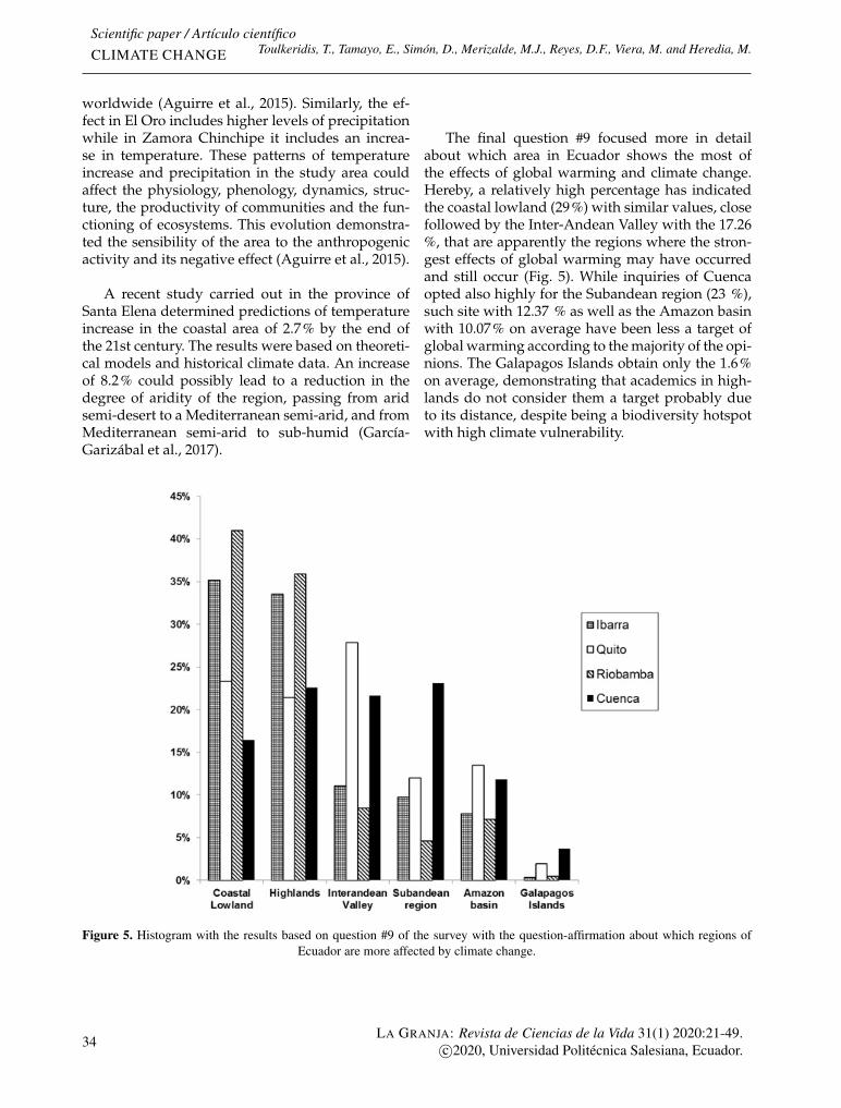
Scientific paper / Artículo científicoCLIMATE CHANGE Toulkeridis, T., Tamayo, E., Simón, D., Merizalde, M.J., Reyes, D.F., Viera, M. and Heredia, M.
worldwide (Aguirre et al., 2015). Similarly, the ef-fect in El Oro includes higher levels of precipitationwhile in Zamora Chinchipe it includes an increa-se in temperature. These patterns of temperatureincrease and precipitation in the study area couldaffect the physiology, phenology, dynamics, struc-ture, the productivity of communities and the fun-ctioning of ecosystems. This evolution demonstra-ted the sensibility of the area to the anthropogenicactivity and its negative effect (Aguirre et al., 2015).
A recent study carried out in the province ofSanta Elena determined predictions of temperatureincrease in the coastal area of 2.7% by the end ofthe 21st century. The results were based on theoreti-cal models and historical climate data. An increaseof 8.2% could possibly lead to a reduction in thedegree of aridity of the region, passing from aridsemi-desert to a Mediterranean semi-arid, and fromMediterranean semi-arid to sub-humid (García-Garizábal et al., 2017).
The final question #9 focused more in detailabout which area in Ecuador shows the most ofthe effects of global warming and climate change.Hereby, a relatively high percentage has indicatedthe coastal lowland (29%) with similar values, closefollowed by the Inter-Andean Valley with the 17.26%, that are apparently the regions where the stron-gest effects of global warming may have occurredand still occur (Fig. 5). While inquiries of Cuencaopted also highly for the Subandean region (23 %),such site with 12.37 % as well as the Amazon basinwith 10.07% on average have been less a target ofglobal warming according to the majority of the opi-nions. The Galapagos Islands obtain only the 1.6%on average, demonstrating that academics in high-lands do not consider them a target probably dueto its distance, despite being a biodiversity hotspotwith high climate vulnerability.
Figure 5. Histogram with the results based on question #9 of the survey with the question-affirmation about which regions ofEcuador are more affected by climate change.
34LA GRANJA: Revista de Ciencias de la Vida 31(1) 2020:21-49.
c©2020, Universidad Politécnica Salesiana, Ecuador.

Climate Change according to Ecuadorian academics–Perceptions versus facts
The results have indicated that people appa-rently tend to see that their own environment is ha-ving some severe effects as also previously demons-trated with #8 of the survey (Fig. 4). This allows topotentially interpret that people most likely do notknow well or less frequent visit other regions inorder to be able to have a better view and moreaspects for a better evaluation of potential effectsof global warming and also other atmospheric ef-fects based on climate change. However, the coastallowlands, with the highest percentage, especiallyin Ibarra and Riobamba (35.2 y 41 %), was an ex-ception since it was generally perceived as highlyimpacted by climate change for the inhabitants ofthe highlands, who often watch on TV and newspa-pers the effects of El Niño and the recurrent floodsin the Ecuadorian coast.
Finally, an overall view based on the surveyshows that the two main patterns have been thetendency to choose options ‘b= Mostly Agree’ and‘c=Probably’ which are ambiguous, but only in spe-cific questions like 1 and 10 the options ‘a= To-tally agree’ or ‘e= Totally disagree’ that are specific,were chosen. These two questions are highly spo-ken about in the media and institutes; hence, it is aclear choice. However, this ‘certainty’ is dependenton information that is broad and vague where noreference to scientific papers or primary source isgiven. The omission of the source in the publica-tions of some newspapers in Ecuador was verifiedin 18 news about climate change. It was noticedthat the answers of the academic population agreedwith the scientific investigation performed aroundthe world, however most of this knowledge lackof deepness. In addition, about the other 50% indi-cates doubt. This is most likely related to the lackof information and poor research and data infor-mation about climate change worldwide in generaland particularly about Ecuador.
4 Conclusions
There is lack of a wider perspective, discussion ofthe role of the government, corporations, academicsand community in emission, mitigation and adap-tation policies implementation.
The Ecuadorean academic community of the
highlands is aware of many globally known facts ofglobal warming and climate change. This includesthe potential damages and disasters for a varietyof environments. However, there is a clear lack ofdeepness of the origin and reach of such climate is-sues. There is also an obvious reduced awareness ofadaptation issues as well as mitigation and perso-nal preparation against eventual disasters as resultof climate change.
Such conditions increase the vulnerability ofEcuador to the Climate change effects, as only fewreflected knowledge about the real impacts andhow they will affect the future of the country. Thereis a lack of think ahead planning, as demonstratedin the given results of the survey. However, the ef-fects of the climate change in Ecuador are undenia-ble, and it is perceived mainly in the more frequentand intense flooding and droughts, and the retreatof the glaciers in the highlands.
AppendixFigure 1A shows the questions corresponding to thesurvey conducted to generate the collection of infor-mation developed in Section 2.
LA GRANJA: Revista de Ciencias de la Vida 31(1) 2020:21-49.c©2020, Universidad Politécnica Salesiana, Ecuador. 35
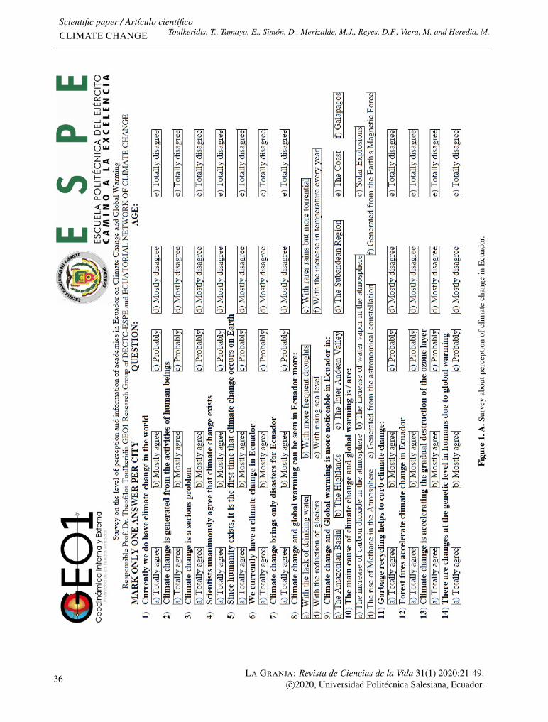
Scientific paper / Artículo científicoCLIMATE CHANGE Toulkeridis, T., Tamayo, E., Simón, D., Merizalde, M.J., Reyes, D.F., Viera, M. and Heredia, M.
Figu
re1.
A.S
urve
yab
outp
erce
ptio
nof
clim
ate
chan
gein
Ecu
ador
.
36LA GRANJA: Revista de Ciencias de la Vida 31(1) 2020:21-49.
c©2020, Universidad Politécnica Salesiana, Ecuador.
Climate Change according to Ecuadorian academics–Perceptions versus facts
ReferencesAceituno, P., del Rosario Prieto, M., Solari, M. E.,
Martínez, A., Poveda, G., and Falvey, M. (2009).The 1877–1878 el niño episode: associated im-pacts in south america. Climatic Change, 92(3-4):389–416. Online: https://bit.ly/38ael47.
Adano, W. R., Dietz, T., Witsenburg, K., and Zaal,F. (2012). Climate change, violent conflict andlocal insti-tutions in kenya’s drylands. Journalof Peace Research, 49(1):65–80. Online: https://bit.ly/32BKNuV.
Agency, I. I. E. (2018). The co2 emissions from fuelcombustion. online: https://bit.ly/32x5TdW.
Aguirre, N., Eguiguren, P., Maita, J., Coronel, V., Sa-maniego, N., Ojeda, L., and Aguirre, T. (2015).Vulnerabilidad al cambio climático en la Región Surdel Ecuador: Potenciales impactos en los ecosistemas,producción de biomasa y producción hídrica.
Allouche, J. (2011). The sustainability and resilienceof global water and food systems: Political analy-sis of the interplay between security, resourcescarcity, political systems and global trade. FoodPoli-cy, 36:S3–S8. Online: https://bit.ly/3afnIke.
Amiro, B. D., Stocks, B. J., Alexander, M. E., Flan-nigan, M. D., and Wotton, B. M. (2001). Fire,climate change, carbon and fuel management inthe canadian boreal forest. International Journal ofWildland Fire, 10(4):405–413. Online: https://bit.ly/2wdrRqf.
Appleby, A. B. (1980). Epidemics and famine in thelittle ice age. The Journal of interdisciplinary history,10(4):643–663. Online: https://bit.ly/32DbPSU.
Asrat, A., Baker, A., Leng, M. J., Hellstrom, J.,Mariethoz, G., Boomer, I., Yu, D., Jex, C., andGunn, J. (2018). Paleoclimate change in ethio-pia around the last interglacial derived fromannually-resolved stalagmite evidence. Quater-nary Science Reviews, 202:197–210. Online: https://bit.ly/2uDarmr.
Atwell, W. S. (2001). Volcanism and short-term cli-matic change in east asian and world history, c.1200-1699. Journal of World History, 12(1):29–98.Online: https://bit.ly/39kTywd.
Baatz, C. (2013). Responsibility for the past? so-me thoughts on compensating those vulnerable
to cli-mate change. Developing Countries, Ethics,Policy & Environment,, 16(1):94–110. Online: https://bit.ly/2vcHqP1.
Barrow, C. J. (2012). Biochar: potential for counte-ring land degradation and for improving agricul-ture. Applied Geography, 34:21–28. Online: https://bit.ly/32yw1Fk.
Bataille, A., Cunningham, A. A., Cedeño, V., Patiño,L., Constantinou, A., Kramer, L. D., and Good-man, S. J. (2009). Natural colonization and adap-tation of a mosquito species in galápagos and itsimplications for disease threats to endemic wild-life. Proceedings of the National Academy of Scien-ces, 106(25):10230–10235. Online: https://bit.ly/2VtnYIw.
Battisti, D. S. and Naylor, R. L. (2009). Historicalwarnings of future food insecurity with unprece-dented seasonal heat. Science, 323(5911):240–244.Online: https://bit.ly/3co6ljk.
Bay, R. C., Bramall, N., and Price, P. B. (2004). Bi-polar correlation of volcanism with millennial cli-mate change. Proceedings of the National Academyof Sciences, 101(17):6341–6345. Online: https://bit.ly/2Tl27A3.
Beach, T., Luzzadder-Beach, S., Dunning, N., andCook, D. (2016). Climatic changes and collap-ses in maya history. Past Global Changes Magazine,24(2):66–67. Online: https://bit.ly/2To0d1w.
Beeman, J. C. and Hernández, J. C. R. (2018). Un-derstanding global climate change from andeanglaciers. ReVista (Cambridge), 18(3):42–82. Online:https://bit.ly/2T38j0Q.
Bendix, J., Trachte, K., Palacios, E., Rollenbeck, R.,Göttlicher, D., Nauss, T., and Bendix, A. (2011).El niño meets la niña—anomalous rainfall pat-terns in the"traditional.el niño region of southernecuador. Erdkunde, pages 151–167. Online: https://bit.ly/2PwVU2S.
Berz, G., Kron, W., Loster, T., Rauch, E., Schimets-chek, J., Schmieder, J., Siebert, A., Smolka, A., andWirtz, A. (2001). World map of natural hazards–a global view of the distribution and intensityof significant exposures. Natural hazards, 23(2-3):443–465. Online: https://bit.ly/3amati3.
LA GRANJA: Revista de Ciencias de la Vida 31(1) 2020:21-49.c©2020, Universidad Politécnica Salesiana, Ecuador. 37

Scientific paper / Artículo científicoCLIMATE CHANGE Toulkeridis, T., Tamayo, E., Simón, D., Merizalde, M.J., Reyes, D.F., Viera, M. and Heredia, M.
Bonan, G. B. (2008). Forests and climate change: for-cings, feedbacks, and the climate benefits of fo-rests. science, 320(5882):1444–1449. Online: https://bit.ly/393TAIs.
Brainard, R. E., Oliver, T., McPhaden, M. J., Cohen,A., Venegas, R., Heenan, A., Vargas-Ángel, B.,Rotjan, R., Mangubhai, S., and Flint, E. (2018).Ecological impacts of the 2015/16 el niño in thecentral equatorial pacific. Bulletin of the Ameri-can Meteorological Society, 99(1):S21–S26. Online:https://bit.ly/2T5pX48.
Brecht, H., Dasgupta, S., Laplante, B., Murray, S.,and Wheeler, D. (2012). Sea-level rise and stormsurges: High stakes for a small number of develo-ping countries. The Journal of Environment & De-velopment, 21(1):120–138. Online: https://bit.ly/3cgI6Dm.
Brönnimann, S., Franke, J., Nussbaumer, S. U.,Zumbühl, H. J., Steiner, D., Trachsel, M., Hegerl,G. C., Schurer, A., Worni, M., and Malik, A. (2019).Last phase of the little ice age forced by volcaniceruptions. Nature geoscience, 12(8):650–656. Onli-ne: https://bit.ly/2T71s6x.
Brook, B. W., Sodhi, N. S., and Bradshaw, C. J. A.(2008). Synergies among extinction drivers un-der global change. Trends in ecology & evolution,23(8):453–460. Online: https://nus.edu/2VrOyl6.
Brown, M. E. and Funk, C. C. (2008). Food securityunder climate change. Science, 319(5863):580–581.Online: https://bit.ly/2I4ZM72.
Buytaert, W., Moulds, S., Acosta, L., De Bievre, B.,Olmos, C., Villacis, M., Tovar, C., and Verbist, K.M. J. (2017). Glacial melt content of water use inthe tropical andes. Environmental Research Letters,12(11):114014. Online: https://bit.ly/397g8rJ.
Buytaert, W., Vuille, M., Dewulf, A., Urrutia, R.,Karmalkar, A., and Célleri, R. (2010). Uncer-tainties in climate change projections and regio-nal downscaling in the tropical andes: implica-tions for water resources management. Hydro-logy and Earth System Sciences, 14(7):1247. Online:https://bit.ly/2T5Cp3V.
Cai, W., Wu, L., Lengaigne, M., Li, T., McGre-gor, S., Kug, J.-S., Yu, J.-Y., Stuecker, M., Santo-so, A., Li, X., Ham, Y.-G., Chikamoto, Y., Ng,B., McPhaden, M., Du, Y., Dommenget, D., Jia,
F., Kajtar, J., Keenlyside, N., Lin, X., Luo, J.-J.,Martín-Rey, M., Ruprich-Robert, Y., Wang, G.,Xie, S.-P., Yang, Y., Kang, S., Choi, J.-Y., Gan, B.,Kim, G.-I., Kim, C.-E., Kim, S., Kim, J.-H., andChang, P. (2019). Pantropical climate interac-tions. Science, 363(6430):eaav4236. Online: https://bit.ly/381FyFX.
Calliari, E. (2018). Loss and damage: a criticaldiscourse analysis of parties’ positions in clima-te change negotiations. Journal of Risk Research,21(6):725–747. Online: https://bit.ly/3caydHD.
Cassman, K. G. (1999). Ecological intensificationof cereal production systems: yield potential, soilquality, and precision agriculture. Proceedings ofthe National Academy of Sciences, 96(11):5952–5959.Online: https://bit.ly/3ac3msm.
Cazenave, A. (2006). How fast are the ice sheetsmelting? Science, 314(5803):1250–1252. Online:https://bit.ly/39ap7sk.
Chadwell, C. D., Hardy, D. R., Braun, C., Brecher,H. H., and Thompson, L. G. (2016). Thinning ofthe quelccaya ice cap over the last thirty years. In2016 Cryosphere Discuss.
Chaves, J. A. (2018). Genetic consequences of invasi-ve species in the galapagos islands. In Understan-ding Invasive Species in the Galapagos Islands, pages19–32. Online: https://bit.ly/32y2ono. Springer.
Chen, J. L., Wilson, C. R., Ries, J. C., and Tapley, B. D.(2013). Rapid ice melting drives earth’s pole tothe east. Geophysical Research Letters, 40(11):2625–2630. Online: https://bit.ly/2PwnEol.
Christensen, T. R., Arora, V. K., Gauss, M., Höglund-Isaksson, L., and Parmentier, F. J. W. (2019). Tra-cing the climate signal: Mitigation of anthropoge-nic methane emissions can outweigh a large arcticnatural emission increase. Scientific reports, 9(1):1–8. Online: https://go.nature.com/3a39EKK.
Cifuentes Lira, L. A. (2008). Cambio climático: con-secuencias y desafíos para chile. In 2008 Temas dela agenda pública, number 19, pages 6–22. Online:https://bit.ly/2vd3Pf5. Centro Interdisciplinariode Cambio Global (CICG-UC).
Clauer, N., Chaudhuri, S., Toulkeridis, T., and Blanc,G. (2000). Fluctuations of caspian sea level: Be-yond climatic variations? Geology, 28(11):1015–1018. Online: https://go.aws/2vd2xkf.
38LA GRANJA: Revista de Ciencias de la Vida 31(1) 2020:21-49.
c©2020, Universidad Politécnica Salesiana, Ecuador.

Climate Change according to Ecuadorian academics–Perceptions versus facts
Crona, B., Wutich, A., Brewis, A., and Gartin, M.(2013). Perceptions of climate change: Linkinglocal and global perceptions through a culturalknowledge approach. Climatic change, 119(2):519–531. Online: https://bit.ly/3cbt41L.
Cronin, T. M., Hayo, K., Thunell, R. C., Dwyer,G. S., Saenger, C., and Willard, D. A. (2010).The medieval climate anomaly and little ice agein chesapeake bay and the north atlantic ocean.Palaeogeography, Palaeoclimatology, Palaeoecology,297(2):299–310. Online: https://bit.ly/397DE7Z.
Crowley, T. J. (2000). Causes of climate change overthe past 1000 years. Science, 289(5477):270–277.Online: https://bit.ly/39ayBnq.
Crowley, T. J., Criste, T. A., and Smith, N. R. (1993).Reassessment of crete (greenland) ice core aci-dity/volcanism link to climate change. Geophy-sical Research Letters, 20(3):209–212. Online: https://bit.ly/32zCYpO.
Cucalon, E. (1987). Oceanographic variabilityoff ecuador associated with an el nino eventin 1982–1983. Journal of Geophysical Research:Oceans, 92(C13):14309–14322. Online: https://bit.ly/2w7YC8r.
Dasgupta, S., Laplante, B., Murray, S., and Wheeler,D. (2011). Exposure of developing countries tosea-level rise and storm surges. Climatic Change,106(4):567–579. Online: https://bit.ly/2VEnkIj.
de Menocal, P. B. (1995). Plio-pleistocene africanclimate. Science, 270(5233):53–59. Online: https://bit.ly/2VtRE8o.
Diamond, J. (2002). Evolution, consequences andfuture of plant and animal domestication. Natu-re, 418(6898):700–707. Online: https://go.nature.com/2I30To0.
Diaz, G. (2012). El cambio climático. Ciencia y Socie-dad, pages 2–15.
Dolan, A. H. and Walker, I. J. (2006). Understan-ding vulnerability of coastal communities to cli-mate change related risks. Journal of Coastal Re-search, pages 1316–1323. Online: https://bit.ly/2Vuovdc.
Doney, S. C. (2006). The dangers of ocean acidifi-cation. Scientific American, 294(3):58–65. Online:https://bit.ly/3831pNq.
Douglas, P. M. J., Pagani, M., Canuto, M. A., Bren-ner, M., Hodell, D. A., Eglinton, T. I., and Cur-tis, J. H. (2015). Drought, agricultural adap-tation, and sociopolitical collapse in the mayalowlands. Proceedings of the National Academy ofSciences, 112(18):5607–5612. Online: https://bit.ly/3960Ljf.
Duro Mota, E., Campillos Páez, M. T., and Cau-sín Serrano, S. (2003). El sol y los filtros sola-res. Medifam, 13(3):39–45. Online: https://bit.ly/2Vv9eIP.
Echegaray-Aveiga, R. C., Masabanda, M., Rodrí-guez, F., Toulkeridis, T., and Mato, F. (2018). So-lar energy potential in ecuador. In 2018 Inter-national Conference on Democracy & Government(ICEDEG), pages 46–51. Online: https://bit.ly/2uF6NbS. IEEE.
Edwards, R. D., Smith, K. R., Zhang, J., and Ma, Y.(2004). Implications of changes in household sto-ves and fuel use in china. Energy policy, 32(3):395–411. Online: https://bit.ly/3abKVUx.
El Universo (2018). El calentamiento global favoreceaumento de incendios forestales.
Enkvist, P., Nauclér, T., and Rosander, J. (2007). Acost curve for greenhouse gas reduction. Mc-Kinsey Quarterly, 1:34. Online: https://bit.ly/2T33NPV.
Epstein, P. R. (2000). Is global warming harmful tohealth? Scientific American, 283(2):50–57. Online:https://bit.ly/395i83L.
Epstein, P. R. (2001). Climate change and emer-ging infectious diseases. Microbes and infection,3(9):747–754. Online: https://bit.ly/2w9tJAk.
Esper, J., Cook, E. R., and Schweingruber, F. H.(2002). Low-frequency signals in long tree-ringchronologies for reconstructing past temperaturevariability. science, 295(5563):2250–2253. Online:https://bit.ly/2HZlZ6v.
Falkenmark, M. (2013). Growing water scarcityin agriculture: future challenge to global watersecurity. Philosophical Transactions of the RoyalSociety A: Mathematical, Physical and EngineeringSciences, 371(2002):20120410. Online: https://bit.ly/391B9nP.
LA GRANJA: Revista de Ciencias de la Vida 31(1) 2020:21-49.c©2020, Universidad Politécnica Salesiana, Ecuador. 39
Scientific paper / Artículo científicoCLIMATE CHANGE Toulkeridis, T., Tamayo, E., Simón, D., Merizalde, M.J., Reyes, D.F., Viera, M. and Heredia, M.
Farmer, K. C., Naylor, M. F., Roca-Acén, J., and La-rouche, M. (1996). Sun exposure, sunscreens,and skin cancer prevention: a year-round con-cern. Annals of Pharmacotherapy, 30(6):662–673.Online: https://bit.ly/2TlQOYv.
Flannigan, M., Stocks, B., Turetsky, M., and Wotton,M. (2009). Impacts of climate change on fire acti-vity and fire management in the circumboreal fo-rest. Global change biology, 15(3):549–560. Online:https://bit.ly/2T4Np19.
Francou, B., Ramirez, E., Cáceres, B., and Mendoza,J. (2000). Glacier evolution in the tropical andesduring the last decades of the 20th century: Cha-caltaya, bolivia, and antizana, ecuador. AMBIO: AJournal of the Human Environment, 29(7):416–422.Online: https://bit.ly/2Tjr3be.
Francou, B., Ribstein, P., Wagnon, P., Ramirez, E.,and Pouyaud, B. (2005). Glaciers of the tropicalandes: indicators of global climate variability. InGlobal change and mountain regions, pages 197–204.Online: https://bit.ly/2TpHrXG. Springer.
Frank, D., Reichstein, M., Bahn, M., Thonicke, K.,Frank, D., Mahecha, M. D., Smituh, P., van derVelde, M., Vicca, S., Babst, F., Beer, C., Buchmann,N., Canadell, J. G., Ciasis, P., Cramer, W., Ibrom,A., Miglietta, F., Poulter, B., Ramming, A., Senevi-ratne, S. I., Walz, A., Wattenbach, M., Zavala, M.,and Zscheischler, J. (2015). Effects of climate ex-tremes on the terrestrial carbon cycle: concepts,processes and potential future impacts. GlobalChange Biology, 21(8):2861–2880. Online: https://bit.ly/3cdKwmr.
Friel, S., Dangour, A. D., Garnett, T., Lock, K., Cha-labi, Z., Roberts, I., Butler, A., Butler, C. D., Waa-ge, J., McMichael, A. J., and Haines, A. (2009).Public health benefits of strategies to reducegreenhouse-gas emissions: food and agriculture.The Lancet, 374(9706):2016–2025. Online: https://bit.ly/381VJTT.
Friman, M. and Hjerpe, M. (2015). Agreement, sig-nificance, and understandings of historical res-ponsibility in climate change negotiations. Cli-mate Policy, 15(3):302–320. Online: https://bit.ly/3aakWgb.
Frölicher, T. L. and Laufkötter, C. (2018). Emergingrisks from marine heat waves. Nature communi-cations, 9(1):650. Online: https://go.nature.com/32yyfVh.
Fuertes, W., Cadena, A., Torres, J., Benítez, D., Ta-pia, F., and Toulkeridis, T. (2019). Data analy-tics on real-time air pollution monitoring sys-tem derived from a wireless sensor network. InInternational Conference on Information Technology& Systems, pages 57–67. Online: https://bit.ly/395mOXn. Springer, Cham.
Furley, T. H., Brodeur, J., Silva de A., H. C., Carri-quiriborde, P., Chagas, K. R., Corrales, J., Dena-dai, M., Fuchs, J., Mascarenhas, R., Miglioranza,K. S., Miguez Carames, D. M., Navas, J. M., Nu-gegoda, D., Planes, E., Rodriguez-Jorquera, I. A.,Orozco-Medina, M., and Brooks, B. W. (2018). To-ward sustainable environmental quality: Identif-ying priority research questions for latin ameri-ca. Integrated environmental assessment and ma-nagement, 14(3):344–357. Online: https://bit.ly/2PvnLQZ.
Gabastou, J. M., Pesantes, C., Escalante, S., Nar-váez, Y., Vela, E., García, L., Zabala, D., and Ya-don, Z. E. (2002). Characteristics of the chole-ra epidemic of 1998 in ecuador during el nino.Revista panamericana de salud publica= Pan Ameri-can journal of public health, 12(3):157–164. Online:https://bit.ly/2T5noyT.
García-Garizábal, I., Romero, P., Jiménez, S., andJordá, L. (2017). Evolución climática en la costade ecuador por efecto del cambio climático. Dy-na, 84(203. Online: https://bit.ly/2PvPVf0).
Geng, X., Zhang, W., Stuecker, M. F., Liu, P., Jin,F. F., and Tan, G. (2017). Decadal modulationof the enso–east asian winter monsoon relations-hip by the atlantic multidecadal oscillation. Cli-mate Dynamics, 49(7-8):2531–2544. Online: https://bit.ly/2wdpEuO.
Githeko, A. K., Lindsay, S. W., Confalonieri, U. E.,and Patz, J. A. (2000). Climate change and vector-borne diseases: a regional analysis. Bulletin of theWorld Health Organization, 78:1136–1147. Online:https://bit.ly/3a773PK.
Gleick, P. H. (2014). Water, drought, climate change,and conflict in syria. Weather, Climate, and Society,6(3):331–340. Online: https://bit.ly/2uxYaj8.
40LA GRANJA: Revista de Ciencias de la Vida 31(1) 2020:21-49.
c©2020, Universidad Politécnica Salesiana, Ecuador.
Climate Change according to Ecuadorian academics–Perceptions versus facts
Gornall, J., Betts, R., Burke, E., Clark, R., Camp,J., Willett, K., and Wiltshire, A. (2010). Implica-tions of climate change for agricultural produc-tivity in the early twenty-first century. Philo-sophical Transactions of the Royal Society B: Biolo-gical Sciences, 365:2973–2989. Online: https://bit.ly/2waIIKs.
Goworek, H., Land, C., Burt, G., Zundel, M., Sa-ren, M., Parker, M., and Lambe, B. (2018). Scalingsustainability: Regulation and resilience in mana-gerial responses to climate change. British Jour-nal of Management, 29(2):209–219. Online: https://bit.ly/2VuhCZq.
Grace, J., Berninger, F., and Nagy, L. (2002). Im-pacts of climate change on the tree line. Annalsof Botany, 90(4):537–544. Online: https://bit.ly/2PxIpA5.
Grau, H. R. and Aide, M. (2008). Globalization andland-use transitions in latin america. Ecology andsociety, 13(2. Online: https://bit.ly/3893hnE).
Greenwood, S. (2014). Water insecurity, climatechange and governance in the arab world. MiddleEast Policy, 21(2):140–156. Online: https://bit.ly/3af6rb9.
Groucutt, H. S., Petraglia, M. D., Bailey, G., Scerri,E. M. L., Parton, A., Clark-Balzan, L., Jennings,R. P., Lewis, L., Blinkhorn, J., Drake, N. A., Breeze,P. S., Inglis, R. H., Devés, M., Meredith-williams,M., Boivin, N., Thomas, M. G., and Scally, A.(2015). Rethinking the dispersal of homo sapiensout of africa. Evolutionary Anthropology: Issues,News, and Reviews, 24(4):149–164. Online: https://bit.ly/2T35k8u.
Guanochanga, B., Cachipuendo, R., Fuertes, W., Sal-vador, S., Benítez, D. S., Toulkeridis, T., Torres,J., Villacís, C., Tapia, F., and Meneses, F. (2018).Real-time air pollution monitoring systems usingwireless sensor networks connected in a cloud-computing, wrapped up web services. In Pro-ceedings of the Future Technologies Conference, vo-lume 880, pages 171–184. Online: https://bit.ly/2I0EmYK. Springer.
Gueri, M., González, C., and Morin, V. (1986). Theeffect of the floods caused by “el niño” on health.Disasters, 10(2):118–124. Online: https://bit.ly/3ad0cEI.
Guo, Y., Gasparrini, A., Li, S., Sera, F., Vicedo-Cabrera, A. M., Coelho, M. S. Z., Saldiva, P. H. N.,Lavigne, E., Tawatsupa, B., and Punnasiri, K.(2018). Quantifying excess deaths related to heat-waves under climate change scenarios: A multi-country time series modelling study. PLoS medici-ne, 15(7):e1002629.
Haase, B. (1997). The impact of the el niño southernoscillation (enso) on birds: update from ecuador1997. Cotinga, 8:64–65. Online: https://bit.ly/3cf11P7.
Haines, A., Kovats, R. S., Campbell-Lendrum, D.,and Corvalán, C. (2006). Climate change andhuman health: impacts, vulnerability and pu-blic health. Public health, 120(7):585–596. Online:https://bit.ly/2wf1gcA.
Harley, C. D. G., Randall Hughes, A., Hultgren,K. M., Miner, B. G., Sorte, C. J. B., Thornber, C. S.,Rodriguez, L. F., Tomanek, L., and Williams, S. L.(2006). The impacts of climate change in coastalmarine systems. Ecology letters, 9(2):228–241. On-line: https://bit.ly/394PD6k.
Haug, G. H., Günther, D., Peterson, L. C., Sigman,D. M., Hughen, K. A., and Aeschlimann, B. (2003).Climate and the collapse of maya civilization.Science, 299(5613):1731–1735. Online: https://bit.ly/3abdDEX.
Hedlund, J., Fick, S., Carlsen, H., and Benzie, M.(2018). Quantifying transnational climate impactexposure: New perspectives on the global distri-bution of climate risk. Global environmental change,52:75–85. Online: https://bit.ly/396MIKx.
Helgenberger, S. and Jänicke, M. (2017). Mobi-lizing the co-benefits of climate change mitiga-tion. Technical report, IASS Working Paper. Onli-ne: https://bit.ly/3af90tN.
Hemery, G. (2008). Forest management and silvicul-tural responses to projected climate change im-pacts on european broadleaved trees and forests.International Forestry Review, 10(4):591–607. Onli-ne: https://bit.ly/38bK0Cl.
Hemery, G. E., Clark, J., Aldinger, E., Claessens, H.,Malvolti, M. E., O’connor, E., Raftoyannis, Y., Sa-vill, P. S., and Brus, R. (2010). Growing scatte-red broadleaved tree species in europe in a chan-ging climate: a review of risks and opportuni-
LA GRANJA: Revista de Ciencias de la Vida 31(1) 2020:21-49.c©2020, Universidad Politécnica Salesiana, Ecuador. 41
Scientific paper / Artículo científicoCLIMATE CHANGE Toulkeridis, T., Tamayo, E., Simón, D., Merizalde, M.J., Reyes, D.F., Viera, M. and Heredia, M.
ties. Forestry, 83(1):65–81. Online: https://bit.ly/2VvAvem.
Henley, B. J., Gergis, J., Karoly, D. J., Power, S., Ken-nedy, J., and Folland, C. K. (2015). A tripole in-dex for the interdecadal pacific oscillation. Clima-te Dynamics, 45(11-12):3077–3090. Online: https://bit.ly/39iEwXq.
Herrero, S. T., Ürge-Vorsatz, D., and Petrichenko,K. (2013). Fuel poverty alleviation as a co-benefit of climate investments: evidence fromhungary. In European Council for an Energy EfficientEconomy Summer Study (ECEEE) Summer StudyProceed-ings, pages 1605–1616. Online: https://bit.ly/2VzYCJ3.
Hodell, D. A., Curtis, J. H., and Brenner, M. (1995).Possible role of climate in the collapse of classicmaya civilization. Nature, 375(6530):391–394. On-line: https://go.nature.com/2I1qmht.
Hoegh-Guldberg, O., Jacob, D., Taylor, M., Bindi,M., Brown, S., Camilloni, I., Diedhiou, A., Djalan-te, R., Ebi, K., Engelbrecht, F., Guiot, J., Hijioka,Y., Mehrotra, S., Payne, A., Seneviratne, S. I., Tho-mas, A., Warren, R., and Zhou, G. (2018). Globalwarming of 1.5C. An IPCC Special Report on the im-pacts of global warming of 1.5C above pre-industriallevels and related global greenhouse gas emission path-ways, in the context of strength-ening the global res-ponse to the threat of climate change, sustainable de-velopment, and efforts to eradicate poverty, chapterImpacts of 1.5oC global warming on natural andhuman systems. Press.
Hoegh-Guldberg, O., Mumby, P. J., Hooten, A. J.,Steneck, R. S., Greenfield, P., Gomez, E., Har-vell, C. D., Sale, P. F., Edwards, A., Caldeira,K., Knowlton, N., Eakin, C. M., Iglesias-Prieto,R., Muthiga, N., Bradbury, R. H., Dubi, A., andHatziolos, M. E. (2007). Coral reefs under rapidclimate change and ocean acidification. Scien-ce, 318(5857):1737–1742. Online: https://bit.ly/39c2eVp.
Huang-Lachmann, J. T., Hannemann, M., andGuenther, E. (2018). Identifying links bet-ween economic opportunities and climate changeadaptation: empirical evidence of 63 cities. Ecolo-gical Economics, 145:231–243. Online: https://bit.ly/3acfObm.
Ibárcena, M. and Scheelje, J. M. (2003). El cambioclimático principales causantes, consecuencias ycompromisos de los países involucrados. In Foodand Agriculture Organization of the United Nations,Quebec Canada.
Johansen, K. S., Alfthan, B., Baker, E., Hesping, M.,Schoolmeester, T., and Verbist, K. (2018). The An-dean glacier and water atlas: the impact of glacier re-treat on water resources. UNESCO Publishing.
Jones, P. D., Briffa, K. R., Osborn, T. J., Lough,J. M., van Ommen, T. D., Vinther, B. M., Luter-bacher, E. R., Wahl, F. W., Zwiers, M. E., Mann,G. A., Schmidt, C. M., Ammann, B. M., Buckley,K. M., Cobb, J., Esper, H., Goosse, N., Graham,E., Jansen, T., Kiefer, C., Kull, M., Küttel, E.,Mosley-Thompson, J. T., Overpeck, N., Riedwyl,M., Schulz, A. W., Tudhope, R., Villalba, H., Wan-ner, E., Wolff, E., and Xoplaki, E. (2009). High-resolution palaeoclimatology of the last millen-nium: a review of current status and future pros-pects. The Holocene, 19(1):3–49. Online: https://bit.ly/2TqJn26.
Jones, P. D. and Mann, M. E. (2004). Climate overpast millennia. Reviews of Geophysics, 42(2. Onli-ne: https://bit.ly/2I0X42z).
Jordan, E., Ungerechts, L., Cáceres, B., Penafiel, A.,and Francou, B. (2005). Estimation by photogram-metry of the glacier recession on the cotopaxi vol-cano (ecuador) between 1956 and 1997/estima-tion par photogrammétrie de la récession glaciai-re sur le volcan cotopaxi (equateur) entre 1956 et1997. Hydrological Sciences Journal, 50(6. Online:https://bit.ly/2vlvquk).
Junk, W. J. (2013). Current state of knowledge re-garding south america wetlands and their futu-re under global climate change. Aquatic Sciences,75(1):113–131. Online: https://bit.ly/2Tlp8Dd.
Kalkstein, L. S. and Greene, J. S. (1997). An evalua-tion of climate/mortality relationships in large uscities and the possible impacts of a climate chan-ge. Environmental health perspectives, 105(1):84–93.Online: https://bit.ly/2Tm7A9N.
Karl, T. R. and Knight, R. W. (1997). The 1995 chica-go heat wave: how likely is a recurrence? Bulletinof the American Meteorological Society, 78(6):1107–1120. Online: https://bit.ly/3ceE9iK.
42LA GRANJA: Revista de Ciencias de la Vida 31(1) 2020:21-49.
c©2020, Universidad Politécnica Salesiana, Ecuador.
Climate Change according to Ecuadorian academics–Perceptions versus facts
Kayano, M. T., Andreoli, R. V., and Souza, R. A. F. D.(2019). El niño–southern oscillation related te-leconnections over south america under distinctatlantic multidecadal oscillation and pacific inter-decadal oscillation backgrounds: La niña. Interna-tional Journal of Climatology, 39(3):1359–1372. On-line: https://bit.ly/2vox3HF.
Khasnis, A. A. and Nettleman, M. D. (2005). Globalwarming and infectious disease. Archives of medi-cal research, 36(6):689–696. Online: https://bit.ly/2vqOeIP.
Knapp, A. K., Beier, C., Briske, D. D., Classen, A. T.,Luo, Y., Reichstein, M., Smith, M. D., Smith, S. D.,Bell, J. E., Fay, P. A., Heisler, J. L., Leavitt, S. W.,Sherry, R., Smith, B., and Weng, E. (2008). Con-sequences of more extreme precipitation regimesfor terrestrial ecosystems. Bioscience, 58(9):811–821. Online: https://bit.ly/3adcEnW.
Kovats, R. S., Campbell-Lendrum, D. H., McMichel,A. J., Woodward, A., and Cox, J. S. H. (2001). Earlyeffects of climate change: do they include chan-ges in vector-borne disease? Philosophical Transac-tions of the Royal Society of London. Series B: Biolo-gical Sciences, 356(1411):1057–1068. Online: https://bit.ly/2vnerYK.
Kovats, R. S. and Hajat, S. (2008). Heat stressand public health: a critical review. Annu. Rev.Public Health, 29:41–55. Online: https://bit.ly/2Py5PVU.
La Frenierre, J. and Mark, B. (2017). Detectingpatterns of climate change at volcán chimbora-zo, ecuador, by integrating instrumental data, pu-blic observations, and glacier change analysis.Annals of the American Association of Geographers,107(4):979–997.
Laraque, A., Ronchail, J., Cochonneau, G., Pombo-sa, R., and Guyot, J. L. (2007). Heterogeneousdistribution of rainfall and discharge regimes inthe ecuadorian amazon basin. Journal of hydrome-teorology, 8(6):1364–1381. Online: https://bit.ly/386YQd8.
Lhotka, O., K., J., and F., A. (2018). Climate chan-ge scenarios of heat waves in central europe andtheir uncertainties. Theoretical and applied clima-tology, 131(3-4):1043–1054. Online: https://bit.ly/32zZyOX.
Lobell, D. B., Burke, M. B., Tebaldi, C., Mastrandrea,M. D., Falcon, W. P., and Naylor, R. L. (2008). Prio-ritizing climate change adaptation needs for foodsecurity in 2030. Science, 319(5863):607–610. Onli-ne: https://bit.ly/2TjSH89.
Luque, A., Edwards, G. A. S., and Lalande, C.(2013). The local governance of climate change:new tools to respond to old limitations in esme-raldas, ecuador. Local Environment, 18(6):738–751.Online: https://bit.ly/2HYLllc.
Luterbacher, J., Dietrich, D., Xoplaki, E. Grosjean,M., and Wanner, H. (2004). European seasonaland annual temperature variability, trends andextremes since 1500. Science, 303:1499–1503. Onli-ne: https://bit.ly/2T82NtJ.
MacDougall, A. S., McCann, K. S., Gellner, G., andTurkington, R. (2013). Diversity loss with persis-tent human disturbance increases vulnerability toecosystem collapse. Nature, 494(7435):86–89. On-line: https://go.nature.com/383wpwv.
MAE (2017). Tercera comunicación nacional delecuador a la convención marco de las nacionesunidas sobre el cambio climático. Technical re-port, Ministerio del Ambiente del Ecuador.
MAE (2019). Ndc: Nationally determined contri-bution. primera contribución determinada a nivelnacional para el acuerdo de parís bajo la conven-ción marco de naciones unidas sobre cambio cli-mático. Technical report, Ministerio del Ambientedel Ecuador,.
Manzer, L. E. (1990). The cfc-ozone issue: pro-gress on the development of alternatives to cfcs.Science, 249(4964):31–35. Online: https://bit.ly/3cerL2f.
Markus, T., Stroeve, J. C., and Miller, J. (2009). Re-cent changes in arctic sea ice melt onset, freezeup,and melt season length. Journal of GeophysicalResearch: Oceans, 114(C12. Online: https://bit.ly/2wS0tyl).
Martens, W. J. M., Jetten, T. H., Rotmans, J., andNiessen, L. W. (1995). Climate change and vector-borne diseases: a global modelling perspective.Global environmental change, 5(3):195–209. Online:https://bit.ly/32wVcIc.
Mathisen, I. E., Mikheeva, A., Tutubalina, O. V.,Aune, S., and Hofgaard, A. (2014). Fifty years
LA GRANJA: Revista de Ciencias de la Vida 31(1) 2020:21-49.c©2020, Universidad Politécnica Salesiana, Ecuador. 43
Scientific paper / Artículo científicoCLIMATE CHANGE Toulkeridis, T., Tamayo, E., Simón, D., Merizalde, M.J., Reyes, D.F., Viera, M. and Heredia, M.
of tree line change in the k hibiny m ountains,r ussia: advantages of combined remote sensingand dendroecological approaches. Applied Vege-tation Science, 17(1):6–16. Online: https://bit.ly/2T4yNiw.
Mato, F. and Toulkeridis, T. (2017). The missinglink in el niño’s phenomenon generation. Scien-ce of tsunami hazards, 36:128–144. Online: https://bit.ly/2TnFE5C.
Mauchamp, A. (1997). Threats from alien plant spe-cies in the galápagos islands. Conservation Biology,11(1):260–263. Online: https://bit.ly/3a9y7xW.
Mayewski, P. A., Rohling, E. E., Stager, J. C., Karlén,W., Maasch, K. A., Meeker, L. D., Gasse, F., vanKreveld, S., Holmgre, K., Lee-Thorp, J., Rosqvist,G., Rack, F., Schneider, R. R., and Steig, E. J. (2004).Holocene climate variability. Quaternary research,62(3):243–255. Online: https://bit.ly/2we0JY2.
McClanahan, T. R., Weil, E., and Baird, A. H. (2018).Consequences of coral bleaching for sessile reeforganisms. In Coral bleaching, pages 231–263. On-line: https://bit.ly/2Vvb6Bq. Springer.
McManus, J. F., Bond, G. C., Broecker, W. S., John-sen, S., Labeyrie, L., and Higgins, S. (1994). High-resolution climate records from the north atlanticduring the last interglacial. Nature, 371(6495):326–329. Online: https://go.nature.com/3cpurdw.
McMichael, A. J. and Haines, A. (1997). Globalclimate change: the potential effects on health.Bmj: British Medical Journal, 315(7111):805. Online:https://bit.ly/386Luh9.
McNeil, B. I. and Matear, R. J. (2008). Sout-hern ocean acidification: A tipping point at 450-ppm atmospheric co2. Proceedings of the NationalAcademy of Sciences, 105(48):18860–18864. Online:https://bit.ly/2VxE6Zl.
Meehl, G. A. and Tebaldi, C. (2004). More intense,more frequent, and longer lasting heat waves inthe 21st century. Science, 305(5686):994–997. Onli-ne: https://bit.ly/2VArhO9.
Mertz, O., Halsnæs, K., Olesen, J. E., and Rasmus-sen, K. (2009). Adaptation to climate change indeveloping countries. Environmental management,43(5):743–752. Online: https://bit.ly/399cIVo.
Messerli, B., Viviroli, D., and Weingartner, R. (2004).Mountains of the world: vulnerable water towersfor the 21st century. Ambio, pages 29–34. Online:https://bit.ly/2TfQaLW.
Milly, P. C., Dunne, K. A., and Vecchia, A. V. (2005).Global pattern of trends in streamflow and wa-ter availability in a changing climate. Natu-re, 438(7066):347. Online: https://go.nature.com/3806Uwg.
Milner, A. M., Khamis, K., Battin, T. J., Brittain,J. E., Barrand, N. E., Füreder, L., Cauvy-Fraunié,S., Gislason, G. M., Jacobsen, D., Hannah, D. M.,Hodson, A. J., Hood, E., Lencioni, V., Olafsson,H. S., Robinson, C. T., Tranter, M., and Brown,L. E. (2017). Glacier shrinkage driving globalchanges in downstream systems. Proceedingsof the National Academy of Sciences, 114(37):9770–9778. Online: https://bit.ly/3chokrF.
Miranzo, M. (2015). Las consecuencias del cambioclimático en el magreb. UNISCI discussion papers,pages 127–150. Online: https://bit.ly/2TljUau.
Moberg, A., Sonechkin, D. M., Holmgren, K.,Datsenko, N. M., and Karlén, W. (2005). Highlyvariable northern hemisphere temperatures re-constructed from low-and high-resolution proxydata. Nature, 433(7026):613–617. Online: https://go.nature.com/2ve9IZt.
Moret, P., Aráuz, M. D. L. A., Gobbi, M., and Ba-rragán, A. (2016). Climate warming effects in thetropical andes: first evidence for upslope shifts ofcarabidae (coleoptera) in ecuador. Insect Conser-vation and Diversity, 9(4):342–350. Online: https://bit.ly/3agoMVf.
Moritz, M. A., Parisien, M. A., Batllori, E., Kraw-chuk, M. A., Van Dorn, J., Ganz, D. J., and Hay-hoe, K. (2012). Climate change and disruptionsto global fire activity. Ecosphere, 3(6):1–22. Online:https://bit.ly/2T7Y23e.
Müller, B., Höhne, N., and Ellermann, C. (2009). Dif-ferentiating (historic) responsibilities for clima-te change. Climate Policy, 9(6):593–611. Online:https://bit.ly/2w87FpL.
Neukom, R., Barboza, L. A., Erb, M. P., Shi, F.,Emile-Geay, J., Evans, M. N., Franke, J., Kauf-man, D. S., Lücke, L., Rehfeld, K., Schurer, A.,Zhu, F., Brönnimann, S., Hakim, G. J., Henley,
44LA GRANJA: Revista de Ciencias de la Vida 31(1) 2020:21-49.
c©2020, Universidad Politécnica Salesiana, Ecuador.
Climate Change according to Ecuadorian academics–Perceptions versus facts
B., Charpentier Ljungqvist, F., McKay, N., Va-ller, V., and von Gunten, L. (2019a). Consistentmultidecadal variability in global temperature re-constructions and simulations over the commonera. Nature Geoscience, 12(7. Online: https://bit.ly/2Vuk2XZ).
Neukom, R., Gómez-Navarro, J. J., Wang, J., andWerner, J. P. (2019b). No evidence for globallycoherent warm and cold periods over the prein-dustrial common era. Nature Geoscience, 12(7).
O’Brien, K. L. and Wolf, J. (2010). A values-basedapproach to vulnerability and adaptation to cli-mate change. Wiley Interdisciplinary Reviews: Cli-mate Change, 1(2):232–242. Online: https://bit.ly/2wboOPu.
Olesen, J. E. and Bindi, M. (2002). Consequencesof climate change for european agricultural pro-ductivity, land use and policy. European journal ofagronomy, 16(4):239–262. Online: https://bit.ly/2PwbifT.
on Biodiversity, I. I. S.-P. P. and Services, E. (2019).Summary for policymakers of the global assess-ment report on biodiversity and ecosystem ser-vices – unedited advance version. In Secreta-riat of the Intergovernmental Science-Policy Platformon Biodiversity and Ecosystem Services, Bonn, Ger-many.
on Climate Change, I. . P. (2007). Climate change. In2007 The physical science basis. Agenda, volume 6,page 333.
Overpeck, J., Hughen, K., Hardy, D., Bradley, R., Ca-se, R., Douglas, M., Finney, B., Gajewski, K., Ja-coby, G., Jennings, A. andLamoureux, S., Lasca,A., MacDonald, G., Moore, J., Retelle, M., Smith,S., Wolfe, A., and Zielinski, G. (1997). Arcticenvironmental change of the last four centuries.Science, 278(5341):1251–1256. Online: https://bit.ly/2I1jv7E.
P., Z., Yu, R., Guo, Y., Li, Q., Ren, X., Wang, Y., Xu,W., Liu, Y., and Ding, Y. (2016). The strong el ni-ño of 2015/16 and its dominant impacts on globaland china’s climate. Springer link, 30:283–29. On-line: https://bit.ly/2waILpF.
Padilla, O., Rosas, P., Moreno, W., and Toulkeridis,T. (2017). Modeling of the ecological niches of
the anopheles spp in ecuador by the use of geo-informatic tools. Spatial and spatio-temporal epide-miology, 21:1–11. Online: https://bit.ly/32z5TtP.
Page, E. A. (2008). Distributing the burdens of cli-mate change. Environmental Politics, 17(4):556–575. Online: https://bit.ly/2wUzu5m.
Page, E. A. and Heyward, C. (2017). Compensa-ting for climate change loss and damage. Politi-cal Studies, 65(2):356–372. Online: https://bit.ly/2VwfKPE.
Patz, J. A., Campbell-Lendrum, D., Holloway, T.,and Foley, J. A. (2005). Impact of regional climatechange on human health. Nature, 438(7066):310.Online: https://go.nature.com/2VtjXne.
Patz, J. A., Epstein, P. R., Burke, T. A., and Balbus,J. M. (1996). Global climate change and emerginginfectious diseases. Jama, 275(3):217–223. Online:https://bit.ly/2wfGwkY.
Pelling, M. and Uitto, J. I. (2001). Small islanddeveloping states: natural disaster vulnerabilityand global change. Global Environmental ChangePart B: Environmental Hazards, 3(2):49–62. Online:https://bit.ly/2TqDGBz.
Poulenard, J., Podwojewski, P., Janeau, J. L., and Co-llinet, J. (2001). Runoff and soil erosion underrainfall simulation of andisols from the ecuado-rian páramo: effect of tillage and burning. Catena,45(3):185–207. Online: https://bit.ly/32Gdsza.
Prather, M. and Spivakovsky, C. M. (1990). Troposp-heric oh and the lifetimes of hydrochlorofluoro-carbons. Journal of Geophysical Research: Atmosphe-res, 95(D11):18723–18729. Online: https://bit.ly/2PxgekI.
Rahn, E., Läderach, P., Baca, M., Cressy, C., Schroth,G., Malin, D., van Rikxoort, H., and Shriver, J.(2014). Climate change adaptation, mitigationand livelihood benefits in coffee production: whe-re are the synergies? Mitigation and AdaptationStrategies for Global Change, 19(8):1119–1137. On-line: https://bit.ly/2T84wiA.
Rajamani, L. (2000). The principle of common butdifferentiated responsibility and the balance ofcommitments under the climate regime. Rev. Eur.Comp. & Int’l Envtl. L., 9:120. Online: https://bit.ly/3abnQkN.
LA GRANJA: Revista de Ciencias de la Vida 31(1) 2020:21-49.c©2020, Universidad Politécnica Salesiana, Ecuador. 45
Scientific paper / Artículo científicoCLIMATE CHANGE Toulkeridis, T., Tamayo, E., Simón, D., Merizalde, M.J., Reyes, D.F., Viera, M. and Heredia, M.
Rajamani, L. and Brunnée, J. (2017). The lega-lity of downgrading nationally determined con-tributions under the paris agreement: Lessonsfrom the us disengagement. Journal of Environ-mental Law, 29(3):537–551. Online: https://bit.ly/2HZhfOx.
Rampino, M. R. and Self, S. (1993). Climate-volcanism feedback and the toba eruptionof 74,000 years ago. Quaternary Research,40(3):269–280. Online: https://bit.ly/2T5btRy.
Reguero, B. G., Losada, I. J., Diaz-Simal, P., Mendez,F. J., and Beck, M. W. (2015). Effects of climatechange on exposure to coastal flooding in latinamerica and the caribbean. PLoS One, pages 1–9. Online: https://bit.ly/2TkkWnb.
Reuveny, R. (2007). Climate change-induced mi-gration and violent conflict. Political geography,26(6):656–673. Online: https://bit.ly/2T5HIQx.
Richerson, P. J., Boyd, R., and Bettinger, R. L. (2001).Was agriculture impossible during the pleistoce-ne but mandatory during the holocene? a climatechange hypothesis. American Antiquity, 66(3):387–411. Online: https://bit.ly/2T5tSxA.
Riedinger, M. A., Steinitz-Kannan, M., Last, W. M.,and Brenner, M. (2002). A 6100 14 c yr recordof el niño activity from the galápagos islands.Journal of Paleolimnology, 27(1):1–7. Online: https://bit.ly/2T4NOko.
Rightmire, G. P. (2008). Homo in the middle pleisto-cene: hypodigms, variation, and species recogni-tion. Evolutionary Anthropology: Issues, News, andReviews: Issues, News, and Reviews, 17(1):8–21. On-line: https://bit.ly/2T7li1s.
Rodbell, D. T., Seltzer, G. O., Anderson, D. M.,Abbott, M. B., Enfield, D. B., and Newman,J. H. (1999). An 15,000-year record of elniño-driven alluviation in southwestern ecua-dor. Science, 283(5401):516–520. Online: https://bit.ly/39dCR5O.
Rogers, D. J. and Randolph, S. E. (2000). The glo-bal spread of malaria in a future, warmer world.Science, 289(5485):1763–1766. Online: https://bit.ly/398IFxl.
Rojas, J. (2016). Society, environment, vulnerabi-lity, and climate change in latin america: Cha-
llenges of the twenty-first century. Latin Ameri-can Perspectives, 43(4):29–42. Online: https://bit.ly/2I1xvOT.
Roque Albelo, L. and Causton, C. (1999). El niñoand introduced insects in the galapagos islands:different dispersal strategies, similar effects. No-ticias de Galápagos, 60:30–36. Online: https://bit.ly/2I5suFc.
Rossel, F. and Cadier, E. (2009). El niño andprediction of anomalous monthly rainfalls inecuador. Hydrological Processes: An InternationalJournal, 23(22):3253–3260. Online: https://bit.ly/2Tqkhk7.
Rubino, M., Etheridge, D. M., Trudinger, C. M.,Allison, C. E., Rayner, P. J., Enting, I., Mulva-ney, R., Steele, L. P., Langenfelds, R. L., Sturges,W. T., Curran, M., and Smith, A. M. (2016). Lowatmospheric co2 levels during the little ice agedue to cooling-induced terrestrial uptake. Na-ture Geoscience, 9(9):691–694. Online: https://go.nature.com/2TmQ859.
Rueda, D., Carrion, V., Castaño, P. A., Cunningha-me, F., Fisher, P., Hagen, E., Ponder, J. B., Rieke-na, C. A., Sevilla, C., Shield, H., Campbell, K. J.,and Will, D. (2019). Preventing extinctions: plan-ning and undertaking invasive rodent eradica-tion from pinzon island, galapagos. Island invasi-ves: scaling up to meet the challenge, (62):51. Online:https://bit.ly/2VpHQMy.
Ruiz, W. and Roeger, A. (1994). The socioecono-mic impact of malaria in colombia and ecuador.Health Policy and Planning, 9(2):144–154. Online:https://bit.ly/3c9Ywxz.
Sathre, R. and Gustavsson, L. (2011). Time-dependent climate benefits of using forest resi-dues to substitute fossil fuels. Biomass and Bio-energy, 35(7):2506–2516. Online: https://bit.ly/2PyrYUh.
Schofield, E. K. (1989). Effects of introduced plantsand animals on island vegetation: examples fromgalápagos archipelago. Conservation Biology,3(3):227–239. Online: https://bit.ly/2VAU4lk.
Schramski, J. R., Gattie, D. K., and Brown, J. H.(2015). Human domination of the biosphere: Ra-pid discharge of the earth-space battery foretells
46LA GRANJA: Revista de Ciencias de la Vida 31(1) 2020:21-49.
c©2020, Universidad Politécnica Salesiana, Ecuador.
Climate Change according to Ecuadorian academics–Perceptions versus facts
the future of humankind. Proceedings of the Na-tional Academy of Sciences, 112(31):9511–9517. On-line: https://bit.ly/2T4QiPK.
Séguin, J., Berry, P., Bouchet, V., Clarke, K. L., Fur-gal, C., Environmental, I., and MacIver, D. (2008).Human health in a changing climate: a canadianassessment of vulnerabilities and adaptive capa-city. In Human health in a changing climate, page 1.
Shea, J. J. (2008). Transitions or turnovers?climatically-forced extinctions of homo sapiensand neanderthals in the east mediterranean le-vant. Quaternary Science Reviews, 27(23-24):2253–2270. Online: https://bit.ly/2TlbCPL.
Sissoko, K., van Keulen, H., Verhagen, J., Tekken, V.,and Battaglini, . (2011). Agriculture, livelihoodsand climate change in the west african sahel. Re-gional Environmental Change, 11(1):119–125. Onli-ne: https://bit.ly/3chAJfd.
Skillington, T. (2018). Climate change and intergenera-tional justice. Routledge.
Solomon, S., G., P., Reto, K., and Friedlingstein, P.(2009). Irreversible climate change due to car-bon dioxide emissions. Proceedings of the natio-nal academy of sciences, 106(6):1704–1709. Online:https://bit.ly/2wNaywq.
Stewart-Ibarra, A. M. and Lowe, R. (2013). Climateand non-climate drivers of dengue epidemics insouthern coastal ecuador. The American journal oftropical medicine and hygiene, 88(5):971–981. Onli-ne: https://bit.ly/2whE651.
Stewart-Ibarra, A. M., Muñoz, A. G., Ryan, S. J.,Ayala, E. B., Borbor-Cordova, M. J., Finkelstein,J. L., Mejía, R., Ordoñez, T., Recalde-Coronel,G. C., and Rivero, K. (2014). Spatiotemporal clus-tering, climate periodicity, and social-ecologicalrisk factors for dengue during an outbreak in ma-chala, ecuador, in 2010. BMC infectious diseases,14(1):610. Online: https://bit.ly/3ceKPxl.
Stott, P. A., Stone, D. A., and Allen, M. R. (2004).Human contribution to the european heatwaveof 2003. Nature, 432(7017):610–614. Online: https://go.nature.com/2wekgYm.
Sullivan, C. (2002). Calculating a water poverty in-dex. World development, 30(7):1195–1210. Online:https://n9.cl/te0u.
Svarva, H. L., Thun, T., Kirchhefer, A. J., and Nes-je, A. (2018). Little ice age summer temperatu-res in western norway from a 700-year tree-ringchronology. The Holocene, 28(10):1609–1622. Onli-ne: https://n9.cl/mmk4.
Telégrafo, E. (2016). Cambio climático: acercamien-to a sus efectos en ecuador. In PUNTO DE VISTA,number 05 October 2016. El Telégrafo.
Terneus, A. and Gioda, A. (2006). In search of colo-nial el niño events and a brief history of meteoro-logy in ecuador. Advances in Geosciences. Online:https://bit.ly/2VtxJpW.
Terrell, J. E., Hart, J. P., Barut, S., Cellinese, N., Curet,A., Denham, T., Kusimba, C. M., Latinis, K., Oka,R., Palka, J., Pohl, M. E., Pope, K. O., Williams,P. R., Haines, H., and Staller, J. E. (2003). Do-mesticated landscapes: The subsistence ecologyof plant and animal domestication. Journal of Ar-chaeological Method and Theory, 10(4):323–368. On-line: https://bit.ly/2wPCSOM.
Thomas, C. D., Cameron, A., Green, R. E., Bakke-nes, M., Beaumont, L. J., Collingham, Y. C., Tim-mermann, A., Oberhuber, J., Bacher, A., Esch, M.,Latif, M., and Roeckner, E. (1999). Increased el ni-ño frequency in a climate model forced by futuregreenhouse warming. Nature, 398(6729):694.
Timmermann, A., Oberhuber, J., Bacher, A., Esch,M., Latif, M., and Roeckner, E. (1999). Increasedel niño frequency in a climate model forced by fu-ture greenhouse warming. Nature, 398(6729):694–697. Online: https://go.nature.com/2PuSeyG.
Tol, R. S. and Dowlatabadi, H. (2001). Vector-bornediseases, development & climate change. Integra-ted Assessment, 2(4):173–181. Online: https://bit.ly/3ceQqnl.
Torre, L. A., Bray, F., Siegel, R. L., Ferlay, J., Lortet-Tieulent, J., and Jemal, A. (2015). Global cancerstatistics, 2012. CA: a cancer journal for clinicians,65(2):87–108. Online: https://bit.ly/2VtdlFn.
Urquía, D., Gutierrez, B., Pozo, G., Pozo, M. J., Es-pín, A., and de Lourdes Torres, M. (2019). Psi-dium guajava in the galapagos islands: popula-tion genetics and history of an invasive species.PloS one, 14(3):e0203737. Online: https://bit.ly/2Ta2nmR.
LA GRANJA: Revista de Ciencias de la Vida 31(1) 2020:21-49.c©2020, Universidad Politécnica Salesiana, Ecuador. 47
Scientific paper / Artículo científicoCLIMATE CHANGE Toulkeridis, T., Tamayo, E., Simón, D., Merizalde, M.J., Reyes, D.F., Viera, M. and Heredia, M.
Valdivia, C., Seth, A., Gilles, J. L., García, M., Ji-ménez, E., Cusicanqui, J., Navia, F., and Yucra,E. (2010). Adapting to climate change in an-dean ecosystems: Landscapes, capitals, and per-ceptions shaping rural livelihood strategies andlinking knowledge systems. Annals of the Associa-tion of American Geographers, 100(4):818–834. Onli-ne: https://bit.ly/3ait7ax.
Van Vuuren, D. P., Den Elzen, M. G., Lucas, P. L.,Eickhout, B., Strengers, B. J., Van Ruijven, B., Wo-nink, S., and Van Houdt, R. (2007). Stabilizinggreenhouse gas concentrations at low levels: anassessment of reduction strategies and costs. Cli-matic change, 81(2):119–159. Online: https://bit.ly/2Vvd1WU.
Veettil, B. K., Bremer, U. F., de Souza, S. F., Maier,E. L. B., and Simões, J. C. (2016). Influence ofenso and pdo on mountain glaciers in the outertropics: case studies in bolivia. Theoretical and ap-plied climatology, 125(3-4):757–768. Online: https://bit.ly/2uC4CFU.
Veettil, B. K., Wang, S., de Souza, S. F., Bremer, U. F.,and Simões, J. C. (2017). Glacier monitoring andglacier-climate interactions in the tropical andes:A review. Journal of South American Earth Sciences,77:218–246. Online: https://bit.ly/2wgx8x6.
Verchot, L. V., Van Noordwijk, M., Kandji, S., To-mich, T., Ong, C., Albrecht, A., Mackensen, J.,Bantilan, C., Anupama, K. V., and Palm, C. (2007).Climate change: linking adaptation and mitiga-tion through agroforestry. Mitigation and adapta-tion strategies for global change, 12(5):901–918. On-line: https://bit.ly/2wgxx2A.
Walther, G. R., Post, E., Convey, P., Menzel, A., Par-mesan, C., Beebee, T. J., Fromentin, J. M., Hoeg-Guldberg, O., and Bairlein, F. (2002). Ecologi-cal responses to recent climate change. Natu-re, 416(6879):389. Online: https://go.nature.com/381TvUo.
Wassmann, R., Jagadish, S. V. K., Heuer, S., Ismail,A., Redona, E., Serraj, R., Singh, R. K., Howell,G., Pathak, H., and Sumfleth, K. (2009). Climatechange affecting rice production: the physiologi-cal and agronomic basis for possible adaptationstrategies. Advances in agronomy, 101:59–122. On-line: https://bit.ly/3a876uE.
Watson, R. T., Zinyowera, M. C., Moss, R. H., andDokken, D. J. (1998). The regional impacts ofclimate change. an assessment of vulnerability.Technical report, A Special Report of IPCC Wor-king Group II, 517.
Wikelski, M., Foufopoulos, J., Vargas, H., and Snell,H. (2004). Galápagos birds and diseases: in-vasive pathogens as threats for island species.Ecology and Society, 9(1. Online: https://bit.ly/2veumZu).
Wilke, A. B., Beier, J. C., and Benelli, G. (2019). Com-plexity of the relationship between global war-ming and urbanization–an obscure future for pre-dicting increases in vector-borne infectious disea-ses. Current opinion in insect science. Online: https://bit.ly/32AMetF.
Williams, M., Zalasiewicz, J., Waters, C. N., Ed-geworth, M., Bennett, C., Barnosky, A. D., Ellis,E. C., Ellis, M. A., Carreta, A., Haff, P. K., do Sul,J. A. I., Leinfelde, R., McNeill, J. R., Odada, R.,Oreskes, N., Revkin, A., deB Richter, D., Steffen,W., Summerhayes, C., Syvitski, J. P., Vidas, D.,Wagreich, M., Wing, S. L., Wolfe, A., and Zhis-heng, A. (2016). The anthropocene: a conspicuousstratigraphical signal of anthropogenic changesin production and consumption across the biosp-here. Earth’s Future, 4(3):34–53. Online: https://bit.ly/2PtYab5.
Worm, B., Barbier, E. B., Beaumont, N., Duffy, J. E.,Folke, C., Halpern, B. S., Jackson, J. B. C., Lotze,H. K., Micheli, F., Palumbi, S. R., Sala, E., Selkoe,K., Stachowicz, J., and Watson, R. (2006). Im-pacts of biodiversity loss on ocean ecosystem ser-vices. science, 314(5800):787–790. Online: https://bit.ly/2T8Y1fD.
Wu, K., Liu, S., Jiang, Z., Xu, J., and Wei, J. (2019).Glacier mass balance over the central nyain-qentanglha range during recent decades derivedfrom remote-sensing data. Journal of Glaciology,65(251):422–439. Online: https://bit.ly/2veBtkD.
Wu, X., Lu, Y., Zhou, S., Chen, L., and Xu, B. (2016).Impact of climate change on human infectious di-seases: Empirical evidence and human adapta-tion. Environment international, 86:14–23. Online:https://bit.ly/3abzdJx.
Yarleque, C., Vuille, M., Hardy, D. R., Timm, O. E.,De la Cruz, J., Ramos, H., and Rabatel, A. (2018).
48LA GRANJA: Revista de Ciencias de la Vida 31(1) 2020:21-49.
c©2020, Universidad Politécnica Salesiana, Ecuador.
Climate Change according to Ecuadorian academics–Perceptions versus facts
Projections of the future disappearance of thequelccaya ice cap in the central andes. Scientific re-ports, 8(1):1–11. Online: https://go.nature.com/39at00y.
Yates, D. N. (1997). Climate change impacts on thehydrologic resources of south america: an annual,continental scale assessment. Climate research, 9(1-2):147–155. Online: https://bit.ly/2uGSnYO.
Zenghelis, D. (2006). Stern Review: The economics ofclimate change. London, England.
Zografos, C., Goulden, M. C., and Kallis, G. (2014).Sources of human insecurity in the face of hydro-climatic change. Global environmental change,29:327–336. Online: https://bit.ly/2PxC0VC.
Zubieta, R., Getirana, A., and Espinoza, J. C. and-Lavado, W. (2015). Impacts of satellite-based pre-cipitation datasets on rainfall–runoff modeling ofthe western amazon basin of peru and ecuador.Journal of Hydrology, 528:599–612. Online: https://bit.ly/3ai1bDD.
LA GRANJA: Revista de Ciencias de la Vida 31(1) 2020:21-49.c©2020, Universidad Politécnica Salesiana, Ecuador. 49

Scientific paper/ Artículo científico
URBAN ECOLOGYpISSN:1390-3799; eISSN:1390-8596
http://doi.org/10.17163/lgr.n31.2020.03
GERMINATION ECOPHYSIOLOGY FOR THREE PERI-URBAN
EPHEMERAL WEEDS FROM MORELIA, MICHOACÁN, MEXICO
ECOFISIOLOGÍA DE LA GERMINACIÓN DE TRES MALEZAS EFÍMERAS
PERIURBANAS EN MORELIA, MICHOACÁN, MÉXICO
D. Nayeli Martínez1,2 and Erick de la Barrera*2
1 Faculty of Biological Sciences. Meritorious Autonomous University of Puebla, Puebla, 72000, México.2 Institute of Research in Ecosystems and Sustainability. National Autonomous University of Mexico, Morelia, Michoacán,58190, México.
*Corresponding author: [email protected]
Article received on april 29th, 2019. Accepted, after review, on december 10th, 2019. Published on March 1st, 2020.
Resumen
Se determinaron las características ambientales que conducen a la germinación de tres especies comunes encontradasdurante la temporada de lluvias entre junio-octubre de 2009 en un área periurbana de Morelia, Michoacán, México,donde se llevaba a cabo la construcción de un campus de la Universidad Nacional Autónoma de México (UNAM).En particular, se evaluaron en el laboratorio las respuestas a la estratificación a baja temperatura, la temperatura delaire en el día/noche y el potencial de agua para los nativos Onagraceae Lopezia racemosa y Ludwigia octovalvis, y lasexóticas Polygonaceae Rumex crispus. La estratificación a baja temperatura no tuvo ningún efecto sobre la germinaciónpor L. racemosa, para lo cual la germinación máxima promedio 88% fue óptima a 25/15 y 30/20 ◦C. La germinacióna 21 d se redujo a la mitad a –0,5 MPa e inhibió por completo a –1,0 MPa. Las semillas de L. octovalvis tampocomostraron sensibilidad a la estratificación a baja temperatura y su germinación nunca superó el 70%, siendo las dostemperaturas más altas de 30/20 y 35/25 ◦C las óptimas. Para esta especie la germinación fue máxima a 0,0 MPa,disminuyendo significativamente bajo cada tratamiento con una germinación mínima del 21% para las semillas incu-badas a –0,1 MPa. La germinación para R. crispus se retrasó por la estratificación a baja temperatura, aunque todas sussemillas germinaron independientemente de la temperatura o el tratamiento potencial de agua. Si bien los requisitosambientales para la germinación de especies efímeras a menudo coinciden con el clima típico de su temporada de cre-cimiento, las respuestas diferenciales encontradas para las especies consideradas en el presente estudio proporcionanuna cierta visión de los mecanismos que conducen a cambios en la composición de las especies para las comunidadesde ambientes perturbados, incluyendo el desplazamiento de especies nativas y la proliferación de plantas exóticas ypotencialmente invasoras.
Palabras clave: Especies invasoras, ecofisiología reproductiva, estratificación, temperatura, ecología urbana, potencialhídrico.
50LA GRANJA: Revista de Ciencias de la Vida 31(1) 2020:50-58.c©2020, Universidad Politécnica Salesiana, Ecuador.
Germination ecophysiology for three peri-urban ephemeral weeds from Morelia, Michoacán,Mexico
Abstract
The environmental requirements leading to germination were determined by three common species found duringthe June-October 2009 rainy season in a peri-urban site from Morelia, Michoacán, Mexico, where the construction ofa campus of the Universidad Nacional Autónoma de México (UNAM) was underway. In particular, we evaluatedresponses in the laboratory to low-temperature stratification, day/night air temperature, and water potential for thenative Onagraceae Lopezia racemosa and Ludwigia octovalvis, and the exotic Rumex crispus. Low-temperature stratifica-tion had no effect on germination by Polygonaceae L. racemosa, for which maximum germination averaging 88% wasoptimal at 25/15 and 30/20 ◦C. Germination at 21 d was halved at –0.5 MPa and completely inhibited at –1.0 MPa.The seeds of L. octovalvis were also insensitive to low temperature stratification and their germination never exceeded70%, with the two highest temperatures of 30/20 and 35/25 ◦C being the optimum. For this species germination wasmaximal at 0.0 MPa, decreasing significantly under every treatment with a minimum germination of 21% for seedsincubated at –0.1 MPa. Germination for the exotic R. crispus was delayed by low-temperature stratification, althoughall its seeds germinated regardless of the temperature or water potential treatment. While the environmental require-ments for germination of ephemeral species often match the typical climate of their growing season, the differentialresponses found for the species considered in the present study provide some insight into the mechanisms leading tochanges in species composition for communities from disturbed environments, including the displacement of nativespecies and the proliferation of exotic, potentially invasive plants.
Keywords: Invasive species, reproductive ecophysiology, stratification, temperature, urban ecology, water potential.
Suggested citation: Martínez, D.N. and De la Barrera, E. (2020). Germination ecophysiology for three peri-urban ephemeral weeds from Morelia, Michoacán, Mexico. La Granja: Revista de Cien-cias de la Vida. Vol. 31(1):50-58. http://doi.org/10.17163/lgr.n31.2020.03.
Orcid IDs:D. Nayeli Martínez: http://orcid.org/0000-0002-5927-4781Erick de la Barrera: http://orcid.org/0000-0002-0073-3410
LA GRANJA: Revista de Ciencias de la Vida 31(1) 2020:50-58.c©2020, Universidad Politécnica Salesiana, Ecuador. 51
Scientific paper / Artículo científicoURBAN ECOLOGY Martínez, D.N. and De la Barrera, E.
1 Introduction
The species composition of annual and ephemeralplant communities can change substantially fromyear to year (Cousens and Mortimer, 2009; Chai-deftou et al., 2012). The identities of the speciesobserved in any given growing season depends, ofcourse, on which species are present in the seedbank or have dormant regeneration structures inthe soil, but their emergence is greatly modula-ted by their interactions with the physical envi-ronment. Indeed, the prevalent temperature andavailable water can differentially trigger germina-tion at various times during the growing seasonof a particular year or along various years (De laBarrera et al., 2009), mediated by structural (suchas a thick testa) (Debeaujon et al., 2000; Dübbernde Souza and Marcos-Filho, 2001; Rowarth et al.,2007) or physiological seed traits (such as the needfor cold-vernalization) (Larcher, 2001; Fenner andThompson, 2005) that determine both the momentand the rate of germination.
In this respect, the environmental conditionscreated in habitats resulting from the clearing ofvegetation for agricultural purposes, roads, urbandevelopment, etc., can restrict the persistence ofnative species in plant communities, while favo-ring the establishment of species, native or not,that can tolerate and even thrive under disturban-ce (Cousens and Mortimer, 2009; Dekker, 2016).Indeed, landscape modification by human actionsis a major threat to global biodiversity (Sala et al.,2000; Rockström et al., 2009). This is an issue of spe-cial concern in Mexico, one of twelve megadiversecountries, which is, however, experiencing a rapidloss of vegetation cover. Indeed, while 62% of thecountry’s surface had vegetation cover in 1976, amere 38% remained with vegetation by 2002 (De laBarrera and Andrade, 2005; Challenger and Dirzo,2009).
Three species that are commonly found in suchdisturbed sites in Mexico, as agricultural weeds, arethe native Onagraceae Lopezia racemosa and Ludwi-gia octovalvis, and the exotic Polygonaceae Rumexcrispus (Calderón and Rzedowski, 2004; Vibransand Tenorio-Lezama, 2012). Lopezia racemosa can befound in various vegetation types including conifer,oak, and cloud forests, in addition to grasslands andthorn scrub. Ludwigia octovalvis is mostly restricted
to sites with high soil humidity such as riparianecosystems and along irrigation canals. In turn, R.crispus, which is native to Eurasia, has become acommon weed throughout the world, especially inthe temperate zones of the Northern Hemisphere.These three species were abundant elements of theephemeral flora of our university campus, duringthe summer growing season of 2009 (unpublishedobservations). Located in a peri-urban site, the cam-pus was established in 2005 in a former eucalyptusplantation and has been undergoing constructionto house various academic entities, which makes itsephemeral flora an interesting research subject as itchanges over the years.
In order to determine the environmental con-ditions leading to seed germination by L. racemo-sa, L. octavalvis, and R. crispus, three ephemeralplants from a peri-urban site with different ecolo-gical niches, a series of controlled-environment ex-periments were conducted to determine the tempe-rature relations and the influence of water potentialon the time and rate of germination.
2 Materials and Methods
Seeds of Lopezia racemosa Cav. (Onagraceae; hereaf-ter referred to as Lopezia), Ludwigia octovalvis (Jacq.)Raven (Onagraceae; Ludwigia), and Rumex crispusL. (Polygonaceae; Rumex) were collected during thegrowing season of June-October 2009 from Univer-sidad Nacional Autónoma de México, Campus Mo-relia (19◦38
′55.9
′′N; 101◦13
′45′′
O; 1967 m), wherea lack of construction and landscaping allowed theestablishment of spontaneous vegetation. Seeds ofat least 7 individuals per species were collected byshaking the main stem of plants. The released seedswere placed in cloth bags and mixed into a com-pound sample. Seeds were kept in black paper bagsand stored in the Agrarian Ecophysiology Labora-tory, Instituto de Investigaciones en Ecosistemas ySustentabilidad, UNAM (in the dark at 23 ◦C, 40%relative humidity) until utilized within 6 months.Seeds were rinsed with running water during 48 himmediately before the beginning of each experi-ment.
Germination was studied for experimental unitsconsisting of 25 seeds placed in covered plastic petridishes (55 mm in diameter, 15 mm high) with two
52LA GRANJA: Revista de Ciencias de la Vida 31(1) 2020:50-58.
c©2020, Universidad Politécnica Salesiana, Ecuador.
Germination ecophysiology for three peri-urban ephemeral weeds from Morelia, Michoacán,Mexico
layers of sterile filter paper as substrate. Usually5 ml of sterile distilled water were added to eachpetri dish, with additional water being added overthe course of the experiments to keep the filter pa-per saturated. The petri dishes were placed in anI-35LL germination chamber fitted with fluorescentlight tubes (Percival Scientific, Boone, Iowa, USA)under a photoperiod of 12 h, usually at a day/nighttemperature of 20/10 ◦C. Germination, which wasscored as seeds with radicle protrusion, was eva-luated daily, until no further germination occurred.
Germination responses to low-temperature stra-tification were evaluated by placing a sample ofseeds at 8 ◦C during 3 months and their germina-tion was compared to that of a control of untreatedseeds. The effect of air temperature on germinationwas evaluated for seeds incubated under day/nightair temperatures of 20/10, 25/15, 30/20 o 35/25 ◦C.In turn, the effect of water potential on germina-tion was evaluated for seeds incubated under waterpotentials of 0.00, –0.01, –0.05 y –0.1 MPa that we-re created with aqueous solutions of polyethyleneglycol (PEG; molecular weight of 20.000) of variousconcentrations that were determined following Mi-chel and Radcliffe (1985).
Twelve replicates of 25 seeds each were utilizedfor each measurement. Statistical analyses for theonset of germination, i.e., the first day significantlyhigher than 0%, consisted of a Mann-Whitney Utest (alpha = 0.05) for stratification and a Kruskal-Wallis test (alpha = 0.05) for temperature and wa-ter potential, which were performed with Statistica7.0 (StatSoft Inc., Tulsa, Oklahoma, USA). In addi-tion, the process of germination was analyzed witha repeated measures Friedman test followed by posthoc Tukey tests (alpha = 0.05) performed with Sig-maStat 3.5 (Systat Software, Richmond, California,USA).
3 Results
3.1 Lopezia racemosaLow-temperature stratification had no effect on ger-mination for Lopezia (Table 1; Fig. 1A). For both thecontrol and treated seeds the onset of germinationaveraged 6.2 ± 0.7 days after the start of the expe-riment. In turn, the maximum germination for thisspecies averaged 78.7 ± 1.6 % after 21 days of the
start of the experiment.
The temperature regime, in turn, had a signifi-cant effect on the germination of Lopezia (Table 1;Fig. 1D). For instance, the onset of germination oc-curred after one day of the start of the experimentfor seeds incubated under 25/15 ◦C, after two daysfor those under 30/20 y 35/25 ◦C, while six dayswere required to trigger the germination for seedsof L. racemosa incubated under 20/10 ◦C. Final ger-mination averaged 87.7± 2.7 % for seeds incubatedunder 25/15 and 30/20 ◦C and they were 79.0 ± 2.0and 76.0± 1.3 % lower for those under the extremesof 20/10 and 35/25 ◦C, respectively.
Germination by Lopezia responded to the waterpotential (Table 1; Fig. 1G). The onset of germina-tion occurred at 2 days after the start of the expe-riment for seeds incubated under 0.0 MPa, the fo-llowing day for those under –0.01 MPa, and at daysix for those under –0.05 MPa, while the seeds in-cubated under –0.10 MPa failed to germinate. A fi-nal germination of 91.33 ± 1.69 % observed after 21d of the start of the experiment was maximal forseeds incubated under 0.00 MPa, decreasing withincreasingly negative water potential until a mini-mum that was 41.67 ± 1.94 % lower was observedfor seeds incubated under –0.05 MPa.
3.2 Ludwigia octovalvis
Low-temperature stratification improved germina-tion for Ludwigia (Table 1; Fig. 1B). Indeed, the onsetof germination occurred at 11.1 ± 0.7 days after thestart of the experiment for the control, while treatedseeds germinated 2.3 days earlier. Also, while thefinal germination after 21 days of incubation wassimilar for both groups of seeds, it occurred at afaster rate for stratified seeds.
The temperature regime had a significant effecton germination by Ludwigia (Table 1; Fig. 1E). Inparticular, the onset of germination increased withair temperature and it ranged from 2.0 ± 0.0 daysafter the start of the experiment for seeds incuba-ted at 35/25 ◦C to 9 days later for seeds under thelowest temperature regime of 20/10 ◦C. Final ger-mination at 21 days after the start of the experimentwas also higher and occurred at a faster rate withincreasing temperature. For instance, 68.0 ± 3.0 %of seeds germinated when incubated under 35/25
LA GRANJA: Revista de Ciencias de la Vida 31(1) 2020:50-58.c©2020, Universidad Politécnica Salesiana, Ecuador. 53
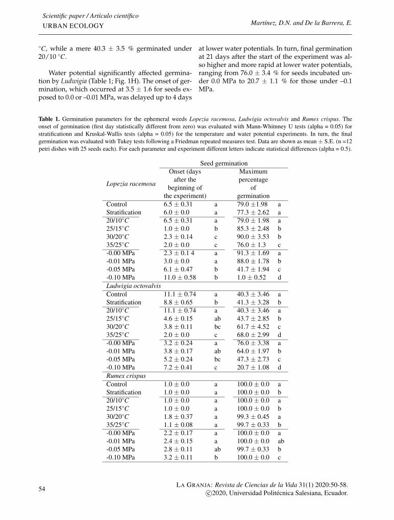
Scientific paper / Artículo científicoURBAN ECOLOGY Martínez, D.N. and De la Barrera, E.
◦C, while a mere 40.3 ± 3.5 % germinated under20/10 ◦C.
Water potential significantly affected germina-tion by Ludwigia (Table 1; Fig. 1H). The onset of ger-mination, which occurred at 3.5 ± 1.6 for seeds ex-posed to 0.0 or –0.01 MPa, was delayed up to 4 days
at lower water potentials. In turn, final germinationat 21 days after the start of the experiment was al-so higher and more rapid at lower water potentials,ranging from 76.0 ± 3.4 % for seeds incubated un-der 0.0 MPa to 20.7 ± 1.1 % for those under –0.1MPa.
Table 1. Germination parameters for the ephemeral weeds Lopezia racemosa, Ludwigia octovalvis and Rumex crispus. Theonset of germination (first day statistically different from zero) was evaluated with Mann-Whitnney U tests (alpha = 0.05) forstratificationn and Kruskal-Wallis tests (alpha = 0.05) for the temperature and water potential experiments. In turn, the finalgermination was evaluated with Tukey tests following a Friedman repeated measures test. Data are shown as mean ± S.E. (n =12petri dishes with 25 seeds each). For each parameter and experiment different letters indicate statistical differences (alpha = 0.5).
Seed germination
Lopezia racemosa
Onset (daysafter the
beginning ofthe experiment)
Maximumpercentage
ofgermination
ControlStratification
6.5 ± 0.31 a 79.0 ±1.98 a6.0 ± 0.0 a 77.3 ± 2.62 a
20/10◦C 6.5 ± 0.31 a 79.0 ± 1.98 a25/15◦C 1.0 ± 0.0 b 85.3 ± 2.48 b30/20◦C 2.3 ± 0.14 c 90.0 ± 3.53 b35/25◦C 2.0 ± 0.0 c 76.0 ± 1.3 c-0.00 MPa 2.3 ± 0.1 4 a 91.3 ± 1.69 a-0.01 MPa 3.0 ± 0.0 a 88.0 ± 1.78 b-0.05 MPa 6.1 ± 0.47 b 41.7 ± 1.94 c-0.10 MPa 11.0 ± 0.58 b 1.0 ± 0.52 dLudwigia octovalvisControlStratification
11.1 ± 0.74 a 40.3 ± 3.46 a8.8 ± 0.65 b 41.3 ± 3.28 b
20/10◦C 11.1 ± 0.74 a 40.3 ± 3.46 a25/15◦C 4.6 ± 0.15 ab 43.7 ± 2.85 b30/20◦C 3.8 ± 0.11 bc 61.7 ± 4.52 c35/25◦C 2.0 ± 0.0 c 68.0 ± 2.99 d-0.00 MPa 3.2 ± 0.24 a 76.0 ± 3.38 a-0.01 MPa 3.8 ± 0.17 ab 64.0 ± 1.97 b-0.05 MPa 5.2 ± 0.24 bc 47.3 ± 2.73 c-0.10 MPa 7.2 ± 0.41 c 20.7 ± 1.08 dRumex crispusControlStratification
1.0 ± 0.0 a 100.0 ± 0.0 a1.0 ± 0.0 a 100.0 ± 0.0 b
20/10◦C 1.0 ± 0.0 a 100.0 ± 0.0 a25/15◦C 1.0 ± 0.0 a 100.0 ± 0.0 b30/20◦C 1.8 ± 0.37 a 99.3 ± 0.45 a35/25◦C 1.1 ± 0.08 a 99.7 ± 0.33 b-0.00 MPa 2.2 ± 0.17 a 100.0 ± 0.0 a-0.01 MPa 2.4 ± 0.15 a 100.0 ± 0.0 ab-0.05 MPa 2.8 ± 0.11 ab 99.7 ± 0.33 b-0.10 MPa 3.2 ± 0.11 b 100.0 ± 0.0 c
54LA GRANJA: Revista de Ciencias de la Vida 31(1) 2020:50-58.
c©2020, Universidad Politécnica Salesiana, Ecuador.
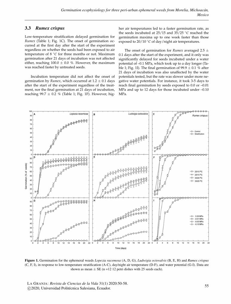
Germination ecophysiology for three peri-urban ephemeral weeds from Morelia, Michoacán,Mexico
3.3 Rumex crispus
Low-temperature stratification delayed germination forRumex (Table 1; Fig. 1C). The onset of germination oc-curred at the first day after the start of the experimentregardless on whether the seeds had been exposed to airtemperature of 8 ◦C for three months or not. Maximumgermination after 21 days of incubation was not affectedeither, reaching 100.0 ± 0.0 %. However, the maximumwas reached faster by untreated seeds.
Incubation temperature did not affect the onset ofgermination by Rumex, which occurred at 1.2 ± 0.1 daysafter the start of the experiment regardless of the treat-ment, nor the final germination at 21 days of incubation,reaching 99.7 ± 0.2 % (Table 1; Fig. 1F). However, hig-
her air temperatures led to a faster germination rate, asthe seeds incubated at 25/15 and 35/25 ◦C reached thegermination maxima up to one week faster than thoseexposed to 20/10 ◦C of day/night air temperatures.
The onset of germination for Rumex averaged 2.5 ±0.1 days after the start of the experiment, and it only wassignificantly delayed for seeds incubated under a waterpotential of –0.1 MPa, which took up to a day longer (Ta-ble 1; Fig. 1I). The final germination of 99.9 ± 0.1 % after21 days of incubation was also unaffected by the waterpotentials tested, but the rate was slower under more ne-gative water potentials. For instance, it took 3-5 days toreach final germination by seeds exposed to 0.0 or –0.01MPa and up to 12 days for those incubated under –0.10MPa.
Figure 1. Germination for the ephemeral weeds Lopezia racemosa (A, D, G), Ludwigia octovalvis (B, E, H) and Rumex crispus(C, F, I), in response to low-temperature stratification (A-C), day/night air temperature (D-F), and water potential (G-I). Data are
shown as mean ± SE (n =12 12 petri dishes with 25 seeds each).
LA GRANJA: Revista de Ciencias de la Vida 31(1) 2020:50-58.c©2020, Universidad Politécnica Salesiana, Ecuador. 55
Scientific paper / Artículo científicoURBAN ECOLOGY Martínez, D.N. and De la Barrera, E.
4 DiscussionThe identity of the species that persist in a communitysubjected to disturbance depends on which species wereoriginally present in the seed bank and how they respondto the new environmental conditions. Indeed, germina-tion for generalists and species with rapid germinationand preference for open sites are likely to be favored bydisturbance (Grime, 2006; Del-Val et al., 2015; Gorgone-Barbosa et al., 2016). In the present study, both the exoticweed Rumex and the generalist native Lopezia germinatedunder all the experimental conditions, although their ger-mination was delayed or diminished under the most ex-treme treatments. In contrast, germination for Ludwigia, aspecialist of high-humidity environments only exceeded50% under the most benign conditions. These differen-tial responses of co-occurring species can provide someinsight on potential trends of community compositionfollowing disturbance.
Species from regions with marked seasonality, i.e.,with distinct dry and wet seasons or with prolongedsub-freezing periods, often display an embryonic dor-mancy that can delay the onset of germination until theseason with environmental conditions, favoring seedlingestablishment (Donohue et al., 2010). For these plants,germination is often improved by exposing seeds to lowtemperatures during several weeks, by which germina-tion is avoided during the winter, when the prevailinglow air temperatures can be lethal for seedlings, even ifsome precipitation occurs.
This appears to be the case for Ludwigia whose strati-fied seeds germinated 2 days faster than untreated seeds,in agreement with previous studies with its congenericsL. alternifolia and L. decurrens (Baskin and Baskin, 1988).However, this was not the case for Lopezia not for Ru-mex, suggesting that they either lack primary dormancyor that it had been overcome during storage (Totterdelland Roberts, 1979; Chi, 2006; Finch-Savage and Leubner-Metzger, 2006).
Higher temperatures tended to hasten and increasefinal germination for the species considered in the pre-sent work. However, the highest temperature resultedin the lowest germination for Lopezia.A similar respon-se, where germination improves with temperature un-til an optimum, is reached followed by an inhibition ofgermination observed for the seeds of Ludwigia whichwere the most sensitive. In turn, the exotic weed Rumexreached maximum germination regardless of the incu-bation temperature, confirming observations for manyweeds, which are able to tolerate and even thrive underhigh temperatures, an advantageous trait for survivalin the extreme environmental conditions of naked soil(Dahlquist et al., 2007; Baskin and Baskin, 2014).
Germination tended to decrease as the incubation wa-ter potentials became more negative, especially at and be-low –0.05 MPa, similar to responses of other species suchas Campsis radicans (Chachalis and Reddy, 2000). In con-trast, germination for Rumex was maximal regardless ofthe water potential, in agreement with the germinationbehavior of its congeneric R. acetosella, which reaches 90% germination under –0.1 MPa (Fani et al., 2013). Consi-dering that substantial amounts of water are required tosustain cell elongation for plants following germination,especially for species that escape or avoid drought bycompleting their lifecycle during the rainy season, it maybe advantageous to restrict germination to times when anadequately high water potential signals that the rainy sea-son is well underway or that at least sufficient water isstored in the soil, allowing seedling development (De laBarrera et al., 2009). However, the water potentials assa-yed here correspond to a mere ca. 7 days after suspendingirrigation for a sandy loam, well above the permanentwilting point of –1.5 MPa, which indicates the sensitivityof germination (Young and Nobel, 1986; Nobel, 2009).
5 ConclusionsThe environmental requirements for germination of ep-hemeral species are often predictable to match those re-sulting from the typical weather of their growing season(De la Barrera and Nobel, 2003; Donohue et al., 2010; Bas-kin and Baskin, 2014). However, interspecific differences,however small, can determine the identities of the plantsthat grow in a community during a given year, contri-buting to the high interannual species variation that hasbeen observed for ephemeral and annual floras (Cousensand Mortimer, 2009; Chaideftou et al., 2012; Dekker, 2016;Gorgone-Barbosa et al., 2016). The differential responsesfound in the present study illustrate these interspecificidiosyncrasies and provide insight, for instance, into themechanisms that enable exotic species to become domi-nant or for native species to be displaced. The emergen-ce of novel environments resulting from human interven-tions poses a risk to the prevalence of native floras. Furt-her studies considering larger community subsets or evenwhole communities are required, including long-term ob-servations aimed at characterizing the rate at which nati-ve floras may be shifting in response to anthropic envi-ronmental changes.
AcknowledgementsThe authors thank the personnel of the IIES, UNAM Bota-nical Gardens, especially Nidia Pérez-Nasser, for the tech-nical support and access to the environmental chambers,as well as useful discussions with Drs. M. Camacho and
56LA GRANJA: Revista de Ciencias de la Vida 31(1) 2020:50-58.
c©2020, Universidad Politécnica Salesiana, Ecuador.
Germination ecophysiology for three peri-urban ephemeral weeds from Morelia, Michoacán,Mexico
E.A. Díaz. This work was funded by Dirección General deAsuntos del Personal Académico, Universidad NacionalAutónoma de México (PAPIIT IN221407 and IN211519),including an undergraduate research fellowship awardedto DNM.
ReferencesBaskin, C. C. and Baskin, J. M. (1988). Germination
ecophysiology of herbaceous plant species in a tempe-rate region. American Journal of Botany, 75(2):286–305.Online: https://bit.ly/2tHFEnA.
Baskin, C. C. and Baskin, J. M. (2014). Seeds: Ecology, Bio-geography, and Evolution of Dormancy and Germination.Elsevier. Online: https://bit.ly/2QWLM3A, 2 edition.
Calderón, R. G. and Rzedowski, J. (2004). Manual de Ma-lezas de la Región de Salvatierra, Guanajuato. Mexico.
Chachalis, D. and Reddy, K. N. (2000). Factors affec-ting campsis radicans seed germination and seedlingemergence. Weed Science, 48:212–216. Online: https://bit.ly/37RIMvV.
Chaideftou, E., Kallimanis, A. S., Bergmeier, E., and Di-mopolous, P. (2012). How does plant species com-position change from year to year? a case study fromthe herbaceous layer of a submediterranean oak wood-land. Community Ecology, 13:88–96. Online: https://bit.ly/2N4PR4j.
Challenger, A. and Dirzo, R. (2009). Factores de cambioy estado de la biodiversidad. Capital Natural de México,2:37–73. Online: https://bit.ly/35AgQLJ.
Chi, B. J. (2006). Efecto de tratamientos pregerminativosen la germinación de semillas de lopezia racemosa cav.b.s.
Cousens, R. and Mortimer, M. (2009). Dynamics of weedpopulations. Cambridge University Press, United King-dom, 1 edition.
Dahlquist, R. M., Prather, T. S., and Stapleton, J. J. (2007).Time and temperature requirements for weed seedthermal death. Weed Science, 55:619–625. Online: https://bit.ly/2QUn6sm.
De la Barrera, E. and Andrade, J. L. (2005). Challengesto plant megadiversity: How environmental physio-logy can help. New Phytologist, 167:5–8. Online: https://bit.ly/2N4TgQD.
De la Barrera, E. and Nobel, P. S. (2003). Physiological eco-logy of seed germination for the columnar cactus ste-nocereus queretaroensis. Journal of Arid Environments,53(3):297–306. Online: https://bit.ly/303kPz7.
De la Barrera, E., Pimienta-Barrios, E., and Schondube,J. E. (2009). Reproductive ecophysiology. Perspectives inBiophysical Plant Ecophysiology: A Tribute to Park S. No-bel, pages 301–335.
Debeaujon, I., Léon-Kloosterziel, K. M., and Koornneef,M. (2000). Influence of the testa on seed dormancy,germination, and longevity in arabidopsis. Plant Phy-siology, 122:403–414. Online: https://bit.ly/2QXoTNt.
Dekker, J. (2016). Evolutionary Ecology of Weeds. CreateS-pace Independent Publishing Platform, USA, 2 edition.
Del-Val, E., Balvanera, P., Castellarini, F., Espinosa-García,F. J., Murguía, M., and Pacheco, C. (2015). Identifyingareas of high invasion risk: a general model and an ap-plication to mexico. Revista mexicana de biodiversidad,86:208–216. Online: https://bit.ly/36Hyq1S.
Donohue, K., Rubio De Casas, R., Burhardt, L., Kovach,K., and Willis, C. G. (2010). Germination, postgermina-tion adaptation, and species ecological ranges. AnnualReview of Ecology, Evolution, and Systematics, 41:293–319.Online: https://bit.ly/2N8XQh0.
Dübbern de Souza, F. H. and Marcos-Filho, J. (2001).The seed coat as a modulator of seed-environment re-lationships in fabaceae. Brazilian Journal of Botany,24(4):365–375. Online: https://bit.ly/35C3q1R.
Fani, F. Y. S., Rezvani, M., Rashed, M. M. H., and Gha-nizadeh, H. (2013). Factors affecting seed germinationand seedling emergence of sheep sorrel (rumex aceto-sella). Romanian agricultural research, 30:373–380. Onli-ne: https://bit.ly/2tGdPMJ.
Fenner, M. and Thompson, K. (2005). The Ecology of Seeds.Cambridge University Press, U.K.
Finch-Savage, W. and Leubner-Metzger, G. (2006). Seeddormancy and the control of germination. New Phyto-logist, 171:501–523. Online: https://bit.ly/2N5ZY92.
Gorgone-Barbosa, E., Pivello, V. R., Baeza, M. J., and Fide-lis, A. (2016). Disturbance as a factor in breaking dor-mancy and enhancing invasiveness of african grassesin a neotropical savanna. Acta Botanica Brasilica, 30:131–137. Online: https://bit.ly/2N5V1gy.
Grime, J. P. (2006). Plant Strategies, Vegetation Processes, andEcosystem Properties. Wiley, U.S.A., 2 edition.
Larcher, W. (2001). Physiological Plant Ecology: Ecophysio-logy and stress physiology of functional groups. Springer,U.S.A., 4 edition.
Michel, B. E. and Radcliffe, D. (1985). A computer pro-gram relating solute potential to solution compositionfor five solutes. Agronomy Journal, 87:126–130.
Nobel, P. S. (2009). Physicochemical and Environmental PlantPhysiology. Academic Press, U.S.A., 4 edition.
LA GRANJA: Revista de Ciencias de la Vida 31(1) 2020:50-58.c©2020, Universidad Politécnica Salesiana, Ecuador. 57
Scientific paper / Artículo científicoURBAN ECOLOGY Martínez, D.N. and De la Barrera, E.
Rockström, J., Steffen, W., Noone, K., Persson, A., Cha-pin III, F. S., Lambin, E. F., Lenton, T. M., Scheffer, M.,Folke, C., and Schellnhuber, H. J. (2009). A safe opera-ting spece for humanity. Nature, 461:472–475. Online:https://bit.ly/2N8VDlx.
Rowarth, J. S., Hampton, J. G., and Hill, M. J. (2007). Newzealand native seed germination requirements: A re-view. New Zealand Journal of Botany, 45:485–501. Online:https://bit.ly/35G8NgB.
Sala, O. E., Chapin III, F. S., Armesto, J. J., Berlow, E.,Bloomfield, J., Dirzo, R., Huber-Sanwald, E., Huennke,L. F., Jackson, R. B., and Kinzig, A. (2000). Global bio-diversity scenarios for the year 2100. Science, 287:1770–1774. Online: https://bit.ly/2QydZi1.
Totterdell, S. and Roberts, E. H. (1979). Effects of lowtemperatures on the loss of innate dormancy and thedevelopment of induced dormancy in seeds of rumexobtusifolius l. and rumex crispus l. Plant Cell and Envi-ronment, 2:131–137. Online: https://bit.ly/35z1oQ6.
Vibrans, H. and Tenorio-Lezama, P. (2012). Malezas deméxico. comisión nacional para el conocimiento y usode la biodiversidad.
Young, D. R. and Nobel, P. S. (1986). Predictions of soil-water potentials in the north-western sonoran desert.Journal of Ecology, 74:143–154.
58LA GRANJA: Revista de Ciencias de la Vida 31(1) 2020:50-58.
c©2020, Universidad Politécnica Salesiana, Ecuador.
Scientific paper/ Artículo científico
POLLUTANT ANALYTICpISSN:1390-3799; eISSN:1390-8596
http://doi.org/10.17163/lgr.n31.2020.04
VERIFICATION OF THE ATOMIC ABSORPTION SPECTROSCOPY
WITH GRAPHITE FURNACE ANALYTICAL METHOD FOR THE
QUANTIFICATION OF CADMIUM IN COCOA ALMONDS
(Theobroma cacao)
VERIFICACIÓN DEL MÉTODO ANALÍTICO DE ESPECTROSCOPÍA DE ABSORCIÓN
ATÓMICA CON HORNO DE GRAFITO PARA LA CUANTIFICACIÓN DE CADMIO
EN ALMENDRA DE CACAO (Theobroma cacao)
Salomé Araujo-Abad*1 , Wilson Tapia2 and Adrián Villamarín-Ortiz3
1 Biotechnology Center. Nacional University of Loja, 110111, Loja, Ecuador.2 Department of Chemical. University of Américas, 170503, Quito, Ecuador.3 Department of Health Sciences. Private Technical University of Loja, 1101608, Loja, Ecuador.
*Corresponding author: [email protected]
Article received on August 19th, 2019. Accepted, after review, on January 16th, 2020. Published on March 1st, 2020.
Resumen
El método de espectroscopía de absorción atómica (AA) de llama para la determinación de cadmio (Cd) en almendrade cacao (Theobroma cacao) utilizado por Agrocalidad es tóxico para el ser humano y el ambiente; por ello, se pretendeutilizar el método de espectroscopia de absorción atómica con horno de grafito (GFAAS) por ser más confiable yseguro. Así, se realizó la verificación de cuatro parámetros de desempeño del método GFAAS para cuantificar Cd enalmendra de cacao utilizando material de referencia certificado (MRC) y muestras provenientes de cuatro fincas (A,B, C, D) ubicadas en la zona cacaotera de Ecuador, cantón Flavio Alfaro, provincia de Manabí. Se realizó una pruebainter-laboratorios y finalmente se elaboró el protocolo (PEE/B/14). Sobre el MRC (Cód. 07206B y 07167A) se verificó:linealidad, precisión, veracidad e incertidumbre de acuerdo con la Guía Eurachem de Eurolab España et al. (2016), ycon el estándar IRAM 35050 (2001) se encontró linealidad entre 0 y 8 ppb con R2=0.9988; desviación estándar de 0.0005y 0.0022 respectivamente; sesgo en 0.007 y porcentaje de recuperación de 109.75; la incertidumbre estándar de 0.00013y 0.00082. El contenido de Cd en las muestras de la finca A con 0.54 ppm, las Fincas B-D con 0.26 ppm y 0.15 ppm enla finca C. En la prueba inter-laboratorios se estableció la misma concentración de cadmio para la muestra C3 y, deacuerdo con lo estipulado por la Unión Europea, el cacao de las cuatro fincas podría ser exportado sin restricciones.Palabras clave: Cadmio, cacao, verificación, análisis, método.
59LA GRANJA: Revista de Ciencias de la Vida 31(1) 2020:59-73.c©2020, Universidad Politécnica Salesiana, Ecuador.
Scientific paper / Artículo científicoPOLLUTANT ANALYTIC Araujo-Abad, L.S., Tapia, W. and Villamarín-Ortiz, A.
Abstract
The flame atomic absorption (AA) spectroscopy method for the determination of cadmium (Cd) in cocoa almond(Theobroma cacao) used by Agrocalidad is toxic to humans and the environment, reason for which the atomic absor-ption spectroscopy method with graphite furnace (GFAAS) was used, because it is more reliable and safer. Thus, fourperformance parameters of GFAAS method were used to quantify Cd in cocoa almond, by using certified referencematerial (MRC) and samples from four farms (A,B,C,D) located in the most important cocoa area of Ecuador, Fla-vio Alfaro city, province of Manabi. An interlaboratory test was performed and finally a protocol (PEE/B/14) wasdeveloped. Using the MRC (Code 07806B and 07167) was verified: linearity, precision, veracity and uncertainty inaccordance with international standards, Eurachem Guide of Eurolab España et al. (2016), and with the standard IRAM35050 (2001) were found linearity between 0 and 8 ppb with R2 = 0.9988; standard deviation 0.0005 and 0.0022, res-pectively; slant was 0.007 and the recovery percentage was 109.75; standard uncertainty was 0.00013 and 0.00082. Thecontent of Cd in samples from farm A was 0.54 ppm, B and D farms 0.26 ppm and 0.15 ppm in farm C. In the interla-boratory test, the same concentration of Cd was established for simple C3 and, in accordance with the stipulated bythe European Union, cocoa from the four farms could be exported without restrictions.Keywords: Cadmium, cocoa, verification, analysis, method.
Suggested citation: Araujo-Abad, L.S., Tapia, W. and Villamarín-Ortiz, A. (2020). Verification of the atomicabsorption spectroscopy with graphite furnace analytical method for the quantificationof cadmium in cocoa almonds (Theobroma cacao). La Granja: Revista de Ciencias de laVida. Vol. 31(1):59-73. http://doi.org/10.17163/lgr.n31.2020.04.
Orcid IDs:Lourdes Salomé Araujo Abad: https://orcid.org/0000-0001-7387-0363Wilson Fabián Tapia Hernández: https://orcid.org/0000-0002-7010-6324Marcos Adrián Villamarín Ortiz: https://orcid.org/0000-0003-2768-9162
60LA GRANJA: Revista de Ciencias de la Vida 31(1) 2020:59-73.
c©2020, Universidad Politécnica Salesiana, Ecuador.
Verification of the atomic absorption spectroscopy with graphite furnace analytical method for thequantification of cadmium in cocoa almonds (Theobroma cacao)
1 Introduction
Cocoa beans are the seeds of the Theobroma cacao tree(native to the Amazon Region of South America),which are widely consumed worldwide (Almeidaand Valle, 2007). It is an important neotropical, pe-rennial crop growing at 20◦ north and 20◦ southof the equatorial line (Shavez Beg et al., 2017). Itis grown at a height of less than 400 m.a.s.l; theoptimal temperature ranges from 22 ◦C to 30 ◦C, de-pending on the variety (Damatta et al., 2018), andrain should be at least 1500 to 2500 mm of waterper year. The almonds are brown and are coveredon the outside by a sweet white mucilage that isedible (Waizel-Haiat et al., 2012); grains are proces-sed to obtain chocolate liqueur, cocoa powder andcocoa butter, which are the main ingredients of cho-colate and a wide range of products such as cocoadrinks, ice cream, bakery products that distributea distinctive flavor to derivatives (Dasgupta andKlein, 2014). Cocoa beans are the raw material forthe multibillion-dollar industry that produces cho-colate and confectionery products, the economicimportance of the chocolate industry in the worldmarket has recently been revised (Squicciarini andSwinnen, 2016) rising 13% from 2010 to US$101billion in 2015, with Switzerland as the highest con-sumer rate (Wickramasuriya and Dunwell, 2018).
Ecuador, because of its geographical conditionsand its richness in biological resources, is the quin-tessential producer of fine-scented cocoa (63% ofworld production) from the national variety, whoseflavor has been recognized for centuries on the in-ternational market. This type of grain is used in allrefined chocolates. Of the total Ecuadorian export,75% is estimated to be fine-scented cocoa whilethe remaining 25% belong to other varieties suchas CCN51. Ecuador ranks as the most competitivecountry in Latin America in this field, followed byVenezuela, Panama and Mexico, which are coun-tries that have gradually increased their share ofthe global market (Anecacao, 2019).
Various attributes of grain quality, both physi-cal and chemical, are required by manufacturers,cocoa buyers and control bodies to encourage thecocoa community towards better quality produc-tion (CAOBISCO/ECA/FCC, 2015). These qua-lity characteristics include taste, purity and health(e.g. bacteria-free, infestation, allergens, mycoto-
xins, heavy metals and pesticide residues), physicalcharacteristics (e.g. consistency, yield of grain ediblematerial, size and uniformity, shell content, fat con-tent and moisture content) and the characteristics ofcocoa butter (e.g. free of fatty acid) (Dasgupta andKlein, 2014). Some of the attributes of grain quality,such as the total fat content, acidity, total phenols,organic acids, heavy metals, amino acids, caffeine,theobromine, pH, sugars, macro content and mi-cronutrients, have been considered in the proposalCocoa Quality Index (CQI) for some types of grain(Araujo et al., 2014).
Heavy metals are defined as elements with adensity of more than 5 g/cm3 (Navarro-Aviñó et al.,2007). Copper, iron, magnesium and zinc in lowconcentrations are essential for biochemical andphysiological processes in plants, while arsenic,cadmium and lead do not have a known role inthem (Ali et al., 2013). The accumulation of heavymetals in plants is affected by several factors such aspH, organic matter content and soil texture, plantgenotype and heavy metal content in the growthmedium. Latin America has the highest levels ofheavy metals in cocoa beans, especially cadmiumand lead (Bertoldi et al., 2016), compared to otherproducers in the world. The presence of heavy me-tals in cocoa beans represents a threat to cocoa pro-ducers, as a high heavy metal content could affectthe export of the grains.
Chocolate has been attributed to the achieve-ment of optimal human health and development,due to its high content of flavonoids that are crucialto reducing the risk or in turn delaying the develop-ment of cardiovascular disease, cancer and othersrelated to age (Cooper et al., 2008).
In 2014, the European Union announced, th-rough the Regulation (EU) No. 488/2014, plans toimplement regulations on chocolate and cocoa pro-ducts containing excessive levels of cadmium (Cd),which entered into force on January 1, 2019 (Com-mission Regulation EU, 2014). Non-compliancewith regulations would have significant economicand social consequences for cocoa-producing coun-tries, such as Ecuador, from the date of entry intoforce of that regulation. The Cd has received atten-tion in the last decade due to its importance in foodquality/safety, and in human health, since the con-sumption of foods high in this heavy metal could
LA GRANJA: Revista de Ciencias de la Vida 31(1) 2020:59-73.c©2020, Universidad Politécnica Salesiana, Ecuador. 61
Scientific paper / Artículo científicoPOLLUTANT ANALYTIC Araujo-Abad, L.S., Tapia, W. and Villamarín-Ortiz, A.
lead to renal tubular dysfunction, the formation ofkidney stones, the alteration of calcium metabolismand skeletal, endocrine, reproductive and respira-tory defects (Järup and Akesson, 2009).
Analytical techniques for the determination ofCd are based on the use of reagents that act onthe grain digestion and that are highly hazardous.One of the reagents of frequent use is Agua Regia(HCl : HNO3), which is subjected to heat resultingin irritating and corrosive vapors; the protocol usedcorresponds to an adaptation of the official AOACmethod: 999.11 (AOAC, 2005).
As a more effective analytical method and lesstoxic to humans and the environment, this paper ve-rified the performance of the graphite furnace ato-mic absorption spectroscopy (GFAAS) method inthe determination of Cd in cocoa almond (Theobro-ma cacao), by determining linearity, accuracy and ve-racity (Eurolab España et al., 2016) and uncertainty(IRAM 35050, 2001) on certified reference material,and the analytical protocol for the determination ofthe concentration of Cd in cocoa almond sampleswas validated; in addition, an inter-lab comparisontest was performed.
2 Materials and methods
First Phase: the verification of the analytical met-hod was performed by evaluating the linearity, ac-curacy, veracity and uncertainty parameters, basedon certified material MRC 07206B and 07167A.
Second phase: cocoa samples (ears) were co-llected by designated AGROCALIDAD personnel,on four farms in the country’s cocoa area: FlavioAlfaro-Manabí, Ecuador, referred to as A, B, C,D. Subsequently, the corresponding samples wereanalyzed in the Nutritional Science and Microbio-logy Laboratory to determine their Cd content, afterhaving verified the calibration status of the instru-ments and volumetric materials to be used.
Third phase: the PEE/B/14 protocol for the de-termination of Cd in cocoa almond by GFAAS wasdeveloped, containing the sample preparation pro-cess (cocoa ear) from their reception, drying, homo-genization, microwave digestion and subsequentreading in the graphite oven spectrometer.
2.1 Verification of the analytical methodThe verification of the analytical method was doneas reference to the Eurolab Spain Eurachem GuideEurolab España et al. (2016), and to the IRAM 35050(2001), following the PEE/B/14 protocol.
2.1.1 Linearity
A curve with 10 concentrations was developed fromthe Cd standard of 20 ppb, the concentrations usedwere 0 to 18 ppb. In the curve, the theoretical con-centration was expressed in µg/L on the axis of the“x”, and on the axis of the “y” the calculated con-centration was expressed in µg/L; from the resultingcurve, the linear range was chosen and a new curvewas drawn. In this linear range, a white, six diffe-rent dilutions of the standard of 20 ppb and finallythe MRC 07206B and 07167A were evaluated by tri-plicate.
2.1.2 Accuracy
Fifteen readings were made for each MRC 07206Band 07167A and the standard deviation (s) of eachmaterial was calculated, using the following formu-la:
s =
√1
n−1
n
∑k=1
(x− x)2 (1)
Standard deviation (s)Where:n = number of total measurements of the referencematerial.x = average of the readings.x = each measurement performed.
2.1.3 Veracity
Ten readings for MRC 07206B, ten readings for threedigested targets and ten readings for three whitesadded with 2, 3 and 4 ppb of Cd were done; in ad-dition; ten readings were also performed on threesamples analyzed. In the first instance, by the met-hod normally used by the laboratory, using acid di-gestion with Agua Regia (HCl : HNO3), followed bya reading using flame atomic absorption spectros-copy (AA) and, secondly, by the verified GFAASmethod and the analysis protocol proposed in thisresearch.
62LA GRANJA: Revista de Ciencias de la Vida 31(1) 2020:59-73.
c©2020, Universidad Politécnica Salesiana, Ecuador.
Verification of the atomic absorption spectroscopy with graphite furnace analytical method for thequantification of cadmium in cocoa almonds (Theobroma cacao)
The data obtained for the MRC 07206B procee-ded to perform the calculations with the followingformulas provided by Eurolab España et al. (2016):
b = x− xre f (2)
Biasb(%) =
x− xre f
xre f×100 (3)
Bias in Percentage
R(%) =x
xre f×100 (4)
Relative RecoveryWhere:x = mean of the readings of the MRC 07206B.xre f = theoretical value that the certificate grants tothe reference material.The calculated values obtained a measure of bias ta-king into account the effects of the laboratory com-pared to the bias method data.For the analysis of the data obtained from the mea-surements of digested and added whites, the follo-wing formula Eurolab España et al. (2016) was used:
R′ (%) =x′− x
xaddition×100 (5)
Relative retrieval of additionsWhere:x′ = average value of the added whites.x = is the average value of the digested whites.xaddition = concentration value added.Finally, with the data obtained from the reading ofsamples by the method normally used in the labora-tory, the verified GFAAS method and the proposedanalysis protocol, the calculations were performedbased on the following equations Eurolab Españaet al. (2016):
b = x− xre f (6)
Bias
b(%) =x− xre f
xre f×100 (7)
Bias in Percentage
R(%) =x
xre f×100 (8)
Relative RecoveryWhere:
x = means of the sample readings by the old met-hod.xre f = average sample readings by the proposednew method.The measurement of bias was obtained accordingto the verified GFAAS method and the proposedanalysis protocol, in order to demonstrate its effec-tiveness and replace the method normally used byAGROCALIDAD.
2.1.4 Uncertainty
10 readings of the concentration of the reference ma-terial were performed and the uncertainty valueswere calculated with the following formulas (IRAM35050, 2001):
I =1n
n
∑k=1
Ik (9)
Average (I) of readingsWhere:n = number of measurements of the reference mate-rial.Ik = each measurement of the reference material
S (Ik) =
√1
n−1
n
∑k=1
(Ik− I
)2 (10)
Standard deviation (Ik)Where:n = number of total measurements of the referencematerial.I = the average of the readings.Ik = each measurement performed.
S(I)=
S (Ik)√n
(11)
Standard uncertainty S (I)Where:S (Ik) = the standard deviationn = number of total measurements of the referencematerial.
2.2 Determination of cadmium in cocoa al-mond
With samples obtained from Farms A, B, C and D,the elaborate protocol (Procedure PEE/B/14) wasdone for the determination of Cd in cocoa almonds,detailing:
LA GRANJA: Revista de Ciencias de la Vida 31(1) 2020:59-73.c©2020, Universidad Politécnica Salesiana, Ecuador. 63
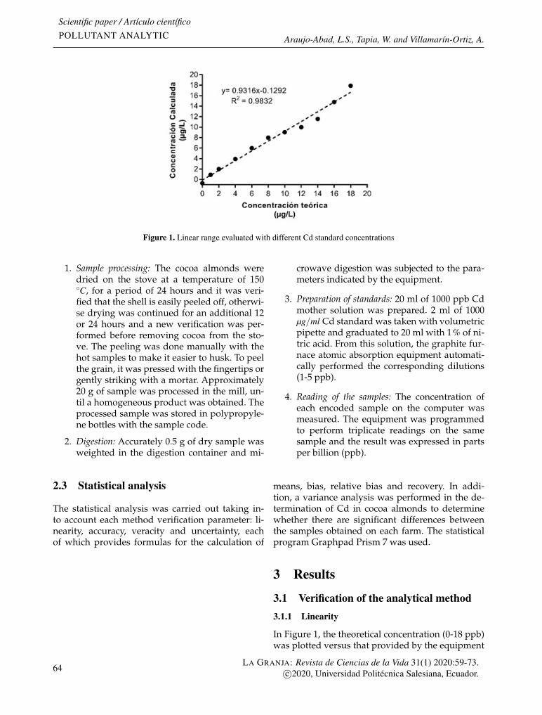
Scientific paper / Artículo científicoPOLLUTANT ANALYTIC Araujo-Abad, L.S., Tapia, W. and Villamarín-Ortiz, A.
Figure 1. Linear range evaluated with different Cd standard concentrations
1. Sample processing: The cocoa almonds weredried on the stove at a temperature of 150◦C, for a period of 24 hours and it was veri-fied that the shell is easily peeled off, otherwi-se drying was continued for an additional 12or 24 hours and a new verification was per-formed before removing cocoa from the sto-ve. The peeling was done manually with thehot samples to make it easier to husk. To peelthe grain, it was pressed with the fingertips orgently striking with a mortar. Approximately20 g of sample was processed in the mill, un-til a homogeneous product was obtained. Theprocessed sample was stored in polypropyle-ne bottles with the sample code.
2. Digestion: Accurately 0.5 g of dry sample wasweighted in the digestion container and mi-
crowave digestion was subjected to the para-meters indicated by the equipment.
3. Preparation of standards: 20 ml of 1000 ppb Cdmother solution was prepared. 2 ml of 1000µg/ml Cd standard was taken with volumetricpipette and graduated to 20 ml with 1% of ni-tric acid. From this solution, the graphite fur-nace atomic absorption equipment automati-cally performed the corresponding dilutions(1-5 ppb).
4. Reading of the samples: The concentration ofeach encoded sample on the computer wasmeasured. The equipment was programmedto perform triplicate readings on the samesample and the result was expressed in partsper billion (ppb).
2.3 Statistical analysis
The statistical analysis was carried out taking in-to account each method verification parameter: li-nearity, accuracy, veracity and uncertainty, eachof which provides formulas for the calculation of
means, bias, relative bias and recovery. In addi-tion, a variance analysis was performed in the de-termination of Cd in cocoa almonds to determinewhether there are significant differences betweenthe samples obtained on each farm. The statisticalprogram Graphpad Prism 7 was used.
3 Results
3.1 Verification of the analytical method3.1.1 Linearity
In Figure 1, the theoretical concentration (0-18 ppb)was plotted versus that provided by the equipment
64LA GRANJA: Revista de Ciencias de la Vida 31(1) 2020:59-73.
c©2020, Universidad Politécnica Salesiana, Ecuador.
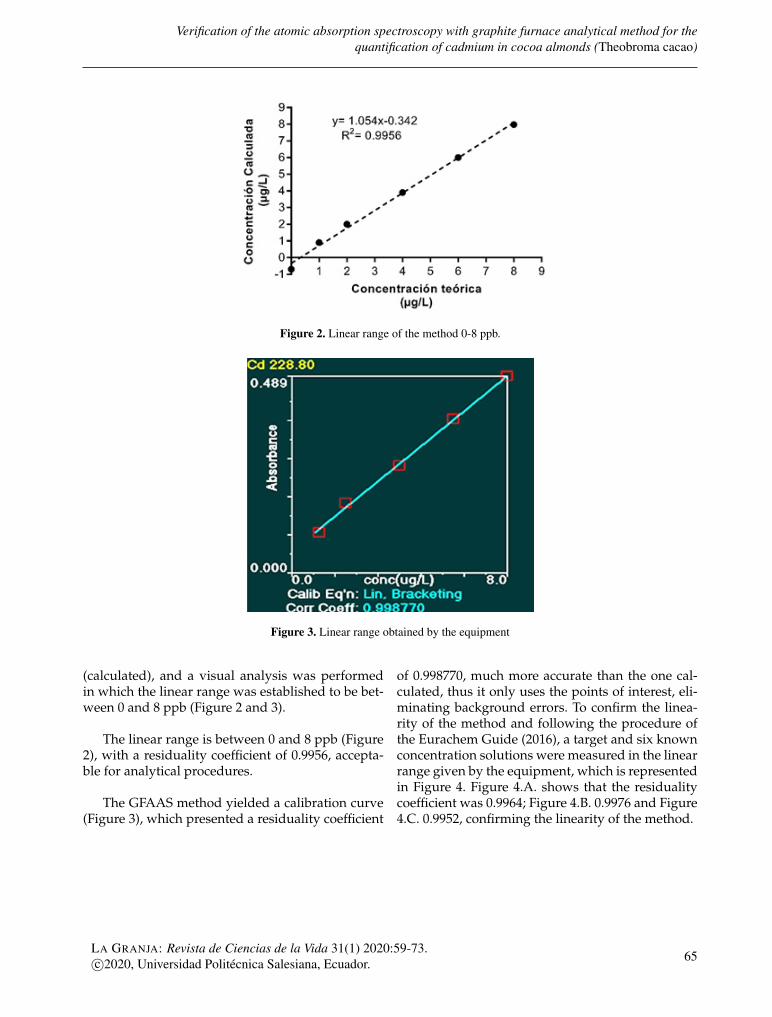
Verification of the atomic absorption spectroscopy with graphite furnace analytical method for thequantification of cadmium in cocoa almonds (Theobroma cacao)
Figure 2. Linear range of the method 0-8 ppb.
Figure 3. Linear range obtained by the equipment
(calculated), and a visual analysis was performedin which the linear range was established to be bet-ween 0 and 8 ppb (Figure 2 and 3).
The linear range is between 0 and 8 ppb (Figure2), with a residuality coefficient of 0.9956, accepta-ble for analytical procedures.
The GFAAS method yielded a calibration curve(Figure 3), which presented a residuality coefficient
of 0.998770, much more accurate than the one cal-culated, thus it only uses the points of interest, eli-minating background errors. To confirm the linea-rity of the method and following the procedure ofthe Eurachem Guide (2016), a target and six knownconcentration solutions were measured in the linearrange given by the equipment, which is representedin Figure 4. Figure 4.A. shows that the residualitycoefficient was 0.9964; Figure 4.B. 0.9976 and Figure4.C. 0.9952, confirming the linearity of the method.
LA GRANJA: Revista de Ciencias de la Vida 31(1) 2020:59-73.c©2020, Universidad Politécnica Salesiana, Ecuador. 65
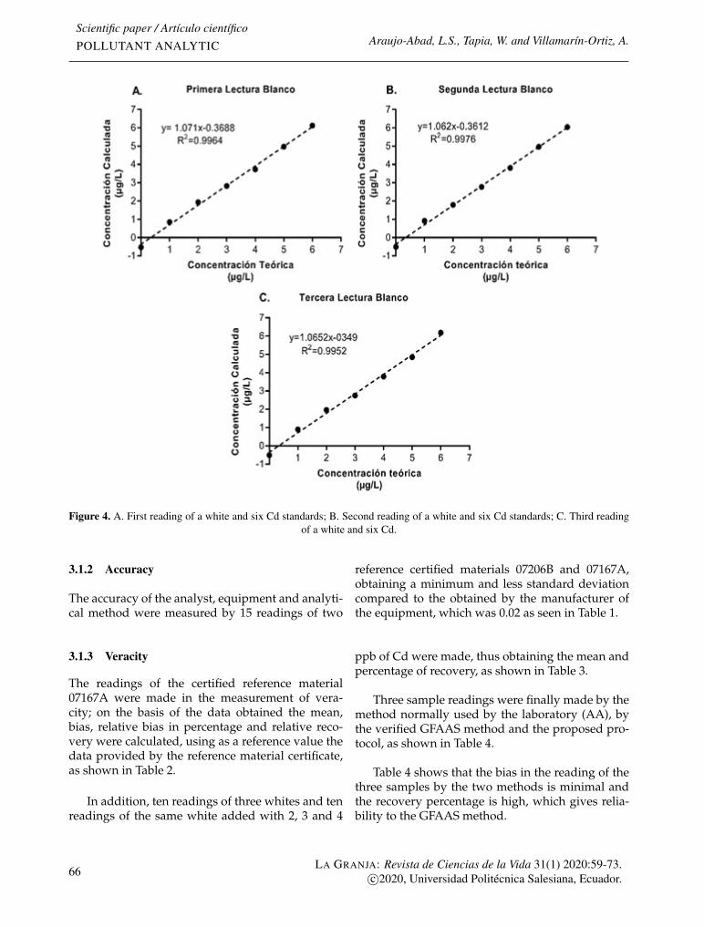
Scientific paper / Artículo científicoPOLLUTANT ANALYTIC Araujo-Abad, L.S., Tapia, W. and Villamarín-Ortiz, A.
Figure 4. A. First reading of a white and six Cd standards; B. Second reading of a white and six Cd standards; C. Third readingof a white and six Cd.
3.1.2 Accuracy
The accuracy of the analyst, equipment and analyti-cal method were measured by 15 readings of two
reference certified materials 07206B and 07167A,obtaining a minimum and less standard deviationcompared to the obtained by the manufacturer ofthe equipment, which was 0.02 as seen in Table 1.
3.1.3 Veracity
The readings of the certified reference material07167A were made in the measurement of vera-city; on the basis of the data obtained the mean,bias, relative bias in percentage and relative reco-very were calculated, using as a reference value thedata provided by the reference material certificate,as shown in Table 2.
In addition, ten readings of three whites and tenreadings of the same white added with 2, 3 and 4
ppb of Cd were made, thus obtaining the mean andpercentage of recovery, as shown in Table 3.
Three sample readings were finally made by themethod normally used by the laboratory (AA), bythe verified GFAAS method and the proposed pro-tocol, as shown in Table 4.
Table 4 shows that the bias in the reading of thethree samples by the two methods is minimal andthe recovery percentage is high, which gives relia-bility to the GFAAS method.
66LA GRANJA: Revista de Ciencias de la Vida 31(1) 2020:59-73.
c©2020, Universidad Politécnica Salesiana, Ecuador.
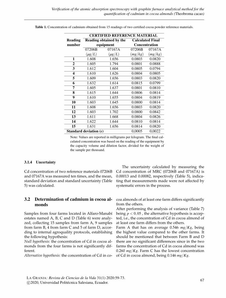
Verification of the atomic absorption spectroscopy with graphite furnace analytical method for thequantification of cadmium in cocoa almonds (Theobroma cacao)
Table 1. Concentration of cadmium obtained from 15 readings of two certified cocoa powder reference materials.
Readingnumber
CERTIFIED REFERENCE MATERIALReading obtained by the
equipmentCalculated FinalConcentration
07206B(µg/L)
07167A(µg/L)
07206B(mg/kg)
07167A(mg/kg)
1 1.608 1.656 0.0803 0.08202 1.605 1.794 0.0801 0.08883 1.612 1.604 0.0805 0.07944 1.610 1.626 0.0804 0.08055 1.609 1.656 0.0803 0.08206 1.632 1.614 0.0815 0.07997 1.605 1.637 0.0801 0.08108 1.615 1.644 0.0806 0.08149 1.610 1.655 0.0804 0.0819
10 1.603 1.645 0.0800 0.081411 1.608 1.656 0.0803 0.082012 1.603 1.702 0.0800 0.084213 1.611 1.668 0.0804 0.082614 1.622 1.644 0.0810 0.081415 1.631 1.656 0.0814 0.0820
Standard deviation (s) 0,0005 0,0022Note: Values are reported in milligrams per kilogram. The final cal-culated concentration was based on the reading of the equipment bythe capacity volume and dilution factor, divided for the weight ofthe sample per thousand.
3.1.4 Uncertainty
Cd concentration of two reference materials 07206Band 07167A was measured ten times, and the mean,standard deviation and standard uncertainty (Table5) was calculated.
The uncertainty calculated by measuring theCd concentration of MRC (07206B and 07167A) is0.00013 and 0.00082, respectively (Table 5), indica-ting that measurements made were not affected bysystematic errors in the process.
3.2 Determination of cadmium in cocoa al-monds
Samples from four farms located in Alfaro-Manabíestates named A, B, C and D (Table 6) were analy-zed, collecting 15 samples from farm A, 9 samplesfrom farm B, 4 from farm C and 5 of farm D, accor-ding to internal agroquality protocols, establishingthe following hypothesis:Null hypothesis: the concentration of Cd in cocoa al-monds from the four farms is not significantly dif-ferent.Alternative hypothesis: the concentration of Cd in co-
coa almonds of at least one farm differs significantlyfrom the others.After performing the analysis of variance (Table 7)being p < 0,05 , the alternative hypothesis is accep-ted, i.e., the concentration of Cd in cocoa almond ofat least one farm differs from the others.Farm A that has on average 0.546 mg/Kg, beingthe highest value compared to the other farms. Itshould be mentioned that between Farm B and Dthere are no significant differences since in the twofarms the concentration of Cd in cocoa almond was0.260 mg/Kg. Farm C has the lowest concentrationof Cd in cocoa almond, being 0.146 mg/Kg.
LA GRANJA: Revista de Ciencias de la Vida 31(1) 2020:59-73.c©2020, Universidad Politécnica Salesiana, Ecuador. 67

Scientific paper / Artículo científicoPOLLUTANT ANALYTIC Araujo-Abad, L.S., Tapia, W. and Villamarín-Ortiz, A.
Table 2. Cadmium concentration obtained from 10 readings of the certified cocoa powder reference material
Reading Reference Material07167A(µg/L)
07167A(mg/Kg)
1 1.614 0.0802 1.637 0.0813 1.655 0.0824 1.655 0.0825 1.645 0.0816 1.656 0.0827 1.612 0.0808 1.668 0.0839 1.623 0.080
10 1.644 0.081Media 0.081Reference Value 0.074Bias 0.007Relative bias in percentage 9.75Relative recovery 109.75
Note: The values reported by the equipmentare in µg/L. The calculated final concentra-tion (mg/kg), is based on the reading of theequipment by the volume of capacity and di-lution factor, divided for the weight of thesample per thousand.
Table 3. Reading of three whites and whites added with 2, 3 and 4 ppb of cadmium
No. ReadingWHITES(µg/L)
ADDED WHITES(µg/L)
B2V B3V B4V BA2V BA3V BA4V1 −0.5278 −0.7799 −0.4077 2.098 3.115 3.7802 −0.5017 −0.7791 −0.3903 2.084 3.185 3.8983 −0.5106 −0.7442 −0.4038 1.962 3.247 4.1654 −0.5613 −0.7247 −0.4415 1.939 3.025 4.0365 −0.4176 −0.7153 −0.4453 1.962 3.004 4.0546 −0.5200 −0.7298 −0.4692 1.963 3.027 4.0767 −0.6586 −0.7062 −0.4406 1.876 3.057 4.1858 −0.5363 −0.7423 −0.4894 1.878 2.947 4.1969 −0.5810 −0.7847 −0.4962 1.890 3.030 4.22310 −0.5134 −0.7700 −0.4194 1.800 3.137 4.263
Media −0.53283 −0.74762 −0.44034 1.945 3.077 4.088Recovery (%) 123.902 127.501 113.199
Note: The units are reported in µg/L. in the B2V code means: White number two veracity.BA2V stands for, BA2: White added with 2 ppb of Cd; V: veracity.
3.3 Inter-laboratory test
The sample with code C3 was sent to UBA Labora-tories located in the city of Guayaquil, Ecuador. The
reported result was 0.11 ppm of Cd, which coinci-des with the result obtained in Laboratory of Nuri-tional Science and Microbiology of Agroquality.
68LA GRANJA: Revista de Ciencias de la Vida 31(1) 2020:59-73.
c©2020, Universidad Politécnica Salesiana, Ecuador.
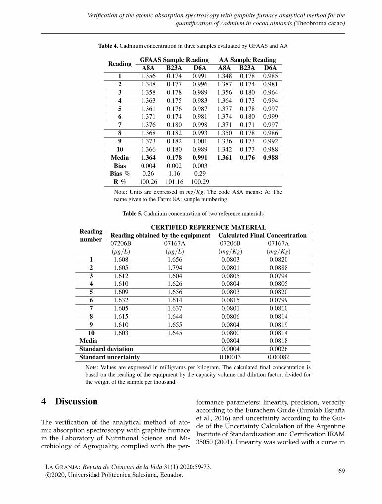
Verification of the atomic absorption spectroscopy with graphite furnace analytical method for thequantification of cadmium in cocoa almonds (Theobroma cacao)
Table 4. Cadmium concentration in three samples evaluated by GFAAS and AA
Reading GFAAS Sample Reading AA Sample ReadingA8A B23A D6A A8A B23A D6A
1 1.356 0.174 0.991 1.348 0.178 0.9852 1.348 0.177 0.996 1.387 0.174 0.9813 1.358 0.178 0.989 1.356 0.180 0.9644 1.363 0.175 0.983 1.364 0.173 0.9945 1.361 0.176 0.987 1.377 0.178 0.9976 1.371 0.174 0.981 1.374 0.180 0.9997 1.376 0.180 0.998 1.371 0.171 0.9978 1.368 0.182 0.993 1.350 0.178 0.9869 1.373 0.182 1.001 1.336 0.173 0.99210 1.366 0.180 0.989 1.342 0.173 0.988
Media 1.364 0.178 0.991 1.361 0.176 0.988Bias 0.004 0.002 0.003
Bias % 0.26 1.16 0.29R % 100.26 101.16 100.29Note: Units are expressed in mg/Kg. The code A8A means: A: Thename given to the Farm; 8A: sample numbering.
Table 5. Cadmium concentration of two reference materials
Readingnumber
CERTIFIED REFERENCE MATERIALReading obtained by the equipment Calculated Final Concentration07206B(µg/L)
07167A(µg/L)
07206B(mg/Kg)
07167A(mg/Kg)
1 1.608 1.656 0.0803 0.08202 1.605 1.794 0.0801 0.08883 1.612 1.604 0.0805 0.07944 1.610 1.626 0.0804 0.08055 1.609 1.656 0.0803 0.08206 1.632 1.614 0.0815 0.07997 1.605 1.637 0.0801 0.08108 1.615 1.644 0.0806 0.08149 1.610 1.655 0.0804 0.0819
10 1.603 1.645 0.0800 0.0814Media 0.0804 0.0818Standard deviation 0.0004 0.0026Standard uncertainty 0.00013 0.00082
Note: Values are expressed in milligrams per kilogram. The calculated final concentration isbased on the reading of the equipment by the capacity volume and dilution factor, divided forthe weight of the sample per thousand.
4 Discussion
The verification of the analytical method of ato-mic absorption spectroscopy with graphite furnacein the Laboratory of Nutritional Science and Mi-crobiology of Agroquality, complied with the per-
formance parameters: linearity, precision, veracityaccording to the Eurachem Guide (Eurolab Españaet al., 2016) and uncertainty according to the Gui-de of the Uncertainty Calculation of the ArgentineInstitute of Standardization and Certification IRAM35050 (2001). Linearity was worked with a curve in
LA GRANJA: Revista de Ciencias de la Vida 31(1) 2020:59-73.c©2020, Universidad Politécnica Salesiana, Ecuador. 69
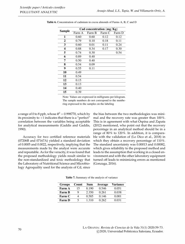
Scientific paper / Artículo científicoPOLLUTANT ANALYTIC Araujo-Abad, L.S., Tapia, W. and Villamarín-Ortiz, A.
Table 6. Concentration of cadmium in cocoa almonds of Farms A, B, C and D
Sample Cad concentration (mg/Kg)Farm A Farm B Farm C Farm D
1 0.60 0.60 0.12 0.122 0.79 0.10 0.18 0.113 0.60 0.01 0.11 0.244 0.88 0.34 0.17 0.305 0.74 0.30 0.546 0.89 0.407 0.50 0.408 0.54 0.099 0.55 0.1110 0.4911 0.5412 0.1513 0.1314 0.4015 0.39Note: Values are expressed in milligrams per kilogram.The sample numbers do not correspond to the numbe-ring expressed to the samples on the labeling
a range of 0 to 8 ppb, whose R2 = 0.998770, which byits proximity to +1 indicates that there is a “perfect”correlation between the variables being acceptablefor analytical measurements (Gaddis and Gaddis,1990).
Accuracy for two certified reference materials(07206B and 07167A) yielded a standard deviationof 0.0005 and 0.0022, respectively, implying that themeasurements made by the analyst were accurateand repeatable. As for the veracity, it was found thatthe proposed methodology yields result similar tothe non-standardized and toxic methodology thatthe Laboratory of Nutritional Science and Microbio-logy Agroquality used for the analysis of Cd, since
the bias between the two methodologies was mini-mal and the recovery rate was greater than 100%.This is in agreement with what Ospina and Zapata(2012) mentioned, who point out that the recoverypercentage in an analytical method should be in arange of 80% to 120%. In addition, it is compara-ble with the validation of (Lo Dico et al., 2018) inwhich they obtain a recovery percentage of 110%.The standard uncertainty was 0.00013 and 0.00082,which gives reliability to the proposed method andleads to the assumption that working in a closed en-vironment and with the other laboratory equipmentturned off leads to minimizing errors as mentioned(Gonzaga, 2016).
Table 7. Summary of the analysis of variance
Groups Count Sum Average VarianceFarm A 15 8.190 0.546 0.051Farm B 9 2.350 0.261 0.038Farm C 4 0.585 0.146 0.001Farm D 5 1.310 0.262 0.031
70LA GRANJA: Revista de Ciencias de la Vida 31(1) 2020:59-73.
c©2020, Universidad Politécnica Salesiana, Ecuador.
Verification of the atomic absorption spectroscopy with graphite furnace analytical method for thequantification of cadmium in cocoa almonds (Theobroma cacao)
A related investigation is that of Acosta and Po-zo (2013) in which the official Method AOAC 999.11was applied, where the verification of performan-ce parameters in the Agroquality laboratory is notevident, thus the results are unreliable. However,the same author recommends using for the diges-tion of the sample, a type of microwave digestionwhich is faster and more effective; therefore, in thisresearch this methodology of digestion based onthe standard was used (AOAC, 2010), obtaininggood results. In related research, the technique offlame-coupled spectroscopy with perchloric diges-tion such as Mite et al. (2010), and a pre-couplednitric digestion followed by atomic emission spec-troscopy reading is used (ICP-MS) from Chavezet al. (2015). However, ICP-MS can be used aftermicrowave digestion, which gives greater specifi-city of the analysis (Lo Dico et al., 2018).
As stipulated by the European Union (0.8 ppmof Cd in cocoa powder), which entered into for-ce in January 2019, the cocoa from the four farmspresented in this study could be exported withoutrestriction, having been at its levels (0.546 A; 0.261B; 0.146 C; 0.262 D) within the allowed range. Theyalso comply with the codex Committee on FoodPollutants (CCCF), which, at the 9th session in theNetherlands, stipulates a limit of 1.5 ppm (CCCF,2015).
According to Chavez et al. (2015) the differen-ce in the content of Cd in the four farms can beattributed to the existence of heavy metal contami-nation in the irrigation water or soil contamination(Rankin et al., 2005). On the other hand, Acosta andPozo (2013) refer to the location of the crops, i.e., ifthey are near the paved road, heavy metals are mo-re likely to accumulate in both soil and aerial partsof the plants, because of emissions from vehiclescirculating into the atmosphere, which would nothappen with farms far from the road. In additionto the above, Mite et al. (2010) note that Cd conta-mination of cocoa almonds can also be caused byburning urban waste, use of urban sludge in agri-culture, agrochemicals and, pollution by petroleumderivatives when drying cocoa on the roads. Ar-güello et al. (2019) in a recent investigation mentionthat the concentration of Cd in cocoa almonds mayvary from farm to farm with respect to the genotypecultivated (CCN-51 vs. National).
Although this study did not focus on the de-termination of Cd in cocoa almonds but on a va-lidation of the analytical method for quantifyingthis metal, it has been possible to contribute signi-ficantly to the development of subsequent studieswhere GFAAS is used and, investigate the traceabi-lity of the Cd in the almonds, it being clear that thesoil is the largest supply of this metal, being able toimplement mitigation strategies, such as bioreme-diation.
5 Conclusions
The performance parameters of the analytical met-hod of atomic absorption spectroscopy with grap-hite furnace were successfully verified, thus ensu-ring that the method is reliable and that it can beused in the Laboratory of Nutritional Science andMicrobiology of Agroquality. The developed pro-tocol (PEE/B/14) allows the correct application ofthe method in the analysis of Cd in cocoa Almond,since it defines a standard operating procedure thatensures faithful compliance with the test require-ments for reliable results. Furthermore, differenceswere evident in the concentration of Cd in cocoa al-monds of the farms under study, which are relatedto the source of the samples. However, all the sam-ples analyzed revealed lower concentrations of Cdthan the stipulated by the European Union (0.8 ppmof Cd in cocoa powder); in addition, they complywith the CCCF’s standard, a limit of 1.5 ppm, so thiscocoa could be exported unrestricted.The inter-laboratory test carried out confirms thevalidity of the method verified in this investigation.In view of the difference in the concentration of Cdaccording to the source of the samples, it is advi-sable to carry out other investigations concerningthe factors involved in the contamination of this ele-ment in cocoa.
Acknowledgments
This research was carried out in the Laboratory ofNutritional Science and Microbiology of Agroqua-lity, as part of the National Cocoa Project, Project:I001 Agrocalidad “Implementation of an optimizedanalysis process to determine the concentration ofcadmium in fresh, fermented and dried cocoa al-monds”.
LA GRANJA: Revista de Ciencias de la Vida 31(1) 2020:59-73.c©2020, Universidad Politécnica Salesiana, Ecuador. 71
Scientific paper / Artículo científicoPOLLUTANT ANALYTIC Araujo-Abad, L.S., Tapia, W. and Villamarín-Ortiz, A.
ReferencesAcosta, S. and Pozo, P. (2013). Determinación de
cadmio en la almendra de cacao (Theobroma cacao)de cinco fincas ubicadas en la vía santo domin-go - esmeraldas, mediante espectrofotometría deabsorción atómica con horno de grafito. infoANA-LÍTICA, 1(1):Onine: https://bit.ly/2S3GuDm.
Ali, H., Khan, E., and Anwar Sajad, M. (2013). Phy-toremediation of heavy metals—concepts and ap-plications. Chemosphere, 91(7):869–881. Online:doi: 10.1016/j.chemosphere.2013.01.075.
Almeida, A. A. and Valle, R. R. (2007). Ecophysio-logy of the cacao tree. Brazilian Journal of PlantPhysiology, 19(4):425–448. Online: https://bit.ly/2SAb5KD.
Anecacao (2019). Cacao nacional, un producto em-blemático del ecuador.
AOAC (2005). Official method 999.11: Determina-tion of lead, cadmium, copper, iron, and zinc infoods. page Online: https://bit.ly/2XyGfGp.
AOAC (2010). Aoac official method 999.10: Lead,cadmium, zinc, cooper, and iron in foods. Wi-lliam Horwitz and George W Latimer (eds) Officialmethods of analysis of AOAC International. 18th edn.Gaithersburg, MD.:AOAC International, pp. 17–19.,page Online: https://bit.ly/325aDag.
Araujo, Q., Fernandes, C., Ribeiro, D., Efraim, P.,Steinmacher, D., Lieberei, R., Bastide, P., andAraujo, T. (2014). Cocoa quality index - a pro-posal. Food Control, 46:49–54. Online: https://bit.ly/2SBvpvm.
Argüello, D., Chavez, E., Lauryssen, F., Vanders-chueren, R., Smolders, E., and Montalvo, D.(2019). Soil properties and agronomic factors af-fecting cadmium concentrations in cacao beans:A nationwide survey in ecuador. Science of The To-tal Environment, 649:120–127. Online: https://bit.ly/37F7vmF.
Bertoldi, D., Barbero, A., Camin, F., Caligiani, A.,and Larcher, R. (2016). Multielemental finger-printing and geographic traceability of theobro-ma cacao beans and cocoa products. Food Control,65:46–53. Online: https://bit.ly/3bHPAiC.
CAOBISCO/ECA/FCC (2015). Cocoa Beans: Choco-late and Cocoa Industry Quality Requirements. Onli-ne: https://bit.ly/2xB2PP9.
CCCF, editor (2015). Programa Conjunto FAO/OMSsobre normas alimentarias. Documento de debate pa-ra el establecimiento de niveles máximos de cadmio enchocolate y productos derivados del cacao.
Chavez, E., He, Z. L., Stoffella, P. J., Mylavarapu,R. S., Li, Y. C., Moyano, B., and Baligar, V. C.(2015). Concentration of cadmium in cacao beansand its relationship with soil cadmium in sout-hern ecuador. Science of the Total Environment,533:205–214. Online: https://bit.ly/38G1mYU.
Cooper, K. A., Donovan, J., Waterhouse, A., and Wi-lliamson, G. (2008). Cocoa and health: a decadeof research. British Journal of Nutrition, 99(1):1–11.Online: https://bit.ly/38MixId.
Damatta, F. M., Avila, R., Cardoso, A., Martins,S., and Ramalho, J. (2018). Physiological andagronomic performance of the coffee crop in thecontext of climate change and global warming:a review. Journal of Agricultural and Food Che-mistry, 66(21):5264–5274. Online: https://bit.ly/2HLbUKx.
Dasgupta, A. and Klein, K. (2014). Tea, coffee, andchocolate: Rich sources of antioxidants. In Anti-oxidants in Food, Vitamins and Supplements, page237–257. Online: https://bit.ly/2SLHwWu. Else-vier.
Eurolab España, Morillas, P. P., Barwick, V., Ellison,S. L. R., and Engman, J.and Gjengedal, E. L. F.(2016). Guia eurachem: La adecuación al uso delos métodos analíticos una guía de laboratorio pa-ra validación de métodos y temas relacionados. 1ed. Technical report, Eurachem.
Gaddis, M. L. and Gaddis, G. M. (1990). Introduc-tion to biostatistics: Part 6, correlation and regres-sion. Annals of emergency medicine, 19(12):1462–1468. Online: https://bit.ly/2HIZFhx.
Gonzaga, P. A. (2016). Validación de métodos ana-líticos para la determinación de metales pesa-dos, mediante absorción atómica en las matricesde aguas residuales, naturales y de consumo hu-mano en los laboratorios de la utpl.
IRAM 35050 (2001). Procedimientos para la evalua-ción de la incertidumbre de la medición. Techni-cal report, Instituto Argentino de Normalización.Online: https://bit.ly/2XRnbma, Argentina.
72LA GRANJA: Revista de Ciencias de la Vida 31(1) 2020:59-73.
c©2020, Universidad Politécnica Salesiana, Ecuador.
Verification of the atomic absorption spectroscopy with graphite furnace analytical method for thequantification of cadmium in cocoa almonds (Theobroma cacao)
Järup, L. and Akesson, A. (2009). Current sta-tus of cadmium as an environmental health pro-blem. Toxicol Appl Pharmacol, 238(3):201–208. On-line: https://bit.ly/2SKVCaQ.
Lo Dico, G. M., Galvano, F., Dugo, G., D’ascenzi, C.,Macaluso, A., Vella, A., Giangrosso, G., Cammi-lleri, G., and Ferrantelli, V. (2018). Toxic metallevels in cocoa powder and chocolate by icp-msmethod after microwave-assisted digestion. FoodChemistry, 245:1163–1168. Online: https://bit.ly/2HHJfpN.
Mite, F., Carrillo, M., and Durango, W. (2010). Avan-ces del monitoreo de presencia de cadmio en al-mendras de cacao, suelos y aguas en ecuador.In XII Congreso Ecuatoriano de la Ciencia del Sue-lo, volume 1, page 1–21. Online: https://bit.ly/2LgnFMt.
Navarro-Aviñó, J., Aguilar Alonso, I., and López-Moya, J. (2007). Aspectos bioquímicos y gené-ticos de la tolerancia y acumulación de metalespesados en plantas. Asociación Española de Eco-logía Terrestre, 12(2):10–25. Online: https://bit.ly/2NptmI7.
Ospina, C. and Zapata, M. (2012). Validación dela metodología de detección de los metales cad-
mio, níquel y plomo en agua tratada por absor-ción atómica de llama en el laboratorio de análisisde aguas y alimentos de la universidad tecnológi-ca de pereira.
Rankin, C. W., Nriagu, J., Aggarwal, J., Arowolo, T.,Adebayo, K., and Flegal, A. (2005). Lead conta-mination in cocoa and cocoa products: isotopicevidence of global contamination. Environmen-tal health perspectives, 113(10):1344–1348. Online:https://bit.ly/2HI5QlM.
Shavez Beg, M., Ahmad, S., Jan, K., and Bashir, K.(2017). Status, supply chain and processing of co-coa - a review. Trends in Food Science & Technology,66:108–116. Online: https://bit.ly/2SLObAc.
Squicciarini, M. P. and Swinnen, J. F. M. (2016). TheEconomics of Chocolate. Oxford University Press.
Waizel-Haiat, S., Waizel-Bucay, J., Magaña-Serrano,J., Campos-Bedoya, P., and San Esteban-Sosa, J.(2012). Cacao y chocolate: seducción y terapéu-tica. Anales Médicos, 57(3):236–245. Online: https://bit.ly/2LNJ13t.
Wickramasuriya, A. M. and Dunwell, J. M. (2018).Cacao biotechnology: current status and futureprospects. Plant Biotechnol Journal, 16(1):4–17. On-line: https://bit.ly/3c02qZw.
LA GRANJA: Revista de Ciencias de la Vida 31(1) 2020:59-73.c©2020, Universidad Politécnica Salesiana, Ecuador. 73

Scientific paper/ Artículo científico
BIOTECHNOLOGYpISSN:1390-3799; eISSN:1390-8596
http://doi.org/10.17163/lgr.n31.2020.05
PROPAGATION in vitro OF QUSIHUAR
(Buddleja incana Ruíz & Pav)
PROPAGACIÓN in vitro DE QUISHUAR
(Buddleja incana Ruíz & Pav)
Paola Jiménez Enriquez1 , Paulo Barrera Aguilar2 , Laura Huachi Espín*3 ,Antonio Vera Zambrano4 and Carlos Caicedo Vargas5
1 Biotechnology Engineer, Universidad Politécnica Salesiana. Sede El Girón, Av. 12 de Octubre y Wilson, Quito, Ecuador.2 Master in Forestry Sciences, National Institute of Agricultural Research. Experimental station at Amazonía. Sacha- San Carlos3 Km from the entrance to Parker, Joya de los Sachas parish, Orellana, Ecuador.3 Master in Environmental Management. Specialist in Nutrition and plant fertilization. Universidad Politécnica Salesiana,Campus El Girón. Av. 12 de Octubre and Wilson, Pichincha- Ecuador.4 Master in Agroforestry, National Institute of Agricultural Research. Experimental station at Amazonía. Sacha- San Carlos 3Km from the entrance to Parker, Joya de los Sachas parish, Orellana. Ecuador.5 Agronomy Engineer, National Institute of Agricultural Research. Experimental station at Amazonía. Sacha- San Carlos 3 Kmfrom the entrance to Parker, Joya de los Sachas parish, Orellana, Ecuador.
*Corresponding author: [email protected]
Article received on may 8th, 2019. Accepted, after review, on february 4th, 2020. Published on March 1st, 2020.
Resumen
Quishuar es una especie forestal apreciada por sus usos. La explotación intensiva y la oferta insatisfecha de plantashan sido limitantes para cumplir con programas de reforestación. La micropropagación es una técnica que ayudaríaa erradicar este problema ya que el propósito es producir mayor cantidad de plantas en menor tiempo. El objetivode esta investigación fue desarrollar protocolos para la desinfección, establecimiento y multiplicación in vitro, para elefecto se realizaron ensayos partiendo de semillas y brotes de plantas. La primera fase se realizó con semillas, utili-zando kilol y benomil, junto con NaOCl al 3 % (10 min). Los resultados indican que el porcentaje de germinación fuede 100 % en MS (Murashige y Skoog medium) y el porcentaje de contaminación y oxidación de 0 %. Por otro lado, losbrotes sometidos a fungicidas con adición de antioxidantes y NaOCl al 1 % (10 min) no presentaron contaminación nioxidación. El porcentaje de brotación fue de 100 % en WPM (Woody Plant Medium). En la segunda fase en medio MSsin adición de hormonas se observó una mayor longitud de brote (1.95 cm), número de nudos (1.94 nudos) e índicede multiplicación (2.47). Basándose en los resultados, se sugiere que los protocolos son efectivos para la propagaciónin vitro.
Palabras clave: contaminación, in vitro, micropropagación, oxidación, Quishuar
74LA GRANJA: Revista de Ciencias de la Vida 31(1) 2020:74-84.c©2020, Universidad Politécnica Salesiana, Ecuador.

Propagation in vitro of qusihuar (Buddleja incana Ruíz & Pav)
Abstract
Quishuar is a forest species which is well known for its uses. Intensive farming and unsatisfied plant supply havebeen limited to meet reforestation programs. Micropropagation is a technique that would help eradicate this problemas the purpose is to produce more plants in less time. The objective of this research was to develop protocols for di-sinfection, establishment, and multiplication in vitro; for this reason, tests from seeds and plants sprouts were carriedout; the first phase with seeds, using kilol and benomil, together with NaOCl at 3 % (10 min). The results indicate thatthe germination percentage was 100 % in MS (Murashige y Skoog medium) and the contamination, oxidation percen-tage was 0 %. On the other hand, plants sprouts exposed to fungicides, antioxidants and NaOCl at 1 % (10 min), didnot have contamination or oxidation. The sprouting percentage was 100 % in WPM (Woody Plant Medium). In thesecond phase in MS medium without the addition of hormones, plant sprouts (1.95 cm), knots number (1.94 knots)and multiplication rate (2.67) were observed. Based on the results, it is suggested that protocols are effective for invitro propagation.
Keywords: contamination, in vitro, micropropagation, oxidation, Quishuar
Suggested citation: Jiménez, P., Barrera, P., Huachi, L., Vera, A. and Caicedo, C. (2020). Propagation in vitroof qusihuar (Buddleja incana Ruíz & Pav). La Granja: Revista de Ciencias de la Vida. Vol.31(1):74-84. http://doi.org/10.17163/lgr.n31.2020.05.
Orcid IDs:Paola Jiménez Enriquez: https://orcid.org/0000-0001-7026-8537Paulo Barrera Aguilar: https://orcid.org/0000-0003-1465-1114Laura Huachi Espín: https://orcid.org/0000-0002-5367-3714Antonio Vera Zambrano: https://orcid.org/0000-0002-9136-8825Carlos Caicedo Vargas: https://orcid.org/0000-0002-2777-5282
LA GRANJA: Revista de Ciencias de la Vida 31(1) 2020:74-84.c©2020, Universidad Politécnica Salesiana, Ecuador. 75
Scientific paper / Artículo científicoBIOTECHNOLOGY Jiménez, P., Barrera, P., Huachi, L., Vera, A. and Caicedo, C.
1 Introducion
Ecuador is considered a country with a forest voca-tion and yet this sector contributes little to the na-tion’s economy. There are about 7 million hectaresof forests with a forest management potential lo-wer than 10 %, but which are economically eligibleto be subjected to sustainable forest management(Sánchez, 2012).
Forest genetic resources FGR are being lost atan alarming rate due to indiscriminate use and lackof incentives for the preservation and its sustaina-ble use. The knowledge of FGR is still precariousand insufficient, studies and institutions carryingout activities for their protection are scarce, and thecurrent availability of specific information on thesituation, trends and recovery of FGR is deficient(Ministerio del Ambiente-MAE, 2005).
Thus, Quishuar (Buddleja incana) is a tree of theScropulariaceae family with 15 m of height appro-ximately, with flowers grouped on small heads andfruits of 5-6 mm of length. This tree is a forest spe-cies native to Ecuador, located in the provinces ofChimborazo, Pichincha, Tungurahua, Azuay, Lojaand Imbabura (Grijalva et al., 2012). Wood is usedfor the making of plows, rudders, hoe capes, poles,stakes, crafts, house building and corrals. In addi-tion, the infusion of leaves is used for medicinalpurposes such as antirheumatic, healing, antibac-terial and antifungal, as well as to stimulate theproliferation of the endometrium and regeneratorof the skin; in mice it has been shown to inhibit cy-clooxygenase (COX2) (Gómez, 2006).
The propagation through the conventional met-hods established for Quishuar has several pro-blems; the multiplication in nursery requires 5months, resulting in higher production costs andless plant production per year (Gárate, 2010). Theamount of vegetal material available is insufficientfor afforestation, reforestation in degraded areas ofwastelands and watersheds, and one of the strate-gies for overcoming conventional propagation dif-ficulties is in vitro cultivation of vegetable tissues(Delgado et al., 2008). In vitro culture is a techni-que of plant production under totally aseptic con-ditions; it is based on cell potency, i.e., the ability ofa plant cell to form a complete plant under certainconditions. Thus, the rapid and massive propaga-
tion of plants identical to the original is achievedfrom any part of the plant, whether pieces of tis-sues, meristhematic apices or even isolated cells(Reyes and y Hewstone, 1994).
According to Vallejo (1988), the spread of thisspecies at the laboratory level presents some pro-blems such as the length of shoots 8.6 mm, lowpercentage of number of knots per plant (1.5 knots),but there are no reported data regarding pollution.However, Cárdenas (2011), states that pollution isthe main limiting in the in vitro development ofthis forest species, since the survival rate does notexceed 54 %, mainly due to fungal and bacterialconditions.
Due to the difficulties of conventional propa-gation and the results obtained in the laboratoryby Cárdenas (2011) and Vallejo (1988), it has beenproposed to establish a method for the disinfec-tion, establishment and multiplication of Quishuarthrough the application of in vitro, culture techni-ques, because it is essential to generate strategiesthat allow the propagation and conservation of thisspecies.
The aim of this research was to develop a proto-col for the in vitro propagation of Quishuar (Buddlejaincana).
2 Methodology
This study was conducted in the plant tissue culturelaboratory of the National Department of Biotech-nology at INIAP (National Agricultural ResearchInstitute), Cutuglahua, Mejía parish, Pichincha Pro-vince and in the Kichwa communities located in themountain range.
3 Vegetal Material and ExplantPreparation
Seeds and buds (axillary and apical) of Quishuarplants in the Kichwa San Juan community, Chimbo-razo, were used. Prior to the research the plants we-re moved to the greenhouse of the National Depart-ment of Biotechnology, fumigated every 8 days withan application of Carbendazim 1 ml l−1 and Skul Fe(Thiodicarb) 1 ml l−1 to prevent contamination, the
76LA GRANJA: Revista de Ciencias de la Vida 31(1) 2020:74-84.
c©2020, Universidad Politécnica Salesiana, Ecuador.
Propagation in vitro of qusihuar (Buddleja incana Ruíz & Pav)
plants were fertilized every 15 days with Stimufol1 g l−1 and irrigation was performed twice a weekwith 200 ml l−1 of drinking water per plant (Labo-ratorio de Cultivo de Tejidos (LCT-INIAP), 2014).
4 Propagation Phases in vitro
Disinfection and establishment phases. The co-llected seeds were placed in a container with a so-lution of water and detergent, then were rinsedwith running water until all residues were remo-ved. Once washed, they were immersed in a 1 %Povidone solution (Iodine-povidone) for 60 minu-tes, then were transferred to a Benomyl solution(Benzimidazole) 0,10 g l−1 adding 30 drops of Kilol(Citrus paradisi). The seeds were taken to a laminarflow chamber, where 2 rinses with distilled waterwere made and immediately were immersed in asolution of Sodium Hypochlorite (NaOCl) 3 % for10 minutes, subsequently 5 rinses were performedwith distilled sterile water. The seeds were sownin the culture medium MS (Murashige and Skoogmedium) and WPM (Woody Medium Plant), incu-bated 18 ◦C for 30 days.
On the other hand, buds (axillary and apical)were also washed with a solution of water with de-tergent and running water to remove all detergentresidues. Subsequently, these were disinfected in aPovidone solution (Iodine−povidone) 1 % for 60minutes, and then were transferred to a fungicidesolution (Phyton 0,5 ml l−1 + Carbendazim 0,5 mll−1), antioxidants (Ascorbic acid + Citric acid 0,1 gl−1),30 drops of Kilol Citrus paradisi and activatedcharcoal 0,5 g l−1 for 20 minutes. Buds were placedin a laminar flow chamber with two solutions ofSodium Hypochlorite (NaOCl), the first 0,5 % for60 minutes and the second 1 % NaOCl with the ad-dition of 3 drops of Tween 20 for 10 minutes, with5 rinses of sterile distilled water. Buds were plantedin two MS and WPM culture media and incubatedat 21 ◦C for 30 days (Laboratorio de Cultivo de Teji-dos (LCT-INIAP), 2014).
Multiplication phase. Explants of 2-3 cm oflength were cut from the plants obtained fromseeds, which were transferred to different culturemedia, MS and WPM without the addition of hor-mones and with the addition of 0,5 g l−1 and 0,1g l−1 of BAP (Benzyl adenine) and gibberellic acid
AG3 (Hernández et al., 1999). 10 observations weremade, with evaluations at 30 and 45 days.Explants of 1-3 cm of length were cut from plantsobtained from shoots, then were transferred to cul-ture media MS and WPM without the addition ofhormones and with the addition of 0.5 g l−1 and 0,1g l−1 of BAP (Benzyl adenine) and gibberellic acidAG3 (Hernández et al., 1999).
Incubation and photoperiod of vitroplants.During the multiplication phase, 5 explants we-re placed per bottle, sealed with parafilm paperto avoid contamination, kept in the growing roomwith light intensity of 2000 luxe at a temperatureof 18 ◦C and 21 % humidity. Plants were evaluatedevery 30 days.
5 Experimental Design and Statisti-cal Analysis
A split plot design was used for the analysis, forthe first phase the plot design was (3×2) with sixtreatments and a second phase with a plot design(2×2×3) with 12 treatments. 10 observations wereused in each stage.
PFor the data, a variance analysis (ADEVA) andmean separation were performed at 95 % de proba-bilidad. probability. To establish statistical differen-ces between treatments, the Tukey Multiple RangeTest (p <0.05). was performed. The data that hada value of 0 were transformed with the formula√
x+1, in order to decrease the variation coefficientand adjust the data to the normal distribution (Vi-nueza, 2013).
6 Results and Discussion
6.1 Disinfection and Seed Setting Phase
In several researches conducted by the Statistics Di-vision of the Nutrition Institute of Central Americaand Panama (INCAP) it is stated that laboratorystudies using the following control measures: ho-mogeneous experimental material, external factorcontrol, the allocation of few experimental units totreatments and the refinement of the techniques ap-plied in the research, result in the continuation of
LA GRANJA: Revista de Ciencias de la Vida 31(1) 2020:74-84.c©2020, Universidad Politécnica Salesiana, Ecuador. 77
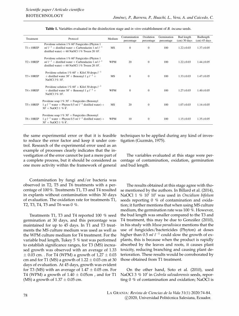
Scientific paper / Artículo científicoBIOTECHNOLOGY Jiménez, P., Barrera, P., Huachi, L., Vera, A. and Caicedo, C.
Table 1. Variables evaluated in the disinfection stage and in vitro establishment of B. incana seeds.
Treatment Protocol MediumContamination
percentageOxidationpercentage
Germinationpercentage
Bud length(cm) 30 days
Budlength(cm) 45 days
T1×10REPPovidone solution 1% 60′ Fungicides (Phyton 1ml l−1 + distilled water + Carbendazim 1 ml l−1
distilled water) + 60 NaOCl 1% Tween 20 10′.MS 0 0 100 1.22±0.03 1.37±0.05
T2×10REPPovidone solution 1% 60′ Fungicides (Phyton 1ml l−1 + distilled water + Carbendazim 1 ml l−1
distilled water) + 60 NaOCl 1% Tween 20 10′.WPM 20 0 100 1.22±0.03 1.44±0.05
T3×10REPPovidone solution 1% 60′ + Kilol 30 drops l−1
+ distilled water 30′ + Benomyl 1 g l−1 +NaOCl 3% 10′.
MS 0 0 100 1.33±0.03 1.47±0.05
T4×10REPPovidone solution 1% 60′ + Kilol 30 drops l−1
+ distilled water 30′ + Benomyl 1 g l−1 +NaOCl 3% 10′.
WPM 0 0 100 1.27±0.03 1.40±0.05
T5×10REPPovidone soap 1% 30′ + Fungicides (Benomyl1 g l−1 water + Phyton 0.5 ml l−1 distilled water) +30′ + NaOCl 1 % 8′.
MS 20 0 100 1.07±0.03 1.14±0.05
T6×10REPPovidone soap 1% 30′ + Fungicides (Benomyl1 g l−1 water + Phyton 0.5 ml l−1 distilled water) +30′ + NaOCl 1 % 8′.
WPM 10 0 100 1.15±0.03 1.35±0.05
the same experimental error or that it is feasibleto reduce the error factor and keep it under con-trol. Research of the experimental error used as anexample of processes clearly indicates that the in-vestigation of the error cannot be just a mere part ofa complete process, but it should be considered asone more activity within the framework of general
techniques to be applied during any kind of inves-tigation (Guzmán, 1975).
The variables evaluated at this stage were per-centage of contamination, oxidation, germinationand bud length.
Contamination by fungi and/or bacteria wasobserved in T2, T5 and T6 treatments with a per-centage of 100%. Treatments T1, T3 and T4 resultedin explants without contamination within 30 daysof evaluation. The oxidation rate for treatments T1,T2, T3, T4, T5 and T6 was 0 %.
Treatments T1, T3 and T4 reported 100 % seedgermination at 30 days, and this percentage wasmaintained for up to 45 days. In T1 and T3 treat-ments the MS culture medium was used as well asthe WPM culture medium for T4 treatment. For thevariable bud length, Tukey 5 % test was performedto establish significance ranges, for T3 (MS) increa-sed growth was observed with an average of 1.33± 0.03 cm. . For T4 (WPM) a growth of 1,27 ± 0.03cm and for T1 (MS) a growth of 1.22 ± 0.03 cm at 30days of evaluation. At 45 days, growth was evidentfor T3 (MS) with an average of 1.47 ± 0.05 cm. ForT4 (WPM) a growth of 1.40 ± 0.05cm , and for T1(MS) a growth of 1.37 ± 0.05 cm.
The results obtained at this stage agree with tho-se mentioned by the authors. In Billard et al. (2014),NaOCl 1 % 10′ 10′ was used in Oncidium bifolumseeds reporting 0 % of contamination and oxida-tion; it further mentions that when using MS culturemedium, the germination rate was 100 %. However,the bud length was smaller compared to the T3 andT4 treatment, this may be due to González (2010),in his study with Musa paradisiaca mentions that theuse of fungicides/bactericides (Phyton) at doseshigher than 0.5 ml l−1 could slow the growth of ex-plants, this is because when the product is rapidlyabsorbed by the leaves and roots, it causes planttoxicity, reducing branching and causing plant de-terioration. These results would be corroborated bythose obtained from T1 treatment.
On the other hand, Soto et al. (2010), usedNaOCl 3 % 10′ in Cedrela salvadorensis seeds, repor-ting 0 % of contamination and oxidation; NaOCl is
78LA GRANJA: Revista de Ciencias de la Vida 31(1) 2020:74-84.
c©2020, Universidad Politécnica Salesiana, Ecuador.
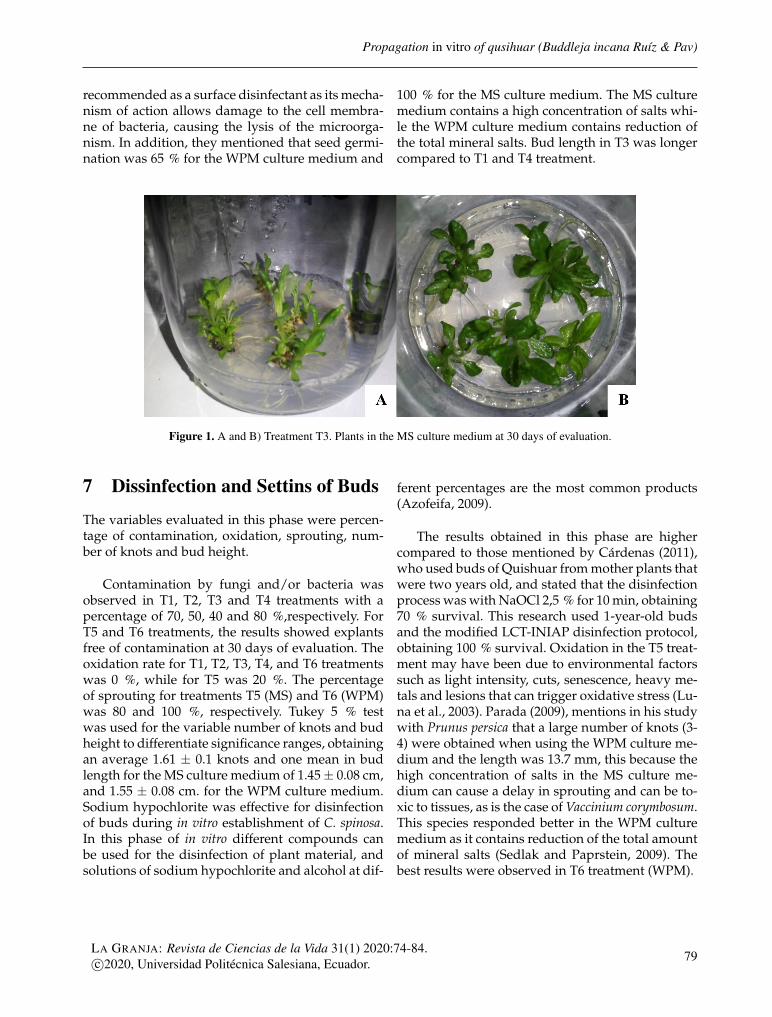
Propagation in vitro of qusihuar (Buddleja incana Ruíz & Pav)
recommended as a surface disinfectant as its mecha-nism of action allows damage to the cell membra-ne of bacteria, causing the lysis of the microorga-nism. In addition, they mentioned that seed germi-nation was 65 % for the WPM culture medium and
100 % for the MS culture medium. The MS culturemedium contains a high concentration of salts whi-le the WPM culture medium contains reduction ofthe total mineral salts. Bud length in T3 was longercompared to T1 and T4 treatment.
Figure 1. A and B) Treatment T3. Plants in the MS culture medium at 30 days of evaluation.
7 Dissinfection and Settins of Buds
The variables evaluated in this phase were percen-tage of contamination, oxidation, sprouting, num-ber of knots and bud height.
Contamination by fungi and/or bacteria wasobserved in T1, T2, T3 and T4 treatments with apercentage of 70, 50, 40 and 80 %,respectively. ForT5 and T6 treatments, the results showed explantsfree of contamination at 30 days of evaluation. Theoxidation rate for T1, T2, T3, T4, and T6 treatmentswas 0 %, while for T5 was 20 %. The percentageof sprouting for treatments T5 (MS) and T6 (WPM)was 80 and 100 %, respectively. Tukey 5 % testwas used for the variable number of knots and budheight to differentiate significance ranges, obtainingan average 1.61 ± 0.1 knots and one mean in budlength for the MS culture medium of 1.45± 0.08 cm,and 1.55 ± 0.08 cm. for the WPM culture medium.Sodium hypochlorite was effective for disinfectionof buds during in vitro establishment of C. spinosa.In this phase of in vitro different compounds canbe used for the disinfection of plant material, andsolutions of sodium hypochlorite and alcohol at dif-
ferent percentages are the most common products(Azofeifa, 2009).
The results obtained in this phase are highercompared to those mentioned by Cárdenas (2011),who used buds of Quishuar from mother plants thatwere two years old, and stated that the disinfectionprocess was with NaOCl 2,5 % for 10 min, obtaining70 % survival. This research used 1-year-old budsand the modified LCT-INIAP disinfection protocol,obtaining 100 % survival. Oxidation in the T5 treat-ment may have been due to environmental factorssuch as light intensity, cuts, senescence, heavy me-tals and lesions that can trigger oxidative stress (Lu-na et al., 2003). Parada (2009), mentions in his studywith Prunus persica that a large number of knots (3-4) were obtained when using the WPM culture me-dium and the length was 13.7 mm, this because thehigh concentration of salts in the MS culture me-dium can cause a delay in sprouting and can be to-xic to tissues, as is the case of Vaccinium corymbosum.This species responded better in the WPM culturemedium as it contains reduction of the total amountof mineral salts (Sedlak and Paprstein, 2009). Thebest results were observed in T6 treatment (WPM).
LA GRANJA: Revista de Ciencias de la Vida 31(1) 2020:74-84.c©2020, Universidad Politécnica Salesiana, Ecuador. 79

Scientific paper / Artículo científicoBIOTECHNOLOGY Jiménez, P., Barrera, P., Huachi, L., Vera, A. and Caicedo, C.
Table 2. Variables evaluated at the disinfection stage and in vitro establishment of B. incana buds
Treatment Protocol MediumContamination
PercentageOxidationPercentage
BudPercentage
Percentage ofknots (30
days)
Bud length(30 days)
T1×10REP
Povidone Solution 1% 20′ + Fungicides(Benomyl 1 g l−1 + Phyton 1 ml l−1 +Rinfapicina 0.5 ml l−1) 60′ + Alcohol 70% 1′
+ NaOCl 2% 15′.
MS 70 0 30 1.22±0.1 1.17±0.08
T2×10REP
Povidone Solution 1% 20′ + Fungicides(Benomyl 1 g l−1 + Phyton 1 ml l−1 +Rinfapicina 0.5 ml l−1) 60′ + Alcohol 70% 1′
+ NaOCl 2% 15′.
WPM 50 0 50 1.30±0.1 1.27±0.08
T3×10REP
Povidone Solution 1% + Kilol 20 drops l−1 +distilled water 30′ + Benomyl 1 g l−1 90′ +Alcohol 70% 30′′ + NaOCl 1% 15′ +Activated carbon (0,5 g l−1).
MS 40 0 60 1.41±0.1 1.33±0.08
T4×10REP
Povidone Solution 1% + Kilol 20 drops l−1 +distilled water 30′ + Benomyl 1 g l−1 90′ +Alcohol 70% 30′′ + NaOCl 1% 15′ +Activated carbon (0,5 g l−1).
WPM 80 0 20 1.11±0.1 1,11±0.08
T5×10REP
Povidone solution 1% 60′ + Activatedcarbon 0.5 g l−1 + Fungicides (Phyton 0.5ml l−1 + Carbendazim 0.5 ml l−1) + Kilol 30drops/ 100 ml + Ascorbic acid 0.1g l−1 20′
+ NaOCl 0.5 % 60′ + NaOCl 1 % 10′ + Tween20
MS 0 20 80 1.55±0.1 1.45±0.08
T6×10REP
Povidone solution 1% 60′ + Activatedcarbon 0.5 g l−1 + Fungicides (Phyton 0.5ml l−1 + Carbendazim 0.5 ml l−1) +Kilol 30drops l−1 + Ascorbic acid 0.1g l−1 20′ +NaOCl 0.5 % 60′ + NaOCl 1 % 10′ + Tween20
WPM 0 0 100 1.67±0.1 1.55±0.08
8 Multiplication Phase
The variables evaluated in this phase were budheight, number of knots, multiplication rate androot length. Plants obtained from the seed pha-se of the T3 treatment were used. The MS cul-ture medium without the addition of BAP (6-Bencilaminopurin) showed the best result, obtai-ning a bud height of 1.95 ± 0.05 cm and numberof knots 1.94 ± 0.04, followed by MS without ad-dition of AG3 ((Gibberellic acid) with an averageof 1.78 ± 0.05 cm and number of knots of 1.79 ±0.04 after 30 days of evaluation. These results arehigher than those mentioned by Cárdenas (2011),in which the bud height obtained was 0.4 cm andthe number of knots 1.25, using MS without theaddition of hormones. In the study with C. espino-sa, the concentration of BAP (6-Bencilaminopurin)did not significantly influence the number of initialexplants regarding the control treatment. Howe-
ver, the addition of 0.25 and 0.50 mg l−1 signifi-cantly favored the number of buds obtained froman initial explant. The lowest concentration of BAP(6-Bencilaminopurin) 0.25 mg l−1 was selected asthe best treatment for this phase of the process, with96.6% sprouting and in 30 days of cultivation an es-tablished vigorous explant was achieved, with anaverage of 2.07 buds of 6.71 cm long (Núñez et al.,2017).
The multiplication rate is the arithmetic meanof the number of buds generated at 30 days in eachtreatment. It was 2.60 for the culture medium MSwithout the addition of BAP (6-Bencilaminopurin),and 2.38 for MS without the addition of AG3 (Gib-berellic acid). The MS culture medium without theaddition of hormones guaranteed a multiplicationrate of 2.60.García et al. (2018), mentions that culture mediumsupplemented with hormones such as BAP (6-
80LA GRANJA: Revista de Ciencias de la Vida 31(1) 2020:74-84.
c©2020, Universidad Politécnica Salesiana, Ecuador.
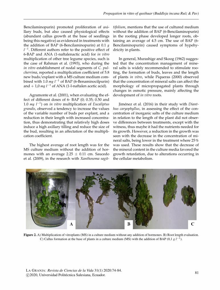
Propagation in vitro of qusihuar (Buddleja incana Ruíz & Pav)
Bencilaminopurin) promoted proliferation of axi-llary buds, but also caused physiological effects(abundant callus growth at the base of seedlingsbeing this negative) as evidenced in treatments withthe addition of BAP (6-Bencilaminopurin) at 0.1 gl−1. Different authors refer to the positive effect of6-BAP and ANA (1-naftalenactic acid) for in vitromultiplication of other tree legume species, such isthe case of Rahman et al. (1993), who during thein vitro establishment of nodal segments of C. pul-cherrima, reported a multiplication coefficient of 5.8new buds/explant with a MS culture medium com-bined with 1.0 mg l−1 of BAP (6-Benaminocilpurin)and + 1,0 mg l−1 of ANA (1-l-naftalen acetic acid).
Agramonte et al. (2001), when evaluating the ef-fect of different doses of 6- BAP (0; 0.35; 0.50 and1.0 mg l−1) on in vitro multiplication of Eucaliptusgrandis, observed a tendency to increase the valuesof the variable number of buds per explant, and areduction in their length with increased concentra-tion, thus demonstrating that relatively high dosesinduce a high axillary tilling and reduce the size ofthe bud, resulting in an affectation of the multipli-cation coefficient.
The highest average of root length was for theMS culture medium without the addition of hor-mones with an average 2.25 ± 0.11 cm. Saucedoet al. (2009), in the research with Xanthosoma sagit-
tifolium, mentions that the use of cultured mediumwithout the addition of BAP (6-Bencilaminopurin)in the rooting phase developed longer roots, ob-taining an average of 4.5 cm. The use of BAP (6-Bencilaminopurin) caused symptoms of hypehy-dricity in plants.
In general, Murashige and Skoog (1962) sugges-ted that the concentration management of mine-ral salts is widely recommended to stimulate roo-ting, the formation of buds, leaves and the lengthof plants in vitro, while Piqueras (2000) observedthat the concentration of mineral salts can affect themorphology of micropropagated plants throughchanges in osmotic pressure, mainly affecting thedevelopment of in vitro roots.
Jiménez et al. (2016) in their study with Diant-hus caryophyllus, in assessing the effect of the con-centration of inorganic salts of the culture mediumin relation to the length of the plant did not obser-ve differences between treatments, except with thewitness, thus maybe it had the nutrients needed forits growth. However, a reduction in the growth wasseen with the decrease in the concentration of mi-neral salts, being lower in the treatment where 25%was used. These results show that the decrease ofthe mineral content in the culture media favored thegrowth retardation, due to alterations occurring inthe cellular metabolism.
Figure 2. A) Multiplication of vitroplants (MS) in a culture medium without any addition of hormones. B) Root length evaluation.C) Callus formation at the base of plants in a culture medium (MS) with the addition of BAP (0,1 g l−1).
LA GRANJA: Revista de Ciencias de la Vida 31(1) 2020:74-84.c©2020, Universidad Politécnica Salesiana, Ecuador. 81
Scientific paper / Artículo científicoBIOTECHNOLOGY Jiménez, P., Barrera, P., Huachi, L., Vera, A. and Caicedo, C.
9 Conclusions
The best treatment for the disinfection phase and invitro establishment of Buddleja incana seeds was T3(Povidone solution 1% 60′ + Kilol 30 drops l−1 +distilled water 30′ + Benomil 1 g l−1 + NaOCl 3%10′), with a contamination rate of 0% and survivalrate of 100%. The T3 treatment contained MS cul-ture medium that was effective for the variable budlength, as the highest values were 1.33 ± 0.03 cm at30 days and 1.47 ± 0.03 cm at 45 days. Accordingto Jiménez et al. (2001), it is important to take intoaccount the area of the tissue used to start in vitro,cultivation, since it has a great influence on the effi-ciency of disinfection.
The in vitro establishment phase of Buddleja in-cana buds, showed that the best treatment was T6(Phyton 0.5 ml l−1 + Carbendazim 0.5 ml l−1) +Kilol 30 drops l−1 + Ascorbic acid 0.1g l−1 20′ +NaOCl 0.5 % 60′ + NaOCl 1 % 10′ + Tween 20)with 0% contamination. The bud percentage in thistreatment was 100%. The number and length ofbuds had an average of 1.67 ± 0.1 buds/explantand 1.55 ± 0.08 cm of length. In the work carriedout by Gutiérrez (2002), in Alnus acuminata fromnod segments and leaf, a disinfection protocol wasused with very similar concentrations of NaClOand times proposed in Marulanda and Isaza (2004).The results indicated that disinfection treatmentwith NaClO at 1% resulted in less oxidation in theleaves than in the nodal segments.
In in vitro multiplication essays of Buddleja in-cana, the MS culture medium presented the bestresults in treatments without the addition of thehormones BAP and AG3. The bud length had anaverage of 1.95 ± 0.05 cm, the number of knots hadan average of 1.94 ± 0.04 knots/explant and mul-tiplication rate of 2.60. The results obtained in themultiplication phase showed that no rooting pro-moter was required since the root length had anaverage of 2.25 ± 0.08 cm.
This research represents an initial phase of esta-blishment and in vitro multiplication, where the re-sults indicate a probability of success in the micro-propagation process of this species; however, feasi-bility studies in the field still need to be performed.
References
Agramonte, D., Delgado, L., Trocones, A., Pérez, M.,Ramirez, D., and Gutiérrez, O. (2001). Micropro-pagación del eucalyptus grandis (hill ex maiden)a partir de segmentos nodales. Biotecnología vege-tal, 1(2):109–114. Online: https://bit.ly/39X58x4.
Azofeifa, A. (2009). Problemas de oxidación y os-curecimiento de explantes in vitro. Agronomíamesoamericana, 20(1):153–175. Online: https://bit.ly/2uozSrY.
Billard, C. E., Dalzotto, C. A., and Lallana, V. H.(2014). Desinfección y siembra asimbiótica de se-millas de dos especies y una variedad de orqui-deas del género oncidium. Revista Polibotanica,(38):145–157. Online: https://bit.ly/32emkf9.
Cárdenas, M. (2011). Determinación del protoco-lo de establecimiento y multiplicación in vitro dequishuar (buddleja incana) a partir de yemas axi-lares de plantas madre, como una herramientapara la preservación de esta especie dentro deldistrito metropolitano de quito.
Delgado, M., Hechenleitner, P., and Thiers, O.(2008). Propagación vegetativa de taique (des-fontainia spinosa) y tepa (laureliopsis philippana)con fines ornamentales. Revista Bosque, 29(2):120–126. Online: https://bit.ly/2VaTpa7.
Gárate, M. (2010). Técnicas de propagación por es-tacas.
García, L., Moreno, L., Pérez, M., La O, M., Padrón,Y., Rodríguez, Y., and Rivero, L. (2018). Protocolopara la micropropagación de anthurium cuben-se engler a partir de semilla botánica. Biotecnolo-gía Vegetal, 18(3):161–166. Online: https://bit.ly/2vZvcZN.
Gómez, M. (2006). Evaluación de alternativas sil-vopastoriles utilizando yagual (polylepis racemo-sa), quishuar (buddleja incana), colle (buddlejacoriacea) en la microcuenca del río chimborazo.
González, H. (2010). Evaluación de la eficacia in vi-tro de productos naturales y químicos en el con-trol de especies fúngicas que afectan al cultivo demusa paradisiaca. Technical report, Informe téc-nico (1).
82LA GRANJA: Revista de Ciencias de la Vida 31(1) 2020:74-84.
c©2020, Universidad Politécnica Salesiana, Ecuador.
Propagation in vitro of qusihuar (Buddleja incana Ruíz & Pav)
Grijalva, J., Ramos, R., Checa, X., Anti, A., Barrera,P., and Telenchano, A. (2012). Gestión sosteni-ble de microcuencas en los andes. instituto nacio-nal de investigaciones agropecuarias, programanacional de forestería, quito. Revista InformativaINIAP, (7):11–13. Online: .
Gutiérrez, L. G. (2002). Embriogénesis somática en Al-nus acuminata H.B.K. y estudio de la variación soma-clonal mediante marcadores moleculares. Tesis docto-ral.
Guzmán, M. (1975). El error experimental en la in-vestigación científica: Cuantificación de elemen-tos contribuyentes. Technical report, Boletín dela Oficina Sanitaria Panamericana. Online: https://bit.ly/2PgCyir.
Hernández, C., Lopera, M., Mora, B., and Cárde-nas, J. (1999). Desarrollo de un protocolo para lapropagación masiva de la mora de castilla (rubusglaucus bent) mediante la utilización del cultivode tejidos vegetales in vitro. Revista ActualidadesBiológicas, 21(70):3–12.
Jiménez, L., Silva, J., Borges, M., and Fonseca, M.(2016). Conservación in vitro de clavel español(dianthus caryophyllus l) a partir de sales mine-rales. Revista Agronomía Mesoamericana, 27(1):On-line: https://bit.ly/32iCgwT.
Jiménez, V. M., Castillo, J., Tavares, E., Guevara, E.,and Montiel, M. (2001). Micropropagación deguadua angustifolia kunth a partir de explantesnodales. In Memorias del Simposio InternacionalGuadua. Pereira, Colombia: Universidad Tecnológicade Pereira. Online: https://bit.ly/2SOooY9.
Laboratorio de Cultivo de Tejidos (LCT-INIAP)(2014). Informe técnico. protocolos de desinfec-ción de especies forestales. Technical Report 1,Informes Iniap.
Luna, C., Sansberro, J., Mroginski, L., and Tarragó,J. (2003). Micropropagation of ilex dumosa fromnodal segments in a tissue culture system. Biocelll,27(2):120–135. Online: https://bit.ly/3a0IIeJ.
Marulanda, M. L. and Isaza, L. (2004). Estableci-miento in vitro de heliconias con fines de produc-ción masiva. Scientia et Technica, (26):193–197. On-line: https://bit.ly/2VeUBcC.
Ministerio del Ambiente-MAE (2005). Informe téc-nico de árboles del ecuador. Technical report, Mi-nisterio del Ambiente, Ecuador.
Murashige, T. and Skoog, F. (1962). A revised me-dium for rapid growth and biossays with tobac-co tissue cultures. Physiological Plantarum, 15:473–497. Online: https://bit.ly/2uXxNUh.
Núñez, J., Quiala, E., De Feria, M., Mestanza, S., andTeanga, S. (2017). Propagación in vitro de cae-salpinia spinosa (mol.) o. kuntz a partir de ye-mas axilares de árboles plus seleccionadas. Revis-ta Biotecnología Vegetal, 17(2):67–75. Online: https://bit.ly/38RGM87.
Parada, D. (2009). Propagación in vitro del hí-brido almendro x durazno h1. Revista Fitotec-nia mexicana, 32(2):103–109. Online: https://bit.ly/3bXmGLu.
Piqueras, A., y. D. P. . . I. . E. b. A. P. p. .-. (2000).Morphogenesis in micropro Morphogenesis in micro-propagation, pages 443–462. Online: https://bit.ly/2HMzDtH. Kluwers Academics Publishers.
Rahman, S. M., Hossain, M., Biswas, B. K., Joarder,O. I., and Islam, R. (1993). Micropropagation ofcaesalpinia pulcherrima through nodal bud cul-ture of mature tree. Plant Cell, Tissue and Or-gan Culture, 32:363–365. Online: https://bit.ly/2Pg4Gm2.
Reyes, H. and y Hewstone, N. (1994). Cultura detejidos en la agricultura. Revista Tierra Adentro,(24):30–33. Online: https://bit.ly/2SQ5HDy.
Sánchez, Y. (2012). Elaboración de tablas de volú-menes y determinación de factores de forma delas especies forestales: Chuncho (cedrelinga ca-tenaeformis), laurel (cordia alliadora), sangre degallina (otoba sp.), ceibo (ceiba samauma) y cane-lo (nectandra sp.), en la provincia de orellana.
Saucedo, S., Ramos, L., and Reyes, T. (2009). Efec-to de los reguladores de crecimiento para la pro-pagación in vitro de la malanga (xanthosoma sa-gittifolium (l) schott). Revista Cienica y Tecnología,1(1):17–21. Online: https://bit.ly/37V65VD.
Sedlak, J. and Paprstein, F. (2009). In vitro multipli-cation of highbush blueberry (vaccinium corym-bosum l.) cultivars. In ISHS Acta Horticulturae, pa-ges 575–580. Online: https://bit.ly/3c0T2Fi.
LA GRANJA: Revista de Ciencias de la Vida 31(1) 2020:74-84.c©2020, Universidad Politécnica Salesiana, Ecuador. 83
Scientific paper / Artículo científicoBIOTECHNOLOGY Jiménez, P., Barrera, P., Huachi, L., Vera, A. and Caicedo, C.
Soto, B., Valverde, L., Rojas, A., and Gómez, A.(2010). Establecimiento in vitro de cedrela sal-vadorensis standl. Revista Tecnología en marcha,23(4):66–73. Online: https://bit.ly/2VemQbC.
Vallejo, S. (1988). Multiplicación a través de culti-vo de tejidos vegetales de las especies: quishuar(buddleja incana h.b.k.), cedro (cedrela montana
vill) y pumamaqui (oreopanax ecuadorensis see-men).
Vinueza, D. (2013). Evaluación morfológica e histo-lógica de las etapas de formación de la embriogé-nesis somática en las variedades duke 7 y pueblade aguacate (persea americana mill).
84LA GRANJA: Revista de Ciencias de la Vida 31(1) 2020:74-84.
c©2020, Universidad Politécnica Salesiana, Ecuador.
Scientific paper/ Artículo científico
LIVESTOCK SYSTEMSpISSN:1390-3799; eISSN:1390-8596
http://doi.org/10.17163/lgr.n31.2020.06
INTEGRAL TYPIFICATION OF GOAT SYSTEMS OF SANTA ELENA
PROVINCE, ECUADOR
TIPIFICACIÓN INTEGRAL DE SISTEMAS CAPRINOS DE LA PROVINCIA DE
SANTA ELENA, ECUADOR
Araceli Solís Lucas*1 , María Rosa Lanari2 and María Inés Oyarzabal3
1 Faculty of Agricultural Sciences. State University Santa Elena Peninsula, Av. Principal Santa Elena-La Libertad, Santa Elena,Ecuador.2 Agricultural Experimental Station (EEA). National Institute of Agricultural Technology (INTA). Grenville Morris, 8400, Ba-riloche, Argentina.3 Faculty of Veterinary Sciences. CIC. National University of Rosario, 2170, Casilda, Argentina.
*Corresponding author: [email protected]
Article received on april 27th, 2019. Accepted, after review, on december 4th, 2019. Published on march 1st, 2020.
Resumen
Como paso previo para proponer estrategias de desarrollo en sistemas de producción caprina (SPC) de la provin-cia de Santa Elena, Ecuador, se propuso tipificar los sistemas mediante indicadores socio-económicos, productivos yambientales. Se encuestó a 172 productores sobre composición familiar y participación en el trabajo, tecnología adop-tada, comunicaciones, composición del hato, existencias ganaderas, uso del suelo, ingresos, infraestructura y serviciosbásicos, acceso a las explotaciones, asistencia técnica y capacitación, trabajo e ingresos extraprediales, manejo e insta-laciones, fuente de agua y suplemento alimenticio, aspecto reproductivo, dificultades en la producción de caprinos,comercialización de caprinos. Se redujo el número de variables mediante análisis de componentes principales (ACP)y pruebas de χ2, para las variables cuantitativas y cualitativas, respectivamente. Con las CP que explicaron el 80%de la variabilidad se llevó a cabo un análisis de conglomerados (AC) que dividió a los establecimientos en 7 grupos.Mediante un análisis de correspondencias múltiples (ACM) se identificaron asociaciones entre grupos y modalida-des de las variables cualitativas. Las variables que más aportaron a la diferenciación de los grupos de SP estabanrelacionadas con la producción caprina, el tamaño de la familia, las producciones avícola, agrícola, porcina y bovina,la participación en el trabajo de la familia, los ingresos por beneficios sociales, el tamaño de la finca y la tecnologíaadoptada. Dos grupos eran mixtos; uno con mayor actividad porcina; dos se caracterizaron por la cría de cabras parael consumo cuyos ingresos provenían de fuentes externas y dos grupos se definieron por la edad de sus productores.
Palabras clave: Indicadores económicos, indicadores productivos, indicadores socio-culturales, sistemas de produc-ción, cabras.
85LA GRANJA: Revista de Ciencias de la Vida 31(1) 2020:85-97.c©2020, Universidad Politécnica Salesiana, Ecuador.
Scientific paper / Artículo científicoLIVESTOCK SYSTEMS Solís Lucas, A., Lanari, M.R. and Oyarzabal, M.I.
Abstract
As a preliminary step to propose development strategies in the goat productive systems (SPC) of the Santa Elenaprovince, Ecuador, the SPC were typified by means of socio-economic, productive and environmental indicators. Asample of 172 producers was surveyed on family composition and participation in work, adopted technology, com-munications, composition of the herd, livestock stock, land use, income, infrastructure and basic services, access tofarms, technical assistance and training, off-farm work and income, management and facilities, water sources andfood supplement, reproductive aspects, difficulties in the production of goats, marketing of goats. The number ofproposed variables was reduced by principal component analysis (PCA) and χ2 tests for quantitative and qualitativevariables, respectively. Based on the main components that explained 80% of the variability, a conglomerate analysis(CA) was carried out, resulting in the division of the SPC into 7 groups. Through a multiple correspondence analy-sis (MCA), associations between groups and modalities of qualitative variables were identified. The variables thatcontributed most to the differentiation of SPC groups were related to goat production, family size, poultry, agricul-tural, pig and bovine production, participation in family work, income from social benefits, the size of the farm andthe technology adopted. Two groups were mixed, one with a predominance of livestock activity and the other withagricultural activity; a group with greater swine activity; two groups were characterized by the breeding of goats forconsumption, whose income came from external sources; and two groups were defined by the age of their producers.
Keywords: Economic indicators, productive indicators, socio-cultural indicators, production systems, goats.
Suggested citation: Solís Lucas, A., Lanari, M.R. and Oyarzabal, M.I. (2020). Integral typification of goatsystems of Santa Elena province, Ecuador. La Granja: Revista de Ciencias de la Vida.Vol. 31(1):85-97. http://doi.org/10.17163/lgr.n31.2020.06.
Orcid IDs:Ligia Araceli Solís Lucas: http://orcid.org/ 0000-0002-4428-3888María Rosa Lanari: http://orcid.org/0000-0002-2186-601XMaría Inés Oyarzabal: http://orcid.org/0000-0001-5429-5789
86LA GRANJA: Revista de Ciencias de la Vida 31(1) 2020:85-97.
c©2020, Universidad Politécnica Salesiana, Ecuador.
Integral typification of goat systems of Santa Elena province, Ecuador
1 Introduction
Knowing the reality of production systems is neces-sary in order to propose solutions to critical situa-tions, implement genetic improvement plans, as-sess the environmental impact of livestock, amongothers. The identification of strengths and weak-nesses allows to propose strategies that should bespecific to each type of production units if there wasdiversity between the systems of a region (Cabreraet al., 2004; Dufumier, 1990).
It is recommended to propose development al-ternatives along with the producers for productivesubsistence systems (Macías, 2015), with the aimof stimulating deep personal interest in the care ofanimals and crops; offering more products for salethrough a better use of what is available locally (bio-logical resources, native vegetation, livestock, etc.);introducing knowledge and technology along withthe assessment of skills, existing knowledge andexperiences; collaborating with producers to do abetter performance (Hodges et al., 2014). On theother hand, subsistence systems host valuable zoo-genetic resources that need to be preserved becausethey have evolved in their adaptation to adverseenvironments and there are moments in which ge-netic biodiversity is being lost (Núñez-Domínguezet al., 2016; Dorji et al., 2017).
Differentiated groups can be identified and typi-fied from the initial state analysis and system cha-racterization. Different methods for carrying outstratification based on a wide range of environ-mental, productive, economic and social aspects,which meet different objectives, have been propo-sed. Another form of stratification of systems is theapplication of statistical grouping methods (Robin-son et al., 2011).
The goat production systems (SPC) of the pro-vince of Santa Elena (PSE), Ecuador, are low-incomesubsistence systems. Santa Elena has the highestpercentage of goats at the coastal level (53%) and7.2% of the country’s total stocks (Sistema Nacio-nal de Información, 2018). As a pre-developmentstep, it was proposed to test whether there is he-terogeneity among the province’s goat systems. Aprocess was carried out which included: surveyingestablishments, survey to the producers and clas-sification of prevailing production systems using
socio-cultural, productive and economic indicators.
2 Materials and methods
Santa Elena is a province located in the coast ofthe Republic of Ecuador, located southwest of theEcuadorian coast. Politically, it is divided into th-ree parishes: La Libertad, Salinas and Santa Elena(3668.9 km2). The latter is the largest parish of theprovince, with a high rural population. It has 67communes registered at the Agricultural ProvincialDirectorate of Santa Elena (Ministerio de Agricultu-ra y Ganadería, 2018).
Based on oral information received from thecommunity and the Ministry of Agriculture and Li-vestock (MAG), 586 goat production systems wereidentified, with an estimated total of 11,977 heads,in the 3 climatic zones in which the province is di-vided. Within each zone, a frequency distributionof the number of goat producers was performedaccording to the herd size. The total number of es-tablishments to be sampled was estimated throughthe application of the finite sample formula (FAO,2012). Once the total sample size was defined, stra-tified sampling was performed by zone and herdsize using proportional allocation.
A structured survey was designed for the pro-ducers, taking as reference those used by Falagan(1988), Bedotti (2000) and Lanari (2004), includingsocio-cultural, productive and economic aspects(Tables 1, 2 and 3).
It was tested whether there were differences bet-ween agro-ecological zones by means of a multiva-riate variance analysis (MANOVA) for the quanti-tative variables. In order to decrease the numberof variables: the association degree between the27 quantitative variables was estimated to definethe exclusion of those variables that had the sa-me characteristic (r > 0,70); and a main componentanalysis (ACP) was performed (Peña, 2002), withthe components explaining at least 80% of the totalvariability chosen.
With the main components selected through acluster analysis (AC) (Dallas, 2000), production sys-tems were classified into homogeneous groups byapplying: the hierarchical method, the Euclidean
LA GRANJA: Revista de Ciencias de la Vida 31(1) 2020:85-97.c©2020, Universidad Politécnica Salesiana, Ecuador. 87

Scientific paper / Artículo científicoLIVESTOCK SYSTEMS Solís Lucas, A., Lanari, M.R. and Oyarzabal, M.I.
distance and the Ward method (Ward, 1963). Theprofiles of each group (G) were described by thestandardized averages of all variables and repre-sented on a radial chart.
For the 77 qualitative variables, the relative fre-quencies for each of the resulting producer groupsof AC and the total frequencies were estimated.Pearson tests were performed (p < 0,05) with theaim of selecting the variables with significant diffe-rences between the groups. With the selected varia-bles, a multi-match analysis (CMA) was performedto identify the most important associations betweenthe modalities of the qualitative variables (Greena-cre, 1984) and the groups of the producers. Statisti-cal calculations were performed with the professio-nal Infostat programme (Di Rienzo et al., 2008).
3 ResultsOn the basis of the information received on the totalnumber of producers per zone, they were distribu-ted according to the size of the herd, and the sam-ple was estimated at 229. The proportional alloca-tion by area and size of the herd is detailed in Table4. Out of these, 22% were not surveyed by differentreasons: duplicate information, absence of the pro-ducer at the time of the visit, abandonment of theactivity, etc. None of the producer belonging to thesemi-wet zone was surveyed due to inaccessibilityto the area at the time of the survey. A total of 172 es-tablishments were not taken into account, 69 in thedry area and 103 in the semi-arid area.
Table 1. Quantitative variables related to socio-cultural, productive and economic aspects
Type of information Variables
Family composition andparticipation in the work
Age of the producer reflected in years EDNumber of family members living in the same house TPNumber of people who work exclusively in the farm PDNumber of people who work exclusively outside the farm PFNumber of people who work inside and outside the farm PDF
Technology used Knowledge of the reproductive cycle GCRDegree of health control GCS
Communication Distance to the town that the producer has more communication with (km) DL
Composition of the herd(number of heads percategory))
Female goat CHVAFemale nanny goat CBLAFemale kid CBTAMale goat CHVOMale nanny goat CHTOMale kid CBTO
Livestock inventory
Goat ECBovine EBSwine EPPoultry EA
Use of the soil Hectares sown HaSSurface of the farm in hectares HaF
Revenue in $ the lastyear
By the sale of agricultural crops $IAGBy the bovine sale $IBBy the caprine sale $ICBy the swine sale $IPBy the poultry sale $IABy other external sources $IEXBy other social benefits $IBS
88LA GRANJA: Revista de Ciencias de la Vida 31(1) 2020:85-97.
c©2020, Universidad Politécnica Salesiana, Ecuador.
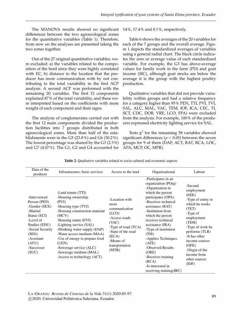
Integral typification of goat systems of Santa Elena province, Ecuador
The MANOVA results showed no significantdifferences between the two agroecological zonesfor the quantitative variables (Table 1). Therefore,from now on the analyses are presented taking thetwo zones together.
Out of the 27 original quantitative variables, we-re excluded: a) the variables related to the compo-sition of the herd since they were highly correlatedwith EC; b) distance to the location that the pro-ducer has more communication with by not con-tributing to the total variability in the first ACPanalysis. A second ACP was performed with theremaining 20 variables. The first 12 componentsexplained 87% of the total variability, and these we-re interpreted based on the coefficients with moreweight of each component and their signs.
The analysis of conglomerates carried out withthe first 12 main components divided the produc-tion facilities into 7 groups distributed in bothagroecological zones. More than half of the esta-blishments were in the G5 (23.8%) and G6 (30.2%).The lowest percentage was shared by the G3 (2.3%)and G7 (4.07%). The G1, G2 and G4 accounted for
14%, 17.4% and 8.1%, respectively.
Table 6 shows the averages of the 20 variables foreach of the 7 groups and the overall average. Figu-re 1 depicts the standardized averages of variablesusing a general radial chart. The black circle indica-tes the zero or average value of each standardizedvariable. For example, the G3 has above-averagevalues for family work in the farm (PD) and goatincome ($IC), although goat stocks are below theaverage it is the group with the highest poultryproduction.
Qualitative variables that did not provide varia-bility within groups and had a relative frequencyfor a category higher than 95% PEN, TTI, PVI, TVI,SAL, ALC, MAL, VAC, TEM, IOF, ICA, CEC, TI,SCT, CDC, DOB, VRE, LCO, FPA) were excludedfrom the analysis. For example, 100% of the produ-cers expressed electricity lighting service for SAL.
Tests χ2 for the remaining 58 variables showedsignificant differences (p < 0,05) between the sevengroups for 9 of them (DAP, ACT, RAT, RCA, LOC,APA, MCP, OC, MPR).
Table 2. Qualitative variables related to socio-cultural and economic aspects
Data of theproducer Infrastructure, basic services Access to the land Organizational Labour
-InterviewedPerson (PEN)-Gender (SEX)-MaritalStatus (ECI)-Level ofStudies (EDU)-Social Security(SEG)-Assistant(AYU)-Successor(SUC)
-Land tenure (TTI)-Housing ownership(PVI)-Housing type (TVI)-Housing construction material(MCV)-Housing status (EVI)-Lighting service (SAL)-Drinking water supply (DAP)-Water access medium (MAA)-Use of energy to prepare food(UEN)-Sewerage service (ALC)-Sewerage medium (MAL)-Access to technology (ACT)
-Location withmorecommunication(LCO)-Access roads(VAC)-Type of road (TCA)-State of the road(ECA)-Means oftransportation(MTR)
-Participates in anorganization (POrg)-Organization inwhich the personparticipates (OPA)-Receives technicalassistance (RAT)-Institution fromwhich the personreceives technicalassistance (IRA)-Type of institution(TIS)-Applies Techniques(ATE)-Observed Results(ORE)-Receives training(RCA)-Is interested inreceiving training(IRC)
-Secondemployment(EEE)-Type of entity inwhich he works(TET)-Type ofemployment(TEM)-Type of work heperforms (TLR)-It has otherincome sources(OFE)-Origin of theincome fromother sources(IOF)
LA GRANJA: Revista de Ciencias de la Vida 31(1) 2020:85-97.c©2020, Universidad Politécnica Salesiana, Ecuador. 89

Scientific paper / Artículo científicoLIVESTOCK SYSTEMS Solís Lucas, A., Lanari, M.R. and Oyarzabal, M.I.
The ACM showed that in the first dimension theuse of technical assistance and training were sig-nificant (RATsi and RCAsi), and in the second thenon-access to technology (ACTno). These first twodimensions explained 37% of the variability of so-ciocultural and management variables. The third,fourth and fifth dimensions were related to the in-terest of receiving or not training, and the sixth withthe farm as a grazing area of the goats.
3.1 Overview of the production systems ofSanta Elena Peninsula
Most goat herd owners are male, with elementaryschool studies (61%), with peasant social insuran-
ce, and whose helpers in the handling of goats isa family member, and it is sure that their childrenwould continue with the breeding of goats.
Producers participate in the communal mee-tings and only one-third claimed to having receivedtechnical assistance, most of the beneficiaries werethose producers who participated in state projectsand who introduced goats from other areas in thelast two decades. There is a strong interest of smallproducers of the PSE in improving goat production(94%), despite the highest current incomes not co-ming from goat production but from other externalsources. They have extra income from jobs of priva-te companies and on a temporary basis or receivethe Human Development Bonus (BDH).
Table 3. Qualitative variables related to the goat production aspect
Management and infrastructure ofgoat systems
Water sourceand food
supplementation
Reproductiveaspect
Difficulties in theproduction of
goats
Commercializationof goats
-Place of origin of goats (LOC)-Grazing system (SPA)-Grazing area (APA)-The goats of the neighbor graze inthe same place (CVP)-Water/food implementation used inthe field (ICA)-Farmyards for the goats (CEC)-Farmyard owner (PCO)-Farmyard location (UCO)-Construction material walls and floor(MCP)- Roof construction material(MCT)-Use of implements in the water/foodpen (UI)-Type of water/food implements (TI)-Implement manufacturing material (MFI)-Implement origin (PI)-Goats are released every day (SCT)-Time in which goats are taken inside(HSC)-Goats are locked every day (ECT)-Time in which goats are locked(HEC)-Daily control of goats (CDC)-Maximum distance that goats walk(km) (DMC)-A dog helps with the goats (TPC)-Other paddock (OC)
-Purchase ofthe foodsupplement(CSA)-Goat waterfountain (FAG)
-Parity Control(CPA)-Obtaining of MaleBreeders (ORM)-Difficulty forobtaining breeders(DOB)-Interest in buyingmales (ICM)-Obtaining offemale breeders(ORH)
-Diseases (ENF)-Problems in theproduction ofgoats (PPC)-What is neededto improve theproduction (MPR)
-Goat productobtained (PCO)-Breedingobjective (OCR)-Reasons to sale(MVE)-Way the animal issold (FVE)-Sale of breeders(VRE)-Places ofmarketing (LCO)-Payment method(FPA)-Difficulties inmarketing (DCO)
90LA GRANJA: Revista de Ciencias de la Vida 31(1) 2020:85-97.
c©2020, Universidad Politécnica Salesiana, Ecuador.
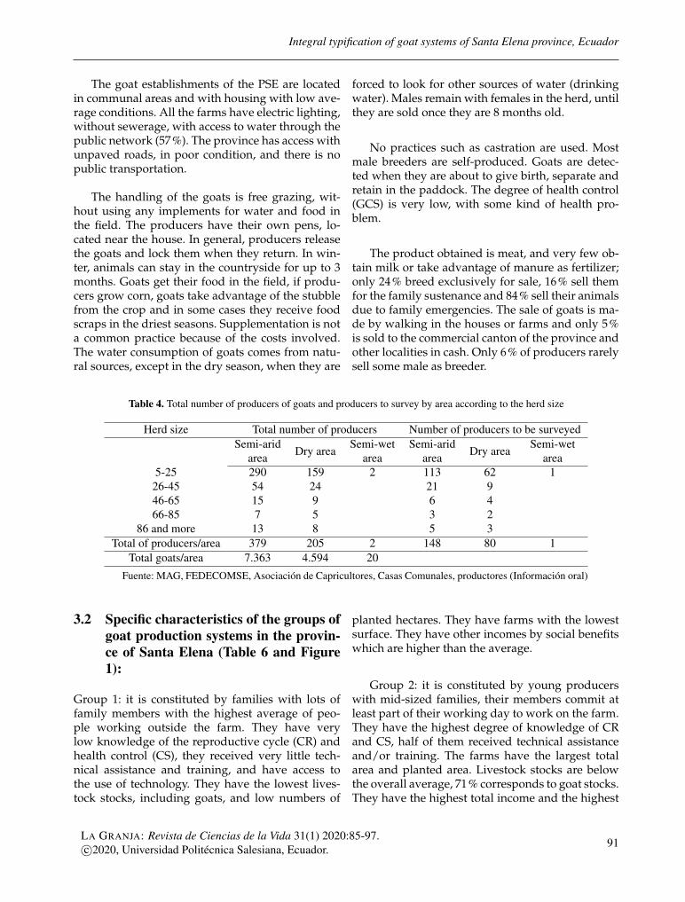
Integral typification of goat systems of Santa Elena province, Ecuador
The goat establishments of the PSE are locatedin communal areas and with housing with low ave-rage conditions. All the farms have electric lighting,without sewerage, with access to water through thepublic network (57%). The province has access withunpaved roads, in poor condition, and there is nopublic transportation.
The handling of the goats is free grazing, wit-hout using any implements for water and food inthe field. The producers have their own pens, lo-cated near the house. In general, producers releasethe goats and lock them when they return. In win-ter, animals can stay in the countryside for up to 3months. Goats get their food in the field, if produ-cers grow corn, goats take advantage of the stubblefrom the crop and in some cases they receive foodscraps in the driest seasons. Supplementation is nota common practice because of the costs involved.The water consumption of goats comes from natu-ral sources, except in the dry season, when they are
forced to look for other sources of water (drinkingwater). Males remain with females in the herd, untilthey are sold once they are 8 months old.
No practices such as castration are used. Mostmale breeders are self-produced. Goats are detec-ted when they are about to give birth, separate andretain in the paddock. The degree of health control(GCS) is very low, with some kind of health pro-blem.
The product obtained is meat, and very few ob-tain milk or take advantage of manure as fertilizer;only 24% breed exclusively for sale, 16% sell themfor the family sustenance and 84% sell their animalsdue to family emergencies. The sale of goats is ma-de by walking in the houses or farms and only 5%is sold to the commercial canton of the province andother localities in cash. Only 6% of producers rarelysell some male as breeder.
Table 4. Total number of producers of goats and producers to survey by area according to the herd size
Herd size Total number of producers Number of producers to be surveyedSemi-arid
area Dry areaSemi-wet
areaSemi-arid
area Dry areaSemi-wet
area5-25 290 159 2 113 62 1
26-45 54 24 21 946-65 15 9 6 466-85 7 5 3 2
86 and more 13 8 5 3Total of producers/area 379 205 2 148 80 1
Total goats/area 7.363 4.594 20Fuente: MAG, FEDECOMSE, Asociación de Capricultores, Casas Comunales, productores (Información oral)
3.2 Specific characteristics of the groups ofgoat production systems in the provin-ce of Santa Elena (Table 6 and Figure1):
Group 1: it is constituted by families with lots offamily members with the highest average of peo-ple working outside the farm. They have verylow knowledge of the reproductive cycle (CR) andhealth control (CS), they received very little tech-nical assistance and training, and have access tothe use of technology. They have the lowest lives-tock stocks, including goats, and low numbers of
planted hectares. They have farms with the lowestsurface. They have other incomes by social benefitswhich are higher than the average.
Group 2: it is constituted by young producerswith mid-sized families, their members commit atleast part of their working day to work on the farm.They have the highest degree of knowledge of CRand CS, half of them received technical assistanceand/or training. The farms have the largest totalarea and planted area. Livestock stocks are belowthe overall average, 71% corresponds to goat stocks.They have the highest total income and the highest
LA GRANJA: Revista de Ciencias de la Vida 31(1) 2020:85-97.c©2020, Universidad Politécnica Salesiana, Ecuador. 91
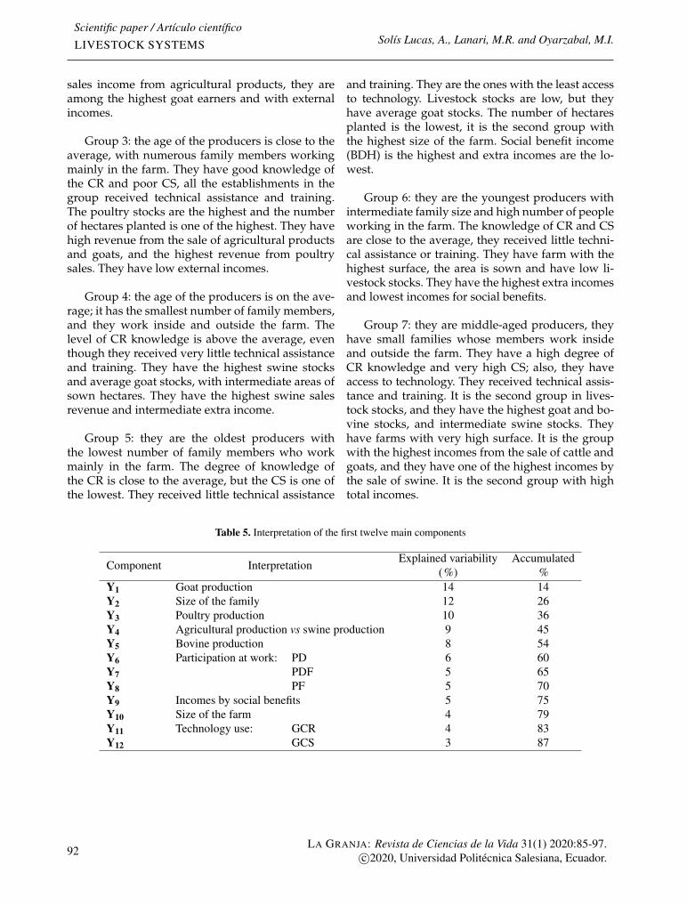
Scientific paper / Artículo científicoLIVESTOCK SYSTEMS Solís Lucas, A., Lanari, M.R. and Oyarzabal, M.I.
sales income from agricultural products, they areamong the highest goat earners and with externalincomes.
Group 3: the age of the producers is close to theaverage, with numerous family members workingmainly in the farm. They have good knowledge ofthe CR and poor CS, all the establishments in thegroup received technical assistance and training.The poultry stocks are the highest and the numberof hectares planted is one of the highest. They havehigh revenue from the sale of agricultural productsand goats, and the highest revenue from poultrysales. They have low external incomes.
Group 4: the age of the producers is on the ave-rage; it has the smallest number of family members,and they work inside and outside the farm. Thelevel of CR knowledge is above the average, eventhough they received very little technical assistanceand training. They have the highest swine stocksand average goat stocks, with intermediate areas ofsown hectares. They have the highest swine salesrevenue and intermediate extra income.
Group 5: they are the oldest producers withthe lowest number of family members who workmainly in the farm. The degree of knowledge ofthe CR is close to the average, but the CS is one ofthe lowest. They received little technical assistance
and training. They are the ones with the least accessto technology. Livestock stocks are low, but theyhave average goat stocks. The number of hectaresplanted is the lowest, it is the second group withthe highest size of the farm. Social benefit income(BDH) is the highest and extra incomes are the lo-west.
Group 6: they are the youngest producers withintermediate family size and high number of peopleworking in the farm. The knowledge of CR and CSare close to the average, they received little techni-cal assistance or training. They have farm with thehighest surface, the area is sown and have low li-vestock stocks. They have the highest extra incomesand lowest incomes for social benefits.
Group 7: they are middle-aged producers, theyhave small families whose members work insideand outside the farm. They have a high degree ofCR knowledge and very high CS; also, they haveaccess to technology. They received technical assis-tance and training. It is the second group in lives-tock stocks, and they have the highest goat and bo-vine stocks, and intermediate swine stocks. Theyhave farms with very high surface. It is the groupwith the highest incomes from the sale of cattle andgoats, and they have one of the highest incomes bythe sale of swine. It is the second group with hightotal incomes.
Table 5. Interpretation of the first twelve main components
Component InterpretationExplained variability
(%)Accumulated
%Y1 Goat production 14 14Y2 Size of the family 12 26Y3 Poultry production 10 36Y4 Agricultural production vs swine production 9 45Y5 Bovine production 8 54Y6 Participation at work: PD 6 60Y7 PDF 5 65Y8 PF 5 70Y9 Incomes by social benefits 5 75Y10 Size of the farm 4 79Y11 Technology use: GCR 4 83Y12 GCS 3 87
92LA GRANJA: Revista de Ciencias de la Vida 31(1) 2020:85-97.
c©2020, Universidad Politécnica Salesiana, Ecuador.
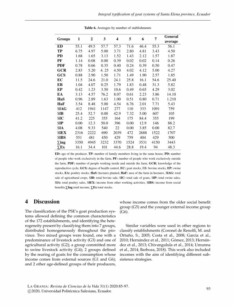
Integral typification of goat systems of Santa Elena province, Ecuador
Table 6. Averages by number of stablishments
Groups 1 2 3 4 5 6 7 Generalaverage
ED 55.1 49.5 57.7 57.3 71.6 46.4 55.3 56.1TP 6.75 4.97 5.00 3.71 2.80 4.81 3.43 4.50PD 1.68 1.65 3.13 1.52 1.43 2.12 1.57 1.87PF 1.14 0.08 0.00 0.39 0.02 0.02 0.14 0.26PDF 0.78 0.66 0.35 0.40 0.24 0.39 0.50 0.47GCR 2.83 5.20 4. 25 4.50 4.02 4.12 5.00 4.27GCS 0.88 2.90 1.50 1.71 1.49 1.90 2.57 1.85EC 11.5 24.6 21.0 24.1 25.8 16.1 54.6 25.40EB 1.04 4.07 0.25 1.79 1.83 0.48 31.3 5.82EP 0.42 1.23 3.50 10.6 0.49 0.65 4.29 3.02EA 3.13 4.57 76.2 8.07 0.61 2.23 3.86 14.10HaS 0.96 2.89 1.63 1.00 0.51 0.80 0.71 1.210HaF 3.54 8.48 5.00 4.54 6.76 2.01 7.71 5.43$IAG 412 1941 1147 277 110 333 1091 759$IB 25.4 52.7 0.00 42.9 7.32 5.00 607 105$IC 41.2 225 355 164 175 84.4 355 199$IP 0.00 12.3 50.0 396 0.00 12.9 146 88.2$IA 4.08 9.33 540 22 0.00 3.85 0.00 82.7$IEX 2316 2222 690 2039 472 2688 1522 1707$IBS 551 481 450 429 759 404 429 500∑ing 3350 4945 3232 3370 1524 3531 4150 3443∑Ex 16.1 34.4 101 44.6 28.8 19.4 94 48.3
ED: age of the producer, TP: number of family members living in the same house, PD: numberof people who work exclusively in the farm, PF: number of people who work exclusively outsidethe farm, PDF: number of people working inside and outside the farm, GCR: knowledge of thereproductive cycle, GCS: degree of health control, EC: goat stocks, EB: bovine stocks, EP: swinestocks, EA: poultry stocks, HaS: hectares planted, HaF: area of the farm in hectares, $IAG: totalsale of agricultural crops, $IB: total bovine sale, $IC: total sale of goats, $IP: total swine sales,$IA: total poultry sales, $IEX: income from other working activities, $IBS: income from socialbenefits,∑Ing total income, ∑Ex total stocks.
4 DiscussionThe classification of the PSE’s goat production sys-tems allowed defining the common characteristicsof the 172 establishments, and identifying the hete-rogeneity present by classifying them into 7 groups,distributed homogeneously throughout the pro-vince. Two mixed groups were found, one with apredominance of livestock activity (G3) and one ofagricultural activity (G2); a group committed moreto swine livestock activity (G4); 2 groups definedby the rearing of goats for the consumption whoseincome comes from external sources (G1 and G6);and 2 other age-defined groups of their producers,
whose income comes from the older social benefitgroup (G5) and the younger external income group(G6).
Similar variables were used in other regions toclassify establishments (Coronel de Renolfi, M. andOrtuño, S., 2005; Costa et al., 2008; Garcia et al.,2010; Hernández et al., 2011; Gómez, 2013; Hernán-dez et al., 2013; Chivangulula et al., 2014; Umunnaet al., 2014; Barboza, 2018). This work also includedincomes with the aim of identifying different sub-sistence strategies.
LA GRANJA: Revista de Ciencias de la Vida 31(1) 2020:85-97.c©2020, Universidad Politécnica Salesiana, Ecuador. 93
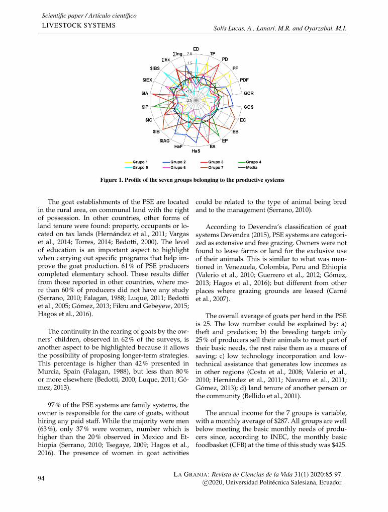
Scientific paper / Artículo científicoLIVESTOCK SYSTEMS Solís Lucas, A., Lanari, M.R. and Oyarzabal, M.I.
Figure 1. Profile of the seven groups belonging to the productive systems
The goat establishments of the PSE are locatedin the rural area, on communal land with the rightof possession. In other countries, other forms ofland tenure were found: property, occupants or lo-cated on tax lands (Hernández et al., 2011; Vargaset al., 2014; Torres, 2014; Bedotti, 2000). The levelof education is an important aspect to highlightwhen carrying out specific programs that help im-prove the goat production. 61% of PSE producerscompleted elementary school. These results differfrom those reported in other countries, where mo-re than 60% of producers did not have any study(Serrano, 2010; Falagan, 1988; Luque, 2011; Bedottiet al., 2005; Gómez, 2013; Fikru and Gebeyew, 2015;Hagos et al., 2016).
The continuity in the rearing of goats by the ow-ners’ children, observed in 62% of the surveys, isanother aspect to be highlighted because it allowsthe possibility of proposing longer-term strategies.This percentage is higher than 42% presented inMurcia, Spain (Falagan, 1988), but less than 80%or more elsewhere (Bedotti, 2000; Luque, 2011; Gó-mez, 2013).
97% of the PSE systems are family systems, theowner is responsible for the care of goats, withouthiring any paid staff. While the majority were men(63%), only 37% were women, number which ishigher than the 20% observed in Mexico and Et-hiopia (Serrano, 2010; Tsegaye, 2009; Hagos et al.,2016). The presence of women in goat activities
could be related to the type of animal being bredand to the management (Serrano, 2010).
According to Devendra’s classification of goatsystems Devendra (2015), PSE systems are categori-zed as extensive and free grazing. Owners were notfound to lease farms or land for the exclusive useof their animals. This is similar to what was men-tioned in Venezuela, Colombia, Peru and Ethiopia(Valerio et al., 2010; Guerrero et al., 2012; Gómez,2013; Hagos et al., 2016); but different from otherplaces where grazing grounds are leased (Carnéet al., 2007).
The overall average of goats per herd in the PSEis 25. The low number could be explained by: a)theft and predation; b) the breeding target: only25% of producers sell their animals to meet part oftheir basic needs, the rest raise them as a means ofsaving; c) low technology incorporation and low-technical assistance that generates low incomes asin other regions (Costa et al., 2008; Valerio et al.,2010; Hernández et al., 2011; Navarro et al., 2011;Gómez, 2013); d) land tenure of another person orthe community (Bellido et al., 2001).
The annual income for the 7 groups is variable,with a monthly average of $287. All groups are wellbelow meeting the basic monthly needs of produ-cers since, according to INEC, the monthly basicfoodbasket (CFB) at the time of this study was $425.
94LA GRANJA: Revista de Ciencias de la Vida 31(1) 2020:85-97.
c©2020, Universidad Politécnica Salesiana, Ecuador.
Integral typification of goat systems of Santa Elena province, Ecuador
The goat systems of the PSE have characteristicsof family rural systems, with a subsistence economywith less than 25 goats per herd, with monthly inco-mes that do not allow them to access the basic foodbasket; therefore, they do not cover the basic needsof the producers and their families. They are part ofthe the marginal category proposed by the Institu-to Nacional de Estadística y Censos (2010) and theMinisterio de Agricultura y Ganadería (2018). Ho-wever, they have knowledge and experience gainedover time in the management and care of biodiver-sity. The management of this biodiversity acquiredover years, as well as a set of knowledge and practi-ces, which is not easy to describe, should not disap-pear (Jarvis et al., 2011). Despite the low availabi-lity of assets and low levels of productivity, familyfarming is a major supplier of popular staple foods(FAO/BID, 2007; Hodges et al., 2014).
5 Conclusions
The goat production systems of the province of San-ta Elena have been classified for the first time. Theresults obtained in this research show that there isheterogeneity between the goat systems in SantaElena, and they are a contribution to take into ac-count when planning options to enhance their de-velopment.
Acknowledgment
The authors thank the Ministry of Higher Edu-cation, Science, Technology and Innovation (SE-NESCYT) and the State University of Santa Ele-na Peninsula (UPSE), by their financial support tocarry out this research.Also, to the goat producers who provided all the in-formation and allowed to enter in their farms.
References
Barboza, M. (2018). Caracterización de los sistemasde producción caprinos en la región huetar nortede costa rica.
Bedotti, D. (2000). Caracterización de los sistemas deproducción caprina en el Oeste pampeano (Argentina).Tesis doctoral, Córdoba, España.
Bedotti, D., Gómez, A., Sánchez, M., García, M.,and Martos, P. (2005). Aspectos sociológicos delos sistemas de producción caprina en el oes-te pampeano (argentina). Archivos de zootecnia,54(208):599–608. Online: https://bit.ly/2KULJFr.
Bellido, M., Escribano, M., Mesías, F., Rodríguez deLedesma, A., and Pulido, F. (2001). Sistemasextensivos de producción animal. Archivos deZootecnia, 50(192):465–489. Online: https://bit.ly/2GEdqOL.
Cabrera, D., García, A., Acero de la Cruz, R., Cas-taldo, A., Perea, J., and Peinado, J. (2004). Me-todología para la caracterización y tipificación desistemas ganaderos. Documentos de trabajo 1. Dpto.Producción Animal. Universidad de Córdoba, 1:Onli-ne: https://bit.ly/2UU6TrW.
Carné, S., Roig, N., and Jordana, J. (2007). La ca-bra blanca de rasquera: Caracterización estruc-tural de las explotaciones. Archivos de Zootecnia,56(213):43–54. Online: https://bit.ly/2W49Wu5.
Chivangulula, M., Torres, V., Varela, M., Morais, J.,Mario, J., and Sánchez, L. (2014). Characteriza-tion of the livestock production cooperative sys-tems in the municipality of caála, huambo pro-vince, republico f angola. Cuban Journal of Agri-cultural Science, 48(2):97. Online: https://bit.ly/2Wi0LGR.
Coronel de Renolfi, M. and Ortuño, S. (2005). Tipi-ficación de los sistemas productivos agropecua-rios en el área de riego de santiago del estero,argentina. Problemas del Desarrollo. Revista La-tinoamericana de economía, 36(140):64–88. Online:https://bit.ly/2ZtrClb.
Costa, R., Almeida, C., Pimenta, E., Holanda, E., andSantos, N. (2008). Caracterização do sistema deprodução caprino e ovino na região semi-árida doestado da paraíba, brasil. Archivos de Zootecnia,57(218):195–205. Online: https://bit.ly/2L05DPo.
Dallas, E. (2000). Métodos multivariados aplicados alanálisis de datos. International Thomson Editores,México.
Devendra, C. (2015). Dynamics of goat meat pro-duction in extensive systems in asia: Improve-ment of productivity and transformation of li-velihoods. Agrotechnoly, 4(1):131. Online: https://bit.ly/38Z81xP.
LA GRANJA: Revista de Ciencias de la Vida 31(1) 2020:85-97.c©2020, Universidad Politécnica Salesiana, Ecuador. 95
Scientific paper / Artículo científicoLIVESTOCK SYSTEMS Solís Lucas, A., Lanari, M.R. and Oyarzabal, M.I.
Di Rienzo, J., Casanoves, F., Balzarini, M., González,L., Tablada, M., and Robledo, C. (2008). Infostat,versión 2008, grupo infostat.
Dorji, J., Tamang, S., and Dorji, T. Y. (2017). Decli-ne of jakar sheep population in pastoral commu-nities of bhutan: A consequence of diminishingutility, alternate income opportunities and increa-sing challenges. Policy and Practice, 7(4):Online:https://bit.ly/2EEVyl9.
Dufumier, M. (1990). Importancia de la tipología deunidades de producción agrícolas en el análisis de diag-nóstico de realidades agrarias, pages 63– 81. Onli-ne: https://bit.ly/392KjAV. Red Internacional deMetodología de Investigación de Sistemas de Pro-ducción - RIMISP, Santiago de Chile.
Falagan, A. (1988). Caracterización productiva dela raza caprina murciana-granadina en la regiónde murcia. aspectos técnicos y sociales. TechnicalReport 63, Instituto Nacional de InvestigacionesAgrarias. Ministerio de Agricultura, Pesca y Ali-mentación, MAPA. Colección Monografías INIA.,Madrid.
FAO (2012). Phenotypic characterization of ani-mal genetic resources. fao animal production andhealth guidelines no. 11. rome.
FAO/BID (2007). Políticas para la agricultura fami-liar en américa latina. oficina regional de la faopara américa latina y el caribe.
Fikru, S. and Gebeyew, K. (2015). Sheep and goatproduction systems in degehabur zone, easternethiopia: Challenge and opportunities. Advancesin Dairy Research, 3(2):134. Online: https://bit.ly/2QkZiPa.
Garcia, A., Perea, J., Acero, R., Angón, E., Toro,P., Rodríguez, V., and Gómez, A. (2010). Ca-racterización estructural de los sistemas gana-deros de las dehesas andaluzas. Archivos deZootecnia, 59(228):577–588. Online: https://bit.ly/2DBCYKp.
Gómez, N. (2013). Caracterización estructural, morfo-lógica y genética de la población de cabras autóctonasde la región Apurímac del Perú. Tesis doctoral.
Greenacre, M. (1984). Theory and Applications of Co-rrespondence Analysis. Academic Press, London.
Guerrero, L., Tellezz, J., Vera, M., Garza, B., Rincón,J., Martínez, B., Serrano, N., and Vargas, J. (2012).Caracterización de los sistemas de producción ca-prinos presentes en el municipio de jordán, san-tander, colombia. AICA, 2:171–174. Online: https://bit.ly/2Wh6kFv.
Hagos, G., Kebede, K., Benerje, A., and Wolde, Z.(2016). On-farm phenotypic characterization ofbegait goat and their production system in wes-tern zone of tigray, ethiopia. International Journalof Research and Innovation is Earth Science, 3(1):15–20. Online: https://bit.ly/2Zwi1tE.
Hernández, J., Franco, F., Villarreal, O., Camacho,J., and Pedraza, R. (2011). Caracterización socio-económica y productiva de unidades caprinas fa-miliares en la mixteca poblana. redalyc, sistemade información científica, red de revistas científi-cas de américa latina, el caribe, españa y portu-gal. Archivos de Zootecnia, 60(230):175–182. Onli-ne: https://bit.ly/2Dy2ccN.
Hernández, P., Estrada, J., Avilés, F., Yong, G., Ló-pez, F., Solís, A., and Castelán, O. (2013). Tipifi-cación de los sistemas campesinos de producciónde leche del sur del estado de méxico. Universi-dad y Ciencia, Trópico húmedo, 29(1):19–31. Online:https://bit.ly/2voDOWB.
Hodges, J., Foggin, M., Long, R., and Zhaxi, G.(2014). Globalisation and the sustainability offarmers, livestock-keepers, pastoralists and fragi-le habitats. Biodiversity, 15(2-3):109–118. Online:https://bit.ly/35qpCeZ.
Instituto Nacional de Estadística y Censos (2010).Fascículo santa elena.
Jarvis, D., Padoch, C., and Cooper, D. (2011). Manejode la agrobiodiversidad en los ecosistemas agrícolas.
Lanari, M. R. (2004). Variación y diferenciación genéti-ca y fenotípica de la cabra criolla Neuquina en relacióncon su sistema rural campesino. Tesis doctoral.
Luque, C. (2011). Caracterización y evaluación delas razas caprinas autóctonas españolas de orientacióncárnica. Tesis doctoral.
Macías, A. (2015). Propuesta de mejoramiento en la ges-tión de pequeños productores caprinos en Capitanejo,Santander. Doctoral dissertation.
96LA GRANJA: Revista de Ciencias de la Vida 31(1) 2020:85-97.
c©2020, Universidad Politécnica Salesiana, Ecuador.
Integral typification of goat systems of Santa Elena province, Ecuador
Ministerio de Agricultura y Ganadería (2018). En-trega de nombramiento a los cabildos comunaleselectos para el periodo 2018. online: https://bit.ly/2kFfT3j.
Navarro, M., Fernández, G., and Perezgrovas, R.(2011). Characterization of majorera goat produc-tion systems in the canary islands. in bernués a.(ed.), boutonnet j.p. (ed.), casasús i. (ed.), chen-touf m. (ed.), gabiña d. (ed.), joy m. (ed.), lópez-francos a. (ed.), morand-fehr p. (ed.), pacheco f.(ed.). economic, social and environmental sustai-nability in sheep and goat production systems.zaragoza: Ciheam /fao/cita-dga. 205-210. Op-tions Méditerranéennes: Série A. Séminaires Médite-rranéens, (100):Online: https://bit.ly/2vjW8A3.
Núñez-Domínguez, R., Ramírez-Valverde, R.,Saavedra-Jiménez, L. A., and García-Muñiz,J. G. (2016). La adaptabilidad de los recur-sos zoogenéticos criollos, base para enfrentarlos desafíos de la producción animal. Ar-chivos de Zootecnia, 65(251):461–468. Online:https://bit.ly/2QPVGEa.
Peña, D. (2002). Análisis de Datos Multivariante. McGraw-Hill, España.
Robinson, T. P., Thornton, P. K., Franceschini, G.,Kruska, R. L., Chiozza, F., Notenbaert, A., Cec-chi, G., Herrero, M., Epprecht, M., Fritz, S., You,L., Conchedda, G., and See, L. (2011). Global li-vestock production systems. FAO & ILRI, pageOnline: https://bit.ly/35i8cBf.
Serrano, M. (2010). Análisis del sistema de produc-ción de cabras con fines lecheros en la región delibres, puebla. Tesis de maestría, México.
Sistema Nacional de Información (2018). Encuestade superficie y producción agropecuaria continua(espac) 2004-2013.
Torres, P. (2014). Caracterização e modelagem dossistemas de produção de caprinos leiteiros. Mas-ter’s thesis, Macaíba/RN – Brasil.
Tsegaye, T. (2009). Characterization of goat pro-duction systems and on-farm evaluation of thegrowth performance of grazing goats supple-mented with different protein sources in mete-ma woreda, amhara region, ethiopia. M.sc. thesis,science in agriculture (animal nutrition).
Umunna, M., Olafadehan, O., and Arowona, A.(2014). Small rumiant production and manage-ment systems in urban area of southern guineasavanna of nigeria. Asian Journal of Agricultu-re and Food Science, 2(2):107–114. Online: https://bit.ly/2ZIh8hW.
Valerio, D., García, A., Acero, R., Perea, J., and Ta-pia, M. an Romero, M. (2010). Caracterizaciónestructural del sistema ovino-caprino de la re-gión noroeste de república dominicana. Archi-vos de Zootecnia, 59(227):333–343. Online: https://bit.ly/2QIiPIy.
Vargas, J., Serrano, C., Martínez, D., Rodríguez, G.,and Zaragoza, L. (2014). Caracterización de lossistemas de producción caprina en el municipiode aratoca, santander sobre la cuenca del río chi-camocha. AICA, 4:234–236. Online: https://bit.ly/2vj794B.
Ward, H. (1963). Hierarchical grouping to optimi-ze an objective function. Journal of the AmericanStatistical Association, 58:236–244. Online: https://bit.ly/2ZwusFX.
LA GRANJA: Revista de Ciencias de la Vida 31(1) 2020:85-97.c©2020, Universidad Politécnica Salesiana, Ecuador. 97
Scientific paper/ Artículo científico
VETERINARY SCIENCESpISSN:1390-3799; eISSN:1390-8596
http://doi.org/10.17163/lgr.n31.2020.07
META-ANALYSIS OF THE EFFECT OF GLUTAMINE DIETARY
INCLUSION ON PRODUCTIVE PERFORMANCE IN PIGLETS
META-ANÁLISIS DEL EFECTO DE LA INCLUSIÓN ALIMENTICIA DE GLUTAMINA
SOBRE EL DESEMPEÑO PRODUCTIVO EN LECHONES
Jimmy Rolando Quisirumbay Gaibor
Faculty of Veterinary Medicine and Zootechnics. Central University of Ecuador, Av. Universitaria, Quito, 170129, Ecuador.
*Corresponding author: [email protected]
Article received on April 21th, 2019. Accepted, after review, on January 24th, 2020. Published on March 1st, 2020.
Resumen
La glutamina no es considerada un aminoácido esencial; sin embargo, juega un rol importante en la salud y cre-cimiento de neonatos y adultos. En lechones el destete genera atrofia de las vellosidades intestinales y retraso enel crecimiento. Varios trabajos han demostrado que la suplementación de glutamina (0,2-2%) disminuye los efectosadversos del estrés post-destete en lechones. El objetivo de este manuscrito fue evaluar el tamaño de efecto de la su-plementación de glutamina sobre el rendimiento productivo de lechones, la consistencia de su efecto y la influenciade otros factores mediante el uso de meta-análisis. La administración de glutamina mejora la conversión alimenticia(p < 0,001), y los lechones que reciben glutamina convierten mejor el alimento cuando la suplementación duró entre7 a 14 días (p = 0,0023), pues requieren 121,6 g menos de alimento en comparación con el grupo control para hacer1 kg de peso vivo. Cuando la suplementación se realiza por un periodo de 15 a 30 días y 7 a 30 días, el ahorro dealimento es de 70,6 g (p < 0,001) y 87,3 g (p < 0,001) por kg de peso vivo respectivamente. La ganancia diaria de pesoes superior en 20,3 g/día (p = 0,0029) frente al grupo control entre los 7 a 30 días de suplementación y de 28,2 g/día(p = 0,0002) entre los 15 a 30 días. La edad y peso del lechón al inicio de la suplementación, el nivel de lisina, laproteína cruda y el número de repeticiones por tratamiento influyen en el efecto de la glutamina sobre las variablesevaluadas.Palabras clave: nutrición, dieta, nutrientes, aminoácidos, cerdos
Abstract
Glutamine is not considered an essential amino acid; however, it plays an important role in the health and growthof neonates and adults. In piglets, weaning generates atrophy of the intestinal villi and growth retardation. Several
98LA GRANJA: Revista de Ciencias de la Vida 31(1) 2020:98-110.c©2020, Universidad Politécnica Salesiana, Ecuador.
Meta-analysis of the effect of glutamine dietary inclusion on productive performance in piglets
studies have shown that glutamine supplementation (0.2-2%) decreases the adverse effects of post-weaning stressin piglets. The aim of this article was to evaluate the effect size of glutamine supplementation on the productiveperformance of piglets, the consistency of their effect and the influence of other factors through the use of meta-analysis. The administration of glutamine improves the feed conversion (p <0.001), the piglets that receive glutamineconvert the feed better when the supplementation lasted between 7 to 14 days (p =0.0023), since they require 121.6 gless of feed in comparison with the control group to make 1 kg of body weight. When the supplementation is done fora period of 15 to 30 days and 7 to 30 days, the saving of feed is 70.6 g (p <0.001) and 87.3 g (p <0.001) per kg of bodyweight, respectively. The daily weight gain is higher in 20.3 g/day (p = 0.0029) compared to the control group between7 to 30 days of supplementation and 28.2 g/day (p = 0.0002) between 15 to 30 days. Age and weight of the piglet at thebeginning of the supplementation, level of lysine, crude protein and the number of repetitions per treatment influenceon the effect of glutamine on the variables evaluated.Keywords: nutrition, diet, nutrients, amino acids, pigs
Suggested citation: Quisirumbay Gaibor, J.R. (2020). Meta-analysis of the effect of glutamine dietary inclu-sion on productive performance in piglets. La Granja: Revista de Ciencias de la Vida.Vol. 31(1):98-110. http://doi.org/10.17163/lgr.n31.2020.07.
Orcid IDs:Jimmy Rolando Quisirumbay Gaibor: http://orcid.org/ 0000-0001-8938-9849
LA GRANJA: Revista de Ciencias de la Vida 31(1) 2020:98-110.c©2020, Universidad Politécnica Salesiana, Ecuador. 99
Scientific paper / Artículo científicoVETERINARY SCIENCES Quisirumbay Gaibor, J.R.
1 IntroductionWetting, stress by transportation and thermal stressincrease the incidence of diseases, especially whenthey occur simultaneously (Varley and Wiseman,2001). During the weaning process, stress can beinduced by separation of the mother’s piglet, relo-cation and mixture of litters, additionally there maybe sudden changes in the diet that reduce or elimi-nate the food consumption in the first few hoursof life (Wijtten et al., 2011; Campbell et al., 2013).Stress during weaning alters the development of thebarrier functions of the gastro-intestinal tract thatleads to permanent harmful consequences for intes-tinal health during the life of the pig (Moeser et al.,2017; Pluske et al., 2018). To combat the negative ef-fects of weaning on the health of piglet, several stra-tegies have been implemented, including weaningage management, environmental conditioning, nu-tritional manipulation and antibiotic use through adiet (Lalles et al., 2007; Gresse et al., 2017; Solà-Orioland Gasa, 2017). Antibiotics applied in the diet mayallow weaned piglet to reduce pathogenic burdenand promote growth (Cromwell, 2002). However,due to the possible contribution of antibiotics to thedevelopment of antibiotic-resistant bacterial lines(Smith et al., 2010), their use is being limited. Glu-tamine dietary supplementation decreases healthproblems, prevents intestinal atrophy, maintainsantioxidant status, decreases incidence of diarrhea,resulting in increased weight gain and improvedefficiency (Haynes et al., 2009; Zhong et al., 2011;Wang et al., 2014; Watford, 2015). Similar resultshave also been reported in broiler chicken (NassiriMoghaddam and Alizadeh-Ghamsari, 2013; Jazi-deh et al., 2014; Nascimento et al., 2014; Manvaileret al., 2015; Muro et al., 2015; Olubodun et al., 2015;Ribeiro Jr et al., 2015; Luquetti et al., 2016; Maiorkaet al., 2016; Namroud et al., 2017).
Glutamine is the preferred fuel of intestinal cellsand the immune system (Horio et al., 2008; Sakiya-ma et al., 2009; Zhong et al., 2012), supplementationof this amino acid aims to maintain intestinal fun-ction through weaning (Curi et al., 2007). Researchshows that glutamine is an amino acid that is abun-dant in physiological fluids and body proteins andis a regulator of the genetic expression (Wu et al.,2011; Xi et al., 2011). Glutamine serves as an energysubstrate for rapidly dividing cells and the cons-truction of polypeptides and proteins (Rhoads andWu, 2009), as it is an essential precursor of bioactive
molecules (Boza et al., 2000). Endogenous produc-tion of Gln in mammals is insufficient during ad-verse conditions and there is evidence that Gln sup-plementation may be necessary in feeding younganimals during states of poor nutrition (Wu et al.,1996; Chamorro et al., 2010). Numerous studies ha-ve investigated glutamine dietary supplementationin order to improve the productive performance ofthe piglet. However, several have been the levels ofdietary inclusion and experimental circumstancesunder which these studies have been developed.
The aim of this article was to evaluate the size ofGln supplementation on the productive yield of pi-glets, the consistency of its effect and the influenceof other factors by using the statistical meta-analysistool.
2 Materials and methods
2.1 Source of information (data)An electronic search of scientific articles was con-ducted in double-blind peer-reviewed indexed jour-nals in the following electronic bases: CAB direct,Elsevier biobase-CABS, Google Scholar, MEDLINE,PubMed, Science Direct (Journal), Scopus, Acade-mic Search Complete, CAB Abstract, Directory ofOpen Access Journals. A combination of keywordswas used: glutamine, amino acids, diet, food, nutri-tion, piglets, weaning and their English equivalents,without date restrictions.
2.2 Inclusion criteriaItems in which glutamine was administered ex-clusively in piglets through a diet were selected.The articles had to include information regardingthe number of experimental units (replications) pertreatment, and the experiments needed include atleast 2 treatments (including the control group: wit-hout Gln), weight and age of the piglet at the be-ginning of the study period, level of glutamine in-cluded in the food and duration of supplementa-tion, level of lysine and raw protein in the foodused (covariates). In addition, it should have inclu-ded at least one of the interest response variables:daily weight gain (GDP), average daily food con-sumption (CDPA), and food conversion (CA). Theyshould include mean (average) and some measu-re of variation (standard deviation (SD), standarderror (SE)).
100LA GRANJA: Revista de Ciencias de la Vida 31(1) 2020:98-110.
c©2020, Universidad Politécnica Salesiana, Ecuador.
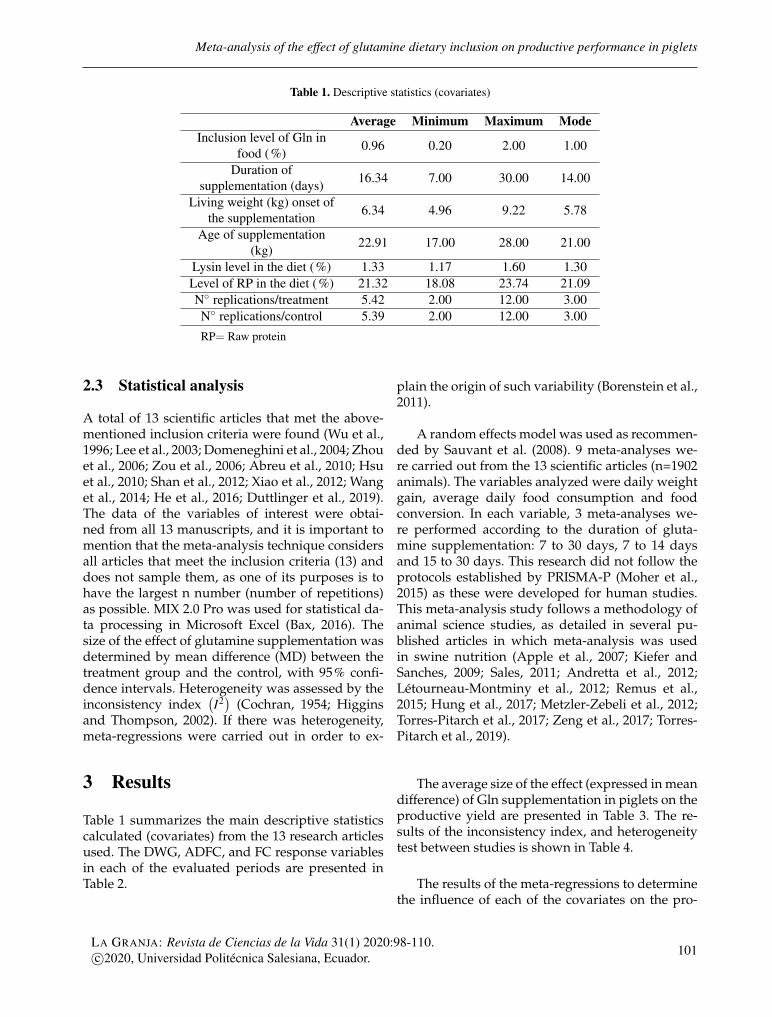
Meta-analysis of the effect of glutamine dietary inclusion on productive performance in piglets
Table 1. Descriptive statistics (covariates)
Average Minimum Maximum ModeInclusion level of Gln in
food (%) 0.96 0.20 2.00 1.00
Duration ofsupplementation (days) 16.34 7.00 30.00 14.00
Living weight (kg) onset ofthe supplementation 6.34 4.96 9.22 5.78
Age of supplementation(kg) 22.91 17.00 28.00 21.00
Lysin level in the diet (%) 1.33 1.17 1.60 1.30Level of RP in the diet (%) 21.32 18.08 23.74 21.09N◦ replications/treatment 5.42 2.00 12.00 3.00N◦ replications/control 5.39 2.00 12.00 3.00RP= Raw protein
2.3 Statistical analysis
A total of 13 scientific articles that met the above-mentioned inclusion criteria were found (Wu et al.,1996; Lee et al., 2003; Domeneghini et al., 2004; Zhouet al., 2006; Zou et al., 2006; Abreu et al., 2010; Hsuet al., 2010; Shan et al., 2012; Xiao et al., 2012; Wanget al., 2014; He et al., 2016; Duttlinger et al., 2019).The data of the variables of interest were obtai-ned from all 13 manuscripts, and it is important tomention that the meta-analysis technique considersall articles that meet the inclusion criteria (13) anddoes not sample them, as one of its purposes is tohave the largest n number (number of repetitions)as possible. MIX 2.0 Pro was used for statistical da-ta processing in Microsoft Excel (Bax, 2016). Thesize of the effect of glutamine supplementation wasdetermined by mean difference (MD) between thetreatment group and the control, with 95% confi-dence intervals. Heterogeneity was assessed by theinconsistency index
(I2)
(Cochran, 1954; Higginsand Thompson, 2002). If there was heterogeneity,meta-regressions were carried out in order to ex-
plain the origin of such variability (Borenstein et al.,2011).
A random effects model was used as recommen-ded by Sauvant et al. (2008). 9 meta-analyses we-re carried out from the 13 scientific articles (n=1902animals). The variables analyzed were daily weightgain, average daily food consumption and foodconversion. In each variable, 3 meta-analyses we-re performed according to the duration of gluta-mine supplementation: 7 to 30 days, 7 to 14 daysand 15 to 30 days. This research did not follow theprotocols established by PRISMA-P (Moher et al.,2015) as these were developed for human studies.This meta-analysis study follows a methodology ofanimal science studies, as detailed in several pu-blished articles in which meta-analysis was usedin swine nutrition (Apple et al., 2007; Kiefer andSanches, 2009; Sales, 2011; Andretta et al., 2012;Létourneau-Montminy et al., 2012; Remus et al.,2015; Hung et al., 2017; Metzler-Zebeli et al., 2012;Torres-Pitarch et al., 2017; Zeng et al., 2017; Torres-Pitarch et al., 2019).
3 Results
Table 1 summarizes the main descriptive statisticscalculated (covariates) from the 13 research articlesused. The DWG, ADFC, and FC response variablesin each of the evaluated periods are presented inTable 2.
The average size of the effect (expressed in meandifference) of Gln supplementation in piglets on theproductive yield are presented in Table 3. The re-sults of the inconsistency index, and heterogeneitytest between studies is shown in Table 4.
The results of the meta-regressions to determinethe influence of each of the covariates on the pro-
LA GRANJA: Revista de Ciencias de la Vida 31(1) 2020:98-110.c©2020, Universidad Politécnica Salesiana, Ecuador. 101
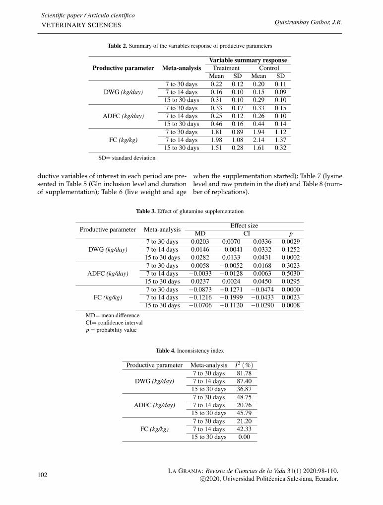
Scientific paper / Artículo científicoVETERINARY SCIENCES Quisirumbay Gaibor, J.R.
Table 2. Summary of the variables response of productive parameters
Productive parameter Meta-analysisVariable summary response
Treatment ControlMean SD Mean SD
DWG (kg/day)7 to 30 days 0.22 0.12 0.20 0.117 to 14 days 0.16 0.10 0.15 0.09
15 to 30 days 0.31 0.10 0.29 0.10
ADFC (kg/day)7 to 30 days 0.33 0.17 0.33 0.157 to 14 days 0.25 0.12 0.26 0.10
15 to 30 days 0.46 0.16 0.44 0.14
FC (kg/kg)7 to 30 days 1.81 0.89 1.94 1.127 to 14 days 1.98 1.08 2.14 1.37
15 to 30 days 1.51 0.28 1.61 0.32SD= standard deviation
ductive variables of interest in each period are pre-sented in Table 5 (Gln inclusion level and durationof supplementation); Table 6 (live weight and age
when the supplementation started); Table 7 (lysinelevel and raw protein in the diet) and Table 8 (num-ber of replications).
Table 3. Effect of glutamine supplementation
Productive parameter Meta-analysis Effect sizeMD CI p
DWG (kg/day)7 to 30 days 0.0203 0.0070 0.0336 0.00297 to 14 days 0.0146 −0.0041 0.0332 0.1252
15 to 30 days 0.0282 0.0133 0.0431 0.0002
ADFC (kg/day)7 to 30 days 0.0058 −0.0052 0.0168 0.30237 to 14 days −0.0033 −0.0128 0.0063 0.5030
15 to 30 days 0.0237 0.0024 0.0450 0.0295
FC (kg/kg)7 to 30 days −0.0873 −0.1271 −0.0474 0.00007 to 14 days −0.1216 −0.1999 −0.0433 0.0023
15 to 30 days −0.0706 −0.1120 −0.0290 0.0008MD= mean differenceCI= confidence intervalp = probability value
Table 4. Inconsistency index
Productive parameter Meta-analysis I2 (%)
DWG (kg/day)7 to 30 days 81.787 to 14 days 87.4015 to 30 days 36.87
ADFC (kg/day)7 to 30 days 48.757 to 14 days 20.7615 to 30 days 45.79
FC (kg/kg)7 to 30 days 21.207 to 14 days 42.3315 to 30 days 0.00
102LA GRANJA: Revista de Ciencias de la Vida 31(1) 2020:98-110.
c©2020, Universidad Politécnica Salesiana, Ecuador.

Meta-analysis of the effect of glutamine dietary inclusion on productive performance in piglets
4 Discussion
Glutamine works as an energy source for thegrowth of enterocytes, thus reducing the intestinalwall atrophy and the damage of the intestinal epit-helium (Wang et al., 2014, 2015). Piglets receivingGln food supplementation improve the protectionof the intestinal barrier which leads to increasedresistance to pathogens (Peng et al., 2004), and in-creased activity of digestive enzymes (Shan et al.,2012), consequently the increased nutrient utiliza-tion and the improvement in the productive perfor-mance (Jiang et al., 2009; Johnson and Lay Jr, 2017).The above can be seen in this research paper, as itwas found that the food supplementation of Glnimproved (p <0.001) the food conversion into pi-glets in any of the periods evaluated. It emphasizesthat the piglets that receive Gln convert the foodbetter when supplementation lasted between 7 to14 days (MD= −0.1216; p =0.0023). Supplementedpiglets require 121.6 g less food compared to thecontrol group to make 1 kg of body weight between7 to 14 days. When supplementation was done fora longer period (15 to 30 days) the food savings are70.6 g to make a kg of body weight and 87.3 g when
the Gln was supplemented between 7 to 30 days.With regard to the daily weight gain, Gln causes anincrease in gain of 20.3 g/day (p =0.0029) over theDWG of the control group between 7 and 30 daysof supplementation, and 28.2 g/day (p =0.0002) bet-ween 15 to 30 days.
The ADFC variable only has a significant increa-se when Gln administration was 15 to 30 days, con-suming an additional 23.7 grams per day comparedto the witness group. Similarly, in broiler chickensit was found that food supplementation of glutami-ne allows a more efficient use of ingested nutrients,improving the productive performance (Namroudet al., 2017), associated with the effect of Gln on thelength of intestinal villi (Abdulkarimi et al., 2019).This will require less food to lead pigs to the mar-ket weight or shorten the days needed to reach themarket weight, representing significant savings forthe pig industry. In addition, Gln supplementationhas shown to favor the immune system of pigletsby ensuring better health and thus preserving nu-trients for growth (Johnson et al., 2006; Zhong et al.,2012).
Table 5. Meta-regression for Gln inclusion level (%) duration of supplementation (days)
Productiveparameter
Meta-regression
Gln inclusion level (%) Duration of supplementation (days)Intercept Regression Coef. Intercept Regression Coef.
Estimated p Estimated p Estimated p Estimated p
DWG(kg/day)
7 to 30 days 0.024 0.007 0.006 0.503 0.041 <0.001 −0.001 0.0027 to 14 days 0.025 0.010 0.005 0.578 0.094 <0.001 −0.007 <0.00115 to 30 days 0.014 0.505 0.011 0.577 0.121 0.002 −0.004 0.013
ADFC(kg/day)
7 to 30 days 0.003 0.762 −0.003 0.737 −0.019 0.002 0.002 <0.0017 to 14 days 0.004 0.700 −0.010 0.372 −0.025 0.064 0.002 0.11715 to 30 days 0.048 0.176 −0.025 0.475 0.097 0.018 −0.003 0.069
FC(kg/kg)
7 to 30 days −0.050 0.044 −0.021 0.434 −0.063 0.143 −0.0002 0.9277 to 14 days −0.050 0.051 −0.025 0.456 −0.260 0.260 0.015 0.39015 to 30 days −0.054 0.599 −0.016 0.873 −0.080 0.638 0.0004 0.953
p = probability value
Regarding the heterogeneity between studies,it is reported that only in DWG (7 to 30d and 7 to14d) the variability is high (> 75%). In the other va-riables, heterogeneity is between low to moderate(< 50%). In order to explain the variability betweenstudies, meta-regressions were performed betweenthe response variable and each of the co-variablesindicated above. Gln inclusion level (%) in the diet
for piglets has no impact (p>0.05) on any of the pro-ductive variables evaluated. The most commonlyused level is 1%; however, the values range from0.1 a 2%. Studies in chicken report that supplemen-tation of high levels of glutamine negatively affectsthe production performance because they cause areduction in the food consumption, as shown inthe results found when a 4% level was used. Ad-
LA GRANJA: Revista de Ciencias de la Vida 31(1) 2020:98-110.c©2020, Universidad Politécnica Salesiana, Ecuador. 103
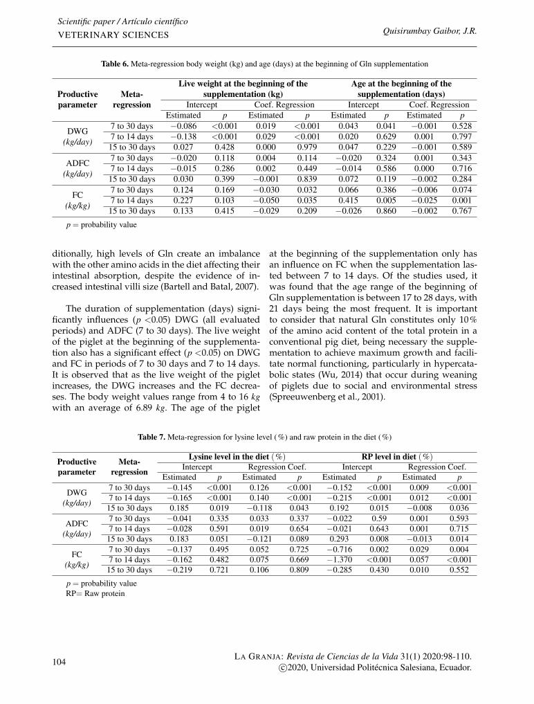
Scientific paper / Artículo científicoVETERINARY SCIENCES Quisirumbay Gaibor, J.R.
Table 6. Meta-regression body weight (kg) and age (days) at the beginning of Gln supplementation
Productiveparameter
Meta-regression
Live weight at the beginning of thesupplementation (kg)
Age at the beginning of thesupplementation (days)
Intercept Coef. Regression Intercept Coef. RegressionEstimated p Estimated p Estimated p Estimated p
DWG(kg/day)
7 to 30 days −0.086 <0.001 0.019 <0.001 0.043 0.041 −0.001 0.5287 to 14 days −0.138 <0.001 0.029 <0.001 0.020 0.629 0.001 0.797
15 to 30 days 0.027 0.428 0.000 0.979 0.047 0.229 −0.001 0.589
ADFC(kg/day)
7 to 30 days −0.020 0.118 0.004 0.114 −0.020 0.324 0.001 0.3437 to 14 days −0.015 0.286 0.002 0.449 −0.014 0.586 0.000 0.716
15 to 30 days 0.030 0.399 −0.001 0.839 0.072 0.119 −0.002 0.284
FC(kg/kg)
7 to 30 days 0.124 0.169 −0.030 0.032 0.066 0.386 −0.006 0.0747 to 14 days 0.227 0.103 −0.050 0.035 0.415 0.005 −0.025 0.001
15 to 30 days 0.133 0.415 −0.029 0.209 −0.026 0.860 −0.002 0.767
p = probability value
ditionally, high levels of Gln create an imbalancewith the other amino acids in the diet affecting theirintestinal absorption, despite the evidence of in-creased intestinal villi size (Bartell and Batal, 2007).
The duration of supplementation (days) signi-ficantly influences (p <0.05) DWG (all evaluatedperiods) and ADFC (7 to 30 days). The live weightof the piglet at the beginning of the supplementa-tion also has a significant effect (p <0.05) on DWGand FC in periods of 7 to 30 days and 7 to 14 days.It is observed that as the live weight of the pigletincreases, the DWG increases and the FC decrea-ses. The body weight values range from 4 to 16 kgwith an average of 6.89 kg. The age of the piglet
at the beginning of the supplementation only hasan influence on FC when the supplementation las-ted between 7 to 14 days. Of the studies used, itwas found that the age range of the beginning ofGln supplementation is between 17 to 28 days, with21 days being the most frequent. It is importantto consider that natural Gln constitutes only 10%of the amino acid content of the total protein in aconventional pig diet, being necessary the supple-mentation to achieve maximum growth and facili-tate normal functioning, particularly in hypercata-bolic states (Wu, 2014) that occur during weaningof piglets due to social and environmental stress(Spreeuwenberg et al., 2001).
Table 7. Meta-regression for lysine level (%) and raw protein in the diet (%)
Productiveparameter
Meta-regression
Lysine level in the diet (%) RP level in diet (%)Intercept Regression Coef. Intercept Regression Coef.
Estimated p Estimated p Estimated p Estimated p
DWG(kg/day)
7 to 30 days −0.145 <0.001 0.126 <0.001 −0.152 <0.001 0.009 <0.0017 to 14 days −0.165 <0.001 0.140 <0.001 −0.215 <0.001 0.012 <0.001
15 to 30 days 0.185 0.019 −0.118 0.043 0.192 0.015 −0.008 0.036
ADFC(kg/day)
7 to 30 days −0.041 0.335 0.033 0.337 −0.022 0.59 0.001 0.5937 to 14 days −0.028 0.591 0.019 0.654 −0.021 0.643 0.001 0.715
15 to 30 days 0.183 0.051 −0.121 0.089 0.293 0.008 −0.013 0.014
FC(kg/kg)
7 to 30 days −0.137 0.495 0.052 0.725 −0.716 0.002 0.029 0.0047 to 14 days −0.162 0.482 0.075 0.669 −1.370 <0.001 0.057 <0.001
15 to 30 days −0.219 0.721 0.106 0.809 −0.285 0.430 0.010 0.552
p = probability valueRP= Raw protein
104LA GRANJA: Revista de Ciencias de la Vida 31(1) 2020:98-110.
c©2020, Universidad Politécnica Salesiana, Ecuador.

Meta-analysis of the effect of glutamine dietary inclusion on productive performance in piglets
Table 8. Meta-regression number of replications
Productiveparameter
Meta-regression
Number of replicationsIntercept Regression Coef.
Estimated p Estimated p
DWG (kg/day)7 to 30 days −0.006 0.143 0.005 <0.0017 to 14 days −0.010 0.022 0.006 <0.00115 to 30 days 0.030 0.071 −0.001 0.819
ADFC (kg/day)7 to 30 days 0.008 0.209 −0.002 0.1537 to 14 days 0.006 0.393 −0.003 0.07915 to 30 days 0.064 <0.001 −0.009 0.024
FC (kg/kg)7 to 30 days −0.036 0.211 −0.007 0.2457 to 14 days −0.032 0.313 −0.009 0.19915 to 30 days −0.070 0.384 0.001 0.972
p = probability value
Dietary formulation factors also have significanteffect on DWG, ADFC and FC after the Gln supple-mentation in piglets. The level of lysine (p <0.05)and raw protein (p <0.05) affects DWG over the 3periods evaluated. It is evident that as the level oflysine and RP increases the DWG also increases forthe periods 7 to 30 days and 7 to 14 days. Howe-ver, in the period 15 to 30 days there is a reduc-tion in the DWG. In addition, the RP level affectsADFC when supplementation lasted between 15and 30 days (p =0.014) and FC when Gln adminis-tration was from 7 to 30 days (p =0.004) and 7 to14 days (p <0.001). In this work, the RP and lysinevalues of the diets used in piglets were between 18to 23% and 1.17 a 1.6%, respectively. One strategyto improve the use of protein in piglets and preventintestinal disorders is to reduce the level of rawprotein with adequate free amino acid supplemen-tation (synthetic) (Le Floc’h et al., 2018).
Gloaguen et al. (2014) confirms the effectivenessof this strategy and the possibility of formulatingdiets with low RP levels (13.5%) piglets between 10and 20 kg of body weight. Additionally, diets withmoderate protein restriction (13-15.3%) proved tobe beneficial for the health of the gut microbiota,metabolic activity in the large intestine and for theimprovement in the function of the piglet intesti-nal barrier (Peng et al., 2017). The reduction of RPcontent allows to reduce the nitrogen consumptionand prevents the excess of amino acids, therefore,prevents metabolic overloads.
Finally, the number of replications influenced
the DWG in the periods 7 to 30 (p<0.001) and 7 to 14days (p <0.001), as well as the ADFC when supple-mentation lasted between 15 and 30 days (p=0.024).The number of replications in the different worksused for this study ranged from 2 to 12, 3 beingthe most used. This confirms the importance statedby Aaron and Hays (2004) of considering an appro-priate number of individuals to be used in experi-mental studies in pigs. In the face of an inadequa-te number of replications per treatment, significantdifferences may not be detected, leading to a wasteof time and money for the researcher.
5 Conclusion
Glutamine supplementation improves the produc-tive performance in piglets, being an excellent op-tion to be used in weaning diets to reduce the stressoccurring in this stage.
ReferencesAaron, D. K. and Hays, V. W. (2004). How
many pigs? statistical power considerations inswine nutrition experiments. Journal of animalscience, 82(13):E245–E254. Onine: https://bit.ly/2GxHTxP.
Abdulkarimi, R., Shahir, M. H., and Daneshyar,M. (2019). Effects of dietary glutamine and ar-ginine supplementation on performance, intesti-nal morphology and ascites mortality in broilerchickens reared under cold environment. Asian-
LA GRANJA: Revista de Ciencias de la Vida 31(1) 2020:98-110.c©2020, Universidad Politécnica Salesiana, Ecuador. 105

Scientific paper / Artículo científicoVETERINARY SCIENCES Quisirumbay Gaibor, J.R.
Australasian Journal of Animal Sciences, 32(1):110–117. Online: https://bit.ly/38e5UWF.
Abreu, M., Donzele, J., Oliveira, R., Fortes, E., andGraña, G. (2010). Glutamina, nucleotídeos e plas-ma suíno em rao̧ões para leitões desmamados.R. Bras. Zootec, 39(3):520–525. Online: https://bit.ly/2IyrJX9.
Andretta, I., Kipper, M., Lehnen, C. R., Demori,A. B., Remus, A., and Lovatto, P. A. (2012). Meta-analysis of the relationship between ractopamineand dietary lysine levels on carcass characteris-tics in pigs. Livestock Science, 143(1):91–96. Online:https://bit.ly/2Ls5sKy.
Apple, J. K., Rincker, P. J., McKeith, F. K., Carr, S. N.,Armstrong, T. A., and Matzat, P. D. (2007). Meta-analysis of the ractopamine response in finishingswine. The Professional Animal Scientist, 23(3):179–196. Online: https://bit.ly/2OVJkdF.
Bartell, S. M. and Batal, A. B. (2007). The effect ofsupplemental glutamine on growth performan-ce, development of the gastrointestinal tract, andhumoral immune response of broilers. PoultryScience, 86(9):1940–1947. Online: https://bit.ly/2T39mN0.
Bax, L. (2016). Mix 2.0 -professional software formeta-analysis in excel. version 2.0. biostatxl.
Borenstein, M., Hedges, L. V., Higgins, J. P., andRothstein, H. R. (2011). Introduction to meta-analysis. John Wiley & Sons, Chichester.
Boza, J. J., Moënnoz, D., Bournot, C. E., Blum, S.,Zbinden, I., Finot, P. A., and Ballèvre, O. (2000).Role of glutamine on the de novo purine nucleo-tide synthesis in caco-2 cells. European journalof nutrition, 39(1):38–46. Online: https://bit.ly/2Iyrs6W.
Campbell, J. M., Crenshaw, J. D., and Polo, J. (2013).The biological stress of early weaned piglets. Jour-nal of animal science and biotechnology, 4(19):Onli-ne: https://bit.ly/2Xt1EfN.
Chamorro, S., De Blas, C., Grant, G., Badiola, I.,Menoyo, D., and Carabaño, R. (2010). Effectof dietary supplementation with glutamine anda combination of glutamine-arginine on intesti-nal health in twenty-five-day-old weaned rab-bits. Journal of animal science, 88(1):170–180. On-line: https://bit.ly/2Pjt5px.
Cochran, W. G. (1954). The combination of es-timates from different experiments. Biometrics,10(1):101–129. Online:https://bit.ly/2UO6QOc.
Cromwell, G. L. (2002). Why and how antibioticsare used in swine production. Animal biotechno-logy, 13(1):7–27. Online: https://bit.ly/2UKuX0q.
Curi, R., Newsholme, P., Procopio, J., Lagranha,C., Gorjão, R., and Pithon-Curi, T. C. (2007).Glutamine, gene expression, and cell function.Front Biosci, 12(1):344–357. Online: https://bit.ly/2VZD4mu.
Domeneghini, C., Di Giancamillo, A., Savoini, G.,Paratte, R., Bontempo, V., and Dell Orto, V. (2004).Structural patterns of swine ileal mucosa follo-wing l-glutamine and nucleotide administrationduring the weaning period. an histochemical andhistometrical study. Histology and Histopathology,19(1):49–58. Online: https://bit.ly/2GxXIEY.
Duttlinger, A. W., Kpodo, K. R., Lay, D. C., Richert,B. T., and Johnson, J. S. (2019). Replacing die-tary antibiotics with 0.20diets: Impact on healthand productivity of pigs following weaning andtransport. Journal of Animal Science, 97:2035–2052.Online: https://bit.ly/2VXZTa3.
Gloaguen, M., Le Floc’h, N., Corrent, E., Primot,Y., and Van Milgen, J. (2014). The use of freeamino acids allows formulating very low crudeprotein diets for piglets. Journal of animal science,92(2):637–644. Online: https://bit.ly/2s0Wzkk.
Gresse, R., Chaucheyras-Durand, F., Fleury, M. A.,Van de Wiele, T., Forano, E., and Blanquet-Diot, S.(2017). Gut microbiota dysbiosis in postweaningpiglets: understanding the keys to health. Trendsin microbiology, 25(10):851–873. Online: https://bit.ly/2ISCqDF.
Haynes, T. E., Li, P., Li, X., Shimotori, K., Sa-to, H., Flynn, N. E., and Wu, G. (2009).L-glutamine or l-alanyl-l-glutamine preventsoxidant-or endotoxin-induced death of neonatalenterocytes. Amino acids, 37(1):131–142. Online:https://bit.ly/2GnZXJI.
He, J., Feng, G. D., Ao, X., Li, Y. F., Qian, H. X., Liu,J. B., and He, Z. Z. (2016). Effects of l-glutamineon growth performance, antioxidant ability, im-munity and expression of genes related to intes-tinal health in weanling pigs. Livestock Science,189:102–109. Online: https://bit.ly/2Uv7ScU.
106LA GRANJA: Revista de Ciencias de la Vida 31(1) 2020:98-110.
c©2020, Universidad Politécnica Salesiana, Ecuador.
Meta-analysis of the effect of glutamine dietary inclusion on productive performance in piglets
Higgins, J. P. and Thompson, S. G. (2002). Quan-tifying heterogeneity in a metaanalysis. Statis-tics in medicine, 21(11):1539–1558. Online: https://bit.ly/2UMynQq.
Horio, Y., Osawa, S., Takagaki, K., Hishida, A.,Furuta, T., and Ikuma, M. (2008). Glutaminesupplementation increases th1-cytokine respon-ses in murine intestinal intraepithelial lymphocy-tes. Cytokine, 44(1):92–95. Online: https://bit.ly/2Vh7G5C.
Hsu, C. B., Huang, H. J., Wang, C. H., Yen, H. T.,and Yu, B. (2010). The effect of glutamine sup-plement on small intestinal morphology and xy-lose absorptive ability of weaned piglets. AfricanJournal of Biotechnology, 9(41):7003–7008. Online:https://bit.ly/2PhX5Ss.
Hung, Y. T., Hanson, A. R., Shurson, G. C., andUrriola, P. E. (2017). Peroxidized lipids redu-ce growth performance of poultry and swine: ameta-analysis. Animal Feed Science and Technology,231:47–58. Online: https://bit.ly/2rZU81q.
Jazideh, F., Farhoomand, P., Daneshyar, M., and Na-jafi, G. (2014). The effects of dietary glutami-ne supplementation on growth performance andintestinal morphology of broiler chickens rearedunder hot conditions. Turkish Journal of Veteri-nary and Animal Sciences, 38(3):264–270. Online:https://bit.ly/2UuAUJT.
Jiang, Z. Y., Sun, L. H., Lin, Y. C., Ma, X. Y., Zheng,C. T., Zhou, G. L., and Zou, S. T. (2009). Effects ofdietary glycyl-glutamine on growth performan-ce, small intestinal integrity, and immune respon-ses of weaning piglets challenged with lipopoly-saccharide. Journal of Animal Science, 87(12):4050–4056. Online: https://bit.ly/2VWQhMB.
Johnson, I. R., Ball, R. O., Baracos, V. E., and Field,C. J. (2006). Glutamine supplementation influen-ces immune development in the newly weanedpiglet. Developmental & Comparative Immunology,30(12):1191–1202. Online: https://bit.ly/2reFe7E.
Johnson, J. S. and Lay Jr, D. C. (2017). Evaluatingthe behavior, growth performance, immune pa-rameters, and intestinal morphology of weanedpiglets after simulated transport and heat stresswhen antibiotics are eliminated from the diet orreplaced with l-glutamine. Journal of animal scien-ce, 95(1):91–102. Online: https://bit.ly/2XC9AeT.
Kiefer, C. and Sanches, J. F. (2009). Metanálisedos níveis de ractopamina em dietas para suí-nos em terminação. Revista Brasileira de Zootecnia,38(6):1037–1044. Online: https://bit.ly/2rjTADu.
Lalles, J. P., Bosi, P., Smidt, H., and Stokes, C. R.(2007). Nutritional management of gut health inpigs around weaning. Proceedings of the Nutri-tion Society, 66(2):260–268. Online: https://bit.ly/2XvJTMY.
Le Floc’h, N., Wessels, A., Corrent, E., Wu, G., andBosi, P. (2018). The relevance of functional aminoacids to support the health of growing pigs. Ani-mal Feed Science and Technology, 245,:104–116. On-line: https://bit.ly/2Ppr7nO.
Lee, D. N., Cheng, Y. H., Wu, F. Y., Sato, H., Shin-zato, I., Chen, S. P., and Yen, H. T. (2003). Effectof dietary glutamine supplement on performanceand intestinal morphology of weaned pigs. Asian-australasian journal of animal sciences, 16(12):1770–1776. Online: https://bit.ly/2XsS50f.
Létourneau-Montminy, M. P., Jondreville, C., Sau-vant, D., and Narcy, A. (2012). Meta-analysisof phosphorus utilization by growing pigs: ef-fect of dietary phosphorus, calcium and exoge-nous phytase. Animal, 6(10):1590–1600. Online:https://bit.ly/38i4BpR.
Luquetti, B. C., Alarcon, M. F. F., Lunedo, R., Cam-pos, D. M. B., Furlan, R. L., and Macari, M. (2016).Effects of glutamine on performance and intes-tinal mucosa morphometry of broiler chickensvaccinated against coccidiosis. Scientia Agricola,73(4):322–327. Online: https://bit.ly/2VdafWw.
Maiorka, A., Silva, A. V. F., Santin, E., Dahlke, F.,Bruno, L. D. G., Boleli, I. C., Macari, M., and Trau-tenmuller, H. (2016). Effect of broiler breeder ageand glutamine supplementation on the develop-ment of the intestinal mucosa of 7-day-old chicks.Revista Brasileira de Ciência Avícola, 18(1):17–22.Online: https://bit.ly/2VXMA9o.
Manvailer, G. V., Kiefer, C., de Souza, K. M. R.,Marçal, D. A., Paiva, L. L., Rodrigues, G. P.,and Ozelame, A. M. (2015). Glutamine forbroilers reared in hot environment. Archivosde Zootecnia, 64(248):377–382. Online: https://bit.ly/2HOv4PG.
LA GRANJA: Revista de Ciencias de la Vida 31(1) 2020:98-110.c©2020, Universidad Politécnica Salesiana, Ecuador. 107
Scientific paper / Artículo científicoVETERINARY SCIENCES Quisirumbay Gaibor, J.R.
Metzler-Zebeli, B. U., Trevisi, P., Prates, J. A., Tang-he, S., Bosi, P., Canibe, N., and Zebeli, Q. (2012).Assessing the effect of dietary inulin supplemen-tation on gastrointestinal fermentation, digestibi-lity and growth in pigs: A meta-analysis. AnimalFeed Science and Technology, 233:120–132. Online:https://bit.ly/2sShs1E.
Moeser, A. J., Pohl, C. S., and Rajput, M. (2017).Weaning stress and gastrointestinal barrier de-velopment: Implications for lifelong gut healthin pigs. Animal Nutrition, 3(4):313–321. Online:https://bit.ly/2UMQgP3.
Moher, D., Shamseer, L., Clarke, M., Ghersi, D., Li-berati, A., Petticrew, M., and Stewart, L. A. (2015).Preferred reporting items for systematic reviewand meta-analysis protocols (prisma-p) 2015 sta-tement. Systematic reviews, 4(1):1–8. Online: https://bit.ly/2sN1Lso.
Muro, E. M., Pelícia, V. C., Vercese, F., de Souza,I. M. G. P., Pimenta, G. E. M., Oliveira, R. S. D.S. G., and Sartori, J. R. (2015). Aditivos fitogê-nicos e glutamina mais ácido glutâmico na dietade frangos desafiados com coccidiose. Agrarian,8(29):304–311. Online: https://bit.ly/2KSJVwV.
Namroud, N. F., Shivazad, M., Zaghari, M., Ma-dadgar, O., and Nourijelyani, K. (2017). Impactof dietary glutamine on amino acid digestibilityvalues and intestinal morphometric parametersin neonate chicks. South African Journal of Ani-mal Science, 47(4):440–453. Online: https://bit.ly/2XBa5G3.
Nascimento, G. M., Leandro, N. S. M., Café, M. B.,Stringhini, J. H., Andrade, M. A., Martinez, K.L. D. A., and Mascarenhas, A. G. (2014). Per-formance and intestinal characteristics of broilerchicken fed diet with glutamine in the diet wit-hout anticoccidials agents. Revista Brasileira deSaúde e Produção Animal, 15(3):637–648. Online:https://bit.ly/2UuBg39.
Nassiri Moghaddam, H. and Alizadeh-Ghamsari,A. H. (2013). Improved performance and smallintestinal development of broiler chickens by die-tary l-glutamine supplementation. Journal of ap-plied animal research, 41(1):1–7. Online: https://bit.ly/2PqveQk.
Olubodun, J. O., Zulkifli, I., Farjam, A. S., Hair-Bejo,M., and Kasim, A. (2015). Glutamine and gluta-mic acid supplementation enhances performance
of broiler chickens under the hot and humid tro-pical condition. Italian Journal of Animal Science,14(1):3263. Online: https://bit.ly/2IyMYIo.
Peng, X., Yan, H., You, Z., Wang, P., and Wang,S. (2004). Effects of enteral supplementationwith glutamine granules on intestinal mucosalbarrier function in severe burned patients. Burns,30(2):135–139. Online: https://bit.ly/2zPWRf9.
Peng, Y., Yu, K., Mu, C., Hang, S., Che, L., and Zhu,W. (2017). Progressive response of large intesti-nal bacterial community and fermentation to thestepwise decrease of dietary crude protein levelin growing pigs. Applied microbiology and biotech-nology, 101(13):5415–5426. Online: https://bit.ly/34ZDZaO.
Pluske, J. R., Turpin, D. L., and Kim, J. C. (2018).Gastrointestinal tract (gut) health in the youngpig. Animal Nutrition, 4(2):187–196. Online: https://bit.ly/2XBHUXv.
Remus, A., Peres, F. M., Hauschild, L., Andretta,I., Kipper, M., de Paula, G. J., and Pomar, C.(2015). Exploratory study on the utilization ofdifferent dietary methionine sources and methio-nine to lysine ratio for growing–finishing pigs.Livestock Science, 181:96–102. Online: https://bit.ly/2YpVmPu.
Rhoads, J. M. and Wu, G. (2009). Glutamine, ar-ginine, and leucine signaling in the intestine.Amino acids, 37(1):111–122. Online: https://bit.ly/2Iwvexo.
Ribeiro Jr, V., Albino, L. F. T., Rostagno, H. S., Han-nas, M. I., Ribeiro, C. L. N., Vieira, R. A., and daSilva, D. L. (2015). Effects of dietary l-glutamineor l-glutamine plus l-glutamic acid supplemen-tation programs on the performance and breastmeat yield uniformity of 42-d-old broilers. Brazi-lian Journal of Poultry Science, 17(SPE):93–98. Onli-ne: https://bit.ly/2Gp1yPi.
Sakiyama, T., Musch, M. W., Ropeleski, M. J., Tsu-bouchi, H., and Chang, E. B. (2009). Glutami-ne increases autophagy under basal and stressedconditions in intestinal epithelial cells. Gastro-enterology, 136(3):924–932. Online: https://bit.ly/2IGV7Kl.
Sales, J. (2011). A meta-analysis of the effects of die-tary betaine supplementation on finishing perfor-mance and carcass characteristics of pigs. Animal
108LA GRANJA: Revista de Ciencias de la Vida 31(1) 2020:98-110.
c©2020, Universidad Politécnica Salesiana, Ecuador.
Meta-analysis of the effect of glutamine dietary inclusion on productive performance in piglets
Feed Science and technology, 165(1-2):68–78. Online:https://bit.ly/2YmDGnW.
Sauvant, D., Schmidely, P., Daudin, J. J., and St-Pierre, N. R. (2008). Meta-analyses of experimen-tal data in animal nutrition. Animal, 2(8):1203–1214. Online: https://bit.ly/39Vgq5a.
Shan, Y., Shan, A., Li, J., and Zhou, C. (2012). Die-tary supplementation of arginine and glutami-ne enhances the growth and intestinal muco-sa development of weaned piglets. LivestockScience, 150(1-3):369–373. Online: https://bit.ly/2UJy4Wi.
Smith, M. G., Jordan, D., Chapman, T. A., Chin,J. C., Barton, M. D., Do, T. N., and Trott, D. J.(2010). Antimicrobial resistance and virulence ge-ne profiles in multi-drug resistant enterotoxige-nic escherichia coli isolated from pigs with post-weaning diarrhoea. Veterinary microbiology, 145(3-4):299–307. Online: https://bit.ly/2IHZyEu.
Solà-Oriol, D. and Gasa, J. (2017). Feeding strategiesin pig production: Sows and their piglets. Ani-mal feed Science and technology, 233:34–52. Online:https://bit.ly/2GB3A0d.
Spreeuwenberg, M. A. M., Verdonk, J. M. A. J., Gas-kins, H. R., and Verstegen, M. W. A. (2001). Smallintestine epithelial barrier function is compro-mised in pigs with low feed intake at weaning.The Journal of nutrition, 131(5):1520–1527. Online:https://bit.ly/2s0AX7G.
Torres-Pitarch, A., Hermans, D., Manzanilla, E. G.,Bindelle, J., Everaert, N., Beckers, Y., and Law-lor, P. G. (2017). Effect of feed enzymes on di-gestibility and growth in weaned pigs: A sys-tematic review and meta-analysis. Animal FeedScience and Technology, 233:145–159. Online: https://bit.ly/2DPa5KF.
Torres-Pitarch, A., Manzanilla, E. G., Gardiner,G. E., O’Doherty, J. V., and Lawlor, P. G. (2019).Systematic review and meta-analysis of the ef-fect of feed enzymes on growth and nutrient di-gestibility in grow-finisher pigs: Effect of enzy-me type and cereal source. Animal Feed Scienceand Technology, 251:153–165. Online: https://bit.ly/2rbVRAU.
Varley, M. A. and Wiseman, J. (2001). The weaner pig:nutrition and management. CABI, New York.
Wang, B., Wu, G., Zhou, Z., Dai, Z., Sun, Y., Ji, Y.,and Wu, Z. (2015). Glutamine and intestinal ba-rrier function. Amino acids, 47(10):2143–2154. On-line: https://bit.ly/2VhbEeG.
Wang, H., Zhang, C., Wu, G., Sun, Y., Wang, B.,He, B., and Wu, Z. (2014). Glutamine enhancestight junction protein expression and modulatescorticotropin-releasing factor signaling in the je-junum of weanling piglets. The Journal of nutrition,145(1):25–31. Online: https://bit.ly/2Gyy5DO.
Watford, M. (2015). Glutamine and glutamate:Nonessential or essential amino acids? Ani-mal Nutrition, 1(3):119–122. Online: https://bit.ly/2GpLxsA.
Wijtten, P. J., van der Meulen, J., and Verstegen,M. W. (2011). Intestinal barrier function and ab-sorption in pigs after weaning: a review. Bri-tish Journal of Nutrition, 105(7):967–981. Online:https://bit.ly/2KVfhTq.
Wu, G. (2014). Dietary requirements of synthesi-zable amino acids by animals: a paradigm shiftin protein nutrition. Journal of Animal Scienceand Biotechnology, 5(1):34. Online: https://bit.ly/2OUFBgz.
Wu, G., Bazer, F. W., Johnson, G. A., Knabe, D. A.,Burghardt, R. C., Spencer, T. E., and Wang, J. J.(2011). Triennial growth symposium: importantroles for l-glutamine in swine nutrition and pro-duction. Journal of Animal Science, 89(7):2017–2030. Online: https://bit.ly/2IxO8UN.
Wu, G., Meier, S. A., and Knabe, D. A. (1996). Die-tary glutamine supplementation prevents jeju-nal atrophy in weaned pigs. The Journal of nu-trition, 126(10):2578–2584. Online: https://bit.ly/2wCPKHX.
Xi, P., Jiang, Z., Zheng, C., Lin, Y., and Wu, G. (2011).Regulation of protein metabolism by glutamine:implications for nutrition and health. Front Bios-ci, 16(1):578–597. Online: https://bit.ly/2Gqsled.
Xiao, Y. P., Wu, T. X., Sun, J. M., Yang, L., Hong,Q. H., Chen, A. G., and Yang, C. M. (2012). Res-ponse to dietary l-glutamine supplementation inweaned piglets: a serum metabolomic compari-son and hepatic metabolic regulation analysis.Journal of animal science, 90(12):4421–4430. Online:https://bit.ly/2Gr0rPf.
LA GRANJA: Revista de Ciencias de la Vida 31(1) 2020:98-110.c©2020, Universidad Politécnica Salesiana, Ecuador. 109
Scientific paper / Artículo científicoVETERINARY SCIENCES Quisirumbay Gaibor, J.R.
Zeng, Z. K., Shurson, G. C., and Urriola, P. E.(2017). Prediction of the concentration of stan-dardized ileal digestible amino acids and safetymargins among sources of distillers dried grainswith solubles for growing pigs: A meta-analysisapproach. Animal feed science and technology,231:150–159. Online: https://bit.ly/2sQ5vcF.
Zhong, X., Li, W., Huang, X., Wang, Y., Zhang, L.,Zhou, Y., and Wang, T. (2012). Effects of gluta-mine supplementation on the immune status inweaning piglets with intrauterine growth retar-dation. Archives of animal nutrition, 66(5):347–356.Online: https://bit.ly/2Iz0Z9d.
Zhong, X., Zhang, X. H., Li, X. M., Zhou, Y. M., Li,W., Huang, X. X., and Wang, T. (2011). Intestinalgrowth and morphology is associated with the in-
crease in heat shock protein 70 expression in wea-ning piglets through supplementation with gluta-mine. Journal of animal science, 89(11):3634–3642.Online: https://bit.ly/2XCf3lV.
Zhou, R. Y., Peng, J., Liu, Z. L., and Fang, Z. F. (2006).Effects of biocom as a replacement of glutami-ne on performance and blood biochemical inde-xes of early weaned piglets. Asian-australasianjournal of animal sciences, 19(6):872–876. Online:https://bit.ly/2DpwbU6.
Zou, X. T., Zheng, G. H., Fang, X. J., and Jiang, J. F.(2006). Effects of glutamine on growth perfor-mance of weanling piglets. Czech Journal of Ani-mal Science, 51(10):444–448. Online: https://bit.ly/2vkm3Y9.
110LA GRANJA: Revista de Ciencias de la Vida 31(1) 2020:98-110.
c©2020, Universidad Politécnica Salesiana, Ecuador.
Scientific paper/ Artículo científico
VETERINARY SCIENCESpISSN:1390-3799; eISSN:1390-8596
http://doi.org/10.17163/lgr.n31.2020.08
ANTIBIOTIC RESISTANCE OF SALMONELLA SPP, ESCHERICHIA
COLI ISOLATED FROM ALPACAS (Vicugna pacus) WITH AND
WITHOUT DIARRHEA
RESISTENCIA ANTIBIÓTICA DE SALMONELLA SPP, ESCHERICHIA COLI
AISLADAS DE ALPACAS (Vicugna pacus) CON Y SIN DIARREA
Victor Carhuapoma Dela Cruz*1 , Nicasio Valencia Mamani2 , TeresaHuamán Gonzales2 , Rufino Paucar Chanca2 , Epifanio Hilario Lizana2 and
Jorge L. Huere Peña3
1 Scientific Multidisciplinary of Engineering Research Center, National University of Huancavelica. Huancavelica, Dos de Ma-yo, Acobamba 09380, Perú.2 EP Zootechnics, National University of Huancavelica. Huancavelica, Dos de Mayo, Acobamba 09380, Perú.3 Environmental Engineering, National University of Huancavelica. Huancavelica, Dos de Mayo, Acobamba 09380, Perú.
*Corresponding author: [email protected]
Article received on May 12th, 2019. Accepted, after review, on January 27th, 2019. Published on March 1st, 2020.
Resumen
A nivel mundial, el problema de resistencia a antibióticos es considerado de prioridad sanitaria pública y veterinaria,por ello el objetivo de esta investigación fue evaluar la presencia de resistencia antibiótica frente a Salmonella sp., yEscherichia coli provenientes de crías de alpacas con y sin diarrea. La investigación fue de tipo descriptivo transversalmúltiple. Se recolectaron 300 muestras de heces por hisopado rectal de crías de alpacas entre 10 a 60 días nacidas con ysin cuadros diarreicos provenientes de Comunidades Campesinas de Huancavelica-Perú. La presencia de Escherichiacoli y Salmonella spp. Se identificó mediante pruebas bioquímicas la susceptibilidad antibacteriana por método KirbyBauer y se evaluaron 8 antibióticos usuales del mercado veterinaria. El 100% de muestras con diarreas fueron posi-tivas a Escherichia coli, 40,0% Salmonella spp., 20% Escherichia coli-Salmonella spp. y muestras sin diarrea 57,0%positivas a Escherichia coli, 24,0% Salmonella spp., 19.0% E. coli-Salmonella spp. Las cepas de Escherichia coli y Sal-monella spp. fueron resistentes a Ampicilina (10,4± 0,3), (9,3± 0,2); Novomicina (11,1± 0,2), (11,2± 0,1); Tetraciclina(8,2± 0,1), (9,2± 0,3); Penicilina (9,1± 0,4), (11,1± 0,3); Gentamicina (10,1± 0,4), (10,2± 0,3) provenientes de muestrascon diarrea y en muestras sin diarrea resistentes a Gentamicina (10,3± 0,1), (8,2± 0,1); Tetraciclina (9,2± 0,4), (8,2±0,4); Ampicilina (11,2± 0,1), (9,3± 0,2); Penicilina (10,2± 0,4), (10,1± 0,3). Las cepas de Salmonella spp., y Escherichiacoli aisladas de crías de alpacas con y sin diarreas evidencian resistencia antibacteriana a múltiples antibióticos usadosen la veterinaria.
111LA GRANJA: Revista de Ciencias de la Vida 31(1) 2020:111-120.c©2020, Universidad Politécnica Salesiana, Ecuador.
Scientific paper / Artículo científicoVETERINARY SCIENCES Carhuapoma, V., Valencia,N., Huamán, T., Paucar, R., Hilario, E. and Huere, J.L.
Palabras clave: alpaca, Salmonella spp, Escherichia coli, resistencia antibiótica.
Abstract
The problem of antibiotic resistance is considered a public and veterinary sanitary priority worldwide, for that reasonthe aim of the study was to evaluate the presence of antibiotic resistance against Salmonella spp., Escherichia colicoming from alpaca calves with and without diarrhea. The research was cross-sectional descriptive. 300 stool samplesper rectal swab were collected from alpaca calves aging from 10 and 60 days with and without diarrhea from PeasantCommunities in Huancavelica – Peru. The presence of Escherichia coli and Salmonella spp. was identified by conven-tional biochemical test, antibacterial susceptibility by Kirby Bauer method and 8 usual antibiotics from the veterinarymarket were evaluated. 100% of samples with diarrhea were positive to Escherichia coli; 40.0% Salmonella spp.; 40%Escherichia coli -Salmonella spp., and samples without diarrhea 48.3% positive to Escherichia Coli; 14.0% Salmonellaspp.; 9.3% Escherichia coli -Salmonella spp. The CMI in Escherichia coli and Salmonella spp. strains were resistant toAmpicillin (10.4 ± 0.3), (9.3 ± 0.2); Novomycin (11.1 ± 0.2), (11.2 ± 0. 1); Tetracycline (8.2 ± 0.1), (9.2 ± 0.3); Penicillin(9.1 ± 0. 4), (11.1 ± 0. 3); Gentamicin (10.1 ± 0. 4), (10.2 ± 0. 3) from samples with diarrhea and in samples withoutdiarrhea resistant to Gentamicin (10.3 ± 0.1), (8.2 ± 0.1); Tetracycline (9.2 ± 0.4), (8.2 ± 0.4); Ampicillin (11.2 ± 0.1),(9.3 ± 0.2); Penicillin (10.2 ± 0.4), (10.1 ± 0.3). Salmonella spp., Escherichia coli strains isolated from alpaca calveswith and without diarrhea show antibacterial resistance to multiple antibiotics used in veterinary.
Keywords: alpaca, Salmonella spp., Escherichia coli, antibiotic resistance.
Suggested citation: Carhuapoma, V., Valencia,N., Huamán, T., Paucar, R., Hilario, E. and Huere, J.L. (2020).Antibiotic resistance of Salmonella spp, Escherichia coli isolated from alpacas (Vicug-na pacus) with and without diarrhea. La Granja: Revista de Ciencias de la Vida. Vol.31(1):111-120. http://doi.org/10.17163/lgr.n31.2020.08.
Orcid IDs:Victor Carhuapoma Dela Cruz: https://orcid.org/0000-0002-4330-6099Nicasio Valencia Mamani: https://orcid.org/0000-0002-9408-7770Teresa Huamán Gonzales: https://orcid.org/0000-0003-2945-3874Rufino Paucar Chanca: https://orcid.org/0000-0001-6820-6185Epifanio Lizana Hilario: https://orcid.org/0000-0002-5909-2996Jorge L. Huere Peña: https://orcid.org/0000-0002-3114-8134
112LA GRANJA: Revista de Ciencias de la Vida 31(1) 2020:111-120.
c©2020, Universidad Politécnica Salesiana, Ecuador.
Antibiotic resistance of Salmonella spp, Escherichia coli isolated from alpacas (Vicugna pacus)with and without diarrhea
1 Introduction
The breeding of alpacas for the high Andean fami-lies of Peru is an activity with socioeconomic impor-tance, since it provides high protein meat with lowcholesterol content and its fiber has a high demandin the national and global market (Rosadio et al.,2012; Siuce et al., 2015). More than 85% of Alpacabreeding in Peru is distributed in the Peasant Com-munities and in small producers who live in extre-me poverty and with lack of technical advice, thusfacing significant economic losses from pathologicalproblems and high mortality from parasitic, bacte-rial and viral etiologies (Lucas et al., 2016). Highmortality rates in alpaca calves reach 12 to 50%,mainly due to enteropathogenic diarrheal problemsof Escherichia coli and Salmonella spp. (Ramírez,1990; Rosadio et al., 2012), and the resistance of an-tibacterials to Escherichia coli and Salmonella spp.causes global concern due to the serious impact onpublic health and animal production, conceived byconditions of inappropriate and indiscriminate useof antibacterials (Yagui, 2018).
From the perspective of animal production, theuse of antibiotics has increased really fast, gene-rating a risk of resistant bacteria (Centeno et al.,2018), because these bacteria may have undergonegenetic modifications to their residency mechanismas an enzymatic inactivation, altered receptors andtransportation of the altered antibiotic which makethe permanence of bacterial genotypes resistant toEscherichia coli and Salmonella spp., and there arefew animal production-oriented studies that couldpossibly be related to what was reported in humanhealth (Schwarz et al., 2017).
Salmonella spp. and Escherichia coli are patho-gens with clinical importance in the Animal Healthin the Peruvian Andes, being the causal agent ofpathologies that cause intestinal dysfunction, gene-rating the neonatal diarrheal in alpacas, which ma-kes difficult the therapeutic treatment (Silvera et al.,2012; Rosadio et al., 2012). Several studies reportan increase in antimicrobial resistance and minimalsensitivity to different antibiotics to pathogenic mi-croorganisms of Salmonella spp. and Escherichiacoli in bird, pig, guinea pigs, bovine and silvestriaanimals such as monkeys, generating important los-ses of genetic and socioeconomic value in breeders(Oha, 2012; Medina et al., 2017; S., 2018). There are
no related studies on the use of antibiotics in vete-rinary against Salmonella spp. and Escherichia colifrom alpaca calves with and without diarrheal en-teropathies, even though Peru constitutes a majorproducer worldwide of the textile and meat market,these microns being of emerging clinical importan-ce in the production of alpacas.
It is believed that there may be cases of strainswith resistance phenotypes similar to those in chic-ken, pig, bovine and domestic species (Ortiz, 2011),which would make it possible for the use of diffe-rent antibacterial antibiotics in the therapeutic treat-ment in alpaca calves with diarrheal enteropathies(salmonellosis and Escherichia coli) that are not ef-fective in high-zone Andeans communities of Peru.Because of the latter, there is a need to evaluate theantibiotic resistance of Salmonella spp. and Escheri-chia coli in alpaca calves with and without diarrhealenteropathies, which will allow future actions to beimplemented to reduce the use of antimicrobials toprevent the generation, dissemination of antibiotic-resistant bacteria through the application of goodhealth practices and the good use of antimicrobials.
2 Materials and methods
According to the central limit theorem, a total of300 samples of alpaca calves with diarrhea and300 samples of calves without diarrhea of Huacayabreed from 10 to 60 days of birth, regardless theirsex were used, since the birth population is unk-nown because it is progressive and temporary. SixRural Communities of Huancavelica alpaca –Peruwere taken into account, which were located above4 200 m.a.s.l, with temperatures ranging from 5.6 to8.5 ◦C, from January to March 2018. Likewise, theminutes of communal authorization and consentinformed by the owners of the herds under studywere also taken into account.
Samples were collected by triplicate per sam-pled animal by rectal swab in sterile cryovials sus-pended in means of Stuart transport (bufferted) atdawn (6.00 am to 7.30 am) without the presenceof sun rays and with efficient biosecurity mana-gement, labeled and registered (Carhuapoma et al.,2018), transported in a refrigerant medium at a tem-perature 8-12 ◦C (technopor box with biologicalice) to the Animal Health Laboratory (Microbiology
LA GRANJA: Revista de Ciencias de la Vida 31(1) 2020:111-120.c©2020, Universidad Politécnica Salesiana, Ecuador. 113
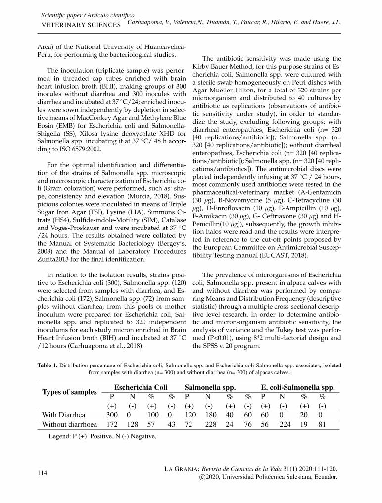
Scientific paper / Artículo científicoVETERINARY SCIENCES Carhuapoma, V., Valencia,N., Huamán, T., Paucar, R., Hilario, E. and Huere, J.L.
Area) of the National University of Huancavelica-Peru, for performing the bacteriological studies.
The inoculation (triplicate sample) was perfor-med in threaded cap tubes enriched with brainheart infusion broth (BHI), making groups of 300inocules without diarrhea and 300 inocules withdiarrhea and incubated at 37 ◦C/24; enriched inocu-les were sown independently by depletion in selec-tive means of MacConkey Agar and Methylene BlueEosin (EMB) for Escherichia coli and Salmonella-Shigella (SS), Xilosa lysine deoxycolate XHD forSalmonella spp. incubating it at 37 ◦C/ 48 h accor-ding to ISO 6579:2002.
For the optimal identification and differentia-tion of the strains of Salmonella spp. microscopicand macroscopic characterization of Escherichia co-li (Gram coloration) were performed, such as: sha-pe, consistency and elevation (Murcia, 2018). Sus-picious colonies were inoculated in means of TripleSugar Iron Agar (TSI), Lysine (LIA), Simmons Ci-trate (HS4), Sulfide-indole-Motility (SIM), Catalaseand Voges-Proskauer and were incubated at 37 ◦C/24 hours. The results obtained were collated bythe Manual of Systematic Bacteriology (Bergey’s,2008) and the Manual of Laboratory ProceduresZurita2013 for the final identification.
In relation to the isolation results, strains posi-tive to Escherichia coli (300), Salmonella spp. (120)were selected from samples with diarrhea, and Es-cherichia coli (172), Salmonella spp. (72) from sam-ples without diarrhea, from this pools of motherinoculum were prepared for Escherichia coli, Sal-monella spp. and replicated to 320 independentinoculums for each study micron enriched in BrainHeart Infusion broth (BIH) and incubated at 37 ◦C/12 hours (Carhuapoma et al., 2018).
The antibiotic sensitivity was made using theKirby Bauer Method, for this purpose strains of Es-cherichia coli, Salmonella spp. were cultured witha sterile swab homogeneously on Petri dishes withAgar Mueller Hilton, for a total of 320 strains permicroorganism and distributed to 40 cultures byantibiotic as replications (observations of antibio-tic sensitivity under study), in order to standar-dize the study, excluding following groups: withdiarrheal enteropathies, Escherichia coli (n= 320[40 replications/antibiotic]); Salmonella spp. (n=320 [40 replications/antibiotic]); without diarrhealenteropathies, Escherichia coli (n= 320 [40 replica-tions/antibiotic]); Salmonella spp. (n= 320 [40 repli-cations/antibiotics]). The antimicrobial discs wereplaced independently infusing at 37 ◦C / 24 hours,most commonly used antibiotics were tested in thepharmaceutical-veterinary market (A-Gentamicin(30 µg), B-Novomycine (5 µg), C-Tetracycline (30µg), D-Enrofloxacin (10 µg), E-Ampicillin (10 µg),F-Amikacin (30 µg), G- Ceftriaxone (30 µg) and H-Penicillin(10 µg)), subsequently, the growth inhibi-tion halos were read and the results were interpre-ted in reference to the cut-off points proposed bythe European Committee on Antimicrobial Suscep-tibility Testing manual (EUCAST, 2018).
The prevalence of microrganisms of Escherichiacoli, Salmonella spp. present in alpaca calves withand without diarrhea was performed by compa-ring Means and Distribution Frequency (descriptivestatistic) through a multiple cross-sectional descrip-tive level research. In order to determine antibio-tic and micron-organism antibiotic sensitivity, theanalysis of variance and the Tukey test was perfor-med (P<0.01), using 8*2 multi-factorial design andthe SPSS v. 20 program.
Table 1. Distribution percentage of Escherichia coli, Salmonella spp. and Escherichia coli-Salmonella spp. associates, isolatedfrom samples with diarrhea (n= 300) and without diarrhea (n= 300) of alpacas calves.
Types of samples Escherichia Coli Salmonella spp. E. coli-Salmonella spp.P
(+)N(-)
%(+)
%(-)
P(+)
N(-)
%(+)
%(-)
P(+)
N(-)
%(+)
%(-)
With Diarrhea 300 0 100 0 120 180 40 60 60 0 20 0Without diarrhoea 172 128 57 43 72 228 24 76 56 224 19 81
Legend: P (+) Positive, N (-) Negative.
114LA GRANJA: Revista de Ciencias de la Vida 31(1) 2020:111-120.
c©2020, Universidad Politécnica Salesiana, Ecuador.
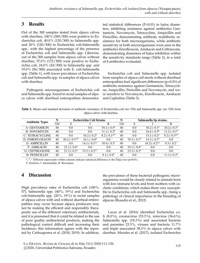
Antibiotic resistance of Salmonella spp, Escherichia coli isolated from alpacas (Vicugna pacus)with and without diarrhea
3 ResultsOut of the 300 samples tested from alpaca calveswith diarrhea, 100% (300/300) were positive to Es-cherichia coli, 40.0% (120/300) to Salmonella spp.and 20% (120/300) to Escherichia coli-Salmonellaspp., with the highest percentage of the presenceof Escherichia coli and Salmonella spp. Likewise,out of the 300 samples from alpaca calves withoutdiarrhea, 57.0% (172/300) were positive to Esche-richia coli, 24.0% (24/300) to Salmonella spp. and19.0% (56/300) associated with E. coli-Salmonellaspp. (Table 1), with lower prevalence of Escherichiacoli and Salmonella spp. in samples of alpaca calveswith diarrhea.
Pathogenic microorganisms of Escherichia coliand Salmonella spp. found in rectal samples of alpa-ca calves with diarrheal enteropathies demonstra-
ted statistical differences (P<0.01) in halos diame-ters, inhibiting resistance against antibiotics Gen-tamicin, Novomycin, Tetracycline, Ampicillin andPenicillin; demonstrating antibiotic multibiotic re-sistance for both microorganisms, while antibioticsensitivity in both microorganisms were seen in theantibiotics Enrofloxacin, Amikacin and Ceftriaxone,demonstrating diameters of halos inhibition withinthe sensitivity standards range (Table 2), in a totalof 8 antibiotics evaluated.
Escherichia coli and Salmonella spp. isolatedfrom samples of alpaca calf stools without diarrhealenteropathies had significant differences (p<0.01) ofantibiotic resistance against Gentamicin, Tetracycli-ne, Ampicillin, Penicillin and Novomycin, and we-re sensitive to Novomycin, Enrofloxacin, Amikacinand Cephaline (Table 3).
Table 2. Means and standard deviation of antibiotic resistance of Escherichia coli (n= 320) and Salmonella spp. (n= 320) fromalpaca calves with diarrhea.
Antibiotic Types N Escherichia Coli Strains N Salmonella Sp strains.320 S I R 320 S I R
A- GENTAMICIN 40 0.0 0.0 10.1± 0.4a 40 0.0 16.2± 0.1a 10.2± 0.3a
B- NOVOMYCIN 40 0.0 0.0 11.1± 0.2b 40 0.0 16.4± 0.5b 11.2± 0.1b
C- TETRACYCLINE 40 0.0 16.2± 0.2a 8.2± 0.1a,b 40 0.0 15.1± 0.2a 9.2± 0.3a,b
D- ENROFLOXACIN 40 20.2± 0.3a,b 16.1± 0.6b 0.0 40 19.3± 0.1b 14.3± 0.1b 0.0E- AMPICILLIN 40 0.0 14.1± 0.1a,c 10.4± 0.3c 40 0.0 16.2± 0.2a,c 9.3± 0.2c
F- AMIKACIN 40 23.1± 0.4a 0.0 0.0 40 19.1± 0.4a 0.0 0.0G- CEFTRIAXONE 40 21.3± 0.3a 15.2± 0.2a,c 0.0 40 23.3± 0.3a 0.0 0.0
H- PENECILLIN 40 0.0 0.0 9.1± 0.4b 40 0.0 0.0 11.1± 0.3a
a, b, c Different superscripts within columns indicate statistical difference to the Tukey test (p<0.01).S Sensitive, I Intermediate, R Resistance.
4 Discussion
High prevalence rates of Escherichia coli (100%,57), Salmonella spp. (40%, 19%) and Escherichiacoli-Salmonella spp. (20%, 19%) in rectal samplesof alpaca calves with and without diarrheal entero-pathies may occur because alpaca producers maynot be making the efficient and responsibly thera-peutic use of the different veterinary antibacterials,and it is presumed that it could be related to the useof poor quality antibacterial products, making thepathological control difficult and increasing theirincidence; this information agrees with the repor-ted by Carhuapoma et al. (2018, 2019). In addition,
the prevalence of these bacterial pathogenic micro-organisms would be closely related to animals bornwith low immune levels and from mothers with ca-chetic conditions, which makes them very suscepti-ble to Escherichia coli and Salmonella spp., being apathology of clinical importance in the breeding ofalpacas (Rosadio et al., 2012)
Lucas et al. (2016) identified Escherichia co-li (8.0%), coronavirus (53.3%), rotavirus (36.6%),Salmonella spp. (18.3%) and associated bacteriaand parasites 23.3%, viruses and bacteria 11.7%and triple associated 38.3% in alpaca calves withdiarrhea. Morales et al. (2017), isolated Escherichia
LA GRANJA: Revista de Ciencias de la Vida 31(1) 2020:111-120.c©2020, Universidad Politécnica Salesiana, Ecuador. 115
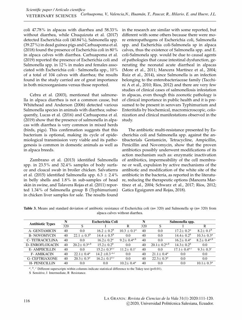
Scientific paper / Artículo científicoVETERINARY SCIENCES Carhuapoma, V., Valencia,N., Huamán, T., Paucar, R., Hilario, E. and Huere, J.L.
coli 47.78% in alpacas with diarrhea and 58.33%without diarrhea, while Chuquizuta et al. (2017)detected Escherichia coli (40.84%), Salmonella spp.(39.27%) in dead guinea pigs and Carhuapoma et al.(2018) found the presence of Escherichia coli in 80%in alpaca calves with diarrhea. Carhuapoma et al.(2019) reported the presence of Escherichia coli andSalmonella spp. in 12% in males and females asso-ciated with Escherichia coli - Salmonella spp., 10%of a total of 104 calves with diarrhea; the resultsfound in the study carried are of great importancein both microorganisms versus those reported.
Cebra et al. (2003), mentioned that salmone-lla in alpaca diarrhea is not a common cause, butWhitehead and Anderson (2006) detected variousSalmonella species in animals with diarrhea; subse-quently, Lucas et al. (2016) and Carhuapoma et al.(2019) show that the presence of salmonella in alpa-cas with diarrhea is very common in mixed herds(birds, pigs). This confirmation suggests that thisbacterium is optional, making its cycle of epide-miological transmission very viable and its patho-genesis is common in domestic animals as well asin alpaca breeds.
Zambrano et al. (2013) identified Salmonellaspp. in 23.5% and 32.4% samples of body surfa-ce and cloacal swab in broiler chicken. Salvatierraet al. (2015) identified Salmonella spp. 6.3 ± 2.4%in belly shells and 1.8% in sub-samples of headskin in swine, and Talavera Rojas et al. (2011) repor-ted 1.34% of Salmonella group B (Typhimurium)in chicken liver samples for sale. The results found
in the research are similar with some reported, butdifferent with some others because there were mo-re enteropathogens of Escherichia coli, Salmonellaspp. and Escherichia coli-Salmonela sp in alpacacalves, thus the existence of Salmonella spp. and E.coli-Salmonela spp. would be due to causal agentsof pathologies that cause intestinal dysfunction, ge-nerating the neonatal acute diarrheal in alpacas(More et al., 2011; Mancera Martínez et al., 2004;Ruiz et al., 2014), since Salmonella is an infectionbelonging to the enterobacteriaceae family (Tacchi-ni A et al., 2010; Ríos, 2012) and there are very fewstudies of clinical cases of salmonellosis infestationin alpacas, even though this zoonotic pathology isof clinical importance in public health and it is pre-sumed to be present in serovars Typhimurium andEnteritidis by biochemical, macromicroscopic, colo-nization and clinical manifestations observed in thestudy.
The antibiotic multi-resistance presented by Es-cherichia coli and Salmonella spp. against the an-tibacterials Gentamicin, Tetracycline, Ampicillin,Penicillin and Novomycin, show that the provenantibiotics possibly underwent modifications of itsaction mechanism such as: enzymatic inactivationof antibiotics, impermeability of the cell membra-ne or wall, expulsion by active mechanisms of theantibiotic and modification of the white site of theantibiotic in the bacteria, as reported in the literatu-re, reducing the therapeutic options (Mancera Mar-tínez et al., 2004; Schwarz et al., 2017; Ríos, 2012;Gatica Eguiguren and Rojas, 2018).
Table 3. Means and standard deviation of antibiotic resistance of Escherichia coli (n= 320) and Salmonella sp (n= 320) fromalpaca calves without diarrhea.
Antibiotic Types N Escherichia Coli N Salmonella spp.320 S I R 320 S I R
A- GENTAMICIN 40 0.0 16.2 ± 0.2b 10.3 ± 0.1a 40 0.0 17.2± 0.2a 8.2± 0.1b
B- NOVOMYCIN 40 22.1 ± 0.3b 14.4 ± 0.5b 0.0 40 0.0 14.4± 0.2b 10.3± 0.3a
C- TETRACICLINA 40 0.0 16.2± 0.2a 9.2± 0.4a.b 40 0.0 16.2± 0.4a 8.2± 0.4a.b
D- ENROFLOXACIN 40 20.2± 0.3a.b 15.2± 0.2b 0.0 40 20.1± 0.2a.b 14.3± 0.2b 0.0E- AMPIICILLIN 40 0.0 15.2± 0.3a.c 11.2± 0.1c 40 0.0 17.1± 0.4a.c 9.3± 0.3c
F- AMIKACIN 40 22.1± 0.4a 14.2 ±0.3 a.c 0.0 40 21.1± 0.4a 0.0 0.0G- CEFTRIAXONE 40 20.3± 0.3a 16.2± 0.1a.c 0.0 40 22.3± 0.3a 0.0 0.0
H- PENECILLIN 40 0.0 0.0 10.2± 0.4a 40 0.0 0.0 10.1± 0.3a
a, b, c Different superscripts within columns indicate statistical difference to the Tukey test (p<0.01).S Sensitive, I Intermediate, R Resistance.
116LA GRANJA: Revista de Ciencias de la Vida 31(1) 2020:111-120.
c©2020, Universidad Politécnica Salesiana, Ecuador.
Antibiotic resistance of Salmonella spp, Escherichia coli isolated from alpacas (Vicugna pacus)with and without diarrhea
In addition, the high resistant of 8 antibioticstested in the study would be linked to the poor ap-plication in the health management and the inap-propriate use of antibiotics that have been practicedby producers in their herds, and by the irrespon-sibly massive distribution of drugs by national pro-grams promoted by unskilled professionals, whichmakes the progressive trend of antibiotic resistancebetween humans and animals. Lucas et al. (2016),report that Salmonella spp. and Escherichia coliwould possibly be resistant to first-line antibacte-rial such as Phosphomycin, Enrofloxacin, Cipro-floxacin, Gentamicin, Oxytetracycline, Penicillin,Ceftazidime and Trimethoprim-sulfamethoxazolebecause they are most commonly used indiscri-minately by veterinarians from many years agoin cattle, chicken, sparrows and pigs; therefore, itwould not be advisable to use antibiotics as firstchoice for the treatment of diarrhea in alpaca calveswithout carrying out susceptibility tests in labora-tories (Pinto Jiménez et al., 2010; Siuce et al., 2015;Carhuapoma et al., 2019).
Barboza and Suarez (2012), found antibiotic re-sistance in 30% against Gentamicin, Norfloxacinand Tetracycline in Salmonella spp. isolated fromcases of avian Tiphosis. Cordero Ruíz et al. (2002),reported multi-resistance in 84.4% to Tetracycli-ne, Gentamicin, Ampicillin and Amikacin in gram-positive and negative bacteria of 11 proven antibio-tics, and De la Fuente et al. (2015) found 91% resis-tance in strains of Salmonella spp. to Ampicillin, Ni-trofurantoin and 55% to Cephalotin and Chloramp-henicol; while Quesada et al. (2016) report multi-resistance of Salmonella spp. to Nalidixic acid an-tibiotics, Streptomycin, Tetracycline, Chloramphe-nicol, Ampicillin, Trimethoprim/sulfamethoxazole,Gentamicin, Ciprofloxacin and Cephalosporin, the-se reports are similar to the results found in thisstudy as they match almost all the antibiotics stu-died and these same resistance behaviors can begenerated in hot-blooded animals (Castillo et al.,2014), for this reason, the antibiotic resistance of Sal-monella spp. and Escherichia coli could be an epi-demiological alarm for veterinarians (Rivera Cal-derón et al., 2012), caused by a lack of practice ofconducting sensitivity tests in laboratories and bypoor pharmacological knowledge capacity of vete-rinarians and operational technicians (Barboza andSuarez, 2012; Carhuapoma et al., 2018).
The antibiotic sensitivity demonstrated by thestrains of Escherichia coli and Salmonella spp. iso-lated from rectal swab from alpaca calves with andwithout diarrhea versus the antibacterials of En-rofloxacin, Amikacin, Novomycin and Ceftriaxo-ne, seem to be microbial that were not long-termused or were indiscriminate in herds (Carhuapomaet al., 2018), and may not have generated the mo-dification of their mechanisms of antibiotic action,as well as the genes of DNA gyrase and topoiso-mesase IV (Romeu Álvarez et al., 2012; Lee et al.,2003; Ruiz et al., 2014; Schwarz et al., 2017). Addi-tionally, Barrios-Arpi et al. (2016) found Escherichiacoli sensitive to Trimethoxyprim (98%), Gentami-cin (95%) and Phosphomycin (88%), Ciprofloxacin( 85%), Ceftadizime (79%), and resistant to Nitro-furantoin (85%) from healthy and sick alpaca cal-ves, results that differ from the ones obtained in thisstudy with 4 antibacterial (Enrofloxacin, Amikacin,Novomiacin and Ceftriaxone) that proved to be sen-sitive and that would be specific for the therapeuticuse of alpacas with and without diarrheal entero-pathies.
5 Conclusions
The isolations of Salmonella spp. and Escherichiacoli from alpaca calves with and without diarrheawere shown to be multi-resistance to the most com-mon antibiotics in the pharmaceutical-veterinarymarket and only 4 antibiotics were sensitive, thus,comparative studies are required in the high An-dean areas of Peru for the prevention and dissemi-nation of antibacterial resistance.
Ethical commitments: The research team decla-res that strict management of animal welfare hasbeen carried out for this research under the proto-cols established before and during the collection ofsamples for the study.
Confidentiality of data: The research team sta-ted that a strict methodological management hasbeen done to obtain adequate bases, as a statisticalmodel and SPSS v. 20 program for data processing.
Reported consent: For the execution of the in-vestigation no informed consent was required as itwas a laboratory study based on protocols withoutthe handling of animals, but they were taken into
LA GRANJA: Revista de Ciencias de la Vida 31(1) 2020:111-120.c©2020, Universidad Politécnica Salesiana, Ecuador. 117
Scientific paper / Artículo científicoVETERINARY SCIENCES Carhuapoma, V., Valencia,N., Huamán, T., Paucar, R., Hilario, E. and Huere, J.L.
account for greater reliability of the study.
Funding source: No internal or external institu-tional funding has been granted for the implemen-tation of the study.
Conflicts of interest: The authors declare noconflict of interest.
AcknowledgmentsThe authors thank the executive administrator ofthe Animal Health Laboratory of the National Uni-versity of Huancavelica and the alpaca breeders–Peru; for providing the collaboration and facilitiesfor the execution of this study.
ReferencesBarboza, D. and Suarez, J. (2012). Sensibilidad a la
fosfomicina ante los diferentes agentes patógenosaislados en animales domésticos en venezuela. InMemorias de la XVI Reunión Científico Técnica de laAsociación Argentina de Veterinarios de Laboratoriosde Diagnóstico (AAVLD), Mar del Plata (BuenosAires) Argentina. Buenos Aires (CF).
Barrios-Arpi, M., Morales, S., and Villacaqui-Ayllon, E. (2016). Susceptibilidad antibiótica decepas de escherichia coli en crías de alpaca cony sin diarrea. Revista de Investigaciones Veterina-rias del Perú, 27(2):381–387. Online: https://bit.ly/3a8CiKs.
Bergey’s (2008). Manual of systematic bacteriology, se-cond edition volume three the firmicutes edition.
Carhuapoma, D., Mayhua, M., Valencia, M., andLizana, H. (2018). Antibacterial in vitro of ef-fect urtica dioica and piper angustifolium in al-pacas (vicugna pacus) with diarrheal enteropat-hies. MOJ Anat Physiol, 5:160–162. Online: https://bit.ly/2T4HLw1.
Carhuapoma, V., Valencia, N., Paucar, R., Mayhua,P. H., Lizana-Hilario, E., et al. (2019). Efecto deescherichia coli y salmonella spp en el crecimien-to y mortalidad de crías de alpacas (vicugna pa-cos). Revista de Investigaciones Veterinarias del Perú,30(2):946–953. Online: https://bit.ly/2I2EeZ2.
Castillo, G., Koga, Y., Alvarado, A., Tinoco, R., andFernández, D. (2014). Aislamiento e identifica-ción bioquímica de cepas de pasteurella multo-cida y gallibacterium anatis en aves de produc-ción con signos respiratorios. Revista de Investiga-ciones Veterinarias del Perú, 25(4):516–522. Online:https://bit.ly/2T4F4e0.
Cebra, C. K., Mattson, D. E., Baker, R. J., Sonn, R. J.,and Dearing, P. L. (2003). Potential pathogensin feces from unweaned llamas and alpacas withdiarrhea. Journal of the American Veterinary Me-dical Association, 223(12):1806–1808. Online:https://bit.ly/2T6SrKS.
Centeno, S., Salvatierra, G., and Calle, S. (2018). De-tección de fenotipos de resistencia accsut, blee yampc en cepas de salmonella enterica aisladasde infecciones en animales. Revista de Investiga-ciones Veterinarias del Perú, 29(2):580–587. Online:https://bit.ly/2HZbWOO.
Cordero Ruíz, D. M., García Pérez, A. L., Ba-rreal González, R. T., Jiménez Armada, J., and Ro-jas Hernández, N. (2002). Comportamiento dela infección nosocomial en las unidades de tera-pia en un período de 5 años. Revista cubana deHigiene y Epidemiologia, 40(2):79–88. Online:https://bit.ly/32w3Bf7.
De la Fuente, M., Castañeda, C., Cortes, V., and Es-pino, A. (2015). Analisis comparativo de la sus-ceptibilidad de cepas de salmonella sp aisladasde vegetales (lactuca sativa) contra antibióticos,bacteriocinas de bacillus thuringiensis y nisina. InXII Congreso Nacional de Ciencia y Tecnología de Ali-mentos, pages 1–4, Salamanca España. Universi-dad Guanajato- Facultad de Ciencias Biol’ogicas.
EUCAST (2018). Routine and extended internalquality control for mic determination and diskdiffusion as recommended by eucast version 8.0.Technical report, European Committee on Anti-microbial Susceptibility Testing.
Gatica Eguiguren, M. d. l. A. and Rojas, H. (2018).Gestión sanitaria y resistencia a los antimicrobia-nos en animales de producción. Revista Peruana deMedicina Experimental y Salud Pública, 35:118–125.Online:https://bit.ly/2Vu4svw.
Lee, Y. J., Kim, K. S., Kwon, Y. K., and Tak, R. B.(2003). Biochemical characteristics and antimi-crobials susceptibility of salmonella gallinarum
118LA GRANJA: Revista de Ciencias de la Vida 31(1) 2020:111-120.
c©2020, Universidad Politécnica Salesiana, Ecuador.

Antibiotic resistance of Salmonella spp, Escherichia coli isolated from alpacas (Vicugna pacus)with and without diarrhea
isolated in korea. Journal of veterinary science,4(2):161–166. Online: https://bit.ly/2PvHIay.
Lucas, J. R., Morales, S., Barrios, M., Rodríguez, J.,Vásquez, M., Lira, B., Torres, B., Casas, E., andEspinoza, J. (2016). Patógenos involucrados encasos fatales de diarrea en crías de alpaca de lasierra central del perú. Revista de InvestigacionesVeterinarias del Perú, 27(1):169–175. Online:https://bit.ly/2I00Gll.
Mancera Martínez, A., Corpus, O., de Lourdes, M.,Tenorio Gutiérrez, V. R., and Vázquez Navarrete,J. (2004). Determinación de la existencia de plás-midos en aislamientos de salmonella enteritidis(fagotipos 4 y 8) y su análisis en la resistencia anti-microbiana. Técnica Pecuaria en México, 42(3):325–332. Online:https://bit.ly/3caGXNH.
Medina, C., Morales, S., and Navarrete, M. (2017).Resistencia antibiotica de enterobacterias aisladasde monos (ateles, callicebus y lagothrix) en semi-cautiverio en un centro de rescate, peru. Revista deInvestigaciones Veterinarias del Perú, 28(2):418–425.Online:https://bit.ly/3a7L2jW.
Morales, S., Siu, E., Ramírez, P., and Navarro, A.(2017). Determinación de serotipos de escherichiacoli aisladas de crías de alpacas (vicugna pacos)con y sin diarrea en huancavelica. REDVET. Re-vista Electrónica de Veterinaria, 18(9):1–14. Online:https://bit.ly/2T4MNbT.
More, J., Manchego, A., Sandoval, N., Ramírez, M.,Pezo, D., Chiok, K. L., and Rivera, H. (2011). De-tección genómica y expresión de péptidos antimi-crobianos (α-y β-defensinas) en mucosa intestinalde crνas de alpaca (vicugna pacos). Revista deInvestigaciones Veterinarias del Perú, 22(4):324–335.Online:https://bit.ly/385VOpB.
Murcia, M. (2018). Identificación de enterobacterias.Link.
Oha, R. (2012). Anatomía patológica de las diarreas in-fecciosas en crías de alpaca (Lama pacos) en la SAISAricoma Ltda. 57. PhD thesis, Tesis de Médico Ve-terinario y Zootecnista: Facultad de Medicina Ve-terinaria, Univ. Nacional del Altiplano, Puno. Pe-rú.
Ortiz, S. (2011). Evaluación de algunos métodos de con-trol de la mortalidad en crías de alpaca (Lama pacos) en
explotaciones familiares. PhD thesis, Tesis de Médi-co Veterinario. Lima: Universidad Nacional Ma-yor de San Marcos.
Pinto Jiménez, C. E., Martín Espada, C., andCid Vázquez, M. D. (2010). Camélidos sudameri-canos: estado sanitario de sus crías. Revista Com-plutense de Ciencias Veterinarias, 4(1):37–50. Onli-ne: https://bit.ly/2SQAVdJ.
Quesada, A., Reginatto, G. A., Ruiz Español, A., Co-lantonio, L. D., and Burrone, M. S. (2016). Re-sistencia antimicrobiana de salmonella spp ais-lada de alimentos de origen animal para consu-mo humano. Revista Peruana de Medicina Expe-rimental y Salud Pública, 33:32–44. Online:https://bit.ly/2Tpnmke.
Ramírez, A. (1990). Colibacilosis entérica en críasde alpacas. Avances sobre investigación en salud ani-mal camélidos sudamericanos. UNMSM. Bol Div No,23:64.
Ríos, W. (2012). Determinacóin del perfil de resisten-cia antibiótica de Salmonella entérica aislada de cerdosfaenados en un matadero de Lima Metropolitana. PhDthesis, Tesis de Médico Veterinario. Lima: Univer-sidad Nacional Mayor de San Marcos.
Rivera Calderón, L. G., Delgado, P. A. M., Urbano,M. F. C., and Coy, F. A. C. (2012). Resistenciade la salmonela a los antimicrobianos conven-cionales para su tratamiento. Revista CES Me-dicina Veterinaria y Zootecnia, 7(1):116–129. Onli-ne:https://bit.ly/2w9bw5V.
Romeu Álvarez, B., Salazar Jiménez, P., Lugo Mo-ya, D., Rojas Hernández, N. M., and Eslava Cam-pos, C. A. (2012). Susceptibilidad antimicrobia-na de aislamientos de escherichia coli proceden-tes de ecosistemas dulceacuícolas. Revista Cubanade Medicina Tropical, 64(2):132–141. Online:https://bit.ly/32iPiKC.
Rosadio, A., Yaya, L., Véliz, A., Quispe, T., et al.(2012). Efecto protector de una vacuna poliva-lente anticlostridial sobre la mortalidad neona-tal en alpacas. Revista de Investigaciones Veteri-narias del Perú, 23(3):299–306. Online: https://bit.ly/2Tk02of.
Ruiz, D., Suárez, M. C., and Uribe, C. (2014). Sus-ceptibilidad antimicrobiana in vitro de cepas de
LA GRANJA: Revista de Ciencias de la Vida 31(1) 2020:111-120.c©2020, Universidad Politécnica Salesiana, Ecuador. 119
Scientific paper / Artículo científicoVETERINARY SCIENCES Carhuapoma, V., Valencia,N., Huamán, T., Paucar, R., Hilario, E. and Huere, J.L.
salmonella spp. en granjas de ponedoras comer-ciales del departamento de antioquia. Revista Co-lombiana de Ciencias Pecuarias, 19(3):297–305. Onli-ne:https://bit.ly/2T7yz91.
S., M. (2018). Identificación, serotipificación y re-sistencia de cepas de salmonella entérica aisladasde cuyes (cavia porcellus) clínicamente enfermos.REDVET - Revista electrónica de Veterinaria, 19(1).
Salvatierra, G., Pinto, C., Inga, E., Siuce, J., and Ca-lle, S. (2015). Detección de salmonella sp en carca-sas porcinas en camales de lima, perú. Revista deInvestigaciones Veterinarias del Perú, 26(4):682–688.Online:https://bit.ly/3ab3Q1L.
Schwarz, S., Loeffler, A., and Kadlec, K. (2017). Bac-terial resistance to antimicrobial agents and itsimpact on veterinary and human medicine. Ad-vances in Veterinary Dermatology, 8:95–110. Onli-ne:https://bit.ly/386SElc.
Silvera, E., Perales, R., Rodríguez, J., López, T., Ga-vidia, C., Agapito, J., and Palacios, C. (2012). Pre-sencia de escherichia coli o157 en crías de alpacas(vicugna pacos). Revista de Investigaciones Vete-rinarias del Perú, 23(1):98–104. Online:https://bit.ly/2TykQZl.
Siuce, J., Manchego, A., Sandoval, N., More, J.,Chiok, K.-L., Pezo, D., and Rivera, H. (2015). Ex-
presión de defensinas en yeyuno de crías de alpa-cas (vicugna pacos) con enteropatías. Revista deInvestigaciones Veterinarias del Perú, 26(2):317–327.Online:https://bit.ly/2T1ZaWa.
Tacchini A, M. D. M., Caraffini F, A., Montamat C,M. S., Spitale A, N., Bosio D, Y., and Min-guez G, A. (2010). Empiema causado por sal-monella typhimurium. Revista chilena de enferme-dades respiratorias, 26(2):91–94. Online:https://bit.ly/3cecGxx.
Talavera Rojas, M., Reyes Rodríguez, N. E., La-gunas Bernabé, S., Fernández Rosas, P., Mora-les Erasto, V., and Soriano Vargas, E. (2011). Va-riabilidad genética de aislamientos de salmone-lla typhimurium (grupo b) obtenidos de híga-dos de pollo destinados para consumo humano.Revista mexicana de ciencias pecuarias, 2(4):Online:https://bit.ly/3c6Y1Ei.
Whitehead, C. E. and Anderson, D. E. (2006). Neo-natal diarrhea in llamas and alpacas. Small Ru-minant Research, 61(2-3):207–215. Online:https://bit.ly/3abW6g4.
Yagui, M. (2018). Resistencia antimicrobiana: nuevoenfoque y oportunidad. Revista Peruana de Medi-cina Experimental y Salud Pública, 35(1):7–8. Onli-ne:https://bit.ly/3814xtb.
120LA GRANJA: Revista de Ciencias de la Vida 31(1) 2020:111-120.
c©2020, Universidad Politécnica Salesiana, Ecuador.
Scientific paper/ Artículo científico
AGRICULTURAL PRODUCTIONpISSN:1390-3799; eISSN:1390-8596
http://doi.org/10.17163/lgr.n31.2020.09
ECONOMIC ANALYSIS OF HYDROPONIC LETTUCE UNDER
FLOATING ROOT SYSTEM IN SEMI-ARID CLIMATE
ANÁLISIS ECONÓMICO DE LECHUGAS HIDROPÓNICAS BAJO SISTEMA RAÍZ
FLOTANTE EN CLIMA SEMIÁRIDO
Rosa Pertierra Lazo*1 and Jimmy Quispe Gonzabay2
1 Faculty of Agricultural Sciences. State University Santa Elena Peninsula, Av. Principal Santa Elena-La Libertad, Santa Elena,Ecuador.2 Faculty of Administrative Sciences. State University Santa Elena Peninsula, Av. Principal Santa Elena-La Libertad, SantaElena, Ecuador.
*Corresponding author: [email protected]
Article received on January 15th, 2019. Accepted, after review, on August 30th, 2019. Published on March 1st, 2020.
Resumen
Los cultivos sin suelo se presentan como una alternativa de cultivo ante la presencia de suelos marginales con es-casez hídrica característicos de la provincia de Santa Elena (PSE). La hidroponía presenta a nivel mundial una altaproductividad por unidad de superficie, ahorro de agua y cosechas durante todo el año. La lechuga (Lactuca sativaL.), especie de estación fría, es la más representativa de un sistema hidropónico, pero no es una especie cultivada enla costa ecuatoriana. El objetivo fue analizar desde el punto de vista económico-financiero la propuesta técnica de uncultivo protegido de lechuga bajo sistema hidropónico de raíz flotante llevado a cabo en el clima semiárido de la PSE.Se realizaron cuatro siembras con el cv. Crespa, utilizando la solución nutritiva Hoagland y Arnon. El rendimiento ylos costos se extrapolaron a una infraestructura de 1,000 m2 equivalente a una superficie productiva efectiva de 240m2. Se asumen supuestos donde la producción se vende en jornadas laborales de acuerdo a la ley a una proyección de5 años, con un stock de inventario para una semana, ventas al por mayor y un margen de beneficio en el año 1 de 30%y ascendente en los siguientes períodos. Bajo estos criterios, el costo de producción unitario (en dólares americanos)ascendió a USD 0,49 y el precio de venta a USD 0,70. La inversión total sumó USD 27.077,99, el VAN USD 58.581,07,con una TIR del 40% y un índice beneficio-costo de 1,26; por lo que económica y financieramente el proyecto se con-sideró viable.Palabras clave: Cultivos sin suelo, costo de producción, inversión, cultivo protegido, Lactuca sativa L.
121LA GRANJA: Revista de Ciencias de la Vida 31(1) 2020:121-133.c©2020, Universidad Politécnica Salesiana, Ecuador.
Scientific paper / Artículo científicoAGRICULTURAL PRODUCTION Pertierra Lazo, R. and Quispe Gonzabay, J.
Abstract
Soilless crops are a farming alternative to marginal soils with limited water availability, which are widespread in theprovince of Santa Elena (PSE), Ecuadorian coast. This province has semi-arid climate. Hydroponics have worldwidehigh productivity per unit area, save of water and cultivation cycles throughout the year. Lettuce (Lactuca sativa L.)is a cold-season crop, the most representative crop in hydroponic cultivation, but it is not currently cultivated in theEcuadorian coastal area. The aim of this study was to analyze the economic-financial viability of lettuce cultivationunder hydroponic system of floating root. Four lettuce cultivation experiments were carried out with cv. Crespa,using the Hoagland and Arnon nutrient solution. Yields and costs were extrapolated to an infrastructure of 1,000 m2
equivalent to an effective productive area of 240 m2. The assumptions used in the analysis were: all production is sold,working days were calculated according to the law, 5-year projection, stock of inventory for a week, wholesale selling,and profit margin in Year 1 of 30% and increasing in the following periods. Under these criteria, the production cost(in US dollars) per unit amounted to USD 0.49/unit and the sale price to USD 0.70/unit. The total investment USD27,077.99, the NPV USD 58,581.07, with an IRR of 40% and a benefit-cost ratio of 1.26; thus, the project was consideredviable from an economic point of view.Keywords: Soilless culture, production costs, investment, greenhouse crop, Lactuca sativa L.
Suggested citation: Pertierra Lazo, R. and Quispe Gonzabay, J. (2020). Economic analysis of hydroponiclettuce under floating root system in semi-arid climate. La Granja: Revista de Cienciasde la Vida. Vol. 31(1):121-133. http://doi.org/10.17163/lgr.n31.2020.09.
Orcid IDs:Rosa Pertierra Lazo: http://orcid.org/ 0000-0001-8938-9849Jimmy Quispe Gonzabay: http://orcid.org/0000-0002-7519-1257
122LA GRANJA: Revista de Ciencias de la Vida 31(1) 2020:121-133.
c©2020, Universidad Politécnica Salesiana, Ecuador.
Economic analysis of hydroponic lettuce under floating root system in semi-arid climate
1 Introduction
The increase in the population and the reductionin agricultural soils have caused concern in rela-tion to the food supply. Technology evolves in pur-suit of increased productivity and sustainability th-rough genetic improvement, including high-impacttechnologies on product performance and quality,agriculture, irrigation technologies and nutrition,among others. Soilless protected crops have the sa-me objective, obtaining high yield on less surfacearea and throughout the year.
Hydroponics with recirculation (closed system)is the most technically, economically and environ-mentally efficient system by its considerable sa-vings in water and fertilizers, and minimal dischar-ge of residual fertilizer solution into the environ-ment (Urrestarazu, 2015). In the protected crops,hydroponic systems are presented as an interestingoption in the face of increased soil and sanitary li-mitations and the need for short marketing circuits.In Mexico, these already account for 50% of protec-ted crops (INTAGRI, 2017). In the US, in the period2013-2018, this form of production annually obtai-ned US $ 891 million, with a rate of 1.2% and itgenerated an employment increase rate of 10.1%(IBISWORLD, 2018). Hydroponics in the closedsystem has been more efficient compared to con-ventional cultivation (in open or greenhouse soil)(INTAGRI, 2017), resulting in better cost-benefit.However, one of the disadvantages of this system isthe high initial investment in the infrastructure.
The world production of this vegetable is esti-mated at 26 866 557 t per year with an average yieldof 21,89 T ha−1 (FAO, 2019). Data from the FoodOrganization of the United Nations (FAO) indica-te that the main producer of this species is Spain,exporting to more than 53 countries, and exceeding900 000 tons per year. Lettuce occupies 2% in the USin the hydroponic market, while in South Americathe percentage is 49% (INTAGRI, 2017).
Ecuador’s horticulture has increased due to therevival of the peasant economy and exporting agri-business (Álvarez et al., 2014), as well as the in-crease in the consumption due to changes in ea-ting habits (Espinoza, 2015). In 2000, the productionof 9.770 metric tons was recorded, carried out bysmallholder farmers with 58 and 63% of produc-
tion units with less than 1 ha, in cultivation andassociated, respectively (INEC, 2002). Meanwhile,FAO (2019) in 2017 recorded an increase of 17 301t produced. The Survey of Consumption and Hou-sehold Expenses in Ecuador (INEC, 2013) showsthat rural people invest 32% of their income in foodand non-alcoholic beverages and only 2% is spenton vegetable purchases in this category. If the va-lue of the Basic Family Basket in the Sierra regionis considered to be $722.44 and the Costa 695.52value, this expenditure on vegetables would corres-pond to USD 14 in the coastal area (INEC, 2017).According to (Zaruma, 2009), peasant family far-ming (AFC) for productive areas is 500 to 2000 m2,while for small producers it is 0.25 to 1 ha and forthe median 1 to 3 ha. If at the level of Latin America80% of farms are in the hands of the TFA, in Ecua-dor this figure rises to 84.5% (Salcedo and Guzmán,2014). The cultivation and production of vegetablesdepend on small producers and on peasant familyfarming. In Ecuador, 83% of this production is des-tined for domestic consumption. Lettuce culture istraditionally grown in the open field, but also underprotected cultivation in soil and hydroponic sys-tems. It is a specied that grows during cold seasonwith optimal temperatures of growth and dayti-me development between 18 and 25 ◦C and nightlyfrom 10 to 15◦C (Maroto, 2002; Saavedra et al., 2017).
In the province of Santa Elena, a project of agroe-cological family orchards has been carried out sin-ce 2014 in charge of the Ministry of Agriculture(MAG), and since 2017 it has been in charge ofthe peasant family farming project (AFC) coveringthe rural and urban sector (Prefectura Santa Elena,2017; Mateo, 2019). Lettuce occupies an importantplace among the species produced there. The mainproblems affecting agricultural productivity in theprovince are low water availability, semi-arid weat-her conditions and degraded soils. Barbosa et al.(2015) estimated that this technique manages to in-crease annual productivity by 10 times with a con-sumption of only 8% of water, but 87 times higherconsumption of energy compared to a conventionalcrop in the United states (NFT, irrigation, heating,artificial lighting). Treftz and Omaye (2012) indicatepositive aspects that point to the sustainability ofsoilless crops such as saving water, fertilizers andpesticides. They also mention that it can be carriedout in arid and urban areas, bringing the productcloser to the consumer, and not requiring crop rota-
LA GRANJA: Revista de Ciencias de la Vida 31(1) 2020:121-133.c©2020, Universidad Politécnica Salesiana, Ecuador. 123
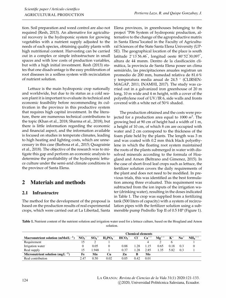
Scientific paper / Artículo científicoAGRICULTURAL PRODUCTION Pertierra Lazo, R. and Quispe Gonzabay, J.
tion. Soil preparation and weed control are also notrequired (Resh, 2013). An alternative for agricultu-ral recovery is the hydroponic system for growingvegetables with a nutrient supply adjusted to theneeds of each species, obtaining quality plants withhigh nutritional content. Harvesting can be carriedout in a complex or simple infrastructure in smallspaces and with low costs of production variables,but with a high initial investment. Resh (2013) sta-tes that one disadvantage is the easy proliferation ofroot diseases in a soilless system with recirculationof nutrient solution.
Lettuce is the main hydroponic crop nationallyand worldwide, but due to its status as a cold sea-son plant it is important to evaluate its technical andeconomic feasibility before recommending its cul-tivation in the province in this productive systemthat requires high capital investment. In the litera-ture, there are numerous technical contributions tothe topic (Khan et al., 2018; Sharma et al., 2018), butthere is little information regarding the economicand financial aspect, and the information availableis focused on studies in temperate climates, leadingto high heating and lighting costs, which are unne-cessary in this case (Barbosa et al., 2015; Quagrainieet al., 2018). The objective of the research was to mi-tigate this gap and perform an economic analysis todetermine the profitability of the hydroponic lettu-ce culture under the semi-arid climate conditions inthe province of Santa Elena.
2 Materials and methods
2.1 Infrastructre
The method for the development of the proposal isbased on the production results of real experimentalcrops, which were carried out at La Libertad, Santa
Elena provinces, in greenhouses belonging to theproject "P06 System of hydroponic production, al-ternative to the change of the agroproductive matrixin Santa Elena"located in the Faculty of Agricultu-ral Sciences of the State Santa Elena University (UP-SE). The geographical location of the place is southlatitude 2◦13
′56,46”, longitud oeste 80◦52
′30,097”,
altura de 44 msnm. Dentro de la clasificación cli-mática, la provincia de Santa Elena posee un climasemiárido, las precipitaciones anuales registran unpromedio de 200 mm, humedad relativa de 81.6%y temperatura media anual de 24.5 ◦ (CLIRSEN-MAGAP, 2011; INAMHI, 2017). The study was ca-rried out in a galvanized iron greenhouse of 20 mlong, 10 m wide and 4 m height, with a cover of thepolyethylene roof of UV/IR 6, side walls and frontscovered with a white net of 50% shaded.
The production obtained and the costs were pro-jected for a production area equal to 1000 m2. Thegrowing bed at 90 cm of height had a width of 1 m,a height of 10 cm, of which 8 cm are occupied withwater and 2 cm correspond to the thickness of thefoam plate held by the plants. The length was 3 mand was coated with 0.2 mm thick black polyethy-lene in which the floating root system maintainedthe roots of the plants submerged in water with dis-solved minerals according to the formula of Hoa-gland and Arnon (Beltrano and Gimenez, 2015). Inthe case of short-lived leaf crops such as lettuce, thefertilizer solution covers the daily requirements ofthe plant and does not need to be modified. In pre-vious trials, this was identified as the best formula-tion among three evaluated. This requirement wassubtracted from the ion inputs of the irrigation wa-ter (drinking water), resulting in the doses indicatedin Table 1. The crop was supplied from a fertilizingtank (500 liters of capacity) with a system of recircu-lation pipes with the fertilizer solution using a sub-mersible pump Pedrollo Top II of 0.5 HP (Figure 1).
Table 1. Nutrient content of the nutrient solution and irrigation water used for a lettuce culture, based on the Hoagland and Arnonsolution.
Chemical elementsMacronutrient solution (mMolL−1) NO3
− SO4= H2PO4
− HCO3− Cl− Ca++ Mg++ K+ Na+ NH4
++
Requirement 15 2 1 4 2 6 1Irrigation water 0 0.05 0 0.88 1.28 1.15 0.65 0.18 0.3 0Real supply 15 1.948 1 0.37 1.28 2.85 1.35 5.82 0.3 1Micronutrient solution (mgL−1) Fe Mn Cu Zn B MoReal contribution 2.47 0.50 0.02 0.05 0.42 0.01
124LA GRANJA: Revista de Ciencias de la Vida 31(1) 2020:121-133.
c©2020, Universidad Politécnica Salesiana, Ecuador.
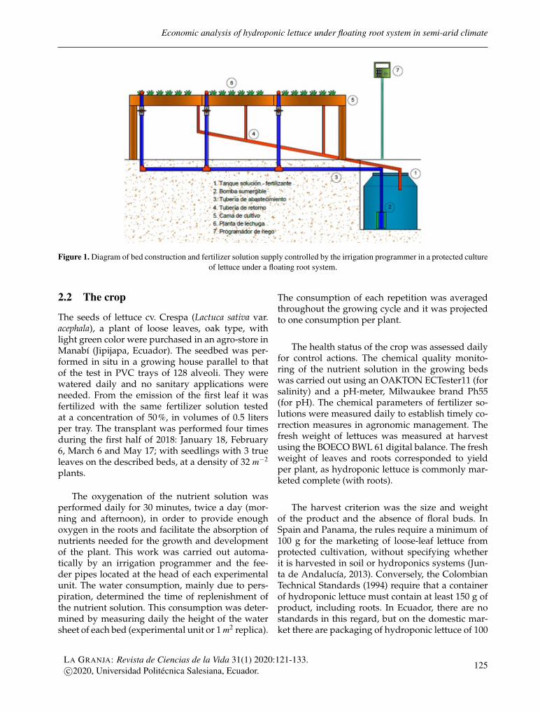
Economic analysis of hydroponic lettuce under floating root system in semi-arid climate
Figure 1. Diagram of bed construction and fertilizer solution supply controlled by the irrigation programmer in a protected cultureof lettuce under a floating root system.
2.2 The crop
The seeds of lettuce cv. Crespa (Lactuca sativa var.acephala), a plant of loose leaves, oak type, withlight green color were purchased in an agro-store inManabí (Jipijapa, Ecuador). The seedbed was per-formed in situ in a growing house parallel to thatof the test in PVC trays of 128 alveoli. They werewatered daily and no sanitary applications wereneeded. From the emission of the first leaf it wasfertilized with the same fertilizer solution testedat a concentration of 50%, in volumes of 0.5 litersper tray. The transplant was performed four timesduring the first half of 2018: January 18, February6, March 6 and May 17; with seedlings with 3 trueleaves on the described beds, at a density of 32 m−2
plants.
The oxygenation of the nutrient solution wasperformed daily for 30 minutes, twice a day (mor-ning and afternoon), in order to provide enoughoxygen in the roots and facilitate the absorption ofnutrients needed for the growth and developmentof the plant. This work was carried out automa-tically by an irrigation programmer and the fee-der pipes located at the head of each experimentalunit. The water consumption, mainly due to pers-piration, determined the time of replenishment ofthe nutrient solution. This consumption was deter-mined by measuring daily the height of the watersheet of each bed (experimental unit or 1 m2 replica).
The consumption of each repetition was averagedthroughout the growing cycle and it was projectedto one consumption per plant.
The health status of the crop was assessed dailyfor control actions. The chemical quality monito-ring of the nutrient solution in the growing bedswas carried out using an OAKTON ECTester11 (forsalinity) and a pH-meter, Milwaukee brand Ph55(for pH). The chemical parameters of fertilizer so-lutions were measured daily to establish timely co-rrection measures in agronomic management. Thefresh weight of lettuces was measured at harvestusing the BOECO BWL 61 digital balance. The freshweight of leaves and roots corresponded to yieldper plant, as hydroponic lettuce is commonly mar-keted complete (with roots).
The harvest criterion was the size and weightof the product and the absence of floral buds. InSpain and Panama, the rules require a minimum of100 g for the marketing of loose-leaf lettuce fromprotected cultivation, without specifying whetherit is harvested in soil or hydroponics systems (Jun-ta de Andalucía, 2013). Conversely, the ColombianTechnical Standards (1994) require that a containerof hydroponic lettuce must contain at least 150 g ofproduct, including roots. In Ecuador, there are nostandards in this regard, but on the domestic mar-ket there are packaging of hydroponic lettuce of 100
LA GRANJA: Revista de Ciencias de la Vida 31(1) 2020:121-133.c©2020, Universidad Politécnica Salesiana, Ecuador. 125

Scientific paper / Artículo científicoAGRICULTURAL PRODUCTION Pertierra Lazo, R. and Quispe Gonzabay, J.
and 200 g.
For the purposes of this study, which has an eco-nomic approach, only the weight of full lettuce, ave-raged of the four planting dates, was consideredas the only relevant agronomic variable (Table 2).The results were statistically analyzed with the In-fostat v2018e program. Parametric variables wereanalyzed with the F test and nonparametric varia-bles with the Kruskall Wallis test.
2.3 Economic analysis
A budget was developed based on the model pro-posed by Díaz et al. (2012), where the initial balanceis first identified and operational processes are thendetermined in order to quantify them in time andcurrency. The calculation of the investment of thegalvanized iron and polyethylene cover was for anarea corresponding to 5 sheds covering 1000 m2 ofsurface, each shed was 30 m long, 7 m wide and3.5 m height. This area had an efficiency of 24%,i.e., it implies 240 m2 of effective productive area.The number of annual harvests was estimated ac-cording to the duration of the plantings carried outin the project. 32 plants were obtained per m2 anda product loss of 20% was assumed. Whereas theproduction is sold in its entirety and a week’s in-ventory is planned with 1 418 lettuces, relative tothe annual production of 73 728 units per year.
The costing process was carried out in site by
quantifying everything related to the project. Forthe cost projection, an average inflation of 2.40%Banco Central del Ecuador (2018) and a discountrate of 15.40% were considered. As a comparisonpoint for expected prices, a value was determinedbased on the analysis at 9 outlets of the province ofSanta Elena, which sell a wide variety of vegetables.A token was applied for each sale point selectedin Salinas, La Libertad and Santa Elena provinces(Ecuador). The instrument allows to obtain productinformation regarding quality, specifications accor-ding to the brand, quantities, prices and grams perpack. The budget was done using Excel.
3 Results and discussion
3.1 Yield of hydroponic lettucesThe duration of transplant to harvest at the differentdates of establishment varied from 21 to 25 days(Table 2), the longer period corresponded to the ti-me with lower temperatures (Ecuador). This allo-wed to project 12 harvests annually, considering thestaggered elaboration of seedlings to avoid downti-me. Therefore, no matter the time of the year (winteror summer), the duration of the growing cycle is si-milar due to the small variation in the climatic con-ditions of the Ecuadorian coast. Unlike a countrywith a temperate climate such as Spain, where thesame variety has growing cycles between 31 (hotseason) and 81 days (cold season) (Sábada et al.,2007).
Table 2. Dates of establishment of four planting cycles of hydroponic lettuce cv. Crespa cultivated in floating root system during2018 in the province of Santa Elena and the associated climate.
Transplant HarvestDuration of the
Cycle (days)Average of temperatures
Max. - Min. (◦C)Average of relative humidity
Max. - Min.18-Jan 06-Feb 22 37.31 - 24.34 88.20 - 25.3506-Feb 27-Feb 21 35.94 - 24.10 91.59 - 29.1906-Mar 25-Mar 22 36.59 - 23.43 84.90 - 27.4617-May 08-Jun 25 32.01 - 21.55 83.74 - 36.00
Hydroponic lettuce can be marketed with roots,which demonstrate the production method usedand the freshness of the product. Based on the fourcrops carried out between January and May 2018,
harvest weights (parametric variable) were obtai-ned between 115.8 and 150,1 g plant−1, with an ave-rage of 139.0 g (Figure 2).
126LA GRANJA: Revista de Ciencias de la Vida 31(1) 2020:121-133.
c©2020, Universidad Politécnica Salesiana, Ecuador.
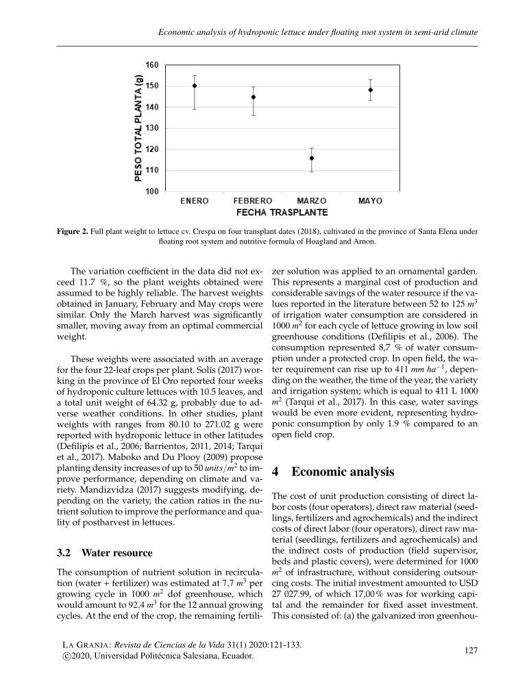
Economic analysis of hydroponic lettuce under floating root system in semi-arid climate
Figure 2. Full plant weight to lettuce cv. Crespa on four transplant dates (2018), cultivated in the province of Santa Elena underfloating root system and nutritive formula of Hoagland and Arnon.
The variation coefficient in the data did not ex-ceed 11.7 %, so the plant weights obtained wereassumed to be highly reliable. The harvest weightsobtained in January, February and May crops weresimilar. Only the March harvest was significantlysmaller, moving away from an optimal commercialweight.
These weights were associated with an averagefor the four 22-leaf crops per plant. Solís (2017) wor-king in the province of El Oro reported four weeksof hydroponic culture lettuces with 10.5 leaves, anda total unit weight of 64.32 g, probably due to ad-verse weather conditions. In other studies, plantweights with ranges from 80.10 to 271.02 g werereported with hydroponic lettuce in other latitudes(Defilipis et al., 2006; Barrientos, 2011, 2014; Tarquiet al., 2017). Maboko and Du Plooy (2009) proposeplanting density increases of up to 50 units/m2 to im-prove performance, depending on climate and va-riety. Mandizvidza (2017) suggests modifying, de-pending on the variety, the cation ratios in the nu-trient solution to improve the performance and qua-lity of postharvest in lettuces.
3.2 Water resource
The consumption of nutrient solution in recircula-tion (water + fertilizer) was estimated at 7,7 m3 pergrowing cycle in 1000 m2 dof greenhouse, whichwould amount to 92,4 m3 for the 12 annual growingcycles. At the end of the crop, the remaining fertili-
zer solution was applied to an ornamental garden.This represents a marginal cost of production andconsiderable savings of the water resource if the va-lues reported in the literature between 52 to 125 m3
of irrigation water consumption are considered in1000 m2 for each cycle of lettuce growing in low soilgreenhouse conditions (Defilipis et al., 2006). Theconsumption represented 8,7 % of water consum-ption under a protected crop. In open field, the wa-ter requirement can rise up to 411 mm ha−1, depen-ding on the weather, the time of the year, the varietyand irrigation system; which is equal to 411 L 1000m2 (Tarqui et al., 2017). In this case, water savingswould be even more evident, representing hydro-ponic consumption by only 1.9 % compared to anopen field crop.
4 Economic analysis
The cost of unit production consisting of direct la-bor costs (four operators), direct raw material (seed-lings, fertilizers and agrochemicals) and the indirectcosts of direct labor (four operators), direct raw ma-terial (seedlings, fertilizers and agrochemicals) andthe indirect costs of production (field supervisor,beds and plastic covers), were determined for 1000m2 of infrastructure, without considering outsour-cing costs. The initial investment amounted to USD27 027.99, of which 17,00% was for working capi-tal and the remainder for fixed asset investment.This consisted of: (a) the galvanized iron greenhou-
LA GRANJA: Revista de Ciencias de la Vida 31(1) 2020:121-133.c©2020, Universidad Politécnica Salesiana, Ecuador. 127
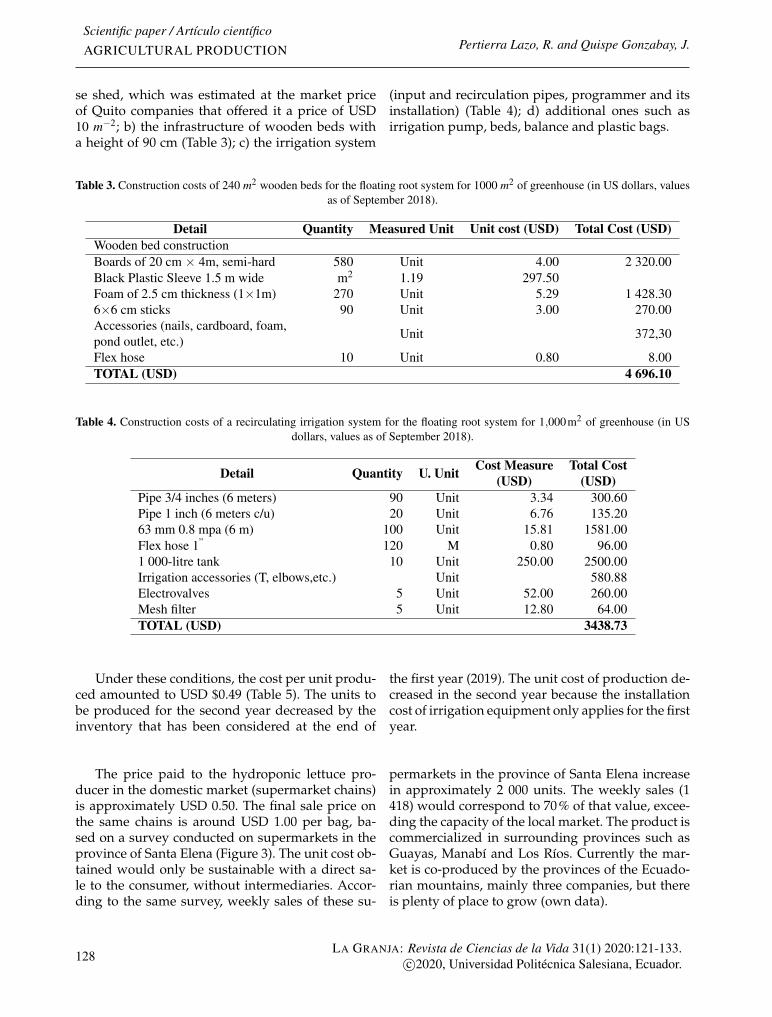
Scientific paper / Artículo científicoAGRICULTURAL PRODUCTION Pertierra Lazo, R. and Quispe Gonzabay, J.
se shed, which was estimated at the market priceof Quito companies that offered it a price of USD10 m−2; b) the infrastructure of wooden beds witha height of 90 cm (Table 3); c) the irrigation system
(input and recirculation pipes, programmer and itsinstallation) (Table 4); d) additional ones such asirrigation pump, beds, balance and plastic bags.
Table 3. Construction costs of 240 m2 wooden beds for the floating root system for 1000 m2 of greenhouse (in US dollars, valuesas of September 2018).
Detail Quantity Measured Unit Unit cost (USD) Total Cost (USD)Wooden bed constructionBoards of 20 cm × 4m, semi-hard 580 Unit 4.00 2 320.00Black Plastic Sleeve 1.5 m wide m2 1.19 297.50Foam of 2.5 cm thickness (1×1m) 270 Unit 5.29 1 428.306×6 cm sticks 90 Unit 3.00 270.00Accessories (nails, cardboard, foam,pond outlet, etc.) Unit 372,30
Flex hose 10 Unit 0.80 8.00TOTAL (USD) 4 696.10
Table 4. Construction costs of a recirculating irrigation system for the floating root system for 1,000m2 of greenhouse (in USdollars, values as of September 2018).
Detail Quantity U. Unit Cost Measure(USD)
Total Cost(USD)
Pipe 3/4 inches (6 meters) 90 Unit 3.34 300.60Pipe 1 inch (6 meters c/u) 20 Unit 6.76 135.2063 mm 0.8 mpa (6 m) 100 Unit 15.81 1581.00Flex hose 1” 120 M 0.80 96.001 000-litre tank 10 Unit 250.00 2500.00Irrigation accessories (T, elbows,etc.) Unit 580.88Electrovalves 5 Unit 52.00 260.00Mesh filter 5 Unit 12.80 64.00TOTAL (USD) 3438.73
Under these conditions, the cost per unit produ-ced amounted to USD $0.49 (Table 5). The units tobe produced for the second year decreased by theinventory that has been considered at the end of
the first year (2019). The unit cost of production de-creased in the second year because the installationcost of irrigation equipment only applies for the firstyear.
The price paid to the hydroponic lettuce pro-ducer in the domestic market (supermarket chains)is approximately USD 0.50. The final sale price onthe same chains is around USD 1.00 per bag, ba-sed on a survey conducted on supermarkets in theprovince of Santa Elena (Figure 3). The unit cost ob-tained would only be sustainable with a direct sa-le to the consumer, without intermediaries. Accor-ding to the same survey, weekly sales of these su-
permarkets in the province of Santa Elena increasein approximately 2 000 units. The weekly sales (1418) would correspond to 70% of that value, excee-ding the capacity of the local market. The product iscommercialized in surrounding provinces such asGuayas, Manabí and Los Ríos. Currently the mar-ket is co-produced by the provinces of the Ecuado-rian mountains, mainly three companies, but thereis plenty of place to grow (own data).
128LA GRANJA: Revista de Ciencias de la Vida 31(1) 2020:121-133.
c©2020, Universidad Politécnica Salesiana, Ecuador.
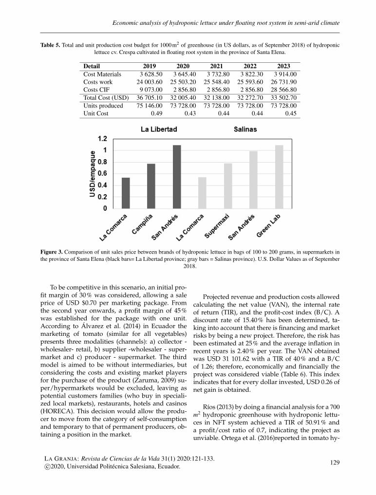
Economic analysis of hydroponic lettuce under floating root system in semi-arid climate
Table 5. Total and unit production cost budget for 1000m2 of greenhouse (in US dollars, as of September 2018) of hydroponiclettuce cv. Crespa cultivated in floating root system in the province of Santa Elena.
Detail 2019 2020 2021 2022 2023Cost Materials 3 628.50 3 645.40 3 732.80 3 822.30 3 914.00Costs work 24 003.60 25 503.20 25 548.40 25 593.60 26 731.90Costs CIF 9 073.00 2 856.80 2 856.80 2 856.80 28 566.80Total Cost (USD) 36 705.10 32 005.40 32 138.00 32 272.70 33 502.70Units produced 75 146.00 73 728.00 73 728.00 73 728.00 73 728.00Unit Cost 0.49 0.43 0.44 0.44 0.45
Figure 3. Comparison of unit sales price between brands of hydroponic lettuce in bags of 100 to 200 grams, in supermarkets inthe province of Santa Elena (black bars= La Libertad province; gray bars = Salinas province). U.S. Dollar Values as of September
2018.
To be competitive in this scenario, an initial pro-fit margin of 30% was considered, allowing a saleprice of USD $0.70 per marketing package. Fromthe second year onwards, a profit margin of 45%was established for the package with one unit.According to Álvarez et al. (2014) in Ecuador themarketing of tomato (similar for all vegetables)presents three modalities (channels): a) collector -wholesaler- retail, b) supplier -wholesaler - super-market and c) producer - supermarket. The thirdmodel is aimed to be without intermediaries, butconsidering the costs and existing market playersfor the purchase of the product (Zaruma, 2009) su-per/hypermarkets would be excluded, leaving aspotential customers families (who buy in speciali-zed local markets), restaurants, hotels and casinos(HORECA). This decision would allow the produ-cer to move from the category of self-consumptionand temporary to that of permanent producers, ob-taining a position in the market.
Projected revenue and production costs allowedcalculating the net value (VAN), the internal rateof return (TIR), and the profit-cost index (B/C). Adiscount rate of 15.40% has been determined, ta-king into account that there is financing and marketrisks by being a new project. Therefore, the risk hasbeen estimated at 25% and the average inflation inrecent years is 2.40% per year. The VAN obtainedwas USD 31 101.62 with a TIR of 40% and a B/Cof 1.26; therefore, economically and financially theproject was considered viable (Table 6). This indexindicates that for every dollar invested, USD 0.26 ofnet gain is obtained.
Ríos (2013) by doing a financial analysis for a 700m2 hydroponic greenhouse with hydroponic lettu-ces in NFT system achieved a TIR of 50.91% anda profit/cost ratio of 0.7, indicating the project asunviable. Ortega et al. (2016)reported in tomato hy-
LA GRANJA: Revista de Ciencias de la Vida 31(1) 2020:121-133.c©2020, Universidad Politécnica Salesiana, Ecuador. 129
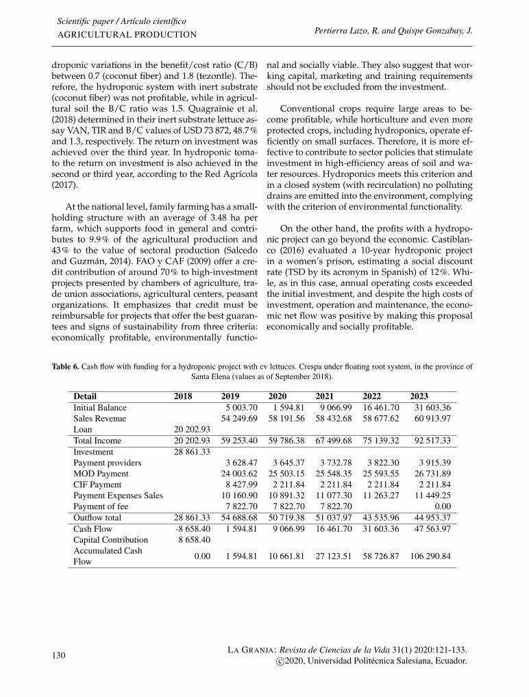
Scientific paper / Artículo científicoAGRICULTURAL PRODUCTION Pertierra Lazo, R. and Quispe Gonzabay, J.
droponic variations in the benefit/cost ratio (C/B)between 0.7 (coconut fiber) and 1.8 (tezontle). The-refore, the hydroponic system with inert substrate(coconut fiber) was not profitable, while in agricul-tural soil the B/C ratio was 1.5. Quagrainie et al.(2018) determined in their inert substrate lettuce as-say VAN, TIR and B/C values of USD 73 872, 48.7%and 1.3, respectively. The return on investment wasachieved over the third year. In hydroponic toma-to the return on investment is also achieved in thesecond or third year, according to the Red Agrícola(2017).
At the national level, family farming has a small-holding structure with an average of 3.48 ha perfarm, which supports food in general and contri-butes to 9.9% of the agricultural production and43% to the value of sectoral production (Salcedoand Guzmán, 2014). FAO y CAF (2009) offer a cre-dit contribution of around 70% to high-investmentprojects presented by chambers of agriculture, tra-de union associations, agricultural centers, peasantorganizations. It emphasizes that credit must bereimbursable for projects that offer the best guaran-tees and signs of sustainability from three criteria:economically profitable, environmentally functio-
nal and socially viable. They also suggest that wor-king capital, marketing and training requirementsshould not be excluded from the investment.
Conventional crops require large areas to be-come profitable, while horticulture and even moreprotected crops, including hydroponics, operate ef-ficiently on small surfaces. Therefore, it is more ef-fective to contribute to sector policies that stimulateinvestment in high-efficiency areas of soil and wa-ter resources. Hydroponics meets this criterion andin a closed system (with recirculation) no pollutingdrains are emitted into the environment, complyingwith the criterion of environmental functionality.
On the other hand, the profits with a hydropo-nic project can go beyond the economic. Castiblan-co (2016) evaluated a 10-year hydroponic projectin a women’s prison, estimating a social discountrate (TSD by its acronym in Spanish) of 12%. Whi-le, as in this case, annual operating costs exceededthe initial investment, and despite the high costs ofinvestment, operation and maintenance, the econo-mic net flow was positive by making this proposaleconomically and socially profitable.
Table 6. Cash flow with funding for a hydroponic project with cv lettuces. Crespa under floating root system, in the province ofSanta Elena (values as of September 2018).
Detail 2018 2019 2020 2021 2022 2023Initial Balance 5 003.70 1 594.81 9 066.99 16 461.70 31 603.36Sales Revenue 54 249.69 58 191.56 58 432.68 58 677.62 60 913.97Loan 20 202.93Total Income 20 202.93 59 253.40 59 786.38 67 499.68 75 139.32 92 517.33Investment 28 861.33Payment providers 3 628.47 3 645.37 3 732.78 3 822.30 3 915.39MOD Payment 24 003.62 25 503.15 25 548.35 25 593.55 26 731.89CIF Payment 8 427.99 2 211.84 2 211.84 2 211.84 2 211.84Payment Expenses Sales 10 160.90 10 891.32 11 077.30 11 263.27 11 449.25Payment of fee 7 822.70 7 822.70 7 822.70 0.00Outflow total 28 861.33 54 688.68 50 719.38 51 037.97 43 535.96 44 953.37Cash Flow -8 658.40 1 594.81 9 066.99 16 461.70 31 603.36 47 563.97Capital Contribution 8 658.40Accumulated CashFlow 0.00 1 594.81 10 661.81 27 123.51 58 726.87 106 290.84
130LA GRANJA: Revista de Ciencias de la Vida 31(1) 2020:121-133.
c©2020, Universidad Politécnica Salesiana, Ecuador.
Economic analysis of hydroponic lettuce under floating root system in semi-arid climate
Likewise, these productive systems can be acti-vated in urban or rural community orchards, withtraining and strengthening of the society. In the pro-vince of Santa Elena, people work massively in the-se orchards (Prefectura Santa Elena, 2017), but hy-droponic systems have not yet been implemented.With regard to social viability in this low-scale pro-posal, four direct and indirect jobs associated withthe transportation and marketing of the productwere achieved, thus improving the living condi-tions of those involved. Additionally, it would en-rich the basket and the family diet, generate em-ployment and savings in the purchase of fresh pro-ducts.
5 Conclusions
The total weight of lettuces obtained on four trans-plant dates under the agroecological conditions ofthe province of Santa Elena, meets the minimumcommercial weight, is relevant to the current offerin shopping centers and it is competitive in the mar-ket as long as it is sold without intermediaries.
The consumption of nutrient solution (fertili-zing water) was estimated at 7.7 m3 per growingcycle in 1000 m2 of greenhouse, representing 8.7 %of the consumption of water under protected crop,and only 1.9% compared to an open field crop.
With the established assumptions and thetechnical-economic evaluation, a unit productioncost of USD 0.49 was obtained. A VAN of USD $ 31101.62, was obtained with a sale price of each pac-kage of USD 0.70 (higher than zero), a TIR of 40%.This value was higher than the discount rate. Theprofit-cost ratio obtained was 1.26.
The sustainability of the proposal was evident inthe economic and financial viability, the considera-ble savings of the water resource, the non-pollutionof the environment as a closed system and the socialviability shown in the generation of employmentand improvement of quality of life of those invol-ved, as well as being a contribution to the local diet.
It will be a future task to evaluate other gene-tic materials of lettuce that have a higher toleran-ce to high temperatures, with the aim of obtainingbetter yields and exploring with other horticultu-
ral, aromatic or medicinal species, baby vegetablesor fourth-range products that have an economic ac-tivity. On the other hand, an increase in produc-tivity can occur by increasing plant density or byapplying biostimulants that allow lettuce to copebetter with abiotic stress.
AcknowledgmentThe authors thank the Santa Elena Peninsula Sta-te University for having provided the researchersthe public resources available through funds for re-search projects with internal funding. This projectwas assigned under the number P06 entitled "Hy-droponic production systems: alternative for thechange of the agroproductive matrix in the SantaElena Peninsula"(Code 91870000.0000.381020). Theauthors also thank the participation of the stu-dent Jeniffer Ricardo Morales in the implementa-tion, execution and collection of data during trials.
ReferencesÁlvarez, T., Bravo, E., and Armendaris, E. (2014).
Soberanía alimentaria y acceso a semillas hortí-colas en el ecuador. LA GRANJA: Revista de Cien-cias de la Vida, 20(2):45–57. Onine: http://bit.ly/2Q1JKA8.
Banco Central del Ecuador (2018). Información eco-nómica.
Barbosa, G., Gadelha, F., Kublik, N., Proctor, A.,Reichelm, L., Weissinger, E., Wohlleb, G., andHalden, R. (2015). Comparison of land, wa-ter, and energy requirements of lettuce grownusing hydroponic vs. conventional agriculturalmethods. International Journal of Environmental Re-search and Public Health, 12(6):6879–6891. Online:http://doi.org/10.3390/ijerph120606879.
Barrientos, H. (2011). Determinación de la intensi-dad lumínica en plásticos de cubierta (agrofilm)para ambientes atemperados en tres localidadesdel departamento de la paz.
Barrientos, H. (2014). Análisis de crecimiento fun-cional, acumulación de biomasa y translocaciónde materia seca de ocho hortalizas cultivadasen invernadero. Tesis de maestría, Universi-dad Mayor de San Andrés. Online: http://bit.ly/2K6N5KC, La Paz, Bolivia.
LA GRANJA: Revista de Ciencias de la Vida 31(1) 2020:121-133.c©2020, Universidad Politécnica Salesiana, Ecuador. 131
Scientific paper / Artículo científicoAGRICULTURAL PRODUCTION Pertierra Lazo, R. and Quispe Gonzabay, J.
Beltrano, J. and Gimenez, D. (2015). Cultivo en hidro-ponía. Editorial de la Universidad Nacional de LaPlata (EDULP). Online: http://bit.ly/2Cvu7cg, 1ed edition.
Castiblanco, A. (2016). Cultivos hidropónicos comopropuesta rehabilitadora en equipamientos peni-tenciarios femeninos. Especialización en gerenciaintegral de proyectos, Universidad Militar NuevaGranada. Online: https://bit.ly/34QqmtY.
CLIRSEN-MAGAP (2011). Memoria técnica: cantónsalinas. proyecto: Generación de geoinformaciónpara la gestión del territorio a nivel nacional es-cala 1:25.000. Technical report.
Defilipis, C., Pariani, S., Jimenez, A., and Bouzo, C.(2006). Respuesta al riego de lechuga (lactuca sa-tiva l.) cultivada en invernadero. page Online:https://bit.ly/32ARDPR.
Díaz, M., Parra, R., and López, L. (2012). Presu-puestos: Enfoque para la planeación financiera, pages45–225. Online: https://bit.ly/2CsksDs. Pearson,Colombia.
Espinoza, E. (2015). Aumenta producción y consu-mo de hortalizas. Revista El Agro, (227):8–11. On-line: https://bit.ly/34LdF3M.
FAO (2019). Datos sobre alimentación y agricultura.cultivos.
FAO y CAF (2009). Ecuador: Nota de análisis sec-torial agricultura y desarrollo rural. Technicalreport, ORGANIZACIÓN DE LAS NACIONESUNIDAS PARA LA AGRICULTURA Y LA ALI-MENTACIÓN, DIRECCIÓN DEL CENTRO DEINVERSIONES y CORPORACIÓN ANDINA DEFOMENTO (CAF), Quito, Ecuador. Online: https://bit.ly/2X2Rgwe.
IBISWORLD (2018). Hydroponic crop farming in-dustry in the usa.
INAMHI (2017). Boletines agroclimáticos.
INEC (2002). Iii censo nacional agropecuario. Tech-nical report, Instituto Nacional de Estadísticas yCensos, Online: https://bit.ly/2Q583NO.
INEC (2013). Encuesta nacional de ingresos ygastos. instituto nacional de estadística y censos(enighur) 2011-2012.
INEC (2017). Inflación mensual. diciembre 2017.Technical report, Instituto Nacional de Estadísticay Censos. Online: https://bit.ly/2pYHsqZ.
INTAGRI (2017). La industria de los cultivos hidro-pónicos. Artículos Técnicos de INTAGRI, (31):Onli-ne: https://bit.ly/2O4LW7E.
Junta de Andalucía (2013). Lechuga.
Khan, F., Kurklu, A., Ghafoor, A., Ali, Q., Umair,M., and Shahzaib (2018). A review on hydropo-nic greenhouse cultivation for sustainable agri-culture. International Journal of Agriculture, En-vironment and Food Sciences, 2(2):59–66. Online:https://bit.ly/2rtUBIV.
Maboko, M. and Du Plooy, C. (2009). Effect ofplant spacing on growth and yield of lettuce (lac-tuca sativa l.) in a soilless production system.South African Journal of Plant and Soil, 26(3):195–198. Online: https://doi.org/10.1080/02571862.2009.10639954.
Mandizvidza, T. (2017). Influence of nutrient andlight management on postharvest quality of let-tuce (lactuca sativa l.) in soilless production sys-tems. Tesis msc. en agricultura, Stellenbosch Uni-versity. Online: https://bit.ly/34OSI8c.
Maroto, J. (2002). Horticultura herbácea especia.Mundi-Prensa. Online: https://bit.ly/34U8DSN,España, 5 ed edition.
Mateo, A. (2019). Agricultura familiar campesi-na proyecto de huertos familiares agroecológicos.Ministerio de Agricultura y Ganadería (MAG)Santa Elena. Comunicación personal.
Ortega, L., Martínez, C., Ocampo, J., Sandoval, E.,and Pérez, B. (2016). Eficiencia de sustratos enel sistema hidropónico y de suelo para la pro-ducción de tomate en invernadero. [efficiencyof substrates in soil and hydroponic system forgreenhouse tomato production]. Revista Mexicanade Ciencias Agrícolas, 7(3):643–653. Online: https://bit.ly/2K99vLn.
Prefectura Santa Elena (2017). 250 huertos familia-res están activados en la provincia de santa elena.
Quagrainie, K., Flores, R., Kim, H., and McClain, V.(2018). Economic analysis of aquaponics and hy-droponics production in the u.s. midwest. Journalof Applied Aquaculture, 30(1):1–14. Online: https://doi.org/10.1080/10454438.2017.1414009.
132LA GRANJA: Revista de Ciencias de la Vida 31(1) 2020:121-133.
c©2020, Universidad Politécnica Salesiana, Ecuador.

Economic analysis of hydroponic lettuce under floating root system in semi-arid climate
Red Agrícola (2017). Cultivo hidropónico de agrotop en quillota.
Resh, H. (2013). Hydroponic Food Production. CRCPress, Online: https://bit.ly/34TlV1x, 7 ed edi-tion.
Ríos, J. (2013). Plan de negocios para una empre-sa de hidropónicos localizada en el municipio delretiro en antioquia.
Saavedra, G., Corradini, F., Antúnez, A., Felmer, S.,Estay, P., and Sepúlveda, P. (2017). Manual de pro-ducción de lechuga. Instituto de Desarrollo Agro-pecuario - Instituto de Investigaciones Agrope-cuarias, Santiago, Chile. Online: https://bit.ly/32D42Tg, 9 ed edition.
Sábada, S., Del Castillo, J., Sanz de Galdeano, J., Uri-barri, A., and Aguado, G. (2007). Lechuga en cul-tivo hidropónico. acercamiento a nuevas formasde producción. Navarra Agraria, (161):29–34. On-line: https://bit.ly/2NYYfSJ.
Salcedo, S. and Guzmán, L. (2014). Agricultura fami-liar en América Latina y el Caribe. Recomendacionesde política. FAO. Online: https://bit.ly/2K9cjIq,Santiago de Chile.
Sharma, N., Acharya, J., Kumar, K., Singh, N., andO., C. (2018). Hydroponics as an advanced techni-que for vegetable production: An overview. Jour-nal of Soil and Water Conservation, 17(4):364–371.Online: https://bit.ly/2Q72yye.
Solís, F. (2017). Evaluación del rendimiento en elcultivo de lechuga (lactuca sativa) en sistemas hi-dropónicos y aeropónicos automatizados.
Tarqui, M., Chipana, R., Mena, F., Quino, J., Talla-cagua, R., and Gutiérrez, S. (2017). Índice de es-trés hídrico del cultivo de lechuga (lactuca sati-va), mediante termometría infrarroja a diferentesláminas de riego. [index of water stress of let-tuce crop (lactuca sativa), through infrared ther-mometry to different irrigation sheets]. Revistade Investigación e Innovación Agropecuaria y de Re-cursos Naturales, 4(1):7–18. Online: https://bit.ly/2NyfkE7.
Urrestarazu, M. (2015). Manual práctico del culti-vo sin suelo e Hidroponía. Ed. Mundi Prensa Li-bros SA. (Grupo Paraninfo). Online: https://bit.ly/2Q8j0hl, España, 1 ed edition.
Zaruma, S. (2009). Incidencia de la cadena producti-va de hortalizas en el desarrollo socio económicodel proyecto cañar-murcia.
LA GRANJA: Revista de Ciencias de la Vida 31(1) 2020:121-133.c©2020, Universidad Politécnica Salesiana, Ecuador. 133

Scientific paper/ Artículo científico
AGRICULTURAL PRODUCTIONpISSN:1390-3799; eISSN:1390-8596
http://doi.org/10.17163/lgr.n31.2020.10
EFFECT OF THE ROOF (LOW TUNNEL) ON THE PRODUCTIVITY OF
TWO VARIETIES OF STRAWBERRY (Fragaria vesca) IN CAJANUMA,LOJA
EFECTO DE LA CUBIERTA (MICROTÚNEL) EN LA PRODUCTIVIDAD DE DOS
VARIEDADES DE FRESA (Fragaria vesca) EN EL SECTOR CAJANUMA CANTÓN
LOJA
Carlos Fausto Abad Abad*1 , Leticia Salomé Jiménez Álvarez2 and EdwinDaniel Capa Mora3,1
1 Carreara de Ingeniería Agropecuaría. Universidad Técnica Particular de Loja, San Cayetano alto s/n, 1101608 Loja, Ecuador2 Departamento de Ciencias Biológicas, Ecología y Sistemática, Universidad Técnica Particular de Loja, San Cayetano alto s/n,1101608 Loja, Ecuador3 Departamento de Ciencias Biológicas, Biotecnología y Producción, Universidad Técnica Particular de Loja, San Cayetano altos/n, 1101608 Loja, Ecuador
*Corresponding author: [email protected]
Article received on December 12th, 2018. Accepted, after review, on August 30th, 2019. Published on March 1st, 2020.
Resumen
La fresa (Fragaria vesca) es un cultivo de gran aceptación a nivel mundial, no siendo la excepción en Ecuador. Lamayor parte de la producción se realiza a campo abierto, haciendo que existan limitaciones por el ataque de factoresbióticos y la influencia de factores abióticos, generando pérdidas en la producción. El presente trabajo se planteóen la provincia de Loja al no existir información precisa de este cultivo e investigaciones sobre el uso de sistemasprotegidos (microtúnel). El objetivo principal fue evaluar el efecto de la producción de fresa en los dos sistemas deproducción (Campo abierto y microtúnel), con variedades Albion y Monterey; además analizar el costo y rentabilidadde la producción. El sistema a campo abierto fue considerado como un tratamiento testigo para su evaluación frenteal de microtunel. El experimento se realizó en la Estación Agropecuaria de la Universidad Técnica Particular de Loja,bajo condiciones de microtúnel y campo abierto, en la cuales se comparó el desarrollo fenológico y productivo de lafresa. Los resultados encontrados en el estudio en los dos sistemas a campo abierto y microtúnel no presentaron unadiferencia estadística en las variables fisiológicas evaluadas, concluyendo que la cubierta con microtúnel al cultivo noinfluyó en el desarrollo en las dos variedades. En relación al análisis de costos-beneficio de la producción, este fuesuperior en el sistema microtúnel, la inversión fue más fuerte al inicio, sin embargo, se debe indicar que existen variasventajas productivas en relación con campo abierto, generando beneficios al productor de fresa.Palabras clave: Fresa, Microtúnel, producción, rendimiento, rentabilidad.
134LA GRANJA: Revista de Ciencias de la Vida 31(1) 2020:134-143.c©2020, Universidad Politécnica Salesiana, Ecuador.
Effect of the roof (Low tunnel) on the productivity of two varieties of strawberry (Fragaria vesca) inCajanuma, Loja
Abstract
The strawberry (Fragaria vesca) is a crop of great acceptance worldwide. In Ecuador, most of the production is done inopen field, presenting limitations by the attack of biotic factors and abiotic factors that generate losses in the produc-tion. This research was carried out in the province of Loja, since there was no precise information on this crop, andresearch on the use of protected systems (low tunnels). The main objective of the study was to evaluate the effect ofstrawberry production on the two production systems (open field and low tunnels), with Albion and Monterey varie-ties, as well as to analyze the costs and profitability of production. The experiment was conducted at the AgriculturalStation of Universidad Técnica Particular de Loja, under low tunnels and open field conditions, in which the pheno-logical and productive development of the strawberry was compared. The results found in the study in the two openfield and low tunnel systems did not present a statistical difference in the physiological variables evaluated, whichallow to conclude that the low tunnel cover on the crop did not influence the development of the two varieties. Inrelation to the cost-benefit analysis of production, it was higher in the low tunnel system, the investment was strongerat the beginning, but it must be indicated that there are several productive advantages in relation to the open fieldthat generate benefits for the strawberry producer.Keywords: Low tunnels, production, profitability, strawberry yield.
Suggested citation: Abad-Abad, C.F., Jiménez-Álvarez, L.S. and Capa-Mora, E.D. (2020). Effect of theroof (Low tunnel) on the productivity of two varieties of strawberry (Fragaria ves-ca) in Cajanuma, Loja. La Granja: Revista de Ciencias de la Vida. Vol. 31(1):134-143.http://doi.org/10.17163/lgr.n31.2020.10.
Orcid IDs:Carlos Fausto Abad Abad: http://orcid.org/0000-0003-4349-8446Leticia Salomé Jiménez Álvarez: http://orcid.org/0000-0002-7933-1368Edwin Daniel Capa Mora: http://orcid.org/0000-0002-9843-0388
LA GRANJA: Revista de Ciencias de la Vida 31(1) 2020:134-143.c©2020, Universidad Politécnica Salesiana, Ecuador. 135

Scientific paper / Artículo científicoAGRICULTURAL PRODUCTION Duque Abad-Abad, C.F., Jiménez-Álvarez, L.S. and Capa-Mora, E.D.
1 Introduction
The crop of strawberry by agricultural producersand its consumption has a very good acceptanceworldwide (Khoshnevisan et al., 2013), the samehappens in Ecuador, where it has started to be partof the family consumption (Vizcaino, 2011). Thefruit is quite attractive to the consumer for its aro-ma and exquisite taste; it also has a lot of vitamins,minerals and organic acids, acting as disinfectantsand anti-inflammatory drugs that decreases choles-terol. In addition, essential oils can be extracted, andtheir consumption can be fresh or processed (Karimet al., 2011; Giampieri et al., 2012; Pradas et al., 2015;Bernarda and Bawab, 2017; Estrada et al., 2017).Strawberry is characterized by being herbaceousand perennial, it is very sensitive to environmen-tal conditions and its development is subjected tothe climatic characteristics, chemical, physical andstructural properties of the soil (Ferriol, 2010; Lópezet al., 2011; Pineda, 2017). There are short-day varie-ties subjected to photoperiod, fewer hours of lightfor the development of flower buds; and neutral-day varieties that are not subjected to photoperiodfor the development of flower buds (Undurragaand Vargas, 2013; Pérez et al., 2017).
The mostly used production systems are openfield and under protection (Rubio et al., 2014). Openfield production is highly susceptible to biotic andabiotic factors such as pests, diseases, high tem-peratures, precipitation, winds and frosts (Dominí,2012; Pineda, 2017), which can affect productivity.Lamont and William (2009) mention that techno-logy helps to have better control of the climaticconditions for its cultivation. Environmental, gene-tic and variety factors are important in the plantgrowth, productivity and fruit quality (Rodríguezet al., 2012). The cultivation of strawberry in pro-tected systems such as the low tunnel system canbe an alternative in the production of this crop, be-cause these systems have some advantages such aslow cost, small size and practicality of installation(Juárez et al., 2011; Pernuzz et al., 2016), comparedto other protected systems such as greenhouses.
In Ecuador an area of 108 ha is harvested,reaching a yield of 16.27 T/ha, being very lowcompared to other strawberry producing countries,such as the United States with 66.90 T/ha of pro-duction; Spain (47.6 T/ha); Egypt 46.6 T/ha; Israel
with 43.5 T/ha, and Colombia with 36.5 T/ha ofstrawberry production per year (Corrêa and Peres,2013; FAOSTAT, 2016). However, in the last decadeit has had an interesting growth, either by adoptingnew technology or new varieties.
The search and application of new innovationsin agricultural production to improve productionsystems are very important, since each area dedi-cated to strawberry cultivation has its common fea-tures. In the province of Loja, it is necessary to carryout research on the subject in the absence of accu-rate information or research on the use of protec-ted systems (low tunnel) in this crop. Therefore, thisstudy aims to assess the effect of the use of protec-tion (low tunnel) on the development and produc-tivity of strawberry cultivation in the Albion andMonterey varieties, which are the most commercia-lized in this area, in order to analyze the most fea-sible alternatives, so that smallholder farmers at thelocal level increase yield and economic benefits.
2 Materials and Methods
2.1 Study area
This study was carried out in the province of Loja– Ecuador, at the Agricultural Station of the Techni-cal University of Loja, located in the Cajanuma sec-tor, 9 km away from the city, with the X coordina-tes: −4,0887 Y: −79,2082 (Google Maps, 2018). at analtitude of approximately 2230 m.a.s.l; an averagetemperature of 16 ◦C and an average rainfall of 780mm/m2 according to data from Estación meteoroló-gica «La Argelia» (2017).
2.2 Experimental design
The study area is a place with homogeneous to-pography and edaphoclimatic characteristics. Fourplots (treatments) were established under an expe-rimental design of complete blocks. The establis-hed treatments were: two low cover (low tunnel)in which the Monterey and Albion varieties we-re grown (one variety in each low tunnel), and thesame treatments were established in open field (wit-hout cover). Each treatment had a total of 54 plants(F1) and each was considered as an experimentalunit (Pernuzz et al., 2016).
136LA GRANJA: Revista de Ciencias de la Vida 31(1) 2020:134-143.
c©2020, Universidad Politécnica Salesiana, Ecuador.

Effect of the roof (Low tunnel) on the productivity of two varieties of strawberry (Fragaria vesca) inCajanuma, Loja
The symbols established for the treatments we-re: CAV1= Open field treatment monterey variety,CAV2 = Open field treatment albion variety, MTV1= low tunnel system treatment monterey variety,MTV2 = low tunnel system treatment albion va-riety. The size of the low tunnels was 8 m long × 1m wide and 0.90 m high, with polyethylene plasticcover Nro 8. A planting density of 0.30 × 0.40 mbetween row and plant (54 plants per treatment)was used in each treatment.
The fertilization was similar in all treatments,using organic fertilizer (BioCompost) at the timeof transplantation (250 g/plant), and mineral fer-tilizers based on N−P2O5 −K2O−MgO−CaO−S(200 − 200 − 300 − 40 − 100 − 40 Kg/ha, respecti-vely), all based on soil analyses and crop needs(Patiño et al., 2013; Avitia et al., 2014).
The irrigation system was installed by low flowdrip, with vortex emitters inserted and flow output2 to 4 Lt/hour, and was watered based on the weat-her conditions, as commonly handled by farmers inthe area. The integrated management of pests anddiseases (MIP) was thorough, each plant was moni-tored, preemptively performing sanitation pruningto avoid diseases such as Botrytis cinerea, Colletotri-chun sp. y de Trips sp. (Santoyo and Martinez, 2010).
2.3 Variables evaluatedThe evaluation variables are detailed below: De-tachment percentage: it was performed by coun-ting the total of plants (experimental unit) of eachtreatment that was successful in its detachment,indicating that the results were expressed as per-centage (Ibadango, 2017).Number of flowers: The number of flowers on eachplant of the four treatments was counted; this da-ta was recorded throughout the project evaluation(Yaselga, 2015).Number of fruits: The amount of fruits in the plantsof each treatment was determined for a period of 6months, the data were recorded daily in order tohave more detail of the productivity by productionsystem and variety of cultivated strawberries (Iba-dango, 2017).
Fruit diameter: The data was taken from the fruitsharvested with a Vernier calibrator, the measure-ment was done from the central part of the fruit(unfructescence), expressing the values in centime-ters (Verdugo, 2011).Fruit weight: The weight of each harvested fruitwas considered. It should be mentioned that straw-berry fruits were harvested when they were ripe,just as the registration of the previous variables,this was done daily once the production started(Verdugo, 2011).Economic analysis of strawberry production: Theproduction of the crop was calculated taking intoaccount the total harvested (without consideringthe losses), and the final production of the treat-ments was transferred and expressed in kg/ha.
The net income (benefit) of these production sys-tems in this study was estimated with the differencebetween the input and costs of strawberry produc-tion (Cost/benefit (C/B) = Input/expenses) (Infan-te Villarreal, 1984), calculating inputs from sales ofthe fruit at average MAG (2018). Total costs wereestimated from the average planting costs and itsmanagement: fertilization, weed control, irrigationsystem, pest control, diseases, pruning, among ot-hers.
2.4 Statistical analysisThe normality or abnormality of the data was chec-ked with KS tests to establish statistical differencesin the measured parameters (variables), then one-way ANOVA was applied with homogeneous Tu-key tests at a significance level p < 0,05, for this thestatistical software SPSS 24.0 was used.
3 Results and discussionTable 1 details the results obtained in the differenttreatments. It is observed that there are not signi-ficant statistical differences between the physiolo-gical variables evaluated, indicating that the coverof low tunnel did not influence the developmentof strawberry cultivation in the two varieties, pro-bably because there were no heavy periods of rain.
LA GRANJA: Revista de Ciencias de la Vida 31(1) 2020:134-143.c©2020, Universidad Politécnica Salesiana, Ecuador. 137
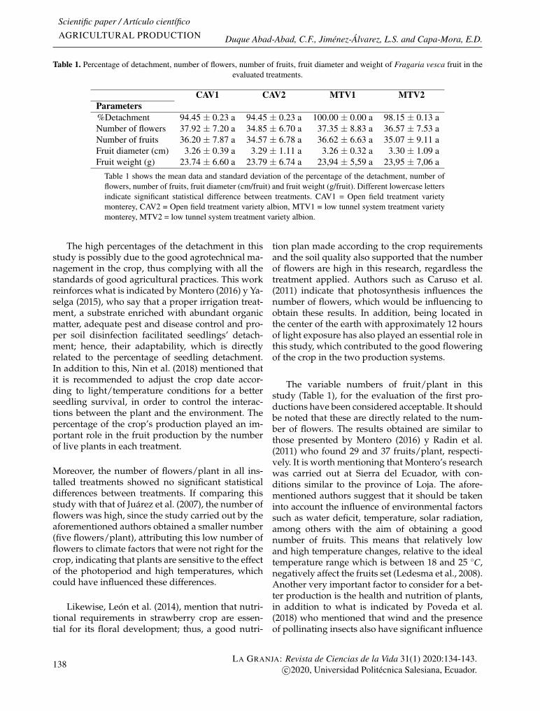
Scientific paper / Artículo científicoAGRICULTURAL PRODUCTION Duque Abad-Abad, C.F., Jiménez-Álvarez, L.S. and Capa-Mora, E.D.
Table 1. Percentage of detachment, number of flowers, number of fruits, fruit diameter and weight of Fragaria vesca fruit in theevaluated treatments.
CAV1 CAV2 MTV1 MTV2Parameters%Detachment 94.45 ± 0.23 a 94.45 ± 0.23 a 100.00 ± 0.00 a 98.15 ± 0.13 aNumber of flowers 37.92 ± 7.20 a 34.85 ± 6.70 a 37.35 ± 8.83 a 36.57 ± 7.53 aNumber of fruits 36.20 ± 7.87 a 34.57 ± 6.78 a 36.62 ± 6.63 a 35.07 ± 9.11 aFruit diameter (cm) 3.26 ± 0.39 a 3.29 ± 1.11 a 3.26 ± 0.32 a 3.30 ± 1.09 aFruit weight (g) 23.74 ± 6.60 a 23.79 ± 6.74 a 23,94 ± 5,59 a 23,95 ± 7,06 a
Table 1 shows the mean data and standard deviation of the percentage of the detachment, number offlowers, number of fruits, fruit diameter (cm/fruit) and fruit weight (g/fruit). Different lowercase lettersindicate significant statistical difference between treatments. CAV1 = Open field treatment varietymonterey, CAV2 = Open field treatment variety albion, MTV1 = low tunnel system treatment varietymonterey, MTV2 = low tunnel system treatment variety albion.
The high percentages of the detachment in thisstudy is possibly due to the good agrotechnical ma-nagement in the crop, thus complying with all thestandards of good agricultural practices. This workreinforces what is indicated by Montero (2016) y Ya-selga (2015), who say that a proper irrigation treat-ment, a substrate enriched with abundant organicmatter, adequate pest and disease control and pro-per soil disinfection facilitated seedlings’ detach-ment; hence, their adaptability, which is directlyrelated to the percentage of seedling detachment.In addition to this, Nin et al. (2018) mentioned thatit is recommended to adjust the crop date accor-ding to light/temperature conditions for a betterseedling survival, in order to control the interac-tions between the plant and the environment. Thepercentage of the crop’s production played an im-portant role in the fruit production by the numberof live plants in each treatment.
Moreover, the number of flowers/plant in all ins-talled treatments showed no significant statisticaldifferences between treatments. If comparing thisstudy with that of Juárez et al. (2007), the number offlowers was high, since the study carried out by theaforementioned authors obtained a smaller number(five flowers/plant), attributing this low number offlowers to climate factors that were not right for thecrop, indicating that plants are sensitive to the effectof the photoperiod and high temperatures, whichcould have influenced these differences.
Likewise, León et al. (2014), mention that nutri-tional requirements in strawberry crop are essen-tial for its floral development; thus, a good nutri-
tion plan made according to the crop requirementsand the soil quality also supported that the numberof flowers are high in this research, regardless thetreatment applied. Authors such as Caruso et al.(2011) indicate that photosynthesis influences thenumber of flowers, which would be influencing toobtain these results. In addition, being located inthe center of the earth with approximately 12 hoursof light exposure has also played an essential role inthis study, which contributed to the good floweringof the crop in the two production systems.
The variable numbers of fruit/plant in thisstudy (Table 1), for the evaluation of the first pro-ductions have been considered acceptable. It shouldbe noted that these are directly related to the num-ber of flowers. The results obtained are similar tothose presented by Montero (2016) y Radin et al.(2011) who found 29 and 37 fruits/plant, respecti-vely. It is worth mentioning that Montero’s researchwas carried out at Sierra del Ecuador, with con-ditions similar to the province of Loja. The afore-mentioned authors suggest that it should be takeninto account the influence of environmental factorssuch as water deficit, temperature, solar radiation,among others with the aim of obtaining a goodnumber of fruits. This means that relatively lowand high temperature changes, relative to the idealtemperature range which is between 18 and 25 ◦C,negatively affect the fruits set (Ledesma et al., 2008).Another very important factor to consider for a bet-ter production is the health and nutrition of plants,in addition to what is indicated by Poveda et al.(2018) who mentioned that wind and the presenceof pollinating insects also have significant influence
138LA GRANJA: Revista de Ciencias de la Vida 31(1) 2020:134-143.
c©2020, Universidad Politécnica Salesiana, Ecuador.
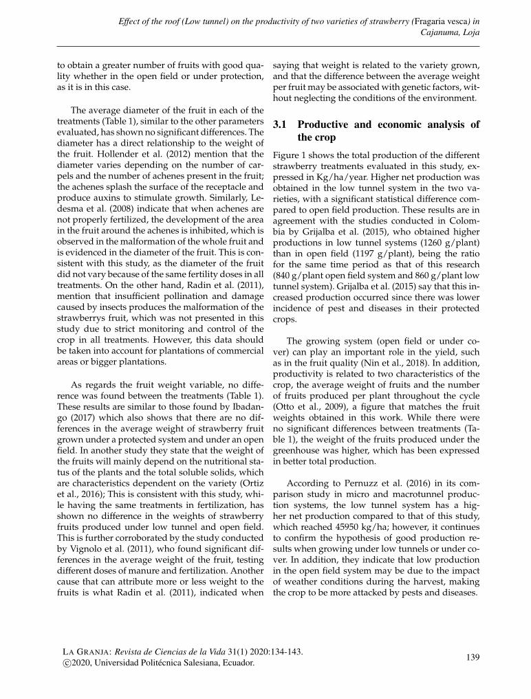
Effect of the roof (Low tunnel) on the productivity of two varieties of strawberry (Fragaria vesca) inCajanuma, Loja
to obtain a greater number of fruits with good qua-lity whether in the open field or under protection,as it is in this case.
The average diameter of the fruit in each of thetreatments (Table 1), similar to the other parametersevaluated, has shown no significant differences. Thediameter has a direct relationship to the weight ofthe fruit. Hollender et al. (2012) mention that thediameter varies depending on the number of car-pels and the number of achenes present in the fruit;the achenes splash the surface of the receptacle andproduce auxins to stimulate growth. Similarly, Le-desma et al. (2008) indicate that when achenes arenot properly fertilized, the development of the areain the fruit around the achenes is inhibited, which isobserved in the malformation of the whole fruit andis evidenced in the diameter of the fruit. This is con-sistent with this study, as the diameter of the fruitdid not vary because of the same fertility doses in alltreatments. On the other hand, Radin et al. (2011),mention that insufficient pollination and damagecaused by insects produces the malformation of thestrawberrys fruit, which was not presented in thisstudy due to strict monitoring and control of thecrop in all treatments. However, this data shouldbe taken into account for plantations of commercialareas or bigger plantations.
As regards the fruit weight variable, no diffe-rence was found between the treatments (Table 1).These results are similar to those found by Ibadan-go (2017) which also shows that there are no dif-ferences in the average weight of strawberry fruitgrown under a protected system and under an openfield. In another study they state that the weight ofthe fruits will mainly depend on the nutritional sta-tus of the plants and the total soluble solids, whichare characteristics dependent on the variety (Ortizet al., 2016); This is consistent with this study, whi-le having the same treatments in fertilization, hasshown no difference in the weights of strawberryfruits produced under low tunnel and open field.This is further corroborated by the study conductedby Vignolo et al. (2011), who found significant dif-ferences in the average weight of the fruit, testingdifferent doses of manure and fertilization. Anothercause that can attribute more or less weight to thefruits is what Radin et al. (2011), indicated when
saying that weight is related to the variety grown,and that the difference between the average weightper fruit may be associated with genetic factors, wit-hout neglecting the conditions of the environment.
3.1 Productive and economic analysis ofthe crop
Figure 1 shows the total production of the differentstrawberry treatments evaluated in this study, ex-pressed in Kg/ha/year. Higher net production wasobtained in the low tunnel system in the two va-rieties, with a significant statistical difference com-pared to open field production. These results are inagreement with the studies conducted in Colom-bia by Grijalba et al. (2015), who obtained higherproductions in low tunnel systems (1260 g/plant)than in open field (1197 g/plant), being the ratiofor the same time period as that of this research(840 g/plant open field system and 860 g/plant lowtunnel system). Grijalba et al. (2015) say that this in-creased production occurred since there was lowerincidence of pest and diseases in their protectedcrops.
The growing system (open field or under co-ver) can play an important role in the yield, suchas in the fruit quality (Nin et al., 2018). In addition,productivity is related to two characteristics of thecrop, the average weight of fruits and the numberof fruits produced per plant throughout the cycle(Otto et al., 2009), a figure that matches the fruitweights obtained in this work. While there wereno significant differences between treatments (Ta-ble 1), the weight of the fruits produced under thegreenhouse was higher, which has been expressedin better total production.
According to Pernuzz et al. (2016) in its com-parison study in micro and macrotunnel produc-tion systems, the low tunnel system has a hig-her net production compared to that of this study,which reached 45950 kg/ha; however, it continuesto confirm the hypothesis of good production re-sults when growing under low tunnels or under co-ver. In addition, they indicate that low productionin the open field system may be due to the impactof weather conditions during the harvest, makingthe crop to be more attacked by pests and diseases.
LA GRANJA: Revista de Ciencias de la Vida 31(1) 2020:134-143.c©2020, Universidad Politécnica Salesiana, Ecuador. 139
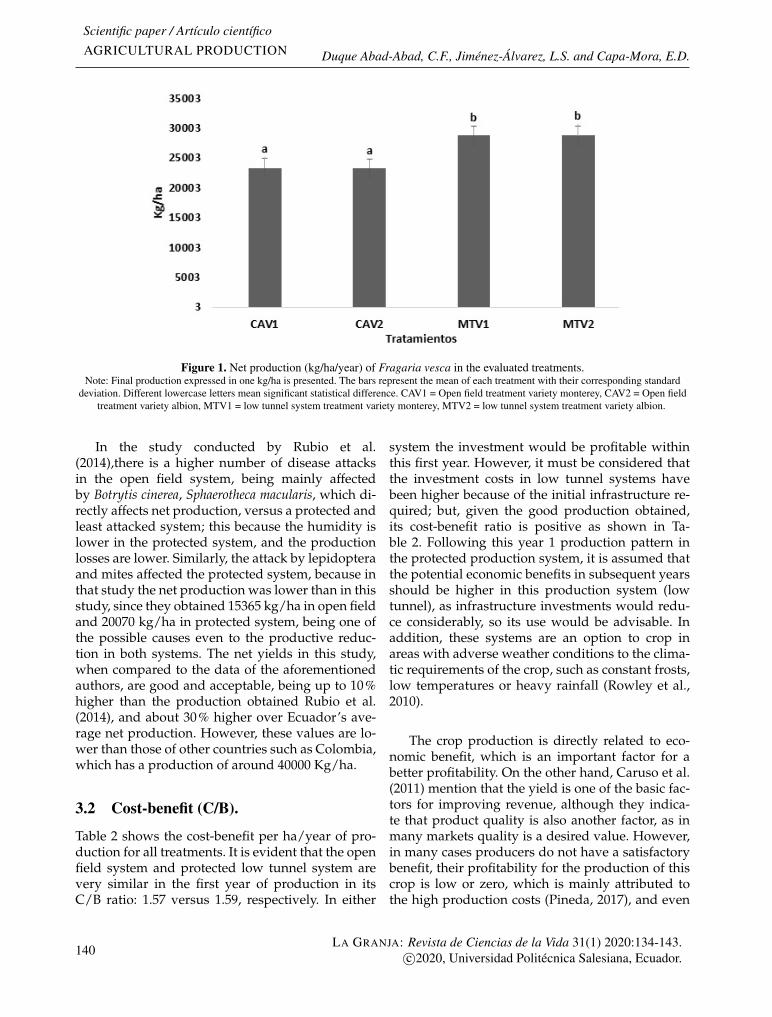
Scientific paper / Artículo científicoAGRICULTURAL PRODUCTION Duque Abad-Abad, C.F., Jiménez-Álvarez, L.S. and Capa-Mora, E.D.
Figure 1. Net production (kg/ha/year) of Fragaria vesca in the evaluated treatments.Note: Final production expressed in one kg/ha is presented. The bars represent the mean of each treatment with their corresponding standard
deviation. Different lowercase letters mean significant statistical difference. CAV1 = Open field treatment variety monterey, CAV2 = Open fieldtreatment variety albion, MTV1 = low tunnel system treatment variety monterey, MTV2 = low tunnel system treatment variety albion.
In the study conducted by Rubio et al.(2014),there is a higher number of disease attacksin the open field system, being mainly affectedby Botrytis cinerea, Sphaerotheca macularis, which di-rectly affects net production, versus a protected andleast attacked system; this because the humidity islower in the protected system, and the productionlosses are lower. Similarly, the attack by lepidopteraand mites affected the protected system, because inthat study the net production was lower than in thisstudy, since they obtained 15365 kg/ha in open fieldand 20070 kg/ha in protected system, being one ofthe possible causes even to the productive reduc-tion in both systems. The net yields in this study,when compared to the data of the aforementionedauthors, are good and acceptable, being up to 10%higher than the production obtained Rubio et al.(2014), and about 30% higher over Ecuador’s ave-rage net production. However, these values are lo-wer than those of other countries such as Colombia,which has a production of around 40000 Kg/ha.
3.2 Cost-benefit (C/B).
Table 2 shows the cost-benefit per ha/year of pro-duction for all treatments. It is evident that the openfield system and protected low tunnel system arevery similar in the first year of production in itsC/B ratio: 1.57 versus 1.59, respectively. In either
system the investment would be profitable withinthis first year. However, it must be considered thatthe investment costs in low tunnel systems havebeen higher because of the initial infrastructure re-quired; but, given the good production obtained,its cost-benefit ratio is positive as shown in Ta-ble 2. Following this year 1 production pattern inthe protected production system, it is assumed thatthe potential economic benefits in subsequent yearsshould be higher in this production system (lowtunnel), as infrastructure investments would redu-ce considerably, so its use would be advisable. Inaddition, these systems are an option to crop inareas with adverse weather conditions to the clima-tic requirements of the crop, such as constant frosts,low temperatures or heavy rainfall (Rowley et al.,2010).
The crop production is directly related to eco-nomic benefit, which is an important factor for abetter profitability. On the other hand, Caruso et al.(2011) mention that the yield is one of the basic fac-tors for improving revenue, although they indica-te that product quality is also another factor, as inmany markets quality is a desired value. However,in many cases producers do not have a satisfactorybenefit, their profitability for the production of thiscrop is low or zero, which is mainly attributed tothe high production costs (Pineda, 2017), and even
140LA GRANJA: Revista de Ciencias de la Vida 31(1) 2020:134-143.
c©2020, Universidad Politécnica Salesiana, Ecuador.
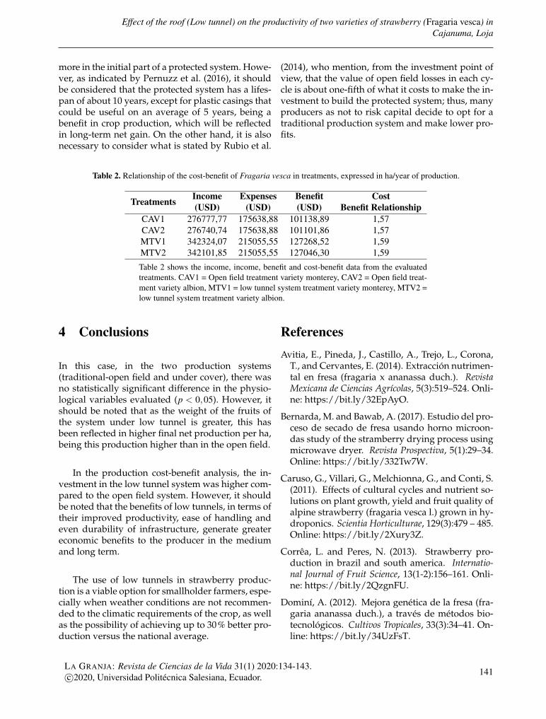
Effect of the roof (Low tunnel) on the productivity of two varieties of strawberry (Fragaria vesca) inCajanuma, Loja
more in the initial part of a protected system. Howe-ver, as indicated by Pernuzz et al. (2016), it shouldbe considered that the protected system has a lifes-pan of about 10 years, except for plastic casings thatcould be useful on an average of 5 years, being abenefit in crop production, which will be reflectedin long-term net gain. On the other hand, it is alsonecessary to consider what is stated by Rubio et al.
(2014), who mention, from the investment point ofview, that the value of open field losses in each cy-cle is about one-fifth of what it costs to make the in-vestment to build the protected system; thus, manyproducers as not to risk capital decide to opt for atraditional production system and make lower pro-fits.
Table 2. Relationship of the cost-benefit of Fragaria vesca in treatments, expressed in ha/year of production.
Treatments Income(USD)
Expenses(USD)
Benefit(USD)
CostBenefit Relationship
CAV1 276777,77 175638,88 101138,89 1,57CAV2 276740,74 175638,88 101101,86 1,57MTV1 342324,07 215055,55 127268,52 1,59MTV2 342101,85 215055,55 127046,30 1,59Table 2 shows the income, income, benefit and cost-benefit data from the evaluatedtreatments. CAV1 = Open field treatment variety monterey, CAV2 = Open field treat-ment variety albion, MTV1 = low tunnel system treatment variety monterey, MTV2 =low tunnel system treatment variety albion.
4 Conclusions
In this case, in the two production systems(traditional-open field and under cover), there wasno statistically significant difference in the physio-logical variables evaluated (p < 0,05). However, itshould be noted that as the weight of the fruits ofthe system under low tunnel is greater, this hasbeen reflected in higher final net production per ha,being this production higher than in the open field.
In the production cost-benefit analysis, the in-vestment in the low tunnel system was higher com-pared to the open field system. However, it shouldbe noted that the benefits of low tunnels, in terms oftheir improved productivity, ease of handling andeven durability of infrastructure, generate greatereconomic benefits to the producer in the mediumand long term.
The use of low tunnels in strawberry produc-tion is a viable option for smallholder farmers, espe-cially when weather conditions are not recommen-ded to the climatic requirements of the crop, as wellas the possibility of achieving up to 30% better pro-duction versus the national average.
ReferencesAvitia, E., Pineda, J., Castillo, A., Trejo, L., Corona,
T., and Cervantes, E. (2014). Extracción nutrimen-tal en fresa (fragaria x ananassa duch.). RevistaMexicana de Ciencias Agrícolas, 5(3):519–524. Onli-ne: https://bit.ly/32EpAyO.
Bernarda, M. and Bawab, A. (2017). Estudio del pro-ceso de secado de fresa usando horno microon-das study of the stramberry drying process usingmicrowave dryer. Revista Prospectiva, 5(1):29–34.Online: https://bit.ly/332Tw7W.
Caruso, G., Villari, G., Melchionna, G., and Conti, S.(2011). Effects of cultural cycles and nutrient so-lutions on plant growth, yield and fruit quality ofalpine strawberry (fragaria vesca l.) grown in hy-droponics. Scientia Horticulturae, 129(3):479 – 485.Online: https://bit.ly/2Xury3Z.
Corrêa, L. and Peres, N. (2013). Strawberry pro-duction in brazil and south america. Internatio-nal Journal of Fruit Science, 13(1-2):156–161. Onli-ne: https://bit.ly/2QzgnFU.
Dominí, A. (2012). Mejora genética de la fresa (fra-garia ananassa duch.), a través de métodos bio-tecnológicos. Cultivos Tropicales, 33(3):34–41. On-line: https://bit.ly/34UzFsT.
LA GRANJA: Revista de Ciencias de la Vida 31(1) 2020:134-143.c©2020, Universidad Politécnica Salesiana, Ecuador. 141
Scientific paper / Artículo científicoAGRICULTURAL PRODUCTION Duque Abad-Abad, C.F., Jiménez-Álvarez, L.S. and Capa-Mora, E.D.
Estación meteorológica «La Argelia» (2017). Climaloja/la argelia. Online: https://bit.ly/2q3ImCt.
Estrada, M., Portillo, M., Calderón, G., Segarra, E.,Martííez, M., and Medina, S. (2017). Potenciali-dades para el fortalecimiento de exportación defresa de michoacán a estados unidos de américa.Revista Chapingo Serie Horticultura, 23(3):135–146.Online: https://bit.ly/2ra848Q.
FAOSTAT (2016). Organización de las naciones uni-das para la agricultura y la alimentación - fao.,2017. Online: https://bit.ly/32Y6KTG.
Ferriol, M. (2010). Propiedades nutritivas y otrascuriosidades de la fresa. Revista CitriFrut,27(3005):72–74. Online: https://bit.ly/2QxfoG3.
Giampieri, F., Tulipani, S., Alvarez, J., Quiles, J.,Mezzetti, B., and Battino, M. (2012). The straw-berry: Composition, nutritional quality, and im-pact on human health. Nutrition, 28(1):9–19. On-line: https://bit.ly/2CY19lz.
Google Maps (2018). Online: https://bit.ly/2p7jCsB.
Grijalba, C., Pérez, M., Ruiz, D., and Ferrucho, A.(2015). Strawberry yields with high-tunnel andopen-field cultivations and the relationship withvegetative and reproductive plant characteris-tics. Agronomía Colombiana, 33(2):147–154. Online:https://bit.ly/35hC8hn.
Hollender, C., Geretz, A., Slovin, J., and Liu, Z.(2012). Flower and early fruit development ina diploid strawberry, fragaria vesca. Planta,235(6):1123–1139. Online: https://bit.ly/2raJh49.
Ibadango, F. (2017). Eficiencia y rentabilidad del sis-tema hidropónico vertical frente al convencionalen la producción de tres variedades de fresa (fra-garia vesca l.), en la granja experimental yuyuco-cha, imbabura. Master’s thesis, Ibarra-Ecuador.
Infante Villarreal, A. (1984). Evaluación financiera deproyectos de inversión. El Ateneo, Buenos Aires.
Juárez, C., Rodríguez, M., and Sandoval, M. (2007).Comparación de tres sistemas de producciónde fresa en invernadero. Terra Latinoamericana,25(1):17–23. Online: https://bit.ly/2K9lmJl.
Juárez, P., Bugarín, R., Castro, R., Sánchez, A., Cruz,E., Juárez, R., Alejo, G., and Balois, R. (2011). Es-tructuras utilizadas en la agricultura protegida.
Revista Fuente, 3(8):21–27. Online: https://bit.ly/2Q8k3Ok.
Karim, M., Aziz, A., Roy, U., Hoque, M., Hossain,M., and Rezaul, M. (2011). In vitro response ofstrawberry ( fragaria x ananassa dutch .) for ca-llus induction and shoot regeneration. Internatio-nal Journal of Agronomy and Agricultural Research,1(1):29–36. Online: https://bit.ly/2Q5UxJK.
Khoshnevisan, B., Rafiee, S., and Mousazadeh, H.(2013). Environmental impact assessment ofopen field and greenhouse strawberry produc-tion. European Journal of Agronomy, 50:29–37. On-line: https://bit.ly/2O3h5Ju.
Lamont, J. and William, J. (2009). Overview of theuse of high tunnels worldwide. HortTechnology,19(1):25–29. Online: https://bit.ly/2p9nzx5.
Ledesma, N., Nakata, M., and Sugiyama, N. (2008).Effect of high temperature stress on the reproduc-tive growth of strawberry cvs. “nyoho” and “to-yonoka”. Scientia Horticulturae, 116(2):186–193.Online: https://bit.ly/2QEm9WN.
León, L., Guzmán, D., García, J., Chávez, C., andPeña, J. (2014). Consideraciones para mejorarla competitividad de la región “el bajío” en laproducción nacional de fresa. Revista Mexicanade Ciencias Agrícolas, 5(4):673–686. Online: https://bit.ly/37k3vta.
López, J., Soria, C., Santos, B., Miranda, L., Do-mínguez, P., and Medina, J. (2011). Strawberryproduction in mild climates of the world: A re-view of current cultivar use. International Jour-nal of Fruit Science, 11(3):232–244. Online: https://bit.ly/2pCboco.
MAG (2018). Ministerio de agricultura y ganaderia,2018. Online: https://bit.ly/2K94qm2.
Montero, M. (2016). Determinación productiva dela frutilla (fragaria vesca) probando dos tipos deacolchamiento y tres distancias de trasplante enla zona agroecologica de guano. Tesis de grado.
Nin, S., Petrucci, W., Giordani, E., and Marinelli, C.(2018). Soilless systems as an alternative to wildstrawberry (fragaria vesca l.) traditional open-field cultivation in marginal lands of the tuscanapennines to enhance crop yield and producers’income. Journal of Horticultural Science and Bio-technology, 93(3):323–335. Online: https://bit.ly/2Xus6H5.
142LA GRANJA: Revista de Ciencias de la Vida 31(1) 2020:134-143.
c©2020, Universidad Politécnica Salesiana, Ecuador.
Effect of the roof (Low tunnel) on the productivity of two varieties of strawberry (Fragaria vesca) inCajanuma, Loja
Ortiz, J., Delgadillo, J., Rodríguez, M., and Calde-rón, G. (2016). Inoculación bacteriana en el cre-cimiento y calidad del fruto de cinco varieda-des de fresa en suelos con ph contrastante. Te-rra Latinoamericana, 34(2):177–185. Online: https://bit.ly/2NDuUy9.
Otto, R., Morakami, R., Reghin, M., and Caíres, E.(2009). Cultivares de morango de dia neutro: pro-dução em função de doses de nitrogênio duranteo verão. Horticultura Brasileira, 27(2):217–221. On-line: https://bit.ly/2KaN88d.
Patiño, D., García, E., Barrera, E., Quejada, O., Ro-dríguez, H., and Arroyabe, I. (2013). Manual técni-co del cultivo de fresa bajo buenas prácticas agrícolas.
Pérez, M., Ojeda, M., Giménez, A., González, M.,and Hernández, A. (2017). Atributos de ca-lidad en frutos de fresa “capitola” cosechadosen diferente condiciones climaticas en venezue-la. Bioagro, 29(3):163–174. Online: https://bit.ly/36Quvjv.
Pernuzz, C., Sordo, M., Travadelo, M., Maina, M.,and Acetta, P. (2016). Evaluación de la convenien-cia de los macrotúneles en comparación con mi-crotúneles para el cultivo de frutilla en coronda.Revista FAVE - Ciencias Agrarias, 15(2):51–62. On-line: https://bit.ly/2NBMkLw.
Pineda, D. (2017). Diseño de un modelo de pro-gramación lineal para la planeación de produc-ción en un cultivo de fresa , según factores costo/ beneficio y capacidades productivas en un pe-riodo temporal definido linear programming mo-del design for production planning in a st. Inge-nierías USBMed, 8(1):7–11. Online: https://bit.ly/2D1dp4E.
Poveda, C., Riaño, D., Aguilar, L., and Cure, J.(2018). Eficiencia de polinización de coloniashuerfanas de bombus atratus (hymenoptera: Api-dae) en fresa (fragaria x ananassa) bajo cubier-ta. Acta Biológica Colombiana, 23(1):73–79. Online:https://bit.ly/2XtmdtD.
Pradas, I., Medina, J., Ortiz, V., and Moreno, J.(2015). “fuentepina” and “amiga”, two newstrawberry cultivars: Evaluation of genotype, ri-pening and seasonal effects on quality characte-ristics and health-promoting compounds. Jour-nal of Berry Research, 5(3):157–171. Online: https://bit.ly/2r3kxeq.
Radin, B., Lisboa, B., Witter, S., Barni, V., Reis-ser, C., Matzenauer, R., and Fermino, M. (2011).Desempenho de quatro cultivares de moranguei-ro em duas regiões ecoclimáticas do rio grande dosul. Horticultura Brasileira, 29(3):287–291. Online:https://bit.ly/32ZPbCF.
Rodríguez, G., Calderón, G., Jaen, D., and Curiel,A. (2012). Capacidad de propagación y calidadde planta de variedades mexicanas y extranje-ras de fresa. Revista Chapingo Serie Horticultura,18(1):113–123. Online: https://bit.ly/2X5APPV.
Rowley, D., Black, B., and Drost, D. (2010). Hightunnel strawberry production. Master’s thesis,Logan.
Rubio, S., Alfonso, A., Grijalba, C., and Pérez, M.(2014). Determinación de los costos de pro-ducción de la fresa cultivada a campo abiertoy bajo macrotúnel. Revista Colombiana de Cien-cias Hortícolas, 8(1):67–79. Online: https://bit.ly/2CZZVGo.
Santoyo, J. and Martinez, C. (2010). Paquete tecno-lógico para la producción de fresa. Technical re-port, Sagarpa. Online: https://bit.ly/32HQLJn.
Undurraga, P. and Vargas, S. (2013). Manual de Fru-tilla, Boletín INIA N 262. Editorial Trama Impreso-res S.A. Online: https://bit.ly/37gzN8p, Chillán,Chile.
Verdugo, W. (2011). Introducción de dos variedadesde fresa (fragaria vesca) y tecnica de fertilizaciónempleando cuatro biofertilizantes líquidos en pa-blo sexto - morona santiago. Master’s thesis.
Vignolo, G., Fernandes, V., Jeske, R., Posser, C., andCorrêa, L. (2011). Produção de morangos a partirde fertilizantes alternativos em pré-plantio. Ciên-cia Rural, 41(10):1755–1761. Online: https://bit.ly/35dmxzt.
Vizcaino, L. (2011). Estudio de factibilidad para laproducción y comercialización de frutilla (fraga-ria chiloensis) en checa – pichincha. Master’s the-sis.
Yaselga, R. (2015). Rendimiento de dos variedadesde fresa (fragaria vesca l.) bajo dos tipos de cober-tura de suelos en sistemas de microtúneles. Mas-ter’s thesis, Carchi – Ecuador.
LA GRANJA: Revista de Ciencias de la Vida 31(1) 2020:134-143.c©2020, Universidad Politécnica Salesiana, Ecuador. 143