Editing soft shadows in a digital photograph

Published by the IEEE Computer Society 0272-1716/07/$25.00 © 2007 IEEE IEEE Computer Graphics and Applications 23

Computational Photography

T he pixels in a digital photograph blendtogether scene components in seemingly

irreversible ways and provide us precious little infor-mation about the scene’s apparent shape, illumination,and reflectance properties. Barrow and Tenenbaumproposed a way of decomposing a single photographinto many intrinsic images, each representing one phys-ical constituent of the scene, such as reflectance andillumination.1 However, this problem is severely ill-posed; estimating scene and material propertiesrequires much more information. Consequently, chang-ing the physical parameters of a scene in a digital pho-tograph is a nontrivial task.

Perceptually, shadows are perhaps one of the mostimportant illumination componentsin any photograph. They provideimportant visual cues for under-standing shape, occlusion, contactbetween objects, and even surfacetexture. A shadow’s sharpness,shape, and color depend on theshape of the light source, the geom-etry and opacity of the occluder, thereflectance properties of the shad-owed surface, and the interreflec-tions among objects within thescene. In this article, we develop

tools for shadow modification in images where a shad-owed region is characterized by soft boundaries withvarying sharpness along the shadow edges. Modelingshadow edges presents an interesting challenge becausethey can vary from infinitely sharp edges for shadowsproduced by a point light source to extremely soft edgesfor shadows produced by large area light sources. (Seethe “Related Work in Shadow Modeling” sidebar on thenext page for previous methods.)

We propose an entirely image-based shadow editingtool for a single-input image. We fit a gradient-domainshadow-edge model to the shadows and then remove theshadow from the image itself, leaving behind gradientestimates for a uniformly illuminated scene. Once we’veseparated these elements, we can independently manip-ulate the shadow-edge model to simulate a much widerrange of lighting conditions, including ambient-onlylighting, direct lighting from the camera viewpoint with

no significant shadows, shadows from synthetic or ide-alized occluders, and area light sources (see Figure 1a–don page 24). These machine-adjustable photographs canoffer interactivity that might improve images’ expres-siveness and help us investigate the influence of bound-ary sharpness on the perception of object-to-objectcontact, as well as understand how humans assess shad-ows to estimate object height above a ground plane.

Gradient-domain shadow edgesWe manipulate shadows by accurately describing

their edges with a controllable, shadow edge model. Wethen use this shadow edge model to replace and editshadows in the original photograph. The term shadowedge describes any visually apparent boundary betweendifferently illuminated regions in the photograph. Ourgoal is to find a model that describes the changes in illu-mination well enough such that any difference betweenour model and the photograph are imperceptible or eas-ily ignored.

Our shadow-editing algorithm’s effectivenessdepends on how accurately we can model the shadowedges. Consider a sharp shadow edge in 1D. The inten-sity function has a step-like shape across the shadowedge (see Figure 2a on page 25). But these step func-tions make awkward shadow models. Steps are notlocalized; their unbounded spatial extent would tangletogether many visually unrelated shadow features fromeither side of the shadow edge. Instead, we describe theshadow edges in their intensity gradients (see Figure2b): a unit step in the intensity domain becomes animpulse function in the gradient domain. For softershadows (see Figure 2c), we can model the shadow edgein the gradient domain as a convolution of the impulsefunction (�) whose amplitude (w) is the intensity changeacross the shadow, with a triangle shaped sharpness fil-ter of width (�) that matches that of the shadow penum-bra (see Figure 2d).

We illustrate our shadow-editing algorithm for a sim-ple 1D signal in Figure 3 on page 25. A shadowed regionwith a textured background forms a noisy, step-like 1Dintensity signal (I). The derivative of the intensity sig-nal forms the gradient signal (F), where the transitionfrom the shadowed to the nonshadowed region pro-duces a narrow, spike-like feature. As in Figure 2, we

This technique for modeling,editing, and rendering shadowedges in a photograph or asynthetic image lets usersseparate the shadow from therest of the image and makearbitrary adjustments to itsposition, sharpness, andintensity.

Ankit Mohan and Jack TumblinNorthwestern University

Prasun ChoudhuryAdobe Systems

Editing SoftShadows in a Digital Photograph


24 March/April 2007

model the spike-like feature representing the shadowedge model (Fe) as an impulse function convolved by asharpness filter and subtract it from the gradient signalto leave behind a shadowless, texture gradient signal(Ft). We can then adjust our shadow edge model para-meters by repositioning the impulse functions, chang-ing its weights (wi) and broadening (or narrowing) thefilter kernel (�). We add this modified shadow edgemodel ( ) to the texture gradient (Ft) to form the mod-ified image gradient ( ). We then integrate the modi-fied image gradient to form the final image with theappearance of modified shadows (Iout).

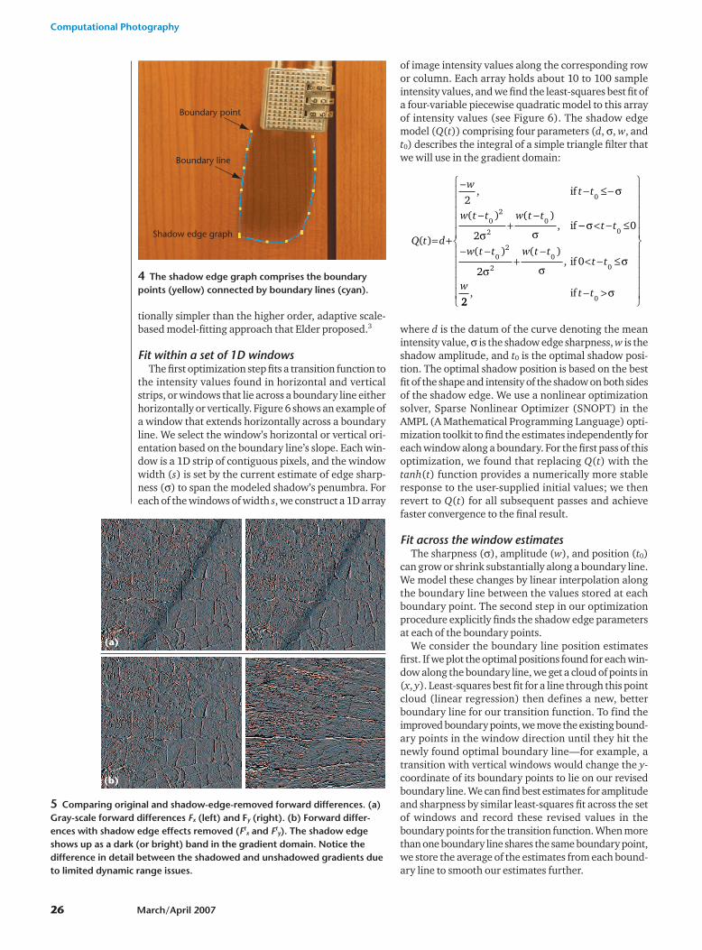
For a complete 2D image, we represent the shadowmodel with a shadow edge graph (see Figure 4 on page26), which is a 2D planar graph of connected line seg-ments called boundary lines and their labeled endpoints.These line segments mark each controllable shadowboundary’s position with subpixel precision. Every bound-ary line shares its endpoints with zero or more neighbor-ing boundary lines, and the labeled nodes of our 2D planargraph describe these endpoints, called boundary points.Boundary lines and points mark the location of a transitionin illumination between shadowed and directly lit regions.The shadow sharpness filter describes the change in illu-mination across the boundary line. The sharpness filter is

FF e

Related Work in Shadow Modeling

Image space shadow modeling, editing, and renderinghas remained an active research topic in computer graphics.Finlayson et al. proposed an entirely image space shadowremoval technique for totally removing shadow effects froman image.1 Like our method, theirs uses a gradient domainapproach, but it works for only the complete removal ofshadows and isn’t suitable for shadow editing.

Agrawal et al. used multiple images to suppress theeffects of edges and remove shadows in an image.2 Theyrequire an example image for shadow removal and alsocan’t edit soft shadows.

Elder and Goldberg proposed a contour-based imageediting method in which they can manipulate all edgefeatures, such as silhouettes and shadow edges, from anexisting photograph.3 They assume the image curvature tobe zero for all nonedge regions and use only the contourinformation to represent the image. Our method uses thesoft edges to augment the texture information in the rest ofthe image and achieves cleaner and higher-quality resultsfor shadow edges with a textured background.

Chuang et al. proposed a shadow matting algorithm toextract shadows from one natural scene and insert theminto another scene.4 Weiss presented a technique forextracting a shadow-free intrinsic image from a sequence ofimages with changing illumination.5

Our shadow-editing method is along the lines of thework of Elder and Goldberg and Finlayson et al., but it’stargeted toward controlling the sharpness of the shadowedges—that is, a shadow’s penumbra regions. We use asingle input image along with user-supplied information forthe shadow edges’ approximate location.

Our shadow representation and editing method also has

strong connections to the work by Sen6 and Tumblin andChoudhury7 on encoding discontinuities in images inmachine readable form. Their work represents the imagediscontinuities in the intensity domain and explicitly storesthe infinitely sharp changes in intensities across thediscontinuities. In addition, these methods can’t handleedges with varying sharpness. We represent our subpixel-accurate edges in the gradient domain to explicitly modeland edit soft edges at the shadow boundaries.

References1. G.D. Finlayson et al., “On the Removal of Shadows from Images,”

IEEE Trans. Pattern Analysis and Machine Intelligence, vol. 28, no.1, 2006, pp. 59-68.

2. A. Agrawal, R. Raskar, and R. Chellappa, “Edge Suppression byGradient Field Transformation Using Cross-Projection Tensors,”Proc. IEEE Computer Society Conf. Computer Vision and PatternRecognition (CVPR), IEEE CS Press, 2006, pp. 2301-2308.

3. J. Elder and R. Goldberg, “Image Editing in the Contour Domain,”IEEE Trans. Pattern Analysis and Machine Intelligence, vol. 23, no.3, 2001, pp. 291-296.

4. Y.Y. Chuang et al., “Shadow Matting and Compositing,” ACMTrans. Graphics, vol. 22, no. 3, 2003, pp. 494-500.

5. Y. Weiss, “Deriving Intrinsic Images from Image Sequences,” Proc.Int’l Conf. Computer Vision (ICCV), IEEE Press, 2001, pp. 68-75.

6. P. Sen, “Silhouette Maps for Improved Texture Magnification,”Proc. ACM Siggraph/Eurographics Conf. Graphics Hardware, ACMPress, 2004, pp. 65-73.

7. J. Tumblin and P. Choudhury, “Bixels: Picture Samples with SharpEmbedded Boundaries,” Eurographics Symp. Rendering (EGSR),Eurographics Association, 2004, pp. 255-264.

1 Shadow manipulation. (a) Source photograph of a shadow across a brickwall. Shadow editing can (b) simulate a larger light source, (c) completelyremove the shadow, and (d) reverse the shadowed and nonshadowedregions. (Source photo courtesy Vit Hassan.)

(a)

(c)

(b)

(d)

IEEE Computer Graphics and Applications 25

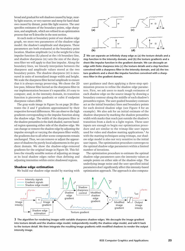
broad and gradual for soft shadows caused by large, near-by light sources, or very narrow and steep for hard shad-ows caused by distant, point-like light sources. The userspecifies estimates of the boundary points, edge sharp-ness, and amplitude, which are refined in an optimizationprocess that we’ll describe in the next section.

At each node or boundary point of our shadow edgegraph, we store two parameters of the shadow edgemodel: the shadow’s amplitude and sharpness. Theseparameters are both evaluated at the boundary pointlocation. Shadow amplitude (wi) is the weight for a lineimpulse function (�i) placed at the i-th boundary line,and shadow sharpness (�i) sets the size of the sharp-ness filter we will apply to that line impulse. Along theboundary lines, we linearly interpolate between thesharpness and amplitude values stored at the twoboundary points. The shadow sharpness (�) is mea-sured in units of normalized image width and height.We scale the sharpness filter kernel amplitude to ensurethat it is always energy preserving. We chose the 2Dlow pass, bilinear filter kernel as the sharpness filter inour implementation because it’s separable; it’s easy tocompute; and, in the intensity domain, its transitionfunction is piecewise quadratic or cubic if endpointsharpness values differ.

The gray-scale image in Figure 5a on page 26 illus-trates the X and Y gradients approximated by theirrespective forward differences. We can observe the highgradients corresponding to the impulse function alongthe shadow edge. The width of the sharpness filter orthe shadow penumbra is the dark shaded, narrow band-ed region spanning either side of the shadow edge. Wecan change or remove the shadow edge by adjusting theimpulse strength or varying the sharpness filter width;the gradients due to all other scene components remainunchanged. Thus, we can remove or adjust the appear-ance of shadows by purely local adjustments in the gra-dient domain. We show the shadow-edge-removedgradients for the original image in Figure 5b. This fol-lows the visually sensible notion of adjusting an imageat its local shadow edges rather than defining andadjusting intensities within entire shadowed regions.

Shadow edge estimationWe build our shadow edge model by starting with

user guidance and then applying a three-step opti-mization process to refine the shadow edge parame-ters. First, we ask users to mark rough estimates ofeach shadow edge on the source image by drawing aboundary contour along the middle of each shadow’spenumbra region. The user-guided boundary contoursact as the initial boundary lines and boundary pointsfor each desired shadow edge (see Figure 4 for anexample). We also ask for an initial estimate of theshadow sharpness by marking the shadow penumbrawidth with marks that reach just outside the shadow’stransition from a dark to a light region. These userinputs are enough to begin our optimization proce-dure and are similar to the trimap-like user inputsused for video and shadow matting applications.2 Aswith the matting techniques using trimaps, our shad-ow edge model is also not very sensitive to the initialuser inputs. The optimization procedure converges tothe optimal shadow edge parameters within a limitednumber of iterations.

The optimization procedure to estimate the optimalshadow edge parameters uses the intensity values atsample points on either side of the shadow edge. Theunderlying image noise and the user specified initialparameters don’t significantly affect this intensity-basedoptimization approach. The approach is also computa-

(c)

(d)

wσ

σ(a)

(b)

w

ww ⊗

⊗

Δ

Outputimageintesity

Modifiedimage

gradient

F Iout

Fe

Fe

Ft

FI

Imageintesity

Imagegradient

Shadow edgeestimation Texture gradient

Shadowedge

gradient

Modifiedshadow

edgegradient +

Shadowsharpnesscontrol

Intensity signalsGradient signalsShadow edge model

3 The algorithm for rendering images with variable sharpness shadow edges. We decouple the image gradientinto texture details and the shadow edge model, independently modify the shadow edge model, and add it backto the texture detail. We then integrate the resulting image gradients with modified shadows to render the outputintensity image.

2 We can separate an infinitely sharp edge as (a) the texture details and astep function in the intensity domain, and (b) the texture gradients and asheet-like impulse function in the gradient domain. We can decouple anedge with finite sharpness into (c) the texture details and a step functionconvolved with a sharpness filter in the intensity domain, and (d) the tex-ture gradients and a sheet-like impulse function convolved with a sharp-ness filter in the gradient domain.


26 March/April 2007

tionally simpler than the higher order, adaptive scale-based model-fitting approach that Elder proposed.3

Fit within a set of 1D windowsThe first optimization step fits a transition function to

the intensity values found in horizontal and verticalstrips, or windows that lie across a boundary line eitherhorizontally or vertically. Figure 6 shows an example ofa window that extends horizontally across a boundaryline. We select the window’s horizontal or vertical ori-entation based on the boundary line’s slope. Each win-dow is a 1D strip of contiguous pixels, and the windowwidth (s) is set by the current estimate of edge sharp-ness (�) to span the modeled shadow’s penumbra. Foreach of the windows of width s, we construct a 1D array

of image intensity values along the corresponding rowor column. Each array holds about 10 to 100 sampleintensity values, and we find the least-squares best fit ofa four-variable piecewise quadratic model to this arrayof intensity values (see Figure 6). The shadow edgemodel (Q(t)) comprising four parameters (d, �, w, andt0) describes the integral of a simple triangle filter thatwe will use in the gradient domain:

where d is the datum of the curve denoting the meanintensity value, � is the shadow edge sharpness, w is theshadow amplitude, and t0 is the optimal shadow posi-tion. The optimal shadow position is based on the bestfit of the shape and intensity of the shadow on both sidesof the shadow edge. We use a nonlinear optimizationsolver, Sparse Nonlinear Optimizer (SNOPT) in theAMPL (A Mathematical Programming Language) opti-mization toolkit to find the estimates independently foreach window along a boundary. For the first pass of thisoptimization, we found that replacing Q(t) with thetanh(t) function provides a numerically more stableresponse to the user-supplied initial values; we thenrevert to Q(t) for all subsequent passes and achievefaster convergence to the final result.

Fit across the window estimatesThe sharpness (�), amplitude (w), and position (t0)

can grow or shrink substantially along a boundary line.We model these changes by linear interpolation alongthe boundary line between the values stored at eachboundary point. The second step in our optimizationprocedure explicitly finds the shadow edge parametersat each of the boundary points.

We consider the boundary line position estimatesfirst. If we plot the optimal positions found for each win-dow along the boundary line, we get a cloud of points in(x, y). Least-squares best fit for a line through this pointcloud (linear regression) then defines a new, betterboundary line for our transition function. To find theimproved boundary points, we move the existing bound-ary points in the window direction until they hit thenewly found optimal boundary line—for example, atransition with vertical windows would change the y-coordinate of its boundary points to lie on our revisedboundary line. We can find best estimates for amplitudeand sharpness by similar least-squares fit across the setof windows and record these revised values in theboundary points for the transition function. When morethan one boundary line shares the same boundary point,we store the average of the estimates from each bound-ary line to smooth our estimates further.

Q t d

wt t

w t t w t t

( )

,

) ),

= +

− − −

−+

−2

2

0

02

0

if

( (if

2

≤ σ

σ σ−− < −

− −+

−< −

σ

σ σσ

t t

w t t w t tt t

w

0

02

00

0

20

≤

≤( (

if2

) ),

22if, t t− >

0σ

⎧

⎨

⎪⎪⎪⎪⎪

⎩

⎪⎪⎪⎪⎪

⎫

⎬

⎪⎪⎪⎪⎪

⎭

⎪⎪⎪⎪⎪

5 Comparing original and shadow-edge-removed forward differences. (a)Gray-scale forward differences Fx (left) and Fy (right). (b) Forward differ-ences with shadow edge effects removed (Ft

x and Fty). The shadow edge

shows up as a dark (or bright) band in the gradient domain. Notice thedifference in detail between the shadowed and unshadowed gradients dueto limited dynamic range issues.

(a)

(b)

Boundary point

Boundary line

Shadow edge graph

4 The shadow edge graph comprises the boundarypoints (yellow) connected by boundary lines (cyan).


Refine the window size and repeatThe 1D fitting results from the “Fit within a set of 1D

windows” section can depend strongly on the windowsize (s) itself. Excessively wide windows include extra-neous samples outside the shadow penumbra, and nar-row windows exclude important shadow shape data.We optimize each window size by updating its width ateach iteration from our current sharpness (�) estimate:s � k � �. We found that k � 1.2 gave rapid convergence,and, by repeating the three steps, we arrive at a stablesolution in as few as two to three iterations.

Shadow modification and renderingThe shadow edge parameters estimated in the previ-

ous section form a substantially complete description ofthe visible shadow effects in the scene. We separate theshadows from the rest of the image by subtracting themodeled shadow gradient from the input image’s gradi-ent. In the discrete domain, this means subtracting theshadow-edge-model forward differences (Fe) from thesource forward differences (F) (see Figure 3). Forwarddifferences for the source image are trivial to compute,but computing the forward differences for the shadowedge model requires careful antialiased sampling of acontinuous-valued gradient function.

The shadow edge model we developed in the previ-ous section describes gradients for the i-th boundary lineas a continuous-valued vector field (Ei). The shadowedge gradient map for the i-th shadow edge is given by:

Ei(x, y) � wi(x, y)�i � �x(�i) � �y(�i)

where �x(�i) and �y(�i) are 1D triangle filters along thex- and the y-axes, �i is the width of the sharpness filter,and wi is the weight of the line impulse function corre-sponding to the i-th shadow edge. Both the sharpness(�i) and amplitude (wi) vary linearly along the bound-ary line between the values stored at boundary line end-points. Although this shadow edge model directlydescribes the continuous-valued gradients without pixelsampling, the source image can only approximate themby forward differences between pixels along the gridintervals in the x and the y direction:

Fx[i, j] � I[i 1, j] I[i, j],Fy[i, j] � I[i, j 1] I[i, j] (1)

To subtract the modeled shadows from source imageforward differences, we must first convert the shadowedge gradient map into a shadow-edge forward differ-ence (Fe) image whose resolution matches the resolu-tion of the source-image forward differences:

(Fex[i, j], Fe

y[i, j]) � �(�Ei(x, y)) (2)

where �(.) converts a continuous gradient field into itsforward difference representation, and � denotes thecumulative effect of all the shadow edges Ei that inter-sect a horizontal (or vertical) line connecting two con-secutive sample-pixel locations. We discuss ourimplementation of the discretization operator �(.) inthe next section.

To obtain the shadow-free texture forward difference(Ft) image, we now subtract the shadow edge forwarddifference image (Fe) from the source forward differ-ence image (F),

Ftx[i, j] � Fx[i, j] Fe

x[i, j], Ft

y[i, j] � Fy[i, j] Fey[i, j]

Shadow editingHaving separated the shadow edges from the source

photographs, we can arbitrarily modify any of theshadow edge parameters. We can change the penum-bra width at any boundary point by adjusting thesharpness filter width (�i), set the shadow contrast ordepth and its sign—that is, the side of the occluderwhere the shadow will be cast by adjusting the weight(wi)—and alter shadow positions by moving theboundary points around the image. After editing theshadow, we convert the modified shadow-edge gradi-ent map (x, y) to an antialiased forward differencemap: ( [i, j], [i, j]) = �(� (x, y)). Adding thismodified shadow-edge forward difference image to thetexture forward difference image creates the modifiedforward differenced intensity ( )(see Figure 3 for thecomplete procedure):

Rendering to pixelsFinally, we create the displayable shadow-edited out-

put image, Iout [i, j], by integrating the modified forwarddifference intensity image. For reconstruction, we usea conventional Poisson solver with the Neumann bound-ary conditions:4

∇2 ( )I divout

= F

F i j F i j F i j

F i j F i jx x

txe

y yt

[ , ] [ , ] [ , ],

[ , ] [ , ]

= +

= + FF i jye[ , ]

F

Ei

FyeF

xeE

i

6 Shadow edge parameter estimation: The cyan line in the image repre-sents a portion of the shadow edge boundary line. The horizontal magentaline is a window of width s across the boundary line. The red dot on thehorizontal window of width s is the position (x,y) of the shadow edge forthat particular window scanline. The blue plot below shows the intensityvalues along the window, and the red curve indicates a least-squares bestfit of a piecewise quadratic function Q(t). We use the least-squares fit toestimate the sharpness, amplitude, position, and datum of the edge for the1D window under consideration.

Sharpness (2σ)

Amplitude (w)

Position (t0)

Window size (s)

Shadow edge

Datum (d)

(x,y)


28 March/April 2007

where 2 is the Laplacian operator, div(.) is the diver-gence operator, and is the modified forwarddifferenced intensity image. Since both 2 and div arelinear operators, approximating them with finite differ-ence yields a linear system of equations. We approxi-mate the Laplacian operator as

2Iout[i, j] � Iout[i 1, j] Iout[i 1, j] Iout[i, j 1] Iout[i, j 1] 4Iout[i, j]

We compute the discrete gradients Fx and Fy using theforward difference (see Equation 1), while we use thebackward difference for the div(.) operator on a func-tion

The combination of forward and backward differ-ences ensure that the approximation of div(.) is consis-tent with the central difference scheme of computingLaplacians. The finite difference scheme yields a largeset of linear equations, and we solve it using an itera-tive successive over relaxation-based Poisson solver.5

We can also accelerate the Poisson solver’s convergenceusing faster multigrid methods and leveraging theGPU’s computational efficiency.

Edge map: continuous to discreteconversion

The �(.) function in Equation 2 converts a continu-ous-domain gradient vector field to the correspondingforward differences defined between the same integerpixel locations of the source image. Forward differencesmade by naively sampling the edge model’s gradients atinteger pixel locations can cause severe aliasing because

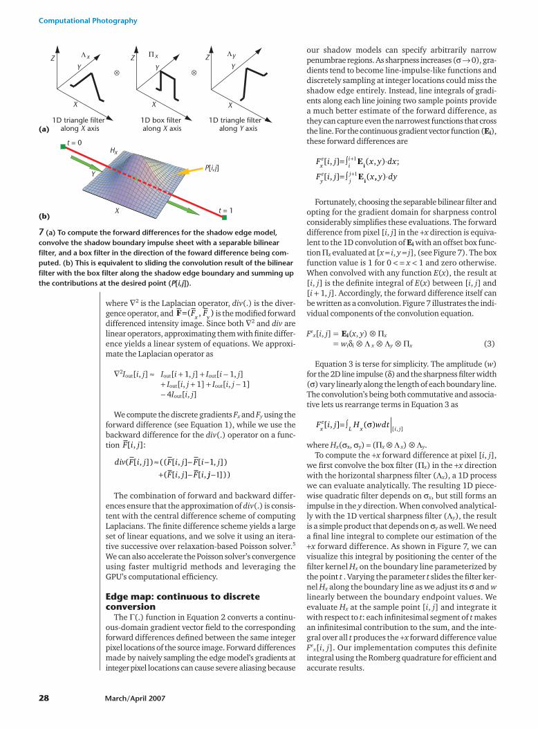
our shadow models can specify arbitrarily narrowpenumbrae regions. As sharpness increases (�� 0), gra-dients tend to become line-impulse-like functions anddiscretely sampling at integer locations could miss theshadow edge entirely. Instead, line integrals of gradi-ents along each line joining two sample points providea much better estimate of the forward difference, asthey can capture even the narrowest functions that crossthe line. For the continuous gradient vector function (Ei),these forward differences are

Fortunately, choosing the separable bilinear filter andopting for the gradient domain for sharpness controlconsiderably simplifies these evaluations. The forwarddifference from pixel [i, j] in the x direction is equiva-lent to the 1D convolution of Ei with an offset box func-tion �x evaluated at [x � i, y � j], (see Figure 7). The boxfunction value is 1 for 0 � � x � 1 and zero otherwise.When convolved with any function E(x), the result at [i, j] is the definite integral of E(x) between [i, j] and [i 1, j]. Accordingly, the forward difference itself canbe written as a convolution. Figure 7 illustrates the indi-vidual components of the convolution equation.

Fex[i, j] = Ei(x, y) � �x

= wi�i � � x � �y � �x (3)

Equation 3 is terse for simplicity. The amplitude (w)for the 2D line impulse (�) and the sharpness filter width(�) vary linearly along the length of each boundary line.The convolution’s being both commutative and associa-tive lets us rearrange terms in Equation 3 as

where Hx(�x, �y) � (�x � � x) � �y.To compute the x forward difference at pixel [i, j],

we first convolve the box filter (�x) in the x directionwith the horizontal sharpness filter (�x), a 1D processwe can evaluate analytically. The resulting 1D piece-wise quadratic filter depends on �x, but still forms animpulse in the y direction. When convolved analytical-ly with the 1D vertical sharpness filter (�y), the resultis a simple product that depends on �y as well. We needa final line integral to complete our estimation of thex forward difference. As shown in Figure 7, we canvisualize this integral by positioning the center of thefilter kernel Hx on the boundary line parameterized bythe point t . Varying the parameter t slides the filter ker-nel Hx along the boundary line as we adjust its � and wlinearly between the boundary endpoint values. Weevaluate Hx at the sample point [i, j] and integrate itwith respect to t: each infinitesimal segment of t makesan infinitesimal contribution to the sum, and the inte-gral over all t produces the x forward difference valueFe

x[i, j]. Our implementation computes this definiteintegral using the Romberg quadrature for efficient andaccurate results.

F i j H wdtxe

L x i j[ , ] ( )

[ , ]= ∫ σ

F i j x y dx

F i j xxe

ii

ye

jj

[ , ] ( , ) ;

[ , ] (

=

=

+1

+1

∫ ⋅

∫

E

Ei

i,, )y dy⋅

div F i j F i j F i j

F i j F i

( [ , ]) (( [ , ] [ , ])

( [ , ] [ ,

≈ − −+ −

1

jj−1]))

F i j[ , ]:

F=( , )y

F Fx

7 (a) To compute the forward differences for the shadow edge model,convolve the shadow boundary impulse sheet with a separable bilinearfilter, and a box filter in the direction of the foward difference being com-puted. (b) This is equivalent to sliding the convolution result of the bilinearfilter with the box filter along the shadow edge boundary and summing upthe contributions at the desired point (P[i,j]).

X

X X

Y Y YZ Z Z

Y

t = 0

t = 1

P[i,j]

Hx

1D triangle filter along X axis

1D triangle filter along Y axis

1D box filter along X axis

X

Λx Πx Λy

⊗ ⊗

(a)

(b)


ResultsWe demonstrate our shadow modification algorithm

with example results shown in Figure 1 and Figures 8through 12. In particular, we illustrate moving the shad-ow edges, controlling the shadow edge sharpness, flip-ping the shadowed and unshadowed region, andremoving the shadows in the given input image. We showmodification of the shadow edges where the shadow edgeranges from the soft shadow due to an area light sourcein Figure 10 to an infinitely sharp shadow due to a pointlight source in Figure 12. In Figures 1c, 8a, and 9b, thealgorithm performs well in removing the shadow effectsfrom the images. In Figures 1b, 8b, 9c, and 10c, we blurthe shadow edges of the input image at different scalesto simulate the effect of lighting from an area light source.In Figure 8c, we demonstrate sharpening the shadowedges to generate the effect of lighting from a point lightsource. In Figure 1d, we interchange images’ shadowedand unshadowed regions, and in Figure 8d, we modifythe shadow’s shape without affecting the underlyingimage texture. Figures 8 and 9 contain curved shadows.We use a moderate number (5–10) of boundary line seg-ments to model such curved shadow edges. Figure 10a–ccontains a shadow-depth discontinuity where a part ofthe shadow is cast on the vertical sidewalk face and theremaining portion is on the horizontal sidewalk and road.

8 Original image shown in Figure 4: (a) shadowremoved from the original image; (b) softer shadow tosimulate an area light source and (c) sharp shadow tomimic the effect of a point light source; and (d) shadowmoved and shape changed.

(a)

(c)

(b)

(d)

9 (a) A car with a curved shadow falling on the ground on its right; (b) the shadow edge removed from the origi-nal image; and (c) softening the relatively sharp shadow edge of the input image. Completely removing the shad-ow edge makes the image gradient field nonconservative. The Poisson solver finds the best least-squares solution,resulting in a somewhat dark image.

(a) (b) (c)

10 (a) The input image shows a discontinuous and moderately soft shadow. (b) The sharpened discontinuousshadow edge and (c) the smoothed shadow edge preserving the discontinuity and the related features of the scene.The mismatch in the shadow edge position on the road and the vertical part of the sidewalk in (b) appears physical-ly inaccurate because our edge model does not account for perspective effects and sudden changes in geometry.

(a) (b) (c)


30 March/April 2007

Figure 11a shows the original image we use to com-pare our shadow-removal method with an approachsimilar to that of Finlayson et al.6 Instead of using ourshadow edge model to separate the estimated shadowfrom the image, we first set the gradient to zero in thepenumbra region of the shadow edge. Then, we spreadthe residual edge amplitude error in the penumbraregion to conserve energy. As Figure 11b shows, thisleads to a loss in texture detail in the shadow edge regionthat can look bad for soft edges. Although our removalresults (Figure 11c) might not be perfect, they do pre-serve texture detail quite well. Also, while Finlayson etal.6 automatically find shadow regions using a moresophisticated color constancy-based approach, theirmethod makes a binary decision for each pixel to decideif it is in a pure shadow or not. This works well when theshadow is sharp and the boundary is a pixel wide, but itcan’t handle smooth shadow edges well. It would be fair-ly interesting to combine their shadow-finding algo-rithm with our shadow edge model.

Figure 12a–b shows an example of a failure case of ourtechnique. Banding artifacts are visible in our resultsbecause our edge model is not able to accurately describesome of the shadow edges. This effect is due to the exces-sive in-camera sharpening applied to the image, partic-ularly noticeable near the sharp shadow boundaries.Over-sharpening results in a slight over and undershootof the image intensity around a shadow edge, a featurethat our shadow edge model doesn’t capture.

Discussion and future workWe computed the shadow modeling and modification

results in this article without knowledge of the originat-ing camera’s response curve, lens point spread function,camera lens placement, illuminant color or position, orany other scene geometry. In some results, such as inFigure 12, close inspection reveals subtle but perceiv-able residue or ghost artifacts from the original shadowin the form of a dark band at the original shadow edgeposition. This is probably due to our imperfect and sim-plistic shadow edge model that doesn’t account well forthe camera point spread function, in-camera sharpeningperformed on the image, geometry of the surface onwhich the shadow is cast, and so on. An inadequatenumber of boundary points to describe an edge, wildlyincorrect starting estimates, and regions with lots ofedges might affect our optimization process and resultin inaccurate edge parameters.

Because we model and edit only the shadow edges,the shadow regions themselves can exhibit contrast ordynamic range and self-shadowing artifacts in the edit-ed images (see the cracks between bricks in Figures 1dand 11c). One possible way of alleviating this would bea recent technique that incorporates perceptual correct-ness during the Poisson reconstruction process.7 Theshadow model as described is inadequate to work withclosed shadow contours, though it seems to work rea-sonably well in Figure 8. This is because we only modelillumination discontinuities and not depth discontinu-ities, which are generally infinitely sharp.

With further refinement, we might apply the basicmethods in this article to other visually important, vari-able sharpness boundaries within images, such as out-lines of specular highlights, object-to-object contact,seams and cracks, occlusion boundaries, and thintranslucent coverings. In addition, our shadow estima-tion algorithm assumes that shadowed and unshad-owed surface textures roughly share the same localmean intensity. For some strongly self-shadowed sur-faces and unusual illuminants, these assumptions mightfail. Investigations into a broader array of self-shadow-ing textures under varying illuminants could provideuseful refinements. We believe that the current researchthrust in this direction might eventually lead to a muchricher image description where visually important

11 (a) The straight line shadow edge in the original image; (b) the shadow edge removal by estimating the shad-ow edge model using our method and setting the gradients in the penumbra of the shadow to zero (similar toFinlayson et al.)6; (c) shadow edge removal using our algorithm.

(a) (b) (c)

12 Original photograph showing (a) shadows on wooden steps, and (b)our result with shadows softened. Notice that banding artifacts in theresult, due to oversharpening artifacts in the input, give it an imperfect fitof the edge model. (Source photo courtesy Elizabeth West.)

(a) (b)


boundaries can be explicitly stored separately from therest of the image. ■

AcknowledgmentsThanks to the anonymous reviewers for their helpful

comments and the Northwestern University graphicsgroup for their support. This material is based on worksupported by the National Science Foundation undergrant 0535236.

References1. H.G. Barrow and J.M. Tenenbaum, “Recovering Intrinsic

Scene Characteristics from Images,” Computer Vision Sys-tems, Academic Press, 1978, pp. 3-26.

2. Y.Y. Chuang et al., “Shadow Matting and Compositing,”ACM Trans. Graphics, vol. 22, no. 3, 2003, pp. 494-500.

3. J. Elder, “Are Edges Incomplete?” Int’l J. Computer Vision,vol. 34, nos. 2/3, 1999, pp. 97-122.

4. R. Fattal, D. Lischinski, and M. Werman, “Gradient DomainHigh Dynamic Range Compression,” ACM Trans. Comput-er Graphics, vol. 21, no. 3, 2002, pp. 249-256.

5. P. Perez, M. Gangnet, and A. Blake, “Poisson Image Edit-ing,” ACM Trans. Computer Graphics, vol. 22, no. 3, 2003,pp. 313-318.

6. G.D. Finlayson et al., “On the Removal of Shadows fromImages,” IEEE Trans. Pattern Analysis and Machine Intelli-gence, vol. 28, no. 1, 2006, pp. 59-68.

7. T. Georgiev, “Covariant Derivatives and Vision,” Proc. 9thEuropean Conf. Computer Vision, Part IV, LNCS 3954,Springer, 2006, pp. 56-69.

Ankit Mohan is a graduate studentin the Department of Electrical Engi-neering and Computer Science atNorthwestern University. His researchinterests include computational pho-tography, image-based lighting, glob-al illumination, operating systems,and photography. Mohan has a BE in

instrumentation and control engineering from Netaji Sub-has Institute of Technology, India. Contact him [email protected].

Prasun Choudhury is a computerscientist at Adobe Systems. His re-search interests include realistic ren-dering, image-based lighting, compu-tational photography, and renderingwith programmable shaders. Choud-hury has a PhD in robotics fromNorthwestern University. Contact him

at [email protected].

Jack Tumblin is an assistant pro-fessor in the Department of ElectricalEngineering and Computer Science atNorthwestern University. His researchinterests include computational pho-tography and illumination, comput-er vision, high dynamic range images,digital archives for museum collec-

tions, and human visual perception. Tumblin has a PhDin computer science from Georgia Institute of Technology.Contact him at [email protected].

Get accessto individual IEEE Computer Society

documents online.

More than 100,000 articles and conference papers available!

$9US per article for members

$19US for nonmembers

www.computer.org/publications/dlib

Editing soft shadows in a digital photograph

Documents

Transcript of Editing soft shadows in a digital photograph