Ecosystem fluxes of hydrogen: a comparison of flux-gradient methods
19
Atmos. Meas. Tech., 7, 2787–2805, 2014 www.atmos-meas-tech.net/7/2787/2014/ doi:10.5194/amt-7-2787-2014 © Author(s) 2014. CC Attribution 3.0 License. Ecosystem fluxes of hydrogen: a comparison of flux-gradient methods L. K. Meredith 1,* , R. Commane 2 , J. W. Munger 2 , A. Dunn 3 , J. Tang 4 , S. C. Wofsy 2 , and R. G. Prinn 1 1 Center for Global Change Science, Massachusetts Institute of Technology, Cambridge, Massachusetts, USA 2 School of Engineering and Applied Sciences and Department of Earth and Planetary Sciences, Harvard University, Cambridge, Massachusetts, USA 3 Department of Physical and Earth Science, Worcester State University, Worcester, Massachusetts, USA 4 Ecosystems Center, Marine Biological Laboratory, Woods Hole, Massachusetts, USA * now at: Environmental Earth System Science, Stanford University, Stanford, California, USA Correspondence to: L. K. Meredith ([email protected]) Received: 10 March 2014 – Published in Atmos. Meas. Tech. Discuss.: 25 March 2014 Revised: 29 July 2014 – Accepted: 31 July 2014 – Published: 3 September 2014 Abstract. Our understanding of biosphere–atmosphere ex- change has been considerably enhanced by eddy covariance measurements. However, there remain many trace gases, such as molecular hydrogen (H 2 ), that lack suitable analyt- ical methods to measure their fluxes by eddy covariance. In such cases, flux-gradient methods can be used to calculate ecosystem-scale fluxes from vertical concentration gradients. The budget of atmospheric H 2 is poorly constrained by the limited available observations, and thus the ability to quan- tify and characterize the sources and sinks of H 2 by flux- gradient methods in various ecosystems is important. We de- veloped an approach to make nonintrusive, automated mea- surements of ecosystem-scale H 2 fluxes both above and be- low the forest canopy at the Harvard Forest in Petersham, Massachusetts, for over a year. We used three flux-gradient methods to calculate the fluxes: two similarity methods that do not rely on a micrometeorological determination of the eddy diffusivity, K , based on (1) trace gases or (2) sensi- ble heat, and one flux-gradient method that (3) parameter- izes K . We quantitatively assessed the flux-gradient meth- ods using CO 2 and H 2 O by comparison to their simultane- ous independent flux measurements via eddy covariance and soil chambers. All three flux-gradient methods performed well in certain locations, seasons, and times of day, and the best methods were trace gas similarity for above the canopy and K parameterization below it. Sensible heat similarity required several independent measurements, and the results were more variable, in part because those data were only available in the winter, when heat fluxes and temperature gradients were small and difficult to measure. Biases were often observed between flux-gradient methods and the inde- pendent flux measurements, and there was at least a 26 % difference in nocturnal eddy-derived net ecosystem exchange (NEE) and chamber measurements. H 2 fluxes calculated in a summer period agreed within their uncertainty and pointed to soil uptake as the main driver of H 2 exchange at Harvard Forest, with H 2 deposition velocities ranging from 0.04 to 0.10 cm s -1 . 1 Introduction Atmospheric H 2 , with a global average mole fraction of 530 ppb (parts per billion; 10 -9 , nmol mol -1 ), exerts a no- table influence on atmospheric chemistry and radiation. H 2 is scavenged by the hydroxyl radical (OH radical), thereby attenuating the ability of OH to scavenge potent green- house gases, like methane (CH 4 ) from the atmosphere, which classifies H 2 as an indirect greenhouse gas (Novelli et al., 1999). H 2 is also a significant source of water vapor to the stratosphere, and as such may adversely perturb strato- spheric ozone chemistry (Solomon, 1999; Tromp et al., 2003; Warwick et al., 2004). The two major atmospheric H 2 sources are photochemical production from methane and non-methane hydrocarbons and combustion of fossil fuels and biomass (Novelli et al., 1999). The major H 2 sinks are Published by Copernicus Publications on behalf of the European Geosciences Union.
Transcript of Ecosystem fluxes of hydrogen: a comparison of flux-gradient methods
Atmos. Meas. Tech., 7, 2787–2805, 2014www.atmos-meas-tech.net/7/2787/2014/doi:10.5194/amt-7-2787-2014© Author(s) 2014. CC Attribution 3.0 License.
Ecosystem fluxes of hydrogen: a comparisonof flux-gradient methods
L. K. Meredith 1,*, R. Commane2, J. W. Munger2, A. Dunn3, J. Tang4, S. C. Wofsy2, and R. G. Prinn1
1Center for Global Change Science, Massachusetts Institute of Technology, Cambridge, Massachusetts, USA2School of Engineering and Applied Sciences and Department of Earth and Planetary Sciences, Harvard University,Cambridge, Massachusetts, USA3Department of Physical and Earth Science, Worcester State University, Worcester, Massachusetts, USA4Ecosystems Center, Marine Biological Laboratory, Woods Hole, Massachusetts, USA* now at: Environmental Earth System Science, Stanford University, Stanford, California, USA
Correspondence to:L. K. Meredith ([email protected])
Received: 10 March 2014 – Published in Atmos. Meas. Tech. Discuss.: 25 March 2014Revised: 29 July 2014 – Accepted: 31 July 2014 – Published: 3 September 2014
Abstract. Our understanding of biosphere–atmosphere ex-change has been considerably enhanced by eddy covariancemeasurements. However, there remain many trace gases,such as molecular hydrogen (H2), that lack suitable analyt-ical methods to measure their fluxes by eddy covariance. Insuch cases, flux-gradient methods can be used to calculateecosystem-scale fluxes from vertical concentration gradients.The budget of atmospheric H2 is poorly constrained by thelimited available observations, and thus the ability to quan-tify and characterize the sources and sinks of H2 by flux-gradient methods in various ecosystems is important. We de-veloped an approach to make nonintrusive, automated mea-surements of ecosystem-scale H2 fluxes both above and be-low the forest canopy at the Harvard Forest in Petersham,Massachusetts, for over a year. We used three flux-gradientmethods to calculate the fluxes: two similarity methods thatdo not rely on a micrometeorological determination of theeddy diffusivity, K, based on (1) trace gases or (2) sensi-ble heat, and one flux-gradient method that (3) parameter-izes K. We quantitatively assessed the flux-gradient meth-ods using CO2 and H2O by comparison to their simultane-ous independent flux measurements via eddy covariance andsoil chambers. All three flux-gradient methods performedwell in certain locations, seasons, and times of day, and thebest methods were trace gas similarity for above the canopyand K parameterization below it. Sensible heat similarityrequired several independent measurements, and the resultswere more variable, in part because those data were only
available in the winter, when heat fluxes and temperaturegradients were small and difficult to measure. Biases wereoften observed between flux-gradient methods and the inde-pendent flux measurements, and there was at least a 26 %difference in nocturnal eddy-derived net ecosystem exchange(NEE) and chamber measurements. H2 fluxes calculated in asummer period agreed within their uncertainty and pointedto soil uptake as the main driver of H2 exchange at HarvardForest, with H2 deposition velocities ranging from 0.04 to0.10 cm s−1.
1 Introduction
Atmospheric H2, with a global average mole fraction of530 ppb (parts per billion; 10−9, nmol mol−1), exerts a no-table influence on atmospheric chemistry and radiation. H2is scavenged by the hydroxyl radical (OH radical), therebyattenuating the ability of OH to scavenge potent green-house gases, like methane (CH4) from the atmosphere, whichclassifies H2 as an indirect greenhouse gas (Novelli et al.,1999). H2 is also a significant source of water vapor tothe stratosphere, and as such may adversely perturb strato-spheric ozone chemistry (Solomon, 1999; Tromp et al.,2003; Warwick et al., 2004). The two major atmosphericH2 sources are photochemical production from methane andnon-methane hydrocarbons and combustion of fossil fuelsand biomass (Novelli et al., 1999). The major H2 sinks are
Published by Copernicus Publications on behalf of the European Geosciences Union.
2788 L. K. Meredith et al.: A comparison of flux-gradient methods
soil consumption, representing about 81± 8 % of the totalsink, and oxidation by OH being about 17± 3 % based ona global inversion of sparse atmospheric H2 measurements(Xiao et al., 2007). The major sources and sinks are nearlybalanced so atmospheric H2 concentrations are stable. Al-though the global atmospheric H2 budget has been derivedthrough a variety of methods, it remains poorly constrainedat the regional level and disputed at the global level, anda process-based understanding is lacking (as reviewed byEhhalt and Rohrer, 2009). Therefore, there are large uncer-tainties in the estimated impact of changes to the H2 biogeo-chemical cycle that might arise from changes in energy use,land use, and climate. Field and laboratory measurements areneeded to improve the process-level understanding of atmo-spheric H2 sources and sinks, especially regarding its sensi-tivity to biological activity in the soils.
The paucity of data on key H2 processes is related to dif-ficulties in measuring sources and sinks in situ, in particularthe soil sink. H2 soil uptake is typically measured using soilflux chambers (e.g., Conrad and Seiler, 1980; Lallo et al.,2008; Smith-Downey et al., 2008). Chamber measurementsare labor intensive and typically yield infrequent and discon-tinuous data that are difficult to scale up to the landscapescale, especially in ecosystems with high spatial heterogene-ity (Baldocchi et al., 1988). Although chambers are subject toartifacts if not implemented carefully (Davidson et al., 2002;Bain et al., 2005), they are well suited for process-level stud-ies. Boundary layer methods have been used to calculate H2soil uptake rates from H2 mole fraction measurements andassumptions about atmospheric winds and mixing, bound-ary layer height, and/or the uptake rates of other trace gases(Simmonds et al., 2000; Steinbacher et al., 2007). The needfor assumptions in these methods can introduce large uncer-tainties into reported H2 fluxes. Most studies have focusedon soil processes, and we have little information about anyother processes in the canopy that affect H2.
Despite the limitations of these traditional methods, fewalternatives are available for the measurement or estimationof atmospheric H2 fluxes. The gas chromatographic methodsused to measure H2 are slow (> 4 min), which precludes useof eddy covariance techniques that rely on high-frequencymeasurement of the covariation of the trace gas mole frac-tion with the vertical wind component. In such cases, whereno high-accuracy fast-response instrument (≥ 1 Hz samplingfrequency) is available, a variety of micrometeorologicalmethods under the umbrella of flux-gradient theory can beused to non-intrusively measure the biosphere–atmosphereexchange of trace gases from relatively slow (� 1 Hz) mea-surements of vertical gradients of trace gas mole fractions(Fuentes et al., 1996; Meyers et al., 1996). Flux-gradientmethods assume that fluxes are equal to the gradient of thequantity in question scaled by the rate of turbulent exchange.These methods can be automated for near-continuous datacollection, and by averaging over time, the spatial hetero-geneity within the tower footprint is integrated (Baldocchi et
al., 1988). As a result, flux-gradient methods avoid some ofthe aforementioned problems that arise from the use of fluxchambers and box models. These methods are also useful incases where fluxes are small and fast-response instrumentslack the precision to resolve deviations in trace gas molefraction from background levels (Simpson et al., 1998). Thestructure of the turbulence below the canopy can make eddycovariance measurements difficult, and flux-gradient meth-ods may be a superior choice (Black et al., 1996). Flux-gradient methods do rely on simplifying assumptions, suchas the one-dimensional representation of a three-dimensionalprocess, the existence of steady-state conditions, horizontalhomogeneity in the source–sink distributions, and flat topog-raphy (Baldocchi et al., 1988).
Recognizing the potential for flux-gradient methods fordetermining the H2 flux, we designed, constructed, and eval-uated a fully automated, continuous measurement system fordetermining H2 fluxes in a forest ecosystem by three differentflux-gradient methods: (1) trace gas similarity, (2) sensibleheat similarity, and (3)K parameterization. Critical issues ininstrument design and performance for making flux-gradientmeasurements were considered, including instrument preci-sion, sampling error, and measurement accuracy. The valid-ity of each flux-gradient method was demonstrated by ap-plication to CO2 and H2O fluxes, for which simultaneouseddy covariance or chamber flux measurements were avail-able for comparison. Finally, H2 fluxes were calculated usingthe flux-gradient methods in the above- and below-canopyenvironment. The approach and findings could be extendedto other trace gases that present similar measurement chal-lenges to H2.
2 Experimental
2.1 Measurement site
The study site, Harvard Forest (42◦32′ N, 72◦11′ W; eleva-tion 340 m), is located in Petersham, Massachusetts, approx-imately 100 km west of Boston, Massachusetts. The largelydeciduous 80- to 115-year old forest is dominated by redoak, red maple, red and white pine, and hemlock (Urbanksiet al., 2007). Harvard Forest soils are acidic and originatefrom sandy loam glacial till (Allen, 1995). Measurementspresented in this study were made from November 2010to March 2012 at the Environmental Measurement Station(EMS) (Wofsy et al., 1993), located in the Prospect Hilltract of Harvard Forest. The station is surrounded for sev-eral kilometers by moderately hilly terrain and forest that hasbeen relatively undisturbed since the 1930s. Previous work atthe site found no evidence for anomalous flow patterns thatwould interfere with eddy-flux measurements (Moore et al.,1996), the local energy budget has been balanced to within20 % (Goulden et al., 1996), and about 80 % of the turbulent
Atmos. Meas. Tech., 7, 2787–2805, 2014 www.atmos-meas-tech.net/7/2787/2014/
L. K. Meredith et al.: A comparison of flux-gradient methods 2789
Ventnulling
line
NOCOM
NC
IRGA 1
IRGA 2
Pumpto ventBallast
volume
Flow controllers
Pressurecontrollers
Infrared gas analyzers (IRGA)
Bypass
Referencecell
CO2/H2O scrubber
HI
M
LO
CO2calibrationstandards Zero
air
Bypass
Tubingto tower
Nulling volume
Shedwall
H2calibration
standard
Pump
Integrating volume
Na�ondryer
Streamselection
valve
Pressure transducerFlow
controller
NO
COM NC
NC
NO
Counterpurge�ow
COM
Sampling valve
(load position)
Gas chromatograph (GC)
NO
COM
NC
Pumpto vent
PC
AC
HeCG
1
2
6
1211
10
3
4
57
89
NVVPHI
RS
HePHeP
HeP
HeP
SI
SO
SL
DPORG
HeP
V
EPC3
EPC4
HePDD
RS
Key:
AC = analytical columnCG = carrier gasDPO = discharge purge outletEPC = electronic pressure controllerHeP = helium puri�erHePDD = He pulsed discharge detectorNV = needle valvePC = pre-columnRG = regulatorRS = restrictorSI = sample inSL = sample loopSO = sample outV = ventVPHI = valve purged housing inlet
Figure 1. Schematic of the flux-gradient instrument system, which includes a gas chromatograph (GC-HePDD, H2 measurements), infraredgas analyzers (IRGA, CO2, and H2O measurements), and the gas stream selection system.
fluxes originate within a 0.7–1 km radius of the tower (Sakaiet al., 2001; Urbanski et al., 2007).
2.2 Instrumentation
An instrument system was designed to measure mole frac-tion gradients and ancillary variables needed to calculate H2fluxes above and below the forest canopy at four heights(Fig. 1). H2 mole fractions were measured with a gaschromatograph (GC, model 6890, Agilent Technologies)equipped with a pulsed discharge helium ionization detec-tor (HePDD, model D-3 PDD, Valco Instruments Co. Inc.(VICI)) and two columns (HayeSep DB, 1/8 in. OD stainlesssteel, 2 m pre-column 80/100 and 4.5 m analytical column100/120, Chromatographic Specialties). A 2-position, 12-port injection valve (UW type, 1/16 in. ports, M-type rotor,purged housing, VICI) was used to introduce 2 mL samplesand control the chromatographic timing. The GC-HePDDwas run with research-grade helium carrier gas (99.9999 %purity, Airgas) and was configured as in Novelli et al. (2009),with the exception of a shorter pre-column to reduce the anal-ysis time to 4 min (Meredith, 2012, Fig. 2-3). Sample looppressure (transducer model 722B13TFF3FA, MKS Instru-ments) and temperature (thermistor affixed to sample loop)were measured to quantify the exact number of moles of sam-ple air injected. The GC sample stream was dried using aNafion drying tube (MD-070-12S-2, Perma Pure). CO2 andH2O mole fractions were measured at four heights using apair of nondispersive, infrared gas analyzers (model 6262,LI-COR) configured to measure vertical gradients (Dunn etal., 2009).
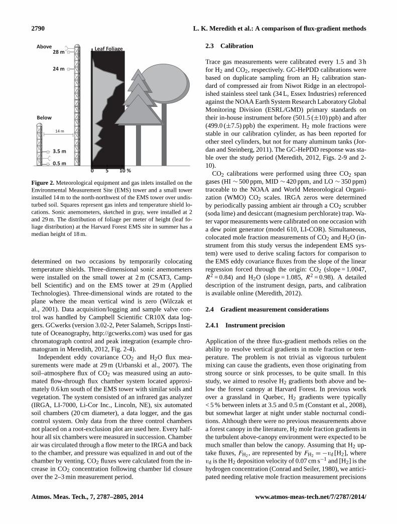
Gas sampling inlets were installed at 24 and 28 m on theEMS tower and at 0.5 and 3.5 m on a small tower erected14 m to the north-northwest of the EMS tower in an area ofundisturbed vegetation and soil (Fig. 2). The leaf foliage dis-tribution (Fig. 2) during summer at the Harvard Forest EMSsite is top heavy and is important to consider for its inter-actions with the turbulent structures at the site (Parker, un-published data). In this manuscript, we refer to measurementheights by their relation to the median forest canopy height(18 m; Fig. 2) when relevant to the topic at hand:abovecanopyfor 24 and 28 m andbelow canopyfor 0.5 and 3.5 m.Tubing lines (OD 1/4 in., Synflex®) of lengths 45–55 m wereinstalled with inline PFA filter holders (47 mm PFA, ColePalmer) containing 0.2 µm pore size filters (Zefluor™, PallCorporation) and inverted Teflon funnels to protect the tubinginlet from precipitation. During the normal sampling routine,H2 GC-HePDD measurements were made at 28, 24, 3.5, and0.5 m over a 16 min cycle. Meanwhile, the IRGAs measured1 Hz CO2 and H2O mole fractions in either the 28 and 0.5 mor the 24 and 3.5 m gas sample streams (250 mL min−1),switching on 1 min intervals. Each sample stream was mixedin 2 L glass integrating volumes with fans (Meredith, 2012;Fig. A1). Three times per week, we used a nulling procedureto assess measurement accuracy, in which all gas streamssampled a common gas inlet installed at 2 m connected toan unmixed 25 L nulling reservoir (glass carboy).
Custom-designed small-footprint aspirated temperatureshields (Dunn et al., 2009) containing thermistors (YSI)were colocated with the gas inlets. Temperature data werecorrected for offsets between the sensors, which were
www.atmos-meas-tech.net/7/2787/2014/ Atmos. Meas. Tech., 7, 2787–2805, 2014
2790 L. K. Meredith et al.: A comparison of flux-gradient methods
0 5 10
Leaf FoliageDistribution
%
28 m
24 m
Above
Below
3.5 m
0.5 m
14 m
Figure 2. Meteorological equipment and gas inlets installed on theEnvironmental Measurement Site (EMS) tower and a small towerinstalled 14 m to the north-northwest of the EMS tower over undis-turbed soil. Squares represent gas inlets and temperature shield lo-cations. Sonic anemometers, sketched in gray, were installed at 2and 29 m. The distribution of foliage per meter of height (leaf fo-liage distribution) at the Harvard Forest EMS site in summer has amedian height of 18 m.
determined on two occasions by temporarily colocatingtemperature shields. Three-dimensional sonic anemometerswere installed on the small tower at 2 m (CSAT3, Camp-bell Scientific) and on the EMS tower at 29 m (AppliedTechnologies). Three-dimensional winds are rotated to theplane where the mean vertical wind is zero (Wilczak etal., 2001). Data acquisition/logging and sample valve con-trol was handled by Campbell Scientific CR10X data log-gers. GCwerks (version 3.02-2, Peter Salameh, Scripps Insti-tute of Oceanography,http://gcwerks.com) was used for gaschromatograph control and peak integration (example chro-matogram in Meredith, 2012, Fig. 2-4).
Independent eddy covariance CO2 and H2O flux mea-surements were made at 29 m (Urbanski et al., 2007). Thesoil–atmosphere flux of CO2 was measured using an auto-mated flow-through flux chamber system located approxi-mately 0.6 km south of the EMS tower with similar soils andvegetation. The system consisted of an infrared gas analyzer(IRGA, LI-7000, Li-Cor Inc., Lincoln, NE), six automatedsoil chambers (20 cm diameter), a data logger, and the gascontrol system. Only data from the three control chambersnot placed on a root-exclusion plot are used here. Every half-hour all six chambers were measured in succession. Chamberair was circulated through a flow meter to the IRGA and backto the chamber, and pressure was equalized in and out of thechamber by venting. CO2 fluxes were calculated from the in-crease in CO2 concentration following chamber lid closureover the 2–3 min measurement period.
2.3 Calibration
Trace gas measurements were calibrated every 1.5 and 3 hfor H2 and CO2, respectively. GC-HePDD calibrations werebased on duplicate sampling from an H2 calibration stan-dard of compressed air from Niwot Ridge in an electropol-ished stainless steel tank (34 L, Essex Industries) referencedagainst the NOAA Earth System Research Laboratory GlobalMonitoring Division (ESRL/GMD) primary standards ontheir in-house instrument before (501.5 (±10) ppb) and after(499.0 (±7.5) ppb) the experiment. H2 mole fractions werestable in our calibration cylinder, as has been reported forother steel cylinders, but not for many aluminum tanks (Jor-dan and Steinberg, 2011). The GC-HePDD response was sta-ble over the study period (Meredith, 2012, Figs. 2-9 and 2-10).
CO2 calibrations were performed using three CO2 spangases (HI∼ 500 ppm, MID∼ 420 ppm, and LO∼ 350 ppm)traceable to the NOAA and World Meteorological Organi-zation (WMO) CO2 scales. IRGA zeros were determinedby periodically passing ambient air through a CO2 scrubber(soda lime) and desiccant (magnesium perchlorate) trap. Wa-ter vapor measurements were calibrated on one occasion witha dew point generator (model 610, LI-COR). Simultaneous,colocated mole fraction measurements of CO2 and H2O (in-strument from this study versus the independent EMS sys-tem) were used to derive scaling factors for comparison tothe EMS eddy covariance fluxes from the slope of the linearregression forced through the origin: CO2 (slope = 1.0047,R2 = 0.84) and H2O (slope = 1.085,R2 = 0.98). A detaileddescription of the instrument design, parts, and calibrationis available online (Meredith, 2012).
2.4 Gradient measurement considerations
2.4.1 Instrument precision
Application of the three flux-gradient methods relies on theability to resolve vertical gradients in mole fraction or tem-perature. The problem is not trivial as vigorous turbulentmixing can cause the gradients, even those originating fromstrong source or sink processes, to be quite small. In thisstudy, we aimed to resolve H2 gradients both above and be-low the forest canopy at Harvard Forest. In previous workover a grassland in Quebec, H2 gradients were typically< 5 % between inlets at 3.5 and 0.5 m (Constant et al., 2008),but somewhat larger at night under stable nocturnal condi-tions. Although there were no previous measurements abovea forest canopy in the literature, H2 mole fraction gradients inthe turbulent above-canopy environment were expected to bemuch smaller than below the canopy. Assuming that H2 up-take fluxes,FH2, are represented byFH2 = −vd [H2], wherevd is the H2 deposition velocity of 0.07 cm s−1 and[H2] is thehydrogen concentration (Conrad and Seiler, 1980), we antici-pated needing relative mole fraction measurement precisions
Atmos. Meas. Tech., 7, 2787–2805, 2014 www.atmos-meas-tech.net/7/2787/2014/
L. K. Meredith et al.: A comparison of flux-gradient methods 2791
for high levels of turbulence of 0.07 and 0.7 % to resolvemeaningful gradients under unstable and stable stratification,respectively (Wesely et al., 1989). The required precisionswould be 0.4 and 4 % under unstable and stable stratificationunder low-turbulence conditions, but under the latter, eddycovariance measurements may not be valid.
Commonly used H2 detectors were not adequate for thedesired measurement precision: reported precisions were0.5–5 % for mercuric oxide reduced gas detectors (Novelliet al., 1999, 2009; Constant et al., 2008; Simmonds et al.,2000) and 1.1–2 % for N2O-doped electron capture detec-tors (Barnes et al., 2003; Moore et al., 2003). Therefore, weused the GC-HePDD to measure H2 mole fractions becauseit had been used to measure H2 with precisions of 0.06 %(1σ) under laboratory conditions (Novelli et al., 2009). Oursystem achieved median H2 measurement precisions over thefield study between 0.06 and 0.11 %, and nearly always bet-ter than 0.3 % (95 % level) (Meredith, 2012, Fig. 2-8), whichwere on par with the laboratory-based configuration (Novelliet al., 2009) and at a 10-fold improvement over methods pre-viously deployed to the field. The IRGA instruments mea-sured mole fractions of CO2 and H2O with high precisions aswell: between 0.025 and 0.043 and between 0.04 and 0.05 %(Meredith, 2012, Fig. 2-12). The high precision capabilitywas critical for measuring the small vertical differences inmole fractions (Sect. 3.1).
2.4.2 Sampling error
We used well-mixed integrating volumes to smooth out thetemporal fluctuations in gas sample streams to retain rele-vant information from each gradient level and reduce sam-pling error (Woodruff, 1986). An integrating volume (V ) actsas an exponential filter on a gas flow (Q) with an e-foldingtimescale (τV = V/Q) that is set to span the time (Tc) tomeasure both H2 mole fractions of a given gradient pair:specifically,τV ∼ Tc = 8 min. The sampling error increaseswith the ratio of the timescale of the measurement cycle (Tc)
to the timescale of the scalar in turbulent flow (τT ). Specif-
ically, percent sampling error = 6(
TcτT
)0.8, and sampling er-
rors can be in excess of 50 % for a 90 min GC-based mea-surement cycle (Woodruff, 1986; Meyers et al., 1996). Theintegrating volumes avoided sampling errors of around 10 %for our GC configuration that would have resulted from in-termittent sampling with a single instrument (see Sect. 2.4.3)assumingτT = 200–300 s (Baldocchi and Meyers, 1991).Sampling intervals interact systematically with the autocor-relation of the time series arising from the eddy structures(Woodruff, 1986). Integrating volumes (known also as buffervolumes) have been used in previous studies to dampen tem-poral fluctuations in trace gas mole fractions for flux-gradientmeasurements (Griffith et al., 2002), for contributions of ad-vection (Yi et al., 2008), and for flask sampling (Bowlinget al., 2003). A block-averaging effect is accomplished in
flux-gradient measurements that trap the compound of in-terest over periods of minutes or hours (Müller et al., 1993;Goldstein et al., 1995, 1996, 1998; Meyers et al., 1996) andeddy accumulation methods that use high-precision differen-tial collection apparatus to trap and then sample air from up-and down-drafts to determine the flux (Businger and Onlcey,1990; Guenther et al., 1996; Bowling et al., 1998).
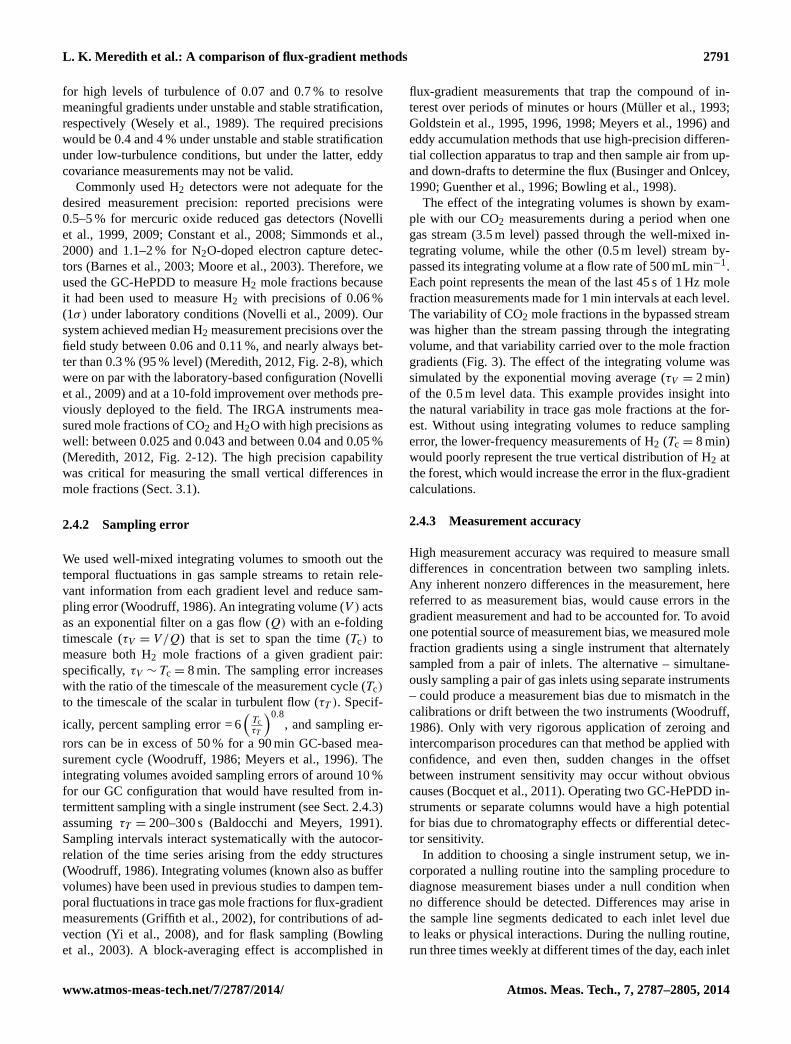
The effect of the integrating volumes is shown by exam-ple with our CO2 measurements during a period when onegas stream (3.5 m level) passed through the well-mixed in-tegrating volume, while the other (0.5 m level) stream by-passed its integrating volume at a flow rate of 500 mL min−1.Each point represents the mean of the last 45 s of 1 Hz molefraction measurements made for 1 min intervals at each level.The variability of CO2 mole fractions in the bypassed streamwas higher than the stream passing through the integratingvolume, and that variability carried over to the mole fractiongradients (Fig. 3). The effect of the integrating volume wassimulated by the exponential moving average (τV = 2 min)of the 0.5 m level data. This example provides insight intothe natural variability in trace gas mole fractions at the for-est. Without using integrating volumes to reduce samplingerror, the lower-frequency measurements of H2 (Tc = 8 min)would poorly represent the true vertical distribution of H2 atthe forest, which would increase the error in the flux-gradientcalculations.
2.4.3 Measurement accuracy
High measurement accuracy was required to measure smalldifferences in concentration between two sampling inlets.Any inherent nonzero differences in the measurement, herereferred to as measurement bias, would cause errors in thegradient measurement and had to be accounted for. To avoidone potential source of measurement bias, we measured molefraction gradients using a single instrument that alternatelysampled from a pair of inlets. The alternative – simultane-ously sampling a pair of gas inlets using separate instruments– could produce a measurement bias due to mismatch in thecalibrations or drift between the two instruments (Woodruff,1986). Only with very rigorous application of zeroing andintercomparison procedures can that method be applied withconfidence, and even then, sudden changes in the offsetbetween instrument sensitivity may occur without obviouscauses (Bocquet et al., 2011). Operating two GC-HePDD in-struments or separate columns would have a high potentialfor bias due to chromatography effects or differential detec-tor sensitivity.
In addition to choosing a single instrument setup, we in-corporated a nulling routine into the sampling procedure todiagnose measurement biases under a null condition whenno difference should be detected. Differences may arise inthe sample line segments dedicated to each inlet level dueto leaks or physical interactions. During the nulling routine,run three times weekly at different times of the day, each inlet
www.atmos-meas-tech.net/7/2787/2014/ Atmos. Meas. Tech., 7, 2787–2805, 2014
2792 L. K. Meredith et al.: A comparison of flux-gradient methods
14:30 15:00 15:30 16:00407
408
409
410
411a) CO
2 mole fractions
[ppm
]
3.5 m0.5 m: bypass IV0.5 m: exp �lter
14:30 15:00 15:30 16:00
−0.4
−0.2
0
b)CO
2 gradients
[ppm
m−1
]
2 m: bypass 1 IV2 m: exp �lter
Figure 3. Two-hour period highlighting the importance of usingintegrating volumes for our mole fraction gradient measurements.During this period, the 0.5 m inlet sample stream bypassed the in-tegrating volume (a, blue diamonds), while the 3.5 m inlet samplestream passed through the integrating volume and was physicallysmoothed (a, pink points). The effect the integrating volume wouldhave had on the 0.5 m inlet measurements was simulated with anexponential moving average (a, dark-blue points). The mole frac-tion gradients from the physically smoothed 3.5 m inlet data andthe 0.5 m inlet measurements bypassing the integrating volume (b,blue diamonds) were more variable than the physically smoothed3.5 m inlet data and the computationally smoothed (exponential fil-ter) 0.5 m inlet data (b, dark-blue points).
sampled ambient air from a 25 L glass carboy, which can bethought of as a large integrating volume. The volume waspre-flushed at 3 L min−1 (τV = 8.3 min) and then sampled byall sample streams at 2 L min−1 total flow (τV = 12.5 min).Similar systems have been engineered to sample air fromthe same inlet height by temporarily placing inlets at thesame height or frequently interchanging the inlet positions(Goldstein et al., 1995; Meyers et al., 1996; Wesely et al.,1989), but that ambient air is still subject to atmospheric vari-ability. Our goal was to have an automated nulling procedurewhere all inlets would sample from the same reservoir of airthat had nearly the same thermal, barometric, and chemicalcharacteristics as the ambient air, but with the high-frequencyatmospheric variability filtered out.
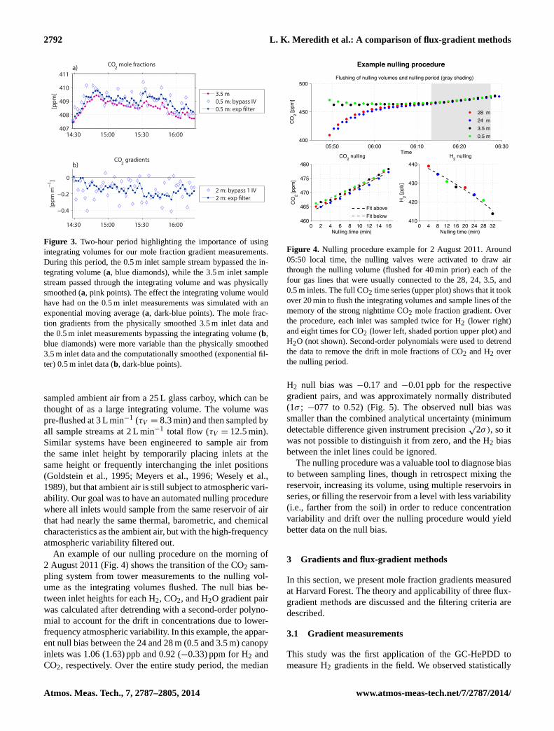
An example of our nulling procedure on the morning of2 August 2011 (Fig. 4) shows the transition of the CO2 sam-pling system from tower measurements to the nulling vol-ume as the integrating volumes flushed. The null bias be-tween inlet heights for each H2, CO2, and H2O gradient pairwas calculated after detrending with a second-order polyno-mial to account for the drift in concentrations due to lower-frequency atmospheric variability. In this example, the appar-ent null bias between the 24 and 28 m (0.5 and 3.5 m) canopyinlets was 1.06 (1.63) ppb and 0.92 (−0.33) ppm for H2 andCO2, respectively. Over the entire study period, the median
18
358 Figure 4. Nulling procedure example: 2 August 2011. Around 05:50 local time, the 359
nulling valves were activated to draw air through the nulling volume (flushed for 40 min 360
prior) each of the four gas lines that were usually connected to the 28 m, 24 m, 3.5 m, and 361
0.5 m inlets. The full CO2 time series (upper plot) shows that it took over 20 min to flush 362
the integrating volumes and sample lines of the memory of the strong nighttime CO2 363
mole fraction gradient. Over the procedure, each inlet was sampled twice for H2 (lower 364
right) and eight times for CO2 (lower left; shaded portion upper plot) and H2O (not 365
shown). Second-order polynomials were used to detrend the data to remove the drift in 366
mole fractions of CO2 and H2 over the nulling period. 367
368
05:50 06:00 06:10 06:20 06:30400
450
500
Time
CO
2 [ppm
]
Flushing of nulling volumes and nulling period (gray shading)
28 m24 m3.5 m0.5 m
0 2 4 6 8 10 12 14 16460
465
470
475
480
Nulling time (min)
CO
2 [ppm
]
CO2 nulling
Fit aboveFit below
0 4 8 12 16 20 24 28 32410
420
430
440H2 nulling
H 2 [ppb
]
Nulling time (min)
Example nulling procedure
Figure 4. Nulling procedure example for 2 August 2011. Around05:50 local time, the nulling valves were activated to draw airthrough the nulling volume (flushed for 40 min prior) each of thefour gas lines that were usually connected to the 28, 24, 3.5, and0.5 m inlets. The full CO2 time series (upper plot) shows that it tookover 20 min to flush the integrating volumes and sample lines of thememory of the strong nighttime CO2 mole fraction gradient. Overthe procedure, each inlet was sampled twice for H2 (lower right)and eight times for CO2 (lower left, shaded portion upper plot) andH2O (not shown). Second-order polynomials were used to detrendthe data to remove the drift in mole fractions of CO2 and H2 overthe nulling period.
H2 null bias was−0.17 and−0.01 ppb for the respectivegradient pairs, and was approximately normally distributed(1σ ; −077 to 0.52) (Fig. 5). The observed null bias wassmaller than the combined analytical uncertainty (minimumdetectable difference given instrument precision
√2σ), so it
was not possible to distinguish it from zero, and the H2 biasbetween the inlet lines could be ignored.
The nulling procedure was a valuable tool to diagnose biasto between sampling lines, though in retrospect mixing thereservoir, increasing its volume, using multiple reservoirs inseries, or filling the reservoir from a level with less variability(i.e., farther from the soil) in order to reduce concentrationvariability and drift over the nulling procedure would yieldbetter data on the null bias.
3 Gradients and flux-gradient methods
In this section, we present mole fraction gradients measuredat Harvard Forest. The theory and applicability of three flux-gradient methods are discussed and the filtering criteria aredescribed.
3.1 Gradient measurements
This study was the first application of the GC-HePDD tomeasure H2 gradients in the field. We observed statistically
Atmos. Meas. Tech., 7, 2787–2805, 2014 www.atmos-meas-tech.net/7/2787/2014/
L. K. Meredith et al.: A comparison of flux-gradient methods 2793 19
369
Figure 5. Time series (upper plots) and distributions (lower plots) of the measurement 370
bias between sampling lines for the 24 m and 28 m (left plots) and the 0.5 m and 3.5 m 371
(right plots) H2 measurements as determined by the nulling procedure. The median and 372
the 1σ confidence intervals are reported for each distribution and are compared with 373
minimum detectable difference given the median instrument 1σ precision (grey shading). 374
375
The nulling procedure was a valuable tool to diagnose bias to between sampling 376
lines, though in retrospect mixing the reservoir, increasing its volume, using multiple 377
reservoirs in series, or filling the reservoir from a level with less variability (i.e., farther 378
Nov10 Apr11 Sep11 Feb12
−2
0
2
24 m and 28 m inlets
H2 n
ull b
ias
[ppb
]
Nov10 Apr11 Sep11 Feb12
−2
0
2
0.5 m and 3.5 m inlets
H2 n
ull b
ias
[ppb
]
−2 0 20
10
20Median, −1m, 1m−0.17, −0.77, 0.35
H2 null bias [ppb]
Cou
nts
−2 0 20
10
20
H2 null bias [ppb]
Cou
nts
Median, −1m, +1m−0.01, −0.60, 0.52
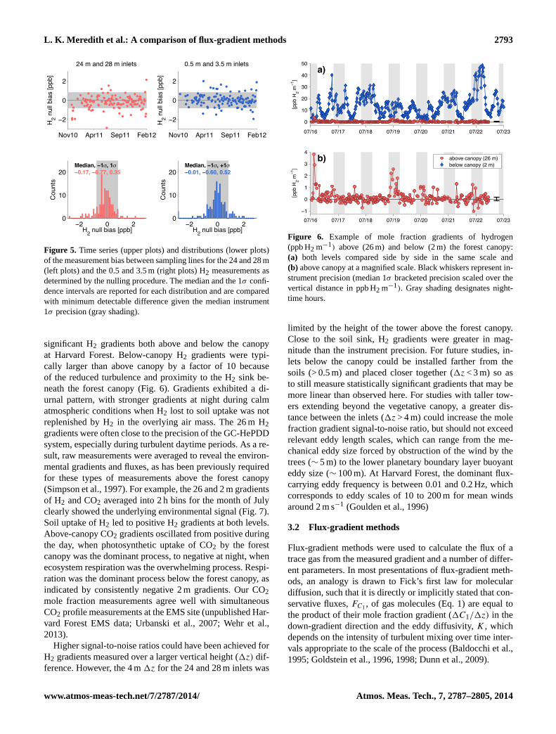
Figure 5. Time series (upper plots) and distributions (lower plots)of the measurement bias between sampling lines for the 24 and 28 m(left plots) and the 0.5 and 3.5 m (right plots) H2 measurements asdetermined by the nulling procedure. The median and the 1σ confi-dence intervals are reported for each distribution and are comparedwith minimum detectable difference given the median instrument1σ precision (gray shading).
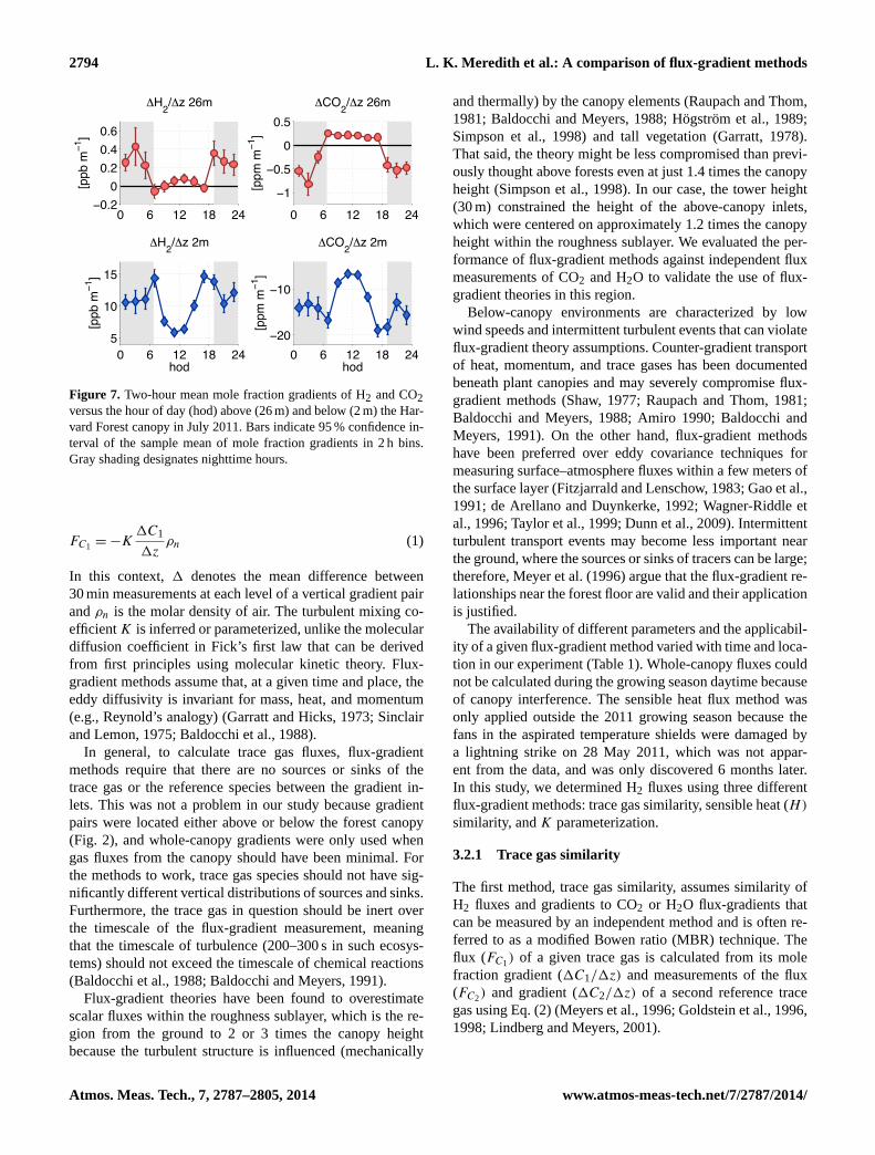
significant H2 gradients both above and below the canopyat Harvard Forest. Below-canopy H2 gradients were typi-cally larger than above canopy by a factor of 10 becauseof the reduced turbulence and proximity to the H2 sink be-neath the forest canopy (Fig. 6). Gradients exhibited a di-urnal pattern, with stronger gradients at night during calmatmospheric conditions when H2 lost to soil uptake was notreplenished by H2 in the overlying air mass. The 26 m H2gradients were often close to the precision of the GC-HePDDsystem, especially during turbulent daytime periods. As a re-sult, raw measurements were averaged to reveal the environ-mental gradients and fluxes, as has been previously requiredfor these types of measurements above the forest canopy(Simpson et al., 1997). For example, the 26 and 2 m gradientsof H2 and CO2 averaged into 2 h bins for the month of Julyclearly showed the underlying environmental signal (Fig. 7).Soil uptake of H2 led to positive H2 gradients at both levels.Above-canopy CO2 gradients oscillated from positive duringthe day, when photosynthetic uptake of CO2 by the forestcanopy was the dominant process, to negative at night, whenecosystem respiration was the overwhelming process. Respi-ration was the dominant process below the forest canopy, asindicated by consistently negative 2 m gradients. Our CO2mole fraction measurements agree well with simultaneousCO2 profile measurements at the EMS site (unpublished Har-vard Forest EMS data; Urbanski et al., 2007; Wehr et al.,2013).
Higher signal-to-noise ratios could have been achieved forH2 gradients measured over a larger vertical height (1z) dif-ference. However, the 4 m1z for the 24 and 28 m inlets was
21
at night when ecosystem respiration was the overwhelming process. Respiration was the 402
dominant process below the forest canopy, as indicated by consistently negative 2 m 403
gradients. Our CO2 mole fraction measurements agree well with simultaneous CO2 404
profile measurements at the EMS site (unpublished Harvard Forest EMS data; Urbanski 405
et al., 2007; Wehr et al., 2013). 406
407
408
Figure 6. Example of mole fraction gradients of hydrogen (ppb H2 m-1) above (26 m) and 409
below (2 m) the forest canopy: a) both levels compared side-by-side in the same scale 410
and b) above canopy at a magnified scale. Black whiskers represent instrument precision 411
(median 1σ bracketed precision scaled over the vertical distance in ppb H2 m-1). Grey 412
shading designates nighttime hours. 413
07/16 07/17 07/18 07/19 07/20 07/21 07/22 07/23
0
10
20
30
40
50
[ppb
H2 m
−1]
a)
07/16 07/17 07/18 07/19 07/20 07/21 07/22 07/23−1
0
1
2
3
4
[ppb
H2 m
−1]
b) above canopy (26 m)
below canopy (2 m)
Figure 6. Example of mole fraction gradients of hydrogen(ppb H2 m−1) above (26 m) and below (2 m) the forest canopy:(a) both levels compared side by side in the same scale and(b) above canopy at a magnified scale. Black whiskers represent in-strument precision (median 1σ bracketed precision scaled over thevertical distance in ppb H2 m−1). Gray shading designates night-time hours.
limited by the height of the tower above the forest canopy.Close to the soil sink, H2 gradients were greater in mag-nitude than the instrument precision. For future studies, in-lets below the canopy could be installed farther from thesoils (> 0.5 m) and placed closer together (1z < 3 m) so asto still measure statistically significant gradients that may bemore linear than observed here. For studies with taller tow-ers extending beyond the vegetative canopy, a greater dis-tance between the inlets (1z > 4 m) could increase the molefraction gradient signal-to-noise ratio, but should not exceedrelevant eddy length scales, which can range from the me-chanical eddy size forced by obstruction of the wind by thetrees (∼ 5 m) to the lower planetary boundary layer buoyanteddy size (∼ 100 m). At Harvard Forest, the dominant flux-carrying eddy frequency is between 0.01 and 0.2 Hz, whichcorresponds to eddy scales of 10 to 200 m for mean windsaround 2 m s−1 (Goulden et al., 1996)
3.2 Flux-gradient methods
Flux-gradient methods were used to calculate the flux of atrace gas from the measured gradient and a number of differ-ent parameters. In most presentations of flux-gradient meth-ods, an analogy is drawn to Fick’s first law for moleculardiffusion, such that it is directly or implicitly stated that con-servative fluxes,FC1, of gas molecules (Eq. 1) are equal tothe product of their mole fraction gradient (1C1/1z) in thedown-gradient direction and the eddy diffusivity,K, whichdepends on the intensity of turbulent mixing over time inter-vals appropriate to the scale of the process (Baldocchi et al.,1995; Goldstein et al., 1996, 1998; Dunn et al., 2009).
www.atmos-meas-tech.net/7/2787/2014/ Atmos. Meas. Tech., 7, 2787–2805, 2014
2794 L. K. Meredith et al.: A comparison of flux-gradient methods 22
414 Figure 7. Two-hour mean mole fraction gradients of H2 and CO2 versus the hour of day 415
(hod) above (26 m) and below (2 m) the Harvard Forest canopy in July 2011. Bars 416
indicate 95% confidence interval of the sample mean of mole fraction gradients in 2-hour 417
bins. Grey shading designates nighttime hours. 418
419
Higher signal-to-noise ratios could have been achieved for H2 gradients measured 420
over a larger vertical height (Δz) difference. However, the 4 m Δz for the 24 m and 28 m 421
inlets was limited by the height of the tower above the forest canopy. Close to the soil 422
sink, H2 gradients were greater in magnitude than the instrument precision. For future 423
studies, inlets below the canopy could be installed farther from the soils (> 0.5 m) and be 424
placed closer together (Δz < 3 m), to still measure statistically significant gradients that 425
0 6 12 18 24−0.2
00.20.40.6
[ppb
m−1
]6H2/6z 26m
0 6 12 18 24−1
−0.5
0
0.5
[ppm
m−1
]
6CO2/6z 26m
0 6 12 18 245
10
15
[ppb
m−1
]
6H2/6z 2m
hod0 6 12 18 24
−20
−10
[ppm
m−1
]6CO2/6z 2m
hod
Figure 7. Two-hour mean mole fraction gradients of H2 and CO2versus the hour of day (hod) above (26 m) and below (2 m) the Har-vard Forest canopy in July 2011. Bars indicate 95 % confidence in-terval of the sample mean of mole fraction gradients in 2 h bins.Gray shading designates nighttime hours.
FC1 = −K1C1
1zρn (1)
In this context,1 denotes the mean difference between30 min measurements at each level of a vertical gradient pairandρn is the molar density of air. The turbulent mixing co-efficientK is inferred or parameterized, unlike the moleculardiffusion coefficient in Fick’s first law that can be derivedfrom first principles using molecular kinetic theory. Flux-gradient methods assume that, at a given time and place, theeddy diffusivity is invariant for mass, heat, and momentum(e.g., Reynold’s analogy) (Garratt and Hicks, 1973; Sinclairand Lemon, 1975; Baldocchi et al., 1988).
In general, to calculate trace gas fluxes, flux-gradientmethods require that there are no sources or sinks of thetrace gas or the reference species between the gradient in-lets. This was not a problem in our study because gradientpairs were located either above or below the forest canopy(Fig. 2), and whole-canopy gradients were only used whengas fluxes from the canopy should have been minimal. Forthe methods to work, trace gas species should not have sig-nificantly different vertical distributions of sources and sinks.Furthermore, the trace gas in question should be inert overthe timescale of the flux-gradient measurement, meaningthat the timescale of turbulence (200–300 s in such ecosys-tems) should not exceed the timescale of chemical reactions(Baldocchi et al., 1988; Baldocchi and Meyers, 1991).
Flux-gradient theories have been found to overestimatescalar fluxes within the roughness sublayer, which is the re-gion from the ground to 2 or 3 times the canopy heightbecause the turbulent structure is influenced (mechanically
and thermally) by the canopy elements (Raupach and Thom,1981; Baldocchi and Meyers, 1988; Högström et al., 1989;Simpson et al., 1998) and tall vegetation (Garratt, 1978).That said, the theory might be less compromised than previ-ously thought above forests even at just 1.4 times the canopyheight (Simpson et al., 1998). In our case, the tower height(30 m) constrained the height of the above-canopy inlets,which were centered on approximately 1.2 times the canopyheight within the roughness sublayer. We evaluated the per-formance of flux-gradient methods against independent fluxmeasurements of CO2 and H2O to validate the use of flux-gradient theories in this region.
Below-canopy environments are characterized by lowwind speeds and intermittent turbulent events that can violateflux-gradient theory assumptions. Counter-gradient transportof heat, momentum, and trace gases has been documentedbeneath plant canopies and may severely compromise flux-gradient methods (Shaw, 1977; Raupach and Thom, 1981;Baldocchi and Meyers, 1988; Amiro 1990; Baldocchi andMeyers, 1991). On the other hand, flux-gradient methodshave been preferred over eddy covariance techniques formeasuring surface–atmosphere fluxes within a few meters ofthe surface layer (Fitzjarrald and Lenschow, 1983; Gao et al.,1991; de Arellano and Duynkerke, 1992; Wagner-Riddle etal., 1996; Taylor et al., 1999; Dunn et al., 2009). Intermittentturbulent transport events may become less important nearthe ground, where the sources or sinks of tracers can be large;therefore, Meyer et al. (1996) argue that the flux-gradient re-lationships near the forest floor are valid and their applicationis justified.
The availability of different parameters and the applicabil-ity of a given flux-gradient method varied with time and loca-tion in our experiment (Table 1). Whole-canopy fluxes couldnot be calculated during the growing season daytime becauseof canopy interference. The sensible heat flux method wasonly applied outside the 2011 growing season because thefans in the aspirated temperature shields were damaged bya lightning strike on 28 May 2011, which was not appar-ent from the data, and was only discovered 6 months later.In this study, we determined H2 fluxes using three differentflux-gradient methods: trace gas similarity, sensible heat (H)
similarity, andK parameterization.
3.2.1 Trace gas similarity
The first method, trace gas similarity, assumes similarity ofH2 fluxes and gradients to CO2 or H2O flux-gradients thatcan be measured by an independent method and is often re-ferred to as a modified Bowen ratio (MBR) technique. Theflux (FC1) of a given trace gas is calculated from its molefraction gradient (1C1/1z) and measurements of the flux(FC2) and gradient (1C2/1z) of a second reference tracegas using Eq. (2) (Meyers et al., 1996; Goldstein et al., 1996,1998; Lindberg and Meyers, 2001).
Atmos. Meas. Tech., 7, 2787–2805, 2014 www.atmos-meas-tech.net/7/2787/2014/
L. K. Meredith et al.: A comparison of flux-gradient methods 2795
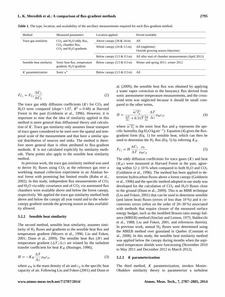
Table 1.The type, location, and availability of the ancillary measurements required for each flux-gradient method.
Method Measured parameters Location applied Period available
Trace gas similarity CO2 and H2O eddy flux, Above canopy (28 & 24 m) AllCO2 chamber flux,
Whole canopy (24 & 3.5 m) All (nighttime)CO2 and H2O gradients
Outside growing season (daytime)
Below canopy (3.5 & 0.5 m) All after start of chamber measurements (April 2011)
Sensible heat similarity Sonic heat flux, temperature Below canopy (3.5 & 0.5 m) Winter and spring 2011, winter 2012gradient, H2O gradient
K parameterization Sonicu∗ Below canopy (3.5 & 0.5 m) All
FC1 = FC2
1C1
1C2(2)
The trace gas eddy diffusion coefficients (K) for CO2 andH2O were compared (slope = 1.07,R2
= 0.68) at HarvardForest in the past (Goldstein et al., 1996). However, it isimportant to note that the idea of similarity applied in thismethod is more general than diffusional theory and calcula-tion of K. Trace gas similarity only assumes linear transportof trace gases considered to be inert over the spatial and tem-poral scale of the measurement and that have a similar spa-tial distribution of sources and sinks. The method is there-fore more general than is often attributed to flux-gradientmethods.K is not calculated explicitly by similarity meth-ods. These points also apply to the sensible heat similaritymethod.
In previous work, the trace gas similarity method was usedto derive H2 fluxes using CO2 as the reference gas over aweeklong manual collection experiment in an Alaskan bo-real forest with promising but limited results (Rahn et al.,2002). In this study, independent flux measurements of CO2and H2O via eddy covariance and of CO2 via automated fluxchambers were available above and below the forest canopy,respectively. We applied the trace gas similarity method bothabove and below the canopy all year round and to the whole-canopy gradient outside the growing season as data availabil-ity allowed.
3.2.2 Sensible heat similarity
The second method, sensible heat similarity, assumes simi-larity of H2 fluxes and gradients to the sensible heat flux andtemperature gradient (Meyers et al., 1996; Liu and Foken,2001; Dunn et al., 2009). The sensible heat flux (H) andtemperature gradient (1T/1z) are related by the turbulenttransfer coefficient for heatKH (Businger, 1986),
H = −KH
1T
1zρmcp, (3)
whereρm is the mass density of air andcp is the specific heatcapacity of air. Following Liu and Foken (2001) and Dunn et
al. (2009), the sensible heat flux was obtained by applyinga water vapor correction to the buoyancy flux derived fromsonic anemometer temperature measurements, and the cross-wind term was neglected because it should be small com-pared to the other terms,
H =w′T ′
s1T1z
+ 0.51T 1q1z
1T
1zρmcp, (4)
wherew′T ′s is the sonic heat flux andq represents the spe-
cific humidity (kg H2O kg air−1). Equation (4) gives the flux-gradient form (Eq. 1) for sensible heat, which can then beused to determine the H2 flux (Eq. 5) by inferringKH .
FC1 = H1C1
1T
ρn
ρmcp
(5)
The eddy diffusion coefficients for trace gases (K) and heat(KH ) were measured at Harvard Forest in the past, agree-ing within 12± 10 % when compared to both H2O and CO2(Goldstein et al., 1996). The method has been applied to de-termine hydrocarbon fluxes above a forest canopy (Goldsteinet al., 1996) and the specific method adopted in our study wasdeveloped for the calculation of CO2 and H2O fluxes closeto the ground (Dunn et al., 2009). This is an MBR technique(Liu and Foken, 2001) that can be used to determine sensible(and latent heat) fluxes (errors of less than 10 %) and it cir-cumvents errors (often on the order of 20–30 %) associatedwith methods that require closure of the measured surfaceenergy budget, such as the modified Bowen ratio energy bal-ance (MREB) method (Sinclair and Lemon, 1975; Baldocchiet al., 1988; Liu and Foken, 2001, and references therein).In previous work, annual H2 fluxes were determined usingthe MREB method over grassland in Quebec (Constant etal., 2008). In this study, the sensible heat similarity methodwas applied below the canopy during months when the aspi-rated temperature shields were functioning (November 2010to May 2011 and December 2012 to March 2012).
3.2.3 K parameterization
The third method,K parameterization, invokes Monin–Obukhov similarity theory to parameterize a turbulent
www.atmos-meas-tech.net/7/2787/2014/ Atmos. Meas. Tech., 7, 2787–2805, 2014
2796 L. K. Meredith et al.: A comparison of flux-gradient methods
exchange coefficient (K) from sonic anemometer measure-ments, and is often referred to as an aerodynamic method(Monin and Obukhov, 1954; Simpson et al., 1998).K can beestimated by means of a variety of aerodynamic methods de-rived from energy or momentum balances (Högström et al.,1989; Celier and Brunet, 1992; Simpson et al., 1998; Foken,2006). For example,K can be determined from
K =u∗ k(z − d)
φm, (6)
whereu∗ is the friction velocity (a characteristic velocityscale calculated from the square root of covariance betweenvertical and horizontal wind),k is von Karman’s constant(taken as 0.4),z is the height above the ground,d is thezero-plane displacement height, andφm is the diabatic influ-ence function for momentum (Monin and Obukhov, 1954;Simpson et al., 1998). The Monin–Obukhov length (L =
−u3∗
kgT
Hρmcp
) is used to determineφm from the empirical de-
scriptions outlined by Eqs. (22a) and (22b) in Foken (2006).The method has been applied close to the surface (Fritscheet al., 2008) and above the forest canopy (Simpson et al.,1997, 1998). In this study, theK parameterization methodwas applied below the canopy. Assuming thatz = 2 m (theheight of theu∗ measurement), the displacement height wasinferred empirically to be around 1.63 m (z−d = 0.37 m) bycomparing parameterizedK values to the values forK de-termined from the chamber flux and concentration gradientusing Eq. (1). The determination ofd is often problematic(Raupach and Thom, 1981). Physically,d represents an ad-justment of the basis height to reflect the displacement by thesurface features of the profiles of micrometeorological vari-ables fundamental to theK parameterization at hand. Theinferred value ford was consistent throughout the study pe-riod and may reflect the effect of below-canopy environmenton the turbulent fluxes at the EMS site.
3.3 Data filtering
Data were filtered to reject unrealistic values and to appro-priately apply flux-gradient methodology. By their nature,the trace gas similarity and sensible heat similarity methodsare not valid when the gradient of the comparative species(Eqs. 2 and 5, denominator) approaches zero or changessign over the measurement period. Similarity methods can-not work during such periods, so we limited flux calculationsto periods when gradients in the denominator exceeded theirmeasurement precision. In general, the fluxes calculated dur-ing dawn and dusk periods are not included in averages orcomparative assessments because of the tendency for condi-tions to change such that the observed fluxes and gradientsprovide no information about the turbulence. For example,conditions pass through an isothermal point when air and sur-faces have the same temperature so that there is no gradientdriving a heat flux; when air is saturated, there is no gradient
driving a water vapor flux; and when photosynthesis ceases,CO2 gradients change sign.
Data were rejected during rainy periods with more than0.2 mm of rain per 30 min (Baldocchi and Meyers, 1991).Periods withu∗ < 0.07 m s−1 and u∗ < 0.17 m s−1 were ex-cluded for below- and above-canopy data, respectively, be-cause of poorly developed turbulent conditions (Goulden etal., 1996; Liu and Foken, 2001; Bocquet et al., 2011) and po-tential for advective fluxes driven by drainage flows on slop-ing terrain (Yi et al., 2008). We excluded unrealistic valuesof the implied turbulent transfer coefficients,K, such that0 ≤ K ≤ 0.5 m2 s−1 and 0≤ K ≤ 5 m2 s−1 for the below-canopy and the whole/above-canopy fluxes, respectively. Wedid not filter based on the wind sector because we found nointerference from the tower and instrument shed to the east(45 to 180◦). We considered quantile–quantile plots of theresidual between flux-gradient methods and eddy covariancefluxes, and excluded clear outliers: residual absolute values> 20 and > 10 mmol m−2 s−1 for CO2 and H2O fluxes. Ad-ditional filters were applied to the sensible heat flux methodto retain only reasonable sonic and sensible heat flux val-
ues:∣∣∣w′T ′
s
∣∣∣ < 0.1 K m s−1 and −100 <H < 200 W m−2. Fi-
nally, data were excluded when the temperature gradient wasgreater than 0◦C at the same time asH was greater than3 W m−2, which occurred at sunrise and sunset because ofthe rapidly changing conditions over the 30 min averaginginterval (Meyers et al., 1996; Dunn et al., 2009).
Filtering is known to result in a large amount of rejecteddata in flux-gradient methods (e.g., net 57 % data loss in de-tailed analysis by Bocquet et al., 2011). Conditions at thesite, external to the measurement system, resulted in a 13, 19,and 6 % loss of data based on the above-canopyu∗, below-canopyu∗, and precipitation filter criteria, respectively. Fil-tering criteria related to the flux methods resulted in a rawdata loss over the experimental period of around 40–82 %for trace gas similarity, 87 % for sensible heat similarity, and18–26 % forK parameterization.
4 Flux-gradient methods: evaluation and application
Using independent flux measurements of CO2 and H2O de-rived from eddy covariance and chamber techniques, we pro-duced a quantitative guide (Table 2) for the performanceof each flux-gradient method (trace gas similarity, sensibleheat similarity, andK parameterization) at each measure-ment location (above, whole, and below canopy) for differentseasons and times of day. We compared measurements dur-ing summer (23 June 2011 to 16 October 2011) and winter(15 November 2011 to 28 February 2012) during daytime(10:00–16:00) and nighttime (21:00–05:00) periods. We as-signed a performance flag of good, fair, or poor based on thestatistical tests described in Table 2, and we indicated statis-tically significant correlations with∗ and zero bias with †. Inthe framework of this study, a negative flux indicates uptake
Atmos. Meas. Tech., 7, 2787–2805, 2014 www.atmos-meas-tech.net/7/2787/2014/
L. K. Meredith et al.: A comparison of flux-gradient methods 2797
by the underlying biosphere, while a positive flux indicatesemission.
4.1 Comparing eddy covariance and chamberCO2 flux measurements
We assessed the consistency between the eddy covarianceand chamber CO2 flux data before using these independentflux measurements to evaluate our flux-gradient methods.Eddy covariance measurements represent the entire ecosys-tem flux and chamber measurements just the soil flux. Stud-ies comparing nocturnal CO2 eddy flux with chamber mea-surements often report significant discrepancies of 20 to over50 % (e.g., Goulden et al., 1996; Lavigne et al., 1997; Phillipset al., 2010). We did not expect exact agreement betweeneddy and chamber fluxes because of the mismatch in mea-surement footprints, but we expected to see fluxes of a com-parable magnitude with similar diel patterns.
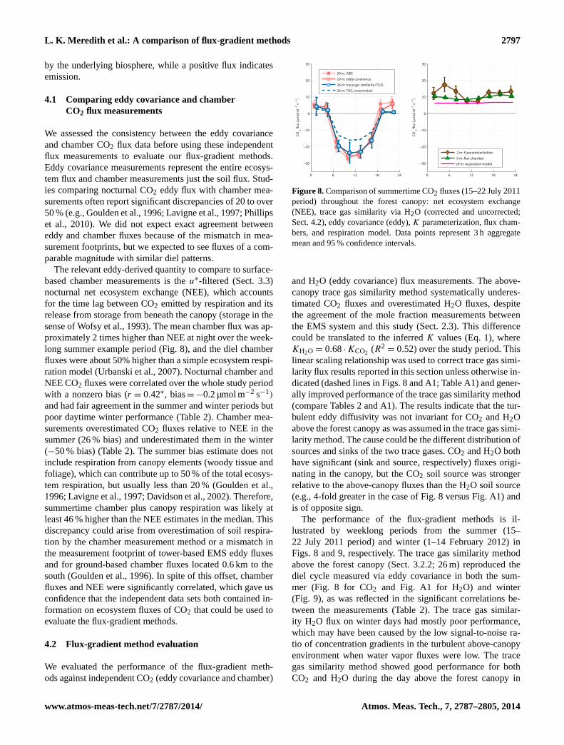
The relevant eddy-derived quantity to compare to surface-based chamber measurements is theu∗-filtered (Sect. 3.3)nocturnal net ecosystem exchange (NEE), which accountsfor the time lag between CO2 emitted by respiration and itsrelease from storage from beneath the canopy (storage in thesense of Wofsy et al., 1993). The mean chamber flux was ap-proximately 2 times higher than NEE at night over the week-long summer example period (Fig. 8), and the diel chamberfluxes were about 50% higher than a simple ecosystem respi-ration model (Urbanski et al., 2007). Nocturnal chamber andNEE CO2 fluxes were correlated over the whole study periodwith a nonzero bias (r = 0.42∗, bias= −0.2 µmol m−2 s−1)
and had fair agreement in the summer and winter periods butpoor daytime winter performance (Table 2). Chamber mea-surements overestimated CO2 fluxes relative to NEE in thesummer (26 % bias) and underestimated them in the winter(−50 % bias) (Table 2). The summer bias estimate does notinclude respiration from canopy elements (woody tissue andfoliage), which can contribute up to 50 % of the total ecosys-tem respiration, but usually less than 20 % (Goulden et al.,1996; Lavigne et al., 1997; Davidson et al., 2002). Therefore,summertime chamber plus canopy respiration was likely atleast 46 % higher than the NEE estimates in the median. Thisdiscrepancy could arise from overestimation of soil respira-tion by the chamber measurement method or a mismatch inthe measurement footprint of tower-based EMS eddy fluxesand for ground-based chamber fluxes located 0.6 km to thesouth (Goulden et al., 1996). In spite of this offset, chamberfluxes and NEE were significantly correlated, which gave usconfidence that the independent data sets both contained in-formation on ecosystem fluxes of CO2 that could be used toevaluate the flux-gradient methods.
4.2 Flux-gradient method evaluation
We evaluated the performance of the flux-gradient meth-ods against independent CO2 (eddy covariance and chamber)
0 6 12 18 24
−30
−20
−10
0
10
20
30
CO2 �
ux [µm
ol m
−2 s
−1]
29 m : NEE
29 m: eddy covariance
26 m: trace gas similarity (TGS)
26 m: TGS, uncorrected
0 6 12 18 24
−30
−20
−10
0
10
20
30
CO2 �
ux [µm
ol m
−2 s
−1]
2 m: K parameterization
0 m: �ux chamber
29 m: respiration model
Figure 8.Comparison of summertime CO2 fluxes (15–22 July 2011period) throughout the forest canopy: net ecosystem exchange(NEE), trace gas similarity via H2O (corrected and uncorrected;Sect. 4.2), eddy covariance (eddy),K parameterization, flux cham-bers, and respiration model. Data points represent 3 h aggregatemean and 95 % confidence intervals.
and H2O (eddy covariance) flux measurements. The above-canopy trace gas similarity method systematically underes-timated CO2 fluxes and overestimated H2O fluxes, despitethe agreement of the mole fraction measurements betweenthe EMS system and this study (Sect. 2.3). This differencecould be translated to the inferredK values (Eq. 1), whereKH2O = 0.68·KCO2 (R2
= 0.52) over the study period. Thislinear scaling relationship was used to correct trace gas simi-larity flux results reported in this section unless otherwise in-dicated (dashed lines in Figs. 8 and A1; Table A1) and gener-ally improved performance of the trace gas similarity method(compare Tables 2 and A1). The results indicate that the tur-bulent eddy diffusivity was not invariant for CO2 and H2Oabove the forest canopy as was assumed in the trace gas simi-larity method. The cause could be the different distribution ofsources and sinks of the two trace gases. CO2 and H2O bothhave significant (sink and source, respectively) fluxes origi-nating in the canopy, but the CO2 soil source was strongerrelative to the above-canopy fluxes than the H2O soil source(e.g., 4-fold greater in the case of Fig. 8 versus Fig. A1) andis of opposite sign.
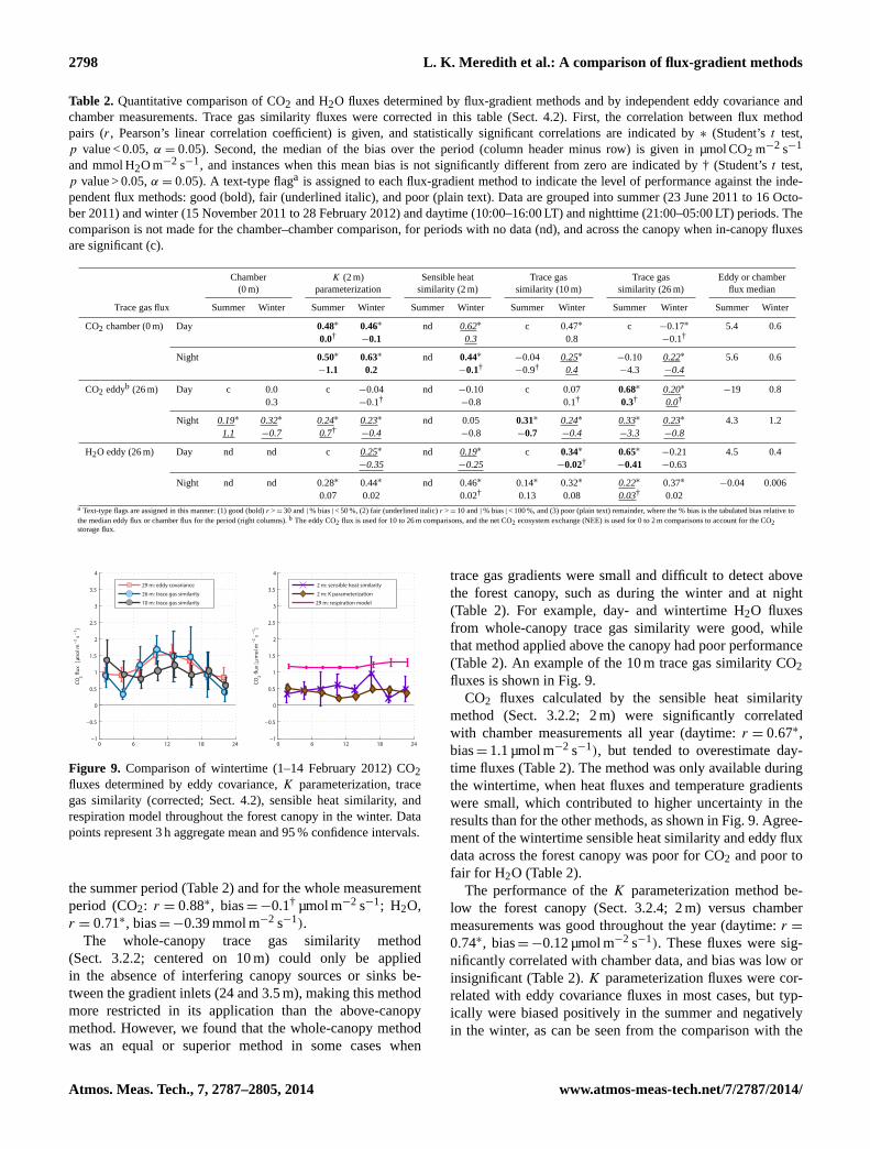
The performance of the flux-gradient methods is il-lustrated by weeklong periods from the summer (15–22 July 2011 period) and winter (1–14 February 2012) inFigs. 8 and 9, respectively. The trace gas similarity methodabove the forest canopy (Sect. 3.2.2; 26 m) reproduced thediel cycle measured via eddy covariance in both the sum-mer (Fig. 8 for CO2 and Fig. A1 for H2O) and winter(Fig. 9), as was reflected in the significant correlations be-tween the measurements (Table 2). The trace gas similar-ity H2O flux on winter days had mostly poor performance,which may have been caused by the low signal-to-noise ra-tio of concentration gradients in the turbulent above-canopyenvironment when water vapor fluxes were low. The tracegas similarity method showed good performance for bothCO2 and H2O during the day above the forest canopy in
www.atmos-meas-tech.net/7/2787/2014/ Atmos. Meas. Tech., 7, 2787–2805, 2014
2798 L. K. Meredith et al.: A comparison of flux-gradient methods
Table 2. Quantitative comparison of CO2 and H2O fluxes determined by flux-gradient methods and by independent eddy covariance andchamber measurements. Trace gas similarity fluxes were corrected in this table (Sect. 4.2). First, the correlation between flux methodpairs (r, Pearson’s linear correlation coefficient) is given, and statistically significant correlations are indicated by∗ (Student’st test,p value < 0.05,α = 0.05). Second, the median of the bias over the period (column header minus row) is given in µmol CO2 m−2 s−1
and mmol H2O m−2 s−1, and instances when this mean bias is not significantly different from zero are indicated by † (Student’st test,p value > 0.05,α = 0.05). A text-type flaga is assigned to each flux-gradient method to indicate the level of performance against the inde-pendent flux methods: good (bold), fair (underlined italic), and poor (plain text). Data are grouped into summer (23 June 2011 to 16 Octo-ber 2011) and winter (15 November 2011 to 28 February 2012) and daytime (10:00–16:00 LT) and nighttime (21:00–05:00 LT) periods. Thecomparison is not made for the chamber–chamber comparison, for periods with no data (nd), and across the canopy when in-canopy fluxesare significant (c).
Chamber K (2 m) Sensible heat Trace gas Trace gas Eddy or chamber(0 m) parameterization similarity (2 m) similarity (10 m) similarity (26 m) flux median
Trace gas flux Summer Winter Summer Winter Summer Winter Summer Winter Summer Winter Summer Winter
CO2 chamber (0 m) Day 0.48∗ 0.46∗ nd 0.62∗ c 0.47∗ c −0.17∗ 5.4 0.60.0†
−0.1 0.3 0.8 −0.1†
Night 0.50∗ 0.63∗ nd 0.44∗ −0.04 0.25∗ −0.10 0.22∗ 5.6 0.6−1.1 0.2 −0.1†
−0.9† 0.4 −4.3 −0.4
CO2 eddyb (26 m) Day c 0.0 c −0.04 nd −0.10 c 0.07 0.68∗ 0.20∗ −19 0.80.3 −0.1†
−0.8 0.1† 0.3† 0.0†
Night 0.19∗ 0.32∗ 0.24∗ 0.23∗ nd 0.05 0.31∗ 0.24∗ 0.33∗ 0.23∗ 4.3 1.21.1 −0.7 0.7†
−0.4 −0.8 −0.7 −0.4 −3.3 −0.8
H2O eddy (26 m) Day nd nd c 0.25∗ nd 0.19∗ c 0.34∗ 0.65∗ −0.21 4.5 0.4−0.35 −0.25 −0.02† −0.41 −0.63
Night nd nd 0.28∗ 0.44∗ nd 0.46∗ 0.14∗ 0.32∗ 0.22∗ 0.37∗ −0.04 0.0060.07 0.02 0.02† 0.13 0.08 0.03† 0.02
a Text-type flags are assigned in this manner: (1) good (bold)r >= 30 and| % bias| < 50 %, (2) fair (underlined italic)r >= 10 and| % bias| < 100 %, and (3) poor (plain text) remainder, where the % bias is the tabulated bias relative tothe median eddy flux or chamber flux for the period (right columns).b The eddy CO2 flux is used for 10 to 26 m comparisons, and the net CO2 ecosystem exchange (NEE) is used for 0 to 2 m comparisons to account for the CO2storage flux.
0 6 12 18 24−1
−0.5
0
0.5
1
1.5
2
2.5
3
3.5
4
CO2 �
ux [µm
ol m
−2 s
−1]
29 m: eddy covariance
26 m: trace gas similarity
10 m: trace gas similarity
0 6 12 18 24−1
−0.5
0
0.5
1
1.5
2
2.5
3
3.5
4
CO2 �
ux [µm
ol m
−2 s
−1]
2 m: sensible heat similarity
2 m: K parameterization
29 m: respiration model
Figure 9. Comparison of wintertime (1–14 February 2012) CO2fluxes determined by eddy covariance,K parameterization, tracegas similarity (corrected; Sect. 4.2), sensible heat similarity, andrespiration model throughout the forest canopy in the winter. Datapoints represent 3 h aggregate mean and 95 % confidence intervals.
the summer period (Table 2) and for the whole measurementperiod (CO2: r = 0.88∗, bias= −0.1† µmol m−2 s−1; H2O,r = 0.71∗, bias= −0.39 mmol m−2 s−1).
The whole-canopy trace gas similarity method(Sect. 3.2.2; centered on 10 m) could only be appliedin the absence of interfering canopy sources or sinks be-tween the gradient inlets (24 and 3.5 m), making this methodmore restricted in its application than the above-canopymethod. However, we found that the whole-canopy methodwas an equal or superior method in some cases when
trace gas gradients were small and difficult to detect abovethe forest canopy, such as during the winter and at night(Table 2). For example, day- and wintertime H2O fluxesfrom whole-canopy trace gas similarity were good, whilethat method applied above the canopy had poor performance(Table 2). An example of the 10 m trace gas similarity CO2fluxes is shown in Fig. 9.
CO2 fluxes calculated by the sensible heat similaritymethod (Sect. 3.2.2; 2 m) were significantly correlatedwith chamber measurements all year (daytime:r = 0.67∗,bias= 1.1 µmol m−2 s−1), but tended to overestimate day-time fluxes (Table 2). The method was only available duringthe wintertime, when heat fluxes and temperature gradientswere small, which contributed to higher uncertainty in theresults than for the other methods, as shown in Fig. 9. Agree-ment of the wintertime sensible heat similarity and eddy fluxdata across the forest canopy was poor for CO2 and poor tofair for H2O (Table 2).
The performance of theK parameterization method be-low the forest canopy (Sect. 3.2.4; 2 m) versus chambermeasurements was good throughout the year (daytime:r =
0.74∗, bias= −0.12 µmol m−2 s−1). These fluxes were sig-nificantly correlated with chamber data, and bias was low orinsignificant (Table 2).K parameterization fluxes were cor-related with eddy covariance fluxes in most cases, but typ-ically were biased positively in the summer and negativelyin the winter, as can be seen from the comparison with the
Atmos. Meas. Tech., 7, 2787–2805, 2014 www.atmos-meas-tech.net/7/2787/2014/
L. K. Meredith et al.: A comparison of flux-gradient methods 2799
NEE-derived simple ecosystem respiration model in Figs. 8and 9. The overestimation of nocturnal summertime fluxesby K parameterization was likely related to the large andnonlinear CO2 gradients (determined from profile measure-ments) that arise under calm nocturnal conditions. In con-trast, trace gas and sensible heat similarity methods use ra-tios of vertical mole fraction or temperature gradients, whichcan compensate for nonlinear vertical concentration gradi-ents. TheK parameterization has been shown to agree withtrace gas similarity and eddy covariance-derived fluxes inthe past (Fritsche et al., 2008). A larger period of overlap-ping data for the sensible heat similarity method was avail-able withK parameterization results than chamber data, andthe two flux-gradient methods were highly correlated but hada relative positive bias of the CO2 flux in the sensible heatmethod relative toK parameterization over the whole period(day r = 0.63∗, bias= 0.37 µmol m−2 s−1; night r = 0.42∗,bias= 0.10 µmol m−2 s−1).
4.3 Flux-gradient method application:H2 gradient fluxes
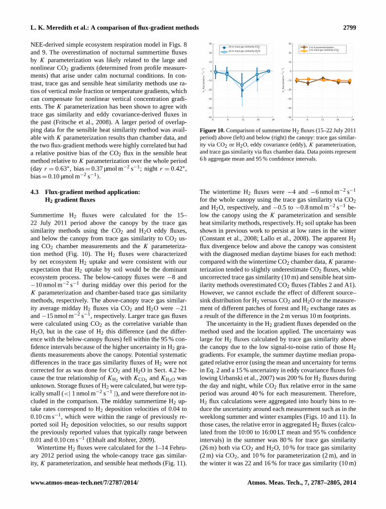
Summertime H2 fluxes were calculated for the 15–22 July 2011 period above the canopy by the trace gassimilarity methods using the CO2 and H2O eddy fluxes,and below the canopy from trace gas similarity to CO2 us-ing CO2 chamber measurements and theK parameteriza-tion method (Fig. 10). The H2 fluxes were characterizedby net ecosystem H2 uptake and were consistent with ourexpectation that H2 uptake by soil would be the dominantecosystem process. The below-canopy fluxes were−8 and−10 nmol m−2 s−1 during midday over this period for theK parameterization and chamber-based trace gas similaritymethods, respectively. The above-canopy trace gas similar-ity average midday H2 fluxes via CO2 and H2O were−21and−15 nmol m−2 s−1, respectively. Larger trace gas fluxeswere calculated using CO2 as the correlative variable thanH2O, but in the case of H2 this difference (and the differ-ence with the below-canopy fluxes) fell within the 95 % con-fidence intervals because of the higher uncertainty in H2 gra-dients measurements above the canopy. Potential systematicdifferences in the trace gas similarity fluxes of H2 were notcorrected for as was done for CO2 and H2O in Sect. 4.2 be-cause the true relationship ofKH2 with KCO2 andKH2O wasunknown. Storage fluxes of H2 were calculated, but were typ-ically small (<| 1 nmol m−2 s−1
|), and were therefore not in-cluded in the comparison. The midday summertime H2 up-take rates correspond to H2 deposition velocities of 0.04 to0.10 cm s−1, which were within the range of previously re-ported soil H2 deposition velocities, so our results supportthe previously reported values that typically range between0.01 and 0.10 cm s−1 (Ehhalt and Rohrer, 2009).
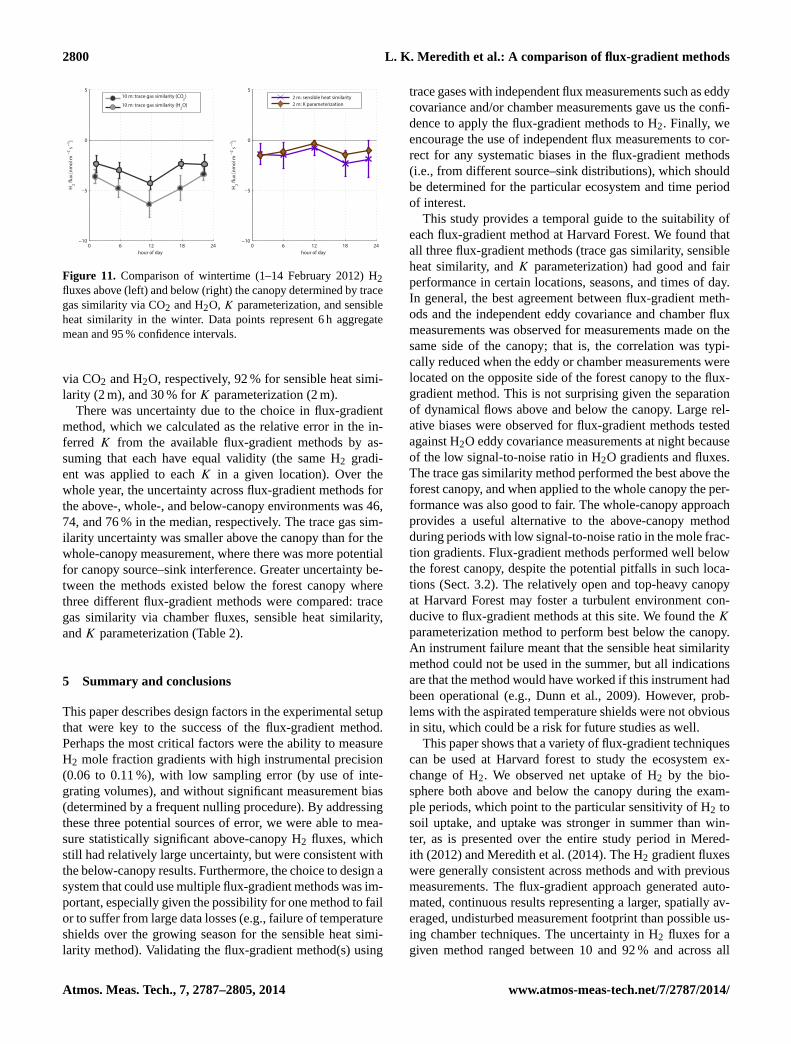
Wintertime H2 fluxes were calculated for the 1–14 Febru-ary 2012 period using the whole-canopy trace gas similar-ity, K parameterization, and sensible heat methods (Fig. 11).
0 6 12 18 24−50
−40
−30
−20
−10
0
10
20
30
H2 �
ux [n
mol
m−2
s−1
]
26 m: trace gas similarity (CO
2)
26 m: trace gas similarity (H2O)
0 6 12 18 24−50
−40
−30
−20
−10
0
10
20
30
H2 �
ux [n
mol
m−2
s−1
]
2 m: K parameterization 2 m: trace gas similarity (CO
2)
Figure 10.Comparison of summertime H2 fluxes (15–22 July 2011period) above (left) and below (right) the canopy: trace gas similar-ity via CO2 or H2O, eddy covariance (eddy),K parameterization,and trace gas similarity via flux chamber data. Data points represent6 h aggregate mean and 95 % confidence intervals.
The wintertime H2 fluxes were−4 and −6 nmol m−2 s−1
for the whole canopy using the trace gas similarity via CO2and H2O, respectively, and−0.5 to−0.8 nmol m−2 s−1 be-low the canopy using theK parameterization and sensibleheat similarity methods, respectively. H2 soil uptake has beenshown in previous work to persist at low rates in the winter(Constant et al., 2008; Lallo et al., 2008). The apparent H2flux divergence below and above the canopy was consistentwith the diagnosed median daytime biases for each method:compared with the wintertime CO2 chamber data,K parame-terization tended to slightly underestimate CO2 fluxes, whileuncorrected trace gas similarity (10 m) and sensible heat sim-ilarity methods overestimated CO2 fluxes (Tables 2 and A1).However, we cannot exclude the effect of different source–sink distribution for H2 versus CO2 and H2O or the measure-ment of different patches of forest and H2 exchange rates asa result of the difference in the 2 m versus 10 m footprints.
The uncertainty in the H2 gradient fluxes depended on themethod used and the location applied. The uncertainty waslarge for H2 fluxes calculated by trace gas similarity abovethe canopy due to the low signal-to-noise ratio of those H2gradients. For example, the summer daytime median propa-gated relative error (using the mean and uncertainty for termsin Eq. 2 and a 15 % uncertainty in eddy covariance fluxes fol-lowing Urbanski et al., 2007) was 200 % for H2 fluxes duringthe day and night, while CO2 flux relative error in the sameperiod was around 40 % for each measurement. Therefore,H2 flux calculations were aggregated into hourly bins to re-duce the uncertainty around each measurement such as in theweeklong summer and winter examples (Figs. 10 and 11). Inthose cases, the relative error in aggregated H2 fluxes (calcu-lated from the 10:00 to 16:00 LT mean and 95 % confidenceintervals) in the summer was 80 % for trace gas similarity(26 m) both via CO2 and H2O, 10 % for trace gas similarity(2 m) via CO2, and 10 % for parameterization (2 m), and inthe winter it was 22 and 16 % for trace gas similarity (10 m)
www.atmos-meas-tech.net/7/2787/2014/ Atmos. Meas. Tech., 7, 2787–2805, 2014
2800 L. K. Meredith et al.: A comparison of flux-gradient methods
0 6 12 18 24−10
−5
0
5
hour of day
H2 �
ux [n
mol
m−2
s−1
]
10 m: trace gas similarity (CO
2)
10 m: trace gas similarity (H2O)
0 6 12 18 24−10
−5
0
5
H2 �
ux [n
mol
m−2
s−1
]
hour of day
2 m: sensible heat similarity 2 m: K parameterization
Figure 11. Comparison of wintertime (1–14 February 2012) H2fluxes above (left) and below (right) the canopy determined by tracegas similarity via CO2 and H2O, K parameterization, and sensibleheat similarity in the winter. Data points represent 6 h aggregatemean and 95 % confidence intervals.
via CO2 and H2O, respectively, 92 % for sensible heat simi-larity (2 m), and 30 % forK parameterization (2 m).
There was uncertainty due to the choice in flux-gradientmethod, which we calculated as the relative error in the in-ferred K from the available flux-gradient methods by as-suming that each have equal validity (the same H2 gradi-ent was applied to eachK in a given location). Over thewhole year, the uncertainty across flux-gradient methods forthe above-, whole-, and below-canopy environments was 46,74, and 76 % in the median, respectively. The trace gas sim-ilarity uncertainty was smaller above the canopy than for thewhole-canopy measurement, where there was more potentialfor canopy source–sink interference. Greater uncertainty be-tween the methods existed below the forest canopy wherethree different flux-gradient methods were compared: tracegas similarity via chamber fluxes, sensible heat similarity,andK parameterization (Table 2).
5 Summary and conclusions
This paper describes design factors in the experimental setupthat were key to the success of the flux-gradient method.Perhaps the most critical factors were the ability to measureH2 mole fraction gradients with high instrumental precision(0.06 to 0.11 %), with low sampling error (by use of inte-grating volumes), and without significant measurement bias(determined by a frequent nulling procedure). By addressingthese three potential sources of error, we were able to mea-sure statistically significant above-canopy H2 fluxes, whichstill had relatively large uncertainty, but were consistent withthe below-canopy results. Furthermore, the choice to design asystem that could use multiple flux-gradient methods was im-portant, especially given the possibility for one method to failor to suffer from large data losses (e.g., failure of temperatureshields over the growing season for the sensible heat simi-larity method). Validating the flux-gradient method(s) using
trace gases with independent flux measurements such as eddycovariance and/or chamber measurements gave us the confi-dence to apply the flux-gradient methods to H2. Finally, weencourage the use of independent flux measurements to cor-rect for any systematic biases in the flux-gradient methods(i.e., from different source–sink distributions), which shouldbe determined for the particular ecosystem and time periodof interest.
This study provides a temporal guide to the suitability ofeach flux-gradient method at Harvard Forest. We found thatall three flux-gradient methods (trace gas similarity, sensibleheat similarity, andK parameterization) had good and fairperformance in certain locations, seasons, and times of day.In general, the best agreement between flux-gradient meth-ods and the independent eddy covariance and chamber fluxmeasurements was observed for measurements made on thesame side of the canopy; that is, the correlation was typi-cally reduced when the eddy or chamber measurements werelocated on the opposite side of the forest canopy to the flux-gradient method. This is not surprising given the separationof dynamical flows above and below the canopy. Large rel-ative biases were observed for flux-gradient methods testedagainst H2O eddy covariance measurements at night becauseof the low signal-to-noise ratio in H2O gradients and fluxes.The trace gas similarity method performed the best above theforest canopy, and when applied to the whole canopy the per-formance was also good to fair. The whole-canopy approachprovides a useful alternative to the above-canopy methodduring periods with low signal-to-noise ratio in the mole frac-tion gradients. Flux-gradient methods performed well belowthe forest canopy, despite the potential pitfalls in such loca-tions (Sect. 3.2). The relatively open and top-heavy canopyat Harvard Forest may foster a turbulent environment con-ducive to flux-gradient methods at this site. We found theK
parameterization method to perform best below the canopy.An instrument failure meant that the sensible heat similaritymethod could not be used in the summer, but all indicationsare that the method would have worked if this instrument hadbeen operational (e.g., Dunn et al., 2009). However, prob-lems with the aspirated temperature shields were not obviousin situ, which could be a risk for future studies as well.
This paper shows that a variety of flux-gradient techniquescan be used at Harvard forest to study the ecosystem ex-change of H2. We observed net uptake of H2 by the bio-sphere both above and below the canopy during the exam-ple periods, which point to the particular sensitivity of H2 tosoil uptake, and uptake was stronger in summer than win-ter, as is presented over the entire study period in Mered-ith (2012) and Meredith et al. (2014). The H2 gradient fluxeswere generally consistent across methods and with previousmeasurements. The flux-gradient approach generated auto-mated, continuous results representing a larger, spatially av-eraged, undisturbed measurement footprint than possible us-ing chamber techniques. The uncertainty in H2 fluxes for agiven method ranged between 10 and 92 % and across all
Atmos. Meas. Tech., 7, 2787–2805, 2014 www.atmos-meas-tech.net/7/2787/2014/

L. K. Meredith et al.: A comparison of flux-gradient methods 2801
available flux-gradient methods at a location ranged between46 and 76 %. Further analyses of H2 gradient fluxes willweigh uncertainty against data availability for each method.These methods can be used to partition the net ecosystemH2 flux between above- and below-canopy contributions toyield additional information regarding the underlying fluxes.
These measurements will help to elucidate specific processrates and reduce uncertainty in the H2 budget. In this study,we demonstrate that flux-gradient methods can inform ourunderstanding of ecosystem processes for H2, and presum-ably, a wide variety of trace gases.
www.atmos-meas-tech.net/7/2787/2014/ Atmos. Meas. Tech., 7, 2787–2805, 2014
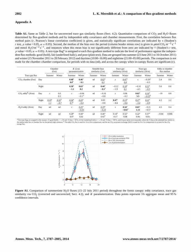
2802 L. K. Meredith et al.: A comparison of flux-gradient methods
Appendix A
Table A1. Same as Table 2, but for uncorrected trace gas similarity fluxes (Sect. 4.2). Quantitative comparison of CO2 and H2O fluxesdetermined by flux-gradient methods and by independent eddy covariance and chamber measurements. First, the correlation between fluxmethod pairs (r, Pearson’s linear correlation coefficient) is given, and statistically significant correlations are indicated by∗ (Student’st test,p value < 0.05,α = 0.05). Second, the median of the bias over the period (column header minus row) is given in µmol CO2 m−2 s−1
and mmol H2O m−2 s−1, and instances when this mean bias is not significantly different from zero are indicated by † (Student’st test,p value > 0.05,α = 0.05). A text-type flaga is assigned to each flux-gradient method to indicate the level of performance against the indepen-dent flux methods: good (bold), fair (underlined italic), and poor (plain text). Data are grouped into summer (23 June 2011 to 16 October 2011)and winter (15 November 2011 to 28 February 2012) and daytime (10:00–16:00) and nighttime (21:00–05:00) periods. The comparison is notmade for the chamber–chamber comparison, for periods with no data (nd), and across the canopy when in-canopy fluxes are significant (c).
Chamber K (2 m) Sensible heat Trace gas Trace gas Eddy or chamber(0 m) parameterization similarity (2 m) similarity (10 m) similarity (26 m) flux median
Trace gas flux Summer Winter Summer Winter Summer Winter Summer Winter Summer Winter Summer Winter
CO2 chamber (0 m) Day 0.48∗ 0.46∗ nd 0.62∗ c 0.47∗ c −0.20∗ 5.4 0.60.0†
−0.1 0.3 0.4 −0.3
Night 0.50∗ 0.63∗ nd 0.44∗ −0.12 0.18∗ −0.10 0.22∗ 5.6 0.6−1.1 0.2 −0.1†
−1.9 0.1 −4.5 −0.5
CO2 eddyb (26 m) Day c 0.0 c −0.04 nd −0.10 c 0.06 0.62∗ 0.16∗ −19 0.80.3 −0.1†
−0.8 −0.2 5.5 −0.23†
Night 0.19∗ 0.32∗ 0.24∗ 0.23∗ nd 0.05 0.47∗ 0.13∗ 0.27∗ 0.21∗ 4.3 1.21.1 −0.7 0.7†
−0.4 −0.8 −1.5 −0.6 −3.4 −0.9
H2O eddy (26 m) Day nd nd c 0.25∗ nd 0.19∗ c 0.34∗ 0.65∗ −0.21 4.5 0.4−0.35 −0.25 −0.02† 1.13 −0.57
Night nd nd 0.28∗ 0.44∗ nd 0.46∗ 0.14∗ 0.32∗ 0.22∗ 0.37∗ −0.04 0.0060.07 0.02 0.02† 0.17 0.08 0.06 0.03
a Text-type flags are assigned in this manner: (1) good (bold)r >= 30 and| % bias| < 50 %, (2) fair (underlined italic)r >= 10 and| % bias| < 100 %, and (3) poor (plain text) remainder, where the % bias is the tabulated bias relative tothe median eddy flux or chamber flux for the period (right columns).b The eddy CO2 flux is used for 10 to 26 m comparisons, and the net CO2 ecosystem exchange (NEE) is used for 0 to 2 m comparisons to account for the CO2storage flux.
0 6 12 18 24
0
2
4
6
8
10
12
H2O
�ux
[mm
ol m
−2 s
−1]
29 m: eddy covariance26 m: trace gas similarity (TGS)26 m: TGS, uncorrected 2 m: K parameterization
Figure A1. Comparison of summertime H2O fluxes (15–22 July 2011 period) throughout the forest canopy: eddy covariance, trace gassimilarity via CO2 (corrected and uncorrected; Sect. 4.2), andK parameterization. Data points represent 3 h aggregate mean and 95 %confidence intervals.
Atmos. Meas. Tech., 7, 2787–2805, 2014 www.atmos-meas-tech.net/7/2787/2014/
L. K. Meredith et al.: A comparison of flux-gradient methods 2803
Acknowledgements.The authors are grateful to Peter Salameh forproviding the GCwerks automated gas chromatograph software andsupport (http://www.gcwerks.com), and to Andrew Crotwell fortraining on use of GC-HePDD systems for H2 measurement. Wewould also like to thank Elaine Gottlieb, Brad Hall, Paul Novelli,and Duane Kitzis for help with standard tank calibrations, andAlfram Bright and Bruce Daube for their contributions to theIRGA system. Furthermore, the authors are grateful for help atHarvard Forest from Emery Boose, Mark VanScoy, Josh McLaren,Leland Werden, Rick Wehr, and Ben Lee. L. K. Meredith wassupported through the following funding sources: NSF GraduateResearch Fellowship, multiple grants from NASA to MIT for theAdvanced Global Atmospheric Gases Experiment (AGAGE), MITCenter for Global Change Science, MIT Joint Program on theScience and Policy of Global Change, MIT Martin Family Societyof Fellows for Sustainability, MIT Ally of Nature Research Fund,MIT William Otis Crosby Lectureship, and MIT Warren KleinFund. Operation of the EMS flux tower was supported by the Officeof Science (BER), US Dept. of Energy (DE-SC0004985), and isa component of the Harvard Forest LTER, supported by NationalScience Foundation.
Edited by: D. Heard
References
Allen, A.: Soil science and survey at Harvard Forest, Soil Surv.Horiz., 36, 133–142, 1995.
Amiro, B. D.: Comparison of turbulence statistics within threeboreal forest canopies, Bound.-Lay. Meteorol., 51, 99–121,doi:10.1007/BF00120463, 1990.
Bain, W. G., Hutyra, L., Patterson, D. C., Bright, A. V.,Daube, B. C., Munger, J. W., and Wofsy, S. C.: Wind-induced error in the measurement of soil respiration usingclosed dynamic chambers, Agr. Forest Meterorol., 131, 225–232,doi:10.1016/j.agrformet.2005.06.004, 2005.
Baldocchi, D. D. and Meyers, T. P.: A spectral and lag-correlationanalysis of turbulence in a deciduous forest canopy, Bound.-Lay.Meteorol., 45, 31–58, doi:10.1007/BF00120814, 1988.
Baldocchi, D. D. and Meyers, T. P.: Trace gas exchange above thefloor of a deciduous forest 1. Evaporation and CO2 efflux, J. Geo-phys. Res., 96, 7271–7285, doi:10.1029/91JD00269, 1991.
Baldocchi, D. D., Hincks, B. B., and Meyers, T. P.: Measuringbiosphere-atmosphere exchanges of biologically related gaseswith micrometeorological methods, Ecology, 69, 1331–1340,doi:10.2307/1941631, 1988.
Baldocchi, D. D., Guenther, A., Harley, P., Klinger, L., Zimmerman,P., Lamb, B., and Westberg, H.: The fluxes and air chemistry ofisoprene above a deciduous hardwood forest, Philos. T. Roy. Soc.A, 351, 279–296, doi:10.1098/rsta.1995.0034, 1995.
Barnes, D. H., Wofsy, S. C., Fehlau, B. P., Gottlieb, E. W., Elkins,J. W., Dutton, G. S., and Novelli, P. C.: Hydrogen in the atmo-sphere: Observations above a forest canopy in a polluted environ-ment, J. Geophys. Res., 108, 1–10, doi:10.1029/2001JD001199,2003.
Black, T. A., Den Hartog, G., Neumann, H. H., Blanken, P.D., Yang, P. C., Russell, C., Nesic, Z., Lee, X., Chen, S.G., Staebler, R., and Novak, M. D.: Annual cycles of watervapour and carbon dioxide fluxes in and above a boreal as-
pen forest, Glob. Change Biol., 2, 219–229, doi:10.1111/j.1365-2486.1996.tb00074.x, 1996.
Bocquet, F., Helmig, D., Van Dam, B. A., and Fairall, C. W.: Evalua-tion of the flux gradient technique for measurement of ozone sur-face fluxes over snowpack at Summit, Greenland, Atmos. Meas.Tech., 4, 2305–2321, doi:10.5194/amt-4-2305-2011, 2011.
Bowling, D. R., Turnipseed, A. A., Delany, A. C., Baldocchi, D. D.,Greenberg, J. P., and Monson, R. K.: The use of relaxed eddyaccumulation to measure biosphere-atmosphere exchange of iso-prene and other biological trace gases, Oecologia, 116, 306–315,doi:10.1007/s004420050592, 1998.
Bowling, D. R., Sargent, S. D., Tanner, B. D., and Ehleringer, J.R.: Tunable diode laser absorption spectroscopy for stable iso-tope studies of ecosystem-atmosphere CO2 exchange, Agr. For-est Meterorol., 118, 1–19, doi:10.1016/S0168-1923(03)00074-1,2003.
Businger, J. A.: Evaluation of the accuracy with which drydeposition can be measured with current micrometeorolog-ical techniques, J. Clim. Appl. Meterorol., 25, 1100–1124,doi:10.1175/1520-0450(1986)025<1100:EOTAWW>2.0.CO;2,1986.
Businger, J. A. and Oncley, S. P.: Flux measurement withconditional sampling, J. Atmos. Ocean. Tech., 7, 349-352,doi:10.1175/1520-0426(1990)007<0349:FMWCS>2.0.CO;2,1990.
Cellier, P. and Brunet, Y.: Flux-gradient relationships abovetall plant canopies, Agr. Forest Meterorol., 58, 93–117,doi:10.1016/0168-1923(92)90113-I, 1992.
Conrad, R. and Seiler, W: Contribution of hydrogen production bybiological nitrogen fixation to the global hydrogen budget. J.Geophys. Res., 85, 5493–5498, doi:10.1029/JC085iC10p05493,1980.
Constant, P., Poissant, L., and Villemur, R.: Annual hydrogen, car-bon monoxide and carbon dioxide concentrations and surface toair exchanges in a rural area (Québec, Canada), Atmos. Environ.,42, 5090–5100, doi:10.1016/j.atmosenv.2008.02.021, 2008.
Davidson, E. A., Savage, K., Verchot, L. V., and Navarro, R.:Minimizing artifacts and biases in chamber-based measure-ments of soil respiration, Agr. Forest Meterorol., 113, 21–37,doi:10.1016/S0168-1923(02)00100-4, 2002.
de Arellano, J. V.-G. and Duynkerke, G. P.: Influence of chemistryon the flux-gradient relationships for the NO-O3-NO2 system,Bound.-Lay. Meteorol., 61, 375–387, doi:10.1007/BF00119098,1992.
Dunn, A. L., Wofsy, S. C., and Bright, A. v. H.: Landscape het-erogeneity, soil climate, and carbon exchange in a boreal blackspruce forest, Ecol. App., 19, 495–504, doi:10.1890/07-0771.1,2009.
Ehhalt, D. H. and Rohrer, F.: The tropospheric cycle of H2:a critical review, Tellus B, 61, 500–535, doi:10.1111/j.1600-0889.2009.00416.x, 2009.
Fitzjarrald, D. R. and Lenschow, J. H.: Mean concentration and fluxprofiles for chemically reactive species in the atmospheric sur-face layer, Atmos. Environ., 17, 2505–2512, doi:10.1016/0004-6981(83)90076-8, 1983.
Foken, T.: 50 Years of the Monin-Obukhov similarity theory,Bound.-Layer Meteorol., 119, 431–447, doi:10.1007/s10546-006-9048-6, 2006.
www.atmos-meas-tech.net/7/2787/2014/ Atmos. Meas. Tech., 7, 2787–2805, 2014
2804 L. K. Meredith et al.: A comparison of flux-gradient methods
Fritsche, J., Obrist, D., Zeeman, M., Conen, F., Eugster, W., andAlewell, C.: Elemental mercury fluxes over a sub-alpine grass-land determined with two micrometeorological methods, Atmos.Environ., 42, 2922–2933, doi:10.1016/j.atmosenv.2007.12.055,2008.
Fuentes, J. D., Wang, D., Neumann, H. H., Gillespie, T. J., DenHartog, G., and Dann, T. F.: Ambient biogenic hydrocarbonsand isoprene emissions from a mixed deciduous forest, J. Atmos.Chem., 25, 67–95, doi:10.1007/BF00053286, 1996.
Gao, W., Wesely, M. L., and Lee, I. Y.: A numerical study of theeffects of air chemistry on fluxes of NO, NO2, and O3 near thesurface, J. Geophys. Res., 96, 761–769, doi:10.1029/91JD02106,1991.
Garratt, J. R.: Flux profile relations above tall vegetation, Q. J. Roy.Meteorol. Soc., 104, 199–211, doi:10.1002/qj.49710443915,1978.
Garratt, J. R. and Hicks, B. B.: Momentum, heat and water vapourtransfer to and from natural and artificial surfaces, Q. J. Roy. Me-teorol. Soc., 99, 680–687, doi:10.1002/qj.49709942209, 1973.
Goldstein, A. H., Daube, B. C., Munger, J. W., and Wofsy, S. C.:Automated in-situ monitoring of atmospheric non-methane hy-drocarbon concentrations and gradients, J. Atmos. Chem., 21,43–59, doi:10.1007/BF00712437, 1995.
Goldstein, A. H., Fan, S. M., Goulden, M. L., Munger, J. W.,and Wofsy, S. C.: Emissions of ethene, propene, and 1-buteneby a midlatitude forest, J. Geophys. Res., 101, 9149–9157,doi:10.1029/96JD00334, 1996.
Goldstein, A. H., Goulden, M. L., Munger, J. W., Wofsy, S. C., andGeron, C. D.: Seasonal course of isoprene emissions from a mid-latitude deciduous forest, J. Geophys. Res., 103, 31045–31056,doi:10.1029/98JD02708, 1998.
Goulden, M. L., Munger, J. W., Fan, S.-M., Daube, B. C., andWofsy, S. C.: Measurements of carbon sequestration by long-term eddy covariance: methods and a critical evaluation of ac-curacy, Glob. Change Biol., 2, 169–182, doi:10.1111/j.1365-2486.1996.tb00070.x, 1996.
Griffith, D. W. T., Leuning, R., Denmead, O. T., and Jamie, I.M.: Air-land exchanges of CO2, CH4 and N2O measured byFTIR spectrometry and micrometeorological techniques, Atmos.Environ., 36, 1833–1842, doi:10.1016/S1352-2310(02)00139-5,2002.
Guenther, A., Baugh, W., Davis, K., Hampton, G., Harley, P.,Klinger, L., Vierling, L., Zimmerman, P., Allwine, E., Dilts, S.,Lamb, B., Westberg, H., Baldocchi, D., Geron, C., and Pierce, T.:Isoprene fluxes measured by enclosure, relaxed eddy accumu-lation, surface layer gradient, mixed layer gradient, and mixedlayer mass balance techniques, J. Geophys. Res., 101, 18555–18567, doi:10.1029/96JD00697, 1996.
Högström, U., Bergström, H., Smedman, A.-S., Halldin, S. andLindroth, A.: Turbulent exchange fluxes above a pine forest,I: fluxes and gradients, Bound.-Lay. Meteorol., 49, 197–217,doi:10.1007/BF00116411, 1989.
Jordan, A. and Steinberg, B.: Calibration of atmospheric hy-drogen measurements, Atmos. Meas. Tech., 4, 509–521,doi:10.5194/amt-4-509-2011, 2011.
Lallo, M., Aalto, T., Laurila, T., and Hatakka, J.: Seasonal variationsin hydrogen deposition to boreal forest soil in southern Finland,Geophys. Res. Lett., 35, 1–4, doi:10.1029/2007GL032357, 2008.
Lavigne, M. B., Ryan, M. G., Anderson, D. E., Baldocchi, D.D., Crill, P. M., Fitzjarrald, D. R., Goulden, M. L., Gower,S. T., Massheder, J. M., Rayment, M., and Striegp, R. G.:Comparing nocturnal eddy covariance measurements to esti-mates of ecosystem respiration made by scaling chamber mea-surements at six coniferous boreal sites, 102, 28977–28985,doi:10.1029/97JD01173, 1997.
Lindberg, S. E. and Meyers, T. P.: Development of an automatedmicrometeorological method for measuring the emission of mer-cury vapor from wetland vegetation, Wetl. Ecol. Manag., 9, 333–347, doi:10.1023/A:1011804516643, 2001.
Liu, H. and Foken, T.: A modified Bowen ratio method to deter-mine sensible and latent heat fluxes, Meteorol. Z., 10, 71–80,doi:10.1127/0941-2948/2001/0010-0071, 2001.
Meredith, L. K.: Field measurement of the fate of atmosphericH2 in a forest environment: from canopy to soil, Doctor ofphilosophy thesis, Massachusetts Institute of Technology, MITCenter for Global Change Science, 250 pp., available at:http://globalchange.mit.edu/research/publications/2366, 2012.
Meredith, L. K., Commane, R., Keenan, T., Munger, J. W., Wofsy,S. C., and Prinn, R. G.: Ecosystem fluxes of hydrogen: a year ofmeasurements at Harvard Forest, MA, in preparation, 2014.
Meyers, T. P., Hall, M. E., Lindberg, S. E., and Kim, K.: Useof the modified Bowen-ratio technique to measure fluxes oftrace gases, Atmos, Environ., 30, 3321–3329, doi:10.1016/1352-2310(96)00082-9, 1996.
Monin, A. S. and Obukhov, A. M.: Basic laws of turbulent mixingin the surface layer of the atmosphere, Tr. Akad. Nauk SSSRGeophiz. Inst., 24, 163–187, 1954.
Moore, K. E., Fitzjarrald, D. R., Sakai, R. K., Goulden, M. L.,Munger, J. W., and Wofsy, S. C.: Seasonal variation in radia-tive and turbulent exchange at a deciduous forest in central Mas-sachusetts, J. Appl. Meteorol., 35, 122–134, doi:10.1175/1520-0450(1996)035<0122:SVIRAT>2.0.CO;2, 1996.
Moore, F. L., Elkins, J. W., Ray, E. A., Dutton, G. S., Dunn,R. E., Fahey, D. W., McLaughlin, R. J., Thompson, T. L.,Romashkin, P. A., Hurst, D. F., and Wamsley, P. R.: Bal-loonborne in situ gas chromatograph for measurements in thetroposphere and stratosphere, J. Geophys. Res., 108, 1–20,doi:10.1029/2001JD000891, 2003.
Müller, H., Kramm, G., Meixner, F., Dollard, G., Fowler, D., andPossanzini, M.: Determination of HNO3 dry deposition by mod-ified Bowen ratio and aerodynamic profile techniques, Tellus B,45, 346–367, doi:10.1034/j.1600-0889.45.issue4.1.x, 1993.
Novelli, P. C., Lang, P. M., Masarie, K. A., Hurst, D. F., Myers,R., and Elkins, J. W.: Molecular hydrogen in the troposphere:Global distribution and budget, J. Geophys. Res., 104, 30427–30444, doi:10.1029/1999JD900788, 1999.
Novelli, P. C., Crotwell, A. M., and Hall, B. D.: Application of gaschromatography with a pulsed discharge helium ionization detec-tor for measurements of molecular hydrogen in the atmosphere,Environ. Sci. Technol., 43, 2431–2436, doi:10.1021/es803180g,2009.
Phillips, S. C., Varner, R. K., Frolking, S., Munger, J. W., Bubier,J. L., Wofsy, S. C., and Crill, P. M.: Interannual, seasonal, anddiel variation in soil respiration relative to ecosystem respirationat a wetland to upland slope at Harvard Forest, J. Geophys. Res.,115, 1–18, doi:10.1029/2008JG000858, 2010.
Atmos. Meas. Tech., 7, 2787–2805, 2014 www.atmos-meas-tech.net/7/2787/2014/
L. K. Meredith et al.: A comparison of flux-gradient methods 2805
Rahn, T., Eiler, J. M., Kitchen, N., Fessenden, J. E., and Rander-son, J. T.: Concentration andδD of molecular hydrogen in borealforests: Ecosystem-scale systematics of atmospheric H2, Geo-phys. Res. Lett., 29, 1–4, doi:10.1029/2002GL015118, 2002.
Raupach, M. R. and Thom, A. S.: Turbulence in and aboveplant canopies, Ann. Rev. Fluid Mech., 13, 97–129,doi:10.1146/annurev.fl.13.010181.000525, 1981.
Sakai, R., Fitzjarrald, D., and Moore, K.: Importance of low-frequency contributions to eddy fluxes observed over rough sur-faces, J. Appl. Meteorol., 40, 2178–2192, doi:10.1175/1520-0450(2001)040<2178:IOLFCT>2.0.CO;2, 2001.
Shaw, R. H.: Secondary wind speed maxima inside plantcanopies, J. Appl. Meteorol., 16, 514–521, doi:10.1175/1520-0450(1977)016<0514:SWSMIP>2.0.CO;2, 1977.
Simmonds, P. G., Derwent, R. G., O’Doherty, S., Ryall, D. B.,Steele, L. P., Langenfelds, R. L., Salameh, P., Wang, H. J., Dim-mer, C. H., and Hudson, L. E.: Continuous high-frequency ob-servations of hydrogen at the Mace Head baseline atmosphericmonitoring station over the 1994–1998 period, J. Geophys. Res.,105, 12105–12121, doi:10.1029/2000JD900007, 2000.
Simpson, I. J., Edwards, G. C., Thurtell, G. W., den Hartog, G.,Neumann, H. H., and Staebler, R. M.: Micrometeorologicalmeasurements of methane and nitrous oxide exchange abovea boreal aspen forest, J. Geophys. Res., 102, 29331–29341,doi:10.1029/97JD03181, 1997.
Simpson, I. J., Thurtell, G. W., Neumann, H. H., den Hartog, G., andEdwards, G. C.: The validity of similarity theory in the rough-ness sublayer above forests, Bound.-Lay. Meteorol., 87, 69–99,doi:10.1023/A:1000809902980, 1998.
Sinclair, T. R. and Lemon, E. R.: An analysis of errors in thecalculation of energy flux densities above vegetation by aBowen-ratio profile method, Bound.-Lay. Meteorol., 8, 129–139,doi:10.1007/BF00241333, 1975.
Smith-Downey, N. V., Randerson, J. T., and Eiler, J. M.:Molecular hydrogen uptake by soils in forest, desert, andmarsh ecosystems in California, J. Geophys. Res., 113, 1–11,doi:10.1029/2008JG000701, 2008.
Solomon, S.: Stratospheric ozone depletion: A reviewof concepts and history, Rev. Geophys., 37, 275–316,doi:10.1029/1999RG900008, 1999.
Steinbacher, M., Fischer, A., Vollmer, M. K., Buchmann, B.,Reimann, S., and Hueglin, C.: Perennial observations of molecu-lar hydrogen (H2) at a suburban site in Switzerland, Atmos. Envi-ron., 41, 2111–2124, doi:10.1016/j.atmosenv.2006.10.075, 2007.
Taylor, N. M., Wagner-Riddle, C., Thurtell, G. W., and Beauchamp,E. G.: Nitric oxide fluxes from an agricultural soil using aflux-gradient method, J. Geophys. Res., 104, 12213–12220,doi:10.1029/1999JD900181, 1999.
Tromp, T. K., Shia, R.-L., Allen, M., Eiler, J. M., andYung, Y. L.: Potential environmental impact of a hydro-gen economy on the stratosphere, Science, 300, 1740–1742,doi:10.1126/science.1085169, 2003.
Urbanski, S., Barford, C., Wofsy, S., Kucharik, C., Pyle, E., Bud-ney, J., McKain, K., Fitzjarrald, D., Czikowsky, M., and Munger,J. W.: Factors controlling CO2 exchange on timescales fromhourly to decadal at Harvard Forest, J. Geophys. Res., 112, 1–25, doi:10.1029/2006JG000293, 2007.
Wagner-Riddle, C., Thurtell, G. W., King, K. M., Kidd,G. E., and Beauchamp, E. G.: Nitrous oxide and car-bon dioxide fluxes from a bare soil using a microm-eteorological approach, J. Environ. Qual., 25, 898–907,doi:10.2134/jeq1996.00472425002500040035x, 1996.
Warwick, N. J., Bekki, S., Nisbet, E. G., and Pyle, J. A.: Im-pact of a hydrogen economy on the stratosphere and tropo-sphere studied in a 2-D model, Geophys. Res. Lett., 31, 1–4,doi:10.1029/2003GL019224, 2004.
Wehr, R., Munger, J. W., Nelson, D. D., McManus, J. B.,Zahniser, M. S., Wofsy, S. C., and Saleska, S. R.: Long-term eddy covariance measurements of the isotopic com-position of the ecosystem-atmosphere exchange of CO2 ina temperate forest, Agr. Forest Meterorol., 181, 69–84,doi:10.1016/j.agrformet.2013.07.002, 2013.
Wesely, M. L., Lenschow, D. H., and Denmead, O. T.: Fluxmeasurement techniques, in: Global Tropospheric Chemistry-Chemical Fluxes in the Global Atmosphere, edited by:Lenschow, D. H. and Hicks, B. B., National Center for Atmo-spheric Research, Boulder, CO, 31–46, 1989.
Wilczak, J. M., Oncley, S. P., and Stage, S. A.: Sonic anemometertilt correction algorithms, Bound.-Lay. Meteorol., 99, 127–150,doi:10.1023/A:1018966204465, 2001.
Wofsy, S. C., Goulden, M. L., Munger, J. W., Fan, S. M., Bakwin,P. S., Daube, B. C., Bassow, S. L., and Bazzaz, F. A.: Net ex-change of CO2 in a mid-latitude forest, Science, 260, 1314–1317,doi:10.1126/science.260.5112.1314, 1993.
Woodruff, B. L.: Sampling error in a single-instrument vertical gra-dient measurement in the atmospheric surface layer, 91 pp., Col-orado State University, 1986.
Xiao, X., Prinn, R. G., Simmonds, P. G., Steele, L. P., Novelli, P. C.,Huang, J., Langenfelds, R. L., O’Doherty, S., Krummel, P. B.,Fraser, P. J., Porter, L. W., Weiss, R. F., Salameh, P., and Wang,R. H. J.: Optimal estimation of the soil uptake rate of molecularhydrogen from AGAGE and other measurements, J. Geophys.Res., 112, 1–15, doi:10.1029/2006JD007241, 2007.
Yi, C., Anderson, D. E., Turnipseed, A. A., Burns, S. P., Sparks,J. P., Stannard, D. I., and Monson, R. K.: The contribution ofadvective fluxes to net ecosystem exchange in a high-elevation,subalpine forest, Ecol. Appl., 18, 1379–1390, doi:10.1890/06-0908.1, 2008.
www.atmos-meas-tech.net/7/2787/2014/ Atmos. Meas. Tech., 7, 2787–2805, 2014