Physical controls on carbon dioxide transfer velocity and flux in low-gradient river systems and...
17
Physical controls on carbon dioxide transfer velocity and flux in low‐gradient river systems and implications for regional carbon budgets Simone R. Alin, 1,2 Maria de Fátima F. L. Rasera, 3 Cleber I. Salimon, 4 Jeffrey E. Richey, 1 Gordon W. Holtgrieve, 5 Alex V. Krusche, 3 and Anond Snidvongs 6 Received 20 April 2010; revised 30 September 2010; accepted 13 October 2010; published 27 January 2011. [1] Outgassing of carbon dioxide (CO 2 ) from rivers and streams to the atmosphere is a major loss term in the coupled terrestrial‐aquatic carbon cycle of major low‐gradient river systems (the term “river system” encompasses the rivers and streams of all sizes that compose the drainage network in a river basin). However, the magnitude and controls on this important carbon flux are not well quantified. We measured carbon dioxide flux rates (F CO2 ), gas transfer velocity (k), and partial pressures (pCO 2 ) in rivers and streams of the Amazon and Mekong river systems in South America and Southeast Asia, respectively. F CO2 and k values were significantly higher in small rivers and streams (channels <100 m wide) than in large rivers (channels >100 m wide). Small rivers and streams also had substantially higher variability in k values than large rivers. Observed F CO2 and k values suggest that previous estimates of basinwide CO 2 evasion from tropical rivers and wetlands have been conservative and are likely to be revised upward substantially in the future. Data from the present study combined with data compiled from the literature collectively suggest that the physical control of gas exchange velocities and fluxes in low‐ gradient river systems makes a transition from the dominance of wind control at the largest spatial scales (in estuaries and river mainstems) toward increasing importance of water current velocity and depth at progressively smaller channel dimensions upstream. These results highlight the importance of incorporating scale‐appropriate k values into basinwide models of whole ecosystem carbon balance. Citation: Alin, S. R., M. F. F. L. Rasera, C. I. Salimon, J. E. Richey, G. W. Holtgrieve, A. V. Krusche, and A. Snidvongs (2011), Physical controls on carbon dioxide transfer velocity and flux in low‐gradient river systems and implications for regional carbon budgets, J. Geophys. Res., 116, G01009, doi:10.1029/2010JG001398. 1. Introduction [2] Quantifying the exchange of biogeochemically active gases such as carbon dioxide (CO 2 ) and oxygen (O 2 ) between atmospheric and aquatic reservoirs plays a critical role in at least three types of studies: (1) the formulation of regional to global carbon budgets, (2) understanding processes related to water quality and pollution, and (3) rate studies of metabolic/ ecological processes (i.e., production and respiration). Typi- cally, carbon budget studies involving air‐water gas exchange have been carried out in large‐scale ecosystems (large rivers, large lakes, and global ocean) [e.g., Richey et al., 2002; Alin and Johnson, 2007; Takahashi et al., 2009], whereas studies addressing water quality or metabolic rates have been done in small lake or stream‐scale systems [e.g., Melching and Flores, 1999; Hall and Tank, 2003; Hanson et al., 2006]. As a consequence of the different sizes of the study ecosystems as well as the differing goals of studies across these fields, the literature on gas exchange can be difficult to reconcile across the boundaries of different types of ecosys- tems (e.g., streams vs. rivers). In this paper, we focus on the role of air‐water CO 2 exchange in the rivers and streams of major low‐gradient river systems in regional to global carbon budgets, with the ultimate goal of improving our ability to scale up small‐scale observations to meaningful basin‐scale flux estimates. To do so, it is critical to be able to glean in- sights from the frequently disjunct historical bodies of liter- ature on stream and river‐estuary gas exchange. [3] The flux of CO 2 across the air‐water interface (F CO2 , mol m −2 s −1 ) is described by the following equation: F CO2 ¼ kC w C 0 ð Þ; ð1Þ 1 School of Oceanography, University of Washington, Seattle, Washington, USA. 2 Now at Pacific Marine Environmental Laboratory, National Oceanic and Atmospheric Administration, Seattle, Washington, USA. 3 Centro de Energia Nuclear na Agricultura, Universidade de São Paulo, Piracicaba, Brazil. 4 Universidade Federal do Acre, Rio Branco, Brazil. 5 School of Aquatic and Fishery Sciences, University of Washington, Seattle, Washington, USA. 6 Southeast Asia START Global Change Regional Center, Chulalongkorn University, Bangkok, Thailand. Copyright 2011 by the American Geophysical Union. 0148‐0227/11/2010JG001398 JOURNAL OF GEOPHYSICAL RESEARCH, VOL. 116, G01009, doi:10.1029/2010JG001398, 2011 G01009 1 of 17
-
Upload
independent -
Category
Documents
-
view
0 -
download
0
Transcript of Physical controls on carbon dioxide transfer velocity and flux in low-gradient river systems and...
Physical controls on carbon dioxide transfer velocity and fluxin low‐gradient river systems and implications for regionalcarbon budgets
Simone R. Alin,1,2 Maria de Fátima F. L. Rasera,3 Cleber I. Salimon,4 Jeffrey E. Richey,1
Gordon W. Holtgrieve,5 Alex V. Krusche,3 and Anond Snidvongs6
Received 20 April 2010; revised 30 September 2010; accepted 13 October 2010; published 27 January 2011.
[1] Outgassing of carbon dioxide (CO2) from rivers and streams to the atmosphere is amajor loss term in the coupled terrestrial‐aquatic carbon cycle of major low‐gradient riversystems (the term “river system” encompasses the rivers and streams of all sizes thatcompose the drainage network in a river basin). However, the magnitude and controls onthis important carbon flux are not well quantified. We measured carbon dioxide flux rates(FCO2), gas transfer velocity (k), and partial pressures (pCO2) in rivers and streams of theAmazon and Mekong river systems in South America and Southeast Asia, respectively.FCO2 and k values were significantly higher in small rivers and streams (channels <100 mwide) than in large rivers (channels >100 m wide). Small rivers and streams also hadsubstantially higher variability in k values than large rivers. Observed FCO2 and k valuessuggest that previous estimates of basinwide CO2 evasion from tropical rivers andwetlands have been conservative and are likely to be revised upward substantially in thefuture. Data from the present study combined with data compiled from the literaturecollectively suggest that the physical control of gas exchange velocities and fluxes in low‐gradient river systems makes a transition from the dominance of wind control at the largestspatial scales (in estuaries and river mainstems) toward increasing importance of watercurrent velocity and depth at progressively smaller channel dimensions upstream. Theseresults highlight the importance of incorporating scale‐appropriate k values into basinwidemodels of whole ecosystem carbon balance.
Citation: Alin, S. R., M. F. F. L. Rasera, C. I. Salimon, J. E. Richey, G. W. Holtgrieve, A. V. Krusche, and A. Snidvongs(2011), Physical controls on carbon dioxide transfer velocity and flux in low‐gradient river systems and implications for regionalcarbon budgets, J. Geophys. Res., 116, G01009, doi:10.1029/2010JG001398.
1. Introduction
[2] Quantifying the exchange of biogeochemically activegases such as carbon dioxide (CO2) and oxygen (O2) betweenatmospheric and aquatic reservoirs plays a critical role in atleast three types of studies: (1) the formulation of regional toglobal carbon budgets, (2) understanding processes related towater quality and pollution, and (3) rate studies of metabolic/ecological processes (i.e., production and respiration). Typi-cally, carbon budget studies involving air‐water gas
exchange have been carried out in large‐scale ecosystems(large rivers, large lakes, and global ocean) [e.g.,Richey et al.,2002; Alin and Johnson, 2007; Takahashi et al., 2009],whereas studies addressing water quality or metabolic rateshave been done in small lake or stream‐scale systems [e.g.,Melching and Flores, 1999; Hall and Tank, 2003; Hanson etal., 2006]. As a consequence of the different sizes of the studyecosystems as well as the differing goals of studies acrossthese fields, the literature on gas exchange can be difficult toreconcile across the boundaries of different types of ecosys-tems (e.g., streams vs. rivers). In this paper, we focus on therole of air‐water CO2 exchange in the rivers and streams ofmajor low‐gradient river systems in regional to global carbonbudgets, with the ultimate goal of improving our ability toscale up small‐scale observations to meaningful basin‐scaleflux estimates. To do so, it is critical to be able to glean in-sights from the frequently disjunct historical bodies of liter-ature on stream and river‐estuary gas exchange.[3] The flux of CO2 across the air‐water interface (FCO2,
mol m−2 s−1) is described by the following equation:
FCO2 ¼ k Cw � C0ð Þ; ð1Þ
1School of Oceanography, University of Washington, Seattle,Washington, USA.
2Now at Pacific Marine Environmental Laboratory, National Oceanicand Atmospheric Administration, Seattle, Washington, USA.
3Centro de Energia Nuclear na Agricultura, Universidade de São Paulo,Piracicaba, Brazil.
4Universidade Federal do Acre, Rio Branco, Brazil.5School of Aquatic and Fishery Sciences, University of Washington,
Seattle, Washington, USA.6Southeast Asia START Global Change Regional Center,
Chulalongkorn University, Bangkok, Thailand.
Copyright 2011 by the American Geophysical Union.0148‐0227/11/2010JG001398
JOURNAL OF GEOPHYSICAL RESEARCH, VOL. 116, G01009, doi:10.1029/2010JG001398, 2011
G01009 1 of 17

where k is the gas transfer velocity at the in situ temperature(m s−1 or cm h−1), Cw is the CO2 gas concentration in thewell‐mixed bulk fluid underlying the surface skin (molm−3), and C0 is the CO2 gas concentration at the watersurface in exchange with the atmosphere [Wanninkhof et al.,2009]. Cw and C0 are typically calculated from the CO2
solubility, K0 (mol m−3 atm−1), and the partial pressure ofCO2 (pCO2, matm or 10−6 atm) in the water (pCO2w) and air(pCO2a), respectively (i.e., Cw,0 = K0 × pCO2w,a). Positivevalues of FCO2 represent fluxes from the water to air, andnegative FCO2 values indicate CO2 invasion from air towater. Measuring pCO2 in air and water samples isstraightforward [Hesslein et al., 1991], and solubility can becalculated on the basis of temperature [Weiss, 1974].However, k is difficult to measure accurately.[4] The magnitude of k is controlled by microscale tur-
bulence on the water side of the air‐water interface [Jähneand Haubecker, 1998]. Gas exchange fluxes and k mayvary widely across environment types as the physicalfactors controlling them change [cf. Kremer et al., 2003a].Temperature‐normalized gas transfer velocity values (k600)are used in parameterizations relating gas exchange to envi-ronmental drivers such as wind speed, where k600 representsthe freshwater gas transfer velocity at a temperature of 20°C.In lakes and the open ocean, the dominant controls onsurface turbulence, and thus gas transfer, are wind speed andpenetrative convection [e.g., Wanninkhof, 1992; Cole andCaraco, 1998; MacIntyre et al., 2002]. In stream environ-ments, k600 has classically been modeled as a function ofstream depth, water current velocity, discharge, and slope[e.g., O’Connor and Dobbins, 1958; Owens et al., 1964;Wilcock, 1984; Melching and Flores, 1999]. Studies of gasexchange in estuarine systems indicate that wind speed,water current velocity, and water depth all contribute to therate of air‐water gas transfer [Borges et al., 2004a, 2004b].Fetch is also important and decreases steeply along a gra-dient from the open ocean to river headwaters. In large riversystems, we expect that a transition occurs in the dominantphysical controls on gas exchange as one traverses a land-scape from shallow stream channels sheltered from the windby forest canopies to deep, wide channels where wind im-pinges on the water surface.[5] The turbulence controlling k600 in river systems
should thus be induced by a dynamic and channel size‐dependent combination of water currents, depth (a proxy forthe effects of channel bed friction), and wind (speed andfetch). A large literature exists on gas exchange and re-aeration at the stream scale [e.g., Owens et al., 1964;Wanninkhof et al., 1990; Genereux and Hemond, 1992;Melching and Flores, 1999; Hall and Tank, 2003], andseveral articles have also been published on gas exchange inlarge rivers [e.g., Elsinger and Moore, 1983; Devol et al.,1987; Clark et al., 1994; Ho et al., 2002]. However, gen-erally the methods for collecting and analyzing data as wellas conventions for data reporting are sufficiently divergentbetween the stream and river gas flux literatures that it isdifficult to attribute observed differences in fluxes andtransfer velocities across the size spectrum of lotic systemsto natural processes when methodological and analyticalartifacts may also influence the results. Further, estuarineecosystems vary in the magnitude of their observed k600values, depending on exposure to wind (i.e., fetch) and the
strength of tidal currents [Kremer et al., 2003a; Borges etal., 2004a], highlighting the importance of taking mea-surements in a wide range of environments before at-tempting to delineate a generalized relationship betweenk600 and physical factors, such as wind speed, water depth,and current velocity. Thus, quantifying CO2 fluxes across anentire river system requires a large number of spatiallydistributed measurements to parameterize the physicalcontrols on k600.[6] This study sought to measure air‐water CO2 exchange
fluxes and k600 values in low‐gradient river systems in aconsistent and logistically tractable manner from the widestriver channels to the smallest streams. An important appli-cation of this work will be to facilitate the accurate upscalingof CO2 evasion across major river systems from headwaterstreams to estuaries. For example, estimates suggest thatlowland tropical rivers outgas 10‐fold more carbon as CO2
than is lost to the global oceans as organic matter throughriver export [Richey et al., 2002]. This global estimate isbased on work in the Amazon River basin, where the esti-mated 0.5 Gt C a−1 lost as CO2 to the atmosphere fromAmazonian rivers and wetlands is based on k600 and pCO2
measurements collected only in large‐river milieus withinthe Amazon mainstem corridor, which accounts for less thanone third of the total area of the basin [Richey et al., 2002].To generate more accurate basinwide carbon budgets orestimates of the contribution of rivers to the global carboncycle, it is essential to better understand what transitions thekey physical controls on gas exchange undergo along a sizespectrum from first‐order streams to the mainstem channelsof the largest rivers in the world. To this end, we measuredcarbon dioxide flux and transfer velocity in rivers andstreams across a wide range of channel widths, from a fewmeters to kilometers, to determine the magnitude of differ-ences in gas exchange fluxes and transfer velocities acrossthis channel‐size spectrum and to understand what thecorresponding physical controls are. To the extent possible,we use the reporting conventions of the gas exchange lit-erature rather than the reaeration literature because theyfacilitate more straightforward intercomparability acrossenvironment types on the stream‐to‐ocean continuum.
2. Study Areas
[7] All field measurements for this study were conductedin the Amazon and Mekong river systems. The AmazonRiver originates in the Andes Mountains and drains nearly7 million km2 of South America (Figure 1a). The AmazonRiver accounts for 20% of global freshwater discharge tothe ocean and delivers an average of 3 Mt d−1 of sedimentto the ocean [Dunne et al., 1998]. The variety of chemicalconditions existing among aquatic environments in theAmazon is impressive, with measured pH values rangingfrom 3.1 to 8.9; pCO2 values that are usually supersaturatedand range from below atmospheric equilibrium to >50‐foldhigher (∼140 to >20,000 matm); and wide ranges in dissolvedorganic carbon concentration (<1–35 mg L−1) and suspendedsediment loads (<1–1960 mg L−1) (A. V. Krusche and others,unpublished data, 2010).[8] The Mekong River drains ∼800,000 km2 of Southeast
Asia, originating in the Himalayas and running throughChina, Tibet, Burma, Laos, Thailand, and Cambodia before
ALIN ET AL.: CO2 EXCHANGE IN RIVER SYSTEMS G01009G01009
2 of 17
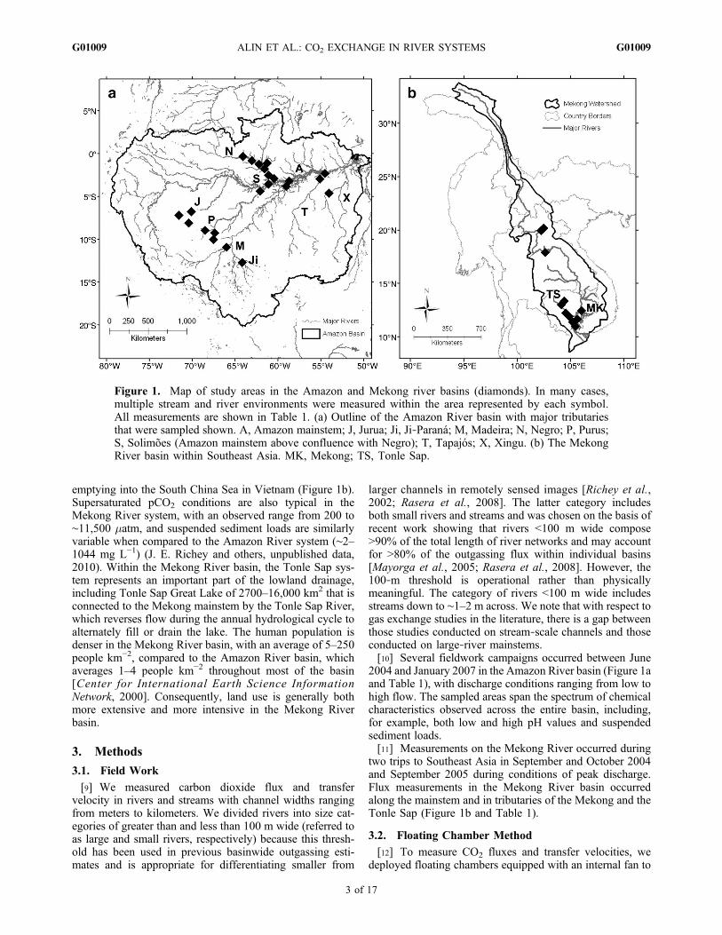
emptying into the South China Sea in Vietnam (Figure 1b).Supersaturated pCO2 conditions are also typical in theMekong River system, with an observed range from 200 to∼11,500 matm, and suspended sediment loads are similarlyvariable when compared to the Amazon River system (∼2–1044 mg L−1) (J. E. Richey and others, unpublished data,2010). Within the Mekong River basin, the Tonle Sap sys-tem represents an important part of the lowland drainage,including Tonle Sap Great Lake of 2700–16,000 km2 that isconnected to the Mekong mainstem by the Tonle Sap River,which reverses flow during the annual hydrological cycle toalternately fill or drain the lake. The human population isdenser in the Mekong River basin, with an average of 5–250people km−2, compared to the Amazon River basin, whichaverages 1–4 people km−2 throughout most of the basin[Center for International Earth Science InformationNetwork, 2000]. Consequently, land use is generally bothmore extensive and more intensive in the Mekong Riverbasin.
3. Methods
3.1. Field Work
[9] We measured carbon dioxide flux and transfervelocity in rivers and streams with channel widths rangingfrom meters to kilometers. We divided rivers into size cat-egories of greater than and less than 100 m wide (referred toas large and small rivers, respectively) because this thresh-old has been used in previous basinwide outgassing esti-mates and is appropriate for differentiating smaller from
larger channels in remotely sensed images [Richey et al.,2002; Rasera et al., 2008]. The latter category includesboth small rivers and streams and was chosen on the basis ofrecent work showing that rivers <100 m wide compose>90% of the total length of river networks and may accountfor >80% of the outgassing flux within individual basins[Mayorga et al., 2005; Rasera et al., 2008]. However, the100‐m threshold is operational rather than physicallymeaningful. The category of rivers <100 m wide includesstreams down to ∼1–2 m across. We note that with respect togas exchange studies in the literature, there is a gap betweenthose studies conducted on stream‐scale channels and thoseconducted on large‐river mainstems.[10] Several fieldwork campaigns occurred between June
2004 and January 2007 in the Amazon River basin (Figure 1aand Table 1), with discharge conditions ranging from low tohigh flow. The sampled areas span the spectrum of chemicalcharacteristics observed across the entire basin, including,for example, both low and high pH values and suspendedsediment loads.[11] Measurements on the Mekong River occurred during
two trips to Southeast Asia in September and October 2004and September 2005 during conditions of peak discharge.Flux measurements in the Mekong River basin occurredalong the mainstem and in tributaries of the Mekong and theTonle Sap (Figure 1b and Table 1).
3.2. Floating Chamber Method
[12] To measure CO2 fluxes and transfer velocities, wedeployed floating chambers equipped with an internal fan to
Figure 1. Map of study areas in the Amazon and Mekong river basins (diamonds). In many cases,multiple stream and river environments were measured within the area represented by each symbol.All measurements are shown in Table 1. (a) Outline of the Amazon River basin with major tributariesthat were sampled shown. A, Amazon mainstem; J, Jurua; Ji, Ji‐Paraná; M, Madeira; N, Negro; P, Purus;S, Solimões (Amazon mainstem above confluence with Negro); T, Tapajós; X, Xingu. (b) The MekongRiver basin within Southeast Asia. MK, Mekong; TS, Tonle Sap.
ALIN ET AL.: CO2 EXCHANGE IN RIVER SYSTEMS G01009G01009
3 of 17
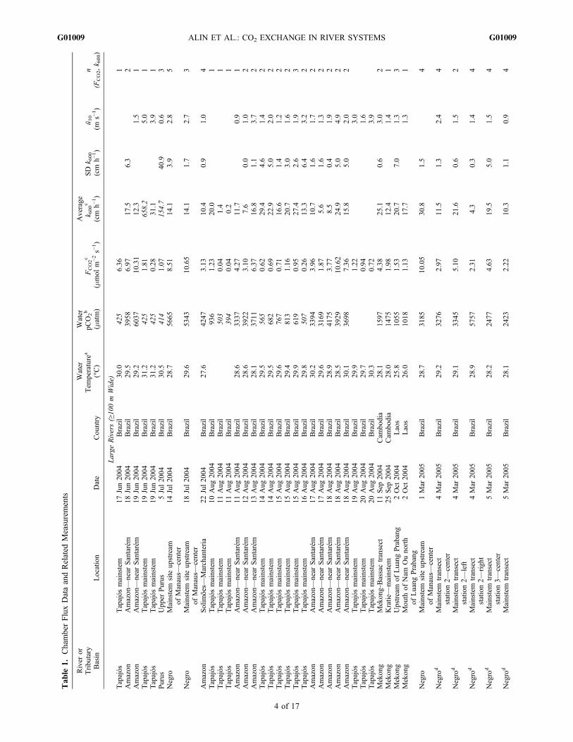
Tab
le1.
ChamberFluxDataandRelated
Measurements
River
orTribu
tary
Basin
Location
Date
Cou
ntry
Water
Tem
perature
a
(°C)
Water
pCO2b
(matm)
FCO2c
(mmol
m−2
s−1)
Average
k 600c
(cm
h−1)
SD
k 600
(cm
h−1)
ū 10
(ms−
1)
n(F
CO2,k 6
00)
Large
Rivers(≥10
0m
Wide)
Tapajós
Tapajós
mainstem
17Jun20
04Brazil
30.0
425
6.36
1Amazon
Amazon
—near
Santarém
18Jun20
04Brazil
29.5
3958
6.97
17.5
6.3
2Amazon
Amazon
—near
Santarém
19Jun20
04Brazil
29.2
6037
10.31
12.3
1.5
1Tapajós
Tapajós
mainstem
19Jun20
04Brazil
31.2
425
1.81
658.2
5.0
1Tapajós
Tapajós
mainstem
19Jun20
04Brazil
31.2
425
0.28
31.1
3.9
1Purus
Upp
erPurus
5Jul20
04Brazil
30.5
414
1.07
154.7
40.9
0.6
3Negro
Mainstem
site
upstream
ofManaus—
center
14Jul20
04Brazil
28.7
5665
8.51
14.1
3.9
2.8
5
Negro
Mainstem
site
upstream
ofManaus—
center
18Jul20
04Brazil
29.6
5343
10.65
14.1
1.7
2.7
3
Amazon
Solim
ões—
Marchanteria
22Jul20
04Brazil
27.6
4247
3.13
10.4
0.9
1.0
4Tapajós
Tapajós
mainstem
10Aug
2004
Brazil
936
1.23
20.0
1Tapajós
Tapajós
mainstem
11Aug
2004
Brazil
503
0.04
1.4
1Tapajós
Tapajós
mainstem
11Aug
2004
Brazil
394
0.04
0.2
1Amazon
Amazon
—near
Santarém
11Aug
2004
Brazil
28.6
3337
4.27
11.7
0.9
1Amazon
Amazon
—near
Santarém
12Aug
2004
Brazil
28.6
3922
3.10
7.6
0.0
1.0
2Amazon
Amazon
—near
Santarém
13Aug
2004
Brazil
28.1
3711
6.37
16.8
1.1
3.7
2Tapajós
Tapajós
mainstem
14Aug
2004
Brazil
29.5
565
0.62
29.4
4.6
1.4
2Tapajós
Tapajós
mainstem
14Aug
2004
Brazil
29.5
682
0.69
22.9
5.0
2.0
2Tapajós
Tapajós
mainstem
15Aug
2004
Brazil
29.6
767
0.71
16.6
1.4
1.2
2Tapajós
Tapajós
mainstem
15Aug
2004
Brazil
29.4
813
1.16
20.7
3.0
1.6
2Tapajós
Tapajós
mainstem
15Aug
2004
Brazil
29.9
619
0.95
27.4
2.6
1.9
3Tapajós
Tapajós
mainstem
16Aug
2004
Brazil
29.8
507
0.26
13.3
6.4
3.2
2Amazon
Amazon
—near
Santarém
17Aug
2004
Brazil
30.2
3394
3.96
10.7
1.6
1.7
2Amazon
Amazon
—near
Santarém
17Aug
2004
Brazil
29.6
3169
1.87
5.6
1.6
1.3
2Amazon
Amazon
—near
Santarém
18Aug
2004
Brazil
28.9
4175
3.77
8.5
0.4
1.9
2Amazon
Amazon
—near
Santarém
18Aug
2004
Brazil
28.5
3929
10.62
24.9
5.0
4.9
2Amazon
Amazon
—near
Santarém
18Aug
2004
Brazil
30.1
3698
7.36
15.8
5.0
2.0
2Tapajós
Tapajós
mainstem
19Aug
2004
Brazil
29.9
1.22
3.0
Tapajós
Tapajós
mainstem
20Aug
2004
Brazil
29.7
0.94
1.6
Tapajós
Tapajós
mainstem
20Aug
2004
Brazil
30.3
0.72
3.9
Mekon
gMekon
g‐Bassactransect
11Sep
2004
Cam
bodia
28.1
1597
4.38
25.1
0.6
3.0
2Mekon
gKratie—
mainstem
25Sep
2004
Cam
bodia
28.0
1475
1.98
12.4
1.4
1Mekon
gUpstream
ofLuang
Prabang
2Oct
2004
Laos
25.8
1055
1.53
20.7
7.0
1.3
3Mekon
gMou
thof
Nam
Ouno
rth
ofLuang
Prabang
2Oct
2004
Laos
26.0
1018
1.13
17.7
1.3
1
Negro
Mainstem
site
upstream
ofManaus—
center
1Mar
2005
Brazil
28.7
3185
10.05
30.8
1.5
4
Negro
dMainstem
transect
station2—
center
4Mar
2005
Brazil
29.2
3276
2.97
11.5
1.3
2.4
4
Negro
dMainstem
transect
station2—
left
4Mar
2005
Brazil
29.1
3345
5.10
21.6
0.6
1.5
2
Negro
dMainstem
transect
station2—
righ
t4Mar
2005
Brazil
28.9
5757
2.31
4.3
0.3
1.4
4
Negro
dMainstem
transect
station3—
center
5Mar
2005
Brazil
28.2
2477
4.63
19.5
5.0
1.5
4
Negro
dMainstem
transect
5Mar
2005
Brazil
28.1
2423
2.22
10.3
1.1
0.9
4
ALIN ET AL.: CO2 EXCHANGE IN RIVER SYSTEMS G01009G01009
4 of 17

Tab
le1.
(con
tinued)
River
orTribu
tary
Basin
Location
Date
Cou
ntry
Water
Tem
perature
a
(°C)
Water
pCO2b
(matm)
FCO2c
(mmol
m−2
s−1)
Average
k 600c
(cm
h−1)
SD
k 600
(cm
h−1)
ū 10
(ms−
1)
n(F
CO2,k 6
00)
station3—
left
Negro
dMainstem
transect
station3—
righ
t5Mar
2005
Brazil
28.1
3318
4.19
13.3
1.1
2.4
4
Negro
dMainstem
transect
station4—
center
7Mar
2005
Brazil
28.5
2374
2.52
11.8
4.1
1.6
4
Negro
dMainstem
transect
station4—
left
7Mar
2005
Brazil
27.7
2708
4.53
19.5
1.1
0.7
4
Negro
dMainstem
transect
station4—
righ
t7Mar
2005
Brazil
27.4
3781
1.43
3.5
2.5
0.3
4
Negro
dSão
Gabriel
daCacho
eira
8Mar
2005
Brazil
28.0
4.06
1.0
3Negro
dMainstem
transect
station5—
center
9Mar
2005
Brazil
28.1
2905
3.45
11.4
2.2
1.6
3
Negro
dMainstem
transect
station5—
left
9Mar
2005
Brazil
28.0
2905
2.31
7.9
0.9
0.9
4
Negro
Rio
Branco
12Mar
2005
Brazil
30.1
1697
13.22
96.8
11.9
4Negro
Unini
13Mar
2005
Brazil
27.3
6.84
0.7
4Negro
Mainstem
site
upstream
ofManaus—
center
13Jul20
05Brazil
28.8
4919
10.63
21.9
1.8
1.7
3
Negro
Mainstem
site
upstream
ofManaus—
left
13Jul20
05Brazil
28.8
4919
7.09
14.7
1.8
1.7
4
Purus
Low
erPurus—
center
15Jul20
05Brazil
28.5
1019
55.59
5.3
0.8
0.0
4Purus
Low
erPurus—
left
15Jul20
05Brazil
28.6
1031
714
.23
10.3
1.9
0.8
3Madeira
Mou
thof
Madeira—
center
19Jul20
05Brazil
29.7
2889
2.09
8.7
2.0
0.9
4Madeira
Mou
thof
Madeira—
righ
t19
Jul20
05Brazil
29.9
2978
7.15
24.9
3.4
4.5
4Amazon
Solim
ões—
Marchanteria
21Jul20
05Brazil
28.6
5810
6.23
9.8
0.8
1.2
4Negro
Cuieiras
25Jul20
05Brazil
25.8
1114
53.98
3.4
0.2
4Negro
Cuieiras
26Jul20
05Brazil
25.8
1114
53.19
2.7
0.4
0.6
4Negro
CuieirasTucum
ã26
Jul20
05Brazil
30.1
1252
33.91
2.8
1.4
0.3
4Negro
Mou
thof
Cuieiras
27Jul20
05Brazil
27.0
1261
61.63
1.2
0.2
0.3
4Jurua
Upp
erJurua
18Aug
2005
Brazil
28.5
3947
9.10
21.8
9.2
1.6
4Purus
Upp
erPurus
29Aug
2005
Brazil
30.5
1375
1.00
8.6
2.0
1.5
4Madeira
Upstream
ofPorto
Velho
4Sep
2005
Brazil
28.1
1110
1.04
9.7
0.6
0.6
4Mekon
gMainstem
northof
Phn
omPenh
6Oct
2005
Cam
bodia
28.8
945
3.26
51.4
5.9
0.7
6
Ton
leSap
Pou
satRiver
11Oct
2005
Cam
bodia
1404
1.14
10.8
2.8
3Mekon
gMainstem
northof
Phn
omPenh
12Oct
2005
Cam
bodia
2912
571.28
12.3
3.6
1.3
7
Mekon
gVientiane—mid‐chann
el15
Oct
2005
Laos
2770
31.02
32.5
0.3
3.7
4Mekon
gVientiane—mid‐chann
el15
Oct
2005
Laos
2770
31.76
52.0
5.1
2.9
3Mekon
gVientiane—nearshore
15Oct
2005
Laos
2770
31.90
44.5
2.6
4.9
4
Average
28.7
3317
3.90
14.7
1.8
Stand
arddeviation
1.3
3089
3.40
8.6
1.2
SmallRivers(<10
0m
Wide)
andStream
sPurus
Catuaba
1Jul20
04Brazil
26.0
141
3.45
−58.8
5.4
0.0
5Purus
Hum
aita
2Jul20
04Brazil
24.9
860
1.27
18.1
3.0
0.3
6Purus
Iaco
5Jul20
04Brazil
30.2
141
1.87
−62.9
43.6
0.9
2
ALIN ET AL.: CO2 EXCHANGE IN RIVER SYSTEMS G01009G01009
5 of 17
Tab
le1.
(con
tinued)
River
orTribu
tary
Basin
Location
Date
Cou
ntry
Water
Tem
perature
a
(°C)
Water
pCO2b
(matm)
FCO2c
(mmol
m−2
s−1)
Average
k 600c
(cm
h−1)
SD
k 600
(cm
h−1)
ū 10
(ms−
1)
n(F
CO2,k 6
00)
Negro
IgarapéBarro
Branco
20Jul20
04Brazil
25.2
7548
9.21
11.6
0.6
0.0
2Xingu
Rio
Curua
(beforemou
thbay)
23Aug
2004
Brazil
24.5
5937
0.80
14.9
2.1
0.0
2Xingu
Rio
Curua
(inmou
thbay)
23Aug
2004
Brazil
30.4
6607
0.99
1.2
0.2
0.5
2Xingu
Rio
Curua
(inmou
thbay)
23Aug
2004
Brazil
32.3
6607
9.54
1.0
0.1
0.3
3Xingu
Caixiuana
24Aug
2004
Brazil
31.2
4283
6.85
13.8
1.3
1.0
3Ton
leSap
Stung
Siem
Reap
20Sep
2004
Cam
bodia
27.4
3066
1.61
5.6
0.9
0.8
3Negro
Igarapé1
2Mar
2005
Brazil
26.0
1.63
4Negro
Igarapé2
3Mar
2005
Brazil
26.3
24.30
4Negro
Igarapé4
4Mar
2005
Brazil
25.7
5666
12.13
24.2
1.3
0.0
4Negro
Igarapé5
7Mar
2005
Brazil
25.3
2807
5.72
18.3
4.0
0.0
4Negro
Igarapé6
9Mar
2005
Brazil
26.4
4762
8.53
15.7
0.3
0.0
4Negro
IgarapéBarro
Branco
16Jul20
05Brazil
25.6
9569
12.41
11.8
1.4
0.3
4Jurua
Moa
18Aug
2005
Brazil
28.4
1462
6.41
58.7
0.9
1.2
4Jurua
Env
ira
20Aug
2005
Brazil
29.9
1924
6.75
45.0
1.8
4Jurua
Tarauaca
20Aug
2005
Brazil
27.9
1720
6.80
71.1
3.8
4Purus
Hum
aita
26Aug
2005
Brazil
23.5
2775
1.13
4.4
1.0
4Purus
Catuaba
30Aug
2005
Brazil
24.7
1980
2.87
11.4
1.2
0.5
4Purus
Acre
31Aug
2005
Brazil
30.7
1175
4.07
38.6
5.3
0.9
3Ji‐Paranáe
Riozinh
o25
Nov
2006
Brazil
28.5
2416
0.67
2.8
0.9
0.8
3Ji‐Paranáe
BandeiraBranca
27Nov
2006
Brazil
28.1
3918
7.31
17.2
1.6
1.3
3Ji‐Paranáe
Bam
burro
30Nov
2006
Brazil
27.9
2.21
0.5
4Ji‐Paranáe
Arenito
30Nov
2006
Brazil
28.6
0.67
1.2
4Ji‐Paranáe
Cornélio
11Dec
2006
Brazil
26.7
6430
5.46
7.3
0.9
0.8
4Ji‐Paranáe
Shank
e11
Dec
2006
Brazil
28.1
3073
7.23
22.9
2.9
2.2
2Ji‐Paranáe
Mandi
11Dec
2006
Brazil
27.9
2908
11.05
37.8
0.7
0.5
3Ji‐Paranáe
Riachuelo
13Dec
2006
Brazil
27.0
2591
5.09
44.8
2.1
0.5
3Ji‐Paranáe
Igarapé1
13Dec
2006
Brazil
26.1
3865
7.17
15.4
18.1
1.4
3Ji‐Paranáe
Igarapé2
13Dec
2006
Brazil
28.3
3190
9.58
30.1
3.5
2.2
3Ji‐Paranáe
Igarapé3
13Dec
2006
Brazil
26.8
2047
2.69
16.2
3.6
0.5
4Ji‐Paranáe
Igarapé4
13Dec
2006
Brazil
27.1
3.38
0.0
4Ji‐Paranáe
Paulistão
13Dec
2006
Brazil
26.7
2278
10.11
55.1
3.3
0.5
2Ji‐Paranáe
São
João
15Dec
2006
Brazil
27.3
1393
3.36
23.1
30.1
0.5
4Ji‐Paranáe
Rio
Branco
11Jan20
07Brazil
26.5
2390
6.85
31.4
6.8
0.4
3Ji‐Paranáe
Pregão
11Jan20
07Brazil
28.9
1674
4.14
31.9
1.3
0.8
2Ji‐Paranáe
Trincheira
11Jan20
07Brazil
28.0
2137
3.82
16.6
0.4
0.8
2Ji‐Paranáe
Esm
eril
11Jan20
07Brazil
28.9
3549
5.95
37.3
6.5
0.8
4Ji‐Paranáe
São
José
23Jan20
07Brazil
28.2
4451
6.14
13.1
2.5
1.1
3
Average
27.5
3353
5.45
23.3
0.7
Stand
arddeviation
1.9
2168
3.39
17.3
0.6
a Missing
values
forwater
temperature
werefilledin
whenpo
ssibleusingdatafrom
nearby
samplinglocatio
nsandtim
es.T
hesensitivity
ofcalculations
towater
temperature
intherang
eob
served
throug
hthestud
yarea
issm
all.
bThe
k 600data
forthepC
O2values
initalicswereexclud
edfrom
regression
analyses
becausethecalculationerroron
samples
with
DpC
O2<20
0ma
tmishigh
[Borgeset
al.,20
04a].
c Datain
italicsin
thesecolumns
wereexclud
edfrom
thecalculationof
averagevalues
andallstatistical
comparisons
becausethevaluewas
identifiedas
anou
tlier.
dMainstem
stations
2–5wereoccupied
during
atransect
oftheRio
Negro
from
Manausto
São
Gabriel
daCacho
eira
during
March
2005
.e D
atacollected
byRaseraet
al.[200
8].
ALIN ET AL.: CO2 EXCHANGE IN RIVER SYSTEMS G01009G01009
6 of 17

circulate air through the chamber [see Sebacher et al., 1983].The chamber (50 cm length × 20 cm width × 20 cm height)was made of Plexiglas with a stopcock in the top torelease air pressure. The chamber was connected via CO2‐impermeable tubing to a portable infrared CO2 analyzer(LI‐820; LI‐COR Instruments). Air was circulated throughthe LI‐820 system via an air filter using a miniature airpump (AS‐200; Spectrex) with a flow of approximately150 mL min−1. Closed‐cell foam was used for flotation.[13] To take chamber measurements, we gently placed the
chamber on the water surface to avoid inducing additionalturbulence. Data were recorded continuously on a laptop ordata logger at 1–5 s intervals from the time the chamber wasplaced on the water for 5 min or until the CO2 accumulationcurve began to flatten out.[14] Floating chambers generate results consistent with
mass balance and injected tracer methods of measuring gasexchange when the chamber is moving at the same speed asthe water surface (rather than being tethered to a stationaryobject) and at wind speeds less than 8–10 m s−1 and low tomoderate wave conditions [Kremer et al., 2003b; Cole et al.,2010]. Chambers with and without fans have been found togive results within the range of normal variability when usedunder moderately windy conditions (<5 m s−1) [Kremer etal., 2003b]. These conditions were routinely met duringour deployments.[15] Chamber measurements on rivers with navigable
channels were executed from small boats (both river sizeclasses) while drifting with the river current. In streams andthe smallest river environments, measurements were con-ducted from shore, with the chamber deployed in parts ofthe channel where the chamber was not pulled downstreamby the current and was connected to shore by way of thelines connecting it to the gas analyzer. The rope securing thechamber to shore was not taut during any of the measure-ments reported here. However, these locations may not berepresentative of the entire cross section of the stream, aswater current velocity may be lower and water depth shal-lower than in the main flow of the stream. These factorswould tend to decrease and increase k600, respectively. Thus,these measurements may not be representative of conditionsacross the entire channel.
3.3. The pCO2 Measurements
[16] We measured the partial pressure of CO2 at each siteby headspace equilibration. A 1 L polycarbonate bottle wasoverflowed for two to three volume changes, with waterpumped from the upper meter of the water column beforesecurely sealing the bottle with a stopper fitted with stop-cocks [Hesslein et al., 1991]. A headspace of 60 mL ofambient air (collected from upwind and overhead to avoidelevated CO2 concentrations from breath and motors, forexample) was introduced into the bottle while removing thesame volume of water. The bottle was shaken vigorously forat least 60 s. The headspace was then removed while thewater was reinjected at the same rate. Air samples were alsocollected in syringes to measure air pCO2.[17] All pCO2 samples were measured by infrared gas
analysis on a LI‐COR LI‐820 using standards of approxi-mately 300, 1000, and 10,000 matm CO2 in nitrogen (ScottSpecialty Gases). Samples were run directly from syringeswithin 24 h of collection or were stored in vials previously
flushed with nitrogen until analysis. Vial‐stored pCO2 va-lues were corrected for dilution by the nitrogen remaining inthe vials after evacuation with a hand pump (15%).
3.4. Chamber Data Analysis
[18] Air‐water gas exchange fluxes were calculated asfollows:
FCO2 ¼d pCO2ð Þ
dt
� �V
RTKS
� �; ð2Þ
where d(pCO2)/dt is the slope of the CO2 accumulation inthe chamber (matm s−1), V is the chamber volume (L), TK isair temperature (in degrees Kelvin, K), S is the surface areaof the chamber at the water surface (m2), and R is the gasconstant (L atm K−1 mol−1) [Frankignoulle, 1988]. Fluxeswere calculated using the first 30, 60, and 90 s of the initialCO2 accumulation in the chamber. The k value measuredduring each chamber deployment was calculated as follows:
k ¼ h
�
� �ln
pCO2w � pCO2að ÞiðpCO2w � pCO2aÞf
" #tf � ti� ��1
; ð3Þ
where h is the chamber height (cm), a is the Ostwald sol-ubility coefficient (dimensionless), t is time (s), and thesubscripts w, a, i, and f represent water, air, initial, and final,respectively [MacIntyre et al., 1995]. The Ostwald solubilitycoefficient can be calculated from K0 as a function of tem-perature as described by Wanninkhof et al. [2009]. Tocompare gas transfer velocity values among sites, k valueswere normalized to a temperature of 20°C (i.e., k600) usingthe following equation:
k600 ¼ kT600
ScT
� ��0:5
; ð4Þ
where kT is the measured k value at the in situ temperature(T), ScT is the Schmidt number for temperature T, and theSchmidt number for 20°C in freshwater is 600 [Jähne et al.,1987]. The Schmidt value for freshwater is calculated as afunction of temperature:
ScT ¼ 1911:1� 118:11T þ 3:4527T 2 � 0:04132T 3; ð5Þ
with T in degrees Celsius [Wanninkhof, 1992].
3.5. Ancillary Data
[19] In addition to chamber and pCO2 measurements, wemeasured wind speed and air and water temperatures. Windspeed was measured for 3–5 min at the time of flux mea-surements using a hand‐held anemometer (Kestrel 3000)facing into the wind at ∼1.5 m above the water surface.Wind speeds were averaged over the period of the fluxmeasurement as described by Borges et al. [2004a, 2004b].Wind speeds were normalized to a height of 10 m above thesurface using the following equation:
uz ¼u*�
� �ln
z
z0
� �; ð6Þ
where ūz is mean wind speed (m s−1) at the height z, u* isfriction velocity (m s−1), � is von Karman’s constant
ALIN ET AL.: CO2 EXCHANGE IN RIVER SYSTEMS G01009G01009
7 of 17
(ffi0.40), and z0 is roughness length (10−5 m, an intermediate
value for water surfaces) [Oke, 1988]. Friction velocity wasfirst calculated by rearranging equation (6) to solve for u*and using the mean wind speed measured at 1.5 m as ūz. Airtemperature was also measured with the Kestrel 3000. Watertemperature was measured with a Thermo‐Orion pH ordissolved oxygen probe.[20] For a subset of the Rasera et al. [2008] small‐river
measurements (n = 14 of 40), water current velocity (w,cm s−1), depth (z, m), and discharge (Q, m3 s−1) were mea-sured using a General Oceanics flow meter (model 2030) atthe same time chamber flux measurements were taken. Flowmeasurements were either taken from bridges or near shoreand thus may not represent the current velocity at the exactsite of the chamber measurement. Further, as the measure-ments were taken at only a single point for each site, currentvelocity data can only be viewed as estimates rather thansitewide averages of water current velocity.[21] For all other sampling events, no water current velocity
or discharge data were available at the same stations and timesthat flux measurements were taken. For the purpose of qual-itative comparisons of velocity, discharge, and water depth,we obtained data on average discharge, current velocity, anddepth at the time of sampling or from long‐term monthlyor weekly averages from the nearest monitoring station(s).For sites in the Amazon, hydrological data came from theBrazilian national water agency web site (Agência Nacionalde Águas, http://hidroweb.ana.gov.br), and for Mekong sites,hydrological data came from Mekong River Commissionmonitoring stations [cf. Costa‐Cabral et al., 2008].
3.6. Data Analysis and Statistics
[22] Prior to statistical analysis, we divided the results intothe two river size class categories for river channels greater
than and less than 100 m wide. For the purposes of all sta-tistical analyses, extreme outliers were excluded from theFCO2 and k600 data sets. Extreme outliers were defined asthose data beyond the outer fences on boxplots constructedfor each size category (http://www.itl.nist.gov/div898/handbook/). In total, one outlier was excluded from thesmall‐river FCO2 data set, and five and two outliers wereexcluded from the large‐river and small‐river k600 data sets,respectively. We also excluded k600 data from statisticalanalysis when the air‐water pCO2 gradient (DpCO2) was lessthan 200 matm, as the error in the k600 calculation increasessteeply asDpCO2 approaches zero [Borges et al., 2004a]. Alloutliers and low DpCO2 samples that have been excludedfrom statistical analyses are identified in Table 1.[23] Differences between small and large rivers were tested
using two‐tailed Fisher’s t‐tests for all parameters. Proba-bility density function (PDF) plots were generated for all fluxand gas transfer parameters as well as ancillary environ-mental variables using the kernel density estimation functionin R to compare the distribution of data in the small‐river andlarge‐river data sets. PDFs essentially represent smoothedhistograms and reflect the relative likelihood that values foreach parameter fall into a given range of values.[24] Within each river size category, we examined rela-
tionships between k600 and estimates of the controllingphysical processes and compared our results with previouslypublished estimates. For the subset of small‐river chamberflux measurements for which flow data were available, weused stepwise multiple linear regression to evaluate modelsfor the dependence of k600 on physical parameters includingwind speed, current velocity, and water depth. For large‐river measurements, simple linear regression was used totest for a statistical relationship between k600 and windspeed, but the water current velocity, depth, and discharge
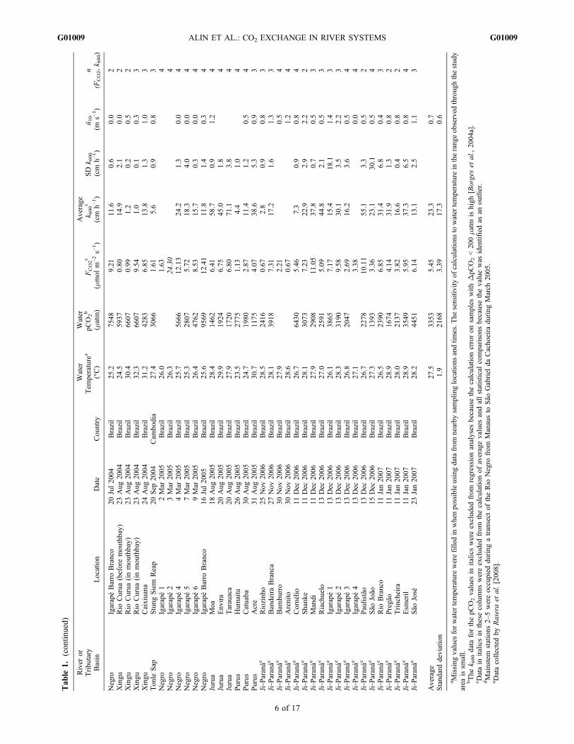
Figure 2. Probability density plots for flux and environmental parameters presented in Table 1(excluding outliers) for large and small rivers (solid and dashed lines, respectively). CO2 flux (FCO2),partial pressure of CO2 (pCO2), gas transfer velocity (k600), temperature (T), average wind speed at 10 m(ū10), water current velocity (w), water depth (z), and discharge (Q). Parameters with disjunct distributions(z and Q) were log‐transformed prior to plotting to make the curves legible and have logged units in thex‐axis labels. Shaded lines represent large‐river hydrology data from the closest hydrological monitoringstations and are not matched in space and time with chamber measurements. Thus, shaded lines onlyqualitatively represent the ranges of hydrological conditions present in large rivers during this study.
ALIN ET AL.: CO2 EXCHANGE IN RIVER SYSTEMS G01009G01009
8 of 17
data were not collected sufficiently close to the flux mea-surements to allow a multiple linear regression includingboth wind speed and water current velocity.
4. Results
[25] Overall, we observed higher average FCO2 and k600values in small‐river and stream environments than in riverswith channels wider than 100 m (averages and standarddeviations for all parameters are given in Table 1). Smallrivers also showed greater variability in k600 than largerivers. Probability density plots for pCO2, flux, k600, andenvironmental parameters (T, ū10, w, z, and Q) reveal theirdistributions across large‐river and small‐river data sets(Figure 2). Distributions for all parameters overlapped atleast to some extent between large and small rivers, butpCO2 was the only parameter for which no statisticallysignificant difference existed between the small‐river andlarge‐river data sets (Tables 1 and 2).[26] After excluding invalid values (i.e., DpCO2 <
200 matm), chamber measurements revealed similar rangesand large variation in FCO2 values in both river size classes,ranging from 0.04 to 14.2 mmol m−2 s−1 in large rivers andfrom 0.7 to 12.4 mmol m−2 s−1 in small rivers (Figure 2 andTable 1). Average fluxes were ∼40% higher from small riversthan from large rivers, as small rivers had more large fluxesand vice versa (Figure 2 and Tables 1 and 2).[27] To account for the larger CO2 fluxes observed in
small rivers, either CO2 concentrations or k600 must also
differ significantly between river size classes. Partial pres-sures of CO2 varied across two orders of magnitude in riversof all sizes, with values of 390–12,620 matm in large riversand 140–9,230 matm in small rivers and streams (Figure 2and Table 1). There was no statistically significant differ-ence in pCO2 values across the river size spectrum (Tables 1and 2).[28] The data presented here suggest, however, that k600 in
small rivers and streams (i.e., channels <100 m wide) washigher on average and more variable than in larger rivers(Figures 2–4) [see also Rasera et al., 2008]. k600 rangedover more than an order of magnitude in both size classes,from 1.2 to 44.5 cm h−1 in large rivers and from 1.0 to 71.1cm h−1 in small rivers (Table 1). The average k600 in smallrivers was nearly 60% higher than in large rivers, and thisdifference was significant (Tables 1 and 2).[29] Water temperature measurements are essential for
normalizing gas transfer velocities to a common temperature(i.e., k600 values). Temperatures in the streams and rivers inthis study occupied a relatively small range (24.5–31.2°C;Table 1). Water temperatures in large rivers occupied anarrower range of water temperatures than observed in smallrivers (Figure 2). Although the mean temperature in largerivers was significantly higher statistically, the averageswere only 1.5°C apart and their ranges overlapped sub-stantially (Tables 1 and 2). To model fluxes of CO2 in realrivers ultimately, in situ water temperatures must be used toconvert k600 values to in situ gas transfer velocities (i.e., k).Since temperatures in our study rivers and streams wereconsistently higher than the k600 standard temperature (20°C),which would not be the case for temperate and high‐latitudestreams and rivers, our in situ k values are consistently higherthan the k600 values, reflecting enhanced gas transfer at higherwater temperatures.[30] Environmental variables that may explain some of the
variance observed in k600 values included wind speed andthe hydrological variables (w, z, Q). Average wind speedmeasurements extrapolated to 10 m above the water surface(ū10) ranged from 0.0 to 5.2 m s−1 over large rivers com-pared to 0.0 to 2.2 m s−1 for small rivers (Figure 2 andTable 1). Average wind speed was significantly higher over
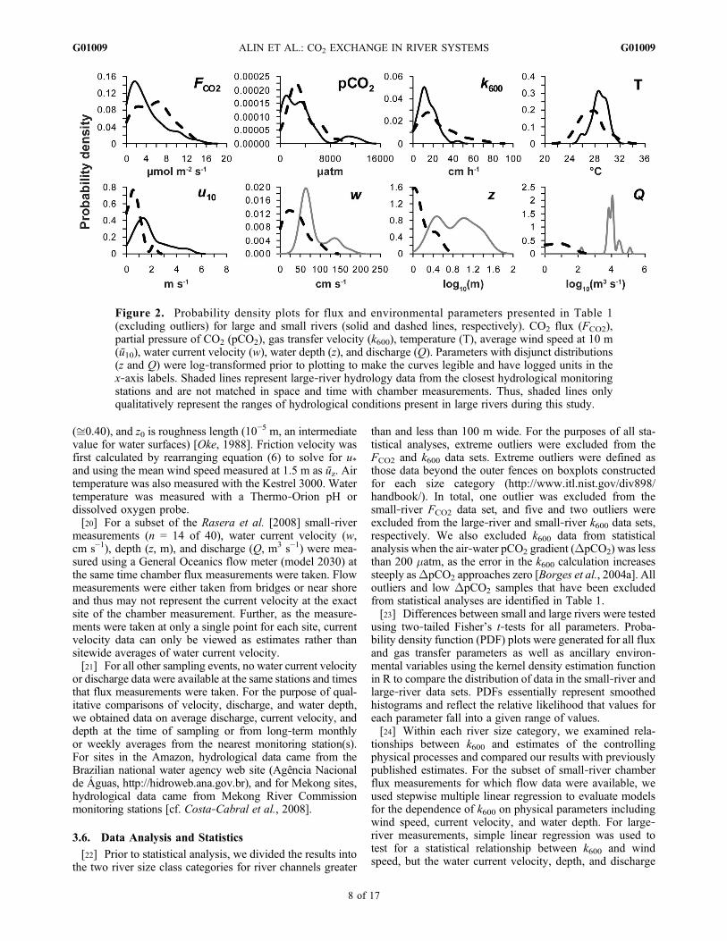
Table 2. Statistical Comparisons Between Large and Small Rivers
Parameter t df p
FCO2 −2.19 105 0.03pCO2 −0.04 93 0.97k600 −2.55 44 0.01Twater 3.70 59 0.0005ū10 5.94 91 <0.00001w 4.07 25 0.0002z 5.80 10 0.0001Q 2.21 10 0.03
Figure 3. Distribution of k600 data against ū10 in (a) rivers >100 m wide (triangles) and (b) rivers <100 mwide, including streams (squares). Previously published k600‐ū10 relationships for rivers and estuaries areshown in both Figure 3a and Figure 3b (solid black line, Raymond and Cole [2001]; short‐dashed line,Borges et al. [2004b]; long‐dashed line, Marino and Howarth [1993]). Shading indicates values used byRichey et al. [2002] for their central Amazon CO2 evasion estimate. The ū10‐k600 relationship for largerivers in this study (R2 = 0.53) is shown in Figures 3a and 3b as a thick shaded line. (c) The relationshipbetween k600 and water current velocity (w) in small rivers (squares; R2 = 0.41). Note the different x‐axisand y‐axis scales across Figures 3a–3c.
ALIN ET AL.: CO2 EXCHANGE IN RIVER SYSTEMS G01009G01009
9 of 17

Figure 4. Binned k600 data from Figure 3 in 0.5–1 m s−1 wind speed intervals in (a) large rivers and(b) small rivers and streams. Binned ū10–k600 data from estuaries in the work of Borges et al. [2004b] areshown in Figure 4a as shaded circles with error bars, and the Borges et al. [2004b] ū10–k600 relationshipis indicated by the shaded dashed line. For wind speed binning, bin size was selected on the basis of datadensity and distribution. Error bars for the x‐axis and y‐axis were calculated individually for each bin andrepresent 1 standard deviation from the mean. Lines plotted on the basis of published relationshipsbetween k600 and ū10 are as described in the Figure 3 legend (except that the Borges et al. [2004b]relationship in Figure 3a is shaded rather than black in Figure 4a). Note the different scaling of theaxes between Figures 3 and 4.
Table 3. Hydrological Measurements From Nearest Monitoring Stations for Large Rivers and From Direct Measurements for SmallRivers and Streams
Tributary Basin Flux Measurement Location DateAverage
w (cm s−1)Averagez (m)
AverageQ (m3 s−1)
Nearest Hydrological Stations on Large Rivers (≥100 m Wide)Mekong Kratie—mainstem 25 Sep 2004 173 22.7 35,413Mekong Upstream of Luang Prabang 2 Oct 2004 137 12.6 7,138Negro Mainstem transect stations 2–3 and
São Gabriel da Cachoeira4 Mar 2005 64 9.5 11,279
Negro Mainstem transect station 4 7 Mar 2005 62 7.9 6,537Negro Mainstem site upstream of Manaus 13 Jul 2005 69.4Purus Lower Purus 15 Jul 2005 69 22.7 11,280Amazon Solimões—near Madeira confluence 21 Jul 2005 144 27.2 127,007Negro Cuieiras 25 Jul 2005 53Negro Cuieiras 26 Jul 2005 52.8Jurua Upper Jurua 18 Aug 2005 50 2.1 159Madeira Upstream of Porto Velho 4 Sep 2005 63 9.6 5,049Mekong Mainstem north of Phnom Penh 6 Oct 2005 146 22 28,509Tonle Sap Pousat River 11 Oct 2005 75Mekong Mainstem north of Phnom Penh 12 Oct 2005 128 21.5 24,021Mekong Vientiane—mid‐channel 15 Oct 2005 101 9.7 6,968Average 92 15 23,950Standard deviation 42 8 35,900
Small Rivers (<100 m Wide) and StreamsJurua Moa 18 Aug 2005 100Jurua Envira 20 Aug 2005 28 1.3 36Purus Acre 31 Aug 2005 49 1.0 38Ji‐Paraná Bandeira Branca 27 Nov 2006 5.4 0.3 0.1Ji‐Paraná Cornélio 11 Dec 2006 13.9 1.0 2.1Ji‐Paraná Mandi 11 Dec 2006 53.8 1.2 7.6Ji‐Paraná Igarapé 2 13 Dec 2006 29.9 0.1 0.3Ji‐Paraná Igarapé 3 13 Dec 2006 44.7 0.2 0.4Ji‐Paraná São João 15 Dec 2006 83 1.0 14.1Ji‐Paraná Rio Branco 11 Jan 2007 16.4 1.0 3.3Ji‐Paraná Pregão 11 Jan 2007 42.2 0.6 0.8Ji‐Paraná Trincheira 11 Jan 2007 10.3 0.5 0.5Ji‐Paraná Esmeril 11 Jan 2007 56.7 1.3 8.8Ji‐Paraná São José 23 Jan 2007 13.3 2.3 5.2Average 39 0.9 9.0Standard deviation 28 0.6 13.1
ALIN ET AL.: CO2 EXCHANGE IN RIVER SYSTEMS G01009G01009
10 of 17
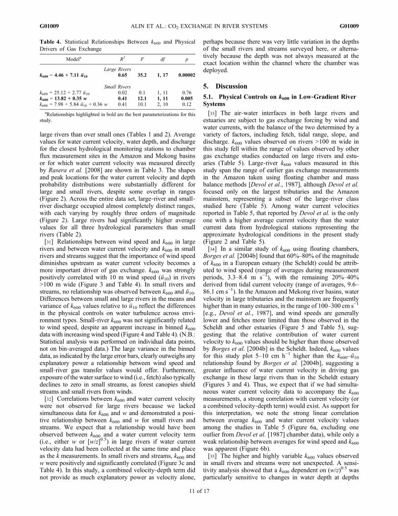
large rivers than over small ones (Tables 1 and 2). Averagevalues for water current velocity, water depth, and dischargefor the closest hydrological monitoring stations to chamberflux measurement sites in the Amazon and Mekong basinsor for which water current velocity was measured directlyby Rasera et al. [2008] are shown in Table 3. The shapesand peak locations for the water current velocity and depthprobability distributions were substantially different forlarge and small rivers, despite some overlap in ranges(Figure 2). Across the entire data set, large‐river and small‐river discharge occupied almost completely distinct ranges,with each varying by roughly three orders of magnitude(Figure 2). Large rivers had significantly higher averagevalues for all three hydrological parameters than smallrivers (Table 2).[31] Relationships between wind speed and k600 in large
rivers and between water current velocity and k600 in smallrivers and streams suggest that the importance of wind speeddiminishes upstream as water current velocity becomes amore important driver of gas exchange. k600 was stronglypositively correlated with 10 m wind speed (ū10) in rivers>100 m wide (Figure 3 and Table 4). In small rivers andstreams, no relationship was observed between k600 and ū10.Differences between small and large rivers in the means andvariance of k600 values relative to ū10 reflect the differencesin the physical controls on water turbulence across envi-ronment types. Small‐river k600 was not significantly relatedto wind speed, despite an apparent increase in binned k600data with increasing wind speed (Figure 4 and Table 4). (N.B.:Statistical analysis was performed on individual data points,not on bin‐averaged data.) The large variance in the binneddata, as indicated by the large error bars, clearly outweighs anyexplanatory power a relationship between wind speed andsmall‐river gas transfer values would offer. Furthermore,exposure of the water surface to wind (i.e., fetch) also typicallydeclines to zero in small streams, as forest canopies shieldstreams and small rivers from winds.[32] Correlations between k600 and water current velocity
were not observed for large rivers because we lackedsimultaneous data for k600 and w and demonstrated a posi-tive relationship between k600 and w for small rivers andstreams. We expect that a relationship would have beenobserved between k600 and a water current velocity term(i.e., either w or [w/z]0.5) in large rivers if water currentvelocity data had been collected at the same time and placeas the k measurements. In small rivers and streams, k600 andw were positively and significantly correlated (Figure 3c andTable 4). In this study, a combined velocity‐depth term didnot provide as much explanatory power as velocity alone,
perhaps because there was very little variation in the depthsof the small rivers and streams surveyed here, or alterna-tively because the depth was not always measured at theexact location within the channel where the chamber wasdeployed.
5. Discussion
5.1. Physical Controls on k600 in Low‐Gradient RiverSystems
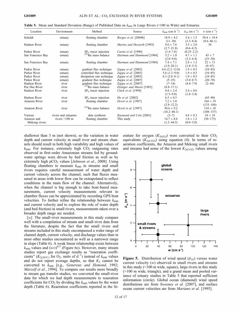
[33] The air‐water interfaces in both large rivers andestuaries are subject to gas exchange forcing by wind andwater currents, with the balance of the two determined by avariety of factors, including fetch, tidal range, slope, anddischarge. k600 values observed on rivers >100 m wide inthis study fell within the range of values observed by othergas exchange studies conducted on large rivers and estu-aries (Table 5). Large‐river k600 values measured in thisstudy span the range of earlier gas exchange measurementsin the Amazon taken using floating chamber and massbalance methods [Devol et al., 1987], although Devol et al.focused only on the largest tributaries and the Amazonmainstem, representing a subset of the large‐river classstudied here (Table 5). Among water current velocitiesreported in Table 5, that reported by Devol et al. is the onlyone with a higher average current velocity than the watercurrent data from hydrological stations representing theapproximate hydrological conditions in the present study(Figure 2 and Table 5).[34] In a similar study of k600 using floating chambers,
Borges et al. [2004b] found that 60%–80% of the magnitudeof k600 in a European estuary (the Scheldt) could be attrib-uted to wind speed (range of averages during measurementperiods, 3.3–8.4 m s−1), with the remaining 20%–40%derived from tidal current velocity (range of averages, 9.6–86.1 cm s−1). In the Amazon and Mekong river basins, watervelocity in large tributaries and the mainstem are frequentlyhigher than in many estuaries, in the range of 100–300 cm s−1
[e.g., Devol et al., 1987], and wind speeds are generallylower and fetches more limited than those observed in theScheldt and other estuaries (Figure 5 and Table 5), sug-gesting that the relative contribution of water currentvelocity to k600 values should be higher than those observedby Borges et al. [2004b] in the Scheldt. Indeed, k600 valuesfor this study plot 5–10 cm h−1 higher than the k600–ū10relationship found by Borges et al. [2004b], suggesting agreater influence of water current velocity in driving gasexchange in these large rivers than in the Scheldt estuary(Figures 3 and 4). Thus, we expect that if we had simulta-neous water current velocity data to accompany the k600measurements, a strong correlation with current velocity (ora combined velocity‐depth term) would exist. As support forthis interpretation, we note the strong linear correlationbetween average k600 and water current velocity valuesamong the studies in Table 5 (Figure 6a, excluding oneoutlier from Devol et al. [1987] chamber data), while only aweak relationship between averages for wind speed and k600was apparent (Figure 6b).[35] The higher and highly variable k600 values observed
in small rivers and streams were not unexpected. A sensi-tivity analysis showed that a k600 dependent on (w/z)0.5 wasparticularly sensitive to changes in water depth at depths
Table 4. Statistical Relationships Between k600 and PhysicalDrivers of Gas Exchange
Modela R2 F df p
Large Riversk600 = 4.46 + 7.11 ū10 0.65 35.2 1, 17 0.00002
Small Riversk600 = 25.12 + 2.77 ū10 0.02 0.1 1, 11 0.76k600 = 13.82 + 0.35 w 0.41 12.1 1, 11 0.005k600 = 7.98 + 5.84 ū10 + 0.36 w 0.41 10.1 2, 10 0.12
aRelationships highlighted in bold are the best parameterizations for thisstudy.
ALIN ET AL.: CO2 EXCHANGE IN RIVER SYSTEMS G01009G01009
11 of 17
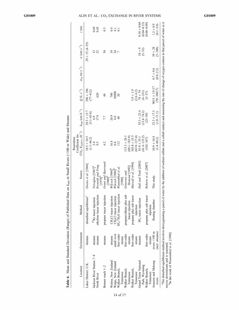
shallower than 3 m (not shown), so the variation in waterdepth and current velocity in small river and stream chan-nels should result in both high variability and high values ofk600. For instance, extremely high CO2 outgassing ratesobserved in first‐order Amazonian streams fed by ground-water springs were driven by bed friction as well as byextremely high pCO2 values [Johnson et al., 2008]. Usingfloating chambers to measure k600 in streams and smallrivers requires careful measurement of water depth andcurrent velocity across the channel, such that fluxes mea-sured in areas with lower flow can be extrapolated to reflectconditions in the main flow of the channel. Alternatively,when the channel is big enough to take boat‐based mea-surements, current velocity measurements relevant tochamber fluxes can be approximated by recording GPS boatvelocities. To further refine the relationship between k600and current velocity and to explore the role of water depth(and bed friction) in small rivers, measurements taken over abroader depth range are needed.[36] The small‐river measurements in this study compare
well with a compilation of stream and small‐river data fromthe literature, despite the fact that the small rivers andstreams included in this study encompassed a wider range ofchannel depth, current velocity, and discharge values than inmost other studies encountered as well as a narrower rangein slope (Table 6). A weak linear relationship exists betweenk600 values and (w/z)0.5 (Figure 6c). However, many streamstudies report gas exchange results as “reaeration coeffi-cients” (K2(20°C) for O2, units of d
−1) instead of k600 valuesand do not report average depths, so that K2 cannot beconverted to k600 [e.g., Genereux and Hemond, 1992;Marzolf et al., 1994]. To compare our results more broadlyto stream gas transfer studies, we converted the small‐riverdata for which we had depth measurements to reaerationcoefficients for CO2 by dividing the k600 values by the waterdepth (Table 6). Reaeration coefficients reported in the lit-
erature for oxygen (K2(O2)) were converted to their CO2
equivalents (K2(CO2)) using equation (4). In terms of re-aeration coefficients, the Amazon and Mekong small riversand streams had some of the lowest K2(CO2) values among
Table 5. Mean and Standard Deviation (Range) of Published Data on k600 in Large Rivers (>100 m Wide) and Estuaries
Location Environment Method Source k600 (cm h−1) ū10 (m s−1) w (cm s−1)
Scheldt estuary floating chamber Borges et al. [2004b] 18.9 ± 4.2(11–30)
5.4 ± 1.5(3.3–8.4)
58.4 ± 19.4(9.6–86.1)
Hudson River estuary floating chamber Marino and Howarth [1993] 9.6 ± 7.6(2.7–21.8)
3.5 ± 2.0(0.6–6.5)
38
Parker River estuary SF6 tracer injection Carini et al. [1996] (1.4–7.8) (0.25–2.2)San Francisco Bay estuary 222Rn mass balance Hartman and Hammond [1984] 5.2 ± 1.0
(2.0–9.0)4.7 ± 1.1(3.2–6.4)
43 ± 7(33–50)
San Francisco Bay estuary floating chamber Hartman and Hammond [1984] 7.4 ± 7.1(1.0–28.1)
2.8 ± 1.2(1.8–5.3)
22 ± 13(0–47)
Parker River estuary gradient flux technique Zappa et al. [2003] 6.6 (2.2–12.0) 1.9 ± 0.5 (10–85)Parker River estuary controlled flux technique Zappa et al. [2003] 5.6 (1.2–9.0) 1.9 ± 0.5 (10–85)Parker River estuary dissipation rate technique Zappa et al. [2003] 6.3 (2.8–8.1) 1.9 ± 0.5 (10–85)Parker River estuary gradient flux technique Zappa et al. [2007] (5–25) (3.0–8.7) (20–70)Hudson River river gradient flux technique Zappa et al. [2007] (7–14) (4.4–7.9) (2–44)Pee Dee River river 222Rn mass balance Elsinger and Moore [1983] (8.8–17.1)Hudson River river SF6 tracer injection Clark et al. [1994] 4.8 ± 2.4
(1.5–9.0)2.4 ± 0.6(1.8–3.4)
Hudson River river SF6 tracer injection Ho et al. [2002] 6.5 ± 0.5 (65–90)Amazon River river floating chamber Devol et al. [1987] 7.2 ± 3.0
(2.9–12.2)164 ± 19(133–184)
Amazon River river 222Rn mass balance Devol et al. [1987] 30.6 ± 9.2(16.2–40.1)
134 ± 18(108–157)
Various rivers and estuaries data synthesis Raymond and Cole [2001] (3–7) 4.6 ± 0.3 34 ± 18Amazon and
Mekong riversrivers >100 m floating chamber This study 14.7 ± 8.6
(1.2–44.5)1.8 ± 1.2(0.0–5.0)
(50–173)
Figure 5. Distribution of wind speed (ū10) versus watercurrent velocity (w) observed in small rivers and streamsin this study (<100 m wide, square), large rivers in this study(>100 m wide, triangle), and a grand mean and pooled var-iance of estuary studies in Table 5 that reported sufficientinformation (circle). Global ocean (diamond) wind speeddistributions are from Sweeney et al. [2007], and surfaceocean current velocities are from Mariano et al. [1995].
ALIN ET AL.: CO2 EXCHANGE IN RIVER SYSTEMS G01009G01009
12 of 17
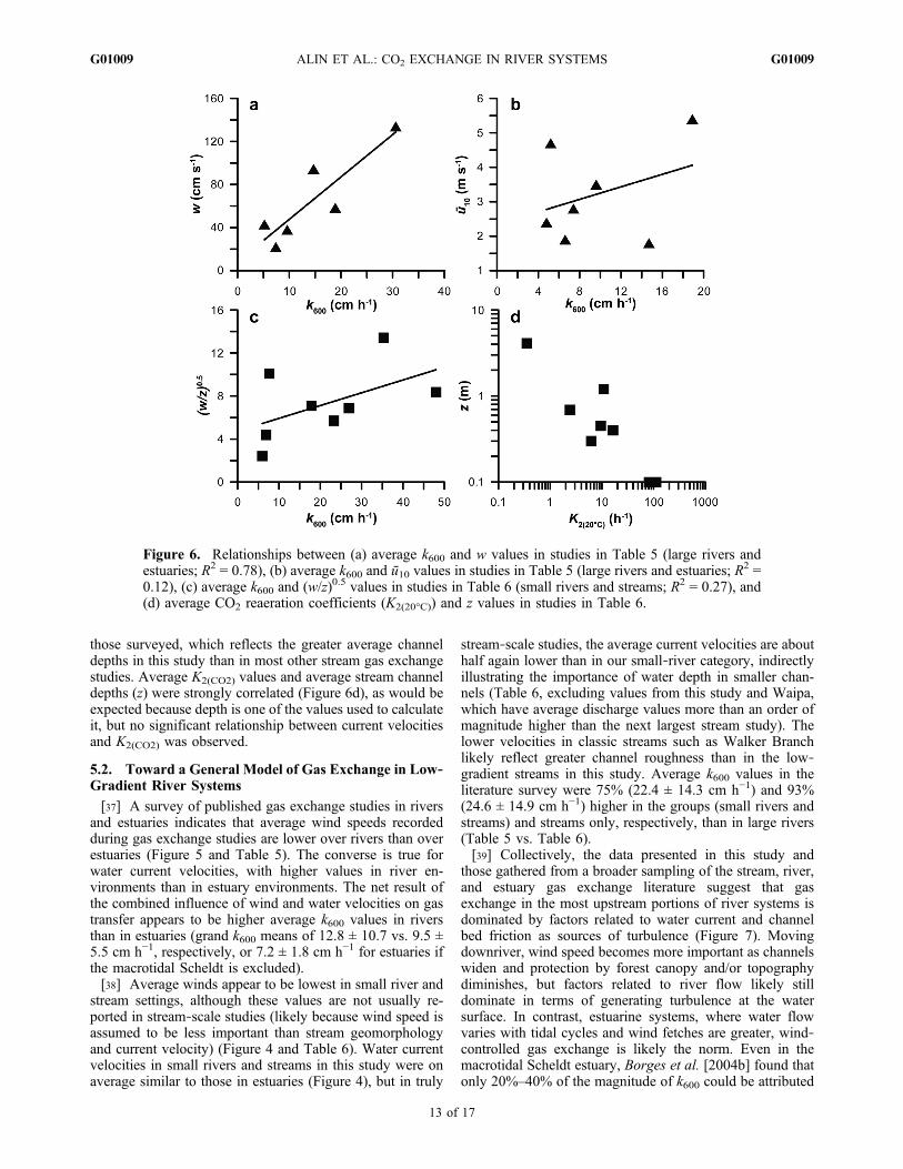
those surveyed, which reflects the greater average channeldepths in this study than in most other stream gas exchangestudies. Average K2(CO2) values and average stream channeldepths (z) were strongly correlated (Figure 6d), as would beexpected because depth is one of the values used to calculateit, but no significant relationship between current velocitiesand K2(CO2) was observed.
5.2. Toward a General Model of Gas Exchange in Low‐Gradient River Systems
[37] A survey of published gas exchange studies in riversand estuaries indicates that average wind speeds recordedduring gas exchange studies are lower over rivers than overestuaries (Figure 5 and Table 5). The converse is true forwater current velocities, with higher values in river en-vironments than in estuary environments. The net result ofthe combined influence of wind and water velocities on gastransfer appears to be higher average k600 values in riversthan in estuaries (grand k600 means of 12.8 ± 10.7 vs. 9.5 ±5.5 cm h−1, respectively, or 7.2 ± 1.8 cm h−1 for estuaries ifthe macrotidal Scheldt is excluded).[38] Average winds appear to be lowest in small river and
stream settings, although these values are not usually re-ported in stream‐scale studies (likely because wind speed isassumed to be less important than stream geomorphologyand current velocity) (Figure 4 and Table 6). Water currentvelocities in small rivers and streams in this study were onaverage similar to those in estuaries (Figure 4), but in truly
stream‐scale studies, the average current velocities are abouthalf again lower than in our small‐river category, indirectlyillustrating the importance of water depth in smaller chan-nels (Table 6, excluding values from this study and Waipa,which have average discharge values more than an order ofmagnitude higher than the next largest stream study). Thelower velocities in classic streams such as Walker Branchlikely reflect greater channel roughness than in the low‐gradient streams in this study. Average k600 values in theliterature survey were 75% (22.4 ± 14.3 cm h−1) and 93%(24.6 ± 14.9 cm h−1) higher in the groups (small rivers andstreams) and streams only, respectively, than in large rivers(Table 5 vs. Table 6).[39] Collectively, the data presented in this study and
those gathered from a broader sampling of the stream, river,and estuary gas exchange literature suggest that gasexchange in the most upstream portions of river systems isdominated by factors related to water current and channelbed friction as sources of turbulence (Figure 7). Movingdownriver, wind speed becomes more important as channelswiden and protection by forest canopy and/or topographydiminishes, but factors related to river flow likely stilldominate in terms of generating turbulence at the watersurface. In contrast, estuarine systems, where water flowvaries with tidal cycles and wind fetches are greater, wind‐controlled gas exchange is likely the norm. Even in themacrotidal Scheldt estuary, Borges et al. [2004b] found thatonly 20%–40% of the magnitude of k600 could be attributed
Figure 6. Relationships between (a) average k600 and w values in studies in Table 5 (large rivers andestuaries; R2 = 0.78), (b) average k600 and ū10 values in studies in Table 5 (large rivers and estuaries; R2 =0.12), (c) average k600 and (w/z)0.5 values in studies in Table 6 (small rivers and streams; R2 = 0.27), and(d) average CO2 reaeration coefficients (K2(20°C)) and z values in studies in Table 6.
ALIN ET AL.: CO2 EXCHANGE IN RIVER SYSTEMS G01009G01009
13 of 17
Tab
le6.
MeanandStand
ardDeviatio
n(Range)of
Pub
lishedDataon
k 600in
SmallRivers(<10
0m
Wide)
andStreams
Location
Env
iron
ment
Metho
dSou
rce
Reaeration
Coefficient
for
CO2,K2(20°C
)(h
−1)
k 600(cm
h−1)
Q(L
s−1)
ū 10(m
s−1)
w(cm
s−1)
z(m
)
Lakes
District,U.K.
stream
sdisturbedequilib
rium
aOwenset
al.[196
4]18
.5±10
.5(1.1–46.2)
29.5
±15
.7(3.1–65.6)
396±19
6(77–61
2)29
±15
(4–5
5)
JacksonRiver
Statio
n7–
8stream
s85Krtracer
injection
Tsivoglou
[196
7]b
2.4
6.9
130.69
North
River
stream
sethy
lene
tracer
injection
Kwasnikan
dFeng
[197
9]b
9.5
17.9
620
230.45
Bon
nerreach1–2
stream
sprop
anetracer
injection
Grant
andSkavronek
[198
0]b
6.2
7.7
4830
0.3
Waitoa,
New
Zealand
stream
sCH3Cltracer
injection
Wilcock[198
4]b
16.4
26.9
700
190.4
Waipa,New
Zealand
smallriver
CH3Cltracer
injection
Wilcock[198
4]b
0.4
6.0
3600
024
4.1
WalkerBranch,
Tennessee
first‐order
stream
SF6/3H2O
tracer
injection
Wan
ninkho
fet
al.
[199
0]11
248
207
0.1
WalkerBranch,
Tennessee
first‐order
stream
prop
ane/ethane
plus
salt
tracer
injection
Genereuxan
dHem
ond[199
2]11
5.3±28
.1(60.1–
183.9)
WalkerBranch,
Tennessee
first‐order
stream
prop
aneplus
salttracer
injection
Marzolfet
al.[199
4]10
3.8±35
.5(63.0–
127.4)
3.9±1.9
(2.6–6.2)
Grand
Teton
National
Park,
Wyo
ming
stream
sSF6tracer
injection
Hallan
dTan
k[200
3]81
.0±35
.1(41.4–
135.2)
35.3
±23
.4(13.8–
74.2)
78±74
(4–231
)18
±9
(5–3
3)0.10
±0.04
(0.04–
0.15
)WalkerBranch,
Tennessee
first‐order
stream
prop
aneplus
salttracer
injection
Rob
ertset
al.[200
7](102–167
)(23–59
)(5–57)
(0.06–
0.09
)
Amazon
andMekon
grivers
rivers
<10
0m
(incl.stream
s)floatin
gcham
ber
Thisstud
y10
.9±14
.4(1.4–60.2)
23.3
±17
.3(1.0–71.1)
9015
±13
117
(70–38
017)
0.7±0.6
(0.0–2
.2)
39±28
(5–1
00)
1.2±0.9
(0.1–3
.0)
a The
disturbedequilib
rium
metho
dinvo
lves
deox
ygenatingaparcelof
water
bytheadditio
nof
sodium
sulfateandacobaltcatalystandmeasuring
therateof
change
ofox
ygen
contentinthatparcelof
water
asit
mov
esdo
wnstream
andisreaerated.
bIn
theworkof
Wan
ninkho
fet
al.[199
0].
ALIN ET AL.: CO2 EXCHANGE IN RIVER SYSTEMS G01009G01009
14 of 17

to the action of water currents. Gas exchange in the openocean, at the far end of the stream‐to‐ocean transect, isdominated by wind forcing of gas transfer [Wanninkhof etal., 2009]. Thus, within river systems, transitions in thephysical controls on k600 occur with the decreasing size ofthe river channel upstream. As one travels upriver from theestuary to streams of the lowest order, the relative impor-tance of wind in controlling k600 declines to zero while theinfluence of water current and bed friction progressivelyincrease (Figure 7). Regional models of fluvial biogeo-chemistry in low‐gradient systems must thus be correctlyparameterized to reflect this transition to correctly handleupscaling of individual measurements to large‐scale carbonbudgets appropriately.
5.3. Implications for Regional Carbon Budgets
[40] The results of this study have implications for mod-eling gas exchange fluxes at the scale of the whole riverbasin. The magnitude of CO2 fluxes and physical controlson k600 appear to vary substantially across the river channel‐size spectrum (Tables 2, 5, and 6). The Richey et al. [2002]basinwide estimate of CO2 outgassing for the AmazonRiver system used static values for k in different environ-
ments (i.e., not including the effects of wind or currentvelocity): 9.6 ± 3.8 cm h−1 in the mainstem Amazon Riverand 5.0 ± 2.1 cm h−1 in both primary tributaries (>100 mwide) and small rivers and streams (<100 m wide). Theaverage k600 value in this study for all rivers >100 m wide,including both mainstem and tributary environments, was8.0 ± 4.8 cm h−1 for wind speeds under 1 m s−1. When thisk600 value is corrected to water temperatures typical ofAmazonian aquatic ecosystems (∼25°C–30°C), the averagerises to 9.0–10.3 cm h−1, which is comparable to themainstem k value used by Richey et al. [2002] but roughlytwice as large as the value they used for primary tributaries(i.e., tributaries >100 m wide). Richey et al. [2002] did notdifferentiate between mainstem and primary tributary en-vironments in calculating FCO2 values, but our resultssuggest that the contribution of primary tributaries to basin‐scale CO2 outgassing may be nearly double the Richey et al.[2002] estimate for primary tributaries under a new detailedanalysis.[41] When the average small river and stream k600 value
of 23.3 cm h−1 is corrected to typical tropical river watertemperatures, it rises to 26–30 cm h−1, which is five to sixtimes higher than the value used by Richey et al. [2002]. All
Figure 7. Schematic representation of the changing absolute magnitudes (top) of average wind speed(ū10; black lines) and water current velocity (w; shaded lines) as one travels along a transect from the openocean to headwater streams. (bottom) The changing relative influence of wind speed and water currentvelocity on the overall magnitude of k600 along the same transect as wind fetch and water depth progres-sively decrease.
ALIN ET AL.: CO2 EXCHANGE IN RIVER SYSTEMS G01009G01009
15 of 17
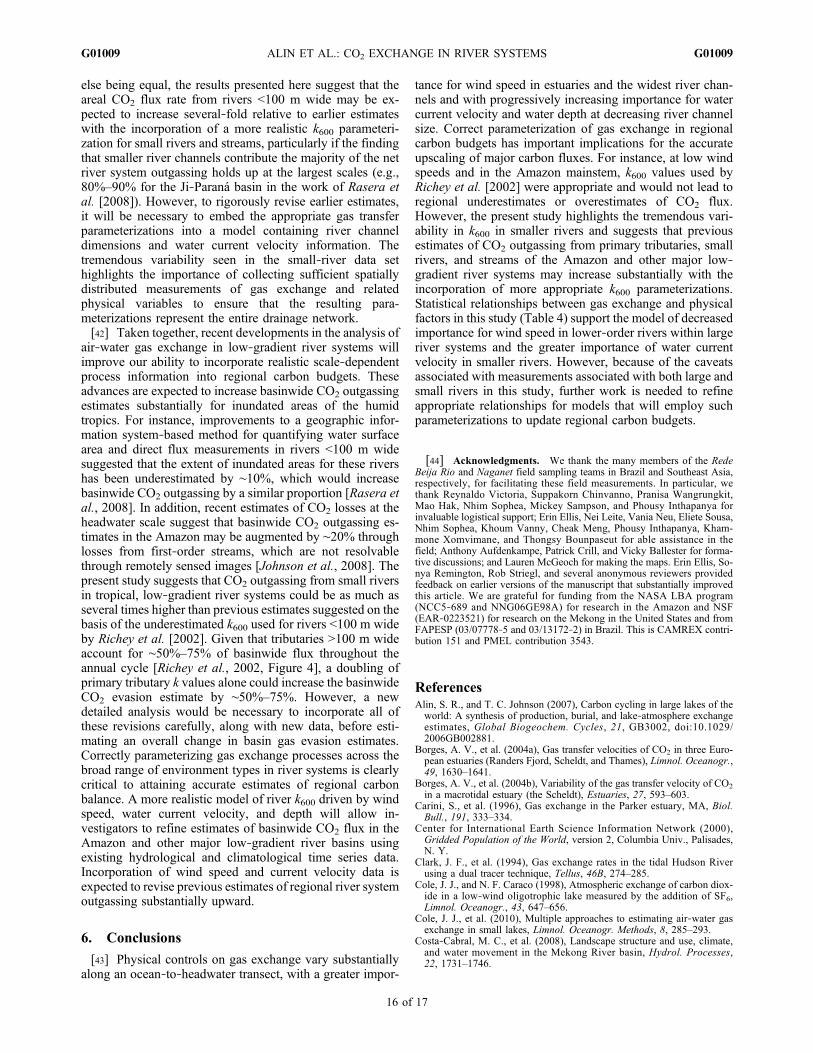
else being equal, the results presented here suggest that theareal CO2 flux rate from rivers <100 m wide may be ex-pected to increase several‐fold relative to earlier estimateswith the incorporation of a more realistic k600 parameteri-zation for small rivers and streams, particularly if the findingthat smaller river channels contribute the majority of the netriver system outgassing holds up at the largest scales (e.g.,80%–90% for the Ji‐Paraná basin in the work of Rasera etal. [2008]). However, to rigorously revise earlier estimates,it will be necessary to embed the appropriate gas transferparameterizations into a model containing river channeldimensions and water current velocity information. Thetremendous variability seen in the small‐river data sethighlights the importance of collecting sufficient spatiallydistributed measurements of gas exchange and relatedphysical variables to ensure that the resulting para-meterizations represent the entire drainage network.[42] Taken together, recent developments in the analysis of
air‐water gas exchange in low‐gradient river systems willimprove our ability to incorporate realistic scale‐dependentprocess information into regional carbon budgets. Theseadvances are expected to increase basinwide CO2 outgassingestimates substantially for inundated areas of the humidtropics. For instance, improvements to a geographic infor-mation system‐based method for quantifying water surfacearea and direct flux measurements in rivers <100 m widesuggested that the extent of inundated areas for these rivershas been underestimated by ∼10%, which would increasebasinwide CO2 outgassing by a similar proportion [Rasera etal., 2008]. In addition, recent estimates of CO2 losses at theheadwater scale suggest that basinwide CO2 outgassing es-timates in the Amazon may be augmented by ∼20% throughlosses from first‐order streams, which are not resolvablethrough remotely sensed images [Johnson et al., 2008]. Thepresent study suggests that CO2 outgassing from small riversin tropical, low‐gradient river systems could be as much asseveral times higher than previous estimates suggested on thebasis of the underestimated k600 used for rivers <100 m wideby Richey et al. [2002]. Given that tributaries >100 m wideaccount for ∼50%–75% of basinwide flux throughout theannual cycle [Richey et al., 2002, Figure 4], a doubling ofprimary tributary k values alone could increase the basinwideCO2 evasion estimate by ∼50%–75%. However, a newdetailed analysis would be necessary to incorporate all ofthese revisions carefully, along with new data, before esti-mating an overall change in basin gas evasion estimates.Correctly parameterizing gas exchange processes across thebroad range of environment types in river systems is clearlycritical to attaining accurate estimates of regional carbonbalance. A more realistic model of river k600 driven by windspeed, water current velocity, and depth will allow in-vestigators to refine estimates of basinwide CO2 flux in theAmazon and other major low‐gradient river basins usingexisting hydrological and climatological time series data.Incorporation of wind speed and current velocity data isexpected to revise previous estimates of regional river systemoutgassing substantially upward.
6. Conclusions
[43] Physical controls on gas exchange vary substantiallyalong an ocean‐to‐headwater transect, with a greater impor-
tance for wind speed in estuaries and the widest river chan-nels and with progressively increasing importance for watercurrent velocity and water depth at decreasing river channelsize. Correct parameterization of gas exchange in regionalcarbon budgets has important implications for the accurateupscaling of major carbon fluxes. For instance, at low windspeeds and in the Amazon mainstem, k600 values used byRichey et al. [2002] were appropriate and would not lead toregional underestimates or overestimates of CO2 flux.However, the present study highlights the tremendous vari-ability in k600 in smaller rivers and suggests that previousestimates of CO2 outgassing from primary tributaries, smallrivers, and streams of the Amazon and other major low‐gradient river systems may increase substantially with theincorporation of more appropriate k600 parameterizations.Statistical relationships between gas exchange and physicalfactors in this study (Table 4) support the model of decreasedimportance for wind speed in lower‐order rivers within largeriver systems and the greater importance of water currentvelocity in smaller rivers. However, because of the caveatsassociated with measurements associated with both large andsmall rivers in this study, further work is needed to refineappropriate relationships for models that will employ suchparameterizations to update regional carbon budgets.
[44] Acknowledgments. We thank the many members of the RedeBeija Rio and Naganet field sampling teams in Brazil and Southeast Asia,respectively, for facilitating these field measurements. In particular, wethank Reynaldo Victoria, Suppakorn Chinvanno, Pranisa Wangrungkit,Mao Hak, Nhim Sophea, Mickey Sampson, and Phousy Inthapanya forinvaluable logistical support; Erin Ellis, Nei Leite, Vania Neu, Eliete Sousa,Nhim Sophea, Khoum Vanny, Cheak Meng, Phousy Inthapanya, Kham-mone Xomvimane, and Thongsy Bounpaseut for able assistance in thefield; Anthony Aufdenkampe, Patrick Crill, and Vicky Ballester for forma-tive discussions; and Lauren McGeoch for making the maps. Erin Ellis, So-nya Remington, Rob Striegl, and several anonymous reviewers providedfeedback on earlier versions of the manuscript that substantially improvedthis article. We are grateful for funding from the NASA LBA program(NCC5‐689 and NNG06GE98A) for research in the Amazon and NSF(EAR‐0223521) for research on the Mekong in the United States and fromFAPESP (03/07778‐5 and 03/13172‐2) in Brazil. This is CAMREX contri-bution 151 and PMEL contribution 3543.
ReferencesAlin, S. R., and T. C. Johnson (2007), Carbon cycling in large lakes of theworld: A synthesis of production, burial, and lake‐atmosphere exchangeestimates, Global Biogeochem. Cycles, 21, GB3002, doi:10.1029/2006GB002881.
Borges, A. V., et al. (2004a), Gas transfer velocities of CO2 in three Euro-pean estuaries (Randers Fjord, Scheldt, and Thames), Limnol. Oceanogr.,49, 1630–1641.
Borges, A. V., et al. (2004b), Variability of the gas transfer velocity of CO2in a macrotidal estuary (the Scheldt), Estuaries, 27, 593–603.
Carini, S., et al. (1996), Gas exchange in the Parker estuary, MA, Biol.Bull., 191, 333–334.
Center for International Earth Science Information Network (2000),Gridded Population of the World, version 2, Columbia Univ., Palisades,N. Y.
Clark, J. F., et al. (1994), Gas exchange rates in the tidal Hudson Riverusing a dual tracer technique, Tellus, 46B, 274–285.
Cole, J. J., and N. F. Caraco (1998), Atmospheric exchange of carbon diox-ide in a low‐wind oligotrophic lake measured by the addition of SF6,Limnol. Oceanogr., 43, 647–656.
Cole, J. J., et al. (2010), Multiple approaches to estimating air‐water gasexchange in small lakes, Limnol. Oceanogr. Methods, 8, 285–293.
Costa‐Cabral, M. C., et al. (2008), Landscape structure and use, climate,and water movement in the Mekong River basin, Hydrol. Processes,22, 1731–1746.
ALIN ET AL.: CO2 EXCHANGE IN RIVER SYSTEMS G01009G01009
16 of 17
Devol, A. H., et al. (1987), The role of gas exchange in the inorganic carbon,oxygen, and 222Rn budgets of the Amazon River, Limnol. Oceanogr., 32,235–248.
Dunne, T., et al. (1998), Exchanges of sediment between the flood plainand channel of the Amazon River in Brazil, Geol. Soc. Am. Bull., 110,450–467.
Elsinger, R. J., and W. S. Moore (1983), Gas exchange in the Pee‐DeeRiver based on 222Rn evasion, Geophys. Res. Lett., 10, 443–446,doi:10.1029/GL010i006p00443.
Frankignoulle, M. (1988), Field measurements of air‐sea CO2 exchange,Limnol. Oceanogr., 33, 313–322.
Genereux, D. P., and H. F. Hemond (1992), Determination of gas exchangerate constants for a small stream on Walker Branch watershed, Tennes-see, Water Resour. Res., 28, 2365–2374, doi:10.1029/92WR01083.
Grant, R. S., and S. Skavronek (1980), Comparison of tracer methods andpredictive equations for determination of stream reaeration coefficientson three small streams in Wisconsin, Water Res. Invest., 193642: WRI80‐19.
Hall, R. O., and J. L. Tank (2003), Ecosystem metabolism controls nitrogenuptake in streams in Grand Teton National Park, Wyoming, Limnol.Oceanogr., 48, 1120–1128.
Hanson, P. C., et al. (2006), Lake dissolved inorganic carbon and dissolvedoxygen: Changing drivers from days to decades, Ecol. Monogr., 76,343–363.
Hartman, B., and D. E. Hammond (1984), Gas exchange rates across thesediment‐water and air‐water interfaces in south San Francisco Bay,J. Geophys. Res., 89, 3593–3603, doi:10.1029/JC089iC03p03593.
Hesslein, R. H., et al. (1991), Carbon dioxide pressure in surface waters ofCanadian lakes, in Air‐Water Mass Transfer: Selected Papers From theSecond International Symposium on Gas Transfer at Water Surfaces,edited by S. C. Wilhelms and J. S. Gulliver, pp. 413–432, Am. Soc. ofCiv. Eng., New York.
Ho, D. T., et al. (2002), Determination of longitudinal dispersion coeffi-cient and net advection in the tidal Hudson River with a large‐scale, highresolution SF6 tracer release experiment, Environ. Sci. Technol., 36,3234–3241.
Jähne, B., and H. Haubecker (1998), Air‐water gas exchange, Annu. Rev.Fluid Mech., 30, 443–468.
Jähne, B., K. Münnich, R. Dutzi, W. Huber, and P. Libner (1987), On theparameters influencing air‐water gas exchange, J. Geophys. Res., 92,1937–1949, doi:10.1029/JC092iC02p01937.
Johnson, M. S., J. Lehmann, S. J. Riha, A. V. Krusche, J. E. Richey, J. P.H. B. Ometto, and E. G. Couto (2008), CO2 efflux from Amazonianheadwater streams represents a significant fate for deep soil respiration,Geophys. Res. Lett., 35, L17401, doi:10.1029/2008GL034619.
Kremer, J. N., et al. (2003a), Technical note: Conditions for using the float-ing chamber method to estimate air‐water gas exchange, Estuaries, 26,985–990.
Kremer, J. N., et al. (2003b), Estuary‐specific variation in the air‐water gasexchange coefficient for oxygen, Estuaries, 26, 829–836.
Kwasnik, J. M., and T. H. Feng (1979), Development of a modified tracertechnique for measuring the stream reaeration rate, Rep. PB 296317,Natl. Tech. Inf. Serv., Springfield, Va.
MacIntyre, S., et al. (1995), Trace gas exchange across the air‐water inter-face in freshwater and coastal marine environments, in Biogenic TraceGases: Measuring Emissions From Soil and Water, edited by P. A.Matson and R. C. Harriss, pp. 52–97, Blackwell Sci., Oxford, U. K.
MacIntyre, S., et al. (2002), The critical importance of buoyancy flux forgas flux across the air‐water interface, in Gas Transfer at Water Surfaces,edited by M. A. Donelan et al., pp. 135–139, AGU, Washington, D. C.
Mariano, A. J., E. H. Ryan, B. D. Perkins, and S. Smithers (1995), TheMariano Global Surface Velocity Analysis 1.0, U.S. Coast Guard Tech.Rep., CG‐D‐34‐95.
Marino, R., and R. W. Howarth (1993), Atmospheric oxygen exchangein the Hudson River: Dome measurements and comparison with othernatural waters, Estuaries, 16, 433–445.
Marzolf, E. R., et al. (1994), Improvements to the diurnal upstream‐down-stream dissolved oxygen change technique for determining whole‐streammetabolism in small streams, Can. J. Fish. Aquat. Sci., 51, 1591–1598.
Mayorga, E., et al. (2005), Young organic matter as a source of carbondioxide outgassing from Amazonian rivers, Nature, 436, 538–541.
Melching, C. S., and H. E. Flores (1999), Reaeration equations derivedfrom U.S. Geological Survey database, J. Environ. Eng., 125, 407–414.
O’Connor, D. J., and E. Dobbins (1958), Mechanism of reaeration in nat-ural streams, Trans. Am. Soc. Civ. Eng., 123, 641–684.
Oke, T. R. (1988), Boundary Layer Climates, Routledge, Boca Raton, Fla.Owens, M., et al. (1964), Some reaeration studies in streams, Int. J. AirWater Pollut., 8, 469–486.
Rasera, M. F. F. L., et al. (2008), Estimating the surface area of small riversin the southwestern Amazon and their role in CO2 outgassing, EarthInteract., 12(6), 1–15.
Raymond, P. A., and J. J. Cole (2001), Gas exchange in rivers and estuar-ies: Choosing a gas transfer velocity, Estuaries, 24, 312–317.
Richey, J. E., et al. (2002), Outgassing from Amazonian rivers and wet-lands as a large tropical source of atmospheric CO2, Nature, 416, 617–620.
Roberts, B. J., et al. (2007), Multiple scales of temporal variability in eco-system metabolism rates: results from 2 years of continuous monitoringin a forested headwater stream, Ecosystems, 10, 588–606.
Sebacher, D. I., et al. (1983), Methane flux across the air‐water interface:Air velocity effects, Tellus, 35B, 103–109.
Sweeney, C., et al. (2007), Constraining global air‐sea gas exchange forCO2 with recent bomb 14C measurements, Global Biogeochem. Cycles,21, GB2015, doi:10.1029/2006GB002784.
Takahashi, T., et al. (2009), Climatological mean and decadal change insurface ocean pCO2, and net sea‐air CO2 flux over the global oceans,Deep Sea Res., Part II, 56, 554–577.
Tsivoglou, E. C. (1967), Tracer measurements of stream reaeration, Fed.Water Pollut. Control Admin., U.S. Dep. of Interior, Washington, D. C.
Wanninkhof, R. (1992), Relationship between wind speed and gasexchange over the ocean, J. Geophys. Res. , 97 , 7373–7382,doi:10.1029/92JC00188.
Wanninkhof, R., P. Mulholland, and J. Elwood (1990), Gas exchange ratesfor a first‐order stream determined with deliberate and natural tracers,Water Resour. Res., 26, 1621–1630, doi:10.1029/WR026i007p01621.
Wanninkhof, R., et al. (2009), Advances in quantifying air‐sea gasexchange and environmental forcing, Annu. Rev. Mar. Sci., 1, 213–244.
Weiss, R. F. (1974), Carbon dioxide in water and seawater: The solubilityof a non‐ideal gas, Mar. Chem., 2, 203–215.
Wilcock, R. J. (1984), Reaeration studies on some New Zealand riversusing methyl chloride as a gas tracer, in Gas Transfer at Water Surfaces,edited by W. Brutsaert and G. J. Jirka, pp. 413–421, D. Reidel, Hingham,Mass.
Zappa, C. J., et al. (2003), Variation in surface turbulence and the gas trans-fer velocity over a tidal cycle in a macro‐tidal estuary, Estuaries, 26,1401–1415.
Zappa, C. J., W. R. McGillis, P. A. Raymond, J. B. Edson, E. J. Hintsa,H. J. Zemmelink, J. W. H. Dacey, and D. T. Ho (2007), Environmentalturbulent mixing controls on air‐water gas exchange in marine andaquatic systems, Geophys. Res. Lett., 34, L10601, doi:10.1029/2006GL028790.
S. R. Alin, Pacific Marine Environmental Laboratory, National Oceanicand Atmospheric Administration, Seattle, WA 98115, USA. ([email protected])G. W. Holtgrieve, School of Aquatic and Fishery Sciences, University of
Washington, Seattle, WA 98195, USA.A. V. Krusche and M. F. F. L. Rasera, Centro de Energia Nuclear na
Agricultura, Universidade de São Paulo, Piracicaba, SP 13400‐970, Brazil.J. E. Richey, School of Oceanography, University of Washington,
Seattle, WA 98195, USA.C. I. Salimon, Universidade Federal do Acre, Rio Branco, AC 69915‐
900, Brazil.A. Snidvongs, Southeast Asia START Global Change Regional Center,
Chulalongkorn University, Bangkok 10330, Thailand.
ALIN ET AL.: CO2 EXCHANGE IN RIVER SYSTEMS G01009G01009
17 of 17