Economics (2-downloads) - E-Learning KIMEP

55

PART TWO How Markets Work

After studying this chapter, you will be able to:

� Describe a competitive market and think about a price as an opportunity cost

� Explain the influences on demand� Explain the influences on supply� Explain how demand and supply determine prices

and quantities bought and sold� Use the demand and supply model to make

predictions about changes in prices and quantities

hat makes the price of oil double and the price of gasoline almost double injust one year? Will these prices keep on rising? Are the oil companies takingadvantage of people? This chapter enables you to answer these and similarquestions about prices—prices that rise, prices that fall, and prices thatfluctuate.

You already know that economics is about the choices people make to copewith scarcity and how those choices respond to incentives. Prices act asincentives. You’re going to see how people respond to prices and how pricesget determined by demand and supply. The demand and supply model that

you study in this chapter is the main tool of economics. Ithelps us to answer the big economic question: What, how,and for whom goods and services are produced?

At the end of the chapter, in Reading Between the Lines, we’ll apply themodel to the market for coffee and explain why its price increased sharply in2010 and why it was expected to rise again.

DEMAND AND SUPPLY

W

3

56 CHAPTER 3 Demand and Supply

Let’s begin our study of demand and supply,starting with demand.

◆ Markets and PricesWhen you need a new pair of running shoes, want abagel and a latte, plan to upgrade your cell phone, orneed to fly home for Thanksgiving, you must find aplace where people sell those items or offer those ser-vices. The place in which you find them is a market.You learned in Chapter 2 (p. 42) that a market is anyarrangement that enables buyers and sellers to getinformation and to do business with each other.

A market has two sides: buyers and sellers. Thereare markets for goods such as apples and hiking boots,for services such as haircuts and tennis lessons, for fac-tors of production such as computer programmers andearthmovers, and for other manufactured inputs suchas memory chips and auto parts. There are also mar-kets for money such as Japanese yen and for financialsecurities such as Yahoo! stock. Only our imaginationlimits what can be traded in markets.

Some markets are physical places where buyers andsellers meet and where an auctioneer or a brokerhelps to determine the prices. Examples of this typeof market are the New York Stock Exchange and thewholesale fish, meat, and produce markets.

Some markets are groups of people spread aroundthe world who never meet and know little about eachother but are connected through the Internet or by tele-phone and fax. Examples are the e-commerce marketsand the currency markets.

But most markets are unorganized collections ofbuyers and sellers. You do most of your trading inthis type of market. An example is the market forbasketball shoes. The buyers in this $3 billion-a-yearmarket are the 45 million Americans who play bas-ketball (or who want to make a fashion statement).The sellers are the tens of thousands of retail sportsequipment and footwear stores. Each buyer can visitseveral different stores, and each seller knows that thebuyer has a choice of stores.

Markets vary in the intensity of competition thatbuyers and sellers face. In this chapter, we’re going tostudy a competitive market—a market that has manybuyers and many sellers, so no single buyer or sellercan influence the price.

Producers offer items for sale only if the price ishigh enough to cover their opportunity cost. Andconsumers respond to changing opportunity cost byseeking cheaper alternatives to expensive items.

We are going to study how people respond toprices and the forces that determine prices. But to

pursue these tasks, we need to understand the rela-tionship between a price and an opportunity cost.

In everyday life, the price of an object is the num-ber of dollars that must be given up in exchange for it.Economists refer to this price as the money price.

The opportunity cost of an action is the highest-valued alternative forgone. If, when you buy a cup ofcoffee, the highest-valued thing you forgo is somegum, then the opportunity cost of the coffee is thequantity of gum forgone. We can calculate the quan-tity of gum forgone from the money prices of thecoffee and the gum.

If the money price of coffee is $1 a cup and themoney price of gum is 50¢ a pack, then the opportu-nity cost of one cup of coffee is two packs of gum. Tocalculate this opportunity cost, we divide the price ofa cup of coffee by the price of a pack of gum and findthe ratio of one price to the other. The ratio of oneprice to another is called a relative price, and a relativeprice is an opportunity cost.

We can express the relative price of coffee in termsof gum or any other good. The normal way ofexpressing a relative price is in terms of a “basket” ofall goods and services. To calculate this relative price,we divide the money price of a good by the moneyprice of a “basket” of all goods (called a price index).The resulting relative price tells us the opportunitycost of the good in terms of how much of the “bas-ket” we must give up to buy it.

The demand and supply model that we are aboutto study determines relative prices, and the word“price” means relative price. When we predict that aprice will fall, we do not mean that its money pricewill fall—although it might. We mean that its relativeprice will fall. That is, its price will fall relative to theaverage price of other goods and services.

REVIEW QUIZ1 What is the distinction between a money price

and a relative price?2 Explain why a relative price is an opportunity cost.3 Think of examples of goods whose relative price

has risen or fallen by a large amount.You can work these questions in Study Plan 3.1 and get instant feedback.

◆ DemandIf you demand something, then you

1. Want it,2. Can afford it, and3. Plan to buy it.

Wants are the unlimited desires or wishes that peo-ple have for goods and services. How many timeshave you thought that you would like something “ifonly you could afford it” or “if it weren’t so expen-sive”? Scarcity guarantees that many—perhapsmost—of our wants will never be satisfied. Demandreflects a decision about which wants to satisfy.

The quantity demanded of a good or service is theamount that consumers plan to buy during a giventime period at a particular price. The quantitydemanded is not necessarily the same as the quantityactually bought. Sometimes the quantity demandedexceeds the amount of goods available, so the quan-tity bought is less than the quantity demanded.

The quantity demanded is measured as an amountper unit of time. For example, suppose that you buyone cup of coffee a day. The quantity of coffee thatyou demand can be expressed as 1 cup per day, 7cups per week, or 365 cups per year.

Many factors influence buying plans, and one ofthem is the price. We look first at the relationshipbetween the quantity demanded of a good and itsprice. To study this relationship, we keep all otherinfluences on buying plans the same and we ask:How, other things remaining the same, does thequantity demanded of a good change as its pricechanges?

The law of demand provides the answer.

The Law of DemandThe law of demand states

Other things remaining the same, the higher theprice of a good, the smaller is the quantitydemanded; and the lower the price of a good, thegreater is the quantity demanded.

Why does a higher price reduce the quantitydemanded? For two reasons:

■ Substitution effect■ Income effect

Substitution Effect When the price of a good rises,other things remaining the same, its relative price—its opportunity cost—rises. Although each good isunique, it has substitutes—other goods that can beused in its place. As the opportunity cost of a goodrises, the incentive to economize on its use andswitch to a substitute becomes stronger.

Income Effect When a price rises, other thingsremaining the same, the price rises relative to income.Faced with a higher price and an unchanged income,people cannot afford to buy all the things they previ-ously bought. They must decrease the quantitiesdemanded of at least some goods and services.Normally, the good whose price has increased will beone of the goods that people buy less of.

To see the substitution effect and the income effectat work, think about the effects of a change in theprice of an energy bar. Several different goods aresubstitutes for an energy bar. For example, an energydrink could be consumed instead of an energy bar.

Suppose that an energy bar initially sells for $3 andthen its price falls to $1.50. People now substituteenergy bars for energy drinks—the substitution effect.And with a budget that now has some slack from thelower price of an energy bar, people buy even moreenergy bars—the income effect. The quantity of energybars demanded increases for these two reasons.

Now suppose that an energy bar initially sells for$3 and then the price doubles to $6. People now buyfewer energy bars and more energy drinks—the sub-stitution effect. And faced with a tighter budget, peo-ple buy even fewer energy bars—the income effect.The quantity of energy bars demanded decreases forthese two reasons.

Demand Curve and Demand ScheduleYou are now about to study one of the two most usedcurves in economics: the demand curve. You are alsogoing to encounter one of the most critical distinc-tions: the distinction between demand and quantitydemanded.

The term demand refers to the entire relationshipbetween the price of a good and the quantitydemanded of that good. Demand is illustrated by thedemand curve and the demand schedule. The termquantity demanded refers to a point on a demandcurve—the quantity demanded at a particular price.

Demand 57

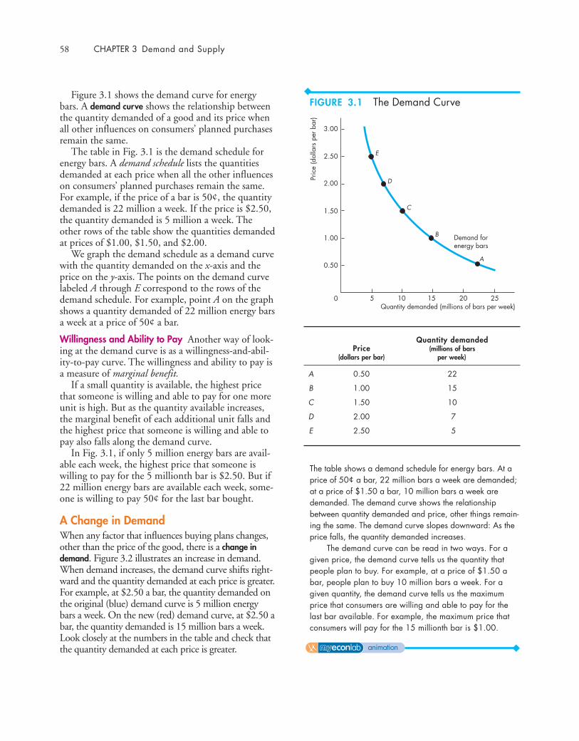
Figure 3.1 shows the demand curve for energybars. A demand curve shows the relationship betweenthe quantity demanded of a good and its price whenall other influences on consumers’ planned purchasesremain the same.

The table in Fig. 3.1 is the demand schedule forenergy bars. A demand schedule lists the quantitiesdemanded at each price when all the other influenceson consumers’ planned purchases remain the same.For example, if the price of a bar is 50¢, the quantitydemanded is 22 million a week. If the price is $2.50,the quantity demanded is 5 million a week. Theother rows of the table show the quantities demandedat prices of $1.00, $1.50, and $2.00.

We graph the demand schedule as a demand curvewith the quantity demanded on the x-axis and theprice on the y-axis. The points on the demand curvelabeled A through E correspond to the rows of thedemand schedule. For example, point A on the graphshows a quantity demanded of 22 million energy barsa week at a price of 50¢ a bar.

Willingness and Ability to Pay Another way of look-ing at the demand curve is as a willingness-and-abil-ity-to-pay curve. The willingness and ability to pay isa measure of marginal benefit.

If a small quantity is available, the highest pricethat someone is willing and able to pay for one moreunit is high. But as the quantity available increases,the marginal benefit of each additional unit falls andthe highest price that someone is willing and able topay also falls along the demand curve.

In Fig. 3.1, if only 5 million energy bars are avail-able each week, the highest price that someone iswilling to pay for the 5 millionth bar is $2.50. But if22 million energy bars are available each week, some-one is willing to pay 50¢ for the last bar bought.

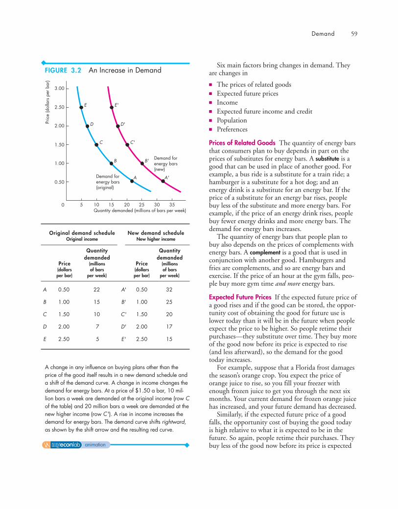
A Change in DemandWhen any factor that influences buying plans changes,other than the price of the good, there is a change indemand. Figure 3.2 illustrates an increase in demand.When demand increases, the demand curve shifts right-ward and the quantity demanded at each price is greater.For example, at $2.50 a bar, the quantity demanded onthe original (blue) demand curve is 5 million energybars a week. On the new (red) demand curve, at $2.50 abar, the quantity demanded is 15 million bars a week.Look closely at the numbers in the table and check thatthe quantity demanded at each price is greater.


3.00

5 15 20 25

Pric

e (d

olla

rs p

er b

ar)

Quantity demanded (millions of bars per week)

Demand forenergy bars

10

E

D

C

B

A

2.50

2.00

1.50

1.00

0.50

0

The table shows a demand schedule for energy bars. At aprice of 50¢ a bar, 22 million bars a week are demanded;at a price of $1.50 a bar, 10 million bars a week aredemanded. The demand curve shows the relationshipbetween quantity demanded and price, other things remain-ing the same. The demand curve slopes downward: As theprice falls, the quantity demanded increases.

The demand curve can be read in two ways. For agiven price, the demand curve tells us the quantity thatpeople plan to buy. For example, at a price of $1.50 abar, people plan to buy 10 million bars a week. For agiven quantity, the demand curve tells us the maximumprice that consumers are willing and able to pay for thelast bar available. For example, the maximum price thatconsumers will pay for the 15 millionth bar is $1.00.

Quantity demandedPrice (millions of bars

(dollars per bar) per week)

A 0.50 22

B 1.00 15

C 1.50 10

D 2.00 7

E 2.50 5

FIGURE 3.1 The Demand Curve

animation

Six main factors bring changes in demand. Theyare changes in

■ The prices of related goods■ Expected future prices■ Income■ Expected future income and credit■ Population■ Preferences

Prices of Related Goods The quantity of energy barsthat consumers plan to buy depends in part on theprices of substitutes for energy bars. A substitute is agood that can be used in place of another good. Forexample, a bus ride is a substitute for a train ride; ahamburger is a substitute for a hot dog; and anenergy drink is a substitute for an energy bar. If theprice of a substitute for an energy bar rises, peoplebuy less of the substitute and more energy bars. Forexample, if the price of an energy drink rises, peoplebuy fewer energy drinks and more energy bars. Thedemand for energy bars increases.

The quantity of energy bars that people plan tobuy also depends on the prices of complements withenergy bars. A complement is a good that is used inconjunction with another good. Hamburgers andfries are complements, and so are energy bars andexercise. If the price of an hour at the gym falls, peo-ple buy more gym time and more energy bars.

Expected Future Prices If the expected future price ofa good rises and if the good can be stored, the oppor-tunity cost of obtaining the good for future use islower today than it will be in the future when peopleexpect the price to be higher. So people retime theirpurchases—they substitute over time. They buy moreof the good now before its price is expected to rise(and less afterward), so the demand for the goodtoday increases.

For example, suppose that a Florida frost damagesthe season’s orange crop. You expect the price oforange juice to rise, so you fill your freezer withenough frozen juice to get you through the next sixmonths. Your current demand for frozen orange juicehas increased, and your future demand has decreased.

Similarly, if the expected future price of a goodfalls, the opportunity cost of buying the good todayis high relative to what it is expected to be in thefuture. So again, people retime their purchases. Theybuy less of the good now before its price is expected

Demand 59

3.00

5 15 20 35

Pric

e (d

olla

rs p

er b

ar)

Quantity demanded (millions of bars per week)

Demand forenergy bars(original)

Demand forenergy bars(new)

10

E

D

C

B

A

2.50

2.00

1.50

1.00

0.50

0 3025

E'

D'

C'

B'

A'

Original demand schedule New demand scheduleOriginal income New higher income

Quantity Quantitydemanded demanded

Price (millions Price (millions(dollars of bars (dollars of barsper bar) per week) per bar) per week)

A 0.50 22 A' 0.50 32

B 1.00 15 B' 1.00 25

C 1.50 10 C' 1.50 20

D 2.00 7 D' 2.00 17

E 2.50 5 E' 2.50 15

A change in any influence on buying plans other than theprice of the good itself results in a new demand schedule anda shift of the demand curve. A change in income changes thedemand for energy bars. At a price of $1.50 a bar, 10 mil-lion bars a week are demanded at the original income (row Cof the table) and 20 million bars a week are demanded at thenew higher income (row C'). A rise in income increases thedemand for energy bars. The demand curve shifts rightward,as shown by the shift arrow and the resulting red curve.

FIGURE 3.2 An Increase in Demand

animation

Preferences Demand depends on preferences.Preferences determine the value that people place oneach good and service. Preferences depend on suchthings as the weather, information, and fashion. Forexample, greater health and fitness awareness hasshifted preferences in favor of energy bars, so thedemand for energy bars has increased.

Table 3.1 summarizes the influences on demandand the direction of those influences.

A Change in the Quantity Demanded Versus a Change in DemandChanges in the influences on buying plans bringeither a change in the quantity demanded or achange in demand. Equivalently, they bring either amovement along the demand curve or a shift of thedemand curve. The distinction between a change in


to fall, so the demand for the good decreases todayand increases in the future.

Computer prices are constantly falling, and thisfact poses a dilemma. Will you buy a new computernow, in time for the start of the school year, or willyou wait until the price has fallen some more? Becausepeople expect computer prices to keep falling, the cur-rent demand for computers is less (and the futuredemand is greater) than it otherwise would be.

Income Consumers’ income influences demand.When income increases, consumers buy more of mostgoods; and when income decreases, consumers buyless of most goods. Although an increase in incomeleads to an increase in the demand for most goods, itdoes not lead to an increase in the demand for allgoods. A normal good is one for which demandincreases as income increases. An inferior good is onefor which demand decreases as income increases. Asincomes increase, the demand for air travel (a normalgood) increases and the demand for long-distance bustrips (an inferior good) decreases.

Expected Future Income and Credit When expectedfuture income increases or credit becomes easier toget, demand for the good might increase now. Forexample, a salesperson gets the news that she willreceive a big bonus at the end of the year, so she goesinto debt and buys a new car right now, rather thanwait until she receives the bonus.

Population Demand also depends on the size and theage structure of the population. The larger the popu-lation, the greater is the demand for all goods andservices; the smaller the population, the smaller is thedemand for all goods and services.

For example, the demand for parking spaces ormovies or just about anything that you can imagineis much greater in New York City (population 7.5million) than it is in Boise, Idaho (population150,000).

Also, the larger the proportion of the populationin a given age group, the greater is the demand forthe goods and services used by that age group.

For example, during the 1990s, a decrease in thecollege-age population decreased the demand for col-lege places. During those same years, the number ofAmericans aged 85 years and over increased by morethan 1 million. As a result, the demand for nursinghome services increased.

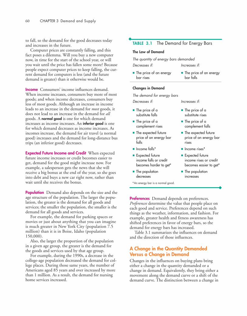
TABLE 3.1 The Demand for Energy Bars

The Law of Demand

The quantity of energy bars demanded

Decreases if: Increases if:

■ The price of an energy bar rises

■ The price of an energy bar falls

■ The price of a substitute falls

■ The price of acomplement rises

■ The expected futureprice of an energy barfalls

■ Income falls*

■ Expected future income falls or creditbecomes harder to get*

■ The population decreases

■ The price of a substitute rises

■ The price of acomplement falls

■ The expected futureprice of an energy barrises

■ Income rises*

■ Expected future income rises or creditbecomes easier to get*

■ The population increases

Changes in Demand

The demand for energy bars


*An energy bar is a normal good.

the quantity demanded and a change in demand isthe same as that between a movement along thedemand curve and a shift of the demand curve.

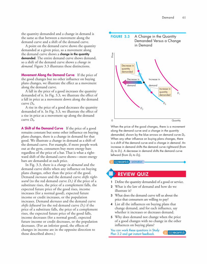
A point on the demand curve shows the quantitydemanded at a given price, so a movement alongthe demand curve shows a change in the quantitydemanded. The entire demand curve shows demand,so a shift of the demand curve shows a change indemand. Figure 3.3 illustrates these distinctions.

Movement Along the Demand Curve If the price ofthe good changes but no other influence on buyingplans changes, we illustrate the effect as a movementalong the demand curve.

A fall in the price of a good increases the quantitydemanded of it. In Fig. 3.3, we illustrate the effect ofa fall in price as a movement down along the demandcurve D0.

A rise in the price of a good decreases the quantitydemanded of it. In Fig. 3.3, we illustrate the effect ofa rise in price as a movement up along the demandcurve D0.

A Shift of the Demand Curve If the price of a goodremains constant but some other influence on buyingplans changes, there is a change in demand for thatgood. We illustrate a change in demand as a shift ofthe demand curve. For example, if more people workout at the gym, consumers buy more energy barsregardless of the price of a bar. That is what a right-ward shift of the demand curve shows—more energybars are demanded at each price.

In Fig. 3.3, there is a change in demand and thedemand curve shifts when any influence on buyingplans changes, other than the price of the good.Demand increases and the demand curve shifts right-ward (to the red demand curve D1) if the price of asubstitute rises, the price of a complement falls, theexpected future price of the good rises, incomeincreases (for a normal good), expected futureincome or credit increases, or the populationincreases. Demand decreases and the demand curveshifts leftward (to the red demand curve D2) if theprice of a substitute falls, the price of a complementrises, the expected future price of the good falls,income decreases (for a normal good), expectedfuture income or credit decreases, or the populationdecreases. (For an inferior good, the effects ofchanges in income are in the opposite direction tothose described above.)

Demand 61

Quantity

Pric

e

Decrease in

demand

D

D0

2

Increase in

demandIncrease inquantitydemanded

Decrease inquantitydemanded

0

D1

When the price of the good changes, there is a movementalong the demand curve and a change in the quantitydemanded, shown by the blue arrows on demand curve D0.When any other influence on buying plans changes, thereis a shift of the demand curve and a change in demand. Anincrease in demand shifts the demand curve rightward (fromD0 to D1). A decrease in demand shifts the demand curveleftward (from D0 to D2).

FIGURE 3.3 A Change in the QuantityDemanded Versus a Change in Demand

animation

REVIEW QUIZ1 Define the quantity demanded of a good or service.2 What is the law of demand and how do we

illustrate it?3 What does the demand curve tell us about the

price that consumers are willing to pay?4 List all the influences on buying plans that

change demand, and for each influence, saywhether it increases or decreases demand.

5 Why does demand not change when the priceof a good changes with no change in the otherinfluences on buying plans?

You can work these questions in Study Plan 3.2 and get instant feedback.

◆ SupplyIf a firm supplies a good or service, the firm

1. Has the resources and technology to produce it,2. Can profit from producing it, and3. Plans to produce it and sell it.

A supply is more than just having the resources andthe technology to produce something. Resources andtechnology are the constraints that limit what ispossible.

Many useful things can be produced, but they arenot produced unless it is profitable to do so. Supplyreflects a decision about which technologically feasi-ble items to produce.

The quantity supplied of a good or service is theamount that producers plan to sell during a giventime period at a particular price. The quantity sup-plied is not necessarily the same amount as thequantity actually sold. Sometimes the quantity sup-plied is greater than the quantity demanded, so thequantity sold is less than the quantity supplied.

Like the quantity demanded, the quantity sup-plied is measured as an amount per unit of time. Forexample, suppose that GM produces 1,000 cars aday. The quantity of cars supplied by GM can beexpressed as 1,000 a day, 7,000 a week, or 365,000 ayear. Without the time dimension, we cannot tellwhether a particular quantity is large or small.

Many factors influence selling plans, and againone of them is the price of the good. We look firstat the relationship between the quantity supplied ofa good and its price. Just as we did when we studieddemand, to isolate the relationship between thequantity supplied of a good and its price, we keepall other influences on selling plans the same andask: How does the quantity supplied of a goodchange as its price changes when other thingsremain the same?

The law of supply provides the answer.

The Law of SupplyThe law of supply states:

Other things remaining the same, the higher theprice of a good, the greater is the quantity supplied;and the lower the price of a good, the smaller is thequantity supplied.

Why does a higher price increase the quantity sup-plied? It is because marginal cost increases. As thequantity produced of any good increases, the mar-ginal cost of producing the good increases. (SeeChapter 2, p. 33 to review marginal cost.)

It is never worth producing a good if the pricereceived for the good does not at least cover the mar-ginal cost of producing it. When the price of a goodrises, other things remaining the same, producers arewilling to incur a higher marginal cost, so theyincrease production. The higher price brings forth anincrease in the quantity supplied.

Let’s now illustrate the law of supply with a supplycurve and a supply schedule.

Supply Curve and Supply ScheduleYou are now going to study the second of the twomost used curves in economics: the supply curve.You’re also going to learn about the critical distinc-tion between supply and quantity supplied.

The term supply refers to the entire relationshipbetween the price of a good and the quantity sup-plied of it. Supply is illustrated by the supply curveand the supply schedule. The term quantity suppliedrefers to a point on a supply curve—the quantitysupplied at a particular price.

Figure 3.4 shows the supply curve of energy bars. Asupply curve shows the relationship between the quan-tity supplied of a good and its price when all otherinfluences on producers’ planned sales remain the same.The supply curve is a graph of a supply schedule.

The table in Fig. 3.4 sets out the supply schedulefor energy bars. A supply schedule lists the quantitiessupplied at each price when all the other influences onproducers’ planned sales remain the same. For exam-ple, if the price of an energy bar is 50¢, the quantitysupplied is zero—in row A of the table. If the price ofan energy bar is $1.00, the quantity supplied is 6 mil-lion energy bars a week—in row B. The other rows ofthe table show the quantities supplied at prices of$1.50, $2.00, and $2.50.

To make a supply curve, we graph the quantitysupplied on the x-axis and the price on the y-axis.The points on the supply curve labeled A through Ecorrespond to the rows of the supply schedule. Forexample, point A on the graph shows a quantity sup-plied of zero at a price of 50¢ an energy bar. Point Eshows a quantity supplied of 15 million bars at $2.50an energy bar.


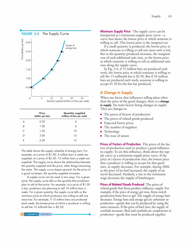
Minimum Supply Price The supply curve can beinterpreted as a minimum-supply-price curve—acurve that shows the lowest price at which someone iswilling to sell. This lowest price is the marginal cost.

If a small quantity is produced, the lowest price atwhich someone is willing to sell one more unit is low.But as the quantity produced increases, the marginalcost of each additional unit rises, so the lowest priceat which someone is willing to sell an additional unitrises along the supply curve.

In Fig. 3.4, if 15 million bars are produced eachweek, the lowest price at which someone is willing tosell the 15 millionth bar is $2.50. But if 10 millionbars are produced each week, someone is willing toaccept $1.50 for the last bar produced.

A Change in SupplyWhen any factor that influences selling plans otherthan the price of the good changes, there is a changein supply. Six main factors bring changes in supply.They are changes in

■ The prices of factors of production■ The prices of related goods produced■ Expected future prices■ The number of suppliers■ Technology■ The state of nature

Prices of Factors of Production The prices of the fac-tors of production used to produce a good influenceits supply. To see this influence, think about the sup-ply curve as a minimum-supply-price curve. If theprice of a factor of production rises, the lowest pricethat a producer is willing to accept for that goodrises, so supply decreases. For example, during 2008,as the price of jet fuel increased, the supply of airtravel decreased. Similarly, a rise in the minimumwage decreases the supply of hamburgers.

Prices of Related Goods Produced The prices ofrelated goods that firms produce influence supply. Forexample, if the price of energy gel rises, firms switchproduction from bars to gel. The supply of energy barsdecreases. Energy bars and energy gel are substitutes inproduction—goods that can be produced by using thesame resources. If the price of beef rises, the supply ofcowhide increases. Beef and cowhide are complements inproduction—goods that must be produced together.

Supply 63

3.00

5 15 20 25

Pric

e (d

olla

rs p

er b

ar)

Quantity supplied (millions of bars per week)

Supply ofenergy bars

10

E

D

C

B

A

2.50

2.00

1.50

1.00

0.50

0

Price Quantity supplied(dollars per bar) (millions of bars per week)

A 0.50 0

B 1.00 6

C 1.50 10

D 2.00 13

E 2.50 15

The table shows the supply schedule of energy bars. Forexample, at a price of $1.00, 6 million bars a week aresupplied; at a price of $2.50, 15 million bars a week aresupplied. The supply curve shows the relationship betweenthe quantity supplied and the price, other things remainingthe same. The supply curve slopes upward: As the price ofa good increases, the quantity supplied increases.

A supply curve can be read in two ways. For a givenprice, the supply curve tells us the quantity that producersplan to sell at that price. For example, at a price of $1.50a bar, producers are planning to sell 10 million bars aweek. For a given quantity, the supply curve tells us theminimum price at which producers are willing to sell onemore bar. For example, if 15 million bars are producedeach week, the lowest price at which a producer is willingto sell the 15 millionth bar is $2.50.

FIGURE 3.4 The Supply Curve

animation

Expected Future Prices If the expected future price ofa good rises, the return from selling the good in thefuture increases and is higher than it is today. So sup-ply decreases today and increases in the future.

The Number of Suppliers The larger the number offirms that produce a good, the greater is the supply ofthe good. As new firms enter an industry, the supplyin that industry increases. As firms leave an industry,the supply in that industry decreases.

Technology The term “technology” is used broadly tomean the way that factors of production are used toproduce a good. A technology change occurs when anew method is discovered that lowers the cost of pro-ducing a good. For example, new methods used inthe factories that produce computer chips have low-ered the cost and increased the supply of chips.

The State of Nature The state of nature includes allthe natural forces that influence production. Itincludes the state of the weather and, more broadly,the natural environment. Good weather can increasethe supply of many agricultural products and badweather can decrease their supply. Extreme naturalevents such as earthquakes, tornadoes, and hurricanescan also influence supply.

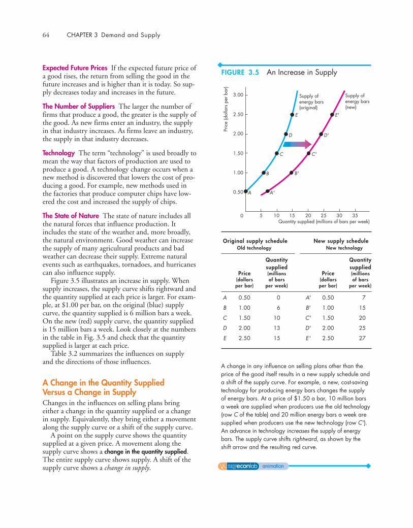
Figure 3.5 illustrates an increase in supply. Whensupply increases, the supply curve shifts rightward andthe quantity supplied at each price is larger. For exam-ple, at $1.00 per bar, on the original (blue) supplycurve, the quantity supplied is 6 million bars a week.On the new (red) supply curve, the quantity suppliedis 15 million bars a week. Look closely at the numbersin the table in Fig. 3.5 and check that the quantitysupplied is larger at each price.

Table 3.2 summarizes the influences on supplyand the directions of those influences.

A Change in the Quantity Supplied Versus a Change in SupplyChanges in the influences on selling plans bringeither a change in the quantity supplied or a changein supply. Equivalently, they bring either a movementalong the supply curve or a shift of the supply curve.

A point on the supply curve shows the quantitysupplied at a given price. A movement along thesupply curve shows a change in the quantity supplied.The entire supply curve shows supply. A shift of thesupply curve shows a change in supply.


3.00

5 15 20 35

Pric

e (d

olla

rs p

er b

ar)

Quantity supplied (millions of bars per week)

Supply ofenergy bars(original)

Supply ofenergy bars(new)

10

E

D

C

B

A

2.50

2.00

1.50

1.00

0.50

0 3025

E'

D'

C'

B'

A'

Original supply schedule New supply scheduleOld technology New technology

Quantity Quantitysupplied supplied

Price (millions Price (millions(dollars of bars (dollars of barsper bar) per week) per bar) per week)

A 0.50 0 A' 0.50 7

B 1.00 6 B' 1.00 15

C 1.50 10 C' 1.50 20

D 2.00 13 D' 2.00 25

E 2.50 15 E' 2.50 27

A change in any influence on selling plans other than theprice of the good itself results in a new supply schedule anda shift of the supply curve. For example, a new, cost-savingtechnology for producing energy bars changes the supplyof energy bars. At a price of $1.50 a bar, 10 million barsa week are supplied when producers use the old technology(row C of the table) and 20 million energy bars a week aresupplied when producers use the new technology (row C').An advance in technology increases the supply of energybars. The supply curve shifts rightward, as shown by theshift arrow and the resulting red curve.

FIGURE 3.5 An Increase in Supply

animation

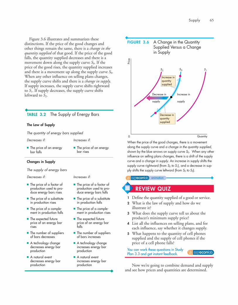
Figure 3.6 illustrates and summarizes thesedistinctions. If the price of the good changes andother things remain the same, there is a change in thequantity supplied of that good. If the price of the goodfalls, the quantity supplied decreases and there is amovement down along the supply curve S0. If theprice of the good rises, the quantity supplied increasesand there is a movement up along the supply curve S0.When any other influence on selling plans changes,the supply curve shifts and there is a change in supply.If supply increases, the supply curve shifts rightwardto S1. If supply decreases, the supply curve shiftsleftward to S2.

Now we’re going to combine demand and supplyand see how prices and quantities are determined.

Supply 65

Quantity

Pric

e

Decrease in

supply

Increase in

supply

0

Decrease inquantitysupplied

Increase inquantitysupplied

S2 S0 S1

When the price of the good changes, there is a movementalong the supply curve and a change in the quantity supplied,shown by the blue arrows on supply curve S0. When any otherinfluence on selling plans changes, there is a shift of the supplycurve and a change in supply. An increase in supply shifts thesupply curve rightward (from S0 to S1), and a decrease in sup-ply shifts the supply curve leftward (from S0 to S2).

FIGURE 3.6 A Change in the QuantitySupplied Versus a Changein Supply

animation

REVIEW QUIZ1 Define the quantity supplied of a good or service.2 What is the law of supply and how do we

illustrate it?3 What does the supply curve tell us about the

producer’s minimum supply price?4 List all the influences on selling plans, and for

each influence, say whether it changes supply.5 What happens to the quantity of cell phones

supplied and the supply of cell phones if theprice of a cell phone falls?


TABLE 3.2 The Supply of Energy Bars

The Law of Supply

The quantity of energy bars supplied


■ The price of an energybar falls

■ The price of an energybar rises

■ The price of a factor ofproduction used to pro-duce energy bars rises

■ The price of a substitutein production rises

■ The price of a comple-ment in production falls

■ The expected futureprice of an energy barrises

■ The number of suppliersof bars decreases

■ A technology changedecreases energy barproduction

■ A natural eventdecreases energy barproduction

■ The price of a factor ofproduction used to pro-duce energy bars falls

■ The price of a substitutein production falls

■ The price of a comple-ment in production rises

■ The expected futureprice of an energy barfalls

■ The number of suppliersof bars increases

■ A technology changeincreases energy barproduction

■ A natural eventincreases energy barproduction

Changes in Supply

The supply of energy bars


◆ Market EquilibriumWe have seen that when the price of a good rises, thequantity demanded decreases and the quantity sup-plied increases. We are now going to see how the priceadjusts to coordinate buying plans and selling plansand achieve an equilibrium in the market.

An equilibrium is a situation in which opposingforces balance each other. Equilibrium in a marketoccurs when the price balances buying plans and sell-ing plans. The equilibrium price is the price at whichthe quantity demanded equals the quantity supplied.The equilibrium quantity is the quantity bought andsold at the equilibrium price. A market moves towardits equilibrium because

■ Price regulates buying and selling plans.■ Price adjusts when plans don’t match.

Price as a RegulatorThe price of a good regulates the quantitiesdemanded and supplied. If the price is too high, thequantity supplied exceeds the quantity demanded. Ifthe price is too low, the quantity demanded exceedsthe quantity supplied. There is one price at which thequantity demanded equals the quantity supplied.Let’s work out what that price is.

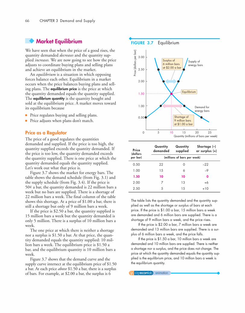
Figure 3.7 shows the market for energy bars. Thetable shows the demand schedule (from Fig. 3.1) andthe supply schedule (from Fig. 3.4). If the price is50¢ a bar, the quantity demanded is 22 million bars aweek but no bars are supplied. There is a shortage of22 million bars a week. The final column of the tableshows this shortage. At a price of $1.00 a bar, there isstill a shortage but only of 9 million bars a week.

If the price is $2.50 a bar, the quantity supplied is15 million bars a week but the quantity demanded isonly 5 million. There is a surplus of 10 million bars aweek.

The one price at which there is neither a shortagenor a surplus is $1.50 a bar. At that price, the quan-tity demanded equals the quantity supplied: 10 mil-lion bars a week. The equilibrium price is $1.50 abar, and the equilibrium quantity is 10 million bars aweek.

Figure 3.7 shows that the demand curve and thesupply curve intersect at the equilibrium price of $1.50a bar. At each price above $1.50 a bar, there is a surplusof bars. For example, at $2.00 a bar, the surplus is 6


3.00

0 5 15 20 25Pr

ice

(dol

lars

per

bar

)Quantity (millions of bars per week)


10

2.50

2.00

1.50

1.00

0.50


Equilibrium

Surplus of 6 million barsat $2.00 a bar

Shortage of 9 million barsat $1.00 a bar

PriceQuantity Quantity Shortage (–)

(dollarsdemanded supplied or surplus (+)

per bar) (millions of bars per week)

0.50 22 0 –22

1.00 15 6 –9

1.50 10 10 0

2.00 7 13 +6

2.50 5 15 +10

The table lists the quantity demanded and the quantity sup-plied as well as the shortage or surplus of bars at eachprice. If the price is $1.00 a bar, 15 million bars a weekare demanded and 6 million bars are supplied. There is ashortage of 9 million bars a week, and the price rises.

If the price is $2.00 a bar, 7 million bars a week aredemanded and 13 million bars are supplied. There is a sur-plus of 6 million bars a week, and the price falls.

If the price is $1.50 a bar, 10 million bars a week aredemanded and 10 million bars are supplied. There is neithera shortage nor a surplus, and the price does not change. Theprice at which the quantity demanded equals the quantity sup-plied is the equilibrium price, and 10 million bars a week isthe equilibrium quantity.

FIGURE 3.7 Equilibrium

animation

million bars a week, as shown by the blue arrow. Ateach price below $1.50 a bar, there is a shortage of bars.For example, at $1.00 a bar, the shortage is 9 millionbars a week, as shown by the red arrow.

Price AdjustmentsYou’ve seen that if the price is below equilibrium,there is a shortage and that if the price is above equi-librium, there is a surplus. But can we count on theprice to change and eliminate a shortage or a surplus?We can, because such price changes are beneficial toboth buyers and sellers. Let’s see why the pricechanges when there is a shortage or a surplus.

A Shortage Forces the Price Up Suppose the price ofan energy bar is $1. Consumers plan to buy 15 millionbars a week, and producers plan to sell 6 million bars aweek. Consumers can’t force producers to sell morethan they plan, so the quantity that is actually offeredfor sale is 6 million bars a week. In this situation, pow-erful forces operate to increase the price and move ittoward the equilibrium price. Some producers, notic-ing lines of unsatisfied consumers, raise the price.Some producers increase their output. As producerspush the price up, the price rises toward its equilib-rium. The rising price reduces the shortage because itdecreases the quantity demanded and increases thequantity supplied. When the price has increased to thepoint at which there is no longer a shortage, the forcesmoving the price stop operating and the price comesto rest at its equilibrium.

A Surplus Forces the Price Down Suppose the priceof a bar is $2. Producers plan to sell 13 million bars aweek, and consumers plan to buy 7 million bars aweek. Producers cannot force consumers to buy morethan they plan, so the quantity that is actually boughtis 7 million bars a week. In this situation, powerfulforces operate to lower the price and move it towardthe equilibrium price. Some producers, unable to sellthe quantities of energy bars they planned to sell, cuttheir prices. In addition, some producers scale backproduction. As producers cut the price, the price fallstoward its equilibrium. The falling price decreases thesurplus because it increases the quantity demandedand decreases the quantity supplied. When the pricehas fallen to the point at which there is no longer asurplus, the forces moving the price stop operatingand the price comes to rest at its equilibrium.

The Best Deal Available for Buyers and SellersWhen the price is below equilibrium, it is forcedupward. Why don’t buyers resist the increase andrefuse to buy at the higher price? The answer isbecause they value the good more highly than its cur-rent price and they can’t satisfy their demand at thecurrent price. In some markets—for example, themarkets that operate on eBay—the buyers mighteven be the ones who force the price up by offeringto pay a higher price.

When the price is above equilibrium, it is biddownward. Why don’t sellers resist this decrease andrefuse to sell at the lower price? The answer is becausetheir minimum supply price is below the currentprice and they cannot sell all they would like to at thecurrent price. Sellers willingly lower the price to gainmarket share.

At the price at which the quantity demanded andthe quantity supplied are equal, neither buyers norsellers can do business at a better price. Buyers pay thehighest price they are willing to pay for the last unitbought, and sellers receive the lowest price at whichthey are willing to supply the last unit sold.

When people freely make offers to buy and selland when demanders try to buy at the lowest possibleprice and suppliers try to sell at the highest possibleprice, the price at which trade takes place is the equi-librium price—the price at which the quantitydemanded equals the quantity supplied. The pricecoordinates the plans of buyers and sellers, and noone has an incentive to change it.

Market Equilibrium 67

REVIEW QUIZ 1 What is the equilibrium price of a good or service?2 Over what range of prices does a shortage arise?

What happens to the price when there is ashortage?

3 Over what range of prices does a surplus arise?What happens to the price when there is asurplus?

4 Why is the price at which the quantitydemanded equals the quantity supplied theequilibrium price?

5 Why is the equilibrium price the best dealavailable for both buyers and sellers?


◆ Predicting Changes in Price and Quantity

The demand and supply model that we have juststudied provides us with a powerful way of analyzinginfluences on prices and the quantities bought andsold. According to the model, a change in price stemsfrom a change in demand, a change in supply, or achange in both demand and supply. Let’s look first atthe effects of a change in demand.

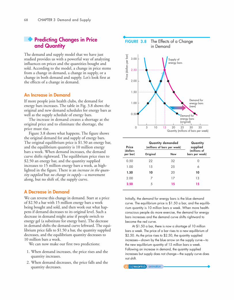
An Increase in DemandIf more people join health clubs, the demand forenergy bars increases. The table in Fig. 3.8 shows theoriginal and new demand schedules for energy bars aswell as the supply schedule of energy bars.

The increase in demand creates a shortage at theoriginal price and to eliminate the shortage, theprice must rise.

Figure 3.8 shows what happens. The figure showsthe original demand for and supply of energy bars.The original equilibrium price is $1.50 an energy bar,and the equilibrium quantity is 10 million energybars a week. When demand increases, the demandcurve shifts rightward. The equilibrium price rises to$2.50 an energy bar, and the quantity suppliedincreases to 15 million energy bars a week, as high-lighted in the figure. There is an increase in the quan-tity supplied but no change in supply—a movementalong, but no shift of, the supply curve.

A Decrease in DemandWe can reverse this change in demand. Start at a priceof $2.50 a bar with 15 million energy bars a weekbeing bought and sold, and then work out what hap-pens if demand decreases to its original level. Such adecrease in demand might arise if people switch toenergy gel (a substitute for energy bars). The decreasein demand shifts the demand curve leftward. The equi-librium price falls to $1.50 a bar, the quantity supplieddecreases, and the equilibrium quantity decreases to10 million bars a week.

We can now make our first two predictions:

1. When demand increases, the price rises and thequantity increases.

2. When demand decreases, the price falls and thequantity decreases.


3.00

5 15 20 35Pr

ice

(dol

lars

per

bar



10

2.50

2.00

1.50

1.00

0.50

0 3025

Demand forenergy bars(original)

Demand forenergy bars(new)

Quantity demanded QuantityPrice (millions of bars per week) supplied

(dollars (millions ofper bar) Original New bars per week)

0.50 22 32 0

1.00 15 25 6

1.50 10 20 10

2.00 7 17 13

2.50 5 15 15

Initially, the demand for energy bars is the blue demandcurve. The equilibrium price is $1.50 a bar, and the equilib-rium quantity is 10 million bars a week. When more health-conscious people do more exercise, the demand for energybars increases and the demand curve shifts rightward tobecome the red curve.

At $1.50 a bar, there is now a shortage of 10 millionbars a week. The price of a bar rises to a new equilibrium of$2.50. As the price rises to $2.50, the quantity suppliedincreases—shown by the blue arrow on the supply curve—tothe new equilibrium quantity of 15 million bars a week.Following an increase in demand, the quantity suppliedincreases but supply does not change—the supply curve doesnot shift.

FIGURE 3.8 The Effects of a Changein Demand

animation

Predicting Changes in Price and Quantity 69

Economics in ActionThe Global Market for Crude OilThe demand and supply model provides insights intoall competitive markets. Here, we’ll apply what you’velearned about the effects of an increase in demand tothe global market for crude oil.

Crude oil is like the life-blood of the global econ-omy. It is used to fuel our cars, airplanes, trains, andbuses, to generate electricity, and to produce a widerange of plastics. When the price of crude oil rises,the cost of transportation, power, and materials allincrease.

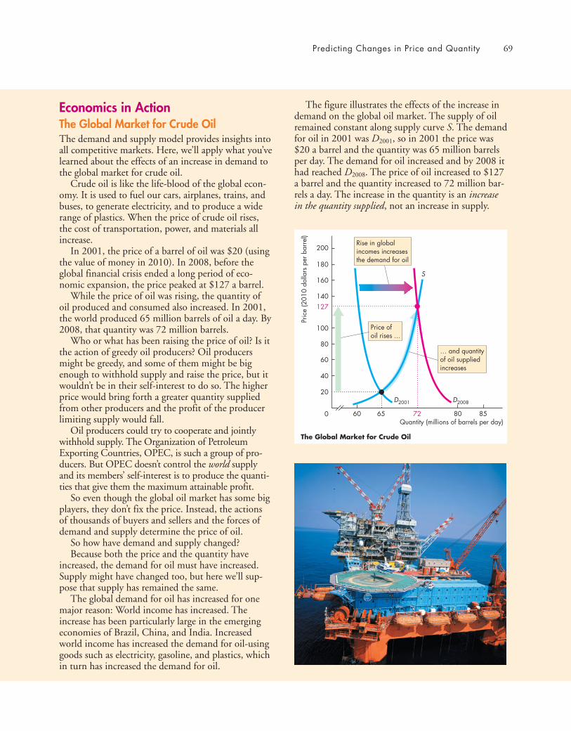
In 2001, the price of a barrel of oil was $20 (usingthe value of money in 2010). In 2008, before theglobal financial crisis ended a long period of eco-nomic expansion, the price peaked at $127 a barrel.

While the price of oil was rising, the quantity ofoil produced and consumed also increased. In 2001,the world produced 65 million barrels of oil a day. By2008, that quantity was 72 million barrels.

Who or what has been raising the price of oil? Is itthe action of greedy oil producers? Oil producersmight be greedy, and some of them might be bigenough to withhold supply and raise the price, but itwouldn’t be in their self-interest to do so. The higherprice would bring forth a greater quantity suppliedfrom other producers and the profit of the producerlimiting supply would fall.

Oil producers could try to cooperate and jointlywithhold supply. The Organization of PetroleumExporting Countries, OPEC, is such a group of pro-ducers. But OPEC doesn’t control the world supplyand its members’ self-interest is to produce the quanti-ties that give them the maximum attainable profit.

So even though the global oil market has some bigplayers, they don’t fix the price. Instead, the actionsof thousands of buyers and sellers and the forces ofdemand and supply determine the price of oil.

So how have demand and supply changed?Because both the price and the quantity have

increased, the demand for oil must have increased.Supply might have changed too, but here we’ll sup-pose that supply has remained the same.

The global demand for oil has increased for onemajor reason: World income has increased. Theincrease has been particularly large in the emergingeconomies of Brazil, China, and India. Increasedworld income has increased the demand for oil-usinggoods such as electricity, gasoline, and plastics, whichin turn has increased the demand for oil.

The figure illustrates the effects of the increase indemand on the global oil market. The supply of oilremained constant along supply curve S. The demandfor oil in 2001 was D2001, so in 2001 the price was$20 a barrel and the quantity was 65 million barrelsper day. The demand for oil increased and by 2008 ithad reached D2008. The price of oil increased to $127a barrel and the quantity increased to 72 million bar-rels a day. The increase in the quantity is an increasein the quantity supplied, not an increase in supply.

200

60 72 85

Pric

e (2

010

dolla

rs p

er b

arre

l)

Quantity (millions of barrels per day)65

127

20

40

0

60

80

100

140

160

180

80

S

D2001 D2008

Rise in globalincomes increasesthe demand for oil

The Global Market for Crude Oil

Price ofoil rises ...

… and quantityof oil suppliedincreases


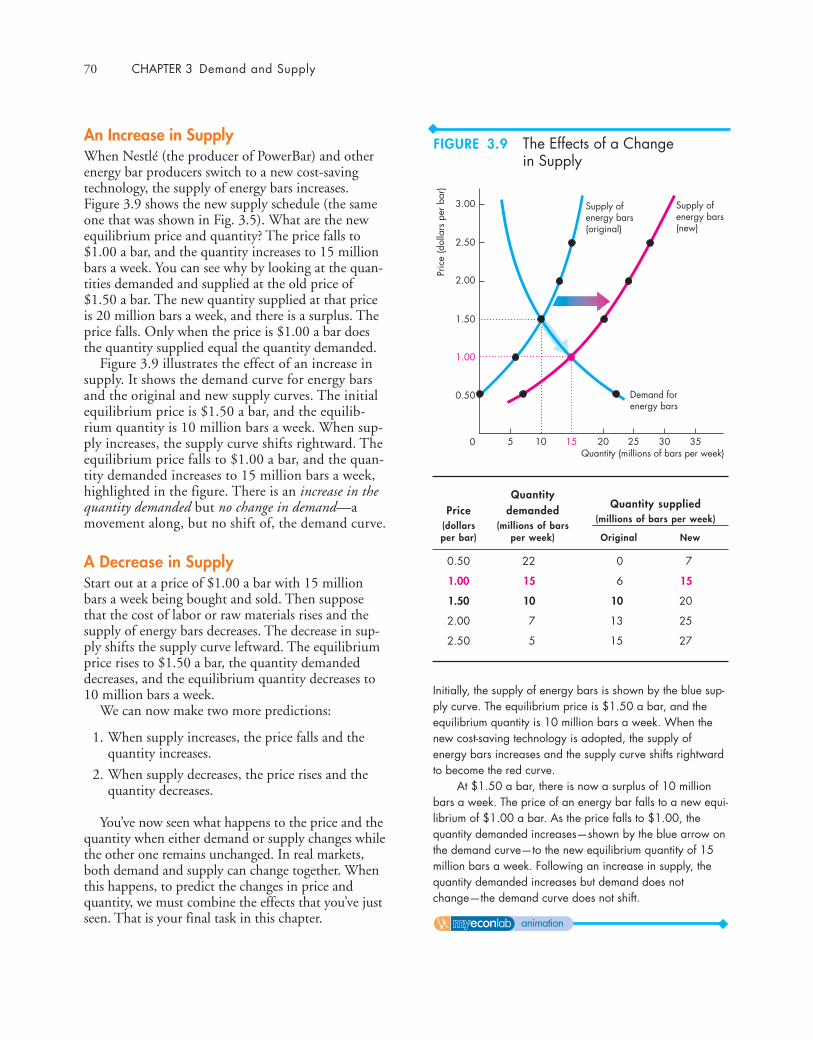
An Increase in SupplyWhen Nestlé (the producer of PowerBar) and otherenergy bar producers switch to a new cost-savingtechnology, the supply of energy bars increases.Figure 3.9 shows the new supply schedule (the sameone that was shown in Fig. 3.5). What are the newequilibrium price and quantity? The price falls to$1.00 a bar, and the quantity increases to 15 millionbars a week. You can see why by looking at the quan-tities demanded and supplied at the old price of$1.50 a bar. The new quantity supplied at that priceis 20 million bars a week, and there is a surplus. Theprice falls. Only when the price is $1.00 a bar doesthe quantity supplied equal the quantity demanded.

Figure 3.9 illustrates the effect of an increase insupply. It shows the demand curve for energy barsand the original and new supply curves. The initialequilibrium price is $1.50 a bar, and the equilib-rium quantity is 10 million bars a week. When sup-ply increases, the supply curve shifts rightward. Theequilibrium price falls to $1.00 a bar, and the quan-tity demanded increases to 15 million bars a week,highlighted in the figure. There is an increase in thequantity demanded but no change in demand—amovement along, but no shift of, the demand curve.

A Decrease in SupplyStart out at a price of $1.00 a bar with 15 millionbars a week being bought and sold. Then supposethat the cost of labor or raw materials rises and thesupply of energy bars decreases. The decrease in sup-ply shifts the supply curve leftward. The equilibriumprice rises to $1.50 a bar, the quantity demandeddecreases, and the equilibrium quantity decreases to10 million bars a week.

We can now make two more predictions:

1. When supply increases, the price falls and thequantity increases.

2. When supply decreases, the price rises and thequantity decreases.

You’ve now seen what happens to the price and thequantity when either demand or supply changes whilethe other one remains unchanged. In real markets,both demand and supply can change together. Whenthis happens, to predict the changes in price andquantity, we must combine the effects that you’ve justseen. That is your final task in this chapter.

3.00

5 15 20 35Pr

ice

(dol

lars

per

bar


Supply ofenergy bars(original)


Supply ofenergy bars(new)

10

2.50

2.00

1.50

1.00

0.50

0 3025

QuantityPrice demanded Quantity supplied

(dollars (millions of bars (millions of bars per week)

per bar) per week) Original New

0.50 22 0 7

1.00 15 6 15

1.50 10 10 20

2.00 7 13 25

2.50 5 15 27

Initially, the supply of energy bars is shown by the blue sup-ply curve. The equilibrium price is $1.50 a bar, and theequilibrium quantity is 10 million bars a week. When thenew cost-saving technology is adopted, the supply ofenergy bars increases and the supply curve shifts rightwardto become the red curve.

At $1.50 a bar, there is now a surplus of 10 millionbars a week. The price of an energy bar falls to a new equi-librium of $1.00 a bar. As the price falls to $1.00, thequantity demanded increases—shown by the blue arrow onthe demand curve—to the new equilibrium quantity of 15million bars a week. Following an increase in supply, thequantity demanded increases but demand does notchange—the demand curve does not shift.

FIGURE 3.9 The Effects of a Changein Supply

animation

Economics in ActionThe Market for StrawberriesCalifornia produces 85 percent of the nation’s straw-berries and its crop, which starts to increase inMarch, is in top flight by April. During the wintermonths of January and February, Florida is the mainstrawberry producer.

In a normal year, the supplies from these tworegions don’t overlap much. As California’s produc-tion steps up in March and April, Florida’s produc-tion falls off. The result is a steady supply ofstrawberries and not much seasonal fluctuation in theprice of strawberries.

But 2010 wasn’t a normal year. Florida had excep-tionally cold weather, which damaged the strawberryfields, lowered crop yields, and delayed the harvests.The result was unusually high strawberry prices.

With higher than normal prices, Florida farmersplanted strawberry varieties that mature later thantheir normal crop and planned to harvest this fruitduring the spring. Their plan worked perfectly andgood growing conditions delivered a bumper crop bylate March.

On the other side of the nation, while Florida wasfreezing, Southern California was drowning underunusually heavy rains. This wet weather put thestrawberries to sleep and delayed their growth. Butwhen the rains stopped and the temperature began torise, California joined Florida with a super abun-dance of fruit.

With an abundance of strawberries, the price tum-bled. Strawberry farmers in both regions couldn’t hireenough labor to pick the super-sized crop, so somefruit was left in the fields to rot.

The figure explains what was happening in themarket for strawberries.

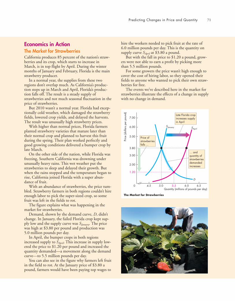
Demand, shown by the demand curve, D, didn’tchange. In January, the failed Florida crop kept sup-ply low and the supply curve was SJanuary. The pricewas high at $3.80 per pound and production was 5.0 million pounds per day.

In April, the bumper crops in both regionsincreased supply to SApril. This increase in supply low-ered the price to $1.20 per pound and increased thequantity demanded—a movement along the demandcurve—to 5.5 million pounds per day.

You can also see in the figure why farmers left fruitin the field to rot. At the January price of $3.80 apound, farmers would have been paying top wages to

hire the workers needed to pick fruit at the rate of6.0 million pounds per day. This is the quantity onsupply curve SApril at $3.80 a pound.

But with the fall in price to $1.20 a pound, grow-ers were not able to earn a profit by picking morethan 5.5 million pounds.

For some growers the price wasn’t high enough tocover the cost of hiring labor, so they opened theirfields to anyone who wanted to pick their own straw-berries for free.

The events we’ve described here in the market forstrawberries illustrate the effects of a change in supplywith no change in demand.


7.00

5.5 6.5

Pric

e (d

olla

rs p

er p

ound

)

Quantity (millions of pounds per day)5.0

1.20

2.00

3.80

0

6.00

3.00

5.00

6.04.5

D

SJanuary SApril

Price ofstrawberriesfalls ...

Late Florida cropincreases supplyin April

The Market for Strawberries

… andquantity ofstrawberriesdemandedincreases

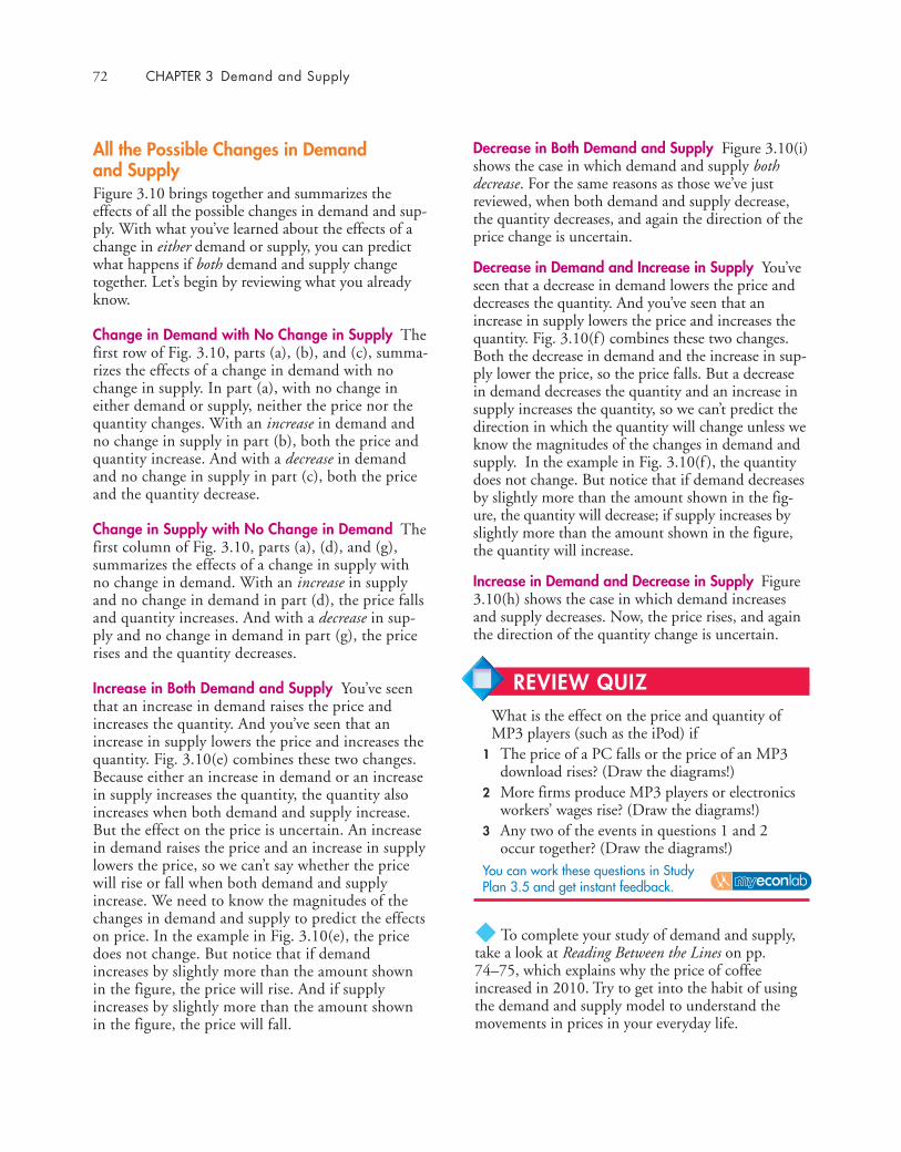
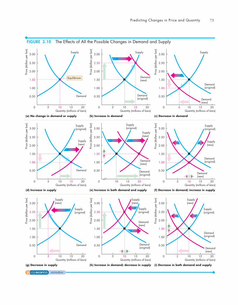
Decrease in Both Demand and Supply Figure 3.10(i)shows the case in which demand and supply bothdecrease. For the same reasons as those we’ve justreviewed, when both demand and supply decrease,the quantity decreases, and again the direction of theprice change is uncertain.

Decrease in Demand and Increase in Supply You’veseen that a decrease in demand lowers the price anddecreases the quantity. And you’ve seen that anincrease in supply lowers the price and increases thequantity. Fig. 3.10(f ) combines these two changes.Both the decrease in demand and the increase in sup-ply lower the price, so the price falls. But a decreasein demand decreases the quantity and an increase insupply increases the quantity, so we can’t predict thedirection in which the quantity will change unless weknow the magnitudes of the changes in demand andsupply. In the example in Fig. 3.10(f ), the quantitydoes not change. But notice that if demand decreasesby slightly more than the amount shown in the fig-ure, the quantity will decrease; if supply increases byslightly more than the amount shown in the figure,the quantity will increase.

Increase in Demand and Decrease in Supply Figure3.10(h) shows the case in which demand increasesand supply decreases. Now, the price rises, and againthe direction of the quantity change is uncertain.

All the Possible Changes in Demand and SupplyFigure 3.10 brings together and summarizes theeffects of all the possible changes in demand and sup-ply. With what you’ve learned about the effects of achange in either demand or supply, you can predictwhat happens if both demand and supply changetogether. Let’s begin by reviewing what you alreadyknow.

Change in Demand with No Change in Supply Thefirst row of Fig. 3.10, parts (a), (b), and (c), summa-rizes the effects of a change in demand with nochange in supply. In part (a), with no change ineither demand or supply, neither the price nor thequantity changes. With an increase in demand andno change in supply in part (b), both the price andquantity increase. And with a decrease in demandand no change in supply in part (c), both the priceand the quantity decrease.

Change in Supply with No Change in Demand Thefirst column of Fig. 3.10, parts (a), (d), and (g),summarizes the effects of a change in supply withno change in demand. With an increase in supplyand no change in demand in part (d), the price fallsand quantity increases. And with a decrease in sup-ply and no change in demand in part (g), the pricerises and the quantity decreases.

Increase in Both Demand and Supply You’ve seenthat an increase in demand raises the price andincreases the quantity. And you’ve seen that anincrease in supply lowers the price and increases thequantity. Fig. 3.10(e) combines these two changes.Because either an increase in demand or an increasein supply increases the quantity, the quantity alsoincreases when both demand and supply increase.But the effect on the price is uncertain. An increasein demand raises the price and an increase in supplylowers the price, so we can’t say whether the pricewill rise or fall when both demand and supplyincrease. We need to know the magnitudes of thechanges in demand and supply to predict the effectson price. In the example in Fig. 3.10(e), the pricedoes not change. But notice that if demandincreases by slightly more than the amount shownin the figure, the price will rise. And if supplyincreases by slightly more than the amount shownin the figure, the price will fall.

◆ To complete your study of demand and supply,take a look at Reading Between the Lines on pp.74–75, which explains why the price of coffeeincreased in 2010. Try to get into the habit of usingthe demand and supply model to understand themovements in prices in your everyday life.

REVIEW QUIZ What is the effect on the price and quantity ofMP3 players (such as the iPod) if

1 The price of a PC falls or the price of an MP3download rises? (Draw the diagrams!)

2 More firms produce MP3 players or electronicsworkers’ wages rise? (Draw the diagrams!)

3 Any two of the events in questions 1 and 2occur together? (Draw the diagrams!)




Demand

3.00

0 5 15 20

Pric

e (d

olla

rs p

er b

ar)

Quantity (millions of bars)10

2.50

2.00

1.50

1.00

0.50

Demand

3.00

0 5 15 20

Pric

e (d

olla

rs p

er b

ar)


2.50

2.00

1.50

1.00

0.50

(d) Increase in supply (e) Increase in both demand and supply (f) Decrease in demand; increase in supply

(g) Decrease in supply (i) Decrease in both demand and supply(h) Increase in demand; decrease in supply

Demand(original)

Demand(new)

Supply(new)

Supply(original)

Demand(original)

Demand(new)

Supply(new)

Supply(original)

Demand(new)

Demand(original)

Supply(original)

Supply(new)

Demand(new)

Demand(original)

3.00

0 5 15 20

Pric

e (d

olla

rs p

er b

ar)


2.50

2.00

1.50

1.00

0.50

Supply(new)

Supply(original)3.00

0 15 20

Pric

e (d

olla

rs p

er b

ar)


2.50

2.00

1.50

1.00

0.50

Supply(new)

Supply(original)

3.00

0 5 15 20

Pric

e (d

olla

rs p

er b

ar)


2.50

2.00

1.50

1.00

0.50

3.00

0 5 15 20

Pric

e (d

olla

rs p

er b

ar)


2.50

2.00

1.50

1.00

0.50

Supply(new)

Supply(original)

Demand

Supply3.00

0 5 15 20

Pric

e (d

olla

rs p

er b

ar)

Quantity (millions of bars)

(a) No change in demand or supply

10

2.50

2.00

1.50

1.00

0.50

(c) Decrease in demand(b) Increase in demand

Equilibrium

Supply3.00

0 5 15 20

Pric

e (d

olla

rs p

er b

ar)


2.50

2.00

1.50

1.00

0.50

Demand(new)

Demand(original)

Supply3.00

0 6 15 20

Pric

e (d

olla

rs p

er b

ar)


2.50

2.00

1.50

1.00

0.50Demand(new)

Demand(original)

?

?

?

?

?

?

? ?

FIGURE 3.10 The Effects of All the Possible Changes in Demand and Supply

animation

74

Coffee Surges on Poor Colombian HarvestsFT.comJuly 30, 2010

Coffee prices hit a 12-year high on Friday on the back of low supplies of premium Arabicacoffee from Colombia after a string of poor crops in the Latin American country.

The strong fundamental picture has also encouraged hedge funds to reverse their previousbearish views on coffee prices.

In New York, ICE September Arabica coffee jumped 3.2 percent to 178.75 cents per pound,the highest since February 1998. It traded later at 177.25 cents, up 6.8 percent on the week.

The London-based International Coffee Organization on Friday warned that the “currenttight demand and supply situation” was “likely to persist in the near to medium term.”

Coffee industry executives believe prices could rise toward 200 cents per pound in New Yorkbefore the arrival of the new Brazilian crop laterthis year.

“Until October it is going to be tight on highquality coffee,” said a senior executive at one ofEurope’s largest coffee roasters. He said: “Theindustry has been surprised by the scarcity ofhigh quality beans.”

Colombia coffee production, key for supplies ofpremium beans, last year plunged to a 33-yearlow of 7.8m bags, each of 60kg, down nearly athird from 11.1m bags in 2008, tightening sup-plies worldwide. ...

Excerpted from “Coffee Surges on Poor Colombian Harvests” by JavierBlas. Financial Times, July 30, 2010. Reprinted with permission.

READING BETWEEN THE L INES

Demand and Supply: The Price of Coffee

■ The price of premium Arabica coffee increasedby 3.2 percent to almost 180 cents per pound inJuly 2010, the highest price since February1998.

■ A sequence of poor crops in Columbia cut theproduction of premium Arabica coffee to a 33-year low of 7.8 million 60 kilogram bags, downfrom 11.1 million bags in 2008.

■ The International Coffee Organization said thatthe “current tight demand and supply situation”was “likely to persist in the near to medium term.”

■ Coffee industry executives say prices mightapproach 200 cents per pound before the arrivalof the new Brazilian crop later this year.

■ Hedge funds previously expected the price of cof-fee to fall but now expect it to rise further.

ESSENCE OF THE STORY

75

Figure 2 The effects of the expected future price

D

S1

S0

Figure 1 The effects of the Columbian crop

Decrease inColumbia crop ...

Pric

e (c

ents

per p

ound

)

Quantity (millions of bags)0

160

110 116 130 140120

170174

180

190

200

100

... anddecreasesquantity

... raisesprice ...

D0

D1

S1

S0

Rise in expected futureprice increases demandand decreases supply ...

Pric

e (c

ents

per p

ound

)

Quantity (millions of bags)0

160

110 116 130 140120

170

180

190

200

210

220

230

100

... and raisesprice further

ECONOMIC ANALYSIS

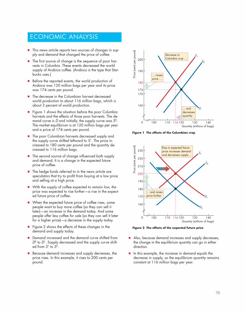
■ This news article reports two sources of changes in sup-ply and demand that changed the price of coffee.

■ The first source of change is the sequence of poor har-vests in Columbia. These events decreased the worldsupply of Arabica coffee. (Arabica is the type that Star-bucks uses.)

■ Before the reported events, the world production ofArabica was 120 million bags per year and its pricewas 174 cents per pound.

■ The decrease in the Columbian harvest decreasedworld production to about 116 million bags, which isabout 3 percent of world production.

■ Figure 1 shows the situation before the poor Columbiaharvests and the effects of those poor harvests. The de-mand curve is D and initially, the supply curve was S0.The market equilibrium is at 120 million bags per yearand a price of 174 cents per pound.

■ The poor Columbian harvests decreased supply andthe supply curve shifted leftward to S1. The price in-creased to 180 cents per pound and the quantity de-creased to 116 million bags.

■ The second source of change influenced both supplyand demand. It is a change in the expected futureprice of coffee.

■ The hedge funds referred to in the news article arespeculators that try to profit from buying at a low priceand selling at a high price.

■ With the supply of coffee expected to remain low, theprice was expected to rise further—a rise in the expect-ed future price of coffee.

■ When the expected future price of coffee rises, somepeople want to buy more coffee (so they can sell itlater)—an increase in the demand today. And somepeople offer less coffee for sale (so they can sell it laterfor a higher price)—a decrease in the supply today.

■ Figure 2 shows the effects of these changes in thedemand and supply today.

■ Demand increased and the demand curve shifted fromD0 to D1. Supply decreased and the supply curve shift-ed from S1 to S2.

■ Because demand increases and supply decreases, theprice rises. In this example, it rises to 200 cents perpound.

■ Also, because demand increases and supply decreases,the change in the equilibrium quantity can go in eitherdirection.

■ In this example, the increase in demand equals thedecrease in supply, so the equilibrium quantity remainsconstant at 116 million bags per year.


MATHEMATICAL NOTEDemand, Supply, and Equilibrium

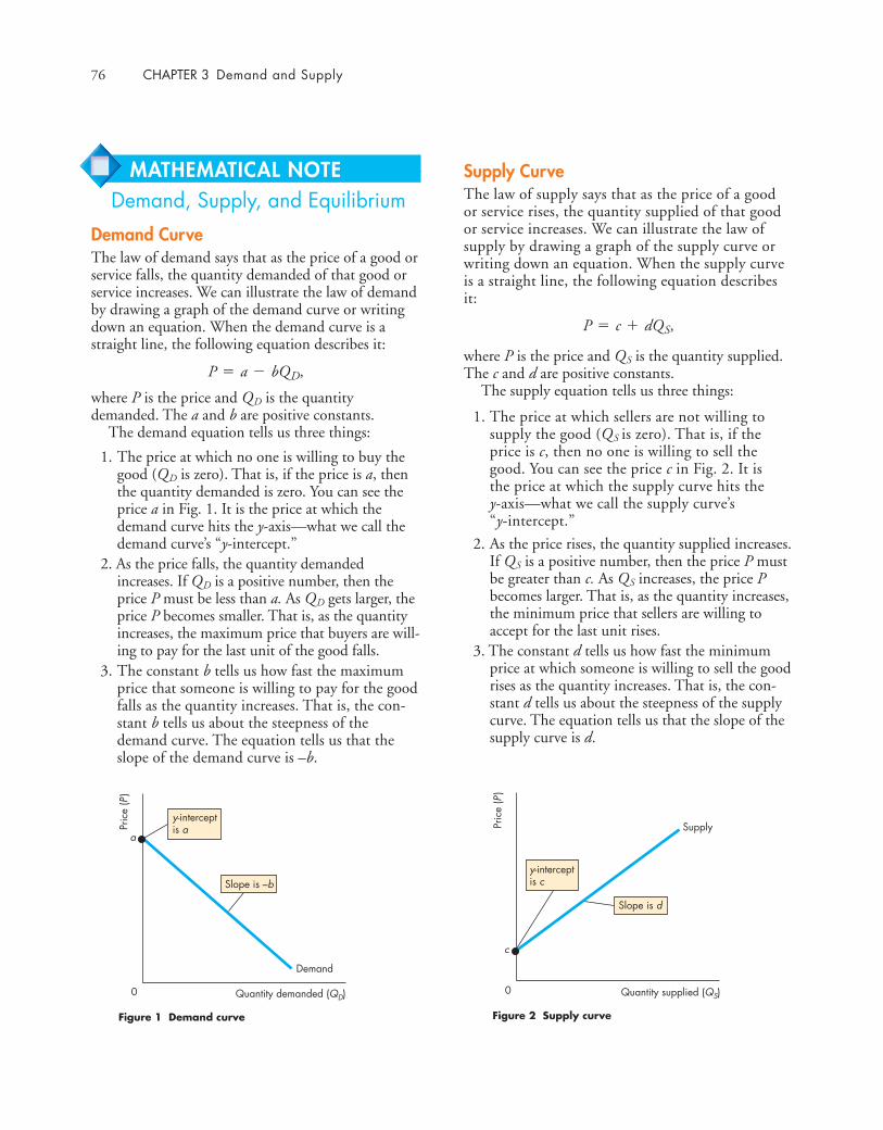
Demand CurveThe law of demand says that as the price of a good orservice falls, the quantity demanded of that good orservice increases. We can illustrate the law of demandby drawing a graph of the demand curve or writingdown an equation. When the demand curve is astraight line, the following equation describes it:

where P is the price and QD is the quantitydemanded. The a and b are positive constants.

The demand equation tells us three things:

1. The price at which no one is willing to buy thegood (QD is zero). That is, if the price is a, thenthe quantity demanded is zero. You can see theprice a in Fig. 1. It is the price at which thedemand curve hits the y-axis—what we call thedemand curve’s “y-intercept.”

2. As the price falls, the quantity demandedincreases. If QD is a positive number, then theprice P must be less than a. As QD gets larger, theprice P becomes smaller. That is, as the quantityincreases, the maximum price that buyers are will-ing to pay for the last unit of the good falls.

3. The constant b tells us how fast the maximumprice that someone is willing to pay for the goodfalls as the quantity increases. That is, the con-stant b tells us about the steepness of thedemand curve. The equation tells us that theslope of the demand curve is –b.

Quantity demanded (QD)0

Pric

e (P

)

a

Demand

y-interceptis a

Slope is –b

Figure 1 Demand curve

P = a - bQD,

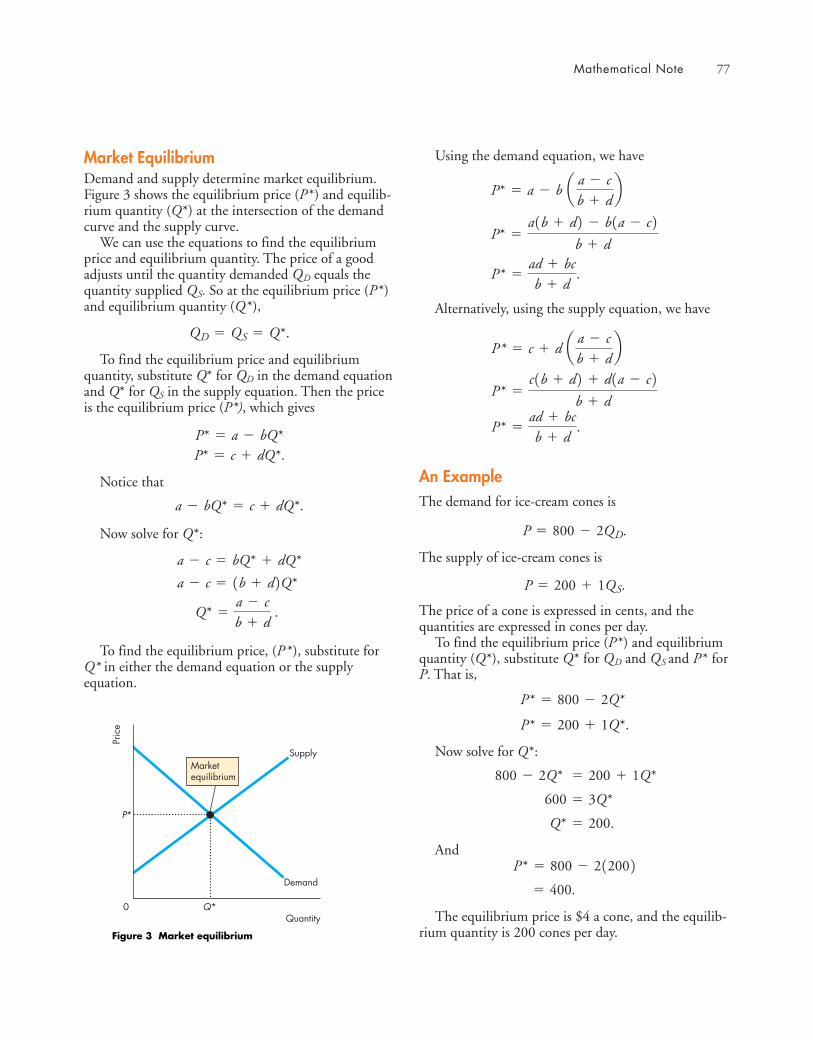
Supply CurveThe law of supply says that as the price of a goodor service rises, the quantity supplied of that goodor service increases. We can illustrate the law ofsupply by drawing a graph of the supply curve orwriting down an equation. When the supply curveis a straight line, the following equation describesit:

where P is the price and QS is the quantity supplied.The c and d are positive constants.

The supply equation tells us three things:

1. The price at which sellers are not willing tosupply the good (QS is zero). That is, if theprice is c, then no one is willing to sell thegood. You can see the price c in Fig. 2. It is the price at which the supply curve hits the y-axis—what we call the supply curve’s “y-intercept.”

2. As the price rises, the quantity supplied increases.If QS is a positive number, then the price P mustbe greater than c. As QS increases, the price Pbecomes larger. That is, as the quantity increases,the minimum price that sellers are willing toaccept for the last unit rises.

3. The constant d tells us how fast the minimumprice at which someone is willing to sell the goodrises as the quantity increases. That is, the con-stant d tells us about the steepness of the supplycurve. The equation tells us that the slope of thesupply curve is d.

P = c + dQS,

Quantity supplied (QS)0

Pric

e (P

)

c

Supply

Slope is d

Figure 2 Supply curve

y-interceptis c

Market EquilibriumDemand and supply determine market equilibrium.Figure 3 shows the equilibrium price (P*) and equilib-rium quantity (Q*) at the intersection of the demandcurve and the supply curve.

We can use the equations to find the equilibriumprice and equilibrium quantity. The price of a goodadjusts until the quantity demanded QD equals thequantity supplied QS. So at the equilibrium price (P* )and equilibrium quantity (Q* ),

To find the equilibrium price and equilibriumquantity, substitute Q* for QD in the demand equationand Q* for QS in the supply equation. Then the priceis the equilibrium price (P*), which gives

Notice that

Now solve for Q*:

To find the equilibrium price, (P* ), substitute forQ* in either the demand equation or the supplyequation.

Quantity0

Pric

e

P*

Q*

Demand

SupplyMarketequilibrium

Figure 3 Market equilibrium

Q* =a - cb + d

.

a - c = 1b + d2Q*

a - c = bQ* + dQ*

a - bQ* = c + dQ*.

P* = c + dQ*.P* = a - bQ*

QD = QS = Q*.

Using the demand equation, we have

Alternatively, using the supply equation, we have

An ExampleThe demand for ice-cream cones is

The supply of ice-cream cones is

The price of a cone is expressed in cents, and thequantities are expressed in cones per day.

To find the equilibrium price (P*) and equilibriumquantity (Q*), substitute Q* for QD and QS and P* forP. That is,

Now solve for Q*:

And

The equilibrium price is $4 a cone, and the equilib-rium quantity is 200 cones per day.

= 400.

P* = 800 - 212002Q* = 200.

600 = 3Q*

800 - 2Q* = 200 + 1Q*

P* = 200 + 1Q*.

P* = 800 - 2Q*

P = 200 + 1QS.

P = 800 - 2QD.

P* =ad + bcb + d

.

P* =c1b + d2 + d1a - c2

b + d

P * = c + d a a - cb + d

b

P* =ad + bcb + d

.

P* =a1b + d2 - b1a - c2

b + d

P* = a - b a a - cb + d

b

Mathematical Note 77

■ Supply depends on the prices of factors of produc-tion used to produce a good, the prices of relatedgoods produced, expected future prices, the num-ber of suppliers, technology, and the state ofnature.

Working Problems 6 to 9 will give you a better under-standing of supply.

Market Equilibrium (pp. 66–67)

■ At the equilibrium price, the quantity demandedequals the quantity supplied.

■ At any price above the equilibrium price, there is asurplus and the price falls.

■ At any price below the equilibrium price, there is ashortage and the price rises.

Working Problems 10 and 11 will give you a better under-standing of market equilibrium

Predicting Changes in Price and Quantity (pp. 68–73)

■ An increase in demand brings a rise in the priceand an increase in the quantity supplied. Adecrease in demand brings a fall in the price and adecrease in the quantity supplied.

■ An increase in supply brings a fall in the price andan increase in the quantity demanded. A decreasein supply brings a rise in the price and a decreasein the quantity demanded.

■ An increase in demand and an increase in supply bringan increased quantity but an uncertain price change.An increase in demand and a decrease in supply bringa higher price but an uncertain change in quantity.

Working Problems 12 and 13 will give you a better under-standing of predicting changes in price and quantity.


Key Points

Markets and Prices (p. 56)

■ A competitive market is one that has so many buy-ers and sellers that no single buyer or seller caninfluence the price.

■ Opportunity cost is a relative price.■ Demand and supply determine relative prices.

Working Problem 1 will give you a better understandingof markets and prices.

Demand (pp. 57–61)

■ Demand is the relationship between the quantitydemanded of a good and its price when all otherinfluences on buying plans remain the same.

■ The higher the price of a good, other thingsremaining the same, the smaller is the quantitydemanded—the law of demand.

■ Demand depends on the prices of related goods (sub-stitutes and complements), expected future prices,income, expected future income and credit, the pop-ulation, and preferences.

Working Problems 2 to 5 will give you a better under-standing of demand.

Supply (pp. 62–65)

■ Supply is the relationship between the quantitysupplied of a good and its price when all otherinfluences on selling plans remain the same.

■ The higher the price of a good, other thingsremaining the same, the greater is the quantitysupplied—the law of supply.

SUMMARY

Key TermsChange in demand, 58Change in supply, 63Change in the quantity

demanded, 61Change in the quantity supplied, 64Competitive market, 56Complement, 59Demand, 57

Demand curve, 58Equilibrium price, 66Equilibrium quantity, 66Inferior good, 60Law of demand, 57Law of supply, 62Money price, 56Normal good, 60

Quantity demanded, 57Quantity supplied, 62Relative price, 56Substitute, 59Supply, 62Supply curve, 62

how do you expect the following would change:a. The demand for beef? Explain your answer.b. The demand for rice? Explain your answer.

5. In January 2010, the price of gasoline was$2.70 a gallon. By spring 2010, the price hadincreased to $3.00 a gallon. Assume that therewere no changes in average income, popula-tion, or any other influence on buying plans.Explain how the rise in the price of gasolinewould affecta. The demand for gasoline.b. The quantity of gasoline demanded.

Supply (Study Plan 3.3)

6. In 2008, the price of corn increased by 35 per-cent and some cotton farmers in Texas stoppedgrowing cotton and started to grow corn.a. Does this fact illustrate the law of demand or

the law of supply? Explain your answer.b. Why would a cotton farmer grow corn?

Use the following information to work Problems 7 to 9.

Dairies make low-fat milk from full-cream milk. Inthe process of making low-fat milk, the dairies pro-duce cream, which is made into ice cream. In themarket for low-fat milk, the following events occurone at a time:

(i) The wage rate of dairy workers rises.(ii) The price of cream rises.(iii) The price of low-fat milk rises.(iv) With the period of low rainfall extending,

dairies raise their expected price of low-fatmilk next year.

(v) With advice from health-care experts, dairyfarmers decide to switch from producingfull-cream milk to growing vegetables.

(vi) A new technology lowers the cost of pro-ducing ice cream.

7. Explain the effect of each event on the supply oflow-fat milk.

8. Use a graph to illustrate the effect of each event.

9. Does any event (or events) illustrate the law ofsupply?

Study Plan Problems and Applications 79

Markets and Prices (Study Plan 3.1)

1. William Gregg owned a mill in South Carolina.In December 1862, he placed a notice in theEdgehill Advertiser announcing his willingnessto exchange cloth for food and other items.Here is an extract:

1 yard of cloth for 1 pound of bacon2 yards of cloth for 1 pound of butter4 yards of cloth for 1 pound of wool8 yards of cloth for 1 bushel of salt

a. What is the relative price of butter in terms ofwool?

b. If the money price of bacon was 20¢ a pound,what do you predict was the money price ofbutter?

c. If the money price of bacon was 20¢ a poundand the money price of salt was $2.00 abushel, do you think anyone would acceptMr. Gregg’s offer of cloth for salt?

Demand (Study Plan 3.2)

2. The price of food increased during the past year.a. Explain why the law of demand applies to

food just as it does to all other goods andservices.

b. Explain how the substitution effect influencesfood purchases and provide some examples ofsubstitutions that people might make whenthe price of food rises and other things remainthe same.

c. Explain how the income effect influencesfood purchases and provide some examplesof the income effect that might occur whenthe price of food rises and other things re-main the same.

3. Place the following goods and services into pairsof likely substitutes and pairs of likely comple-ments. (You may use an item in more than onepair.) The goods and services are

coal, oil, natural gas, wheat, corn, rye, pasta,pizza, sausage, skateboard, roller blades, videogame, laptop, iPod, cell phone, text message,email, phone call, voice mail

4. During 2010, the average income in Chinaincreased by 10 percent. Compared to 2009,

You can work Problems 1 to 17 in MyEconLab Chapter 3 Study Plan and get instant feedback.

STUDY PLAN PROBLEMS AND APPLICATIONS

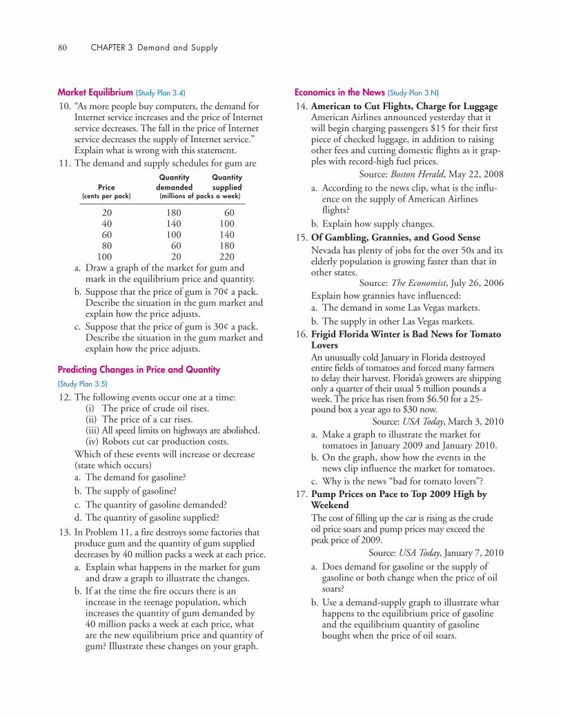
Market Equilibrium (Study Plan 3.4)

10. “As more people buy computers, the demand forInternet service increases and the price of Internetservice decreases. The fall in the price of Internetservice decreases the supply of Internet service.”Explain what is wrong with this statement.

11. The demand and supply schedules for gum areQuantity Quantity

Price demanded supplied(cents per pack) (millions of packs a week)

20 180 6040 140 10060 100 14080 60 180

100 20 220a. Draw a graph of the market for gum and

mark in the equilibrium price and quantity.b. Suppose that the price of gum is 70¢ a pack.

Describe the situation in the gum market andexplain how the price adjusts.

c. Suppose that the price of gum is 30¢ a pack.Describe the situation in the gum market andexplain how the price adjusts.

Predicting Changes in Price and Quantity (Study Plan 3.5)

12. The following events occur one at a time:(i) The price of crude oil rises.(ii) The price of a car rises.(iii) All speed limits on highways are abolished.(iv) Robots cut car production costs.

Which of these events will increase or decrease(state which occurs)a. The demand for gasoline?b. The supply of gasoline?c. The quantity of gasoline demanded?d. The quantity of gasoline supplied?

13. In Problem 11, a fire destroys some factories thatproduce gum and the quantity of gum supplieddecreases by 40 million packs a week at each price.a. Explain what happens in the market for gum

and draw a graph to illustrate the changes.b. If at the time the fire occurs there is an

increase in the teenage population, whichincreases the quantity of gum demanded by40 million packs a week at each price, whatare the new equilibrium price and quantity ofgum? Illustrate these changes on your graph.


Economics in the News (Study Plan 3.N)

14. American to Cut Flights, Charge for LuggageAmerican Airlines announced yesterday that itwill begin charging passengers $15 for their firstpiece of checked luggage, in addition to raisingother fees and cutting domestic flights as it grap-ples with record-high fuel prices.

Source: Boston Herald, May 22, 2008a. According to the news clip, what is the influ-

ence on the supply of American Airlinesflights?

b. Explain how supply changes.15. Of Gambling, Grannies, and Good Sense

Nevada has plenty of jobs for the over 50s and itselderly population is growing faster than that inother states.

Source: The Economist, July 26, 2006 Explain how grannies have influenced: a. The demand in some Las Vegas markets.b. The supply in other Las Vegas markets.

16. Frigid Florida Winter is Bad News for TomatoLovers An unusually cold January in Florida destroyedentire fields of tomatoes and forced many farmersto delay their harvest. Florida’s growers are shippingonly a quarter of their usual 5 million pounds aweek. The price has risen from $6.50 for a 25-pound box a year ago to $30 now.

Source: USA Today, March 3, 2010a. Make a graph to illustrate the market for

tomatoes in January 2009 and January 2010.b. On the graph, show how the events in the

news clip influence the market for tomatoes.c. Why is the news “bad for tomato lovers”?

17. Pump Prices on Pace to Top 2009 High byWeekendThe cost of filling up the car is rising as the crudeoil price soars and pump prices may exceed thepeak price of 2009.

Source: USA Today, January 7, 2010a. Does demand for gasoline or the supply of

gasoline or both change when the price of oilsoars?

b. Use a demand-supply graph to illustrate whathappens to the equilibrium price of gasolineand the equilibrium quantity of gasolinebought when the price of oil soars.

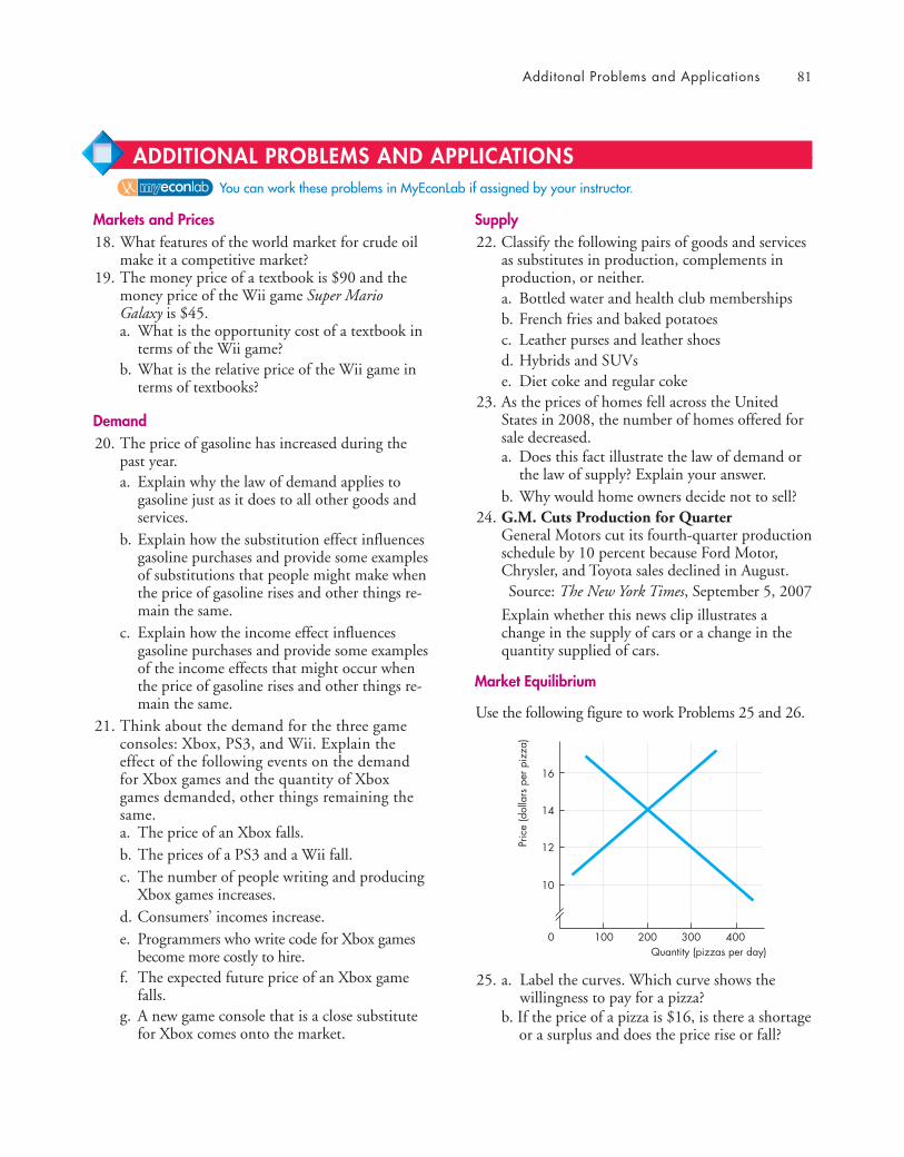
Markets and Prices18. What features of the world market for crude oil

make it a competitive market?19. The money price of a textbook is $90 and the

money price of the Wii game Super MarioGalaxy is $45.a. What is the opportunity cost of a textbook in

terms of the Wii game?b. What is the relative price of the Wii game in

terms of textbooks?

Demand20. The price of gasoline has increased during the

past year.a. Explain why the law of demand applies to

gasoline just as it does to all other goods andservices.

b. Explain how the substitution effect influencesgasoline purchases and provide some examplesof substitutions that people might make whenthe price of gasoline rises and other things re-main the same.

c. Explain how the income effect influencesgasoline purchases and provide some examplesof the income effects that might occur whenthe price of gasoline rises and other things re-main the same.

21. Think about the demand for the three gameconsoles: Xbox, PS3, and Wii. Explain theeffect of the following events on the demandfor Xbox games and the quantity of Xboxgames demanded, other things remaining thesame.a. The price of an Xbox falls.b. The prices of a PS3 and a Wii fall.c. The number of people writing and producing

Xbox games increases.d. Consumers’ incomes increase.e. Programmers who write code for Xbox games

become more costly to hire.f. The expected future price of an Xbox game

falls.g. A new game console that is a close substitute

for Xbox comes onto the market.

Supply22. Classify the following pairs of goods and services

as substitutes in production, complements inproduction, or neither.a. Bottled water and health club membershipsb. French fries and baked potatoesc. Leather purses and leather shoesd. Hybrids and SUVse. Diet coke and regular coke

23. As the prices of homes fell across the UnitedStates in 2008, the number of homes offered forsale decreased.a. Does this fact illustrate the law of demand or

the law of supply? Explain your answer.b. Why would home owners decide not to sell?

24. G.M. Cuts Production for QuarterGeneral Motors cut its fourth-quarter productionschedule by 10 percent because Ford Motor,Chrysler, and Toyota sales declined in August. Source: The New York Times, September 5, 2007

Explain whether this news clip illustrates achange in the supply of cars or a change in thequantity supplied of cars.

Market Equilibrium

Use the following figure to work Problems 25 and 26.

25. a. Label the curves. Which curve shows the willingness to pay for a pizza?

b. If the price of a pizza is $16, is there a shortageor a surplus and does the price rise or fall?

10

12

14

Quantity (pizzas per day)0 100 200 300 400

16

Pric

e (d

olla

rs p

er p

izza

)

Additonal Problems and Applications 81

You can work these problems in MyEconLab if assigned by your instructor.

ADDITIONAL PROBLEMS AND APPLICATIONS

c. Sellers want to receive the highest possibleprice, so why would they be willing to acceptless than $16 a pizza?

26. a. If the price of a pizza is $12, is there a short-age or a surplus and does the price rise or fall?

b. Buyers want to pay the lowest possible price,so why would they be willing to pay morethan $12 for a pizza?

27. The demand and supply schedules for potatochips are

Price Quantity Quantity(cents demanded supplied

per bag) (millions of bags per week)

50 160 13060 150 14070 140 15080 130 16090 120 170

100 110 180a. Draw a graph of the potato chip market and

mark in the equilibrium price and quantity.b. If the price is 60¢ a bag, is there a shortage or

a surplus, and how does the price adjust?

Predicting Changes in Price and Quantity28. In Problem 27, a new dip increases the quantity

of potato chips that people want to buy by 30million bags per week at each price.a. How does the demand and/or supply of chips

change?b. How does the price and quantity of chips

change?29. In Problem 27, if a virus destroys potato crops

and the quantity of potato chips produceddecreases by 40 million bags a week at each price,how does the supply of chips change?

30. If the virus in Problem 29 hits just as the newdip in Problem 28 comes onto the market, howdoes the price and quantity of chips change?

Economics in the News31. After you have studied Reading Between the Lines

on pp. 74–75 answer the following questions.a. What happened to the price of coffee in 2010?b. What substitutions do you expect might have

been made to decrease the quantity of coffeedemanded?

c. What influenced the demand for coffee in2010 and what influenced the quantity ofcoffee demanded?

d. What influenced the supply of coffee during

2010 and how did the supply of coffeechange?

e. How did the combination of the factors youhave noted in parts (c) and (d) influence theprice and quantity of coffee?

f. Was the change in quantity of coffee a changein the quantity demanded or a change in thequantity supplied?

32. Strawberry Prices Drop as Late Harvest HitsMarketShoppers bought strawberries in March for $1.25 apound rather than the $3.49 a pound they paidlast year. With the price so low, some growersplowed over their strawberry plants to make wayfor spring melons; others froze their harvests andsold them to juice and jam makers.

Source: USA Today, April 5, 2010a. Explain how the market for strawberries would

have changed if growers had not plowed in theirplants but offered locals “you pick for free.”

b. Describe the changes in demand and supplyin the market for strawberry jam.

33. “Popcorn Movie” Experience Gets PricierCinemas are raising the price of popcorn.Demand for field corn, which is used for animalfeed, corn syrup, and ethanol, has increased andits price has exploded. That’s caused some farm-ers to shift from growing popcorn to easier-to-grow field corn.

Source: USA Today, May 24, 2008Explain and illustrate graphically the eventsdescribed in the news clip in the market fora. Popcorn b. Movie tickets

Use the following news clip to work Problems 34 and 35.Sony’s Blu-Ray Wins High-Definition WarToshiba Corp. yesterday withdrew from the race to bethe next-generation home movie format, leaving SonyCorp.’s Blu-ray technology the winner. The move couldfinally jump-start a high-definition home DVD market.

Source: The Washington Times, February 20, 200834. a. How would you expect the price of a used

Toshiba player on eBay to change? Will theprice change result from a change in demand,supply, or both, and in which directions?

b. How would you expect the price of a Blu-rayplayer to change?

35. Explain how the market for Blu-ray formatmovies will change.


Economics (2-downloads) - E-Learning KIMEP

Documents

Transcript of Economics (2-downloads) - E-Learning KIMEP