Ecological Economics 114 (2015) 47–57

Contents lists available at ScienceDirect

Ecological Economics

j ourna l homepage: www.e lsev ie r .com/ locate /eco lecon

Analysis

Economic tradeoffs in mitigation, due to different atmospheric lifetimesof CO2 and black carbon

Ashwin K. SeshadriDivecha Centre for Climate Change, Indian Institute of Science, Bangalore, India

E-mail address: ashwin@fastmail.fm.

http://dx.doi.org/10.1016/j.ecolecon.2015.03.0040921-8009/© 2015 Elsevier B.V. All rights reserved.

a b s t r a c t

a r t i c l e i n f o

Article history:Received 13 April 2014Received in revised form 25 February 2015Accepted 10 March 2015Available online xxxx

Keywords:Global climate changeClimate change mitigationBlack carbonCarbon dioxideMitigation tradeoffsMitigation timescales

Tradeoffs are examined between mitigating black carbon (BC) and carbon dioxide (CO2) for limiting peak globalmeanwarming, using the following set of methods. A two-box climatemodel is used to simulate temperatures ofthe atmosphere and ocean for different rates of mitigation. Mitigation rates for BC and CO2 are characterized byrespective timescales for e-folding reduction in emissions intensity of gross global product. There are respectiveemissions models that force the box model. Lastly there is a simple economics model, with cost of mitigationvarying inversely with emission intensity.Constantmitigation timescale corresponds tomitigation at a constant annual rate, for example an e-folding time-scale of 40 years corresponds to 2.5% reduction each year. Discounted present cost depends only on respectivemitigation timescale and respective mitigation cost at present levels of emission intensity. Least-cost mitigationis posed as choosing respective e-folding timescales, to minimize total mitigation cost under a temperature con-straint (e.g. within 2 °C above preindustrial). Peakwarming ismore sensitive tomitigation timescale for CO2 thanfor BC. Therefore rapid mitigation of CO2 emission intensity is essential to limiting peak warming, but simulta-neous mitigation of BC can reduce total mitigation expenditure.

© 2015 Elsevier B.V. All rights reserved.

1. Introduction

There are different views on what role the mitigation of emission ofshort lived climate pollutants (SLCPs) can play in climate policy. SLCPsare agents with relatively short lifetimes in the atmosphere and thatwarm the Earth's climate (CCAC, 2014). These include methane, blackcarbon (BC), tropospheric ozone, and hydrofluorocarbons (HFCs).

Early mitigation of SLCP emissions has been suggested as importantfor reducing near-term warming (MacCracken, 2008; Jackson, 2009;Wallack and Ramanathan, 2009; Penner et al., 2010; Ramanathan andXu, 2010; UNEP, 2011; Shindell et al., 2012; Hu et al., 2013). This hasalso been suggested to buy time for more expensive activities thatwould mitigate carbon dioxide (CO2) emissions (Ramanathan andVictor, 2010), which is germane because global progress towardsmitigat-ing CO2 emissions has been slow (Quéré et al., 2009; Peters et al., 2013).With early and rapidmitigation of SLCPs, if their anthropogenic emissionscould be completely stopped then their excess concentrations and radia-tive forcing due to human activities can be eliminated in about 10 years.By contrast a fraction of airborne CO2 persists in the atmosphere for sev-eral thousand years (Archer and Brovkin, 2008; Archer et al., 2009).

Studies have pointed out (Berntsen et al., 2010; Bowerman et al.,2013; Shoemaker et al., 2013; Shoemaker and Schrag, 2013; Allen andStocker, 2014; Pierrehumbert, 2014) limitations of the strategy of early

elimination of SLCP emissions as a way to buy time while awaiting largereductions of CO2 emissions. SLCPs affect peak temperature only whenCO2 emissions are decreasing (Bowerman et al., 2013), so early actionon SLCPs has limited effect on peak temperature if this is not incipient.For the case of methane, if overvaluation of methane emissions leads toneglect of CO2 reductions, then near term reductions in warming couldbe offset by future increases in warming (Shoemaker and Schrag, 2013).In contrast to SLCPs, CO2 accumulates in the atmosphere for a very longtime. Therefore the level of peak warming already committed to by pastemissions of CO2 rises in proportion to cumulative emissions (Allen andStocker, 2014). While the prevailing view is difficult to characterize, ap-preciation of the need to simultaneously reduce SLCP and CO2 emissionsseems to be growing (Berntsen et al., 2010; Shoemaker et al., 2013).

As the term denotes, SLCPs not only affect climate but also are air pol-lutants. Controlling thesewould have benefits for human health (Jackson,2009; Shindell et al., 2012; Smith and Mizrahi, 2013) and agriculture(Shindell et al., 2012). Methane is an ozone precursor, and controllingits emissions would benefit global agriculture by increasing crop yields(Shindell et al., 2012). Controlling BC emissions would have regionalbenefits for human health (Shindell et al., 2012). Harmful effects of BCemission on human health result from increases in near-surface concen-trations of ozone and PM2.5, with the latter playing the main role(Jacobson, 2010). BC from fossil fuel emission has smaller particle sizes,leading to larger increases in PM2.5 concentrations than BC from biomassburning (Jacobson, 2010), but biomass burning most often occurs indensely populated regions, and effects on mortality are amplified by

1 The e-folding lifetime is meant to describe effective timescale over which radiativeforcing decays. For BC, this strictly must include effects of BC deposited on ice or snow.For simplicity, the terminology used is “atmospheric lifetime”.

48 A.K. Seshadri / Ecological Economics 114 (2015) 47–57

higher population densities. Epidemiological studies show evidence ofmortality from sulfate, BC and tropospheric ozone (Smith et al., 2009).Controlling these pollutants will reduce premature mortality.

Therefore the question about the role of anthropogenic SLCPs in cli-mate policy is not whether they should be controlled, butwhether earlymitigation of SLCPs can adequately substitute for immediate rapid ac-tions on CO2. This paper partly explores this by considering tradeoffsin rates of mitigation of BC and CO2. It is assumed that sustainedmitiga-tion begins in the present, and continues at a constant rate. Varying thisrate sheds light on the tradeoff. The resulting analysis of rapid versusslow mitigation does not completely illuminate policy issues regardingearly versus late mitigation, but there are parallels. Rapid and earlymitigation both cost more, and decrease warming. However rate andtiming of mitigation are different.

Anthropogenic emissions of BC make significant contributions tototal radiative forcing and observed temperature change (Shindellet al., 2009; Bond et al., 2013). Despite uncertainty about themagnitudeof warming effects from BC, multiple studies suggest that controlling BCwill reduce warming (Shindell et al., 2012; Smith and Mizrahi, 2013;Bowerman et al., 2013; Collins et al., 2013). Furthermore the large dif-ferences in the atmospheric lifetimes of BC and CO2 are illustrative ofmajor differences between effects of mitigating SLCPs and CO2.

Present global radiative forcing of BC is estimated as 1.1Wm−2with90% uncertainty interval of +0.17 to +2.1 W m−2 (Bond et al., 2013).Benefits, from avoided radiative forcing, of reducing BC concentrationsare uncertain. There are additional factors pertinent to understandingthe effects ofmitigating BC. Effects on global radiative forcingwould de-pend on the region where mitigation occurs (Collins et al., 2013). Aero-sols containing BC interactwith clouds and effects of regionalmitigationof BC on global “indirect effects”, i.e. effects occurring when aerosolschange cloud properties, are poorly quantified (Bond et al., 2013). Cli-mate effects of BC also depend on co-emitted species (Bond et al.,2013). For example, carbonaceous aerosol from biomass burning ab-sorbs less sunlight than such aerosol from fossil fuel sources, due tohigher concentrations of light-reflecting organic carbon in biomass(Jacobson, 2010; Kopp and Mauzerall, 2010).

Despite these challenges it is necessary to consider economic aspectsof the tradeoff between mitigating SLCPs and CO2.

When BC and CO2 are co-emitted, reducing emissions of one specieswill reduce the other (Smith and Mizrahi, 2013). But large-scale mitiga-tion of CO2 requires large investments and upfront costs, whereasmitiga-tion of SLCPs generally does not. Therefore the role of co-emission inmitigation of SLCPs and CO2 is likely to be relatively small at the globalscale and over long periods of time. Costs of mitigating SLCP emissionsare generallymuch lower than for CO2 (Wallack and Ramanathan, 2009).

This paper considers economic tradeoffs in mitigation rates of BCand CO2. The approach is along the lines of cost-effectiveness analysis(Koomey (2013)). Costs of alternate trajectories of CO2 and BC mitiga-tion that lead to the same peak warming are compared.

Future costs must be discounted to the present to facilitate compar-ison, and the choice of discount rate affects the analysis (Heal, 1997;Nordhaus, 1997, 2007; Dasgupta, 2008). Two simplifications are intro-duced to avoid this difficulty. Mitigation of each species occurs with e-folding reduction in emission intensity. Specifically, emission intensityof gross global product (GGP) decreases in time as e−t=τm , where τm isthe e-folding mitigation timescale. Hence emission intensity μ(t) variesas μ tð Þ ¼ μ 0ð Þe−t=τm where μ(0) is emission intensity at the presenttime. Therefore the rate of change in emission intensity is dμ(t)/dt =(−1/τm)μ(t). Constant mitigation timescale corresponds to the samepercentage decrease in emission intensity each year.

Second, mitigation costs are modeled as varying inversely withemission intensity.

Effects of BC and CO2 mitigation timescales on peak warming areexamined using a two-box model of the atmosphere and oceans(Gregory, 2000; Williams et al., 2008; Winton et al., 2010; Held

et al., 2010). The two boxes describe mean temperature evolutionof the atmosphere+ surface ocean and of the deep oceans respectively.Respective emissions models yield the forcings to the box model fromBC and CO2. Radiative forcing from other species is made to followthe scenario of Representative Concentration Pathway (RCP) 4.5,i.e. which involves stabilization of total radiative forcing at 4.5 W m−2

(Meinshausen et al., 2011; Shindell et al., 2013; Myhre et al., 2013).Lastly there is an economics model describing mitigation cost.Section 2 describes these methods.

Mitigation pathways to keep peak warming below 2 °C above prein-dustrial conditions are calculated. An upper limit to global warming of2 °C above preindustrial is an important goal of mitigation (Ramanathanand Feng, 2008; Parry et al., 2009; Stocker, 2013), but options for satisfy-ing this constraint seem to be closing rapidly under current mitigationpathways (Rogelj et al., 2009; Stocker, 2013; UNEP, 2013).

2. Methods

2.1. Concentration in the atmosphere as a result of mitigation

This section describes how the burden or mean concentration of BCand CO2 evolves through time as global emissions are mitigated. Thecalculations are used to estimate forcing terms in a two-box model ofthe atmosphere and oceans. The model of concentration relies on theidealizations below. BC has atmospheric lifetime on the order of days(Solomon et al., 2012; Bond et al., 2013). When deposited on snow orice, the radiative effects of BC persist across seasons. But the lifetimefor the decay of BC radiative effects is much shorter than the timescaleover which globalmitigation of BCwould occur. By contrast a part of at-mospheric CO2 lasts for several thousand years in the atmosphere(Archer and Brovkin, 2008). Its atmospheric lifetime is much longerthan the timescale over which CO2 mitigation must occur to limitglobal warming. In both cases there can be large differences betweenrespective mitigation timescale and atmospheric lifetime. Theselarge differences aid analysis. Themodeling of concentrations adoptsthe following assumptions.

The first assumption is that global burden of BC has constant e-folding lifetime in the atmosphere. Then the relation governing burdenconsists of its rate of growth via emission and its rate of loss, with thelatter represented in terms of atmospheric lifetime. 1

The burden x(t) then follows

dxdt

¼ m tð Þ− x tð Þ−xPIτx

ð1Þ

where m(t) is the emissions at time t, xPI is the natural or preindustrialequilibrium value, τx its constant e-folding lifetime, and t = 0 corre-sponds to the present. Emission m(t) characterizes rate of increase inburden in the hypothetical limit that τx→ ∞. Time is measured in years.

For BC, the atmospheric burden for the year 1750 has been estimat-ed as 32 × 106 kg (Skeie et al., 2011), and this has been taken in ourcalculations to be the preindustrial equilibrium value. This burden ismainly from biomass burning. Biomass burning does not depend onindustrialization, and not all of this burden in 1750 is fromnatural emis-sions. Hence this is anupper boundonnatural equilibriumburden of BC.Using estimates of total BC emissions in the year 2000 of 7.1 × 109 kgand in 2007 of 7.8 × 109 kg (Skeie et al., 2011) yields an annual growthrate of 1.34%. Using this growth rate and assuming the same atmospher-ic lifetime as estimated for 2008, emissions andmean atmospheric bur-den for 2014 are estimated as 8.6 × 109 kg and 200 × 106 kgrespectively. These are the initial conditions of the emissionsmodel. At-mospheric lifetime of BC in the emissions model is taken as 10 days, an

2 This can be seen explicitly in the following. Eq. (7) can bewritten as (Held et al., 2010)

csdxdt

¼ B x; yð Þ−γ x−yð Þ þ F0 tð Þ þ F1 tð Þ þ F2 tð Þ

where B(x, y) =− βx− (�− 1)γ(x− y) describes changes to radiative flux at the top ofthe atmosphere. Near to equilibriumwhere x= y these changes vary onlywith x as− βx,but towards the beginning of the forced responsewhere y≈ 0 theflux ismore sensitive tochanges in x. This is implementedwith � N 1;while uncertain, the estimatedmedian value� = 1.3 (Held et al., 2010) has been used in our study.

49A.K. Seshadri / Ecological Economics 114 (2015) 47–57

upper bound of the estimates of Skeie et al. (2011) and Bond et al.(2013). This does not include the effects of persistence of radiative forc-ing following deposition on snow and ice.

As for atmospheric CO2, there is comparatively rapid uptake by theland biosphere and ocean mixed-layer, followed by slower uptake bymixingwith the deep ocean, and finally very slow reactionwith silicates(Pierrehumbert, 2014). In themeantime, ocean acidity is reduced by thedissolution of carbonates, but the process is very slow (Pierrehumbert,2014). The consequence is that three-fourths of anthropogenic CO2

in the atmosphere dissolves in the ocean over few centuries, with theremainder remaining for many thousand years until reaction withCaCO3 or silicate rocks on land (Archer and Brovkin, 2008; Archeret al., 2009; Montenegro et al., 2007). It is not accurate to treat decayof anthropogenic CO2 in the atmosphere using a single e-folding life-time. One way to characterize the response, assuming linearity, is byan impulse response, i.e. the response to a pulse emission of CO2. Thedetails of the carbon cycle differs between models, and Joos et al.(2013) have computed the mean impulse response for a 100 GigatonC pulse emission of CO2 among a group of Earth system models

IRFCO2 ¼ 0:276e−t=4:30 þ 0:282e−t=36:5 þ 0:224e−t=394 þ 0:217 ð2Þ

with corresponding concentration given by

CO2 tð Þ ¼Z t

−∞m t0� �IRFCO2 t−t0� �

dt0 þ CO2PI: ð3Þ

Annual CO2 emissions starting in the year 1751 are taken fromBoden et al. (2011).

To illustrate the main differences between the responses of BC andCO2 to mitigation, analytic calculations are made in Section 3.1. Forthese calculations alone, we approximate decay of anthropogenic CO2

using a single e-folding lifetime. However, it is known that there is nosingle value of lifetime that can describe the response of atmosphericCO2 over all the relevant time-horizons. For example the apparentadjustment time increases with the time-horizon and depends on thelevel of emissions (Tubiello and Oppenheimer, 1995; Archer et al.,2009; Tanaka et al., 2012).

CO2 is well-mixed in the atmosphere because of its long lifetime, butconcentrations of BC vary with location. However globally averagedconcentrations and temperatures are studied in this paper, so the treat-ment of BC is same as for CO2 in characterizing evolution of the globalburden of BC. Numerical integration of the relevant equation above isused to calculate forcing terms for BC and CO2 in the two-boxmodel in-troduced in Section 2.2.

Emissions are described in terms of gross global product (GGP) andemission intensity. This terminology is used in lieu of gross world prod-uct to avoid confusion with global warming potentials (Lashof andAhuja, 1990). The relation is

m tð Þ ¼ GGP tð Þμ tð Þ ð4Þ

where μ(t) is the emission intensity at time t. Economic growth is notnecessarily accompanied by increase in emission of air pollutants. How-ever since the relation here is between GGP and emissions, it is assumedthat emission intensity of GGP remains constant unless actions aretaken to decrease it.

The second assumption is that emission intensity decreases withe-folding timescale τm as a result of mitigation of forcing agent x, sothat μ tð Þ ¼ μ 0ð Þe−t=τm . This e-folding timescale is also called themitiga-tion timescale. The decrease follows the rate dμ(t)/dt=(−1/τm)μ(t), soconstant e-folding timescale gives the same percentage decrease inemission intensity each year. For example, τm = 20 years correspondsto a 5% decrease each year. This contrasts with widely used emissionscenarios where mitigation effort begins gradually and increases(Nakicenovic et al., 2000; Pacala and Socolow, 2004; Moss et al., 2010).

Heuristically, e-folding of emission intensity can result from the fact thatas reduction occurs, it becomesmore difficult to obtain subsequent reduc-tions. But at present this must be taken as postulated, meant to distin-guish different rates of reduction. Later it will be shown that it offers athought experiment by simplifying economic analysis.

GGP is assumed to increase at constant annual rate g for 50 years,after which it is held constant. Hence emissionsm(t) vary with time as

m tð Þ ¼ m0 1þ gð Þmin t;50ð Þe−t=τm ð5Þ

wherem0=m(t=0) is current emission, and the exponentially declin-ing term describes effect of decrease in emission intensity of GGP. De-grees of mitigation effort are characterized by the value of τm. Forexample, τm→∞ denotes the absence ofmitigation effort, while smallervalues of τm indicate increasing levels of mitigation effort.

Eqs. (1) and (5) are solved for the special case of no growth in GGP(Appendix A) yielding

x tð Þ ¼ x0e−t=τx þ τmτx

τx−τmm0 e−t=τx−e−t=τm� �

þ xPI 1−e−t=τx� �

ð6Þ

where x0 is the present concentration in the atmosphere. SLCPs such asBC differ from CO2 in a critical way. For BC,mitigation of emission inten-sitywill occurwith e-folding timescalemuch longer than its atmospher-ic lifetime. Whereas for CO2, mitigation needs to occur on a timescalemuch shorter than its atmospheric lifetime.

2.2. Box model of temperature change

A two-box global mean climate model (Gregory, 2000; Williamset al., 2008;Winton et al., 2010; Held et al., 2010) is used to study effectsof alternatemitigation pathways of BC and CO2. The system of two ordi-nary differential equations represents departures Ts and Td respectivelyof global mean air + surface ocean temperature and deep ocean tem-perature from their preindustrial values. Model equations are

csdTs

dt¼ −βTs−�γ Ts−Tdð Þ þ F0 tð Þ þ F1 tð Þ þ F2 tð Þ ð7Þ

cddTd

dt¼ γ Ts−Tdð Þ: ð8Þ

Eq. (7) describes changes in the energy budget of the atmosphere +ocean surface layer (the upper box), and corresponding evolution of tem-perature anomaly Ts. Anomalies are with respect to preindustrial values,so Ts = 0 denotes preindustrial temperature. These layers respond rela-tively rapidly to forcing. Coefficient cs denotes the heat capacity of thisupper box. Coefficient γ controls heat exchange with the deep oceanbox, which is γ(Ts − Td).

The factor ε denotes efficacy of heat uptake by the deep ocean. It hasbeen introduced to adjust for a limitation of two-boxmodels, as a resultof their not representing changes in the spatial pattern of warming asthe climate warms. As the climate warms, the relation between globalmean surface temperature and outgoing flux to space changes. The fac-tor ε characterizes this changing relation (Williams et al., 2008;Wintonet al., 2010; Held et al., 2010).2

Eq. (8) represents changes in the energy content of the deep oceanbox. This has large heat capacity cd, causing much slower approach

Table 1Radiative forcing by other substances (Myhre et al., 2013).

Species RF (IPCC AR5 best estimate,W m−2)

Other well-mixed GHGs (CH4, N2O, halocarbons) 0.97 + 0.18 + 0.17 = 1.32Short-lived gases (CO, NMVOC, NOx) 0.23 + 0.10 − 0.15 = 0.18Aerosols other than BC and OC (primarily sulfate) −0.50Cloud adjustment due to aerosols −0.55Total 0.45

50 A.K. Seshadri / Ecological Economics 114 (2015) 47–57

towards equilibrium. The two-box climate model above has beenshown to reproduce transient warming simulated by a comprehensiveclimate model (Held et al., 2010). Based on values estimated therein(Held et al., 2010), parameter estimates are γ = 1.0 W m−2 K−1 and�=1.3. The heat capacity cs includes the atmosphere and the ocean sur-face layer, and we use cs = 9.28W yearm−2 K−1 following an estimateobtained in Held et al. (2010) for a single climate model, and based onthe fast-response timescale therein. This heat capacity corresponds toroughly 95 m of the surface ocean, in addition to the mass of theatmosphere.3 With mean depth of the oceans of about 4.3 km, theratio of heat capacities of the two boxes is then cd/cs ≅ 43. Of course,these numbers are model-dependent. For our study the actual ratio ofheat capacities has weak influence on peak warming, as long as theratio is very large, because the deep ocean box responds very slowlyto external forcing.

The coefficient β is related to equilibrium climate sensitivityΔTcs, i.e.the equilibrium rise in temperature following instantaneous doubling ofCO2 from its preindustrial concentration. From the equilibrium condi-tion this relation is ΔTcsβ= 5.35loge2. For equilibrium climate sensitiv-ity of 3 °C, the coefficient is β = 1.24 W m−2 K−1.

Forcing term F0(t) is the total effect of the primary contributions toanthropogenic radiative forcing other than BC and CO2. It depends ontime, and the present contribution is listed in Table 1 (Myhre et al.,2013). Total present contribution is 0.45 W m−2. The time-variation ofthis forcing affects levels of abatement of BC and CO2 necessary tomeet the peak warming constraint. The RCP4.5 scenario is used to de-scribe variation of these other forcers' contribution to total forcing(Meinshausen et al., 2011; Shindell et al., 2013; Myhre et al., 2013). Acommon feature of these scenarios is a reduction in aerosol forcing by2100, with differences at this time arising mainly from well-mixedGHGs.

Time-varying forcing terms F1(t) and F2(t) represent contributionsof BC and CO2 respectively.

Radiative forcing of BC is related to burden as F1(t)= α1x1(t), wherex1(t) is the burden of BC in the atmosphere. Coefficient α1 is theassumed constant radiative efficiency per unit mass. With F1(0) =1 W m−2, or approximately the present-day best-estimate radiativeforcing of BC (Bond et al., 2013), and present burden estimated as200 × 106 kg, we obtain α1 = 5.0 × 10−9 W m−2 kg−1. However wenote that estimates of radiative forcing of BC are uncertain (Bondet al., 2013; Smith and Mizrahi, 2013). BC burden x1 at future times isobtained by solving Eq. (1) numerically with Eq. (5) describingemissions.

Radiative forcing of CO2 is calculated using F2(t) = 5.35log(x2(t)/x2,PI)W/m2, where x2(t) is its atmospheric concentration in parts permillion. For CO2 at future times, the model with multiple time-constants in Eqs. (2) and (3) is integrated with Eq. (5) describingemissions.

For the historical period, estimates of the combined historical anthro-pogenic radiative forcing are used (Meinshausen et al., 2011; Shindellet al., 2013; Myhre et al., 2013). Starting from the present at t = 0 inthe model, contributions F0(t), F1(t) and F2(t) are computed separately.

2.3. Economics of mitigation

The treatment of economics is idealized, involving mitigation costfunction

p μ tð Þ; μ0ð Þ ¼ p0 μ0ð Þμ tð Þ=μ0

ð10Þ

where p is the cost of reducing emission intensity of GGP by one unit.

3 Neglecting effects of atmospheric water, this means that 96.5% of the heat capacity ofthe upper box comes from the top 95 m of surface ocean and only 3.5% from the atmo-sphere. This is not far from estimates of the fraction of excess energy of the Earth due toanthropogenic radiative forcing that is being stored by the oceans (Rhein et al., 2013;Stocker et al., 2013).

Coefficient p0 depends only on present emission intensity μ0, so giventhe present state of the world it is constant in time. Coefficient p0 alsodescribes the present cost of mitigation by one unit, i.e. the cost whenμ = μ0. The cost p(μ(t), μ0) varies inversely with emission intensity. Asemission intensity goes towards zero, the unit cost ofmaking further re-ductions goes towards infinity. This is meant to approximate situationswhere mitigation becomes progressively more costly (Enkvist et al.,2007; Morris et al., 2008; Kesicki and Elkins, 2012). However theequation above is motivated not empirically, but by consequences foranalysis described below. The model in Eq. (10) assumes economicequilibrium and ignores the presence of mitigation opportunities atzero or negative cost. It also ignores learning, which could reduce miti-gation costs over time.

Emissions at time t+Δt is the result of two contributions. First is theemissions resulting from economic activities that existed at time t butwith a changed emission intensity found at time t+Δt. Second is the in-crease in emissions due to change in GGP between t and t+Δt, butwiththe emission intensity found at time t. Therefore

m t þ Δtð Þ ¼ GGP tð Þμ t þ Δtð Þ þ ΔGGP tð Þμ tð Þ: ð11Þ

From the above expression, Δm(t) = GGP(t)Δμ(t) + ΔGGP(t)μ(t)and hence this is equivalent to Eq. (4).

In Eq. (11) thefirst term on the right describes the effect of deliberate-ly changing emission intensity, as via mitigation. Therefore the activitiesrepresented by this term are what constitute mitigation expenditures.Hence total expenditure on mitigation between time t and t+ Δt is

Pt:tþΔt ¼ p μ tð Þ; μ0ð Þ � GGP tð Þ � abs Δμ tð Þð Þ ¼ p0μ0

τm� GGP tð ÞΔt ð12Þ

where we have used Eq. (10) and the relation Δμ(t) =− μ(t)Δt/τm. Thisexpenditure towards mitigation, over fixed intervals of time Δt, varieswith time proportionally to the variation of GGP with time. With time-discounting factor 0 b δ(Δt) b 1 that depends only on the time interval,the net present value of the series of expenditures towards mitigation isdescribed by the infinite series

X Pt;tþΔt

1þ δ Δtð Þð Þt ð13Þ

which simplifies to

p0μ0

τm�X GGP tð ÞΔt

1þ δ Δtð Þð Þt : ð14Þ

The summation in the above expression depends only on evolu-tion of GGP and the discount-factor, and therefore takes the samevalue for BC and CO2. This series is convergent if the discount factoris strictly positive, because GGP increases at most for a finite time pe-riod (i.e. 50 years) in the model. (In general, without assuming finitegrowth of GGP, the series would also be convergent if discount rate islarger than growth rate of GGP).

The discounted expenditure in Eq. (14) is inversely proportional tomitigation timescale τm and increases with p0μ0. Therefore discountedcosts of mitigating BC and CO2 differ only in their respective factorsp0,1μ0,1/τm,1 and p0,2μ0,2/τm,2. Thus it is possible to compare relative

51A.K. Seshadri / Ecological Economics 114 (2015) 47–57

costs of mitigating BC and CO2, independently of the time-discount fac-tor. The product p0μ0 is the cost of reducing emission intensity by a fac-tor of e, starting from the present.4 Hencewe call this themitigation costfactor, recognizing that it is the cost required to bring down emission in-tensity by a factor of e; and if this occurs with e-folding reductions inemission intensity, the cost is incurred over the mitigation timescale.

Our primary goal is to characterize e-folding timescales τm,1 and τm,2

that minimize mitigation cost while maintaining surface temperaturewithin the constraint, and the corresponding optimization problem is

minimize f τm;1; τm;2

� �¼ 1

τm;1þ rcτm;2

ð15Þ

subject to g τm;1; τm;2

� �¼ 0 ð16Þ

where the nonlinear constraint equation g(τm,1, τm,2) = 0 correspondsto the curve describing the threshold temperature that must not beexceeded, and rc = p0,2μ0,2/p0,1μ0,1 is the ratio of mitigation cost factorsfor CO2 and BC. The rate of growth of GGP affects the constraint ofEq. (16), but does not appear in the objective function in Eq. (15). At atangent solution to this constrainedminimization problem the gradientof the objective function is some multiple λ of the gradient of theconstraint equation. Along directions of τm,1 and τm,2 this yields theexpressions

λ∂g

∂τm;1¼ 1

τ�m;1

� �2 ð17Þ

λ∂g

∂τm;2¼ rc

τ�m;2

� �2 : ð18Þ

The ratio between the twomitigation timescales at the least-cost so-lution is then

τ�m;2

τ�m;1

!2

¼ rc

∂g∂τm;1

∂g∂τm;2

ð19Þ

while the ratio of mitigation expenditures on CO2 and BC is

C�2

C�1¼ rcτ

�m;1

τ�m;2¼ rc

∂g∂τm;2

∂g∂τm;1

0@

1A1=2

: ð20Þ

3. Results

3.1. Behavior of concentration in the atmosphere

Here we analytically approximate the model with a single atmo-spheric lifetime to understand qualitatively the effects of mitigationtimescale on peak atmospheric concentration for two different typesof cases. We limit analysis to the case of zero GGP growth, followingEq. (6), because this illustrates the major differences between BC andCO2.

4 From Eq. (10), total cost of reducing emissions intensity from μ0 to μ(t) is −

∫μ tð Þμ0

p μ tð Þ; μ0ð Þdμ, which can be written as−∫μ

μ0

p0μ0

μdμ , simplifying to p0μ0loge

μ0

μ.

3.1.1. Short-lived forcer, with τx ≪ τmUnder the condition τx/τm ≪ 1, the rate of change of concentration

with time is described by

dx Tð Þdt

¼ m0−x0−xPI

τx

� �e−T=τx−m0

τxτm

e−T=τm ð21Þ

where, from Eq. (1), m0 N (x0 − xPI)/τx if concentration is rising atpresent time t = 0, as it is for BC in the Earth's atmosphere. Time Tp atwhich concentration peaks is defined by dx(Tp)/dt = 0. Once againusing the approximation that τx/τm ≪ 1, we find

Tp ≅ τxloge τmð Þ−τxloge τxð Þ þ τxloge 1− x0−xPIm0τx

� �ð22Þ

so that dTp/dτm= τx/τm. Peak concentration is estimated by substitutingthe approximation for Tp in Eq. (22) into the expression (6)

xp ≡ x Tp

� �≅ x0−τxm0ð Þe−Tp=τx þ τxm0e

−Tp=τm þ xPI ð23Þ

where we have also assumed that Tp ≫ τx. The sensitivity of peak con-centration to change in mitigation timescale is

dxpdτm

¼ ∂xp∂τm

þ ∂xp∂Tp

dTp

dτm: ð24Þ

With the simplification Tp ≪ τm,5 the above expression simplifies to

dxpdτm

≅τxm0Tp

τ2m: ð25Þ

Using Eq. (22), Eq. (25) above has the form (c0 + c1logeτm)/τm2 forpositive constants c0 and c1 that do not depend on τm. For sufficientlylarge τm, the second (i.e. logarithmic) term dominates and is smallerthan c1/τm. Since this expression refers to the dependence of the deriv-ative of xp with respect to τm, integration shows that the increase withmitigation timescale of peak concentration is slower than logarithmic.One implication is that slower mitigation of SLCPs, i.e. involving longere-folding timescale τm, has progressively smaller influence on peak con-centration xp. The converse is, of course, that faster mitigation has pro-gressively larger effect.

We compare the two limiting cases: no mitigation, with τm → ∞,and instantaneous mitigation with τm = 0. In the first case, emissionm(t) in Eq. (1) is equal to m0 indefinitely, and the concentrationtends asymptotically to the value of xPI + m0τx. In the second case,emission m(t) in Eq. (1) is equal to zero for t N 0, so peak concentra-tion is equal to its present value x0. The relative difference betweenthe cases of no mitigation and instantaneous mitigation is equal to((xPI +m0τx)/x0)− 1; from Eq. (1), this expression is equal to the at-mospheric lifetime τx multiplied by the annual growth rate of con-centration at t = 0. This means that for SLCPs, without growth inGGP, the difference in peak concentration between the two extrememitigation cases is equal to the atmospheric buildup over its lifetimewhen concentration grows at the initial rate. For BC with atmospher-ic lifetime of about a week and present emission growth of a few per-cent, this difference appears small.

3.1.2. Long-lived forcer, with τx ≫ τmMitigation of CO2 would have to occur with timescale much

shorter than its atmospheric lifetime if global warming is to be limit-ed. With the approximation that τx/τm ≫ 1, the rate of change of

5 This assumption was necessary, and implicitly made, in the derivation of Eq. (22).

52 A.K. Seshadri / Ecological Economics 114 (2015) 47–57

concentration with time is

dx Tð Þdt

¼ m0e−T=τm− x0−xPI

τxþm0τm

τx

� �e−T=τx : ð26Þ

The time Tp at which concentration peaks, so that dx(Tp)/dt = 0, is

Tp ≅ τmloge1

x0−xPIm0τx

þ τmτx

: ð27Þ

There is a term τm in the numerator of Eq. (27), and a term involvingτm in the denominator of the logarithmic term. Therefore time to reachpeak concentration increases slower than linearly with τm. It is only forthe limiting casewhere τm→ 0 that this latter term is negligible, so thatTp increases linearly with τm. Substituting the above expression intoEq. (6) with the further approximation that Tp/τx ≪ 1,6 the peak con-centration is described by

xp−xPI ≅ x0−xPIð Þ þ τm m0 1− τmτx

� �− x0−xPI

τx

� �: ð28Þ

Let us see if the quadratic term involving τm plays a significant role.In aid of this we introduce the quantity η0 = (m0/x0)− (x0 − xPI)/τxx0,which describes growth rate relative to present concentration at t = 0,from Eq. (1). Further writing 1/τx = ε0η0, and using these to eliminatem0 from the expression (28) yields

dxpdτm

≅x0η0 1−2τmτx

1þ ε0x0−xPI

x0

� �� �: ð29Þ

The quantity η0 has units of inverse time. It represents the presentdisequilibrium in concentration, and is defined as the fractional increasein concentration within a year, starting from present time t = 0. Thequantity ε0 relates this disequilibrium to the atmospheric lifetime. Forexample, if atmospheric concentration was growing at 1%/year, as ap-proximately in the case of CO2, ε0 = 100/τx. Then the quadratic termin Eq. (29) is negligible if (τm/τx)(100/τx) ≪ 1. This is the case of CO2

in the atmosphere if the mitigation timescale is rapid, compared to itslifetime. Under this condition peak-concentration increases almost line-arly with τm, at a rate that increases with initial concentration x0 andinitial disequilibrium η0. Under the condition that τm ≪ τx for CO2

only if the present disequilibrium in concentration was vanishinglysmall, i.e. large ε0, would the quadratic term be significant.

3.1.3. Numerical resultsFig. 1 confirms the above approximations made for the hypothetical

condition of zero GGP growth. Left panels show cases for BCwith atmo-spheric lifetime of 10 days; right panels show cases for CO2 describedwith a single atmospheric lifetime of 150 years. A single atmosphericlifetime does not describe CO2, but considering such a model is illustra-tive of major differences in behavior of BC and CO2.7 Upper panels plotconcentration pathways for different values of τm. Plotted are normal-ized concentrations x(t)/x0. Lower panels plot normalized peak concen-trations xp/x0 versus τm. In these panels, continuous lines depict theexact results obtained from Eq. (6), whereas crosses indicate the corre-sponding approximations derived previously in Section 3.1. For BC theapproximation improves as τm becomes longer, whereas the approxi-mation for CO2 is accurate only for short τm. Although accuracy de-creases away from these regimes, the exact solutions confirmqualitativelywhat the analytic solutions suggest. For BCpeak concentra-tion in the atmosphere increases slower than logarithmically with e-

6 This approximation was implicitly made in the derivation of Eq. (27).7 A lifetime of 150 years corresponds to 51% of pulse emissions remaining after

100 years, which is within the range described in the multi-model study of Joos et al.(2013).

folding timescale ofmitigation, if this timescale is sufficiently large. Con-sequently the effect of the mitigation rate on peak concentration issmall. By contrast for CO2, peak concentration continues to increase ap-proximately linearly with mitigation timescale in the regime whereτm ≪ τx. These differences play a role in what follows.

3.2. Peak temperatures in the box model

From this point on we use the multiple time-constant model (Jooset al., 2013) for describing atmospheric CO2 and allow GGP growth tooccur in the emissionsmodel. Fig. 2 shows peakwarming Ts,max simulat-ed by the two-box climatemodel of Eqs. (7) and (8), asmitigation time-scales are varied for BC and CO2. Plotted are isopleths of Ts,max, withrespect to timescales τm,1 and τm,2. These denote e-folding timescalesfor reduction of emission intensity of BC and CO2 respectively. Slowermitigation of one forcer can be partly compensated by rapid mitigationof the other. In case of short timescales for mitigating BC, shorter time-scales do not reduce peakwarming bymuch. These are situationswhereanthropogenic BC concentration is largely eliminated before peakwarming occurs, so more rapid reductions have little effect on peakwarming. In such cases the window for elimination of anthropogenicBC concentrations is shorter if themitigation of CO2 occursmore rapidly.

At the other extreme where mitigation timescale of BC is increasedsufficiently, the sensitivity to further increases in this timescale dimin-ishes. This is because BC does not accumulate in the atmosphere andhence its influence on peak warming is limited. Both rapid and slowmitigation of SLCPs experience diminishing returns. The exceptionwhere peak warming is sensitive to BC mitigation timescale corre-sponds to where small decrease in this timescale leads to eliminationof BC at the time of the warming peak.

But in general isopleths are more closely spaced along the axisdescribing rate of CO2 mitigation, indicating that gradients generallyhave a larger component along τm,2 than along τm,1, specifically∂Ts,max/τm,2 N ∂Ts,max/τm,1. Hence the sensitivity of peak warming toCO2 mitigation timescale is larger. This affects the least-cost pathwaysfor mitigation of BC and CO2. For example, limiting peak warmingbelow 2 °C in this case requires CO2 mitigation timescale shorter than40 years, but is consistent with large BC mitigation timescale.

3.3. Mitigation timescales for least-cost pathways

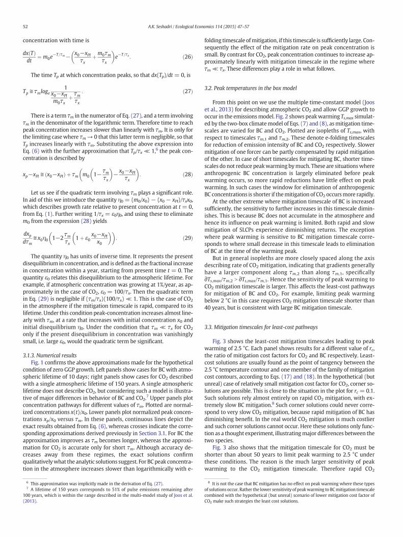
Fig. 3 shows the least-cost mitigation timescales leading to peakwarming of 2.5 °C. Each panel shows results for a different value of rc,the ratio of mitigation cost factors for CO2 and BC respectively. Least-cost solutions are usually found as the point of tangency between the2.5 °C temperature contour and onemember of the family of mitigationcost contours, according to Eqs. (17) and (18). In the hypothetical (butunreal) case of relatively small mitigation cost factor for CO2, corner so-lutions are possible. This is close to the situation in the plot for rc =0.1.Such solutions rely almost entirely on rapid CO2 mitigation, with ex-tremely slow BC mitigation.8 Such corner solutions could never corre-spond to very slow CO2 mitigation, because rapid mitigation of BC hasdiminishing benefit. In the real world CO2 mitigation is much costlierand such corner solutions cannot occur. Here these solutions only func-tion as a thought experiment, illustratingmajor differences between thetwo species.

Fig. 3 also shows that the mitigation timescale for CO2 must beshorter than about 50 years to limit peak warming to 2.5 °C underthese conditions. The reason is the much larger sensitivity of peakwarming to the CO2 mitigation timescale. Therefore rapid CO2

8 It is not the case that BCmitigation has no effect on peak warming where these typesof solutions occur. Rather the lower sensitivity of peakwarming to BCmitigation timescalecombined with the hypothetical (but unreal) scenario of lower mitigation cost factor ofCO2 make such strategies the least cost solutions.

t (years)0 10 20 30 40

x(t)

/ x 0

0.8

1

1.2

1.4BC:

x = 0.0275 year

m (years)

20 40 60 80 100

x p /

x 0

1.32

1.325

1.33

1.335

exactapprox

t (years)0 50 100 150 200 250

0.8

0.9

1

1.1

1.2CO

2:

x = 150 years

m (years)

10 20 30 401

1.1

1.2

1.3

exactapprox

(a) (b)

(c) (d)

Fig. 1. For BC, peak concentration in the atmosphere increases slower than logarithmically with e-folding timescale of mitigation if this timescale is large. For CO2, peak concentration in-creases approximately linearly with e-folding timescale of mitigation. Upper panels (a)–(b) show time-evolution of concentration, by solving Eq. (6), for different values of τm. Lowerpanels (c)–(d) show variation of normalized peak concentration with the value of τm. Results are shown for BC with τx ≪ τm (left panels) and CO2 with τm ≪ τx (right panels). Curvesmarked “exact” denote the result of Eq. (6), while those marked “approx” denote the approximations in Eqs. (23) and (28) respectively.

53A.K. Seshadri / Ecological Economics 114 (2015) 47–57

mitigation is part of the least-cost solution even for the casewhere suchmitigation is comparatively very expensive.

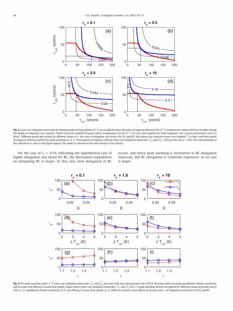
Fig. 4 shows least-cost mitigation timescales τm,1⁎ and τm,2⁎ for limitingpeak warming to 2 °C. Results are plotted for different values of GGPgrowth rate g (a–c), equilibrium climate sensitivity ΔTcs (d–f), andocean heat uptake efficacy � (g–i). Different columns plot results for dif-ferent values of the ratio of mitigation cost factors rc of CO2 and BC. In-creasing GGP growth rate, increasing equilibrium climate sensitivity,

1.61.8

2

2

2.2

2.2

2.4

2.4

2.5

2.5

2.5

2.6

2.6

2.6

2.8

2.8

2.8

3

3

3

3.2

3.2

3.2

3.4

3.4

3.4

3.6

3.6

3.6

peak temperature (K)

E-folding mitigation timescale m1

for black-carbon (years)20 40 60 80 100 120 140 160 180 200

E-f

oldi

ng m

itiga

tion

times

cale

m

2 fo

r C

O2 (

year

s)

10

20

30

40

50

60

70

80

90

100

Fig. 2. Peak warming is more sensitive to the mitigation timescale of CO2 than of BC. Sen-sitivity to BCmitigation timescale τm,1 is reduced for small or large values of the timescale.Mitigation of CO2 on a relatively short timescale is necessary to limit peakwarming to 2 °C.Shown are isopleths of peakwarming Ts,maxwith respect to mitigation timescales τm,1 andτm,2. In this plot, annual GGP growth rate g = 0.03.

and decreasing ocean heat uptake efficacy, all increase the rate of mitiga-tion required (i.e. decrease mitigation timescales).

Rapid CO2 mitigation is necessary to limit peak warming. The corre-sponding timescale τm,2⁎ is much shorter than 100 years and closer to10 years across some conditions. The latter corresponds to a 10% reduc-tion in emission intensity of GGP each year.

Although rapid BC mitigation is not essential to limit peak warmingto 2 °C (Fig. 2), the least-cost solution (Fig. 4) generally involves rapidBC mitigation as well. This corresponds to near-complete eliminationof anthropogenic BC concentrations before the warming peak occurs.Corresponding to Eq. (19), BCmitigation plays a significant role because∂g/∂τm,1 is comparable to ∂g/∂τm,2 where rapid mitigation of BC caneliminate its anthropogenic concentration. This accounts for the similare-folding timescales in the conditions where the ratio of mitigation costfactors is unity.

3.4. Mitigation expenditures for the least-cost pathways

The ratio of discountedmitigation expenditures on CO2 andBC in theleast-cost solution (Eq. (20)) increaseswith the ratio rc of themitigationcost factors and the ratio of gradient components (∂g/∂τm,2)/(∂g/∂τm,1).These expenditures are plotted in Fig. 5, and follow conditions depictedin Fig. 4. Only the sources of differences between CO2 and BC are plotted,involving quantities p0,1μ0,1/τm,1⁎ and p0,2μ0,2/τm,2⁎ . Therefore these num-bers cannot be interpreted literally but only relative to each other. Thenumbers in different panels can be compared.

For the case of rc =10, where mitigation cost factor for CO2 is muchhigher, the discounted expenditure on mitigating CO2 is much largerthan on BC. Following Eq. (20), two effects are involved. The first isthe mitigation cost factors, which vary by 10. The second effect is theratio of gradient components, which can be inferred from plots inFigs. 2 and 3. This is larger for CO2 than for BCwhere the least-cost solu-tion occurs, but the cost difference is governed by the different mitiga-tion cost factors.

0 50 100 150 200

m2 (

year

s)

0

50

100

0.0093

0.025

(a)

rc = 0.1

0 50 100 150 2000

50

100

0.021

0.046

(b)

rc = 0.5

m1 (years)

0 50 100 150 200

m2 (

year

s)

0

50

100

0.044

0.09

0.09

(c)

rc = 2.0

m1 (years)

0 50 100 150 2000

50

100

0.16

0.30.3

(d)

rc = 10

Fig. 3. Least-costmitigation timescales for keeping peakwarming below 2.5 °C are usually found as the point of tangency between the 2.5 °C temperature contour and onemember amongthe family of mitigation cost contours. Panels show the isopleth for peak surface temperature rise of 2.5 °C (in red) and isopleths for total mitigation cost (convex-downward curves inblack). Different panels plot results for different values of rc, the ratio of mitigation cost factors for CO2 and BC. Also shown are respective least-cost isopleth f* (in blue) and their pointsof tangency with the isopleth for peakwarming of 2.5 °C. These points of tangency indicate least-cost mitigation timescales τm,1

⁎ and τm,2⁎ . GGP growth rate g=0.03. (For interpretation of

the references to color in this figure legend, the reader is referred to the web version of this article.)

54 A.K. Seshadri / Ecological Economics 114 (2015) 47–57

For the case of rc = 0.10, indicating the hypothetical case ofhigher mitigation cost factor for BC, the discounted expenditureon mitigating BC is larger. In this case slow mitigation of BC

g0.02 0.04

*

0

50

100(a)

rc = 0.1

0.020

50

100(b)

rc

Δ Tcs

(K)2 3 4 5

*

0

50

100(d)

Δ T2 3

0

50

100(e)

1.1 1.2 1.3

*

0

50

100(g)

1.1 1.20

50

100(h)

Fig. 4. For peak warming under 2 °C, least-cost mitigation timescales τm,1⁎ and τm,2

⁎ decrease witand increase with efficacy of ocean heat uptake. Figure shows least-cost mitigation timescales τGGP (a–c), equilibrium climate sensitivity (d–f) and efficacy of ocean heat uptake (g–i). Differe

occurs, and hence peak warming is insensitive to BC mitigationtimescale. But BC mitigation is relatively expensive, so its costis larger.

g0.04

= 1.0

g0.02 0.04

0

50

100(c)

rc = 10

1

2

cs (K)

4 5Δ T

cs (K)

2 3 4 50

50

100(f)

1.3 1.1 1.2 1.30

50

100(i)

h increasing growth rate of GGP, decrease with increasing equilibrium climate sensitivity,m,1⁎ and τm,2

⁎ for 2 °C peakwarming. Results are plotted for different values of growth rate ofnt columns show effects of varying ratio rc of mitigation cost factors of CO2 and BC.

g0.02 0.04

cost

0.020.040.060.080.1 (a)

rc = 0.1

g0.02 0.04

0.020.040.060.080.1 (b)

rc = 1.0

g0.02 0.04

0.020.040.060.08

0.1 (c)

rc = 10

BCCO

2

Δ Tcs

(K)2 3 4 5

cost

0.020.040.060.080.1 (d)

Δ Tcs

(K)2 3 4 5

0.020.040.060.080.1 (e)

Δ Tcs

(K)2 3 4 5

0.020.040.060.08

0.1 (f)

1.1 1.2 1.3

cost

0.020.040.060.080.1 (g)

1.1 1.2 1.3

0.020.040.060.080.1 (h)

1.1 1.2 1.3

0.020.040.060.08

0.1 (i)

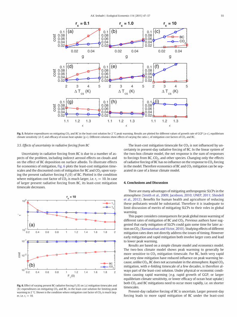
Fig. 5. Relative expenditures on mitigating CO2 and BC in the least-cost solution for 2 °C peak warming. Results are plotted for different values of growth rate of GGP (a–c), equilibriumclimate sensitivity (d–f) and efficacy of ocean heat uptake (g–i). Different columns show effects of varying the ratio rc of mitigation cost factors of CO2 and BC.

55A.K. Seshadri / Ecological Economics 114 (2015) 47–57

3.5. Effects of uncertainty in radiative forcing from BC

Uncertainty in radiative forcing from BC is due to a number of as-pects of the problem, including indirect aerosol effects on clouds andon the effect of BC deposition on surface albedo. To illustrate effectsfor economics of mitigation, Fig. 6 plots the least-cost mitigation time-scales and the discounted costs of mitigation for BC and CO2 upon vary-ing the present radiative forcing F1(0) of BC. Plotted is the conditionwhere mitigation cost factor of CO2 is much larger, i.e. rc = 10. In caseof larger present radiative forcing from BC, its least-cost mitigationtimescale decreases.

0.2 0.4 0.6 0.8 1 1.2 1.4 1.6 1.

τ*

101

102

(a)

rc = 10

τ1

τ2

F1(0)

0.2 0.4 0.6 0.8 1 1.2 1.4 1.6 1.

8 2

8 2

cost

10-3

10-2

10-1

(b) BCCO

2

Fig. 6. Effect of varying present BC radiative forcing F1(0) on (a) mitigation timescales and(b) expenditures on mitigating CO2 and BC, in the least-cost solution for limiting peakwarming to 2 °C. Shown is the condition wheremitigation cost factor of CO2 is much larg-er, i.e. rc = 10.

The least-cost mitigation timescale for CO2 is not influenced by un-certainty in present-day radiative forcing of BC. In the linear system ofthe two-box climate model, the net response is the sum of responsesto forcings from BC, CO2, and other species. Changing only the effectsof radiative forcing of BC has no influence on the response to CO2 forcingin themodel. Therefore economics of BC and CO2mitigation can be sep-arated in case of a linear climate model.

4. Conclusions and Discussion

There aremany advantages ofmitigating anthropogenic SLCPs in theatmosphere (Smith et al., 2009; Jacobson, 2010; UNEP, 2011; Shindellet al., 2012). Benefits for human health and agriculture of reducingthese pollutants would be substantial. Therefore it is inadequate tolimit discussion of merits of mitigating SLCPs to their roles in globalwarming.

This paper considers consequences for peak globalmeanwarming ofdifferent rates of mitigation of BC and CO2. Previous authors have sug-gested that early mitigation of SLCPs could gain some time for later ac-tion on CO2 (Ramanathan andVictor, 2010). Studying effects of differentmitigation rates does not directly address the issues of timing. Howeverearly mitigation and rapid mitigation both involve larger costs and leadto lower peak warming.

Results are based on a simple climate model and economics model.The two-box climate model shows peak warming to generally bemore sensitive to CO2 mitigation timescale. For BC, both very rapidand very slow mitigation have reduced influence on peak warming be-cause, unlike CO2, BC does not accumulate in the atmosphere. Rapid CO2

mitigation, with e-folding timescale of a few decades, is therefore al-ways part of the least-cost solution. Under physical or economic condi-tions causing rapid warming (e.g. rapid growth of GGP, or largerequilibrium climate sensitivity, or lower efficacy of ocean heat uptake)both CO2 and BC mitigations need to occur more rapidly, i.e. on shortertimescales.

Present-day radiative forcing of BC is uncertain. Larger present-dayforcing leads to more rapid mitigation of BC under the least-cost

56 A.K. Seshadri / Ecological Economics 114 (2015) 47–57

solution. Uncertainty in present-day forcing of BC does not affect theCO2mitigation timescale under the least-cost solution. The two-box cli-matemodel is linear, so the net response is a superposition of responsesto BC and CO2. Therefore any variable that affects only the response toBC does not influence the least-cost mitigation pathway of the otherforcer.

The economic model has cost of reducing emission intensity of GGPbyoneunit varying inverselywith emission intensity.With e-folding re-ductions in emission intensity, this results in mitigation expendituresthat vary in time only with the GGP and time-discount factor. Thereforeit is simple to compare expenditures on mitigating emissions of BC andCO2. The discounted total expenditure also becomes inversely propor-tional to the e-folding timescales of mitigation for BC and CO2.

Posing mitigation rates in terms of e-folding timescales also shedslight on different characteristics of SLCPs and CO2 in the atmosphere.For SLCPs, with e-folding mitigation timescale much longer than atmo-spheric lifetime, peak concentration in the atmosphere increases slowerthan logarithmicallywith the value ofmitigation timescale.Whereas forCO2, in case e-folding timescale ofmitigation ismuch shorter than its ef-fective atmospheric lifetime, peak concentration increases approxi-mately linearly with mitigation timescale. These differences affect therelation between peak warming and rates of mitigation for BC and CO2.

The two-box model implicitly characterizes large differences be-tween atmospheric + surface oceanic and deep-oceanic responsetimes. Where peak warming occurs within a century or two, the deepocean temperature change is very small. In such scenarios, peakwarming depends approximately on maximum radiative forcing. Thiscan be appreciated quite easily upon setting deep ocean temperatureanomaly Td = 0 in Eqs. (7) and (8). Then peak warming in Eq. (7) isgoverned by the maximum in total radiative forcing.

Hence peak warming is less sensitive to the rate of mitigation of BCbecause this rate has a smaller effect on maximum radiative forcing.CO2 accumulates in the atmosphere and its mitigation rate has a com-paratively large influence on maximum radiative forcing. It is thereforenot surprising that these results broadly agree with prior studies dem-onstrating the importance of mitigating CO2 for reducing long termwarming (Solomon et al., 2012; Smith and Mizrahi, 2013; Shoemakerand Schrag, 2013; Bowerman et al., 2013; Allen and Stocker, 2014;Pierrehumbert, 2014). The additional contributions made here are thefollowing. We show what role their vastly different atmospheric life-times play in the different effects on peak warming of the rates of miti-gation of BC and CO2.

Furthermore the economics of mitigation is introduced here in asimple, but approximate, manner. Thereby the extent to which changesin mitigation rates of BC and CO2 can be substituted for each other hasbeen examined. Consequently it is found that despite these above differ-ences between BC and CO2, BC plays an important role in the least-costsolution because the possibility of eliminating the anthropogenic contri-bution to its atmospheric burden makes peak warming sensitive to itsmitigation timescale in the regime where such elimination occurs. Inother words, it would be more expensive to limit peak warming if theanthropogenic radiative forcing of BC was not eliminated by the timethe peak in total radiative forcing occurs. In summary, it is not possibleto limit peak warming without rapid mitigation of CO2 emission inten-sity, but simultaneousmitigation of BC can reduce the total expenditureon mitigation.

Many simplifications have been made for analytic insight, creatingcorresponding limitations. The e-folding pathway for reducing emissionintensity differs from realistic emission pathways, and is intended as athought experiment. One effect of e-folding reductions in emission in-tensity is earlier emission peak compared to the case where mitigationeffort starts slowly and increases with time. The economics model is asimplification of mitigation cost. The two-box model simplifies treat-ment of global climate dynamics. Mitigation of CO2 and BC is treatedas being independent and radiative forcing from other agents is variedindependently according to the RCP4.5 scenario, neglecting especially

the effects of co-emission between CO2 and BC and between CO2 andSO2 in alternate mitigation scenarios (Barker et al., 2007). Indirect cli-mate effects are not included in estimates of radiative forcing from BC.Regional climate effects of BC and ice-albedo effects have not beencounted in the global view that has been adopted in this paper.

The results suggest that BCmitigation plays an important role in lim-iting peak warming especially when economics is considered, but itsrapid mitigation cannot compensate for failure to mitigate CO2 rapidlyenough. These two species are far from being substitutes. This assumesa tradeoff being made between rates of mitigation of BC and CO2, andthat effects on peak global warming are alone counted. There areother reasons tomitigate SLCPsmore quickly. Benefits for health and ag-riculture ofmitigating SLCPs (co-benefits) could support according theirmitigation greater weight in comparison to their role in peak warming.

Acknowledgments

This research has been supported by Divecha Centre for ClimateChange, Indian Institute of Science. The author thanks several colleaguesand two anonymous reviewers for helpful suggestions.

Appendix A. Solving the Equation for Concentration in theAtmosphere

This Appendix solves for the concentration in the atmosphere for thespecial case of zero growth in GGP. The equation that must be solved is,from Eqs. (1) and (5)

dx tð Þdt

þ x tð Þτx

¼ m0e−t=τm þ xPI

τx: ð30Þ

Multiplying both sides by et=τx and integrating between 0 and T andsolving for x(T) gives the solution

x Tð Þ ¼ x0e−T=τx þ τxτm

τm−τxm0 e−T=τm−e−T=τx� �

þ xPI 1−e−T=τx� �

: ð31Þ

It can be verified that Eq. (31) solves Eq. (30) within initial conditionx(0) = x0.

References

Allen, M.R., Stocker, T.F., 2014. Impact of delay in reducing carbon dioxide emissions. Nat.Clim. Chang. 4, 23–26. http://dx.doi.org/10.1038/nclimate2077.

Archer, D., Brovkin, V., 2008. The millennial atmospheric lifetime of anthropogenic CO2.Clim. Chang. 90 (3), 283–297. http://dx.doi.org/10.1007/s10584-008-9413-1.

Archer, D., Eby, M., Brovkin, V., Ridgwell, A., Cao, L., 2009. Atmospheric lifetime of fossilfuel carbon dioxide. Annu. Rev. Earth Planet. Sci. 37, 117–134. http://dx.doi.org/10.1146/annurev.earth.031208.100206.

Barker, T., Bashmakov, I., Alharthi, A., Amann, M., Cifuentes, L., Drexhage, J., Duan, M.,2007. Climate change 2007: mitigation. Chap. Mitigation from a Cross-Sectoral Per-spective. Cambridge University Press.

Berntsen, T., Tanaka, K., Fuglestvedt, J.S., 2010. Does black carbon abatement hamper CO2

abatement? Clim. Chang. 103, 627–633. http://dx.doi.org/10.1007/s10584-010-9941-3.Boden, T., Marland, G., Andres, B., 2011. Global CO2 Emissions From Fossil-Fuel Burning,

Cement Manufacture, and Gas Flaring. pp. 1751–2008.Bond, T.C., Doherty, S.J., Fahey, D.W., Forster, P.M., Bernsten, T., 2013. Bounding the role of

black carbon in the climate system: a scientific assessment. J. Geophys. Res. Atmos.118 (11), 5380–5552. http://dx.doi.org/10.1002/jgrd.50171.

Bowerman, N.H.A., Frame, D.J., Huntingford, C., Lowe, J.A., Smith, S.M., Allen, M.R., 2013.The role of short-lived climate pollutants in meeting temperature goals. Nat. Clim.Chang. 3, 1021–1024. http://dx.doi.org/10.1038/nclimate2034.

CCAC, 2014. Short-lived climate pollutants. doi:http://www.unep.org/ccac/Short-LivedClimatePollutants/Definitions/tabid/130285/Default.aspx.

Collins, W.J., Fry, M.M., Yu, H., Fuglestvedt, J.S., Shindell, D.T., West, J.J., 2013. Global andregional temperature-change potentials for near-term climate forcers. Atmos.Chem. Phys. 13, 2471–2485. http://dx.doi.org/10.5194/acp-13-2471-2013.

Dasgupta, P., 2008. Discounting climate change. J. Risk Uncertain. 37 (2–3), 141–169.http://dx.doi.org/10.1007/s11166-008-9049-6.

Enkvist, P.-A., Nauclér, T., Rosander, J., 2007. A cost curve for greenhouse gas reduction.McKinsey Q. 1, 35–45.

Gregory, J.M., 2000. Vertical heat transports in the ocean and their effect on time-dependent climate change. Clim. Dyn. 16, 501–515. http://dx.doi.org/10.1007/s003820000059.

57A.K. Seshadri / Ecological Economics 114 (2015) 47–57

Heal, G., 1997. Discounting and climate change: an editorial comment. Clim. Chang. 37(2), 335–343. http://dx.doi.org/10.1023/A:1005384629724.

Held, I.M., Winton, M., Takahashi, K., Delworth, T., Zeng, F., 2010. Probing the fast andslow components of global warming by returning abruptly to preindustrial forcing.J. Clim. 23, 2418–2427. http://dx.doi.org/10.1175/2009JCLI3466.1.

Hu, A., Xu, Y., Tebaldi, C., Washington, W.M., Ramanathan, V., 2013. Mitigation of shortlived climate pollutants slows sea-level rise. Nat. Clim. Chang. 3, 730–734. http://dx.doi.org/10.1038/nclimate1869.

Jackson, S.C., 2009. Parallel pursuit of near-term and long-term climate mitigation. Sci-ence 326 (5952), 526–527. http://dx.doi.org/10.1126/science.1177042.

Jacobson, M.Z., 2010. Short-term effects of controlling fossil-fuel soot, biofuel soot andgases, and methane on climate, Arctic ice, and air pollution health. J. Geophys. Res.115, D14,209. http://dx.doi.org/10.1029/2009JD013795.

Joos, F., Roth, R., Fuglestvedt, J.S., Peters, G., Brovkin, V., Eby, M., Edwards, N., Eleanor, B.,2013. Carbon dioxide and climate impulse response functions for the computationof greenhouse gas metrics: a multi-model analysis. Atmos. Chem. Phys. 13,2793–2825. http://dx.doi.org/10.5194/acp-13-2793-2013.

Kesicki, F., Elkins, P., 2012. Marginal abatement cost curve: a call for caution. Clim. Pol. 12(2), 219–236. http://dx.doi.org/10.1080/14693062.2011.582347.

Koomey, J., 2013. Moving beyond benefit–cost analysis of climate change. Environ. Res.Lett. 8, 1–4. http://dx.doi.org/10.1088/1748-9326/8/4/041005.

Kopp, R.E., Mauzerall, D.L., 2010. Assessing the climatic benefits of black carbon mitiga-tion. Proc. Natl. Acad. Sci. U. S. A. 107, 11,703–11,708. http://dx.doi.org/10.1073/pnas.0909605107.

Lashof, D.A., Ahuja, D.R., 1990. Relative contributions of greenhouse gas emissions to glob-al warming. Nature 344, 529–531. http://dx.doi.org/10.1038/344529a0.

MacCracken,M.C., 2008. Prospects for future climate change and the reasons for early action.J. Air Waste Manag. Assoc. 58, 735–786. http://dx.doi.org/10.3155/1047-3289.58.6.735.

Meinshausen, M., Smith, S.J., Calvin, K., Daniel, J.S., Kainuma, M.L.T., 2011. The RCP green-house gas concentrations and their extensions from 1765 to 2300. Clim. Chang. 109,213–241. http://dx.doi.org/10.1007/s10584-011-0156-z.

Montenegro, A., Brovkin, V., Eby, M., Archer, D., Weaver, A.J., 2007. Long term fate of an-thropogenic carbon. Geophys. Res. Lett. 34, L19,707.

Morris, J., Paltsev, S., Reilly, J., 2008. Marginal abatement costs and marginal welfare costsfor greenhouse gas emissions reductions: results from the EPPA model. Tech. Rep.164. MIT Joint Program on the Science and Policy of Global Change.

Moss, R.H., Edmonds, J.A., Hibbard, K.A., Manning, M.R., Rose, S.K., van Vuuren, D.P., 2010.The next generation of scenarios for climate change research and assessment. Nature463, 747–756. http://dx.doi.org/10.1038/nature08823.

Myhre, G., Shindell, D., Bréon, F.-M., Collins, W., Fuglestvedt, J., Huang, J., 2013. Climatechange 2013: the physical science basis. Contribution of working group I to thefifth assessment report of the intergovernmental panel on climate change. Chap. An-thropogenic and Natural Radiative Forcing. Cambridge University Press, pp. 659–740.

Nakicenovic, N., Alcamo, J., Davis, G., Vries, B.D., Fenhann, J., 2000. Emissions Scenarios.Cambridge University Press.

Nordhaus, W.D., 1997. Discounting in economics and climate change: an editorial com-ment. Clim. Chang. 37 (2), 315–328. http://dx.doi.org/10.1023/A:1005347001731.

Nordhaus, W., 2007. Critical assumptions in the Stern review on climate change. Science317, 201–202. http://dx.doi.org/10.1126/science.1137316.

Pacala, S., Socolow, R., 2004. Stabilization wedges: solving the climate problem for thenext 50 years with current technologies. Science 305, 968–972. http://dx.doi.org/10.1126/science.1100103.

Parry, M., Lowe, J., Hanson, C., 2009. Overshoot, adapt and recover. Nature 458, 1102–1103.http://dx.doi.org/10.1038/4581102a.

Penner, J.E., Prather, M.J., Isaksen, I.S.A., Fuglestvedt, J.S., Klimont, Z., 2010. Short-lived un-certainty? Nat. Geosci. 3, 587–588. http://dx.doi.org/10.1038/ngeo932.

Peters, G.P., Andew, R.M., Boden, T., Canadell, J.G., Ciais, P., 2013. The challenge to keep globalwarming below 2 °C. Nat. Clim. Chang. 3, 4–6. http://dx.doi.org/10.1038/nclimate1783.

Pierrehumbert, R.T., 2014. Short-lived climate pollution. Annu. Rev. Earth Planet. Sci. 42,341–379. http://dx.doi.org/10.1146/annurev-earth-060313-054843.

Quéré, C.L., Raupach, M.R., Canadell, J.G., Marland, G., 2009. Trends in the sources andsinks of carbon dioxide. Nat. Geosci. 2, 831–836. http://dx.doi.org/10.1038/ngeo689.

Ramanathan, V., Feng, Y., 2008. On avoiding dangerous anthropogenic interference withthe climate system: formidable challenges ahead. Proc. Natl. Acad. Sci. U. S. A. 105,14,245–14,250. http://dx.doi.org/10.1073/pnas.0803838105.

Ramanathan, V., and D. G. Victor (2010), To fight climate change, clean the air, New YorkTimes.

Ramanathan, V., Xu, Y., 2010. The Copenhagen Accord for limiting global warming:criteria, constraints, and available avenues. Proc. Natl. Acad. Sci. U. S. A. 107 (18),8055–8062. http://dx.doi.org/10.1073/pnas.1002293107.

Rhein, M., Rintoul, S.R., Aoki, S., Campos, E., Cahmbers, D., 2013. Climate change 2013: thephysical science basis. Contribution of working group 1 to the fifth assessment reportof the intergovernmental panel on climate change. Chap. Observations: Ocean. Cam-bridge University Press.

Rogelj, J., Hare, B., Nabel, J., Macey, K., Schaeffer, M., 2009. Halfway to Copenhagen, nowayto 2 °C. Nat. Rep. Clim. Chang. 3, 81–83. http://dx.doi.org/10.1038/climate.2009.57.

Shindell, D.T., Faluvegi, G., Koch, D.M., Schmidt, G.A., 2009. Improved attribution of cli-mate forcing to emissions. Science 326 (5953), 716–718. http://dx.doi.org/10.1126/science.1174760.

Shindell, D., Kuylenstierna, J.C.I., Vignati, E., van Dingenen, R., Amann, M., 2012. Simulta-neouslymitigating near-term climate change and improving human health and food se-curity. Science 335 (6065), 183–189. http://dx.doi.org/10.1126/science.1210026.

Shindell, D.T., Lamarque, J.-F., Schulz, M., Flanner, M., Jiao, C., 2013. Radiative forcing in theACCMIP historical and future climate simulations. Atmos. Chem. Phys. 13, 2939–2974.http://dx.doi.org/10.5194/acp-13-2939-2013.

Shoemaker, J.K., Schrag, D.P., 2013. The danger of overvaluing methane's influence on fu-ture climate change. Clim. Chang. 120, 903–914. http://dx.doi.org/10.1007/s10584-013-0861-x.

Shoemaker, J.K., Schrag, D.P., Molina, M.J., Ramanathan, V., 2013. What role for short-livedclimate pollutants in mitigation policy? Science 342, 1323–1324. http://dx.doi.org/10.1126/science.1240162.

Skeie, R.B., Bernstsen, T., Myhre, G., Pedersen, C.A., Strom, J., 2011. Black carbon in the at-mosphere and snow, from pre-industrial times until present. Atmos. Chem. Phys. 11,6809–6836. http://dx.doi.org/10.5194/acp-11-6809-2011.

Smith, S.J., Mizrahi, A., 2013. Near-term climate mitigation by short-lived forcers. Proc.Natl. Acad. Sci. U. S. A. 110 (35), 14,202–14,206. http://dx.doi.org/10.1073/pnas.1308470110.

Smith, K.R., Jerrett, M., Anderson, H.R., Burnett, R.T., Stone, V., Derwent, R., Atkinson, R.W.,Cohen, A., Shonkoff, S.B., Krewski, D., III, C.A.P., Thun, M.J., Thurston, G., 2009. Publichealth benefits of strategies to reduce greenhouse-gas emissions: health implicationsof short-lived greenhouse pollutants. Lancet 374, 2091–2103. http://dx.doi.org/10.1016/S0140-6736(09)61716-5.

Solomon, S., Pierrehumbert, R.T., Matthews, D., Daniel, J.S., 2012. Climate science for serv-ing society: research, modelling and prediction priorities. Chap. Atmospheric Compo-sition, Irreversible Climate Change, and Mitigation Policy. Springer.

Stocker, T.F., 2013. The closing door of climate targets. Science 339, 280–282. http://dx.doi.org/10.1126/science.1232468.

Stocker, T.F., Qin, D., Plattner, G.-K., Tignor, M., Allen, S.K. (Eds.), 2013. Climate change2013: the physical science basis. Contribution of working group 1 to the fifth assess-ment report of the intergovernmental panel on climate change. Chap. IPCC, 2013:Summary for Policymakers. Cambridge University Press.

Tanaka, K., Berntsen, T., Fuglestvedt, J.S., Rypdal, K., 2012. Climate effects of emission stan-dards: the case for gasoline and diesel cars. Environ. Sci. Technol. 46, 5205–5213.http://dx.doi.org/10.1021/es204190w.

Tubiello, F.N., Oppenheimer, M., 1995. Impulse-response functions and anthropogenicCO2. Geophys. Res. Lett. 22, 413–416. http://dx.doi.org/10.1029/94GL03276.

UNEP, 2011. Near-Term Climate Protection and Clean Air Benefits: Actions for ControllingShort-Lived Climate Forcers. United Nations Environment Programme, Nairobi, Kenya.

UNEP, 2013. The emissions gap report 2013. Tech. rep. United Nations EnvironmentProgramme.

Wallack, J.S., Ramanathan, V., 2009. The other climate changers: why black carbon andozone also matter. Foreign Aff. 88 (5), 105–113.

Williams, K.D., Ingram, W.J., Gregory, J.M., 2008. Time variation of effective climate sensi-tivity in GCMs. J. Clim. 23, 2333–2344. http://dx.doi.org/10.1175/2008JCLI2371.1.

Winton, M., Takahashi, K., Held, I.M., 2010. Importance of ocean heat uptake efficacy to tran-sient climate change. J. Clim. 23, 2333–2344. http://dx.doi.org/10.1175/2009JCLI3139.1.