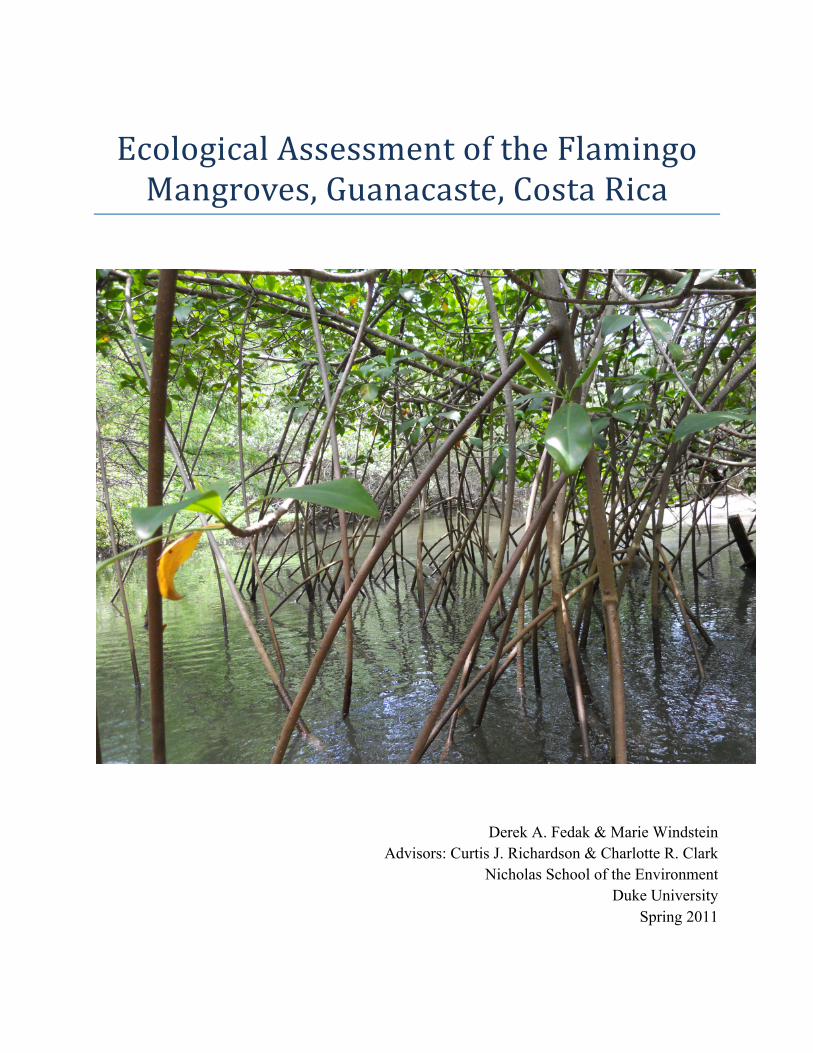
Ecological  Assessment  of  the  Flamingo  Mangroves,  Guanacaste,  Costa  Rica  

Derek A. Fedak & Marie Windstein Advisors: Curtis J. Richardson & Charlotte R. Clark

Nicholas School of the Environment Duke University

Spring 2011

   

II    

Abstract

Mangroves are tropical and subtropical ecosystems found in intertidal zones that provide

vital ecosystem services including sustenance of commercially important fishery species,

improvement of coastal water quality through nutrient cycling and sediment interception, and

protection of coastal communities from storm surge and erosion. However, land use conversion

and water pollution are threatening these ecosystems and their associated services worldwide.

This master’s project conducted an ecological assessment on a mangrove forest adjoining

the property of the Flamingo Beach Resort and Spa in Playa Flamingo, located in the Guanacaste

province of Costa Rica. The project analyzed vegetation health, water and soil quality, bird

species richness, and identified threats to the forest. It also assessed several options for the

resort’s development of ecotourism, such as community involvement, the construction of an

educational boardwalk, and the creation of a vegetation buffer adjoining the mangroves.

The results indicate that the Flamingo Mangroves are generally in a healthy state.

Vegetation structure like canopy height, biomass, vegetation importance values, and species

distribution compares well with previous ecological studies on mature tidal mangroves. The

ecosystem supports 42 resident bird species and likely up to 30 migratory species. However,

water quality is a major concern, which reported elevated levels of nitrogen and phosphorus

through runoff and discharged wastewater in the northern section of the forest. Additionally, the

western edge of the forest adjoining the beach road is frequently disturbed by automotive traffic

and runoff, displaying reduced or stunted vegetation and sandy soil.

This report contains several recommendations on how to preserve the mangroves by

improving water quality, reducing physical and chemical disturbances, and engaging the

community. The results of the project will be incorporated into our client‘s and Flamingo

community‘s future management practices to conserve the Flamingo Mangroves and emphasize

the value of this ecosystem.

   

III    

Table  of  Contents  

Introduction  ................................................................................................................................................  1  

Study  Site  .................................................................................................................................................  2  

Client’s  Objectives  ...................................................................................................................................  3  

Study’s  Objectives  ....................................................................................................................................  4  

Chapter  I:  Vegetation  Survey  ......................................................................................................................  6  

Objectives  ................................................................................................................................................  6  

Background  ..............................................................................................................................................  6  

Methods  ..................................................................................................................................................  9  

Results  and  Discussion  ...........................................................................................................................  12  

Overall  Picture  .......................................................................................................................................  20  

Chapter  II:  Analysis  of  Water  Samples  .....................................................................................................  21  

Objectives  ..............................................................................................................................................  21  

Background  ............................................................................................................................................  21  

Methods  ................................................................................................................................................  25  

Results  and  Discussion  ...........................................................................................................................  27  

Salinity  ...............................................................................................................................................  27  

Total  Nitrogen  ....................................................................................................................................  28  

Total  Phosphorus  ...............................................................................................................................  31  

N:P  ratio  .............................................................................................................................................  33  

Overall  Picture  .......................................................................................................................................  33  

Chapter  III:  Analysis  of  Soil  Samples  .........................................................................................................  35  

Objectives  ..............................................................................................................................................  35  

Background  ............................................................................................................................................  35  

Methods  ................................................................................................................................................  39  

Results  and  Discussion  ...........................................................................................................................  43  

Transects  ............................................................................................................................................  43  

Total  Carbon,  Nitrogen,  and  Phosphorus  Along  the  Two  Transects  and  in  the  Tidal  Channels  .........  47  

Overall  Picture  .......................................................................................................................................  52  

   

IV    

Chapter  IV:  Birds  .......................................................................................................................................  53  

Objectives  ..............................................................................................................................................  53  

Background  ............................................................................................................................................  53  

Methods  ................................................................................................................................................  54  

Results  and  Discussion  ...........................................................................................................................  56  

Overall  Picture  .......................................................................................................................................  58  

Chapter  V:  Community  Involvement  ........................................................................................................  62  

Goals  ......................................................................................................................................................  62  

Mangrove  Cleanup  ................................................................................................................................  62  

Presentation  to  La  Paz  School  ................................................................................................................  63  

Youth  Involvement  in  Conservation  of  Flamingo  Mangroves  ................................................................  64  

Chapter  VI:  Recommendations  and  Conclusions  .....................................................................................  65  

Water  Quality  ........................................................................................................................................  65  

Boardwalk  ..............................................................................................................................................  66  

Beach  Road  ............................................................................................................................................  69  

Community  Involvement  .......................................................................................................................  71  

Ramsar  Listing  ........................................................................................................................................  72  

Appendix  ...................................................................................................................................................  76  

Bibliography  ..............................................................................................................................................  83  

 

   

   

V      

List  of  Figures  

Figure  1:  Map  of  Flamingo  Mangrove  Area  in  NW  Costa  Rica  .....................................................................  3  

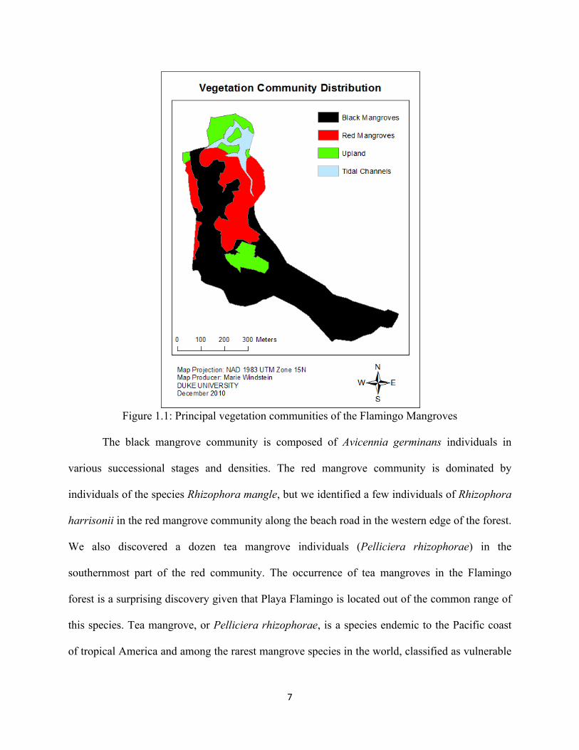
Figure  1.1:  Principal  vegetation  communities  in  the  Flamingo  Mangroves  ................................................  7  

Figure  1.2:  Vegetation  survey  plots  in  the  Flamingo  Mangroves  ..............................................................  10  

Figure  1.3:  Species  and  size  class  distribution  within  each  plot  surveyed  ...  1Error!  Bookmark  not  defined.  

Figure  1.4:  Biomass  distribution  within  each  plot  surveyed  ......................................................................  15  

Figure  1.5:  Regression  of  DBH  vs.  Height  for  Avicennia  .............................................................................  16  

Figure  1.6:  Regression  of  DBH  vs.  Height  for  Rhizophora  ..........................................................................  16  

Figure  1.7:  Tallest  tree  per  plot  .................................................................................................................  18  

Figure  1.8:  Interpolation  of  canopy  height  using  Kriging  and  Inverse  Distance  Weighting  .......................  19  

Figure  2.1:  Point  sources  of  water  input  to  the  Flamingo  Mangroves  ......................................................  24  

Figure  2.2:  Water  sampling  locations  in  the  Flamingo  Mangroves  ...........................................................  26  

Figure  2.3:  TN  and  TP  water  concentration  on  June  17th,  2010  .................................................................  29  

Figure  2.4:  Water  aspect  downstream  of  sampling  site  1  after  paint  effluent  discharge  on    

May  27th,  2010  ...........................................................................................................................................  30  

Figure  2.5:  Blue-­‐green  algae  (cyanobacteria)  bloom  near  FBRS  WWTP,  March  2010  ...............................  32  

Figure  3.1:  Soil  sampling  locations  in  the  Flamingo  Mangroves  ................................................................  40  

Figure  3.2:  Map  of  bioavailable  nitrogen  concentration  in  transect  soil  samples  .....................................  43  

Figure  3.3:  Map  of  phosphate  concentration  in  transect  soil  samples  ......................................................  46  

Figure  3.4:  Total  carbon  in  soil  samples  along  the  two  transects  and  in  the  tidal  channels  .....................  48  

Figure  3.5:  Total  nitrogen  in  soil  samples  along  the  two  transects  and  in  the  tidal  channels  ...................  49  

Figure  3.6:  Total  phosphorus  in  soil  samples  along  the  two  transects  and  in  the  tidal  channels  ..............  50  

Figure  3.7:  Soil  salinity  on  July  6th,  2010  ....................................................................................................  51  

Figure  4.1:  Bird  survey  locations  in  Flamingo  Mangroves  .........................................................................  55  

Figure  4.2:  Wading  habitat  avian  distribution  in  Flamingo  Mangroves  .....................................................  58  

Figure  4.3:  Total  mangrove  avian  distribution  in  Flamingo  Mangroves  ....................................................  58  

Figure  4.4:  Black  mangrove  avian  distribution  in  Flamingo  Mangroves  ....................................................  59  

Figure  4.5:  Near-­‐development  avian  distribution  in  Flamingo  Mangroves  ...............................................  59  

Figure  4.6:  Peripheral  and  upland  avian  distribution  in  Flamingo  Mangroves  ..........................................  59  

Figure  6.1:  Proposed  boardwalk  path  and  entry  points  ............................................................................  68  

 

   

VI    

List  of  Tables  

Table  1.1:  Plant  community  structure  from  29  vegetation  survey  plots  .....  Error!  Bookmark  not  defined.2  

Table  4.1:  Resident  Flamingo  Mangrove  bird  species  list  from  field  survey  .............................................  60  

Table  A1:  Individual  plot’s  basal  area  and  biomass  ...................................................................................  76  

Table  A2:  Salinity,  total  nitrogen,  and  total  phosphorus  concentration  in  the  water  samples    

collected  in  Flamingo  between  May  20th  and  July  8th,  2010  ......................................................................  77  

Table  A3:  Total  nitrogen  and  total  phosphorus  reference  concentration  in  four  ecoregions    

of  the  Southeastern  U.S.  ............................................................................................................................  77  

Table  A4:  Bioavailable  nutrient  concentration  in  soil  samples  along  the  two  transects  ...........................  78  

Table  A5:  Total  nutrient  concentration  in  soil  samples  along  the  two  transects  and  in  the    

tidal  channels  .............................................................................................................................................  79  

Table  A6:  Nutrient  concentration  in  other  mangrove  systems  .................................................................  80  

Table  A7:  Qualitative  severity  of  soil  salinity  in  selected  samples  .............................................................  80  

Table  A8:  Species,  likelihood,  and  timespan  of  potential  migratory  birds  to  Flamingo  ............................  81  

Table  A9:  Species,  likelihood,  and  timespan  of  supplemental  birds  to  Flamingo  ......................................  82  

 

 

 

   

1    

Introduction  

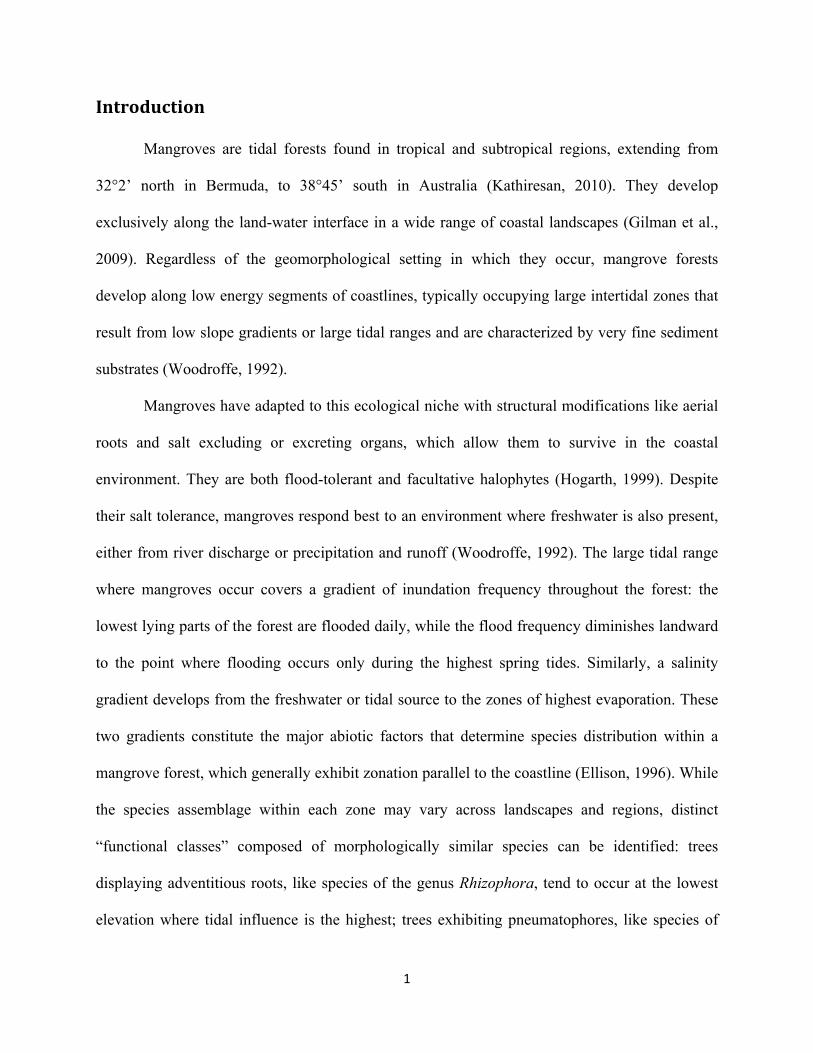
Mangroves are tidal forests found in tropical and subtropical regions, extending from

32°2’ north in Bermuda, to 38°45’ south in Australia (Kathiresan, 2010). They develop

exclusively along the land-water interface in a wide range of coastal landscapes (Gilman et al.,

2009). Regardless of the geomorphological setting in which they occur, mangrove forests

develop along low energy segments of coastlines, typically occupying large intertidal zones that

result from low slope gradients or large tidal ranges and are characterized by very fine sediment

substrates (Woodroffe, 1992).

Mangroves have adapted to this ecological niche with structural modifications like aerial

roots and salt excluding or excreting organs, which allow them to survive in the coastal

environment. They are both flood-tolerant and facultative halophytes (Hogarth, 1999). Despite

their salt tolerance, mangroves respond best to an environment where freshwater is also present,

either from river discharge or precipitation and runoff (Woodroffe, 1992). The large tidal range

where mangroves occur covers a gradient of inundation frequency throughout the forest: the

lowest lying parts of the forest are flooded daily, while the flood frequency diminishes landward

to the point where flooding occurs only during the highest spring tides. Similarly, a salinity

gradient develops from the freshwater or tidal source to the zones of highest evaporation. These

two gradients constitute the major abiotic factors that determine species distribution within a

mangrove forest, which generally exhibit zonation parallel to the coastline (Ellison, 1996). While

the species assemblage within each zone may vary across landscapes and regions, distinct

“functional classes” composed of morphologically similar species can be identified: trees

displaying adventitious roots, like species of the genus Rhizophora, tend to occur at the lowest

elevation where tidal influence is the highest; trees exhibiting pneumatophores, like species of

   

2      

the genus Avicennia tend to occur at higher elevations, where flooding frequency and duration

are reduced (Woodroffe, 1992; 1995).

Despite the potential for export of litter by the daily ebbing tidal flow, mangrove

ecosystems are generally regarded as “highly productive sources of organic matter, [which

support] complex estuarine and near shore food webs” (Woodroffe, 1992). The energy flow

within mangrove forests is mainly oriented in a bottom-up direction, where primary productivity

is regulated by salinity, hydrology, and nutrient availability (Hogarth, 1999). The principal

source of organic matter within mangrove ecosystems comes from microbial decomposition and

macro-faunal breakdown of litter material, which in turn sustains a wide range of biodiversity

including aquatic, terrestrial and arboreal invertebrates, reef fish, migratory and resident birds,

and mammals (Hogarth, 1999; Dinwiddie et al., 2009). Mangroves are essential to the adjacent

marine ecosystems, as the complex habitat formed by the stilt roots of some mangrove species

are used as nurseries by many reef species, providing shelter to juveniles from predators.

Throughout the world, mangrove forests are associated with several ecosystem services

that benefit local communities. These benefits include sustenance of commercially important

fishery species, improvement of coastal water quality through nutrient cycling, adsorption of

pollutants, and interception of sediments, protection of coastal infrastructures from storm surge

and erosion, and carbon sequestration (Gilman et al., 2009); (Donato et al., 2011).

Study  Site  

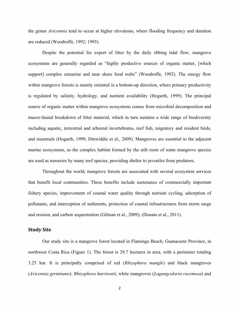
Our study site is a mangrove forest located in Flamingo Beach, Guanacaste Province, in

northwest Costa Rica (Figure 1). The forest is 29.7 hectares in area, with a perimeter totaling

3.25 km. It is principally comprised of red (Rhizophora mangle) and black mangroves

(Avicennia germinans). Rhizophora harrisonii, white mangroves (Lagungcularia racemosa) and

   

3      

buttonwoods (Conocarpus erectus) are present in the northwest of the forest and along the beach.

A few tea mangroves (Pelliciera rhizophorae) and Avicennia bicolor individuals are present in

the heart of the forest, in the red and black mangrove communities respectively. Small evergreen

communities border the mangroves when not contiguous with the ocean or development.

Figure 1: Map of the Flamingo Mangrove Area in NW Costa Rica

The Flamingo Mangrove forest is surrounded by development. Flamingo Beach Resort

and Spa borders the forest to the north. Paved or dirt roads, agricultural areas, and touristic,

residential, and other commercial developments border the forest on the rest of its periphery.

Tidal waters, precipitation, and treated and untreated wastewater feed the forest. The system is

exclusively tide dominated, as no river flows through the forest. The mangroves only connection

to the ocean is through a channel adjacent to a marina located in the northeast of the system.

Client’s  Objectives  

In 2010, the Flamingo Beach Resort and Spa (subsequently referred to as FBRS) initiated

its participation in the Certification for Sustainable Tourism, a program developed by the

   

4      

Department of Sustainability of the Costa Rica Board of Tourism. This certification evaluates

establishments on several characteristics, notably their stewardship of surrounding natural

habitats (Costa Rica Tourist Board, 2010). In this perspective, the owners of the FBRS expressed

their wish to take management measures to conserve the mangroves adjoining their property and

emphasize the value of this ecosystem. As part of their ecotourism ethos, they also sought to

involve the community in this initiative to ensure that the protection of the Flamingo Mangroves

would environmentally, culturally, and socio-economically benefit the Flamingo community.

In the context of this project, the management of FBRS formulated three axes of ecosystem

enhancement:

1. Make significant efforts and encourage the surrounding community to improve the quality of

the water discharged into the mangroves. The FBRS’s management already stated its

intention to upgrade its wastewater treatment facility to include UV light technology aimed at

removing fecal coliforms and other pathogens.

2. Close the beach road bordering the western part of the forest to automobile traffic and

potentially replace it with a vegetated trail designed to prevent further damages from car

circulation but allow access to pedestrians and non-motorized vehicles.

3. Implement a conservation-oriented management where there was no significant interest in

protecting the ecosystem before, and assess the ecotourism potential of the site.

Study’s  Objectives  

The main goals of our investigation were to evaluate the general health of the ecosystem

and identify potential or existing stresses to the forest. With these objectives in mind, we

conducted an ecological assessment of the forest focusing on three major axes: 1) assessing the

population and structure of the plant community; 2) collecting soil and water samples to assess

   

5      

the nutrient status of the forest and determine the origin and nature of pollutants potentially being

discharged into the mangroves; and 3) evaluating the avian diversity found within the Flamingo

forest and its surrounding area. We collected these data to advise the FBRS and Flamingo

community on the appropriate measures to adopt to maintain the forest in its current vigorous

state and restore threatened areas to a healthier equilibrium.

The second objective was to assess the possibility of developing ecotourism activities in

the mangroves. The vegetation and bird surveys helped determine the educational potential of the

site as well as the feasibility of an educational boardwalk through the forest. Central to the effort

of creating an ecotourism project and following the philosophy of the FBRS, we wished to

involve the community in the protection of the Flamingo Mangroves through the organization of

educational events and cleanup efforts during our stay in Flamingo. Finally, we wanted to create

opportunities that involved the community in the protection of the forest on the long term by

identifying the management, monitoring, and stewardship needs of the ecosystem.

   

   

6      

Chapter  I:  Vegetation  Survey  

Objectives  

The first objective of the vegetation survey was to create an initial assessment of the state

of the forest by identifying the different plant communities and recording the extent, distribution,

density, abundance, and size of the plant species within each community. Since this survey is the

first evaluation of the Flamingo Mangroves, it should be used as a comparative baseline for any

future monitoring of the plant community.

The second objective was to identify possible path locations for an educational boardwalk

through the forest. The vegetation survey was central in investigating aspects such as ease of

access for construction, vegetation density and diversity, and educational potential. This

information was used along with the criteria of the FBRS’s management to design the most

adequate path for the boardwalk. The discussion on the path of the boardwalk can be found in

our Recommendations section.

Background  

We identified three dominant vegetation communities in the Flamingo forest: red

mangroves, black mangroves, and upland vegetation (Figure 1.1). The black mangrove

community encompasses 18.8 hectares and the red mangrove community encompasses 6.4

hectares, which represent respectively 75% and 25% of the mangrove cover of the forest. The

vegetation survey revealed the occurrence of white mangroves at multiple sampling locations,

notably along the transition between the red and black communities in the northwest of the

forest. White mangrove trees consistently occurred within a black or red matrix and did not

display a clear distribution pattern. Therefore, we include those individuals in the previously

identified communities instead of recognizing a white mangrove community.

   

7      

Figure 1.1: Principal vegetation communities of the Flamingo Mangroves

The black mangrove community is composed of Avicennia germinans individuals in

various successional stages and densities. The red mangrove community is dominated by

individuals of the species Rhizophora mangle, but we identified a few individuals of Rhizophora

harrisonii in the red mangrove community along the beach road in the western edge of the forest.

We also discovered a dozen tea mangrove individuals (Pelliciera rhizophorae) in the

southernmost part of the red community. The occurrence of tea mangroves in the Flamingo

forest is a surprising discovery given that Playa Flamingo is located out of the common range of

this species. Tea mangrove, or Pelliciera rhizophorae, is a species endemic to the Pacific coast

of tropical America and among the rarest mangrove species in the world, classified as vulnerable

   

8      

by the IUCN (Ellison, Farnsworth, and Moore, 2007). Currently, “significant stands of the

species exist only from the Gulf of Nicoya, Costa Rica to the Esmeraldas River, Ecuador. In

addition, some isolated individuals grow close to the tidal channels north of the Gulf of Nicoya

and south of the Esmeraldas River” (Jimenez, 1984). Flamingo is located to the north of the

Nicoya peninsula, in a region where only a few isolated individuals have been identified.

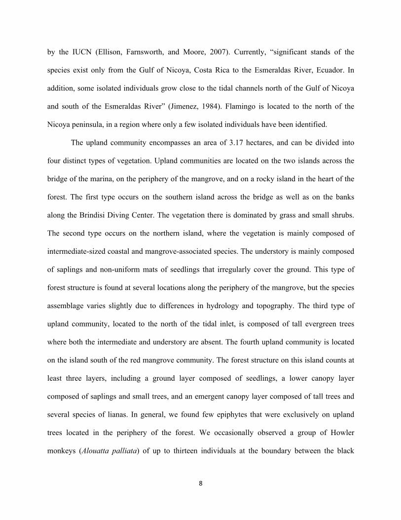
The upland community encompasses an area of 3.17 hectares, and can be divided into

four distinct types of vegetation. Upland communities are located on the two islands across the

bridge of the marina, on the periphery of the mangrove, and on a rocky island in the heart of the

forest. The first type occurs on the southern island across the bridge as well as on the banks

along the Brindisi Diving Center. The vegetation there is dominated by grass and small shrubs.

The second type occurs on the northern island, where the vegetation is mainly composed of

intermediate-sized coastal and mangrove-associated species. The understory is mainly composed

of saplings and non-uniform mats of seedlings that irregularly cover the ground. This type of

forest structure is found at several locations along the periphery of the mangrove, but the species

assemblage varies slightly due to differences in hydrology and topography. The third type of

upland community, located to the north of the tidal inlet, is composed of tall evergreen trees

where both the intermediate and understory are absent. The fourth upland community is located

on the island south of the red mangrove community. The forest structure on this island counts at

least three layers, including a ground layer composed of seedlings, a lower canopy layer

composed of saplings and small trees, and an emergent canopy layer composed of tall trees and

several species of lianas. In general, we found few epiphytes that were exclusively on upland

trees located in the periphery of the forest. We occasionally observed a group of Howler

monkeys (Alouatta palliata) of up to thirteen individuals at the boundary between the black

   

9      

mangrove and the peripheral upland vegetation in the southwest and northeast of the forest.

Additionally, we repeatedly found tracks and skeletons of small mammals at the interface

between the black and upland communities throughout the forest. In comparison, we encountered

only a few Howler monkeys and observed only one mammal’s tracks in the red mangroves. This

indicates that the upland vegetation is an important habitat for mammals foraging in the

mangroves and contributes to the diversity of the ecosystem.

Methods  

Vegetation Data Collection:

We used stratified random sampling to survey the red and black mangrove communities.

The area surveyed in both communities was at least 1% of its total area. For areas dominated by

adult trees, we used circular quadrats of 100 m2 (radius of 5.64 meters). For areas dominated by

small saplings or seedlings, we used four circular quadrats of 25 m2 (radius of 2.82 meters); the

center of each of the four sampling plots was located 3 meters to the north, south, east, and west

of the center point. The location of the center of each sampling plot was randomly determined

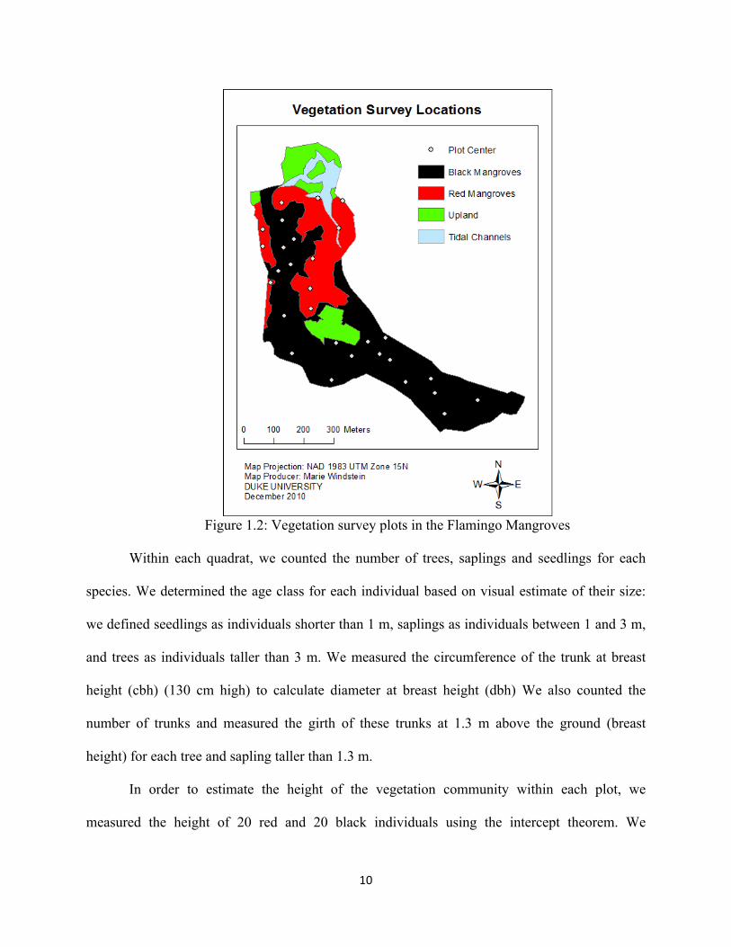
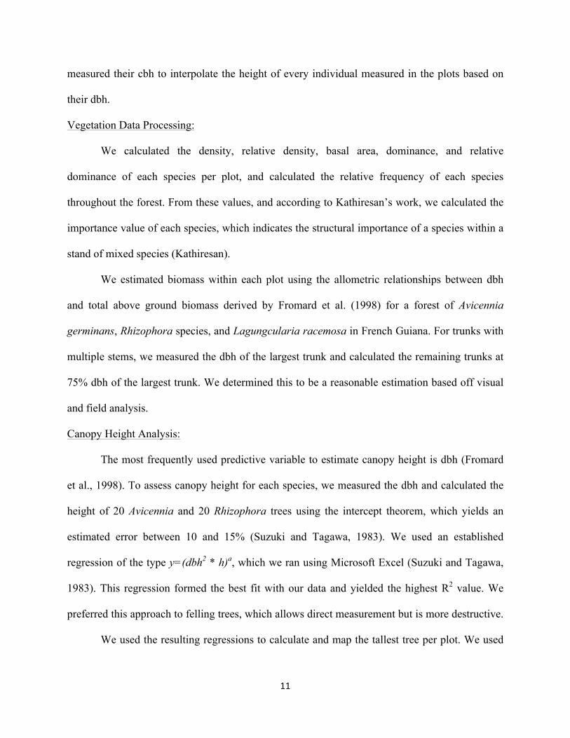
using a random point generator in ArcMap (Figure 1.2). We surveyed an area of 1,600 m2 within

the black mangrove community, and of 1,100 m2 in the red mangrove community.

   

10    

Figure 1.2: Vegetation survey plots in the Flamingo Mangroves

Within each quadrat, we counted the number of trees, saplings and seedlings for each

species. We determined the age class for each individual based on visual estimate of their size:

we defined seedlings as individuals shorter than 1 m, saplings as individuals between 1 and 3 m,

and trees as individuals taller than 3 m. We measured the circumference of the trunk at breast

height (cbh) (130 cm high) to calculate diameter at breast height (dbh) We also counted the

number of trunks and measured the girth of these trunks at 1.3 m above the ground (breast

height) for each tree and sapling taller than 1.3 m.

In order to estimate the height of the vegetation community within each plot, we

measured the height of 20 red and 20 black individuals using the intercept theorem. We

   

11    

measured their cbh to interpolate the height of every individual measured in the plots based on

their dbh.

Vegetation Data Processing:

We calculated the density, relative density, basal area, dominance, and relative

dominance of each species per plot, and calculated the relative frequency of each species

throughout the forest. From these values, and according to Kathiresan’s work, we calculated the

importance value of each species, which indicates the structural importance of a species within a

stand of mixed species (Kathiresan).

We estimated biomass within each plot using the allometric relationships between dbh

and total above ground biomass derived by Fromard et al. (1998) for a forest of Avicennia

germinans, Rhizophora species, and Lagungcularia racemosa in French Guiana. For trunks with

multiple stems, we measured the dbh of the largest trunk and calculated the remaining trunks at

75% dbh of the largest trunk. We determined this to be a reasonable estimation based off visual

and field analysis.

Canopy Height Analysis:

The most frequently used predictive variable to estimate canopy height is dbh (Fromard

et al., 1998). To assess canopy height for each species, we measured the dbh and calculated the

height of 20 Avicennia and 20 Rhizophora trees using the intercept theorem, which yields an

estimated error between 10 and 15% (Suzuki and Tagawa, 1983). We used an established

regression of the type y=(dbh2 * h)a, which we ran using Microsoft Excel (Suzuki and Tagawa,

1983). This regression formed the best fit with our data and yielded the highest R2 value. We

preferred this approach to felling trees, which allows direct measurement but is more destructive.

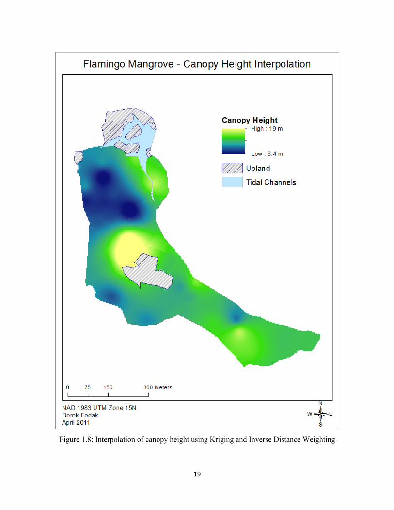
We used the resulting regressions to calculate and map the tallest tree per plot. We used

   

12    

the largest 10-15% dbh measurement within each plot to calculate an average height for each

plot (Mougin et al., 1999). We then ran Kriging and Inverse Distance Weighted interpolations on

our average plot canopy height. We then averaged the values from the two interpolations to

minimize variation, giving us a map of interpolated canopy height throughout the forest.

Results  and  Discussion  

Structure of the plant community:

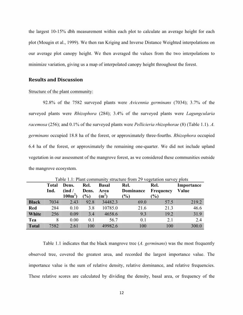
92.8% of the 7582 surveyed plants were Avicennia germinans (7034); 3.7% of the

surveyed plants were Rhizophora (284); 3.4% of the surveyed plants were Lagungcularia

racemosa (256); and 0.1% of the surveyed plants were Pellicieria rhizophorae (8) (Table 1.1). A.

germinans occupied 18.8 ha of the forest, or approximately three-fourths. Rhizophora occupied

6.4 ha of the forest, or approximately the remaining one-quarter. We did not include upland

vegetation in our assessment of the mangrove forest, as we considered these communities outside

the mangrove ecosystem.

Table 1.1: Plant community structure from 29 vegetation survey plots Total

Ind. Dens. (ind / 100m2)

Rel. Dens. (%)

Basal Area (m2)

Rel. Dominance (%)

Rel. Frequency (%)

Importance Value

Black 7034 2.43 92.8 34482.3 69.0 57.5 219.2 Red 284 0.10 3.8 10785.0 21.6 21.3 46.6 White 256 0.09 3.4 4658.6 9.3 19.2 31.9 Tea 8 0.00 0.1 56.7 0.1 2.1 2.4 Total 7582 2.61 100 49982.6 100 100 300.0

Table 1.1 indicates that the black mangrove tree (A. germinans) was the most frequently

observed tree, covered the greatest area, and recorded the largest importance value. The

importance value is the sum of relative density, relative dominance, and relative frequencies.

These relative scores are calculated by dividing the density, basal area, or frequency of the

   

13    

species in question by the sum of all species’ values for those variables, respectively. These

parameters are calculated using standard methodology (Cintron and Schaeffer-Novellie, 1984).

A. germinans recorded the largest value for each relative variable. Our values are comparable to

previous studies on coastal mangroves, which report the same order of importance but different

values. Fromard et al. (1989) reported importance values of 181, 53, 34, and 32 for Avicennia,

Rhizophora, others, and Laguncularia respectively for a mature coastal mangrove in French

Guiana. Studies on riverine mangroves at tidal estuaries often report higher importance values

for L. racemosa than all other species, though coastal mangroves like Flamingo have lower

importance values for L. racemosa (Ramirez-Garcia, Lopez-Blanco, and Ocana, 1998).

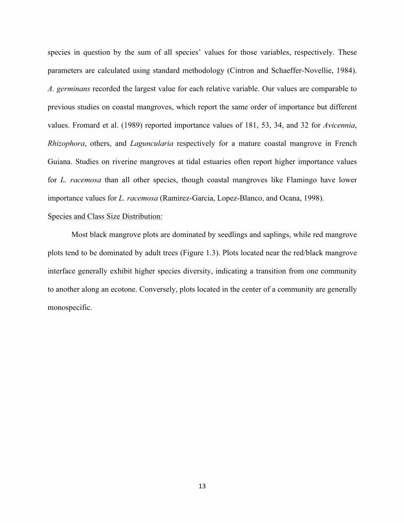
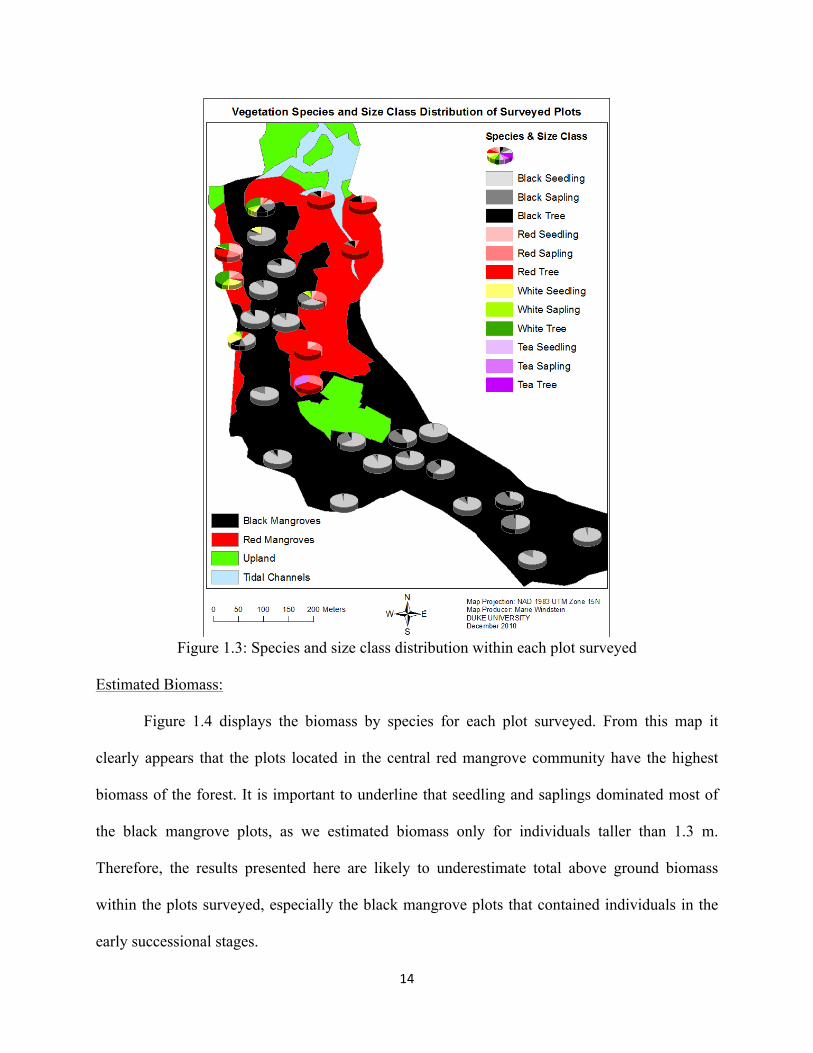
Species and Class Size Distribution:

Most black mangrove plots are dominated by seedlings and saplings, while red mangrove

plots tend to be dominated by adult trees (Figure 1.3). Plots located near the red/black mangrove

interface generally exhibit higher species diversity, indicating a transition from one community

to another along an ecotone. Conversely, plots located in the center of a community are generally

monospecific.

   

14    

 Figure 1.3: Species and size class distribution within each plot surveyed

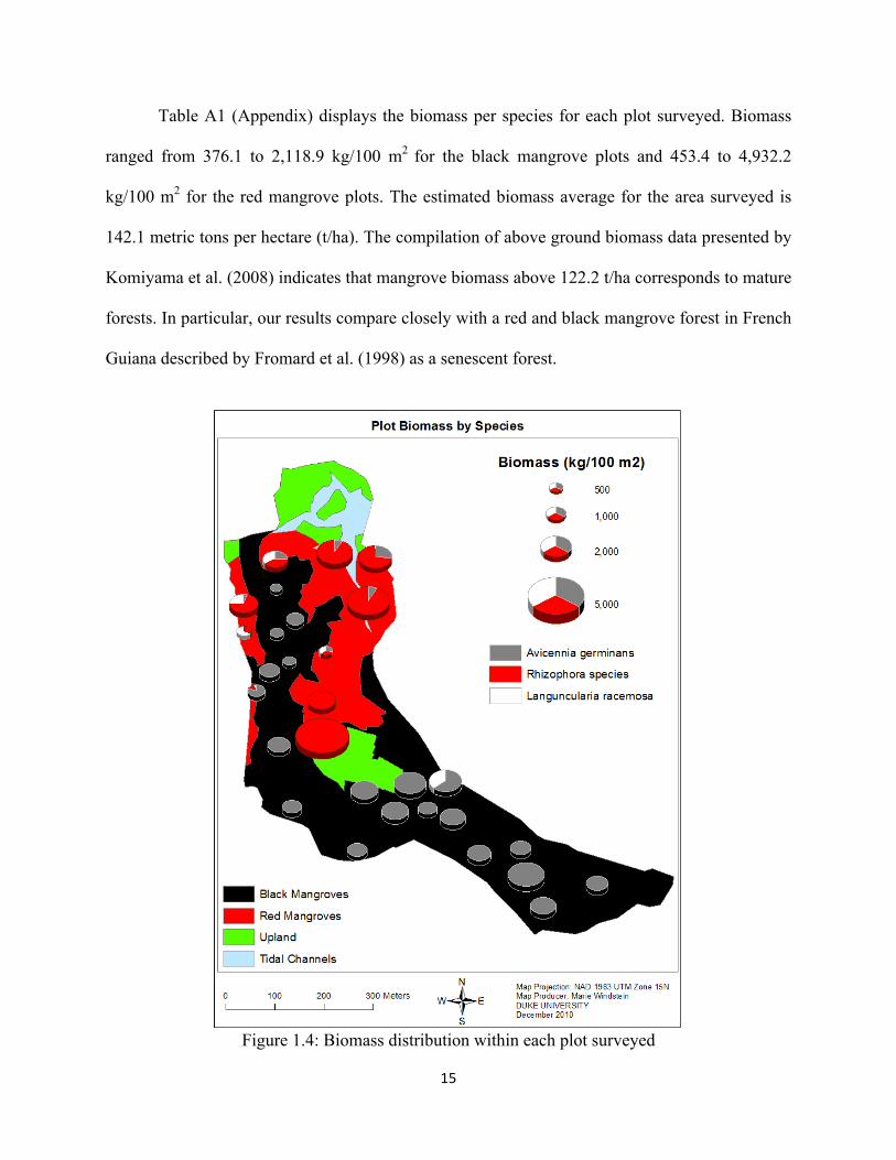
Estimated Biomass:

Figure 1.4 displays the biomass by species for each plot surveyed. From this map it

clearly appears that the plots located in the central red mangrove community have the highest

biomass of the forest. It is important to underline that seedling and saplings dominated most of

the black mangrove plots, as we estimated biomass only for individuals taller than 1.3 m.

Therefore, the results presented here are likely to underestimate total above ground biomass

within the plots surveyed, especially the black mangrove plots that contained individuals in the

early successional stages.

   

15    

Table A1 (Appendix) displays the biomass per species for each plot surveyed. Biomass

ranged from 376.1 to 2,118.9 kg/100 m2 for the black mangrove plots and 453.4 to 4,932.2

kg/100 m2 for the red mangrove plots. The estimated biomass average for the area surveyed is

142.1 metric tons per hectare (t/ha). The compilation of above ground biomass data presented by

Komiyama et al. (2008) indicates that mangrove biomass above 122.2 t/ha corresponds to mature

forests. In particular, our results compare closely with a red and black mangrove forest in French

Guiana described by Fromard et al. (1998) as a senescent forest.

Figure 1.4: Biomass distribution within each plot surveyed

   

16    

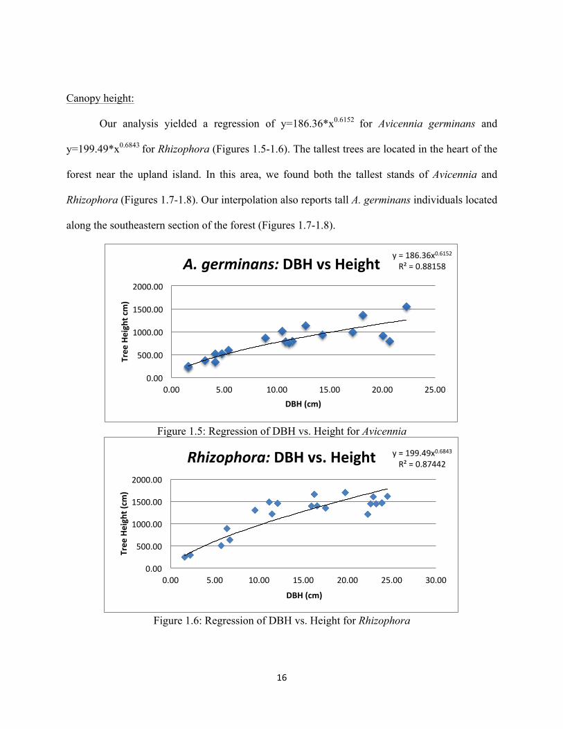
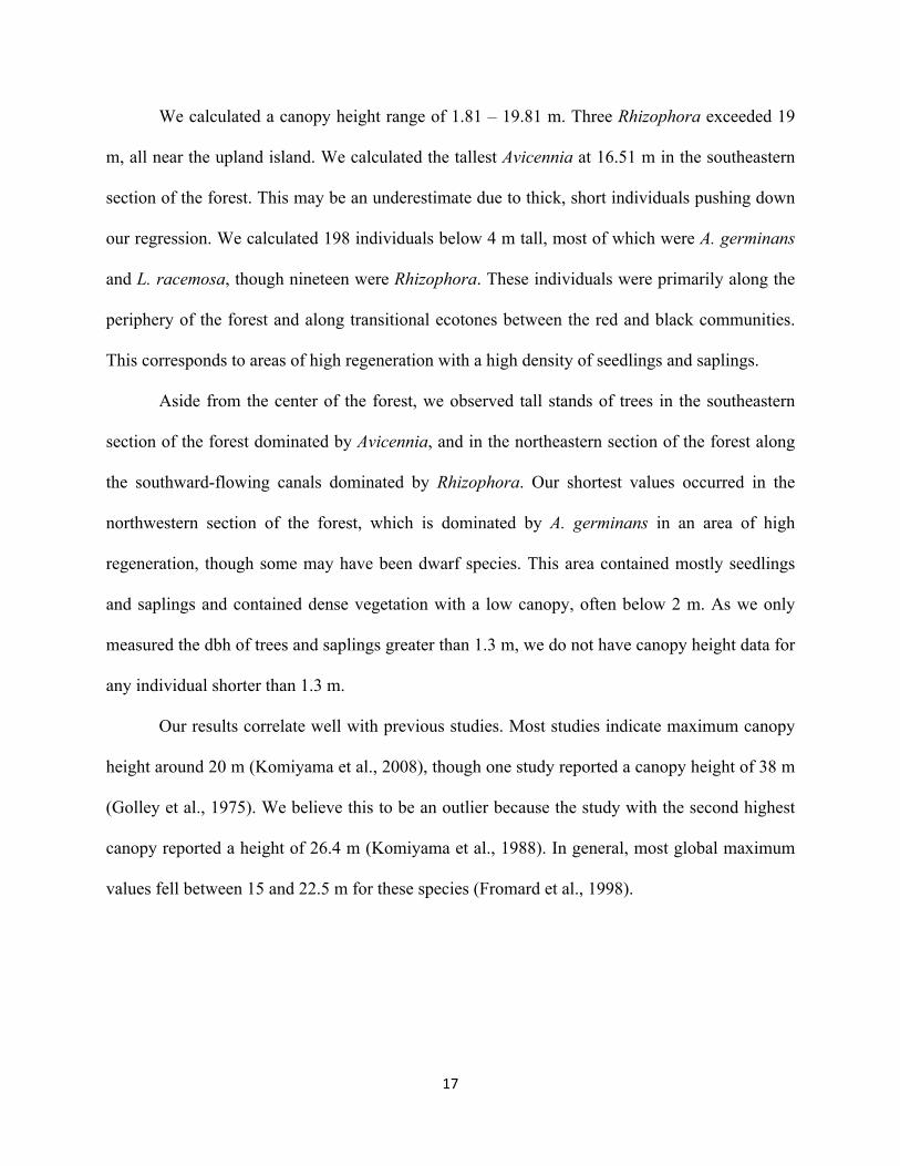
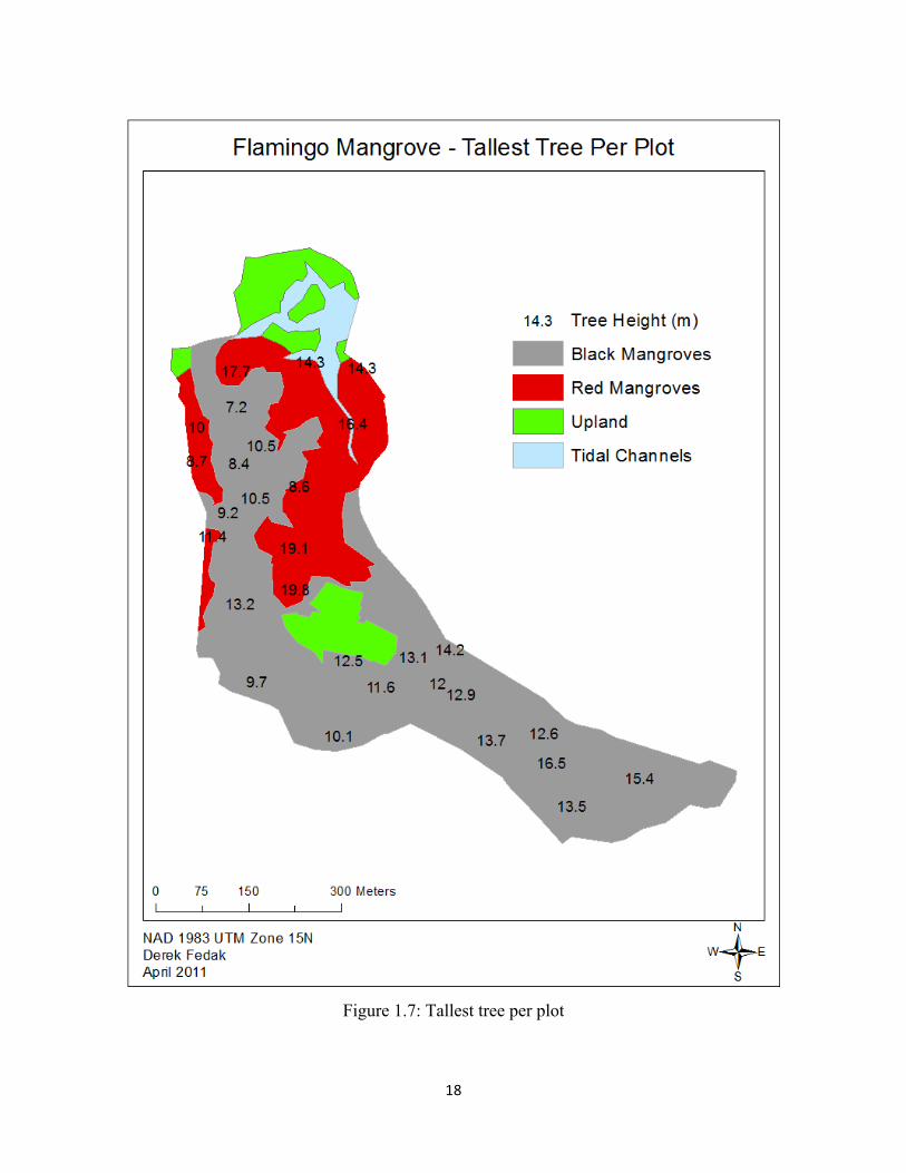
Canopy height:

Our analysis yielded a regression of y=186.36*x0.6152 for Avicennia germinans and

y=199.49*x0.6843 for Rhizophora (Figures 1.5-1.6). The tallest trees are located in the heart of the

forest near the upland island. In this area, we found both the tallest stands of Avicennia and

Rhizophora (Figures 1.7-1.8). Our interpolation also reports tall A. germinans individuals located

along the southeastern section of the forest (Figures 1.7-1.8).

Figure 1.5: Regression of DBH vs. Height for Avicennia

Figure 1.6: Regression of DBH vs. Height for Rhizophora

y  =  186.36x0.6152  R²  =  0.88158  

0.00  

500.00  

1000.00  

1500.00  

2000.00  

0.00   5.00   10.00   15.00   20.00   25.00  

Tree  Height  cm)  

DBH  (cm)  

A.  germinans:  DBH  vs  Height    

y  =  199.49x0.6843  R²  =  0.87442  

0.00  

500.00  

1000.00  

1500.00  

2000.00  

0.00   5.00   10.00   15.00   20.00   25.00   30.00  

Tree  Height  (cm

)  

DBH  (cm)  

Rhizophora:  DBH  vs.  Height  

   

17    

We calculated a canopy height range of 1.81 – 19.81 m. Three Rhizophora exceeded 19

m, all near the upland island. We calculated the tallest Avicennia at 16.51 m in the southeastern

section of the forest. This may be an underestimate due to thick, short individuals pushing down

our regression. We calculated 198 individuals below 4 m tall, most of which were A. germinans

and L. racemosa, though nineteen were Rhizophora. These individuals were primarily along the

periphery of the forest and along transitional ecotones between the red and black communities.

This corresponds to areas of high regeneration with a high density of seedlings and saplings.

Aside from the center of the forest, we observed tall stands of trees in the southeastern

section of the forest dominated by Avicennia, and in the northeastern section of the forest along

the southward-flowing canals dominated by Rhizophora. Our shortest values occurred in the

northwestern section of the forest, which is dominated by A. germinans in an area of high

regeneration, though some may have been dwarf species. This area contained mostly seedlings

and saplings and contained dense vegetation with a low canopy, often below 2 m. As we only

measured the dbh of trees and saplings greater than 1.3 m, we do not have canopy height data for

any individual shorter than 1.3 m.

Our results correlate well with previous studies. Most studies indicate maximum canopy

height around 20 m (Komiyama et al., 2008), though one study reported a canopy height of 38 m

(Golley et al., 1975). We believe this to be an outlier because the study with the second highest

canopy reported a height of 26.4 m (Komiyama et al., 1988). In general, most global maximum

values fell between 15 and 22.5 m for these species (Fromard et al., 1998).

   

18    

Figure 1.7: Tallest tree per plot

   

19    

Figure 1.8: Interpolation of canopy height using Kriging and Inverse Distance Weighting

   

20    

Overall  Picture  

We found that the Flamingo Mangroves support a healthy floral ecosystem. The forest

contains all community types generally found in mangroves in the expected arrangement of

where channels meeting meet a red mangrove community, which is eventually replaced by a

black mangrove community interspersed with white mangrove individuals. The mangrove

ecosystem is eventually replaced by upland vegetation above the high-tide line. The vegetation

structure, including importance value, calculated biomass, and calculated canopy height

correspond with previous studies on coastal mangroves. The forest contains a zone of high

regeneration in the northwestern section as well as tall stands of mature forest near the upland

island in the center of the forest and in the southeastern section of the forest. Lastly, the presence

of the tea mangrove, P. rhizophorae, north of its expected range further indicates that the

Flamingo Mangroves supports a healthy and diverse ecosystem. We have found no major issues

indicating that the vegetation is being adversely affected by anthropogenic influences within the

mangroves.

 

   

   

21    

Chapter  II:  Analysis  of  Water  Samples  

Objectives    

We collected water samples to have a preliminary assessment of the composition of the

water entering the system, identify potential sources of pollutants, and determine if management

efforts were necessary to maintain or restore the quality of the waters flowing in and out of the

mangrove.

Background  

We identified four types of water input to the Flamingo Mangroves: tidal, precipitation,

runoff, and wastewater. While we did not quantify the volume of ocean water flowing into the

system, it is reasonable to assume that the tidal flow constitutes the largest fraction of water

input. In this region of the world, tides are semi diurnal, rising and ebbing twice a day, resulting

in seawater that flushes in and out of the forest at the same frequency.

In terms of volume, precipitation is likely to be the second largest source of water to the

forest; however, it is important to emphasize that it is the largest source of fresh water. Both

spatial and temporal distribution of rainfall differs greatly from the daily tidal flow. The tidal

inlet is located in the northeast of the forest. The influence of seawater is limited to the lowest

lying areas adjacent to this inlet and to the tidal channels, as seawater rarely reaches higher

locations. Rainfall, on the other hand, exerts an influence over the entire ecosystem. Its influence

fluctuates seasonally with the strongest impact during the rainy season (invierno) between June

and October. Based on the mean annual precipitation and the area of the forest, we estimated that

approximately 4.15x108 liters of precipitation feed the mangroves annually, with most of it

falling over the five months of the wet season.

   

22    

Besides tidal and rainwater, discharge of freshwater from runoff and wastewater

contributes to the hydrologic budget of the forest. Runoff is the fraction of precipitation that is

not intercepted by vegetation or human structures, nor absorbed in the ground, retained in

depression, or evaporated, but flows over the land surface towards the lowest lying parts of the

landscape, usually wetlands (USGS, 2011). During runoff, water becomes enriched with

pollutants; the chemical and physical composition, as well as the quantity of pollutants carried in

the overflow depends on the land cover type. Compounds found in surface runoff are primarily

composed of sediment inputs from soil erosion and wash-off of pollutants accumulated on

impervious surfaces (Novotny, pp. 108-14). Impervious surface pollutants include wet and dry

atmospheric deposits as well as particulates from vehicles, pavement and other surfaces wearing

off. They notably consist of hydrocarbons, heavy metals, organic compounds, nitrogen and

phosphorus (Novotny, pp. 387-8). Pollutants are transported in runoff water in both the dissolved

and solid phase and can disrupt ecological processes of the receiving water bodies when present

in high concentration. (Novotny, pp. 108-14).

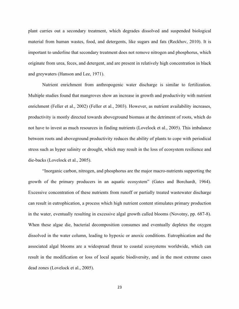
We identified four point sources discharging runoff water: 1) the northwest corner of the

forest draining water from the FBRS parking lot; 2) north of the bridge on the eastern side of the

forest draining water from a nearby developed and mostly impervious hill; 3) the southwest side

of the forest draining water from a vegetated area; and 4) the east side of the forest draining

water from open land, likely pasture or agricultural lands (Figure 2.1)

Wastewater in Flamingo originates almost entirely from commercial and touristic

development. Therefore, the wastewater produced in the vicinity of the mangrove is exclusively

composed of domestic wastewater. All blackwater and greywater from the FBRS are processed

through their wastewater treatment plant (WWTP) prior to discharge in the mangrove. The FBRS

   

23    

plant carries out a secondary treatment, which degrades dissolved and suspended biological

material from human wastes, food, and detergents, like sugars and fats (Reckhov, 2010). It is

important to underline that secondary treatment does not remove nitrogen and phosphorus, which

originate from urea, feces, and detergent, and are present in relatively high concentration in black

and greywaters (Hanson and Lee, 1971).

Nutrient enrichment from anthropogenic water discharge is similar to fertilization.

Multiple studies found that mangroves show an increase in growth and productivity with nutrient

enrichment (Feller et al., 2002) (Feller et al., 2003). However, as nutrient availability increases,

productivity is mostly directed towards aboveground biomass at the detriment of roots, which do

not have to invest as much resources in finding nutrients (Lovelock et al., 2005). This imbalance

between roots and aboveground productivity reduces the ability of plants to cope with periodical

stress such as hyper salinity or drought, which may result in the loss of ecosystem resilience and

die-backs (Lovelock et al., 2005).

“Inorganic carbon, nitrogen, and phosphorus are the major macro-nutrients supporting the

growth of the primary producers in an aquatic ecosystem” (Gates and Borchardt, 1964).

Excessive concentration of these nutrients from runoff or partially treated wastewater discharge

can result in eutrophication, a process which high nutrient content stimulates primary production

in the water, eventually resulting in excessive algal growth called blooms (Novotny, pp. 687-8).

When these algae die, bacterial decomposition consumes and eventually depletes the oxygen

dissolved in the water column, leading to hypoxic or anoxic conditions. Eutrophication and the

associated algal blooms are a widespread threat to coastal ecosystems worldwide, which can

result in the modification or loss of local aquatic biodiversity, and in the most extreme cases

dead zones (Lovelock et al., 2005).

   

24    

The wastewater treatment plant of the FBRS located on the northern edge of the forest is

the only known source of treated wastewater. We identified one point source located south of the

beach road discharging untreated wastewater. In addition, we found two pipes originating from

properties bordering the forest: one partially buried in the ground and the other directed towards

the center of the mangroves (Figure 2.1). We were unable to locate their origins, as we never

witnessed water discharge.

Figure 2.1: Point sources of water input to the Flamingo Mangroves

   

25    

Methods  

Water Samples Collection

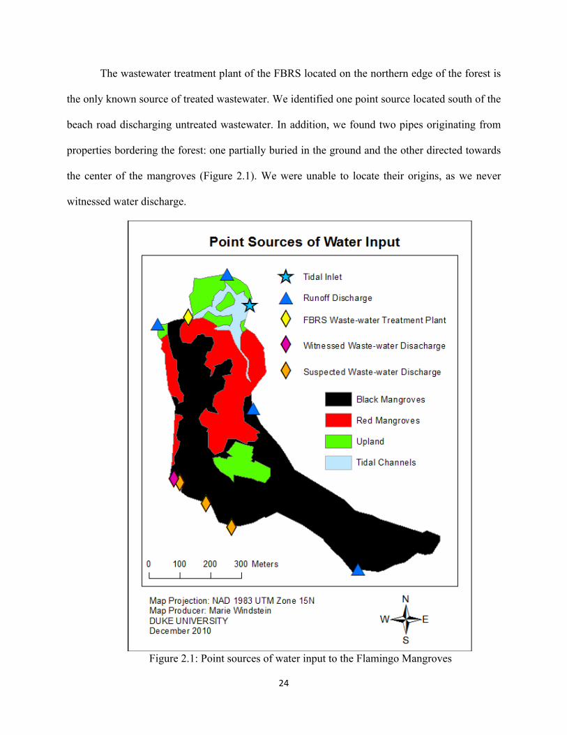
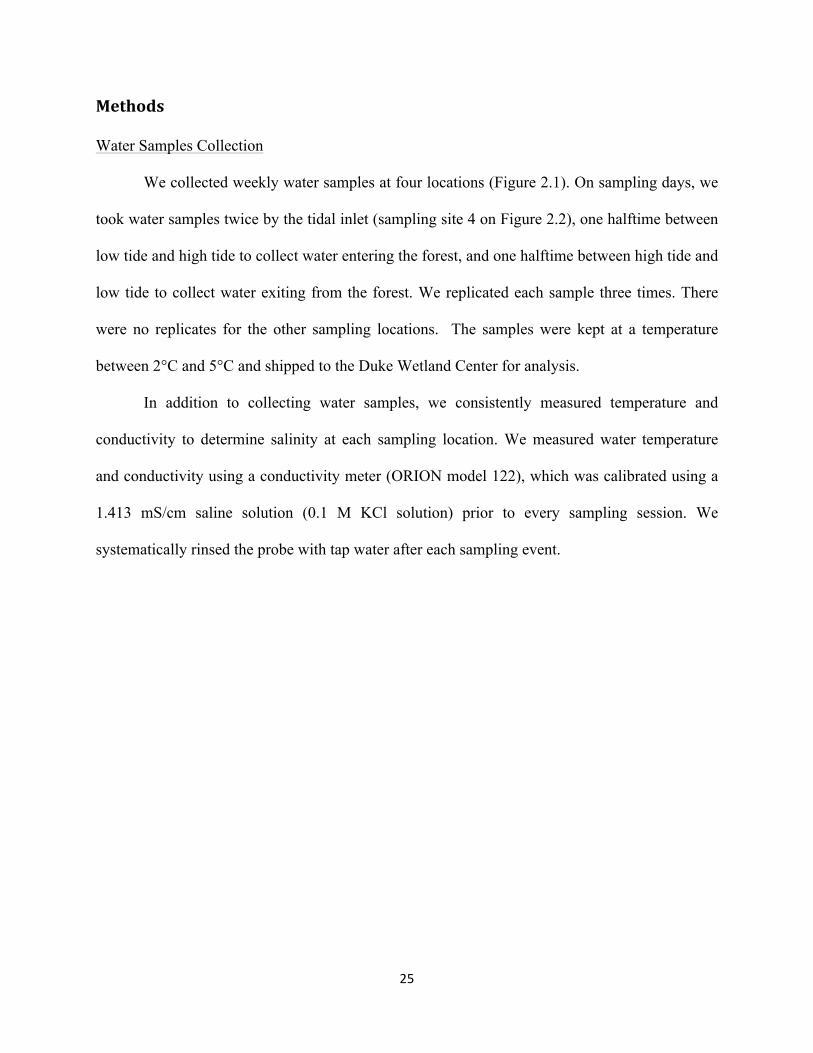
We collected weekly water samples at four locations (Figure 2.1). On sampling days, we

took water samples twice by the tidal inlet (sampling site 4 on Figure 2.2), one halftime between

low tide and high tide to collect water entering the forest, and one halftime between high tide and

low tide to collect water exiting from the forest. We replicated each sample three times. There

were no replicates for the other sampling locations. The samples were kept at a temperature

between 2°C and 5°C and shipped to the Duke Wetland Center for analysis.

In addition to collecting water samples, we consistently measured temperature and

conductivity to determine salinity at each sampling location. We measured water temperature

and conductivity using a conductivity meter (ORION model 122), which was calibrated using a

1.413 mS/cm saline solution (0.1 M KCl solution) prior to every sampling session. We

systematically rinsed the probe with tap water after each sampling event.

   

26    

Figure 2.2: Water sampling locations in the Flamingo Mangroves

Water Samples Laboratory Analyses

Total Nitrogen: ammonium, nitrite, nitrate, and organic nitrogen (EPA Method 353.2)

This analysis determined the amount of total nitrogen (TN) in the water. In individual

glass vials, we added 7 mL of alkaline persulfate reagent to 10 mL of sampled water and

autoclaved them at 121ºC and 17 atmospheres for 30 minutes. During the digestion, the oxygen

unbinds from the persulfate molecule and oxidizes all forms of nitrogen to nitrate (NO3-). The

nitrate concentration of each sample is then determined spectrophotometrically and calculated

using Beer’s Law, which relates the absorbance of a solution to the concentration of a

compound.

   

27    

Total phosphorus: organic and inorganic phosphorus (EPA Method 365.4)

This analysis determined the amount of total phosphorus (TP) in the water. We used the

same method described above, but added 7 mL acidic persulfate solution to 10 mL of sample

water. During digestion, persulfate oxidizes all phosphorus in solution to phosphate (PO43-).

Water Samples Statistical Analyses

We ran t-tests to determine if there was a significant difference in the composition of the

tidal water entering and leaving the mangrove. A t-test is a common way to analyze the

difference in two data sets. Because it is nearly impossible to know the true mean of a

population, we collected samples and calculated a sample mean. We can place a confidence

interval around the sample mean based on the variance of the dataset and the number of samples.

We are able to decrease the confidence interval by increasing the sample size, thus narrowing the

range of estimates for the sample mean. T-tests can only be conducted when datasets fit a normal

distribution. Therefore, it is typical for many environmental datasets to be fit to a log curve so

that they exhibit a normal distribution.

Generally, a confidence interval of 0.95, or 95%, is used when conducting a t-test. A t-

test compares the sample means of two datasets, giving a resulting p-value. A p-value below 0.05

allows us to reject the hypothesis that the two sample means are the same. Thus, we can state that

there is a significant difference in the means of the two populations with a 95% confidence level.

Results  and  Discussion  

Salinity  

The initial field survey, conducted from March 19th to 21st 2010, indicated that the water

inside the mangrove was from marine origin, reporting salinity near ocean concentrations (32 to

35 ppt (parts per thousands)) (Richardson, 2010). Water salinity data collected at the tidal inlet

   

28    

(sampling site 4, Figure 2.2) between May 20th and July 8th 2010 ranged between 14.9 and 35.0

ppt, averaging near 26 ppt for both incoming and receding waters (Table A2, Appendix). These

values are characteristic of brackish water and indicate an important freshwater input from

precipitation. These results compare with tidal water in the mangroves of Terminos Lagoon,

Mexico, where salinity ranged between 21 and 42 ppt, depending on the time of the year (Rivera-

Monory et al., 1995).

Salinity data collected at the runoff pipe (sampling site 1, Figure 2.2) was consistently

lower than 0.5 ppt except for July 8th, which clearly indicates freshwater discharge (Table A2).

Water salinity directly upstream and downstream of the WWTP (sampling sites 2 and 3, Figure

2.2) ranged between 17.7 and 28.9 ppt, averaging near 24 ppt (Table A2). Salinity in the vicinity

of the WWTP is slightly lower than at the tidal inlet due to the freshwater discharge from the

WWTP. The sharp increase in salinity between sampling sites 1 and 2 indicates an important

tidal influence and flushing near the WWTP.

Total  Nitrogen  

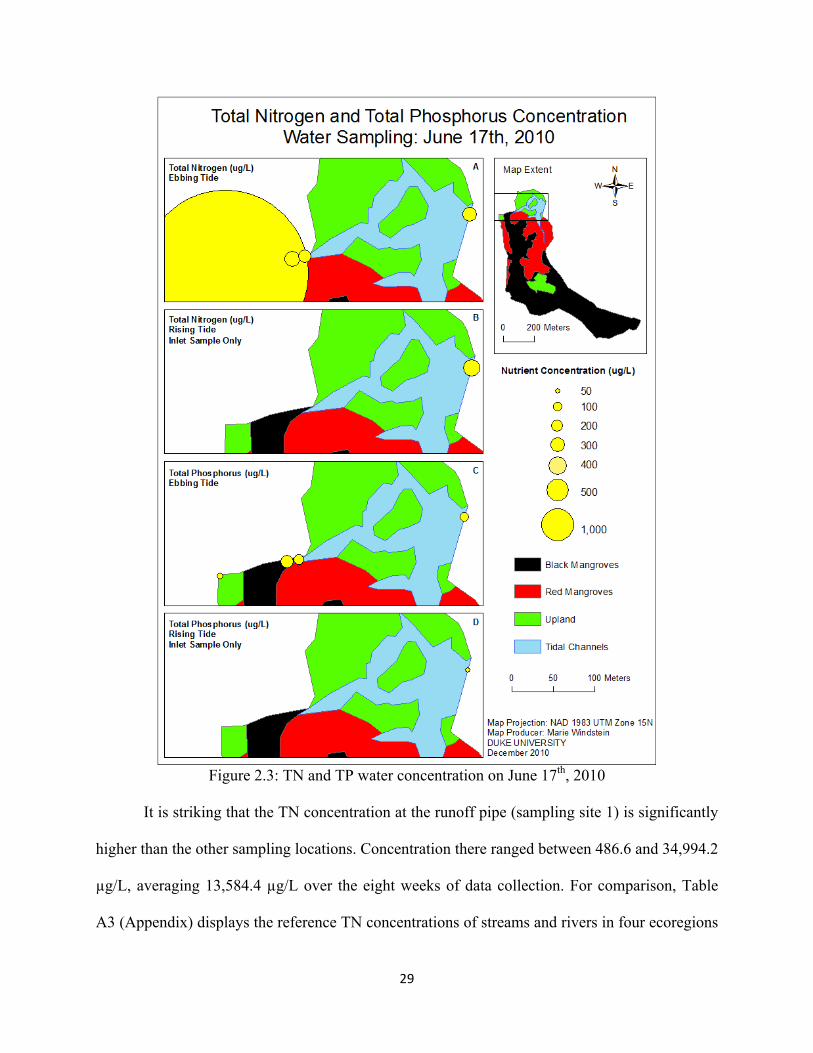
Figure 2.3 (A & B) shows the total nitrogen content of the water on June 17th, which is

representative of the general trend in TN concentration between May 20th and July 8th, 2010.

   

29    

Figure 2.3: TN and TP water concentration on June 17th, 2010

It is striking that the TN concentration at the runoff pipe (sampling site 1) is significantly

higher than the other sampling locations. Concentration there ranged between 486.6 and 34,994.2

µg/L, averaging 13,584.4 µg/L over the eight weeks of data collection. For comparison, Table

A3 (Appendix) displays the reference TN concentrations of streams and rivers in four ecoregions

   

30    

of the southeast United States, which “reflect pristine or minimally impacted waters” (EPA a.,

2000). From this data, it is clear that nitrogen levels at sampling site 1 are problematic, reporting

average concentrations eight to twenty-two times higher than pristine waters (Southeastern plains

and Piedmont stream reference, respectively, Table A3).

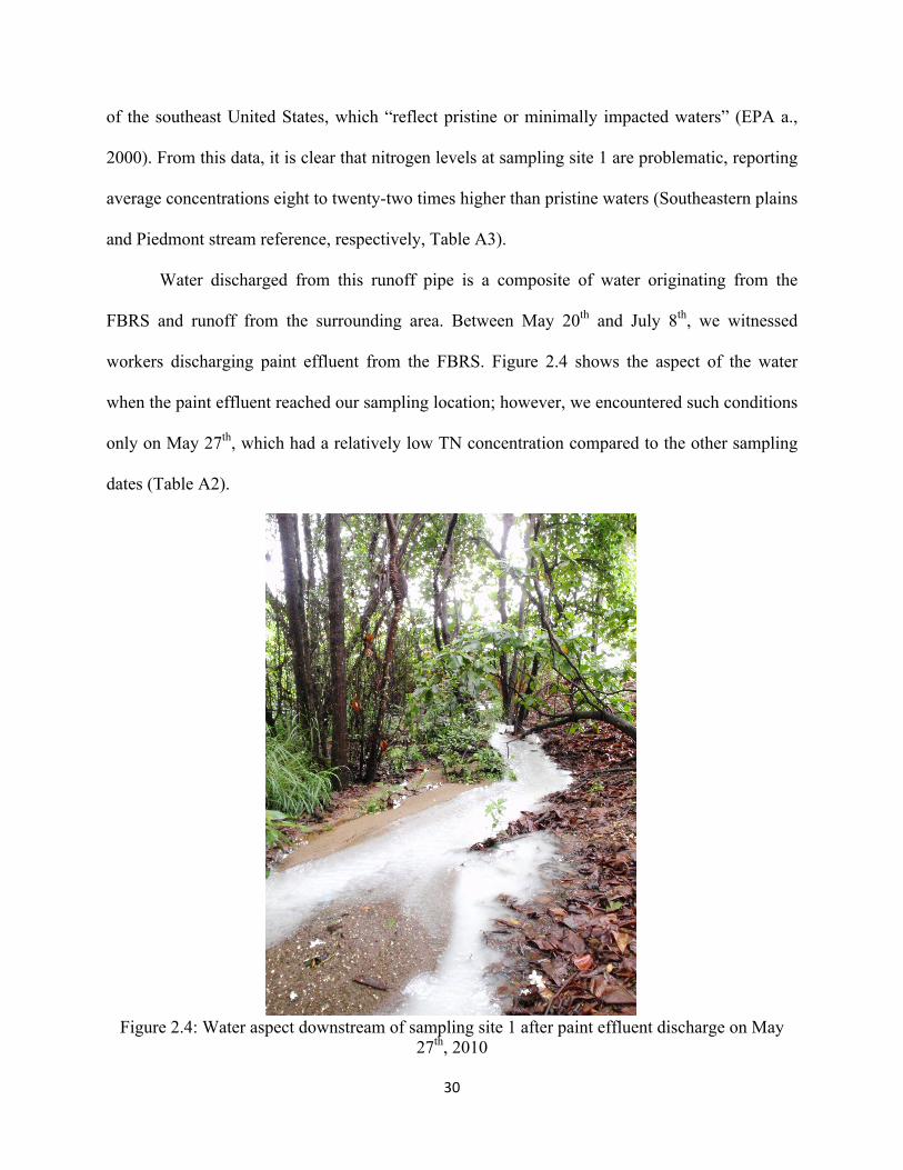
Water discharged from this runoff pipe is a composite of water originating from the

FBRS and runoff from the surrounding area. Between May 20th and July 8th, we witnessed

workers discharging paint effluent from the FBRS. Figure 2.4 shows the aspect of the water

when the paint effluent reached our sampling location; however, we encountered such conditions

only on May 27th, which had a relatively low TN concentration compared to the other sampling

dates (Table A2).

Figure 2.4: Water aspect downstream of sampling site 1 after paint effluent discharge on May

27th, 2010

   

31    

The total nitrogen concentration in samples collected near the WWTP (sampling sites 2

and 3) ranged between 298.5 and 1915.5 µg/L, averaging 551.5 µg/L and 555.3 µg/L for sites 2

and 3 respectively (Table A2). The preliminary investigation in March 2010 revealed a TN

concentration of 5,300 µg/L for these sites, or ten times the average nitrogen concentration found

in the samples collected between May and July of the same year (Richardson, 2010). It is

important to underline that we collected water samples on Thursdays during the low tourism

season, while March data were collected on a weekend during the high tourism season. Variation

in guest number between weekdays and weekends and low and high tourism season greatly

influences wastewater discharge and nutrient concentration in the samples collected. Thus, the

data presented in Table A2 for sites 2 and 3 can reasonably be considered as the lower end of the

TN concentration spectrum.

The nitrogen concentration at the tidal inlet (site 4) ranged between 304.6 and 473.2

µg/L, averaging 368.1 and 357.5 µg/L for the incoming and ebbing water, respectively. We

found no significant difference in the nitrogen concentration of water coming in or exiting the

mangrove (p-value = 0.4997).

Total  Phosphorus  

Similarly to nitrogen concentrations, the highest total phosphorus occurred at the runoff

pipe (sampling site 1). TP here ranged from 38.48 to 963.23 µg/L, averaging 357.6 µg/L over the

eight weeks of data collection. For comparison, Table A3 displays the EPA’s reference TP

concentrations of streams and rivers in four ecoregions of the southeast United States. In general,

freshwater containing phosphorus concentrations below 30 µg/L are considered unpolluted,

while concentrations above 100 µg/L can result in eutrophication (L.E.O).

   

32    

The phosphorus concentration in samples collected near the WWTP averaged 204.0 and

85.0 µg/L for sites 2 and 3 respectively (Table A2). Similar to nitrogen concentrations, it is likely

that the data collected between May and July is at the lower end of the phosphorus concentration

spectrum due to reduced tourist numbers during this time of the year. Indeed, phosphorus

concentration in water collected between May 20th and July 8th never exceeded 179 µg/L, and we

never witnessed algae growth in the vicinity of the WWTP. However, the preliminary

investigation in March 2010 revealed a TP concentration of 1,200 µg/L for waters collected near

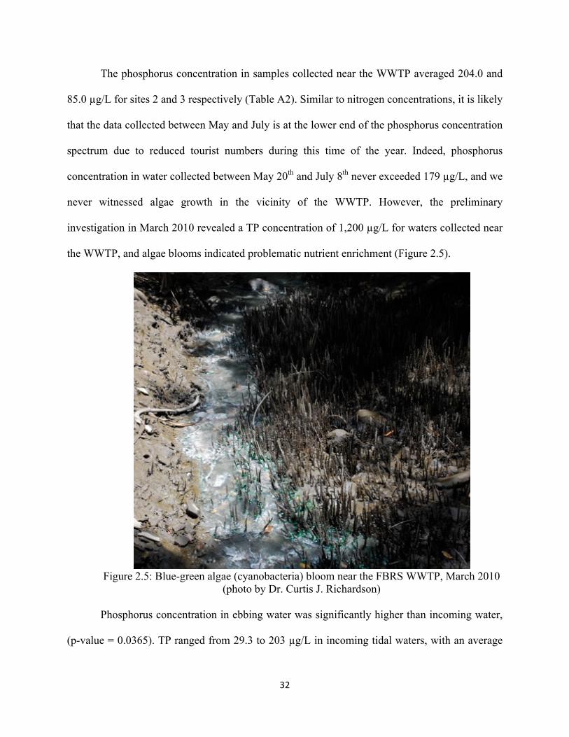
the WWTP, and algae blooms indicated problematic nutrient enrichment (Figure 2.5).

Figure 2.5: Blue-green algae (cyanobacteria) bloom near the FBRS WWTP, March 2010

(photo by Dr. Curtis J. Richardson)

Phosphorus concentration in ebbing water was significantly higher than incoming water,

(p-value = 0.0365). TP ranged from 29.3 to 203 µg/L in incoming tidal waters, with an average

   

33    

of 81.2 µg/L, and ranged from 49.0 to 334.3 µg/L in ebbing waters, with an average of 177.7

µg/L. Comparing these values to the 10 µg/L recommended by the USEPA for maximum

diversity in estuaries (Osmond, 1995), it appears that water leaving the mangroves have

problematic phosphorus concentrations because most samples had phosphorus concentration up

to 30 times higher than the USEPA recommended levels, while many of them were close or

above the 100 µg/L eutrophication threshold.

N:P  ratio  

Table A2 displays the N:P ratio in tidal water entering and leaving the forest, which

ranged from 4.31 to 28.7 in advancing water and 3.24 to 15.51 in receding water. This table

shows that, on average, both advancing and receding water were nitrogen limited (ratio is

inferior to 16:1, Redfield ratio). This is expected in estuarine and marine systems (Osmond,

1995). However, the average ratio for advancing water (10.03) was higher than the average ratio

for receding water (4.45). A closer look at the data collected in June indicates that the water

entering the mangroves were phosphorus limited (ratio greater than 16:1), while water exiting the

mangroves were nitrogen limited, indicating an increase in phosphorus concentration in exiting

water. Overall, our data revealed that the N:P ratio in exiting water was systematically lower

than in entering water as a result of phosphorus enrichment.

Overall  Picture  

  Data collected between March 19th and 21st and between May 20th and July 8th 2010

revealed problematic nutrient concentrations at several locations. The most concerning levels of

nutrients occurred in runoff water collected at sampling site 1. There, both nitrogen and

phosphorus were at least ten times higher on average than the EPA’s reference concentration.

   

34    

Due to a seasonal difference in guest occupancy, the nutrient concentrations found in the

vicinity of the WWTP in March were considerably higher than during the summer. In March,

both TN and TP concentrations were highly problematic, as testified by the presence of algal

blooms in the tidal channel where wastewater is discharged. Nutrient levels during the summer

were not as concerning, but TP frequently exceeded the 100 µg/L threshold. Finally, levels of

phosphorus in tidal water leaving the forests were on average twice the concentration of TP in

water entering the forest, and concentrations were frequently higher than the 100 µg/L level.

   

   

35    

Chapter  III:  Analysis  of  Soil  Samples  

Objectives    

We collected soil samples to evaluate the nutrient levels across the forest and assess the

edaphic characteristics of the site. We sampled the channels in the vicinity of the wastewater

treatment plant to investigate the long-term effects of nutrients discharge by FBRS. We also

sampled along two perpendicular transects to investigate the apparent diminished health of a

section of the forest and compare its nutrient content to more vigorous and remote parts.

Background  

Channel Samples

It is important to underline that we collected water samples in the vicinity of the WWTP

during the low tourism season. It is therefore probable that both the quantity of water discharged

as well as its nutrient content were at their lowest and that our samples are not fully

representative of the annual average nutrient load. In contrast, soils tend to be good indicators of

the general nutrient discharge over time. The concentration of nutrients in soil is mainly

regulated by biogeochemical processes, but is also influenced by the nutrient load carried in the

overflowing water, which absorbs nutrients as it infiltrates and percolates in the ground. This

stores nutrients in the soil, reflecting the nutrients discharge over time (Tam and Wong, 1995).

Transect Samples

The band of vegetation directly adjacent to the road is less densely vegetated than the rest

of the forest. Based on our observations, the vigor of the trees in this area is significantly inferior

to the general health of the system. Additionally, a preliminary assessment indicated that the soil

substrate along the road is sandier than the rest of the forest (Richardson, 2010). The fragile

condition of the vegetation next to the road can be the result of a combination of three factors.

   

36    

First, automobile traffic along the western part of the forest can lead to physical processes like

erosion, soil compaction, and sand intrusion, which might impact the band of vegetation at the

edge of the forest. The second and third factors result from the texture of the soil in this area.

Sandy soils tend to be porous and permeable, which results in mediocre retention of water. This

can lead to a modification of the hydrology and salinity. These two environmental parameters are

central in determining the distribution and health of mangrove species. Finally, low water

retention can also affect the cycling of nutrients by changing the redox conditions of the soil.

Therefore, it is possible that this soil texture creates a nutrient-limiting situation, resulting in

more fragile, slower growing, and sparser vegetation.

Nitrogen

Inorganic nitrogen, which is the bioavailable form of nitrogen, is generally present in

soils in two major forms: NH4+ (ammonium) and NO3

- (nitrate).

The presence and concentration of NH4+ is mainly dependent on two factors: the pH of

the soil and of the surrounding water, and the degree of oxygenation of the soil. NH4+ is the

conjugate acid of the acid/base pair NH4+/NH3, and is prevalent in media with relatively low pH.

Ammonia (NH3), the conjugate base of ammonium, is prevalent in basic media; this form of

nitrogen is volatile and, therefore, unavailable to plants. The degree of oxygenation also

determines the concentration of ammonium in the soil. Nitrification occurs under oxygenated

conditions. During this process bacteria oxidize ammonium to nitrate (Harrison, 2003).

Mangrove soils are typically acidic and anoxic, which prevents the conversion of ammonium to

ammonia and nitrate respectively, thereby making ammonium the primary form of bioavailable

nitrogen to mangroves (Reef, Feller, and Lovelock, 2010).

   

37    

Nitrification is the biological process by which ammonium is oxidized to nitrite (NO2-)

and then nitrate (NO3-) by aerobic bacteria; thus, nitrogen under the nitrite or nitrate form tends

to be rare in flooded wetland soils. In addition, denitrification occurs under these reduced

conditions. Bacteria in the soil use NO3- as an electron acceptor for metabolism, and nitrate

enters a chain of reducing reactions ultimately resulting in the production of nitrogen gas N2 and

the depletion of NO3- from the soil (Harrison, 2003).

Total nitrogen, also expressed as the percentage of nitrogen in the soil, encompasses

ammonium, nitrite, nitrate, and organic nitrogen. Organic nitrogen compounds are molecules in

which nitrogen is bound to carbon atoms. In soils, they occur mostly under the form of amino

acids and peptides and originate from decomposing litter (Winstanley, 2004).

Phosphorus

Phosphate (PO43-) is the form of phosphorus that can be taken up by plants. In the soil,

phosphate adsorbs to the extensive surface of clay minerals (Holford, 1997) and forms phosphate

compounds, notably with iron (Reef, Feller, and Lovelock, 2010). Under this form, however,

phosphorus is immobilized in the soil and not directly available to plants. Phosphate ions

available to plants originate from weakly adsorbed or soluble phosphate compounds (Holford,

1997), and occur when redox conditions dissociate the phosphate compounds (Reef, Feller, and

Lovelock, 2010). In aerobic conditions, phosphate is not available because it is either adsorbed to

sediments or bound to iron. Under anaerobic conditions, however, iron is reduced and phosphate

ions are released (Reef, Feller, and Lovelock, 2010). Other factors including the nature and size

of the sediments and the quantity/species of ions in the pore water may also influence the

availability of phosphate to plants.

   

38    

Total phosphorus encompasses both organic and inorganic phosphorus and is found in

one of three major forms of phosphorus in soil: “solution P”, “active P”, and “fixed P”. “Solution

P” is the fraction of phosphorus bioavailable to plants and is constituted of orthophosphates, the

conjugated acids of phosphate salts; “active P” is the labile, solid phase of phosphate adsorbed to

soil particles or bound to minerals such as aluminum, iron, calcium, and magnesium; the “fixed

P” is composed of insoluble inorganic phosphate and decomposing organic phosphates (Busman,

et al., 2009).

Total Carbon

Total carbon, also expressed as the percentage of carbon in the soil, encompasses

inorganic and organic carbon. Inorganic carbon is found under the form of carbonate salts or

their conjugated acid, and constitutes a very small fraction of total carbon in most soils. Organic

carbon compounds are molecules containing at least carbon, oxygen, and hydrogen atoms, and

that can also contain nitrogen, phosphorus, and sulfur atoms (Heimsath, 2009). Organic carbon

can be divided into complex organic compounds called humic substances, and “compounds such

as sugars, amino acids, and lipids” called non-humic substances. Organic carbon originates from

dead plant and animal tissues, and its concentration in soil is influenced by factors such as soil

texture, climate, and litter production (Heimsath, 2009).

Salinity

Salinity is one of the most important abiotic factors regulating mangrove survival,

distribution, and growth (Chen and Twilley, 1998); (McKee, 1995). All mangrove species are

facultative halophytes that grow on soils where pore water salinity ranges from 0‰ (freshwater)

to 35-45‰ (slightly above seawater) (Hogarth, 1999); (Chen and Twilley, 1998); (Sherman,

Fahey, and Martinez, 2003). Hypersaline conditions caused by the combined action of tidal

   

39    

cycles and evaporation can develop in tropical coastal areas, especially during the dry season.

Mangroves’ tolerance to hypersaline conditions varies among species: “the upper tolerance of

salinity for Rhizophora mangle [red mangrove] is about 70 g.kg-1, compared to 85 g.kg-1 for

Lagungcularia racemosa [white mangrove], and 100 g.kg-1 for Avicennia germinans [black

mangrove]” (Chen and Twilley, 1998). Thus, exacerbation of soil salinity can greatly affect

species distribution and, in most severe cases, result in dieback of mangrove forests.

Methods  

Soil Samples Collection

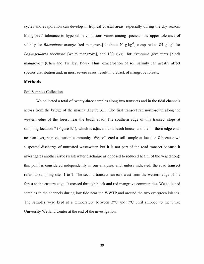
We collected a total of twenty-three samples along two transects and in the tidal channels

across from the bridge of the marina (Figure 3.1). The first transect ran north-south along the

western edge of the forest near the beach road. The southern edge of this transect stops at

sampling location 7 (Figure 3.1), which is adjacent to a beach house, and the northern edge ends

near an evergreen vegetation community. We collected a soil sample at location 8 because we

suspected discharge of untreated wastewater, but it is not part of the road transect because it

investigates another issue (wastewater discharge as opposed to reduced health of the vegetation);

this point is considered independently in our analyses, and, unless indicated, the road transect

refers to sampling sites 1 to 7. The second transect ran east-west from the western edge of the

forest to the eastern edge. It crossed through black and red mangrove communities. We collected

samples in the channels during low tide near the WWTP and around the two evergreen islands.

The samples were kept at a temperature between 2°C and 5°C until shipped to the Duke

University Wetland Center at the end of the investigation.

   

40    

Figure 3.1: Soil sampling locations in the Flamingo Mangroves

Soil Samples Laboratory Analyses

Extractable inorganic nitrogen: NH4+ (EPA Method 350.1) and NO3

- (EPA Method 353.2)

These two analyses determined the amount of bioavailable nitrogen in the soil. We placed

two sets of wet soil weighing between 1.8 and 2.2 grams from each sample location in individual

vials. We filled them with 20 mL of 2 molar KCl solution to extract the bioavailable nitrogen.

The salt solution has a higher affinity for soil than nitrogen. K+ has a higher affinity for soil than

ammonium. Therefore, K+ replaces NH4+ on the substrate, releasing ammonium in the solution.

   

41    

The same process occurs for nitrate, but Cl- replaces NO3- on the substrate. We shook and

centrifuged the vials containing the soil in solution for 1 hour. After the extraction, we

determined the concentration of ammonium (first set) and nitrate (second set) using a Flow

Injection Analysis. In this process, the absorbance of the tested solution is compared to a

baseline. We compared the absorbance of the first set of solutions to the ammonium absorbance

baseline; we compared the absorbance of the second set to the nitrate absorbance baseline. The

output of the absorbance analysis is in microgram (µg) of nitrogen (either under the form of

ammonium or nitrate) per liter of solution. In order to determine the concentration per gram of

soil, we multiplied the concentration per 0.02 (20 mL of KCl solution) and divided the product

by the dry weight of the soil.

Extractable inorganic phosphorus: PO43- (EPA Method 365.2)

This analysis determined the amount of bioavailable phosphorus in the soil. We used the

same method described above for the extraction of nitrogen. However, we used 20 mL of de-

ionized water instead of using a 2M solution of KCl.

Fraction of total carbon and total nitrogen in the soil (CSSS Method 22.4)

This analysis determined the percentage of carbon and nitrogen (organic and inorganic)

in the soil. We weighted 0.02 grams of soil from each sample that we dried at 105ºC, ground,

and analyzed with dry combustion using a Carlo-Erba elemental analyzer (model 1112). During

this process, all nitrogen is converted to N2 and all carbon is converted to CO2 and

chromatographically separated to determine the respective quantity of nitrogen and carbon.

Total phosphorus in the soil (EPA method 365.4)

This analysis determined the total (organic and inorganic) amount of phosphorus in the

soil. We weighted 0.15 grams of soil and added 5 mL of nitric and 3 mL of perchloric acid, and

   

42    

heated them first at 130ºC for nine minutes and then at 210 ºC for 3 hours. During the digestion,

all phosphorus is oxidized to phosphate (PO43-). We spectrophotometrically determined the

absorbance of each sample and calculated phosphorus concentration using Beer’s Law.

Soil salinity

This analysis assessed the soil salinity at six locations along the two transects and in the

tidal channels (Figure 3.7). For each sample, we weighed 2 grams of soil, added 10 mL of

deionized water, measured the temperature and conductivity (Table A7, Appendix) with a

conductivity meter (ORION model 122), and determined the soil salinity based on the

interpretation table from Henschke and Herrmann (Henschke and Herrmann, 2007). The results

of this test are qualitative, as the scale provided by Henschke and Herrmann is a salinity severity

scale. We used this approach instead of the traditional field porewater conductivity measurement

because the soil along the road was too dry and we could not reach the depth where porewater

was present.

Statistical Analysis

We ran t-tests to determine if there was a significant difference between the two transects

(road transect = sites 1 to 7) for the mean concentration of nitrate, ammonium, total bioavailable

nitrogen, phosphate, total carbon, total nitrogen, and total phosphorus. We ran additional t-tests

to determine if there were significant differences between the road transect and the channels and

the forest transect and the channels for the mean concentration of total carbon, total nitrogen, and

total phosphorus.

   

43    

Results  and  Discussion  

Transects  

Inorganic Nitrogen

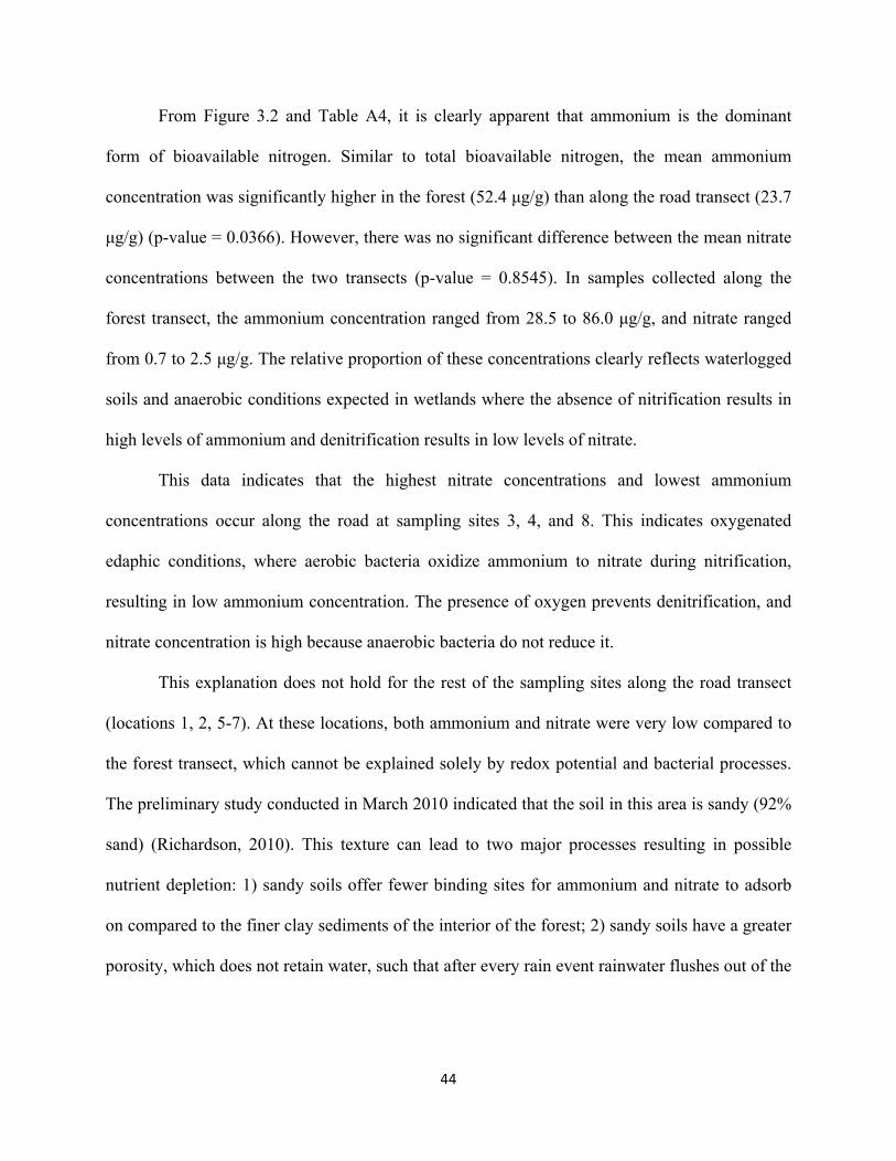
The quantity of nitrogen available to plants is significantly higher in the interior of the

forest than along the road (p-value = 0.0259) (Figure 3.2). The concentrations of ammonium,

nitrate, and total bioavailable nitrogen at each sampling site are presented in Table A4

(Appendix).

Figure 3.2: Map of bioavailable nitrogen concentration in transect soil samples

   

44    

From Figure 3.2 and Table A4, it is clearly apparent that ammonium is the dominant

form of bioavailable nitrogen. Similar to total bioavailable nitrogen, the mean ammonium

concentration was significantly higher in the forest (52.4 µg/g) than along the road transect (23.7

µg/g) (p-value = 0.0366). However, there was no significant difference between the mean nitrate

concentrations between the two transects (p-value = 0.8545). In samples collected along the

forest transect, the ammonium concentration ranged from 28.5 to 86.0 µg/g, and nitrate ranged

from 0.7 to 2.5 µg/g. The relative proportion of these concentrations clearly reflects waterlogged

soils and anaerobic conditions expected in wetlands where the absence of nitrification results in

high levels of ammonium and denitrification results in low levels of nitrate.

This data indicates that the highest nitrate concentrations and lowest ammonium

concentrations occur along the road at sampling sites 3, 4, and 8. This indicates oxygenated

edaphic conditions, where aerobic bacteria oxidize ammonium to nitrate during nitrification,

resulting in low ammonium concentration. The presence of oxygen prevents denitrification, and

nitrate concentration is high because anaerobic bacteria do not reduce it.

This explanation does not hold for the rest of the sampling sites along the road transect

(locations 1, 2, 5-7). At these locations, both ammonium and nitrate were very low compared to

the forest transect, which cannot be explained solely by redox potential and bacterial processes.

The preliminary study conducted in March 2010 indicated that the soil in this area is sandy (92%

sand) (Richardson, 2010). This texture can lead to two major processes resulting in possible

nutrient depletion: 1) sandy soils offer fewer binding sites for ammonium and nitrate to adsorb

on compared to the finer clay sediments of the interior of the forest; 2) sandy soils have a greater

porosity, which does not retain water, such that after every rain event rainwater flushes out of the

   

45    

system and transports away any soluble nutrients. Finally, given the lesser vegetation density in

this area, there is less litter production, which contributes to the replenishment of soil nutrients.

While the ammonium concentrations along the road transect are significantly smaller

than the concentrations inside the forest, their range (4.0 to 45.1 µg/g) is similar to data reported

in other studies, while ammonium levels in the forest are more than double the values found in

most studies reviewed. For comparison, Table A6 displays ammonium and nitrate concentrations

found in mangrove forests throughout the world. In 9 of the 10 forests reviewed, ammonium

concentrations ranged between 2.0 and 31.1 µg/g, which corresponds to the levels found along

the road transect. The only study indicating ammonium concentrations comparable to levels

found along the forest transect investigated mangroves in the Shenzhen Nature Reserve in China,

where the ammonium level reached 68.4 µg/g. The nitrate levels found in the literature ranged

between 0.05 and 2.1 µg/g, which compare to all of our data except the three aerobic sites

mentioned above (sites 3, 4, and 8).

Inorganic Phosphorus

The phosphate concentrations displayed on Figure 3.3 and in Table A4 indicate that the

quantity of bioavailable phosphorus is similar along the road and forest transects, ranging from

0.4 to1.1 µg/g and from 0.4 to 1.4 µg/g respectively. A t-test revealed no significant difference in

the mean concentration between the two transects (p-value = 0.5438).

   

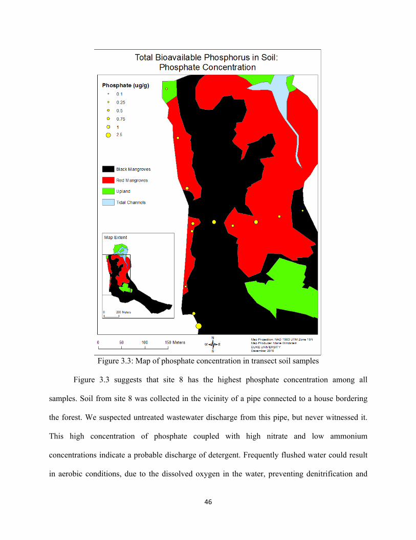
46    

Figure 3.3: Map of phosphate concentration in transect soil samples

Figure 3.3 suggests that site 8 has the highest phosphate concentration among all

samples. Soil from site 8 was collected in the vicinity of a pipe connected to a house bordering

the forest. We suspected untreated wastewater discharge from this pipe, but never witnessed it.

This high concentration of phosphate coupled with high nitrate and low ammonium

concentrations indicate a probable discharge of detergent. Frequently flushed water could result

in aerobic conditions, due to the dissolved oxygen in the water, preventing denitrification and

   

47    

allowing an accumulation of nitrate. Also, soaps tend to be slightly basic, which could reduce the

quantity of ammonium in the soil by transforming it to ammonia. Finally, detergents typically

contain phosphates, which could explain the particularly high concentration of phosphate at this

location.

The phosphate levels found in the Flamingo Mangroves are one to two orders of

magnitude lower than sites included in the literature review presented in Table A6. Depending

on study sites and species, phosphate concentrations ranged between 4.7 and 83.4 µg/g, while it

never exceeded 2.4 µg/g in Flamingo.

Total  Carbon,  Nitrogen,  and  Phosphorus  Along  the  Two  Transects  and  in  the  Tidal  Channels  

Figure 3.4 shows the fraction of total carbon in the soil along the two transects and along

the tidal channels. As expected, the highest percentage of total carbon occurs in the center of the

forest, where biomass and litter production is highest. While the difference between the mean of

total carbon percentage along the road and in the forest is not statistically significant (p-value =

0.4095), there is still a noticeable trend of increasing carbon fraction towards the center of the

forest. The carbon percentages in the soil along the road and in the channel banks, with means of

2.1%, 1.4% and 1.1% for the road transect, the south channel and the north channel respectively,

are typical of low litter production or frequently flushed soils, and correspond to the lowest

carbon percentage values found in the literature, which ranged between 1.1% and 43% (Table

A6).

   

48    

Figure 3.4: Total carbon in soil samples along the two transects and in the tidal channels

Figure 3.5 shows the fraction of total nitrogen in the soil along the two transects and the

tidal channels. Similar to total carbon, the highest concentration of total nitrogen occurs in the

center of the forest (0.4%), but in contrast to the carbon percentage, there was a significant

difference between the mean of total nitrogen along the road transect and in the forest (p-value =

0.0044).

Total nitrogen never exceeded 0.11% in the soil along the channel banks. Overall, the

total nitrogen concentration in the samples collected in Flamingo is generally lower or equivalent

   

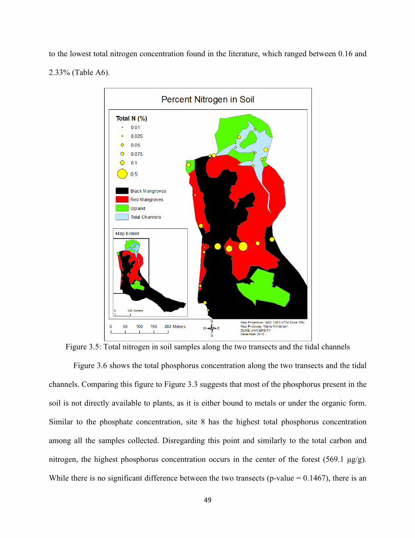
49    

to the lowest total nitrogen concentration found in the literature, which ranged between 0.16 and

2.33% (Table A6).

Figure 3.5: Total nitrogen in soil samples along the two transects and the tidal channels

Figure 3.6 shows the total phosphorus concentration along the two transects and the tidal

channels. Comparing this figure to Figure 3.3 suggests that most of the phosphorus present in the

soil is not directly available to plants, as it is either bound to metals or under the organic form.

Similar to the phosphate concentration, site 8 has the highest total phosphorus concentration

among all the samples collected. Disregarding this point and similarly to the total carbon and

nitrogen, the highest phosphorus concentration occurs in the center of the forest (569.1 µg/g).

While there is no significant difference between the two transects (p-value = 0.1467), there is an

   

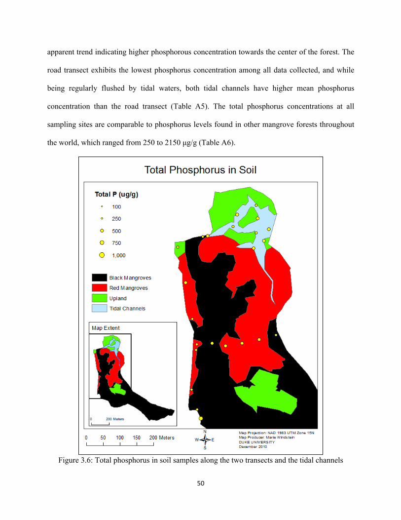
50    

apparent trend indicating higher phosphorous concentration towards the center of the forest. The

road transect exhibits the lowest phosphorus concentration among all data collected, and while

being regularly flushed by tidal waters, both tidal channels have higher mean phosphorus

concentration than the road transect (Table A5). The total phosphorus concentrations at all

sampling sites are comparable to phosphorus levels found in other mangrove forests throughout

the world, which ranged from 250 to 2150 µg/g (Table A6).

Figure 3.6: Total phosphorus in soil samples along the two transects and the tidal channels

   

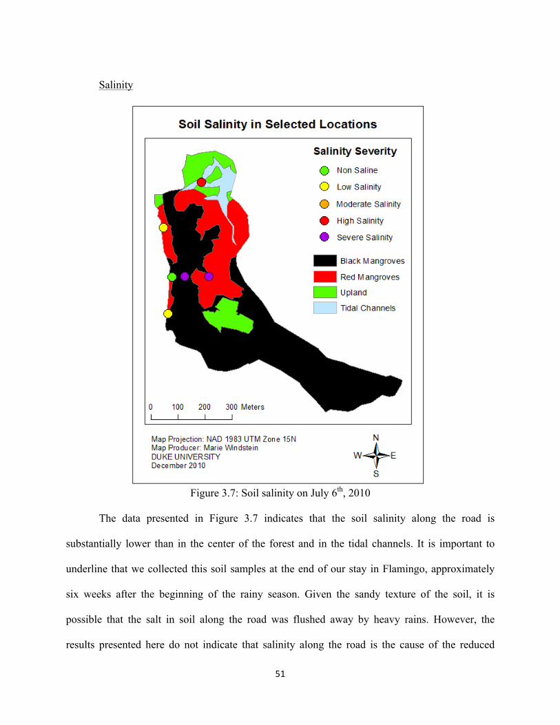
51    

Salinity

Figure 3.7: Soil salinity on July 6th, 2010

The data presented in Figure 3.7 indicates that the soil salinity along the road is

substantially lower than in the center of the forest and in the tidal channels. It is important to

underline that we collected this soil samples at the end of our stay in Flamingo, approximately

six weeks after the beginning of the rainy season. Given the sandy texture of the soil, it is

possible that the salt in soil along the road was flushed away by heavy rains. However, the

results presented here do not indicate that salinity along the road is the cause of the reduced

   

52    

health of the vegetation. Indeed, while being well adapted to severe salinity levels such as those

found in the center of the forest, it is important to reiterate that mangroves are facultative

halophytes. They are generally restricted to areas of high salinity because of competition with

other species in areas of lower soil salinity, but low salinity levels should not result in mangrove

dieback or reduced vigor (Hogarth, 1999).

Overall  Picture  

The data presented in this chapter indicates that the soil along the road is less rich in

bioavailable nitrogen than the soil in the center of the forest. This situation likely results in

nutrient limitation and hinders the development of the mangroves. In addition, the presence of

nitrate as the dominant form of bioavailable nitrogen at certain locations along the road indicates

aerobic conditions, which are unfit for wetland species. Both nutrient limitation and water

restriction are likely to be the cause of the reduced vigor in this part of the forest. Data collected

in the tidal channels did not indicate nutrient build up in the soil as a result of wastewater

discharge. The concentration of TC, TN, and TP were low, as expected in frequently flushed

tidal channels.

   

   

53    

Chapter  IV:  Birds  

Objectives  

The principal objectives of the bird survey were to compile a species list of birds living in

and around the Flamingo Mangrove, map their distribution, and estimate their abundance. Since

this survey is the first assessment of the Flamingo Mangrove bird diversity, it should be used as a

baseline for any future assessment of the avian community. The other objective of this list was to

create an attractive and didactic bird identification pamphlet for the community and the guests of

FBRS, narrowing nearly 900 species present in Costa Rica to less than 50 present in Flamingo

year-round. FBRS could incorporate this information into the educational boardwalk, identifying

where common or notable birds may be seen.

Background  

Costa Rica is regarded as a birding “hotspot” because it supports a high number of

species for its area due to its heterogeneous neotropical landscape (Garrigues and Dean, 2007).

At 51,100 km2, Costa Rica is smaller than the state of West Virginia but is home to an estimated

893 bird species, more than the United States and Canada combined. As a coastal region that

contains mangrove forests, evergreen forests, near offshore islands, hillsides, and open

grasslands, the greater Flamingo area contains diverse ecosystems that potentially support high

avifaunal alpha and beta diversity. Alpha diversity measures the richness and abundance of

species within a defined habitat, which corresponds to the number of species present and how

evenly they are distributed (Whittaker, 1972). Beta diversity compares alpha diversity between

ecosystems or along environmental gradients and depicts the rate of change in species

composition across habitats or communities (Whittaker, 1972).

   

54    

Mangroves and their surrounding area are home to a diverse avifaunal community that

includes wading and water birds such as herons, egrets, bitterns, and kingfishers; passerine birds

such as vireos, warblers, and hummingbirds; birds of prey such as hawks, falcons, and vultures;

and other species such as nightjars. Mangrove forests provide high quality habitat for birds due

to their relatively safe roosting sites and abundant prey (Nisbet, 1968); (Sodh et al., 1997).

Additionally, mangroves’ vast intertidal zones expose invertebrate-filled mudflats to wading

birds during low tide, and offers fish-filled waters to fishing birds during high tide (Cawkwell,

1964). The presence and abundance of several of these species, particularly wading birds, is a

biotic indicator of ecosystem health, as these species are sensitive to environmental contaminants

and are highly visible (Hilty and Merenlender, 2000); (Spalding and Frederick, 1995). Therefore,

an assessment of the avifaunal population may serve as an indirect indicator of the overall

mangrove health.

It is important to note that Costa Rica is a destination for many migrating bird species.

Because we performed this survey from May to July, corresponding to the northern summer, it is

probable that many migrant bird species are absent from this inventory. However, we are

confident that we observed and correctly identified almost all if not all resident bird species. It is

important to underline that we did not undertake a full bird population assessment due to time

constraints. An in-depth assessment would yield more complete results, including true Alpha and

Beta diversity indices like Shannon and Simpson.

Methods  

We recorded most of the bird species through opportunistic encounters while mapping

and collecting vegetation data. When we identified a bird species by sight or call, we noted the

species, location, number of individuals, and behavior whenever possible. In addition, we

   

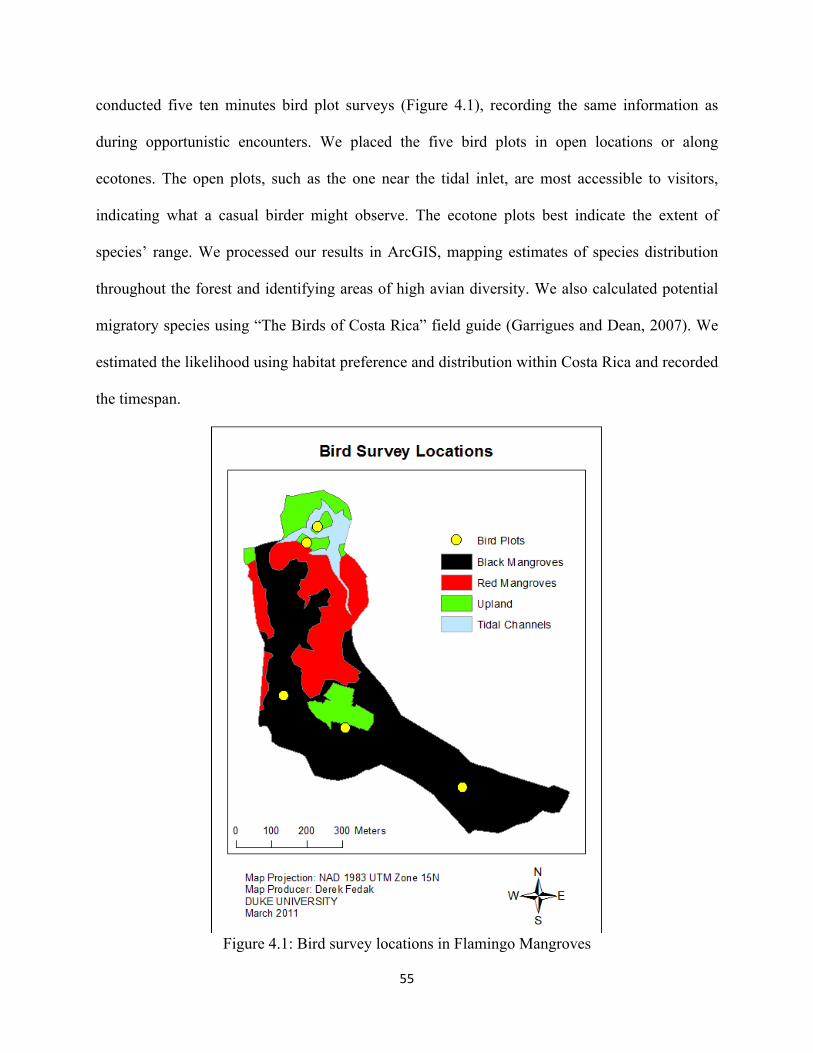
55    

conducted five ten minutes bird plot surveys (Figure 4.1), recording the same information as

during opportunistic encounters. We placed the five bird plots in open locations or along

ecotones. The open plots, such as the one near the tidal inlet, are most accessible to visitors,

indicating what a casual birder might observe. The ecotone plots best indicate the extent of

species’ range. We processed our results in ArcGIS, mapping estimates of species distribution

throughout the forest and identifying areas of high avian diversity. We also calculated potential

migratory species using “The Birds of Costa Rica” field guide (Garrigues and Dean, 2007). We

estimated the likelihood using habitat preference and distribution within Costa Rica and recorded

the timespan.

Figure 4.1: Bird survey locations in Flamingo Mangroves

   

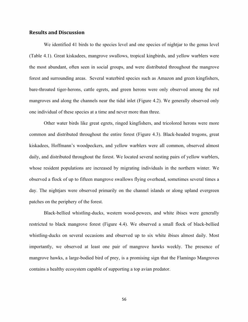
56    

Results  and  Discussion  

We identified 41 birds to the species level and one species of nightjar to the genus level

(Table 4.1). Great kiskadees, mangrove swallows, tropical kingbirds, and yellow warblers were

the most abundant, often seen in social groups, and were distributed throughout the mangrove

forest and surrounding areas. Several waterbird species such as Amazon and green kingfishers,

bare-throated tiger-herons, cattle egrets, and green herons were only observed among the red

mangroves and along the channels near the tidal inlet (Figure 4.2). We generally observed only

one individual of these species at a time and never more than three.

Other water birds like great egrets, ringed kingfishers, and tricolored herons were more

common and distributed throughout the entire forest (Figure 4.3). Black-headed trogons, great

kiskadees, Hoffmann’s woodpeckers, and yellow warblers were all common, observed almost

daily, and distributed throughout the forest. We located several nesting pairs of yellow warblers,

whose resident populations are increased by migrating individuals in the northern winter. We

observed a flock of up to fifteen mangrove swallows flying overhead, sometimes several times a

day. The nightjars were observed primarily on the channel islands or along upland evergreen

patches on the periphery of the forest.

Black-bellied whistling-ducks, western wood-pewees, and white ibises were generally

restricted to black mangrove forest (Figure 4.4). We observed a small flock of black-bellied

whistling-ducks on several occasions and observed up to six white ibises almost daily. Most

importantly, we observed at least one pair of mangrove hawks weekly. The presence of

mangrove hawks, a large-bodied bird of prey, is a promising sign that the Flamingo Mangroves

contains a healthy ecosystem capable of supporting a top avian predator.

   

57    

Eleven of the forty-one species were generally seen on the periphery or upland patches of

the forest. Great-tailed grackles, ruddy pigeons, and white-winged doves were generally

distributed near FBRS or along the beach road (Figure 4.5).

Banded wrens, mangrove vireos, rufous-naped wrens, streak-backed orioles, and

turquoise-browed motmots were all common and distributed on the channel islands, the upland

island in the center of the forest, and along the periphery (Figure 4.6). We observed several

streak-backed oriole nests throughout the periphery of the forest, particularly near the tidal inlet.

Melodious blackbirds, white-lored gnatcatchers, and yellow-green vireos shared a similar

distribution, but were much less common.

Lastly, species such as the black vulture, brown pelican, magnificent frigatebird, orange-

chinned parakeet, turkey vulture, and white-throated magpie-jay were generally observed flying

overhead or perched around the exterior of the mangroves, but not within the forest. We

observed great-tailed grackles, which tend to be associated with development and forest

fragmentation, roosting nightly outside the forest in numbers exceeding 500 in trees adjoining

FBRS. This is notable but not particularly unusual, as much of Flamingo is developed and great-

tailed grackles are well-adapted social birds with a large coastal range.

We identified 34 potential new migratory species and 5 potential supplemental migratory

species (Tables A8-9). We ranked the likelihood that the species would migrate to the Flamingo

Mangroves based off habitat and distribution within Costa Rica. We recorded the likelihood as:

not very, somewhat, and very. We also described a few species’ likelihood as “briefly,” as they

only stop in Costa Rica briefly while migrating further south. The five supplemental species

(tricolored heron, green heron, great egret, belted kingfisher, western wood-pewee, and yellow

warble) are resident species that are likely supplemented by migrating individuals.

   

58    

Overall  Picture  

The Flamingo Mangroves appear to support a healthy and diverse avian population. The

forest has sufficient resources to support at least 42 resident species across its different

vegetation communities. We estimate another 34 potential new and 5 supplemental species that

may migrate to the Flamingo Mangroves in the northern winter based off range maps and their

preferred habitats (Garrigues and Dean, 2007). Lastly, the presence of species like the great

egret, green heron, tricolored heron and mangrove hawk is a sign that the Flamingo Mangroves

are in a healthy state.

Figure 4.2 (left): Wading habitat avian distribution in Flamingo Mangroves;

Figure 4.3 (right): Total mangrove avian distribution in Flamingo Mangroves

   

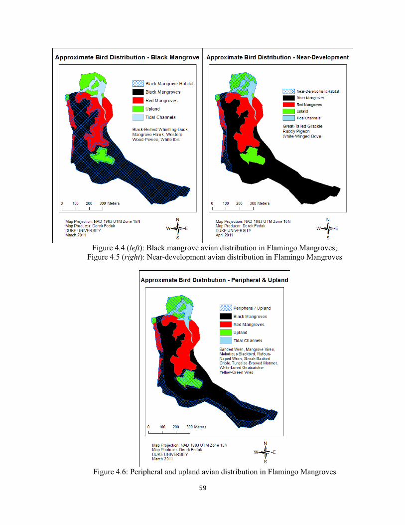
59    

Figure 4.4 (left): Black mangrove avian distribution in Flamingo Mangroves;

Figure 4.5 (right): Near-development avian distribution in Flamingo Mangroves

Figure 4.6: Peripheral and upland avian distribution in Flamingo Mangroves

   

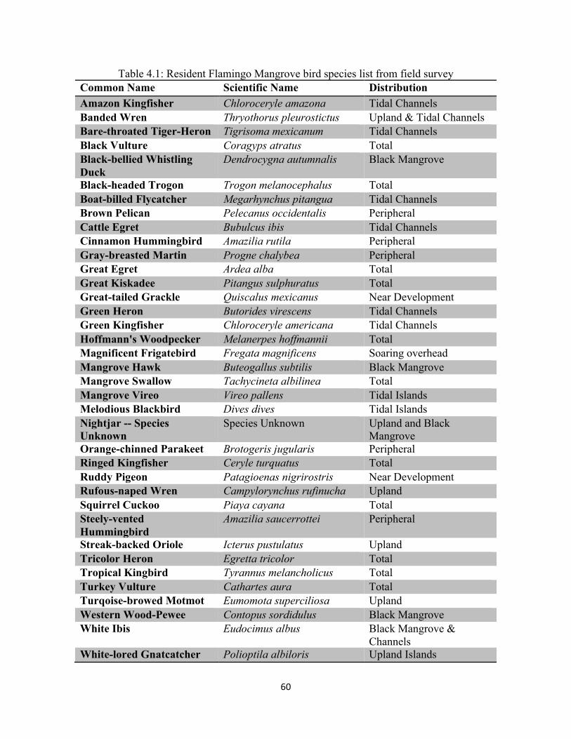
60    

Table 4.1: Resident Flamingo Mangrove bird species list from field survey Common Name Scientific Name Distribution Amazon Kingfisher Chloroceryle amazona Tidal Channels Banded Wren Thryothorus pleurostictus Upland & Tidal Channels Bare-throated Tiger-Heron Tigrisoma mexicanum Tidal Channels Black Vulture Coragyps atratus Total Black-bellied Whistling Duck

Dendrocygna autumnalis Black Mangrove

Black-headed Trogon Trogon melanocephalus Total Boat-billed Flycatcher Megarhynchus pitangua Tidal Channels Brown Pelican Pelecanus occidentalis Peripheral Cattle Egret Bubulcus ibis Tidal Channels Cinnamon Hummingbird Amazilia rutila Peripheral Gray-breasted Martin Progne chalybea Peripheral Great Egret Ardea alba Total Great Kiskadee Pitangus sulphuratus Total Great-tailed Grackle Quiscalus mexicanus Near Development Green Heron Butorides virescens Tidal Channels Green Kingfisher Chloroceryle americana Tidal Channels Hoffmann's Woodpecker Melanerpes hoffmannii Total Magnificent Frigatebird Fregata magnificens Soaring overhead Mangrove Hawk Buteogallus subtilis Black Mangrove Mangrove Swallow Tachycineta albilinea Total Mangrove Vireo Vireo pallens Tidal Islands Melodious Blackbird Dives dives Tidal Islands Nightjar -- Species Unknown

Species Unknown Upland and Black Mangrove

Orange-chinned Parakeet Brotogeris jugularis Peripheral Ringed Kingfisher Ceryle turquatus Total Ruddy Pigeon Patagioenas nigrirostris Near Development Rufous-naped Wren Campylorynchus rufinucha Upland Squirrel Cuckoo Piaya cayana Total Steely-vented Hummingbird

Amazilia saucerrottei Peripheral

Streak-backed Oriole Icterus pustulatus Upland Tricolor Heron Egretta tricolor Total Tropical Kingbird Tyrannus melancholicus Total Turkey Vulture Cathartes aura Total Turqoise-browed Motmot Eumomota superciliosa Upland Western Wood-Pewee Contopus sordidulus Black Mangrove White Ibis Eudocimus albus Black Mangrove &

Channels White-lored Gnatcatcher Polioptila albiloris Upland Islands

   

61    

White-throated Hummingbird

Leucochloris albicollis Peripheral

White-throated Magpie-Jay

Calocitta formosa Peripheral

White-winged Dove Zenaida asiatica Total Yellow Warbler Dendroica petechia Total Yellow-green Vireo Vireo flavoviridis Upland

   

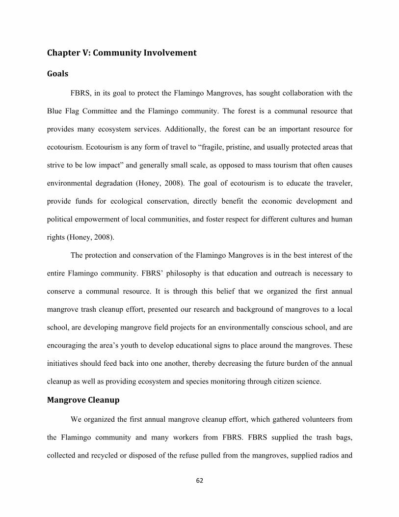
62    

Chapter  V:  Community  Involvement  

Goals    

FBRS, in its goal to protect the Flamingo Mangroves, has sought collaboration with the

Blue Flag Committee and the Flamingo community. The forest is a communal resource that

provides many ecosystem services. Additionally, the forest can be an important resource for

ecotourism. Ecotourism is any form of travel to “fragile, pristine, and usually protected areas that

strive to be low impact” and generally small scale, as opposed to mass tourism that often causes

environmental degradation (Honey, 2008). The goal of ecotourism is to educate the traveler,

provide funds for ecological conservation, directly benefit the economic development and

political empowerment of local communities, and foster respect for different cultures and human

rights (Honey, 2008).

The protection and conservation of the Flamingo Mangroves is in the best interest of the

entire Flamingo community. FBRS’ philosophy is that education and outreach is necessary to

conserve a communal resource. It is through this belief that we organized the first annual

mangrove trash cleanup effort, presented our research and background of mangroves to a local

school, are developing mangrove field projects for an environmentally conscious school, and are

encouraging the area’s youth to develop educational signs to place around the mangroves. These

initiatives should feed back into one another, thereby decreasing the future burden of the annual

cleanup as well as providing ecosystem and species monitoring through citizen science.

Mangrove  Cleanup  

We organized the first annual mangrove cleanup effort, which gathered volunteers from

the Flamingo community and many workers from FBRS. FBRS supplied the trash bags,

collected and recycled or disposed of the refuse pulled from the mangroves, supplied radios and

   

63    

a truck for logistics, and provided lunch for everyone involved. Over the course of the day, we

extracted nearly 60 bags of refuse, most of which was littered along the beach road, the

northeastern edge, and one hill along the southern edge of the forest. Aside from general refuse,

we removed a tire, concrete cinder blocks, several large panes of sheet metal, a microwave, a

printer, and a mattress pad and box spring.

While we removed a significant quantity of refuse, we were not able to remove it all,

which will likely take a few more cleanups. This will also be expedited through education and

community outreach, which will discourage locals and tourists alike from polluting the forest.

Because litter had accumulated mostly in the three aforementioned locations, future cleanup

efforts should focus their efforts there. However, future cleanup should expand areas of focus, as

we encountered trash in even the most remote areas of the forest.

Presentation  to  La  Paz  School  

In hopes of inspiring the area’s youth to protect the mangrove ecosystem, we gave a

presentation on our field research to La Paz School, located next to the mangrove forest. We

gave an overview of mangroves, stressing their important ecosystem services, and discussed how

the Flamingo Mangroves are unique, showing pictures from our field work. We engaged the

children with activities that quizzed them on local fauna and illustrated the connectivity and

potential fragility of food webs through educational games.

We are currently working with their science teachers to develop field projects inside the

mangroves to further their education and provide data by monitoring the mangroves, converting

the classes into citizen scientists and conservationists. These projects will investigate invertebrate

communities within the tidal zone and identify and monitor bird species, especially migratory

species that were not present during our field work.

   

64    

Youth  Involvement  in  Conservation  of  Flamingo  Mangroves  

Lastly, we are working with La Paz School and the neighboring Brasilito School to

develop and construct wooden signs for placement around the mangrove. The signs will identify

and describe common and interesting flora or fauna as well as dissuade locals and tourists from

littering in the forest. This initiative will get the area’s youth involved in conserving the forest

through education and activism and will hopefully dissuade most if not all from littering in the

forest, thus reducing the burden of the annual mangrove cleanup. These sign will also be

incorporated into the proposed boardwalk, adding further ecotourism value.

   

   

65    

Chapter  VI:  Recommendations  and  Conclusions  

Our research findings regarding the health and ecological status of the Flamingo

Mangroves provided us with information that could be used to develop management

recommendations that should be considered if the community wants to sustain this ecosystem for

future generation. Our general recommendations are as follows.

Water  Quality  

Most issues within the Flamingo Mangroves pertain to water quality. Pollution through

wastewater discharge and runoff adversely affects water quality within the forest. These issues,

however, are amenable through the promotion of phosphate-free detergents and community

cooperation. Continued monitoring is required, as we did not determine the full composition and

origin of runoff water entering the forest from the northwest corner south of the FBRS.

As we located several pipes entering the forest but only witnessed a few discharging

water, an inventory of the origin and water composition of these pipes should be made. We have

plotted point sources of runoff in Figure 2.1, which should be monitored. We observed one point

discharging greywater, likely from a dishwasher or laundry washing machine. We recommend

the promotion and use of phosphate-free detergents throughout the Flamingo community. This

could be achieved through public outreach, education, or even a mandate requiring the use of

such detergents in Flamingo. We also recommend the promotion of voluntary community

reporting on the content and location of their wastewater and point source discharge, as this will

greatly alleviate any remediation process, further protecting the mangrove from pollution.

We recommend encouraging or mandating the construction of onsite wastewater

treatment systems for any new development, especially those adjacent to the forest. The FBRS

has taken great initiative in the development of plans to improve their wastewater treatment

   

66    

plant. We advise existing residences and businesses to follow their lead, if it is affordable.

However, any new development adjacent to the forest may cause disturbance to the surrounding

vegetation and water quality, so we strongly urge the Flamingo community to mandate the

inclusion of onsite wastewater treatment systems. We also urge that any construction adjacent to

the forest avoid septic systems, which might overflow during heavy rain events.

Lastly, we recommend that the Flamingo community, the FBRS, or the Blue Flag

Committee continue to monitor the composition of runoff water at sampling site 1 in the

northwest corner of the forest (Figure 2.2). Weekly monitoring and inventorying the sources of

water flowing into this location will determine the severity and origin of the pollution. If the

water quality continues to be poor, testing sources independently uphill or along the drains will

help determine the origin of these problems and allow Flamingo to take appropriate action.

Boardwalk  

An educational boardwalk through the forest would allow visitors to enter and observe

the mangrove ecosystem with little disturbance to the surrounding vegetation. We believe the

presence of an educational boardwalk would increase interest in the forest and instill an

increasing desire to protect the mangroves. Before construction begins, the community should

first have an opportunity to voice their opinion or demonstrate a desire for the construction of a

boardwalk. While this would be an expensive project and requires permits from the Ministry of

Environment and Energy (MINAE), it could be constructed with minimal disturbance and

destruction to the vegetation of the forest. We have identified potential routes and three possible

entry points that would minimize disturbances, restrict the boardwalk to a small section of the

forest, and allow visitors to see most of the integral characteristics of mangrove forests (Figure

6.1).

   

67    

We recommend three possible entry points for the boardwalk: 1) the FBRS parking lot, 2)

a beach access point just south of the FBRS, and 3) the bus stop near the tidal inlet. These

locations would maximize ease of access for visitors, as many tourists and locals live in this area,

visit the nearby commercial center and FBRS, or utilize the adjacent beach. The route would

overlook many key viewing spots in the forest such as the tidal channel, the tidal channel islands,

and both black and red mangrove communities. This route allows visitors to observe much of the

vegetation and avifaunal diversity in the forest, as it is more concentrated in this area. The

addition of educational signs would further increase its ecotourism value. This route also allows

visitors to watch the ebbing and flooding of the tides in the forest.

We recommend that the boardwalk be restricted to the northern section of the forest and

favor a path in areas of lower-density vegetation. This would minimize disturbances to the

vegetation community and limit any adverse impacts from construction and human presence to a

small area of the forest. Once the general route is selected, additional in-depth vegetation surveys

should be conducted to determine its exact placement. We recommend placing the boardwalk

along the channels or channel banks, where possible, as this will least disturb vegetation and will

not affect water quality through shading, as water floods and recedes from the forest with the

tides.

   

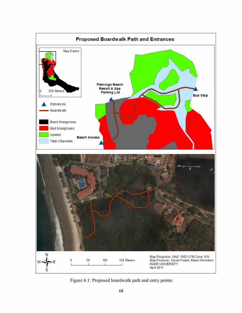
68    

Figure 6.1: Proposed boardwalk path and entry points

   

69    

Beach  Road  

The beach road borders approximately 15% of the forest at 500 m long and contains the

sparsest and most stunted vegetation. The following steps could be taken to minimize physical

and chemical disturbances to the vegetation along the road: at a minimum prohibiting parking on

the mangrove side of the road, or possibly closing the road to motorized vehicles, and developing

a vegetation buffer.

Parking along the mangrove side of the road results in soil compaction, erosion, and sand

and pollutant intrusion in the forest. A first step to prevent these processes from happening

should be to prohibit parking along the mangrove side of the road, while leaving the beach side

available for parking.

Motorized traffic and frequent maintenance of the road through the addition of gravel

enhance these destructive processes, further impacting the soil in this part of the forest. Closing

the road to motorized traffic would be a supplementary step to prevent these disturbances.

Alternative roads already exist around the mangrove, so this closure would not restrict traffic or

deny access to any areas. It is important to ensure and maintain public access to the beach and

provide alternative parking locations to visitors. We have identified two possible alternatives: 1)

widening the beach road on its northern extremity where it is already paved (northwest of the

FBRS) and converting it to a parking area; and 2) allowing public parking at the FBRS, which is

currently reserved for patrons and employees, especially on weekends when many locals visit the

beach.

If the beach road remains open to motorized traffic, we strongly recommend against any

plans to cover the road with impervious pavements. An impervious surface would enhance

   

70    

chemical pollution from runoff into both the forest and the beach. Instead, we encourage the use

of permeable pavements, like pervious concrete or open-jointed blocks for example.

Alternatively, if the beach road is closed to motorized vehicles, it could be converted into

a vegetation buffer. It is crucial to ensure public access to the beach, and thus a walkway should

be incorporated into this project. However, this may be a costly and challenging option for

several reasons. First, the soil is extremely compacted and would require mechanical tillage for

vegetation to germinate. Second, the soil nutrient content underneath the road is probably low,

given its sandy texture. Lastly, sandy soils have low water retention, which could be costly for

vegetation maintenance. Nevertheless, we identified seven plant species that could possibly

survive in this location:

- Coconut tree (Cocos nucifera)

- Buttonwood mangrove (Conocarpus erectus)

- Carao (Cassia grandis)

- Gua (Enterolobium cyclocarpum)

- Manzanillo de playa (Hippomane manicella)

- Hibiscus tree (Hibiscus tiliaceus)

- Cactus (Acanthocereus tetragonus)

Several of these species already occur throughout Flamingo.

In summation, we strongly recommend that the beach road should not be paved with

impervious material. We recommend that the road be closed to parking, which would require

alternative parking locations. While closing the road to automotive traffic is ideal, it may not be

feasible. Alternative routes exist, but closing the road would require support from the

community. If automotive traffic is prohibited, it will be possible to assess the feasibility of

   

71    

converting the beach road into a vegetative walkway, acting as a buffer for the forest. The

walkway, however, will likely be an expensive alternative and we cannot guarantee the

recommended plant species will persist without first aerating and adding nutrients to the soil.

Community  Involvement  

  Inherent in ecotourism is the inclusion and involvement of the local community.

Therefore, the Flamingo community should have the opportunity to remain involved in any

future plans regarding the preservation of the mangroves. There are several current and future

opportunities that could achieve this goal. We believe the FBRS and surrounding schools such as

La Paz and Brasilito School should continue to foster their collaboration, as the schools and other

community volunteers could monitor the forest, acting as citizen scientists.

We recommend that the FBRS take steps to raise public awareness on issues regarding

the mangroves. This report should be made available to the public and be shared with the Blue

Flag Committee. The FBRS should disseminate information regarding the ecological value of

and issues concerning the mangroves. Public seminars, educational pamphlets, or the use of signs

could achieve this. Foremost, the FBRS and the entire community should address the issue of

littering in the forest.

We recommend that the trash cleanup we initiated be continued. This could be an annual

effort involving members from the FBRS and local community. The cleanup should focus its

efforts on the three most impacted areas: along the beach road, a hill along the southern edge of

the forest, and the southeastern section of the forest near the FBRS and bus stop. These are the

areas on which we focused our first effort, but a lot still needs to be removed We recommend

that the FBRS, the Blue Flag Committee, and the Flamingo Association cooperate to provide

supplies and logistics, such as trash bags, a truck for transportation, and radios for

   

72    

communication. Lastly, we recommend signs be developed and placed around the periphery of

the forest discouraging anyone from littering in the forest.

We recommend that the FBRS strengthen its collaboration with the local community. We

are currently developing field projects for La Paz School that will include species monitoring and

basic water quality analysis. These results could be reported to the FBRS and Blue Flag

Committee for assessment and compilation into a long-term dataset. We recommend monitoring

several indicator species like the five observed species of herons inside the forest, as they may

indicate water quality and viable fish and invertebrate populations. The persistence of these

indicator species may reflect suitable habitat conditions, while their subsequent absence may

indicate a decline in ecosystem functioning.

Lastly, we advise the FBRS hire a tour guide familiar with the ecology of mangroves. A

tour guide could lead visitors and locals into the forest and train FBRS staff about the ecology

and issues of the Flamingo Mangroves. This could further their interest in and desire for

conserving the forest. Someone from the local community may be the best option for a tour

guide, as this could empower the community. We also recommend that educational signs about

mangrove and bird ecology be developed and placed along the periphery of the forest and the

boardwalk, if constructed. The students at La Paz and Brasilito School could develop these signs

with material provided by the FBRS, the Blue Flag Committee, or the Flamingo Association.

Ramsar  Listing  

The Ramsar Convention is an international treaty for the conservation and sustainable

utilization of wetlands, particularly regarding waterfowl habitat (Ramsar Treaty, 1971).

Committing countries pledge to maintain the ecological character of their “Wetlands of

International Importance and plan for the ‘wise use’ of all the wetlands in their territories.” Wise

   

73    

use is defined as the “maintenance of wetlands ecological character achieved through the

implementation of ecosystem approaches, within the context of sustainable development”

(Ramsar Treaty, 1971). There are currently 160 contracting countries, including Costa Rica, that

list 1,929 designated Ramsar sites. This yields a total surface area of almost 200 million hectares

of designated Ramsar sites. Costa Rica contains 12 Ramsar sites covering 569,742 ha. The

mangroves in Tamarindo, the closest mangroves to Flamingo, was designated a Ramsar site on

June 9th, 1993.

We believe that the Flamingo Mangroves could be listed as a Ramsar site. The Flamingo

Mangroves contain important ecological characteristics and diversity that make it a wetland of

international importance. The presence of tea mangroves (Peliciera rhizophorae) outside their

historic range may make them the farthest north-growing individuals. The high concentration of

bird species, particularly waterfowl, is another important Ramsar characteristic. We identified

ten resident and nineteen potential migratory waterfowl species, yielding a high density of

waterfowl species utilizing the tidal channel and surrounding mangrove.

The Flamingo Mangroves are considered internationally important based off four Ramsar

Criteria:

1. Contains a representative, rare, or unique example of a natural or near-natural

wetland type found within the appropriate biogeographic region − The Flamingo

Mangrove Forest is a healthy ecosystem

2. Supports vulnerable, endangered, or critically endangered species or threatened

ecological communities − The Flamingo Mangroves support tea mangroves, listed

as “vulnerable.” An assessment of the status of bird species present is necessary.

   

74    

3. Supports populations of plant and/or animals species important for maintaining

the biological diversity of a particular biogeographic region − The Flamingo

Mangroves support birds and vegetation found only in mangrove ecosystems.

4. Supports plant and/or animal species at a critical stage in their life cycles, or

provides refuge during adverse conditions − The Flamingo Mangroves offer

refuge for many migratory and nesting species (Ramsar Treat, 1971).

While the issue of water quality from wastewater and runoff requires mitigation, we

discovered that the mangrove is generally healthy. The issue of water quality is amenable with

community cooperation and regulatory enforcement. While the forest is a relatively small

wetland compared to the largest Ramsar wetland of 6,569,624 ha, the Flamingo Mangroves 33

ha are much larger than several Ramsar wetlands with an area below five ha. There are three

Ramsar wetlands smaller than 0.35 ha (Ramsar, 2010).

More research must be conducted to apply for a Ramsar listing. The Flamingo

community or FBRS must first fill out an Information Sheet on Ramsar Wetlands (RIS), which

may be found at http://ramsar.org/ris/key_ris_index.htm. The Information Sheet contains 34

sections with simple questions such as elevation and area to more complex questions about social

and cultural values. Nearly all the required data can be found throughout this report, though a

few sections will require further research. A Ramsar listing would provide the Flamingo

Mangroves the opportunity for additional partnerships in the international community and make

it eligible for grant funding to support conservation. We recommend that the Flamingo

community, the Blue Flag Committee, and the FBRS apply for Ramsar listing of the Flamingo

Mangroves. If listed as a Ramsar site it will likely increase ecotourism and more importantly

   

75    

help Costa Rica and the Flamingo community preserve this fabulous mangrove for future

generations to enjoy

   

76    

Appendix  

Table A1: Individual plot’s basal area and biomass

Community   Latitude   Longitude  Avg.  

Canopy  H  (m)  

Tallest  Tree  /  Plot  (m)  

Plot  Basal  Area    

(m2/100  m2)  

Plot  Biomass    A.  germinans    (kg/100  m2)  

Plot  Biomass  R.    genus    

(kg/100  m2)  

Plot  Biomass  L.  racemosa  (kg/100  m2)  

Plot  Total  (kg/100  m2)  

Black   10.4362   -­‐85.7916   8.02   8.35   0.11   434.9   0.0   0.0   434.9  Black   10.4364   -­‐85.7913   8.70   10.48   0.17   724.7   0.0   6.0   730.7  Black   10.4356   -­‐85.7914   8.62   10.48   0.09   426.2   0.0   0.0   426.2  Black   10.4370   -­‐85.7916   6.65   7.16   0.11   376.1   0.0   0.0   376.1  Black   10.4354   -­‐85.7918   8.98   9.19   0.22   938.5   0.0   0.0   938.5  Black     10.4333   -­‐85.7891   10.34   13.12   0.40   2043.5   0.0   0.0   2043.5  Black   10.4341   -­‐85.7916   11.43   13.23   0.20   1090.9   0.0   0.0   1090.9  Black   10.4329   -­‐85.7887   10.77   12.02   0.15   804.5   0.0   0.0   804.5  Black   10.4317   -­‐85.7871   14.04   16.52   0.41   2525.8   0.0   0.0   2525.8  Black   10.4327   -­‐85.7884   11.37   12.91   0.24   1310.3   0.0   0.0   1310.3  Black   10.4330   -­‐85.7914   8.90   9.71   0.19   859.3   0.0   0.0   859.3  Black   10.4322   -­‐85.7902   9.74   10.10   0.19   880.3   0.0   0.0   880.3  Black   10.4329   -­‐85.7896   10.83   11.56   0.30   1514.4   0.0   0.0   1514.4  Black   10.4333   -­‐85.7900   11.46   12.47   0.30   1516.2   0.0   0.0   1516.2  Black   10.4321   -­‐85.7880   12.28   13.65   0.21   1192.5   0.0   0.0   1192.5  Black   10.4311   -­‐85.7868   12.90   13.55   0.23   1354.6   0.0   0.0   1354.6  Black   10.4314   -­‐85.7858   11.53   15.37   0.15   1035.9   0.0   0.0   1035.9  Black   10.4334   -­‐85.7886   13.16   14.17   0.35   1369.3   0.0   749.5   2118.9  Black   10.4321   -­‐85.7872   9.40   12.58   0.17   936.4   0.0   0.0   936.4  Red   10.4362   -­‐85.7922   7.76   8.69   0.13   0.0   170.3   357.0   527.2  Red   10.4367   -­‐85.7922   10.08   9.97   0.33   74.1   1141.2   413.1   1628.4  Red   10.4376   -­‐85.7905   13.20   14.32   0.34   216.3   2247.6   0.0   2463.9  Red   10.4375   -­‐85.7916   10.17   17.65   0.25   320.1   542.9   422.3   1285.2  Red   10.4375   -­‐85.7898   12.00   14.32   0.37   601.8   1604.0   28.8   2234.6  Red   10.4343   -­‐85.7908   19.05   19.82   0.51   0.0   4932.2   0.0   4932.2  Red   10.4349   -­‐85.7908   16.36   19.06   0.16   0.0   1561.3   0.0   1561.3  Red   10.4358   -­‐85.7907   6.32   8.64   0.12   121.5   171.0   160.9   453.4  Red   10.4351   -­‐85.7920   9.63   11.44   0.15   569.1   107.5   42.1   718.7  Red   10.4367   -­‐85.7899   14.09   16.36   0.43   284.4   3026.6   0.0   3311.0  Total      

    6.97   23521.64   15504.57   2179.73   41205.94    

   

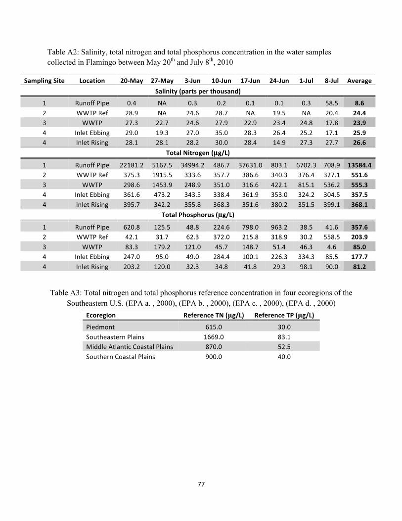
77    

Table A2: Salinity, total nitrogen and total phosphorus concentration in the water samples collected in Flamingo between May 20th and July 8th, 2010

Sampling  Site   Location   20-­‐May   27-­‐May   3-­‐Jun   10-­‐Jun   17-­‐Jun   24-­‐Jun   1-­‐Jul   8-­‐Jul   Average  Salinity  (parts  per  thousand)  

1   Runoff  Pipe   0.4   NA   0.3   0.2   0.1   0.1   0.3   58.5   8.6  2   WWTP  Ref   28.9   NA   24.6   28.7   NA   19.5   NA   20.4   24.4  3   WWTP   27.3   22.7   24.6   27.9   22.9   23.4   24.8   17.8   23.9  4   Inlet  Ebbing   29.0   19.3   27.0   35.0   28.3   26.4   25.2   17.1   25.9  4   Inlet  Rising   28.1   28.1   28.2   30.0   28.4   14.9   27.3   27.7   26.6  

Total  Nitrogen  (µg/L)  1   Runoff  Pipe   22181.2   5167.5   34994.2   486.7   37631.0   803.1   6702.3   708.9   13584.4  2   WWTP  Ref   375.3   1915.5   333.6   357.7   386.6   340.3   376.4   327.1   551.6  3   WWTP   298.6   1453.9   248.9   351.0   316.6   422.1   815.1   536.2   555.3  4   Inlet  Ebbing   361.6   473.2   343.5   338.4   361.9   353.0   324.2   304.5   357.5  4   Inlet  Rising   395.7   342.2   355.8   368.3   351.6   380.2   351.5   399.1   368.1  

Total  Phosphorus  (µg/L)  1   Runoff  Pipe   620.8   125.5   48.8   224.6   798.0   963.2   38.5   41.6   357.6  2   WWTP  Ref   42.1   31.7   62.3   372.0   215.8   318.9   30.2   558.5   203.9  3   WWTP   83.3   179.2   121.0   45.7   148.7   51.4   46.3   4.6   85.0  4   Inlet  Ebbing   247.0   95.0   49.0   284.4   100.1   226.3   334.3   85.5   177.7  4   Inlet  Rising   203.2   120.0   32.3   34.8   41.8   29.3   98.1   90.0   81.2  

Table A3: Total nitrogen and total phosphorus reference concentration in four ecoregions of the Southeastern U.S. (EPA a. , 2000), (EPA b. , 2000), (EPA c. , 2000), (EPA d. , 2000)

Ecoregion   Reference  TN  (µg/L)   Reference  TP  (µg/L)  Piedmont   615.0   30.0  Southeastern  Plains   1669.0   83.1  Middle  Atlantic  Coastal  Plains   870.0   52.5  Southern  Coastal  Plains   900.0   40.0  

   

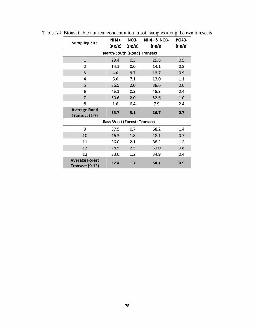
78    

Table A4: Bioavailable nutrient concentration in soil samples along the two transects

Sampling  Site  NH4+  (µg/g)  

NO3-­‐  (µg/g)  

NH4+  &  NO3-­‐  (µg/g)  

PO43-­‐  (µg/g)  

    North-­‐South  (Road)  Transect  1   29.4   0.3   29.8   0.5  2   14.1   0.0   14.1   0.8  3   4.0   9.7   13.7   0.9  4   6.0   7.1   13.0   1.1  5   36.5   2.0   38.6   0.6  6   45.1   0.3   45.3   0.4  7   30.6   2.0   32.6   1.0  8   1.6   6.4   7.9   2.4  

Average  Road  Transect  (1-­‐7)   23.7   3.1   26.7   0.7  

    East-­‐West  (Forest)  Transect  

9   67.5   0.7   68.2   1.4  10   46.3   1.8   48.1   0.7  11   86.0   2.1   88.2   1.2  12   28.5   2.5   31.0   0.8  13   33.6   1.2   34.9   0.4  

Average  Forest  Transect  (9-­‐13)   52.4   1.7   54.1   0.9  

   

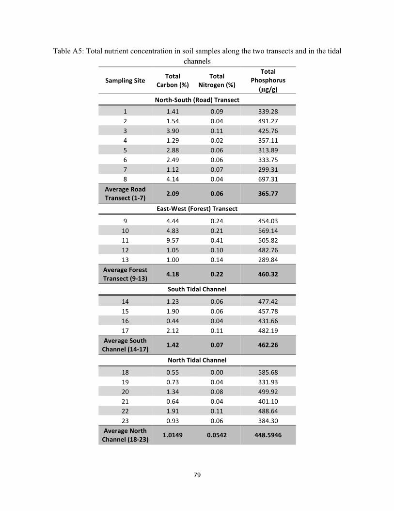
79    

Table A5: Total nutrient concentration in soil samples along the two transects and in the tidal channels

Sampling  Site   Total  Carbon  (%)  

Total  Nitrogen  (%)  

Total  Phosphorus  

(µg/g)  North-­‐South  (Road)  Transect  

1   1.41   0.09   339.28  2   1.54   0.04   491.27  3   3.90   0.11   425.76  4   1.29   0.02   357.11  5   2.88   0.06   313.89  6   2.49   0.06   333.75  7   1.12   0.07   299.31  8   4.14   0.04   697.31  

Average  Road  Transect  (1-­‐7)   2.09   0.06   365.77  

East-­‐West  (Forest)  Transect  

9   4.44   0.24   454.03  10   4.83   0.21   569.14  11   9.57   0.41   505.82  12   1.05   0.10   482.76  13   1.00   0.14   289.84  

Average  Forest  Transect  (9-­‐13)   4.18   0.22   460.32  

South  Tidal  Channel  

14   1.23   0.06   477.42  15   1.90   0.06   457.78  16   0.44   0.04   431.66  17   2.12   0.11   482.19  

Average  South  Channel  (14-­‐17)   1.42   0.07   462.26  

North  Tidal  Channel  

18   0.55   0.00   585.68  19   0.73   0.04   331.93  20   1.34   0.08   499.92  21   0.64   0.04   401.10  22   1.91   0.11   488.64  23   0.93   0.06   384.30  

Average  North  Channel  (18-­‐23)   1.0149   0.0542   448.5946  

   

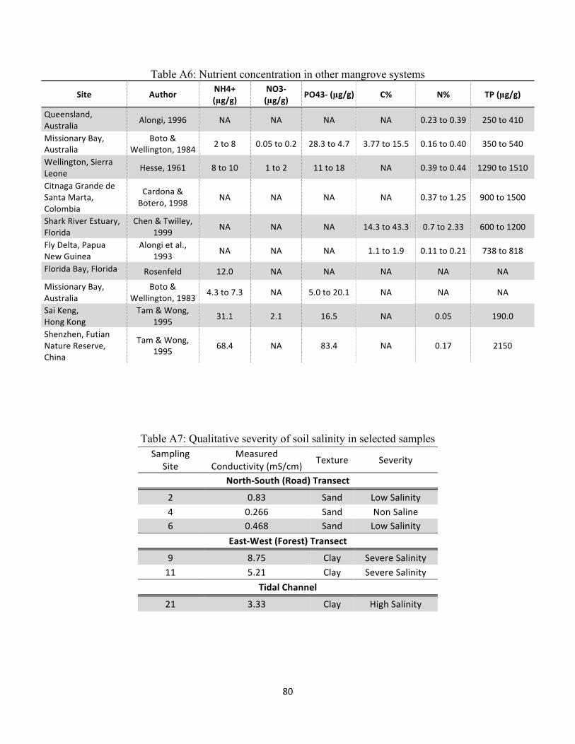
80    

Table A6: Nutrient concentration in other mangrove systems

Site   Author   NH4+  (µg/g)  

NO3-­‐  (µg/g)   PO43-­‐  (µg/g)   C%   N%   TP  (µg/g)  

Queensland,  Australia   Alongi,  1996   NA   NA   NA   NA   0.23  to  0.39   250  to  410  

Missionary  Bay,  Australia  

Boto  &  Wellington,  1984   2  to  8   0.05  to  0.2   28.3  to  4.7   3.77  to  15.5   0.16  to  0.40   350  to  540  

Wellington,  Sierra  Leone   Hesse,  1961   8  to  10   1  to  2   11  to  18   NA   0.39  to  0.44   1290  to  1510  

Citnaga  Grande  de  Santa  Marta,  Colombia  

Cardona  &  Botero,  1998   NA   NA   NA   NA   0.37  to  1.25   900  to  1500  

Shark  River  Estuary,  Florida  

Chen  &  Twilley,  1999   NA   NA   NA   14.3  to  43.3   0.7  to  2.33   600  to  1200  

Fly  Delta,  Papua  New  Guinea  

Alongi  et  al.,  1993   NA   NA   NA   1.1  to  1.9   0.11  to  0.21   738  to  818  

Florida  Bay,  Florida   Rosenfeld   12.0   NA   NA   NA   NA   NA  

Missionary  Bay,  Australia  

Boto  &  Wellington,  1983   4.3  to  7.3   NA   5.0  to  20.1   NA   NA   NA  

Sai  Keng,  Hong  Kong  

Tam  &  Wong,  1995   31.1   2.1   16.5   NA   0.05   190.0  

Shenzhen,  Futian  Nature  Reserve,  China  

Tam  &  Wong,  1995   68.4   NA   83.4   NA   0.17   2150  

Table A7: Qualitative severity of soil salinity in selected samples

Sampling  Site  

Measured  Conductivity  (mS/cm)   Texture   Severity  

North-­‐South  (Road)  Transect  

2   0.83   Sand   Low  Salinity  4   0.266   Sand   Non  Saline  6   0.468   Sand   Low  Salinity  

East-­‐West  (Forest)  Transect  

9   8.75   Clay   Severe  Salinity  11   5.21   Clay   Severe  Salinity  

Tidal  Channel  

21   3.33   Clay   High  Salinity  

   

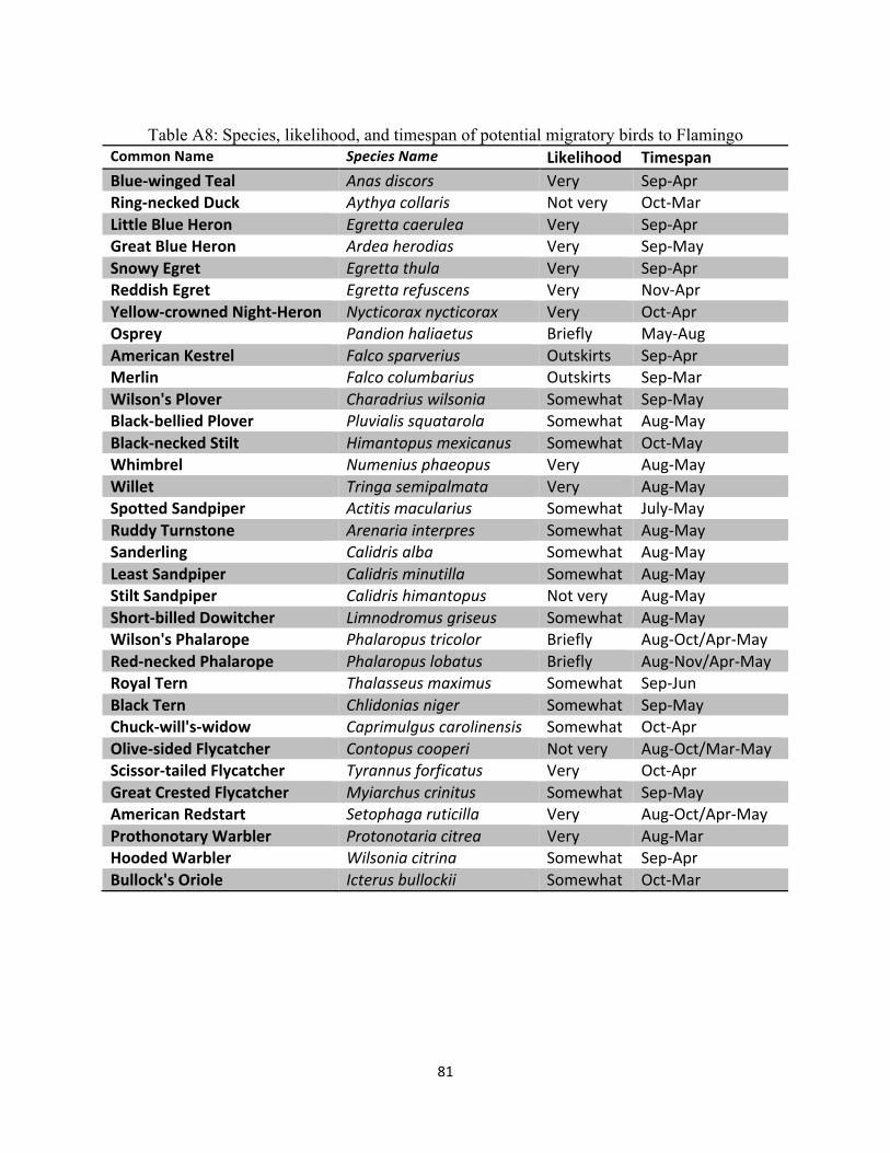
81    

Table A8: Species, likelihood, and timespan of potential migratory birds to Flamingo

Common  Name   Species  Name   Likelihood   Timespan  Blue-­‐winged  Teal   Anas  discors   Very   Sep-­‐Apr  Ring-­‐necked  Duck   Aythya  collaris   Not  very   Oct-­‐Mar  Little  Blue  Heron   Egretta  caerulea   Very   Sep-­‐Apr  Great  Blue  Heron   Ardea  herodias   Very   Sep-­‐May  Snowy  Egret   Egretta  thula   Very   Sep-­‐Apr  Reddish  Egret   Egretta  refuscens   Very   Nov-­‐Apr  Yellow-­‐crowned  Night-­‐Heron   Nycticorax  nycticorax   Very   Oct-­‐Apr  Osprey   Pandion  haliaetus   Briefly   May-­‐Aug  American  Kestrel   Falco  sparverius   Outskirts   Sep-­‐Apr  Merlin   Falco  columbarius   Outskirts   Sep-­‐Mar  Wilson's  Plover   Charadrius  wilsonia   Somewhat   Sep-­‐May  Black-­‐bellied  Plover   Pluvialis  squatarola   Somewhat   Aug-­‐May  Black-­‐necked  Stilt   Himantopus  mexicanus   Somewhat   Oct-­‐May  Whimbrel   Numenius  phaeopus   Very   Aug-­‐May  Willet   Tringa  semipalmata   Very   Aug-­‐May  Spotted  Sandpiper   Actitis  macularius   Somewhat   July-­‐May  Ruddy  Turnstone   Arenaria  interpres   Somewhat   Aug-­‐May  Sanderling   Calidris  alba   Somewhat   Aug-­‐May  Least  Sandpiper   Calidris  minutilla   Somewhat   Aug-­‐May  Stilt  Sandpiper   Calidris  himantopus   Not  very   Aug-­‐May  Short-­‐billed  Dowitcher   Limnodromus  griseus   Somewhat   Aug-­‐May  Wilson's  Phalarope   Phalaropus  tricolor   Briefly   Aug-­‐Oct/Apr-­‐May  Red-­‐necked  Phalarope   Phalaropus  lobatus   Briefly   Aug-­‐Nov/Apr-­‐May  Royal  Tern   Thalasseus  maximus   Somewhat   Sep-­‐Jun  Black  Tern   Chlidonias  niger   Somewhat   Sep-­‐May  Chuck-­‐will's-­‐widow   Caprimulgus  carolinensis   Somewhat   Oct-­‐Apr  Olive-­‐sided  Flycatcher   Contopus  cooperi   Not  very   Aug-­‐Oct/Mar-­‐May  Scissor-­‐tailed  Flycatcher   Tyrannus  forficatus   Very   Oct-­‐Apr  Great  Crested  Flycatcher   Myiarchus  crinitus   Somewhat   Sep-­‐May  American  Redstart   Setophaga  ruticilla   Very   Aug-­‐Oct/Apr-­‐May  Prothonotary  Warbler   Protonotaria  citrea   Very   Aug-­‐Mar  Hooded  Warbler   Wilsonia  citrina   Somewhat   Sep-­‐Apr  Bullock's  Oriole   Icterus  bullockii   Somewhat   Oct-­‐Mar  

   

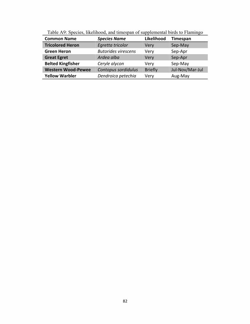
82    

Table A9: Species, likelihood, and timespan of supplemental birds to Flamingo Common  Name   Species  Name   Likelihood   Timespan  Tricolored  Heron   Egretta  tricolor   Very   Sep-­‐May  Green  Heron   Butorides  virescens   Very   Sep-­‐Apr  Great  Egret   Ardea  alba   Very   Sep-­‐Apr  Belted  Kingfisher   Ceryle  alycon   Very   Sep-­‐May  Western  Wood-­‐Pewee   Contopus  sordidulus   Briefly   Jul-­‐Nov/Mar-­‐Jul  Yellow  Warbler   Dendroica  petechia   Very   Aug-­‐May  

   

   

83    

Bibliography  

Alongi,  D.  M.  (1996).  The  dynamics  of  benthic  nutrient  pools  and  fluxes  in  tropical  mangrove  forests.  Journal  of  Marine  research  ,  54,  123-­‐148.  

Alongi,  D.  M.,  Christoffersen,  P.,  &  Tirendi,  F.  (1993).  The  influence  of  forest  type  on  microbial-­‐nutrient  relationships  in  tropical  mangrove  sediemnts.  Journal  of  Experimantal  Marine  Biology  and  Ecology  ,  171,  201-­‐223.  

Board,  C.  R.,  &  Commission,  C.  R.  (2010).  What  is  CST  all  about?  Retrieved  2010  03-­‐August  from  Certification  for  Sustainable  Tourism:  http://www.turismo-­‐sostenible.co.cr/en/cst/about-­‐cst/what-­‐is-­‐cst-­‐all-­‐about.php  

Boto,  K.  G.,  &  Wellington,  J.  T.  (1983).  Phosphorus  and  Nitrogen  Nutritional  Status  of  a  Northern  Australian  Mangrove  Forest.  Marine  Ecology  -­‐  Progress  Series  ,  11,  63-­‐69.  

Boto,  K.  G.,  &  Wellington,  J.  T.  (1984).  Soil  Characteristics  and  Nutrients  Status  in  a  Northern  Australian  Mangrove  Forest.  Estuaries  ,  7,  61-­‐69.  

Busman,  L.,  Lamb,  J.,  Randall,  G.,  Rehm,  G.,  &  Schmitt,  M.  (2009  July).  The  Nature  of  Phosphorus  in  Soils.  Retrieved  2011  йил  19-­‐March  from  University  of  Minnesota  Extension:  http://www.extension.umn.edu/distribution/cropsystems/DC6795.html  

Cardona,  P.,  &  Botero,  L.  (1998).  Soil  Characteristics  and  Vegetation  Structure  in  a  Heavily  Deteriorated  Mangrove  forest  in  the  Carribean  Coast  of  Colombia.  Biotropica  ,  30  (1),  2434.  

Cawkwell,  E.  M.  (1964).  The  Utilization  of  Mangroves  by  African  Birds.  Ibis  ,  106,  251-­‐253.  

Chen,  R.,  &  Twilley,  R.  R.  (1998).  A  gap  dynamic  model  of  manfgrove  forest  development  along  gradients  of  soil  salinity  and  nutrient  resources.  Journal  of  Ecology  ,  86,  37-­‐51.  

Chen,  R.,  &  Twilley,  R.  R.  (1999).  Patterns  of  mangrove  Forest  Structure  and  Soil  Nutrient  Dynamics  Along  the  Shark  River  Estuary,  Florida.  Estuaries  ,  22  (4),  955-­‐970.  

Cintron,  G.  and  Schaeffer-­‐Novelli,  S.Y.  (1984).  Methods  for  studying  mangrove  structure.  In:  Snedaker  SC,  Snedaker  J  (eds)  The  mangrove  ecosystem:  research  methods,  UNESCO,  Paris,  pp  91-­‐113.  

Convention  on  Wetlands  of  International  Importance  Especially  as  Waterfowl  Habitat.  Ramsar  (Iran),  2  February  1971.  UN  Treaty  Series  No.  14583.  As  Amended  by  the  Paris  Protocol,  3  December  1982,  and  Regina  Amendments,  28  May  1987.  

Dinwiddie,  R.,  Eales,  P.,  Scott,  S.,  Scott,  M.,  Bryan,  K.,  Burnie,  D.,  et  al.  (2009).  Mangrove  Swamps.  In  OCEAN  The  World's  Last  Widerness  Revealed  (1st  Edistion  ed.,  pp.  10-­‐137).  DK  Publishing.  

   

84    

Donato,  D.  C.,  Kauffman,  J.  B.,  Murdiyarso,  D.,  Kurninanto,  S.,  Stihdam,  M.,  &  Kanninen,  M.  (2011  April).  Mangroves  among  the  most  carbon-­‐rich  forests  in  the  Tropics.  Nature  Geoscience  ,  Advance  Online  Publication.  

Ellison,  A.,  Farnsworth,  E.,  &  Moore,  G.  (2007).  Pelliciera  rhizophorae.  Retrieved  2011  12-­‐03  from  IUCN  Red  List  of  Threatened  Species:  http://www.iucnredlist.org/apps/redlist/details/178833/0/classify  

Ellison,  J.  C.  (1996).  Climate  Change  and  Sea  Level  Rise  Impact  on  Mangrove  Ecosystems.  In  J.  Pernetta,  Imapcats  of  Claimte  Change  on  Ecosystems  and  Species:  Marine  and  Coastal  Ecosystems  (pp.  19-­‐21).  Gland,  Switzerland:  IUCN.  

EPA,  a.  (2000).  Ambiant  Water  Quality  Criteria  Recommendations  -­‐  Rivers  and  Streams  in  Nutrient  Ecoregion  IX.  U.S.  EPA,  Office  of  Water.  U.S.  EPA.  

EPA,  b.  (2000).  Ambiant  Water  Quality  Criteria  Recommendations  -­‐  Rivers  and  Streams  in  Nutrient  Ecoregion  XII.  U.S.  EPA,  Office  of  Water.  U.S.  EPA.  

EPA,  c.  (2000).  Ambient  Water  Quality  Criteria  Recommendations  -­‐  Rivers  and  Streams  in  Nutrient  Ecoregion  XIV.  U.S.  EPA,  Office  of  Water.  U.S.  EPA.  

EPA,  d.  (2000).  Ambient  Water  Quality  Criteria  Recommendations  -­‐  Wetlands  in  Nutrient  Ecoregion  XIII.  U.S.  EPA,  Ofice  of  Water.  U.S.  EPA.  

Feller,  I.  C.,  McKee,  K.  L.,  Whigham,  D.  F.,  &  O'Neil,  J.  P.  (2002).  Nitrogen  vs.  Phosphorus  limitation  across  an  ecotonal  gradint  in  a  mangrove  forest.  Biogeochemistry  ,  62,  145-­‐175.  

Feller,  I.  C.,  Whigham,  D.  F.,  McKee,  K.  L.,  &  Lovelock,  C.  E.  (2003).  Nitrogen  limitation  of  growth  and  nutrient  dynamics  in  a  disturbed  mangrove  forest,  Indian  River  Lagon,  Florida.  Oecologia  ,  134,  405-­‐414.  

Feller,  I.  C.,  Whigham,  D.  F.,  McKee,  K.  L.,  &  Lovelock,  C.  E.  (2003).  Nitrogen  limitation  of  growth  and  nutrient  dynamics  in  a  mangrove  forest,  Indian  River  Lagoon,  Florida.  Oecologia  ,  134,  405-­‐414.  

Feller,  I.  C.,  Whigham,  D.  F.,  McKee,  K.  L.,  &  O'Neill,  J.  P.  (2002).  Nitrogen  vs.  phosphorous  limitation  across  an  ecotonal  gradient  in  mangrove  forest.  Biogeochemistry  ,  62,  145-­‐175.  

Fromard,  F.,  Puig,  H.,  Mougin,  E.,  Marty,  G.,  Betoulle,  J.,  &  Cadamuro,  L.  (1998).  Structure,  above-­‐ground  biomass  and  dynamics  of  mangrove  ecosystems:  new  data  from  French  Guiana.  Oecologia  ,  115,  39-­‐53.  

Garrigues,  R.,  &  Dean,  R.  (2007).  The  Birds  of  Costa  Rica:  A  Field  Guide.  Ithaca,  NY,  United  States  of  America:  Cornell  University  Press.  

   

85    

Gates,  W.  E.,  &  Borchardt,  J.  A.  (1964).  Nitrogen  and  Phosphorus  E  from  xtractionDomestic  Wastewater  Treatment  Plant  Effluents  by  Controlled  Algal  Culture.  Journal  (Water  Pollution  Control  Federation)  ,  36  (4),  443-­‐462.  

Gilman,  E.,  Van  Lavieren,  H.,  Ellison,  J.,  V,  J.,  Wilson,  L.,  Areki,  F.,  et  al.  (2009).  Pacific  Island  Mangroves  in  a  cHanging  Climate  and  Rising  Sea.  UNEP.  Nairobi:  UNEP  Regional  Seas  Reports  and  Studies  n.  179.  

Hanson,  A.  M.,  &  Lee,  G.  F.  (1971).  Forms  of  Organic  Nitrogen  in  Domestic  Wastewater  (http://www.jstor.org/pss/25037233).  Journal  (Water  Pollution  Control  Federation)  ,  43  (11),  2271-­‐2279.  

Harrison,  A.  (2003).  The  Nitrogen  Cycle.  Retrieved  2010  24-­‐11  from  VisionLearning:  http://www.visionlearning.com/library/module_viewer.php?mid=98  

Heimsath,  A.  (2009  December).  Soil  Organic  Carbon.  Retrieved  2011  19-­‐March  from  The  Encyclopedia  of  Earth:  http://www.eoearth.org/article/Soil_organic_carbon  

Henschke,  C.,  &  Herrmann,  T.  (2007  йил  June).  Testing  for  Soil  and  Water  Salinity.  Retrieved  2011    19-­‐March  from  Government  of  South  Australia:  Primary  Industries  and  Resources  Sa:  http://www.pir.sa.gov.au/pirsa/more/factsheets/fact_sheets/salinity/testing_for_soil_and_water_salinity  

Hesse,  P.  R.  (1961).  Some  Differences  between  the  soils  of  Rhizophora  and  Avicennia  mangrove  swamps  in  Sierra  Leone.  Plant  and  Soil  ,  14  (4),  335-­‐346.  

Hilty,  J.,  &  Merenlender,  A.  (2000).  Faunal  indicator  taxa  selection  for  monitoring  ecosystem  health.  Biological  Conservation  ,  92,  185-­‐197.  

Hogarth.  (1999).  The  Biology  of  Mangroves.  (M.  Crawley,  C.  Little,  T.  Southwood,  &  S.  Ulfstrand,  Eds.)  Oxford,  UK:  Oxford  University  Press.  

Holford,  I.  C.  (1997).  Soil  Phosphorus:  its  measurment,  and  its  uptake  by  plants.  Australian  Journal  of  Soil  Research  ,  35,  227-­‐239.  

Honey,  M.  (2008).  Ecotourism  and  Sustainable  Development:  Who  Owns  Paradise?  (ed.  2nd  Edition).  Washington,  DC,  U.S.:  Island  Press.  

Jimenez,  J.  A.  (1984).  A  Hypothesis  to  Explain  the  Reduced  Distribution  of  the  Mangrove  Pelliciera  rhizophorae  Tr.  &  Pl.  Biotropica  ,  16  (4),  304-­‐308.  

Kathiresan,  K.  (n.d.).  Mangrove  Ecosystems:  Distribution  of  Mangroves.  (A.  University,  Ed.)  Retrieved  2010  December  from  Centre  of  Advanced  Study  in  Marine  Biology:  http://ocw.unu.edu/international-­‐network-­‐on-­‐water-­‐environment-­‐and-­‐health/unu-­‐inweh-­‐course-­‐1-­‐mangroves/Distribution-­‐of-­‐mangroves.pdf  

   

86    

Kathiresan,  K.  (n.d.).  Methods  of  Studying  Mangroves.  (C.  o.  University,  Ed.)  Retrieved  2010  24-­‐May  from  http://ocw.unu.edu/international-­‐network-­‐on-­‐water-­‐environment-­‐and-­‐health/unu-­‐inweh-­‐course-­‐1-­‐mangroves/Methods-­‐of-­‐studying-­‐Mangroves.pdf  

Komiyama,  A.,  Ong,  J.  E.,  &  Poungparn,  S.  (2008).  Allometry,  Biomass,  and  Productivity  of  Mangrove  Forests:  A  Review.  Aquatic  Botany  ,  89,  128-­‐137.  

L.E.O.  (n.d.).  Hydroprobe  Water  Quality  Parameters:  Definitions.  Retrieved  2011  4-­‐April  from  The  Lehigh  Earth  Observatory:  http://www.leo.lehigh.edu/projects/hydroprobe/wqdef.html  

Lovelock,  C.  E.,  Ball,  M.  C.,  Martin,  K.  C.,  &  Feller,  I.  C.  (2005).  Nutrient  Enrichment  Increases  Mortality  of  Mangroves.  PlosOne  ,  4  (5).  

McKee,  K.  L.  (1995).  Seedling  recruitemnt  patterns  in  a  Belizean  mangrove  forest:  effects  of  establishment  ability  and  physico-­‐chemical  factors.  Oecologia  ,  101,  448-­‐460.  

McKee,  K.  (1995).  Seedling  recruitment  patterns  in  a  Belizean  mangrove  forest:  effects  of  establishment  ability  and  physico-­‐chemical  factors.  Oecologia  ,  101,  448-­‐460.  

Nisbet,  I.  C.  (1968).  The  Utilization  of  Mangroves  by  Malaysian  Birds.  Ibis  ,  110,  348-­‐352.  

Novotny,  V.  (2003).  Water  Quality:  Diffuse  Pollution  and  Watershed  Management  (2nd  Edition  ed.).  Boston,  MA:  Wiley.  

Ramirez-­‐Garcia,  P.,  Lopez-­‐Blanco,  J.,  and  Ocana,  D.  (1998).  Mangrove  vegetation  assessment  in  the  Santiago  River  Mouth,  Mexico,  by  means  of  supervised  classification  using  Landsat  TM  imagery.  Forest  Ecology  and  Management,  105,  217-­‐229.  

Reckhov,  K.  (2010  2-­‐February).  Introduction  to  water  and  waste  water  treatment.  ENV  236:  Water  Quality  Management  .  Durham,  NC:  Duke  University.  

Reef,  R.,  Feller,  I.,  &  Lovelock,  C.  (2010).  Nutrition  of  Mangroves.  Tree  Physiology  ,  30  (9),  1148-­‐1160.  

Richardson,  C.  J.  (2010).  Prelinminary  Report  on  Flamingo  Beach  MangroveSurvey.  Duke  University,  Duke  University  Wetland  Center,  Durham.  

Richardson,  C.  (2010).  Preliminary  Report  on  Flamingo  Beach  Mangrove  Survey.  Duke  University.  Durham:  Duke  University  Wetland  Center.  

Rivera-­‐Monory,  V.  H.,  Day,  J.  W.,  Twilley,  R.  R.,  Vera-­‐Herrera,  F.,  &  Coronado-­‐Molina,  C.  (1995).  Flux  of  Nitrogen  and  Sediments  in  a  Fringe  Mangrove  Forest  in  Terminos  Lagoon,  Mexico.  Estuarnie,  Coastal  and  Shelf  Science  ,  40,  139-­‐160.  

Rosenfeld,  J.  K.  (1979).  Interstitial  Water  and  Sediment  Chemistry  of  Two  Cores  From  Florida  Bay.  Journal  of  Sedimentary  Petrology  ,  49,  989-­‐994.  

   

87    

Sherman,  R.  E.,  Fahey,  T.  J.,  &  Howarth,  R.  W.  (1998).  Soil-­‐plant  interactions  in  a  neotropical  mangrove  forest:  iron,  phosphorus  and  sulfur  dynamics.  Oecologia  ,  115,  553-­‐563.  

Sherman,  R.  E.,  Fahey,  T.  J.,  &  Martinez,  P.  (2003).  Spatial  Patterns  of  Biomass  and  Aboveground  Net  Primary  Productivity  in  a  Mangrove  Ecosystem  in  the  Dominican  Republic.  Ecosystems  ,  6,  384-­‐398.  

Sodhi,  N.  S.,  Choo,  J.  P.,  Lee,  B.  P.-­‐H.,  Quek,  K.  C.,  &  Kara,  A.  U.  (1997).  Ecology  of  a  Mangrove  Forest  Bird  Community  in  Singapore.  The  Raffles  Bulletin  of  Zoology  ,  45  (1),  1-­‐13.  

Spalding,  M.  G.,  &  Frederick,  P.  C.  (1995).  The  everglades:  what  can  indicator  species  tell  us  about  ecosystem  health?  Proceedings:  American  Association  of  Zoo  Veterinarians,  American  Association  of  Wildlife  Veterinarians,  Joint  Conference.    

Tam,  N.  F.,  &  Wong,  Y.  S.  (1995).  Mangrove  Soils  as  Sinks  for  Wastewater-­‐borne  Pollutants.  Hydrobiologia  ,  295,  231-­‐241.  

USGS.  (2011  8-­‐February).  Earth's  water:  Runoff.  Retrieved  2011  19-­‐April  from  Water  Science  for  Schools:  http://ga.water.usgs.gov/edu/runoff.html  

Whittaker,  R.  H.  (1972).  Evolution  and  measurement  of  species  diversity.  Taxon  ,  21,  213-­‐251.  

Winstanley,  D.  (2004).  Nitrogen  Cycle  Project.  Retrieved  2011  20-­‐March  from  Illinois  State  Water  Survey:  http://www.isws.illinois.edu/nitro/terms.asp?lpg=biogeo&term=OrgN  

Woodroffe.  (1992).  Mangrove  sediments  and  geomorphology.  In  D.  M.  Alistar  I.  Robertson,  Tropical  mangrove  ecosystems  (p.  Chapter  2).  

Woodroffe.  (1995).  Response  of  Tide  dominated  mangrove  shoreline  in  Northern  Australia  to  anticipated  sea  level  rise.  Earth  Surface  Processes  and  Landforms  ,  20,  65-­‐85.