Dysarthric Speech Synthesis Via Non-Parallel Voice Conversion

Dysarthric Speech Synthesis Via Non-ParallelVoice Conversion

Master’s Thesissubmitted to the Faculty of the

Escola Tecnica d’Enginyeria de Telecomunicacio de BarcelonaUniversitat Politecnica de Catalunya

by

Marc Illa Bello

In partial fulfillmentof the requirements for the

Master’s degree in Advanced Telecommunication Technologies

Supervisors:Marta R. Costa-jussa, PhD. (UPC)

Odette Scharenborg, PhD. (TU Delft)Bence Mark Halpern, PhD candidate. (TU Delft)

Barcelona, June 2021

Abstract

In this thesis we propose and evaluate a voice conversion (VC) method to synthesisedysarthric speech1. This is achieved by a novel method for dysarthric speech synthesisusing VC in a non-parallel manner2, thus allowing VC in incomplete and difficult datacollection situations. We focus on two applications:

First, we aim to improve automatic speech recognition (ASR) of people with dysarthria byusing synthesised dysarthric speech as means of data augmentation. Unimpaired speech isconverted to dysarthric speech and used as training data for an ASR system. The resultstested on unseen dysarthric words show that the recognition of severe dysarthric speakerscan be improved, yet for mild speakers, an ASR trained with unimpaired speech performsbetter.

Secondly, we want to synthesise pathological speech to help inform patients of their patho-logical speech before committing to an oral cancer surgery. Knowing the sound of the voicepost-surgery could reduce the patients’ stress and help clinicians make informed decisionsabout the surgery. A novel approach about pathological speech synthesis is proposed: wecustomise an existing dysarthric (already pathological) speech sample to a new speaker’svoice characteristics and perform a subjective analysis of the generated samples. Theachieved results show that pathological speech seems to negatively affect the perceivednaturalness of the speech. Conversion of speaker characteristics among low and high in-telligibility speakers is successful, but for mid the results are inconclusive. Whether thedifferences in the results for the different intelligibility levels are due to the intelligibilitylevels or due to the speakers needs to be further investigated.

1Dysarthria refers to speech impediments resulting from disturbances in the neuromuscular controlof speech production and is characterised by a poor articulation of phonemes. Dysarthric speech is thespeech produced by someone with dysarthria.

2Parallel data refers to a database containing the same linguistic content for the source and targetutterances. This content can be used to train the voice conversion model in a parallel manner. Forinstance, in an unimpaired to dysarthric speech parallel voice conversion, the unimpaired utteranceswould be the source and the dysarthric utterances the target. In a non-parallel voice conversion only thetarget (dysarthric) utterances are needed for training.

A l’Uri, per ser la millor companyia de confinament.

Acknowledgements

First and foremost I would like to express my deep gratitude to Bence Halpern, for hiswillingness to help and all the constructive criticism throughout the thesis. It has been agreat pleasure working with him.

I would also like to express my very great appreciation to Odette Scharenborg. I amtruly grateful for the scientific view and all the valuable advice given. She has been anexceptional supervisor both on a professional and personal level.

To the rest of the team members of the SALT group: Luke, Siyuan, Lingyun and Xinsheng,and also to Laureano Moro, who has been collaborating with the supervision of this thesis.Thanks for all the feedback and kindness, I am really thankful to have found so nice andcompetent people along the way.

A special word of gratitude is due to Marta R. Costa-Jussa for her guidance and theconveyed enthusiasm for the project since the very beginning.

To the applied AI team of Dolby Labs in Barcelona: Santi Pascual, Jordi Pons and JoanSerra. Their review of the thesis’ proposal was key to approach this project in a betterway from the beginning.

Many thanks to Tessy, for helping with the review of the thesis and caring about what Idid in this project. It is nice to have a friend with a technical background who is genuinelyinterested in what I do and can give a hand when needed.

On a more personal note, I thank my parents for all the love, support, patience and helpduring all these years.

Last but not least, I would like to deeply thank Alba, for making things easy and makingme better.

Revision history and approval record

Revision Date Purpose0 01/05/2021 Document creation1 28/06/2021 Document approval

DOCUMENT DISTRIBUTION LIST

Name e-mailMarc Illa [email protected] R. Costa-jussa [email protected] Scharenborg [email protected] Mark Halpern [email protected]

Written by: Reviewed and approved by:Date 28/06/2021 Date 28/06/2021Name Marc Illa Name Marta R. Costa-jussaPosition Project Author Position Project Supervisor

Contents

List of Figures vii

List of Tables viii

List of Abbreviations ix

1 Introduction 11.1 Context . . . . . . . . . . . . . . . . . . . . . . . . . . . . . . . . . . . . . 11.2 Motivation . . . . . . . . . . . . . . . . . . . . . . . . . . . . . . . . . . . . 11.3 Research goals . . . . . . . . . . . . . . . . . . . . . . . . . . . . . . . . . . 2

1.3.1 Improving automatic speech recognition of dysarthric speech . . . . 21.3.2 Pathological voice conversion . . . . . . . . . . . . . . . . . . . . . 3

1.4 Thesis organisation . . . . . . . . . . . . . . . . . . . . . . . . . . . . . . . 4

2 Literature Review 52.1 Voice conversion . . . . . . . . . . . . . . . . . . . . . . . . . . . . . . . . . 5

2.1.1 Generative adversial networks . . . . . . . . . . . . . . . . . . . . . 52.1.2 Vector-quantisation-based generative models . . . . . . . . . . . . . 72.1.3 Style tokens . . . . . . . . . . . . . . . . . . . . . . . . . . . . . . . 92.1.4 Attention . . . . . . . . . . . . . . . . . . . . . . . . . . . . . . . . 92.1.5 Tempo adaptation . . . . . . . . . . . . . . . . . . . . . . . . . . . 92.1.6 Summary and discussion . . . . . . . . . . . . . . . . . . . . . . . . 10

2.2 Automatic speech recognition . . . . . . . . . . . . . . . . . . . . . . . . . 122.2.1 Overview . . . . . . . . . . . . . . . . . . . . . . . . . . . . . . . . 122.2.2 Listen attend and spell . . . . . . . . . . . . . . . . . . . . . . . . . 132.2.3 Quartznet . . . . . . . . . . . . . . . . . . . . . . . . . . . . . . . . 132.2.4 Dysarthric speech recognition with lattice-free MMI . . . . . . . . . 142.2.5 Summary and discussion . . . . . . . . . . . . . . . . . . . . . . . . 15

3 Methodology 163.1 Voice conversion model . . . . . . . . . . . . . . . . . . . . . . . . . . . . . 16

3.1.1 VQ-VAE structure . . . . . . . . . . . . . . . . . . . . . . . . . . . 163.1.2 VQ-VAE learning . . . . . . . . . . . . . . . . . . . . . . . . . . . . 173.1.3 Voice conversion with a VQ-VAE . . . . . . . . . . . . . . . . . . . 183.1.4 HLE-VQ-VAE-3 . . . . . . . . . . . . . . . . . . . . . . . . . . . . . 18

v

3.2 Automatic speech recognition model . . . . . . . . . . . . . . . . . . . . . 193.2.1 Connectionist Temporal Classification . . . . . . . . . . . . . . . . . 203.2.2 Language Model . . . . . . . . . . . . . . . . . . . . . . . . . . . . 21

4 Experimental Framework 224.1 Dataset, preprocessing and feature extraction . . . . . . . . . . . . . . . . 224.2 Improving automatic speech recognition of dysarthric speech . . . . . . . . 23

4.2.1 Task . . . . . . . . . . . . . . . . . . . . . . . . . . . . . . . . . . . 234.2.2 Algorithms . . . . . . . . . . . . . . . . . . . . . . . . . . . . . . . 244.2.3 Experimental design . . . . . . . . . . . . . . . . . . . . . . . . . . 26

4.3 Pathological voice conversion . . . . . . . . . . . . . . . . . . . . . . . . . . 274.3.1 Experimental design . . . . . . . . . . . . . . . . . . . . . . . . . . 27

5 Results and Discussion 305.1 Improving automatic speech recognition of dysarthric speech . . . . . . . . 30

5.1.1 Results . . . . . . . . . . . . . . . . . . . . . . . . . . . . . . . . . . 305.1.2 Conclusions . . . . . . . . . . . . . . . . . . . . . . . . . . . . . . . 32

5.2 Pathological voice conversion . . . . . . . . . . . . . . . . . . . . . . . . . . 335.2.1 Naturalness . . . . . . . . . . . . . . . . . . . . . . . . . . . . . . . 335.2.2 Similarity . . . . . . . . . . . . . . . . . . . . . . . . . . . . . . . . 345.2.3 Limitations of the proposed approach . . . . . . . . . . . . . . . . . 355.2.4 Accessibility of voice conversion to atypical speakers . . . . . . . . . 365.2.5 Conclusions . . . . . . . . . . . . . . . . . . . . . . . . . . . . . . . 36

6 Conclusions and Future Work 38

Bibliography 41

List of Figures

2.1 Training GANs algorithm . . . . . . . . . . . . . . . . . . . . . . . . . . . 62.2 WER in Hermann et al. [1] . . . . . . . . . . . . . . . . . . . . . . . . . . . 14

3.1 VQ-VAE architecture and embedding space. . . . . . . . . . . . . . . . . . 173.2 HLE-VQ-VAE-3 diagram . . . . . . . . . . . . . . . . . . . . . . . . . . . . 19

4.1 Task design . . . . . . . . . . . . . . . . . . . . . . . . . . . . . . . . . . . 244.2 Subjective evaluation approach . . . . . . . . . . . . . . . . . . . . . . . . 27

5.1 Naturalness mean opinion score results . . . . . . . . . . . . . . . . . . . . 335.2 Similarity experiments results . . . . . . . . . . . . . . . . . . . . . . . . . 34

vii

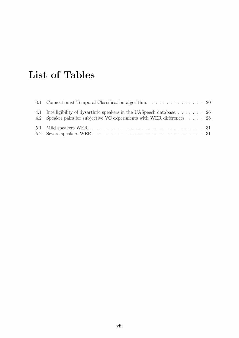
List of Tables

3.1 Connectionist Temporal Classification algorithm. . . . . . . . . . . . . . . 20

4.1 Intelligibility of dysarthric speakers in the UASpeech database. . . . . . . . 264.2 Speaker pairs for subjective VC experiments with WER differences . . . . 28

5.1 Mild speakers WER . . . . . . . . . . . . . . . . . . . . . . . . . . . . . . . 315.2 Severe speakers WER . . . . . . . . . . . . . . . . . . . . . . . . . . . . . . 31

viii

List of Abbreviations

ALS Amyotrophic Lateral Sclerosis

ASR Automatic Speech Recognition

BLSTM Bidirectional Long Short-Term Memory

CRF Conditional Random Fields

CTC Connectionist Temporal Classification

DNN Deep Neural Network

DSVC Dysarthric Speech Voice Conversion

DTW Dynamic Time Warping

E2E End-To-End

ELBO Evidence Lower Bound Objective

EOS End Of Sentence

GAN Generative Adversarial Network

GMM Gaussian Mixture Model

GST Global Style Token

GT Ground Truth

HMM Hidden Markov Models

LF-MMI Lattice-Free Maximum Mutual Information

LM Language Model

LSTM Long Short-Term Memory

MOS Mean Opinion Score

NLL Negative Log Likelihood

SOS Start Of Sentence

SOTA State-Of-The-Art

TDNN Time-Delay Neural Network

ix

LIST OF TABLES

TTS Text-To-Speech

VAE Variational Autoencoder

VC Voice Conversion

VCC Voice Conversion Challenge

VQ-VAE Vector Quantisation Variational Autoencoder

WER Word Error Rate

x

Chapter 1

Introduction

1.1 Context

Dysarthria refers to a group of disorders that typically results from disturbances in theneuromuscular control of speech production and is characterised by a poor articulation ofphonemes [2]. In many diseases such as amyotrophic lateral sclerosis (ALS) or Parkinson’s,further motor neurons are affected, thus negatively impacting the mobility of the patientsand making it difficult for them to initiate and control their muscles movement [3, 4].

Data-driven speech synthesis is an active field of research that has been reaching newheights since the introduction of deep neural networks. However, the performance of thesesystems strongly relies on the amount and quality of their training data. For applicationssuch as dysarthric speech synthesis, the available data is scarce and the recordings areoften made by medical professionals without studio quality. Synthesis techniques such astext-to-speech (TTS) are known to need a large amount of data for training, while voiceconversion (VC) only needs a relatively small amount of data when compared to neuralTTS.

In this thesis, we synthesise dysarthric speech via VC. The motivation of such work isexplained below.

1.2 Motivation

Over the past few years, automatic speech recognition (ASR) systems have started to playa vital role in people’s lives, by making it easier to control digital devices through digi-tal personal assistants (like Alexa or Google Home) and by providing dictation systemsthat, among other use cases, convert speech into text. While these systems work success-fully for typical speech (common dialects without speech impediments), they still fail tosuccessfully recognise dysarthric speech that can generally be recognised by humans [5].

ASR systems have been shown to have a positive psycho-social impact on individuals withphysical disabilities [6], thus we believe that in many cases these systems could improve lifequality of people with dysarthria. These systems could assist patients to master routine

1

Introduction

tasks such as controlling the light, temperature, entertainment systems of their house orcontrolling their smartphone and sending a text message.

One of the challenges to overcome for dysarthric speech ASR is the lack of resourcesfor this type of speech [7]. Currently, most ASR systems are based on deep learningalgorithms which, although incorporating rule-based or unsupervised learning techniques,their real-world performance depends on the quality and quantity of the available datafor training. We believe that converting unimpaired speech to dysarthric speech as meansof data augmentation could improve recognition of dysarthric speech in ASR systems.

Further motivation for work on dysarthric speech synthesis are possible benefits aroundthe treatment of the medical conditions at the root of the pathology. For instance, oralcancer surgery provokes changes to a speaker’s voice. A voice model predicting those soundchanges post-surgery could help the patients and clinicians to make informed decisionsabout the surgery and alleviate the stress of the patients [8, 9].

1.3 Research goals

1.3.1 Improving automatic speech recognition of dysarthric speech

In our work, we aim to provide new solutions improving current state-of-the-art (SOTA)ASR systems performance for dysarthric speech through data augmentation techniques.As ASR performance relies heavily on the available data, augmenting data through unim-paired to dysarthric speech conversion will enable us to improve those models. The intu-ition behind this hypothesis is explained below.

An ASR system can be generally created in two different ways: a hybrid system can bebuilt, where a lexicon is used (mapping of phoneme sequences to words), and an acousticmodel (converting an audio signal to phonemes) and a language model (LM), providingthe relative likelihood of different word sequences, are separately trained. Or an end-to-end (E2E) model that learns these mappings in the same model (speech to transcript)can be trained. In other words, while in hybrid models the acoustic, lexicon and languagemodels are tuned individually before making them work together, in E2E models a uniqueblock with the acoustic, lexicon and language models can be optimised. For the acousticand the E2E models, generally a database consisting of an audio signal and a groundtruth transcription is used to learn the mappings. This database needs to have a sufficientamount of representative data so that the model can generalise well on inference.

In the case of dysarthric speech, the aforementioned mappings are different from non-dysarthric speech as the speech impediments affect the speech on different levels (pro-nunciation, pitch, tempo, etc.). Ideally, for training an ASR system for dysarthric speech,these speech deviations would be consistent i.e. a shift of pronunciation of phonemes acrossall speakers can be observed. However, there are multiples types of dysarthria dependingon which part of the brain is damaged (pastic, flaccid, ataxic, hypokinetic, hyperkineticdysarthria and mixed) [10] which means that usually the mappings are not shared amongspeakers (i.e. deviations due to dysarthric speech are different from type to type). Ad-ditionally, there is little dysarthric speech data available making it difficult for those to

2

Introduction

learn the correct representations and generalise to dysarthric speech. There are severalreasons for having so little data available: recruiting enough dysarthric speakers can bedifficult due to its low prevalence in the population (the exact value is not known) and forthis same reason gathering the speakers in one place to perform a quality recording canbe problematic. Also, as mentioned, there are multiple types of dysarthria and severitylevels which we need to account for, as well as for the different languages and accents thatwe want to recognise, so getting sufficient recordings for all cases is complicated.

Therefore, to overcome the lack of data, we aim to perform data augmentation by con-verting unimpaired speech to dysarthric speech using a generative model. Preferably, wewould want this system to be non-parallel as parallel data is harder to collect: in a paralleldysarthric speech voice conversion (DSVC) set-up we train the model with unimpairedutterances (source) and dysarthric utterances (target) that need to be aligned (i.e. weneed source and target utterances to have the same linguistic content), while in a non-parallel DSVC we train the model with only dysarthric utterances. This also means thatin a non-parallel VC system we can do any-to-many conversions while in a parallel VCsystem, the source speakers are limited to those seen during training. We do not focuson other synthesis techniques such as text-to-speech as they are also known to require alarge amount of data for training. Thus, the first research question that we will try toanswer is the following:

RQ1 Can we improve ASR systems performance for dysarthric speech by doing unimpairedto dysarthric non-parallel voice conversion as means of data augmentation?

1.3.2 Pathological voice conversion

Together with RQ1, we also aim to perform pathological speech VC to evaluate its usefor clinical applications. For instance, knowing how a patient’s voice could sound afteran oral cancer surgery could help to reduce his stress and also help clinicians to makeinformed decisions before the surgery.

Evaluating the model for this use case has some complications: when evaluating unim-paired to pathological VC samples (i.e. speech from an unimapired speaker A convertedto the voice of a pathological speaker B), the listeners (the evaluators of the system)need to be able to rate the success of generating the pathological characteristics and thesynthetic/natural aspects of the speech separately. This is because existing pathologi-cal speech corpora [11, 12, 9, 13] provide unimpaired control speakers, but unimpairedspeech recordings from the same pathological speaker are rarely available. If the listen-ers are not able to distinguish the speech pathology from the synthetic aspects of thespeech we could encounter two counter-intuitive scenarios from the viewpoint of typicalVC: (1) a pathological VC system that is not able to properly capture the characteristicsof the pathological speech could still receive better naturalness scores than the referencepathological speech; (2) Conversely, a VC system that is able to mimic the pathology,albeit exaggeratedly, could produce a naturalness score that is a lot lower than that ofthe reference.

Therefore, we propose a new approach where instead of using unimpaired speech as source

3

Introduction

for the VC, we use dysarthric speech, which is already pathological, and the VC systemonly has to customise it to a new (unimpaired/dysarthric) speaker’s voice characteris-tics, i.e by using some representation of the speaker (speaker embedding). This synthesisapproach alleviates the problem with naturalness ratings as the dysarthric-to-dysarthricVC is not optimised directly for speech degradation, therefore degradation is only dueto the synthetic aspects compared to the source pathological utterance. Our first goal isto assess whether we can convert the voice characteristics of the pathological speakers inthis setup in a natural way, while simultaneously assessing how natural real pathologicalspeech is perceived.

An additional goal is to investigate whether our VC model can be used for non-standardspeech. As mentioned, standard ASR systems perform poorly on atypical speech [14, 15,16, 17, 1], making standard speech technology techniques less accessible to people withatypical speech.

In short, we use the dysarthric VC model proposed in this thesis to answer the followingresearch questions:

RQ2.1 Can we convert the voice characteristics of a pathological speaker to another patho-logical speaker of the same severity with reasonable naturalness (where reasonable meanscomparable to non-parallel VC methods on typical speech)? In other words, is VC technol-ogy accessible to people with pathological speech?

RQ2.2 How does (real) pathological speech affect the mean opinion score (MOS)? In otherwords, what is the maximum attainable naturalness of synthetic pathological speech?

1.4 Thesis organisation

The thesis structure is as follows: Chapter 2 provides the scientific background for thework presented in this thesis. The first part (Section 2.1) deals with a review of VCmethods, the second part (Section 2.2) with a review of automatic speech recognitionmethods. At the end of both sections, a summary of the reviewed methods as well assome conclusions are presented. In Chapter 3, we introduce the VC and ASR modelsused for our tasks. Chapter 4, details our experimental framework, where we present theused dataset, the pre-processing step and the feature extraction. Furthermore, we give adetailed explanation on the two tasks at hand: use synthetic dysarthric speech as meansof data augmentation to train an ASR system and subjectively evaluate dysarthric speechVC for clinical applications. Results for both tasks are presented and discussed in Chapter5. Finally, Chapter 6 closes the dissertation with conclusions and an outline of future work.

4

Chapter 2

Literature Review

The literature review is divided into two sections. First, in Section 2.1, we present a reviewof the most relevant papers to perform dysarthric speech voice conversion DSVC. Then, inSection 2.2, we review the current SOTA for ASR systems that could be used to evaluatehow much improvement is achieved in the ASR performance with the data augmentationresulting from the DSVC model.

2.1 Voice conversion

The goal of this literature review is to aggregate, read and summarise papers that mightbe relevant for DSVC. This means that the research is not limited to one field (voiceconversion), but we draw from other areas (such as text-to-speech and style transfer) toinform us about models or components that could fully or partially be reused for our task.The literature review concludes with a global view of the reviewed papers to establish aproposal of an architecture that performs DSVC (with the goal to augment dysarthricspeech data).

2.1.1 Generative adversial networks

Since their conception in 2014, Generative Adversial Networks (GANs) [18], proposed byIan J. Goodfellow et al. have become increasingly important as a model to generate large-sample distributions. As such, BigGAN [19], presented in 2018, has become the referencegenerative model for image generation. GANs have also become common use for speechtasks, SEGAN [20] being one of the first GAN architectures for speech enhancement andfollowed by many others for other tasks such as voice conversion [21, 22, 23]. In this reviewwe will briefly explain the idea behind GANs, review GAN-based architectures for voiceconversion and finally extract some conclusions about how they compare for the DSVCuse case.

GANs consist of two components: a discriminative model and a generative one. Whilethe generative model aims to generate plausible samples by sampling a latent randomvariable z from a Gaussian distribution pg, the discriminative model aims to distinguish

5

Literature Review

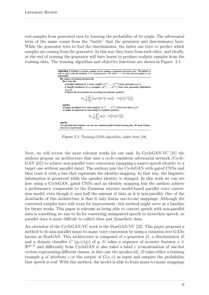
real samples from generated ones by learning the probability of its origin. The adversarialterm of the name comes from the “battle” that the generator and discriminator have.While the generator tries to fool the discriminator, the latter one tries to predict whichsamples are coming from the generator. In this way they learn from each other, and ideally,at the end of training the generator will have learnt to produce realistic samples from thetraining data. The training algorithm and objective functions are shown in Figure 2.1.

Figure 2.1: Training GANs algorithm, taken from [18].

Next, we will review the most relevant works for our task. In CycleGAN-VC [21] theauthors propose an architecture that uses a cycle-consistent adversarial network (Cycle-GAN [24]) to achieve non-parallel voice conversion (mapping a source speech identity to atarget one without parallel data). The authors join the CycleGAN with gated CNNs andthen train it with a loss that represents the identity-mapping. In that way, the linguisticinformation is preserved while the speaker identity is changed. In this work we can seehow using a CycleGAN, gated CNNs and an identity mapping loss the authors achievea performance comparable to the Gaussian mixture model-based parallel voice conver-sion model, even though it uses half the amount of data as it is non-parallel. One of thedrawbacks of this architecture is that it only learns one-to-one mappings. Although theconverted samples have still room for improvement, this method might serve as a baselinefor future works. This paper is relevant as being able to convert speech with non-paralleldata is something we aim to do for converting unimpaired speech to dysarthric speech, asparallel data is more difficult to collect than just dysarthric data.

An extension of the CycleGAN-VC work is the StarGAN-VC [22]. This paper proposes amethod to do non-parallel many-to-many voice conversion by using a variation over GANsknown as StarGAN. This architecture is composed of a generator G, a discriminator Dand a domain classifier C (pC(c|y)) of y. G takes a sequence of acoustic features x ∈RQ×N and differently from CycleGAN it also takes a label c (concatenation of one-hotvectors representing different classes, in this case the speaker-id). D takes either a trainingexample y of attribute c or the output of G(x, c) as input and outputs the probabilitythat speech is real. With this method, the model is able to learn many-to-many mappings

6

Literature Review

simultaneously while being fast enough to be used in real time.

Another related work is the one done by Jiao et al. [25] where they propose a model toconvert unimpaired speech to dysarthric speech as means of data augmentation. To dothat, they convert the spectral features from one type of speech to another using a deepconvolutional generative adversarial network (DCGAN). They objectively evaluate thismethod on a pathological speech classification task: a SVM model is trained to classify thesamples as ataxic or ALS speech. By using their method to balance an existing dataset theauthors are able to improve the accuracy by a 10%. For the subjective evaluation, speechpathologists had to label speech samples as ALS speech or non ALS speech from a groupof samples that contained both unimpaired speech recordings and converted (unimpairedto ALS) speech recordings. The converted recordings where labeled as dysarthric 65% ofthe time. In this work, we see how data augmentation for dysarthric speech can be usedto improve the performance of a classification task. However, further experiments needto be done in order to determine the benefits of the simulated speech samples in otherapplications.

With the presented works we can see how with some modifications over the vanilla GANwe can get powerful models to achieve a good quality voice conversion model that is ableto work with non-parallel data and is able to convert speech features while keeping thespeech content.

2.1.2 Vector-quantisation-based generative models

The first vector-quantisation-based generative model was proposed in [26], where theypropose an architecture that learns discrete representations without supervision.

In order to explain their work we need some context: as any generative model it aims toestimate the probability distribution of high-dimensional data (images, audio, text...) tolearn the underlying structure of the data, capture dependencies between the variables,generate new data with similar properties or learn relevant features of the data with-out supervision. It is also important to highlight the autoregressive generative modelswhich model the joint distribution over the data as a product of conditional distribu-tions that are output by a deep neural network. For instance, in the case of an im-age, the network would predict the next pixel based on the N already predicted pixels:

p(x) =∏n2

i=1 p(xi|x1, ..., xi−1) where n2 is the total number of pixels.

Their architecture (vector quantised variational autoencoder or VQ-VAE), differs fromvariational autoencoders (VAEs) by using discrete codes instead of continuous ones. Also,the prior is learnt instead of being static. They achieve discrete codes by using vectorquantization (VQ), a lossy compression technique where a vector is chosen from a set ofvectors to represent an input vector of samples.

Using discrete representations has several advantages: in real world a lot of categoriesare discrete and it makes no sense to interpolate between them (language representationssuch as words are discrete, speech can be represented with phonemes, images can becategorized...). It is easy to see that discrete representations are intrinsically better formany applications. They are also easier to model since each category has a single value,

7

Literature Review

whereas with a continuous latent space it gets naturally more complex. Moreover, the useof VQ addresses the issue of posterior collapse1 which is often present in VAE architectures.In order to see how this happens, it is necessary to remember how VAEs work: VAEsconsist, firstly, of an encoder that predicts a posterior latent variable z from an inputx. This is expressed as q(z|x). Secondly, there is a decoder that predicts the posteriorprobability, of having an input x given z. This is expressed as p(x|z). In order to buildthe loss function, evidence lower bound objective (ELBO) is used:

L(x; θ, φ) = −Eq(z|x)[logpθ(x|z)] +DKL(qφ(z|x)||p(z))

Here, the first part of the equation is the likelihood, and the second, the Kullback–Leiblerdivergence, measures the difference between the posterior and the prior probability. It actsas a regulariser, meaning that it forces the latent codes to be distributed as a standardnormal distribution N (0, Id). With very powerful decoders, if the codes are too close itmight happen that the posterior collapses into the prior. This means that the decoder endsup ignoring z to rely only on the autoregressive properties of x, resulting in x and z endingup being independent. Differently from VAEs, VQ-VAEs use discrete latent variables, andits training is inspired by vector quantisation. Both the prior and posterior distributionsare categorical, represented in an embedding table, which will be used as input of thedecoder network.

By using these representations together with an autoregressive prior, the authors showthat their model is able to model long-term dependencies in tasks such as image, videoand speech generation in an unsupervised manner. Additionally, it is able to successfullyperform speaker conversion and unsupervised learning of phonemes which is somethingof high interest for this project. The discrete representations could be useful to, not onlysynthesise speech, but also to understand how the learnt representations differ amongdifferent types of speech.

In a second work Van der Oord et al. present the VQ-VAE2 [27], where they show howusing the work done in VQ-VAE [26] but redesigning the structure to have a multi-scale hierarchical organization of latent maps their model is capable of generating highresolution images. In this way, the authors manage to model local information (i.e. texture)captured in the top latents, separately from global information (i.e. shape of an object)captured in the bottom latents. For a speech signal, the local information could be relatedto phonemes and the global information to prosodic features. With this structure, theauthors show that the model is able to compete with actual state of the art GANs forimage generation. In the Jukebox paper [28], we can see how using a WaveNet [29] insteadof a PixelCNN [30] as prior and some other minor modifications over VQ-VAE2, theirmodel is able to generate audio (music) conditioned on different styles and artists andoptionally lyrics. In the VCC2020[31], there is a work submitted by Tuan Vu Ho et al. [32]where they show how this architecture yields to better results for voice conversion than theoriginal VQ-VAE. More concretely, the naturalness is improved as they are able to encodeboth local and global information. It is possible that for our use case, a good decouplingof identity and style for dysarthric speech can be achieved with a good hierarchisation of

1We say that the posterior collapses when the decoder ‘ignores’ a latent code. An example of thiswould be, when performing image reconstruction, seeing that we loose some feature such as the gender.

8

Literature Review

the decomposition in a VQ-VAE2 system. Together with some regularization of the latentspace we might be able to convert and control dysarthric speech style.

2.1.3 Style tokens

The paper Style Tokens: Unsupervised Style Modeling, Control and Transfer in End-to-End Speech Synthesis, presented by Yuxuan Wang et al. [33], proposes an architecturethat joins a bank of embeddings that they name as Global Style Tokens (GSTs), withTacotron (a state-of-the-art end-to-end text-to-speech (TTS) system proposed by Wanget al., 2017a, Shen et al., 2017 [34]).

GSTs are used to perform style modeling, so that the proposed TTS system is able tomodel the speaking style. The generated embeddings are trained without labels, yet eachone of them learns how to control synthesis in a new way (speaking speed, style, pitch,intensity, emotion). In the experiments GSTs show very promising results in non-paralleldata style transfer, which is the main task our VC model will need to do. Also, it isimportant to notice that dysarthric speech recordings are often low quality (made bymedical professionals without studio quality), so being able to model this kind of speechin a way that the noise from the reference can be taken out from the style might be veryrelevant for our use case. Finding some “dysarthric style” tokens might be useful if wecan use them together with our voice conversion model to create recordings which havedysarthric style. In other words, although the paper presents GSTs for TTS we don’t seeany impediment to use them to condition a discrete generative model for VC, such assome of the VQ-VAE structures presented in Section 2.1.2. We could connect the GSTsto the decoder of the VQ-VAE to condition the output style to some “dysarthric speechtokens” in the same way it is done in Neural Discrete Representation Learning [26] forconditioning the decoder to the speaker id.

2.1.4 Attention

Regarding the papers that perform VC with attention-based architectures, there is oneof special interest done by John Harvill et al. [35] where they propose a new task wherethey train an ASR to recognise dysarthric words that are not seen during training. Todo that, they propose a VC-based data augmentation scheme: they train a parallel VCattention-based system (i.e. a Transformer architecture [36]) for unimpaired to dysarthricspeaker pairs and then they use it to synthesise new dysarthric words that will be used totrain the ASR. Then, the ASR performance is evaluated with the real dysarthric speechwords. Their approach effectively reduces WER for mild and mid dysarthric speakers.

2.1.5 Tempo adaptation

One of the characteristics of dysarthric speech is, usually, a slower speaking rate [37] whichdirectly affects ASR systems’ performance [38]. Therefore, a succesful VC system has totake into account the durational aspects of the speech. In our use case, when training withno parallel data, what we do on inference is shifting the acoustic quality from speaker A tospeaker B, by using some representation from speaker B that correspond to the features

9

Literature Review

we want to shift from speaker A (such as the speaker identity), and when doing that theduration remains untouched. There are different ways speech tempo adaptation can beapproached: In the Style Tokens paper (explained in Section 2.1.3) they do attention-baseddecoding where the tokens control the speech rate. In the the work done by Feifei Xiong,Jon Barker and Heidi Christensen, 2019 [39], the authors present an approach to performdata augmentation by converting the speech rate of typical speech towards the speech rateof dysarthric speech with good results. The more data that is augmented, the better theWER is until an eventual saturation in some cases: while speaker-based adaptation seemedto improve results faster, phoneme-based adaptation seems to saturate less the networkand when used with all control data gives better results than speaker-based adaptation.Another option is using dynamic time warping (DTW) as in [35]. Some of these workscan be used to modify the tempo of the speech resulting from our voice conversion modeland we believe that the usage of the converted speech in a data augmentation scheme foran ASR system for dysarthric speech, will improve its performance.

2.1.6 Summary and discussion

To summarise, we have seen promising results in style transfer for TTS with Style Tokens.In VQ-VAE’s review we have shown the advantages of discrete latent codes over continuousones, how these can be related to phonemes, and how we can model, in an unsupervisedway, long-term dependencies. Regarding the VQ-VAE2 paper, we have seen how a goodhierarchic structure of VQ-VAEs can successfully decouple high level features from lowlevel ones and how in some papers it is applied to audio: in Jukebox [28] paper we seehow together with a WaveNet [29], it is possible to generate, condition and model musicand in the VCC2020 paper by Tuan Vu Ho et al. [32] we see how it can be applied to VCwith improved naturalness over a vanilla VQ-VAE. GANs have also been reviewed, withinteresting modifications over the vanilla GAN (DCGAN, CycleGAN and StarGAN). Allof them show to be a good method for doing non-parallel voice conversion by changingthe speaker identities while preserving the speech content. Attention VC has also beenreviewed, and we have seen that it is possible to convert unimpaired to dysarthric speechto improve ASR for dysarthric speech. In this work, they also propose a very interestingtask for recognising out-of-vocabulary words for dysarthric speech. In order to adapt thetempo for the voice converted samples, we reviewed the work done by Xiong et al. inSection 2.1.5, where they show how changing the speech tempo in order to perform dataaugmentation improves the performance of a dysarthric speech ASR system.

As data for dysarthric speech is scarce, we are interested in being able to train the VCmodel with non-parallel data as it is easier to collect. On the reviewed attention methodthe VC uses parallel data, so this is a drawback that we would like to overcome. Also, theproposed attention system only allows for one-to-one mappings, so for each conversionbetween a pair of speakers, we would need to train a new model. From the other reviewedworks, two main groups of models arise from this literature review: the GANs (DCGAN,CycleGan and StarGan) and vector-based variational autoencoders (VQ-VAE, GSTs -which although not based in VQ-VAEs could be joined with a VQ-VAE as proposed inSection 2.1.3 - and VQ-VAE2, together with the JukeBox and the VCC2020 paper [32]).

10

Literature Review

Although GANs have provided very promising results so far, they also present some typicalissues. The most common being the mode collapse (when the variety of samples producedby the generator is scarce) and lack of diversity (it is known that GANs do not capturethe diversity of the true distribution). Also, GAN’s evaluation is challenging as we donot have a test to measure and assess how much it is overfitting. Moreover, continuousrepresentations are less than a natural fit for many situations when compared to discreteones, as explained in Section 2.1.2.

However, models based on likelihood use NLL (negative log-likelihood) as loss function.This makes models comparison and generalization measure easier. Furthermore, they tendto suffer less from mode collapse or lack of diversity as they try to maximize the probabilityto every example seen in the training data. To be fair, it is worth mentioning that withspeech a worse validation loss does not always mean worse quality, and with pathologicalspeech this might be even more the case.

For our use case, a discrete model probably fits our needs better as we can easily givea better interpretation to the learnt vectors such as phonemes (for example, we couldcarry out a unit discovery task). Experimental results show that even non-discrete stylefeatures, such as pitch or intensity, can also be represented in some codewords. In thisway, we could do a better analysis and interpretation of the learnt features: we coulddo an observation of which codewords the network uses to model dysarthric speech andit could be compared versus non-dysarthric speech style easily. For all these reasons, wethink that latent discrete likelihood based models are the way to go. Additionally, we haveseen that hierarchical structures such as VQ-VAE2 or GSTs allow to get rid of irrelevantinformation as well as to disentangle and decouple identity from style easily, which issomething we aim for in our project.

From the VQ-VAE-based models covered in this review two options have been presented.The first proposal is joining VQ-VAE and GSTs to achieve a style transfer model withcontrol over the prosody. To do that, the GSTs would be connected to the VQ-VAE’sdecoder in order to condition the prosody, in the same way that VQ-VAE’s paper usesthe speakerID to condition the output speaker. The second possibility would be using amodel based on VQ-VAE2, using a WaveNet (or similar such as Waveglow [40]) in thesame way that is done in Jukebox.

Between these two proposals, the one that seems more promising to us is using a VQ-VAE2 structure, as we think that in order to achieve a good decoupling of speaker identityfrom dysarthric speech style we need a hierarchical structure, and this work gives us theflexibility to add as many levels as we want. In this way, the effect on the speech couldpossibly be that the first levels correspond to low-level features, such as the content, andas we go up the levels would tend to suprasegmental features. Also, VQ-VAE2 showsbetter performance than a vanilla VQ-VAE. As mentioned in the conclusions of VQ-VAE2 review, we feel that by using this model and performing some regularization overthe latent space, we would be able to convert and control dysarthric speech style. Finally,using the work done in Phonetic Analysis of Dysarthric Speech Tempo and Applicationsto Robust Personalised Dysarthric Speech Recognition [39] we would be able to adapt thedysarthric speech rate, which is shown to be an important feature to train an ASR system

11

Literature Review

for impaired speech.

2.2 Automatic speech recognition

The goal of this literature review is to aggregate, read and summarize papers that mightbe relevant for automatic speech recognition (ASR). The goal is to propose an architectureto evaluate how much we can improve the performance of an ASR system with the dataaugmentation system we propose for synthesising dysarthric speech.

2.2.1 Overview

Since the appearance of deep networks, these have been used for classification problems.For structural ones, for instance, two variable lengths sequences, networks have usuallybeen combined with sequence models i.e. Hidden Markov Models (HMM) [41, 42, 43] orConditional Random Fields (CRF) [44]. However, they cannot be easily trained end-to-end(meaning that you need to train their different components separately), so in many taskssuch as machine translation, image captioning and conversational modeling, sequence tosequence models are used. For speech recognition (speech to text) both hybrid DNN-HMMarchitectures and encoder-decoder based end-to-end architectures have been proposed inthe recent past. Below, a brief overview is done:

Although new end-to-end architectures are being proposed for ASR, DNN-HMM modelsare still an active area of research. Some of these architectures perform SOTA or close toSOTA: in the work done by C. Luscher et al., in RWTH ASR Systems for LibriSpeech:Hybrid vs Attention [45] they show how their HMM-DNN hybrid model outperforms anend-to-end attention based one (between 15% and 40% better depending on the dataset).

One of the first attempts to propose an end-to-end ASR model, in 2014, was in a workdone by Alex Graves (Google DeepMind) using Connectionist Temporal Classification(CTC) together with recurrent neural networks (RNNs)[46]. One of the shortcomings ofCTC-based models is that there is no conditioning between label outputs, so in orderto spell correctly, these usually need a language model (the CTC model maps the inputspeech to either phonemes or letters and then the language model maps them to words).

With the appearance of attention-based networks, and in an attempt to improve someof the flaws of CTC-based models, attention-based models for ASR were proposed, beingthe first one Listen Attend and Spell [47], in 2015. Since then more models have beenproposed, some of which incorporate the Transformer architecture [48, 49].

In order to explore the three main architectures (attention-based, CTC-based and hybridHMM-DNN), we will do a brief review of one paper for each one. The papers that will bereviewed are: Listen Attend and Spell [47] (Section 2.2.2) as it is a well-known attention-based model, Quartznet [50] (Section 2.2.3), a CTC-based model that achieves near SOTAresults with fewer parameters than other models and Dysarthric Speech Recognition withLattice-Free MMI [1] (Section 2.2.4) a hybrid DNN-HMM model that evaluates ASRsystems trained on dysarthric speech.

12

Literature Review

2.2.2 Listen attend and spell

In Listen Attend and Spell [47], O. Vinyals et al., propose an attention-based sequence tosequence model. This model is composed of an encoder RNN (which turns the variable-length input into a fixed-length vector) and a decoder RNN (which takes the encodedvector and produces the variable-length output). During training, in sequence to sequencemodels, the ground-truth labels are fed as inputs to the decoder and during inferencebeam-search is performed (exploration of a graph by expanding the most promising node).Then, only a predetermined number of best partial solutions is kept as candidates togenerate new candidates for the future predictions. However, this is the structure of asimple sequence to sequence model, which can be improved with attention (and this iswhat is proposed in the paper). To do that, the decoder RNN will be provided with moreinformation as the last hidden state of the decoder will be used to create an attentionvector over the input sequence of the encoder for each output step. In this way, instead offeeding the information one time from the encoder to the decoder, this is done each timethe output is computed. Based on the aforementioned model (sequence to sequence withattention), this network will be able to turn speech into a word sequence, by outputtingone character for each step.

This paper is of our interest because the authors propose an attention-based sequence-to-sequence model for ASR that does not use phonemes as a representation, nor relieson pronunciation dictionaries or HMMs, can be trained end-to-end, unlike DNN-HMMmodels that require training separate components. In contrast to CTC based models,the output labels are conditionally dependent of the previous ones. It is remarkable thatthis approach models characters as outputs and shows how to learn an implicit languagemodel that can generate multiple spelling variants given the same acoustics (for examplewith the input phrase ‘triple a’ the model outputs both ‘aaa’ and ‘triple a’ as mostlikely beams) and also handles out-of-vocabulary words gracefully. Also, when a word isrepeated it might be expected that as it is a content-based attention model, it would losethe attention and produce the word less times than the number of times it was spoken.However, the model deals well with these cases.

2.2.3 Quartznet

In the paper Quartznet: Deep Automatic Speech Recognition with 1D Time-Channel Sepa-rable Convolutions [50], the authors propose an end-to-end neural acoustic model for ASRthat is trained using a CTC loss. The main achievement is that with fewer parametersthan other SOTA networks it gets a result very close to SOTA on LibriSpeech [51] andWall Street Journal [52]. This is relevant for our use case as this means that the trainingwill be faster and require less computing power.

In order to achieve that, the design is based on Jasper [53], a CNN based network withCTC loss. The main contribution is using 1D time-channel separable convolutions. Thismeans that each of these convolutional layers is composed of two convolutional layers: oneacting at each channel across different time frames and another one acting at one timeframe but across all channels. This allows the authors to use bigger kernel sizes whilereducing the numbers of parameters.

13

Literature Review

The fact that it has fewer parameters is relevant for our project because the model requiresless resources for training. Furthermore, smaller models are usually more robust to over-fitting. Also, the authors show that the model can be fine-tuned for similar tasks, whichis something we could explore. Another important aspect is that the authors released themodel publicly, which is something that can be of great help.

2.2.4 Dysarthric speech recognition with lattice-free MMI

The work done in Dysarthric Speech Recognition with Lattice-free MMI [1], shows howusing lattice-free maximum mutual information (LF-MMI) can improve dysarthric speechrecognition. Traditionally, both HMM-GMM and HMM-DNN systems have been trainedwith maximum likelihood (the latest using a frame-based cross entropy loss). However,recent SOTA systems are being trained with sequence-discriminative loss functions (i.e.LF-MMI). The authors of this work analyse the performance of HMM-GMM and HMM-DNN systems with LF-MMI together with other techniques such as frame-subsamplingand speed perturbation.

In order to evaluate the proposed techniques, two ASR systems are used: a HMM-GMMand a HMM-DNN one. For the HMM-GMM model, the authors use the Kaldi ASR toolkit[54] with Espana-Bonet and Fonollosa [55] hyperparameters. Regarding the HMM-DNNone, they use a Kaldi model trained on a subset of Librispeech.

The dataset used is the Torgo corpus [12] with only the isolated words and sentencerecordings (there are also utterance recordings). The two sets are treated for separatedtasks, with a different language model for each. The training is done using cross-validation(1 speaker is left for validation and the models are trained on the remaining 14).

For the experiments, they compare the proposed system with a TDNN-LSTM model withcross entropy (CE). Results are shown in Figure 2.2. It can be seen that the proposedsystem gives the best results in every scenario.

Figure 2.2: WER for each ASR model compared in [1]. Adapted from [1].

The authors also try some other experiments. The first one is constraining the languagemodel to output only a word for the single-word task, which consistently improves the re-sults. They also perform speed perturbation, which improves the recognition on dysarthricspeech but makes it worse for control speech (probably because it makes the data too vari-able).

14

Literature Review

With this paper, we can see that hybrid HMM-DNN models still perform state-of-the-art,and how using LF-MMI yields to stronger results for the dysarthric speech recognitiontask (the results are SOTA on Torgo database).

2.2.5 Summary and discussion

In this reviewm we have compared attention-based models (Listen Attend and Spell),CTC-based (Quartznet) and hybrid ones (DNN-HMM with LF-MMI). Each methodpresents its own advantages over the others: the attention one does not rely in dictionaries,can be trained end to end and differently from CTC the output labels are conditionallydependent on previous ones. Quartznet shows how a small model can be trained with fewresources while keeping a performance close to SOTA. Finally, the hybrid model showsthe best performance for a dysarthric speech recognition task. So probably, when it comesto improve ASR for dyarthric speech, the latest is the best option.

15

Chapter 3

Methodology

In this chapter, we explain and present the models used for our data augmentation task.In Section 3.1 the structure of the voice conversion model we use to perform the dataaugmentation is explained in detail, and in Section 3.2 we show the ASR model that isused to evaluate the performance of the data augmentation method for dysarthric speechrecognition.

3.1 Voice conversion model

As stated in Section 2.1.6, we think that the most suitable model for our task should bebased on a hierarchical structure of VQ-VAE (i.e. VQ-VAE2). So, as we are doing a VCtask, we use the same structure as the one used by Tuan Vu Ho et al. [32] at the VCC2020challenge. As it is a non-parallel VC system it allows to do any-to-many conversion, whichmeans that only one voice conversion model needs to be trained to convert any speakerto the target speakers.

Although we provided a high-level explanation of the VQ-VAE architectures in Section2.1.2, in order to present our model we need to review in more detail how these archi-tectures work. First of all, in Section 3.1.1, we show a vanilla VQ-VAE (without multiplelevels) architecture. Then, in Section 3.1.2, we show how the training of a VQ-VAE is done,followed by an explanation in Section 3.1.3 of how to perform VC with this architecture.Finally, in Section 3.1.4, the chosen architecture is presented.

3.1.1 VQ-VAE structure

As explained in Section 2.1.2 the VQ-VAE structure is very similar to a VAE but using adiscrete latent space. This latent embedding space (also referred as codebook) is e ∈ RK×D

where K is the number of latent embedding vectors and D the size of the vectors (alsoreferred as codewords). The flow can be seen in the left part of Figure 3.1: there is aninput x (i.e an image or an audio feature such as a mel-cepstrum) which goes through theencoder (a CNN), resulting in a tensor ze(x). Then, each one of the vectors is quantisedfor every spatial location of ze(x) (the latent variables) by selecting the nearest neighbour

16

Methodology

in the embedding space. With this operation we select the discrete latent variables z (i.e.the codewords). These set of codewords result in the tensor zq(x) that is the input to thedecoder, which is also convolutional.

Figure 3.1: Left: VQ-VAE architecture. Right: Visualisation of the embedding space. The output ofencoder z(x) is mapped to nearest point e2. The gradient, in red, pushes the encoder to change theoutput. Extracted from [26].

The expression that comes out of this reasoning for the posterior q(z|x) (which is expressedas a one-hot) is:

q(z = k|x) =

{1, for k = argminj||ze(x)− ej||20, otherwise

(3.1)

And zq(x) is computed using the euclidean norm:

zq(x) = ek,where k = argminj||ze(x)− ej||2 (3.2)

3.1.2 VQ-VAE learning

The conceptual goal of VQ-VAE training is that the model learns to reconstruct an inputx which is encoded, discretised and decoded. During training, zq(x) is the input to thedecoder, and when backpropagating, the gradient ∇zL is passed to the encoder. Since Dis shared, the gradients computed from the decoder are useful for the encoder to minimizethe loss. The loss function is as follows:

L = log(p(x|zq(x))) + ||sg[ze(x)]− e||22 + β||ze(x)− sg[e]||22 (3.3)

To understand the equation, it is useful to explain the three summed parts separately. Thefirst term, log(p(x|zq(x))) is the reconstruction loss, which is used both by the encoderand the decoder. To learn the embedding space the authors use the second term of theequation, ||sg[ze(x)] − e||22, which is simply the vector quantisation algorithm. It movesthe embedding vectors ei in the the direction of the outputs of the encoder (ze(x), shownin the right part of Figure 3.1). Finally, the third term of the equation, β||ze(x)− sg[e]||22,is the commitment loss which is used to force ze(x) to stay close to the embedding spacee so that it does not changes too often from one code vector to another. In this way we

17

Methodology

avoid the encoder parameters to train faster than the embeddings. In the equation, sg isthe stopgradient operator which avoids computing the gradient for certain variables.

Note that there is no need for a KL term in the objective function, as the nearest em-bedding function acts as a regularizer. This avoids a potential posterior collapse issue asthere is no KL term that can vanish.

Although for image or audio generation a prior is also learnt, for our use case we will notuse it as we only perform VC.

3.1.3 Voice conversion with a VQ-VAE

For the speaker conversion task performed in the VQ-VAE paper [26], the authors trainthe model with the mel-cepstrum of the speech from N speakers, and while training,a one-hot vector xN , which acts as a unique speaker-id for each speaker, is fed to thedecoder together with the discrete latents z. By using the speaker-id to condition thedecoder, this one learns to infer the style of each speaker to the encoded speech. Oncethe model is trained, in a voice conversion scenario, the input to the model is the sourcespeaker speech and the decoder is conditioned with a speaker-id that corresponds tothe target speaker. Then, the output of the decoder (the converted mel-cepstrum) can besynthesised to speech with any vocoder that uses Mel-cepstral features such as a WaveNet[29]. With the VC task this model is able to encode a speech representation that separatesthe speech content information (represented in the latents) from other information suchas the speaker identity.

3.1.4 HLE-VQ-VAE-3

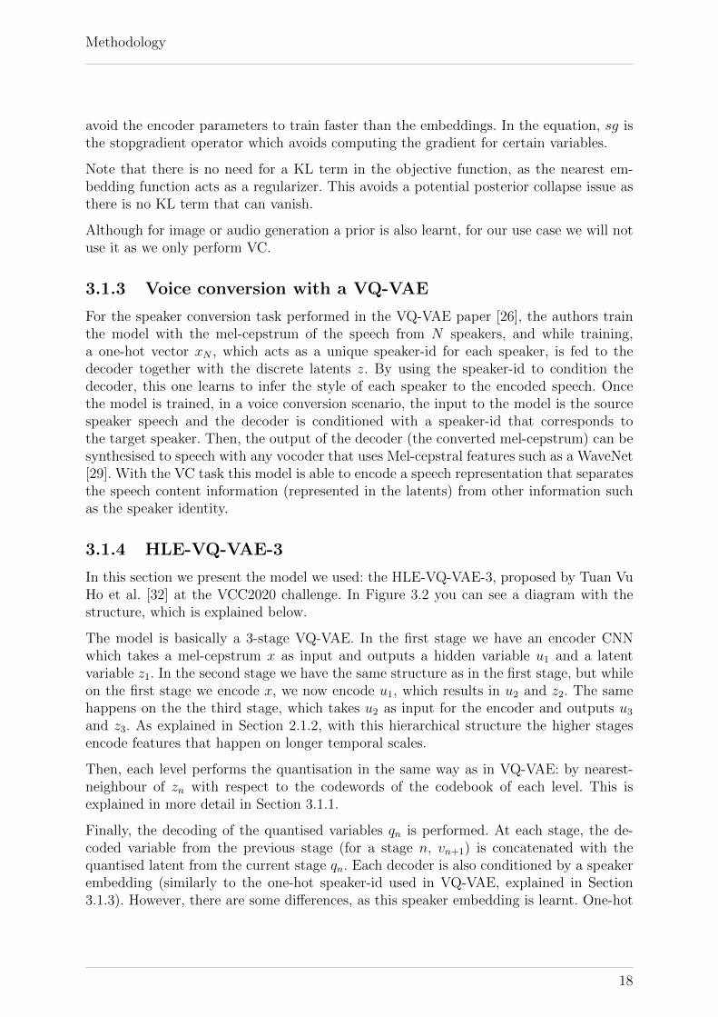
In this section we present the model we used: the HLE-VQ-VAE-3, proposed by Tuan VuHo et al. [32] at the VCC2020 challenge. In Figure 3.2 you can see a diagram with thestructure, which is explained below.

The model is basically a 3-stage VQ-VAE. In the first stage we have an encoder CNNwhich takes a mel-cepstrum x as input and outputs a hidden variable u1 and a latentvariable z1. In the second stage we have the same structure as in the first stage, but whileon the first stage we encode x, we now encode u1, which results in u2 and z2. The samehappens on the the third stage, which takes u2 as input for the encoder and outputs u3and z3. As explained in Section 2.1.2, with this hierarchical structure the higher stagesencode features that happen on longer temporal scales.

Then, each level performs the quantisation in the same way as in VQ-VAE: by nearest-neighbour of zn with respect to the codewords of the codebook of each level. This isexplained in more detail in Section 3.1.1.

Finally, the decoding of the quantised variables qn is performed. At each stage, the de-coded variable from the previous stage (for a stage n, vn+1) is concatenated with thequantised latent from the current stage qn. Each decoder is also conditioned by a speakerembedding (similarly to the one-hot speaker-id used in VQ-VAE, explained in Section3.1.3). However, there are some differences, as this speaker embedding is learnt. One-hot

18

Methodology

Figure 3.2: HLE-VQ-VAE-3 diagram. Extracted from [32].

embeddings are limited by the dimension of the vector (in this case the maximum num-ber of speakers would be the length of the vector). So, as proposed in [56], the speakerembeddings are learned during training. Note that for any new target speaker, we couldfine-tune the speaker embeddings without retraining the VC model. Then, on inference,the target speaker embedding can be retrieved by a table lookup and we can performvoice conversion, as explained in Section 3.1.3.

Once we have the converted mel-cepstrum, we use a Parallel WaveGAN vocoder1 [57] inorder to resynthesise it to the speech waveform.

3.2 Automatic speech recognition model

In Section 2.2.5 we concluded that probably the SOTA model for dysarthric speech recog-nition would be the model presented in Dysarthric Speech Recognition with Lattice-freeMMI [1]. However, for the sake of comparability with Harvill et al. [35] experiments, weuse the same CTC-based ASR model they propose. We do that under the assumptionthat if the data augmentation approach improves the results for one ASR model, it willalso do so for another one.

The ASR model has an input dimension of 80 which corresponds to the dimension ofthe mel spectrogram and is composed by 4 bidirectional long short-term memory layers(BLSTMs) of size 200, followed by a couple of fully-connected layers of size 500. Themodel uses a dropout of 0.1 in the BLSTM layers. For trainig, a batch size of 16, a CTCloss function and the Adam optimizer are used. Regarding the fully-connected layers the

1https://github.com/kan-bayashi/ParallelWaveGAN

19

Methodology

model uses tanh and log softmax as activation functions for the first and second layerrespectively. In Section 3.2.1 we explain the idea behind a CTC loss function.

3.2.1 Connectionist Temporal Classification

Connectionist Temporal Classification (CTC) is a type of neural network output with itscorresponding loss function. It is used for sequence problems, thus with recurrent neuralnetworks (RNNs). In our case the sequence problem is speech recognition. One of theadvantages it provides over hybrid systems is that we do not need to know the datasetalignment. In other words, in a speech recognition task, we do not need to know whereeach phoneme begins and ends in the input utterance as long as we have its transcription.

So, for our task we want to map the input audio which is divided in time-steps X =[x1, x2, ..., xT ] to the transcripts Y = [y1, y2, .., yU ] where y values are character leveltokens. Note that T does not necessarily equal U , in other words, the audio signal can havea different length from the transcription. The alignment for X and Y (i.e. correspondencerelation between xi and yj) is not provided. The CTC algorithm gives the probability ofeach Y output given an input X. On inference, we can use this probability to find themost probable output given an input.

In order to understand how CTC deals with the alignment let’s show a simple case wherewe want to align an input X with length 5 to an output Y = [m, a, p]. The simplest wayto compute the output is to collapse the repetitions:

input X x1 x2 x3 x4 x5alignment p(at|X) m m a a poutput Y m a p

However, for speech we could have parts of silence which should be ignored and we alsoencounter a problem where the output should have the same character repeated: forexample for the word “common” the computed output would be “comon”. To overcomethese issues, CTC introduces a new token blank token, referred as ’-’ in this explanation,which is removed from the output. The procedure is shown in Table 3.1.

Table 3.1: Connectionist Temporal Classification algorithm. The most probable output Y given an inputX is computed. Each row represents the next step in the procedure.

input X x1 x2 x3 x4 x5 x6 x7 x8 x9 x10 x11Compute chars c - o o m - m o n n -Merge repeats c - o m - m o n -Remove ‘-’ c o m m o nOutput c o m m o n

20

Methodology

The CTC loss for an X, Y pair is:

p(Y|X) =∑

A∈AX,Y

T∏t=1

p(at|X) (3.4)

where p(Y |X) is the CTC conditional probability,∑

A∈AX,Y marginalizes over the set of

valid alignments and∏T

t=1 p(at|X) computes the probability for a single alignment step-by-step. To compute the output characters, we could just take the most probable outputcharacter: at each time-step, we get the probability of each possible output character Yoccurring, so we choose this one. So, we want to solve:

Y∗ = argmaxY p(Y|X)

Where Y is the output. The simplest solution is:

A∗ = argmaxA

T∏t=1

pt(at|X)

Where A is a single alignment. In other words, we choose the alignment that maximisesthe CTC conditional probability (see Equation 3.4).

Although this can work well for many situations it might miss outputs with higher proba-bilities as we are not taking into account that a single output can have many alignments.For example: both [a,a,a] and [a,a,-] individually, might have lower probability than [b,b,b]by itself. However, if summed it could be higher. If this happens, we would be choosingY = [b] when the most probable output is Y=[a]. To solve that a modified beam searchcan be used.

While a vanilla beam search computes the new possible outputs at each time step andkeeps track of the top candidates for the next time step, we can change it to, instead ofkeeping all the alignments, keep the output after merging the repeats and removing theblank tokens. In this way, [a,a,a] and [a,a,-] probabilities would be summed as they wouldbe part of the same computed sequence [a].

3.2.2 Language Model

Also for comparability, we use the language model used in [35]. It is basically a phoneN-gram model with maximum N = 15. This value corresponds to the longest phonesequence in the database (see Section 4.1) with the start-of-sentence (SOS) and end-of-sentence (EOS) tokens included. A beam search with a width of 20 is done over all possiblesequences and the ASR model and the language model log probabilities are weightedequally. In order to reduce the decoding time, all frames are removed where the ASRhighest probability prediction is a blank symbol. SOS is then chosen as the first symboland the decoding is performed after it. In this way only sequences that correspond to aword in the dictionary are taken into account.

21

Chapter 4

Experimental Framework

In this chapter, we describe how we plan to carry out the experiments. First, in Section4.1, we present the selected corpus and explain the preprocessing process. Then, in Section4.2, we show the dysarthric ASR task together with the configuration of the experimentsperformed. Finally, in Section 4.3, we explain the design of the subjective analysis of theVC model for dysarthric speech.

4.1 Dataset, preprocessing and feature extraction

For our experiments, we use the UASpeech corpus [11]. This database is composed ofisolated-word recordings of 15 speakers with dysarthria. The total number of words is449, which correspond to digits (10), letters from the International Radio Alphabet (26),computer commands (19), common words (100) and uncommon words (300). All wordsare pronounced three times for each speaker except for the uncommon words, which arepronounced only once. For each speaker, the recordings are divided in 3 blocks of equallength (B1, B2 and B3). Note that the words pronounced for each block are the sameamong the speakers. The speakers are divided into four groups based on their intelligibilityas determined by a human transcription experiment: very low, low, mid and high, whichcorrespond to 75-100%, 50-75%, 25-50% and 0-25% of word error rate (WER), respectively.The database also includes the recordings from 13 control speakers (speakers withoutspeech impediments).

Most of the preprocessing is done following the work done in [35]: we remove the stationarynoise with the Python package Noisereduce [58] and we cut the silence from the beginningand end of the clips.

Then, for the utterances used to train the proposed VC model (HLE-VQ-VAE-3), weapply a resampling from 16kHz to 24kHz with Sox1 and normalise it. Afterwards, weextract 80-dimension mel-spectrograms from the samples (in a similar way to [59]) tocompute the mel-cepstrum, which is used as input to our VC model. Once converted,these are resampled back to 16kHz to train the ASR model.

1http://sox.sourceforge.net

22


Finally, we extract the mel log spectrogram of the files used by the ASR model (either con-verted by the VC model or directly taken from the UASpeech corpus and preprocessed).This is done using Librosa [60] with 80 mel frequency bins and 10ms of frame shift.

For our task, which is proposed in Harvill et al. [35] and explained in Section 4.2.1 andin Figure 4.1, the 449 words are divided in two groups: a “seen” and an “unseen” datasplit. The seen split is divided in a training and a validation partition with 98% and 2%of samples respectively. The unseen split is divided differently for the control speech andthe dysarthric speech: for the control speech the unseen validation set consists of oneutterance of each unseen word from each speaker and the rest is for the unseen trainingset (we do not have a test set), while for the dysarthric speech both the test and thevalidation set consist of one utterance of each unseen word from each speaker and the restis for the unseen training set.

The vocoder we use to synthesize the voice converted mel-cepstrums (see Section 3.1.4) istrained using the VCTK dataset [61]. This consists of the speech from 108 native Englishspeakers with different accents. The preprocessing consists of downsampling the tracksfrom 48 kHz to 24 kHz.

4.2 Improving automatic speech recognition of dysarthric

speech

4.2.1 Task

In order to answer our first research question Can we improve ASR systems performancefor dysarthric speech by doing unimpaired to dysarthric non-parallel voice conversion asmeans of data augmentation? (see Section 1.3.1 for more detail) we perform the taskpresented in Harvill et al. [35] with the model we propose in Section 3.1.4. It is worthmentioning that to the best of our knowledge there are no results for a similar task withother non-parallel voice conversion works, so we compare the results with the closest one,which uses parallel data.

The task consists of training an ASR to recognise words for which there are no recordingsin the dysarthric database. The motivation is that already-proposed data augmentationtechniques over the training data [39, 62, 63] only improve ASR of the words on thetraining data. For commercial applications, the publicly available datasets do not havea big enough vocabulary, so in [35] a task to recognise words outside this vocabulary isproposed. In this way, we can evaluate our method for recognising any word pronouncedby a dysarthric speaker instead of only for the words available in the training data. Todo that, the data is split into two partions: seen and unseen. In this division, of the449 unique words in the UASpeech corpus, half are chosen as seen and half as unseen.The seen partition represents the dysarthric speech available data for training. The unseenpartition is used to test the ASR system on dysarthric speech for out-of-vocabulary words,i.e we want to test the performance of the ASR system for unseen dysarthric words. Fortraining we have access to the seen dysarthric speech and the control (unimpaired) speech(partitions are explained in detail in Section 4.1). The entire workflow is shown in Figure

23


4.1 and explained below. The first step is training the VC model. This is done in a differentway for the parallel and non-parallel voice conversion methods (detailed in Section 4.2.2).When we train a VC in a parallel manner we use the seen control speech as input to convertit to the corresponding seen dysarthric speech utterance. So we use the seen control speechand the seen dysarthric speech. However, in a non-parallel VC, during training we only usethe dysarthric seen data because the VC model (in our case, the HLE-VQ-VAE-3) learnsto reconstruct the input signal, as explained in Section 3.1.4. Then, the second step is touse the trained VC model to convert the unseen control speech partition to synthesizedunseen dysarthric speech (referred as augmented in the Figure). On the third step we usethe synthesized dysarthric data to train the ASR model. To do that, the synthetic data isaugmented by a factor of three using SpecAugment [64], a method proposed by Park etal. that acts as a regulariser and improves generalization by applying time-warping, andtime-frequency masking. Finally, we test the ASR model on the unseen partition of thedysarthric data. Ideally, we would want this ASR to perform better for dysarthric speechthan if it was trained on unimpaired speech.

Figure 4.1: Task design with a parallel and a non-parallel VC approach. Diamond shape refers to controlspeech (unimpaired), and square to dysarthric speech. Blue, red and orange refer to seen, unseen andaugmented data respectively as well as the S, U and A letters. Adapted from [35].

4.2.2 Algorithms

Parallel voice conversion

Below, we show the parallel VC methods used in the experiments: the attention methodproposed in [35] and the DC-GAN (which is a baseline method used in [35]).

24


Attention First of all, the normal and dysarthric utterances are time-aligned usingdynamic time warping (DTW). For the DTW algorithm dtwalign2 is used, with 12-dimensional mel cepstrum envelope (MCEP) features per frame and a frame shift of10ms. Then, the computed DTW is used to time-align the mel log spectrogram features.The VC model is composed of 6 multi-head attention layers [36] with 8 heads each anda dimension of 80 which corresponds to the number of frequency bins. For training, theinput to the VC model are the seen unimpaired time-aligned utterances. Then, a mean-squared error (MSE) loss is applied to the output. The MSE corresponds to the differencebetween the network dysarthric predicted samples and the ones of the dysarthric database.The authors use an Adam optimizer, a batch size of 1, and train the model for 150,000iterations.

DC-GAN The DC-GAN implementation we use is from [35] which is based on the oneused in [25] with some differences: while in [25] the authors use separate networks forMCEP and band aperiodicity features for training, the implementation done by [35] usesmel log spectrograms to be more similar to the attention system. The rest of the workflowis the same as in the attention model, but using a batch size of 32 and training for 10,000iterations.

Non-parallel voice conversion

HLE-VQ-VAE-3 As mentioned, the model we use to perform the VC, the HLE-VQ-VAE-3, performs the VC in a non-parallel manner. The workflow is as follows: First, wetrain the HLE-VQ-VAE-3 (step 1 in Figure 4.1). The other steps are performed as in theother methods but at the end of step 2, after doing the VC of the unseen unimpairedsamples to the synthetic unseen dysarthric samples, we perform a resampling from 24kHzto 16kHz and apply time-stretching to the samples with Sox in the same way that isdone in Xiong et al. [39] (see explanation in Section 2.1.5). Note that we do not use thephoneme-based method, but we stretch the samples with a ratio computed per each targetspeaker.

Lack baseline

In the lack baseline, which is taken from [35] experiments design, we test the scenariowhere we lack all dysarthric speech. To do that we train the ASR with the unimpairedspeech (unseen train and validation control partitions), to test how it performs with thesame words with dysarthric speech (dysarthric unseen test data) as in the other methods.As with the other algorithms, we train the ASR model with the data augmented by a factorof three using SpecAugment [64]. So, in this case instead of augmenting the dysarthricsynthetic data, we augment the unseen control data.

Lack baseline without SpecAugment

We also apply the lack baseline method to train the ASR without SpecAugment.

2https://github.com/statefb/dtwalign/

25


4.2.3 Experimental design

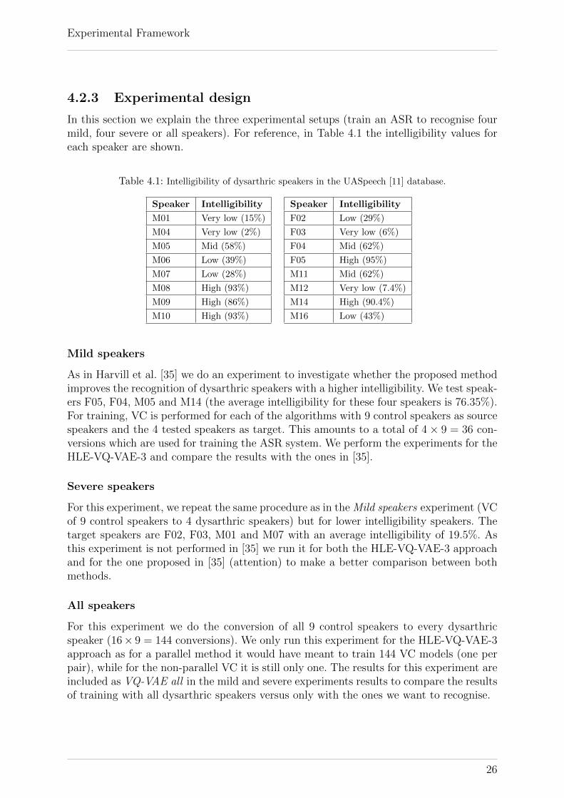
In this section we explain the three experimental setups (train an ASR to recognise fourmild, four severe or all speakers). For reference, in Table 4.1 the intelligibility values foreach speaker are shown.

Table 4.1: Intelligibility of dysarthric speakers in the UASpeech [11] database.

Speaker Intelligibility

M01 Very low (15%)

M04 Very low (2%)

M05 Mid (58%)

M06 Low (39%)

M07 Low (28%)

M08 High (93%)

M09 High (86%)

M10 High (93%)

Speaker Intelligibility

F02 Low (29%)

F03 Very low (6%)

F04 Mid (62%)

F05 High (95%)

M11 Mid (62%)

M12 Very low (7.4%)

M14 High (90.4%)

M16 Low (43%)

Mild speakers

As in Harvill et al. [35] we do an experiment to investigate whether the proposed methodimproves the recognition of dysarthric speakers with a higher intelligibility. We test speak-ers F05, F04, M05 and M14 (the average intelligibility for these four speakers is 76.35%).For training, VC is performed for each of the algorithms with 9 control speakers as sourcespeakers and the 4 tested speakers as target. This amounts to a total of 4× 9 = 36 con-versions which are used for training the ASR system. We perform the experiments for theHLE-VQ-VAE-3 and compare the results with the ones in [35].

Severe speakers

For this experiment, we repeat the same procedure as in the Mild speakers experiment (VCof 9 control speakers to 4 dysarthric speakers) but for lower intelligibility speakers. Thetarget speakers are F02, F03, M01 and M07 with an average intelligibility of 19.5%. Asthis experiment is not performed in [35] we run it for both the HLE-VQ-VAE-3 approachand for the one proposed in [35] (attention) to make a better comparison between bothmethods.

All speakers

For this experiment we do the conversion of all 9 control speakers to every dysarthricspeaker (16× 9 = 144 conversions). We only run this experiment for the HLE-VQ-VAE-3approach as for a parallel method it would have meant to train 144 VC models (one perpair), while for the non-parallel VC it is still only one. The results for this experiment areincluded as VQ-VAE all in the mild and severe experiments results to compare the resultsof training with all dysarthric speakers versus only with the ones we want to recognise.

26


4.3 Pathological voice conversion

In order to answer RQ2.1 and RQ2.2 (see Section 1.3.2 for more detail) we performeda subjective analysis of dysarthric-to-dysarthric voice converted samples with HLE-VQ-VAE-3. This work was accepted in the form of a paper to the 11th ISCA Speech SynthesisWorkshop (SSW11) under the title “Pathological voice adaptation with autoencoder-based voice conversion” [65].

4.3.1 Experimental design

The dataset and preprocessing used are the same as presented in Section 4.1 (UASpeechwith noise removal, silence cut, audio resampling from 16kHz to 24kHz, normalizationand 80-dimension mel spectrograms extraction.

The VC model used is the one we propose in this thesis, the HLE-VQ-VAE-3, explainedin Section 3.1.4 with the same vocoder (Section 4.1).

Design details

Voice conversion

sourcespeaker

convertedspeech

targetspeaker(healthy)

Voice conversion

sourcespeaker

convertedspeech

targetspeaker

(pathological)

EVALUATION

APPLICATION

VOICE BANK

selection of speakerbased on metadata

0 0 1 0 0 0

0 0 1 0 0 0

speaker embedding

speakerconditioning

speaker embedding

speakerconditioning

groundtruth

Figure 4.2: Outline of our approach: the speechfrom a model pathological speaker is convertedinto speech with the characteristics of anotherpathological speaker. Red/orange colours de-note the identity of the speaker. Taken from[65].

As a reminder, in this study, we customisepathological speech to a different pathologi-cal speaker’s voice characteristics. However, theclinical application would need customisationto an unimpaired speaker’s characteristics. Inthe top panel of Figure 4.2, the application sce-nario is visualised, i.e., how the system could beused in a clinical setting. In the bottom part,our proposed evaluation scenario is illustrated.

Looking at the top panel, a source pathologi-cal speaker is first selected from a large voicebank consisting of many samples of patho-logical speakers. Based on metadata, a clini-cal team could decide the kind of pathologicalspeech degradation which is most likely for apatient. In the work, we pair up by severity,but in actual practice an appropriate sourcespeaker could be found matched by age, re-gion, and type of treatment. This leads to a se-lection of a source pathological speaker. Usinga small amount of a new patient’s voice (tar-get speaker), a speaker embedding can be ex-tracted using the VQ-VAE based technique. Fi-nally, we obtain the converted speech, which isexpected to be pathological, but with the newpatient’s voice characteristics. The problem isthat for the UASpeech, we don’t have parallel

27


pre-pathology and post-pathology voices. Therefore, a separate evaluation scheme has tobe setup where we assume that the pathological and the unimpaired speaker embeddingsshould be unchanged for the same speaker, which is not always true, we refer to furtherdiscussion about this in Section 5.2.3.

Table 4.2: Speaker pairs used for the VCexperiments and their subjective WER dif-ferences. Between parentheses () the WERis also specified for each speaker.

Speaker A Speaker B ∆WER (%)M04 (2%) M12 (7.4%) 5.4%M05 (58%) M11 (62%) 4%M08 (93%) M10 (93%) 0%

The evaluation scheme is explained in the bot-tom panel. To circumvent the problem with thepre-pathology and post-pathology, we changethe conversion process for the evaluation as fol-lows. Instead of a new healthy speaker, we en-roll a new dysarthric speaker with a matchedintelligibility of the speech pathology fromthe UASpeech dataset because a ground truth(GT) is available there. The converted speechcan then be compared to this GT to provide aproof of concept for the system.

In our experiments, we convert the speech of three speaker pairs in both directions. Thesetup for the experiments is the following: we train the VC model with all B1 and B3sets of words of every dysarthric speaker to stay consistent with the standard UASpeechtrain-test partitioning.

We perform VC on the speech from B2 between speakers with a similar level of dysarthria.The selected dysarthric speaker pairs along with their corresponding human transcriptionerror rates from UASpeech are summarised in Table 4.2. Unfortunately, it has not beenpossible to include females speakers because all female speakers had a different severityin the UASpeech dataset. Other important factors such as the type of dysarthria are notcontrolled in this design.

Experiments

In order to answer our research questions, we performed subjective evaluation experi-ments. In order to answer RQ2.1 a subjective speaker similarity experiment was carriedout, while for RQ2.2 a subjective naturalness experiment was carried out. The design ofthese experiments (including the composition of different stimuli) closely follow those ofthe VCC challenge standards [66, 67]. These experiments were run on the Qualtrics plat-form, and the participants (10 American English native listeners) were recruited throughProlific. All participants were remunerated justly (7.80 GBP per hour).

For the naturalness experiment, we used a mean opinion score3 (MOS) naturalness test.We hypothesised that listeners will not be able to distinguish between the distortions in theaudio and the pathological characteristics of the speech. To account for this, we includedGT stimuli in the naturalness test, which allows direct comparison of naturalness with realsamples. The GT shows the maximum attainable naturalness (second part of RQ2.2) andthe differences of the GT and VC scores show the reduction due to the synthetic aspects.

3Mean opinion score is a measure of quality. It is defined by a numeric value ranging from 1 to 5(1-Bad, 2-Poor, 3-Fair, 4-Good, 5-Excellent) and it corresponds to the arithmetic mean of individualratings in a panel of users.

28


To answer the first part of RQ2.2, we included unimpaired, natural stimuli, which allows usto measure the reduction in naturalness due to the reduction intelligibility. Nevertheless,we encouraged listeners to ignore the atypical aspects of the speech, by adopting thenaturalness question from the VCC2020 [66]: “Listen to the following audio and rate itfor quality. Some of the audio samples you will hear are of high quality, but some of themmay sound artificial due to deterioration caused by computer processing. Please evaluatethe voice quality on a scale of 1 to 5 from “Excellent” to “Bad.” Quality does not meanthat the pronunciation is good or bad. If the pronunciation of the English is unnaturalbut the sound quality is very good, please choose “Excellent.”. The VCC2020 questionwas proposed for cross-lingual VC, where pronunciation errors could appear, similar topathological speech.

For the speaker similarity test, we used an AB test in which listeners were asked to lis-ten to two stimuli, and indicate if they thought they came from the same speaker, andrate their confidence in this decision. The question for the speaker similarity was directlyadopted from the VCC2016 challenge [67]: “Do you think these two samples could havebeen produced by the same speaker? Some of the samples may sound somewhat degrad-ed/distorted. Please try to listen beyond the distortion and concentrate on identifying thevoice. Are the two voices the same or different? You have the option to indicate how sureyou are of your decision.” Participants were then asked to rate the stimuli on a 4-pointscale: Same (absolutely sure), Same (not sure), Different (not sure), Different (absolutelysure).

29

Chapter 5

Results and Discussion

In this chapter, we present and discuss the results of the experiments presented in Chapter4. First, in Section 5.1, we show the dysarthric ASR experiments results and then, inSection 5.2, we continue with the subjective analysis experiments. At the end of eachsection, we draw conclusions.

5.1 Improving automatic speech recognition of dysarthric

speech

5.1.1 Results

The results are shown in Tables 5.1 and 5.2 for mild and severe speakers experimentsrespectively. The values in the tables correspond to the mean WER, rounded to thenearest decimal. Each row corresponds to a different method, and the columns correspondto the different speakers with the last column being the WER mean for each method. Asmentioned in Section 4.2.1 all data is augmented using SpecAugment except in the Lackbaseline no SpecAugment method.

Mild speakers The results for the mild speakers experiment are shown in Table 5.1.As a reminder, in the VQ-VAE mild the ASR is trained with synthetic dysarthric samplesthat are generated by converting utterances of 9 control speakers to each of the 4 mildspeakers shown in the table, as in Attention and DC-GAN methods. In VQ-VAE all theASR is trained with the control speech converted to all available dysarthric speakers. Inthe Lack baseline the ASR is trained directly with the control speech. The Lack baselinewithout SpecAugment is the same as Lack baseline but without applying SpecAugmentby a factor of three to the ASR training samples. Results for Attention, DC-GAN andLack baseline are taken from Harvill et al. [35].

30


Table 5.1: %WER for mild speakers. The rows correspond to the different methods to generate the ASRtraining data and the columns to the different speakers. In bold: best WER, in italic: best non-parallelVC WER. Results for attention, DC-GAN and Lack baseline taken from [35].

F05 M14 F04 M05 mean WERVQ-VAE mild 25.9 21.7 55.7 59.1 40.6VQ-VAE all 26.8 32.6 57.1 55.8 43.1Attention [35] 15.8 15.8 34.9 50.6 29.3DC-GAN [35] 35.6 22.3 58.0 59.9 44.0

Lack baseline [35] 24.7 24.3 50.9 58.4 39.6Lack baseline no SpecAugment 41.1 36.6 69.9 89.7 59.3

In Table 5.1 we can see that the Attention method has the best performance. This isno surprise as in other works, parallel VC has better WER than non-parallel VC [68].However, regarding our two non-parallel approaches VQ-VAE mild and VQ-VAE all showto be better than DC-GAN which is the baseline in [35]. Of the two VQ-VAE approachesthe one that performs best is VQ-VAE mild, probably because although in VQ-VAE allthe ASR has more training data, the conversions to more severe dysarthric speakers arecounterproductive for training the ASR for mild speakers. Although being better thanDC-GAN, VQ-VAE mild does not perform better than Lack baseline (it only performsbetter for speaker M14). By comparing Lack baseline and Lack baseline no SpecAugment,it can also be seen that SpecAugment improves the results substantially (a 19.7 lowerWER in this case).

Severe speakers The results for the severe speakers experiment are shown in Table5.2. As a reminder, in the VQ-VAE severe the ASR is trained with synthetic dysarthricsamples that are generated by converting utterances of 9 control speakers to each of the4 severe speakers shown in the table, as in Attention. In VQ-VAE all, the ASR is trainedwith the control speech converted to all dysarthric speakers in the database (it is thesame model as in Table 5.1). As in the mild speakers experiment, in the Lack baselinemethod the ASR is trained directly with the control speech, and Lack baseline withoutSpecAugment is the same scenario as Lack baseline but without applying SpecAugmentby a factor of three to the ASR training samples.

Table 5.2: %WER for severe speakers. The rows correspond to the different methods to generate the ASRtraining data and the columns to the different speakers. In bold: best WER, in italic: best non-parallelVC WER.

F02 F03 M01 M07 mean WERVQ-VAE severe 86.6 93.7 88.8 80.8 87.5VQ-VAE all 90.2 91.9 90.6 74.1 86.7Attention 88.0 88.0 89.3 67.4 83.2

Lack baseline 87.5 95.5 92.4 88.8 90.9Lack baseline no SpecAugment 97.3 96.9 94.2 93.3 95.4

By looking at the severe speakers experiment in Table 5.2, we can see that both VQ-VAE severe and VQ-VAE all improve the results from the Lack baseline method. In the

31


case of VQ-VAE severe this happens for all speakers and for VQ-VAE all for 3 out ofthe 4 speakers. Differently from the mild speakers experiment, between the ASR trainedwith only the 4 tested speakers VC samples (VQ-VAE severe) and the one that uses alldysarthric speakers as target speakers (VQ-VAE all), the latest performs slightly better(with a WER difference of 0.7). When comparing VQ-VAE all and lack baseline we cansee that training with the synthetic dysarthric data gives a lower WER value (4.2 WERdifference) than when training with control data. Attention is again the method thatperforms the best, although by a lower margin (3.5 WER difference). When comparingLack baseline with Lack baseline no SpecAugment, we can see that using SpecAugmentby a factor of three gives better results with a WER improvement of 4.5.

5.1.2 Conclusions

In this work, we propose a method to improve automatic speech recognition of dysarthricspeech by using a non-parallel voice conversion approach. In order to do that, we performa task proposed by Harvill et al. [35] where we train an ASR to recognise words for whichthere are no recordings in the dysarthric database.

We show how, following the proposed method, we can use synthetic dysarthric speechsamples generated via non-parallel VC to train an ASR model and improve the WER fordysarthric speech of severe speakers with respect to training the same ASR model withreal unimpaired speech samples. However, this method does not show an improvement forthe case of mild dysarthric speakers.

For mild dysarthric speakers, we see how our method performs better than the DC-GAN,(44.0% vs 40.6% of WER) but it is not able to improve the lack baseline results (40.6% vs39.6%). This needs to be further investigated, but we hypothesize that it might be relatedto the fact that the synthetic VC samples contain some quality degradation (in Section5.2.1 we discuss how for the high intelligibility dysarthric speakers the naturalness of thevoice converted samples is affected) and although we are able to infer the speaker style(this is shown in Section 5.2.2), it might not be enough to get better results than whentraining with real unimpaired speech samples. In other words, there is a chance that thedegradation in naturalness outweighs the improvement of making the speech style moredysarthric.

As mentioned in Section 4.2, we compare the results of the proposed non-parallel VCmodel with other parallel methods because there are no other results in this line, so wechose the closest work. Although attention results are the best, non-parallel VC is valuablein scenarios where we lack data and its collection is hard, such as in dysarthric speechrecognition. Also, in VQ-VAE-based methods, differently from DC-GAN and attention,we only need one model to perform the conversions (any-to-many). It is also possible toperform conversions to unseen speakers by fine-tuning the embedding table only insteadof training a new model, and we get a speaker embedding that can be used in one-shotlearning scenarios.

Whether the dysarthric VC samples can be used together with unimpaired speech samplesin other data augmentation set-ups, could also be further investigated.

32


5.2 Pathological voice conversion

The results are divided in the following Sections: naturalness and similarity, shown inSections 5.2.1 and 5.2.2 respectively. Then, we discuss the limitations of the proposedapproach in Section 5.2.3, the accessibility of VC to atypical speakers in Section 5.2.4 andfinally, we draw the conclusions in Section 5.2.5. Some of the voice converted samples areavailable at https://pathologicalvc.github.io .

5.2.1 Naturalness

The results of the naturalness experiments are presented in Figure 5.1, which shows theMOS score for each of the seven types of speech tested, grouped by intelligibility, and withtheir 95% confidence intervals indicated. For clarity, the actual MOS scores are indicatedon top of each bar.

HealthyHigh (GT)

High (VC)Mid (GT)

Mid (VC)Low (GT)

Low (VC)1

2

3

4

5M

OS sc

ore

4.32 4.3

2.52.02.1 1.9 1.8

Figure 5.1: Mean opinion scores for natural-ness grouped by intelligibility with 95% con-fidence intervals. Blue denotes original, whileorange denotes VC samples. Taken from [65].

We first focus on the question how GT patho-logical speech affects the naturalness perceivedby listeners (RQ2.2) which is measured by theMOS score. Figure 5.1 shows that unimpairedspeech and GT high intelligibility dysarthricspeech have a similar MOS score. However, asintelligibility decreases, so does the MOS score,indicating that the MOS score not only cap-tures naturalness but is influenced by the in-telligibility of the speech. These results showthat naive listeners cannot separate severity ofa pathology and unnaturalness when asked tojudge the naturalness of a speech sample. Thisalso means that the GT MOS results are anupper bound on the achievable naturalness ofsynthetic pathological samples.

Regarding the synthetic pathological speech, the performance on the high (VC) samples issomewhat lower than the performance of the HL-VQ-VAE-3 model on the VCC2020 chal-lenge and identical to the performance of autoencoder-based models (2.1) [32]. However,the type of stimuli is different, so the differences in MOS are not directly comparable.The difference is most likely due to channel differences, the decreased intelligibility ofthe speech, and the different sampling frequency (UASpeech is 16 kHz, while VCC202024 kHz). When we compare the MOS scores for the converted speech of the differentintelligibility speakers, we observe a slight degradation in naturalness with decreasing in-telligibility. Comparing the VC and GT results, however, we observe a large degradationfor the converted high intelligibility speech (Wilcoxon signed-rank test: p ≤ 0.05). Thedifference in VC and GT MOS scores for the mid and low intelligibility speakers is muchsmaller (Wilcoxon signed-rank test: mid p ≤ 0.05, low p ≥ 0.05). Returning to RQ1, wecan conclude that the synthetic speech of mid and low intelligibility pathological speak-ers have a naturalness that is perceived similar to that of real pathological speech, whilesynthetic high intelligibility pathological speech is not perceived as being as natural as

33


real high intelligibility pathological speech.

To summarise, pathological speech is not perceived natural according to the MOS scaleby naive listeners. In the case of mid and low intelligibility pathological speech, the per-ceived naturalness is similar between that of synthetic and real pathological speech. Thisis, however, not the case for high intelligibility synthesised pathological speech which israted as being far less natural than real pathological speech. The performance of the VCapproach is comparable to the one observed with typical speakers, therefore the currentmethod is accessible to typical speakers, however this does not mean that VC is accessibleto typical speakers (see Section 5.2.4).

5.2.2 Similarity

This Section presents and discusses the results of the similarity experiments in order toanswer the question whether it is possible to convert voice characteristics of pathologicalspeakers. The results are presented in Figure 5.2. In each of the 12 panels, we visualisethe results of comparing a voice converted (VC-D / VC-S) sample with the GT source (S)(Similarity to source) or the GT target (Similarity to target). Also, the GT samples arecompared between them: S samples are compared to S samples to know how recognisablethe source speaker is, T samples are compared to T samples to know how recognisablethe target speaker is and S samples are compared to T samples in order to know howdistinguishable is the source from the target speaker. Note that for each speaker pair inthe top panel the source speaker is the target one in the bottom panel and vice versa, sothis information appears repeated in Figure 5.2. Additionally letters in the case of the VCcomparisons are used to help interpretation of the figures: VC-D stands for VC-different(i.e when converting M04 to M12, the converted should be different from M04), VC-Sstands for VC-same (similarly, when converting M04 to M12, the converted should besame as M12).

S VC-D T0

20406080

100Similarity to source

S VC-S T0

20406080

100Similarity to target

S VC-D T0

20406080


S VC-S T0

20406080


S VC-D T0

20406080


S VC-S T0

20406080


S VC-D T0

20406080


S VC-S T0

20406080


S VC-D T0

20406080


S VC-S T0

20406080


S VC-D T0

20406080


S VC-S T0

20406080


M04 to M12 (low)

M12 to M04 (low)

M05 to M11 (mid)

M11 to M05 (mid)

M08 to M10 (high)

M10 to M08 (high)

Same, absolutely sure Same, not sure Different, not sure Different, absolutely sure

Figure 5.2: Results of the speaker similarity experiments grouped by intelligibility pairs. S stands forsource, T for target, VC-D for voice conversion different (VC samples should be different from source)and VC-S for voice conversion same (VC samples should be same as target). Taken from [65].

34


For the low intelligibility pair (left 2 columns of Figure 3), the speakers seem reasonablydistinguishable when looking at the GT as there is a 100% of agreement that M04 samplesare produced by M04 and 90% for M12. For the speech samples of speaker M04 convertedto speaker M12 (top panels), 73.33% of the converted samples were indicated as beingfrom speaker M12 (VC-S), meaning that the conversion is fairly successful for that pair.For the speech samples of speaker M12 converted to speaker M04 (bottom panels), 56.33%of the converted M12-M04 samples (VC-S) were indicated as being from speaker M04.The results show that for the M12-M04 conversion the model is able to remove some ofthe source speaker (M12) characteristics and add some of the target (M04) ones, althoughto a lesser extent than in the M04-M12 conversion. Therefore, we conclude that the voicecharacteristic conversions for the low intelligibility speakers are successful.

For the mid intelligibility pair (middle four panels), the M11 seems to be clearly recog-nisable as there is a 90% of agreement that M11 samples are produced by M11, howeverlisteners have difficulties recognising the voice characteristics of M05, i.e., only 20% of thetrials where both samples were from speaker M05 were judged as both being from M05.For M05-M11 the VC performs poorly, which is indicated by 90% perceiving it differentfrom the target (VC-S result). For M05-M11 the VC-S reaches a 20% of absolutely sureagreement. Notice that although it is a low score, it is the same that the GT samplesexhibit. The voice characteristic conversions for the mid intelligibility speakers are thusinconclusive: while in one case the VC fails, in the other participants fail to recognise thespeaker even from the GT samples. Further experimentation with more speaker pairs isneeded.

For the high intelligibility pairs (right 2 columns of Figure 3), the speakers seem reasonablydistinguishable. We can see that there is a 70% of agreement that M08 samples areproduced by M08 and an 80% for M10. For M08-M10, there is a 46.66% of agreementthat the converted samples sound like M10. For M10 to M08 VC, 75% of the listenersindicate that the converted samples sound like M08. We can see that some of the voicecharacteristics are successfully transferred for the high intelligibility samples, howeverwhile on the conversions M10 to M08 the result is similar to the GT samples, on theother direction (M08 to M10) there is a gap of 33.33% with respect to the GT. Thisbehaviour is the same that we observed with low intelligibility pair conversions: althoughthe speakers from the same pair are recognised with a similar agreement (100% and 90%for low intelligibility and 80% and 70% for the high intelligibility) the conversions aremore successful in one direction than on the other.

5.2.3 Limitations of the proposed approach

An assumption of the proposed approach is that the speaker identity is not affected bythe speech pathology, which is certainly untrue for speech pathologies which are dys-phonic, i.e. where the voice characteristics are known to be affected. By performing ABtesting with GT speakers, we have tried to account for these scenarios in the perceptualevaluations. From the speaker similarity experiment, we have seen that in some cases(i.e., M05) listeners had difficulties of recognising the voice characteristics even in theGT. These results confirm that the proposed approach cannot be used for all types of

35


speech pathologies. To solve this issue, we would need to have a deeper understandingof what happens to the speaker characteristics in these speech pathologies. For example,the speaker embeddings themselves could be used to predict the new pathological speakerembeddings of the same speaker, transformed according to the vocal pathology (i.e. typeof dysphonia).

5.2.4 Accessibility of voice conversion to atypical speakers

VC of atypical speech produced similar naturalness in the high intelligibility case as typicalspeech on VQ-VAE based methods. Nevertheless, we see that there is room for improve-ment compared to typical speech, as other studies employing certain non-parallel VCapproaches can achieve human-like naturalness. Unfortunately, these VC approaches can-not easily be used for our task as they often leverage linguistic features or ASR bottleneckfeatures [69, 70]. The need for ASR features is especially problematic as these featuresare extracted from ASR systems, whose performance on atypical speech is generally muchworse than that on typical speech, meaning that the quality of these extracted features arealso expected to be lower for these speakers. Therefore, we conclude that accessibility toVC is limited for atypical speakers, but this is because parallel and ASR-based techniquescan hardly be used by them.

5.2.5 Conclusions

For answering RQ2.1 and RQ2.2 we propose a new approach to pathological speech syn-thesis, by customising an existing pathological speech sample to a new speaker’s voicecharacteristics. In order to do this pathological-to-pathological speech conversion, we usean autoencoder-based VC technique (HLE-VQ-VAE-3).

When comparing our results with the ones obtained in the VCC2020 challenge dataset [32],we can see that ours are somewhat lower, which is most likely due to channel differences,the decrease in the speech intelligibility and the different sampling rate.

We find that even real pathological speech seems to affect perceived naturalness as shownby MOS scores, meaning that there is a bound on achievable naturalness for pathologicalspeech conversion.

Overall, we observe a decreasing trend in MOS with decreasing intelligibility. Therefore,for low and mid intelligibility, the difference in perceived naturalness between real andVC is small.

Conversion of voice characteristics for low intelligibility speakers is successful, for high in-telligibility it is also possible to transfer the voice characteristics partially. However, moreexperimentation is needed for the mid intelligibility with more speakers: we experiencedthat in one case the VC failed, and on the other participants fail to recognise the speakereven from the real recordings. Whether the differences in the results for the differentintelligibility levels is due to the intelligibility levels or due to other speech characteris-tics needs to be further investigated. The question of pathological intergender (male tofemale) and female VC also needs to be investigated. The performance of the approachis comparable to the one observed with typical speakers, therefore the current method

36


is accessible to atypical speakers. However, we outlined some issues such as the need forlinguistic resources and parallel data, as an obstacle for more natural VC for pathologicalspeakers.

37

Chapter 6

Conclusions and Future Work

Improving ASR of dysarthric speech

Automatic speech recognition is a technology present in our daily lives through digitalpersonal assistants. Yet these systems still fail to successfully recognise impaired speech,thereby excluding those who could benefit the most from ASR: people with physicaldisabilities who oftentimes also present speech impediments.

In this thesis, we propose a non-parallel VC method to synthesise dysarthric speech anduse it as means of data augmentation to improve ASR of dysarthric speakers. As dysarthricspeech data is scarce and hard to collect (it can be difficult to recruit enough dysarhtricspeakers and get sufficient recordings for the different types of dysarthria, severity levels,languages and accents), instead of using a parallel VC (where unimpaired and dysarthricutterances with the same linguistic content are needed for training), a non-parallel modelis trained with only dysarthric utterances. Thanks to this design, the proposed model isable to perform any-to-many conversions: only one voice conversion model needs to betrained to convert any speaker to the target speakers. Furthermore, for adding new targetspeakers only a table embedding needs to be fine-tuned (the speakers’ characteristics areencoded in a table embedding which serves to condition the decoder of the model to thetarget speaker-id). Given that the vocabulary in the available dysarthric databases is toosmall for some commercial ASR applications, we perform the task proposed in [35] whichconsists in recognising words for which there are no recordings in the dysarthric database.The results for this task show that for severe speakers, training an ASR system with thesynthesised dysarthric speech improves the WER by 4.2 points with respect to trainingit with unimpaired speech. However, for mild speakers the proposed approach does notimprove the results: the WER is 1.0 points higher.

Pathological voice conversion

Another goal of the project is to perform pathological voice conversion and evaluate it forclinical applications (i.e. informing a patient of how his voice could sound after oral cancersurgery to reduce his stress or helping clinicians to make informed decisions about thesurgery). This was work has been published in the 11th ISCA Speech Synthesis Workshop

38


[65]. In it, we propose a novel approach to pathological speech synthesis, by customisingan existing pathological speech sample to a new speaker’s voice characteristics and eval-uating the perceived naturalness and similarity. We found that real pathological speechis perceived as less natural than unimpaired speech. As intelligibility decreases, so doesthe MOS score, showing that naive listeners are not able to separate the severity of thepathology from the naturalness. For mid and low intelligibility speakers the perceivednaturalness is close to that of the real samples. For high intelligibility, the results areworse, which is something that also happens in the dysarthric ASR experiments. For thesimilarity evaluation, the best results are for the low intelligibility speakers where voicecharacteristics are transferred successfully, for high intelligibility it is also possible totransfer the voice characteristics partially, and for mid intelligibility speakers, the resultsare inconclusive: we experienced that in one case the VC failed, and on the other, partici-pants fail to recognise the speaker even from the real recordings. Whether the differencesin the results for the different intelligibility levels are due to the intelligibility levels ordue to other speech characteristics needs to be further investigated.

Future work

VQ-VAE-based models have discrete codes, which allow for an easier analysis of the latentspace. As the proposed system has a hierarchical structure, it is possible that performingsome regularisation of the latent space, could lead us to control the dysarthric speechstyle and have a better understanding of how the network is modelling the dysarthricspeech. Being able to control the dysarthric speech style could be of use for creating moresynthetic dysarthric speech, even for styles for which we do not have data, while havinga better understanding of the network behaviour could be useful to design improvementsover it.

Speaker adaptation is known to improve the performance of ASR models. A typical usecase is accented speech [71], but another one is dysarthric speech as the speech style variesacross the multiple types of dysarthria. Therefore, we believe that using the learnt speakerembeddings of the VC model in the ASR model as a form of speaker-adaptation, couldimprove the recognition for those speakers.

Other ASR models explored in the literature review (such as [1]) might give better resultsthan the CTC-based ASR we use. Further work includes trying more ASR models toachieve the lowest possible WER.

In both performed tasks, there are differences in the results among different speakers. Ex-ploring the results with more speakers with different intelligibility levels, gender and typeof dysarthria and analysing their differences could help to have a better understanding ofthe performance of these systems for different dysarthric speakers.

Finally, other data augmentation setups, such as joining unimpaired or dysarthric speechwith the synthesised speech, are possible and could be explored. Depending on the num-ber of recognisable words needed, some setups might be better than others for certainapplications, for example, recognising a keyword for calling an emergency number versusa personal assistant with multiple functions.

39


Final thought

This thesis provides an insight into non-parallel voice conversion for pathological speakersand its applications. With our contribution, the process of synthesising dysarthric speechis simplified and it becomes more accessible as less data is required. Although there isstill a lot of work to be done to adapt voice technologies to pathological speakers, it isencouraging to see that the research field gains traction and more robust systems are builtfor people with speech impediments.

40

Bibliography

[1] Enno Hermann and Mathew Magimai.-Doss. Dysarthric speech recognition withlattice-free MMI. In Proceedings International Conference on Acoustics, Speech, andSignal Processing (ICASSP), pages 6109–6113, 2020.

[2] P. Virginia Good Megan J. McAuliffe, Stephanie A. Borrie and Louise E. Hughes.Motor speech disorders. ACQ, Speech Pathology Australia, (Volume 12, Number1):18, 2010.

[3] Lewis P Rowland and Neil A Shneider. Amyotrophic lateral sclerosis. New EnglandJournal of Medicine, 344(22):1688–1700, 2001.

[4] Anthony E Lang and Andres M Lozano. Parkinson’s disease. New England Journalof Medicine, 339(16):1130–1143, 1998.

[5] Luigi De Russis and Fulvio Corno. On the impact of dysarthric speech on contempo-rary asr cloud platforms. Journal of Reliable Intelligent Environments, 5(3):163–172,Sep 2019.

[6] Robert DeRosier and Ruth S. Farber. Speech recognition software as an assistivedevice: A pilot study of user satisfaction and psychosocial impact. Work, 25:125–134, 2005. 2.

[7] Joel Shor, Dotan Emanuel, Oran Lang, Omry Tuval, Michael Brenner, Julie Cattiau,Fernando Vieira, Maeve McNally, Taylor Charbonneau, Melissa Nollstadt, et al. Per-sonalizing asr for dysarthric and accented speech with limited data. arXiv preprintarXiv:1907.13511, 2019.

[8] Bence Mark Halpern, Julian Fritsch, Enno Hermann, Rob van Son, Odette Scharen-borg, and Mathew.-Magimai Doss. An objective evaluation framework for patholog-ical speech synthesis. Submitted to Signal Processing Letters, 2021.

[9] Bence Mark Halpern, Rob van Son, Michiel van den Brekel, and Odette Scharenborg.Detecting and Analysing Spontaneous Oral Cancer Speech in the Wild. In Proc.Interspeech 2020, pages 4826–4830, 2020.

[10] JR Duffy. Defining, understanding, and categorizing motor speech disorders. MotorSpeech Disorders—Substrates, Differential Diagnosis, and Management, pages 3–16,2013.

41

BIBLIOGRAPHY

[11] Heejin Kim, Mark Hasegawa-Johnson, Adrienne Perlman, Jon Gunderson, Thomas SHuang, Kenneth Watkin, and Simone Frame. Dysarthric speech database for univer-sal access research. In Ninth Annual Conference of the International Speech Com-munication Association, 2008.

[12] Frank Rudzicz, Aravind Kumar Namasivayam, and Talya Wolff. The torgo databaseof acoustic and articulatory speech from speakers with dysarthria. Language Re-sources and Evaluation, 46(4):523–541, 2012.

[13] Catherine Middag. Automatic analysis of pathological speech. PhD thesis, GhentUniversity, 2012.

[14] Siyuan Feng, Olya Kudina, Bence Mark Halpern, and Odette Scharenborg. Quanti-fying bias in automatic speech recognition. arXiv preprint arXiv:2103.15122, 2021.

[15] Martine Adda-Decker and Lori Lamel. Do speech recognizers prefer female speakers?In Ninth European Conference on Speech Communication and Technology, 2005.

[16] Laureano Moro-Velazquez, JaeJin Cho, Shinji Watanabe, Mark A. Hasegawa-Johnson, Odette Scharenborg, Heejin Kim, and Najim Dehak. Study of the Per-formance of Automatic Speech Recognition Systems in Speakers with Parkinson’sDisease. In Proc. Interspeech 2019, pages 3875–3879, 2019.

[17] Allison Koenecke, Andrew Nam, Emily Lake, Joe Nudell, Minnie Quartey, ZionMengesha, Connor Toups, John R Rickford, Dan Jurafsky, and Sharad Goel. Racialdisparities in automated speech recognition. Proceedings of the National Academy ofSciences, 117(14):7684–7689, 2020.

[18] Ian Goodfellow, Jean Pouget-Abadie, Mehdi Mirza, Bing Xu, David Warde-Farley,Sherjil Ozair, Aaron Courville, and Yoshua Bengio. Generative adversarial nets.In Z. Ghahramani, M. Welling, C. Cortes, N. D. Lawrence, and K. Q. Weinberger,editors, Advances in Neural Information Processing Systems 27, pages 2672–2680.Curran Associates, Inc., 2014.

[19] Andrew Brock, Jeff Donahue, and Karen Simonyan. Large scale GAN training forhigh fidelity natural image synthesis. CoRR, abs/1809.11096, 2018.

[20] Santiago Pascual, Antonio Bonafonte, and Joan Serra. Segan: Speech enhancementgenerative adversarial network. arXiv preprint arXiv:1703.09452, 2017.

[21] Takuhiro Kaneko and Hirokazu Kameoka. Cyclegan-vc: Non-parallel voice conversionusing cycle-consistent adversarial networks. In 2018 26th European Signal ProcessingConference (EUSIPCO), pages 2100–2104. IEEE, 2018.

[22] Hirokazu Kameoka, Takuhiro Kaneko, Kou Tanaka, and Nobukatsu Hojo. Stargan-vc: Non-parallel many-to-many voice conversion using star generative adversarialnetworks. In 2018 IEEE Spoken Language Technology Workshop (SLT), pages 266–273. IEEE, 2018.

42

BIBLIOGRAPHY

[23] Chin-Cheng Hsu, Hsin-Te Hwang, Yi-Chiao Wu, Yu Tsao, and Hsin-Min Wang. Voiceconversion from unaligned corpora using variational autoencoding wasserstein gen-erative adversarial networks. arXiv preprint arXiv:1704.00849, 2017.

[24] Jun-Yan Zhu, Taesung Park, Phillip Isola, and Alexei A Efros. Unpaired image-to-image translation using cycle-consistent adversarial networks. In Proceedings of theIEEE international conference on computer vision, pages 2223–2232, 2017.

[25] Yishan Jiao, Ming Tu, Visar Berisha, and Julie Liss. Simulating dysarthric speechfor training data augmentation in clinical speech applications. In 2018 IEEE in-ternational conference on acoustics, speech and signal processing (ICASSP), pages6009–6013. IEEE, 2018.

[26] Aaron van den Oord, Oriol Vinyals, and Koray Kavukcuoglu. Neural discrete repre-sentation learning. CoRR, abs/1711.00937, 2017.

[27] Ali Razavi, Aaron van den Oord, and Oriol Vinyals. Generating diverse high-fidelityimages with VQ-VAE-2. CoRR, abs/1906.00446, 2019.

[28] Prafulla Dhariwal, Heewoo Jun, Christine Payne, Jong Wook Kim, Alec Rad-ford, and Ilya Sutskever. Jukebox: A generative model for music. arXiv preprintarXiv:2005.00341, 2020.

[29] Aaron van den Oord, Sander Dieleman, Heiga Zen, Karen Simonyan, Oriol Vinyals,Alex Graves, Nal Kalchbrenner, Andrew Senior, and Koray Kavukcuoglu. Wavenet:A generative model for raw audio. arXiv preprint arXiv:1609.03499, 2016.

[30] Aaron Van Oord, Nal Kalchbrenner, and Koray Kavukcuoglu. Pixel recurrent neuralnetworks. In Maria Florina Balcan and Kilian Q. Weinberger, editors, Proceedings ofThe 33rd International Conference on Machine Learning, volume 48 of Proceedingsof Machine Learning Research, pages 1747–1756, New York, New York, USA, 20–22Jun 2016. PMLR.

[31] Yi Zhao, Wen-Chin Huang, Xiaohai Tian, Junichi Yamagishi, Rohan Kumar Das,Tomi Kinnunen, Zhenhua Ling, and Tomoki Toda. Voice conversion challenge2020: Intra-lingual semi-parallel and cross-lingual voice conversion. arXiv preprintarXiv:2008.12527, 2020.

[32] Tuan Vu Ho and Masato Akagi. Non-parallel voice conversion based on hierarchicallatent embedding vector quantized variational autoencoder. 2020.

[33] Yuxuan Wang, Daisy Stanton, Yu Zhang, RJ Skerry-Ryan, Eric Battenberg, JoelShor, Ying Xiao, Fei Ren, Ye Jia, and Rif A. Saurous. Style tokens: Unsupervisedstyle modeling, control and transfer in end-to-end speech synthesis, 2018.

[34] Yuxuan Wang, RJ Skerry-Ryan, Daisy Stanton, Yonghui Wu, Ron J Weiss, NavdeepJaitly, Zongheng Yang, Ying Xiao, Zhifeng Chen, Samy Bengio, et al. Tacotron:Towards end-to-end speech synthesis. arXiv preprint arXiv:1703.10135, 2017.

43

BIBLIOGRAPHY

[35] John Harvill, Dias Issa, Mark Hasegawa-Johnson, and Changdong Yoo. Synthesis ofnew words for improved dysarthric speech recognition on an expanded vocabulary.In International Conference on Acoustics, Speech and Signal Processing, 2021.

[36] Ashish Vaswani, Noam Shazeer, Niki Parmar, Jakob Uszkoreit, Llion Jones, Aidan NGomez, L ukasz Kaiser, and Illia Polosukhin. Attention is all you need. In I. Guyon,U. V. Luxburg, S. Bengio, H. Wallach, R. Fergus, S. Vishwanathan, and R. Garnett,editors, Advances in Neural Information Processing Systems, volume 30. Curran As-sociates, Inc., 2017.

[37] H. Martens, T. Dekens, G. Van Nuffelen, L. Latacz, W. Verhelst, and M. De Bodt.Automated Speech Rate Measurement in Dysarthria. J Speech Lang Hear Res,58(3):698–712, Jun 2015.

[38] Frank Rudzicz. Adjusting dysarthric speech signals to be more intelligible. ComputerSpeech & Language, 27(6):1163–1177, 2013.

[39] F. Xiong, J. Barker, and H. Christensen. Phonetic analysis of dysarthric speechtempo and applications to robust personalised dysarthric speech recognition. InICASSP 2019 - 2019 IEEE International Conference on Acoustics, Speech and SignalProcessing (ICASSP), pages 5836–5840, 2019.

[40] Ryan Prenger, Rafael Valle, and Bryan Catanzaro. Waveglow: A flow-based gen-erative network for speech synthesis. In ICASSP 2019-2019 IEEE InternationalConference on Acoustics, Speech and Signal Processing (ICASSP), pages 3617–3621.IEEE, 2019.

[41] Nelson Morgan and Herve Bourlard. Continuous speech recognition using multilayerperceptrons with hidden markov models. In International conference on acoustics,speech, and signal processing, pages 413–416. IEEE, 1990.

[42] Abdel-rahman Mohamed, George Dahl, and Geoffrey Hinton. Deep belief networksfor phone recognition. In Nips workshop on deep learning for speech recognition andrelated applications, volume 1, page 39. Vancouver, Canada, 2009.

[43] Navdeep Jaitly, Patrick Nguyen, Andrew Senior, and Vincent Vanhoucke. Applicationof pretrained deep neural networks to large vocabulary speech recognition. 2012.

[44] Jeremy Morris and Eric Fosler-Lussier. Combining phonetic attributes using condi-tional random fields. In Ninth International Conference on Spoken Language Pro-cessing, 2006.

[45] Christoph Luscher, Eugen Beck, Kazuki Irie, Markus Kitza, Wilfried Michel, AlbertZeyer, Ralf Schluter, and Hermann Ney. RWTH ASR systems for librispeech: Hybridvs attention - w/o data augmentation. CoRR, abs/1905.03072, 2019.

[46] Alex Graves and Navdeep Jaitly. Towards end-to-end speech recognition with re-current neural networks. In International conference on machine learning, pages1764–1772, 2014.

44

BIBLIOGRAPHY

[47] William Chan, Navdeep Jaitly, Quoc V Le, and Oriol Vinyals. Listen, attend andspell. arXiv preprint arXiv:1508.01211, 2015.

[48] Gabriel Synnaeve, Qiantong Xu, Jacob Kahn, Edouard Grave, Tatiana Likhoma-nenko, Vineel Pratap, Anuroop Sriram, Vitaliy Liptchinsky, and Ronan Collobert.End-to-end ASR: from supervised to semi-supervised learning with modern architec-tures. CoRR, abs/1911.08460, 2019.

[49] Yongqiang Wang, Abdelrahman Mohamed, Duc Le, Chunxi Liu, Alex Xiao, Jay Ma-hadeokar, Hongzhao Huang, Andros Tjandra, Xiaohui Zhang, Frank Zhang, ChristianFuegen, Geoffrey Zweig, and Michael L. Seltzer. Transformer-based acoustic modelingfor hybrid speech recognition. CoRR, abs/1910.09799, 2019.

[50] Samuel Kriman, Stanislav Beliaev, Boris Ginsburg, Jocelyn Huang, Oleksii Kuchaiev,Vitaly Lavrukhin, Ryan Leary, Jason Li, and Yang Zhang. Quartznet: Deep auto-matic speech recognition with 1d time-channel separable convolutions, 2019.

[51] Vassil Panayotov, Guoguo Chen, Daniel Povey, and Sanjeev Khudanpur. Librispeech:an asr corpus based on public domain audio books. In 2015 IEEE InternationalConference on Acoustics, Speech and Signal Processing (ICASSP), pages 5206–5210.IEEE, 2015.

[52] Douglas B Paul and Janet Baker. The design for the wall street journal-based csr cor-pus. In Speech and Natural Language: Proceedings of a Workshop Held at Harriman,New York, February 23-26, 1992, 1992.

[53] Jason Li, Vitaly Lavrukhin, Boris Ginsburg, Ryan Leary, Oleksii Kuchaiev,Jonathan M Cohen, Huyen Nguyen, and Ravi Teja Gadde. Jasper: An end-to-endconvolutional neural acoustic model. arXiv preprint arXiv:1904.03288, 2019.

[54] Daniel Povey, Arnab Ghoshal, Gilles Boulianne, Lukas Burget, Ondrej Glembek,Nagendra Goel, Mirko Hannemann, Petr Motlicek, Yanmin Qian, Petr Schwarz, et al.The kaldi speech recognition toolkit. In IEEE 2011 workshop on automatic speechrecognition and understanding, number CONF. IEEE Signal Processing Society, 2011.

[55] Cristina Espana-Bonet and Jose AR Fonollosa. Automatic speech recognition withdeep neural networks for impaired speech. In International Conference on Advancesin Speech and Language Technologies for Iberian Languages, pages 97–107. Springer,2016.

[56] Tuan Vu Ho and Masato Akagi. Non-parallel voice conversion with controllablespeaker individuality using variational autoencoder. In 2019 Asia-Pacific Signal andInformation Processing Association Annual Summit and Conference (APSIPA ASC),pages 106–111. IEEE, 2019.

[57] Ryuichi Yamamoto, Eunwoo Song, and Jae-Min Kim. Parallel WaveGAN: A fastwaveform generation model based on generative adversarial networks with multi-resolution spectrogram. In ICASSP 2020-2020 IEEE International Conference onAcoustics, Speech and Signal Processing (ICASSP), pages 6199–6203. IEEE, 2020.

[58] Tim Sainburg. timsainb/noisereduce: v1.0, June 2019.

45

BIBLIOGRAPHY

[59] RJ Skerry-Ryan, Eric Battenberg, Ying Xiao, Yuxuan Wang, Daisy Stanton, JoelShor, Ron Weiss, Rob Clark, and Rif A Saurous. Towards end-to-end prosody transferfor expressive speech synthesis with Tacotron. In international conference on machinelearning, pages 4693–4702. PMLR, 2018.

[60] Brian McFee, Colin Raffel, Dawen Liang, Daniel PW Ellis, Matt McVicar, Eric Bat-tenberg, and Oriol Nieto. librosa: Audio and music signal analysis in python. 2015.

[61] Christophe Veaux, Junichi Yamagishi, Kirsten MacDonald, et al. CSTR VCTKCorpus: English Multi-speaker Corpus for CSTR Voice Cloning Toolkit (2017). URLhttp://dx. doi. org/10.7488/ds, 2017.

[62] Bhavik Vachhani, Chitralekha Bhat, and Sunil Kumar Kopparapu. Data augmen-tation using healthy speech for dysarthric speech recognition. In Interspeech, pages471–475, 2018.

[63] TA Mariya Celin, T Nagarajan, and P Vijayalakshmi. Data augmentation usingvirtual microphone array synthesis and multi-resolution feature extraction for iso-lated word dysarthric speech recognition. IEEE Journal of Selected Topics in SignalProcessing, 14(2):346–354, 2020.

[64] Daniel S Park, William Chan, Yu Zhang, Chung-Cheng Chiu, Barret Zoph, Ekin DCubuk, and Quoc V Le. Specaugment: A simple data augmentation method forautomatic speech recognition. arXiv preprint arXiv:1904.08779, 2019.

[65] Marc Illa, Bence Mark Halpern, Rob van Son, Laureano Moro-Velazquez, and OdetteScharenborg. Pathological voice adaptation with autoencoder-based voice conversion.In Proc. 11th ISCA Speech Synthesis Workshop, 2021.

[66] Zhao Yi, Wen-Chin Huang, Xiaohai Tian, Junichi Yamagishi, Rohan Kumar Das,Tomi Kinnunen, Zhenhua Ling, and Tomoki Toda. Voice conversion challenge2020—intra-lingual semi-parallel and cross-lingual voice conversion—. In Proc. JointWorkshop for the Blizzard Challenge and Voice Conversion Challenge 2020, pages80–98, 2020.

[67] Tomoki Toda, Ling-Hui Chen, Daisuke Saito, Fernando Villavicencio, Mirjam Wester,Zhizheng Wu, and Junichi Yamagishi. The voice conversion challenge 2016. InInterspeech, pages 1632–1636, 2016.

[68] Luis Serrano, Sneha Raman, David Tavarez, Eva Navas, and Inma Hernaez. Parallelvs. Non-Parallel Voice Conversion for Esophageal Speech. In Proc. Interspeech 2019,pages 4549–4553, 2019.

[69] Li-Juan Liu, Zhen-Hua Ling, Yuan Jiang, Ming Zhou, and Li-Rong Dai. WaveNetVocoder with Limited Training Data for Voice Conversion. In Proc. Interspeech 2018,pages 1983–1987, 2018.

[70] Xiaohai Tian, Junchao Wang, Haihua Xu, Eng Siong Chng, and Haizhou Li. AverageModeling Approach to Voice Conversion with Non-Parallel Data. In Odyssey, volume2018, pages 227–232, 2018.

46

BIBLIOGRAPHY

[71] Reima Karhila and Mikko Kurimo. Unsupervised cross-lingual speaker adaptation foraccented speech recognition. In 2010 IEEE Spoken Language Technology Workshop,pages 109–114, 2010.

47

Dysarthric Speech Synthesis Via Non-Parallel Voice Conversion

Documents

Transcript of Dysarthric Speech Synthesis Via Non-Parallel Voice Conversion