arX

iv:0

903.

2385

v2 [

mat

h.D

S] 3

0 M

ar 2

009

DYNAMICS AND ABSTRACT COMPUTABILITY: COMPUTINGINVARIANT MEASURES.

STEFANO GALATOLO, MATHIEU HOYRUP AND CRISTOBAL ROJAS

Abstract. We consider the question of computing invariant measures from an abstractpoint of view. We work in a general framework (computable metric spaces, computablemeasures and functions) where this problem can be posed precisely. We consider invariantmeasures as fixed points of the transfer operator and give general conditions under whichthe transfer operator is (sufficiently) computable. In this case, a general result ensuresthe computability of isolated fixed points and hence invariant measures (in given classes of“regular” measures). This implies the computability of many SRB measures.

On the other hand, not all computable dynamical systems have a computable invariantmeasure. We exhibit two interesting examples of computable dynamics, one having an SRBmeasure which is not computable and another having no computable invariant measure atall, showing some subtlety in this kind of problems.

Contents

1. Introduction 21.1. Plan of the paper 42. Preliminaries on algorithmic theory 52.1. Analysis and computation 52.2. Background from recursion theory 52.3. From N to countable sets 62.4. Computability of reals 62.5. Computable metric spaces 72.6. Recursively compact sets: approximation from above 92.7. Recursively precompact 112.8. Recursively closed sets: approximable from below 123. Computable measures 134. Dynamical systems, statistical behavior, invariant measures 154.1. The transfer operator 164.2. Computing invariant “regular” measures 164.3. Unbounded densities 185. Computable systems having not computable invariant measures 185.1. A computable system having no computable invariant measure 19References 21

Date: March 12, 2009.1

1. Introduction

An important fact motivating the study of the statistical properties of dynamical systemsis that the pointwise long time prediction of a chaotic system is not possible, while theestimation or forecasting of averages and other long time statistical properties is sometimespossible. This often corresponds in mathematical terms to computing invariant measures,or estimating some of their properties.

Giving a precise meaning to the computation of a continuous object like a measure is nota completely obvious task and involves the definition of effective versions of several conceptsfrom mathematical analysis.

Our approach will be mainly based on the concept of computable metric space. To givea first example, let us consider the set R of real numbers. Beyond Q there are many otherreal numbers that can be handled by algorithms: π or

√2 for instance can be approximated

at any given precision (with rational numbers) by an algorithm. Hence these numbers canbe identified with the algorithm which is able to calculate them (more precisely, with thestring representing the program which approximates it). This set of points is called the setof computable real numbers and was introduced in the famous paper [T36].

This kind of construction can then be generalized to many other metric spaces, consideringa dense countable set that plays the same role as the rationals in the above example. Then,computable or recursive counterparts of many mathematical notions can be defined, andrigorous statements about the algorithmic approximation of abstract objects can be made,also obtaining algorithmic versions of many classical theorems (see section 2). In particular,this general approach also gives the possibility to treat in a simple way measures spaces,define computable measures and computable functions between measure spaces (transferoperators), which will be the main theme of this paper.

The paper is devoted to the problem of computation of invariant measures in discretetime dynamical systems. By discrete time dynamical system we mean a system (X, T )were X is a metric space and T : X → X is a Borel measurable transformation. Herean invariant measure is a Borel measure µ on X such that for each measurable set A itholds µ(A) = µ(T−1(A)). Such measures contain information on the statistical behaviorof the system (X, T ) and on the possible behavior of averages of observables along typicaltrajectories of the system. The map T moreover induces a function LT : PM(X) → PM(X),where PM(X) is the set of Borel probability measures over X and will be endowed with asuitable metric (for details see section 3). LT is called the transfer operator associated to T(basic results about this are reminded in section 4).

Before entering into details about the computation of measures and invariant measuresin particular, we remark that whatever we mean by “approximating a measure by an al-gorithm”, there are only countably many “measure approximating algorithms” whereas, ingeneral, a dynamical system may have uncountably many invariant measures (usually aninfinite dimensional set). So, most of them will not be algorithmically describable. This isnot a serious problem because we can put our attention on the most “meaningful” ones. Animportant part of the theory of dynamical systems is indeed devoted to the understandingof “physically” relevant invariant measures, among these, SRB measures play an importantrole1. These measures are good candidates to be computed. The existence and uniqueness

1Informally speaking, these are measures which represent the asymptotic statistical behavior of “many”(positive Lebesgue measure) initial conditions, see section 4

2

of SRB measures is a widely studied problem (see [Y02]), which has been solved for someimportant classes of dynamical systems.

Let us precise the concept of computable measure. As mentioned before, the frameworkof computable analysis can be applied to abstract spaces as the space PM(X). A measureµ is then computable if it is a computable point of that measure space. In this case thereis an algorithm such that, for each rational ε given as input, outputs a ”finite” measure (afinite rational convex combination of Dirac measures supported on “rational” points) whichis ε-close to µ.

In the literature, there are several works dealing with the problem of approximating in-variant measures, more or less informally from the algorithmic point of view (see e.g. [L01],[H95], [KMY98], [PJ99], [Din93, Din94]). In these works the main technique consists in anadequate discretization of the problem. More precisely, in several of the above works thetransfer operator associated to the dynamics (see subsection 4.1) is approximated by a finitedimensional one and the problem is reduced to the computation of the corresponding relevanteigenvectors (some convergence result then validates the quality of the approximation).

Another strategy to face the problem of computation of invariant measures consist infollowing the way the measure µ can be constructed and check that each step can be realizedin an effective way. In some interesting examples we can obtain the SRB measure as limitof iterates of the Lesbegue measure µ = limn→∞ Ln

T (m) where m is the Lesbegue measureand LT is the transfer operator associated to T . To prove computability of µ the main pointis to recursively estimate the speed of convergence to the limit. This sometimes can bedone using the decay of correlations (see [GHR09b] where computability of SRB measures inuniformly hyperbolic systems is proved in this way, see [GP09] for general relations betweenconvergence of measures and decay of correlations with a point of view similar to the one ofthe present paper).

Let us illustrate the main results of the paper. Informally speaking, a function T : X → Xis said to be computable if its behavior can be described by some algorithm (for the precisedefinitions see sections 2.5 and 3.0.2). In this case the pair (X, T ) is called a computabledynamical system. In this context, the general problem we are facing can be stated in thefollowing terms:

Problem 1. a) Given a computable dynamical system (X, T ) does the set of invariantmeasures contain computable points?

b) Can they be found in an algorithmic way, starting from the description of the system?

We will see that, in general, even the above question a) does not always have a positive an-swer. However, in many interesting situations, both of the above problems can be positivelysolved.

We will take a general point of view finding the interesting invariant measure as a fixedpoint of the transfer operator, giving general conditions ensuring its computability. Thefollowing theorem will be the main tool (see Thm. 4.2.1).

Theorem A Let X be a computable metric space and T a function which is computable onX \D. Let us consider the dynamical system (X, T ). Suppose there is a recursively compactset of probability measures V ⊂ PM(X) such that for every µ ∈ V , µ(D) = 0 holds. Thenevery invariant measure isolated (in the weak topology) in V is computable.

3

The precise meaning of computability on X \ D will be given in section 2.5 however theintuitive meaning of the above proposition is that: if the function T is computable outsidesome singular set D (the discontinuity set for example) and we look for invariant measuresin a set V of measures giving no weight to the set D (some class of regular measures e.g.)and in the set V there is a unique invariant measure, then this measure can be computed.

This will give as a consequence that the SRB measure is computable in many examples ofcomputable systems (uniquely ergodic systems, piecewise expanding maps in one dimensions,systems having an indifferent fixed point and many other systems having an unique absolutelycontinuous invariant measure, see Theorem 3.0.2 and Prop. 4.2.2 ).

Observe that any object which is “computable” in some way (as T, V, µ in the theorem)admits a finite description (a finite program). Theorem A is actually uniform: there isa single algorithm which takes finite descriptions of T and V and which, as soon as thehypothesis in Theorem A are satisfied and µ is a unique invariant measure in V , outputs afinite description of µ (see remark 4.2.1 and the above item b) of Problem 1). Observe thatthe algorithm cannot decide whether the hypotheses are satisfied or not, but computes themeasure whenever they are fulfilled.

After such general statements, one could conjecture that, in computable dynamical sys-tems, SRB measures are always computable. This is not true, and reveals some subtletyabout the general problem of computing an invariant measure. In section 5 we will see that:

Examples There exists a computable dynamical system having no computable measure atall. Moreover, there exists a computable dynamical system on the unit interval having anSRB measure which is not computable.

The interest of the second example comes from the fact that any computable map of theinterval must have some computable invariant measure. The example shows that importantinvariant measures can still be missed.

To further motivate these results, we finally remark that from a technical point of view,computability of the considered measure is a requirement in several results about relationsbetween computation, probability, randomness and pseudo-randomness (see e.g. [LM08],[GHR09a], [GHR09b],[GHR09c]).

1.1. Plan of the paper. In section 2 we give a compact and self contained introductionto the prerequisites about computable analysis which are necessary to work with dynamicalsystems on metric spaces. In this section we also prove some general statements aboutsolutions of equations on metric spaces which will be used to “find” the interesting invariantmeasures as fixed points of the transfer operator (Theorem, 2.6.3).

In section 3 we develop the computable treatment of the space of probability measures ona given (computable) metric space. Some results of these initial sections are new and shouldbe of independent interest. Their usefulness is demonstrated in the next sections.

In section 4 we start considering dynamical systems. A direct application of the resultsof the previous sections allow us to establish general assumptions under which the transferoperator is computable (on a suitable subset, Theorem 4.1.1).

We then use the framework and tools introduced before to face Problem 1. We proveTheorem A above (which also becomes a simple application of previous results) and showhow to apply it in order to prove the computability of many interesting invariant measures.

4

In section 6 we construct the two counter-examples already announced.

2. Preliminaries on algorithmic theory

2.1. Analysis and computation. A way to approach several problems from mathematicalanalysis by computational tools is to approximate the “infinite” mathematical objects (ele-ments of non countable sets, as real numbers or a functions ) involved in the problem by somealgorithm which constructs an approximating sequence of “finite” objects (rational numbers,polynomials with rational coefficients) which are “treatable” by the computer. Usually, thealgorithm has to manipulate and decide questions about the various mathematical objectsinvolved, and convergence results should be provided in order to choose the suitable levelof accuracy for the finite approximation. The actual implementation of the algorithm andthe various decisions are, in most cases, subjected to round off errors which can produceadditional approximation errors, wrong decisions or undecidable situations if the error isnot considered rigorously (how to decide x ≥ y when x = y?). Sometimes, estimates (forthese errors) can be obtained under suitable conditions, but this is in general a further andoften nontrivial task (see e.g. [Bla94]). In this paper we will work in a framework wherethe algorithmic abilities of the computer to represent and manipulate infinite mathematicalobjects are taken into account from the beginning. In this framework (often referred to asComputable Analysis) one can rigorously determine which objects can be algorithmicallyapproximated at any given accuracy (these will be called computable objects), and whichcan not.

Here, the word computable is used, but may be adapted to each particular situation: forinstance, “computable” functions from N to N are called recursive functions, “computable”subsets of N are called r.e sets, etc.

2.2. Background from recursion theory. The starting point of recursion theory was togive a mathematical definition making precise the intuitive notions of algorithmic or effectiveprocedure on symbolic objects. Every mathematician has a more or less clear intuition ofwhat can be computed by algorithms: the multiplication of natural numbers, the formalderivation of polynomials are simple examples.

Several very different formalizations have been independently proposed (by Post, Church,Kleene, Turing, Markov. . . ) in the 30’s, and have proved to be equivalent: they computethe same functions from N to N. This class of functions is now called the class of recursivefunctions. As an algorithm is allowed to run forever on an input, these functions may bepartial, i.e. not defined everywhere. The domain of a recursive function is the set of inputson which the algorithm eventually halts. A recursive function whose domain is N is said tobe total. For formal definitions see for example [Rog87].

With this intuitive description it is more or less clear that there exists an effective procedureto enumerate the class of all partial recursive functions, associating to each of them its Godelnumber. Hence there exists a universal recursive function ϕu : N → N satisfying for alle, n ∈ N, ϕu(〈e, n〉) = ϕe(n) where e is the Godel number of ϕe and 〈·, ·〉 : N2 → N is somerecursive bijection.

The notion of recursive function induces directly an important computability notion onthe class of subsets of N: a set of natural numbers is said to be recursively enumerable(r.e for short) if it is the range of some partial recursive function. That is if there exists

5

an algorithm listing (or enumerating) the set. We denote by Ee the r.e set associated to ϕe,namely: Ee = range(ϕe) = {ϕu(〈e, n〉) : n ∈ N}, where ϕu is the universal recursive function.

Let (Ei)i∈N be a family of r.e subsets of N. We say that Ei is r.e uniformly in i if thereis a single recursive function ϕ such that Ei = {ϕ(〈i, n〉) : n ∈ N}. Taking ϕ = ϕu theuniversal recursive function yields an enumeration (Ei)i∈N of all the r.e subsets of N, suchthat Ei is r.e uniformly in i.

More generally, once a computability notion has been defined for some class of objects inthe following form:

An object x is computable if there is a (partial or total) recursive function ϕ whichcomputes x in some sense.

A uniform version will be implicitly defined and intensively used:

Objects from a family (xi)i∈N of X are uniformly computable if there is a single (total orpartial) recursive function ϕ such that ϕ(〈i, .〉) : N → N computes xi for each i.

2.3. From N to countable sets. Strictly speaking, recursive functions only work on naturalnumbers, but this can be extended to the objects (thought of as “finite” objects) of anycountable set, once a numbering of its elements has been chosen.

Definition 2.3.1. A numbered set O is a countable set together with a surjection νO :N → O called the numbering. We write on for ν(n) and call n a name of on. y

The set Q of rational numbers can be injectively numbered Q = {q0, q1, . . .} in an effectiveway: the number i of a rational a/b can be computed from a and b, and vice versa. We fixsuch a numbering.

Definition 2.3.2. A subset A of a numbered set O is recursively enumerable (r.e) ifthere is a r.e set E ⊆ N such that A = {on : n ∈ E}. y

Uniformity for r.e subsets of O is defined as uniformity for r.e subsets of N.

2.4. Computability of reals. The following notion was already introduced by Turing in[T36].

Definition 2.4.1. Let x be a real number. We say that:• x is lower semi-computable if the set {q ∈ Q : q < x} is r.e.,• x is upper semi-computable if the set {q ∈ Q : q > x} is r.e.,• x is computable if it is lower and upper semi-computable. y

The following classical characterization may be more intuitive: a real number is com-putable if and only if there exists a recursive function ϕ computing a sequence of rationalnumbers converging exponentially fast to x, that is |qϕ(i) − x| < 2−i, for all i. We remarkthat as there exists subsets of integers which are recursively enumerable but not recursive(see [Rog87]), there also exists semi-computable numbers which are not computable.

In the following section we will see how these notions can be generalized to separablemetric spaces, which inherit the computable structure of R via the metric.

6

2.5. Computable metric spaces. In this section we introduce the basic tools of com-putable analysis on metric spaces. Most of the results of this section and several of thefollowing one have been already obtained by Weihrauch, Brattka, Presser and others in theframework of “Type-2 theory of Effectivity”, which is based in the notion of “representation”(infinite binary codes) of mathematical objects. A standard reference book on this approachto Computable Analysis is [W00], and a specific paper on computability of subsets of metricspaces is [BP03]. Our approach to Computable Analysis only uses the notion of recursivefunction (see subsection 2.2). It is intended to emphasize the fact that computability notionsare just the “effective” versions of classical ones. In this way we obtain a theory syntacticallyfamiliar to most mathematicians and computability results can be proved in a transparentand compact way.

A computable metric space is a metric space with a dense numbered set such that thedistance on this set is algorithmically compatible with the numbering (distances betweennumbered points can be uniformly computed up to arbitrary precision). From this point ofview the real line (with euclidean distance) has a natural structure of computable metricspace, whit the rationals as a numbered set.

Definition 2.5.1. A computable metric space (CMS) is a triple X = (X, d,S), where• (X, d) is a separable complete metric space,• S = (si)i∈N is a dense subset of X (the numbered set of ideal points),• The real numbers (d(si, sj))i,j are all computable, uniformly in i, j. y

Symbolic spaces, euclidean spaces, functions spaces and manifolds with a suitable metricscan be endowed with the structure of computable metric spaces. See for example [G93,HR09, GHR09b].

If (X, d,S) and (X ′, d′,S ′) are two computable metric spaces, then the product (X ×X ′, d×,S×S ′) with d×((x, x′), (y, y′)) = max(d(x, y), d′(x′, y′)) is a computable metric space.

The numbered set of ideal points (si)i induces the numbered set of ideal balls B :={B(si, qj) : si ∈ S, qj ∈ Q>0}. We denote by B〈i,j〉 the ideal ball B(si, qj).

Let (X, d,S) be a computable metric space. The computable structure of X assures thatthe whole space can be “reached” using algorithmic means. Since ideal points (the finiteobjects of S) are dense, they can approximate any x at any finite precision. Then, everypoint x has a neighborhood basis consisting of ideal balls, denoted B(x) = {B ∈ B : x ∈ B}and called its ideal neighborhood basis.

Definition 2.5.2 (Computable points). A point x ∈ X is said to be computable if its idealneighborhood basis B(x) is r.e. y

Remark 2.5.1. As in the case of reals we have the following characterization: x is computableif and only if there is a (total) recursive function ϕ such that d(sϕ(i), x) < 2−i. y

Ideal balls are also useful to describe open sets.

Definition 2.5.3 (Recursively open sets). We say that the set U ⊂ X is recursively openif there is some r.e set A of ideal balls such that U =

⋃

B∈A B. That is, if there is some r.eset E ⊆ N such that U =

⋃

i∈E Bi. y

We remark that the collection of r.e. open sets can be algorithmically enumerated.7

Definition 2.5.4. Let (Un)n be a sequence of r.e. open sets. We say that the sequence isuniformly r.e. or that Un is r.e. open uniformly in n if there exists an r.e. set E ⊂ N2

such that for all n we have Un =⋃

i∈EnBi, where En = {i : (n, i) ∈ E}. y

Examples 2.5.1.

(1) Let (Un)n be a sequence of open sets such that Un is uniformly recursively open.Then the union

⋃

n Un is a recursively open set.(2) The universal recursive function ϕu induces an enumeration of the collection U of

all the recursively open sets. Indeed, define E := {(e, ϕu(〈e, n〉)) : e, n ∈ N}. ThenU = {Ue : e ∈ N} where Ue =

⋃

i∈EeBi.

(3) The numbered set U is closed under finite unions and finite intersections. Further-more, these operations are effective in the following sense: there exists recursivefunctions ϕ∪ and ϕ∩ such that for all e, e′ ∈ N, Ue ∪ Ue′ = Uϕ∪(〈e,e′〉) and the sameholds for ϕ∩. Equivalently: Ue∪Ue′ is recursively open uniformly in 〈e, e′〉 (see [HR09]e.g.).

y

Definition 2.5.5 (Computable functions). A function T : X → Y is said to be computableif T−1(UY

e ) is recursively open uniformly in e. y

It follows that computable functions are continuous. Since we will work with functionswhich are not necessarily continuous everywhere, we shall consider functions which are com-putable on some subset of X. More precisely:

Definition 2.5.6. A function T is said to be computable on C (C ⊂ X) if there is UXn

recursively open uniformly in n such that

T−1(BYn ) ∩ C = UX

n ∩ C.

The set C is called the domain of computability of T . y

As an example we show that a monotone real function whose values over the rationals arecomputable, is computable everywhere. This Lemma will also be used later.

Lemma 2.5.1. If f : [0, 1] → [0, 1] is increasing and f(r) can be computed uniformly, foreach rational r then f is computable.

Proof. Let a, q ∈ Q. We remark that f−1((p, q)) = ∪f(a)≥p,f(b)≤q(a, b) this allows to find a r.e.cover of the interval f−1((p, q)). The case of a general r.e. open set is straightforward. �

Definition 2.5.7 (Lower semi-computable functions). A function f : X → R is said to belower semi-computable if f−1(qn,∞) is recursively open uniformly in n. y

It is known that there exists a recursive enumeration of all lower semi-computable functions(fi)i ≥ 0. From the definition follows that lower semi-computable functions are lower semi-continuous. Lower semi-computability on D is defined as for computable functions. Afunction f is upper semi-computable if −f is lower semi-computable. It is easy to seethat a real function f is computable if and only if it is upper and lower semi-computable.

Given a probability measure µ, we say that a function is (lower semi-) computablealmost everywhere if its domain of computability has µ-measure one.

8

2.6. Recursively compact sets: approximation from above. We will give some generalresults about solutions of equations concerning functions computable on some subset. Asin many other mathematical situations, to prove the existence of certain solutions we arehelped by a suitable notion of compactness. In order to the solution be computable, we willneed a recursive version of compacity. Roughly, a compact set is recursively compact if thefact that it is covered by a finite collection of ideal balls can be tested algorithmically (forequivalence with the ǫ-net approach see definition 2.7.1 and proposition 2.7.1 ). This kind ofnotion and the related basic results are already present in the literature in various forms, orparticular cases, we give a very compact self contained introduction based on the previouslyintroduced notions.

Definition 2.6.1. A set K ⊆ X is recursively compact if it is compact and there is arecursive function ϕ : N→ N such that ϕ(〈i1, . . . , ip〉) halts if and only if (Bi1, . . . , Bip) is acovering of K. y

Remark 2.6.1. Let Ui be the collection of r.e open sets (with its uniform enumeration). Itis easy to see that a set K is recursively compact iff K ⊆ Ui is semi-decidable, uniformly ini. y

Here are some basic properties of recursively compact sets:

Proposition 2.6.1. Let K be a recursively compact subset of X.

(1) A singleton {x} is recursively compact if and only if x is a computable point.(2) If K ′ is rec. compact then so is K ∪ K ′.(3) if U is recursively open, then K ′ = K \ U is rec compact.(4) The diameter of K is upper semi-computable.(5) The distance to K : dK(x) := inf{d(x, y) : y ∈ K} is lower-computable(6) If f : X → R is lower-computable then so is infK f(7) if f : X → R is upper-computable then so is supK f

Proof. (1) A point x is computable iff x ∈ Ui is semi-decidable uniformly in i. (2) K∪K ′ ⊂ Uiff K ⊂ U and K ′ ⊂ U . (3) Remark that K \ U ⊆ V ⇐⇒ K ⊆ U ∪ V and U ∪ V isrecursively open uniformly in U and V . (4) diamK = inf{q : ∃s, K ⊆ B(s, q)}. (5) For x ∈ Xand q ∈ Q define Uq,x := {y : d(x, y) > q}, which is a constructive (in x) open set. ThendK(x) = sup{q : K ⊂ Uq,x} is lower-computable. (6) infK f = sup{q : K ⊆ f−1(q, +∞)}.(7) supK f = inf{q : K ⊆ f−1(−∞, q)}.

�

Remarks 2.6.1.

(1) The arguments are uniform. In point 1) for instance, this means that there is analgorithm which takes a program computing x and outputs a program testifying therec. compacity of {x}, and vice-versa.

(2) When X itself is rec. compact, a subset K is rec. compact iff dK is lower-computable.Indeed, K = X \ {x : dK(x) > 0}.

y

Corollary 2.6.1. If (Ki)i∈N are uniformly recursively compact sets, then so is⋂

i∈NKi.

Proof. The complements of recursively compact sets are r.e open. Then by proposition 2.6.1,part (2) the set

⋂

i∈NKi = K0 \ (

⋃

i>0 Kci ) is recursively compact. �

9

It is important to remark that a recursively compact set needs not contain computablepoints. This will be used in section 5.

Proposition 2.6.2. There exists a nonempty recursively compact set K ⊂ [0, 1] containingno computable points.

Proof. Let In be an enumeration of all the rational intervals and ǫ > 0 be a rational number.Put E = {i ≥ 1 : ϕi(i) halts and |Iϕi(i)| < ǫ2−i}. E is a r.e. subset of N. Let U =

⋃

i∈E Ii:λ(U) ≤ ∑

i∈E ǫ2−i ≤ ǫ. Let x ∈ [0, 1] be a computable real number. There is a total recursivefunction ϕi such that |Iϕi(n)| < ǫ2−n and x ∈ Iϕi(n) for all n. Hence i ∈ E, so x ∈ U . HenceU contains all computable points. As [0, 1] is recursively compact, so is K = [0, 1] \ U . �

Now we start to show that many statements about topology and calculus on metric spacescan be easily translated to the computable setting: the first one says that the image of arecursively compact is still a recursively compact.

Proposition 2.6.3 (Stability by computable functions). Let f : K ⊆ X → Y be a com-putable function defined on a recursively compact set K. Then f(K) is recursively compact.

Proof. Indeed, f(K) ⊆ U ⇐⇒ K ⊆ f−1(U). As f−1(Ue) ∩ K = Uϕ(e) ∩ K where ϕ is atotal recursive function, f(K) ⊆ Ue ⇐⇒ K ⊆ Uϕ(e). �

Remark that the argument is uniform: if (Ki)i∈N is a sequence of uniformly recursivelycompact subsets of X on which f is defined, then (f(Ki))i∈N is a sequence of uniformlyrecursively compact subsets of Y . We will say that f(K) is recursively compact uniformlyin K.

As a first simple example of application, we observe that in some cases the global attractorof a (computable) dynamical system can be approximated by an algorithm to any givenaccuracy.

Corollary 2.6.2. Let X be a recursively compact computable metric space and T a com-putable dynamics on it. Then the set:

Λ :=⋂

n≥0

T n(X)

is recursively compact.

Proof. By proposition 2.6.3 and corollary 2.6.1 �

We remark that these and other frameworks of “exact computability and rigorous approx-imation” have been previously used to study the computability of several similar objectssuch as Julia or Mandelbrot sets ([H05, BY06, BBY06, BBY07], [Del97]), or the existenceand some basic properties of Lorentz attractor ([Tuc99]).

Here is a computable version of Heine’s theorem.

Definition 2.6.2. A function f : X → Y between metric spaces is recursively uniformlycontinuous if there is a recursive δ : Q→ Q such that for all ǫ > 0, δ(ǫ) > 0 and ∀x ∈ X,

f(B(x, δ(ǫ))) ⊂ B(f(x), ǫ). (2.1)

y

10

Proposition 2.6.4. Let X and Y be two computable metric spaces. Let K ⊆ X be recur-sively compact and f : K → Y be a computable function. Then f is recursively uniformlycontinuous.

Proof. First, K × K is a recursively compact subset of X × X. For each rational numberǫ > 0, define U(ǫ) = {(x, x′) ∈ K2 : d(f(x), f(x′)) < ǫ} and K(ǫ) = K × K \ U(ǫ): they arerespectively recursively open and recursively compact, uniformly in ǫ. Hence, the functionδ(ǫ) := inf{d(x, y) : (x, y) ∈ K(ǫ)} is lower semi-computable (proposition 6).

Now, f is uniformly continuous if and only if δ(ǫ) > 0 for each ǫ > 0. By the classicalHeine’s theorem, this is the case, so by lower semi-computability of δ(ǫ), one can computefrom ǫ some positive δ ≤ δ(ǫ). �

Theorem 2.6.1. Let K be a recursively compact subset of X and f : K → R be a computablefunction. Then every isolated zero of f is computable.

Proof. Let x0 be an isolated zero of f . Let s, r be an ideal point and a positive rationalnumber such that x ∈ B(s, r) and the only zero of f lying in B(s, r) is x0. The set N ={x : f(x) 6= 0} ∪ {x : d(x, s) > r} is recursively open in K (that is, N ∩ K = U ∩ K withU recursively open), so {x0} = K \ N = K \ U is recursively compact by proposition 2.6.1.Hence, x0 is a computable point. �

Remark 2.6.2. Observe that the argument is uniform in f and an ideal ball isolating thezero. In particular, there is an algorithm which takes a finite description of f and the balland outputs his zero if it is unique. y

Corollary 2.6.3. Let K be a recursively compact subset of X and f : K → X be a com-putable function. Then every isolated fixed point of f is computable.

Proof. Apply the preceding theorem to the function g : X → R defined by g(x) = d(x, f(x)).�

2.7. Recursively precompact. In this subsection we prove the equivalence between thenotion of recursive compactness given above and another natural approach (which will beused later) to recursive compactness, where it is supposed the existence of an algorithm toconstruct ǫ-nets.

Definition 2.7.1. A CMS is recursively precompact if there is a total recursive functionϕ : N → N such that for all n, ϕ(n) computes a 2−n-net: that is ϕ(n) = 〈i1, . . . , ip〉 where(si1 , . . . , sip) is a 2−n-net. y

Here is a computable version of a classical theorem:

Proposition 2.7.1. Let X be a CMS. X is recursively compact if and only if it is completeand recursively precompact.

Proof. If X is recursively compact then we define the following algorithm: it takes n as input,then enumerates all the 〈i1, . . . , ip〉, and tests if (B(si1 , 2

−n), . . . , B(sip, 2−n)) is a covering

of X (this is possible by recursive compacity). As X is compact, hence precompact, sucha covering exists and will be eventually enumerated: output it. The algorithm makes Xrecursively precompact.

Suppose that X is complete and recursively precompact. Let (B(s1, q1), . . . , B(sk, qk)) beideal balls: we claim that (B(s1, q1), . . . , B(sk, qk)) covers X if and only if there exists n such

11

that each point s of the 2−n-net given by recursive precompactness lies in a ball B(si, qi)satisfying d(s, si) + 2−n < qi. The procedure which enumerates all the n and semi-decidesthis halts if and only if the initial sequence of balls covers X. We leave the proof of theclaim to the reader (take n such that 2−n is less than the Lebesgue number of the finitecovering). �

The following observation is also worth noticing.

Proposition 2.7.2. Let X be a computable metric space. If X (as a subset of X) is recur-sively compact, then the set C(X) of continuous functions from X to R with the distanceinduced by the uniform norm is a computable metric space.

The function eval : C(X) × X → R mapping (f, x) to f(x) is computable.Let Y be a computable metric space: for every computable function f : Y × X → R, the

function Y → C(X) mapping y to fy : x 7→ f(y, x) is computable.

2.8. Recursively closed sets: approximable from below. From the computabilityviewpoint, the properties of recursively closed sets are, in a sense, complementary to thoseof recursively compact sets.

Definition 2.8.1. A closed set F is recursively closed if the set {B(s, r) : B(s, r)∩F 6= ∅}is r.e. y

A closed set F is recursively closed if F ∩U is semi-decidable for r.e open sets U . It is easyto see that the union of two recursively closed sets is also recursively closed. The closure ofany recursively open set is recursively closed: B ∩ U 6= ∅ ⇐⇒ ∃s ∈ B ∩ U .

The following proposition will be used later.

Proposition 2.8.1. Let F be a recursively closed subset of X. Then there exists a sequenceof uniformly computable points xi ∈ F which is dense in F .

Proof. Since {n ∈ N : Bn = B(sn, qn) ∩ F 6= ∅} is r.e, given some ideal ball B = B(s, q)intersecting F , the set {n ∈ N : Bn ⊂ B, qn ≤ 2−n, Bn ∩ F 6= ∅} is also r.e. Then wecan effectively construct an exponentially decreasing sequence of ideal balls intersecting F .Hence {x} = ∩kBk is a computable point lying in F .

�

We remark that by this, Proposition 2.6.2 shows a recursive compact which is not recur-sively closed. For the sake of completeness, let us state some useful simple properties.

Proposition 2.8.2. Let F be a recursively closed subset of X. Then:

(1) The diameter of F is lower semi-computable, uniformly in F .(2) If f : F → R is lower semi-computable, then so is supF f .(3) If f : F → R is upper semi-computable, then so is infF f .

Proof. (1) Let C(s, q) be the complement of the closed ball B(s, q), that is C(s, r) = {x :d(x, s) > q}: this is a recursively open set, uniformly in s, q. Then diamF = sup{q :∃s, C(s, r) ∩ F 6= ∅}. (2) supF f = sup{q : f−1(q, +∞) ∩ F 6= ∅}. (3) Apply (2) to −f . �

Corollary 2.8.1. Let K be recursively closed and recursively compact subset of X. If f :K → R+ is a computable function, then so are infK f and supK f .

12

3. Computable measures

Let us consider the space PM(X) of Borel probability measures over X. We recall thatPM(X) can be seen as the dual of the space C0(X) of continuous functions with compactsupport over X and recall the notion of weak convergence of measures:

Definition 3.0.2. µn is said to be weakly convergent to µ if∫

f dµn →∫

f dµ for eachf ∈ C0(X). y

Let us introduce the Wasserstein-Kantorovich distance between measures. Let µ1 and µ2

be two probability measures on X and consider:

W1(µ1, µ2) = supf∈1-Lip(X)

∣

∣

∣

∣

∫

f dµ1 −∫

f dµ2

∣

∣

∣

∣

where 1-Lip(X) is the space of 1-Lipschitz functions on X. We remark that since addinga constant to the test function f does not change the above difference

∫

f dµ1 −∫

f dµ2 thenthe supremum can be taken over the set of 1-Lipschitz functions mapping a distinguishedideal point s0 to 0. The distance W1 has moreover the following useful properties which willbe used in the following

Proposition 3.0.3 ([AGS] Prop 7.1.5).

(1) W1 is a distance and if X is bounded, separable and complete, then PM(X) with thisdistance is a separable and complete metric space.

(2) If X is bounded, a sequence is convergent for the W1 metrics if and only if it isconvergent for the weak topology.

(3) If X is compact PM(X) is compact with this topology.

Item (1) has an effective version: PM(X) inherits the computable metric structure of X.Indeed, given the set SX of ideal points of X we can naturally define a set of ideal pointsSPM(X) in PM(X) by considering finite rational convex combinations of the Dirac measuresδx supported on ideal points x ∈ SX . This is a dense subset of PM(X). The proof of thefollowing proposition can be found in ([HR09])

Proposition 3.0.4. If X bounded then PM(X) with the W1 distance (and SPM(X) as a setof ideal points) is a computable metric space.

A measure µ is then computable if there is a fast sequence (µn) ∈ SPM(X) converging toµ (see remark 2.5.1) in the W1 metric (and hence for the weak convergence).

Now, point (3) of proposition 3.0.3 also has an effective version:

Lemma 3.0.1. If X is a recursively precompact metric space, then PM(X) with the W1

distance is a recursively precompact metric space.

Proof. We will show how to effectively find an r−net for each r of the form r = 1n, n ∈ N.

Let us consider the set Sr = { kn, 0 ≤ k ≤ n} subdividing the unit intervals in equal segments.

Let us also consider an r-net Nr = {x1, ...xm} constructed by recursive compactness of X.Now let us consider the set Υr of measures with support in Nr given by

Υr = {k1δx1+ ... + kmδxm

s.t. ki ∈ Sr , k1 + ... + km = 1}.This is a 2r net in PM(X). To see this let us consider a measure µ on X and a ball B(x1, r)centered in x1 ∈ X. Let us consider the measure µ1 defined by

13

µ1(A) = µ(A) − µ(B(x1, r) ∩ A) + δx1(A)

for each measurable set A ⊂ X. The measure µ1 is obtained transporting the mass containedin the ball B(x1, r) to its center. Then W1(µ1, µ) ≤ rµ(B(x1, r)). Let us now consider thesequence of measures µ1, ..., µm where µ1 is as before and the other ones are given by

µi(A) = µi−1(A) − µi−1(B(xi, r) ∩ A) + δxi(A),

at the end µm is a measure with support in Nr and by the triangle inequality W1(µm, µ) ≤ r.Now µm has the same support as the measures in Υr and there is ν ∈ Υr such that

|∫

f dµn −∫

f dν| ≤ r for each f ∈ 1-Lip(X), hence W1(µm, ν) ≤ r and then W1(µ, ν) ≤ 2rand this proves the statement. �

We now use the recursive enumeration of lower semi-computable functions (fi)i ≥ 0 tocharacterize computability on PM(X) (see [HR09] corollary 4.3.1):

Lemma 3.0.2. Let X be a bounded computable metric space and S be any subset of PM(X),then:

(1) µ ∈ PM(X) is computable iff the function µ 7→∫

fi dµ is lower semi-computable,uniformly in i,

(2) L : PM(X) → PM(X) is computable on S iff the function µ 7→∫

fi dL(µ) is lowersemi-computable on S, uniformly in i.

This gives:

Lemma 3.0.3. If gi : X → R+ is a uniform sequence of functions which are lower semi-computable on X \ D, then µ 7→

∫

gi dµ is lower semi-computable on

PMD(X) := {µ : µ(D) = 0} (3.1)

uniformly in i.

Proof. For each i, one can construct a lower semi-computable function gi satisfying gi = gi onX \D (see [HR09], subsection 3.1). Since the function µ 7→

∫

gi dµ is lower semi-computable,uniformly in i and µ(D) = 0, we have that on PMD(X) it coincides with µ 7→

∫

gi dµ, whichis then lower semi-computable on PMD(X), uniformly in i. �

An interesting remark about computable measures is that they must have computablepoints in the support. This will be used in section 5.1.

Proposition 3.0.5. If µ is a computable probability measure, then there exists computablepoints in the support of µ.

Proof. The sequence of functions fi := 1Bi(the indicator functions of ideal balls) are uni-

formly lower semi-computable. By lemma 3.0.2, the numbers∫

fi dµ = µ(Bi) are uniformlylower semi-computable. Hence, the set {Bi : µ(Bi) > 0} is recursively enumerable. In otherwords, the support of µ is a recursively closed set. Proposition 2.8.1 allows to conclude. �

14

4. Dynamical systems, statistical behavior, invariant measures

Let X be a metric space, let T : X 7→ X be a Borel measurable map. Let µ be an invariantmeasure. A set a A is called T -invariant if T−1(A) = A(mod0). The system (T, µ) is saidto be ergodic if each T -invariant set has total or null measure. In such systems the famousBirkhoff ergodic theorem says that time averages computed along µ typical orbits coincideswith space average with respect to µ. More precisely, for any f ∈ L1(X) it holds

limn→∞

Sfn(x)

n=

∫

fdµ, (4.1)

for µ almost each x, where Sfn = f + f ◦ T + . . . + f ◦ T n−1.

This shows that in an ergodic system, the statistical behavior of observables, under typicalrealizations of the system is given by the average of the observable made with the invariantmeasure.

In case X is a manifold (possibly with boundary). We say that a point x belong to thebasin of an invariant measure µ if Equation 4.1 holds at x for each continuous f (the averageon the x orbit represent the average under the measure). An SRB measure is an invariantmeasure having a positive Lebesgue measure basin (for more details and a general surveysee [Y02]).

In the applied literature the most common method to simulate or understand the abovestatistical behaviors is to compute and study some trajectory. This method has three maintheoretical problems which motivates the search of another approach:

• numerical error,• tipicality of the sample,• how many sample points are necessary?

the first (and widely known) problem is the amplification of the numerical error (if thesystem is sensitive to initial conditions as most interesting systems are). Here the shadowingresults are often invoked to justify the correctness of simulations, but rigorous results areproved only for a small class of systems (see e.g.[Pal00]) and moreover the mere existence ofa shadowing orbit does not say anything about its typicality (see e.g. [Bla89, Bla94] for afurther discussion on numerical errors).

The second problem is indeed that this method should compute, in order to be useful, atrajectory which shows the “typical” behavior of the system: a behavior which take placewith large or full probability in some sense. The main problem here is the fact that theset of initial conditions the computer has access to, being countable, has probability zero.Hence, there is no guarantee that what we see on the screen is typical in some sense. Onthe contrary, in a chaotic system, typical orbits are far from being describable by a finiteprogram. It is true for example that in an ergodic system having positive entropy h a typicaln step orbit segment needs approximatively a program which is hn bits long to be described(up some approximation ǫ, see e.g. [B83] for the original result or [Ga00] and [GHR09c] fora version in the framework of computable analysis). We remark, however, that if one looksfor points which behave as typical for Birkhoff averages (hence they behave as typical forsome given particular aspect) there are some rigorous results partly supporting this way toproceed: in several classes of systems there are computable initial conditions which behaveas typical with respect to Birkhoff averages (see [GHR09b] for a precise result).

15

The third problem however remains. Even if you find a program describing a typical orbitof the system: how many iterations should be considered to be near to the limit behavior,so that the orbit represents the invariant measure up to a certain approximation? althoughthis problem can be approached rigorously in some cases (see [CCS] e.g.) we will not adoptthis point of view. We will study the system’s statistical behavior by directly computing theinvariant measure as fixed points of a certain transfer operator.

4.1. The transfer operator. A function T between metric spaces naturally induces afunction between probability measure spaces. This function LT is linear and is called transferoperator (associated to T ). Measures which are invariant for T Invariant measures are fixedpoints of LT .

Let us consider a computable metric space X endowed with a Borel probability measureµ and with a dynamics defined by a measure-preserving function T : X → X. Let us alsoconsider the space PM(X) of Borel probability measures on X.

Let us define the function LT : PM(X) → PM(X) by duality in the following way: ifµ ∈ PM(X) then LT (µ) is such that

∫

f dLT (µ) =

∫

f ◦ T dµ

for each f ∈ C0(X). In next sections, invariant measures will be found as solutions of theequation W1(µ, L(µ)) = 0. To apply Theorem 2.6.1 and Corollary 2.6.3 to this equation weneed that L is computable. We remark that if T is not continuous then L is not necessarilycontinuous (this can be realized by applying L to some delta measure placed near a discon-tinuity point) hence not computable. Still, we have that L is continuous (and its modulus ofcontinuity is computable) at all measures µ which are “far enough” from the discontinuityset D. This is technically expressed by the condition µ(D) = 0.

We remark that with the general tools introduced before, the proof is immediate.

Theorem 4.1.1. Let X be a computable metric space and T : X → X be a function whichis computable on X \ D. Then LT is computable on the set of measures

PMD(X) := {µ ∈ PM(X) : µ(D) = 0}. (4.2)

Proof. Note that if f is lower semi-computable, then f ◦T is lower semi-computable on X\D.The result then follows from lemmas 3.0.3 and 3.0.2. �

In particular, if T is computable on the whole space X then L is computable on allPM(X).

4.2. Computing invariant “regular” measures. The above tools allow to ensure thecomputability of LT on a large class of measures. This will allow to apply Corollary 2.6.3and see an invariant measure as a fixed point.

Theorem 4.2.1. Let X be a computable metric space and T be a function which is com-putable on X \ D. Suppose there is a recursively compact set of probability measures V ⊂M(X) such that for every µ ∈ V , µ(D) = 0 holds. Then every invariant measure isolated inV is computable.

16

Proof. By Theorem 4.1.1, LT is computable on V . Since V is recursively compact, theorem2.6.1 allows to compute any invariant isolated measure in V as a solution of the equationLT (µ) = µ. �

Remark 4.2.1. This theorem is uniform: there is an algorithm which takes as inputs finitedescriptions of T, V and an ideal ball in M(X) which isolates an invariant measure µ, andoutputs a finite description of µ (see the above proof and Remark 2.6.2). y

A trivial consequence of Theorem 4.2.1 is the following:

Corollary 4.2.1. If a computable system as above is uniquely ergodic and its invariantmeasure µ satisfy µ(D) = 0, then it is a computable measure.

The main problem in the application of theorem 4.2.1 is the requirement that the invariantmeasure we are trying to compute, should be isolated in V . In general the space of invariantmeasures in a given dynamical system could be very large (an infinite dimensional convex inPM(X) ) to isolate a particular measure we can restrict and consider a subclass of ”regular”measures.

Let us consider the following seminorm:

‖µ‖α = supx∈X,r>0

µ(B(x, r))

rα.

Proposition 4.2.1. If X is recursively compact then

Vα,K = {µ ∈ PM(X) : ‖µ‖α ≤ K} (4.3)

is recursively compact.

Proof. U = {µ ∈ PM(X) : ‖µ‖α > K} is recursively open. Indeed, ‖µ‖α > K iff thereexists s, r ∈ S × Q for which µ(B(s, r)) > qrα. As µ 7→ µ(B(s, r)) is lower semi-computableuniformly in s, r, the sets Us,r := {µ : µ(B(s, r)) > Krα} are uniformly recursively opensubsets of PM(X). Hence, U = ∪s,rUs,r is recursively open.

Now, Vα,K = PM(X) \U . As PM(X) is recursively compact (see Lemma 3.0.1) and U isrecursively open, then proposition 2.6.1 part (3) allows to conclude. �

In theorem 4.2.1 we require that µ(D) = 0 holds. This is automatically true in manyexamples when the measure is regular and the set D is reasonably small.

Proposition 4.2.2. Let X be recursively compact and T be computable on X \ D, withdimH(D) < ∞. Then any invariant measure isolated in Vα,K with α > dimH(D) is com-putable.

Proof. Let us first prove that µ(D) = 0 for all µ ∈ Vα,K . For all ǫ > 0, there is a covering(B(xi, ri))i of D satisfying

∑

i rαi < ǫ. Hence µ(D) ≤ ∑

i µB(xi, ri) ≤ 2αK∑

i rαi ≤ 2αKǫ.

As this is true for each ǫ > 0, µ(D) = 0.The result then follows from the fact that Vα,K is recursively compact and Theorem 4.2.1.

�

Remark 4.2.2. Once again, this is uniform in T, α, K. y

The above general proposition allows to obtain as a corollary the computability of manyabsolutely continuous invariant measures. For the sake of simplicity, let us consider mapson the interval.

17

Proposition 4.2.3. If X = [0, 1], T is computable on X \D, with dimH(D) < 1 and (X, T )has an unique a.c.i.m. µ with bounded density, then µ is computable.

Proof. The result follows from the above proposition 4.2.2 and the fact that if µ is absolutelycontinuous and the density of µ is f ∈ L1[0, 1] then ‖µ‖1 = esssup(f). We have to checkthat there could be not other measures having a finite 1 norm and not being absolutelycontinuous.

If we suppose that ‖µ‖1 = l is finite, then µ is absolutely continuous, with bounded densityf ≤ l. Indeed, let us consider the conditional expectation E[µ|In] of µ to the dyadic n-thgrid In = {[k2−n, (k + 1)2−n), 0 ≤ k ≤ 2n}.

If ‖µ‖1 = l a fortiori implies 0 ≤ E[µ|In] ≤ l a.e.. By the first Doobs martingale conver-gence it follows that E[µ|In] has an a.e. pointwise limit f and f ≤ l a.e.. Since f is boundedthen it is a density for µ.

�

d-dimensional submanifolds of Rn can naturally be endowed with a natural structure ofcomputable metric spaces ( see [GHR09b]). Considering a dyadic grid on Rd and chartdiffeomorphisms it is straightforward to prove, in the same way as before

Corollary 4.2.2. Let X be a recursively compact d dimensional C1 submanifold of Rn (withor without boundary). If T is computable on X \ D, with dimH(D) < d and (X, T ) has aunique a.c.i.m. µ with bounded density, then µ is computable.

As it is well known, interesting examples of systems having an unique a.c.i.m. (withbounded density as required) are topologically transitive piecewise expanding maps on theinterval or expanding maps on manifolds (see [V97] for precise definitions). Provided thatthe dynamics is computable we then have by the above propositions that the a.c.i.m. iscomputable too.

4.3. Unbounded densities. The above results ensure computability of measures havingan a.c.i.m. with bounded density. If we are interested in situations where the density isunbounded, we can consider a new norm, “killing” singularities.

Let us hence consider a computable function f : X → R and

‖µ‖f,α = supx∈X,r>0

f(x)µ(B(x, r))

rα.

Propositions 4.2.1 and 4.2.2 also hold for this norm. If f is such that f(x) = 0 when

limr→0µ(B(x,r))

rα = ∞ this can let the norm to be finite when the density diverges.As an example, where this can be applied, let us consider the Manneville Pomeau maps

on the unit interval. These are maps of the type x → x + xz(mod 1). When 1 < z < 2the dynamics has an unique a.c.i.m. µz having density ez(x) which diverges in the origin asez(x) ≍ x−z+1 and it is bounded elsewhere (see [I03] section 10 and [V97] section 3 e.g.). Ifwe consider the norm ‖.‖f,1 with f(x) = x2 we have that ‖µz‖f,1 is finite for each such z. Bythis it follows that the measure µz is computable.

5. Computable systems having not computable invariant measures

We have seen that the technique presented above proves the computability of many a.c.i.m.which are also SRB measures. As we have seen in the introduction, with other techniques

18

it is possible to prove the computability of other SRB measures (axiom A systems e.g.,see [GHR09b]). This raises naturally the following question: a computable systems doesnecessarily have a computable invariant measure? what about ergodic SRB measures?

The following is an easy example showing that this is not true in general even in quiteregular systems, hence the whole question of computing invariant measures has some subtlety.

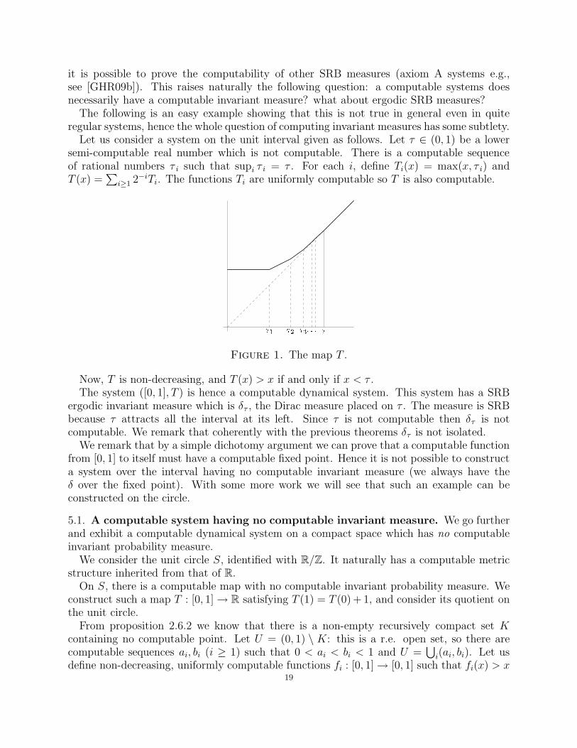
Let us consider a system on the unit interval given as follows. Let τ ∈ (0, 1) be a lowersemi-computable real number which is not computable. There is a computable sequenceof rational numbers τ i such that supi τ i = τ . For each i, define Ti(x) = max(x, τ i) andT (x) =

∑

i≥1 2−iTi. The functions Ti are uniformly computable so T is also computable.

Figure 1. The map T .

Now, T is non-decreasing, and T (x) > x if and only if x < τ .The system ([0, 1], T ) is hence a computable dynamical system. This system has a SRB

ergodic invariant measure which is δτ , the Dirac measure placed on τ . The measure is SRBbecause τ attracts all the interval at its left. Since τ is not computable then δτ is notcomputable. We remark that coherently with the previous theorems δτ is not isolated.

We remark that by a simple dichotomy argument we can prove that a computable functionfrom [0, 1] to itself must have a computable fixed point. Hence it is not possible to constructa system over the interval having no computable invariant measure (we always have theδ over the fixed point). With some more work we will see that such an example can beconstructed on the circle.

5.1. A computable system having no computable invariant measure. We go furtherand exhibit a computable dynamical system on a compact space which has no computableinvariant probability measure.

We consider the unit circle S, identified with R/Z. It naturally has a computable metricstructure inherited from that of R.

On S, there is a computable map with no computable invariant probability measure. Weconstruct such a map T : [0, 1] → R satisfying T (1) = T (0) + 1, and consider its quotient onthe unit circle.

From proposition 2.6.2 we know that there is a non-empty recursively compact set Kcontaining no computable point. Let U = (0, 1) \ K: this is a r.e. open set, so there arecomputable sequences ai, bi (i ≥ 1) such that 0 < ai < bi < 1 and U =

⋃

i(ai, bi). Let usdefine non-decreasing, uniformly computable functions fi : [0, 1] → [0, 1] such that fi(x) > x

19

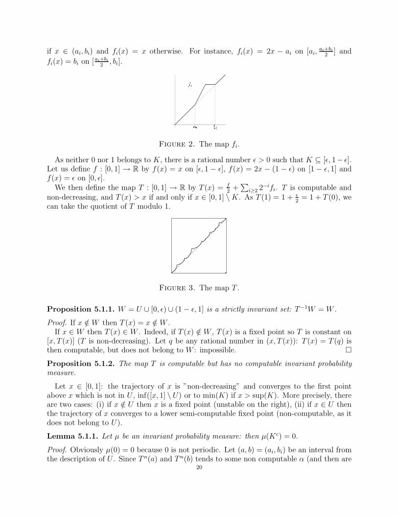
if x ∈ (ai, bi) and fi(x) = x otherwise. For instance, fi(x) = 2x − ai on [ai,ai+bi

2] and

fi(x) = bi on [ai+bi

2, bi].

Figure 2. The map fi.

As neither 0 nor 1 belongs to K, there is a rational number ǫ > 0 such that K ⊆ [ǫ, 1− ǫ].Let us define f : [0, 1] → R by f(x) = x on [ǫ, 1 − ǫ], f(x) = 2x − (1 − ǫ) on [1 − ǫ, 1] andf(x) = ǫ on [0, ǫ].

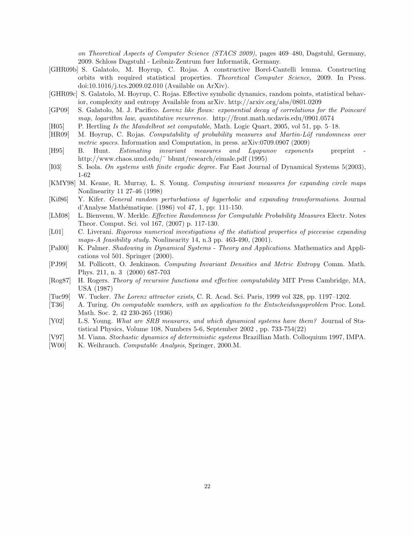
We then define the map T : [0, 1] → R by T (x) = f

2+

∑

i≥2 2−ifi. T is computable andnon-decreasing, and T (x) > x if and only if x ∈ [0, 1] \ K. As T (1) = 1 + ǫ

2= 1 + T (0), we

can take the quotient of T modulo 1.

Figure 3. The map T .

Proposition 5.1.1. W = U ∪ [0, ǫ) ∪ (1 − ǫ, 1] is a strictly invariant set: T−1W = W .

Proof. If x /∈ W then T (x) = x /∈ W .If x ∈ W then T (x) ∈ W . Indeed, if T (x) /∈ W , T (x) is a fixed point so T is constant on

[x, T (x)] (T is non-decreasing). Let q be any rational number in (x, T (x)): T (x) = T (q) isthen computable, but does not belong to W : impossible. �

Proposition 5.1.2. The map T is computable but has no computable invariant probabilitymeasure.

Let x ∈ [0, 1]: the trajectory of x is ”non-decreasing” and converges to the first pointabove x which is not in U , inf([x, 1] \ U) or to min(K) if x > sup(K). More precisely, thereare two cases: (i) if x /∈ U then x is a fixed point (unstable on the right), (ii) if x ∈ U thenthe trajectory of x converges to a lower semi-computable fixed point (non-computable, as itdoes not belong to U).

Lemma 5.1.1. Let µ be an invariant probability measure: then µ(Kc) = 0.

Proof. Obviously µ(0) = 0 because 0 is not periodic. Let (a, b) = (ai, bi) be an interval fromthe description of U . Since T n(a) and T n(b) tends to some non computable α (and then are

20

not stationary, as they are computable), the interval (a, b) is wandering. Hence, by Poincarerecurrence theorem it has null measure. �

Proof. (of proposition 5.1.2) We can conclude: let µ be a computable invariant probabilitymeasure: by the above lemma its support is then included in the complement of W . Butthe support of a computable probability measure always contains computable points (seeproposition 3.0.5) : contradiction. �

Actually, the set of invariant measures is exactly the set of measures which give nullweight to W . It is easy to see that in the above system the set of invariant measures is aconvex recursive compact set. Indeed, the function µ → µ(W ) is lower semi-computable, so{µ : µ(W ) > 0} is a recursive open set. Its complement is then a recursive compact set,as the whole space of probability measures is a recursive compact set. The above examplehence shows an example of a convex, and recursive compact set whose extremal points arenot computable.

We end remarking that with a different construction of the various fi it is possible to givealso a smooth system having the same properties as the examples in this section.

References

[AGS] L. Ambrosio, N. Gigli, G. Savare. Gradient flows: in metric spaces and in the space of probabilitymeasures, Birkhauser Zurich 2005 ebnisse der Mathematik und ihrer Grenzgebiete.

[BY06] M. Braverman, M. Yampolsky. Non-computable Julia sets, Journ. Amer. Math. Soc., 19 (2006),551-578.

[BBY07] I. Binder, M. Braverman, M. Yampolsky. Filled Julia sets with empty interior are computable,Journal FoCM, 7(2007), 405-416.

[BBY06] I. Binder, M. Braverman, M. Yampolsky. On computational complexity of Siegel Julia sets, Com-mun. Math. Phys., 264, 317-334(2006)

[Bla94] M. L. Blank. Pathologies generated by round-off in dynamical systems. Physica D. (1994) vol 78,no 1-2, pp: 93–114.

[Bla89] M. L. Blank. Small perturbations of chaotic dynamical systems. Russian Mathematical Surveys.(1989) vol 44, no 6, pp:1–33.

[BP03] Vasco Brattka and Gero Presser. Computability on subsets of metric spaces. Theoretical ComputerScience, 305(1-3):43–76, 2003.

[B83] A. A. Brudno (1983) Entropy and the complexity of the trajectories of a dynamical system. Trans.Mosc. Math. Soc. 44 127–151.

[CCS] J-R. Chazottes, P. Collet and B. Schmitt. Statistical consequences of the Devroye inequality forprocesses. Applications to a class of non-uniformly hyperbolic dynamical systems 2005 Nonlinearity18 2341-2364.

[Del99] M. Dellnitz, A. Hohmann. On the Approximation of Complicated Dynamical Behavior. SIAM Jour-nal on Numerical Analysis. 1999, vol. 36, no2, pp. 491-515.

[Del97] M. Dellnitz, A. Hohmann. A subdivision algorithm for the computation of unstable manifolds andglobal attractors. Numerische Mathematik. 1997, vol. 75, no3, pp. 293-317.

[Din94] J. Ding, A. Zhou. The projection method for computing multidimensional absolutely continuousinvariant measures. Journal of Statistical Physics.(1994) vol 77, 3-4, pp: 899-908.

[Din93] J. Ding, Q. Du, T. Y. Li. High order approximation of the Frobenius-Perron operator. AppliedMathematics and Computation. (1993) vol 53, pp: 151 - 171.

[G93] P. Gacs. Lectures notes on descriptional complexity and randomness. Boston University (1993)1–67.

[Ga00] S. Galatolo. Orbit complexity by computable structures Nonlinearity 13, 1531-1546 (2000).[GHR09a] P. Gacs, M. Hoyrup, C. Rojas. Randomness on computable probability spaces - a dynamical

point of view. In Susanne Albers and Jean-Yves Marion, editors, 26th International Symposium21

on Theoretical Aspects of Computer Science (STACS 2009), pages 469–480, Dagstuhl, Germany,2009. Schloss Dagstuhl - Leibniz-Zentrum fuer Informatik, Germany.

[GHR09b] S. Galatolo, M. Hoyrup, C. Rojas. A constructive Borel-Cantelli lemma. Constructingorbits with required statistical properties. Theoretical Computer Science, 2009. In Press.doi:10.1016/j.tcs.2009.02.010 (Available on ArXiv).

[GHR09c] S. Galatolo, M. Hoyrup, C. Rojas. Effective symbolic dynamics, random points, statistical behav-ior, complexity and entropy Available from arXiv. http://arxiv.org/abs/0801.0209

[GP09] S. Galatolo, M. J. Pacifico. Lorenz like flows: exponential decay of correlations for the Poincaremap, logarithm law, quantitative recurrence. http://front.math.ucdavis.edu/0901.0574

[H05] P. Hertling Is the Mandelbrot set computable, Math. Logic Quart, 2005, vol 51, pp. 5–18.[HR09] M. Hoyrup, C. Rojas. Computability of probability measures and Martin-Lof randomness over

metric spaces. Information and Computation, in press. arXiv:0709.0907 (2009)[H95] B. Hunt. Estimating invariant measures and Lyapunov exponents preprint -

http://www.chaos.umd.edu/˜ bhunt/research/eimale.pdf (1995)[I03] S. Isola. On systems with finite ergodic degree. Far East Journal of Dynamical Systems 5(2003),

1-62[KMY98] M. Keane, R. Murray, L. S. Young. Computing invariant measures for expanding circle maps

Nonlinearity 11 27-46 (1998)[Kif86] Y. Kifer. General random perturbations of hyperbolic and expanding transformations. Journal

d’Analyse Mathematique. (1986) vol 47, 1, pp: 111-150.[LM08] L. Bienvenu, W. Merkle. Effective Randomness for Computable Probability Measures Electr. Notes

Theor. Comput. Sci. vol 167, (2007) p. 117-130.[L01] C. Liverani. Rigorous numerical investigations of the statistical properties of piecewise expanding

maps-A feasibility study. Nonlinearity 14, n.3 pp. 463-490, (2001).[Pal00] K. Palmer. Shadowing in Dynamical Systems - Theory and Applications. Mathematics and Appli-

cations vol 501. Springer (2000).[PJ99] M. Pollicott, O. Jenkinson. Computing Invariant Densities and Metric Entropy Comm. Math.

Phys. 211, n. 3 (2000) 687-703[Rog87] H. Rogers. Theory of recursive functions and effective computability MIT Press Cambridge, MA,

USA (1987)[Tuc99] W. Tucker. The Lorenz attractor exists, C. R. Acad. Sci. Paris, 1999 vol 328, pp. 1197–1202.[T36] A. Turing. On computable numbers, with an application to the Entscheidungsproblem Proc. Lond.

Math. Soc. 2, 42 230-265 (1936)[Y02] L.S. Young. What are SRB measures, and which dynamical systems have them? Journal of Sta-

tistical Physics, Volume 108, Numbers 5-6, September 2002 , pp. 733-754(22)[V97] M. Viana. Stochastic dynamics of deterministic systems Brazillian Math. Colloquium 1997, IMPA.[W00] K. Weihrauch. Computable Analysis, Springer, 2000.M.

22