Department of Economics

Working Paper No. 166

Dynamic Spillovers of Oil Price Shocks and Policy Uncertainty Nikolaos Antonakakis

Ioannis Chatziantoniou

George Filis

February 2014

Dynamic Spillovers of Oil Price Shocks and Policy Uncertainty

Nikolaos Antonakakisa,b,∗, Ioannis Chatziantonioub, George Filisc

aVienna University of Economics and Business, Department of Economics, Institute for International Economics,Welthandelsplatz 1, 1020, Vienna, Austria.

bUniversity of Portsmouth, Department of Economics and Finance, Portsmouth Business School, Portland Street,Portsmouth, PO1 3DE, United Kingdom

cBournemouth University, Accounting, Finance and Economics Department, 89 Holdenhurst Road, Bournemouth,Dorset, BH8 8EB, United Kingdom

Abstract

This study examines the dynamic relationship between changes in oil prices and the economicpolicy uncertainty index for a sample of both net oil–exporting and net oil–importing countriesover the period 1997:01–2013:06. To achieve that, we extend the Diebold and Yilmaz (2009, 2012)dynamic spillover index using structural decomposition. The results reveal that economic policyuncertainty (oil price shocks) responds negatively to aggregate demand oil price shocks (economicpolicy uncertainty shocks). Furthermore, during the Great Recession of 2007–2009, total spilloversincrease considerably, reaching unprecedented heights. Moreover, in net terms, economic policyuncertainty becomes the dominant transmitter of shocks between 1997 and 2009, while in thepost–2009 period there is a significant role for supply–side and oil specific demand shocks, as nettransmitters of spillover effects. These results are important for policy makers, as well as, investorsinterested in the oil market.

Keywords: Policy uncertainty, Oil price shock, Spillover index, Structural VectorAutoregression, Variance Decomposition, Impulse Response Function

JEL codes: C32; C51; E31; E60; Q41; Q43; Q48

1. Introduction

This paper addresses an important question, which has recently emerged in the economic litera-ture; that is, the relationship between oil prices and economic policy uncertainty. In particular,the aim of this paper is to examine spillovers between Brent crude oil prices and the Baker et al.(2013) economic policy uncertainty. To achieve that, we extend the spillover index approach byDiebold and Yilmaz (2009, 2012), using structural decomposition rather than Choleski decompo-sition (Diebold and Yilmaz, 2009) or generalized forecast error variance decomposition (Diebold

∗Corresponding author, email: nikolaos.antonakakis@wu.ac.at, phone: +43/1/313 36-4141, fax: +43/1/313 36-90-4141.

Email addresses: nikolaos.antonakakis@wu.ac.at,nikolaos.antonakakis@port.ac.uk (NikolaosAntonakakis), ioannis.chatziantoniou@port.ac.uk (Ioannis Chatziantoniou), gfilis@bournemouth.ac.uk(George Filis)

Preprint submitted to WU, Department of Economics Working Paper Series February 7, 2014

and Yilmaz, 2012). Furthermore, in order to generate more informative results, we disentangle oilprice shocks according to their origin (i.e. supply–side shocks, aggregate demand shocks and oilspecific demand shocks), as in Kilian and Park (2009), and we then investigate the spillover effectsbetween these disaggregated shocks and the economic policy uncertainty indices. The countriesunder investigation are the US, Canada, China, the UK, Germany, France, Italy and Spain, aswell as, the aggregate Europe. The study uses monthly data over the period 1997:01–2013:06.The choice of countries, as well as, the sample period is governed by the data availability of theeconomic policy uncertainty indices.

This study builds on the work of Kang and Ratti (2013) who examine the effects of oil priceshocks on economic policy uncertainty in the US, using a Structural VAR framework. They findthat positive aggregate demand shocks exercise a significant negative effect on policy uncertainty,whereas oil specific demand shocks have the opposite effect. Furthermore, supply–side shocks donot seem to exert any effect.

In order to examine the spillover effects between oil prices (or their shocks) and economicpolicy uncertainty, first we need to explain their causal relationship. We argue that bidirectionalrelationship between oil prices and economic policy uncertainty exists, and therefore we posit thefollowing hypotheses:

Hypothesis 1 : Increases in oil prices raise economic policy uncertainty. In particular, we postulatethat negative effects of oil prices on economic activity and inflation put additional pressure onpolicy decision making, which ultimately leads to increased economic policy uncertainty.

Hypothesis 2 : Economic policy uncertainty also affects oil prices. Specifically, policy decisions havea direct effect on firm investment and production decisions, which further impact demand for oiland thus its price.

To elaborate further, we start our analysis with the investigation of the effects of oil priceson economic policy. Since the seminal paper by Hamilton (1983), mounting empirical evidenceindicates that oil prices exercise a strong negative influence on the economy. More specifically,past evidence suggest that there are significant effects of oil prices on industrial production andinflation (see, inter alia, Filis and Chatziantoniou, 2013; Balke et al., 2010; Tang et al., 2010; Duet al., 2010; Filis, 2010; Peter Ferderer, 1997). Furthermore, authors such as, Rahman and Serletis(2011), Elder and Serletis (2010), Cologni and Manera (2008), Cunado and Perez de Gracia (2005),Lee et al. (1995) and Hamilton (1983) confirm that the US economic activity has been significantlyaffected by rises in the oil prices, as well as, by the uncertainty about future oil price changes.Along similar lines, Montoro (2012) and Natal (2012) also establish the link between increasedinflation and low production output given an oil price increase. As it is understood, this trade-offraises the concerns of and creates pressure to the policymakers with regard to choosing the mostappropriate response towards these oil price effects. A much earlier study by Gelb (1988) providesa more direct relationship between oil prices and economic policy, by showing that increased oilprices cause a rise in federal government purchases. Furthermore, a recent study by El Anshasy andBradley (2012) which focuses on oil exporting economies, suggests that higher oil prices increasethe government size, which it turn, raises concerns regarding its efficient operation.

We further our analysis by focusing on the effects of economic policy on oil prices. Economicpolicy decisions have an immediate effect on economic activity. For example, Bloom (2009) empha-sises the effects of economic policy uncertainty on the business cycle. Antonakakis et al. (2013) find

2

that aggregate demand oil price shocks and US recessions affect negatively dynamic correlations ofstock market returns, implied volatility and policy uncertainty. Furthermore, uncertainty pertain-ing to economic policy decisions, regardless of its origin (i.e. whether the uncertainty originatesfrom potential fiscal or monetary policy decisions), discourages firms’ investing activity not onlybecause firms are uncertain about future aggregate demand but also because it puts upward pres-sure on financing costs (see, among others, Pastor and Veronesi, 2012, 2013; Fernandez-Villaverdeet al., 2011; Byrne and Davis, 2004). As expected, lower investment levels will lead to reduceddemand for oil, pushing its price downwards. Malliaris and Malliaris (2013) also maintain thatinflationary pressures exercise a significant impact on oil prices.

All that said, the aforementioned studies do not distinguish between the various types of oilprice shocks. Several authors have documented the significance of disentangling oil price shocksin order to assess their true impact on the economy (see, among others, Degiannakis et al., 2014;Baumeister and Peersman, 2013; Lippi and Nobili, 2012; Kilian and Lewis, 2011; Filis et al., 2011;Kilian and Park, 2009). The pioneers of the notion of oil price shocks are Hamilton (2009a,b)and Kilian (2009b). In particular, Hamilton (2009a,b) identifies two oil price shocks, that is;demand–side oil price shocks, which originate from changes in aggregate demand, and supply–sideoil price shocks, which originate from changes in oil production. Kilian (2009b) further disentanglesdemand–side shocks into two components, i.e. aggregate demand shocks (similar to the Hamilton(2009a,b) classification) and oil specific demand shocks, which are related to the uncertainty of thefuture availability of oil.

Having established the potential relationship between economic policy uncertainty and oil,this study assesses spillover effects between oil prices (or their shocks) and the economic policyuncertainty. We make an important contribution to the existing literature as (i) this study is thefirst to examines time-varying spillover effects between oil prices and economic policy uncertainty,(ii) it investgates both the effects of oil prices and oil price shocks and (iii) it adds to the limitednumber of studies pertaining to Baker et al. (2013) economic policy uncertainty index.

Our findings suggest that according to the impulse response function analysis, there is a negativeresponse from both policy uncertainty and changes in oil prices to respective shocks from eachvariable. Classifying oil price shocks into supply–side, aggregate demand and oil specific demandshocks, we report that economic policy uncertainty responds only to aggregate demand shocks(negatively), whereas all three types of shocks are negatively influenced by policy uncertaintyinnovations. Furthermore, time-varying total spillovers between economic policy uncertainty andchanges in oil prices range between 10%–25% in the pre–2007 period. During the Great Recessionof 2007–2009 we observe a significant peak in spillovers, which ranges between 40%–50%, dependingon the country. When we disentangle oil price shocks, then total spillovers significantly increase,reaching even the level of 75%. Net–spillovers suggest that the main transmitter of shocks is theeconomic policy uncertainty up until the end of the Great Recession of 2007–2009, while in the yearsthat followed it is the changes in oil prices that assume this role. Once we disaggregate oil priceshocks into their three components, we observe that all variables can be either net transmittersor net recipients of spillover shocks, depending on the time period. Finally, results are qualitativesimilar for both net oil–exporters and net oil–importers.

Overall, the findings suggest that unless we disentangle oil price shocks and proceed with atime-varying framework, we are not able to capture the full dynamics of the relationship betweenoil and economic policy uncertainty. These results are important for policy makers, as well as,investors, considering the dynamic interaction between oil and economic policy uncertainty. To be

3

more explicit it is important for investors to understand that during turbulent periods attentionshould be drawn to economic policy uncertainty, considering the fact that the latter affects themarket in which they operate. On the other hand, policy makers should be cautious when formu-lating macroeconomic policies at relatively tranquil times, as oil price shocks could undermine thesuccessful outcomes of these policies.

The remainder of the paper is organized as follows. Section 2 discusses the methodologyand describes the data. Section 3 presents the empirical findings, and Section 4 summarises andconcludes the paper.

2. Empirical Methodology and Data

2.1. Spillover methodology

The spillover index approach introduced by Diebold and Yilmaz (2009) builds on the seminal workon VAR models by Sims (1980) and the well-known notion of variance decompositions. It allowsan assessment of the contributions of shocks to variables to the forecast error variances of both therespective and the other variables of the model. Using rolling-window estimation, the evolution ofspillover effects can be traced over time and illustrated by spillover plots. Starting point for theanalysis is the following p–order, N–variable VAR

yt =P∑i=1

Θiyt−i + εt (1)

where yt = (y1t, y2t, . . . , yNt) is a N × 1 vector of N endogenous variables, Θi, i = 1, ..., P, areN ×N parameter matrices and εt ∼ (0,Σ) is a N ×1 vector of disturbances that are independentlydistributed over time; t = 1, ..., T is the time index and n = 1, ..., N is the variable index.

Key to the dynamics of the system is the moving average representation of model (1), whichis given by yt =

∑∞j=0 Ajεt−j , where the N ×N coefficient matrices Aj are recursively defined as

Aj = Θ1Aj−1 + Θ2Aj−2 + . . .+ ΘpAj−p, where A0 is the N ×N identity matrix and Aj = 0 forj < 0.

Diebold and Yilmaz (2009) use Cholesky decomposition, which yields variance decompositionsdependent on the ordering of the variables, whereas Diebold and Yilmaz (2012) extend the Dieboldand Yilmaz (2009) model, using the generalized VAR framework of Koop et al. (1996) and Pesaranand Shin (1998), in which variance decompositions are invariant to the order of the variables. Bothmodels yield an N × N matrix φ(H) = [φij(H)]i,j=1,...N , where each entry gives the contributionof variable j to the forecast error variance of variable i. The main diagonal elements contain the(own) contributions of shocks to the variable i to its own forecast error variance, the off-diagonalelements show the (cross) contributions of the other variables j to the forecast error variance ofvariable i.

Since the own– and cross–variable variance contribution shares do not sum to one under thegeneralized decomposition, i.e.,

∑Nj=1 φij(H) 6= 1, each entry of the variance decomposition matrix

is normalized by its row sum, such that

φij(H) =φij(H)∑Nj=1 φij(H)

(2)

with∑N

j=1 φij(H) = 1 and∑N

i,j=1 φij(H) = N by construction.

4

This ultimately allows to define a total (volatility) spillover index, which is given by

TS(H) =

∑Ni,j=1,i 6=j φij(H)∑Ni,j=1 φij(H)

× 100 =

∑Ni,j=1,i 6=j φij(H)

N× 100 (3)

which gives the average contribution of spillovers from shocks to all (other) variables to the totalforecast error variance.

This approach is quite flexible and allows to obtain a more differentiated picture by consideringdirectional spillovers: Specifically, the directional spillovers received by variable i from all othervariables j are defined as

DSi←j(H) =

∑Nj=1,j 6=i φij(H)∑Ni,j=1 φij(H)

× 100 =

∑Nj=1,j 6=i φij(H)

N× 100 (4)

and the directional spillovers transmitted by variable i to all other variables j as

DSi→j(H) =

∑Nj=1,j 6=i φji(H)∑Ni,j=1 φji(H)

× 100 =

∑Nj=1,j 6=i φji(H)

N× 100. (5)

Notice that the set of directional spillovers provides a decomposition of total spillovers into thosecoming from (or to) a particular source.

By subtracting Equation (4) from Equation (5) the net spillovers from variable i to all othervariables j are obtained as

NSi(H) = DSi→j(H)−DSi←j(H), (6)

providing information on whether a variable is a receiver or transmitter of shocks in net terms. Putdifferently, Equation (6) provides summary information about how much each variable contributesto the volatility in other variables, in net terms.

Finally, the net pairwise spillovers can be calculated as

NPSij(H) = (φji(H)∑N

i,m=1 φim(H)− φij(H)∑N

j,m=1 φjm(H))× 100

= (φji(H)− φij(H)

N)× 100. (7)

The net pairwise volatility spillover between variables i and j is simply the difference between thegross volatility shocks transmitted from variable i to variable j and those transmitted from j to i.

The spillover index approach provides measures of the intensity of interdependence across coun-tries and variables and allows a decomposition of spillover effects by source and recipient.

The key innovation and contribution in this study is that, instead of using Cholesky or Gener-alised variance decomposition, so as to obtain the total, directional and net spillover indexes, weadopt a Structural variance decomposition methodology, as it allows the identification of oil priceshocks. The choice of structural variance decomposition is predicated upon our empirical exercise.That is, to examine the effects of oil price shocks on economic policy uncertainty. In particular,we disaggregate oil price shocks based on the framework of Kilian and Park (2009). Essentially,with the use of a Structural VAR (SVAR) model, we distinguish between three types of oil price

5

shocks; namely, supply–side shocks (SS), aggregate demand demand (ADS), as well as, oil specificshocks (OSS); and by including the economic policy uncertainty index of Baker et al. (2013) inthe SVAR, we assess the effects of oil price shocks on economic policy uncertainty. The first typeof shock is typically associated with changes in world oil production, whereas the second and thethird type of shocks relate to changes in global economic activity and to concerns regarding thefuture availability of oil, respectively.

For the general case of a p–order Structural VAR model, we obtain the following standardrepresentation:

A0yt = c0 +∑p

i=1Aiyt−i + εt (8)

where, yt is a [N × 1] vector of endogenous variables. In this paper, first, N=2 when we assess therelationship between oil price returns and economic policy uncertainty. For the relationship amongthe three oil price shocks and economic policy uncertainty, N=4, containing world oil production,the global economic activity index, real oil price returns and the economic policy uncertainty index,noting that the order of the variables is important. A0 represents the [N × N ] contemporaneousmatrix, Ai are [N × N ] autoregressive coefficient matrices, εt is a [N × 1] vector of structuraldisturbances, assumed to have zero covariance and be serially uncorrelated. The covariance matrixof the structural disturbances takes the following form:

For N=2:

E[εtε′t] = D =

[σ2

1 00 σ2

2

](9)

For N=4

E[εtε′t] = D =

σ2

1 0 0 00 σ2

2 0 00 0 σ2

3 00 0 0 σ2

4

(10)

In order to get the reduced form of our structural model (8) we multiply both sides with A−10 ,

such as that:yt = a0 +

∑p

i=1Biyt−i + et (11)

where a0 = A−10 c0, Bi = A−1

0 Ai, and et = A−10 εt, i.e. εt = A0et. The reduced form errors et

are linear combinations of the structural errors et, with a covariance matrix of the form E[ete′t] =

A−10 DA−1′

0 .Imposing suitable restrictions on A−1

0 will help identify the structural disturbances of the model.In particular, for N=2 we impose the following short-run restrictions:

e∆Real Oil Prices1,t

eEconomic Policy Uncertainty2,t

=

[α11 0α21 α22

]×

[εOPS

1,t

εEPS2,t

](12)

where OPS =oil price shock and EPS =economic policy uncertainty shock.For N=4, the restriction are as follows:

e∆Oil Production1,t

eReal Global Economic Activity2,t

e∆Real Oil Prices3,t

e∆Economic Policy Uncertainty4,t

=

α11 0 0 0α21 α22 0 0α31 α32 α33 0α41 α42 α43 α44

×

εSS1,t

εADS2,t

εOSS3,t

εEPS4,t

(13)

6

where SS =supply–side shock, ADS =aggregate demand shock and OSS =oil specific demandshock and EPS =economic policy uncertainty shock.

The purpose of the short–run restrictions we impose on the model is to help us identify theunderlying oil price shocks, similarly with Kilian and Park (2009). According to the restrictionsfor N=4, high adjustment costs forbid oil production to contemporaneously respond to changesin demand for oil. Furthermore, changes in the supply of oil are allowed to contemporaneouslyaffect both global economic activity and the price of oil. In addition, given that it takes some timefor the global economy to react to changes in the price of oil, global economic activity is assumednot to receive contemporaneous feedback from oil prices. However, changes in aggregate economicactivity is expected to have a contemporaneous impact on oil prices and this is at large explainedby the instantaneous response of commodities markets. Furthermore, it is understandable that oilprice developments can be triggered by all types of shocks and in this regard all types of shocksare assumed to contemporaneously affect oil prices. Finally, economic policy uncertainty indexresponds contemporaneously to all aforementioned oil price shocks.

2.2. Data description

In this study we use monthly data of the economic policy uncertainty indices for Canada, China,EU, Germany, France, Italy, Spain, the UK and the US. The series come from Baker et al. (2013).In addition, monthly data have been collected for oil prices, world oil production and the real globaleconomic activity index (GEA), which are used for the estimation of oil price shocks. Data for theBrent crude oil price and world oil production have been extracted from the Energy InformationAdministration, whereas the data for the real global economic activity index have been retrievedfrom Lutz Kilian’s personal website (http://www-personal.umich.edu/∼lkilian/). The period ofstudy runs from 1997:01 until 2013:06. Oil prices and world oil production are expressed in log-returns. Furthermore, oil prices are transformed in real terms. Table 1 reports the descriptivestatistics of the series.

Insert Table 1 here

As evident in Table 1, economic policy uncertainty indices have comparable mean values, withthe exception of Canada and the UK which exhibit the lowest and highest mean values, respectively.Economic policy uncertainty indices are fairly volatile, as shown by the standard deviation, theminimum and the maximum values. With regard to oil price changes, we observe a positiveaverage value, with quite a high standard deviation. Furthermore, none of the series is normallydistributed, as indicated by the skewness, kurtosis and the Jarque-Bera statistic. Finally, accordingto the ADF–statistic, all variables are stationary.

Figure 1 exhibits the evolution of the series during the sample period.

Insert Figure 1 here

All economic policy uncertainty indices exhibit some common peaks. For example, in all coun-tries we notice an increase in the level of policy uncertainty during the period 2002–2003 (war inAfghanistan and second war in Iraq), the Great Recession of 2007–2009, as well as, during the Eu-ropean Debt crisis in 2011, signifying the increase of policy uncertainty during turbulent economicperiods. Finally, the effects of the Great Recession of 2007–2009 can also be observed on oil pricechanges, which significantly declined in 2009.

7

3. Empirical Results

3.1. Impulse Response Effects

We begin our analysis by concentrating on the impulse response functions between oil prices andeconomic policy uncertainty. In particular, we seek to portray not only a narrow setting whichmerely describes the relationship between shocks in policy uncertainty and oil prices, but also, abroader framework which allows for the introduction of a disaggregated approach towards oil priceshocks, and thus considers supply–side shocks, aggregate demand shocks and oil specific demandshocks, separately.

Figures 2, 3 and 4 present the structural impulse response functions of our different specifica-tions of model 8 for a time period of 24–months. The upper and lower error bands with percentilesof 0.16 and 0.84, respectively, are constructed using Monte Carlo integration based on 1000 draws.

Figure 2 reports the structural impulse responses of oil prices to one standard deviation shockto policy uncertainty (left column), and the structural impulse responses of policy uncertainty toone standard deviation shock to oil prices (right column) based on the SVARs with oil prices andpolicy uncertainty as the endogenous variables for each country.

According to this figure we see that, in general, a surprise increase in economic policy uncer-tainty shock leads to a very short–lived and statistically significant drop in the price of oil in awindow between one and three months. The effect of an unanticipated positive oil price shockleads to a statistically significant decline on policy uncertainty which is more persistent and morepronounced for some countries. The fact that policy uncertainty responds negatively to positivechanges in oil prices, is counter–intuitive. The peculiar feature of these results might be maskeddue to the aggregate measure of oil price shocks. In other words, we maintain that the disaggre-gation of oil price shocks could provide a clearer picture with reference to the impulse responsefunctions.

Insert Figure 2 here

Therefore, in Figures 3 and 4, we report the structural impulse responses of supply–side (SS),aggregate demand (ADS) and oil specific demand shocks (OSS) to one standard deviation shockto policy uncertainty (see, Figure 3), and the structural impulse responses of policy uncertaintyto one standard deviation shock to supply–side (SS), aggregate demand (ADS) and oil specificdemand shocks (OSS)(see, Figure 4). According to these figures, the picture that emerges becomesmore clear.

In particular, unanticipated innovations to policy uncertainty do not seem to cause any signif-icant effects on supply–side shocks (SS) before 4 months have passed. At that time we observe anegative and significant response of the supply–side shocks to policy uncertainty innovations. Thisis suggestive of the fact that positive policy uncertainty unanticipated shocks trigger a decrease inoil production, which is somewhat expected. Furthermore, unanticipated innovations to policy un-certainty lead to significant reduction of aggregate demand shocks (ADS) and oil specific demandshocks (OSS) as reported in Figure 3. The fact that ADS respond negatively to policy uncertaintyshocks is explained by the fact that the latter is causing a reduction in aggregate demand, whichin turn, drives oil prices at lower levels. In addition, the same response is expected regarding theOSS given that increased policy uncertainty is conducive to lower demand for oil, and thus loweruncertainty about its future availability. These results are also in line with Kang and Ratti (2013).

Turning our attention to policy uncertainty responses to oil price shocks, we find that unantic-ipated positive supply–side shocks do not exert a significant effect on economic policy uncertainty

8

(with the exception of Italy for which a significantly positive effect is reported). This result ac-cords with the related literature which maintains that supply–side shocks are no longer importantfor macroeconomic developments (see, among others, Baumeister and Peersman, 2013; Lippi andNobili, 2012; Hamilton, 2009a,b). Furthermore, unanticipated positive aggregate demand shocks(ADS) lead to lower levels of policy uncertainty. This is expected as rises in aggregate demand, de-spite the fact that push oil prices upwards, are regarded as positive information, reflecting boomingeconomic conditions and thus lowering policy uncertainty. This is partly in line with Antonakakiset al. (2013) who find that aggregate demand oil price shocks affect negatively the dynamic correla-tions of stock market returns, implied volatility and policy uncertainty. Oil specific demand shocksdo not seem to trigger significant responses from policy uncertainty, with the exception of Canada,EU and France. Policy uncertainty in France, exhibits a persistent negative response to oil specificdemand shocks, whereas respective responses are short–lived for Canada and the EU. This resultsis expected for Canada given its net–exporting character. Nevertheless, it is counter–intuitive forFrance and the EU and this deserves further attention.

Finally, we can observe that the negative response of economic policy uncertainty to positiveoil price innovations that was reported in Figure 2 is mainly driven by aggregate demand shocks(ADS), which confirms our initial claim that unless we disaggregate oil price shocks by virtue oftheir origin we cannot attain a deeper understanding of the issue at hand. These results reveal thedominance of aggregate demand shocks, rather than supply–side and oil specific demand shocks,as a source of policy uncertainty innovations.

Insert Figure 3 here

Insert Figure 4 here

Having established the main transmission channels pertaining to the variables of interest, weproceed with the analysis of their spillover effects, which constitutes the main research objectiveof this study.

3.2. Total spillovers between policy uncertainty and oil prices

Spillover effects between policy uncertainty and changes in oil prices are presented in Table 2.Evidence show a quite low average effect, with the exception of Canada and France, where the av-erage total spillover index is 12.6% and 12.1%, respectively. The lowest score is reported for Italy.Overall, the total spillover indices illustrate that, on average, there is a weak–to–moderate interde-pendence between oil and economic policy uncertainty for most countries. Average net spilloversfor the whole sample demonstrate that economic policy uncertainty is the net transmitter of shocksfor China, EU aggregate, Germany, the UK, as well as, the US (see, Table 2). Nevertheless, netspillovers, on average, are relatively small.

Insert Table 2 here

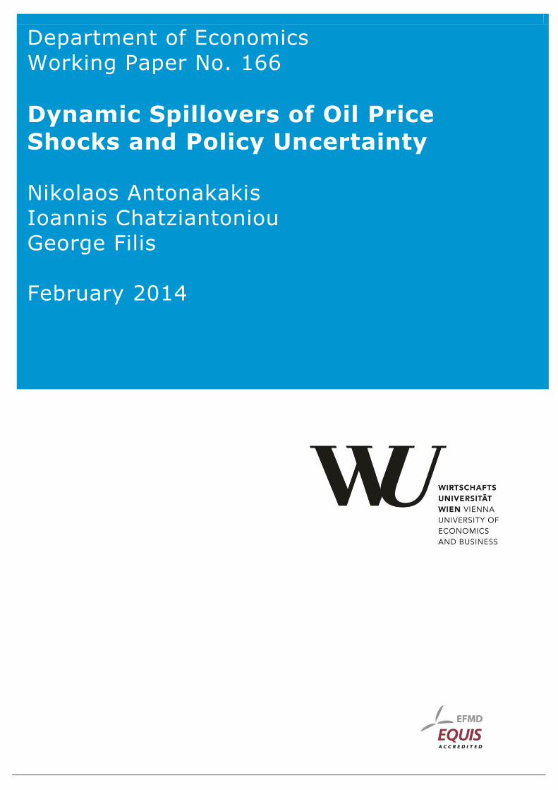
Turning our attention to spillover indices based on the disaggregated oil price shocks (see,Table 3), we observe that total spillovers and net spillovers, increase in magnitude. In addition,it is evident that this magnitude is pretty similar for all the countries in our sample. Moreover,considering all three types of oil shocks, we observe that economic policy uncertainty acts as anet recipient of spillover shocks only in the cases of Spain and Germany, whereas it remains a net

9

transmitter of spillover shocks for all other countries in our sample (Table 3). It is also worthnoting that aggregate demand oil price shocks (ADS) behave as net transmitters for all countriesbut China. This accords with related literature which emphasises the importance of demand–sideshocks, as opposed to supply–side shocks (see, among others, Baumeister and Peersman, 2013;Lippi and Nobili, 2012; Hamilton, 2009a,b).

Insert Table 3 here

Our analysis so far is based on single fixed parameters. Despite the fact that Tables 2 and3 show some interesting information, we should not lose sight of the fact that during our sampleperiod several events took place, such as the was in Afghanistan and Iraq, the Great Recessionof 2007–2009 and the European debt crisis. Hence, the average values presented in Tables 2 and3 are not expected to hold for the whole time span. Thus, it would be valuable to examine howthese spillovers evolve over time. Therefore we proceed with our analysis by presenting the totaland net spillovers using 60–month rolling samples. It should be underlined that different forecasthorizons (from 5 up to 15 months) and different window lengths (48 and 72) were also consideredand the results were qualitatively similar. Thus, we maintain that the results are not sensitive tothe choice of the forecast horizon or the length of the rolling–windows.

The time–varying spillover indices are illustrated in Figure 5. The dotted line represents theintertemporal progression of the total spillover indices between policy uncertainty and changes inoil prices, while the solid line, represents the intertemporal progression of the total spillover indicescorresponding to the relation between policy uncertainty and oil price shocks (disaggregated shocksin virtue of their origin).

Insert Figure 5 here

Starting with spillovers between shocks in economic policy uncertainty and changes in oil prices,we observe that for most countries, in the period preceding the Great Recession, total spilloversfluctuate within a range between 10% and 25%. Furthermore, this range of fluctuation is relativelystable for almost all countries under examination. The only exception to these findings is France,in which total spillover shocks, in the pre Great Recession period, reach a high at almost 40%.During the years of the Great Recession, total spillovers increase considerably reaching unprece-dented heights during the peak of the Great Recession (i.e. mid–2008 until early–2009). In theperiod succeeding the Great Recession (i.e. post–2009) total spillovers return to a stable fluctuationpattern, realised within the same range as in the pre-crisis period, for all countries with the excep-tion of Canada. Evidently, for Canada, the post-crisis period is characterised by a higher level oftotal spillovers. Turning to total spillovers between shocks in economic policy uncertainty and oilprice shocks, the picture is somewhat different. To begin with, total spillovers fluctuate at a muchhigher range (i.e. between 50% and 75%) throughout the period of study. Next, although it is afact that during the peak years of the Great Recession total spillovers reach very high levels, onecould not argue that these levels are indeed unprecedented. Finally, with the exception of Spain,total spillovers appear to revert back to their pre-crisis fluctuation patterns. Interestingly enough,in European countries, Italy aside, another peak of the total spillover indices is observed in thebeginning of 2011, which coincides with increased concerns regarding the migration of the effectsof the debt crisis from Eurozone peripheral countries to the rest of Europe. The aforementionedfindings constitute an indication that unless we disentangle oil prices by virtue of their shocks,

10

we are not able to extract all relevant information. However, in order to provide a more in-depthanalysis of the results, we proceed with reporting country specific total spillover effects.

In the section that follows, we provide additional information aiming to attain deeper knowledgeof the evolution of spillover effects over time in each one of the countries of our sample. We beginby identifying the net spillover transmitters.

3.3. Net spillover transmitters and recipients

By concentrating on net directional spillovers we can deduce whether one of the variables is eithera net transmitter or a net receiver of spillover effects within a particular country. Initially weinvestigate the spillover effects between policy uncertainty and changes in oil prices. Results areshown in Figure 6. Policy uncertainty is considered to be a net transmitter when spillovers appearon the negative lower area of each panel.

Insert Figure 6 here

As can be seen in Figure 6, the early period of our study is characterised by the net transmittingbehaviour of policy uncertainty. Although, this does not hold true for France and Italy, where forthe most period preceding the Great Recession, oil prices are the net transmitters of shocks. Withreference to the Great Recession of 2007–2009, we observe that policy uncertainty assumes an evengreater net transmitting role, suggested by the trough of the time-varying net spillover indices.Prominent among the results is that the this trough is observed at different phases of the GreatRecession. Stellar examples of this, include France, Germany and the UK. As far as the former isconcerned, the net transmitting character of economic policy uncertainty is observed in the earlystages of the Great Recession. In the cases of Germany and the UK, it is during the the last yearof the Great Recession that economic policy uncertainty assumes the net transmitting character.

Furthermore, in the years after 2009, which marked the beginning of the recovery of the globaleconomy, the contribution of policy uncertainty to spillover effects is diminishing (see the upwardtrend in almost all panels of Figure 6) in almost all countries of our sample. Even more, with theexception of Spain and Italy, oil prices are net transmitters of shocks from 2010 onwards, althoughtheir contribution is clearly diminishing during 2012–2013. The latter observation particularlyholds for the European countries which experience the consequences of the ongoing Eurozonecrisis. The fact that for Spain and Italy economic policy uncertainty retains its net transmittingcharacter, even after the Great Recession, can be explained by the strong economic impact thatthe Eurozone crisis exerted on these two countries. Thus, we maintain that at times of economicturbulence, oil prices are the net recipients of shocks, suggesting that they are influenced by thepolicy uncertainty which emerges during these periods.

In order to gain a clearer perception of the situation, we proceed with our analysis by presentingnet spillovers between policy uncertainty and oil price shocks. This information is presented inFigures 7, 8 and 9. Each country is associated with three panels while each panel represents oneof the three possible types of oil price shocks, as these were earlier defined in the study. As before,policy uncertainty is considered to be a net transmitter of spillover effects every time the net effect(depicted by the solid line) lies within the negative lower area of each panel. We have also includeda dotted line which pertains to the results presented in Figure 6, to allow direct comparisons. Byso doing, we are able to trace the contribution of each type of oil price shock and produce a morecredible interpretation of the results.

Insert Figure 7 here

11

Insert Figure 8 here

Insert Figure 9 here

Results presented on Figures 7, 8 and 9 confirm our anticipation that disaggregated oil priceshocks are more informative in relation to the spillover effects between oil and policy uncertainty.More specifically, we notice that spillovers occur between policy uncertainty and aggregate demandshocks, rather than between policy uncertainty and supply–side or oil specific demand shocks.Furthermore, we observe that the magnitude of spillover effects is considerably smaller comparedto Figure 6. In order to gain a deeper understanding of these net spillover effects, we proceed withcountry–specific results.

Starting with Canada (see, Figure 7) the period before and during the Great Recession ischaracterised by the net transmitting role of economic policy uncertainty, as far as supply–sideand oil specific demand shocks are concerned. By contrast, we observe that for the same period,economic policy uncertainty is a net receiver of spillover effects with regard to aggregate demandshocks. Interestingly enough, in Canada, which is a net oil–exporting country, in the years thatfollowed the Great Recession, it is only the oil specific demand shocks that contribute to the forecasterror of policy uncertainty, whereas, supply–side and aggregate demand shocks appear to have noeffect at all. A potential explanation of this result may lie within the arguments put forward byauthors such as Auty and Gelb (2001), Lane (2003), as well as, Afonso and Furceri (2010) whoidentify a strong link between resource-revenues – such as revenues from oil – and fiscal policy. Toelaborate further, Sturm et al. (2009) argue that public finances of resource-abundant countriesmay exhibit high levels of volatility depending on the whims of oil prices and demand for oil andthus they constitute a major source of uncertainty within the country. This is a very crucial insightas in relatively tranquil times the macroeconomic policy of the net oil exporting country appearsto have a strong link to demand-side oil price shocks.

According to IEA (2013) China is the second largest crude net oil–importer in the world.Interestingly enough, Figure 7 reveals similar results for China to those of Canada. Again, we noticethat the aggregate demand shocks are the main source of spillover effect on policy uncertainty.Nevertheless, in the latter period of our study, supply–side and oil specific demand shocks assumea net transmitting character. Authors such as Yuan et al. (2008) highlight the strong nexusbetween oil and economic growth in China and stress the need for the Chinese Government to setup a national policy regarding the accumulation of a strategic level of oil reserves. According toYuan et al. (2008), future availability of oil is a major concern within China and abrupt rises inthe price of oil are generally the source of serious economic concerns, resulting in higher level ofpolicy uncertainty. The necessity for national planning, targeting energy security, has also beenbrought up by authors such as Zhang et al. (2009) and Ma et al. (2011). In addition, Ma et al.(2012) emphasize the lack of some appropriate national policy with respect to energy resourcesin general and oil reserves in particular, which could help stave off future energy turbulence andsecure a solid path of economic growth. This will in turn ease the formulation and implementationof macroeconomic policies.

We further our analysis with the European countries, which are net oil–importers. In thisregard, part of the analysis in connection with China may also apply to most European countriesand especially to countries in which oil is a major input of production. To be more explicit,uncertainty regarding both the future level of the price of oil and its future availability couldinfluence their output level. In Figure 7, we can observe that policy uncertainty in the period

12

that followed the Great Recession was mainly a net recipient of spillover effects transmitted bythe supply–side and oil specific demand shocks. Further, empirical findings concerning individualEuropean countries reveal a similar picture (see, Figures 8 and 9). Notable exceptions in thesepattern are Spain and the UK. In the case of Spain, policy uncertainty appears to be the maintransmitter of spillover effects, throughout our sample period. Although for the period of the GreatRecession, both supply–side and aggregate demand shocks exhibit a net transmitting role. As faras the UK is concerned, it is also the aggregate demand shocks that transmit spillover effects topolicy uncertainty even in the years succeeding the Great Recession.

Both demand–side shocks are important for Germany, although at different time periods. Ac-cording to Carstensen et al. (2013) Germany in 2009 experienced one of its greatest economicdownturns ever and that according to the author can be attributed not only to the financial crisisper se, but also, to developments in the market for crude oil (see also, Hamilton, 2009a; Kilian,2009a). Most importantly, Carstensen et al. (2013) provide evidence suggesting that in the shortrun, despite the appreciation of oil prices due to aggregate demand shocks, an exporting countrycan enjoy economic benefits due to higher demand for its products. In the longer term, though,reduced domestic consumption, due to inflationary pressures driven by higher oil prices, dominatethe economy and could potentially lead to recession. Understandably, this would increase policyuncertainty within the country. Carstensen et al. (2013) put forward the argument that this isexactly what happened in Germany and this is why although the price of crude oil peaked in mid–2008, the German economy did not enter a recession until 2009. This could potentially explainwhy rises in the price of oil that are related to booming global economic conditions can aggra-vate expectation regarding macroeconomic policy conduct, even in an economy which is heavilyexport-oriented, such as Germany. It is understandable that the foregone analysis can also applyto the rest of Europe; in fact, it may be even more appropriate considering that all other Europeancountries export much less commodities than Germany.

According to the IEA (2013), the US economy is the world’s top crude oil–importer. As evidentin Figure 9, the net spillover behaviour for the US resembles the previous cases, although withsome minor differences. More specifically, net spillover effects between supply–side or oil specificdemand shocks and policy uncertainty are very close zero for the pre-crisis period, whereas, forthe same period, aggregate demand shocks are net transmitters of spillover effects. Notably, from2009 onwards it is mainly the supply–side shocks that transmit spillover effects to economic policyuncertainty, although a peak in net spillovers deriving from oil specific demand shocks is observedfor the latter years of the sample period. Despite the arguments put forward by Baumeister andPeersman (2013), among others, that supply–side shocks have a small role to play in the USeconomy, as opposed to demand–side shocks, we provide evidence that the former shocks haveindeed a role to play in economic policy uncertainty developments.

In retrospect, we find that there is not one single net transmitter of spillover shocks, but ratherall variables assume this character at different time periods. This is suggestive of the fact thatthere is no constant relationship between oil price shocks and economic policy uncertainty andeven more this relationship varies with the type of oil price shock. In this regard, claims about therelationship between economic policy uncertainty and oil price shocks, based one static estimates,may not reveal the whole picture and, in cases, they may be misleading. Finally, distinguishingoil price shocks by virtue of their origin and investigating net spillover effects in this disaggregatedframework provides a more thorough picture regarding the said relationship. On a final note, it isworth noting that our findings apply to both net oil–exporting and net oil–importing countries.

13

4. Conclusion

This paper examines the relationship between oil prices and economic policy uncertainty, usingmonthly data on oil and the economic policy uncertainty index produced by Baker et al. (2013),over the period 1997:01–2013:06. We examine the said relationship by extending the spillover indexapproach by Diebold and Yilmaz (2009, 2012) using structural decomposition. In addition, wedisaggregate oil price shocks by virtue of their origin following Kilian and Park (2009) classification,and investigate spillover effects between each of these shocks and economic policy uncertainty.Sample countries include the US, Canada, China, the UK, Germany, France, Italy and Spain andthe aggregate Europe.

According to existing literature, it is anticipated that there is bidirectional relationship be-tween economic policy uncertainty and oil prices. On one hand, higher oil prices exert negativeimpacts on the economy, such as lower productivity and/or higher inflation (see, inter alia, Filis andChatziantoniou, 2013; Montoro, 2012; Natal, 2012; Rahman and Serletis, 2011; Balke et al., 2010;Elder and Serletis, 2010; Tang et al., 2010; Du et al., 2010; Filis, 2010; Cologni and Manera, 2008;Cunado and Perez de Gracia, 2005; Peter Ferderer, 1997; Hamilton, 1983). Such economic condi-tions put pressure on policy makers to mitigate the negative effects of increased oil prices, which itturn, raises concerns regarding the success of these policies. On the other hand, uncertainty sur-rounding economic policy decisions negatively affects firms’ investment and output decisions (see,among others, Wang et al., 2014; Pastor and Veronesi, 2013, 2012; Fernandez-Villaverde et al.,2011; Byrne and Davis, 2004). Considering that reduced investment and output levels cause adownward pressure on oil prices, we opine that economic policy uncertainty exerts an impact onoil prices.

Impulse response functions suggest that both economic policy uncertainty and changes in oilprices respond negatively to each others’ shocks. The response from oil prices is expected, giventhat increased policy uncertainty may lead to lower productivity, and thus lower demand for oil.Decomposing oil price shocks, we observe that changes in economic policy uncertainty causessignificantly negative responses from all types of shocks, although there is a delayed response fromthe supply–sid shocks. The counter-intuitive response of economic policy uncertainty to changesin oil prices can be explained by the contribution of aggregate demand shocks, which is clearlyevidenced once oil price shocks are disaggregated. Furthermore, we provide evidence that supply–side and oil specific demand shocks do not trigger any responses from economic policy uncertainty.These results are in line with Kang and Ratti (2013).

As far as total spillovers are concerned, we show that spillovers between economic policy uncer-tainty and changes in oil prices range between 10%–25% in the pre–2007 period. During the GreatRecession of 2007–2009 total spillovers considerably increase reaching unprecedented heights ofabout 40% to 50%. With reference to the post–2009 period, total spillovers appear to revert backto the pre–2007 fluctuations patterns. Turning our attention to net spillover effects, our resultsreveal that almost for all countries, economic policy uncertainty is net transmitter throughout theperiod up until the end of the Great Recession of 2007–2009. In the post–2009 period economicpolicy uncertainty assumes a net receiving role. This result stands to reason, given that the globaleconomic crisis has ended and thus uncertainty regarding future economic developments reverts tolower levels.

Once we distinguish between the different oil price shocks, we observe that total spillovers ex-hibit considerably different patterns and magnitudes. Prominent among our results is the findingthat total spillovers occur between policy uncertainty and aggregate demand shocks, rather than

14

policy uncertainty and supply–side or oil specific demand shocks. Net spillovers among policyuncertainty and the three oil price shocks reveal that any variable can assume either a net trans-mitting or net receiving character, depending on the time period. In this regard, we maintain thatit is important to investigate this relationship in a dynamic, as opposed to a static framework.

This is suggestive of the fact that unless we use a disaggregated oil price shocks framework,we are not in the position to gain a thorough understanding on the relationship between economicpolicy uncertainty and oil prices. In addition, our results remain qualitatively similar for both netoil–exporting and net oil–importing countries of our sample.

These results are important for policy makers, as well as, investors who are interested in theoil market. To be more explicit it is important for investors to understand that during turbulentperiods attention should be drawn to economic policy uncertainty, considering the fact that thelatter affects the market in which they operate. On the other hand, policy makers should becautious when formulating macroeconomic policies at relatively tranquil times, as oil price shockscould undermine the successful outcomes of these policies.

Finally, investigating the relationship between (i) financial sector uncertainty (as this is ap-proximated by stock market volatility) and oil price shocks, (ii) business sector sentiment and oilprice shocks, as well as, (iii) consumer confidence and oil price shocks, using a similar framework,could constitute potential avenues for further research.

References

Afonso, A., Furceri, D., 2010. Government size, composition, volatility and economic growth. European Journal ofPolitical Economy 26 (4), 517–532.

Antonakakis, N., Chatziantoniou, I., Filis, G., 2013. Dynamic co-movements of stock market returns, implied volatilityand policy uncertainty. Economics Letters 120 (1), 87–92.

Auty, R., Gelb, A., 2001. Political Economy of Resource–Abundant States. In Auty, R.M. (eds), Resource Abundanceand Economic Development . Oxford University Press.

Baker, S., Bloom, N., Davis, S., 2013. Measuring economic policy uncertainty. Chicago Booth Research Paper (13-02).Balke, N. S., Brown, S. P., Yucel, M. K., 2010. Oil price shocks and US economic activity: an international perspective.

Working Papers 1003, Federal Reserve Bank of Dallas, Dallas Fed WP.Baumeister, C., Peersman, G., 2013. Time-Varying Effects of Oil Supply Shocks on the US Economy. American

Economic Journal: Macroeconomics 5 (4), 1–28.Bloom, N., 2009. The impact of uncertainty shocks. Econometrica 77 (3), 623–685.Byrne, J. P., Davis, E. P., 2004. Permanent and temporary inflation uncertainty and investment in the United States.

Economics Letters 85 (2), 271–277.Carstensen, K., Elstner, S., Paula, G., 2013. How much did oil market developments contribute to the 2009 recession

in Germany? Scandinavian Journal of Economics 115 (3), 695–721.Cologni, A., Manera, M., 2008. Oil prices, inflation and interest rates in a structural cointegrated VAR model for

the G-7 countries. Energy Economics 30 (3), 856–888.Cunado, J., Perez de Gracia, F., 2005. Oil prices, economic activity and inflation: evidence for some Asian countries.

The Quarterly Review of Economics and Finance 45 (1), 65–83.Degiannakis, S., Filis, G., Kizys, R., 2014. The effects of oil price shocks on stock market volatility: Evidence from

European data. The Energy Journal 35 (1), 35–56.Diebold, F. X., Yilmaz, K., 2009. Measuring financial asset return and volatility spillovers, with application to global

equity markets. Economic Journal 119 (534), 158–171.Diebold, F. X., Yilmaz, K., 2012. Better to give than to receive: Predictive directional measurement of volatility

spillovers. International Journal of Forecasting 28 (1), 57–66.Du, L., Yanan, H., Wei, C., 2010. The relationship between oil price shocks and Chinas macro-economy: an empirical

analysis. Energy Policy 38 (8), 4142–4151.El Anshasy, A. A., Bradley, M. D., 2012. Oil prices and the fiscal policy response in oil-exporting countries. Journal

of Policy Modeling 34 (5), 605–620.Elder, J., Serletis, A., 2010. Oil price uncertainty. Journal of Money, Credit and Banking 42 (6), 1137–1159.

15

Fernandez-Villaverde, J., Guerron-Quintana, P. A., Kuester, K., Rubio-Ramırez, J., 2011. Fiscal volatility shocks andeconomic activity. Tech. rep., National Bureau of Economic Research.

Filis, G., 2010. Macro economy, stock market and oil prices: Do meaningful relationships exist among their cyclicalfluctuations? Energy Economics 32 (4), 877–886.

Filis, G., Chatziantoniou, I., 2013. Financial and monetary policy responses to oil price shocks: Evidence fromoil–importing and oil–exporting countries. Review of Quantitative Finance and Accounting, 1–21.

Filis, G., Degiannakis, S., Floros, C., 2011. Dynamic correlation between stock market and oil prices: The case ofoil-importing and oil-exporting countries. International Review of Financial Analysis 20 (3), 152–164.

Gelb, A. H., 1988. Oil windfalls: Blessing or curse? Oxford University Press.Hamilton, J. D., 1983. Oil and the macroeconomy since World War II. The Journal of Political Economy, 228–248.Hamilton, J. D., 2009a. Causes and consequences of the oil shock of 2007–08. Brookings Papers on Economic Activity

40 (1), 215–261.Hamilton, J. D., 2009b. Understanding crude oil prices. The Energy Journal 30 (2), 179–206.IEA, 2013. International Energy Agency Key World Energy Statistics 2013.

URL http://www.iea.org/publications/freepublications/publication/name,31287,en.html

Kang, W., Ratti, R. A., 2013. Structural oil price shocks and policy uncertainty. Economic Modelling 35, 314–319.Kilian, L., 2009a. Comment on ”Causes and consequences of the oil shock of 2007–08”. Brookings Papers on Economic

Activity 40 (1), 267–278.Kilian, L., 2009b. Not all oil price shocks are alike: Disentangling demand and supply shocks in the crude oil market.

The American Economic Review 99 (3), 1053–1069.Kilian, L., Lewis, L. T., 2011. Does the fed respond to oil price shocks? The Economic Journal 121 (555), 1047–1072.Kilian, L., Park, C., 2009. The impact of oil price shocks on the US stock market. International Economic Review

50 (4), 1267–1287.Koop, G., Pesaran, M. H., Potter, S. M., 1996. Impulse response analysis in nonlinear multivariate models. Journal

of Econometrics 74 (1), 119–147.Lane, P. R., 2003. The cyclical behaviour of fiscal policy: Evidence from the OECD. Journal of Public Economics

87 (12), 2661–2675.Lee, K., Ni, S., Ratti, R. A., 1995. Oil shocks and the macroeconomy: the role of price variability. The Energy

Journal (4), 39–56.Lippi, F., Nobili, A., 2012. Oil and the macroeconomy: A quantitative structural analysis. Journal of the European

Economic Association 10 (5), 1059–1083.Ma, L., Fu, F., Li, Z., Liu, P., 2012. Oil development in China: Current status and future trends. Energy Policy

45 (0), 43–53.Ma, L., Liu, P., Fu, F., Li, Z., Ni, W., 2011. Integrated energy strategy for the sustainable development of China.

Energy 36 (2), 1143–1154.Malliaris, A., Malliaris, M., 2013. Are oil, gold and the euro inter-related? Time series and neural network analysis.

Review of Quantitative Finance and Accounting 40 (1), 1–14.Montoro, C., 2012. Oil shocks and optimal monetary policy. Macroeconomic Dynamics 16 (02), 240–277.Natal, J., 2012. Monetary policy response to oil price shocks. Journal of Money, Credit and Banking 44 (1), 53–101.Pastor, u., Veronesi, P., 2012. Uncertainty about government policy and stock prices. The Journal of Finance 67 (4),

1219–1264.Pastor, u., Veronesi, P., 2013. Political uncertainty and risk premia. Journal of Financial Economics 110 (3), 520–545.Pesaran, H. H., Shin, Y., 1998. Generalized impulse response analysis in linear multivariate models. Economics

Letters 58 (1), 17–29.Peter Ferderer, J., 1997. Oil price volatility and the macroeconomy. Journal of Macroeconomics 18 (1), 1–26.Rahman, S., Serletis, A., 2011. The asymmetric effects of oil price shocks. Macroeconomic Dynamics 15 (S3), 437–471.Sims, C., 1980. Macroeconomics and reality. Econometrica 48, 1–48.Sturm, M., Gurtner, F. J., Gonzalez, J., 2009. Fiscal Policy Challenges in Oil-Exporting Countries - A Review of

Key Issues. ECB Occasional Paper Series 104, European Central Bank (ECB).Tang, W., Wu, L., Zhang, Z., 2010. Oil price shocks and their short-and long-term effects on the Chinese economy.

Energy Economics 32, S3–S14.Wang, Y., Chen, C. R., Huang, Y. S., 2014. Economic policy uncertainty and corporate investment: Evidence from

China. Pacific-Basin Finance Journal 26 (0), 227–243.Yuan, J.-H., Kang, J.-G., Zhao, C.-H., Hu, Z.-G., 2008. Energy consumption and economic growth: Evidence from

china at both aggregated and disaggregated levels. Energy Economics 30 (6), 3077–3094.Zhang, X.-B., Fan, Y., Wei, Y.-M., 2009. A model based on stochastic dynamic programming for determining China’s

16

optimal strategic petroleum reserve policy. Energy Policy 37 (11), 4397–4406.

Table 1: Descriptive Statistics, 1997:01 until 2013:06

Series Obs Mean Std Error Minimum Maximum Skewness Excess Kurtosis Jarque-Bera ADF

CAN EPU 198 101.7949 39.5358 43.7017 249.2652 1.0228** 0.6428 28.736*** -4.339**CHN EPU 198 109.8563 67.1629 9.0667 363.5231 1.1818** 1.1866** 43.717** -5.413**FRA EPU 198 109.4032 50.3866 36.4004 303.4609 0.6546** -0.2152 11.003** -4.918**GER EPU 198 106.2261 35.0111 42.2477 253.0389 0.9681** 1.0793** 30.713** -5.283**ITA EPU 198 108.7657 37.4112 40.0090 243.9464 0.9206** 1.0747** 28.406** -4.636**SPA EPU 150 104.5135 40.6360 28.3315 241.8103 0.6845** 0.4278 12.857** -5.303**UK EPU 198 117.4592 66.6526 31.8590 297.4211 0.6553** -0.8550* 15.300** -3.596*US EPU 198 109.8556 38.7015 57.2026 245.1263 0.5250** -0.5026 8.4691* -4.119**EU EPU 198 108.5708 34.5199 53.3714 213.5486 0.3745 -0.8731* 8.2701* -3.640*∆(OIL PRICE) 198 0.0074 0.0065 -0.3109 0.2006 -0.7429 0.9128* 24.964** -11.555**∆(OIL PROD) 198 0.0011 0.0005 -0.0249 0.0259 -0.0600 0.9077* 6.8815* -12.134**GEA 198 0.0322 0.0202 -0.5025 0.5914 0.1336 -1.0819** 10.2451** -4.071**

Note: ADF denotes Augmented Dickey Fuller tests with 5% and 1% critical values of -3.44 and -4.02, respectively.* and ** indicate significance at 5% and 1% level, respectively.

17

Table 2: Spillover table (1997M01 2013M06)

CAN CHN EUFrom (j) From (j) From (j)

To (i) OIL EPU From others OIL EPU From others OIL EPU From othersOIL 89.0 11.0 11 93.9 6.1 6.1 87.0 13.0 13.0EPU 14.2 85.8 14.2 3.5 96.5 3.5 9.0 91.0 9.0Contr. to others 14.2 11 Tot. Spillover 3.5 6.1 Tot. Spillover 9.0 13.0 Tot. SpilloverContr. incl. own 103.2 96.8 Index=12.6% 97.4 102.6 Index=4.8% 96 104 Index=11.0%

ESP FRA GERFrom (j) From (j) From (j)

To (i) OIL EPU From others OIL EPU From others OIL EPU From othersOIL 93.7 6.3 6.3 89.9 10.1 10.1 90.2 9.8 9.8EPU 7.3 92.7 7.3 14.0 86.0 14.0 5.5 94.5 5.5Contr. to others 7.3 6.3 Tot. Spillover 14.0 10.1 Tot. Spillover 5.5 98 Tot. SpilloverContr. incl. own 101.0 99.0 Index=6.8% 103.9 96.1 Index=12.1% 15.8 104.2 Index=7.7%

ITA UK USFrom (j) From (j) From (j)

To (i) OIL EPU From others OIL EPU From others OIL EPU From othersOIL 96.4 3.6 3.6 88.1 11.9 11.9 88.6 11.4 11.4EPU 4.9 95.1 4.9 3.9 96.1 3.9 3.6 96.4 3.6Contr. to others 4.9 3.6 Tot. Spillover 3.9 11.9 Tot. Spillover 3.6 11.4 Tot. SpilloverContr. incl. own 101.3 98.7 Index=4.3% 91.9 108.1 Index=7.9% 92.2 107.8 Index=7.5%

Note: Spillover indices, given by Equations (2)-(6), calculated from variance decompositions based on12-step-ahead forecasts.

18

Table

3:

Spillo

ver

table

(1997M

01

2013M

06)

CAN

CHN

EU

From

(j)

From

(j)

From

(j)

To(i)

SS

AD

SO

SS

EP

UF

rom

oth

ers

SS

AD

SO

SS

EP

UF

rom

oth

ers

SS

AD

SO

SS

EP

UF

rom

oth

ers

SS

82.0

8.1

5.7

4.3

18.0

84.0

7.4

6.0

2.6

16.0

80.7

7.8

5.7

5.9

19.3

AD

S3.1

79.8

2.9

14.3

20.2

1.9

57.6

3.3

37.2

42.4

3.0

84.3

2.6

10.1

15.7

OS

S6.9

9.2

74.0

9.8

26.0

6.8

7.2

78.0

7.9

22.0

7.5

8.2

69.3

14.9

30.7

EP

U3.2

7.6

14.3

74.8

25.2

3.2

2.0

4.8

89.9

10.1

4.1

9.7

2.8

83.3

16.7

Contr

.to

oth

ers

13.2

24.9

22.9

28.4

Tot.

Sp

illo

ver

12.0

16.7

14.0

47.7

Tot.

Sp

illo

ver

14.6

25.8

11.2

30.9

Tot.

Sp

illo

ver

Contr

.in

cl.

ow

n95.2

104.7

96.9

103.2

Ind

ex=

22.3

%95.9

74.3

92.1

137.7

Index

=22.6

%95.3

110.1

80.5

114.2

Ind

ex=

20.6

%ESP

FRA

GER

From

(j)

From

(j)

From

(j)

To(i)

SS

AD

SO

SS

EP

UF

rom

oth

ers

SS

AD

SO

SS

EP

UF

rom

oth

ers

SS

AD

SO

SS

EP

UF

rom

oth

ers

SS

72.0

11.0

2.5

14.6

28.0

81.9

7.7

5.7

4.7

18.1

80.7

9.3

5.7

4.3

19.3

AD

S5.0

87.2

5.9

1.9

12.8

3.5

84.8

3.6

8.0

15.2

2.5

91.2

3.9

2.4

8.8

OS

S10.6

10.9

73.0

5.5

27.0

6.8

7.0

75.6

10.6

24.4

6.7

9.4

73.1

10.8

26.9

EP

U3.2

30.1

2.1

64.6

35.4

7.7

4.0

11.5

76.8

23.2

7.3

12.4

5.8

74.4

25.6

Contr

.to

oth

ers

18.8

51.9

10.5

22.0

Tot.

Sp

illo

ver

18.0

18.7

20.8

23.3

Tot.

Sp

illo

ver

16.6

31.1

15.4

17.5

Tot.

Sp

illo

ver

Contr

.in

cl.

ow

n90.8

139.1

83.6

86.5

Ind

ex=

25.8

%99.9

103.6

96.5

100.1

Index

=20.2

%97.3

122.3

88.4

91.9

Ind

ex=

20.2

%IT

AUK

US

From

(j)

From

(j)

From

(j)

To(i)

SS

AD

SO

SS

EP

UF

rom

oth

ers

SS

AD

SO

SS

EP

UF

rom

oth

ers

SS

AD

SO

SS

EP

UF

rom

oth

ers

SS

82.9

9.2

6.6

1.3

17.1

77.7

11.1

5.2

6.1

22.3

78.4

9.1

6.5

6.0

21.6

AD

S2.6

77.2

5.4

14.8

22.8

2.3

76.7

2.9

18.1

23.3

2.7

80.9

4.5

11.9

19.1

OS

S6.5

9.8

79.6

4.1

20.4

8.5

9.2

71.3

10.9

28.7

5.5

7.3

74.6

12.6

25.4

EP

U7.8

4.3

1.8

86.1

13.0

1.4

4.0

1.6

93.0

7.0

2.6

2.8

3.9

90.7

9.3

Contr

.to

oth

ers

16.9

23.3

13.8

20.2

Tot.

Sp

illo

ver

12.3

24.3

9.6

35.1

Tot.

Sp

illo

ver

10.9

19.2

14.8

30.5

Tot.

Sp

illo

ver

Contr

.in

cl.

ow

n99.8

100.5

93.4

106.2

Ind

ex=

18.5

%89.9

101.1

80.9

128.1

Ind

ex=

20.3

%89.3

100

89.4

121.3

Ind

ex=

18.9

%

Note

:Spillo

ver

indic

es,

giv

enby

Equati

ons

(2)-

(6),

calc

ula

ted

from

vari

ance

dec

om

posi

tions

base

don

12-s

tep-a

hea

dfo

reca

sts.

19

Figure 1: Time series employed in the study

CAN EPU

2000 20100

100

200

300

400CAN EPU CHN EPU

2000 20100

100

200

300

400CHN EPU FRA EPU

2000 20100

100

200

300

400FRA EPU

GER EPU

2000 20100

100

200

300

400GER EPU ITA EPU

2000 20100

100

200

300

400ITA EPU ESP EPU

2000 20100

100

200

300

400ESP EPU

UK EPU

2000 20100

100

200

300

400UK EPU US EPU

2000 20100

100

200

300

400US EPU EU EPU

2000 20100

100

200

300

400EU EPU

OIL PRODUCTION (% change)

2000 2010

-0.02

0.00

0.02OIL PRODUCTION (% change) REAL OIL PRICE (% change)

2000 2010

-0.2

0.0

0.2REAL OIL PRICE (% change) REAL GLOBAL ECONOMIC ACTIVITY

2000 2010

-0.5

0.0

0.5REAL GLOBAL ECONOMIC ACTIVITY

20

Figure 2: Structural impulse responses of oil price (policy uncertainty) to one standard deviation shock to policyuncertainty (oil price)

0 4 8 12 16 20 24-2525CAN

CHN

EU

ESP

FRA

GER

ITA

UK

US

0 4 8 12 16 20 24-55

0 4 8 12 16 20 24-2020

0 4 8 12 16 20 24-1010

0 4 8 12 16 20 24-2525

Responses of Oil Returns to Policy Uncertainty Shock Responses of Policy Uncertainty to Oil Returns Shock

0 4 8 12 16 20 24-50

0 4 8 12 16 20 24-2020

0 4 8 12 16 20 24-55

0 4 8 12 16 20 24-2525

0 4 8 12 16 20 24-50

0 4 8 12 16 20 24-2020

0 4 8 12 16 20 24-55

0 4 8 12 16 20 24-1010

0 4 8 12 16 20 24-2.52.5

0 4 8 12 16 20 24-2525

0 4 8 12 16 20 24-55

0 4 8 12 16 20 24-2020

0 4 8 12 16 20 24-2.52.5

Note: Dashed lines denote the upper and lower error bands with percentiles of 0.16 and 0.84, respectively, and areconstructed using Monte Carlo integration based on 1000 draws.

21

Figure 3: Structural impulse responses of SS, ADS and OSS to one standard deviation shock to economic policyuncertainty

0 4 8 12 16 20 24-0.0010.001

Responses of SS to Policy Uncertainty Shock Responses of ADS to Policy Uncertainty Shock Responses of OSS to Policy Uncertainty ShockCAN

CHN

EU

ESP

FRA

GER

ITA

UK

US

0 4 8 12 16 20 24-0.050.00

0 4 8 12 16 20 24-0.020.02

0 4 8 12 16 20 24-0.0010.001

0 4 8 12 16 20 24

-0.050.00

0 4 8 12 16 20 24-0.020.02

0 4 8 12 16 20 24

0.0000.002

0 4 8 12 16 20 24-0.050.00

0 4 8 12 16 20 24-0.020.02

0 4 8 12 16 20 24-0.0020.002

0 4 8 12 16 20 24

0.000.05

0 4 8 12 16 20 24

-0.010.01

0 4 8 12 16 20 24

-0.0010.001

0 4 8 12 16 20 24-0.050.00

0 4 8 12 16 20 24-0.020.02

0 4 8 12 16 20 24-0.0010.001

0 4 8 12 16 20 24-0.020.02

0 4 8 12 16 20 24-0.020.02

0 4 8 12 16 20 24-0.0010.001

0 4 8 12 16 20 24-0.050.00

0 4 8 12 16 20 24

-0.010.01

0 4 8 12 16 20 24

-0.0010.001

0 4 8 12 16 20 24-0.050.00

0 4 8 12 16 20 24-0.020.02

0 4 8 12 16 20 24

-0.0010.001

0 4 8 12 16 20 24-0.050.00

0 4 8 12 16 20 24-0.020.02

Note: Dashed lines denote the upper and lower error bands with percentiles of 0.16 and 0.84, respectively, and areconstructed using Monte Carlo integration based on 1000 draws.

22

Figure 4: Structural impulse responses of economic policy uncertainty to one standard deviation shock to SS, ADSand OSS

0 4 8 12 16 20 24-55

CAN

CHN

EU

ESP

FRA

GER

ITA

UK

US

0 4 8 12 16 20 24-55

0 4 8 12 16 20 24-55

0 4 8 12 16 20 24-1010

Responses of Policy Uncertainty to SS Shock Responses of Policy Uncertainty to ADS Shock Responses of Policy Uncertainty to OSS Shock

0 4 8 12 16 20 24-1010

0 4 8 12 16 20 240

10

0 4 8 12 16 20 24-2.52.5

0 4 8 12 16 20 24-2.52.5

0 4 8 12 16 20 24-2.52.5

0 4 8 12 16 20 24-55

0 4 8 12 16 20 24-10

0

0 4 8 12 16 20 24-55

0 4 8 12 16 20 24-55

0 4 8 12 16 20 24-55

0 4 8 12 16 20 24-50

0 4 8 12 16 20 24-55

0 4 8 12 16 20 24-55

0 4 8 12 16 20 24-55

0 4 8 12 16 20 240

10

0 4 8 12 16 20 24-55

0 4 8 12 16 20 24-2.52.5

0 4 8 12 16 20 24-55

0 4 8 12 16 20 24-55

0 4 8 12 16 20 2405

0 4 8 12 16 20 24-55

0 4 8 12 16 20 24-55

0 4 8 12 16 20 2405

Note: Dashed lines denote the upper and lower error bands with percentiles of 0.16 and 0.84, respectively, and areconstructed using Monte Carlo integration based on 1000 draws.

23

Figure 5: Total spillovers

Tot_Spill_CAN Tot_Spill_CAN_OIL

2005 2008 2011 20140

25

50

75Tot_Spill_CAN Tot_Spill_CAN_OIL Tot_Spill_CHN Tot_Spill_CHN_OIL

2005 2008 2011 20140

25

50

75Tot_Spill_CHN Tot_Spill_CHN_OIL Tot_Spill_EU Tot_Spill_EU_OIL

2005 2008 2011 20140

25

50

75Tot_Spill_EU Tot_Spill_EU_OIL

Tot_Spill_ESP Tot_Spill_ESP_OIL

2005 2008 2011 20140

25

50

75Tot_Spill_ESP Tot_Spill_ESP_OIL Tot_Spill_FRA Tot_Spill_FRA_OIL

2005 2008 2011 20140

25

50

75Tot_Spill_FRA Tot_Spill_FRA_OIL Tot_Spill_GER Tot_Spill_GER_OIL

2005 2008 2011 20140

25

50

75Tot_Spill_GER Tot_Spill_GER_OIL

Tot_Spill_ITA Tot_Spill_ITA_OIL

2005 2008 2011 20140

25

50

75Tot_Spill_ITA Tot_Spill_ITA_OIL Tot_Spill_UK Tot_Spill_UK_OIL

2005 2008 2011 20140

25

50

75Tot_Spill_UK Tot_Spill_UK_OIL Tot_Spill_US Tot_Spill_US_OIL

2005 2008 2011 20140

25

50

75Tot_Spill_US Tot_Spill_US_OIL

24

Figure 6: Net spillovers between policy uncertainty and oil returns

NetSpill_CAN_OIL

2005 2008 2011 2014-40

-20

0

20

40NetSpill_CAN_OIL NetSpill_CHN_OIL

2005 2008 2011 2014-40

-20

0

20

40NetSpill_CHN_OIL NetSpill_EU_OIL

2005 2008 2011 2014-40

-20

0

20

40NetSpill_EU_OIL

NetSpill_ESP_OIL

2005 2008 2011 2014-40

-20

0

20

40NetSpill_ESP_OIL NetSpill_FRA_OIL

2005 2008 2011 2014-40

-20

0

20

40NetSpill_FRA_OIL NetSpill_GER_OIL

2005 2008 2011 2014-40

-20

0

20

40NetSpill_GER_OIL

NetSpill_ITA_OIL

2005 2008 2011 2014-40

-20

0

20

40NetSpill_ITA_OIL NetSpill_UK_OIL

2005 2008 2011 2014-40

-20

0

20

40NetSpill_UK_OIL NetSpill_US_OIL

2005 2008 2011 2014-40

-20

0

20

40NetSpill_US_OIL

25

Figure 7: Net spillovers between policy uncertainty and oil price shocks in Canada, China and EU

NETPWSPILL_CAN_SS-EPU NetSpill_CAN_OIL

2005 2008 2011 2014-35

-25

-15

-5

5

15

25NETPWSPILL_CAN_SS-EPU NetSpill_CAN_OIL NETPWSPILL_CAN_ADS-EPU NetSpill_CAN_OIL

2005 2008 2011 2014-35

-25

-15

-5

5

15

25NETPWSPILL_CAN_ADS-EPU NetSpill_CAN_OIL NETPWSPILL_CAN_OSS-EPU NetSpill_CAN_OIL

2005 2008 2011 2014-35

-25

-15

-5

5

15

25NETPWSPILL_CAN_OSS-EPU NetSpill_CAN_OIL

NETPWSPILL_CHN_SS-EPU NetSpill_CHN_OIL

2005 2008 2011 2014-35

-25

-15

-5

5

15

25NETPWSPILL_CHN_SS-EPU NetSpill_CHN_OIL NETPWSPILL_CHN_ADS-EPU NetSpill_CHN_OIL

2005 2008 2011 2014-35

-25

-15

-5

5

15

25NETPWSPILL_CHN_ADS-EPU NetSpill_CHN_OIL NETPWSPILL_CHN_OSS-EPU NetSpill_CHN_OIL

2005 2008 2011 2014-35

-25

-15

-5

5

15

25NETPWSPILL_CHN_OSS-EPU NetSpill_CHN_OIL

NETPWSPILL_EU_SS-EPU NetSpill_EU_OIL

2005 2008 2011 2014-35

-25

-15

-5

5

15

25NETPWSPILL_EU_SS-EPU NetSpill_EU_OIL NETPWSPILL_EU_ADS-EPU NetSpill_EU_OIL

2005 2008 2011 2014-35

-25

-15

-5

5

15

25NETPWSPILL_EU_ADS-EPU NetSpill_EU_OIL NETPWSPILL_EU_OSS-EPU NetSpill_EU_OIL

2005 2008 2011 2014-35

-25

-15

-5

5

15

25NETPWSPILL_EU_OSS-EPU NetSpill_EU_OIL

26

Figure 8: Net spillovers between policy uncertainty and oil price shocks in Spain, France and Germany

NETPWSPILL_ESP_SS-EPU NetSpill_ESP_OIL

2005 2008 2011 2014-30

-20

-10

0

10

20

30NETPWSPILL_ESP_SS-EPU NetSpill_ESP_OIL NETPWSPILL_ESP_ADS-EPU NetSpill_ESP_OIL

2005 2008 2011 2014-30

-20

-10

0

10

20

30NETPWSPILL_ESP_ADS-EPU NetSpill_ESP_OIL NETPWSPILL_ESP_OSS-EPU NetSpill_ESP_OIL

2005 2008 2011 2014-30

-20

-10

0

10

20

30NETPWSPILL_ESP_OSS-EPU NetSpill_ESP_OIL

NETPWSPILL_FRA_SS-EPU NetSpill_FRA_OIL

2005 2008 2011 2014-30

-20

-10

0

10

20

30NETPWSPILL_FRA_SS-EPU NetSpill_FRA_OIL NETPWSPILL_FRA_ADS-EPU NetSpill_FRA_OIL

2005 2008 2011 2014-30

-20

-10

0

10

20

30NETPWSPILL_FRA_ADS-EPU NetSpill_FRA_OIL NETPWSPILL_FRA_OSS-EPU NetSpill_FRA_OIL

2005 2008 2011 2014-30

-20

-10

0

10

20

30NETPWSPILL_FRA_OSS-EPU NetSpill_FRA_OIL

NETPWSPILL_GER_SS-EPU NetSpill_GER_OIL

2005 2008 2011 2014-30

-20

-10

0

10

20

30NETPWSPILL_GER_SS-EPU NetSpill_GER_OIL NETPWSPILL_GER_ADS-EPU NetSpill_GER_OIL

2005 2008 2011 2014-30

-20

-10

0

10

20

30NETPWSPILL_GER_ADS-EPU NetSpill_GER_OIL NETPWSPILL_GER_OSS-EPU NetSpill_GER_OIL

2005 2008 2011 2014-30

-20

-10

0

10

20

30NETPWSPILL_GER_OSS-EPU NetSpill_GER_OIL

27

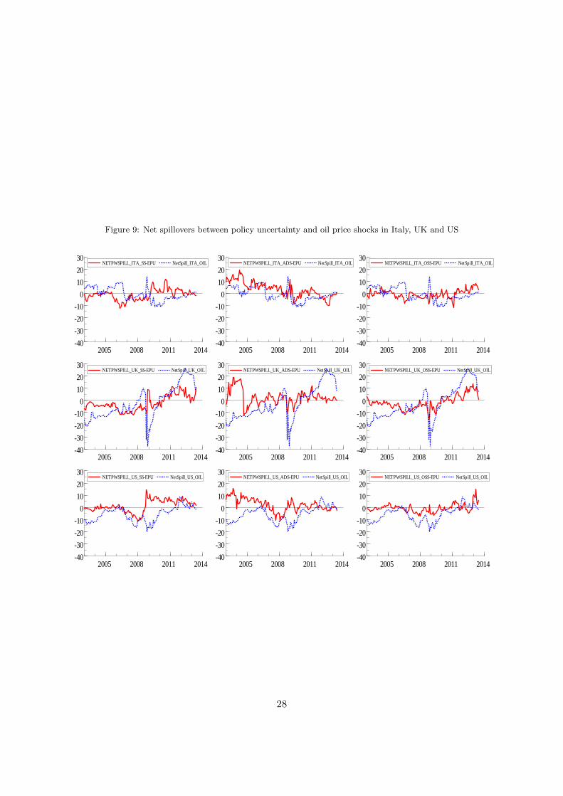
Figure 9: Net spillovers between policy uncertainty and oil price shocks in Italy, UK and US

NETPWSPILL_ITA_SS-EPU NetSpill_ITA_OIL

2005 2008 2011 2014-40-30-20-10

0102030

NETPWSPILL_ITA_SS-EPU NetSpill_ITA_OIL NETPWSPILL_ITA_ADS-EPU NetSpill_ITA_OIL

2005 2008 2011 2014-40-30-20-10

0102030

NETPWSPILL_ITA_ADS-EPU NetSpill_ITA_OIL NETPWSPILL_ITA_OSS-EPU NetSpill_ITA_OIL

2005 2008 2011 2014-40-30-20-10

0102030

NETPWSPILL_ITA_OSS-EPU NetSpill_ITA_OIL

NETPWSPILL_UK_SS-EPU NetSpill_UK_OIL

2005 2008 2011 2014-40-30-20-10

0102030

NETPWSPILL_UK_SS-EPU NetSpill_UK_OIL NETPWSPILL_UK_ADS-EPU NetSpill_UK_OIL

2005 2008 2011 2014-40-30-20-10

0102030

NETPWSPILL_UK_ADS-EPU NetSpill_UK_OIL NETPWSPILL_UK_OSS-EPU NetSpill_UK_OIL

2005 2008 2011 2014-40-30-20-10

0102030

NETPWSPILL_UK_OSS-EPU NetSpill_UK_OIL

NETPWSPILL_US_SS-EPU NetSpill_US_OIL

2005 2008 2011 2014-40-30-20-10

0102030

NETPWSPILL_US_SS-EPU NetSpill_US_OIL NETPWSPILL_US_ADS-EPU NetSpill_US_OIL

2005 2008 2011 2014-40-30-20-10

0102030

NETPWSPILL_US_ADS-EPU NetSpill_US_OIL NETPWSPILL_US_OSS-EPU NetSpill_US_OIL

2005 2008 2011 2014-40-30-20-10

0102030

NETPWSPILL_US_OSS-EPU NetSpill_US_OIL

28