arX

iv:c

ond-

mat

/941

1083

v1 2

1 N

ov 1

994

Dynamic Scaling of Ion–Sputtered Surfaces

R. Cuerno† and A.-L. Barabasi† ‡

† Center for Polymer Studies and Dept. of Physics, Boston University, Boston, MA 02215

‡ IBM T. J. Watson Research Center, P.O. Box 218, Yorktown Heigths, NY 10598

(February 1, 2008)

Abstract

We derive a stochastic nonlinear equation to describe the evolution and

scaling properties of surfaces eroded by ion bombardment. The coefficients

appearing in the equation can be calculated explicitly in terms of the physical

parameters characterizing the sputtering process. We find that transitions

may take place between various scaling behaviors when experimental param-

eters such as the angle of incidence of the incoming ions or their average

penetration depth, are varied.

PACS numbers: 79.20.Rf, 64.60.Ht, 68.35.Rh

Typeset using REVTEX

1

Recently there has been much interest in understanding the formation and roughening of

nonequilibrium interfaces. Applications range from fluid flow in porous media to bacterial

colonies or molecular beam epitaxy [1]. A common feature of most rough interfaces observed

experimentally or in discrete models is that their roughening follows simple scaling laws.

The associated scaling exponents can be obtained using numerical simulations or stochastic

evolution equations. The morphology and dynamics of a rough interface can be characterized

by the surface width, w(t, L), that scales as w2(t, L) = 〈[h(r, t)−h(t)]2〉 = L2αf(t/Lz), where

α is the roughness exponent for the interface h(r, t) and the dynamic exponent z describes

the scaling of the relaxation times with the system size L; h(t) is the mean height of the

interface at time t and 〈 〉 denotes both ensemble and space average. The scaling function

f has the properties f(u → 0) ∼ u2α/z and f(u → ∞) ∼ const.

Much of the attention has focused so far on the kinetics of interfaces generated in growth

processes. However, for a class of technologically important phenomena, such as sputter

etching, the surface morphology evolves as a result of erosion processes [2]. Motivated

by the advances in understanding growth, recently a number of experimental studies have

focused on the scaling properties of surfaces eroded by ion bombardment [3–5]. For graphite

bombarded with 5 keV Ar ions, Eklund et al. [3] reported α ≃ 0.2− 0.4, and z ≃ 1.6 − 1.8,

values consistent with the predictions of the Kardar-Parisi-Zhang (KPZ) equation in 2+1

dimensions [6,7]. Similarly Krim et al. [4] observed a self–affine surface generated by 5 keV

Ar bombardment of an Fe sample, with a larger exponent, α = 0.52. On the other hand,

there exists ample evidence about the development of a periodic ripple structure in sputter

etched surfaces (see e.g. [8]). Chason et al. [5] have recently studied the dynamics of such

eroded surfaces for both SiO2 and Ge bombarded with Xe ions at 1 keV, and found that it

differs from the dynamics expected for the self-affine morphologies observed in [3] and [4].

In this paper we investigate the large scale properties of ion-sputtered surfaces aiming

to understand in an unified framework the various dynamics and scaling behaviors of the

experimentally observed surfaces. For this we derive a stochastic nonlinear equation that

describes the time evolution of the surface height. The coefficients appearing in the equation

2

are functions of the physical parameters characterizing the sputtering process. We find

that transitions may take place between various surface morphologies as the experimental

parameters (e.g. angle of incidence, penetration depth) are varied. Namely, at short length-

scales the equation describes the development of a periodic ripple structure, while at larger

length-scales the surface morphology may be either logarithmically (α = 0) or algebraically

(α > 0) rough. Usually stochastic equations describing growth models are constructed using

symmetry principles and conservation laws. In most cases it is difficult to derive the equation

from a given discrete model. In contrast, here we show that for sputter eroded surfaces the

growth equation can be derived directly from a simple model of the elementary processes

taking place in the system.

Most of the theoretical approaches focusing on the scaling properties of sputter rough-

ened surfaces have assumed that essentially all relevant processes take place at the surface,

and that nonlinear effects would appear only due to non–local effects such as shadowing [9].

However, ion-sputtering is in general determined by atomic processes taking place along a

finite penetration depth inside the bombarded material. The incoming ions penetrate the

surface and transfer their kinetic energy to the atoms of the substrate by inducing cascades

of collisions among the substrate atoms, or through other processes such as electronic ex-

citations. Whereas most of the atoms which are actually sputtered are those located at

the surface, the scattering events that might lead to sputtering take place within a certain

layer of average depth a. As described by Sigmund’s transport theory of sputtering [10], the

average value of the ion deposition depth depends on the energy of the bombarding ions,

their angle of incidence, the microscopic structure of the target material and the features of

the scattering processes taking place inside the sample.

A convenient picture of the ion bombardment process is sketched in the inset of Fig.

1. According to it the ions penetrate a distance a inside the solid before they completely

spread out their kinetic energy with some assumed spatial distribution. An ion releasing its

energy at point P in the solid contributes an amount of energy to the surface point O, that

may induce the atoms in O to break their bonds and leave the surface. Following [10,11], we

3

consider that the average energy deposited at point O due to the ion arriving at P follows

the Gaussian distribution

ED(r′) =ǫ

(2π)3/2σµ2exp

{

− z′2

2σ2− x′2 + y′2

2µ2

}

. (1)

In (1) z′ is the distance measured along the ion trajectory, and x′, y′ are measured in the

plane perpendicular to it (see Fig. 1; for simplicity in the figure x′ has been set to 0); ǫ

denotes the total energy carried by the ion, a is the average penetration length and σ and µ

are the widths of the distribution in directions parallel and perpendicular to the incoming

beam respectively. However, the sample is subject to an uniform flux J of bombarding ions.

A large number of ions penetrate the solid at different points simultaneously and the velocity

of erosion at O depends directly on the total power EO contributed by all the ions deposited

within the range of the distribution (1). If we ignore shadowing effects among neighboring

points, as well as further redeposition of the eroded material, the velocity of erosion at O is

given by

v = p∫

Rdr Φ(r) ED(r), (2)

where the integral is taken over the region R of all the points at which the deposited energy

contributes to EO, Φ(r) is a local correction to the uniform flux J and p is a proportionality

constant between power deposition and rate of erosion. In the following we outline the basic

steps in the calculation of v; further details can be found in Refs. [11,12].

The calculation of (2) is most efficiently perfomed in the local coordinate system (X, Y, Z)

shown in Fig. 1. The ion beam lies in the X-Z plane, forming an angle ϕ with the Z axis,

Z being normal to the surface at O. To simplify the calculations, we assume that: (a)

the radii of curvature (RX , RY ) of the surface at O are much larger than the penetration

depth a, so that only terms up to first order in a/RX,Y are kept; (b) the curvatures attain

their maximum and minimum values along either of the X and Y directions, and thus we

can expand the value of the surface height at O by taking a second order approximation

in the (X,Y ) coordinates and consistently ignoring cross term contributions. Performing

4

the integral (2) the velocity v(ϕ, RX , RY ) is found to be a function of the angle ϕ and the

curvatures 1/RX,Y [11].

Finally, from the expression of v we can obtain the equation of motion for the profile. Now

it is convenient to use the laboratory coordinate frame (x, y, h). In the absence of overhangs

the surface can be described by a single valued height function h(x, y, t), measured from an

initial flat configuration which is taken to lie in the (x,y) plane. The ion beam is parallel

to the x-h plane forming an angle 0 < θ < π/2 with the z axis. The time evolution of h is

given by

∂h(x, y, t)

∂t≃ −v(ϕ, RX , RY ), (3)

where ϕ is the angle of the beam direction with the local normal to the surface at h(x, y).

Now ϕ is a function of the angle of incidence θ and the values of the local slopes ∂xh and

∂yh, and can be expanded in powers of the latter. We will assume that the surface varies

smoothly enough so that products of derivatives of h can be neglected for third or higher

orders.

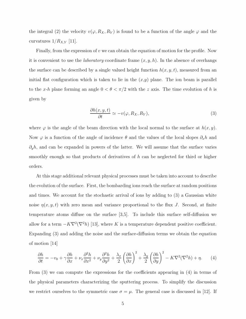
At this stage additional relevant physical processes must be taken into account to describe

the evolution of the surface. First, the bombarding ions reach the surface at random positions

and times. We account for the stochastic arrival of ions by adding to (3) a Gaussian white

noise η(x, y, t) with zero mean and variance proportional to the flux J . Second, at finite

temperature atoms diffuse on the surface [3,5]. To include this surface self-diffusion we

allow for a term −K∇2(∇2h) [13], where K is a temperature dependent positive coefficient.

Expanding (3) and adding the noise and the surface-diffusion terms we obtain the equation

of motion [14]

∂h

∂t= −v0 + γ

∂h

∂x+ νx

∂2h

∂x2+ νy

∂2h

∂y2+

λx

2

(

∂h

∂x

)2

+λy

2

(

∂h

∂y

)2

− K∇2(∇2h) + η. (4)

From (3) we can compute the expressions for the coefficients appearing in (4) in terms of

the physical parameters characterizing the sputtering process. To simplify the discussion

we restrict ourselves to the symmetric case σ = µ. The general case is discussed in [12]. If

5

we write F ≡ (ǫJp/√

2π) exp(−a2

σ/2), s ≡ sin θ, c ≡ cos θ and aσ ≡ a/σ, we find for the

coefficients in (4)

v0 =F

σc , γ =

F

σs(a2

σc2 − 1),

λx =F

σc{

a2

σ(3s2 − c2) − a4

σs2c2 + 1}

,

λy = −γc

s, (5)

νx =F

2aσ

{

2s2 − c2 − a2

σs2c2}

,

νy = −F

2aσc2.

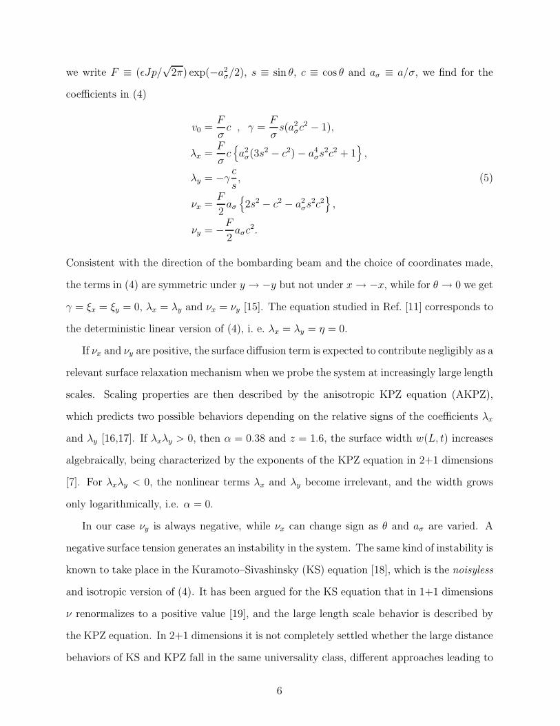
Consistent with the direction of the bombarding beam and the choice of coordinates made,

the terms in (4) are symmetric under y → −y but not under x → −x, while for θ → 0 we get

γ = ξx = ξy = 0, λx = λy and νx = νy [15]. The equation studied in Ref. [11] corresponds to

the deterministic linear version of (4), i. e. λx = λy = η = 0.

If νx and νy are positive, the surface diffusion term is expected to contribute negligibly as a

relevant surface relaxation mechanism when we probe the system at increasingly large length

scales. Scaling properties are then described by the anisotropic KPZ equation (AKPZ),

which predicts two possible behaviors depending on the relative signs of the coefficients λx

and λy [16,17]. If λxλy > 0, then α = 0.38 and z = 1.6, the surface width w(L, t) increases

algebraically, being characterized by the exponents of the KPZ equation in 2+1 dimensions

[7]. For λxλy < 0, the nonlinear terms λx and λy become irrelevant, and the width grows

only logarithmically, i.e. α = 0.

In our case νy is always negative, while νx can change sign as θ and aσ are varied. A

negative surface tension generates an instability in the system. The same kind of instability is

known to take place in the Kuramoto–Sivashinsky (KS) equation [18], which is the noisyless

and isotropic version of (4). It has been argued for the KS equation that in 1+1 dimensions

ν renormalizes to a positive value [19], and the large length scale behavior is described by

the KPZ equation. In 2+1 dimensions it is not completely settled whether the large distance

behaviors of KS and KPZ fall in the same universality class, different approaches leading to

6

conflicting results [20].

In contrast to the KS equation, Eq. (4) is anisotropic, and explicitly contains a noise

term. One can study Eq. (4) using a dynamic renormalization group (DRG) procedure. The

linear instability generated by the negative surface tension leads to additional singularities

in the Feynman diagrams of the perturbation expansion. This is related to the presence of

a characteristic length scale in the system, generated by the competition between surface

tension and surface diffusion, ℓc =√

K/|ν|, where ν is the largest in absolute value of

the negative surface tension coefficients. Below we discuss the possible scaling behaviour

predicted by (4) based on results obtained from DRG calculations performed on its isotropic

version [21], and the results available in the literature for other limits. The complete scaling

picture should be provided by either a DRG analysis or a numerical integration of (4).

The scaling behavior depends on the relative signs of νx, νy, λx and λy [22]. The variations

of these coefficients as functions of aσ and θ lead to the phase diagram shown in Fig. 2. In

the following we discuss the various scaling regimes separately.

Region I — For small θ both νx and νy are negative. As discussed by Bradley and

Harper [11] and experimentally studied by Chason et al. [5], a periodic structure dominates

the surface morphology, with ripples oriented along the direction (x or y) which presents

the largest absolute value for its surface tension coefficient. The wavelength of the ripples

is λc =√

2ℓc.

The large length scale behavior ℓ ≫ ℓc is expected to be different. Now both nonlinear-

ities and the noise may become relevant. A DRG analysis performed for the isotropic case

of Eqn. (4) [21,23] suggests that inside region I, the nonlinearities λx,y flow to zero. The

surface is logarithmically rough, with a roughness exponent α = 0. While in regions Ia-c

the coefficients of the nonlinear terms may change sign as aσ or θ vary, we do not expect

this to modify the scaling behavior.

Region II — This region is characterized by a positive νx and a negative νy. Now the

periodic structure associated with the instability is directed along the y direction and is the

dominant morphology at scales ℓ ∼ ℓc. Much less is known about the scaling behaviour

7

for large length scales. Preliminary results of a DRG calculation indicate that the surface

may be stabilized by the positive νx and the nonlinearities, and (4) reduces to the AKPZ

equation. If this is the case, then the surface roughness increases algebraically in region IIa,

whereas logarithmic scaling characterizes region IIb.

Even though several aspects of the scaling behavior predicted by (4) and (5) remain to be

clarified, we believe that these equations contain the relevant ingredients for understanding

roughening by ion bombardment [24]. To summarize, at short length scales the morphology

consists of a periodic structure oriented along the direction determined by the largest in

absolute value of the negative surface tension coefficients [5]. Modifying the values of aσ

or θ changes the orientation of the ripples [8,11]. At large length scales we expect two

different scaling regimes. One is characterized by KPZ exponents, which might be observed

in region IIa in Fig. 2. Indeed, the values of the exponents reported by Eklund et al. [3] are

consistent within the experimental errors with the KPZ exponents in 2+1 dimensions. The

other regime is characterized by logarithmic scaling (α = 0), which has not been observed

experimentally so far. We believe that it can be experimentally tested for suitable (e.g,

small) values of the angle of incidence. Moreover by tuning the values of θ and/or aσ one

may induce transitions among the different scaling behaviors. For example, fixing aσ and

increasing the value of θ would lead from logarithmic (regions Ia and Ic) to KPZ scaling

(IIa), and again logarithmic scaling (IIb) for large enough angles. Also, the measurement of

the erosion velocity may help to test the applicability of Eqn. (4). Taking spatial and noise

averages in (4), the terms contributing to the erosion velocity are the ones proportional to

v0, ξx, ξy, λx and λy. In the stationary state, modifying θ or aσ changes the average yield,

allowing for a comparison of the experimental yield curves with the ones predicted by (4).

The experimental verification of the above possibilities would constitute an important

step to elucidate the interplay between the mechanisms leading to the different morphologies

and dynamics for sputter-etched surfaces. It will provide as well additional insight into the

scaling behaviors to be expected from equation (4).

We would like to acknowledge discussions, comments and encouragement by L. A. N.

8

Amaral, K. B. Lauritsen, H. Makse and H. E. Stanley. R. C. acknowledges a postdoctoral

Fellowship of the Spanish Ministerio de Educacion y Ciencia.

9

REFERENCES

[1] Dynamics of Fractal Surfaces, edited by F. Family and T. Vicsek (World Scientific,

Singapore, 1991); P. Meakin, Phys. Rep. 235, 189 (1993); T. Halpin-Healey and Y.-C.

Zhang, Phys. Rep. (in press).

[2] Sputtering by Particle Bombardment, edited by R. Behrisch (Springer-Verlag, Heidelberg

1981, 1983), Vols. I, II.

[3] E. A. Eklund, R. Bruinsma, J. Rudnick and R. S. Williams, Phys. Rev. Lett. 67, 1759

(1991); E. A. Eklund, E. J. Snyder and R. S. Williams, Surf. Sci. 285, 157 (1993).

[4] J. Krim, I. Heyvaert, C. Van Haesendonck and Y. Bruynseraede, Phys. Rev. Lett. 70,

57 (1993).

[5] E. Chason, T. M. Mayer, B. K. Kellerman, D. T. McIlroy and A. J. Howard, Phys. Rev.

Lett. 72, 3040 (1994); T. M. Mayer, E. Chason and A. J. Howard, J. Appl. Phys. 76,

1633 (1994).

[6] M. Kardar, G. Parisi and Y.-C. Zhang, Phys. Rev. Lett. 56, 889 (1986).

[7] J. M. Kim and J. M. Kosterlitz, Phys. Rev. Lett. 62, 2289 (1989); B. M. Forrest and L.

Tang, J. Stat. Phys. 60, 181 (1990); K. Moser, D. E. Wolf and J. Kertesz, Physica A

178, 215 (1991); T. Ala Nissila, T. Hjelt, J. M. Kosterlitz and O. Vemoloinen, J. Stat.

Phys. 72, 207 (1993).

[8] G. Carter, B. Navinsek and J. L. Whitton in Vol. II of Ref. [2], p. 231.

[9] For a review see G. S. Bales, R. Bruinsma, E. A. Eklund, R. P. U. Karunasiri, J. Rudnick

and A. Zangwill, Science 249, 264 (1990).

[10] P. Sigmund, Phys. Rev. 184, 383 (1969); J. Mat. Sci. 8, 1545 (1973).

[11] R. M. Bradley and J. M. E. Harper, J. Vac. Sci. Technol. A6, 2390 (1988).

[12] A.–L. Barabasi and R. Cuerno (unpublished).

10

[13] C. Herring, J. Appl. Phys. 21, 301 (1950); W. W. Mullins, J. Appl. Phys. 28, 333 (1957);

in the context of stochastic models see D. E. Wolf and J. Villain, Europhys. Lett. 13,

389 (1990); S. Das Sarma and P. I. Tamborenea, Phys. Rev. Lett. 66, 325 (1991).

[14] In the expansion of (3) two additional nonlinearities are obtained on the rhs of Eqn.

(4): ξx∂h∂x

∂2h∂x2 + ξy

∂h∂x

∂2h∂y2 , where ξx and ξy are functions of a, σ, µ and θ [12]. One can see

that ξx and ξy are irrelevant at large length scales using the known values of α and z

[7] for both the nonlinear and the linear fixed points in 2+1 dimensions.

[15] The θ = 0 case has to be treated separately and is discussed in Ref. [12].

[16] D. E. Wolf, Phys. Rev. Lett. 67, 1783 (1991).

[17] The relevance of the AKPZ equation to sputter erosion has been suggested by R. Bru-

insma in Surface Disordering: Growth, Roughening and Phase Transitions, edited by

R. Jullien, J. Kertesz, P. Meakin and D. E. Wolf (Nova Science, New York, 1992).

[18] Y. Kuramoto and T. Tsuzuki, Prog. Theor. Phys. 55, 356 (1977); G. I. Sivashinsky,

Acta Astronaut. 6, 569 (1979).

[19] S. Zaleski, Physica D 34, 427 (1989); K. Sneppen, J. Krug, M. H. Jensen, C.

Jayaprakash, and T. Bohr, Phys. Rev. A 46, 7352 (1992); F. Hayot, C. Jayaprakash,

and Ch. Josserand, Phys. Rev. E 47, 911 (1993); V. S. L’vov, V. V. Lebedev, M. Paton,

and I. Procaccia, Nonlinearity 6, 25 (1993).

[20] I. Procaccia, M. H. Jensen, V. S. L’vov, K. Sneppen, and R. Zeitak, Phys. Rev. A 46,

3220 (1992); V. S. L’vov and I. Procaccia, Phys. Rev. Lett. 69, 3543 (1992); ibid. 72,

307 (1994); C. Jayaprakash, F. Hayot, and R. Pandit, Phys. Rev. Lett. 71, 12 (1993);

ibid. 72, 308 (1994).

[21] R. Cuerno, K. B. Lauritsen and A.–L. Barabasi (unpublished).

[22] The terms −v0 and ∂xh can be reabsorbed by a change of variables to a comoving frame,

11

and do not affect the scaling properties.

[23] L. Golubovic and R. Bruinsma, Phys. Rev. Lett. 66, 321 (1991); ibid. 67, 2747 (E)

(1991).

[24] Our analysis describes the roughening process in the small slope approximation. How-

ever, at late stages additional non-linear effects, such as shadowing [9], may become

relevant.

12

FIGURES

FIG. 1. Reference frames for the computation of the erosion velocity at point O. Inset: Fol-

lowing a straigh trajectory (solid line) the ion penetrates an average distance a inside the solid

(dotted line) after which it completely spreads out its kinetic energy. The dotted curves are equal

energy contours. Energy released at point P contributes to erosion at O.

FIG. 2. Phase diagram for the isotropic case σ = µ = 1. Region Ia: νx < 0, λx < 0, λy > 0;

Region Ib: νx < 0, λx > 0, λy < 0; Region Ic: νx < 0, λx > 0, λy > 0; Region IIa: νx > 0, λx > 0,

λy > 0; Region IIb: νx > 0, λx > 0, λy < 0.

13

XY

yO

θϕ

a

P

x

y’

Z

z’

a

P

Oh

0.0 0.5 1.0 1.5θ

0.0

1.0

2.0

3.0

a

Ia

Ib

IIb

Ic

IIa