arX

iv:1

302.

6941

v1 [

mat

h.PR

] 27

Feb

201

3

SCALING LIMIT AND CUBE-ROOT FLUCTUATIONS IN SOS SURFACES ABOVE A WALL

PIETRO CAPUTO, EYAL LUBETZKY, FABIO MARTINELLI, ALLAN SLY, AND FABIO LUCIO TONINELLI

ABSTRACT. Consider the classical (2 + 1)-dimensional Solid-On-Solid model above a hard wall onan L ! L box of Z2. The model describes a crystal surface by assigning a non-negative integerheight !x to each site x in the box and 0 heights to its boundary. The probability of a surfaceconfiguration ! is proportional to exp(""H(!)), where " is the inverse-temperature and H(!)sums the absolute values of height differences between neighboring sites.

We give a full description of the shape of the SOS surface for low enough temperatures. Firstwe show that with high probability the height of almost all sites is concentrated on two levels,H(L) = #(1/4") logL$ and H(L) " 1. Moreover, for most values of L the height is concentratedon the single value H(L). Next, we study the ensemble of level lines corresponding to the heights(H(L),H(L)"1, . . .). We prove that w.h.p. there is a unique macroscopic level line for each height.Furthermore, when taking a diverging sequence of system sizes Lk, the rescaled macroscopic levelline at height H(Lk) " n has a limiting shape if the fractional parts of (1/4") logLk convergeto a noncritical value. The scaling limit is an explicit convex subset of the unit square Q and itsboundary has a flat component on the boundary of Q. Finally, the highest macroscopic level line

has L1/3+o(1)k fluctuations along the flat part of the boundary of its limiting shape.

1. INTRODUCTION

The (d + 1)-dimensional Solid-On-Solid model is a crystal surface model whose definitiongoes back to Temperley [36] in 1952 (also known as the Onsager-Temperley sheet). At lowtemperatures, the model approximates the interface between the plus and minus phases in the(d+ 1)D Ising model, with particular interest stemming from the study of 3D Ising.

The configuration space of the model on a finite box ! ! Zd with zero boundary conditionsis the set of all height functions ! on Zd such that ! " x #$ !x % Z whereas !x = 0 for all x /% !.The probability of ! is given by the Gibbs distribution proportional to

exp

!& "

"

x!y

|!x & !y|#, (1.1)

where " > 0 is the inverse-temperature and x ' y denotes a nearest-neighbor bond in Zd.Numerous works have studied the rich random surface phenomena, e.g. roughening, local-

ization/delocalization, layering and wetting to name but a few, exhibited by the SOS model andsome of its many variants. These include the discrete Gaussian (replacing |!x & !y| by |!x & !y|2for the integer analogue of the Gaussian free field), restricted SOS (nearest neighbor gradientsrestricted to {0,±1}), body centered SOS [5], etc. (for more on these flavors see e.g. [1,4,10]).

Of special importance is SOS with d = 2, the only dimension featuring a roughening transition.For d = 1, it is well known ([22, 36, 37]) that the SOS surface is rough (delocalized) for any" > 0, i.e., the expected height at the origin diverges (in absolute value) in the thermodynamiclimit |!| $ (. However, for d ! 3 it is known that the surface is rigid (localized) for any " > 0(see [13]), i.e., |!0| is uniformly bounded in expectation. A simple Peierls argument shows thatthis is also the case for d = 2 and large enough " ([11, 26]). That the surface is rough for

2010 Mathematics Subject Classification. 60K35, 82B41, 82C24 .Key words and phrases. SOS model, Scaling limits, Loop ensembles, Random surface models.This work was supported by the European Research Council through the “Advanced Grant” PTRELSS 228032.

1

2 P. CAPUTO, E. LUBETZKY, F. MARTINELLI, A. SLY, AND F.L. TONINELLI

d = 2 at high temperatures was established in seminal works of Frohlich and Spencer [23–25].Numerical estimates for the critical inverse-temperature "R where the roughening transitionoccurs suggest that "R ) 0.806.

When the (2 + 1)D SOS surface is constrained to stay above a hard wall (or floor), i.e. ! isconstrained to be non-negative in (1.1), Bricmont, El-Mellouki and Frohlich [12] showed in1986 the appearance of entropic repulsion: for large enough ", the floor pushes the SOS surfaceto diverge even though " > "R. More precisely, using Pirogov-Sinaı theory (see the review [35]),the authors of [12] showed that the SOS surface on an L*L box rises, amid the penalizing zeroboundary, to an average height in the interval [(1/C") log L , (C/") log L] for some absoluteconstant C > 0, in favor of freedom to create spikes downwards. In a companion paper [14],focusing on the dynamical evolution of the model, we established that the average height is infact (1/4") log L up to an additive O(1)-error.

Entropic repulsion is one of the key features of the physics of random surfaces. This phenome-non has been rigorously analyzed mainly for some continuous-height variants of the SOS modelin which the interaction potential |!x & !y| is replaced by a strictly convex potential V (!x & !y);see, e.g., [7–9, 16, 18, 38, 39], and also [3] for a recent analysis of the wetting transition in theSOS model. It was shown in the companion paper [14] that entropic repulsion drives the evo-lution of the surface under the natural single-site dynamics. Started from a flat configuration,the surface rises to an average height of (1/4") log L & O(1) through a sequence of metastablestates, corresponding roughly to plateaux at heights 0, 1, 2, . . . , (1/4") log L.

Despite the recent progress on understanding the typical height of the surface, little wasknown on its actual 3D shape. The fundamental problem is the following:

Question. Consider the ensemble of all level lines of the low temperature (2+1)D SOS on an L*Lbox with floor, rescaled to the unit square.

(i) Do these jointly converge to a scaling limit as L $ (, e.g., in Hausdorff distance?(ii) If so, can the limit be explicitly described?

(iii) For finite large L, what are the fluctuations of the level lines around their limit?

In this work we fully resolve parts (i) and (ii) and partially answer part (iii). En route, we alsoestablish that for most values of L the surface height concentrates on the single level + 1

4! logL,.

1.1. Main results. We now state our three main results. As we will see, two parameters rulethe macroscopic behavior of the SOS surface:

H(L) =

$1

4"log(L)

%, #(L) =

1

4"log(L)&H(L) , (1.2)

namely the integer part and the fractional part of 14! log(L). The first result states that with

probability tending to one as L $ ( the SOS surface has a large fraction of sites at height equaleither to H(L) or to H(L) & 1. Moreover only one of the two possibilities holds depending onwhether #(L) is above or below a critical threshold that can be expressed in terms of an explicitcritical parameter $c = $c("). The second result describes the macroscopic shape for large Lof any finite collections of level lines at height H(L),H(L) & 1, . . . . The third result establishescube root fluctuations of the level lines along the flat part of its macroscopic shape.

In what follows we consider boxes ! of the form ! = !L = [1, L]* [1, L], L % N. We write %0!for the SOS distribution on ! with floor and boundary condition at zero, and let %0! be its analogwithout a floor. The function L #$ $(L) % (0,() appearing below is explicitly given in terms of#(L) (see Section 1.3 and Definition 2.5 below). For large " it satisfies $(L)e"4!"(L) - 1.

SOS SURFACES ABOVE A WALL 3

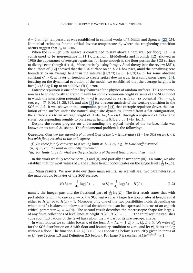
FIGURE 1. Loop ensemble formed by the level lines of an SOS configuration ona box of side-length 1000 with floor (showing loops longer than 100).

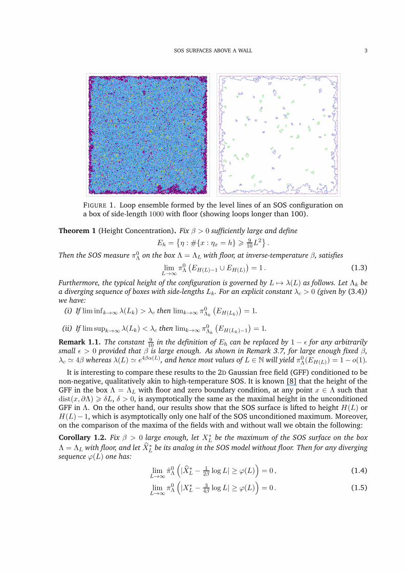
Theorem 1 (Height Concentration). Fix " > 0 sufficiently large and define

Eh =&! : #{x : !x = h} ! 9

10L2'.

Then the SOS measure %0! on the box ! = !L with floor, at inverse-temperature ", satisfies

limL#$

%0!(EH(L)"1 . EH(L)

)= 1 . (1.3)

Furthermore, the typical height of the configuration is governed by L #$ $(L) as follows. Let !k bea diverging sequence of boxes with side-lengths Lk. For an explicit constant $c > 0 (given by (3.4))we have:

(i) If lim infk#$ $(Lk) > $c then limk#$ %0!k

(EH(Lk)

)= 1.

(ii) If lim supk#$ $(Lk) < $c then limk#$ %0!k

(EH(Lk)"1

)= 1.

Remark 1.1. The constant 910 in the definition of Eh can be replaced by 1 & & for any arbitrarily

small & > 0 provided that " is large enough. As shown in Remark 3.7, for large enough fixed ",$c - 4" whereas $(L) - e4!"(L), and hence most values of L % N will yield %0!(EH(L)) = 1& o(1).

It is interesting to compare these results to the 2D Gaussian free field (GFF) conditioned to benon-negative, qualitatively akin to high-temperature SOS. It is known [8] that the height of theGFF in the box ! = !L with floor and zero boundary condition, at any point x % ! such thatdist(x, '!) ! (L, ( > 0, is asymptotically the same as the maximal height in the unconditionedGFF in !. On the other hand, our results show that the SOS surface is lifted to height H(L) orH(L)& 1, which is asymptotically only one half of the SOS unconditioned maximum. Moreover,on the comparison of the maxima of the fields with and without wall we obtain the following:

Corollary 1.2. Fix " > 0 large enough, let X%L be the maximum of the SOS surface on the box

! = !L with floor, and let *X%L be its analog in the SOS model without floor. Then for any diverging

sequence )(L) one has:

limL#$

%0!

+| *X%

L & 12! logL| / )(L)

,= 0 , (1.4)

limL#$

%0!

+|X%

L & 34! logL| / )(L)

,= 0 . (1.5)

4 P. CAPUTO, E. LUBETZKY, F. MARTINELLI, A. SLY, AND F.L. TONINELLI

FIGURE 2. The nested limiting shapes {Lc($(n)# )} of the rescaled loop ensemble 1

L{"n}.

We now address the scaling limit of the ensemble of level lines. The latter is described asfollows (see Section 3 for the full details). As for the 2D Ising model (see e.g. [6, 19]), forthe low-temperature SOS model without floor there is a natural notion of surface tension *(·)satisfying the strict convexity property. We emphasise that the surface tension we consider hereis constructed in the usual way, namely by imposing Dobrushin type conditions (between heightzero and height one) around a box. Consider the associated Wulff shape, namely the convexbody with support function * , and let W1 denote the Wulff shape rescaled to enclose area 1. Fora given s > 0, define the shape Lc(s) by taking the union of all possible translates of +c(s)W1

within the unit square, with an explicit dilation parameter +c(s) which satisfies +c(s) ' 2!s for

large ". (Of course, Lc(s) is defined only if +c(s)W1 fits inside a unit square.) Next, for a fixed

$# > 0, consider the nested shapes {Lc($(n)# )}n ! 0 obtained by taking s equal to $(n)# := e4!n$#,

n = 0, 1, . . . as shown in Figure 2.The next theorem gives a necessary and sufficient condition for the existence of the scaling

limit of ensemble of level lines in terms of the above defined shapes. As a convention, in thesequel we often write “with high probability”, or w.h.p., whenever the probability of an event isat least 1& e"c(logL)2 for some constant c > 0.

Theorem 2 (Shape Theorem). Fix " > 0 sufficiently large and let Lk be a diverging sequence of

side-lengths. Set Hk = H(Lk). For an SOS surface on the box !k with side Lk, let ("(k)0 ,"(k)

1 , . . .)be the collections of loops with length at least (logLk)2 belonging to the level lines at heights(Hk,Hk & 1, . . .), respectively. Then:

(a) W.h.p. the level lines of every height h > Hk consist of loops shorter than (logLk)2, while "(k)0

is either empty or contains a single loop, and "(k)n consists of exactly one loop for each n ! 1.

(b) If $# := limk#$ $(Lk) exists and differs from $c (as given by (3.4)) then the rescaled loop

ensemble 1Lk

("(k)0 ,"(k)

1 , . . .) converges to a limit in the Hausdorff distance: for any , > 0, w.h.p.

• If $# > $c then

supn&0

dH(

1Lk

"(k)n ,Lc($

(n)# ))" , ,

where dH denotes the Hausdorff distance.

• If instead $# < $c then "(k)0 is empty while

supn&1

dH(

1Lk

"(k)n ,Lc($

(n)# ))" , .

SOS SURFACES ABOVE A WALL 5

As for the critical behavior, from the above theorem we immediately read that it is possible tohave $(Lk) $ $c without admitting a scaling limit for the loop ensemble (consider a sequencethat oscillates between the subcritical and supercritical regimes). However, understanding thecritical window around $c and the limiting behavior there remains an interesting open problem.

The fluctuations of the loop "(k)0 (the macroscopic plateau at level H(Lk) if it exists) from its

limit Lc($#) along the side-boundaries are now addressed. As shown in Figure 2, the boundaryof the limit shape Lc($#) coincides with the boundary of the unit square Q except for a neigh-borhood of the four corners of Q. Let the interval [a, 1&a], a = a($#) > 0, denote the horizontalprojection of the intersection of the shape Lc($#) with the bottom side of the unit square Q.

Theorem 3 (Cube-root Fluctuations). In the setting of Theorem 2 suppose $# > $c. Then for any

& > 0, w.h.p. the vertical fluctuation of "(k)0 from the boundary interval

I(k)$ = [a(1 + &)Lk, (1& a(1 + &))Lk]

is of order L13+o(1)k . More precisely, let -(x) = max{y 0 1

2Lk : (x, y) % "(k)0 } be the vertical

fluctuation of "(k)0 from the bottom boundary of !k at coordinate x. Then w.h.p.

L13"$k < sup

x'I(k)!

-(x) < L13+$k .

Remark 1.3. We will actually prove the stronger fact that w.h.p. a fluctuation of at least L13"$k is

attained in every sub-interval of I(k)$ of length L23"$k (cf. Section 6.4).

As a direct corollary of Theorem 3 it was deduced in [15] that the following upper bound on

the fluctuations of all level lines "(k)n (n / 1) holds.

Corollary 1.4 (Cascade of fluctuation exponents). In the same setting of Theorem 3, let -(n, x)

be the vertical fluctuation of "(k)n from the bottom boundary at coordinate x. Let 0 < t < 1 and let

n = +tHk,. Then for any & > 0,

limk#$

%0!k

!sup

x'I(k)!

-(n, x) > L1!t3 +$

k

#= 0 .

1.2. Related work. In the two papers [33, 34] Schonmann and Shlosman studied the limitingshape of the low temperature 2D Ising with minus boundary under a prescribed small positiveexternal field, proportional to the inverse of the side-length L. The behavior of the droplet ofplus spins in this model is qualitatively similar to the behavior of the top loop "0 in our case.Here, instead of an external field, it is the entropic repulsion phenomenon which induces thesurface to rise to level H(L) producing the macroscopic loop "0. In line with this connection, theshape Lc(s) appearing in Theorem 2 is constructed in the same way as the limiting shape of theplus droplet in the aforementioned works, although with a different Wulff shape. In particular,as in [33, 34], the shape Lc(s) arises as the solution to a variational problem; see Section 3below.

An important difference between the two models, however, is the fact that in our case thereexist H(L) levels (rather than just one), which are interacting in two nontrivial ways. First,by definition, they cannot cross each other. Second, they can weakly either attract or repelone another depending on the local geometry and height. Moreover, the box boundary itselfcan attract or repel the level lines. A prerequisite to proving Theorem 2 is to overcome these“pinning” issues. We remark that at times such pinning issues have been overlooked in therelevant literature.

6 P. CAPUTO, E. LUBETZKY, F. MARTINELLI, A. SLY, AND F.L. TONINELLI

As for the fluctuations of the plus droplet from its limiting shape, it was argued in [33] thatthese should be normal (i.e., of order

1L). However, due to the analogy mentioned above

between the models, it follows from our proof of Theorem 3 that these fluctuations are in factL1/3+o(1) along the flat pieces of the limiting shape, while it seems natural to conjecture thatnormal fluctuations appear along the curved portions, where the limiting shapes correspondingto distinct levels are macroscopically separated; see Figure 2.

There is a rich literature of contour models featuring similar cube root fluctuations. In someof these works (e.g., [2, 21, 30, 39]) the phenomenon is induced by an externally imposed con-straint (by conditioning on the event that the contour contains a large area and/or by adding anexternal field); see in particular [39] for the above mentioned case of the 2D Ising model in aweak external field, and the recent works [27,28] for refined bounds in the case of FK percola-tion. In other works, modeling ordered random walks (e.g., [17, 31] to name a few), the exactsolvability of the model (e.g., via determinantal representations) plays an essential role in theanalysis. In our case, the phenomenon is again a consequence of the tilting of the distributionof contours induced by the entropic repulsion. The lack of exact solvability for the (2+1)D SOS,forces us to resort to cluster expansion techniques and contour analysis as in the frameworkof [19].

We conclude by mentioning some problems that remain unaddressed by our results. Firstis to establish the exponents for the fluctuations of all intermediate level lines from the side-boundaries. We believe the upper bound in Corollary 1.4 features the correct cascade of expo-nents. Second, find the correct fluctuation exponent of the level lines {"n} around the curved

part of their limiting shapes {Lc($(n)# )}. Third, we expect that, as in [2, 27, 28], the fluctuation

exponents of the highest level line around its convex envelope is 1/3, while, as mentioned above,there should be normal fluctuations around the curved parts of the deterministic limiting shape.

1.3. On the ensemble of macroscopic level lines. We turn to a high-level description of thestatistics of the level lines of the SOS interface. Given a closed contour . (i.e., a closed loop ofdual edges as for the standard Ising model), a positive integer h and a surface configuration ! wesay that . is an h-contour (or h-level line) for !, if the surface height jumps from being at leasth along the internal boundary of . to at most h & 1 along the external boundary of .. Clearlyan h-contour . is energetically penalized proportionally to its length |.| because of the form ofthe SOS energy function. As in many spin models admitting a contour representation, with highprobability contours are either all small, say |.| = O((logL)2), or there exist macroscopicallylarge ones (i.e. |.| 2 L), if L is the size of the system. An instance of the first situation is the SOSmodel without a wall and zero boundary conditions (see [11]). On the contrary, macroscopiccontours appear in the low temperature 2D Ising model with negative boundary conditions and apositive external field H of the form H = B/L, B > 0, as in [33,34]. In this case the probabilisticweight of a contour separating the inside plus spins from the outside minus spins is roughlygiven by exp

(&"|.|+#(.)+m%

!HA(.)), where A(.) denotes the area enclosed by ., m%

! is the

spontaneous magnetisation and #(.) is a “decoration” term which is not essential for the presentdiscussion. If the parameter B is above a certain threshold then the area term dominates theboundary term and a macroscopic contour appears with high probability. Moreover, by simpleisoperimetric arguments, the macroscopic contour is unique in this case.

The SOS model with a wall shares some similarities with the Ising example above but has aricher structure that can be roughly described as follows.

Suppose {.1, .2, . . . , .n} are macroscopic h-contours corresponding to heights h = 1, 2, . . . nand that no other macroscopic contour exists. Then necessarily the collection {.i}ni=1 must con-sist of nested contours, with .n and .1 being the innermost and outermost contour respectively.

SOS SURFACES ABOVE A WALL 7

If we denote by !i the region enclosed by .i and by Ai the annulus !i \!i+1, then the partitionfunction of all the surfaces satisfying the above requirements can be written as

Z(.1, . . . , .n) = exp+& "

"

i

|.i|,-

i

ZAi

where ZAi is the partition function of the SOS model in Ai, with a wall at height zero, boundary

conditions at height h = i and restricted to configurations without macroscopic contours1.Usually (see, e.g., [19]) in these cases one tries to exponentiate the partition functions ZAi

using cluster expansion techniques. However, because of the presence of the wall, one cannotapply directly this approach and it is instead more convenient to compare ZAi with ZAi , where

ZAi is as ZAi but without the wall. One then observes that the ratio ZAi/ZAi is simply theprobability that the surface is non-negative computed for the Gibbs distribution of the SOSmodel in Ai with boundary conditions at height h = i, no wall, and conditioned to have nomacroscopic contours. The key point, which was already noted in [14], is that w.r.t. the aboveGibbs measure the random variables {1%x&0}x'Ai behave approximately as i.i.d. with

P(!x / 0) - 1& c$e"4!(i+1),

where is c$ a computable constant. Therefore,

ZAi - exp+&c$e"4!(i+1)|Ai|

,ZAi .

In conclusion, rewriting |Ai| = |!i|& |!i+1|,

Z(.1, . . . , .n) 2 exp

."

i

/&"|.i|+ c$e"4!i(1& e"4!)|!i|

01-

i

ZAi .

The terms proportional to the area encode the effect of the entropic repulsion and play the samerole as the magnetic field term in the Ising example. Cluster expansion techniques can nowbe applied to the partition functions ZAi without wall. As in many other similar cases theirnet result is the appearance of a decoration term #(.i) = O(,! |.i|) for each contour, ,! smallfor large ", and an effective many-body interaction $(.1, . . . , .n) among the contours whichhowever is very rapidly decaying with their mutual distance. Thus the probability of the abovemacroscopic contours should then be proportional to

exp

."

i

/&"|.i|+ c$e"4!i(1& e"4!)|!i|+#(.i)

0+ $(.1, . . . , .n)

1

. (1.6)

Note that in each term of the above sum the area part is dominant up to height i - (1/4") log(L).In other words, macroscopic h-contours are sustained by the entropic repulsion up to a heighth - (1/4") log(L) while higher contours are exponentially suppressed. More precisely, if wemeasure heights relatively to H(L) = +(1/4") log(L),, then the ith area term can be rewrittenas

$e4!(H(L)"i)

L|!i|, with $ = $(L) = c$e4!"(L)(1& e"4!).

The quantity $(L) is exactly the key parameter appearing in the main theorems. Notice that theloop "0 appearing in Theorem 2 would correspond to the contour .n if n = H(L).

Summarizing, the macroscopic contours behave like nested random loops with an area biasand with some interaction potential $. While the latter is in many ways a weak perturbation,

1Strictly speaking one should also require that the height is at most i (at least i) along the inner (outer) boundaryof the annulus, but we skip these details for the present discussion.

8 P. CAPUTO, E. LUBETZKY, F. MARTINELLI, A. SLY, AND F.L. TONINELLI

in principle delicate pinning effects may occur among the different level lines, as emphasizedearlier.

Although one could try to implement directly the above line of reasoning, we found it moreconvenient to combine the above ideas with monotonicity properties of the model (w.r.t. theheight of the boundary conditions and/or the height of the wall) to reduce ourselves always tothe analysis of one single macroscopic contour at a time. That allowed us to partially overcomethe above mentioned pinning problem. On the other hand, a stronger control of the interactionbetween level lines seems to be crucial in order to determine the correct fluctuation exponentsof all the intermediate level lines from the side-boundaries (see the open problems discussedabove).

2. GENERAL TOOLS

In this section we collect some preliminary definitions together with basic results which willbe used several times throughout the paper. Once combined together with standard clusterexpansion methods they quantify precisely the effect of the entropic repulsion from the floor.

2.1. Preliminaries. In order to formulate our first tools we need a bit of extra notation.

Boundary conditions and infinite volume limit. Given a height function Z2 " x #$ *x % Z (the

boundary condition) and a finite set ! ! Z2 we denote by %(&)! (resp. %(&)

! ) all the heightfunctions ! on Z2 such that ! " x #$ !x % Z+ (resp. ! " x #$ !x % Z) whereas !x = *x for allx /% !. The corresponding Gibbs measure given by (1.1) will be denoted by %&! (resp. %&!). Inother words %&! describes the SOS model in ! with boundary conditions * and floor at zero while%&! describes the SOS model in ! with boundary conditions * and no floor. The corresponding

partition functions will be denoted by Z&! and Z&

! respectively. If * is constant and equal to j % Zwe will simply replace * by j in all the notation. We will denote by % the infinite volume Gibbsmeasure obtained as the thermodynamic limit of the measure %0! along an increasing sequenceof boxes. The limit exists and does not depend on the sequence of boxes; see [11].

Contours and level lines. The level lines of the SOS surface, and the corresponding loop ensemblethey give rise to, are formally defined as follows.

Definition 2.1 (Geometric contour). We let Z2% be the dual lattice of Z2 and we call a bond anysegment joining two neighboring sites in Z2%. Two sites x, y in Z2 are said to be separated by a bonde if their distance (in R2) from e is 1

2 . A pair of orthogonal bonds which meet in a site x% % Z2%

is said to be a linked pair of bonds if both bonds are on the same side of the forty-five degrees lineacross x%. A geometric contour (for short a contour in the sequel) is a sequence e0, . . . , en of bondssuch that:

(1) ei 3= ej for i 3= j, except for i = 0 and j = n where e0 = en.(2) for every i, ei and ei+1 have a common vertex in Z2%

(3) if ei, ei+1, ej , ej+1 intersect at some x% % Z2%, then ei, ei+1 and ej , ej+1 are linked pairs ofbonds.

We denote the length of a contour . by |.|, its interior (the sites in Z2 it surrounds) by !' and itsinterior area (the number of such sites) by |!' |. Moreover we let &' be the set of sites in Z2 suchthat either their distance (in R2) from . is 1

2 , or their distance from the set of vertices in Z2% where

two non-linked bonds of . meet equals 1/12. Finally we let &+

' = &' 4 !' and &"' = &' \&+

' .

SOS SURFACES ABOVE A WALL 9

Definition 2.2 (h-contour). Given a contour . we say that . is an h-contour (or an h-level line)for the configuration ! if

!#"!"" h& 1, !#"+

"! h.

We will say that . is a contour for the configuration ! if there exists h such that . is an h-contourfor !. Contours longer than (logL)2 will be called macroscopic contours2. Finally C',h will denotethe event that . is an h-contour.

Definition 2.3 (Negative h-contour). We say that a closed contour . is a negative h-contour if theexternal boundary . is at least h whereas its internal boundary is at most h & 1. That is to say,denoting this event by C

"',h, we have that ! % C

"',h iff !#"+

"" h& 1 and !#"!

"! h.

Entropic repulsion parameters. In order to define key parameters measuring the entropic repul-sion we first need the following Lemma whose proof is postponed to Appendix A.1.

Lemma 2.4. For " large enough the limit c$ := limh#$ e4!h%(!0 / h) exists and

|c$ & e4!h%(!0 / h)| = O(e"2!h).

Moreover lim!#$ c$ = 1.

Definition 2.5. Given an integer L > 1 we define

$ := $(L) = e4! "(L)c$(1& e"4!) (2.1)

where #(L) denotes the fractional part of 14! logL. Also, for n / 0, we let $(n) := $(n)(L) = $e4!n.

2.2. An isoperimetric inequality for contours. The following simple lemma will prove usefulin establishing the existence of macroscopic loops.

Lemma 2.6. For all (( > 0 there exists a ( > 0 such the following holds. Let {.i} be a collection ofclosed contours with areas A(.i) satisfying A(.1) ! A(.2) ! . . . , and suppose that

"

i

|.i| 0 (1 + ()4L , and"

i

A(.i) / (1& 2()L2.

Then the interior of .1 contains a sub-square of area at least (1& (()L2.

Proof. Define #i = A(.i)2(1& 2()L2

3"1so that

4i #i / 1. Then (see, e.g., [19, Section 2.8])4

i1#i / 1)

"1. Using the isoperimetric bound |.i| / 4

5A(.i), it follows that

(1 + ()4L /"

i

|.i| / 45

(1& 2()L2"

i

1#i

/ 45

(1& 2()L2 11#1

= 4(1& 2()L2 15A(.1)

.

This implies, for ( small enough,

A(.1) /(1& 2()2

(1 + ()2L2 / (1& 8()L2.

Noting that the unit square is the unique shape with area at least 1 and L1-boundary length atmost 4 it follows by continuity that for all (( > 0 there exists ( > 0 such that if a curve has lengthat most (1 + ()4 and area at least 1& 8( then it contains a square of side-length 1& (( implyingthe last assertion of the lemma. $

2This convention is slightly abusive, since the term macroscopic is usually reserved to objects with size comparableto the system size L. However, as we will see, it is often the case in our context that with overwhelming probability,there are no contours at intermediate scales between (logL)2 and L.

10 P. CAPUTO, E. LUBETZKY, F. MARTINELLI, A. SLY, AND F.L. TONINELLI

2.3. Peierls estimates and entropic repulsion. Our first result is a upper bound on the prob-ability of encountering a given h-contour and it is a refinement of [14, Proposition 3.6]. Recallthe definition of the height H(L), of the parameters $(n) and of the events C',h, C

"',h.

Proposition 2.7. Fix j / 0 and consider the SOS model in a finite connected subset V of Z2

with floor at height 0 and boundary conditions at height j / 0. There exists (h and ,! withlimh#$ (h = lim!#$ ,! = 0 such that, for all h % N:

%jV (C',h) " exp+&"|.|+ c$(1 + (h)|!' |e"4!h

,exp

+,! e

"4!h|.| log(|.|),, (2.2)

%jV(C

"',h

)0 e"!|'|. (2.3)

Remark 2.8. Notice that if h = H(L)& n then c$e"4!h = (1& e"4!)"1$(n)/L.

Proof of (2.2). Let Z+,nin (resp. Z+,n

in ) be the partition function of the SOS model in !' with floor

at height 0 (resp. no floor), b.c. at height n and !#"+"/ n. Similarly call Z",n

out be the partition

function of the SOS model in V \ !' with floor at height 0, b.c. at height j along 'V , at heightn along . and satisfying !#"!

"0 n. One has

%j! (C',h) = e"!|'| Z",h"1out Z+,h

in

ZjV

0 e"!|'| Z",h"1out Z+,h

in

Z",h"1out Z+,h"1

in

= e"!|'| Z+,hin

Z+,h"1in

0 e"!|'| Z+,hin

Z+,h"1in

= e"!|'| Z+,h"1in

Z+,h"1in

,

where in the last equality we used the fact that Z+,nin is independent of n.

Let now %n!"be the Gibbs measure in !' with b.c. at height n and no floor. Then, using first

monotonicity and then the FKG inequality:

Z+,h"1in

Z+,h"1in

= %h"1!"

+!#!"

/ 066 !#"+

"/ h& 1

,

/ %h"1!"

+!#!"

/ 0,/-

x'!"

%h"1!"

(!x / 0) =-

x'!"

/1& %0!"

(!x / h)0. (2.4)

It follows from [14, Proposition 3.9] that maxx'!" %0!"

(!x / h) 0 c exp(&4"h) for some con-

stant c independent of ". Moreover, using the exponential decay of correlations of the SOSmeasure without floor (cf. [11]), we obtain

%0!"(!x / h) 0

7c e"4!h if dist(x, .) 0 ,! log(|!' |)% (!x / h) |+ 1/|!' |2 otherwise

with lim!#$ ,! = 0. If we now use Lemma 2.4 to write % (!x / h) = c$(1 + (h)e"4!h,limh#$ (h = 0, we get

-

x'!"

/1& %0!"

(!x / h)0=

-

x'!"

dist(x,')*(# log(|!" |)

/1& %0!"

(!x / h)0*

-

x'!"

dist(x,')>(# log(|!" |)

/1& %0!"

(!x / h)0

/ exp+&c ,! e

"4!h|.| log(|!' |),exp

+&c$(1 + (h)e

"4!h|!' |,.

The proof is complete using |!' | 0 |.|2/16. $

SOS SURFACES ABOVE A WALL 11

Proof of (2.3). With the same notation as before we write

%j!

+C

"',h

,= e"!|'| Z

+,hout Z

",h"1in

ZjV

0 e"!|'| Z+,hout Z

",h"1in

Z+,hout Z

",hin

0 e"!|'| . $

The next result is a simple geometric criterion to exclude certain large contours.

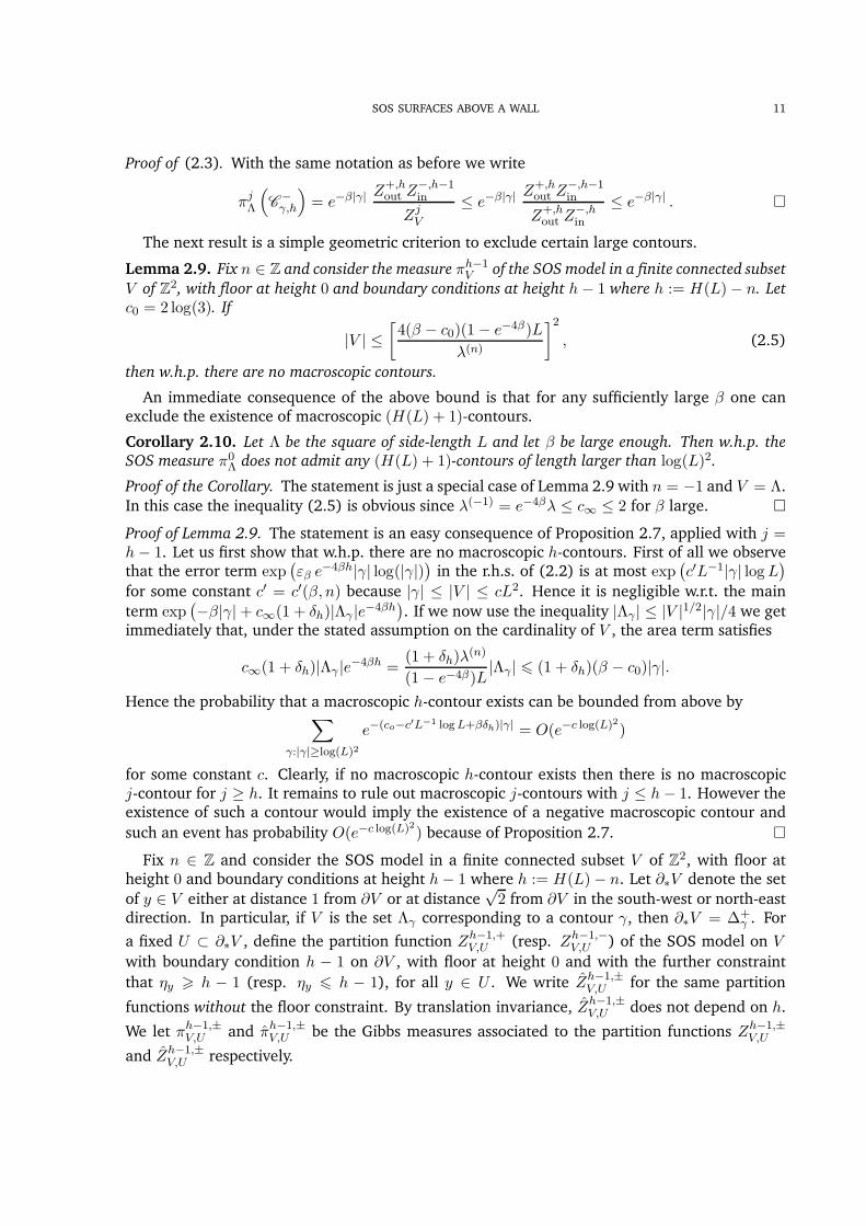
Lemma 2.9. Fix n % Z and consider the measure %h"1V of the SOS model in a finite connected subset

V of Z2, with floor at height 0 and boundary conditions at height h& 1 where h := H(L)& n. Letc0 = 2 log(3). If

|V | 084(" & c0)(1& e"4!)L

$(n)

92, (2.5)

then w.h.p. there are no macroscopic contours.

An immediate consequence of the above bound is that for any sufficiently large " one canexclude the existence of macroscopic (H(L) + 1)-contours.

Corollary 2.10. Let ! be the square of side-length L and let " be large enough. Then w.h.p. theSOS measure %0! does not admit any (H(L) + 1)-contours of length larger than log(L)2.

Proof of the Corollary. The statement is just a special case of Lemma 2.9 with n = &1 and V = !.In this case the inequality (2.5) is obvious since $("1) = e"4!$ 0 c$ 0 2 for " large. $

Proof of Lemma 2.9. The statement is an easy consequence of Proposition 2.7, applied with j =h& 1. Let us first show that w.h.p. there are no macroscopic h-contours. First of all we observethat the error term exp

(,! e"4!h|.| log(|.|)

)in the r.h.s. of (2.2) is at most exp

(c(L"1|.| logL

)

for some constant c( = c((", n) because |.| 0 |V | 0 cL2. Hence it is negligible w.r.t. the mainterm exp

(&"|.|+ c$(1 + (h)|!' |e"4!h

). If we now use the inequality |!' | 0 |V |1/2|.|/4 we get

immediately that, under the stated assumption on the cardinality of V , the area term satisfies

c$(1 + (h)|!' |e"4!h =(1 + (h)$(n)

(1& e"4!)L|!' | " (1 + (h)(" & c0)|.|.

Hence the probability that a macroscopic h-contour exists can be bounded from above by"

':|'|&log(L)2

e"(co"c"L!1 logL+!)h)|'| = O(e"c log(L)2)

for some constant c. Clearly, if no macroscopic h-contour exists then there is no macroscopicj-contour for j / h. It remains to rule out macroscopic j-contours with j 0 h& 1. However theexistence of such a contour would imply the existence of a negative macroscopic contour and

such an event has probability O(e"c log(L)2) because of Proposition 2.7. $

Fix n % Z and consider the SOS model in a finite connected subset V of Z2, with floor atheight 0 and boundary conditions at height h& 1 where h := H(L)& n. Let '%V denote the setof y % V either at distance 1 from 'V or at distance

12 from 'V in the south-west or north-east

direction. In particular, if V is the set !' corresponding to a contour ., then '%V = &+' . For

a fixed U ! '%V , define the partition function Zh"1,+V,U (resp. Zh"1,"

V,U ) of the SOS model on Vwith boundary condition h & 1 on 'V , with floor at height 0 and with the further constraint

that !y ! h & 1 (resp. !y " h & 1), for all y % U . We write Zh"1,±V,U for the same partition

functions without the floor constraint. By translation invariance, Zh"1,±V,U does not depend on h.

We let %h"1,±V,U and %h"1,±

V,U be the Gibbs measures associated to the partition functions Zh"1,±V,U

and Zh"1,±V,U respectively.

12 P. CAPUTO, E. LUBETZKY, F. MARTINELLI, A. SLY, AND F.L. TONINELLI

Remark 2.11. Exactly the same argument given above shows that Lemma 2.9 applies as it is to the

measures %h"1,±V,U for any U ! '%V .

The next proposition quantifies the effect of the floor constraint.

Proposition 2.12. In the above setting, fix , % (0, 1/10) and assume that |'V | 0 L1+(. Then

Zh"1,±V,U ! Zh"1,±

V,U exp+&c$e"4!h|V |+O(L

12+2()

,. (2.6)

If, in addition, (2.5) holds, then

Zh"1,±V,U " Zh"1,±

V,U exp+&c$e"4!h|V |+O(L

12+c(!))

,, (2.7)

where c(") $ 0 as " $ (.

Remark 2.13. In Section 4 we will apply the above result to sets V with area of order L2. In thiscase the error terms in (2.6)–(2.7) will be negligible (recall that e"4!h 2 L"1). In Section 5 we willinstead apply it to sets with area of order L4/3 and then it will be necessary to refine it and showthat, in this case, the error term becomes o(1).

The core of the argument is to show that, w.r.t. the measure %h"1,±V,U , the Bernoulli variables

{1%x ! 0}x'V behave essentially as i.i.d. random variables with P(1%x&0 = 1) ) 1 & %(!0 / h)where % is the infinite volume SOS model without floor.

Proof of (2.6). From the FKG inequality

Zh"1,±V,U

Zh"1,±V,U

= %h"1,±V,U (!x / 0, 5x % V ) /

-

x'V%h"1,±V,U (!x / 0).

At this point one can proceed exactly as in the proof of Proposition 2.7 (see (2.4) and its sequel).Indeed, using |V | " |'V |2 " L2+2(, (h = O(e"2!h) = O(L"1/2), see Lemma 2.4, and e"4!h =O(L"1), one sees that

max+(he

"4!h|V |, e"4!h|'V | log(|V |),= O(L

12+2(). $

Proof of (2.7). The upper bound is more involved and it is here that the area constraint playsa role. Without it, the entropic repulsion could push up the whole surface and the product:

x'V 1%x&0 would no longer behave (under %h"1,±V,U ) as a product of i.i.d variables.

Let S denote the event that there are no macroscopic contours and use the identity

%h"1,±V,U (!x / 0 5x % V ) =

%h"1,±V,U (S)

%h"1,±V,U (S)

%h"1,±V,U (!x / 0 5x % V | S) .

Thanks to Lemma 2.9 (see Remark 2.11) and our area constraint, one has %h"1,±V,U (S) = 1& o(1).

Hence, it is enough to show that

%h"1,±V,U (!x / 0 5x % V | S) 0 exp

+&%(!0 / h)|V |+O(L

12+c(!))

,, (2.8)

where c(") is a constant that can be made small if " is large, since then one can appeal toLemma 2.4 to write %(!0 / h)|V | = c$e"4!h|V | + O(L"3/2|V |). The estimate (2.8) has beenessentially already proved in [14, Section 7]. For the reader’s convenience, we give the detailsin the Appendix A.3. $

SOS SURFACES ABOVE A WALL 13

Remark 2.14. For technical reasons, later in the proofs we will need Proposition 2.7, Lemma 2.9and Proposition 2.12 in a slightly more general case, in the sequel referred to as the “partial floorsetting”, in which the SOS model in V has the floor constraint !x / 0 only for those vertices xinside a certain subset W of V . Exactly the same proofs show that in this new setting the very samestatements hold with !' replaced by |!' 4W | in (2.2), and with |V | replaced by |V 4W | in (2.5)and in the exponent at (2.6)–(2.7).

We conclude by describing a monotonicity trick to upper bound the probability of an increas-ing event A, under the SOS measure %0! in some domain ! with zero-boundary conditions andfloor at height zero.

Lemma 2.15 (Domain-enlarging procedure). Let (! . '!) ! V ! !(, let * be a non-negative(but otherwise arbitrary) boundary condition on '!( and let %&!",V denote the SOS measure on !(,

with b.c. * and floor at zero in V . Let A be an increasing event in %!. Then,

%0!(A) 0 %&!",V (A). (2.9)

Proof. Note first of all that %&"

!",V (A) 0 %&!",V (A) where * ( is obtained from * by setting * (x = 0 for

every x % '!(4'!. Then, %0! can be seen as the marginal in ! of the measure %&"

!",V conditioned

on the decreasing event that ! = 0 on '!. By FKG, removing the conditioning can only increasethe probability of A. $

2.4. Cluster expansion. In order to write down precisely the law of certain macroscopic con-tours we shall use a cluster expansion for partition functions of the SOS with partial or no floor.Given a finite connected set V ! Z2 and U ! '%V (the set '%V has been defined before Proposi-tion 2.12), we write ZV,U for the SOS partition function with the sum over ! restricted to those

! % %0V such that !x ! 0 for all x % U . Notice that ZV,U coincides with the partition function

Zh,+V,U appearing in Proposition 2.12 (the latter does not depend on h). We refer the reader to

[14, Appendix A] for a proof of the following expansion.

Lemma 2.16. There exists "0 > 0 such that for all " ! "0, for all finite connected V ! Z2 andU ! '%V :

log ZV,U ="

V "+V

)U (V(), (2.10)

where the potentials )U (V () satisfy

(i) )U (V () = 0 if V ( is not connected.(ii) )U (V () = )0(V () if dist(V (, U) 3= 0, for some shift invariant potential V ( #$ )0(V () that is

)0(V() = )0(V

( + x) 5x % Z2 .

(iii) For all V ( ! V :sup

U+*#V|)U (V

()| 0 exp(&(" & "0) d(V())

where d(V () is the cardinality of the smallest connected set of bonds of Z2 containing all theboundary bonds of V ( (i.e., bonds connecting V ( to its complement).

3. SURFACE TENSION AND VARIATIONAL PROBLEM

In this section we first collect all the necessary information about surface tension and associ-ated Wulff shapes. We then consider the variational problem of maximizing a certain functionalwhich will play a key role in our main results and describe its solution.

We begin by defining the surface tension of the SOS model without the wall (see also Appen-dix A.4). We assume " is large enough in order to enable cluster expansion techniques [11,19].

14 P. CAPUTO, E. LUBETZKY, F. MARTINELLI, A. SLY, AND F.L. TONINELLI

Definition 3.1. Let !n,m = {&n, . . . , n}*{&m, . . . ,m} and let /(0), 0 % [0,%/2), be the boundarycondition given by

/(0)y =

7+1, if 1n · y ! 0,

0, if 1n · y < 05y % '!n,m

where 1n is the unit vector orthogonal to the line forming an angle 0 with the horizontal axis.The surface tension *(0) in the direction 0 is defined by

*(0) = limn#$

limm#$

&cos(0)

2"nlog

;

<Z+(,)!n,m

Z0!n,m

=

> . (3.1)

Using the symmetry of the SOS model we finally extend * to an even, %/2-periodic function on[0, 2%]. Finally, if one extends *(·) to R2 as x #$ *(x) := |x|*(0x), 0x being the direction of x, then

*(·) becomes (strictly) convex and analytic. See [19, Ch. 1 and 2] for additional information3, andAppendix A.4 for an equivalent definition of *(·) in the cluster expansion language.

Next we proceed to define the Wulff shape.

Definition 3.2. Given a closed rectifiable curve . in R2, let A(.) be the area of its interior and letW (.) be the Wulff functional . #$

?' *(0s)ds, with 0s the direction of the normal with respect to

the curve . at the point s and ds the length element. The convex body with support function *(·)(see e.g. [20]) is denoted by W& . The rescaled set

W1 =

@2

W ('W& )*W&

is called the Wulff shape and it has unit area (see e.g. [19, Ch. 2]). W1 is also the subset of R2 ofunit area that minimizes the Wulff functional. We set w1 := W ('W1).

Now, given $ > 0, consider the problem of maximizing the functional

. #$ F-(.) := &"W (.) + $A(.) (3.2)

among all curves contained in the square Q = [0, 1] * [0, 1]. In order to solve this variationalproblem we proceed as follows.

We first observe that, if +& denotes the side of the smallest square with sides parallel to thecoordinate axes into which W1 can fit, then one has

+& = 2

@2

W ('W& )*(0) = 4

*(0)

w1.

Remark 3.3. As " tends to (, one has *(0) $ | cos(0)|+ | sin(0)| (analyticity is lost in this limit)and the Wulff shape converges to the unit square.

We now set$ = 2"*(0) ; +c($) = "w1/(2$). (3.3)

Definition 3.4. For r, t,$ such that 0 < t+c+& 0 1 and r % (&1, 1) we define the convex bodyL($, t, r) as the (1 + r)-dilation of the set formed by the union of all possible translates of t+cW1

contained inside Q. When t = 1 and r = 0 we write Lc($) for L($, 1, 0).

3Strictly speaking, [19] deals with the nearest-neighbor two-dimensional Ising model, but their proofs are imme-diately extended to our case. Also in the following, whenever a result of [19] can be adapted straightforwardly toour context, we just cite the relevant chapter without an explicit caveat.

SOS SURFACES ABOVE A WALL 15

Remark 3.5. We point out two properties of the parameters +c and $ that are useful to keep inmind. The first one is that, by construction, the rescaled droplet +cW1 can fit inside the unit squareQ iff $ / $. The second one, as shown in Section 6.1, goes as follows. Consider the SOS model withfloor in a box of side L with zero boundary conditions and assume the existence of an (H(L)& n)-contour containing the rescaled Wulff body L+c($(n))W1. Necessarily that requires $(n) / $. Thenw.h.p. the (H(L)&n)-contour actually contains the whole region LLc($(n)) up to o(L) corrections.

Claim 3.6. Set$c = inf{$ / $ : F-(Lc($)) > 0} . (3.4)

Then $c = $+ "w1/2.

Proof. Using the definitions of +c, Lc and +& , we can write

W (Lc($)) = +cw1 + 4*(0)(1 & +c+& ) ="

2$w21 + 4*(0)

!1& 2"

*(0)

$

#;

A(Lc($)) = 1 +"2w2

1

4$2& 4"2*(0)2

$2.

Hence

F-(Lc($)) = &4"*(0) + $& "2w21

4$+ 4

"2*(0)2

$.

Solving the quadratic equation F-(Lc($)) = 0 gives the solutions

$± = 2"*(0) ± "w1/2 = $± "w1/2. $

Remark 3.7. In the limit " $ ( we have: $/" $ 2, $c/" $ 4 and +c($c) $ 1/2.

Claim 3.8. Going back to the variational problem of maximizing F-(.), the following holds [34]:

(i) if $ < $c then the supremum corresponds to a sequence of curves .n that shrinks to a point,so that sup' F-(.) = 0; moreover for any ( > 0 there exists & > 0 such that F-(.) " & & forany curve . enclosing an area larger than (.

(ii) if $ > $c then the maximum is attained for . = 'Lc($) and F-('Lc($)) > 0.

The area (or perimeter) of the optimal curve has therefore a discontinuity at $c.

We conclude with a last observation on the geometry of the Wulff shape W1 which will beimportant in the proof of Theorems 2 and 3.

Lemma 3.9. Fix 0 % [&%/4,%/4] and d 6 1. Let I(d, 0) be the segment of length d and angle 0w.r.t. the x-axis such that its endpoints lie on the boundary of the Wulff shape W1. Let &(d, 0) bethe vertical distance between the midpoint of I(d, 0) and 'W1. Then

&(d, 0) =w1

16 (*(0) + * (((0)) cos(0)d2(1 +O(d2)) as d $ 0.

Proof. Let x be the midpoint of I(d, 0) and let h be the distance between x and 'W1. Clearly&(d, 0) = h

cos(,)(1 +O(h)). From elementary considerations, as d $ 0,

h =d2

8R(0)(1 +O(d2))

where R"1(0) is the curvature of the Wulff shape W1 at angle 0. It is known that (see, e.g., [20])

R(0) =

@2

W ('W& )

(*(0) + * (((0)

)=

2

w1

(*(0) + * (((0)

). $

16 P. CAPUTO, E. LUBETZKY, F. MARTINELLI, A. SLY, AND F.L. TONINELLI

4. PROOF OF THEOREM 1

4.1. An intermediate step: existence of a supercritical (H(L)& 1)-contour. Our first goal isto show that w.h.p. there exists a large droplet at level H(L)& 1.

Proposition 4.1. Let ! be a square of side-length L. If " is large enough, the SOS measure %0!admits an (H(L)& 1)-contour . whose interior contains a square of side-length 9

10L w.h.p.

Proof of Proposition 4.1. The first ingredient is a bound addressing the contribution of micro-scopic contours to the height profile.

Lemma 4.2. Let V ! ! where ! is a square of side-length L with boundary condition / " h & 1,where h = H(L) & n for some fixed n ! 0. Denote by Bh the event that there is no h-contour oflength at least log2 L. Then for any ( > 0 there are constants C1, C2 > 0 such that for any " ! C1,

%+!(#{v : !v ! h} > (L2 , Bh

)" exp(&C2 log

2 L) , (4.1)

and for any closed contour .

%+!(#{v % !' : !v " h& 1} > (L2 | C',h

)" exp(&C2 log

2 L) . (4.2)

Proof. For a configuration ! let Nk(!) denote the number of h-contours of length k " log2 L. Asthere are at most L24k possible such contours, by Proposition 2.7 we have that for some constantC0 > 0, for any m,

%+!(Nk(!) ! m) ""

r ! m

!4kL2

r

#er("!k+C0e!4#hk2) "

"

r ! m

!4kL2

r

#e"r!k/2

"P(Bin(4kL2, e"!k/2) ! m)

(1& e"!k/2)4kL2 " exp+2e"!k/24kL2

,P(Bin(4kL2, e"!k/2) ! m) ,

where we used the fact that 1 & x ! e"2x for 0 " x " 12 as well as that e"!k/2 " 1

2 for " large.

For each 1 " k " log2 L we now wish to apply the above inequality for a choice of

m(k) = 7 · 4kL2e"!k/2 + log2 L .

By the well-known fact that P(X ! µ + t) " exp[&t2/(2(µ + t/3))] for any t > 0 and binomialvariable X with mean µ, which in our setting of t ! 6µ implies a bound of exp(&t), we get

%+!(Nk(!) ! m) " exp+&4e"!k/24kL2 & log2 L

," e" log2 L .

Each h-contour counted by Nk(!) encapsulates at most k2 sites of height larger than h, thus

setting M(L) =4log2 L

k=1 k2m(k) we get

%+! (#{v : !v ! h} > M(L) , Bh) " e"(1"o(1)) log2 L .

The proof is concluded by the fact that M(L) = O(e"!/2L2)+L1+o(1) for any " > 4 log 2, wherethe O(L2)-term is easily less than (L2 for large enough ".

To prove (4.2), observe that by monotonicity

%+!(#{v % !' : !v " h& 1} > (L2 | C',h

)" %h!"

(#{v % !' : !v " h& 1} > (L2

)

(in the inequality we removed the constraint that the heights are at least h on &+.). Thus, ifno large negative contours are present, the argument shown above for establishing (4.1) willimply (4.2). On the other hand, Proposition 2.7 and a simple Peierls bound immediately implythat w.h.p. there exists no macroscopic negative contour. $

We now need to introduce the notion of external h-contours.

SOS SURFACES ABOVE A WALL 17

Definition 4.3. Given a configuration ! % %! we say that {.i}ni=1 forms the collection of theexternal h-contours of ! if every .i is a macroscopic h-contour and there exists no other h-contour.( containing it.

With this notation we have

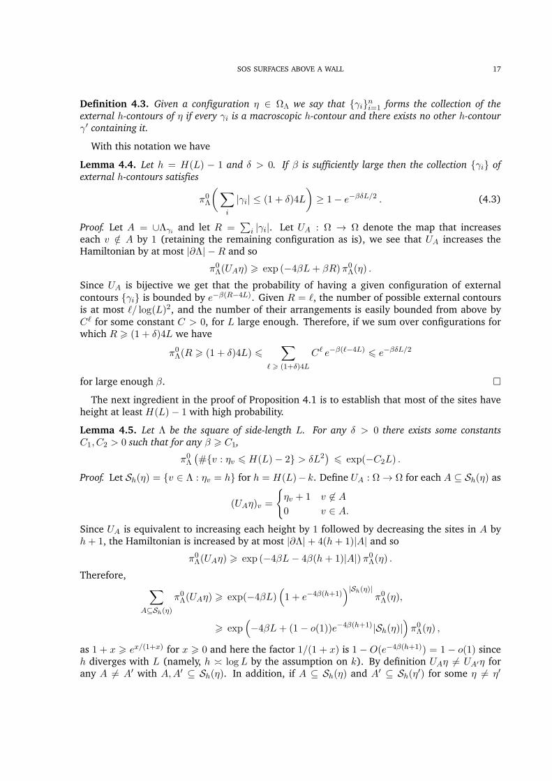
Lemma 4.4. Let h = H(L) & 1 and ( > 0. If " is sufficiently large then the collection {.i} ofexternal h-contours satisfies

%0!

!"

i

|.i| 0 (1 + ()4L

#/ 1& e"!)L/2 . (4.3)

Proof. Let A = .!'i and let R =4

i |.i|. Let UA : % $ % denote the map that increaseseach v /% A by 1 (retaining the remaining configuration as is), we see that UA increases theHamiltonian by at most |'!|&R and so

%0!(UA!) ! exp (&4"L+ "R)%0!(!) .

Since UA is bijective we get that the probability of having a given configuration of externalcontours {.i} is bounded by e"!(R"4L). Given R = +, the number of possible external contoursis at most +/ log(L)2, and the number of their arrangements is easily bounded from above byC. for some constant C > 0, for L large enough. Therefore, if we sum over configurations forwhich R ! (1 + ()4L we have

%0!(R ! (1 + ()4L) ""

. ! (1+))4L

C. e"!(."4L) " e"!)L/2

for large enough ". $

The next ingredient in the proof of Proposition 4.1 is to establish that most of the sites haveheight at least H(L)& 1 with high probability.

Lemma 4.5. Let ! be the square of side-length L. For any ( > 0 there exists some constantsC1, C2 > 0 such that for any " ! C1,

%0!(#{v : !v " H(L)& 2} > (L2

)" exp(&C2L) .

Proof. Let Sh(!) = {v % ! : !v = h} for h = H(L)& k. Define UA : % $ % for each A 7 Sh(!) as

(UA!)v =

7!v + 1 v 3% A

0 v % A.

Since UA is equivalent to increasing each height by 1 followed by decreasing the sites in A byh+ 1, the Hamiltonian is increased by at most |'!|+ 4(h+ 1)|A| and so

%0!(UA!) ! exp (&4"L& 4"(h+ 1)|A|) %0!(!) .Therefore,

"

A,Sh(%)

%0!(UA!) ! exp(&4"L)+1 + e"4!(h+1)

,|Sh(%)|%0!(!),

! exp+&4"L+ (1& o(1))e"4!(h+1)|Sh(!)|

,%0!(!) ,

as 1 + x ! ex/(1+x) for x ! 0 and here the factor 1/(1 + x) is 1 & O(e"4!(h+1)) = 1& o(1) sinceh diverges with L (namely, h 8 logL by the assumption on k). By definition UA! 3= UA"! forany A 3= A( with A,A( 7 Sh(!). In addition, if A 7 Sh(!) and A( 7 Sh(!() for some ! 3= !(

18 P. CAPUTO, E. LUBETZKY, F. MARTINELLI, A. SLY, AND F.L. TONINELLI

then UA! 3= UA"!( (one can read the set A from UA! by looking at the sites at level 0, and thenproceed to reconstruct !). Using the fact that e"4!(h+1) ! e4!(k"1)/L we see that

1 !"

% : |Sh(%)| ! )e!2#(k!1)L2

"

A,Sh(%)

%0!(UA!)

! exp+&4"L+ (( & o(1))e2!(k"1)L

,%0!(|Sh(!)| ! (e"2!(k"1)L2),

and so, for k ! 1

%0!(|Sh(!)| ! (e"2!(k"1)L2) " exp+4"L& (( & o(1))e2!(k"1)L

,.

Summing over k ! 2 establishes the required estimate for any sufficiently large ". $

We now complete the proof of Proposition 4.1. Fix 0 < ( 6 1. By Lemma 4.5, the numberof sites with height less than H(L) & 1 is at most (L2. Condition on the external macroscopic(H(L)&1)-contours {.i} and consider the region obtained by deleting those contours as well astheir interiors and immediate external neighborhood, i.e., V = !\

Ai(!'i .&"

'i). An application

of Lemma 4.2 to %+V where / is the boundary condition induced by '! and {.i} (in particular atmost H(L) & 1 everywhere) shows that w.h.p. there are at most (L2 sites of height larger thanH(L)& 1 in V . Altogether,

"

i

|!'i | ! (1& 2()L2 ,

and therefore, by an application of Lemma 4.4 followed by Lemma 2.6, we can conclude thatw.h.p. one of the .i contains a square with side-length at least 9

10L as required. $

4.2. Absence of macroscopic H(L)-contours when $ < $c. In this section we prove:

Proposition 4.6. Fix ( > 0 and assume that $ < $c & (. W.h.p., there are no macroscopic H(L)-contours.

Proof. The strategy of the proof is the following:

• Step 1: via a simple isoperimetric argument, we show that if a macroscopic H(L) con-tour exists, then it must contain a square of area almost L2;

• Step 2: using the “domain-enlarging procedure” (see Lemma 2.15) we reduce the proofof the non-existence of macroscopic H(L)-contour as in Step 1 to the proof of the samefact in a larger square !( of size 5L with boundary conditions H(L)& 1. That allows usto avoid any pinning issues with the boundary of the original square !. Using Proposi-tion 2.12 we write precisely the law of such a contour (assuming it exists) and we showthat it satisfies a certain “regularity property” w.h.p.;

• Step 3: using the exact form of the law of the macroscopic H(L)-contour in !( we areable to bring in the functional F- defined in Section 3 and to show, via a precise areavs. surface tension comparison, that the probability that an H(L)-contour contains suchsquare is exponentially (in L) unlikely. This implies that no macroscopic H(L) contourexists and Proposition 4.6 is proven.

For lightness of notation throughout this section we will write h for H(L).

SOS SURFACES ABOVE A WALL 19

Step 1. We apply Proposition 2.7 with V = ! and j = 0. Noting that e"4!h log(|.|) = O(logL/L)and recalling Definition 2.1 of $, we have

%0!(C',h) 0 exp

!&(" + o(1))|.| + (1 + o(1))

$

L(1 & e"4!)|!' |

#(4.4)

where o(1) vanishes with L. This has two easy consequences. From |!' | 0 L2 we see that w.h.p.there are no h-contours with |.| / a1L := (1 + &!)L$/". Here and in the following, &! denotessome positive constant (not necessarily the same at each occurrence) that vanishes for " $ (and does not depend on (. From |!' | 0 |.|2/16 (isoperimetry) together with standard Peierlscounting of contours we see that w.h.p. there are no h-contours with

(logL)2 0 |.| 0 a2L :=16

$"L(1& &!). (4.5)

If $ < 4"(1 & &!) then a1 < a2 and we have excluded the occurrence of h-contours longer than(logL)2: Proposition 4.6 is proven. The remaining case is

4"(1 & &!) 0 $ < $c & ( (4.6)

and it remains to exclude h-contours with

16

$"L(1& &!) 0 |.| 0 L(1 + &!)

$

". (4.7)

Recall from Remark 3.7 that $c/(4") tends to 1 for " large so that under condition (4.6) we havethat 4"(1 & &!) 0 $ 0 4"(1 + &!). Then, condition (4.7) implies

4L(1& &!) 0 |.| 0 4L(1 + &!).

For all such ., Eq. (4.4) implies that C',h is extremely unlikely, unless |!' | / L2(1 & &!). But,as in the proof of Lemma 2.6, a contour in ! that has perimeter at most 4L(1 + &!) and area atleast L2(1& &!) necessarily contains a square of area (1& &!)L2, for a different value of &!.

Step 2. We are left with the task of proving

%0!(A) := %0!(9h-contour containing a square Q ! ! with area (1& &!)L2) " e"c(logL)2 . (4.8)

Observe that the event A is increasing. We apply Lemma 2.15, with V = ! . '!, !( a squareof side 5L and concentric to ! and boundary condition h& 1, to write %0!(A) 0 %h"1

!",V (A). From

now on, for lightness of notation, we write %h"1!" instead of %h"1

!",V

Let . denote a contour enclosing a square Q ! ! of area (1& &!)L2. As in the proof of (2.2),

%h"1!" (C',h) = e"!|'|Z

",h"1out Z+,h

in

Zh"1!"

. (4.9)

Here, Zh"1!" is the partition function corresponding to the Gibbs measure %h"1

!" . In the partition

functions Z",h"1out , Z+,h

in , and Zh"1!" , it is implicit the floor constraint that imposes non-negative

heights in ! . '!.Now we can apply Proposition 2.12 (see also Remark 2.13) to the two partition functions in

the numerator. For Z+,hin , we have V = !' (as usual !' is the interior of . and !c

' = !( \ !'),

W = ! 4 '! and n = &1 (recall that $(n) = $e4!n and that $ is around 4" by (4.6)). Since

|!' 4 !| 0 L2 6!

4"L

$e"4!

#2

) L2e8! ,

20 P. CAPUTO, E. LUBETZKY, F. MARTINELLI, A. SLY, AND F.L. TONINELLI

condition (2.5) is satisfied and, for some a % (0, 1) we have4

Z+,hin = Z+,h

in exp/&c$

Le4!"(L)e"4! |!' 4 !|+O(La)

0. (4.10)

To expand Z",h"1out we apply the same argument on the region !( \ !' . Since by assumption .

contains a square Q ! ! with area (1& &!)L2, we have

|! \ !' | 0 &!L2 6

!4"

$L

#2

) L2.

Therefore,

Z",h"1out = Z",h"1

out exp/&c$

Le4!"(L)|! \ !' |+O(La)

0. (4.11)

As for the denominator Zh"1!" , via (2.6) we get

Zh"1!" / Zh"1

!" exp/&c$

Le4!"(L)|!|+O(La)

0. (4.12)

Putting together (4.10), (4.11) and (4.12) and recalling that $ = c$e4!"(L)(1& e"4!), we get

%h"1!" (C',h) = e"!|'| Z

",h"1out Z+,h

in

Zh"1!"

exp

8$

L|! 4 !' |+O(La)

9. (4.13)

Finally, the partition functions Z",h"1out , Z+,h

in and Zh"1!" can be expanded using Lemma 2.16. The

net result is that

Z",h"1out Z+,h

out

Zh"1!"

= exp(#!"(.)) (4.14)

where, for every V ! Z2 and . contained in V ,

#V (.) = &"

W+VW-' .=/

)0(W ) +"

W+!"

W-' .=/

)"+"(W ) +

"

W+V \!"

W-' .=/

)"!"(W ) (4.15)

(see also [14, App. A.3]). Here the notation . 4W 3= : means W 4 (&+' .&"

' ) 3= :.Altogether, we have obtained

%h"1!" (C',h) = exp

8&"|.|+#!"(.) +

$

L|! 4 !' |+O(La)

9. (4.16)

Let ' denote the collection of all possible contours that enclose a square Q ! ! with area(1& &!)L2.

A first observation is that the event that there exists an h-contour . % ' that has distanceless than (logL)2 from '!( (the boundary of the square of side 5L) has negligible probability.Indeed, such contours have necessarily |.| / 5L. Then, the area term $|! 4 !' |/L 0 $L ) 4"Lcannot compensate for &"|.|, and from the properties of the potentials ) in Lemma 2.16, wesee that |#!"(.)| 0 &!|.|. As a consequence, we can safely replace #!"(.) with #Z2(.) in (4.16):indeed, thanks to Lemma 2.16 point (iii), one has |#!"(.) & #Z2(.)| 0 exp(&(logL)2) if . hasdistance at least (logL)2 from '!(.

Secondly, we want to exclude contours with long “button-holes”. Choose a( % (a, 1). Forany contour . and any pair of bonds b, b( % . we let d'(b(, b) denote the number of bonds in "between b and b( (along the shortest of the two portions of . connecting b, b(). Finally, we define

4In principle we should have |!" % (! & #!)| instead of |!" % !|, but since |#!|/L = O(1) the difference can beabsorbed into the error O(La).

SOS SURFACES ABOVE A WALL 21

the set of “contours with button-holes” as the subset '( ! ' such that there exist b, b( % . withd'(b, b() / La" and |x(b)& x(b()| 0 (1/2)d' (b, b(), where x(b), x(b() denote the centers of b, b( and| · | is the +1 distance. The next result states that contours with button-holes are unlikely:

Lemma 4.7. For any c > 0 and " large enough

%h"1!" (9 . % '( such that C',h holds ) 0 e"cLa"

.

Proof. The proof is based on standard arguments [19], so we will be extremely concise. Supposethat . % '(: that implies the existence of two bonds b, b( % ., with d'(b, b() / La" and |x(b) &x(b()| 0 (1/2)d' (b, b(). One can then short-cut the button-hole, to obtain a new contour .( that

is at least (1/2)d' (b, b() / (1/2)La" shorter than . and at the same time contains the same largesquare Q ! ! of area (1& &!)L2. The basic observation is then that the area variation satisfies

66|!' 4 !|& |!'" 4 !|66 0 min

(d'(b, b

()2, &!L2)

so that

&"|.|+#Z2(.) +$

L|! 4 !' | 0 &"|.(|+#Z2(.() +

$

L|! 4 !(

' |& ("/4)La" .

At this point, Eq. (4.16) together with routine Peierls arguments implies the claim (recall thata( > a). $

The important property of contours without button-holes is that the interaction between twoportions of the contour is at most of order La" :

Claim 4.8. If . has no button-holes, then for every decomposition of . into a concatenation of. = .1 ; .2 ; · · · ; .n we have5 |#Z2(.)&

4ni=1#Z2(.i)| 0 nLa" .

Proof. Just use the representation (4.15) and the decay properties of the potentials )(·), seeLemma 2.16 point (iii). $

Step 3. We are now in a position to conclude the proof of Proposition 4.6. Let M denote theset of contours in !(, of length at most 5L, that do not come too close to the boundary of !(,that include a square Q ! ! of side (1 & &!)L2 and finally that have no buttonholes. In view

of the previous discussion, it will be sufficient to upper bound the %h"1!" -probability of the event

.''MC',h. Let Vs = {v = (v1, . . . , vs, vs+1 = v1) : vi % !(} denote a sequence of points in !(.We say that . % Mv if . % M, all the vi appear along . in that order, and for each i ! 2, vi isthe first point x on . after vi"1 such that |x & vi"1| ! &L. Note that since we are considering|.| " 5L we have that s " 5/&.

%h"1!" (9 . % M , C',h) "

5/$"

s=1

"

v'Vs

"

''Mv

%h"1!" (C',h)

"

5/$"

s=1

"

v'Vs

"

''Mv

exp

!&"|.|+#Z2(.) +

$

L|!' 4 !|+O(La)

#,

5strictly speaking, in (4.15) we have defined "!($) for a closed contour. For an open portion $" of a closedcontour $, one can define for instance

"Z2($") = "!

W$Z2

W%"! &='

%0(W ) +!

W$!!

W%"! &='

%"+!(W ) +

!

W$Z2\!!

W%"! &='

%""

!(W ).

22 P. CAPUTO, E. LUBETZKY, F. MARTINELLI, A. SLY, AND F.L. TONINELLI

where we used (4.16) (with #!" replaced by #Z2). Now let Kv denote the convex hull of theset of points v. Since the contour . is never more than at distance &L from a point in V (bydefinition of Mv) we have

|!' 4 !| " |Kv 4 !|+ s&2L2 " |Kv 4 !|+ 5&L2.

Also, from Claim 4.8 we have, if .i,i+1 is the portion of . between vi and vi+1,

|#Z2(.)&s"

i=1

#Z2(.i,i+1)| " sLa" .

Now note that, by standard estimates of [19]

"

''Mv

exp(&"|.|+#Z2(.)) " eO(La")s-

i=1

"

'i,i+1

e"!|'i,i+1|+#Z2('i,i+1)

" eO(La")s-

i=1

exp (&(" + o(1))*(vi+1 & vi))

= exp+&(" + o(1))

B

'v

*(0s)ds +O(La"),

with o(1) vanishing as L $ (, the sum is over all contours .i,i+1 from vi to vi+1, .v denotesthe piecewise linear curve joining v1, v2, . . . , v1 and we applied Appendix A.4 to reconstruct thesurface tension *(vi+1 & vi) from the sum over .i,i+1 (cf. Definition 3.1).

By convexity of the surface tension,B

'v

*(0s)ds !

B

*Kv

*(0s)ds /B

*[Kv-!]*(0s)ds

and so combining the above inequalities we get

"

''Mv

exp

!&"|.|+#Z2(.) +

$

L|!' 4 !|

#" exp

.

&"B

*[Kv-!]*(0s)ds +

$

L|Kv 4 !|+ c &L

1

,

for some constant c > 0 and L large enough. After rescaling Kv 4 ! to the unit square we havea shape with area at least (1& &!). Since $ < $c we have from Claim 3.8 that for all curves .† in[0, 1]2 enclosing such an area

F-(.†) = &"

B

'†*(0s)ds + $A(.†) " & 0($) < 0.

Hence we have that"

''Mv

exp

!&"|.|+#Z2(.) +

$

L|!' 4 !|

#" exp(&0L/2)

provided & > 0 is sufficiently small and L is sufficiently large. Now since s " 5/& we have that|Vs| " |!(|5/$ and so

C%h"1!" (9. % M , C',h) " (5/&)|!(|5/$ exp(&0L/2) " c1e

"c2 log2 L ,

which completes the proof of Proposition 4.6. $

SOS SURFACES ABOVE A WALL 23

4.3. Existence of a macroscopic H(L)-contour when $ > $c. In the special case where$ ! (1 + a)$c for some arbitrarily small absolute constant a > 0 (say, a = 0.01), one can provethe existence of a macroscopic H(L)-contour by following (with some more care) the same lineof arguments used to establish a supercritical H(L)& 1 droplet in Section 4.1. To deal with themore delicate case where $ is arbitrarily close to $c we provide the following proposition.

Proposition 4.9. Let " be sufficiently large. For any ( > 0 there exist constants c1, c2 such that if(1 + ()$c 0 $ 0 $c(1 + a) then

%0!(9. : C',H(L) , |!' | / (9/10)L2

)! 1& c1e

"c2 log2 L .

We emphasize that the difference between the parameters a and ( is that a is small but fixed,while ( can be arbitrarily small with ".

Proof of Proposition 4.9. First of all, from (4.4) and (4.5) we see that, if (1+()$c 0 $ 0 $c(1+a)(and recalling that $c/" ' 4), w.h.p. there are no H(L)-contours of length at least (logL)2 andarea at most (9/10)L2. Let S0 denote the event that there does not exist an H(L)-contour . ofarea larger than (9/10)L2. Thus, on the event S0 w.h.p. the largest H(L)-contour has length atmost log2 L.

By Proposition 4.1 and Theorem 6.2 we have that w.h.p. for any & > 0 there exists an external(H(L)& 1)-contour " containing(1& &)LLc($). We condition on this ". Thus, by monotonicity,

%0!(S0 | ") " %H(L)"1!#

(S0)

so it suffices to work under %H(L)"1!#

. Let S denote the event that there are no macroscopic

contours (of any height, positive or negative). Observe that w.r.t. %H(L)"1!#

w.h.p. there are no

macroscopic contours on the event S0 (cf. e.g. the proof of Lemma 2.9). Thus, %H(L)"1!#

(Sc 4 S0)

is negligible and it suffices to upper bound the probability %H(L)"1!#

(S).To this end, we compare %H(L)"1

!#(S) with the probability of a specific contour . approximating

the optimal curve and then sum over the choices of .. Let

K = '/(L(1& &)& L3/4)Lc($)

0(4.17)

be the suitably dilated solution to the variational problem of maximizing F-. By our choice ofdilation factor, K is at distance at least L3/4 from ". Then for some s growing slowly to infinitywith L let v1, . . . , vs be a sequence of vertices in clockwise order along K with 3L/s " |vi &vi+1| " 5L/s for 1 " i " s where vs+1 = v1.

Let W be the bounded region delimited by the two curves

x #$ /±(x) := ± (x(1& x))3/5 , x % [0, 1].

We define the cigar shaped region Wi between points vi and vi+1 as in [32, Section 1.4.6] tobe given by W modulo a translation/rotation/dilation that brings (0, 0) to vi and (1, 0) to vi+1.Now let . = .1 ; . . . ; .s be a closed contour where each .i is a curve from vi to vi+1 inside theregion Wi. Note that by construction |!' | ! |!K|& s(5L/s)2 = |!K|& o(L2) and . is at least at

distance 12L

3/4 from '!$.In analogy with (4.9) we have that

%H(L)"1!#

(C',H(L))

%H(L)"1!#

(S)= e"!|'|Z

+,H(L)in Z",H(L)"1

out

ZH(L)"1!#

(S)

24 P. CAPUTO, E. LUBETZKY, F. MARTINELLI, A. SLY, AND F.L. TONINELLI

where: Z+,H(L)in (resp. Z",H(L)"1

out ) is the partition function in !' (resp. !$ \ !') with floor atzero, b.c. H(L) (resp. H(L)& 1) and constraint ! / H(L) in &+. (resp. ! 0 H(L)& 1 on &"

' );

ZH(L)"1!#

(S) is the partition function in !$, b.c. H(L)& 1, floor at zero and constraint ! % S. Asin Section 4.2, one can apply Proposition 2.12 to the numerator to get

Z+,H(L)in Z",H(L)"1

out = Z+,H(L)in Z",H(L)"1

out exp/&c$

Le4!"(L)

+e"4! |!' |+ |!$ \ !' |

,+ o(L)

0

where the partition functions with the “hat” have no floor. As for the denominator,

ZH(L)"1!#

(S) 0 ZH(L)"1!#

%H(L)"1!#

(!#!#/ 0|S) " ZH(L)"1

!#exp

/&c$

Le4!"(L)|!$|+ o(L)

0

where we applied (2.8) in the second step. Together with (4.14), the Definition 2.5 of $ and thefact that |!' | / |!K|& o(L2), this yields

%H(L)"1!#

(C',H(L))

%H(L)"1!#

(S)/ exp

!&"|.|+#Z2(.) +

$

L|!K|+ o(L)

#,

where we replaced #!#(.) with #Z2(.), cf. the discussion after (4.16), since by construction .stays at distance at least (1/2)L3/4 from '!$.

At this point we can sum over ., with the constraint that each portion .i,i+1 from vi to vi+1 isin Wi as specified before. Since the cigar Wi is close to Wi±1 only at its tips we have, from thedecay properties of the potentials ) that define #, that [19]

|#Z2(.)&s"

i=1

#Z2(.i)| = O(s) .

Also, by Appendix A.4"

'i'Wi

e"!|'i,i+1|+#Z2('i,i+1) = exp(&(" + o(1))*(vi+1 & vi)) .

Summing over all such contours we then have that4

' %H(L)"1!#

(C',H(L))

%H(L)"1!#

(S)= e

$L |!K|+o(L)

s-

i=1

"

'i,i+1

exp(&"|.i,i+1|+#Z2(.vi,vi+1))

= e$L |!K|+o(L)

s-

i=1

exp(&"*(vi & vi+1))

= exp

!&"B

*K*(0s)ds+

$

L|!K|+ o(L)

#

= exp(LF-(L

"1K) + o(L)),

with F-(·) the functional in (3.2). Since L"1K is a close approximation to Lc($) by Claim 3.8

(ii) it follows that F-(L"1K) > 0. Hence %H(L)"1!#

(S) " e"cL, which concludes the proof. $

4.4. Conclusion: Proof of Theorem 1. Assume that $(Lk) has a limit (otherwise it is sufficientto work on converging sub-sequences). The results established thus far yield that w.h.p.:

• By Proposition 4.1 there exists an (H(Lk)& 1)-contour whose area is at least (9/10)L2k .

• By Corollary 2.10 there are no macroscopic (H(Lk) + 1)-contours.• When limk#$ $(Lk) < $c, by Proposition 4.6 there is no macroscopic H(Lk)-contour.

SOS SURFACES ABOVE A WALL 25

• When limk#$ $(Lk) > $c, by Proposition 4.9 there exists an H(Lk)-contour whose area isat least (9/10)L2

k .Combining these statements with (4.1) and (4.2) completes the proof when limk#$ $(Lk) 3= $c.Whenever $(Lk) $ $c we want to prove that %0!k

(EH(Lk)"1 . EH(Lk)) $ 1, i.e., we want toexclude, say, that half of the sites have height H(Lk) and the other half have height H(Lk)& 1.This is a simple consequence of (4.4) and (4.5) that say that, when $ ) 4", either there are nomacroscopic H(Lk)-contours, or there exists one of area (1& &!)L2. The proof is then concludedalso for limk#$ $(Lk) = $c, invoking again (4.1) and (4.2). $

4.5. Proof of Corollary 1.2. Consider first the case with no floor. With a union bound the

probability that *X%L / )(L) + 1

2! logL can be bounded by L2%0!(!x ! )(L) + 12! logL), which is

O(e"4!/(L)) by Lemma 2.4. For the other direction, let A denote the set of x % ! belonging tothe even sub-lattice of Z2 and such that !y = 0 for all neighbors y of x. Then, by conditioning

on A, and using the Markov property, one finds that the probability of *X%L 0 &)(L) + 1

2! logL

is bounded by the expected value %0!(exp(&e4!/(L)|A|/L2)). Using Chebyshev’s bound and theexponential decay of correlations [11] it is easily established that the event |A| < (L2 hasvanishing %0!-probability as L $ ( if ( is small enough. Since )(L) $ ( as L $ (, this endsthe proof of (1.4).

For the proof of (1.5) we proceed as follows. Consider the %0!-probability that X%L 0 3

4! logL&)(L). Condition on the largest (H(L)&1)-contour ., which contains a square of side-length 9

10Lw.h.p. thanks to Proposition 4.1. By monotonicity we may remove the floor and fix the height ofthe internal boundary condition on !' to H(L)& 1. At this point the argument given above forthe proof of (1.4) yields that

%0!

!X%

L 0 3

4"logL& )(L)

#= o(1),

since H(L)+ 12! logL = 3

4! logL+O(1). To show that %0!

+X%

L / 34! logL+ )(L)

,= o(1), recall

that w.h.p. there are no macroscopic (H(L) + 1)-contours thanks to Corollary 2.10. Conditiontherefore on {.i}, all the external microscopic (H(L) + 1)-contours. The area term in (2.2) isnegligible for these, thus it suffices to treat each .i without a floor and with an external boundaryheight H(L). The probability that a given x % !'i sees an additional height increase of k is thenat most ce"4!k and a union bound completes the proof. $

5. LOCAL SHAPE OF MACROSCOPIC CONTOURS

In this section we establish the following result. Given n % Z+, consider the SOS model in a

domain of linear size + = L23+$, with floor at zero and Dobrushin’s boundary conditions around

it at height {j & 1, j}, where j = H(L)& n. We show that the entropic repulsion from the floorforces the unique open j-contour to have height (1 + o(1))c(j, 0)+1/2+3$/2 above the straight lineL joining its end points. The constant c(j, 0) is explicitly determined in terms of the contourindex j and of the surface tension computed at the angle 0 describing the tilting of L w.r.t. thecoordinate axes. This result will be the key element in proving the scaling limit for the level

lines as well as the L13 -fluctuations around the limit.

5.1. Preliminaries. We call domino any rectangle in Z2 of short and long sides (logL)2 and2(logL)2 respectively. A subset C = {x1, x2, . . . , xk} of the domino will be called a spanningchain if

(i) xi 3= xj if i 3= j;

26 P. CAPUTO, E. LUBETZKY, F. MARTINELLI, A. SLY, AND F.L. TONINELLI

(ii) dist(xi, xi+1) = 1 for all i = 1, . . . k & 1;(iii) C connects the two opposite short sides of the domino.

Remark 5.1. Let Rk be a rectangle with short side 2(log L)2 and long side k(logL)2, k % N, k ! 2.Consider a covering of Rk with horizontal dominos and a covering of Rk with vertical dominos,and fix a choice of a spanning chain for each domino in these coverings. By joining these spanning

chains, one obtains a chain CC = {y1, y2, . . . , yn} ! Rk connecting the opposite short sides of Rk. Achain constructed this way will be called a regular chain.

Given j / 0 consider now the SOS model in a subset V of the L * L box ! with j-boundaryconditions and floor at height 0.

Definition 5.2. Given a SOS-configuration !, a domino entirely contained in V will be called ofpositive type, if there exists a spanning chain C inside it such that !x / j for all x % C. Similarly,if there exists a spanning chain C such that !x 0 j for all x % C, then the domino will be said to beof negative type.

Lemma 5.3. W.h.p. all dominos in V are of positive type.

Proof. A given domino is not of positive type iff there exists a *-chain {y1, . . . , yn} connecting thetwo long opposite sides and such that !yi < j for all i. Such an event is decreasing and thereforeits probability is bounded from above by the probability w.r.t. the SOS model without the floor.Moreover, the above event implies the existence of a (j & 1)-contour larger than (logL)2. The

standard cluster expansion shows that the probability of the latter is O(e"c(logL)2). A unionbound over all possible choices of the domino completes the proof. $

Under the assumption that |V | is not too large depending on j, we can also show that alldominos are of negative type. Recall the definition of c$ and (j from Lemma 2.4.

Lemma 5.4. In the same setting of Lemma 5.3 with j = H(L) & n for fixed n, assume |V |12 0

2e4!(j+1) [(1 + (j)c$]"1. Then w.h.p. all dominos in V are of negative type.

Proof. It follows from Lemma 2.7 that

%jV (C',j+1) 0 e"!|'|+(1+)j) c(e!4#(j+1)|!" | e(#e!4#(j+1)|'| log(|'|),

with lim!#$ ,! = 0. Clearly |!' | 0 |V |1/2|.|/4 and |.| 0 |V |. Hence,

(1 + (j) c$e"4!(j+1)|!' | 0 "|.|/2

,!e"4!(j+1)|.| log(|.|) 6 "|.|

and a standard Peierls bound proves that w.h.p. there are no macroscopic (j+1)-contours. Hencew.h.p. all dominos are of negative type. $

5.2. Main Result.

Definition 5.5 (Regular circuit C%). Let 0 < & 6 1 and let Q (resp. Q) be the rectangle of

horizontal side L23+$ and vertical side 2L

23+$ (resp. L

23+$ + 4(logL)2 and 2L

23+$ + 4(logL)2)

centered at the origin. Write Q \ Q as the union of four thin rectangles (two vertical and twohorizontal) of shorter side 2(logL)2 and pick a regular chain for each one of them as in Remark5.1. Consider the shortest (self-avoiding) circuit C% surrounding the square Q, contained in theunion of the four chains. We call C% a regular circuit.

SOS SURFACES ABOVE A WALL 27

Definition 5.6 (Boundary conditions on C%). Given a regular circuit C% and integers a, b, j with j >

0 and &L23+$ 0 a 0 b 0 L

23+$, we define a height configuration / = /(C%, j, a, b) on C% as follows.

Choose a point P in C%, with zero horizontal coordinate and positive vertical coordinate. Follow thecircuit anti-clockwise (resp. clockwise) until you hit for the first time the vertical coordinate a (resp.b), and call A (resp. B) the corresponding point of C%. Set /x = j & 1 on the portion of C% betweenA and B that includes P , and set /x = j on the rest of the circuit; see Figure 3. It is easy to checkthat, given the regularity properties (cf. Remark 5.1) of the four chains composing the circuit, theconstruction of / is independent of the choice of P as above.

j & 1

j & 1

j

j

A

B

Q

Q

"

FIGURE 3. The region ! delimited by the circuit C%, with the boundary conditionsfrom Definition 5.6, and the open j-contour " joining A and B at height a, brespectively.

With the above definitions let %+! be the SOS measure in the finite subset ! of Q delimited byC%, with boundary condition / on C% and floor at height 0. Note that the boundary conditions/ induce a unique open j-contour " from A to B. Let also 0A,B % [0,%/4] be the angle formedwith the horizontal axis by the segment AB, +A,B be the Euclidean distance between A,B anddA,B = xB & xA where xA, xB denote the horizontal coordinates of A,B respectively.

Theorem 5.7. Recall the Definition 2.5 of $(n). For every n / 0 and every x % [xA, xB ] such that(x&xA)< (xB &x) / 1

10dA,B, let X±(n, x) be the points with horizontal coordinate x and verticalcoordinate

Y ±(n, x) = Y (n, x)± 2(x, 0A,B)L$,

where

Y (n, x) =a(x& xA) + b(xB & x)

dA,B+

$(n) (x& xA)(xB & x)

2"L(*(0A,B) + * (((0A,B))(cos(0A,B))3(5.1)

22(x, 0A,B) =1

"(*(0A,B) + * (((0A,B))(cos(0A,B))3(x& xA)(xB & x)

dA,B.

If the integer j that enters the definition of the boundary condition / is equal to H(L)& n, then:

28 P. CAPUTO, E. LUBETZKY, F. MARTINELLI, A. SLY, AND F.L. TONINELLI

(1) if &12L

23+$ 0 a 0 b 0 L

23+$ & L

13+3$ then w.h.p. the point X"(n, x) lies below ".

(2) if &L23+$ + L

13+3$ 0 a 0 b 0 1

2L23+$ then w.h.p. the point X+(n, x) lies above ".

Remark 5.8. In the above the fraction 1/10 could be replaced by an arbitrarily small constantindependent of L. The core of the argument behind Theorem 5.7 is the fact that the height of "above x is approximately a Gaussian N (Y (n, x),22(x, 0A,B)). Not surprisingly 22(x, 0A,B) has theform of the variance of a Brownian bridge. In the concrete applications (see Section 6) we will only

need the above statement for x = xA+xB2 . Note that, while Y (n, x)& a+b

2 is of order L13+2$, one has

that the fluctuation term 2(x, 0A,B)L$ is only O(L13+

32 $).

Following [14, Sect 7 and App. A], we begin by deriving an expression for the law of the opencontour ". We refer to (4.15) for the definition of the decoration term #!(") (see also [14, App.A.3]).

Lemma 5.9. In the setting of Theorem 5.7:

(i) %+!

+|"| / 2L

23+$,0 e"cL

23+!

.

(ii) Assume |"| 0 2L23+$. Then

%+!(") 2 exp

.

&"|"|+#!(") +$(n)

L|!"|+ ,n(L)

1

,

where |!"| denotes the number of sites in ! below " and ,n(L) = o(1) for any given n.

Proof of the Lemma. We first establish (i). Denote by %+! the SOS measure in ! with b.c. / andno floor. Then

%+!

+|"| / 2L

23+$,0

%+!

+|"| / 2L

23+$,

%+! (!x / 0 5x % !).

The FKG inequality together with the simple bound minx'! %+!(!x / 0) / 1 & c/L, imply that

the denominator is larger than exp(&c|!|/L) for some constant c = c(n) > 0. A simple Peierls

estimate gives instead that the numerator is smaller than exp(&cL23+$). Since |!|/L 0 cL

13+2$

the result follows.We now turn to part (ii). Given ", the region ! is partitioned into two connected regions

!+,!" separated by " (say that !" is the one below "). Thus, if Z+!(") denotes the partition

function restricted to all surfaces whose open contour is ", we have

Z+!(") = e"!|$|Z(j)

!!Z(j"1)!+

, (5.2)

where Z(j)!!

is the partition function of the SOS model in !" with 0-b.c., floor at height &j and

the additional constraint that !x / 0 for all x % !" adjacent to ", Z(j"1)!+

is defined similarly

except that !x 0 0 for all x % !+ adjacent to ".

Let Z!! be defined as Z(j)!!

but without the floor and similarly for Z!+ . From Proposition A.1

we know that

Z(j)!!

Z(j"1)!+

Z!!Z!+

= exp (&%(!0 > j)|!"|& %(!0 / j)|!+|+ ,n(L)) .

SOS SURFACES ABOVE A WALL 29

with ,n(L) = o(1) for any finite n. Since j = H(L)& n, using Lemma 2.4:

%(!0 / j) & %(!0 > j) =$(n)

L(1 +O(L"1/2)).

In conclusion, (5.2) can be rewritten as

Z+!(") 2 exp

.

&"|"|+ $(n)

L|!"|+ ,n(L)

1.Z!!Z!+

Z!

1

Z!.

where |!"| denotes the cardinality of !" and Z! is the partition function in ! with no floor and0-b.c. Using Lemma 2.16, as in (4.14):

Z!!Z!+

Z!

= exp(#!(")),

and the result follows. $

Proof of Theorem 5.7. The fact that the circuit C% enclosing ! is wiggled introduces a numberof inessential technical nuisances. In order not to hide the main ideas we will prove the theoremin the case when ! coincides with Q and we refer to Appendix A.5 for a discussion covering thegeneral case. In what follows we will drop the suffix A,B from +A,B and 0A,B. For simplicity wewill only discuss the case x = 1

2(xA + xB) and we will drop x from Y (n, x), Y ±(n, x). The caseof general x at distance at least dA,B/10 from xA, xB can be treated similarly.

Proof of (1). We observe that the event, in the sequel denoted by U , that the point X"(n) isabove " is decreasing. Thus, by FKG, if G+ denotes the decreasing event that " does not toucha (logL)2-neighborhood of the top side of ! then

%+!(U) 0%+!(U ;G+)

%+!(G+).

The reason for conditioning on G+ will be explained at the end of the proof. Thanks toLemma 5.9 we can write

%+!(U ;G+)

%+!(G+)=

4$'U-G+

e"!|$|+#!($)+$(n)

L A!($)

4$'G+

e"!|$|+#!($)+$(n)

L A!($)*+1 + o(1)

,(5.3)

We observe that A"(") is, apart from an additive constant, the signed area A(") of the contour" w.r.t. the straight line joining A,B. Thus we can safely replace A"(") with A(") in the aboveratio.

Upper bound of the numerator. Let G" denotes the event that " does not touch a (logL)2-neighborhood of the bottom side of !. A simple Peierls argument shows that

"

$'U-G+

e"!|$|+#!($)+$(n)

L A($) = (1 + o(1)) *"

$'U-G+-G!

e"!|$|+#!($)+$(n)

L A($),

since getting close to the bottom side of ! implies an anomalous contour excess length. If nowS denotes the infinite vertical strip through the points A,B, for any " % G+4G" the decorationterm #!(") satisfies

|#!(")&#S(")| = o(1)

30 P. CAPUTO, E. LUBETZKY, F. MARTINELLI, A. SLY, AND F.L. TONINELLI

thanks to (4.15) and Lemma 2.16. Therefore we can upper bound the numerator by

(1 + o(1)) *"

$'Ue"!|$|+#S($)+

$(n)

L A($).

Although we replaced the finite volume decorations #! with the decorations #S associated tothe infinite strip S we emphasize that the contours will always be constrained within the originalbox !.

It will be convenient in what follows to define, for an arbitrary event E,

Z-(n)(E) :="

$'Ee"!|$|+#S($)+

$(n)

L A($); Z-(n) :="

$

e"!|$|+#S($)+$(n)

L A($).

Let now Y % [&L23+$, L

23+$] be the height of the first (following " from A) horizontal bond of

" crossing the middle vertical line of S and let us write U = U1 . U2 where

U1 = U 4 {Y / Y "(n)}, U2 = U 4 {Y 0 Y "(n)}

and Y "(n) = Y (n) & 122(x, 0)L

$. In order to estimate Z-(n)(U1), Z-(n)(U2) we will apply the

bounds of Section 5.3 below with the choice of the parameter µ = $(n).We start with Z-(n)(U1). Multiplying and dividing by Z0 gives

Z-(n)(U1) = Z0 * E-=0

!U1; e

$(n)

L A($)

#0 Ce"!&(,).

!Z2-(n)

Z0

#1/2 5P0(U1) (5.4)

where we used [19, Sect. 4.12] (or Corollary 5.13 below at µ = 0) to upper bound Z0. Againby Corollary 5.13 below

Z2-(n)

Z00 ecL

3!.

Finally we observe that the event U1 implies that the contour " touches the middle vertical line

in two points separated by a distance larger than 122(x, 0)L

$ ! cL13+

32 $. From [19, Ch. 4] such

an event has probability smaller than exp(&cL13 ) under the $ = 0 measure. In conclusion

Z-(n)(U1) 0 Ce"!&(,).e"cL13 . (5.5)

We now turn our attention to the term Z-(n)(U2). We first decompose " = "1 ; "2 into the piece"1 from A to C = (0, Y ) and "2 from C to B. Then we write

A(") = A0 +A1("1) +A2("2)

where A0, A1("1), A2("2) are the signed areas of the triangle (ACB) and of the contours "1,"2

w.r.t. the segments AC,CB respectively. Thus

Z-(n)(U2) 0"

y*Y !(n)

e$(n)

L A0 *"

$: Y=y

e"!|$1|+#S($1)+$(n)

L A1($1)e"!|$2|+#S($2)""#S($1,$2)+$(n)

L A2($2)

=:"

y*Y !(n)

e$(n)

L A0"

$1: Y=y

e"!|$1|+#S($1)+$(n)

L A1($1)Z-,y,$1

where

&#S("1,"2) = #S("1) +#S("2)&#S("1 ; "2) (5.6)

SOS SURFACES ABOVE A WALL 31

It now follows from Corollary 5.13 that

sup$1

Z-(n),y,$10 exp(G-(n)(+2, 02) + L3$/2)

"

$1: Y=y

e"!|$1|+#S($1)+$(n)

L A1($1) 0 exp(G-(n)(+1, 01) + L3$/2)

where +1, +2 denote the distances between A,C and C,B respectively, 01, 02 the angles w.r.t. thehorizontal direction of the segments AC and CB and we define

G-(+, 0) = &"*(0)++ $2 +3

24"(*(0) + * (((0))L2. (5.7)

Putting all together we get

Z-(n)(U2) 0 e2L3!/2 "

y*Y !(n)

exp

D$(n)

LA0 + G-(n)(+1, 01) + G-(n)(+2, 02)

E

=: e2L3!/2

['1 + '2] (5.8)

where

'1 ="

y*(a+b)/2"L13+3!

exp

D$(n)

LA0 + G-(n)(+1, 01) + G-(n)(+2, 02)

E

, '2 = '& '1 (5.9)

Using G-(n)(+, 0) 0 &"*(0)+ + O(L3$) together with the strict convexity of the surface tension[19], we get that the first sum is upper bounded by

'1 0 exp(&"*(0)+& cL5$

)

for some constant c > 0 where we used that A0 0 0 for y 0 (a+ b)/2.

In order to bound '2 we observe that for all y % [(a+ b)/2 & L13+3$, Y "(n)]

) := 01 & 0 = O(L" 13+2$).

Thus it suffices to expand G-(n)(+i, 0i) in ) up to second order. A little trigonometry shows that

+1 = L23+$/ cos(0 + )), +2 = L

23+$/ cos(0 & 3())), 3()) = )+ 2 tan(0))2 +O()3).

Moreover

1

24+3i

($(n))2

"(*(0i) + * (((0i))L2=

1

8+3

($(n))2

24"(*(0) + * (((0))L2+ o(1), i = 1, 2

while

*(01)+1 + *(02)+2 = *(0)++ 2(*(0) + * (((0)

) [y & (a+ b)/2]2 cos(0)2

++ o(1).

In conclusion

G-(n)(+1, 01) + G-(n)(+2, 02)

= G-(n)(+, 0)&1

32

($(n))2 +3

"(*(0) + * (((0))L2& 2"

(*(0) + * (((0)

) [y & (a+ b)/2]2 cos(0)2

++ o(1)

32 P. CAPUTO, E. LUBETZKY, F. MARTINELLI, A. SLY, AND F.L. TONINELLI

and

'2 0 (1 + o(1)) exp

.

G-(n)(+, 0)&1

32

($(n))2 +3

"(*(0) + * (((0))L2

1

*"

y'[(a+b)/2"L13+3!,Y !(n)]

exp

.$(n)

LA0 & 2"

(*(0) + * (((0)

) [y & (a+ b)/2]2 cos(0)2

+

1

. (5.10)

Since A0 =12L

23+$(y & (a+ b)/2) and + cos(0) = L

23+$, one finds that

$(n)

LA0 & 2"

(*(0) + * (((0)

) [y & (a+ b)/2]2 cos(0)2

+

= &(y & Y (n))2

222+

1

32

($(n))2 +3

"(*(0) + * (((0))L2, (5.11)

where

Y (n) =a+ b

2+

1

8

$(n)L13+2$

"(*(0) + * (((0))(cos 0)3,

as in (5.1) for x = (xA + xB)/2, and

22 =+

4" (*(0) + * (((0)) cos(0)2

Therefore, apart from the factor exp(G-(n)(+, 0)), the summand in (5.10) is proportional to a

Gaussian density with mean Y (n) and variance 22. Using Y "(n) = Y (n) & 122(x, 0A,B)L$ 0

Y (n)& cL13+

32 $, and 22 = O(L

23+$), one finds for some c > 0

'2 0 exp(G-(n)(+, 0)& cL2$).

In conclusion, using (5.5) and (5.8), the numerator Z-(n)(U ;G+) appearing in the r.h.s. of (5.3)satisfies

Z-(n)(U ;G+) 0 exp(G-(n)(+, 0)& cL2$) (5.12)

for some new constant c > 0.

Lower bound on the denominator. We consider the restricted class of contours defined as the setof " that stay within the neighborhood of size

(L

23+$)1/2+$/3

around the optimal curve "-(n)

optdefined by

"µopt(x) = "(1)

opt(x) + "(2)opt(x), x % [xA, xB ] (5.13)

where x #$ "(1)opt(x) describes the straight segment AB and

"(2)opt(x) =

.µ+3A,B

2"L(*(0A,B) + * (((0A,B))d3A,B

1

(x& xA)(xB & x), x % [xA, xB ],

where dA,B = xB & xA. Note that, thanks to the assumption a 0 b 0 L23+$ & L

13+3$, the curve

"-(n)

opt is well within the domain Q. For such contours " one has

A(") = A("-(n)

opt ) +O(L1+ 116 $).

Thus

Z-(n)(G+) / eO(L116 !) e

$(n)

L A($$(n)opt )

"

$: dist($,$$(n)opt )*

(L

23+!)1/2+!/3

e"!|$|+#!($).

SOS SURFACES ABOVE A WALL 33

As in the proof of Lemma A.6 of [32], the latter sum is lower bounded by

exp

.

&"B

$$(n)opt

ds *(0s)

1

exp(&(logL)c).

Using (5.17) we finally get

Z-(n)(G+) / exp+G-(n)(+, 0) +O(L

116 $),

(5.14)

where G-(n)(+, 0) is as in (5.7).

Conclusion. By combining (5.12) with (5.14) we finally get point (1) of the theorem. $

Proof of (2). The proof of point (2) follows exactly the same pattern. Using FKG one first condi-tions on G" and then, using Peierls, one restricts to paths in G" 4G+. $

This concludes the proof of Theorem 5.7. $

5.3. Iterative upper bound on the partition function. This is a key technical section whosemain object is a certain contour partition function ZA,B for open contours joining two points

A,B at distance ' L23+$. The exponential weight of a contour contains, besides the familiar

length term with decorations as in [19], an additional term proportional to L"1* the signed areaof the contour w.r.t. the segment AB. The main output is a precise upper bound on ZA,B. Thebound indicates that the main contribution to ZA,B comes from contours close to a deterministiccurve (approximately a parabola) joining A,B and satisfying a variational principle (cf. (5.16)).

Setting. Recall that Q is a rectangle of horizontal side D := L23+$ and vertical side 2D centered

at the origin. Set +0 = L23 and ( = 1/10 and define Rn as the set of pairs (A,B), A,B % Q4(Z2)%,

such that their Euclidean distance +A,B satisfies 1 0 +A,B 0 2n(1"))+0. Call 0A,B the angle formedwith the horizontal axis by the straight line through A,B and assume that 0A,B % [0,%/4].Without loss of generality we assume that xA < xB if xA, xB denote the horizontal coordinatesof A,B.

Choose two open contours "left,"right such that "left joins A with the left vertical side of Qwithout ever going to the right of A and "right joins B with the right vertical side of Q withoutever going to the left of B.

Define now the contour ensemble ( consisting of all contours " joining A,B within Q suchthat the concatenation "left ;";"right is an admissible open contour. Notice that the signed areaA(") of " w.r.t. the segment AB is unambiguously defined. Fix a parameter µ / 0 and to each" % ( assign the weight

w(") = exp+&"|"|+#Z2(") + e"!|" 4QA,B|+

µ

LA(")

,(5.15)

where #Z2(") has been defined in (4.15), and QA,B ! Q consists of all those points whosehorizontal coordinate x satisfies either x 0 xA+(logL)2 or x / xB & (logL)2. The term e"!|"4QA,B| has been added only for technical convenience and, in practice, it will be O((logL)2) forthe “relevant” contours.

Definition 5.10. Let ZA,B :=4

$'%w("). We say that statement Hn holds if

sup$left,$right

ZA,B 0 zneGµ(.A,B ,,A,B) 5A,B % Rn

34 P. CAPUTO, E. LUBETZKY, F. MARTINELLI, A. SLY, AND F.L. TONINELLI

where

Gµ(+, 0) = &"*(0)++ +3µ2

24"(*(0) + * (((0))L2

and z1 = ec(logL)2, zn = (Lz1)

2n!1, n / 2.

With the above notation the following holds.

Proposition 5.11. For any large L, H1 holds. Moreover, for all n 0 nf = &(1 & ()"1 log2(L), Hn

implies Hn+1. In particular Hn holds for all n 0 nf .

Remark 5.12. It is important to observe that znf = O(exp(L3$/2)

).

The reason why Hn holds is that the main contribution to the partition function ZA,B comesfrom contours " which are close to the curve from A to B maximizing the functional

C #$ &"B

C*(0s) ds+

µ

LA(C). (5.16)

By expanding the functional up to second order around the straight line from A to B one findseasily that such optimal curve is approximately the parabola given by (5.13). A short computa-tion shows that

& "

B

$µopt

*(0s) ds+µ

LA("µ

opt) = Gµ(+A,B, 0A,B) + o(1). (5.17)

Before proving the proposition let us state a simple corollary which formalizes a useful conse-quence of the result.

Corollary 5.13. Consider the two partition functions Z(i)A,B :=

4$'%w(i)("), i = 1, 2, correspond-

ing to the weights

w(1)(") = exp+&"|"|+#S(") +

µ

LA(")

,

w(2)(") = exp+&"|"|+#S(")&&#S(","left) +

µ

LA(")

,,

where S is any vertical strip containing the strip through the points A,B and &#S(","left) hasbeen defined in (5.6). Then, uniformly in "left,"right:

max+Z(1)A,B, Z

(2)A,B

,0 exp

+Gµ(+A,B, 0A,B) +O(L3$/2)

,..

Proof of the Corollary. It follows immediately from Proposition 5.11 together with Remark 5.12and the bounds

|#Z2(")&#S(")|+ sup$left

|&#S(","left)| 0 e"!|" 4QA,B|. $

Proof of Proposition 5.11.

Proof of the base case H1.Fix (A,B) % R1 with xA < xB, mutual distance + 0 2+0 = 2L2/3 and angle 0, together with"left,"right and denote by h$ the maximal height (w.r.t. the segment AB) reached by the contour". Then

ZA,B = ZA,B EA,B

+e

µLA($)+e!# |$-QA,B|

,

SOS SURFACES ABOVE A WALL 35

where ZA,B is defined as ZA,B but with modified weights w(") in which the area parameter µ isequal to zero and the term e"! |"4QA,B| is absent. The area A(") clearly satisfies A(") 0 |"|h$.Because of [19, Ch. 4],

PA,B (h$ = j) 0 ce"min(j, j2/.)/c

ZA,B 0 c e"!&(,).

PA,B (|" 4QA,B| / q) 0 e"q+c(logL)2 (5.18)

for suitable constant c and " large enough. From (5.18) it follows that

EA,B

+e2e

!# |$-QA,B |,0 ec

"(logL)2 ,

for some constant c( > 0. Moreover, using Peierls, the excess length (|"|& 2+)+ has exponentialtail with parameter " &O(1). This, combined with the first estimate in (5.18) proves that

EA,B

+e2

µL |$|h#

,0 c(,

for some constant c( > 0. The claim is proved with z1 := ec(logL)2.

Proof of the inductive step Hn > Hn+1.Fix (A,B) % Rn+1 with xA < xB, mutual distance + and angle 0, together with "left,"right.Let C be the midpoint between A and B, and define L the vertical line through C. Write "as " = "1 ; "2 where "1 is the contour from A until the first contact X with L and "2 is theremaining part. Let also +AX , 0AX be the length and angle of AX and similarly for +XB , 0XB .

Call j the vertical coordinate of X minus the vertical coordinate of C. We distinguish twocases.

Case 1: |j| / L13+3$. With the same notation as in the proof of H1 and using (5.18)

"

$:|j|&L13+3!

w(.) 0 ce"!&(,)."c" L5!(5.19)

for some positive c, c( which is clearly negligible compared to the target zn+1 exp(Gµ(+, 0)).

Case 2: |j| 0 L13+3$. Simple geometry shows that both (A,X) and (X,B) belong to Rn and

we can use the induction. Also, Peierls argument shows that we can safely assume that "2 doesnot reach horizontal coordinate xA+(logL)2, with xA the horizontal coordinate of A, otherwisethis would imply an extremely unlikely large deviation of the length |"|.

Note that the area A(") can be written as

A(") = A1("1) +A2("2) +A0,

with A1("1) (resp. A2("2)) the signed area of "1 (resp. "2) w.r.t. the segment AX, (resp. XB)while

A0 =+

2j cos(0)

is the signed area w.r.t. AB of the triangle AXB.Next, remark that

#Z2(") = #Z2("1) +#Z2("2)&&#Z2("1,"2).

Using the decay properties of the potentials ) (see Lemma 2.16 point (iii)), we can bound

|&#Z2("1,"2)| 0 e"! |"2 4QX,B | (5.20)

36 P. CAPUTO, E. LUBETZKY, F. MARTINELLI, A. SLY, AND F.L. TONINELLI

where QX,B was defined just after (5.15) (with A replaced by X). As a consequence,

"

$:|j|*L13+3!

w(.) 0"

$:|j|*L13+3!

exp

8µ

L(A1("1) +A2("2)) +

µ+

2Lj cos(0)

9(5.21)

* exp/e"!(|"1 4QA,X |+ |"2 4QX,B |) +#Z2("1) +#Z2("2)

0. (5.22)

At last we can use the induction: with "left ; "1 playing the role of "left we have (uniformly in"1)

"

$2

exp/µLA2("2) +#Z2("2) + e"! |"2 4QX,B |

00 zn exp(Gµ(+XB , 0XB))

and similarly, with e.g. horizontal contour from X to the right vertical boundary of Q playingthe role of "right,

"

$1

exp/µLA1("1) +#Z2("1) + e"! |"1 4QA,X |

00 zn exp(Gµ(+AX , 0AX)).

To estimate

' := z2n"

|j|*L13+3!

exp

8µ+

2Lj cos(0) + Gµ(+AX , 0AX) + Gµ(+XB , 0XB)

9

we proceed as in the estimate of the sum '2 appearing in (5.9). Using the restriction |j| 0 L13+3$

we can expand up to second order the exponent in e.g. (0 & 0AX) = O(L" 13+3$). The net result

is that

' 0 (1 + o(1))z2n exp

!Gµ(+, 0)&

1

32

µ2 +3

"(*(0) + * (((0))L2

#

*"

j

exp

!µ+

2Lj cos(0)& 2"

(*(0) + * (((0)

) j2 cos(0)2

+

#

0 c(")1+z2n exp (Gµ(+, 0))

where we used a standard Gaussian summation. In conclusion, using (5.19), we showed that

ZA,B 0 cz2n1+ exp (Gµ(+, 0)) 0 zn+1 exp (Gµ(+, 0))

thanks to the definition of the constants {zn}n*nf . The inductive step is complete. $

6. PROOF OF THEOREMS 2 AND 3

In this section we show that for all n % Z+, if there exists a macroscopic (H(L) & n)-contour"n containing the rescaled Wulff body L+c($(n))W1, then with high probability it is unique andit is contained in the annulus (1 + ,0)LLc($(n)) \ (1 & ,0)LLc($(n)), for any ,0 > 0. Combinedwith the results of Section 4, this will prove Theorem 2. Moreover, we prove that along the flat

part of LLc($(n)) the contour "n has fluctuations on the scale L13 up to O(L$) corrections. That

covers Theorem 3.

SOS SURFACES ABOVE A WALL 37

6.1. Growth of droplets. Recall the Definition 3.4 of the sets L($, t, r) and the sets Lc($).Recall also the Definition 2.5 of the parameters $(n). To fix ideas, the Wulff shape W1 appearingbelow is assumed to be centered at the origin. To simplify the exposition, we introduce thefollowing notation.

Definition 6.1. Given a subset A ! Z2, we call En(A) the event that there exists an (H(L) & n)-contour "n that contains the set A.

Theorem 6.2 (Growth of the critical droplet). Fix , % (0, 1/10), and set (L = L"(/8. Let ! be thesquare of side L centered at the origin. Consider the SOS model on ! with 0-boundary conditionsand floor at height zero. For any fixed n % Z+, as L $ (, if

En(L(1 + (L)+c($(n))W1) holds w.h.p., (6.1)

then w.h.p.

a) En(LL($(n), 1 + (L,&L" 23+4()) holds;

b) there exists a unique macroscopic (H(L)& n)-contour.

Remark 6.3. Recall from Remark 3.5 that L+c($(n))W1 can fit inside the box ! iff $(n) / $. Using

that $ ' 2" (see Remark 3.7), we have that for n / 1 this condition is always satisfied (for " largeenough) while if n = 0 we need to require $ / $. However the results of Section 4 show that a

macroscopic H(L)-contour exists w.h.p. iff $ > $c > $.

Remark 6.4 (Growth up to L13 from flat boundary). An immediate corollary of Theorem 6.2

is that assuming (6.1), the unique macroscopic (H(L) & n)-contour is at a distance O(L13+4()

from the target region LLc($(n)), uniformly along most of the flat boundary of LLc($(n)). Indeed,

LL($(n), 1 + (L,&L" 23+4() is uniformly at a distance L

13+4( from the critical region LL($(n), 1 +

(L, 0), which overlaps with LLc($(n)) along the flat boundary of LL($(n), 1 + (L, 0). On the otherhand, concerning the curved portions of LLc($(n)), the above theorem does not allow us to inferan approximation error better than O((LL), since already the region LL($(n), 1 + (L, 0) has radialdistance from LLc($(n)) of that order at a corner.

The proof of Theorem 6.2 part a) will be based on an inductive argument. The proof ofTheorem 6.2 part b) will be a consequence of part a), as we show below.

Proof of Theorem 6.2 part b) assuming part a). Thanks to Theorem 6.2 part a), for any fixed nw.h.p. assuming (6.1), there exists an outermost (H(L) & n)-contour, which we denote "n,containing the set !n := (1& o(1))LLc($(n)) for a suitable choice of the error term o(1). Propo-sition 2.7 and a union bound imply there are no macroscopic negative contours w.h.p. and hencethere are no positive macroscopic (H(L) & n)-contours nested inside "n. Hence the interior ofany other macroscopic contour must be contained inside ! \ !n and

|! \ !n| = (1 + o(1))L2+2c($(n))(+2& & 1) 0 ,!

"2

($(n))2L2

where ,! $ 0 as " $ (. Here we used the fact that +c($(n)) ' 2"/$(n) for " $ ( and the factthat lim!#$ +& = 1 because, in the same limit, the Wulff shape becomes a square.

Now a closed contour . with !' 7 ! \ !n satisfies

|!' | 0!|.|2

16

#1/2

(|! \ !n|)1/2 0|.|4

"

$(n)1&! L.

38 P. CAPUTO, E. LUBETZKY, F. MARTINELLI, A. SLY, AND F.L. TONINELLI

Hence the area term $(n)|!' |/L appearing in the exponential weight in (2.2) is negligible com-pared to the length term "|.| and the probability that there exists any such macroscopic contour

is O(e"c(logL)2) by a simple counting argument. In conclusion, w.h.p. "n is the unique macro-scopic (H(L)& n)-contours. $

The proof of Theorem 6.2 part a) will be based on the following argument.

Proposition 6.5. Fix n % Z+. Let 1 " m " logL and let !( ! Z2 be a region containing

LL($(n), 1 + (L,&(m & 1).L), .L := L" 23+3( logL, and consider the SOS model on !( with

(H(L)& n& 1)-boundary conditions and floor at height zero. Conditionally on the event En(L(1 +(L)+c($(n))W1), then En(LL($(n), 1 + (L,&m.L)) holds w.h.p.

We start with the case n = 0. When n = 0 it is assumed that !( contains A := LL($, 1 +(L,&(m & 1).L) and we condition on the event E0(L(1 + (L)+c($)W1) that there is an H(L)-contour containing the Wulff body L(1 + (L)+c($)W1. We show that w.h.p. this initial dropletgrows until it invades the whole region LL($, 1+(L,&m.L). The proof is divided into two mainsteps.

FIGURE 4. Growth of the initial droplet as described in Step 1: from W(x, +) to W(x, +x).

Step 1. For x % A, + > 0, let W(x, +) denote the rescaled Wulff shape L+W1 centered at x. Also,

let +x denote the maximal value of + such that dist(W(x, +), Ac) > L13+3(. The next lemma shows

that at any x % A such that +x > +c($) one can let an initial droplet W(x, +), +c($) < + < +x,

grow until it touches the boundary of A up to O(L13+3(); see Figure 4.

Lemma 6.6. Fix x % A and +c($)(1 + (L) " + < +x. Conditionally on E0(W(x, +)), thenE0(W(x, +x)) holds w.h.p.

Proof of Lemma 6.6. By simple recursion, it suffices to show that conditionally on E0(W(x, +)),

then E0(W(x, +()) holds w.h.p., with +( = +(1 + L" 23 ), as long as +( " +x. Next, we shall use

the growth gadget of Theorem 5.7 along the boundary of W(x, +) to show that conditionally onE0(W(x, +)), then w.h.p. there is a circuit C surrounding W(x, +() such that !y ! H(L) for ally % C. The latter event implies E0(W(x, +()).

By symmetry, we may restrict our analysis to the north-west corner of the droplet W(x, +).Moreover, using symmetry w.r.t. reflections along the north-west diagonal we may restrict toupper half of the north-west corner. Let 0 % [0,%/4] and consider the chord of W(x, +) forming

an angle 0 with the x axis and whose horizontal projection has length L23+(. Let z = (xz, yz) be

the midpoint of this chord and call (xa, ya), and (xb, yb) the intersection points of the chord with'W(x, +), the boundary of W(x, +). From a natural rescaling of the function &(d, 0) appearingin Lemma 3.9, one finds that the vertical distance &0 from z to 'W(x, +) is given by

&0 = +L&+ L

23+(

+L cos(0), 0,=

w1

16(*(0) + * (((0))(cos(0))3L

13+2(

+.

SOS SURFACES ABOVE A WALL 39

Since "w1/2 = $+c($), for any $ > 0, one can rewrite

&0 =$+c($)/+

8"(*(0) + * (((0))(cos(0))3L

13+2(. (6.2)

Consider the rectangle Q with horizontal side L23+( and vertical side 2L

23+( centered at the point

w = (xw, yw) such that xw = xz and yw = yb + L13+3( & L

23+(, and let Q denote the enlarged

rectangle with the same center, horizontal side L23+( + 4(logL)2 and vertical side 2L

23+( +

4(logL)2. Observe that the assumption that + " +x, or equivalently dist(W(x, +), Ac) > L13+3(,

guarantees that the rectangles Q, Q are indeed contained in our region !( ? A.

Notice that, setting a = (ya & yw), b = (yb & yw), one has &12L

23+( " a " b " L

23+( & L

13+3(,

as required in Theorem 5.7 (1). To ensure that we can indeed apply that statement we nowcheck that w.h.p. there exists a regular circuit C% in Q \Q with the required properties, namelythat one has w.h.p.: 1) heights at least H(L) & 1 in the upper path along C% connecting A andB and 2) heights at least H(L) in the lower path along C% connecting A and B, where A,B aredefined in Definition 5.6; see Figure 3. Point 1) follows from Lemma 5.3 and the fact that wehave b.c. H(L) & 1. Point 2) follows again from Lemma 5.3 and, via the usual monotonicityand conditioning argument, from the assumption that E0(W(x, +)) holds. Then, an applicationof Theorem 5.7 (1), together with monotonicity, shows that the point v = (xv, yv) with xv = xwand yv = yw +K, with

K =a+ b

2+

$L13+2(

8"(*(0) + * (((0))(cos(0))3& c(", 0)L

13+(,

for a suitable constant c(", 0) > 0, lies w.h.p. below a chain C(v) connecting A and B with!y ! H(L) for all y % C(v). Call F(v) this event. Next, observe that the point v lies above

'W(x, +) and has a vertical distance h at least L13+( from 'W(x, +). Indeed, using (6.2)

h = K & a+ b

2&&0 =

$(1& +c($)/+)

8"(*(0) + * (((0))(cos(0))3L

13+2( & c(", 0)L

13+( ! L

13+(,

where we use the assumption 1 & +c($)/+ ! (L and we take L large enough. In particular, it

follows that v lies outside the enlarged shape W(x, +(), +( = +(1 + L" 23 ) since this is larger than

W(x, +) by an additive O(L13 ) only.

Repeating the above argument for all 0 % [0,%/4] (of course O(L) values of 0 in this rangesuffice) and using symmetry to cover the other corners of the droplet, considering the intersec-tion of all events F(v(0)), one has that w.h.p. there exists a chain C surrounding W(x, +() suchthat !y ! H(L) for all y % C as desired. $

Step 2. By assumption we can pretend that E0(W(x0, +)) holds, where x0 is the center of theregion A, which we identify with the origin. Thus, by Step 1, one has that E0(W(x0, +x0)) holdsw.h.p. Next, we establish that this is enough to invade the whole region LL($(n), 1+ (L,&m.L).

Lemma 6.7. Conditionally on E0(W(x0, +x0)), E0(LL($(n), 1 + (L,&m.L)) holds w.h.p.

Before proving Lemma 6.7, we need the following deterministic lemma concerning the en-largement of squeezed Wulff shapes. Fix $ > 0 and +c($) < + < 1/+& . The Wulff body +W1 isstrictly contained in the unit square Q; see Section 3 for the notation. Setting +% = 1/+& one hasthat D0 := +%W1 is tangent to all four sides of Q, i.e. it is the maximal Wulff shape inside Q. Forany 4 % D0 such that +W1 + 4 ! D0, define

t0 = max{t ! 1 : t+W1 + 4 ! Q},

40 P. CAPUTO, E. LUBETZKY, F. MARTINELLI, A. SLY, AND F.L. TONINELLI

FIGURE 5. Growth of the initial droplet as described in Step 2: from W(x0, +) toW(x0, +x0) and from W(x0, +x0) to LL($(n), 1 + (L,&m.L).

with the convention that t0 = 0 if there is no such t. We define D1 = .0'D0

Ft0+W1 + 4

G. We

then repeat the above enlargement procedure. Namely, given the set Dk, we define

Dk+1 = .0'Dk

Ft0+W1 + 4

G,

where t0 = max{t ! 1 : t+W1 + 4 ! Q} for 4 % Dk with +W1 + 4 ! Dk and with t0 = 0 if+W1 + 4 3! Dk. The sequence {Dk}k consists of nested convex subsets of Q.

Lemma 6.8. The sequence Dk converges to D$ := L($, +/+c($), 1). Moreover, the Hausdorff dis-tance between 'Dk and 'D$ is upper bounded by ck for some constant c % (0, 1).

Proof. The set Dk has four symmetric flat pieces where it is tangent to the sides of Q. Let vkdenote the length of one flat piece and write rk = (1 & vk)/2. Moreover, notice that 2rk is theside of the smallest square one can put around the Wulff body skW1, with sk = 2rk/+& . Simplegeometric considerations then show that the sequence rk satisfies

rk+1 = rk+1&

12y/+&

,+

+12y, r0 =

1

2,

where y is the radius of the Wulff body W1 in the direction 0 = %/4. Set a = 1 &12y/+& and

note that a % (0, 1). It follows that rk = 12a

k + .)2y4k"1

j=0 aj . As k $ (, this converges to ++&/2

which is the value corresponding to the limiting shape L($, +/+c($), 1). The Hausdorff distancebetween 'Dk and 'Dk+1 is then of order ak and the desired conclusion follows. $

Proof of Lemma 6.7. Consider the sets Dk, k = 0, 1, . . . defined above. By assumption we knowthat L(1&(m&1).L)D0 ' W(x0, +x0) is contained w.h.p. in an H(L)-contour. We now prove that

conditionally on E0(L(1&(m&1).L&kL" 23+3()Dk), then E0(L(1&(m&1).L&(k+1)L" 2

3+3()Dk+1)holds w.h.p.

Fix + = +c($0)(1 + (L), and consider a droplet W(x, +) such that W(x, +) ! Dk. FromLemma 6.6, we can let W(x, +) grow up to W(x, +x). Repeating this at every x as above yieldsthe desired claim since the parameter t0 in the definition of Dk can be identified with +x/+for x = 4L. This establishes that under the assumptions of Lemma 6.7, for any k, the set

L(1 & (m & 1).L & kL" 23+3()Dk is contained w.h.p. in an H(L)-contour. From Lemma 6.8, we

know that a number k = O(logL) of steps suffices to attain a distance of order 1/L betweenDk and D$, and therefore w.h.p. L(1 &m.L)D$ is contained in an H(L)-contour. This provesLemma 6.7. $

Proof of Proposition 6.5. The above two steps provide a proof in the case n = 0. The other casesare obtained with exactly the same argument, provided one uses $(n) instead of $(0) = $. $

SOS SURFACES ABOVE A WALL 41

Proof of Theorem 6.2 part a). Fix n % Z+. Suppose that the event

En+1(LL($(n), 1 + (L,&(H(L)& n& 1).L)) (6.3)

holds w.h.p. On the latter event, conditioning on the outermost (H(L) & n & 1)-contour " andusing monotonicity, one can assume that there are b.c. at height H(L)&n&1 out of some region!( which contains the set LL($(n), 1+(L,&(H(L)&n&1).L). It follows from Proposition 6.5 that

w.h.p. En(LL($(n), 1+(L,&(H(L)&n).L) holds. Since (H(L)&n).L " (logL)2L" 23+3( " L" 2

3+4(

the desired conclusion follows.Thus, it suffices to prove that (6.3) holds w.h.p. assuming (6.1). We use recursion, starting

from the case of the 1-contour. Here one has 0 b.c. outside the L * L square ! and floor at 0.By monotonicity one can lower the floor down to height &(H(L) & n & 1). Once this is donethe statistics of the 1-contours coincides with the statistics of the (H(L)&n)-contours with floorat 0 and b.c. at (H(L) & n & 1). By Proposition 6.5, with m = 1, one infers that there is a1-contour in the original problem that contains LL($(n), 1 + (L,&.L). Recursively, assume thatw.h.p. there exists a k-contour containing LL($(n), 1+(L,&k.L). Conditioning on the outermostsuch contour, using monotonicity one can assume b.c. k on a set !( that contains LL($(n), 1 +(L,&k.L). Repeating the above argument (lowering the floor and using Proposition 6.5) onehas that w.h.p. there exists a (k + 1)-contour containing LL($(n), 1 + (L,&(k + 1).L). Once wereach the height k = H(L)& n& 1 the proof is complete. $

6.2. Retreat of droplets. We recall that, from Section 4, w.h.p a macroscopic (H(L) & n)-contour exists iff $(n) > $c. In that case it is unique w.h.p. by Theorem 6.2(b).

Theorem 6.9. Fix &, & % (0, 1/10), let ! be the square of side L. Consider the SOS model on !with 0-boundary conditions and floor at height zero. Fix n % Z+ and assume $(n) / $c + &. Thenw.h.p. as L $ ( the unique macroscopic (H(L) & n)-contour is contained in LL($(n), tL, (L) (cf.Definition 3.4) with tL = 1& (L and (L = L"$/8.

Proof.

(i) We begin by treating the base case n = 0. The case n / 1 will then follow by a simpleinduction.

Definition 6.10. Given s % [0, 1] we say that H(s) holds if w.h.p. there exists a unique macroscopicH(L)-contour "0 and it is contained in LL($, s, (L).

With this definition the statement of the theorem for n = 0 follows from the next two Lemmas.

Lemma 6.11 (Base case). For any s small enough H(s) holds.

Lemma 6.12 (Inductive step). Fix s 0 tL. Then H(s) implies H(s+ L" 23 ).

Proof of Lemma 6.11. We actually prove that w.h.p. "0 is contained in LL($, s, 0) for s smallenough. Fix s % (0, 1/4) and define Ti, i = 1, . . . , 4, as the “curved triangle” delimited by thecurved portion of the boundary of LL($, 4s, 0) facing the ith-corner vi of ! and '!. Let A,B bethe end points of the curved portion of the boundary of T1 (both at distance 2s+c+&L from v1)Let now Ei be the event that inside Ti \ LL($, 2s, 0) there exists a macroscopic chain where theheight of the surface is at least H(L). If the macroscopic H(L)-contour "0 — which, under %0!,exists w.h.p. by Proposition 4.9 and is unique by Theorem 6.2 — is not contained in LL($, s, 0),then necessarily one of the four events Ei occurred. By symmetry, it is therefore enough to showthat %0!(E1) = O(e"c(logL)2) for any s small enough.

42 P. CAPUTO, E. LUBETZKY, F. MARTINELLI, A. SLY, AND F.L. TONINELLI

For this purpose let us introduce boundary conditions * on '! as follows:

*x =

7H(L) if x % '! \ 'T1

H(L)& 1 if x % '! 4 'T1.(6.4)

By monotonicity we can bound from above %0!(E1) by %&!(E1). Call " the open H(L)-contour" joining A,B and denote by G the event that " does not get out of LL($, 2s, 0). We can onceagain appeal to [14, Lemma A.2] to get that

%&!(E1 |G) 0 e"c(logL)2 .

Thus we are left with the proof that, for all s small enough, G occurs w.h.p. As in Lemma 5.9we can write

%&!(") 2 exp

!&"|"|+#!(") +

$

LA(") + o(L)

#(6.5)

where A(") is the signed area of " w.r.t. the segment AB with the obvious choice of the signs.Clearly A(") 0 2s2+2c+

2&L

2 0 s2L2 for " large enough. Thus

%&!(Gc) 0 es

2(L+o(L))

4$'Gc e"!|$|+#!($)

4$ e

"!|$|+#!($)+$LA($)

0 es2(L+o(L))

4$'Gc e"(!"e!#)|$|+#

Z2 ($)

4$ e

"(!+e!#)|$|+#Z2($)+

$LA($)

= es2(L+o(L))

4$'Gc e"(!"e!#)|$|+#

Z2($)

4$ e

"(!"e!#)|$|+#Z2($)

*4

$ e"(!"e!#)|$|+#

Z2($)

4$ e

"(!+e!#)|$|+#Z2 ($)+

$LA($)

(6.6)

where we used |#!(") & #Z2(")| 0 e"! |"|. Using [19] the first ratio in the r.h.s. of (6.6)is bounded from above by exp(&csL) with c independent of ", since the event Gc implies anexcess length of order sL for the contour. Using Jensen’s inequality w.r.t. the measure 5 on "corresponding to the weight e"(!"e!#)|$|+#

Z2($), the second ratio is bounded from above by

exp

!2e"!5(|"|) + $

L5(A("))

#.

Using once again [19] we have 5(|"|) 0 2sL and 5(A(")) = O((sL)3/2). Hence %&!(Gc) =

O(e"csL/2) for any s small enough independent of L. $

Proof of Lemma 6.12. Let us fix some notation. Referring to Figure 6 and centering the box ! inthe origin, let

fs :(&(1 + (L)

2L, 0

3#$2&(1 + (L)

2L, 0

3

be the decreasing convex function whose graph is the South-West quarter of '(LL($, s, (L)).Let x(s) be the unique solution of fs(x) = x. In the sequel we will denote by x%(s) (resp.x%(s)) the point after which fs(·) is smaller than &L/2 (resp. after which fs(·) is flat and equals&L

2 (1 + (L)).

For x % [x(s), x%(s()] let x± := x± 12L

23+$ and define

Zs(x) =1

2[fs(x

") + fs(x+)]& $

8"(*(0) + * (((0)) cos(0)3L

13+2$ & 2(x, 0)L$ (6.7)

with 0 = 0x % [0,%/4] such that tan(0) = |f (s(x)| and 22(x, 0) = O(L

23+$) is given in Theorem 5.7.

SOS SURFACES ABOVE A WALL 43

fs

•

x%(s)x(s)

••

x%(s)

(&L2 ,&

L2 ) x• 1

2(LL

FIGURE 6. The graph of the function fs describing the South-West quarter of '(LL($, s, (L)).

We first observe that, if s 0 tL,Zs(x) / fs"(x) (6.8)

where the r.h.s. is larger than &L/2 because x 0 x%(s(). Indeed,

x%(s)& x%(s() / c

5(LL so that x+ < x%(s)

and, using Lemma 3.9 together with simple trigonometry,

fs(x) =1

2[fs(x

") + fs(x+)]& 1

s(1 + (L)

8$

8" (*(0) + * (((0)) cos(0)3L

13+2$

9+ o(1). (6.9)

Moreover,

fs"(x) 0 fs(x) + c(s( & s)L = fs(x) + cL13

for some positive constant c. Therefore, if s 0 (1& (L) = (1& L"$/8),

Zs(x)& fs"(x) /$

8"(*(0) + * (((0)) cos(0)3L

13+2$

!1

s(1 + (L)& 1

#& cL

13

/ $

8"(*(0) + * (((0)) cos(0)3L

13+2$(2L & cL

13

which is positive.We are now going to apply the results of Theorem 5.7 (see Definitions 5.6, 5.5 and Fig-

ure 3). Consider the rectangle Qx of horizontal side L23+$ and vertical side 2L

23+$ centered

at(x, 12 [fs(x

") + fs(x+)]). For simplicity we initially assume that x % [x(s), x%(s()] is such that

Qx ! !. Later on we will explain how to treat the general case. Let Qx denote the 2(logL)2

neighborhood of Qx and let Gx be the event that there exists a regular circuit C% % Qx \Qx suchthat the height !#C# on C% is not higher than the height /(C%, j, a, b) given in Definition 5.6 witha = fs(x") & (logL)2, b = fs(x+) & (logL)2, j = H(L). Here the roles of j, j & 1 have beeninterchanged w.r.t. the setting of Theorem 5.7, i.e. in the present application the b.c. are j aboveA,B and j&1 below. Define Ex as the event that there exists a chain Cx of lattice sites satisfyingthe following conditions:

(i) Cx connects the points A,B;

44 P. CAPUTO, E. LUBETZKY, F. MARTINELLI, A. SLY, AND F.L. TONINELLI

(ii) the point (x,Zs(x)) lies below Cx;(iii) !y 0 H(L)& 1 for all y % Cx.

Claim 6.13. W.h.p. the event Ex occurs.

Before proving the claim let us conclude the proof of Lemma 6.12. If Ex occurs for allx % [x(s), x%(s()], then necessarily there exists a chain C (obtained by patching together the indi-vidual chains Cx) joining the vertical lines through the points with horizontal coordinates x(s)&12L

23+$ and x%(s() +

12L

23+$ and staying above the curve Zs := {(x,Zs(x)); x % [x(s), x%(s()]}

where the surface height is at most H(L) & 1. Notice that (6.8) implies that Zs is above thecurve fs" on the same interval [x(s), x%(s()]. Using the claim the above event occurs w.h.p. Usingsymmetry w.r.t. reflection across the South-West diagonal of ! the corresponding event occurs inthe upper half of the South-West corner of !. By patching together the two chains constructedin this way, we have shown that w.h.p. the left vertical boundary of ! and the bottom horizontalboundary of ! are connected by a chain of sites C which stays above the curve fs" such that!x " H(L) & 1, for all x % C. Since we are assuming H(s) we know that w.h.p. there exists aunique H(L)-contour "0. The contour "0 cannot cross C so that either C is contained in !$0 , theinterior of "0, or it is contained in ! \ !$0 . The first case can be excluded since it would pro-duce a macroscopic negative contour in !, which has negligible probability by Proposition 2.7.The second case implies that the curve fs" lies outside of "0. The same argument can be re-peated for the remaining three corners of the box !. That implies that w.h.p. the macroscopicH(L)-contour "0 is contained inside L($, s(, (L). $

Proof of Claim 6.13. To compute the probability of the event Gx defined above call %s the eventthat the unique macroscopic H(L)-contour "0 is contained in LL($, s, (L). Since we assumeH(s), the event %s occurs w.h.p. On the other hand, conditionally on %s, Gx occurs w.h.p. (cf.Lemma 5.4). In conclusion, Gx occurs w.h.p. We will denote by C% the most external circuitcharacterizing the event Gx.6

Putting all together we have

%0! (Ex) / %0! (Ex |Gx)&O(e"c(logL)2)

/ minC#

%0!(Ex | !#C# 0 /(C%, j, a, b)

)&O(e"c(logL)2)

with (j, a, b) as above and the minimum is taken over all possible regular circuits in Qx \ Qx.Since the event Ex is decreasing, monotonicity gives

minC#

%0!(Ex | !#C# 0 /(C%, j, a, b)

)/ min

C#%0!(Ex | !#C# = /(C%, j, a, b)

).

At this stage we are exactly in the setting of Theorem 5.7 which states that the open H(L)-contour inside the region enclosed by C% and induced by the boundary conditions /(C%, j, a, b)goes above the point (x, Ys(x)) w.h.p. The latter event implies the event Ex by the very definitionof the H(L)-contour. In conclusion

minC#

%0!(Ex | !#C# = /(C%, j, a, b)

)= 1&O(e"c(logL)2)

and Ex occurs w.h.p. $

6Of all this complicated construction the reader should just keep in mind the following simplified picture: C# =#Qx and the height of the surface is at most H(L)" 1 on the portion of #Qx below the curve fs(·) and at least H(L)above it.

SOS SURFACES ABOVE A WALL 45

It remains to consider the case where the rectangle Qx exits the lower side of ! which happensif x is close to x%(s(). In this case, we repeat the same reasoning, except that in order to estimatefrom below

%0!(Ex | !#C# 0 /(C%, j, a, b)

),

we use the domain enlarging procedure of Remark 2.15 and we replace ! with !( = ! . Qx,again with zero boundary conditions on '!(. The proof then proceeds identically as before andin this case by construction the regular circuit C% coincides with 'Qx in the portion of 'Qx thatexits !.

(ii) Here we shortly discuss the case n / 1. As before we denote by "n the (unique w.h.p.)macroscopic (H(L)& n)-contour. Assume inductively that

LL($n"1, t+L ,&(L) ! "n"1 ! LL($n"1, t

"L , (L), w.h.p. (6.10)

where t±L = 1 ± (L, (L = L"$/8 and $0 = $. Notice that the first inclusion has been proved inTheorem 6.2.

For shortness denote by Gn"1 the set of all possible realizations of "n"1 satisfying (6.10) and,for each " % Gn"1, denote by V$ the interior of ". In the base case n = 1 Claim (6.10) followsfrom point (i) together with Theorem 6.2. Define H(n)(s) exactly as H(s) in Definition 6.10 butwith the macroscopic H(L)-contour "0 replaced by "n. In order to get the analog of Lemma 6.11for H(n)(s), i.e., that H(n)(s) holds for s small enough, we write

%0!

+"n ! LL($(n), s, 0)

,0 max

$'Gn!1

%0!

+"n ! LL($(n), s, 0) |"n"1 = "

,+O(e"c(logL)2).

By monotonicity

%0!

+"n ! LL($(n), s, 0) |"n"1 = "

,0 %+

!ext#

+"n ! LL($(n), s, 0)

,

where !ext$ = !\V$ and the boundary conditions / are equal to zero on '! and equal to H(L)&n

on '!ext$ \ '!. We then proceed as in the proof of Lemma 6.11 for the new setting (!ext

$ , /) withthe following modifications:(i) in the definition of A,B, {Ti}4i=1 and {Ei}4i=1 the parameter $ is replaced by $(n);(ii) in the definition (6.4) of the auxiliary boundary conditions * the height H(L) is replaced bythe height H(L)& n.Thus we get

%+!ext#

+"n ! LL($(n), s, 0)

,0 4%&!ext

#(E1) ,

where the measure %&!ext#

describes the SOS model on !ext$ , with floor at height zero and bound-

ary conditions * equal to (H(L) & n & 1) on '!ext$ 4 'T1 and equal to (H(L) & n) elsewhere.

Under %&!ext#

w.h.p. there is no macroscopic (H(L)& n+ 1)-contour inside !ext$ (the argument is

as in the proof of part (b) of Theorem 6.2). We can therefore again write down the distributionof the open (H(L)& n)-contour joining the points A,B exactly as in (6.5). The rest of the prooffollows step by step the proof of Lemma 6.11; one uses the fact that the distance between the“internal” boundary " of !ext

$ and the segment AB is proportional to L to disregard the possible“pinning interaction” between the open contour and ".

Similarly one proves the analog of Lemma 6.12 for H(n)(s). In conclusion (6.10) follows for"n and the induction can proceed. $

46 P. CAPUTO, E. LUBETZKY, F. MARTINELLI, A. SLY, AND F.L. TONINELLI

6.3. Conclusion: proof of Theorem 2. Assume that, along a subsequence Lk, $(Lk) $ $#.Consider first the case $# > $c. Then by Proposition 4.9 one has that the event E0(L(1 +(L)+c($(L))W1) holds w.h.p. (see also Remark 6.3). Therefore, from Theorem 6.2 one has thatfor any ,0 > 0, the unique macroscopic H(L)-contour, say "0, contains the region L(1&,0)Lc($#)w.h.p. Similarly, from Theorem 6.9 one has that "0 is contained in the region L(1 + ,0)L($#)w.h.p. Analogous statements hold for the unique macroscopic (H(L) & n)-contours "n for allfixed values of n % Z+ provided we replace $# by $#e4!n. Since the nested limiting shapesLc($#e4!n) converge to the unit square Q as n $ (, the above statements imply the theoremin the case $# > $c. The case $# < $c uses exactly the same argument, except that here oneknows that w.h.p. there is no macroscopic H(L)-contour by Proposition 4.6, and the results ofTheorem 6.2 and Theorem 6.9 can be applied to the macroscopic (H(L) & n)-contours withn ! 1 only.

6.4. Proof of Theorem 3. Thanks to Proposition 4.9, Theorem 6.2 — see Remark 6.4 — weknow that the distance of the unique macroscopic H(L)-contour "0 from the boundary along

the flat piece of the limiting shape is w.h.p. not larger than O(L13+$) for any fixed & > 0. It

remains to prove the lower bound.

Let us call I the interval I(k)$ of Theorem 3 and write L instead of Lk. Let xi, i = 1, . . . ,K be amesh of equally spaced points on I, xi+1 & xi = 2L2/3"$, with x1 (resp. xK) the left-most (resp.right-most) point in I. Note that K is of order L1/3+$. Let Qi, 1 0 i 0 K be the collection ofdisjoint squares with side of length L2/3"$ centered at xi , Ri = Qi 4 ! be the upper half of Qi

and '+Ri = 'Ri 4 !.

xi

Ci

!!

b.c.= H(L)& 1

b.c.= H(L)

2L2/3&"

L2/3&"

Ri

FIGURE 7. A point xi, the rectangle Ri (dashed line), the chain Ci (wiggled line)enclosing the wiggled rectangle Ri. The thick horizontal line is the boundary of!. The wiggled square Qi is obtained by joining to Ri a rectangle of height L2/3"$

and width 2L2/3+$+O((logL)2), with two corners coinciding with the endpointsof Ci.

Then, under %0!, w.h.p. the following event A occurs: for every 1 0 i 0 K there exists aconnected chain of sites, within distance (logL)2 from '+Ri and touching '! both on the leftand on the right of xi, where the height function ! is at most H(L). On the event A, call Ci themost internal such chain and call C = .iCi.

SOS SURFACES ABOVE A WALL 47

That A occurs w.h.p. is true by monotonicity: A is decreasing, so we can lift the boundaryconditions around ! to H(L) and then apply Lemma 5.4 to deduce that all dominos in ! are ofnegative type (see Definition 5.2, with j = H(L)). The existence of the chains Ci then followseasily (a similar argument was used in the proof of Lemma 6.6).

We want to show that maxx'I -(x) / L1/3"$/2 w.h.p. This is a decreasing event. Then,condition on the realization of C and by monotonicity lift all heights along C to exactly H(L).This way, the height function in each wiggled rectangle Ri enclosed by Ci is independent. Wetherefore concentrate on a single i.

Again by monotonicity, we can apply the domain enlarging procedure of Lemma 2.15. Forthis, we enlarge the domain Ri outside ! as in Figure 7: this way, Ri has been turned into awiggled square Qi of side L2/3"$ + O((logL2)). Then we consider the SOS measure %&

Qiin Qi

with floor at zero and b.c. * that are * = H(L) in 'Qi 4 ! and * = H(L) & 1 on 'Qi \ !. Inthis situation, we have exactly one open H(L)-contour .. Its law can be written by applyingProposition A.1 to the partition function below and above .:

%&Qi(.) 2 exp

8&"|.|+#Qi

(.)& $

LA(.) + o(1)

9

with A(.) the signed area of . w.r.t. the bottom boundary of ! (the minus sign in front of thearea is due to the fact that we are looking at the area below . and not above it).

Call P (·) the law on . given by

P (.) 2 exp/&"|.|+#Qi

(.)0, (6.11)

without the area term. From [29] we know that for L $ ( and rescaling the horizontal (resp.vertical) space direction by L"(2/3"$) (resp. L"(1/3"$/2)), the law P (·) converges weakly to thatof a Brownian Bridge on [0, 1], with a suitable diffusion constant. Now let Ui be the event that .has maximal height less than L1/3"$/2 above the mid-point xi and we want to prove

lim supL#$

%&Qi(Ui) < 1& ( (6.12)

with ( > 0.If this is the case, then it follows that w.h.p. there is some 1 0 i 0 K ' cL1/3+$ such that the

complementary event U ci happens, and the proof of the Theorem is concluded. Actually, note

that (6.12) implies that, if we consider L$/2 “adjacent” points xi, xi+1, . . . , xi+L!/2 , w.h.p. the

event U cj happens for at least one such j. Since xi+L!/2 & xi = O(L2/3"$/2), we have proven the

stronger version of the Theorem, as in Remark 1.3.It remains to prove (6.12). Write

%&Qi(U c

i ) =E+U ci ; e

" $LA(')+o(1)

,

E+e"

$LA(')+o(1)

, , (6.13)

with E the expectation w.r.t. the law P of (6.11). The denominator is 1+o(1) (just use standardtechniques [19] to see that is very unlikely that |A(.)| is much larger than L2/3"$ * L1/3"$/2, asit should be for a random walk). As for the numerator, Cauchy-Schwartz gives

E+U ci ; e

" $LA(')

,0H

P (U ci )

IE+e"2 $

LA(')+o(1),.

The second term is 1 + o(1) like the denominator, while the first factor is uniformly boundedaway from 1 since, in the Brownian scaling mentioned above, the event U c

i becomes the event

48 P. CAPUTO, E. LUBETZKY, F. MARTINELLI, A. SLY, AND F.L. TONINELLI

that the Brownian bridge on [0, 1] is lower than 1 at time 1/2, an event that clearly does nothave full probability.

APPENDIX A.

A.1. This section contains the proof of Lemma 2.4, showing that for large enough " the %-probability that the height at 0 would exceed h is (c$ + (h)e"4!h for some c$ = c$(") > 0tending to one as " $ (.

Proof of Lemma 2.4. Let ah = e4!h% (!0 ! h) and define

&1(", h) =% (!0 ! h , S ! h)

% (!0 ! h , S " h& 1), &2(", h) =

% (!0 ! h& 1 , S ! h)

% (!0 ! h& 1 , S " h& 1),

where S = max{!x : x ' 0} is the maximum height of a neighbor of the origin. With thisnotation,

ahah"1

= e4! · 1 + &1(", h)

1 + &2(", h)· % (!0 ! h , S " h& 1)

% (!0 ! h& 1 , S " h& 1)=

1 + &1(", h)

1 + &2(", h), (A.1)

with the last equality due to the fact that %(!0 ! h, S " h& 1)/%(!0 ! h& 1, S " h& 1) = e"4!.Indeed, this fact easily follows from considering the bijective map T which decreases !0 by 1 anddeducts a cost of 4" from the Hamiltonian of every configuration associated with the numeratorcompared to its image in the denominator.

In order to bound &1 and &2, we note that there exists some absolute constant c1 > 0 indepen-dent of " such that, for any h ! 1 and any large enough ",

% (!0 ! h , S ! h) " c1e"6!h .

(This follows from [14, Section 7], or alternatively from the proof of [14, Proposition 3.9]). Onthe other hand, by [14, Proposition 3.9] we know that %(!0 ! h) ! 1

2 exp(&4"h) for any h ! 0and " ! 1. By combining these with an analogous argument for &2 we deduce that

0 " &1(", h) " c2e"2!h , 0 " &2 " c2 min(e"2!(h"1), e"4!) ,

where c2 > 0 is some absolute constant independent of ". Revisiting (A.1) then gives that

1& c2 min(e"2!(h"1), e"4!) "ahah"1

" 1 + c2e"2!h ,

which readily implies that c$ = limh#$ ah exists together with |c$ & ah| 0 c3e"2!h. Finally ifwe write c$ = a0

:$h=1(ah/ah"1) and use lim!#$ a0 = 1 together with the above bounds we

immediately get that lim!#$ c$(") = 1. $

A.2. Fix L % N, , > 0, and consider ! ! Z2 with area and external boundary such that

|!| " L43+2( , |'!| " L

23+2( (A.2)

Let Zh,±!,U and Z±

!,U be defined as in Proposition 2.12.

Proposition A.1. Fix " ! "0 and , % (0, 1/20), and assume (A.2). Set H(L) = + 14! logL,, and

h = H(L)& n, n = 0, 1, . . . . Then for all fixed n,

Zh,±!,U = Z±

!,U exp (&%(!0 > h)|!|+ o(1)), (A.3)

where % is the probability obtained as infinite volume limit with zero boundary conditions of theSOS model at inverse temperature ".

SOS SURFACES ABOVE A WALL 49

Proof. By shifting the heights by &h one can pretend that there are 0 b.c., that the floor is at &hand that on U the heights are all ! 0 (resp. " 0). Let 6± denote the associated probabilitymeasure with no floor, so that

Zh,±!,U

Z±!,U

= 6± (!x ! & h , x % !) (A.4)

Consider first the lower bound. Notice that 6± satisfies the FKG property. Thus

6± (!x ! & h , x % !) !-

x'!6± (!x ! & h) .

As in [14, Section 7, Eq. (7.19)], one has for some constant C > 0, for all j % N:

C"1e"4!j " 6±(!x ! j) " C e"4!j . (A.5)

In particular, 6±(!x < &h) = O(L"1) for all fixed n, and

6± (!x ! & h) = 1& 6±(!x < &h) = exp2&6±(!x < &h) +O(L"2)

3.

For all x % ! at distance L( from '!, one can write %(!0 > h) instead of 6±(!x < &h) with anadditive error that is O(L"p) for any p > 1, see [14, Eq. (7.47)]. Using (A.2), this proves thelower bound

6± (!x ! & h , x % !) ! exp+&%(!0 > h)|!| +O(L" 1

3+4(),. (A.6)

For the upper bound, we will use essentially the same argument in the proof of [14, Claim 7.7].We sketch the main steps below. From (A.4), setting 3x = 1{%x<"h}, one writes

Zh,±!,U

Z±!,U

= 6±

+-

x'!(1& 3x)

,(A.7)

Partition Z2 into squares P with side r = Lu + 2L1, where 0 < 7 < u will be fixed later (weassume for simplicity that Lu, L1 are both integers). Consider squares Q of side Lu centeredinside the squares P in such a way that each square Q is surrounded within P by a shell ofthickness L1. The set S of dual bonds associated to a non-zero height gradient is decomposedinto connected components (clusters) S. We call I(7) the collection of clusters S in S such that|S| ! L1, where |S| denotes the number of edges in S. A point x % ! can be of four types: 1)those whose distance from the boundary '! is less than L(; 2) those that belong to a shell insome P \Q; 3) those belonging to a square Q ! P such that P intersects one of the clusters inI(7) or its interior; 4) all other x % !.

We now spell out the contribution of each type of points to (A.7). We estimate by 1 theindicator 1& 3x for all x of type 1,2, and 3:

6±

+-

x'!(1& 3x)

," 6±

+ -

x'!"

(1& 3x),,

where !( denotes the (random) set of points of type 4. Next, we claim that

6±

+ -

x'!"

(1& 3x)," 6±

(exp

2&%(!0 > h)|!(|+ o(1)

3). (A.8)

Once this bound is available one can conclude by showing that

6±(exp

2%(!0 > h)|! \ !(|

3)= 1 + o(1). (A.9)

50 P. CAPUTO, E. LUBETZKY, F. MARTINELLI, A. SLY, AND F.L. TONINELLI

Let us first prove (A.9). Recall that %(!0 > h) = O(L"1). Using (A.2), one finds that type 1

points contribute O(L" 13+4() to the exponent in (A.9). Moreover, there are O(L1+u) points in

each shell and O(L43+2("2u) shells, therefore type 2 points contribute O(L

13+2("u+1). Exactly as

in [14], using the fact that contours in I(7) have area at least L1 and at most L4/3+2( = o(L2),one has that type 3 points only contribute o(1) for any fixed 7 > 0, cf. Eq. (7.53) there. We seethat choosing e.g. u = 1

3 +4,, 7 = ,, one has that the total contribution of all points of type 1,2,and 3 is o(1). This proves (A.9).

It remains to prove (A.8). We follow [14]. Any point of type 4 must have the property thatit belongs to some square Q that is surrounded by a circuit C within the shell around Q insideP such that all heights are equal to zero on C. Then, by conditioning on the circuits C one canproceed by expanding separately the different squares Q. Fix a square Q and let %0C denote theSOS measure with b.c. zero on the circuit C surrounding Q. Then Eq. (7.56) in [14] yields

%0C

+ -

x'Q(1& 3x)

," exp

;

<&"

x'Q%0C(3x) +O(L"3/2+2u+c(!)) +O(L6u"3)

=

>, (A.10)

where c(") $ 0 as " $ (. Using exponential decay of correlations ([11]), one can replace4x'Q %

0C(3x) by |Q|%(!0 > h)+O(Lu+)"1) for any ( > 0. Therefore, taking the product over all

squares Q containing points of type 4, and taking the average over the realizations of !( one finds

(A.8), since there are at most O(L43+2("2u) squares Q in !( and u = 1

3 + 4,, and one can absorball the errors in the o(1) term if " is large enough. This ends the proof of Proposition A.1. $

A.3. Proof of (2.8). Let 6± be defined as in Section A.2 above. Let also 6± denote the proba-bility measure 6± conditioned on the event that there are no macroscopic contours. Then, (2.8)becomes equivalent to

6± (!x ! & h , x % !) " exp+&%(!0 > h)|!| +O(L

12+c(!))

,. (A.11)

We proceed as in the proof of Proposition A.1. The proof of Equation (A.8) now yields

6±

+-

x'!(1& 3x)

," 6±

+exp

/&%(!0 > h)|!(|+CL1"u+) + CL

12+c(!) + CL4u"1

0,, (A.12)

where C > 0 is a constant, and ( > 0 is arbitrary. The error terms above are explained asfollows: there are at most O(L2"2u) squares Q in !0 and for each one of those one has a term

O(Lu+)"1) coming from the boundary of Q, and a term O(L" 32+2u+c(!)) + O(L6u"3) coming

from the expansion (A.10).Next, we need the statement corresponding to (A.9). Thanks to the assumption on the ab-

sence of large contours, here there are no points of type 3. Thus the argument behind (A.9)here gives

6±(exp

2%(!0 > h)|! \ !(|

3)" exp

2O(L"1+(|'!|) +O(L2"u+1)

3. (A.13)

The error terms above are explained as follows: the first term is the worst case contributionof boundary terms (points of type 1, i.e. those that are at distance from |'!| at most L(); thesecond term is due to the points of type 2 which are at most O(L2"u+1).

Finally, we can combine (A.12) and (A.13). Taking 7 = ( sufficiently small, with e.g. u = 3/5,

using |'!| = O(L1+(), one finds that the dominant error term is O(L12+c(!)). This implies the

desired upper bound.

SOS SURFACES ABOVE A WALL 51

A

B

A

B

Q

L2L1

FIGURE 8. The rectangle Q, the regular circuit C% (closed wiggled line), thecontour " (thick wiggled line) and the points A, B, A,B defined in the text.

A.4. Given A and B on (Z2)%, let (A,B the set of open contours from A to B that stay withinSA,B, the infinite strip delimited by the vertical lines going through A and B. Contours are self-avoiding paths, with the usual South-West splitting rule (see e.g. Definition 3.3 in [14], whereclosed contours are defined). For " % (A,B, let

w(") = exp(&"|"|+#SA,B (")

)

where |"| is the geometric length of ". The “decoration term” #SA,B (.) was defined in (4.15)for closed contours: in the present case of an open contour " % (A,B, it is understood that !' isthe subset of SA,B above " and &+

' = &' 4!' (resp. &"' = &' 4 (SA,B \!')). Cf. Definition 2.1

for &' .The following limit exists [19]:

*(0) = & lim1

" |A&B|log

"

$'%A,B

w(")

where the limit consists in letting |A & B| (the Euclidean distance between A and B) divergewhile the angle formed by the segment AB with the horizontal axis tends to 0 % (&%/2,%/2).

Remark A.2. As remarked in [19], there is some arbitrariness in the choice of (A,B: for instance,

one could replace #SA,B (") with #V (") for some set V containing a |A & B|12+$-neighborhood of

the segment AB, and the resulting surface tension would be unchanged.

A.5. We briefly discuss the missing details in the proof of Theorem 5.7 given by the wigglingof the regular circuit C%. Referring to Figure 8, let A, B the first and last intersection of "

52 P. CAPUTO, E. LUBETZKY, F. MARTINELLI, A. SLY, AND F.L. TONINELLI

with the two vertical lines L1,L2 going through the vertical sides of Q, and let A,B be thepoints as in Definition 5.6; see also Figure 3. The contribution to the area term A(")/L coming

from the parts of " before A and after B is o(1). Moreover the probability that the height

difference between A, A or B, B is larger that L1/4 is smaller than exp(&cL1/4). In fact thecircuit C%, being a regular one, cannot deterministically force such height differences to be largerthan O((logL)2). Thus a large (of order L1/4) height difference can only be produced by alarge “spontaneous” deviation of the contour ". Without the area term such a deviation hasprobability O(exp(&cL1/4)) (see (5.18)). The area term can be taken care of via an applicationof the Cauchy-Schwarz inequality: using again (5.18), the average of exp(2$A(")/L) is of order

exp(L3$). Notice that L1/4 is negligible w.r.t. Y (n)& (a+ b)/2 ! cL13+2$ defined in Theorem 5.7.

Thus, conditioning on the parts "left,"right of " before A and after B, with A at distance

O(L1/4) from A and similarly for B, we have reduced ourselves to a geometry to which we canapply directly Corollary 5.13 as in the case where the circuit C% is the boundary of Q.

ACKNOWLEDGMENTS

We are grateful to Senya Shlosman for valuable discussions on related cluster expansion ques-tions, as well as to Ofer Zeitouni for illuminating discussions on entropic repulsion in the GFF.Major parts of this work were carried out during visits to ENS Lyon, Universita Roma Tre andthe Theory Group of Microsoft Research, Redmond. PC, FM, AS and FLT would like to thank theTheory Group for its hospitality and for creating a stimulating research environment.

REFERENCES

[1] D. B. Abraham, Structure and Phase Transitions in Surfaces: a Review, Phase Transitions and Critical Phenomena,Volume 10 (Domb C. and J. L. Lebowitz, eds.), Academic Press, 1986, pp. 2–74.

[2] K. S. Alexander, Cube-root boundary fluctuations for droplets in random cluster models, Comm. Math. Phys. 224(2001), no. 3, 733–781.

[3] K. S. Alexander, F. Dunlop, and S. Miracle-Sole, Layering and wetting transitions for an SOS interface, J. Stat.Phys. 142 (2011), no. 3, 524–576.

[4] R. J. Baxter, Exactly solved models in statistical mechanics, Academic Press Inc. [Harcourt Brace JovanovichPublishers], London, 1989. Reprint of the 1982 original.

[5] H. van Beijeren, Exactly Solvable Model for the Roughening Transition of a Crystal Surface, Phys. Rev. Lett. 38(1977), no. 18, 993–996.

[6] T. Bodineau, D. Ioffe, and Y. Velenik, Rigorous probabilistic analysis of equilibrium crystal shapes, J. Math. Phys.41 (2000), no. 3, 1033–1098. Probabilistic techniques in equilibrium and nonequilibrium statistical physics.

[7] E. Bolthausen, J.-D. Deuschel, and O. Zeitouni, Entropic repulsion of the lattice free field, Comm. Math. Phys.170 (1995), no. 2, 417–443.

[8] E. Bolthausen, J.-D. Deuschel, and G. Giacomin, Entropic repulsion and the maximum of the two-dimensionalharmonic crystal, Ann. Probab. 29 (2001), no. 4, 1670–1692.

[9] E. Bolthausen, Random walk representations and entropic repulsion for gradient models, Infinite dimensionalstochastic analysis (Amsterdam, 1999), 2000, pp. 55–83.

[10] E. Bolthausen, Localization-delocalization phenomena for random interfaces, Proceedings of the InternationalCongress of Mathematicians, Vol. III (Beijing, 2002), 2002, pp. 25–39.

[11] R. Brandenberger and C. E. Wayne, Decay of correlations in surface models, J. Statist. Phys. 27 (1982), no. 3,425–440.

[12] J. Bricmont, A. El Mellouki, and J. Frohlich, Random surfaces in statistical mechanics: roughening, rounding,wetting,. . . , J. Statist. Phys. 42 (1986), no. 5-6, 743–798.

[13] J. Bricmont, J.-R. Fontaine, and J. L. Lebowitz, Surface tension, percolation, and roughening, J. Statist. Phys. 29(1982), no. 2, 193–203.

[14] P. Caputo, E. Lubetzky, F. Martinelli, A. Sly, and F. L. Toninelli, Dynamics of 2 + 1 dimensional SOS surfacesabove a wall: slow mixing induced by entropic repulsion, Ann. Probab., to appear.

SOS SURFACES ABOVE A WALL 53

[15] P. Caputo, E. Lubetzky, F. Martinelli, A. Sly, and F. L. Toninelli, The shape of the (2+1)-dimensional SOS surfaceabove a wall, C. R. Math. Acad. Sci. Paris 350 (2012), no. 13-14, 703–706.

[16] P. Caputo and Y. Velenik, A note on wetting transition for gradient fields, Stochastic Process. Appl. 87 (2000),no. 1, 107–113.

[17] I. Corwin and A. Hammond, Brownian Gibbs property for Airy line ensembles, preprint. Available atarXiv:1108.2291 (2011).

[18] J.-D. Deuschel and G. Giacomin, Entropic repulsion for massless fields, Stochastic Process. Appl. 89 (2000), no. 2,333–354.

[19] R. Dobrushin, R. Kotecky, and S. Shlosman, Wulff construction. A global shape from local interaction, Translationsof Mathematical Monographs, vol. 104, American Mathematical Society, Providence, RI, 1992.

[20] H. G. Eggleston, Convexity, Cambridge University Press, New York, 1958.[21] P. L. Ferrari and H. Spohn, Constrained Brownian motion: fluctuations away from circular and parabolic barriers,

Ann. Probab. 33 (2005), no. 4, 1302–1325.[22] M. E. Fisher, Walks, walls, wetting, and melting, J. Statist. Phys. 34 (1984), no. 5-6, 667–729.[23] J. Frohlich and T. Spencer, Kosterlitz-Thouless transition in the two-dimensional plane rotator and Coulomb gas,

Phys. Rev. Lett. 46 (1981), no. 15, 1006–1009.[24] J. Frohlich and T. Spencer, The Kosterlitz-Thouless transition in two-dimensional abelian spin systems and the

Coulomb gas, Comm. Math. Phys. 81 (1981), no. 4, 527–602.[25] J. Frohlich and T. Spencer, The Berezinskiı-Kosterlitz-Thouless transition (energy-entropy arguments and renor-

malization in defect gases), Scaling and self-similarity in physics, Progr. Phys., vol. 7, 1983, pp. 29–138.[26] G. Gallavotti, A. Martin-Lof, and S. Miracle-Sole, Some problems connected with the description of coexisting

phases at low temperatures in the Ising model, Statistical Mechanics and Mathematical Problems (A. Lenard, ed.),Lecture Notes in Physics, Springer, 1973, pp. 162–204.

[27] A. Hammond, Phase separation in random cluster models II: The droplet at equilibrium, and local deviation lowerbounds, Ann. Probab. 40 (2012), no. 3, 921–978.

[28] A. Hammond, Phase separation in random cluster models I: Uniform upper bounds on local deviation, Comm.Math. Phys. 310 (2012), no. 2, 455–509.

[29] O. Hryniv, On local behaviour of the phase separation line in the 2D Ising model, Probab. Theory Related Fields110 (1998), no. 1, 91–107.

[30] O. Hryniv and Y. Velenik, Universality of critical behaviour in a class of recurrent random walks, Probab. TheoryRelated Fields 130 (2004), no. 2, 222–258.

[31] K. Johansson, Discrete polynuclear growth and determinantal processes, Comm. Math. Phys. 242 (2003), no. 1-2,277–329.

[32] F. Martinelli and F. L. Toninelli, On the mixing time of the 2D stochastic Ising model with “plus” boundary condi-tions at low temperature, Comm. Math. Phys. 296 (2010), no. 1, 175–213.

[33] R. H. Schonmann and S. B. Shlosman, Complete analyticity for 2D Ising completed, Comm. Math. Phys. 170(1995), no. 2, 453–482.

[34] R. H. Schonmann and S. B. Shlosman, Constrained variational problem with applications to the Ising model, J.Statist. Phys. 83 (1996), no. 5-6, 867–905.

[35] Ya. G. Sinaı, Theory of phase transitions: rigorous results, International Series in Natural Philosophy, vol. 108,Pergamon Press, Oxford, 1982.

[36] H. N. V. Temperley, Statistical mechanics and the partition of numbers. II. The form of crystal surfaces, Proc.Cambridge Philos. Soc. 48 (1952), 683–697.

[37] H. N. V. Temperley, Combinatorial problems suggested by the statistical mechanics of domains and of rubber-likemolecules, Phys. Rev. (2) 103 (1956), 1–16.

[38] Y. Velenik, Localization and delocalization of random interfaces, Probab. Surv. 3 (2006), 112–169.[39] Y. Velenik, Entropic repulsion of an interface in an external field, Probab. Theory Related Fields 129 (2004),

no. 1, 83–112.

54 P. CAPUTO, E. LUBETZKY, F. MARTINELLI, A. SLY, AND F.L. TONINELLI

P. CAPUTO

DIPARTIMENTO DI MATEMATICA, UNIVERSITA ROMA TRE, LARGO S. MURIALDO 1, 00146 ROMA, ITALIA.E-mail address: caputo@mat.uniroma3.it

E. LUBETZKY

MICROSOFT RESEARCH, ONE MICROSOFT WAY, REDMOND, WA 98052-6399, USA.E-mail address: eyal@microsoft.com

F. MARTINELLI

DIPARTIMENTO DI MATEMATICA, UNIVERSITA ROMA TRE, LARGO S. MURIALDO 1, 00146 ROMA, ITALIA.E-mail address: martin@mat.uniroma3.it

A. SLY

DEPARTMENT OF STATISTICS, UC BERKELEY, BERKELEY, CA 94720, USA.E-mail address: sly@stat.berkeley.edu

F.L. TONINELLI

CNRS AND UNIVERSITE LYON 1, INSTITUT CAMILLE JORDAN, 43 BD DU 11 NOVEMBRE 1918, 69622 VILLEURBANNE,FRANCE

E-mail address: toninelli@math.univ-lyon1.fr