AIRCRAFT OBSERVATIONS OF THE DEVELOPMENT OF THERMALINTERNAL BOUNDARY LAYERS AND SCALING OF THE

CONVECTIVE BOUNDARY LAYER OVER NON-HOMOGENEOUSLAND SURFACES

MICHAIL A. STRUNIN1, TETSUYA HIYAMA2,5,�, JUN ASANUMA3 and TETSUOOHATA4

1Central Aerological Observatory, 3 Pervomayskaya St., Dolgoprudny, Moscow Region 141700,Russia; 2Hydrospheric Atmospheric Research Center, Nagoya University, Nagoya 464-8601,

Japan; 3Terrestrial Environment Research Center, University of Tsukuba, Ibaraki 305-8577, Japan;4Frontier Observational Research System for Global Change, Yokohama 236-0001, Japan;

5Formerly affiliated to the Frontier Observational Research System for Global Change, Japan

(Received in final form 22 April 2003)

Abstract. This study investigates the convective boundary layer (CBL) that develops over a non-homogeneous surface under different thermal and dynamic conditions. Analyses are based on dataobtained from a Russian research aircraft equipped with turbulent sensors during the GAME-Siberiaexperiment over Yakutsk in Siberia, from April to June 2000.

Mesoscale thermal internal boundary layers (MTIBLs) that radically modified CBL developmentwere observed under unstable atmospheric conditions. It was found that MTIBLs strongly influencedthe vertical and horizontal structures of virtual potential temperature, specific humidity and, mostnotably, the vertical sensible and latent heat fluxes. MTIBLs in the vicinity of the Lena River lowlandswere confirmed by cloud distributions in satellite pictures.

MTIBLs spread through the entire CBL and radically modify its structure if the CBL is unstable,and strong thermal features on the underlying surface have horizontal scales exceeding 10 km. MT-IBL detection is facilitated through the use of special parameters linking shear stress and convectivemotion.

The turbulent structure of the CBL with and without MTIBLs was scaled using the mosaic or fluxaggregate approach. A non-dimensional parameter LRau/Lhetero (where LRau is Raupach’s lengthand Lhetero is the horizontal scale of the surface heterogeneity) estimates the application limit of sim-ilarity and local similarity scaling models for the mosaic parts over the surface. Normalized verticalprofiles of wind speed, air temperature, turbulent sensible and latent heat fluxes for the mosaic partswith LRau/Lhetero < 1 could be estimated by typical scaling curves for the homogeneous CBL.Traditional similarity scaling models for the CBL could not be applied for the mosaic parts withLRau/Lhetero > 1.

For some horizontally non-homogeneous CBLs, horizontal sensible heat fluxes were comparablewith the vertical fluxes. The largest horizontal sensible heat fluxes occurred at the top of the surfacelayer and below the top of the CBL.

Keywords: Aircraft observation, Atmospheric boundary layer (ABL), GAME-Siberia, Land-atmosphere interaction, Non-homogeneous land surface, Turbulent characteristic scales.

� E-mail: hiyama@hyarc.nagoya-u.ac.jp

Boundary-Layer Meteorology 111: 491–522, 2004.© 2004 Kluwer Academic Publishers. Printed in the Netherlands.

492 MICHAIL A. STRUNIN ET AL.

1. Introduction

Studies of turbulent fluxes in the atmospheric boundary layer (ABL) have revealeda mechanism of heat and other exchanges between the surface and the atmosphere.Both local and spatially averaged fluxes are important, because thermal features atthe surface are non-homogeneous. Convective boundary layers (CBL) commonlyexist over non-homogeneous land surfaces each day during the summer.

There are descriptions for ABL turbulence. For example, Monin–Obukhov sim-ilarity theory describes surface-layer turbulence over a homogeneous surface. Toaccount for structures introduced by heterogeneities observed in the CBL, and toconnect with features on an underlying surface, several authors have suggestedincluding structures in the boundary layer.

The ‘blending height’ concept assumes that at levels higher than a blendingheight zblend, surface heterogeneity is insignificant for predicting turbulent fluxes.The blending height is estimated in Mahrt (2000), for example, as:

zblend = C(u∗

U

)p

Lhetero, (1)

where U is the spatially averaged wind speed, u∗ is the friction velocity basedon the horizontally averaged momentum flux, Lhetero is the horizontal scale of thesurface heterogeneity, p and C are constants usually assumed to be 2 and unity,respectively. Typical CBL values yield a zblend of less than 100 m. If surface heatingis important, the ‘thermal blending height’ may be more useful. Wood and Mason(1991) suggested a formulation similar to zblend, namely:

zwu = Cwu

H0

Uθ0Lhetero, (2)

where H0 is the spatially averaged surface sensible heat flux, θ0 is the averagepotential temperature, and Cwu ≈ 322.

This concept of the blending height is thought to be applicable only when thelength scale of the surface heterogeneity is smaller than a certain threshold. There-fore, researchers have classified underlying surfaces that interact with the ABLaccording to their length scales. Shuttleworth (1988), among others, illustrated thatterrain patches with a horizontal scale of less than 10 km (type ‘A’) cannot stronglyinfluence the structure of the mixed layer. In contrast, the effect of large-scalesurface features (for example, lakes or rivers) with horizontal scales exceeding10 km (type ‘B’) does extend to the top of the CBL. This categorization of theland surface heterogeneity has an important implication. Type ‘A’ surfaces allowan estimate of aggregate fluxes in the mixed layer by direct spatial averaging along,for example, the flight path of a research aircraft. On the other hand, over a type ‘B’surface, data obtained on long sampling legs can be separated into shorter lengthswith turbulent fluctuations and fluxes obeying the heterogeneous model, called themosaic or flux aggregation approach (Mahrt, 1996; Frech and Jochum, 1999).

DEVELOPMENT OF THERMAL INTERNAL BOUNDARY LAYERS 493

As a practical measure of threshold values of the surface heterogeneity lengthscale, Raupach (1991), and then Raupach and Finnigan (1995), suggested a scaleX for estimating a CBL regime:

X = Uzi

w∗, (3)

where zi is the depth of the CBL and w∗ is the convective or Deardorff velocity(Deardorff, 1970a, b), which is calculated using a spatially averaged surface fluxand the depth of the CBL. If individual terrain patches have scales much lessthan the length X, non-homogeneity is microscale and the concept of a thermalblending height arises. A mesoscale non-homogeneity, which occurs when patcheshave scales much greater than X, leads to the development of a separate meso-scale sub-layer inside CBL. After the proposal by Raupach and Finnigan (1995),Mahrt (2000) suggested using Raupach’s length LRau as a gauge for when to applydifferent ABL turbulence parameterizations:

LRau = CRauUzi

w∗. (4)

Here CRau ≈ 0.8 is a non-dimensional factor determined experimentally. If sur-face non-homogeneities have horizontal scales less than LRau, the effect of surfaceheterogeneity is confined below the CBL height.

There has been some observational or experimental evidence in the literaturethat the influence of large-scale heterogeneity penetrates into the whole CBL.Large-eddy simulations (Albertson and Parlange, 1999) have shown that the in-fluence of surface features extends to the top of the CBL, when the scale length ofthe source of variability at the surface becomes significantly greater than the depthof the CBL. Studies using research aircraft (Strunin and Foken, 1998) have shownthat the effects of large-scale thermal features at the surface (for example, lakes orswamps of about 10 km) can extend 1.5 km or more vertically, to the top of theCBL, and have also revealed the capability of research aircraft to investigate thedisturbed ABL over non-homogeneous land surfaces (Sun et al., 1997).

Internal boundary-layer (IBL) concepts are most applicable over land withlarge-scale patches. IBLs develop in the ABL as air moves horizontally oversurface features (Garratt, 1990). Many studies of IBLs have been carried out fordownwind surface patches with the size of a few hundred metres; these are small-scale or microscale IBLs, with vertical growth confined to the size of the patches. Inthe case of surface features with strong thermal contrast, so-called ‘thermal internalboundary layers’ (TIBLs) develop. The depth of a TIBL can be defined as theheight in the vertical where the potential temperature and specific humidity profileshave a discontinuity or an inflection (Garratt, 1992). Usually TIBLs develop at thecoast and their growth depends on the downwind fetch. TIBLs will be stable if theair mass moves from a warmer to a cooler surface, and can be treated as convective

494 MICHAIL A. STRUNIN ET AL.

TIBLs for flow from a cooler surface to a warmer one (Stull, 1988). We are inter-ested in combinations of these two types of advection, which is typical for the CBLover a land surface with relatively cold lakes or rivers, in summer. Advection over asurface with large-scale (mesoscale) patches under unstable conditions should leadto mesoscale sub-layer development (Garratt, 1992; Mahrt, 2000). It is reasonablethat a TIBL that develops over a mesoscale patch and grows vertically throughthe whole depth of CBL, is named as a mesoscale thermal internal boundary layer(MTIBL). We will retain this terminology through the text of the paper.

The main goals of the present paper are to estimate the relationship betweenthermal and dynamic conditions as they affect the CBL over non-homogeneousterrain, by using turbulence and other data collected with a research aircraft ineastern Siberia from spring through summer. The landscape of the target region isboreal forest, which includes patches of clearing at the scale of a few kilometers,and the Lena River, which has usually a colder and smoother surface, of the scaleof 10 to 20 km. An effort is made to find conditions when the MTIBL is mostmanifest in the CBL. The second purpose is to determine the validity of previoussimilarity models for scaling the CBL over non-homogeneous terrain.

2. Aircraft Observation and Data Set

Observations were obtained as part of the GAME (GEWEX Asian MonsoonExperiment) – Siberia project (Ohata and Fukushima, 2001). The focus of theinvestigation was the ABL over the Lena River and the surrounding area. Theintensive observation period (IOP2000) lasted from April to June 2000. Data werecollected using specially equipped ILYUSHIN-18 aircraft.

One of the main goals of IOP2000 was to investigate seasonal variations ofthe turbulent structure of the ABL. Thus, nine research flights were undertaken, atapproximately one-week intervals (dependent on weather conditions), on April 24,May 1, 9, 12 and 20, and June 1, 5, 9 and 19. Details of the aircraft observationsare in Hiyama et al. (2001, 2003).

2.1. AIRCRAFT INSTRUMENTS AND MEASURED DATA

The ILYUSHIN-18 aircraft carried special instruments to measure atmosphericvariables. A gust-probe system measured the wind speed U , wind direction ψ

and air temperature T . Turbulence measurements included horizontal (longitud-inal with respect to flight direction) wind speed fluctuations u′

h, vertical windspeed fluctuations w′, air temperature fluctuations T ′, and absolute air humidityfluctuations r ′.

The gust-probe system included several sensors. A high-response pressuresensor, connected to a Pitot pressure probe and static pressure holes, measureddynamic pressure. A barometer, connected to the static pressure holes of the aircraft

DEVELOPMENT OF THERMAL INTERNAL BOUNDARY LAYERS 495

pressure system, measured static pressure. A fast-response platinum wire thermo-meter, specially designed for aircraft conditions, measured the temperature. Theangle of attack was based on measured pressure differences in the holes of a spher-ical probe. Gyros measured variations in pitch angle, and a stable accelerometermeasured variations in aircraft vertical acceleration. Doppler radar measured thehorizontal components of the aircraft’s ground speed; the vertical component ofthe aircraft’s ground speed was determined by integrating aircraft accelerations.An ultra-violet hygrometer measured absolute air humidity fluctuations. All in-struments were Russian-manufactured devices, designed at the Central AerologicalObservatory (CAO).

Gust-probe system parameters were written to a computer hard disk with afrequency of 20 Hz. Turbulent vertical and horizontal wind speed fluctuations, andair temperature fluctuations, were calculated using the well-known gas-dynamicsand dynamics equations of Lenschow (1972). Because of parameters specific to theaircraft instruments used, values of u′

h, the fluctuations of the horizontal wind speedcomponent, longitudinal with respect to the flight direction, were in fact the sum oflongitudinal u′ and transverse v′ (with respect to main wind speed direction) wind

speed components. The friction velocity u∗ =√

(−u′hw

′) was calculated based onthe longitudinal component u′

h and the vertical component w′. It is equal to the

velocity, defined with u′ and v′ as in u∗ = (u′w′2 + v′w′2)1/4.Measurement accuracy for wind speed and temperature fluctuations was about

8% of the corresponding values, with sensitivities of 0.1 m s−1 and 0.02 K, respect-ively. Accuracy of air humidity fluctuations was 0.02 g kg−1. Turbulent parameterfrequencies ranged from 0.03 to 8 Hz. These frequencies correspond to the scalerange for atmospheric vortices of size 20–30 m to 3–5 km, at speeds typical ofthe research aircraft. The root-mean-square error (RMSE) of the air temperature T

measurement was 0.4 K. The aircraft instruments are detailed in Strunin (1997),Strunin and Foken (1997), and Mezrin (1997).

Dew point temperature Tw was measured by an aircraft condensation hygro-meter designed at CAO (Mezrin, 1997). A downward-looking infrared radiometricthermometer (model 4000-4GL, Everest) identified the radiative temperature ofthe underlying surface Ts . The Global Positioning System (GPS) tracked aircraftposition (longitude and latitude) with an error of not more than 100 m; an onboardbarometer measured the height of the flight to an accuracy of 10 m. The aircraftnavigation system measured the heading angle ϕ with an error not greater than 1◦.

Turbulence observations were made only along flight paths with no accelera-tions or changes in altitude. Such flight paths are named ‘sampling legs’. Aircraftmotion on sampling legs at lower levels was disturbed by atmospheric turbulence,but the variability in the aircraft speed did not exceed 1.4 m s−1; changes in flightlevel were not more than 20 m and variations in heading and roll angles were notmore than 5◦.

496 MICHAIL A. STRUNIN ET AL.

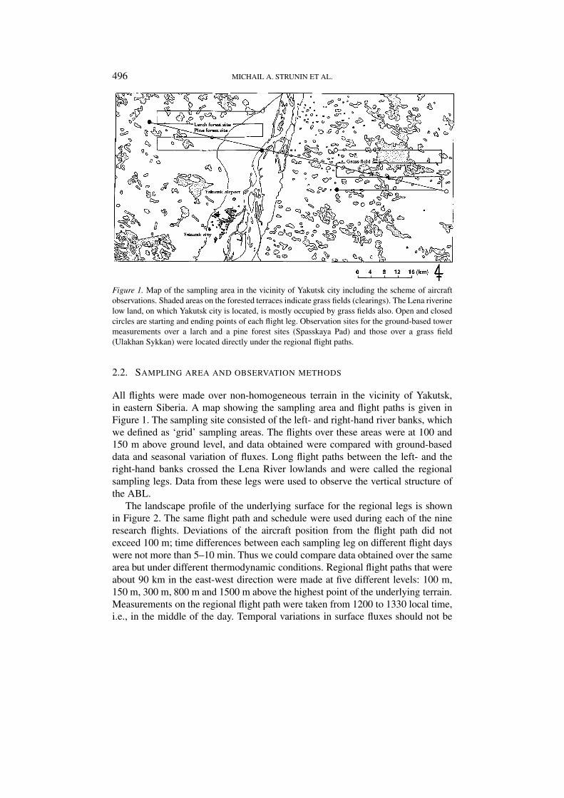
Figure 1. Map of the sampling area in the vicinity of Yakutsk city including the scheme of aircraftobservations. Shaded areas on the forested terraces indicate grass fields (clearings). The Lena riverinelow land, on which Yakutsk city is located, is mostly occupied by grass fields also. Open and closedcircles are starting and ending points of each flight leg. Observation sites for the ground-based towermeasurements over a larch and a pine forest sites (Spasskaya Pad) and those over a grass field(Ulakhan Sykkan) were located directly under the regional flight paths.

2.2. SAMPLING AREA AND OBSERVATION METHODS

All flights were made over non-homogeneous terrain in the vicinity of Yakutsk,in eastern Siberia. A map showing the sampling area and flight paths is given inFigure 1. The sampling site consisted of the left- and right-hand river banks, whichwe defined as ‘grid’ sampling areas. The flights over these areas were at 100 and150 m above ground level, and data obtained were compared with ground-baseddata and seasonal variation of fluxes. Long flight paths between the left- and theright-hand banks crossed the Lena River lowlands and were called the regionalsampling legs. Data from these legs were used to observe the vertical structure ofthe ABL.

The landscape profile of the underlying surface for the regional legs is shownin Figure 2. The same flight path and schedule were used during each of the nineresearch flights. Deviations of the aircraft position from the flight path did notexceed 100 m; time differences between each sampling leg on different flight dayswere not more than 5–10 min. Thus we could compare data obtained over the samearea but under different thermodynamic conditions. Regional flight paths that wereabout 90 km in the east-west direction were made at five different levels: 100 m,150 m, 300 m, 800 m and 1500 m above the highest point of the underlying terrain.Measurements on the regional flight path were taken from 1200 to 1330 local time,i.e., in the middle of the day. Temporal variations in surface fluxes should not be

DEVELOPMENT OF THERMAL INTERNAL BOUNDARY LAYERS 497

Figure 2. Landscape profile under the regional sampling legs, schemes of flight levels andsub-regional legs for mosaic aggregation approach.

large. Vertical aircraft soundings of the ABL from 100 m up to 4000 m over theleft bank, and from 4000 m down to 100 m over the right bank of the Lena River,were taken immediately after finishing regional flight measurements.

Weather conditions that permitted the start of data collection were clouds cov-ering not more than 50% of the sky, no rainfall and weak winds (at most 15 m s−1).Each flight began under these conditions, but clouds developed at around noon,capping the CBL, except on April 24. This allowed us to investigate the influenceof surface heterogeneity on the CBL structure.

The surface under the flight paths can be characterized as non-homogeneous(see Figure 2). Terrain included small hills (terraces) covered with forests (mainlylarch, pine and birch), grass fields, and small lakes. However, the Lena River low-lands, surrounded by bluffs, constituted the central part of the surface under theregional sampling legs. The lowlands included the main channel of the river, aswell as numerous branches. The surface state and the state of the Lena varied withthe seasons. The variation is readily apparent in Photos 2a, 2b and 2c of Hiyama etal. (2003). Initially the ground surface was snow covered and the river was undersolid ice (April 24 and partly May 1). Then, the snow melted and the ice brokeapart, and the water level in the smaller branches of the river rose (observationson May 9, 12; Photo 2a of Hiyama et al., 2003). After most of the ice had melted,water covered most of the lowlands (May 20; Photo 2b of Hiyama et al., 2003).After all the ice had melted, the waters receded (June 1, 5, 9 and 19; Photo 2c ofHiyama et al., 2003). Both the size of the heterogeneous underlying surface, andthe temperature contrast between the river lowland and the surrounding terrace,

498 MICHAIL A. STRUNIN ET AL.

changed. Infrared surface temperature measurements made at the lowest flight level(100 m) were used to estimate seasonal variations in surface heterogeneity. TheLena River lowlands have a horizontal scale of 20 km and strongly influenced boththe surface structure and the CBL development; they also caused, in some cases,MTIBL development inside the CBL. This is fully investigated in Section 3.

The surface under the regional leg can be divided into four relatively uniformsub-regional segments, each with different structures (see Figure 2) but similarhorizontal lengths of 20–22 km. Part 1 was over larch and pine forests on the leftbank of the Lena River, while part 2 was over the Lena River lowlands. Part 3was over the right bank and included mainly larch forest and grass fields. Part 4included small hills covered with larch forests. Turbulence and turbulent flux datafrom these four segments were included in the analysis of the CBL model.

2.3. DATA ANALYSIS

2.3.1. Turbulent Flux CalculationPotential temperature θ and its fluctuation θ ′ (K), and specific humidity q and itsfluctuation q ′ (g kg−1), were based on the observed turbulent and thermodynamicdata. An eddy correlation method was applied to calculate turbulent fluxes.

Vertical sensible heat flux is

H = cpρw′θ ′, (5)

where cp is the specific heat of air and ρ is the density of air. Upward values of H

were treated as positive. Horizontal sensible heat flux is defined as:

S = cpρu′hθ

′, (6)

and was positive if its direction was the same as the flight direction, from the leftto the right banks of the Lena River (see Figure 2).

Vertical latent heat flux is defined as:

λE = λρw′q ′, (7)

where E = ρw′q ′ is the moisture flux, and λ = 4.187{597.3−0.564(T −273.16)}is the latent heat of vaporization (J kg−1). Overbars in Equations (5)–(7) denotetemporal or spatial (along the flight path) means (in the turbulent sense), and primesdenote turbulent fluctuations. The averaging scale depended on the analysis goal.Mean regional turbulent fluxes were obtained from an average along the regionalflight path of 90 km (see the Table I); local flux values were computed from aver-ages over 4 km. Random sampling error in the flux computations was estimated inStrunin and Foken (1998) using the formula originally given by Lumley and Pan-ofsky (1964) and later applied to atmospheric turbulence by Wyngaard (1973) (seealso, Lenschow et al., 1994). For the calculation the integral scales were evaluated

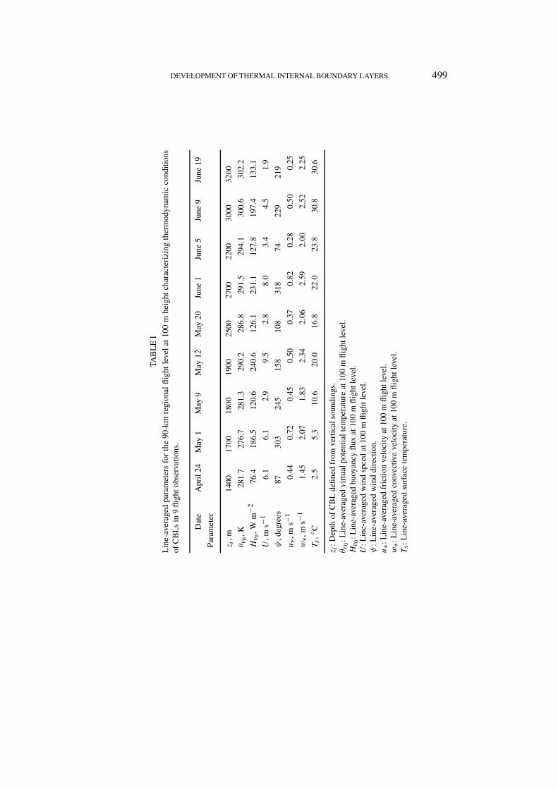
DEVELOPMENT OF THERMAL INTERNAL BOUNDARY LAYERS 499

TAB

LE

I

Lin

e-av

erag

edpa

ram

eter

sfo

rth

e90

-km

regi

onal

flig

htle

vel

at10

0m

heig

htch

arac

teri

zing

ther

mod

ynam

icco

nditi

ons

ofC

BL

sin

9fl

ight

obse

rvat

ions

.

Dat

eA

pril

24M

ay1

May

9M

ay12

May

20Ju

ne1

June

5Ju

ne9

June

19

Para

met

er

z i,m

1400

1700

1800

1900

2500

2700

2200

3000

3200

θ v0,K

281.

727

6.7

281.

329

0.2

286.

829

1.5

294.

130

0.6

302.

2

Hv

0,W

m−2

76.4

186.

512

0.6

240.

612

6.1

231.

112

7.8

197.

413

3.1

U,m

s−1

6.1

6.1

2.9

9.5

2.8

8.0

3.4

4.5

1.9

ψ,d

egre

es87

303

245

158

108

318

7422

921

9

u∗,

ms−

10.

440.

720.

450.

500.

370.

820.

280.

500.

25

w∗,

ms−

11.

452.

071.

832.

342.

062.

592.

002.

522.

25

Ts,◦

C2.

55.

310

.620

.016

.822

.023

.830

.830

.6

z i:D

epth

ofC

BL

defi

ned

from

vert

ical

soun

ding

s.θ v

0:L

ine-

aver

aged

virt

ualp

oten

tial

tem

pera

ture

at10

0m

flig

htle

vel.

Hv

0:L

ine-

aver

aged

buoy

ancy

flux

at10

0m

flig

htle

vel.

U:L

ine-

aver

aged

win

dsp

eed

at10

0m

flig

htle

vel.

ψ:L

ine-

aver

aged

win

ddi

rect

ion.

u∗:

Lin

e-av

erag

edfr

icti

onve

loci

tyat

100

mfl

ight

leve

l.w

∗:L

ine-

aver

aged

conv

ectiv

eve

loci

tyat

100

mfl

ight

leve

l.Ts:L

ine-

aver

aged

surf

ace

tem

pera

ture

.

500 MICHAIL A. STRUNIN ET AL.

with the empirical formula given in Lenschow and Stankov (1986). According tothese calculations, the random sampling error for the average length of 90 km isabout 40%.

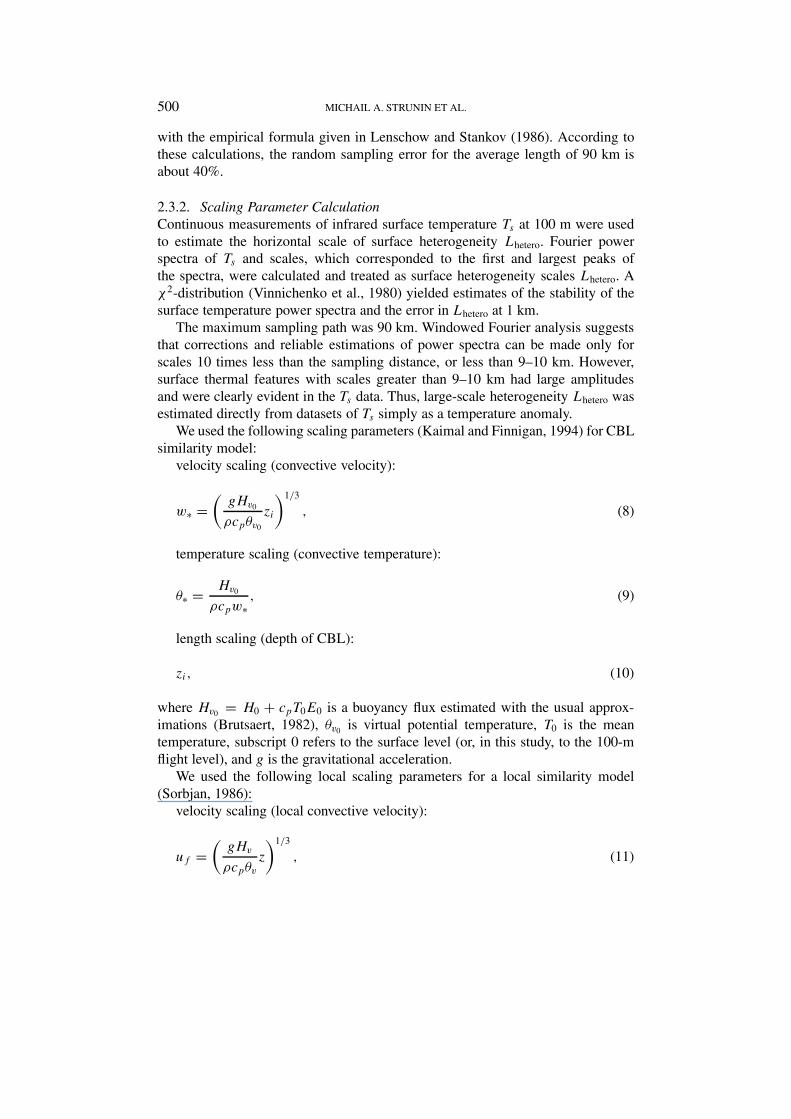
2.3.2. Scaling Parameter CalculationContinuous measurements of infrared surface temperature Ts at 100 m were usedto estimate the horizontal scale of surface heterogeneity Lhetero. Fourier powerspectra of Ts and scales, which corresponded to the first and largest peaks ofthe spectra, were calculated and treated as surface heterogeneity scales Lhetero. Aχ2-distribution (Vinnichenko et al., 1980) yielded estimates of the stability of thesurface temperature power spectra and the error in Lhetero at 1 km.

The maximum sampling path was 90 km. Windowed Fourier analysis suggeststhat corrections and reliable estimations of power spectra can be made only forscales 10 times less than the sampling distance, or less than 9–10 km. However,surface thermal features with scales greater than 9–10 km had large amplitudesand were clearly evident in the Ts data. Thus, large-scale heterogeneity Lhetero wasestimated directly from datasets of Ts simply as a temperature anomaly.

We used the following scaling parameters (Kaimal and Finnigan, 1994) for CBLsimilarity model:

velocity scaling (convective velocity):

w∗ =(

gHv0

ρcpθv0

zi

)1/3

, (8)

temperature scaling (convective temperature):

θ∗ = Hv0

ρcpw∗, (9)

length scaling (depth of CBL):

zi, (10)

where Hv0 = H0 + cpT0E0 is a buoyancy flux estimated with the usual approx-imations (Brutsaert, 1982), θv0 is virtual potential temperature, T0 is the meantemperature, subscript 0 refers to the surface level (or, in this study, to the 100-mflight level), and g is the gravitational acceleration.

We used the following local scaling parameters for a local similarity model(Sorbjan, 1986):

velocity scaling (local convective velocity):

uf =(

gHv

ρcpθv

z

)1/3

, (11)

DEVELOPMENT OF THERMAL INTERNAL BOUNDARY LAYERS 501

temperature scaling (local convective temperature):

Tf = Hv

ρcpuf

, (12)

length scaling (current height of flight):

z, (13)

where Hv and θv are line-averaged buoyancy flux and potential temperature at thelocal level z, respectively.

Obukhov’s length L for estimating magnitude of buoyancy effects was givenby,

L = − u3∗

0.4g

θv0

Hv0

cpρ

, (14)

where u∗ =√

−(u′hw

′).

2.3.3. Vertical Cross Sections of Turbulent FluxesVertical cross sections of the turbulent fluxes were computed as follows. Turbulentfluxes H and λE were the averages of instantaneous fluxes along flight paths oflength 4 km for each flight level. Thus, we obtained matrices including about25 sets of values, along five flight paths at different heights above the surface.Matrix values were interpolated to a 40 × 10 grid of distance along the flightpath and height above the surface. Then, areas with equal parameter values werehighlighted. The same method was used to highlight the vertical cross sections offriction velocity u∗, potential temperature θ and specific humidity q.

This method yielded a qualitative picture of the two-dimensional structure offluxes and other parameters over the non-homogeneous surface. The figures wereused to visualize the CBL structure and aided in its study.

3. Results

Nine aircraft observation flights, at the same time of day, took place duringthe inter-seasonal period over the same underlying surface. Measurements weremade under different wind speed and surface thermal conditions. Thus, we wereable to study the seasonal variation of the ABL and some peculiarities of ABLdevelopment. Aircraft observations, radiosonde data over Yakutsk, and visualcloud observations from aircraft were all incorporated into the analysis of ABLdevelopment.

The surface under our sampling area had a complex structure, but ground-basedmeasurements were made only at two points under the regional sampling legs, at

502 MICHAIL A. STRUNIN ET AL.

stations ‘Spasskaya Pad’ (Ohta et al., 2001; Hamada et al., 2003) and ‘UlakhanSykkan’ (Ishii et al., 2001) in Figures 1 and 2. We compared (spatially) square-averaged heat fluxes obtained at grid legs during aircraft flights over each of thesurface stations at 100 m, and the temporally averaged fluxes measured at thecorresponding ground stations (Hiyama et al., 2001). This comparison yieldedsatisfactory results: aircraft-based sensible heat fluxes were around 20% less thanground-based fluxes. Thus we assumed that flights at 100-m were close to the upperboundary of the surface layer. In what follows we use the line-average values ofbuoyancy flux Hv obtained at 100 m as a substitute of the surface flux Hv0 . Frictionvelocity u∗ estimates were also based on line-averaged momentum flux at 100 m.

Ground-based data obtained at only two points along a sampling leg cannotcorrectly characterize surface conditions along a distance of about 100 km, overvariable topography and thermal structures. Errors from using data obtained closeto the upper boundary of the surface layer should be less than the errors introducedby using distant values of ground-based fluxes, related to quite another dynamicand thermal situation. The main parameters, the line-averaged values along the 90-km regional flight paths at 100 m for each of the nine aircraft observation days,are presented in Table I. We used these parameters instead of the correspondingsurface data for scaling fluxes. To minimize error caused by infrared radiation fromthe underlying air mass, and to achieve maximum resolving power for the thermalheterogeneity of the underlying surface, we used Ts data obtained from the lowestflight level. Values of Ts in Table I were also line-averaged.

3.1. VERTICAL SOUNDINGS

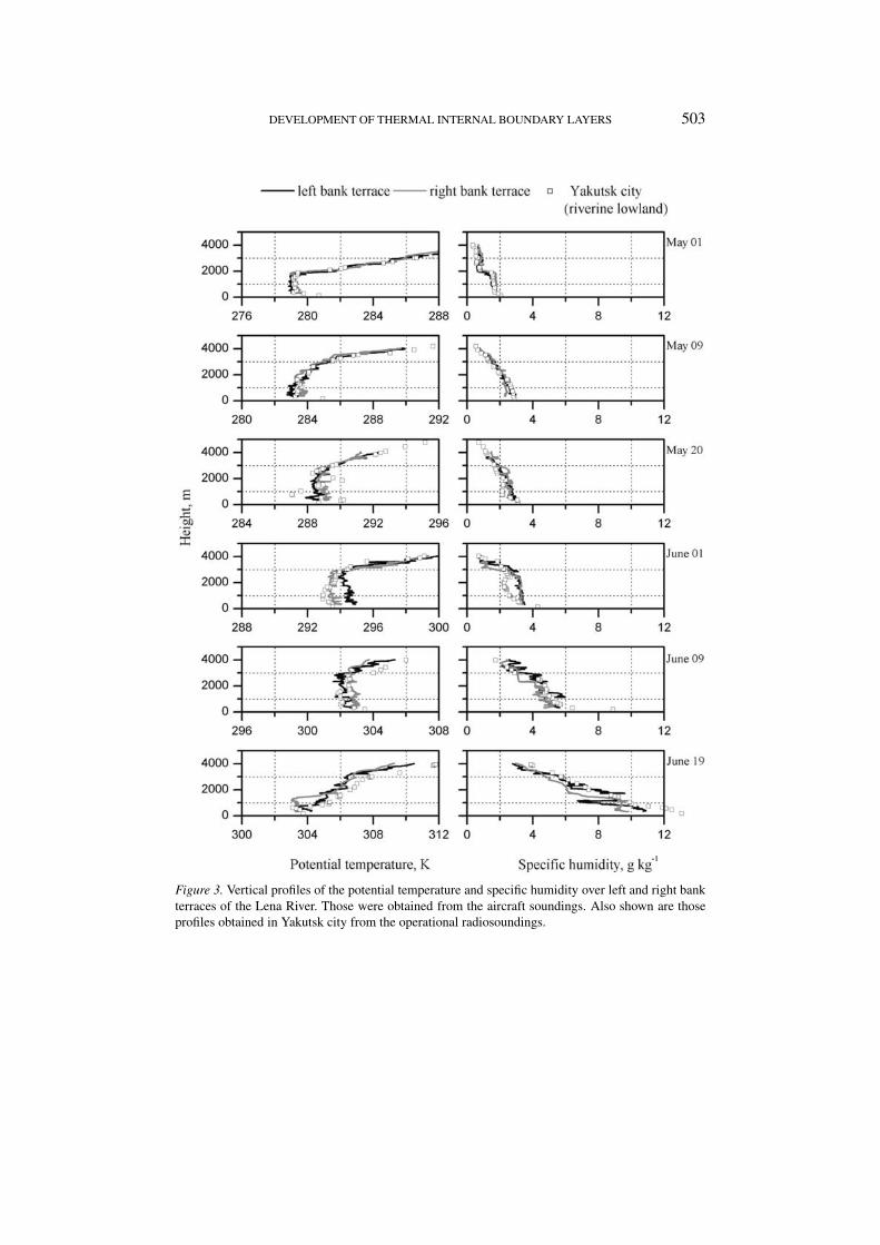
The vertical aircraft soundings were made during aircraft ascent and descent overthe left and right banks of the Lena River. These continuous measurements oftemperature and humidity allowed an estimate of the ABL stability, depth, andsub-layers. Six flight observation days (May 1, 9, 20, June 1, 9 and 19), at approx-imately 10-day intervals, were selected for further illustration. Examples of verticaltemperature stratification and specific humidity profiles are shown in Figure 3.Operational radiosondes, given also in Figure 3 were made simultaneously withaircraft observations at the meteorological station located in Yakutsk (over the riverlowland). Each radiosonde was launched at 1430 local time, i.e., immediately afterthe aircraft soundings. Thus, the operational sounding data can be compared withthe aircraft-measured temperature and humidity data.

The vertical potential temperature profiles (Figure 3) suggest that the ABL overthe sampling area could be treated as a CBL during each of nine observationdays. Temperature profiles in the upper part of the boundary layers were closeto adiabatic. A strong inversion indicated the top of the CBL. Estimations of CBLdepths zi in Table I are based on potential temperature profiles from both aircraftmeasurements and operational radiosondes. Vertical profiles of specific humidityalso supported CBL height estimates. Temperature and humidity profiles from air-

DEVELOPMENT OF THERMAL INTERNAL BOUNDARY LAYERS 503

Figure 3. Vertical profiles of the potential temperature and specific humidity over left and right bankterraces of the Lena River. Those were obtained from the aircraft soundings. Also shown are thoseprofiles obtained in Yakutsk city from the operational radiosoundings.

504 MICHAIL A. STRUNIN ET AL.

craft and from radiosonde agreed well at all levels. Values of zi evaluated fromtemperature and humidity profiles were the same.

Visual observations of cloud base height allowed corroboration of zi estimates.On 19 June, for example, the cloud base estimated by the aircraft observer wasabout 3 km. This corresponds to the inversion height in the temperature profile ofabout 3.2 km. This level is the height of the CBL. A smaller inversion exists atlower levels, indicating a sub-layer in the CBL. Data from flights on May 1 and9 and on June 1 showed no inversions in the temperature profile. In contrast, datafrom May 20, and June 9 and 19, included strong inversions in the temperatureprofile, and especially in the specific humidity profile, at some levels. Such inver-sions indicate the presence of stable sub-layers or residual sub-layers (Stull, 1988),but all observations were made in the middle of the day when the CBL was fullydeveloped. Such behaviour in the vertical stratification suggests the presence ofMTIBLs that have developed over a thermal feature (the Lena River in the presentstudy) at the underlying surface (Garratt, 1990; Kaimal and Finnigan, 1994). Therewere also, at times, significant differences in the humidity profiles over the left andright banks of the Lena. This suggests that a strongly pronounced internal sub-layerexists at times (especially on May 20 and June 9 and 19). This sub-layer expandedthrough the whole depth of the CBL. Data from May 1 and 9, and June 1, did notindicate any distinct mesoscale sub-layers in the CBL.

3.2. VERTICAL CROSS SECTIONS OF FLUXES

The non-monotonous distribution of the turbulent fluxes in a vertical cross sectioncan be another, and more obvious, graphical representation of the existence ofMTIBL. Figures 4, 5 and 6 show the vertical cross sections of the turbulent fluxesand local friction velocity, defined analogously to the friction velocity but with thelocal value of the momentum flux (Sorbjan, 1986; Shao and Hacker, 1990), forMay 1, 9, and 20, and June 1, 9 and 19. Surface temperature is also plotted inthe figures to display surface thermal conditions as well as the horizontal scale ofsurface heterogeneities. Some features of the underlying surface (lowland and theLena River) are also marked.

It was shown in these figures that vertical sensible and latent heat fluxes aresensitive to the presence of large-scale thermal heterogeneity at the surface, andthe fluxes can indicate the existence of a MTIBL. The CBL over homogeneousterrain is typically characterized by strong upward sensible heat fluxes, but thesefluxes change their sign at some levels in the CBL. This sign change was used tomark the presence of a MTIBL. The clearest development of a MTIBL occurred onJune 19. Downward heat fluxes over the river lowlands denoted stable atmosphericconditions that expanded to the top of the CBL over the cold surface. A similar,though not more obvious, CBL structure can be recognized on June 9 and on May20, but the development of MTIBLs was weaker on these days.

DEVELOPMENT OF THERMAL INTERNAL BOUNDARY LAYERS 505

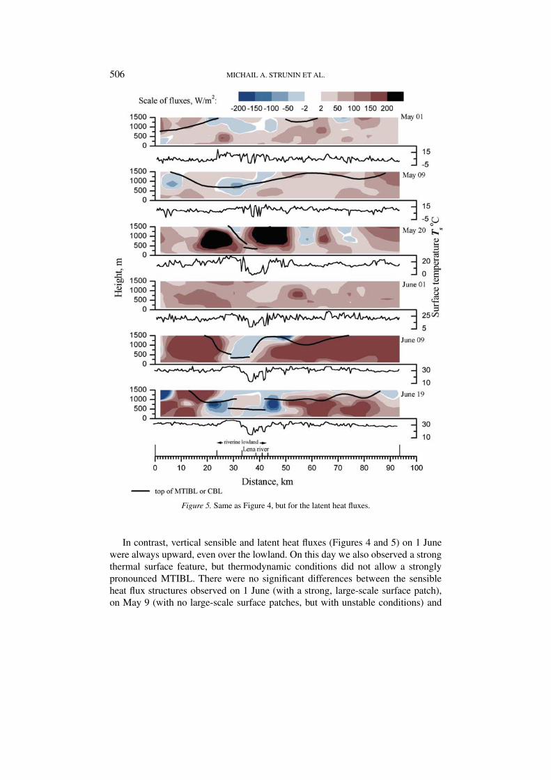
Figure 4. Vertical cross sections of the sensible heat fluxes in CBL over the Lena River and its vicin-ity. Blue and dark blue colours indicate downward fluxes. Wine red colours denote upward fluxes,and white areas correspond to undefined regions (with fluxes less than 2 W m−2). Also shown in thevertical cross sections are the upper boundaries of the MTIBL or the CBL (thick lines). Thin linesattached below the cross sections show the corresponding distributions of the surface temperature.

506 MICHAIL A. STRUNIN ET AL.

Figure 5. Same as Figure 4, but for the latent heat fluxes.

In contrast, vertical sensible and latent heat fluxes (Figures 4 and 5) on 1 Junewere always upward, even over the lowland. On this day we also observed a strongthermal surface feature, but thermodynamic conditions did not allow a stronglypronounced MTIBL. There were no significant differences between the sensibleheat flux structures observed on 1 June (with a strong, large-scale surface patch),on May 9 (with no large-scale surface patches, but with unstable conditions) and

DEVELOPMENT OF THERMAL INTERNAL BOUNDARY LAYERS 507

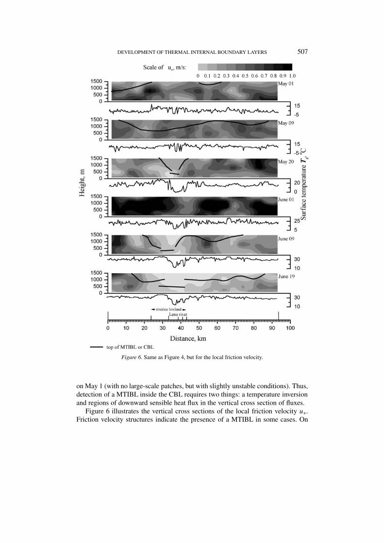
Figure 6. Same as Figure 4, but for the local friction velocity.

on May 1 (with no large-scale patches, but with slightly unstable conditions). Thus,detection of a MTIBL inside the CBL requires two things: a temperature inversionand regions of downward sensible heat flux in the vertical cross section of fluxes.

Figure 6 illustrates the vertical cross sections of the local friction velocity u∗.Friction velocity structures indicate the presence of a MTIBL in some cases. On

508 MICHAIL A. STRUNIN ET AL.

May 20, June 9, and especially on June 19, we were able to detect low values of u∗over the river lowlands.

Figures 4–6 also showed the upper boundary of the MTIBL (or the boundary ofthe CBL if a sub-layer was absent) marked as solid lines. The figure on June 1 doesnot contain the boundary as it was located above the domain. Local MTIBL depths,δi , for unstable conditions were identified based mainly on the vertical cross sectionof the buoyancy fluxes Hv (not presented). The criterion for the estimation was thatthe buoyancy flux must be zero at the top of the boundary layer. This is typical forthe CBL over a homogeneous surface, as shown in previous studies (Kaimal andFinnigan, 1994; Stull, 1988; Garratt, 1992). The criterion of δi estimation for thestable condition (flight segment over the Lena River in some cases) was a zero levelof sensible heat flux.

All these evaluations were validated using vertical profiles of potential temper-ature θ and specific humidity q derived from the flight paths at the five differentvertical levels of the regional sampling legs (not presented in this paper). Thevalues of θ and q obtained along the five levels gave a vertical cross section ofthese parameters, and 10 vertical profiles of the θ and q were obtained every 10 kmhorizontal interval from these vertical cross sections. These vertical profiles gaveanother estimation of δi , which gave rough agreement with the δi obtained above.It is interesting to note that δi estimated through θ and q are practically the sameas each other, and this fact suggests that the thicknesses of the sub-layer in termsof θ and q are also the same.

It should also be noted that vertical cross sections of θ and q on days with andwithout a MTIBL were quite different from each other. Figures for June 9 andespecially for June 19 demonstrate strong stable thermodynamic conditions overthe Lena River, which should be the source of MTIBL development. Moreover,analysis of horizontal wind speed structure showed the presence of regions withthe wind direction opposite to the dominant (synoptic) wind. This suggests thelocal circulation over the Lena River appeared in some cases. On the other hand,local profiles of potential temperature on June 1 (as well as on May 1 and May9) indicated the presence of strong horizontal advection. Perhaps strong horizontaladvection prevented clear pronounced sub-layers. As shown in Figures 4 and 5, theupper boundaries of MTIBL on May 20 and June 9 have some horizontal displace-ments with respect to the corresponding flux distributions. These displacementswere towards the dominant wind direction (see Table II), and therefore these werecaused by influence of horizontal advection.

Satellite pictures of the area being investigated, obtained for the observationperiod (from 1300 to 1400 of local solar time) were also compared in the analysisof vertical cross sections of the fluxes. These pictures (not presented) demonstratethe presence of clouds and a degree of sky covering with clouds. Types of cloudswere recognized by the observer during the flight experiment. One additional cir-cumstance was also taken into account for the flux structure analysis. As numerousobservations of CBL over homogeneous surfaces have shown, the latent heat flux

DEVELOPMENT OF THERMAL INTERNAL BOUNDARY LAYERS 509

TAB

LE

II

Para

met

ers

ofC

BL

san

dM

TIB

Ls

deve

lopm

ent.

Dat

eA

pril

24M

ay1

May

9M

ay12

May

20Ju

ne1

June

5Ju

ne9

June

19

Para

met

er

Exi

sten

ceof

MT

IBL

No

No

No

No

Yes

No

Yes

Yes

Yes

z ble

nd,m

4010

017

015

230

110

8014

024

0

z wu

,m90

190

260

6045

028

037

045

076

0

Lhe

tero

,m20

0060

0070

0030

0011

000

1100

011

000

1100

012

000

LR

au,m

4700

4000

2300

6100

2700

6700

3100

4200

2200

z/L

−1.0

−0.6

−1.6

−2.2

−2.1

−0.6

−6.2

−2.2

−10.

1

Ps

1.62

1.07

1.06

0.60

0.84

1.04

0.64

0.76

0.57

PsL

4.5

1.3

1.3

1.5

0.8

1.1

0.5

0.8

0.6

z ble

nd:B

lend

ing

heig

ht.

z wu

:The

rmal

blen

ding

heig

ht.

Lhe

tero

:Est

imat

edm

axim

umho

rizo

ntal

scal

eof

surf

ace

hete

roge

neit

y.L

Rau

:Rau

pach

’sle

ngth

.z/L

:Par

amet

erof

stab

ilit

yfo

r10

0m

flig

htle

vel.

Ps:P

aram

eter

for

scal

ing.

PsL

:Par

amet

erfo

rin

dica

ting

MT

IBL

.

510 MICHAIL A. STRUNIN ET AL.

often reaches its maximum at the top of CBL, (especially in the case of cloud-topped CBL), where sensible heat flux is minimum. At least the latent heat isusually much larger than the sensible heat flux in the neighborhood of the CBL top(Garratt, 1992). During our observation period on May 9 there was a fully cloud-topped boundary layer with a homogeneous field of stratocumulus (Sc) clouds.As Figures 4 and 5 showed, the vertical structure of both sensible and latent heatfluxes were similar to the classic type for the homogeneous CBL. On the contrary,satellite pictures for May 20 show a dense field of Sc and cumulus (Cu) clouds andthe narrow cloudless street over the Lena River. Figures 4 and 5 present the narrowdownward sensible flux area over the riverine lowland on this day, and very strongupward latent heat fluxes through the top boundary of MTIBL on either side of theriver. A similar situation is observed on June 9 (with Cu clouds), but the cloudlessstrip along the Lena River is much wider and the downward sensible flux area overthe river is wider too. A situation with the strong horizontal advection on June 1led to relatively homogeneous flux distributions and a scattered altocumulus (Ac)and Cu cloud field over the left part of the observation area. The boundary betweenthe cloud field and cloudless area was located over the right bank of the river, inagreement with flux distributions in Figures 4 and 5. On June 19, an Ac cloud ridgewas observed only over the left bank of the river. Figure 5 demonstrates stronglatent heat flux through the top of MTIBL. The latent heat flux over the right bankhas a maximum at 500 m, not on the top of the MTIBL, and there are no clouds overthis area. Thus, this analysis is in a good agreement with the MTIBL developmentand makes the obtained vertical cross section of flux structure convincing.

3.3. EVALUATION OF STEADY-STATE CONDITIONS IN THE CBL

The analyses in the previous section with the vertical cross section of the turbulentfluxes obtained from the regional flight are only valid when the steady state of thewhole CBL is assured. In general, daytime CBL generated by the strong surfaceheating can be associated with a relatively short turbulent time scale, often ex-pressed as zi/w∗, which in turn is associated with quasi-steady state. The analyzeddata in this study were measured from around 1200 to 1330 local solar time, whenthe height of CBL did not change much. In order to further investigate the steady-state condition in each day, wavelet transforms (Grossmann and Morlet, 1984) areapplied to the fluctuation of wind speed and temperature, and the turbulent fluxes.

Wavelet coefficient distributions for the different flight levels (from 100 m upto 1500 m) allowed us to trace the horizontal and vertical location of so-called‘events’ – heterogeneous zones (not shown). We identified the location of a fewevents at different levels (100, 150 and 300 m), at the same distance from thebeginning of the sampling leg. These can be treated as relatively steady whichmeans that, at least up to 300 m, conditions were in a quasi-steady state. Thisjustifies using vertical cross sections to approximate the CBL structure.

DEVELOPMENT OF THERMAL INTERNAL BOUNDARY LAYERS 511

Juxtaposing vertical cross sections of θ and q (not shown) with vertical profilesmeasured during the vertical aircraft soundings is another test of the applicabilityof the steadiness. Good linkage between practically instantaneous measurements(which lasted about 10 min) and distributions obtained through averaging and in-terpolation of the same parameters along the long horizontal sampling legs supportsthe quasi-steady state assumption during the period.

4. Detection of MTIBL Development

In some cases MTIBLs appear in the CBL and radically change its structure; inother cases such layers are not observed. MTIBL development is governed by arelation between shear stress parameters and parameters characterizing convection.In order to further investigate the factors affecting MTIBL development, the para-meters that characterize the structure and development of the CBL were calculatedfor each flight and are shown in Table II. Existence of a MTIBL, noted in Table II,was based on vertical stratification of potential temperature and specific humidity(Figure 3), and vertical cross sections of vertical sensible and latent heat fluxes(Figures 4 and 5). Blending heights zblend, zwu and Raupach’s length LRau in thetable were calculated by (1), (2) and (4), respectively, based on data in Table I.These values are calculated from the 90-km regional flight path obtained at the100-m level. The stability parameter z/L was also estimated from 100-m flightobservations, based on parameters in Table I. The maximum horizontal scale ofsurface heterogeneity, Lhetero, was estimated from the surface temperature spectrameasured during the flights at the 100-m level.

In general, since the configuration of surface features that composes the surfaceheterogeneity is never isotropic, its length scale, Lhetero, depends on the direction inwhich it is measured, and the surface heterogeneity scale that is most relevant to thedevelopment of the internal boundary layer should be taken along the wind direc-tion. In the vicinity of Yakutsk city, the main surface feature that comprises the landsurface heterogeneity is the Lena River and the surrounding forest, which stronglydepends on the direction. During the spring period when the measurements weremade, water flow filled most of the Lena River lowlands and the horizontal sizeof the surface features does not strongly depends on the measurement direction.The earlier observations (April 24 and May 1) were made when the surface of theLena River was frozen and covered with ice. Nevertheless, we can single out a verynarrow range of wind direction for which Lhetero may be significantly larger. Thisis along the Lena River with ψ = 20◦ to 40◦ or ψ = 200◦ to 220◦ (see Figure 1).According to Table I, we did not observe these wind directions in most cases. Allour flights were directed across the river, thus our estimations of Lhetero were theminimum scales.

Most cases in Table II were type ‘B’ at the surface (Shuttleworth, 1988): Strongthermal features at the surface (the surface temperature difference between the

512 MICHAIL A. STRUNIN ET AL.

Lena River and the surrounding area was more than 15 ◦C) had horizontal scales of10 km or more. Nevertheless, MTIBLs developed through the entire CBL in onlyfour cases: on May 20 and June 5, 9, and 19. Moreover, on June 1 a strong thermalfeature with the horizontal scale of 10 km occurred, but a MTIBL did not develop.Additional parameters must be important in influencing the growth of a thermallyforced MTIBL in the CBL.

Values of zblend, estimated from 100-m flight level data, varied day by day anddo not seem to be relevant. The thermal blending height zwu also does not seemto be relevant to MTIBL growth. The values of zwu in Table II predict that thesurface heterogeneity had its effect up to a height of 200 to 400 m in most cases,though the appearance of MTIBL implied the full depth of the CBL is under theeffect of the surface heterogeneity. Data obtained from the nine flights suggest thatthermodynamic conditions have a limit that, when exceeded, allows the MTIBLand an attendant sharp and radically changing CBL structure to appear. Mahrt(2000) suggested Raupach’s length LRau as a parameter to control the surface het-erogeneity effect. The length LRau should be compared with the horizontal scaleof surface heterogeneity. If the length is less than the horizontal heterogeneity,scaling models cannot be successfully applied to predict turbulent structure. FromTable II, the parameter LRau can be used to signal the presence of a MTIBL. IfLRau � Lhetero a MTIBL is present; no sub-layers exist when LRau > Lhetero orLRau ≈ Lhetero. However these criteria fail on May 1 and 9 and June 1.

The non-dimensional parameter Ps , which relates shear stress and convectiveconditions, is a more suitable indicator of MTIBL development:

Ps = u∗θv0

Hv0

, (15)

where buoyancy flux Hv0 , virtual potential temperature θv0 and friction velocity u∗were calculated along the long regional flight path at 100 m (see Table I). ParameterPs is only used for Hv0 > 0 and is closely related to the stability parameter z/L

calculated at the same level. From Table II, Ps < 1 corresponds to z/L < −2, andunstable CBL conditions. Note that Ps does not contain the value of CBL depth orany other vertical scale.

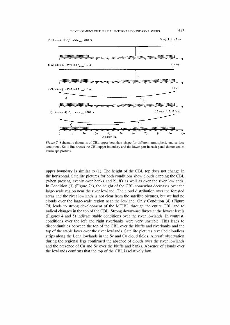
By using Ps and Lhetero, the nine flights can be categorized into four differentconditions:1. Ps > 1 and Lhetero < 10 km (April 24, and May 1 and 9);2. Ps < 1 and Lhetero < 10 km (May 12);3. Ps > 1 and Lhetero > 10 km (June 1);4. Ps < 1 and Lhetero > 10 km (May 20, June 5, 9 and 19).

The four conditions are schematically illustrated in Figure 7. Condition (1) (Figure7a) is typical of a slightly unstable CBL without any internal sub-layers. The topof the CBL has no significant horizontal variations. Condition (2) (Figure 7b) ischaracterized by stronger instability than in Condition (1) but the shape of the CBL

DEVELOPMENT OF THERMAL INTERNAL BOUNDARY LAYERS 513

Figure 7. Schematic diagrams of CBL upper boundary shape for different atmospheric and surfaceconditions. Solid line shows the CBL upper boundary and the lower part in each panel demonstrateslandscape profiles.

upper boundary is similar to (1). The height of the CBL top does not change inthe horizontal. Satellite pictures for both conditions show clouds capping the CBL(when present) evenly over banks and bluffs as well as over the river lowlands.In Condition (3) (Figure 7c), the height of the CBL somewhat decreases over thelarge-scale region near the river lowland. The cloud distribution over the forestedareas and the river lowlands is not clear from the satellite pictures, but we had noclouds over the large-scale region near the lowland. Only Condition (4) (Figure7d) leads to strong development of the MTIBL through the entire CBL and toradical changes in the top of the CBL. Strong downward fluxes at the lowest levels(Figures 4 and 5) indicate stable conditions over the river lowlands. In contrast,conditions over the left and right riverbanks were very unstable. This leads todiscontinuities between the top of the CBL over the bluffs and riverbanks and thetop of the stable layer over the river lowlands. Satellite pictures revealed cloudlessstrips along the Lena lowlands in the Sc and Cu cloud fields. Aircraft observationduring the regional legs confirmed the absence of clouds over the river lowlandsand the presence of Cu and Sc over the bluffs and banks. Absence of clouds overthe lowlands confirms that the top of the CBL is relatively low.

514 MICHAIL A. STRUNIN ET AL.

If Ps > 1, the CBL has no sub-layer, because convective motion does notdominate and shear stress causes horizontal mixing within the CBL. Shear mix-ing accompanied by weak convective motions smoothes out the fields of turbulentparameters in the CBL, even over such a significant and long thermal feature as theLena River. In contrast, if Ps < 1 (or if the magnitude of z/L < −2), convectivemotions dominate and the MTIBL develops over a thermal surface feature with alarge horizontal size. This MTIBL is affected by vertical profiles of potential tem-perature, specific humidity and sensible and latent heat fluxes. Moreover, when theparameter Ps is small, the internal boundary layer is obvious and a larger verticaland horizontal expansion of the MTIBL occurs. Unstable conditions in the CBLwith Ps < 1 (or with z/L < −2), but without large-scale thermal structures (forexample, the May 12 case), do not lead to the development of a MTIBL because asmall-scale disturbance cannot expand from the surface to a significant level.

Thus, a MTIBL develops through the entire CBL and radically modifies itsstructure if two conditions hold. First, there must be strong thermal heterogeneityat the surface with the horizontal scale greater than 10 km. Second, the CBL mustbe strongly unstable with z/L ≈ −2 or Ps < 1. To account for both events weintroduce the parameter PsL to indicate a MTIBL within the CBL:

PsL = CsL

u∗θ0

H0

zi

Lhetero, (16)

where CsL = 4 is a non-dimensional coefficient, chosen such that the critical valuefor a MTIBL appearance occurs at PsL = 1. Values of PsL < 1 suggest MITBLdevelopment; PsL > 1 means that sub-layers do not appear.

The coefficient CsL = 4 may have no physical basis. It was chosen to makeparameter PsL easy to use. If parameter PsL can be related to MTIBL develop-ment at a different site, the coefficient CsL could be a universal non-dimensionalconstant.

5. Scaling the CBL over Non-Homogeneous Land Surface

The parameter PsL diagnoses the existence of a MTIBL but it does not answerthe question of whether it is advisable to apply scaling. Nevertheless, the presenceof a MTIBL in the CBL did change the typical scaling parameters, especially forthe vertical length scale. Previous CBL scaling could not characterize the verticalstructure of MTIBLs.

The surface under the regional legs was considered type ‘B’ for cases that in-cluded MTIBLs. The surface can be separated into parts (sub-regions), each ofwhich can be considered as surface type ‘A’, and after the separation a new scalingmodel can be applied in each sub-region. This is the mosaic or flux aggregationapproach to scaling (Frech and Jochum, 1999; Mahrt, 1996). If the atmosphericboundary layer is in quasi-equilibrium with the underlying surface, the procedure

DEVELOPMENT OF THERMAL INTERNAL BOUNDARY LAYERS 515

is valid (Mahrt, 1996). A minimum horizontal scale Lhom for the homogeneoussub-region is (Mahrt, 1996):

Lhom = zU

CEσw

,

where σw is the standard deviation of the vertical wind speed perturbations andCE ≈ 0.1 is a non-dimensional coefficient. If z = 1500 m (the highest flight level),and U/σw ≈ 4 (a typical value), then Lhom ≈ 60 km. The typical and maximumscales of surface heterogeneity during the flights were 7 and 12 km, respectively.These values are too small to support the flux aggregate approach. However, thevalue of the coefficient CE is not well known; consequently, the value of Lhom maybe off by an order of magnitude.

Therefore, we applied the flux aggregate approach. Regional flight paths weredivided into four segments with relatively uniform surfaces, of about 20–22 kmin length (see Figure 2; a short description of the surface for each segment is insub-Section 2.2). Data obtained for these segments at all flight levels from 100 mto 1500 m were used for constructing profiles.

We replaced the boundary-layer depth zi in Equations (8)–(10) with the localMTIBL heights δi for sub-regional segments. Values of δi were identified basedon the vertical cross section of the buoyancy fluxes, that of potential temperature,and the local vertical profiles of potential temperature (see sub-Section 3.2). If theaveraged sensible heat flux on a sub-regional segment was positive up to 1500 m,the heights of δi obtained from aircraft vertical soundings were used for scaling.

According to Mahrt (2000), a necessary condition for the application of thesimilarity theory is related to the horizontal scale of surface heterogeneity Lhetero

and Raupach’s length LRau. If Lhetero > LRau then use of a similarity scaling modelis possible. If Lhetero < LRau no rigorous approach is available. Thus LRau/Lhetero

is a criterion for the applicability of scaling models. Therefore, wind speed andtemperature fluctuations, and vertical sensible heat flux, can be approximated bylocal similarity models if LRau/Lhetero < 1 but not if LRau/Lhetero > 1. To test thisstatement, we plotted normalized wind speed and temperature variances σ 2

w/w2∗and σ 2

T /θ2∗ against the non-dimensional height z/δi . There were 36 sub-regionalsegments, 22 of which did not obey the similarity model. Fourteen segments werevalid with the similarity model.

Figure 8 shows a clear difference between data types as a function ofLRau/Lhetero. The scatter plots for the normalized moments of wind and temperaturewith LRau/Lhetero < 1 were similar to those over a homogeneous surface (Caughey,1982; Stull, 1988; Schmidt and Schumann, 1989; Sorbjan, 1991; Fedorovich andMironov, 1995). The normalized vertical profiles resemble a smoothed typicalcurve, as shown below. In contrast, the scatter plots for sub-regional legs withLRau/Lhetero > 1 show scattering that is too large for any model. Clear differencesbetween the data are also displayed in the normalized sensible and latent heat fluxes

516 MICHAIL A. STRUNIN ET AL.

Figure 8. Scaling of the vertical wind speed fluctuations, the air temperature fluctuations, the sens-ible heat fluxes, and the latent heat fluxes based on the data with different values of parameterLRau/Lhetero.

(H/H0 and λE/H0, respectively). We used the quasi-surface flux H0 for normal-izing latent heat fluxes because scatter in the corresponding latent heat fluxes wasvery large. Dispersion of points for sub-regional segments with LRau/Lhetero > 1was greater than that for segments with LRau/Lhetero < 1. We conclude that datawith LRau/Lhetero > 1 should not be used in scaling models, but that modelling offluxes along sub-segments when LRau/Lhetero < 1 can give satisfactory results. It isimportant to note if the condition LRau/Lhetero < 1 did not hold true for the somesub-segment, we rejected all points at the correspondent sub-regional segment (i.e.,we removed the full profile consisting of five points at levels from 100 m up to 1500m). This means that a point at some level may be close to scaling curves, but wholeprofile does not satisfactorily obey the model. In fact, plots for LRau/Lhetero < 1in Figure 8 represent the selected profiles, each of them satisfactorily obeys thesimilarity models.

In order to check the applicability of different models for mosaic parts moreaccurately, we built up scatter plots and fitting curves. Figures 9a–f show resultsfrom applying a well-known similarity model, and a local similarity model ofthe CBL for the wind speed and air temperature fluctuations at the sub-regionalsampling segments when LRau/Lhetero < 1. Both models yield satisfactory results.

DEVELOPMENT OF THERMAL INTERNAL BOUNDARY LAYERS 517

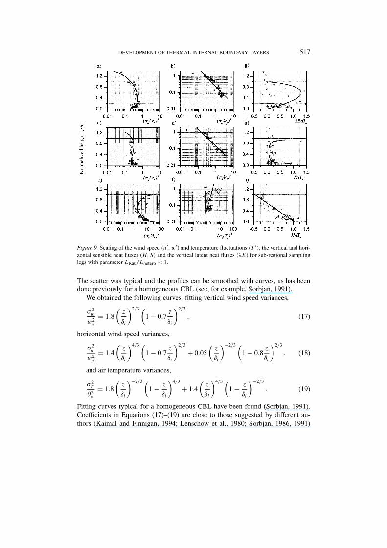
Figure 9. Scaling of the wind speed (u′, w′) and temperature fluctuations (T ′), the vertical and hori-zontal sensible heat fluxes (H, S) and the vertical latent heat fluxes (λE) for sub-regional samplinglegs with parameter LRau/Lhetero < 1.

The scatter was typical and the profiles can be smoothed with curves, as has beendone previously for a homogeneous CBL (see, for example, Sorbjan, 1991).

We obtained the following curves, fitting vertical wind speed variances,

σ 2w

w2∗= 1.8

(z

δi

)2/3 (1 − 0.7

z

δi

)2/3

, (17)

horizontal wind speed variances,

σ 2u

w2∗= 1.4

(z

δi

)4/3 (1 − 0.7

z

δi

)2/3

+ 0.05

(z

δi

)−2/3 (1 − 0.8

z

δi

)2/3

, (18)

and air temperature variances,

σ 2T

θ2∗= 1.8

(z

δi

)−2/3 (1 − z

δi

)4/3

+ 1.4

(z

δi

)4/3 (1 − z

δi

)−2/3

. (19)

Fitting curves typical for a homogeneous CBL have been found (Sorbjan, 1991).Coefficients in Equations (17)–(19) are close to those suggested by different au-thors (Kaimal and Finnigan, 1994; Lenschow et al., 1980; Sorbjan, 1986, 1991)

518 MICHAIL A. STRUNIN ET AL.

for a homogeneous case. This is an additional argument for using the parameterLRau/Lhetero as a data separator for scaling and applying a model developedfor a homogeneous CBL. It gives the possibility to predict wind speed and airtemperature fluctuations in a CBL at mosaic parts of a non-homogeneous landsurface.

Figures 9g–i show the scaling of turbulent fluxes. The scaling of sensible heatfluxes has a character that is typical for a homogeneous CBL (Figure 9i). Thescattering of points for the sensible heat flux is not very large, and the normalizedflux profile is similar to that for the homogeneous case (Kaimal and Finnigan,1994).

Scattering of the normalized latent heat fluxes λE/H0 versus z/δi is large(Figure 9g), but it is possible to discern a tendency in the flux distribution thatis characterized by the solid line in Figure 9g. Figure 9h shows the dependenceof the absolute values of the normalized horizontal sensible heat fluxes (S/H0) onz/δi. The solid line highlights the tendency of the fluxes but is not a fitting curve.Horizontal fluxes at most sub-regional segments do not exceed 25% of the quasi-surface vertical flux value. However, at relative heights of 0.1 (i.e., directly abovethe surface layer) and of 0.9 (directly under the top of the MTIBL), values of S/H0

become relatively large; in some cases they are comparable with vertical sensibleheat fluxes. Figure 9h shows that horizontal heat exchanges take place mainly atthe top and bottom of the mixed layer.

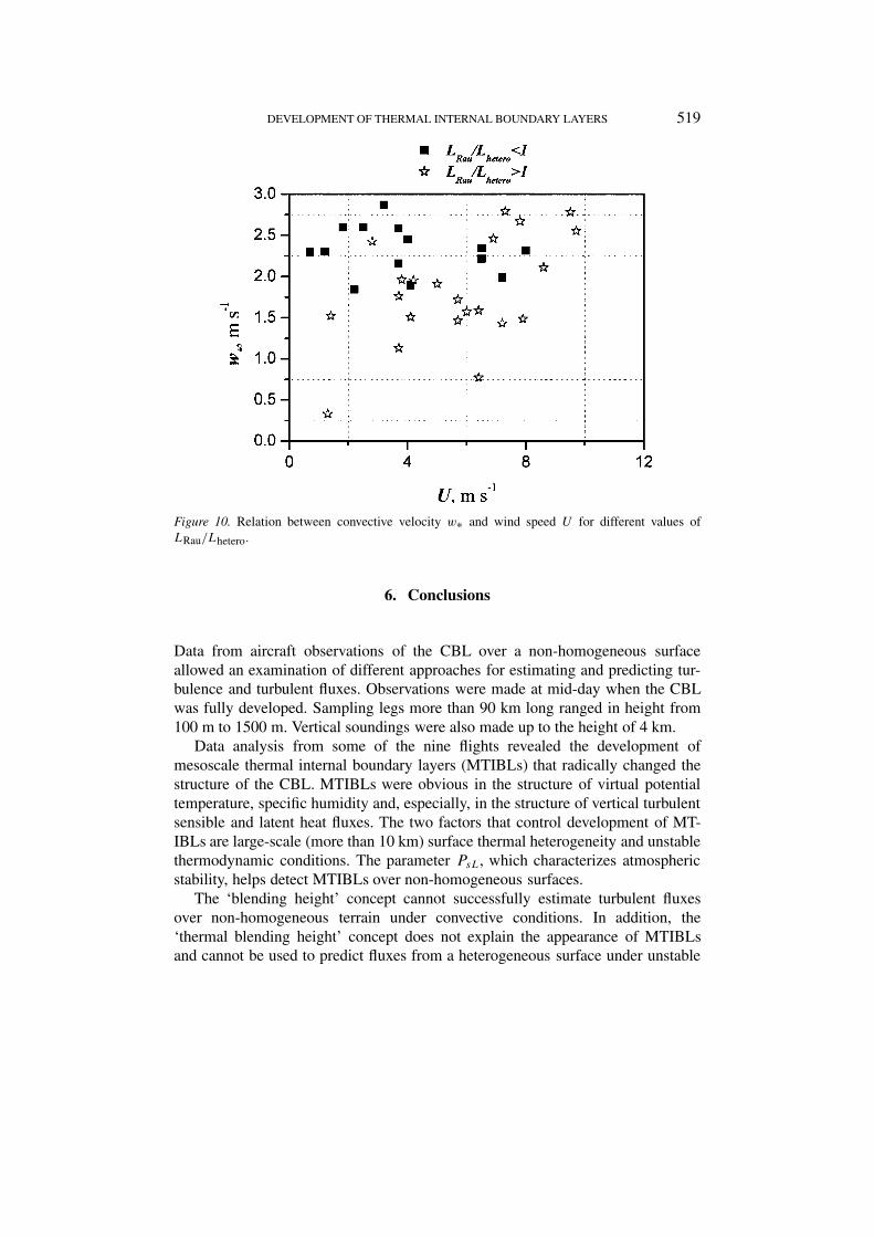
Parameter LRau/Lhetero also helps estimate how thermal and dynamic sourcescontribute to turbulence structures. Convective velocities w∗ characterize thermalcontributions to turbulence, and the mean wind speed U (or friction velocity u∗)helps determine the dynamic part of the turbulence. The scatter plots of convect-ive velocity w∗ versus mean wind speed U are presented in Figure 10. Anotherkind of plot, w∗ versus u∗, demonstrates approximately the same relation (plotare not presented). Figure 10 shows that turbulence in sub-regional segments withLRau/Lhetero < 1 had mainly thermal sources: large values of w∗ occurred withstrong surface heating of the atmosphere, but increasing wind speed does notlead to a growth of convective velocity. On the other hand, turbulence in sub-regional segments with LRau/Lhetero > 1 was primarily mechanically driven. It isclear from Figure 10 that increasing convective velocity corresponds to increasingwind speed for LRau/Lhetero > 1. Thus, the parameter LRau/Lhetero can separatesub-regional segments with thermally and mechanically produced turbulence. Thisconclusion shows good agreement with the statement that the similarity model isvalid for thermally produced turbulence, but the scaling will be unsatisfactory if amechanical turbulence source dominates.

DEVELOPMENT OF THERMAL INTERNAL BOUNDARY LAYERS 519

Figure 10. Relation between convective velocity w∗ and wind speed U for different values ofLRau/Lhetero.

6. Conclusions

Data from aircraft observations of the CBL over a non-homogeneous surfaceallowed an examination of different approaches for estimating and predicting tur-bulence and turbulent fluxes. Observations were made at mid-day when the CBLwas fully developed. Sampling legs more than 90 km long ranged in height from100 m to 1500 m. Vertical soundings were also made up to the height of 4 km.

Data analysis from some of the nine flights revealed the development ofmesoscale thermal internal boundary layers (MTIBLs) that radically changed thestructure of the CBL. MTIBLs were obvious in the structure of virtual potentialtemperature, specific humidity and, especially, in the structure of vertical turbulentsensible and latent heat fluxes. The two factors that control development of MT-IBLs are large-scale (more than 10 km) surface thermal heterogeneity and unstablethermodynamic conditions. The parameter PsL, which characterizes atmosphericstability, helps detect MTIBLs over non-homogeneous surfaces.

The ‘blending height’ concept cannot successfully estimate turbulent fluxesover non-homogeneous terrain under convective conditions. In addition, the‘thermal blending height’ concept does not explain the appearance of MTIBLsand cannot be used to predict fluxes from a heterogeneous surface under unstable

520 MICHAIL A. STRUNIN ET AL.

conditions. Raupach’s length LRau is an important scale for CBL development overheterogeneous surfaces.

The flux aggregation or mosaic approach was successfully used for scaling theturbulent structure of the CBL with and without MTIBLs. In cases with MTIBLs,the local MTIBL depth should be used as a scaling parameter. The parametercontrolling applicability of similarity and local similarity models to the mosaic seg-ments is the relation between scales of surface heterogeneity Lhetero and Raupach’slength LRau. Normalized vertical profiles of wind speed, air temperature and tur-bulent fluxes for sub-regional segments where Lhetero > LRau can be satisfactorilyapproximated by typical curves of the scaling models for a homogeneous CBL.

Heterogeneity in the CBL initiates horizontal turbulent fluxes. In some caseshorizontal sensible heat fluxes became comparable with vertical fluxes. The largestvalues of horizontal sensible heat fluxes occur at the upper boundary of the surfacelayer and just under the top of the mixed layer.

Acknowledgements

The authors gratefully acknowledge the crew of the ILYUSHIN-18 aircraft, es-pecially Captain Dmitry Senkov, for undertaking a number of very difficult anddangerous low-level flights. Their accurate and skilled work made possible thesuccessful observations used in this study. Our thanks are also due to all membersof the scientific aircraft team who produced the on-board measurements: VladimirDmitriev, Nikolaj Alyabev, Nikolaj Ryabtcev, Lidija Sidorjak, Andrej Troitckij andPavel Gaishun.

We would also like to thank Prof. T. Yasunari of Nagoya University, Japanand Prof. Y. Fukushima of the Research Institute for Humanity and Nature, Ja-pan. Without their efforts and leadership, the aircraft observations would not havebeen possible. This research was financially supported, in part, by a grant from theFrontier Observational Research System for Global Change (FORSGC), Japan, andby the Ministry of Education, Culture, Sports, Science and Technology of Japan(Grant No. 11201206 and No. 12460063).

References

Albertson, J. D. and Parlange, M. B.: 1999, ‘Natural Integration of Scalar Fluxes from ComplexTerrain’, Adv. Water Resour. 23, 239–252.

Brutsaert, W. H.: 1982, Evaporation into the Atmosphere, D. Reidel, Dordrecht, 299 pp.Caughey, S. J.: 1982, ‘Observed Characteristics of the Atmospheric Boundary Layer’, in F.

Nieuwstadt and H. van Dop (eds.), Atmospheric Turbulence and Air Pollution Modeling, D.Reidel, Dordrecht, pp. 107–158.

Deardorff, J. W.: 1970a, ‘Preliminary Results from Numerical Integrations of the Unstable PlanetaryBoundary Layer’, J. Atmos. Sci. 27, 1209–1211.

DEVELOPMENT OF THERMAL INTERNAL BOUNDARY LAYERS 521

Deardorff, J. W.: 1970b, ‘Convective Velocity and Temperature Scale for the Unstable PlanetaryBoundary Layer and for Rayleigh Convection’, J. Atmos. Sci. 27, 1212–1213.

Fedorovich, E. and Mironov, D.: 1995, ‘A Model for a Shear-Free Convective Boundary Layer withParameterized Capping Inversion Structure’, J. Atmos. Sci. 1, 83–95.

Frech, M. and Jochum, A.: 1999, ‘The Evaluation of Flux Aggregation Methods Using AircraftMeasurements in the Surface Layer’, Agric. For. Meteorol. 98–99, 121–143.

Garratt, J. R.: 1990, ‘The Internal Boundary Layer – A Review’, Boundary-Layer Meteorol. 50,171–203.

Garratt, J. R.: 1992, The Atmospheric Boundary Layer, Cambridge University Press, U.K., 316 pp.Grossmann, A. and Morlet, J.: 1984, ‘Decomposition of Hardy Functions into Square Integrate

Wavelets of Constant Shape’, SIAM J. Math. Anal. 15, 723–736.Hamada, S., Ohta, T., Hiyama, T., Kuwada, T., Takahashi, A., and Maximov, T. C.: 2003, ‘Hydro-

meteorological Behaviors of Pine and Larch Forests in Eastern Siberia’, Hydrol. Process., inpress.

Hiyama, T., Strunin, M. A., Asanuma, J., Mezrin, M. Y., Suzuki, R., and Ohata, T.: 2001, ‘FluxDistributions of Heat and Carbon Dioxide in the Atmospheric Boundary Layer over Non-Homogeneous Surface in Eastern Siberia’, in Proceedings of the Fifth International StudyConference on GEWEX in Asia and GAME, 3–5 October, 2001, Nagoya, Japan, pp. 307–314.

Hiyama, T., Strunin, M. A., Suzuki, R., Asanuma, J., Mezrin, M. Y., Bezrukova, N. A., and Ohata, T.:2003, ‘Aircraft Observations of the Atmospheric Boundary Layer over a Heterogeneous Surfacein Eastern Siberia’, Hydrol. Process. 17, 2885–2911.

Ishii, Y., Yabuki, H., Nomura, M., Tanaka, H., Kobayashi, N., and Desyatkin, R. V.: 2001, ‘Water andEnergy Flux Observation over an Alas Lake in Central Yakutia, Eastern Siberia’, in Proceedingsof the Fifth International Study Conference on GEWEX in Asia and GAME, 3–5 October, 2001,Nagoya, Japan, pp. 670–673.

Kaimal, J. C. and Finnigan, J. J.: 1994, Atmospheric Boundary Layer Flows, their Structure andMeasurements, Oxford University Press, New York, Oxford, 289 pp.

Lenschow, D. H.: 1972, The Measurements of Air Velocity and Temperature Using the NCAR BuffaloAircraft Measuring System, Technical Note TN/STR-74, NCAR, Boulder, CO, 39 pp.

Lenschow, D. H. and Stankov, B. B.: 1986, ‘Length Scale in the Convective Boundary Layer’, J.Atmos. Sci. 43, 1198–1209.

Lenschow, D. H., Mann, J., and Kristensen, L.: 1994, ‘How Long Is Long Enough When MeasuringFluxes and Other Turbulence Statistics’, J. Atmos. Oceanic Tech. 11, 661–673.

Lenschow, D. H., Wingaard, J. C., and Pennell, W. T.: 1980, ‘Mean Fields and Second-MomentBudgets in a Baroclinic, Convective Boundary Layer’, J. Atmos. Sci. 37, 1313–1326.

Lumley, J. L. and Panofsky, H.: 1964, The Structure of Atmospheric Turbulence, IntersciencePublishers, New York, 239 pp.

Mahrt, L.: 1996, ‘The Bulk Aerodynamic Formulation over Heterogeneous Surface’, Boundary-Layer Meteorol. 78, 87–119.

Mahrt, L.: 2000, ‘Surface Heterogeneity and Vertical Structure of the Boundary Layer’, Boundary-Layer Meteorol. 96, 33–62.

Mezrin, M. Y.: 1997, ‘Humidity Measurements from Aircraft’, Atmos. Res. 44, 53–59.Ohata, T. and Fukushima, Y.: 2001, ‘Progress of GAME-Siberia in 2000’, GAME Publication 26,

Activity Report of GAME-Siberia 2000, Japan National Committee for GAME, GAME-SiberiaSub-Committee, March 2001, 3–8.

Ohta, T., Hiyama, T., Tanaka, H., Kuwada, T., Maximov, T. C., Ohata, T., and Fukushima, Y.: 2001,‘Seasonal Variation in the Energy and Water Exchanges above and below a Larch Forest inEastern Siberia’, Hydrol. Process. 15, 1459–1476.

Raupach, M. R.: 1991, ‘Vegetation-Atmosphere Interaction in Homogeneous and HeterogeneousTerrain: Some Implications of Mixed-Layer Dynamics’, Vegetatio 91, 105–120.

522 MICHAIL A. STRUNIN ET AL.

Raupach, M. R. and Finnigan, J. J.: 1995, ‘Scale Issues in Boundary-Layer Meteorology: SurfaceEnergy Balances in Heterogeneous Terrain’, Hydrol. Process. 9, 589–612.

Schmidt, H. and Schumann, U.: 1989, ‘Coherent Structures of the Convective Boundary Layer’, J.Fluid. Mech. 200, 511–562.

Shao, Y. and Hacker, J. M.: 1990, ‘Local Similarity Relationships in a Horizontally InhomogeneousBoundary Layer’, Boundary-Layer Meteorol. 52, 17–40.

Shuttleworth, W. J.: 1988, ‘Macrohydrology – The New Challenge for Process Hydrology’, J. Hydrol.100, 31–56.

Sorbjan, Z.: 1986, ‘On Similarity in the Atmospheric Boundary Layer’, Boundary-Layer Meteorol.34, 377–397.

Sorbjan, Z.: 1991, ‘Evaluation of Local Similarity Functions in the Convective Boundary Layer’,Boundary-Layer Meteorol. 30, 1565–1583.

Strunin, M. A.: 1997, ‘Meteorological Potential for Contamination of Arctic Troposphere: AircraftMeasuring System for Atmospheric Turbulence and Methods for Calculations its Characteristics.Archive and Database of Atmospheric Turbulence’, Atmos. Res. 44, 17–35.

Strunin, M. A. and Foken, Th.: 1997, ‘Techniques for Quality Assessments of Aircraft TurbulentFlux Measurements’, Deutscher Wetterdienst Forschung und Entwicklung, Arbeitsergebnisse, 44,Offenbach am Main, 17 pp.

Strunin, M. A. and Foken, Th.: 1998, ‘Influence of Non-Homogeneity of Underlying Surface on theStructure of Turbulence in the Atmospheric Boundary Layer’, in Abstracts of the Presentationsfor the 23rd General Assembly EGS, Nice, April, 1998, Annales Geophysicae, Supplement toVolume 16, 1998, Part 2: Hydrology, Oceans & Atmosphere, C427–C808.

Stull, R. B.: 1988, An Introduction to Boundary Layer Meteorology, Kluwer Academic Publishers,Dordrecht, 666 pp.

Sun, J., Lenschow, D. H., Mahrt, L., Crawford, T. L., Davis, K. J., Oncley, S. P., MacPherson, J. I.,Wang, Q., Dobosy, R. J., and Desjardins, R. L.: 1997, ‘Lake-Induced Atmospheric CirculationsDuring BOREAS’, J. Geophys. Res. 102(D24), 29,155–29,166.

Vinnichenko, V. K., Pinus, N. Z., Shmeter, S. M., and Shur, G. N.: 1980, Turbulence in the FreeAtmosphere, Consultants Bureau, New York, 310 pp.

Wood, N. and Mason, P. J.: 1991, ‘The Influence of Stability on the Effective Roughness Lengths forMomentum and Heat Flux’, Quart. J. Roy. Meteorol. Soc. 117, 1025–1056.

Wyngaard, J. C.: 1973, ‘On Surface Layer Turbulence’, in D. A. Haugen (ed.), Workshop onMicrometeorology, Boston, MA: American Meteorological Society, pp. 101–149.