DYNAMIC MONITORING OF CIVIL ENGINEERING ...

Computational Methods for Shell and Spatial Structures

IASS-IACM 2000 M. Papadrakakis, A. Samartin and E. Onate (Eds.)

© ISASR-NTUA, Athens, Greece 2000

DYNAMIC MONITORING OF CIVIL ENGINEERING STRUCTURES

G. De Roeck, B. Peeters and J. Maeck

Department of Civil Engineering K.U.Leuven, Leuven, Belgium

e-mail: [email protected]

Key words: vibration monitoring, bridge testing, system identification, environmental effects, modal analysis, damage detection

Abstract. As part of the Brite-EuRam project BE96-3157 SIMCES (System Identification to Monitor Civil Engineering Structures) the three span box bridge Z24 in Switzerland was monitored during almost one year before it was artificially damaged. In the preceding monitoring period the influence of environmental conditions, such as humidity, wind and especially temperature, on the bridge eigenfrequencies was studied. The goal of the subsequent damage tests, corresponding to realistic and relevant cases, was to prove that damage could be detected, localised and quantified by considering changes in eigenfrequencies and modeshapes. Some of the main conclusions are that ambient vibrations treated by proper system identifications algorithms can provide accurate results for eigenfrequencies and modeshapes, that it is mandatory to filter beforehand the influence of environmental conditions and that small, stiffness degradation producing damage can be detected if the corresponding eigenfrequency diminutions surpass 1%.

G. De Roeck, B. Peeters,J. Maeck

2

1 Introduction

Service loads, environmental and accidental actions may cause damage to structures. Regular inspection and condition assessment of engineering structures are necessary so that early detection of any defect can be made and the structures updated safety and reliability can be determined. Early damage detection and location allows maintenance and repair works to be properly programmed. This minimizes not only the annual costs of repair (e.g. for bridges estimated at 1,5% of their value) but also limits immobilization of traffic which can represent an even higher economic cost

Vibration monitoring of civil engineering structures (e.g. bridges, buildings, dams) has gained a lot of interest over the past few years, due to the rather cheap instrumentation and the development of new powerful system identification techniques.

In the running Brite-EuRam project BE96-3157 SIMCES (System Identification to Monitor Civil Engineering Structures) [1] special attention is be paid to techniques making use of operational data (service loading testing).

Sometimes it is doubted whether the measured deviations of dynamic properties (eigenfrequencies, modeshapes) are significant enough to be a good indicator of damage or deterioration. The comparison of original and new dynamic properties can be troublesome because of changes caused by environmental influences (e.g. temperature changes). Another issue of continuing research is the localisation of damage starting from any observed difference in dynamic properties.

To convince the engineering community that vibration monitoring is a valuable technique for structural assessment a proof of feasibility is essential. In the SIMCES project a full scale test was performed on the Z24 bridge in Switzerland. The test consisted of two parts:

• a long term test for quantifying the degree of variance due to environmental influences;

• a short term loading failure test to prove that changes in dynamic properties are large enough (i.e. statistically relevant) and can be linked to damage in a particular part of the structure.

The main responsible partner for the bridge test was EMPA (Swiss Federal Laboratories for Materials Testing and Research). Other partners in the project were the Division Structural Mechanics of K.U.Leuven, Aalborg University, LMS International, WS Atkins, Sineco and the Technical University of Graz.

The strategy of damage detection by vibration monitoring and the different steps of the detection procedure are presented in figure 1.

IASS-IACM 2000, Chania-Crete, Greece

3

Figure 1: Detection procedure


4

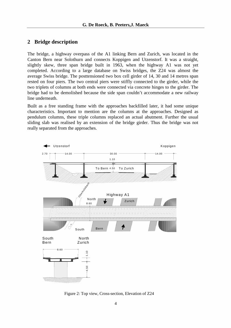
2 Bridge description

The bridge, a highway overpass of the A1 linking Bern and Zurich, was located in the Canton Bern near Solothurn and connects Koppigen and Utzenstorf. It was a straight, slightly skew, three span bridge built in 1963, when the highway A1 was not yet completed. According to a large database on Swiss bridges, the Z24 was almost the average Swiss bridge. The posttensioned two box cell girder of 14, 30 and 14 metres span rested on four piers. The two central piers were stiffly connected to the girder, while the two triplets of columns at both ends were connected via concrete hinges to the girder. The bridge had to be demolished because the side span couldn’t accommodate a new railway line underneath.

Built as a free standing frame with the approaches backfilled later, it had some unique characteristics. Important to mention are the columns at the approaches. Designed as pendulum columns, these triple columns replaced an actual abutment. Further the usual sliding slab was realised by an extension of the bridge girder. Thus the bridge was not really separated from the approaches.

~4

.50

~

4.5

0

1.1

0 8 .60

NorthZurich

SouthBern

Zurich

Bern

N orth

South

8.60

To ZurichTo Bern

U tzenstorf Koppigen

2.70 14 .00 14 .00 30 .00

1.10

4.50

H ighway A1

Obe

rhol

zbac

h

Figure 2: Top view, Cross-section, Elevation of Z24


5

3 Dynamic tests

3.1 Environmental Monitoring System (EMS)

Civil engineering structures and particularly bridges are exposed to the environment. Natural or man induced influences produce alterations in the dynamics of a structure strong enough to hide effects due to damage. With this in mind a system to measure a number of environmental parameters and vibration data was installed on the Z24 in October 1997. The aim was to learn about the environmental influences on the dynamical system characteristics, mainly the eigenfrequencies.

3.1.1 Environmental parameters

The atmospheric conditions were considered to be important environmental factors. Therefore sensors to measure air temperature, humidity, rain or not, wind speed and wind direction were installed.

Temperature has an influence on the elastic properties of the concrete material. Moreover since the Z24's girder was a continuous beam, thermal differences in the girder may have lead to constraints which could have influenced the Z24's dynamic behaviour. Thus a reasonable distribution of thermal measurements over the girder had to be considered. The bridge’s thermal state was measured by 8 thermocouples in three different sections, one in the main span, two other in the side spans. Also the overall elongation of the mid span was measured.

For small span bridges the asphalt used for the pavement contributes not only to the total mass but to a certain extent also to the structural stiffness. The elastic properties of asphalt vary substantially within a few decades of temperature change. The changes are also frequency dependent. For the installation of the EMS, access holes drilled into the centre span's boxes revealed a cover of 18 cm asphalt. In the three before-mentioned sections the pavement temperature was also measured.

Changes of dynamic soil stiffnesses can also cause shifts of dynamic properties. To capture this effect thermocouples were installed underneath the approaches and the piers.

In table 1 an overview of the different sensors is presented. Figure 3 shows the sensor locations.


6

Description Unit Amount Temperature, bridge girder sections 1, 2, and 3 °C 24 Temperature, pavement °C 3 Temperature, approaches °C 6 Temperature, soil °C 6 Elongation, mid span mm 1 Angular deflection, girder at main piers ° 2 Windspeed m/s 1 Winddirection ° 1 Air temperature °C 1 Air humidity % 1 Rain boolean 0/1 1 Traffic, boolean 0/1 1

Table 1: Sensors installed for environmental data

Utzenstorf Koppigen

To ZurichTo Bern

Thermal expansion to be monitored

Soil temperatures

To ZurichTo Bern

Tilt

Bridge temperatures

NorthZurich

SouthBern

TWSi TWCi TWNi

TSWSi TSWNiTPiTDTi

TDSi

TSi

Figure 3: EMS-locations of environmental sensors


7

3.1.2 Vibration data

Force balanced accelerometers were used to measure the dynamical sytem characteristics, i.e. eigenfrequencies and modeshapes. Each acceleration measurement corresponds to one modal amplitude. Vibrations were generated by the traffic underneath the bridge. The number of accelerometers for the EMS was chosen with a future, permanently installed monitoring system in mind. High sensitivity, low frequency accelerometers are expensive so the number should be kept at minimum without jeopardizing the registration of important modal information. It was decided to install 16 accelerometers spread over the bridge as shown in figure 4. The locations were chosen in a way that the lowest modeshapes could be reasonably well visualised by the 16 measured points.

Utzenstorf Koppigen

Figure 4: EMS locations of accelerometers

3.1.3 Data acquisition strategy

It was decided to acquire data at hourly intervals. Every hour prior to and after acquiring acceleration data, 10 scans of environmental data were collected and stored. Then 8 averages of 8192 samples at 100 Hz sampling rate were collected for whole group of the 16 accelerometers. By this strategy daily about 24 megabytes of compressed data were generated.

3.2 Progressive damage tests (PDT)

In the SIMCES project condition assessment based on the monitoring of dynamic properties is proposed. In order to investigate, whether the proposed method is feasible, reliable, objective and sensitive enough or not, Progressive Damage Tests have been set up.

3.2.1 Planning and preparation of the PDT

The first selection of valid damage scenarios (see table 2) was based on literature and case studies. An excellent source for such information can be found in [3] (in German). The selected scenarios had to be relevant for the safety of a bridge, i.e. the damage, if allowed to progress, would have endangered its bearing capacity; occur frequently, based on the

Zurich

Bern

North

South

L

T

V

North, Zurich

Utzenstorf pierSouth, Bern

V

T L


8

number of citations in the literature and experience of Swiss bridge owners; be applicable to Z24. Safety requirements for the traffic on the A1 lead to further limitations for the selection of the scenarios.

ID Description 3.1 Chipping of concrete under the pavement, due to frost thawing cycles and/or

temperature shock while applying de-icing salt 3.2 Chipping of concrete at the underside, due to vehicle overheight, carbonisation and

subsequent corrosion of reinforcement steel 3.3 Settlement of foundation, due to settlement of subsoil, erosion 3.4 Tilt of foundation, due to settlement of subsoil, erosion 3.5 Failure of tendon wires, due to erroneous or 'forgotten' injection of tendon tubes,

chloride influence 3.6 Failure of tendon anchors, due to corrosion, overstress 3.7 Shearfailure on crossbeam, due to corrosion of shear reinforcement, inappropriate

construction or design 3.8 Failure of concrete hinges, due to chloride attack 3.9 Cracks on girder, due to overload, settlement of subsoil, erosion 3.10 Landslide, due to construction activities, heavy rainfall, erosion 3.11 Cracks in piers, due to vehicle impact, settlements

Table 2: Damage scenarios considered for the PDT

For safety reasons 3.7 was not possible, 3.1 was technically very difficult to be realised and very expensive. 3.9 would have been an important scenario, but had to be disregarded due to technical reasons. For 3.11 a numerical simulation showed that only vehicle impacts could generate cracks in the main piers of the Z24.

The final scenario sequence given in table 3 was selected with the safety issues in mind. Reversible scenarios were considered first.

Maximum extent Scenario allowed realised

3.3 Settlement of foundation 0.20m 0.095m 3.3 Tilt of foundation 0.5° 0.1° 3.2 Chipping of concrete at underside 60 m2 24 m2 3.10 Landslide 100 m3 70 m3 3.8 Failure of concrete hinges 3 pcs 1 pc 3.6 Failure of anchor heads 6 pcs 4 pcs 3.5 Failure of posttensioning tendons 6 tendons 6 tendons

Table 3: Sequence and extent of scenarios


9

3.2.2 Vibration tests

First a reference measurement was done. Then after each damage step the next measurement was performed. The measurements consisted of a full ambient and a full forced vibration test. Ambient tests started at about 18:00 hours, when traffic on the highway A1 was still dense. Forced tests followed immediately after the ambient tests and started usually in-between 23:00 hours and 01:00 hours in the morning.

1 5 10 20 30 400-1 43

299 303

199 203

99 103

304 308

204 208

104 108

309 313

209 213

109 113

314 318

214 218

114 118

319 323

219 223

119 123

324 328

224 228

124 128

329 333

229 233

129 133

334 338

234 238

134 138

339 343

239 243

139 143

ZÜRICH

BERN

AVT

FVT

Setup_1 Setup_2 Setup_3 Setup_4 Setup_5 Setup_6 Setup_7 Setup_8 Setup_9

Setup_9 Setup_8 Setup_7 Setup_6 Setup_5 Setup_4 Setup_3 Setup_2 Setup_1

Utzenstorf Koppigen

Utzenstorf Koppigen

Koppigen

542

512

522

532

511

521

531

541

Setup_1

Setup_2

Setup_3

Setup_4

Setup_9

Setup_8

Setup_7

Setup_6

Utzenstorf

412

422

432

442

411

421

431

441

AVT

FVT

Setup_6

Setup_7

Setup_8

Setup_9

Setup_4

Setup_3

Setup_2

Setup_1

FVT

AVT

Figure 5: Measurement grid

For the ambient tests a completely new installed measurement system and new data acquisition software was used. The complete structure was measured in 9 setups of 33 accelerometers (Figure 5). Time signals of 8 series of 8192 samples were recorded at 100 Hz.

Both of EMPA's vertical shakers were used to excite the bridge for the forced tests (Figure 6).

1 5 10 20 30 400-1 43

99 113 143

ZÜRICH

BERN

Utzenstorf Koppigen

SH1

122112

SH1

136

R3V

R1V

R2L

VT

Figure 6: Shaker locations for FVT and references for AVT


10

The shaker input signal was generated using a dual processor PC and inverse FFT software. In this way it was possible to produce a fairly flat force spectrum in the interesting bandwidth of 3 to 30 Hz.

4 Treatment of the data

4.1 Environmental Monitoring System [4,10]

The variation of the central web temperature (TWC1) during the periods that the EMS was operational is shown in figure 7.

3 0 0 3 5 0 4 0 0 4 5 0 5 0 0 5 5 0 6 0 0 6 5 0- 5

0

5

1 0

1 5

2 0

2 5

3 0

D a y N u m b e r

We

b T

em

pe

ratu

re

[°C

]

Figure 7: Variation of web temperature during EMS period

Figure 8 illustrates the dependency of the first eigenfrequency on the web temperature for temperatures above 5°C. 95% Confidence limits are also indicated.

Figure 8: Variation of mode 1 frequency with web temperature


11

The dependency can be expressed by the regression equation (standard deviation σ = 0,014):

with:

T = web temperature (TWC1) in degrees Celsius.

From Figure 9 it can be clearly seen that the measurements corresponding to the Progressive Damage Tests exceed the 95% confidence limits.

Figure 9: Variation of mode 1 frequency with web temperature (95% confidence limits); pre-PDT measurements (+), PDT measurements (x)

More sophisticated ARX models have also be fitted to the data [10]:

where ky is the Auto-Regressive output (in casu an eigenfrequency) at time instant kuk ; is the eXogeneous input (in casu a temperature) and ke is a noise term indicating that the input-output relation is not perfect. It is assumed that ke is white noise, with zero mean

[ ] iikk eeE λδ=− , where iδ is the Kronecker symbol ( 00,10 =⇒≠=⇒= ii ii δδ ). In

knnknnknknknkk eubububyayaybkbkkaa

++++=++ +−−−−−−− 112111 �� (2)

THzfi 00431,00,4)( −= (1)


12

order to be able to establish confidence intervals, we also assume that ke is Gaussian distributed. The ARX model (2) is characterized by 3 numbers: an , the auto-regressive order; bn , the exogeneous order and kn , the pure time delay between input and output. By introducing the shift operator, 1

1−

− = kk yyq , and defining the operator polynomials:

The ARX model (2) can be written as:

ARX models are popular because their parameters can be estimated by simple linear least squares. A regression model is an ARX010 model (with [ kba nnn ,, ]=[0,1,0]).

The advantage of using general ARX models over static regression models is that they include some dynamics: the current output and input are related to outputs and inputs at previous time instants. If more than one input variable is included, equation (2) is still valid but ku is a column vector and the b coefficients are row vectors. With a lot of input candidates and the possible choices for kba nnn ,, there are many different ARX models that can be fitted to the data. Hence criteria are needed to assess and compare the quality of the models. The least squares method minimizes the sum of squares of the equation errors

ke .

A first quality criterion is the value of the loss function, defined as:

with the estimated equation errors defined as:

The loss function is also an estimate of the noise covariance �, what explains the notation. Other criteria include penalties for model complexity like Akaike’s final prediction error (FPE) criterion or Rissanen’s minimum description length criterion.

After a preliminary selection procedure it turned out that a (SISO) ARX model based on temperature TDT2 performed best.

The results are represented in Table 4. The input and output data were normalized before the models were identified. The model for the first mode seems to be much better than the models for the other 3 modes. The static regression results are also represented.

1121

11

)(

1)(+−−−−−

−−

+++=

+++=bk

b

kk

a

a

nnn

nn

nn

qbqbqbqb

qaqaqa

�

�

(3)

kkk euqbyqa += )()( (4)

kkk uqbyqa )(ˆ)(ˆ )ˆ( −=θε (6)

∑=

=N

kkN 1

2 )ˆ(1ˆ θελ (5)


13

Especially for the first 2 modes, the improvements of an ARX model over a static model are spectacular.

ARX model Static regression model Mode

kba nnn ,, λ̂ FPE kba nnn ,, λ̂ FPE

1

2

3

4

2 1 4

3 2 0

2 1 0

2 2 0

0.145

0.533

0.507

0.569

0.145

0.536

0.509

0.572

0 1 0

0 1 0

0 1 0

0 1 0

0.212

0.896

0.548

0.612

0.213

0.897

0.549

0.613

Table 4: Comparison between SISO models: TDT2-eigenfrequency

Another quality criterion for a model is provided by the autocorrelation function of the residuals. In order to justify the least squares approach for finding the model parameters, it was assumed that ke is white noise: the autocorrelations, )(iRe , at time lags i different from zero, have to be zero:

They are estimated as:

Figure 10: Normalized autocorrelqtion of the residuals of the TDT2 – f1 models: ‘--‘,ARX214; ‘–‘,ARX010.

[ ] iikke eeEiR δλ== −)( (7)

∑=

−=N

kikke N

iR1

)ˆ()ˆ(1

)(ˆ θεθε (8)

−200 −150 −100 −50 0 50 100 150 200−0.2

−0.1

0

0.1

0.2

0.3

0.4

0.5

0.6

Time Lags i [−]

Re (i

) / λ

[−]


14

In Figure 10, the normalized autocorrelation functions λ̂/)(ˆ iRe of the SISO ARX214 and ARX010 models are plotted; together with the 99% confidence intervals. The residuals of the static regression model are not white noise at all. This is an indication that more information can be extracted from the data.

4.2 Progressive Damage Tests (PDT)

The PDT scenarios and vibration test dates are summarized in table 5.

K.U.Leuven derived from the ambient acceleration data the eigenfrequencies and the modeshapes for the different damage scenarios by the stochastic subspace identification method.

To facilitate the use of this method a program MACEC (Modal Analysis on Civil Engineering Constructions) was developed [6], [7].

Figure 11 shows the first five modes. The first eigenmode (f=3.918Hz) is a symmetrical bending mode. Mode 2 (f=5.121Hz) is a transversal mode, modes 3 (f=9.929Hz) and 4 (f=10.52Hz) are combined torsional / anti-symmetrical bending modes, mode 5 (f=12.69Hz) is a symmetrical bending mode.

# Date Scenario # Date Scenario

1 04.08.98 1. Reference measurements 10 26.08.98 Chipping of concrete 24 m2

2 09.08.98 2. Reference measurements 11 27.08.98 Landslide

3 10.08.98 Settlement of pier, 20 mm 12 31.08.98 Concrete hinges

4 12.08.98 Settlement of pier, 40 mm 13 02.09.98 Failure of anchor heads

5 17.08.98 Settlement of pier, 80 mm 14 03.09.98 Anchor heads #2

6 18.08.98 Settlement of pier, 95 mm 15 07.09.98 Rupture of tendons #1

7 19.08.98 Tilt of foundation 16 08.09.98 Rupture of tendons #2

8 20.08.98 3. Reference measurements 17 09.09.98 Rupture of tendons #3

9 25.08.98 Chipping of concrete 12 m2

Table 5: PDT scenarios and vibration test dates


15

Figure 11: AVT mode shapes: scenario 1, 1st reference measurements

The evolution of the eigenfrequencies, identified from AVT-data, throughout the damagescenarios can be followed in table 6. Also the temperature measured in cross section 2 at the central longitudinal web of the box girders is given in table 5. In order to obtain one number, the temperature was averaged over the period of the vibration measurements.

Following observations can be made:

• Between scenario #1 and #2, the Koppigen pier was cut and the settlement system was installed. Although the bridge has not yet undergone any settlement, there is already a decrease of the eigenfrequencies, probably due to the changed boundary conditions. It should however be observed that also the temperature difference was quite pronounced (9°C).


16

• The first settlement (#3, 20 mm) seems to have no visible influence on the eigenfrequencies. Further increasing the settlement (#4, 40 mm � #6, 95 mm) has a pronounced influence. This is also apparent from the 5th mode: from figures 12-13 the change of this mode shape between #4 and #6 is obvious.

• Scenario 8 is another reference measurement (after removing of the settlement and tilt). If compared with #2, lower eigenfrequencies are found although the temperature was about the same. The bridge did not completely recover from the settlement; either some damage remained or the support conditions of the Koppigen pier were slightly changed.

• The first chipping of concrete (#9, 12 m2) seems to have no effect. Most of the eigenfrequencies even increased. It must be noted that also here, between #8 and #9, the temperature decrease was quite high (7 �C).

• The landslide (#11) had a large effect on the eigenfrequency of the 2nd mode.

• The cutting of a concrete hinge at side Koppigen (#12) has a very clear influence on the 5th mode. This bending mode (figure 14) obtained a torsion component after cutting the hinge (figure 15).

Figure 12: AVT mode shape 5: scenario 4, Figure 13: AVT mode shape 5: scenario 6; settlement of pier, 40 mm settlement of pier, 95 mm

Figure 14: AVT mode shape 5: scenario 11, Figure 15: AVT mode shape 5: scenario 12, landslide concrete hinges

Mode 5 f = 12.48Hz xi = 2.5%

xy

z

Mode 5 f = 12.05Hz xi = 2.5%

xy

z

Mode 5 f = 11.69Hz xi = 2.5%

xy

z

Mode 5 f = 12.03Hz xi = 2.5%

xy

z


17

Table 6: Evolution of AVT eigenfrequencies, f, and their standard deviations, )f, with respect to the applied damage scenarios.

Scen

ario

T [�

C] mode 1 mode 2 mode 3 mode 4 mode 5

f[Hz]

�f

[Hz]f

[Hz]�f

[Hz]f

[Hz]�f

[Hz]f

[Hz]�f

[Hz]f

[Hz]�f

[Hz]

1 17 3.92 0.02 5.12 0.02 9.93 0.02 10.52 0.08 12.69 0.12

2 26 3.89 0.03 5.02 0.04 9.80 0.03 10.30 0.05 12.67 0.16

3 27 3.87 0.01 5.06 0.02 9.80 0.04 10.33 0.05 12.77 0.15

4 29 3.86 0.01 4.93 0.04 9.74 0.03 10.25 0.03 12.48 0.08

5 26 3.76 0.01 5.01 0.03 9.37 0.04 9.90 0.15 12.18 0.10

6 23 3.67 0.02 4.95 0.03 9.21 0.04 9.69 0.04 12.03 0.08

7 23 3.84 0.01 4.67 0.02 9.69 0.05 10.14 0.08 12.11 0.15

8 23 3.86 0.01 4.90 0.03 9.73 0.06 10.30 0.06 12.43 0.22

9 16 3.88 0.02 4.86 0.02 9.79 0.04 10.32 0.05 12.32 0.11

10 18 3.86 0.02 4.89 0.02 9.77 0.03 10.30 0.05 12.31 0.13

11 17 3.86 0.01 4.71 0.03 9.78 0.04 10.31 0.08 12.05 0.20

12 16 3.86 0.02 4.73 0.03 9.70 0.06 10.23 0.03 11.69 0.10

13 18 3.85 0.01 4.73 0.04 9.72 0.02 10.27 0.06 11.69 0.05

14 19 3.85 0.02 4.72 0.03 9.71 0.06 10.23 0.08 11.62 0.07

15 16 3.86 0.02 4.67 0.03 9.75 0.04 10.24 0.04 11.56 0.10

16 17 3.85 0.02 4.70 0.02 9.73 0.03 10.19 0.03 11.65 0.08

17 18 3.84 0.02 4.74 0.02 9.70 0.02 10.20 0.08 11.68 0.05


18

5 Damage identification

The final goal of the vibration measurements is to identify damage patterns or changes in boundary conditions. Although in case of the bridge Z24 the applied damages were known, the damage identification methods should only rely on the observed shifts in eigenfrequencies and modeshapes.

Afterwards the identified damage should be confronted with the real one.

5.1 Damage identification by FE Model Updating

One way to identify damage is to update a FE-model till a satisfactory correspondence between calculated and measured modal characteristics is obtained (see figure 1).

For bridge Z24 different FE-models were constructed, ranging from detailed three-dimensional shell models to beam models. For damage identification based on the first five modes a simple beam model seemed to be sufficient [8].

The updating method is based on the Gauss-Newton approach in which the set of non-linear equations is solved by the singular-value decomposition. It relies on the minimization of the discrepancies between measured and computed modal parameters through adjusting some uncertain parameters in the finite element model. The updating algorithm makes use of the finite element program ANSYS [4] and the matrix laboratory software MATLAB.

An initial model was updated to obtain a good correspondence with the reference 2 measurement.

Figure 16: Updating parameters – bridge Z24

Figure 16 shows the updating parameters: soil spring stiffnesses Kh, Kv and material properties E,G of the boxgirder.

Kv1 Kv1

Kh4

Kh1

Kh4

Kv4

Kh1

Kv4

E, GUtzenstorf Koppigen


19

The comparison between the eigenfrequencies of the updated FE-model and reference 2 is presented in table 7.

Mode 1 2 3 4 5

Reference 2 3.88 5.01 9.80 10.30 12.67

FE–model 3.86 5.02 9.80 10.46 12.69

% difference 0.51 -0.19 0.00 -1.5 -0.15

Table 7: Comparison of natural frequencies – Updated FE-model and reference 2

In reference [8] the identification of the different damage scenarios is reported. As an example the results for the settlement of 80 mm of the Koppigen pier (PDT scenario #5) are presented. This settlement causes cracks at the bottom side of the box girder near to the pier. From a sensitivity study it was concluded that the measured shift in eigenfrequencies (see table 5) could not be explained by a change in boundary conditions (i.e. soil spring stiffnesses).

Next a few structural damage cases were simulated to localize roughly the most probable damage zone. It was found that reducing the bending and torsional stifness of the bridge girder to the pier produces eigenfrequency shifts similar to the measured ones.

Finally a damage function (figure 17), representing a parametric variation of stiffnesses, was used to update the previous FE-model.

Figure 17: Damage function at pier

EI, GJ

IntactIntact

EIo, GJo EIo, GJo

� b E Io,� t GJo

L

�� 1 L (1-� )�2 L

n2n1

� L (1-� ) L


20

Table 8 contains the comparison between calculated and measured eigenfrequencies.

Mode 1 2 3 4 5

Settlement 80mm 3.76 5.00 9.37 9.90 12.18

FE–model 3.76 4.93 9.28 10.03 12.29

% difference 0.0 1.42 0.96 -1.3 -0.90

Table 8: Converged natural frequencies – Settlement 80mm

After convergence the bending stiffness distribution as shown in figure 18 is obtained: the maximum reduction at the pier section is about 23%.

Figure 24: Converged damage function – Settlement 80 mm

5.2 Damage identification by Direct Stiffness Determination [9]

The direct stiffness calculation uses the experimental eigenfrequencies and modeshapes in deriving the dynamic stiffness. The method makes use of the basic relation that the dynamic bending stiffness (EI) in each section is equal to the bending moment (M) in that section divided by the corresponding curvature (second derivative of bending mode ϕb ).

Firstly the bending moment in each section of the structure has to be determined.

2

2

dxd

MEI

bϕ= (9)

20 25 30 35 40 45 50 550.5

0.55

0.6

0.65

0.7

0.75

0.8

0.85

0.9

0.95

1

EI/E

Io

distance along bridge (m)


21

The eigenvalue problem for the undamped system can be written as:

in which K is the stiffness matrix, M the (analytical) mass matrix, ϕ the measured modeshape and ω the measured eigenpulsation. This can be seen as a pseudo static system: for each mode internal (section) forces are due to inertial forces which can be calculated as the product of local mass (assumed to be known) and local acceleration (= ω2.ϕ).

To calculate the modal internal forces (i.e. modal bending moments) needed to evaluate (9), a hyperstatic analysis with the inertial forces from (10) as load has to be made.

The next step in deriving the dynamic bending stiffness consists of the calculation of the modal curvatures along the beam from the smoothed modeshapes.

This method has been applied to the dynamic measurements of scenarios (reference 2) and 5 (settlement of 80 mm).

Figure 19: El for scenarios 2&5

From figure 19 the stiffness degradation at the Koppigen pier due to the settlement is clearly visible.

ϕωϕ 2 MK = (10)

1.0E+10

1.2E+10

1.4E+10

1.6E+10

1.8E+10

2.0E+10

2.2E+10

2.4E+10

2.6E+10

2.8E+10

3.0E+10

0 10 20 30 40 50 60

bend

ing

stiff

ness

EI

Ansys

Reference 2

Settlement 80mm


22

6. Conclusions

One of the goals of the SIMCES-project was to deliver a full scale validation test for the damage detection methodology based on vibration monitoring.

From the tests on the Swiss bridge Z24 the following conclusions can be drawn:

• Reliable modal information can be obtained by output-only dynamic measurements, i.e. accelerations are due to ambient influences. Traffic under or on top of the bridge can be the cause of the induced vibrations. So closing the bridge to apply controlled force excitation is not necessary.

• The variations between eigenfrequencies obtained by different system identification algorithms are rather small. For the modeshapes more substantial differences occur.

• Peak picking on (averaged normalized) Power Spectral Density functions is a quick way to look to eigenfrequencies and modeshapes and can be recommended for an on side quality check of the measurements.

• The most accurate results were obtained with the stochastic subspace identification method. With this method also closely spaced modes can be separated. The use of this method was greatly facilitated by the development of a GUI (MACEC).

• Changes in environmental conditions, mainly temperature, lead to changes in eigenfrequencies. The order of magnitude being similar to that of structural damage, it is important to filter (eliminate) this environmental influence beforehand. This also means that a monitoring system should include temperature measurements. The relation between eigenfrequencies and temperature can be obtained by the measurements of the intact bridge over a period of at least one year.

For bridge Z24 the decrease of the first eigenfrequency for a temperature increase from 0° to 30°C is about 3%. When this correction is taken into account, the uncertainty interval is � 0,7% corresponding to the � 95% confidence limits.

• The applied damage scenarios cause eigenfrequency shifts up to 7%. Damage has a selective influence on the eigenmodes: especially those eigenmodes will be affected where damage occurs at zones with high modal curvatures. This is also a way to make the distinction between environmental and structural changes.

• Only damage scenarios that produce stiffness reductions could be identified. For instance this was the case for the support settlement. A loss of prestress will only result in a measurable change in eigenfrequencies if it it accompanied by originating cracks.

• Modeshapes, although less accurately determined as eigenfrequencies, can provide useful information about local changes, e.g. of support stiffnesses.


23

7. Acknowledgement

The research has been carried out in the Brite EuRam Programme CT96 0277, SIMCES with a financial contribution of the European Commission. Partners in the project were:

K.U. Leuven (Department Civil Engineering, Afdeling Bouwmechanica),

Aalborg University (Institut for Bybninbsteknik),

EMPA (Swiss Federal Laboratories for Materials Testing and Research, Section Concrete Structures)

LMS (Leuven Measurement and Systems International N.V.; Engineering and Modelling),

WS Atkins Consultants Ltd (Science and Technology),

Sineco Spa (Ufficio Promozione e Sviluppo),

Technische Universität Graz (Structural Concrete Institute).

References

[1] Brite-EuRam BE96-3157-SIMCES Project programme, 1996.

[2] Roberts G.P., Pearson A.J., Dynamic monitoring as a tool for long span bridges, Bridge Management 3, Inspection, Maintenance, Assessment and Repair, pg. 708 ff.

[3] Bundesminister für Verkehr, Schäden and Brücken und anderen Ingenieurtrag-werken (Damages of bridges and other civil engineering structures), (1982 and 1994).

[4] Rushton A., Environmental Monitoring of Z24 bridge, Report N° AM3548/R004, WS Atkins, Almondsbury, Bristol, February (1999).

[5] Peeters B., De Roeck G., Stochastic subspace identification applied to progressive damage test vibration data from the Z24-bridge, Internal Report BWM-1998-07, K.U.Leuven, November (1998).

[6] Peeters B., Van den Branden B., Laquière A., De Roeck G., Output-only Modal Analysis: Development of a GUI for MATLAB, Proceedings IMAC-XVII, Kissimmee, Florida, February 8-11, (1999).

[7] Van den Branden B., Peeters B., De Roeck G., Introduction to MACEC 2, Modal Analysis on Civil Engineering Constructions, a toolbox for use with Matlab 5, Dept. Civil Engineering; K.U.Leuven, see also: www.bwk.kuleuven.ac.be/bwk/mechanics/macec/index.html, (1999)

[8] Abdel Wahab M., Damage detection and evaluation in bridge Z24 using FE Model Updating, Brite-EuRam project BE96-3157, SIMCES, Technical Report, Task D., November (1998).

[9] Maeck J., De Roeck G., Dynamic bending and torsion stiffness derivation from modal curvatures and torsion rates, Journal of Sound and Vibration; 225-1, (1999), 153-170.


24

[10] Peeters B., De Roeck G., One year monitoring of the Z24-bridge: environmental effects versus damage effects, paper submitted to Earthquake Engineering and Structural Dynamics.

[11] Peeters B., De Roeck G., Reference-based stochastic subspace identification for output-only modal analysis, Mechanical Systems and Signal Processing 13-5, (1999), 855-878.

[12] Peeters B., De Roeck G., Reference-based stochastic subspace identification in civil engineering, Inverse Problems in Engineering, Vol. 8, (2000) 47-74.

DYNAMIC MONITORING OF CIVIL ENGINEERING ...

Documents

Transcript of DYNAMIC MONITORING OF CIVIL ENGINEERING ...