Dynamic Modeling of Free Fatty Acid, Glucose, and Insulin ...

DYNAMIC MODELING OF FREE FATTY ACID,

GLUCOSE, AND INSULIN DURING REST AND

EXERCISE IN INSULIN DEPENDENT DIABETES

MELLITUS PATIENTS

by

Anirban Roy

B.S., University of Pune, India, 2001

M.S., University of Arkansas, 2004

Submitted to the Graduate Faculty of

the Swanson School of Engineering in partial fulfillment

of the requirements for the degree of

Doctor of Philosophy

University of Pittsburgh

2008

UNIVERSITY OF PITTSBURGH

THE SWANSON SCHOOL OF ENGINEERING

This dissertation was presented

by

Anirban Roy

It was defended on

July 15, 2008

and approved by

Dr. Robert S. Parker, Associate Professor, Department of Chemical and Petroleum

Engineering

Dr. Joseph J. McCarthy, Associate Professor and W. K. Whiteford Faculty Fellow,

Department of Chemical and Petroleum Engineering

Dr. Steven R. Little, Assistant Professor, Department of Chemical and Petroleum

Engineering

Dr. Gille Clermont, Associate Professor, Department of Critical Care Medicine

Dissertation Director: Dr. Robert S. Parker, Associate Professor, Department of Chemical

and Petroleum Engineering

ii

Copyright c© by Anirban Roy

2008

iii

DYNAMIC MODELING OF FREE FATTY ACID, GLUCOSE, AND

INSULIN DURING REST AND EXERCISE IN INSULIN DEPENDENT

DIABETES MELLITUS PATIENTS

Anirban Roy, PhD

University of Pittsburgh, 2008

Malfunctioning of the β-cells of the pancreas leads to the metabolic disease known as diabetes

mellitus (DM), which is characterized by significant glucose variation due to lack of insulin

secretion, lack of insulin action, or both. DM can be broadly classified into two types: type 1

diabetes mellitus (T1DM) - which is caused mainly due to lack of insulin secretion; and type 2

diabetes mellitus (T2DM) - which is caused due to lack of insulin action. The most common

intensive insulin treatment for T1DM requires administration of insulin subcutaneously 3

- 4 times daily in order to maintain normoglycemia (blood glucose concentration at 70 to

120 mgdl

). Although the effectiveness of this technique is adequate, wide glucose fluctuations

persist depending upon individual daily activity, such as meal intake, exercise, etc. For

tighter glucose control, the current focus is on the development of automated closed-loop

insulin delivery systems. In a model-based control algorithm, model quality plays a vital

role in controller performance.

In order to have a reliable model-based automatic insulin delivery system operating under

various physiological conditions, a model must be synthesized that has glucose-predicting

ability and includes all the major energy-providing substrates at rest, as well as during

physical activity. Since the 1960s, mathematical models of metabolism have been proposed

in the literature. The majority of these models are glucose-based and have ignored the

contribution of free fatty acid (FFA) metabolism, which is an important source of energy

for the body. Also, significant interactions exist among FFA, glucose, and insulin. It is

iv

important to consider these metabolic interactions in order to characterize the endogenous

energy production of a healthy or diabetic patient. In addition, physiological exercise induces

fundamental metabolic changes in the body; this topic has also been largely overlooked by

the diabetes modeling community.

This dissertation takes a more lipocentric (lipid-based) approach in metabolic modeling

for diabetes by combining FFA dynamics with glucose and insulin dynamics in the existing

glucocentric models. A minimal modeling technique was used to synthesize a FFA model, and

this was coupled with the Bergman minimal model [1] to yield an extended minimal model.

The model predictions of FFA, glucose, and insulin were validated with experimental data

obtained from the literature. A mixed meal model was developed to capture the absorption

of carbohydrates (CHO), proteins, and FFA from the gut into the circulatory system. The

mixed meal model served as a disturbance to the extended minimal model. In a separate

study, an exercise minimal model was developed to incorporate the effects of exercise on

glucose and insulin dynamics. Here, the Bergman minimal model [1] was modified by adding

equations and terms to capture the changes in glucose and insulin dynamics during and after

mild-to-moderate exercise.

A single composite model for predicting FFA-glucose-insulin dynamics during rest and

exercise was developed by combining the extended and exercise minimal models. To make the

composite model more biologically relevant, modifications were made to the original model

structures. The dynamical effects of insulin on glucose and FFA were divided into three

parts: (i) insulin-mediated glucose uptake by the tissues, (ii) insulin-mediated suppression

of endogenous glucose production, and (iii) anti-lipolytic effects of insulin. Labeled and

unlabeled intra-venous glucose tolerance test data were used to estimate the parameters of

the glucose model, which facilitated separation of insulin action on glucose utilization and

production. The model successfully captured the FFA-glucose interactions at the systemic

level. The model also successfully predicted mild-to-moderate exercise effects on glucose and

FFA dynamics.

A detailed physiologically-based compartmental model of FFA was synthesized and inte-

grated with the existing physiologically-based glucose-insulin model developed by Sorensen

[2]. Distribution of FFA in the circulatory system was evaluated by developing mass balance

v

equations across the major FFA-utilizing tissues/organs. Rates of FFA production or con-

sumption were added to each of the physiologic compartments. In order to incorporate the

FFA effects on glucose, modifications were made to the existing mass balance equations in

the Sorensen model. The model successfully captured the FFA-glucose-insulin interactions

at the organ/tissue levels.

Finally, the loop was closed by synthesizing model predictive controllers (MPC) based

on the extended minimal model and the composite model. Both linear and nonlinear MPC

algorithms were formulated to maintain glucose homeostasis by rejecting disturbances from

mixed meal ingestion. For comparison purposes, MPC algorithms were also synthesized

based on the Bergman minimal model [1], which does not account for the FFA dynamics.

The closed-loop simulation results indicated a tighter blood glucose control in the post-

prandial period with the MPC formulations based on the lipocentric (extended minimal and

composite) models.

vi

TABLE OF CONTENTS

PREFACE . . . . . . . . . . . . . . . . . . . . . . . . . . . . . . . . . . . . . . . . . xxiv

1.0 INTRODUCTION . . . . . . . . . . . . . . . . . . . . . . . . . . . . . . . . . 1

1.1 A brief overview of the insulin-glucose-FFA system . . . . . . . . . . . . . . 6

1.2 Previous Literature on Mathematical Models of Metabolism . . . . . . . . . 7

1.2.1 Empirical Models . . . . . . . . . . . . . . . . . . . . . . . . . . . . . 10

1.2.2 Semi-Empirical Models . . . . . . . . . . . . . . . . . . . . . . . . . . 12

1.2.3 Physiological Models . . . . . . . . . . . . . . . . . . . . . . . . . . . 18

1.2.4 Metabolic Models Considering FFA and Exercise Effects . . . . . . . 20

1.3 Overview of Closed-loop Insulin Delivery Systems . . . . . . . . . . . . . . 22

1.4 Thesis Overview . . . . . . . . . . . . . . . . . . . . . . . . . . . . . . . . . 27

2.0 AN EXTENDED “MINIMAL” MODEL OF FFA, GLUCOSE, AND

INSULIN . . . . . . . . . . . . . . . . . . . . . . . . . . . . . . . . . . . . . . . 29

2.1 Bergman minimal model . . . . . . . . . . . . . . . . . . . . . . . . . . . . 31

2.2 Extended minimal model . . . . . . . . . . . . . . . . . . . . . . . . . . . . 32

2.3 Parameter estimation and goodness of fit technique . . . . . . . . . . . . . 36

2.4 Results of the extended minimal model . . . . . . . . . . . . . . . . . . . . 38

2.4.1 Antilipolytic Effect of Insulin . . . . . . . . . . . . . . . . . . . . . . 38

2.4.2 Lipolytic Effect of Hyperglycemia . . . . . . . . . . . . . . . . . . . 39

2.4.3 Impairing Effect of FFA on Glucose Uptake Rate . . . . . . . . . . . 41

2.4.4 Model Validation . . . . . . . . . . . . . . . . . . . . . . . . . . . . 42

2.4.4.1 Anti-lipolytic action of insulin: . . . . . . . . . . . . . . . . . 42

2.4.4.2 Intra-venous glucose tolerance test: . . . . . . . . . . . . . . 43

vii

2.4.5 Model Structure Justification . . . . . . . . . . . . . . . . . . . . . . 45

2.5 Mixed Meal Modeling . . . . . . . . . . . . . . . . . . . . . . . . . . . . . . 49

2.5.1 Mixed Meal Modeling . . . . . . . . . . . . . . . . . . . . . . . . . . 50

2.5.2 Mixed Meal Tolerance Test (MTT) . . . . . . . . . . . . . . . . . . 52

2.6 Summary . . . . . . . . . . . . . . . . . . . . . . . . . . . . . . . . . . . . . 54

3.0 “MINIMAL” MODEL WITH EXERCISE EFFECTS ON GLUCOSE

AND INSULIN . . . . . . . . . . . . . . . . . . . . . . . . . . . . . . . . . . . 56

3.1 Quantitating exercise intensity . . . . . . . . . . . . . . . . . . . . . . . . . 58

3.2 Exercise Minimal Model . . . . . . . . . . . . . . . . . . . . . . . . . . . . . 58

3.2.1 Parameter Estimation Technique . . . . . . . . . . . . . . . . . . . . 62

3.3 Results of the exercise minimal model . . . . . . . . . . . . . . . . . . . . . 62

3.3.1 Plasma Insulin Dynamics During Exercise . . . . . . . . . . . . . . . 62

3.3.2 Plasma Glucose Dynamics During Exercise . . . . . . . . . . . . . . 64

3.4 Model Structure Justification . . . . . . . . . . . . . . . . . . . . . . . . . . 72

3.4.1 Validity of Ie(t) (Equation 3.6) . . . . . . . . . . . . . . . . . . . . . 72

3.4.2 Validity of Gup(t) (Equation 3.5) . . . . . . . . . . . . . . . . . . . . 73

3.4.3 Validity of Gprod(t) (Equation 3.4) . . . . . . . . . . . . . . . . . . . 74

3.5 Summary . . . . . . . . . . . . . . . . . . . . . . . . . . . . . . . . . . . . . 77

4.0 A LOWER-ORDER MODEL OF FFA, GLUCOSE, AND INSULIN

AT REST AND DURING EXERCISE . . . . . . . . . . . . . . . . . . . . 79

4.1 Interactions between insulin, glucose, and FFA during rest and exercise . . 80

4.2 Composite model structure . . . . . . . . . . . . . . . . . . . . . . . . . . . 83

4.2.1 Insulin Dynamics . . . . . . . . . . . . . . . . . . . . . . . . . . . . . 83

4.2.2 FFA Dynamics . . . . . . . . . . . . . . . . . . . . . . . . . . . . . . 85

4.2.3 Glucose Dynamics . . . . . . . . . . . . . . . . . . . . . . . . . . . . 96

4.3 Parametric Sensitivity Analysis by Finite Difference Method . . . . . . . . 107

4.4 Validation of the lower-order composite model . . . . . . . . . . . . . . . . 111

4.4.1 Effect of Exercise on Plasma Insulin Concentration . . . . . . . . . . 112

4.4.2 Effect of Insulin on Plasma FFA Dynamics . . . . . . . . . . . . . . . 113

4.4.3 Effect of Exercise on Plasma FFA Dynamics . . . . . . . . . . . . . . 114

viii

4.4.4 Effect of Insulin on Plasma Glucose Dynamics . . . . . . . . . . . . . 116

4.4.5 Effect of Exercise on Glucose Dynamics . . . . . . . . . . . . . . . . 116

4.4.6 Effect of FFA on Glucose Uptake Rate at Rest . . . . . . . . . . . . 117

4.5 Summary . . . . . . . . . . . . . . . . . . . . . . . . . . . . . . . . . . . . . 119

5.0 A PHYSIOLOGICALLY-BASED FFA, GLUCOSE, AND INSULIN

MODEL . . . . . . . . . . . . . . . . . . . . . . . . . . . . . . . . . . . . . . . 123

5.1 Glucose-Insulin Physiological Model of Sorensen . . . . . . . . . . . . . . . 125

5.2 Physiological FFA Model Structure . . . . . . . . . . . . . . . . . . . . . . 135

5.3 Modified version of the Sorensen Glucose-Insulin Model . . . . . . . . . . . 140

5.4 Metabolic Sinks and Sources of the FFA Model . . . . . . . . . . . . . . . . 144

5.4.1 Heart and Lungs FFA Uptake Rate (RHFU) . . . . . . . . . . . . . . 144

5.4.2 Gut FFA Uptake Rate (RGFU) . . . . . . . . . . . . . . . . . . . . . 145

5.4.3 Liver FFA Uptake Rate (RLFU) . . . . . . . . . . . . . . . . . . . . . 146

5.4.4 Kidney FFA Uptake Rate (RKFU) . . . . . . . . . . . . . . . . . . . 146

5.4.5 Muscle FFA Uptake Rate (RMFU) . . . . . . . . . . . . . . . . . . . 146

5.4.6 AT FFA Production Rate (RAFP ) . . . . . . . . . . . . . . . . . . . 148

5.4.7 AT FFA Uptake Rate (RAFU) . . . . . . . . . . . . . . . . . . . . . . 150

5.5 Inter-connecting Points Between the FFA and Glucose Model . . . . . . . . 152

5.6 The Physiologically-based FFA, Glucose, and Insulin Model . . . . . . . . . 160

5.6.1 Modified-Insulin Frequently Sampled Intravenous Glucose Tolerance

Test (MI-FSIGT) . . . . . . . . . . . . . . . . . . . . . . . . . . . . . 160

5.6.2 Validation of the Physiologically-Based Model . . . . . . . . . . . . . 160

5.6.2.1 MI-FSIGT: . . . . . . . . . . . . . . . . . . . . . . . . . . . . 160

5.6.2.2 Effect of plasma FFA on plasma glucose levels: . . . . . . . . 161

5.7 Summary . . . . . . . . . . . . . . . . . . . . . . . . . . . . . . . . . . . . . 162

6.0 MODEL PREDICTIVE CONTROL OF BLOOD GLUCOSE FOR T1DM

PATIENTS . . . . . . . . . . . . . . . . . . . . . . . . . . . . . . . . . . . . . 165

6.1 Model predictive controller . . . . . . . . . . . . . . . . . . . . . . . . . . . 168

6.2 Closed-loop simulation of mixed meal disturbance rejection . . . . . . . . . 172

6.2.1 MPC Formulation Based on the Extended Minimal Model . . . . . . 172

ix

6.2.2 MPC Formulation Based on the Composite Model . . . . . . . . . . 174

6.3 Summary . . . . . . . . . . . . . . . . . . . . . . . . . . . . . . . . . . . . . 180

7.0 SUMMARY AND FUTURE RECOMMENDATIONS . . . . . . . . . . 184

7.1 Summary . . . . . . . . . . . . . . . . . . . . . . . . . . . . . . . . . . . . . 184

7.1.1 Semi-Empirical Metabolic Models . . . . . . . . . . . . . . . . . . . . 184

7.1.2 Physiologically-Based Metabolic Model . . . . . . . . . . . . . . . . . 186

7.1.3 Model-Based Control of Blood Glucose for T1DM . . . . . . . . . . . 187

7.2 Future Recommendations . . . . . . . . . . . . . . . . . . . . . . . . . . . . 187

7.2.1 Incorporating Exercise Effects in the Physiologically-Based Model . . 187

7.2.2 A Priori Structural Identifiability of the Metabolic Models . . . . . . 189

7.2.3 Advanced MPC for Blood Glucose Control of T1DM . . . . . . . . . 190

7.2.3.1 Asymmetric objective function: . . . . . . . . . . . . . . . . . 191

7.2.3.2 Prioritized objective function: . . . . . . . . . . . . . . . . . 192

APPENDIX. LINEARIZATION USING TAYLOR SERIES EXPANSION 195

BIBLIOGRAPHY . . . . . . . . . . . . . . . . . . . . . . . . . . . . . . . . . . . . 197

x

LIST OF TABLES

1.1 Summary of glycemic recommendations for adults with diabetes (adapted from

[3]) . . . . . . . . . . . . . . . . . . . . . . . . . . . . . . . . . . . . . . . . . 3

2.1 Parameters of the Bergman minimal model, from [1] . . . . . . . . . . . . . . 33

2.2 Parameters of the extended minimal model, in addition to those in Table 2.1.

95% confidence interval (CI) bounds were calculated by using the nlparci.m

MATLAB function. . . . . . . . . . . . . . . . . . . . . . . . . . . . . . . . . 37

2.3 Calculated AIC values of the extended minimal model with and without the

Y (t) and Z(t) sub-compartments . . . . . . . . . . . . . . . . . . . . . . . . . 48

3.1 Initial condition of the equations belonging to the exercise minimal model . . 60

3.2 Parameters of the exercise minimal model with 95% confidence intervals (CI),

in addition to those in Table 2.1 . . . . . . . . . . . . . . . . . . . . . . . . . 63

3.3 Calculated AIC values of the exercise minimal model with and without the

Ie(t), Gup(t) and Gprod(t) filter equations . . . . . . . . . . . . . . . . . . . . 76

4.1 Parameter values of the composite model. . . . . . . . . . . . . . . . . . . . . 108

4.2 List of states of the composite model used in the parametric sensitivity analysis111

5.1 Parameter values of the Sorensen model, adapted from [2] . . . . . . . . . . . 133

5.2 Nomenclature of the Sorensen model [2] . . . . . . . . . . . . . . . . . . . . . 134

5.3 Nomenclature of the physiologically-based FFA model . . . . . . . . . . . . . 137

5.4 Parameter values of the physiologically-based FFA model . . . . . . . . . . . 139

5.5 Parameter values of the modified glucose model . . . . . . . . . . . . . . . . 142

5.6 Parameter values of the modified insulin model . . . . . . . . . . . . . . . . . 144

xi

5.7 Closing the FFA mass balance at RAFU . Symbol † indicates mean data

obtained from [4] . . . . . . . . . . . . . . . . . . . . . . . . . . . . . . . . . 152

6.1 Performance of NMPCE−E, LMPCE−LE, NMPCE−B, and LMPCE−LB . . . . 175

6.2 New Parameters of the Bergman minimal model, from [5] . . . . . . . . . . . 179

6.3 Performance of NMPCPB−C , LMPCPB−LC , NMPCPB−B and LMPCPB−LB . 180

6.4 Performance of NMPCPB−PB . . . . . . . . . . . . . . . . . . . . . . . . . . . 181

7.1 Discretized objectives that could be used in PO MPC, numbered in order of

priority. The glucose measurement is represented as G(k + φ) mgdl

, where φ is

the number of steps over which the objective is not enforced (adapted from [6]).194

xii

LIST OF FIGURES

1.1 Schematic diagram of intensive insulin therapy: (A) blood glucose is measured

by using a self-monitoring blood glucose device by finger-pricking before meal

intake/bed-time; (B) estimated insulin dosage is injected subcutaneously via

a syringe to achieve required glycemic goals. This procedure is repeated 3-4

times a day [3, 7] . . . . . . . . . . . . . . . . . . . . . . . . . . . . . . . . . 3

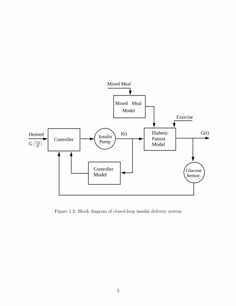
1.2 Block diagram of closed-loop insulin delivery system . . . . . . . . . . . . . . 5

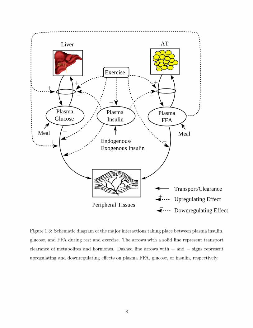
1.3 Schematic diagram of the major interactions taking place between plasma

insulin, glucose, and FFA during rest and exercise. The arrows with a solid

line represent transport clearance of metabolites and hormones. Dashed line

arrows with + and − signs represent upregulating and downregulating effects

on plasma FFA, glucose, or insulin, respectively. . . . . . . . . . . . . . . . . 8

2.1 Bergman minimal model of insulin and glucose dynamics, adapted from [1] . 32

2.2 Extended minimal model of insulin, glucose, and free fatty acid dynamics . . 34

2.3 Predicted (solid lines) and published (cross) [4] (µ ± σ) plasma FFA con-

centration in response to euglycemic hyperinsulinemic clamp. Plasma insulin

concentration was maintained at 20 µUml

[R2 = 0.77] (top), 30 µUml

[R2 = 0.94]

(middle), 100 µUml

[R2 = 0.98] (bottom) . . . . . . . . . . . . . . . . . . . . . 39

2.4 Predicted values of parameter p9 in response to increasing glucose clamps for

90 min. [R2 = 1] . . . . . . . . . . . . . . . . . . . . . . . . . . . . . . . . . . 40

2.5 Predicted and published (µ ± σ) glucose uptake rate in response to no in-

tralipid infusion - control [R2 = 0.9771] (top); low intralipid infusion rate [R2

= 0.9528] (middle); and high intralipid infusion rate [R2 = 0.9115] (bottom) . 42

xiii

2.6 Model simulation validation versus published data (µ ± σ) of plasma FFA

concentration in response to euglycemic hyperinsulinemic clamp (100 µUml

) [R2

= 0.901] . . . . . . . . . . . . . . . . . . . . . . . . . . . . . . . . . . . . . . 43

2.7 Model simulation validation versus published data (µ ± σ) of plasma insulin

[R2 = 0.974] (top) and glucose [R2 = 0.98] (bottom) concentration dynamics

in response to an intra-venous glucose tolerance test . . . . . . . . . . . . . . 44

2.8 Model simulation validation versus published data (µ ± σ) of FFA concen-

tration dynamics in response to an intra-venous glucose tolerance test [R2 =

0.8756] . . . . . . . . . . . . . . . . . . . . . . . . . . . . . . . . . . . . . . . 45

2.9 Extended model prediction versus data (cross) [4] (µ ± σ) of plasma FFA


) with

(solid line) and without (dashed line) the Y (t) sub-compartment . . . . . . . 46

2.10 Extended model prediction versus data (cross) [8] (µ ± σ) of plasma glucose

uptake rate in response to low intralipid infusion rate (0.5 mlmin

) with only Z(t)

sub-compartment (solid line), with Z(t) and Z2(t) sub-compartments (dotted

line), and without any filter sub-compartment (Z(t) or Z2(t)) (dashed line)

sub-compartment . . . . . . . . . . . . . . . . . . . . . . . . . . . . . . . . . 49

2.11 Published data [9] (cross) versus predicted values of parameter p9(G(t)) from

equation (2.7) (solid line) and equation (2.20) (dashed line) in response to

increasing glucose clamps for 90 min . . . . . . . . . . . . . . . . . . . . . . 50

2.12 Model simulation of total meal gastric emptying rate (top); glucose (G) ap-

pearance, protein (P) appearance, and G plus glucose derived from protein

(G(P)) appearance (middle); and FFA appearance (bottom), in response to

108 g mixed meal tolerance test. . . . . . . . . . . . . . . . . . . . . . . . . . 53

2.13 Insulin concentration data from normal subjects [10] (µ ± σ) and piecewise

linear approximation (top), model simulation versus published data [10] (µ

± σ) of plasma glucose concentration dynamics in response to mixed meal

tolerance test (bottom). . . . . . . . . . . . . . . . . . . . . . . . . . . . . . . 54

xiv

3.1 Dependence of time at which hepatic glycogen starts to deplete, tgly, on

exercise intensity (uEx(t)). Published data (cross) from Pruett et al. [11]

and linear fit (solid line) [R2 = 0.9908] . . . . . . . . . . . . . . . . . . . . . 61

3.2 Plasma insulin concentration in response to mild exercise (PV Omax2 = 40)

lasting from tex = 0 to 60 min. Published data (circles) (µ ± σ) from Wolfe

et al. [12], model fit (solid line), and 95% confidence interval of the model

output (dotted line). . . . . . . . . . . . . . . . . . . . . . . . . . . . . . . . 64


lasting from tex = 0 to 120 min. Model simulation validation (solid line) and

published data (cross) (µ ± σ) from Ahlborg et al. [13] . . . . . . . . . . . . 65

3.4 Model simulation (solid lines), 95% confidence intervals of model outputs

(dotted lines) and published data (circles) (µ ± σ) from Wolfe et al. [12] in

response to mild exercise (PV Omax2 = 40) lasting from tex = 0 to 60 min. Top:

hepatic glucose uptake rate (Gup), and Bottom: hepatic glucose production

rate (Gprod). Both Gup and Gprod are plotted in deviation form. . . . . . . . . 66

3.5 Plasma glucose concentration (G) in response to mild exercise (PV Omax2 = 40)

lasting from tex = 0 to 60 min. Model simulation (solid line), 95% confidence

intervals of model output (dotted lines), and published data (circles) (µ ± σ)

from Wolfe et al. [12]. . . . . . . . . . . . . . . . . . . . . . . . . . . . . . . . 67

3.6 Response to moderate exercise (PV Omax2 = 50) lasting from tex = 0 to 45 min.

Model simulation validation (solid lines) and published data (cross) (µ ± σ)

from Zinman et al. [14]. Top: glucose uptake rate (Gup); Middle: hepatic

glucose production rate (Gprod); Bottom: difference [Gprod − Gup]. Both Gup

and Gprod are shown in deviation form. . . . . . . . . . . . . . . . . . . . . . 68

3.7 Plasma glucose concentration (G) in response to moderate exercise (PV Omax2

= 50) lasting from tex = 0 to 45 min. Model simulation validation (solid line)

versus published data (cross) (µ ± σ) from Zinman et al. [14]. . . . . . . . . 69

xv

3.8 Model response to mild exercise (PV Omax2 = 30) lasting from tex = 0 to 120

min. Published data (circles) (µ ± σ) from Ahlborg et al. [13], model fit (solid

line), and 95% confidence interval of fit (dashed line). Top: model prediction

of plasma glucose (G); Middle: model prediction of hepatic glucose uptake rate

(Gup); and Bottom: model prediction of net liver glucose production. Both

Gup and [Gprod - Ggly] are shown in deviation form. . . . . . . . . . . . . . . . 70

3.9 Model response to moderate exercise (PV Omax2 = 60) lasting from tex = 0 to

210 min. Published data (cross) (µ ± σ) from Ahlborg et al. [15] and model

prediction validation (solid line). Top: model prediction of plasma glucose (G);

Middle: model prediction of hepatic glucose uptake rate (Gup); and Bottom:

model prediction of net liver glucose production. Both Gup and [Gprod - Ggly]

are shown in deviation form. . . . . . . . . . . . . . . . . . . . . . . . . . . . 71


lasting from tex = 0 to 60 min. Published data (circles) (µ ± σ) from Wolfe et

al. [12], proposed model fit [AIC = −32.194] (solid line), and reduced model

fit [AIC = −11.83] (dashed line). . . . . . . . . . . . . . . . . . . . . . . . . . 74

3.11 Proposed model simulation (solid lines), reduced model simulation (dotted

lines) and published data (circles) (µ ± σ) from Wolfe et al. [12] in response

to mild exercise (PV Omax2 = 40) lasting from tex = 0 to 60 min. Top: glucose

uptake rate (Gup), and Bottom: hepatic glucose production rate (Gprod). Both

Gup and Gprod are plotted in deviation form. . . . . . . . . . . . . . . . . . . 75

4.1 Schematic diagram of the composite model. Sections I, II, III, and IV represent

the insulin, glucose, FFA, and exercise sub-models, respectively. I: Insulin; G:

Glucose; F: FFA; uI : Exogenously infused insulin; uG, uF : Glucose or FFA

absorbed from meal or infused; uEx: Exercise intensity; PVOmax2 : Percent-

age of maximum rate of oxygen uptake; xG, xEGP , xEFP1: Remote insulin

compartments; yIU , yGU , yGP , y1FU , y1FP : 1st-order filters capturing exercise

effects. . . . . . . . . . . . . . . . . . . . . . . . . . . . . . . . . . . . . . . . 81

xvi

4.2 Plasma insulin concentration in response to mild exercise (PV Omax2 = 40%)

lasting from time tEx = 0 to 60 min. Published data (circles) (µ ± σ) from

Wolfe et al. [12] and model fit (solid line) . . . . . . . . . . . . . . . . . . . . 84

4.3 Model fit (solid line) versus published data (µ ± σ) (circle) [16] of steady

state endogenous FFA production rate, EFP , as a function of normalized

remote insulin concentration xEFP1N. Data-point (a) indicates the lowest FFA

production rate, EFPlo. . . . . . . . . . . . . . . . . . . . . . . . . . . . . . . 87

4.4 Euglycemic hyperinsulinemic clamp study, where plasma insulin concentration

was maintained at 20 µUml

(top); 30 µUml

(middle); and, 100 µUml

(bottom). Model

prediction (solid line) using only one insulin filter (xEFP1) and published data

(µ ± σ) (circle) [4] of plasma FFA concentration. . . . . . . . . . . . . . . . . 88

4.5 MI-FSIGTT study, where plasma insulin boluses were administered at t = 0

and 20 min. Model prediction (solid line) and published data (µ ± σ) (circle)

[17] of plasma insulin concentration (top); model prediction (solid line) of the

unobserved remote insulin concentration xEFP1 (middle); model prediction

using only one insulin filter (xEFP1) (solid line) and published data (µ ± σ)

(circle) [17] of plasma FFA concentration (bottom) . . . . . . . . . . . . . . . 89

4.6 Schematic diagram of the modified insulin model section (I) of the composite

model with modifications . . . . . . . . . . . . . . . . . . . . . . . . . . . . . 90

4.7 Euglycemic hyperinsulinemic clamp study, where plasma insulin concentration


(top); 30 µUml

(middle); 100 µUml

(bottom). Model pre-

diction (solid line) using two insulin filters (xEFP1 and xEFP2) and published

data (µ ± σ) (circle) [4] of plasma FFA concentration. . . . . . . . . . . . . . 91

4.8 MI-FSIGTT study, where plasma insulin boluses were administered at t = 0

and 20 min. Model prediction (solid line) and published data (µ ± σ) (circle)

[17] of plasma insulin concentration (top); model predictions of the first, xEFP1

(solid line), and second xEFP2 (dashed line) remote insulin concentrations

(middle); model prediction (solid line) using both the insulin filters (xEFP1 and

xEFP2) and published data (µ ± σ) (circle) [17] of plasma FFA concentration

(bottom) . . . . . . . . . . . . . . . . . . . . . . . . . . . . . . . . . . . . . . 92

xvii

4.9 Plasma FFA kinetics in response to mild exercise (PV Omax2 = 45%) lasting

from tex = 0 to 240 min. The exercise model is comprised of two compart-

ments, y1FU and y1FP , to capture the FFA kinetics during exercise. Model

prediction (solid line) and published data (µ ± σ) (circle) [18] of plasma FFA

uptake rate (RdF ) (top); model prediction (solid line) and published data

(µ ± σ) (circle) [18] of plasma FFA production rate (RaF ) (middle); model


concentration (bottom) . . . . . . . . . . . . . . . . . . . . . . . . . . . . . . 93

4.10 Schematic diagram of the exercise section (IV) of the composite model with

modifications . . . . . . . . . . . . . . . . . . . . . . . . . . . . . . . . . . . . 94

4.11 Plasma FFA kinetics in response to mild exercise (PV Omax2 = 45%) lasting

from tex = 0 to 240 min. The exercise model is comprised of four compart-

ments, y1FU , y2FU , y1FP and y2FP , to capture the FFA kinetics during exercise.

Model prediction (solid line) and published data (µ ± σ) (circle) [18] of plasma

FFA uptake rate (RdF ) (top); model prediction (solid line) and published data

(µ ± σ) (circle) [18] of plasma FFA production rate (RaF ) (middle); model


concentration (bottom). . . . . . . . . . . . . . . . . . . . . . . . . . . . . . . 95

4.12 Model fit (solid line) versus published data (µ ± σ) (circle) [19, 20] of en-

dogenous glucose production rate, EGP , as a function of normalized insulin

concentration xEGPN. . . . . . . . . . . . . . . . . . . . . . . . . . . . . . . 98

4.13 Model fit (solid line) versus published data (µ± σ) (circle) [8, 21] of normalized

glucose uptake rate, fFG, as a function of normalized FFA concentration FN . 99

4.14 Model prediction (solid line) versus published data (µ ± σ) (circle) [22] of

plasma insulin concentration in response to a labeled-IVGTT (top); normal-

ized insulin action with respect to their basal values on glucose uptake (solid

line) and endogenous glucose production (dashed line) due to administration

of insulin bolus at t=0 min (bottom). . . . . . . . . . . . . . . . . . . . . . . 101

xviii

4.15 Model prediction (solid line) versus published data (µ ± σ) (circle) [22] of total

glucose concentration (endogenous and exogenous labeled-glucose) in response

to a labeled-IVGTT (top); model prediction (solid line) versus published data

(µ ± σ) (circle) [22] of tracer glucose concentration in response to a labeled-

IVGTT (bottom) . . . . . . . . . . . . . . . . . . . . . . . . . . . . . . . . . 102

4.16 Model prediction (solid line) versus published data (µ ± σ) (circle) [12] in

response to mild exercise performed at PV Omax2 = 40% intensity lasting from

tEx = 0 to 60 min. Top: glucose uptake rate (in deviation form) during exercise

(RdG); Middle: glucose production rate (in deviation form) during exercise

(RaG); Bottom: plasma glucose concentration during short-term exercise (G(t)).105

4.17 Model prediction (solid line) versus published data [15] (µ ± σ) (circle) in

response to moderate exercise performed at PV Omax2 = 60% intensity lasting

from tEx = 0 to 210 min. Top: glucose uptake rate in deviation variables

during exercise (RdG); Middle: glucose production rate in deviation variables

during exercise (RaG); Bottom: plasma glucose concentration during pro-

longed exercise (G). . . . . . . . . . . . . . . . . . . . . . . . . . . . . . . . . 107

4.18 Parametric relative sensitivity analysis of the composite model for all the

sixteen states. . . . . . . . . . . . . . . . . . . . . . . . . . . . . . . . . . . . 110

4.19 Parametric relative sensitivity analysis of the composite model for the plasma

insulin, I(t) (top), FFA, F (t) (middle), and glucose, G(t) (bottom) states. . . 112


lasting from tex = 0 to 120 min. Model simulation validation (solid line) and

published data [13] (circles) (µ ± σ) of plasma insulin [R2 = 0.936]. . . . . . 113

4.21 Plasma FFA concentration in response to MI-FSIGT test where boluses of

insulin were administered at time t = 0 and 20 min. Model simulation

validation (solid line) and published data [23] (circles) (µ ± σ) of plasma

insulin concentration [R2 = 0.999] (top); model predictions of remote insulin

xEFP1 (solid line) and xEFP2 (dashed line) concentrations (middle); model

simulation validation (solid line) and published data [23] (circles) (µ ± σ) of

plasma FFA concentration [R2 = 0.998] (bottom). . . . . . . . . . . . . . . . 114

xix

4.22 Plasma FFA concentration in response to mild exercise (PV Omax2 = 30) lasting

from tex = 0 to 120 min. Model prediction of plasma FFA uptake rate,

RdF (top); model prediction (solid line) of plasma FFA production rate, RaF

(middle); model simulation validation and published data [13] (circles) (µ ±

σ) of plasma FFA concentration [R2 = 0.989] (bottom). . . . . . . . . . . . . 115

4.23 Plasma insulin concentration in response to labeled-MI-FSIGT test where

insulin boluses were administered at times t = 0 and 20 min. Model simulation

validation (solid line) and published data [24] (circles) (µ± σ) of plasma insulin

concentration [R2 = 0.997] (top); model predictions of normalized insulin

action, xNG , (solid line) and xN

EGP (dashed line) with respect to their basal

values (bottom). . . . . . . . . . . . . . . . . . . . . . . . . . . . . . . . . . . 117

4.24 Plasma glucose concentration in response to labeled-MI-FSIGT test where

a labeled-glucose bolus was infused at time t = 0 min. Model simulation

validation (solid line) and published data [24] (circles) (µ ± σ) of plasma total

glucose concentration [R2 = 0.999] (top); model simulation validation (solid

line) and published data [24] (circles) (µ ± σ) of labeled-glucose concentration

[R2 = 0.99] (bottom). . . . . . . . . . . . . . . . . . . . . . . . . . . . . . . . 118

4.25 Model simulation validation (solid line) versus published data [15] (µ ± σ)

(circles) in response to moderate exercise performed at PV Omax2 = 50% in-

tensity lasting from tEx = 0 to 45 min. Glucose uptake rate (in deviation

form) during exercise (RdG) [R2 = 0.935] (top); glucose production rate (in

deviation form) during exercise (RaG) [R2 = 0.955] (middle); plasma glucose

concentration during short-term exercise (G(t)) [R2 = 0.82] (bottom). . . . . 119

4.26 Model simulation validation (solid line) versus published data [13] (µ ± σ)

(circle) in response to mild arm exercise performed at PV Omax2 = 30% in-

tensity lasting from tEx = 0 to 120 min. Glucose uptake rate in deviation

variables during exercise (RdG) (top); glucose production rate in deviation

variables during exercise (RaG) (middle); plasma glucose concentration during

prolonged exercise (G) [R2 = 0.861] (bottom). . . . . . . . . . . . . . . . . . 120

xx

4.27 Plasma FFA concentration due to infusion of intralipids at high rate (dotted

line), low rate (dashed line), and saline (no intralipid infusion) (solid line)

(top); published data [8, 21] (µ ± σ) (circle) versus model simulation vali-

dations of plasma glucose uptake rate at high (dotted line) [R2 = 0.923] and

low (dashed line) [R2 = 0.901] intralipid infusion rates, as well as no intralipid

infusion (solid line) [R2 = 0.944] (bottom). . . . . . . . . . . . . . . . . . . . 121

5.1 Physiologically-based metabolic model for glucose, adapted from [2] . . . . . 127

5.2 Schematic representation of a physiologic compartment with no capillary wall

resistance . . . . . . . . . . . . . . . . . . . . . . . . . . . . . . . . . . . . . . 128

5.3 Schematic representation of a typical physiologic compartment with capillary

and interstitial space . . . . . . . . . . . . . . . . . . . . . . . . . . . . . . . 128

5.4 Physiologically-based FFA model block diagram. B: Brain; H: Heart and lungs;

G: Gut; L: Liver; K: Kidney; M: Muscle; AT: Adipose tissue. . . . . . . . . . 138

5.5 Model fit (line) versus published data (µ ± σ) (circle) [25, 26, 27] of FFA

uptake rate multiplier function in the heart/lungs compartment, MFHFU , as a

function of normalized heart/lungs FFA concentration, FNH . . . . . . . . . . 145

5.6 Model fit (line) versus published data (µ ± σ) (circle) [28, 29] of FFA uptake

rate multiplier function in the liver compartment, MFLFU , as a function of

normalized liver FFA concentration, FNL . . . . . . . . . . . . . . . . . . . . . 147

5.7 Model fit (line) versus published data (µ ± σ) (circle) [30, 31] of FFA uptake

rate multiplier function in the muscle compartment, MFMFU , as a function of

normalized muscle interstitial space FFA concentration, FNMI . . . . . . . . . 148

5.8 Model fit (line) versus published data (µ ± σ) (circle) [16] of normalized FFA

production rate in the AT compartment, M I∞AFP , as a function of normalized

adipocyte insulin concentration INAI . The inset includes magnified coordinates,

x-axis ∈ [0 to 45] and y-axis ∈ [0 to 2] . . . . . . . . . . . . . . . . . . . . . . 150

5.9 Model predicted (line) and published (µ ± σ) (circle) [4] plasma FFA con-

centration in response to euglycemic hyperinsulinemic clamps. Plasma insulin


(top), 30 µUml

(middle), 100 µUml

(bottom)151

xxi

5.10 Model fit (line) versus published data (µ ± σ) (circle) of glucose uptake

rate multiplier function in the muscle compartment, MFMGU , as a function of

normalized muscle interstitial space FFA concentration, FNMI , data obtained

from [8, 21] . . . . . . . . . . . . . . . . . . . . . . . . . . . . . . . . . . . . . 156

5.11 Model fit (line) versus published data (µ ± σ) (circle) of glucose uptake

rate multiplier function in the liver compartment, MFHGU , as a function of

normalized liver FFA concentration, FNL , data obtained from [8, 21] . . . . . 157

5.12 Model fit (line) versus published data (µ ± σ) (circle) of glucose production

rate multiplier function in the liver compartment, MFHGP , as a function of

normalized liver FFA concentration, FNL , data obtained from [32, 33] . . . . . 158

5.13 Surface plot of the multiplier function, M IF∞HGP , as a function of normalized

liver insulin, INL , and FFA concentration, FN

L , versus published data (cross)

(µ ± σ) of normalized hepatic glucose production rate with respect to its basal

value [19, 21, 32, 34, 35, 36] . . . . . . . . . . . . . . . . . . . . . . . . . . . 159

5.14 Model fit (line) and experimental data (µ ± σ) (circle) [17] of a MI-FSIGT

test. Glucose bolus was infused at time (t) = 0 min and insulin boluses were

infused at t = 0 min and t = 20 min to obtain predictions of insulin (top);

glucose (middle); and FFA (bottom) concentrations . . . . . . . . . . . . . . 161

5.15 Model validation (line) versus experimental data (µ± σ) (circle) [37] of a MI-

FSIGT test. Glucose bolus was infused at time (t) = 0 min and insulin boluses

were infused at t = 0 min and t = 20 min to obtain predictions of insulin (top),

glucose (middle), and FFA (bottom) concentrations. . . . . . . . . . . . . . 162

5.16 Model validation (line) versus experimental data (µ ± σ) (circle) [33] of the

effects of high FFA levels on plasma glucose concentration. Plasma glucose

concentration reached hyperglycemic levels (top) due to elevation of FFA

concentration by lipid infusion (bottom) . . . . . . . . . . . . . . . . . . . . . 163

6.1 A schematic diagram of the closed-loop model-based insulin delivery system.

Here, r(t) is the desired glucose setpoint, u(t) is the manipulated variable

(exogenous insulin), y(t) is the measured variable, and y(t) is the model

predicted output . . . . . . . . . . . . . . . . . . . . . . . . . . . . . . . . . . 166

xxii

6.2 A schematic diagram of the MPC algorithm implementation . . . . . . . . . 170

6.3 Comparison between mixed meal disturbance rejection by LMPCE−LE (solid

line) and NMPCE−E (dashed line) with input constraint. Setpoint (dotted

line) is set at 81 mgdl

. . . . . . . . . . . . . . . . . . . . . . . . . . . . . . . . 174

6.4 Comparison between mixed meal disturbance rejection by LMPCE−LE (solid

line), NMPCE−B (dashed line), and LMPCE−LB (dotted line) with input

constraint. Setpoint (dotted line) is set at 81 mgdl

. . . . . . . . . . . . . . . . 175

6.5 Comparison between mixed meal disturbance rejection by NMPCPB−C (solid

line) and LMPCPB−LC (dashed line) with input constraints. Setpoint (dotted


. . . . . . . . . . . . . . . . . . . . . . . . . . . . . . . . 177

6.6 Mixed meal disturbance rejection by NMPCPB−B with input constraints. Set-

point (dotted line) is set at 81 mgdl

. Controller model parameters were obtained

from Bergman et al. [1]. . . . . . . . . . . . . . . . . . . . . . . . . . . . . . 178

6.7 Comparison between mixed meal disturbance rejection by NMPCPB−B (solid

line) and LMPCPB−LB (dashed line) with input constraints. Setpoint (dotted


. The Bergman minimal model parameters were obtained

from Table 6.2. . . . . . . . . . . . . . . . . . . . . . . . . . . . . . . . . . . 179

6.8 Mixed meal disturbance rejection by NMPCPB−PB with input constraints.

Setpoint (dotted line) is set at 81 mgdl

. . . . . . . . . . . . . . . . . . . . . . 181

xxiii

PREFACE

The four years of graduate school in Pittsburgh has been one of the most exciting journeys

of my life. I would like to take this opportunity to show my gratitude to all my mentors,

friends, and loved ones who were always there for me at every corner of this eventful trip.

Let me start with my PhD advisor, Dr. Robert S. Parker. Bob has been an excellent

mentor throughout my tenure at University of Pittsburgh as a graduate student. His

guidance and constructive criticism has helped me to become a better researcher. The

meticulous problem-solving approach that I adhered from Bob’s laboratory is going to help

me immensely for the rest of my career. I still remember my first meeting with Bob and the

enthusiasm that he had in his voice while explaining me the challenges in curing diabetes as

a systems engineer; which he has successfully passed on to me.

I would like to show my earnest appreciation to Dr. Gilles Clermont for showing

confidence in me and allowing me to work in the inflammation project as a team member;

furthermore, for being a vital member of my doctoral committee. In addition, I would like

to extend my gratitude to professors Joseph J. McCarthy and Steven R. Little for serving

as internal members of my doctoral committee.

I am extremely grateful to all of my laboratory members (Dr. John Harrold, Dr.

Abhishek Soni, Dr. Jeff Florian, and Dr. Chad Kanick) for sharing their knowledge with

me, especially during the initial stages. I would also like to thank my Masters advisor, Dr.

Robert Beitle, from University of Arkansas for encouraging me to pursue the doctoral degree.

Of course, none of this would have been possible without the support of my family. I

consider myself extremely blessed to have my mother and father beside me throughout my

life. Whenever required, they have gone far beyond their reach to help me fulfill my dreams.

It is a pity, that for these very dreams I have not been able to spend quality time with them

xxiv

as their only child, especially now when they are growing older. Finally, I would like to take

this opportunity to mention few words regarding my lovely wife, Arpita. She is the most

amazing person that I have ever met in my entire life. Apu has provided me an enormous

mental support with her love and care ever since we got married. She always amazes me

with her grace and tolerance during the toughest of times. I feel the luckiest person in the

world to have her beside me.

xxv

1.0 INTRODUCTION

The pancreas plays a vital role in regulating blood glucose concentration in the body. Gluco-

regulatory hormones, such as insulin, secreted by the pancreatic β-cells facilitate transport

of glucose from the circulatory system into the tissues [38]. Absolute or partial deficiency in

insulin secretion by the pancreas, lack of gluco-regulatory action of insulin, or both, leads to a

metabolic disease known as diabetes mellitus (DM) [3, 38, 39]. Several pathological processes

contribute to the development of DM, such as: autoimmune destruction of the pancreatic β-

cells; deficient insulin action resulting from diminished secretion by the pancreas; diminished

tissue response to the gluco-regulatory action of insulin at one or more points of the complex

pathways of hormone action; and genetic defects that prevent regulated secretion of hormone

[38, 39].

DM is largely classified into two categories. Insulin dependent diabetes mellitus (IDDM),

also known as Type 1 diabetes mellitus (T1DM), usually results from an absolute deficiency

of insulin secretion due to auto-immune destruction of the pancreatic β-cells [38]. Patients

with T1DM require exogenous insulin replacement therapy in order to regulate their blood

glucose levels [38]. The much more prevalent form is termed non-insulin dependent diabetes

mellitus (NIDDM), commonly known as Type 2 diabetes mellitus (T2DM). The cause of

T2DM is a combination of resistance to insulin action and an inadequate compensatory

insulin secretion response [38]. Most patients with this form of diabetes are obese, and

obesity may itself cause some degree of insulin resistance [38, 39, 40]. Non-obese T2DM

individuals often reflect elevated circulating levels of free fatty acids (FFA) and triglycerides

(TG). In case of T2DM, initially and often throughout the lifetime, the patients do not

require insulin replacement treatment to survive [38].

1

DM is becoming increasingly prevalent in U.S. and around the world. According to

the American Diabetes Association (ADA), approximately 17.5 million people in the U.S.

have been diagnosed with diabetes in 2007 [3]. This estimation is substantially higher than

the 2002 estimate of 12.1 million people by the ADA [41]. About 5-10% of the diabetic

patients have T1DM [38]. The total (direct plus indirect) estimated cost of diabetes has also

significantly risen from $132 billion in 2002 [41] to $174 billion in 2007 [3].

DM is usually associated with wide blood glucose (G(t)) fluctuations, resulting in hyper-

glycemia (G(t) > 120 mgdL

) or hypoglycemia (G(t) < 70 mgdL

) [42, 43]. Long-term effects of DM

are mainly caused by prolonged hyperglycemia, which may lead to complications such as loss

of vision, peripheral neuropathy with a risk of foot ulcer or even amputation, cardio-vascular

disease, nephropathy and sexual dysfunction [38, 42, 43]. Immediate disease consequences

are primarily caused by hypoglycemia, which may lead to dizziness, unconsciousness, or even

death [42, 43].

Over the years, researchers have shown that an intensive insulin therapy for diabetic

patients can delay the onset of serious complications [44, 45]. According to the findings

of the Diabetes Control and Complications Trial (DCCT) research group, intensive insulin

treatment reduced the risk of retinopathy, nephropathy and neuropathy by 35% to 90% when

compared with conventional treatment [44]. Intensive treatment was most effective when

begun early, before complications were detectable. As shown in Figure 1.1, the most common

insulin intensive treatment for T1DM involves self-monitoring of blood glucose (SMBG) by

finger-pricking at least 3-4 times a day followed by subcutaneous insulin injection in order

to achieve required glycemic goals (see Table 1.1) as recommended by the ADA [3].

Even with such intensive insulin therapy, wide glucose fluctuations persist mainly due to

daily activities such as meal intake and exercise. In an experiment performed by Raskin et

al. [46], the long-term effects of fast-acting insulin aspart (IAsp) and regular human insulin

(HI) on glycemic control were studied on T1DM patients. Blood glucose was measured at

8 time points and insulin was injected before breakfast, before lunch, before dinner, and at

bedtime. Their results revealed significant hyperglycemic events at post-prandial periods for

both the insulin regimens, with HI being worse. The ultimate goal in diabetes treatment

is the development of an automatic closed-loop insulin delivery system that can mimic the

2

Figure 1.1: Schematic diagram of intensive insulin therapy: (A) blood glucose is measured by

using a self-monitoring blood glucose device by finger-pricking before meal intake/bed-time;

(B) estimated insulin dosage is injected subcutaneously via a syringe to achieve required

glycemic goals. This procedure is repeated 3-4 times a day [3, 7]

Table 1.1: Summary of glycemic recommendations for adults with diabetes (adapted from

[3])

Description ValueGlycosylated hemoglobin (A1C) <7.0%

Preprandial capillary plasma glucose 70-130 mgdL

Peak post-prandial (1-2 hr after the beginning <180 mgdL

of meal) capillary plasma glucose

A1C is the primary target for glycemic control

More stringent glycemic goals (i.e., A1C <6.0%)may further reduce complications at the cost ofincreased risk of hypoglycemia

3

activity of a normal pancreas and is capable of maintaining physiological blood glucose levels

for T1DM patients. Such an artificial pancreas system can theoretically produce tight glucose

control without finger-stick blood glucose measurements, subcutaneous insulin injections, or

hypo-/hyper-glycemic events [47], thereby dramatically improving the quality of life for an

insulin-dependent diabetic patient. A device of this type would primarily contain three

components: (i) an insulin pump, (ii) a continuous glucose sensor, and (iii) a mathematical

algorithm to regulate the pump in order to maintain normoglycemia in presence of sensor

measurements [48, 49], as shown in Figure 1.2. In the case of a model-based closed-loop

insulin delivery system, the controller calculates the required insulin dosage for maintenance

of normoglycemia based on the blood glucose predictions obtained from a mathematical

model. Hence, model quality plays a vital role as theoretically available controller perfor-

mance is limited by model accuracy [50]. In addition, superior quality mathematical models

of DM provide numerous significant open-loop advantages. For example, a comprehensive

mathematical model facilitates a better understanding of the complex relationship between

insulin and the major energy-providing metabolic substrates [51]. High fidelity metabolic

models can predict the time-course and effect of insulin on plasma glucose in presence of

various external disturbances such as meal consumption, exercise, etc. Finally, an accurate

T1DM patient-specific metabolic model might be used to adjust daily insulin therapy dosage

for the same individual [51].

Over the years, numerous metabolic models have been published in the literature with

a primary goal of capturing the dynamics of the insulin-glucose system. Such glucocentric

(glucose-based) models largely ignore FFA metabolism and its interaction with glucose and

insulin. FFA is a major metabolic source of energy for the human body. Almost 70-80

% of muscle energy is derived from FFA oxidation during rest [52, 53]. This is because

the energy yeild from 1 g of FFA is approximately 9 kcal, compared to 4 kcalg

for proteins

and carbohydrate (CHO) [54]. Moreover, significant interactions exist between glucose and

FFA metabolism. To further complicate matters, the FFA, glucose, and insulin dynamics

are significantly altered during exercise. In the development of a diabetes mellitus patient

model, it is important to consider all the major energy-providing substrates (glucose and

FFA) and their persisting metabolic interactions during rest and exercise. Such a complete

4

ControllerInsulinDesired

G

GlucoseSensor

Exercise

Meal

Model

Mixed

Mixed Meal

Diabetic PatientModel

ControllerModel

G(t)

Pump

I(t)

(mgdl )

Figure 1.2: Block diagram of closed-loop insulin delivery system

5

metabolic model can provide more accurate glucose predictions under realistic conditions,

such as disturbances provided from mixed meal (containing CHO, protein, and fat) ingestion

and exercise. Finally, metabolic models describing the dynamics of insulin, glucose, and FFA

during rest and exercise can provide the control community an excellent platform for the

development of model-based controllers for maintenance of normoglycemia by rejecting the

various external disturbances.

In the following Section (1.1), a brief overview of the major metabolic interactions taking

place between the major energy-providing substrates and insulin at rest and during exercise

is presented. Sections 1.2 and 1.3 are dedicated for a concise review of the glucose-insulin

models and the closed-loop insulin delivery systems currently present in the literature,

respectively. Finally, a brief overview of the rest of the dissertation Chapters is presented in

Section 1.4.

1.1 A BRIEF OVERVIEW OF THE INSULIN-GLUCOSE-FFA SYSTEM

Glucose from the circulatory system is consumed by the hepatic tissues mostly for storage

in the form of glycogen and by the extra-hepatic tissues for oxidation purpose [55]. To

maintain plasma glucose homeostasis, stored glucose from the liver is released back into

the circulation via a process known as glycogenolysis [56]. Plasma insulin secreted by the

pancreas, or exogenously infused in the case of T1DM patients, facilitates the uptake of

glucose in the tissues [55]. Plasma insulin also inhibits hepatic glucose production [57]. FFA

from the circulatory system is consumed by the adipose tissue (AT) mostly for storage in

the form of triglycerides and by the peripheral tissues (except brain) for oxidation purpose

[54]. Whenever the body requires energy, stored FFA is released back into the circulatory

system via a process known as lipolysis [54]. Insulin acts as a strong anti-lipolytic agent,

in other words, it suppresses the lipolytic process [54]. In the early 1960s, Randle et al.

[58, 59] proposed that glucose and FFA compete for oxidation in the muscle tissues. This

phenomenon, popularly known as the glucose-FFA cycle, was later demonstrated in studies

performed by several researchers [8, 21], where it has been shown that an increase in plasma

6

FFA concentration inhibits muscular glucose uptake rate. Several studies have also reported

that an increase in FFA inhibits insulin-mediated suppression of glycogenolysis [32, 19]. In a

recent publication, Ghanassia et al. [60] has mentioned that FFA and insulin act in synergy

and provide a fine-tuning for regulation of endogenous glucose production rate. Exercise

also plays a major role in influencing the dynamics of plasma glucose, FFA, and insulin.

An elevated exercise level up-regulates plasma glucose and FFA uptake rates [13, 61]. At

the same time, plasma insulin level decreases due to elevated insulin-mediated clearance

rate [62]. To maintain glucose homeostasis, hepatic glucose production also increases during

exercise [63]. Lactate production by working muscles is also increased during exercise [13].

Excess lactate in the plasma is absorbed by the liver for conversion to glucose (known as

gluconeogenesis [64]) in order to support the elevated glucose production rate. The schematic

diagram in Figure 1.3 captures all the major metabolic interactions between the insulin-

glucose-FFA system at rest and during exercise.

1.2 PREVIOUS LITERATURE ON MATHEMATICAL MODELS OF

METABOLISM

Metabolic models currently present in the literature can be classified into three groups (i)

strictly empirical, (ii) semi-empirical, and (iii) physiologically-based. The sole purpose of

a strictly empirical model is to capture the input-output data (insulin-glucose dynamics)

without consideration of any physiology [23, 65, 66, 67]. Hence such models are also called

black-box models. Since only the input-output data is used to develop the models, the

identification of the structure and parameters could be much simpler. Hence, time required

to synthesize these models can be short. As empirical model structures could be selected to

facilitate controller design, a vast number of model-based controllers employ dynamical em-

pirical models [68]. However, these models have several significant drawbacks. Since strictly

empirical models do not consider any biology, separation of specific physiological effects of

metabolic substrates taking place in the various tissues/organs is impossible. Also input-

output models provide no insight regarding the mechanisms underlying the observed system

7

Exercise

Liver AT

Plasma PlasmaFFAGlucose

Peripheral Tissues

MealEndogenous/Exogenous Insulin

Meal

InsulinPlasma

Transport/Clearance

Upregulating Effect

Downregulating Effect

+

++ +

−

− −

−

−

−

+

−

Figure 1.3: Schematic diagram of the major interactions taking place between plasma insulin,

glucose, and FFA during rest and exercise. The arrows with a solid line represent transport

clearance of metabolites and hormones. Dashed line arrows with + and − signs represent

upregulating and downregulating effects on plasma FFA, glucose, or insulin, respectively.

8

dynamics. Moreover, biological processes responsible for glucose dynamics are nonlinear and

vary under many conditions; hence, simple linear input-output models are inadequate to

provide credible predictions for extended future horizons under realistic disturbances, such

as a meal [23].

The semi-empirical models consist of a minimum number of equations capturing the

insulin glucose dynamics with a primary focus on emulating the data by considering only

the necessary physiology [1, 69, 70, 71, 72, 73, 74, 75]. Unlike the strictly empirical models,

minimal models include several macroscopic metabolic parameters, like peripheral tissue

sensitivity to insulin and overall glucose effectiveness of extra-hepatic tissues [5]. However,

these models do not differentiate the distribution of metabolic substrates at various or-

gan/tissue levels, as that will add further model complexity. Hence, the goal in such models

is to capture the major physiological interactions in order to reproduce the data without

sacrificing the structural simplicity. Due to this very nature, semi-empirical models can be

an ideal candidate for the synthesis of model-based controllers capable of maintaining glucose

homeostasis by rejecting disturbances from mixed meal consumption and exercise.

Finally, the physiologically-based models are more detailed and complex in terms of

number of parameters and equations providing an in depth description of the physiology

behind the various metabolic interactions taking place in the body [2, 76, 77, 78]. In

such models, the distribution of metabolic substrates is captured at the organ/tissue and

intracellular levels. Physiologically-based models can be extremely useful, as they can

promote insight, as well as motivation for experiments that could be performed to validate

various model components. In terms of drawbacks, these models are usually time-intensive

to develop. They typically have large number of nonlinear equations with many parameters

that need to be estimated. Even though complexity is an issue, a valid physiologically-based

model can not only describe the dynamics of measurable quantities, but also correctly predict

all the unmeasurable variables relevant to the system.

9

1.2.1 Empirical Models

Strictly empirical models are developed based on the input-output data without considering

the fundamental properties (physiology) of the system. Typically, the model structure is

chosen to facilitate parameter estimation or design of model-based controller. Mitsis and

Marmarelis [79] developed a non-parametric model of the glucose-insulin system by selecting

the Volterra-Wiener approach. The first and second order kernels of the Volterra model

were estimated from input-output data generated from a parametric model [1] by employing

the Laguerre-Volterra Network (LVN) methodology. The simulation results revealed that

synthesis of accurate nonlinear input-output models from insulin-glucose data generated

from parametric models was feasible. The authors also demonstrated the robustness of the

Volterra models under presence of additive output noise. Furthermore, such kind of models

are accommodating to adaptive and patient-specific estimation, which could be necessary

for a model-based blood glucose control algorithm.

A linear input-output model for glucose prediction based on recent blood glucose mea-

surement history was proposed by Bremer and Gough [23]. Autocorrelation function (ACF)

estimates at fixed time intervals were used to identify the model structure. An ACF estimate

provides a statistical measure of the dependence between individual measurements of a

process at different time points. Published data analyzed in their work indicated that

blood glucose dynamics are not random, and that blood glucose values can be predicted

from frequently sampled previous values, at least for the near future. However the model

prediction of blood glucose for extended horizon (in excess of 30 min) was not acceptable.

Parker et al. [65] developed a linear input-output step-response model of insulin delivery

rate (input) effects on glucose concentration (output) by filtering the impulse response

coefficients via projection onto the Laguerre basis. The identified linear input-output model

does not include all the gain information of the diabetic patient, but it does succeed in

capturing the dynamic behavior. Inability to capture the steady state characteristics did not

affect the closed-loop performance of the model. In a separate study, Florian and Parker [80]

synthesized empirical Volterra series models of glucose and insulin behavior by considering

input-output data generated from a physiologically-based metabolic model [2]. In absence

10

of noise, the identified Volterra models accurately predicted the data. However, addition

of Gaussian distributed measurement noise significantly degraded the coefficient estimates.

Significant noise filtering was achieved by projecting the Volterra models onto the Laguerre

basis functions. Closed-loop performance of the nonlinear empirical model with measurement

noise in rejecting 50 g oral glucose challenge was mediocre. Best closed-loop performance

was achieved by a linear MPC with ability to filter noise effects by proper tuning.

Van Herpe et al. [66] developed a control-relevant black-box model for prediction of the

glycemic levels of critically-ill patients in the intensive care unit (ICU) by using real clinical

ICU input-output (insulin-glucose) data. An autoregressive exogenous input (ARX) model

structure was used for predicting blood glucose concentration by considering the following

input variables: insulin infusion rate, body temperature, total CHO calorie intake, total fat

calorie intake, glucocorticoids level, adrenalin level, dopamine level, dobutamine level, and

beta-blockers level. The estimated model coefficients showed clinical relevance with respect

to the behavior of glycemia in relation to insulin, insulin resistance, intake of CHO calories,

etc. However, the authors pointed out that further data is required to make the model more

patient specific especially to capture the diurnal variation of insulin resistance for critically-ill

patients.

In another study, several types of empirical models, like Auto-regressive with exogenous

input (ARX) and Box-Jenkins (BJ), were developed by Finan et al. to evaluate the ‘infinite-

step ahead’ glucose predictions [67]. The input-output models were identified from simulating

a semi-empirical model developed by Hovorka et al. [75]. The higher- and lower-order ARX

and BJ models described normal operating conditions with high accuracy. However, model

accuracy during abnormal situations (e.g., change in insulin sensitivity, underestimates in

CHO content of meals, mismatch between actual and patient-reported timing of meals) were

inaccurate, especially for the lower-order models.

A nonlinear neural network (NN) model of blood glucose concentration identified from

subcutaneous glucose sensor and subcutaneous insulin infusion data was developed by Tra-

jonski et al. [81]. The system identification framework combines a nonlinear autoregressive

with exogenous input (NARX) model representation, regularization approach for construct-

ing radial basis function NNs, and validation methods for nonlinear systems. Numerical

11

studies on system identification and closed loop control of glucose were carried out by using

a comprehensive glucose model and pharmacokinetic model of insulin absorption from a

subcutaneous depot. Closed-loop simulation results showed that stable control is achievable

in the presence of large noise levels. However, one major drawback of the closed-loop system

is that, due to the subcutaneous route of insulin administration, rapid control actions were

not stable which are typically necessary after a standard OGTT.

Bellazzi et al. [82] proposed a fuzzy model for predicting blood glucose levels in T1DM

patients. The underlying idea in their approach consists of the integration of qualitative

modeling techniques with fuzzy logic systems. The resulting hybrid system uses a priori

structural knowledge on the system to initialize a fuzzy inference procedure, which estimates

a functional approximation of the system dynamics by using the experimental data in order

to predict the patient’s future blood glucose concentration. The results obtained showed that

the presented framework generates fuzzy systems that may be used reliably and efficiently

to predict blood glucose concentration for T1DM patients. A potential drawback is that, as

the initialization of the fuzzy system requires a priori knowledge of the qualitative model,

any erroneous approximation of unknown functions could lead to significant degradation of

the fuzzy model performance.

Bleckert et al. [83] developed a model of glucose-insulin metabolism by identifying the

system with stochastic linear differential equations using a mixed graphical models technique.

The model was identified in terms of biological parameters and noise parameters. Density

estimates of the unkown parameters were obtained from the input-output data by using

the exact inference algorithm [83]. The parameter estimates were given as a posteriori

distributions, which can be interpreted as fuzzy probability distributions. These density

estimates convey much more information about the unknown parameters than a point

estimate.

1.2.2 Semi-Empirical Models

The semi-empirical metabolic models consist of minimum number of equations capturing

only the necessary physiology in order to better understand the mechanisms of the glucose-

12

insulin regulatory system. One of the pioneers in this field is Bolie. In 1961, he proposed

a 2-dimensional (2-D) metabolic model consisting of ordinary differential equations (ODE)

[69]. The two ODEs, one capturing glucose and the other capturing insulin concentration,

consisted of 5 parameters. Parameter values were estimated from published data; predomi-

nantly average values obtained from human, as well as animal, experiments. Ackerman et al.

[70] developed a similar 2-D glucose-insulin model which was published in 1965. The model

considered the important fact that changes in insulin and glucose concentration depend on

the concentration of both the components. Serge et al., in the early 1970’s, synthesized

a metabolic model consisting of linear ODEs to capture blood glucose kinetics of normal

T1DM and obese patients [84]. Although all these early models were easily identified from

available data, they oversimplified the actual physiological effects between glucose-insulin.

A huge impact in the field of modeling glucose-insulin dynamics was initiated by the

introduction of the “minimal” model developed by Bergman and colleagues in the late 1970’s

and early 1980’s [1, 85]. There are approximately 500 studies published in the literature,

that involve the Bergman minimal model [86]. The model consists of three ODEs that

capture plasma glucose dynamics, plasma insulin dynamics, and insulin concentration in

an unaccessible remote compartment (which can be conceptualized as interstitial insulin).

Structurally, the model consisted of a minimum number of lumped compartments and

parameters to accurately capture the various physiological phenomena, such as glucose

effectiveness and insulin sensitivity, during an intra-venous glucose tolerance test (IVGTT)

[1]. The addition of the remote insulin compartment and a bilinear term in the glucose

state increased the accuracy of the model without sacrificing any simplicity. However,

several shortcomings of the minimal model have been raised in the literature [87, 88].

Quon et al. reported that the Bergman minimal model tends to overestimate the effect

of glucose on glucose uptake and underestimate the contribution of incremental insulin [87].

Researchers have also raised questions that the minimal model might be too minimal [73].

Despite its shortcomings, the Bergman minimal model [1] has gained enormous popularity

in the diabetes research community, mainly because of its structural simplicity and easily

identifiable parameters [86, 89]. Because of this very nature, the minimal model was selected

in this work to provide a platform for the development of a lipid-based extended minimal

13

model and an exercise minimal model which are detailed in Chapter 2 and 3, respectively.

Cobelli and colleagues have developed numerous metabolic models capturing the various

physiological interactions between glucose and insulin [5, 71, 72, 74, 90, 91]. The Bergman

minimal model [1] does not allow the separation of glucose production from utilization. To

overcome this limitation, Cobelli et al. proposed a revised minimal model which was fitted

to cold and hot (radio-labeled) IVGTT data [5], as the hot data reflects glucose utilization

only. In another publication by Cobelli et al. [74], the over-estimation of glucose effectiveness

(SG) and under-estimation of insulin sensitivity (SI) of the Bergman minimal model due to

under-modeling was addressed by adding a second non-accessible glucose compartment for

a better description of the glucose kinetics. The two-compartment glucose model improved

the accuracy of SG and SI estimates from a standard IVGTT in humans. In a series of

publications Cobelli and co-authors [71, 72, 90] developed an extensive model of glucose and

two hormones, insulin and glucagon. Glucagon is a counter-regulatory hormone secreted by

the α-cells of the pancreas. Its role is to enhance the release of glucose from the liver into the

plasma by speeding the breakdown of hepatic glycogen. The glucose sub-system explicitly

considered the net hepatic glucose balance (NHGB), renal excretion of glucose, and insulin-

dependent and insulin-independent glucose utilization by peripheral tissues, red blood cells

and the central nervous system. The insulin sub-system is divided into five compartments,

whereas the glucagon subsystem consisted of a single compartment. The nonlinear equations

employed saturating functions (hyperbolic tangents) to capture the saturation behavior

observed in biological systems (e.g., hepatic glucose production). Incorporation of all these

physiological interactions provided further insight into glucose-insulin metabolism.

Berger and Rodbard [92] developed a computer program for the simulation of plasma

insulin and glucose dynamics after subcutaneous injection of insulin. A pharmacokinetic

model was used to calculate the time courses of plasma insulin for various combinations of

popular preparations. The program can predict the time course of plasma glucose in response

to a change in CHO intake and/or insulin dose, with the use of a pharmacodynamic model

describing the dependence of glucose dynamics on plasma insulin and glucose levels. A set

of parameters for the model were estimated from the literature. The model can be used to

theoretically explore the impact of various factors associated with glycemic control in T1DM.

14

Results of the glucose dynamics generated by the simulator were not exact, particularly after

perturbations from larger CHO intake sizes. One potential drawback is that, due to the

absence of FFA effects, the simulator may be incapable of predicting plasma glucose level

accurately in the presence of disturbances from mixed meals containing CHO and fat.

In a much more recent work, Hovorka et al. [75] extended the 2-compartment minimal

model developed by Cobelli et al. [74] by separating the effect of insulin on glucose distrib-

ution/transport, glucose disposal, and endogenous glucose production during an IVGTT by

employing a dual-tracer dilution methodology. The model consisted of a two-compartment

glucose sub-system, a single compartment for plasma insulin, and three remote insulin

compartments capturing the different physiological effects of insulin on glucose. By using

the dual-tracer technique along with the model, the authors demonstrated a novel approach

of separating the three actions of insulin on glucose kinetics successfully. The results

showed that the insulin-mediated suppression of endogenous glucose production accounts for

approximately one-half of the overall insulin action on glucose after an IVGTT. However, the

absence of any saturating functions, particularly for the mathematical expression capturing

the endogenous glucose production rate, could generate erroneous predictions for experiments

with higher insulin boluses.

Salzsieder et al. developed a biologically relevant model describing the in vivo glucose-

insulin relationship of T1DM patients [93]. Four linear state variables were used to model

the system. The physiologically relevant states represented the circulating concentration

of insulin and glucose, net endogenous glucose balance, and peripheral insulin-dependent

glucose uptake. The model was calibrated and validated using published data of dogs [94,

93, 95]. Slow dynamics, as well as steady state glucose behavior, were accurately captured by

the model. However, this accuracy was absent during faster insulin dynamics. The original

model was verified within the limit of linearity, which was the upper normoglycemic level.

This might prove to be disadvantageous, as during the post-prandial period the blood glucose

level often hovers in the hyperglycemic level, especially for T1DM patients.

In another glucose-insulin modeling effort, Boroujerdi et al. [96] developed a glucose

kinetics model which represented glucose utilization as two processes: insulin dependent and

insulin independent. The overall glucose disposal comprised of glucose transport and utiliza-

15

tion and the effect of insulin on these processes. The model consisted of five compartments

representing, plasma glucose, insulin sensitive and insulin-insensitive glucose interstitial

space, and a glucose-transporter limited metabolism compartment for each of the interstitial

spaces. An important finding of their model was that saturation of the glucose-transporter

mechanism in diabetic patients leads to hyperglycemia. Inclusion of such physiological

phenomenon would definitely make the model more accurate. However, the model lacked in

specifying tissue-specific saturating phenomena and its characterization of insulin effects on

endogenous glucose production.

A semi-empirical model of glucose-insulin interaction was developed by Lehman and

Deutsch for T1DM patient evaluation [97]. The purpose of the model was to simulate

glycemic and plasma insulin responses to a given insulin therapy and dietary regimen for 24

hr. The model contains a single glucose pool into which glucose enters via both intestinal

absorption and hepatic glucose production. Glucose is removed from this space by insulin-

independent glucose utilization in red blood cells, insulin-dependent glucose utilization in

liver and periphery, and renal glucose excretion. Since the introduction of this model in the

World Wide Web (www.2aida.org) for noncommercial use, a significant number of copies

of this model have been downloaded to assist T1DM treatment [98]. Although, the main

purpose of the model is to provide valuable knowledge to T1DM patients regarding their

glucose dynamics after meal consumption, absence of FFA absorption from a mixed meal

intake might limit the accuracy of the model prediction. Also, the model was incapable of

predicting the glucose dynamics accurately during a continuous steady state insulin infusion

(to maintain basal level) experiment, as shown by Steil et al. [51]. Utilization of two glucose

compartments might have improved the accuracy of the model.

Tolic et al. [99] developed a model to evaluate insulin-glucose feedback regulation under

pulsatile supply of insulin. The feedback loops present in the model consist of glucose-

stimulated pancreatic insulin secretion, insulin-stimulated glucose uptake, insulin-stimulated

inhibition of hepatic glucose production, and glucose-stimulated enhancement of its own

uptake. Delays are also incorporated in the model to represent the physiologic delay of

insulin action on hepatic glucose production. The results obtained from the model have

shown that when hepatic glucose release rate is operating at its upper limit, an oscillatory

16

insulin infusion will be more effective in lowering blood glucose level than constant infusion.

As the authors pointed out, more work is required to refine the model. For example, the

time delay between plasma insulin and hepatic glucose production needs to be replaced by

more physiologically relevant states. Also, the pulsatile effect of insulin on down-regulation

of the insulin receptors should be incorporated in the model.

Originally, the “minimal” model was developed to capture the glucose kinetics of a single

individual [1] and was never used to estimate the metabolic portrait for a whole population.

A population-based approach can be useful in the study of diabetes for classification of

patients being in risk groups or not. Furthermore, information from population estimates

can provide prior information for statistical analysis of a single individual. Vicini and Cobelli

[100] were the first to propose a Bayesian approach to the population-based minimal model.

They used IVGTT data from sixteen healthy individuals to obtain distributions of glucose

effectiveness and insulin sensitivity in the population. The mean and standard deviation

obtained from the distributions were used as a prior information for individual analysis.

Their method produced precise glucose effectiveness and insulin sensitivity estimates, even

with a small sampling size. However, the method was employed on only the glucose part

of the model. Recently, Andersen and Hojbjerre [101], proposed a similar version of the

stochastic minimal model, where they combined both the glucose and insulin parts of the

model. The population-based minimal model accounted for error terms associated with the

measurement and the process. The Markov chain Monte Carlo technique was successfully

implemented in estimation of the parameters by using the Bayesian approach. The method

was demonstrated on experimental IVGTT data performed on 19 normal glucose-tolerant

subjects.

Engelborghs and co-authors [102] developed a semi-empirical model with two delayed

differential equations (DDE) for the plasma glucose and insulin concentration in a diabetic

patient connected to an exogenous insulin delivery system. The model has two delays: the

intrinsic delay involved with the external device, and the physiological delay associated with

the action of insulin on glucose. Bifurcation analysis of steady state solutions and periodic

solutions revealed two categories of diabetic patients for which the insulin delivery system

had different efficiencies.

17

For better understanding of the insulin absorption kinetics produced by continuous

subcutaneous infusion of insulin, Kraegen and Chisholm [103] used a kinetic model to

quantitate the dynamics. The authors used a two-pool system to reasonably capture the

systemic insulin delivery profile following a subcutaneous infusion. The model revealed that

subcutaneous insulin degradation is low regardless of the input profile. Such kinetic models

of subcutaneous insulin absorption should be useful to predict the impact of programming

strategies for continuous subcutaneous insulin infusion therapy. Later, Puckett and Lightfoot

[104] developed a three-compartment model representing the link between dosage and blood

insulin levels. A comparison study revealed that the 3-D model fitted the data of individual

patients better than the 2-D model from [103]. They also performed parameter identification

and sensitivity analysis which highlighted insulin kinetic features that may significantly

influence glucose dynamics. Their results showed significant inter-, as well as intra-patient

variability of insulin absorption kinetics.

A semi-empirical model capable of capturing the absorption kinetics of subcutaneously

injected insulin was developed by Wach et al. [105]. The model consisting of partial

differential equations (PDE), described the diffusion of soluble insulin, equilibration between

monomeric and dimeric insulin, and absorption of monomeric insulin molecules. The authors

solved the PDEs numerically by dividing the subcutaneous region into spherical shells for

space distribution. Parameters of the model were estimated by fitting published glucose-

clamp data. The model predictions of dose- and concentration-dependent insulin abosrption

within the therapeutic range were in good accordance with the experimental data. According

to the authors, the model could be used in a clinical setup to describe the subcutaneous

insulin absorption kinetics of individual patients.

1.2.3 Physiological Models

In the mid-70s, Tiran and co-authors [76, 106] were among the first to attempt to develop

physiologically-based “circulation model” of the glucose-insulin system. Several compart-

ments were used to represent major organs and tissues in the human body. Each com-

partments were divided into two regions representing the capillary and interstitial space.

18

Glucose and insulin were distributed in these compartments via the blood circulation path-

ways. Nonlinear effects of glucose metabolism were also incorporated in the model. The

model performed reasonably well in predicting venous glucose concentration in response to

perturbations from glucose boluses of small sizes (<30 g). However, the model over-predicted

glucose concentration for bolus sizes in excess of 30 g. The model also lacked in capturing the

threshold metabolic behaviors of the physiological system. As the authors pointed out, the

whole body model has the potential to serve as a basis for examining hypothesis regarding

the glucose-insulin system.

A physiologically-based model of metabolism was developed by Sorensen, in his Ph.D.

dissertation [2], based on an earlier model by Guyton et al. [107]. The model is comprised

of 19 differential equations: 11 are used to define the glucose system, 7 define the insulin

system, and one models glucagon. The glucose model consists of compartments representing

the vital glucose-utilizing body organs and tissues: brain, heart/lungs, gut, liver, kidney, and

periphery. In the model, ‘periphery’ represents skeletal muscle as well as adipose tissues (AT).

Blood pumped from the heart enters into each compartment through the arterial circulation

and exits to the venous circulation. Mass balances were performed across each tissue or

organ in order to capture the plasma glucose distribution. Some of the compartments (such as

‘brain’ and ‘periphery’) were divided into sub-compartments (capillary and interstitial space)

to incorporate resistance to glucose transport. Metabolic sinks representing glucose uptake

were added to all the compartments. As the liver consumes, as well as produces glucose,

both metabolic sink and source were incorporated in the ‘liver’ compartment. Most of the

metabolic sinks/sources were functions of glucose, insulin, or glucagon concentration. The

model accepted exogenous glucose input in the form of meal consumption. The insulin model

has a similar structure to the glucose model [2]. The only difference, is that the ‘brain’ in the

insulin model had a single compartment, because insulin does not cross the brain capillary

barrier. Metabolic sinks representing insulin clearance were added to the ‘liver’, ‘kidney’,

and ‘periphery’ compartments. The model does an excellent job in capturing the glucose and

insulin distributions in all the major organs and tissues. Validation studies revealed that the

model accurately predicted plasma glucose concentrations after intravenous and oral glucose

tolerance tests. Because of its high accuracy and structural integrity, the Sorensen model

19

[2] was selected to provide a platform for the development of a physiologically-based FFA

model to capture the fatty acid distribution at organ/tissue levels, as described in Chapter

5.

A semi-physiologic nonlinear model of glucose and insulin was developed by Cobelli

et al. [78]. The model consisted of mathematical functions capturing peripheral glucose

consumption, renal glucose excretion, hepatic glucose production and utilization, glucose

absorption from a meal, insulin secretion, and insulin degradation. Delay terms were also

included in the model to incorporate the physiologic delay involved in the gluco-regulatory

action of insulin on glucose. Simulation studies revealed that the model successfully described

physiological events occurring in a normal human after the ingestion of standard meals on a

24 hour horizon. However, the model does not account for glucose distribution at the major

glucose-consuming organ levels.

1.2.4 Metabolic Models Considering FFA and Exercise Effects

All the metabolic models so far discussed spanning five decades exclusively focus on the

interactions between glucose and insulin. Effects of FFA and exercise on plasma glucose

dynamics have been largely neglected. For the synthesis of high quality and robust closed-

loop model-based controllers for maintenance of glucose homeostasis, it is essential to develop

models that take into account the external disturbances encountered by a T1DM patient in

his/her daily life, like mixed meal ingestion and exercise. There are only few metabolic

models present in the literature that consider FFA and exercise effects on glucose dynamics.

A physiologically-based model of insulin, glucose, and fatty acids has been proposed by

Srinivasan et al. [77]. The model is made of interconnected sub-systems, each representing

one or more physiological processes. Known physiology was incorporated with an intention to

reproduce the effects of FFA and glucose metabolism for a short-term period (< 2 hr). This

complex model was the first of its kind to include FFA dynamics in the glucose-insulin system.

The model, qualitatively, did a reasonable job in predicting glucose and FFA dynamics

after an IVGTT. One potential drawback is that the model ignored the effects of blood

circulation on metabolism. Also, as pointed out by the authors, the model lacked the ability

20

to adequately reproduce the finer details of plasma glucose, FFA, and insulin changes caused

due to introduction of disturbances in the metabolic system. According to the authors,

further refinement of the mathematical functions and inclusion of more hormonal controls

might yield better results. From a control point of view, a major drawback of the model is

its inability to predict plasma glucose and FFA dynamics at longer time periods (in excess

of 2 hr).

Recently, Kim et al. [108] developed a physiologically-based model of metabolism to

capture the whole-body fuel homeostasis during exercise. The model was divided into seven

physiologic compartments representing the brain, heart, liver, GI (gastrointestinal) tract,

muscle, AT, and other tissues. Dynamic mass balance equations along with cellular metabolic

reactions were considered in each of the compartments. Hormonal control by insulin and

glucagon over the cellular metabolic processes were incorporated in the model to predict

the changes in fuel homeostasis during exercise. Model simulations were validated with

experimental data where normal subjects performed moderate intensity exercise for 60 min.

The model successfully captured the exercise-induced changes in hormonal signals at various

tissues in order to regulate metabolic fluxes for maintenance of glucose homeostasis. The

model also successfully captured the dynamics of variables like, hepatic glycogenolysis and

gluconeogenesis, which are hard to measure. In addition, the model can also indicate the

relative contributions to fuel oxidation of glucose and FFA in the muscle during exercise. This

novel mechanistic model that links cellular metabolism to whole-body fuel homeostasis can

be used for testing hypotheses of hormonal control and dynamical predictions of metabolite

concentrations in various tissues during exercise. However, due to the scale and complexity

in terms of number of equations and parameters, the model has limited applicability in a

clinical setup to be calibrated to individual patients. Also, the model fails to capture the

experimental data of arterial lactate concentration.

From a control prospective, the complexity of both the above mentioned models [77, 108]

can prove to be a liability for the synthesis of a model-based control system for T1DM

patients. Due to the sheer scale of the model, it is hard to design experimental protocols

to identify parameters for individual patients. Hence, parametric identifiability can be a

major issue. One potential method for overcoming the parameter estimation problem is a

21

priori identifiability, which is discussed as a potential direction of future work in Section

7.2.2. A further complication of the detailed models is the difficulty in using them in an

adaptive control environment, as no identifiable parameter or combination of parameters are

necessarily available to be updated online. As the long-term goal of the present work is to

develop models that can be used for the synthesis of a model-based controller, development

of accurate lower-order structurally simple metabolic models capturing the insulin, glucose,

and FFA dynamics during rest and exercise is essential.

1.3 OVERVIEW OF CLOSED-LOOP INSULIN DELIVERY SYSTEMS

A fully automated closed-loop (CL) insulin delivery system (also known as an artificial

pancreas) could potentially be the ultimate answer for blood glucose control in diabetic

patients. According to Klonoff [47], the artificial pancreas is a system of integrated devices

containing only synthetic materials, which substitutes for a pancreas by sensing plasma

glucose concentration, calculating the amount of insulin needed, and then delivering the

correct amount of insulin. Typically, such a device is comprised of a glucose monitoring

sensor, an insulin pump, and a control algorithm to regulate the pump. Such an approach

of glucose measurement, determination of proper insulin dose, and delivery of insulin can

theoretically result in physiologic glycemic levels with a high level of precision.

The first CL insulin delivery device (an ‘on-off’ system) was developed by Kadish [109]

in 1964. The device measured venous blood glucose concentration every 15 seconds and

delivered either insulin (if the blood glucose level was above 150 mgdL

) or glucagon (if the

blood glucose level was below 50 mgdL

) to maintain the glycemic level within a range of 50–150

mgdL

. The performance of the Kadish device was hampered due to the lack of computational

power at the time. Also, the size of the device was equivalent to a large back-pack.

In the mid 1970’s, Albisser et al. [110, 111] synthesized a true artificial pancreas. In

order to automate insulin delivery, the integrated device consisted of a continuous glucose

monitor with control algorithms implemented on a micro-computer. The device used a two

channel system, one of which was dedicated to dextrose infusion and the other one was

22

for insulin infusion. One of the major limitations of the device is that the control algorithm

required several patient-dependent parameters. In addition, the initial controller response to

a glucose surge was sluggish. The first commercially available CL insulin-delivery system, the

Biostator (Miles laboratory), was available in 1977 [112]. A nonlinear proportional-derivative

(PD) control algorithm was used to regulate a dual infusion system (insulin and dextrose) to

maintain glucose homeostasis. For the feedback signal, venous blood was sampled at a regular

interval to measure plasma glucose concentration and the associated measurement noise was

filtered by using a 5-point moving average. The device suffers from serious limitations,

mainly due its size, and necessity of constant supervision. Also, it requires individualization

before use. The Biostator is no longer commercially available. A modified version of the

Albisser [110] algorithm based on glucose measurement and rate of change of glucose was

presented by Botz [113], Marliss [114], and Kragen et al. [115] to reduce post-prandial hypo-

/hyper-glycemic events. In a review paper, Broekhuyse et al. [116] concluded that none of

the above-mentioned algorithms were superior.

Fischer and colleagues have extensively studied closed-loop feedback control of blood

glucose in T1DM [94]. They raised the question of whether or not only an adaptive algorithm

would guarantee optimal feedback control of glycemia in insulin-dependent diabetes. In

their experiment, insulin was applied intravenously and an oral glucose load was given to

fasting diabetic dogs at rest. Three different control strategies were employed: (i) online

identification of the glucose-insulin system for 4 hr followed by an adaptive feedback control

algorithm where the control parameters were adapted continuously at every sampling time

(∆t=1 min), [Test A]; (ii) online system identification just like the previous test followed by a

fixed command control using the initial estimates without any further changes in the control

parameters [Test B]; and (iii) fixed command control employed on the basis of individually

optimized offline control constants (no online system identification was performed) [Test C].

Normal glycemic profiles were obtained with the adaptive control setup (Test A) and the

fixed command control optimized to meet individual needs (Test C).

Recently, Medtronic Minimed has developed an external physiological insulin delivery

system (ePID) [117]. The fundamental design criterion of the controller is to emulate the

characteristics of the β-cell, in particular the first and the second phase insulin secretion as

23

observed during hyperglycemic glucose clamps [118, 119]. This was achieved by adapting a

proportional-integral-derivative (PID) controller [120] which can be considered to reproduce

the first phase insulin secretion by linking insulin administration to the rate of change in

glucose concentration (the derivative component of the controller) and the second phase by

linking insulin administration to the difference between the actual and target glucose (the

proportional and integral component of the controller). A recent evaluation of the ePID

system on 6 T1DM patients revealed satisfactory performance. However, the controller was

unable to prevent hypoglycemic events during the post-prandial periods [117].

In 1982, Swan [121] developed an optimal controller for maintenance of normoglycemia

in diabetic patients. He used a linear diabetic patient model and a quadratic performance

criterion to estimate the optimal insulin infusion rate by solving the nonlinear algebraic

Riccati equation. The authors did not examine the controller performance during post-

prandial conditions. Ollerton [122] applied optimal control theory to the minimal model

developed by Bergman [1] for maintenance of glucose homeostasis, where he utilized an

integral-squared error objective function based on deviation from the target glucose value.

In order to reduce calculation time, the Bergman minimal model was discretized with a

10 min sampling time. The control formulation was sensitive to oscillations in the glucose

profile about the basal state.

In another study by Fisher and Teo [123], blood glucose control during post-prandial,

as well as fasting condition was examined. Various insulin infusion protocols were tested

to minimize the objective function, which was basically the sum-squared error in glucose

setpoint tracking. An insulin impulse at t=0 provided superior setpoint tracking if a good

meal estimate was available.

One of the most promising control approaches is a model predictive controller (MPC).

As the name suggests, MPC is a model-based control approach where a metabolic model of

a patient is used to predict future plasma glucose concentration. The controller solves an

optimization problem by minimizing a quadratic objective function at every sampling time.

The terms in the objective function include setpoint error, which is the difference between

predicted future blood glucose concentration and the desired reference trajectory, as well as a

penalty for the insulin delivery rate. MPC performance depends largely on the ability of the

24

model to accurately predict future glucose concentration based on the current physiological

condition [50] and available measurements.

Trajonski et al. [81] developed a MPC framework for glycemic control of diabetic

patients. Using the subcutaneous route for insulin infusion and glucose measurement, a

radial basis function (RBF) neural network model for glucose prediction was identified from

past insulin infusion rates and glucose measurements. A nonlinear MPC was synthesized

based on the identified model for maintenance of glucose homeostasis. According to the

simulation results, stable control was achievable in the presence of large noise levels.

Parker et al. [65] used a linear version of the physiologically-based Sorensen model

[2] to synthesize a MPC, both with and without state estimation, for glycemic control

[65]. Input constraints were implemented for both input delivery rate and rate of change

of insulin delivery rate. For simulation purposes, the full nonlinear Sorensen model was

treated as the patient in order to represent the effects of plant-model mismatch. The control

formulation was tested successfully to regulate blood glucose for both meal disturbance

rejection and hyperglycemic initial condition. A linear MPC based on the input-output

model was sufficient to maintain normoglycemia after a 50 g oral glucose tolerance test

(OGTT).

Lynch and Bequette [124] synthesized a constrained MPC based on a modified version

of the Bergman minimal model [1] developed by Fisher [125]. A Kalman filter was used for

state estimation based on subcutaneous blood glucose measurements. In order to incorporate

plant-model mismatch, the patient was represented by the higher-order Sorensen model [2].

With proper tuning, the closed-loop controller successfully returned blood glucose to the

normoglycemic range by rejecting disturbances from meal consumption.

A nonlinear MPC was developed by Hovorka et al. [126] to maintain normoglycemia of

T1DM patients during fasting conditions. The controller employed a compartment model

developed by Hovorka et al. [75], which represents the glucoregulatory system, and included

submodels representing absorption dynamics of the subcutaneous short-acting insulin. The

controller used Bayesian parameter estimation to determine time-varying model parameters.

The algorithm also employed gradually decreasing setpoint trajectory in order to facilitate

controlled normalization of hyperglycemic glucose levels, and faster normalization of hy-

25

poglycemic glucose levels. The closed-loop system employed inta-venous glucose sampling

every 15 min and subcutaneous infusion of insulin. For clinical evaluation, the controller was

implemented on ten T1DM patients over a period of 8–10 hr. The authors concluded that

the performance of the adaptive nonlinear MPC was promising for glucose control during

the fasting state. However, the controller was not examined for the post-prandial state.

Advanced control strategies were developed by Parker et al. [6] by utilizing the MPC

framework to deliver exogenous insulin to T1DM patients for maintenance of normoglycemia.

To satisfy the performance requirement of a diabetic patient, an asymmetric objective

function MPC was synthesized to minimize the post-prandial hypoglycemic events. This

technique was compared to another formulation where a prioritized objective function MPC

was synthesized to ensure desired objectives were met according to their level priority. The

asymmetric objective function MPC performed well in avoiding hypoglycemia as compared

to the PO MPC [6].

Out of all these control approaches, MPC is of particular interest as it has many po-

tential advantages. An unconstrained MPC provides optimal insulin delivery by solving

an optimization problem at every sampling time [127]; this optimality is purchased at the

expense of computational effort, in general. One of the major benefits of a MPC controller is

that it can adjust the insulin delivery rate in response to a predicted future hyper- or hypo-

glycemic event much before the actual incident has actually occurs. A MPC controller has

the capability, within reason, to compensate for the dynamics associated with the glucose

sensor and the appearance of insulin in the circulatory system after being released from

the pump [51]. Also, the lower and upper constraints for insulin delivery rate can be

intrinsically formulated in the MPC algorithm [127], which is an important safety issue

for such biomedical systems. Finally, the MPC framework can be tailored to fulfill inherent

requirements of a physiological system by altering the objective function [6, 128].

26

1.4 THESIS OVERVIEW

The goal of this dissertation is to incorporate the FFA dynamics and its physiologic interac-

tions with glucose and insulin at rest, as well as during exercise, into the published glucose-

insulin metabolic models [1, 2]. This will be accomplished by synthesizing physiologically-

relevant mathematical expressions (ordinary differential and algebraic equations) calibrated

to experimental data obtained from the literature. Validation of the models will be performed

by comparing model predictions with new data sets procured from the literature.

Chapter 2 concentrates on a minimalistic approach for the synthesis of a lipid-based

(FFA) model. The “minimal” model developed by Bergman [1] was extended to incorporate

the FFA dynamics and the physiological interactions that exist between FFA, glucose, and

insulin. This enables the model to provide valuable insight regarding the disturbance

provided by FFA on plasma glucose level after consumption of a mixed meal, i.e. meal

containing CHO, protein, and fat. Hence, a mixed meal model has also been developed in

Chapter 2 to capture the absorption of CHO, protein, and fat (as FFA) from gut into the

circulatory system. The mixed meal model served as a disturbance to the extended minimal

model.

The exercise effects on glucose and insulin dynamics were addressed in Chapter 3. Here,

once again the Bergman minimal model was modified to incorporate the physiological effects

of mild-to-moderate exercise on plasma glucose and insulin levels. Chapter 4 focuses on a

lower-order model of the insulin-glucose-FFA system which is capable of predicting plasma

insulin, glucose, and FFA concentrations at rest, as well as during exercise. Basically, this

model combines the FFA model from Chapter 2 and the exercise model from Chapter 3 with

relevant physiologically-motivated modifications to form a lower-order composite model.

In Chapter 5, the focus was shifted from developing minimal models to physiologically-

based metabolic models. A physiological multi-compartmental FFA model was synthesized

and coupled with the glucose-insulin model developed by Sorensen [2]. This model is more

complex than the FFA minimal model (developed in Chapter 2), in terms of number of

equations and parameters. The model is capable of predicting insulin, glucose, and FFA

dynamics at the organ/tissue levels.

27

One objective of developing accurate metabolic models is to synthesize model-based

insulin delivery systems for maintaining normoglycemia [65, 124]. The current treatment

procedure for T1DM (insulin intensive treatment) is unable to produce tight glucose control

causing prolonged periods of hypoglycemic and/or hyperglycemic events. To minimize

the glucose fluctuations caused due to meal intake, a part of the thesis focused on the

development of a model-based closed-loop insulin delivery system, which have been shown

to produce superior glucose control [126]. Hence, in Chapter 6 the loop was closed by

employing a MPC algorithm based on the metabolic models for meal disturbance rejection

and maintenance of normoglycemia. A summary of all the conclusions of this work, as well

as possible future directions are presented in the penultimate Chapter (Chapter 7).

28

2.0 AN EXTENDED “MINIMAL” MODEL OF FFA, GLUCOSE, AND

INSULIN1

One of the most widely used and validated metabolic models of glucose-insulin dynamics is

the so-called “minimal” model developed by Bergman and colleagues [1, 85]. The model was

proposed more than 25 years ago, and over the years it has become a major clinical tool for

analyzing glucose effectiveness (ability of glucose to promote its own disposal) and insulin

sensitivity (ability of insulin to enhance glucose effectiveness) during an IVGTT for diabetic

patients [1, 131]. Prior to the Bergman minimal model [1], only few mathematical models

of metabolism existed [69, 70, 77, 84]. These models were either too simple [69, 70, 84]

or too complex [77], as discussed in Chapter 1. Hence, Bergman et al. hypothesized the

existence of a metabolic model with “optimal” complexity. In other words, a model complex

enough to account for the feedback relationship between insulin and glucose, but simple

enough so that it can be used to evaluate metabolic functions of a diabetic patient with a

simple clinical protocol. Because of these characteristics, the Bergman minimal model [1]

has gained immense popularity in the diabetes treatment and research community, despite

of its shortcomings as pointed by Quon et al. [87] and others [5, 73].

The primary focus of the Bergman minimal model [1] was to describe the feedback rela-

tionship within the glucose-insulin system. The model has proven to be effective particularly

in quantifying the glucose disposal process, by providing a measure of insulin sensitivity and

glucose effectiveness [5]. Such non-invasive measurements of glucose kinetics are essential to

understand the etiology of various forms of impaired glucose tolerances.

Historically, insulin was believed to be the exclusive regulator of blood glucose concentra-

tion, hence, majority of the published mathematical models dealt with the glucose-insulin

1Portions of this chapter have been published in [129] and [130]

29

feedback system only. However, in the last three decades researchers have demonstrated

that FFA plays a significant role in altering the glucose-insulin system [132, 133, 8, 134].

Despite FFA being an important metabolite, its incorporation in the metabolic models has

been largely overlooked. This void in the literature has motivated us to synthesize “lipid-

based” metabolic models with a long-term goal of developing model-based controllers for

maintaining normoglycemia by rejecting disturbances from mixed meal ingestion.

FFA in the human plasma pool is mostly composed of long chain carbon molecules

with varying numbers of unsaturated bonds. The primary constituents of this mixture

are: palmitate (16:0), stearate (18:0), oleate (18:1), linolate (18:2), palmitoleate (16:1), and

myristate (14:0) [135]. The nomenclature (A:B) describes the length of the carbon chain,

A, and the number of unsaturated bonds, B. Approximately 80% of the muscle energy is

derived from FFA metabolism when the body is at rest [52, 53]. The main reason for this is

because FFA, when compared with plasma glucose, accounts for a greater energy flux [54];

ATP yield from the breakdown of 16-carbon fatty acid is approximately 2.5 times greater

than glucose per gram [136].

Significant interactions exist between FFA, glucose, and insulin. Randle et al. proposed

that an increased delivery of FFA to muscle tissue enhanced the rate of fat oxidation, which

led to increased acetyl-CoA and resulted in downregulation of the rate-limiting glucose

metabolizing enzymes, thereby attenuating glucose uptake into the tissues [58, 59]. In vitro

studies have also revealed that prolonged hyperglycemia promotes release of stored FFA

from the AT into the the circulatory system [9, 137]. As a first step towards the synthesis

of lipid-based models, the Bergman minimal model [1] was extended to include plasma FFA

dynamics, and its interactions with glucose and insulin, with a primary focus on T1DM

patients. Care was taken to include all the major physiological interactions between glucose,

insulin, and FFA without sacrificing the simplifying approach of the minimal model.

The following Section (2.1) provides a detailed description regarding the structure of the

Bergman minimal model [1]. The structure of the extended minimal model capturing the

dynamics of FFA, glucose, and insulin is introduced in the Section 2.2. Section 2.3 presents

a detailed description of the parameter estimation technique and goodness of fit. Results

of the extended minimal model along with structural justifications are provided in Section

30

2.4. One of the objectives in synthesizing the extended minimal model is to evaluate the

effects of mixed meal ingestion on closed-loop glucose control. Hence, in Section 2.5 a mixed

meal model was developed to capture the gut absorption of glucose, protein, and FFA from a

mixed meal into the circulatory system. The outputs of the meal model served as disturbance

inputs to the extended minimal model. Finally, the chapter ends with a brief summary 2.6.

2.1 BERGMAN MINIMAL MODEL

In order to quantify the insulin sensitivity and glucose effectiveness of a T1DM patient

during an IVGTT, Bergman et al. [1] developed a three compartment mathematical model,

as shown in Figure 2.1. Compartment I(t), X(t), and G(t) represent the plasma insulin

(µUml

), remote insulin (µUml

), and plasma glucose concentration (mgdl

), respectively. The model

as written assumes that all the necessary insulin is infused exogenously (u1(t)), thereby

modeling the insulin-dependent diabetic patient. A portion of the infused insulin enters into

the remote compartment, X(t), from the circulatory system, I(t). The unaccessible remote

insulin (X(t)) actively takes part in promoting uptake of plasma glucose (G(t)) into the liver

and peripheral (extra-hepatic) tissues.

The Bergman minimal model, adapted from [1], is mathematically given by:

dI(t)

dt= −nI(t) + p5u1(t); I(0) = Ib =

p4

nu1b (2.1)

dX(t)

dt= −p2X(t) + p3[I(t)− Ib]; X(0) = 0 (2.2)

dG(t)

dt= −p1G(t)− p4X(t)G(t) + p1Gb +

u2(t)

V olG; G(0) = Gb (2.3)

Here, Ib and Gb are the basal plasma insulin and glucose concentrations, respectively. The

exogenous insulin infusion rate to maintain Ib is represented by u1b (mU/min). The rate

constant n represents clearance of plasma insulin. Parameter p5 represents the inverse of

31

G

I

X

Liver

p3

Periphery

n

k3 k4

k6

u2

p2

p5u1

p1 (k5 + k6)

p4 (k3 + k4)

k5

Figure 2.1: Bergman minimal model of insulin and glucose dynamics, adapted from [1]

insulin distribution space. The rates of appearance of insulin in, and disappearance of remote

insulin from, the remote insulin compartment (X(t)) are governed by the parameters p2 and

p3, respectively. Dietary absorption or external infusion of glucose is indicated by u2(t), and

the glucose distribution space is indicated by V olG. Parameter p1 represents the rate at

which glucose is removed from the plasma space into the liver (mostly for storage) or into

the periphery (mostly for oxidation) independent of the influence of insulin. Glucose uptake

under the influence of insulin is governed by the parameter p4. Parameter values for the

Bergman minimal model [1] are provided in Table 2.1.

2.2 EXTENDED MINIMAL MODEL

The Bergman minimal model [1] was extended to incorporate FFA dynamics and its inter-

action with glucose and insulin. Modifications were made to the original model structure

32

Table 2.1: Parameters of the Bergman minimal model, from [1]

Parameter Value Units Parameter Value Unitsp1 0.068 1

min p5 0.000568 1mL

p2 0.037 1min n 0.142 1

min

p3 0.000012 1min Gb 98.0 mg

dL

p4 1.0 mLmin·µU V olG 117.0 dL

by adding extra compartments, as shown in Figure 2.2. Compartment F (t) represents the

plasma FFA concentration. Similar to compartment X(t) in the Bergman minimal model,

an unaccessible compartment Y (t) was added to the FFA model representing the remote

insulin concentration inhibiting FFA release from the AT into the circulatory system. An

additional first order filter, compartment Z(t), was added to the model to represent the

remote FFA concentration affecting glucose uptake dynamics.

Similar to the Bergman minimal model, the extended minimal model assumes that no

insulin is produced endogenously. Equations, (2.1) and (2.2) from the Bergman minimal

model (Section 2.1) are used to describe the dynamics of plasma insulin and remote insulin

concentration for the extended minimal model, respectively.

The plasma glucose dynamics are represented by the following equation:

dG(t)

dt= −p1G(t)− p4X(t)G(t) + p6G(t)Z(t) + p1Gb − p6GbZb +

u2(t)

V olG(2.4)

Parameters p1, p4, Gb, V olG and u2(t) are same as in equation (2.3). The additional impairing

action of plasma FFA on glucose uptake is represented by the parameter p6.

33

G

X

Periphery

F

Z

Y

I

AdiposeTissue

Periphery

Liver

pF3

k4

k9 k10

n

p3 p2

k3

k12

u1

u2

u3

k13

k6

k14

pF2

p5

k11

p1 (k5 + k6)

p4 (k3 + k4)

p6 (k13 + k14)

p7 (k11 + k12)

p8 (k9 + k10)

p9 (k7 + k8)

k7 k8

p11 p10

k5

Figure 2.2: Extended minimal model of insulin, glucose, and free fatty acid dynamics

34

The release of stored FFA into the circulatory system, which is known as lipolysis, is

inhibited by the insulin in the unaccessible compartment Y (t). The remote insulin dynamics

for FFA (Y (t)) are represented as follows:

dY (t)

dt= −pF2Y (t) + pF3[I(t)− Ib] (2.5)

The rate of disappearance of insulin from this remote insulin compartment is governed by

the parameter pF2, and the rate at which plasma insulin enters into the remote insulin

compartment is governed by the parameter pF3.

Plasma FFA is taken up by the periphery (for oxidation) and by the AT (for storage).

Prolonged hyperglycemia, i.e., high glucose levels, induces lipolysis, thereby promoting

release of FFA from the AT into the circulatory system. The dynamical equation representing

plasma FFA is given by:

dF (t)

dt= −p7F (t)− p8Y (t)F (t) + p9(G)F (t)G(t) + p7Fb − p9(G)FbGb +

u3(t)

V olF(2.6)

Here, the basal FFA concentration and FFA distribution space are given by Fb and V olF ,

respectively. Dietary FFA absorption or external lipid infusion is represented by u3(t). The

combined rate at which FFA is taken up by the AT and periphery without the influence

of insulin is governed by the parameter p7. Similarly, parameter p8 represents the rate

of disappearance of plasma FFA under the influence of insulin, or, in other words, the

anti-lipolytic effect of insulin. The lipolytic effect of plasma glucose concentration level is

indicated by the parameter p9(G), which is a function of glucose concentration, as follows:

p9(G(t)) = ae−bG(t) (2.7)

35

FFA from the circulatory system enters in the unaccessible compartment Z(t), which affects

glucose uptake in the liver and peripheral tissues. The remote FFA dynamics (Z(t)) are

represented by:

dZ(t)

dt= −k2[Z(t)− Zb] + k1[F (t)− Fb] (2.8)

Here, Zb represents the basal remote FFA concentration. The rate of FFA concentration

disappearance from, and appearance in compartment Z(t) are governed by the parameters

k2 and k1, respectively.

2.3 PARAMETER ESTIMATION AND GOODNESS OF FIT TECHNIQUE

The parameters for the extended model were estimated using the nonlinear ‘least square’

technique as described by Carson and Cobelli [138]. The normalized residual is obtained as:

χ2 ≡N∑

i=1

[yi − y(ti, θ1...θM)

σi

]2

(2.9)

Here, yi is the measured data at time ti, which has a standard deviation of σi. The model

prediction is given by y(ti, θ1...θM), where θi represent model parameters. Equation (2.9) is

the objective of a weighted minimization having ( 1σ)2 as the weights and θi as the degrees

of freedom. N is the number of data points, and M is the total number of estimated model

parameters.

The parameters n, p1, p2, p3, p4, p5, and n, were fixed to the values in Table 2.1. First, the

rate constants representing plasma FFA concentration with (p8, pF2, and pF3) and without

(p7) the influence of insulin were estimated in order to fit published data [4]. Next, the

lipolytic effect of glucose (p9(G)) was estimated using data from the literature [9]. Finally,

the parameters representing the effect of plasma FFA on glucose uptake (p6) and the remote

FFA concentration (k1 and k2) were estimated from published data [8]. All the estimated

parameter values of the extended model are given in Table 2.2.

36

Table 2.2: Parameters of the extended minimal model, in addition to those in Table 2.1. 95%

confidence interval (CI) bounds were calculated by using the nlparci.m MATLAB function.

Parameter Value Lower 95% CI Upper 95% CI Units

p6 0.00006 4.5e− 5 7.5e− 5 L/(min ·µ mol)p7 0.03 0.026 0.033 1/minp8 4.5 3.86 5.14 mL/(min ·µ U)a 0.21e− 3 0.2079e− 3 0.2121e− 3 dL/(min · mg)b 0.0055 0.00536 0.00563 dL/mgk1 0.02 0.0158 0.0242 1/mink2 0.03 0.0231 0.0369 1/minpF2 0.17 0.1438 0.1961 1/minpF3 0.00001 8.577e− 6 1.1423e− 5 1/minFb 380 – – µ mol/L

V olF 11.7 – – L

The quality of the model fits was assessed by measuring the statistical correlation between

data and model predictions (R2). R2 can be defined as:

R2 = 1− χ2

SST(2.10)

Here, χ2 is the weighted sum squared error from equation (2.9), and SST is the weighted

sum of squares about the data mean. SST can be calculated using the following equation:

SST ≡N∑

i=1

[yi − y

σi

]2

(2.11)

Here, N is the number of data points and y is the mean of all the data points. R2 takes

values between 0 and 1, with a value closer to 1 indicating a better fit.

Akaike’s Information Criterion (AIC) [139] was employed to establish a statistical com-

parison between the extended model with and without the remote insulin compartment,

37

Y (t), and remote fatty acid compartment, Z(t), as described below in Section 2.4.5. The

value of AIC can be calculated from the following equation:

AIC = (N) ln

(χ2

N

)+ 2(M) (2.12)

Here, M is the number of model parameters. The criterion may be minimized over choices

of M to form a tradeoff between the fit of the model, which lowers the sum squared error

(χ2), and the model’s complexity, which is quantitated by M . Hence, AIC not only rewards

goodness of fit, it discourages over-parameterizing. When comparing two models having

different values of M , it is always desirable to prefer the model that has a lower AIC value.

However, in settings where the sample size (N) is small, AIC tends to favor inappropriately

the high-dimensional candidate models [140].

2.4 RESULTS OF THE EXTENDED MINIMAL MODEL

2.4.1 Antilipolytic Effect of Insulin

FFA movement across AT capillary walls is bi-directional, unlike any other tissue [54]. In

other words, plasma FFA is taken up by the AT for storage purposes, and at the same time,

stored FFA from AT is released back into the circulatory system whenever necessary. Insulin

plays a major role in altering the balance between lipid storage and release in AT, by acting

as a strong antilipolytic agent. Basically, insulin inhibits the release of stored FFA into the

circulatory system. This antilipolytic effect of insulin was well demonstrated by an in vivo

study performed by Howard et al. [4].

In the experiment, an euglycemic hyperinsulinemic clamp was employed in healthy

subjects, as shown in Figure 2.3. Insulin was infused at three different rates in order to

maintain the plasma insulin concentration at 20, 30, and 100 µUml

[4]. The plasma FFA

concentration decreased significantly below the basal state in response to the insulin clamps.

Parameters p7, p8, pF2, and pF3 of equations (2.5) and (2.6) were adjusted in order to

38

0 50 100 150

200

400

0 50 100 150

200

400

FF

A C

onc.

(µm

ol/l)

0 50 100 150

200

400

Time (min)

Figure 2.3: Predicted (solid lines) and published (cross) [4] (µ ± σ) plasma FFA

concentration in response to euglycemic hyperinsulinemic clamp. Plasma insulin


[R2 = 0.77] (top), 30 µUml

[R2 = 0.94] (middle),

100 µUml

[R2 = 0.98] (bottom)

minimize equation (2.9) using the published data from [4], as described in Section 2.3. The

resulting model predictions of plasma FFA concentration are consistent with the published

data, as shown in Figure 2.3. Estimated parameter values are provided in Table 2.2.

2.4.2 Lipolytic Effect of Hyperglycemia

Prolonged hyperglycemia enhances lipolysis in adipocytes [9, 137]. The rate-limiting step of

adipocyte lipolysis is due to the hydrolysis of stored triglycerides by hormone-sensitive lipase

39

0 50 100 150 200 250 3000

0.5

1

1.5

2

2.5x 10

−4

Glucose Conc. (mg/dl)

p9

Figure 2.4: Predicted values of parameter p9 in response to increasing glucose clamps for 90

min. [R2 = 1]

(HSL) enzyme [137]. Hyperglycemia induces activation of HSL, which in turn enhances

lipolysis [137]. In an in vitro study by Szkudelski et al., isolated rat adipocytes were

treated with increasing glucose concentration (36, 144, and 288 mgdl

) [9]. After 90 min of

incubation the increment in lipolysis was measured by analyzing the total glycerol released

in the incubating medium (recorded as, 342 ± 7, 445 ± 5, and 506 ± 12 nmolml−106cells−90min

,

respectively). In order to estimate the value of parameter p9, the glucose concentration of

the FFA minimal model during a 90 min simulation was held constant at 36, 144, or 288

mgdl

, and p9 was adjusted to acquire the respective increment in FFA concentration. The

variation of p9 with increasing glucose concentration clamps is shown in Figure 2.4. The

40

relationship of p9 with G is provided in equation (2.7) and Table 2.2. In a separate in vitro

study, Moussalli et al. [141] treated isolated human adipocytes with 36 mgdl

of glucose. The

glycerol released from the human AT (331 ± 15 nmolml−106cells−90min

) was similar to that of the

rat AT (342 ± 7 nmolml−106cells−90min

) treated at the same glucose concentration in [9]. Due to the

comparable glycerol release rates, the lipolytic effects of glucose on rat and human adipocytes

were treated as equivalent for the present study. The validation of this assumption at higher

glucose concentrations requires additional experimental data.

2.4.3 Impairing Effect of FFA on Glucose Uptake Rate

Studies as early as 1963 [58] had revealed that high plasma FFA concentration impairs net

glucose uptake rate. The postulated mechanism is that increased FFA oxidation causes

accumulation of glucose-6-phosphate in the muscle and AT, which would inhibit hexokinase

II expression (an important enzyme required for glycolysis) resulting in decreased glucose

uptake [142]. To demonstrate this impairing effect of elevated FFA concentration, Thiebaud

et al. [8] performed an in vivo experiment with 25 healthy subjects where plasma glucose

and insulin concentrations were maintained at 93 ± 2 mgdl

and 60 ± 4 µUml

, respectively

(euglycemic-hyperinsulinemic condition). Intralipid was infused at low and high rates to

achieve plasma FFA concentrations of 340 ± 13 and 650 ± 10 µmoll

, respectively. It can be

observed from Figure 2.5 that the total glucose uptake rate increased to a maximum level

of 3.53 ± 0.012 mgdl·min

for the control (no intralipid infusion) as soon as the insulin clamps

were applied. Furthermore, glucose uptake rate was lowest (2.09 ± 0.013 mgdl·min

) when the

intralipid infusion rate was highest. The net glucose uptake rate, GUP ( mgdl−min

), obtained

from equation (2.4) can be written as;

GUP (t) = −p1G(t)− p4X(t)G(t) + p6G(t)Z(t) + p1Gb − p6GbZb (2.13)

Parameters p6, k1, and k2 were estimated in order to fit the data [8] (see Table 2.2 for

the estimated parameter values). While the model slightly over-predicts GUP at the 20

min time point, the remainder of the model prediction is consistent with the experimental

41

data (Figure 2.5). Improving the model fit is possible through the inclusion of additional

dynamics; however, this is at the expense of model complexity and an increased number of

parameters, thereby decreasing confidence in parameter estimates.

0 50 100 1500

2

4

Time (min)

0 50 100 1500

2

4

Glu

cose

Upt

ake

(mg/

dl−

min

)

0 50 100 1500

2

4

modeldata (Thiebaud et al. 1982)

Figure 2.5: Predicted and published (µ ± σ) glucose uptake rate in response to no intralipid

infusion - control [R2 = 0.9771] (top); low intralipid infusion rate [R2 = 0.9528] (middle);

and high intralipid infusion rate [R2 = 0.9115] (bottom)

2.4.4 Model Validation

2.4.4.1 Anti-lipolytic action of insulin: In order to verify the anti-lipolytic action

of insulin in the model, an euglycemic hyperinsulinemic clamp simulation was performed.

Insulin concentration was elevated to 100 µUml

, thereby matching the conditions of a study

on healthy subjects by Coon et al [143]. The conditions employed in the experimental

42

study [143] are identical to that of Figure 2.3 (bottom). After allowing the simulated initial

condition to match the study data (see Figure 2.6), the insulin clamp led to a decrease in

simulated plasma FFA concentration below its basal level. The model predictions (without

parameter value changes) are consistent with this data set [143].

0 50 100 1500

100

200

300

400

500

600

700

800

FF

A (µ

mol

/l)

Time (min)

modeldata (Coon et al. 1992)

Figure 2.6: Model simulation validation versus published data (µ ± σ) of plasma FFA


) [R2 = 0.901]

2.4.4.2 Intra-venous glucose tolerance test: In an IVGTT simulation, the model

was subjected to a bolus of glucose, as shown in Figure 2.7. Exogenous insulin infusion (bolus

at t = 0, then constant infusion at 24 mUmin

) yielded a decline in plasma glucose concentration

until it returned to its basal level of 87 ± 6 mgdl

. Comparison between the model predictions

of plasma glucose and insulin concentrations with published data [1] are shown in Figure 2.7.

It can be observed that the simulated results are consistent with the published data, which

43

is to be expected as the glucose-insulin dynamics of the extended model are essentially those

of Bergman et al. [1], except for modifications to equation (2.3), as shown in (2.4).

In response to the IVGTT, the simulated plasma FFA concentration declined significantly

below its basal level. Comparison between the model prediction and published data of FFA

concentration in response to an IVGTT [144] are shown in Figure 2.8. It can be observed

that the model predictions are within the measurement error.

0 20 40 60 80 1000

100

200

Insu

lin (

µU/m

l)

0 20 40 60 80 1000

200

400

600

Glu

cose

(m

g/dl

)

Time (min)

modeldata (Bergman et al. 1981)

Figure 2.7: Model simulation validation versus published data (µ ± σ) of plasma insulin [R2

= 0.974] (top) and glucose [R2 = 0.98] (bottom) concentration dynamics in response to an

intra-venous glucose tolerance test

44

0 20 40 60 80 100 120200

400

600

800

1000

1200F

FA

(µm

ol/l)

Time (min)

modeldata (Bruce et al. 1994)

Figure 2.8: Model simulation validation versus published data (µ ± σ) of FFA concentration

dynamics in response to an intra-venous glucose tolerance test [R2 = 0.8756]

2.4.5 Model Structure Justification

While designing an empirical mathematical model, it is generally preferable to decrease the

complexity of the model by reducing the number of parameters. Simultaneously, it is equally

important to capture the observed dynamics of the system, i.e, to have high model accuracy.

The trade-off between the fit of the model and model complexity, as measured by the number

of parameters, can be quantified by using the AIC as discussed in Section 2.3.

A remote insulin compartment Y (t) was added to the model to slow down the insulin-

mediated FFA uptake from the circulatory system into the AT. This addition was necessary

to capture the dynamic response observed in the published data [4]. The extended model

45

prediction of FFA dynamics with and without the compartment Y (t) is shown in Figure 2.9.

By omitting Y (t) from the extended model structure, equation (2.6) becomes:

dF (t)

dt= −p7F (t)− p8X(t)F (t) + p9(G)F (t)G(t) + p7Fb

−p9(G(t))FbGb +u3(t)

V olF(2.14)

AIC [139] was employed to establish a statistical comparison between the extended model

with and without the Y (t) compartment, as shown in Table 2.3. As it can be observed, the

model with the Y (t) compartment has a lower AIC value and hence is more desirable.

0 50 100 150100

150

200

250

300

350

400

Time (min)

FF

A C

onc.

(µm

ol/l)

Figure 2.9: Extended model prediction versus data (cross) [4] (µ ± σ) of plasma FFA


) with (solid line)

and without (dashed line) the Y (t) sub-compartment

46

Similarly, to slow down the impairing effect of FFA on glucose uptake, a remote compart-

ment Z(t) was added to the extended model based on the published data [8]. The extended

model prediction of glucose uptake rate with (solid line) and without (dashed line) the Z(t)

compartment is shown in Figure 2.10. By excluding Z(t) from the extended model structure,

equation (2.4) changes to:

dG(t)

dt= −p1G(t)− p4X(t)G(t) + p6G(t)F (t) + p1Gb − p6GbFb +

u2(t)

V olG(2.15)

Hence, the net glucose uptake rate, equation (2.13), can be written as:

GUP (t) = −p1G(t)− p4X(t)G(t) + p6G(t)F (t) + p1Gb − p6GbFb (2.16)

AIC comparison of the extended model with and without the Z(t) sub-compartment is also in

Table 2.3. Again, it can be observed that the AIC value favors the extended model having the

Z(t) compartment. However, Figure 2.10 clearly reveals that the model overpredicts glucose

uptake rate at the 20 min time point. This can be rectified by incorporating additional FFA

filter equations at the cost of model complexity. An AIC comparison was used to quantitate

the worthiness of an extra FFA filter compartment in order to achieve better GUP (t) fit,

especially at the 20 min point. Hence the net glucose uptake rate (equation 2.13) with a

second FFA filter (Z2(t)) can be re-written as:

GUP (t) = −p1G(t)− p4X(t)G(t) + p6G(t)Z2(t) + p1Gb − p6GbZ2b (2.17)

dZ(t)

dt= −k2[Z(t)− Zb] + k1[F (t)− Fb] (2.18)

dZ2(t)

dt= k3(Z(t)− Z2(t)) (2.19)

The additional unmeasurable variable, Z2(t), adds an extra lag in the dynamics of plasma

FFA effects on GUP (t), as shown in Figure 2.10 (dotted line). At basal steady state, Z2b is

equal to Zb.

47

Table 2.3: Calculated AIC values of the extended minimal model with and without the Y (t)

and Z(t) sub-compartments

AIC Extended Minimal Modelwithout with

FFA dynamics Eq. (2.14) Eq. (2.6)(Y (t)) 22.7782 14.8778Glucose uptake dynamics Eq. (2.16) Eq. (2.13)(Z(t)) 36.5598 33.2001Glucose uptake dynamics Eq. (2.13) Eq. (2.19)(Z2(t)) 33.2001 32.90

Table 2.3 indicates that two FFA filters in series, Z(t) and Z2(t) (AIC = 32.90), only

marginally improves the model fit as compared to only one filter, Z(t) (AIC = 33.2001).

Hence, it is probably not worth incorporating the added complexity in terms of the new

parameter (k3).

In order to justify the selection of an exponential function to capture the effect of glucose

on parameter p9(G(t)) (equation (2.7)) as opposed to a linear fit, an AIC evaluation was per-

formed. A linear expression capturing the glucose effects on p9(G(t)) can be mathematically

written as:

p9(G(t)) = −5.232× 10−7G(t) + 1.869× 10−4 (2.20)

The dynamics of p9(G(t)) as a function of glucose obtained from the equations (2.7) and

(2.20) are indicated in Figure 2.11. It is clear from the data that higher values of glucose

will generate negative values for parameter p9(G(t)) in case of the equation (2.20), thereby

making the system unstable; a phenomenon which will be absent in case of equation (2.7).

Moreover, the calculated AIC value for equation (2.7) (−54.509) is much lower than that of

equation (2.20) (−25.461).

48

0 50 100 1500

0.5

1

1.5

2

2.5

3

3.5

Time (min)

Glu

cose

Upt

ake

(mg/

dl/m

in)

Figure 2.10: Extended model prediction versus data (cross) [8] (µ ± σ) of plasma glucose

uptake rate in response to low intralipid infusion rate (0.5 mlmin

) with only Z(t) sub-

compartment (solid line), with Z(t) and Z2(t) sub-compartments (dotted line), and without

any filter sub-compartment (Z(t) or Z2(t)) (dashed line) sub-compartment

2.5 MIXED MEAL MODELING

A diabetic patient consume meals at least three times a day causing substantial fluctuations

of the plasma glucose and FFA levels. One of the key objective of developing the extended

minimal model was to evaluate the physiological response of the major energy-providing

metabolites to disturbances from mixed meal ingestion. Hence, a mixed meal model was

developed to capture the absorption of CHO (as glucose), protein, and fat (as FFA) from

49

0 50 100 150 200 250 3000

0.5

1

1.5

2

2.5x 10

−4

Glucose Conc. (mg/dL)

P9

Figure 2.11: Published data [9] (cross) versus predicted values of parameter p9(G(t)) from

equation (2.7) (solid line) and equation (2.20) (dashed line) in response to increasing glucose

clamps for 90 min

the gut into the circulatory system. The meal model outputs served as disturbance inputs

to the extended minimal model.

2.5.1 Mixed Meal Modeling

A mixed meal usually consist of all the three major nutrients: glucose, protein, and fat. After

ingestion, the stomach converts the meal contents to chyme via a combination of mechanical

and chemical processes. The partly digested meal then empties into the intestine for further

digestion and absorption into the circulatory system. The extended minimal model accepts

50

meal-induced disturbance in the form of glucose (u2(t)), as well as, FFA (u3(t)) absorption

from the gut into the circulatory system. The meal models proposed in the literature typically

focus on the gut absorption of glucose only [145, 146]. Thus, a mixed meal model describing

CHO, protein, and FFA absorption is needed to test the accuracy of the extended minimal

model. The present study employs the Lehmann and Deutsch meal model [145] structure to

explicitly account for protein, fat, and CHO, absorption from the gut into the circulatory

system.

The model assumes that the gastric emptying rate (Gemp) has a trapezoidal shape

(adapted from [145]), which can be mathematically written as:

Gemp(t) =

Vmax

Tasct t < Tasc

Vmax Tasc < t ≤ Tasc + Tmax

Vmax − Vmax

Tdes(t− Tasc − Tmax) Tasc + Tmax ≤ t < Tmax + Tasc + Tdes

0 otherwise

(2.21)

Vmax =2Ntot

Tasc + 2Tmax + Tdes

(2.22)

Here, Vmax is the maximum rate of gastric emptying. The duration for which Gemp is

maximum (Vmax) and constant is given by Tmax (min). Tasc (min) and Tdes (min) are the

respective ascending and descending periods of Gemp. Total nutrient consumed is given by

Ntot (g). The gastric emptying function is an input to the model of intestinal absorption.

Nutrient absorption from the gut into the circulatory system is given by the following

differential equations:

NG(t) = xGGemp(t)− kGNG(t) (2.23)

NP (t) = xP Gemp(t)− kP NP (t) (2.24)

NF (t) = xF Gemp(t)− kF NF (t) (2.25)

Here, NG(t), NP (t), and NF (t) are the amount of digestible glucose, protein and FFA in the

gut, respectively. The mass fraction of digestible glucose, protein and FFA in the meal are

given by xG, xP , and xF , respectively. Similarly, the intestinal absorption rate constant for

digestible glucose, protein, and FFA are given by kG, kP , and kF , respectively. The model

51

assumes that 60% of the protein is converted to glucose [147]. Hence, the rates of appearance

of glucose and FFA in the circulatory system, i.e., u2(t) from equation (2.4) and u3(t) from

equation (2.6), are given by:

u2(t) = kGNG(t) + 0.6[kP NP (t)] (2.26)

u3(t) = kF NF (t) (2.27)

The second part of the right hand side (RHS) of equation (2.26) enabled the model to capture

the effects of protein on plasma glucose and FFA concentrations after ingestion of a mixed

meal. Graphical representations of the Gemp of the total meal, and rate of appearance of the

three nutrients in the circulatory system are given in Figure 2.12, based on the simulation

conditions described in the next section (Section 2.5.2).

2.5.2 Mixed Meal Tolerance Test (MTT)

A mixed meal (CHO = 70 g, protein = 18 g, and FFA = 20 g) was consumed by healthy

subjects in 10 min in an MTT study by Owens et al. [10]. Blood samples were taken at

various times after the meal consumption to measure glucose and insulin concentrations.

To investigate MTT response in simulation, the mixed meal model was coupled with the

extended minimal model from Section 2.2. Since insulin concentration measurements were

available, the insulin dynamics, equation (2.1) from Section 2.1, were replaced by a piecewise

linear approximation of the normal subject’s insulin profile (Figure 2.13, top). Parameters

Tmax, kG, kP , and kF of the mixed meal model were estimated using the nonlinear least

square technique (Section 2.3) to fit the glucose profile obtained from [10] (as shown in

Figure 2.13, bottom). Parameters of the FFA minimal model were directly obtained from

Table 2.2. The parameter values of the meal model are Tmax = 35 min, kG = 0.022 min−1,

kP = 0.015 min−1, and kF = 0.0097 min−1. Vmax calculated from equation (2.22) is 2.2

gmin

. This is similar in value to other maximum Gemp rates reported in the literature using

similar meal sizes [148]. Literature data also suggested that the time to reach Vmax for a

medium size mixed meal, such as the one used here, is typically 10 - 15 min [149]. Based

52

on that, the Tasc and Tdes values were fixed at 10 min. It can be observed that the meal

model, when coupled to the FFA minimal model, yielded glucose concentration predictions

consistent with experimental data (see Figure 2.13). The slight underprediction of glucose

in the first 50 min could be due to differences in dynamics between the patients modeled in

the FFA minimal model and the patient responses in [10]. More accurate glucose predictions

could be achieved by reducing Tasc to a lower value; however this would violate generally

accepted physiological limits on Tasc [149].

0 50 100 150 200 250 300 3500

1

2

Gem

p (

g/m

in)

0 50 100 150 200 250 300 3500

0.5

1

Glu

cose

and

Pr

otei

n (g

/min

)

0 50 100 150 200 250 300 3500

0.1

0.2

Time (min)

FFA

(g/

min

)

G appearanceP appearanceG + G(P) appearance

FFA appearance

Figure 2.12: Model simulation of total meal gastric emptying rate (top); glucose (G)

appearance, protein (P) appearance, and G plus glucose derived from protein (G(P))

appearance (middle); and FFA appearance (bottom), in response to 108 g mixed meal

tolerance test.

53

0 50 100 150 200 250 300 350

80

100

120

140

160

Glu

cose

(m

g/dl

)

Time (min)

0 50 100 150 200 250 300 3500

50

100In

sulin

(µU

/ml) model

data (Owens et al. 1996

Figure 2.13: Insulin concentration data from normal subjects [10] (µ ± σ) and piecewise

linear approximation (top), model simulation versus published data [10] (µ ± σ) of plasma

glucose concentration dynamics in response to mixed meal tolerance test (bottom).

2.6 SUMMARY

Bergman’s minimal model [1] was extended to include FFA dynamics. Differential equations

representing FFA dynamics, as well as remote insulin and fatty acid concentrations, were

added to the minimal model. This model successfully captured plasma FFA concentration

behavior, plasma glucose and insulin concentrations, and the physiological interactions that

exist between these species. The addition of parameter p6 in equation (2.4) made it possible

to capture the impairing effect of FFA on net glucose uptake. The model also successfully

54

predicted the anti-lipolytic effect of insulin. This was possible due to the addition of

parameter p8 in equation (2.6).

By incorporating the FFA dynamics and its effect on plasma glucose, the ability of

the model to predict glucose concentration dynamics after a mixed meal (meal containing

carbohydrates (CHO) and fat) has been increased. With the given structure, the extended

model is capable of predicting the fluctuations in FFA level due to meal intake. This

broadens the scope of further investigation regarding plasma FFA disturbance effects on

glucose dynamics and the glucoregulatory action of insulin. Also, when coupled with a

mixed meal model, the extended model can be utilized to determine the different dynamics

of glucose and FFA absorption and distribution via the circulatory system when ingested in

various proportions.

With the long term goal of synthesizing an automatic closed-loop insulin delivery system

comprised of a continuous glucose measuring device, an insulin pump, and a model-based

control algorithm, it is necessary to develop accurate models that characterize expected

physiological conditions [50]. Hence, this more complete model of the major energy providing

metabolic substrates provides the control community with a more detailed model for use in

control design. Also, due to the easily identifiable parameters, the model could be used in

an adaptive control environment, thus facilitating patient specificity. The extended minimal

model could be considered as an important step towards the development of an externally

wearable pancreas which will be capable of maintaining normoglycemia by rejecting mixed

meal (CHO and fat) disturbances. However, validation of the extended model requires

additional experimental data. For example, in vivo studies involving human adipocytes are

needed to verify the lipolytic effect of hyperglycemia.

55

3.0 “MINIMAL” MODEL WITH EXERCISE EFFECTS ON GLUCOSE

AND INSULIN1

Exercise induces several fundamental metabolic changes in the body [62]. Elevated physical

activity promotes a drop in plasma insulin concentration from its basal level [151]. This

suppression of insulin level could be necessary to enhance hepatic glucose production and

lipolysis of free fatty acids from AT to meet the augmented energy uptake by the working

tissues [12]. It has been shown by Seals et al. (1984) that exercise reduces insulin secretion

[152]. In addition, a more recent study [153] has demonstrated that exercise augments

clearance of insulin from the plasma in both healthy as well as T1DM patients. A study

performed by Wolfe et al. (1986) [12] has revealed that clamping insulin at its basal level

during exercise increased the rate of glucose uptake above normal, and the rate of glucose

production was not sufficient to fully compensate the elevated muscle glucose uptake rate.

An increase in exercise intensity also amplifies glucose uptake by the working tissues

[154]. In order to maintain plasma glucose homeostasis, hepatic glucose release increases

with increasing work intensity [155]. During mild-to-moderate exercise (also known as the

aerobic exercise range, i.e., when the body utilizes oxygen to breakdown glucose [156]),

the increased splanchnic glucose release is primarily due to by elevated hepatic glycogenol-

ysis. Glycogenolysis is a metabolic process in which stored glycogen (a polymeric form

of glucose) is catabolized into glucose. As the duration of exercise increases, the rate of

hepatic glycogenolysis diminishes due to the limited supply of liver glycogen stores [15].

Simultaneously, hepatic gluconeogenesis is accelerated during elevated physical work [13].

Gluconeogenesis is the generation of glucose from non-sugar carbon substrates like pyruvate,

lactate, glycerol, and glucogenic amino acids. However, the rate of glucose produced via

1Portions of this chapter have been published in [150]

56

liver gluconeogenesis does not fully compensate for the decrease in glucose release by liver

glycogenolysis (the former is a slower process), thereby resulting in a net decrease in hepatic

glucose release during prolonged exercise [157]. Due to this imbalance between glucose uptake

and hepatic glucose release, the plasma glucose concentration declines, and hypoglycemia

occurs [13, 15]. As an added complication in glucose regulation, studies have shown that

liver glycogen content declines more rapidly with increasing exercise intensity [15, 11].

During the recovery period after short term exercise, both the elevated glucose uptake

rate by working muscles and the rate of hepatic glucose release, decline gradually to their

respective basal levels. On the other hand, glucose fluxes after prolonged exercise are quite

different. Due to the substantial depletion of liver glycogen stores during prolonged exercise,

the rate of glycogenolysis is significantly suppressed leading to a net decrease in hepatic

glucose release rate. During the recovery period, the elevated muscle glucose uptake rate

gradually declines to the basal level. The already suppressed hepatic glucose release rate also

declines back to its basal level [157]. In vivo studies have revealed a significant increment in

hepatic lactate consumption immediately after prolonged exercise, and this lactate serves as

a substrate for the repletion of the liver glycogen stores [158, 15].

The existing control-relevant metabolic models present in the literature fail to consider

most of the above-mentioned physiologic effects of exercise on glucose and insulin dynamics.

With the ultimate goal of developing a closed-loop model-based insulin delivery system,

it is essential to synthesize lower-order metabolic models which are capable of predicting

fluctuations in glucose dynamics during exercise. Open-loop simulations from such models

can also give prior intimation to T1DM patients regarding the time-span during which

exercise could be performed at a given intensity without reaching hypoglycemia.

In this chapter, the various effects of exercise were incorporated into the classical Bergman

minimal model [1] (described in Section 2.1) in order to capture the plasma glucose and

insulin dynamics during, as well as after, periods of mild-to-moderate exercise. In Section

3.1, a technique to quantitate exercise intensity is presented. In the following Section (3.2),

a detailed description regarding the structure of the exercise minimal model is introduced.

The data fitting results along with model validation simulations are presented in Section 3.3.

Finally, Section (3.4) explores model structure justification by employing AIC technique.

57

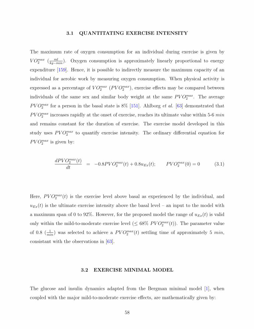
3.1 QUANTITATING EXERCISE INTENSITY

The maximum rate of oxygen consumption for an individual during exercise is given by

V Omax2 ( ml

kg−min). Oxygen consumption is approximately linearly proportional to energy

expenditure [159]. Hence, it is possible to indirectly measure the maximum capacity of an

individual for aerobic work by measuring oxygen consumption. When physical activity is

expressed as a percentage of V Omax2 (PV Omax

2 ), exercise effects may be compared between

individuals of the same sex and similar body weight at the same PV Omax2 . The average

PV Omax2 for a person in the basal state is 8% [151]. Ahlborg et al. [63] demonstrated that

PV Omax2 increases rapidly at the onset of exercise, reaches its ultimate value within 5-6 min

and remains constant for the duration of exercise. The exercise model developed in this

study uses PV Omax2 to quantify exercise intensity. The ordinary differential equation for

PV Omax2 is given by:

dPV Omax2 (t)

dt= −0.8PV Omax

2 (t) + 0.8uEx(t); PV Omax2 (0) = 0 (3.1)

Here, PV Omax2 (t) is the exercise level above basal as experienced by the individual, and

uEx(t) is the ultimate exercise intensity above the basal level – an input to the model with

a maximum span of 0 to 92%. However, for the proposed model the range of uEx(t) is valid

only within the mild-to-moderate exercise level (≤ 68% PV Omax2 (t)). The parameter value

of 0.8 ( 1min

) was selected to achieve a PV Omax2 (t) settling time of approximately 5 min,

consistant with the observations in [63].

3.2 EXERCISE MINIMAL MODEL

The glucose and insulin dynamics adapted from the Bergman minimal model [1], when

coupled with the major mild-to-moderate exercise effects, are mathematically given by:

58

dI(t)

dt= −nI(t)− Ie(t) + p5u1(t) (3.2)

dX(t)

dt= −p2X(t) + p3[I(t)− Ib]

dG(t)

dt= −p1[G(t)−Gb]− p4X(t)G(t) +

W

V olG[Gprod(t)−Ggly(t)]

− W

V olGGup(t) +

u2(t)

V olG(3.3)

dGprod(t)

dt= a1PV Omax

2 (t)− a2Gprod(t) (3.4)

dGup(t)

dt= a3PV Omax

2 (t)− a4Gup(t) (3.5)

dIe(t)

dt= a5PV Omax

2 (t)− a6Ie(t) (3.6)

The insulin dynamics, equation (3.2), have been modified from the Bergman minimal model,

equation (2.1), by adding the final term. Here, Ie(t) ( µUml−min

) is the rate of insulin removal

from the circulatory system due to exercise-induced physiological changes. The plasma

glucose dynamics, equation (3.3), differ from equation (2.3) of the Bergman minimal model

by addition of the following terms: WV olG

[Gprod(t) − Ggly(t)] − WV olG

Gup(t). Variables Gup(t)

( mgkg−min

) and Gprod(t) ( mgkg−min

) represent the rates of glucose uptake and hepatic glucose

production induced by exercise, respectively. W (kg) represents the weight of the subject.

Variable Ggly(t) ( mgkg−min

) represents the decline of glycogenolysis rate during prolonged ex-

ercise due to depletion of liver glycogen stores. The dynamics of hepatic glucose production,

glucose uptake, and plasma insulin removal induced by exercise are represented in equations

(3.4), (3.5), and (3.6), respectively. Initial conditions of the above ODEs are listed in Table

3.1.

The rate of glycogenolysis (Ggly(t)) starts to decrease when the energy expenditure

exceeds a critical threshold value (ATH) which is a function of exercise intensity and duration.

ATH can be mathematically represented as:

ATH = uEx(t)tgly(uEx(t)) (3.7)

Here, tgly(uEx(t)) is the duration of exercise that can be performed at intensity uEx(t) before

the rate of hepatic glycogenolysis starts to decrease. The rate of hepatic glycogen depletion

increases with increasing exercise intensity [15, 11]. Hence, tgly(uEx(t)) is a function of

59

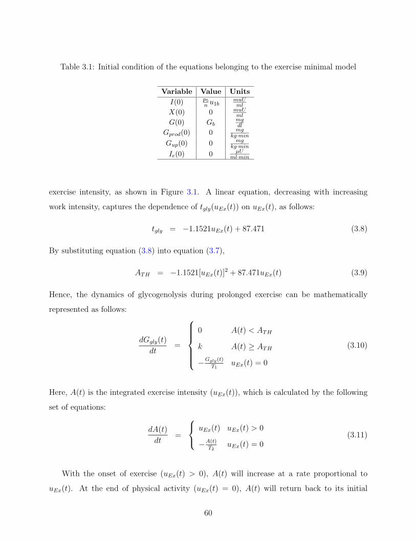
Table 3.1: Initial condition of the equations belonging to the exercise minimal model

Variable Value UnitsI(0) p5

n u1bmuUml

X(0) 0 muUml

G(0) Gbmgdl

Gprod(0) 0 mgkg·min

Gup(0) 0 mgkg·min

Ie(0) 0 µUml·min

exercise intensity, as shown in Figure 3.1. A linear equation, decreasing with increasing

work intensity, captures the dependence of tgly(uEx(t)) on uEx(t), as follows:

tgly = −1.1521uEx(t) + 87.471 (3.8)

By substituting equation (3.8) into equation (3.7),

ATH = −1.1521[uEx(t)]2 + 87.471uEx(t) (3.9)

Hence, the dynamics of glycogenolysis during prolonged exercise can be mathematically

represented as follows:

dGgly(t)

dt=

0 A(t) < ATH

k A(t) ≥ ATH

−Ggly(t)

T1uEx(t) = 0

(3.10)

Here, A(t) is the integrated exercise intensity (uEx(t)), which is calculated by the following

set of equations:

dA(t)

dt=

uEx(t) uEx(t) > 0

−A(t)T2

uEx(t) = 0(3.11)

With the onset of exercise (uEx(t) > 0), A(t) will increase at a rate proportional to

uEx(t). At the end of physical activity (uEx(t) = 0), A(t) will return back to its initial

60

10 20 30 40 50 60 700

10

20

30

40

50

60

70

80

uEx

(t) (% VO2max above basal)

t gly (

min

)

Figure 3.1: Dependence of time at which hepatic glycogen starts to deplete, tgly, on exercise

intensity (uEx(t)). Published data (cross) from Pruett et al. [11] and linear fit (solid line)

[R2 = 0.9908]

condition (which is zero) at rate governed by T2. Both rat and human studies have revealed

that majority of the liver glycogen stores are repleted within 1 hr of the recovery period

[160, 161]. Hence, the time constant T2 was assigned a value of 10 min. As long as A(t) is

less than the critical threshold value (ATH), enough glycogen is still available to maintain

a sufficient rate of hepatic glucose release. However, once A(t) reaches ATH , the rate of

glycogenolysis rate starts to decline at a rate given by k, due to the depletion of available

liver glycogen stores. The end of exercise (when uEx(t) returns to zero), which is also the

beginning of the recovery period, marks the commencement of repletion of glycogen stores

61

via a continued elevation in the rate of hepatic gluconeogenesis. The time required for Ggly(t)

to return to its basal value after exercise is governed by the pseudo-time constant T1.

3.2.1 Parameter Estimation Technique

Parameters for the exercise minimal model were estimated using the nonlinear least square

technique, as described in Section 2.3 (equation (2.9)). Data from [12] were used to estimate

the parameters a5 and a6, thereby quantifying the depletion of plasma insulin during exercise

and its repletion during the recovery period. After fixing a5 and a6, the insulin model was

validated by comparing with the data from [13]. Parameters a1 and a2 for Gprod dynamics and

a3 and a4 for Gup(t) dynamics were also estimated from [12]. The glucose model was validated

by comparing the model predictions of Gprod(t), Gup(t) and G(t) with T1DM patient data

from [14]. After fixing the parameters a1−6 to their estimated values, the effects of glycogen

depletion during prolonged exercise, and recovery were modeled. In order to capture these

effects, data from [13] was used to estimate the parameters k and T1 in equation (3.10).

For further validation of the model during prolonged exercise, plasma glucose concentration

was compared with the data from another study performed at higher exercise intensity [15].

All the parameter values for the exercise minimal model along with their 95% confidence

interval (CI) bounds calculated by using the nlparci.m function from the MATLAB Statistics

Toolbox ( c©2008 The Mathworks Inc., Natick, MA) are given in Table 3.2. The quality of the

model fits was assessed by using the R2 technique (for details see Section 2.3). Calculated

R2 values for every model fit and validation are provided in the figure legends.

3.3 RESULTS OF THE EXERCISE MINIMAL MODEL

3.3.1 Plasma Insulin Dynamics During Exercise

Simulation study of mild exercise (PV Omax2 (t) = 40) for 60 min was performed to evaluate

the physiological effects of exercise on plasma insulin concentration. With the onset of

exercise, plasma insulin declined from its basal level (12.2 µUmL

), and continued to do so along

62

Table 3.2: Parameters of the exercise minimal model with 95% confidence intervals (CI), in

addition to those in Table 2.1

Parameter Value Lower Limit Upper Limit Unit95% CI 95% CI

a1 0.00158 0.0013 0.0019 mg/kg·min2

a2 0.056 0.0441 0.0679 1/mina3 0.00195 0.0015 0.0024 mg/kg·min2

a4 0.0485 0.0355 0.0617 1/mina5 0.00125 0.001 0.0015 µ U/mL·mina6 0.075 0.0588 0.0912 1/mink 0.0108 0.0085 0.0131 mg/kg·min2

T1 6.0 1.86 10.14 min

a first-order-type response trajectory until the end of the experiment, as shown in Figure 3.2.

During the recovery period (t > 60 min), the plasma insulin concentration climbed back to

its basal level. Quantitatively, the model predictions were consistently within one standard

deviation of the mean of experimental data [12] from which the relevant parameters (a5 and

a6) were estimated. The 95% CI bounds of plasma insulin concentration were simulated by

choosing a set of parameter values from Table 3.2 that had the maximum overestimation (a5

= 0.001, a6 = 0.0912) and maximum underestimation (a5 = 0.0015, a6 = 0.0588) of insulin

concentration, as shown in Figure 3.2 (dotted lines).

For validation of the model, a separate simulation study was performed keeping the

parameter values of a5 and a6 unchanged with a different exercise intensity level (PV Omax2 (t)

= 30) which lasted for a longer time duration (tex = 0 to 120 min). With the onset of exercise,

the insulin level declined well below the basal level (10.2 µUmL

), and this hypoinsulinemic state

persisted until the end of the experiment. A comparison between model prediction of insulin

and experimental data [13] with same exercise protocol is shown in Figure 3.3. Plasma

insulin gradually returned back to the basal level during the recovery period (t > 120 min).

Overall, the insulin model fits the experimental data sets.

63

0 20 40 60 80 1006

7

8

9

10

11

12

13

14

Time (min)

Insu

lin (

µU/m

l)

Figure 3.2: Plasma insulin concentration in response to mild exercise (PV Omax2 = 40) lasting

from tex = 0 to 60 min. Published data (circles) (µ ± σ) from Wolfe et al. [12], model fit

(solid line), and 95% confidence interval of the model output (dotted line).

3.3.2 Plasma Glucose Dynamics During Exercise

To evaluate the exercise effects on plasma glucose concentration, a simulation study of mild

exercise was performed (PV Omax2 (t) = 40) for 60 min. With the onset of exercise, Gup(t)

increased from its basal state to 1.15 mgkg·min

. During the recovery period (t > 60 min), Gup

returned to its basal level. Model prediction of Gup(t) along with experimental data [12] with

same exercise protocol from which parameters a3 and a4 were estimated is shown in Figure

3.4 (Top). The 95% CIs of Gup(t) were simulated by choosing a set of parameter values from

Table 3.2 that had the maximum underestimation (a3 = 0.0015, a4 = 0.0617) and maximum

64

0 50 100 1505

6

7

8

9

10

11

Insu

lin (

µU/m

l)

Time (min)

Figure 3.3: Plasma insulin concentration in response to mild exercise (PV Omax2 = 30) lasting

from tex = 0 to 120 min. Model simulation validation (solid line) and published data (cross)

(µ ± σ) from Ahlborg et al. [13]

overestimation (a3 = 0.0024, a4 = 0.0355) of glucose uptake rate, as shown by the dotted

lines in Figure 3.4 (Top). In order to maintain plasma glucose homeostasis, hepatic glucose

production rate (Gprod(t),mg

kg·min) also increased from its basal level to 0.95 mg

kg·minfor the

duration of exercise. In conjunction with glucose uptake rate, Gprod(t) decreased to its basal

level after the end of exercise. Parameters a1 and a2 were estimated to fit the data, as shown

in Figure 3.4 (Bottom). Again, 95% CIs of Gprod(t) were simulated by choosing a set of

parameter values from Table 3.2 that had the maximum underestimation (a1 = 0.0013, a2 =

0.0679) and the maximum overestimation (a1 = 0.0019, a2 = 0.0441) of glucose production

65

rate, as shown by the dotted lines in Figure 3.4 (Bottom). Both Gup(t) and Gprod(t) are

represented in deviation form in Figure 3.4.

0 20 40 60 80 100

0

0.5

1

1.5

Time (min)

Gpr

od (

mg/

kg/m

in)

0 20 40 60 80 100

0

0.5

1

1.5

Gup

(m

g/kg

/min

)

Figure 3.4: Model simulation (solid lines), 95% confidence intervals of model outputs (dotted

lines) and published data (circles) (µ ± σ) from Wolfe et al. [12] in response to mild exercise

(PV Omax2 = 40) lasting from tex = 0 to 60 min. Top: hepatic glucose uptake rate (Gup),

and Bottom: hepatic glucose production rate (Gprod). Both Gup and Gprod are plotted in

deviation form.

The accelerated glucose uptake rate during exercise is compensated for by enhanced

hepatic glucose production; hence, normoglycemia is maintained throughout the course

of physical activity. A comparison between the model prediction of glucose concentration

including Gup(t) plus Gprod(t) effects and experimental data [12] is provided in Figure 3.5.

The predictions of the glucose model are in good accordance with the published data. In

order to simulate the 95% CIs for plasma glucose concentration, a combination of parameter

66

0 20 40 60 80 10078

80

82

84

86

88

Time (min)

G (

mg/

dl)

Figure 3.5: Plasma glucose concentration (G) in response to mild exercise (PV Omax2 = 40)

lasting from tex = 0 to 60 min. Model simulation (solid line), 95% confidence intervals of

model output (dotted lines), and published data (circles) (µ ± σ) from Wolfe et al. [12].

values were chosen from Table 3.2 that generated the maximum underestimation (a1 =

0.0013, a2 = 0.0679, a3 = 0.0024, a4 = 0.0355, a5 = 0.001, a6 = 0.0912) and the maximum

overestimation (a1 = 0.0019, a2 = 0.0441, a3 = 0.0015, a4 = 0.0617, a5 = 0.0015, a6 =

0.0588) of plasma glucose, as indicated by the dotted lines in Figure 3.5.

For the validation of the glucose model, another simulation test was performed at

moderate level of exercise for 45 min at PV Omax2 (t) = 50. Again, with the onset of exercise,

both Gup(t) and Gprod(t) increased. During the recovery period (t > 45 min), Gup(t) and

Gprod(t) gradually declined to their respective basal levels. Model validation simulations (i.e.,

67

0 20 40 60 80 100

0

1

2

Gup

(m

g/kg

/min

)

0 20 40 60 80 100

0

1

2

G

prod

(mg/

kg/m

in)

0 20 40 60 80 100−0.1

0

0.1

[Gpr

od −

Gup

]

(mg/

kg/m

in)

Time (min)

Figure 3.6: Response to moderate exercise (PV Omax2 = 50) lasting from tex = 0 to 45 min.

Model simulation validation (solid lines) and published data (cross) (µ ± σ) from Zinman

et al. [14]. Top: glucose uptake rate (Gup); Middle: hepatic glucose production rate (Gprod);

Bottom: difference [Gprod − Gup]. Both Gup and Gprod are shown in deviation form.

no model parameter changes) are plotted alongside experimental data of T1DM patients

[14] in Figure 3.6, top and bottom (both in deviation form). Figure 3.7 reveals the model

prediction of plasma glucose concentration including the combined effects of Gup(t) and

Gprod(t) during exercise along with experimental data [14] with the same group of patients.

To evaluate the plasma glucose dynamics during prolonged exercise, data from Ahlborg

et al. [13] was considered (see Figure 3.8). With the onset of exercise, both Gup(t) and

Gprod(t) rates were elevated from the basal level; this resulted in the maintenance of glucose

68

0 20 40 60 80 10085

86

87

88

89

90

91

92

G (

mg/

dl)

Time (min)

Figure 3.7: Plasma glucose concentration (G) in response to moderate exercise (PV Omax2 =

50) lasting from tex = 0 to 45 min. Model simulation validation (solid line) versus published

data (cross) (µ ± σ) from Zinman et al. [14].

homeostasis during the first hour of exercise. As the integrated exercise intensity exceeded

a critical threshold (which is a function of exercise intensity and duration), the hepatic

glycogenolysis rate started to decline as a result of which net liver glucose production rate,

[Gprod(t) - Ggly(t)], decreased until the end of exercise (Figure 3.8: Bottom). However, Gup

remained elevated due to continuing physical activity (Figure 3.8: Middle). This mismatch

between Gup(t) and Gprod(t) resulted in a net decrease of plasma glucose level (Figure 3.8:

Top). During the post-exercise recovery period, lactate consumption by the liver increases

significantly, serving as a substrate for accelerated post-exercise gluconeogenesis [157]. It is

69

0 50 100 150 20060

70

80

G (

mg/

dl)

0 50 100 150 2000

0.5

1

Gup

(m

g/kg

/min

)

0 50 100 150 200−0.5

00.5

1

[Gpr

od −

Ggl

y]

(mg/

kg/m

in)

Time (min)

Figure 3.8: Model response to mild exercise (PV Omax2 = 30) lasting from tex = 0 to 120 min.

Published data (circles) (µ ± σ) from Ahlborg et al. [13], model fit (solid line), and 95%

confidence interval of fit (dashed line). Top: model prediction of plasma glucose (G); Middle:

model prediction of hepatic glucose uptake rate (Gup); and Bottom: model prediction of net

liver glucose production. Both Gup and [Gprod - Ggly] are shown in deviation form.

believed that the purpose of this elevated gluconeogenesis is to replete the liver glycogen

stores and restore normoglycemia [157]. Keeping parameters a1−6 unchanged, parameters

k and T1 from equation (3.10) were adjusted to capture the dynamical behavior of plasma

glucose concentration. To simulate the 95% CIs for plasma glucose concentration during

prolonged exercise, the same combination of parameter values were chosen from Table 3.2 as

in Figure 3.5, with the addition of (k = 0.0131, T1 = 10.14) for maximum underestimation

70

0 50 100 150 200 25040

60

80

G (

mg/

dl)

0 50 100 150 200 2500

1

2

Gup

(mg/

kg/m

in)

0 50 100 150 200 250

−1012

[Gpr

od −

Ggl

y]

(mg/

kg/m

in)

Time (min)

Figure 3.9: Model response to moderate exercise (PV Omax2 = 60) lasting from tex = 0 to 210

min. Published data (cross) (µ ± σ) from Ahlborg et al. [15] and model prediction validation

(solid line). Top: model prediction of plasma glucose (G); Middle: model prediction

of hepatic glucose uptake rate (Gup); and Bottom: model prediction of net liver glucose

production. Both Gup and [Gprod - Ggly] are shown in deviation form.

and (k = 0.0085, T1 = 1.86) for the maximum overestimation, as shown by the dotted lines

in Figure 3.8 (Top). To simulate the CIs for Gup(t), the same parameter value sets as those

used in Figure 3.4 (Top), were chosen (see Figure 3.8: Middle). Finally, to simulate the 95%

CIs of net liver glucose production rate, a combination of parameter values were chosen from

Table 3.2 to generate the maximum underestimation (a1 = 0.0013, a2 = 0.0679, k = 0.0131,

T1 = 10.14) and the maximum overestimation (a1 = 0.0019, a2 = 0.0441, k = 0.0085, T1=

71

1.86) of [Gprod(t) - Ggly(t)], as shown by the dotted lines in Figure 3.8 (Bottom). In order

to validate the model during prolonged exercise, a separate simulation study was performed

where exercise was performed for 3 hours at a moderate exercise intensity (PV Omax2 = 60).

Due to the higher exercise intensity, glycogen stores depleted at a faster rate; the result is

an inability to maintain glucose homeostasis beyond tex = 30 min (see Figure 3.9: Top).

A comparison between model simulations (without changing any parameters) and data [15]

are given in Figure 3.9.

3.4 MODEL STRUCTURE JUSTIFICATION

The purpose of the proposed model was to extend the classical minimal model [1] in order to

capture the vital physiological effects induced by mild-to-moderate exercise on glucose and

insulin dynamics during and immediately after physical activity. The states added (equations

(3.4), (3.5), (3.6), and (3.10)) were essential to describe accurately the acute exercise effects

on plasma insulin and glucose concentrations. However, including extra equations certainly

added complexity to the proposed model. Hence, this Section explores reduced versions of

the proposed exercise model. AIC (see Section 2.3) was employed to establish a statistical

comparison between the proposed model and its reduced versions.

3.4.1 Validity of Ie(t) (Equation 3.6)

Equation (3.6) was added to the proposed model to capture the dynamics of Ie(t), which

represents the rate of insulin clearance from the circulatory system due to exercise. As

mentioned in Section 3.2.1, parameters a5 and a6 from equation (3.6) were estimated using

the data from Wolfe et al. [12] (for the values, refer to Table 3.2). In the reduced version,

Ie(t) (equation 3.6) was omitted. Hence, the exercise induced plasma insulin clearance was

captured directly by the PV Omax2 (t) variable coupled with a new parameter, b1. Thus,

equation (3.2) could be re-written as follows:

72

dI(t)

dt= −nI(t) + p4u1(t)− b1PV Omax

2 (t) (3.12)

The parameter value of b1 = 0.0148 µUml·min

was estimated from the data [12] via the

nonlinear least square technique (Section 2.3). The calculated AIC values with and without

the variable Ie(t) (equation (3.6)) are presented in Table 3.3. It is clearly evident that the

proposed model is superior to the reduced version, in terms of their AIC values. Simulation

of these two models, along with the experimental data [12] are shown in Figure 3.10. Insulin

dynamics during exercise without the filter equation (3.6) is much faster as compared to the

data [12].

3.4.2 Validity of Gup(t) (Equation 3.5)

In the proposed model, exercise-induced glucose uptake (Gup(t)) was captured by equation

(3.5). Parameters a3 and a4 belonging to equation (3.5) were estimated by using the data

from [12], as mentioned in Section 3.2.1 (for the values, refer Table 3.2). In the reduced

version, equation (3.5) (Gup(t)), was omitted. Hence, the exercise induced glucose uptake

rate, Gup(t), was captured by the term b2PV Omax2 (t), which is a product of a new gain

parameter, b2, and exercise intensity, PV Omax2 (t). Therefore, equation (3.3) could be re-

written as follows:

dG(t)

dt= −p1[G(t)−Gb]−X(t)G(t) +

W


− W

V olGGup(t) +

u2(t)

V olG(3.13)

Gup(t) = b2PV Omax2 (t) (3.14)

The value of parameter b2 (0.03114 mgkg·min

) was estimated by using the data obtained

from [12] via the nonlinear least square technique. The calculated AIC values of the proposed

and reduced models are provided in Table 3.3. Once again, from the AIC values it is clearly

73

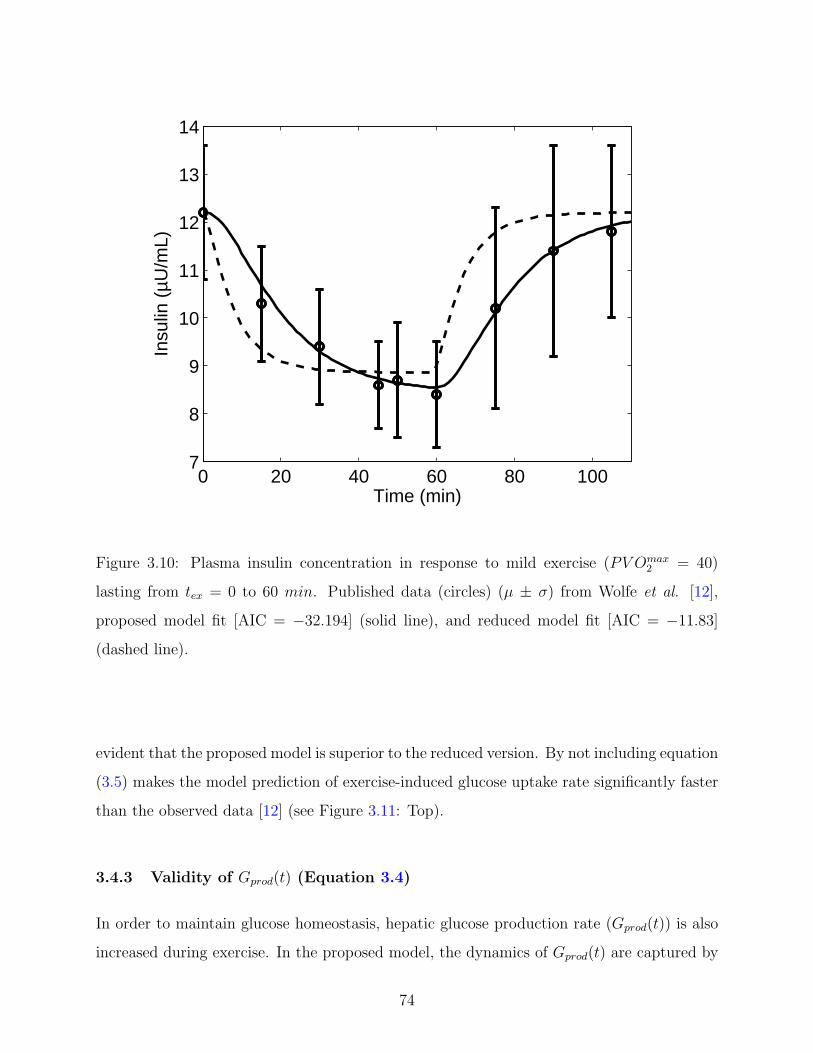
0 20 40 60 80 1007

8

9

10

11

12

13

14

Time (min)

Insu

lin (

µU/m

L)

Figure 3.10: Plasma insulin concentration in response to mild exercise (PV Omax2 = 40)

lasting from tex = 0 to 60 min. Published data (circles) (µ ± σ) from Wolfe et al. [12],

proposed model fit [AIC = −32.194] (solid line), and reduced model fit [AIC = −11.83]

(dashed line).

evident that the proposed model is superior to the reduced version. By not including equation

(3.5) makes the model prediction of exercise-induced glucose uptake rate significantly faster

than the observed data [12] (see Figure 3.11: Top).

3.4.3 Validity of Gprod(t) (Equation 3.4)

In order to maintain glucose homeostasis, hepatic glucose production rate (Gprod(t)) is also

increased during exercise. In the proposed model, the dynamics of Gprod(t) are captured by

74

0 20 40 60 80 100

0

0.5

1G

up

(mg/

kg/m

in)

0 20 40 60 80 1000

0.5

1

Time (min)

Gpr

od

(mg/

kg/m

in)

Figure 3.11: Proposed model simulation (solid lines), reduced model simulation (dotted

lines) and published data (circles) (µ ± σ) from Wolfe et al. [12] in response to mild exercise

(PV Omax2 = 40) lasting from tex = 0 to 60 min. Top: glucose uptake rate (Gup), and Bottom:

hepatic glucose production rate (Gprod). Both Gup and Gprod are plotted in deviation form.

equation (3.4). As mentioned earlier, parameters a1 and a2 belonging to equation (3.4) were

estimated by using the data from [12] via nonlinear least square algorithm.

In the reduced version, equation (3.4) (Gprod(t)) is eliminated. Therefore, the acceler-

ated plasma glucose production induced by exercise is captured directly by the PV Omax2 (t)

variable coupled with the new parameter, b3. Hence, equation (3.3) could be re-written as

shown below:

75

dG(t)

dt= −p1[G(t)−Gb]−X(t)G(t) +

W


− W

V olGGup(t) +

u2(t)

V olG(3.15)

Gprod(t) = b3PV Omax2 (t) (3.16)

Data from [12] was utilized to estimate the parameter, b3 = 0.02491 mgkg·min

via the nonlinear

least square technique. From the AIC values it is clearly evident that the proposed model is

superior to the reduced model. The model prediction of exercise-induced glucose production

(Gprod(t)) without equation 3.4 is significantly faster than the observed data [12] (see Figure

3.11: Bottom).

By comparing all the AIC values of the proposed exercise model and its reduced versions,

it is evident that the originally proposed additional states (equation (3.4), (3.5), and (3.6))

are essential to accurately capture the dynamics of plasma glucose and insulin concentrations

under the influence of exercise. Any further simplification than the proposed structure will

compromise the quality of the model.

Table 3.3: Calculated AIC values of the exercise minimal model with and without the Ie(t),

Gup(t) and Gprod(t) filter equations

AIC Exercise Minimal Modelwithout with

Insulin clearance dynamics Eq. (3.12) Eq. (3.2)(Ie(t)) −11.830 −32.194Glucose uptake dynamics Eq. (3.14) Eq. (3.5)(Gup(t)) 8.880 −15.705Glucose production dynamics Eq. (3.16) Eq. (3.4)(Gprod(t)) 4.20 −26.78

76

3.5 SUMMARY

A model of exercise effects on plasma glucose-insulin dynamics was developed. The principal

goal was to extend the Bergman minimal model [1] by adding state equations in order to to

predict plasma glucose and insulin concentrations. This was accomplished by mathematically

capturing the necessary physiological phenomenon induced by exercise. All the added

equations in the proposed model are linear in nature thus maintaining the simplifying

approach of the original minimal model [1]. The model successfully captured the effects of

mild-to-moderate aerobic exercise on plasma glucose and insulin concentrations. Inclusion

of separate dynamics in the model for glucose uptake (equation (3.5)) and hepatic glucose

production (equation (3.4)) made it possible to capture the simultaneous rise of these rates

with the onset of short term exercise in order to maintain glucose homeostasis. These

equations were also successful in capturing the dynamics of glucose fluxes during the post-

exercise recovery period. As the integrated exercise intensity extends beyond a critical

threshold (which is a function of exercise intensity and duration), a decline in splanchnic

glucose release is expected. As glucose uptake rate remains elevated, maintenance of glucose

homeostasis is no longer possible. Due to this, plasma glucose continues to decline until the

end of physical activity. At the end of prolonged exercise, the hepatic gluconeogenesis rate is

increased, and this facilitates repletion of glycogen stores and helps to achieve normoglycemia

[157]. A substantial amount of lactate is released from the post-exercising muscles during the

recovery period, which serves as a substrate for gluconeogenesis. To capture the dynamics

of plasma glucose during the various stages of prolonged exercise, equation (3.10) was

incorporated. The model also successfully captured the clearance of plasma insulin from

the circulatory system during physical exercise due to the addition of equation (3.6).

With a focus on closed-loop insulin delivery systems for T1DM patients, it is necessary

to develop models that can accurately predict plasma glucose concentration during rest, as

well as during physical exercise. Hence, this model provides the control community with

an alternative benchmark problem in glucose control for diabetic patients by allowing the

analysis of meal and exercise disturbances alone or in combination. The exercise model can

also be used to predict the duration of exercise at a given intensity that can be executed while

77

keeping plasma glucose within the normoglycemic range. However, a prospective validation

of the components of the minimal exercise model is necessary before the model, or a model-

based controller, is employed in any clinical setting.

The proposed model as presented in this Chapter does not include the FFA dynamics

and its interactions with blood glucose. As discussed in Chapter 2, FFA plays a significant

role in influencing plasma glucose concentration. Also, FFA dynamics is profoundly altered

during physical activity. Hence, in the following Chapter a lower-order composite model was

synthesized by combining the FFA model from Chapter 2 and the exercise model from this

Chapter. The composite model, as proposed in Chapter 4, is capable of predicting plasma

FFA, glucose, and insulin dynamics during rest, as well as exercise.

78

4.0 A LOWER-ORDER MODEL OF FFA, GLUCOSE, AND INSULIN AT

REST AND DURING EXERCISE

So far in the dissertation, two different metabolic models were developed by modifying the

Bergman minimal model [1] in order to incorporate various physiological effects of FFA and

exercise on the insulin-glucose system [129, 150]. The extended minimal model developed

in Chapter 2 is capable of predicting FFA along with glucose dynamics during pre- and

post-prandial states. The model is also equipped to capture the inhibitory effects of FFA on

glucose uptake rate by the peripheral and hepatic tissues. However, the extended minimal

model does not consider the exercise effects on insulin, glucose, and FFA kinetics. In Chapter

3, an exercise minimal model was developed to capture the effects of exercise on glucose and

insulin dynamics. The model successfully captured insulin-glucose concentrations during

and immediately after mild-to-moderate exercise. The model is also capable of predicting

the plasma glucose excursion towards hypoglycemia during prolonged exercise periods. The

major drawback of this model is the absence of FFA dynamics and its interactions with

glucose and insulin.

Instead of having two different minimal models capturing the effects of FFA and exercise

on the glucose-insulin system separately, a single low-order metabolic model capturing all the

physiological effects on the glucose-insulin system can be developed. Hence, in this Chapter a

composite metabolic model capable of predicting plasma glucose, insulin, and FFA dynamics

at rest, as well as during mild-to-moderate exercise was developed.

One objective of the model was to represent the physiology more accurately. Hence,

necessary modifications were made to the original model structures obtained from Chapters

2 and 3. For example, insulin action on glucose was divided into two parts having separate

dynamics: one capturing the insulin-mediated tissue glucose uptake, and the other part

79

capturing the insulin-mediated suppression of endogenous glucose production. Moreover,

saturating functions were used to represent the effects of insulin on endogenous glucose

and FFA production rates. In order to accurately model literature data, unobservable

filter equations capturing the interactions between insulin, glucose, FFA, and exercise were

added wherever necessary. However, addition of extra equations increased the complexity

of the model in terms of number of parameters which are required to be estimated. Hence,

the trade-off between model accuracy and model complexity was measured by using AIC

(equation (2.12)) as described in Section 2.3. The model structure with a lower AIC value

was selected in synthesizing the composite model. The resulting composite model consisted

of four parts: insulin, glucose, FFA, and exercise sub-models.

In the following Section (4.1), a brief overview of the physiological interactions between

the plasma insulin, glucose, and FFA at rest and during exercise is presented. In Section 4.2,

a detailed description of the structure of the composite model is introduced. A parametric

sensitivity analysis is performed in Section 4.3. Finally, the results of model validation

simulations are presented in Section 4.4.

4.1 INTERACTIONS BETWEEN INSULIN, GLUCOSE, AND FFA

DURING REST AND EXERCISE

The major metabolic interactions captured by the composite model are given in Figure

4.1. Basically, the lower-order model is divided into four parts capturing the plasma insulin

(section-I), plasma glucose (section-II), plasma FFA (section-III), and exercise (section-IV)

dynamics, as shown in the schematic diagram. The continuous lines in the diagram represent

transport or clearance of metabolic substrates and hormones; the dashed lines represent

interactions taking place between the substrates, hormones, and exercise.

80

GLiver

F

Periphery

I

AT

Transport/Clearance

Interaction

I

II

IV

III

xEGP

xG

yIU

yGP

yGU

y1FU

y1FP

uG

uI

uF

uEx

xEFP1

PVOmax2

Figure 4.1: Schematic diagram of the composite model. Sections I, II, III, and IV represent

the insulin, glucose, FFA, and exercise sub-models, respectively. I: Insulin; G: Glucose;

F: FFA; uI : Exogenously infused insulin; uG, uF : Glucose or FFA absorbed from meal or

infused; uEx: Exercise intensity; PVOmax2 : Percentage of maximum rate of oxygen uptake;

xG, xEGP , xEFP1: Remote insulin compartments; yIU , yGU , yGP , y1FU , y1FP : 1st-order filters

capturing exercise effects.

81

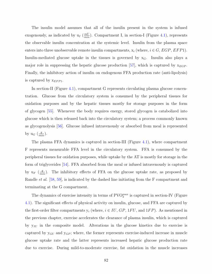
The insulin model assumes that all of the insulin present in the system is infused

exogenously, as indicated by uI ( mUmin

). Compartment I, in section-I (Figure 4.1), represents

the observable insulin concentration at the systemic level. Insulin from the plasma space

enters into three unobservable remote insulin compartments, xi (where, i ∈G, EGP , EFP1).

Insulin-mediated glucose uptake in the tissues is governed by xG. Insulin also plays a

major role in suppressing the hepatic glucose production [57], which is captured by xEGP .

Finally, the inhibitory action of insulin on endogenous FFA production rate (anti-lipolysis)

is captured by xEFP1.

In section-II (Figure 4.1), compartment G represents circulating plasma glucose concen-

tration. Glucose from the circulatory system is consumed by the peripheral tissues for

oxidation purposes and by the hepatic tissues mostly for storage purposes in the form

of glycogen [55]. Whenever the body requires energy, stored glycogen is catabolized into

glucose which is then released back into the circulatory system; a process commonly known

as glycogenolysis [56]. Glucose infused intravenously or absorbed from meal is represented

by uG ( gmin

).

The plasma FFA dynamics is captured in section-III (Figure 4.1), where compartment

F represents measurable FFA level in the circulatory system. FFA is consumed by the

peripheral tissues for oxidation purposes, while uptake by the AT is mostly for storage in the

form of triglycerides [54]. FFA absorbed from the meal or infused intravenously is captured

by uF ( gmin

). The inhibitory effects of FFA on the glucose uptake rate, as proposed by

Randle et al. [58, 59], is indicated by the dashed line initiating from the F compartment and

terminating at the G compartment.

The dynamics of exercise intensity in terms of PVOmax2 is captured in section-IV (Figure

4.1). The significant effects of physical activity on insulin, glucose, and FFA are captured by

the first-order filter compartments yi (where, i ∈ IU , GP , 1FU , and 1FP ). As mentioned in

the previous chapter, exercise accelerates the clearance of plasma insulin, which is captured

by yIU in the composite model. Alterations in the glucose kinetics due to exercise is

captured by yGU and yGP ; where, the former represents exercise-induced increase in muscle

glucose uptake rate and the latter represents increased hepatic glucose production rate

due to exercise. During mild-to-moderate exercise, fat oxidation in the muscle increases

82

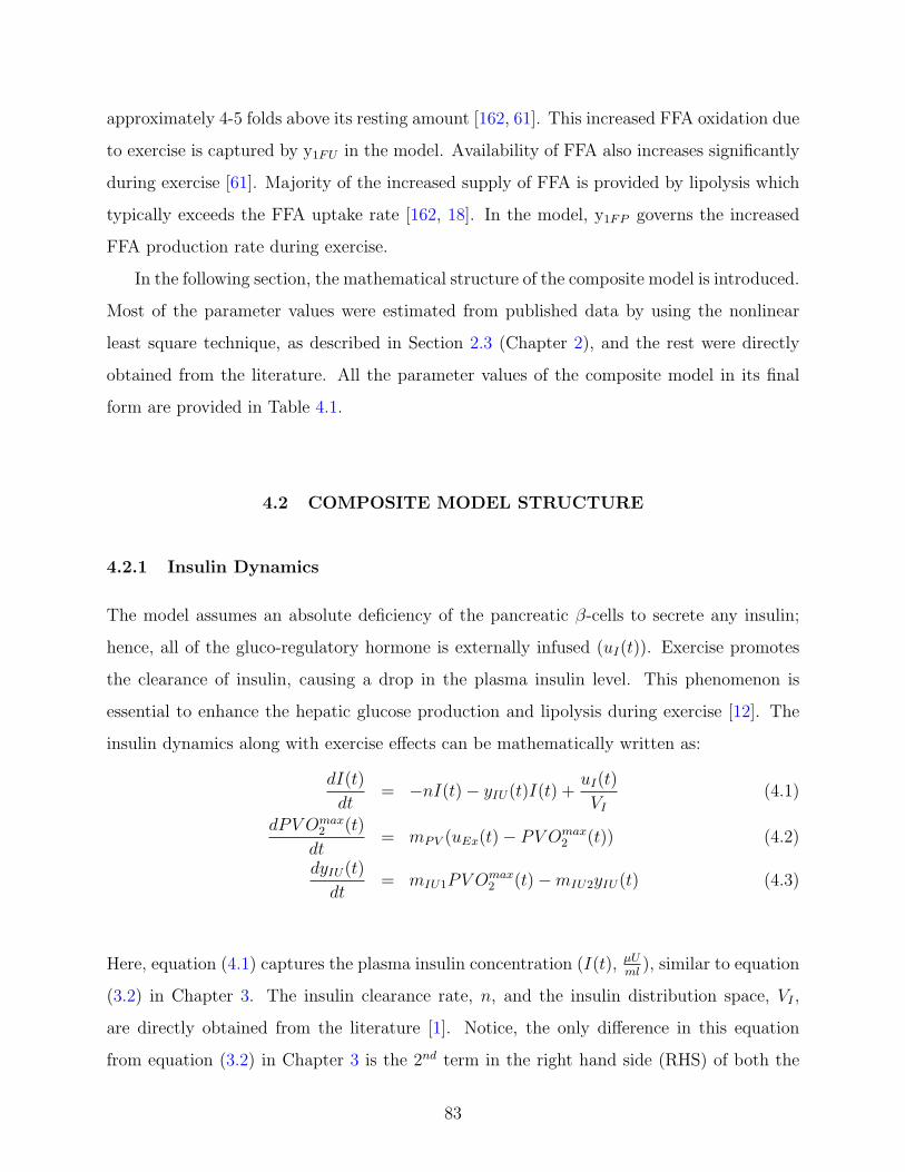
approximately 4-5 folds above its resting amount [162, 61]. This increased FFA oxidation due

to exercise is captured by y1FU in the model. Availability of FFA also increases significantly

during exercise [61]. Majority of the increased supply of FFA is provided by lipolysis which

typically exceeds the FFA uptake rate [162, 18]. In the model, y1FP governs the increased

FFA production rate during exercise.

In the following section, the mathematical structure of the composite model is introduced.

Most of the parameter values were estimated from published data by using the nonlinear

least square technique, as described in Section 2.3 (Chapter 2), and the rest were directly

obtained from the literature. All the parameter values of the composite model in its final

form are provided in Table 4.1.

4.2 COMPOSITE MODEL STRUCTURE

4.2.1 Insulin Dynamics

The model assumes an absolute deficiency of the pancreatic β-cells to secrete any insulin;

hence, all of the gluco-regulatory hormone is externally infused (uI(t)). Exercise promotes

the clearance of insulin, causing a drop in the plasma insulin level. This phenomenon is

essential to enhance the hepatic glucose production and lipolysis during exercise [12]. The

insulin dynamics along with exercise effects can be mathematically written as:

dI(t)

dt= −nI(t)− yIU(t)I(t) +

uI(t)

VI

(4.1)

dPV Omax2 (t)

dt= mPV (uEx(t)− PV Omax

2 (t)) (4.2)

dyIU(t)

dt= mIU1PV Omax

2 (t)−mIU2yIU(t) (4.3)

Here, equation (4.1) captures the plasma insulin concentration (I(t), µUml

), similar to equation

(3.2) in Chapter 3. The insulin clearance rate, n, and the insulin distribution space, VI ,

are directly obtained from the literature [1]. Notice, the only difference in this equation

from equation (3.2) in Chapter 3 is the 2nd term in the right hand side (RHS) of both the

83

equations representing the exercise-induced clearance rate of insulin. Unlike the exercise

minimal model in Chapter 3, introduction of the bilinear term (yIU(t)I(t)) in the composite

model will prevent I(t) from reaching negative values during exercise in absence of any

plasma insulin, which might happen for T1DM patients. Equation (4.2), which quantifies the

exercise intensity above its basal level, is same as equation (3.1) in Chapter 3. The dynamics

of the unobserved variable yIU(t) ( 1min

) is represented by equation (4.3). Parameters mIU1

and mIU2 were estimated by utilizing data obtained from Wolfe et al. [12], where healthy

subjects performed bicycle exercise for 60 min at an intensity PV Omax2 = 40%. Blood

samples were collected during exercise and the recovery period to measure the plasma insulin

concentration, as shown in Figure 4.2. With the onset of exercise, plasma insulin declined

below its basal level due to the elevated clearance rate and remained low until the end of

exercise. During the recovery period, plasma insulin climbed back to its basal value.

0 20 40 60 80 100 1206

7

8

9

10

11

12

13

14

15

I(t)

(µ

U/m

L)

Time (min)

Figure 4.2: Plasma insulin concentration in response to mild exercise (PV Omax2 = 40%)

lasting from time tEx = 0 to 60 min. Published data (circles) (µ ± σ) from Wolfe et al. [12]

and model fit (solid line)

84

4.2.2 FFA Dynamics

FFA is released from the AT into the plasma via the lipolytic process. The circulating FFA

is consumed by the various organs and tissues mostly for oxidation, except the AT where it

is consumed for storage purposes. Insulin is one of the major hormones that regulates the

lipolytic process by suppressing the activation of hormone sensitive lipase (HSL), which is

the primary enzyme responsible for lipolysis [137]. The following equations capture the FFA

dynamics at rest.

dF (t)

dt= −pF1F (t) + EFP (t) +

uF

VF

(4.4)

EFP (t) = EFP0

(1− kEFP

(xEFP1N

(t)

xEFP1N(t) + sEFPN

))(4.5)

dxEFP1(t)

dt= pF2(I(t)− xEFP1(t)) (4.6)

xEFP1N(t) =

xEFP1(t)

xEFP1B

(4.7)

Here, equation (4.4) represents the plasma FFA concentration (F (t), µmoll

). The plasma

FFA distribution volume (VF , l) is directly obtained from the literature [18]. Parameter pF1

represents the rate at which FFA is consumed by the tissues. The rate of endogenous FFA

production (i.e., lipolysis) is captured by the variable EFP (t) ( µmoll·min

), which is a function

of insulin concentration as shown in equations (4.5)–(4.7). The unobserved variable xEFP1

(µmoll

) represents the effect of remote insulin concentration on lipolysis. Variable xEFPN(t)

is the remote insulin concentration normalized with respect to its basal level (xEFPB, µmol

l),

as shown in equation (4.7).

To establish the correlation between endogenous FFA production rate and insulin con-

centration, data was obtained from Campbell et al. [16], where the lipolytic rate of healthy

humans was measured at various steady state hyperinsulinemic levels. As we can see in

Figure 4.3, an increasing insulin level significantly suppressed the FFA production rate. In

fact, saturation was reached for the EFP when insulin level was approximately 40 fold

above its basal level. The rate of lipolysis at zero insulin in equation (4.5), EFP0 ( µmoll·min

),

was obtained from the literature [16]. The gain parameter, kEFP , was also extracted from the

85

data [16] by considering the data-point having the lowest EFP value (EFPlo), as indicated

by the point (a) in Figure 4.3, as follows: When,

EFP (t) = EFPlo

xEFP1N>> sEFPN

Hence,

xEFP1N(t)

xEFP1N(t) + sEFPN

≈ 1

As a result, equation (4.5) reduces to:

kEFP = 1− EFPlo

EFP0

(4.8)

In order to fit the data [16] in Figure 4.3, only the saturation constant, sEFPN, from equation

(4.5) was estimated.

The value of parameter pF1 representing the plasma uptake rate of FFA can be directly

obtained from equation (4.4) at the basal steady state condition, as shown below:

pF1 =EFPB

FB

(4.9)

Here, EFPB ( µmoll·min

) is the lipolytic rate at basal conditions and FB (µmoll

) is the basal plasma

FFA concentration. Both these values were directly obtained from the literature [16].

In order to capture the dynamical effects of insulin on endogenous FFA production,

parameter pF2 in equation (4.6) was estimated by utilizing data from two different studies

simultaneously [4, 17]. In [4], euglycemic-hyperinsulinemic clamps were employed on normal

subjects. Plasma insulin concentration was elevated to 20, 30, and 100 µUml

, as shown in the

top, middle, and bottom panels in Figure 4.4, respectively. Due to the antilipolytic action of

elevated insulin levels, plasma FFA was suppressed in all the three cases. In the second study

86

0 50 100 150 200 2500

50

100

150

200

250

xEFP1

N

EF

P (

µmol

/L/m

in)

(a)

Figure 4.3: Model fit (solid line) versus published data (µ ± σ) (circle) [16] of steady

state endogenous FFA production rate, EFP , as a function of normalized remote insulin

concentration xEFP1N. Data-point (a) indicates the lowest FFA production rate, EFPlo.

[17], a modified insulin frequently sampled intravenous glucose tolerance test (MI-FSIGT)

was performed, where boluses of insulin at time t = 0 and 20 min were administered to

normal subjects, as indicated by the top panel of Figure 4.5. Due to the insulin boluses,

plasma FFA concentration was suppressed well below its basal level as shown in the bottom

panel of Figure 4.5. The model predictions indicated in Figure 4.4 and 4.5 were obtained by

adjusting the parameter pF2 = 0.014782 1min

. The AIC value of the model estimated by using

the technique as discussed in Section 2.3 is −22.74. By analyzing the model performances

in both the studies, it is evident that the model predictions underestimate the FFA data,

particularly in the first 50 min of the bottom panels in both the Figures (4.4 and 4.5).

Therefore, to delay the FFA action on lipolysis a second filter compartment (xEFP2) was

introduced in series, as shown in Figure 4.6.

87

0 50 100 150 200

200

400

0 50 100 150 200

200

400

FF

A

(µm

ol/L

)

0 50 100 150 200

200

400

Time (min)

Figure 4.4: Euglycemic hyperinsulinemic clamp study, where plasma insulin concentration


(top); 30 µUml

(middle); and, 100 µUml

(bottom). Model prediction

(solid line) using only one insulin filter (xEFP1) and published data (µ ± σ) (circle) [4] of

plasma FFA concentration.

Hence, the endogenous FFA production rate after addition of the extra lag can be mathe-

matically expressed as follows:

EFP (t) = EFP0

(1− kEFP

(xEFP2N

(t)

xEFP2N(t) + sEFPN

))(4.10)

dxEFP2(t)

dt= pF3(xEFP1(t)− xEFP2(t)) (4.11)

xEFP2N(t) =

xEFP2(t)

xEFP2B

(4.12)

88

0 50 100 150 200 2500

100

200

I(t)

(μU

/mL)

0 50 100 150 200 250

20

40

60

x EF

P1(t

)

(μU

/mL)

0 50 100 150 200 250200

400

600

FF

A(μ

mol

/L)

Time (min)

Figure 4.5: MI-FSIGTT study, where plasma insulin boluses were administered at t = 0 and

20 min. Model prediction (solid line) and published data (µ ± σ) (circle) [17] of plasma

insulin concentration (top); model prediction (solid line) of the unobserved remote insulin

concentration xEFP1 (middle); model prediction using only one insulin filter (xEFP1) (solid

line) and published data (µ ± σ) (circle) [17] of plasma FFA concentration (bottom)

The additional filter equation (4.11) introduced a new parameter, pF3. Once again, para-

meters pF2 and pF3 were adjusted to capture the data from [4] and [17], simultaneously.

Introduction of the new lag slowed down the FFA dynamics significantly thereby increasing

the accuracy of the model predictions, as indicated in Figures 4.7 and 4.8. Although, in

Figure 4.8 the FFA data seems to have reached a pseudo-basal level which is higher than the

initial basal concentration. This could be due to diurnal variations of plasma FFA, which

are unrelated to the insulin or glucose kinetics, as pointed out by the authors [17]. The two

separate filter equations in the insulin dynamics could be visualized as the lag associated

89

I I

Transport/Clearance

Interaction

To FFA model (III)

xEGP

xG

uI

xEFP1 xEFP2

Figure 4.6: Schematic diagram of the modified insulin model section (I) of the composite

model with modifications

with transport of insulin in the adipocyte from the circulatory system and the lag associated

with the action of insulin on deactivation of HSL, due to which lipolysis is suppressed. Even

with the added complexity (in terms of the one added parameter), the AIC value of the

modified model is −54.42, which is much lower than the AIC value of the previous insulin

model structure.

Exercise increases FFA uptake, as well as production in the body. In order to incorporate

the effects of exercise on FFA dynamics, equation (4.4) can be re-written as follows:

dF (t)

dt= −pF1F (t)− W

VF

y1FU(t) + EFP (t) +W

VF

y1FP (t) +uF (t)

VF

(4.13)

dy1FU(t)

dt= mFU1PV Omax

2 (t)−mFU2y1FU(t) (4.14)

dy1FP (t)

dt= mFP1PV Omax

2 (t)−mFP2y1FP (t) (4.15)

Here, y1FU(t) ( µmolkg·min

) represents the rate of disappearance of FFA by the working tissues

due to exercise. Exercise-induced production of FFA is captured by y1FP (t) ( µmolkg·min

). W

90

0 50 100 150 200

200

400

0 50 100 150 200

200

400

FF

A (µ

mol

/L)

0 50 100 150 200

200

400

Time (min)

Figure 4.7: Euglycemic hyperinsulinemic clamp study, where plasma insulin concentration


(top); 30 µUml

(middle); 100 µUml

(bottom). Model prediction (solid

line) using two insulin filters (xEFP1 and xEFP2) and published data (µ ± σ) (circle) [4] of

plasma FFA concentration.

(kg) is the weight of the patient. In order to estimate the parameters of equations (4.14)

and (4.15), data was obtained from an experiment performed by Klein et al. [18] where

healthy subjects performed exercise at PV Omax2 = 45% intensity for 240 min. FFA kinetics

were measured during and immediately after the physical activity, to measure the whole-

body plasma FFA appearance rate, RaF ( µmoll·min

), and plasma disappearance rate, RdF ( µmoll·min

),

was measured along with the FFA concentration at the systemic level. With the onset of

exercise, both RdF and RaF increased rapidly over the first 30 min. Thereafter, RdF and

RaF gradually increased until the end of exercise. As RaF exceeded RdF , plasma FFA

concentration increased steadily throughout the duration of exercise. During the recovery

91

0 50 100 150 200 250

50

100

150

200

I(t)

(μU

/mL)

0 50 100 150 200 250

50

100

x EF

P1(t

)/x E

FP

2(t)

(μU

/mL)

0 50 100 150 200 250200

400

600

FF

A(μ

mol

/L)

Time (min)

Figure 4.8: MI-FSIGTT study, where plasma insulin boluses were administered at t = 0 and

20 min. Model prediction (solid line) and published data (µ ± σ) (circle) [17] of plasma

insulin concentration (top); model predictions of the first, xEFP1 (solid line), and second

xEFP2 (dashed line) remote insulin concentrations (middle); model prediction (solid line)

using both the insulin filters (xEFP1 and xEFP2) and published data (µ ± σ) (circle) [17] of

plasma FFA concentration (bottom)

period, the FFA returned to its basal level slowly. On the RHS of equation (4.13), the first

two terms represent the rate of disappearance of plasma FFA (RdF ); whereas, the third

and fourth terms represent the rate of appearance of plasma FFA (RaF ). Parameters mFU1

= 0.0093287 ( µmolkg·min2 ), mFU2 = 0.021622 ( 1

min), mFP1 = 0.0094836 ( µmol

kg·min2 ), and mFP2 =

0.019745 ( 1min

) were estimated to obtain the model predictions as shown in Figure 4.9. The

calculated AIC value of the model is −14.6116. By closely analyzing the top and middle

panels of Figure 4.9, it is quite evident that equations (4.14) and (4.15) are inadequate to

92

capture the rapid initial rise in RdF and RaF during exercise (especially the 30 min point).

To increase the model accuracy in terms of capturing the FFA kinetics during physical

activity, the exercise model structure was modified by incorporating two extra compartments

(y2FU and y2FP ), as shown in Figure 4.10. All the parameter values of the model are provided

in Table 4.1.

0 50 100 150 200 250 300 3500

200400600800

Rd F

(µm

ol/L

/min

)

0 50 100 150 200 250 300 3500

200400600800

Ra F

(µm

ol/L

/min

)

0 50 100 150 200 250 300 350500

100015002000

FF

A(µ

mol

/L)

Time (min)

Figure 4.9: Plasma FFA kinetics in response to mild exercise (PV Omax2 = 45%) lasting from

tex = 0 to 240 min. The exercise model is comprised of two compartments, y1FU and y1FP , to

capture the FFA kinetics during exercise. Model prediction (solid line) and published data (µ

± σ) (circle) [18] of plasma FFA uptake rate (RdF ) (top); model prediction (solid line) and

published data (µ ± σ) (circle) [18] of plasma FFA production rate (RaF ) (middle); model

prediction (solid line) and published data (µ ± σ) (circle) [18] of plasma FFA concentration

(bottom)

93

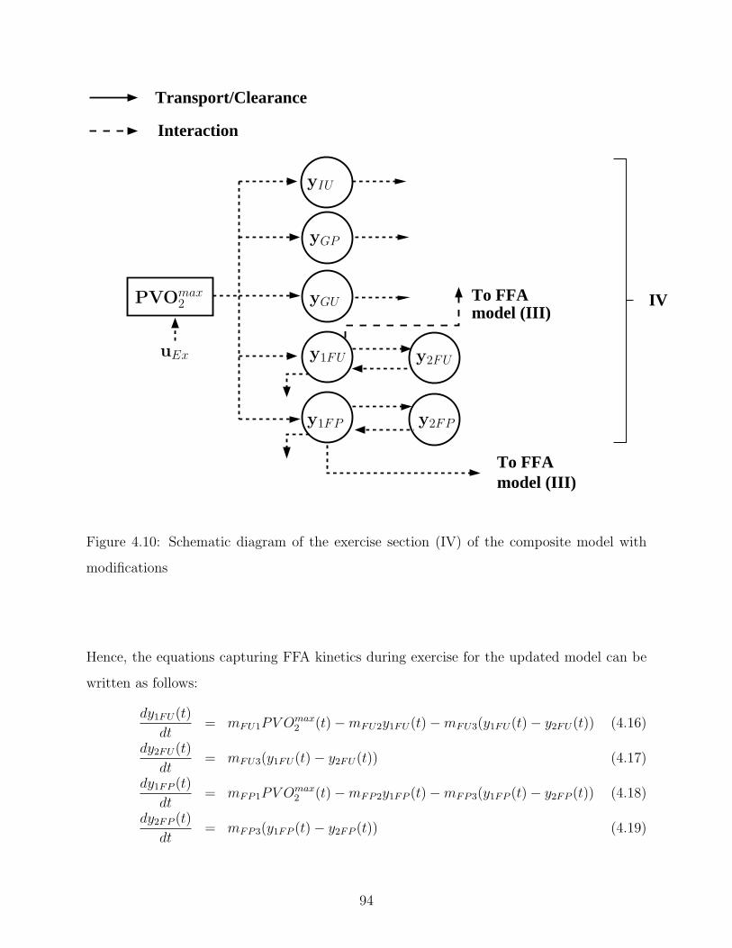
IV

Transport/Clearance

Interaction

To FFAmodel (III)

To FFAmodel (III)

yIU

yGP

yGU

y1FU

y1FP

uEx y2FU

y2FP

PVOmax2

Figure 4.10: Schematic diagram of the exercise section (IV) of the composite model with

modifications

Hence, the equations capturing FFA kinetics during exercise for the updated model can be

written as follows:

dy1FU(t)

dt= mFU1PV Omax

2 (t)−mFU2y1FU(t)−mFU3(y1FU(t)− y2FU(t)) (4.16)

dy2FU(t)

dt= mFU3(y1FU(t)− y2FU(t)) (4.17)

dy1FP (t)

dt= mFP1PV Omax

2 (t)−mFP2y1FP (t)−mFP3(y1FP (t)− y2FP (t)) (4.18)

dy2FP (t)

dt= mFP3(y1FP (t)− y2FP (t)) (4.19)

94

0 50 100 150 200 250 300 3500

200400600800

Rd F

(µm

ol/L

/min

)

0 50 100 150 200 250 300 3500

200400600800

Ra F

(µm

ol/L

/min

)

0 50 100 150 200 250 300 350500

100015002000

FF

A(µ

mol

/L)

Time (min)

Figure 4.11: Plasma FFA kinetics in response to mild exercise (PV Omax2 = 45%) lasting

from tex = 0 to 240 min. The exercise model is comprised of four compartments, y1FU ,

y2FU , y1FP and y2FP , to capture the FFA kinetics during exercise. Model prediction (solid

line) and published data (µ ± σ) (circle) [18] of plasma FFA uptake rate (RdF ) (top); model

prediction (solid line) and published data (µ ± σ) (circle) [18] of plasma FFA production

rate (RaF ) (middle); model prediction (solid line) and published data (µ ± σ) (circle) [18]

of plasma FFA concentration (bottom).

Due to the addition of two new compartments, two extra parameters were introduced (mFU3

and mFP3). Once again, all the parameters (mFU1−FU3 and mFP1−FP3) capturing the exercise

effects on FFA kinetics were estimated by using data from Klein et al. [18]. As it can be

seen in Figure 4.11, the new structure of the exercise model provided a better fit of RdF

95

and RaF during exercise. The superiority of the modified structure is further suggested

by calculating the AIC value (−34.35), which is far less than the previous exercise model

structure. However, the proposed model was unable to capture the sudden burst in plasma

FFA concentration at the commencement of the recovery period, as observed in the mean

data (Figure 4.11: bottom). In order to capture such kind of plasma FFA dynamics at the

end of the exercise period, additional equations are required. Incorporation of extra equations

will increase the number of unknown parameters which are required to be estimated, thereby

increasing the complexity of the model.

4.2.3 Glucose Dynamics

Glucose is taken up from the circulating pool by hepatic tissues for storage (primarily)

and by the peripheral tissue for oxidation purposes. Glucose influences its own uptake in the

hepatic and extra-hepatic tissue (known as glucose effectiveness [5]). Glucose uptake into the

tissues is further facilitated by insulin (known as insulin sensitivity [5]). To maintain plasma

glucose homeostasis, stored glucose in the liver is released back into the circulatory system

via glycogenolysis. The rate of hepatic glucose production (HGP) is indirectly regulated by

insulin [57]. Plasma insulin inhibits glucagon secretion from the pancreatic α-cells [163, 164],

and the latter is a crucial hormone for maintaining HGP [165]. Furthermore, increased

availability of FFA has an inhibitory effect on tissue glucose uptake [58, 59, 166, 167]. The

dynamics of plasma glucose at rest along with the actions of insulin on glucose uptake and

endogenous glucose production, plus the inhibitory effect of FFA on glucose uptake at the

systemic level can be mathematically expressed as given below:

dG(t)

dt= (−pG1G(t)− xG(t)G(t)) fFG(t) + EGP (t) +

uG(t)

VG

(4.20)

dxG(t)

dt= pG2I(t)− pG3xG(t) (4.21)

fFG(t) = fFG0

(1− kFG

(F 3

N(t)

F 3N(t) + s3

FGN

))(4.22)

FN(t) =F (t)

FB

(4.23)

96

EGP (t) = EGP0

(1− kEGP

(x3

EGPN(t)

x3EGPN

(t) + s3EGPN

))(4.24)

dxEGP (t)

dt= pG4(I(t)− xEGP (t)) (4.25)

xEGPN(t) =

xEGP (t)

xEGPB

(4.26)

Here, equation (4.20) represents plasma glucose concentration, G(t) (mgdl

). The first term in

the parenthesis on the RHS of equation (4.20) represents the glucose uptake rate under its

own influence. The bilinear term, xG(t)G(t), captures glucose uptake under the influence of

insulin; xG(t) ( 1min

) represents the action of insulin on tissue glucose uptake. The dynamics

of xG(t) are captured by equation (4.21). The multiplier function fFG(t) is a dimensionless

variable that captures the inhibitory effect of FFA on glucose uptake rate (RdG). Variables

xEGPNand FN are the remote insulin and FFA concentrations normalized with respect to

their basal levels, xEGPBand FB, respectively. The rate of endogenous glucose production

is represented by EGP (t), which is a function of plasma insulin as shown in equation

(4.24). EGP0 ( mgdl·min

) is the rate of hepatic glucose production in the absence of insulin.

The dynamical effect of insulin on EGP (t) is captured by the unobserved remote insulin

concentration, xEGP (t) (µUml

).

To establish the correlation between HGP and insulin concentration, data was obtained

from [19, 20]. In these studies, the rate of glucose production was estimated by measuring

the arterial-venous glucose concentration difference across the liver along with the hepatic

blood flow rate. Due to the nature of the EGP dynamics with respect to the normalized

remote insulin concentration (xEGPN), a 3rd-order Hill function was selected for superior

model accuracy, as indicated in equation (4.24). The value of EGP0 and kEGP were directly

obtained from the literature [20]. Only the saturation constant sEGPNwas estimated to fit

the data, as shown in Figure 4.12.

Randle et al. were the first to introduce the glucose-FFA cycle [58, 59] to explain the

interaction between CHO and fat metabolism. It was proposed that an increase in FFA

availability will enhance fat oxidation, thus causing an increase in acetyl-CoA production,

which will result in downregulating the rate-limiting CHO metabolizing enzymes. Due to

97

0 1 2 3 4 5 60

0.5

1

1.5

2

2.5

xEGP

N

EG

P (

mg/

dL/m

in)

Figure 4.12: Model fit (solid line) versus published data (µ± σ) (circle) [19, 20] of endogenous

glucose production rate, EGP , as a function of normalized insulin concentration xEGPN

this phenomenon, tissue glucose uptake will decrease [168]. The correlation between glucose

uptake rate, RdG, and plasma FFA was captured by utilizing data from [8, 21], where

experiments were performed on healthy subjects by employing euglycemic-hyperinsulinemic

clamps. The overall glucose uptake rate was measured at various plasma FFA levels (Figure

4.13). In Figure 4.13, the y-axis represents glucose uptake rate normalized with respect to

its basal level (fFG). The x-axis represents normalized plasma FFA concentration (FN). The

gain parameter, kFG, from equation (4.22) was directly obtained from the data [8, 21]. Only

the saturation constant, sFGN, was estimated to fit the data. Once again, due to the nature

of the dynamics of fFG with respect to the normalized FFA concentration, a 3rd-order Hill

function was selected, as shown in equation (4.22). All the parameter values are given in

Table 4.1.

98

0 0.5 1 1.5 2 2.5 30.5

0.6

0.7

0.8

0.9

1

1.1

1.2

1.3

FN

f FG

Figure 4.13: Model fit (solid line) versus published data (µ ± σ) (circle) [8, 21] of normalized

glucose uptake rate, fFG, as a function of normalized FFA concentration FN

At basal steady state conditions (i.e., F (t) = FB), the value of fFG becomes equal to 1.

Hence, equations (4.20) and (4.21) reduce to:

pG1 =EGPB

GB

− xGB(4.27)

xGB=

pG2

pG3

IB (4.28)

Here, EGPB, GB, and IB are the endogenous glucose production rate, plasma glucose

concentration, and plasma insulin concentration at the basal level, respectively.

99

Parameters pG2 and pG3 from equation (4.21), representing the insulin action on tissue

glucose uptake, and parameter pG4 from equation (4.25), capturing the dynamical effect

of insulin mediated-suppression on hepatic glucose production, were estimated by using

data from Regittnig et al. [22]. In this study, a labeled-IVGTT was performed in T1DM

patients. At time t=0 min, a bolus of glucose labeled with a stable isotope tracer, D-

[6,62H2]glucose, (hot glucose) was administered intravenously. A bolus of insulin was also

injected at t=0 min, followed by a continuous insulin infusion at constant rate to maintain

the basal level (Figure 4.14). Blood samples were gathered at regular intervals to measure

the concentrations of plasma insulin, tracer glucose, and total glucose (endogenous glucose

plus the labeled exogenous glucose), as shown in Figure 4.14 and 4.15. Parameters estimated

from the labeled-IVGTT data provide a significant advantage over the unlabeled-IVGTT [5].

Due to the presence of tracer, it is possible to monitor the dynamics of glucose disappearance

only. Hence, labeled IVGTT data can separate the individual contributions of insulin on

glucose production and utilization, which is impossible to achieve from unlabeled-IVGTT

data. This technique was first introduced by Cobelli et al. [5] to minimize model errors and

ambiguities that may arise when estimating parameters of the classical minimal model [1]

from the unlabeled data only.

To estimate the parameters (pG2, pG3, and pG4) from the labeled-IVGTT data [22], two

glucose models were used simultaneously. The total glucose concentration was captured by

using equations (4.20), (4.21), (4.24), (4.25), and (4.22); this forms the cold glucose model.

On the other hand, the tracer glucose concentration was captured by a new ODE as shown

below:

dGh(t)

dt= (−pG1Gh(t)− xG(t)Gh(t)) fFG (4.29)

Here, Gh(t) (mgdl

) represents concentration of the tracer glucose. Equation (4.29) along with

equations (4.21) and (4.22) forms the hot glucose model. Simultaneous fitting of the total

and tracer glucose data (as shown in Figure 4.15) by using the cold and hot glucose models,

respectively, should provide better informed parameter estimates.

100

0 50 100 150 200 250 300

20

40

60

80In

sulin

(µ

U/m

L)

0 50 100 150 200 250 3000

2

4

x GN/x

EG

PN

Time (min)

Figure 4.14: Model prediction (solid line) versus published data (µ± σ) (circle) [22] of plasma

insulin concentration in response to a labeled-IVGTT (top); normalized insulin action with

respect to their basal values on glucose uptake (solid line) and endogenous glucose production

(dashed line) due to administration of insulin bolus at t=0 min (bottom).

Exercise induces an elevation in glucose uptake rate, RdG ( mgdl·min

), by the working muscles.

To maintain glucose homeostasis in the systemic level, glucose production rate (RaG, mgdl·min

)

is also elevated during exercise due to the accelerated rate of glycogenolysis. As mentioned

earlier, an increased FFA oxidation results in downregulation of pyruvate dehydrogenase

(PDH) [168]; this is an important enzyme for glucose oxidation. This regulatory mechanism,

which is true at rest, is overridden by other factors during exercise [168]. Hence, studies have

revealed no effect of elevated FFA on glucose uptake during exercise [168, 169]. In order to

101

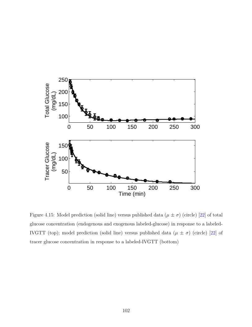
0 50 100 150 200 250 300

100

150

200

250

Tot

al G

luco

se(m

g/dL

)

0 50 100 150 200 250 300

50

100

150

Tra

cer

Glu

cose

(mg/

dL)

Time (min)

Figure 4.15: Model prediction (solid line) versus published data (µ ± σ) (circle) [22] of total

glucose concentration (endogenous and exogenous labeled-glucose) in response to a labeled-

IVGTT (top); model prediction (solid line) versus published data (µ ± σ) (circle) [22] of

tracer glucose concentration in response to a labeled-IVGTT (bottom)

102

incorporate all these important physiological effects of mild-to-moderate short-term exercise

on glucose dynamics, equations (4.20) and (4.23) were modified as follows:

dG(t)

dt= (−pG1G(t)− xG(t)G(t)) fFG(t)− W

VG

yGU(t) + EGP (t) +W

VG

yGP (t)

+uG(t)

VG

(4.30)

FN(t) =1

FB

((1− b)F (t) + bF0) (4.31)

The dynamics of the new terms yGU(t), yGP (t), and b, can be written as:

yGU(t)

dt= mGU1PV Omax

2 (t)−mGU2yGU(t) (4.32)

yGP (t)

dt= mGP1PV Omax

2 (t)−mGP2yGP (t) (4.33)

b =PV Omax

2 (t)

PV Omax2 (t) + sPV

(4.34)

Here, the variables yGU(t) and yGP (t) ( mgkg·min

) represent the exercise-induced glucose uptake

and production rates. F0 represents the FFA concentration at initial (or basal) conditions

(F0 = F (0)). At rest, b becomes equal to zero, as PV Omax2 = 0. Hence, equation (4.31)

reduces to equation (4.23). However, during exercise (PV Omax2 � 1) b approaches 1, as sPV

is assigned a value of 1. Therefore, equation (4.31) becomes FN(t) = F0/FB at PV Omax2 (t)

� 1. As the normalized FFA concentration is fixed at its initial condition during physical

activity, fFG remains unperturbed at its initial condition. As a result of this, the increasing

concentration of plasma FFA during exercise has no effect on glucose uptake rate. The

motivation behind selecting sPV = 1 is that at PV Omax2 = 40% almost 97% of FN(t) is

contributed by the second part of the RHS of equation 4.31 (i.e, F0

FB), which concur with the

experiment performed by Odland et al. [168] where elevated FFA had no significant effect

on glucose uptake rate at the same level of exercise.

In order to capture the exercise-induced changes in glucose kinetics, data was procured

from Wolfe et al. [12], where healthy subjects performed exercise at PV Omax2 = 40% for 60

min. Blood samples were obtained at regular intervals to measure glucose uptake rate and

103

hepatic glucose production rate during and after exercise, as shown in Figure 4.16. From

equation (4.30), plasma glucose uptake (RdG) and production (RaG) rate can be written as:

RdG = −[(−pG1G(t)− xG(t)G(t)) fFG(t)− W

VG

yGU(t)

](4.35)

RaG = EGP (t) +W

VG

yGP (t) (4.36)

In order to obtain the model prediction of glucose uptake rate during exercise, parameters

mGU1 and mGU2 were estimated, as shown in Figure 4.16 (top). To capture the glucose

production rate during exercise, parameters mGP1 and mGP2 were adjusted, as shown in

Figure 4.16 (middle). With the onset of exercise, both RdG and RaG were elevated. As

the production matched utilization, the overall plasma glucose homeostasis was maintained

(Figure 4.16: bottom).

During prolonged exercise, the rate of hepatic glycogenolysis diminishes due to the limited

supply of liver glycogen stores [15]. As a result of this, the net endogenous glucose production

rate also decreases. As glucose production can no longer match the uptake rate, plasma

glucose concentration declines and reaches hypoglycemic levels during prolonged exercise

[13, 15]. In order to capture the glucose dynamics during prolonged exercise, equation (4.30)

can be re-written as follows:

dG(t)

dt= (−pG1G(t)− xG(t)G(t)) fFG(t)− W

VG

yGU(t) + EGP (t)

+W

VG

(yGP (t)− yGly(t)) +uG(t)

VG

(4.37)

The new variable yGly(t) ( mgkg·min

) represents the dynamics associated with the rate of glycogenol-

ysis due to depletion of the available hepatic glycogen stores. It captures the same physio-

logical effects of prolonged exercise on plasma glucose level as the variable Ggly(t) (equation

3.10) used in the exercise minimal model in Section 3.2.

104

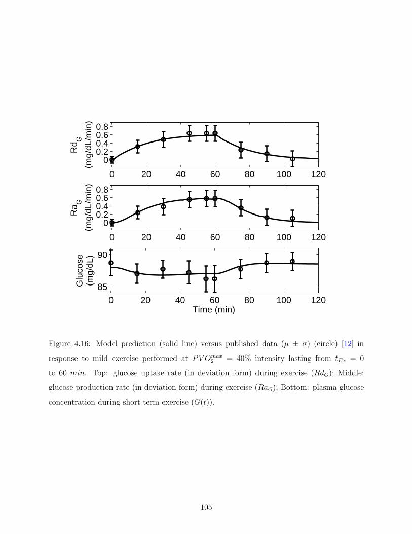
0 20 40 60 80 100 120

00.20.40.60.8

Rd G

(mg/

dL/m

in)

0 20 40 60 80 100 120

00.20.40.60.8

Ra G

(mg/

dL/m

in)

0 20 40 60 80 100 120

85

90

Glu

cose

(mg/

dL)

Time (min)

Figure 4.16: Model prediction (solid line) versus published data (µ ± σ) (circle) [12] in

response to mild exercise performed at PV Omax2 = 40% intensity lasting from tEx = 0

to 60 min. Top: glucose uptake rate (in deviation form) during exercise (RdG); Middle:

glucose production rate (in deviation form) during exercise (RaG); Bottom: plasma glucose

concentration during short-term exercise (G(t)).

105

Hence, the dynamics of glycogenolysis during prolonged exercise can be mathematically

expressed as follows, adapted from equation (3.10):

dyGly(t)

dt=

0 A(t) < ATH

k A(t) ≥ ATH

−yGly(t)

T1uEx(t) = 0

(4.38)

Here, A(t) is the integrated exercise intensity (uEx(t)) having the same mathematical ex-

pression as equation (3.11) in Section 3.2. ATH is the critical threshold value of energy

expenditure which is a function of exercise intensity and duration, same as equation (3.9)

(Section 3.2). After the commencement of exercise, as long as A is less than ATH , the rate

of glycogenolysis (yGly) remains unaffected due to the presence of sufficient hepatic glycogen

stores. However, yGly starts to decline at a rate k, once A exceeds the threshold value (ATH).

At the end of exercise, i.e., the recovery period, liver glycogen stores are replenished back

to its basal level. The time required for yGly to return back to its basal level after exercise

is represented by the pseudo-time constants T1 and T2 (equation (3.11) from Section 3.2).

In order to estimate the parameter values of k and T1, data was obtained from an

experiment performed by Ahlborg et al. [15], where healthy subjects performed moderate

level exercise (PV Omax2 = 60%) lasting for 210 min. Blood samples were taken at regular

intervals during and immediately after exercise to measure blood glucose concentration, as

shown in Figure 4.17 (bottom). With the onset of exercise, both RdG and RaG are elevated

above their basal levels, as shown in Figure 4.17 (top) and (middle) panels, respectively. As

the duration of exercise exceeded a certain threshold, the rate of glycogenolysis started to

decrease from its original value. As a result of this, RaG started to decline until the end of

exercise, causing plasma glucose to reach hypoglycemic levels (Figure 4.17: bottom).

106

0 50 100 150 200 2500

0.5

1R

d G(m

g/dL

/min

)

0 50 100 150 200 2500

0.5

1

Ra G

(mg/

dL/m

in)

0 50 100 150 200 250

60

80

Glu

cose

(mg/

dL)

Time (min)

Figure 4.17: Model prediction (solid line) versus published data [15] (µ ± σ) (circle) in

response to moderate exercise performed at PV Omax2 = 60% intensity lasting from tEx = 0

to 210 min. Top: glucose uptake rate in deviation variables during exercise (RdG); Middle:

glucose production rate in deviation variables during exercise (RaG); Bottom: plasma glucose

concentration during prolonged exercise (G).

4.3 PARAMETRIC SENSITIVITY ANALYSIS BY FINITE DIFFERENCE

METHOD

The composite model can be expressed as a set of Nx differential equations with Nx states

(x) and M parameters (θ). The Nx by M parameter sensitivity matrix can be calculated by

using the finite difference approximation method, in which the sensitivity coefficients (si,j)

107

Table 4.1: Parameter values of the composite model.

Nos. Parameters Values Source Nos. Parameters Values Source

1 kEFP 0.92889 [16] 20 pG3

(1

min

)0.35 –

2 sEFPN1.169 [16] 21 pG4

(1

min

)0.073535 –

3 EFP0

(µmolL·min

)209.09 [16] 22 mIU1

(1

min2

)0.0028176 –

4 kEGP 0.9909 [20, 19] 23 mIU2

(1

min

)1.7354 –

5 sEGPN0.84115 [20, 19] 24 mFU1

(mumolkg·min2

)0.013736 –

6 EGP0

( mgdL·min

)2.618 [20, 19] 25 mFU2

(1

min

)0.032272 –

7 sFG 1.0472 [8, 21] 26 mFU3

(1

min

)0.0023229 –

8 fFG0 1.202 [21] 27 mFP1

(mumolkg·min2

)0.016831 –

9 kFG 0.38075 [8, 21] 28 mFP2

(1

min

)0.018241 –

10 n(

1min

)0.38075 [1] 29 mFP3

(1

min

)0.024841 –

11 VI (mL) 10.133 [1] 30 mGU1

(mg

kg·min2

)0.0021874 –

12 pF1

(1

min

)0.18727 – 31 mGU2

(1

min

)0.058974 –

13 W (kg) 70.0 [18] 32 mGP1

(mg

kg·min2

)0.0009152 –

14 VF (L) 3.0 [18] 33 mGP2

(1

min

)1.3073 –

15 VG (dL) 117.0 [1] 34 T1 (min) 1 –16 pF2

(1

min

)0.036513 – 35 k

(1

min

)0.0038 –

17 pF3

(1

min

)0.03909 – 36 sPV 1 –

18 pG1

(1

min

)0.0076 – 37 T2 (min) 10 –

19 pG2

(mL

µU ·min2

)0.00010259 – 38 mPV

(1

min

)0.8 [63]

are calculated from the difference of nominal and perturbed solutions [170, 171].

si,j(t) =∂xi(t)

∂θj

=xi(θj + ∆θj, t)− xi(θj, t)

∆θj

(4.39)

Here, i ∈ [1, Nx] and j ∈ [1, M ]. To facilitate direct comparison of responses across different

parameters, a normalized sensitivity coefficient (si,j) is calculated [170]:

si,j(t) =∂xi(t)

∂θj

· θj

xi

(4.40)

108

For the evaluation of dynamic sensitivity, a L2-norm operation is performed to calculate the

relative sensitivity (RS) along the time axis. RS can be mathematically expressed as:

RSi,j =1

NP

√√√√ NP∑k=1

|si,j(k)|2 (4.41)

Here, k is the point in time when a sample is collected and NP is the total number of sample

points observed.

By using this method, a parametric relative sensitivity matrix (RSi,j) of the composite

model was generated. The matrix was comprised of 16 rows (i ∈ [1 to 16]), representing

the states, and 38 columns (j ∈ [1 to 38]), representing all the parameters of the model. A

graphical representation of the RSi,j values is provided in Figure 4.18. The y-axis lists the

parameters by number; this mapping is provided in Table 4.1. The x-axis lists the states

of the model as per Table 4.2, and the z-axis represents the parametric relative sensitivity

values corresponding to each state. A higher RSi,j value indicates the state is more sensitive

to the specified parameter.

By closely observing the insulin state (I(t)), RS1,1:38, reveals that the plasma insulin is

highly sensitive to its own parameters, n and VI , which is expected (Figure 4.19: top). The

FFA state (F (t)), RS2,1:38, indicates that plasma FFA is most sensitive to parameter pF1

followed by parameter EFP0 (Figure 4.19: middle). Plasma FFA also exhibits significant

sensitivity towards the parameters associated with I(t). The parameters associated with

FFA production during exercise (mFP1, mFP2, and mFP3) are relatively more sensitive than

the parameters associated with FFA uptake during exercise (mFU1, mFU2, and mFU3). For

the glucose state (G(t)), RS3,1:38, the most sensitive parameters are the ones associated

with I(t), as shown in Figure 4.19 (bottom). Parameters associated with the endogenous

glucose production rate (kEGP , sEGP , and EGP0) are more sensitive than the parameter

pG1, which captures the effect of glucose on its own uptake rate. Parameters representing

insulin action on glucose uptake by the tissues (pG2 and pG3) are more sensitive than the

parameter representing the insulin action on suppression of endogenous glucose production

rate (pG4). Also, the parameters representing glucose uptake during exercise (mGU1 and

109

2 4 6 8 10121416

0

10

20

30

40

0

50

100

150

200

250

States

Parameters

Rel

. Sen

sitiv

ity

Figure 4.18: Parametric relative sensitivity analysis of the composite model for all the sixteen

states.

110

Table 4.2: List of states of the composite model used in the parametric sensitivity analysis

Nos. Equations Nos. Equations1 (4.1) 9 (4.3)2 (4.13) 10 (4.16)3 (4.37) 11 (4.17)4 (4.2) 12 (4.18)5 (4.6) 13 (4.19)6 (4.11) 14 (4.32)7 (4.21) 15 (4.33)8 (4.25) 16 (4.38)

mGU2) are significantly more sensitive than the parameters representing glucose production

during exercise (mGP1 and mGP2).

Lots of important informations can be extracted from the parametric sensitivity analysis.

For example, endogenous glucose production plays a major role in maintaining glucose

homeostasis. Hence, more experiments are required to accurately define the correlation

between EGP (t) and I(t). Moreover, the RSi,j matrix indicates that the suppression of

insulin plays a bigger role in elevating endogenous glucose production rate during physical

activity than the exercise-mediated glucose production. However in case of FFA, the exercise-

mediated fat production was more prominent than the elevated lipolysis due to insulin

suppression during exercise. Experimental studies could be performed to verify the extent

of hypoglycemia that might be reached during short-term exercise by clamping the plasma

insulin at basal level.

4.4 VALIDATION OF THE LOWER-ORDER COMPOSITE MODEL

Once the model was formulated and the parameters were estimated from the literature data,

simulation studies were performed to validate the various components of the model. Model

predictions were compared with new data sets (i.e., data different from the ones used for

111

0 5 10 15 20 25 30 35 400

100

200

300

0 5 10 15 20 25 30 35 400

100

200

300

Rel

. Sen

sitiv

ity

0 5 10 15 20 25 30 35 400

100

200

300

Parameters

RS1,1:38

RS2,1:38

RS3,1:38

Figure 4.19: Parametric relative sensitivity analysis of the composite model for the plasma

insulin, I(t) (top), FFA, F (t) (middle), and glucose, G(t) (bottom) states.

parameter estimation), without manipulating the estimated parameter values. As described

in Section 2.3, R2 was used to quantitate the goodness of fit.

4.4.1 Effect of Exercise on Plasma Insulin Concentration

For validation of the insulin model, a simulation test was performed at a mild level of

exercise, PV Omax2 = 30%, lasting for 120 min. With the onset of exercise, plasma insulin

112

level declined due to the accelerated insulin clearance rate. During the recovery period,

plasma insulin concentration climbed back to its basal level. Model validation along with

experimental data of healthy individuals subjected to same exercise protocol [13] is shown

in Figure 4.20. The model prediction emulates the data well. Although, at the 40 min mark

the model slightly underpredicts the data.

0 50 100 150

6

7

8

9

10

11

12

Insu

lin (

μU/m

L)

Time (min)

Figure 4.20: Plasma insulin concentration in response to mild exercise (PV Omax2 = 30)

lasting from tex = 0 to 120 min. Model simulation validation (solid line) and published data

[13] (circles) (µ ± σ) of plasma insulin [R2 = 0.936].

4.4.2 Effect of Insulin on Plasma FFA Dynamics

In order to validate the insulin effects on FFA dynamics, a MI-FSIGT simulation test was

performed, where boluses of insulin were infused at time t = 0 and 20 min at a rate similar to

the experiment performed by Brehm et al. [23] (Figure 4.21: top). Due to the anti-lipolytic

113

action of insulin, plasma FFA declined well below its basal level (Figure 4.21: bottom). The

model predictions, as shown in Figure 4.21, are within one standard deviation of the data.

After the two hour mark, however, the model seems to slightly underpredict the plasma FFA

data.

0 50 100 150 200

200400600800

I(t)

(μU

/mL)

0 50 100 150 200

50

100

150

x EF

P1/x

EF

P2

(μU

/mL)

0 50 100 150 200

200

400

FF

A(μ

mol

/L)

Time (min)

Figure 4.21: Plasma FFA concentration in response to MI-FSIGT test where boluses of

insulin were administered at time t = 0 and 20 min. Model simulation validation (solid line)

and published data [23] (circles) (µ ± σ) of plasma insulin concentration [R2 = 0.999] (top);

model predictions of remote insulin xEFP1 (solid line) and xEFP2 (dashed line) concentrations

(middle); model simulation validation (solid line) and published data [23] (circles) (µ ± σ)

of plasma FFA concentration [R2 = 0.998] (bottom).

4.4.3 Effect of Exercise on Plasma FFA Dynamics

For validation of the exercise effects on plasma FFA, a simulation study of a mild level of

exercise, PV Omax2 = 30%, was performed for 2 hours. With the onset of exercise, plasma

114

FFA utilization (RdF ) and production (RaF ) rate continuously increased until the end of

physical activity. As the lipolytic rate was more than the uptake rate, FFA concentration

increased steadily until the end of exercise. During the recovery period, FFA level remained

elevated for about 20-30 min before it started to gradually decline toward its basal level.

A comparison of the model prediction and experimental data from subjects undergoing the

same exercise protocol [13] is provided in Figure 4.22. The model performed well during the

exercise period, however, the model predictions during the recovery period were slower than

the data.

0 50 100 1500

100200300

Rd F

(µm

ol/L

/min

)

0 50 100 150

100200300

Ra F

(µm

ol/L

/min

)

0 50 100 1501000

1500

2000

FF

A(µ

mol

/L)

Time (min)

Figure 4.22: Plasma FFA concentration in response to mild exercise (PV Omax2 = 30) lasting

from tex = 0 to 120 min. Model prediction of plasma FFA uptake rate, RdF (top); model

prediction (solid line) of plasma FFA production rate, RaF (middle); model simulation

validation and published data [13] (circles) (µ ± σ) of plasma FFA concentration [R2 =

0.989] (bottom).

115

4.4.4 Effect of Insulin on Plasma Glucose Dynamics

For the glucose model validation, a labeled MI-FSIGT simulation test was performed, where

boluses of insulin were administered at time t = 0 and 20 min (Figure 4.23) and a bolus of

labeled glucose was infused at t = 0 min, at a rate similar to the experiment performed by

Nagasaka et al. [24]. Model predictions of the total glucose concentration (i.e., endogenous

glucose plus the labeled exogenous glucose) and tracer glucose concentrations obtained from

the cold (equation (4.20)) and hot glucose model (equation (4.29)), respectively, along with

the data [24] are provided in Figure 4.24. The model predicted glucose kinetics after the first

insulin bolus seems to be marginally slower than the data. However, the model performed

quite well in emulating the data after the second insulin bolus.

4.4.5 Effect of Exercise on Glucose Dynamics

In order to validate the short-term exercise effects on glucose kinetics, a simulation test was

performed at moderate level exercise, PV Omax2 = 50%, for 45 min. With the onset of exercise,

both RdG and RaG were elevated. As production matched uptake, the overall plasma

glucose concentration remained within the normoglycemic range. The model predictions

alongside experimental data of T1DM patients [14] are plotted in Figure (4.25). The model

predicted glucose kinetics are well within one standard deviation of the data. Validation of

the composite model using T1DM patient data increased the confidence in the model.

To validate the glucose model during prolonged exercise, a separate simulation study of

mild exercise was performed at PV Omax2 = 30% which lasted for 120 min. As the integrated

exercise intensity exceeded the threshold value, hepatic glycogen stores started to deplete;

this caused a net reduction in glucose production. Due to this imbalance between production

and utilization, plasma glucose concentration started to decline at the later stages of exercise.

A comparison between the model predictions and data obtained from a study performed by

Ahlborg et al. on healthy subjects using the same exercise protocol are provided in Figure

4.26. Once again, the model predictions are well within one standard deviation of the data.

116

0 50 100 150 200

20

40

60

80

Insu

lin(μ

U/m

L)

0 50 100 150 200

2

4

6

8

10

x GN/x

EG

PN

Time (min)

Figure 4.23: Plasma insulin concentration in response to labeled-MI-FSIGT test where

insulin boluses were administered at times t = 0 and 20 min. Model simulation validation

(solid line) and published data [24] (circles) (µ ± σ) of plasma insulin concentration [R2

= 0.997] (top); model predictions of normalized insulin action, xNG , (solid line) and xN

EGP

(dashed line) with respect to their basal values (bottom).

4.4.6 Effect of FFA on Glucose Uptake Rate at Rest

At rest, an increasing FFA concentration suppresses plasma glucose uptake rate. This

inhibitory effect of FFA on RdG is captured by the dimensionless multiplicative function,

fFG (equation (4.22)). In order to validate this physiological interaction between FFA and

glucose, a simulation study was performed where euglycemic-hyperinsulinemic clamps were

employed. Insulin was elevated up to 62 µUml

to match the data obtained from an experimental

study performed by Thiebaud et al. [8]. Intralipids were infused at either: )i) a low rate

117

0 50 100 150 200

100

200

300T

otal

Glu

cose

(mg/

dL)

0 50 100 150 2000

100

200

Hot

Glu

cose

(mg/

dL)

Time (min)

Figure 4.24: Plasma glucose concentration in response to labeled-MI-FSIGT test where a

labeled-glucose bolus was infused at time t = 0 min. Model simulation validation (solid line)

and published data [24] (circles) (µ ± σ) of plasma total glucose concentration [R2 = 0.999]

(top); model simulation validation (solid line) and published data [24] (circles) (µ ± σ) of

labeled-glucose concentration [R2 = 0.99] (bottom).

to maintain basal levels of 340 µmoll

FFA, or (ii) a high rate elevating FFA levels to 650

µmoll

. These FFA model predictions are shown by the dashed and dotted lines in Figure

4.27 (top). In absence of intralipid infusion (control study), FFA declined freely without

any restrictions, as shown by the solid line in Figure 4.27 (top). Due to the elevated plasma

FFA levels, glucose uptake rate was suppressed as shown by the dashed and dotted lines in

Figure 4.27 (bottom). The model predictions are well within one standard deviation of the

experimental data [8], thus indicating the capability of the model to accurately predict the

glucose-FFA cycle.

118

0 20 40 60 80 100 120

0

0.5

1

Rd G

(mg/

dL/m

in)

0 20 40 60 80 100 120

0

0.5

1

Ra G

(mg/

dL/m

in)

0 20 40 60 80 100 12080

100

Glu

cose

(mg/

dL)

Time (min)

Figure 4.25: Model simulation validation (solid line) versus published data [15] (µ ± σ)

(circles) in response to moderate exercise performed at PV Omax2 = 50% intensity lasting

from tEx = 0 to 45 min. Glucose uptake rate (in deviation form) during exercise (RdG)

[R2 = 0.935] (top); glucose production rate (in deviation form) during exercise (RaG) [R2 =

0.955] (middle); plasma glucose concentration during short-term exercise (G(t)) [R2 = 0.82]

(bottom).

4.5 SUMMARY

In this chapter, a 16-state metabolic model of insulin, glucose, and FFA was developed. The

primary goal was to characterize the dynamics of the major energy-providing substrates and

insulin at rest, as well as during exercise. The model successfully captured the physiological

effects of FFA and mild-to-moderate exercise on plasma glucose concentration. This novel

approach of incorporating both FFA and exercise effects in the glucose-insulin metabolic

119

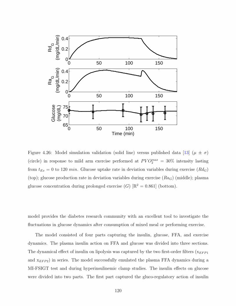
0 50 100 1500

0.2

0.4

Rd G

(mg/

dL/m

in)

0 50 100 1500

0.2

0.4

Ra G

(mg/

dL/m

in)

0 50 100 15065

70

75

Glu

cose

(mg/

dL)

Time (min)

Figure 4.26: Model simulation validation (solid line) versus published data [13] (µ ± σ)

(circle) in response to mild arm exercise performed at PV Omax2 = 30% intensity lasting

from tEx = 0 to 120 min. Glucose uptake rate in deviation variables during exercise (RdG)

(top); glucose production rate in deviation variables during exercise (RaG) (middle); plasma

glucose concentration during prolonged exercise (G) [R2 = 0.861] (bottom).

model provides the diabetes research community with an excellent tool to investigate the

fluctuations in glucose dynamics after consumption of mixed meal or performing exercise.

The model consisted of four parts capturing the insulin, glucose, FFA, and exercise

dynamics. The plasma insulin action on FFA and glucose was divided into three sections.

The dynamical effect of insulin on lipolysis was captured by the two first-order filters (xEFP1

and xEFP2) in series. The model successfully emulated the plasma FFA dynamics during a

MI-FSIGT test and during hyperinsulinemic clamp studies. The insulin effects on glucose

were divided into two parts. The first part captured the gluco-regulatory action of insulin

120

0 50 100 150

200

400

600

FF

A(µ

mol

/L)

0 50 100 1500

0.5

1

1.5

Rd G

(mg/

dL/m

in)

Time (min)

Figure 4.27: Plasma FFA concentration due to infusion of intralipids at high rate (dotted

line), low rate (dashed line), and saline (no intralipid infusion) (solid line) (top); published

data [8, 21] (µ ± σ) (circle) versus model simulation validations of plasma glucose uptake

rate at high (dotted line) [R2 = 0.923] and low (dashed line) [R2 = 0.901] intralipid infusion

rates, as well as no intralipid infusion (solid line) [R2 = 0.944] (bottom).

in promoting glucose uptake into the tissues via the filter xG. The second part captured the

insulin-mediated suppression of endogenous glucose production by considering the saturating

function EGP (t), along with the filter xEGP . Parameters of the filter equations were

estimated by using a labeled-IVGTT. This technique of using hot and cold IVGTT data

facilitates separation of the insulin action on glucose utilization and production [75, 5], thus

providing more confidence in the estimated parameters.

The exercise effects on insulin, glucose, and FFA were divided into five sections. The

exercise-induced clearance of insulin was captured by the first-order filter, yIU . For the

121

glucose dynamics, the elevated rates of glucose production and utilization during exercise

were captured by yGP and yGU , respectively. During short-term mild-to-moderate exercise,

plasma glucose typically remains within the normoglycemic range as glucose production

matches the utilization rate. However, as the integrated exercise intensity exceeded a certain

threshold, the rate of glycogenolysis is expected to decline due to the depletion of available

hepatic glycogen stores. As a result of this, the net glucose production rate will also decrease.

This phenomenon was captured by incorporating the yGly variable. In order to capture the

exercise effects on FFA kinetics, four compartments were used as shown in Figure 4.10. A

set of two compartments represented the exercise-induced FFA uptake rate (y1FU and y2FU),

and the remaining two compartments captured the elevated rate of FFA production during

exercise (y1FP and y2FP ).

The model also successfully captured the inhibitory effects of FFA on glucose uptake rate

at rest. This phenomenon is also known as the glucose-FFA cycle, which was first introduced

by Randle et al. [58, 59] in the early 1960’s.

This more complete metabolic model has the potential to provide an excellent plat-

form for the control community in development of model-based closed-loop insulin delivery

systems for T1DM patients. The primary advantage of utilizing the composite model in

the development of an artificial pancreas instead of other metabolic models present in the

literature, is because of its unique ability to predict plasma glucose concentration in response

to disturbances from mixed meals (CHO and fat) consumption and from exercise. The model

can also accurately predict the interactions taking place between the major energy-providing

metabolites and hormones during rest and exercise.

122

5.0 A PHYSIOLOGICALLY-BASED FFA, GLUCOSE, AND INSULIN

MODEL

In the earlier chapters, semi-empirical metabolic models were developed to capture the effects

of FFA and exercise on glucose-insulin dynamics. In Chapter 2, the extended minimal

model was synthesized by modifying the classical minimal model [1] to incorporate plasma

FFA dynamics and the interactions of FFA with glucose and insulin. The model consisted

of lumped compartments and parameters capturing the systemic physiological interactions

between FFA, glucose, and insulin. Only the necessary metabolic processes of FFA were

considered in order to maintain the simplifying approach of the minimal model. Due to the

minimum number of equations, a lesser number of parameters needed to be estimated, which

generally makes simplified models easily identifiable, as well as less time intensive to build.

However, these models do not differentiate the distribution of metabolic substrates at the

various organ/tissue levels. Typically, in such models the entire body is treated as a single

well-mixed space. Hence, the semi-empirical model fails to provide a detailed explanation of

the biology that is actually taking place in the body, particularly at the organ/tissue scale.

In contrast, physiologically-based models are much more complex in terms of number

of equations and parameters. These models provide a great deal of insight into the system

as they are derived from known physiology. Typically in such models, the body is divided

into compartments representing the major organs and tissues. Biologically relevant organ-

specific metabolism can be captured, thereby making the model more structurally accurate.

Physiologically-based models can also provide motivation to perform new experiments in

order to validate certain model components, thereby incorporating biological understanding

of tissue metabolic processes. However, such detailed models come at a price. Usually,

123

these models are very time intensive to develop, and often a large number of parameters are

required to be estimated from limited available data sets.

Tiran et al. were the first to attempt to develop a physiologically-based glucose-insulin

model in the mid 1970s [76, 106]. Compartments representing the major glucose utilizing or-

gans/tissues were used. Glucose and insulin were distributed into each of these compartments

via the circulatory system. Constant glucose uptake or production rates were incorporated in

each of the physiological compartments. Later, a pharmacokinetic-pharmacodynamic model

of metabolism was developed by Sorensen [2] in the mid 1980s, which was based on an

earlier model by Guyton et al. [107]. The model was comprised of two sub-units capturing

the glucose and insulin concentrations just like the Guyton model; in addition it also included

the glucagon dynamics and its interactions with the glucose-insulin system. In the glucose

and insulin sub-units, distribution of the energy-providing substrate and the gluco-regulatory

hormone were modeled at the organ/tissue levels, respectively. The glucagon sub-unit

consisted of a single well-mixed compartment representing the glucagon concentration at

the systemic level. Metabolic rates causing addition or removal of glucose were assigned to

each of the compartments. Hyperbolic tangent functions were used to represent the sigmoidal

nonlinearities observed in the experimental data between the metabolic sinks/sources and

the regulatory hormones.

Later in the 1990s, Cobelli et al. [78] developed another semi-physiological glucose-

insulin model. The model consisted of several components representing physiologically-

based glucose and insulin interactions; however, glucose distribution at the organ level was

not considered. Most of the detailed metabolic models present in the literature do not

consider FFA dynamics. As mentioned earlier, FFA plays a vital role in providing energy

to the tissues. Also fluctuations in FFA dynamics alter glucose dynamics to a significant

level. Hence, in this chapter a physiologically-based FFA model was developed and was

coupled with the existing glucose-insulin model developed by Sorensen [2], which has a

similar structure. The objective is to predict FFA distribution at the organ/tissue levels and

to capture the interactions between glucose, insulin, and FFA through out the body.

In Section 5.1, the glucose-insulin model developed by Sorensen [2] is presented in detail.

The physiologically-based FFA model is presented in Section 5.2. The original Sorensen

124

model was modified in order to integrate the FFA model, as indicated in Section 5.3.

Metabolic sinks and sources of the FFA model are presented in Section 5.4. In Section

5.5, the interconnection points between the FFA and the glucose model are discussed in

details. Finally, the simulation results of the physiologically-based model are presented in

Section 5.6.

5.1 GLUCOSE-INSULIN PHYSIOLOGICAL MODEL OF SORENSEN

The model is comprised of three sub-systems: glucose, insulin, and glucagon. Eleven

ODEs are used to define the glucose sub-system, seven define the insulin sub-system, and

one models the glucagon dynamics. The glucose model consisted of several compartments

representing the vital glucose-utilizing organs/tissues: brain, heart/lungs, kidney, liver, gut,

and periphery, as shown in Figure 5.1. The peripheral compartment represents skeletal

muscle, as well as adipose tissue (AT). The heart/lungs, kidney, liver, and gut compartments

consist of a single well-mixed space where the substrate concentrations are assumed to be

homogeneous, as shown in Figure 5.2. Each compartment is fed by the arterial blood

influx and drained by the venous blood efflux. In some organs and tissues (mainly the

brain and periphery) the capillary wall permeability is sufficiently low, thereby causing a

slow equilibration of substrates between the capillary and the interstitial spaces. Hence,

compartments representing such organs/tissues included two well-mixed spaces (capillary

and interstitial space) where the substrate concentrations are assumed to be homogeneous

(see Figure 5.3). Once again, substrates enter the capillary space via the arterial route and

is drained by the venous route. The substrates diffuse through the capillary wall into the

interstitial space from where they are ultimately consumed by the cells. Metabolic sinks,

representing the rate of glucose consumption due to oxidation or storage, were added to each

of these compartments. In the liver glucose flux is bi-directional, as it consumes glucose

mostly for storage purposes in the form of glycogen, as well as releases the stored glucose in

the circulatory system whenever the body requires energy. Hence, both metabolic sink and

source were incorporated in the liver compartment. The insulin model had a similar structure

125

like the glucose model. Only difference is that, the brain had a single compartment unlike

the glucose model, as studies have shown that the capillary wall of the brain is impermeable

to insulin passage to the interstitial fluid space [172]. Metabolic sinks representing insulin

clearance were added to the liver, kidney, and periphery compartments. Glucagon was

modeled using a single ODE capturing the systemic glucagon concentration.

Mass balances were performed across each physiologic compartment to capture the solute

distribution. Typically, where the capillary wall resistance is negligible thus allowing a rapid

equilibration of the solute (X) between the capillary and the interstitial fluid spaces, only

one mass balance equation is sufficient to capture the dynamics, as given below:

V XJ

dCJ(t)

dt= QX

J (CJi(t)− CJ(t))−RJU (5.1)

As indicated in the left hand side (LHS) of the above equation (5.1), the rate of mass

accumulation in the homogeneously mixed single compartment is equal to the product of

organ/tissue volume, V XJ (l3), and the rate of change of solute concentration. CJi(t) (mass/l3)

is the arterial blood solute concentration and CJ(t) (mass/l3) is the solute concentration in

the organ/tissue and the outlet port, i.e., the vein. Finally, RJU (mass/time) is the rate

of solute uptake by the cells (metabolic sink). Subscript J represents the compartment.

The first term in the right hand side (RHS) of equation (5.1) represents convection and the

second term represents metabolic sink/source.

In some cases where the capillary wall resistance is significantly high (Figure 5.3), two

mass balance equations can be written to capture the solute concentrations in the capillary

and interstitial space as shown below:

V XJV

dCPV (t)

dt= QX

J (CJi(t)− CJV (t))− V XPI

TXJ

(CJV (t)− CJI(t)) (5.2)

V XJI

dCPI(t)

dt=

V XPI

TXJ

(CJV (t)− CJI(t))−RJU (5.3)

Here, V XJV (l3) is the capillary blood volume and V X

JI (l3) is the interstitial fluid volume.

The volumetric blood flow rate is given by QXJ (l3/time). CJV (t) (mass/l3) is the venous

126

KIDNEY

GUT

LIVER

LUNGSHEART/

BRAIN

PERIPHERY

Metabolic Source

MEAL

Metabolic Sink

Figure 5.1: Physiologically-based metabolic model for glucose, adapted from [2]

127

Arterial Blood

Flow

Venous Blood

Flow

RJU

QXJ , CJi

CJ , V XJ

QXJ , CJ

Figure 5.2: Schematic representation of a physiologic compartment with no capillary wall

resistance

Interstitial Space

Arterial Blood

Flow

Venous Blood

FlowCapillary Space

CJI , V XJI

CJV , V XJV

RJU

QXJ , CJi QX

J , CJV

Figure 5.3: Schematic representation of a typical physiologic compartment with capillary

and interstitial space

solute concentration, assumed in equilibrium with the capillary space solute concentration.

The interstitial fluid solute concentration is given by CJI(t) (mass/l3). TXJ (time) is the

transcapillary diffusion time constant.

The rate of mass accumulation in the capillary space is equal to the product of the

capillary blood volume and the rate of change of solute concentration in the capillary

(equation 5.2). This rate of mass accumulation is the net additive result of contributions by

128

convection (first term on the RHS of equation (5.2)) and diffusion (second term on the RHS

of equation (5.2)). A similar mass balance equation is written for the interstitial fluid space,

as indicated by equation (5.3). In this case, the rate of mass accumulation is the result of

contribution by diffusion (first term on the RHS of equation (5.3)) and any metabolic sink

or source (second term on the RHS of equation (5.3)). Convection does not influence the

interstitial fluid space.

By applying the above mathematical analysis, mass balance equations were generated

for the glucose and insulin models at each physiologic compartments. Following are the

physiologically-based model equations along with the nomenclature (Table 5.2) and parame-

ter values (Table 5.1) adapted from [2]:

Glucose model

Brain:

dGBV (t)

dt=

QGB

V GBV

(GH(t)−GBV (t))− VBI

V GBV TG

B

(GBV (t)−GBI(t)) (5.4)

dGBI(t)

dt=

1

TGB

(GBV (t) −GBI(t))−RBGU

VBI

(5.5)

Heart and Lungs:

dGH(t)

dt=

1

V GH

(QGBGBV (t) + QG

LGL(t) + QGKGK(t) + QG

P GPV (t)−QGHGH(t)) (5.6)

−RRBCU

V GH

(5.7)

Gut:

dGG(t)

dt=

QGG

V GG

(GH(t)−GG(t))− RGGU

V GG

(5.8)

Liver:

dGL(t)

dt=

1

V GL

(QGY GH(t) + QG

GGG(t)−QGLGL(t) + RHGP )− RHGU

V GL

(5.9)

129

Kidney:

dGK(t)

dt=

QGK

V GK

(GH(t)−GK(t))− RKGE

V GK

(5.10)

(5.11)

Periphery:

dGPV (t)

dt=

QGP

V GPV

(GH(t)−GPV (t))− V GPI

V GPV TG

P

(GPV (t)−GPI(t)) (5.12)

dGPI(t)

dt=

1

TGP

(GPV (t)−GPI(t))−RPGU

V GPI

(5.13)

Metabolic sources and sinks:

RPGU = M IPGU ×MG

PGU × 35 (5.14)

M IPGU = 7.03 + 6.52× tanh[0.338(IN

PI(t)− 5.82)] (5.15)

MGPGU = GN

PI(t) (5.16)

RHGP = M IHGP ×MX

HGP ×MGHGP × 155 (5.17)

dM IHGP

dt=

1

τI

(M I∞HGP −M I

HGP ) (5.18)

M I∞HGP = 1.2793− 1.0647× tanh[1.733(IN

L (t)− 0.849)] (5.19)

MXHGP = MX0

HGP − f2 (5.20)

MX0HGP = 2.7× tanh[0.39XN(t)] (5.21)

df2

dt=

1

τX

[MX0

HGP − 1

2− f2

](5.22)

MGHGP = 1.42− 1.41× tanh[0.62(GN

L (t)− 0.497)] (5.23)

RHGU = M IHGU ×MG

HGU × 20 (5.24)

dM IHGU

dt=

1

τI

(M I∞HGU −M I

HGU) (5.25)

M I∞HGU = 2.0× tanh[0.55IN

L (t)] (5.26)

MGHGU = 5.66 + 5.66× tanh[2.44(GN

L (t)− 1.48)] (5.27)

RKGE = 71 + 71× tanh[0.11(GK(t)− 460)] 0 < GK(t) < 460 mg/dL (5.28)

RKGE = −330 + 0.872G(t)K GK(t) ≥ 460 mg/dL (5.29)

130

Insulin model

Brain:

dIB(t)

dt=

QIB

V IB

(IH(t)− IB(t)) (5.30)

Heart and Lungs:

dI(t)H

dt=

1

V IH

(QIBIB(t) + QI

LIL(t) + QIKIK(t) + QI

P IP (t)−QIHIH(t)) (5.31)

Gut:

dIG(t)

dt=

QIG

V IG

(IH(t)− IG(t)) (5.32)

Liver:

dIL(t)

dt=

1

V IL

(QIY IH(t) + QI

GIG(t)−QILIL(t))− RLIC

V IL

(5.33)

Kidney:

dIK(t)

dt=

QIK

V IK

(IH(t)− IK(t))− RKIC

V IK

(5.34)

Muscle:

dIPV (t)

dt=

QIP

V IPV

(IH(t)− IPV (t))− V IPI

V IPV T I

P

(IPV (t)− IPI(t)) (5.35)

dIPI(t)

dt=

1

T IP

(IPV (t)− IPI(t))−RPIC

V IPI

(5.36)

131


RLIC = fLIC(QIY IH(t) + QI

GIG(t)) (5.37)

RKIC = fKIC(QIKIK(t)) (5.38)

RPIC =IPI(t)(

1−fPIC

fPIC

) (1

QIP

)− T I

P

VPI

(5.39)

Glucagon model

dXN(t)

dt=

1

V X(RMXCRN

PXR −RPXC(t)) (5.40)


RPXC(t) = RMXCXN(t) (5.41)

RNPXR = M I

PXRMGPXR (5.42)

MGPXR = 2.93− 2.10× tanh[4.18(GNH(t)− 0.61)] (5.43)

M IPXR = 1.31− 0.61× tanh[1.06(INH (t)− 0.47)] (5.44)

132

Table 5.1: Parameter values of the Sorensen model, adapted from [2]

Parameters Values Parameters Values

RBGU (mg/min) 70 TGP (min) 5.0

RRBCU (mg/min) 10 fLIC 0.4

RGGU (mg/min) 20 fKIC 0.3

τI (min) 25 fPIC 0.15

τX (min) 65 V IB (L) 0.26

V GBV (dL) 3.5 V I

H (L) 0.99

V GBI (dL) 4.5 V I

G (L) 0.94

V GH (dL) 13.8 V I

L (L) 1.14

V GL (dL) 25.1 V I

K (L) 0.51

V GG (dL) 11.2 V I

PV (L) 0.74

V GK (dL) 6.6 V I

PI (L) 6.74

V GPV (dL) 10.4 QI

B (L/min) 0.45

V GPI (dL) 63.0 QI

H (L/min) 3.35

QGB (dL/min) 5.9 QI

Y (L/min) 0.18

QGH (dL/min) 43.7 QI

K (L/min) 0.72

QGY (dL/min) 2.5 QI

P (L/min) 1.28

QGL (dL/min) 12.6 QI

G (L/min) 0.72

QGG (dL/min) 10.1 QI

L (L/min) 0.9

QGK (dL/min) 10.1 T I

P (min) 20.0

QGP (dL/min) 15.1 RMXC (L/min) 0.91

TGB (min) 2.1 V X (L) 9.94

133

Table 5.2: Nomenclature of the Sorensen model [2]

Variables DescriptionG Glucose concentration (mg

dL )Q Vascular blood flow ( dL

min)R Metabolic source or sink ( mg

min)M Multiplier functionT Transcapillary diffusion time (min)V Volume (L)τ time constantt Time (min)I insulin concentration ( µU

mL)f fractional clearanceX glucagon concentration ( pg

mL)First Subscript: Description

Physiologic CompartmentB BrainH Heart and LungsG GutL LiverK KidneyP PeripheryY Hepatic Artery tissue

Second Subscript DescriptionPhysiologic Subcompartment

I Interstitial fluid spaceV Vascular blood space

Metabolic Rate Subscript DescriptionBGU Brain glucose uptakeGGU Gut glucose uptakeHGU Hepatic glucose uptakeHGP Hepatic glucose productionKGE Kidney glucose excretionPGU Periphery glucose uptake

RBCU Red blood cell glucose uptakeKIC Kidney insulin clearanceLIC Liver insulin clearancePIC Periphery insulin clearancePXC Plasma glucagon clearanceMXC Metabolic glucagon clearancePXR Pancreatic glucagon release

Superscript DescriptionG glucoseI insulinX glucagonB basal valueN normalized value (divided by basal value)

134

5.2 PHYSIOLOGICAL FFA MODEL STRUCTURE

A physiologically-based FFA model similar in structure to the existing glucose-insulin model

of Sorensen [2] was developed to capture FFA distribution in various tissues and its interac-

tions with other metabolic substrates and hormones. The model consists of compartments

representing the major FFA utilizing tissues and organs, as shown in Figure 5.4. In this

case, unlike the original glucose-insulin Sorensen model, the periphery compartment was

divided into AT and muscle compartments, as these have different roles in FFA dynamics.

For example, FFA movement across AT is bi-directional, unlike muscle tissues [54]. During

fasting, FFA is predominantly generated within the AT by breaking down stored triglycerides

(TG), and there is a net outflow of FFA from AT into the systemic circulation. However in

the fed state, FFA released from circulating TG is taken up by the AT for esterification and

storage as TG [173]. As shown in Figure 5.4, only the muscle and AT compartments were

divided into two sub-compartments representing the capillary and interstitial fluid spaces.

Blood pumped from the heart entered into the compartments via the arterial route and

is drained out through the venous route. The rate of consumption of FFA at the various

compartments is represented by the vertically-downward pointing arrows, as shown in Figure

5.4 (metabolic sinks). The only vertically-upward pointing arrow at the AT compartment

captured the rate of lipolysis, or, the rate of production of FFA (metabolic source). The

brain is the only organ which neither consumes nor produces FFA [174]. The mass balance

equations across each of the physiologic compartments are formulated as follows:

Brain:

dFB(t)

dt=

QFB

V FB

(FH(t)− FB(t)) (5.45)

Heart and lungs:

dFH(t)

dt=

1

V FH

(QFBFB(t) + QF

LFL(t) + QFKFK(t) + QF

MFMV (t) + QFAFAV (t)−QF

HFH(t))

−RHFU

V FH

(5.46)

135

Gut:

dFG(t)

dt=

QFG

V FG

(FH(t)− FG(t))− RGFU

V FG

(5.47)

Liver:

dFL(t)

dt=

1

V FL

(QFY FH(t) + QF

GFG(t)−QFLFL(t))− RLFU

V FL

(5.48)

Kidney:

dFK(t)

dt=

QFK

V FK

(FH(t)− FK(t))− RKFE

V FK

(5.49)

Muscle:

dFMV

dt=

QFM

V FMV

(FH − FMV )− VMI

V FMV T F

M

(FMV − FMI) (5.50)

dFMI

dt=

1

T FM

(FMV − FMI)−RMFU

VMI

(5.51)

AT:

dFAV (t)

dt=

QFA

V FAV

(FH(t)− FAV (t))− VAI

V FAV T F

A

(FAV (t)− FAI(t)) (5.52)

dFAI(t)

dt=

1

T FA

(FAV (t)− FAI(t))−RAFU

VAI

+RAFP

VAI

(5.53)

136

Table 5.3: Nomenclature of the physiologically-based FFA model

Variables DescriptionF FFA concentration (µmol

L )Q Vascular blood flow ( L

min)R Metabolic source or sink (µmol

min )T Transcapillary diffusion time (min)V Volume (L)t Time (min)

First Subscript: DescriptionPhysiologic Compartment

B BrainH Heart and LungsG GutL LiverK KidneyM MuscleA Adipose tissueY Hepatic Artery tissue

Second Subscript DescriptionPhysiologic Subcompartment

I Interstitial fluid spaceV Vascular blood space

Metabolic Rate Subscript DescriptionBFU Brain FFA uptakeHFU heart/lungs FFA uptakeGFU Gut FFA uptakeLFU Liver FFA uptakeKFE Kidney FFA uptakeMFU Muscle FFA uptakeAFU AT FFA uptakeAFP AT FFA production

Superscript DescriptionF FFA model

137

MEAL

V FB FB

H

M

V FH

V FL

V FG

V FK

V FMI

V FAV

V FAI

L

G

K

V FMV

AT

FH

FG

FL

FK

FMI

FAV

FAI

FMV

RHFU

RLFU

RMFU

RGFU

QFB

QFK

QFG

QFM

QFA

QFL

FH

QFH

B

QFA

RAFU RAFP

RKFU

QFG

Figure 5.4: Physiologically-based FFA model block diagram. B: Brain; H: Heart and lungs;

G: Gut; L: Liver; K: Kidney; M: Muscle; AT: Adipose tissue.

138

Table 5.4: Parameter values of the physiologically-based FFA model

Parameters Values Source Parameters Values Source

QFB (L/min) 0.4 [175] V F

H (L) 0.84 [175]

QFK (L/min) 0.7 [175] V F

G (L) 0.94 [175]

QFM (L/min) 0.42 [175] V F

L (L) 1.02 [175]

QFA (L/min) 0.15 [175] V F

MV (L) 0.51 [176]

QFY (L/min) 0.2 [175] V F

MI (L) 2.4 [176]

QFG (L/min) 0.62 [175] V F

AV (L) 0.057 [176]

QFL (L/min) 0.82 [175] V F

AI (L) 0.77 [176]

QFH (L/min) 2.49 [175] TF

M (min) 2.95 –

V FB (L) 0.82 [175] TF

A (min) 15.45 –

V FK (L) 0.16 [175] TAFP (min) 0.11 –

The FFA model with 7 physiologic compartments consist of 9 ODEs (including the

sub-compartments of muscle and AT). The nomenclature of the FFA model is provided in

Table 5.3 and corresponds with the symbols used in the schematic diagram (Figure 5.4). In

general the first subscript represents the various organs/tissues, and if required, the second

subscript represents the fluid spaces within the physiologic compartments. The superscript

‘F’ indicates the FFA model in order to distinguish similar parameter nomenclature used in

different models (glucose, insulin, glucagon, and FFA) having different numeric values. All

the physiologic parameters (flow rates, QFi , and volumes, V F

i ) were directly obtained from

the published literature [175, 176], as shown in Table 5.4. The metabolic rate at which FFA

is consumed from, or released back into, the circulatory system is predominantly a function

of its own concentration [54] and the concentration of insulin [54, 173]. This phenomenon

was captured in the model by using the metabolic sink and source functions. In general,

the rates for consumption or release of FFA have the following mathematical formulation

(adapted from Sorensen [2]):

Rj = MGj ×M I

j ×MFj ×RB

j (5.54)

139

Here, Rj (mass/time) is the metabolic rate of mass addition/removal via process j. MGj , M I

j ,

and MFj (dimensionless) are the multiplicative effects of glucose, insulin, and FFA, respec-

tively on process Rj. Finally, RBj (mass/time) is the metabolic rate of mass addition/removal

in the basal state. Since hyperbolic tangent functions have been found to be readily suitable

for representing the sigmoidal nonlinearities commonly observed in biological systems, the

rate multiplier functions will have the following mathematical form (adapted from [2]):

M qj = A + B × tanh[C(q(t)−D)] (5.55)

Here, q(t) is insulin, glucose, or FFA concentration, and A, B, C, and D are the parameters.

Wherever sufficient data was available to support the relationship between metabolic

rates and glucose/insulin/FFA concentration, the multiplier functions were fitted using the

nonlinear least square technique (see Section 2.3) by adjusting the four parameters. Data

were obtained primarily from published literature where regional FFA uptake rates were

calculated by measuring the arterial-venous FFA concentration difference coupled with blood

flow rate across a particular organ or tissue [25, 26, 28].

5.3 MODIFIED VERSION OF THE SORENSEN GLUCOSE-INSULIN

MODEL

Some modifications were made to the original glucose-insulin model of Sorensen [2] in order

to facilitate the incorporation of the FFA model. Mainly, the periphery compartment in the

glucose and insulin models (which consists of 0.75 weight fraction of muscle tissue and the

remaining is adipocytes [2, 177]) was partitioned into two compartments: muscle and AT.

This facilitated the separate capture of the glucose and insulin distributions and dynamics in

the muscle and adipose tissues, respectively. Just like the periphery compartment, both the

muscle and AT compartments were further divided into two subcompartments representing

140

the capillary and interstitial fluid spaces, in order to incorporate the effect of capillary wall

resistance.

In the glucose model (Section 5.1), equations (5.12) and (5.13) representing the glucose

dynamics in the periphery compartment were replaced by new equations capturing the

glucose dynamics in the muscle and AT compartments. Hence, the mass balance equations

for the muscle compartment can be written as follows:

dGMV (t)

dt=

QGM

V GMV

(GH(t)−GMV (t))− V GMI

V GMV TG

M

(GMV (t)−GMI(t)) (5.56)

dGMI(t)

dt=

1

TGM

(GMV (t)−GMI(t))−RMGU

V GMI

(5.57)

Here, the first subscript M for the physiologic parameters represents the muscle compartment

and the subscript MGU in the metabolic sink term (RMGU) represents muscle glucose uptake.

Peripheral glucose uptake rate (equation (5.14)) in Section 5.1 is replaced by the rate of

muscle glucose uptake which can be written as follows:

RMGU = M IMGU ×MG

MGU × 35× fM (5.58)

M IMGU = 7.03 + 6.52× tanh[0.338(IN

MI(t)− 5.82)] (5.59)

MGMGU = GN

MI(t) (5.60)

The term fM represents the mass fraction of muscle in the periphery compartment, which

is considered to be 0.75 [2, 177]. The multiplier functions M IMGU and MG

MGU capture the

muscle glucose uptake rate as a function of insulin and glucose concentrations, respectively.

Similarly, the mass balance equation for the AT compartment can be written as shown

below:

dGAV (t)

dt=

QGA

V GAV

(GH(t)−GAV (t))− VAI

V GAV TG

A

(GAV (t)−GAI(t)) (5.61)

dGAI(t)

dt=

1

TGA

(GAV (t)−GAI(t))−RAGU

VAI

(5.62)

141

In this case, the first subscript A for the physiologic parameters represents the AT compart-

ment. Subscript AGU in the metabolic sink term (RAGU) represents AT glucose uptake.

The AT glucose uptake rate can be written as follows:

RAGU = M IAGU ×MG

AGU × 35× fA (5.63)

M IAGU = 7.03 + 6.52× tanh[0.338(IN

AI(t)− 5.82)] (5.64)

MGAGU = GN

AI(t) (5.65)

Mass fraction of AT in the periphery compartment is given by fA = 0.25 [2, 177]. The AT

glucose uptake rate as a function of insulin concentration is captured by M IAGU , whereas

MGAGU represents the effect of glucose concentration on AT glucose uptake rate. All the

physiologic parameters of the muscle and AT compartments belonging to the glucose model

are provided in Table 5.5. The flow rate and volumes of the muscle compartment were

obtained by multiplying fM with the equivalent parameters of the periphery compartment,

while the physiologic parameters of the AT compartment were calculated by multiplying fA

with the equivalent parameters of the periphery compartment in the glucose model.

Table 5.5: Parameter values of the modified glucose model


QGM (dL/min) 11.33 QG

A (dL/min) 3.77

V GMV (dL) 7.8 V G

AV (dL) 2.6

V GMI (dL) 47.25 V G

AI (dL) 15.75

TGM (min) 5.0 TG

A (min) 5.0

Similarly, in the insulin model (Section 5.1), equations (5.35) and (5.36) representing the

insulin dynamics in the periphery compartment were replaced by new equations capturing the

insulin dynamics in the muscle and AT compartments. Hence, the mass balance equations

for the muscle compartment can be written as follows:

142

dIMV (t)

dt=

QIM

V IMV

(IH(t)− IMV (t))− V IMI

V IMV T I

M

(IMV (t)− IMI(t)) (5.66)

dIMI(t)

dt=

1

T IM

(IMV (t)− IMI(t))−RMIC

V IMI

(5.67)

Once again, the first subscript M in the physiologic parameters represent the muscle com-

partment and the subscript MIC in the metabolic sink term (RMIC) indicates muscle insulin

clearance. Hence, the peripheral insulin clearance rate (equation (5.39)) is replaced by muscle

insulin clearance rate, as shown below:

RMIC =IMI(t)(

1−fMIC

fMIC

) (1

QIM

)− T I

M

VMI

(5.68)

Similarly, the mass balance equation for the AT compartment can be written as:

dIAV (t)

dt=

QIA

V IAV

(IH(t)− IAV (t))− V IAI

V IAV T I

A

(IAV (t)− IAI(t)) (5.69)

dIAI(t)

dt=

1

T IA

(IAV (t)− IAI(t))−RAIC

V IAI

(5.70)

Again, the first subscript A for the physiologic parameters represents the AT compartment.

Subscript AIC in the metabolic sink term (RAIC) represents AT insulin clearance. The AT

insulin clearance rate can be written as follows:

RAIC =IAI(t)(

1−fAIC

fAIC

) (1

QIA

)− T I

A

VAI

(5.71)

The fractional insulin clearance by the muscle tissues and the AT are represented by fMIC

(equation (5.68)) and fAIC (equation (5.71)), respectively. All the parameter values of

the insulin model are given in Table 5.6. Once again, the flow rates and volumes of the

muscle compartment were obtained by multiplying fM with the equivalent parameters of

the periphery compartment, while the physiologic parameters of the AT compartment were

calculated by multiplying fA with the equivalent parameters of the periphery compartment

in the insulin model (Table 5.6).

143

Table 5.6: Parameter values of the modified insulin model


QIM (L/min) 1.01 QI

A (L/min) 0.27

V IMV (L) 0.55 V I

AV (L) 0.19

V IMI (dL) 5.05 V I

AI (dL) 1.68

T IM (min) 20.0 T I

A (min) 20.0

fMIC 0.15 fAIC 0.15

5.4 METABOLIC SINKS AND SOURCES OF THE FFA MODEL

5.4.1 Heart and Lungs FFA Uptake Rate (RHFU)

FFA is a major energy source for myocardial oxidative metabolism in the resting, postabsorp-

tive state [27]. Uptake of FFA across the heart was calculated by measuring the myocardial

blood flow together with venous and arterial FFA concentration difference [25, 26, 27]. Basal

heart and lungs uptake rate of FFA (RBHFU) was estimated from published literature and

was fixed at 18 µmolmin

[25, 26]. The rate of FFA uptake by the heart and lungs is mediated

by changes in FFA concentration at the heart/lungs compartment [178], and it is largely

unaffected by fluctuations in glucose or insulin concentrations [54]. It can be mathematically

expressed as:

RHFU = MFHFU ×RB

HFU (5.72)

The FFA multiplicative function, MFHFU , can be written as:

MFHFU = 0.8894 + 1.0674× tanh(1.2617(FN

H (t)− 0.9497)) (5.73)

Here FNH is the normalized FFA concentration at heart and lungs with respect to its basal

value (FNH = FH/FB

H , where FBH is the basal FFA concentration at heart/lungs). The

144

parameters of equation (5.73) were estimated from published data [25, 26, 27] as shown

in Figure 5.5. The figure indicates the effect of FFA concentration on FFA uptake rate in

the heart/lungs compartment.

0 0.5 1 1.5 20

0.5

1

1.5

2

MF H

FU

FHN

Figure 5.5: Model fit (line) versus published data (µ ± σ) (circle) [25, 26, 27] of FFA uptake

rate multiplier function in the heart/lungs compartment, MFHFU , as a function of normalized

heart/lungs FFA concentration, FNH

5.4.2 Gut FFA Uptake Rate (RGFU)

The gut, mainly comprised of the gastrointestinal tract, pancreas, and spleen, metabolizes

FFA at a rate of 27 µmolmin

[179]. FFA utilization by gut tissue appears to be relatively

insensitive to FFA, glucose, or insulin concentration. Hence, the value of RGFU was fixed at

27 µmolmin

.

145

5.4.3 Liver FFA Uptake Rate (RLFU)

Liver is an important site for removal of FFA from plasma [29]. Other than β-oxidation, a

substantial amount of the consumed FFA in the liver is converted to glucose by a process

known as gluconeogenesis [180]. Liver FFA uptake rate is calculated by measuring the

arterial-venous difference of FFA concentration along with hepatic blood flow rate [28]. Once

again, the liver FFA uptake rate is predominantly a function of the liver FFA concentration.

The mathematical expression for RLFU can be written as:

RLFU = MFLFU ×RB

LFU (5.74)

MFLFU = 0.6007 + 0.6931× tanh(1.4279(FN

L (t)− 0.91324)) (5.75)

The basal rate of liver FFA uptake rate, RBLFU , was fixed at 232 µmol

min[28]. In equation (5.75),

FNL represents the normalized liver FFA concentration. Parameters in equation (5.75) were

estimated from published literature [29, 28], as shown in Figure 5.6.

5.4.4 Kidney FFA Uptake Rate (RKFU)

Studies have revealed that the kidney is an important organ for FFA disposal [181]. Arterial-

venous differences of plasma FFA concentration across the kidney have indicated a significant

drop in venous FFA concentration. Data obtained from both animal and human studies

have not indicated any significant change in FFA uptake rate with varying arterial FFA

concentration [181]. Hence, the rate of kidney FFA uptake, RKFU , was fixed at 20 µmolmin

[181].

5.4.5 Muscle FFA Uptake Rate (RMFU)

FFA is the major source of skeletal muscle energy at rest [30]. Almost 75-80% of the resting

muscle energy is provided by FFA oxidation [178]. The importance of FFA as an energy

source is best highlighted by their rapid plasma turnover that allows for the transfer of

high energy carbons from the AT stores to the muscle cells. Once FFA diffuses into the

146

0 0.5 1 1.5 2

0

0.2

0.4

0.6

0.8

1

1.2

1.4

MF LF

U

FHN

Figure 5.6: Model fit (line) versus published data (µ ± σ) (circle) [28, 29] of FFA uptake

rate multiplier function in the liver compartment, MFLFU , as a function of normalized liver

FFA concentration, FNL

muscle cells, FFA is oxidized to acetyl CoA, which then enters the Krebs cycle and results

in production of ATP [178]. Arterial-venous FFA concentration measurement along with

blood flow rate across the muscle tissue was used to estimate muscle FFA uptake rates

[30, 31]. Muscular FFA uptake is primarily a function of the muscle FFA concentration.

Mathematically, RMFU can be expressed as:

RMFU = MFMFU ×RB

MFU (5.76)

MFMFU = 0.78016 + 0.88336× tanh(1.4145(FN

MI(t)− 0.98)) (5.77)

147

Here, MFMFU is the multiplier function capturing the effect of muscle interstitial space FFA

concentration on the rate of muscle FFA uptake. FNMI is the normalized FFA concentration

at the interstitial space of muscle tissue. The parameters of equation (5.77) were estimated

from published data [30, 31], as shown in Figure 5.7. Basal rate of FFA uptake, RBMFU , was

fixed at 130 µmolmin

[31].

0 0.5 1 1.5 2

0

0.2

0.4

0.6

0.8

1

1.2

1.4

1.6

MM

FU

F

FMIN

Figure 5.7: Model fit (line) versus published data (µ ± σ) (circle) [30, 31] of FFA uptake rate

multiplier function in the muscle compartment, MFMFU , as a function of normalized muscle

interstitial space FFA concentration, FNMI

5.4.6 AT FFA Production Rate (RAFP )

The main function of AT is to store and release energy in the form of fatty acids [182]. During

the pre-prandial period, FFA are predominantly generated in the adipocyte by the action of

hormone sensitive lipase (HSL), which hydrolyzes stored TG into FFA and glycerol. Once

148

hydrolyzed, FFA enters into the common intracellular pool from where it might be released

into the circulatory system. This process is known as lipolysis. Insulin is reported to have

a profound inhibiting effect on lipolysis [173, 182]. Insulin reduces the intracellular levels

of cAMP, thus reducing the activation of HSL [182]. This suppression of lipolysis under

the influence of insulin lowers the rate of FFA production from AT, thereby reducing the

circulating levels of FFA. For modeling purposes, RAFP could be written as:

RAFP = M IAFP ×RB

AFP (5.78)

dM IAFP

dt=

1

TAFP

(M I∞AFP −M I

AFP ) (5.79)

M I∞AFP =

[6.2937× IN

AI(t)

INAI(t) + 12.297

+ 0.57879

]−1

(5.80)

The inhibitory effect of insulin on lipolysis is captured by the multiplier function M I∞AFP . The

superscript ‘∞’ indicates that this is the steady state effect of insulin on lipolysis. Parameters

in equation (5.80) were estimated from data obtained from Campbell et al. [16], where the

lipolytic rate of healthy humans was measured at various hyperinsulinemic levels, as shown

in Figure 5.8. INAI represents the normalized interstitial space AT insulin concentration. The

basal rate of FFA production, RBAFP , was fixed at 575.35 µmol

min[16]. Due to the nature of the

dynamics as observed in the data, an inverse Michaelis-Menten expression (equation (5.80))

was used instead of a hyperbolic tangent function to capture the correlation between AT

FFA production and insulin. A hyperbolic tangent function was inadequate to capture the

slow decrease in M I∞AFP after the IAI concentration exceeded 15-fold of its basal value.

In order to capture the time course of insulin inhibition on lipolysis, a first-order filter,

equation (5.79) was introduced. The time constant, TAFP , was estimated from a study

performed by Howard et al. [4], where euglycemic-hyperinsulinemic clamps were employed.

Plasma insulin concentration was elevated to 20, 30, and 100 µUml

(10 µUml

being the basal

level), as shown in the top, middle, and bottom plots in Figure 5.9. Due to the elevation of

plasma insulin concentration, FFA concentration was suppressed in all the three cases.

149

0 50 100 150 200 2500

0.5

1

1.5

2

MI∞ A

FP

IAIN

0 10 20 30 400

0.5

1

1.5

2

Figure 5.8: Model fit (line) versus published data (µ ± σ) (circle) [16] of normalized FFA

production rate in the AT compartment, M I∞AFP , as a function of normalized adipocyte insulin

concentration INAI . The inset includes magnified coordinates, x-axis ∈ [0 to 45] and y-axis ∈

[0 to 2]

5.4.7 AT FFA Uptake Rate (RAFU)

.

As discussed earlier, FFA is mainly taken up by the AT for storage purpose in the

form of TG [54, 182]. This phenomenon is known as lipogenesis. Lipoprotein lipase (LPL)

enzyme present in the adipocyte capillary hydrolyzes circulating chylomicrons, low-density

lipoproteins (LDL) and very low-density lipoproteins (VLDL) into FFA and glycerol. The

released FFA then enters into the AT where it is esterified into TG. Fatty acids influx

into the adipocytes depends mainly upon the existence of an FFA concentration gradient

150

0 50 100 150100200300400

0 50 100 150100200300400

FF

A c

onc.

(µm

ol/L

)

0 50 100 150100200300400

Time (min)

Figure 5.9: Model predicted (line) and published (µ ± σ) (circle) [4] plasma FFA

concentration in response to euglycemic hyperinsulinemic clamps. Plasma insulin


(top), 30 µUml

(middle), 100 µUml

(bottom)

[54]. Researchers have estimated the rate of lipogenesis by measuring the arterial-venous

differences in vivo [173, 183]. Data obtained from such studies are quite scattered and

hence portray less confidence. In the model, AT FFA uptake rate was used to close the

FFA mass balance. Studies performed by Howard et al. [4] was used to calculate the

correlation between RAFU and FFA concentration, where plasma fatty acid concentrations

were measured at various hyperinsulinemic levels. From the steady state FFA values at given

hyperinsulinemic levels, the total FFA uptake rates, RTot (where, RTot = RHFU + RLFU +

RKFU + RGFU + RMFU), and the AT FFA production rate, RAFP , were estimated by using

151

the above FFA metabolic sink/source rate equations. AT FFA uptake rates (RAFU) were

calculated by taking the difference between RTot and RAFP values, as shown in Table 5.7.

Mathematically RAFU can be written as:

RAFU = MFAFU ×RB

AFU (5.81)

MFAFU = 0.63198 + 2.3088× tanh(0.4434(FN

AI(t)− 0.6339)) (5.82)

Here, FNAI is the normalized AT interstitial space FFA concentration. The basal rate of AT

FFA uptake, RBAFU , was fixed at 218.62 µmol

min[4]. The uptake of FFA in the AT is unaffected

by fluctuations in insulin or glucose concentrations [54].

Table 5.7: Closing the FFA mass balance at RAFU . Symbol † indicates mean data obtained

from [4]

Basal Steady State Total Uptake Rate (RTot) RAFP RAFU

FFA† Insulin† FFA† Insulin† = RHFU + RLFU + RKFU = RAFP − RTot

(µmolL ) ( µU

mL) (µmolL ) ( µU

mL) + RGFU + RMFU (µmolmin ) (µmol

min ) (µmolmin )

377 10 377 10 328.22 546.85 218.62377 10 285 20 227.1 394.28 164.12419 10 230 30 156.68 317.33 118.28352 10 110 100 98.27 169.14 66.16

5.5 INTER-CONNECTING POINTS BETWEEN THE FFA AND

GLUCOSE MODEL

Randle and colleagues [184] were the first to postulate a glucose-fatty acid cycle in which

FFA competes with glucose as an energy providing metabolic substrate. Over the years

research has demonstrated that FFA reduces skeletal muscle and hepatic glucose uptake

152

rate [185, 186], thereby leading to glucose intolerance [8]. Studies performed by Boden et

al. [21] have revealed that an increase in FFA oxidation in the muscle inhibits pyruvate

dehydrogenase, which is a key enzyme for controlling glucose oxidation. The authors also

reported that high FFA concentration is associated with an increase in tissue glucose-6-

phosphate levels, which decreases glucose transport into cells.

To capture this inhibitory effect of FFA on muscular and hepatic glucose uptake rate,

multiplier functions representing FFA effects were added to the equations (5.58) and (5.24),

respectively. Therefore, the updated version of equation (5.58) is given by:

RMGU = MGMGU ×M I

MGU ×MFMGU × 35× fM (5.83)

The only new term, MFMGU , captures the correlation between the muscular glucose uptake

rate and FFA concentration, and can be mathematically written as:

MFMGU = 1.4228 + 0.52007× tanh(−1.86(FN

MI(t)− 0.42743)) (5.84)

Here, FNMI is the normalized FFA concentration at the interstitial space of the muscle.

Parameters in equation (5.84) were estimated using data from [8, 21], where euglycemic-

hyperinsulinemic clamps were employed to healthy subjects and then peripheral and hepatic

glucose uptake rates were measured at various plasma FFA levels. Figure 5.10 clearly

indicates the inhibitory effects of FFA on muscle glucose uptake rate. Similarly, the hepatic

glucose uptake rate (equation 5.24), was updated by adding MFHGU , which captured the

inhibitory effects of FFA on RHGU . This can be mathematically written as:

RHGU = MGHGU ×M I

HGU ×MFHGU × 20 (5.85)

MFHGU = 1.0557 + 0.3308× tanh(−1.6429(FN

L (t)− 0.91148)) (5.86)

153

Here, FNL is the normalized liver FFA concentration. Parameters in equation (5.86) were

estimated using data from [8, 21], as shown in Figure 5.11. Once again, it could be observed

from the figure that increasing FFA downregulates RHGU .

Historically, it is believed that insulin is the primary direct regulator of hepatic glucose

production (HGP) [32]. However, recent studies have revealed that some of insulin’s HGP

regulatory effect is indirect and may be mediated by plasma FFA concentration [32, 187].

Experiments performed by Boden et al. [21] have revealed that elevated plasma FFA concen-

tration inhibited insulin-induced suppression of hepatic glucose production by attenuating

the insulin suppression of glycogenolysis. In another euglycemic-hyperinsulinemic study

performed by Rebrin et al. [35], FFA was either allowed to fall or was prevented from falling

with liposyn plus heparin infusion. It was observed that preventing the fall in FFA at higher

insulin level significantly prevented the fall in HGP rate. The effect of FFA concentration

on hepatic glucose production can be captured by the following multiplier function:

MF∞HGP = 0.96123 + 0.34199× tanh(1.8663(FN

L (t)− 0.85815)) (5.87)

Parameters in equation (5.87) were estimated using data obtained from [32, 33], where

hepatic glucose production rate was estimated at various FFA concentrations and constant

basal insulin level, as shown in Figure 5.12.

In the original Sorensen model [2], the rate of hepatic glucose production is math-

ematically expressed as shown in equation (5.17). Multiplier functions M IHGP , MX

HGP ,

and MGHGP capture the effects of insulin, glucagon, and glucose concentration on hepatic

glucose production, as represented by equations (5.18), (5.20), and (5.23), respectively. The

function M I∞HGP (equation (5.19)) captures the effect of steady state insulin on RHGP . In

order to estimate the parameters of M I∞HGP , data were obtained from [19, 20] where FFA

concentration was allowed to fluctuate freely along with changing levels of insulin without

any restriction. Hence, M I∞HGP basically represented the combined effect of insulin and FFA

on RHGP . Therefore, in order to separate the effects of insulin and FFA on the rate of hepatic

glucose production, equation (5.19) was modified as follows:

154

M I∞HGP = M IF∞

HGP (5.88)

M IF∞HGP = M Io∞

HGP ×MF∞HGP (5.89)

M Io∞HGP = 1.019 + 0.3512× tanh(2.095(IN

L (t)− 0.97867)) (5.90)

Here, the multiplier function M IF∞HGP , represents the combined steady state effect of FFA and

insulin concentrations on hepatic glucose production rate. INL is the normalized liver insulin

concentration. The multiplier function, M Io∞HGP , captures the steady state effect of only insulin

concentration on hepatic glucose production rate. The steady state FFA effect on hepatic

glucose production represented by the multiplier function MF∞HGP is given in equation (5.87).

Parameters of equation (5.90) were estimated to emulate the dynamics of M I∞HGP obtained

from the Sorensen model [2]. The three dimensional surface plot in Figure 5.13 captures

the combined steady state effect of insulin and FFA concentrations on RHGP . The data

obtained from several studies, including the one used to estimate the parameters in equation

(5.19), [19, 21, 32, 34, 35, 36] coincided with the surface within one standard deviation

(Figure 5.13). It is clear from the surface plot that an increasing liver insulin concentration

suppresses hepatic glucose production rate. On the other hand, an increasing liver FFA

concentration promotes hepatic glucose production rate.

155

0 0.5 1 1.5 2

0.8

1

1.2

1.4

1.6

1.8

MF M

GU

FMIN

Figure 5.10: Model fit (line) versus published data (µ ± σ) (circle) of glucose uptake rate

multiplier function in the muscle compartment, MFMGU , as a function of normalized muscle

interstitial space FFA concentration, FNMI , data obtained from [8, 21]

156

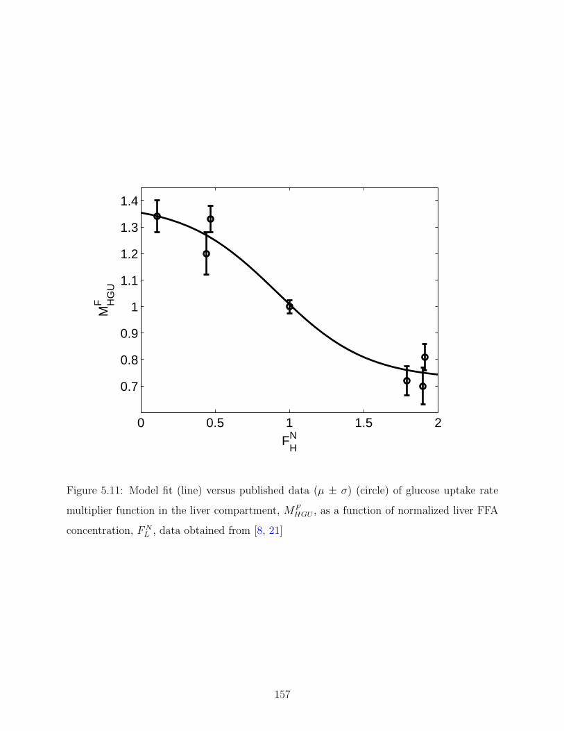
0 0.5 1 1.5 2

0.7

0.8

0.9

1

1.1

1.2

1.3

1.4

MF H

GU

FHN

Figure 5.11: Model fit (line) versus published data (µ ± σ) (circle) of glucose uptake rate

multiplier function in the liver compartment, MFHGU , as a function of normalized liver FFA

concentration, FNL , data obtained from [8, 21]

157

0 0.5 1 1.5 20.6

0.7

0.8

0.9

1

1.1

1.2

1.3

FLN

MH

GP

F

Figure 5.12: Model fit (line) versus published data (µ ± σ) (circle) of glucose production

rate multiplier function in the liver compartment, MFHGP , as a function of normalized liver

FFA concentration, FNL , data obtained from [32, 33]

158

Figure 5.13: Surface plot of the multiplier function, M IF∞HGP , as a function of normalized liver

insulin, INL , and FFA concentration, FN

L , versus published data (cross) (µ ± σ) of normalized

hepatic glucose production rate with respect to its basal value [19, 21, 32, 34, 35, 36]

159

5.6 THE PHYSIOLOGICALLY-BASED FFA, GLUCOSE, AND INSULIN

MODEL

5.6.1 Modified-Insulin Frequently Sampled Intravenous Glucose Tolerance Test

(MI-FSIGT)

For the MI-FSIGT simulation study, a bolus of glucose was infused at t = 0 min and boluses

of insulin were infused at t = 0 and t = 20 min, in order to emulate the data obtained from

Sumner et al. [17]. Due to the second insulin peak, glucose concentration was suppressed

below its original basal level between 50 and 100 min. The insulin boluses caused the FFA

level to decline and achieve a nadir at around 70 min. After the 80 min mark, FFA level

rose gradually and returned to its original basal state. The model predictions captured the

data well, except the last 70 min of the FFA dynamics where the fatty acid level of the data

reached a pseudo-basal level which is higher than the original basal condition. The authors

have suggested that this phenomenon is due to the diurnal variation of the FFA level and has

nothing to do with insulin or glucose kinetics [17]. The muscle (T FM) and AT (T F

A ) diffusion

time constants were estimated to fit the data [17], as shown in Figure 5.14. The parameter

values are given in Table 5.4.

5.6.2 Validation of the Physiologically-Based Model

5.6.2.1 MI-FSIGT: For validation purpose all the model parameters were fixed and

then a MI-FSIGT simulation study was performed, where a bolus of glucose was infused

at t = 0 and boluses of insulin were infused at t = 0 and t = 20 min at a rate similar to

the experiment performed by Brehm et al. [37]. Due to the insulin boluses, FFA level was

suppressed much below its original basal level. After the 60 min mark, FFA level increased

gradually in order to return to its basal state. The comparison between model predictions

and experimental data are provided in Figure 5.15. The model predictions are within one

standard deviation of the experimental data.

160

0 50 100 150 200 250

50100150200

In

sulin

(

µU/m

L)

0 50 100 150 200 250

100

200

300

Glu

cose

(m

g/dL

)

0 50 100 150 200 250200

400

600

FF

A

(µm

ol/L

)

Time (min)

Figure 5.14: Model fit (line) and experimental data (µ±σ) (circle) [17] of a MI-FSIGT test.

Glucose bolus was infused at time (t) = 0 min and insulin boluses were infused at t = 0 min

and t = 20 min to obtain predictions of insulin (top); glucose (middle); and FFA (bottom)

concentrations

5.6.2.2 Effect of plasma FFA on plasma glucose levels: In order to validate the

inhibitory effect of insulin on glucose uptake and insulin-mediated HGP suppression, a

simulation study was performed where plasma FFA concentration was elevated at a rate

similar to Staehr et al. [33]. Plasma insulin concentration was maintained at the basal

level. Due to the elevation of plasma FFA level, plasma glucose concentration reached

hyperglycemic levels, as shown in Figure 5.16.

161

0 50 100 150 200

200400600800

Insu

lin(µ

U/m

L)

0 50 100 150 200

200

400

Glu

cose

(mg/

dL)

0 50 100 150 200

200

400

FF

A(µ

mol

/L)

Time (min)

Figure 5.15: Model validation (line) versus experimental data (µ ± σ) (circle) [37] of a MI-

FSIGT test. Glucose bolus was infused at time (t) = 0 min and insulin boluses were infused

at t = 0 min and t = 20 min to obtain predictions of insulin (top), glucose (middle), and

FFA (bottom) concentrations.

5.7 SUMMARY

In this chapter, a physiological FFA model was developed and incorporated with the existing

glucose-insulin model of Sorensen [2]. The FFA model has the same structural formulation as

the Sorensen model. Here, the human body was divided into seven physiologic compartments

representing the major FFA utilizing organs/tissues. Mass balances were performed across

162

0 50 100 150 200 250 300120

130

140

150P

lasm

a

Glu

cose

(m

g/dL

)

0 50 100 150 200 250 300

400

600

800

1000

Pla

sma

F

FA

(µm

ol/L

)

Time (min)

Figure 5.16: Model validation (line) versus experimental data (µ ± σ) (circle) [33] of the

effects of high FFA levels on plasma glucose concentration. Plasma glucose concentration

reached hyperglycemic levels (top) due to elevation of FFA concentration by lipid infusion

(bottom)

each compartment to obtain the FFA distribution at various organ/tissue levels. Metabolic

sinks and sources, representing the rate of FFA consumption and addition, respectively,

were added to the compartments. The insulin model [2] was linked with the FFA model at

the AT compartment to capture the anti-lipolytic effect of insulin. In order to capture the

effects of fatty acids on glucose, the FFA model was linked with the glucose model [2] at

the muscle and liver compartments. The physiologically-based model successfully emulated

163

insulin, glucose, and FFA concentrations after a MI-FSIGT test. The model is also capable

of predicting the physiological effects of FFA on glucose at the organ/tissue level.

Such a detailed physiological model enables the diabetes research community to visualize

the profiles of the major energy-providing substrates at the organ/tissue levels, particularly at

the postprandial period. It also helps researchers to better understand the various physiologic

interactions taking place between glucose, FFA, and insulin at the various body parts. But,

such a level of detailed knowledge comes at the cost of model complexity. The physiologically-

based model as proposed, consists of 34 ODEs. Even though the complexity of the model in

terms of dynamic order and total number of parameters is high, majority of the physiologic

parameters (i.e., volumes and flow rates) can be directly obtained from the literature. The

only estimated parameters were the trans-capillary time constants and those belonging to

the metabolic sink/source equations.

The model is capable of generating ‘what-if’ scenarios to investigate the effect of fluc-

tuating FFA levels on plasma glucose concentration. With the long-term goal of synthe-

sizing an automatic closed-loop model-based insulin delivery system, this more complete

physiologically-based model of the major energy-providing metabolic substrates gives the

control community a more detailed model for use in control design. This detailed model

could contribute substantially in developing a realistic (true-to-life) artificial pancreas, which

would be capable of maintaining normoglycemia by rejecting disturbances such as mixed meal

consumption.

164

6.0 MODEL PREDICTIVE CONTROL OF BLOOD GLUCOSE FOR T1DM

PATIENTS1

As mentioned in Chapter 1, the long-term goal is to develop a closed-loop artificial pancreas

system to control blood glucose levels for T1DM patients. The three major components of an

artificial pancreas are a continuous insulin pump, a continuous glucose sensor, and a control

algorithm to regulate the insulin pump in order to maintain normoglycemia [48, 47, 65]. In

a model-based control approach, a diabetic patient model is integrated in the controller, as

shown in Figure 6.1. Based on the model output and the current measurement obtained from

the sensor, the controller calculates the next manipulated input value. Theoretically, such a

device can produce tight glucose control during pre- and post-prandial conditions [48]. Hence,

fully automatic glucose control by an artificial pancreatic system can efficiently prevent or

delay the chronic complications of hyperglycemia and lower the risk of hypoglycemia.

Various types of control algorithms for blood glucose control have been reported in the

literature. Some of these algorithms include: Biostator and related nonlinear PD control [110,

112], PID control [117, 120, 188], optimal control [121, 122], MPC [65, 124, 126], control based

on neural networks incorporating MPC [81, 189], advanced model-based control technique

using parametric programming algorithms [190], etc. Some of these control algorithms were

tested on T1DM patients [120, 126], whereas, others were mainly simulation studies. The

main purpose of all of the published closed-loop algorithms is to maintain the blood glucose

level near its basal value.

The control algorithm used in the first commercially available closed-loop insulin delivery

system, Biostator, was adapted from the nonlinear control algorithm synthesized by Albisser

et al. [110]. Mathematically, the Albisser algorithm can be expressed as follows:

1Portions of this chapter have been published in [130]

165

Model

Diabetic

r(t)Controller

Insulin

Pump

Sensor

Glucose

Diabetic Patient

y(t)u(t)

y(t)

Figure 6.1: A schematic diagram of the closed-loop model-based insulin delivery system.

Here, r(t) is the desired glucose setpoint, u(t) is the manipulated variable (exogenous insulin),

y(t) is the measured variable, and y(t) is the model predicted output

ui(t) =1

2Mi [1 + tanh(Si(Gp(t)−Bi))] (6.1)

ud(t) =1

2Md [1 + tanh(Sd(Gp(t)−Bd))] (6.2)

Here, subscripts i and d represent insulin and glucose (dextrose) infusions, respectively. The

insulin infusion was based on projected blood glucose, Gp(t), which included a difference

factor, DF(t):

Gp(t) = G(t) + DF (t) (6.3)

DF (t) = K1

[exp

(dG(t)/dt

K2

)− 1

](6.4)

166

The rate of change of glucose (dG(t)/dt) was averaged over the previous 4 min. For adjusting

insulin infusion rate, five tuning parameters were available (Mi, Si, Bi, K1, and K2). Later,

Clemens et al. [112] modified the Albisser algorithm by including a quadratic function of

the derivative of glucose with time in order to expedite the insulin infusion dynamics during

post-prandial periods. All these Biostator-related algorithms can be classified as nonlinear

PD controllers [48].

A closely studied control approach for the automated insulin delivery system is the PID

controller [120, 117]. The PID algorithm has the following mathematical representation

[191]:

u(t) = u0 + kc

[e(t) +

1

τI

∫e(t) + τD

de(t)

dt

](6.5)

Here, e(t) (error) is the difference between the desired glucose concentration and the mea-

sured glucose signal, u(t) is the insulin infusion rate, and u0 is the basal insulin infusion rate.

The PID controller is composed of three functions: (i) a term directly proportional to the

error (tuning parameter kc); (ii) a correction proportional to the integral of the error (tuning

parameter τI); and (iii) a term proportional to the derivative of the error (tuning parameter

τD). The PID-based insulin pump currently under development by Medtronic MiniMed is

aptly named as the external Physiologic Insulin Delivery (ePID) system [120, 117, 192, 51].

Linear quadratic (LQ) optimal control of blood glucose for diabetic patient, compares

the model predicted output obtained from a linear state–space model of the glucose-insulin

system with the actual measured output, updates the model, and calculates the next ma-

nipulated input value by minimizing a quadratic cost function [121, 122]. The cost function

can be mathematically written as follows (adapted from [121]):

J(u) =

∫ ∞

0

{[x1(t)− xd]

2 + ρu2(t)}

dt (6.6)

Here, xd denotes a predetermined glucose setpoint value. x1(t) and u(t) represent the state

and input variables obtained from the state–space model. Constant ρ (> 0) is a weighting

factor; higher values of ρ will make the control performance sluggish. The main goal here is

167

to determine the positive, bounded, control u(t) in order to minimize the deviation of blood

glucose from the desired setpoint while penalizing usage of large amounts of infused insulin.

One of the most promising control approaches for diabetes is MPC [6, 65, 124, 126]. It

was primarily developed by the petrochemical industry in the 1970s to control large-scale

constrained processes with many manipulated inputs and measured outputs [193]. Compared

to a LQ controller, a model predictive controller is more robust to measurement noise and

plant-model mismatch [194], which is primarily a result of the MPC controller being a

discrete-time relaxation of the LQ controller in the linear model case. The gained robustness

is critical in the diabetes implementation given the prevalence of glucose sensor noise and

model inaccuracy (both structural and parametric). Also, nonlinear MPC formulations can

be constructed and constraints are handled in a straightforward manner in the optimization

problem. A detailed description of the model predictive controller is presented in the

following Section (6.1).

6.1 MODEL PREDICTIVE CONTROLLER

The MPC controller solves an optimization problem at each time step by calculating the

manipulated variable sequence (in this case, insulin delivery rate) that minimizes a user-

specified objective function. The optimization scheme uses the process model (in this case,

a diabetic patient model) to generate future output predictions. Based on these future

model predictions (in this case, glucose concentration), the user-defined objective function is

minimized by computing a manipulated variable sequence. Process measurements obtained

at each sampling time are used to update the optimization, thus incorporating feedback in

the control scheme. From the calculated manipulated variable sequence, only the first step

is implemented, and the algorithm is repeated for the next sampling time [195].

The control algorithm minimizes the following 2-norm squared objective function:

min4U(k|k)

‖Γy(R(k + 1|k)− Y (k + 1|k))‖22 + ‖Γu4U(k|k)‖2

2 (6.7)

168

Here, vectors R(k + 1|k) and Y (k + 1|k) of length p are the desired future glucose trajectory

and the future model prediction resulting from the open-loop optimal control sequence vector

4U(k|k) of length m (where, m ≤ p). The goal is to minimize the objective function

(equation (6.7)) by manipulating 4U(k|k). The first part of equation (6.7) represents the

error in setpoint tracking, and the second part represents the penalization factor which

restricts the controller from making drastic changes in the manipulated variable sequence.

Γy and Γu are the weighing matrices for setpoint tracking and control move penalization,

respectively. Controller tuning involves adjustments to the four parameters p, m, Γy, and

Γu.

Figure 6.2 presents the schematic diagram of implementation of the MPC algorithm.

The x-axis represents the time scale. The reference trajectory, representing the desired

blood glucose concentration, is indicated by the horizontal dashed line. At current time,

k, the diabetes model calculates blood glucose concentration for a predetermined future

horizon p, in absence of further control action. The same model is used to calculate a

sequence of control moves (u(k), . . .,u(k + m− 1)), as indicated by the solid line, in order to

minimize the objective function (equation (6.7)) subject to prespecified operating constraints

so that the desired output behavior for p time steps into the future (dash-dotted line with

circles) is obtained. To incorporate the unmodeled errors in the optimization process, glucose

measurements from the sensor (ym(k)) are obtained at every sampling time to compare with

the model prediction (y(k)), and the prediction error, ε(k) = ym(k) − y(k), thus obtained is

used to update future predictions.

As the optimization process of MPC relies on the forecast of process behavior obtained

from a model, therefore the process model is regarded as an essential component of the MPC

[196, 195]. Based on the type of the model used and the constraints used, model predictive

control algorithms can be classified into linear and nonlinear MPC. A linear model predictive

controller (LMPC) refers to a particular case when the process model linear. A state–space

linear model used in an LMPC has the following form (adapted from [195]):

169

k k+1 k+p

Past Future

Current

Measurements

ModelPredictions

Horizon

VariableManipulated

k+m−1

Process

Reference Trajectory

ym(k)

ym(k − 2)y(k)

y(k+1)

u(k+m-1)

u(k)

Figure 6.2: A schematic diagram of the MPC algorithm implementation

dx(t)

dt= Ax(t) + Bu(t) (6.8)

y(t) = Cx(t) (6.9)

Here, vector x(t), y(t), and u(t) represent state variables, measured output variables, and

input variables. A, B, and C are constant coefficient matrices. A quadratic objective

function is commonly used for the online optimization subjected to linear input and output

constraints (if present).

170

In case of a nonlinear model predictive controller (NMPC), a nonlinear process model is

used. The motivation of using a nonlinear model is the possibility to improve control action

by improving the quality of the forecasting, particularly in systems with a high degree of

nonlinearity [196, 195]. A state space form of a nonlinear model used in a MPC can be

written as follows (adapted from [196]):

dx(t)

dt= f(x(t), u(t)) (6.10)

y(t) = g(x(t)) (6.11)

Functions f(·, ·) and g(·) are smooth nonlinear mappings for the state and output variables,

respectively. The objective function can be non-quadratic. In addition, the optimization

problem can be subjected to nonlinear input and output constraints.

The MPC has an edge over the other control algorithms for blood glucose control because

of its characteristics. For example, an unconstrained MPC can guarantee optimal insulin

dosage when Γu = 0 [127]. Also for safety reasons and mechanical limitations of the pump,

input constraints can be intrinsically formulated in the MPC algorithm [127]. Moreover, the

MPC can take control actions much before a hyper- or hypo-glycemic event has occurred un-

der certain formulations. Successful implementation of MPC for meal disturbance rejection

in simulations and to maintain glucose homeostasis during fasting state in T1DM patients

can be found in [65, 124] and [126], respectively.

Previously, closed-loop simulation studies have been performed to evaluate the perfor-

mance of MPC in the presence of a CHO-containing meal disturbance [65, 124]. Closed-loop

performance in response to mixed meal containing fat and protein along with CHO has been

ignored, mainly due to lack of lipid-based metabolic models. In this chapter, performance of

closed-loop MPC algorithms for maintenance of normoglycemia in presence of mixed meals

was evaluated. In Section 6.2.1, both NMPC and LMPC algorithms were synthesized based

on the extended minimal model from Chapter 2. In the following Section (6.2.2), a separate

closed-loop simulation study was performed where both NMPC and LMPC algorithms were

171

developed by using the composite model from Chapter 4. Finally, the Chapter ends with a

brief Summary 6.3.

6.2 CLOSED-LOOP SIMULATION OF MIXED MEAL DISTURBANCE

REJECTION

6.2.1 MPC Formulation Based on the Extended Minimal Model

Both linear and nonlinear MPC algorithms were synthesized based on the extended minimal

model for disturbance rejection from mixed meal ingestion. The optimization problem was

solved by minimizing the quadratic objective function as presented in Equation (6.7). In a

diabetic system, input magnitude constraints are essential, mainly for safety reasons. This

makes the MPC an ideal candidate for the glucose-insulin feedback system, as the algorithm

can explicitly enforce constraints. It has been observed that the plasma insulin level can

reach upto 70 µUml

in healthy patients after consumption of 108 g of mixed meal [10]. Hence

the upper bound of insulin delivery rate was set at 100 mUmin

which corresponded to a plasma

insulin concentration of 69.5 µUml

. The insulin input magnitude bounds used for the simulation

study can be written as:

0 ≤ U(k|k) ≤ 100mU

min(6.12)

In order to make sure that the maximum change in insulin delivery rate is not higher than

the mechanical characteristics of the pump, a maximum rate of change of input constraint

was employed as shown below:

|4U(k)| ≤ 50mU

min · 4Ts

(6.13)

In case of the NMPC (NMPCE−E), the controller model was represented by the extended

minimal model developed in Chapter 2. For simulation purposes, the diabetic patient

172

measurements were also obtained from the extended minimal model, thus assuming a perfect

model scenario (no plant-model mismatch). For the LMPC (LMPCE−LE) case, the extended

minimal model was linearized using a first-order Taylor series expansion (see Appendix).

Plant-model mismatch was considered by incorporating the unmodeled disturbances at

every sampling time (4Ts) given by the difference between the plant (patient) measure-

ment, obtained from the original extended minimal model, and the controller model output

represented by the linearized extended minimal model. A mixed meal of 108 g (CHO = 70

g, protein = 18 g, and FFA = 20 g) was consumed by the simulated patient, at t = 20 min.

Gut absorption kinetics of the nutrients from mixed meal into the circulatory system was

captured by the meal model presented in Section 2.5.1. The controller tuning parameters

were adjusted such that the setpoint sum squared error (SSE) (i.e., the deviation of glucose

concentration from the reference trajectory) was minimized. Best controller performance was

achieved when the tuning parameters were: p = 10, m = 2, Γy = 1, and Γu = 0.002; sampling

time (4Ts) was set at 5 min. Comparison between the NMPCE−E and the LMPCE−LE are

provided in Figure 6.3. It can be observed that the performance of LMPCE−LE is closely

comparable with the performance of NMPCE−E (Table 6.1).

For comparison purposes, another set of NMPC (NMPCE−B) and LMPC (LMPCE−LB)

algorithms were synthesized. For the NMPCE−B formulation, the model was represented

by the original Bergman minimal model [1] (from Section 2.1) and the patient (plant)

measurements were obtained from the original extended minimal model. In case of the

LMPCE−LB formulation, a linearized version of the Bergman minimal model (see Appendix)

was used to represent the controller model and, once again, the patient measurements were

obtained from the original extended minimal model. A mixed meal of equal mass and

composition as above was consumed by the simulated patient. Unlike the extended minimal

model, the Bergman model and its linearized version does not consider FFA dynamics.

Tuning parameters and input constraints were the same as above. Closed-loop simulation

results of LMPCE−LE, NMPCE−B, and LMPCE−LB are shown in Figure 6.4. Based on the

simulated performance of the three controllers (see Table 6.1), it can be concluded that

LMPCE−LE provides a tighter glucose control than the NMPCE−B or LMPCE−LB. The

oscillation in the closed-loop performances of NMPCE−B and LMPCE−LB is due to the

173

0 100 200 300 40050

100

150

200

Glu

cose

(m

g/dl

)

0 100 200 300 4000

50

100

Insu

lin

In

fusi

on (

mU

/min

)

Time (min)

Figure 6.3: Comparison between mixed meal disturbance rejection by LMPCE−LE (solid

line) and NMPCE−E (dashed line) with input constraint. Setpoint (dotted line) is set at 81

mgdl

plant-model mismatch between the extended minimal model (plant) and the original/linear

Bergman minimal model (controller model). Presence of FFA dynamics in the extended

minimal model caused the plasma glucose to subside slower than the Bergman minimal

model (original/linear) after consumption of a mixed meal.

6.2.2 MPC Formulation Based on the Composite Model

In order to evaluate the closed-loop performance of the composite model developed in

Chapter 4, both LMPC and NMPC algorithms were developed based on the composite model.

Once again, the objective of the closed-loop simulation was to maintain normoglycemia by

174

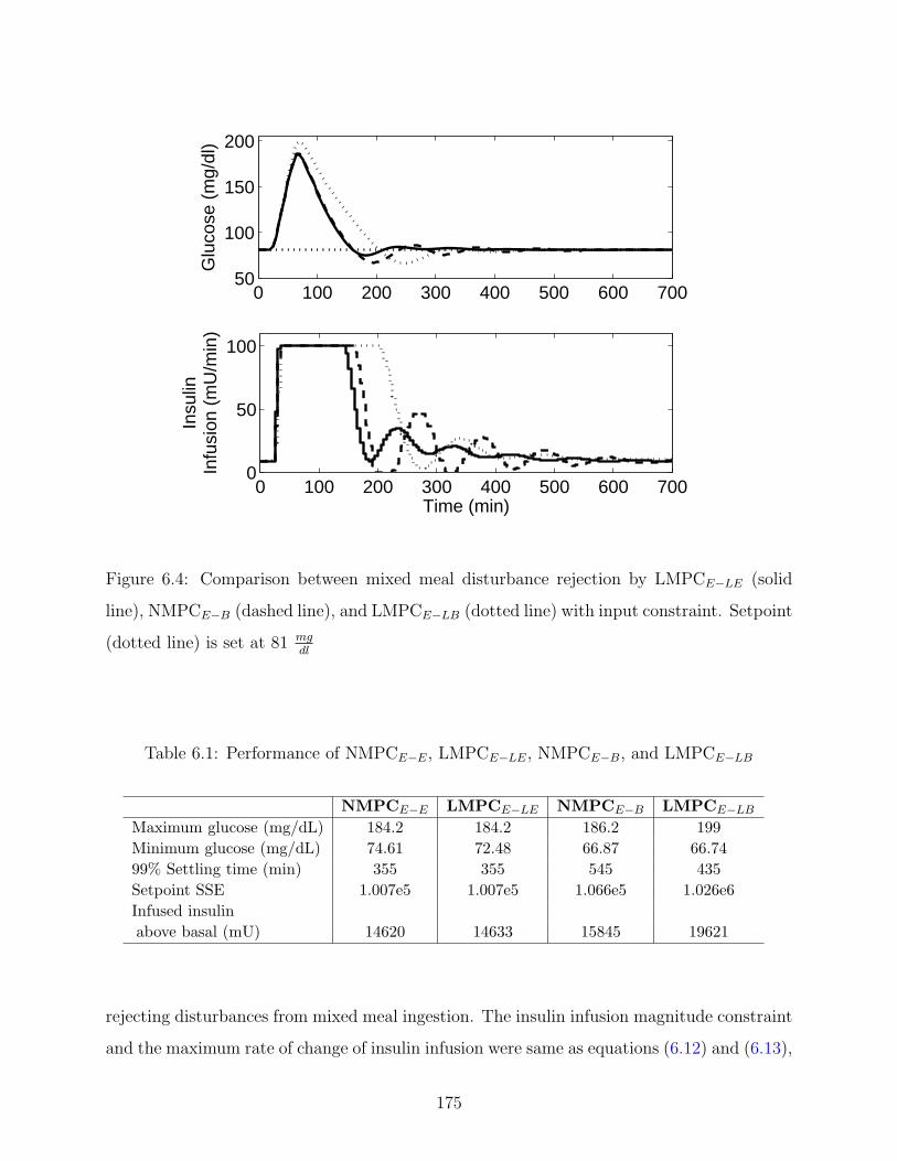
0 100 200 300 400 500 600 70050

100

150

200

Glu

cose

(m

g/dl

)

0 100 200 300 400 500 600 7000

50

100

Time (min)

Insu

linIn

fusi

on (

mU

/min

)

Figure 6.4: Comparison between mixed meal disturbance rejection by LMPCE−LE (solid

line), NMPCE−B (dashed line), and LMPCE−LB (dotted line) with input constraint. Setpoint

(dotted line) is set at 81 mgdl

Table 6.1: Performance of NMPCE−E, LMPCE−LE, NMPCE−B, and LMPCE−LB

NMPCE−E LMPCE−LE NMPCE−B LMPCE−LB

Maximum glucose (mg/dL) 184.2 184.2 186.2 199Minimum glucose (mg/dL) 74.61 72.48 66.87 66.7499% Settling time (min) 355 355 545 435Setpoint SSE 1.007e5 1.007e5 1.066e5 1.026e6Infused insulinabove basal (mU) 14620 14633 15845 19621

rejecting disturbances from mixed meal ingestion. The insulin infusion magnitude constraint

and the maximum rate of change of insulin infusion were same as equations (6.12) and (6.13),

175

respectively. The quadratic objective function, as presented in equation (6.7), was minimized

to achieve the desired control action.

For the NMPC (NMPCPB−C) case, the in-built controller model was represented by

the composite model. To simulate the diabetic patient (plant), a physiologically-based

metabolic model from Chapter 5 was used. This strategy of using a higher-order model

for the plant and a lower-order model for the controller model introduced a plant-model

mismatch in the closed-loop system; a phenomenon which is expected if implemented in a

clinical setup due to inter- and intra-patient variability. In case of the LMPC (LMPCPB−LC),

the composite model was linearized using a first-order Taylor-series expansion, just like the

previous section (see Appendix). The linearized composite model represented the controller

model and patient data was obtained from the physiologically-based metabolic model for

feedback to the controller in order to incorporate the unmodeled errors. A mixed meal

of same size and composition as the previous section (108 g of 65% CHO, 17% protein,

and 18% fat) was ingested by the simulated patient at t = 20 min. The controller tuning

parameters were adjusted such that sum-squared deviation of glucose concentration from

reference trajectory (81 mgdl

) was minimized. Best closed-loop performance was achieved at

p = 18, m = 2, and Γy = 2 and Γu = 0.02. Once again, measurements were obtained

at every 5 min intervals. Comparison between the closed-loop simulations of NMPCPB−C

and LMPCPB−LC are provided in Figure 6.5. It is clearly noticable that NMPCPB−C (solid

lines in Figure 6.5 (top)) produced tighter glucose control. In case of the LMPCPB−LC ,

hypoglycemia was reached after 170 min of meal consumption and blood glucose remained

suppressed below the normal level for more than 200 min. The mismatch between the plant

data obtained from the physiologically-based model and the model prediction procured from

the linearized composite model was significantly high when the insulin infusion rate deviated

more than 4-fold of its basal value, thereby causing hypoglycemia.

For comparison purposes, LMPC and NMPC algorithms were developed using the Bergman

minimal model [1] (Section 2.1). In case of the NMPC (NMPCPB−B), the controller model

was represented by the original Bergman minimal model, whereas the diabetic patient was

simulated by the physiologically-based metabolic model. Input constraints and controller

tuning parameters were used as above. As pointed out by Quon et al. [87] and Cobelli et al.

176

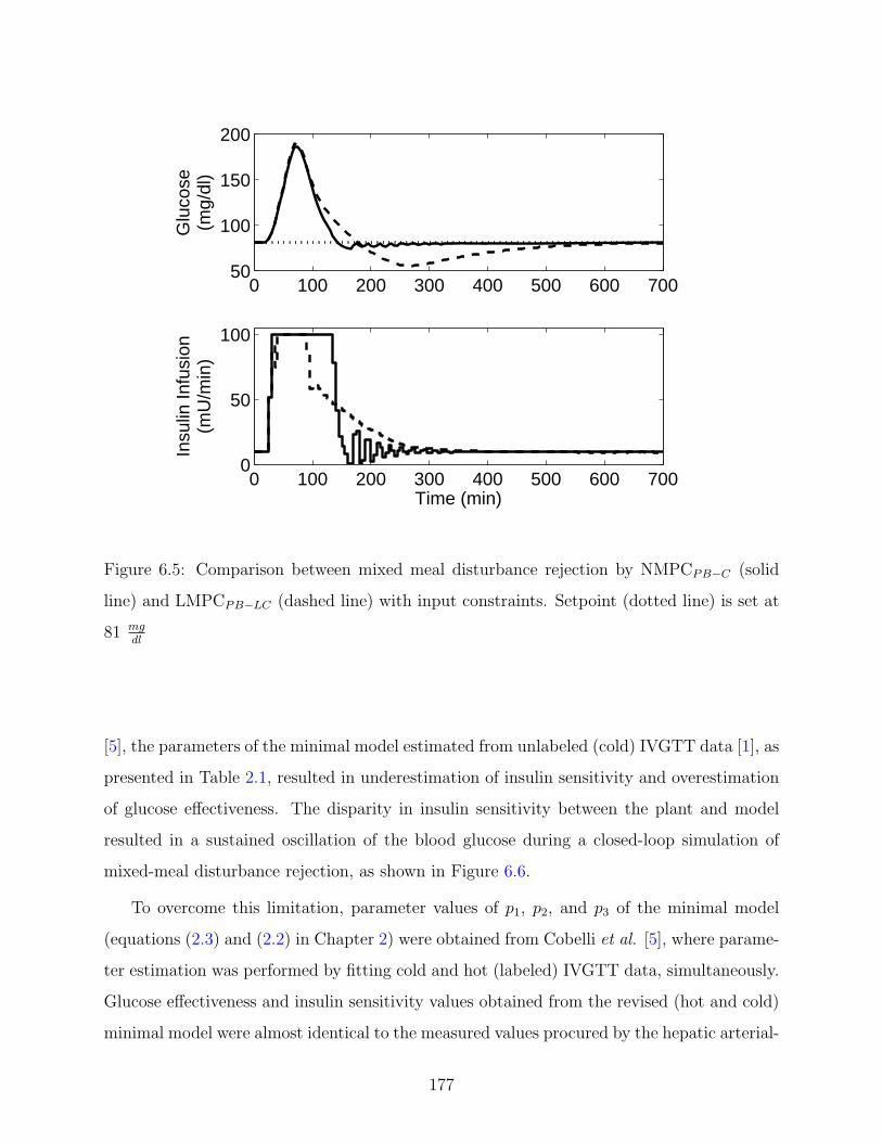
0 100 200 300 400 500 600 70050

100

150

200

Glu

cose

(mg/

dl)

0 100 200 300 400 500 600 7000

50

100

Insu

lin In

fusi

on(m

U/m

in)

Time (min)

Figure 6.5: Comparison between mixed meal disturbance rejection by NMPCPB−C (solid

line) and LMPCPB−LC (dashed line) with input constraints. Setpoint (dotted line) is set at

81 mgdl

[5], the parameters of the minimal model estimated from unlabeled (cold) IVGTT data [1], as

presented in Table 2.1, resulted in underestimation of insulin sensitivity and overestimation

of glucose effectiveness. The disparity in insulin sensitivity between the plant and model

resulted in a sustained oscillation of the blood glucose during a closed-loop simulation of

mixed-meal disturbance rejection, as shown in Figure 6.6.

To overcome this limitation, parameter values of p1, p2, and p3 of the minimal model

(equations (2.3) and (2.2) in Chapter 2) were obtained from Cobelli et al. [5], where parame-

ter estimation was performed by fitting cold and hot (labeled) IVGTT data, simultaneously.

Glucose effectiveness and insulin sensitivity values obtained from the revised (hot and cold)

minimal model were almost identical to the measured values procured by the hepatic arterial-

177

0 100 200 300 400 5006080

100120140160180

Glu

cose

(mg/

dl)

0 100 200 300 400 5000

50

100

Insu

lin In

fusi

on(m

U/m

in)

Time (min)

Figure 6.6: Mixed meal disturbance rejection by NMPCPB−B with input constraints.


. Controller model parameters were obtained from

Bergman et al. [1].

venous difference technique [5], thereby validating the model estimates. The new parameter

values of the minimal model are provided in Table 6.2. A more stable closed-loop performance

of the NMPCPB−B was obtained by using the minimal model with the new parameter values,

as shown by the solid lines in Figure 6.7 (top).

The LMPC (LMPCPB−LB) algorithm was developed based on a linearized version of the

Bergman minimal model. Once again, patient data was obtained from the physiologically-

based model. Closed-loop performance of the LMPCPB−LB algorithm is presented in Figure

6.7 (dashed-lines). Due to plant-model mismatch, both the NMPCPB−B and LMPCPB−LB

algorithms produced hypoglycemic events; especially, in the case of LMPCPB−LB the mini-

mum glucose concentration was dangerously low. The performances of all the four control

178

0 100 200 300 400 500 600 70050

100

150

200

Glu

cose

(mg/

dl)

0 100 200 300 400 500 600 7000

50

100

Insu

lin In

fusi

on(m

U/m

in)

Time (min)

Figure 6.7: Comparison between mixed meal disturbance rejection by NMPCPB−B (solid

line) and LMPCPB−LB (dashed line) with input constraints. Setpoint (dotted line) is set at

81 mgdl

. The Bergman minimal model parameters were obtained from Table 6.2.

Table 6.2: New Parameters of the Bergman minimal model, from [5]

Parameter Value Unitp1 0.0092 1

min

p2 0.116 1min

p3 0.00068 1min

algorithms are highlighted in Table 6.3. It is quite evident that NMPCPB−C produced the

tightest glucose control. Both the LMPC algorithms caused blood glucose concentration to

reach below 60 mgdl

, which could be a source of major concern as hypoglycemia may lead to

179

unconsciousness or even death. Once again, the closed-loop simulation results revealed that

incorporation of FFA dynamics significantly improved the controller performance.

Table 6.3: Performance of NMPCPB−C , LMPCPB−LC , NMPCPB−B and LMPCPB−LB

NMPCPB−C LMPCPB−LC NMPCPB−B LMPCPB−LB

Maximum glucose (mg/dL) 186 189.2 199.2 204Minimum glucose (mg/dL) 74.65 55.47 66.77 47.5999% Settling time (min) 415 650 345 820Setpoint SSE 9.228e4 1.119e6 1.538e5 1.119e6Infused insulinabove basal (mU) 10495 10404 10541 10150

For comparison purposes, a closed-loop NMPC formulation (NMPCPB−PB) was designed

with no plant-model mismatch. In other words, the model was assumed to be perfect. Hence,

both the plant (patient) and the controller model were represented by the physiologically-

based model (from Chapter 5). In such an ideal case, best possible glucose control is expected

due to the absence of unmodelled errors. A mixed meal of the same size and composition as

the above cases was ingested at t = 20 min. No alterations were made to the controller tuning

parameters. The simulation results as shown in Figure 6.8 (and Table 6.4) revealed a much

superior control performance than any other previously studied closed-loop formulations in

terms of the minimum glucose level, and 99% settling time.

6.3 SUMMARY

For a tighter blood glucose control of T1DM patients, the current focus is on developing

automated closed-loop insulin delivery systems. One of the most optimistic approaches for

controlling an insulin pump is the MPC algorithm. In this chapter, both nonlinear and linear

MPC algorithms were developed to evaluate the effects of FFA on closed-loop glucose control.

The simulated controller performances were evaluated by perturbing the system with mixed

meal ingestion. MPC algorithms based on the extended minimal model (Chapter 2) and

the composite model (Chapter 4) provided a tighter glucose control as compared to MPC

180

0 100 200 300 400 50080

100120140160180

Glu

cose

(mg/

dl)

0 100 200 300 400 5000

50

100

Insu

lin In

fusi

on(m

U/m

in)

Time (min)

Figure 6.8: Mixed meal disturbance rejection by NMPCPB−PB with input constraints.


Table 6.4: Performance of NMPCPB−PB

NMPCPB−PB

Maximum glucose (mg/dL) 185.8Minimum glucose (mg/dL) 76.2599% Settling time (min) 165Setpoint SSE 9.163e4Infused insulinabove basal (mU) 10250

algorithms based on the Bergman minimal model [1]. Hence, the simulated results indicated

that inclusion of FFA absorption from mixed meal and its interactions with glucose improved

the quality of the controller performance.

181

In case of plant-model mismatch simulations, where the plant was represented by the

higher-order physiologically-based model (Chapter 5), the NMPC performances were far su-

perior than the LMPC formulations. Prolonged hypoglycemia was observed for LMPCPB−LC

and LMPCPB−LB. The deviation in glucose prediction between the linearized models and

their original nonlinear forms was significantly high when the insulin infusion rate exceeded

4-fold of its basal value. This is mainly due to the presence of the saturation terms in the

physiologically-based model describing the effects of insulin on glucose uptake and hepatic

glucose production rates. During higher insulin infusion rates (4-fold above basal), the effects

of insulin on tissue glucose uptake and hepatic glucose production rates reach a saturation

point for the physiologically-based model. Such a biologically-relevant characteristic is absent

in the linearized composite or the Bergman minimal model (both linear and nonlinear forms).

The LMPC formulations, especially LMPCPB−LC , performed far better when the mixed meal

load was reduced to 67 g with the same composition (which is equivalent to approximately

50 g of glucose).

The simulated results demonstrated the capability of the closed-loop algorithms to pro-

duce tight blood glucose control by rejecting disturbances from meals containing all the

major nutrients. The inclusion of gut absorption of FFA and protein, along with glucose

in the closed-loop simulation might prove to be beneficial for the control community in

development of robust automated artificial pancreas equipped to handle disturbances which

are confronted in real life. In order to minimize hypoglycemic events after meal consumption

without sacrificing controller aggressiveness, the MPC framework can be tailored by altering

the objective function [6, 128]. More details of such advanced control strategies are provided

in Chapter 7.

Efforts have been made to develop automated insulin delivery systems since the 1960s

[109]. Commercial pumps to deliver insulin subcutaneously have been available since the

1980s [197], continuous glucose monitoring sensors have been available since the late 1990s

[198], and controller algorithms for delivery of insulin have been in development since the

early 1960s [69]. Still, there are many reasons that not a single closed-loop automated

insulin delivery pump is available commercially [188]. Starting with the continuous glucose

sensors, the accuracy of such a device is in the 15 - 20% error range [199]. Also the

182

reliability of continuous monitoring systems is questionable mainly because of the time

lag due to glucose equilibration between blood and subcutaneous interstitial fluid [200].

Insulin delivery is likely to be either intravenous using an external insulin pump (as shown

in Figure 6.1), or intraperitoneal using an implantable pump [188]. Both delivery sites

introduce additional dynamics in the insulin kinetics [201]. Closed-loop algorithms have

not adequately demonstrated ability to efficiently handle these delays especially during meal

intake and exercise [188]. Also, closed-loop controller performance is significantly affected by

the intra-patient variability of insulin sensitivity throughout the day [188, 201]. Extensive

research and validation is still required before a fully automated insulin delivery system could

be used by a T1DM patient at home.

183

7.0 SUMMARY AND FUTURE RECOMMENDATIONS

The work presented in this dissertation focused on incorporation of the physiological effects of

FFA and exercise into existing glucose-insulin metabolic models [1, 2]. Both low-order semi-

empirical model structures and higher-order physiologically-based model structures were

investigated. A mixed meal model was also developed to emulate the absorption kinetics of

major nutrients (CHO, protein, and fat) present in a mixed meal into the circulatory system.

The meal model outputs served as disturbance inputs for the metabolic models. One of the

major goal of developing metabolic models accounting for all the major energy-providing

metabolites was to evaluate the closed-loop performance of a model-based controller in

maintaining normoglycemia during the post-prandial period, particularly after ingestion of

a mixed meal. Hence, MPC algorithms were synthesized based on the newly developed

metabolic models for maintenance of glucose homeostasis. The contribution of each of the

investigations have been presented in the summary section of each chapter. The following

section once again summarizes the major findings of this dissertation.

7.1 SUMMARY

7.1.1 Semi-Empirical Metabolic Models

The glucose-insulin metabolic model developed by Bergman et al. [1] was extended to include

FFA dynamics and its interactions with glucose and insulin. Three additional ODEs were

added to the original model to capture the dynamics of plasma FFA, the anti-lipolytic action

of insulin on FFA, and the inhibitory effect of FFA on glucose uptake rate. Due to inclusion

184

of FFA dynamics, the extended minimal model in its present form is capable of predicting

FFA fluctuations and its effects on plasma glucose dynamics. Also, the extended minimal

model coupled with a mixed meal model can be utilized to determine the dynamics of plasma

glucose and FFA after mixed meal ingestion of varying sizes and compositions. This more

complete minimal model of the major energy-providing metabolic substrates may provide

the control community a better tool for the design of model-based controllers.

In a separate study, a semi-empirical model of exercise effects on the glucose-insulin

system was developed. Once again, the Bergman minimal model [1] was extended to

incorporate mild-to-moderate exercise effects on plasma glucose and insulin. Linear ODEs

were added in the model to capture the exercise-induced accelerated clearance rate of plasma

insulin, elevated glucose consumption rate, and increased hepatic glucose production rate.

During prolonged exercise, the model successfully captured the decline in hepatic glucose

production due to depletion of the rate of glycogenolysis leading towards hypoglycemia.

With the ultimate goal of developing a closed-loop model-based insulin delivery system, it

is essential to synthesize control-relevant metabolic models that are capable of predicting

fluctuations in glucose dynamics during exercise. Hence, the exercise minimal model can

provide the control community an alternative tool for use in controller design for maintenance

of glucose homeostasis especially during exercise. Open-loop simulations from such models

can also give prior intimation to T1DM patients regarding the time-span during which

exercise could be performed at a given intensity without reaching hypoglycemia.

Although, the extended minimal model developed in Chapter 2 successfully captured

FFA, glucose, and insulin dynamics, the effects of exercise on these metabolites and hormones

were neglected. Similarly, the exercise minimal model developed in Chapter 3 success-

fully captured the effects of exercise on plasma glucose and insulin levels; however, the

model overlooked the contributions (interactions) of FFA. Hence, in order to obtain a single

metabolic model capturing the effects of FFA and exercise, a composite model was developed

by integrating the extended minimal model with the exercise minimal model. To make

the composite model more biologically relevant, necessary modifications were made to the

original model structures. The model consisted of four parts capturing the insulin, glucose,

FFA, and exercise dynamics. The dynamical effects of insulin on glucose and FFA were

185

divided into three sections: the anti-lipolytic action to suppress endogenous FFA release;

the gluco-regulatory action to promote glucose uptake in the tissues; and, the suppression of

hepatic glucose production. Parameters of the insulin action on glucose were fitted by using

labeled-IVGTT data which facilitated separation of insulin action on glucose utilization and

production. Exercise effects on insulin, glucose, and FFA were divided into five sections.

Mainly, these effects are the exercise-mediated plasma insulin clearance, elevated glucose

uptake and production rate during exercise, and elevated FFA uptake and production rate

during exercise. The model also captured the decline of plasma glucose concentration during

prolonged exercise due to the depletion of glycogen leading to a decrease in the rate of hepatic

glycogenolysis. The model can be used in development of model-based controller for blood

glucose control particularly in presence of disturbances from mixed meal ingestion, as well

as exercise.

7.1.2 Physiologically-Based Metabolic Model

A detailed physiologically-based circulation model of FFA was developed, where the body

was divided into compartments representing the major organs/tissues. FFA was distributed

to each of these physiologic compartments via the circulatory system. Mass balances were

considered at each compartment to obtain the FFA distribution at various organ/tissue

levels. Metabolic sinks and sources were added to represent the rate of FFA consumption

and addition at various organs and tissues, respectively. The FFA model was integrated with

the existing glucose-insulin model developed by Sorensen [2], which has a similar structure.

The model successfully captured the glucose, FFA, and insulin dynamics after a modified

insulin-frequently sampled intravenous glucose tolerance test. It also captured the effects of

FFA on tissue glucose uptake rate and hepatic glucose production rate.

Such a detailed model can prove to be a valuable tool for the diabetes research community

for better understanding of the various physiologic interactions taking place between glucose,

FFA, and insulin at the organ/tissue levels. The integrated physiologically-based model

accounting for all the major energy-providing substrates has a better chance of accurately

predicting glucose concentration at the major organs/tissues after consumption of a mixed

186

meal. The model can also provide more insight regarding the combined effects of insulin and

FFA on hepatic glucose production rate. However, such in-depth knowledge comes at the

cost of model complexity in terms of number of states and parameters.

7.1.3 Model-Based Control of Blood Glucose for T1DM

Both linear and nonlinear MPC were developed to evaluate the effects of mixed meal ingestion

on closed-loop performance of blood glucose control. The MPC algorithms were tested after

perturbing the system with mixed meal ingestion. The control algorithms based on the

extended minimal model (Chapter 2) and the composite model (Chapter 4) provided superior

blood glucose control when compared to controller based on the Bergman minimal model [1].

Hence, the closed-loop results indicated that inclusion of FFA dynamics and its interactions

with glucose improved the quality of the controller performance in rejecting disturbances

from mixed meal ingestion. In case of the plant-model mismatch, the patient data (plant)

was obtained either from the extended minimal model or the physiologically-based model

(Chapter 5), and the controller model was represented either by the composite model or

the Bergman minimal model. The nonlinear MPC formulations provided a tighter glucose

control in terms of maximum glucose level, minimum glucose level, and 99% settling time,

than the linear MPC formulations.

7.2 FUTURE RECOMMENDATIONS

7.2.1 Incorporating Exercise Effects in the Physiologically-Based Model

The physiologically-based model developed in Chapter 5 did not include the exercise effects

on FFA, glucose, and insulin. As discussed earlier, exercise plays a significant role in

altering the dynamics of the major energy-providing metabolites. With the long-term goal of

developing model-based controllers for the maintenance of glucose homeostasis by rejecting

disturbances from mixed meal ingestion and exercise, it is essential to develop accurate

187

metabolic models capturing all the major energy-providing metabolites (glucose and FFA)

at rest and during exercise.

Lenart and Parker [202] modified the physiologically-based glucose-insulin model devel-

oped by Sorensen [2] to incorporate the effects of short-term mild-to-moderate exercise. The

model captured the changes in blood flow dynamics associated with exercise. An increase in

glucose uptake by the active muscles during exercise was also captured successfully for t <

90 min. However, the model as proposed considered liver to be an infinite source of glucose

in the form of glycogen, which is not physiologically accurate.

A similar strategy can be implemented to incorporate exercise effects in the physiologically-

based FFA model developed in Chapter 5. To capture the increased muscle FFA uptake

(RMFU) during exercise, multiplier functions representing the exercise effects on RMFU

(MEMFU) can be incorporated in equation (5.76) (Chapter 5). Hence, the modified form

of equation (5.76) can be written as follows:

RMFU = MFMFU ×ME

MFU ×RBMFU (7.1)

The correlation between the exercise intensity and muscle FFA uptake (MEMFU) can

be obtained from published literature [162, 203], where stable isotope tracer and indirect

calorimetry techniques were used to evaluate regulation of FFA metabolism at various levels

and duration of exercise. Data from these studies revealed that the contribution of plasma

FFA as a source of muscle fuel declines as the exercise intensity increases from 25% to 65%

PV Omax2 .

Similarly, exercise effects on the rate of FFA release from the AT into the circulatory

system (lipolysis) can be captured by incorporating a multiplier function, MEAFP , in equation

(5.78) (Chapter 5), as shown below:

RAFP = M IAFP ×ME

AFP ×RBAFP (7.2)

Once again, the correlation between the exercise intensity and the lipolytic rate (MEAFP ) can

be procured from the same studies as above [162, 203]. The experimental results showed

188

that, unlike the endogenous glucose production rate, the lipolytic rate was maximum at mild

intensity exercise (PV Omax2 = 25%), and decreased with increasing exercise intensity.

The hepatic glucose production rate due to exercise can be represented by two separate

multiplying functions capturing the gluconeogenesis and glycogenolysis process, as the rel-

ative contributions of these processes in total glucose production change according to the

exercise duration and intensity [204]. This will enable the model to capture the depletion of

glycogenolysis due to exhaustion of hepatic glycogen reservoir during prolonged exercise.

7.2.2 A Priori Structural Identifiability of the Metabolic Models

Dynamical models representing biological systems usually contains unknown parameters

describing unobservable states. Typically, these parameters cannot be directly measured,

and are required to be estimated from data collected experimentally by measuring the

observable model variables (inputs and outputs). An important criterion for the parameter

estimation to be well posed is global identifiability of the parametric model [205, 206, 207].

In other words, under ideal conditions of noise free measurements and error free model

structure, the unknown parameters of the proposed model can be uniquely recovered from

the specially designed input-output experimental data [205]. If the proposed model is not

a priori identifiable, then the estimates of the unknown parameters could be unreliable and

erroneous [205, 208].

Identifiability also impacts on the design of the experimental study by providing guide-

lines on the selection of input and output sites to allow unique identifiability [209]. It has

been shown that a priori identifiability results can be used to formulate a minimal (necessary

and sufficient) input-output configuration for experimental data.

For a priori global identifiability of linear and nonlinear models, various approaches have

been proposed: power series [210], differential algebra [207], and similarity transformation

methods [206]. Audoli et al. developed an algorithm to test a priori global identifiability of

a class of nonlinear models [208]. The algorithm automatically tests a priori identifiability

of nonlinear models of state space structure with a general input/output experimental

configuration, as shown below:

189

dx(t)

dt= f(x(t), p) +

m∑i=1

gi(x(t), p)ui(t) (7.3)

y(t) = h(u(t), x(t), p) (7.4)

Here, x(t) is the n-dimensional state variable, u(t) is the m-dimensional input vector, and

y(t) is the r-dimensional output vector. The υ-dimensional vector of unknown parameters

is represented by p ∈ P . The entries f , G = [g1, ..., gm] and h are assumed to be polynomial

functions of their arguments with no fraction or negative order expressions.

The algorithm resorts to tools from differential algebra; in particular, it is based on

the characteristic set of a differential ideal generated by the polynomial defining the model

[208]. A characteristic set is a special (“minimal”) set of differential polynomials which

consists only the input-output relation of the dynamic system. It generates r polynomial

differential equations involving only variables u(t) and y(t) [211]. Studies have shown that

the characteristic set of a dynamic system in state space form has a special structure which

easily allows parameter identifiability testing [205, 208, 209]. The algorithm computes the

characteristic set via Ritt’s pseudo-division algorithm [211].

An analysis of a priori parameter identifiability of the extended minimal model and

the exercise minimal model developed in Chapter 2 and 3, respectively, can be performed

by employing the software developed by Audoli et al. [208]. A priori global identifiability

will guarantee uniqueness of the solution for the unknown model parameters from measured

input-output data. It can also be helpful to provide guidelines to deal with non-identifiability,

either by providing information on how to simplify the model structure or indicating when

more information (in terms of measured data) is needed for the specific experiment.

7.2.3 Advanced MPC for Blood Glucose Control of T1DM

Advanced control strategies using the MPC framework can be developed to deliver exoge-

nous insulin to T1DM patients in order to improve the closed-loop control performance by

minimizing hypoglycemic events in the post-prandial condition without sacrificing controller

190

aggressiveness during hyperglycemia [6, 212]. Two types of controller formulations can be

studied: (i) asymmetric objective function MPC, and (ii) prioritized objective MPC.

7.2.3.1 Asymmetric objective function: For diabetic patients, the performance re-

quirement of a controller is asymmetric in nature, as hypoglycemic events are much less

tolerable than hyperglycemia. To capture this asymmetric performance requirement, an

alternative formulation of equation (6.7) (Chapter 6) is required. One way is to use different

weights for positive and negative deviation of glucose from the reference trajectory [6].

The objective function equation, (6.7), can be re-written as:

min4U(k|k)

[eT (k + 1|k)ΓT

y Γye(k + 1|k) +4UT (k|k)ΓTu Γu4U(k|k)

](7.5)

subject to:

R(k + 1|k)− Y (k + 1|k) ≤ e(k + 1|k) (7.6)

−R(k + 1|k) + Y (k + 1|k) ≤ e(k + 1|k) (7.7)

Here, e(k + 1|k) is the reference error across the prediction horizon which is given by:

e(k + 1|k) = |R(k + 1|k)− Y (k + 1|k)| (7.8)

Equation (7.6) is an active constraint when the error term is positive (glucose concentration is

below the desired level) and equation (7.7) becomes active when the error is negative (glucose

concentration is above the desired level). For asymmetric objective function weighting, the

above two equations (7.6), (7.7) can be written as:

R(k + 1|k)− Y (k + 1|k) ≤ Γ−e(k + 1|k) (7.9)

−R(k + 1|k) + Y (k + 1|k) ≤ Γ+e(k + 1|k) (7.10)

191

Here, two different weights, Γ− and Γ+, are used such that positive and negative deviations

of glucose have different contributions to the objective function value. The optimization

may be performed by using the fmincon function from the MATLAB Optimization Toolbox

( c©2008 The Mathworks Inc., Natick, MA).

7.2.3.2 Prioritized objective function: Another way of formulating MPC to ensure

desired objectives are met is by designing a prioritized objective function (PO). Just like the

asymmetric objective formulation, PO is a technique to implement soft output constraints

[213], avoiding possible numerical infeasibilities associated with hard output constraints in

MPC [214, 215]. One major advantage of such a formulation is that control objectives

are explicitly stated and prioritized, making it easy to follow for people from non-technical

backgrounds. In PO MPC, the objective function equation (6.7) is modified to describe

whether the objectives were met in a pre-specified ranking of priority or not. Large objective

function penalties are assigned if a specified objective is not met, and even larger penalties

are implemented on not meeting in order of their priority. PO MPC incorporates both binary

(0 or 1) and continuous variables making it a standard mixed-integer optimization problem

(MIP).

In a PO formulation, the following objective function is minimized at each sampling time

(adapted from [212]):

min4U(k|k),P,O

[−ΓpP − ΓoO + ‖Γy(R(k + 1|k)− Y (k + 1|k))‖2

2 + ‖Γu4U(k|k)‖22

](7.11)

Here, P and O are the vectors of priority and objective variables which can be mathematically

written as (adapted from [212]):

P = [p1, p2, .....pN ] (7.12)

O = [o1, o2, .....oN ] (7.13)

pj, oj ∈ {0, 1} ∀j = 1, 2, ...N (7.14)

192

The binary variables, pj and oj, represent the status of objectives met in order of priority

and the satisfied objective for the control problem, respectively. Objectives are implemented

by defining ranges (±Bj) in the output (and/or input) variables as shown below (adapted

from [6]):

|R(k + i)− Y (k + i)| < Bj(k + i)

∀, i = 1.....p; ∀, j = 1.....N (7.15)

The objective constraints can be written as (adapted from [6]):

R(k + i)− Y (k + i)−Bj(k + i) ≤ Ow(1− oj) (7.16)

−R(k + i) + Y (k + i)−Bj(k + i) ≤ Ow(1− oj) (7.17)

where, Ow is a large number. When the objective constraint, Eq. (7.15), is satisfied, the

left hand side of Eq. (7.16) and (7.17) will always be negative; hence, the value of oj can

be 1. These constraints can be relaxed by setting Bj(k + i) = ∞, ∀ i = 0.....φ, where φ

is the number of steps over which objective constraint is relaxed. The binary values of pj

can be used to weight heavily for objectives to be met according to their level of priority. If

objective j cannot be met, then the variable for the corresponding priority must be 0. This

can be expressed mathematically as:

p1 ≤ o1

...

pN ≤ oN

193

The constraints are imposed such that the priorities are met according to their level of

importance (priority). If priority j is not met, then the values of lower priorities, j + 1 to

j + N , are forced to be 0. This can be mathematically expressed as:

p2 ≤ p1

...

pN ≤ pN−1

Table 7.1, adapted from [6], represents the discretized objectives that could be used in

PO MPC. The optimization problem may be formulated in MATLAB. However, as it is

an MIP optimization, the fmincon.m function might not be able to efficiently handle the

problem. In such a case, other optimization tools, like CPLEX, might be considered for

solving the problem. By using such tailored objective functions for a MPC-based insulin

delivery system, hypoglycemic events could be minimized thereby preventing insulin shock

leading towards unconsciousness or even death for T1DM patients, thus enforcing safety

without compromising controller performance.

Table 7.1: Discretized objectives that could be used in PO MPC, numbered in order of

priority. The glucose measurement is represented as G(k + φ) mgdl

, where φ is the number of

steps over which the objective is not enforced (adapted from [6]).

No. Objectives No. Objectives1. G > 70, φ = 2 6. G > 75, φ = 02. G > 70, φ = 1 7. G < 110, φ = 23. G > 70, φ = 0 8. G < 110, φ = 14. G > 75, φ = 2 9. G < 110, φ = 05. G > 75, φ = 1

194

APPENDIX

LINEARIZATION USING TAYLOR SERIES EXPANSION

A general nonlinear model can be written as follows (adapted from [191]):

dx

dt= f(x, u) (.1)

y = h(x) (.2)

Here, f(·, ·) is a generalized nonlinear function of process state variables (x) and process

input (u). The process output is indicated by y, and the relationship between y and x is

captured by another nonlinear function h(·).

The linearization of the nonlinear model can be obtained by employing Taylor series

expansion around the point (xs,us), as follows (adapted from [191]):

dx(t)

dt= f(xs, us) +

(∂f

∂x

)(xs,us)

(x− xs) + . . . +

(∂nf

∂xn

)(xs,us)

(x− xs)n

n!+ . . .

+

(∂f

∂u

)(xs,us)

(u− us) + . . . +

(∂nf

∂un

)(xs,us)

(u− us)n

n!(.3)

y(t) = h(xs) +

(∂h

∂x

)(xs)

(x− xs) + . . . +

(∂nh

∂xn

)(xs)

(x− xs)n

n!(.4)

195

Ignoring the higher order terms, the linear approximation can be written as:

dx

dt= f(xs, us) + a(xs, us)(x− xs) + b(xs, us)(u− us) (.5)

y = h(xs) + c(xs)(x− xs) (.6)

where,

a(·, ·) =

(∂f

∂x

)(xs,us)

(.7)

b(·, ·) =

(∂f

∂u

)(xs,us)

(.8)

c(·, ·) =

(∂h

∂x

)(xs)

(.9)

Usually, equations (.5) and (.6) are written in deviation variables:

x = x− xs (.10)

u = u− us (.11)

y = y − ys (.12)

In addition to this, linearization point (xs, us) is chosen to be a steady state operating

condition. Hence, equations (.5) and (.6) can be written as:

dx

dt= ax + bu (.13)

y = cx (.14)

196

BIBLIOGRAPHY

[1] R. N. Bergman, L. S. Phillips, and C. Cobelli. Physiological evaluation of factorscontrolling glucose tolerance in man. J. Clin. Invest., 68:1456–1467, 1981.

[2] J. T. Sorensen. A physiologic model of glucose metabolism in man and its use to designand access improved insulin therapies for diabetes. PhD thesis, Department of ChemicalEngineering, MIT, Cambridge, MA, 1985.

[3] American Diabetes Association. Standards of medical care in diabetes-2008. DiabetesCare, 31(Suppl. 1):S12–S54, 2008.

[4] B. V. Howard, I. Klimes, B. Vasquez, D. Brady, M. Nagulesparan, and R. H. Unger. Theantilipolytic action of insulin in obese subjects with resistance to its glucoregulatoryaction. J. Clin. Endocrinol. Metab., 58:544–548, 1984.

[5] C. Cobelli, G. Pacini, G. Toffolo, and L. Sacca. Estimation of insulin sensitivity andglucose clearance from minimal model: New insights from labeled IVGTT. Am. J.Physiol., 250:E591–E598, 1986.

[6] R. S. Parker, E. P. Gatzke, and F. J. Doyle III. Advanced model predictive control(MPC) for type 1 diabetic patient blood glucose control. In Proc. of American ControlConf., 2000. Chicago, IL.

[7] D. E. DeWitt and I. B. Hirsch. Outpatient insulin therapy in type 1 and type 2 diabetesmellitus. JAMA, 289:2254–2264, 2003.

[8] D. Thiebaud, R. A. DeFronzo, E. Jacot, A. Golay, K. Acheson, E. Maeder, E. Jequier,and J. P. Felber. Effect of long chain triglyceride infusion on glucose metabolism inman. Metabolism, 31(11):1128–1136, 1982.

[9] T. Szkudelski and K. Szkudelska. Glucose as a lipolytic agent: Studies on isolated ratadipocytes. Physiol. Res., 49:213–217, 2000.

[10] D. R. Owens, S. D. Luzio, and P. A. Coates. Insulin secretion and sensitivity in newlydiagnosed NIDDM caucasians in the UK. Diabet. Med., 13:S19–S24, 1996.

[11] E. D. R. Pruett. Glucose and insulin during prolonged work stress in men living ondifferent diets. J. App. Physiol., 28:199–208, 1970.

197

[12] R. R. Wolfe, E. R. Nadel, J. F. Shaw, L. A. Stephenson, and M. H. Wolfe. Role ofchanges in insulin and glucagon in glucose homeostasis in exercise. Am. Soc. Clin.Invest., 77:900–907, 1986.

[13] G. Ahlborg, J. Wahren, and P. Felig. Splanchnic and peripheral glucose and lactatemetabolism during and after prolonged arm exercise. J. Clin. Invest., 77:690–699, 1986.

[14] B. Zinman, F. T. Murray, M. Vranic, A. M. Albisser, B. S. Leibel, P. A. McClean, andE. B. Marliss. Glucoregulation during moderate exercise in insulin treated diabetes.J. Clin. Endocrinol. Metab., 45:641–652, 1977.

[15] G. Ahlborg and P. Felig. Lactate and glucose exchange across the forearm, legs, andsplanchnic bed during and after prolonged exercise in man. J. Clin. Invest., 69:45–54,1982.

[16] P. J. Campbell, M. G. Carlson, J. O. Hill, and N. Nurhahan. Regulation of free fattyacid metabolism by insulin in humans: Role of lipolysis and reesterification. Am. J.Physiol., 263:E1063–E1069, 1992.

[17] A. E. Sumner, R. N. Bergman, G. L. Vega, D. J. Genovese, C. S. Cochran, K. Pacak,R. M. Watanabe, and R. C. Boston. The multiphasic profile of free fatty acids duringthe intravenous glucose tolerance test is unresponsive to exogenous insulin. Diabetes,52:1202–1207, 2003.

[18] S. Klein, E. F. Coyle, and R. R. Wolfe. Fat metabolism during low-intensity exercisein endurance-trained and untrained man. Am. J. Physiol., 267:E934–E934, 1994.

[19] J. M. Miles, R. A. Rizza, M. W. Haymond, and J. E. Gerich. Effects of acute insulindeficiency on glucose and ketone body turnover in man. Diabetes, 29:926–930, 1980.

[20] R. A. DeFronzo, E. Ferrannini, R. Hendler, P. Felig, and J. Wahren. Regulationof splanchnic and peripheral glucose uptake by insulin and hyperglycemia in man.Diabetes, 32:35–45, 1983.

[21] G. Boden, X. Chen, J. Ruiz, J. V. White, and L. Rossetti. Mechanisms of fatty acid-induced inhibition of glucose uptake. J. Clin. Invest., 93:2438–2446, 1994.

[22] W. Regittnig, Z. Trajanoski, H-J. Leis, M. Ellmerer, A. Wutte, G. Sendlhofer,L. Schaupp, G. A. Brunner, P. Wach, and T. R. Pieber. Plasma and interstitial glucosedynamics after intravenous glucose injection. Diabetes, 48:1070–1081, 1999.

[23] T. Bremer and D. A. Gough. Is blood glucose predictable from previous values? Asolicitation for data. Diabetes, 48:445–451, 1999.

[24] S. Nagasaka, K. Tokuyama, I. Kusaka, H. Hayashi, K. Rokkaku, T. Nakamura,A. Kawakami, M. Higashiyama, S. Ishikawa, and T. Saito. Endogenous glucoseproduction and glucose effectiveness in type 2 diabetic subjects derived from stable-labeled minimal model approach. Diabetes, 8:1054–1060, 1999.

198

[25] F. B. Ballard, W. H. Danforth, S. Naegle, and R. J. Bing. Myocardial metabolism offatty acids. J. Clin. Invest., 39(5):717–723, 1960.

[26] M. E. Rothlin and R. J. Bing. Extraction and release of individual free fatty acids bythe heart and fat depots. J. Clin. Invest., 40:1380–1386, 1961.

[27] E. W. Gertz, J. A. Wisneski, W. C. Stanley, and R. A. Neese. Myocardial substrateutilization during exercise in humans. J. Clin. Invest., 82:2017–2025, 1988.

[28] L. Hagenfeldt, J. Wahren, B. Pernow, and L. Raf. Uptake of individual free fatty acidsby skeletal muscle and liver in man. J. Clin. Invest., 51:2324–2330, 1972.

[29] P. Lozzo, A. K. Turpeinen, T. Takala, V. Oikonen, O. Solin, E. Ferrannini, P. Nuutila,and J. Knuuti. Liver uptake of free fatty acids in vivo in humans as determinedwith 14(R,S)-[18F]fluoro-6-thia-heptadecanoic acid and PET. Eur. J. Nucl. Med. Mol.Imaging, 30:1160–1164, 2003.

[30] B. Capaldo, R. Napoli, L. D. Marino, R. Guida, F. Pardo, and L. Sacca. Role of insulinand free fatty acid availability on regional FFA kinetics in the human forearm. J. Clin.Endocrinol. Metab., 79:879–882, 1994.

[31] D. E. Kelley, M. Mokan, J. Simoneau, and L. J. Mandarino. Interaction betweenglucose and free fatty acid metabolism. J. Clin. Invest., 92:91–98, 1993.

[32] S. D. Mittelman and R. N. Bergman. Inhibition of lipolysis causes suppression ofendogenous glucose production independent of changes in insulin. Am. J. Physiol.Endocrinol. Metab., 279:E630–E637, 2000.

[33] P. Staehr, O. Hother-Nielsen, B. R. Landau, V. Chandramouli, J. J. Holst, and H. Beck-Nielsen. Effects of free fatty acids per se on glucose production, gluconeogenesis, andglycogenolysis. Diabetes, 52:260–267, 2003.

[34] E. Ferrannini, E. J. Barrett, S. Bevilacqua, and R. A. DeFronzo. Effect of fatty acidson glucose production and utilization in man. J. Clin. Invest., 72:1737–1747, 1983.

[35] K. Rebrin, G. M. Steil, S. D. Mittelman, and R. N. Bergman. Causal linkage betweeninsulin suppression of lipolysis and suppression of liver glucose output in dogs. J. Clin.Invest., 98:741–749, 1996.

[36] G. Boden, P. Cheung, T. P. Stein, K. Kresge, and M. Mozzoli. FFA cause hepaticinsulin resistance by inhibiting insulin suppression of glycogenolysis. Am. J. Physiol.Endocrinol. Metab., 283:E12–E19, 2002.

[37] A. Brehm, K. Thomaseth, E. Bernroider, P. Nowotny, W. Waldhausl, G. Pacini, andM. Roden. The role of endocrine counterregulation for estimating sensitivity fromintravenous glucose tolerance tests. J. Clin. Endocrinol. Metab., 91:2272–2278, 2006.

199

[38] American Diabetes Association. Diagnosis and classification of diabetes mellitus.Diabetes Care, 30(Suppl. 1):S42–S47, 2007.

[39] P. Dejkhamron, R. K. Menon, and M. A. Sperling. Childhood diabetes mellitus: Recentadvances and future prospects. Indian J. Med. Res., 125:231–250, 2007.

[40] J. D. McGarry. Banting lecture 2001: Dysregulation of fatty acid metabolism in theetiology of type 2 diabetes. Diabetes, 51:7–18, 2002.

[41] American Diabetes Association. Economic costs of diabetes in the US in 2002. DiabetesCare, 26(3):917–932, 2003.

[42] DCCT − The Diabetes Control and Complications Trial Research Group. The effectof intensive treatment of diabetes on the development and progress of long-termcomplications in insulin-dependent diabetes mellitus. N. Engl. J. Med., 329:977–986,1993.

[43] DCCT − The Diabetes Control and Complications Trial Research Group. Theabsence of a glycemic threshold for the development of long-term complications: Theperspective of the diabetes control and complications trial. Diabetes, 51:7–18, 1996.

[44] DCCT/EDIC − The Writing Team for the Diabetes Control, Complica-tions Trial/Epidemiology of Diabetes Interventions, and Complications ResearchGroup. Effect of intensive therapy on the microvascular complications of type 1 diabetesmellitus. JAMA, 287:2563–2569, 2002.

[45] DCCT/EDIC − The Writing Team for the Diabetes Control, Complica-tions Trial/Epidemiology of Diabetes Interventions, and Complications ResearchGroup. Sustained effect of intensive treatment of type 1 diabetes mellitus ondevelopment and progression of diabetic nephropathy: The epidemiology of diabetesinterventions and complications (EDIC) study. JAMA, 290:2159–2167, 2003.

[46] P. Raskin, A. Riis, R. A. Guthrie, L. Jovanovic, and L. Leiter. Use of insulin aspart, afast-acting insulin analog, as the mealtime insulin in the management of patients withtype 1 diabetes. Diabetes Care, 23:583–588, 2000.

[47] D. C. Klonoff. The artificial pancreas: How sweet engineering will solve bitter problems.J. Diabetes Sci. Technol., 1(1):72–80, 2007.

[48] W. Bequette. A critical assessment of algorithms and challenges in the developmentof a closed-loop artificial pancreas. Diabetes Technol. Ther., 7(1):28–47, 2005.

[49] R. S. Parker, F. J. Doyle III, and N. A. Peppas. The intravenous route to blood glucosecontrol. IEEE Eng. Med. Biol., 20(1):65–73, 2001.

[50] M. Morari and E. Zafiriou. Robust Process Control. Prentice-Hall, Englewood Cliffs,NJ, 1989.

200

[51] G. M. Steil, B. Clark, S. Kanderian, and K. Rebrin. Modeling insulin action fordevelopment of a closed-loop artificial pancreas. Diabetes Technol. Ther., 7(1):94–108,2005.

[52] G. R. Dagenais, R G. Tancredi, and K. L. Zierler. Free fatty acid oxidation by forearmmuscle at rest, and evidence for an intramuscular lipid pool in the human forearm. J.Clin. Invest., 58:421–431, 1976.

[53] G. A. Brooks and J. Mercier. Balance of carbohydrate and lipid utilization duringexercise: The “crossover” concept. J. Appl. Physiol., 76(6):2253–2261, 1994.

[54] K. N. Frayn. Non-esterified fatty acid metabolism and postprandial lipaemia.Atherosclerosis, 141 (Suppl. 1):S41–S46, 1998.

[55] A. H. Khan and J. E. Pessin. Insulin regulation of glucose uptake: A complex interplayof intracellular singnalling pathways. Diabetologia, 45:1475–1483, 2002.

[56] D. A. Hems and P. D. Whitton. Control of hepatic glycogenolysis. Physiol. Rev.,60:1–50, 1980.

[57] A. Girard. The inhibitory effects of insulin on hepatic glucose production are bothdirect and indirect. Diabetes, 55:1475–1483, 2006.

[58] P. J. Randle, C. N. Hales, P. B. Garland, and E. A. Newsholme. The glucose-fatty acidcycle. its role in insulin sensitivity and the metabolic disturbances of diabetes mellitus.Lancet I, pages 785–789, 1963.

[59] P. J. Randle, E. A. Newsholme, and P. B. Garland. Regulation of glucose uptake bymuscle. Effects of fatty acids, ketone bodies, and pyruvate, and of alloxan-diabetes andstarvation, on the uptake and metabolic fate of glucose in rate heart and diaphragmmuscles. Biochem. J., 93:652–665, 1964.

[60] E. Ghanassia, J. F. Brun, J. Mercier, and E. Raynaud. Oxidative mechanisms at restand during exercise. Clinica. Chemica. Acta., 383:1–20, 2007.

[61] J. F. Horowitz and S. Klein. Lipid metabolism during endurance exercise. Am. J. Clin.Nutr., 72:558S–563S, 2000.

[62] D. H. Wasserman, R. J. Geer, D. E. Rice, D. Bracy, P. J Flakoll, L. L. Brown, J. O.Hill, and N. Abumrad. Interaction of exercise and insulin action in humans. Am.Physiol. Society., 34:E37–E45, 1991.

[63] G. Ahlborg, P. Felig, L. Hagenfeldt, R. Hendler, and J. Wahren. Substrate turnoverduring prolonged exercise in man. J. Clin. Invest., 53:1080–1090, 1974.

[64] J. H. Exton and C. R. Park. Control of gluconeogenesis in liver. I. General features ofgluconeogenesis in the perfused liver of rats. J. Biol. Chem., 242(11):2622–2632, 1967.

201

[65] R. S. Parker, F. J. Doyle III, and N. A. Peppas. A model-based algorithm for bloodglucose control in type I diabetic patients. IEEE Trans. Biomed. Eng., 46:148–157,1999.

[66] T. Van Herpe, M. Espinoza, B. Pluymers, P. Wouters, F. De Smet, G. Van DenBerghe, and B. De Moor. Development of a critically ill patient input-output model.In Proceedings of the 14th IFAC Symposium System Identification, 2006. Newcastle,Australia.

[67] D. A. Finan, H. Zisser, L Jovanovic, W. C. Bevier, and D. E. Seborg. Identification oflinear dynamic models for type 1 diabetes: a simulation study. In Proceedings of the14th IFAC ADCHEM Symposium, 2006. Gramado, Brazil.

[68] S. J. Qin and T. A. Badgwell. An overview of nonlinear MPC applications, In,Nonlinear model predictive control: assesment and future directions. Birkhauser, 1999.

[69] V. W. Bolie. Coefficients of normal blood glucose regulation. J. Appl. Physiol., 16:783–788, 1961.

[70] E. Ackerman, L. C. Gatewood, J. W. Rosevear, and G. D. Molnar. Model studies ofblood glucose regulation. Bull. Math. Biophys., 37:21–37, 1965.

[71] C. Cobelli, G. Federspil, G. Pacini, A. Salvan, and C. Scandellari. An integratedmathematical model of the dynamics of blood glucose and its hormonal control. Math.Biosci., 58:27–60, 1982.

[72] C. Cobelli and A. Mari. Validation of mathematical models of complex endocrinemetabolic systems. A case study on a model of glucose regulation. Med. Biol. Eng.Comput., 21:390–399, 1983.

[73] A. Caumo, P. Vicini, and C. Cobelli. Is the minimal model too minimal? Diabetologia,39:997–1000, 1996.

[74] C. Cobelli, A. Caumo, and M. Omenetto. Minimal model SG overestimation and SIunderestimation: Improved accuracy by a Bayesian two compartment model. Am. J.Physiol. – End. Metab., 277:481–488, 1999.

[75] R. Hovorka, F. Shojaee-Moradie, P. V. Carroll, L. J. Chassin, I. J. Gowrie, N. C.Jackson, R. S. Tudor, A. M. Umpleby, and R. H. Jones. Partitioning glucosedistribution/transport, disposal, and endogenous production during IVGTT. Am. J.Physiol., 282:E992–E1007, 2002.

[76] J. Tiran, L. I. Avruch, and A. M. Albisser. A circulation and organs model for insulindynamics. Am. J. Physiol.: Endocrinol. Metab. Gastrointest. Physiol., 237:E331–E339,1979.

202

[77] R. Srinivasan, A. H. Kadish, and R. Sridhar. A mathematical model for the controlmechanism of free fatty acid-glucose metabolism in normal humans. Comput. Biomed.Res., 3:146–166, 1970.

[78] C. Cobelli, G. Nucci, and S. D. Prato. A physiological simulation model of the glucose-insulin system. In Proc. IEEE Eng. Med. Biol. Soc., 1999. Atlanta, GA.

[79] G. D. Mitsis and V. Z. Marmarelis. Nonlinear modeling of glucose metabolism:comparison of parametric vs. nonparametric methods. In, Proc. IEEE-EMBS AnnualInt. Conf., Lyon, France, 29:5968–5971, 2007.

[80] J. A. Florian Jr. and R. S. Parker. Empirical modeling for glucose control in criticalcare and diabetes. Eur. J. Control, 11:601–616, 2005.

[81] Z. Trajanoski, W. Regittnig, and P. Wach. Simulation studies on neural predictivecontrol of glucose using the subcutaneous route. Comput. Methods Programs Biomed.,56:133–139, 1998.

[82] R. Bellazzi, L. Ironi, R. Guglielmann, and M. Stefanelli. Qualitative models and fuzzysystems: An integrated approach for learning from data. Artif. Intell. Med., 14:5–28,1998.

[83] G. Bleckert, U. G. Oppel, and E. Salzsieder. Mixed graphical models for simultaneousmodel identification and control applied to the glucose-insulin metabolism. Comput.Methods Programs Biomed., 56:141–155, 1998.

[84] G. Serge, M. Turcogl, and G. Varcellone. Modelling blood glucose and insulin kineticsin normal diabetic and obese subjects. Diabetes, 22:94–97, 1973.

[85] R. N. Bergman, Y. Z. Ider, C. R. Bowden, and C. Cobelli. Quantitative estimation ofinsulin sensitivity. Amer. J. Physiol., 5:E667–E677, 1979.

[86] R. N. Bergman and J. C. Lovejoy. The minimal model: Yesterday, today, and tomorrow.LSU Press, 1997.

[87] M. J. Quon, C. Cochran, S. I. Taylor, and R. C. Eastman. Non-insulin-mediated glucosedisappearance in subjects with IDDM. discordance between experimental results andminimal model analysis. Diabetes, 43:890–896, 1994.

[88] K. Weber, I. K. Martin, J. D. Best, F. P. Alford, and R. C. Boston. Alternativemethod for minimal model analysis of intravenous glucose tolarance data. Am. J.Physiol. Endocrinol. Metab., 256:E524–E535, 1989.

[89] R. N. Bergman. Minimal model: perspective from 2005. Horm. Res., 64:8–15, 2005.

[90] C. Cobelli and A. Ruggeri. Evaluation of portal/peripheral route and of algorithms forinsulin delivery in the closed-loop control of glucose in diabetes – a modeling study.IEEE Trans. Biomed. Eng., 30:93–103, 1983.

203

[91] G. Pacini and C. Cobelli. Estimation of β-cell secretion and insulin hepatic extractionby minimal modeling technique. Comp. Method. Program. Biomed., 32:241–248, 1990.

[92] M. Berger and D. Rodbard. Computer simulation of plasma insulin and glucosedynamics after subcutaneous insulin injection. Diabetes Care, 12:725–736, 1989.

[93] E. Salzsieder, G. Albrecht, U. Fischer, and E. J. Freyse. Kinetic modeling of theglucoregulatory system to improve insulin therapy. IEEE Trans. Biomed. Eng., 32:846–855, 1985.

[94] U. Fischer, W. Schenk, E. Salzsieder, G. Albrecht, P. Abel, and E. J. Freyse. Doesphysiological blood glucose control require an adaptive strategy? IEEE Trans. Biomed.Eng., 34:575–582, 1987.

[95] U. Fischer, E. Salzsieder, E. J. Freyse, and G. Albrecht. Experimental validation of aglucose-insulin control model to simulate patterns in glucose turnover. Comp. Meth.Prog. Biomed., 32:249–258, 1990.

[96] M. A. Boroujerdi, A. M. Umpleby, R. H. Jones, and P. H. Sonksen. A simulation modelfor glucose kinetics and estimates of glucose utilization rate in type 1 diabetic patients.Am. J. Physiol., 268:E766–E774, 1995.

[97] E. D. Lehman and T. Deutsch. A clinical model of glucose-insulin interaction.Computer Modelling, North Holland, Amsterdam, 1991.

[98] E. D. Lehman. Preliminary experience with the internet release of AIDA – aninteractive educational diabetes simulator. Comput. Methods Programs Biomed.,32:311–318, 1995.

[99] I. M. Tolic, E. Mosekilde, and J. Sturis. Modeling the insulin glucose feedback system:The significance of pulsatile insulin secretion. J. Theor. Biol., 207:361–375, 2000.

[100] P. Vicini and C. Cobelli. The iterative two-stage population approach to IVGTTminimal modeling: Improved precision with reduced sampling. Am. J. Physiol.,280:E179–E186, 2001.

[101] K. E. Andersen and M. Hojbjerre. A population-based bayesian approach to theminimal model of glucose and insulin homeostasis. Statistics in Medicine, 24:2381–2400, 2005.

[102] K. Engelborghs, V. Lemaire, J. Belair, and D. Roose. Numerical bifurcation analysisof delay differential equations arising from physiological modeling. J. Math. Biol.,42:361–385, 2001.

[103] E. W. Kraegen and D. J. Chisholm. Insulin responses to varying profiles ofsubcutaneous insulin infusion: Kinetic modelling studies. Diabetologia, 26:208–213,1984.

204

[104] W. R. Puckett and E. N. Lightfoot. A model for multiple subcutaneous insulininjections developed from individual diabetic patient data. Am. J. Physiol. Endocrinol.Metab., 269:E1115–E1124, 1995.

[105] P. Wach, Z. Trajonoski, P. Kotanko, and F. Skrabal. Numerical approximation ofmathematical model for absorption of subcutaneously injected insulin. Med. Biol.Engrg. Comput., 33(1):18–23, 1995.

[106] J. Tiran, K. R. Gale, and D. Porte Jr. A simulation model of extracellular glucosedistribution in the human body. Ann. Biomed., 3:34–46, 1975.

[107] J. R. Guyton, R. O. Foster, J. S. Soeldner, M. H. Tan, C. B. Kahn, L. Koncz, andR. E. Gleason. A model of glucose-insulin homeostasis in man that incorporates theheterogenous fast pool theory of pancreatic insulin release. Diabetes, 27:1027–1042,1978.

[108] J. Kim, G. M. Saidel, and M. E. Cabrera. Multi-scale computational model of fuelhomeostasis during exercise: effect of hormonal control. Ann. Biomed. Eng., 35:69–90,2007.

[109] A. H. Kadish. Automation control of blood sugar. I. A servomechanism for glucosemonitoring and control. Am. J. Med. Electron., 39:82–86, 1964.

[110] A. M. Albisser, B. S. Leibel, T. G. Ewart, Z. Davidovac, C. K. Botz, and W. Zingg.An artificial endocrine pancreas. Diabetes, 23:389–396, 1974.

[111] A. M. Albisser, B. S. Leibel, T. G. Ewart, Z. Davidovac, C. K. Botz, and W. Zingg.Clinical control of diabetes by the artificial pancreas. Diabetes, 23:397–404, 1974.

[112] A. H. Clemens, P. H. Chang, and R. W. Myers. The development of biostator, aglucose-controlled insulin infusion system. Horm. Metab. Res. Supplement, 7:23–33,1977.

[113] C. K. Botz. An improved control algorithm for an artificial beta-cell. IEEE Trans.Biomed. Eng., 23:252–255, 1974.

[114] E. B. Marliss, F. T. Murray, E. F. Stokes, B. Zinman, A. F. Nakhooda, and A. Denoga.Normalization of glycemia in diabetes during meals with insulin and glucagon deliveryby the artificial pancreas. Diabetes, 26:663–672, 1977.

[115] E. W. Kraegen, L. V. Campbell, Y. O. Chia, H. Meler, and L. Lazarus. Control ofblood glucose in diabetes using an artificial pancreas. Aust. NZ. J. Medical, 7:280–286,1977.

[116] H. M. Broekhuyse, J. D. Nelson, B. Zinman, and A. M. Albisser. Comparison ofalgorithms for the closed-loop control of blood glucose using the artificial beta cell.IEEE Trans. Biomed. Eng., 28:678–687, 1981.

205

[117] G. M. Steil, K. Rebrin, F. Hariri, Y. Chen, C. Darwin, and M. F. Saad. Continuousautomated insulin delivery based on subcutaneous glucose sensing and an externalinsulin pump. Diabetes, 53:A2, 2004.

[118] G. M. Grodsky. A threshold distribution hypothesis for packet storage of insulin andits mathematical modeling. J. Clin. Invest., 51:2047–2059, 1972.

[119] A. D. Cherrington, D. Sindelar, D. Edgerton, K. Steiner, and O. P. McGuinness.Physiological consequences of phasic insulin release in the normal animal. Diabetes,51:S103–S108, 2002.

[120] G. M. Steil, K. Rebrin, R. Janowski, C. Darwin, and M. F. Saad. Modeling β-cellinsulin secretion–implications for closed-loop glucose homeostasis. Diabetes Technol.Ther., 5:953–964, 2003.

[121] G. W. Swan. An optimal control model of diabetes mellitus. Bull. Math. Bio., 44:793–808, 1982.

[122] R. L. Ollerton. Application of optimal control theory to diabetes mellitus. Int. J.Control, 50:2503–2522, 1989.

[123] M. E. Fisher and K. L. Teo. Optimal insulin infusion resulting from a mathematicalmodel of blood glucose dynamics. IEEE Trans. Biomed. Eng., 36:479–486, 1989.

[124] S. M. Lynch and B. W. Bequette. Model predictive control of blood glucose in typei diabetics using subcutaneous glucose measurements. In Proc. American ControlConference, 2002. Anchorage, AK.

[125] M. E. Fisher. A semi-closed loop algorithm for the control of blood-glucose levels indiabetics. IEEE Trans. Biomed. Eng., 38:57–61, 1991.

[126] R. Hovorka, V. Canonico, L. J. Chassin, U. Haueter, M. Massi-Benedetti, M. O.Federici, T. R. Pieber, H. C. Schaller, L. Schaupp, T. Vering, and M. E. Wilinska.Nonlinear model predictive control of glucose concentration in subjects with type 1diabetes. Physiol. Meas., 25(4):905–920, 2004.

[127] M. Morari and N. L. Ricker. Model Predictive Control Toolbox. The MathWorks, Inc.,Natick, MA, 1994.

[128] E. P. Gatzke and F. J. Doyle III. Model predictive control of a granulation systemusing soft output constraints and prioritized control objectives. J. Powder Technology,121(2):149–158, 2004.

[129] A. Roy and R. S. Parker. Dynamic modeling of free fatty acid, glucose, and insulin:An extended “minimal model”. Diabetes Technol. Ther., 8(6):617–626, 2006.

206

[130] A. Roy and R. S. Parker. Mixed meal modeling and disturbance rejection in type 1diabetes patients. In, Proc. IEEE-EMBS Annual Int. Conf., New York, NY, 28:323–326, 2006.

[131] R. N. Bergman. Pathogenesis and prediction of diabetes mellitus: Lessons fromintegrative physiology, in: Irving l. schwartz lecture. Mount Sinai J. Medicine, 60:280–290, 2002.

[132] M. Ader and R. N. Bergman. Peripheral effects of insulin dominate suppression offasting hepatic glucose production. Am. J. Physiol. Endocrinol. Metab., 258:E1020–E1032, 1990.

[133] K. Rebrin, G. M. Steil, L. Getty, and R. N. Bergman. Free fatty acid as a link inregulation of hepatic glucose production by peripheral insulin. Diabetes, 44:1038–1045,1995.

[134] P. J. Randle, A. L. Kerbey, and J. Esinol. Mechanisms decreasing glucose oxidationin diabetes and starvation: role of lipid fuels and hormones. Diabetes Metab. Rev.,4:623–628, 1988.

[135] V. Mougios, C. Kotzamanidis, C. Koutsari, and S. Atsopardis. Exercise inducedchanges in the concentration of individual fatty acids and triglycerols of human plasma.Metabolism, 44:681–688, 1995.

[136] G. M. Cooper. The cell: A molecular approach. 2nd Edition. Sinauer AssociatesPublication, Washington, DC, 2000.

[137] L. M. Botion and A. Green. Long-term regulation of lipolysis and hormone-sensitivelipase by insulin and glucose. Diabetes, 48:1691–1697, 1999.

[138] E. Carsonc and C. Cobelli. Modelling methodology for physiology and medicine.Academic press, San Diego, CA, 2001.

[139] H. Akaike. A bayesian extension of the minimum AIC procedure of autoregressivemodel fitting. Biometrika, 66(2):237–242, 1979.

[140] C. M. Hurvich and C. L. Tsai. Regression and time series model selection in smallsamples. Biometrika, 76:297–307, 1989.

[141] E. Moussalli, R.W. Downs, and J.M. May. Potentiation by glucose of lipolyticresponsiveness of human adipocytes. Diabetes, 35:759–763, 1986.

[142] M. Roden, T. B. Price, G. Perseghin, K. Petersen, D. Rothman, and G. Cline.Mechanism of free fatty acid-induced insulin resistance in humans. J. Clin. Invest.,97:2859–2865, 1996.

207

[143] P. J. Coon, E. M. Rogus, and A. P. Goldberg. Time course of plasma free fatty acidconcentration in response to insulin: Effect of obesity and physical fitness. Metabolism,41:711–716, 1992.

[144] G. Boden, X. Chen, J. Ruiz, J. V. White, and L. Rossetti. Mechanism of fatty acidinduced inhibition of glucose uptake. J. Clin. Invest., 93:2438–2446, 1993.

[145] E. D. Lehman and T. Deutsch. The physiological model of glucose-insulin interactionin t1dm. J. Biomed. Eng., 14:235–242, 1992.

[146] C. Dalla Man, R. A. Rizza, and C. Cobelli. Meal simulation model of the glucose-insulinsystem. IEEE Trans. Biomed. Eng., 54:1740–1749, 2007.

[147] S. L. Wolman, A. L. Fields, S. Cheema-Dhadli, and M. L. Halperin. Protein conversionto glucose: An evaluation of the quantitative aspects. J. Parenter. Enteral. Nutr.,4(5):487–489, 1980.

[148] P. J. Collins, M. Horowitz, A. Maddox, J. C. Myers, and B. E. Chatterton. Effectsof increasing solid compartment size of a mixed solid/liquid meal on solid and liquidgastric emptying. Am. Physiol. Soc., 39:G549–G554, 1996.

[149] S. Doran, K. L. Jones, J. M. Andrews, and M. Horowitz. Effects of meal volume andposture of gastric emptying of solids and appetite. Am. J. Physiol., 275:R1712–R1718,1998.

[150] A. Roy and R. S. Parker. Dynamic modeling of exercise effects on plasma glucose andinsulin levels. J. Diabetes Sci. Technol., 1(3):164–173, 2007.

[151] R. Felig and J. C. Wahren. Fuel homeostasis in exercise. N. Engl. J. Med., 293:1078–1084, 1975.

[152] D. R. Seals, J. M. Hagberg, W. K. Allen, B. F. Hurley, G. P. Dalsky, A. A. Ehsani,and J. O. Holloszy. Glucose tolerance in young and older athletes and sedentary men.J. Appl. Physiol., 56(6):1521–1525, 1984.

[153] J. A. Tuominen, P. Ebeling, and V. A. Koivisto. Exercise increase insulin clearancein healthy man and insulin-dependent diabetes mellitus patients. Clinical Physiology,17:19–30, 1997.

[154] D. H. Wasserman and A. D. Cherrington. Hepatic fuel metabolism during muscularwork: Role and regulation. Am. J. Physiol., 260:E811–E824, 1991.

[155] J. Wahren and R. Felig. Glucose metabolism during leg exercise in man. J. Clin.Invest., 50:2715–2725, 1971.

[156] E. B. Marliss and M. Vranic. Intense exercise has unique effects on both insulin releaseand its roles in glucoregulation. Diabetes, 51:S271–S283, 2002.

208

[157] E. S. Horton and R. L. Terjung. Exercise, nutrition and energy metabolism. MacmillanPublishing Company, New York, NY, 1988.

[158] D. H. Wasserman, D. B. Lacy, D. R. Green, P. E. Williams, and A. D. Cherrington.Dynamics of hepatic lactate and glucose balances during prolonged exercise andrecovery in the dog. J. Appl. Physiol., 63:2411–2417, 1987.

[159] I. Astrand. Aerobic work capacity in men and women with specific reference to age.Acta. Physiol. Scan., 49:1–92, 1960.

[160] P. A. Ivey and G. A. Gaesser. Postexercise muscle and liver glycogen metabolism inmale and female rats. J. Appl. Physiol., 62:1250–1254, 1987.

[161] G. I. Shulman, D. L. Rothman, D. Smith, C. M. Johnson, J. B. Blair, R. G. Shulman,and R. A. DeFronzo. Mechanism of liver glycogen repletion in vivo by nuclear magneticresonance spectroscopy. J. Clin. Invest., 76:12291236, 1985.

[162] R. R. Wolfe, S. Klein, F. Carraro, and J. M. Weber. Role of triglyceride-fatty acid cyclein controlling fat metabolism in humans during and after exercise. Am. J. Physiol.,258:E382–E389, 1990.

[163] P. Raskin, Y. Fujita, and R. Unger. Effect of insulin-glucose infusions on plasmaglucagon levels in fasting diabetics and nondiabetics. J. Clin. Invest., 56:1132–1138,1975.

[164] C. Asplin, T. Paquette, and J. Palmer. In vitro inhibition of glucagon secretion bypancreatic beta cell activity in man. J. Clin. Invest., 56:314–318, 1981.

[165] A. Cherrington. Control of glucose uptake and release by the liver in vivo. Diabetes,48:1198–1214, 1999.

[166] P. B. Garland and P. J. Randle. Regulation of glucose uptake by muscle. Biochem. J.,93:678–687, 1964.

[167] P. B. Garland, P. J. Randle, and E. A. Newsholme. Citrate as an intermediary in theinhibition of phosphofructokinase in rat heart by fatty acids, ketone bodies, pyruvate,diabetes, and starvation. Nature, 200:678–687, 1963.

[168] L. M. Odland, G. J. F. Heigenhauser, D. Wong, M. G. Hollidge-Horvat, and L. L. Spriet.Effects of increased fat availability on fat-carbohydrate interaction during prolongedexercise in men. Am. J. Physiol., 274:1198–1214, 1998.

[169] D. J. Dyck, C. T. Putman, G. J. F. Heigenhauser, E. Hultman, and L. L. Spriet.Regulation of fat-carbohydrate interaction in skeletal muscle during intense aerobiccycling. Am. J. Physiol., 265:E852–E859, 1993.

209

[170] H. Yue, M. Brown, J. Knowles, H. Wang, D. S. Broomhead, and D. B. Kell. Insightsinto the behavior of systems biology models from dynamic sensitivity and identifiabilityanalysis: A case study of an NF-κβ signalling pathway. Mol. Biosyst., 2:640–649, 2006.

[171] D. E. Zak, G. E. Gonye, J. S. Schwaber, and F. J. Doyle III. Importance of inputperturbations and stochastic gene expression in the reverse engineering of geneticregulatory networks: Insights from an identifiability analysis of an in silico network.Genome Res., 13:2396–2405, 2003.

[172] H. Davson and E. Spaziani. The blood-brain barrier and the extracellular space of thebrain. J. Physiol., 149:135–143, 1959.

[173] S. W. Coppack, M. D. Jensen, and J. M. Miles. In vivo regulation of lipolysis inhumans. J. Lipid Research, 35:177–193, 1994.

[174] O. E. Owen, A. P. Morgan, H. G. Kemp, J. M. Sullivan, M. G. Herrera, and Jr.G. F. Cahill. Brain metabolism during fasting. J. Clin. Invest., 46:1589–1595, 1967.

[175] B. Davies and T. Morris. Physiological parameters in laboratory animals and humans.Pharmaceutical Research, 10(7):1093–1095, 1993.

[176] A. Tsuji, K. Nishide, H. Minami, E. Nakashima, T. Terasaki, and T. Yamana.Physiologically based pharmacokinetic model for cefazolin in rabbits and itspreliminary extrapolation to man. Drug Metab. Dispos., 13:729–739, 1985.

[177] R. Kawai, D. Mathew, C. Tanaka, and M. Rowland. Physiologically basedpharmacokinetics of cyclosporine A: Extension to tissue distribution kinetics in ratsand scale-up to human. Pharmaceuticals/biotech, 287(2):457–468, 1998.

[178] B. J. Potter, D. Sorrentino, and P. D. Berk. Mechanisms of cellular uptake of free fattyacids. Annu. Rev. Nutr., 9:253–270, 1989.

[179] L. V. Basso and R. J. Havel. Hepatic metabolism of free fatty acids in normal anddiabetic dogs. J. Clin. Invest., 49:537–547, 1970.

[180] T. K. Lam, A. Carpentier, G. F. Lewis, G. Van de Werve, I. G. Fantus, and A. Giacca.Mechanisms of the free fatty acid-induced increase in hepatic glucose production. Am.J. Physiol. Endocrinol. Metab., 284:E863–E873, 2003.

[181] C. Meyer, V. Nadkarni, M. Stumvoll, and J. Gerich. Human kidney free fatty acidand glucose uptake: Evidence for a renal glucose-fatty acid cycle. Am. J. Physiol.,273:E650–E654, 1997.

[182] J. Saleh, A. D. Sniderman, and K. Cianflone. Regulation of plasma fatty acidmetabolism. Clinica. Chimica. Acta, 286:163–180, 1999.

[183] R. R. Wolfe and E. J. Peters. Lipolytic response to glucose infusion in human subjects.Am. J. Physiol., 252:E218–E223, 1987.

210

[184] P. J. Randle, P. B. Garland, E. A. Newsholme, and C. N. Hales. The glucose fatty acidcycle in obesity and maturity onset diabetes mellitus. An. NY Acad. Sci., 131:324–333,1965.

[185] M. Walker, G. R. Fulcher, C. F. Sum, H. Orskov, and K. G. Alberti. Effect of glycemiaand nonesterified fatty acids on forearm glucose uptake in normal humans. Am. J.Physiol., 261:E304–E311, 1991.

[186] P. M. Piatti, L. D. Monti, M. Pacchioni, A. E. Pontiroli, and G. Pozza. Forearminsulin- and noninsulin-mediated glucose uptake and muscle metabolism in man: Roleof free fatty acids and blood glucose in man. Metabolism, 40:926–933, 1991.

[187] G. F. Lewis, B. Zinman, Y. Groenewoud, M. Vranic, and A. Giacca. Hepatic glucoseproduction is regulated both by direct hepatic and extrahepatic effects of insulin inhumans. Diabetes, 45:454–462, 1996.

[188] G. M. Steil and M. F. Saad. Automated insulin delivery for type 1 diabetes. Curr.Opin. Endocrinol. Diabetes, 13:205–211, 2006.

[189] G. Schlotthauer, L. G. Gamero, M. E. Torres, and G. A. Nicolini. Modelingidentification and nonlinear model predictive control of type 1 diabetic patient. Med.Eng. Phys., 28:240–250, 2006.

[190] P. Dua, III F. J. Doyle, and E. N. Pistikopoulos. Model-based blood glucose controlfor type 1 diabetes via parametric programming. IEEE Trans. Biomed. Eng., 53:1478–1491, 2006.

[191] B. A. Ogunnaike and W. H. Ray. Process dynamics, modeling and control. OxfordUniversity Press, New York, NY, 1994.

[192] G. M. Steil, A. E. Panteleon, and K. Rebrin. Close-loop insulin delivery – the path tophysiological glucose control. Adv. Drug Deliv. Rev., 56:125–144, 2004.

[193] B. W. Bequette. Process Control: Modeling, Design, and Simulation. Prentice-Hall,Upper Saddle River, NJ, 2003.

[194] G. Pannocchia, N. Laachi, and J. B. Rawlings. A candidate to replace PID control:SISO-constrained LQ control. AIChE Journal, 51:1178–1189, 2005.

[195] J. B. Rawlings. Tutorial overview of model predictive control. IEEE Control SystemsMagazine, pages 38–52, 2000.

[196] J. B. Rawlings. Tutorial: Model predictive control technology. In Proc. AmericanControl Conf., San Diego, CA, pages 662–676, 1999.

[197] H. Wolpert. Smart pumping: A practical approach to mastering the insulin pump.American Diabetes Association, 2002.

211

[198] K. Rebrin, G. M. Steil, W. P. Van Antwerp, and J. J. Mastrototaro. Subcutaneousglucose predicts plasma glucose independent of insulin: implications for continuousmonitoring. Am. J. Physiol. Endocrinol Metab., 277:E561–E571, 1999.

[199] B. H. Ginsberg. The current environment of CGM technologies. J. Diabetes Sci.Technol., 1:117–121, 2007.

[200] H. A. Wolpert. Use of continuous glucose monitoring in the detection and preventionof hypoglycemia. J. Diabetes Sci. Technol., 1:146–150, 2007.

[201] V. R. Kondepati and H. M. Heise. Recent progress in analytical instrumentation forglycemic control in diabetic and critically ill patients. Anal. Bional. Chem., 388:545–563, 2007.

[202] P. J. Lenart and R. S. Parker. Modeling exercise effects in type 1 diabetic patients.In, Proc. of the 15th Triennial World Congress, Barcelona, Spain, 2002.

[203] J. A. Romijn, E. F. Coyle, L. S. Sidossis, A. Gastaldelli, J. F. Horowitz, E. Endert, andR. R. Wolfe. Regulation of endogenous fat and carbohydrate metabolism in relationto exercise intensity. Am. J. Physiol., 265:E380–E391, 1993.

[204] J. Radziuk and S. Pie. Hepatic glucose uptake, gluconeogenesis, and regulation ofglycogen synthesis. Diabetes Metab., 17:250–272, 2001.

[205] S. Audoly, L. D. Angio, M. P. Saccomani, and C. Cobelli. Global identifiability oflinear compartmental models. IEEE Trans. Biomed. Eng., 45:36–47, 1998.

[206] M. J. Chappel and K. R. Godfrey. Structural identifiability of the parameters of anonlinear batch reactor model. Math. Biosci., 108:245–251, 1992.

[207] L Ljung and S. T. Glad. On global identifiability for arbitrary model parameterization.Automatica, 30(2):265–276, 1994.

[208] S. Audoly, G. Bellu, L. D. Angio, M. P. Saccomani, and C. Cobelli. Global identifiabilityof nonlinear models of biological systems. IEEE Trans. Biomed. Eng., 48(1):55–65,2001.

[209] M. P. Saccomani and C. Cobelli. A minimal input-output configuration for a prioriidentifiability of a compartmental model of leucine metabolism. IEEE Trans. Biomed.Eng., 40:797–803, 1993.

[210] H. Pohjanpalo. Systems identifiability based on the power series expansion of thesolution. Math. Biosci., 41:21–33, 1978.

[211] J. F. Ritt. Differential Algebra. American Mathematical Society, Providence, RI, 1950.

212

[212] E. P. Gatzke and F. J. Doyle III. Model predictive control of a granulation systemusing soft output constraints and prioritized control objectives. J. Powder Technology,121(1):149–158, 2001.

[213] M. L. Tyler and M. Morari. Propositional logic in control and monitoring problems.Automatica, 35:565–582, 1999.

[214] E. Zafiriou and H. W. Chiou. Output constraint softening for SISO model predictivecontrol. In Proc. American Control Conf., San Francisco, CA, pages 372–376, 1993.

[215] A. Bemporad and M. Morari. Control of systems integrating logic, dynamics, andconstraints. Automatica, 35:407–427, 1999.

213

Dynamic Modeling of Free Fatty Acid, Glucose, and Insulin ...

Documents

Transcript of Dynamic Modeling of Free Fatty Acid, Glucose, and Insulin ...