Dynamic model development and validation for a nitrifying moving bed biofilter: Effect of...

www.elsevier.com/locate/procbio

(2008) 384–397
Process Biochemistry 43
Dynamic model development and validation for a nitrifying moving bed

biofilter: Effect of temperature and influent load on the performance

Gurkan Sin a,b,*, Jan Weijma c, Henri Spanjers a, Ingmar Nopens a

a BIOMATH, Department of Applied Mathematics, Biometrics and Process Control, Ghent University, Coupure Links 653, B-9000 Gent, Belgiumb Department of Chemical and Biochemical Engineering, Technical University of Denmark, Building 229, DK-2800 Kgs. Lyngby, Denmark

c PAQUES BV, P.O. Box 52, NL-8560 AB BALK, The Netherlands

Received 12 July 2007; received in revised form 14 November 2007; accepted 6 January 2008

Abstract

A mathematical model with adequate complexity integrating hydraulics, biofilm and microbial conversion processes is successfully developed

for a continuously moving bed biofilter performing tertiary nitrification. The model was calibrated and validated using data from Nether Stowey

pilot plant in UK. For the model, the mixing is approximated using tanks-in-series approach, the biofilm is described using a one-dimensional

multi-species model, and the microbial processes are described by ASM1. A scenario analysis with the model revealed that the temperature has a

significant impact on the ammonium removal efficiency, doubling nitrification capacity every 5 8C increase. However, at temperatures higher than

20 8C, the biofilm thickness starts to decrease due to increased decay rate. The influent nitrogen load was also found to be influential on the filter

performance, while the hydraulic loading had relatively negligible impact. Overall, the calibrated model can now reliably be used for design and

process optimization purposes.

# 2008 Elsevier Ltd. All rights reserved.

Keywords: ASTRASAND; Biofilm; Modeling; Moving bed sand filter; Nitrification; Tertiary treatment

1. Introduction

Wastewater treatment in general involves three comple-

mentary steps: primary treatment aiming at solids removal,

secondary treatment that focuses on mainly biological but

sometimes chemical removal of carbonaceous matter, nitrogen

and phosphorus from the wastewater and tertiary treatment that

polishes the effluent before discharging into receiving bodies,

e.g. rivers, surface waters or ground water. The interest into

tertiary treatment has been revived due to strict effluent

legislation introduced by the European Water Framework

Directive (EWFD, 2000/60/CE). This requires a significant

improvement of the existing treatment plant performance [1,2].

Other alternatives to improve the treatment plant perfor-

mance include optimization of operation (e.g. developing

optimal operational strategies [3,4,5,20]), upgrade of existing

* Corresponding author at: Department of Chemical Engineering, Technical

University of Denmark, Building 229, DK-2800 Kgs. Lyngby, Denmark.

Tel.: +45 45252960; fax: +45 45252960.

E-mail address: [email protected] (G. Sin).

1359-5113/$ – see front matter # 2008 Elsevier Ltd. All rights reserved.

doi:10.1016/j.procbio.2008.01.009

Wastewater Treatment Plants (WWTPs) with Membrane Bio-

Reactor (MBR) technology [6], storm water tank storage to

avoid hydraulic overloading of the plant and bioaugmentation

or advanced nitrogen removal process to decrease nitrogen load

coming from sludge digestion [7]. Although the above-

mentioned alternatives may be successful and feasible to some

extent (not all treatment plants may be suitable for such

alternatives), ensuring a reliable ammonia removal down to 1–

2 mg N/l will remain a particularly challenging task for some

other plants. To this end, tertiary treatment of nitrogen, e.g.

using sand filters, is expected to provide a feasible solution.

The studied process, so-called ASTRASAND (Paques BV,

The Netherlands), is a sand filter that removes suspended solids

physically through sand filtration and performs nitrification by

specialized bacteria enriched in the biofilm developed on the

sand particles [8]. Finally, the sand particles are recycled

continuously in the reactor bed using an airlift concept to

control clogging (typically occurring) in the sand filter. This

system has been successfully applied in full-scale for tertiary

nitrification in the UK and tertiary denitrification in Belgium

and the Netherlands in both industrial and domestic wastewater

treatment plants. To date, the design, operation optimization

mailto:[email protected]

http://dx.doi.org/10.1016/j.procbio.2008.01.009

Table 1

Characteristics and operational parameters of the Nether Stowey pilot plant

Parameter Meaning Value Unit

Areactor Cross-sectional surface area of the reactor bed 0.7 m2

Hreactor bed Height of reactor bed 2 m

e Porosity of the sand bed 0.4 m3-bulk/m3-sand

rsand,bulk Bulk density of the sand bed 1,590,000 g/m3 sand bed

rsand Density of the sand grains 2,500,000 g/m3 sand

rsand grain Average radius of a sand grain 0.0008 m

Vsand washer Bulk liquid volume in sand washer 0.005 m3

Msand, sand washer Mass of sand in the sand washer 7600 g

vsand bed Settling velocity of the sand bed 14.4 m/d

Fig. 1. Illustration of the ASTRASAND continuously moving bed biofilter.

G. Sin et al. / Process Biochemistry 43 (2008) 384–397 385

and control of such systems rely on process engineering and

empirical/experimental knowledge.

To gain more insight and better understand this rather

complex treatment configuration, we developed an integrated

dynamic model for the process that takes into account: (i)

hydraulics (mixing in bulk water and continuous recirculation

of sand particles), (ii) biofilm matrix (mass transport and

transfer into and out of biofilm), (iii) microbial transformations

(in biofilm and bulk water). This integrated modeling approach

helps systematically taking into account different and inter-

acting processes in the reactor in one framework. The ultimate

objective of the model is to mainly describe the nitrification

process in the filter.

The integrated model is evaluated using data from a pilot

plant located in Nether Stowey (UK). For the model

development, the mixing is described using tanks-in-series

approach and the airlift recirculation of the sand particles is

described by appropriately modifying the biofilm model in

WEST1 modeling and simulation platform. The mass transport

and transfer in the biofilm compartment was described using

the 1D numerical dynamical model of Rauch et al [9]. The

microbial transformations (mainly nitrification but also decay

and growth of heterotrophic organisms) taking place in the

biofilm matrix are described using ASM1 [10]. The model was

calibrated using a set of 3 months data of influent and effluent

ammonium and solids load measurements. After the model was

validated with an independent 2 weeks data set, several

scenarios were performed and discussed in view of better

understanding the process performance under different opera-

tional conditions.

2. Materials and methods

2.1. Nether Stowey pilot plant

This pilot plant has a capacity of 1.4 m3 bed volume and 0.7 m2 surface area.

The pilot plant is located after the secondary treatment step, hence it receives the

effluent of the Nether Stowey sewage treatment plant. The most relevant

operational parameters and characteristics of the pilot plant are given in Table 1.

In the sand filter process shown in Fig. 1, the wastewater to be treated is

fed into the cylindrical reactor via a feed pipe (1), a supply pipe (2), and

distribution arms (3). It then moves upward through a sand bed (4) in which

suspended solids and ammonia are removed. The filtrate is discharged into

the upper part of the filter (5), whereas the sand particles, which contain a

biofilm, move down gravitationally. From the bottom (6), the sand particles

are then transported via a pipeline using airlift concept (8) to the sand washer

unit (9), located at the top of the reactor. The airlift principle forces a mixture

of polluted sand particles and water upward through the central pipe by

providing pressurized air at the bottom of the filter bed (6). In the sand washer

unit (9), part of the filtrate is used to wash the sand particles, which have

grown polluted partly due to biofilm growth resulting from autotrophic

ammonia conversion but also due to the attachment of suspended solids,

originating from the influent, in the filter bed. While the wash water contain-

ing high-suspended solids exits the reactor through a drain pipe (9), the sand

particles settle down through the washing unit. The washing unit has a

specially designed hydraulic features, which ensure washing of sand particles

by a counter current flow of clean filtrate coming from the filter bed (10). This

counter-current flow is generated by a hydraulic difference in discharge levels

between the filtrate (11) and the wash water (9). Finally, these washed sand

particles are returned to the process on the top of the filter bed (7). In this way,

the sand particles are re-circulated continuously in the filter bed. This

G. Sin et al. / Process Biochemistry 43 (2008) 384–397386

provides both cleaning of the sand particles (thereby controlling the head loss

during the filtration) and also wastage of excess biomass.

2.2. Measurements and data for model development

The pilot plant performance was monitored for 2 months long (27 April to 5

July 2005) by off-line measurements of NH4-N, BOD and TSS in the influent

and mainly NH4-N in the effluent. A dedicated measurement campaign was also

performed to obtain a profile of ammonium in the filter bed. Additional

measurements were also performed to experimentally approximate the biofilm

thickness in the filter. Additionally, sporadic measurements in the discharged

wash water for TKN, NH4-N and TSS were also available. During the operation

of the pilot plant, the influent ammonia load was controlled at 1.35 kg N/d (see

below).

The average biofilm thickness of sand particles was measured based on the

Kjeldahl nitrogen measurement of the sand. First, the Kjeldahl nitrogen content

of the sand was measured. Then the biofilm content (mass) of the sand was

calculated using 10% nitrogen content on mass basis (g N/g biofilm). Next, the

volume of the biofilm layer was calculated taking a biofilm density of 1.05 kg/l.

Finally the biofilm thickness was obtained by dividing the biofilm volume to the

surface area of the sand (using an average sand diameter of 1.5 mm).

2.3. Statistical criteria used for model prediction accuracy

The model fits were assessed using the following three statistical criteria

[11]:

i. M
ean absolute error (MAE) that assesses the bias, i.e. systematic error,
of the model predictions. This criterion should be ideally zero. The

calculation of the MAE is given in Eq. (1) where n denotes total

number of data points used for the calibration or validation, ymeas,i is

the ith measurement of variable y and y(ti, u) is the ith model

predictions:

MAE ¼ 1

n

Xn

i

��ymeas;i � yðti; uÞ�� (1)

ii. M
ean squared errors (MSE) that indicates the accuracy of the model
fits and should be as small as possible. The calculation of MSE is

shown in Eq. (2) where scy denotes the scaling factor that is usually the

variance of measurement errors. In this study, it is taken one since

there is only one type of measurements used for calibration and

validation. The other variables are as mentioned above:

MSE ¼ 1

n

Xn

i

�ymeas;i � yðti; uÞ

scy

�2

(2)

iii. J

Fig. 2. Conceptual process model of the pilot plant implemented in WEST1:

liquid flow (bold line) and sand recirculation flow (straight line).

anus coefficient (J) indicates both the accuracy of a model fit and any

change in the model structure during validation period. It is calculated

as the ratio of model prediction errors in the validation to the

calibration period (see Eq. (3)) where n_cal is the total number of data

used in the calibration period and n_val is the total number of data

used in the validation period. The Janus coefficient can have a value

between 0 and1, but ideally it is desired to be close to 1. Values that

are either lower or higher than 1, are not desired as it implies that the

model structure is no longer valid:

J2 ¼ð1=n valÞ

Pn vali¼1 ððymeas;i � yðti; uÞÞ=scyÞ2

ð1=n calÞPn cal

i¼1 ððymeas;i � yðti; uÞÞ=scyÞ2(3)

2.4. Model calibration

Model calibration was performed using the traditional expert-based manual

trial and error approach [12–15]. In this approach, one changes a few system

specific parameters (e.g. attachment, detachment, biofilm thickness, etc.) and

assigns default values for the majority of the remaining model parameters. Note

that for approximating steady-state results, the model is simulated long enough.

Typically in continuous suspended solids systems, this equals to 3 times the

solids retention time (SRT), whereas in attached growth systems this is typically

taken as 1000 d.

2.5. Modeling and simulation platform

In this study, the model building, simulation and calibration were performed

using WEST1 (MostForWater NV, Kortrijk, Belgium) a dedicated modeling

and simulation environment for wastewater treatment plants.

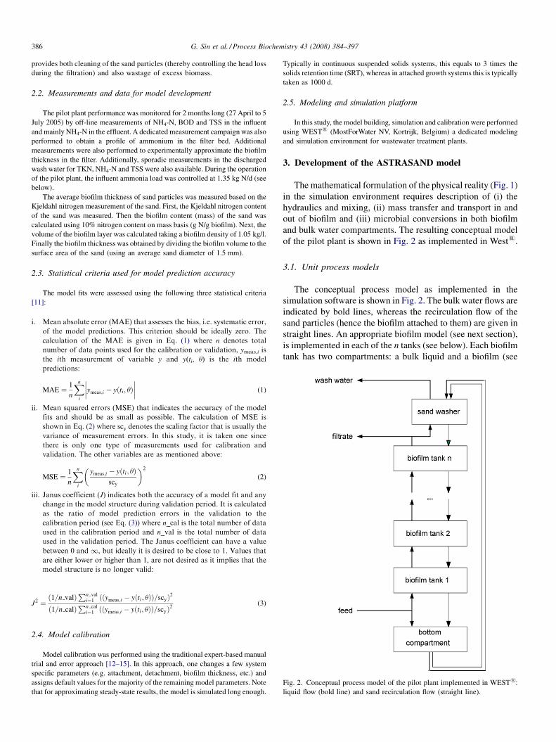
3. Development of the ASTRASAND model

The mathematical formulation of the physical reality (Fig. 1)

in the simulation environment requires description of (i) the

hydraulics and mixing, (ii) mass transfer and transport in and

out of biofilm and (iii) microbial conversions in both biofilm

and bulk water compartments. The resulting conceptual model

of the pilot plant is shown in Fig. 2 as implemented in West1.

3.1. Unit process models

The conceptual process model as implemented in the

simulation software is shown in Fig. 2. The bulk water flows are

indicated by bold lines, whereas the recirculation flow of the

sand particles (hence the biofilm attached to them) are given in

straight lines. An appropriate biofilm model (see next section),

is implemented in each of the n tanks (see below). Each biofilm

tank has two compartments: a bulk liquid and a biofilm (see


below). The microbial conversion processes take place in the

biofilm (mainly nitrification and BOD removal). Next to that,

the TSS present in the influent of the filter is removed by

physical filtering in the sand matrix. The bottom part of the

reactor is assumed to be biologically inactive for this particular

configuration and operation of the biofilm reactor for the

following reasons: (i) it is not aerated hence no nitrification and

heterotrophic carbon oxidation process can occur, (ii) it

receives not enough BOD (since the influent to the biofilm

reactor contains mainly unbiodegradable COD left from the

secondary treatment step of the WWTP) to initiate any

significant biological denitrification, (iii) no aerobic decay

process can occur due to absence of oxygen and last (iv) anoxic

decay of autotrophs was found substantially low under anoxic

conditions [22]. Hence, it is modeled as a non-reactive buffer

tank with a constant volume (only transport considered).

Finally, the sand washer unit uses the same biofilm model

structure as in the other tanks.

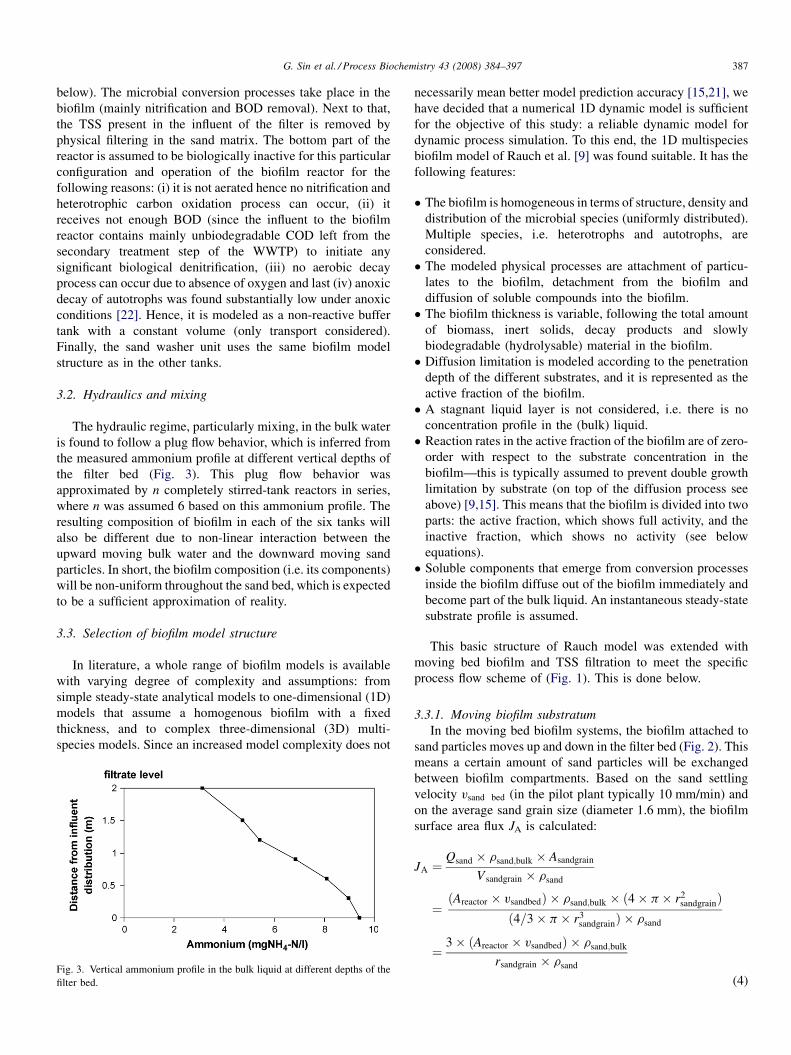
3.2. Hydraulics and mixing

The hydraulic regime, particularly mixing, in the bulk water

is found to follow a plug flow behavior, which is inferred from

the measured ammonium profile at different vertical depths of

the filter bed (Fig. 3). This plug flow behavior was

approximated by n completely stirred-tank reactors in series,

where n was assumed 6 based on this ammonium profile. The

resulting composition of biofilm in each of the six tanks will

also be different due to non-linear interaction between the

upward moving bulk water and the downward moving sand

particles. In short, the biofilm composition (i.e. its components)

will be non-uniform throughout the sand bed, which is expected

to be a sufficient approximation of reality.

3.3. Selection of biofilm model structure

In literature, a whole range of biofilm models is available

with varying degree of complexity and assumptions: from

simple steady-state analytical models to one-dimensional (1D)

models that assume a homogenous biofilm with a fixed

thickness, and to complex three-dimensional (3D) multi-

species models. Since an increased model complexity does not

Fig. 3. Vertical ammonium profile in the bulk liquid at different depths of the

filter bed.

necessarily mean better model prediction accuracy [15,21], we

have decided that a numerical 1D dynamic model is sufficient

for the objective of this study: a reliable dynamic model for

dynamic process simulation. To this end, the 1D multispecies

biofilm model of Rauch et al. [9] was found suitable. It has the

following features:

� T
he biofilm is homogeneous in terms of structure, density and
distribution of the microbial species (uniformly distributed).

Multiple species, i.e. heterotrophs and autotrophs, are

considered.

� T
he modeled physical processes are attachment of particu-
lates to the biofilm, detachment from the biofilm and

diffusion of soluble compounds into the biofilm.

� T
he biofilm thickness is variable, following the total amount
of biomass, inert solids, decay products and slowly

biodegradable (hydrolysable) material in the biofilm.

� D
iffusion limitation is modeled according to the penetration
depth of the different substrates, and it is represented as the

active fraction of the biofilm.

� A
stagnant liquid layer is not considered, i.e. there is no
concentration profile in the (bulk) liquid.

� R
eaction rates in the active fraction of the biofilm are of zero-
order with respect to the substrate concentration in the

biofilm—this is typically assumed to prevent double growth

limitation by substrate (on top of the diffusion process see

above) [9,15]. This means that the biofilm is divided into two

parts: the active fraction, which shows full activity, and the

inactive fraction, which shows no activity (see below

equations).

� S
oluble components that emerge from conversion processes
inside the biofilm diffuse out of the biofilm immediately and

become part of the bulk liquid. An instantaneous steady-state

substrate profile is assumed.

This basic structure of Rauch model was extended with

moving bed biofilm and TSS filtration to meet the specific

process flow scheme of (Fig. 1). This is done below.

3.3.1. Moving biofilm substratum

In the moving bed biofilm systems, the biofilm attached to

sand particles moves up and down in the filter bed (Fig. 2). This

means a certain amount of sand particles will be exchanged

between biofilm compartments. Based on the sand settling

velocity vsand bed (in the pilot plant typically 10 mm/min) and

on the average sand grain size (diameter 1.6 mm), the biofilm

surface area flux JA is calculated:

JA ¼Qsand � rsand;bulk � Asandgrain

V sandgrain � rsand

¼ðAreactor � vsandbedÞ � rsand;bulk � ð4� p� r2

sandgrainÞð4=3� p� r3

sandgrainÞ � rsand

¼3� ðAreactor � vsandbedÞ � rsand;bulk

rsandgrain � rsand

(4)

Fig. 4. The attachment and detachment processes in the sand bed and the sand washer: liquid flow (bold line) and sand recirculation flow (straight line).


where JA is the flux of sand surface area (m2/d), Qsand the sand

bed flowrate (m3 sand bed/d), Asand grain the surface area of sand

grain (m2), Vsand grain the volume of sand grain (m3) and other

parameters as defined earlier. Together with the biofilm thick-

ness, this sand surface area flux will be used in Eq. (15) to

calculate the masses of biofilm components that leave each

biofilm compartment.

3.3.2. Filtration of solids

In reality, a major part of the solids in the feed flow is filtered

from the water by physical processes: some solids ‘stick’ or

attach to the biofilm, others get captured in the pores of the sand

bed. In either way, they are transported to the sand washer

together with the sand, where they are separated from it, and

end up in the wash water. It is assumed that these two types of

solids filtering processes can be modeled by means of

attachment to the biofilm in the sand bed and detachment

from it in the sand washer.

In the sand bed as well as in the sand washer, the attachment

and detachment processes are split up for biomass and non-

biomass compounds (Fig. 4). Since the shear stress induced by

the mechanical configuration of the sand washer unit is higher,

the detachment coefficient in the sand washer is assumed higher

than the detachment coefficient in the sand bed. These

processes are described with first order reaction rates:

rAt;biomass ¼ kAt;biomass � XB;rAt;nonbiomass ¼ kAt;nonbiomass � XnonB;rDt;biomass ¼ kDt;biomass �MB;rDt;nonbiomass ¼ kDt;nonbiomass �MnonB

(5)

More specifically, four parameters are introduced: kAt,bio-

mass, kDt,biomass, fAt,nonbiomass and fDt,nonbiomass. The attachment

and detachment process rate coefficients for non-biomass

compounds are expressed as being proportional to the rates of

the biomass compounds:

kAt;nonbiomass ¼ f At;nonbiomass � kAt;biomass;kDt;nonbiomass ¼ f Dt;nonbiomass � kDt;biomass

(6)

In this way, the rate coefficients for biomass and non-

biomass are coupled for redundancy purposes. By adjusting the

values for these four parameters in the sand bed and in the sand

washer, one can manipulate the amount of biofilm growth or

retention in the model. This is analogous to the manipulation of

the SRT in suspended solids systems.

3.4. Selection of a model for microbial conversions

The microbial conversions in both biofilm and bulk liquid

were described using the industry standard ASM1 model

[10]. To be consistent with the assumption of the Rauch

biofilm model, the ASM1 Monod functions for growth

limiting substrate were replaced with zero order kinetics.

Finally the ASM1 model integrated with Rauch model of

physical attachment detachment and diffusion processes are

summarized in a matrix presentation in Appendix A. For the

matrix model presentation, reference is made to Henze et al.

[10].

As a last step, the model components need to be defined for

the two compartments. The bulk liquid components are taken

the same as in ASM1, whereas for the biofilm components only

particulate components of ASM1 are considered (see Table 2).

Note that the masses of the biofilm components are expressed

relative to the volume of bulk (interstitial) water present in the

reactor, not to the volume of biofilm. This is a convention often

used in biofilm modeling to simplify the numerical coding of

the model. In this way, the mass of biofilm can be obtained by

summing up all of the biofilm particulates and multiplying them

with the volume of the bulk water.

3.5. Numerical calculation procedure of the model

To help picture the basis for the calculation presented in

Eq. (7) and (8), the relationship between the sand surface,

biofilm thickness, biofilm volume and masses are shown in

Fig. 5. As already mentioned a spherical biofilm surface is

assumed although in reality the biofilm has a more irregular

Table 2

Definition and units of the model components

Component Definition Unit

Bulk liquid

SALK Alkalinity (Molar units)

SI Soluble inert organic matter g COD/m3 water

SND Soluble biodegradable

organic nitrogen

g N/m3 water

SNH Ammonia g N/m3 water

SNO Nitrate g N/m3 water

SO Dissolved oxygen g COD/m3 water

SS Readily biodegradable substrate g COD/m3 water

XBA Autotrophic biomass g COD/m3 water

XBH Heterotrophic biomass g COD/m3 water

XI Inert particulate matter g COD/m3 water

XND Particulate biodegradable

organic nitrogen

g N/m3 water

XP Particulate products arising

from biomass decay

g COD/m3 water

XS Slowly biodegradable substrate g COD/m3 water

Biofilm

MBH Heterotrophic biomass g COD/m3 water

MBA Autotrophic biomass g COD/m3 water

MS Slowly biodegradable

particulate substrate

g COD/m3 water

MPH Products arising from

heterotroph biomass decay

g COD/m3 water

MPA Products arising from

autotroph biomass decay

g COD/m3 water

MI Inert matter g COD/m3 water


shape. This is a common approximation in biofilm modeling

literature and often provides realistic results [15,16].

During a simulation, the set of differential and algebraic

equations contained in the model (the combined Rauch and

ASM1 models) is solved at each time-step. In this study a

fourth order Runge Kutta numerical integration algorithm

with adaptive step size is used. These equations yield the

values of certain state variables, which then are used as data

for the calculations at the next time-step. To start this iterative

process, initial values must be given to all derived state

variables. The masses of the biofilm components are

calculated as

Mk ¼ Asand � Lbiofilm;initial � rbiofilm|fflfflfflfflfflfflfflfflfflfflfflfflfflfflfflfflfflfflfflfflfflfflfflffl{zfflfflfflfflfflfflfflfflfflfflfflfflfflfflfflfflfflfflfflfflfflfflfflffl}total biofilm mass

� f k;initial|fflfflffl{zfflfflffl}mass fraction

(7)

Fig. 5. The relationship between sand surface area, biofilm thickness, biofilm

where Mk is the mass of kth biofilm component relative to bulk

liquid volume (g COD/m3).

After having calculated the initial masses Mk, the sequence

of equations to be solved at each time-step can be summarized

as follows:Calculate the thickness of the biofilm:

Lbiofilm ¼Vwater �

Pk¼1! 6Mk

rbiofilm � Asand

(8)

Calculate the conversion rates for the model components

assuming there is no limiting substrate (note that the maximum

specific growth rates were corrected for the effect of tempera-

ture using the Arrhenius equation (see Appendix A)).Calculate

the dimensionless penetration depth bi of each growth related

substrates, i.e. SNH, SS and SO. For the substrate i, this becomes

as follows:

bi ¼ffiffiffiffiffiffiffiffiffiffiffiffiffiffiffiffiffiffiffiffiffiffiffiffiffiffiffiffiffiffi2� Di � Si;bulk

ð�riÞ � L2biofilm

s(9)

where D is the diffusion coefficient, Sbulk the model component

concentration in the bulk liquid, r the overall reaction rate

derived in Eq. (9) and i denoting substrate i.Determine the

active fraction of the biofilm for each biomass species (see

Rauch et al. [9]) by considering the minimum substrate pene-

tration depth in the biofilm. For the growth of heterotrophs, the

penetration depths of SO, SNH and SS are considered:

’H ¼ minðbSO;bSS

;bSNHÞ (10)

For the growth of autotrophs, the penetration depths of SO

and SNH are considered:

’A ¼ minðbSO;bSNH

Þ (11)

Re-calculate the process rates to incorporate the substrate

diffusion limitations. This is done by multiplying the process

rates calculated in step 2 with the corresponding active fractions

wA and wH obtained in step 4.Calculate the overall conversion

rates for all components using the recalculated process rates in

step 5, e.g. the overall rate for the heterotrophic biomass in the

biofilm equals

rMBH¼ ðmH � uT�T ref

mH�MBH � ’HÞ � ðbH � uT�T ref

bH�MBHÞ

þ ðkAt;biomass � XBHÞ � ðkDt;biomass �MBHÞ (12)

volume, biofilm density, biofilm mass and biofilm particulate components.

Table 3

Steady-state influent fractionation for the model

Component (unit) Average value Reference/explanation

Flow (m3/d) 117.6 Measurements

SALK (mol/m3) 7 [10]

SI (g COD/m3 water) 0 Assumed (simplification)

SND (g N/m3 water) 0 Assumed (simplification)

SNH (g N/m3 water) 11.67 Measurements

SNO (g N/m3 water) 0 Not considered in the modeling objective

SO (g COD/m3 water) 5 Measurements

SS (g COD/m3 water) 0 Assumed (simplification)

XBA (g COD/m3 water) 0.18 TSSf TSS:CODp

� BODt

� �� f XB

� f A

XBH (g COD/m3 water) 1.63 TSSf TSS:CODp

� BODt

� �� f XB

� ð1� f AÞ

XI (g COD/m3 water) 10.24 TSSf TSS:CODp

� BODt

� �� ð1� f XB

Þ

XND (g N/m3 water) 0.77 ðXS � f ND:SÞ þ ðXI � f ND:IÞ

XP (g COD/m3 water) 0 Assumed (simplification)

XS (g COD/m3 water) 9.41 BODt measurements (SS included here)

fTSS:COD (g SS/g COD) 0.75 [10]

fND:I (g N/g COD) 0.02 [10]

fND:S (g N/g COD) 0.06 [10]

fXB (g COD/g COD) 0.15 Biomass content of the influent COD (assumed)

fA (g COD/g COD) 0.1 Fraction of autotrophs in the influent (assumed)

BODt (g BOD/m3) 9.41 Short-term BOD measurements

TSS (g SS/m3) 16.09 Measurements


Solve the differential equations to determine the concentration

of each component in the bulk liquid:

dSi

dt¼ Q

Vwater

ðSi;in � SiÞ þ rSi (13)

Determine the flow rate of biofilm being transported to a lower

tank compartment due to the sedimentation of the sand grains:

QMk¼ JA � Lbiofilm � rbiofilm � f k (14)

where QMkis the mass of kth biofilm component transported out

of a compartment (g COD/d).Solve the differential equations to

determine the concentration of each biofilm component:

dMk

dt¼ QMk ;in � QMk

þ rMk(15)

4. Results

4.1. Steady-state calibration

In this first step of the calibration procedure, the aim is to use

the steady-state influent load to numerically solve the model

equations and compare model predictions with steady-state

plant performance.

4.1.1. Influent characterization

The ASM1 model requires influent fractionation such that

the typically measured influent variables (mainly NH4-N, BOD

and TSS) are properly partitioned into the model (ASM1)

components. Although numerous methods exist to fractionate

influent wastewater [17,18], there is no fractionation metho-

dology developed for the effluent wastewater of the WWTPs,

which is the feed (the influent) of the pilot plant in this study.

Hence, we relied on process knowledge and provided the

following empirical fractionation for the influent of the pilot

plant (see Table 3).

4.1.2. Steady-state calibration results

Most of the model parameters particularly those relating to

stoichiometric, kinetic and diffusion are assumed from

literature (see Table 4). For calibrating the model predictions

to the measurements, system specific parameters were selected

following the guidelines proposed by Wanner et al for biofilm

model applications [15]. These include initial biofilm thickness,

Lbiofilm,init (mm), fAt,nonbiomass in sand bed, kAt,biomass in sand bed

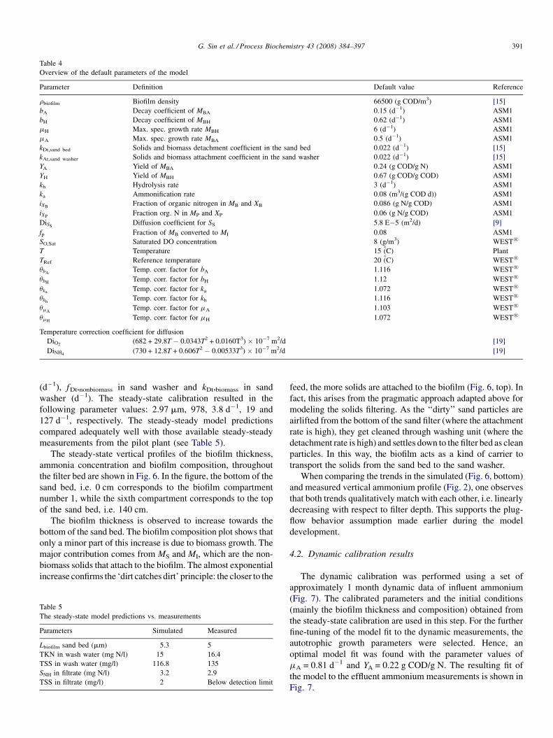
Table 4

Overview of the default parameters of the model

Parameter Definition Default value Reference

rbiofilm Biofilm density 66500 (g COD/m3) [15]

bA Decay coefficient of MBA 0.15 (d�1) ASM1

bH Decay coefficient of MBH 0.62 (d�1) ASM1

mH Max. spec. growth rate MBH 6 (d�1) ASM1

mA Max. spec. growth rate MBA 0.5 (d�1) ASM1

kDt,sand bed Solids and biomass detachment coefficient in the sand bed 0.022 (d�1) [15]

kAt,sand washer Solids and biomass attachment coefficient in the sand washer 0.022 (d�1) [15]

YA Yield of MBA 0.24 (g COD/g N) ASM1

YH Yield of MBH 0.67 (g COD/g COD) ASM1

kh Hydrolysis rate 3 (d�1) ASM1

ka Ammonification rate 0.08 (m3/(g COD d)) ASM1

iXBFraction of organic nitrogen in MB and XB 0.086 (g N/g COD) ASM1

iXPFraction org. N in MP and XP 0.06 (g N/g COD) ASM1

DiSSDiffusion coefficient for SS 5.8 E�5 (m2/d) [9]

fp Fraction of MB converted to MI 0.08 ASM1

SO,Sat Saturated DO concentration 8 (g/m3) WEST1

T Temperature 15 (C) Plant

TRef Reference temperature 20 (C) WEST1

ubATemp. corr. factor for bA 1.116 WEST1

ubHTemp. corr. factor for bH 1.12 WEST1

uka Temp. corr. factor for ka 1.072 WEST1

ukhTemp. corr. factor for kh 1.116 WEST1

umATemp. corr. factor for mA 1.103 WEST1

umHTemp. corr. factor for mH 1.072 WEST1

Temperature correction coefficient for diffusion

DiO2(682 + 29.8T � 0.0343T2 + 0.0160T3) � 10�7 m2/d [19]

DiNH4(730 + 12.8T + 0.606T2 � 0.00533T3) � 10�7 m2/d [19]


(d�1), fDt,nonbiomass in sand washer and kDt,biomass in sand

washer (d�1). The steady-state calibration resulted in the

following parameter values: 2.97 mm, 978, 3.8 d�1, 19 and

127 d�1, respectively. The steady-steady model predictions

compared adequately well with those available steady-steady

measurements from the pilot plant (see Table 5).

The steady-state vertical profiles of the biofilm thickness,

ammonia concentration and biofilm composition, throughout

the filter bed are shown in Fig. 6. In the figure, the bottom of the

sand bed, i.e. 0 cm corresponds to the biofilm compartment

number 1, while the sixth compartment corresponds to the top

of the sand bed, i.e. 140 cm.

The biofilm thickness is observed to increase towards the

bottom of the sand bed. The biofilm composition plot shows that

only a minor part of this increase is due to biomass growth. The

major contribution comes from MS and MI, which are the non-

biomass solids that attach to the biofilm. The almost exponential

increase confirms the ‘dirt catches dirt’ principle: the closer to the

Table 5

The steady-state model predictions vs. measurements

Parameters Simulated Measured

Lbiofilm sand bed (mm) 5.3 5

TKN in wash water (mg N/l) 15 16.4

TSS in wash water (mg/l) 116.8 135

SNH in filtrate (mg N/l) 3.2 2.9

TSS in filtrate (mg/l) 2 Below detection limit

feed, the more solids are attached to the biofilm (Fig. 6, top). In

fact, this arises from the pragmatic approach adapted above for

modeling the solids filtering. As the ‘‘dirty’’ sand particles are

airlifted from the bottom of the sand filter (where the attachment

rate is high), they get cleaned through washing unit (where the

detachment rate is high) and settles down to the filter bed as clean

particles. In this way, the biofilm acts as a kind of carrier to

transport the solids from the sand bed to the sand washer.

When comparing the trends in the simulated (Fig. 6, bottom)

and measured vertical ammonium profile (Fig. 2), one observes

that both trends qualitatively match with each other, i.e. linearly

decreasing with respect to filter depth. This supports the plug-

flow behavior assumption made earlier during the model

development.

4.2. Dynamic calibration results

The dynamic calibration was performed using a set of

approximately 1 month dynamic data of influent ammonium

(Fig. 7). The calibrated parameters and the initial conditions

(mainly the biofilm thickness and composition) obtained from

the steady-state calibration are used in this step. For the further

fine-tuning of the model fit to the dynamic measurements, the

autotrophic growth parameters were selected. Hence, an

optimal model fit was found with the parameter values of

mA = 0.81 d�1 and YA = 0.22 g COD/g N. The resulting fit of

the model to the effluent ammonium measurements is shown in

Fig. 7.

Fig. 6. Steady-state model predictions of the biofilm thickness, ammonium, nitrate and biofilm composition throughout the sand bed.

Fig. 7. Results of the dynamic calibration: the influent ammonium (&), the simulated effluent ammonium (line) and the measured effluent ammonium (&).



4.3. Model validation results

To validate the predictions of the model, a 10-d long

independent data set has been used. The data set is taken from a

period prior to the calibration data set, that is from the first week

of June 2004 as shown in Fig. 8. Visual inspection shows that

the model matches the measurements quite well during the

validation period. The statistical analysis of the fits, however, is

given below.

5. Discussion

5.1. Model prediction accuracy and validity

The MAE was found 0.76 and 0.72 in the calibration

and validation periods respectively. This means the bias

of the model remain similar in both periods. It also means

that the model predictions will be accompanied with a

bias of 0.7 mg NH4-N/l in the effluent. This average

systematic difference between the model and the reality

is usually deemed acceptable for many modeling applica-

tions such as scenario analysis for process optimization

[14,21].

The MSE was found 0.73 and 0.78 in the calibration and

validation periods indicating that the accuracy of the

predictions remained similar in both periods. Finally, these

results are confirmed by the Janus coefficient that was

calculated to be 0.9 which is quite close to 1. This suggests

that the model structure did not require significant change

during the validation period [11]. Overall, these criteria confirm

that the model predictions, albeit accompanied with an

acceptable bias, are statistically accurate and valid. Hence,

this increases the confidence into the model.

Fig. 8. Results of the model validation: the influent ammonium (&), the simul

Fig. 9. Effect of temperature: biofilm thicknes

5.2. Effect of temperature on the filter performance

Temperature has a profound effect on the nitrification

performance in the biofilm systems and also on determining the

optimal nitrogen loading rate to the system [23,24]. Therefore,

to understand the effect of temperature on the nitrification

performance of the moving bed biofilm reactor, we have

performed dedicated simulations following one-factor-at-a-

time approach. In this approach, the temperature was varied and

other factors (e.g. influent load) were kept constant. The

resulting effect of temperature on the ammonium removal

performance is shown Fig. 9 (right). One observes that

increasing temperature has a positive effect on the ammonium

removal as expected. For example, a 5 8C increase in the

operating temperature of the plant (15 8C) leads to the complete

nitrification of ammonium (see Fig. 9, right). Further increasing

temperature does not affect any longer the filter performance as

the influent ammonium load becomes rate limiting rather than

the nitrification capacity of the filter.

As regards the biofilm thickness (Fig. 9, left), one observes

that it increases with increasing temperature until 20 8C,

beyond which it drops. This phenomenon is explained by the

combined effect of temperature on the growth and decay of

nitrifying biomass in the system. We observe that at

temperatures between 5 and 20 8C, the growth of nitrifying

biomass offsets the amount lost due to decay hence resulting in

a net increase in the thickness of biofilm. For temperatures

exceeding 20 8C, the growth of nitrifying biomass becomes

limited by the influent ammonium load, while the decay of

nitrifying biomass continues to increase exponentially. The

latter follows from the assumption of ASM1 model [10] that

states that decay rate increases with the increasing temperature.

As a result, the observed yield of nitrifying biomass decreases,

ated effluent ammonium (line) and the measured effluent ammonium (&).

s (left), NH4-N removal efficiency (right).

Fig. 10. The effect influent ammonium load and hydraulic load on the filter

performance: constant HRT and variable HRT.


which in turn leads to decrease in the biofilm thickness that is

observed in Fig. 9 (left).

Overall this model-based analysis presented above showed

that the temperature effect as well as the optimal operating

temperature on the nitrification performance depends on the

influent nitrogen load and could be either positive or neutral. To

this end, it is advised to perform an integrated analysis to

understand the temperature effect for different biofilm systems.

5.3. Effect of the influent load

The effect of the influent nitrogen load on the nitrogen

removal efficiency was investigated in two ways. In the first

approach, the influent load was increased by manipulating the

wastewater strength but keeping the flow of the wastewater

constant. In the second approach, the influent flow rate was

increased while the wastewater strength was kept constant. The

main difference between the two approaches is that the

hydraulic retention time (HRT) is constant in the first approach,

whereas it is variable in the second one. All other factors

(including temperature) were kept constant during these

scenarios.

The results obtained from the two approaches are shown in

Fig. 10. One observes that the ammonium removal efficiency

decreases as the influent ammonium load increases (see the line

with fixed HRT). This is understandable as the amount of

ammonium removal from the influent is determined by the

nitrification capacity present in the plant. Therefore increasing

the influent load without increasing the nitrification capacity

will simply overload the plant with more ammonium than it can

handle. This results in a decreasing removal efficiency as

observed in Fig. 10.

As regards hydraulic loading, whether the HRT is varied or

kept constant does not change much the observed impact on the

ammonium removal efficiency (see both curves are similar in

Fig. 10). This means that the HRT has a negligible effect on the

ammonium removal efficiency. In suspended activated sludge

systems, the effect of HRT may become more pronounced

especially if the system is hydraulically overloaded. In such a

case, the biomass may even be completely washed out leading

to a complete system failure. In attached growth systems,

however, we observe that HRT is effectively decoupled from

SRT. In fact in this way, it becomes feasible to enrich slowly

growing specialized bacteria such as the nitrifying bacteria

enriched in the biofilm system studied here.

It should be noted that variable hydraulic loading may also

affect attached growth systems via the detachment process.

This aspect is not considered in this study. Some studies and

models suggest that increasing shear stress (that may be due to

hydraulic overloading) further increases the detachment rates in

the system, which may eventually lead to washout of biomass

[15].

Overall, the current operating influent ammonium load

(1 kg N/d-m3 filter bed) seems to be approximately 30% higher

than the maximum load that corresponds to complete

nitrification (0.75 kg N/d-m3 filter bed see in Fig. 10). If the

goal is to achieve a complete nitrification, the load needs to be

decreased or the capacity of the active sand bed of the filter

needs to be increased, for example by increasing the height of

the filter.

5.4. Future perspectives

The dynamic model presented here was developed and

validated using full-scale ammonia measurements, which

helped verify the model for ammonium predictions in the

filter. However, future validation of the model predictions

against more measurements particularly the oxygen and nitrate

are certainly desirable to extend the prediction spectrum of the

model. Moreover, the entrapment of suspended solids is an

important function of the filter. Detailed experimental analysis

of the solids trajectory in the filter is expected to improve the

verification of the pragmatic approach used in the model.

Further, as the quality of the input data to the model determines

the quality of the model outputs, using process performance

under stress or more changing influent load will help

consolidate the validity of the model to describe fast-changing

phenomena in the process. Such a model can improve

understanding of fast-changing reactions in the filter and be

useful for testing different control strategies.

Moreover, the general steps followed here for the model

development is expected to be useful as a method to aid in the

development of biofilm models for other biofilm applications,

particularly continuously moving bed filters performing not

only nitrification but also denitrification.

Overall the dynamic model can be used to support the design

of moving bed filters for ammonium removal process. This can

be done as follows: once the initial design of the moving bed

filter is obtained (typically using rules of thumbs or empirical

(pilot-scale) studies under steady-state loading), one can then

perform dynamic simulations under fluctuating influent loading

(e.g. considering dry-weather versus wet-weather influent flow

loading profiles). In this way, one obtains deeper insight into the

robustness and the performance of the initial design and hence

opportunities to further improve the design in an iterative way.

The dynamic model, especially if well calibrated and

validated, can also be used for optimization purposes. The latter

is defined as the process of searching in an iterative way the

optimal performance of running the system (see e.g. Sin et al.


[5]). Since model predictions are subject to certain assump-

tions, it is important to cross check the predictions with

valuable process engineering/expert knowledge about the

system as presented above. Ultimately this is expected to

ensure the quality of the models before being used as support

tools for taking engineering decisions for design and

optimization problems.

6. Conclusions

In this study, a mathematical model with adequate

complexity integrating hydraulic, biofilm and microbial

conversion processes was successfully developed, calibrated

and validated for a particular continuously moving bed biofilter

process.

For the steady-state calibration of the model, a good match

could be obtained by changing a few system specific parameters

(such as attachment rate coefficient, detachment rate coefficient

and biofilm thickness), whereas the remaining model para-

meters could be adapted from relevant literature. Building on

the steady-state calibration results, the model was calibrated

using a dynamic (1 month) data set by changing only two

autotrophic growth related parameters: maximum specific

growth rate (mA = 0.81 d�1) and yield (YA = 0.22 g COD/g N).

The model confrontation with an independent data set showed

that the model predictions remained largely valid (Janus

coefficient is 0.9) albeit with a bias the effluent ammonium

concentration equal to 0.8 mg N/l.

Scenario analysis with the validated model revealed some

new insights and confirmed several conclusions about biofilm

systems: (i) increasing temperature has a significant and

positive effect on the nitrification performance. (ii) The biofilm

thickness is affected considerably by temperature. The biofilm

thickness may decrease at high temperatures due to increasing

decay rate. (iii) The influent nitrogen load is more influential

than the influent hydraulic load on the ammonium removal

efficiency. The latter has a negligible impact on the filter

performance.

Overall the model can be used to support some engineering

tasks including design and process optimization of ammonium

removal in this particular moving bed filters at full-scale.

Acknowledgements

Authors acknowledge the valuable contribution of ir.

Webbey Keyser to the model development and calibration.

Paques BV, The Netherlands supported the project financially

and provided all the necessary data used in this research project.

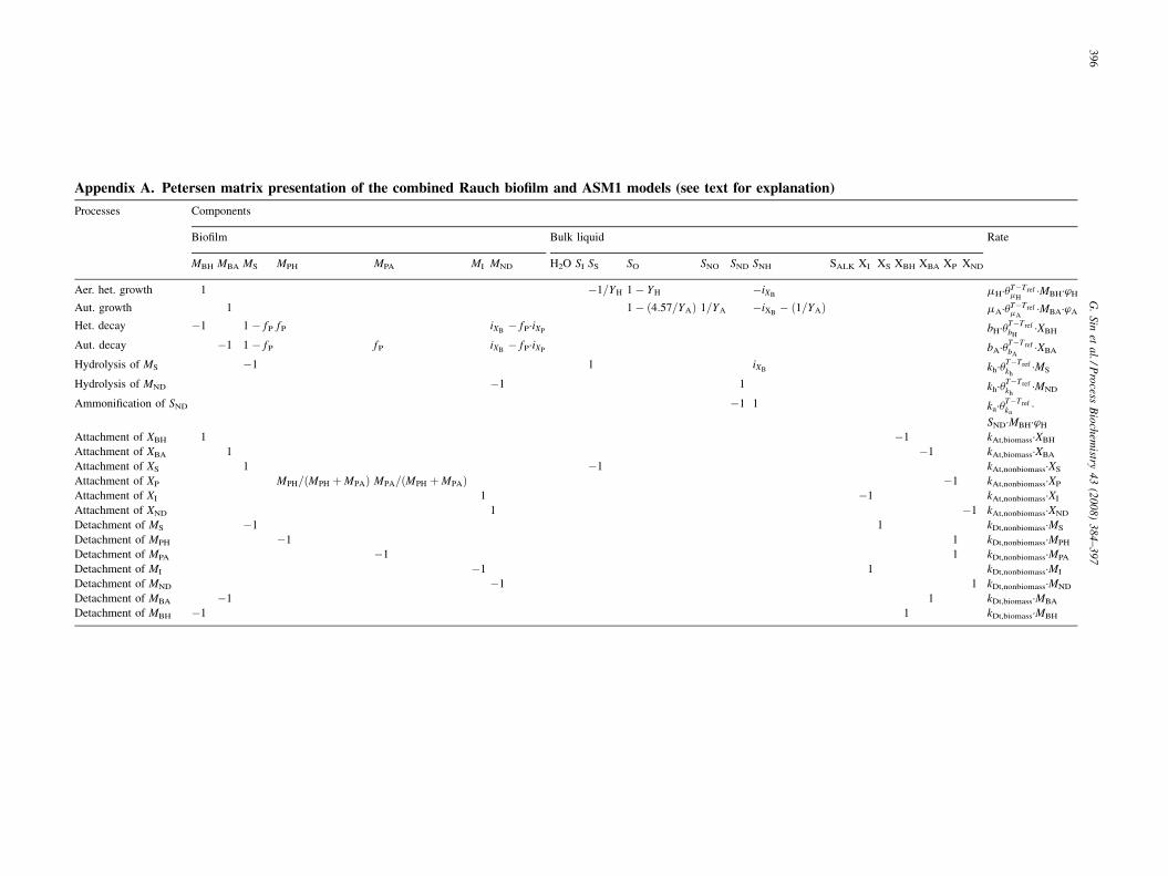
Appendix A. Petersen matrix presentation of the combined Rauch biofilm and ASM1 models (see text for explanation)

Processes Components

Biofilm Bulk liquid Rate

MBH MBA MS MPH MPA MI MND H2O SI SS SO SNO SND SNH SALK XI XS XBH XBA XP XND

Aer. het. growth 1 �1=YH 1� YH �iXB mH�uT�TrefmH

�MBH�wH

Aut. growth 1 1� ð4:57=YAÞ 1=YA �iXB� ð1=YAÞ mA�uT�Tref

mA�MBA�wA

Het. decay �1 1 � fP fP iXB� fP�iXP bH�uT�T ref

bH�XBH

Aut. decay �1 1 � fP fP iXB� fP�iXP bA�uT�T ref

bA�XBA

Hydrolysis of MS �1 1 iXB kh�uT�Trefkh

�MS

Hydrolysis of MND �1 1 kh�uT�Trefkh

�MND

Ammonification of SND �1 1 ka�uT�T refka

�SND�MBH�wH

Attachment of XBH 1 �1 kAt,biomass�XBH

Attachment of XBA 1 �1 kAt,biomass�XBA

Attachment of XS 1 �1 kAt,nonbiomass�XS

Attachment of XP MPH=ðMPH þMPAÞ MPA=ðMPH þMPAÞ �1 kAt,nonbiomass�XP

Attachment of XI 1 �1 kAt,nonbiomass�XI

Attachment of XND 1 �1 kAt,nonbiomass�XND

Detachment of MS �1 1 kDt,nonbiomass�MS

Detachment of MPH �1 1 kDt,nonbiomass�MPH

Detachment of MPA �1 1 kDt,nonbiomass�MPA

Detachment of MI �1 1 kDt,nonbiomass�MI

Detachment of MND �1 1 kDt,nonbiomass�MND

Detachment of MBA �1 1 kDt,biomass�MBA

Detachment of MBH �1 1 kDt,biomass�MBH

G.

Sin

eta

l./Pro

cessB

ioch

emistry

43

(20

08

)3

84

–3

97

39

6


References

[1] Ockier P, Thoeye C, De Gueldre G. Key tools to accelerate fulfillment of

the EU urban waste water treatment directive in the Flemish region of

Belgium. Water Sci Technol 2001;44(1):7–14.

[2] Obenaus F, Kraft A. Realisation of the EU Directive 91/271/EWG in

Germany—technical and economic effects from the perspective of an

operator of large wastewater treatment plants. Water Sci Technol

2004;50(7):257–63.

[3] Demuynck C, Vanrolleghem PA, Mingneau C, Liessens J, Verstraete W.

NDBEPR process optimisation in SBRs: reduction of external carbon

source and oxygen supply. Water Sci Technol 1994;30(4): 169–79.

[4] Artan N, Wilderer P, Orhon D, Tasli R, Morgenroth E. Model evaluation

optimisation of nutrient removal potential for sequencing batch reactors.

Water Sci Technol 2001;28(4):423–32.

[5] Sin G, Insel G, Lee DS, Vanrolleghem PA. Optimal but robust N and P

removal in SBRs: a model-based systematic study of operation scenarios.

Water Sci Technol 2004;50(10):97–105.

[6] Yang WB, Cicek N, Ilg J. State-of-the-art of membrane bioreactors:

worldwide research and commercial applications in North America. J

Membr Sci 2006;270(1/2):201–11.

[7] van Loosdrecht MC, Salem S. Biological treatment of sludge digester

liquids. Water Sci Technol 2006;53:11–20.

[8] Kramer JP, Wouters JW, Noordink MP, Anink DM, Janus JM. Dynamic

denitrification of 3,600 m3/h sewage effluent by moving bed biofiltration.

Water Sci Technol 2000;41(4/5):29–33.

[9] Rauch W, Vanhooren H, Vanrolleghem PA. A simplified mixed-culture

biofilm model. Water Res 1999;33:2148–62.

[10] Henze M, Gujer W, Mino T, van Loosdrecht MCM. Activated sludge

models ASM1, ASM2, ASM2d and ASM3. IWA scientific and technical

report 9. London: IWA publishing; 2000.

[11] Power M. The predictive validation of ecological and environmental-

models. Ecol Modell 1993;68(1/2):33–50.

[12] Hulsbeek JJW, Kruit J, Roeleveld PJ, van Loosdrecht MCM. A practical

protocol for dynamic modelling of activated sludge systems. Water Sci

Technol 2002;45(6):127–36.

[13] Insel G, Sin G, Lee DS, Nopens I, Vanrolleghem PA. A calibration

methodology and model-based systems analysis for SBRs removing

nutrients under limited aeration conditions. J Chem Technol Biotechnol

2006;81:679–87.

[14] Melcer H, Dold PL, Jones RM, Bye CM, Takacs I, Stensel HD, et al.

Methods for wastewater characterisation in activated sludge modelling.

Alexandria: Water Environment Research Foundation (WERF); 2003.

[15] Wanner O, Eberl, H, Morgenroth E, Noguera D, Picioreanu C, Rittman B,

et al. Mathematical modelling of biofilms. Scientific and technical report

no. 18. London: IWA Publishing; 2006.

[16] Wanner O, Reichert P. Mathematical modeling of mixed-culture biofilms.

Biotechnol Bioeng 1996;49:172–84.

[17] Roeleveld PJ, van Loosdrecht MCM. Experiences with guidelines for

wastewater characterization in The Netherlands. Water Sci Technol

2002;45(6):77–87.

[18] Petersen B, Gernaey K, Henze M, Vanrolleghem PA. Calibration of

activated sludge models: a critical review of experimental designs. In:

Biotechnology for the Environment, Agathos SN, Reineke W, editors.

Wastewater treatment and modeling, waste gas handling. Dordrecht:

Kluwer Academic Publishers; 2003. p. 101–86.

[19] Gujer W, Boller M. Design of a nitrifying tertiary trickling filter based on

theoretical concepts. Water Res 1986;20:1353–2136.

[20] Casellas M, Dagot C, Baudu M. Set up and assessment of a control

strategy in a SBR in order to enhance nitrogen and phosphorus removal.

Process Biochem 2006;41:1994–2001.

[21] Perez J, Poughon L, Dussap C-G, Montesinos JL, Godia F. Dynamics and

steady state operation of a nitrifying fixed bed biofilm reactor: mathe-

matical model based description. Process Biochem 2005;40:2359–69.

[22] Manser R, Gujer W, Siegrist H. Decay processes of nitrifying bacteria in

biological wastewater treatment systems. Water Res 2006;40:2416–26.

[23] Hao XD, Heijnen JJ, van Loosdrecht MCM. Model-based evaluation of

temperature and inflow variations on a partial nitrification-ANAMMOX

biofilm process. Water Res 2002;36:4839–49.

[24] Bougard D, Bernet N, Cheneby D, Delgenes J-P. Nitrification of a high-

strength wastewater in an inverse turbulent bed reactor: effect of tem-

perature on nitrite accumulation. Process Biochem 2006;41:106–13.

Dynamic model development and validation for a nitrifying moving bed biofilter: Effect of...

Documents

Transcript of Dynamic model development and validation for a nitrifying moving bed biofilter: Effect of...