ORIGINAL PAPER

Short-term prediction of influent flow in wastewater treatmentplant

Xiupeng Wei • Andrew Kusiak

Published online: 8 May 2014

� Springer-Verlag Berlin Heidelberg 2014

Abstract Predicting influent flow is important in the

management of a wastewater treatment plant (WWTP).

Because influent flow includes municipal sewage and

rainfall runoff, it exhibits nonlinear spatial and temporal

behavior and therefore makes it difficult to model. In this

paper, a neural network approach is used to predict influent

flow in the WWTP. The model inputs include historical

influent data collected at a local WWTP, rainfall data and

radar reflectivity data collected by the local weather sta-

tion. A static multi-layer perceptron neural network per-

forms well for the current time prediction but a time lag

occurs and increases with the time horizon. A dynamic

neural network with an online corrector is proposed to

solve the time lag problem and increase the prediction

accuracy for longer time horizons. The computational

results show that the proposed neural network accurately

predicts the influent flow for time horizons up to 300 min.

Keywords Influent flow � Radar reflectivity � Rainfall �Wastewater treatment plant � Neural networks

1 Introduction

The influent flow to a wastewater treatment plant (WWTP)

has a significant impact on the energy consumption (Wei

et al. 2013). To maintain the required water level in the wet

well, the number of running raw wastewater pumps should

be scheduled according to the influent rate to the plant. The

optimal selection and scheduling of pumps can greatly

reduce electricity usage. In addition, the pollutants in the

wastewater, including the total suspended solids (TSS) and

biochemical oxygen demand (BOD), are also correlated

with the influent flow (Bechmann et al. 1999). The treat-

ment process should be adjusted based on the pollutant

concentration in the influent. For example, a high BOD

concentration requires a longer aeration time and greater

oxygen supply (Qasim 1998). Therefore, it is important to

predict the influent flow in the near future in order to

improve the process efficiency and save energy use.

The accurate prediction of the influent flow remains a

challenge in the wastewater processing industry. Several

studies have focused on developing models to predict

influent flow (Kim et al. 2006; Kurz et al. 2009; Beraud

et al. 2007; Keyser et al. 2010; Djebbar and Kadota 1998;

Gernaey et al. 2010). Hernebring et al. (2002) presented an

online system for short-term sewer flow forecasts that

optimized the effects of the received wastewater. A more

complex phenomenological model was built in (Gernaey

et al. 2005) based on 1 year of full-scale WWTP influent

data. It included diurnal phenomena, a weekend effect,

seasonal phenomena, and holiday periods. Carstensen et al.

(1998) reported prediction results for the hydraulic load of

storm water. Three models, a simple regression model,

adaptive grey-box model, and complex hydrological and

full dynamic wave model, represented three different levels

of complexity and showed different abilities to predict

water loads 1 h ahead. Although these models accounted

for temporal correlations of the influent flow, they ignored

its spatial feature.

The wastewater processing industry has used physics-

based deterministic models to estimate the influent flow.

X. Wei (&) � A. Kusiak

Department of Mechanical and Industrial Engineering, The

University of Iowa, 3131 Seamans Center, Iowa City, IA 52242,

USA

e-mail: xiupeng-wei@uiowa.edu

A. Kusiak

e-mail: andrew-kusiak@uiowa.edu

123

Stoch Environ Res Risk Assess (2015) 29:241–249

DOI 10.1007/s00477-014-0889-0

Online sensors are used to provide flow data at sub-

pumping stations. Based on empirical data such as the

distance between the sub-station and WWTP, and the

sewer piping size, the influent flow could be roughly esti-

mated and calibrated using the historical data to improve

the estimation accuracy (Pons et al. 1998). Such simple

models did not fully consider the temporal correlations of

the influent flow. In the case of a large rainfall or a lack of

sensors covering large areas, the predicted influent flow

involves a significant error.

A WWTP usually receives municipal sewer and storm

water from different areas around the plant (Vesillind

2003). The quantity of the generated wastewater or pre-

cipitation may vary in space and time. In fact, to accurately

predict the influent flow to a WWTP, the spatial and

temporal characteristics should be considered simulta-

neously. To authors’ knowledge no such research has been

done. Therefore, the short-term prediction (300 min ahead)

of influent flow is presented in this paper taking into

account the spatial–temporal characteristics discussed

above. Rainfall data measured at different tipping buckets,

radar reflectivity data covering the entire area handled by

the WWTP, and the historical influent data to the plant are

used as input parameters to build prediction models. The

rainfall data provided by tipping buckets offers valuable

precipitation measurements containing spatial information.

However, this kind of point based data has limitations due

to physical location of tipping buckets. The actual precip-

itation of the whole area usually cannot be simply summed

up by measurements of all tipping buckets. As weather

radar offers spatial–temporal data covering a large area,

including the places not covered by the tipping buckets,

Kusiak et al. (2013) obtained more accurate rainfall pre-

diction using tipping bucket data together with radar

reflectivity data than only tipping bucket data. In addition,

the high frequency of the radar data makes it useful for

forecasting rainfall several hours ahead. The historical

influent time series data contains temporal influent infor-

mation that is useful for predicting the influent flow. There

are other data resources, e.g., substation influent flows.

They are not considered as input parameters as they are

somehow redundant to above mentioned data. Data con-

taining weather information such as temperature and

humidity are not considered either due to low relevancy

with the plant influent flow.

The remainder of this paper is organized as follows.

Section 2 describes the data collection, preparation, and

preprocessing, as well as the metrics used to evaluate the

accuracy of models. Section 3 presents the static multi-

layer perceptron (MLP) neural network that is employed to

build a prediction model for the influent flow. In Sect. 4, a

data-driven dynamic neural network (DNN) is proposed to

solve the time lag problem appearing in the models by the

static MLP neural network. The neural network structure

and computational results are discussed. Section 5 presents

the conclusions.

2 Data preparation

The Wastewater Reclamation Facility (WRA) studied in

this paper is located in Des Moines, Iowa. It treats the

collected sewage and rainfall runoff from the surrounding

areas. To build an influent flow prediction model for this

WRA, historical influent data, rainfall data, and radar

reflectivity data are considered. The influent flow data were

collected at 15-s intervals at WRA. The data are prepro-

cessed to find 15-min averages to match the frequency of

the rainfall data.

The rainfall data were measured at six tipping buckets

(blue icons in Fig. 1) in the vicinity of WRA (red icon in

Fig. 1). As WRA receives wastewater from a large area,

including rainfall data in the model inputs satisfies the

spatial characteristic of the influent flow. Figure 2 illus-

trates the rainfall rates at the tipping buckets over time. It

shows that the rainfall is location dependent and may vary

despite the proximity of the tipping buckets. This indicates

the importance of the rainfall data in building the influent

flow prediction model.

The rainfall graphs in Fig. 2 illustrate the runoff

amounts at several locations, rather than completely reflect

the precipitation over the entire area covered by WRA.

Therefore, the use of radar reflectivity data is proposed to

provide additional input for influent flow prediction. By

doing this the limitations of tipping bucket based models

will be overcome due to high spatiotemporal characteristics

of radar reflectivity data. The NEXRAD-II radar data used

in this paper are from weather station KDMX in Des

Moines, Iowa, which is located approximately 32 km from

WRA. KDMX uses Doppler WSR-88D radar to collect

high resolution data for each full 360� scan at 5-min

intervals with a range of 230 km and a spatial resolution of

about 1 by 1 km. The radar reflectivity data were collected

at 1, 2, 3, and 4 km Wastewater Reclamation Facility

(CAPPIs). As shown in Fig. 3, the reflectivity may be quite

different at different heights for the same scanning time.

The terrain and flocks of birds may produce errors in the

radar readings. In addition, the reflectivity at one height

may not fully describe a storm occurring at a different

height. To deal with these issues, it is necessary to use

radar reflectivity data from different CAPPIs.

The radar reflectivity data at nine grid points sur-

rounding each tipping bucket are selected and averaged

with the center data to be the reflectivity for that tipping

bucket. Null values are treated as missing values and are

filled using the reflectivity at the surrounding gird points.

242 Stoch Environ Res Risk Assess (2015) 29:241–249

123

The NEXRAD radar data were collected at 5-min intervals

and then processed to find 15-min averages by averaging 3

radar data reflectivity values.

Table 1 summarizes the dataset used in this paper. In

addition to 4 historical influent flow inputs at 15, 30, 45, and

60 min ahead, 6 rainfall and 24 radar reflectivity inputs

Fig. 1 Location of tipping buckets and WRA

Stoch Environ Res Risk Assess (2015) 29:241–249 243

123

provide temporal and spatial parameters for the model. The

data were collected from January 1, 2007, through March 31,

2008. The data from January 1, 2007, through November 1,

2007, containing 32,697 data points, are used to train the

neural networks. The remaining 11,071 data points are used

to test the performance of the constructed models.

Three commonly used metrics, the mean absolute

error (MAE), mean squared error (MSE), and correlation

coefficient (R2) are used to evaluate the performance of

the prediction models (Eq. (1)–(3)).

MAE ¼ 1

n

Xn

i¼1

jfi � yij ð1Þ

MSE ¼ 1

n

Xn

i¼1

jfi � yij2 ð2Þ

R2 ¼ 1�

Pi

ðfi � yiÞ2

Pi

ðfi � yiÞ2 þP

i

ðfi � �yiÞ2ð3Þ

where fi is the predicted value produced by the model, yi is

the observed value, �yi is the mean of the observed value,

and n represents the number of test data points.

Table 1 Data set description

Inputs Description Unit

x1 - x6 Rainfall at 6 tipping buckets Inch

x7 - x30 Radar reflectivity at 6 tipping

buckets at 4 CAPPI

Number

x31 - x34 Historical influent flow MGD

Fig. 2 Rainfall at six tipping

buckets

0

5

10

15

20

25

30

35

1 11 21 31 41 51 61 71 81 91

Ref

lect

ivit

y

Time (15min)

CAPPI1

CAPPI2

CAPPI3

CAPPI4

Fig. 3 Radar reflectivity at

different CAPPIs

244 Stoch Environ Res Risk Assess (2015) 29:241–249

123

3 Modeling by static multi-layer perceptron neural

network

Successful applications of neural networks (NNs) based

prediction models have been reported in the literature.

Singh and Borah (2013) used feed-forward back-propaga-

tion (BP) NN to forecast of Indian summer monsoon

rainfall and obtained more accurate results than the existing

model. Two models using NN (Paleologos et al. 2013)

were developed to simulate spring flow. The results

showed less 3 % of under/over of the observed values. Wu

et al. (2008) found that BP-NN showed an advantage in

heavy snow risk evaluation compared to the conventional

method of evaluation criteria equation. As neural network

based models are capable of forecasting with satisfactory

prediction results, NNs are applied in the research reported

in this paper to build prediction models.

To build the influent flow prediction model, a static

MLP neural network is developed. The MLP neural net-

work has been one of the most widely used network

topologies since its introduction in 1960 (Gurney 1997). It

overcomes the limitations of the single-layer perceptron to

handle model nonlinearity. Prediction and classification

applications of MLP neural networks have been reported in

a variety of scientific and engineering fields. Kusiak and

Wei (2012) employed MLP NNs to model and predict

methane production during sludge treatment and obtained

better accuracy rather than other data-mining algorithms.

In addition, MLP NN has been showing good performance

in non-linear prediction. Verma et al. (2013) had similar

conclusion that MLP NN outperforming other algorithms

when predicting TSSs in wastewater. Therefore, MLP NN

has been selected to build the influent flow prediction

models in this paper.

The structure of the MLP neural network reported in this

paper is shown in Fig. 4. It is a supervised BP network with

three layers. Each layer has one or more neurons, which are

interconnected to each neuron of the previous and next

layers. The connections between two neurons are param-

eterized using a weight and bias. Different activation

functions, including the logistic, hyperbolic tangent, iden-

tity, sine, and exponential functions, are used for the hid-

den and output layers.

In the MLP in Fig. 4, output y1 is calculated as shown in

Eq. (4):

y1 ¼ foX

j

fhX

i

xiwij þ bj

!wj1 þ b1

!ð4Þ

where i denotes the ith neuron in the input layer, j is the jth

neuron in the hidden layer, and fo and fh are the activation

functions for output layer and hidden layer, respectively.

wij is the weight connecting the ith neuron to the jth

neuron, and wj1 is the weight between the jth neuron in the

hidden layer and the neuron in the output layer. bj and b1

are the bias values of neuron j and the output neuron.

Weights wij are calculated in the training process based

on Eq. (5), minimizing the target output,

eðnÞ ¼ 1

2

X

k

ðTðnÞ � y1ðnÞÞ2 ð5Þ

where e is the mean of the square error, n denotes the nth

data point, k is the kth output neuron (in this paper k ¼ 1),

and T represents the targeted output value.

Automated network search was employed to create a

variety of different networks and choose the network with

the best performance in all networks. In total, 200 MLP

neural networks were trained to obtain a generalized net-

work structure. The number of neurons in the hidden layer

varied from 3 to 30. The weights were randomly initialized

between -1 and 1 and iteratively improved by minimizing

the mean of the square error. Different hidden and output

activation functions were used, including logistic, expo-

nential, tanh, identity, hyperbolic, etc. To improve the

convergence speed of the training process, the BFGS

(Broyden-Fletcher-Goldfarb-Shanno) algorithm (Saini

2002) was used.

The influent flow prediction model at current time t was

built first. The dataset described in Sect. 2 was used to train

and test the MLP neural networks. The best MLP had 25

neurons in the hidden layer with the logistic hidden acti-

vation function and the exponential output activation

function. The calculated MAE, MSE, and correlation

coefficient were 1.09 MGD, 4.21 MGD2, and 0.988,

respectively. These metrics indicate that the prediction

model is accurate. The first 300 observed and predicted

influent flow values from the test dataset are shown in

Fig. 5. Most of the predicted values are very close to the

observed ones, and the predicted influent flow follows the

trend of the observed flow rate.

Fig. 4 Structure of MLP neural network

Stoch Environ Res Risk Assess (2015) 29:241–249 245

123

MLP neural network models were also built at

t ? 15 min, t ? 30 min, t ? 60 min, t ? 90 min,

t ? 120 min, t ? 150 min, and t ? 180 min with the same

procedure as the model built at time t. As shown in Fig. 6,

the predicted influent flow is similar to the observed value,

and the predicted trend is the same as the observed one.

However, a small time lag appears between the predicted

and observed influent flows. This lag increases over time

and can be clearly observed in Fig. 7, which shows the

predicted influent flow at t ? 180 min ahead.

Table 2 summarizes the accuracy of the prediction

results at current time t through t ? 180 min. The predic-

tion accuracy decreases with longer time horizon. The

MAE and MSE increase quickly after t ? 30 min, while

the correlation decreases as well. The prediction models for

horizons smaller than t ? 150 min have acceptable accu-

racy when the threshold of the correlation coefficient is set

at 0.85 which is still more accurate than the estimations by

WWTP. However, the time lag is too large to provide a

useful real-time influent flow rate even though the trend

can be well predicted.

4 Modeling by dynamic neural network

The computational results in Sect. 3 indicated that a static

MLP neural network is unable to capture the dynamics in the

dataset at long time horizons. As DNN is an effective and

suitable method to predict dynamic system and has been

successful applied in scientific and engineering problems

(Chiang et al. 2010; Shaw et al. 1997; Hussain et al. 2009), it

is then used in this research to improve the prediction

accuracy. Considering the increasing time lag issue which

has not appeared in DNN applications, a DNN with an online

corrector is proposed and tested in this section.

A DNN involves a memory structure and predictor. As

the memory captures the past time series information, it

can be used by the predictor to learn the temporal patterns

of the time series. This paper uses a focused time-delay

Table 2 Prediction accuracy

Prediction

horizon

MAE

(MGD)

MSE

(MGD2)

Correlation

coefficient

t 1.09 4.21 0.98

t ? 15 1.48 5.83 0.98

t ? 30 1.89 8.20 0.97

t ? 60 2.75 14.59 0.95

t ? 90 3.61 22.95 0.93

t ? 120 4.46 33.21 0.90

t ? 150 5.26 44.88 0.87

t ? 180 6.02 57.39 0.83

Fig. 5 Predicted and actual influent flows at current time t

Fig. 7 Predicted and actual influent flows at time t ? 180 min

Fig. 6 Predicted and actual influent flows at time t ? 30 min

246 Stoch Environ Res Risk Assess (2015) 29:241–249

123

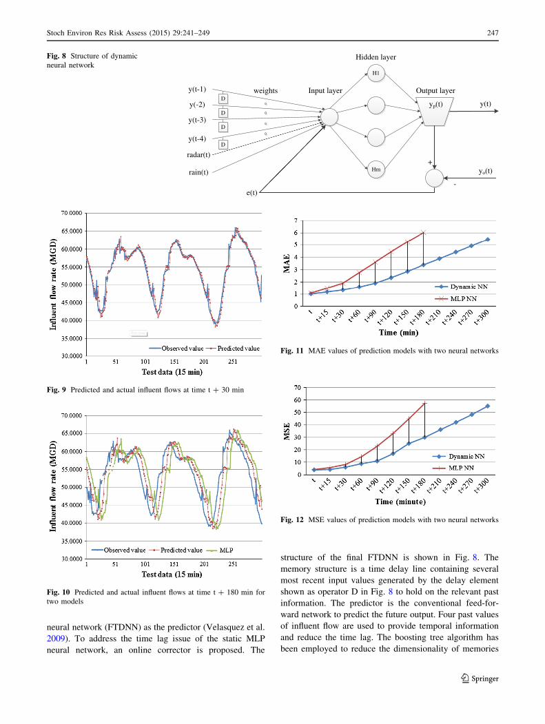
neural network (FTDNN) as the predictor (Velasquez et al.

2009). To address the time lag issue of the static MLP

neural network, an online corrector is proposed. The

structure of the final FTDNN is shown in Fig. 8. The

memory structure is a time delay line containing several

most recent input values generated by the delay element

shown as operator D in Fig. 8 to hold on the relevant past

information. The predictor is the conventional feed-for-

ward network to predict the future output. Four past values

of influent flow are used to provide temporal information

and reduce the time lag. The boosting tree algorithm has

been employed to reduce the dimensionality of memories

y(t-1)

y(-2)

y(t-3)

y(t-4)

radar(t)

rain(t)

y(t)

yo(t)

yp(t)

+

-e(t)

H1

Hm

D

D

D

D

weights Input layer Output layer

Hidden layerFig. 8 Structure of dynamic

neural network

Fig. 9 Predicted and actual influent flows at time t ? 30 min

Fig. 10 Predicted and actual influent flows at time t ? 180 min for

two models

Fig. 11 MAE values of prediction models with two neural networks

Fig. 12 MSE values of prediction models with two neural networks

Stoch Environ Res Risk Assess (2015) 29:241–249 247

123

by identifying the appropriate number of past values. It has

been found that the prediction accuracy could not be

improved but the computation time would significantly

increase when more than five past influent flows are used as

memories. The most recent four past values also have the

highest rankings that contribute to the prediction accuracy.

The radar reflectivity data and tipping bucket data are also

used to provide spatial–temporal information to the net-

work. Therefore, the inputs of the prediction model include

four past values of influent flow (as memory values), radar

reflectivity, rainfall, and the online corrector, eðtÞ (Eq. 6),

at current time t.

eðtÞ ¼ jypðtÞ � yoðtÞj ð6Þ

where ypðtÞ and yoðtÞ are the predicted and actual influent

flows at current time t. In fact, the online corrector provides

the time lag information back to the input layer to calibrate

the prediction results during training. Similar to MLP

neural network, therefore, the output of the neuron in

hidden layerHi is calculated by

Hi ¼ fh

�X4

k

yiðt � kÞwiðkÞ þ radarðtÞwið5Þ

þrainðtÞwið6Þ þ bj þ eðtÞ�

ð7Þ

where k means the synaptic weight for neuron i, t means

current time, radarðtÞ and rainðtÞ are the input radar

reflectivity and rainfall tipping bucket data at time t. Other

symbols in above formula have the same meaning as

described in Eq. 4. The final output of the FTDNN can be

given in Eq. 8. j is the neuron in output layer, aj is the

output bias.

yjðtÞ ¼ fo

Xm

i¼1

Hiwji þ aj

!ð8Þ

The same approach presented in Sect. 3 was applied to

train the FTDNN. As shown in Fig. 9, the influent flow is

well predicted at time t ? 30. There is a slight time lag. Fig-

ure 10 shows the predicted influent flow and the observed

values at time t ? 180 min for the dynamic and static net-

works. It clearly shows that the time lag of the predictions by

the DNN is much smaller than that of the predictions by the

static MLP neural network. The values of MAE, MSE, and the

correlation coefficient for the results produced by the two

neural networks are illustrated in Figs. 11, 12, and 13,

respectively. The prediction model constructed using the

DNN outperforms the model with the static MLP neural net-

work. Its MAE and MSE values increase slowly with longer

time horizons. The correlation coefficient decreases slowly

and is still acceptable at time t ? 300 min (R2 [ 0.85).

The results indicate that the DNN is capable of model-

ing the influent flow. The static MLP neural network is

effective at handling complex non-linear relationships

rather than a temporal time series. On the other hand, a

DNN is suitable for temporal data processing. The online

corrector provides additional time series information as an

input to correct the time lag generated in the model. The

accuracy gain comes at the cost of the additional compu-

tation time needed to construct the DNN.

Because knowing the future values of influent flow is

important for the management of WWTPs, the 300-min-

ahead predictions provided by the DNN offer ample time to

schedule the pumps and adjust the parameters of the treat-

ment process. However, even the 150-min-ahead predictions

offered by the static MLP neural network are acceptable for

lower precipitation seasons (for example, spring and winter)

because it need shorter computational time.

5 Conclusion

This paper focused on predicting the influent flow to a

wastewater processing plant using two data-driven neural

networks. To satisfy the spatial and temporal characteristics

of the influent flow, rainfall data collected at six tipping

buckets, radar data measured by a radar station, and histor-

ical influent data were used as model inputs. The static MLP

neural network provided good prediction up to 150 min

ahead with 85 % accuracy. The MAE and MSE increased

quickly while the correlation decreased as well with longer

time horizon. The increasing time lag generated the problem

of providing a useful real-time influent flow.

To solve this issue and extend the time horizon of the

predictions, to 300 min, a DNN with an online corrector

was proposed. The online corrector provided additional

time series information as an input to correct the time lag

generated in the model. The time lag that appeared in the

MLP neural network model was significantly reduced. The

proposed method could provide good prediction up to

300 min ahead with 85 % accuracy. This extended time

Fig. 13 Correlation coefficient of prediction models with two neural

networks

248 Stoch Environ Res Risk Assess (2015) 29:241–249

123

horizon would be useful for managing the energy effi-

ciency of wastewater processing plants.

Acknowledgments This research was supported by funding from

the Iowa Energy Center Grant No. 10-1.

References

Bechmann H, Nielsen MK, Madsen H, Poulsen NK (1999) Grey-box

modeling of pollutant loads from a sewer system. Urban Water

1:71–78

Beraud B, Steyer JP et al (2007) Model-based generation of

continuous influent data from daily mean measurements avail-

able at industrial scale. In: Proceedings 3rd international IWA

conference on automation in water quality monitoring, Septem-

ber 5–7, Gent, Belgium

Carstensen J, Nielsen MK, Strandbæk H (1998) Prediction of

hydraulic load for urban storm control of a municipal WWT

plant. Water Sci Technol 37:363–370

Chiang YM, Chang LC, Tsai MJ, Wang YF, Chang FJ (2010)

Dynamic neural networks for real-time water level predictions of

sewerage systems-covering gauged and ungauged sites. Hydrol

Earth Syst Sci 7:2317–2345

Djebbar Y, Kadota PT (1998) Estimating sanitary flows using neural

networks. Water Sci Technol 38:215–222

Gernaey KV, Rosen C, Benedetti L, Jeppsson U (2005) Phenome-

nological modeling of wastewater treatment plant influent

disturbance scenarios. In: Proceedings 10th international con-

ference on urban drainage (10ICUD), August 21–26, Copenha-

gen, Denmark

Gernaey KV, Rosen C, Jeppsson U (2010) BSM2: a model for

dynamic influent data generation, Technical Report, No. 8, IWA

Task Group on Benchmarking of Control Strategies for Waste-

water Treatment Plants

Gurney K (1997) An introduction to neural networks. CRC, London

Hernebring C, Jonsson LE, Thoren UB, Moller A (2002) Dynamic

online sewer modeling in Helsingborg. Water Sci Technol

45:429–436

Hussain AJ, Jumeily DA, Lisboa P (2009) Time series prediction

using dynamic ridge polynomial neural networks. In: Second

international conference on developments in eSystems Engi-

neering, pp. 354–363, Abu Dhabi, December 14–16

Keyser WD, Gevaert V et al (2010) An emission time series generator

for pollutant release modeling in urban areas. Environ Model

Softw 25:554–561

Kim JR, Ko JH et al (2006) Forecasting influent flow rate and

composition with occasional data for supervisory management

system by time series model. Water Sci Technol 53:185–192

Kurz GE, Ward B, Ballard GA (2009) Simple method for estimating

I/I using treatment plant flow monitoring reports—a self help

tool for operators. In: Proceedings of the water environment

federation, collection systems, vol 9, pp. 568–576

Kusiak A, Wei X (2012) A data-driven model for maximization of

methane production in a wastewater treatment plant. Water Sci

Technol 65:1116–1122

Kusiak A, Wei X, Verma A, Roz E (2013) Modeling and prediction of

rainfall using radar reflectivity data: a data-mining approach.

IEEE Trans Geosci Remote Sens 51:2337–2342

Paleologos EK, Skitzi I, Katsifarakis K, Darivianakis N (2013) Neural

network simulation of spring flow in Karst environments. Stoch

Environ Res Risk Assess 27:1829–1837

Pons MN, Lourenco MC, Bradford J (1998) Modeling of wastewater

treatment influent for WWTP benchmarks. In: Proceedings 10th

IWA conference on conference on instrumentation, control and

automation, June 14–17, Cairns, Australia

Qasim SR (1998) Wastewater treatment plants: planning, design, and

operation. CRC, Boca Raton

Saini LM (2002) Artificial neural network based peak load forecasting

using Levenberg–Marquardt and quasi-Newton methods. IEE

Proc Gener Transm Distrib 149:578–584

Shaw AM, Doyle FJ III, Schwaber JS (1997) A dynamic neural

network approach to nonlinear process modeling. Comput Chem

Eng 21:371–385

Singh P, Borah B (2013) Indian summer monsoon rainfall prediction

using artificial neural network. Stoch Environ Res Risk Assess

27:1585–1599

Velasquez JD, Rios SA, Howlett RJ, Jain LC (2009) Knowledge-

based and intelligent information and engineering systems.

Springer, Germany

Verma A, Wei X, Kusiak A (2013) Predicting the total suspended

solids in wastewater: a data-mining approach. Eng Appl Artif

Intell 26:1366–1372

Vesillind PA (2003) Wastewater treatment plant design. IWA,

Alexandria

Wei X, Kusiak A, Rahil H (2013) Prediction of influent flow rate: a

data-mining approach. J Energy Eng 139:118–123

Wu JD, Li N, Yang HJ, Li CH (2008) Risk evaluation of heavy snow

disasters using BP artificial neural network: the case of Xilingol

in Inner Mongolia. Stoch Environ Res Risk Assess 22:719–725

Stoch Environ Res Risk Assess (2015) 29:241–249 249

123