Dynamic instability of microtubules: Effect of catastrophe-suppressing drugs
14
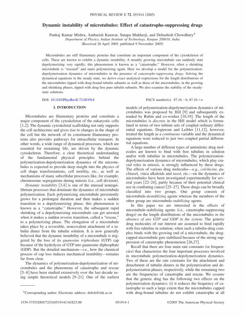
Dynamic instability of microtubules: Effect of catastrophe-suppressing drugs Pankaj Kumar Mishra, Ambarish Kunwar, Sutapa Mukherji, and Debashish Chowdhury * Department of Physics, Indian Institute of Technology, Kanpur 208016, India Received 26 April 2005; published 9 November 2005 Microtubules are stiff filamentary proteins that constitute an important component of the cytoskeleton of cells. These are known to exhibit a dynamic instability. A steadily growing microtubule can suddenly start depolymerizing very rapidly; this phenomenon is known as a “catastrophe.” However, often a shrinking microtubule is “rescued” and starts polymerizing again. Here we develop a model for the polymerization- depolymerization dynamics of microtubules in the presence of catastrophe-suppressing drugs. Solving the dynamical equations in the steady state, we derive exact analytical expressions for the length distributions of the microtubules tipped with drug-bound tubulin subunits as well as those of the microtubules, in the growing and shrinking phases, tipped with drug-free pure tubulin subunits. We also examine the stability of the steady- state solutions. DOI: 10.1103/PhysRevE.72.051914 PACS numbers: 87.16.b, 87.10.e I. INTRODUCTION Microtubules are filamentary proteins and constitute a major component of the cytoskeleton of the eukaryotic cells 1,2. The dynamic cytoskeletal scaffolding not only supports the cell architecture and gives rise to changes in the shape of the cell but the network of its constituent filamentary pro- teins also provides pathways for intracellular transport. In other words, a wide range of dynamical processes, which are essential for sustaining life, are driven by the dynamic cytoskeleton. Therefore, a clear theoretical understanding of the fundamental physical principles behind the polymerization-depolymerization dynamics of the microtu- bules is expected to provide deep insight into the physics of cell shape transformations, cell motility, etc., as well as mechanisms of many subcellular processes like, for example, chromosome segregations during mitosis i.e., cell division. Dynamic instability 3,4 is one of the unusual nonequi- librium processes that dominate the dynamics of microtubule polymerization. Each polymerizing microtubule persistently grows for a prolonged duration and then makes a sudden transition to a depolymerizing phase; this phenomenon is known as a ‘‘catastrophe.” However, the subsequent rapid shrinking of a depolymerizing microtubule can get arrested when it makes a sudden reverse transition, called a “rescue,” to a polymerizing phase. The elongation of a microtubule takes place by a reversible, noncovalent attachment of a tu- bulin dimer from the tubulin solution. It is now generally believed that the dynamic instability of a microtubule is trig- gered by the loss of its guanosine triphoshate GTP cap because of the hydrolysis of GTP into guanosine diphosphate GDP. But the detailed mechanism—i.e., how the chemical process of cap loss induces mechanical instability—remains far from clear. The dynamics of polymerization-depolymerization of mi- crotubules and the phenomena of catastrophe and rescue 5–8 have been studied extensively over the last decade us- ing simple theoretical models 9–21. One of the earliest models of polymerization-depolymerization dynamics of mi- crotubules was proposed by Hill 9 and subsequently ex- tended by Rubin and co-worker 10,19. The length of the microtubules is discrete in the Hill model which is formu- lated in terms of two infinite sets of coupled ordinary differ- ential equations. Dogterom and Leibler 11,12, however, treated the length as a continuous variable and the dynamical equations were reduced to just two coupled partial differen- tial equations. A large number of different types of antimitotic drug mol- ecules are known to bind with free tubulins in solution and/or with tubulins in microtubules. The polymerization- depolymerization dynamics of microtubules, which play cru- cial roles in mitosis, is strongly influenced by these drugs. The effects of various drug molecules—e.g., colchicine, pa- clitaxel, vinca alkaloids and taxol, etc.—on the dynamics of microtubules have been investigated experimentally for sev- eral years 22–24, partly because of their potential clinical use in combating cancer 25–27. These drugs can be broadly classified into two groups. One group consists of microtubule-destablizing agents whereas the members of the other group are microtubule-stabilizing agents. In this paper we are interested in the effects of microtubule-stabilizing agents i.e., catastrophe-suppressing drugs on the length distributions of the microtubules in the absence of any GTP and GDP in the system. The generic drug molecules of our interest are assumed to bind rapidly with free tubulins in solution; when such a tubulin-drug com- plex binds with the growing end of a microtubule, the drug- capped microtubule gets stabilized because of the strong sup- pression of catastrophe phenomenon 26,27. Recall that there are four main rate constants or frequen- cies that characterize the four important processes involved in microtubule polymerization-depolymerization dynamics. Two of these are the rate constants for the attachment and detachment of tubulin dimers in the polymerization and de- polymerization phases, respectively, while the remaining two are the frequencies of catastrophe and rescue. We assume that the generic drug has the following two effects on the polymerization dynamics: i it reduces the frequency of ca- tastrophe to such a large extent that the microtubules capped with drug-bound tubulins do not exhibit catastrophe at all *Corresponding author. Electronic address: [email protected] PHYSICAL REVIEW E 72, 051914 2005 1539-3755/2005/725/05191414/$23.00 ©2005 The American Physical Society 051914-1
-
Upload
independent -
Category
Documents
-
view
0 -
download
0
Transcript of Dynamic instability of microtubules: Effect of catastrophe-suppressing drugs
Dynamic instability of microtubules: Effect of catastrophe-suppressing drugs
Pankaj Kumar Mishra, Ambarish Kunwar, Sutapa Mukherji, and Debashish Chowdhury*Department of Physics, Indian Institute of Technology, Kanpur 208016, India
�Received 26 April 2005; published 9 November 2005�
Microtubules are stiff filamentary proteins that constitute an important component of the cytoskeleton ofcells. These are known to exhibit a dynamic instability. A steadily growing microtubule can suddenly startdepolymerizing very rapidly; this phenomenon is known as a “catastrophe.” However, often a shrinkingmicrotubule is “rescued” and starts polymerizing again. Here we develop a model for the polymerization-depolymerization dynamics of microtubules in the presence of catastrophe-suppressing drugs. Solving thedynamical equations in the steady state, we derive exact analytical expressions for the length distributions ofthe microtubules tipped with drug-bound tubulin subunits as well as those of the microtubules, in the growingand shrinking phases, tipped with drug-free pure tubulin subunits. We also examine the stability of the steady-state solutions.
DOI: 10.1103/PhysRevE.72.051914 PACS number�s�: 87.16.�b, 87.10.�e
I. INTRODUCTION
Microtubules are filamentary proteins and constitute amajor component of the cytoskeleton of the eukaryotic cells�1,2�. The dynamic cytoskeletal scaffolding not only supportsthe cell architecture and gives rise to changes in the shape ofthe cell but the network of its constituent filamentary pro-teins also provides pathways for intracellular transport. Inother words, a wide range of dynamical processes, which areessential for sustaining life, are driven by the dynamiccytoskeleton. Therefore, a clear theoretical understandingof the fundamental physical principles behind thepolymerization-depolymerization dynamics of the microtu-bules is expected to provide deep insight into the physics ofcell shape transformations, cell motility, etc., as well asmechanisms of many subcellular processes like, for example,chromosome segregations during mitosis �i.e., cell division�.
Dynamic instability �3,4� is one of the unusual nonequi-librium processes that dominate the dynamics of microtubulepolymerization. Each polymerizing microtubule persistentlygrows for a prolonged duration and then makes a suddentransition to a depolymerizing phase; this phenomenon isknown as a ‘‘catastrophe.” However, the subsequent rapidshrinking of a depolymerizing microtubule can get arrestedwhen it makes a sudden reverse transition, called a “rescue,”to a polymerizing phase. The elongation of a microtubuletakes place by a reversible, noncovalent attachment of a tu-bulin dimer from the tubulin solution. It is now generallybelieved that the dynamic instability of a microtubule is trig-gered by the loss of its guanosine triphoshate �GTP� capbecause of the hydrolysis of GTP into guanosine diphosphate�GDP�. But the detailed mechanism—i.e., how the chemicalprocess of cap loss induces mechanical instability—remainsfar from clear.
The dynamics of polymerization-depolymerization of mi-crotubules and the phenomena of catastrophe and rescue�5–8� have been studied extensively over the last decade us-ing simple theoretical models �9–21�. One of the earliest
models of polymerization-depolymerization dynamics of mi-crotubules was proposed by Hill �9� and subsequently ex-tended by Rubin and co-worker �10,19�. The length of themicrotubules is discrete in the Hill model which is formu-lated in terms of two infinite sets of coupled ordinary differ-ential equations. Dogterom and Leibler �11,12�, however,treated the length as a continuous variable and the dynamicalequations were reduced to just two coupled partial differen-tial equations.
A large number of different types of antimitotic drug mol-ecules are known to bind with free tubulins in solutionand/or with tubulins in microtubules. The polymerization-depolymerization dynamics of microtubules, which play cru-cial roles in mitosis, is strongly influenced by these drugs.The effects of various drug molecules—e.g., colchicine, pa-clitaxel, vinca alkaloids and taxol, etc.—on the dynamics ofmicrotubules have been investigated experimentally for sev-eral years �22–24�, partly because of their potential clinicaluse in combating cancer �25–27�. These drugs can be broadlyclassified into two groups. One group consists ofmicrotubule-destablizing agents whereas the members of theother group are microtubule-stabilizing agents.
In this paper we are interested in the effects ofmicrotubule-stabilizing agents �i.e., catastrophe-suppressingdrugs� on the length distributions of the microtubules in theabsence of any GTP and GDP in the system. The genericdrug molecules of our interest are assumed to bind rapidlywith free tubulins in solution; when such a tubulin-drug com-plex binds with the growing end of a microtubule, the drug-capped microtubule gets stabilized because of the strong sup-pression of catastrophe phenomenon �26,27�.
Recall that there are four main rate constants �or frequen-cies� that characterize the four important processes involvedin microtubule polymerization-depolymerization dynamics.Two of these are the rate constants for the attachment anddetachment of tubulin dimers in the polymerization and de-polymerization phases, respectively, while the remaining twoare the frequencies of catastrophe and rescue. We assumethat the generic drug has the following two effects on thepolymerization dynamics: �i� it reduces the frequency of ca-tastrophe to such a large extent that the microtubules cappedwith drug-bound tubulins do not exhibit catastrophe at all*Corresponding author. Electronic address: [email protected]
PHYSICAL REVIEW E 72, 051914 �2005�
1539-3755/2005/72�5�/051914�14�/$23.00 ©2005 The American Physical Society051914-1

and �ii� it also affects the rate of elongation of the microtu-bules because the rate constant for the attachment of a drug-bound tubulin is, in general, different from that of a drug-freetubulin. The effects of real catastrophe-suppressing drugs arequite complicated and depend also on the dosage of the drug;some even induce a “paused” phase �26�.
The aim of this paper is to investigate theoretically thegeneric effects of catastrophe-suppressing drugs by extend-ing the earlier theoretical models, developed by Hill �9� andFreed �20�, for the dynamics of polymerization of drug-freepure tubulins. We derive exact analytical expressions for thesteady-state distributions of the lengths of the microtubulestipped with the drug-bound tubulin subunits as well as thoseof microtubules tipped with pure �i.e., drug-free� tubulin sub-units. We carry out a linear stability analysis of the steady-state distributions and physically interpret the implications ofthe spectrum of the eigenvalues of the stability matrix.
This paper is organized as follows. In Sec. II we brieflyreview some of the relevant earlier theoretical models of dy-namic instability. In paricular, we summarize the mathemati-cal frameworks of the Hill model �9� and the recent Freedmodel �20� of dynamic instability of microtubules. In Sec. IIIwe propose an extension of the Hill model so as to capturethe effects of the catastrophe-suppressing drugs in a simpleway. The model is made more realistic in Sec. IV by treatingthe dynamics of the concentration of the drug-free tubulinsexplicitly following a Freed-like approach. The paper endswith a conclusion Sec. V.
II. BRIEF REVIEW OF EARLIER MODELSOF DYNAMIC INSTABILITY
A. Hill model
Microtubules consist of 13 protofilaments, each consistingof monomeric units �actually a �-� heterodimer� each ofwhich is approximately 8 nm long. On the other hand, thepolymers in the Hill model are one dimensional. Therefore,some authors �see, for example, �28�� identify “monomericunits” of the one-dimensional Hill model to have a length ofapproximately 8/13=0.6 nm.
Let PH+ �n , t� and PH
− �n , t� be the probabilities of finding amicrotubule of length n, at time t, in the growing ��� andshrinking ��� phases, respectively. Moreover, let PH�0, t� bethe probability that the MT nucleating site is empty at time t.Furthermore, we denote the growth rate of the growing mi-crotubules and decay rate of the shrinking microtubules bypg
H and pdH, respectively, while the frequencies of catastro-
phes �the transition from growing to the shrinking phase� andrescues �the transition from the shrinking to growing phase�are denoted by the symbols p+−
H and p−+H , respectively. Inter-
estingly, the four parameters pgH, pd
H, p+−H , and p−+
H were mea-sured as functions of free tubulin concentration first in 1988�29� by observing single microtubules using video light mi-croscopy. However, the concentration dependence of theseparameters, if any, does not appear explicitly in the Hillmodel.
The master equations for these probabilities are given by�9�
dPH+ �n,t�dt
= pgHPH
+ �n − 1,t� + p−+H PH
− �n,t�
− �pgH + p+−
H �PH+ �n,t� for n � 2, �1�
dPH− �n,t�dt
= pdHPH
− �n + 1,t� + p+−H PH
+ �n,t�
− �pdH + p−+
H �PH− �n,t� for n � 1, �2�
dPH+ �1,t�dt
= pgHPH�0,t� + p−+
H PH− �1,t� − �pg
H + p+−H �PH
+ �1,t� ,
�3�
and
dPH�0,t�dt
= − pgHPH�0,t� + pd
HPH− �1,t� . �4�
Imposing the normalization
�n=1
�
PH+ �n� + �
n=1
�
PH− �n� + PH�0� = 1, �5�
the steady-state solutions of Eqs. �1�–�4� are given by �9�
PH+ �n� = xH
n PH�0� �6�
and
PH− �n� = xH
n−1yHPH�0� , �7�
with
PH�0� =1 − xH
1 + yH, �8�
xH =pg
H�pdH + p−+
H �pd
H�pgH + p+−
H �, �9�
and
yH =pg
H
pdH . �10�
In order that the distributions PH± �n� are decreasing, rather
than increasing, functions of n we must have xH�1 whichimposes the constraint pg
H�pdH+ p−+
H �� pdH�pg
H+ p+−H �, i.e.,
pgHp−+
H � pdHp+−
H , �11�
on the magnitudes of the parameters. Interestingly, in theDogterom-Leibler model �11�, a steady state characterized byexponentially decaying distributions P± of the lengths of themicrotubules is attained only if the condition �11� is satisfiedby the parameters; otherwise, the system never reaches anysteady state and the mean of the �Gaussian� distribution ofthe lengths of the microtubules continues to increase linearlywith time.
B. Freed model
It has been realized for quite some time �16,17,29� thatthe rate of growth of the growing microtubules should de-
MISHRA et al. PHYSICAL REVIEW E 72, 051914 �2005�
051914-2

pend on the availability of free tubulin monomers in thesolution. However, in the Hill model �9� the kinetic rateequations do not involve the concentration of the tubulinmonomers. Recently, Freed �20� has generalized the Hillmodel to incorporate the dependence of the rates on the tu-bulin monomer concentration. Hammele and Zimmermann�21� carried out independent analytical calculations of thesame phenomenon by extending the Dogterom-Leibler �11�model. Since our calculations in the Sec. IV are based on anextension of Freed’s model, we summarize here the mainpoints of this approach.
Suppose that �0 is the initial concentration of the tubulinsubunits and � is the corresponding instantaneous concentra-tion at time t. Similarly, N0 and N are the initial and instan-taneous concentrations of the free �i.e., without bound tubu-lin� nucleating sites, respectively. The symbols PF
±�n , t� inthis section denote the concentrations, rather than probabili-ties, of microtubules in the growing and the shrinkingphases, respectively. Moreover, binding of a tubulin subunitwith a free nucleating site takes place at a rate pn
F. Usingthese quantities, the kinetic rate equations in the Freed model�20� can now be written as
dPF+�n,t�dt
= pgF�PF
+�n − 1,t� + p−+F PF
−�n,t�
− �pgF� + p+−
F �PF+�n,t� for n � 2, �12�
dPF−�n,t�dt
= pdFPF
−�n + 1,t� + p+−F PF
+�n,t�
− �pdF + p−+
F �PF−�n,t� for n � 1, �13�
dPF+�1,t�dt
= pnF�N + p−+
F PF−�1,t� − �pg
F� + p+−F �PF
+�1,t� ,
�14�
and
d�
dt= − pn
F�N − pgF��
n=1
�
PF+�n,t� + pd
F�n=1
�
PF−�n,t� . �15�
Moreover, tubulin mass conservation imposes the condition
�0 = � + QF+ + QF
− , �16�
where
QF± = �
n=1
�
nPF±�n,t� . �17�
Furthermore,
N0 = N + PF+ + PF
− , �18�
where
PF± = �
n=1
�
PF±�n,t� . �19�
There is one-to-one correspondence between the param-eters and dynamical variables in the Freed model and those
in the Hill model. For example, pgF�, pd
F, p+−F , and p−+
F corre-spond to pg
H, pdH, p+−
H , and p−+H , respectively.
The steady-state solution of this system of kinetic equa-tions is given by �30�
PF+ = pn
FN0��p−+F + pd
F�/D , �20�
PF− = pn
FN0��p+−F + pg
F��/D , �21�
and
PF−�1� = �� = pn
FN0��pdFp+−
F − pgF�p−+
F �/�pdFD� , �22�
where
D = pnFpg
F�2 + �pdFpn
F + pnFp+− − pg
Fp−+F �� + �pd
Fp+−F + pn
F�p−+F � .
�23�
Finally, using a generating function technique, Freed �20�derived the analytical expressions
PF+�n� = �a�c���n−1�/2��f� + ��d��Un−1���
− �a�c��−1/2a�f�Un−2���� �24�
and
PF−�n� = �a�c���n−1�/2���Un−1��� + �a�c��−1/2
�b�f� − c����Un−2���� for n � 2, �25�
where
a� = �pdF + p−+
F �/pdF, �26�
b� = − p+−F /pd
F, �27�
c� = pgF�/�pg
F� + p+−F � , �28�
d� = p−+F /�pg
F� + p+−F � , �29�
f� = pnF�N/�pg
F� + p+−F � , �30�
� = �a� + b�d� + c��/�2�a�c��1/2� , �31�
and Un��� are the Chebyshev polynomial of the second kindgiven by
Un��� = sin��n + 1�arccos ��/�1 − �2�1/2, �32�
together with U−1���=0.The distributions PF
±�n� will be decreasing functions of nprovided that the condition a�c��1 is satisfied; this condi-tion imposes the constraint
pgF�p−+
F � pdFp+−
F �33�
on the magnitudes of the parameters and the value of thedrug-free tubulin subunits � in the steady state. The condi-tion �33� becomes identical to �11� if we identify pg
F� withpg
H.While expressing the steady-state distributions PF
±�n� interms of Chebyshev polynomial, Freed �20� implicitly as-sumed that ����1. However, as shown in Appendix A, �is, in general, larger than unity. We revise the Freed’s result
DYNAMIC INSTABILITY OF MICROTUBULES: … PHYSICAL REVIEW E 72, 051914 �2005�
051914-3
in Sec. IV by taking ��1 and, consequently, we get a dif-ferent polynomial instead of the Chebyshev polynomialgiven in Eq. �32�.
Freed �20� derived the exact form of the stability matrix.We define
�± = �n=1
�
�P±�n� �34�
and the column vectors
V�t� = ��+
�−
��� , �35�
NF = �0
− pd
0� . �36�
The equations obtained from the linear stability analysisabove can be written as
dV�t�dt
= MFV�t� + NF�P−F�1� , �37�
where the matrix MF is given by
MF = �− p+− − pn���ss p−+ − pn���ss M13
p+− − p−+ 0
�pn − pg����ss pn���ss + pd M33� , �38�
with
M13 = pnN0 − �P+�ss − �P−�ss �39�
and
M33 = �pn − pg��P+�ss − pn�N0 − �P−�ss� . �40�
The nature of the stability of the steady state is deter-mined by the eigenvalues of the matrix MF. The steady stateis stable if all the eigenvalues are real and negative. On theother hand, if some roots are positive, these would indicateunbounded growth and the corresponding steady state wouldbe unstable. If the characteristic equation has a pair of com-plex conjugate roots, then the system will either oscillateabout the steady state �if the real part is negative� or exhibitoscillatory unbounded growth �if the real part is positive�.
We have carried out a numerical analysis of this stabilitymatrix and obtained the eigenvalues for several sets of valuesof the model parameters; the eigenvalues corresponding tofive different values of �, for a fixed set of values of the othermodel parameters, are shown in the Table I. Thus, the steady-state distribution is stable over the entire range of � for thechosen set of parameters values.
III. HILL-LIKE MODEL WITH DRUGS
Let pch be the rate of growth of a microtubule by addition
of a drug-bound tubulin. Since addition of catastrophe-suppressing drugs to the system strongly reduce the catastro-
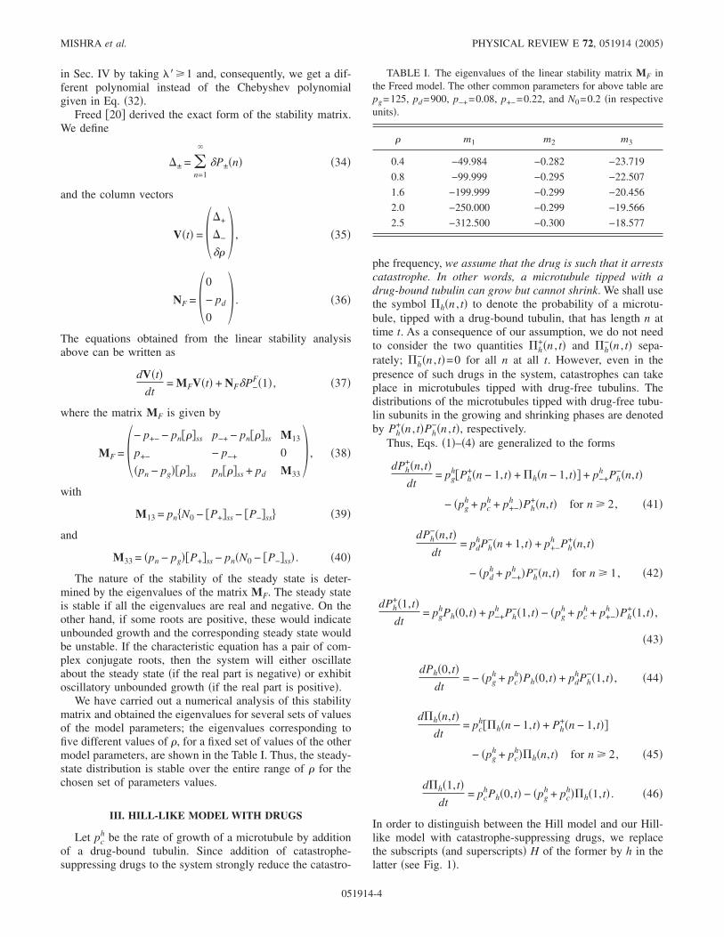
phe frequency, we assume that the drug is such that it arrestscatastrophe. In other words, a microtubule tipped with adrug-bound tubulin can grow but cannot shrink. We shall usethe symbol h�n , t� to denote the probability of a microtu-bule, tipped with a drug-bound tubulin, that has length n attime t. As a consequence of our assumption, we do not needto consider the two quantities h
+�n , t� and h−�n , t� sepa-
rately; h−�n , t�=0 for all n at all t. However, even in the
presence of such drugs in the system, catastrophes can takeplace in microtubules tipped with drug-free tubulins. Thedistributions of the microtubules tipped with drug-free tubu-lin subunits in the growing and shrinking phases are denotedby Ph
+�n , t�Ph−�n , t�, respectively.
Thus, Eqs. �1�–�4� are generalized to the forms
dPh+�n,t�dt
= pgh�Ph
+�n − 1,t� + h�n − 1,t�� + p−+h Ph
−�n,t�
− �pgh + pc
h + p+−h �Ph
+�n,t� for n � 2, �41�
dPh−�n,t�dt
= pdhPh
−�n + 1,t� + p+−h Ph
+�n,t�
− �pdh + p−+
h �Ph−�n,t� for n � 1, �42�
dPh+�1,t�dt
= pghPh�0,t� + p−+
h Ph−�1,t� − �pg
h + pch + p+−
h �Ph+�1,t� ,
�43�
dPh�0,t�dt
= − �pgh + pc
h�Ph�0,t� + pdhPh
−�1,t� , �44�
d h�n,t�dt
= pch� h�n − 1,t� + Ph
+�n − 1,t��
− �pgh + pc
h� h�n,t� for n � 2, �45�
d h�1,t�dt
= pchPh�0,t� − �pg
h + pch� h�1,t� . �46�
In order to distinguish between the Hill model and our Hill-like model with catastrophe-suppressing drugs, we replacethe subscripts �and superscripts� H of the former by h in thelatter �see Fig. 1�.
TABLE I. The eigenvalues of the linear stability matrix MF inthe Freed model. The other common parameters for above table arepg=125, pd=900, p−+=0.08, p+−=0.22, and N0=0.2 �in respectiveunits�.
� m1 m2 m3
0.4 −49.984 −0.282 −23.719
0.8 −99.999 −0.295 −22.507
1.6 −199.999 −0.299 −20.456
2.0 −250.000 −0.299 −19.566
2.5 −312.500 −0.300 −18.577
MISHRA et al. PHYSICAL REVIEW E 72, 051914 �2005�
051914-4

The steady-state solutions of these kinetic equations �seeAppendix B for details� are
Ph+�n� = xh�xh + zh�n−1Ph�0� , �47�
Ph−�n� = yh�xh + zh�n−1Ph�0� , �48�
h�n� = zh�xh + zh�n−1Ph�0� , �49�
where
Ph�0� =1 − xh − zh
1 + yh, �50�
with
xh =pg
h�pdh + p−+
h � + pchp−+
h
pdh�pg
h + p+−h � + pc
hpdh �51�
and
yh =pg
h + pch
pdh , �52�
zh =pc
h
pch + pg
h . �53�
The distributions �51�–�53� are decreasing functions of nprovided �xh+zh��1—i.e.,
�pgh + pc
h�2p−+h � pg
hpdhp+−
h ; �54�
this condition �54� reduces to the condition �11� in the limitpc
h→0. Note that in the limit pch→0, zh→0 while expres-
sions �51� and �52� for xh and yh reduce to xH and yH givenby expressions �9� and �10�, respectively; hence, in this limit,
h�n�→0 and expressions �47� and �48� for Ph±�n� reduce to
the corresponding expressions �6� and �7� for PH± �n�.
The parameters pgh, pd
h, p+−h , p−+
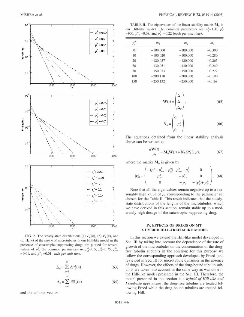
h , etc., have dimensions�time−1�. For a typical set of values of these parameters, wehave plotted the distributions Ph
+�n�, Ph−�n�, and h�n� in
Figs. 2�a�, 2�b�, and 2�c�, respectively, each for several dif-ferent numerical values of pc
h. The straight lines on the semi-logarithmic plots are a reflection of the exponential decay ofthe distribution with increasing length of the microtubules.Moreover, the longer tails of these distributions at at highervalues of pc
h demonstrates that higher pch causes stronger sup-
pression of the catastrophe phenomenon.
A. Stability of the steady state
Let us define the small deviations
�Ph±�n� = Ph
±�n,t� − �Ph±�ss, �55�
� h�n� = h�n,t� − � h�ss �56�
from the corresponding steady states where the steady-statevalues �P±�ss and � �ss are given by Eqs. �47�, �48�, and �49�,respectively. Linear stability analysis of the steady-state dis-tributions leads to the equations
d�Ph+�n,t�dt
= pgh��Ph
+�n − 1,t� + � h�n − 1,t��
+ �pgh + pc
h + p+−h ��Ph
+�n,t� for n � 2,
�57�
d�Ph−�n,t�dt
= pdh�Ph
−�n + 1,t� + p+−h �Ph
+�n,t�
− �pdh + p−+
h ��Ph−�n,t� for n � 1, �58�
d� h�n,t�dt
= pch� h�n − 1,t� + �Ph
+�n − 1,t�
− �pgh + pc
h�� h�n,t� for n � 2, �59�
d�Ph+�1,t�dt
= pgh�P�0,t� + p−+
h �Ph−�1,t�
− �pgh + pc
h + p+−h ��Ph
+�1,t� , �60�
d� h�1,t�dt
= pch�P�0,t� − �pg
h + pch�� h�1,t� . �61�
Using the normalization condition we get
�P�0,t� = − �n=1
�
�Ph+�n,t� − �
n=1
�
�Ph−�n,t� − �
n=1
�
� h�n,t� .
�62�
Next, we define
FIG. 1. �Color online� A schematic description of our Hill-likemodel in the presence of catastrophe-suppressing drugs. The super-script h has been dropped from the symbols denoting the modelparameters.
DYNAMIC INSTABILITY OF MICROTUBULES: … PHYSICAL REVIEW E 72, 051914 �2005�
051914-5
�± = �n=1
�
�Ph±�n� , �63�
�0 = �n=1
�
� h�n� �64�
and the column vectors
W�t� = ��+
�−
�0� , �65�
Nh = �0
− pdh
0� . �66�
The equations obtained from the linear stability analysisabove can be written as
dW�t�dt
= MhW�t� + Nh�Ph−�1,t� , �67�
where the matrix Mh is given by
Mh = �− �pch + p+−
h − pgh� p−+
h − pgh 0
p+−h − p−+
h 0
0 − pc − �pgh + pc
h�� . �68�
Note that all the eigenvalues remain negative up to a rea-sonably high value of pc corresponding to the parameter setchosen for the Table II. This result indicates that the steady-state distributions of the lengths of the microtubules, whichwe have derived in this section, remain stable up to a mod-erately high dosage of the catastrophe suppressing drug.
IV. EFFECTS OF DRUGS ON MT:A HYBRID HILL-FREED-LIKE MODEL
In this section we extend the Hill-like model developed inSec. III by taking into account the dependence of the rate ofgrowth of the microtubules on the concentration of the drug-free tubulin subunits in the solution; for this purpose wefollow the corresponding approach developed by Freed �andreviewed in Sec. II� for microtubule dynamics in the absenceof drugs. However, the effects of the drug-bound tubulin sub-units are taken into account in the same way as was done inthe Hill-like model presented in the Sec. III. Therefore, themodel presented in this section is a hybrid of Hill-like andFreed-like approaches; the drug-free tubulins are treated fol-lowing Freed while the drug-bound tubulins are treated fol-lowing Hill.
TABLE II. The eigenvalues of the linear stability matrix Mh inour Hill-like model. The common parameters are pg
h=100, pdh
=900, p−+h =0.08, and p+−
h =0.22 �each per unit time�.
pch m1 m2 m3
0 −100.000 −100.000 −0.300
10 −100.020 −100.000 −0.280
20 −120.037 −120.000 −0.263
30 −130.051 −130.000 −0.249
50 −150.073 −150.000 −0.227
100 −200.110 −200.000 −0.190
150 −250.132 −250.000 −0.168
FIG. 2. The steady-state distributions �a� Ph+�n�, �b� Ph
−�n�, and�c� h�n� of the size n of microtubules in our Hill-like model in thepresence of catastrophe-suppressing drugs are plotted for severalvalues of pc
h; the common parameters are pgh=0.5, pd
h=0.75, p+−h
=0.01, and p−+h =0.01, each per unit time.
MISHRA et al. PHYSICAL REVIEW E 72, 051914 �2005�
051914-6
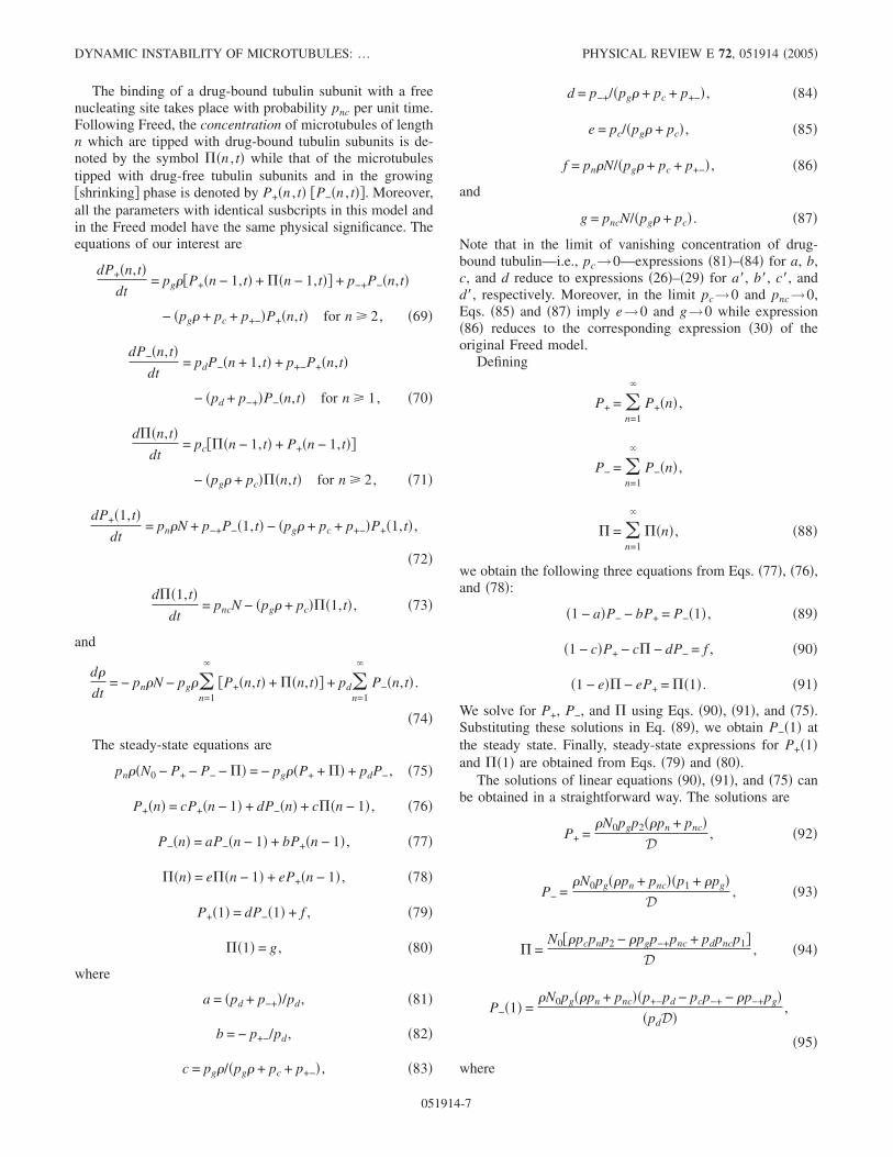
The binding of a drug-bound tubulin subunit with a freenucleating site takes place with probability pnc per unit time.Following Freed, the concentration of microtubules of lengthn which are tipped with drug-bound tubulin subunits is de-noted by the symbol �n , t� while that of the microtubulestipped with drug-free tubulin subunits and in the growing�shrinking� phase is denoted by P+�n , t� �P−�n , t��. Moreover,all the parameters with identical susbcripts in this model andin the Freed model have the same physical significance. Theequations of our interest are
dP+�n,t�dt
= pg��P+�n − 1,t� + �n − 1,t�� + p−+P−�n,t�
− �pg� + pc + p+−�P+�n,t� for n � 2, �69�
dP−�n,t�dt
= pdP−�n + 1,t� + p+−P+�n,t�
− �pd + p−+�P−�n,t� for n � 1, �70�
d �n,t�dt
= pc� �n − 1,t� + P+�n − 1,t��
− �pg� + pc� �n,t� for n � 2, �71�
dP+�1,t�dt
= pn�N + p−+P−�1,t� − �pg� + pc + p+−�P+�1,t� ,
�72�
d �1,t�dt
= pncN − �pg� + pc� �1,t� , �73�
and
d�
dt= − pn�N − pg��
n=1
�
�P+�n,t� + �n,t�� + pd�n=1
�
P−�n,t� .
�74�
The steady-state equations are
pn��N0 − P+ − P− − � = − pg��P+ + � + pdP−, �75�
P+�n� = cP+�n − 1� + dP−�n� + c �n − 1� , �76�
P−�n� = aP−�n − 1� + bP+�n − 1� , �77�
�n� = e �n − 1� + eP+�n − 1� , �78�
P+�1� = dP−�1� + f , �79�
�1� = g , �80�
where
a = �pd + p−+�/pd, �81�
b = − p+−/pd, �82�
c = pg�/�pg� + pc + p+−� , �83�
d = p−+/�pg� + pc + p+−� , �84�
e = pc/�pg� + pc� , �85�
f = pn�N/�pg� + pc + p+−� , �86�
and
g = pncN/�pg� + pc� . �87�
Note that in the limit of vanishing concentration of drug-bound tubulin—i.e., pc→0—expressions �81�–�84� for a, b,c, and d reduce to expressions �26�–�29� for a�, b�, c�, andd�, respectively. Moreover, in the limit pc→0 and pnc→0,Eqs. �85� and �87� imply e→0 and g→0 while expression�86� reduces to the corresponding expression �30� of theoriginal Freed model.
Defining
P+ = �n=1
�
P+�n� ,
P− = �n=1
�
P−�n� ,
= �n=1
�
�n� , �88�
we obtain the following three equations from Eqs. �77�, �76�,and �78�:
�1 − a�P− − bP+ = P−�1� , �89�
�1 − c�P+ − c − dP− = f , �90�
�1 − e� − eP+ = �1� . �91�
We solve for P+, P−, and using Eqs. �90�, �91�, and �75�.Substituting these solutions in Eq. �89�, we obtain P−�1� atthe steady state. Finally, steady-state expressions for P+�1�and �1� are obtained from Eqs. �79� and �80�.
The solutions of linear equations �90�, �91�, and �75� canbe obtained in a straightforward way. The solutions are
P+ =�N0pgp2��pn + pnc�
D, �92�
P− =�N0pg��pn + pnc��p1 + �pg�
D, �93�
=N0��pcpnp2 − �pgp−+pnc + pdpncp1�
D, �94�
P−�1� =�N0pg��pn + pnc��p+−pd − pcp−+ − �p−+pg�
�pdD�,
�95�
where
DYNAMIC INSTABILITY OF MICROTUBULES: … PHYSICAL REVIEW E 72, 051914 �2005�
051914-7
D = �3pg2pn + pdpncp1 + �2pg
2�pnc − p−+�
+ �2pgpn�p1 + p2� + �pcp2pn + �pgpc�pnc − p−+�
+ �pgpncp+− + �pgpd�pnc + p+−� , �96�
with
p1 = pc + p+− �97�
and
p2 = pd + p−+. �98�
In the following the generating function method is used toobtain the P+�n�, P−�n�, and �n� for arbitrary n. We proceedby multiplying both sides of Eqs. �76�, �77�, and �78� by xn
and then suming over n from n=1 to �. Defining
P+�x� = �n=1
�
P+�n�xn, �99�
P−�x� = �n=1
�
P−�n�xn, �100�
and
�x� = �n=1
�
�n�xn, �101�
we have the following equations for P+�x�, P−�x�, and �x�:
�1 − cx�P+�x� − dP−�x� − cx �x� = xf , �102�
bxP+�x� + �ax − 1�P−�x� = − x� , �103�
exP+�x� + �ex − 1� �x� = − xg , �104�
where �= P−�1�. Solving this set of linear equations forP+�x�, P−�x�, and �x�, we find
P+�x� =�aef − acg�x3 − ��de − cg + ef + af�x2 + ��d + f�x
�,
�105�
P−�x� =�bcg − bef�x3 + �bf − �c − �e�x2 + �x
�, �106�
�x� =�acg − aef�x3 + ��de − cg + ef − ag − bdg�x2 + gx
�,
�107�
where
� = �ac + ae + bde�x2 − �a + c + e + bd�x + 1, �108�
P+�x� =�aef − acg�x3 − ��de − cg + ef + af�x2 + ��d + f�x
y2 − 2y + 1,
�109�
P−�x� =�bcg − bef�x3 + �bf − �c − �e�x2 + �x
y2 − 2y + 1, �110�
�x� =�acg − aef�x3 + ��de − cg + ef − ag − bdg�x2 + gx
y2 − 2y + 1,
�111�
where
= �a + e + c + bd�/�2�ac + ae + bde�1/2� �112�
and
y = �a + e + c + bd�1/2x . �113�
Solutions for P±�n� and �n� can be obtained by expand-ing term
1
y2 − 2y + 1�114�
in the above equations using Taylor series expansion for �1 and y�1 and then equating the coefficients of yn on bothsides. Thus, the expressions for P±�n� and �n� are as fol-lows:
P+�n� = ��n−1�/2��3Un−1�� − �2Un−2�� + �1Un−3���
for n � 2, �115�
P+�1� = �3U0�� , �116�
where
� = �ac + ae + bde� , �117�
�1 = �aef − acg�/� , �118�
�2 = ��de − cg + ef + af�/�1/2, �119�
�3 = ��d + f� , �120�
and
Un�� = �m=0
�n/2�
�− 1�m �n − m�!m!�n − 2m�!
�2�n−2m, �121�
with U−1��=0, where the symbol �n /2� represents the larg-est integer smaller than or equal to n /2. Similarly,
P−�n� = ��n−1�/2��Un−1�� + �2Un−2�� + �1Un−3���
for n � 2, �122�
P−�1� = �U0�� , �123�
where
�1 = �bcg − bef�/� , �124�
�2 = �bf − �c − �e�/�1/2. �125�
Finally,
�n� = ��n−1�/2�gUn−1�� + �2Un−2�� + �1Un−3��� ,
�126�
�1� = gU0�� , �127�
where
MISHRA et al. PHYSICAL REVIEW E 72, 051914 �2005�
051914-8

�1 = �acg − aef�/� , �128�
�2 = ��de − cg + ef − ag − bdg�/�1/2. �129�
It can be easily checked that these solutions approachFreed’s solutions in the limit pnc→0, pc→0. In order thatthe steady-state solutions for P+�n�, P−�n�, and �n� are de-creasing, rather than increasing, functions of n, we demandthat ��1 which imposes the following constraint on themagnitudes of the parameters:
p−+�pc + �pg�2 � �pgpdp+−. �130�
The condition �130� reduces to the corresponding condition�33� of the Freed model in the limit pc→0.
In order to plot the steady-state distributions �115�, �122�,and �126� in our hybrid Hill-Freed-like model and to com-pare these with the distributions �47�–�49� for the same set ofparameters, we first converted the concentrations of the dif-ferent types of microtubules into probabilities and, then,chose the numerical values of the parameters so as to satisfythe following relations:
pgh = pg� ,
pdh = pd,
pch = pc,
p+−h = p+−,
p−+h = p−+. �131�
The distributions plotted in Fig. 3 show that with properrescaling of the parameters, as mentioned in Eq. �130�, theresults for the Hill-like model and the hybrid Hill-Freed-likemodel are almost identical. Moreover, the higher is the valueof pc, the longer are the tails of the distributions; this, asexplained already in the context of the Hill-like model, is aconsequence of the stronger suppression of the catastrophesby higher pc.
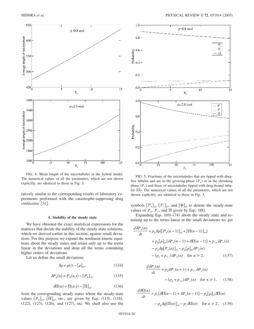
The mean lengths of the microtubules, which correspondto the distributions plotted in the Fig. 3, are plotted against pcin Fig. 4. Surprisingly, for this set of parameter values themean lengths of the microtubules tipped with drug-boundtubulin and those tipped with drug-free tubulins �both in thegrowing and shrinking phases� are identical for almost allvalues of pc. However, even for this set of parameters values,the fraction of microtubules with drug-bound cap increaseswith increasing pc while that with drug-free cap decreases�see Fig. 5�.
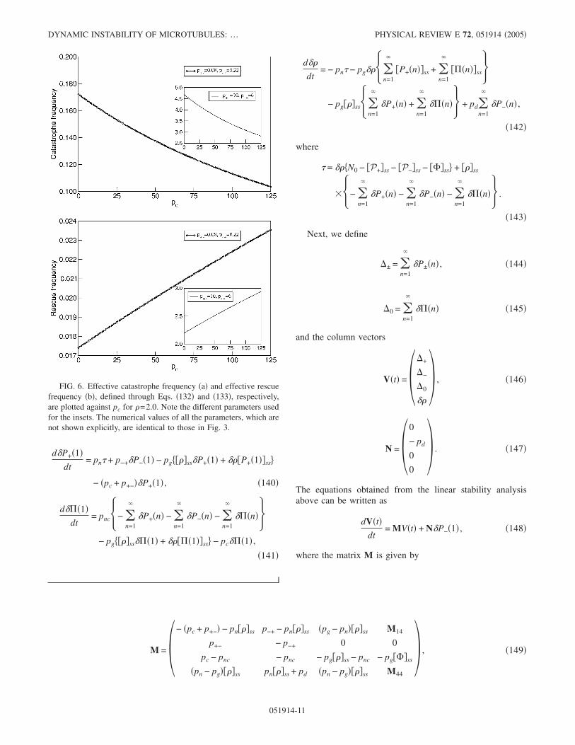
We now define the effective catastrophe frequency and theeffective rescue frequency by the relations
p+−ef f =
p+−P+
P+ + P− + =
p+−P+
1 − P0�132�
and
p−+ef f =
p−+P−
P+ + P− + =
p−+P−
1 − P0. �133�
These effective frequencies of catastrophe and rescue areplotted against pc in Fig. 6. This trend of variation is quali-
FIG. 3. The steady-state length distributions �a� P+�n�, �b�P−�n�, and �c� �n� of microtubules in our hybrid model for severalvalues of pc and compared with corresponding distributions in ourHill-like model �with appropriate rescaling of the parameters andvariables following Eq. �131��; the common parameters are pg= pn
=125, pd=900, p−+=0.08, p+−=0.22, pnc= pc, and �=0.8, N0=0.2�in respective units�.
DYNAMIC INSTABILITY OF MICROTUBULES: … PHYSICAL REVIEW E 72, 051914 �2005�
051914-9
tatively similar to the corresponding results of laboratory ex-periments performed with the catastrophe-supprssing drugvinblastine �31�.
A. Stability of the steady state
We have obtained the exact analytical expressions for thematrices that decide the stability of the steady-state solutions,which we derived earlier in this section, against small devia-tions. For this purpose we expand the nonlinear kinetic equa-tions about the steady states and retain only up to the termslinear in the deviations and drop all the terms containinghigher orders of deviations.
Let us define the small deviations
�� = ��t� − ���ss, �134�
�P±�n� = P±�n,t� − �P±�ss, �135�
� �n� = �n,t� − � �ss �136�
from the corresponding steady states where the steady-statevalues �P±�ss, � �ss, etc., are given by Eqs. �115�, �116�,�122�, �123�, �126�, and �127�, etc. We shall also use the
symbols �P+�ss, �P−�ss, and ���ss to denote the steady-statevalues of P+, P−, and given by Eqs. �88�.
Expanding Eqs. �69�–�74� about the steady state and re-taining up to the terms linear in the small deviations we get
d�P+�n�dt
= pg���P+�n − 1��ss + � �n − 1��ss
+ pg���ss�P+�n − 1� + � �n − 1� + p−+�P−�n�
− pg���P+�n��ss − pg���ss�P+�n�
− �pc + p+−��P+�n� for n � 2, �137�
d�P−�n�dt
= pd�P−�n + 1� + p+−�P+�n�
− �pd + p−+��P−�n� for n � 1, �138�
d� �n�dt
= pc� �n − 1� + �P+�n − 1� − pg���ss� �n�
− pg��� �n��ss − pc� �n� for n � 2, �139�
FIG. 4. Mean length of the microtubules in the hybrid model.The numerical values of all the parameters, which are not shownexplicitly, are identical to those in Fig. 3.
FIG. 5. Fractions of the microtubules that are tipped with drug-free tubulin and are in the growing phase �P+� or in the shrinkingphase �P−� and those of microtubules tipped with drug-bound tubu-lin � �. The numerical values of all the parameters, which are notshown explicitly, are identical to those in Fig. 3.
MISHRA et al. PHYSICAL REVIEW E 72, 051914 �2005�
051914-10
d�P+�1�dt
= pn� + p−+�P−�1� − pg���ss�P+�1� + ���P+�1��ss
− �pc + p+−��P+�1� , �140�
d� �1�dt
= pnc�− �n=1
�
�P+�n� − �n=1
�
�P−�n� − �n=1
�
� �n��− pg���ss� �1� + ��� �1��ss − pc� �1� ,
�141�
d��
dt= − pn� − pg����
n=1
�
�P+�n��ss + �n=1
�
� �n��ss�− pg���ss��
n=1
�
�P+�n� + �n=1
�
� �n�� + pd�n=1
�
�P−�n� ,
�142�
where
� = ��N0 − �P+�ss − �P−�ss − ���ss + ���ss
�− �n=1
�
�P+�n� − �n=1
�
�P−�n� − �n=1
�
� �n�� .
�143�
Next, we define
�± = �n=1
�
�P±�n� , �144�
�0 = �n=1
�
� �n� �145�
and the column vectors
V�t� =��+
�−
�0
��� , �146�
N =�0
− pd
0
0� . �147�
The equations obtained from the linear stability analysisabove can be written as
dV�t�dt
= MV�t� + N�P−�1� , �148�
where the matrix M is given by
M =�− �pc + p+−� − pn���ss p−+ − pn���ss �pg − pn����ss M14
p+− − p−+ 0 0
pc − pnc − pnc − pg���ss − pnc − pg���ss
�pn − pg����ss pn���ss + pd �pn − pg����ss M44
� , �149�
FIG. 6. Effective catastrophe frequency �a� and effective rescuefrequency �b�, defined through Eqs. �132� and �133�, respectively,are plotted against pc for �=2.0. Note the different parameters usedfor the insets. The numerical values of all the parameters, which arenot shown explicitly, are identical to those in Fig. 3.
DYNAMIC INSTABILITY OF MICROTUBULES: … PHYSICAL REVIEW E 72, 051914 �2005�
051914-11

where
M14 = pg���ss + pnN0 − �P+�ss − �P−�ss − ���ss ,
�150�
M44 = �pn − pg���P+�ss + ���ss� − pn�N0 − �P−�ss� .
�151�
The characteristic equation is quartic in the eigenvalue .We have systematically investigated the trend of variation ofthe eigenvalues �m1 ,m2 ,m3 ,m4� of the matrix M with thevariation of pc for several sets of values of the other param-eters; those for two values of � are given in Table III. In boththese cases, there is a range 0� pc� pc
max of values of pcwhere all the eigenvalues remain negative, indicating stabil-ity of the steady state. Moreover, the higher is the steady-state density � of free tubulins in the solution, the larger isthe value of pc
max. As pc is incresed beyond pcmax, one of the
negative eigenvalues simply changes sign which indicatesinstability of the steady state. The physical reason for theinstability of the steady state at sufficiently high pc is that thehigher is the pc, the larger is the fraction of microtubulestipped with drug-bound tubulin which can only grow butcannot shrink.
Thus, although the steady-state distributions of the micro-tubules in the Hill-like model and those in the hybrid Hill-Freed-like model can be made practically identical by mak-ing appropriate correspondence of the parameters in the twomodels, the latter has a richer dynamics which is reflectedalso in the linear stability analysis.
V. SUMMARY AND CONCLUSION
In this paper we have developed models for studyingsome generic effects of a class of drugs on the
polymerization-depolymerization dynamics of microtubulesin the absence of GTP and GDP. The class of generic drugsunder consideration suppresses catastrophes; more specifi-cally, we assumed that �i� the microtubules capped withdrug-bound tubulins do not exhibit catastrophe and �ii� therate constant for the attachment of a drug-bound tubulin is, ingeneral, different from that of a drug-free tubulin. Althoughthe effects of real catastrophe-suppressing drugs are known�26� to be more complicated than those of the generic modelassumed here, some predictions of the model are in goodqualitative agreement with the corresponding effects of vin-blastine over a limited parameter regime.
One of the two models—namely, the Hill-like model pro-posed here—is an extension of the model developed by Hill�9� to describe microtubule polymerization-depolymerizationdynamics in the absence of drugs. Although mathematicaltreatment of this model is quite simple, it does not take ex-plicitly account for the dynamics of the tubulin concentrationin the solution. Therefore, we have also developed a moredetailed model in which the effects of the concentration ofthe pure �i.e., drug-free� tubulin subunits are taken into ac-count in our model in a manner similar to that done by Freed�20� in his recent theoretical study of the microtubule dy-namics in the absence of drugs. However, in this model theeffects of the tubulin subunits bound to the drug moleculescould not be taken into account in a similar manner.
The reason for the difficulty in treating the concentrationsof the drug-free and drug-bound tubulins in solution on anequal footing is generic to the Hill-Freed approach. In orderthat the dynamical equation for the concentration of drug-bound tubulin subunits can reach a steady state, we have toallow both attachment and detachment of the drug-boundsubunits to the microtubule. However, if shrinking of a mi-crotubule tipped with drug-bound tubulin is allowed, thenimmediately after such a detachment, one needs to know thestatus of the subunit at the newly exposed tip—i.e., whetherthe tip consists of a drug-free tubulin or a drug-bound tubu-lin. But in the Hill-Freed approach, the system does not havea memory of the past history in the sense that the the modeldoes not keep a record of the status �i.e., whether or notbound to a drug molecule� of all the tubulin subunits, startingfrom the nucleation center up to the tip.
Therefore, in order to overcome this technical difficulty,we have incorporated the effects of the drug-bound tubulinsubunits in a manner similar to the approach followed in theHill model �9�. Thus, our second model may be regarded asa hybrid of the Hill-like and Freed-like modeling strategiesfor the concentrations of the tubulin subunits.
For both the Hill-like model and the Hill-Freed-like hy-brid model we have derived exact analytical expressions forthe steady-state probability distributions of the lengths ofmicrotubules tipped with drug-bound tubulin subunits aswell as those of microtubules tipped with pure �i.e., drug-free� tubulin subunits in the growing and shrinking phases.We have also compared the trends of variations of some ofthe relevant quantities with the variation of the dosage of thecatastrophe-suppressing drug.
We have carried out a linear stability analysis of thesteady states and established that in both the models the
TABLE III. The eigenvalues of the linear stability matrix M.The common parameters are pg= pn=125, pd=900, p−+=0.08, p+−
=0.22, pnc= pc, and N0=0.2 �in respective units�.
�=0.8M
pc m1 m2 m3 m4
0 −99.998 −0.295 −22.506 −100.000
5 −105.000 −0.185 −22.633 −104.982
10 −110.000 −0.094 −22.734 −109.972
15 −115.000 −0.019 −22.814 −114.967
16 −116.000 −0.005 −22.828 −115.967
17 −117.000 0.008 −22.842 −116.966
�=2.0M
pc m1 m2 m3 m4
0 −249.999 −0.299 −19.566 −250.000
50 −300.000 −0.121 −19.717 −300.023
100 −350.000 −0.030 −19.785 −350.051
126 −376.000 −0.001 −19.803 −376.061
127 −377.000 0.002 −19.804 −377.062
MISHRA et al. PHYSICAL REVIEW E 72, 051914 �2005�
051914-12

length distributions of the microtubules remain stable unlesspc becomes sufficiently high to destabilize the steady state.
ACKNOWLEDGMENTS
We thank Balaji Prakash for fruitful discussions and KarlFreed for useful comments on a preliminary draft of themanuscript.
APPENDIX A: ON THE USE OF THE CHEBYSHEVPOLYNOMIAL
It is straightforward to see that
a� + c� + b�d� = 1 +pg
F��pdF + p−+
F �pd
F�pgF� + p+−
F �= 1 + a�c�. �A1�
Therefore, reexpressing � as
� =1 + a�c�
2�a�c��1/2 =1
2��a�c��1/4 − �a�c��−1/42 + 2� , �A2�
we find, in general, ��1.
APPENDIX B: STEADY-STATE SOLUTIONSOF THE HILL-LIKE MODEL WITH DRUGS
Here we obtain the steady-state solutions of Eqs.�41�–�46� for the Hill-like model in the presence of drugs byequating the right-hand side of these equations to zero. Thesolution for P−�1� is obtained by demanding dP�0, t� /dt=0.This leads to
P−�1� =�pg + pc�
pdP�0� = yP�0� , �B1�
where y is given by Eq. �52�. Similarly, claimingdP+�1, t� /dt=0 and d �1, t� /dt=0, we have
P+�1� =�pgpd + p−+�pg + pc��
pd�pg + pc + p+−�P�0� = xP�0� , �B2�
�1� =pc
pc + pgP�0� = zP�0� , �B3�
where x and z are given by Eqs. �51� and �53�, respectively.The special case corresponding to n=1 of the equationdP�n , t� /dt=0 leads to the steady-state solution for P−�2�,
P−�2� =1
pd��pd + p−+�y − p+−x�P�0� . �B4�
A little bit of algebraic manipulation leads to
P−�2� = y�x + z�P�0� . �B5�
Steady-state solutions for P+�2� and �2� can be obtained ina similar way. Steady-state solutions for P−�n�, P+�n�, and �n�, for arbitrary n, are straightforward generalizations ofour observations upto n=4.
Since P+�n�, P−�n�, and �n� are probabilities of findingmicrotubules of n subunits in growing, shrinking, andcatastrophe-arrested phases, we expect the normalizationcondition
P�0� + �n=1
�
�P+�n� + P−�n� + �n�� = 1. �B6�
This leads to the form �50� for P�0�.
�1� B. Alberts, J. Lewis, M. Raff, K. Roberts, and J. D. Watson,Molecular Biology of the Cell �Garland, New York, 1994�.
�2� See the following special issues of journals on the cytoskel-eton: Curr. Opin. Cell Biol. 8, 1 �1996�; ibid. 9, 1 �1997�; Nat.Cell Biol. 2, E1 �1999�; Curr. Opin. Cell Biol. 12, 17 �2000�;Nature �London� 422, 739 �2003�.
�3� T. Mitchison and M. Kirschner, Nature �London� 312, 232�1984�.
�4� T. Mitchison and M. Kirschner, Nature �London� 312, 237�1984�.
�5� H. P. Erickson and E. T. O’Brien, Annu. Rev. Biophys. Bio-mol. Struct. 21, 145 �1992�.
�6� A. Desai and T. J. Mitchison, Annu. Rev. Cell Dev. Biol. 13,83 �1997�.
�7� E. Nogales, Annu. Rev. Biophys. Biomol. Struct. 30, 397�2001�.
�8� J. Howard and A. A. Hyman, Nature �London� 422, 753�2003�.
�9� T. L. Hill, Proc. Natl. Acad. Sci. U.S.A. 81, 6728 �1984�.�10� R. J. Rubin, Proc. Natl. Acad. Sci. U.S.A. 85, 446 �1988�.�11� M. Dogterom and S. Leibler, Phys. Rev. Lett. 70, 1347 �1993�.�12� M. Dogterom and B. Yurke, Phys. Rev. Lett. 81, 485 �1998�.
�13� H. Flyvbjerg, T. E. Holy, and S. Leibler, Phys. Rev. Lett. 73,2372 �1994�.
�14� H. Flyvbjerg, T. E. Holy, and S. Leibler, Phys. Rev. E 54,5538 �1996�.
�15� H. Flyvbjerg and E. Jobs, Phys. Rev. E 56, 7083 �1997�.�16� E. Jobs, D. E. Wolf, and H. Flyvbjerg, Phys. Rev. Lett. 79, 519
�1997�.�17� B. Houchmandzadeh and M. Vallade, Phys. Rev. E 53, 6320
�1996�.�18� D. J. Bicout, Phys. Rev. E 56, 6656 �1997�.�19� D. J. Bicout and R. J. Rubin, Phys. Rev. E 59, 913 �1999�.�20� K. F. Freed, Phys. Rev. E 66, 061916 �2002�.�21� M. Hammele and W. Zimmermann, Phys. Rev. E 67, 021903
�2003�.�22� B. Perez-Ramirez, J. M. Andreu, M. J. Gorbunoff, and S. N.
Timasheff, Biochemistry 35, 3277 �1996�.�23� A. Vandecandelaere, S. R. Martin, M. J. Schilstra, and P. M.
Bayley, Biochemistry 33, 2792 �1994�.�24� A. Vandecandelaere, S. R. Martin, and Y. Engelbroghs, Bio-
chem. J. 323, 189 �1997�.�25� J. R. Peterson and T. J. Mitchison, Chem. Biol. 9, 1275
�2002�.
DYNAMIC INSTABILITY OF MICROTUBULES: … PHYSICAL REVIEW E 72, 051914 �2005�
051914-13
�26� M. A. Jordan and L. Wilson, Nat. Rev. Cancer 4, 253 �2004�.�27� J. J. Correia and S. Lobert, Curr. Pharma. Design 7, 1213
�2001�.�28� B. S. Govindan and W. B. Spillman, Jr., Phys. Rev. E 70,
032901 �2004�.�29� R. A. Walker, E. T. O’Brien, N. K. Pryer, M. F. Soboiero, and
W. A. Voter, J. Cell Biol. 107, 1437 �1988�.�30� There are some errors in the formulas in Ref. �20�; here we
give the corresponding corrected expressions.�31� D. Panda, M. A. Jordan, K. C. Chu, and L. Wilson, J. Biol.
Chem. 271, 29807 �1996�.
MISHRA et al. PHYSICAL REVIEW E 72, 051914 �2005�
051914-14