Dynamic Collapse of the Hull Girder in a Container Ship in ...
176
Dynamic Collapse of the Hull Girder in a Container Ship in Waves Tjark Tilman Schwebe Maritime Engineering Supervisor: Jørgen Amdahl, IMT Department of Marine Technology Submission date: June 2016 Norwegian University of Science and Technology
-
Upload
khangminh22 -
Category
Documents
-
view
3 -
download
0
Transcript of Dynamic Collapse of the Hull Girder in a Container Ship in ...
Dynamic Collapse of the Hull Girder in aContainer Ship in Waves
Tjark Tilman Schwebe
Maritime Engineering
Supervisor: Jørgen Amdahl, IMT
Department of Marine Technology
Submission date: June 2016
Norwegian University of Science and Technology


NTNU Norges teknisk-naturvitenskapelige universitet Institutt for marin teknikk
1
MASTER THESIS 2016
for
Stud. Techn. Tjark Tilman Schwebe
Dynamic collapse of the hull girder in a container ship in waves Dynamisk sammenbrudd av skrogbjelken til et containerskip i bølger
Recently the importance of whipping stresses on the extreme hull girder loadings has received much attention. Full scale measurements clearly show magnifications of the usual wave-induced bending moment by a factor of two due to the hull girder elasticity, see e.g. Andersen and Jensen (2014), in moderate sea states. The hull girder collapse of MOL Comfort in 2013 has also increased the focus on this matter.
The whipping induced stresses have a considerable higher frequency than the ordinary wave induced hull girder stresses. An important issue is whether the whipping induced stresses (on top of the wave induced stresses) can be allowed to exceed the static capacity of hull girder, which is typically governed by buckling of stiffened plates in compression. One reason is to the whipping stress component during buckling may be displacement controlled, so that the plate is not pushed far into the post-buckling range. Further, dynamic effects, such as inertia forces during buckling and/or strain rate effects may yield additional strength reserves for the stiffened plate. Change in hydrostatic hull loads due to “rigid body” rotation at the critical cross-section may also contribute positively.
In addition to checking of static and dynamic buckling, failure in the form of incremental plasticity or low-cycle fatigue during the repeated action of large waves must also be considered.
The project work is proposed carried out in the following steps:
1. Brief review of work related to investigation of the MOL Comfort accident. Review requirements issued by ship classification societies (e.g. DNV-GL) concerning the use of nonlinear finite element methods for assessment of hull girder capacity.
2. Establish relevant wave and whipping induced bending moment histories for the container vessel based on available full scale measurements. Discuss the frequency/temporal characteristics of the histories and the expected ship response to
NTNU Fakultet for marin teknikk Norges teknisk-naturvitenskapelige universitet Institutt for marin teknikk
2
these histories. Determine the lay-out and scantlings of a representative hull girder, based on drawings of similar vessels and software for ship design based on rule requirements (e.g. DNV-GL)
3. Establish a detailed finite element model of three holds in the midship area of a
container vessels connected to a beam model of the forward and aft part of the ship. Include also the effect of water plane stiffness for “rigid body rotation” of the hull girder. Discuss various options for modelling of initial imperfections and explain why the selected strategy was chosen. Discuss the choice of boundary conditions for the finite element model. Apply relevant hull girder and local sea loads. Perform static analysis of hull girder resistance subjected to extreme hull bending moment. Identify when yielding and buckling starts in various strength members.
4. Perform time domain analysis of the resistance to regular wave induced hull girder
loads, where the wave histories are increased proportionally, bringing the response of the most exposed members into the inelastic region. Compare the results with those from the static analysis.
5. Perform analysis of the hull girder response when it is subjected to whipping induced
vibrations in addition to regular wave loads. It is especially interesting to see if stiffened panels loaded beyond their static capacity will buckle or develop permanent plastic shortening that may give rise to low cycle fatigue problems or incremental collapse. Do the bottom panels buckle in the “hungry horse” or the “asymmetric” mode? Can the bottom panels, which undergo plastic straining in compression be subjected to reversed cycling?
6. Establish the hysteresis loop for members/cross-section carried out into the nonlinear
domain. Estimate the number of load cycles the ship can sustain before failure, depending upon the magnitude of the hull girder loads. Discuss the severity of whipping induced loads on regular wave loads. Discuss how whipping induced stresses could be accounted for in ship rules.
7. Conclusions and recommendations for further work
References: Andersen, I.M.V., Jensen, J.J. (2012). On the Effect of Hull Girder Flexibility on the Vertical Wave Bending Moment for Ultra Large Container Vessels. Proc. OMAE2012, paper no. 83043, Rio de Janeiro, Brazil, June 2012 Andersen, I.M.V., Jensen, J.J. (2014). Measurements in a container ship of wave-induced hull girder stresses in excess of design values. Accepted for publication Marine Structures Iijima, K., Fujikubo, M. and Xu, W. (2011), Hydroelasto-plasticity approach to predicting the post-ultimate strength behavior of a ship’s hull girder in waves. J Mar Science & Technology, 16:379-389 Xu, W., Iijima, K. and Fujikubo, M. (2012). Investigation into dynamic collapse behavior of a bulk carrier under extreme loads. Proc. Hydroelasticity in Marine Technology, Japan
NTNU Fakultet for marin teknikk Norges teknisk-naturvitenskapelige universitet Institutt for marin teknikk
3
Xu, W., Iijima, K. and Fujikubo, M. (2012). Parametric dependencies of the post-ultimate strength behavior of a ship’s hull girder in waves. J Mar Science & Technology, 17:203-215 Xia J, Wang, S. and Jensen, J.J. (1998), ‘Non-linear Wave Loads and Ship Responses by Time-Domain Strip Theory’, Marine Structures, 11(3):101-123. Seng, S., Andersen, I.M.V., Jensen, J.J. (2012). On the influence of hull girder flexibility on the wave induced bending moments. Proc. Hydroelasticity 2012, Tokyo, 2012 Seng, S., Jensen, J.J. (2013). An Application of a Free Surface CFD method in the Short-Term Extreme Response Analysis of Ships, Proceedings PRADS’2013 The work scope may prove to be larger than initially anticipated. Subject to approval from the supervisors, topics may be deleted from the list above or reduced in extent. In the thesis the candidate shall present her personal contribution to the resolution of problems within the scope of the thesis work. Theories and conclusions should be based on mathematical derivations and/or logic reasoning identifying the various steps in the deduction. The candidate should utilise the existing possibilities for obtaining relevant literature. Thesis format The thesis should be organised in a rational manner to give a clear exposition of results, assessments, and conclusions. The text should be brief and to the point, with a clear language. Telegraphic language should be avoided. The thesis shall contain the following elements: A text defining the scope, preface, list of contents, summary, main body of thesis, conclusions with recommendations for further work, list of symbols and acronyms, references and (optional) appendices. All figures, tables and equations shall be numerated. The supervisors may require that the candidate, in an early stage of the work, presents a written plan for the completion of the work. The plan should include a budget for the use of computer and laboratory resources which will be charged to the department. Overruns shall be reported to the supervisors. The original contribution of the candidate and material taken from other sources shall be clearly defined. Work from other sources shall be properly referenced using an acknowledged referencing system. The report shall be submitted in two copies: - Signed by the candidate - The text defining the scope included - In bound volume(s)
- Drawings and/or computer prints which cannot be bound should be organised in a separate folder.
NTNU Fakultet for marin teknikk Norges teknisk-naturvitenskapelige universitet Institutt for marin teknikk
4
- The report shall also be submitted in pdf format along with essential input files for computer analysis, spreadsheets, MATLAB files etc. in digital format.
Ownership NTNU has according to the present rules the ownership of the thesis. Any use of the thesis has to be approved by NTNU (or external partner when this applies). The department has the right to use the thesis as if the work was carried out by a NTNU employee, if nothing else has been agreed in advance. Thesis supervisors Prof. Jørgen Amdahl /Prof 2 Jørgen Juncher Jensen Deadline: June 10 2016 Trondheim, January 25, 2016 Jørgen Amdahl
Abstract
The interest on the influence of dynamic effects on the hull girder loading has increased in
the last years. Research shows a high influence of whipping and springing on the fatigue
loading. The influence on the extreme loading and the resulting dynamic collapse is cur-
rently not estimated. The ultimate capacity is described by a static estimation neglecting dy-
namic influences. Recent research has proven a high contribution of whipping and springing
on the hull girder strains. In this thesis methods are discussed and a first approach on the
estimation of the dynamic collapse is performed. A broad literature review is performed to
base the work on solid research.
Calculations are performed in the non-linear finite element program ANSYS. The influence
of several parameters on the buckling behaviour is checked and the method validated against
analytical results. A model of the midship section is build and is verified by a check of the ul-
timate capacity against an incremental method. The effect of inertia and rigid body motion
of the ship is accounted for. A measured strain series is applied on the hull girder as a quasi-
static load set and a full load set including whipping. The results are critical discussed and
a plan for future research is provided. The project means to give a first investigation in this
topic and shows the pitfalls encountered during the work.
i

ii

Preface
This report is a result of the master thesis conducted by Stud. Techn. Tjark Tilman Schwebe.
The thesis is carried out as a cooperation between DTU and NTNU in terms of the Nordic
Master in Maritime Engineering. The work is performed at the Department of Marine Tech-
nology at NTNU in spring of 2016 and build up on the previous project thesis.
Trondheim, 2016-06-27
Tjark Tilman Schwebe
iii

iv

Acknowledgments
The work has been carried out under the supervision of Professor Jørgen Amdahl (NTNU)
and Professor Jørgen Juncher Jensen (DTU). I would like to thank both for the good super-
vision and the inspirations through out the thesis. Jørgen Amdahl has helped me a lot with
the set up of the finite element analysis and Jørgen Juncher Jensen brought insides into the
dynamic effects.
Additionally I would like to thank Dr. Ingrid Marie Andersen her helping thoughts and for
providing me with the measured strain data and the program to assess them. As well I would
like to thank Dr. Henry Piehl for his help with the theoretical background of the non-linear
finite element method and their application.
Especially I would like to thank the Lloyd Werft Bremerhaven AG for supporting my master
studies and in person Benedikt Dreymann and Grzegorz Drozd for the help with the design
of the midship section.
Last but not least I would like to thank every body else involved in interesting discussions
about the topic and proofreading this thesis.
v

vi

Summary
In recent events, the container vessels MSC Napoli and MOL Comfort broke into two parts.
In both cases, whipping loads are assumed to contribute to the failure of the ships structure.
However the dynamic collapse of ships is insufficiently studied so far. Currently the ultimate
capacity of a container vessel is defined through a static calculation, thus dynamic effects
like springing and whipping are not directly included. Research has shown a high influence
of dynamic effects on the fatigue loading but there has been no adaptions for the ultimate
strength.
The topic is of high relevance because the classification societies are forced to implement
whipping loads in their class rules from 1. July 2016. The developed rules of the different
classification societies are presented in the thesis. Main objective of this thesis is to apply
measured strain data of a container ship on a finite element model. The ANSYS 15.0 code is
used to calculate the structural effects. A container ship similar to the MOL Comfort is de-
signed according to the Germanischer Lloyd SE (GL) design rules in POSEIDON. The method
has been verified on a simple plate and compared with analytical solutions. The midship sec-
tion is modeled as a non-linear finite element model. The ultimate capacity is calculated and
compared with an incremental method. A procedure to include the effect of inertia and rigid
body motions is reviewed and applied.
In a next step, quasi-static loads and full wave loads including whipping are applied on the
structure. The results are discussed. The thesis is meant to lay a foundation for future re-
search. Especially the difficulties which have arisen during the work and the evaluation of
the results are discussed in depth. Thoughts are given for the continuation of this topic.
vii

viii
Contents
Abstract i
Preface iii
Acknowledgments v
Summary vii
Contents ix
Acronyms xv
Latin Symbols xvii
Greek Symbols xxiii
1. Introduction 1
1.1. Background . . . . . . . . . . . . . . . . . . . . . . . . . . . . . . . . . . . . . . . . 2
1.2. Objective . . . . . . . . . . . . . . . . . . . . . . . . . . . . . . . . . . . . . . . . . . 2
1.3. Limitation . . . . . . . . . . . . . . . . . . . . . . . . . . . . . . . . . . . . . . . . . 4
2. Literature Survey 5
2.1. Composition of Wave Loads . . . . . . . . . . . . . . . . . . . . . . . . . . . . . . . 5
2.2. Influence of Dynamic Loads . . . . . . . . . . . . . . . . . . . . . . . . . . . . . . 8
2.3. Measured strain data on a container vessel . . . . . . . . . . . . . . . . . . . . . . 9
2.4. Prediction of whipping loads . . . . . . . . . . . . . . . . . . . . . . . . . . . . . . 12
2.5. Influence of Rigid Body Motion in Ultimate Strength Analysis . . . . . . . . . . . 13
ix
2.6. Finite Element Modelling . . . . . . . . . . . . . . . . . . . . . . . . . . . . . . . . 14
2.7. MSC Napoli Accident . . . . . . . . . . . . . . . . . . . . . . . . . . . . . . . . . . . 16
2.8. MOL Comfort Accident . . . . . . . . . . . . . . . . . . . . . . . . . . . . . . . . . . 18
2.9. Ultimate Strength Design Rules . . . . . . . . . . . . . . . . . . . . . . . . . . . . . 20
3. Methodology 21
3.1. Modelling the Loads . . . . . . . . . . . . . . . . . . . . . . . . . . . . . . . . . . . 21
3.2. Modelling the structure . . . . . . . . . . . . . . . . . . . . . . . . . . . . . . . . . 22
3.3. Planning and verification of work . . . . . . . . . . . . . . . . . . . . . . . . . . . 23
4. Individual Studies 25
4.1. Coordinate & Unit System Definition . . . . . . . . . . . . . . . . . . . . . . . . . 25
4.2. Estimated Ship . . . . . . . . . . . . . . . . . . . . . . . . . . . . . . . . . . . . . . 26
4.3. Material Properties . . . . . . . . . . . . . . . . . . . . . . . . . . . . . . . . . . . . 30
4.4. Element Choice & Meshing . . . . . . . . . . . . . . . . . . . . . . . . . . . . . . . 36
4.5. Model Size . . . . . . . . . . . . . . . . . . . . . . . . . . . . . . . . . . . . . . . . . 39
4.6. Application of Imperfections . . . . . . . . . . . . . . . . . . . . . . . . . . . . . . 41
4.7. Inertia and Rigid Body Motion Effects . . . . . . . . . . . . . . . . . . . . . . . . . 42
5. Theory 45
5.1. Hull Girder Failure . . . . . . . . . . . . . . . . . . . . . . . . . . . . . . . . . . . . 45
5.1.1. Buckling Failure Modes . . . . . . . . . . . . . . . . . . . . . . . . . . . . . 46
5.1.2. Effect of Boundaries . . . . . . . . . . . . . . . . . . . . . . . . . . . . . . . 47
5.1.3. Effect of Imperfections . . . . . . . . . . . . . . . . . . . . . . . . . . . . . . 49
5.2. Verification Methods . . . . . . . . . . . . . . . . . . . . . . . . . . . . . . . . . . . 49
5.2.1. Analytical Solution . . . . . . . . . . . . . . . . . . . . . . . . . . . . . . . . 49
5.2.2. Semi Analytical Solution PULS . . . . . . . . . . . . . . . . . . . . . . . . . 52
5.2.3. Ultimate Capacity POSEIDON . . . . . . . . . . . . . . . . . . . . . . . . . 53
5.3. Finite Element Method Theory . . . . . . . . . . . . . . . . . . . . . . . . . . . . . 54
5.3.1. Non-linearity . . . . . . . . . . . . . . . . . . . . . . . . . . . . . . . . . . . 54
5.3.2. Transient Effects . . . . . . . . . . . . . . . . . . . . . . . . . . . . . . . . . 55
5.3.3. Mass Matrix . . . . . . . . . . . . . . . . . . . . . . . . . . . . . . . . . . . . 55
x
5.3.4. Damping Matrix . . . . . . . . . . . . . . . . . . . . . . . . . . . . . . . . . 56
5.3.5. Stiffness Matrix . . . . . . . . . . . . . . . . . . . . . . . . . . . . . . . . . . 57
5.4. Finite Element Analysis Solver . . . . . . . . . . . . . . . . . . . . . . . . . . . . . 59
5.4.1. Eigenfrequency Solver . . . . . . . . . . . . . . . . . . . . . . . . . . . . . . 59
5.4.2. Linear Static Solver . . . . . . . . . . . . . . . . . . . . . . . . . . . . . . . . 60
5.4.3. Linear Buckling Solver . . . . . . . . . . . . . . . . . . . . . . . . . . . . . . 60
5.4.4. Transient Solver . . . . . . . . . . . . . . . . . . . . . . . . . . . . . . . . . . 61
5.4.5. Distributed ANSYS . . . . . . . . . . . . . . . . . . . . . . . . . . . . . . . . 62
5.4.6. Multi Point Constraint . . . . . . . . . . . . . . . . . . . . . . . . . . . . . . 63
5.4.7. Convergence Problems . . . . . . . . . . . . . . . . . . . . . . . . . . . . . 64
5.5. Whipping Rule Values . . . . . . . . . . . . . . . . . . . . . . . . . . . . . . . . . . 64
5.5.1. DNV . . . . . . . . . . . . . . . . . . . . . . . . . . . . . . . . . . . . . . . . . 65
5.5.2. DNVGL . . . . . . . . . . . . . . . . . . . . . . . . . . . . . . . . . . . . . . . 66
5.5.3. Bureau Veritas . . . . . . . . . . . . . . . . . . . . . . . . . . . . . . . . . . . 66
5.5.4. ClassNK . . . . . . . . . . . . . . . . . . . . . . . . . . . . . . . . . . . . . . 67
5.5.5. American Bureau of Shipping . . . . . . . . . . . . . . . . . . . . . . . . . . 67
5.5.6. Lloyds Register . . . . . . . . . . . . . . . . . . . . . . . . . . . . . . . . . . 68
6. Results 69
6.1. Simple Plate and Panel validations . . . . . . . . . . . . . . . . . . . . . . . . . . . 69
6.1.1. Comparison of Analytical, PULS and FEM Results . . . . . . . . . . . . . . 69
6.1.2. PULS results . . . . . . . . . . . . . . . . . . . . . . . . . . . . . . . . . . . . 71
6.1.3. Mesh Convergence Study . . . . . . . . . . . . . . . . . . . . . . . . . . . . 73
6.2. Case Study on a Simple Plate using FEM . . . . . . . . . . . . . . . . . . . . . . . 74
6.2.1. Influence of Material Hardening . . . . . . . . . . . . . . . . . . . . . . . . 74
6.2.2. Influence of Added Mass . . . . . . . . . . . . . . . . . . . . . . . . . . . . . 75
6.2.3. Influence of Dynamic Loads . . . . . . . . . . . . . . . . . . . . . . . . . . 76
6.3. Full Model Results . . . . . . . . . . . . . . . . . . . . . . . . . . . . . . . . . . . . 76
6.3.1. Static Case on full Model . . . . . . . . . . . . . . . . . . . . . . . . . . . . . 77
6.3.2. Influence of Structural Damping . . . . . . . . . . . . . . . . . . . . . . . . 79
6.3.3. Ultimate Capacity of the Midship Section . . . . . . . . . . . . . . . . . . . 80
xi
6.3.4. Post Collapse Behaviour of Midship Section . . . . . . . . . . . . . . . . . 83
6.3.5. Ultimate Capacity of Floating Model . . . . . . . . . . . . . . . . . . . . . 84
6.3.6. Effect of Rigid Body Motion . . . . . . . . . . . . . . . . . . . . . . . . . . . 86
6.3.7. Application of Measured Strain Data . . . . . . . . . . . . . . . . . . . . . 87
6.3.8. Quasi-Static Wave Loads on the 3 Web Model . . . . . . . . . . . . . . . . 88
6.3.9. Quasi-Static Wave Loads on the 3 Web Rigid Model . . . . . . . . . . . . . 91
6.3.10. Quasi-Static Wave Loads on the Floating Model . . . . . . . . . . . . . . . 91
6.3.11. Dynamic Wave Loads on the 3 Web Models . . . . . . . . . . . . . . . . . 92
6.3.12. Partial Safety Factors based on Rule Values . . . . . . . . . . . . . . . . . . 92
7. Discussion 95
7.1. Evaluation of ANSYS on a simple Plate . . . . . . . . . . . . . . . . . . . . . . . . 95
7.2. Validation of midship model . . . . . . . . . . . . . . . . . . . . . . . . . . . . . . 96
7.3. Application of time history data . . . . . . . . . . . . . . . . . . . . . . . . . . . . 99
8. Conclusion 101
9. Recommendation for further work 103
Bibliography 105
A. Theoretical Background A-1
A.1. Elastic Buckling of Initially Perfect Plates . . . . . . . . . . . . . . . . . . . . . . . A-1
A.2. Establish the Dynamic Equation of Motion . . . . . . . . . . . . . . . . . . . . . . A-2
A.3. Eigenvalue problem . . . . . . . . . . . . . . . . . . . . . . . . . . . . . . . . . . . A-3
B. Calculation of Rule Bending Moments A-5
B.1. DNVGL Rules Still Water Bending Moment . . . . . . . . . . . . . . . . . . . . . . A-5
B.2. GL Rules Wave Bending Moment . . . . . . . . . . . . . . . . . . . . . . . . . . . . A-6
C. Calculation of external Pressure A-9
C.1. Static External Pressure . . . . . . . . . . . . . . . . . . . . . . . . . . . . . . . . . A-9
C.2. Dynamic External Pressure . . . . . . . . . . . . . . . . . . . . . . . . . . . . . . . A-9
xii

D. Beam Model Extensions A-11
E. PULS Figures A-13
E.1. Simple Plate Results . . . . . . . . . . . . . . . . . . . . . . . . . . . . . . . . . . . A-13
E.2. Panel Results . . . . . . . . . . . . . . . . . . . . . . . . . . . . . . . . . . . . . . . . A-14
F. ANSYS Figures A-17
F.1. Results for the simple Plate . . . . . . . . . . . . . . . . . . . . . . . . . . . . . . . A-17
F.2. Used Finite Element Midship Models . . . . . . . . . . . . . . . . . . . . . . . . . A-19
F.3. Ultimate Limit State of 3 Web Model . . . . . . . . . . . . . . . . . . . . . . . . . . A-21
F.4. Post Collapse of 3 Web Model . . . . . . . . . . . . . . . . . . . . . . . . . . . . . . A-22
F.5. Quasi-Static Wave Load on the 3 Web Model . . . . . . . . . . . . . . . . . . . . . A-24
G. APDL Listings A-27
G.1. Eigenvalue Solver . . . . . . . . . . . . . . . . . . . . . . . . . . . . . . . . . . . . . A-27
G.2. Static Solver . . . . . . . . . . . . . . . . . . . . . . . . . . . . . . . . . . . . . . . . A-27
G.3. Linear Buckling Solver . . . . . . . . . . . . . . . . . . . . . . . . . . . . . . . . . . A-28
G.4. Non-linear Buckling Solver . . . . . . . . . . . . . . . . . . . . . . . . . . . . . . . A-29
H. VILJE Input Listings A-31
xiii

xiv
Acronyms
ABS American Bureau of Shipping Inc.
BV Bureau Veritas SA
CFD Computational Fluid Dynamic
ClassNK Nippon Kaiji Kyokai
COV Coefficient of Variation
CS Cowper-Symonds
CSE College of Shipbuilding Engineering
DNV Det Norske Vertitas AS
DNVGL DNVGL AS
DoF Degree of Freedom
DTU Danish Technical University
EPP Elastic Perfectly Plastic
FEA Finite Element Analysis
FEM Finite Element Method
FEU Fourty foot equivalent unit
FFT Fast Fourier Transformation
xv

GL Germanischer Lloyd SE
HF High Frequency
HPC High performance cluster
IACS International Association of Classification Societies LTD.
ISUM Idealized structural unit method
LF Low Frequency
LR Lloyds Register Ltd.
MPC Multi Point Constraint
NAPA Naval Architecture Package
NTNU Norwegian University of Technology
SLS Serviceability limit state
TEU Twenty foot equivalent unit
TULCS Tools for Ultra Large Container Ships
ULCC Ultra large container carrier
ULS Ulitmate limit state
VBM Vertical Bending Moment
VFLS Very large floating structures
xvi
Latin Symbols
Symbol Unit Description
ai ° Connectivity matrix
Aw ater pl ane m2 Water plane area of the section
B m Breadth
b m Width of the plate
B ° Strain-displacement matrix
be m Effective width of the plate
Bx ° Moulded Breadth at the Waterline at the considered
cross section
Cx ° Coefficient
C ° Strain rate material coefficient
c0 ° Wave coefficient
C ° Global damping matrix
CB ° Block coefficient
C fT ° Service Area reduction factor
cL ° Distribution factor
CM ° Distribution factor
cS ° Distribution factor
xvii
CT 1 ° Distribution factor
CT 2 ° Distribution factor
CW ° Wave coefficient
D m Draft
D ° Stiffness
5 m3 Displacement at scantling draft
Dpl ate ° Plate stiffness
E Pa Youngs’ Modulus
fh ° Coefficient
fm ° Distribution factor
fnl ° Coefficient for non-linear effects
fnl°s ° Non-linear effects for sagging coefficient
fnl°vh ° Non-linear effects for hogging coefficient
fnl°v s ° Non-linear effects for sagging coefficient
fp ° Coefficient
fps ° Coefficient for strength assessement
fSW ° Ship length distribution factor
fT ° Reduction factor related to service restriction
fyB ° Ratio between Y-coordinate and the load point
fy z ° Girth coefficient
g m/s2 Gravitational acceleration
I m4 Moment of Inertia
I ° Unit matrix (Identity matrix)
K ° Power Law coefficient
xviii

k ° Linear Buckling coefficient
k ° Modal stiffness
K ° Global stiffness Matrix
k ° Local stiffness matrix in global coordinates
k ° Local stiffness matrix in local coordinates
K0 ° Small displacement global stiffness Matrix
KG ° Geometric global stiffness Matrix
ka ° Amplitude coefficient in the longitudinal direction
kp ° Phase coefficient
kspr i ng N /m Spring stiffness
L0 m Design Length
L ° Lower triangular matrix
L| ° Upper triangular matrix
Lao m Length over all
LPP m Length between perpendicular
LRul e m Rule Length of the Ship
LW L m Length of waterline
m ° Modal mass
M ° Global mass matrix
MS N m Permissible still water bending moment
MST N m Static torsional moment
MSW N m Vertical still water bending moment
MSW °h°mi n N m DNVGL vertical still water bending moment hogging
MSW °s°mi n N m DNVGL vertical still water bending moment sagging
xix
MT N m Total vertical bending moment
MU N m Hull girder ultimate bending moment capacity
MW N m Vertical wave bending moment
MW V N m Vertical wave bending moment
MW V °h°mi d N m DNVGL vertical wave bending moment hogging
MW V °s°mi d N m DNVGL vertical wave bending moment sagging
n ° Power Law coefficient
N ° Vector of shape functions
nmodi f i ed ° Modified Power Law coefficient
Nx N /m Membrane stress resultant in x direction
Nx y N /m Membrane shear stress resultant
Ny N /m Membrane stress resultant in y direction
p ° Strain rate material coefficient
Pex N /m2 Total external pressure
PHS N /m2 Hydrodynamic pressures for headseas
PS N /m2 Hydrostatic pressure
PW N /m2 Wave pressure
PW,W L N /m2 Wave pressure at the waterline
q N /m Line Load
QSW N Vertical still water shear force
QT N Total vertical shear shear force
QW V N Vertical wave shear force
r ° Global displacement vector
R ° Global total nodal load vector
xx

T m Depth
t m Thickness of the plate
TLC m/s2 Draft at midship
U S N m Ultimate state
V kn Ship velocity
w ° Interpolation polynominal
Wbot m3 Section Moduli Bottom
Wtop m3 Section Moduli Top
x ° Eigenvector
xxi

xxii
Greek Symbols
Symbol Unit Description
Æ1 ° Rayleigh mass damping parameter
Æ2 ° Rayleigh stiffness damping parameter
Ø - Plate slenderness parameter
¢ - Laplace Operator
± ° Imperfection scaling factor
±pl ate m Maximum Imperfection of a plate
±st i f f ener,i p m Maximum Imperfection of a stiffener in plane
±st i f f ener,op m Maximum Imperfection of a stiffener out of plane
±uni t m Unit displacement
µ - Location parameter
≤ m Elongation
≤ m Uniaxial strain rate
≤eng N /m2 Engineering strain
≤ f r actur e m Fracture strain
≤necki ng m Necking strain
≤pl ateau m Plateau strain
≤tr ue m True strain
xxiii
∞DB - Partial safety factor for the bending moment capacity
∞dU - Partial safety factor reducing effectivness of whipping
∞M - Partial safety factor for the ultimate capacity
∞R - Partial safety factor for the ultimate bending capacity
∞S - Partial safety factor for the still water bending moment
∞W - Partial safety factor for the wave bending moment
∞W H - Partial safety factor for add. whipping contribution
∞W h - Min. partial safety factor wave bending + whipping
∞W Hmi n - Min. partial safety factor for add. whipping contr.
∏ m Wave length
∏ - Slenderness parameter
∏i ° Eigenvalue
r - Nabla Operator
∫ ° Poisson ration
! ° Circular frequency
!0 r ad/s Eigenfrequency
¡ - Johnson-Ostenfeld parameter
¡ ° Mode Shape
Ω kg /m3 Density
æ - Scale parameter
æcr N /m2 Johnson-Ostenfeld stress
æd ynami c N /m2 Yield stress accounting for strain rate effects
æE N /m2 Euler Buckling Stress
æeng N /m2 Engineering stress
xxiv

æst ati c N /m2 Static yield stress
ætr ue N /m2 True stress
æU T S N /m2 Tensile stress
æxm N /m2 Effective width stress
æy N /m2 Yield stress
ªi ° Damping ratio
xxv

xxvi
1. Introduction
The dynamic collapse of the hull girder is insufficiently studied so far. Ultimate limit state
calculations are typically performed in a static manner. The collapse behaviour of a con-
tainer vessel in a realistic load environment is not estimated. Measured strain data reveal
a high influence of dynamic loads caused by hull girder vibrations. The fatigue loading in-
creases up to 73 % due to springing and whipping. Their influence on the extreme loading is
not fully studied so far.
In this thesis the non-linear Finite Element Method (FEM) program ANSYS 15.0 is used. A
simple plate is considered to verify the finite element method against analytical models and
semi analytical program PULS 2.0.6. Further is the influence of several parameters on the
collapse behaviour checked.
A midship section of a container vessel with main dimensions similar the evaluated load
data is designed according to the GL design rules in POSEIDON 16.0. The design is mod-
elled in ANSYS. The ultimate capacity of the hull girder is estimated and compared with an
incremental method. The structure is extended to represent realistic inertias and eigenfre-
quencies of a ship in a marine environment.
Further a transient analyses with measured strain data of a 9,400 Twenty foot equivalent unit
(TEU) container vessel is applied on the structure as a bending moment. Aim is develop a
method to estimate the effect of the dynamic loads on the collapse. The focus of this thesis
is the validation of the model and the results, as it should serve as the foundation for further
research. The pre- and post-processing is performed in MATLAB R2016a.
1

2 1. Introduction
1.1. Background
The influence of dynamic collapse is a current topic of research. On January 2007 the con-
tainer vessel MSC Napoli encountered severe damage of the hull girder it then beached and
later broke into two (Marine Accident Investigation Branch, 2008).
More recently the container vessel MOL Comfort split in June 2013 in the arabic ocean into
two (Sumi et al., 2013). Both parts sunk after a short time. In both cases an influence of dy-
namic effects on the collapse is likely and might have contributed to the loss of both vessels.
Intensive investigations have been undertaken in both cases to estimate causes of the loss.
Additionally intensive research is going on in the field of the estimation of whipping loads
and the effect on the hull girder. Whipping loads were not considered in classification rules
until June 2015 when the International Association of Classification Societies LTD. (IACS) an-
nounced its new (IACS UR-S, 2016, Unified Requirements for Large Container Ships) rules.
After short time, in October 2015, DNVGL AS (DNVGL) published its new merged rules.
Therein a safety factor for whipping loads is defined which needs to be considered for con-
tainer ships.
1.2. Objective
The objectives are taken from the previous problem description and are defined as:
1) Brief review of work related to investigation of the MOL Comfort accident. Review
requirements issued by ship classification societies (e.g. DNV-GL) concerning the use
of non-linear finite element methods for assessment of hull girder capacity.
2) Establish relevant wave and whipping induced bending moment histories for the con-
tainer vessel based on available full scale measurements. Discuss the frequency/tem-
poral characteristics of the histories and the expected ship response to these histories.
Determine the lay-out and scantlings of a representative hull girder, based on draw-
ings of similar vessels and software for ship design based on rule requirements (e.g.
DNV-GL)
1.2. Objective 3
3) Establish a detailed finite element model of three holds in the midship area of a con-
tainer vessels connected to a beam model of the forward and aft part of the ship. In-
clude also the effect of water plane stiffness for “rigid body rotation” of the hull girder.
Discuss various options for modelling of initial imperfections and explain why the se-
lected strategy was chosen. Discuss the choice of boundary conditions for the finite
element model. Apply relevant hull girder and local sea loads. Perform static analysis
of hull girder resistance subjected to extreme hull bending moment. Identify when
yielding and buckling starts in various strength members.
4) Perform time domain analysis of the resistance to regular wave induced hull girder
loads, where the wave histories are increased proportionally, bringing the response of
the most exposed members into the inelastic region. Compare the results with those
from the static analysis.
5) Perform analysis of the hull girder response when it is subjected to whipping induced
vibrations in addition to regular wave loads. It is especially interesting to see if stiffened
panels loaded beyond their static capacity will buckle or develop permanent plastic
shortening that may give rise to low cycle fatigue problems or incremental collapse.
Do the bottom panels buckle in the “hungry horse” or the “asymmetric” mode? Can
the bottom panels, which undergo plastic straining in compression be subjected to
reversed cycling?
6) Establish the hysteresis loop for members/cross-section carried out into the non-linear
domain. Estimate the number of load cycles the ship can sustain before failure, de-
pending upon the magnitude of the hull girder loads. Discuss the severity of whipping
induced loads on regular wave loads. Discuss how whipping induced stresses could be
accounted for in ship rules.
7) Conclusions and recommendations for further work
4 1. Introduction
1.3. Limitation
The main factor of limitation is the required calculation time. Non-linear analysis have a
high time consumption because several iteration steps are necessary. The calculations have
been performed on a Mac Book Pro (Retina, 13", End 2012) using Parallels Desktop 11.1.3
as a virtual machine for Windows 7. On the personal computer ANSYS Mechanical 15.0 is
used. For the final calculations, the High performance cluster (HPC) VILJE with the following
specification has been used:
Number of Nodes 1404 Intel Xeon E5-2670
Cores per Node 16 (dual eight-core)
Processor Speed 2.6 GHz
Memory per Node 32 GB DDR3
Norwegian University of Technology (NTNU) has licenses available for 16 nodes. A submit-
ted will be queued up to four days until a suitable spot is available. This limits the use of the
HPC to only a few nodes with a relatively long queuing time. This restricts the number of
calculations during the limited time of the thesis.

2. Literature Survey
The topic is in a field of several recent research projects. To be able to put this project into
perspective it is necessary to mention previous work. The following chapter will give an
introduction into topic of the dynamic influence of wave loads, the applied finite element
method, the two recent accident and the newly developed classification rules.
2.1. Composition of Wave Loads
Vessels are exposed to a frequently changing environment. Several external loads are causing
stresses on the hull girder. Static loads are static water pressure and those loads resulting
from different loading conditions of the ship. Main interest in this thesis is the composition
and superposition of the vertical bending moment on the midship section of a container
vessel. The considered contributions are:
• Still water bending moment
• Quasi-static wave bending moment
• Whipping bending moment
• Springing bending moment
The still water bending moment is results from the difference between load distribution and
buoyancy distribution over the ship length. The typical large bow and stern flares of modern
container vessels increase this effect. Therefore the mass of the ship and loading higher at
the ends compared to the buoyancy. Vice versa the buoyancy is higher than the mass of the
5

6 2. Literature Survey
Vibration Modes of a Container Vessel
2 Node
3 Node
Figure 2.1.: Two- and three-noded vertical vibration mode of a ship. (Jensen, 2001, Fig.: 6.1).
ship at midship to satisfy equilibrium. This results in a hogging still water bending moment.
The quasi static wave bending moment is caused by wave passing the ship. The severest case
occur when the wave length is equal to the ship length. The ship can either bend in hogging
or sagging. First condition is reached if a wave crest is located at midship and wave troughs
are located at bow and stern. Latter if a trough is at midship and crests at bow and stern. The
change of loading, from hogging to sagging condition appears with the wave frequency. The
frequency of load change is equal to the wave encounter frequency. For a wave with length
equal ship length the frequency is roughly ten seconds. The change of load is comparably
slow, thus mass and inertia effects can be neglected. The loading is thereafter called quasi
static.
Whipping loads are caused for instance by slamming loads resulting in transient elastic vi-
bration of the hull girder (Faltinsen, 1990). In the last years container vessels have rapidly
grown in size and slenderness. This makes the considered ships more flexible and unfavour-
able for vibrations. Additionally, the requirement to carry more cargo has caused changes
in hull design. Large bow and stern flare is common, leading to greater risk of high impact
loading due to slamming. A ship hull can vibrate in several modes. The most severe are the
two-, three- and sometimes even the four-node vibration mode. The vibration pattern is
shown in Figure 2.1. Container ships possess a high damping ratio caused by the interaction
of the cargo, thus vibrations are dying out after certain time. In a nutshell, a slamming im-
2.1. Composition of Wave Loads 7
0 25 50 75 100 125 150 175 200 225 250 275 300 325 350 375 400
Time t [s]
-1.5
-1.25
-1
-0.75
-0.5
-0.25
0
0.25
0.5
0.75
1
1.25
1.5
VerticalBendingMom
ent
Vertical Bending Moment Superposition
Stillwater VBMWave VBMWhipping VBM
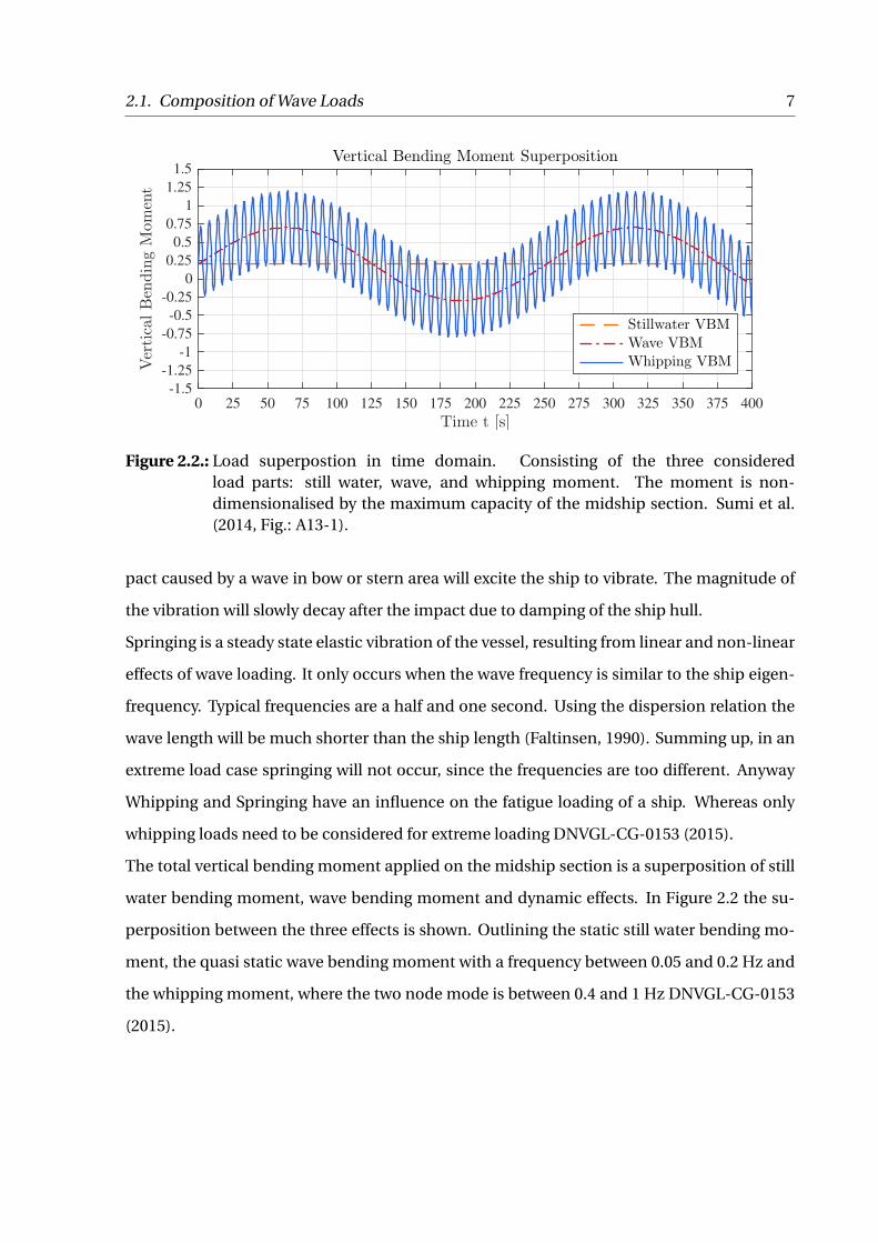
Figure 2.2.: Load superpostion in time domain. Consisting of the three consideredload parts: still water, wave, and whipping moment. The moment is non-dimensionalised by the maximum capacity of the midship section. Sumi et al.(2014, Fig.: A13-1).
pact caused by a wave in bow or stern area will excite the ship to vibrate. The magnitude of
the vibration will slowly decay after the impact due to damping of the ship hull.
Springing is a steady state elastic vibration of the vessel, resulting from linear and non-linear
effects of wave loading. It only occurs when the wave frequency is similar to the ship eigen-
frequency. Typical frequencies are a half and one second. Using the dispersion relation the
wave length will be much shorter than the ship length (Faltinsen, 1990). Summing up, in an
extreme load case springing will not occur, since the frequencies are too different. Anyway
Whipping and Springing have an influence on the fatigue loading of a ship. Whereas only
whipping loads need to be considered for extreme loading DNVGL-CG-0153 (2015).
The total vertical bending moment applied on the midship section is a superposition of still
water bending moment, wave bending moment and dynamic effects. In Figure 2.2 the su-
perposition between the three effects is shown. Outlining the static still water bending mo-
ment, the quasi static wave bending moment with a frequency between 0.05 and 0.2 Hz and
the whipping moment, where the two node mode is between 0.4 and 1 Hz DNVGL-CG-0153
(2015).
8 2. Literature Survey
2.2. Influence of Dynamic Loads
Several studies have been performed to estimate the influence of dynamic effects. The first
published study has been performed by Moe et al. (2005) including strain measurements on
the fatigue loading of a 4,000 TEU container carrier. The finding was a considerable contri-
bution by wave induced vibrations to the total fatigue damage.
Drummen (2008) has investigated a 4,440 TEU container ship. Model tests of an elastic ship
model with spring connections were performed at MARINTEK, Norway. The model con-
tained four rigid parts connected by springs. As a core statement the fatigue damage caused
by vibrations was estimated to be approximately 40 % for this ships
Moa (2010) and Mao et al. (2010) have done research on the effects of whipping on the fatigue
and extreme load. Conclusion was that whipping contributes about 30 % to fatigue loading
of the estimated 2,800 TEU container vessel. The influence on extreme loads was left open
for further studies.
Heggelund et al. (2011) have performed full scale measurements for fatigue and extreme
loading on a post panmax container vessel. Strain on a 8,600 TEU vessel has been meas-
ured amidship over a period of 20 months. The measurements have been evaluated and
compared to the design rules applied for the vessel, concluding that the vibrations dominate
the fatigue damage. It is observed for the extreme loading that in harsh conditions the value
is well above the design level for the hogging condition. Additionally the damping of the ship
seems to be higher, than for other ship types, causing the loads to decay faster.
Storhaug et al. (2010) have performed model test with a 13,000 TEU container ship. Aim
was to estimate the fatigue and extreme loading caused by whipping and springing. The
model tests have been performed at MARINTEK. The model was divided into four rigid ele-
ments connected by three flexible joints. This ensured, that the model is able to vibrate in
the governing two-node mode. Several sea states and wave directions have been tested, cor-
responding to typical trading routes. Outcome is that the vibration load is the dominating
fatigue load at midship with 65 %. The extreme loading exceeds the IACS design values and
further investigations are required.
In addition Storhaug et al. (2011) have done tests on the same model in bow quartering seas.
2.3. Measured strain data on a container vessel 9
The results regarding the effect of different wave encounter angles have been evaluated. The
outcome shows, that the heading direction to the wave does not effect the influence of whip-
ping loads. Thus a change of the course, does not effect the whipping loads.
More recently Barhoumi and Storhaug (2014) have evaluated measured strain data on a 8,600
TEU container vessel. The measured effect of fatigue loading from whipping is assessed to be
57 %. The rule based extreme loads has been exceeded by up to 48 % at aft quarter length. For
further rule development the recommendation is to keep realistic loading situations, caused
by seamanship in perspective to avoid over conservative class rules.
Kahl et al. (2014) have evaluated full scale measurements on board a 4,600 TEU Panmax and
a 14,000 TEU Post-Panmax container vessel. The results for the fatigue design are between
41 % and 73 % influence from hull girder vibrations.
Andersen and Jensen (2014) have published an assessment of measured strain data on 9,400
TEU container vessel. The outcome is, that quasi-static wave loads and high frequency ef-
fects can have roughly the same magnitude. Additionally in moderate conditions the design
values for extreme loading can be exceeded. The results of this paper will be one of the pro-
ject’s main components and will be discussed in more depth in the next section.
Andersen (2014) compared strain measurements from the 14,000 TEU, 9,400 TEU, 8,600 TEU
and 4,400 TEU ships mentioned earlier. The response of the 9,400 TEU vessel with a bow flare
angle of 45 degrees and the 8,600 TEU vessel with a bow flare angle of 58 degrees have been
compared. The response was very different and the bow flare angle was assumed to be one
important parameter.
Storhaug (2014) summed up the performed work so far. He describes the previously men-
tioned measurements and verifications of the findings. He states the problems by using
model test and strain measured data on real ships. It is pointed out, that so far the effect
of whipping loads is not fully developed.
2.3. Measured strain data on a container vessel
Andersen and Jensen (2014) have recently published an investigation of measurements of
hull girder stresses on an Ultra large container carrier (ULCC). The estimated vessel was the

10 2. Literature Survey
0 0.2 0.4 0.6 0.8 1 1.2 1.4 1.6
Frequency [Hz]
10-5
10-4
10-3
10-2
10-1
100
101
Str
ess
resp
onse
spec
trum
[MP
a^2/s
]
Logarithmic stress response spectrum
Wave frequency rangeHigh frequency range
Figure 2.3.: FFT of the measured strain data on a 9,400 TEU ULCC in a sea state with a signi-ficant wave height of eight meter on a logarithmic scale. (Andersen and Jensen,2014)
9,400 TEU container ship.
The strain data has been measured on 02 October 2011 when the ship went through a storm
while sailing about ten knots in a sea state with significant wave height around eight meters.
The strain has been measured using two long-base strain gauges in the passageway amid-
ship. The stress measured at starboard and port has be averaged to exclude torsional and
horizontal loads.
A FFT has been performed on the measured strain series. Four peaks are visible in Figure 2.3,
corresponding to the most common loading frequency. The signal is considered between
the borders of 0.01 Hz and 1.6 Hz according to the DNV-RC (2011) recommendations. The
frequency range from 0.01 Hz to 0.3 Hz is called the Low Frequency (LF) range, the frequency
range from 0.3 Hz to 1.6 Hz is called the High Frequency (HF) range. The peak in the LF range
displays the wave load frequency, whereas the range above 0.3 Hz displays the whipping con-
tribution. Herein the two node mode can be estimated at 0.48 Hz and the three node mode
at 0.99 Hz.
By using a FFT and their inverse it is possible to switch between time and frequency domain.

2.3. Measured strain data on a container vessel 11
0 200 400 600 800 1000 1200 1400 1600 1800
-100
-50
0
50
100
Stress[M
Pa]
Original (unfiltered) time series
0 200 400 600 800 1000 1200 1400 1600 1800
-100
-50
0
50
100
Stress[M
Pa]
Low-pass filtered time series
0 200 400 600 800 1000 1200 1400 1600 1800
Time [s]
-100
-50
0
50
100
Stress[M
Pa]
High-pass filtered time series
Figure 2.4.: Time series of the measured strain data over 30 minutes. The unfiltered series isshown as well as the low-pass filtered time series and the high-pass filtered timeseries. (Andersen and Jensen, 2014)
Advantage hereby is the ability of erasing certain frequencies of the time series. In Figure 2.4
the unfiltered time series as well as the filtered LF and HF range is shown. For the wave loads
it can be seen, that the magnitude of the stress varies, but is always present over the time.
For vibration loads, it can be seen how the load start abrupt and decays thereafter again. The
average load level is low, but the peak loads are high.
Comparing the magnitude of the wave loads and the dynamic loads, for their peak values,
e.g. at second 350, the stress is roughly of same magnitude. Andersen and Jensen (2014)
have compared further the measured stresses with the allowed stress for the container ships
according to the classification society rules. The measured loads exceed the design values
during the peaks already in this moderate sea state.

12 2. Literature Survey
2.4. Prediction of whipping loads
So far it is known, that dynamic effects have an influence on the fatigue load and might in-
fluence the extreme load. Thus the estimation of whipping loads is a topic of great interest.
The estimation of slamming loads has already been defined by von Karman in 1929 and has
been improved by Wagner in 1932 (Faltinsen, 1990). Consequently the exercise is to estimate
from known slamming loads, the corresponding whipping loads.
Research at Danish Technical University (DTU) has been performed to combine strip theory
developed by Salvesen et al. (1970) with hydro elasticity. Based on the perturbation method
by Jensen and Pedersen (1978), Xia et al. (1998) present a non-linear time domain strip the-
ory accounting for hydrodynamic memory effects. The "momentum slamming" force is in-
cluded. The ship is modelled with Timoshenko beams and allows rigid body motion. The
beam model combined with the non-linear hydro elasticity model makes it possible to pre-
dict vibration loads.
Andersen and Jensen (2012) have used the in-house strip theory code SHIPSTAR and com-
pared the results with model tests in regular waves. The tests have been performed with a
flexible model ship at CEHIPAR, Spain. For longer wavelength, both methods are applicable.
For shorter wavelengths the results are poorer. Nonetheless is the method able to simulate
momentum slamming.
More recently Computational Fluid Dynamic (CFD) is used for the whipping prediction.
Seng and Jensen (2012) compared slamming loads received by a free surface Navier-Stokes
equation with the results of non-linear strip theory. Further Seng et al. (2012a) compared
strip theory with a CFD solver in terms of whipping loads. Even though the CFD method
is the more advanced method, strip theory reveals similar accurate results. For reasons of
comparison, again the model test are consulted, showing good agreement for long crested
waves.
Seng et al. (2012b) have applied a direct three-dimensional, fully non-linear numerical cal-
culation in a realistic wave environment. The method of a model correction factor approach
is proposed, to apply the complex processes of hydro elasticity in strip theory. This improves
the accuracy of strip theory, especially for bow quartering sea and following seas.

2.5. Influence of Rigid Body Motion in Ultimate Strength Analysis 13
Seng and Jensen (2013) applied the model correction factor approach and worked out diffi-
culties using it with strip theory. Since strip theory is not able to include radiation effects, it
is likely to detect slamming in the stern of the vessel, even though in reality this is not the
case. Thus recommendation is to use a modified aft model to avoid this pitfall.
In a nutshell, strip theory is improved to account for the effect of hydro elasticity. Further
CFD is used to improve the accuracy of the strip theory results.
2.5. Influence of Rigid Body Motion in Ultimate
Strength Analysis
When investigating the post collapse region of a hull girder, it is important to estimate the
influence of rigid body motion. During the collapse of a 350 meter long ship, the ends ex-
perience a big change in draft even for small angles. The increasing buoyancy will force the
midship section to lift and generate moment capacity. This will define the severity for a fail-
ure of the hull girder.
Xu et al. (2011a) have developed a new approach for the dynamic collapse behaviour. The
basic model contains two rigid body elements and a rotational spring connecting both parts
at the hinge. Strip theory is further used to apply the loads. It shows, that the collapse in-
creases rapidly until unloading occurs. Tank tests have been performed to prove the results.
Herein a specimen links both rigid parts and defines the collapse behaviour. Of special in-
terest is the extend to which the ship collapses until equilibrium is reached.
Xu et al. (2011b) have improved the existing strip theory model and compared it with effects
which will occur in reality. Focus is put on post ultimate strength. Effects such as develop-
ment of buckling pattern, a higher capacity drop and stiffness recovery when unloading due
to residual capacities have been discussed.
Iijima et al. (2011) have performed model test to validate the non-linear strip theory includ-
ing a plastic hinge. Outcome is that the hull girder collapses rapidly unless unloading due to
rigidity occurs. As well that the severity of the collapse is highly depending on the capacity
drop after failing.

14 2. Literature Survey
Figure 2.5.: Extension of the rigid body motion model, using flexible beams to model therigid part of the vessel. The collapse region is displayed by a non-linear rotationalspring. The beams are embed on springs. (Iijima and Fujikubo, 2012)
Xu et al. (2012) have performed a parametric study on the post buckling behaviour. The dy-
namic collapse is characterised by the eigenvalue. Whereas the eigenvalues are depending
on the moment of inertia and the stiffness. The latter is highly dependent on the restoring
forces from hydrostatic pressure and rigidity of the structure.
An extension for very large floating structures is done by Iijima and Fujikubo (2012). The
definition of rigid elements is not sufficient enough due to hull girder flexibility. An approach
with flexible ends is developed, but more sophisticated models should be consulted.
Xu et al. (2014) have replaced the non-linear spring with a finite element approach. The loads
have been applied using the developed strip theory method. The bending moment on the
finite element model is applied using Multi Point Constraint (MPC) elements at the height of
the neutral axis. The FEM shows good agreement with the developed strip theory approach
for the total collapse of the structure.
Summing up, strip theory has been combined with a plastic hinge and a finite element model.
This enables the estimation of the post collapse path for the ship. Several methods have been
applied to increase the accuracy of the non linear spring and the rigid body parts.
2.6. Finite Element Modelling
Finite Element Analysis (FEA) has been performed from several authors on different subjects.
Amlashi (2008) has built a model of the midship section of a Bulk carrier. He used a 1/2 + 1 +
1/2 cargo hold model (Amlashi and Moan, 2008). The longitudinal parts of the middle cargo
hold are defined with non-linear material. The other parts are modelled with linear material.
2.6. Finite Element Modelling 15
consumption and computational time. On the other hand, ifthe mesh is too coarse in the critical areas, such as bottom
panels for the assessment of ultimate hull girder strength in
hogging, the local buckling of structural members cannotbe captured, which will lead to an unrealistically higher
ultimate longitudinal strength. However, for a ship in
hogging condition, it is only the bottom part that willexhibit buckling under compressive stresses. The present
study focuses on the ultimate longitudinal strength of the
target bulk carrier under combined global vertical bendingmoment and local lateral pressure loads in the hogging and
AHL condition. In the hogging and AHL condition, the
double bottom of the empty hold in the middle of themodel is under the combined actions of lateral sea pressure
from the bottom, longitudinal thrust from global vertical
bending and double bottom bending and transverse thrustfrom lateral pressure acting on the side shell and interaction
between side shell and double bottom structures. There-
fore, the bottom panels in the empty hold are prone tocollapse due to buckling, which is expected to have a
significant influence on the ultimate longitudinal strength
of the hull structure of bulk carriers in the hogging andAHL condition. Hence, a fine mesh is needed in that part of
the FE model.
Before performing a large nonlinear finite elementanalysis, mesh convergence studies (test analyses) must be
conducted for the whole model or at least for the critical
(typical) region. The mesh size, mesh distribution andelement types adopted in the present study are based on the
work by Østvold et al. [10] and Amlashi and Moan [11].
The shell element S4 is selected for the FE model.
Relatively coarse meshes are applied in the holds on the
forward and aft ends as well as to the adjacent parts of the
centre hold which are far away from the region of interest.This coarse mesh part has 1 9 3 elements in the plate
bounded by longitudinal stiffeners and transverse web
frames in the double bottom. The webs of stiffeners are stillmodelled as shell elements, while the flanges are repre-
sented using beam elements. The web stiffeners are mod-
eled as beam elements and the manholes on the transverseweb are accounted in the model by reducing the thickness.
The middle part of the centre hold is modelled with very
fine mesh density in the lower part. The mesh density in thefine mesh region of the double bottom, as shown in Fig. 3,
can be summarized as follows,
• 5 9 15 shell elements in the plate bounded by longi-
tudinal stiffeners and transverse web frames.
• Five shell elements across the height of the longitudinalstiffeners.
• Twenty-one shell elements across the height of double
bottom girders and floors.• Two shell elements across the flange of the longitudinal
stiffeners.
This mesh strategy is considered to be good enough to
capture the proper collapse modes of the stiffened bottom
panels at a practical computational time and places rea-sonable requirements on the computer’s disk and memory
storage capacity. However, this type of dense mesh could
not be used everywhere in the model, as the size of themodel would quickly grow beyond the computer capacity.
Therefore, only critical regions where the structural col-
lapse is expected have been be modelled by the fine mesh.Dense mesh is employed in the double bottom of the centre
cargo hold where the buckling/yielding of the stiffened
panels is most likely to occur. Coarse mesh is used for theside shell and deck. The model geometry is based on the
net offered scantlings according to CSR-BC. It is noted that
the focus of the present study is the ultimate hull girderstrength of the target bulk carrier in the hogging and AHL
condition. Coarse mesh is employed for the upper deck.
Therefore this model is not suitable for estimating theultimate hull girder strength in a sagging condition. The
total number of elements in the FE model is around 186000
and the total number of degrees of freedom is about990000.
Table 3 Material properties ofthe ISSC-2000 Capesize bulkcarrier
MS Hs32 Hs36 Hs40
Young’s modulus (N/mm2) 2.1 9 105 2.1 9 105 2.1 9 105 2.1 9 105
Poisson ratio 0.3 0.3 0.3 0.3
Strain hardening parameter (N/mm2) 825 625 675 600
Yielding stress (N/mm2) 235 313.6 352.8 392
Fig. 2 Three-cargo-hold FE model of the ISSC-2000 Capesize bulkcarrier
98 J Mar Sci Technol (2012) 17:94–113
123
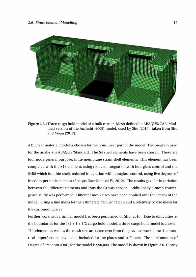
Figure 2.6.: Three cargo hold model of a bulk carrier. Mesh defined in ABAQUS/CAE. Mod-ified version of the Amlashi (2008) model, used by Shu (2010), taken from Shuand Moan (2012).
A bilinear material model is chosen for the non-linear part of the model. The program used
for the analysis is ABAQUS/Standard. The S4 shell elements have been chosen. These are
four node general purpose, finite membrane strain shell elements. This element has been
compared with the S4R element, using reduced integration with hourglass control and the
S4R5 which is a thin shell, reduced integration with hourglass control, using five degrees of
freedom per node element (Abaqus User Manual IV, 2012). The results gave little variation
between the different elements and thus the S4 was chosen. Additionally a mesh conver-
gence study was performed. Different mesh sizes have been applied over the length of the
model. Using a fine mesh for the estimated "failure" region and a relatively coarse mesh for
the surrounding area.
Further work with a similar model has been performed by Shu (2010). Due to difficulties at
the boundaries for the 1/2 + 1 + 1/2 cargo hold model, a three cargo hold model is chosen.
The element as well as the mesh size are taken over from the previous work done. Geomet-
rical imperfections have been included for the plates and stiffeners. The total amount of
Degree of Freedom (DoF) for the model is 990,000. The model is shown in Figure 2.6. Clearly

16 2. Literature Survey
visible is the refine midship area of the model. For both models only the port side has been
designed. Symmetric boundaries have been applied to reduce the number of DoF. For the
application of the external loads have the programs VERES and WASIM been used. VERES is
based on 2D strip theory and WASIM is based on 3D Rankine panel method.
2.7. MSC Napoli Accident
On the 18th January of 2007 the 4,419 TEU container vessel MSC Napoli suffered structural
hull girder failure in the English Channel. The ship was sailing with wind of storm force
measuring between 10 and 11 on the Beaufort scale. The wave height was between 5 and 9
meters with a wave period of 9 to 10 seconds. The wave length was 150 meters and the water
depth 80 meters (Marine Accident Investigation Branch, 2008).
The hull girder collapsed right behind the engine front bulkhead, in the area of the engine
room. Intensive research have been done to determine the triggers of failure. The ship was
classified under Det Norske Vertitas AS (DNV) rules. Thus DNV as well as Bureau Veritas SA
(BV) investigated this matter. Both methods will be presented within this section.
The DNV method described in Marine Accident Investigation Branch Annex A-D (2008) has
been performed in the following steps:
1) Hydrodynamic Wave Load analysis using DNV’s wave load tool WASIM
2) Global linear stress analyses with fine mesh in examined area using DNV’s finite ele-
ment program SESAM
3) Non-linear stress and ultimate capacity analysis with fine mesh in examined area using
ABAQUS.
The still water bending moment has been analysed using the software package Naval Archi-
tecture Package (NAPA) based on strip theory, from the actual loading condition. The wave
loads have been analysed for linear and non-linear effects in WASIM. Two different wave
scenarios have been estimated to define a possible load range. Whipping loads have been
mentioned as an additional factor, increasing the load.

2.7. MSC Napoli Accident 17
DET NORSKE VERITAS
Page -32 Report No. 2007 - 1928, Rev. No. 00
7 SUMMARY
7.1 General The computer analyses demonstrate that a very high vertical hull girder moment, close to or exceeding the corresponding capacity limit, may lead to a type of structural failure between #81 to #88, as is observed on MSC Napoli in open sea. This is evident from a comparison between a photo taken of the vessel’s starboard side, before it is beached with the failure visible, and a computer simulation image of the same area, see Fig. 7.1. This is further supported by diving surveys while beached and also later from surveys of the forward part in dry dock.
Fig. 7.1 Comparison of real life failure mode with computer simulations (ABAQUS FE model)
( with permission from Gargolaw)
Given the assumptions and uncertainties as described earlier in this report, the computer analyses carried out and documented herein indicate that the total hull girder loads in way of the engine room area may have been on the limit or have exceeded the corresponding hull capacity for MSC Napoli, see Fig. 7.2.
Figure 2.7.: Comparison between the collapsed MSC Napoli hull and the calculated failureusing the non-linear finite element program ABAQUS. (Marine Accident Invest-igation Branch Annex A-D, 2008)
The loads from WASIM have been transferred onto the linear SESAM Model and equilibrium
solved. The stresses have been found close to the yield stress and the results have been trans-
ferred onto the non-linear ABAQUS model.
The global model has been defined as linear except of the engine part, which has been
defined as a non-linear super element using very fine mesh. The determination of the fine
mesh area will be discussed later in this thesis. Small imperfections have been included in
order to capture the real buckling and collapse behaviour.
The non-linear material has been defined as a bilinear material curves. Three different ma-
terial sets have been used:
1) Lower 5 % quantile yield stress
2) Mean value yield stress
3) Upper 5 % quantile yield stress.
The lower 5% quantile yield stress are rule based values. This will in 95 % underestimate the
structure and a higher value is more realistic. The calculations result in different ultimate
capacities, corresponding to the yield stress levels.
Comparing the capacity range with the estimated load range, reveals a certain overlap. In
this area, the capacity is lower than the load and failure occur. The collapse pattern received
18 2. Literature Survey
in ABAQUS has been compared with the real collapse pattern. Figure 2.7 shows a good agree-
ment for the model. The loss was in this case caused by insufficient rules of DNV. The rules
have been changed and the hull girder capacity has been increased thereafter.
BV uses a more simplified approach. The conditions at time of the accident are interpolated
from data of the hindcast model provided by the British government. A Jonswap spectrum is
used to determine the most likely sea state.
Whipping loads are estimated in matter of measuring slamming forces in a time domain ana-
lysis and receiving a whipping response. The result is, that the load is increased by 30 % when
slamming loads are considered. The calculation however does have a number of uncertain-
ties, namely: structural damping, speed, heading, wave spectrum and mass distribution.
A finite element model of the engine room area is modelled in ABAQUS. The material is
chosen to follow the Ramsberg-Osgood theory. The yield and tensile strength are defined
according to the design values. Riks method is used. Finally the ultimate structural capa-
city is defined and evaluated. The angle of the ultimate capacity is found to be 10°3 radiant.
Taking uncertainties as whipping into consideration a collapse is possible.
2.8. MOL Comfort Accident
On 17th June 2013 the 8,110 TEU container vessel MOL Comfort broke near the midship sec-
tion into two pieces. Pictures of the ship can be seen in the problem description. The ship
was sailing with a speed of 17 knots in a sea state with a significant wave height of 5.5 meter,
wave period of 10.3 seconds and wind of force 7 Beaufort. The accident happened in the
Indian Ocean on a voyage from Singapore to Saudi Arabia. The ship was classified under
Nippon Kaiji Kyokai (ClassNK).
After the accident ClassNK published and interims investigation report (Sumi et al., 2013)
and a final report (Sumi et al., 2013) about the loss of the ship. The ship experienced severe
collapse of the bottom structure at the midship section. After the accident six sister ships
and four similar ship have been examined in the affected bottom area. In five of the six sister
ships and in one of the four similar ships deformations in the bottom area were found. The
out of plane deformation has been in the area of the section weld and has been on average
2.8. MOL Comfort Accident 19
28
Fig. 5.2.4 Example of deformation nearby hull girder structure strength (Ultimate hull girder strength) (by
simulation)
Comparison of deformation under still water condition and resicual deformation after
unloading from 14.8x10⁶ kN-m to still water condition for the case when initial imperfection
of “hungry-horse” mode was given (In the case of hull structure strength (ultimate hull
girder strength) of 15.0×10⁶kN-m)
(including initial shape imperfection of 3.14 mm at the relevant position)
Fig. 5.2.5 Reproduction of deformation of bottom shell plate (unloading from 14.8×10⁶ kN-m to still water
condition in the case when hull structure strength (Ultimate hull girder strength) was 15.0×10⁶
kN-m)
7.73mm 6.66mm
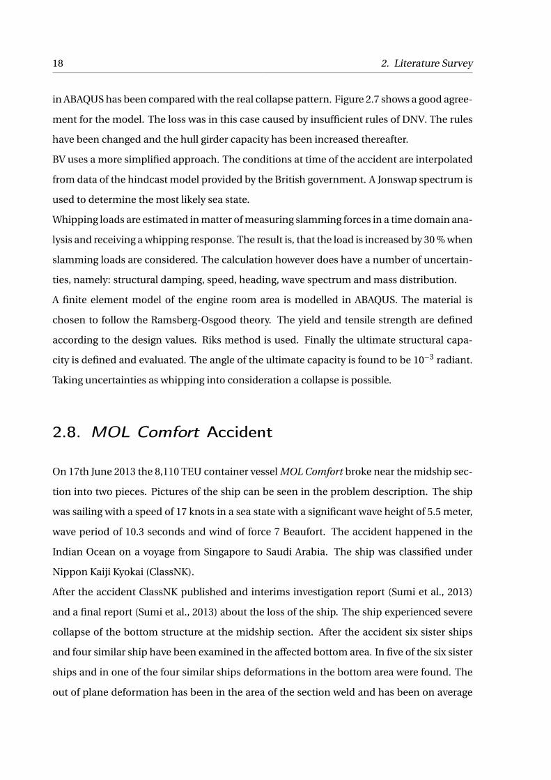
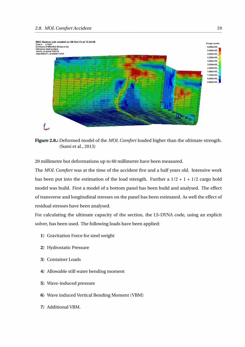
Figure 2.8.: Deformed model of the MOL Comfort loaded higher than the ultimate strength.(Sumi et al., 2013)
20 millimetre but deformations up to 60 millimetre have been measured.
The MOL Comfort was at the time of the accident five and a half years old. Intensive work
has been put into the estimation of the load strength. Further a 1/2 + 1 + 1/2 cargo hold
model was build. First a model of a bottom panel has been build and analysed. The effect
of transverse and longitudinal stresses on the panel has been estimated. As well the effect of
residual stresses have been analysed.
For calculating the ultimate capacity of the section, the LS-DYNA code, using an explicit
solver, has been used. The following loads have been applied:
1) Gravitation Force for steel weight
2) Hydrostatic Pressure
3) Container Loads
4) Allowable still water bending moment
5) Wave-induced pressure
6) Wave induced Vertical Bending Moment (VBM)
7) Additional VBM.

20 2. Literature Survey
The additional VBM was increased until the hull girder collapsed. Thus the ultimate capacity
can be estimated by looking at the load displacement curve. The failed hull girder can be
seen in Figure 2.8. The outcome is, taking all uncertainities into account, that a failure of the
hull girder is possible.
2.9. Ultimate Strength Design Rules
IACS UR-S (2016, S11A.5) defines rules for hull girder ultimate strength, given by:
∞S MS +∞W MW ∑ MU
∞M∞DB. (2.1)
With ∞ denoting partial safety factors and M vertical hull bending moments. The equation
is divided into three parts. Where the left hand side of the equation is the load part. The
still water bending is denoted with S, the wave bending with W . On the right hand side of
the equation is the capacity. Having the ultimate capacity denoted with U and two safety
factors covering material, geometric and strength prediction uncertainties M and double
bottom bending effect DB . The new amendment IACS UR-S (2016, S11A.6.3) states, that each
classification society must take the effect of whipping into account. The way of inclusion is
left open to the classification societies.
3. Methodology
The aim of this thesis is to verify the influence of dynamic load effects, such as whipping,
on the hull girder. Several classification societies have published a recommendation, as this
might be done. The influence factors will be compared with the results of this thesis. To
evaluate the effects, a certain strategy must be defined. In the following, the modelling of
loads, structure and finally verification of the results is discussed.
3.1. Modelling the Loads
As mentioned in Chapter 2 several researches have been performed to use strip theory, for
including whipping loads. Effort has been performed to use CFD to improve the results.
(Seng and Jensen, 2013) The structural and hydrodynamic damping is hard to predict and
has a big influence on the contribution of dynamic effects (Iijima et al., 2011). Additionally
strip theory does not account for radiation effects and requires a special definition of the
vessels stern. (Seng and Jensen, 2013)
Alternatively the loads can be applied by using model test data, or strain measurements on a
container vessel. Heggelund et al. (2011) mentioned, that the damping of vibrations depends
on size of the vessel. Generally container vessels have higher damping due to interaction
of the cargo. In model testing it is hard to achieve a high enough damping rate for large
container vessels, thus whipping loads might be too high. (Storhaug et al., 2010)
The best way of applying loads with a realistic whipping contribution is to use measured
strain data. The author is fortunate to be able to use the strain data evaluated in Andersen
and Jensen (2014). The data is transferred from stresses into a bending moment and further
21
22 3. Methodology
scaled in magnitude to reach certain values of interest. To reduce the required calculation
time a suitable wave is picked out of the measured set to represent an extreme event. To
estimate the effect of the dynamic collapse a longer time period is used.
3.2. Modelling the structure
For the definition and calculations of the structure the program ANSYS is chosen. Due to a
lack of data a container vessel in dimensions close to the estimated ship is designed. Main
focus is to match the eigenfrequencies of the 9,400 TEU ship used in the load data. The pro-
gram POSEIDON is used to design a suitable midship section according to the regulations of
the GL
Several studies have proven the use of finite element analysis valid for the analysis of the ul-
timate capacity of the hull girder. On the one hand the model needs to have a certain size,
to neglect influence of boundaries. On the other hand it must be sufficiently simplified to
reduce calculation time. A first approach on the model size is taken according to the MOL
Comfort survey. This ensures symmetry conditions in the longitudinal direction and ensures
steady deflections between the cargo holds and the bulkheads. Only the starboard side is
modelled and symmetry condition in transverse direction is applied as well.
The dynamic collapse is the main consideration of the thesis. Thus dynamic effects need to
be considered. For this matter it is important that the ship has the same eigenfrequencies
as the load data. This can be done by defining masses in the extensions of the ship. They
account for the mass of the ship and container loads. The eigenfrequencies are known from
Andersen and Jensen (2014). The ship in water will have to deal with the effect of added
mass. Thus the external weights are scaled until the structure has the corresponding wet ei-
genfrequencies. To avoid the masses to create a bending moment on the structure, loads are
applied to ensure equilibrium.
A loading scenario is developed, including static and dynamic external pressure, container
and tanks. Since the inertia of the masses are important for the dynamic behaviour, contain-
ers are defined as masses instead of loads.
Intensive research has been done on the ultimate collapse behaviour of ships. To account

3.3. Planning and verification of work 23
for the relaxation effect of "rigid" body motion the procedure of Iijima and Fujikubo (2012)
is followed, by applying beam elements in the extension of the shell model. These beams are
constrained by springs in vertical direction to account for the change in displacement.
The provided load data is applied at the ends of the shell model using MPC elements. The
effect of the rigid body is measured and excluded for the collapse behaviour.
3.3. Planning and verification of work
To reach the goal of estimating the dynamic collapse several steps need to be considered
on the forehand. The finite element method is chosen for the work. Since this numerical
method does not necessarily reflect realistic behaviour it is required to validate the result
with analytical solutions. First evaluations are performed with a simple plate. The analytical
results are given by the Euler buckling loads and the concept of effective width which will be
introduced later. Additionally the semi analytical program PULS by DNV is used to compare
the results. Also the effect of different parameters e.g. materials, added mass, imperfections,
etc. on the structure can be checked with this simple model.
When the method is validated, the midship section can be designed and modelled. For a
non linear buckling analysis it is necessary to include imperfections. These imperfections
are obtained from an eigenvalue analysis of the "crash" section. Important for the dynamic
collapse later on is the representation of the correct eigenfrequencies. These will be mod-
elled by beam elements at the rigid ends.
With this set up it is possible to calculate the static collapse of the structure. An incremental
method provided by POSEIDON is used to compare the results. Next the incremental col-
lapse using wave data with the whipping loads can be estimated. A load level will need to
be estimated at which plasticity occurs. With this level defined, several waves will be loaded
onto the structure and the dynamic collapse can be estimated. The whole process can be
seen in Figure 3.1.

24 3. Methodology
Finite Element Method
Plate bucklingAnalytical SolutionPULS
Solver Verification
Parameter Studies Material Law, etc.
DesignRule ValuesPOSEIDON
Crashsection Model
Linear Buckling Analysis Imperfections
Full Model
Rigid Body PartTULCS Geometry Eigenfrequencies
Collapse BehaviourIncremental SolutionPOSEIDON
Ultimate Limit State
Incremental Collapse Incremental Factor
Dynamic Collapse
Implement
Figure 3.1.: Flowchart steps necessary to estimate the dynamic collapse of the structure.
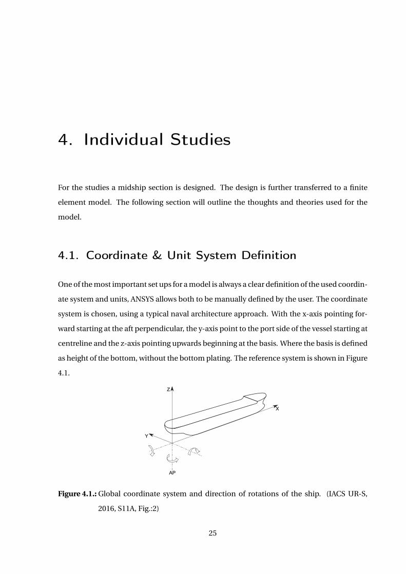
4. Individual Studies
For the studies a midship section is designed. The design is further transferred to a finite
element model. The following section will outline the thoughts and theories used for the
model.
4.1. Coordinate & Unit System Definition
One of the most important set ups for a model is always a clear definition of the used coordin-
ate system and units, ANSYS allows both to be manually defined by the user. The coordinate
system is chosen, using a typical naval architecture approach. With the x-axis pointing for-
ward starting at the aft perpendicular, the y-axis point to the port side of the vessel starting at
centreline and the z-axis pointing upwards beginning at the basis. Where the basis is defined
as height of the bottom, without the bottom plating. The reference system is shown in Figure
4.1.
Sec
tion
1
Class guideline — DNVGL-CG-0127. Edition October 2015 Page 8Finite element analysis
DNV GL AS
Table 1 Material properties
Young’s Modulus
[kN/m2]Poisson Value Shear Modulus
[kN/m2]Density[t/m3]
Steel 2.06.108 0.30 0.792.108 7.80
Alu 0.70.108 0.33 0.263.108 2.75
The minimum yield stress ReH has to be related to the material defined as indicated in the rules, RU SHIPPt.3 Ch.3 Sec.1 Table 1. Consequently, it is recommended that every steel grade is represented by a separatematerial data set in the model, as the materials are defined in the structural drawings.
1.5 Global coordinate systemThe following co-ordinate system is recommended; right hand co-ordinate system, with the x-axis positiveforward, y-axis positive to port and z-axis positive vertically from baseline to deck. The origin should belocated at the intersection between aft perpendicular (AP), baseline and centreline. The co-ordinate system isillustrated in Figure 1.It should be noted that loads according to the rules, RU SHIP Pt.3 Ch.4 refer to a coordinate system with adifferent x-origin (located at aft end (AE) of the rule length L). This coordinate system is defined in the rules,RU SHIP Pt.3 Ch.1 Sec.4 [3.6.1].
Figure 1 Global coordinate system
1.6 Corrosion DeductionFE models are to be based on the scantlings with the corrosion deductions according to the rules, RU SHIPPt.3 Ch.3 Sec.2 Table 1, as follows
— 50% corrosion deduction for ships with class notation ESP;— 0% corrosion deduction for other ships.
Buckling capacity assessment based on FE analysis is to be carried out with 100% corrosion deduction.
Figure 4.1.: Global coordinate system and direction of rotations of the ship. (IACS UR-S,
2016, S11A, Fig.:2)
25
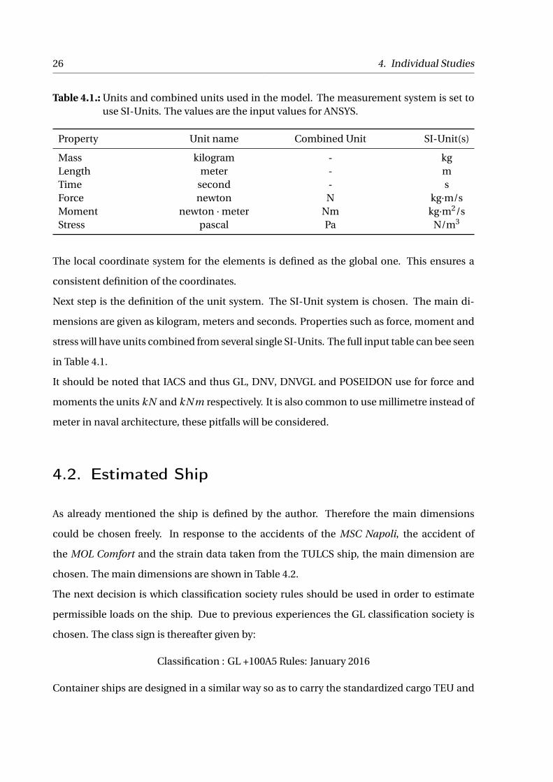
26 4. Individual Studies
Table 4.1.: Units and combined units used in the model. The measurement system is set touse SI-Units. The values are the input values for ANSYS.
Property Unit name Combined Unit SI-Unit(s)
Mass kilogram - kgLength meter - mTime second - sForce newton N kg·m/sMoment newton · meter Nm kg·m2/sStress pascal Pa N/m3
The local coordinate system for the elements is defined as the global one. This ensures a
consistent definition of the coordinates.
Next step is the definition of the unit system. The SI-Unit system is chosen. The main di-
mensions are given as kilogram, meters and seconds. Properties such as force, moment and
stress will have units combined from several single SI-Units. The full input table can bee seen
in Table 4.1.
It should be noted that IACS and thus GL, DNV, DNVGL and POSEIDON use for force and
moments the units kN and kN m respectively. It is also common to use millimetre instead of
meter in naval architecture, these pitfalls will be considered.
4.2. Estimated Ship
As already mentioned the ship is defined by the author. Therefore the main dimensions
could be chosen freely. In response to the accidents of the MSC Napoli, the accident of
the MOL Comfort and the strain data taken from the TULCS ship, the main dimension are
chosen. The main dimensions are shown in Table 4.2.
The next decision is which classification society rules should be used in order to estimate
permissible loads on the ship. Due to previous experiences the GL classification society is
chosen. The class sign is thereafter given by:
Classification : GL +100A5 Rules: January 2016
Container ships are designed in a similar way so as to carry the standardized cargo TEU and

4.2. Estimated Ship 27
Table 4.2.: Main Dimensions of the MSC Napoli, MOL Comfort, TULCS project ship andthe designed ship.(Marine Accident Investigation Branch Annex A-D, 2008) Sumiet al. (2014) (Andersen and Jensen, 2014) (Andersen, 2014)
Property Symbol MSC Napoli MOL Comfort TULCS Ship Unit
Class - DNV ClassNK BV GL -Length over all Loa 275.66 - 349.00 350.00 mRule Length LRul e - - 329.70 340.00 mLength btw. pp. LPP 261.40 302.00 333,40 330.00 mBreadth B 38.18 45.60 42.80 46.00 mDraft D 21.50 25.00 25.00 25.00 mDepth T 13.50 14.50 14.50 14.50 mBlock Coefficient CB 0.609 - 0.66 0.66 -Max. Displacement 5 82,052 - 136,559 149,674 m3
Max. velocity V 24.10 25.25 25.40 25.00 knContainer Capacity - 4,419 8,110 9,400 10,500 TEUDeadweight - 62,277 - 113,000 120,000 ton
Table 4.3.: Main dimension of a TEU and a FEU, an ISO 20’ Container and an ISO 40’Container.
Property TEU FEU Unit
Length 6,058 12,192 mmWidth 2,438 2,438 mmHeight 2,591 2,591 mmHeight HC 2,896 2,896 mmAverage loaded weight 7,000 14,000 kg
Fourty foot equivalent unit (FEU). The dimensions are shown in Table 4.3. The cargo hold is
designed to accommodate at the midship section sixteen container besides each other. The
stack will be nine container height with the out most row only eight.
After a sketch of the midship section is defined, caused by geometric considerations the next
step is to estimate the bending moment and shear forces acting on the section. Therefore
several sources have been consulted. As earlier mentioned the still water and wave bending
moment must be estimated. The still water bending moment is usually found by calculating
the required loading conditions, which represent the most severe cases. In this case, no hy-
drodynamic model is developed and a coarser method is chosen. DNVGL Rules (2016) has
developed a formula to estimate the still water loads in a rough estimation. The calculation
is given in Section B.2 and the results are shown in Table 4.4.
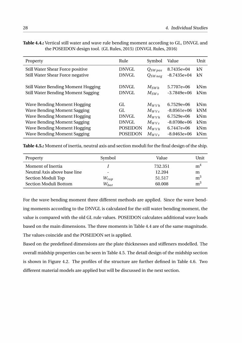
28 4. Individual Studies
Table 4.4.: Vertical still water and wave rule bending moment according to GL, DNVGL andthe POSEIDON design tool. (GL Rules, 2015) (DNVGL Rules, 2016)
Property Rule Symbol Value Unit
Still Water Shear Force positive DNVGL QSW pos 8.7435e+04 kNStill Water Shear Force negative DNVGL QSW neg -8.7435e+04 kN
Still Water Bending Moment Hogging DNVGL MSW h 5.7707e+06 kNmStill Water Bending Moment Sagging DNVGL MSW s -3.7849e+06 kNm
Wave Bending Moment Hogging GL MW V h 6.7529e+06 kNmWave Bending Moment Sagging GL MW V s -8.0561e+06 kNMWave Bending Moment Hogging DNVGL MW V h 6.7529e+06 kNmWave Bending Moment Sagging DNVGL MW V s -8.0708e+06 kNmWave Bending Moment Hogging POSEIDON MW V h 6.7447e+06 kNmWave Bending Moment Sagging POSEIDON MW V s -8.0463e+06 kNm
Table 4.5.: Moment of inertia, neutral axis and section moduli for the final design of the ship.
Property Symbol Value Unit
Moment of Inertia I 732.351 m4
Neutral Axis above base line - 12.204 mSection Moduli Top Wtop 51.517 m3
Section Moduli Bottom Wbot 60.008 m3
For the wave bending moment three different methods are applied. Since the wave bend-
ing moments according to the DNVGL is calculated for the still water bending moment, the
value is compared with the old GL rule values. POSEIDON calculates additional wave loads
based on the main dimensions. The three moments in Table 4.4 are of the same magnitude.
The values coincide and the POSEIDON set is applied.
Based on the predefined dimensions are the plate thicknesses and stiffeners modelled. The
overall midship properties can be seen in Table 4.5. The detail design of the midship section
is shown in Figure 4.2. The profiles of the structure are further defined in Table 4.6. Two
different material models are applied but will be discussed in the next section.
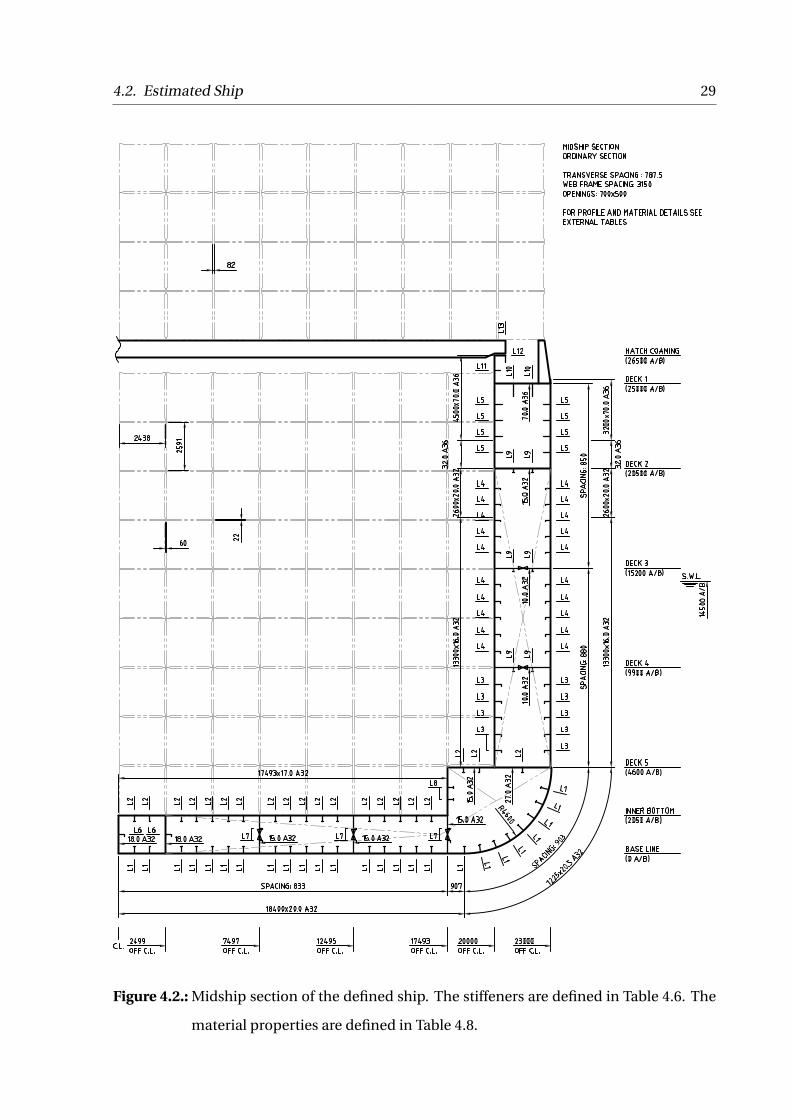
4.2. Estimated Ship 29
Figure 4.2.: Midship section of the defined ship. The stiffeners are defined in Table 4.6. The
material properties are defined in Table 4.8.
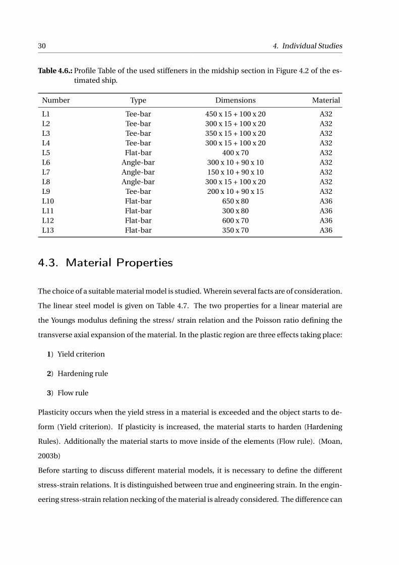
30 4. Individual Studies
Table 4.6.: Profile Table of the used stiffeners in the midship section in Figure 4.2 of the es-timated ship.
Number Type Dimensions Material
L1 Tee-bar 450 x 15 + 100 x 20 A32L2 Tee-bar 300 x 15 + 100 x 20 A32L3 Tee-bar 350 x 15 + 100 x 20 A32L4 Tee-bar 300 x 15 + 100 x 20 A32L5 Flat-bar 400 x 70 A32L6 Angle-bar 300 x 10 + 90 x 10 A32L7 Angle-bar 150 x 10 + 90 x 10 A32L8 Angle-bar 300 x 15 + 100 x 20 A32L9 Tee-bar 200 x 10 + 90 x 15 A32L10 Flat-bar 650 x 80 A36L11 Flat-bar 300 x 80 A36L12 Flat-bar 600 x 70 A36L13 Flat-bar 350 x 70 A36
4.3. Material Properties
The choice of a suitable material model is studied. Wherein several facts are of consideration.
The linear steel model is given on Table 4.7. The two properties for a linear material are
the Youngs modulus defining the stress/ strain relation and the Poisson ratio defining the
transverse axial expansion of the material. In the plastic region are three effects taking place:
1) Yield criterion
2) Hardening rule
3) Flow rule
Plasticity occurs when the yield stress in a material is exceeded and the object starts to de-
form (Yield criterion). If plasticity is increased, the material starts to harden (Hardening
Rules). Additionally the material starts to move inside of the elements (Flow rule). (Moan,
2003b)
Before starting to discuss different material models, it is necessary to define the different
stress-strain relations. It is distinguished between true and engineering strain. In the engin-
eering stress-strain relation necking of the material is already considered. The difference can
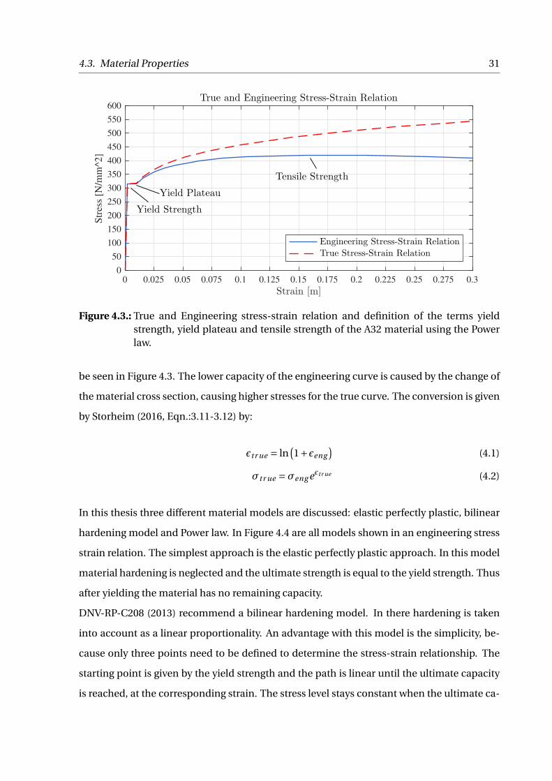
4.3. Material Properties 31
0 0.025 0.05 0.075 0.1 0.125 0.15 0.175 0.2 0.225 0.25 0.275 0.3
Strain [m]
0
50
100
150
200
250
300
350
400
450
500
550
600S
tres
s [N
/mm
^2
]True and Engineering Stress-Strain Relation
Yield Strength
Yield Plateau
Tensile Strength
Engineering Stress-Strain RelationTrue Stress-Strain Relation
Figure 4.3.: True and Engineering stress-strain relation and definition of the terms yieldstrength, yield plateau and tensile strength of the A32 material using the Powerlaw.
be seen in Figure 4.3. The lower capacity of the engineering curve is caused by the change of
the material cross section, causing higher stresses for the true curve. The conversion is given
by Storheim (2016, Eqn.:3.11-3.12) by:
≤tr ue = ln°1+≤eng
¢(4.1)
ætr ue =æeng e≤tr ue (4.2)
In this thesis three different material models are discussed: elastic perfectly plastic, bilinear
hardening model and Power law. In Figure 4.4 are all models shown in an engineering stress
strain relation. The simplest approach is the elastic perfectly plastic approach. In this model
material hardening is neglected and the ultimate strength is equal to the yield strength. Thus
after yielding the material has no remaining capacity.
DNV-RP-C208 (2013) recommend a bilinear hardening model. In there hardening is taken
into account as a linear proportionality. An advantage with this model is the simplicity, be-
cause only three points need to be defined to determine the stress-strain relationship. The
starting point is given by the yield strength and the path is linear until the ultimate capacity
is reached, at the corresponding strain. The stress level stays constant when the ultimate ca-
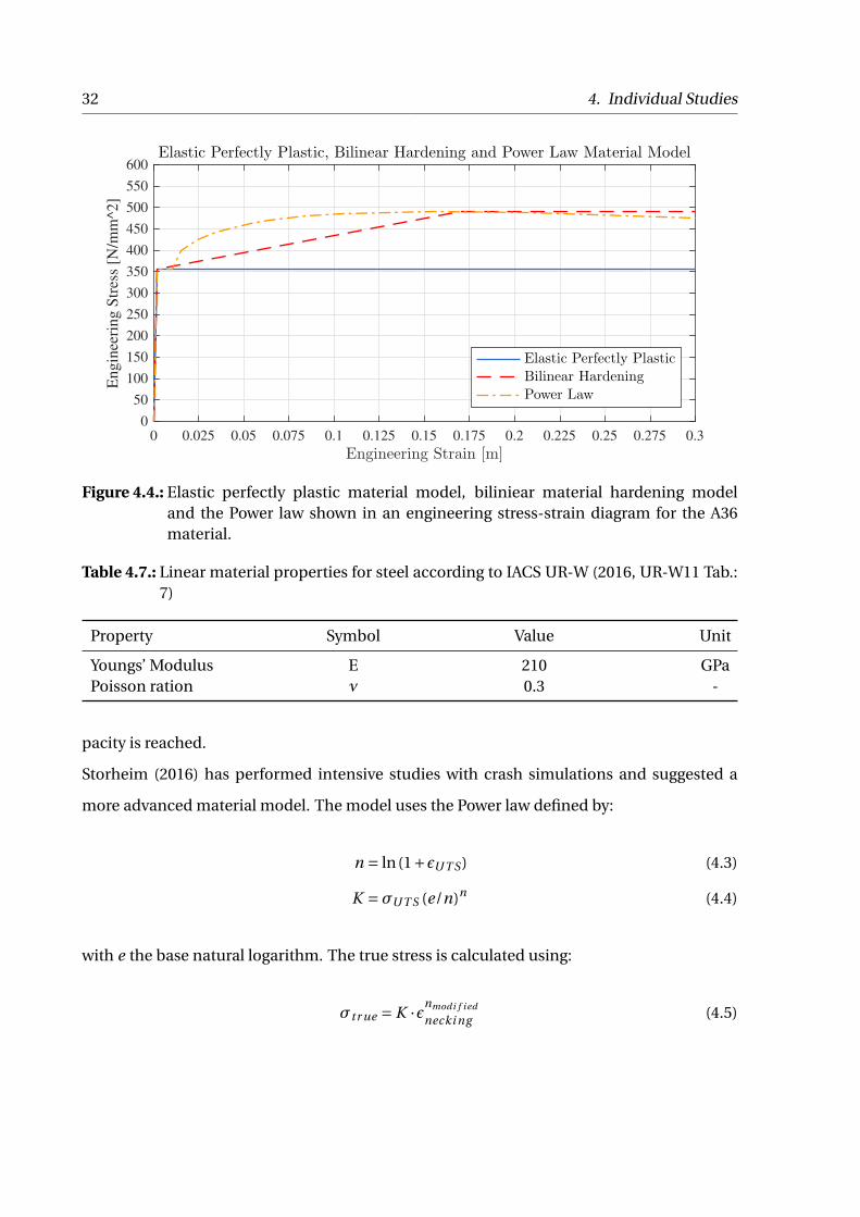
32 4. Individual Studies
0 0.025 0.05 0.075 0.1 0.125 0.15 0.175 0.2 0.225 0.25 0.275 0.3
Engineering Strain [m]
0
50
100
150
200
250
300
350
400
450
500
550
600
En
gin
eeri
ng
Str
ess
[N/m
m^2
]
Elastic Perfectly Plastic, Bilinear Hardening and Power Law Material Model
Elastic Perfectly PlasticBilinear HardeningPower Law
Figure 4.4.: Elastic perfectly plastic material model, biliniear material hardening modeland the Power law shown in an engineering stress-strain diagram for the A36material.
Table 4.7.: Linear material properties for steel according to IACS UR-W (2016, UR-W11 Tab.:7)
Property Symbol Value Unit
Youngs’ Modulus E 210 GPaPoisson ration ∫ 0.3 -
pacity is reached.
Storheim (2016) has performed intensive studies with crash simulations and suggested a
more advanced material model. The model uses the Power law defined by:
n = ln(1+≤U T S) (4.3)
K =æU T S (e/n)n (4.4)
with e the base natural logarithm. The true stress is calculated using:
ætr ue = K ·≤nmodi f i ed
necki ng (4.5)

4.3. Material Properties 33
Table 4.8.: Non-linear material properties according to IACS UR-W (2016, UR-W11 Tab.: 7)and calculated Power law parameters.
Grade Min æy æU T S ≤ f r actur e ≤necki ng ≤pl ateau nmodi f i ed K[MPa] [MPa] [%] [%] [%]
A32 315 440-570 22 18 -1 0.157 657.17 E6A36 355 490-630 21 17 -1 0.148 753.83 E6
Table 4.9.: Elongation ≤necki ng in dependence of the material grade and component thick-ness according to IACS UR-W (2016, UR-W11 Tab.: 7).
Thickness Grade >5 >10 >15 >20 >25 >30 >40mm ∑ 5 ∑ 10 ∑ 15 ∑ 20 ∑ 25 ∑ 30 ∑ 40 ∑ 50
Elongation ≤necki ng A32 14 16 17 18 19 20 21 22% A36 13 15 16 17 18 19 20 21
The model has been validated with material tests and gave good results. Additionally he sug-
gests to include a plateau of 1 % to increase the accuracy.
For all of these models, the yield stress and for the latter models the tensile stress and the
necking strain are required as inputs. In reality these values vary greatly between different
steel manufactures and batches. Thus a decision has to be made to define the required val-
ues. Storheim (2016) has estimated the distributions for these values based on data from
VanDerHorn and Wang (2011). The statistical properties are given in Table 4.10 and shown
in Figure 4.5. The yield stress can be distributed by using a log normal distribution:
f°x,µ,æ
¢= 1
xæp
2ºe°
°ln(x)°µ
¢2
2æ2 (4.6)
with the mean defined as m and the standard deviation as v given the two statistical para-
meters:
µ=
0
B@m
q1+ v
m2
1
CA (4.7)
æ=r
ln≥1+ v
m2
¥. (4.8)
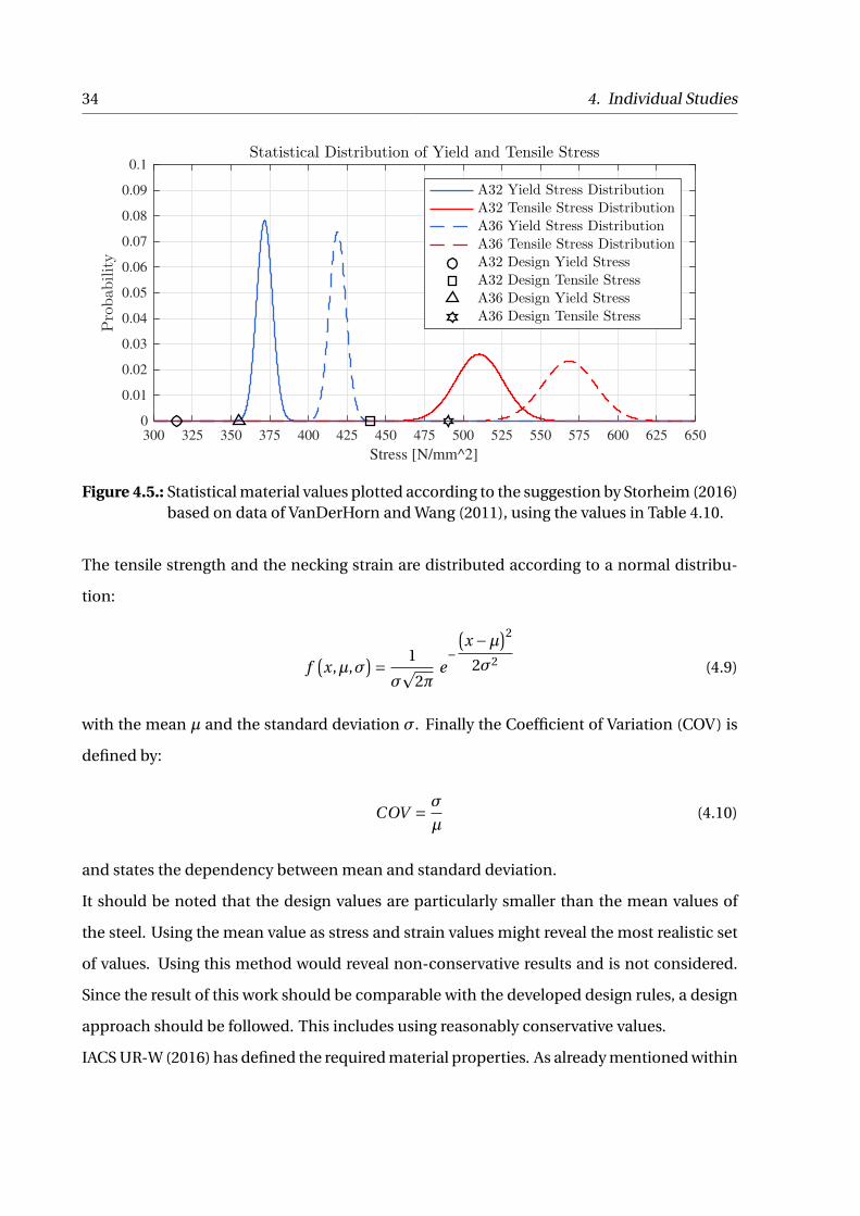
34 4. Individual Studies
300 325 350 375 400 425 450 475 500 525 550 575 600 625 650
Stress [N/mm^2]
0
0.01
0.02
0.03
0.04
0.05
0.06
0.07
0.08
0.09
0.1
Probability
Statistical Distribution of Yield and Tensile Stress
A32 Yield Stress Distribution
A32 Tensile Stress Distribution
A36 Yield Stress Distribution
A36 Tensile Stress Distribution
A32 Design Yield Stress
A32 Design Tensile Stress
A36 Design Yield Stress
A36 Design Tensile Stress
Figure 4.5.: Statistical material values plotted according to the suggestion by Storheim (2016)based on data of VanDerHorn and Wang (2011), using the values in Table 4.10.
The tensile strength and the necking strain are distributed according to a normal distribu-
tion:
f°x,µ,æ
¢= 1
æp
2ºe°
°x °µ
¢2
2æ2 (4.9)
with the mean µ and the standard deviation æ. Finally the Coefficient of Variation (COV) is
defined by:
COV = æ
µ(4.10)
and states the dependency between mean and standard deviation.
It should be noted that the design values are particularly smaller than the mean values of
the steel. Using the mean value as stress and strain values might reveal the most realistic set
of values. Using this method would reveal non-conservative results and is not considered.
Since the result of this work should be comparable with the developed design rules, a design
approach should be followed. This includes using reasonably conservative values.
IACS UR-W (2016) has defined the required material properties. As already mentioned within
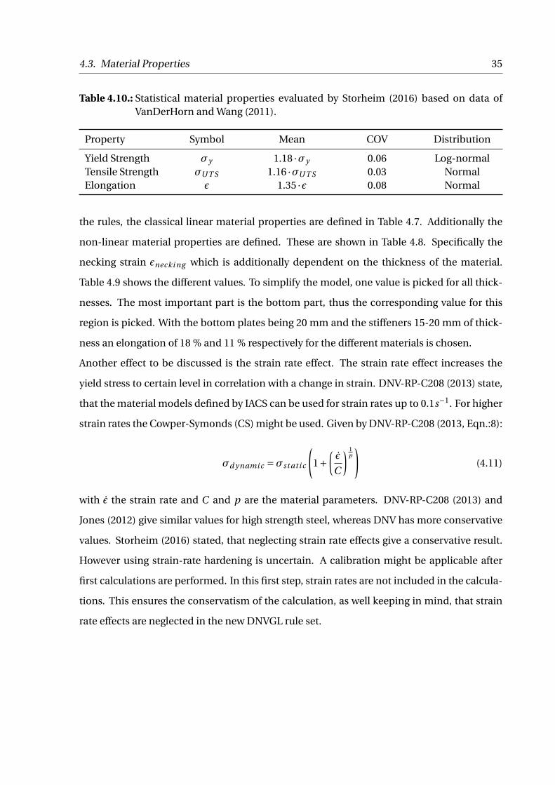
4.3. Material Properties 35
Table 4.10.: Statistical material properties evaluated by Storheim (2016) based on data ofVanDerHorn and Wang (2011).
Property Symbol Mean COV Distribution
Yield Strength æy 1.18 ·æy 0.06 Log-normalTensile Strength æU T S 1.16 ·æU T S 0.03 NormalElongation ≤ 1.35 ·≤ 0.08 Normal
the rules, the classical linear material properties are defined in Table 4.7. Additionally the
non-linear material properties are defined. These are shown in Table 4.8. Specifically the
necking strain ≤necki ng which is additionally dependent on the thickness of the material.
Table 4.9 shows the different values. To simplify the model, one value is picked for all thick-
nesses. The most important part is the bottom part, thus the corresponding value for this
region is picked. With the bottom plates being 20 mm and the stiffeners 15-20 mm of thick-
ness an elongation of 18 % and 11 % respectively for the different materials is chosen.
Another effect to be discussed is the strain rate effect. The strain rate effect increases the
yield stress to certain level in correlation with a change in strain. DNV-RP-C208 (2013) state,
that the material models defined by IACS can be used for strain rates up to 0.1s°1. For higher
strain rates the Cowper-Symonds (CS) might be used. Given by DNV-RP-C208 (2013, Eqn.:8):
æd ynami c =æst ati c
√
1+µ≤
C
∂ 1p!
(4.11)
with ≤ the strain rate and C and p are the material parameters. DNV-RP-C208 (2013) and
Jones (2012) give similar values for high strength steel, whereas DNV has more conservative
values. Storheim (2016) stated, that neglecting strain rate effects give a conservative result.
However using strain-rate hardening is uncertain. A calibration might be applicable after
first calculations are performed. In this first step, strain rates are not included in the calcula-
tions. This ensures the conservatism of the calculation, as well keeping in mind, that strain
rate effects are neglected in the new DNVGL rule set.

36 4. Individual Studies
4.4. Element Choice & Meshing
One of the most important decisions is the use of the element type and the corresponding
meshing of the model. The presented calculations in Chapter 2 are taken as reference. The
methods of Amlashi (2008), Shu and Moan (2012), Xu et al. (2014), Marine Accident Invest-
igation Branch Annex A-D (2008), Marine Accident Investigation Branch Annex E-G (2008)
and Sumi et al. (2014) are compared in Table 4.11.
Additionally different regulations are consulted such as GL Guidelines (2011), DNV-RP-C208
(2013), DNVGL Rules Part 3 Chapter 7 (2016), DNVGL Rules Part 3 Chapter 8 (2016), DNVGL-
CG-0128 (2015) and DNVGL-CG-0153 (2015).
In most cases the FEM program ABAQUS is used. For the time domain calculation of the
MOL Comfort and the crash simulations performed by Storheim (2016) the explicit solver
LS-DYNA have been used. In ABAQUS have either the element S4 or S4R have been used.
The S4 element is a "4-node general-purpose shell, finite membrane strains" whereas the
S4R is a "4-node general-purpose shell, reduced integration with hourglass control, finite
membrane strains" (Abaqus User Manual IV, 2012, P.:29.6.7–1). Storheim (2016) used LS-
DYNA with Belytschko-Lin-Tsay shell elements. The element is a 4-node shell using one
integration point and is the recommend element for most applications (ANSYS LS-DYNA,
2009, P.:8-12). No information is given about the elements used in the MOL Comfort report.
These elements all have four nodes. In this thesis the corresponding element is the SHELL181
element. ANSYS uses different element description than ABAQUS and LS-DYNA, thus no dir-
ect comparison can be made. For ABAQUS elements the difference is the reduced integra-
tion with hourglass control in the elements. ANSYS Element Reference (2009) recommends
for shell structures, to use the "Reduced integration with hourglass control" option for the
structure. Anyhow for stiffener webs the "Full integration with incompatible modes" is en-
dorsed. The recommendation will be followed in thesis and the element with the respectively
recommended key option is used. The number of integration points for elements experien-
cing plastic strains is automatically increased from 3 to 5.
An alternative approach, not discussed in this thesis is the use of Idealized structural unit
method (ISUM) elements by Fujikubo and Kaeding (2002). The elements are especially de-

4.4. Element Choice & Meshing 37
Tab
le4.
11.:
Com
par
ison
ofth
ew
ork
per
form
edby
Am
lash
i(20
08),
Shu
and
Moa
n(2
012)
,Xu
etal
.(20
14),
Mar
ine
Acc
iden
tIn
vest
iga-
tion
Bra
nch
An
nex
A-D
(200
8),M
arin
eA
ccid
entI
nve
stig
atio
nB
ran
chA
nn
exE
-G(2
008)
and
Sum
ieta
l.(2
014)
wit
hre
spec
tto
met
hod
s,el
emen
tsm
esh
,mat
eria
lmod
els
and
load
s.(*
cou
nte
dfr
omfi
gure
,-n
otkn
own
,3ap
plie
d,7
not
app
lied)
Prop
erty
Am
lash
iSh
uXu
etal
.M
SCN
apol
iM
SCN
apol
iM
OL
Com
fort
Inst
itu
tion
NT
NU
NT
NU
NT
NU
DN
VB
VC
lass
NK
Pro
gram
Prog
ram
AB
AQ
US
AB
AQ
US
AB
AQ
US
AB
AQ
US
AB
AQ
US
MA
RC
/LS-
DYN
ASo
lver
met
hod
Rik
sIm
plic
itR
iks
-R
iks
Imp
licit
/Exp
licit
Mes
hin
g"c
rash
"ar
eaE
lem
ent
S4S4
S4R
S4-
-G
loba
lSiz
e[m
]0.
10.
10.
10.
15-
0.1
Bet
wee
nLo
ngi
tudi
nal
Stif
fen
ers
[n]
55
95-
66*
9*
Bet
wee
nTr
ansv
erse
Web
s[n
]15
1526
6*8*
6*Lo
ngi
tudi
nal
Stif
fen
erw
eb[n
]5
54
3*2*
5*Lo
ngi
tudi
nal
stif
fen
erfl
ange
[n]
22
21*
1*2*
Hei
ghto
fgir
der
[n]
2121
2819
*12
*26
*M
ater
ial
Mat
eria
lMod
elB
ilin
ear
Bili
nea
rE
PPB
ilin
ear
Ram
sber
g-O
sgoo
dE
PP+
Har
den
ing
Yiel
dSt
ress
Des
ign
Des
ign
Des
ign
3Se
tsD
esig
nAv
erag
eSi
zeEx
ten
dof
Mod
el1/
2+1+
1/2
1+1+
11
Web
Glo
bal
Loca
l1/
2+1+
1/2
Nu
mbe
rof
DoF
non
linea
r[n
]-
-54
1,00
1.06
·106
--
Nu
mbe
rof
DoF
linea
r[n
]-
-54
1,00
01.
22·1
0633
0,49
8-
Lo
ads
Gra
vita
tion
33
33
33
Stat
icPr
essu
re3
33
33
3D
ynam
icPr
essu
re3
3-
DN
VB
VC
lass
NK
Ben
din
gM
omen
tIn
crea
sed
Incr
ease
dSt
rip
Th
eory
WA
SIM
BV
Incr
easi
ng
Res
idu
alSt
ress
es-
73
77
Fact
orW
hip
pin
gLo
ads
77
77
BV
Mod
elFa
ctor
38 4. Individual Studies
veloped to represent the occurring buckling modes and to simulate the buckling and collapse
behaviour of plate panels. The advantage of these elements is the reduced calculation time
compared with regular finite elements.
Another important factor of the finite element model is the mesh size. The mesh size in this
work has been orientated on the MOL Comfort investigation. For the crash section a fine
mesh with a size 100 mm x 100 mm is used. The surrounding area is meshed using an ele-
ment size of 200 m x 200 mm. Above the neutral axis a global element size approach is used,
which will be explained later. The fine mesh size is based on several previous calculations.
Only the DNV MSC Napoli investigation uses a different approach of a mesh size of 150 mm x
150 mm. Also super elements are used and the transitions zone has been defined differently.
In crash simulations Storheim (2016) has used an element size of 100 mm x 100 mm. The
choice of 100 mm x 100 mm seems reasonable. A mesh convergence study is performed later
on and will prove this assumption.
The area above the neutral axis is meshed using a global mesh approach. The rules therefore
are given by Johansen and Bratbak (2015) with:
• 2 x 2 meter mesh
• Usually 8-node Shell elements and 3-node beams
• as quadratic elements as possible, maximal ration 5:1
• lumped stiffeners should follow the actual stiffener direction as close as possible
• primary girders modelled with shell elements should have 2 or more elements over the
height
Additionally in the global mesh area stiffeners are not defined as shell elements but as beam
elements. The element BEAM188 is chosen. The 2-node element corresponds with the defin-
ition of the shell elements.
Using several different mesh size will create the struggle of connecting the elements. The
approach used in this thesis is to use triangular elements. A typical mesh transition using
triangular elements can be seen in Figure 4.6. The advantage with this method is, that the
mesh size is doubled with each row of triangular elements.
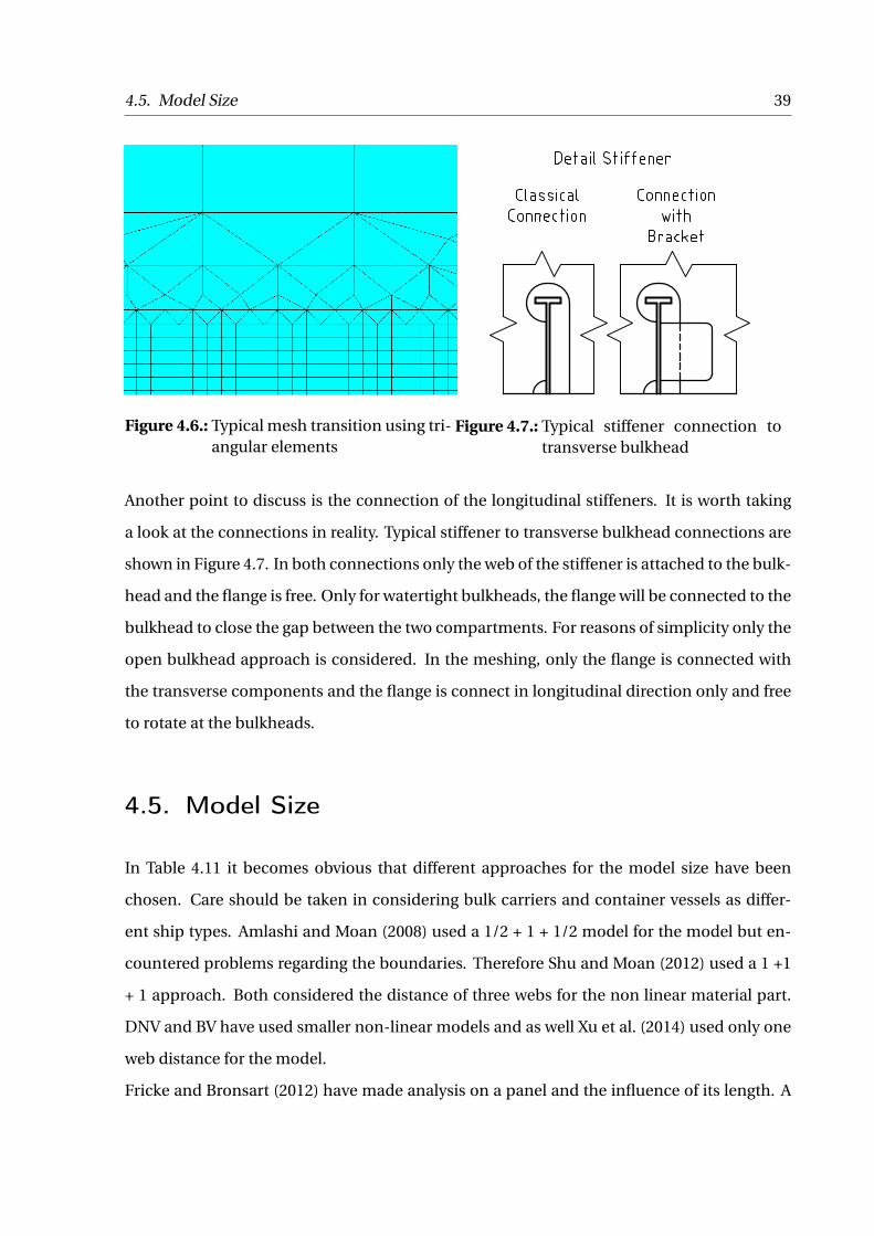
4.5. Model Size 39
Figure 4.6.: Typical mesh transition using tri-angular elements
Figure 4.7.: Typical stiffener connection totransverse bulkhead
Another point to discuss is the connection of the longitudinal stiffeners. It is worth taking
a look at the connections in reality. Typical stiffener to transverse bulkhead connections are
shown in Figure 4.7. In both connections only the web of the stiffener is attached to the bulk-
head and the flange is free. Only for watertight bulkheads, the flange will be connected to the
bulkhead to close the gap between the two compartments. For reasons of simplicity only the
open bulkhead approach is considered. In the meshing, only the flange is connected with
the transverse components and the flange is connect in longitudinal direction only and free
to rotate at the bulkheads.
4.5. Model Size
In Table 4.11 it becomes obvious that different approaches for the model size have been
chosen. Care should be taken in considering bulk carriers and container vessels as differ-
ent ship types. Amlashi and Moan (2008) used a 1/2 + 1 + 1/2 model for the model but en-
countered problems regarding the boundaries. Therefore Shu and Moan (2012) used a 1 +1
+ 1 approach. Both considered the distance of three webs for the non linear material part.
DNV and BV have used smaller non-linear models and as well Xu et al. (2014) used only one
web distance for the model.
Fricke and Bronsart (2012) have made analysis on a panel and the influence of its length. A
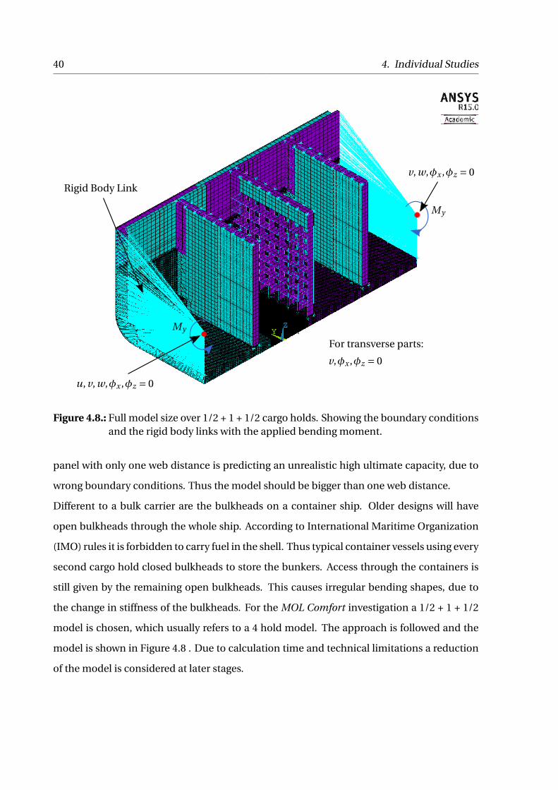
40 4. Individual Studies
v, w,¡x ,¡z = 0
u, v, w,¡x ,¡z = 0
v,¡x ,¡z = 0
My
My
Rigid Body Link
For transverse parts:
Figure 4.8.: Full model size over 1/2 + 1 + 1/2 cargo holds. Showing the boundary conditionsand the rigid body links with the applied bending moment.
panel with only one web distance is predicting an unrealistic high ultimate capacity, due to
wrong boundary conditions. Thus the model should be bigger than one web distance.
Different to a bulk carrier are the bulkheads on a container ship. Older designs will have
open bulkheads through the whole ship. According to International Maritime Organization
(IMO) rules it is forbidden to carry fuel in the shell. Thus typical container vessels using every
second cargo hold closed bulkheads to store the bunkers. Access through the containers is
still given by the remaining open bulkheads. This causes irregular bending shapes, due to
the change in stiffness of the bulkheads. For the MOL Comfort investigation a 1/2 + 1 + 1/2
model is chosen, which usually refers to a 4 hold model. The approach is followed and the
model is shown in Figure 4.8 . Due to calculation time and technical limitations a reduction
of the model is considered at later stages.
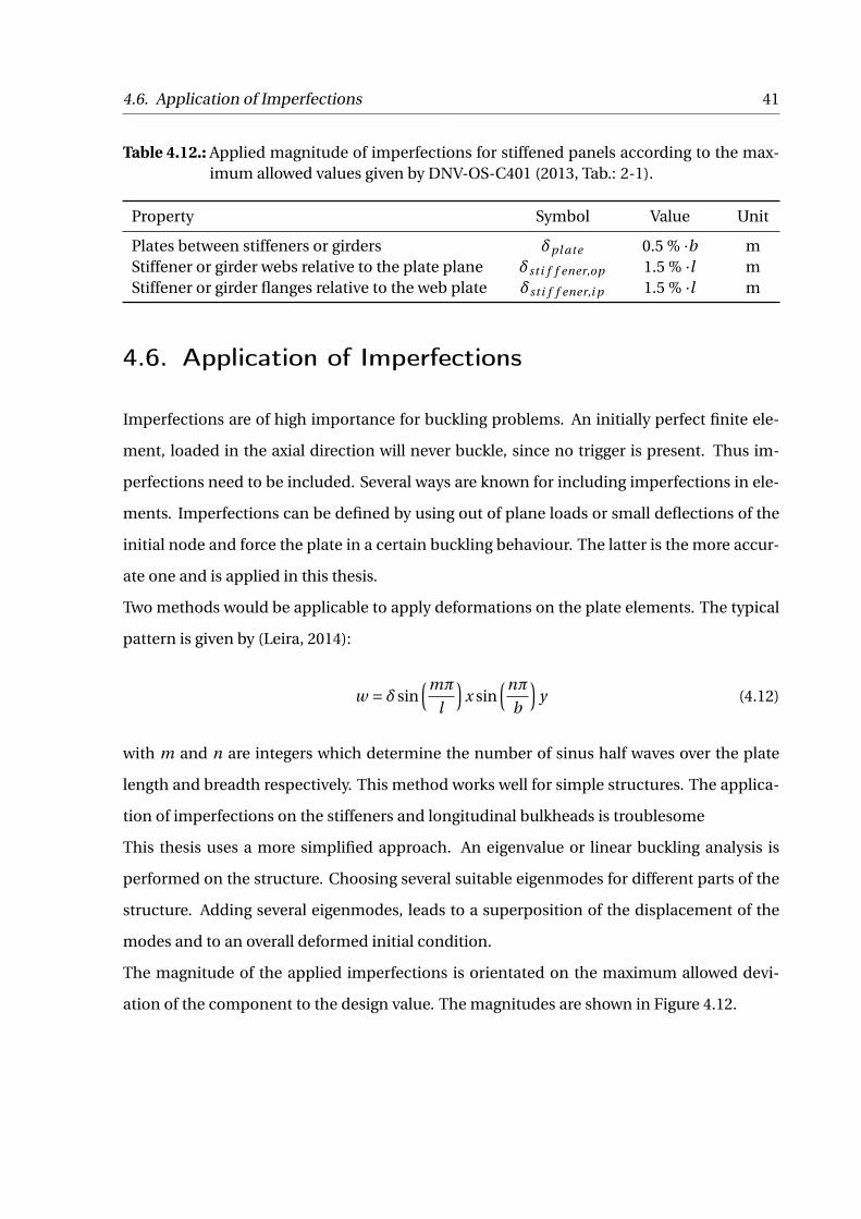
4.6. Application of Imperfections 41
Table 4.12.: Applied magnitude of imperfections for stiffened panels according to the max-imum allowed values given by DNV-OS-C401 (2013, Tab.: 2-1).
Property Symbol Value Unit
Plates between stiffeners or girders ±pl ate 0.5 % ·b mStiffener or girder webs relative to the plate plane ±st i f f ener,op 1.5 % ·l mStiffener or girder flanges relative to the web plate ±st i f f ener,i p 1.5 % ·l m
4.6. Application of Imperfections
Imperfections are of high importance for buckling problems. An initially perfect finite ele-
ment, loaded in the axial direction will never buckle, since no trigger is present. Thus im-
perfections need to be included. Several ways are known for including imperfections in ele-
ments. Imperfections can be defined by using out of plane loads or small deflections of the
initial node and force the plate in a certain buckling behaviour. The latter is the more accur-
ate one and is applied in this thesis.
Two methods would be applicable to apply deformations on the plate elements. The typical
pattern is given by (Leira, 2014):
w = ±sin≥mº
l
¥x sin
≥nºb
¥y (4.12)
with m and n are integers which determine the number of sinus half waves over the plate
length and breadth respectively. This method works well for simple structures. The applica-
tion of imperfections on the stiffeners and longitudinal bulkheads is troublesome
This thesis uses a more simplified approach. An eigenvalue or linear buckling analysis is
performed on the structure. Choosing several suitable eigenmodes for different parts of the
structure. Adding several eigenmodes, leads to a superposition of the displacement of the
modes and to an overall deformed initial condition.
The magnitude of the applied imperfections is orientated on the maximum allowed devi-
ation of the component to the design value. The magnitudes are shown in Figure 4.12.
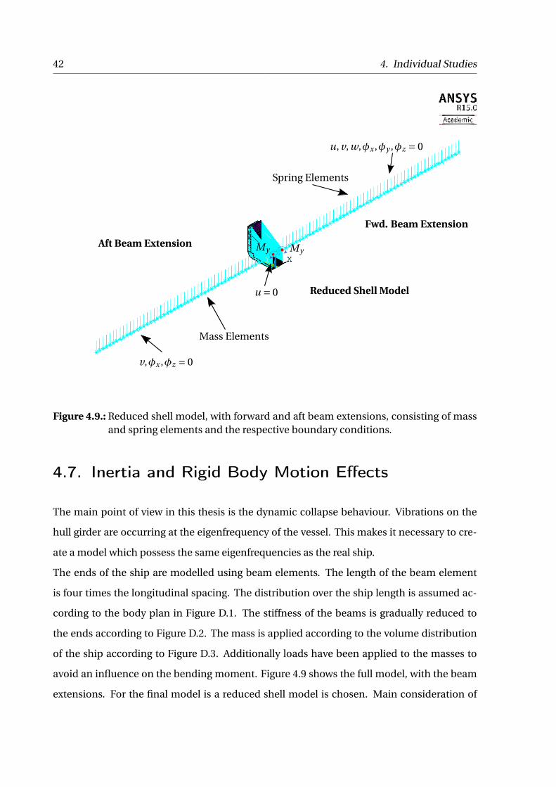
42 4. Individual Studies
Reduced Shell Model
Aft Beam Extension
Fwd. Beam Extension
Mass Elements
Spring Elements
u, v, w,¡x ,¡y ,¡z = 0
v,¡x ,¡z = 0
u = 0
MyMy
Figure 4.9.: Reduced shell model, with forward and aft beam extensions, consisting of massand spring elements and the respective boundary conditions.
4.7. Inertia and Rigid Body Motion Effects
The main point of view in this thesis is the dynamic collapse behaviour. Vibrations on the
hull girder are occurring at the eigenfrequency of the vessel. This makes it necessary to cre-
ate a model which possess the same eigenfrequencies as the real ship.
The ends of the ship are modelled using beam elements. The length of the beam element
is four times the longitudinal spacing. The distribution over the ship length is assumed ac-
cording to the body plan in Figure D.1. The stiffness of the beams is gradually reduced to
the ends according to Figure D.2. The mass is applied according to the volume distribution
of the ship according to Figure D.3. Additionally loads have been applied to the masses to
avoid an influence on the bending moment. Figure 4.9 shows the full model, with the beam
extensions. For the final model is a reduced shell model is chosen. Main consideration of
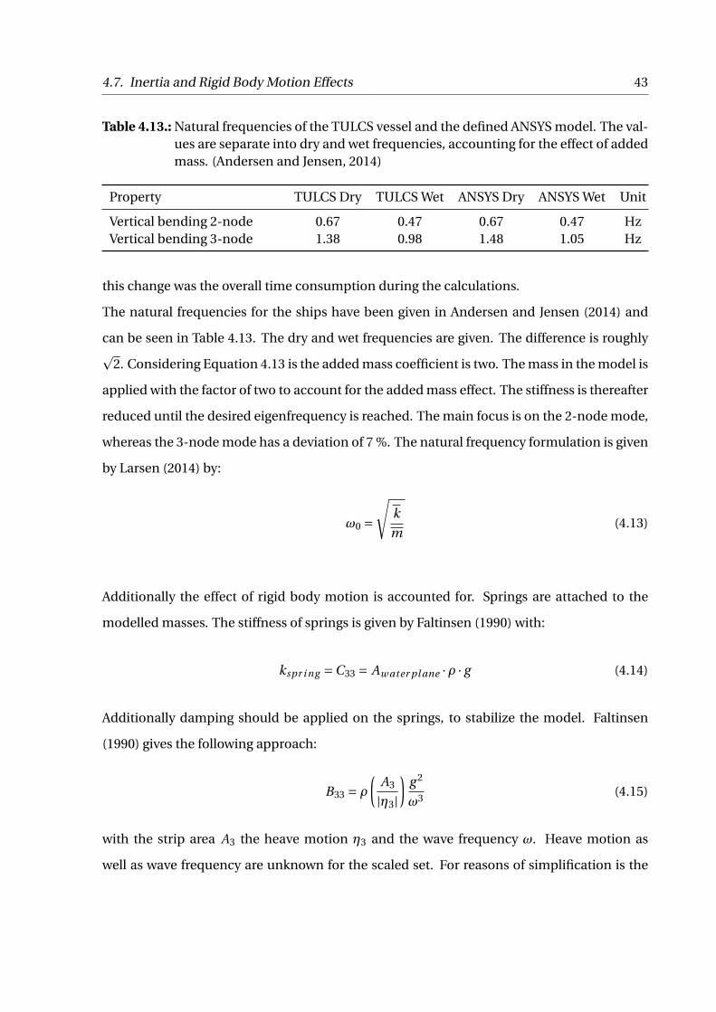
4.7. Inertia and Rigid Body Motion Effects 43
Table 4.13.: Natural frequencies of the TULCS vessel and the defined ANSYS model. The val-ues are separate into dry and wet frequencies, accounting for the effect of addedmass. (Andersen and Jensen, 2014)
Property TULCS Dry TULCS Wet ANSYS Dry ANSYS Wet Unit
Vertical bending 2-node 0.67 0.47 0.67 0.47 HzVertical bending 3-node 1.38 0.98 1.48 1.05 Hz
this change was the overall time consumption during the calculations.
The natural frequencies for the ships have been given in Andersen and Jensen (2014) and
can be seen in Table 4.13. The dry and wet frequencies are given. The difference is roughlyp
2. Considering Equation 4.13 is the added mass coefficient is two. The mass in the model is
applied with the factor of two to account for the added mass effect. The stiffness is thereafter
reduced until the desired eigenfrequency is reached. The main focus is on the 2-node mode,
whereas the 3-node mode has a deviation of 7 %. The natural frequency formulation is given
by Larsen (2014) by:
!0 =
skm
(4.13)
Additionally the effect of rigid body motion is accounted for. Springs are attached to the
modelled masses. The stiffness of springs is given by Faltinsen (1990) with:
kspr i ng =C33 = Aw ater pl ane ·Ω · g (4.14)
Additionally damping should be applied on the springs, to stabilize the model. Faltinsen
(1990) gives the following approach:
B33 = Ω
µA3
|¥3|
∂g 2
!3 (4.15)
with the strip area A3 the heave motion ¥3 and the wave frequency !. Heave motion as
well as wave frequency are unknown for the scaled set. For reasons of simplification is the

44 4. Individual Studies
following approach is chosen:
cv = ª ·2 ·p
(M + A)K (4.16)
with the damping coefficient cv , the damping ratio of critical damping ª, mass of the strip M ,
added mass of the strip A and the stiffness K . The damping ratio is assumed to be in range of
2 % and mass, added mass and stiffness are already defined for the mass and spring system.

5. Theory
The following chapter provides an insight into the applied methods and formulas. The depth
of explanation differs according to the relevance of the topic. A short description of the FEM
is given and the applied solution methods. This chapter should give a rough overview, for a
deeper description, corresponding literature should be consulted.
In the following section ( ) denotes a matrix and ( ) denotes a vector. A simple derivative
with respect to time t is shown by (˙) and a double derivative of t is shown by ( ¨ ) respectively.
Derivations with respect to certain directions are written out.
5.1. Hull Girder Failure
Structural failure occurs in several different ways. The direction of the load is of importance.
The two considered cases on a ship are sagging and hogging. This means that the upper
and lower fibre experience either compression or tension. Loaded under latter, failure of
the plate will appear when the stress exceeds the yield level and the material starts yielding.
The limit state under compression might be reached earlier depending on the slenderness
of the structure. The stress deflection curve for a structure experiencing extreme loading in
compression is shown in Figure 5.1. The girder is loaded until failure. In the pre-buckling
region, the deflection is linear and follows the linear deformation of the material defined by
Young’s modulus. Exceeding the elastic buckling level brings the plate into the post buckling
range. Mechanisms acting are linear buckling of the plate. When buckling exceeds the elastic
range, yielding of the components occurs and the structure loses faster capacity until the
ultimate capacity is reached and the structure can no longer take the load.
45
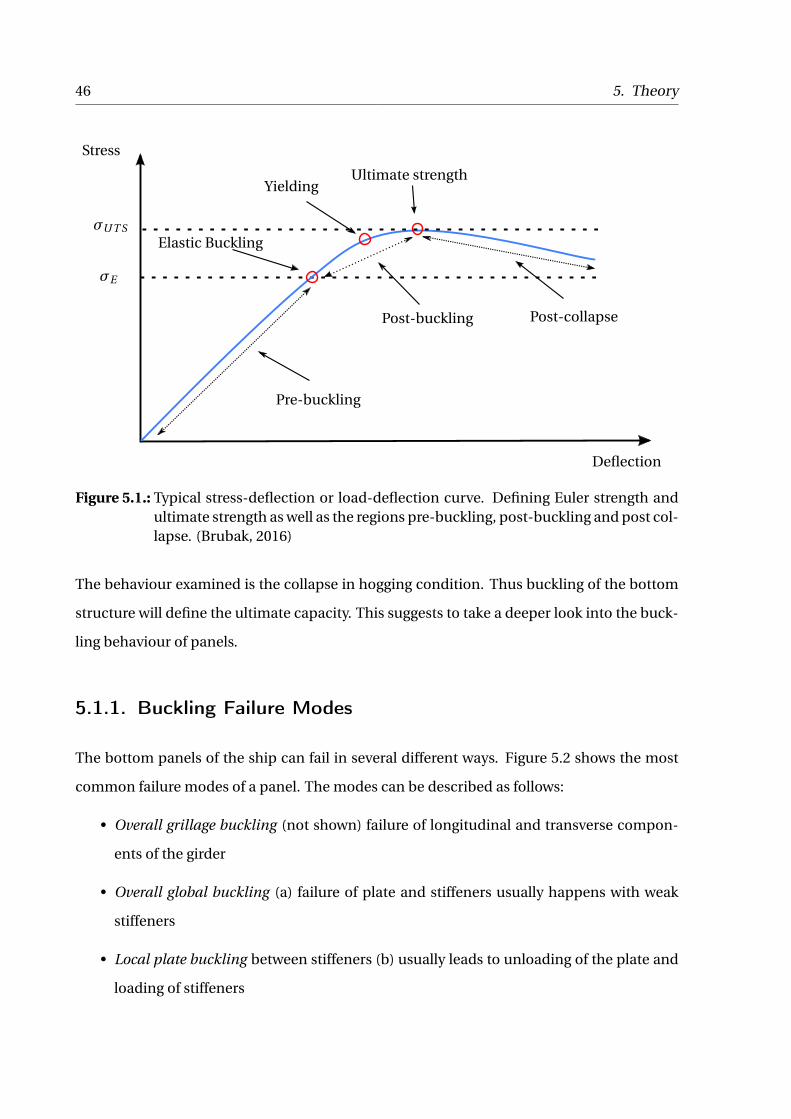
46 5. Theory
Elastic Buckling
YieldingUltimate strength
Pre-buckling
Post-buckling Post-collapse
Deflection
æE
æU T S
Stress
Figure 5.1.: Typical stress-deflection or load-deflection curve. Defining Euler strength andultimate strength as well as the regions pre-buckling, post-buckling and post col-lapse. (Brubak, 2016)
The behaviour examined is the collapse in hogging condition. Thus buckling of the bottom
structure will define the ultimate capacity. This suggests to take a deeper look into the buck-
ling behaviour of panels.
5.1.1. Buckling Failure Modes
The bottom panels of the ship can fail in several different ways. Figure 5.2 shows the most
common failure modes of a panel. The modes can be described as follows:
• Overall grillage buckling (not shown) failure of longitudinal and transverse compon-
ents of the girder
• Overall global buckling (a) failure of plate and stiffeners usually happens with weak
stiffeners
• Local plate buckling between stiffeners (b) usually leads to unloading of the plate and
loading of stiffeners
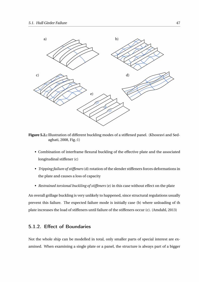
5.1. Hull Girder Failure 47
a) b)
c) d)
e)
Figure 5.2.: Illustration of different buckling modes of a stiffened panel. (Khosravi and Sed-aghati, 2008, Fig.:1)
• Combination of interframe flexural buckling of the effective plate and the associated
longitudinal stiffener (c)
• Tripping failure of stiffeners (d) rotation of the slender stiffeners forces deformations in
the plate and causes a loss of capacity
• Restrained torsional buckling of stiffeners (e) in this case without effect on the plate
An overall grillage buckling is very unlikely to happened, since structural regulations usually
prevent this failure. The expected failure mode is initially case (b) where unloading of th
plate increases the load of stiffeners until failure of the stiffeners occur (c). (Amdahl, 2013)
5.1.2. Effect of Boundaries
Not the whole ship can be modelled in total, only smaller parts of special interest are ex-
amined. When examining a single plate or a panel, the structure is always part of a bigger
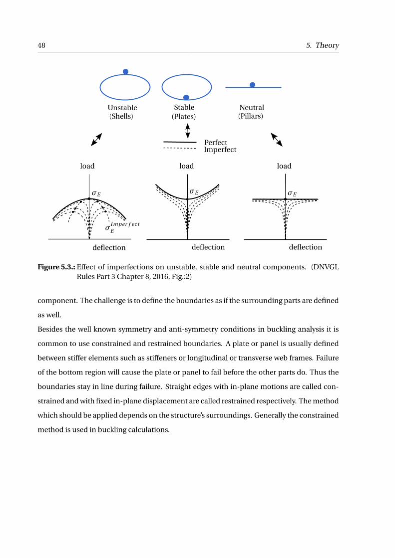
48 5. Theory
Unstable(Shells)
Stable(Plates)
Neutral(Pillars)
deflection deflection deflection
load load load
PerfectImperfect
æE æE æE
æImper f ectE
Figure 5.3.: Effect of imperfections on unstable, stable and neutral components. (DNVGLRules Part 3 Chapter 8, 2016, Fig.:2)
component. The challenge is to define the boundaries as if the surrounding parts are defined
as well.
Besides the well known symmetry and anti-symmetry conditions in buckling analysis it is
common to use constrained and restrained boundaries. A plate or panel is usually defined
between stiffer elements such as stiffeners or longitudinal or transverse web frames. Failure
of the bottom region will cause the plate or panel to fail before the other parts do. Thus the
boundaries stay in line during failure. Straight edges with in-plane motions are called con-
strained and with fixed in-plane displacement are called restrained respectively. The method
which should be applied depends on the structure’s surroundings. Generally the constrained
method is used in buckling calculations.
5.2. Verification Methods 49
5.1.3. Effect of Imperfections
Uncertainties arises from the topic of imperfections. When an initially perfect finite element
plate is exposed to axial pressure, the plate is compressed. For this plate, no buckling would
occur, since no trigger is given, forcing the plate to deflect in either of its normals. Imper-
fections can be introduced in several ways. Out of plane loads are an option to force the
structure to buckle, or small initial deflections in the assumed final buckling shape. In real-
ity a structure will never be perfect. Imperfections are introduced by microscopic material
defaults and assembly and/or welding deformations.
The effect of imperfections on different structure types is shown in Figure 5.3. Shell struc-
tures are unstable components once buckling occurs the structure collapses totally. The ini-
tial imperfections have a huge effect on the ultimate strength of the unit. Pillars are neutral
components. Once the buckling limit is reached the required load stays equal. Plate ele-
ments are stable structures. Once the buckling load is exceeded the plate has still capacity
preventing the total collapse.
5.2. Verification Methods
The used finite element analysis is a numerical method and thus simplifies the real pro-
cesses. Applying a simplified methodology also requires a way of verifying the received res-
ults. The used models are presented in following.
5.2.1. Analytical Solution
The buckling load for simple initially perfect plates can be estimated. The formula accounts
for the elastic buckling load of the plate and is given by Amdahl (2013, Eqn.:3.7):
æE = º2E
12°1°∫2
¢µ
tb
∂2
·k. (5.1)
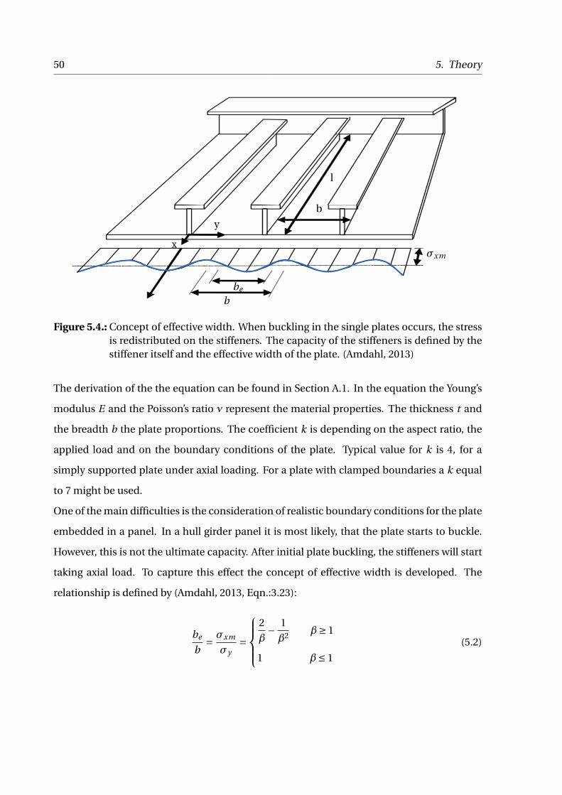
50 5. Theory
be
b
y
xæxm
l
b
Figure 5.4.: Concept of effective width. When buckling in the single plates occurs, the stressis redistributed on the stiffeners. The capacity of the stiffeners is defined by thestiffener itself and the effective width of the plate. (Amdahl, 2013)
The derivation of the the equation can be found in Section A.1. In the equation the Young’s
modulus E and the Poisson’s ratio ∫ represent the material properties. The thickness t and
the breadth b the plate proportions. The coefficient k is depending on the aspect ratio, the
applied load and on the boundary conditions of the plate. Typical value for k is 4, for a
simply supported plate under axial loading. For a plate with clamped boundaries a k equal
to 7 might be used.
One of the main difficulties is the consideration of realistic boundary conditions for the plate
embedded in a panel. In a hull girder panel it is most likely, that the plate starts to buckle.
However, this is not the ultimate capacity. After initial plate buckling, the stiffeners will start
taking axial load. To capture this effect the concept of effective width is developed. The
relationship is defined by (Amdahl, 2013, Eqn.:3.23):
be
b= æxm
æy=
8>><
>>:
2Ø° 1Ø2 Ø∏ 1
1 Ø∑ 1
(5.2)
5.2. Verification Methods 51
Where be is the effective width and æxm is the corresponding stress. The equation is only
dependent on the plate slenderness parameter Ø, defined by (Amdahl, 2013, Eqn.: 3.24):
Ø= bt
ræy
E(5.3)
The plate slenderness parameter is dependent on the geometrical dimensions and the ma-
terial properties. The process is shown in Figure 5.4. When unloading of the plates occur, the
stress is redistributed to the stiffeners and the overall critical buckling load is increased. Des-
pite the two mentioned techniques a few other methods which will be shortly introduced.
The Johnson-Ostenfeld formula has been developed to account for the effect of plasticity of
slender plates. The slenderness ratio is defined by (Amdahl, 2013, Eqn.:3.14):
∏=sæy
æE(5.4)
The corresponding buckling stress is defined by (Amdahl, 2013, Eqn.:3.14):
æcr =¡ ·æy (5.5)
with ¡, the Johnson-Ostenfeld parameter, defined by(Amdahl, 2013, Eqn.:3.17):
¡=
8>><
>>:
1° ∏2
4∏2 ∑ 2
1
∏2∏2 ∏ 2
(5.6)
The Johnson-Ostenfeld parameter depends only on the slenderness ratio. Another approach
has been developed by DNV. A difference is made in here if buckling of the structure impairs
the functionality . The Serviceability limit state (SLS) is defined to avoid all kinds of deforma-
tion, whereas the Ulitmate limit state (ULS) allows for smaller deformations of the structure.
Since deformations in the bottom area of a container vessel do not effect the functionality
the ULS equation given by (Amdahl, 2013, Eqn.:3.22):
æul t =æy
∏p
2, 1.0 < ∏∑ 5.0 (5.7)
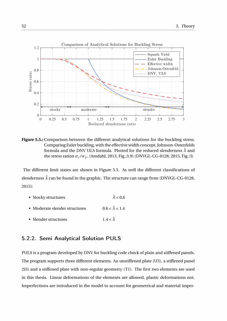
52 5. Theory
0 0.25 0.5 0.75 1 1.25 1.5 1.75 2 2.25 2.5 2.75 3
Reduced slenderness ratio
0
0.2
0.4
0.6
0.8
1
1.2
Stressratio
Comparison of Analytical Solutions for Buckling Stress
stocky moderate slender
Squash Yield
Euler Buckling
Effective width
Johnson-Ostenfeld
DNV, ULS
Figure 5.5.: Comparison between the different analytical solutions for the buckling stress.Comparing Euler buckling, with the effective width concept, Johnson-Ostenfeldsformula and the DNV ULS formula. Plotted for the reduced slenderness ∏ andthe stress ration æc /æy . (Amdahl, 2013, Fig.:3.9) (DNVGL-CG-0128, 2015, Fig.:3)
The different limit states are shown in Figure 5.5. As well the different classifications of
slenderness ∏ can be found in the graphic. The structure can range from (DNVGL-CG-0128,
2015):
• Stocky structures ∏ < 0.6
• Moderate slender structures 0.6 < ∏ < 1.4
• Slender structures 1.4 < ∏
5.2.2. Semi Analytical Solution PULS
PULS is a program developed by DNV for buckling code check of plain and stiffened panels.
The program supports three different elements. An unstiffened plate (U3), a stiffened panel
(S3) and a stiffened plate with non-regular geometry (T1). The first two elements are used
in this thesis. Linear deformations of the elements are allowed, plastic deformations not.
Imperfections are introduced in the model to account for geometrical and material imper-
5.2. Verification Methods 53
fections. (DNV PULS, 2006). PULS follows four design principles:
• Estimation of extreme Loads
• Acceptation of buckling deflection
• Do not accepts permanent buckles in plates
• Ensureing strong stiffeners
The considered elements are using von Karmen and Marguerre’s non-linear plate theory.
The equilibrium is established by use of the energy method, the principle of virtual work and
stationary potential energy. The discretization of the deflections is done by the Rayleigh-Ritz
method. Finally the equation is solved by using an incremental perturbation procedure with
arc-length control. (Brubak, 2016)
5.2.3. Ultimate Capacity POSEIDON
The design tool POSEIDON includes a method to calculate the ultimate capacity of the mid-
ship section. The approach follows the GL guidelines for the ultimate vertical bending mo-
ment given in GL Rules (2015, R.I,P1,C.5,S.5,E.5) by:
ØØØØMSW + ∞W V MW V
cS
ØØØØ∑ØØØØ
MU
∞R
ØØØØ (5.8)
with the partial safety factors defined as:
∞W V = 1.2 ; ∞R = 1.2 (5.9)
and the distribution factor cS = 1 for the midship section. Calculation of the ultimate state is
shown in POSEIDON User Manual (2016) and given by:
U S =
ØØØØMSW + ∞W V MW V
cS
ØØØØØØØØ
MU
∞R
ØØØØ
∑ 1. (5.10)

54 5. Theory
In the incremental method used is the curvature step by step increased until the post collapse
region. The calculation works for the hogging and sagging condition.
5.3. Finite Element Method Theory
The FEM is used for the the analyses. The model is divided into several elements, i.e. the
finite elements. The main equation solving a system is given by (Cook, 1995, Eqn.:1.6-6):
K r = R (5.11)
With the stiffness matrix K , displacement vector r and nodal load vector R. This holds true
for calculations with small displacements and linear elastic materials. Since the dynamic
collapse behaviour should be estimated, non-linearities and transient effects need to be ac-
counted for.
5.3.1. Non-linearity
To be able to evaluate the collapse behaviour non linear effects need to be considered. Three
non-linearities are known:
• Non linear material properties
• Non linear geometries
• Contact problems
The latter is not used in this thesis, the other two are included. The used material properties
have been described earlier. Non linear geometries are occurring when large deformations
are present. The deformations causing a change in stiffness of the structure. Thus Equation
5.11 need to be changed into (Moan, 2003a, Eqn.:12.6):
K°
r¢
r = R (5.12)
5.3. Finite Element Method Theory 55
where K°
r¢
is called the secant stiffness. The secant stiffness is a combination of the linear
stiffness matrix K0 and the geometric stiffness KG written as:
≥K0 +KG
°r
¢ ¥r = R. (5.13)
The stiffness matrix is now dependent on the displacement of the different elements. Thus
an update for every single substep is necessary.
5.3.2. Transient Effects
Two additional effects are important to capture the dynamic behaviour of a structure. Inertia
and damping need to be included in the calculation to build a realistic model. The derivation
of the dynamic equation of motion can be found in section A.2, revealing the full equation of
motion by:
M r (t )+C r (t )+K r (t ) = R (t ) (5.14)
with the mass matrix M and the damping matrix C added through the already introduced
equation. Applying stress stiffening effects yields the following equation:
M r (t )+C r (t )+K°r (t )
¢r (t ) = R (t ) (5.15)
5.3.3. Mass Matrix
In the calculations a consistent mass matrix is chosen. The mass matrix for the whole struc-
ture is given by (Langen and Sigbjörnsson, 1979, Eqn.:5.3):
M =X
iai
| mi ai (5.16)

56 5. Theory
Damping ratio
0.4
0.3
0.2
0.1
00 1.0 2.0 3.0 4.0 6.05.0 !
∏
∏i = 1/2µÆi
!i+Æ2!i
∂
Asymptote: ∏i = 1/2Æ2!i
Asymptote: !i = 0
∏2
∏1
!2!1
Figure 5.6.: Full Newton-Raphson iteration scheme, which is recommended for non-lineartransient finite element calculations. (Moan, 2003a, Fig.:12.27)
with the connectivity matrix ai and the consistent mass matrix for each element is defined
by (Langen and Sigbjörnsson, 1979, Eqn.:5.1):
m =Z
VΩN|N dV (5.17)
with the material density Ω and the vector of shape functions N , which will be defined later.
5.3.4. Damping Matrix
Damping can be defined in several different ways. The approach in this thesis is to use Pro-
portional or Rayleigh damping. The damping therein is dependent on the mass and stiffness
matrix given by Langen and Sigbjörnsson (1979, Eqn.:9.46):
C =Æ1M +Æ2K (5.18)
with the two damping coefficientsÆ1 andÆ2. The dependency can be seen in Figure 5.6. The
graph follows the two asymptotes, along the y-axis and along the x-axis. The damping ratio
5.3. Finite Element Method Theory 57
is further defined as (Langen and Sigbjörnsson, 1979, Eqn.:9.47):
ªi =12
µÆ1
!i+Æ2!i
∂(5.19)
with the damping ratio ªi and the eigenfrequencies !i . The coefficients Æ1 and Æ2 can be
calculated by using two eigenfrequencies and the corresponding critical damping given by
Langen and Sigbjörnsson (1979, Eqn. (9.48)):
Æ1 =2!1!2
!22 °!2
1
(∏1!2 °∏2!1) (5.20)
Æ2 =2(!2∏2 °!1∏1)
!22 °!2
1
(5.21)
However in most practical structural problems the mass damping coefficient Æ1 is ignored
and the structural damping defined by (ANSYS Structural Analysis Guide, 2009):
Æ2 = 2ªi
!i(5.22)
This is shown in the figure as the x-axis asymptote.
5.3.5. Stiffness Matrix
The stiffness matrix is defined similar to the mass matrix given by (Langen and Sigbjörnsson,
1979, Eqn.:2.5):
K =X
iai
| ki ai (5.23)
with ai the already introduced connectivity matrix and the individual local stiffness matrix
ki in global coordinates. The local stiffness matrix is transformed into global coordinates by
(Langen and Sigbjörnsson, 1979, Eqn.:2.3b):
k = T | k T . (5.24)
58 5. Theory
The transformation matrix T changes the local stiffness matrix k from local to global co-
ordinates. The local stiffness matrix is defined by (Moan, 2003a, Eqn.:3.34):
k =Z
VD| B DdV (5.25)
with the stiffness D and the strain-displacement matrix B . The generation is shown for the
common used 4-node shell elements. ANSYS uses for all plates Mindlin-Reissner theory or
thick plate theory. The strain-displacement relation is based on the linear material proper-
ties and given by (Moan, 2003a, Eqn.:7.30):
D = E1°∫2
2
66666666664
1 ∫ 0 0 0
∫ 1 0 0 0
0 0 12 (1°∫) 0 0
0 0 0 12k (1°∫) 0
0 0 0 0 12k (1°∫)
3
77777777775
(5.26)
The stiffness is defined by (Moan, 2003a, Eqn.:7.32):
B =
2
666666666666664
0 °z@N
@x0
0 0 °z@N
@y
0 °z@N
@y°z
@N
@x@N
@xN 0
@N
@y0 °N
3
777777777777775
(5.27)
with the shape functions N . For the used SHELL181 element the shape function is given by
(ANSYS Element Reference, 2009):
N =∑
14
≥1° x
a
¥≥1° y
b
¥,
14
≥1+ x
a
¥≥1° y
b
¥,
14
≥1+ x
a
¥≥1+ y
b
¥,
14
≥1° x
a
¥≥1+ y
b
¥∏(5.28)
with a the half width and b the half plate length and the coordinates x and y on the plate.
The coordinate system with the nodes and degrees of freedom can be seen in Figure 5.7. The
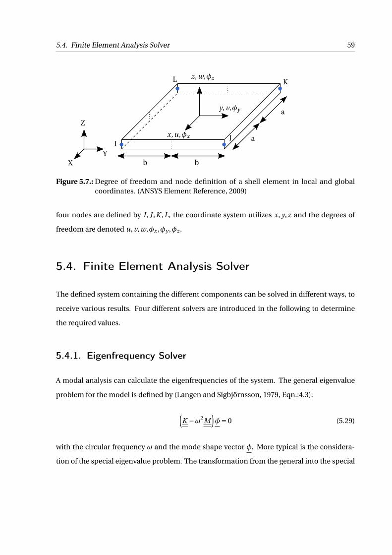
5.4. Finite Element Analysis Solver 59
IJ
KL
XY
Z
x,u,¡x
y, v,¡y
z, w,¡z
b
a
b
a
Figure 5.7.: Degree of freedom and node definition of a shell element in local and globalcoordinates. (ANSYS Element Reference, 2009)
four nodes are defined by I , J ,K ,L, the coordinate system utilizes x, y, z and the degrees of
freedom are denoted u, v, w,¡x ,¡y ,¡z .
5.4. Finite Element Analysis Solver
The defined system containing the different components can be solved in different ways, to
receive various results. Four different solvers are introduced in the following to determine
the required values.
5.4.1. Eigenfrequency Solver
A modal analysis can calculate the eigenfrequencies of the system. The general eigenvalue
problem for the model is defined by (Langen and Sigbjörnsson, 1979, Eqn.:4.3):
≥K °!2M
¥¡= 0 (5.29)
with the circular frequency ! and the mode shape vector ¡. More typical is the considera-
tion of the special eigenvalue problem. The transformation from the general into the special
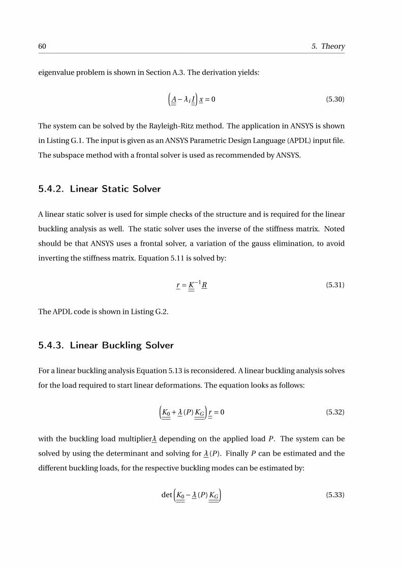
60 5. Theory
eigenvalue problem is shown in Section A.3. The derivation yields:
≥A°∏i I
¥x = 0 (5.30)
The system can be solved by the Rayleigh-Ritz method. The application in ANSYS is shown
in Listing G.1. The input is given as an ANSYS Parametric Design Language (APDL) input file.
The subspace method with a frontal solver is used as recommended by ANSYS.
5.4.2. Linear Static Solver
A linear static solver is used for simple checks of the structure and is required for the linear
buckling analysis as well. The static solver uses the inverse of the stiffness matrix. Noted
should be that ANSYS uses a frontal solver, a variation of the gauss elimination, to avoid
inverting the stiffness matrix. Equation 5.11 is solved by:
r = K °1R (5.31)
The APDL code is shown in Listing G.2.
5.4.3. Linear Buckling Solver
For a linear buckling analysis Equation 5.13 is reconsidered. A linear buckling analysis solves
for the load required to start linear deformations. The equation looks as follows:
≥K0 +∏ (P )KG
¥r = 0 (5.32)
with the buckling load multiplier∏ depending on the applied load P . The system can be
solved by using the determinant and solving for ∏ (P ). Finally P can be estimated and the
different buckling loads, for the respective buckling modes can be estimated by:
det≥K0 °∏ (P )KG
¥(5.33)
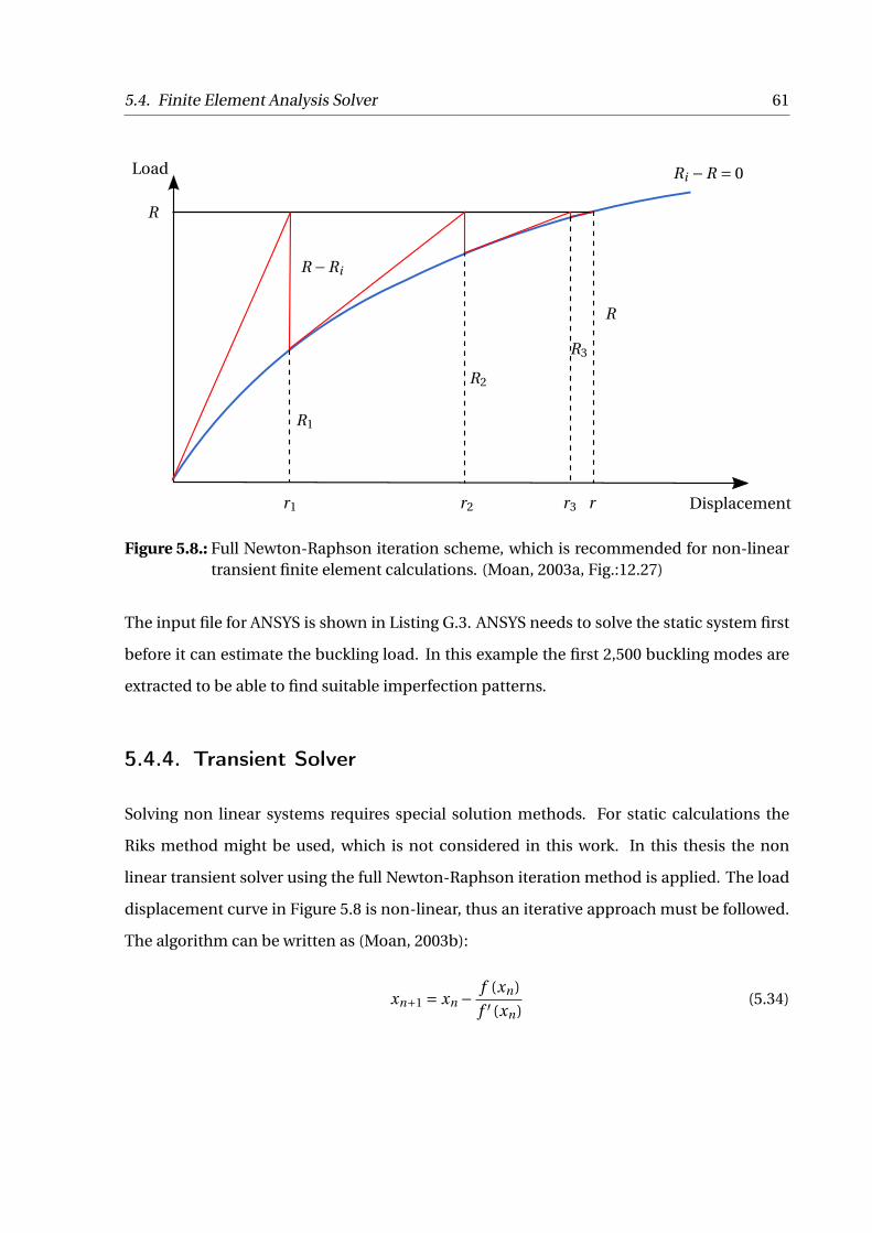
5.4. Finite Element Analysis Solver 61
R
Ri °R = 0
R °Ri
r1 r2 r3 r
R1
R2
R
Load
Displacement
R3
Figure 5.8.: Full Newton-Raphson iteration scheme, which is recommended for non-lineartransient finite element calculations. (Moan, 2003a, Fig.:12.27)
The input file for ANSYS is shown in Listing G.3. ANSYS needs to solve the static system first
before it can estimate the buckling load. In this example the first 2,500 buckling modes are
extracted to be able to find suitable imperfection patterns.
5.4.4. Transient Solver
Solving non linear systems requires special solution methods. For static calculations the
Riks method might be used, which is not considered in this work. In this thesis the non
linear transient solver using the full Newton-Raphson iteration method is applied. The load
displacement curve in Figure 5.8 is non-linear, thus an iterative approach must be followed.
The algorithm can be written as (Moan, 2003b):
xn+1 = xn ° f (xn)f 0 (xn)
(5.34)
62 5. Theory
Applied on the finite element problem, the equation looks like:
rn+1 = rn °KI°1
≥rn
¥≥Ri nt °R
¥(5.35)
or:
rn+1 ° rn =¢rn+1 = KI°1
≥rn
¥≥Ri nt °R
¥(5.36)
The aim is, to find an equilibrium between the internal forces Ri and the external forces R.
The stiffness matrix is updated for each step until the convergence criterion is reached. The
final formulation is given by (Moan, 2003b, Eqn.:12.98a):
R °Ri nt = KI (n) ¢rn+1 (5.37)
The application in ANSYS is shown in Listing G.4. Additionally to the activation of the full
Newton-Raphson method, several other adjustments must be made. Automatic time step-
ping is activated, allowing the program to include several substeps based on the complexity
of the system. Additionally the load is ramped, which means, that high loads can be split
into several steps to reach equilibrium. The maximum number of substeps is set to 1,000.
For unstable structures it might occur that for one substep the system can not find equilib-
rium. In this case the solver will ignore this substep and continue with the next step. Often
equilibrium is reached in the next step and the result might be considered to right. Another
important factor is the output values. Huge models create huge amounts of data for several
steps and substeps. Since only a few values are usually needed the output is redefined.
5.4.5. Distributed ANSYS
On the personal computer, ANSYS 15.0 is used. To be able to solve larger systems the HPC
VILJE of NTNU is used. The specifications of the cluster have been mentioned in the in-
troduction. For calculations on several cores and nodes a special application exists, ANSYS
Distributed (Distributed ANSYS Guide, 2009).
5.4. Finite Element Analysis Solver 63
Using two different ANSYS applications causes difficulties. ANSYS Distributed does not sup-
port the MPC element MPC184 with a direct elimination method. Alternatives are discussed
in the following section. The second unsupported feature is the arc-length method or Riks
method. The arc-length method allows the investigation into the post collapse region in a
non linear static analysis excluding transient effects. The method could have been used for
comparisons and validation of the transient results.
5.4.6. Multi Point Constraint
The bending moment acting on the ship section is applied at the ends of the model. A master
node is defined at the hight of the neutral axis of the section and the corresponding bounded
points are connected as slaves using multi point constrained. ANSYS offers several possibil-
ities to do so. The RBE3 element defines a load distributing element, which is in a strict sense
non rigid body connection and causes problems due to deformations of the boundaries. The
CERIG element is however a rigid connection. Unfortunately the element does not support
large deformations, which occur in a buckling analysis.
The preferred element to use would be the MPC184. Two calculation options within the
element formulation are given, the direct elimination method and the Lagrange multiplier
method. As already mentioned is the direct elimination method not supported by ANSYS
Distributed, which would usually be the recommended method to use, the Lagrange multi-
plier method is troublesome with overconstrained problems. In this case, the method reveals
zero pivot messages and causes convergence difficulties.
A last alternative is to use very stiff beam elements connecting the master and slave nodes.
The BEAM181 element is used. Care should be taken with the definition of the Youngs mod-
ulus. It is important the restrain all elements to avoid shifts between the different elements.
Difficulties arise due to excessively stiff elements causing pivots in the stiffness matrix and
causes convergence difficulties. A stable Youngs modulus with a factor 106 higher than steel
is chosen.
64 5. Theory
5.4.7. Convergence Problems
When solving non linear problems convergence problems might occur. Convergence prob-
lems describe the state when the system can not be solved to find equilibrium. This can
be caused by an insufficiently constrained model with rigid body motions. If this is not the
problem, it can be caused by a few elements behaving in a non realistic manner and causing
large displacements. The calculation is thereafter forced to terminate. This behaviour can
have several triggers.
A first approach is to include reasonable damping in the model, which stabilises the calcu-
lations. Extreme displacements are damped and the structure moves in a closed manner. If
the error still occurs the fault can be overcome by use of any of these methods:
• Change time and/or time stepping
• Change number of substeps
• Switch between stepping or ramping of loads
• Change of convergence tolerances
Experiencing convergence errors does not necessarily suggest input errors. In some cases
just the combination of several parameters causes the calculation to fail. Generally it should
be ensured that the loads be applied gently and the number of substeps and the substeps
size is small enough to solve the system. (PADT, 2012a) (PADT, 2012b)
5.5. Whipping Rule Values
As already mention IACS defined in their new IACS UR-S (2016) rule set, coming into force
on the 1st July 2016, the inclusion of whipping loads. The way is left open to the respective
classification societies. The methods of the different institutions are presented in following.

5.5. Whipping Rule Values 65
5.5.1. DNV
DNV published as the first classification society regulation for the inclusion of whipping
loads. In DNV-CN-No.30.12 (2013) an extension to the partial safety factor method is sug-
gested. It should be mentioned, that these rules are now out ruled, since the DNVGL rule set
came in force the 1st January 2016. The rule is valid for container ships with:
1) Length between perpendicular > 350 m
2) Bow flare angle > 55°
3) Vessel design speed at 85 % MCR > 25 knots
The equation has been extended by the partial safety factor for whipping loads ∞W H and the
partial safety factor for the dynamic collapse ∞dU are introduced as:
∞S MS +°∞W +
°∞W H °∞W
¢∞dU
¢MW ∑ MU
∞R. (5.38)
With ∞R defined by:
∞R = ∞M∞DB . (5.39)
The safety factors are defined as follows:
∞S = 1.0 ; ∞W = 1.2 ; ∞dU = 1.0 ; ∞M = 1.1 ; ∞DB = 1.0. (5.40)
The safety factor for whipping is given by:
∞W H = 1+k1 (L+k2)(V +k3)2≥tan
≥Æ
º
180
¥+k4
¥; ∞W Hmi n = 1.3 (5.41)
With
k1 = 4.83 ·10°7 ; k2 = 1,100 ; k3 = 4.1 ; k4 =°0.19

66 5. Theory
5.5.2. DNVGL
DNVGL has overtaken most of the former DNV rules. However some parts have changed.
The special treatment of container ships is defined in DNVGL Rules Part 6 Chapter 1 (2016).
The rules provided by DNVGL-CG-0153 (2015) contain special considerations for whipping
loads. The validity range is given by:
1) Block coefficient in the order of 0.6 to 0.7
2) Speed in the range of 20 to 29 knots
3) Length in the range of 90 to 400 meters
The partial safety factor approach is given by:
∞S MS +°∞W +
°∞W H °∞W
¢∞dU
¢MW ∑ MU
∞M∞DB. (5.42)
with the partial safety factors defined as:
∞S = 1.0 ; ∞W = 1.2 ; ∞dU = 0.9 ; ∞M = 1.05 ; ∞DB = 1.1 (5.43)
The partial safety factor for the whipping loads is given by:
∞W H = 1+ cL°3.8 ·10°7 (L+1100)(V +4.1)2 /tanÆ°0.19)
¢∏ ∞W (5.44)
with the distribution factor cL given with 1 for the midship position.
5.5.3. Bureau Veritas
BV-NR-583 (2015) have introduced three additional service features "WhiSp1", "WhiSp2" and
"WhiSp3". The designed ship will fall into the category "WhiSp1" and only a linear fatigue
assessment is required. An ultimate strength assessment including dynamics effects is only
required for ships LPP ∏ 350m in class "WhiSp2". Since the fatigue calculation is not part
of this thesis it is neglected. For larger ships, the inclusion of whipping loads is done by
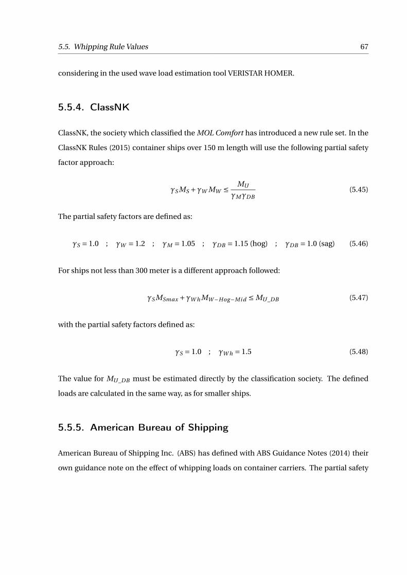
5.5. Whipping Rule Values 67
considering in the used wave load estimation tool VERISTAR HOMER.
5.5.4. ClassNK
ClassNK, the society which classified the MOL Comfort has introduced a new rule set. In the
ClassNK Rules (2015) container ships over 150 m length will use the following partial safety
factor approach:
∞S MS +∞W MW ∑ MU
∞M∞DB(5.45)
The partial safety factors are defined as:
∞S = 1.0 ; ∞W = 1.2 ; ∞M = 1.05 ; ∞DB = 1.15 (hog) ; ∞DB = 1.0 (sag) (5.46)
For ships not less than 300 meter is a different approach followed:
∞S MSmax +∞W h MW °Hog°Mi d ∑ MU _DB (5.47)
with the partial safety factors defined as:
∞S = 1.0 ; ∞W h = 1.5 (5.48)
The value for MU _DB must be estimated directly by the classification society. The defined
loads are calculated in the same way, as for smaller ships.
5.5.5. American Bureau of Shipping
American Bureau of Shipping Inc. (ABS) has defined with ABS Guidance Notes (2014) their
own guidance note on the effect of whipping loads on container carriers. The partial safety
68 5. Theory
factor concept is given by:
∞S MSmax +∞W h MW °Hog°Mi d ∑ MU _DB
∞R(5.49)
with the partial safety factors given as:
∞S = 1.0 ; ∞R = 1.1 (5.50)
The partial safety factor is the maximum value of the approach for the wave loads ∞W = 1.05
or an approach resulting from the calculated whipping loads. Whipping loads are addition-
ally included in the wave moment MW . ABS has developed a closed form approach to es-
timate whipping loads and prorate them with the wave bending moment. This approach
exceeds the capacities of this thesis and is not further investigated.
5.5.6. Lloyds Register
Lloyds Register Ltd. (LR) has developed a class notation "WDA" for the assessment of whip-
ping loads. The longitudinal strength procedure is described in LR Rules (2016). In the rules
correction factors for the Ship Right program have been developed. These values can’t be
compared directly with the previous ones and will not be investigated further.
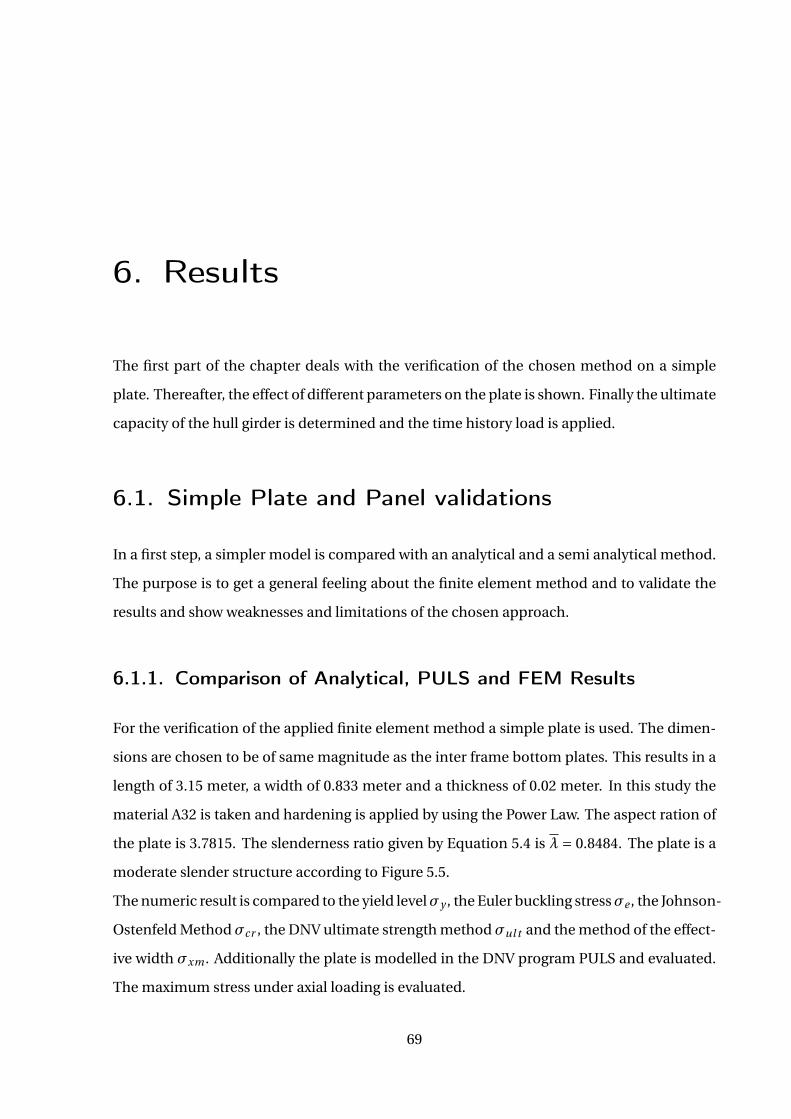
6. Results
The first part of the chapter deals with the verification of the chosen method on a simple
plate. Thereafter, the effect of different parameters on the plate is shown. Finally the ultimate
capacity of the hull girder is determined and the time history load is applied.
6.1. Simple Plate and Panel validations
In a first step, a simpler model is compared with an analytical and a semi analytical method.
The purpose is to get a general feeling about the finite element method and to validate the
results and show weaknesses and limitations of the chosen approach.
6.1.1. Comparison of Analytical, PULS and FEM Results
For the verification of the applied finite element method a simple plate is used. The dimen-
sions are chosen to be of same magnitude as the inter frame bottom plates. This results in a
length of 3.15 meter, a width of 0.833 meter and a thickness of 0.02 meter. In this study the
material A32 is taken and hardening is applied by using the Power Law. The aspect ration of
the plate is 3.7815. The slenderness ratio given by Equation 5.4 is ∏ = 0.8484. The plate is a
moderate slender structure according to Figure 5.5.
The numeric result is compared to the yield levelæy , the Euler buckling stressæe , the Johnson-
Ostenfeld Methodæcr , the DNV ultimate strength methodæul t and the method of the effect-
ive width æxm . Additionally the plate is modelled in the DNV program PULS and evaluated.
The maximum stress under axial loading is evaluated.
69

70 6. Results
Table 6.1.: Comparison of ultimate capacity for a simple plate with a width of 0.833 meterand a length of 3.15 meter with constrained edges. Calculated by the yield level,Euler buckling, Johnson-Ostenfeld assumption, ultimate strength method, themethod of effective width, PULS and ANSYS.
Method æy æe æcr æul t æxm æPU LS æAN SY S Unit
Stress 315.00 437.65 258.32 262.54 269.50 273.00 271.91 MPaDeviation 13.68 37.87 5.26 2.40 0.89 0.40 1 %
The plate is modelled in ANSYS and loaded in the longitudinal direction. The boundaries
on the short edges are modelled by using multi point constrains. The boundaries on the
long edges are defined as constrained. Imperfections are implemented using an eigenvalue
analysis on the forehand. As expected, by an aspect ratio close the four, the first eigenvalue
consists of four half waves and is shown in Figure F.1 in the appendix. The imperfections
are applied with the maximum allowed magnitude according to DNV-OS-C401 (2013). The
displacement controlled calculation are performed until the plate is well inside the post col-
lapse region. The maximum value of the load-displacement curve is shown in Table 6.1. The
final deflections are shown in Figure F.2 in the appendix.
Comparing the results according to their deviation of the ANSYS values, shows that the Euler
buckling load is much higher than the expected value. Considering Figure 5.5 the plate is in
the moderate slender range and the Euler buckling load is out of the range. The yield stress
level is well above the buckling stress level, thus buckling occurs and need to be considered.
The Johnson-Ostenfeld result reveals a deviation of 5.26 % and the ultimate strength concept
reveals a deviation of 2.4 % to the ANSYS result. These values are not very satisfying, but
might be considered as an indication of valid results. However the most accurate approach,
Faulkners method, gives an error of 0.89 %. More sophisticated is only the semi analytical
method used in PULS. The results are close to match with an error of 0.4 %. Thus the method
of effective width, PULS and ANSYS reveal trustworthy results.
The comparison is performed for several thicknesses. The best convergence could be found
for the already examined thickness. In the range between 15 millimetre and 35 millimetre
the results are within 5 % difference and thus valid. Below 15 millimetre thickness the res-
ults start to diverge. This happens for all three considered values in Figure 6.1. This can
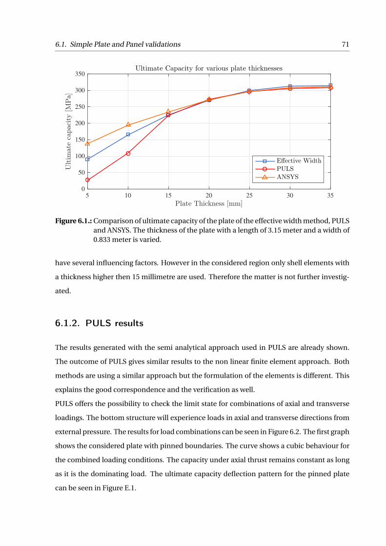
6.1. Simple Plate and Panel validations 71
5 10 15 20 25 30 35
Plate Thickness [mm]
0
50
100
150
200
250
300
350Ultim
atecapacity[M
Pa]
Ultimate Capacity for various plate thicknesses
Effective WidthPULSANSYS
Figure 6.1.: Comparison of ultimate capacity of the plate of the effective width method, PULSand ANSYS. The thickness of the plate with a length of 3.15 meter and a width of0.833 meter is varied.
have several influencing factors. However in the considered region only shell elements with
a thickness higher then 15 millimetre are used. Therefore the matter is not further investig-
ated.
6.1.2. PULS results
The results generated with the semi analytical approach used in PULS are already shown.
The outcome of PULS gives similar results to the non linear finite element approach. Both
methods are using a similar approach but the formulation of the elements is different. This
explains the good correspondence and the verification as well.
PULS offers the possibility to check the limit state for combinations of axial and transverse
loadings. The bottom structure will experience loads in axial and transverse directions from
external pressure. The results for load combinations can be seen in Figure 6.2. The first graph
shows the considered plate with pinned boundaries. The curve shows a cubic behaviour for
the combined loading conditions. The capacity under axial thrust remains constant as long
as it is the dominating load. The ultimate capacity deflection pattern for the pinned plate
can be seen in Figure E.1.

72 6. Results
0 50 100 150 200 250 300 350
Sigma x [MPa]
0
50
100
150
200
250
300
350
Sigmay[M
Pa]
PULS Comparison Plate and Panel
Plate pinnedPlate clampedPanel
Figure 6.2.: PULS results for the plate of length 3.15 meter, 0.833 meter width and a thicknessof 0.02 meter with clamped and pinned boundaries loaded under biaxial load. Aswell as the result for a panel of 3.15 meter length and 4.998 meter width and fivemounted tee-bar profiles of 450x15+100x20 mm loaded under biaxial stress isgiven.
The combined load case for the same plate with clamped boundaries has a different shape.
The capacity under pure axial pressure is slightly higher than for the pinned plate. The ef-
fect of the different boundary condition is especially visible when biaxial loading is applied.
Generally shows the plate a higher capacity for transverse and combined loading then the
pinned plate. Additionally the deflection pattern changed into six half waves as seen on Fig-
ure E.2. This does not corresponds with the aspect ratio of the plate.
PULS gives the opportunity to design a whole panel. A typical bottom panel including six
plates and five stiffeners is modelled. The biaxial loading curve is shows high correspond-
ence with the simple plate result. PULS includes two different sets of imperfections on the
panel. The local imperfections are shown in Figure E.3 and the global imperfections in Figure
E.4. The ultimate capacity pattern is a combination of both, dominated by the local deform-
ations. The stiffeners are failing due to tripping and the plate shows the local plate deflection
with four half waves over the plate length. The deflection pattern in Figure E.5 might give an
outlook on the expected failure of the hull girder.
In a nutshell the pinned plate and the panel do not show drops in their capacity as long as
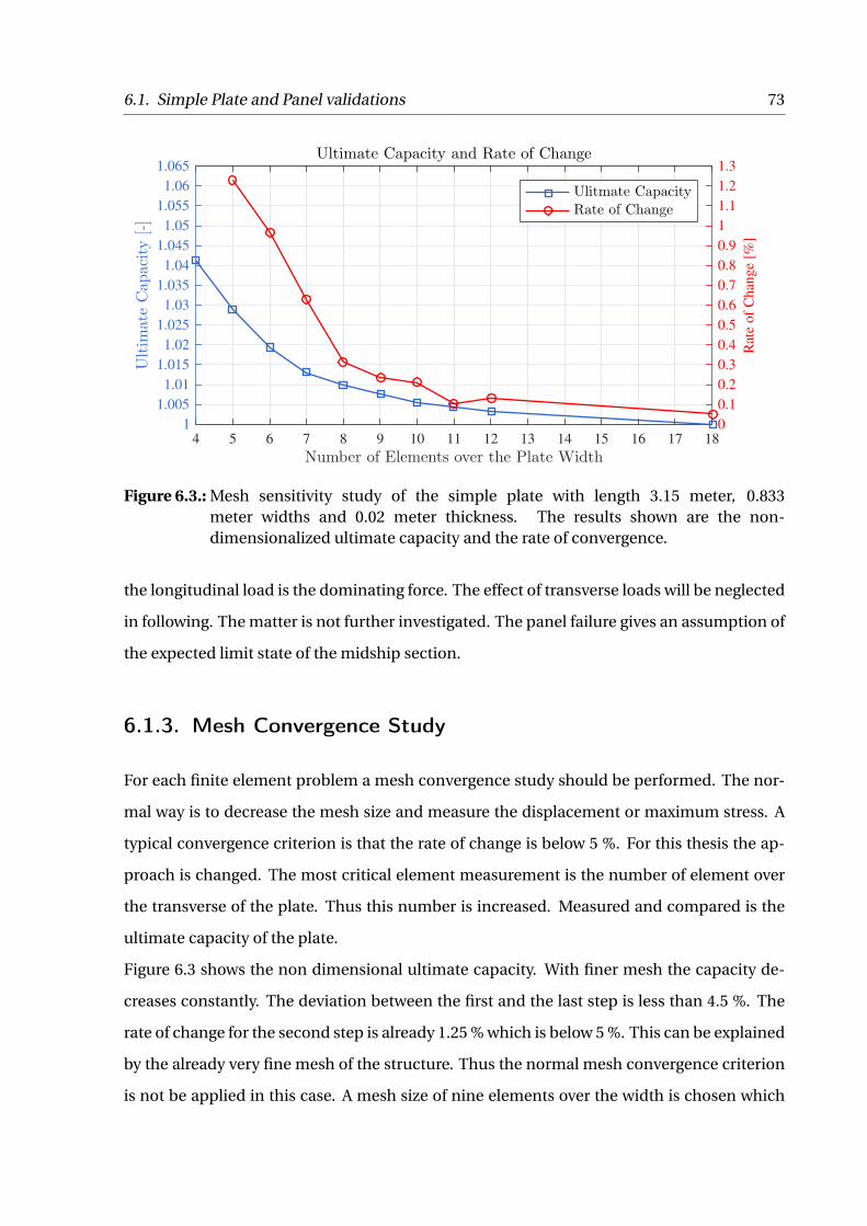
6.1. Simple Plate and Panel validations 73
4 5 6 7 8 9 10 11 12 13 14 15 16 17 18
Number of Elements over the Plate Width
1
1.005
1.01
1.015
1.02
1.025
1.03
1.035
1.04
1.045
1.05
1.055
1.06
1.065
Ultim
ateCap
acity[-]
0
0.1
0.2
0.3
0.4
0.5
0.6
0.7
0.8
0.9
1
1.1
1.2
1.3
Rat
e of
Chan
ge
[%]
Ultimate Capacity and Rate of Change
Ulitmate CapacityRate of Change
Figure 6.3.: Mesh sensitivity study of the simple plate with length 3.15 meter, 0.833meter widths and 0.02 meter thickness. The results shown are the non-dimensionalized ultimate capacity and the rate of convergence.
the longitudinal load is the dominating force. The effect of transverse loads will be neglected
in following. The matter is not further investigated. The panel failure gives an assumption of
the expected limit state of the midship section.
6.1.3. Mesh Convergence Study
For each finite element problem a mesh convergence study should be performed. The nor-
mal way is to decrease the mesh size and measure the displacement or maximum stress. A
typical convergence criterion is that the rate of change is below 5 %. For this thesis the ap-
proach is changed. The most critical element measurement is the number of element over
the transverse of the plate. Thus this number is increased. Measured and compared is the
ultimate capacity of the plate.
Figure 6.3 shows the non dimensional ultimate capacity. With finer mesh the capacity de-
creases constantly. The deviation between the first and the last step is less than 4.5 %. The
rate of change for the second step is already 1.25 % which is below 5 %. This can be explained
by the already very fine mesh of the structure. Thus the normal mesh convergence criterion
is not be applied in this case. A mesh size of nine elements over the width is chosen which

74 6. Results
0 0.002 0.004 0.006 0.008 0.01 0.012 0.014 0.016 0.018 0.02
End shorting [m]
0
0.1
0.2
0.3
0.4
0.5
0.6
0.7
0.8
0.9
1
1.1
1.2
Load[-]
Influence of Strain Hardening on Post Buckling Behaviour
Elastic Perfectly PlasticBilinear HardeningPower Law
Figure 6.4.: Influence of elastic perfectly plastic, bilinear and power law hardening on thepost buckling behaviour of a simple plate.
corresponds to an element size of 100x100 millimetre. This is based on comparisons with
other studies.
6.2. Case Study on a Simple Plate using FEM
After the applied method is verified the influence of several parameters on the buckling and
post collapse behaviour is estimated.
6.2.1. Influence of Material Hardening
The influence of the already discussed different non-linear material models should to be
evaluated. All three models are applied in ANSYS. The plates are pushed far into the post
collapse region to evaluate the results. The load-displacement curves are shown in Figure
6.4. The pre- and post-buckling curve are equal for all three material models. Differences are
occurring in the post-collapse region. Including hardening with the DNV recommended bi-
linear model gives the plate a higher post collapse capacity than the elastic-perfectly plastic
model. Increasing a simple hardening model increases the remaining capacity of the plate

6.2. Case Study on a Simple Plate using FEM 75
0 0.002 0.004 0.006 0.008 0.01 0.012 0.014 0.016 0.018 0.02
End shorting [m]
0
0.1
0.2
0.3
0.4
0.5
0.6
0.7
0.8
0.9
1
1.1
1.2Load[-]
Influence of Added Mass on Post Buckling Behaviour
No added massFactor 2.0 Added Mass
Figure 6.5.: Influence of added mass on the collapse of a simple plate under axial loading.
compared with the elastic perfectly plastic model. The Power law increases the plates capa-
city directly after the collapse, but nearly follows the bilinear hardening model afterwards.
6.2.2. Influence of Added Mass
In dynamic analysis for marine structures, added mass is a topic of concern. The added mass
factor for the load is defined as two. This factor is as well applied for the bottom plates. The
mass of the plate is multiplied by the factor 2. Noted should be that neither external pressure
or gravitational acceleration are considered in this test case. The two load - displacement
curves are shown in Figure 6.5.
The graphs are identical until the post collapse region. After collapse the plate with higher
mass continues to collapse faster compared to the lighter plate. Both paths are matching
after a while again at the same capacity. Thus only the last part of the unloading path is
influenced by added mass. In general added mass has a minor influence on the static case,
but might come in play in the dynamic case.
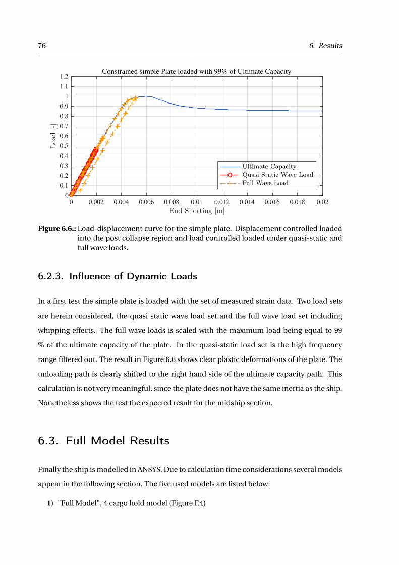
76 6. Results
0 0.002 0.004 0.006 0.008 0.01 0.012 0.014 0.016 0.018 0.02
End Shorting [m]
0
0.1
0.2
0.3
0.4
0.5
0.6
0.7
0.8
0.9
1
1.1
1.2
Load[-]
Constrained simple Plate loaded with 99% of Ultimate Capacity
Ultimate CapacityQuasi Static Wave LoadFull Wave Load
Figure 6.6.: Load-displacement curve for the simple plate. Displacement controlled loadedinto the post collapse region and load controlled loaded under quasi-static andfull wave loads.
6.2.3. Influence of Dynamic Loads
In a first test the simple plate is loaded with the set of measured strain data. Two load sets
are herein considered, the quasi static wave load set and the full wave load set including
whipping effects. The full wave loads is scaled with the maximum load being equal to 99
% of the ultimate capacity of the plate. In the quasi-static load set is the high frequency
range filtered out. The result in Figure 6.6 shows clear plastic deformations of the plate. The
unloading path is clearly shifted to the right hand side of the ultimate capacity path. This
calculation is not very meaningful, since the plate does not have the same inertia as the ship.
Nonetheless shows the test the expected result for the midship section.
6.3. Full Model Results
Finally the ship is modelled in ANSYS. Due to calculation time considerations several models
appear in the following section. The five used models are listed below:
1) "Full Model", 4 cargo hold model (Figure F.4)
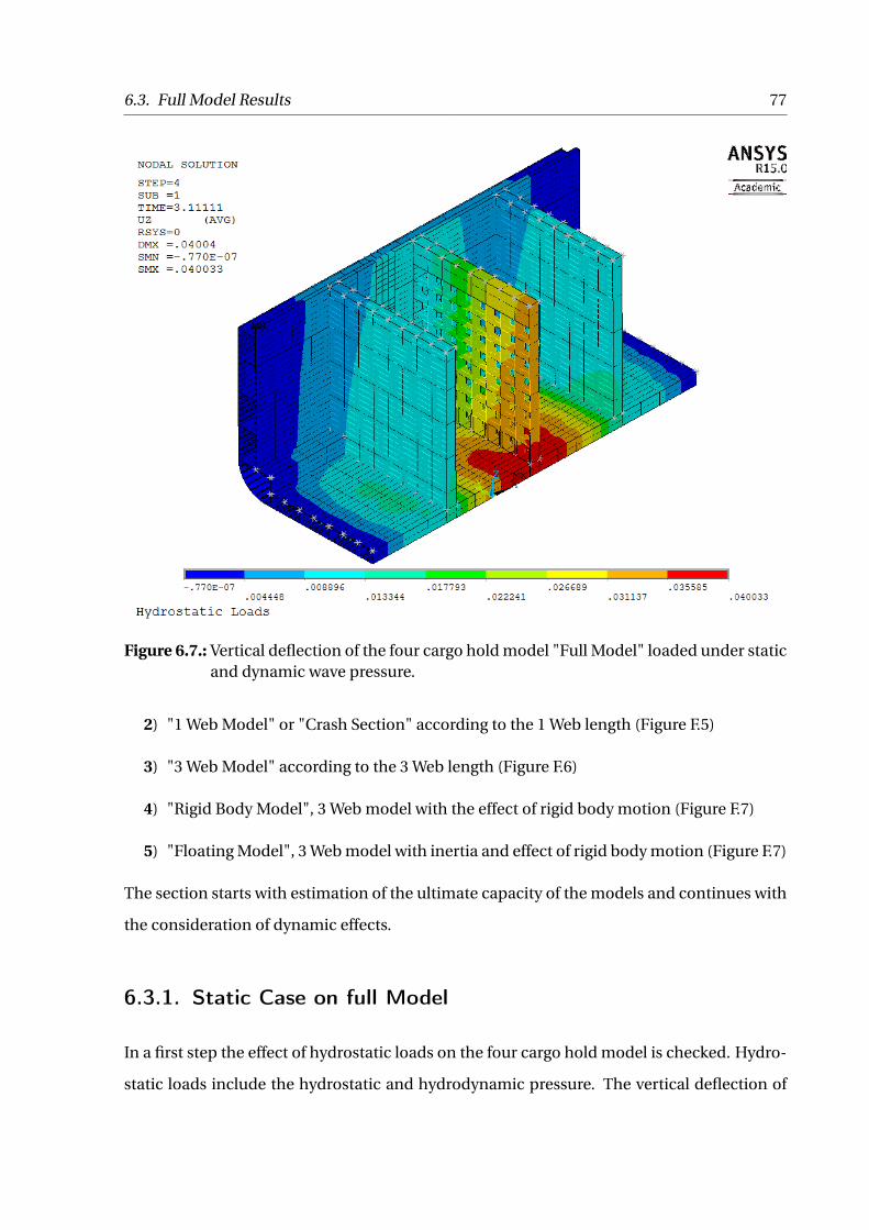
6.3. Full Model Results 77
Figure 6.7.: Vertical deflection of the four cargo hold model "Full Model" loaded under staticand dynamic wave pressure.
2) "1 Web Model" or "Crash Section" according to the 1 Web length (Figure F.5)
3) "3 Web Model" according to the 3 Web length (Figure F.6)
4) "Rigid Body Model", 3 Web model with the effect of rigid body motion (Figure F.7)
5) "Floating Model", 3 Web model with inertia and effect of rigid body motion (Figure F.7)
The section starts with estimation of the ultimate capacity of the models and continues with
the consideration of dynamic effects.
6.3.1. Static Case on full Model
In a first step the effect of hydrostatic loads on the four cargo hold model is checked. Hydro-
static loads include the hydrostatic and hydrodynamic pressure. The vertical deflection of
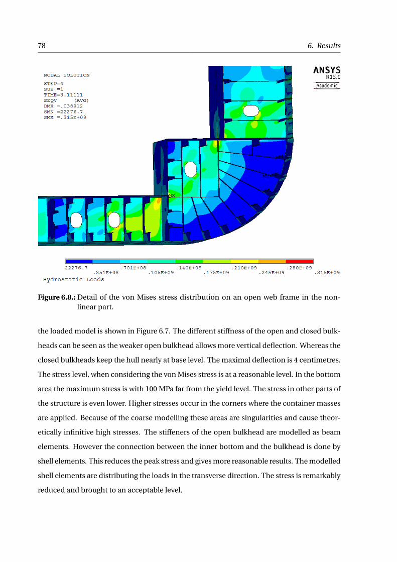
78 6. Results
Figure 6.8.: Detail of the von Mises stress distribution on an open web frame in the non-linear part.
the loaded model is shown in Figure 6.7. The different stiffness of the open and closed bulk-
heads can be seen as the weaker open bulkhead allows more vertical deflection. Whereas the
closed bulkheads keep the hull nearly at base level. The maximal deflection is 4 centimetres.
The stress level, when considering the von Mises stress is at a reasonable level. In the bottom
area the maximum stress is with 100 MPa far from the yield level. The stress in other parts of
the structure is even lower. Higher stresses occur in the corners where the container masses
are applied. Because of the coarse modelling these areas are singularities and cause theor-
etically infinitive high stresses. The stiffeners of the open bulkhead are modelled as beam
elements. However the connection between the inner bottom and the bulkhead is done by
shell elements. This reduces the peak stress and gives more reasonable results. The modelled
shell elements are distributing the loads in the transverse direction. The stress is remarkably
reduced and brought to an acceptable level.
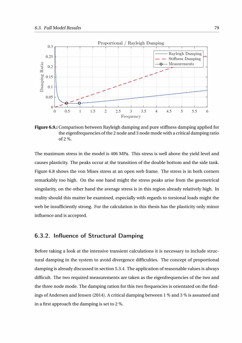
6.3. Full Model Results 79
0 0.5 1 1.5 2 2.5 3 3.5 4 4.5 5 5.5 6
Frequency
0
0.05
0.1
0.15
0.2
0.25
0.3
Dam
pingRatio
Proportional / Rayleigh Damping
Rayleigh DampingStiffness DampingMeasurements
Figure 6.9.: Comparison between Rayleigh damping and pure stiffness damping applied forthe eigenfrequencies of the 2 node and 3 node mode with a critical damping ratioof 2 %.
The maximum stress in the model is 406 MPa. This stress is well above the yield level and
causes plasticity. The peaks occur at the transition of the double bottom and the side tank.
Figure 6.8 shows the von Mises stress at an open web frame. The stress is in both corners
remarkably too high. On the one hand might the stress peaks arise from the geometrical
singularity, on the other hand the average stress is in this region already relatively high. In
reality should this matter be examined, especially with regards to torsional loads might the
web be insufficiently strong. For the calculation in this thesis has the plasticity only minor
influence and is accepted.
6.3.2. Influence of Structural Damping
Before taking a look at the intensive transient calculations it is necessary to include struc-
tural damping in the system to avoid divergence difficulties. The concept of proportional
damping is already discussed in section 5.3.4. The application of reasonable values is always
difficult. The two required measurements are taken as the eigenfrequencies of the two and
the three node mode. The damping ration for this two frequencies is orientated on the find-
ings of Andersen and Jensen (2014). A critical damping between 1 % and 3 % is assumed and
in a first approach the damping is set to 2 %.

80 6. Results
0 0.1 0.2 0.3 0.4 0.5 0.6 0.7 0.8 0.9 1
Hull girder rotation [rad]×10
-3
0
0.25
0.5
0.75
1
1.25
1.5
1.75
2
Verticalbendingmom
ent[N
m]
×1010 Ultimate Strength of Midship Section
Yield Capacity
Rule Capacity
Incremental1 Web Model3 Web ModelFull Model
Figure 6.10.: Moment-rotation curve for the ultimate strength of the midship section for the1 Web Model, the 3 Web Model and the Full Model. Additionally the incre-mental result obtained by POSEIDON,the rule loading and the yield capacityare shown.
The second decision is to choose the simplified stiffness damping, defined by only one fre-
quency or the full proportional damping approach. The stiffness damping carries the risk
of the overestimation of very low frequency loads. Thus the full proportional damping is
applied defined by Æ1 = 0.0127 and Æ2 = 0.0276.
6.3.3. Ultimate Capacity of the Midship Section
After the static consideration the Full Model is gradually loaded with a hogging bending mo-
ment, until the hull girder collapses. The required computational time exceeds a reasonable
time limit by far. A smaller 1 Web and a 3 Web model are considered and loaded. Also the
program POSEIDON is used to calculate the ultimate state with the incremental method.
The Results are shown in Figure 6.10.
No result could be reached for the Full Model, due to several instability problems and time
computational. Only the pre buckling part of the the calculation is solved. The ultimate ca-
pacity for the 1 Web and 3 Web is calculated. First point of interest are the different slopes of
the pre buckling parts. This is caused by the way the deflection is measured. Measuring at

6.3. Full Model Results 81
1
23
4
Figure 6.11.: Von Mises stress at the bottom of the 3 Web Model with the GL rule load appliedlooking forward.
the same points where the moments are applied will include the stiffness of the model. Thus
a longer model will be weaker than a shorter one.
Of interest are the maximum ultimate capacities of the two models. Suspicious for the 1 Web
model is the fact that the ultimate strength exceed the yield strength level. This is caused by
influence of the boundaries. The behaviour is matching with the results received by Fricke
and Bronsart (2012). The clamped boundaries close to the considered areas are over predict-
ing the ultimate capacity. Thus the 1 Web model is non-conservative and not suitable for this
thesis.
The 3 Web model gives more reasonable values. The ultimate capacity is in a valid range.
Comparing the maximum value of the incremental result with the FEM result shows a differ-
ence of 0.5 %. This is a very good match for both values. A second check is done by compar-
ing the FEM ratio between yield and buckling strength of the simple plate and the midship
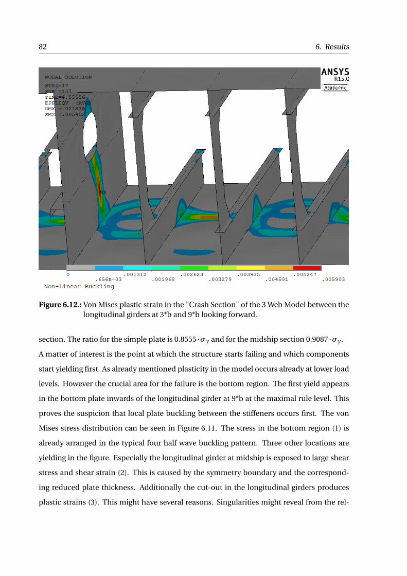
82 6. Results
Figure 6.12.: Von Mises plastic strain in the "Crash Section" of the 3 Web Model between thelongitudinal girders at 3*b and 9*b looking forward.
section. The ratio for the simple plate is 0.8555 ·æy and for the midship section 0.9087 ·æy .
A matter of interest is the point at which the structure starts failing and which components
start yielding first. As already mentioned plasticity in the model occurs already at lower load
levels. However the crucial area for the failure is the bottom region. The first yield appears
in the bottom plate inwards of the longitudinal girder at 9*b at the maximal rule level. This
proves the suspicion that local plate buckling between the stiffeners occurs first. The von
Mises stress distribution can be seen in Figure 6.11. The stress in the bottom region (1) is
already arranged in the typical four half wave buckling pattern. Three other locations are
yielding in the figure. Especially the longitudinal girder at midship is exposed to large shear
stress and shear strain (2). This is caused by the symmetry boundary and the correspond-
ing reduced plate thickness. Additionally the cut-out in the longitudinal girders produces
plastic strains (3). This might have several reasons. Singularities might reveal from the rel-

6.3. Full Model Results 83
atively coarse mesh around the opening. Otherwise the neglected local reinforcements will
reduce the local stresses as well. An other possible error can be the insufficient stiff design
of the design, which should be further investigated. Also plasticity occurs at the boundaries
of the model. In the webs of the stiffeners below the flanges occur plasticity at all bottom
stiffeners (4). This is caused by the clamped boundary and the constrained rotation of the
rigid body link and is negligible.
Loading the structure until ultimate capacity creates more plasticity. The status of failure is
shown in Figure 6.12. The Crash Section is shown with all longitudinal components and the
transverse parts are hidden. The plastic strain follows clearly the buckling pattern already
seen for the first yield case. On top of that occurs large plastic strain below the cut-out in the
longitudinal girder. This might indicate an insufficient thickness of the girder in combina-
tion with the cut out. The strain has reached the stiffener webs from the bottom plates and
starts to deform the stiffeners upwards. This indicates a plate induced failure of the structure.
Further occurs plasticity in the stiffener flange. On the one hand at the forward end of the
flange at the transverse bulkhead and on the other hand at the end of the vertical stiffeners of
the aft web frame. The global deflection at the ultimate capacity can be seen in the Appendix
in Figure F.8. The buckling pattern shows clearly the four half sine waves with deflections up
to 0.02 meter. The pattern spreads slowly through the width of the ship. Thus the buckling
pattern is clearly anti-symmetric and does not follow the hungry horse mode. The pattern
shows good correspondence with the panel calculated in PULS.
6.3.4. Post Collapse Behaviour of Midship Section
In this calculation the considered models are pushed further into the post collapse region.
The idea is to get a grasp on how the structure will ultimately fail. The results in Figure 6.13
are the computational most time consuming results. The CPU time was 84 hours using one
Node on VILJE. This is caused by the large non-linear deformations of the structure. The
exact ultimate capacity can not be estimated using this calculation, because the used time
steps are too coarse to capture the right value.
Even though the ultimate capacity is different for both models the paths are matching later

84 6. Results
0 0.2 0.4 0.6 0.8 1 1.2 1.4 1.6 1.8 2
Hull girder rotation [rad]×10
-3
0
0.25
0.5
0.75
1
1.25
1.5
1.75
2
Verticalbendingmom
ent[N
m]
×1010 Post Collapse Behaviour of Midship Section
Yield Capacity
Rule Capacity
1 Web Model3 Web ModelFull Model
Figure 6.13.: Post Collapse path of the 1 Web Model, 3 Web model and Full Model.
on. This might lead to the assumption that the influence of the boundaries is reduced for the
post collapse region compared to the collapse behaviour.
The post collapse deformation is shown in Figure 6.14. The buckling pattern is fully de-
veloped and the distortion reaches from midship until the height of the neutral axis over the
whole shell. The inwards deflection of the bottom shells is up to 0.7 meter. The inner bottom
has started to buckle as well. The pattern in Figure F.9 shows distortion in the crash section
from the neutral axis downwards until the inner bottom is reached. The deformation at the
inner bottom is spreading to the boundaries where distortions occur.
A closer look inside the crash box is given in Figure F.10. The stiffeners have started to buckle
as well, which is caused by the excessive plate buckling. Additionally to the stiffeners have
the longitudinal bulkheads started to display large deformations. Finally the whole structure
has began to unload and shows large plastic deformations.
6.3.5. Ultimate Capacity of Floating Model
The next step is to validate the Floating Model with verified 3 Web Model. In Figure 6.15
the ultimate capacity curves are compared. The Floating Model follows the 3 Web Model
relatively close. The undamped model shows high fluctuations above the true path. This is

6.3. Full Model Results 85
Figure 6.14.: Displacement vector sum of the 3 Web Model at the last time step, showingexcessive distortion in the bottom region.
unacceptable, especially the ultimate capacity can not be estimated due to the high oscilla-
tions. The path varies between the buckling load and the yield level which is a difference of
9.1 %.
The variations can be diminished by the introduction of damping on the springs. In reality
this corresponds with the heave damping of the ship. The applied 2 % damping of the critical
damping smooths the path remarkably. The deviation is reduced to an oscillation of 2 %. The
post collapse path is followed by all three graphs, thus no differences can be seen. The model
with damping is suitable for calculations and the results are reasonable correct. Nonetheless
care should be taken during the post processing due to the oscillations.
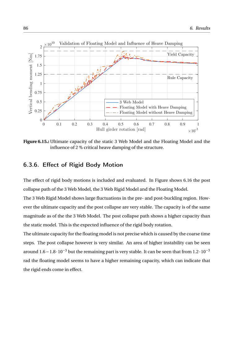
86 6. Results
0 0.1 0.2 0.3 0.4 0.5 0.6 0.7 0.8 0.9 1
Hull girder rotation [rad]×10
-3
0
0.25
0.5
0.75
1
1.25
1.5
1.75
2
Verticalbendingmom
ent[N
m]
×1010 Validation of Floating Model and Influence of Heave Damping
Yield Capacity
Rule Capacity
3 Web ModelFloating Model with Heave DampingFloating Model without Heave Damping
Figure 6.15.: Ultimate capacity of the static 3 Web Model and the Floating Model and theinfluence of 2 % critical heave damping of the structure.
6.3.6. Effect of Rigid Body Motion
The effect of rigid body motions is included and evaluated. In Figure shows 6.16 the post
collapse path of the 3 Web Model, the 3 Web Rigid Model and the Floating Model.
The 3 Web Rigid Model shows large fluctuations in the pre- and post-buckling region. How-
ever the ultimate capacity and the post collapse are very stable. The capacity is of the same
magnitude as of the the 3 Web Model. The post collapse path shows a higher capacity than
the static model. This is the expected influence of the rigid body rotation.
The ultimate capacity for the floating model is not precise which is caused by the coarse time
steps. The post collapse however is very similar. An area of higher instability can be seen
around 1.6°1.8 ·10°3 but the remaining part is very stable. It can be seen that from 1.2 ·10°3
rad the floating model seems to have a higher remaining capacity, which can indicate that
the rigid ends come in effect.
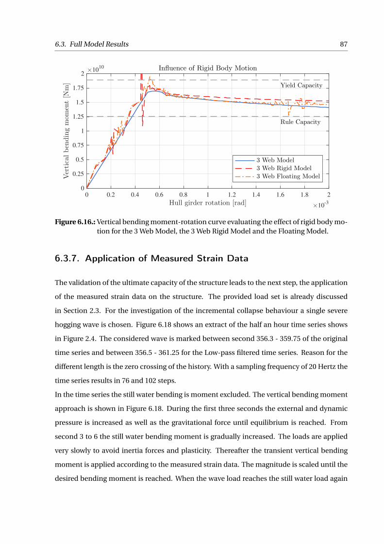
6.3. Full Model Results 87
0 0.2 0.4 0.6 0.8 1 1.2 1.4 1.6 1.8 2
Hull girder rotation [rad]×10
-3
0
0.25
0.5
0.75
1
1.25
1.5
1.75
2
Verticalbendingmom
ent[N
m]
×1010 Influence of Rigid Body Motion
Yield Capacity
Rule Capacity
3 Web Model3 Web Rigid Model3 Web Floating Model
Figure 6.16.: Vertical bending moment-rotation curve evaluating the effect of rigid body mo-tion for the 3 Web Model, the 3 Web Rigid Model and the Floating Model.
6.3.7. Application of Measured Strain Data
The validation of the ultimate capacity of the structure leads to the next step, the application
of the measured strain data on the structure. The provided load set is already discussed
in Section 2.3. For the investigation of the incremental collapse behaviour a single severe
hogging wave is chosen. Figure 6.18 shows an extract of the half an hour time series shows
in Figure 2.4. The considered wave is marked between second 356.3 - 359.75 of the original
time series and between 356.5 - 361.25 for the Low-pass filtered time series. Reason for the
different length is the zero crossing of the history. With a sampling frequency of 20 Hertz the
time series results in 76 and 102 steps.
In the time series the still water bending is moment excluded. The vertical bending moment
approach is shown in Figure 6.18. During the first three seconds the external and dynamic
pressure is increased as well as the gravitational force until equilibrium is reached. From
second 3 to 6 the still water bending moment is gradually increased. The loads are applied
very slowly to avoid inertia forces and plasticity. Thereafter the transient vertical bending
moment is applied according to the measured strain data. The magnitude is scaled until the
desired bending moment is reached. When the wave load reaches the still water load again

88 6. Results
320 330 340 350 360 370 380 390 400
-100
0
100
Stress[M
Pa]
Original (unfiltered) time series
320 330 340 350 360 370 380 390 400
-100
0
100
Stress[M
Pa]
Low-pass filtered time series
320 330 340 350 360 370 380 390 400
Time [s]
-100
-50
0
50
100
Stress[M
Pa]
High-pass filtered time series
Figure 6.17.: Detailed plot of the filtered time series shown in Figure 2.4 with the positionsused for the application on the structure. (Andersen and Jensen, 2014)
the load is smoothly reduced until zero.
6.3.8. Quasi-Static Wave Loads on the 3 Web Model
The quasi static wave load is applied on the 3 Web model and loaded until rule or ultimate
capacity level. The moment-rotation curve is shown in Figure 6.19. The graph has a semi
logarithmic scale for the x-axis. This enables to compare the results. The trend is similar
with the plate test case in Figure 6.6. For the plate the loading follows the same path as the
ultimate path for loading. When plasticity occurs the path to the base line is shifted in x-
direction. For the plate the path is perfectly legible from the graph, however for the 3 Web
Model not. The path follows parallel to the ultimate state, thus plasticity can be seen at the
base line. Therefore the figure is given in a logarithmic scale.
The plasticity seen in the rotation is very small. The rotation occurs in the magnitude of
10°6 radiant. The plate loaded under axial thrust has a permanent deflection of 5 % of the
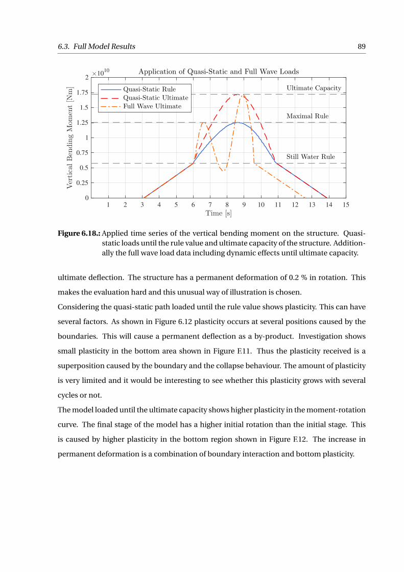
6.3. Full Model Results 89
1 2 3 4 5 6 7 8 9 10 11 12 13 14 15
Time [s]
0
0.25
0.5
0.75
1
1.25
1.5
1.75
2
VerticalBendingMom
ent[N
m]
×1010 Application of Quasi-Static and Full Wave Loads
Ultimate Capacity
Maximal Rule
Still Water Rule
Quasi-Static RuleQuasi-Static UltimateFull Wave Ultimate
Figure 6.18.: Applied time series of the vertical bending moment on the structure. Quasi-static loads until the rule value and ultimate capacity of the structure. Addition-ally the full wave load data including dynamic effects until ultimate capacity.
ultimate deflection. The structure has a permanent deformation of 0.2 % in rotation. This
makes the evaluation hard and this unusual way of illustration is chosen.
Considering the quasi-static path loaded until the rule value shows plasticity. This can have
several factors. As shown in Figure 6.12 plasticity occurs at several positions caused by the
boundaries. This will cause a permanent deflection as a by-product. Investigation shows
small plasticity in the bottom area shown in Figure F.11. Thus the plasticity received is a
superposition caused by the boundary and the collapse behaviour. The amount of plasticity
is very limited and it would be interesting to see whether this plasticity grows with several
cycles or not.
The model loaded until the ultimate capacity shows higher plasticity in the moment-rotation
curve. The final stage of the model has a higher initial rotation than the initial stage. This
is caused by higher plasticity in the bottom region shown in Figure F.12. The increase in
permanent deformation is a combination of boundary interaction and bottom plasticity.
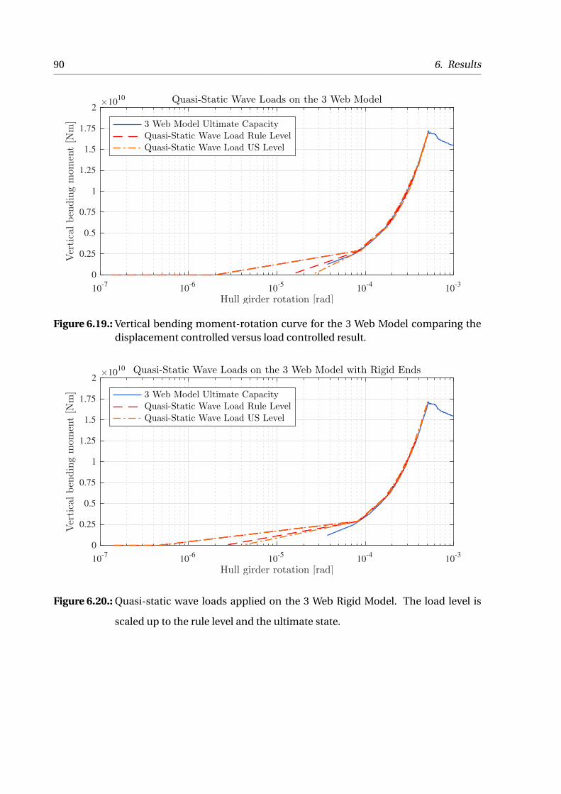
90 6. Results
10-7
10-6
10-5
10-4
10-3
Hull girder rotation [rad]
0
0.25
0.5
0.75
1
1.25
1.5
1.75
2
Verticalbendingmom
ent[N
m]
×1010 Quasi-Static Wave Loads on the 3 Web Model
3 Web Model Ultimate CapacityQuasi-Static Wave Load Rule LevelQuasi-Static Wave Load US Level
Figure 6.19.: Vertical bending moment-rotation curve for the 3 Web Model comparing thedisplacement controlled versus load controlled result.
10-7
10-6
10-5
10-4
10-3
Hull girder rotation [rad]
0
0.25
0.5
0.75
1
1.25
1.5
1.75
2
Verticalbendingmom
ent[N
m]
×1010 Quasi-Static Wave Loads on the 3 Web Model with Rigid Ends
3 Web Model Ultimate CapacityQuasi-Static Wave Load Rule LevelQuasi-Static Wave Load US Level
Figure 6.20.: Quasi-static wave loads applied on the 3 Web Rigid Model. The load level is
scaled up to the rule level and the ultimate state.
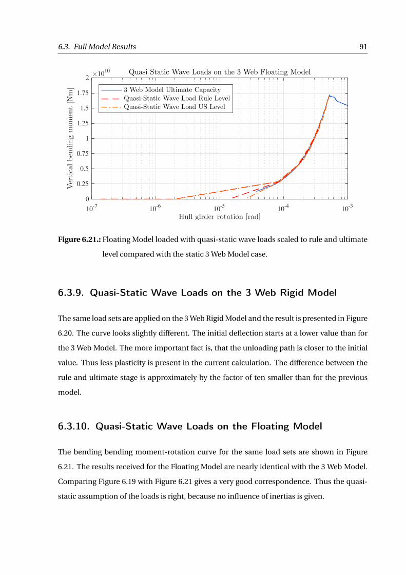
6.3. Full Model Results 91
10-7
10-6
10-5
10-4
10-3
Hull girder rotation [rad]
0
0.25
0.5
0.75
1
1.25
1.5
1.75
2
Verticalbendingmom
ent[N
m]
×1010 Quasi Static Wave Loads on the 3 Web Floating Model
3 Web Model Ultimate CapacityQuasi-Static Wave Load Rule LevelQuasi-Static Wave Load US Level
Figure 6.21.: Floating Model loaded with quasi-static wave loads scaled to rule and ultimate
level compared with the static 3 Web Model case.
6.3.9. Quasi-Static Wave Loads on the 3 Web Rigid Model
The same load sets are applied on the 3 Web Rigid Model and the result is presented in Figure
6.20. The curve looks slightly different. The initial deflection starts at a lower value than for
the 3 Web Model. The more important fact is, that the unloading path is closer to the initial
value. Thus less plasticity is present in the current calculation. The difference between the
rule and ultimate stage is approximately by the factor of ten smaller than for the previous
model.
6.3.10. Quasi-Static Wave Loads on the Floating Model
The bending bending moment-rotation curve for the same load sets are shown in Figure
6.21. The results received for the Floating Model are nearly identical with the 3 Web Model.
Comparing Figure 6.19 with Figure 6.21 gives a very good correspondence. Thus the quasi-
static assumption of the loads is right, because no influence of inertias is given.
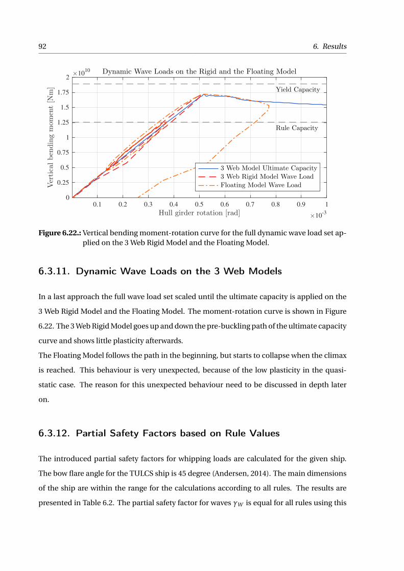
92 6. Results
0.1 0.2 0.3 0.4 0.5 0.6 0.7 0.8 0.9 1
Hull girder rotation [rad]×10
-3
0
0.25
0.5
0.75
1
1.25
1.5
1.75
2
Verticalbendingmom
ent[N
m]
×1010 Dynamic Wave Loads on the Rigid and the Floating Model
Yield Capacity
Rule Capacity
3 Web Model Ultimate Capacity3 Web Rigid Model Wave LoadFloating Model Wave Load
Figure 6.22.: Vertical bending moment-rotation curve for the full dynamic wave load set ap-plied on the 3 Web Rigid Model and the Floating Model.
6.3.11. Dynamic Wave Loads on the 3 Web Models
In a last approach the full wave load set scaled until the ultimate capacity is applied on the
3 Web Rigid Model and the Floating Model. The moment-rotation curve is shown in Figure
6.22. The 3 Web Rigid Model goes up and down the pre-buckling path of the ultimate capacity
curve and shows little plasticity afterwards.
The Floating Model follows the path in the beginning, but starts to collapse when the climax
is reached. This behaviour is very unexpected, because of the low plasticity in the quasi-
static case. The reason for this unexpected behaviour need to be discussed in depth later
on.
6.3.12. Partial Safety Factors based on Rule Values
The introduced partial safety factors for whipping loads are calculated for the given ship.
The bow flare angle for the TULCS ship is 45 degree (Andersen, 2014). The main dimensions
of the ship are within the range for the calculations according to all rules. The results are
presented in Table 6.2. The partial safety factor for waves ∞W is equal for all rules using this
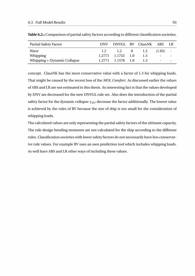
6.3. Full Model Results 93
Table 6.2.: Comparison of partial safety factors according to different classification societies.
Partial Safety Factor DNV DNVGL BV ClassNK ABS LR
Wave 1.2 1.2 0 1.2 (1.05) -Whipping 1.2771 1.1753 1.0 1.3 - -Whipping + Dynamic Collapse 1.2771 1.1578 1.0 1.3 - -
concept. ClassNK has the most conservative value with a factor of 1.3 for whipping loads.
That might be caused by the recent loss of the MOL Comfort. As discussed earlier the values
of ABS and LR are not estimated in this thesis. An interesting fact is that the values developed
by DNV are decreased for the new DNVGL rule set. Also does the introduction of the partial
safety factor for the dynamic collapse ∞dU decrease the factor additionally. The lowest value
is achieved by the rules of BV because the size of ship is too small for the consideration of
whipping loads.
The calculated values are only representing the partial safety factors of the ultimate capacity.
The rule design bending moments are not calculated for the ship according to the different
rules. Classification societies with lower safety factors do not necessarily have less conservat-
ive rule values. For example BV uses an own prediction tool which includes whipping loads.
As well have ABS and LR other ways of including these values.

94 6. Results
7. Discussion
In this chapter is a brief discussion about the validity and applicability of the received results.
The methods performed are critically examined and interpreted.
7.1. Evaluation of ANSYS on a simple Plate
A bunch of tests are performed on the simple plate with constrained edges. For the con-
sidered 20 millimetre thick plate the ultimate capacity is compared with several analytical
approaches. Especially the most advanced methods, the method of effective width and the
semi analytical program PULS show good correspondence with the ANSYS results.
The thickness of the plate is varied between zero and a plate thickness close to the yield limit.
For plates between 15 - 35 mm the results are reasonable. For thinner plates the results of
the method of effective width, PULS and ANSYS are very different. In this thesis, plate thick-
nesses of 15 mm and above are used, thus the deviations are ignored. For evaluating thinner
plates, this phenomena should be investigated. Possible reasons might be the influence of
the boundaries or a too coarse mesh size. Also other factors are not ruled out and should be
investigated.
The mesh convergence study already shows good results for coarser meshes. A typical ap-
proach is to decrease the mesh size until the rate of change is below 5 %. In this case this is
not reasonable since the deviation is already lower. Instead of using the global mesh size as
the indicated value, the number of elements over the plate width is applied. The error has
been analysed and an approved approach of a mesh size of 100 x 100 mm is chosen. The
method has been used and acknowledged in several previously mentioned investigations.
95

96 7. Discussion
The effect of different material models is examined. The material model has no influence on
the ultimate capacity. Hardening affects the material behaviour in the post collapse region
strongly while in the far post collapse region, the model is not of high importance. The direct
collapse behaviour is drastically influenced by the material model used. DNV recommends
the bilinear model which is compared with the Power law. Latter keeps the load longer in the
ultimate region before the structure starts to unload. The model is recommended and tests
have proven that it is the most realistic model (Storheim, 2016). The design stresses are taken
to reveal conservative results.
7.2. Validation of midship model
Imperfections are included in the model to perform non-linear analysis. The deformations
have been taken from the results of a linear buckling analysis. The first 2,500 eigenmodes are
extracted of the Crash Section Model. The most suitable modes are selected and applied on
the structure. ANSYS does not provide a function for applying a static load in the buckling
analysis in addition to the buckling load like ABAQUS. An iterative process is necessary to
include the external pressure loads. This effect is neglected in the linear buckling analysis.
Also the application of several imperfection modes in a superposition is more troublesome
than in ABAQUS. Specific deflection pattern can be applied on different parts of the model
and stored separately. The different parts of the model can thereafter be reconsidered and
merged. This enables the use of different imperfection eigenmodes on different parts of the
structure.
A better controllable approach is the use of the introduced formula to induce a desired num-
ber of half waves over the length of the plate. This enables the use of different patterns, for
example the hungry horse mode. The effect of both asymmetric and hungry horse mode
should be investigated. The asymmetric mode is most likely to occur when overloading
emerges, whereas the hungry horse mode is the likely existing imperfection. Troublesome
with this method is the application of imperfections on the stiffeners. A second approach
would be needed for the inclusion of stiffener imperfections. The introduction of residual
stresses is neglected in this work. In the MOL Comfort case residual stresses are the trigger
7.2. Validation of midship model 97
of the plasticity starting point. This can play an important role in the first yield estimation
of the structure. The static case of the full model shows an unsymmetrical deflection over
the length of the ship. This is not included in the short model. The influence of it should be
evaluated. Smaller singularities are present in the model. For this case the effect is minor
and neglected. For a more realistic consideration the presented parts of the structure should
be considered.
Estimating the ultimate strength of the midship section is problematic. Convergence dif-
ficulties are discussed and solution methods are proposed. Damping is a very important
factor for the numerical stability and should be included in all calculations. The difficulties
with the application of the bending moment through a rigid body link has been discussed
and are solved for the use of ANSYS Distributed. Even though the use of a real MPC element
would increase the accuracy of the calculation and decrease the computational expense.
A full four cargo hold model is designed with open and watertight web frames and open and
closed bulkheads. Due to the time consuming calculations it has not been possible to solve
this model. An optimisation for the working process would be to initially calculate a smaller
model and slowly increase the model size. An idea might be to start with a simple plate, run
a smaller panel, run a one web length model, run a three web length model and finally run
a four cargo hold model. Also a more realistic time schedule should be set for the required
calculation time. Problematic is the use of a HPC. The queuing time can be up to four days.
For calculations running on one node, it might be more beneficial to run jobs on a strong
personal computer with e.g. a 16 core processor. When a stable model is realized the use of
a HPC might be considered.
Another opportunity of reducing the required calculation time is considering the explicit
method instead of the implicit method. This would require very small time steps depending
on the speed of sound through the material and the size of the smallest element. The explicit
method is generally faster and used for crash simulations. If the higher amount of time steps
still decreases the calculation might be estimated by test runs of a simple plate with a time
history load set. A potential explicit solver might be the LS-DYNA code.
The ultimate strength of the system is analysed using a displacement controlled analysis. An
alternative use of the arc-length method is impossible because of the used ANSYS Distrib-
98 7. Discussion
uted. Thus a good guess of the ultimate capacity rotation is necessary to get results close to
the ultimate strength. As a first try the value 10°3 radiant should be considered. The value is
verified by the MSC Napoli BV estimations and in this thesis.
The model size is reduced to a 1 Web model according to the work of Xu et al. (2014). The
reduced model reveals an ultimate capacity higher than the yield level. This is caused by the
close clamped boundaries. A 3 Web model is used as a second option. The ultimate capacity
shows good agreement with the applied incremental method by POSEIDON. A comparison
with the full model would have been an opportunity to evaluate if a 3 Web model is large
enough to consider the ultimate capacity correctly. This would be contrary to the recom-
mendations given out by the classification societies suggesting a three cargo hold model.
The 3 Web model shows heavy distortion in the middle of the bottom area, whereas the in-
ner bottom deforms largely at the boundaries. In most ultimate capacity models the number
of non-linear compartments is limited to three and linear material is assumed in the rest of
the ship. It is questionable if this distortion in the inner bottom occurs for the designed Full
Model as well, but the use of more non-linear areas might be considered. The use of a non-
linear material between stiffer parts of the structure, e.g. between two bulkheads might be a
better method.
The Floating Model is validated against the regular 3 Web Model. The model fluctuates
around the assumed path. This makes it impossible to read correct values of the graph.
Spring damping is included for the spring elements. This corresponds with heave damp-
ing used in strip theory. The system is reasonable damped and the ultimate capacity can be
estimated. The oscillation takes place above the ultimate capacity curve, thus an undamped
system would be non-conservative.
The rigid ends seem to have no influence on the collapse process. An increase of the capa-
city can be seen further in the post collapse path. Thus the effect of rigid body motion can
be neglected for the estimation of the ultimate capacity.
It should be noted that the combination of large variations in element sizes, element stiff-
ness and material properties causes calculation instability. All calculations of the 3 Web Ri-
gid Model or the Floating Model show oscillations of a certain level. Also combining values
of different magnitudes inside the stiffness and mass matrix causes a larger solution time.
7.3. Application of time history data 99
Further research might be necessary to stabilize the calculations.
7.3. Application of time history data
The provided measured strain data set is used. The most severe wave of the set is examined. A
method to apply the loads on the structure is developed by loading the external loads gradu-
ally first. In a second step the bending moment is increased until the still water bending
moment is reached. Thereafter the quasi static or full wave set respectively is loaded onto
the structure. When the load reaches the still water bending moment again the load is re-
duced gradually in order to neglect inertia effects.
An initial angle of rotation occurs due to the external pressure on the structure. The loading
of the structure follows the expected path. The ends of the path are compared in the result
chapter. This reveals the plasticity and the permanent change in the initial angle. For the
loading up to the rule level plasticity is already present. This has two reasons. Yielding oc-
curs at the boundaries, due to the wrong clamped conditions and yielding occurs due to a
slight overloading of the structure. The model loaded until the ultimate capacity level reveals
more plasticity in the bottom area.
The effect of plasticity on the boundaries should be evaluated in depth. An interesting aspect
is to see whether or not the plasticity of the boundaries vanish after several cycles. Further-
more a larger model might reduce this effect. The validation of a larger model would be of
high interest.
The bending moment rotation curves show a good agreement for the 3 Web Model and the
Floating Model in terms of initial and final condition for either the rule level as well as the
ultimate level load case. Inertia does not change the results of the two cases. Thus a quasi-
static assumption is correct. The 3 Web Rigid Model reveals lower rotations than both other
models. This can be caused by an influence of the springs on the initial bending moment
from the external pressure.
Running several cycles will increase the required calculation time. The time is highly de-
pending on the number of substeps and iterations. Both numbers increase for non-linear
deflections. With a computational time of 3 hours, the cases mentioned are very fast. An ul-

100 7. Discussion
timate state calculation takes around 80 hours. The difference between both values is large
and makes it hard to predict a reasonable wall clock time for these calculations. Hence, sev-
eral cycles causing the collapse of the hull girder will increase the required computational
time.
The models loaded with the full wave load deliver interesting results. The result for the 3
Web Rigid Model is similar to the static case. However the Floating Model collapses for the
dynamic load case. This behaviour is unexpected and indicates a wrong model description.
The collapse is caused by the accelerated masses at the rigid ends. Thus the method of apply-
ing bending moments on the developed model is not correct. The problem arises from the
mixture of applying bending moments at midship and using a strip theory approach. Where
as the quasi-static case shows normal results, in the dynamic case the masses do not follow
the desired behaviour.
In a nutshell the loads should either be applied on the 3 Web Rigid Model even thought the
inertia of the ship is not correct. It should be evaluated if a pure shell model is suitable to
represent a bigger structure in case of withstanding dynamic loads. Also should the model
size be carefully evaluated because size and masses of and on the model might play an im-
portant role. Another option is to use a pure strip theory approach in which the loads are
generated by the accelerates masses caused by incoming waves. This would avoid the prob-
lem of the wrongly accelerated masses at the ends. Using a strip theory approach accounting
for hydro-elasticity will include whipping loads as well.
8. Conclusion
The thesis gives an entrance into the subject of dynamic collapse. The finite element method
used in ANSYS is proven to be valid in the applied range. Compliance between the analytical
results, the semi analytical approach used in PULS and the numerical finite element method
are shown. The ultimate capacity of the designed midship section is estimated and verified
by the incremental method used in POSEIDON. A first set of time history data is applied and
the results are compared.
The global design of the midship section using POSEIDON is valid. Local plasticity occurs
when loading the structure. This can be neglected and has no influence on the ultimate
capacity and is considered as valid.
Grand calculation times have led to large difficulties in meeting the estimated time frame.
A better estimation of the required time should be done for future projects. The use of the
explicit method instead of the implicit method might be considered. For future checks a
comparable computer program study on a simple panel should be performed with a time
series, calculating high and low deformation problems. It should be considered to avoid the
use of ANSYS Distributed to get around the limitations for the arc length method and MPC
elements. The use of a strong personal computer should be considered.
Applying a strip theory approach in the finite element method shows good agreement for
the Floating Model in static conditions. This holds true for the static ultimate capacity curve
as well as for the quasi-static wave load. The model fails when loaded with the full wave
load set. This is caused by the acceleration of the masses at the end, which are predicting
wrong bending moments. The combination of strip theory as load generator and a non-
linear midship section should be considered.
101
102 8. Conclusion
The findings might be summed up as follows:
• The capacity of a single plate and panel loaded under axial thrust does not decrease
severely when transverse pressure is applied
• Material hardening has only influence on post collapse path
• The used 1 Web model is too short for the estimation of the ultimate capacity and a
larger model should be used
• The incremental method gives good correspondence with the finite element approach
• No influence of the rigid body parts is measured for the ultimate capacity
• Stabilization of the system in the form of damping is necessary to solve it
• A single wave with bending moment corresponding to the ultimate strength causes
only a small angle of plasticity
• The result of the quasi static wave reveals no difference for the 3 Web and the Floating
Model, thus the assumption of a quasi-static load is valid
• The combination of ship masses and applied bending moments is not valid and causes
wrong inertia accelerations
9. Recommendation for further work
This thesis discuss the basic assumptions for the work performed and give first results on the
influence of a static wave. Since the topic could not be brought to an end the work should be
continued. This work proves, that the chosen method for the static case reveals valid results
and is worth to investigate in.
The influence of imperfection on the initial structure is not discussed in this thesis. Espe-
cially the differences between the hungry horse mode and the asymmetrical buckling mode
are of interest. Also the effect of residual stresses, which is considered to be of high import-
ance for the loss of the MOL Comfort is not evaluated. Both are important factors influencing
the capacity of the structure and should be considered in future work.
Additional uncertainties are present for the length of the non-linear part of the model. The
inner bottom shows high deformations along the ends of the non-linear model. Thus an ex-
tension of the non-linear part until the bulkheads of a container ship might be considered.
Prior to future research it might be beneficial to estimate the time difference between the use
of the implicit or explicit method, regarding the required calculation time. This might reduce
the computation time and the calculations become easier to handle.
The used method has failed to predict the influence of dynamic loads on the hull girder. It
should be evaluated if the application of bending moments on a pure shell model produces
trustworthy results. An other option is to investigate the possibility of combining strip theory
with the finite element model. The loads would than be generated by the accelerated masses
of the strips and not by a measured strain history. This approach assures the right inertia of
the global system.
103

104 9. Recommendation for further work
Bibliography
Abaqus User Manual IV (2012). Abaqus 12.6 Analysis User’s Manual Volume IV: Elements.
Dassault Systèmes Simulia Corp.
ABS Guidance Notes (2014). Guidance Notes on Whipping Assessment for Container Carriers.
ABS American Bureau o Shipping.
Amdahl, J. (2013). TMR4205 Buckling and Ultimate Strength of Marine Structures, Chapter 3:
Buckling of Stiffened Plates.
Amlashi, H. K. K. (2008). Ultimate Strength and Reliability-based Design of Ship Hulls with
Emphasis on Combined Global and Local Loads. PhD thesis, NTNU Norwegian University
of Science and Technology Institute for Marine Technology.
Amlashi, H. K. K. and Moan, T. (2008). Ultimate strength analysis of a bulk carrier hull girder
under alternate hold loading condition – A case study Part 1: Nonlinear finite element
modelling and ultimate hull girder capacity. In Marine Structures, volume 21, pages 327–
352. Elsevier Ltd.
Andersen, I. M. V. (2014). Full Scale Measurements of the Hydro-Elastic Response of Large
Container Ships for Decision Support. PhD thesis, Kgs. Lyngby: Technical University of
Denmark (DTU). (DCAMM Special Report; No. S166).
Andersen, I. M. V. and Jensen, J. J. (2012). On the Effect of Hull Girder Flexibility on the Ver-
tical Wave Bending Moment for Ultra Large Container Vessels. In Proceedings of the ASME
2012 31st International Conference on Ocean, Offshore and Arctic Engineering, volume 31,
pages 1–8, Rio de Janeiro, Brazil. ASME.
105

106 Bibliography
Andersen, I. M. V. and Jensen, J. J. (2014). Measurements in a container ship of wave-induced
hull girder stresses in excess of design values. In Marine Structures, volume 37, pages 54–
85. Elsevier Ltd.
ANSYS Element Reference (2009). ANSYS Element Reference. ANSYS Inc.
ANSYS LS-DYNA (2009). ANSYS LS-DYNA User’s Guide. ANSYS Inc.
ANSYS Structural Analysis Guide (2009). ANSYS Structural Analysis Guide. ANSYS Inc.
Barhoumi, M. and Storhaug, G. (2014). Assessment of whipping and springing on a large
container vessel. In International Journal of Naval Architecture and Ocean Engineering, 6,
pages 442–458.
Brubak, L. (2016). Advanced Buckling & Panel Ultimate Limit State (PULS). Technical Sem-
inar. DNVGL AS.
BV-NR-583 (2015). Rule Note NR 583 DT R01 E Whipping and Springing Assessment. Bureau
Veritas.
ClassNK Rules (2015). Rules for the Survey and Construction of Steel Ships, Guidance for the
Survey and Construction of Steel Ships, Part C Hull Construction and Equipment, Amend-
ment No.3. ClassNK Nippon Kaiji Kyokai.
Cook, R. D. (1995). Finite element modeling for stress analysis, volume 1. John Wiley and Sons
Inc.
Distributed ANSYS Guide (2009). Distributed ANSYS Guide. ANSYS Inc.
DNV-CN-No.30.12 (2013). Class Notes No. 30.12 Fatigue Strength and Ultimate Capacity
Check of Container Vessels Including the Effect of Springing and Whipping. DNV Det Nor-
ske Vertitas AS.
DNV-OS-C401 (2013). Offshore Standard DNV-OS-C401 Fabrication and Testing of Offshore
Structures. Det Norske Veritas.
DNV PULS (2006). Nauticus Hull User Manual PULS. DNV Det Norske Vertitas AS.
Bibliography 107
DNV-RC (2011). Rule for Classification of Ships/ High Speed, Light Craft and Naval Surface
Craft Part 6 Chapter 11 Hull Monitoring Systems. DNV Det Norske Vertitas AS.
DNV-RP-C208 (2013). Recommended Practice DNV-RP-C208 Determination of Structural Ca-
pacity by Non-linear FE analysis Methods. DNV Det Norske Vertitas AS.
DNVGL-CG-0128 (2015). Class Guideline DNVGL-CG-0128 Buckling. DNVGL AS.
DNVGL-CG-0153 (2015). Class Guideline DNVGL-CG-0153 Fatigue and ultimate strength as-
sessment of container ships including whipping and springing. DNVGL AS.
DNVGL Rules (2016). Rules for Classification, Ships, Part 3 Hull, Chapter 4 Loads. DNVGL AS.
DNVGL Rules Part 3 Chapter 7 (2016). Rules for Classification, Ships, Part 3 Hull, Chapter 7
Finite element analysis. DNVGL AS.
DNVGL Rules Part 3 Chapter 8 (2016). Rules for Classification, Ships, Part 3 Hull, Chapter 8
Buckling. DNVGL AS.
DNVGL Rules Part 6 Chapter 1 (2016). Rules for Classification, Ships, Part 6 Additional class
notations, Chapter 1 Sructural strength and integrity. DNVGL AS.
Drummen, I. (2008). Experimental and Numerical Investigation of Nonlinear Wave-Induced
Load Effects in Containerships considering Hydroelasticity. PhD thesis, NTNU Norwegian
University of Science and Technology Institute for Marine Technology.
Faltinsen, O. M. (1990). Sea loads on ships and offshore strucures. Cambridge University Press.
ISBN 0-521-45870-6.
Fricke, W. and Bronsart, R., editors (2012). Commitee III.1 Ultimate Strength. 18th Interna-
tional Ship and Offshore Structures Congress (ISSC 2012), Rostock, Germany, ISBN 978-3-
87700-131-5,8.
Fujikubo, M. and Kaeding, P. (2002). New simplified approach to collapse analysis of stiffened
plates. In Marine Structures, volume 15, pages 251–283.
108 Bibliography
GL Guidelines (2011). Rules for Classification and Construction, V Analysis Techniques, 1 Hull
Structural Design Analyses, 1 Guidelines for Global Strength Analysis of Container Ships.
Germanischer Lloyd SE.
GL Rules (2015). Rules for Classification and Construction, I Ship Technology, 1 Seagoing
Ships, 5 Structural Rules for Container Ships. Germanischer Lloyd SE.
Heggelund, S. E., Storhaug, G., and Choi, B.-K. (2011). Full scale measurement of fatigue and
extreme loading including whipping on an 8600 teu post panmax container vessel in the
asia to europe trade. In Proceedings of the ASME 2011 30th International Conference on
Ocean, Offshore and Arctic Engineering, volume 30, pages 1–10, Rotterdam, The Nether-
lands.
IACS UR-S (2016). UR-S Requirements concerning Strength of Ships. International Association
of Classification Societies LTD.
IACS UR-W (2016). UR-W Requirements concerning Material and Welding. International
Association of Classification Societies LTD.
Iijima, K. and Fujikubo, M. (2012). Post-ultimate strength behaviour of very large floating
structures subjected to extreme wave loads. In Proceedings of the ASME 2012 31st Interna-
tional Conference on Ocean, Offshore and Arctic Engineering, 31, Rio de Janeiro, Brazil.
Iijima, K., Kimura, K., Xu, W., and Fujikubo, M. (2011). Hydroelasto-plasticity approach to
predicting the post-ultimate strength behavior of a ship’s hull girder in waves. Journal of
Marine Science and Technology, 16(4):379–389.
Jensen, J. J. (2001). Load and global response of ships, volume 4 of Ocean Engineering Book
Series. Elsevier, 1 edition.
Jensen, J. J. and Pedersen, P. T. (1978). Wave-induced Bending Moments in Ships - A Quad-
ratic Theory. Trans RINA, 121:151–65.
Johansen, T. and Bratbak, F. (2015). Structural strength and modelling strategy. In TMR 4305
Advanced Analysis of Marine Structures. NTNU Norwegian University of Science and Tech-
nology Institute for Marine Technology.
Bibliography 109
Jones, N. (2012). Structural Impact, 2nd Edition. Cambridge University Press, New York, USA.
ISBN 9781107010963.
Kahl, A., Fricke, W., Paetzold, H., and von Selle, H. (2014). Whipping Investigations Based
on Large-Scale Measurements and Experimental Fatigue Testing. In International Journal
of Offshore and Polar Engineering, volume 25, pages 247–254. The International Society of
Offshore and Polar Engineering.
Khosravi, P. and Sedaghati, R. (2008). Local Buckling and Mode Switching in the Optimum
Design of Stiffened Panels. AIAA, 46(6).
Langen, I. and Sigbjörnsson, R. (1979). Dynamisk analyse av konstruksjoner. [Dynamic ana-
lysis of structures]. Tapir.
Larsen, C. M. (2014). TMR4182 Marine Dynamics. NTNU Norwegian University of Science
and Technology Institute for Marine Technology. Kompendieforlaget.
Leira, B. J. (2014). TMR4170 Marine Structures Basic Course. NTNU Norwegian University of
Science and Technology Institute for Marine Technology. Kompendieforlaget.
LR Rules (2016). Rules and Regulatons for the Classification of Ships. LR Lloyd’s Register.
Mao, W., Ringsberg, J. W., and Rychlik, I. (2010). The effect of whipping/springing on fatigue
damage and extreme response of ship structure. In Proceedings of the ASME 2010 29th
International Conference on Ocean, Offshore and Arctic Engineering, volume 29, pages 1–9,
Shanghai, China.
Marine Accident Investigation Branch (2008). Report on the investigation of the structural
failure of MSC Napoli English Channel on 18 January 2007. Marine Accident Investigation
Branch.
Marine Accident Investigation Branch Annex A-D (2008). Report on the investigation of the
structural failure of MSC Napoli English Channel on 18 January 2007 Annex A-D. Marine
Accident Investigation Branch.

110 Bibliography
Marine Accident Investigation Branch Annex E-G (2008). Report on the investigation of the
structural failure of MSC Napoli English Channel on 18 January 2007 Annex E-G. Marine
Accident Investigation Branch.
Moa, W. (2010). Fatigue Assessment and Exreme Response Prediction of Ship Structures. PhD
thesis, Chalmers University of Gothenburg.
Moan, T. (2003a). Kompendium TMR4190 Finite Element Modelling and Analysis of Marine
Structure. Kompendieforlaget.
Moan, T. (2003b). Kompendium TMR4190 Finite Element Modelling and Analysis of Marine
Structure, Chapter 12 - Nonlinear Analysis. Kompendieforlaget.
Moe, E., Holtsmark, G., and Storhaug, G. (2005). Full scale measurements of the wave in-
duced hull girder virbrations of an ore carrier trading the north atlantic. In Trans RINA,
International Conference, Design and Operation of Bulk carriers, pages 57–85, London, UK.
PADT (2012a). Overcoming Convergence Difficulties in ANSYS Workbench Mechanical, Part I:
Using Newton-Raphson Residual Information. PADT Inc.
PADT (2012b). Overcoming Convergence Difficulties in ANSYS Workbench Mechanical, Part
II: Quick Usage of Mechanical APDL to Plot Distorted Elements. PADT Inc.
POSEIDON User Manual (2016). POSEIDON 16.0 User Manual - GL Rules Edition 2016. DN-
VGL - Maritime.
Salvesen, N., Tuck, E. O., and Faltinsen, O. (1970). Ship Motions and Sea Loads. Trans SNAME,
78(6):250–87.
Schwebe, T. T. (2015). Dynamic Collapse of the hull girder in a container ship in waves. Pro-
ject Thesis. NTNU Norwegian University of Science and Technology Institute for Marine
Technology.
Seng, S., Andersen, I. M. V., and Jensen, J. J. (2012a). On the influence of hull girder flexib-
ility on the wave. In Proceedings of the 6th International Conference on Hydroelasticity in
Marine Technology, volume 6, pages 341–353, Tokyo, JAPAN. University of Tokyo Press.
Bibliography 111
Seng, S. and Jensen, J. J. (2012). Slamming Simulations in a conditional wave. In Proceedings
of the ASME 2012 31st International Conference on Ocean, Offshore and Arctic Engineering,
volume 31, Rio de Janeiro, Brazil. OMAE2012-83310.
Seng, S. and Jensen, J. J. (2013). An Application of a Free Surface CFD Method in the Short-
Term Extreme Response Analysis of Ships. In Proceedings of the PRADS2013, volume 12,
pages 747 – 754, Changwon City, Korea. CECO.
Seng, S., Jensen, J. J., and Pedersen, P. T. (2012b). Numerical prediction of slamming loads. In
Journal of Engineering for the Maritime Environment, volume 226, pages 120–134. Institu-
tion of Mechanical Engineers.
Shu, Z. (2010). Uncertainty Assessment of Wave Loads and Ultimate Strength of Tankers and
Bulk Carriers in a Reliability Framework. PhD thesis, NTNU Norwegian University of Sci-
ence and Technology Institute for Marine Technology.
Shu, Z. and Moan, T. (2012). Ultimate hull girder strength of a bulk carrier under combined
global and local loads in the hogging and alternate hold loading condition using nonlinear
finite element analysis. J. Mar. Sci. Technol., 17:94–113.
Storhaug, G. (2014). The measured contribution of whipping and springing on the fatigue
and extreme loading of container vessels. In International Journal of Naval Architecture
and Ocean Engineering, volume 6, pages 1096–1110.
Storhaug, G., Derbanne, Q., Choi, B.-K., Moan, T., and Hermundstad, O. A. (2011). Effect of
whipping on fatigue and extreme loading of a 13000 teu container vessel in bow quatering
sea based on model tests. In Proceedings of the ASME 2011 30th International Conference
on Ocean, Offshore and Arctic Engineering, volume 30.
Storhaug, G., Malenica, S., Choi, B.-K., Zhu, S., and Hermundstad, O. A. (2010). Consequence
of whipping and springing on fatigue and extreme loading for a 13000teu container vessel
based on model tests. In PRADS 11th triennial, Practical Design of Ships and Other Floating
Structures, pages 1200–1209, Rio de Janeiro, Brazil.
112 Bibliography
Storheim, M. (2016). Structural Response in Ship-Platform and Ship-Ice Collisions. PhD
thesis, Norwegian University of Science and Technology.
Sumi, Y., Fujikubo, M., Kawagoe, Y., Kidogawa, M., Kobayashi, K., Nakajima, Y., Nakano, T.,
Sunouchi, M., Tamura, K., and Ueda, N. (2013). Interim report of committee on large
container ship safety. Technical report, Committee on Large Container Ship Safety.
Sumi, Y., Fujikubo, M., Kawagoe, Y., Kidogawa, M., Kobayashi, K., Nakajima, Y., Nakano, T.,
Sunouchi, M., Tamura, K., and Ueda, N. (2014). Investigation report on structural safety of
large container ships. Technical report, Committee on Large Container Ship Safety.
VanDerHorn, E. and Wang, G. (2011). A statistical study on the material properties of ship-
building steel. Sustainable Maritime Transportation and Exploitation of Sea Resources,
pages 371–378.
Xia, J., Wang, Z., and Jensen, J. J. (1998). Non-linear wave loads and ship responses by a
time-domain strip theory. Marine Structures, 11(3):101–123.
Xu, W., Duan, W., and Han, D. (2014). Investigation into the dynamic collapse behaviour of a
bulk carrier under extreme wave loads. In Ocean Engineering, volume 106, pages 115–127.
Xu, W., Iijima, K., and Fujikubo, M. (2011a). Hydro-elastoplasticity approach to ship’s hull
girder collapse behavior in waves. In Guedes Soares & Fricke (eds.), Advances in Marine
Structures, pages 239–247, Hamburg, Germany. Taylor & Francis Group, London.
Xu, W., Iijima, K., and Fujikubo, M. (2011b). Investigation into post-ultimate strength beha-
viour of ship’s hull girder in waves by analytical solution. In Proceedings of the ASME 2011
30th International Conference on Ocean, Offshore and Arctic Engineering, volume 30 of 30,
pages 455–462, Rotterdam, The Netherlands.
Xu, W., Iijima, K., and Fujikubo, M. (2012). Parametric dependencies of the post-ultimate
strength behavior of a ship’s hull girder in waves. Journal of Marine Science and Technology
(Japan), 17(2):203–215.
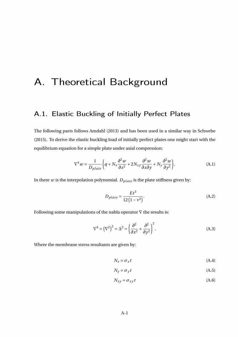
A. Theoretical Background
A.1. Elastic Buckling of Initially Perfect Plates
The following parts follows Amdahl (2013) and has been used in a similar way in Schwebe
(2015). To derive the elastic buckling load of initially perfect plates one might start with the
equilibrium equation for a simple plate under axial compression:
r4w = 1Dpl ate
µq +Nx
@2w@x2 +2Nx y
@2w@x@y
+Ny@2w@y2
∂. (A.1)
In there w is the interpolation polynomial. Dpl ate is the plate stiffness given by:
Dpl ate =Et 3
12°1°∫2
¢ . (A.2)
Following some manipulations of the nabla operator r the results is:
r4 =°r2¢2 =¢2 =
µ@2
@x2 + @2
@y2
∂2
. (A.3)
Where the membrane stress resultants are given by:
Nx =æx t (A.4)
Ny =æy t (A.5)
Nx y =æx y t (A.6)
A-1
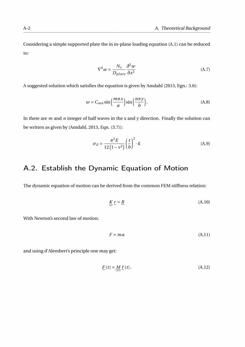
A-2 A. Theoretical Background
Considering a simple supported plate the in in-plane loading equation (A.1) can be reduced
to:
r4w = Nx
Dpl ate
@2w@x2 (A.7)
A suggested solution which satisfies the equation is given by Amdahl (2013, Egn.: 3.6):
w =Cmn sin≥mºx
a
¥sin
≥nºyb
¥. (A.8)
In there are m and n integer of half waves in the x and y direction. Finally the solution can
be written as given by (Amdahl, 2013, Eqn. (3.7)):
æE = º2E
12°1°∫2
¢µ
tb
∂2
·k (A.9)
A.2. Establish the Dynamic Equation of Motion
The dynamic equation of motion can be derived from the common FEM stiffness relation:
K r = R (A.10)
With Newton’s second law of motion:
F = ma (A.11)
and using d’Alembert’s principle one may get:
F (t ) = M r (t ) . (A.12)
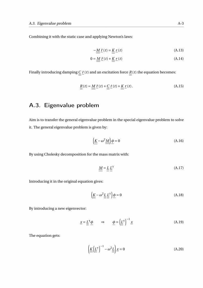
A.3. Eigenvalue problem A-3
Combining it with the static case and applying Newton’s laws:
°M r (t ) = K r (t ) (A.13)
0 = M r (t )+K r (t ) (A.14)
Finally introducing damping C r (t ) and an excitation force R (t ) the equation becomes:
R (t ) = M r (t )+C r (t )+K r (t ) . (A.15)
A.3. Eigenvalue problem
Aim is to transfer the general eigenvalue problem in the special eigenvalue problem to solve
it. The general eigenvalue problem is given by:
≥K °!2M
¥¡= 0 (A.16)
By using Cholesky decomposition for the mass matrix with:
M = L L| (A.17)
Introducing it in the original equation gives:
≥K °!2L L|
¥¡= 0 (A.18)
By introducing a new eigenvector:
x = L|¡ ) ¡=≥L|
¥°1x (A.19)
The equation gets:
µK
≥L|
¥°1°!2L
∂x = 0 (A.20)
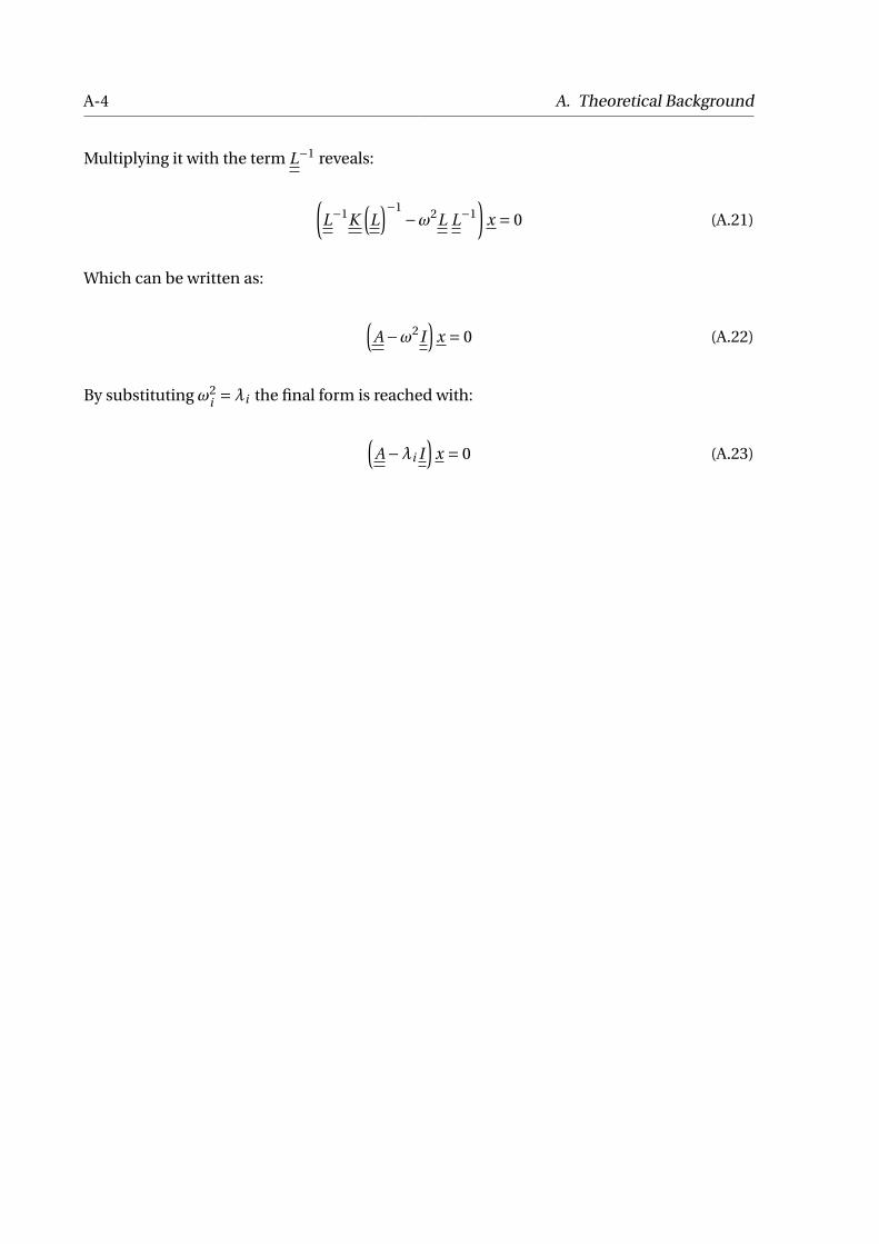
A-4 A. Theoretical Background
Multiplying it with the term L°1 reveals:
µL°1K
≥L¥°1
°!2L L°1∂
x = 0 (A.21)
Which can be written as:
≥A°!2I
¥x = 0 (A.22)
By substituting !2i =∏i the final form is reached with:
≥A°∏i I
¥x = 0 (A.23)
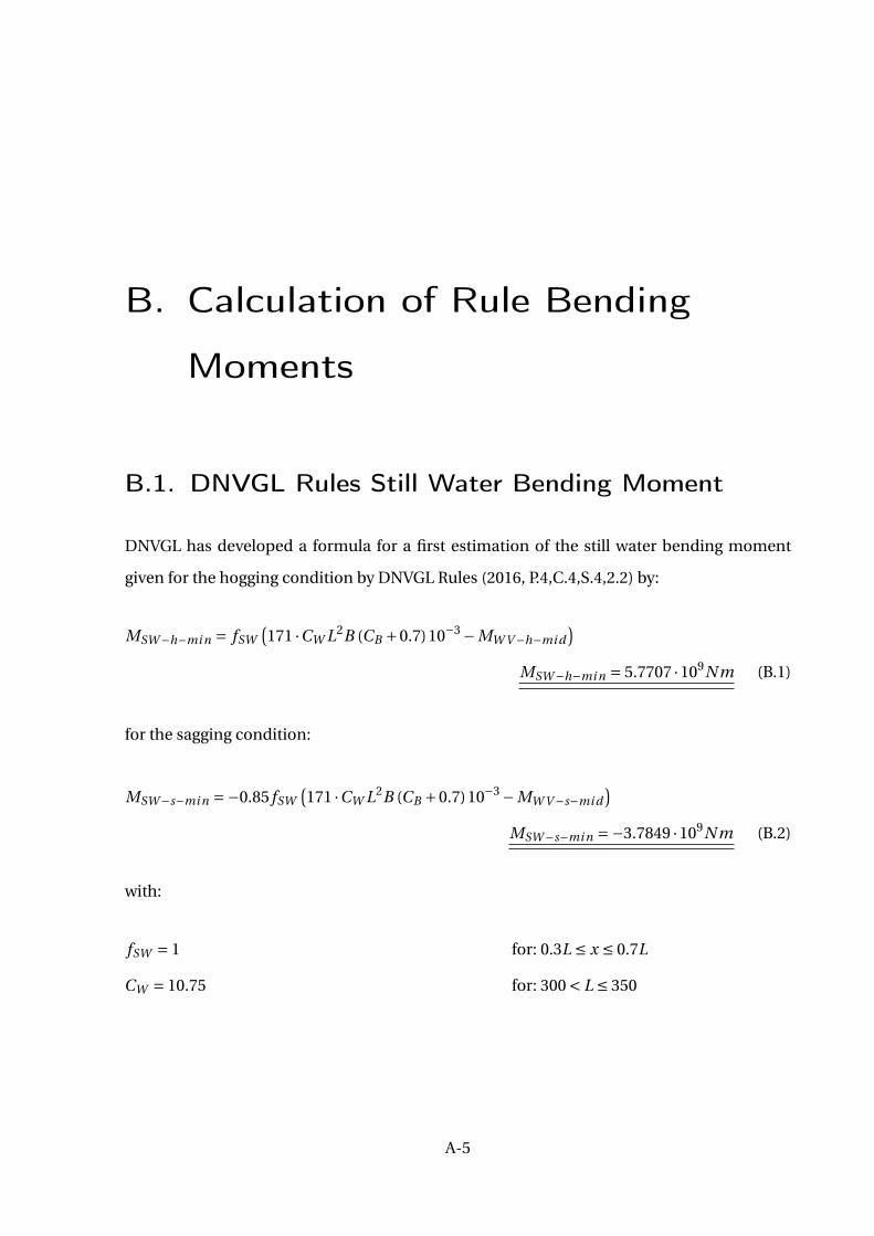
B. Calculation of Rule Bending
Moments
B.1. DNVGL Rules Still Water Bending Moment
DNVGL has developed a formula for a first estimation of the still water bending moment
given for the hogging condition by DNVGL Rules (2016, P.4,C.4,S.4,2.2) by:
MSW °h°mi n = fSW°171 ·CW L2B (CB +0.7)10°3 °MW V °h°mi d
¢
MSW °h°mi n = 5.7707 ·109N m (B.1)
for the sagging condition:
MSW °s°mi n =°0.85 fSW°171 ·CW L2B (CB +0.7)10°3 °MW V °s°mi d
¢
MSW °s°mi n =°3.7849 ·109N m (B.2)
with:
fSW = 1 for: 0.3L ∑ x ∑ 0.7L
CW = 10.75 for: 300 < L ∑ 350
A-5
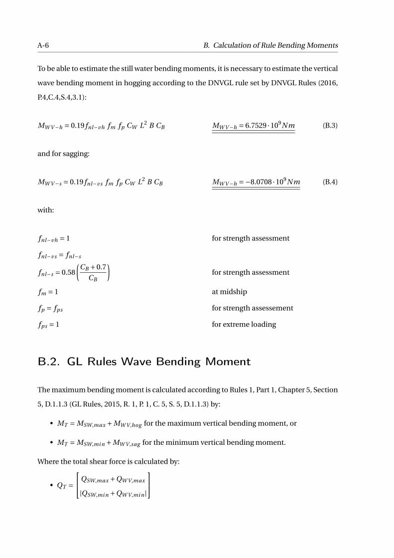
A-6 B. Calculation of Rule Bending Moments
To be able to estimate the still water bending moments, it is necessary to estimate the vertical
wave bending moment in hogging according to the DNVGL rule set by DNVGL Rules (2016,
P.4,C.4,S.4,3.1):
MW V °h = 0.19 fnl°vh fm fp CW L2 B CB MW V °h = 6.7529 ·109N m (B.3)
and for sagging:
MW V °s = 0.19 fnl°v s fm fp CW L2 B CB MW V °h =°8.0708 ·109N m (B.4)
with:
fnl°vh = 1 for strength assessment
fnl°v s = fnl°s
fnl°s = 0.58µ
CB +0.7CB
∂for strength assessment
fm = 1 at midship
fp = fps for strength assessement
fps = 1 for extreme loading
B.2. GL Rules Wave Bending Moment
The maximum bending moment is calculated according to Rules 1, Part 1, Chapter 5, Section
5, D.1.1.3 (GL Rules, 2015, R. 1, P. 1, C. 5, S. 5, D.1.1.3) by:
• MT = MSW,max +MW V ,hog for the maximum vertical bending moment, or
• MT = MSW,mi n +MW V ,sag for the minimum vertical bending moment.
Where the total shear force is calculated by:
• QT =
2
4 QSW,max +QW V ,max
|QSW,mi n +QW V ,mi n |
3
5
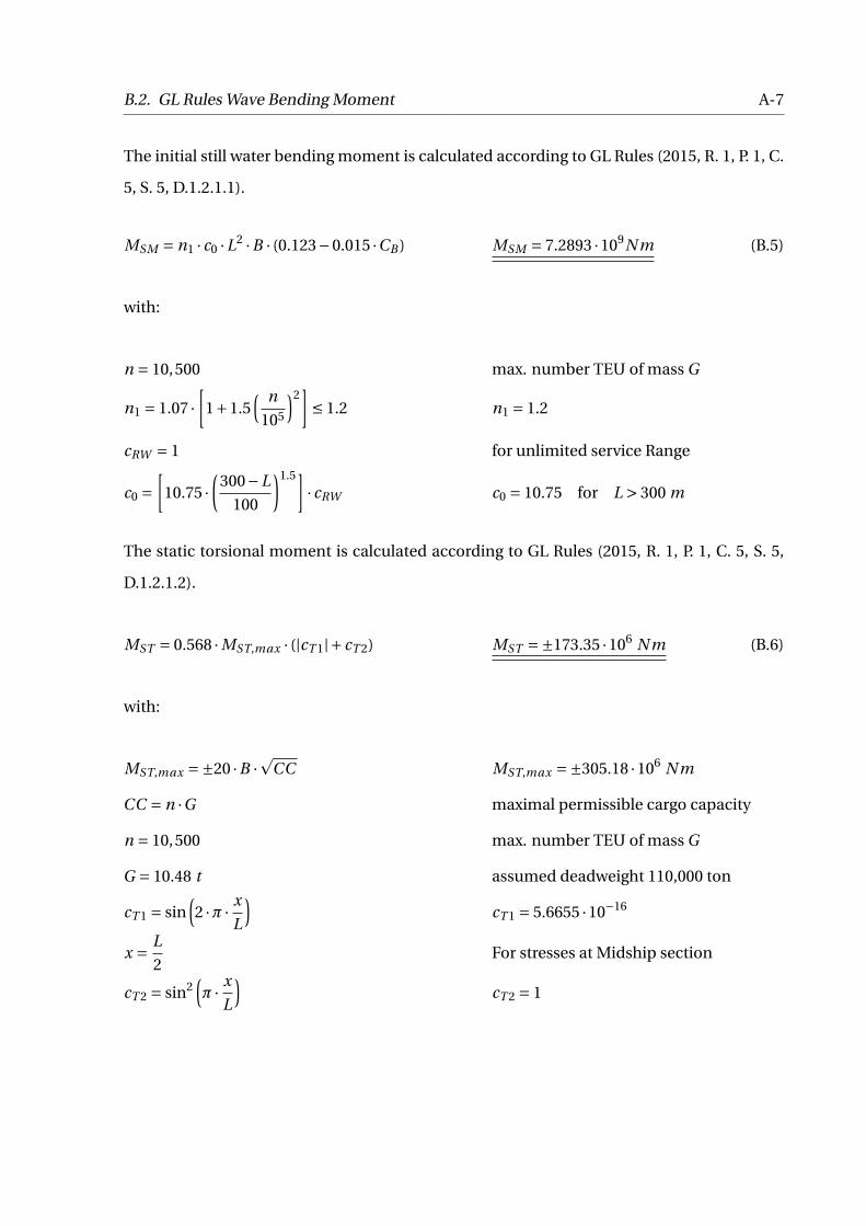
B.2. GL Rules Wave Bending Moment A-7
The initial still water bending moment is calculated according to GL Rules (2015, R. 1, P. 1, C.
5, S. 5, D.1.2.1.1).
MSM = n1 · c0 ·L2 ·B · (0.123°0.015 ·CB ) MSM = 7.2893 ·109N m (B.5)
with:
n = 10,500 max. number TEU of mass G
n1 = 1.07 ·∑
1+1.5≥ n
105
¥2∏∑ 1.2 n1 = 1.2
cRW = 1 for unlimited service Range
c0 =∑
10.75 ·µ
300°L100
∂1.5∏· cRW c0 = 10.75 for L > 300 m
The static torsional moment is calculated according to GL Rules (2015, R. 1, P. 1, C. 5, S. 5,
D.1.2.1.2).
MST = 0.568 ·MST,max · (|cT 1|+ cT 2) MST =±173.35 ·106 N m (B.6)
with:
MST,max =±20 ·B ·p
CC MST,max =±305.18 ·106 N m
CC = n ·G maximal permissible cargo capacity
n = 10,500 max. number TEU of mass G
G = 10.48 t assumed deadweight 110,000 ton
cT 1 = sin≥2 ·º · x
L
¥cT 1 = 5.6655 ·10°16
x = L2
For stresses at Midship section
cT 2 = sin2≥º · x
L
¥cT 2 = 1

A-8 B. Calculation of Rule Bending Moments
Dynamic loads are calculated starting by the vertical wave bending moment in hogging. (GL
Rules, 2015, R. 1, P. 1, C. 5, S. 5, D.1.3.1)
MW V ,hog = L2 ·B · c0 · c1 · cM MW V ,hog = 6.9576 ·109 N m (B.7)
with:
c0 =∑
10.75 ·µ
300°L100
∂1.5∏· cRW c0 = 10.75 for L > 300 m
c1,hog = 0.19 ·CB c1,hog = 0.1292
cM = 1 for midship section
For the vertical bending moment in sagging occurs the following result. (GL Rules, 2015, R.
1, P. 1, C. 5, S. 5, D.1.3.1)
MW V ,sag = L2 ·B · c0 · c1 · cM MW V ,sag = 8.1746 ·109 N m (B.8)
with:
c1,sag =°0.11 · (CB +0.7) c1,sag =°0.1518
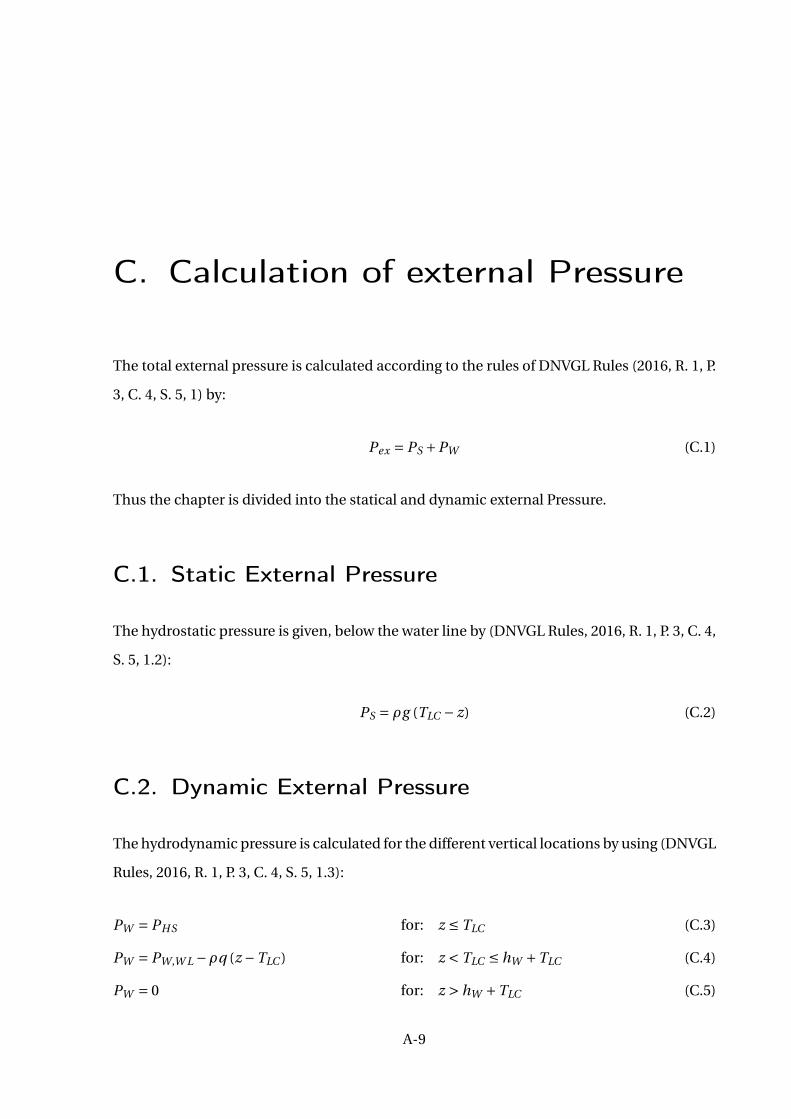
C. Calculation of external Pressure
The total external pressure is calculated according to the rules of DNVGL Rules (2016, R. 1, P.
3, C. 4, S. 5, 1) by:
Pex = PS +PW (C.1)
Thus the chapter is divided into the statical and dynamic external Pressure.
C.1. Static External Pressure
The hydrostatic pressure is given, below the water line by (DNVGL Rules, 2016, R. 1, P. 3, C. 4,
S. 5, 1.2):
PS = Ωg (TLC ° z) (C.2)
C.2. Dynamic External Pressure
The hydrodynamic pressure is calculated for the different vertical locations by using (DNVGL
Rules, 2016, R. 1, P. 3, C. 4, S. 5, 1.3):
PW = PHS for: z ∑ TLC (C.3)
PW = PW,W L °Ωq (z °TLC ) for: z < TLC ∑ hW +TLC (C.4)
PW = 0 for: z > hW +TLC (C.5)
A-9
A-10 C. Calculation of external Pressure
Where the hydrostatic pressure is given by:
PHS =C fT fps fnl fh ka kp fy z CW
sL0 +∏°125
L(C.6)
with:
C fT = fT +0.5°°0.7 · fT °0.2
¢CB (C.7)
fT = 1
fnl = 0.9
fh = 3 ·°1.21°0.66 · fT
¢
ka = 1 for: 0.15 ∑ fxL ∑ 0.7
kp = 1 for: 0.8°0.2 fT
fy z =Cx ·z
TLC+ (2°Cx) fyB +1
Cx = 1.5° |x °0.5L|L
fyB = |2y |Bx
CW = 10.75 for: 300 < L ∑ 350
∏= 340
L0 = 340
Resulting in
PHS = 23.86248 ·≥≥
1.5 · zT
¥+
≥0.5 · y
B/2
¥+1
¥(C.8)
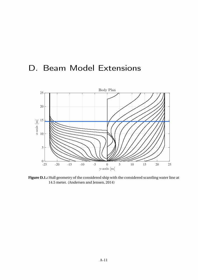
D. Beam Model Extensions
-25 -20 -15 -10 -5 0 5 10 15 20 25
y-axis [m]
0
5
10
15
20
25
z-ax
is[m
]
Body Plan
Figure D.1.: Hull geometry of the considered ship with the considered scantling water line at14.5 meter. (Andersen and Jensen, 2014)
A-11
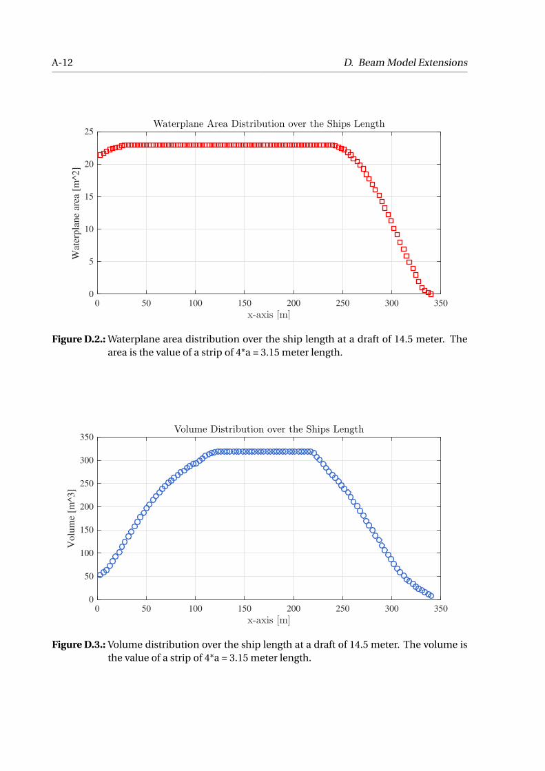
A-12 D. Beam Model Extensions
0 50 100 150 200 250 300 350
x-axis [m]
0
5
10
15
20
25
Wat
erpla
ne
area
[m
^2]
Waterplane Area Distribution over the Ships Length
Figure D.2.: Waterplane area distribution over the ship length at a draft of 14.5 meter. Thearea is the value of a strip of 4*a = 3.15 meter length.
0 50 100 150 200 250 300 350
x-axis [m]
0
50
100
150
200
250
300
350
Volu
me
[m^3]
Volume Distribution over the Ships Length
Figure D.3.: Volume distribution over the ship length at a draft of 14.5 meter. The volume isthe value of a strip of 4*a = 3.15 meter length.
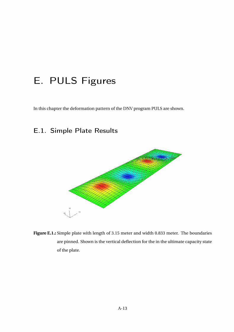
E. PULS Figures
In this chapter the deformation pattern of the DNV program PULS are shown.
E.1. Simple Plate Results
Figure E.1.: Simple plate with length of 3.15 meter and width 0.833 meter. The boundaries
are pinned. Shown is the vertical deflection for the in the ultimate capacity state
of the plate.
A-13

A-14 E. PULS Figures
Figure E.2.: Simple plate with length of 3.15 meter and width 0.833 meter. The boundaries
at the sides are clamped, the boundaries at the short ends are pinned . Shown is
the vertical deflection for the ultimate capacity of the plate.
E.2. Panel Results
Figure E.3.: Model of the double bottom panel between the longitudinal bulkheads and
webs. The length of the panel is 3.15 meter and the width is 6 x 0.833 meter.
Five tee-bar stiffeners with the dimensions of 450x15+100x20 mm are mounted.
The boundaries represent the plate in a continuous hull girder. Shown is the
local imperfection.
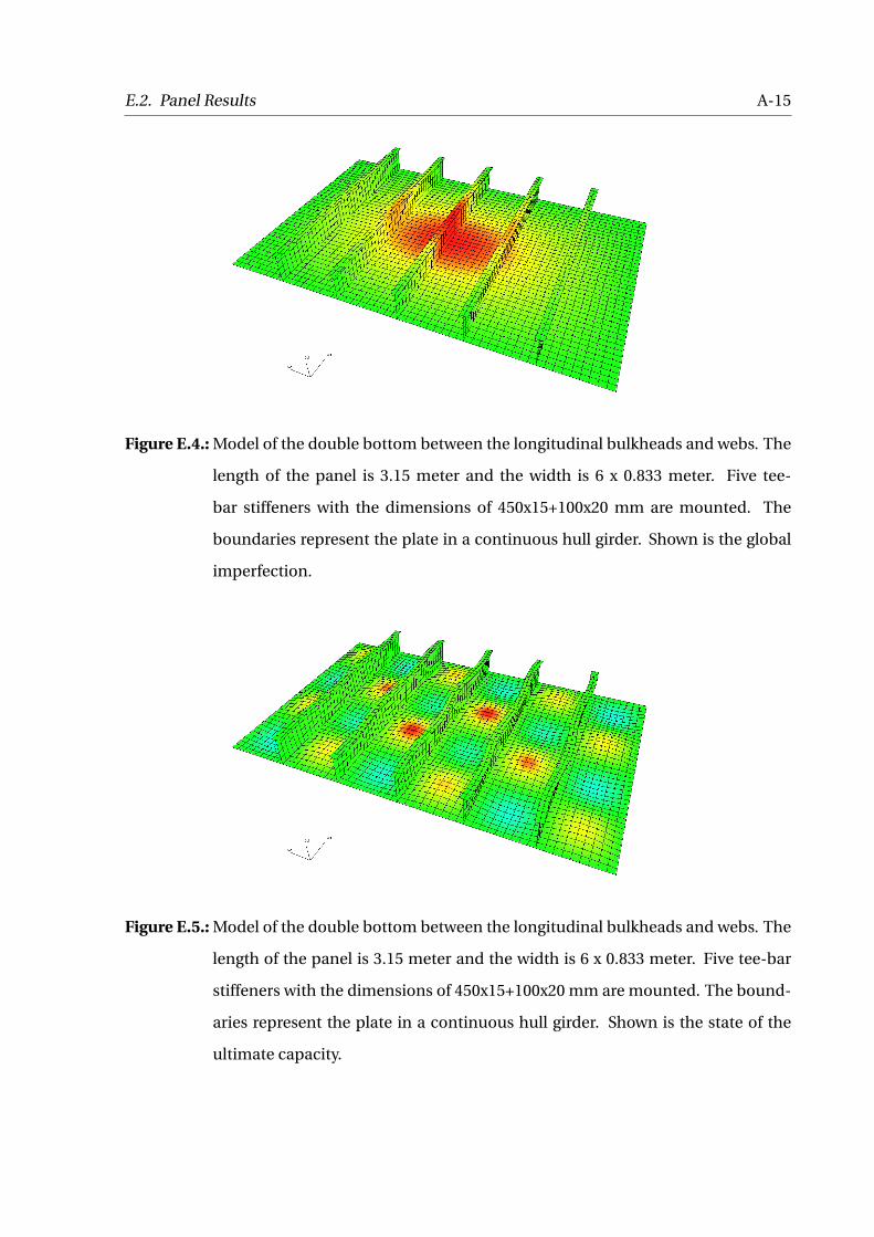
E.2. Panel Results A-15
Figure E.4.: Model of the double bottom between the longitudinal bulkheads and webs. The
length of the panel is 3.15 meter and the width is 6 x 0.833 meter. Five tee-
bar stiffeners with the dimensions of 450x15+100x20 mm are mounted. The
boundaries represent the plate in a continuous hull girder. Shown is the global
imperfection.
Figure E.5.: Model of the double bottom between the longitudinal bulkheads and webs. The
length of the panel is 3.15 meter and the width is 6 x 0.833 meter. Five tee-bar
stiffeners with the dimensions of 450x15+100x20 mm are mounted. The bound-
aries represent the plate in a continuous hull girder. Shown is the state of the
ultimate capacity.

A-16 E. PULS Figures
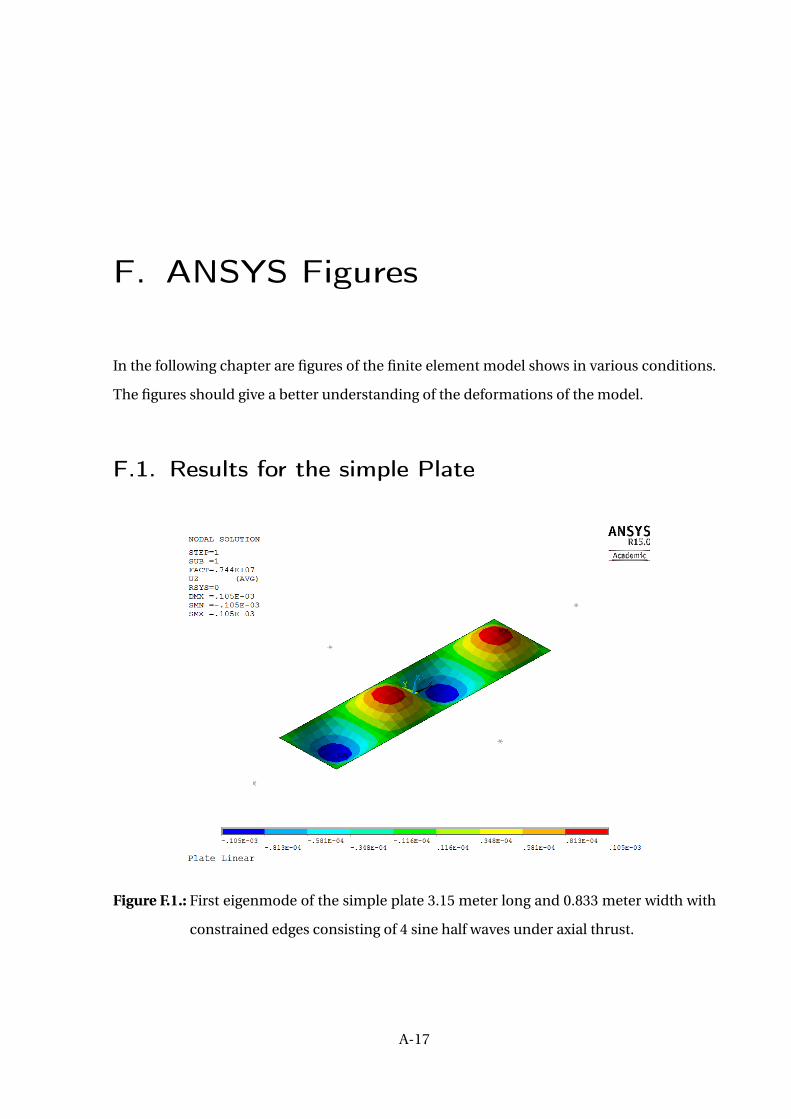
F. ANSYS Figures
In the following chapter are figures of the finite element model shows in various conditions.
The figures should give a better understanding of the deformations of the model.
F.1. Results for the simple Plate
Figure F.1.: First eigenmode of the simple plate 3.15 meter long and 0.833 meter width with
constrained edges consisting of 4 sine half waves under axial thrust.
A-17
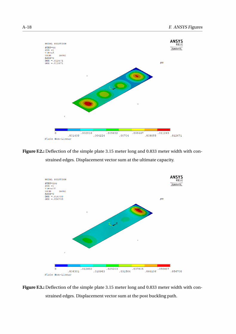
A-18 F. ANSYS Figures
Figure F.2.: Deflection of the simple plate 3.15 meter long and 0.833 meter width with con-
strained edges. Displacement vector sum at the ultimate capacity.
Figure F.3.: Deflection of the simple plate 3.15 meter long and 0.833 meter width with con-
strained edges. Displacement vector sum at the post buckling path.
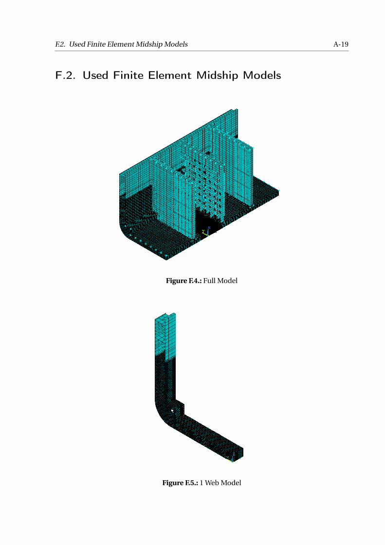
F.2. Used Finite Element Midship Models A-19
F.2. Used Finite Element Midship Models
Figure F.4.: Full Model
Figure F.5.: 1 Web Model

A-20 F. ANSYS Figures
Figure F.6.: 3 Web Model
Figure F.7.: 3 Web Rigid Model & Floating Model

F.3. Ultimate Limit State of 3 Web Model A-21
F.3. Ultimate Limit State of 3 Web Model
Figure F.8.: 3 Web model loaded until ultimate capacity and showing clearly the assumedfour half waves buckling pattern in the bottom region.
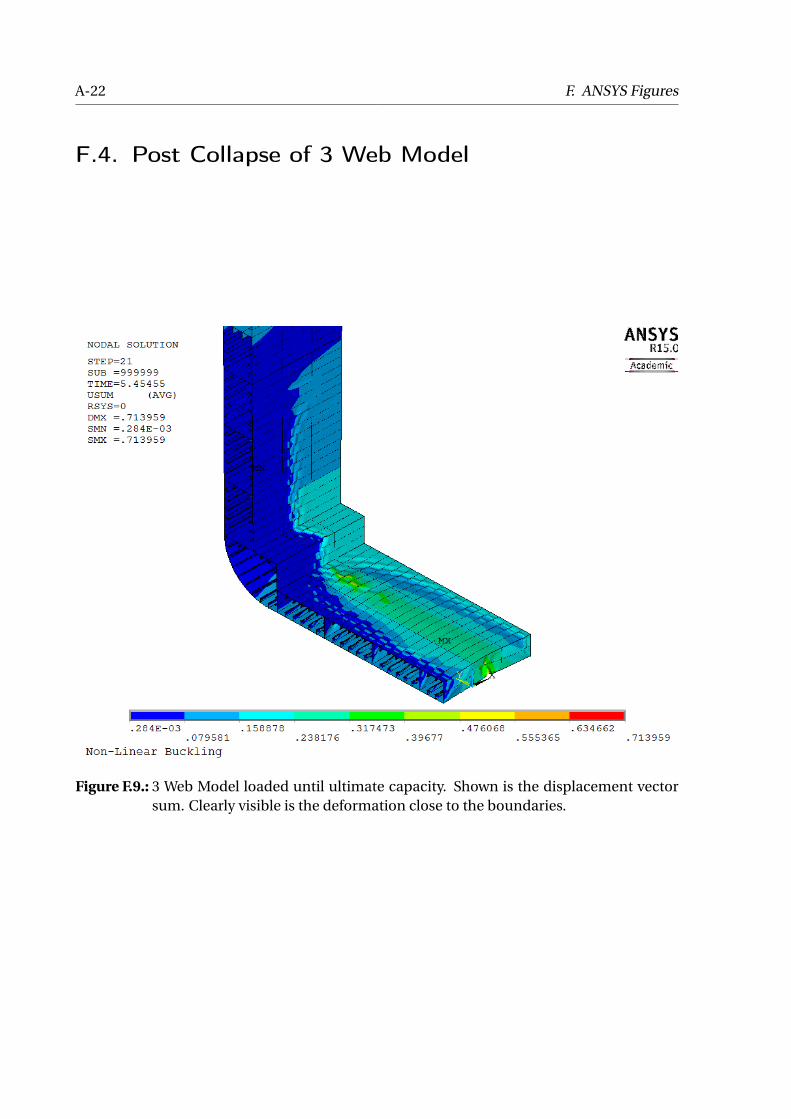
A-22 F. ANSYS Figures
F.4. Post Collapse of 3 Web Model
Figure F.9.: 3 Web Model loaded until ultimate capacity. Shown is the displacement vectorsum. Clearly visible is the deformation close to the boundaries.

F.4. Post Collapse of 3 Web Model A-23
Figure F.10.: Detail of the Crash Section far in the post collapse range. Shown is the displace-ment vector sum. All members have started to deform.
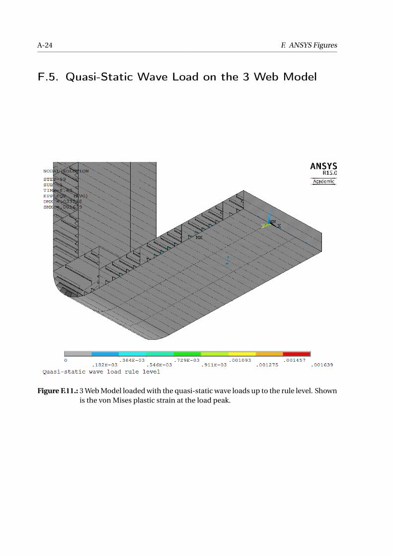
A-24 F. ANSYS Figures
F.5. Quasi-Static Wave Load on the 3 Web Model
Figure F.11.: 3 Web Model loaded with the quasi-static wave loads up to the rule level. Shownis the von Mises plastic strain at the load peak.
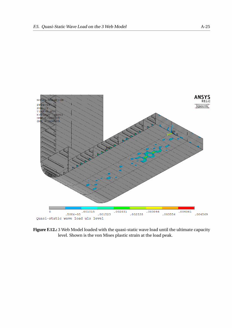
F.5. Quasi-Static Wave Load on the 3 Web Model A-25
Figure F.12.: 3 Web Model loaded with the quasi-static wave load until the ultimate capacitylevel. Shown is the von Mises plastic strain at the load peak.

A-26 F. ANSYS Figures
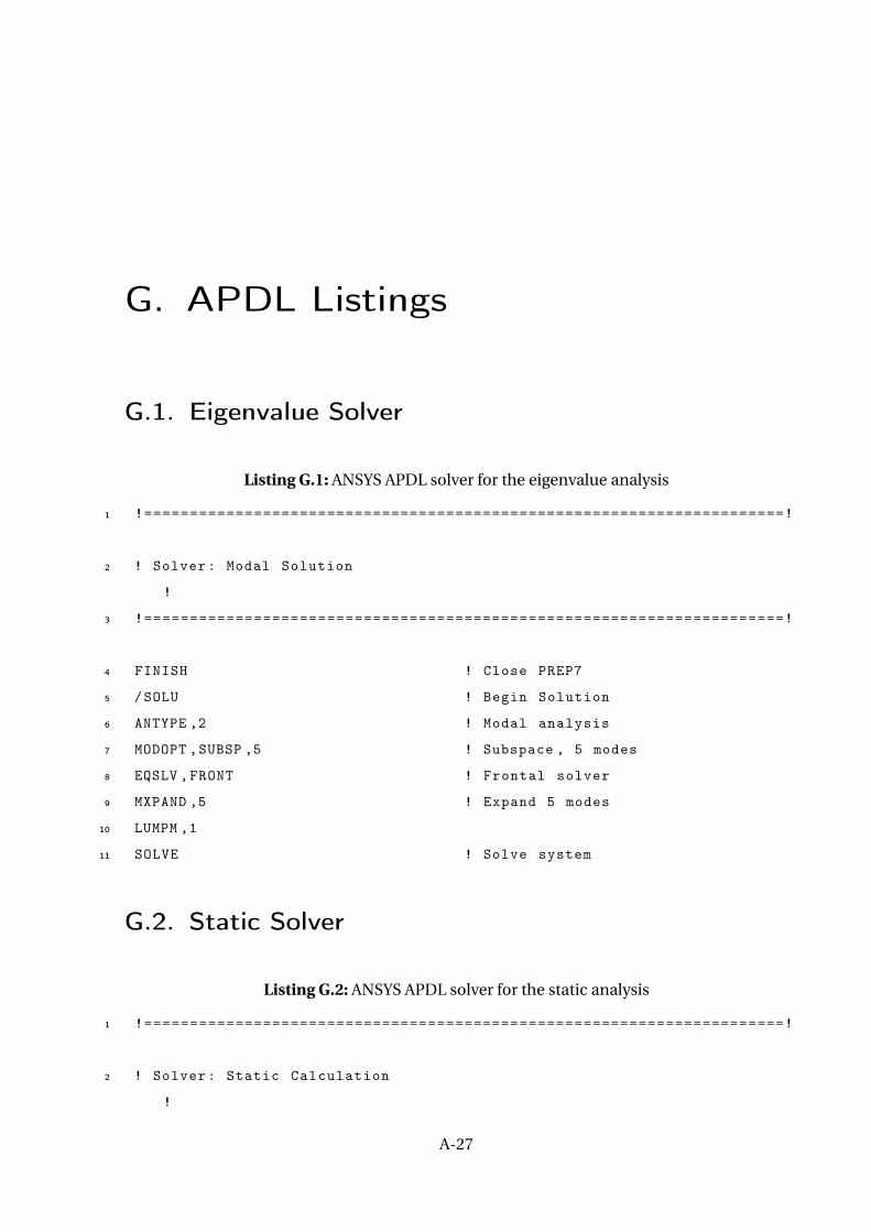
G. APDL Listings
G.1. Eigenvalue Solver
Listing G.1: ANSYS APDL solver for the eigenvalue analysis
1 !======================================================================!
2 ! Solver: Modal Solution
!
3 !======================================================================!
4 FINISH ! Close PREP7
5 /SOLU ! Begin Solution
6 ANTYPE ,2 ! Modal analysis
7 MODOPT ,SUBSP ,5 ! Subspace , 5 modes
8 EQSLV ,FRONT ! Frontal solver
9 MXPAND ,5 ! Expand 5 modes
10 LUMPM ,1
11 SOLVE ! Solve system
G.2. Static Solver
Listing G.2: ANSYS APDL solver for the static analysis
1 !======================================================================!
2 ! Solver: Static Calculation
!
A-27
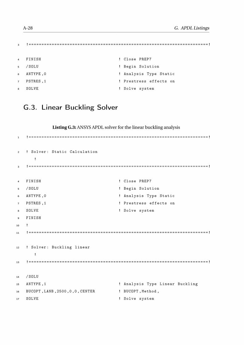
A-28 G. APDL Listings
3 !======================================================================!
4 FINISH ! Close PREP7
5 /SOLU ! Begin Solution
6 ANTYPE ,0 ! Analysis Type Static
7 PSTRES ,1 ! Prestress effects on
8 SOLVE ! Solve system
G.3. Linear Buckling Solver
Listing G.3: ANSYS APDL solver for the linear buckling analysis
1 !======================================================================!
2 ! Solver: Static Calculation
!
3 !======================================================================!
4 FINISH ! Close PREP7
5 /SOLU ! Begin Solution
6 ANTYPE ,0 ! Analysis Type Static
7 PSTRES ,1 ! Prestress effects on
8 SOLVE ! Solve system
9 FINISH
10 !
11 !======================================================================!
12 ! Solver: Buckling linear
!
13 !======================================================================!
14 /SOLU
15 ANTYPE ,1 ! Analysis Type Linear Buckling
16 BUCOPT ,LANB ,2500,0,0, CENTER ! BUCOPT ,Method ,
17 SOLVE ! Solve system
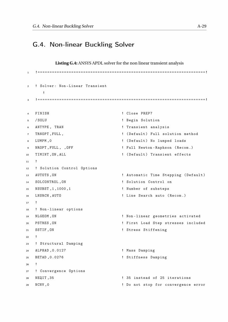
G.4. Non-linear Buckling Solver A-29
G.4. Non-linear Buckling Solver
Listing G.4: ANSYS APDL solver for the non linear transient analysis
1 !======================================================================!
2 ! Solver: Non -Linear Transient
!
3 !======================================================================!
4 FINISH ! Close PREP7
5 /SOLU ! Begin Solution
6 ANTYPE , TRAN ! Transient analysis
7 TRNOPT ,FULL , ! (Default) Full solution method
8 LUMPM ,0 ! (Default) No lumped loads
9 NROPT ,FULL , ,OFF ! Full Newton -Raphson (Recom .)
10 TIMINT ,ON,ALL ! (Default) Transient effects
11 !
12 ! Solution Control Options
13 AUTOTS ,ON ! Automatic Time Stepping (Default)
14 SOLCONTROL ,ON ! Solution Control on
15 NSUBST ,1 ,1000,1 ! Number of substeps
16 LNSRCH ,AUTO ! Line Search auto (Recom .)
17 !
18 ! Non -linear options
19 NLGEOM ,ON ! Non -linear geometries activated
20 PSTRES ,ON ! First Load Step stresses included
21 SSTIF ,ON ! Stress Stiffening
22 !
23 ! Structural Damping
24 ALPHAD ,0.0127 ! Mass Damping
25 BETAD ,0.0276 ! Stiffness Damping
26 !
27 ! Convergence Options
28 NEQIT ,35 ! 35 instead of 25 iterations
29 NCNV ,0 ! Do not stop for convergence error
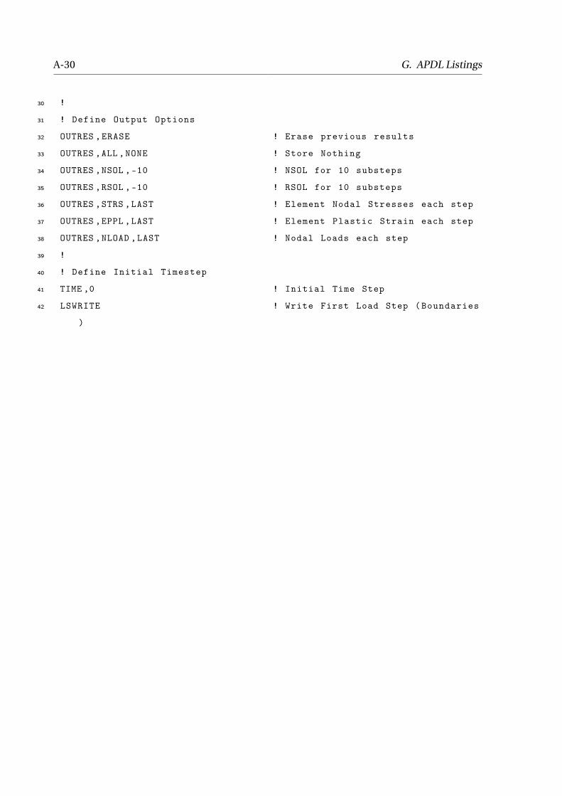
A-30 G. APDL Listings
30 !
31 ! Define Output Options
32 OUTRES ,ERASE ! Erase previous results
33 OUTRES ,ALL ,NONE ! Store Nothing
34 OUTRES ,NSOL ,-10 ! NSOL for 10 substeps
35 OUTRES ,RSOL ,-10 ! RSOL for 10 substeps
36 OUTRES ,STRS ,LAST ! Element Nodal Stresses each step
37 OUTRES ,EPPL ,LAST ! Element Plastic Strain each step
38 OUTRES ,NLOAD ,LAST ! Nodal Loads each step
39 !
40 ! Define Initial Timestep
41 TIME ,0 ! Initial Time Step
42 LSWRITE ! Write First Load Step (Boundaries
)
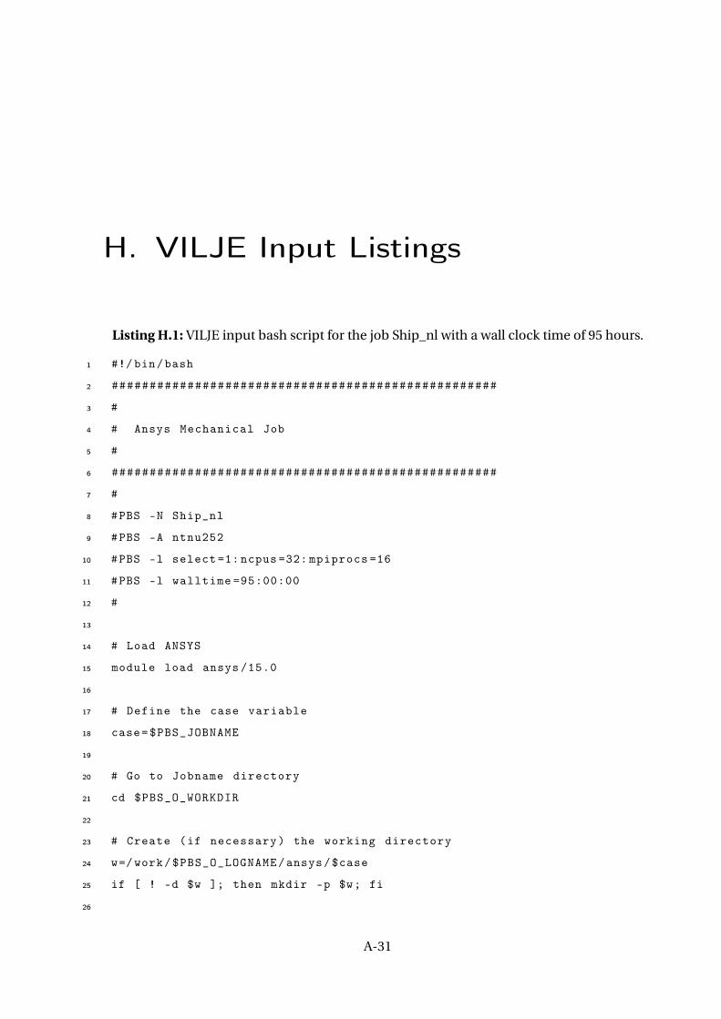
H. VILJE Input Listings
Listing H.1: VILJE input bash script for the job Ship_nl with a wall clock time of 95 hours.
1 #!/ bin/bash
2 ###################################################
3 #
4 # Ansys Mechanical Job
5 #
6 ###################################################
7 #
8 #PBS -N Ship_nl
9 #PBS -A ntnu252
10 #PBS -l select =1: ncpus =32: mpiprocs =16
11 #PBS -l walltime =95:00:00
12 #
13
14 # Load ANSYS
15 module load ansys /15.0
16
17 # Define the case variable
18 case=$PBS_JOBNAME
19
20 # Go to Jobname directory
21 cd $PBS_O_WORKDIR
22
23 # Create (if necessary) the working directory
24 w=/work/$PBS_O_LOGNAME/ansys/$case
25 if [ ! -d $w ]; then mkdir -p $w; fi
26
A-31

A-32 H. VILJE Input Listings
27 # Copy inputfiles and move to working directory
28 cp $case.db $w
29 cp $case.inp $w
30 cd $w
31
32 machines=‘uniq -c ${PBS_NODEFILE} | awk ’{print $2 ":" $1}’ | paste -s
-d ’:’‘
33
34 export MPI_WORKDIR=$w
35
36 ansys150 -j $case -b -dis -usessh -machines $machines -i $case.inp -o
$case.out
37
38 # Copying the results back to the own directory
39 cp $case.out /home/ntnu/tjarkts/$case/
40 cp Ship_nl0.err /home/ntnu/tjarkts/$case/
41 cp $case.db /home/ntnu/tjarkts/$case/
42 cp $case.rst /home/ntnu/tjarkts/$case/