ETE471 (LAB)

Lab 1: Introduction to MATLAB

PART I

1. Warm-up

MATLAB is a high-level programming language that has been used extensively to solve complex engineering problems. MATLAB works with three types of windows on your computer screen. These are the

1. Command window,

2. The Figure window and 3. The Editor window.

The Figure window only pops up whenever you plot something.

The Editor window is used for writing and editing MATLAB programs (called M-

files) and can be invoked in Windows from the pull-down menu after selecting File | New | M-file. In UNIX, the Editor window pops up when you type in the command window: edit filename („filename‟ is the name of the file you want to create).

The command window is the main window in which you communicate with the

MATLAB interpreter. The MATLAB interpreter displays a command >> indicating that it is ready to accept commands from you.

• View the MATLAB introduction by typing >> intro

at the MATLAB prompt. This short introduction will demonstrate some basic MATLAB commands. • Explore MATLAB‟s help capability by trying the following:

>> help >> help plot >> help ops >> help arith

• Type demo and explore some of the demos of MATLAB commands. • You can use the command window as a calculator, or you can use it to call other MATLAB programs (M-files). Say you want to evaluate the expression a3

bd 4c , where a 1.2 , b 2.3 , c 4.5 and d 4 . Then in the command window, type:

>> a = 1.2; >> b=2.3; >> c=4.5; >> d=4; >> a^3+sqrt(b*d)-4*c

ans = -13.2388

Note the semicolon after each variable assignment. If you omit the semicolon, then MATLAB echoes back on the screen the variable value.

2. Arithmetic Operations

There are four different arithmetic operators: + addition - subtraction * multiplication / division (for matrices it also means inversion) There are also three other operators that operate on an element by element basis:

.* multiplication of two vectors, element by element ./ division of two vectors, element-wise .^ raise all the elements of a vector to a power.

Suppose that we have the vectors x [x1 , x2 ,.........., xn ] and. Then x.* y [x1 y1 , x2 y2 ,.......,xn yn ] x./ y [x1 / y1 , x2 / y2 ,.......,xn /

yn ] x.^ p [x1 p , x2 p ,.......,xn p ]

The arithmetic operators + and — can be used to add or subtract matrices, scalars or vectors.

By vectors we mean one-dimensional arrays and by matrices we mean multi-dimensional arrays.

This terminology of vectors and matrices comes from Linear Algebra.

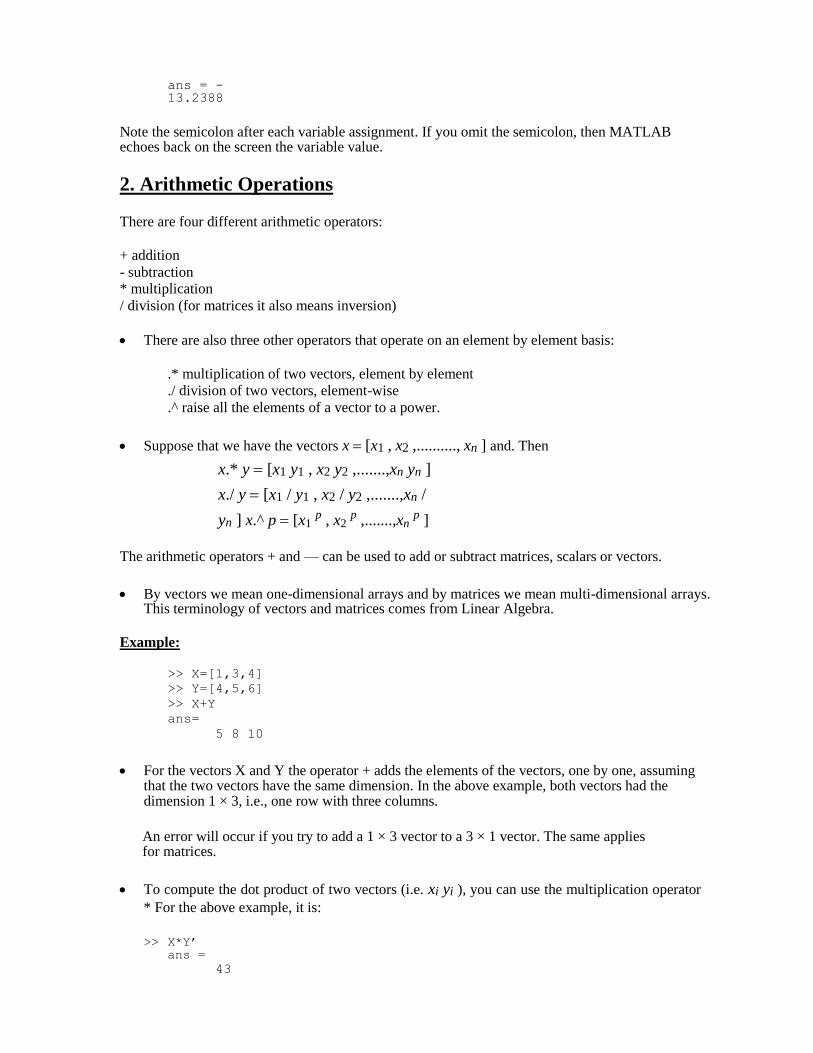
Example:

>> X=[1,3,4] >> Y=[4,5,6] >> X+Y ans=

5 8 10

For the vectors X and Y the operator + adds the elements of the vectors, one by one, assuming

that the two vectors have the same dimension. In the above example, both vectors had the dimension 1 × 3, i.e., one row with three columns.

An error will occur if you try to add a 1 × 3 vector to a 3 × 1 vector. The same applies for matrices.

To compute the dot product of two vectors (i.e. xi yi ), you can use the multiplication operator

* For the above example, it is:

>> X*Y’

ans =

43

Note the single quote after Y. The single quote denotes the transpose of a matrix or a vector.

To compute an element by element multiplication of two vectors (or two arrays), you can use the .* operator:

>> X .* Y ans = 4 15 24

That is, X.*Y means [1×4, 3×5, 4×6] = [4 15 24]. The „.*‟ operator is used very often (and is highly recommended) because it is executed much faster compared to the code that uses for loops.

3. Complex numbers

MATLAB also supports complex numbers. The imaginary number is denoted with the symbol i or j, assuming that you did not use these symbols anywhere in your program (that is very important!). Try the following:

>> z=3 + 4i % note that you do not need the ‘*’ after 4 >> conj(z) % computes the conjugate of z >> angle(z) % computes the phase of z >> real(z) % computes the real part of z >> imag(z) % computes the imaginary part of z >> abs(z) % computes the magnitude of z

4. Array indexing

In MATLAB, all arrays (vectors) are indexed starting with 1, i.e., y(1) is the first element of the array y. Note that the arrays are indexed using parenthesis (.) and not square brackets [.] as in C/C++. To create an array having as elements the integers 1 through 6, just enter:

>> x=[1,2,3,4,5,6] Alternatively, you can use the : notation,

>> x=1:6

The colon( “:”) notation above creates a vector starting from 1 to 6, in steps of 1. If you want to create a vector from 1 to 6 in steps of say 2, then type:

>> x=1:2:6

Ans = 1 3 5

Try the following code:

>> a=2:4:17 >> b=20:-2:0

>> a=2:(1/10):4 Extracting or inserting numbers in a vector can be done very easily. To concatenate an array, you can use the [ ] operator, as shown in the example below:

>> x=[1:3 4 6 100:110]

To access a subset of the array, try the following:

>> x(3:7) >> length(x) % gives the size of the array or vector >> x(2:2:length(x))

5. Allocating memory

You can allocate memory for one-dimensional arrays (vectors) using the zeros command. The following command allocates memory for a 100-dimensional array:

>> Y=zeros(100,1); >> Y(30)

ans = 0

Similarly, you can allocate memory for two-dimensional arrays (matrices). The command

>> Y=zeros(4,5)

defines a 4 by 5 matrix. Similar to the zeros command, you can use the command ones to define a vector containing all ones,

>> Y=ones(1,5)

ans= 1 1 1 1 1

6. Special characters and functions

Some common special characters used in MATLAB are given below: Symbol Meaning

pi ð(3.14...)

sqrt indicates square root e.g., sqrt(4)=2

ˆ indicates power(e.g., 3ˆ2=9)

abs Absolute value | .| e.g., abs(-3)=3

; Indicates the end of a row in a matrix. It is also used to suppress printing on the screen (echo o.)

% Denotes a comment. Anything to the right of % is ignored by the MATLAB interpreter and

is considered as comments

‟ Denotes transpose of a vector or matrix. It‟s also used to define strings, e.g.,str1=‟DSP‟;

Some special functions are given below:

length(x) - gives the dimension of the array x size(x) - Finds the size of array x.

Example:

>> x=1:10;

>> length(x)

ans = 10

The function size works similarly. But the output is slightly different. Example:

>> x=2:8;

>> size(x) ans = 1 7

Here, 1 in the answer is the number of rows in the vector x, while 7 denotes the number of columns.

PART II

1. Control flow

MATLAB has the following flow control constructs: • if statements • switch statements

• for loops • while loops • break statements

The if, for, switch and while statements need to terminate with an end statement.

If statement: The general form of a simple if-else statement is:

if relation

statements end

The general form of a simple if-elseif-else statement is:

if relation

statements

elseif relation statements

else statements

end

Statement syntax Example

if <case> if x > 10 <do this> y = y + 1;

elseif <case> elseif x > 5 <do this> y = y – 1;

else else

<do this> y = y – 4; end end

Example:

x=-3; if x>0

str=’positive’

elseif x<0 str=’negative’

elseif x= = 0 str=’zero’

else

str=’error’ end

What is the value of ‟str‟ after execution of the above code?

While statement:

The general form of a while loop is: while relation statements end

Statement syntax Example

while <case> while x < 20 <do this> y = y/3;

end x = x + 1; end

Example:

x=-10;

while x<0

x=x+1;

end

What is the value of x after execution of the above loop?

For loop: Statement syntax Example

for <variable = statement> for n = 1:1:10 <do this> x(n) = 2*n; end end

Example: X=0;

for i=1:10

X=X+1; end

The above code computes the sum of all numbers from 1 to 10.

Break:

The break statement lets you exit early from a for or a while loop:

x=-10; while x < 0

x=x+2;

if x = = -2

break;

end

end

MATLAB supports the following relational and logical operators:

2. Relational Operators:

Symbol Meaning

<= Less than equal < Less than

>= Greater than equal > Greater than

== Equal

˜ = Not equal

3. Logical Operators:

Symbol Meaning & AND | OR ˜ (tilde) NOT

4. Polynomials:

Polynomials in MATLAB are represented by arrays. The usual representation is that the elements in an array are the coefficients of the polynomial starting from the highest order term to the lowest order term. If a term is not present then its coefficient is entered as 0. An example is:

y 5x3 9x 1 is represented by

>> y = [5 0 9 1]

The other way to represent polynomials is via their roots. In MATLAB these are also represented by arrays. The polynomial:

y (x 3)(x 5)(x 9) is represented by

>> y = [-3 5 -9];

Two very useful commands are roots and poly.

The command roots() will factorize a polynomial into its roots and return the roots in an

array.

The function poly() does the opposite. It takes in the roots of a polynomial and returns the coefficients of the polynomial.

5. Generating sinusoidal waves:

Example

To generate a sine wave y 5sin(210t)

f = 10;

A = 5; t = 0:0.001:1; y = A*sin(2*pi*f*t)

6. Plotting

You can plot arrays using MATLAB‟s function plot. The function plot (.) is used to generate line plots. The function stem(.) plots every point of the array without connecting them with a smooth line.

More generally, plot(X,Y) plots vector Y versus vector X. Various line types, plot symbols and colors may be obtained using plot(X,Y,S) where S is a character string indicating the color of the line, and the type of line (e.g., dashed, solid, dotted, etc.). Examples for the string S include:

r red + plus -- dashed g green * star b blue s square

You can insert x-labels, y-labels and title to the plots, using the functions xlabel(.), ylabel(.) and title(.) respectively.

To plot two or more graphs on the same figure, use the command subplot.

For instance, to show the above sine wave, type: >> plot(t,y)

Again, using the stem command: >> stem(t,y)

To plot the two figures in the same plot, type:

>> subplot(2,1,1), plot(y) >> subplot(2,1,2), stem(y)

The (m,n,p) argument in the subplot command indicates that the figure will be split in m rows and n columns. The „p‟ argument takes the values 1, 2, . . . , m× n. In the example above, m = 2, n = 1,and, p = 1 for the top figure and p = 2 for the bottom figure. To get more help on plotting, type: help plot or help subplot.

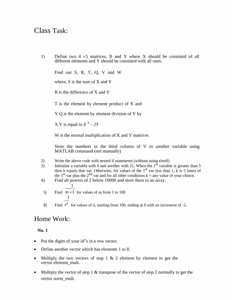
Class Task:

1) Define two 4 5 matrices, X and Y where X should be consisted of all different elements and Y should be consisted with all ones.

Find out S, R, T, Q, V and W

where, S is the sum of X and Y

R is the difference of X and Y

T is the element by element product of X and

Y Q is the element by element division of Y by

X V is equal to X 3 2Y

W is the normal multiplication of X and Y matrices

Store the numbers in the third column of V in another variable using MATLAB command (not manually)

2) Write the above code with nested if statements (without using elseif) 3) Initialize a variable with 6 and another with 21. When the 1st variable is greater than 5

then k equals that var. Otherwise, for values of the 1st var less than 1, k is 5 times of

the 1st var plus the 2nd var and for all other conditions k = any value of your choice. 4) Find all powers of 2 below 10000 and store them in an array.

5) Find

1

for values of m from 1 to 100

m 1

6) Find

1

for values of n, starting from 100, ending at 0 with an increment of -2.

en

Home Work:

No. 1

Put the digits of your id‟s in a row vector. Define another vector which has elements 1 to 8. Multiply the two vectors of step 1 & 2 element by element to get the

vector element_mult.

Multiply the vector of step 1 & transpose of the vector of step 2 normally to get the

vector norm_mult.

Now multiply element_mult & norm_mult to find final_value. Find the square root of the final value and define this vector as root_fv Obtain the size of the vector element_mult to get the vector sz Use the last element of the id vector as the power of each element of root_fv. Thus find the

vector p. Those having 0 as the last digit of id should use the 2nd

last digit instead.

Define a vector sum, which is the summation of vector p and the 2nd

element of the

size vector s. Find the mean of the vector sum. Display all the values. No. 2:

Define a vector t which has values from 0 to 80 ms with an interval of 0.001 Make two sine waves with frequencies 15 & 30 and amplitudes 10 & 2 respectively. Plot the two sine waves in two different figure windows. Again plot them in the same figure window. Using the subplot command, plot them on the same window, but different plots.

Using the stem function plot them on another figure, again in the same window but

different plots.