de l'Document de travail

PRESENTATION OF THE THREE-ME MODEL: MULTI-SECTOR MACROECONOMIC MODEL FOR THE EVALUATION OF ENVIRONMENTAL AND ENERGY POLICY

N° 2011-10 Mai 2011

Frédéric REYNÈS ♠ ♦, Yasser YEDDIR-TAMSAMANI ♠

Gaël CALLONNEC ♣

♣ ADEME – Agence de l’environnement et de la maîtrise d’énergie ♦ Université libre d’Amsterdam, Institut des études environnementales

♠ OFCE – Observatoire français des conjonctures économiques

OFCE - Centre de recherche en économie de Sciences Po 69, quai d’Orsay - 75340 Paris Cedex 07 Tél/ 01 44 18 54 00 - Fax/ 01 45 56 06 15

www.ofce.sciences-po.fr

1

Presentation of the Three-ME model: Multi-sector

Macroeconomic Model for the Evaluation of Environmental and

Energy policy

Frédéric REYNÈS ♠ ♦, Yasser YEDDIR-TAMSAMANI ♠ and Gaël CALLONNEC ♣

♣ ADEME - French Environment and Energy Management Agency ♦ VU University Amsterdam, IVM - Institute for Environmental Studies

♠ OFCE - French Economic Observatory

Abstract

This paper presents the structure and the main properties of Three-ME. This new model of the

French economy has been especially designed to evaluate the medium and long term impact of

environmental and energy policies at the macroeconomic and sector levels. To do so Three-ME

combines two important features. Firstly, it has the main characteristics of neo-Keynesian models by

assuming a slow adjustment of effective quantities and prices to their notional level. Compared to

standard multi-sectors CGEM, this has the advantage to allow for the existence of under-optimum

equilibriums such as the presence of involuntary unemployment. Secondly, production and

consumption structures are represented with a generalized CES function which allows for the elasticity

of substitution to differ between each couple of inputs or goods. This is an improvement compared to

the standard approach that uses nested CES functions which has the disadvantage to impose a common

elasticity of substitution between the goods located in two different nested structures.

Key word: neo-Keynesian model, macroeconomic modeling, energy and environmental policy

modeling

JEL code: E12, E17, E27, E37, E47, D57, D58

Acknowledgments: The authors acknowledge the financial support of the ADEME.

2

Contents

I Introduction.......................................................................................................................................... 4 

II Overview of the model ....................................................................................................................... 6 

III Demand and supply equilibrium...................................................................................................... 10 

IV The producer ................................................................................................................................... 15 

IV.1 Demand for production factors................................................................................................ 15 

IV.2 Debt in the private sector......................................................................................................... 20 

V The household’s behaviour............................................................................................................... 21 

V.1 Consumption............................................................................................................................. 24 

V.2 Investment................................................................................................................................. 26 

V.3 Saving and financial wealth ...................................................................................................... 28 

VI The labor market ............................................................................................................................. 31 

VII External trade................................................................................................................................. 32 

VII.1 Imports ................................................................................................................................... 33 

VII.2 Exports ................................................................................................................................... 34 

VIII Prices structure ............................................................................................................................. 35 

VIII.1 Production prices .................................................................................................................. 36 

VIII.2 Import market prices............................................................................................................. 39 

VIII.3 Domestic market prices ........................................................................................................ 39 

VIII.4 Consumer price index ........................................................................................................... 40 

IX Interest rate...................................................................................................................................... 41 

X Public administrations behaviour ..................................................................................................... 41 

XI CO2 emissions ................................................................................................................................. 43 

XII Analytical scenarios ....................................................................................................................... 44 

XII.1 Expansionary policy: one GDP point-increase of public spending ........................................ 45 

XII.2 Expansionary policy: decrease of the employer social security rate ...................................... 49 

XII.3 A 50% increase of the oil price .............................................................................................. 52 

XII.4 A increase of one point of the labor participation ratio.......................................................... 54 

Appendix A.  Long term of the model ............................................................................................... 56 

Additive equations........................................................................................................................... 58 

Unit elasticity logarithm equations .................................................................................................. 59 

Accumulation equations .................................................................................................................. 59 

Error correction model (ECM) equations ........................................................................................ 60 

Appendix B.  Generalized CES production function and factors demand ......................................... 61 

GCES production function and factors demand .............................................................................. 61 

GCES consumer utility function and demand for goods ................................................................. 64 

Appendix C.  Glossary of terms used................................................................................................. 66 

Index and exponents ........................................................................................................................ 66 

3

Volume variables............................................................................................................................. 67 

Value variables ................................................................................................................................ 68 

Prices ............................................................................................................................................... 69 

Parameters ....................................................................................................................................... 69 

Appendix D.  The choice of the sectorial disaggregation .................................................................. 72 

Industrie manufacturière.................................................................................................................. 74 

Producteurs et distributeurs de l’énergie ......................................................................................... 80 

Conclusion sur la désagrégation sectorielle..................................................................................... 81 

Sources de données utilisées lors de la désagrégation ..................................................................... 82 

Appendix E.  The structure on French economy at the base year of the model and calibration values

of the elasticities of substitutions ..................................................................................................................... 84 

References ............................................................................................................................................ 93 

4

I Introduction

At the country level, there are generally two types of model able to evaluate of the

economic impact of environmental and energy policy: Computable General Equilibrium

Models (CGEM) and neo-Keynesian macroeconomic models. Widely used to analyze a large

range of economic problems, CGEM have the advantage to combine tractability with a high

level of detail, being able to distinguish different countries, goods, type of consumer, etc1.

Particularly important for the analysis of the economic impact of environmental and energy

policy, they often account for an important number of sectors: e.g. GREEN has 11 sectors

(Burniaux et al., 1992), GEMINI-E3 has 18 sectors of which 5 energy sectors (Bernard and

Vielle, 2008), GEM-E3 has 14 sectors (Capros et al., 1997), IMACLIM-S has 10 sectors

(Ghersi and Thubin, 2009). But CGEM have the drawback to rely on very restrictive

assumptions relative to the functioning of the economy especially in the short and medium

run. CGEM are supply models where the hypothesis of perfect price flexibility often insures

the full and optimal use of production factors and thus rule out permanent or transitory under-

optimum equilibrium such as the presence of involuntary unemployment.

Neo-Keynesian macroeconomic models try to give a more realistic representation of the

actual functioning of the economy taking explicitly into account slow adjustments of prices

and quantities, thus allowing for permanent or transitory under-optimum equilibrium. This

effort seems to have a cost in terms of the detail of the disaggregation which is often limited

to a small number. This is typically the case for currently running macroeconomic models for

the French economy: e.g. MESANGE of the French ministry of Economy has three sectors

(Allard-Prigent et al., 2002), E-Mod of the OFCE (Chauvin et al., 2002) and MASCOTTE of

the French central bank (Baghli et al., 2004) have only one. However, earlier versions of

theses model in the 1980’s and 1990’s had a higher level of disaggregation, between 6 and 8

products (see Economie et Prévision, 1998). But still, neo-Keynesian macroeconomic models

generally do not distinguish between the different types of energy or of transport which are

particularly important for the assessment of environmental and energy policy2. They are thus

likely to neglect the effect of activity transfers in terms of growth and employment from high

to low intensive energy sectors.

1 For a survey on CGEM see Böhringer and Löschel (2006). 2 NEMESIS is an exception with 30 sectors covering 16 European countries (Brécard et al., 2006; Zagamé et al.,

2010)

5

Three-ME (Multi-sector Macroeconomic Model for the Evaluation of Environmental

and Energy policy) is a new model of the French economy developed by ADEME, OFCE and

IVM. Its main purpose is to evaluate the impact of environmental and energy policy measures

on the economy at the macroeconomic and sectoral levels. Having the general structure of

neo-Keynesian macroeconomic models, Three-ME seems more realistic than the standard

CGEM for describing the actual dynamic of the economy at least in the short and medium

run. Disaggregated in 24 sectors with an explicitly distinction between four types of energy

and five types of transports, it allows for the neo-Keynesian short term macroeconomic

modeling approach to catch-up with the most advanced CGEM in terms of sectoral analysis.

Moreover, Three-ME aims to overcome the restriction imposed by nested Constant

Elastiscity of Substitution (CES) functions by assuming a more flexible form of the

production function. This is a clear difference with most CGEM where the technology is

generally represented by a series of nested CES production function (e.g. Bernard and Vielle,

2008; Burniaux et al., 1992). Nested CES functions proposed by Sato (1967) have the

advantage to allow for different elasticity of substitutions between production factors that are

not in the same nested structure. But within the same CES, the elasticity of substitution is

common to all factors. For instance, if several energy inputs are represented within the same

CES, the elasticity of substitution is the same between all these energy inputs. This may be a

very strong assumption in some cases. Three-ME does not impose this restriction by assuming

a generalized CES function where the elasticity of substitution is not necessary common

between all the inputs of the same nested structure. This allows changing easily the

hypotheses about the value of elasticity of substitutions without having to change the structure

of the nest. This flexible form is also assumed to represent the substitutability possibilities

between the different investment and consumption goods.

Section 2 presents an overview of the model by summarizing its main characteristics.

Section 3 describes the demand and supply equilibrium. Section 4 describes the supply side

and shows how we derive a simple specification of the production factor demand from a

generalized CES function. Section 5 and 6 presents respectively the household and the labor

market equations. In each sectors, the wage equation is an augmented Phillips curve including

possible hysteresis phenomena. Under the assumption of full hysteresis, this specification has

the same properties as a Wage Setting (WS) curve in level. Section 7 presents the external

trade equations. Section 8 describes the price structure and how firms in each sector determine

their production price. The behavior of the European Central Bank (ECB) about the

6

determination of the interest rate is presented in Section 9. Section 10 treats the public

administrations equation block. Section 11 deals with the specification of CO2 emissions of

sectors and households by type of fossil energy. Section 12 looks at the dynamic properties of

the model by simulating the macroeconomic and sectoral impact of various shocks such a

positive demand shock via the increase in public spending, a positive supply shock via the

decrease in the employer social security rate, and the increase in the oil price and in the labor

participation rate.

II Overview of the model

The overall structure of the model is schematized in Figure 1. In the short term, Three-

ME has the main characteristics of a standard neo-Keynesian macroeconomic model of

demand in an open economy. An important one is that demand determines supply. The

demand is composed of (intermediate and final) consumption, investment and export whereas

the supply comes from imports and the domestic production. As a feed-back with eventually

some lags, the supply affects the demand through several mechanisms. The level of

production determines the quantity of inputs used by the firms and thus the quantity of their

intermediate consumptions and investment which are two components of the demand. It

determines the level of employment as well and consequently the households’ final

consumption. Another effect of employment on demand goes through the wage setting via the

unemployment rate which is also determined by the active population. The active population

is mainly determined by exogenous factors such as the demography but also by endogenous

factors: because of discouraged worker effects, the unemployment rate may affect the labor

participation rate and thus the active population.

The unemployment rate is an important determinant of the wages dynamic which is

defined by a Phillips curve. The inflationary property of the model is determined by the

feedback loop between wages, production cost and prices. Prices are assumed to adjust slowly

to their optimum level that corresponds to a mark-up over marginal costs. Consequently,

wages, which affect production costs, affect directly prices. Prices have in return an impact on

wages because of they are indexed on the consumer price. Production costs are also directly

affected by prices via the cost of intermediate consumptions and of investment.

7

This dynamic between wages, cost and prices affects the demand through several

canals. Wages affect the household consumption because they are an important part of their

income. Prices and cost affect profits and thus sectors’ debts level. But they affect the

households’ consumption and investment too because they finance a part of the private debt

of the economy. Another canal is the monetary policy which is defined by a Taylor rule. The

European central bank determines the interest rate level based on the European level of

inflation and unemployment. This has an effect on the demand via the negative effect of the

real interest rate on consumption and investment.

The dynamic of prices is the driver of the substitution mechanisms of the model. The

evolution of relative prices between imported and domestic goods defines the repartition

between imported and domestic products to satisfy the internal (consumption and

investments) and external (export) demand. The evolution of relative prices between types of

goods and services defines the structure of consumption of the economy. Importantly for the

analysis of environmental and energy policies, it defines the share of each energy and

transport into (intermediate and final) consumptions.

Three-ME explicitly distinguishes between five types of transports and four types of

energy (resp. red and yellow lines in Table 1). Energy intensity was the main criterion for the

selection of the 24 sectors (see Appendix C). This relatively high level of disaggregation is

important to capture the complexity of the substitution mechanisms involved after a change in

the relative price between energies. For instance, an increase in the oil price tends to lead to

substitution from oil to the other energy in several ways. In addition to direct substitutions by

producer and consumer, indirect effects occur via the increase of the production price of oil

intensive sectors. This leads to intermediate and final consumptions structure less oil

intensive. The decrease of the use of transport by road would be the most typical example.

Three-ME accounts also for endogenous energy efficiency and sobriety effects. In

contrast with the substitution mechanisms, the reduction of a given energy consumption does

not imply the increase of the use of another energy. Sobriety consists in refraining from

consuming energy by for instance staying home during the weekend instead of taking the car

or by lowering the heating temperature in the house. In general, sobriety leads to a decrease in

the welfare of the consumer. In contrast, in the case of efficiency, the same welfare is

achieved with a lower quantity of energy. Energy efficiency implies an investment in a more

efficient technology by for instance switching from a high to a low oil consumption car or by

using more efficient insulation techniques for the house. In the current version of model,

8

endogenous efficiency phenomena are introduced through an explicit distinction between two

types of housing and automobile investments: energy saving housing and “comfort” housing

investments; low and high oil consumption cars.

Figure 1 Overall structure of Three-ME

In Three-ME, efficiency and sobriety phenomena decrease the consumer price since the

share of energy into consumption decreases (see Section V ). This allows for directly

9

capturing the so-called “rebound effect” in consumption behaviour often observed at the

micro level (Bentzen, 2004; Sorrell and al., 2009). There is a rebound effect when the

effective energy saving from an investment in energy efficiency is less than the energy saving

expected ex ante because the consumer uses a part of the reduction of her energy bill to

increase her energy consumption. A typical example is the case of certain poor households

who live in badly insulated houses and set a low heating temperature to reduce their energy

bill. After an insulation investment, they will have the tendency to increase the heating

temperature of their house keeping their energy bill more or less constant. This effect is

explicitly taken into account in the model: an energy efficiency investment decreases the

consumer price and thus increases the real income which leads to a higher level of (energy)

consumption.

The short and medium run dynamic is largely driven by the demand side through multiplier

and accelerator mechanisms. Because of the slow adjustment of price and quantity to their

optimal value, the allocation of production factors is sub-optimal in the short and medium run.

The long term is driven by the supply constrain. All adjustment processes are achieved: there

is no error of anticipation and the effective quantities coincide with the optimal ones. The

prices are fully adjusted and all markets are in equilibrium. The unemployment reaches its

structural level. The economy thus converges toward a stable equilibrium growth path à la

Solow (1956) where all real variables grow at the same rate defined as the sum of the growth

rates of the technical progress and of the population. Per capita real variables grow thus at the

same rate as the technical progress. All prices grow at the rate of inflation which is defined by

the exogenous rate of inflation in the rest of the world. The endogenous dynamic of the model

is determined by capital accumulation of households and firms, the specification of the

anticipation and of the adjustment dynamic.

Three-ME model is programmed on the E-views 7 package software and simulated with

the Broyden algorithm.

10

Table 1 Sectoral disaggregation in Three-ME

Index Sectors NAF 118 code1 Agriculture, forestry and fishing GA01-03

2 M anufacture of food products and beverages GB01-06

3 M anufacture of motor vehicles, trailers and semi-trailers GD01-02

4 M anufacture of glass and glass products GF13

5 M anufacture of ceramic products and building materials GF14

6 M anufacture of articles of paper and paperboard GF32-33

7 M anufacture of inorganic basic chemicals GF41

8 M anufacture of organic basic chemicals GF42

9 M anufacture of plastics products GF46

10 M anufacture of basic iron and steel and of ferro-alloys GF51

11 M anufacture of non-ferrous metals GF52

12 Other industries GC11-12, GC20, GC31-32, GC41-46, GE11-14, GE21-28, GE31-35, GF11-12, GF21-23, GF31, GF43-45, GF53-56, GF61-62, GG12-14, GG22

13 Construction of buildings and Civil engineering GH01-02

14 Rail transport (Passenger and Freight) GK01

15 Passenger transport by road GK02

16 Freight transport by road and transport via pipeline GK03

17 Water transport GK04

18 Air transport GK05

19 Business services GJ10, GJ20, GJ30, GK07-08, GK69, GL01-03, GM01-02, GN10, GN21-25, GN31-34, GN4A, GP10, GP21, GP2A, GP2B, GP31-32, GQ1A, GQ2A, GQ2C, GQ2D

20 Public services GN4B, GQ1B, GQ2B, GQ2E, GR10, GR20

21 M ining of coal and lignite GG11

22 M anufacture of refined petroleum products GG15

23 Electric power generation, transmission and distribution GG2A

24 M anufacture and distribution of gas GG2B

III Demand and supply equilibrium

The model assumes that the French economy uses 24 products (goods or services)

which can be imported or produced domestically by the 24 sectors3. The supply for imported

and domestics products is determined by demand. Consequently, the demand and supply

equilibriums for domestic (d) and imported (m) products written in vector form are:

3 If each sector produces only one good, the production of sector j is equal to the production of product i (once

one account for transport and commercial margins and subsidies and taxes on product). In practice, national

accounts statistics do not respect this equality because sectors generally produces more than one good (e.g. see

Piriou, 2008). Published input-output tables are generally too aggregated to identify the exact quantities

transferred between one sector to another. To respect the accountancy equilibrium, one would have to made

hypotheses about the direction of these transfers. To avoid this complication and since transfers are relatively

small, we have merge them with the changes in inventories.

11

d d d d d dt t t t t t tY IC C G I S X= + + + + Δ + [1]

m m m m m mt t t t t t tM IC C G I S X= + + + + Δ + [2]

where 1

24

( )t

t it

t

YY Y

Y

⎛ ⎞⎜ ⎟= =⎜ ⎟⎜ ⎟⎝ ⎠

M and 1

24

( )t

t it

t

MM M

M

⎛ ⎞⎜ ⎟= =⎜ ⎟⎜ ⎟⎝ ⎠

M are respectively a vectors of the domestic

and imported production of product i, ( )t itIC IC= the intermediate consumptions of product

i, ( )t itC C= the households’ final consumption, ( )t itG G= the public spending (general

government final consumption), ( )t itI I= the investment (gross fixed capital formation of

households, general government and sectors), ( )t itS SΔ = Δ the changes in inventories and

( )t itX X= the exports4.

The domestic and imported demand and supply equilibriums are expressed in

purchaser’s price and thus include taxes and subventions on products as well as transportation

and commercial margins. The base year 2006 has been calibrated on the input-output tables

and resources and uses tables of the French national accounts (available on www.insee.fr) (see

the Appendix E for the French economy structure at the base year).

Domestic and imported intermediate consumptions can be expressed as a function of

the domestic production of each product:

1,1 1,24

24,1 24,24

with z { ; }

( ) ( / )

zt t t

z zt t

z zt ijt ijt it

z zt t

IC Y d m

IC Yα α

αα α

= Α =

⎛ ⎞⎜ ⎟

Α = = =⎜ ⎟⎜ ⎟⎝ ⎠

K

M O M

L

[3]

4 In this paper, lower-case variables are in logarithm. Variables in first difference and in growth rate are

respectively referred to as 1t t tX X X −Δ = − and 1/ 1t t t tX X X x−= − ≈ Δ& . X ′ is the transpose of matrix X. The t as

an index is the time operator. All parameters written in Greek letter are positive. The constant of every equation

written in log form is omitted.

12

where zijtIC is the quantity of product i (domestic if z = d or imported if z = m) consumed by

sector j. [0;1]zijtα = is this same quantity expressed in proportion of the production of product

i, that is the share of the intermediate consumption of sector j in the total production of i. As

we shall see in Section IV , this share is determined by the specification of the demand for

input and may thus vary because of technical progress and substitution mechanisms between

inputs. Α is the matrix of these technical coefficients and the sum of the parameters of a

matrix A’s column, 24

1,

zijt

iz d m

α==

∑ , corresponds to the share of the total intermediate consumption

in the production of sector j.

Defining an import share matrix, the domestic and imported components of the final

uses defined to the right of equation [1] and [2] can conveniently be expressed as a function of

the aggregated final use:

1

24,24

24

0( B ) with B

0

B

vt

d v vt t t t

vt

m vt t t

V V

V V

γ

γ

⎛ ⎞⎜ ⎟

= − = ⎜ ⎟⎜ ⎟⎝ ⎠

=

K

M O M

L

I [4]

where the vector ( ) { ; ; ; ; }t it t t t t tV V C G I S X= = Δ refers to the various final uses that composes

the demand (final consumption, investment, change in inventories, export), d mit it itV V V= + is

the sum of the domestic and imported final use of product i. vtB is the diagonal import share

matrix of the final use V, /v vit it itV Vγ = being the import share of product i. 24,24

1 0

0 1

⎛ ⎞⎜ ⎟= ⎜ ⎟⎜ ⎟⎝ ⎠

K

M O M

L

I

is the identity matrix with a 24 24× dimension.

13

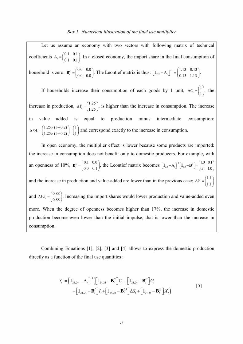
Box 1 Numerical illustration of the final use multiplier

Let us assume an economy with two sectors with following matrix of technical

coefficients 0.1 0.10.1 0.1⎛ ⎞

Α = ⎜ ⎟⎝ ⎠

t . In a closed economy, the import share in the final consumption of

household is zero: 0.0 0.00.0 0.0

Ct

⎛ ⎞= ⎜ ⎟⎝ ⎠

B . The Leontief matrix is thus: 1

2,2

1.13 0.130.13 1.13

− ⎛ ⎞⎡ ⎤− Α = ⎜ ⎟⎣ ⎦

⎝ ⎠tI .

If households increase their consumption of each goods by 1 unit, 11⎛ ⎞

Δ = ⎜ ⎟⎝ ⎠

tC , the

increase in production, 1.251.25tY ⎛ ⎞

Δ = ⎜ ⎟⎝ ⎠

, is higher than the increase in consumption. The increase

in value added is equal to production minus intermediate consumption:

1.25 (1 0.2) 11.25 (1 0.2) 1tVA

× −⎛ ⎞ ⎛ ⎞Δ = =⎜ ⎟ ⎜ ⎟× −⎝ ⎠ ⎝ ⎠

and correspond exactly to the increase in consumption.

In open economy, the multiplier effect is lower because some products are imported:

the increase in consumption does not benefit only to domestic producers. For example, with

an openness of 10%, 0.1 0.00.0 0.1

Ct

⎛ ⎞= ⎜ ⎟⎝ ⎠

B , the Leontief matrix becomes 1

2,2 2,2

1.0 0.10.1 1.0

Ct t

− ⎛ ⎞⎡ ⎤⎡ ⎤−Α − =⎜ ⎟⎣ ⎦ ⎣ ⎦ ⎝ ⎠BI I

and the increase in production and value-added are lower than in the previous case: 1.11.1tY ⎛ ⎞

Δ = ⎜ ⎟⎝ ⎠

and 0.880.88tVA ⎛ ⎞

Δ = ⎜ ⎟⎝ ⎠

. Increasing the import shares would lower production and value-added even

more. When the degree of openness becomes higher than 17%, the increase in domestic

production become even lower than the initial impulse, that is lower than the increase in

consumption.

Combining Equations [1], [2], [3] and [4] allows to express the domestic production

directly as a function of the final use quantities :

()

1

24,24 24,24 24,24

24,24 24,24 24,24

C Gt t t t t t

I S Xt t t t t t

Y C G

I S X

−

Δ

⎡ ⎤ ⎡ ⎤⎡ ⎤= −Α − + −⎣ ⎦ ⎣ ⎦ ⎣ ⎦

⎡ ⎤ ⎡ ⎤ ⎡ ⎤+ − + − Δ + −⎣ ⎦ ⎣ ⎦ ⎣ ⎦

B B

B B B

I I I

I I I [5]

14

Equation [5] allows the calculation of the increase of production that follows the

increase of a given final use. The matrix1

24,24 24,24v

t t

−⎡ ⎤⎡ ⎤− Α −⎣ ⎦ ⎣ ⎦BI I , generally referred as

Leontief matrix, can be interpreted as the final use multiplier: for instance, an increase of each

consumption goods by 1 unit leads to an increase of each sector production by 1

24,24 24,24C

t t

−⎡ ⎤⎡ ⎤− Α −⎣ ⎦ ⎣ ⎦BI I units. With a positive value of At, characteristic of the multi-sector

models, the final demand multipliers are higher. This propriety illustrates the advantage of a

multi-sector model over an aggregate macroeconomic model for the evaluation of an

economic policy. The numerical illustration presented in Box 1 shows that the importance of

this multiplier depends to a great extend to the degree of openness of the economy.

In order to calculate the Gross Domestic Product (GDP), it is useful to express the

value-added (VA) as a function of the level of production:

24

24,1 24,11

( ) (1 ) .( )Dt jt jt ijt t t

i

VA VA Y Yα=

′= = − = − Α∑ I I [6]

Where . is the Hadamard product (or product component by component) of two matrices of

same dimensions, 24,1

1

1

⎛ ⎞⎜ ⎟= ⎜ ⎟⎜ ⎟⎝ ⎠

MI is matrix with a 24 1× dimension composed of 1.

The actual sector production ( jtY ) is expressed at basic price and thus exclude

transportation and commercial margins ( arjtM ), net taxes (i.e. taxes minus subventions) on

products ( taxitPR ). For all sectors except the commercial sector (19) and the transport sectors

(14 to 18), margins enter with a negative sign since they must be deducted from the

production expressed in purchaser’s price. On the contrary, for the commercial and transport

sectors (14 to 18), transportation and commercial margins enter with a positive sign since they

are a production of these sectors5. Let us conveniently index commercial and transport

5 Conceptually commercial and transportation margins could be treated as intermediate consumption that

increase the production of the commercial and transport sectors when the production of the other sector

increases. As such they intervene in the calculation of the Leontief matrix. By convention they are not treated as

15

margins (14 to 19) with i and the all the other products with i’. The actual sector production is

thus:

' ' ' '

for {14;15;16;17;18;19}

for ' '

ar taxjt it jt it

ar taxj t i t j t i t

Y Y M PR j i

Y Y M PR j i i

= + − = =

= − − = ≠ [7]

For the commercial and the transport sectors and for the others sectors, margins are

respectively:

''

' '

for {14;15;16;17;18;19}

for ' '

= = =

= = ≠

∑

∑

ar arjt i jt

i

ar arj t ij t

i

M M j i

M M j i i [8]

where 'arij tM is the quantity of commercial or transport product i used as a margin by the (non-

commercial or non-transport) sector j'. By definition the sum of the margins received by the

commercial and transports sectors is equal to the sum of the margins paid by the other sectors:

''

ar arjt j t

j jM M=∑ ∑ [9]

IV The producer

IV.1 Demand for production factors

As shown in Figure 2, the production structure is decomposed in 3 levels. The first level

assumes a technology with four production factors (or inputs) sometimes referred as a KLEM

(Capital, Labor, Energy, Material) technology, thus splitting intermediary consumptions into

energy and material. Compared to most existing models, we do not necessarily assume a

Constant Elastiscity of Substitution (CES) between these factors. For instance the elasticity of

substitution between capital and labor may differ from the one between capital and energy. To

do so we use a generalized CES (GCES) function. We added a fifth element at the level one:

an intermediate consumption by national account statistics because margins are not incorporated in the product

or destroyed during the production process.

16

the transport and commercial margins. Stricto sensu, they cannot be considered as production

factors since they intervene after the production process. Thus they are not substitutable with

the production factor. But they are closely related to the level of production since once a good

has been processed, it has to be transported and commercialized. At the second level, the

investment, energy, material and margins aggregates are further decomposed. The investment

level is determined by the capital stock assuming a constant depreciation ratio.

At the third level, the demand for each factor or margin is either imported or produced

domestically. The generalized CES function is also used to capture substitutions effect at the

level 2 and 3. Moreover, we assume at each level a degree 1 homogenous function that a

constant return-to-scale technology.

Figure 2 Production structure of Three-ME

Appendix B shows that the cost minimizing program of the firm in the case of a

constant return-to-scale GCES technology leads to the following notional production factors

(or) demand (Equation [102]):

17

_, ' ' '

' 1'

1

( ) with η ϕ ϕ′=≠

=

= − − − =∑∑

Input nputHhjt hjtnput n rog val Input Input val

hjt jt hjt hh j h j hjt h jt h jt HInput nputh

h h hjt hjth

P Ii y p p p

P I [10]

where nputhjtI and _nput n

hjtI is the effective and notional demand of input h in sector j, ',ηhh j the

elasticity of substitution between the production factors h et h' in sector j, roghjtP the technical

progress of input h in sector j, valhjtϕ the value share of input h into the production of sector j.

The superscript n refers to the adjective “notional” as opposed to “effective” as defined by

neo-Keynesian disequilibrium theory (e.g. see Benassy, 1975). The notional demand is the

optimal demand of the firm derived from its maximization program. We may also use the

adjective “desired” since it would be the demand the firm would like to achieve immediately

if there were no constrains such as adjustment costs. Moreover relation [10] can be interpreted

as the equation of the Leontief technical coefficients which corresponds to the input to

production ratio ( _ /nput nhjt jtI Y ). Unlike the Leontief model, they may here vary over time

because of substitution mechanisms between inputs and of the technical progress.

In coherence with the real observations of nominal and real rigidities, Three-ME

assumes that effective prices and quantities adjust slowly to their notional value according to

an Error Correction Model (ECM):

1 1 2 3 1 1( )α α α− − −Δ = Δ + Δ − −n nt t t t tx x x x x [11]

where X and Xn are respectively the effective and notional value of a given variable X. Section

4 of Appendix A shows that the use of ECM has important implication for the calibration of

the long run steady state. If one does not constrain 1 2 1α α+ = , a gap between the effective and

notional quantities remains even at the steady state. The base year notional value should then

be calibrated accordingly.

Equation [10] is used to model the demand factors for the three levels described in

Figure 2. For illustration purposes, we derive explicitly the first level which assumes a KLEM

four-production-factors function: ; ; ;nput atijt jt jt jt jtI K L E M⎡ ⎤= ⎣ ⎦ referring respectively to capital,

18

labor, energy and material. As Three-ME assumes a Harrod-neutral technical progress, the

technical progress appears only in the labor demand:

_ _ _1 1 1

_ _ _1 1 1

( ) ( ) ( )

( ) ( ) ( )

η ϕ η ϕ η ϕ

η ϕ η ϕ η ϕ

− − −

− − −

= − − − − − −

= − − − − − − −

= −

at at at

at at at

n KL Val L K L KE Val E K E KM Val M K Mjt jt j jt jt jt j jt jt jt j jt jt jt

n rog KL Val K L K LE Val E L E LM Val M L Mjt jt jt j jt jt jt j jt jt jt j jt jt jt

njt jt

k y p p p p p p

l y p p p p p p p

e y _ _ _1 1 1

, _ _ _1 1 1

( ) ( ) ( )

( ) ( ) ( )

η ϕ η ϕ η ϕ

η ϕ η ϕ η ϕ

− − −

− − −

⎧⎪⎪⎪⎨

− − − − −⎪⎪

= − − − − − −⎪⎩

at at at

at at at at at at

KE Val K E K LE Val L E L EM Val M E Mj jt jt jt j jt jt jt j jt jt jt

at n KM Val K M K LM Val L M L EM Val E E Mjt jt j jt jt jt j jt jt jt j jt jt jt

p p p p p p

m y p p p p p p

[12]

Where 'hhjη is the elasticity of substitution between input h and h' with , ; ; ; ath h K L E M′ ⎡ ⎤= ⎣ ⎦ .

As explained previously, the effective production factor demand adjust slowly to the

notional one according to the ECM [11]:

1 1 2 3 1 1

1 1 2 3 1 1

1 1 2 3 1 1

_1 1 2 3 1 1

_

( )

( )

( )

( )

K K n K njt jt jt jt jt

L L n L njt jt jt jt jt

E E n E njt jt jt jt jt

at M M M at at njt jt jt jt jt

at t ata at nat

k k k k k

l l l l l

e e e e e

m m m m m

α α α

α α α

α α α

α α α

− − −

− − −

− − −

− − −

⎧Δ = Δ + Δ − −⎪Δ = Δ + Δ − −⎪⎪⎨Δ = Δ + Δ − −⎪⎪Δ = Δ + Δ − −⎪⎩

[13]

The investment in sector j ( jtI ) is calculated by inverting the capital accumulation

equation assuming a constant depreciation rate ( depjR ) of capital:

1dep

jt jt j jtI K R K −= Δ + [14]

The depreciation rate is calibrated on national account data by inverting Equation [14],

using the net fixed capital stock data for capital and the gross fixed capital formation data for

investment.

Because of access restriction to National account investment data disaggregated by

sector, it is not possible to identify different investment patterns between the different private

19

sectors6. Consequently, we assumed the same substitution behaviour between investment

goods across private sectors by first calculating the aggregate private investment ( stI )7:

24

120

st jt

jj

I I=≠

= ∑ [15]

Then the notional demand equations for private investment in good i results from the

producer optimization program described in Appendix B. For a given desired volume of

aggregate private investment, the producer minimize the cost of investment subject to GCES

technical constraint; The notional investment demand for each good thus depends on the

aggregate private investment [15] and substitution effects:

_', ' '

' 1 1'

( ) with ( ) /I I

s n s val I I val I s I sit t ii j i j it i t ij it it it it

i ii i

i i p p P I P Iη ϕ ϕ= =≠

= − − =∑ ∑ [16]

Because of data availability, the investment general government (Sector 20) is treated

separately:

_20 ',20 '20 20 '20

' 1'

( )I

g n g val I It t ii i i t i t

ii i

i i p pη ϕ=≠

= − −∑ [17]

The index i could refer to every product produced by each sector. In practice however,

only the goods produced by the sectors 1, 3, 5, 12, 13 and 19 of Table 1 are used as

investment by the private and public sectors.

In current version of the model, labor is assuming homogenous inside each sector, and

is thus not disaggregated further8. On the contrary, the aggregate of energy and material

6 Such a disaggregation is now possible and will be included in a future version of Three-ME. 7 The exponents s, h and g refer respectively to sectors, household and public administrations. 8 On the contrary, the JULIEN model (Laffargue, 1996) applied to the French economy distinguishes two types

of worker qualification. As suggested by econometric studies (e.g. Shadman-Mehta and Sneessens, 1995), this

would allows to reproduce more accurately the recent evolution in the industry sector by accounting for different

20

inputs are disaggregated in a second level of production structure assuming a GCES function.

The notional demand for energy i and material i are respectively:

', '' 1'

( )I

n val E Eijt jt ii j i j ijt ijt

ii i

e e p pη ϕ=≠

= − −∑ [18]

_' ' '

' 1'

( )I

at n at val M Mijt jt ii j i j ijt i jt

ii i

at atm m p pη ϕ

=≠

= − −∑ [19]

In both cases, the demand for each type of energy and material is the function of the

aggregates defined in the first level by Equations [13] and [12] and of the relative prices

between type of energy and material.

Finally, in the third level, each type of investment products, energy and material can be

domestically produced or imported. As in Armignton (1969), a CES function is used to

describe the possibilities of substitutions between imported and domestic goods.

IV.2 Debt in the private sector

The dynamic of the debt in the private sector ( stD ) is determined by the accumulation

equation [20], which depend on the gap between the private investment spending and the

Gross Operating Surplus ( stGOS ) :

1(1 ) s s s inv s s taxt t t t t jt tD D R P I GOS FP−= + + − + [20]

_(1 )= + − − +s VA Y Y em contt t t t t t t tGOS P VA SUB TAX LW R [21]

substitution pattern between each kind of labor and capital, and biased technical progress in favor of less

qualified labor.

21

where YtSUB and Y

tTAX are respectively the subvention and tax on production. Wt is the gross

wage and stR the interest rate paid by the private sector. tax

tFP is the total firms profit tax,

_em conttR the apparent rate of employer social security contribution.

V The household’s behaviour

Assuming that all households are homogenous with respect to incomes and allocation

of resources, the current version of Three-ME has one “macroeconomic” household with a

gross disposable income ( )disptI consisting of net labor revenue, a net financial wealth

earnings and government transfers ( )_transf hT :

24_ _ _

11( * (1 )) . * (1 )t

disp esc net h h ransf h i taxt jt jt t t

jI L W R FW R T R−

=

⎛ ⎞= − + + −⎜ ⎟⎝ ⎠∑ [22]

where _net htFW corresponds to the household’s net financial wealth, defined as the difference

between financial assets and liabilities, htR is the average rate of return9 deduced from the

ratio between the net property revenues and the net financial wealth. It is composed of the net

interests (interests received minus interests paid) and of the dividends received by household. escR and _i taxR are respectively the average rates of the employee social contribution and of

the income tax.

Figure 3 summarizes the household’s optimization behaviour. In the first level, the

household chooses the respective shares of the gross disposable income going to expenditure

and to savings. In Three-ME, these shares are stable at long term when the economy is on its

stationary state. They may depend on the real interest rate if one wants to account for eviction

effect on households demand: households tend to increase their savings share when the

interest rate increases. These shares may also depend on the ratio between the national

9 Symmetrically to the private sector, we do not differentiate between the possible forms of financial assets

which is equivalent to assuming the same rate of return for all assets.

22

(government and private) debt and the household’s financial wealth. This allows accounting

for Ricardian effects in saving behaviours: when the national debt increases faster than their

financial wealth, households may increase their savings anticipating a future increase in taxes:

( )1 2_( ) ( ) ( ) /

.

h disp h s gt t t t t t t

h disp ht t t t

net htexp i p R P D D FW

with P EXP I S

β β= − − − − +

= −

& [23]

where htEXP are the volume of total expenditures of the household, Pt their price and h

tS the

households’ saving. The unitary elasticity between the real total expenditures of households

and their real income guarantees the long-run stability of the expenditures to income ratio.

At the second level, the household allocates these expenditures between the final

consumption (Section V.1 ) and the capital stock accumulation of automobile and housing

(Section V.2 ) by maximizing a GCES utility function subject to a budget constraint:

( )

, ,Max , ,

st .+ + =t t t

t t t tC AUTO HOUS

c auto hous ht t t t t t t t

U C AUTO HOUS

P C P AUTO P HOUS P EXP [24]

where tC is the aggregate consumption of goods, tAUTO and tHOUS the automobile and

housing stocks, , , c auto houst t tP P P their respective price.

In a third level, following the same logic, the optimizer household allocates the

aggregate consumption to three types of composite consumption goods: transport, energy and

other final consumption goods. In a fourth level of consumption structure, these three types of

final consumption are further disaggregated between different sorts of transport, energy and

other final consumption. Following the producer’s behaviours, the substitution mechanisms

are described with a GCES in each step of the consumer structure. The adjustment process of

effective to notional values is also specified as an ECM (according to Equation[11]).

23

Figure 3 Households’ behaviour structure

Other housing investment

Other housing stock

Sober auto investment

en_21…24

Gross disposable income

Net financial wealth

SavingTotal expenditure

Composite Transport

Automobile stock

Aggregate consumption

Housing investment

Composite Final consumption

Automobile investment

Housing stock

Energy saving housing

investment

Trsp_14… 18 fc_01…13, 19, 20

Energy saving housing stock

Composite Energy

All energy prices evolution

Oil price evolution

Consumption module

Other auto investment

Other auto stock

Sober auto stock

Oil price

Household investments in housing and automobile are determined by the desired stock

level assuming a constant rate of depreciation. Then in order to account for energy efficiency

24

effects, two types of housing and automobile investments are explicitly distinguished (Figure

3). In the first case, depending on the energy aggregated price, the household arbitrates

between energy saving housing and “comfort” housing investments. In the second case,

depending on the oil price, the household chooses between low and high oil consumption

cars. This in return reduces the energy consumption.

V.1 Consumption

Appendix B shows that the resolution of the optimization program [24] gives the

following notional demand for each type of expenditures in volume ( _ _h e ntEXP ):

_ _ _ _ '

,. ( ) , ,η ϕ′ ′

′

′= − − = =∑h e n h e e val e e et t t t t

e eexp exp p p e e c auto hous [25]

etP and 'e

tP are the consumer prices (resp. the user cost of automobile and housing) if

(resp. , )′= =e e c auto hous . _η ′e e and _ϕval et are the elasticities of substitution between two

given expenditure and the share in value of a given expenditure. The adjustment process of

effective to notional expenditures is specified as an ECM (according to Equation[11]). This

slow adjustment reflects the inertia observed empirically in consumption pattern. As

households’ expenditures are strongly influenced by past habits, one generally observes that

consumption fluctuates less than income during the business cycle. Indeed households tend to

use their saving to damper the fluctuation of their consumption.

Assuming again a GCES utility function at the first level of the consumption module

(see Figure 3), the aggregate consumption is decomposed into three composite consumptions

with the following notional demand:

' ' ', '

. .( ) , , ' , ,n val c cct t cc c ct c t

c c

c c p p c fc trsp c fc trsp enη ϕ= − − = =∑ [26]

25

( ), , ' ' , ', '

. .( ) . ' ,n val c c hous effen t t en c c en t c t t t

c c

c c p p hous hous c cf trspη ϕ η= − − − − =∑ [27]

Where cctp is the price of the composite good consumption c. fc, trsp and en are respectively

the composite of final consumption10, transport and energy. thous and effthous are respectively

the total housing capital stock and the energy saving housing capital stock.

The energy demand defined in Equation [27] includes, in addition to the revenue and

substitution effects, an endogenous energy efficiency effect related to the household’s

investment in energy efficiency. The sensibility of the aggregate energy demand to the share

of energy saving housing capital stock in the total housing capital stock is measured by the

positive parameter enη . This effect was calibrated using the recent ADEME (2011)11 micro

simulation studies on the effect of measures taken during the Grenelle de l’environnement12.

As mentioned earlier, the three types of consumption goods (transport, energy and other

final consumption goods) are further disaggregated assuming a GCES substitution pattern.

We assume further a zero-elasticity of substitution between all components of the other final

consumption goods. In addition to substitution effect between energies, the demand for oil

(en22) depends on the real oil price and on the share of low energy consumption cars:

( )22 , 22, 22 22 22. .( ) .( ) .

with 21,23,24

n val c c en c auto efft en t i it t it t t t t

ien c p p p p auto auto

i

η ϕ η η= − − − − − −

=

∑ [28]

10 Our definition of the final consumption is slightly different from the real final consumption of national

accounting which includes the public administration services provided free of charge and an estimation of the

pseudo-rent paid by house owner households. Here we only take into account the marketed consumption goods. 11 These studies are not published yet. For more results, you could contact Gaël Callonnec from ADEME. 12 The Grenelle de l’environnement translated as Grenelle Environment Round Table process is the open debate

held during summer 2007 in France. The aim of the debate was to define a coherent public policy on ecology and

sustainable development issues. It led to a series of political measures (see www.legrenelle-environnement.fr).

For instance, concerning the housing sector, the generalization of low consumption standards in the new housing

and the setting-up of economic incentives in favor of energy efficiency were adopted.

26

where 22cP is the oil price, P the price of the total expenditures of households, AUTOeff the

stock of low consumption (energy efficient) automobiles and AUTO the total stock of

automobiles. 22enη and autoη measure respectively the sobriety and efficiency effects which lead

to an endogenous decrease in the trend of the share of the oil consumption into the energy

consumption ( 22 ,n

t en ten c− ). For the calibration of their magnitude, we used two recent studies

of the ADEME (2011)11. According to the first one, a 1% increase of the real oil price, leads

to a decrease of 0.33% ( )22enη= of the French household’s oil demand. The direct oil effect

price reflects sobriety effect or the development of environmental friendly household

behaviours and not substitution between energies: the consumption of the other kind of energy

is not affected. The household change its way of leaving in order to consume less energy by,

for instance, reducing the heating temperature of the house or choosing hobbies that does not

involve the use of the car.

The second effect captures the energy efficiency improvement that results from the

investment strategy of the household. A second study of ADEME relating to the effect of the

Bonus-Malus car systems shows that the dynamic of household oil demand is closely related

to the increase of the share of low consumption cars. An increase of 1% of this share would

lead to a decrease of 0.20% ( )autoη= of the share of the oil consumption into the energy

consumption.

V.2 Investment

From the optimal stocks of automobile and housing defined by Equation [25], it is

possible to derive the equation of investment in automobile and housing (as we did for the

business sector, Equation [14]) from a standard equation of capital stock accumulation:

, 1.h dephous t t t housI HOUS HOUS R−= Δ + [29]

, 1.h depauto t t t autoI AUTO AUTO R−= Δ + [30]

27

where hI and depR are respectively the annual investment flows and the specific depreciation

rate.

For each of these investments, we assume two types of investment: the investment

improving the energy efficiency and the other investment. Concerning the housing

investment, depending on the relative prices of oil, electricity and gas, the household is

assumed to arbitrate between an investment that reduces the energy bill and an investment

that improves the house comfort. In the other hand, the household could also choose to invest

in sober cars13 depending on the real oil price:

24

_ , ,22

.( )h h chous eff t hous t i it t

ii i p pη

=

= + −∑ [31]

_ , , 22 22.( )h h cauto eff t auto t t ti i p pη= + − [32]

_ , , _ ,h h hhous oth t hous t hous eff ti i i= − [33]

_ , , _ ,h h hauto oth t auto t auto eff ti i i= − [34]

Equations [31] and [32] describe the “green” household investment in housing

( )_hhous effi and in automobile ( )_

hauto effi . The other types of investment ( _

hhous othi , _

hauto othi ) are

deduced as a difference between the aggregate investment and the green investment

(Equations [33] and [34]14). The stocks of “green” housing and cars are derived from a

standard capital accumulation equation:

1 _ ,(1 )eff dep eff ht hous t hous eff tHOUS R HOUS I−= − + [35]

1 _ ,(1 )eff dep eff ht auto t auto eff tAUTO R AUTO I−= − + [36]

13 The sober cars correspond to the cars with a A, B or C classification that is characterized by a lower level of

CO2 emissions (< 140 g/km). 14 Supposing one producer sector of the « green » and « no green » investment goods in both kind of household

investments, the disaggregated and aggregated prices are equal and the equalities in volume (Equations [33] and

[34]) are respected.

28

V.3 Saving and financial wealth

The household’s financial saving ( )htS is given by the following equation:

13,19,20 18 24_

1 14 21 ,. . . .h disp c c c inv h h

t t it it it it it it it iti i i i auto hous

S I P FC P TRSP P EN P I= = = =

= − − − −∑ ∑ ∑ ∑ [37]

where _inv hitP is the price of investment.

The stock of the net household financial wealth is determined by a standard

accumulation formula:

_ _1

net h net h ht t tFW FW S−= + [38]

Box 2 Stability condition in household behaviours’ structure

If we assume that the dynamic homogeneity hypotheses are respected by the ECM

adjustment equations, the long term notional quantities of household consumption and

investment are equal to their effective levels. Given unitary income elasticity, consumption

and investment are fixed shares ( , )c invt tϕ ϕ of the real disposable income ( /disp

t tI P ). These shares

can be defined as the marginal propensities to consume and to invest. They depend positively

on relative prices and a scale parameter.

. /c dispt t t tC I Pϕ= [39]

_, . /h inv hous disp

hous t t t tI I Pϕ= [40]

_, . /h inv auto disp

auto t t t tI I Pϕ= [41]

In this box, the small letters with accent refer to the per capita variables expressed in

real efficient unit (deflated by inflation and technical progress) and “χ” refer to the growth

rate of nominal variables defined as (1 ).(1 ) 1χ μ π= + + − , where μ and π are respectively the

growth rate of real variables and the inflation rate. Dividing all the variables demanded by

29

household (Equation [39] to [41]) by the effective employment, the real per capita variables

are constants (noted without the index t) along a stationary growth path and the household

equations system can be rewritten as:

_24

_ _

1( *(1 )) . *(1 )

(1 )

net h

disp real esc h ransf i taxj

j

fwi w R R t R

χ=

⎛ ⎞⎜ ⎟= − + + −⎜ ⎟+⎝ ⎠∑

) )) [42]

.c dispc iϕ=)) [43]

_ .h inv auto dispautoi iϕ=) ) with _ .

1

depinv auto auto autoRμ

ϕ ϕμ

⎛ ⎞+= ⎜ ⎟+⎝ ⎠

[44]

_ .h inv hous disphousi iϕ=) ) with _ .

1

depinv hous hous housRμ

ϕ ϕμ

⎛ ⎞+= ⎜ ⎟+⎝ ⎠

[45]

,

disp hi

i auto houss i c i

=

= − − ∑) )) ) [46]

( )1.

hfw s

χχ+

= ) [47]

where autoϕ and housϕ are the ratios between the automobile and housing stocks to the gross

real disposable income. The marginal propensities to invest depend also on the exogenous

depreciation rate, i.e. the intensity of investment is affected by the life duration of equipments.

Thus, the reduced form of the previous system corresponds to the single following

equation of household financial wealth accumulation:

24_ _

1

.(1 ). *(1 ) *(1 )

.

snet h esc ransf i taxjh s

jfw w R t R

Rϕ χχ ϕ =

⎛ ⎞⎛ ⎞+= − + −⎜ ⎟⎜ ⎟⎜ ⎟− ⎝ ⎠⎝ ⎠

∑)) [48]

where _

,

1s c inv ittdisp

i auto houst

SI

ϕ ϕ ϕ=

= = − − ∑ is the constant long term saving rate.

Equation [48] show that the stability condition of the system is h sRχ ϕ> , which is

largely respected by the parameterization of Three-ME. For a saving rate equal to 1, the per

capita financial wealth is positive only if the rate of economic growth is higher than the

interest rate. When the saving rate is smaller than 1, the constraint on the rate of economic

growth is less tied. With a low saving rate, the interest rate can lie above the growth rate of

the nominal production. Consequently, the per capita household consumption and investment

demand equations are:

30

24_

1

. . *(1 ) *(1 ).

c esc ransf i taxjh s

j

c w R t RRχϕ

χ ϕ =

⎛ ⎞⎛ ⎞⎛ ⎞= − + −⎜ ⎟⎜ ⎟⎜ ⎟ ⎜ ⎟−⎝ ⎠ ⎝ ⎠⎝ ⎠

∑ )) ) [49]

24_ _

1. . *(1 ) *(1 )

.h inv auto esc ransf i tax

auto jh sj

i w R t RRχϕ

χ ϕ =

⎛ ⎞⎛ ⎞⎛ ⎞= − + −⎜ ⎟⎜ ⎟⎜ ⎟ ⎜ ⎟−⎝ ⎠ ⎝ ⎠⎝ ⎠

∑) )) [50]

24_ _

1

. . *(1 ) *(1 ).

h inv hous esc ransf i taxhous jh s

j

i w R t RRχϕ

χ ϕ =

⎛ ⎞⎛ ⎞⎛ ⎞= − + −⎜ ⎟⎜ ⎟⎜ ⎟ ⎜ ⎟−⎝ ⎠ ⎝ ⎠⎝ ⎠

∑) )) [51]

In the long run, the wage per efficient unit is stable and the household’s consumption

and investment depend on the economic policy parameters: the variation in the tax rate or in

government transfers requires a variation more than proportional in consumption and

investment for the stability condition to hold.

Box 3 Sustainability condition of domestic debt

Assuming that the long-run external account of the economy is in equilibrium, the total

domestic debt is financed entirely by the net financial wealth of households. The total

domestic debt is composed by the private (or sector) debt sD∞ and the gross public debt gD∞

(excluding the financial and real estate assets that are not accounted for in the model):

_net h s gFW D D∞ ∞ ∞= + [52]

The sustainability of the domestic debt requires that the ratio between the deficit and

the financial wealth respects the following condition:

_

111

s gt t

net ht

B DEFFW χ+

= −+

[53]

For a higher level of nominal growth rate “χ” due to a higher potential of economic

growth or a higher inflation rate, the ratio between the flows to domestic debts and the stock

of household wealth can be maintained at a higher level which means that the economy can

accumulate larger debt in period of high activity or inflation.

Such a long term constraint can be incorporated in the model by assuming that the

households’ consumption and investment adjust such as that the debt can be reimbursed by

the nation (Ricardian effect). When the domestic debt is growing faster than the financial

household’s wealth, for a given value of “χ”, the household demand tends to decrease. This

increases the saving and financial wealth until the ratio [53] returns to its equilibrium level.

31

In the case of an open economy characterized by the accumulation of an external

commercial deficit ( )xtDEF (e.g. the French economy), a part of the debt is financed by the

rest of the world and the sustainability condition becomes:

_

111

s g xt t t

net ht

B DEF DEFFW μ

+ −= −

+ [54]

VI The labor market

We assume that the average gross wage (that is including employee social security

contributions) in sector j ( jtW ) is determined by a Phillips curve. Wages may be indexed on

the consumer price inflation ( 2 0jρ > ) and on productivity gains of the sector j ( 3 0jρ > ).

Trade unions may accept lower wage increases in case of a degradation of the terms of trade,

that is in case of competitiveness losses ( 4 0jρ > ). In addition to the level of unemployment

( tU ), the variation of unemployment may influence the Phillips curve ( 6 0jρ > ), because

wages can be affected not only by the level but also by the evolution of employment (Phillips,

1958; Lipsey, 1960) or due to hysteresis phenomena15. Finally, it is possible that the wage

dynamic differs across sectors because of differences in employment situation ( 7 0jρ > ).

1 2 3 4 5 6 7( ) ( )n rog m yjt j j t j jt j jt jt j t j t j jt tw p p p p U U l lρ ρ ρ ρ ρ ρ ρΔ = + Δ + Δ − Δ − − − Δ + Δ − [55]

The parameter 1 jρ reflects the labor market tensions and the bargaining power of trade

unions. tL is the aggregated employment:

24

=∑t jtj

L L [56]

15 Hysteresis occurs when the long-term unemployed workers exert no influence on wage-setting (Blanchard and

Summers, 1986; Lindbeck, 1993). However, some authors contest the use of the term hysteresis to describe this

phenomenon (Cross, 1995).

32

It can be shown that the WS curve in level is a particular case of the Phillips curve [55]:

the case of full hysteresis (Reynès, 2010) that is the case where the level of unemployment

does not have any effect on the wage setting ( 5 0jρ = ). Moreover, we assume a slow

adjustment of wages: the effective wage growth adjusts to its notional level defined in [55]

according to the ECM [11].

The unemployment rate is calculated according to its conventional definition:

_ _

_

( ) /op act op actt t t top act op

t t t

U P L P

P Pκ

= −

= [57]

where _op acttP is the active population which is by definition the product between the labor

participation ratio ( tκ ) and the total population ( optP ) assumed to be exogenous.

Since the seminal works of Strand and Dernburg (1964) and Dernburg and Strand

(1966), several studies have observed that the labor force participation depends on the labor

market situation in particular because of a discouraged-worker effect. Thus, the labor

participation ratio may be endogenous and depend negatively on the unemployment rate:

1 2t tUκ ψ ψ= − [58]

where 1ψ is a constant term and 2ψ is the discouraged-worker effect parameter.

VII External trade

33

The external trade in Three-ME is treated with a relatively high level of detail. On the

one hand, import behaviours are specific for each economic actor and each product. On the

other hand, the model integrates explicit external demand functions of both the domestic

production and the importations with a constant price elasticity.

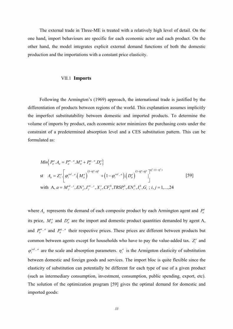
VII.1 Imports

Following the Armington’s (1969) approach, the international trade is justified by the

differentiation of products between regions of the world. This explanation assumes implicitly

the imperfect substitutability between domestic and imported products. To determine the

volume of imports by product, each economic actor minimizes the purchasing costs under the

constraint of a predetermined absorption level and a CES substitution pattern. This can be

formulated as:

{ }

( ) ( ) ( ))/ )/

_ _

/ (1 )

_ _

_ _

(1 (1

. . .

st . . 1 .

with A, , , , , , , , , ; , 1,...,24

a ai i

i i i ia a a a

a m a a q a ait it it it it it

a vol a a vol a ait i i it i it

at s s nv s s h h h hj j j j i i i i i

Min P A P M P D

A Z M D

a M EN I X CF TRSP EN I G i j

η ηη η η ηϕ ϕ

−− −

= +

⎡ ⎤= + −⎢ ⎥

⎣ ⎦= =

[59]

where itA represents the demand of each composite product by each Armington agent and aitP

its price, aitM and a

itD are the import and domestic product quantities demanded by agent A,

and _m aitP and _q a

itP their respective prices. These prices are different between products but

common between agents except for households who have to pay the value-added tax. aiZ and

_vol aiϕ are the scale and absorption parameters. a

iη is the Armignton elasticity of substitution

between domestic and foreign goods and services. The import bloc is quite flexible since the

elasticity of substitution can potentially be different for each type of use of a given product

(such as intermediary consumption, investment, consumption, public spending, export, etc).

The solution of the optimization program [59] gives the optimal demand for domestic and

imported goods:

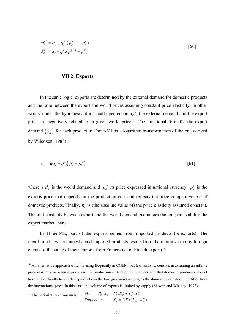
34

_

_

.( )

.( )

n

n

a a m a ait it i it it

a a q a ait it i it it

m a p p

d a p p

η

η

= − −

= − − [60]

VII.2 Exports

In the same logic, exports are determined by the external demand for domestic products

and the ratio between the export and world prices assuming constant price elasticity. In other

words, under the hypothesis of a "small open economy", the external demand and the export

price are negatively related for a given world price16. The functional form for the export

demand ( )itx for each product in Three-ME is a logarithm transformation of the one derived

by Wilcoxen (1988):

( ).x x wit it i it itx wd p pη= − − [61]

where itwd is the world demand and witp its price expressed in national currency. x

itp is the

exports price that depends on the production cost and reflects the price competitiveness of

domestic products. Finally, iη is (the absolute value of) the price elasticity assumed constant.

The unit elasticity between export and the world demand guarantees the long run stability the

export market shares.

In Three-ME, part of the exports comes from imported products (re-exports). The

repartition between domestic and imported products results from the minimization by foreign

clients of the value of their imports from France (i.e. of French export)17:

16 An alternative approach which is using frequently in CGEM, but less realistic, consists in assuming an infinite

price elasticity between exports and the production of foreign competitors and that domestic producers do not

have any difficulty to sell their products on the foreign market as long as the domestic price does not differ from

the international price. In this case, the volume of exports is limited by supply (Shoven and Whalley, 1992).

17 The optimization program is: . . .

( , )

x q d m mit it it it it it

d mit it it

Min P X P X P X

Subject to X CES X X

= +

=.

35

,

,

.( )

.( )

d x q xit it d m it it

m x m xit it d m it it

x x p p

x x p p

η

η

= − −

= − − [62]

where ditx and m

itx are the optimal level of domestic and import products that are exported.

,xd mη is the elasticity of substitution between domestic and imported products.

As the exchange rate is exogenous in the model, the external balance ( )xtDEF may

differ from zero:

. .x m xt it it it it

i iDEF P M P X= −∑ ∑ [63]

with mitP as the import product price (see equation[68]).

VIII Prices structure

The prices in TRHEE-ME follow a bottom-up structure, where the prices of all

intermediate levels are calculated as weighted average (Figure 4).

36

Figure 4 Prices structure

C arbone t ax

C arbon tax

Aggregat ed energy p rice by

s ector

Taxes les s subsid ies on production

Uni fo rm carbon tax com pensation

Aggregated m ateriel p ri ce by

secto r

Des ired Price

Net unit cost

Gros s unit cost

Labor cos t by sector

Cap ita l c os t by s ector

Production (basic) p rice of sector j

Desired m ark-up

Transport s and com m ercial m argins

M aterial p ri ce by product

Energy price by product

Dom esti c m aterial

price

Im ported m aterial

p rice

Domes tic Energy

p rice

Im ported Energy

price

Aggregated Investm en t p ri ce

In flation , in terest rate

Wage, p roductiv ity , em ployer con tributi ons

Exchange rate, p roducts and energy taxes

M arket price o f p roduc t i

Taxes l ess subs idies on products including excis e du ties on a lcohol, tobacco and energy

Dom es tic househo ld consum pt ion and invest m ent p ri ces

Exportation and public demand prices

Domes tic energy price

Value added tax

Domes tic m aterial and investm ent prices

VIII.1 Production prices

In order to describe as clearly as possible the construction of prices in Three-ME, we

begin with the production prices fixed by firms. With the import prices, the system of

37

production prices is the key element in the price structure since all other prices are derived

from them by adding taxes or/and deducting subsidies according to the destination of each

product.

In the case of imperfect competition, firms choose the price that maximizes their profit

as a mark-up ( )mujR over the unit cost of production:

( ). 1Y mujt jt jtDP NUC R= + [64]

where YjtDP is the optimal (or desired or notional) production price. jtNUC is the net unit cost

of production calculated by adding over the gross level all taxes on production and deducting

operating subsidies. The mark-up rate is calibrated so that the growth of the effective price is

constant by inverting Equation [65] at the stationary state.

The effective price adjusts slowly the desired level according to an ECM:

1 1 2 3 1 1. . .( )y py y py y py y yjt jt jt jt jtp p dp p dpα α α− − −Δ = Δ + Δ − − [65]

This price is calibrated to unity in the base year for all model sectors. Considering that the

public services sector does not optimize financial profits, we assume that the mark-up is null

and that the production price adjusts to the net unit cost instantaneously.

The steps that lead to the calculation of the gross unit cost ( )jtGUC are described in

Figure 4. It follows a bottom-up approach starting from the most disaggregated price levels to

reach the most aggregated one by determining the prices of composite factors in intermediate

steps. At the bottom of the price structure, we calculate the composite prices for each energy

and material in each sector according to their geographic origins. These prices depend on the

domestic ( )qijtP and import ( )_m a

ijtP prices including taxes, and a volume share parameters

( )volijtϕ :

38

( )( )

_

_

. 1 .

. 1 .

mat vol q vol m matijt ijt ijt ijt ijt

en vol q vol m enijt ijt ijt ijt ijt

P P P

P P P

ϕ ϕ

ϕ ϕ

= + −

= + − [66]

At the upper level, we calculate the prices for each composite factor in each sector:

The composite materiel price in sector j: 20

1

.mat vol matjt it ijt

iP Pϕ

=

= ∑

The composite energy price in sector j: 24

21

.en vol enjt it ijt

iP Pϕ

=

= ∑

The user capital cost per unity produced in sector j: ( )_ _.k inv s decl s inv sjt t j t tP P R R P= + − &

where:

o _inv stP : The investment price common to all sectors18;

o stR : The long-run nominal interest rate.

The labor cost per unity produced in sector j: _.(1 ) /l em cont rogjt jt jt jtP W R P= +

where:

o jtW : The average gross wage;

o _em contjtR : The employer social security contributions.

Finally, the gross unit cost of production in sector j is equal to19:

_ _ _ _. . . .vol mat mat vol en en vol k k vol l ljt jt jt jt jt jt jt jt jtGUC P P P Pϕ ϕ ϕ ϕ= + + + [67]

18 The published French Input-Output table describes only the repartition investment by product only for one

aggregated sector of production. 19 The sum of volume shares is not equal to one since the prices of capital and labour are different from one and

since the sum of the volumes of the production factors do not equal the volume of production.

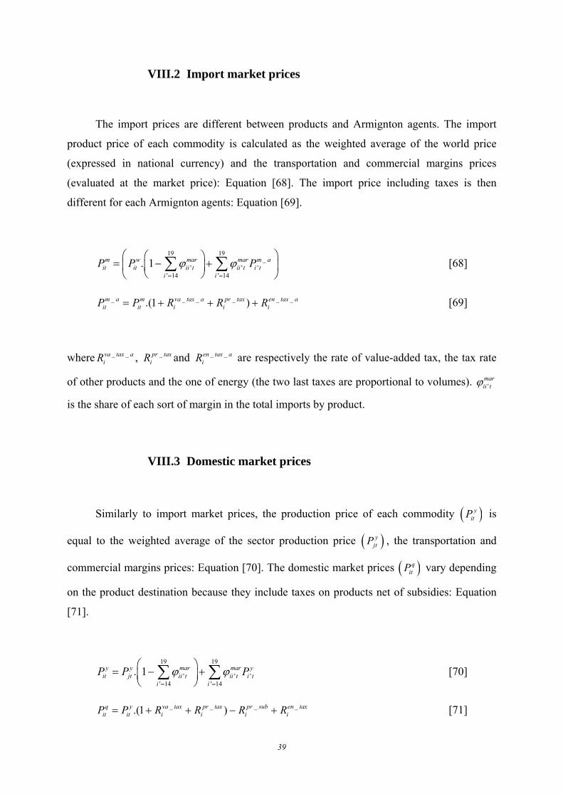
39

VIII.2 Import market prices

The import prices are different between products and Armignton agents. The import

product price of each commodity is calculated as the weighted average of the world price

(expressed in national currency) and the transportation and commercial margins prices

(evaluated at the market price): Equation [68]. The import price including taxes is then

different for each Armignton agents: Equation [69].

19 19_

' ' '' 14 ' 14

. 1m w mar mar m ait it ii t ii t i t

i iP P Pϕ ϕ

= =

⎛ ⎞⎛ ⎞= − +⎜ ⎟⎜ ⎟

⎝ ⎠⎝ ⎠∑ ∑ [68]

_ _ _ _ _ _.(1 )m a m va tax a pr tax en tax ait it i i iP P R R R= + + + [69]

where _ _va tax aiR , _pr tax

iR and _ _en tax aiR are respectively the rate of value-added tax, the tax rate

of other products and the one of energy (the two last taxes are proportional to volumes). 'marii tϕ

is the share of each sort of margin in the total imports by product.

VIII.3 Domestic market prices

Similarly to import market prices, the production price of each commodity ( )yitP is

equal to the weighted average of the sector production price ( )yjtP , the transportation and

commercial margins prices: Equation [70]. The domestic market prices ( )qitP vary depending

on the product destination because they include taxes on products net of subsidies: Equation

[71].

19 19

' ' '' 14 ' 14

. 1y y mar mar yit jt ii t ii t i t

i i

P P Pϕ ϕ= =

⎛ ⎞= − +⎜ ⎟⎝ ⎠

∑ ∑ [70]

_ _ _ _.(1 )q y va tax pr tax pr sub en taxit it i i i iP P R R R R= + + − + [71]

40

where _pr subiR is the apparent rate of public product subsidy applied on the volume of

product.

VIII.4 Consumer price index

The consumer price index ( )tP is defined as a weighted average of prices of all total

expenditure household components:

_ _ _. . .vol c c vol auto auto vol hous houst t t t t t tP P P Pϕ ϕ ϕ= + + [72]

where 24

_

13;13

.c vol c ct it it

ii

P Pϕ=≠

= ∑ is the aggregate consumer price with _ _ _(1 )c vol q q vol q m cit it it it itP P Pϕ ϕ= + −

the consumption price of each commodities calculated as a weighted average between the

domestic and import price.

The household user cost of automobile and housing stocks is:

( )_ _. ,i inv h decl h inv ht it i t itP P R R P i auto hous= + − =&

with _ _ _ _(1 )inv h vol q q vol q m invit it it it itP P Pϕ ϕ= + − the household investment price (also calculated as a

weighted average between the domestic and import price).

41

IX Interest rate

In Three-ME, money supply is endogenous. The interest rate is determined at the euro

area (EA) level according to a reaction function à la Taylor. We assume that the European

Central Bank (ECB) sets the short-term interest rate taking into account inflation and the

situation on the labor market in the euro area:

* *0 1 2

1

1

( ) ( )s ea ea ea eat t t t t

Eea e

t e te

Eea et e t

e

R P P U U

P P

U U

ς ς ς

σ

σ

=

=

= + − − −

=

=

∑

∑

& &

& & [73]

Where stR is the nominal short run interest rate, ea

tP& the inflation rate within the EA, *eatP& the

ECB inflation target, eatU the unemployment rate in the EA and ea

tU the ECB unemployment

rate target. etP& , e

tU et eσ are respectively the inflation rate, the unemployment rate and the

GDP weight of country e in the EA. We assume further that the long-term interest rate adjusts

slowly to the short-term interest rate according to a ECM [11].

X Public administrations behaviour

According to the French national accounts, public administrations refer to the central

and regional government services and social security administration. In Three-ME, we have

aggregated these three components in order to focus on transfers between public

administrations, household and sectors. These transfers are accounted for in the government’s

resources ( )gtRES and expenditures ( )g

tEXP :

( ) _20 20.g tax c tax tax tax tax tax tax

t t t t it t t t jt t tRES Y NUC VA VA PR EN Y SC W FP= + + + + + + + + [74]

42

_1.

g g ransf h g g g gt t t t t t t tEXP G SUB T I PFD D R−= + + + + + [75]

with:

o The marketed part of public administrations production is evaluated at its net production

cost: 20 20.t tY NUC ;

o The household’s consumption value-added tax : ( )_ _. .tax c y c m c va taxt it it it it i

iVA P D P M R= +∑ ;

o The household’s investment value-added tax: ( )_ _ _

,

. . .tax y h d m h m va taxit it it it it i

i auto hous

VA P I P I R=

= +∑ ;

o In contrast with the value-added tax which is calculated only on the household

consumption and investment, the taxes on products net of subsidies are applied to all

components of demand: ( ) _ _. . . .tax y m pr tax pr subt it it it it i it i

i iPR P Q P M R Q R= + −∑ ∑ ;

o The energy tax : ( )24

_

21

.tax en taxt it it i

iEN Q M R

=

= +∑ ;

o The production taxes net of operating subsidies : ( )24

_ _

120

.tax y tax y subt jt j j

jj

Y Y R R=≠

= −∑ ;

o Employer and employee social security contributions: ( )24

120

. . esc sscjt jt jt j

jj

SC L W R R=≠

= +∑ ;

o The income tax : ( )_ _ _. / 1disp tax disp i tax i taxt tI I R R= − ;

o The total firm profit tax :24

_ _1 2

120

. .tax s net s s FP taxt jt t

jj

FP GOS FD R R− −=≠

⎛ ⎞⎜ ⎟= −⎜ ⎟⎜ ⎟⎝ ⎠∑ , 1

sjtGOS − is the total

gross operating profit and _2

net stFD − the total net financial debt of firms ;

o Total public expenditures : ( )_. .q d m g mt it it it it

iG P G P G= +∑ ;

o Total public investment : _ .g inv g gt it it

iI P I=∑ ;

43

o The total demand of production factors:

( ) ( ) ( ) ( )20 20 20 20 20 20 20 20. . . .g k l en at matt t t t t t t t tPFD C P L P EN P M P= + + + ;

o Public subventions to sectors consist of subventions on production and products. Both

types are applied on volume20 which means that changes in price caused by a shock do not

affect the amount of subsidies: ( )_ _ .g pr sub y subit i i itSUB R R Y= +

The public deficit ( )gtDEF and debt ( )g

tD accumulation equations are written as

follows:

g g gt t tDEF EXP RES= − [76]

1g g gt t tD D DEF−= + [77]

XI CO2 emissions

In France, the anthropogenic CO2 emissions represent about 70% of the total gross

greenhouse gases (GHG). They come from the burning of fossil fuels and decarbonation

process. The modeling of the demand for fossil energy in Three-ME is detailed by economic

agent, by kind of fossil energy and by procedure of emissions. This allows for a precise

estimation of the variation in the national CO2 emissions. The calculation of emissions level

consists in multiplying the fossil energy demand by the corresponding emission coefficients.

These coefficients are specifics for each economic actor, each sector and each energy sources

depending on their carbon intensity.

The CO2 emissions due to the combustion of fossil energy by sectors and households

are calculated according to the following equations:

, , , , ,

, ,

2

2

..

s s sen j t en j en j t

hh hh hhen t en en t

CO

CO

EE

ξ

ξ

=

= [78]

20 At the stationary state, we assume that all taxes or subsidies rates applied on volume quantity grow at the rate

of inflation.

44

The coefficients of CO2 emissions intensity, , ,s hhen j enξ ξ , are specific for each fossil

energy (en) but also for each sector (s) and households (hh), and are calibrated by inverting

Equation [78] in the base year.

Finally, CO2 emissions from decarbonation during production process in glass and

ceramic sectors are assumed proportional to the quantity of intermediate raw material used in

the production process (Mat) :

, ,2 4,5.s s atj t j j tCO jMξ= = [79]

XII Analytical scenarios

In this section, we conduct several analytical scenarios in order to test the properties of

the model. In particular we look how the main macroeconomic and sectoral indicators react

after standard shocks such as an expansionary policy, a tax decrease or an increase in the oil

price. Analytical scenarios are sometimes referred by modeler as “naïve” scenarios in the

sense that they do not integrate the most realistic feature of the model. Typically here, we

assume a reference scenario where all variables grow at a constant rate at every period which

implies some constraint that may not be realistic. For instance, the share of oil into the final

consumption is assumed stable over time which is in contradiction with empirical fact: in

reality, the share of energy consumption tends to decrease with economic development since

energy is generally a necessity good. With this hypothesis, the model tends to exaggerate the

increase in GHG emissions of any policy that increases the revenue of households. Avoiding

this problem is particularly important when one wants to evaluate for instance the impact of a

carbon tax. This requires the use of a “realistic scenario” that assumes that the elasticity

between oil consumption and revenue is lower than one. Another necessary constraint to have

a stationary reference scenario from the base year onwards is the assumption that the

unemployment rate is at its equilibrium level at the base year (above 8% in 2006). The

interpretation of any analytical scenario should keep in mind such hypothesis. If there are

good reasons to believe that the equilibrium rate of unemployment is below 8%, this

45

simulation tends to exaggerate the inflationary pressure of any policy that reduces the

unemployment rate.

Despite this caveat, analytical scenarios provide useful information on the long term

and dynamic properties of the model. In particular, they allow for testing the dynamic stability

of the model after a given shock and to control if the specification of the model insures the

convergence to the long term equilibrium. In general, after a shock all the variables converge

towards their long term value following a damped cyclical dynamic. The second cycle is

generally very close to the long term values. This cyclical dynamic comes mainly from the

interaction between the Keynesian multipliers (in particular of investment due to the

specification of the equation of capital accumulation) and the inflation dynamic. In a first

phase, the investment multiplier accentuates the effect of any favorable shock. This tends to

decrease the unemployment rate below its equilibrium level. The subsequent increase in

inflation reduces the internal and external demand bringing back the economy below its long

term trend. This brings the unemployment rate above its equilibrium value. When inflation is

low enough, the favorable phase of the cycle starts again. The length of the cycle is

determined by the delay in the adjustment process of the effective prices and quantities

toward their notional values. Because all the adjustment process follows an ECM, effective

values reach their notional values only asymptotically. To measure how fast, this adjustment

process is, is it useful to define the adjustment delay as the length time it takes to reach a 90%

adjustment. Under this definition, the calibrated adjustment delays are 3 years for the

production prices and wages, 4 years for the production factors, 2 years for consumption, and

2 years for energy.

XII.1 Expansionary policy: one GDP point-increase of public spending

We first simulate the medium and long term impact of an expansionary policy: a one

GDP point-increase of public spending. Since, government spending at the base year accounts

for about one quarter of the GDP, this shock corresponds to an increase of 4% of public

expenditure. The repartition of this impulse in terms of products is proportional to the base

year public consumption:

46

Tableau 2 Structure of public consumption by product in 2006

Public consumption by product

Percentage

G_12 6.10G_14 0.04G_15 0.37G_16 0.00G_19 19.37G_20 74.12G_24 0.00

In the short and medium term, this impulse has a positive effect on the economy. Because

of the consumption and investment Keynesian multipliers, during the first ten year the GDP

increase is higher than the original impulse (Tableau 3). The decrease of the unemployment

leads to an increase in inflation and in the interest rate which slowly interrupt this favorable

dynamic. The increase in inflation degrades the external position by decreasing exports and

increasing imports. The increase in the interest rate degrades further the investment dynamic.

This loss in domestic revenues gradually brings back the economy to its long term path and

the favorable effect in terms of employment and GDP vanishes. Because of this eviction

effect, the long term Keynesian multipliers are zero and after 30 years the public debt has

increased by more than 8 points. The path of employment and production at sector level

exhibit a similar profile than the one at the aggregate level. A restrictive policy through a

contraction of public spending gives an opposite and symmetric effect.

47

Tableau 3 Macroeconomic effect of a one GDP point-increase of public spending

1  year  2 years  3 years 4 years 5 years 10 years 20 years 30 yearsGDP 1 763 774                   * 1.70 1.70 1.60 1.51 1.45 1.05 0.36 ‐0.01

Private Sectors GDP 1 478 578                   * 1.26 1.32 1.23 1.14 1.07 0.61 ‐0.18 ‐0.60Production 3 232 382                   * 1.16 1.36 1.40 1.40 1.36 0.95 0.22 ‐0.18Private Sector Production 2 855 640                   * 0.86 1.08 1.14 1.13 1.09 0.63 ‐0.19 ‐0.62Public sector production 376 742                      * 3.44 3.44 3.43 3.43 3.42 3.37 3.25 3.15

Consumption 963 871                      * 0.09 0.25 0.40 0.54 0.65 0.67 0.02 ‐0.47Household Investment

Automobile 1 883                          * 0.40 0.72 0.90 0.98 0.99 0.50 ‐0.12 ‐0.39Housing 93 561                        * 0.14 ‐0.04 ‐0.11 0.04 0.31 0.78 ‐0.44 ‐1.22

Productive Investments 385 789                      * 4.37 4.63 3.99 3.27 2.66 0.84 0.04 ‐0.06Private Sector Investments 338 712                      * 2.96 3.56 3.27 2.73 2.20 0.37 ‐0.49 ‐0.56Public Sector Investments 47 077                        * 14.51 12.29 9.21 7.18 6.00 4.27 3.79 3.58

Exports 488 019                      * 0.00 0.00 ‐0.02 ‐0.06 ‐0.12 ‐0.68 ‐1.42 ‐1.75Imports 571 023                      * 0.79 1.07 1.18 1.21 1.22 1.12 0.85 0.70Employment  22 476 184                0.48 0.92 1.23 1.44 1.56 1.46 0.71 0.25Unemployment rate 8.1% ‐0.44 ‐0.84 ‐1.13 ‐1.32 ‐1.43 ‐1.34 ‐0.65 ‐0.23Inflation rate 2.0% 0.07 0.13 0.14 0.14 0.14 0.13 0.08 0.04Average gross wage deflated by Value‐Added Price 30 365.74                   ** 0.08 0.23 0.36 0.46 0.54 0.77 1.01 1.19

Real Disposable Income 1 179 497.89             * 0.17 0.34 0.48 0.59 0.66 0.60 ‐0.02 ‐0.48Interest rate 4% 0.02 0.05 0.09 0.12 0.14 0.18 0.10 0.04Public Deficit (% of GDP) 3% 0.78 0.70 0.66 0.62 0.59 0.50 0.51 0.56Public Debt (% of GDP) 65% ‐0.23 0.49 1.13 1.65 2.08 3.85 6.17 8.44Trade Deficit (% of GDP) 5% 0.18 0.27 0.29 0.29 0.27 0.08 ‐0.18 ‐0.31* Million Euros; ** Euro

Level at 2006 

48

Tableau 4 Sectoral effect of a one GDP point-increase of public spending

Sectors Variables Level at 2006  1  year  2 years  3 years 4 years 5 years 10 years 20 years 30 yearsProduction (Y) 77 956          0.2 0.3 0.4 0.4 0.5 0.2 ‐0.6 ‐1.1Employment (L) 390 189        0.0 0.1 0.2 0.3 0.3 0.2 ‐0.7 ‐1.3Production price (PY) 1                    0.0 0.1 0.2 0.3 0.4 1.4 2.9 3.6

Y 121 773        0.1 0.3 0.4 0.5 0.6 0.3 ‐0.6 ‐1.2L 484 066        0.0 0.1 0.2 0.3 0.4 0.3 ‐0.7 ‐1.4PY 1                    0.0 0.0 0.1 0.2 0.3 1.3 2.8 3.5Y 90 738          1.2 1.4 1.3 1.1 0.9 ‐0.2 ‐1.1 ‐1.5L 209 964        0.4 0.7 0.9 1.0 0.9 ‐0.1 ‐1.3 ‐1.9PY 1                    0.0 ‐0.1 ‐0.1 0.0 0.1 1.1 2.1 2.6Y 6 645             0.3 0.5 0.6 0.6 0.6 ‐0.1 ‐1.1 ‐1.6L 37 597          0.1 0.2 0.3 0.4 0.4 0.0 ‐1.2 ‐1.8PY 1                    0.0 0.0 0.1 0.2 0.3 1.4 2.8 3.4Y 19 667          1.0 1.7 1.9 1.8 1.7 1.0 0.0 ‐0.6L 84 480          0.3 0.7 1.1 1.4 1.5 1.0 ‐0.1 ‐0.8PY 1                    0.0 ‐0.1 ‐0.1 0.0 0.1 1.3 2.7 3.4Y 19 280          0.2 0.4 0.6 0.6 0.6 0.0 ‐1.0 ‐1.5L 72 927          0.1 0.2 0.3 0.4 0.4 0.1 ‐1.1 ‐1.9PY 1                    0.0 0.0 0.1 0.1 0.2 1.1 2.3 2.9Y 5 976             0.1 0.2 0.3 0.3 0.3 ‐0.4 ‐1.4 ‐2.0L 13 672          0.0 0.1 0.2 0.2 0.2 ‐0.3 ‐1.6 ‐2.3PY 1                    0.0 0.0 0.1 0.2 0.3 1.1 2.2 2.7Y 23 286          0.1 0.1 0.2 0.2 0.1 ‐0.3 ‐1.0 ‐1.4L 18 657          0.0 0.1 0.1 0.1 0.1 ‐0.3 ‐1.2 ‐1.7PY 1                    0.0 0.0 0.1 0.1 0.2 0.7 1.4 1.7Y 25 454          0.3 0.6 0.8 0.8 0.7 0.1 ‐0.9 ‐1.3L 153 969        0.1 0.3 0.4 0.5 0.6 0.1 ‐1.0 ‐1.7PY 1                    0.0 0.0 0.0 0.1 0.2 1.1 2.2 2.7Y 24 196          0.2 0.4 0.5 0.5 0.4 ‐0.4 ‐1.4 ‐1.9L 37 599          0.1 0.2 0.3 0.3 0.3 ‐0.3 ‐1.6 ‐2.3PY 1                    0.0 0.0 0.1 0.1 0.2 1.0 2.0 2.4Y 11 506          0.1 0.2 0.2 0.2 0.2 ‐0.4 ‐1.2 ‐1.6L 14 268          0.0 0.1 0.1 0.1 0.1 ‐0.4 ‐1.5 ‐2.1PY 1                    0.0 0.0 0.1 0.1 0.2 0.8 1.6 1.9Y 449 449        0.6 0.9 0.9 0.9 0.8 0.1 ‐0.8 ‐1.3L 2 036 834     0.2 0.4 0.6 0.7 0.7 0.2 ‐1.0 ‐1.6PY 1                    0.0 0.0 0.0 0.1 0.2 1.2 2.6 3.2Y 247 504        3.2 3.1 2.6 2.2 2.0 1.4 0.5 0.0L 1 498 411     1.0 1.7 2.0 2.1 2.0 1.5 0.4 ‐0.2PY 1                    ‐0.1 ‐0.3 ‐0.3 ‐0.2 0.0 1.4 3.1 3.8Y 10 033          0.4 0.5 0.6 0.6 0.6 0.2 ‐0.6 ‐1.0L 96 348          0.1 0.3 0.4 0.5 0.6 0.3 ‐0.8 ‐1.5PY 1                    0.1 0.2 0.5 0.7 0.9 1.9 3.1 3.7Y 17 137          0.8 1.1 1.3 1.4 1.5 1.4 0.8 0.4L 184 850        0.2 0.5 0.8 1.0 1.2 1.4 0.8 0.3PY 1                    0.0 0.0 0.0 0.1 0.3 1.7 3.6 4.5Y 36 670          0.4 0.6 0.7 0.7 0.7 0.2 ‐0.7 ‐1.2L 328 404        0.1 0.2 0.4 0.5 0.5 0.2 ‐0.8 ‐1.4PY 1                    0.0 0.0 0.1 0.1 0.3 1.4 2.9 3.5Y 10 138          0.1 0.1 0.2 0.1 0.1 ‐0.5 ‐1.3 ‐1.7L 16 833          0.0 0.1 0.1 0.1 0.1 ‐0.4 ‐1.4 ‐1.9PY 1                    0.0 0.0 0.1 0.1 0.2 1.2 2.5 3.1Y 17 992          0.1 0.1 0.2 0.2 0.1 ‐0.4 ‐1.3 ‐1.8L 66 244          0.0 0.1 0.1 0.1 0.1 ‐0.4 ‐1.4 ‐2.0PY 1                    0.0 0.0 0.1 0.2 0.3 1.3 2.6 3.2Y 1 521 601     0.7 1.0 1.1 1.2 1.2 0.8 0.1 ‐0.4L 10 355 121   0.2 0.5 0.7 0.9 1.0 0.9 ‐0.1 ‐0.6PY 1                    0.0 0.0 0.1 0.3 0.4 1.6 3.2 3.9Y 35                  0.9 1.8 2.4 2.8 2.9 0.1 ‐4.0 ‐5.3L 599                0.3 0.7 1.3 1.8 2.2 1.0 ‐3.6 ‐5.4PY 1                    0.0 0.0 0.0 0.0 0.1 1.7 3.7 4.2Y 49 658          0.2 0.5 0.6 0.7 0.8 0.7 0.4 0.2L 13 640          0.1 0.2 0.3 0.4 0.5 0.7 0.2 0.0PY 1                    0.0 0.0 0.0 0.0 0.0 0.2 0.5 0.6Y 46 120          0.3 0.5 0.7 0.8 0.9 0.8 0.2 ‐0.1L 95 291          0.1 0.2 0.4 0.6 0.7 0.7 0.0 ‐0.4PY 1                    0.0 0.1 0.1 0.2 0.4 1.3 2.7 3.3Y 22 826          0.3 0.5 0.8 0.9 1.0 1.1 0.7 0.6L 27 958          0.1 0.2 0.4 0.6 0.7 1.0 0.6 0.4PY 1                    0.0 0.0 0.0 0.0 0.0 0.4 1.0 1.2

21

22

23

24

16

17

18

19

12

13

14

15

8

9

10

11

Manufacture of refined petroleum products

Electric power generation, transmission and distribution

Manufacture and distribution of gas

1

2

3

4

5

6

7

Water transport

Air transport

Business services

Mining of coal and lignite

Construction of buildings and Civil engineering

Rail transport (Passenger and Freight) 

Passenger transport by road

Freight transport by road and transport via pipeline

Manufacture of plastics products

Manufacture of basic iron and steel and of ferro‐alloys

Manufacture of non‐ferrous metals

Other industries

Manufacture of ceramic products and building materials

Manufacture of articles of paper and paperboard

Manufacture of inorganic basic chemicals

Manufacture of organic basic chemicals

Agriculture, forestry and fishing

Manufacture of food products and beverages

Manufacture of motor vehicles, trailers and semi‐trailers

Manufacture of glass and glass products

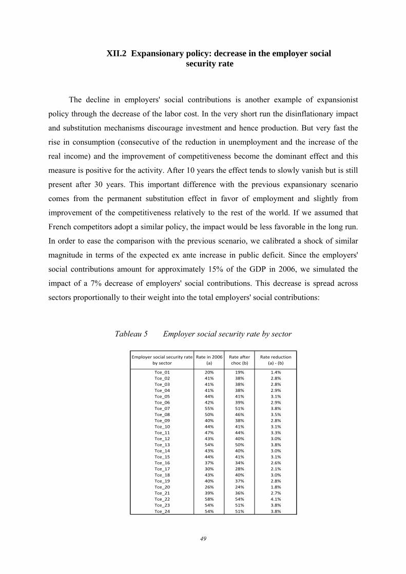
49

XII.2 Expansionary policy: decrease in the employer social security rate

The decline in employers' social contributions is another example of expansionist

policy through the decrease of the labor cost. In the very short run the disinflationary impact

and substitution mechanisms discourage investment and hence production. But very fast the

rise in consumption (consecutive of the reduction in unemployment and the increase of the

real income) and the improvement of competitiveness become the dominant effect and this

measure is positive for the activity. After 10 years the effect tends to slowly vanish but is still

present after 30 years. This important difference with the previous expansionary scenario

comes from the permanent substitution effect in favor of employment and slightly from

improvement of the competitiveness relatively to the rest of the world. If we assumed that

French competitors adopt a similar policy, the impact would be less favorable in the long run.

In order to ease the comparison with the previous scenario, we calibrated a shock of similar

magnitude in terms of the expected ex ante increase in public deficit. Since the employers'

social contributions amount for approximately 15% of the GDP in 2006, we simulated the

impact of a 7% decrease of employers' social contributions. This decrease is spread across

sectors proportionally to their weight into the total employers' social contributions:

Tableau 5 Employer social security rate by sector

Employer social security rate by sector

Rate in 2006 (a)

Rate after choc (b)

Rate reduction     (a) ‐ (b)

Tce_01 20% 19% 1.4%Tce_02 41% 38% 2.8%Tce_03 41% 38% 2.8%Tce_04 41% 38% 2.9%Tce_05 44% 41% 3.1%Tce_06 42% 39% 2.9%Tce_07 55% 51% 3.8%Tce_08 50% 46% 3.5%Tce_09 40% 38% 2.8%Tce_10 44% 41% 3.1%Tce_11 47% 44% 3.3%Tce_12 43% 40% 3.0%Tce_13 54% 50% 3.8%Tce_14 43% 40% 3.0%Tce_15 44% 41% 3.1%Tce_16 37% 34% 2.6%Tce_17 30% 28% 2.1%Tce_18 43% 40% 3.0%Tce_19 40% 37% 2.8%Tce_20 26% 24% 1.8%Tce_21 39% 36% 2.7%Tce_22 58% 54% 4.1%Tce_23 54% 51% 3.8%Tce_24 54% 51% 3.8%

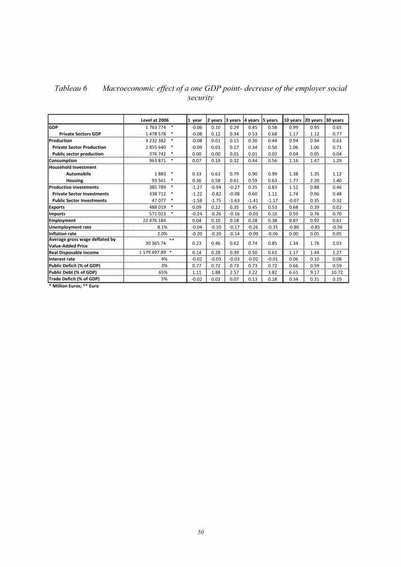
50

Tableau 6 Macroeconomic effect of a one GDP point- decrease of the employer social security

1  year  2 years  3 years 4 years 5 years 10 years 20 years 30 yearsGDP 1 763 774                   * ‐0.06 0.10 0.29 0.45 0.58 0.99 0.95 0.65

Private Sectors GDP 1 478 578                   * ‐0.08 0.12 0.34 0.53 0.68 1.17 1.12 0.77Production 3 232 382                   * ‐0.08 0.01 0.15 0.30 0.44 0.94 0.94 0.63Private Sector Production 2 855 640                   * ‐0.09 0.01 0.17 0.34 0.50 1.06 1.06 0.71Public sector production 376 742                      * 0.00 0.00 0.01 0.01 0.02 0.04 0.05 0.04

Consumption 963 871                      * 0.07 0.19 0.32 0.44 0.56 1.16 1.47 1.29Household Investment

Automobile 1 883                          * 0.33 0.63 0.79 0.90 0.99 1.38 1.35 1.12Housing 93 561                        * 0.36 0.58 0.61 0.59 0.63 1.77 2.20 1.40

Productive Investments 385 789                      * ‐1.27 ‐0.94 ‐0.27 0.35 0.83 1.52 0.88 0.46Private Sector Investments 338 712                      * ‐1.22 ‐0.82 ‐0.08 0.60 1.11 1.74 0.96 0.48Public Sector Investments 47 077                        * ‐1.58 ‐1.75 ‐1.63 ‐1.41 ‐1.17 ‐0.07 0.35 0.32

Exports 488 019                      * 0.09 0.22 0.35 0.45 0.53 0.68 0.39 0.02Imports 571 023                      * ‐0.24 ‐0.26 ‐0.16 ‐0.03 0.10 0.59 0.76 0.70Employment  22 476 184                0.04 0.10 0.18 0.28 0.38 0.87 0.92 0.61Unemployment rate 8.1% ‐0.04 ‐0.10 ‐0.17 ‐0.26 ‐0.35 ‐0.80 ‐0.85 ‐0.56Inflation rate 2.0% ‐0.20 ‐0.20 ‐0.14 ‐0.09 ‐0.06 0.00 0.05 0.05Average gross wage deflated by Value‐Added Price 30 365.74                   ** 0.23 0.46 0.62 0.74 0.85 1.34 1.76 2.03

Real Disposable Income 1 179 497.89             * 0.14 0.28 0.39 0.50 0.61 1.17 1.44 1.27Interest rate 4% ‐0.02 ‐0.03 ‐0.03 ‐0.02 ‐0.01 0.06 0.10 0.08Public Deficit (% of GDP) 3% 0.77 0.72 0.73 0.73 0.72 0.66 0.59 0.59Public Debt (% of GDP) 65% 1.11 1.88 2.57 3.22 3.82 6.61 9.17 10.72Trade Deficit (% of GDP) 5% ‐0.02 0.02 0.07 0.13 0.18 0.34 0.31 0.19* Million Euros; ** Euro

Level at 2006 

51

Tableau 7 Sectoral effect of a one GDP point- decrease of the employer social security

Sectors Variables Level at 2006  1  year  2 years  3 years 4 years 5 years 10 years 20 years 30 yearsProduction (Y) 77 956          0.0 0.1 0.2 0.3 0.5 1.0 1.1 0.8Employment (L) 390 189        0.1 0.1 0.2 0.3 0.4 1.0 1.1 0.8Production price (PY) 1                    ‐0.1 ‐0.3 ‐0.5 ‐0.6 ‐0.8 ‐1.0 ‐0.5 0.2

Y 121 773        0.1 0.2 0.3 0.5 0.6 1.2 1.3 1.0L 484 066        0.1 0.2 0.3 0.5 0.6 1.3 1.5 1.1PY 1                    ‐0.2 ‐0.4 ‐0.7 ‐0.8 ‐1.0 ‐1.3 ‐0.7 0.0Y 90 738          ‐0.3 ‐0.1 0.2 0.5 0.7 1.2 0.8 0.3L 209 964        0.0 0.0 0.2 0.4 0.6 1.3 1.0 0.4PY 1                    ‐0.1 ‐0.3 ‐0.5 ‐0.7 ‐0.8 ‐1.0 ‐0.5 0.0Y 6 645             0.1 0.2 0.3 0.5 0.7 1.2 1.0 0.5L 37 597          0.1 0.2 0.3 0.4 0.6 1.2 1.2 0.6PY 1                    ‐0.3 ‐0.6 ‐0.8 ‐1.0 ‐1.2 ‐1.3 ‐0.7 0.0Y 19 667          ‐0.1 ‐0.1 0.0 0.1 0.3 1.2 1.3 0.8L 84 480          0.0 0.1 0.1 0.2 0.3 1.1 1.4 0.9PY 1                    ‐0.2 ‐0.5 ‐0.7 ‐0.9 ‐1.1 ‐1.4 ‐0.8 0.0Y 19 280          0.0 0.1 0.3 0.4 0.6 1.1 1.0 0.5L 72 927          0.1 0.2 0.3 0.4 0.6 1.2 1.2 0.6PY 1                    ‐0.2 ‐0.4 ‐0.6 ‐0.8 ‐0.9 ‐1.1 ‐0.6 0.0Y 5 976             0.1 0.2 0.3 0.5 0.6 1.1 0.9 0.4L 13 672          0.1 0.2 0.4 0.5 0.7 1.3 1.1 0.6PY 1                    ‐0.2 ‐0.5 ‐0.7 ‐0.8 ‐0.9 ‐1.1 ‐0.6 ‐0.1Y 23 286          0.0 0.1 0.2 0.3 0.4 0.7 0.5 0.2L 18 657          0.1 0.2 0.3 0.4 0.5 0.9 0.7 0.3PY 1                    ‐0.1 ‐0.2 ‐0.4 ‐0.5 ‐0.5 ‐0.7 ‐0.4 0.0Y 25 454          0.0 0.1 0.2 0.4 0.5 1.1 1.0 0.5L 153 969        0.1 0.2 0.3 0.4 0.5 1.2 1.2 0.6PY 1                    ‐0.2 ‐0.5 ‐0.7 ‐0.8 ‐0.9 ‐1.1 ‐0.6 0.0Y 24 196          0.0 0.1 0.2 0.4 0.6 1.0 0.8 0.3L 37 599          0.1 0.2 0.3 0.5 0.6 1.2 1.0 0.4PY 1                    ‐0.1 ‐0.3 ‐0.4 ‐0.6 ‐0.7 ‐0.9 ‐0.5 0.0Y 11 506          0.0 0.1 0.3 0.4 0.5 0.8 0.6 0.2L 14 268          0.1 0.2 0.4 0.5 0.6 1.0 0.8 0.3PY 1                    ‐0.1 ‐0.2 ‐0.4 ‐0.5 ‐0.5 ‐0.7 ‐0.4 0.0Y 449 449        0.0 0.1 0.3 0.5 0.7 1.1 0.9 0.4L 2 036 834     0.1 0.1 0.3 0.4 0.6 1.2 1.1 0.6PY 1                    ‐0.3 ‐0.5 ‐0.8 ‐1.0 ‐1.1 ‐1.3 ‐0.7 0.0Y 247 504        ‐0.4 ‐0.3 ‐0.1 0.1 0.3 1.3 1.4 0.9L 1 498 411     0.0 ‐0.1 0.0 0.1 0.3 1.2 1.5 1.0PY 1                    ‐0.3 ‐0.7 ‐1.0 ‐1.3 ‐1.4 ‐1.8 ‐1.1 ‐0.2Y 10 033          0.1 0.2 0.3 0.4 0.5 0.9 1.0 0.7L 96 348          0.1 0.3 0.5 0.6 0.8 1.3 1.3 0.8PY 1                    ‐0.2 ‐0.4 ‐0.6 ‐0.6 ‐0.7 ‐0.8 ‐0.5 0.1Y 17 137          0.1 0.1 0.3 0.4 0.5 1.0 1.1 0.9L 184 850        0.0 0.1 0.2 0.3 0.4 0.9 1.2 1.0PY 1                    ‐0.5 ‐1.1 ‐1.5 ‐1.7 ‐1.8 ‐1.9 ‐1.1 ‐0.2Y 36 670          0.0 0.1 0.3 0.4 0.6 1.1 0.9 0.5L 328 404        0.0 0.1 0.2 0.3 0.5 1.0 1.1 0.6PY 1                    ‐0.3 ‐0.6 ‐0.9 ‐1.1 ‐1.2 ‐1.4 ‐0.7 0.0Y 10 138          0.0 0.2 0.3 0.4 0.5 0.8 0.6 0.2L 16 833          0.1 0.2 0.3 0.4 0.5 0.9 0.7 0.2PY 1                    ‐0.1 ‐0.3 ‐0.5 ‐0.7 ‐0.8 ‐1.1 ‐0.6 0.0Y 17 992          0.1 0.3 0.5 0.6 0.7 1.0 0.8 0.3L 66 244          0.1 0.2 0.4 0.5 0.7 1.1 0.9 0.4PY 1                    ‐0.3 ‐0.6 ‐0.9 ‐1.0 ‐1.2 ‐1.3 ‐0.7 0.0Y 1 521 601     ‐0.1 0.0 0.1 0.3 0.5 1.0 1.1 0.8L 10 355 121   0.1 0.1 0.2 0.4 0.5 1.1 1.3 0.9PY 1                    ‐0.3 ‐0.6 ‐0.8 ‐1.0 ‐1.1 ‐1.3 ‐0.7 0.0Y 35                  0.3 0.9 1.5 2.1 2.8 4.6 3.1 1.2L 599                0.2 0.5 0.9 1.3 1.9 4.4 3.6 1.6PY 1                    ‐0.3 ‐0.7 ‐1.0 ‐1.3 ‐1.5 ‐1.8 ‐0.7 0.2Y 49 658          0.0 0.0 0.1 0.2 0.3 0.7 0.8 0.7L 13 640          0.0 0.1 0.1 0.2 0.3 0.8 0.9 0.7PY 1                    0.0 ‐0.1 ‐0.1 ‐0.1 ‐0.2 ‐0.3 ‐0.1 0.0Y 46 120          0.0 0.1 0.2 0.3 0.4 1.0 1.0 0.8L 95 291          0.1 0.2 0.3 0.4 0.5 1.1 1.2 0.9PY 1                    ‐0.2 ‐0.5 ‐0.7 ‐0.8 ‐0.9 ‐1.2 ‐0.8 ‐0.1Y 22 826          0.0 0.1 0.1 0.3 0.4 0.9 1.0 0.8L 27 958          0.0 0.1 0.1 0.2 0.3 0.8 1.1 0.9PY 1                    ‐0.1 ‐0.3 ‐0.4 ‐0.5 ‐0.5 ‐0.6 ‐0.4 ‐0.1

Agriculture, forestry and fishing

Manufacture of food products and beverages

Manufacture of motor vehicles, trailers and semi‐trailers

Manufacture of glass and glass products

Manufacture of ceramic products and building materials

Manufacture of articles of paper and paperboard

Manufacture of inorganic basic chemicals

Manufacture of organic basic chemicals

Manufacture of plastics products

Manufacture of basic iron and steel and of ferro‐alloys

Manufacture of non‐ferrous metals

Other industries

Construction of buildings and Civil engineering

Rail transport (Passenger and Freight) 

Passenger transport by road

Freight transport by road and transport via pipeline

Water transport

Air transport

Business services

Mining of coal and lignite

Manufacture of refined petroleum products

Electric power generation, transmission and distribution

Manufacture and distribution of gas

1

2

3

4

5

6

7

8

9

10

11

12

13

14

15

16

17

18

19

21

22

23

24

52

XII.3 A 50% increase of the oil price

As expected, a 50% increase of the oil price has a negative impact on the economy

through a reduction of all the components of the demand. The reduction of the real income

reduces consumption which affects in return private investment. Moreover the increase in

inflation degrades French exports because we assume that higher oil prices do not increase the

world prices of other goods and services. This is quite unrealistic since most French

competitors will also be affected by such a shock21. As an increase in the oil price is a shock

on the world economy, its negative impact evaluated here are likely to be exaggerated.

Tableau 8 Macroeconomic effect of a 50% increase of the oil price

1  year  2 years  3 years 4 years 5 years 10 years 20 years 30 yearsGDP 1 763 774                   * ‐0.82 ‐1.12 ‐1.25 ‐1.34 ‐1.43 ‐1.73 ‐1.44 ‐1.03

Private Sectors GDP 1 478 578                   * ‐0.97 ‐1.33 ‐1.48 ‐1.59 ‐1.69 ‐2.06 ‐1.72 ‐1.23Production 3 232 382                   * ‐0.50 ‐0.80 ‐1.01 ‐1.17 ‐1.30 ‐1.71 ‐1.43 ‐0.99Private Sector Production 2 855 640                   * ‐0.56 ‐0.91 ‐1.14 ‐1.32 ‐1.47 ‐1.93 ‐1.61 ‐1.11Public sector production 376 742                      * ‐0.01 ‐0.02 ‐0.03 ‐0.04 ‐0.04 ‐0.06 ‐0.05 ‐0.04

Consumption 963 871                      * ‐0.38 ‐0.73 ‐1.03 ‐1.26 ‐1.44 ‐1.94 ‐1.74 ‐1.21Household Investment

Automobile 1 883                           * ‐1.88 ‐2.19 ‐2.13 ‐1.99 ‐1.88 ‐1.71 ‐1.25 ‐0.77Housing 93 561                        * ‐5.25 ‐4.98 ‐3.39 ‐1.97 ‐1.16 ‐1.72 ‐1.90 ‐0.62

Productive Investments 385 789                      * ‐1.38 ‐1.97 ‐2.13 ‐2.19 ‐2.27 ‐2.22 ‐1.13 ‐0.66Private Sector Investments 338 712                      * ‐1.53 ‐2.36 ‐2.66 ‐2.76 ‐2.82 ‐2.48 ‐1.19 ‐0.68Public Sector Investments 47 077                        * ‐0.27 0.79 1.69 1.95 1.72 ‐0.36 ‐0.67 ‐0.52

Exports 488 019                      * ‐0.17 ‐0.45 ‐0.72 ‐0.93 ‐1.07 ‐1.09 ‐0.56 ‐0.17Imports 571 023                      * ‐0.51 ‐0.84 ‐1.07 ‐1.25 ‐1.41 ‐2.05 ‐2.17 ‐2.04Employment  22 476 184                ‐0.11 ‐0.28 ‐0.47 ‐0.63 ‐0.78 ‐1.24 ‐0.98 ‐0.50Unemployment rate 8.1% 0.10 0.26 0.43 0.58 0.72 1.14 0.90 0.46Inflation rate 2.0% 1.29 0.44 0.21 0.06 ‐0.01 ‐0.07 ‐0.06 ‐0.05Average gross wage deflated by Value‐Added Price

30 365.74                  ** 1.77 1.47 1.14 0.86 0.64 ‐0.03 ‐0.45 ‐0.69

Real Disposable Income 1 179 497.89             * ‐0.77 ‐1.02 ‐1.21 ‐1.37 ‐1.49 ‐1.86 ‐1.67 ‐1.16Interest rate 4% 0.12 0.13 0.10 0.06 0.01 ‐0.12 ‐0.11 ‐0.07Public Deficit (% of GDP) 3% 0.15 0.38 0.41 0.42 0.44 0.77 1.22 1.53Public Debt (% of GDP) 65% 0.96 1.03 1.14 1.37 1.71 5.09 12.81 20.81Trade Deficit (% of GDP) 5% 1.01 0.73 0.54 0.41 0.33 0.16 0.26 0.39* Million Euros; ** Euro

Level at 2006 

Because of the drop in demand, all sectors suffer from this shock (Tableau 9). The other

energy sectors suffer less than the oil sectors, benefiting from the possibilities of substitution

with oil.

21 We suppose also that the recycling of the oil revenue of oil producing countries compensates exactly the

decrease in demand of other commercial partners of France.

53

Tableau 9 Sectoral effect of a 50% increase of the oil price

l

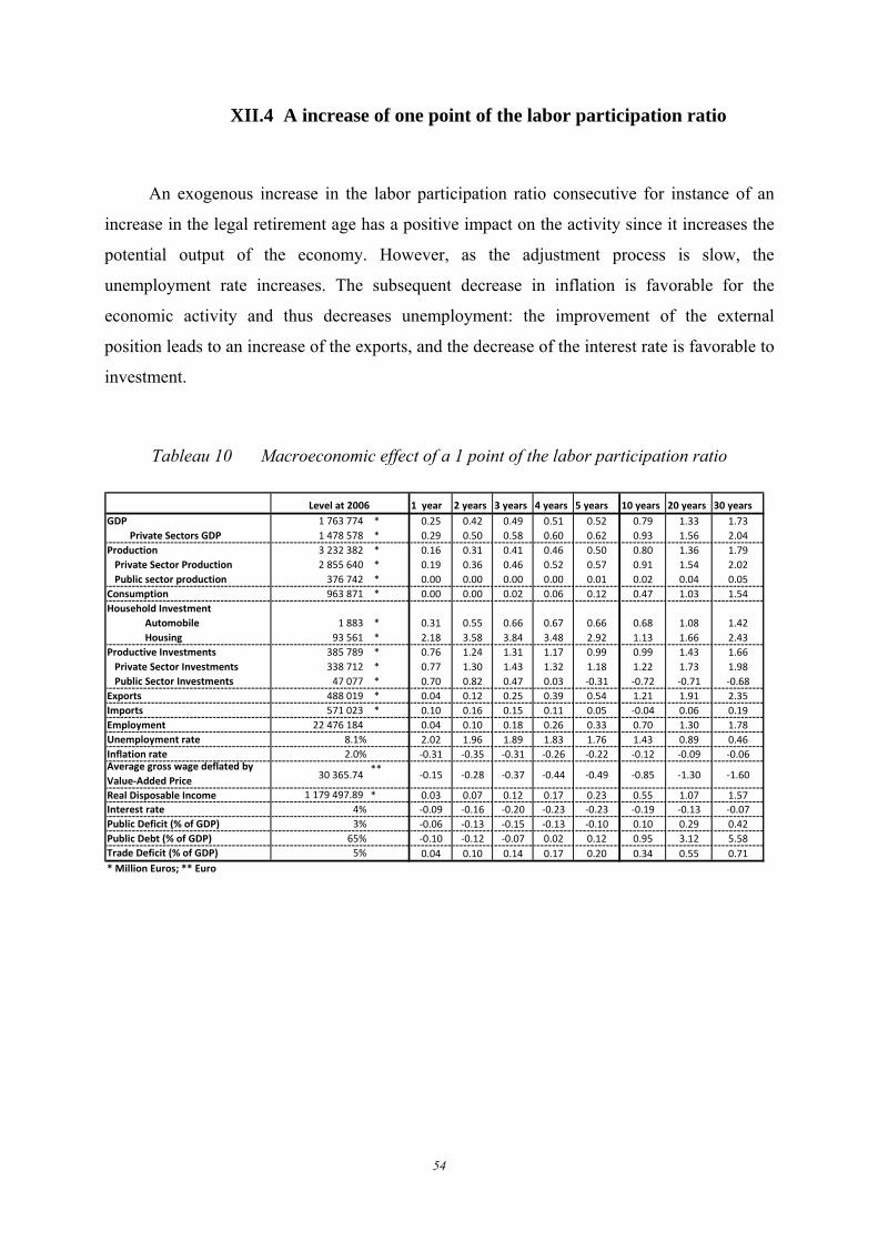
54

XII.4 A increase of one point of the labor participation ratio

An exogenous increase in the labor participation ratio consecutive for instance of an

increase in the legal retirement age has a positive impact on the activity since it increases the

potential output of the economy. However, as the adjustment process is slow, the

unemployment rate increases. The subsequent decrease in inflation is favorable for the

economic activity and thus decreases unemployment: the improvement of the external

position leads to an increase of the exports, and the decrease of the interest rate is favorable to

investment.

Tableau 10 Macroeconomic effect of a 1 point of the labor participation ratio

1  year  2 years  3 years 4 years 5 years 10 years 20 years 30 yearsGDP 1 763 774                   * 0.25 0.42 0.49 0.51 0.52 0.79 1.33 1.73

Private Sectors GDP 1 478 578                   * 0.29 0.50 0.58 0.60 0.62 0.93 1.56 2.04Production 3 232 382                   * 0.16 0.31 0.41 0.46 0.50 0.80 1.36 1.79Private Sector Production 2 855 640                   * 0.19 0.36 0.46 0.52 0.57 0.91 1.54 2.02Public sector production 376 742                      * 0.00 0.00 0.00 0.00 0.01 0.02 0.04 0.05

Consumption 963 871                      * 0.00 0.00 0.02 0.06 0.12 0.47 1.03 1.54Household Investment

Automobile 1 883                          * 0.31 0.55 0.66 0.67 0.66 0.68 1.08 1.42Housing 93 561                        * 2.18 3.58 3.84 3.48 2.92 1.13 1.66 2.43

Productive Investments 385 789                      * 0.76 1.24 1.31 1.17 0.99 0.99 1.43 1.66Private Sector Investments 338 712                      * 0.77 1.30 1.43 1.32 1.18 1.22 1.73 1.98Public Sector Investments 47 077                        * 0.70 0.82 0.47 0.03 ‐0.31 ‐0.72 ‐0.71 ‐0.68

Exports 488 019                      * 0.04 0.12 0.25 0.39 0.54 1.21 1.91 2.35Imports 571 023                      * 0.10 0.16 0.15 0.11 0.05 ‐0.04 0.06 0.19Employment  22 476 184                0.04 0.10 0.18 0.26 0.33 0.70 1.30 1.78Unemployment rate 8.1% 2.02 1.96 1.89 1.83 1.76 1.43 0.89 0.46Inflation rate 2.0% ‐0.31 ‐0.35 ‐0.31 ‐0.26 ‐0.22 ‐0.12 ‐0.09 ‐0.06Average gross wage deflated by Value‐Added Price 30 365.74                   ** ‐0.15 ‐0.28 ‐0.37 ‐0.44 ‐0.49 ‐0.85 ‐1.30 ‐1.60

Real Disposable Income 1 179 497.89             * 0.03 0.07 0.12 0.17 0.23 0.55 1.07 1.57Interest rate 4% ‐0.09 ‐0.16 ‐0.20 ‐0.23 ‐0.23 ‐0.19 ‐0.13 ‐0.07Public Deficit (% of GDP) 3% ‐0.06 ‐0.13 ‐0.15 ‐0.13 ‐0.10 0.10 0.29 0.42Public Debt (% of GDP) 65% ‐0.10 ‐0.12 ‐0.07 0.02 0.12 0.95 3.12 5.58Trade Deficit (% of GDP) 5% 0.04 0.10 0.14 0.17 0.20 0.34 0.55 0.71* Million Euros; ** Euro

Level at 2006 

55

Tableau 11 Sectoral effect of a 1 point of the labor participation ratio

Sectors Variables Level at 2006  1  year  2 years  3 years 4 years 5 years 10 years 20 years 30 yearsProduction (Y) 77 956          0.0 0.1 0.2 0.3 0.4 0.9 1.6 2.1Employment (L) 390 189        0.0 0.0 0.1 0.2 0.3 0.9 1.9 2.6Production price (PY) 1                    ‐0.1 ‐0.3 ‐0.6 ‐0.9 ‐1.2 ‐2.5 ‐3.7 ‐4.6

Y 121 773        0.0 0.1 0.2 0.3 0.4 1.0 1.8 2.4L 484 066        0.0 0.0 0.1 0.2 0.3 1.0 2.0 2.8PY 1                    ‐0.1 ‐0.2 ‐0.5 ‐0.7 ‐1.0 ‐2.3 ‐3.7 ‐4.5Y 90 738          0.3 0.5 0.6 0.7 0.8 1.3 2.1 2.6L 209 964        0.1 0.2 0.4 0.5 0.7 1.4 2.4 3.1PY 1                    ‐0.1 ‐0.2 ‐0.4 ‐0.6 ‐0.8 ‐1.7 ‐2.7 ‐3.3Y 6 645             0.1 0.2 0.4 0.5 0.7 1.3 2.2 2.8L 37 597          0.0 0.1 0.2 0.3 0.5 1.3 2.4 3.2PY 1                    ‐0.1 ‐0.3 ‐0.5 ‐0.8 ‐1.1 ‐2.3 ‐3.6 ‐4.3Y 19 667          0.4 0.8 1.2 1.3 1.3 1.0 1.6 2.1L 84 480          0.1 0.4 0.6 0.9 1.1 1.2 1.8 2.5PY 1                    ‐0.1 ‐0.3 ‐0.6 ‐0.9 ‐1.1 ‐2.2 ‐3.4 ‐4.2Y 19 280          0.1 0.2 0.3 0.5 0.6 1.4 2.2 2.9L 72 927          0.0 0.1 0.2 0.3 0.4 1.4 2.5 3.3PY 1                    ‐0.1 ‐0.2 ‐0.4 ‐0.7 ‐0.9 ‐2.0 ‐3.0 ‐3.6Y 5 976             0.1 0.2 0.3 0.5 0.7 1.5 2.5 3.1L 13 672          0.0 0.1 0.2 0.3 0.5 1.5 2.7 3.5PY 1                    ‐0.1 ‐0.2 ‐0.4 ‐0.7 ‐0.9 ‐1.9 ‐2.8 ‐3.4Y 23 286          0.0 0.1 0.2 0.4 0.5 1.0 1.6 2.0L 18 657          0.0 0.1 0.1 0.2 0.4 1.1 1.9 2.5PY 1                    0.0 ‐0.1 ‐0.3 ‐0.4 ‐0.6 ‐1.2 ‐1.8 ‐2.2Y 25 454          0.1 0.3 0.4 0.6 0.7 1.2 2.0 2.5L 153 969        0.0 0.1 0.3 0.4 0.5 1.3 2.3 3.1PY 1                    ‐0.1 ‐0.2 ‐0.4 ‐0.6 ‐0.8 ‐1.8 ‐2.8 ‐3.4Y 24 196          0.1 0.3 0.4 0.6 0.8 1.5 2.4 3.0L 37 599          0.0 0.1 0.2 0.4 0.6 1.6 2.8 3.6PY 1                    ‐0.1 ‐0.2 ‐0.4 ‐0.6 ‐0.8 ‐1.7 ‐2.5 ‐3.1Y 11 506          0.1 0.2 0.3 0.5 0.6 1.2 1.9 2.4L 14 268          0.0 0.1 0.2 0.3 0.5 1.4 2.4 3.1PY 1                    ‐0.1 ‐0.2 ‐0.3 ‐0.5 ‐0.7 ‐1.3 ‐2.0 ‐2.4Y 449 449        0.1 0.3 0.4 0.5 0.7 1.3 2.1 2.6L 2 036 834     0.0 0.1 0.3 0.4 0.5 1.3 2.3 3.0PY 1                    ‐0.1 ‐0.2 ‐0.4 ‐0.7 ‐0.9 ‐2.1 ‐3.3 ‐4.0Y 247 504        1.2 1.9 2.1 1.8 1.5 0.7 1.1 1.6L 1 498 411     0.4 0.9 1.3 1.5 1.6 1.0 1.3 1.9PY 1                    ‐0.1 ‐0.4 ‐0.7 ‐1.0 ‐1.3 ‐2.3 ‐3.8 ‐4.8Y 10 033          0.1 0.2 0.4 0.6 0.7 1.2 2.0 2.5L 96 348          0.0 0.0 0.1 0.2 0.4 1.2 2.3 3.1PY 1                    ‐0.3 ‐0.8 ‐1.2 ‐1.6 ‐1.9 ‐2.9 ‐4.0 ‐4.7Y 17 137          0.0 0.0 0.1 0.1 0.2 0.5 1.0 1.4L 184 850        0.0 0.0 0.0 0.1 0.1 0.4 1.0 1.5PY 1                    ‐0.1 ‐0.3 ‐0.6 ‐0.9 ‐1.3 ‐2.9 ‐4.5 ‐5.6Y 36 670          0.1 0.2 0.3 0.4 0.5 1.1 1.9 2.4L 328 404        0.0 0.1 0.2 0.3 0.4 1.1 2.0 2.7PY 1                    ‐0.1 ‐0.3 ‐0.5 ‐0.8 ‐1.1 ‐2.3 ‐3.6 ‐4.4Y 10 138          0.0 0.1 0.2 0.4 0.5 1.2 2.0 2.4L 16 833          0.0 0.1 0.1 0.2 0.4 1.2 2.2 2.8PY 1                    ‐0.1 ‐0.2 ‐0.4 ‐0.7 ‐0.9 ‐2.1 ‐3.2 ‐3.9Y 17 992          0.0 0.1 0.3 0.4 0.6 1.3 2.2 2.7L 66 244          0.0 0.1 0.1 0.2 0.4 1.3 2.3 3.0PY 1                    ‐0.1 ‐0.2 ‐0.5 ‐0.7 ‐1.0 ‐2.2 ‐3.3 ‐4.1Y 1 521 601     0.1 0.2 0.3 0.4 0.4 0.8 1.4 1.9L 10 355 121   0.0 0.1 0.1 0.2 0.3 0.8 1.6 2.2PY 1                    ‐0.2 ‐0.5 ‐0.8 ‐1.1 ‐1.4 ‐2.7 ‐4.1 ‐5.0Y 35                  0.2 0.6 1.2 1.9 2.6 5.9 8.6 10.4L 599                0.0 0.2 0.5 1.0 1.5 5.0 8.3 10.4PY 1                    ‐0.1 ‐0.4 ‐0.8 ‐1.2 ‐1.6 ‐3.2 ‐4.4 ‐5.2Y 49 658          0.0 0.0 0.0 0.1 0.1 0.2 0.4 0.5L 13 640          0.0 0.0 0.0 0.1 0.1 0.3 0.6 0.8PY 1                    0.0 0.0 ‐0.1 ‐0.1 ‐0.2 ‐0.4 ‐0.6 ‐0.8Y 46 120          0.0 0.1 0.2 0.2 0.3 0.6 1.0 1.2L 95 291          0.0 0.0 0.1 0.1 0.2 0.7 1.2 1.6PY 1                    ‐0.1 ‐0.4 ‐0.7 ‐0.9 ‐1.2 ‐2.3 ‐3.5 ‐4.2Y 22 826          0.0 0.0 0.0 0.0 0.0 0.1 0.3 0.3L 27 958          0.0 0.0 0.0 0.0 0.1 0.2 0.4 0.5PY 1                    0.0 ‐0.1 ‐0.1 ‐0.2 ‐0.3 ‐0.8 ‐1.2 ‐1.5

Agriculture, forestry and fishing

Manufacture of food products and beverages

Manufacture of motor vehicles, trailers and semi‐trailers

Manufacture of glass and glass products

Manufacture of ceramic products and building materials

Manufacture of articles of paper and paperboard

Manufacture of inorganic basic chemicals

Manufacture of organic basic chemicals

Manufacture of plastics products

Manufacture of basic iron and steel and of ferro‐alloys

Manufacture of non‐ferrous metals

Other industries

Construction of buildings and Civil engineering

Rail transport (Passenger and Freight) 

Passenger transport by road

Freight transport by road and transport via pipeline

Water transport

Air transport

Business services

Mining of coal and lignite

Manufacture of refined petroleum products

Electric power generation, transmission and distribution

Manufacture and distribution of gas

1

2

3

4

5

6

7

8

9

10

11

12

13

14

15

16

17

18

19

21

22

23

24

56

Appendix A. Long term of the model

The long term steady state of the model is generally defined as a state where all

variables grow at a constant rate. This state is coherent with the representation of a stable

economy able to maintain a given configuration forever. This implies that rates such as the

unemployment or labor participation ratios, tax rates are constant in the long run. This is

coherent with the fact that these ratios lie by definition between 0 and 100% and thus cannot

be affected by a trend forever.

Most shares should also be constant. For instance, the shares of investment or of

consumption into GDP should be constant. Otherwise the effect of one these two determinants

of the GDP vanishes over time. The same argument holds for the share of one sector in the

total in terms of labor or production: we expect an economy where all sectors remains in the

long run, which implies that some economic mechanisms guaranty stable share for each

sectors.

Some exceptions are possible. As empirically observed, it seems realistic that the share

of labor into the GDP decreases over time because of the technical progress. But the share of

the efficient labor, that is including the technical progress, remains constant. Because of the

globalization of the economy, the ratio between export and production may also increase

permanently in the long run. But in the long run this effect is expected to be compensated by

the increase in the ratio between import and production so that the share of the external

balance into production remains constant.

In the long run, all relative prices are expected to be constant. This implies that all

prices grow at the same rate. This guaranty that the economy is not affected by substitution

mechanisms in the long run: firms do not want to change the share of each production factors

into production and consumers are satisfied with share of each good into their aggregate

consumption. It implies also that each agent is satisfied with their share of the global revenue:

firms do not want to change the growth rate of their price whereas employees do not want to

change the growth rate of their wage.

Assuming that ν, τ, μ, π and ω are the growth rates of the population, of the technical

progress, of the real economy (i.e. of the GDP), of prices (i.e. inflation), and of wages, the

long run value of these rate cannot be chosen independently. First, the growth rate of the real

economy should be equal to the sum of the growth rate of the population and of the technical

57

progress: μ ν τ= + . This condition is a direct consequence of the hypothesis of constant

return to scales (homogeneous of degree 1) of the production function. In the long run,

relative price are constant and the labor demand [12] implies that production grows at the sum

of the growth rates of labor and technical progressΔ = Δ +Δ rodjt jt jty l p . In addition, the stability

of unemployment implies that labor grows at the same rate as the population (Equation[57]).

In the long run, the price equation implies that the growth rate of wages should be equal

to the sum of inflation and of the growth rate of the technical progressω π τ= + . This holds

only if some economic mechanisms imply that the unemployment rate converge to the

NAIRU. The latter depends on the parameter of the Phillips curve [55]:

( )1 2 3 5(1 ) (1 ) /U ρ ρ π ρ τ ρ∞ = − − − − [80]

In the model several stabilizing equation guaranty that the economy return to stationary

path after a shock. Inflationary shocks degrade the external position of France by decreasing

export and increasing imports. In addition, the Taylor rule combined with the negative impact

of the real interest rate on the demand prevents inflationary shock to lead to an explosive

inflation dynamic. The negative impact of the real interest rate on the activity has several

possible canals:

o Consumption: in coherence with a life-cycle model and the possibility of an intertemporal

allocation of their resource, households may increase their savings when the real interest

rate increases and thus reduces their consumptions. They may also have Ricardian

behavior in the long run by internalizing the government and firms' budget constraints.

They may thus adjust their consumption in such way that the ratio between their saving

and the national debt is constant in order to insure the sustainability of the debt (see Box

3).

o Investment: firms may choose their investment level that is coherent with the stability of

their debt into the value-added.

o Tax and public spending: the government is expected to choose the tax rate and public

spending levels that are coherent with a stable debt into the GDP.

The consistency of a dynamic model with a stationary equilibrium requires long term

constraints which depend on the type of mathematical equation. We briefly detailed the main

cases that are encountered in Three-ME and how the model can be calibrated in order to be at

the stationary state from the first period of the simulation onward.

58

Additive equations

In the model, many relations enter in an additive form:

,1=

= ∑I

t i ti

Y X [81]

These are in general definitions such as the GDP decomposition or income, etc. In case

of an additive equation [81], the variable Y grows at the rate μ from the first period onward if

all its components X grow also at that rate:

,0 01

(1 ) (1 )I

t tt i

i

Y X Yμ μ=

⎛ ⎞= + = +⎜ ⎟⎝ ⎠∑ [82]

Moreover in that case all ratios between variables (Xi/Y and Xi/Xj) are constant over

time. In the case of the GDP equation this seems a realistic long run property. Otherwise the

share of each component in the GDP is not stable over time and the long run growth rate of

the GDP corresponds to the component’s highest growth rate. Indeed, if the X-variables do

not grow at the same rate, the growth rate of Y (μ) converges to the highest X-variable growth

rate. And the share of the X-variable with a lower growth rate tends toward zero.

This mathematical property may imply unrealistic constraint on the model if one wants

to be at the steady states at the first period of the simulation. This is particularly true if one

wishes to calibrate the model on real data. We can give 2 examples:

For instance, it is unrealistic to assume that a negative inventory change will decrease

indefinitely because the level of inventories becomes at some point negative. One possibility

is to amend the calibration in order to impose a zero-inventory change at the base years.

In the real world, most countries’ imports and exports do not grow at the rate of the

GDP but at a higher rate because of the trade globalization. In fact Equation [81] allows that

several X-variables grow at a different rate than Y in the long run as long their sum grows at

the same rate as Y. Consequently, imports and exports may grow faster that the GDP forever

as long as their effect cancel out, that is as long as the foreign trade balance grows at the rate

of the GDP. If the long run foreign trade balance is zero, imports and exports grow at the

same rate. If not, they grow at the same rate asymptotically, the smallest (in absolute value)

growing faster. This implies mechanism that imposes import and export to grow consistently.

59

The most common way is to assume that the exchange rate adjusts in order to reach the

external balance objective.

Unit elasticity logarithm equations

Many relations in the model impose a unit-elasticity specified in logarithm form:

ln( ) ln( ) α= +t tY X [83]

This specification is used for all production factor demand since we systematically

assume a constant return-to-scale technology. If the coefficient α is calibrated in the initial

period as a simple inversion of equation [83] and constant over time, this specification implies

that Y always grows at the same rate as X.

In the production factors demand, α depends on the relative prices and thus may vary

over time in case of shock or if they are not in equilibrium in the initial period. In that case,

the growth rate of Y and X differs over time but they tend to converge toward each other

provided that mechanisms in the price equation guaranty the long run stability of relative

prices.

Accumulation equations

The model contains several accumulation equations: capital stock dynamic, public and

private debt, household savings. All can be represented with the following equation:

1(1 )β−= + +t t tY Y X [84]

In the case of capital accumulation, β is the depreciation rate and is negative. In the case

of debt or saving equation, β is the interest rate and is thus positive. Dividing both sides by

1−tY give the growth rate of the stock variable:

1/β −= +&t t tY X Y [85]

At the steady states, X should grow at the same rate as Y which is defined by Equation

[85]. Consequently, being at the stationary states from the first period onward implies that X

60

cannot be calibrated on real data. For the base year, X is calibrated as an inversion of Equation

[84]:

.1

X Yμ βμ

⎛ ⎞−= ⎜ ⎟+⎝ ⎠

[86]

Error correction model (ECM) equations

All adjustment processes are assumed to follow an Error Correction Model (ECM)

where the variable Y adjusts slowly to its target or notional value Yn:

1 1 2 3 1 1( )n nt t t t tY Y Y Y Yα α α− − −Δ = Δ + Δ − − [87]

This specification was used to specify the dynamic of prices and quantities and thus

describe how effective values adjust to notional values. If the change in the target Yn is

constant, Equation [87] implies that in the long run change in Y is also constant: n

t tY Y μΔ = Δ = . This property can be used to calibrate the initial period in order to be at the

steady state from the first period onward. To do so, the initial target level should be:

0 0 1 2 3.(1 ) /nY Y μ α α α= + − − [88]

Unless 1 2 1α α+ = , the target is never reach even in the long run. For instance, the

notional price becomes a function of inflation and the model is not super-neutral. This

property is sometimes viewed as theoretically inconsistent (Allard-Prigent et al., 2002) but is

frequently found empirically (Chagny et al., 2002).

One can notice that if 1 0α = and 2 3α α α= = , Equation [87] simplifies:

1(1 )nt t tY Y Yα α −= + − [89]

If moreover the variables Y and Yn are expressed in logarithm, Equation [89] is nothing

else but a geometric adjustment process. This particular case has the advantage to allow only

monotonous adjustment whereas the more general form of the ECM [87] may lead to cyclical

adjustment. This generally arise when the autoregressive term has an important impact, that is

when 1α is high.

61

Appendix B. Generalized CES production function and factors demand

This appendix derives the optimality program of the producer and the consumer

assuming a generalized CES (GCES) production and utility function. We show that the GCES

function can be approximated in the neighborhood of the optimal stationary state by a Cobb-

Douglas function for which the technical coefficients vary with the relative prices. This result

greatly facilitates the deduction of linear demands functions for input and goods.

GCES production function and factors demand

Let us define a GCES production function as a H inputs-production function with

different elasticities of substitution between each pair of input. We still assume a constant

elasticity of substitution between 2 inputs along the isoquant. Let us assume that technology

may be represented by a continuous and twice differentiable function, linearly homogeneous,

strictly increasing ( ' ( ) 0t htQ x > ) and concave ( ''( ) 0t htQ x < ) reflecting the law of diminishing

marginal returns:

( )=t htQ Q X [90]

Where htX is the quantity of input (or production factor) [1; ]=h H used to produce the

quantity of production (or output) tQ .

For algebraic simplicity, we assume a technology with constant returns to scale (i.e. the

production function [90] is homogeneous of degree 1) and the absence of technical progress.

We shall relax these constraints latter. Driven by maximizing profit behaviour, the producer

chooses her demand for each input by minimizing her production cost [91] subject to the

technical constraint [90]:

1==∑

HX

t ht hth

C P X [91]

Where XhtP is the price of input h. The Lagrangien to this problem is:

( )( )λ= − −t t t t htL C Q Q X [92]

62

The necessary first order conditions are ( ) 0′ =htL X for all h and ( ) 0λ′ =L . The second

order conditions ensure that the optimum is a minimum is always verified because of the

convexity of the cost function [91] and strict convexity of the isoquants formed by the

production function [90] 22. The well-known first order condition says that at the optimum,

the ratio between marginal productivities of two inputs equals the one between their prices:

' '( ) / ( ) /′ ′ =X X

ht h t ht h tQ X Q X P P [93]

The production function [90] can be linearized with the following first-order Taylor

expansion:

1

( )( )=

′=∑& &

Hht ht

t hth ht

Q X XQ XQ X

[94]

Euler’s Theorem states that a function which is homogeneous of degree 1 can be

express as the sum of its arguments weighted by their first partial derivatives:

1( ) ( )

=

′= ∑H

ht ht hth

Q X Q X X [95]

The fact that in equilibrium, the remuneration of the production factors must be equal to

the value of the production provides another useful relation:

1==∑

HX Q

ht ht t th

P X P Q [96]

The combination of equations [93] to [96] gives at the neighbourhood of the stationary

state a linear specification of the production function:

1 1ϕ ϕ

= =

= ⇔ =∑ ∑& &H H

t ht ht t ht hth h

Q X q x [97]

Where ϕht is the share (in value) of input h in the production sometimes called Leontief

technical coefficient:

/ ( )ϕ = X Qht ht ht t tP X P Q [98]

22 According to the technological constraint [90], the strict convexity of the isoquant ( ( ) 0′′′ >ht h tX X ) implies that

( ) 2 ( )′′ ′<ht htQ X Q X . This condition is always verified since by assumption the left-hand side is negative

( ( ) 0′′ <htQ X ) while the right-hand side is positive ( ( ) 0′ >htQ X ).

63

We have just shown that at the neighbourhood of the optimum any linearly

homogeneous, twice differentiable, strictly increasing and concave production function can be

approximated by a Cobb-Douglas with technical coefficients that varies over time. Moreover

these technical coefficients correspond to the input share into production. They are stable in

the long run because the specification of Three-ME guaranties the stability of ratios between

prices and of input to production ratios.

Suppose further that the direct elasticity of substitution – in the sense of Hicks (1932)

and Robinson (1933) – between inputs h and h' ( 'ηhh ) is not necessarily the same between

each couple of production factors. This elasticity measures the change in the ratio between

two factors of production due to a change in their relative marginal productivity, i.e. in the

marginal rate of substitution (in the slope of the iso-production curve):

( ) ( )' 'ln( / ) ln( / ) ln ( ) / ( )

ln ( ) / ( )η η′

′ ′′

∂ ′ ′− = ⇔ ∂ = − ∂′ ′∂

ht h thh ht h t hh ht h t

ht h t

X X X X Q X Q XQ X Q X

[99]

Integrating [99] with respect to time and then combining it with the optimality

condition [93] gives:

( ) '

' ' '/ /η

ξ−

=hhX X

ht h t hh ht h tX X P P [100]

Where 'ξhh is the constant of integration which we calibrate to one for algebraic simplicity.

Rewriting [100] in terms of input share, ( ) '1

' ' '/ /η

ϕ ϕ ξ−

=hhX X

ht h t hh ht h tP P , gives the well-known

result that the inputs share is constant over time only in case of unit elasticity of substitution

between all factors of production (Cobb-Douglas technology).

The first order conditions [100] and the production function [97] constitute a system of

H linearly independent equations and H unknowns. Its resolution give the demand for each

factor as a positive function of output and negative function of relative prices between

production factors:

' ' '' 1'

( )η ϕ=≠

= − −∑H

X Xht t hh h t ht h t

hh h

x q p p [101]

The introduction of technical progress and non constant return-to-scale is

straightforward and does not alter the results. In the first case one can simply define

=rognput

ht ht htX I P as the efficient input, which includes the technical progress rog

htP , nputhtI being

64

the effective input. In the second case, one can simply define production as an homogenous

function of Q of degree θ : θ=t tY Q . In case of a technology with increasing (resp. decreasing)

return-to-scale, θ > 1 (resp. < 1). Integrating technical progress and non constant return-to-

scale leads to the following input demand:

1' ' '

' 1'

( )θ η ϕ−

=≠

= − − −∑rog

Hnput X Xht t ht hh h t ht h t

hh h

i y p p p [102]

Assuming constant return to scale, this log-linear specification has been recently

estimated for the Euro area by Lemoine et al. (2010) using the Kalman filter to extract the

trend of technical progress.

GCES consumer utility function and demand for goods

In Three-ME, the demand for goods is treated in a similar way as the demand for input.

Let us assume that at a first stage the consumer divides (eventually via an intertemporal

maximization program) her revenue between expenditures and savings. For a given level

desired volume of expenditure Q, the consumer is then assumed to minimize the cost of this

expenditure. The substitutability between the different consumption goods (or expenditures),

Xh, is measured through a J goods-utility function having the same property as the production

function defined in [90]. Formally the optimization program is the same as the one of the

producer. It consists in minimizing the cost of expenditure [91] subject to the utility function

constraint [90]. The demand for goods is thus [101].

Notice that minimizing the cost of expenditure subject to a utility function constraint

give the same result as the standard approach which consists in maximizing the utility [90]

subject to a budget constraint [103]:

1==∑

HX Q

ht ht t th

P X P Q [103]

The Lagrangien to this problem is:

1

λ=

⎛ ⎞= − −⎜ ⎟⎝ ⎠∑

HX Q

t t ht ht t th

L Q P X P Q [104]

65

The necessary first order conditions ( ( ) 0′ =htL X for all h and ( ) 0λ′ =L ) are the well-

know conditions that the ratio between marginal utilities of two goods equals the one between

their prices (Equation [93] and thus [100]) and the budget constraint (Equation [103]). Using a

first-order Taylor expansion on Equation [103] (devided by PQ) in the neighbourhood of the

stationary equilibrium characterized by the stability of price ratios ( '/X Xh hP P , /X Q

hP P ),

allows for rewriting the budget constraint as [97]. As we have now the same system to solve

as in the producer case (Equations [100] and [97]), the demand for good is thus [101].

Notice that the particular case of a CES function ( 'η η=hh ), [101] simplifies. To see

this, let us first use a first-order Taylor expansion on Equation [103] (devided by Qt) in the

neighbourhood of the stationary equilibrium characterized by the stability of ratios between

volumes (Xh/Xh', Xh/Q). This conveniently allows expressing the consumer price as a weighted

average of the prices of goods, the weight being the share into consumption (Equation [98]):

1 1

H HQ X Q X

t ht ht t ht hth h

P P p pϕ ϕ= =

= ⇔ =∑ ∑& & [105]

Assuming a constant elasticity of substitution ( 'η η=hh ) between goods and combining

the price equation [105] to [101], the demand for goods simplifies and depends only on the

relative price between the price of goods and the consumer price:

( )η= − −X Qht t ht tx q p p [106]

Not surprisingly this relation is the same as the one deduced from a direct maximization

of CES utility function subject to a budget constraint (see Blanchard and Fischer, 1989;

Blanchard and Kiyotaki, 1987; Dixit and Stiglitz, 1977). The only difference is that the

consumer price index ( QtP ) is a linear approximation of the Dixit-Stiglitz index which is a

CES function of the price of goods. As demonstrated by Arrow et al. (1961), Leontief and

Cobb-Douglas functions are particular cases of a CES function whereη tends to 0 and 1

respectively.

66

Appendix C. Glossary of terms used

Index and exponents

a Armington economic agent (sectors, consumers and public administrations)

auto Automobile

c Consumption

d Domestic

e Country

eff Efficient

en Energy

ea Euro area

fc Final consumption

g Public administration

h Input (capital, labor, energy, material); or euro area country

hh Household

hous Housing

i, i’ Product varying between 1 and 24

inv Investment

j Sector varying between 1 and 24

m Import

n Notional or optimal

real Real

s Sector

sub Subsidies

t Time

tax Taxes

trsp Transport

val Value

vol Volume

x Export

y Production

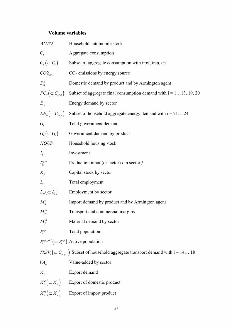
67

Volume variables

tAUTO Household automobile stock

tC Aggregate consumption

( )it tC C⊂ Subset of aggregate consumption with i=cf, trsp, en

,2en tCO CO2 emissions by energy source

aitD Domestic demand by product and by Armington agent

( ),it cf tFC C⊂ Subset of aggregate final consumption demand with i = 1…13, 19, 20

jtE Energy demand by sector

( ),it en tEN C⊂ Subset of household aggregate energy demand with i = 21… 24

tG Total government demand

( )it tG G⊂ Government demand by product

tHOUS Household housing stock

tI Investment

nputijtI Production input (or factor) i in sector j

jtK Capital stock by sector

tL Total employment

( )jt tL L⊂ Employment by sector

aitM Import demand by product and by Armington agent aritM Transport and commercial margins atjtM Material demand by sector

optP Total population

( )_op act opt tP P⊂

Active population

( ),it trsp tTRSP C⊂ Subset of household aggregate transport demand with i = 14… 18

jtVA Value-added by sector

itX Export demand

( )dit itX X⊂ Export of domestic product

( )mit itX X⊂ Export of import product

68

jtY Production by sector

Value variables

sB Sector financing-needs gD Public debt sD Sector (or private) debt

gDEF Public deficit xDEF External commercial deficit

taxtEN Energy taxes

gtEXP Government total expenditures h

tEXP Household total expenditures _

2net stFD − Total firms net financial debt tax

tFP Total firm profit tax

_1

net htFW −

Net financial wealth of household

1sjtGOS − Total gross operating profit

disptI Gross disposable income

gtPFD Total demand of production factors

taxtPR Product taxes net of subsidies

gtRES Government total resources

htS Financial private saving

jtSC Employer and employee social security contributions

gitSUB Total public subsidies

_ransf htT Government social transfers to household

taxtVA Value-added tax

_disp taxtI Income tax tax

tY Production taxes net of operating subsidies

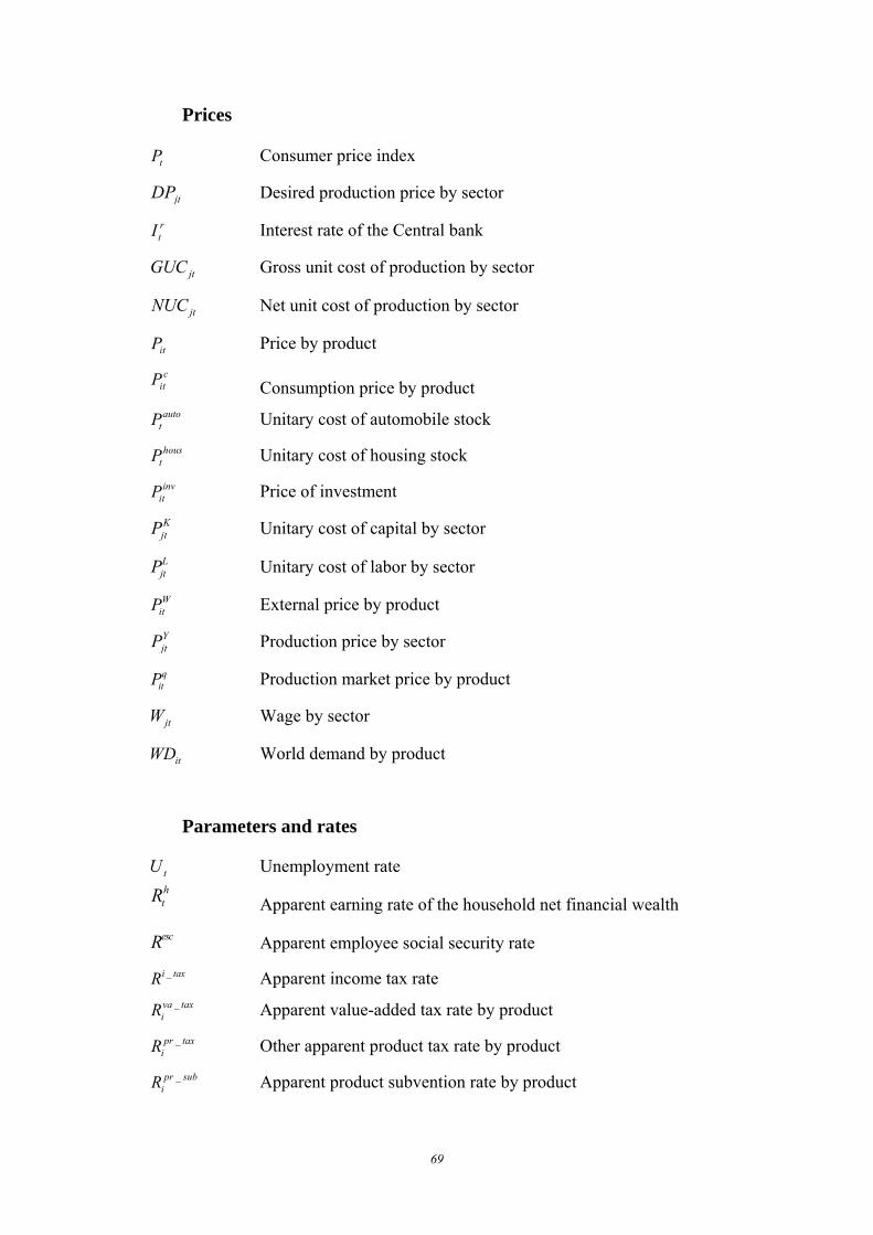
69

Prices

tP Consumer price index

jtDP Desired production price by sector

rtI Interest rate of the Central bank

jtGUC Gross unit cost of production by sector

jtNUC Net unit cost of production by sector

itP Price by product c

itP Consumption price by product

autotP Unitary cost of automobile stock hous

tP Unitary cost of housing stock inv

itP Price of investment KjtP Unitary cost of capital by sector

LjtP Unitary cost of labor by sector

WitP External price by product YjtP Production price by sector

qitP Production market price by product

jtW Wage by sector

itWD World demand by product

Parameters and rates

tU Unemployment rate htR Apparent earning rate of the household net financial wealth

escR Apparent employee social security rate _i taxR Apparent income tax rate

_va taxiR Apparent value-added tax rate by product

_pr taxiR Other apparent product tax rate by product

_pr subiR Apparent product subvention rate by product

70

_y subiR Apparent production subvention rate

_en taxiR Apparent energy tax rate by type of energy depR Depreciation rate of capital stock mujtR Mark-up rate by sector

_em contjtR Apparent rate of employer social security contribution

_FP taxR Apparent rate of firms profit rate valhtϕ Value share of input h volhtϕ Volume share of input h ctϕ Marginal propensity to consume invtϕ Marginal propensity to invest autotϕ Ratio of household automobile stock to her disposable income houstϕ Ratio of household housing stock to her disposable income

'marii tϕ Share of transports and commercial margins by product

1α ECM parameter: measures the sensitivity to the past dynamic of effective variables

2α ECM parameter: measures the sensitivity to the dynamic of notional variables

3α ECM correcting force parameter: measures the sensitivity to the gap between effective and notional variables

',ii jη Substitution elasticity between two products or productions factors by sector

housη Sensitivity parameter of household energy demand to the share of efficiency housing equipments

22enη Sensitivity parameter of household oil demand to the oil price

iη Sensitivity parameter of household investments to the energy prices autoiη Sensitivity parameter of household oil demand to the share sober cars aiη Armington substitution elasticity aiη Export price elasticity rogjtp Productivity by sector

1 jρ Constant in the Phillips curve

71

2 jρ Sensitivity parameter of nominal wage growth to inflation

3 jρ Sensitivity parameter of nominal wage growth to productivity

4 jρ Sensitivity parameter of nominal wage growth to the terms of trade

5 jρ Sensitivity parameter of nominal wage growth to the unemployment level

6 jρ Sensitivity parameter of nominal wage growth to the unemployment variation

7 jρ Sensitivity parameter of nominal wage growth to labor market evolution in sector j

tκ Labor participation ratio

1ψ Constant in labor participation equation

2ψ Flexion effect parameter

τ Growth rate of technical progress

ν Growth rate of population

μ Growth rate of real variables

π Growth rate of price index of consumption

χ Growth rate of nominal variables

ω Growth rate of wage

ξ CO2 emissions coefficient of conversion

72

Appendix D. The choice of the sectorial disaggregation

Le choix du niveau de désagrégation sectorielle varie fortement d’un modèle à l’autre.

Par exemple, les modèles de Shoven et Walley (1992) et Harrison et Rutherford (1997)

retiennent respectivement 2 et 117 secteurs productifs. Ce choix dépend des spécificités du

modèle (modèle statique versus dynamique ; la nature des politiques à évaluer, avec ou sans

coûts d’ajustements, etc.), des objectifs du modélisateur et de la disponibilité des données.

Dans la perspective d’un modèle macroéconomique multisectoriel destiné à quantifier les

effets des politiques économiques structurelles, le rôle joué par le niveau de désagrégation

sectorielle est très important dans la mesure où les prédictions et les enseignements qui en

découlent dépendent largement du niveau de décomposition du tissu productif retenu. Des

lors, un arbitrage doit être fait entre d’une part, le désir de disposer d’un modèle le plus

détaillé possible afin de gagner en réalisme, et d’autre part, la lourdeur de construction et de

chiffrage d’un gros modèle. Face à ce dilemme, Schubert (1993) propose d’adopter une

stratégie de désagrégation permettant de mettre en avant les branches d’activités qui rentrent

en jeu dans les questions auxquelles le modélisateur tente de répondre.

Il parait donc primordial de définir d’une manière claire les critères de la désagrégation

sectorielle. Ces derniers doivent permettre d’identifier les canaux de transmission d’une

politique économique sur les différentes grandeurs macroéconomiques afin d’identifier les

perdants et les gagnants d’une telle politique. Etant donné que notre modèle a pour objectif

d’étudier les effets de la fiscalité environnementale sur la consommation de combustibles

fossiles, la croissance et l’emploi, quatre critères ont été privilégiés dans le choix de la

désagrégation :

L’intensité énergétique relative du secteur : ce critère permet de distinguer les secteurs

selon le poids de leur consommation énergétique dans le niveau total et selon leur

participation aux émissions de CO223.

La possibilité de bénéficier d’une exonération de taxe : dans un cadre d’analyse des

répercussions de la mise en place d’une taxe carbone, il s’avère important d’identifier les

secteurs qui sont susceptibles de bénéficier d’une exonération fiscale totale ou partielle, afin

de pouvoir estimer les différents scénarios possibles. Ces secteurs seront désignés selon les

23 Dans notre analyse, nous ne retenons que les émissions de CO2 d’origine anthropique.

73

critères prévus par les directives européennes sur l’énergie. A priori, il s’agit de la branche

« énergie », des secteurs industriels qui consomment des combustibles à double usage

(comme la sidérurgie et la chimie), des secteurs de production de biens minéraux non

métalliques, ainsi que les secteurs soumis au Système Européen d’Echange de Quotas de CO2

(SEEQ).

Le degré d’ouverture à la concurrence internationale : ce critère permet d’estimer les

effets d’une nouvelle contrainte environnementale sur la compétitivité des secteurs. Il est

d’autant plus important que la politique environnementale est mise en œuvre par le pays de

manière unilatérale. Ainsi, Farmer et Steininger (1999) justifient le choix de ce critère de

désagrégation en faisant valoir que les trois secteurs les plus pollueurs en Autriche sont ceux

qui sont les plus exposés à la concurrence internationale.

L’homogénéité du secteur : C’est un critère primordial à respecter pour toute

décomposition des activités économiques. Il est nécessaire de regrouper au sein d’un même

secteur les activités productives qui ont des comportements énergétiques et un niveau

d’émission de CO2 semblables. Un tel regroupement présente l’avantage de réduire la taille

du modèle tout en préservant son pouvoir explicatif. Ce critère assure la cohérence globale de

la structure de production dans le modèle, en distinguant les principaux grands secteurs de la

comptabilité nationale. Outre les secteurs et sous secteurs énergivores et ceux bénéficiant

d’une exonération fiscale, nous allons aussi distinguer l’agriculture des autres secteurs

industriels (hors ceux retenus selon les deux premiers critères cités plus haut), le Bâtiment et

Travaux Publics (BTP), les transports et les services. Ce critère conduit à désagréger le

secteur des transports entre le transport routier, ferroviaire, aérien et maritime. S’agissant des

services, la différence sera faite entre les services publics et privés.

Sur la base de ces quatre critères, nous avons procédé à une décomposition en groupes

et sous-groupes de secteurs permettant d’éviter toute juxtaposition entre un secteur dont le

comportement aura une grande incidence sur les résultats, et ceux qui auront un rôle marginal.

Pour cela, la stratégie suivie consiste à scinder d’abord l’ensemble des secteurs en sous-

groupes en fonction de leurs intensités énergétiques et de leurs niveaux d’émissions de CO2

respectives, tout en isolant les secteurs susceptibles de bénéficier d’une exonération. Par la

suite, le troisième et le quatrième critère seront introduits afin d’évaluer la pertinence de la

désagrégation obtenue sur la base des deux premiers critères.

74

Les première et deuxième parties justifient la désagrégation retenue dans l’industrie

manufacturière et le secteur énergétique. La troisième décrit les bases de données utilisées,

tandis que la quatrième conclut et résume la désagrégation finalement retenue et expose ses

limites.

Industrie manufacturière

Pour l’année 2005, les émissions de CO2 provenant des secteurs de l’industrie

manufacturière (hors production d’énergie) représentent environ 22% des émissions hors puit

de l’ensemble des secteurs productifs en France. Tandis que sa part dans la consommation

énergétique finale24 est d’environ 39%. Cet écart entre le poids de l’industrie manufacturière

dans la consommation énergétique totale et les émissions de CO2 est dû au fait que les

émissions liées à la consommation d’électricité sont imputées à la branche productrice de

cette énergie, afin d’éviter le double enregistrement de ces flux. Du coup l’utilisation de

l’électricité dans toute branche d’activité, hors la branche qui la produit, ne peut être

considérée comme source d’émissions25.

Sachant que la répartition de la consommation énergétique finale et des émissions de

CO2, entre les différents secteurs, sous-secteurs et branches d’activités composants l’industrie

manufacturière, est très hétérogène, il est nécessaire de les ventiler au sein de catégories

homogènes distinctes, afin d’évaluer de manière pertinente les effets sectoriels d’une nouvelle

contrainte environnementale.

Pour cela, nous avons repris le niveau 5 de la Nomenclature d’Activités Françaises

(NAF) contenant 712 postes dont 345 relevant de l’industrie manufacturière afin de faire

correspondre à chaque poste la consommation énergétique par type de combustible qui lui

revient. Ensuite, nous avons estimé leurs émissions de CO2 en appliquant à chaque

combustible un coefficient d’émission propre, commun à tous les secteurs et sous-secteurs.

Les sous-secteurs de l’industrie manufacturière du modèle qui sont les plus énergivores et/ ou

qui sont les plus émetteurs sont clairement identifiés.

24 Il s’agit de la consommation totale d’énergie diminuée de la consommation primaire du secteur « énergie ». 25 Ce qui est d’ailleurs ordonné par le Système National d’Inventaires des Emissions de Polluants

Atmosphériques (SNIEPA) qui prévoit que les émissions polluantes ne sont calculées que pour les secteurs qui

les produisent.

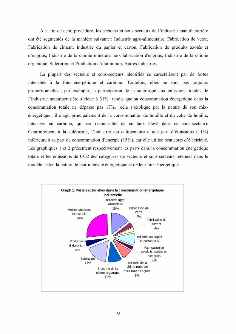
75

A la fin de cette procédure, les secteurs et sous-secteurs de l’industrie manufacturière

ont été segmentés de la manière suivante : Industrie agro-alimentaire, Fabrication de verre,

Fabrication de ciment, Industrie du papier et carton, Fabrication de produits azotés et

d’engrais, Industrie de la chimie minérale hors fabrication d'engrais, Industrie de la chimie

organique, Sidérurgie et Production d’aluminium, Autres industries.

La plupart des secteurs et sous-secteurs identifiés se caractérisent par de fortes

intensités à la fois énergétique et carbone. Toutefois, elles ne sont pas toujours

proportionnelles ; par exemple, la participation de la sidérurgie aux émissions totales de

l’industrie manufacturière s’élève à 31% tandis que sa consommation énergétique dans la

consommation totale ne dépasse pas 17%, (cela s’explique par la nature de son mix-

énergétique : il s’agit principalement de la consommation de houille et du coke de houille,

intensive en carbone, qui est responsable de ce taux élevé dans ce sous-secteur).

Contrairement à la sidérurgie, l’industrie agro-alimentaire a une part d’émissions (11%)

inférieure à sa part de consommation d’énergie (15%), car elle utilise beaucoup d’électricité.

Les graphiques 1 et 2 présentent respectivement les parts dans la consommation énergétique

totale et les émissions de CO2 des catégories de secteurs et sous-secteurs retenues dans le

modèle, selon la nature de leur intensité énergétique et de leur mix-énergétique.

Graph 1: Parts sectorielles dans la consommation énergétique

industrielle

Autres secteurs industriels

26% Fabrication de ciment

4%

Production d'aluminium

4%

Sidérurgie17%

Industrie de la chimie organique

10%

Industrie du papier et carton; 9%

Fabrication de verre4%

Industrie agro-alimentaire

15%

Industrie de la chimie minérale

hors fabr d'engrais8%

Fabrication de produits azotés et

d'engrais3%

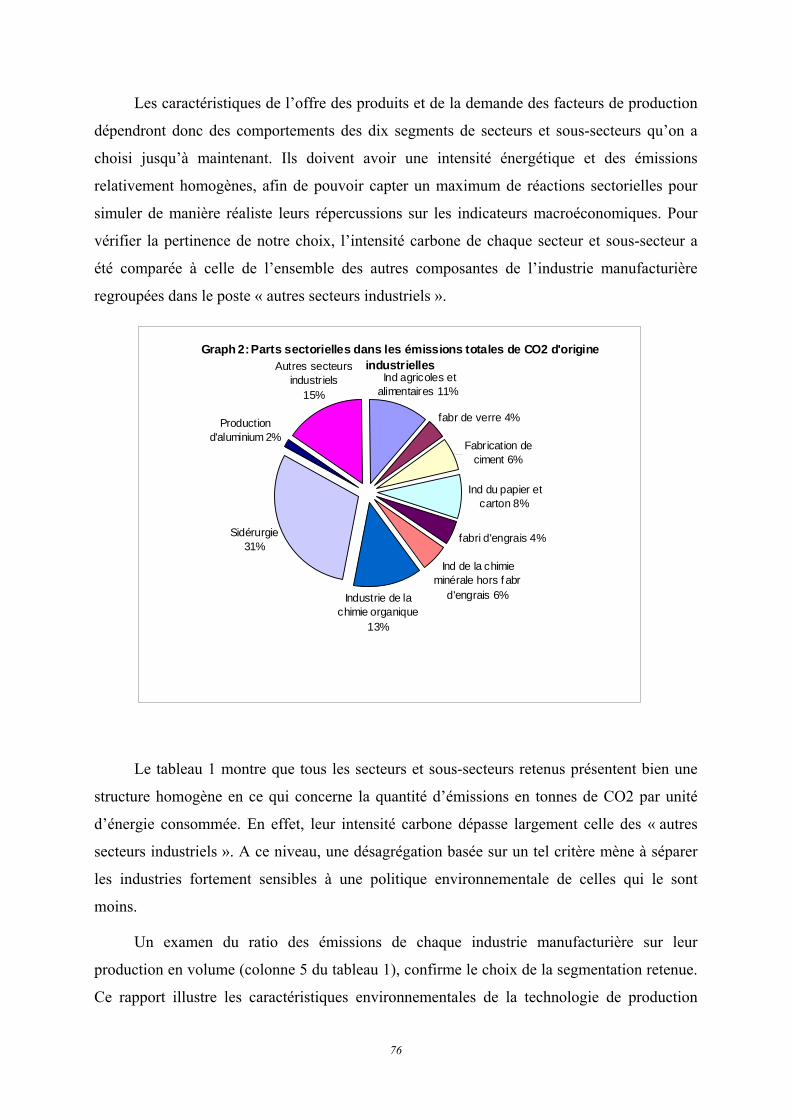
76

Les caractéristiques de l’offre des produits et de la demande des facteurs de production

dépendront donc des comportements des dix segments de secteurs et sous-secteurs qu’on a

choisi jusqu’à maintenant. Ils doivent avoir une intensité énergétique et des émissions

relativement homogènes, afin de pouvoir capter un maximum de réactions sectorielles pour

simuler de manière réaliste leurs répercussions sur les indicateurs macroéconomiques. Pour

vérifier la pertinence de notre choix, l’intensité carbone de chaque secteur et sous-secteur a

été comparée à celle de l’ensemble des autres composantes de l’industrie manufacturière

regroupées dans le poste « autres secteurs industriels ».

Graph 2: Parts sectorielles dans les émissions totales de CO2 d'origine

industrielles

Sidérurgie31%

Production d'aluminium 2%

Ind agricoles et alimentaires 11%

Autres secteurs industriels

15%

Industrie de la chimie organique

13%

Ind de la chimie minérale hors f abr

d'engrais 6%

fabr de verre 4%

Fabrication de ciment 6%

Ind du papier et carton 8%

fabri d'engrais 4%

Le tableau 1 montre que tous les secteurs et sous-secteurs retenus présentent bien une

structure homogène en ce qui concerne la quantité d’émissions en tonnes de CO2 par unité

d’énergie consommée. En effet, leur intensité carbone dépasse largement celle des « autres

secteurs industriels ». A ce niveau, une désagrégation basée sur un tel critère mène à séparer

les industries fortement sensibles à une politique environnementale de celles qui le sont

moins.

Un examen du ratio des émissions de chaque industrie manufacturière sur leur

production en volume (colonne 5 du tableau 1), confirme le choix de la segmentation retenue.

Ce rapport illustre les caractéristiques environnementales de la technologie de production

77

utilisée dans chacune de ces industries. Il reflète aussi le degré de contraste chez les

industriels entre leur participation au bien être social par le biais de la production et les

externalités négatives qu’ils font subir aux citoyens en émettant du dioxyde de carbone. Ainsi,

ce ratio donne une idée de ce qu’on peut appeler l’« efficacité environnementale » d’un

processus de production.

Le poste « Autres secteurs industriels » a un indicateur d’ « efficacité

environnementale » de 0.02, qui est le plus faible de l’ensemble des catégories de secteurs et

sous-secteurs retenues. Ce qui veut dire que pour une participation de ce groupe de secteurs et

branches d’activités de 1000 euros à la production nationale, les émissions de CO2 qui en

découlent ne sont que de 0.02 tep. Pour les autres postes du tableau 1, cet indice reste

largement supérieur de celui des « autres secteurs industriels ». Le modèle distingue donc bien

d’un côté le poste des « autres industries manufacturières », qui sera relativement peu impacté

par la politique environnementale et de l’autre, le reste des secteurs et sous-secteurs

énergivores et émetteurs, listés dans le tableau 1, dont le comportement aura un effet

déterminant sur la dynamique macroéconomique du modèle.

Tableau 12 L’intensité carbone dans l’industrie manufacturière en France (en 2005)

Secteurs retenus selon NES

Conso.énerg.

Hors éléct (en tep)

(a)

Emissions en t de co2

(b)

Intensité carbone

(b)/(a)

Emissions / Production

(en milliers

d’euros)

Industrie agro-alimentaire 3 362 349,42 9 154 565,48 2,72 0,08

Fabrication de verre 1 117 948.00 3 046 568,88 2,72 0,48

Fabrication de ciment 1 332 730.00 5 071 750,06 3,80 1,86

Industrie du papier et carton 2 049 403.00 6 591 251,37 3,22 0,35

Fabrication de produits azotés et

d’engrais 1 452 145.00 3 488 804,46 2,40 1,77

Industrie de la chimie minérale

hors fabrication d'engrais 1 457 580,99 4 381 960,31 3,01 1,09

Industrie de la chimie organique 3 821 954,00 10 244 119,48 2,68 0,48

Sidérurgie 6 281 176.00 24 068 084,12 3,83 1,07

Production d'aluminium 416 708,00 1 259 591,61 3,02 0,29

Autres secteurs industriels 6 607 529,35 12 308 289,43 1,86 0,02

Total 25 898 946,92 79 614 985,16 3,07 0,11

S

ource: Calculs de l’auteur

78

Sachant qu’en économie ouverte, une modification de la compétitivité relative a une

forte incidence sur les équilibres macroéconomiques ; sachant que l’économie française est

très ouverte sur l’Europe et que la politique fiscale environnementale ne sera pas sans effet

sur la compétitivité des entreprises françaises ; il est essentiel de discriminer les secteurs en

fonction de leur exposition à la concurrence internationale. Leur degré d’ouverture doit donc

être considéré comme un troisième critère de désagrégation déterminant. Cette approche est

importante puisque les pays industrialisés ne sont pas soumis aux mêmes contraintes de

réduction des Gaz à Effet de Serre (GES).

Une mesure de la part des exportations dans la production des segments industriels

identifiés dans le modèle, montre qu’une grande partie des retombées d’une taxe

environnementale sur la compétitivité des entreprises industrielles sera captée et quantifiée.

Le graphique 3 montre que la moitié des groupes de secteurs et sous-secteurs retenus vendent

plus de 50% de leur production sur le marché mondial.

Graph.3 : Part des exportations dans la production sectorie lle

25%

42%

82%

34%27%

48%

79%

62% 63%

54%

Industrie ag ro-alimen taire

Fabrication de verre

Fabrication de ciment

Industrie du papie r et carton

Fabrication de produit s azotés et d'engrais

Industrie de la chim ie minérale h ors fabr d'engrais

Industrie de la chim ie organique

SidérurgieProduction d'aluminium

Aut res se cteurs industriels

Part

s

79

En se référant au deuxième critère de désagrégation sectorielle annoncé dans

l’introduction, tous les secteurs susceptibles de bénéficier d’une exonération partielle ou totale

sur leurs émissions polluantes apparaissent déjà dans les segments distingués sur la base du

critère de l’intensité énergétique et carbone, à l’exception des secteurs de « Fabrication des

produits céramiques et de métaux de construction hors le ciment », de « Transformation des

matières plastiques » et de « Production de plomb et de zinc ». Ce dernier ne sera pas

désagrégé des « autres industries », puisque sa contribution aux émissions totales de CO2 est

quasi nulle et que toute nouvelle politique environnementale n’aura vraisemblablement que

des effets directs secondaires sur ce secteur.

Les critères de désagrégation sectorielle définis plus haut nous ont permis de réaliser

une ventilation en secteurs et sous-secteurs de l’industrie manufacturière française cohérente

avec l’objectif de notre exercice de modélisation. Le tableau 2 liste les secteurs et sous-

secteurs représentant l’industrie manufacturière du modèle, selon qu’ils peuvent bénéficier ou

non d’une exonération.

Tableau 13 L'industrie manufacturière dans le modèle

Secteurs et sous-secteurs du modèle Partiellement/totalement

exonérés

Industrie agro-alimentaire Non

Fabrication de verre Oui

Fabrication de ciment Oui

Fabrication de produits céramiques et de

métaux de construction hors le ciment Oui

Industrie du papier et carton Oui

Fabrication de produits azotés et

d'engrais Oui

Industrie de la chimie minérale hors fabr

d'engrais Oui

Industrie de la chimie organique Non

Transformation des matières plastiques Oui

Sidérurgie Oui

Production d'aluminium Oui

80

Outre l’industrie manufacturière, le bloc de production dans le modèle devrait expliciter

les comportements d’autres secteurs et tout particulièrement le secteur de l’énergie, des

transports et des BTP.

Producteurs et distributeurs de l’énergie

Etant donné que le modèle a pour objectif de répondre à des problématiques

environnementales, énergétiques et fiscales, il est primordial de spécifier finement l’offre

d’énergie, car il est important de prendre en compte les effets macroéconomiques de la

substituabilité entre l’énergie et les autres facteurs de production, mais aussi de la

substituabilité des différents produits énergétiques entre eux. Cette distinction est essentielle

puisque l’intensité carbone des divers sources d’énergie n’est pas la même et que la

consommation d’électricité peut faire l’objet d’une exonération fiscale.

Ainsi, la production d’énergie provient de cinq secteurs (Tableau 3), à l’intensité

carbone très variable. La différenciation retenue permet d’étudier de manière satisfaisante les

éventuelles substituabilités qui pourraient s’opérer entre les sources d’énergie suite à la

variation de prix relatifs causée par une nouvelle taxe environnementale.

Comme le montre le tableau 3, la production et la distribution d’électricité occupent le

premier rang dans la consommation énergétique et les émissions qui en découlent. Elles

représentent respectivement 57% et 65% des quantités totales d’énergie consommées et des

émissions totales ; suivie par le raffinage de pétrole avec des pourcentages de 24% et 17%. La

production de combustibles minéraux solides et le secteur d’électricité ont une intensité

carbone parmi les plus élevées de la branche, bien supérieure à l’intensité moyenne de toutes

les sources d’énergie confondues. Ceci s’explique par l’utilisation dans leur processus de

production de gaz hautement émetteurs de CO2. Il s’agit du gaz des hauts fourneaux pour le

premier secteur et du gaz sidérurgique pour le deuxième. En revanche, pour une unité

d’énergie consommée dans le secteur de production et distribution de gaz naturel, les

émissions de CO2 ne sont que de 0.19 tonne. Ce résultat n’est pas étonnant dans la mesure où

la production nationale en gaz naturel ne dépasse pas les 2% de la consommation nationale de

ce type d’énergie et qu’environ 92% de l’énergie qu’il consomme provient d’électricité dont

les émissions ne leurs sont pas imputées.

81

Tableau 14 Intensité carbone par source d’énergie

Sources d'énergie Consommation

énergétique en tep

émissions de

CO2 en tonne

Intensité

carbone

Production de combustibles minéraux

solides 1 279 280,48 8 856 605,41 6,92

Raffinage de pétrole 6 208 180,75 16 351 680,80 2,63

Production et distribution d'électricité 14 732 552,56 60 601 341,18 4,11

Production et distribution de gaz naturel 537 905,63 101 886,66 0,19

Chauffage urbain 3 206 742,96 8 014 811,91 2,50

Total 25 964 662,37 93 926 325,97 3,62

Source: calcul de l’auteur

Conclusion sur la désagrégation sectorielle

La segmentation retenue permet d’analyser de manière pertinente les effets

macroéconomiques des politiques fiscales environnementales. Elle est représentée par

l’ensemble des secteurs et sous-secteurs listés dans le Tableau 1 de la section 2.

Il est important de noter que cette décomposition sectorielle présente plusieurs limites.

En particulier, elle ne permet pas de répondre à certaines questions importantes pour l’analyse

des enjeux de la protection de l’environnement à long terme. Il s’agit principalement des

questions liées au progrès technique induit par une taxe environnementale. Dans quelle

direction une taxe environnementale peut affecter le changement technologique ? Avec

quelles mesures économiques peut-on encourager les industriels à faire plus d’efforts dans

l’activité de recherche et développement en faveur de l’environnement ? Il est difficile de

répondre à ce genre de questions avec une modélisation de type top-down et une structure

sectorielle qui ne fait pas apparaître les secteurs innovants en la matière comme l’industrie

automobile.

Une deuxième faiblesse provient du fait que la production d’énergie renouvelable n’a

pas été isolée des autres secteurs producteurs d’énergie. Par ailleurs, il pourrait se révéler utile

d’incorporer d’autres raffinements. Par exemple, le modèle Mégapestes de Beaumais (1995)

scinde le bloc de production en deux, avec d’un côté des secteurs qualifiés de « verts » et d’un

autre des secteurs dits « standards ». Cette différentiation est introduite pour pouvoir

82

modéliser l’offre des produits « verts » dans l’objectif d’analyser le comportement des

consommateurs français suite à un changement de prix relatifs en faveur de ces derniers.

Sources de données utilisées lors de la désagrégation

Pour le choix d’un niveau d’agrégation sectorielle compatible avec les objectifs du

modèle, nous avons été amenés à construire une base de données contenant la consommation

énergétique par type de combustible de l’ensemble des activités productives en France et à en

calculer par la suite les émissions de CO2 pour chacune de ces activités.

A ce stade, nous avons gardé le même niveau de détail pour les combustibles considérés

que dans l’Enquête Annuelle sur la Consommation d’Energie dans l’Industrie (EACEI)26.

Quant aux acteurs économiques, nous nous sommes basés sur la présentation la plus fine

(niveau 5) des activités économiques en France de la comptabilité (NAF) datant de 2005 et

contenant 712 activités productives27.

Le modèle a été calibré sur la base de l’année 2005. C’est l’année pour laquelle nous

disposions des données détaillées les plus récentes, à la fois sur le plan énergétique et macro-

économique, au moment où on débutés nos travaux. Le contenu de la base énergétique

provient de plusieurs sources différentes, qui sont parfois divergentes. Les regrouper dans un

seul cadre cohérent nécessite un travail minutieux de consolidation. Différentes sources ont

été utilisées:

Les données sur la consommation d’énergie par type de combustible dans les secteurs

producteurs de l’énergie émanent du Centre d’Etudes et recherches économiques sur l’énergie

(CEREN), de la base Pégase de l’observatoire de l’énergie et du CITEPA qui lui-même se

base, entre autres, pour ses inventaires des émissions polluantes, sur les données de

l’observatoire de l’énergie ;

Les données pour les secteurs de l’industrie manufacturière proviennent de l’Enquête

annuelle sur la Consommation d’Energie dans l’Industrie (EACEI) menée par le ministère de

l’économie, de l’industrie et de l’emploi ;

26 Il s’agit du gaz naturel, autres gaz, houille, gaz de pétrole liquéfié, lignite coke de houille, coke de pétrole,

fioul lourd, fioul domestique, liqueur noire, autres produits pétroliers et de l’électricité. 27 Une nouvelle version révisée de la NAF est entrée en vigueur le 01 janvier 2008, elle comprend 732 postes.

83

Pour l’agriculture, les données proviennent du Service Central des Enquêtes et Etudes

Statistiques (SCEES) du ministère de tutelle ;

Les données relatives aux secteurs des transports et du tertiaire sont tirées

principalement de la base Enerdata du CEREN et du ministère de transport pour le premier

secteur.

84

Appendix E. The structure of the French economy in the model base and calibration values of the elasticities of substitution

Tableau 15 The supply and demand structure in the base year (in %)

Production Import MarginsProduct taxes off subsidies

Products Total consumption

Total investment Export Stock

variation

82 13 5 All sectors 77 10 122 2 7 -1 Agriculture, forestry and fishing 3 2 514 10 22 12 Manufacture of food products and beverages 7 7 -4 3 27 7 6 Manufacture of motor vehicles, trailers and semi-trailers 2 14 10 -1

23 Manufacture of glass and glass products 11 11 3 Manufacture of ceramic products and building materials 1 31 25 2 Manufacture of articles of paper and paperboard 1 1 1

35 1 Manufacture of inorganic basic chemicals 11 39 1 Manufacture of organic basic chemicals 1 41 23 1 Manufacture of plastics products 1 11 32 1 Manufacture of basic iron and steel and of ferro-alloys 1 3 1

45 1 Manufacture of non-ferrous metals 1 2 613 25 50 17 Other industries 18 18 43 437 11 Construction of buildings and Civil engineering 2 45

15 -1 -1 Rail transport (Passenger and Freight) 1 -1 Passenger transport by road1 38 -10 Freight transport by road and transport via pipeline 1

48 -1 Water transport 21 36 Air transport 1 2

49 4 -89 33 Business services 43 22 15 610 Public services 11

83 Mining of coal and lignite -1 2 34 5 18 Manufacture of refined petroleum products 4 3 -4 1 1 3 Electric power generation, transmission and distribution 2 11 26 1 Manufacture and distribution of gas 1

Supply Demand

Source: INSEE, National Accounts

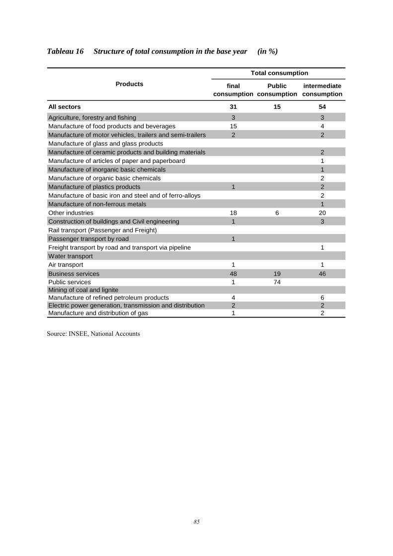
85

Tableau 16 Structure of total consumption in the base year (in %)

final consumption

Public consumption

intermediate consumption

All sectors 31 15 54Agriculture, forestry and fishing 3 3Manufacture of food products and beverages 15 4Manufacture of motor vehicles, trailers and semi-trailers 2 2Manufacture of glass and glass productsManufacture of ceramic products and building materials 2Manufacture of articles of paper and paperboard 1Manufacture of inorganic basic chemicals 1Manufacture of organic basic chemicals 2Manufacture of plastics products 1 2Manufacture of basic iron and steel and of ferro-alloys 2Manufacture of non-ferrous metals 1Other industries 18 6 20Construction of buildings and Civil engineering 1 3Rail transport (Passenger and Freight) Passenger transport by road 1Freight transport by road and transport via pipeline 1Water transportAir transport 1 1Business services 48 19 46Public services 1 74Mining of coal and ligniteManufacture of refined petroleum products 4 6Electric power generation, transmission and distribution 2 2Manufacture and distribution of gas 1 2

Total consumption

Products

Source: INSEE, National Accounts

86

Tableau 17 Structure of total investment in the base year (in %)

Household invest Sector invest Public Invest

Repartition by post 55 32 13Agriculture, forestry and fishing 1 0Manufacture of food products and beveragesManufacture of motor vehicles, trailers and semi-trailers 10 28 4Manufacture of glass and glass productsManufacture of ceramic products and building materialsManufacture of articles of paper and paperboardManufacture of inorganic basic chemicalsManufacture of organic basic chemicalsManufacture of plastics productsManufacture of basic iron and steel and of ferro-alloysManufacture of non-ferrous metalsOther industries 30 11Construction of buildings and Civil engineering 24 72 72Rail transport (Passenger and Freight) Passenger transport by roadFreight transport by road and transport via pipelineWater transportAir transportBusiness services 37 14Public servicesMining of coal and ligniteManufacture of refined petroleum productsElectric power generation, transmission and distributionManufacture and distribution of gas

Total investment

Products

Source: INSEE, National Accounts

87

Tableau 18 Structure of intermediate consumption by sector at the base year * (in %)

1 2 3 4 5 6 7 8 9 10 11 12 13 14 15 16 17 18 19 20 21 22 23 24Agriculture, forestry and fishing 1 32 33 2 1 1 1 1Manufacture of food products and beverages 2 14 30 1 2 1 1 2 4 4Manufacture of motor vehicles, trailers and semi-trailers 3 34 1 1 2 1 1 1Manufacture of glass and glass products 4 1 1 1 8 1 1 1Manufacture of ceramic products and building materials 5 1 12 29 1 1 1 1 14 1 1Manufacture of articles of paper and paperboard 6 2 5 1 44 1 1 3 2 1 1Manufacture of inorganic basic chemicals 7 7 5 1 34 6 1 1 1 1Manufacture of organic basic chemicals 8 1 1 1 5 2 23 47 3 2Manufacture of plastics products 9 1 3 5 1 1 2 3 2 10 1 3 3 1 1 1Manufacture of basic iron and steel and of ferro-alloys 10 5 2 1 40 4 2Manufacture of non-ferrous metals 11 1 3 1 2 4 52 3 1Other industries 12 20 5 35 18 27 12 18 9 11 26 22 51 24 1 4 3 10 14 9 26 17Construction of buildings and Civil engineering 13 1 1 1 1 1 23 1 1 2 1 2 7 1 9 1Rail transport (Passenger and Freight) 14 1 1Passenger transport by road 15 7 2Freight transport by road and transport via pipeline 16 1 18 1 1Water transport 17 21Air transport 18 21 1Business services 19 13 22 17 33 27 23 18 13 22 20 18 27 28 81 55 47 52 38 75 49 77 9 25 7Public services 20 1Mining of coal and lignite 21 2 14 3Manufacture of refined petroleum products 22 9 1 1 2 4 1 2 36 1 1 3 3 25 28 13 22 3 2 85 2 1Electric power generation, transmission and distribution 23 2 1 1 4 2 4 7 2 2 3 3 1 11 3 1 3 9 40 1Manufacture and distribution of gas 24 1 5 2 3 11 4 2 1 1 1 2 2 90

Intermediate consumption by sector

*The sum of each column equals to 100%. The diagonal of the matrix represents the auto-consumption in the sectors.

Source: INSEE, National Accounts

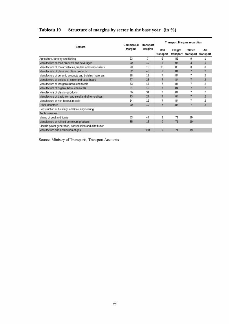
88

Tableau 19 Structure of margins by sector in the base year (in %)

Rail transport

Freight transport

Water transport

Air transport

Agriculture, forestry and fishing 93 7 6 85 9 1Manufacture of food products and beverages 90 10 2 94 3 1Manufacture of motor vehicles, trailers and semi-trailers 90 10 11 83 3 3Manufacture of glass and glass products 52 48 7 84 7 2Manufacture of ceramic products and building materials 88 12 7 84 7 2Manufacture of articles of paper and paperboard 77 23 7 84 7 2Manufacture of inorganic basic chemicals 53 47 7 84 7 2Manufacture of organic basic chemicals 81 19 7 84 7 2Manufacture of plastics products 66 34 7 84 7 2Manufacture of basic iron and steel and of ferro-alloys 73 27 7 84 7 2Manufacture of non-ferrous metals 84 16 7 84 7 2Other industries 90 10 7 84 7 2Construction of buildings and Civil engineeringPublic servicesMining of coal and lignite 53 47 9 71 19Manufacture of refined petroleum products 85 15 9 71 19Electric power generation, transmission and distributionManufacture and distribution of gas 100 9 71 19

Commercial Margins

Transport Margins repartitionTransport MarginsSectors

Source: Ministry of Transports, Transport Accounts

89

Tableau 20 Product taxes and subsidies by sectors at the base year (in %)

Oil tax Electricity tax

Natural gas tax Coal tax Other

products taxValue add

tax Subsidy

All sectors 13 1 24 68 -6Agriculture, forestry and fishing 1 24Manufacture of food products and beverages 29 8 5Manufacture of motor vehicles, trailers and semi-trailers 1 8Manufacture of glass and glass productsManufacture of ceramic products and building materialsManufacture of articles of paper and paperboard 1Manufacture of inorganic basic chemicalsManufacture of organic basic chemicalsManufacture of plastics products 1Manufacture of basic iron and steel and of ferro-alloysManufacture of non-ferrous metalsOther industries 5 24Construction of buildings and Civil engineering 2 16 1Rail transport (Passenger and Freight) 15Passenger transport by road 1 28Freight transport by road and transport via pipelineWater transport 1Air transport 1 1Business services 58 29 12Public servicesMining of coal and lignite 100Manufacture of refined petroleum products 100 1 7Electric power generation, transmission and distribution 100 3 2 13Manufacture and distribution of gas 100 1

Product taxes and subsidies

Source: INSEE, Ministry of Finances

90

Tableau 21 Import shares by sectors in the base year (in %)

1 2 3 4 5 6 7 8 9 10 11 12 13 14 15 16 17 18 19 20 21 22 23 24 Agriculture, forestry and fishing 1 6 7 7 35 7 6 39 16 6 6 37 44Manufacture of food products and beverages 2 9 17 23 26 23 11 26 28 24 25 24 18 18 21 16 14 13 19 20 18 24 25 20 20Manufacture of motor vehicles, trailers and semi-trailers 3 48 49 49 48 49 49 49 49 49 48 49 82 49 49 49 49 50 49 48 39 48 48 49 52 53Manufacture of glass and glass products 4 36 36 36 36 36 36 36 36 36 36 36 36 36 36 0 36 36 36 31 60 25 7Manufacture of ceramic products and building materials 5 16 16 16 16 16 16 16 16 16 16 16 17 16 16 16 16 16 15 16 16 16 36 13 4Manufacture of articles of paper and paperboard 6 21 31 43 38 40 45 38 39 25 37 37 37 42 48 47 21 38 20 40 44 49 33Manufacture of inorganic basic chemicals 7 51 51 51 51 51 51 51 51 51 51 51 51 51 51 51 51 51 51 48 93 51 51 50Manufacture of organic basic chemicals 8 72 72 72 72 72 72 72 72 72 72 72 72 72 72 72 72 72 71 79 72 72 72 68Manufacture of plastics products 9 27 27 27 27 27 27 27 27 27 27 27 27 27 27 27 27 27 27 26 27 27 27 27 66Manufacture of basic iron and steel and of ferro-alloys 10 46 46 46 46 46 46 46 46 46 46 46 46 46 46 45 46 46 46 8Manufacture of non-ferrous metals 11 70 70 70 70 70 70 70 70 70 70 70 70 70 70 68Other industries 12 42 28 31 31 25 32 24 39 45 37 55 37 31 34 38 30 16 34 35 30 33 18 28 51 46 10Construction of buildings and Civil engineering 13 Rail transport (Passenger and Freight) 14 13 13 13 13 13 13 13 13 13 13 13 15 13 13 13 13 13 13 12 14 13 13 13 8Passenger transport by road 15 0 0 0Freight transport by road and transport via pipeline 16 10 10 10 10 10 10 10 10 10 10 10 30 10 10 10 10 10 10 10 10 10 10 10Water transport 17 12 3 11 28 20Air transport 18 43 43 43 43 43 43 43 43 43 43 43 18 43 43 43 43 43 43 33 49 43 43 43 37

Business services 19 4 4 5 5 5 5 5 4 4 5 5 6 5 5 4 4 6 5 4 5 2 6 6 5 1 4Public services 20 Mining of coal and lignite 21 93 93 93 93 93 93 92 93 93 93 93 93Manufacture of refined petroleum products 22 30 30 30 30 30 30 34 34 30 30 30 30 30 30 30 30 30 30 90 30 80 30 7Electric power generation, transmission and distribution 23 1Manufacture and distribution of gas 24 7 7 86 61

ExportProducts Intermediate consumption by sector Final consumption Investment

Source: INSEE

91

Tableau 22 Weight and composition of Value-Added by sector in the base year (in %)

Value Added by sector

Employemnt cost

Gross operating

profit

Production tax

Production subvention

All sectors 100.00 57.95 38.81 4.67 -1.43Agriculture, forestry and fishing 2.06 26.73 90.90 4.43 -22.07Manufacture of food products and beverages 1.78 57.73 35.66 7.36 -0.75Manufacture of motor vehicles, trailers and semi-trailers 0.82 73.73 19.19 8.00 -0.92Manufacture of glass and glass products 0.15 70.16 22.61 7.92 -0.69Manufacture of ceramic products and building materials 0.40 58.42 34.23 7.80 -0.45Manufacture of articles of paper and paperboard 0.28 71.90 18.77 9.79 -0.46Manufacture of inorganic basic chemicals 0.05 127.76 -43.88 17.94 -1.82Manufacture of organic basic chemicals 0.24 45.77 42.19 12.72 -0.67Manufacture of plastics products 0.46 75.55 17.30 7.71 -0.56Manufacture of basic iron and steel and of ferro-alloys 0.29 48.01 44.57 7.83 -0.41Manufacture of non-ferrous metals 0.12 44.96 47.39 8.10 -0.45Other industries 8.27 69.97 25.02 6.22 -1.21Construction of buildings and Civil engineering 6.17 54.41 43.19 2.84 -0.44Rail transport (Passenger and Freight) 0.38 79.44 15.37 6.73 -1.54Passenger transport by road 0.72 65.72 31.14 6.63 -3.49Freight transport by road and transport via pipeline 1.12 63.63 32.28 4.62 -0.53Water transport 0.12 38.91 57.43 4.02 -0.36Air transport 0.41 73.93 23.37 3.75 -1.06Business services 56.87 49.07 47.13 4.77 -0.98Public services 17.66 85.07 13.43 2.68 -1.18Manufacture of refined petroleum products 0.15 26.69 55.09 19.56 -1.33Electric power generation, transmission and distribution 1.17 36.65 52.53 11.06 -0.23Manufacture and distribution of gas 0.31 39.53 54.41 6.50 -0.44

Value added sectors composition

Source: INSEE

Tableau 23 Elasticities of substitutions between production factors

ValuesSubstitution elasticities between:

Capital-Labor 0.3Capital-Aggregate Energy 0.06Capital-Intermediate Consumption 0Labor-Aggregate Energy 0.04Labor-Intermediate Consumption 0.15Aggregate Energy-Intermediate Consumption 0.17

Substitution elasticities between intermediate consumptions 0Substitution elasticities between product investments of sectors 0Armignton Elasticity 0.6

Source: Own estimates, Reynès and Tamsamani (2010) , Cochard and Blot (2008).

92

Tableau 24 Elasticities of substitutions between energies

Coal-Oil Oil-Electricity Coal-Natural Gas Oil-Electricity Electricity-

Natural GasOil-Natural

GasAgriculture, forestry and fishing 0.35 2.29Manufacture of food products and beverages 0.13 0.61Manufacture of motor vehicles, trailers and semi-trailers 0.14 0.78Manufacture of glass and glass products 0.13 0.56Manufacture of ceramic products and building materials 0.68 2.29 0.20 0.87Manufacture of articles of paper and paperboard 1.95 1.17 0.10 0.50Manufacture of inorganic basic chemicals 1.39 0.86 0.07 0.29Manufacture of organic basic chemicals 0.39 1.11 1.16Manufacture of plastics products 0.08 0.74Manufacture of basic iron and steel and of ferro-alloys 0.67 0.29Manufacture of non-ferrous metals 0.21Other industries 0.80 1.56 0.14 0.80Construction of buildings and Civil engineering 0.44 2.87Rail transport (Passenger and Freight) 0.07 0.91Passenger transport by road 0.63 3.63Freight transport by road and transport via pipelineWater transportAir transportBusiness services 0.49 2.60 0.23 1.39Public services 1.06 1.29 0.11 0.61Mining of coal and lignite 0.76Manufacture of refined petroleum productsElectric power generation, transmission and distribution 0.33 0.03 0.19Manufacture and distribution of gas 0.05

Substitution elasticities between:

Source: Blanc and Callonnec (2009).

93

References

Agence De l’Environnement et de la Maîtrise de l’Energie (ADEME), 2005 « Facteurs d’émissions de dioxyde de carbone pour les combustibles ». (Disponible en ligne)

Allard-Prigent, C., Audenis, C., Berger, K., Carnot, N., Duchêne, S., Pesin, F., 2002. Présentation du modèle MESANGE; Modèle Econométrique de Simulation et d'Analyse Générale de l'Economie. Working Paper of the Direction de la Prévision. Available at http://www.minefi.gouv.fr/directions_services/dgtpe/etudes/doctrav/05_ 2002.pdf.

Armignton,P. 1969 “A Theory of Demand for Products Distinguished by Place of Production” IMF Staff Papers, vol.16, n°1.

Arrow, K. J., Chenery, H. B., Minhas, B. S., Solow, R. M., 1961. Capital-Labor Substitution and Economic-Efficiency. Review of Economics and Statistics 43 (3), 225-250.

Baghli, M., Brunhes-Lesage, V., De bandt, O., Fraisse, H., Villetelle, J.-P., 2004. MASCOTTE, Modèle d'Analyse et de préviSion de la COnjoncture TrimesTriellE. Note d'Etudes et de Recherche de la Banque de France. Available at http://www.banque-france.fr/fr/publications/telechar/ner/ner106.pdf.

Beaumais O., 1995, « Une réinterprétation des politiques de l’environnement par les Modèles », Université de Paris I Panthéon – Sorbonne, Thèse de doctorat.

Bellone F., Patrick M., Lionel N. et Warzynski F., 2009 «L’effet pro-concurrenciel de l’intégration européenne : une analyse de l’évolution des taux de marge dans les industries manufacturières françaises », Revue de l’OFCE, n° 108, juillet, pp.139-163.

Benassy, J. P., 1975. Neo-Keynesian Disequilibrium Theory in A Monetary Economy. Review of Economic Studies 42 (4), 503-523.

Bentzen, J., 2004, “Estimating the rebound effect in US manufacturing energy consumption”, Energy Economics, n° 26 (1).

Bernard, A., Vielle, M., 2008. GEMINI-E3, a general equilibrium model of international national interactions between economy, energy and the environment. Computational Management Science 5 (3), 173-206.

Bils, M. (1987), « The cyclical behaviour of marginal cost and price », American Economic Review (77), pp. 838-855.

Blanc N. and Callonnec G., 2009 « Carbon Tax and Substitution Effects in the French Industrial Sector: An Econometric Assessment » Presentation in the European Council for an Energy Efficient Economy Summer study.

Blanchard, O. J., Fischer, S., 1989. Lectures on macroeconomics. Cambridge, Mass. and London: MIT Press.

Blanchard, O. J., Kiyotaki, N., 1987. Monopolistic Competition and the Effects of Aggregate Demand. The American Economic Review 77 (4), 647-666.

Blanchard, O. J., and L. H. Summers, “Hysteresis and the European Unemployment”, in:

94

Fischer S. (Eds.), NBER Macroeconomics Annual, Fall, (Cambridge: MIT Press, 1986), 15-78.

Böhringer, C., Löschel, A., 2006. Computable general equilibrium models for sustainability impact assessment: Status quo and prospects. Ecological Economics 60 (1), 49-64.

Brécard, D., Fougeyrollas, A., Le Mouël, P., Lemiale, L., Zagamé, P., 2006. Macro-economic consequences of European research policy: Prospects of the Nemesis model in the year 2030. Research Policy 35 (7), 910-924.

Burniaux, J.-M., Martin, J. P., Nicoletti, G., Martins, J. O., 1992. GREEN a Multi-Sector, Multi-Region General Equilibrium Model for Quantifying the Costs of Curbing CO2 Emissions. OECD Economic Department Working Papers 116. Available at http://www.oecdilibrary.org/oecd/content/workingpaper/744101452772.

Caballero, R.J., Lyons, R.K. (1990), « Internal versus external economies in European industry », European Economic Review, 34, pp. 805-830.

Capros, P., Georgakopoulos, T., Filippoupolitis, A., Kotsomiti, S., Atsaves, G., Proost, S. et al., 1997. The GEM-E3 Model Reference Manual. National Technical University, Athens. Available at http://www.e3mlab.ntua.gr/manuals/GEMref.PDF.

Centre Interprofessionnel Technique de l’Etude de la Pollution Atmosphérique (CITEPA), 2007 « Inventaire des émissions de polluants atmosphériques en France – séries sectorielles et analyse étendue ». (Disponible en ligne)

CITEPA, 2008 « Organisation et Méthodes des Inventaires Nationaux des Emissions Atmosphérique en France –OMINEA- » 5éme édition. (Disponible en ligne)

Centre d’analyse stratégique, 2008 « Perspectives énergétiques de la France à l’horizon 2020-2020 » La documentation française 12 (1).

Chagny, O., Reynès, F., et Sterdyniak, Henry, 2002 « The equilibrium rate of unemployment: a theoretical discussion and an empirical evaluation for 6 OECD countries» OFCE Working papers 2002-04. Available at http://www.ofce.sciences-po.fr/pdf/dtravail/wp2002-04.pdf.

Chauvin, V., Dupont, G., Heyer, É., Plane, M., et Timbeau, X., 2002 « Le modèle France de l'OFCE; La nouvelle version : e-mod.fr» Revue de l'OFCE 81 (2), 245-300.

Cochard M. and Blot C., 2008 « L’énigme des exportations revisitée : que faut-il retenir des données de panel ? » Revue de l’OFCE, n° 106.

Crépon B., Desplatz R. et Mairesse J., 2002 « Price-cost margins and rent-sharing: evidence from a panel of French manufacturing firms», mimeo.

Cross, R., 1995 “Is the natural rate hypothesis consistent with Hysteresis?”, in: Cross R. (Eds.), The natural rate of unemployment, Reflections on 25 years of hypothesis, (Cambridge University Press).

Dernburg, T. and Strand, K., 1966. Hidden Unemployment 1953-62 - Quantitative Analysis by Age and Sex. American Economic Review 56 (1), 71-95.

Dixit, A. K. and Stiglitz, J. E., 1977 « Monopolistic Competition and Optimum Product Diversity» The American Economic Review 67 (3), 297-308.

95

Dobbelaere S. et Mairesse J., 2007 « Panel data estimates of the production function and product and labor market imperfections », Working Paper Series 782, Banque centrale européenne.

Economie et Prévision, 1998. Structures et propriétés de cinq modèles macroéconomiques français. Economie et prévision 134, 1-70.

Farmer, K., et Steininger. K.W., 1999, « Reducing CO2-emissions under Fiscal retrenchment: A multi-cohort CGE-model for Austria » Environmental & Resource Economics 13(3).

Ghersi, F., Thubin, C., 2009. Le modèle IMACLIM-S Version 2.3. CIRED Working Paper. Available at http://www.centre-cired.fr/spip.php?article527.

Hall, R.E. (1988), « The relation between price and marginal cost in US industry », Journal of Political Economy 96, pp. 921-947.

Harrison, G.W. and T.F. Rutherford, 1997, « Burden Sharing, Joint Implementation, andCarbon Coalitions » in International Environmental Agreements on Climate Change, Amsterdam: Kluwer Academic Press.

Hicks, J., 1932, The Theory of Wages, 2ième édition, 1963, Macmillan, New-York.

Laffargue J.P., 1996 « Fiscalité, charges sociales, qualifications et emploi. Étude à

l'aide du modèle d'équilibre général calculable de l'économie française "Julien" »,

Économie et prévision, 125, 87-105.

Lemoine, M., Mazzi, G. L., Monperrus-Veroni, P., Reynès, F., 2010 « A new production function estimate of the euro area output gap» Journal of Forecasting 29 (1-2), 29-53.

Lindbeck, A., 1993 « Unemployment and Macroeconomics» Cambridge: MIT Press.

Lipsey, R., 1960 « The Relation between Unemployment and the Rate of Change of

Money Wage Rates in the United Kingdom, 1862-1957: A further Analysis»

Economica 27 (105), 1-32.

Ministère de l’économie, des finances et des industries, 2006 « Tableaux des consommations d’énergie en France » Observatoire de l’énergie.

Ministère de l’économie, des finances et des industries, 2005 « l’Enquête annuel sur la Consommation d’Energie dan l’Industrie ». (Disponible en ligne)

Phillips A. W., 1958 « The relationship between unemployment and the rate of change of money wages in the UK 1861-1957» Economica, 25 (100), 283-299.

Piriou, J.-P., 2008. La comptabilité nationale. (15th, La Découverte, Collection Repères ed.).

Reynès, F., 2010 “The Phillips curve as a more general model than the Wage Setting curve” OFCE Working paper, n°28.

Reynès F. and Tamsamani Y.Y. 2009 « Substituabilité des facteurs et rendements d’échelle sectoriels en France : une estimation par une fonction de coût flexible » OFCE working paper, n° 37.

Robinson, J., 1933, The Economics of Imperfect Competition , Macmillan, New-York.

96

Roeger W., 1995 « Can imperfect competition explain the difference between primal and dual productivity measures? Estimates for US manufacturing », Journal of Political Economy, 103, pp. 316-330.

Romain Bouis, 2008 « Niveau et évolution de la concurrence sectorielle en France » Economie et Prévision, n°185 (4),

Sato, K., 1967. 2-Level Constant-Elasticity-Of-Substitution Production Function. Review of Economic Studies 34 (2), 201-218.

Schubert, K., 1993 « Les modèles d’équilibre générale calculable », Revue Economie Politique 103 (6), 777-821.

Shadman-Mehta, F. and Sneessens, H. R., 1995 « Skill Demand and Factor Substitution » CEPR Discussion Papers, 1279.

Shapiro M., 1987 « Measuring market power in US industry », NBER Working Paper n° 2212, Cambridge, MA.

Shoven J.B., and Whalley J., 1992 « Applying general equilibrium » Cambridge surveys of economic literature.

Solow R. M., 1956 « A Contribution to the Theory of Economic Growth » Quarterly Journal of Economics 70 (1), 65–94.

Sorrell, S., Dimitropoulos, J. and Sommerville, M., 2009, “Empirical estimates of the direct rebound effect: A review” Energy Policy, n°37 (4).

Strand, K., Dernburg, T., 1964 “Cyclical Variation in Civilian Labor Force Participation” Review of Economics and Statistics 46 (4), 378-391.

Warzynski, F., 2009 « Estimation des taux de marge dans l’industrie manufacturière européenne » revue de l’OFCE, n°108

Wilcoxen, P.J., 1988 “The Effects of Environmental Regulation and Energy Prices on U.S. Economic Performance” PhD thesis, Harvard University.

Zagamé P., Boitier B., Fougeyrollas, A., Le Mouël P., Capros P., Kouvaritakis N., Bossier F., Thierry F., Melon A., 2010, The NEMESIS Reference Manual, http://www.erasme-team.eu/index.php/erasme-nemesis.html.