Doctoral Thesis - Universidad Politécnica de Madrid
208
Doctoral Thesis Dynamic analysis and control of broadband frequency harmonic vibrations in lightweight pedestrian structures Jos´ e Manuel Soria Herrera Ingeniero de Caminos, Canales y Puertos Madrid, 2019
-
Upload
khangminh22 -
Category
Documents
-
view
2 -
download
0
Transcript of Doctoral Thesis - Universidad Politécnica de Madrid
Doctoral Thesis
Dynamic analysis and control of broadband
frequency harmonic vibrations in lightweight
pedestrian structures
Jose Manuel Soria Herrera
Ingeniero de Caminos, Canales y Puertos
Madrid, 2019

UNIVERSIDAD POLITECNICA DE MADRID
Escuela Tecnica Superior de Ingenieros de
Caminos, Canales y Puertos
Dynamic analysis and control of broadband
frequency harmonic vibrations in lightweight
pedestrian structures
by
MEng. Civil Eng. Jose Manuel Soria Herrera
A dissertation submitted in partial fulfillment for the
degree of Doctor of Philosophy
in the
Department of Continuum Mechanics and Theory of Structures
under the supervision of
Dr. Ivan Munoz Dıaz
Dr. Jaime H. Garcıa Palacios
Madrid, 2019

How to cite this work:
J.M. Soria (2019). Dynamic analysis and control of broadband frequency harmonic
vibrations in lightweight pedestrian structures (Doctoral thesis). ETSICCP,
Universidad Politecnica de Madrid, Spain.
The work in this thesis was carried out in the Structural Engineering
Group (GIE), consolidated research group of the UPM.
http://ingstruct.mecanica.upm.es
c© Copyright by J.M. Soria ([email protected]). ISBN: 978-84-09-14587-4.
This work is licensed under a Creative Commons Attribution-
ShareAlike 3.0 Unported License. Any further distribution of
this work must maintain attribution to the author and the title
of the work.
Declaration of Authorship
The author declares that this dissertation is the result of his own research work,specifically performed to get the candidature submitted for the degree of Doctorof Philosophy in Civil Engineering at Universidad Politecnica de Madrid (UPM).The thesis is based entirely on the independent work carried out by the author inUPM between May 2015 and September 2019 under the supervision of Dr IvanM. Dıaz and Dr Jaime H. Garcıa-Palacios.
Published work of others is always clearly attributed with the correspondingsources given. All the work and ideas recorded are original except for what isreferenced in the text. No part of this has been previously submitted for a degreeor any other qualification at any university or institution.
Signed: Jose Manuel Soria Herrera
Date: 23/09/2019

Tribunal nombrado por el Magfco. y Excmo. Sr. Rector de la UniversidadPolitecnica de Madrid, el dıa 16 de octubre de 2019.
Presidente : D. Juan Jose Lopez Cela
Vocal : D. Antolın Lorenzana Iban
Vocal : D. Javier Oliva Quecedo
Vocal : D. Manuel Teixeira Braz Cesar
Secretario : D. Carlos Zanuy Sanchez
Suplente : D. Javier Fernando Jimenez Alonso
Suplente : D. Emiliano Pereira Gonzalez
Realizado el acto de defensa y lectura de la tesis el dıa 28 de octubre de 2019 enla Escuela Tecnica Superior de Ingenieros de Caminos, Canales y Puertos de laUniversidad Politecnica de Madrid.
Calificacion: ......................................................................
EL PRESIDENTE, LOS VOCALES,
EL SECRETARIO.


Abstract
Lightweight and/or long-span pedestrian structures are usually prone to vibrateexcessively. Although current codes may be fulfilled, these structures are not usu-ally comfortable in any way. Control devices can mitigate vibration and signifi-cantly improve the comfort as well as increasing the structure’s life span. Dampingsystems for civil structures have been continuously proposed; however, the civilengineering community has not generally accepted these damping systems, al-though they have shown great potential for cancelling vibrations. This thesis hasbeen carried out within the Public Research Project “Development of novel sys-tems for reducing vibrations in pedestrian structures” REVES-P (DPI2013-47441).Thus, this research provides tools for the dynamic analysis of structures withtime-varying modal parameters and for addressing the vibration control of broad-band–frequency harmonic vibrations produced by human-induced excitations.
In this thesis, two main subjects have been dealt with. The first one is relatedto the long-term monitoring and dynamic analysis of an in-service steel-platedstress-ribbon footbridge. A methodology for tracking the vibration modes is de-veloped and the modal parameters are correlated against external factors. It hasbeen shown that this type of structure can be highly sensitive to temperaturevariations (frequency changes of more than 20 %) with highly seasonal and dailytrends. These correlations enable the influence of these uncertainties on modalestimates to be removed, thus facilitating their use as possible damage-sensitivefeatures. Additionally, interesting long-term vibration serviceability predictors arederived and assessed according to current codes.
The second subject is related to semi-active vibration control. When structuresshow modal properties changing over time, and/or several vibration modes mustbe cancelled by the same device, passive devices (tuned mass dampers, TMD, arethe device usually adopted for footbridges) may detune and thus experience a sig-nificant loss of efficiency. Under these circumstances, the use of semi-active devicesmay be the most promising alternative. This research concentrates on the upgrad-ing of classical TMDs to be totally adaptable to the actual characteristics of theexternal action or significant changes to the structure’s modal properties (so as tobe robust to the device changes). As a result, a methodology to numerically testand design passive and semi-active strategies for broad-frequency band vibrationsis proposed. The semi-active action is controlled using magneto-rheological (MR)dampers. In this sense, experimental and simulated studies have been carried outto optimize the tuning of semi-active strategies taking into account the existingnon-linearities, including an MR model. Existing control laws, based on tuningthe TMD phase in real-time, have been adapted in order to make them usableexperimentally. Finally, experimental results have shown the potentiality of theproposed semi-active control design methodology.

Resumen
Las estructuras peatonales esbeltas y/o de grandes vanos suelen ser propensas avibrar en exceso. Aunque las normativas actuales se cumplan, estas estructuraspueden resultar incomodas. Los dispositivos de control pueden reducir las vibra-ciones y mejorar significativamente el nivel de confort, ası como aumentar la vidautil de las estructuras. Se han propuesto numerosos sistemas de amortiguacionpara estructuras civiles; sin embargo, en este campo no se han adoptado estossistemas de amortiguacion de forma general, aunque estos son muy eficaces en lacancelacion de vibraciones. Esta tesis se ha llevado a cabo dentro del Proyecto deInvestigacion de financiacion Publica “Desarrollo de nuevos sistemas para reducirlas vibraciones en estructuras peatonales” REVES-P (DPI2013-47441). Ası, enesta tesis se proporcionan herramientas para el analisis dinamico de estructurascon parametros modales que varıan en el tiempo y que permiten abordar el controlvibraciones producidas por peatones en un amplio espectro en frecuencias.
Esta tesis tiene dos objetivos principales. El primero se relaciona con la moni-torizacion permanente y el analisis dinamico de una pasarela de banda tesa enservicio. Se desarrolla una metodologıa para el seguimiento de los modos de vi-bracion y la correlacion de los parametros modales con factores externos. Se hademostrado que la estructura es muy sensible a las variaciones de temperatura(cambios en la frecuencia de mas del 20 %) con dependencia estacional y diaria.Estas correlaciones permiten eliminar gran parte de la influencia de estas incer-tidumbres en las estimaciones modales, facilitando ası su posible uso como ındicesensible al dano estructural. Ademas, se han obtenido predictores representativosdel servicio de vibraciones en monitorizaciones continuas y se han evaluado estosde acuerdo con los codigos actuales.
El segundo objetivo esta relacionado con el control de vibraciones semi-activo.Cuando se tienen estructuras cuyas propiedades modales cambian con el tiempoy/o se quieren cancelar varios modos de vibracion con el mismo dispositivo decontrol, los sistemas pasivos (amortiguadores de masa sintonizados, TMD, porsus siglas en ingles, habitualmente adoptados para puentes peatonales) se puedendesintonizar, experimentando una perdida significativa de eficiencia. En estas cir-cunstancias, el uso de dispositivos semi-activos puede ser una solucion alternativaprometedora. Esta investigacion se centra en la mejora de los TMD clasicos paraque sean totalmente adaptables a las acciones externas y/o a cambios significativosen las propiedades modales de la estructura (e incluso a cambios del propio dis-positivo). Como resultado, se propone una metodologıa para el analisis numericoy el diseno de estrategias pasivas y semi-activas para el control de vibracionesen una amplia banda de frecuencias. La accion semi-activa se controla medianteamortiguadores magneto-reologicos (MR). En este sentido, se han llevado a caboestudios experimentales y simulaciones numercias para la optimizacion del sin-tonizado de diferentes estrategias de control semi-activas teniendo en cuenta lasno linealidades existentes, incluido un modelo del amortiguador MR, ası como laevaluacion de su funcionamiento. Las leyes de control existentes, basadas en el

ajuste de la fase del TMD en tiempo real, se han adaptado/mejorado para hacerlasimplementables. Finalmente, a partir de los resultados experimentales se ha de-mostrado el potencial de la metodologıa propuesta para el diseno e implementacionde un sistema de control semi-activo.

About the author
Jose Manuel Soria Herrera
Jose Manuel Soria Herrera is Assistant Pro-fessor in the Department of Continuum Me-chanics and Theory of Structures of theETSI Caminos, Universidad Politecnica deMadrid (UPM). He teaches courses relatedto structural dynamics and experimentalanalysis of structures. Since 2015 he hasbeen a member of the Structural Engineer-ing Group (GIE), a consolidated researchgroup of the UPM. He has also taught sev-eral training courses of LATEX and Pythonfor academics through the Instituto de Cien-cias de la Educacion (ICE).
He has participated in numerous experimen-tal campaigns of structures (lab and field testing) involving dynamic testing ofdifferent types of structures: buildings, bridges, footbridges, dams, etc. In 2016,he completed a 3-month research stay at the ViBest Research Group (Faculty ofCivil Engineering, University of Oporto). He participated in the characterizationcampaign in the laboratory as well as the installation of a Tuned Mass Damper(TMD) in the footbridge of the Transparent Building, Porto (Portugal).
He has been involved in research projects supported by public financing and inthe publication of several papers in JCR indexed journals. Moreover, he carriesout continuously reports and research projects funded by private companies. Heis a member of the Spanish Association of Structural Dynamics (AEDE).


About the supervisors
Ivan Munoz Dıaz
Ivan Munoz Dıaz has a PhD in MechanicalEngineering (with honours) from the Schoolof Industrial Engineering, Universidad deCastilla-La Mancha (2007).
Currently, he is Associate Professor (tenured)with the Department of Continuum Me-chanics and Theory of Structures, EscuelaTecnica Superior de Ingenieros de Caminos,Canales y Puertos, Universidad Politecnicade Madrid.
His research has focused on the implementa-tion and analysis of vibrations in structures(especially in light civil structures such as
floors or footbridges). He has developed several active control systems based oninertial vibration actuators. Moreover, he collaborates with renowned nationaland international research groups and he regularly publishes papers in high-qualityjournals and attends international conferences organising special sessions. He hassupervised several PhD theses.
Jaime H. Garcıa Palacios
Jaime H. Garcıa-Palacios received hisDiploma (M.Sc.) degree in Civil Engineer-ing from the Universidad de Cantabria, San-tander, Spain, in 1992 and his PhD from theUniversidad Politecnica de Madrid in 2004.
Currently, he is Tenured Professor with theDepartment of Civil Engineering, EscuelaTecnica Superior de Ingenieros de Caminos,Canales y Puertos, Universidad Politecnicade Madrid, where he carries out both re-search and teaching activities. He has beeninvolved in projects related to vibrationmonitoring in civil engineering structuressuch as bridges, buildings and dams.

Agradecimientos
Llegado el final de esta intensa etapa, quisiera agradecer a todos aquellos que, deuna forma u otra, han contribuido al desarrollo de esta Tesis Doctoral.
Resulta casi imposible expresar en unas pocas lıneas el profundo agradecimientoque siento hacia Ivan Munoz Dıaz como director de esta Tesis Doctoral. Hansido muchısimas las horas que me ha dedicado, demostrandome estar profunda-mente comprometido conmigo y haciendo de este trabajo, un trabajo mas calidad.Ademas, me ha demostrado tener una fuerza excepcional en algunos momentosverdaderamente difıciles que le ha tocado superar en estos anos, es por ello quea dıa de hoy es un referente para mı, tanto en lo profesional como investigador ydocente como en lo personal. Para mı ha sido todo un privilegio que haya sidodirector de este trabajo. En segundo lugar, quisiera agradecer a Jaime GarcıaPalacios que confiase en mı para aquella oportunidad laboral que me inicio pro-fesionalmente en el mundo de la investigacion. Su orientacion y consejos, tantoen el ambito de la Tesis como fuera de este han sido y siguen siendo un pilarfundamental en mi desarrollo profesional. Tanto a el como a su mujer Margarita,gracias por el apoyo y los animos que siempre me han dado.
Por otra parte, quisiera dar mi mas sincero agradecimiento a Antolın Lorenzanapor las muchas lecciones que me ha dado, ası como las conversaciones en las queme ha hecho pensar para mejorar este trabajo, sin perder nunca la sonrisa y elbuen humor. Tambien quiero agradecer a su pupilo Alvaro Magdaleno toda laayuda que me ha brindado sin pedir nunca nada a cambio, se que tengo en el unamigo para siempre, espero que sepa que es algo mutuo. Estoy seguro de que nosespera un futuro lleno de colaboraciones.
A Emiliano Pereira y Javier Cara, agradecerles lo mucho que he aprendido deellos y el haber estado dispuestos a ayudarme en todo momento. A la gente de laETS de Ingenieros de Telecomunicaciones de la UPM (Francisco Tirado, GuillermoJara, Alvaro Araujo y Octavio Nieto) todos los buenos ratos que hemos pasadojuntos tanto en su Laboratorio como en los ensayos experimentales realizados.
Quisiera agradecer a todos los profesores con los que he tenido el placer de co-laborar, especialmente a Carlos Zanuy, Rafael Fernandez, Jose Marıa Goicolea,Khanh Nguyen, Javier Leon, Leonardo Todisco y Javier Jimenez, por lo bien queme han orientado siempre. Agradecer tambien a Luis Plaza y Antonio Madridesos examenes de mas que han tenido que corregir para darme cancha con laredaccion de este trabajo. Agradecer tambien al Departamento de Mecanica deMedios Continuos y Teorıa de Estructuras el apoyo recibido.
No puedo olvidarme de los Maestros de Laboratorio, Isidro Garcıa y Miguel AngelPena, agradecerles su ayuda en las configuraciones de todos los ensayos experimen-tales realizados en esta tesis, derrochando profesionalidad y buen humor. Agrade-cer a Julia Chamorro sus numerosas infusiones que han hecho mas llevaderas

aquellas duras tardes de trabajo, ası como a Beatriz Gutierrez sus numerosos de-talles a lo largo de estos anos. Quiero dar las gracias tambien a mis companerosdel Laboratorio de Estructuras por su apoyo: Carlos de la Concha, Xidong Wang,Gonzalo Sanz-Diez, Cristian Barrera, Carlos Iturregui, Carlos Velarde, y los recienincorporados Rafael Ruız y Mar Corral. Mencion especial para Carlos de la Con-cha que ha sido un amigo en el que he podido apoyarme en esta recta final cuandomis animos estaban mas decaıdos.
Tambien quiero agradecer al equipo de Pondio Ingenieros la confianza que handepositado en mı siempre, empezando por Juan Calvo, Joaquın Arroyo, LucıaLopez y Jose Vicente Martınez, y siguiendo con el resto de companeros. Han sidomuchos los ratos que he pasado junto a ellos y ha sido un placer formar parte deesa gran familia.
Por otra parte, no solo durante la realizacion de esta Tesis sino tambien a lo largode toda mi vida, he contado con el apoyo incondicional de mis padres. Siemprehan sido un ejemplo para mı. Sin ellos no me habrıa sido posible llegar hasta aquıni ser la persona que hoy soy. Gracias.
Por ultimo, quiero agradecer a Mamen, no se que serıa de mı sin ella. Han sidomuchas las horas de trabajo que ha aguantado y sin embargo ha estado a mi ladoapoyandome en todo momento. Incluso en mis dıas de estres y mal humor, hasabido tranquilizarme y darme la serenidad que necesitaba. En breve me hara elmejor regalo que se me puede hacer, una hija, Clara. Gracias a ellas, la etapa finalde esta Tesis no solo ha sido un camino mas facil, sino un paseo para recordar.
Gracias a todos,
Jose Manuel Soria
El autor tambien quiere agradecer el apoyo economico proporcionado por el Minis-terio de Economıa y Competitividad (Gobierno de Espana) para la financiacion delProyecto de Investigacion REVES-P (DPI2013-47441) y la beca FPI disfrutada.

“If you want to find the secrets of the universe,think in terms of energy, frequency and vibration.”
Nikola Tesla (1856 – 1943)


To my wife Mamen and
my daughter Clara.

Contents
Declaration of Authorship iii
Abstract / Resumen vii
About the author xi
Jose Manuel Soria Herrera . . . . . . . . . . . . . . . . . . . . . . . . . . xi
About the supervisors xiii
Ivan Munoz Dıaz . . . . . . . . . . . . . . . . . . . . . . . . . . . . . . . xiii
Jaime H. Garcıa-Palacios . . . . . . . . . . . . . . . . . . . . . . . . . . . xiii
Acknowledgements xv
Contents xxi
List of Figures xxv
List of Tables xxix
Abbreviations xxxi
1 Introduction and objectives 1
1.1 Introduction . . . . . . . . . . . . . . . . . . . . . . . . . . . . . . . 1
1.1.1 Vibration serviceability problems . . . . . . . . . . . . . . . 2
1.1.2 Motivation . . . . . . . . . . . . . . . . . . . . . . . . . . . . 4
1.2 Tuned Mass Dampers . . . . . . . . . . . . . . . . . . . . . . . . . . 8
1.3 Semi-active Tuned Mass Dampers . . . . . . . . . . . . . . . . . . . 15
1.4 Thesis objectives . . . . . . . . . . . . . . . . . . . . . . . . . . . . 16
1.5 Thesis outline . . . . . . . . . . . . . . . . . . . . . . . . . . . . . . 17
2 Vibration control 19
2.1 Human-induced vibration . . . . . . . . . . . . . . . . . . . . . . . 20
2.1.1 Human vibration excitation . . . . . . . . . . . . . . . . . . 20
2.1.2 Vibration serviceability . . . . . . . . . . . . . . . . . . . . . 23
2.1.2.1 Guidelines and Standards . . . . . . . . . . . . . . 23
2.1.2.2 Comfort predictors . . . . . . . . . . . . . . . . . . 24
2.2 Modal parameter uncertainty . . . . . . . . . . . . . . . . . . . . . 28
2.2.1 Sources of uncertainty . . . . . . . . . . . . . . . . . . . . . 28
2.2.2 Examples of study . . . . . . . . . . . . . . . . . . . . . . . 32
2.3 Vibration control generalities . . . . . . . . . . . . . . . . . . . . . 33
xxi
Contents
2.3.1 Passive Vibration Control . . . . . . . . . . . . . . . . . . . 38
2.3.2 Active and Hybrid Vibration Control . . . . . . . . . . . . . 38
2.3.3 Semi-active Vibration Control . . . . . . . . . . . . . . . . . 40
2.4 Passive control via Tuned Mass Dampers . . . . . . . . . . . . . . . 42
2.4.1 Theoretical design . . . . . . . . . . . . . . . . . . . . . . . 45
2.4.2 Examples of vertical TMD in footbridges . . . . . . . . . . . 46
2.5 Semi-active Tuned Mass Dampers . . . . . . . . . . . . . . . . . . . 51
2.5.1 Examples of vertical STMD in bridges . . . . . . . . . . . . 53
2.5.2 Semi-active control 1 . . . . . . . . . . . . . . . . . . . . . . 57
2.5.3 Semi-active control 2 . . . . . . . . . . . . . . . . . . . . . . 57
2.6 Magneto-rheological dampers . . . . . . . . . . . . . . . . . . . . . 59
2.6.1 Magneto-rheological fluids . . . . . . . . . . . . . . . . . . . 59
2.6.2 Modelling of MR dampers . . . . . . . . . . . . . . . . . . . 61
2.6.3 Bingham model . . . . . . . . . . . . . . . . . . . . . . . . . 62
2.6.4 Bouc-Wen model . . . . . . . . . . . . . . . . . . . . . . . . 66
2.6.5 Application of MR for STMD . . . . . . . . . . . . . . . . . 66
3 Tracking modal parameters of a lightweight structure 69
3.1 Introduction . . . . . . . . . . . . . . . . . . . . . . . . . . . . . . . 69
3.2 The footbridge and its vibration monitoring . . . . . . . . . . . . . 70
3.2.1 Structure description . . . . . . . . . . . . . . . . . . . . . . 70
3.2.2 Monitoring system . . . . . . . . . . . . . . . . . . . . . . . 72
3.3 Peered analysis of one test . . . . . . . . . . . . . . . . . . . . . . . 74
3.3.1 Data processing . . . . . . . . . . . . . . . . . . . . . . . . . 75
3.3.2 Operational Modal Analysis using three SSI techniques . . . 75
3.3.3 Operational Modal Analysis using the same SSI technique . 84
3.4 Continuous dynamic analysis . . . . . . . . . . . . . . . . . . . . . . 85
3.4.1 Tracking of modal properties . . . . . . . . . . . . . . . . . . 85
3.4.2 Effects of external factors . . . . . . . . . . . . . . . . . . . 89
3.4.3 Statistical analysis . . . . . . . . . . . . . . . . . . . . . . . 92
3.4.4 Removing external factors . . . . . . . . . . . . . . . . . . . 95
3.5 Vibration Serviceability Assessment . . . . . . . . . . . . . . . . . . 99
3.6 Conclusions . . . . . . . . . . . . . . . . . . . . . . . . . . . . . . . 101
4 Study of semi-active implementable strategies 105
4.1 Introduction . . . . . . . . . . . . . . . . . . . . . . . . . . . . . . . 105
4.2 Structure models . . . . . . . . . . . . . . . . . . . . . . . . . . . . 106
4.3 Loading cases . . . . . . . . . . . . . . . . . . . . . . . . . . . . . . 107
4.4 Vibration control strategies . . . . . . . . . . . . . . . . . . . . . . 109
4.4.1 Passive and semi-active control . . . . . . . . . . . . . . . . 109
4.4.2 Active control . . . . . . . . . . . . . . . . . . . . . . . . . . 110
4.5 Results with TMD, STMD 1 and STMD 2 . . . . . . . . . . . . . . 113
4.5.1 Single degree of freedom system . . . . . . . . . . . . . . . . 114
xxiii
4.5.1.1 Nominal case . . . . . . . . . . . . . . . . . . . . . 114
4.5.1.2 Full year tests . . . . . . . . . . . . . . . . . . . . . 114
4.5.2 Multi-degree of freedom system . . . . . . . . . . . . . . . . 115
4.5.2.1 Nominal case . . . . . . . . . . . . . . . . . . . . . 115
4.5.2.2 Full year tests . . . . . . . . . . . . . . . . . . . . . 116
4.6 Results with TMD, STMD 1 and AMD . . . . . . . . . . . . . . . . 117
4.7 Discussion . . . . . . . . . . . . . . . . . . . . . . . . . . . . . . . . 119
5 Optimal tuning of semi-active TMD 125
5.1 Introduction . . . . . . . . . . . . . . . . . . . . . . . . . . . . . . . 125
5.2 Semi-active Tuned Mass Damper . . . . . . . . . . . . . . . . . . . 127
5.2.1 Tuned Mass Damper . . . . . . . . . . . . . . . . . . . . . . 127
5.2.2 Semi-active control strategy . . . . . . . . . . . . . . . . . . 127
5.2.3 Optimal control design . . . . . . . . . . . . . . . . . . . . . 127
5.3 Simulation results . . . . . . . . . . . . . . . . . . . . . . . . . . . . 129
5.3.1 Sensitivity analysis . . . . . . . . . . . . . . . . . . . . . . . 129
5.3.2 Control design parameters . . . . . . . . . . . . . . . . . . . 130
5.3.3 Ideal viscous damper . . . . . . . . . . . . . . . . . . . . . . 130
5.3.4 Effect of damper force saturation . . . . . . . . . . . . . . . 132
5.3.5 Effect of considering an MR damper model . . . . . . . . . . 133
5.3.5.1 Experimental tests . . . . . . . . . . . . . . . . . . 133
5.3.5.2 Equivalent damping ratio of MR damper in off state138
5.3.5.3 Optimization process of MR-TMD and MR-STMD 140
5.4 Experimental results . . . . . . . . . . . . . . . . . . . . . . . . . . 141
5.4.1 Structure description and experimental setup . . . . . . . . 141
5.4.2 Mechanical design of the Tuned Mass Damper . . . . . . . . 142
5.4.3 Implementation of the control law . . . . . . . . . . . . . . . 143
5.4.3.1 Switching-on/off function . . . . . . . . . . . . . . 143
5.4.3.2 Low-pass filter . . . . . . . . . . . . . . . . . . . . 143
5.4.3.3 Estimation of the inertial mass velocity . . . . . . . 144
5.4.4 Experimental tests . . . . . . . . . . . . . . . . . . . . . . . 145
5.5 Conclusions . . . . . . . . . . . . . . . . . . . . . . . . . . . . . . . 146
6 Conclusions 149
6.1 Conclusions . . . . . . . . . . . . . . . . . . . . . . . . . . . . . . . 149
6.2 Perspectives for future work . . . . . . . . . . . . . . . . . . . . . . 151
6.3 Publications . . . . . . . . . . . . . . . . . . . . . . . . . . . . . . . 153
6.3.1 JCR journal papers . . . . . . . . . . . . . . . . . . . . . . . 153
6.3.2 Conference proceedings . . . . . . . . . . . . . . . . . . . . . 154
Bibliography 157

List of Figures
1.1 Structure treated as an input-output system. . . . . . . . . . . . . . 2
1.2 Passive controlled structure with a passive control device. . . . . . . 2
1.3 Structure with a TVA. . . . . . . . . . . . . . . . . . . . . . . . . . 3
1.4 Example of a practical application of a TMD in an in-service structure. 4
1.5 Structure with a semi-active control device treated as a feedbacksystem. Red symbol ( −→) means changing over time. . . . . . . . . . 5
1.6 Semi-active controlled structure with semi-active control device.Red symbol ( −→) means changing over time. . . . . . . . . . . . . . 5
1.7 Footbridge, Porto (Portugal). . . . . . . . . . . . . . . . . . . . . . 6
1.8 Experimental test of 1-hour recording at the Porto footbridge. . . . 7
1.9 Tracked frequencies of the first three vibration modes of the foot-bridge for 6-month monitoring. . . . . . . . . . . . . . . . . . . . . 8
1.10 Information about TMDs installed. . . . . . . . . . . . . . . . . . . 9
1.11 Equivalent SDOF system at mid-span. . . . . . . . . . . . . . . . . 9
1.12 Typically adopted simplified model for a structure with a vibrationcontrol device at mid-span. . . . . . . . . . . . . . . . . . . . . . . . 10
1.13 Examples of mechanical design of TMD development by VICODA. 10
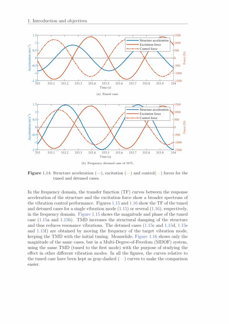
1.14 Structure acceleration ( ), excitation ( ) and control( ) forcesfor the tuned and detuned cases. . . . . . . . . . . . . . . . . . . . . 12
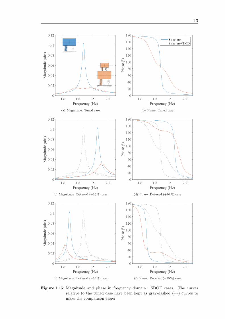
1.15 Magnitude and phase in frequency domain. SDOF cases. Thecurves relative to the tuned case have been kept as gray-dashed( ) curves to make the comparison easier . . . . . . . . . . . . . . 13
1.16 Magnitude in frequency domain. MDOF cases. The curves relativeto the tuned case have been kept as gray-dashed ( ) curves tomake the comparison easier . . . . . . . . . . . . . . . . . . . . . . 14
1.17 Model of structure with TMD (left) upgraded into a structure withSTMD model (right). Red arrow ( −→) means changing over time. . . 16
2.1 Walking force generated by a pedestrian. . . . . . . . . . . . . . . . 21
2.2 Vertical pedestrian force measured by a 3D instrumented tread-mill [30]. . . . . . . . . . . . . . . . . . . . . . . . . . . . . . . . . . 22
2.3 Suggested loading coefficient to be applied in the design stage (- -), rehabilitation (–) and (black) original, as defined in Setra andHiVoSS for vertical (a) and lateral (b) loading [189]. . . . . . . . . . 24
2.4 Frequency weighting depending on user’s position [96]. . . . . . . . 25
2.5 CDF curves. . . . . . . . . . . . . . . . . . . . . . . . . . . . . . . . 26
2.6 A general view of the laboratory structure, instrumented with ac-celerometers underneath. . . . . . . . . . . . . . . . . . . . . . . . . 27
2.7 Example of time history acceleration for an experimental test of afull-scale laboratory structure with computed predictors. . . . . . . 29
xxv
List of Figures
2.8 Example of H∞ and H2 graphical representations. . . . . . . . . . . 30
2.9 Uncertainties in the modal parameter identification process. . . . . 30
2.10 Analysis carried out on the Infante D. Henrique Arch Bridge [125]. . 33
2.11 Example of structure with uncertainties in the modal parameters [91]. 34
2.12 Examples of different vibration control system schemes [209]. . . . . 35
2.13 Feedforward and feedback control applied to a structure. . . . . . . 36
2.14 Scheme of vibration control strategies. . . . . . . . . . . . . . . . . 37
2.15 Examples of uncontrolled and controlled structure’s response curvesin frequency domain for different types of vibration control strategies. 37
2.16 Inertial mass actuator. APS Dynamic Model 400. . . . . . . . . . . 40
2.17 Laboratory stress-ribbon footbridge (a) using pneumatic actuators(b) for active control at TU Berlin [23]. . . . . . . . . . . . . . . . . 41
2.18 Passive and active vibration control on an in-service footbridge [39]. 42
2.19 MIMO vibration control application in an indoor footbridge [158]. . 43
2.20 Control scheme of a structure with semi-active vibration control. . . 44
2.21 FRF amplitude of a primary structure with a TMD, changing itsdamping ratio along the frequency. . . . . . . . . . . . . . . . . . . 47
2.22 Vibration reduction reached in frequency domain for Figure 2.21example. . . . . . . . . . . . . . . . . . . . . . . . . . . . . . . . . . 47
2.23 TMDs in Millenium Bridge (2001). GERB company. . . . . . . . . 48
2.24 TMDs in Solferino footbridge (1999). GERB company. . . . . . . . 49
2.25 TMDs in Abandoibarra Footbridge (1997). MAURER company. . . 49
2.26 TMDs in Forchheim Footbridge (2003). MAURER company. . . . . 50
2.27 TMDs in Pedro e Ines Footbridge (2007) [34]. . . . . . . . . . . . . 50
2.28 TMDs of one of the footbridges in Las Vegas (2007) (Taylor Devicescompany). . . . . . . . . . . . . . . . . . . . . . . . . . . . . . . . . 51
2.29 STMDs in the Volgograd Bridge (2011) [196]. . . . . . . . . . . . . 54
2.30 STMD in FEUP Footbridge (2017) [140]. . . . . . . . . . . . . . . . 56
2.31 Scheme of the two semi-active strategies studied. Red symbol ( −→)means changing over time. . . . . . . . . . . . . . . . . . . . . . . . 56
2.32 MR fluid particles (Lord Corporation). . . . . . . . . . . . . . . . . 59
2.33 Automotive suspension systems (Lord Corporation). . . . . . . . . . 60
2.34 Main parameters of an MR damper model [151]. . . . . . . . . . . . 62
2.35 Bingham and Bouc-Wen mechanical models [209]. . . . . . . . . . . 62
2.36 Time response force of Bingham and Bouc-Wen MR-damper modelsfor 1.00 Hz sinusoidal excitation with 5 mm amplitude and differentinput currents (0.00 A, 0.25 A and 0.50 A). . . . . . . . . . . . . . . 63
2.37 Response of Bingham and Bouc-Wen MR-damper models for 1.00 Hzsinusoidal excitation with 5 mm amplitude and different input cu-rrents (0.00 A, 0.25 A and 0.50 A). . . . . . . . . . . . . . . . . . . . 64
2.38 Sponge RD-1097-1 MR damper from Lord Corporation company. . 65
2.39 Model of MR damper for control applications. Red symbol ( −→)means changing over time. . . . . . . . . . . . . . . . . . . . . . . . 67
2.40 Feedforward control strategy applied to MR damper. . . . . . . . . 67

xxvii
3.1 Pedro Gomez Bosque Footbridge, Valladolid (Spain). . . . . . . . . 71
3.2 Data logger, router and other monitoring devices [62]. . . . . . . . . 73
3.3 Fixed system (blue) and rotated system(red) [62]. . . . . . . . . . . 74
3.4 Processed raw data of 4 central channels for upstream side. . . . . . 76
3.5 Signal processing effects in time domain. . . . . . . . . . . . . . . . 77
3.6 Signal processing effects in frequency domain. . . . . . . . . . . . . 78
3.7 Diagrams of stabilization obtained and MAC matrix. . . . . . . . . 80
3.8 Selected poles: SSI-cov (dashed lines), SSI-data (circles) and SSI-EM (crosses). . . . . . . . . . . . . . . . . . . . . . . . . . . . . . . 81
3.9 First seven modes shapes obtained with SSI-cov. . . . . . . . . . . . 83
3.10 MAC comparison between SSI-cov and SSI-data. . . . . . . . . . . . 84
3.11 Tracking procedure for modal parameters. . . . . . . . . . . . . . . 86
3.12 Distribution per hour of the repeatability for mode 4. . . . . . . . . 89
3.13 Results at day and night test for channel 16. . . . . . . . . . . . . . 90
3.14 Tracked frequency estimates for the whole year. . . . . . . . . . . . 91
3.15 Frequency estimates and temperature recorded for mode 4. . . . . . 92
3.16 Frequency estimates versus temperature for mode 1 and 4 (fromTable 3.5). . . . . . . . . . . . . . . . . . . . . . . . . . . . . . . . . 93
3.17 Overlaid distributions of the identified natural frequencies. . . . . . 96
3.18 Overlaid distributions of the identified natural damping ratios. . . . 97
3.19 Validation of the statistical model with unseen data. (o) SSI esti-mates, (x) estimates from the statistical model. . . . . . . . . . . . 98
3.20 Removing the external factors for mode 4. (x) SSI estimates f (SSI),
(x) corrected frequency estimates f ∗, and (- -) corrected frequency f ∗.100
3.21 Mean value per hour of several predictors. . . . . . . . . . . . . . . 102
3.22 Mean curve of likelihood of non-exceeded for weighted vertical accel-eration. The shaded area indicates the range between the minimumand maximum curves for one-year monitoring. . . . . . . . . . . . . 103
4.1 Distribution density. The line shows the normal distribution withthe same mean and standard deviation as the original distributiondensity. Extracted from Figures 3.17 and 3.18. . . . . . . . . . . . . 106
4.2 Magnitude of Transfer Functions of the models considered over theyear. . . . . . . . . . . . . . . . . . . . . . . . . . . . . . . . . . . . 108
4.3 Weighted force amplitude, F0 (f). . . . . . . . . . . . . . . . . . . . 110
4.4 Active control scheme. . . . . . . . . . . . . . . . . . . . . . . . . . 112
4.5 Root locus. × open-loop poles, � closed-loop poles. . . . . . . . . . 112
4.6 Response of SDOF system. . . . . . . . . . . . . . . . . . . . . . . . 115
4.7 MTVV vs Frequency. . . . . . . . . . . . . . . . . . . . . . . . . . . 116
4.8 CDF curves for SDOF case. . . . . . . . . . . . . . . . . . . . . . . 117
4.9 Response of MDOF system. . . . . . . . . . . . . . . . . . . . . . . 118
4.10 CDF curves for MDOF case. . . . . . . . . . . . . . . . . . . . . . . 119
4.11 Results for 400-N chirp amplitude. . . . . . . . . . . . . . . . . . . 120
4.12 Results for 1500-N chirp amplitude. . . . . . . . . . . . . . . . . . . 121
List of Figures
4.13 Distribution of % of vibration reduction for the three strategies. . . 122
5.1 Simplified control scheme with an inertial controller. . . . . . . . . . 128
5.2 Model of the 2-DOF systems studied. Red symbol ( −→) meanschanging over time. . . . . . . . . . . . . . . . . . . . . . . . . . . . 129
5.3 Contour plot of the PI for TMD and STMD with linear-viscousdamper. . . . . . . . . . . . . . . . . . . . . . . . . . . . . . . . . . 131
5.4 Uncontrolled case. Obtaining the PI. . . . . . . . . . . . . . . . . . 132
5.5 Envelope curve and PI. Optimization for the case of viscous damp-ing. The legend shows the PI values for these cases: ( ) uncon-trolled, ( ) initial solution and ( ) optimized solution. . . . 132
5.6 Performance in terms of the CDF of the MTVV for several damperforce saturations FDmax . . . . . . . . . . . . . . . . . . . . . . . . . . 134
5.7 Experimental setup for MR damper model identification. . . . . . . 135
5.8 Summary of the experimental results conducted for the identifica-tion of the MR damper model. . . . . . . . . . . . . . . . . . . . . . 135
5.9 Comparison between experimental response and Bingham and Bouc-Wen models predicted responses. . . . . . . . . . . . . . . . . . . . 137
5.10 Contour plot of the PI for MR-TMD and MR-STMD with the Bing-ham MR damper model. . . . . . . . . . . . . . . . . . . . . . . . . 138
5.11 MR damper experimental results for 2 and 6 Hz in off state (0 A). . 139
5.12 Envelope curve and PI. Optimization for the case in which the Bing-ham MR damper model is included. The legend shows the PI valuesfor these cases: ( ) uncontrolled, ( ) initial solution and (
) optimized solution. . . . . . . . . . . . . . . . . . . . . . . . . . 140
5.13 Description of the experimental test. . . . . . . . . . . . . . . . . . 141
5.14 Description of the experimental test. . . . . . . . . . . . . . . . . . 142
5.15 Control scheme for practical implementation of the semi-active con-trol law. . . . . . . . . . . . . . . . . . . . . . . . . . . . . . . . . . 143
5.16 Original and low-filtered acceleration for two cut-off frequencies. . . 144
5.17 Braking the inertial mass due to the blocking force of the MRdamper. The gray area represents the damper force turned on. . . . 144
5.18 Experimental vibration results in frequency domain comparing theuncontrolled structure, MR-TMD and MR-TMD for the three casesof Table 5.5. The dashed red line ( ) in the phase plots indicates90o delay between the structure acceleration and the control force,which means perfect tuning. . . . . . . . . . . . . . . . . . . . . . . 147
6.1 Hardware and external cell of the low-cost prototype. . . . . . . . . 152
6.2 MR damper feedback control scheme. . . . . . . . . . . . . . . . . . 152
6.3 Controlled displacement assembly for MR damper identification tests.153
List of Tables
1.1 Mean values of the modal parameters of the Porto footbridge stud-ied [139]. . . . . . . . . . . . . . . . . . . . . . . . . . . . . . . . . . 7
1.2 Parameters of the TMD tuned for the first mode of the Porto foot-bridge. . . . . . . . . . . . . . . . . . . . . . . . . . . . . . . . . . . 11
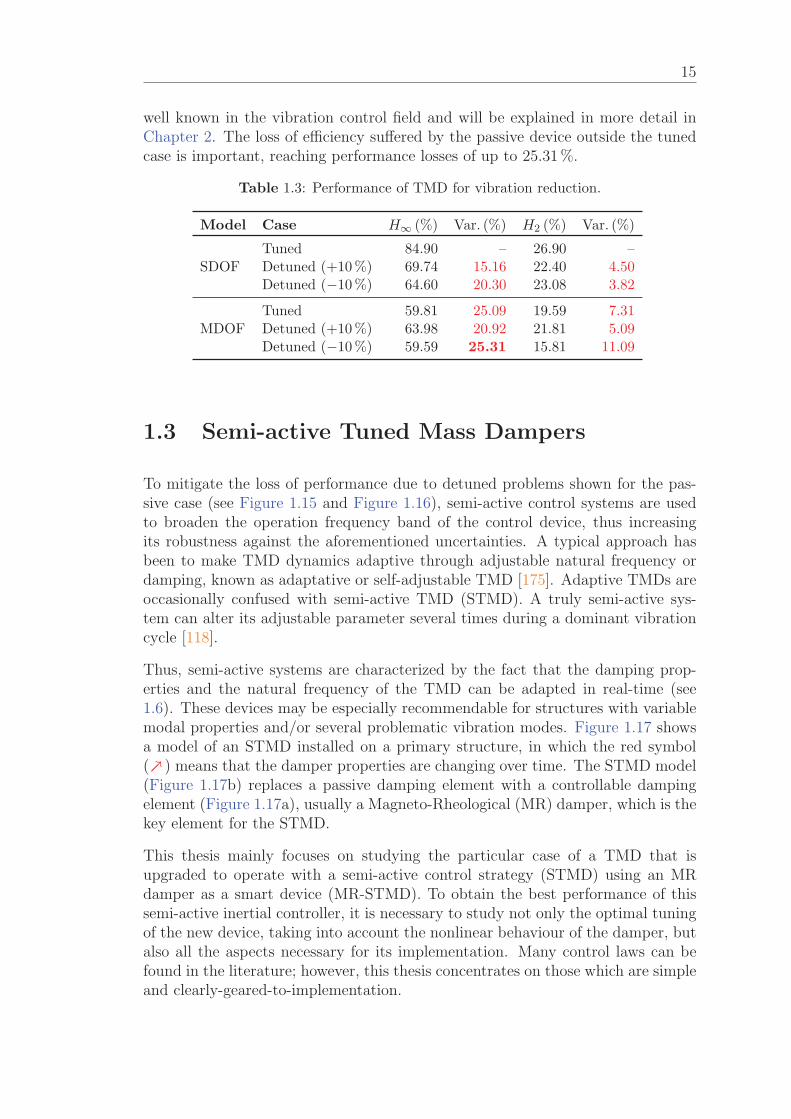
1.3 Performance of TMD for vibration reduction. . . . . . . . . . . . . 15
2.1 Typical frequency ranges for different types of human activity [16]. . 21
2.2 Comfort for vertical acceleration according to guidelines. . . . . . . 24
3.1 Natural frequencies (f) and damping ratios (ζ) identified by thethree SSI techniques. . . . . . . . . . . . . . . . . . . . . . . . . . . 82
3.2 Summary of identified modes and statistical comparison for thethree techniques: mean frequency (f), mean damping (ζ) and thecorresponding errors. . . . . . . . . . . . . . . . . . . . . . . . . . . 82
3.3 Natural frequencies (f) and damping ratios (ζ) identified by SSI-covand different time blocks. . . . . . . . . . . . . . . . . . . . . . . . . 85
3.4 Summary of identified mode frequencies and statistical comparisonfor the 20-minute against 60-minute time block: mean frequency(f), mean damping (ζ) and the corresponding errors. . . . . . . . . 87
3.5 Summary of identified natural frequencies and damping ratios forone year monitoring and their statistics: mean frequency (f), meandamping (ζ), standard deviation (Std) and the corresponding vari-ation (ν). . . . . . . . . . . . . . . . . . . . . . . . . . . . . . . . . 88
3.6 Adjusted R-Squared Radj,k and independent variable for each sta-tistical model according to the number of predictors k. . . . . . . . 98
4.1 Summary of modal participation factors, αi, for each vibrationmode at the maximum amplitude node of mode 4. . . . . . . . . . . 107
4.2 Summary of vibration reduction (%) for each case. . . . . . . . . . . 123
5.1 Parameters used for the sensitivity analysis. . . . . . . . . . . . . . 130
5.2 Results from the optimization procedure for TMD and STMD. Theimprovement is computed from the initial solution of each device. . 133
5.3 Variation range of the input parameters for the MR damper iden-tification. . . . . . . . . . . . . . . . . . . . . . . . . . . . . . . . . 134
5.4 Results from the optimization procedure for the MR-TMD and theMR-STMD. The improvement is computed from the initial solutionof each device. . . . . . . . . . . . . . . . . . . . . . . . . . . . . . . 141
5.5 Modal parameters of the beam for the three cases studied. . . . . . 142
5.6 Experimental vibration reduction (dB) for MR-TMD and MR-STMDfor the three cases studied. . . . . . . . . . . . . . . . . . . . . . . . 146
xxix

List of Tables
5.7 Summary of the results obtained numerically for TMD, STMD, MR-TMD and MR-STMD. . . . . . . . . . . . . . . . . . . . . . . . . . 148
Abbreviations
AMD Active Mass Damper
AVC Active Vibration Control
BI Base Isolation
CDF Cumulative Distribution Function
DBG Displacement Based Groundhook
DLF Dynamic Loading Factor
DOF Degree Of Freedom
DVFC Direct Velocity Feedback Control
EM Expectation Maximization
FEM Finite Element Model
FFT Fast Fourier Transform
FRF Frequency Response Function
HTMD Hybrid Tuned Mass Damper
HVC Hybrid Vibration Control
KKF Kinematic Kalman Filter
LIF Leaky-Integrator Filter
LQR Linear Quadratic Regulator
LVDT Linear Variable Differential Transducer
MAC Modal Assurance Criterion
MDOF Multi-Degree Of Freedom
MEMS Micro Electro-Mechanical System
MLR Multiple Linear Regression
MR Magneto-Rheological
MTVV Maximum Transient Vibration Value
NI National Instruments
OMA Operational Modal Analysis
PED Passive Energy Dissipation
xxxi
Abbreviations
PGB Pedro Gomez Bosque
PI Performance Index
PID Proportional Integral Derivative
PSD Power Spectral Density
PVC Passive Vibration Control
RMS Root Mean Square
SDOF Single Degree Of Freedom
SHM Structural Health Monitoring
SLS Serviceability Limit State
SSI Stochastic Subspace Identification
STMD Semi-active Tuned Mass Damper
TF Transfer Function
TMD Tuned Mass Damper
TVA Tuned Vibration Absorber
ULS Ultimate Limit State
VBG Velocity Based Groundhook
VDV Vibration Dose Value
VS Vibration Serviceability
VSA Vibration Serviceability Assessment
VSLS Vibration Serviceability Limit State
1Introduction and objectives
Contents
1.1 Introduction . . . . . . . . . . . . . . . . . . . . . . . . . 1
1.1.1 Vibration serviceability problems . . . . . . . . . . . . . 2
1.1.2 Motivation . . . . . . . . . . . . . . . . . . . . . . . . . 4
1.2 Tuned Mass Dampers . . . . . . . . . . . . . . . . . . . . 8
1.3 Semi-active Tuned Mass Dampers . . . . . . . . . . . . 15
1.4 Thesis objectives . . . . . . . . . . . . . . . . . . . . . . . 16
1.5 Thesis outline . . . . . . . . . . . . . . . . . . . . . . . . . 17
1.1 Introduction
This Thesis is part of the Research Project “Development of novel systems forreducing vibrations in pedestrian structures” REVES-P (DPI2013-47441) fundedby the Ministry of Economy and Competitiveness. The said Project was devotedto the development of semi-active and active vibration control strategies and tocontribute to the acceptation of these advanced vibration control techniques bythe civil engineering community. The PhD candidate got a 4-year research grantwithin the aforementioned project to carry out this thesis under the supervisionof Dr Ivan M. Dıaz.
1
1. Introduction and objectives
1.1.1 Vibration serviceability problems
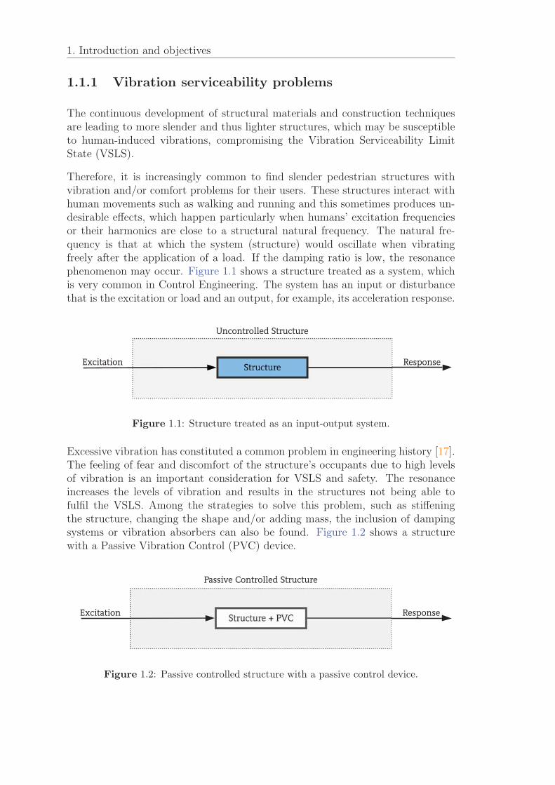
The continuous development of structural materials and construction techniquesare leading to more slender and thus lighter structures, which may be susceptibleto human-induced vibrations, compromising the Vibration Serviceability LimitState (VSLS).
Therefore, it is increasingly common to find slender pedestrian structures withvibration and/or comfort problems for their users. These structures interact withhuman movements such as walking and running and this sometimes produces un-desirable effects, which happen particularly when humans’ excitation frequenciesor their harmonics are close to a structural natural frequency. The natural fre-quency is that at which the system (structure) would oscillate when vibratingfreely after the application of a load. If the damping ratio is low, the resonancephenomenon may occur. Figure 1.1 shows a structure treated as a system, whichis very common in Control Engineering. The system has an input or disturbancethat is the excitation or load and an output, for example, its acceleration response.
Figure 1.1: Structure treated as an input-output system.
Excessive vibration has constituted a common problem in engineering history [17].The feeling of fear and discomfort of the structure’s occupants due to high levelsof vibration is an important consideration for VSLS and safety. The resonanceincreases the levels of vibration and results in the structures not being able tofulfil the VSLS. Among the strategies to solve this problem, such as stiffeningthe structure, changing the shape and/or adding mass, the inclusion of dampingsystems or vibration absorbers can also be found. Figure 1.2 shows a structurewith a Passive Vibration Control (PVC) device.
Figure 1.2: Passive controlled structure with a passive control device.
3
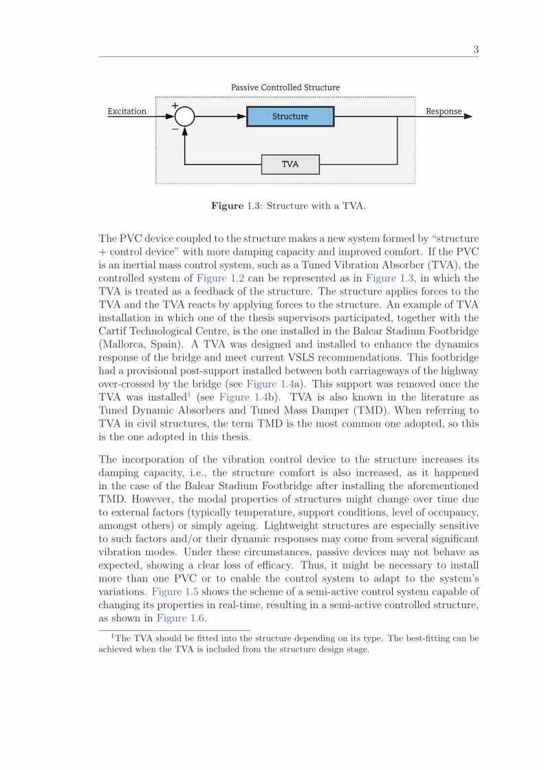
Figure 1.3: Structure with a TVA.
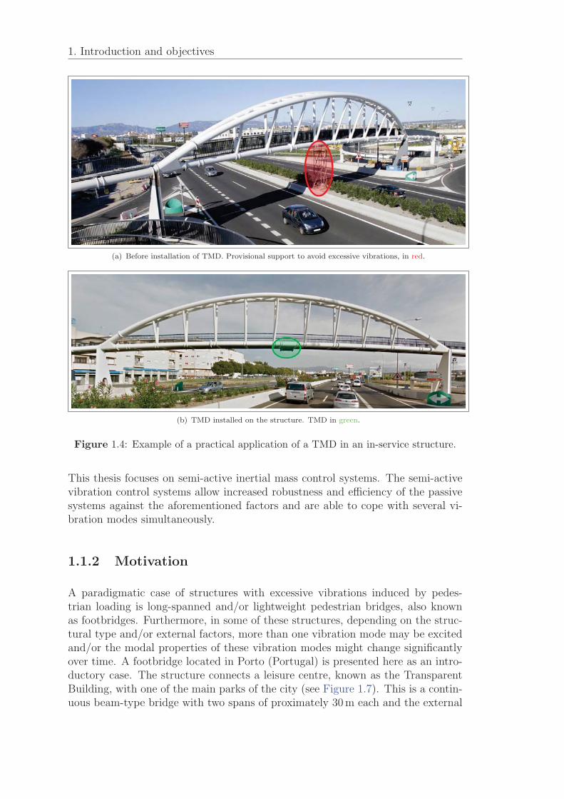
The PVC device coupled to the structure makes a new system formed by “structure+ control device” with more damping capacity and improved comfort. If the PVCis an inertial mass control system, such as a Tuned Vibration Absorber (TVA), thecontrolled system of Figure 1.2 can be represented as in Figure 1.3, in which theTVA is treated as a feedback of the structure. The structure applies forces to theTVA and the TVA reacts by applying forces to the structure. An example of TVAinstallation in which one of the thesis supervisors participated, together with theCartif Technological Centre, is the one installed in the Balear Stadium Footbridge(Mallorca, Spain). A TVA was designed and installed to enhance the dynamicsresponse of the bridge and meet current VSLS recommendations. This footbridgehad a provisional post-support installed between both carriageways of the highwayover-crossed by the bridge (see Figure 1.4a). This support was removed once theTVA was installed1 (see Figure 1.4b). TVA is also known in the literature asTuned Dynamic Absorbers and Tuned Mass Damper (TMD). When referring toTVA in civil structures, the term TMD is the most common one adopted, so thisis the one adopted in this thesis.
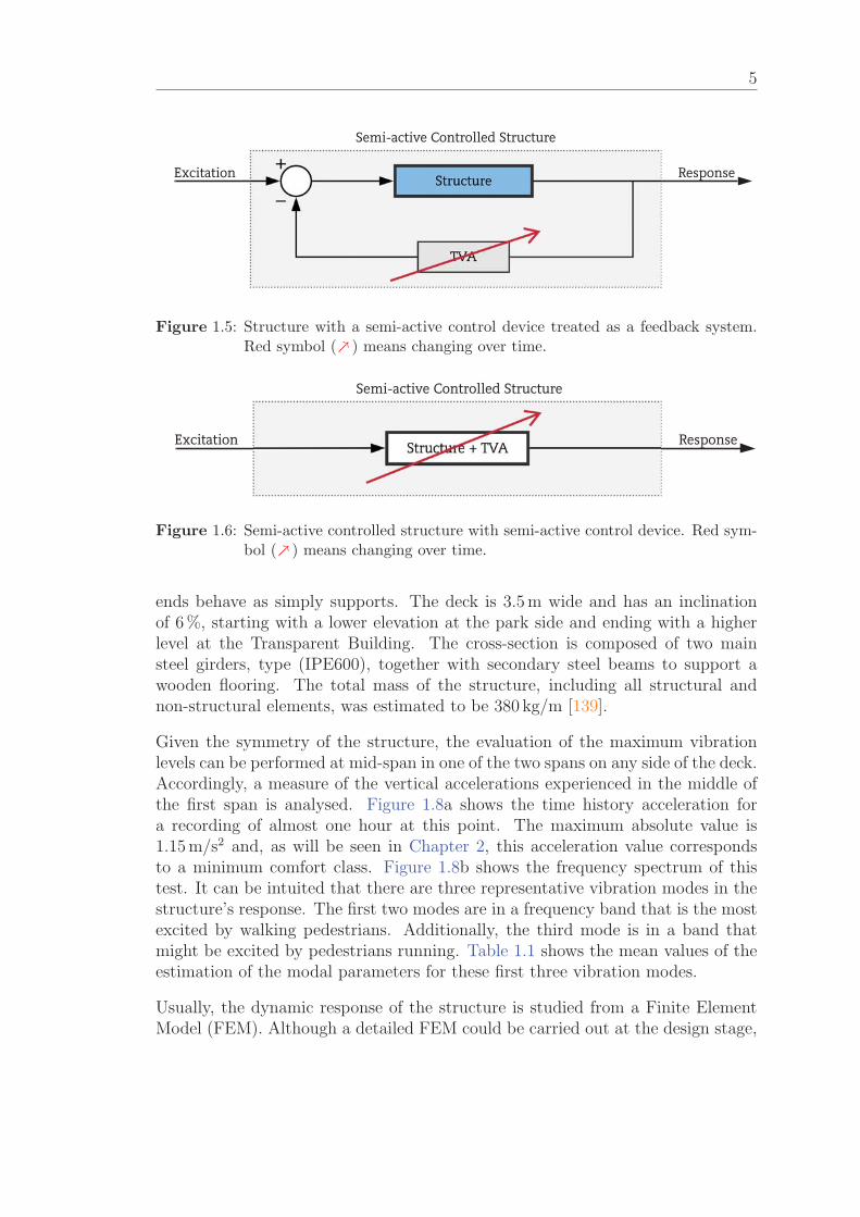
The incorporation of the vibration control device to the structure increases itsdamping capacity, i.e., the structure comfort is also increased, as it happenedin the case of the Balear Stadium Footbridge after installing the aforementionedTMD. However, the modal properties of structures might change over time dueto external factors (typically temperature, support conditions, level of occupancy,amongst others) or simply ageing. Lightweight structures are especially sensitiveto such factors and/or their dynamic responses may come from several significantvibration modes. Under these circumstances, passive devices may not behave asexpected, showing a clear loss of efficacy. Thus, it might be necessary to installmore than one PVC or to enable the control system to adapt to the system’svariations. Figure 1.5 shows the scheme of a semi-active control system capable ofchanging its properties in real-time, resulting in a semi-active controlled structure,as shown in Figure 1.6.
1The TVA should be fitted into the structure depending on its type. The best-fitting can beachieved when the TVA is included from the structure design stage.
1. Introduction and objectives
(a) Before installation of TMD. Provisional support to avoid excessive vibrations, in red.
(b) TMD installed on the structure. TMD in green.
Figure 1.4: Example of a practical application of a TMD in an in-service structure.
This thesis focuses on semi-active inertial mass control systems. The semi-activevibration control systems allow increased robustness and efficiency of the passivesystems against the aforementioned factors and are able to cope with several vi-bration modes simultaneously.
1.1.2 Motivation
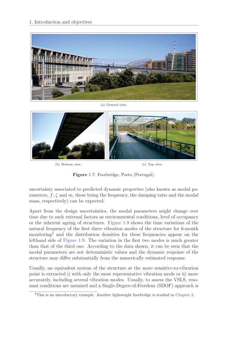
A paradigmatic case of structures with excessive vibrations induced by pedes-trian loading is long-spanned and/or lightweight pedestrian bridges, also knownas footbridges. Furthermore, in some of these structures, depending on the struc-tural type and/or external factors, more than one vibration mode may be excitedand/or the modal properties of these vibration modes might change significantlyover time. A footbridge located in Porto (Portugal) is presented here as an intro-ductory case. The structure connects a leisure centre, known as the TransparentBuilding, with one of the main parks of the city (see Figure 1.7). This is a contin-uous beam-type bridge with two spans of proximately 30 m each and the external
5
Figure 1.5: Structure with a semi-active control device treated as a feedback system.Red symbol ( −→) means changing over time.
Figure 1.6: Semi-active controlled structure with semi-active control device. Red sym-bol ( −→) means changing over time.
ends behave as simply supports. The deck is 3.5 m wide and has an inclinationof 6 %, starting with a lower elevation at the park side and ending with a higherlevel at the Transparent Building. The cross-section is composed of two mainsteel girders, type (IPE600), together with secondary steel beams to support awooden flooring. The total mass of the structure, including all structural andnon-structural elements, was estimated to be 380 kg/m [139].
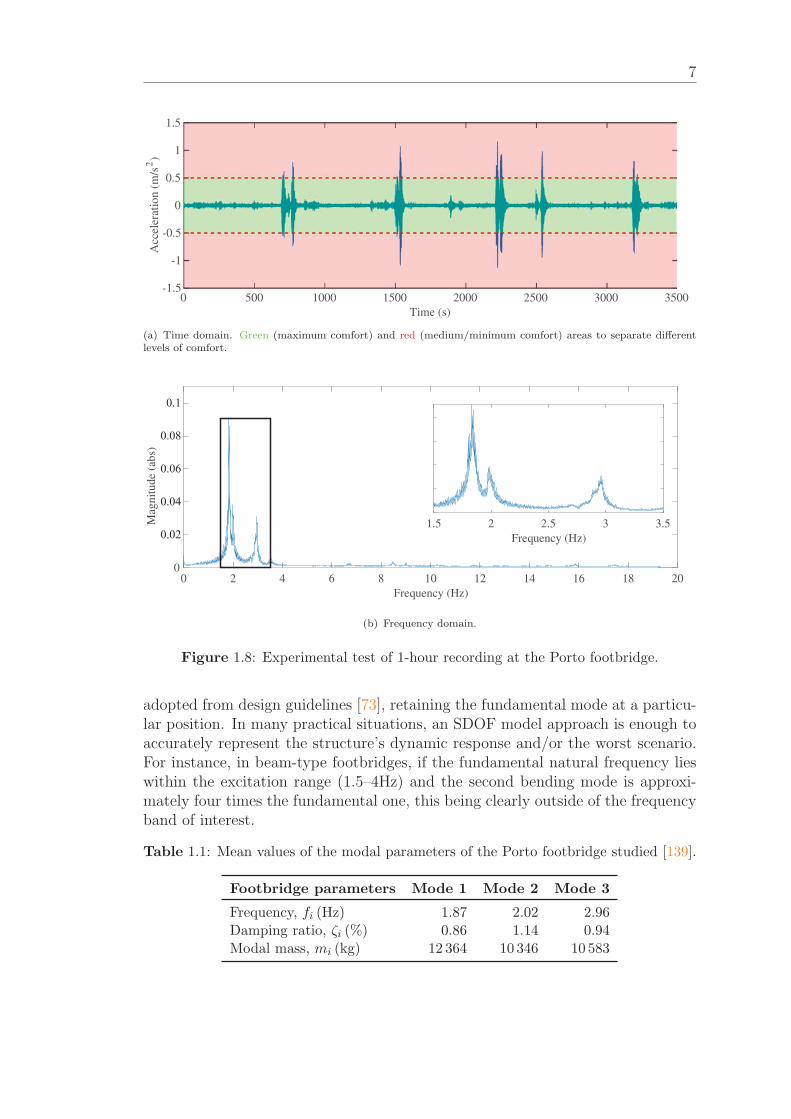
Given the symmetry of the structure, the evaluation of the maximum vibrationlevels can be performed at mid-span in one of the two spans on any side of the deck.Accordingly, a measure of the vertical accelerations experienced in the middle ofthe first span is analysed. Figure 1.8a shows the time history acceleration fora recording of almost one hour at this point. The maximum absolute value is1.15 m/s2 and, as will be seen in Chapter 2, this acceleration value correspondsto a minimum comfort class. Figure 1.8b shows the frequency spectrum of thistest. It can be intuited that there are three representative vibration modes in thestructure’s response. The first two modes are in a frequency band that is the mostexcited by walking pedestrians. Additionally, the third mode is in a band thatmight be excited by pedestrians running. Table 1.1 shows the mean values of theestimation of the modal parameters for these first three vibration modes.
Usually, the dynamic response of the structure is studied from a Finite ElementModel (FEM). Although a detailed FEM could be carried out at the design stage,
1. Introduction and objectives
(a) General view.
(b) Bottom view. (c) Top view.
Figure 1.7: Footbridge, Porto (Portugal).
uncertainty associated to predicted dynamic properties (also known as modal pa-rameters, f , ζ and m, these being the frequency, the damping ratio and the modalmass, respectively) can be expected.
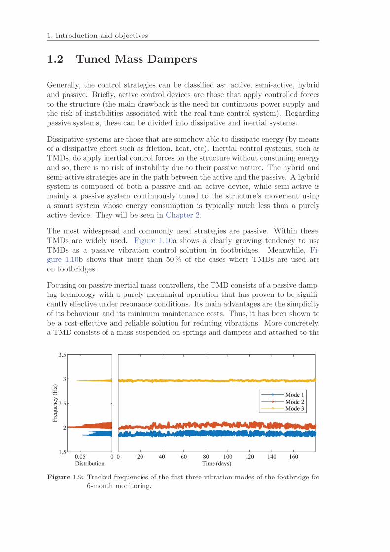
Apart from the design uncertainties, the modal parameters might change overtime due to such external factors as environmental conditions, level of occupancyor the inherent ageing of structures. Figure 1.9 shows the time variations of thenatural frequency of the first three vibration modes of the structure for 6-monthmonitoring2 and the distribution densities for these frequencies appear on thelefthand side of Figure 1.9. The variation in the first two modes is much greaterthan that of the third one. According to the data shown, it can be seen that themodal parameters are not deterministic values and the dynamic response of thestructure may differ substantially from the numerically estimated response.
Usually, an equivalent system of the structure at the more sensitive-to-vibrationpoint is extracted i) with only the most representative vibration mode or ii) moreaccurately, including several vibration modes. Usually, to assess the VSLS, reso-nant conditions are assumed and a Single-Degree-of-Freedom (SDOF) approach is
2This is an introductory example. Another lightweight footbridge is studied in Chapter 3.
7
(a) Time domain. Green (maximum comfort) and red (medium/minimum comfort) areas to separate differentlevels of comfort.
(b) Frequency domain.
Figure 1.8: Experimental test of 1-hour recording at the Porto footbridge.
adopted from design guidelines [73], retaining the fundamental mode at a particu-lar position. In many practical situations, an SDOF model approach is enough toaccurately represent the structure’s dynamic response and/or the worst scenario.For instance, in beam-type footbridges, if the fundamental natural frequency lieswithin the excitation range (1.5–4Hz) and the second bending mode is approxi-mately four times the fundamental one, this being clearly outside of the frequencyband of interest.
Table 1.1: Mean values of the modal parameters of the Porto footbridge studied [139].
Footbridge parameters Mode 1 Mode 2 Mode 3
Frequency, fi (Hz) 1.87 2.02 2.96Damping ratio, ζi (%) 0.86 1.14 0.94Modal mass, mi (kg) 12 364 10 346 10 583
1. Introduction and objectives
1.2 Tuned Mass Dampers
Generally, the control strategies can be classified as: active, semi-active, hybridand passive. Briefly, active control devices are those that apply controlled forcesto the structure (the main drawback is the need for continuous power supply andthe risk of instabilities associated with the real-time control system). Regardingpassive systems, these can be divided into dissipative and inertial systems.
Dissipative systems are those that are somehow able to dissipate energy (by meansof a dissipative effect such as friction, heat, etc). Inertial control systems, such asTMDs, do apply inertial control forces on the structure without consuming energyand so, there is no risk of instability due to their passive nature. The hybrid andsemi-active strategies are in the path between the active and the passive. A hybridsystem is composed of both a passive and an active device, while semi-active ismainly a passive system continuously tuned to the structure’s movement usinga smart system whose energy consumption is typically much less than a purelyactive device. They will be seen in Chapter 2.
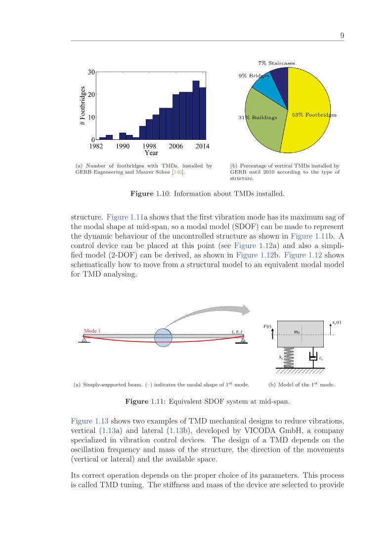
The most widespread and commonly used strategies are passive. Within these,TMDs are widely used. Figure 1.10a shows a clearly growing tendency to useTMDs as a passive vibration control solution in footbridges. Meanwhile, Fi-gure 1.10b shows that more than 50 % of the cases where TMDs are used areon footbridges.
Focusing on passive inertial mass controllers, the TMD consists of a passive damp-ing technology with a purely mechanical operation that has proven to be signifi-cantly effective under resonance conditions. Its main advantages are the simplicityof its behaviour and its minimum maintenance costs. Thus, it has been shown tobe a cost-effective and reliable solution for reducing vibrations. More concretely,a TMD consists of a mass suspended on springs and dampers and attached to the
Figure 1.9: Tracked frequencies of the first three vibration modes of the footbridge for6-month monitoring.
9
(a) Number of footbridges with TMDs, installed byGERB Engeneering and Maurer Sohne [145].
(b) Percentage of vertical TMDs installed byGERB until 2010 according to the type ofstructure.
Figure 1.10: Information about TMDs installed.
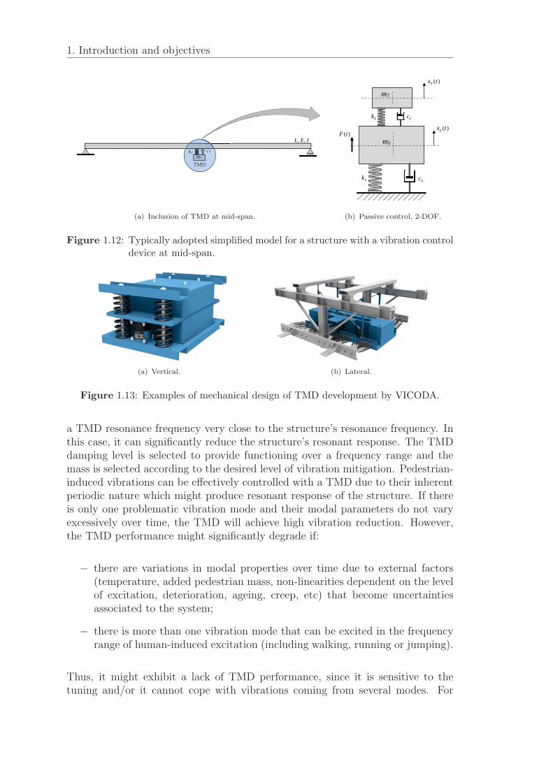
structure. Figure 1.11a shows that the first vibration mode has its maximum sag ofthe modal shape at mid-span, so a modal model (SDOF) can be made to representthe dynamic behaviour of the uncontrolled structure as shown in Figure 1.11b. Acontrol device can be placed at this point (see Figure 1.12a) and also a simpli-fied model (2-DOF) can be derived, as shown in Figure 1.12b. Figure 1.12 showsschematically how to move from a structural model to an equivalent modal modelfor TMD analysing.
L, E, I Mode 1
(a) Simply-supported beam. (–) indicates the modal shape of 1st mode.
( )F t( )Sx t
SkSc
c
mS
(b) Model of the 1st mode.
Figure 1.11: Equivalent SDOF system at mid-span.
Figure 1.13 shows two examples of TMD mechanical designs to reduce vibrations,vertical (1.13a) and lateral (1.13b), developed by VICODA GmbH, a companyspecialized in vibration control devices. The design of a TMD depends on theoscillation frequency and mass of the structure, the direction of the movements(vertical or lateral) and the available space.
Its correct operation depends on the proper choice of its parameters. This processis called TMD tuning. The stiffness and mass of the device are selected to provide
1. Introduction and objectives
kT cT
L, E, I
TMDmT
kT ccT
TMDmT
(a) Inclusion of TMD at mid-span.
( )F t
( )Tx t
( )Sx tTk Tc
SkSc
c
c
mS
mT
(b) Passive control, 2-DOF.
Figure 1.12: Typically adopted simplified model for a structure with a vibration controldevice at mid-span.
(a) Vertical. (b) Lateral.
Figure 1.13: Examples of mechanical design of TMD development by VICODA.
a TMD resonance frequency very close to the structure’s resonance frequency. Inthis case, it can significantly reduce the structure’s resonant response. The TMDdamping level is selected to provide functioning over a frequency range and themass is selected according to the desired level of vibration mitigation. Pedestrian-induced vibrations can be effectively controlled with a TMD due to their inherentperiodic nature which might produce resonant response of the structure. If thereis only one problematic vibration mode and their modal parameters do not varyexcessively over time, the TMD will achieve high vibration reduction. However,the TMD performance might significantly degrade if:
− there are variations in modal properties over time due to external factors(temperature, added pedestrian mass, non-linearities dependent on the levelof excitation, deterioration, ageing, creep, etc) that become uncertaintiesassociated to the system;
− there is more than one vibration mode that can be excited in the frequencyrange of human-induced excitation (including walking, running or jumping).
Thus, it might exhibit a lack of TMD performance, since it is sensitive to thetuning and/or it cannot cope with vibrations coming from several modes. For

11
example, the eigenfrequencies of a structure may not be known to a sufficient levelof accuracy when the TMDs are designed and the final parameters are usuallydetermined through in-situ testing. The tuning of the TMD parameters to thefirst vibration mode (see Table 1.1) of the Porto footbridge as a target is shownin Table 1.2.
Table 1.2: Parameters of the TMD tuned for the first mode of the Porto footbridge.
TMD parameters Values
Frequency, fT (Hz) 1.85Frequency ratio, η (–) 0.9893Damping ratio, ζT (%) 8.65Mass, mT (kg) 247.28Mass ratio, μ (–) 0.02
The motion control of the primary mass mS
is obtained by the pair of forcesapplied by the spring F
Sand the damper F
Dthat connect the two bodies, given
respectively by
FS
= kT
(xT− x
S) , (1.1)
FD
= cT
(xT− x
S) , (1.2)
where (xT− x
S) represents the relative displacement between the two masses and
(xT− x
S) the corresponding relative velocity while, k
Tand c
Tare the spring and
damper constants respectively. Both forces generate the total control force, FC
=F
S+ F
D. The tuning of TMD parameters is much more sensitive to frequency
than to damping deviations. This happens due to the greater weight of the springforce relative to the damper force in the control action.
Figure 1.14 shows a time history of the steady-state acceleration of the primarymass m
Swhen it is subjected to a harmonic load of the type F = F0 sin(2πf
St)
where F is the dynamic force overtime (t), and F0 and fS
are the force amplitudeand structural natural frequency (first vibration mode) to which the TMD is tuned,respectively. Also the control force F
Cis shown in Figure 1.14. For Figure 1.14a
(tuned case), a first observation is that the control force is in opposite phase tothe excitation force and both forces are delayed ± 90o relative to the structureacceleration. The phase control theory indicates that the TMD can develop themaximum structural vibration reduction with this phase lag. However, for a fre-quency detuned case of 10 % (see Figure 1.14b), the opposite phase between thecontrol and excitation force begins to be lost, which causes a significant loss ofefficiency of the passive control device since the peak acceleration goes from being0.97 m/s2 to 1.57 m/s2. It can be concluded that a small detuning (which obvi-ously is really easy to happen) of the TMD frequency leads to a phase angle farfrom the opposite phase between the excitation and control forces, correspondingto a degradation in the control action. The detuning of the damping ratio is notso conditioning, because the excitation and control force curves remain mostlyopposite in phase.
1. Introduction and objectives
353 353.1 353.2 353.3 353.4 353.5 353.6 353.7 353.8 353.9 354Time (s)
-1.5
-1
-0.5
0
0.5
1
1.5
Acc
eler
atio
n (m
/s2 )
-1500
-1000
-500
0
500
1000
1500
Forc
e (N
)
Structure accelerationExcitation forceControl force
(a) Tuned case.
353 353.1 353.2 353.3 353.4 353.5 353.6 353.7 353.8 353.9 354Time (s)
-1.5
-1
-0.5
0
0.5
1
1.5
Acc
eler
atio
n (m
/s2 )
-1500
-1000
-500
0
500
1000
1500
Forc
e (N
)
Structure accelerationExcitation forceControl force
(b) Frequency detuned case of 10%.
Figure 1.14: Structure acceleration ( ), excitation ( ) and control( ) forces for thetuned and detuned cases.
In the frequency domain, the transfer function (TF) curves between the responseacceleration of the structure and the excitation force show a broader spectrum ofthe vibration control performance. Figures 1.15 and 1.16 show the TF of the tunedand detuned cases for a single vibration mode (1.15) or several (1.16), respectively,in the frequency domain. Figure 1.15 shows the magnitude and phase of the tunedcase (1.15a and 1.15b). TMD increases the structural damping of the structureand thus reduces resonance vibrations. The detuned cases (1.15c and 1.15d, 1.15eand 1.15f) are obtained by moving the frequency of the target vibration mode,keeping the TMD with the initial tuning. Meanwhile, Figure 1.16 shows only themagnitude of the same cases, but in a Multi-Degree-of-Freedom (MDOF) system,using the same TMD (tuned to the first mode) with the purpose of studying theeffect in other different vibration modes. In all the figures, the curves relative tothe tuned case have been kept as gray-dashed ( ) curves to make the comparisoneasier.
13
(a) Magnitude. Tuned case.
1.6 1.8 2 2.2Frequency (Hz)
0
20
40
60
80
100
120
140
160
180
Phas
e (º)
StructureStructure+TMD
(b) Phase. Tuned case.
1.6 1.8 2 2.2Frequency (Hz)
0
0.02
0.04
0.06
0.08
0.1
0.12
Mag
nitu
de (a
bs)
(c) Magnitude. Detuned (+10%) case.
1.6 1.8 2 2.2Frequency (Hz)
0
20
40
60
80
100
120
140
160
180Ph
ase
(º)
(d) Phase. Detuned (+10%) case.
1.6 1.8 2 2.2Frequency (Hz)
0
0.02
0.04
0.06
0.08
0.1
0.12
Mag
nitu
de (a
bs)
(e) Magnitude. Detuned (−10%) case.
1.6 1.8 2 2.2Frequency (Hz)
0
20
40
60
80
100
120
140
160
180
Phas
e (º)
(f) Phase. Detuned (−10%) case.
Figure 1.15: Magnitude and phase in frequency domain. SDOF cases. The curvesrelative to the tuned case have been kept as gray-dashed ( ) curves tomake the comparison easier

1. Introduction and objectives
1.5 2 2.5 3 3.5Frequency (Hz)
0
0.02
0.04
0.06
0.08
0.1
0.12M
agni
tude
(abs
)
StructureStructure+TMD
(a) Tuned case.
1.5 2 2.5 3 3.5Frequency (Hz)
0
0.02
0.04
0.06
0.08
0.1
0.12
Mag
nitu
de (a
bs)
(b) Detuned (+10%) case.
1.5 2 2.5 3 3.5Frequency (Hz)
0
0.02
0.04
0.06
0.08
0.1
0.12
Mag
nitu
de (a
bs)
(c) Detuned (−10%) case.
Figure 1.16: Magnitude in frequency domain. MDOF cases. The curves relative tothe tuned case have been kept as gray-dashed ( ) curves to make thecomparison easier
Table 1.3 shows a summary of the TMD performance, in terms of vibration re-duction, for all the cases. The values are obtained according to two performanceindicators: one related with the maximum value of TF magnitude (H∞) and an-other indicator associated to the area under the curve (H2). These indicators are
15
well known in the vibration control field and will be explained in more detail inChapter 2. The loss of efficiency suffered by the passive device outside the tunedcase is important, reaching performance losses of up to 25.31 %.
Table 1.3: Performance of TMD for vibration reduction.
Model Case H∞ (%) Var. (%) H2 (%) Var. (%)
Tuned 84.90 – 26.90 –SDOF Detuned (+10%) 69.74 15.16 22.40 4.50
Detuned (−10%) 64.60 20.30 23.08 3.82
Tuned 59.81 25.09 19.59 7.31MDOF Detuned (+10%) 63.98 20.92 21.81 5.09
Detuned (−10%) 59.59 25.31 15.81 11.09
1.3 Semi-active Tuned Mass Dampers
To mitigate the loss of performance due to detuned problems shown for the pas-sive case (see Figure 1.15 and Figure 1.16), semi-active control systems are usedto broaden the operation frequency band of the control device, thus increasingits robustness against the aforementioned uncertainties. A typical approach hasbeen to make TMD dynamics adaptive through adjustable natural frequency ordamping, known as adaptative or self-adjustable TMD [175]. Adaptive TMDs areoccasionally confused with semi-active TMD (STMD). A truly semi-active sys-tem can alter its adjustable parameter several times during a dominant vibrationcycle [118].
Thus, semi-active systems are characterized by the fact that the damping prop-erties and the natural frequency of the TMD can be adapted in real-time (see1.6). These devices may be especially recommendable for structures with variablemodal properties and/or several problematic vibration modes. Figure 1.17 showsa model of an STMD installed on a primary structure, in which the red symbol( −→) means that the damper properties are changing over time. The STMD model(Figure 1.17b) replaces a passive damping element with a controllable dampingelement (Figure 1.17a), usually a Magneto-Rheological (MR) damper, which is thekey element for the STMD.
This thesis mainly focuses on studying the particular case of a TMD that isupgraded to operate with a semi-active control strategy (STMD) using an MRdamper as a smart device (MR-STMD). To obtain the best performance of thissemi-active inertial controller, it is necessary to study not only the optimal tuningof the new device, taking into account the nonlinear behaviour of the damper, butalso all the aspects necessary for its implementation. Many control laws can befound in the literature; however, this thesis concentrates on those which are simpleand clearly-geared-to-implementation.

1. Introduction and objectives
( )F t
( )Tx t
( )Sx tTk Tc
SkSc
( )F t
( )Tx t
( )Sx tTk ( )Tc t
SkSc
Passive damping Controllable damping
c
mS
mT
c
mS
mT
Tcc ( )Tc (Tc
Figure 1.17: Model of structure with TMD (left) upgraded into a structure with STMDmodel (right). Red arrow ( −→) means changing over time.
1.4 Thesis objectives
This thesis deals with the complete path followed from the moment that a struc-ture is perceived as uncomfortable by the users to the final possible solution. Ittakes into account the problem of identification, tracking modal parameters andvibration control in structures with time-varying modal parameters and/or severalproblematic vibration modes that need to be cancelled. The aims of this DoctoralThesis are to:
◦ Study the variability of the main parameters that identify a structure throughreal measurements, frequency and damping, in order to quantify the errorlimits associated with the identification method and the computational ap-proach.
◦ Develop a method for tracking the modal parameters of a structure and studytheir variations. This tracking may be carried out for structures whose modalparameters change significantly. This step is prior to the implementationof the most convenient vibration control strategies. Additionally, once themodal parameters have been tracked, the influence of external factors can beremoved and these might be considered for a Structural Health Monitoring(SHM) system.
◦ Study the performance of several easy-to-implement semi-active strategiesfor inertial controllers applied to one-year experimental estimates of an in-service structure considering also the implementation difficulties of each one.
◦ Develop a design methodology for the parameters of the semi-active inertialcontroller in order to optimise the vibration reduction over a broad-frequencyband.
17
◦ Study an MR damper through experimental tests and identify the param-eters of a phenomenological model. The derived model will be included inthe optimization process in such a way that the degradation from an idealdamper can be quantified.
◦ Assess the technical and practical feasibility of implementing STMD in alaboratory structure and study its performance as compared to its passiveversion.
1.5 Thesis outline
This document has been divided into 6 chapters. The first introduces the researchline. An example of a structure with time-varying modal parameters that mightexhibit excessive vibration has also been presented. The solution of installing aTMD in the structure has been studied numerically and the problem of detuninghas been described, both for the case of an SDOF model with uncertainty and forthat of an MDOF model.
The remaining chapters are organized as follows:
− Chapter 2 briefly reviews the fundamentals of vibration control, focusingon vibration serviceability, human vibration perception and human-inducedexcitations. Research works on structures with time-varying modal param-eters are presented. Also, this chapter brings together the theory of andresearch into passive and semi-active control via inertial controllers. Finally,the chapter ends by describing MR dampers as the smart device used tomaterialise the semi-active vibration control system.
− Chapter 3 studies an in-service structure in which the modal parametersvary over time. In this chapter, a tracking method is developed.
− Chapter 4 studies two implementable semi-active control strategies for iner-tial controllers. Furthermore, performance and assessment of the pros andcons of the possible practical implementation are fully described.
− In Chapter 5, an optimization procedure through a Performance Index (PI)to design the STMD parameters using a phase control law is presented. Thedegradation of the STMD performance when an MR damper model is used(as compared to an ideal viscous damper) is studied. Finally, to completethe procedure, a methodology for the identification of MR dampers usingphenomenological models is presented.
− Chapter 6 presents the main conclusions of the thesis and possible futureresearch lines are proposed. The main publications due to the research workcarried out within this thesis are also listed.

2Vibration control
Contents2.1 Human-induced vibration . . . . . . . . . . . . . . . . . 20
2.1.1 Human vibration excitation . . . . . . . . . . . . . . . . 20
2.1.2 Vibration serviceability . . . . . . . . . . . . . . . . . . 23
2.2 Modal parameter uncertainty . . . . . . . . . . . . . . . 28
2.2.1 Sources of uncertainty . . . . . . . . . . . . . . . . . . . 28
2.2.2 Examples of study . . . . . . . . . . . . . . . . . . . . . 32
2.3 Vibration control generalities . . . . . . . . . . . . . . . 33
2.3.1 Passive Vibration Control . . . . . . . . . . . . . . . . . 38
2.3.2 Active and Hybrid Vibration Control . . . . . . . . . . . 38
2.3.3 Semi-active Vibration Control . . . . . . . . . . . . . . . 40
2.4 Passive control via Tuned Mass Dampers . . . . . . . . 42
2.4.1 Theoretical design . . . . . . . . . . . . . . . . . . . . . 45
2.4.2 Examples of vertical TMD in footbridges . . . . . . . . 46
2.5 Semi-active Tuned Mass Dampers . . . . . . . . . . . . 51
2.5.1 Examples of vertical STMD in bridges . . . . . . . . . . 53
2.5.2 Semi-active control 1 . . . . . . . . . . . . . . . . . . . . 57
2.5.3 Semi-active control 2 . . . . . . . . . . . . . . . . . . . . 57
2.6 Magneto-rheological dampers . . . . . . . . . . . . . . . 59
2.6.1 Magneto-rheological fluids . . . . . . . . . . . . . . . . . 59
2.6.2 Modelling of MR dampers . . . . . . . . . . . . . . . . . 61
2.6.3 Bingham model . . . . . . . . . . . . . . . . . . . . . . . 62
2.6.4 Bouc-Wen model . . . . . . . . . . . . . . . . . . . . . . 66
2.6.5 Application of MR for STMD . . . . . . . . . . . . . . . 66
19
2. Vibration control
A state-of-the-art of structure serviceability due to human-induced vibration, vi-bration control and MR dampers is presented in this Chapter. Also, some back-ground knowledge used in the thesis is introduced.
2.1 Human-induced vibration
According to [55], the designed structure must satisfy a set of safety and service-ability requirements. The former concerns extreme loadings that are likely to occurno more than once during a structure’s lifetime. Serviceability is associated withmoderate loadings that can occur several times during the structure’s lifetime. Thestructure should ideally be fully operational during service loadings, for example,the structure may suffer inconsequential damage, while the motion experienced bythe structure should not exceed the specified comfort limits for humans and themotion sensitive equipment mounted on the structure. One example of a humancomfort limit is a restriction on acceleration; humans begin to feel uncomfortablewhen acceleration reaches a certain value; however that value depends on the typeof structure, the position of the person (sitting, standing, lying on the floor), thefrequency of the vibration and the discomfort threshold of each particular person.
Advanced material technologies, together with the use of new construction tech-niques, may lead to slender structures with low fundamental natural frequencies aswell as low damping ratios. These structures are sometimes susceptible to humanmovements such as walking, running, bouncing or jumping. This happens partic-ularly when excitation frequencies, or their harmonics, are close to a structuralnatural frequency. Because of their slenderness, contemporary footbridges are of-ten highly susceptible to human-induced vibrations. Pedestrians may excite thefootbridge deck with a periodic load and they might even synchronize their motionwith other pedestrians or the structure itself. This situation can introduce largevibrations into the structure. These vibrations might not compromise the struc-ture’s Ultimate Limit State (ULS) but they might lead to excessive vibrations,disturbing the user, who may feel unsafe [146].
2.1.1 Human vibration excitation
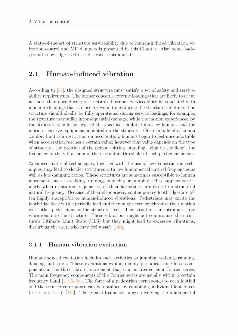
Human-induced excitation includes such activities as jumping, walking, running,dancing and so on. These excitations exhibit mainly periodical time force com-ponents in the three axes of movement that can be treated as a Fourier series.The main frequency components of the Fourier series are usually within a certainfrequency band [1, 95, 96]. The force of a pedestrian corresponds to each footfalland the total force response can be obtained by combining individual foot forces(see Figure 2.1b) [213]. The typical frequency ranges involving the fundamental
21
frequency (pacing frequency) are defined by Bachmann et al. [16] for differenttypes of human activities and they are shown in Table 2.1.
Activity Frequency (Hz)
Walking 1.6 – 2.4Running 2.0 – 3.5Jumping 1.8 – 3.4Bouncing 1.5 – 3.0
Table 2.1: Typical frequency ranges for different types of human activity [16].
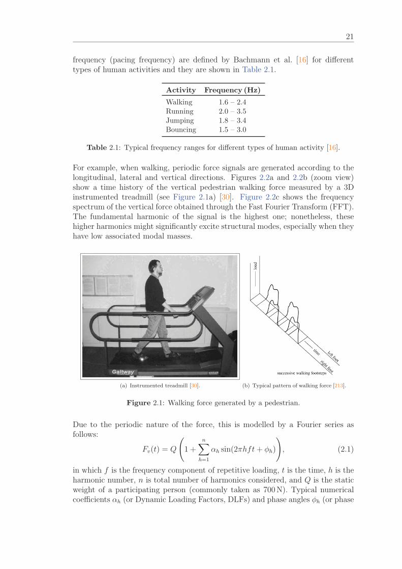
For example, when walking, periodic force signals are generated according to thelongitudinal, lateral and vertical directions. Figures 2.2a and 2.2b (zoom view)show a time history of the vertical pedestrian walking force measured by a 3Dinstrumented treadmill (see Figure 2.1a) [30]. Figure 2.2c shows the frequencyspectrum of the vertical force obtained through the Fast Fourier Transform (FFT).The fundamental harmonic of the signal is the highest one; nonetheless, thesehigher harmonics might significantly excite structural modes, especially when theyhave low associated modal masses.
(a) Instrumented treadmill [30]. (b) Typical pattern of walking force [213].
Figure 2.1: Walking force generated by a pedestrian.
Due to the periodic nature of the force, this is modelled by a Fourier series asfollows:
Fv(t) = Q
(1 +
n∑h=1
αh sin(2πhft+ φh)
), (2.1)
in which f is the frequency component of repetitive loading, t is the time, h is theharmonic number, n is total number of harmonics considered, and Q is the staticweight of a participating person (commonly taken as 700 N). Typical numericalcoefficients αh (or Dynamic Loading Factors, DLFs) and phase angles φh (or phase
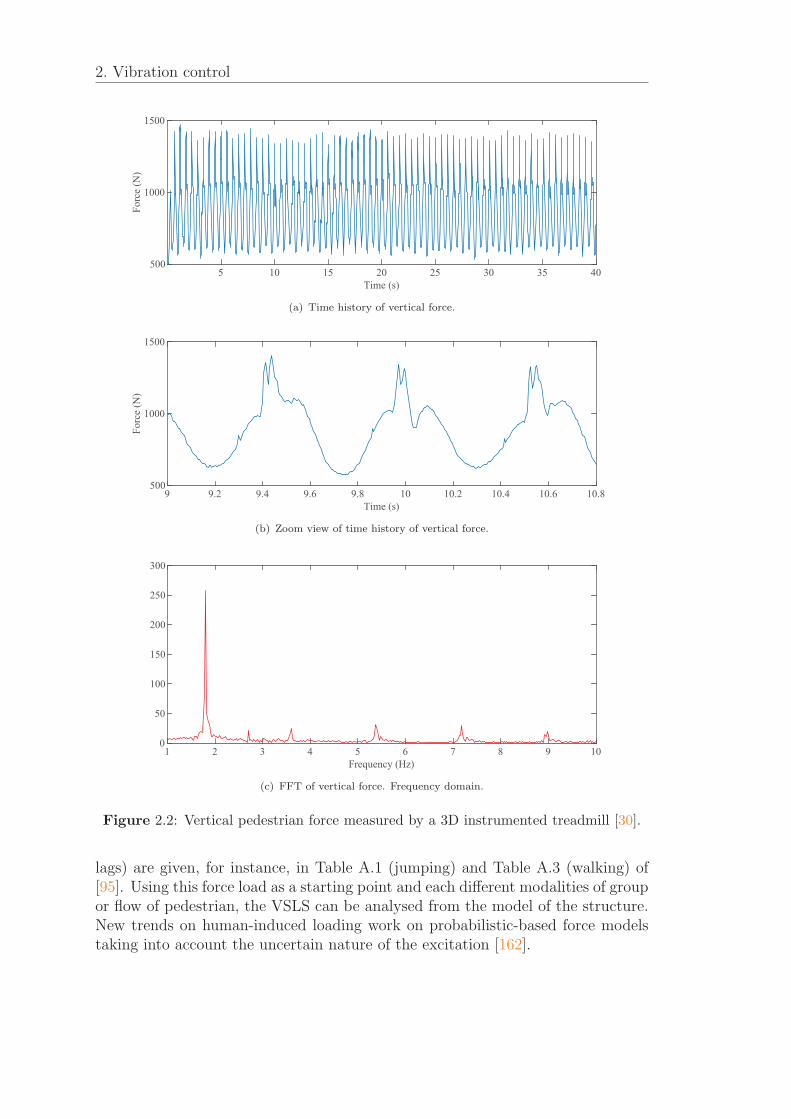
2. Vibration control
5 10 15 20 25 30 35 40Time (s)
500
1000
1500Fo
rce
(N)
(a) Time history of vertical force.
9 9.2 9.4 9.6 9.8 10 10.2 10.4 10.6 10.8Time (s)
500
1000
1500
Forc
e (N
)
(b) Zoom view of time history of vertical force.
1 2 3 4 5 6 7 8 9 10Frequency (Hz)
0
50
100
150
200
250
300
(c) FFT of vertical force. Frequency domain.
Figure 2.2: Vertical pedestrian force measured by a 3D instrumented treadmill [30].
lags) are given, for instance, in Table A.1 (jumping) and Table A.3 (walking) of[95]. Using this force load as a starting point and each different modalities of groupor flow of pedestrian, the VSLS can be analysed from the model of the structure.New trends on human-induced loading work on probabilistic-based force modelstaking into account the uncertain nature of the excitation [162].
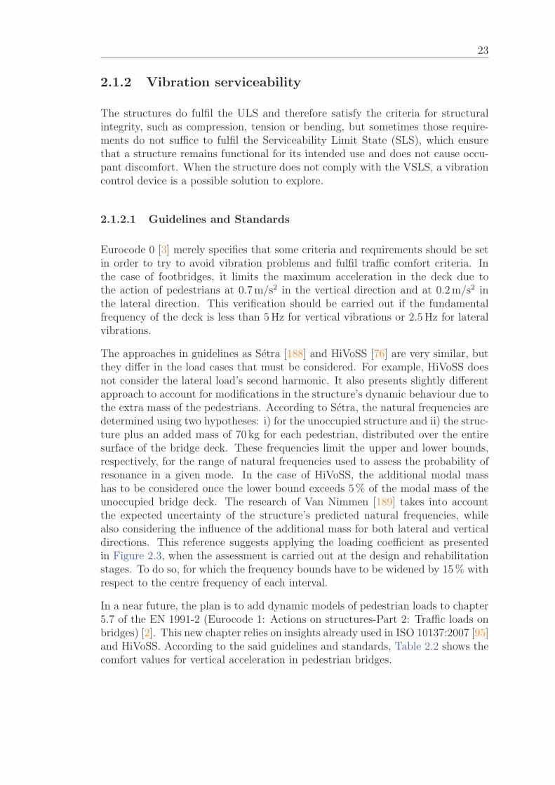
23
2.1.2 Vibration serviceability
The structures do fulfil the ULS and therefore satisfy the criteria for structuralintegrity, such as compression, tension or bending, but sometimes those require-ments do not suffice to fulfil the Serviceability Limit State (SLS), which ensurethat a structure remains functional for its intended use and does not cause occu-pant discomfort. When the structure does not comply with the VSLS, a vibrationcontrol device is a possible solution to explore.
2.1.2.1 Guidelines and Standards
Eurocode 0 [3] merely specifies that some criteria and requirements should be setin order to try to avoid vibration problems and fulfil traffic comfort criteria. Inthe case of footbridges, it limits the maximum acceleration in the deck due tothe action of pedestrians at 0.7 m/s2 in the vertical direction and at 0.2 m/s2 inthe lateral direction. This verification should be carried out if the fundamentalfrequency of the deck is less than 5 Hz for vertical vibrations or 2.5 Hz for lateralvibrations.
The approaches in guidelines as Setra [188] and HiVoSS [76] are very similar, butthey differ in the load cases that must be considered. For example, HiVoSS doesnot consider the lateral load’s second harmonic. It also presents slightly differentapproach to account for modifications in the structure’s dynamic behaviour due tothe extra mass of the pedestrians. According to Setra, the natural frequencies aredetermined using two hypotheses: i) for the unoccupied structure and ii) the struc-ture plus an added mass of 70 kg for each pedestrian, distributed over the entiresurface of the bridge deck. These frequencies limit the upper and lower bounds,respectively, for the range of natural frequencies used to assess the probability ofresonance in a given mode. In the case of HiVoSS, the additional modal masshas to be considered once the lower bound exceeds 5 % of the modal mass of theunoccupied bridge deck. The research of Van Nimmen [189] takes into accountthe expected uncertainty of the structure’s predicted natural frequencies, whilealso considering the influence of the additional mass for both lateral and verticaldirections. This reference suggests applying the loading coefficient as presentedin Figure 2.3, when the assessment is carried out at the design and rehabilitationstages. To do so, for which the frequency bounds have to be widened by 15 % withrespect to the centre frequency of each interval.
In a near future, the plan is to add dynamic models of pedestrian loads to chapter5.7 of the EN 1991-2 (Eurocode 1: Actions on structures-Part 2: Traffic loads onbridges) [2]. This new chapter relies on insights already used in ISO 10137:2007 [95]and HiVoSS. According to the said guidelines and standards, Table 2.2 shows thecomfort values for vertical acceleration in pedestrian bridges.

2. Vibration control
(a) Vertical. (b) Lateral.
Figure 2.3: Suggested loading coefficient to be applied in the design stage (- -), rehabil-itation (–) and (black) original, as defined in Setra and HiVoSS for vertical(a) and lateral (b) loading [189].
Comfort classes Degree of comfort alim (m/s2)
CL1 Maximum < 0.5CL2 Medium 0.5 – 1.0CL3 Minimum 1.0 – 2.5CL4 Intolerable vibrations > 2.5
Table 2.2: Comfort for vertical acceleration according to Setra [44] and HiVoSS [76].
2.1.2.2 Comfort predictors
The acceleration, compared to other parameters, has the advantage that it is anabsolute measurement in which no reference is needed. Current accelerometertechnology offers a wide variety of sensors at fairly reasonable prices. Thus, avail-able instrumentation for measuring acceleration can be used for human-inducedvibration measurement.
The vibration that can be perceived by a human depends on the direction ofincidence in relation to the human body, the duration of sustained vibration andthe frequency content of the said vibration (for a given amplitude), among otherfactors. The variation in the frequency sensitivity for a body position can betaken into account by enhancing or attenuating the system response for frequencieswhere perception is more or less sensitive, respectively. The degree to which theresponse is enhanced or attenuated is referred to as frequency weighting and itsfunctions are applied to make the vibrations for different directions and bodypositions acceptable. ISO 2631-1:1997 [96] gives details of frequency and directionweighting functions that can be applied and they are all based on the basicentriccoordinate system shown in Figure 2.4a. According to ISO 2631-1:1997, for z-axisvibration and standing and seating, the frequency weighting function (Wk) is afilter with the frequency response shown in Figure 2.4b.
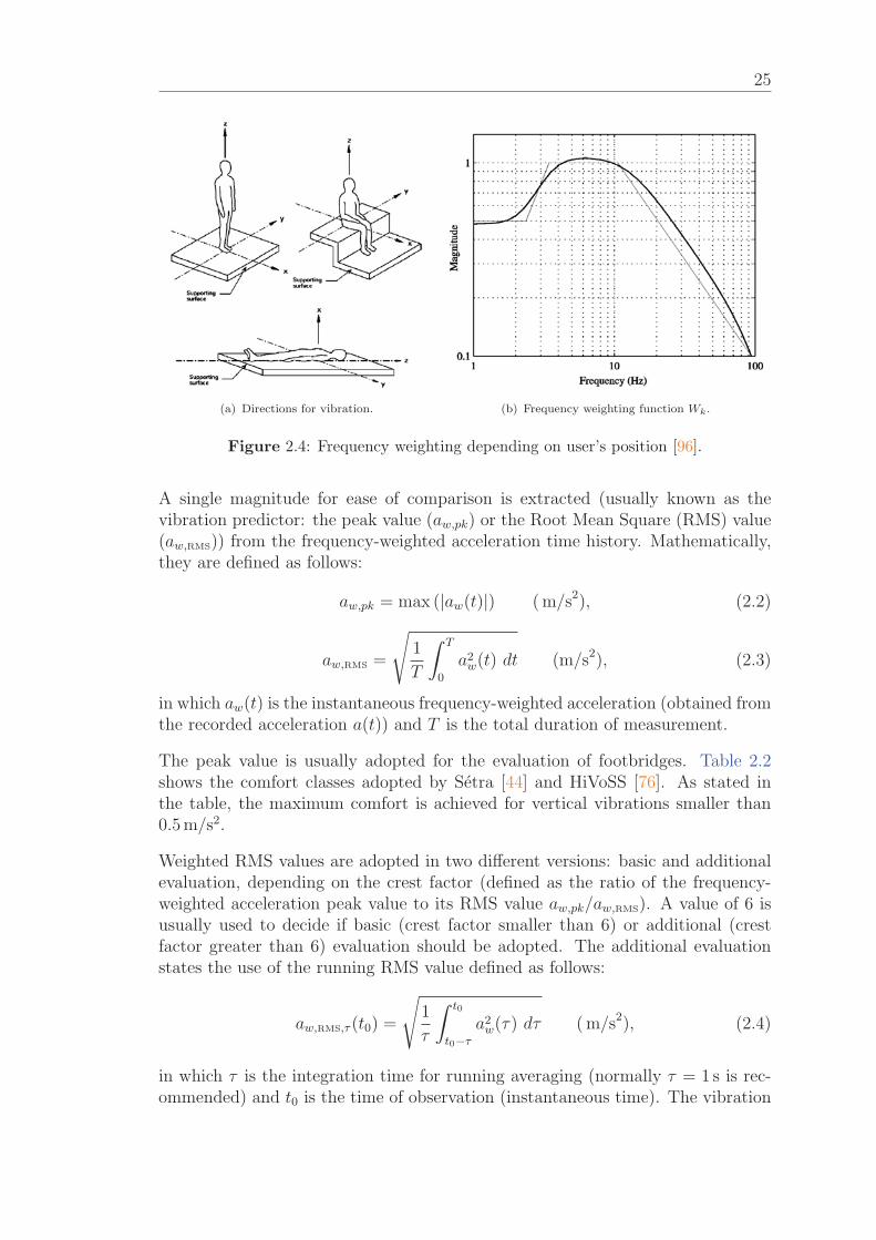
25
(a) Directions for vibration. (b) Frequency weighting function Wk.
Figure 2.4: Frequency weighting depending on user’s position [96].
A single magnitude for ease of comparison is extracted (usually known as thevibration predictor: the peak value (aw,pk) or the Root Mean Square (RMS) value(aw,RMS)) from the frequency-weighted acceleration time history. Mathematically,they are defined as follows:
aw,pk = max (|aw(t)|) ( m/s2), (2.2)
aw,RMS =
√1
T
∫ T
0
a2w(t) dt (m/s2), (2.3)
in which aw(t) is the instantaneous frequency-weighted acceleration (obtained fromthe recorded acceleration a(t)) and T is the total duration of measurement.
The peak value is usually adopted for the evaluation of footbridges. Table 2.2shows the comfort classes adopted by Setra [44] and HiVoSS [76]. As stated inthe table, the maximum comfort is achieved for vertical vibrations smaller than0.5 m/s2.
Weighted RMS values are adopted in two different versions: basic and additionalevaluation, depending on the crest factor (defined as the ratio of the frequency-weighted acceleration peak value to its RMS value aw,pk/aw,RMS). A value of 6 isusually used to decide if basic (crest factor smaller than 6) or additional (crestfactor greater than 6) evaluation should be adopted. The additional evaluationstates the use of the running RMS value defined as follows:
aw,RMS,τ (t0) =
√1
τ
∫ t0
t0−τ
a2w(τ) dτ ( m/s2), (2.4)
in which τ is the integration time for running averaging (normally τ = 1 s is rec-ommended) and t0 is the time of observation (instantaneous time). The vibration
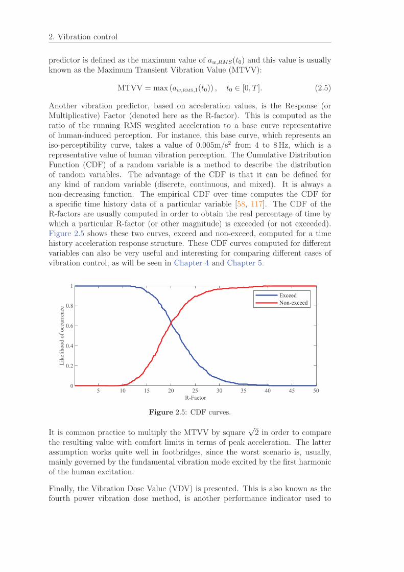
2. Vibration control
predictor is defined as the maximum value of aw,RMS(t0) and this value is usuallyknown as the Maximum Transient Vibration Value (MTVV):
MTVV = max (aw,RMS,1(t0)) , t0 ∈ [0, T ]. (2.5)
Another vibration predictor, based on acceleration values, is the Response (orMultiplicative) Factor (denoted here as the R-factor). This is computed as theratio of the running RMS weighted acceleration to a base curve representativeof human-induced perception. For instance, this base curve, which represents aniso-perceptibility curve, takes a value of 0.005m/s2 from 4 to 8 Hz, which is arepresentative value of human vibration perception. The Cumulative DistributionFunction (CDF) of a random variable is a method to describe the distributionof random variables. The advantage of the CDF is that it can be defined forany kind of random variable (discrete, continuous, and mixed). It is always anon-decreasing function. The empirical CDF over time computes the CDF fora specific time history data of a particular variable [58, 117]. The CDF of theR-factors are usually computed in order to obtain the real percentage of time bywhich a particular R-factor (or other magnitude) is exceeded (or not exceeded).Figure 2.5 shows these two curves, exceed and non-exceed, computed for a timehistory acceleration response structure. These CDF curves computed for differentvariables can also be very useful and interesting for comparing different cases ofvibration control, as will be seen in Chapter 4 and Chapter 5.
5 10 15 20 25 30 35 40 45 50R-Factor
0
0.2
0.4
0.6
0.8
1
Like
lihoo
d of
occ
urre
nce
ExceedNon-exceed
Figure 2.5: CDF curves.
It is common practice to multiply the MTVV by square√
2 in order to comparethe resulting value with comfort limits in terms of peak acceleration. The latterassumption works quite well in footbridges, since the worst scenario is, usually,mainly governed by the fundamental vibration mode excited by the first harmonicof the human excitation.
Finally, the Vibration Dose Value (VDV) is presented. This is also known as thefourth power vibration dose method, is another performance indicator used to
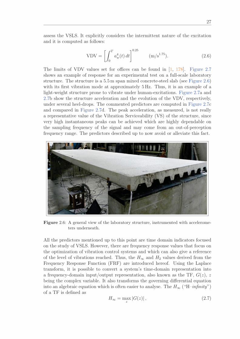
27
assess the VSLS. It explicitly considers the intermittent nature of the excitationand it is computed as follows:
VDV =
[∫ T
0
a4w(t) dt
]0.25(m/s1.75). (2.6)
The limits of VDV values set for offices can be found in [1, 178]. Figure 2.7shows an example of response for an experimental test on a full-scale laboratorystructure. The structure is a 5.5 m span mixed concrete-steel slab (see Figure 2.6)with its first vibration mode at approximately 5 Hz. Thus, it is an example of alight-weight structure prone to vibrate under human-excitations. Figure 2.7a and2.7b show the structure acceleration and the evolution of the VDV, respectively,under several heel-drops. The commented predictors are computed in Figure 2.7cand compared in Figure 2.7d. The peak acceleration, as measured, is not reallya representative value of the Vibration Serviceability (VS) of the structure, sincevery high instantaneous peaks can be achieved which are highly dependable onthe sampling frequency of the signal and may come from an out-of-perceptionfrequency range. The predictors described up to now avoid or alleviate this fact.
Figure 2.6: A general view of the laboratory structure, instrumented with accelerome-ters underneath.
All the predictors mentioned up to this point are time domain indicators focusedon the study of VSLS. However, there are frequency response values that focus onthe optimization of vibration control systems and which can also give a referenceof the level of vibrations reached. Thus, the H∞ and H2 values derived from theFrequency Response Function (FRF) are introduced hereof. Using the Laplacetransform, it is possible to convert a system’s time-domain representation intoa frequency-domain input/output representation, also known as the TF, G(z), zbeing the complex variable. It also transforms the governing differential equationinto an algebraic equation which is often easier to analyse. The H∞ (“H–infinity”)of a TF is defined as
H∞ = maxz
|G(z)| , (2.7)
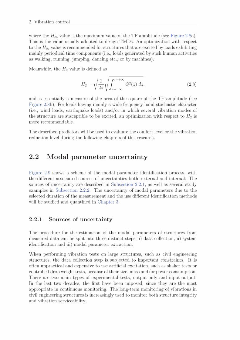
2. Vibration control
where the H∞ value is the maximum value of the TF amplitude (see Figure 2.8a).This is the value usually adopted to design TMDs. An optimization with respectto the H∞ value is recommended for structures that are excited by loads exhibitingmainly periodical time components (i.e., loads generated by such human activitiesas walking, running, jumping, dancing etc., or by machines).
Meanwhile, the H2 value is defined as
H2 =
√1
2π
√∫ z=+∞
z=−∞G2(z) dz, (2.8)
and is essentially a measure of the area of the square of the TF amplitude (seeFigure 2.8b). For loads having mainly a wide frequency band stochastic character(i.e., wind loads, earthquake loads) and/or in which several vibration modes ofthe structure are susceptible to be excited, an optimization with respect to H2 ismore recommendable.
The described predictors will be used to evaluate the comfort level or the vibrationreduction level during the following chapters of this research.
2.2 Modal parameter uncertainty
Figure 2.9 shows a scheme of the modal parameter identification process, withthe different associated sources of uncertainties both, external and internal. Thesources of uncertainty are described in Subsection 2.2.1, as well as several studyexamples in Subsection 2.2.2. The uncertainty of modal parameters due to theselected duration of the measurement and the use different identification methodswill be studied and quantified in Chapter 3.
2.2.1 Sources of uncertainty
The procedure for the estimation of the modal parameters of structures frommeasured data can be split into three distinct steps: i) data collection, ii) systemidentification and iii) modal parameter extraction.
When performing vibration tests on large structures, such as civil engineeringstructures, the data collection step is subjected to important constraints. It isoften unpractical and expensive to use artificial excitation, such as shaker tests orcontrolled drop weight tests, because of their size, mass and/or power consumption.There are two main types of experimental tests, output-only and input-output.In the last two decades, the first have been imposed, since they are the mostappropriate in continuous monitoring. The long-term monitoring of vibrations incivil engineering structures is increasingly used to monitor both structure integrityand vibration serviceability.
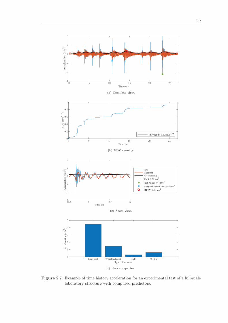
29
0 5 10 15 20 25Time (s)
-6
-4
-2
0
2
4
Acc
eler
atio
n (m
/s2 )
(a) Complete view.
0 5 10 15 20 25Time (s)
0
0.2
0.4
0.6
0.8
1
VD
V (m
/s1.
75)
VDV(end): 0.92 m/s1.75
(b) VDV running.
10.5 11 11.5 12Time (s)
-6
-4
-2
0
2
4
Acc
eler
atio
n (m
/s2 ) Raw
WeightedRMS runningRMS: 0.28 m/s2
Peak-value: 4.47 m/s2
Weighted Peak-Value: 1.47 m/s2
MTVV: 0.58 m/s2
(c) Zoom view.
Raw peak Weighted peak RMS MTVVType of measure
0
1
2
3
4
5
Acc
eler
atio
n (m
/s2 )
(d) Peak comparison.
Figure 2.7: Example of time history acceleration for an experimental test of a full-scalelaboratory structure with computed predictors.
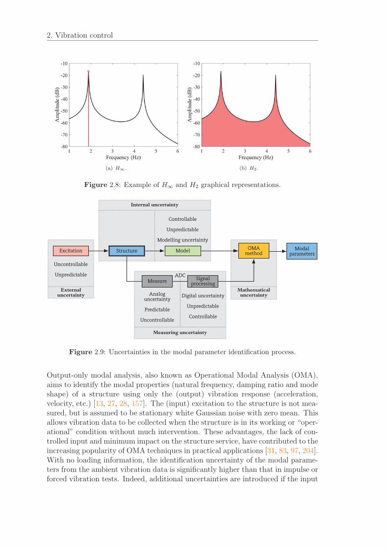
2. Vibration control
(a) H∞. (b) H2.
Figure 2.8: Example of H∞ and H2 graphical representations.
Figure 2.9: Uncertainties in the modal parameter identification process.
Output-only modal analysis, also known as Operational Modal Analysis (OMA),aims to identify the modal properties (natural frequency, damping ratio and modeshape) of a structure using only the (output) vibration response (acceleration,velocity, etc.) [13, 27, 28, 157]. The (input) excitation to the structure is not mea-sured, but is assumed to be stationary white Gaussian noise with zero mean. Thisallows vibration data to be collected when the structure is in its working or “oper-ational” condition without much intervention. These advantages, the lack of con-trolled input and minimum impact on the structure service, have contributed to theincreasing popularity of OMA techniques in practical applications [31, 83, 97, 204].With no loading information, the identification uncertainty of the modal parame-ters from the ambient vibration data is significantly higher than that in impulse orforced vibration tests. Indeed, additional uncertainties are introduced if the input
31
does not fulfil the stationary white Gaussian noise assumption and the effects ofstructural/environmental changes [10, 106, 108]. Therefore, uncertainty quantifi-cation and quality control of the identified modal properties become especiallyrelevant [35, 82, 107, 152].
A number of examples of bridges and footbridges that are equipped with a mon-itoring system can be found [60, 81, 89, 138], where the said systems measureand record the vibrations due to traffic or wind. These data can then be usedto continuously extract the modal parameters (natural frequencies, damping ra-tios and modal shapes) that may then be useful for assessing the structural in-tegrity, as structural damage leads to changes in the modal parameters. Thus,vibration-based SHM systems using automated OMA identification have been ex-tensively proposed [68, 126]. One of the main problems of these systems is thatthey have to cope with changing environmental/operational conditions, which of-ten significantly affect the modal estimation. Hence, the removal of these spuriousfactors on modal estimates becomes crucial in the implementation of an SHM sys-tem that uses modal parameters as damage-sensitive features. These factors maymask meaningful changes for damage detection, due to, for instance, extraordinaryevents such as earthquakes or very dense traffic [186], especially in structures, suchas bridges, that are always exposed to environmental factors.
As for the use of modal parameter variations as possible damage detectors instructures, the modal variations over time due to the influence of some externalagents acting on the undamaged structure must be observed [115, 123]. Evalu-ating the magnitude of this modal variation is important. The most significantenvironmental factor is usually the temperature [211]. However, there are otherfactors, such as operational or boundary conditions, which may significantly affectthe modal estimates [14, 115]. Several studies have dealt with this problem andhave carried out correlation analyses between modal estimates and these externalfactors [92, 120, 121, 136, 144], as it is crucial to discriminate between modal varia-tion induced by environmental or external factors and those induced by structuraldamages.
Methods generally consist of automated peak-picking for frequency domain meth-ods [29, 163] or clustering methods for stabilization diagram interpretation [32,167]. Since all OMA techniques require some user judgment, a non-trivial degreeof automation is necessary to bridge the gap between traditional and continuousOMA. Research into automated OMA for civil structures has recently been on therise. Formulations that use state-space models, designated as Stochastic SubspaceIdentification (SSI) methods, constitute the parametric approach which is morecommonly adopted for civil engineering applications in the time domain. Two ofthe most popular and accepted SSI implementations are [155]: a covariance-driven(SSI-cov) and a data-driven (SSI-data) implementation [165]. They are also rec-ommended when there are closely-spaced eigenfrequencies [122, 124]. Accordingly,the methods used in Chapter 3 are based on SSI.
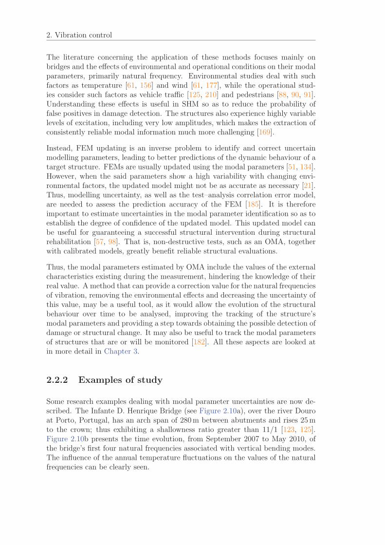
2. Vibration control
The literature concerning the application of these methods focuses mainly onbridges and the effects of environmental and operational conditions on their modalparameters, primarily natural frequency. Environmental studies deal with suchfactors as temperature [61, 156] and wind [61, 177], while the operational stud-ies consider such factors as vehicle traffic [125, 210] and pedestrians [88, 90, 91].Understanding these effects is useful in SHM so as to reduce the probability offalse positives in damage detection. The structures also experience highly variablelevels of excitation, including very low amplitudes, which makes the extraction ofconsistently reliable modal information much more challenging [169].
Instead, FEM updating is an inverse problem to identify and correct uncertainmodelling parameters, leading to better predictions of the dynamic behaviour of atarget structure. FEMs are usually updated using the modal parameters [51, 134].However, when the said parameters show a high variability with changing envi-ronmental factors, the updated model might not be as accurate as necessary [21].Thus, modelling uncertainty, as well as the test–analysis correlation error model,are needed to assess the prediction accuracy of the FEM [185]. It is thereforeimportant to estimate uncertainties in the modal parameter identification so as toestablish the degree of confidence of the updated model. This updated model canbe useful for guaranteeing a successful structural intervention during structuralrehabilitation [57, 98]. That is, non-destructive tests, such as an OMA, togetherwith calibrated models, greatly benefit reliable structural evaluations.
Thus, the modal parameters estimated by OMA include the values of the externalcharacteristics existing during the measurement, hindering the knowledge of theirreal value. A method that can provide a correction value for the natural frequenciesof vibration, removing the environmental effects and decreasing the uncertainty ofthis value, may be a useful tool, as it would allow the evolution of the structuralbehaviour over time to be analysed, improving the tracking of the structure’smodal parameters and providing a step towards obtaining the possible detection ofdamage or structural change. It may also be useful to track the modal parametersof structures that are or will be monitored [182]. All these aspects are looked atin more detail in Chapter 3.
2.2.2 Examples of study
Some research examples dealing with modal parameter uncertainties are now de-scribed. The Infante D. Henrique Bridge (see Figure 2.10a), over the river Douroat Porto, Portugal, has an arch span of 280 m between abutments and rises 25 mto the crown; thus exhibiting a shallowness ratio greater than 11/1 [123, 125].Figure 2.10b presents the time evolution, from September 2007 to May 2010, ofthe bridge’s first four natural frequencies associated with vertical bending modes.The influence of the annual temperature fluctuations on the values of the naturalfrequencies can be clearly seen.

33
(a) General view.
(b) Time evolution of the natural frequencies of the first 4 vertical bending modes.
Figure 2.10: Analysis carried out on the Infante D. Henrique Arch Bridge [125].
For this thesis, pedestrian structures, such as footbridges, are even more interest-ing, since fluctuations or uncertainties can be the main source of losing effective-ness for a TMD device. The studies carried out by Hu et al. [88, 91] analysed themodal parameter uncertainties associated to the stress-ribbon footbridge locatedat the FEUP University Campus. Figure 2.11 shows the structure (2.11a) and theevolution of frequencies over time (2.11b and 2.11c). The evaluation of vibrationlevels, the measurement of temperatures, the analysis of frequency componentsand automated structural modal identification are carried out in [88, 91] in orderto examine and remove the effects of environmental and operational factors on themodal properties, while also detecting early structural changes under operationalconditions.
2.3 Vibration control generalities
During the past few decades, structural control has attracted the attention of manyresearchers. The aim is to reduce excessive vibration using appropriate methods.
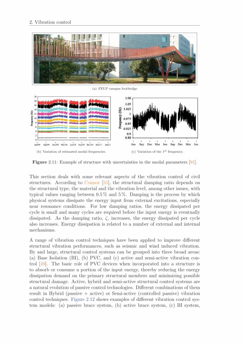
2. Vibration control
(a) FEUP campus footbridge
(b) Variation of estimated modal frequencies. (c) Variation of the 1st frequency.
Figure 2.11: Example of structure with uncertainties in the modal parameters [91].
This section deals with some relevant aspects of the vibration control of civilstructures. According to Connor [55], the structural damping ratio depends onthe structural type, the material and the vibration level, among other issues, withtypical values ranging between 0.5 % and 5 %. Damping is the process by whichphysical systems dissipate the energy input from external excitations, especiallynear resonance conditions. For low damping ratios, the energy dissipated percycle is small and many cycles are required before the input energy is eventuallydissipated. As the damping ratio, ζ, increases, the energy dissipated per cyclealso increases. Energy dissipation is related to a number of external and internalmechanisms.
A range of vibration control techniques have been applied to improve differentstructural vibration performances, such as seismic and wind induced vibration.By and large, structural control systems can be grouped into three broad areas:(a) Base Isolation (BI), (b) PVC, and (c) active and semi-active vibration con-trol [49]. The basic role of PVC devices when incorporated into a structure isto absorb or consume a portion of the input energy, thereby reducing the energydissipation demand on the primary structural members and minimizing possiblestructural damage. Active, hybrid and semi-active structural control systems area natural evolution of passive control technologies. Different combinations of themresult in Hybrid (passive + active) or Semi-active (controlled passive) vibrationcontrol techniques. Figure 2.12 shows examples of different vibration control sys-tem models: (a) passive brace system, (b) active brace system, (c) BI system,
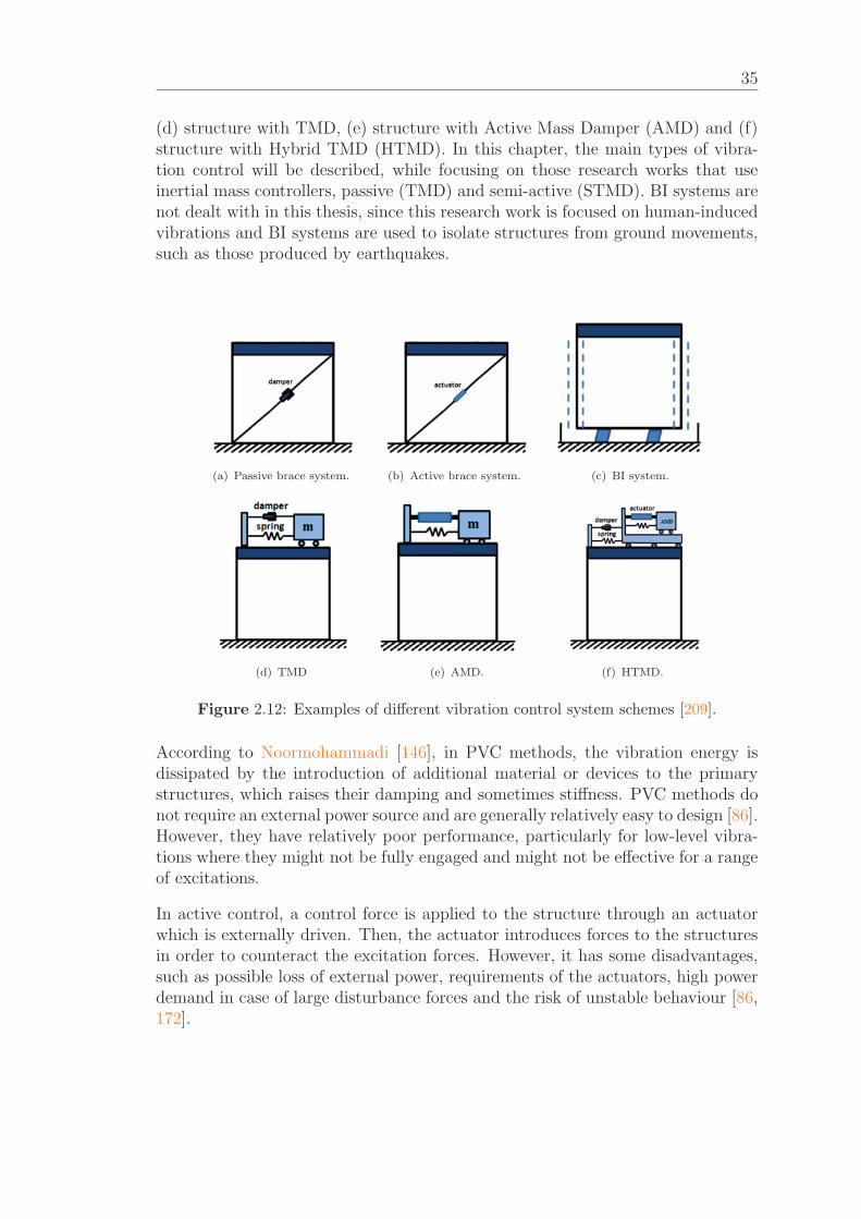
35
(d) structure with TMD, (e) structure with Active Mass Damper (AMD) and (f)structure with Hybrid TMD (HTMD). In this chapter, the main types of vibra-tion control will be described, while focusing on those research works that useinertial mass controllers, passive (TMD) and semi-active (STMD). BI systems arenot dealt with in this thesis, since this research work is focused on human-inducedvibrations and BI systems are used to isolate structures from ground movements,such as those produced by earthquakes.
(a) Passive brace system. (b) Active brace system. (c) BI system.
(d) TMD (e) AMD. (f) HTMD.
Figure 2.12: Examples of different vibration control system schemes [209].
According to Noormohammadi [146], in PVC methods, the vibration energy isdissipated by the introduction of additional material or devices to the primarystructures, which raises their damping and sometimes stiffness. PVC methods donot require an external power source and are generally relatively easy to design [86].However, they have relatively poor performance, particularly for low-level vibra-tions where they might not be fully engaged and might not be effective for a rangeof excitations.
In active control, a control force is applied to the structure through an actuatorwhich is externally driven. Then, the actuator introduces forces to the structuresin order to counteract the excitation forces. However, it has some disadvantages,such as possible loss of external power, requirements of the actuators, high powerdemand in case of large disturbance forces and the risk of unstable behaviour [86,172].
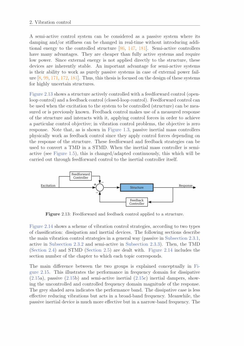
2. Vibration control
A semi-active control system can be considered as a passive system where itsdamping and/or stiffness can be changed in real-time without introducing addi-tional energy to the controlled structure [86, 147, 181]. Semi-active controllershave many advantages. They are cheaper than fully active systems and requirelow power. Since external energy is not applied directly to the structure, thesedevices are inherently stable. An important advantage for semi-active systemsis their ability to work as purely passive systems in case of external power fail-ure [8, 99, 171, 172, 181]. Thus, this thesis is focused on the design of these systemsfor highly uncertain structures.
Figure 2.13 shows a structure actively controlled with a feedforward control (open-loop control) and a feedback control (closed-loop control). Feedforward control canbe used when the excitation to the system to be controlled (structure) can be mea-sured or is previously known. Feedback control makes use of a measured responseof the structure and interacts with it, applying control forces in order to achievea particular control objective; in vibration control problems, the objective is zeroresponse. Note that, as is shown in Figure 1.3, passive inertial mass controllersphysically work as feedback control since they apply control forces depending onthe response of the structure. These feedforward and feedback strategies can beused to convert a TMD in a STMD. When the inertial mass controller is semi-active (see Figure 1.5), this is changed/adapted continuously, this which will becarried out through feedforward control to the inertial controller itself.
Figure 2.13: Feedforward and feedback control applied to a structure.
Figure 2.14 shows a scheme of vibration control strategies, according to two typesof classification: dissipation and inertial devices. The following sections describethe main vibration control strategies in a general way (passive in Subsection 2.3.1,active in Subsection 2.3.2 and semi-active in Subsection 2.3.3). Then, the TMD(Section 2.4) and STMD (Section 2.5) are dealt with. Figure 2.14 includes thesection number of the chapter to which each topic corresponds.
The main difference between the two groups is explained conceptually in Fi-gure 2.15. This illustrates the performance in frequency domain for dissipative(2.15a), passive (2.15b) and semi-active inertial (2.15c) inertial dampers, show-ing the uncontrolled and controlled frequency domain magnitude of the response.The grey shaded area indicates the performance band. The dissipative case is lesseffective reducing vibrations but acts in a broad-band frequency. Meanwhile, thepassive inertial device is much more effective but in a narrow-band frequency. The
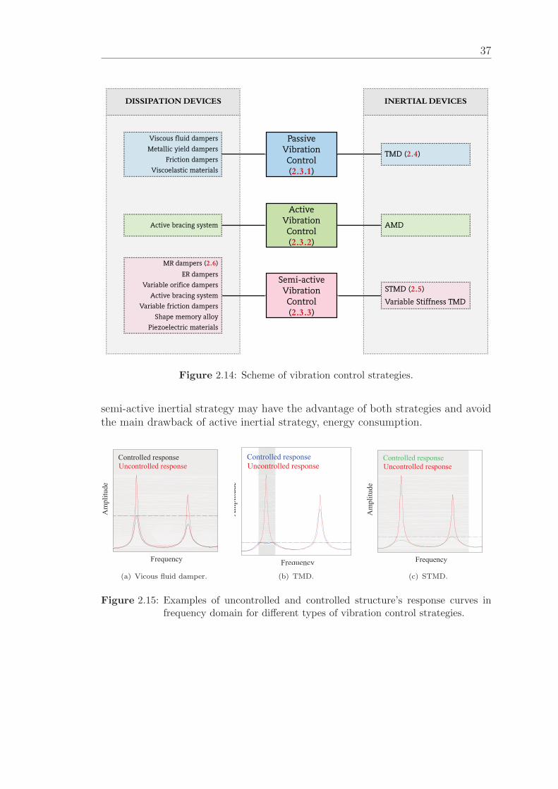
37
Figure 2.14: Scheme of vibration control strategies.
semi-active inertial strategy may have the advantage of both strategies and avoidthe main drawback of active inertial strategy, energy consumption.
(a) Vicous fluid damper. (b) TMD. (c) STMD.
Figure 2.15: Examples of uncontrolled and controlled structure’s response curves infrequency domain for different types of vibration control strategies.
2. Vibration control
2.3.1 Passive Vibration Control
In PVC, the reduction of vibration can be achieved by adding viscoelastic materialsand/or devices to dissipate vibration energy are required; however, no externalenergy is needed. PVC has been used to mitigate vibrations under a range ofexcitations, such as seismic, wind, machinery and human induced vibration [56,180].
There are various mechanisms by which passive systems may operate, such asmetal yielding, frictional sliding, stage transformation in metals and viscoelasticdeformation in solid or liquid materials and fluid orifices. Regarding the type ofpassive systems, these can be divided into dissipative and inertial. Dissipativesystems are those that do not apply forces to the structure but which are able todissipate energy. Inertial control systems do apply inertial control forces on thestructure but do not consume energy, there is no risk of instability due to theirpassive nature and they have a relatively lower cost [6, 147, 148, 172, 174, 181,201]. However, passive control methods typically have a number of drawbacks,such as lack of damping capacity and they are subject to various trade offs whenexcited across a large frequency bandwidth [8, 174]. Figure 1.2 from Chapter 1shows a structure with PVC. Some examples of passive controllers are TMDs, baseisolation, viscoelastic dampers, metallic yield dampers, friction dampers, viscousfluid dampers and tuned liquid dampers [181].
TMDs have been widely used to mitigate vibration in civil, mechanical and aerospacestructures and much theoretical and practical research has been done in thisarea [147, 171, 181]. TMDs have been found to be an effective device to reducehuman induced vibration caused by pedestrian activities on footbridges [170].
Apart form the inherent limitations of passive systems, their performance dependshighly on the inertial mass value and, if the mass is too small, the effect of a TMDis limited. Also, since the dynamic properties of structures commonly vary overtime due to external factors, the TMDs may not remain optimally tuned and theirperformance may be reduced. Furthermore, TMDs are generally efficient whenthe primary structure has low damping [6, 18, 148, 170, 171, 201].
2.3.2 Active and Hybrid Vibration Control
The inability to dynamically change a passive control system to compensate for anunexpected load tends to result in an over-conservative design. Considering thislimitation, there is a potential for improving performance by real-time modifyingthe load and system properties [55]. The performance of Active Vibration Control(AVC) is based on force generation using an external source of energy. In thismethod, a control force is exerted on the structure through an actuator which aimsto counteract the vibration caused by disturbance forces [174]. In this method,the disturbance (input) force and/or the response of the structure is monitored
39
continuously and the output information is used to calculate and generate theappropriate control force [71, 93, 187].
Generally, an active scheme consists of sensors and actuators in combination witha control unit [11, 174, 207]. The actuator force changes in real-time according tothe control law adopted and the response of the structure [133]. The active controlapproach is the combination of several engineering disciplines, such as electronicengineering, computer engineering, control engineering and materials engineer-ing [181]. AMD is a typical example of inertial mass active control device [146].
AMDs have the advantage that i) they are more effective than passive inertialsystems for the same inertial mass, ii) the control target can be selected in a widefrequency band and, when robustly designed, iii) they are not sensitive to changesin the modal parameters of the structure or in the excitation load. On the otherhand, they are systems more expensive than passive or semi-active and mightbecome unstable (control law should be carefully designed); they stop working ina power supply failure, as could happen in the case of earthquakes [176, 179].
Active and passive control methods have some advantages and drawbacks. Inan attempt to have the advantages of both, hybrid vibration control methodshave been developed [174]. A hybrid controller is a combination of passive andactive control systems [45], which is an attractive option for structural vibrationcontrol [9, 54, 141, 142].
Figure 2.16 shows a commercial inertial mass actuator (APS model 400) which hasbeen used in this thesis as an exciter to apply controlled forces to the structuresfor identification purposes. This shaker has been extensively used as an AMD forcontrolling human-induced vibrations [69–71].
Up to now, some examples of AVCs in pedestrian structures have been reported.For instance, the research work carried out by Bleicher et al. [23] at TU Berlindescribes the development of an AVC system for a light and flexible stress ribbonlaboratory footbridge of 13.05 m span. To reduce pedestrian-induced vibrations,on-off pneumatic actuators are introduced into the handrail in order to change thestress of the ribbon in real-time. Figure 2.17 shows the laboratory stress-ribbonfootbridge (2.17a) and pneumatic actuators for active control (2.17b). The maindrawback is the nonlinear and discontinuous behaviour of these actuators.
A few of examples of AVC for human-induced vibration in footbridges and floorsusing AMD have been carried out over the last decade, both as a single-inputsingle-output version and a multi-input multi-output version [39, 158, 191, 193].The research work of Casado et al. [39] is concerned with the design and experimen-tal implementation of a TMD (see Figure 2.18b) and an AMD (see Figure 2.18c) tomitigate human-induced vibrations on an in-service footbridge (see Figure 2.18a).Although the structure had one dominant vibration mode (which was well sep-arated from the others) prone to be excited by human loading, the TMD masshad to be fine-tuned periodically, since structural natural frequencies change withstructural ageing. Furthermore, environmental conditions (mainly temperature
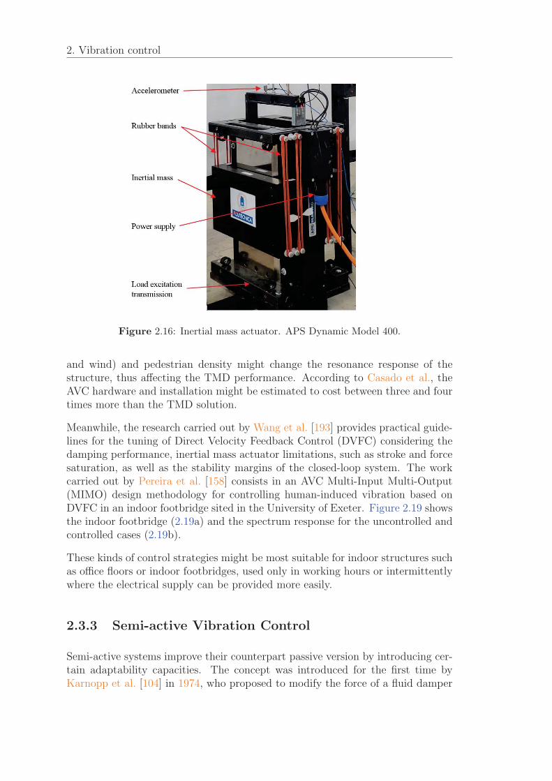
2. Vibration control
Figure 2.16: Inertial mass actuator. APS Dynamic Model 400.
and wind) and pedestrian density might change the resonance response of thestructure, thus affecting the TMD performance. According to Casado et al., theAVC hardware and installation might be estimated to cost between three and fourtimes more than the TMD solution.
Meanwhile, the research carried out by Wang et al. [193] provides practical guide-lines for the tuning of Direct Velocity Feedback Control (DVFC) considering thedamping performance, inertial mass actuator limitations, such as stroke and forcesaturation, as well as the stability margins of the closed-loop system. The workcarried out by Pereira et al. [158] consists in an AVC Multi-Input Multi-Output(MIMO) design methodology for controlling human-induced vibration based onDVFC in an indoor footbridge sited in the University of Exeter. Figure 2.19 showsthe indoor footbridge (2.19a) and the spectrum response for the uncontrolled andcontrolled cases (2.19b).
These kinds of control strategies might be most suitable for indoor structures suchas office floors or indoor footbridges, used only in working hours or intermittentlywhere the electrical supply can be provided more easily.
2.3.3 Semi-active Vibration Control
Semi-active systems improve their counterpart passive version by introducing cer-tain adaptability capacities. The concept was introduced for the first time byKarnopp et al. [104] in 1974, who proposed to modify the force of a fluid damper
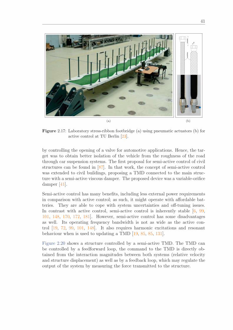
41
(a) (b)
Figure 2.17: Laboratory stress-ribbon footbridge (a) using pneumatic actuators (b) foractive control at TU Berlin [23].
by controlling the opening of a valve for automotive applications. Hence, the tar-get was to obtain better isolation of the vehicle from the roughness of the roadthrough car suspension systems. The first proposal for semi-active control of civilstructures can be found in [87]. In that work, the concept of semi-active controlwas extended to civil buildings, proposing a TMD connected to the main struc-ture with a semi-active viscous damper. The proposed device was a variable-orificedamper [41].
Semi-active control has many benefits, including less external power requirementsin comparison with active control; as such, it might operate with affordable bat-teries. They are able to cope with system uncertainties and off-tuning issues.In contrast with active control, semi-active control is inherently stable [6, 99,101, 148, 170, 172, 181]. However, semi-active control has some disadvantagesas well. Its operating frequency bandwidth is not as wide as the active con-trol [19, 72, 99, 101, 148]. It also requires harmonic excitations and resonantbehaviour when is used to updating a TMD [19, 85, 85, 131].
Figure 2.20 shows a structure controlled by a semi-active TMD. The TMD canbe controlled by a feedforward loop, the command to the TMD is directly ob-tained from the interaction magnitudes between both systems (relative velocityand structure displacement) as well as by a feedback loop, which may regulate theoutput of the system by measuring the force transmitted to the structure.
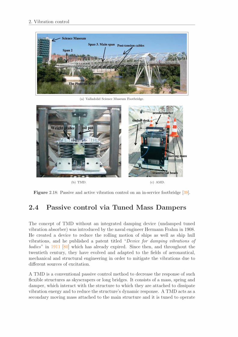
2. Vibration control
(a) Valladolid Science Museum Footbridge.
(b) TMD. (c) AMD.
Figure 2.18: Passive and active vibration control on an in-service footbridge [39].
2.4 Passive control via Tuned Mass Dampers
The concept of TMD without an integrated damping device (undamped tunedvibration absorber) was introduced by the naval engineer Hermann Frahm in 1908.He created a device to reduce the rolling motion of ships as well as ship hullvibrations, and he published a patent titled “Device for damping vibrations ofbodies” in 1911 [80] which has already expired. Since then, and throughout thetwentieth century, they have evolved and adapted to the fields of aeronautical,mechanical and structural engineering in order to mitigate the vibrations due todifferent sources of excitation.
A TMD is a conventional passive control method to decrease the response of suchflexible structures as skyscrapers or long bridges. It consists of a mass, spring anddamper, which interact with the structure to which they are attached to dissipatevibration energy and to reduce the structure’s dynamic response. A TMD acts as asecondary moving mass attached to the main structure and it is tuned to operate

43
(a) Forum Footbridge. AMDs are marked with red area.
(b) Experimental results. Power Spectral Density response.
Figure 2.19: MIMO vibration control application in an indoor footbridge [158].
at a specific frequency, which is generally the one of the dominant structuralvibration mode. Thus, when that frequency is excited, the inertial mass of theTMD vibrates in the opposite phase to the main system, imparting control forcesto the structure and hence the vibration energy of the structure is transferredto the auxiliary mass, to be dissipated through the TMD damping element (seeFigures 1.12b, 1.13 and 2.12d). This is why TMDs are effective mostly in resonantcases, where the frequency of the external force is close to the frequency of thestructure [55, 148, 171, 201, 207]. The effectiveness of the TMD depends on a) theaccuracy of its tuning, b) the inertial mass value as compared to the modal massof the target mode, that is, its mass ratio, and c) the level of internal dampingof the TMD. Apart from these main aspects, the TMD performance is highlydependent on the level of the excitation and the structure response since when theresponse is not purely resonant, the TMD will degrade rapidly its performance.Viscous dampers are commonly used as the energy dissipation element inside the
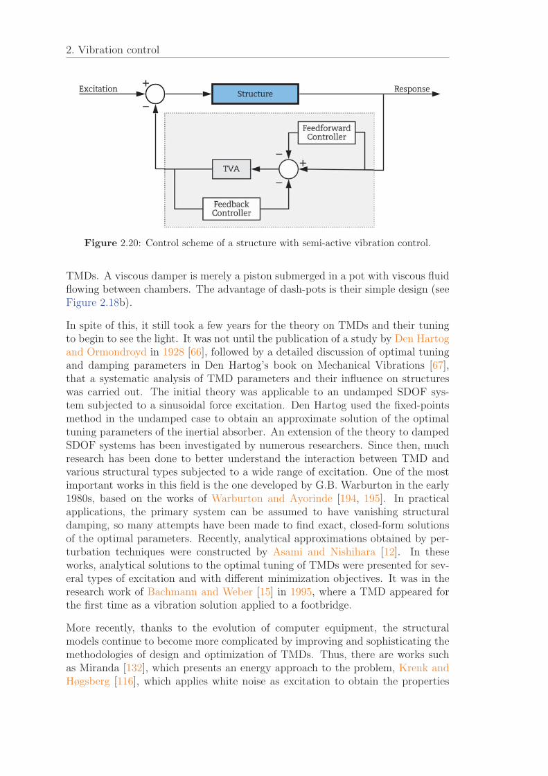
2. Vibration control
Figure 2.20: Control scheme of a structure with semi-active vibration control.
TMDs. A viscous damper is merely a piston submerged in a pot with viscous fluidflowing between chambers. The advantage of dash-pots is their simple design (seeFigure 2.18b).
In spite of this, it still took a few years for the theory on TMDs and their tuningto begin to see the light. It was not until the publication of a study by Den Hartogand Ormondroyd in 1928 [66], followed by a detailed discussion of optimal tuningand damping parameters in Den Hartog’s book on Mechanical Vibrations [67],that a systematic analysis of TMD parameters and their influence on structureswas carried out. The initial theory was applicable to an undamped SDOF sys-tem subjected to a sinusoidal force excitation. Den Hartog used the fixed-pointsmethod in the undamped case to obtain an approximate solution of the optimaltuning parameters of the inertial absorber. An extension of the theory to dampedSDOF systems has been investigated by numerous researchers. Since then, muchresearch has been done to better understand the interaction between TMD andvarious structural types subjected to a wide range of excitation. One of the mostimportant works in this field is the one developed by G.B. Warburton in the early1980s, based on the works of Warburton and Ayorinde [194, 195]. In practicalapplications, the primary system can be assumed to have vanishing structuraldamping, so many attempts have been made to find exact, closed-form solutionsof the optimal parameters. Recently, analytical approximations obtained by per-turbation techniques were constructed by Asami and Nishihara [12]. In theseworks, analytical solutions to the optimal tuning of TMDs were presented for sev-eral types of excitation and with different minimization objectives. It was in theresearch work of Bachmann and Weber [15] in 1995, where a TMD appeared forthe first time as a vibration solution applied to a footbridge.
More recently, thanks to the evolution of computer equipment, the structuralmodels continue to become more complicated by improving and sophisticating themethodologies of design and optimization of TMDs. Thus, there are works suchas Miranda [132], which presents an energy approach to the problem, Krenk andHøgsberg [116], which applies white noise as excitation to obtain the properties
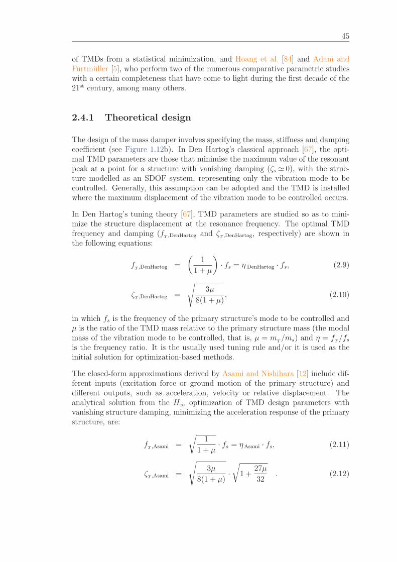
45
of TMDs from a statistical minimization, and Hoang et al. [84] and Adam andFurtmuller [5], who perform two of the numerous comparative parametric studieswith a certain completeness that have come to light during the first decade of the21st century, among many others.
2.4.1 Theoretical design
The design of the mass damper involves specifying the mass, stiffness and dampingcoefficient (see Figure 1.12b). In Den Hartog’s classical approach [67], the opti-mal TMD parameters are those that minimise the maximum value of the resonantpeak at a point for a structure with vanishing damping (ζs � 0), with the struc-ture modelled as an SDOF system, representing only the vibration mode to becontrolled. Generally, this assumption can be adopted and the TMD is installedwhere the maximum displacement of the vibration mode to be controlled occurs.
In Den Hartog’s tuning theory [67], TMD parameters are studied so as to mini-mize the structure displacement at the resonance frequency. The optimal TMDfrequency and damping (f
T ,DenHartog and ζT ,DenHartog, respectively) are shown in
the following equations:
fT ,DenHartog =
(1
1 + μ
)· fs = η DenHartog · fs, (2.9)
ζT ,DenHartog =
√3μ
8(1 + μ), (2.10)
in which fs is the frequency of the primary structure’s mode to be controlled andμ is the ratio of the TMD mass relative to the primary structure mass (the modalmass of the vibration mode to be controlled, that is, μ = m
T/ms) and η = f
T/fs
is the frequency ratio. It is the usually used tuning rule and/or it is used as theinitial solution for optimization-based methods.
The closed-form approximations derived by Asami and Nishihara [12] include dif-ferent inputs (excitation force or ground motion of the primary structure) anddifferent outputs, such as acceleration, velocity or relative displacement. Theanalytical solution from the H∞ optimization of TMD design parameters withvanishing structure damping, minimizing the acceleration response of the primarystructure, are:
fT ,Asami =
√1
1 + μ· fs = ηAsami · fs, (2.11)
ζT ,Asami =
√3μ
8(1 + μ)·√
1 +27μ
32. (2.12)

2. Vibration control
The stiffness and damping ratio for the TMD are then obtained from
kT
= ω2Tm
T, (2.13)
cT
= 2ζTm
Tω
T, (2.14)
respectively. TMDs are tuned to control the vibration due to a specific vibra-tion mode. However, detuning effects should be considered due to the possibleuncertainties associated with this mode. Figure 2.21 shows the maximum valueof the FRF amplitude (H∞ value) for a range of TMD parameters. A significantreduction in the response of the primary system under the target vibration modeis observed when the TMD parameters are properly selected/tuned. The perfor-mance of the TMD is more sensitive to the frequency tuning than the dampingtuning. TMDs are sized so that their inertial mass is large enough to achievethe expected vibration cancellation performance. Increasing the inertial mass ofTMD results in a greater vibration cancellation capacity and increasing the TMDdamping results in a greater frequency-band of effectiveness. However, the vibra-tion cancellation capacity at the target frequency is reduced. That is, the TMDdamping reduces the relative displacement of the inertial mass of the TMD (themotion of the TMD mass relative to the structure). Figure 2.22 shows the vibra-tion reduction (%) obtained for the Figure 2.21 example, in the area of interest,from 0.9 to 1.1 for the frequency ratio (–) and from 0 to 10 % for the TMD damp-ing ratio. It should be noted that, for very low damping values, the reduction goesfrom almost 100 % to 20 %. To avoid these irregular performance due to slightfrequency detuning, the damping is increased and reductions close to 50 % arereached, losing the optimum previously achieved, but increasing the bandwidth offunctioning. However, less effective vibration reduction is obtained under differentfrequency harmonics, impulsive or random excitation is also obtained due to itsinability to reach a resonant condition and therefore dissipate energy under thesedifferent excitations.
2.4.2 Examples of vertical TMD in footbridges
TMD can be set to cancel vertical or lateral vibration. This thesis is concerned withvertical TMDs for human-induced vibrations. Some examples of TMD installationare briefly described hereof.
The case of the Millennium Bridge (see Figure 2.23a) is one of the best known dueto the serious consequences that the vibrations had on this pedestrian structure,causing its closure to the public for two years. It is a steel suspension footbridgelocated in London. The design of the structure was the result of a collaborationbetween Arup Group, Foster and Partners, and the sculptor Anthony Caro. Thebridge has two piers and is compounded of three main spans of 81 m, 144 m, and108 m with a total structure length of 325 m. On the opening day, the structureshowed excessive vibrations, mainly laterally. A retrofitting, including vertical andhorizontal TMDs and lateral structure stiffening was undertaken. Focusing on the
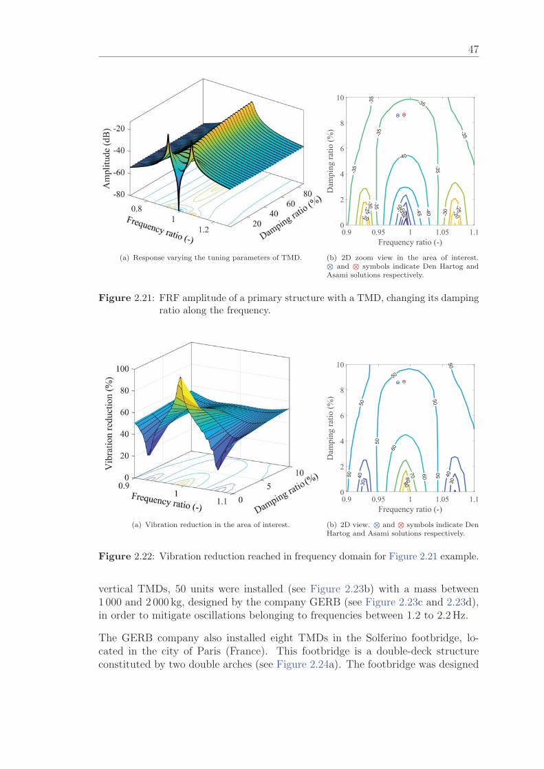
47
(a) Response varying the tuning parameters of TMD.
-60-5
5-50 -45
-40
-40
-35
-35
-35-35
-35
-35
-35
-30
-30
-25
-25
-20
-20
0.9 0.95 1 1.05 1.1Frequency ratio (-)
0
2
4
6
8
10
Dam
ping
ratio
(%)
(b) 2D zoom view in the area of interest.⊗ and ⊗ symbols indicate Den Hartog andAsami solutions respectively.
Figure 2.21: FRF amplitude of a primary structure with a TMD, changing its dampingratio along the frequency.
(a) Vibration reduction in the area of interest.
30 30
40 40
50
50
5050
50
50
50
60
60
708090
0.9 0.95 1 1.05 1.1Frequency ratio (-)
0
2
4
6
8
10
Dam
ping
ratio
(%)
(b) 2D view. ⊗ and ⊗ symbols indicate DenHartog and Asami solutions respectively.
Figure 2.22: Vibration reduction reached in frequency domain for Figure 2.21 example.
vertical TMDs, 50 units were installed (see Figure 2.23b) with a mass between1 000 and 2 000 kg, designed by the company GERB (see Figure 2.23c and 2.23d),in order to mitigate oscillations belonging to frequencies between 1.2 to 2.2 Hz.
The GERB company also installed eight TMDs in the Solferino footbridge, lo-cated in the city of Paris (France). This footbridge is a double-deck structureconstituted by two double arches (see Figure 2.24a). The footbridge was designed

2. Vibration control
(a) General view of the footbridge. (b) TMDs installed below the bridge.
(c) TMD installation process 1. (d) TMD installation process 2.
Figure 2.23: TMDs in Millenium Bridge (2001). GERB company.
by the architect Marc Mimram and built by the Eiffel company. The main struc-ture is 140 m length with a main span of 106 m. The steel wight is approximately990 tn. Due to the excessive vibrations, several solutions were analysed to reducethem. It was considered impossible to stiffen the structure for aesthetical reasonsbut also for technical ones. Indeed, the use of horizontal stiffeners would reducethe vibration amplitudes, but they not change the acceleration levels, and conse-quently, would not improve the pedestrian comfort [59]. Finally, an alternativewas to increase the modal damping by adding TMDs (see Figure 2.24b). Thus,the GERB company installed eight vertical TMDs, 4 of 2 500 kg for a vibrationmode at 1.94 Hz and another 4 of 1 900 kg for other vibration mode at 2.22 Hz.
Another example is a footbridge located in the city of Bilbao (Spain). The struc-ture has a total length of 142.25 meters and the main span of 84 meters (seeFigure 2.25a). Several vibration modes of the structure laid within the commonhuman-induced frequencies. Three couples of TMDs were installed by the com-pany MAURER to mitigate vibration modes with frequencies of 1.85, 2.32 and2.78 Hz, respectively. They all had the same basic design, but different vibrationmasses: 550, 725 and 1 200 kg, respectively (see Figure 2.25b). The same companyinstalled two TMDs of 1 000 and 1 660 kg in a cable-stayed footbridge of 117.5 m

49
(a) General view of the footbridge. (b) TMDs installed below the footbridge [59].
Figure 2.24: TMDs in Solferino footbridge (1999). GERB company.
length sited in Forchheim (Germany) (see Figure 2.26a and 2.26b) to mitigate thevibration modes at 1.26 and 2.70 Hz, respectively.
(a) General view. (b) TMD view.
Figure 2.25: TMDs in Abandoibarra Footbridge (1997). MAURER company.
Another well-known structure with a TMD installed is the Pedro e Ines Foot-bridge at Coimbra (Portugal). The footbridge has a total length of 275 m and isformed by a parabolic central arch with a span of 110 m and two half lateral steelarches, supporting a composite steel-concrete deck (see Figure 2.27a). Numericaland experimental studies developed by the Laboratory of Vibration and Struc-tural Monitoring (ViBest) of FEUP showed that this slender footbridge would beprone to excessive lateral and vertical vibrations caused by groups or streams ofpedestrians [90]. ViBest installed six vertical TMDs, each one with a mass of2 465 kg (see Figure 2.27b and 2.27c), adding a total of 14 790 kg (mass ratio of7.3 %) [34]. In this structure, the mass of pedestrians corresponding to a densityof 1.3 people/m2 leads to a decrease in the natural frequency at the end of con-struction from 0.86 (bridge unloaded) to 0.79 Hz. Thus, the frequency tuning ofthe TMDs was 0.83 Hz, associated with the presence of 0.5 people/m2.
The Taylor Devices company installed eighteen TMDs for three new footbridgesin Las Vegas (Nevada), each one with 44, 48 and 50 meters span, respectively.
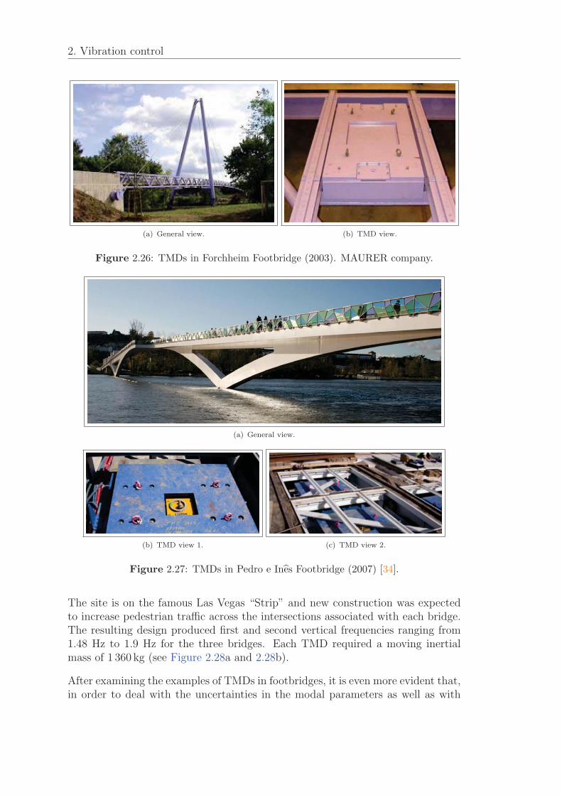
2. Vibration control
(a) General view. (b) TMD view.
Figure 2.26: TMDs in Forchheim Footbridge (2003). MAURER company.
(a) General view.
(b) TMD view 1. (c) TMD view 2.
Figure 2.27: TMDs in Pedro e Ines Footbridge (2007) [34].
The site is on the famous Las Vegas “Strip” and new construction was expectedto increase pedestrian traffic across the intersections associated with each bridge.The resulting design produced first and second vertical frequencies ranging from1.48 Hz to 1.9 Hz for the three bridges. Each TMD required a moving inertialmass of 1 360 kg (see Figure 2.28a and 2.28b).
After examining the examples of TMDs in footbridges, it is even more evident that,in order to deal with the uncertainties in the modal parameters as well as with
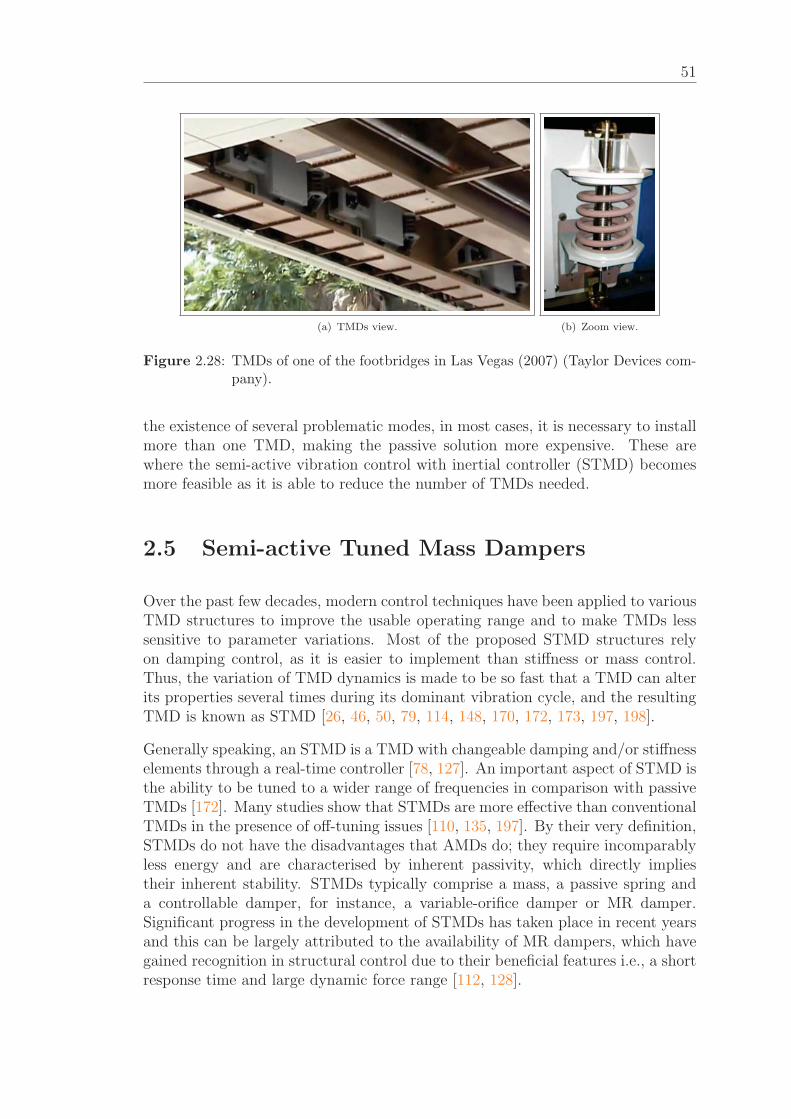
51
(a) TMDs view. (b) Zoom view.
Figure 2.28: TMDs of one of the footbridges in Las Vegas (2007) (Taylor Devices com-pany).
the existence of several problematic modes, in most cases, it is necessary to installmore than one TMD, making the passive solution more expensive. These arewhere the semi-active vibration control with inertial controller (STMD) becomesmore feasible as it is able to reduce the number of TMDs needed.
2.5 Semi-active Tuned Mass Dampers
Over the past few decades, modern control techniques have been applied to variousTMD structures to improve the usable operating range and to make TMDs lesssensitive to parameter variations. Most of the proposed STMD structures relyon damping control, as it is easier to implement than stiffness or mass control.Thus, the variation of TMD dynamics is made to be so fast that a TMD can alterits properties several times during its dominant vibration cycle, and the resultingTMD is known as STMD [26, 46, 50, 79, 114, 148, 170, 172, 173, 197, 198].
Generally speaking, an STMD is a TMD with changeable damping and/or stiffnesselements through a real-time controller [78, 127]. An important aspect of STMD isthe ability to be tuned to a wider range of frequencies in comparison with passiveTMDs [172]. Many studies show that STMDs are more effective than conventionalTMDs in the presence of off-tuning issues [110, 135, 197]. By their very definition,STMDs do not have the disadvantages that AMDs do; they require incomparablyless energy and are characterised by inherent passivity, which directly impliestheir inherent stability. STMDs typically comprise a mass, a passive spring anda controllable damper, for instance, a variable-orifice damper or MR damper.Significant progress in the development of STMDs has taken place in recent yearsand this can be largely attributed to the availability of MR dampers, which havegained recognition in structural control due to their beneficial features i.e., a shortresponse time and large dynamic force range [112, 128].
2. Vibration control
In the practical implementation of these devices, if the control law requires thedominant frequency of vibration to be known in order to set its behaviour, it canbe determined, for instance, on the basis of the relative motion of the STMD. Inthe case of the harmonic vibration of an assumed unknown frequency, or in thecase of non-harmonic vibration, the semi-active control force can be calculatedfrom a variety of control algorithms. For example, the clipped Linear QuadraticRegulator (LQR) [159] or the clipped Linear Quadratic Gaussian control [168],various groundhook control approaches [111, 190], bang-bang control [206], optimalfuzzy logic control [105], PID (Proportional, Integral and Derivative) control [65],or the recently developed on-off phase control algorithms [50, 79, 139] can befound, amongst others. Groundhook and skyhook are actually modalities of phasecontrol. Hereinafter, the most significant works using simple laws based on phasecontrol are described, since this has been the approach in this thesis.
Koo et al. [109, 110] tested four algorithms to control an STMD with a linearvariable damping: 1) DBG (Displacement Based Groundhook) control, an ideainitially proposed by Hrovat et al. [87]. In this type of control, the dampingcoefficient of the semi-active damper is obtained from the product of the structuredisplacement multiplied by the relative velocity of the TMD. Two versions of thisalgorithm are presented: a) an on-off DBG: The damper takes its maximum orminimum value depending on whether the product signal is positive or negative,respectively; b) a Continuous DBG: The variation of the damping coefficient isproportional to the structure displacement; 2) VBG (Velocity Based Groundhook)control, in which the damping coefficient of the semi-active damper is obtainedfrom the product of the structure velocity multiplied by the relative velocity of theTMD. Also, two versions of this algorithm are presented: a) an on-off VBG: Thedamper takes its maximum or minimum value depending on whether the productsignal is negative or positive, respectively; b) a Continuous VBG: The variation ofthe damping coefficient is proportional to the velocity value of the structure. Theauthors verified a low efficiency of the VBG algorithm in relation to the passivesystem. However, the DBG algorithm guarantees a higher efficacy than VBGwith the ability to improve substantially the vibration response obtained withthe passive system. They also concluded that the continuous and on-off DBGalgorithms presented very similar results. The explanation for this is that theoptimal gain determined was very high, causing the continuous algorithm to havea similar behaviour to the on-off version.
Liedes [118] proposed a mixed algorithm between DBG and VBG, which wascalled DaVBG (Displacement and Velocity Based Groundhook), in which feed-back is given based on a combination of the displacement and velocity of thestructure. This method uses a weighted sum of displacement and velocity sig-nals as a reference signal. Indeed, the feedback is nonlinear, which means thatthe optimal feedback matrix varies depending on the response frequency of thestructure. This algorithm is based on the fact that the DBG algorithm is the onethat contributes to reducing the high-frequency response. Liedes concluded that,in theory, it is possible to improve the DBG algorithm using this combination. Ithas been found, however, that the complexity of the practical implementation of

53
this system increases substantially, requiring a more complex observation systemwith a real-time vibration frequency detection system. A displacement sensor lo-cated between the primary structure and the fixed base is not feasible. However,the displacement of the primary structure could possibly be integrated from theacceleration of the primary systems. The integration process typically involvessignal processing, which may induce errors in the signal. Consequently, furtherexamination and development is needed.
In 2013, Chung et al. [50] presented an STMD ruled by a phase control algorithm,thus reducing the structural response through a control action that guaranteesthat the velocity of the TMD and the displacement of the primary structure are inopposing phases. Different researchers [79] reached the same STMD dynamics byusing different control formulations, to be precise: the displacement-based ground-hook presented in 2002 by Setareh [172] and the clipped-optimal LQR presentedin 2002 by Occhiuzzi et al. [148].
Ferreira [77] studied three high potential semi-active systems and only STMDproved to be able to largely overcome the efficiency of a TMD for the control ofharmonic motion, mainly due to its ability to reduce system sensitivity to detuning.Ferreira et al. [79] also studied the dynamics of the phase control law applied toSTMDs, including other practical application features, such as the analysis of thetime delaying effect and locking damping. They also proposed an optimum tuningto reduce not only the structural response, but also the TMD stroke, which is acommon limiting factor in civil engineering structures. A tuning method for thissystem should be studied in detail, since its behaviour is different from the TMD,whose tuning process is well established in the literature.
The above-mentioned algorithms differ in terms of calculation complexity, effec-tiveness, the purpose of generated semi-active control force and feedback signalsused. Despite using different formulations and even different sensor inputs (ac-celeration, velocity and displacements) the practical control effect in the systemdynamics is the same. This research work has focused on those strategies of semi-active control that can be materialised from a controllable smart damper (dampingcontrol), usually an MR damper.
2.5.1 Examples of vertical STMD in bridges
One of the most iconic examples of the application of an STMD on a bridge wascarried out by Weber [196] on the Volgograd Bridge (Russia) in 2011. The Vol-gograd Bridge (see Figure 2.29a), which is 7 km long, is one of the longest bridgesin Europe. It was inaugurated in October 2009, after 13 years of construction.This structure became world-famous in May 2010, when the bridge deck beganto suffer strong oscillations, in the order of ±40cm. The bridge has several vi-bration modes that can be excited and these characteristics suggested that STMDsolution would be the best to study it. The study was carried out by the MAURER
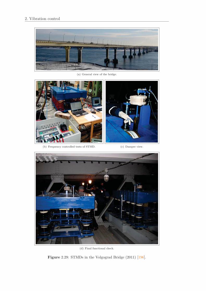
2. Vibration control
(a) General view of the bridge.
(b) Frequency controlled tests of STMD. (c) Damper view.
(d) Final functional check.
Figure 2.29: STMDs in the Volgograd Bridge (2011) [196].
55
company and the Universitat der Bundeswehr Munchen. Field measurements andwind tunnel tests demonstrated that the first three vertical bending vibrationmodes at 0.45, 0.56 and 0.68 Hz should be mitigated. The problem was dealtwith by three groups of 4 STMD with an inertial mass of 5 200 kg each (a totalnumber of 12) installed in 3 different sections of the bridge. Weber proposedan MR damper that emulates stiffness and damping variations that reduces theTMD sensitivity to detuning (see Figure 2.31b). According to MAURER, it wouldrequire 36 passive TMDs to reach the efficiency level verified with the 12 STMDinstalled.
In the pedestrian bridge of Forchheim show in Figure 2.26, a study concludedthat the structure was susceptible to modifications of its dynamic properties dueto the mass variation on the bridge. It was decided to upgrade the passive de-vice into STMD to control a wider frequency range and thereby increase its effi-ciency. The control algorithm uses the clipped-optimal LQR law [148]. Occhiuzziet al. [148] proposed a semi-active algorithm in which the feedback is determinedby the clipped-optimal LQR formulation, having concluded that the optimal LQRfeedback converges to the DBG algorithm. This is explained by the fact that theDBG algorithm is the one that optimally corrects the phase opposition betweenthe TMD and the structure. The semi-active control device demonstrated a highervibration reduction than the passive TMD, especially when the structure presentsvariations in its dynamic properties [170].
The work developed by Moutinho et al. [140] summarizes the study, the experi-mental analysis and the installation of a passive TMD in the FEUP Footbridgeshown above in Figure 2.11a, as well as its upgrading to a semi-active system. Be-cause the structure has several critical vibration modes with natural frequenciesclose to 2 Hz and also with uncertainties associated to these modal parameters (seeFigure 2.11b and 2.11c), a single device cannot act efficiently on all of them, whichlimits the control efficiency. Upgrading the TMD to an STMD was the option se-lected to increase the robustness, given the self-tuning capabilities of these devices,as well as the possibility of performing multimode control. As a continuous dy-namic monitoring system had been installed in 2009, it was possible to evaluatethe structure’s vibration levels measured over the previous few years, includingthe periods prior to and after the installation of the control solutions. A tendencywas noted in the reduction of the peak accelerations of some sections of the deckafter the installation of the passive TMD, which were even more attenuated withthe activation of the semi-active system.
Many semi-active vibration control laws have been proposed; however, most arenot geared to implementation and/or important practical issues are neglected.This thesis concentrates on two control laws with clearly developed thinking intheir practical implementation. The selected laws are those used in the works ofWeber [196] and Moutinho [139], respectively. The semi-active strategy used inthe Forchheim Footbridge example converges to the DBG phase control algorithm,from which the Moutinho law comes, and that is why it is not studied in detailhere. The law presented by Moutinho [139] will be called “Semi-active control 1”

2. Vibration control
(a) Laboratory test. (b) Layaout of control system.
Figure 2.30: STMD in FEUP Footbridge (2017) [140].
and is an on-off phase control (see Figure 2.31a). This law stands out for itssimplicity. On the other hand, the law presented by Weber [196], “Semi-activecontrol 2”, is a strategy in which the control force is continuously modified (seeFigure 2.31b). Both laws are explained in more depth in the following sectionsand are studied numerically in Chapter 4.
( )F t
( )Tx t
( )Sx tTk ( )Tc t
SkSc
c
c
mS
mT
(a) STMD 1.
( )F t
( )Tx t
( )Sx tTk ( )Dc t
SkSc
( )Dk t
c
mS
mT
c
(b) STMD 2.
Figure 2.31: Scheme of the two semi-active strategies studied. Red symbol ( −→) meanschanging over time.
57
2.5.2 Semi-active control 1
The phase control presented in [50, 180] and adapted by Moutinho [139] is de-scribed here. This is clearly geared to practical implementation due to the mea-sured real-time parameters employed: the structure acceleration instead of dis-placement and the inertial mass velocity instead of the relative velocity. Thiscontrol law will thus be effective when structure velocity is negligible with respectto the inertial mass velocity, which usually happens in civil engineering structuresunder resonant events. The lowest structural response is achieved when the ve-locity of the inertial mass and structure acceleration have opposing phases, so thesemi-active device objective is to bring the inertial mass motion as close as possibleto this phase. This is equivalent to a phase lag of 90o between the structure accel-eration and the control force. Figure 2.31a shows an STMD (hereafter denoted asSTMD 1), whose damping can be changed continuously. Thus, the adopted con-trol law that originally assumes a controllable, ideal viscoelastic damper is definedas follows:{
xS· x
T≤ 0 ⇒ c
T= cmin (normal functioning),
xS· x
T> 0 ⇒ c
T= cmax (blocking functioning),
(2.15)
in which cmax is the maximum damping coefficient to block the TMD inertialmass movement, cmin is the optimal damping obtained from Equation 2.14, x
Sis
the structure acceleration (recorded by an accelerometer) and xT
is the absolutevelocity of the inertial mass (which might be obtained from the integration1 of anaccelerometer signal installed on the inertial mass controller).
2.5.3 Semi-active control 2
Figure 2.31b depicts the STMD strategy proposed by Weber [196] and denoted asSTMD 2 hereafter. The key feature of this control law is that the energy dissipationand natural frequency of the STMD, respectively, are adjusted by changing thedamping force continuously according to Den Hartog’s formula in real-time tofw instead of f
S, fw being the actual instantaneous frequency of the vibration
response, independently of whether this frequency corresponds to the resonantfrequency of the targeted vibration mode or represents an excitation frequency dueto forced excitation out of resonance. The damper works in parallel with a virtualpassive spring, designed according to Den Hartog’s formula (see Figure 2.31b) anddenoted by k
T.
The damper emulates the sum of a controllable stiffness force (positive or negative),F
KD, and a controllable dissipative force, F
CD, as follows
F = FKD
+ FCD. (2.16)
1This and other aspects of the implementation are described in greater depth in Chapter 5.

2. Vibration control
It is a real-time adaptive control law that aims to tune the controller to the vibra-tion frequency at every instant. However, these forces are clipped to zero (ideallyor at the minimum frictional force, Fmin) in order to make its operation dissipative.It yields to the semi-active force, F
D, as follows
FD
=
{F, sgn(x
S− x
T) · F ≥ 0
Fmin, sgn(xS− x
T) · F < 0
, (2.17)
in which sgn(xS− x
T) is the sign of the relative velocity between the structure
and TMD mass. The actual frequency, fw, is estimated from the zero-crossings ofthe relative displacement, x
S−x
T, through the half period time, Thalf. The actual
frequency is then estimated as follows:
fw =1
2Thalf. (2.18)
Thus, the stiffness and energy dissipation of the STMD 2 are tuned to the actualfrequency of vibration fw by the modified mass ratio
∼μ, which depends on the
frequency shift between fw and fS
as follows
∼μ = μ
(fwfS
), (2.19)
and then the damper properties are derived as
kD
= kS
∼μ
(1 +∼μ)2
− kT, (2.20)
ζD
=
√3
∼μ
8 (∼μ+ 1)
, (2.21)
cD
= 2 ζDm
T(2πfw). (2.22)
Finally, the control forces to compute (Equation 2.16) and apply the semi-activecontrol law (Equation 2.17) are,
FKD
= kD
(xS− x
T), (2.23)
FCD
= sgn(xS− x
T){π
4cD
(2πfw) (xS− x
T)}. (2.24)
It should be mentioned that this algorithm requires the relative displacement tobe measured, as well as knowing the sign of the relative velocity. This might beundertaken using a displacement transducer between the structure and the TMDmass.
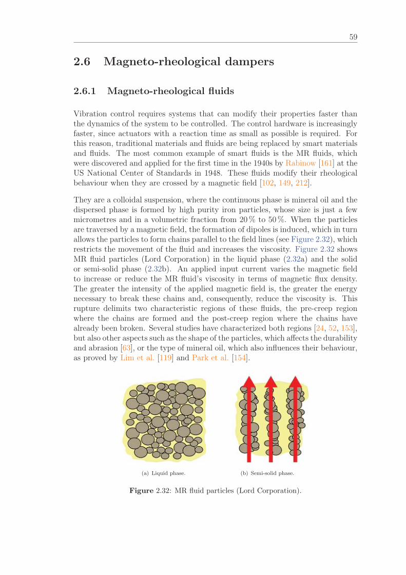
59
2.6 Magneto-rheological dampers
2.6.1 Magneto-rheological fluids
Vibration control requires systems that can modify their properties faster thanthe dynamics of the system to be controlled. The control hardware is increasinglyfaster, since actuators with a reaction time as small as possible is required. Forthis reason, traditional materials and fluids are being replaced by smart materialsand fluids. The most common example of smart fluids is the MR fluids, whichwere discovered and applied for the first time in the 1940s by Rabinow [161] at theUS National Center of Standards in 1948. These fluids modify their rheologicalbehaviour when they are crossed by a magnetic field [102, 149, 212].
They are a colloidal suspension, where the continuous phase is mineral oil and thedispersed phase is formed by high purity iron particles, whose size is just a fewmicrometres and in a volumetric fraction from 20 % to 50 %. When the particlesare traversed by a magnetic field, the formation of dipoles is induced, which in turnallows the particles to form chains parallel to the field lines (see Figure 2.32), whichrestricts the movement of the fluid and increases the viscosity. Figure 2.32 showsMR fluid particles (Lord Corporation) in the liquid phase (2.32a) and the solidor semi-solid phase (2.32b). An applied input current varies the magnetic fieldto increase or reduce the MR fluid’s viscosity in terms of magnetic flux density.The greater the intensity of the applied magnetic field is, the greater the energynecessary to break these chains and, consequently, reduce the viscosity is. Thisrupture delimits two characteristic regions of these fluids, the pre-creep regionwhere the chains are formed and the post-creep region where the chains havealready been broken. Several studies have characterized both regions [24, 52, 153],but also other aspects such as the shape of the particles, which affects the durabilityand abrasion [63], or the type of mineral oil, which also influences their behaviour,as proved by Lim et al. [119] and Park et al. [154].
(a) Liquid phase. (b) Semi-solid phase.
Figure 2.32: MR fluid particles (Lord Corporation).
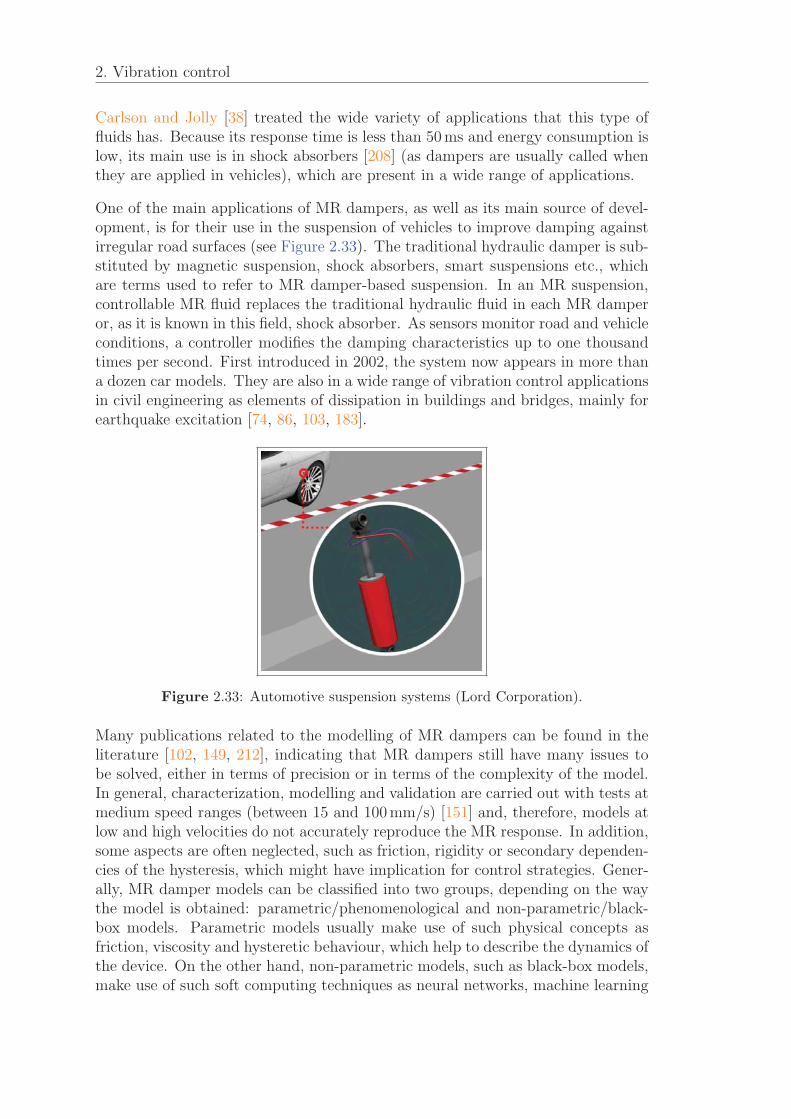
2. Vibration control
Carlson and Jolly [38] treated the wide variety of applications that this type offluids has. Because its response time is less than 50 ms and energy consumption islow, its main use is in shock absorbers [208] (as dampers are usually called whenthey are applied in vehicles), which are present in a wide range of applications.
One of the main applications of MR dampers, as well as its main source of devel-opment, is for their use in the suspension of vehicles to improve damping againstirregular road surfaces (see Figure 2.33). The traditional hydraulic damper is sub-stituted by magnetic suspension, shock absorbers, smart suspensions etc., whichare terms used to refer to MR damper-based suspension. In an MR suspension,controllable MR fluid replaces the traditional hydraulic fluid in each MR damperor, as it is known in this field, shock absorber. As sensors monitor road and vehicleconditions, a controller modifies the damping characteristics up to one thousandtimes per second. First introduced in 2002, the system now appears in more thana dozen car models. They are also in a wide range of vibration control applicationsin civil engineering as elements of dissipation in buildings and bridges, mainly forearthquake excitation [74, 86, 103, 183].
Figure 2.33: Automotive suspension systems (Lord Corporation).
Many publications related to the modelling of MR dampers can be found in theliterature [102, 149, 212], indicating that MR dampers still have many issues tobe solved, either in terms of precision or in terms of the complexity of the model.In general, characterization, modelling and validation are carried out with tests atmedium speed ranges (between 15 and 100 mm/s) [151] and, therefore, models atlow and high velocities do not accurately reproduce the MR response. In addition,some aspects are often neglected, such as friction, rigidity or secondary dependen-cies of the hysteresis, which might have implication for control strategies. Gener-ally, MR damper models can be classified into two groups, depending on the waythe model is obtained: parametric/phenomenological and non-parametric/black-box models. Parametric models usually make use of such physical concepts asfriction, viscosity and hysteretic behaviour, which help to describe the dynamics ofthe device. On the other hand, non-parametric models, such as black-box models,make use of such soft computing techniques as neural networks, machine learning
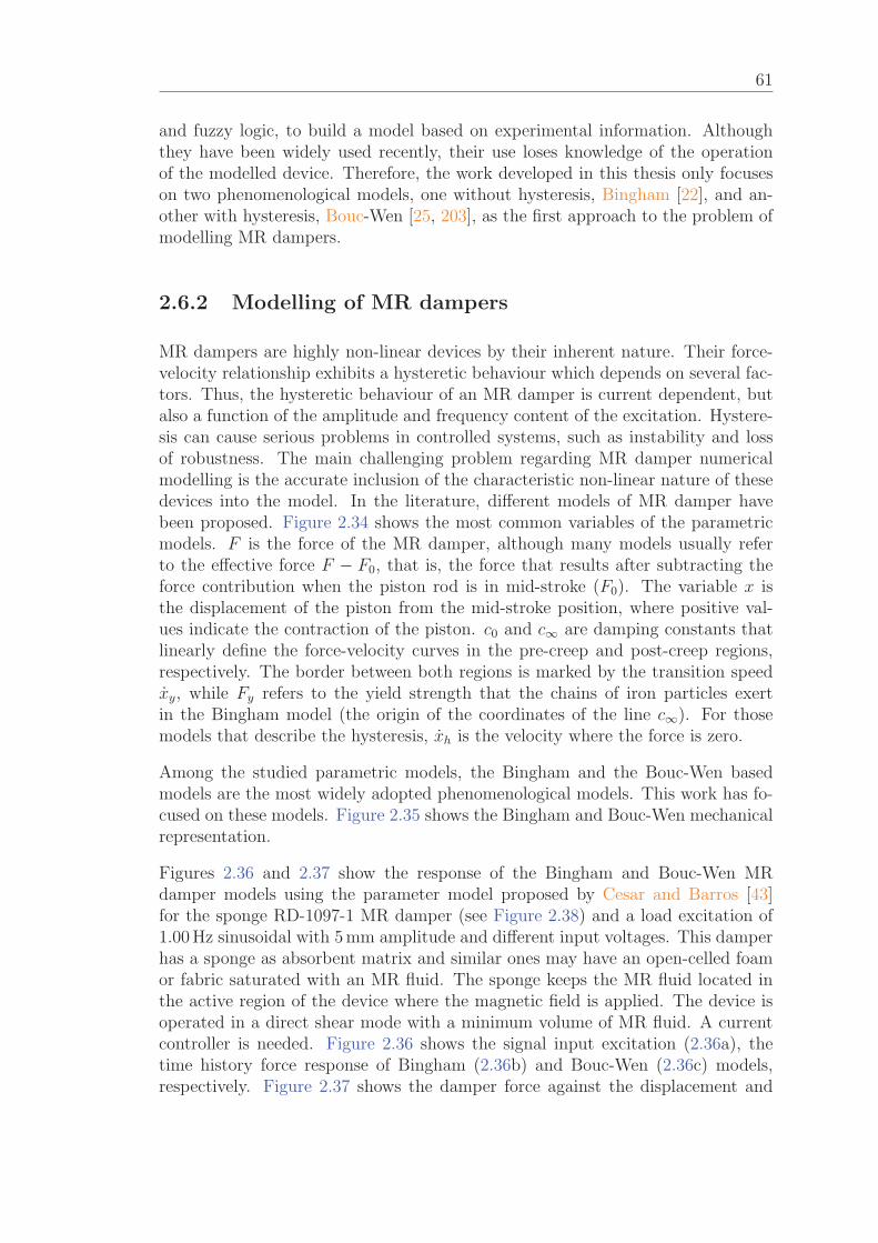
61
and fuzzy logic, to build a model based on experimental information. Althoughthey have been widely used recently, their use loses knowledge of the operationof the modelled device. Therefore, the work developed in this thesis only focuseson two phenomenological models, one without hysteresis, Bingham [22], and an-other with hysteresis, Bouc-Wen [25, 203], as the first approach to the problem ofmodelling MR dampers.
2.6.2 Modelling of MR dampers
MR dampers are highly non-linear devices by their inherent nature. Their force-velocity relationship exhibits a hysteretic behaviour which depends on several fac-tors. Thus, the hysteretic behaviour of an MR damper is current dependent, butalso a function of the amplitude and frequency content of the excitation. Hystere-sis can cause serious problems in controlled systems, such as instability and lossof robustness. The main challenging problem regarding MR damper numericalmodelling is the accurate inclusion of the characteristic non-linear nature of thesedevices into the model. In the literature, different models of MR damper havebeen proposed. Figure 2.34 shows the most common variables of the parametricmodels. F is the force of the MR damper, although many models usually referto the effective force F − F0, that is, the force that results after subtracting theforce contribution when the piston rod is in mid-stroke (F0). The variable x isthe displacement of the piston from the mid-stroke position, where positive val-ues indicate the contraction of the piston. c0 and c∞ are damping constants thatlinearly define the force-velocity curves in the pre-creep and post-creep regions,respectively. The border between both regions is marked by the transition speedxy, while Fy refers to the yield strength that the chains of iron particles exertin the Bingham model (the origin of the coordinates of the line c∞). For thosemodels that describe the hysteresis, xh is the velocity where the force is zero.
Among the studied parametric models, the Bingham and the Bouc-Wen basedmodels are the most widely adopted phenomenological models. This work has fo-cused on these models. Figure 2.35 shows the Bingham and Bouc-Wen mechanicalrepresentation.
Figures 2.36 and 2.37 show the response of the Bingham and Bouc-Wen MRdamper models using the parameter model proposed by Cesar and Barros [43]for the sponge RD-1097-1 MR damper (see Figure 2.38) and a load excitation of1.00 Hz sinusoidal with 5 mm amplitude and different input voltages. This damperhas a sponge as absorbent matrix and similar ones may have an open-celled foamor fabric saturated with an MR fluid. The sponge keeps the MR fluid located inthe active region of the device where the magnetic field is applied. The device isoperated in a direct shear mode with a minimum volume of MR fluid. A currentcontroller is needed. Figure 2.36 shows the signal input excitation (2.36a), thetime history force response of Bingham (2.36b) and Bouc-Wen (2.36c) models,respectively. Figure 2.37 shows the damper force against the displacement and

2. Vibration control
Figure 2.34: Main parameters of an MR damper model [151].
(a) Bingham. (b) Bouc-Wen.
Figure 2.35: Bingham and Bouc-Wen mechanical models [209].
velocity of the MR damper. This is the modelled damper and, its parameters areidentified and then used for the experimental vibration control tests of MR-STMDin this thesis.
2.6.3 Bingham model
In 1922, Eugene C. Bingham proposed a mathematical model for visco-plasticmaterials that behave like a rigid body when subjected to low stresses and as aviscous fluid when they are subjected to high stresses [22]. The Bingham model haslong been used to characterize MR dampers. This model consists of a Coulombfriction element placed in parallel with a viscous damper. A schematic of thismodel is shown in Figure 2.35a. The stress-strain behaviour of the Binghamvisco-plastic model is used to describe the behaviour of MR fluids. In this model,
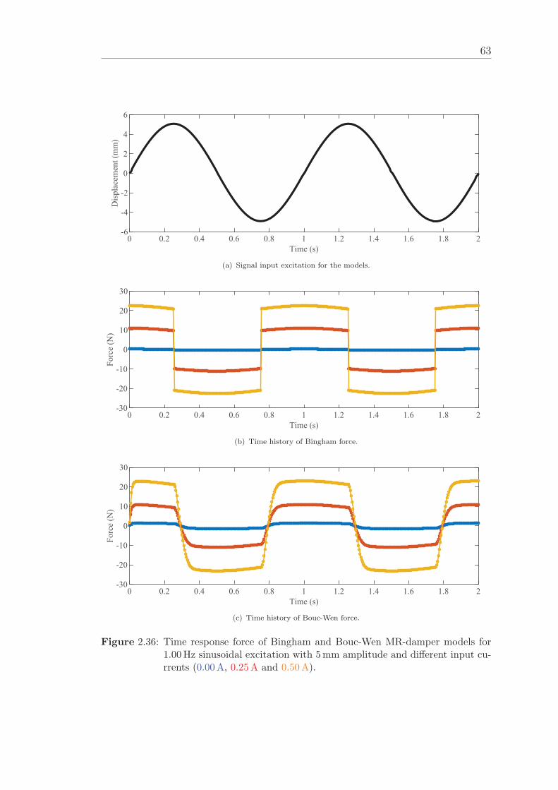
63
0 0.2 0.4 0.6 0.8 1 1.2 1.4 1.6 1.8 2Time (s)
-6
-4
-2
0
2
4
6D
ispl
acem
ent (
mm
)
(a) Signal input excitation for the models.
0 0.2 0.4 0.6 0.8 1 1.2 1.4 1.6 1.8 2Time (s)
-30
-20
-10
0
10
20
30
Forc
e (N
)
(b) Time history of Bingham force.
0 0.2 0.4 0.6 0.8 1 1.2 1.4 1.6 1.8 2Time (s)
-30
-20
-10
0
10
20
30
Forc
e (N
)
(c) Time history of Bouc-Wen force.
Figure 2.36: Time response force of Bingham and Bouc-Wen MR-damper models for1.00Hz sinusoidal excitation with 5mm amplitude and different input cu-rrents (0.00A, 0.25A and 0.50A).

2. Vibration control
-6 -4 -2 0 2 4 6Displacement (mm)
-30
-20
-10
0
10
20
30
Forc
e (N
)
(a) Bingham force-displacement curves.
-6 -4 -2 0 2 4 6Displacement (mm)
-30
-20
-10
0
10
20
30
Forc
e (N
)
(b) Bouc-Wen force-displacement curves.
-40 -20 0 20 40Velocity (mm/s)
-30
-20
-10
0
10
20
30
Forc
e (N
)
(c) Bingham force-velocity curves.
-40 -20 0 20 40Velocity (mm/s)
-30
-20
-10
0
10
20
30
Forc
e (N
)
(d) Bouc-Wen force-velocity curves.
Figure 2.37: Response of Bingham and Bouc-Wen MR-damper models for 1.00Hz sinu-soidal excitation with 5mm amplitude and different input currents (0.00A,0.25A and 0.50A).
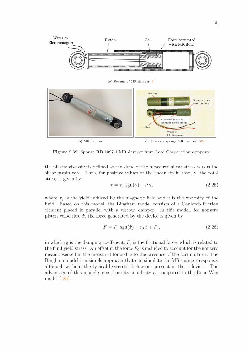
65
(a) Scheme of MR damper [7].
(b) MR damper. (c) Pieces of sponge MR damper [109].
Figure 2.38: Sponge RD-1097-1 MR damper from Lord Corporation company.
the plastic viscosity is defined as the slope of the measured shear stress versus theshear strain rate. Thus, for positive values of the shear strain rate, γ, the totalstress is given by
τ = τγ sgn(γ) + ν γ, (2.25)
where τγ is the yield induced by the magnetic field and ν is the viscosity of thefluid. Based on this model, the Bingham model consists of a Coulomb frictionelement placed in parallel with a viscous damper. In this model, for nonzeropiston velocities, x, the force generated by the device is given by
F = Fc sgn(x) + c0 x+ F0, (2.26)
in which c0 is the damping coefficient, Fc is the frictional force, which is related tothe fluid yield stress. An offset in the force F0 is included to account for the nonzeromean observed in the measured force due to the presence of the accumulator. TheBingham model is a simple approach that can simulate the MR damper response,although without the typical hysteretic behaviour present in these devices. Theadvantage of this model stems from its simplicity as compared to the Bouc-Wenmodel [184].

2. Vibration control
2.6.4 Bouc-Wen model
This was initially formulated by Bouc [25] and subsequently generalized by Wenet al. [203]. This hysteresis model is one of the mathematically simplest yet effec-tive models that can represent a large class of hysteretic behaviour. The Bouc-Wenmodel is extremely versatile and can exhibit a wide variety of hysteretic behaviour.A schematic of this model is shown in Figure 2.35b. The force in this system isgiven by
F = c0 x+ k0 (x− x0) + αz, (2.27)
where the evolutionary variable z for the hysteresis behaviour is governed by
z = −γ |x| z |z|n−1 − βx |z|n + Ax. (2.28)
By adjusting the parameters γ, β and A of the model, the linearity in the unloadingcan be controlled, as well as the smoothness of the transition from the pre-yieldto the post-yield region. In addition, the force F0 due to the accumulator can bedirectly incorporated into this model as an initial deflection x0 of the linear springk0. The Bouc-Wen model predicts the force-displacement behaviour of the damperwell, while also possessing force-velocity behaviour that more closely resembles theexperimental data [184].
2.6.5 Application of MR for STMD
The research work of this thesis has focused on STMDs through MR dampers. Thetuning of the semi-active device should be done differently from in a passive device.This is why the uncertainties of the structure and the non-linearities of the damperdevice are taken into account. Performance and optimisation analysis are carriedout in Chapter 5 to generate the appropriate parameters for the proposed semi-active device. The studies will be considered both analytically and experimentally.Figure 2.39 shows the 2-DOF systems in which both control devices, 2.39a and2.39b, have an MR damper instead of linear viscous damper, which is why thevariable to control the damping of the MR damper is I (constant value) for thepassive case (2.39a) and I(t) (time-varying value) for the semi-active case (2.39b).This is because the semi-active one (see Figure 2.39b) has the capacity to changethe force of the MR damper in real-time and, with an adequate control strategy,to increase the vibration reduction of the structure.
The inertial controller physically works as a feedback control (see Figure 2.40a),but the semi-active control laws that have been studied in this thesis are, inthemselves, feedforward strategies applied to the control of MR dampers (see Fi-gure 2.40b).
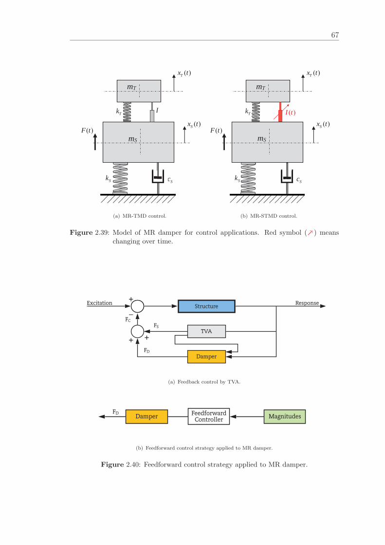
67
( )F t
( )Tx t
( )Sx tTk I
SkSc
c
mS
mT
(a) MR-TMD control.
( )F t
( )Tx t
( )Sx tTk ( )I t
SkSc
c
mS
mT
(b) MR-STMD control.
Figure 2.39: Model of MR damper for control applications. Red symbol ( −→) meanschanging over time.
(a) Feedback control by TVA.
(b) Feedforward control strategy applied to MR damper.
Figure 2.40: Feedforward control strategy applied to MR damper.


3Tracking modal parameters of a
lightweight structure
Contents3.1 Introduction . . . . . . . . . . . . . . . . . . . . . . . . . 69
3.2 The footbridge and its vibration monitoring . . . . . . 70
3.2.1 Structure description . . . . . . . . . . . . . . . . . . . . 70
3.2.2 Monitoring system . . . . . . . . . . . . . . . . . . . . . 72
3.3 Peered analysis of one test . . . . . . . . . . . . . . . . . 74
3.3.1 Data processing . . . . . . . . . . . . . . . . . . . . . . . 75
3.3.2 Operational Modal Analysis using three SSI techniques 75
3.3.3 Operational Modal Analysis using the same SSI technique 84
3.4 Continuous dynamic analysis . . . . . . . . . . . . . . . 85
3.4.1 Tracking of modal properties . . . . . . . . . . . . . . . 85
3.4.2 Effects of external factors . . . . . . . . . . . . . . . . . 89
3.4.3 Statistical analysis . . . . . . . . . . . . . . . . . . . . . 92
3.4.4 Removing external factors . . . . . . . . . . . . . . . . . 95
3.5 Vibration Serviceability Assessment . . . . . . . . . . . 99
3.6 Conclusions . . . . . . . . . . . . . . . . . . . . . . . . . . 101
3.1 Introduction
This chapter describes the work carried out on a lightweight stress-ribbon foot-bridge including the vibration monitoring system, modal properties tracking andvibration serviceability assessment.
69
3. Tracking modal parameters of a lightweight structure
The main obstacle for a more widespread adoption of vibration monitoring sys-tems is the cost associated to their installation. This chapter describes a successfulattempt to reduce the cost of a monitoring system through the use of low-costsensors to measure structural vibrations on a footbridge. Thus, a low-cost contin-uous vibration monitoring system using small MEMS (Micro Electro-mechanicalSystems) accelerometers were developed and installed on Pedro Gomez Bosque(PGB) footbridge (Valladolid, Spain) in order to track its long-term dynamic per-formance. The system continuously measures: the acceleration (using 18 triaxialMEMS accelerometers distributed along the structure), the ambient temperatureand the wind velocity and direction [62]. PGB footbridge is a singular steel-platedstress-ribbon footbridge with a single span of 85 m. The dynamic behaviour showsseveral low-frequency vibration modes with closely-spaced natural frequencies andlow damping ratios.
A procedure to track vibration modes was programmed to carry out an automaticmodal parameter estimation. This procedure has to cope with vibration modeswith closely-spaced natural frequencies. In this case, sorting vibration modes usingfrequency criteria and removing outliers that lay out of intervals of frequencyvariation might not be adequate [123, 138]. This chapter describes the detailedprocedure carried out to track vibration modes of PGB footbridge over time. Theprocedure uses three tolerances based on the Modal Assurance Criterion (MAC).This approach allows reliable monitoring of vibration modes that are maintainedover time.
The chapter continues with the description of the structure and its monitoringsystem. Section 3.3 analyses the uncertainties associated to a single time historyrecord. The output-only modal parameter estimation using three SSI based OMAtechniques and different data blocks is carried out. Thus, uncertainties due tothe selection of the SSI technique and the data block are quantified. The resultsof continuous dynamic analysis are described in Section 3.4. A tracking methodto follow the evolution of the persistent vibration modes over time is proposed.The influence of the environmental/operational factors on the modal estimatesis studied and correlation models are derived to remove the influence of thesespurious factors. Finally, some conclusions are drawn.
3.2 The footbridge and its vibration monitoring
3.2.1 Structure description
PGB footbridge, sited in Valladolid (Spain), is a slender and lightweight structurethat creates a pedestrian link over the Pisuerga River between a sport complexand the city centre (see Figure 3.1). This bridge, built in 2011, is a singularstress-ribbon footbridge born by a pre-tensioned catenary-shape steel band witha single span of 85 m that provides minimal impact on the surroundings. The
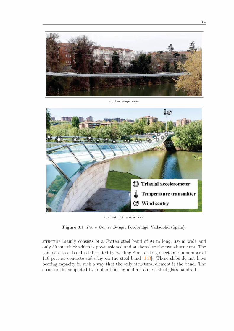
71
(a) Landscape view.
(b) Distribution of sensors.
Figure 3.1: Pedro Gomez Bosque Footbridge, Valladolid (Spain).
structure mainly consists of a Corten steel band of 94 m long, 3.6 m wide andonly 30 mm thick which is pre-tensioned and anchored to the two abutments. Thecomplete steel band is fabricated by welding 8-meter long sheets and a number of110 precast concrete slabs lay on the steel band [143]. These slabs do not havebearing capacity in such a way that the only structural element is the band. Thestructure is completed by rubber flooring and a stainless steel glass handrail.
3. Tracking modal parameters of a lightweight structure
3.2.2 Monitoring system
A structural vibration monitoring system was devised in order to continuouslyestimate the modal parameters of the structure and to assess their changes un-der varying environmental conditions. Therefore, apart from the accelerometersneeded to perform a modal analysis, sensors for the wind and environmental tem-perature conditions were installed. The monitoring system comprises 18 triaxialaccelerometers, 9 at each side of the deck, a temperature sensor and an anemome-ter with a vane. Wires and acceleration sensors were installed inside the handrailso the structure aesthetic was not modified in any way. This fact introduced ad-ditional complications: (i) the installation process was a laborious task, and (ii)additional angular transformations are required to obtain the acceleration vectorin the structure axes for each accelerometer.
The vibration sensor used for the monitoring system was the low-cost MEMSaccelerometer ADXL327 (ANALOG DEVICES) able to measure the static accel-eration of gravity. The ADXL327 is a very small, low power, 3-axis accelerometerwith signal condition voltage output. The key properties of this sensor are: mea-surement range up to ± 2.5g, sensitivity up to 500 mV/g and bandwidth up to550 Hz. However, this sensor is not designed to transmit the signal over longdistances. To overcome this problem, an ad-hoc conditioning circuit was designedto enhance its long-distance performance. First, three capacitors, one to eachchannel, were placed to fix the frequency bandwidth to 100 Hz. Second, since theaccelerometer has to be supplied by 3.6 V to get its maximum nominal sensitiv-ity of 500 mV/g, the power supply unit of 12 V and a voltage regulator to 3.6 Vwere integrated into each circuit board in order to avoid power losses by the longdistance wires. Thirdly, an operational amplifier was used to reduce significantlythe output impedance, achieving thus a good signal-to-noise ratio for accelerationparameter (constant sensitivity and low noise). The achieved signal-to-noise ratiowas 25 μg/
√Hz, which was considered to be enough for monitoring the structural
vibrations. Finally, each circuit board with all its components was covered with aplastic coating to protect it from environmental conditions. Then, the accelerome-ters were ready to be installed inside the tube of the handrail. The sensing systemwas completed by a temperature sensor (model T0110 transmitter of Comet) anda wind sentry (model 03002L of R.M. Young Company) to measure the speed anddirection of the wind. The temperature sensor and wind sentry were installed onthe public light tower sited closed to the structure (see Figure 3.1b).
The monitoring system then comprises 57 voltage channels that are processedcontinuously. The data logger CompactRIO 9076 (National Instruments, NI) withtwo NI 9205 with 32 analog input channels is used for real-time data acquisition.The frequency sampling for each channel was chosen to be 200 Hz, enough toidentify the modal parameters of the structure and to avoid aliasing problemsduring the post-processing. Figure 3.2 shows the data logger and the two sets ofwires from the NI cards, among other monitoring devices.

73
(a) Sensor installation. (b) Data acquisition components.
(c) Circuit board with integrated MEMS accelerometer. (d) Local x, y and z axis.
Figure 3.2: Data logger, router and other monitoring devices [62].
The actual orientation of the accelerometers installed inside the handrail is un-known (see Figure 3.2a). However, the Euler angles between the accelerometercoordinate system and the structure coordinate system (see Figure 3.3) can bederived taking into account the following: (i) the longitudinal axis of each ac-celerometer matches with the longitudinal axis of the footbridge, and (ii) theaccelerometers are able to measure acceleration due to gravity from 0 Hz (staticacceleration). Therefore, the transformation matrix between both coordinate sys-tems is obtained, and then, the acceleration in the global axes can be finallycalculated. The x-accelerometer axis remains in the xz absolute plane so thereis no rotation about z absolute axis (γ = 0) which simplifies the initial expres-sion [62]. The other two angles, α and β, can be calculated using a change ofbasis matrix Q between the absolute coordinate and the accelerometer coordinatesystems using the following simplified expression:
⎛⎝ asxasyasz
⎞⎠︸ ︷︷ ︸
as
=
⎛⎝ cos β 0 − sin βsin β sinα cosα cos β sinαsin β cosα sinα cos β cosα
⎞⎠︸ ︷︷ ︸
Q
⎛⎝ 00
−9.81
⎞⎠︸ ︷︷ ︸
g
,
with as being the static acceleration vector measured in accelerometer axis and gthe gravity acceleration vector. Thus, the acceleration of the structure in absoluteaxes are calculated as follows:
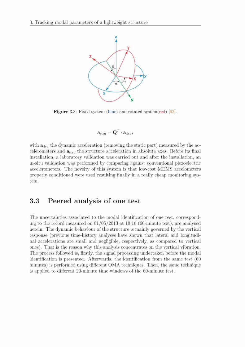
3. Tracking modal parameters of a lightweight structure
Figure 3.3: Fixed system (blue) and rotated system(red) [62].
astru = QT · adyn,
with adyn the dynamic acceleration (removing the static part) measured by the ac-celerometers and astru the structure acceleration in absolute axes. Before its finalinstallation, a laboratory validation was carried out and after the installation, anin-situ validation was performed by comparing against conventional piezoelectricaccelerometers. The novelty of this system is that low-cost MEMS accelometersproperly conditioned were used resulting finally in a really cheap monitoring sys-tem.
3.3 Peered analysis of one test
The uncertainties associated to the modal identification of one test, correspond-ing to the record measured on 01/05/2013 at 19:16 (60-minute test), are analysedherein. The dynamic behaviour of the structure is mainly governed by the verticalresponse (previous time-history analyses have shown that lateral and longitudi-nal accelerations are small and negligible, respectively, as compared to verticalones). That is the reason why this analysis concentrates on the vertical vibration.The process followed is, firstly, the signal processing undertaken before the modalidentification is presented. Afterwards, the identification from the same test (60minutes) is performed using different OMA techniques. Then, the same techniqueis applied to different 20-minute time windows of the 60-minute test.
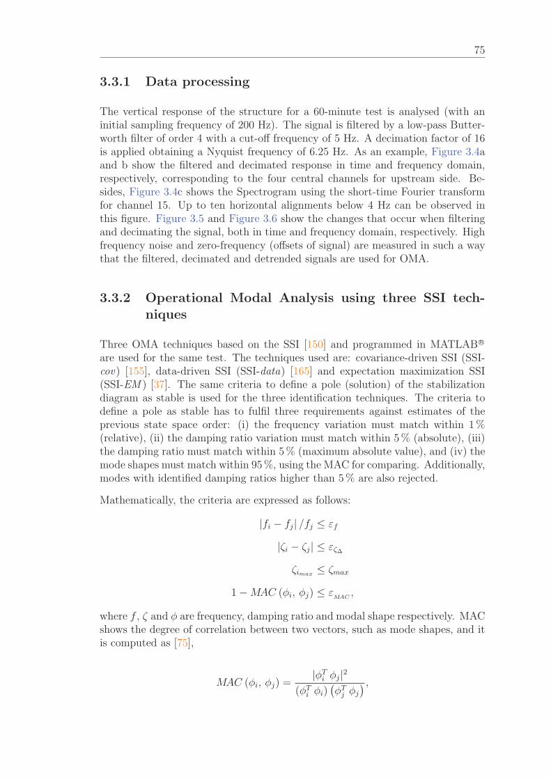
75
3.3.1 Data processing
The vertical response of the structure for a 60-minute test is analysed (with aninitial sampling frequency of 200 Hz). The signal is filtered by a low-pass Butter-worth filter of order 4 with a cut-off frequency of 5 Hz. A decimation factor of 16is applied obtaining a Nyquist frequency of 6.25 Hz. As an example, Figure 3.4aand b show the filtered and decimated response in time and frequency domain,respectively, corresponding to the four central channels for upstream side. Be-sides, Figure 3.4c shows the Spectrogram using the short-time Fourier transformfor channel 15. Up to ten horizontal alignments below 4 Hz can be observed inthis figure. Figure 3.5 and Figure 3.6 show the changes that occur when filteringand decimating the signal, both in time and frequency domain, respectively. Highfrequency noise and zero-frequency (offsets of signal) are measured in such a waythat the filtered, decimated and detrended signals are used for OMA.
3.3.2 Operational Modal Analysis using three SSI tech-niques
Three OMA techniques based on the SSI [150] and programmed in MATLABR©
are used for the same test. The techniques used are: covariance-driven SSI (SSI-cov) [155], data-driven SSI (SSI-data) [165] and expectation maximization SSI(SSI-EM ) [37]. The same criteria to define a pole (solution) of the stabilizationdiagram as stable is used for the three identification techniques. The criteria todefine a pole as stable has to fulfil three requirements against estimates of theprevious state space order: (i) the frequency variation must match within 1 %(relative), (ii) the damping ratio variation must match within 5 % (absolute), (iii)the damping ratio must match within 5 % (maximum absolute value), and (iv) themode shapes must match within 95 %, using the MAC for comparing. Additionally,modes with identified damping ratios higher than 5 % are also rejected.
Mathematically, the criteria are expressed as follows:
|fi − fj| /fj ≤ εf
|ζi − ζj| ≤ εζΔ
ζimax ≤ ζmax
1 −MAC (φi, φj) ≤ εMAC
,
where f , ζ and φ are frequency, damping ratio and modal shape respectively. MACshows the degree of correlation between two vectors, such as mode shapes, and itis computed as [75],
MAC (φi, φj) =|φT
i φj|2(φT
i φi)(φTj φj
) ,
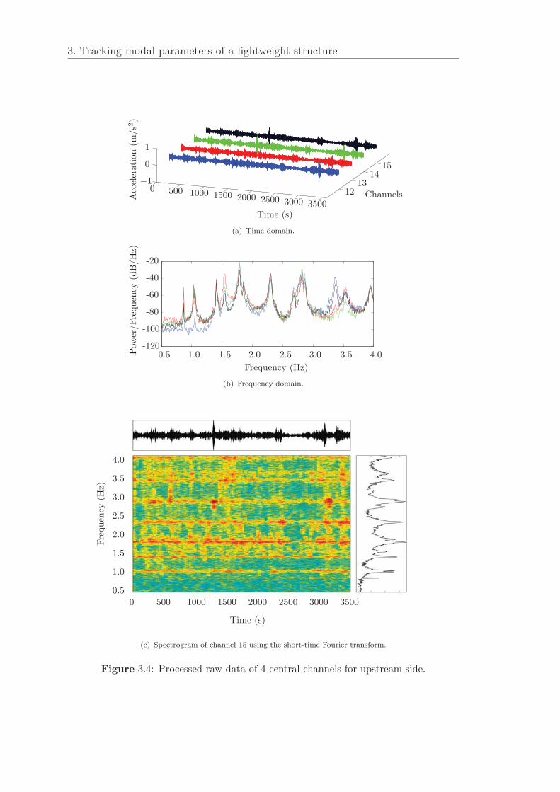
3. Tracking modal parameters of a lightweight structure
0 500 1000 1500 2000 2500 3000 3500
1213
1415
−1
0
1
Channels
Time (s)
Acceleration(m
/s2)
(a) Time domain.
0.5 1.0 1.5 2.0 2.5 3.0 3.5 4.0-120
-100
-80
-60
-40
-20
Frequency (Hz)
Pow
er/Frequency
(dB/Hz)
(b) Frequency domain.
0 500 1000 1500 2000 2500 3000 35000.5
1.0
1.5
2.0
2.5
3.0
3.5
4.0
Time (s)
Frequency
(Hz)
(c) Spectrogram of channel 15 using the short-time Fourier transform.
Figure 3.4: Processed raw data of 4 central channels for upstream side.
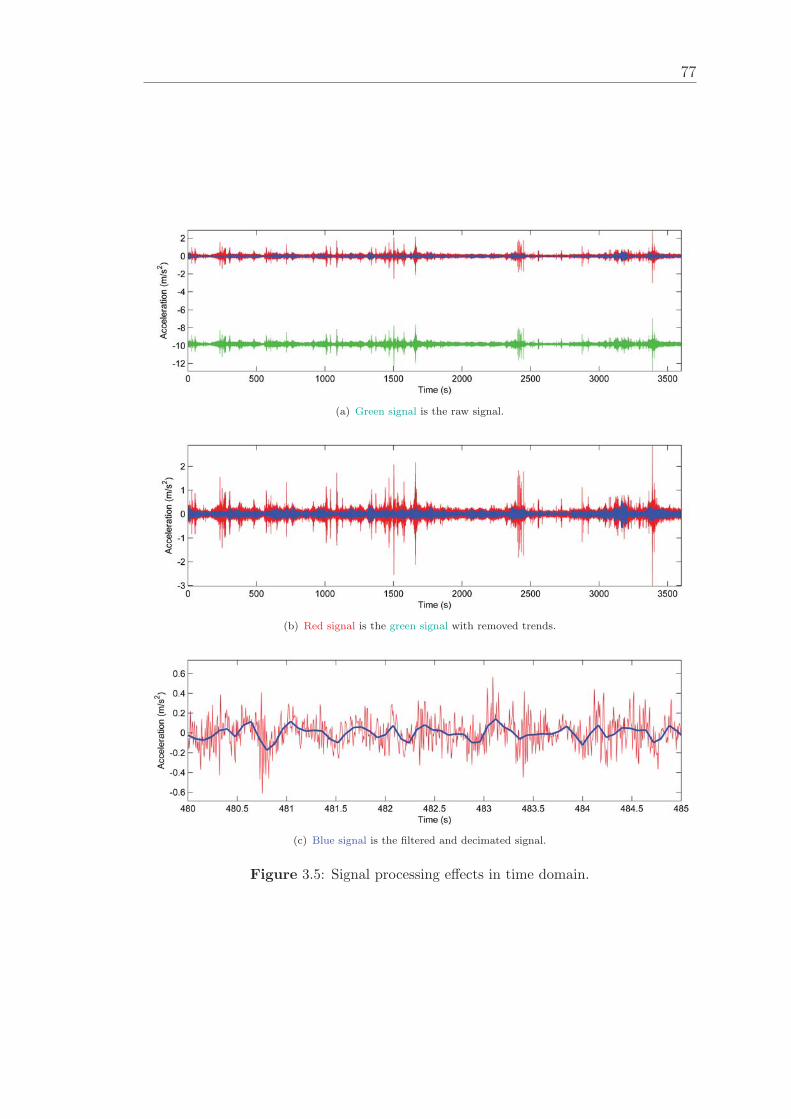
77
(a) Green signal is the raw signal.
(b) Red signal is the green signal with removed trends.
(c) Blue signal is the filtered and decimated signal.
Figure 3.5: Signal processing effects in time domain.
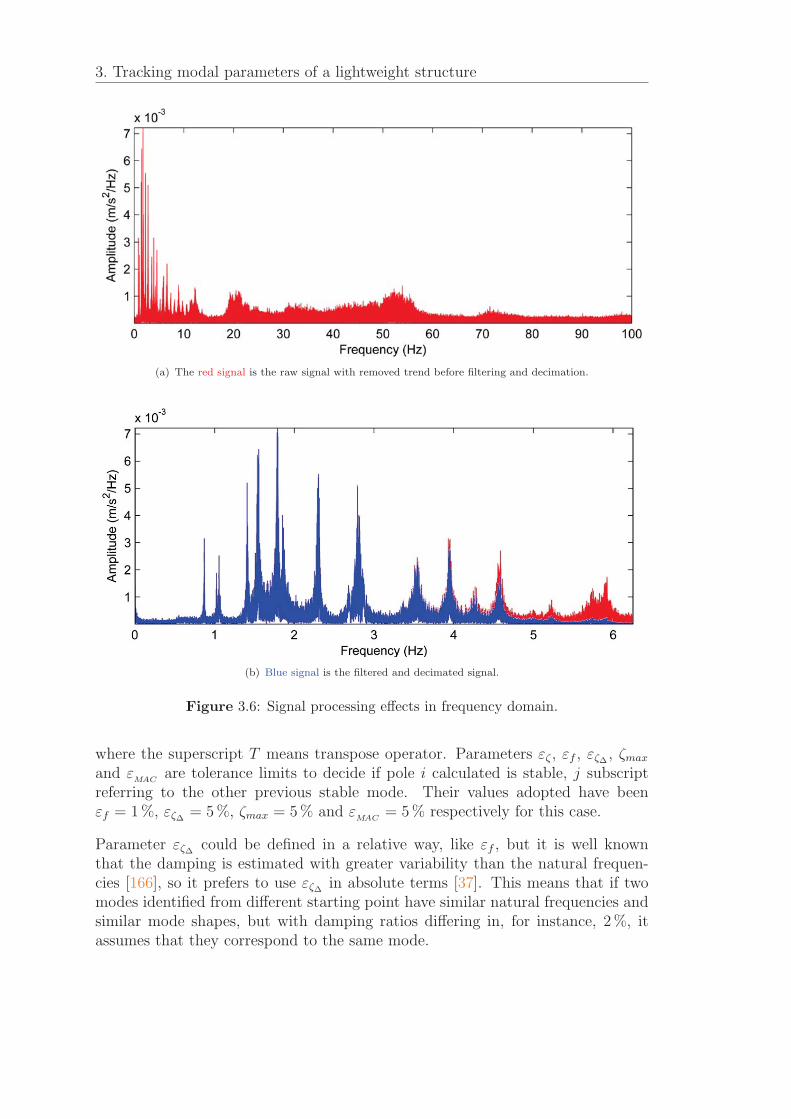
3. Tracking modal parameters of a lightweight structure
(a) The red signal is the raw signal with removed trend before filtering and decimation.
(b) Blue signal is the filtered and decimated signal.
Figure 3.6: Signal processing effects in frequency domain.
where the superscript T means transpose operator. Parameters εζ , εf , εζΔ , ζmax
and εMAC
are tolerance limits to decide if pole i calculated is stable, j subscriptreferring to the other previous stable mode. Their values adopted have beenεf = 1 %, εζΔ = 5 %, ζmax = 5 % and ε
MAC= 5 % respectively for this case.
Parameter εζΔ could be defined in a relative way, like εf , but it is well knownthat the damping is estimated with greater variability than the natural frequen-cies [166], so it prefers to use εζΔ in absolute terms [37]. This means that if twomodes identified from different starting point have similar natural frequencies andsimilar mode shapes, but with damping ratios differing in, for instance, 2 %, itassumes that they correspond to the same mode.
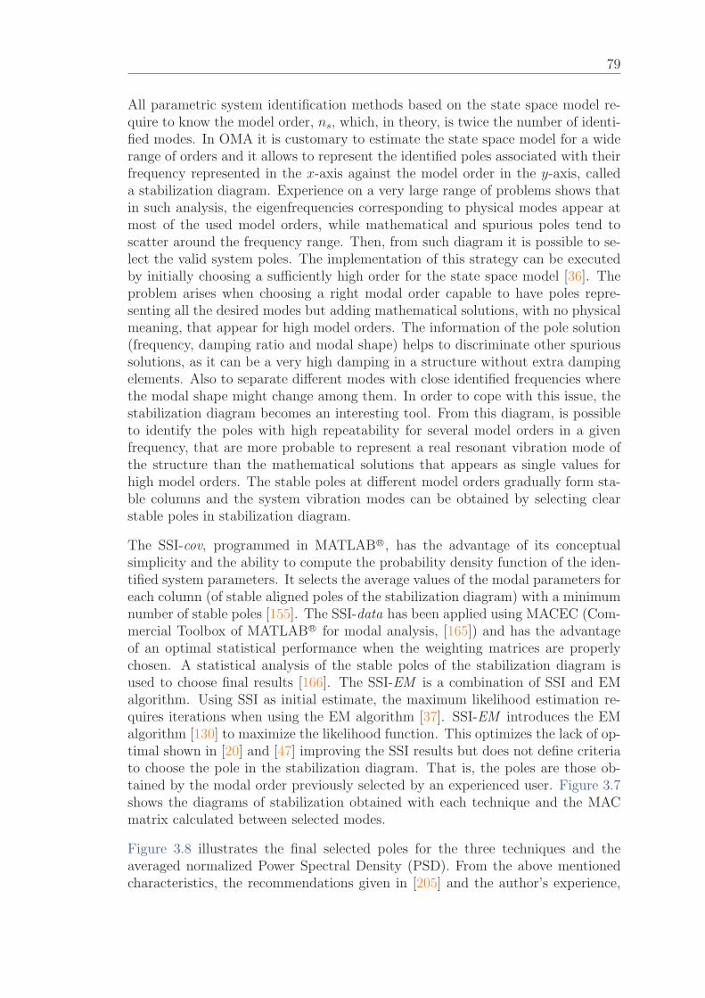
79
All parametric system identification methods based on the state space model re-quire to know the model order, ns, which, in theory, is twice the number of identi-fied modes. In OMA it is customary to estimate the state space model for a widerange of orders and it allows to represent the identified poles associated with theirfrequency represented in the x-axis against the model order in the y-axis, calleda stabilization diagram. Experience on a very large range of problems shows thatin such analysis, the eigenfrequencies corresponding to physical modes appear atmost of the used model orders, while mathematical and spurious poles tend toscatter around the frequency range. Then, from such diagram it is possible to se-lect the valid system poles. The implementation of this strategy can be executedby initially choosing a sufficiently high order for the state space model [36]. Theproblem arises when choosing a right modal order capable to have poles repre-senting all the desired modes but adding mathematical solutions, with no physicalmeaning, that appear for high model orders. The information of the pole solution(frequency, damping ratio and modal shape) helps to discriminate other spurioussolutions, as it can be a very high damping in a structure without extra dampingelements. Also to separate different modes with close identified frequencies wherethe modal shape might change among them. In order to cope with this issue, thestabilization diagram becomes an interesting tool. From this diagram, is possibleto identify the poles with high repeatability for several model orders in a givenfrequency, that are more probable to represent a real resonant vibration mode ofthe structure than the mathematical solutions that appears as single values forhigh model orders. The stable poles at different model orders gradually form sta-ble columns and the system vibration modes can be obtained by selecting clearstable poles in stabilization diagram.
The SSI-cov, programmed in MATLABR©, has the advantage of its conceptualsimplicity and the ability to compute the probability density function of the iden-tified system parameters. It selects the average values of the modal parameters foreach column (of stable aligned poles of the stabilization diagram) with a minimumnumber of stable poles [155]. The SSI-data has been applied using MACEC (Com-mercial Toolbox of MATLABR© for modal analysis, [165]) and has the advantageof an optimal statistical performance when the weighting matrices are properlychosen. A statistical analysis of the stable poles of the stabilization diagram isused to choose final results [166]. The SSI-EM is a combination of SSI and EMalgorithm. Using SSI as initial estimate, the maximum likelihood estimation re-quires iterations when using the EM algorithm [37]. SSI-EM introduces the EMalgorithm [130] to maximize the likelihood function. This optimizes the lack of op-timal shown in [20] and [47] improving the SSI results but does not define criteriato choose the pole in the stabilization diagram. That is, the poles are those ob-tained by the modal order previously selected by an experienced user. Figure 3.7shows the diagrams of stabilization obtained with each technique and the MACmatrix calculated between selected modes.
Figure 3.8 illustrates the final selected poles for the three techniques and theaveraged normalized Power Spectral Density (PSD). From the above mentionedcharacteristics, the recommendations given in [205] and the author’s experience,
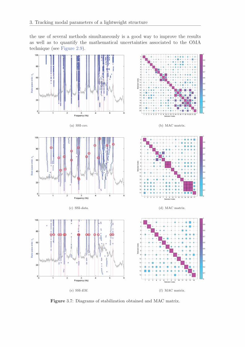
3. Tracking modal parameters of a lightweight structure
the use of several methods simultaneously is a good way to improve the resultsas well as to quantify the mathematical uncertainties associated to the OMAtechnique (see Figure 2.9).
(a) SSI-cov. (b) MAC matrix.
(c) SSI-data. (d) MAC matrix.
(e) SSI-EM. (f) MAC matrix.
Figure 3.7: Diagrams of stabilization obtained and MAC matrix.
81
0.5 1.0 1.5 2.0 2.5 3.0 3.5 4.00
20
40
60
80
100
Frequency (Hz)
State
space
order
Figure 3.8: Selected poles: SSI-cov (dashed lines), SSI-data (circles) and SSI-EM(crosses).
Table 3.1 shows the estimated natural frequencies and damping ratios. A MACcorrelation between the modal shapes estimated by three techniques has been car-ried out. Modes that exhibit a MAC value greater than 0.95 for all of the crossvalues are highlighted in bold. Note that even the mode at 1.05 Hz is estimatedby the three techniques, it is not finally selected due to the MAC discriminationparameter. Modes with natural frequencies over 4 Hz (0.8 times the cut-off fre-quency of the filter) are not included. Figure 3.9 shows an example of identifiedmodal shapes corresponding to the lowest seven modes obtained with SSI-cov.
Table 3.2 shows the summary of the selected modes. The table shows the meanvalues, the maximum relative error of the natural frequencies and the maximumabsolute error of the damping ratios. It is well known that the damping is esti-mated with greater variability than the natural frequencies [164], so it is betterto use absolute errors for damping estimates. The maximum errors obtained are0.6669 % and 26.67 % for frequencies and damping ratios, respectively. It is worthnoting the very low values obtained for the damping ratios although its estimationuncertainty is high, as usual [137].
The purpose of this subsection is to quantify uncertainties from the same time his-tory but employing three different SSI techniques to be sure that the comparisonof modal parameters of vibration modes corresponds to actually estimations of thesame vibration modes. The MAC value is usually used to compare experimentaland numerical modes shapes, nevertheless, this value can be used to compare any
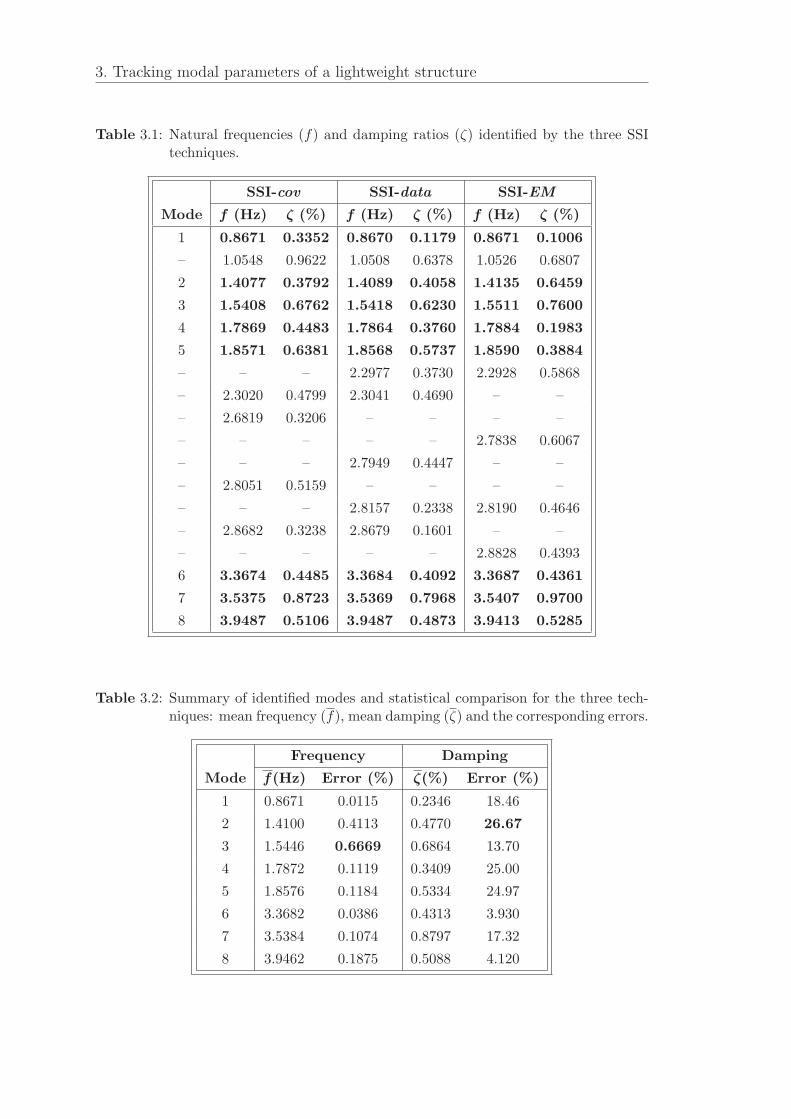
3. Tracking modal parameters of a lightweight structure
Table 3.1: Natural frequencies (f) and damping ratios (ζ) identified by the three SSItechniques.
SSI-cov SSI-data SSI-EM
Mode f (Hz) ζ (%) f (Hz) ζ (%) f (Hz) ζ (%)
1 0.8671 0.3352 0.8670 0.1179 0.8671 0.1006
– 1.0548 0.9622 1.0508 0.6378 1.0526 0.6807
2 1.4077 0.3792 1.4089 0.4058 1.4135 0.6459
3 1.5408 0.6762 1.5418 0.6230 1.5511 0.7600
4 1.7869 0.4483 1.7864 0.3760 1.7884 0.1983
5 1.8571 0.6381 1.8568 0.5737 1.8590 0.3884
– – – 2.2977 0.3730 2.2928 0.5868
– 2.3020 0.4799 2.3041 0.4690 – –
– 2.6819 0.3206 – – – –
– – – – – 2.7838 0.6067
– – – 2.7949 0.4447 – –
– 2.8051 0.5159 – – – –
– – – 2.8157 0.2338 2.8190 0.4646
– 2.8682 0.3238 2.8679 0.1601 – –
– – – – – 2.8828 0.4393
6 3.3674 0.4485 3.3684 0.4092 3.3687 0.4361
7 3.5375 0.8723 3.5369 0.7968 3.5407 0.9700
8 3.9487 0.5106 3.9487 0.4873 3.9413 0.5285
Table 3.2: Summary of identified modes and statistical comparison for the three tech-niques: mean frequency (f), mean damping (ζ) and the corresponding errors.
Frequency Damping
Mode f(Hz) Error (%) ζ(%) Error (%)
1 0.8671 0.0115 0.2346 18.46
2 1.4100 0.4113 0.4770 26.67
3 1.5446 0.6669 0.6864 13.70
4 1.7872 0.1119 0.3409 25.00
5 1.8576 0.1184 0.5334 24.97
6 3.3682 0.0386 0.4313 3.930
7 3.5384 0.1074 0.8797 17.32
8 3.9462 0.1875 0.5088 4.120
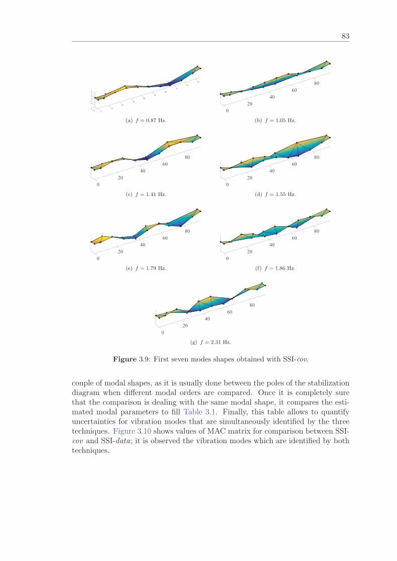
83
90
80
70
60
50
40
30
20-6-4-20
10
2
4
4
2 0 0
(a) f = 0.87 Hz.
8060
4020
0
(b) f = 1.05 Hz.
8060
4020
0
(c) f = 1.41 Hz.
8060
4020
0
(d) f = 1.55 Hz.
8060
4020
0
(e) f = 1.79 Hz.
8060
4020
0
(f) f = 1.86 Hz.
8060
4020
0
(g) f = 2.31 Hz.
Figure 3.9: First seven modes shapes obtained with SSI-cov.
couple of modal shapes, as it is usually done between the poles of the stabilizationdiagram when different modal orders are compared. Once it is completely surethat the comparison is dealing with the same modal shape, it compares the esti-mated modal parameters to fill Table 3.1. Finally, this table allows to quantifyuncertainties for vibration modes that are simultaneously identified by the threetechniques. Figure 3.10 shows values of MAC matrix for comparison between SSI-cov and SSI-data; it is observed the vibration modes which are identified by bothtechniques.

3. Tracking modal parameters of a lightweight structure
1 2 3 4 5 6 7 8 9 10111213
14
12345678910111213
0
0.2
0.4
0.6
0.8
1
0
0.1
0.2
0.3
0.4
0.5
0.6
0.7
0.8
0.9
1
SSI-dataSSI-cov
MAC
(a) 3D view.
1 2 3 4 5 6 7 8 9 10 11 12 13 14
1
2
3
4
5
6
7
8
9
10
11
12
13
0
0.1
0.2
0.3
0.4
0.5
0.6
0.7
0.8
0.9
1
SSI-data
SSI-cov
(b) 2D view.
Figure 3.10: MAC comparison between SSI-cov and SSI-data.
3.3.3 Operational Modal Analysis using the same SSI tech-nique
In order to track the modal parameters of a structure, it is recommended to usethe minimum test duration that leads to a successful identification. As a rule ofthumb, the minimum duration of the measurement should be at least 1000 cyclesof the lowest natural frequency is expected to be identified [205]. This durationis usually recommended as the minimum one for noise-contaminated signals andclose vibration modes. Therefore, this duration, which corresponds approximatelyto 20 minutes, has been adopted here to carry out the modal tracking.
Now, three consecutive windows of 20-minute data are considered to identify themodal parameters using only SSI-cov. These results are compared with thoseobtained using the 60-minute record. Table 3.3 shows the estimates obtained fromthe four data blocks. Using the same criterion as in the previous case, modes thatexhibit a MAC value greater than 0.95 for all of the cross values are highlightedin bold. The average temperature for each time window was 16.42, 13.84 and11.56 ◦C, respectively, and 13.94 ◦C for the 60-minute record.
Table 3.4 presents a summary of the selected modes. The table shows the meanvalues for the 20-minute tests and the maximum errors compared with the resultsobtained with the 60-minute test. In this case, the maximum errors obtainedare 0.2855 % and 61.09 % for frequencies and damping ratios, respectively. Theerrors in natural frequency estimates using 20 minutes as compared with 60 arenegligible.
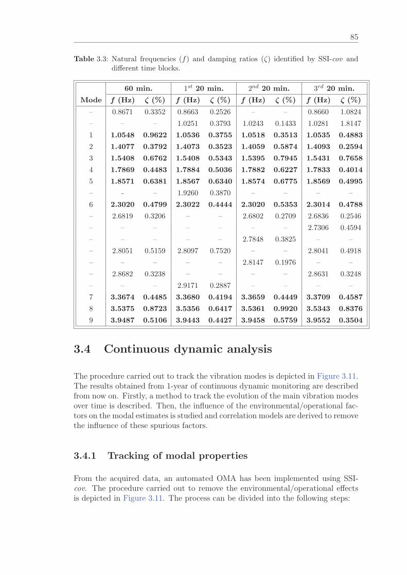
85
Table 3.3: Natural frequencies (f) and damping ratios (ζ) identified by SSI-cov anddifferent time blocks.
60 min. 1st 20 min. 2nd 20 min. 3rd 20 min.
Mode f (Hz) ζ (%) f (Hz) ζ (%) f (Hz) ζ (%) f (Hz) ζ (%)
– 0.8671 0.3352 0.8663 0.2526 – – 0.8660 1.0824
– – – 1.0251 0.3793 1.0243 0.1433 1.0281 1.8147
1 1.0548 0.9622 1.0536 0.3755 1.0518 0.3513 1.0535 0.4883
2 1.4077 0.3792 1.4073 0.3523 1.4059 0.5874 1.4093 0.2594
3 1.5408 0.6762 1.5408 0.5343 1.5395 0.7945 1.5431 0.7658
4 1.7869 0.4483 1.7884 0.5036 1.7882 0.6227 1.7833 0.4014
5 1.8571 0.6381 1.8567 0.6340 1.8574 0.6775 1.8569 0.4995
– - – 1.9260 0.3870 – – – –
6 2.3020 0.4799 2.3022 0.4444 2.3020 0.5353 2.3014 0.4788
– 2.6819 0.3206 – – 2.6802 0.2709 2.6836 0.2546
– – – – – – – 2.7306 0.4594
– – – – – 2.7848 0.3825 – –
– 2.8051 0.5159 2.8097 0.7520 – – 2.8041 0.4918
– – – – – 2.8147 0.1976 – –
– 2.8682 0.3238 – – – – 2.8631 0.3248
– – – 2.9171 0.2887 – – – –
7 3.3674 0.4485 3.3680 0.4194 3.3659 0.4449 3.3709 0.4587
8 3.5375 0.8723 3.5356 0.6417 3.5361 0.9920 3.5343 0.8376
9 3.9487 0.5106 3.9443 0.4427 3.9458 0.5759 3.9552 0.3504
3.4 Continuous dynamic analysis
The procedure carried out to track the vibration modes is depicted in Figure 3.11.The results obtained from 1-year of continuous dynamic monitoring are describedfrom now on. Firstly, a method to track the evolution of the main vibration modesover time is described. Then, the influence of the environmental/operational fac-tors on the modal estimates is studied and correlation models are derived to removethe influence of these spurious factors.
3.4.1 Tracking of modal properties
From the acquired data, an automated OMA has been implemented using SSI-cov. The procedure carried out to remove the environmental/operational effectsis depicted in Figure 3.11. The process can be divided into the following steps:
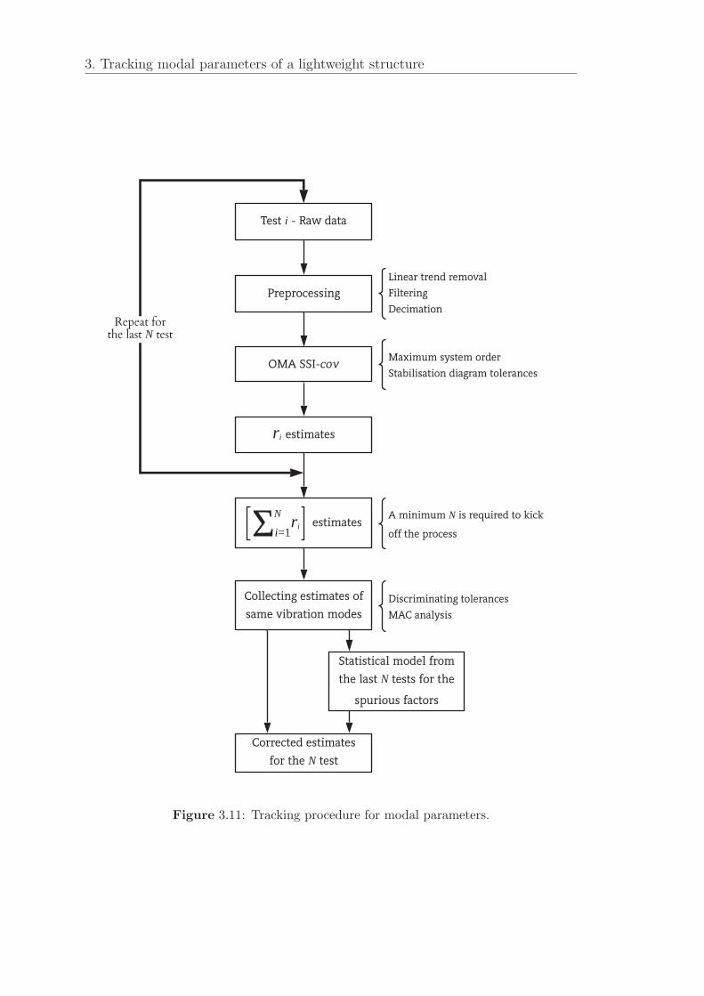
3. Tracking modal parameters of a lightweight structure
Figure 3.11: Tracking procedure for modal parameters.
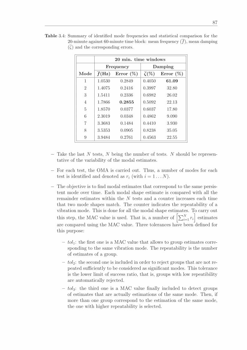
87
Table 3.4: Summary of identified mode frequencies and statistical comparison for the20-minute against 60-minute time block: mean frequency (f), mean damping(ζ) and the corresponding errors.
20 min. time windows
Frequency Damping
Mode f(Hz) Error (%) ζ(%) Error (%)
1 1.0530 0.2849 0.4050 61.09
2 1.4075 0.2416 0.3997 32.80
3 1.5411 0.2336 0.6982 26.02
4 1.7866 0.2855 0.5092 22.13
5 1.8570 0.0377 0.6037 17.80
6 2.3019 0.0348 0.4862 9.090
7 3.3683 0.1484 0.4410 3.930
8 3.5353 0.0905 0.8238 35.05
9 3.9484 0.2761 0.4563 22.55
− Take the last N tests, N being the number of tests. N should be represen-tative of the variability of the modal estimates.
− For each test, the OMA is carried out. Thus, a number of modes for eachtest is identified and denoted as ri (with i = 1 . . . N).
− The objective is to find modal estimates that correspond to the same persis-tent mode over time. Each modal shape estimate is compared with all theremainder estimates within the N tests and a counter increases each timethat two mode shapes match. The counter indicates the repeatability of avibration mode. This is done for all the modal shape estimates. To carry out
this step, the MAC value is used. That is, a number of[∑N
i=1 ri
]estimates
are compared using the MAC value. Three tolerances have been defined forthis purpose:
– tol1: the first one is a MAC value that allows to group estimates corre-sponding to the same vibration mode. The repeatability is the numberof estimates of a group.
– tol2: the second one is included in order to reject groups that are not re-peated sufficiently to be considered as significant modes. This toleranceis the lower limit of success ratio, that is, groups with low repeatibilityare automatically rejected.
– tol3: the third one is a MAC value finally included to detect groupsof estimates that are actually estimations of the same mode. Then, ifmore than one group correspond to the estimation of the same mode,the one with higher repeatability is selected.
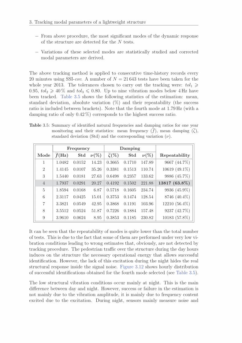
3. Tracking modal parameters of a lightweight structure
− From above procedure, the most significant modes of the dynamic responseof the structure are detected for the N tests.
− Variations of these selected modes are statistically studied and correctedmodal parameters are derived.
The above tracking method is applied to consecutive time-history records every20 minutes using SSI-cov. A number of N = 21 643 tests have been taken for thewhole year 2013. The tolerances chosen to carry out the tracking were: tol1 �0.95, tol2 � 40 % and tol3 � 0.80. Up to nine vibration modes below 4 Hz havebeen tracked. Table 3.5 shows the following statistics of the estimation: mean,standard deviation, absolute variation (%) and their repeatability (the successratio is included between brackets). Note that the fourth mode at 1.79 Hz (with adamping ratio of only 0.42 %) corresponds to the highest success ratio.
Table 3.5: Summary of identified natural frequencies and damping ratios for one yearmonitoring and their statistics: mean frequency (f), mean damping (ζ),standard deviation (Std) and the corresponding variation (ν).
Frequency Damping
Mode f(Hz) Std ν(%) ζ(%) Std ν(%) Repeatability
1 1.0482 0.0152 14.23 0.3665 0.1710 147.89 9667 (44.7%)
2 1.4145 0.0107 35.26 0.3381 0.1513 110.74 10619 (49.1%)
3 1.5440 0.0181 27.63 0.6498 0.2357 133.62 9886 (45.7%)
4 1.7937 0.0291 20.27 0.4192 0.1502 221.88 13817 (63.8%)
5 1.8594 0.0168 6.87 0.5718 0.1605 234.74 9936 (45.9%)
6 2.3117 0.0425 15.01 0.3753 0.1474 128.54 8746 (40.4%)
7 3.3821 0.0549 42.95 0.3868 0.1191 103.96 12210 (56.4%)
8 3.5512 0.0524 51.87 0.7226 0.1884 157.48 9237 (42.7%)
9 3.9610 0.0624 8.95 0.3853 0.1185 230.82 10183 (57.8%)
It can be seen that the repeatability of modes is quite lower than the total numberof tests. This is due to the fact that some of them are performed under very low vi-bration conditions leading to wrong estimates that, obviously, are not detected bytracking procedure. The pedestrian traffic over the structure during the day hoursinduces on the structure the necessary operational energy that allows successfulidentification. However, the lack of this excitation during the night hides the realstructural response inside the signal noise. Figure 3.12 shows hourly distributionof successful identifications obtained for the fourth mode selected (see Table 3.5).
The low structural vibration conditions occur mainly at night. This is the maindifference between day and night. However, success or failure in the estimation isnot mainly due to the vibration amplitude, it is mainly due to frequency contentexcited due to the excitation. During night, sensors mainly measure noise and
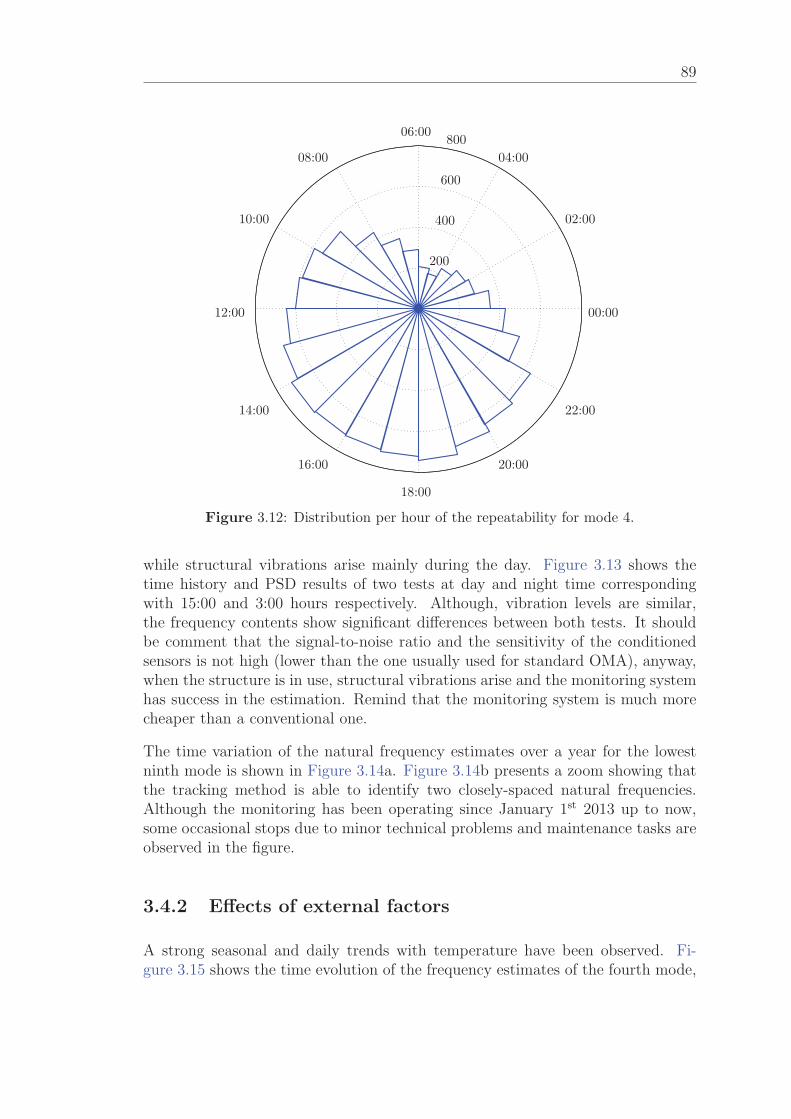
89
200
400
600
800
02:00
14:00
04:00
16:00
06:00
18:00
08:00
20:00
10:00
22:00
12:00 00:00
Figure 3.12: Distribution per hour of the repeatability for mode 4.
while structural vibrations arise mainly during the day. Figure 3.13 shows thetime history and PSD results of two tests at day and night time correspondingwith 15:00 and 3:00 hours respectively. Although, vibration levels are similar,the frequency contents show significant differences between both tests. It shouldbe comment that the signal-to-noise ratio and the sensitivity of the conditionedsensors is not high (lower than the one usually used for standard OMA), anyway,when the structure is in use, structural vibrations arise and the monitoring systemhas success in the estimation. Remind that the monitoring system is much morecheaper than a conventional one.
The time variation of the natural frequency estimates over a year for the lowestninth mode is shown in Figure 3.14a. Figure 3.14b presents a zoom showing thatthe tracking method is able to identify two closely-spaced natural frequencies.Although the monitoring has been operating since January 1st 2013 up to now,some occasional stops due to minor technical problems and maintenance tasks areobserved in the figure.
3.4.2 Effects of external factors
A strong seasonal and daily trends with temperature have been observed. Fi-gure 3.15 shows the time evolution of the frequency estimates of the fourth mode,
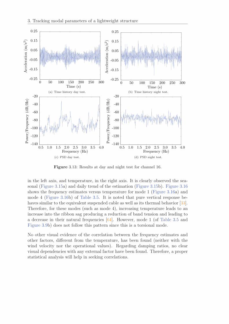
3. Tracking modal parameters of a lightweight structure
0 50 100 150 200 250 300-0.25
-0.15
-0.05
0.05
0.15
0.25
Time (s)
Acceleration(m
/s2)
(a) Time history day test.
0 50 100 150 200 250 300-0.25
-0.15
-0.05
0.05
0.15
0.25
Time (s)
Acceleration(m
/s2)
(b) Time history night test.
0.5 1.0 1.5 2.0 2.5 3.0 3.5 4.0-140
-120
-100
-80
-60
-40
-20
Frequency (Hz)
Pow
er/Frequency
(dB/Hz)
(c) PSD day test.
0.5 1.0 1.5 2.0 2.5 3.0 3.5 4.0-140
-120
-100
-80
-60
-40
-20
Frequency (Hz)
Pow
er/Frequency
(dB/Hz)
(d) PSD night test.
Figure 3.13: Results at day and night test for channel 16.
in the left axis, and temperature, in the right axis. It is clearly observed the sea-sonal (Figure 3.15a) and daily trend of the estimation (Figure 3.15b). Figure 3.16shows the frequency estimates versus temperature for mode 1 (Figure 3.16a) andmode 4 (Figure 3.16b) of Table 3.5. It is noted that pure vertical response be-haves similar to the equivalent suspended cable as well as its thermal behavior [33].Therefore, for these modes (such as mode 4), increasing temperature leads to anincrease into the ribbon sag producing a reduction of band tension and leading toa decrease in their natural frequencies [64]. However, mode 1 (of Table 3.5 andFigure 3.9b) does not follow this pattern since this is a torsional mode.
No other visual evidence of the correlation between the frequency estimates andother factors, different from the temperature, has been found (neither with thewind velocity nor the operational values). Regarding damping ratios, no clearvisual dependencies with any external factor have been found. Therefore, a properstatistical analysis will help in seeking correlations.
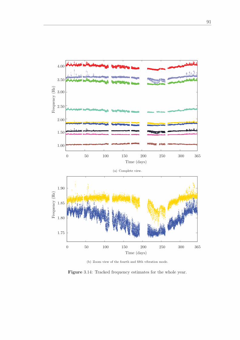
91
0 50 100 150 200 250 300 365
1.00
1.50
2.00
2.50
3.00
3.50
4.00
Time (days)
Frequency
(Hz)
(a) Complete view.
0 50 100 150 200 250 300 365
1.75
1.80
1.85
1.90
Time (days)
Frequency
(Hz)
(b) Zoom view of the fourth and fifth vibration mode.
Figure 3.14: Tracked frequency estimates for the whole year.

3. Tracking modal parameters of a lightweight structure
1.72
1.77
1.83
1.88Frequency
(Hz)
Time (days)
0 50 100 150 200 250 300 365−10
10
30
50
Tem
perature
(◦C)
(a) Complete view.
1.75
1.77
1.80
1.83
Frequency
(Hz)
Time (days)
130 132 134 136 138 140 142 144 146 148 1500
10
20
30
Tem
perature
(◦C)
(b) Zoom view of 20 days.
Figure 3.15: Frequency estimates and temperature recorded for mode 4.
3.4.3 Statistical analysis
A correlation analysis has been carried out in order to study the influence of theexternal effects on the natural frequencies and damping ratios. The technique em-ployed to study the dependence of a dependent variable y with other independentvariables or predictors has been the Multiple Linear Regression (MLR). Generally,the equation of MLR can be written as
y = Zβ + ε = y + ε, (3.1)
Z = [1, Z1, . . . , Zk] is a row vector of (k+ 1) terms that contains the k predictors,β = [β0, β1, . . . , βk]′ is a column vector of (k + 1) coefficients to be determined
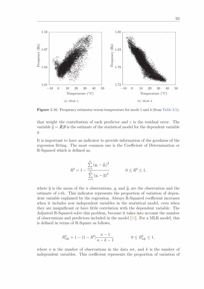
93
−10 0 10 20 30 40 50
1.04
1.07
1.01
1.10
Temperature (◦C)
Frequency
(Hz)
(a) Mode 1.
−10 0 10 20 30 40 501.72
1.78
1.83
1.88
Temperature (◦C)
Frequency
(Hz)
(b) Mode 4.
Figure 3.16: Frequency estimates versus temperature for mode 1 and 4 (from Table 3.5).
that weight the contribution of each predictor and ε is the residual error. Thevariable y = Zβ is the estimate of the statistical model for the dependent variabley.
It is important to have an indicator to provide information of the goodness of theregression fitting. The most common one is the Coefficient of Determination orR-Squared which is defined as,
R2 = 1 −
n∑i=1
(yi − yi)2
n∑i=1
(yi − y)20 ≤ R2 ≤ 1,
where y is the mean of the n observations, yi and yi are the observation and theestimate of i-th. This indicator represents the proportion of variation of depen-dent variable explained by the regression. Always R-Squared coefficient increaseswhen it includes new independent variables in the statistical model, even whenthey are insignificant or have little correlation with the dependent variable. TheAdjusted R-Squared solve this problem, because it takes into account the numberof observations and predictors included in the model [53]. For a MLR model, thisis defined in terms of R-Square as follows,
R2adj = 1 − (1 −R2)
n− 1
n− k − 10 ≤ R2
adj ≤ 1,
where n is the number of observations in the data set, and k is the number ofindependent variables. This coefficient represents the proportion of variation of
3. Tracking modal parameters of a lightweight structure
the dependent variable explained by the regression model. The increase in the Ad-justed R-Squared by each additional predictor indicates the improvement providedby this predictor.
The independent variables have been considered as function of the ambient temper-ature, structure acceleration and wind speed. Thus, the statistical model adoptedconsists of linearly fitting the independent variables (that might be non linear func-tions of environmental/operational measurements) which are selected according toits statistical relevance. Furthermore, temperature dependence is also explored notonly at current test, but also on the temperatures observed in previous tests. Thatis, a dynamic regression model is adopted regarding the temperature dependence.
The estimates have been considered as function of the following variables
y = g (T, (ΔT/Δt)i , TRj, amax, aRMS, VDV, Vmax, VRMS), (3.2)
where y is the modal estimate, T is the temperature associated of each test (themean temperature of the test is taken), (ΔT/Δt)i is the gradient of temperaturebetween the current test and the i-times former test, TRj
is the running averagedtemperature using the j previous tests, a is the vertical acceleration and V isthe wind velocity. Variables aRMS and VDV are measures suitable to asses thevibration serviceability for pedestrian structures [95]. Contrary to peak and RMSaccelerations, VDV accumulates the vibration effects rather than averaging themand increases with duration. Equation 3.2 according to Equation 3.1 is consideredas
y = β0 +k∑
r=1
βr Zr, (3.3)
in which Zr ∈ [zr, z2r , . . . , z
nr , 1/zr, 1/z2r , . . . , 1/znr ], exploring thus nonlinear rela-
tionships, with zr being the independent variables that appear in Equation 3.2,the coefficients βr are obtained from the linear-least square solutions and k thenumber of predictors for the model.
In order to extract the corrected estimates and remove the spurious effects, modelof Equation 3.3 is rewritten as follows
y =
(β0 +
k∑r=1
βr Zr
)︸ ︷︷ ︸
y∗
+k∑
r=1
βr(Zr − Zr
), (3.4)
where Zr is the mean value of all the observations of Zr and y∗ is the correctedestimate, defined as
95
y∗ = β0 +k∑
r=1
βr Zr. (3.5)
The MLR presented above has been applied to frequency and damping ratio es-timates for all of the tracked modes (of Table 3.5). It is considered i = 1, 2,. . ., 30, j = 50, 100, 250, 1000, 1500, 2000 (see Equation 3.2), and n = 3 andk = 4 (see Equation 3.3 and definition of Zr). Eventually, it has been considered252 candidates for predictors. Thus, Table 3.6 shows the values of the AdjustedR-Squared for all the natural frequency estimates of the selected modes as thenumber of predictors increase in the statistical models. The predictors of thosemodels that obtain a value of the Adjusted R-Squared greater than 0.80 are alsoshown in Table 3.6. The last column of the table is the maximum Adjusted R-Squared, R2
max, obtained for the maximum number of predictors, kmax, for eachmodel (which is shown between brackets). It is observed that those modes withhigher Adjusted R-Squared (modes 4, 6, 7 and 9), R2
max > 0.90, have independentvariables related to the temperature as predictors. It is also observed that thereare two modes, 1 and 2, both with Adjusted R-Square close to 0.80, in whichserviceability parameters are used as predictors 3rd and 4th for their respectivemodels (see Table 3.6).
The frequency distribution for each mode is shown in Figure 3.17. There are somemodes (3, 5 and 8) whose frequencies have a very narrow distribution, indicatingthat: (i) they do not change significantly, (ii) they do not need any correctionand (iii) they might be already used for SHM. Therefore, the variation of thesemodes can not be explained, leading thus to Adjusted R-Squared lower than theremainders. Figure 3.18 shows the damping ratio distribution for each mode. Itcan be observed that the damping of these modes of the structure are most of themvery low (mean value less than 0.5 %), except for modes 3, 5 and 8, for which itsmean value is greater than 0.5 %. These modes are the same which also have avery narrow distribution frequency.
Finally, very low values for the Adjusted R-Squared (smaller than 0.20) wereachieved for damping ratios. Therefore, the results for the damping ratios are notpresented here because there is no clear dependency of damping ratio variations.
3.4.4 Removing external factors
As an example, the model obtained for the natural frequency estimate of mode 4 isexpounded in detail. This is the mode with highest success ratio and whose modelachieves the highest Adjusted R-Squared. The model obtained for the statisticalfrequency is the following,

3. Tracking modal parameters of a lightweight structure
1 1.5 2 2.5 3 3.5 4 4.5
1
2
3
4
5
6
7
8
9
Frequency (Hz)
Distributionforeach
mode
Figure 3.17: Overlaid distributions of the identified natural frequencies.
f = β0 + β1 · T + β2 · (ΔT/Δt)19 + β4 · T 2︸ ︷︷ ︸Daily
+ β3 · TR1000︸ ︷︷ ︸Seasonal
, (3.6)
where f is the frequency estimate by statistical model. Equation 3.6 shows thedependency on the temperature, on the temperature gradient with respect tothe 19-times former test (Δt19 = 19 · 20 = 380 minutes), the running averagedtemperature using 1000 previous tests and the temperature to the second power.These values have provided the higher increment into the Adjusted R-Squared.Additional predictors introduce only marginal improvements into the correlation.
In order to test this statistical model, the first 20 days of January 2014 are used as“unseen data”. Figure 3.19 shows the frequency estimates by the SSI-cov techniqueand by the statistical model of Equation 3.6. The maximum relative error did notexceeded 1 %.
As stated in Equation 3.5 and according to Equation 3.6, the corrected frequencyis as follows
f ∗ = β0 + β1 · T + β2 ·(
ΔT/Δt)19
+ β3 · TR1000 + β4 · T 2. (3.7)
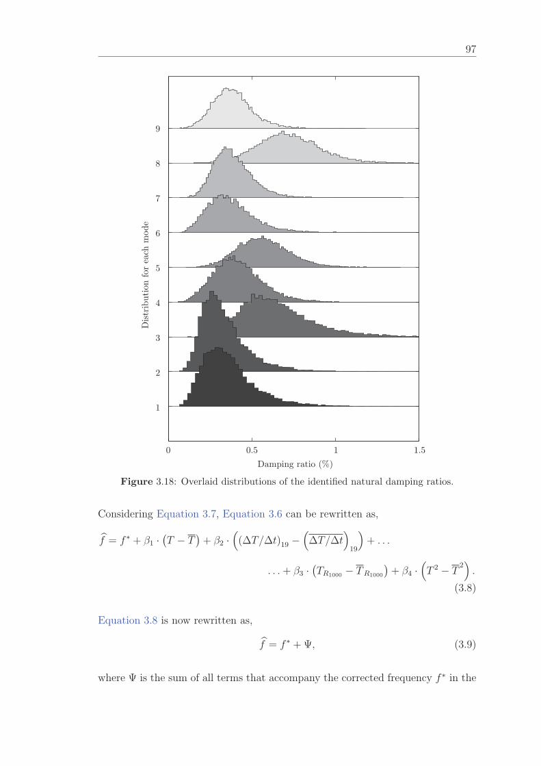
97
0 0.5 1 1.5
1
2
3
4
5
6
7
8
9
Damping ratio (%)
Distributionforeach
mode
Figure 3.18: Overlaid distributions of the identified natural damping ratios.
Considering Equation 3.7, Equation 3.6 can be rewritten as,
f = f ∗ + β1 ·(T − T
)+ β2 ·
((ΔT/Δt)19 −
(ΔT/Δt
)19
)+ . . .
. . .+ β3 ·(TR1000 − TR1000
)+ β4 ·
(T 2 − T
2).
(3.8)
Equation 3.8 is now rewritten as,
f = f ∗ + Ψ, (3.9)
where Ψ is the sum of all terms that accompany the corrected frequency f ∗ in the
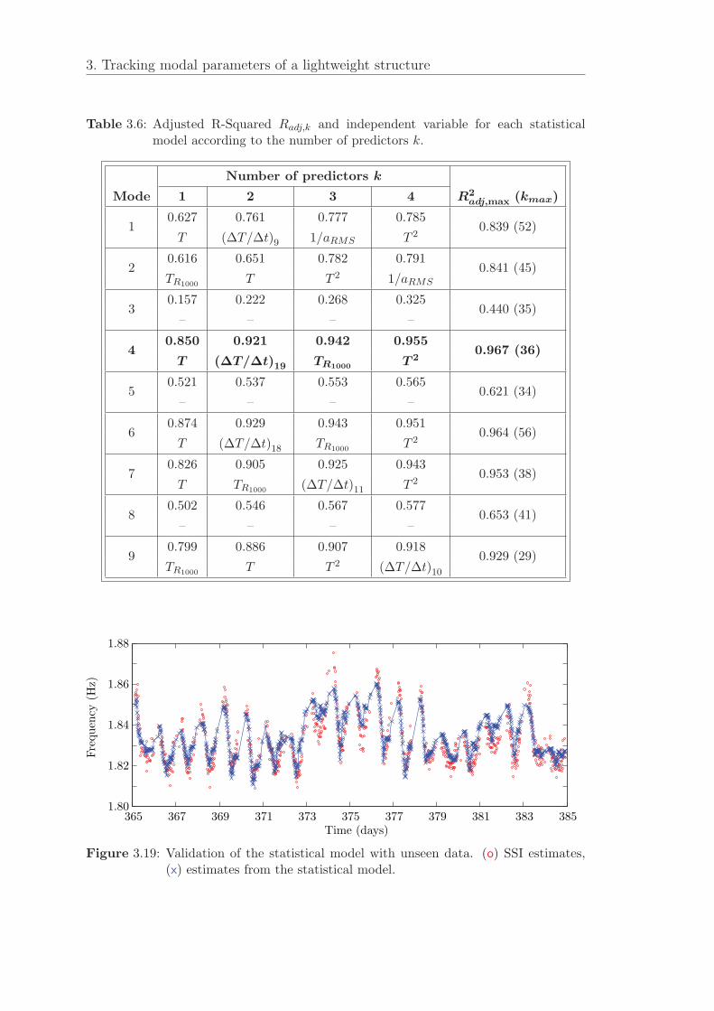
3. Tracking modal parameters of a lightweight structure
Table 3.6: Adjusted R-Squared Radj,k and independent variable for each statisticalmodel according to the number of predictors k.
Number of predictors k
Mode 1 2 3 4 R2adj,max (kmax)
10.627 0.761 0.777 0.785
0.839 (52)T (ΔT/Δt)9 1/aRMS T 2
20.616 0.651 0.782 0.791
0.841 (45)TR1000 T T 2 1/aRMS
30.157 0.222 0.268 0.325
0.440 (35)– – – –
0.850 0.921 0.942 0.9554
T (ΔT/Δt)19 TR1000 T 20.967 (36)
50.521 0.537 0.553 0.565
0.621 (34)– – – –
60.874 0.929 0.943 0.951
0.964 (56)T (ΔT/Δt)18 TR1000 T 2
70.826 0.905 0.925 0.943
0.953 (38)T TR1000 (ΔT/Δt)11 T 2
80.502 0.546 0.567 0.577
0.653 (41)– – – –
90.799 0.886 0.907 0.918
0.929 (29)TR1000 T T 2 (ΔT/Δt)10
365 367 369 371 373 375 377 379 381 383 3851.80
1.82
1.84
1.86
1.88
Time (days)
Frequency
(Hz)
Figure 3.19: Validation of the statistical model with unseen data. (o) SSI estimates,(x) estimates from the statistical model.
99
right hand side of Equation 3.8. Taking into account that, in this case, the inde-pendent variable is the natural frequency estimated by SSI (f (SSI)), Equation 3.1can be expressed
f (SSI) = f + ε, (3.10)
where ε is the residual error. Replacing Equation 3.9 into Equation 3.10, it leadsto
f (SSI) − Ψ = f ∗ + ε = f ∗, (3.11)
in which f ∗ is the corrected frequency estimate, i.e. the corrected frequency in-cluding the residual error, which is independent of the influence of the consideredpredictors. Figure 3.20a and Figure 3.20b show f (SSI), f ∗ and f ∗ for mode 4. Itcan be observed that the variability range decreases from 0.1422 to 0.0446 Hz (thatis, a 70 % reduction has been achieved). Finally, Figures 3.20c and 3.20d show thedistribution of the residual errors for the SSI frequency estimate f (SSI) and thecorrected frequency estimate f ∗ as well as their fittings to a Normal Gaussian Dis-tribution. It is worthy to remark that the residual error for the corrected estimatefits to a Normal Gaussian Distribution, indicating that dependencies with externalagents have been successfully eliminated.
3.5 Vibration Serviceability Assessment
The data collected with the low-cost vibration monitoring system have been alsoused to assess vibration serviceability using a general standard for human-inducedvibration [40, 182]. Current codes and design guidelines for footbridges considersingle-frequency excitation and rely on peak-acceleration-based criteria. However,standards ISO 2631-1:1997 [96] and ISO 10137:2007 [94], suitable for general hu-man exposure evaluation to whole-body vibrations, are used here to obtain severalvibration predictors: RMS acceleration, MTVV, VDV, CDF of peak weighted ver-tical acceleration and crest factor which is obtained from the ratio between thepeak weighted acceleration and the total RMS value. These predictors are in-teresting when long-term vibration assessment is carried out since they take intoaccount the duration of the vibration exposure as well as the effect of combinedmulti-axis, multi-frequency vibration.
The Vibration Serviceability Analysis (VSA) presented here is for one-year mon-itoring. Mode 4 is the most persistent throughout the one year of monitoringbecause it is the most excited and the most representative of the structure re-sponse (see Table 3.5). Because of this, the VSA presented in this section is onlycarried out for the accelerometer corresponding to the point of maximum displace-ment of this mode. This point is at one lateral side of the deck at 77.25 m fromabutment.
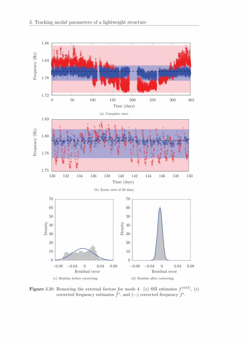
3. Tracking modal parameters of a lightweight structure
0 50 100 150 200 250 300 3651.72
1.78
1.83
1.88
Time (days)
Frequency
(Hz)
(a) Complete view.
130 132 134 136 138 140 142 144 146 148 150
1.75
1.78
1.80
1.83
Time (days)
Frequency
(Hz)
(b) Zoom view of 20 days.
−0.08 −0.04 0 0.04 0.08
0
10
20
30
40
50
60
70
Residual error
Den
sity
(c) Residue before correcting.
−0.08 −0.04 0 0.04 0.08
0
10
20
30
40
50
60
70
Residual error
Den
sity
(d) Residue after correcting.
Figure 3.20: Removing the external factors for mode 4. (x) SSI estimates f (SSI), (x)corrected frequency estimates f∗, and (- -) corrected frequency f∗.
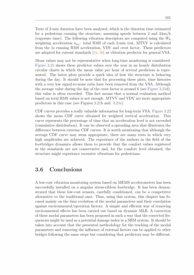
101
Tests of 2-min duration have been analysed, which is the duration time estimatedfor a pedestrian crossing the structure, assuming speeds between 2 and 3 km/h(exposure time). The following vibration descriptors are computed using the Wk
weighting acceleration awk: total RMS of each 2-min test, MTVV is calculated
from the 1s running RMS acceleration, VDV and crest factor. These predictorsare adopted for current standards [94, 96] as vibration predictor for general VSA.
Mean values may not be representative when long-time monitoring is considered.Figure 3.21 shows these predictor values over the year in an hourly distributioncircular charts in which the mean value per hour of several predictors is repre-sented. The latter plots provide a quick idea of how the structure is behavingduring the day. It should be note that for processing these plots, time historieswith a very low signal-to-noise ratio have been removed from the VSA. Althoughthe average value during the day of the crest factor is around 6 (see Figure 3.21d),this value is often exceeded. This fact means that a normal evaluation methodbased on total RMS values is not enough. MTVV and VDV are more appropriatepredictors in this case (see Figures 3.21b and 3.21c).
CDF curves provides a really valuable information for long-term VSA. Figure 3.22shows the mean CDF curve obtained for weighted vertical acceleration. Thiscurve represents the percentage of time that an acceleration level is not exceeded(cumulative distribution). It can be observed a spreading area that illustrates thedifference between extreme CDF curves. It is worth mentioning that although theaverage CDF curve may seem appropriate, there are many tests in which veryhigh amplitudes are achieved. The experience of the authors in the field of thefootbridges dynamics allows them to provide that the comfort values registeredin the standards are not conservative and, for the comfort level obtained, thestructure might experience excessive vibrations for pedestrians.
3.6 Conclusions
A low-cost vibration monitoring system based on MEMS accelerometers has beensuccessfully installed on a singular stress-ribbon footbridge. It has been demon-strated that these low-cost sensors, carefully conditioned, can be a competitivealternative to the traditional ones. Thus, using this system, this chapter has fo-cused mainly on the time evolution of the modal parameters and their correlationagainst environmental/operation factors. A simple and efficient way of removingenvironmental effects has been carried out based on dynamic MLR. A correctionof these modal parameters has been proposed in such a way that the corrected fre-quencies might be used as a potential damage index in a SHM system. It should betaken into account that the presented methodology for the tracking of the modalparameters and removing the influence of external factors can be applied to otherbridges following the same steps but considering that predictors may be different.
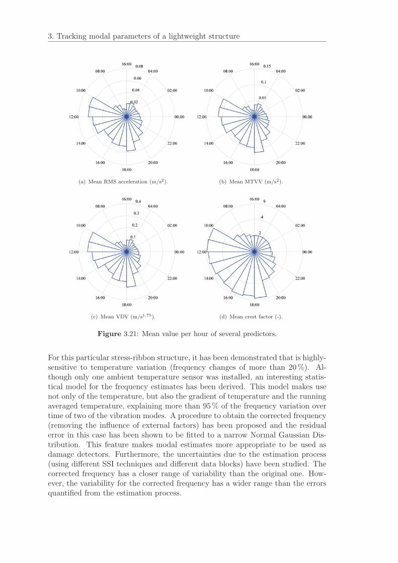
3. Tracking modal parameters of a lightweight structure
(a) Mean RMS acceleration (m/s2). (b) Mean MTVV (m/s2).
(c) Mean VDV (m/s1.75). (d) Mean crest factor (-).
Figure 3.21: Mean value per hour of several predictors.
For this particular stress-ribbon structure, it has been demonstrated that is highly-sensitive to temperature variation (frequency changes of more than 20 %). Al-though only one ambient temperature sensor was installed, an interesting statis-tical model for the frequency estimates has been derived. This model makes usenot only of the temperature, but also the gradient of temperature and the runningaveraged temperature, explaining more than 95 % of the frequency variation overtime of two of the vibration modes. A procedure to obtain the corrected frequency(removing the influence of external factors) has been proposed and the residualerror in this case has been shown to be fitted to a narrow Normal Gaussian Dis-tribution. This feature makes modal estimates more appropriate to be used asdamage detectors. Furthermore, the uncertainties due to the estimation process(using different SSI techniques and different data blocks) have been studied. Thecorrected frequency has a closer range of variability than the original one. How-ever, the variability for the corrected frequency has a wider range than the errorsquantified from the estimation process.
103
Figure 3.22: Mean curve of likelihood of non-exceeded for weighted vertical acceler-ation. The shaded area indicates the range between the minimum andmaximum curves for one-year monitoring.
A VSA of an in-service footbridge for vertical direction has been presented, em-ploying a group of vibration predictors, such as RMS acceleration, MTVV, or crestfactor, over one-year monitoring. Therefore, a comfort level for the structure couldbe properly established. The different predictors for general VSA are computed.

4Study of semi-active
implementable strategies
Contents4.1 Introduction . . . . . . . . . . . . . . . . . . . . . . . . . 105
4.2 Structure models . . . . . . . . . . . . . . . . . . . . . . . 106
4.3 Loading cases . . . . . . . . . . . . . . . . . . . . . . . . . 107
4.4 Vibration control strategies . . . . . . . . . . . . . . . . 109
4.4.1 Passive and semi-active control . . . . . . . . . . . . . . 109
4.4.2 Active control . . . . . . . . . . . . . . . . . . . . . . . . 110
4.5 Results with TMD, STMD 1 and STMD 2 . . . . . . . 113
4.5.1 Single degree of freedom system . . . . . . . . . . . . . . 114
4.5.2 Multi-degree of freedom system . . . . . . . . . . . . . . 115
4.6 Results with TMD, STMD 1 and AMD . . . . . . . . . 117
4.7 Discussion . . . . . . . . . . . . . . . . . . . . . . . . . . . 119
4.1 Introduction
The in-service steel-plated stress-ribbon PGB Footbridge presented in the pre-vious chapter was analysed and the influence of the environmental factors onmodal parameter estimation was therefore extensively studied. It was found thatthis structure has the most perceptible vibration mode at approximately 1.8 Hz(within the normal range of walking). Through a peered analysis of a full-yearmonitoring, it was obtained that this mode changes up to 20 % during the yearwith both seasonal and daily trends and that these changes were mainly explainedby temperature variation. Furthermore, the structure has other vibration modes
105
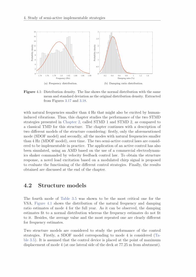
4. Study of semi-active implementable strategies
1.74 1.76 1.78 1.8 1.82 1.84 1.86 1.88Frequency (Hz)
0
2
4
6
8
10
12
14
16
18Pr
obab
ility
den
sity
(a) Frequency distribution.
0.2 0.4 0.6 0.8 1 1.2 1.4Damping ratio (%)
0
0.5
1
1.5
2
2.5
3
Prob
abili
ty d
ensi
ty
(b) Damping ratio distribution.
Figure 4.1: Distribution density. The line shows the normal distribution with the samemean and standard deviation as the original distribution density. Extractedfrom Figures 3.17 and 3.18.
with natural frequencies smaller than 4 Hz that might also be excited by human-induced vibrations. Thus, this chapter studies the performance of the two STMDstrategies presented in Chapter 2, called STMD 1 and STMD 2, as compared toa classical TMD for this structure. The chapter continues with a description oftwo different models of the structure considering: firstly, only the aforementionedmode (SDOF model) and secondly, all the modes with natural frequencies smallerthan 4 Hz (MDOF model), over time. The two semi-active control laws are consid-ered to be implementable in practice. The application of an active control has alsobeen simulated, using an AMD based on the use of a commercial electrodynam-ics shaker commanded by velocity feedback control law. To obtain the structureresponse, a novel load excitation based on a modulated chirp signal is proposedto evaluate the functioning of the different control strategies. Finally, the resultsobtained are discussed at the end of the chapter.
4.2 Structure models
The fourth mode of Table 3.5 was shown to be the most critical one for theVSA. Figure 4.1 shows the distribution of the natural frequency and dampingratio estimates of mode 4 for the full year. As it can be observed, the dampingestimates fit to a normal distribution whereas the frequency estimates do not fitto it. Besides, the average value and the most repeated one are clearly differentfor frequency estimates.
Two structure models are considered to study the performance of the controlstrategies. Firstly, a SDOF model corresponding to mode 4 is considered (Ta-ble 3.5). It is assumed that the control device is placed at the point of maximumdisplacement of mode 4 (at one lateral side of the deck at 77.25 m from abutment).
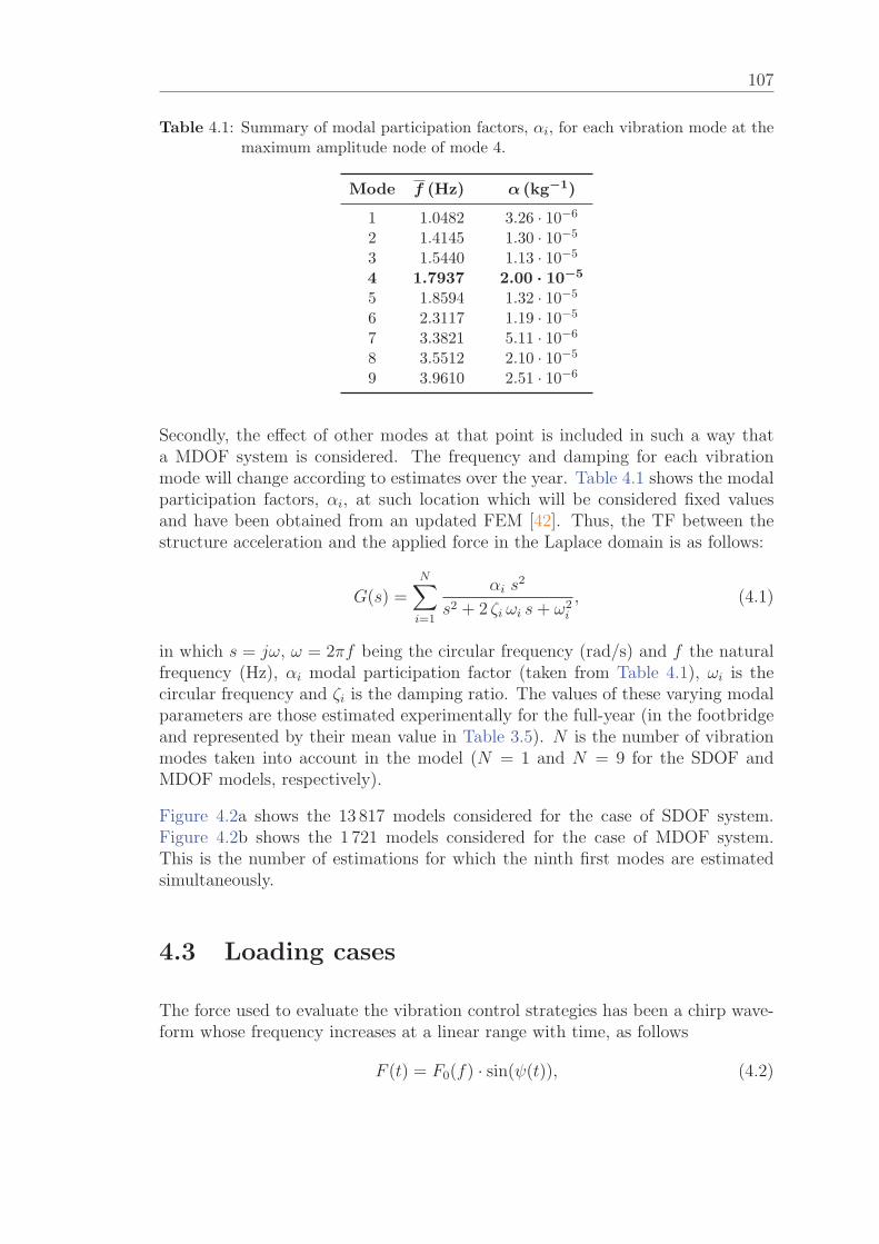
107
Table 4.1: Summary of modal participation factors, αi, for each vibration mode at themaximum amplitude node of mode 4.
Mode f (Hz) α (kg−1)
1 1.0482 3.26 · 10−6
2 1.4145 1.30 · 10−5
3 1.5440 1.13 · 10−5
4 1.7937 2.00 · 10−5
5 1.8594 1.32 · 10−5
6 2.3117 1.19 · 10−5
7 3.3821 5.11 · 10−6
8 3.5512 2.10 · 10−5
9 3.9610 2.51 · 10−6
Secondly, the effect of other modes at that point is included in such a way thata MDOF system is considered. The frequency and damping for each vibrationmode will change according to estimates over the year. Table 4.1 shows the modalparticipation factors, αi, at such location which will be considered fixed valuesand have been obtained from an updated FEM [42]. Thus, the TF between thestructure acceleration and the applied force in the Laplace domain is as follows:
G(s) =N∑i=1
αi s2
s2 + 2 ζi ωi s+ ω2i
, (4.1)
in which s = jω, ω = 2πf being the circular frequency (rad/s) and f the naturalfrequency (Hz), αi modal participation factor (taken from Table 4.1), ωi is thecircular frequency and ζi is the damping ratio. The values of these varying modalparameters are those estimated experimentally for the full-year (in the footbridgeand represented by their mean value in Table 3.5). N is the number of vibrationmodes taken into account in the model (N = 1 and N = 9 for the SDOF andMDOF models, respectively).
Figure 4.2a shows the 13 817 models considered for the case of SDOF system.Figure 4.2b shows the 1 721 models considered for the case of MDOF system.This is the number of estimations for which the ninth first modes are estimatedsimultaneously.
4.3 Loading cases
The force used to evaluate the vibration control strategies has been a chirp wave-form whose frequency increases at a linear range with time, as follows
F (t) = F0(f) · sin(ψ(t)), (4.2)
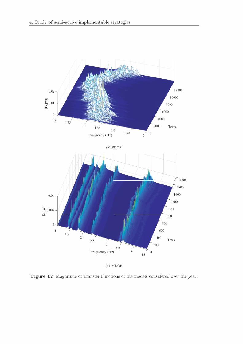
4. Study of semi-active implementable strategies
(a) SDOF.
(b) MDOF.
Figure 4.2: Magnitude of Transfer Functions of the models considered over the year.
109
in which ψ(t) = 2πf(t) t is the angle of the chirp signal, t being the time, whichis defined depending of the instantaneous frequency:
f(t) = fi + kt,
k =ff − fiTf
,
(4.3)
where k is the rate of frequency change, ff is the final frequency, fi is the startingfrequency and Tf is the time it takes to sweep from fi to ff . The frequency rangehas been chosen in order to excite the nine vibration modes below 4 Hz. The finaltime, Tf , has been 500 s and 1000 s, for the SDOF and MDOF system, respectively.These values were chosen to ensure that sweeping at each frequency is sufficientlyslow so that the results do not depend on the final time.
The amplitude of the force has been frequency weighted according to dynamicload factors for walking induced vertical forces [30, 192]. The following definitionfor F0 (f) has been taken here,
F0 (f) =
⎧⎪⎪⎨⎪⎪⎩17.09 f, f < 1.2 Hz316.25 f − 358.98, 1.2 Hz ≤ f < 2.4 Hz−2.56 f − 51.28, 2.4 Hz ≤ f < 20 Hz0, f ≥ 20 Hz
. (4.4)
Figure 4.3 shows F0(f) for the considered frequency range. Note that the ampli-tude is representative of the load imparted by a pedestrian walking at differentfrequencies. Besides, this input force can be easily generated by a shaker to assesscontrol devices designed for cancelling human-induced vibration.
4.4 Vibration control strategies
4.4.1 Passive and semi-active control
The TMD mass is fixed as a fraction of the modal mass (which is the inverse ofthe modal participation factor αi, Equation 4.1) of the targeted vibration mode;the stiffness of the springs is selected to obtain the optimum TMD frequency, andthe viscous dampers ensure the operation of the TMD in a range of frequenciesaround the tuning frequency. The primary system is the structure modelled as aSDOF system, which is composed of a mass m
S, a spring of constant k
Sand a
viscous damper of constant cS. These physical parameters are equivalent to the
modal parameters of Equation 4.1 with N = 1: αS
= 1/mS, k
S= ω2
S/αS and
cS
= (2ζSω
S)/α
S.
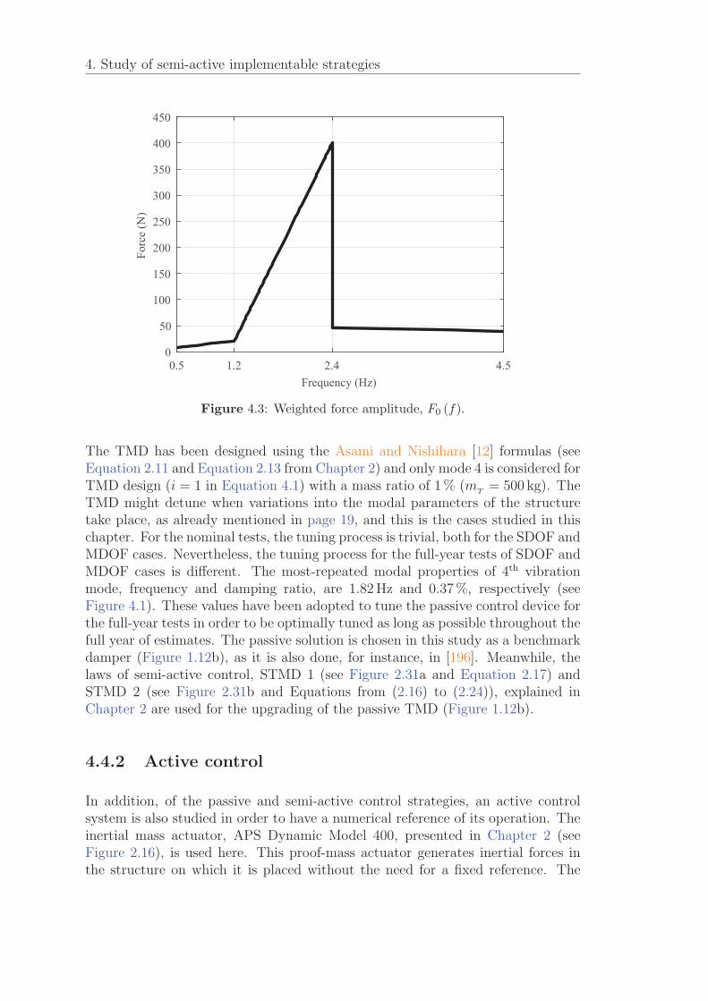
4. Study of semi-active implementable strategies
0.5 1.2 2.4 4.5Frequency (Hz)
0
50
100
150
200
250
300
350
400
450
Forc
e (N
)
Figure 4.3: Weighted force amplitude, F0 (f).
The TMD has been designed using the Asami and Nishihara [12] formulas (seeEquation 2.11 and Equation 2.13 from Chapter 2) and only mode 4 is considered forTMD design (i = 1 in Equation 4.1) with a mass ratio of 1 % (m
T= 500 kg). The
TMD might detune when variations into the modal parameters of the structuretake place, as already mentioned in page 19, and this is the cases studied in thischapter. For the nominal tests, the tuning process is trivial, both for the SDOF andMDOF cases. Nevertheless, the tuning process for the full-year tests of SDOF andMDOF cases is different. The most-repeated modal properties of 4th vibrationmode, frequency and damping ratio, are 1.82 Hz and 0.37 %, respectively (seeFigure 4.1). These values have been adopted to tune the passive control device forthe full-year tests in order to be optimally tuned as long as possible throughout thefull year of estimates. The passive solution is chosen in this study as a benchmarkdamper (Figure 1.12b), as it is also done, for instance, in [196]. Meanwhile, thelaws of semi-active control, STMD 1 (see Figure 2.31a and Equation 2.17) andSTMD 2 (see Figure 2.31b and Equations from (2.16) to (2.24)), explained inChapter 2 are used for the upgrading of the passive TMD (Figure 1.12b).
4.4.2 Active control
In addition, of the passive and semi-active control strategies, an active controlsystem is also studied in order to have a numerical reference of its operation. Theinertial mass actuator, APS Dynamic Model 400, presented in Chapter 2 (seeFigure 2.16), is used here. This proof-mass actuator generates inertial forces inthe structure on which it is placed without the need for a fixed reference. The
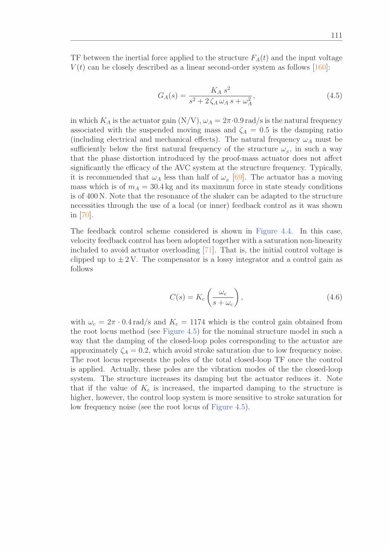
111
TF between the inertial force applied to the structure FA(t) and the input voltageV (t) can be closely described as a linear second-order system as follows [160]:
GA(s) =KA s
2
s2 + 2 ζA ωA s+ ω2A
, (4.5)
in which KA is the actuator gain (N/V), ωA = 2π·0.9 rad/s is the natural frequencyassociated with the suspended moving mass and ζA = 0.5 is the damping ratio(including electrical and mechanical effects). The natural frequency ωA must besufficiently below the first natural frequency of the structure ω
S, in such a way
that the phase distortion introduced by the proof-mass actuator does not affectsignificantly the efficacy of the AVC system at the structure frequency. Typically,it is recommended that ωA less than half of ω
S[69]. The actuator has a moving
mass which is of mA = 30.4 kg and its maximum force in state steady conditionsis of 400 N. Note that the resonance of the shaker can be adapted to the structurenecessities through the use of a local (or inner) feedback control as it was shownin [70].
The feedback control scheme considered is shown in Figure 4.4. In this case,velocity feedback control has been adopted together with a saturation non-linearityincluded to avoid actuator overloading [71]. That is, the initial control voltage isclipped up to ± 2 V. The compensator is a lossy integrator and a control gain asfollows
C(s) = Kc
(ωc
s+ ωc
), (4.6)
with ωc = 2π · 0.4 rad/s and Kc = 1174 which is the control gain obtained fromthe root locus method (see Figure 4.5) for the nominal structure model in such away that the damping of the closed-loop poles corresponding to the actuator areapproximately ζA = 0.2, which avoid stroke saturation due to low frequency noise.The root locus represents the poles of the total closed-loop TF once the controlis applied. Actually, these poles are the vibration modes of the the closed-loopsystem. The structure increases its damping but the actuator reduces it. Notethat if the value of Kc is increased, the imparted damping to the structure ishigher, however, the control loop system is more sensitive to stroke saturation forlow frequency noise (see the root locus of Figure 4.5).
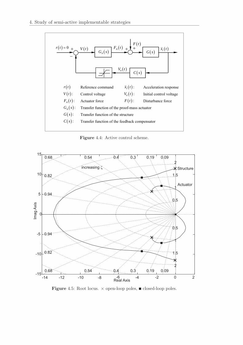
4. Study of semi-active implementable strategies
0r t V t AF tF t
1x t
0V t
r t Reference command 1 :x t Acceleration response:V t Control voltage 0 :V t Initial control voltage:AF t Actuator force :F t Disturbance force:AG s Transfer function of the proof-mass actuator
:G s Transfer function of the structure:C s Transfer function of the feedback compensator
AG s G s
C s
Figure 4.4: Active control scheme.
Real Axis
Imag
Axis
-15
-10
-5
0
5
10
15
2
0.5
1
1.5
2
0.5
1
1.5
0.09
0.090.19
0.190.3
0.30.4
0.40.54
0.54
0.68
0.68
0.94
0.82
0.94
0.82
-14 -12 -10 -8 -6 -4 -2 0 2
Structure
Actuator
increasing �
Figure 4.5: Root locus. × open-loop poles, � closed-loop poles.
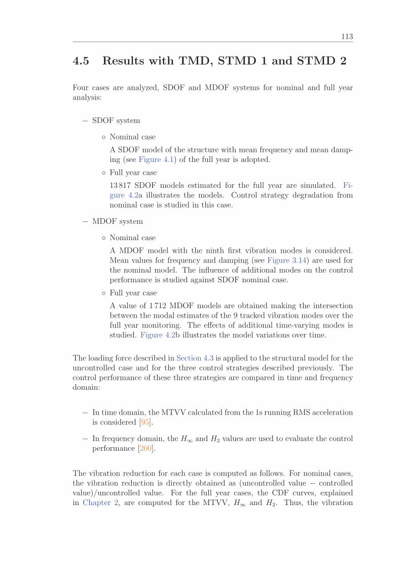
113
4.5 Results with TMD, STMD 1 and STMD 2
Four cases are analyzed, SDOF and MDOF systems for nominal and full yearanalysis:
− SDOF system
◦ Nominal case
A SDOF model of the structure with mean frequency and mean damp-ing (see Figure 4.1) of the full year is adopted.
◦ Full year case
13 817 SDOF models estimated for the full year are simulated. Fi-gure 4.2a illustrates the models. Control strategy degradation fromnominal case is studied in this case.
− MDOF system
◦ Nominal case
A MDOF model with the ninth first vibration modes is considered.Mean values for frequency and damping (see Figure 3.14) are used forthe nominal model. The influence of additional modes on the controlperformance is studied against SDOF nominal case.
◦ Full year case
A value of 1 712 MDOF models are obtained making the intersectionbetween the modal estimates of the 9 tracked vibration modes over thefull year monitoring. The effects of additional time-varying modes isstudied. Figure 4.2b illustrates the model variations over time.
The loading force described in Section 4.3 is applied to the structural model for theuncontrolled case and for the three control strategies described previously. Thecontrol performance of these three strategies are compared in time and frequencydomain:
− In time domain, the MTVV calculated from the 1s running RMS accelerationis considered [95].
− In frequency domain, the H∞ and H2 values are used to evaluate the controlperformance [200].
The vibration reduction for each case is computed as follows. For nominal cases,the vibration reduction is directly obtained as (uncontrolled value − controlledvalue)/uncontrolled value. For the full year cases, the CDF curves, explainedin Chapter 2, are computed for the MTVV, H∞ and H2. Thus, the vibration
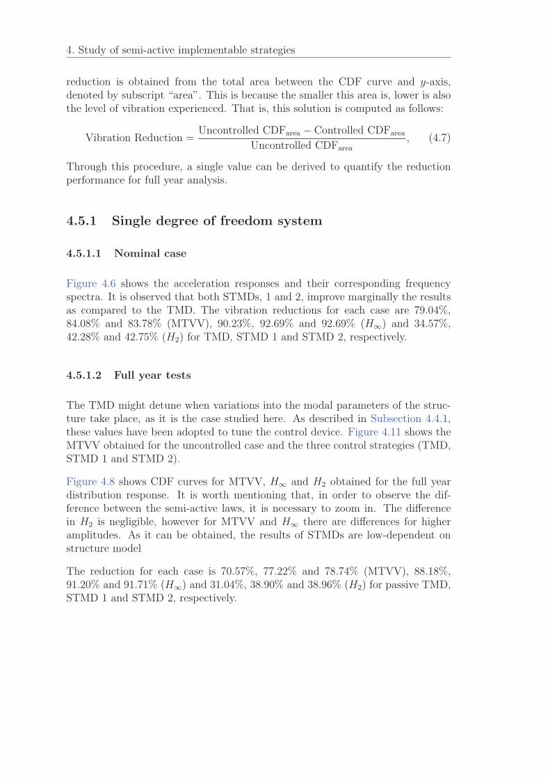
4. Study of semi-active implementable strategies
reduction is obtained from the total area between the CDF curve and y-axis,denoted by subscript “area”. This is because the smaller this area is, lower is alsothe level of vibration experienced. That is, this solution is computed as follows:
Vibration Reduction =Uncontrolled CDFarea − Controlled CDFarea
Uncontrolled CDFarea
, (4.7)
Through this procedure, a single value can be derived to quantify the reductionperformance for full year analysis.
4.5.1 Single degree of freedom system
4.5.1.1 Nominal case
Figure 4.6 shows the acceleration responses and their corresponding frequencyspectra. It is observed that both STMDs, 1 and 2, improve marginally the resultsas compared to the TMD. The vibration reductions for each case are 79.04%,84.08% and 83.78% (MTVV), 90.23%, 92.69% and 92.69% (H∞) and 34.57%,42.28% and 42.75% (H2) for TMD, STMD 1 and STMD 2, respectively.
4.5.1.2 Full year tests
The TMD might detune when variations into the modal parameters of the struc-ture take place, as it is the case studied here. As described in Subsection 4.4.1,these values have been adopted to tune the control device. Figure 4.11 shows theMTVV obtained for the uncontrolled case and the three control strategies (TMD,STMD 1 and STMD 2).
Figure 4.8 shows CDF curves for MTVV, H∞ and H2 obtained for the full yeardistribution response. It is worth mentioning that, in order to observe the dif-ference between the semi-active laws, it is necessary to zoom in. The differencein H2 is negligible, however for MTVV and H∞ there are differences for higheramplitudes. As it can be obtained, the results of STMDs are low-dependent onstructure model
The reduction for each case is 70.57%, 77.22% and 78.74% (MTVV), 88.18%,91.20% and 91.71% (H∞) and 31.04%, 38.90% and 38.96% (H2) for passive TMD,STMD 1 and STMD 2, respectively.
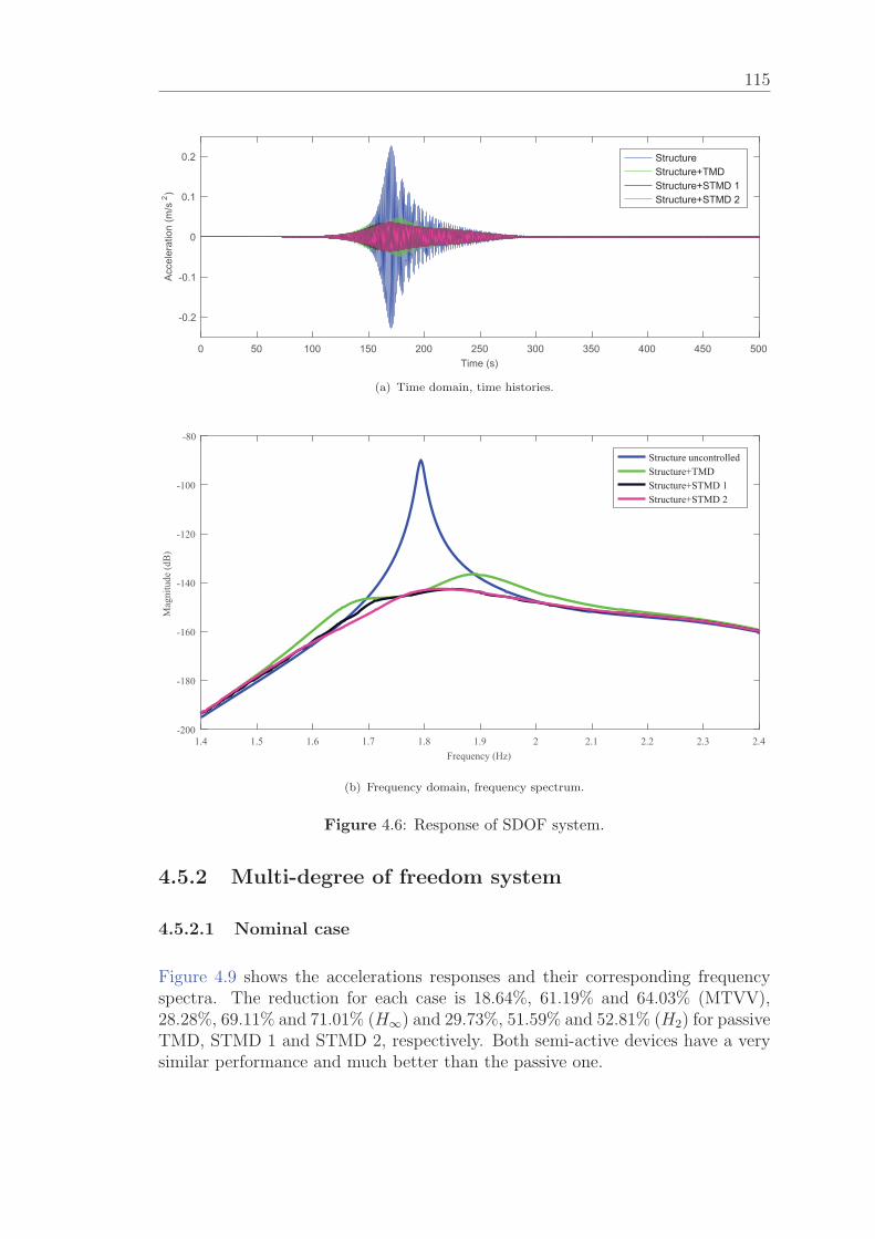
115
0 50 100 150 200 250 300 350 400 450 500Time (s)
-0.2
-0.1
0
0.1
0.2Ac
cele
ratio
n (m
/s2 )
StructureStructure+TMDStructure+STMD 1Structure+STMD 2
(a) Time domain, time histories.
1.4 1.5 1.6 1.7 1.8 1.9 2 2.1 2.2 2.3 2.4Frequency (Hz)
-200
-180
-160
-140
-120
-100
-80
Mag
nitu
de (d
B)
Structure uncontrolledStructure+TMDStructure+STMD 1Structure+STMD 2
(b) Frequency domain, frequency spectrum.
Figure 4.6: Response of SDOF system.
4.5.2 Multi-degree of freedom system
4.5.2.1 Nominal case
Figure 4.9 shows the accelerations responses and their corresponding frequencyspectra. The reduction for each case is 18.64%, 61.19% and 64.03% (MTVV),28.28%, 69.11% and 71.01% (H∞) and 29.73%, 51.59% and 52.81% (H2) for passiveTMD, STMD 1 and STMD 2, respectively. Both semi-active devices have a verysimilar performance and much better than the passive one.
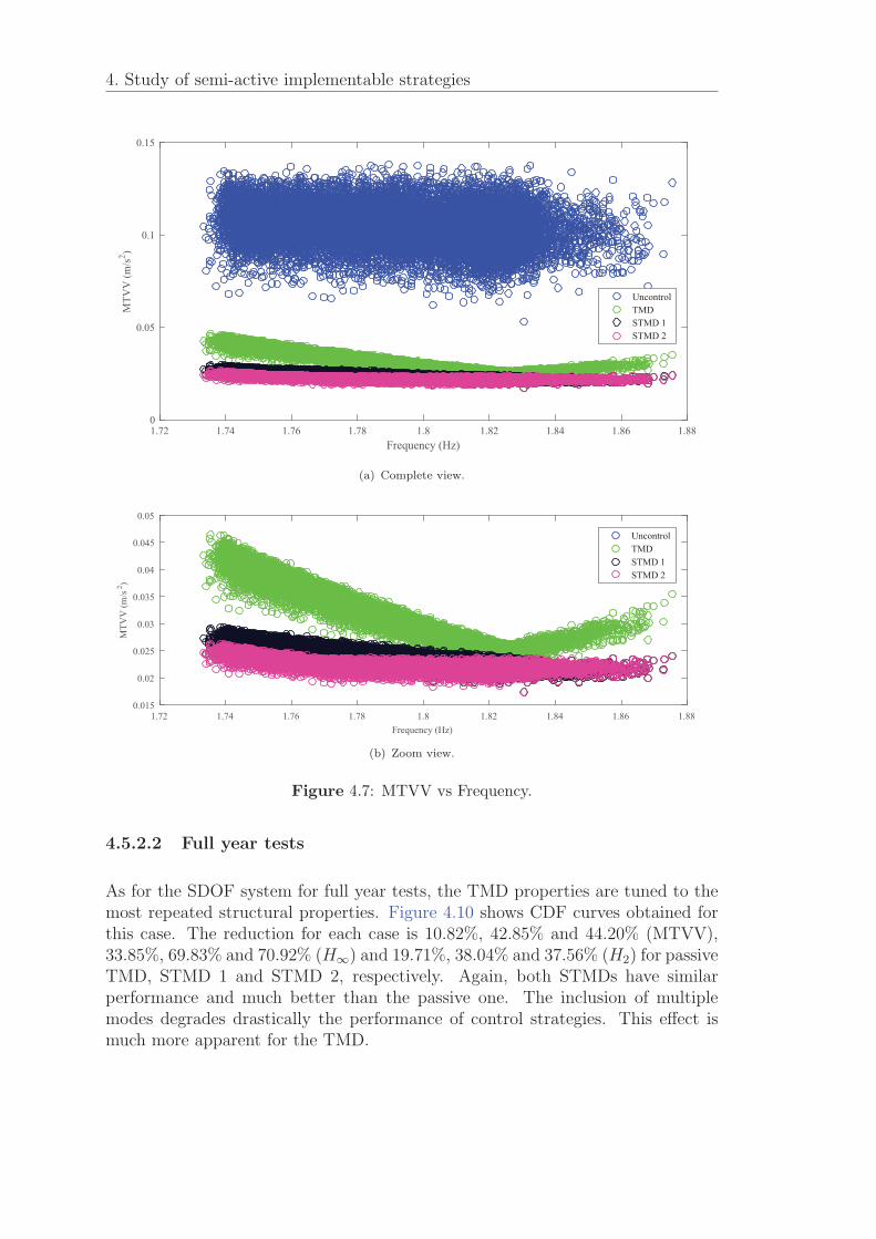
4. Study of semi-active implementable strategies
1.72 1.74 1.76 1.78 1.8 1.82 1.84 1.86 1.88Frequency (Hz)
0
0.05
0.1
0.15M
TVV
(m/s
2 )
UncontrolTMDSTMD 1STMD 2
(a) Complete view.
1.72 1.74 1.76 1.78 1.8 1.82 1.84 1.86 1.88Frequency (Hz)
0.015
0.02
0.025
0.03
0.035
0.04
0.045
0.05
MTV
V (m
/s2 )
UncontrolTMDSTMD 1STMD 2
(b) Zoom view.
Figure 4.7: MTVV vs Frequency.
4.5.2.2 Full year tests
As for the SDOF system for full year tests, the TMD properties are tuned to themost repeated structural properties. Figure 4.10 shows CDF curves obtained forthis case. The reduction for each case is 10.82%, 42.85% and 44.20% (MTVV),33.85%, 69.83% and 70.92% (H∞) and 19.71%, 38.04% and 37.56% (H2) for passiveTMD, STMD 1 and STMD 2, respectively. Again, both STMDs have similarperformance and much better than the passive one. The inclusion of multiplemodes degrades drastically the performance of control strategies. This effect ismuch more apparent for the TMD.
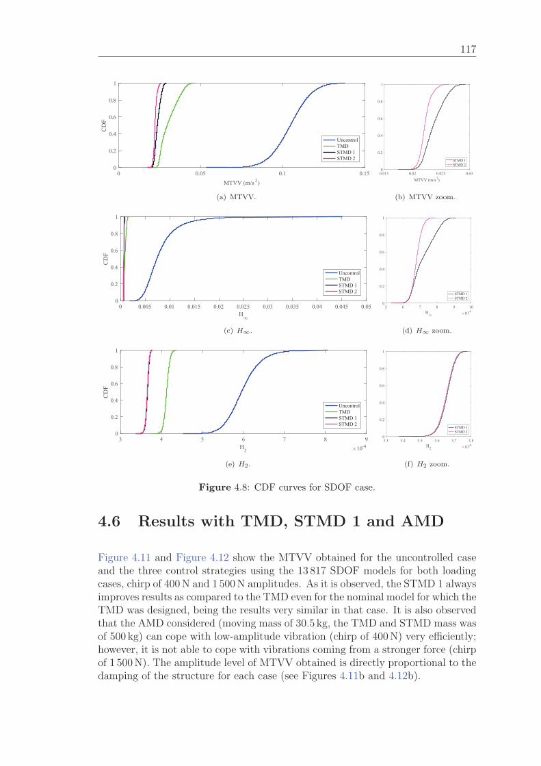
117
0 0.05 0.1 0.15
MTVV (m/s 2)
0
0.2
0.4
0.6
0.8
1
CD
F
UncontrolTMDSTMD 1STMD 2
(a) MTVV.
0.015 0.02 0.025 0.03MTVV (m/s2)
0
0.2
0.4
0.6
0.8
1
STMD 1STMD 2
(b) MTVV zoom.
0 0.005 0.01 0.015 0.02 0.025 0.03 0.035 0.04 0.045 0.05H∞
0
0.2
0.4
0.6
0.8
1
CD
F
UncontrolTMDSTMD 1STMD 2
(c) H∞.
5 6 7 8 9 10H∞
×10-4
0
0.2
0.4
0.6
0.8
1
STMD 1STMD 2
(d) H∞ zoom.
3 4 5 6 7 8 9H2 ×10-4
0
0.2
0.4
0.6
0.8
1
CD
F
UncontrolTMDSTMD 1STMD 2
(e) H2.
3.3 3.4 3.5 3.6 3.7 3.8H2 ×10-4
0
0.2
0.4
0.6
0.8
1
STMD 1STMD 2
(f) H2 zoom.
Figure 4.8: CDF curves for SDOF case.
4.6 Results with TMD, STMD 1 and AMD
Figure 4.11 and Figure 4.12 show the MTVV obtained for the uncontrolled caseand the three control strategies using the 13 817 SDOF models for both loadingcases, chirp of 400 N and 1 500 N amplitudes. As it is observed, the STMD 1 alwaysimproves results as compared to the TMD even for the nominal model for which theTMD was designed, being the results very similar in that case. It is also observedthat the AMD considered (moving mass of 30.5 kg, the TMD and STMD mass wasof 500 kg) can cope with low-amplitude vibration (chirp of 400 N) very efficiently;however, it is not able to cope with vibrations coming from a stronger force (chirpof 1 500 N). The amplitude level of MTVV obtained is directly proportional to thedamping of the structure for each case (see Figures 4.11b and 4.12b).
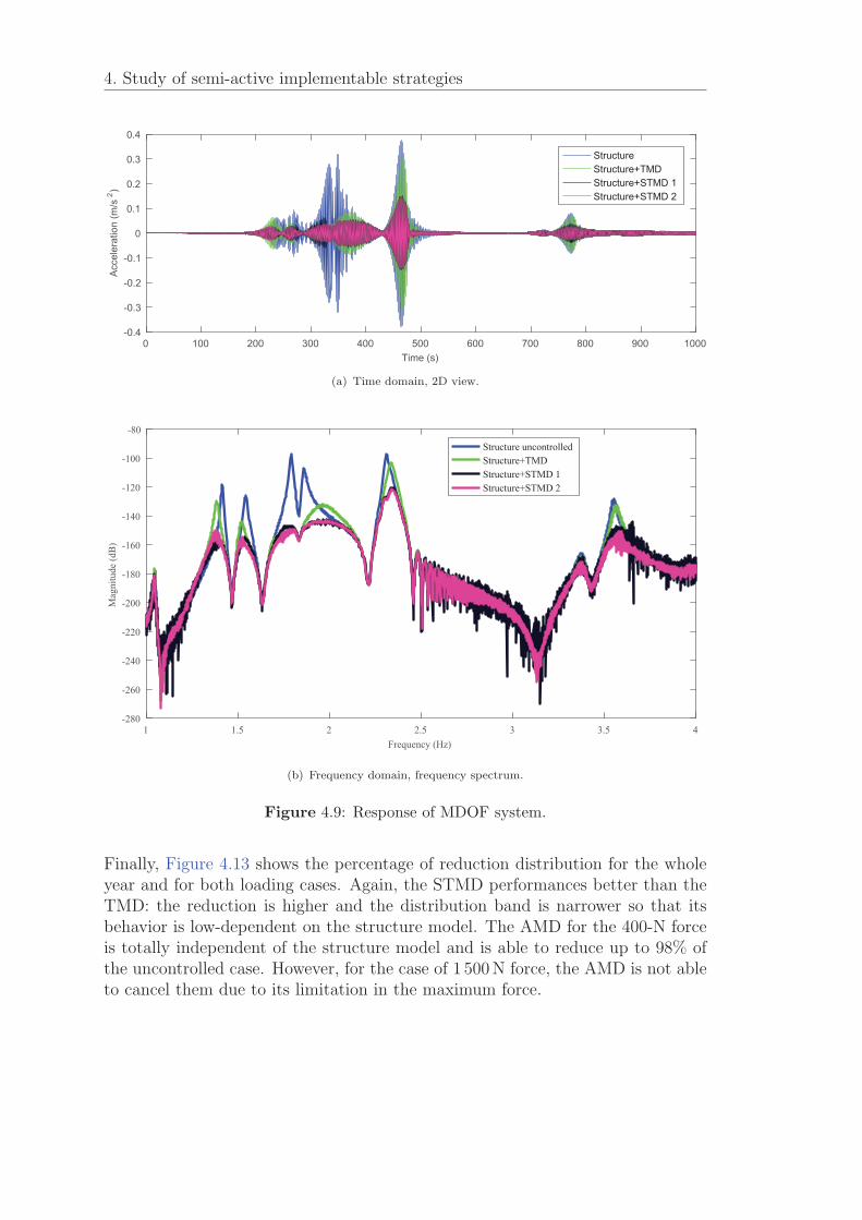
4. Study of semi-active implementable strategies
0 100 200 300 400 500 600 700 800 900 1000Time (s)
-0.4
-0.3
-0.2
-0.1
0
0.1
0.2
0.3
0.4
Acce
lera
tion
(m/s
2 )
StructureStructure+TMDStructure+STMD 1Structure+STMD 2
(a) Time domain, 2D view.
1 1.5 2 2.5 3 3.5 4Frequency (Hz)
-280
-260
-240
-220
-200
-180
-160
-140
-120
-100
-80
Mag
nitu
de (d
B)
Structure uncontrolledStructure+TMDStructure+STMD 1Structure+STMD 2
(b) Frequency domain, frequency spectrum.
Figure 4.9: Response of MDOF system.
Finally, Figure 4.13 shows the percentage of reduction distribution for the wholeyear and for both loading cases. Again, the STMD performances better than theTMD: the reduction is higher and the distribution band is narrower so that itsbehavior is low-dependent on the structure model. The AMD for the 400-N forceis totally independent of the structure model and is able to reduce up to 98% ofthe uncontrolled case. However, for the case of 1 500 N force, the AMD is not ableto cancel them due to its limitation in the maximum force.
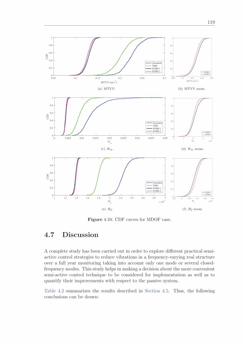
119
0.05 0.1 0.15 0.2 0.25 0.3
MTVV (m/s 2)
0
0.2
0.4
0.6
0.8
1
CD
F
UncontrolTMDSTMD 1STMD 2
(a) MTVV.
0.08 0.1 0.12 0.14 0.16MTVV (m/s2)
0
0.2
0.4
0.6
0.8
1
STMD 1STMD 2
(b) MTVV zoom.
0 0.005 0.01 0.015 0.02 0.025 0.03 0.035 0.04H∞
0
0.2
0.4
0.6
0.8
1
CD
F
UncontrolTMDSTMD 1STMD 2
(c) H∞.
2 3 4 5 6H∞
×10-3
0
0.2
0.4
0.6
0.8
1
STMD 1STMD 2
(d) H∞ zoom.
1 1.2 1.4 1.6 1.8 2 2.2 2.4 2.6 2.8 3H2 ×10-3
0
0.2
0.4
0.6
0.8
1
CD
F
UncontrolTMDSTMD 1STMD 2
(e) H2.
1.25 1.3 1.35 1.4 1.45 1.5H2 ×10-3
0
0.2
0.4
0.6
0.8
1
STMD 1STMD 2
(f) H2 zoom.
Figure 4.10: CDF curves for MDOF case.
4.7 Discussion
A complete study has been carried out in order to explore different practical semi-active control strategies to reduce vibrations in a frequency-varying real structureover a full year monitoring taking into account only one mode or several closed-frequency modes. This study helps in making a decision about the more convenientsemi-active control technique to be considered for implementation as well as toquantify their improvements with respect to the passive system.
Table 4.2 summarizes the results described in Section 4.5. Thus, the followingconclusions can be drawn:
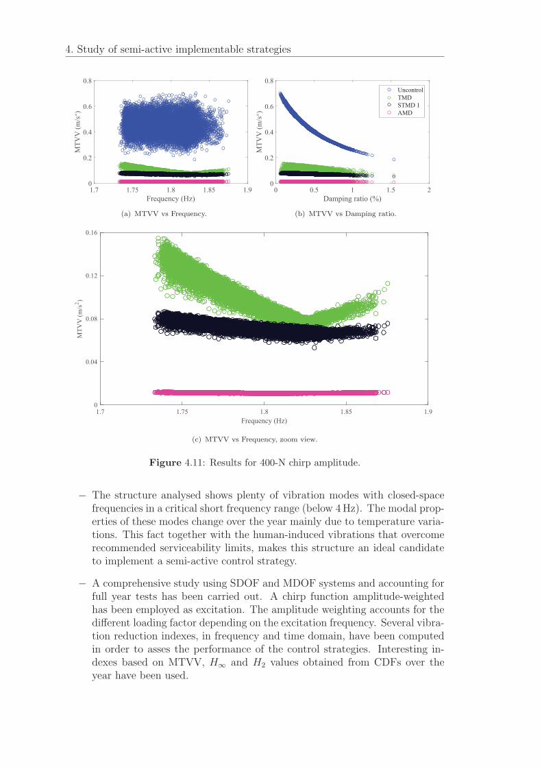
4. Study of semi-active implementable strategies
1.7 1.75 1.8 1.85 1.9Frequency (Hz)
0
0.2
0.4
0.6
0.8M
TVV
(m/s
2 )
(a) MTVV vs Frequency.
0 0.5 1 1.5 2Damping ratio (%)
0
0.2
0.4
0.6
0.8
MTV
V (m
/s2 )
UncontrolTMDSTMDAMD
(b) MTVV vs Damping ratio.
1.7 1.75 1.8 1.85 1.9Frequency (Hz)
0
0.04
0.08
0.12
0.16
MTV
V (m
/s2 )
(c) MTVV vs Frequency, zoom view.
Figure 4.11: Results for 400-N chirp amplitude.
− The structure analysed shows plenty of vibration modes with closed-spacefrequencies in a critical short frequency range (below 4 Hz). The modal prop-erties of these modes change over the year mainly due to temperature varia-tions. This fact together with the human-induced vibrations that overcomerecommended serviceability limits, makes this structure an ideal candidateto implement a semi-active control strategy.
− A comprehensive study using SDOF and MDOF systems and accounting forfull year tests has been carried out. A chirp function amplitude-weightedhas been employed as excitation. The amplitude weighting accounts for thedifferent loading factor depending on the excitation frequency. Several vibra-tion reduction indexes, in frequency and time domain, have been computedin order to asses the performance of the control strategies. Interesting in-dexes based on MTVV, H∞ and H2 values obtained from CDFs over theyear have been used.
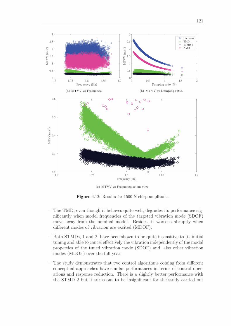
121
1.7 1.75 1.8 1.85 1.9Frequency (Hz)
0
0.5
1
1.5
2
2.5
3
MTV
V (m
/s2 )
(a) MTVV vs Frequency.
0 0.5 1 1.5 2Damping ratio (%)
0
0.5
1
1.5
2
2.5
3
MTV
V (m
/s2 )
UncontrolTMDSTMDAMD
(b) MTVV vs Damping ratio.
1.7 1.75 1.8 1.85 1.9Frequency (Hz)
0.2
0.3
0.4
0.5
0.6
MTV
V (m
/s2 )
(c) MTVV vs Frequency, zoom view.
Figure 4.12: Results for 1500-N chirp amplitude.
− The TMD, even though it behaves quite well, degrades its performance sig-nificantly when model frequencies of the targeted vibration mode (SDOF)move away from the nominal model. Besides, it worsens abruptly whendifferent modes of vibration are excited (MDOF).
− Both STMDs, 1 and 2, have been shown to be quite insensitive to its initialtuning and able to cancel effectively the vibration independently of the modalproperties of the tuned vibration mode (SDOF) and, also other vibrationmodes (MDOF) over the full year.
− The study demonstrates that two control algorithms coming from differentconceptual approaches have similar performances in terms of control oper-ations and response reduction. There is a slightly better performance withthe STMD 2 but it turns out to be insignificant for the study carried out
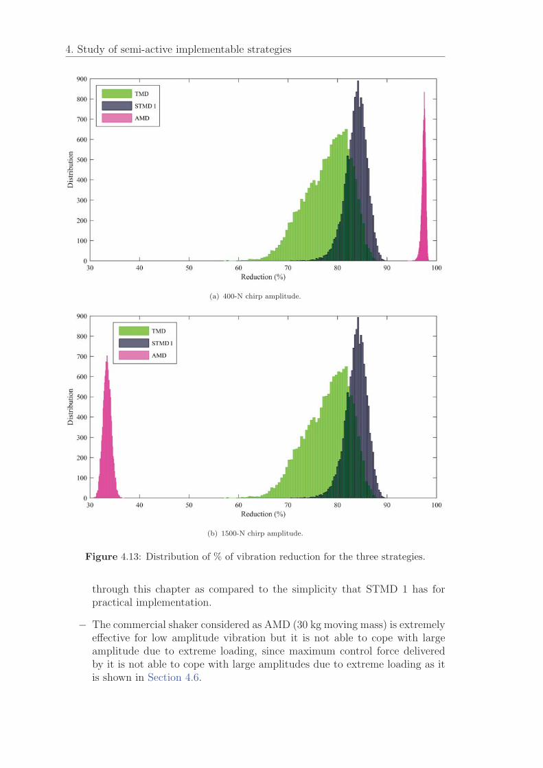
4. Study of semi-active implementable strategies
(a) 400-N chirp amplitude.
(b) 1500-N chirp amplitude.
Figure 4.13: Distribution of % of vibration reduction for the three strategies.
through this chapter as compared to the simplicity that STMD 1 has forpractical implementation.
− The commercial shaker considered as AMD (30 kg moving mass) is extremelyeffective for low amplitude vibration but it is not able to cope with largeamplitude due to extreme loading, since maximum control force deliveredby it is not able to cope with large amplitudes due to extreme loading as itis shown in Section 4.6.
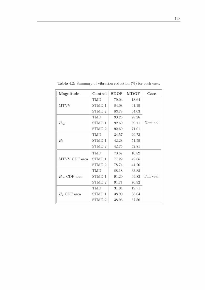
123
Table 4.2: Summary of vibration reduction (%) for each case.
Magnitude Control SDOF MDOF Case
TMD 79.04 18.64
MTVV STMD 1 84.08 61.19
STMD 2 83.78 64.03
TMD 90.23 28.28
NominalH∞ STMD 1 92.69 69.11
STMD 2 92.69 71.01
TMD 34.57 29.73
H2 STMD 1 42.28 51.59
STMD 2 42.75 52.81
TMD 70.57 10.82
MTVV CDF area STMD 1 77.22 42.85
STMD 2 78.74 44.20
TMD 88.18 33.85
Full yearH∞ CDF area STMD 1 91.20 69.83
STMD 2 91.71 70.92
TMD 31.04 19.71
H2 CDF area STMD 1 38.90 38.04
STMD 2 38.96 37.56

5Optimal tuning of semi-active
TMD
Contents5.1 Introduction . . . . . . . . . . . . . . . . . . . . . . . . . 125
5.2 Semi-active Tuned Mass Damper . . . . . . . . . . . . . 127
5.2.1 Tuned Mass Damper . . . . . . . . . . . . . . . . . . . . 127
5.2.2 Semi-active control strategy . . . . . . . . . . . . . . . . 127
5.2.3 Optimal control design . . . . . . . . . . . . . . . . . . . 127
5.3 Simulation results . . . . . . . . . . . . . . . . . . . . . . 129
5.3.1 Sensitivity analysis . . . . . . . . . . . . . . . . . . . . . 129
5.3.2 Control design parameters . . . . . . . . . . . . . . . . . 130
5.3.3 Ideal viscous damper . . . . . . . . . . . . . . . . . . . . 130
5.3.4 Effect of damper force saturation . . . . . . . . . . . . . 132
5.3.5 Effect of considering an MR damper model . . . . . . . 133
5.4 Experimental results . . . . . . . . . . . . . . . . . . . . 141
5.4.1 Structure description and experimental setup . . . . . . 141
5.4.2 Mechanical design of the Tuned Mass Damper . . . . . 142
5.4.3 Implementation of the control law . . . . . . . . . . . . 143
5.4.4 Experimental tests . . . . . . . . . . . . . . . . . . . . . 145
5.5 Conclusions . . . . . . . . . . . . . . . . . . . . . . . . . . 146
5.1 Introduction
In the previous chapter, it has been studied the performance of the two STMDstrategies presented in Chapter 2. But several issues have to be tackled to achieve
125
5. Optimal tuning of semi-active TMD
a successful implementation for broad frequency-band vibration: i) the designof the control law to implement, ii) the frequency tuning in passive mode, iii)the damping in passive mode, iv) the definition of a PI able to represent theperformance in a broad frequency band and v) practical issues such as filteringand switching on-off function. Some of these issues have been partially addressedpreviously in other research works [79, 113, 199].
An MR damper can be used within control systems. However, MR dampers have astrongly non-linear nature that has to be modelled and included in control design.Otherwise, the simulated performance may differ considerably from the experi-mental performance.
Although sensitivity studies of semi-active control law parameters have been ac-complished, as well as optimal tuning proposals [79, 140], the main purpose ofthe semi-active device has not considered for its tuning: be effective in a broadfrequency-band spectrum. Cases such as modal properties varying with time dueto external factors (temperature, level of occupancy or ageing) and structureswith several vibration modes with closely-spaced frequencies prone to vibrate arecommon in practice (see Chapter 3). Under these circumstances, much greater ro-bustness than that provided by the TMD is required and a design approach thatconsiders both uncertainties in structure modal parameters and an MR damper isdesirable.
Thus, the tuning of the semi-active system should take into account its broadspectrum of operation and the significant non-linearities, such as the control lawitself, as well as the operation of the MR damper. Then, a new approach totuning STMDs is carried out in this article and compared to the passive perfor-mance. Necessary aspects to implement the control law are also described andtaken into account within the optimization problem. Although the problem isstated in a general way, this is clearly geared to highly resonant structures (forinstance, lightweight footbridges) and the PI to be minimised is focused on usercomfort. The following issues are considered: i) the velocity of the inertial massshould be estimated from its acceleration, ii) a continuous trigger function shouldbe implemented in order to avoid unnecessary damper actions when structureacceleration is of low amplitude, and iii) acceleration of the structure should becarefully filtered to avoid spillover effects and unnecessary damper action whenthis signal is crossing over zero.
The chapter continues with a description of the semi-active inertial controller andthe vibration control strategy adopted in Section 5.2. A sensitivity analysis ofthe tuning parameters of the control device is carried out in Section 5.3. Theeffect of including damper force saturation and an MR damper model instead ofa linear-viscous damper are also analysed. Lastly, an optimization procedure totune the semi-active device is proposed. Section 5.4 shows the experimental resultsconducted on a steel beam and carefully explains the implementation of the semi-active control and the practical issues that have been considered. Finally, someconclusions are given in Section 5.5.
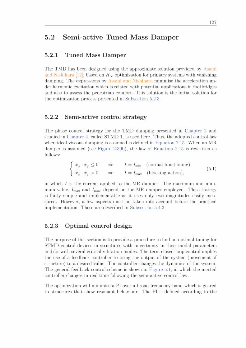
127
5.2 Semi-active Tuned Mass Damper
5.2.1 Tuned Mass Damper
The TMD has been designed using the approximate solution provided by Asamiand Nishihara [12], based on H∞ optimization for primary systems with vanishingdamping. The expressions by Asami and Nishihara minimise the acceleration un-der harmonic excitation which is related with potential applications in footbridgesand also to assess the pedestrian comfort. This solution is the initial solution forthe optimization process presented in Subsection 5.2.3.
5.2.2 Semi-active control strategy
The phase control strategy for the TMD damping presented in Chapter 2 andstudied in Chapter 4, called STMD 1, is used here. Thus, the adopted control lawwhen ideal viscous damping is assumed is defined in Equation 2.15. When an MRdamper is assumed (see Figure 2.39b), the law of Equation 2.15 is rewritten asfollows: {
xS· x
T≤ 0 ⇒ I = Imin (normal functioning)
xS· x
T> 0 ⇒ I = Imax (blocking action),
(5.1)
in which I is the current applied to the MR damper. The maximum and mini-mum value, Imax and Imin, depend on the MR damper employed. This strategyis fairly simple and implementable as it uses only two magnitudes easily mea-sured. However, a few aspects must be taken into account before the practicalimplementation. These are described in Subsection 5.4.3.
5.2.3 Optimal control design
The purpose of this section is to provide a procedure to find an optimal tuning forSTMD control devices in structures with uncertainty in their modal parametersand/or with several critical vibration modes. The term closed-loop control impliesthe use of a feedback controller to bring the output of the system (movement ofstructure) to a desired value. The controller changes the dynamics of the system.The general feedback control scheme is shown in Figure 5.1, in which the inertialcontroller changes in real time following the semi-active control law.
The optimization will minimise a PI over a broad frequency band which is gearedto structures that show resonant behaviour. The PI is defined according to the
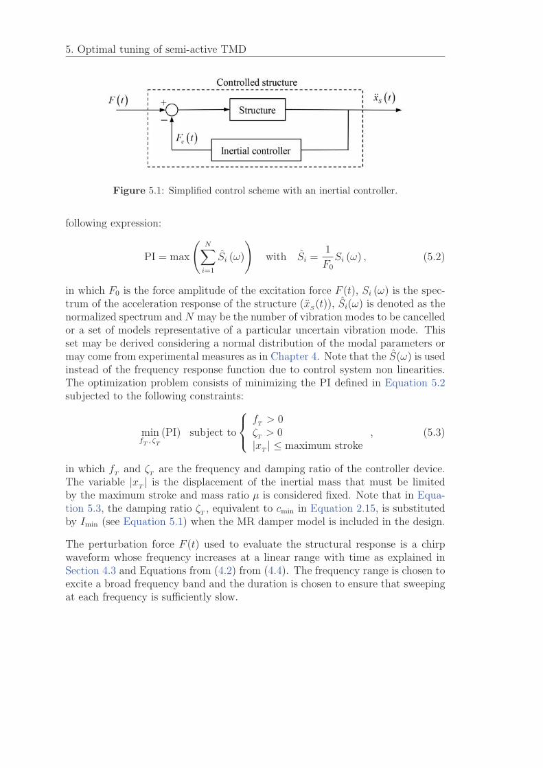
5. Optimal tuning of semi-active TMD
Figure 5.1: Simplified control scheme with an inertial controller.
following expression:
PI = max
(N∑i=1
Si (ω)
)with Si =
1
F0
Si (ω) , (5.2)
in which F0 is the force amplitude of the excitation force F (t), Si (ω) is the spec-trum of the acceleration response of the structure (x
S(t)), Si(ω) is denoted as the
normalized spectrum and N may be the number of vibration modes to be cancelledor a set of models representative of a particular uncertain vibration mode. Thisset may be derived considering a normal distribution of the modal parameters ormay come from experimental measures as in Chapter 4. Note that the S(ω) is usedinstead of the frequency response function due to control system non linearities.The optimization problem consists of minimizing the PI defined in Equation 5.2subjected to the following constraints:
minfT, ζ
T
(PI) subject to
⎧⎨⎩fT> 0
ζT> 0
|xT| ≤ maximum stroke
, (5.3)
in which fT
and ζT
are the frequency and damping ratio of the controller device.The variable |x
T| is the displacement of the inertial mass that must be limited
by the maximum stroke and mass ratio μ is considered fixed. Note that in Equa-tion 5.3, the damping ratio ζ
T, equivalent to cmin in Equation 2.15, is substituted
by Imin (see Equation 5.1) when the MR damper model is included in the design.
The perturbation force F (t) used to evaluate the structural response is a chirpwaveform whose frequency increases at a linear range with time as explained inSection 4.3 and Equations from (4.2) from (4.4). The frequency range is chosen toexcite a broad frequency band and the duration is chosen to ensure that sweepingat each frequency is sufficiently slow.
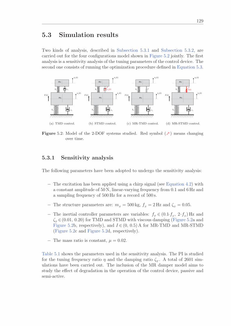
129
5.3 Simulation results
Two kinds of analysis, described in Subsection 5.3.1 and Subsection 5.3.2, arecarried out for the four configurations model shown in Figure 5.2 jointly. The firstanalysis is a sensitivity analysis of the tuning parameters of the control device. Thesecond one consists of running the optimization procedure defined in Equation 5.3.
( )F t
( )Tx t
( )Sx tTk Tc
SkSc
c
c
mS
mT
(a) TMD control.
( )F t
( )Tx t
( )Sx tTk ( )Tc t
SkSc
c
c
mS
mT
(b) STMD control.
( )F t
( )Tx t
( )Sx tTk I
SkSc
c
mS
mT
(c) MR-TMD control.
( )F t
( )Tx t
( )Sx tTk ( )I t
SkSc
c
mS
mT
(d) MR-STMD control.
Figure 5.2: Model of the 2-DOF systems studied. Red symbol ( −→) means changingover time.
5.3.1 Sensitivity analysis
The following parameters have been adopted to undergo the sensitivity analysis:
− The excitation has been applied using a chirp signal (see Equation 4.2) witha constant amplitude of 50 N, linear-varying frequency from 0.1 and 6 Hz anda sampling frequency of 500 Hz for a record of 500 s.
− The structure parameters are: mS
= 500 kg, fS
= 2 Hz and ζS
= 0.05.
− The inertial controller parameters are variables: fT∈ (0.1·f
S, 2·f
S) Hz and
ζT∈(0.01, 0.20) for TMD and STMD with viscous damping (Figure 5.2a and
Figure 5.2b, respectively), and I ∈ (0, 0.5) A for MR-TMD and MR-STMD(Figure 5.2c and Figure 5.2d, respectively).
− The mass ratio is constant, μ = 0.02.
Table 5.1 shows the parameters used in the sensitivity analysis. The PI is studiedfor the tuning frequency ratio η and the damping ratio ζ
T. A total of 2601 sim-
ulations have been carried out. The inclusion of the MR damper model aims tostudy the effect of degradation in the operation of the control device, passive andsemi-active.
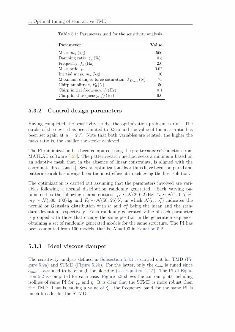
5. Optimal tuning of semi-active TMD
Table 5.1: Parameters used for the sensitivity analysis.
Parameter Value
Mass, mS (kg) 500Damping ratio, ζS (%) 0.5Frequency, fS (Hz) 2.0Mass ratio, μ 0.02Inertial mass, mT (kg) 10Maximum damper force saturation, FDmax (N) 75Chirp amplitude, F0 (N) 50Chirp initial frequency, fi (Hz) 0.1Chirp final frequency, ff (Hz) 6.0
5.3.2 Control design parameters
Having completed the sensitivity study, the optimization problem is run. Thestroke of the device has been limited to 0.3 m and the value of the mass ratio hasbeen set again at μ = 2 %. Note that both variables are related, the higher themass ratio is, the smaller the stroke achieved.
The PI minimization has been computed using the patternsearch function fromMATLAB software [129]. The pattern-search method seeks a minimum based onan adaptive mesh that, in the absence of linear constraints, is aligned with thecoordinate directions [4]. Several optimization algorithms have been compared andpattern-search has always been the most efficient in achieving the best solution.
The optimization is carried out assuming that the parameters involved are vari-ables following a normal distribution randomly generated. Each varying pa-rameter has the following characteristics: fS ∼ N (2, 0.2) Hz, ζS ∼ N (1, 0.5) %,mS ∼ N (500, 100) kg and F0 ∼ N (50, 25) N, in which N (νi, σ
2i ) indicates the
normal or Gaussian distribution with νi and σ2i being the mean and the stan-
dard deviation, respectively. Each randomly generated value of each parameteris grouped with those that occupy the same position in the generation sequence,obtaining a set of randomly generated models for the same structure. The PI hasbeen computed from 100 models, that is, N = 100 in Equation 5.2.
5.3.3 Ideal viscous damper
The sensitivity analysis defined in Subsection 5.3.1 is carried out for TMD (Fi-gure 5.2a) and STMD (Figure 5.2b). For the latter, only the cmin is tuned sincecmax is assumed to be enough for blocking (see Equation 2.15). The PI of Equa-tion 5.2 is computed for each case. Figure 5.3 shows the contour plots includingisolines of same PI for ζ
Tand η. It is clear that the STMD is more robust than
the TMD. That is, taking a value of ζT, the frequency band for the same PI is
much broader for the STMD.
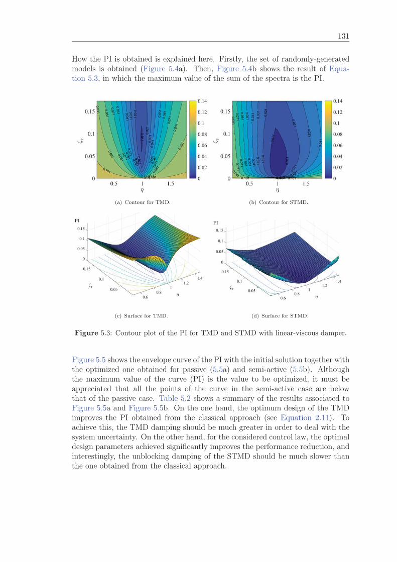
131
How the PI is obtained is explained here. Firstly, the set of randomly-generatedmodels is obtained (Figure 5.4a). Then, Figure 5.4b shows the result of Equa-tion 5.3, in which the maximum value of the sum of the spectra is the PI.
(a) Contour for TMD. (b) Contour for STMD.
(c) Surface for TMD. (d) Surface for STMD.
Figure 5.3: Contour plot of the PI for TMD and STMD with linear-viscous damper.
Figure 5.5 shows the envelope curve of the PI with the initial solution together withthe optimized one obtained for passive (5.5a) and semi-active (5.5b). Althoughthe maximum value of the curve (PI) is the value to be optimized, it must beappreciated that all the points of the curve in the semi-active case are belowthat of the passive case. Table 5.2 shows a summary of the results associated toFigure 5.5a and Figure 5.5b. On the one hand, the optimum design of the TMDimproves the PI obtained from the classical approach (see Equation 2.11). Toachieve this, the TMD damping should be much greater in order to deal with thesystem uncertainty. On the other hand, for the considered control law, the optimaldesign parameters achieved significantly improves the performance reduction, andinterestingly, the unblocking damping of the STMD should be much slower thanthe one obtained from the classical approach.
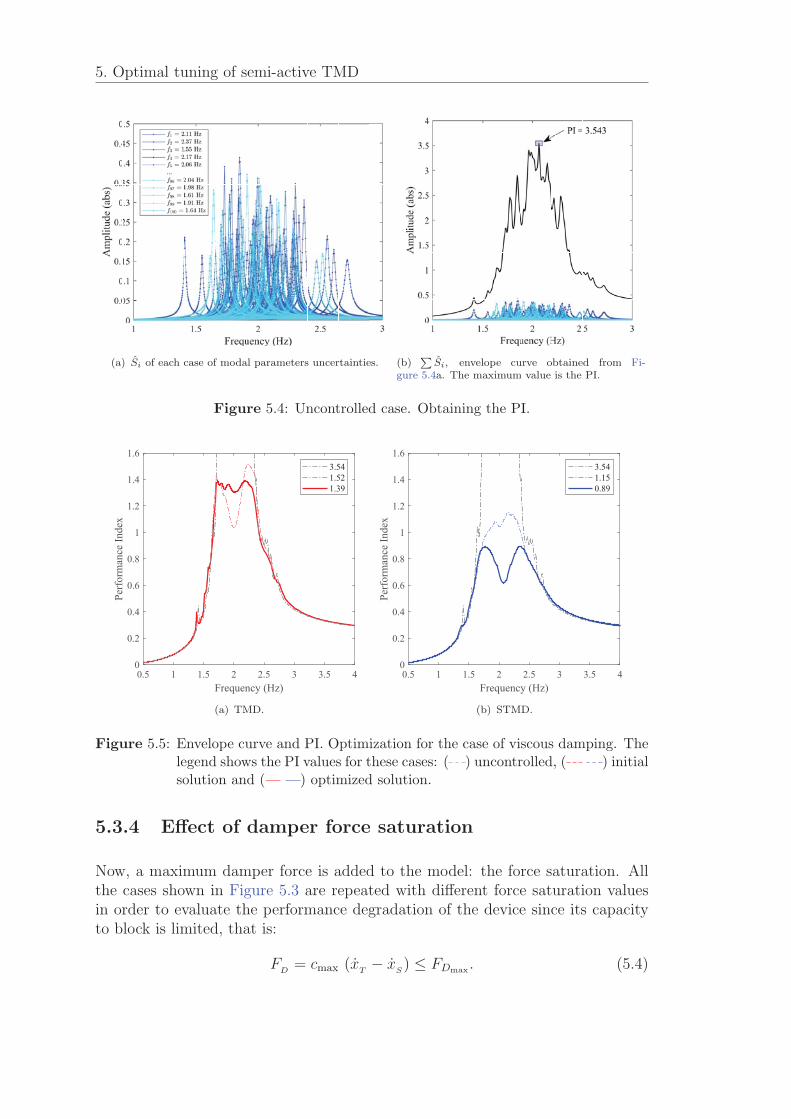
5. Optimal tuning of semi-active TMD
(a) Si of each case of modal parameters uncertainties. (b)∑
Si, envelope curve obtained from Fi-gure 5.4a. The maximum value is the PI.
Figure 5.4: Uncontrolled case. Obtaining the PI.
0.5 1 1.5 2 2.5 3 3.5 4Frequency (Hz)
0
0.2
0.4
0.6
0.8
1
1.2
1.4
1.6
Perf
orm
ance
Inde
x
3.541.521.39
(a) TMD.
0.5 1 1.5 2 2.5 3 3.5 4Frequency (Hz)
0
0.2
0.4
0.6
0.8
1
1.2
1.4
1.6
Perf
orm
ance
Inde
x
3.541.150.89
(b) STMD.
Figure 5.5: Envelope curve and PI. Optimization for the case of viscous damping. Thelegend shows the PI values for these cases: ( ) uncontrolled, ( ) initialsolution and ( ) optimized solution.
5.3.4 Effect of damper force saturation
Now, a maximum damper force is added to the model: the force saturation. Allthe cases shown in Figure 5.3 are repeated with different force saturation valuesin order to evaluate the performance degradation of the device since its capacityto block is limited, that is:
FD
= cmax (xT− x
S) ≤ FDmax . (5.4)
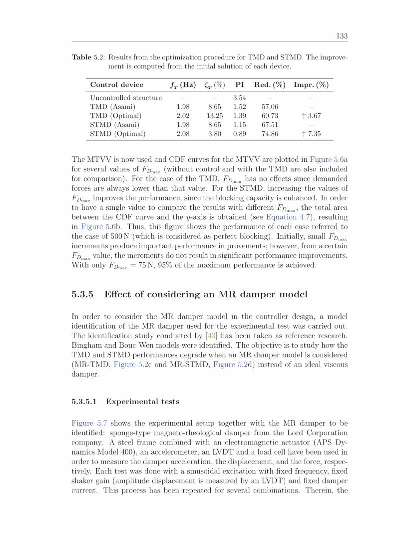
133
Table 5.2: Results from the optimization procedure for TMD and STMD. The improve-ment is computed from the initial solution of each device.
Control device fT (Hz) ζT (%) PI Red. (%) Impr. (%)
Uncontrolled structure – – 3.54 – –TMD (Asami) 1.98 8.65 1.52 57.06 –TMD (Optimal) 2.02 13.25 1.39 60.73 ↑ 3.67STMD (Asami) 1.98 8.65 1.15 67.51 –STMD (Optimal) 2.08 3.80 0.89 74.86 ↑ 7.35
The MTVV is now used and CDF curves for the MTVV are plotted in Figure 5.6afor several values of FDmax (without control and with the TMD are also includedfor comparison). For the case of the TMD, FDmax has no effects since demandedforces are always lower than that value. For the STMD, increasing the values ofFDmax improves the performance, since the blocking capacity is enhanced. In orderto have a single value to compare the results with different FDmax , the total areabetween the CDF curve and the y-axis is obtained (see Equation 4.7), resultingin Figure 5.6b. Thus, this figure shows the performance of each case referred tothe case of 500 N (which is considered as perfect blocking). Initially, small FDmax
increments produce important performance improvements; however, from a certainFDmax value, the increments do not result in significant performance improvements.With only FDmax = 75 N, 95% of the maximum performance is achieved.
5.3.5 Effect of considering an MR damper model
In order to consider the MR damper model in the controller design, a modelidentification of the MR damper used for the experimental test was carried out.The identification study conducted by [43] has been taken as reference research.Bingham and Bouc-Wen models were identified. The objective is to study how theTMD and STMD performances degrade when an MR damper model is considered(MR-TMD, Figure 5.2c and MR-STMD, Figure 5.2d) instead of an ideal viscousdamper.
5.3.5.1 Experimental tests
Figure 5.7 shows the experimental setup together with the MR damper to beidentified: sponge-type magneto-rheological damper from the Lord Corporationcompany. A steel frame combined with an electromagnetic actuator (APS Dy-namics Model 400), an accelerometer, an LVDT and a load cell have been used inorder to measure the damper acceleration, the displacement, and the force, respec-tively. Each test was done with a sinusoidal excitation with fixed frequency, fixedshaker gain (amplitude displacement is measured by an LVDT) and fixed dampercurrent. This process has been repeated for several combinations. Therein, the
5. Optimal tuning of semi-active TMD
0 0.5 1 1.5 2 2.5 3 3.5MTVV (m/s2)
0
0.2
0.4
0.6
0.8
1
CD
F
Without controlTMDSTMD (25 N)STMD (50 N)STMD (75 N)STMD (100 N)STMD (500 N)
(a) CDF curves of the MTVV for several FDmax .
(b) Percentage of the maximum performance for several FDmax .
Figure 5.6: Performance in terms of the CDF of the MTVV for several damper forcesaturations FDmax .
damping ratio is changed by the input current of the MR damper. The selectedrange of frequencies, shaker gains and current supplies involved in the experimentalprocedure are specified in Table 5.3. A total of 252 tests were completed.
Table 5.3: Variation range of the input parameters for the MR damper identification.
Parameter Range
Shaker gain (V) 0.05 to 0.8Frequency (Hz) 1 to 7Input current I (A) 0 to 0.5
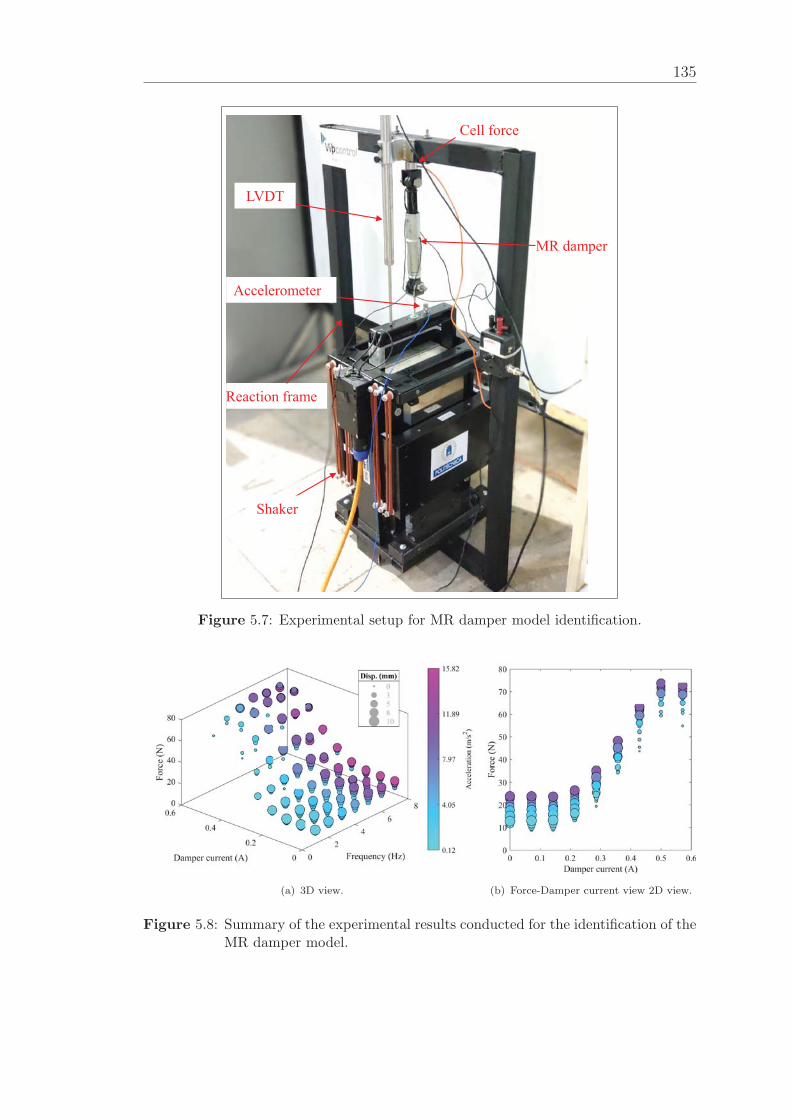
135
Cell force
LVDT
Accelerometer
MR damper
Shaker
Reaction frame
Figure 5.7: Experimental setup for MR damper model identification.
(a) 3D view. (b) Force-Damper current view 2D view.
Figure 5.8: Summary of the experimental results conducted for the identification of theMR damper model.
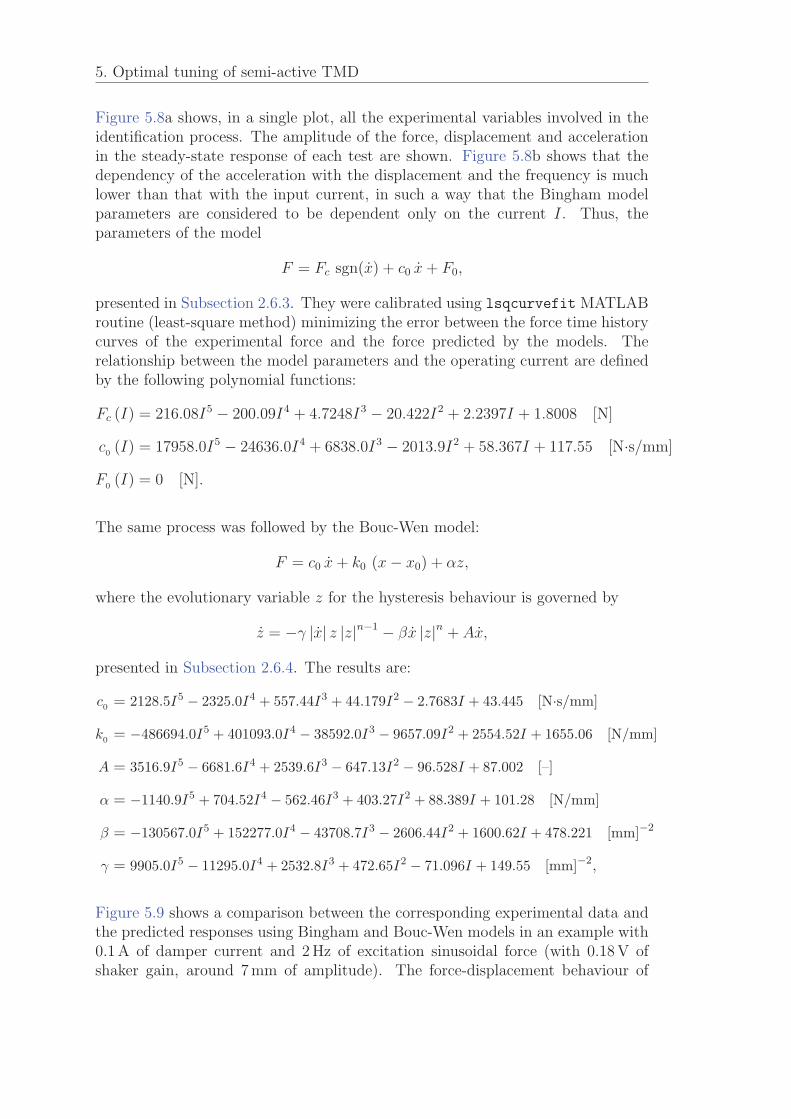
5. Optimal tuning of semi-active TMD
Figure 5.8a shows, in a single plot, all the experimental variables involved in theidentification process. The amplitude of the force, displacement and accelerationin the steady-state response of each test are shown. Figure 5.8b shows that thedependency of the acceleration with the displacement and the frequency is muchlower than that with the input current, in such a way that the Bingham modelparameters are considered to be dependent only on the current I. Thus, theparameters of the model
F = Fc sgn(x) + c0 x+ F0,
presented in Subsection 2.6.3. They were calibrated using lsqcurvefit MATLABroutine (least-square method) minimizing the error between the force time historycurves of the experimental force and the force predicted by the models. Therelationship between the model parameters and the operating current are definedby the following polynomial functions:
Fc (I) = 216.08I5 − 200.09I4 + 4.7248I3 − 20.422I2 + 2.2397I + 1.8008 [N]
c0 (I) = 17958.0I5 − 24636.0I4 + 6838.0I3 − 2013.9I2 + 58.367I + 117.55 [N·s/mm]
F0 (I) = 0 [N].
The same process was followed by the Bouc-Wen model:
F = c0 x+ k0 (x− x0) + αz,
where the evolutionary variable z for the hysteresis behaviour is governed by
z = −γ |x| z |z|n−1 − βx |z|n + Ax,
presented in Subsection 2.6.4. The results are:
c0 = 2128.5I5 − 2325.0I4 + 557.44I3 + 44.179I2 − 2.7683I + 43.445 [N·s/mm]
k0 = −486694.0I5 + 401093.0I4 − 38592.0I3 − 9657.09I2 + 2554.52I + 1655.06 [N/mm]
A = 3516.9I5 − 6681.6I4 + 2539.6I3 − 647.13I2 − 96.528I + 87.002 [–]
α = −1140.9I5 + 704.52I4 − 562.46I3 + 403.27I2 + 88.389I + 101.28 [N/mm]
β = −130567.0I5 + 152277.0I4 − 43708.7I3 − 2606.44I2 + 1600.62I + 478.221 [mm]−2
γ = 9905.0I5 − 11295.0I4 + 2532.8I3 + 472.65I2 − 71.096I + 149.55 [mm]−2,
Figure 5.9 shows a comparison between the corresponding experimental data andthe predicted responses using Bingham and Bouc-Wen models in an example with0.1 A of damper current and 2 Hz of excitation sinusoidal force (with 0.18 V ofshaker gain, around 7 mm of amplitude). The force-displacement behaviour of
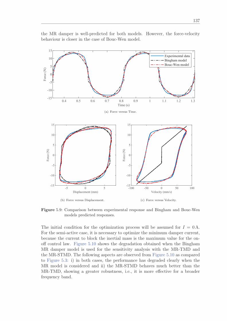
137
the MR damper is well-predicted for both models. However, the force-velocitybehaviour is closer in the case of Bouc-Wen model.
0.4 0.5 0.6 0.7 0.8 0.9 1 1.1 1.2 1.3Time (s)
-15
-10
-5
0
5
10
15
Forc
e (N
)
Experimental dataBingham modelBouc-Wen model
(a) Force versus Time.
-5 0 5Displacement (mm)
-15
-10
-5
0
5
10
15
Forc
e (N
)
(b) Force versus Displacement.
-100 -50 0 50 100Velocity (mm/s)
-15
-10
-5
0
5
10
15Fo
rce
(N)
(c) Force versus Velocity.
Figure 5.9: Comparison between experimental response and Bingham and Bouc-Wenmodels predicted responses.
The initial condition for the optimization process will be assumed for I = 0 A.For the semi-active case, it is necessary to optimize the minimum damper current,because the current to block the inertial mass is the maximum value for the on-off control law. Figure 5.10 shows the degradation obtained when the BinghamMR damper model is used for the sensitivity analysis with the MR-TMD andthe MR-STMD. The following aspects are observed from Figure 5.10 as comparedto Figure 5.3: i) in both cases, the performance has degraded clearly when theMR model is considered and ii) the MR-STMD behaves much better than theMR-TMD, showing a greater robustness, i.e., it is more effective for a broaderfrequency band.
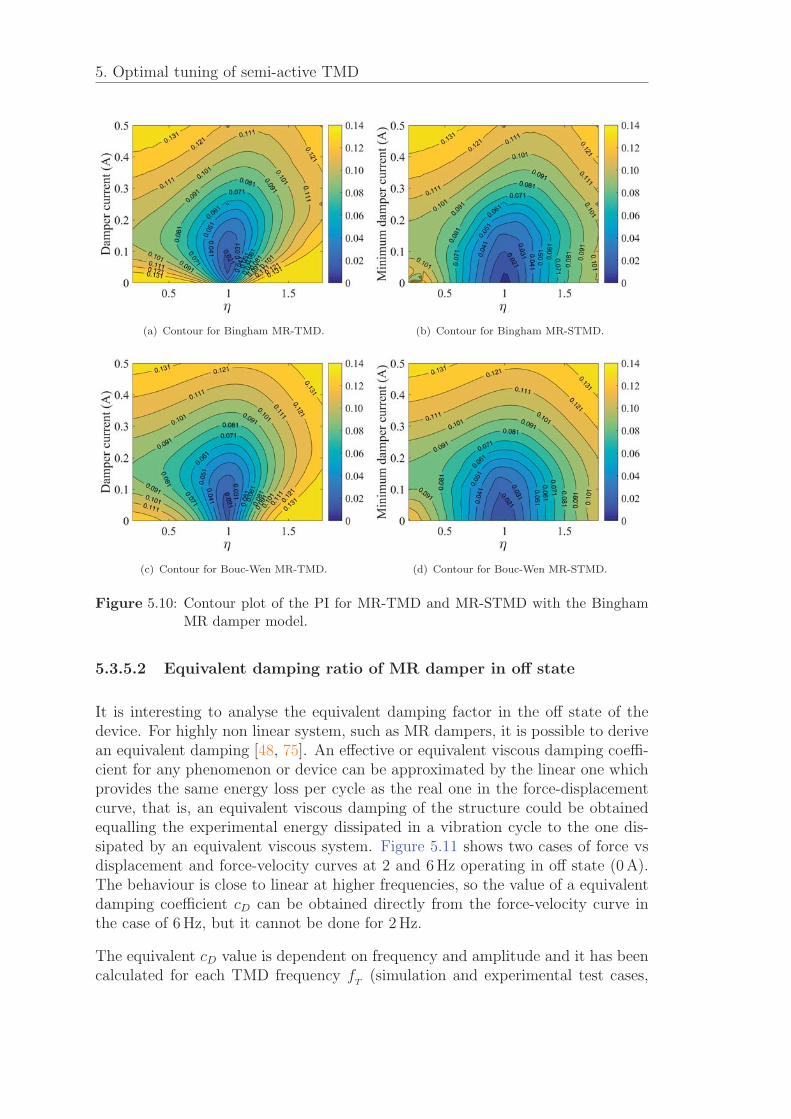
5. Optimal tuning of semi-active TMD
(a) Contour for Bingham MR-TMD. (b) Contour for Bingham MR-STMD.
(c) Contour for Bouc-Wen MR-TMD. (d) Contour for Bouc-Wen MR-STMD.
Figure 5.10: Contour plot of the PI for MR-TMD and MR-STMD with the BinghamMR damper model.
5.3.5.2 Equivalent damping ratio of MR damper in off state
It is interesting to analyse the equivalent damping factor in the off state of thedevice. For highly non linear system, such as MR dampers, it is possible to derivean equivalent damping [48, 75]. An effective or equivalent viscous damping coeffi-cient for any phenomenon or device can be approximated by the linear one whichprovides the same energy loss per cycle as the real one in the force-displacementcurve, that is, an equivalent viscous damping of the structure could be obtainedequalling the experimental energy dissipated in a vibration cycle to the one dis-sipated by an equivalent viscous system. Figure 5.11 shows two cases of force vsdisplacement and force-velocity curves at 2 and 6 Hz operating in off state (0 A).The behaviour is close to linear at higher frequencies, so the value of a equivalentdamping coefficient cD can be obtained directly from the force-velocity curve inthe case of 6 Hz, but it cannot be done for 2 Hz.
The equivalent cD value is dependent on frequency and amplitude and it has beencalculated for each TMD frequency f
T(simulation and experimental test cases,
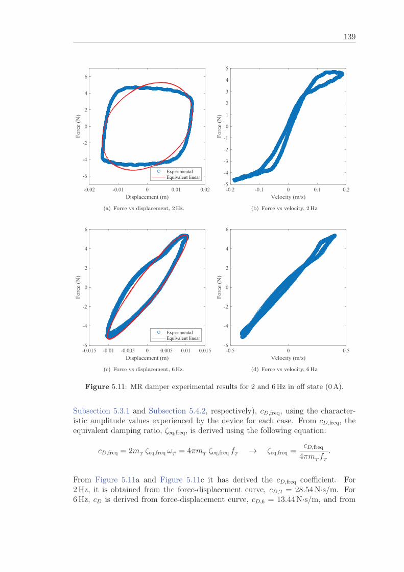
139
-0.02 -0.01 0 0.01 0.02Displacement (m)
-6
-4
-2
0
2
4
6Fo
rce
(N)
ExperimentalEquivalent linear
(a) Force vs displacement, 2Hz.
-0.2 -0.1 0 0.1 0.2Velocity (m/s)
-5
-4
-3
-2
-1
0
1
2
3
4
5
Forc
e (N
)
(b) Force vs velocity, 2Hz.
-0.015 -0.01 -0.005 0 0.005 0.01 0.015Displacement (m)
-6
-4
-2
0
2
4
6
Forc
e (N
)
ExperimentalEquivalent linear
(c) Force vs displacement, 6Hz.
-0.5 0 0.5Velocity (m/s)
-6
-4
-2
0
2
4
6
Forc
e (N
)
(d) Force vs velocity, 6Hz.
Figure 5.11: MR damper experimental results for 2 and 6Hz in off state (0A).
Subsection 5.3.1 and Subsection 5.4.2, respectively), cD,freq, using the character-istic amplitude values experienced by the device for each case. From cD,freq, theequivalent damping ratio, ζeq,freq, is derived using the following equation:
cD,freq = 2mTζeq,freq ωT
= 4πmTζeq,freq fT
→ ζeq,freq =cD,freq
4πmTfT
.
From Figure 5.11a and Figure 5.11c it has derived the cD,freq coefficient. For2 Hz, it is obtained from the force-displacement curve, cD,2 = 28.54 N·s/m. For6 Hz, cD is derived from force-displacement curve, cD,6 = 13.44 N·s/m, and from
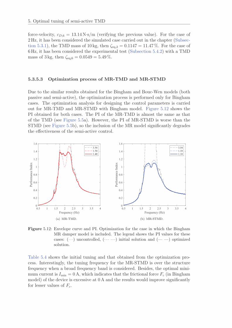
5. Optimal tuning of semi-active TMD
force-velocity, cD,6 = 13.14 N·s/m (verifying the previous value). For the case of2 Hz, it has been considered the simulated case carried out in the chapter (Subsec-tion 5.3.1), the TMD mass of 10 kg, then ζeq,2 = 0.1147 = 11.47 %. For the case of6 Hz, it has been considered the experimental test (Subsection 5.4.2) with a TMDmass of 3 kg, then ζeq,6 = 0.0549 = 5.49 %.
5.3.5.3 Optimization process of MR-TMD and MR-STMD
Due to the similar results obtained for the Bingham and Bouc-Wen models (bothpassive and semi-active), the optimization process is performed only for Binghamcases. The optimization analysis for designing the control parameters is carriedout for MR-TMD and MR-STMD with Bingham model. Figure 5.12 shows thePI obtained for both cases. The PI of the MR-TMD is almost the same as thatof the TMD (see Figure 5.5a). However, the PI of MR-STMD is worse than theSTMD (see Figure 5.5b), so the inclusion of the MR model significantly degradesthe effectiveness of the semi-active control.
0.5 1 1.5 2 2.5 3 3.5 4Frequency (Hz)
0
0.2
0.4
0.6
0.8
1
1.2
1.4
1.6
Perf
orm
ance
Inde
x
3.541.541.40
(a) MR-TMD.
0.5 1 1.5 2 2.5 3 3.5 4Frequency (Hz)
0
0.2
0.4
0.6
0.8
1
1.2
1.4
1.6
Perf
orm
ance
Inde
x
3.541.181.10
(b) MR-STMD.
Figure 5.12: Envelope curve and PI. Optimization for the case in which the BinghamMR damper model is included. The legend shows the PI values for thesecases: ( ) uncontrolled, ( ) initial solution and ( ) optimizedsolution.
Table 5.4 shows the initial tuning and that obtained from the optimization pro-cess. Interestingly, the tuning frequency for the MR-STMD is over the structurefrequency when a broad frequency band is considered. Besides, the optimal mini-mum current is Imin = 0 A, which indicates that the frictional force Fc (in Binghammodel) of the device is excessive at 0 A and the results would improve significantlyfor lesser values of Fc.
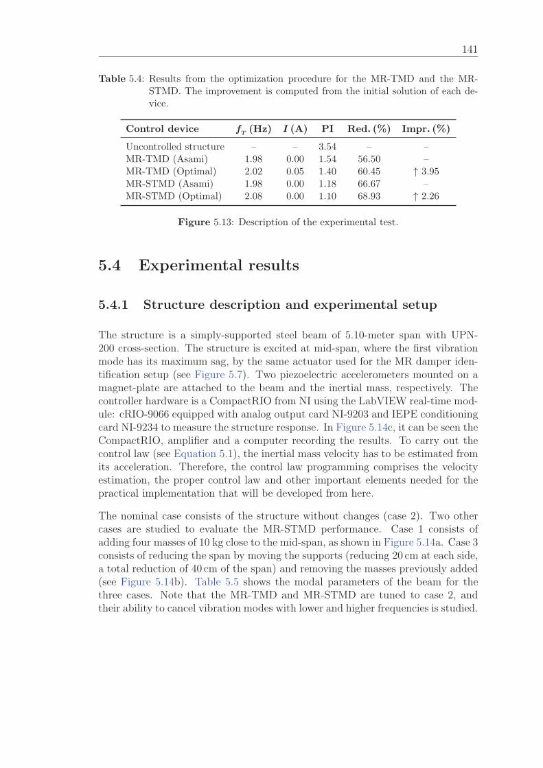
141
Table 5.4: Results from the optimization procedure for the MR-TMD and the MR-STMD. The improvement is computed from the initial solution of each de-vice.
Control device fT (Hz) I (A) PI Red. (%) Impr. (%)
Uncontrolled structure – – 3.54 – –MR-TMD (Asami) 1.98 0.00 1.54 56.50 –MR-TMD (Optimal) 2.02 0.05 1.40 60.45 ↑ 3.95MR-STMD (Asami) 1.98 0.00 1.18 66.67 –MR-STMD (Optimal) 2.08 0.00 1.10 68.93 ↑ 2.26
Figure 5.13: Description of the experimental test.
5.4 Experimental results
5.4.1 Structure description and experimental setup
The structure is a simply-supported steel beam of 5.10-meter span with UPN-200 cross-section. The structure is excited at mid-span, where the first vibrationmode has its maximum sag, by the same actuator used for the MR damper iden-tification setup (see Figure 5.7). Two piezoelectric accelerometers mounted on amagnet-plate are attached to the beam and the inertial mass, respectively. Thecontroller hardware is a CompactRIO from NI using the LabVIEW real-time mod-ule: cRIO-9066 equipped with analog output card NI-9203 and IEPE conditioningcard NI-9234 to measure the structure response. In Figure 5.14c, it can be seen theCompactRIO, amplifier and a computer recording the results. To carry out thecontrol law (see Equation 5.1), the inertial mass velocity has to be estimated fromits acceleration. Therefore, the control law programming comprises the velocityestimation, the proper control law and other important elements needed for thepractical implementation that will be developed from here.
The nominal case consists of the structure without changes (case 2). Two othercases are studied to evaluate the MR-STMD performance. Case 1 consists ofadding four masses of 10 kg close to the mid-span, as shown in Figure 5.14a. Case 3consists of reducing the span by moving the supports (reducing 20 cm at each side,a total reduction of 40 cm of the span) and removing the masses previously added(see Figure 5.14b). Table 5.5 shows the modal parameters of the beam for thethree cases. Note that the MR-TMD and MR-STMD are tuned to case 2, andtheir ability to cancel vibration modes with lower and higher frequencies is studied.
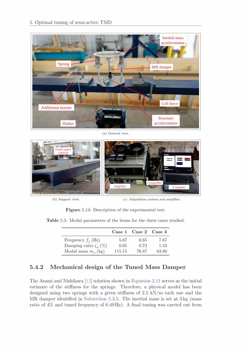
5. Optimal tuning of semi-active TMD
Inertial mass accelerometer
MR damper
Cell forceAdditional masses
ShakerStructure
accelerometer
Spring
(a) General view.
Simple support condition
(b) Support view.
AmplifierCompactRIO
Computer
(c) Adquisition system and amplifier.
Figure 5.14: Description of the experimental test.
Table 5.5: Modal parameters of the beam for the three cases studied.
Case 1 Case 2 Case 3
Frequency fS (Hz) 5.67 6.65 7.67Damping ratio ζS (%) 0.65 0.72 1.53Modal mass mS (kg) 115.15 76.87 63.80
5.4.2 Mechanical design of the Tuned Mass Damper
The Asami and Nishihara [12] solution shown in Equation 2.11 serves as the initialestimate of the stiffness for the springs. Therefore, a physical model has beendesigned using two springs with a given stiffness of 2.5 kN/m each one and theMR damper identified in Subsection 5.3.5. The inertial mass is set at 3 kg (massratio of 4% and tuned frequency of 6.49 Hz). A final tuning was carried out from
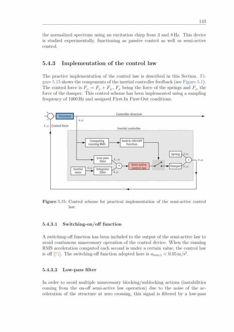
143
the normalized spectrum using an excitation chirp from 3 and 8 Hz. This deviceis studied experimentally, functioning as passive control as well as semi-activecontrol.
5.4.3 Implementation of the control law
The practice implementation of the control law is described in this Section. Fi-gure 5.15 shows the components of the inertial controller feedback (see Figure 5.1).The control force is F
C= F
S+ F
D, F
Sbeing the force of the springs and F
Dthe
force of the damper. This control scheme has been implemented using a samplingfrequency of 1000 Hz and assigned First-In First-Out conditions.
Figure 5.15: Control scheme for practical implementation of the semi-active controllaw.
5.4.3.1 Switching-on/off function
A switching-off function has been included to the output of the semi-active law toavoid continuous unnecessary operation of the control device. When the runningRMS acceleration computed each second is under a certain value, the control lawis off [71]. The switching-off function adopted here is aRMS,1 < 0.05 m/s2.
5.4.3.2 Low-pass filter
In order to avoid multiple unnecessary blocking/unblocking actions (instabilitiescoming from the on-off semi-active law operation) due to the noise of the ac-celeration of the structure at zero crossing, this signal is filtered by a low-pass
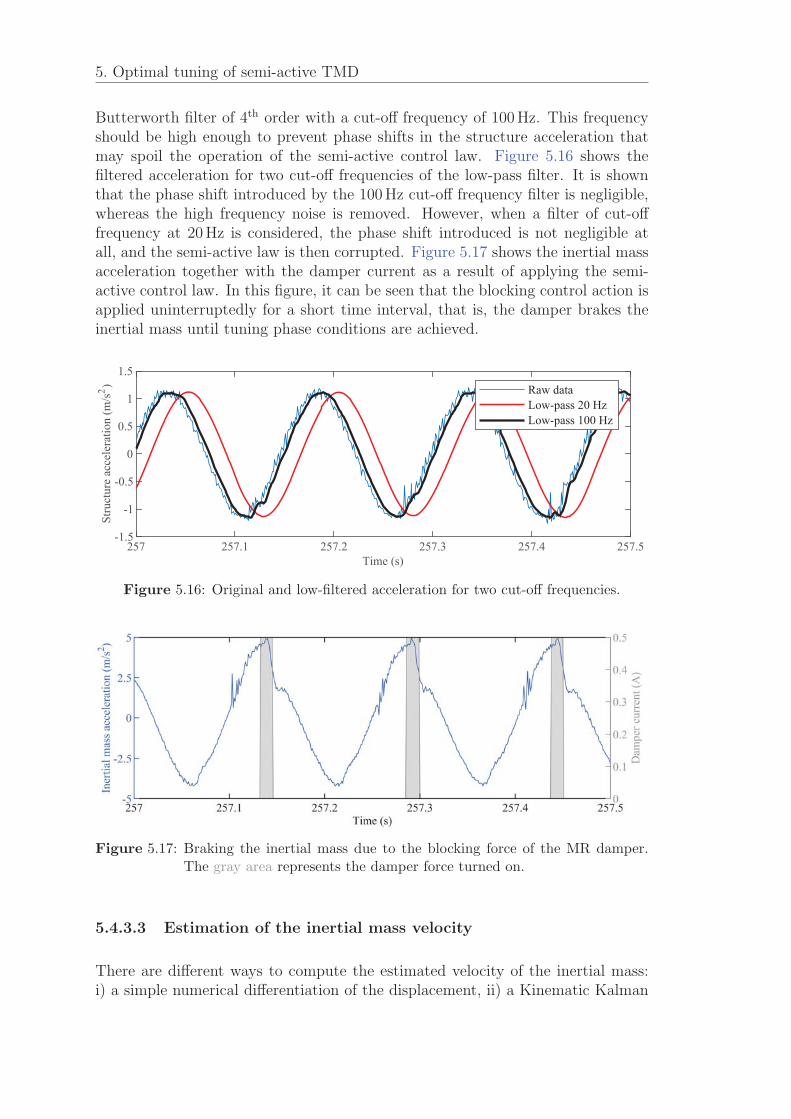
5. Optimal tuning of semi-active TMD
Butterworth filter of 4th order with a cut-off frequency of 100 Hz. This frequencyshould be high enough to prevent phase shifts in the structure acceleration thatmay spoil the operation of the semi-active control law. Figure 5.16 shows thefiltered acceleration for two cut-off frequencies of the low-pass filter. It is shownthat the phase shift introduced by the 100 Hz cut-off frequency filter is negligible,whereas the high frequency noise is removed. However, when a filter of cut-offfrequency at 20 Hz is considered, the phase shift introduced is not negligible atall, and the semi-active law is then corrupted. Figure 5.17 shows the inertial massacceleration together with the damper current as a result of applying the semi-active control law. In this figure, it can be seen that the blocking control action isapplied uninterruptedly for a short time interval, that is, the damper brakes theinertial mass until tuning phase conditions are achieved.
257 257.1 257.2 257.3 257.4 257.5Time (s)
-1.5
-1
-0.5
0
0.5
1
1.5
Stru
ctur
e ac
cele
ratio
n (m
/s2 ) Raw data
Low-pass 20 HzLow-pass 100 Hz
Figure 5.16: Original and low-filtered acceleration for two cut-off frequencies.
Figure 5.17: Braking the inertial mass due to the blocking force of the MR damper.The gray area represents the damper force turned on.
5.4.3.3 Estimation of the inertial mass velocity
There are different ways to compute the estimated velocity of the inertial mass:i) a simple numerical differentiation of the displacement, ii) a Kinematic Kalman
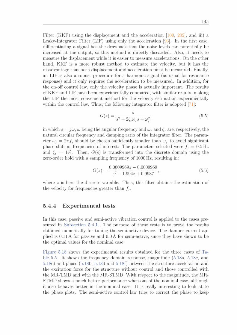
145
Filter (KKF) using the displacement and the acceleration [100, 202], and iii) aLeaky-Integrator Filter (LIF) using only the acceleration [93]. In the first case,differentiating a signal has the drawback that the noise levels can potentially beincreased at the output, so this method is directly discarded. Also, it needs tomeasure the displacement while it is easier to measure accelerations. On the otherhand, KKF is a more robust method to estimate the velocity, but it has thedisadvantage that both displacement and acceleration must be measured. Finally,an LIF is also a robust procedure for a harmonic signal (as usual for resonanceresponse) and it only requires the acceleration to be measured. In addition, forthe on-off control law, only the velocity phase is actually important. The resultsof KKF and LIF have been experimentally compared, with similar results, makingthe LIF the most convenient method for the velocity estimation experimentallywithin the control law. Thus, the following integrator filter is adopted [71]:
G(s) =s
s2 + 2ζIω
Is+ ω2
I
, (5.5)
in which s = jω, ω being the angular frequency and ωI
and ζI
are, respectively, thenatural circular frequency and damping ratio of the integrator filter. The param-eter ω
I= 2πf
Ishould be chosen sufficiently smaller than ω
Sto avoid significant
phase shift at frequencies of interest. The parameters selected were fI
= 0.5 Hzand ζ
I= 1%. Then, G(s) is transformed into the discrete domain using the
zero-order hold with a sampling frequency of 1000 Hz, resulting in:
G(z) =0.0009969z − 0.0009969
z2 − 1.994z + 0.9937, (5.6)
where z is here the discrete variable. Thus, this filter obtains the estimation ofthe velocity for frequencies greater than f
I.
5.4.4 Experimental tests
In this case, passive and semi-active vibration control is applied to the cases pre-sented in Subsection 5.4.1. The purpose of these tests is to prove the resultsobtained numerically for tuning the semi-active device. The damper current ap-plied is 0.11 A for passive and 0.0 A for semi-active, since they have shown to bethe optimal values for the nominal case.
Figure 5.18 shows the experimental results obtained for the three cases of Ta-ble 5.5. It shows the frequency domain response, magnitude (5.18a, 5.18c, and5.18e) and phase (5.18b, 5.18d and 5.18f) between the structure acceleration andthe excitation force for the structure without control and those controlled withthe MR-TMD and with the MR-STMD. With respect to the magnitude, the MR-STMD shows a much better performance when out of the nominal case, althoughit also behaves better in the nominal case. It is really interesting to look at tothe phase plots. The semi-active control law tries to correct the phase to keep
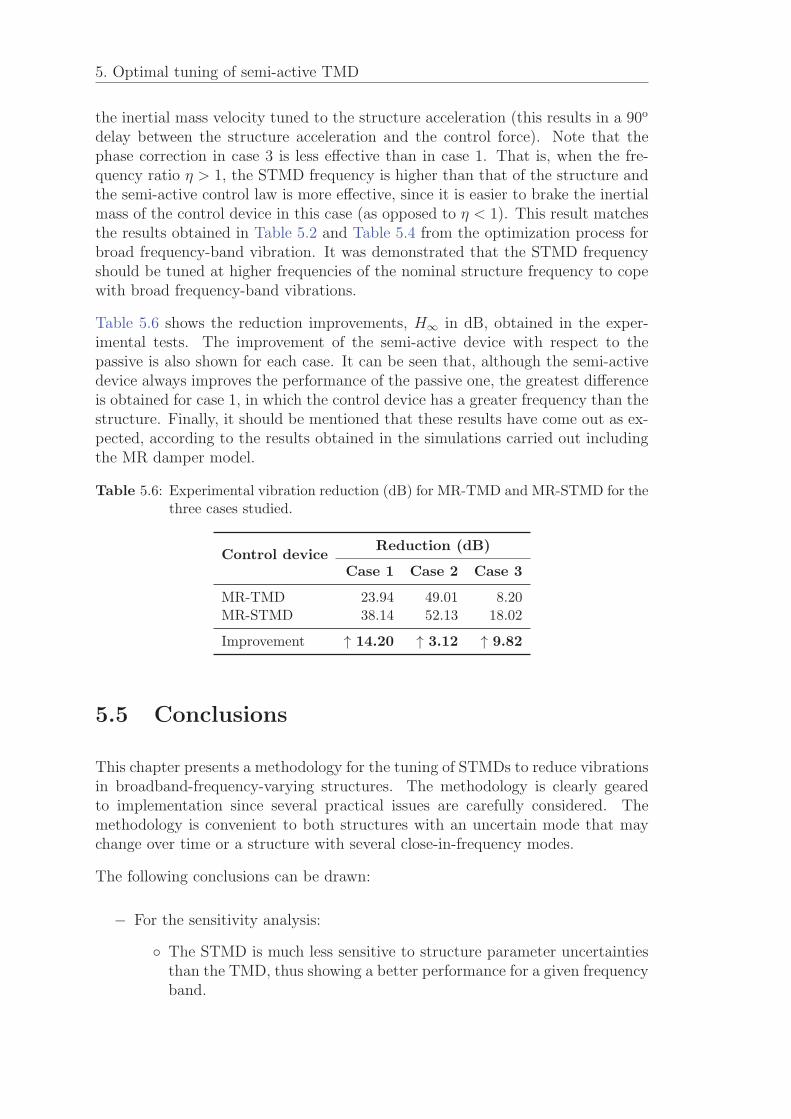
5. Optimal tuning of semi-active TMD
the inertial mass velocity tuned to the structure acceleration (this results in a 90o
delay between the structure acceleration and the control force). Note that thephase correction in case 3 is less effective than in case 1. That is, when the fre-quency ratio η > 1, the STMD frequency is higher than that of the structure andthe semi-active control law is more effective, since it is easier to brake the inertialmass of the control device in this case (as opposed to η < 1). This result matchesthe results obtained in Table 5.2 and Table 5.4 from the optimization process forbroad frequency-band vibration. It was demonstrated that the STMD frequencyshould be tuned at higher frequencies of the nominal structure frequency to copewith broad frequency-band vibrations.
Table 5.6 shows the reduction improvements, H∞ in dB, obtained in the exper-imental tests. The improvement of the semi-active device with respect to thepassive is also shown for each case. It can be seen that, although the semi-activedevice always improves the performance of the passive one, the greatest differenceis obtained for case 1, in which the control device has a greater frequency than thestructure. Finally, it should be mentioned that these results have come out as ex-pected, according to the results obtained in the simulations carried out includingthe MR damper model.
Table 5.6: Experimental vibration reduction (dB) for MR-TMD and MR-STMD for thethree cases studied.
Control deviceReduction (dB)
Case 1 Case 2 Case 3
MR-TMD 23.94 49.01 8.20MR-STMD 38.14 52.13 18.02
Improvement ↑ 14.20 ↑ 3.12 ↑ 9.82
5.5 Conclusions
This chapter presents a methodology for the tuning of STMDs to reduce vibrationsin broadband-frequency-varying structures. The methodology is clearly gearedto implementation since several practical issues are carefully considered. Themethodology is convenient to both structures with an uncertain mode that maychange over time or a structure with several close-in-frequency modes.
The following conclusions can be drawn:
− For the sensitivity analysis:
◦ The STMD is much less sensitive to structure parameter uncertaintiesthan the TMD, thus showing a better performance for a given frequencyband.
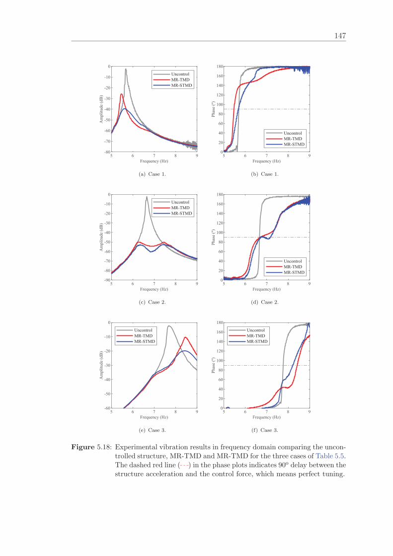
147
5 6 7 8 9Frequency (Hz)
-80
-70
-60
-50
-40
-30
-20
-10
0
Am
plitu
de (d
B)
UncontrolMR-TMDMR-STMD
(a) Case 1.
5 6 7 8 9Frequency (Hz)
0
20
40
60
80
100
120
140
160
180
Phas
e (º)
UncontrolMR-TMDMR-STMD
(b) Case 1.
5 6 7 8 9Frequency (Hz)
-90
-80
-70
-60
-50
-40
-30
-20
-10
0
Am
plitu
de (d
B)
UncontrolMR-TMDMR-STMD
(c) Case 2.
5 6 7 8 9Frequency (Hz)
0
20
40
60
80
100
120
140
160
180
Phas
e (º)
UncontrolMR-TMDMR-STMD
(d) Case 2.
5 6 7 8 9Frequency (Hz)
-60
-50
-40
-30
-20
-10
0
Am
plitu
de (d
B)
UncontrolMR-TMDMR-STMD
(e) Case 3.
5 6 7 8 9Frequency (Hz)
0
20
40
60
80
100
120
140
160
180
Phas
e (º)
UncontrolMR-TMDMR-STMD
(f) Case 3.
Figure 5.18: Experimental vibration results in frequency domain comparing the uncon-trolled structure, MR-TMD and MR-TMD for the three cases of Table 5.5.The dashed red line ( ) in the phase plots indicates 90o delay between thestructure acceleration and the control force, which means perfect tuning.
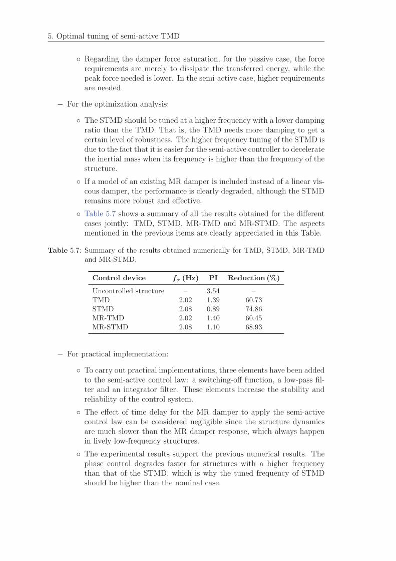
5. Optimal tuning of semi-active TMD
◦ Regarding the damper force saturation, for the passive case, the forcerequirements are merely to dissipate the transferred energy, while thepeak force needed is lower. In the semi-active case, higher requirementsare needed.
− For the optimization analysis:
◦ The STMD should be tuned at a higher frequency with a lower dampingratio than the TMD. That is, the TMD needs more damping to get acertain level of robustness. The higher frequency tuning of the STMD isdue to the fact that it is easier for the semi-active controller to deceleratethe inertial mass when its frequency is higher than the frequency of thestructure.
◦ If a model of an existing MR damper is included instead of a linear vis-cous damper, the performance is clearly degraded, although the STMDremains more robust and effective.
◦ Table 5.7 shows a summary of all the results obtained for the differentcases jointly: TMD, STMD, MR-TMD and MR-STMD. The aspectsmentioned in the previous items are clearly appreciated in this Table.
Table 5.7: Summary of the results obtained numerically for TMD, STMD, MR-TMDand MR-STMD.
Control device fT (Hz) PI Reduction (%)
Uncontrolled structure – 3.54 –TMD 2.02 1.39 60.73STMD 2.08 0.89 74.86MR-TMD 2.02 1.40 60.45MR-STMD 2.08 1.10 68.93
− For practical implementation:
◦ To carry out practical implementations, three elements have been addedto the semi-active control law: a switching-off function, a low-pass fil-ter and an integrator filter. These elements increase the stability andreliability of the control system.
◦ The effect of time delay for the MR damper to apply the semi-activecontrol law can be considered negligible since the structure dynamicsare much slower than the MR damper response, which always happenin lively low-frequency structures.
◦ The experimental results support the previous numerical results. Thephase control degrades faster for structures with a higher frequencythan that of the STMD, which is why the tuned frequency of STMDshould be higher than the nominal case.
6Conclusions
Contents6.1 Conclusions . . . . . . . . . . . . . . . . . . . . . . . . . . 149
6.2 Perspectives for future work . . . . . . . . . . . . . . . . 151
6.3 Publications . . . . . . . . . . . . . . . . . . . . . . . . . . 153
6.3.1 JCR journal papers . . . . . . . . . . . . . . . . . . . . 153
6.3.2 Conference proceedings . . . . . . . . . . . . . . . . . . 154
The present chapter summarizes the most relevant conclusions conducted through-out this thesis, followed by suggestions for future research and the publicationsderived from this thesis.
6.1 Conclusions
This thesis covers from the analysis of the dynamics of pedestrian structures whosemodal parameters change over time up to the vibration control using an state-of-the-art strategy based on semi-active control. In between, it has been consideredthe existence of more than one problematic vibration mode, modal parameteruncertainties, non-linearities in the control design and, finally, a few of interestingconclusions are achieved through the thesis. From the research conducted withinthe scope of this PhD thesis, according to the goals outlined in Chapter 1 andseparately from the particular conclusions of each chapter, the following generalconclusions can be drawn:
◦ A review of VSA under human loading, sources of uncertainty in the modalparameter extraction, vibration control strategies and MR dampers has beencarried out in Chapter 2. Issues studied in this chapter serve as sustenance
149

6. Conclusions
for later chapters of this thesis. Special care has been taken to mode fre-quency variability and the implications of that into the tuning and perfor-mance of TMDs. Indeed, it has been shown that footbridge may have severalvibration modes into the human excitation range, which actually makes thecontrol system design more challenging. Thus, the thesis has focused onSTMD as a solution to structures with several problematic modes whosemodal properties may indeed change over time. Finally, the thesis has builton STMD with phase control, showing that properly design and conditionedsimple control laws can make the STMD succeeded in this challenging prob-lem.
◦ The variability of the modal parameters that characterise a structure (fre-quencies, damping ratios and modal shapes) has been analysed in Chapter 3using three different SSI OMA techniques to estimate the uncertainties as-sociated to the OMA techniques. Moreover, the uncertainness associatedthe the selected raw data and the time block selected for a particular OMAtechniques are studied. The errors in natural frequency estimates using 20minutes as compared with 60 are negligible. It does not happen with thedamping ratio estimates, which experience greater variability.
◦ A novel methodology for tracking the modal parameters of a structure whichmay change significantly over time is proposed and tested in Chapter 3 for anin-service stress-ribbon footbridge. Unless natural frequency estimates arewell-separated, a sufficient number of spatially located sensors will be neededto associate correctly a particular estimate to its mode shape (through theMAC as the first indicator). The application of this methodology has allowedto analyse and remove the influence of the external factors on the post-process (i.e. temperature). Also an ad-hoc statistical model is developed toremove the influence of external factors on the final estimates. Thus, thefrequency estimates might be used within SHM system.
◦ Several easy-to-implement semi-active strategies for inertial controllers arestudied in Chapter 4. They have been compared with other vibration controlstrategies as passive or active ones under broad frequency-band excitations.Focusing on the semi-active strategies and their implementability withinconstructable devices, it has been concluded that the on-off semi-active phasecontrol is easy to implement, robust to the MR dynamics and it has shownan excellent capacity to cope with broad band-frequency vibrations.
◦ A design methodology, through an optimization of the parameters of thesemi-active inertial controller, for structures with modal parameter uncer-tainties and considering a wide frequency range of operation, has been pro-posed in Chapter 5. In this chapter, the influence of the tuning parametersof the STMD has been studied. Important conclusions have been derivedabout the tuning of STMDs: 1) very low damping for off stage of the MRis recommendable; 2) the tuning of STMD should be for a higher frequencythat the one is usually used (mean frequency) for TMDs designed consid-ering broad frequency-band vibrations; and 3) simple but necessary actions

151
such has filtering the inertial mass acceleration, switching-off function or lowpass filtering should be included into the control law and even in the designmethodology.
◦ Two phenomenological models, Bighman and Bouc-Wen models, have beenidentified through experimental tests with an MR damper. It has been shownthat the non-linear behaviour of MR dampers should be taken into accountto obtain more reliable results. It has been demonstrated that the Binghammodel (the simplest one) is enough in order to account for the MR non-linearities into the design methodology. This is due to the fact the controlis on-off, so the hysteresis does not play an important role into the STMDperformance. Obviously, for other control laws, more accurate models mightbe required.
◦ The design methodology has been applied and experimentally tested into alab beam structure in Chapter 5. The different steps for its materializationhave been described. Finally, its robustness has been compared to the passivecase for two types of frequency detuned cases, above and below detuning. Ithas been demonstrated the STMD capacity of phase correction keeping theinertial controller tuned for a broad frequency band.
6.2 Perspectives for future work
Firstly, the STMD studied and developed has been tested on a laboratory beam.Efforts should be made in order to get the STMD interesting to be considered infuture structures. To achieve that, the following actions have been planned fromthe research carried out through this thesis:
◦ A modular TMD will be designed in order to be easily adaptable to a rangeof structures and also easy to incorporate MR dampers to upgrade it to anSTMD.
◦ Both the TMD and STMD will be tested on a lively in-service footbridge.
◦ In order to keep the STMD under reasonable cost, a low-cost instrumentationwill be included to both, carrying out the semi-active control law and monitorthe VS continuously. To this point, an instrumentation based on RaspberryPi (+ Arduino) and low-cost accelerometers (MEMS) properly conditionedwill be considering (see Figure 6.1).
All these actions are focused on getting affordable STMDs to be incorporated fromthe design stage or as remedial action to structure which comfort is wanted to beenhanced.
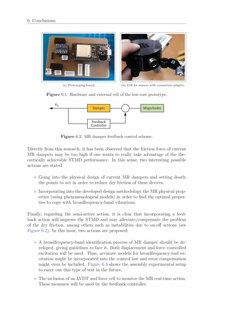
6. Conclusions
(a) Prototyping board. (b) Cell for sensors with connection adapter.
Figure 6.1: Hardware and external cell of the low-cost prototype.
Figure 6.2: MR damper feedback control scheme.
Directly from this research, it has been observed that the friction force of currentMR dampers may be too high if one wants to really take advantage of the the-oretically achievable STMD performance. In this sense, two interesting possibleactions are stated:
◦ Going into the physical design of current MR dampers and setting dearlythe points to act in order to reduce dry friction of these devices.
◦ Incorporating into the developed design methodology the MR physical prop-erties (using phenomenological models) in order to find the optimal proper-ties to cope with broadfrequency-band vibrations.
Finally, regarding the semi-active action, it is clear that incorporating a feed-back action will improve the STMD and may alleviate/compensate the problemof the dry friction, among others such as instabilities due to on-off actions (seeFigure 6.2). In this issue, two actions are proposed:
◦ A broadfrequency-band identification process of MR damper should be de-veloped, giving guidelines to face it. Both displacement and force controlledexcitation will be used. Thus, accurate models for broadfrequency-bad ex-citation might be incorporated into the control law and error compensationmight even be included. Figure 6.3 shows the assembly experimental setupto carry out this type of test in the future.
◦ The inclusion of an LVDT and force cell to monitor the MR real-time action.These measures will be used by the feedback controller.
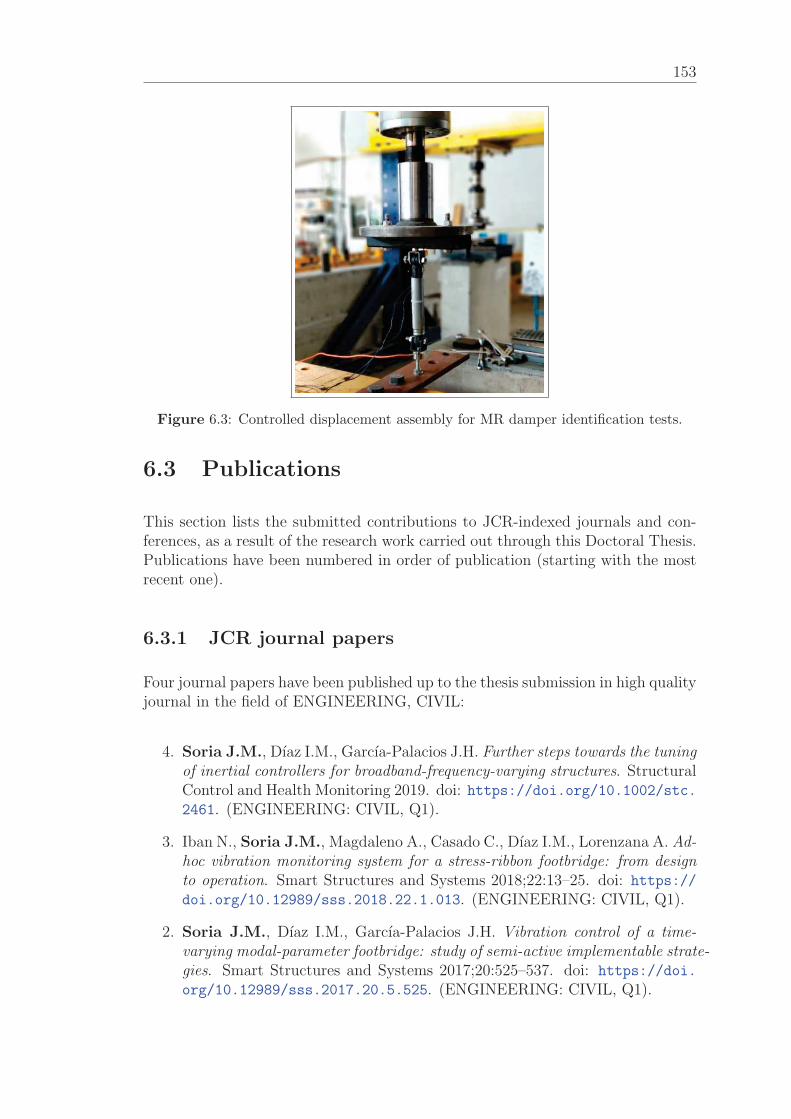
153
Figure 6.3: Controlled displacement assembly for MR damper identification tests.
6.3 Publications
This section lists the submitted contributions to JCR-indexed journals and con-ferences, as a result of the research work carried out through this Doctoral Thesis.Publications have been numbered in order of publication (starting with the mostrecent one).
6.3.1 JCR journal papers
Four journal papers have been published up to the thesis submission in high qualityjournal in the field of ENGINEERING, CIVIL:
4. Soria J.M., Dıaz I.M., Garcıa-Palacios J.H. Further steps towards the tuningof inertial controllers for broadband-frequency-varying structures. StructuralControl and Health Monitoring 2019. doi: https://doi.org/10.1002/stc.2461. (ENGINEERING: CIVIL, Q1).
3. Iban N., Soria J.M., Magdaleno A., Casado C., Dıaz I.M., Lorenzana A. Ad-hoc vibration monitoring system for a stress-ribbon footbridge: from designto operation. Smart Structures and Systems 2018;22:13–25. doi: https://
doi.org/10.12989/sss.2018.22.1.013. (ENGINEERING: CIVIL, Q1).
2. Soria J.M., Dıaz I.M., Garcıa-Palacios J.H. Vibration control of a time-varying modal-parameter footbridge: study of semi-active implementable strate-gies. Smart Structures and Systems 2017;20:525–537. doi: https://doi.
org/10.12989/sss.2017.20.5.525. (ENGINEERING: CIVIL, Q1).
6. Conclusions
1. Soria J.M., Dıaz I.M., Garcıa-Palacios J.H., Iban N. Vibration Monitoringof a Steel-Plated Stress-Ribbon Footbridge: Uncertainties in the Modal Esti-mation. Journal of Bridge Engineering (ASCE) 2016;21:1–13. doi: https://doi.org/10.1061/(ASCE)BE.1943-5592.0000830. (ENGINEERING: CIVIL,Q2).
6.3.2 Conference proceedings
The communications in conferences directly related to the thesis content are listedhere:
18. Magdaleno, A., Casado, C., Soria J.M., Pereira, E., Dıaz, I.M., Lorenzana,A. Comparison of passive and active mitigation devices for vibration con-trol in slender structures. IX ECCOMAS Thematic Conference on SmartStructures and Materials (SMART 2019), Paris, France: 2019.
17. Renedo C.M., Dıaz IM, Soria J.M., Garcıa-Palacios J.H. Designing a foot-bridge with integrated TMD: improvement assessment. Congresso de MetodosNumericos em Engenharia, Guimaraes, Portugal: 2019.
16. Barrera C.A., Soria J.M., Wang X., Garcıa-Palacios J.H., Dıaz I.M. Onthe search of TMD configurations for a vibration mode with changing modalproperties. I Conferencia de Dinamica Estructural (DinEst 2018), Madrid,Spain: 2018.
15. Soria J.M., Dıaz I.M., Garcıa-Palacios J.H., Zanuy C., Wang X. Tun-ing a phase-controlled smart TMD for broad-band-frequency-varying vibra-tion modes. I Conferencia de Dinamica Estructural (DinEst 2018), Madrid,Spain: 2018.
14. Bukovics M., Soria J.M., Dıaz I.M., Arroyo J., Calvo J. Enhancementof vibration pedestrian comfort of a footbridge via Tuned Mass Damper. IConferencia de Dinamica Estructural (DinEst 2018), Madrid, Spain: 2018.
13. Casado C.M., Fernandez J., Pereda J., Soria J.M., Castano J. Design ofvibration damping systems using simplified models for lightweight footbridges.4th International Conference on Mechanical Models in Structural Engineering(CMMoST 20117), Madrid, Spain: 2017.
12. Marinas-Sanz G., Dıaz I.M., Soria J.M., Garcıa-Palacios J.H., Zanuy C.Construccion, analisis dinamico y cancelacion de vibraciones de un forjadomixto ligero. 4th International Conference on Mechanical Models in Struc-tural Engineering (CMMoST 2017), Madrid, Spain: 2017.
11. Dıaz I.M., Garcıa-Palacios J.H., Soria J.M., Pereira E. Vibration controlstrategies for pedestrian structures. 4th International Conference on Me-chanical Models in Structural Engineering (CMMoST 2017), Madrid, Spain:2017.
155
10. Canales Sanchez-Castro F., Soria J.M., Dıaz I.M., Marinas-Sanz G., Garcıa-Palacios JH. Identifying a TMD and its final tuning once installed on a livelycomposite slab. 4th International Conference on Mechanical Models in Struc-tural Engineering (CMMoST 20117), Madrid, Spain: 2017.
9. Soria J.M., Dıaz I.M., Garcıa-Palacios J.H., Lorenzana A. Long-term vibra-tion serviceability assessment of a steel-plated stress-ribbon footbridge. Foot-bridge 2017, Berlin, Germany: 2017, p. 384–393.
8. Dıaz I.M., Garcıa-Palacios J.H., Garcıa-Cruz A., Soria J.M. Computingserviceability predictors for an in-service footbridge. Footbridge 2017, Berlin,Germany: 2017, p. 426–435.
7. Soria J.M., Dıaz I.M., Garcıa-Palacios J.H., Marinas-Sanz G., Pereira E.Designing a smart TMD for a composite steel-concrete slender slab. VIII EC-COMAS Thematic Conference on Smart Structures and Materials (SMART2017), Madrid: 2017, p. 764–775.
6. Soria J.M., Dıaz I.M., Pereira E., Garcıa-Palacios J.H., Wang X. Exploringvibration control strategies for a footbridge with time-varying modal param-eters. MOVIC & RASD 2016, Southampton, England: 2016, p. 118-131.
5. Garcıa-Palacios J.H., Tirado-Andres F., Soria J.M., Dıaz I.M., Araujo A.Effects of time synchronization on operational Modal analysis. 6th Interna-tional Operational Modal Analysis Conference, IOMAC 2015, Gijon, Spain:2015, p. 249–258.
4. Soria J.M., Dıaz I.M., Garcıa-Palacios J.H., Iban N., Lorenzana A. A pro-cedure to track vibration modes under changing external factors: applicationto a pedestrian bridge. 3rd International Conference on Mechanical Modelsin Structural Engineering, CMMoST 2015, Sevilla, Spain: 2015, p. 41–57.
3. Iban N., Castano J., Soria J.M., Dıaz I.M., Lorenzana A. Dynamic char-acterization, modelling and model updating of a lively footbridge. 3rd Inter-national Conference on Mechanical Models in Structural Engineering, CM-MoST 2015, Sevilla, Spain: 2015, p. 235–244.
2. Garcıa-Palacios J.H., Dıaz I.M., Soria J.M., Cara F.J., Garcıa S. Un-certainty optimization of Automated Operational Modal Analysis applied toStructural Health Monitoring techniques. 6th World Conference on StructuralControl and Monitoring, Barcelona: 2014, p. 1420–1427.
1. Dıaz I.M., Soria J.M., Iban N., Cacho M., Garcıa-Palacios J.H. Vibrationmonitoring of a steel-plated stress-ribbon footbridge: effects of environmen-tal and operational factors on modal properties. 6th World Conference onStructural Control and Monitoring, Barcelona: 2014, p. 457–466.

Bibliography
[1] Guide to evaluation of human exposure to vibration in buildings: Vibrationsources other than blasting. Technical report, British Standards Institution,2008.
[2] E. 1991-2. Eurocode 1: Actions on structures–part 2: Traffic loads onbridges, 2003.
[3] E. 1991-2. Eurocode 0: Basis of structural design, 2003.
[4] M. A. Abramson. Pattern search algorithms for mixed variable general con-strained optimization problems. Technical report, 2002.
[5] C. Adam and T. Furtmuller. Seismic performance of tuned mass dampers. InMechanics and model-based control of smart materials and structures, pages11–18. Springer, 2010.
[6] G. Aguirre, M. Gorostiaga, T. Porchez, and J. Munoa. Self-tuning semi-active tuned-mass damper for machine tool chatter suppression. ISMA2012-USD2012, pages 109–124, 2012.
[7] N. Aguirre. Magnetorheological dampers: Modeling and Control Design forCivil Engineering Structures. PhD thesis, Technical University of Catalunya,2009.
[8] A. Ahlawat and A. Ramaswamy. Multi-objective optimal design of flc drivenhybrid mass damper for seismically excited structures. Earthquake engineer-ing & structural dynamics, 31(7):1459–1479, 2002.
[9] A. Ahlawat and A. Ramaswamy. Multiobjective optimal fuzzy logic con-troller driven active and hybrid control systems for seismically excited non-linear buildings. Journal of engineering mechanics, 130(4):416–423, 2004.
[10] S. Alampalli. Effects of testing, analysis, damage, and environment on modalparameters. Mechanical Systems and Signal Processing, 14(1):63–74, 2000.
[11] Y. Arfiadi and M. N. Hadi. Passive and active control of three-dimensionalbuildings. Earthquake engineering & structural dynamics, 29(3):377–396,2000.
[12] T. Asami and O. Nishihara. Closed-Form Exact Solution to H∞ Opti-mization of Dynamic Vibration Absorbers (Application to Different TransferFunctions and Damping Systems). Journal of Vibration and Acoustics, 125(3):398, 2003. ISSN 07393717.
157
Bibliography
[13] S.-K. Au, J. M. W. Brownjohn, and J. E. Mottershead. Quantifying andmanaging uncertainty in operational modal analysis. Mechanical Systemsand Signal Processing, 102:139–157, 2018. ISSN 0888-3270.
[14] O. Avci. Modal Parameter Variations due to Joist Bottom Chord Exten-sion Installations on Laboratory Footbridges. Journal of Performance ofConstructed Facilities, 04014140, 2014. doi: 10.1061/(ASCE)CF.1943-5509.0000635.
[15] H. Bachmann and B. Weber. Tuned vibration absorbers for damping oflively structures. Structural Engineering International, 5(1):31–36, 1995.
[16] H. Bachmann, A. Pretlove, and H. Rainer. Dynamic forces from rhythmicalhuman body motions. practical guidelines, 1995.
[17] H. Bachmann, W. J. Ammann, F. Deischl, J. Eisenmann, I. Floegl, G. H.Hirsch, G. K. Klein, G. J. Lande, O. Mahrenholtz, H. G. Natke, et al.Vibration problems in structures: practical guidelines. Birkhauser, 2012.
[18] J.-S. Bae, J.-H. Hwang, J.-H. Roh, J.-H. Kim, M.-S. Yi, and J. H. Lim.Vibration suppression of a cantilever beam using magnetically tuned-mass-damper. Journal of Sound and Vibration, 331(26):5669–5684, 2012.
[19] A. Bahar, F. Pozo, L. Acho, J. Rodellar, and A. Barbat. Parameter identi-fication of large-scale magnetorheological dampers in a benchmark building.Computers & structures, 88(3-4):198–206, 2010.
[20] D. Bauer. Asymptotic properties of subspace estimators. Automatica, 41(3):359–376, 2005.
[21] A. Bayraktar, A. C. Altunisik, B. Sevim, and T. Turker. Modal Testing,Finite-Element Model Updating, and Dynamic Analysis of an Arch TypeSteel Footbridge. Journal of Performance of Constructed Facilities, 23(2):81–89, Apr. 2009. ISSN 0887-3828. doi: 10.1061/(ASCE)0887-3828(2009)23:2(81).
[22] E. C. Bingham. Fluidity and plasticity, volume 2. McGraw-Hill, 1922.
[23] A. Bleicher, M. Schlaich, Y. Fujino, and T. Schauer. Model-based design andexperimental validation of active vibration control for a stress ribbon bridgeusing pneumatic muscle actuators. Engineering structures, 33(8):2237–2247,2011.
[24] G. Bossis, S. Lacis, A. Meunier, and O. Volkova. Magnetorheological fluids.Journal of magnetism and magnetic materials, 252:224–228, 2002.
[25] R. Bouc. A mathematical model for hysteresis. Acta Acustica united withAcustica, 24(1):16–25, 1971.
[26] M. J. Brennan. Some recent developments in adaptive tuned vibration ab-sorbers/neutralisers. Shock and Vibration, 13(4, 5):531–543, 2006.
159
[27] R. Brincker and P. H. Kirkegaard. Special issue on operational modal anal-ysis. Mechanical systems and signal processing, 5(24):1209–1212, 2010.
[28] R. Brincker and C. Ventura. Introduction to operational modal analysis.John Wiley & Sons, 2015.
[29] R. Brincker, P. Andersen, and N.-J. Jacobsen. Automated frequency domaindecomposition for operational modal analysis. In Proceedings of The 25thInternational Modal Analysis Conference (IMAC), Orlando, Florida, volume415, 2007.
[30] J. Brownjohn, A. Pavic, and P. Omenzetter. A spectral density approach formodeling continuous vertical forces on pedestrian structures due to walking.Canadian Journal of Civil Engineering, 2004.
[31] J. M. W. Brownjohn, A. De Stefano, Y.-L. Xu, H. Wenzel, and A. E. Aktan.Vibration-based monitoring of civil infrastructure: challenges and successes.Journal of Civil Structural Health Monitoring, 1(3-4):79–95, 2011.
[32] A. Cabboi, F. Magalhaes, C. Gentile, and A. Cunha. Automated modalidentification and tracking: Application to an iron arch bridge. StructuralControl and Health Monitoring, 24(1):e1854, 2017.
[33] M. Cacho-Perez, N. Frechilla, I. Diaz, and A. Lorenzana. Simplified me-chanical model for a stress-ribbon monitorized footbridge. analylitical andexperimental results. In 6th World Conference on Structural Control andMonitoring, pages 358–368, Barcelona (Spain), July 2014. Proceedings ofthe WCSCM.
[34] E. Caetano, A. Cunha, C. Moutinho, and F. Magalhaes. Studies for control-ling human-induced vibration of the Pedro e Ines footbridge, Portugal. Part2: Implementation of tuned mass dampers. Engineering Structures, 32(4):1082–1091, 2010. ISSN 01410296.
[35] C. Cappello, D. Sigurdardottir, B. Glisic, D. Zonta, and M. Pozzi. Onpredicting monitoring system effectiveness. In Sensors and Smart StructuresTechnologies for Civil, Mechanical, and Aerospace Systems 2015, volume9435, page 94352M. International Society for Optics and Photonics, 2015.
[36] F. J. Cara. Maximum likelihood estimation of new state space models foroperational modal analysis. PhD thesis, Universidad Politecnica de Madrid,2013.
[37] F. J. Cara, J. Carpio, J. Juan, and E. Alarcon. An approach to operationalmodal analysis using the expectation maximization algorithm. MechanicalSystems and Signal Processing, 31:109–129, 2012.
[38] J. D. Carlson and M. R. Jolly. Mr fluid, foam and elastomer devices. mecha-tronics, 10(4-5):555–569, 2000.
Bibliography
[39] C. M. Casado, I. M. Dıaz, J. D. Sebastian, A. V. Poncela, and A. Lorenzana.New methodology for the application of vibration-based damage detectiontechniques. Structural Control and Health Monitoring, 20(1):70–87, 2011.ISSN 15452255.
[40] C. M. Casado, I. Dıaz, J. Sebastian, A. Poncela, and A. Lorenzana. Imple-mentation of passive and active vibration control on an in-service footbridge.Structural Control and Health Monitoring, 20:70–87, 2013. ISSN 15452255.
[41] F. Casciati, G. Magonette, and F. Marazzi. Technology of semiactive devicesand applications in vibration mitigation. John Wiley & Sons, 2006.
[42] J. Castano, O. Cosido, J. Pereda, M. Cacho-Perez, and A. Lorenzana. Static,modal and dynamic behaviour of a stress ribbon footbridge: Experimentaland computational results. In Third International Conference on MechanicalModels in Structural Engineering (CMMoST 2015), 2015.
[43] M. B. Cesar and R. C. D. Barros. Properties and Numerical Modeling ofMR Dampers. In 15th International Conference on Experimental Mechanics,Porto, Portugal, 2012.
[44] P. Charles and W. Hoorpah. Evaluation du comportement vibratoire despasserelles pietonnes sous l’action des pietons, 2006.
[45] F. Y. Cheng and H. Jiang. Hybrid control of seismic structures with optimalplacement of control devices. Journal of Aerospace Engineering, 11(2):52–58,1998.
[46] M.-H. Chey, J. G. Chase, J. B. Mander, and A. J. Carr. Semi-active tunedmass damper building systems: design. Earthquake Engineering & StructuralDynamics, 39(2):119–139, 2010.
[47] A. Chiuso and G. Picci. The asymptotic variance of subspace estimates.Journal of Econometrics, 118(1):257–291, 2004.
[48] A. K. Chopra. Dynamics of structures: theory and applications to earthquakeengineering. Prentice Hall, 1995.
[49] S. Chu, T. T. Soong, and A. Reinhorn. Active, hybrid and semi-activestructural control–a design and implementation handbook. John Wiley &Sons, 2005.
[50] L. L. Chung, Y. Lai, and C. W. Yang. Semi-active tuned mass dampers withphase control. Journal of Sound and Vibration, 332(15):1–16, 2013.
[51] C. Cismasiu, A. C. Narciso, and F. P. P. Amarante dos Santos. Experimen-tal Dynamic Characterization and Finite-Element Updating of a FootbridgeStructure. Journal of Performance of Constructed Facilities, 64014116, 2014.ISSN 0887-3828. doi: 10.1061/(ASCE)CF.1943-5509.0000615.
161
[52] J. Claracq, J. Sarrazin, and J.-P. Montfort. Viscoelastic properties of mag-netorheological fluids. Rheologica Acta, 43(1):38–49, 2004.
[53] J. Cohen, P. Cohen, S. G. West, and L. S. Aiken. Applied multiple regres-sion/correlation analysis for the behavioral sciences. Routledge, 2013.
[54] R. Collins, B. Basu, and B. Broderick. Control strategy using bang–bangand minimax principle for frf with atmds. Engineering Structures, 28(3):349–356, 2006.
[55] J. J. Connor. Introdution to Structural Motion Control. Pearson Education,Inc, 2002. ISBN 0130091383.
[56] M. C. Constantinou, T. T. Soong, and G. F. Dargush. Passive energy dissipa-tion systems for structural design and retrofit. Technical report, MonographNo.1. Buffalo (NY): Multidisciplinary Center for Earthquake EngineeringResearch, 1998.
[57] B. J. A. Costa, F. Magalhaes, A. Cunha, and J. Figueiras. Modal Analysisfor the Rehabilitation Assessment of the Luiz I Bridge. Journal of BridgeEngineering, 19(12):05014006, 2014. ISSN 1084-0702. doi: 10.1061/(ASCE)BE.1943-5592.0000632.
[58] D. Cox and D. Oakes. Analysis if survival data, 1984.
[59] C. Cremona. Dynamic investigations of the solferino footbridge. In IOMAC2009 - 3rd International Operational Modal Analysis Conference, pages 63–72, 2009.
[60] E. Cross, K. Y. Koo, J. M. W. Brownjohn, and K. Worden. Long-termmonitoring and data analysis of the Tamar Bridge. Mechanical Systems andSignal Processing, 35(1-2):16–34, Feb. 2013. ISSN 08883270. doi: 10.1016/j.ymssp.2012.08.026.
[61] E. Cross, K. Y. Koo, J. M. W. Brownjohn, and K. Worden. Long-termmonitoring and data analysis of the tamar bridge. Mechanical Systems andSignal Processing, 35(1-2):16–34, 2013.
[62] J. de Sebastian, A. Escudero, R. Arnaz, I. M. Dıaz, A. Poncela, and A. Loren-zana. A low-cost vibration monitoring system for a stress-ribbon footbridge.In 6th ECCOMAS Conference on Smart Structures and Materials, 2013.
[63] J. De Vicente, D. J. Klingenberg, and R. Hidalgo-Alvarez. Magnetorheolog-ical fluids: a review. Soft matter, 7(8):3701–3710, 2011.
[64] D. C. del Arco, A. Aparicio, and A. Marı. Preliminary design of prestressedconcrete stress ribbon bridge. Journal of Bridge Engineering, 6:234–242,August 2001.
Bibliography
[65] D. Demetriou, N. Nikitas, and K. D. Tsavdaridis. Performance of fixed-parameter control algorithms on high-rise structures equipped with semi-active tuned mass dampers. The Structural Design of Tall and Special Build-ings, 25(7):340–354, 2016.
[66] J. Den Hartog and J. Ormondroyd. Theory of the dynamic vibration ab-sorber. ASME J. Appl. Mech, 50(7):11–22, 1928.
[67] J. P. Den Hartog. Mechanical vibrations. McGraw-Hill Book Company, NewYork, 1934.
[68] A. Deraemaeker, E. Reynders, G. De Roeck, and J. Kullaa. Vibration-based structural health monitoring using output-only measurements underchanging environment. Mechanical Systems and Signal Processing, 22(1):34–56, Jan. 2008. ISSN 08883270. doi: 10.1016/j.ymssp.2007.07.004.
[69] I. Diaz and P. Reynolds. Robust saturated control of human-induced floorvibrations via a proof-mass actuator. Smart Materials and Structures, 18(12):125024, 2009. ISSN 0964-1726.
[70] I. Dıaz, E. Pereira, M. Hudson, and P. Reynolds. Enhancing active vibrationcontrol of pedestrian structures using inertial actuators with local feedbackcontrol. Engineering Structures, 41:157–166, 2012. ISSN 01410296.
[71] I. M. Dıaz and P. Reynolds. On-off nonlinear active control of floor vibra-tions. Mechanical Systems and Signal Processing, 24(6):1711–1726, 2010.ISSN 08883270.
[72] A. Dominguez, R. Sedaghati, and I. Stiharu. Modeling and application ofmr dampers in semi-adaptive structures. Computers & structures, 86(3-5):407–415, 2008.
[73] F. du beton and I. Concrete. Guidelines for the Design of Footbridges: Guideto Good Practice. Bulletin (fib Federation internationale du beton). Inter-national Federation for Structural Concrete, 2005. ISBN 9782883940727.
[74] S. Dyke, B. Spencer Jr, M. Sain, and J. Carlson. Modeling and control ofmagnetorheological dampers for seismic response reduction. Smart materialsand structures, 5(5):565, 1996.
[75] D. J. Ewins. Modal testing: theory and practice, volume 15. Research studiespress Letchworth, 1984.
[76] M. Feldmann. Human-induced vibration of steel structures (Hivoss). Officefor Official Publ. of the European Communities, 2010.
[77] F. Ferreira. Controlo semi-activo de estruturas de engenharia civil. PhDthesis, Faculadde de Engenharia da Universidade do Porto, 2013.

163
[78] F. Ferreira, C. Moutinho, A. Cunha, and E. Caetano. Use of Semi-ActiveTuned Mass Dampers to Control Footbridges Subjected to Synchronous Lat-eral Excitation. Journal of Sound and Vibration, 2018.
[79] F. Ferreira, C. Moutinho, A. Cunha, and E. Caetano. Proposal of optimumtuning of semiactive tmds used to reduce harmonic vibrations based on phasecontrol strategy. Structural Control and Health Monitoring, 25(4):e2131,2018.
[80] H. Frahm. Device for damping vibrations of bodies., 1911. US Patent989,958.
[81] H. C. Gomez, P. J. Fanning, M. Q. Feng, and S. Lee. Testing and long-termmonitoring of a curved concrete box girder bridge. Engineering Structures,33(10):2861–2869, Oct. 2011. ISSN 01410296. doi: 10.1016/j.engstruct.2011.05.026.
[82] G. C. Goodwin and R. L. Payne. Dynamic system identification: experimentdesign and data analysis. Academic press, 1977.
[83] L. Hermans and H. Van der Auweraer. Modal testing and analysis of struc-tures under operational conditions: industrial applications. Mechanical sys-tems and signal processing, 13(2):193–216, 1999.
[84] N. Hoang, Y. Fujino, and P. Warnitchai. Optimal tuned mass damper forseismic applications and practical design formulas. Engineering Structures,30(3):707–715, 2008.
[85] L. Hong-Nan and C. Zhi-Guo. Intelligent algorithm based semi-active controlfor mr damper for structures. In Fifth World Congress on Intelligent Controland Automation (IEEE Cat. No. 04EX788), volume 3, pages 2428–2432.IEEE, 2004.
[86] G. W. Housner, L. A. Bergman, T. K. Caughey, A. G. Chassiakos, R. O.Claus, S. F. Masri, R. E. Skelton, T. T. Soong, B. Spencer, and J. T. Yao.Structural control: past, present, and future. Journal of engineering me-chanics, 123(9):897–971, 1997.
[87] D. Hrovat, P. Barak, and M. Rabins. Semi-active versus passive or activetuned mass dampers for structural control. Journal of Engineering Mechan-ics, 109(3):691–705, 1983.
[88] W. H. Hu, A. Cardoso, F. Magalhaes, E. Caetano, and A. Cunha. Envi-ronmental Effects on Modal Variability of a Stress-Ribbon Footbridge underOperational Conditions. In 24th International Conference on Noise and Vi-bration engineering, pages 1387–1402, Leuven, 2010.
[89] W. H. Hu, E. Caetano, and A. Cuhna. Structural health monitoring of astress-ribbon footbridge. Engineering Structures, 47:578–593, 2012.
Bibliography
[90] W.-H. Hu, C. Moutinho, E. Caetano, F. Magalhaes, and A. Cunha. Contin-uous dynamic monitoring of a lively footbridge for serviceability assessmentand damage detection. Mechanical Systems and Signal Processing, 33:38–55,2012.
[91] W. H. Hu, E. Caetano, and A. Cunha. Structural health monitoring ofa stress-ribbon footbridge. Engineering Structures, 57:578–593, Dec. 2013.ISSN 01410296. doi: 10.1016/j.engstruct.2012.06.051.
[92] X. Hua, Y. Ni, J. Ko, and K. Wong. Modeling of temperature–frequencycorrelation using combined principal component analysis and support vectorregression technique. Journal of Computing in Civil Engineering, 21(2):122–135, 2007.
[93] M. J. Hudson and P. Reynolds. Implementation considerations for activevibration control in the design of floor structures. Engineering Structures,44:334–358, 2012.
[94] ISO 10137. Bases for Design of Structures – Serviceability of Buildings andWalkways against Vibrations, international organization for standardizationedition, 2007.
[95] ISO 10137. Bases for Design of Structures – Serviceability of Buildings andWalkways against Vibrations, international organization for standardizationedition, 2007.
[96] ISO 2631-1. Mechanical Vibration and Shock: Evaluation of Human Expo-sure to Whole-body Vibration. Part 1: General Requirements, internationalorganization for standardization edition, 1997.
[97] S. S. Ivanovic, M. D. Trifunac, and M. Todorovska. Ambient vibration testsof structures-a review. ISET Journal of earthquake Technology, 37(4):165–197, 2000.
[98] S. Ivorra, D. Foti, D. Bru, F. B. Javier, and F. J. Baeza. Dynamic Be-havior of a Pedestrian Bridge in Alicante, Spain. Journal of Performanceof Constructed Facilities, 2013. ISSN 0887-3828. doi: 10.1061/(ASCE)CF.1943-5509.0000556.
[99] L. M. Jansen and S. J. Dyke. Semiactive control strategies for mr dampers:comparative study. Journal of Engineering Mechanics, 126(8):795–803, 2000.
[100] S. Jeon, M. Tomizuka, and T. Katou. Kinematic kalman filter (kkf) forrobot end-effector sensing. Journal of dynamic systems, measurement, andcontrol, 131(2):021010, 2009.
[101] H.-R. Ji, Y.-J. Moon, C.-H. Kim, and I.-W. Lee. Structural vibration controlusing semiactive tuned mass damper. In The eighteenth KKCNN symposiumon civil engineering-KAIST6, Taiwan, pages 18–20, 2005.
165
[102] M. R. Jolly, J. W. Bender, and J. D. Carlson. Properties and applicationsof commercial magnetorheological fluids. Journal of intelligent material sys-tems and structures, 10(1):5–13, 1999.
[103] H. Jung, B. J. Spencer, Y. Ni, and I. Lee. State-of-the-art of semiactivecontrol systems using MR fluid dampers in civil engineering applications.Structural Engineering and Mechanics, 17(3 4):493–526, 2004. ISSN 1225-4568.
[104] D. Karnopp, M. J. Crosby, and R. Harwood. Vibration control using semi-active force generators. Journal of engineering for industry, 96(2):619–626,1974.
[105] H.-S. Kim and J.-W. Kang. Semi-active fuzzy control of a wind-excited tallbuilding using multi-objective genetic algorithm. Engineering Structures, 41:242–257, 2012.
[106] S.-Y. Kim, I.-B. Lee, B.-H. Cho, H.-H. Son, M.-J. Kim, C.-I. Seok, and C.-M.Um. Dentin bond strength of bonding agents cured with light emitting diode.Journal of Korean Academy of Conservative Dentistry, 29(6):504–514, 2004.
[107] P. H. Kirkegaard and R. Brincker. On the optimal location of sensors forparametric identification of linear structural systems. Mechanical Systemsand Signal Processing, 8(6):639–647, 1994.
[108] J. Ko, J. Wang, Y. Ni, and K. Chak. Observation on environmental variabil-ity of modal properties of a cable-stayed bridge from one-year monitoringdata. Structural health monitoring, 2003:467–474, 2003.
[109] J. H. Koo. Using Magneto-Rheological Dampers in Semiactive Tuned Vibra-tion Absorbers to Control Structural Vibrations. PhD thesis, Faculty of theVirginia Polytechnic Institute, 2003.
[110] J. H. Koo, M. Ahmadian, M. Setareh, and T. Murray. In Search of SuitableControl Methods for Semi-Active Tuned Vibration Absorbers. Journal ofVibration and Control, 10(2):163–174, 2004.
[111] J. H. Koo, M. Ahmadian, and M. Setareh. Experimental robustness analysisof magneto-rheological tuned vibration absorbers subject to mass off-tuning.Journal of vibration and acoustics, 128(1):126–131, 2006.
[112] J. H. Koo, F. D. Goncalves, and M. Ahmadian. A comprehensive analysisof the response time of mr dampers. Smart materials and structures, 15(2):351, 2006.
[113] J. H. Koo, A. Shukla, and M. Ahmadian. Dynamic performance analysis ofnon-linear tuned vibration absorbers. Communications in Nonlinear Scienceand Numerical Simulation, 13(9):1929–1937, 2008. ISSN 10075704.
Bibliography
[114] J. H. Koo, A. Shukla, and M. Ahmadian. Dynamic performance analysis ofnon-linear tuned vibration absorbers. Communications in Nonlinear Scienceand Numerical Simulation, 13(9):1929–1937, 2008.
[115] K. Y. Koo, J. M. W. Brownjohn, D. I. List, and R. Cole. Structural healthmonitoring of the Tamar suspension bridge. Structural Control and HealthMonitoring, 20(4):609–625, Apr. 2013. ISSN 15452255. doi: 10.1002/stc.1481.
[116] S. Krenk and J. Høgsberg. Tuned mass absorbers on damped structuresunder random load. Probabilistic Engineering Mechanics, 23(4):408–415,2008.
[117] J. F. Lawless. Statistical models and methods for lifetime data, volume 362.John Wiley & Sons, 2011.
[118] T. Liedes. Improving the performance of the Semi-Active Tuned MassDamper. PhD thesis, University of Oulu, 2009.
[119] S. T. Lim, M. S. Cho, I. B. Jang, and H. J. Choi. Magnetorheologicalcharacterization of carbonyl iron based suspension stabilized by fumed silica.Journal of magnetism and magnetic materials, 282:170–173, 2004.
[120] C. Liu and J. T. DeWolf. Effect of Temperature on Modal Variability of aCurved Concrete Bridge under Ambient Loads. Journal of Structural Engi-neering, 133(12):1742–1751, 2007.
[121] J. A. Lopez and M. A. Astiz. An Experimental Analysis of the Evolution ofDynamic Parameters of a Long-Span Metal Arch Bridge. Structural Engi-neering International, 24(1):8–19, Feb. 2014. ISSN 10168664.
[122] F. Magalhaes and A. Cunha. Explaining operational modal analyisis withdata from an arch bridge. Mechanical Systems and Signal Processing, 25:1431–1450, 2011.
[123] F. Magalhaes, A. Cunha, and E. Caetano. Dynamic monitoring of a longspan arch bridge. Engineering Structures, 30(11):3034–3044, Nov. 2008.ISSN 01410296. doi: 10.1016/j.engstruct.2008.04.020.
[124] F. Magalhaes, A. Cunha, and E. Caetano. Permanent monitoring of “InfanteD. Henrique” bridge based on FDD and SSI-COV methods. In Interna-tional Conference on Noise and Vibration Engineering, Leuven, Belgium,September 2008.
[125] F. Magalhaes, A. Cunha, and E. Caetano. Online automatic identificationof the modal parameters of a long span arch bridge. Mechanical Systemsand Signal Processing, 23(2):316–329, Feb. 2009. ISSN 08883270. doi: 10.1016/j.ymssp.2008.05.003.
167
[126] F. Magalhaes, A. Cunha, and E. Caetano. Vibration based structural healthmonitoring of an arch bridge: From automated OMA to damage detection.Mechanical Systems and Signal Processing, 28:212–228, Apr. 2012. ISSN08883270. doi: 10.1016/j.ymssp.2011.06.011.
[127] M. Maslanka. Optimised semi-active tuned mass damper with accelerationand relative motion feedbacks. Mechanical Systems and Signal Processing,130:707–731, 2019. ISSN 08883270.
[128] M. Maslanka. Optimised semi-active tuned mass damper with accelerationand relative motion feedbacks. Mechanical Systems and Signal Processing,130:707–731, 2019.
[129] MATLAB. Version R2018b. The MathWorks Inc., Natick, Massachusetts,2018.
[130] G. McLachlan and T. Krishnan. The EM algorithm and extensions, volume382. John Wiley & Sons, 2007.
[131] L. Miller. An approach to semi-active control of multiple degree-of-freedomsystems. PhD thesis, North Carolina State University, 1988.
[132] J. C. Miranda. On tuned mass dampers for reducing the seismic response ofstructures. Earthquake engineering & structural dynamics, 34(7):847–865,2005.
[133] R. Mitchell, Y. Kim, T. El-Korchi, and Y.-J. Cha. Wavelet-neuro-fuzzycontrol of hybrid building-active tuned mass damper system under seismicexcitations. Journal of Vibration and Control, 19(12):1881–1894, 2013.
[134] B. Moaveni and I. Behmanesh. Effects of changing ambient temperature onfinite element model updating of the Dowling Hall Footbridge. EngineeringStructures, 43:58–68, Oct. 2012. ISSN 01410296. doi: 10.1016/j.engstruct.2012.05.009.
[135] F. L. Moon. Impacts of Epistemic (Bias) Uncertainty on Structural Identifi-cation of Constructed (Civil) Systems. The Shock and Vibration Digest, 38(5):399–420, Sept. 2006. ISSN 0583-1024. doi: 10.1177/0583102406068068.
[136] A. A. Mosavi, R. Seracino, and S. Rizkalla. Effect of Temperature onDaily Modal Variability of a Steel-Concrete Composite Bridge. Journalof Bridge Engineering, 17(6):979–983, 2012. doi: 10.1061/(ASCE)BE.1943-5592.0000372.
[137] P. Moser and B. Moaveni. Environmental effects on the identified naturalfrequencies of the Dowling Hall Footbridge. Mechanical Systems and SignalProcessing, 25(7):2336–2357, Oct. 2011. ISSN 08883270. doi: 10.1016/j.ymssp.2011.03.005.
Bibliography
[138] P. Moser and B. Moaveni. Design and deployment of a continuous monitoringsystem for the dowling hall footbridge. Experimental Techniques, 37(1):15–26, Jan. 2013. ISSN 07328818. doi: 10.1111/j.1747-1567.2011.00751.x.
[139] C. Moutinho. Testing a simple control law to reduce broadband frequencyharmonic vibrations using semi-active tuned mass dampers. Smart Materialsand Structures, 24(5):964–1726, 2015.
[140] C. Moutinho, A. Cunha, E. Caetano, and J. de Carvalho. Vibration controlof a slender footbridge using passive and semiactive tuned mass dampers.Structural Control and Health Monitoring, 25(9):e2208, 2018.
[141] I. Nagashima, R. Maseki, Y. Asami, J. Hirai, and H. Abiru. Performanceof hybrid mass damper system applied to a 36-storey high-rise building.Earthquake engineering & structural dynamics, 30(11):1615–1637, 2001.
[142] Y. Nakamura, K. Tanaka, M. Nakayama, and T. Fujita. Hybrid massdampers using two types of electric servomotors: Ac servomotors and linear-induction servomotors. Earthquake engineering & structural dynamics, 30(11):1719–1743, 2001.
[143] A. Narros. Pasarela Peatonal “Pedro Gomez Bosque” sobre el Rıo Pisuergaen la Ciudad de Valladolid. Un Nuevo Record de Longitud en PasarelasColgadas de Banda Tesa. Revista Tecnica Cemento-Hormigon, 947:80–86,2011. (In Spanish).
[144] Y. Ni, X. Hua, K. Fan, and J. Ko. Correlating modal properties with tem-perature using long-term monitoring data and support vector machine tech-nique. Engineering Structures, 27:1762–1773, 2005.
[145] K. V. Nimmen, P. Verbeke, G. Lombaert, G. D. Roeck, and P. V. D. Broeck.Numerical and Experimental Evaluation of the Dynamic Performance of aFootbridge with Tuned Mass Dampers. Journal of Bridge Engineering, 21(8):1–14, 2016. ISSN 15213994.
[146] N. Noormohammadi. Hybrid control of human-induced. PhD thesis, TheUniversity of Sheffield, 2014.
[147] D. Nyawako and P. Reynolds. Technologies for mitigation of human-inducedvibrations lin civil engineering structures. The shock and vibration digest,39(6):465–494, 2007.
[148] A. Occhiuzzi, M. Spizzuoco, and G. Serino. Semi-Active MR Dampers inTMD’s for Vibration Control of Footbridges, Part I: Numerical modellingand control algorithm. In Footbridge 2002, 2002.
[149] A.-G. Olabi and A. Grunwald. Design and application of magneto-rheologicalfluid. Materials & design, 28(10):2658–2664, 2007.
169
[150] P. V. Overschee and B. D. Moor. Subspace Identification for Linear Systems.Boston: Kluwer Academic, 1996.
[151] E. Palomares Novalbos. Mejora del confort en vehıculos con elementosneumaticos y magnetoreologicos. PhD thesis, Universidad de Castilla - LaMancha, 2019.
[152] C. Papadimitriou. Optimal sensor placement methodology for parametricidentification of structural systems. Journal of sound and vibration, 278(4-5):923–947, 2004.
[153] B. J. Park, F. F. Fang, and H. J. Choi. Magnetorheology: materials andapplication. Soft Matter, 6(21):5246–5253, 2010.
[154] J. H. Park, B. D. Chin, and O. O. Park. Rheological properties and stabi-lization of magnetorheological fluids in a water-in-oil emulsion. Journal ofcolloid and interface science, 240(1):349–354, 2001.
[155] B. Peeters and G. De Roeck. Reference-Based Stochastic Subspace Identi-fication for Output-Only Modal Analysis. Mechanical Systems and SignalProcessing, 13(6):855–878, Nov. 1999. ISSN 08883270. doi: 10.1006/mssp.1999.1249.
[156] B. Peeters and G. De Roeck. One-year monitoring of the z24-bridge: envi-ronmental effects versus damage events. Earthquake engineering & structuraldynamics, 30(2):149–171, 2001.
[157] B. Peeters and G. De Roeck. Stochastic system identification for operationalmodal analysis: a review. Journal of Dynamic Systems, Measurement, andControl, 123(4):659–667, 2001.
[158] E. Pereira, I. M. Dıaz, E. J. Hudson, and P. Reynolds. Optimal control-basedmethodology for active vibration control of pedestrian structures. Engineer-ing Structures, 80:153–162, 2014.
[159] T. Pinkaew and Y. Fujino. Effectiveness of semi-active tuned mass dampersunder harmonic excitation. Engineering Structures, 23(7):850–856, 2001.
[160] A. Preumont. Vibration Control of Active Structures. An Introduction. KluwAcademic Publishers, 2002. ISBN 0306484226.
[161] J. Rabinow. The magnetic fluid clutch. AIEE Transactions, 67(2):1308–1315, 1948.
[162] V. Racic, A. Pavic, and J. M. Brownjohn. Experimental identification andanalytical modelling of human walking forces: Literature review. Journal ofSound and Vibration, 326(1-2):1–49, 2009. ISSN 0022460X.
[163] C. Rainieri and G. Fabbrocino. Automated output-only dynamic identifica-tion of civil engineering structures. Mechanical Systems and Signal Process-ing, 24(3):678–695, 2010.
Bibliography
[164] E. Reynders. System identification methods for (operational) modal analysis:Review and comparison. Archives of Computational Methods in Engineering,19(1):51–124, 2012.
[165] E. Reynders, M. Schevenels, and G. D. Roeck. MACEC: a MATLAB Tool-box for Experimental and Operational Modal Analysis. Technical report,University of Leuven (KUL), Belgium, 2008.
[166] E. Reynders, J. Houbrechts, and G. De Roeck. Fully automated (operational)modal analysis. Mechanical Systems and Signal Processing, 29:228–250, May2012. ISSN 08883270. doi: 10.1016/j.ymssp.2012.01.007.
[167] E. Reynders, J. Houbrechts, and G. De Roeck. Fully automated (opera-tional) modal analysis. Mechanical Systems and Signal Processing, 29:228–250, 2012.
[168] M. Roso�l and P. Martynowicz. Implementation of the lqg controller fora wind turbine tower-nacelle model with an mr tuned vibration absorber.Journal of Theoretical and Applied Mechanics, 54(4):1109–1123, 2016.
[169] R. Sarlo and P. A. Tarazaga. Modal Parameter Uncertainty Estimatesas a Tool for Automated Operational Modal Analysis: Applications to aSmart Building. In Dynamics ofCivil Structures, volume 2. 2019. ISBN9783319744216.
[170] C. Seiler, O. Fischer, and P. Huber. Semi-Active MR Dampers in TMD’s forVibration Control of Footbridges, Part II: Numerical Analysis and PracticalRealisation. In Footbridge 2002, 2002.
[171] M. Setareh. Application of semi-active tuned mass dampers to base-excitedsystems. Earthquake engineering & structural dynamics, 30(3):449–462,2001.
[172] M. Setareh. Floor vibration control using semi-active tuned mass dampers.Canadian Journal of Civil Engineering, 29(1):76–84, 2002.
[173] M. Setareh, M. Asce, J. K. Ritchey, T. M. Murray, and J. H. Koo. SemiactiveTuned Mass Dampers for Floor Vibration Control. Journal of StructuralEngineering, 133(2):242–250, 2007.
[174] K. Seto. Control of vibration in civil structures. Proceedings of the In-stitution of Mechanical Engineers, Part I: Journal of Systems and ControlEngineering, 218(7):515–529, 2004.
[175] W. Shi, L. Wang, Z. Lu, and H. Wang. Experimental and numerical studyon adaptive-passive variable mass tuned mass damper. Journal of Soundand Vibration, 452(April):97–111, 2019. ISSN 0022460X.
[176] P. Shing, M. Dixon, N. Kermiche, R. Su, and D. Frangopol. Control ofbuilding vibrations with active/passive devices. Earthquake engineering &structural dynamics, 25(10):1019–1039, 1996.
171
[177] D. M. Siringoringo and Y. Fujino. System identification of suspension bridgefrom ambient vibration response. Engineering Structures, 30(2):462–477,2008.
[178] A. L. Smith, S. J. Hicks, and P. J. Devine. Design of floors for vibration: Anew approach. Steel Construction Institute Ascot, Berkshire, UK, 2007.
[179] T. T. Soong. Active structural control: theory and practice. 1990. Essex,UK: Longman Scientific and Technical, 1990.
[180] T. T. Soong and G. F. Dargush. Passive energy dissipation systems instructural engineering. John Wiley & Sons, Inc., New York, 1997.
[181] T. T. Soong and B. Spencer Jr. Supplemental energy dissipation: state-of-the-art and state-of-the-practice. Engineering structures, 24(3):243–259,2002.
[182] J. M. Soria, I. M. Dıaz, J. H. Garcıa-Palacios, and N. Iban. VibrationMonitoring of a Steel-Plated Stress-Ribbon Footbridge: Uncertainties in theModal Estimation. Journal of Bridge Engineering, 108(5):1175–1183, 2016.ISSN 10840702.
[183] B. Spencer Jr and S. Nagarajaiah. State of the art of structural control.Journal of structural engineering, 129(7):845–856, 2003.
[184] B. Spencer Jr, S. Dyke, M. Sain, and J. Carlson. Phenomenological modelfor magnetorheological dampers. Journal of Engineering Mechanics, 123(3):230–238, 1997.
[185] G. Steenackers and P. Guillaume. Finite element model updating takinginto account the uncertainty on the modal parameters estimates. Journal ofSound and Vibration, 296:919–934, 2006.
[186] S. Stiros and F. Moschas. Rapid Decay of a Timber Footbridge and Changesin Its Modal Frequencies Derived from Multiannual Lateral Deflection Mea-surements. Journal of Bridge Engineering, 19(12):05014005, 2014. ISSN1084-0702. doi: 10.1061/(ASCE)BE.1943-5592.0000629.
[187] J. Suhardjo, B. Spencer Jr, and M. Sain. Feedback-feedforward control ofstructures under seismic excitation. Structural Safety, 8(1-4):69–89, 1990.
[188] SETRA/AFGC. Footbridges – Assessment of vibrational behaviour of foot-bridges under pedestrian loading. Technical Department for Transport,Roads and Bridges Engineering and Road Safety, Ministry of Transport andInfrastructure, 2016.
[189] K. Van Nimmen, G. Lombaert, G. De Roeck, and P. Van den Broeck. Vibra-tion serviceability of footbridges: Evaluation of the current codes of practice.Engineering Structures, 59:448–461, 2014. ISSN 01410296.
Bibliography
[190] L. Viet, N. Nghi, N. Hieu, D. Hung, N. Linh, and L. Hung. On a combinationof ground-hook controllers for semi-active tuned mass dampers. Journal ofMechanical Science and Technology, 28(6):2059–2064, 2014.
[191] Q. Wang, L. Ziyi, G. Ankit, H. Zhuangning, and X. Budhaditya. Effects oftuned mass damper on correlation of wind-induced responses and combina-tion coefficients of equivalent static wind loads of high-rise buildings. TheStructural Design of Tall and Special Buildings, 2019.
[192] X. Wang, I. M. Dıaz, and E. Pereira. MIMO control design including input-output frequency weghting for human-induced vibrations. In EACS 2016 –6th Eurperan Conference on Structural Control, Sheffield, U.K., 2016.
[193] X. Wang, E. Pereira, I. M. Dıaz, and J. H. Garcıa-Palacios. Velocity feed-back for controlling vertical vibrations of pedestrian-bridge crossing. Prac-tical guidelines. Smart Structures and Systems, 22(1):95–103, 2018. ISSN17381991.
[194] G. Warburton. Optimum absorber parameters for various combinations ofresponse and excitation parameters. Earthquake Engineering & StructuralDynamics, 10(3):381–401, 1982.
[195] G. Warburton and E. Ayorinde. Optimum absorber parameters for sim-ple systems. Earthquake Engineering & Structural Dynamics, 8(3):197–217,1980.
[196] F. Weber. Dynamic characteristics of controlled MR-STMDs of volgogradbridge. Smart Materials and Structures, 22(095008):16pp, 2013.
[197] F. Weber and M. Maslanka. Frequency and damping adaptation of a tmdwith controlled mr damper. Smart Materials and Structures, 21(5):055011,2012.
[198] F. Weber and M. Maslanka. Precise stiffness and damping emulation with mrdampers and its application to semi-active tuned mass dampers of wolgogradbridge. Smart Materials and Structures, 23(1):015019, 2013.
[199] F. Weber and M. Maslanka. Precise stiffness and damping emulation withMR dampers and its application to semi-active tuned mass dampers of Wol-gograd Bridge. Smart Materials and Structures, 23(1), 2014. ISSN 09641726.
[200] F. Weber, G. Feltrin, and O. Huth. Guidelines for Structural Control.Technical report, Structural Engineering Research Laboratory, Swiss FederalLaboratories for Materials Testing and Research, Dubendorf, Switzerland,2006.
[201] F. Weber, G. Feltrin, and O. Huth. Guidelines for structural control. Struc-tural Engineering Research Laboratory, Swiss Federal Laboratories for Ma-terial Testing and Research, Dubendorf, Switzerland, 2006.
173
[202] F. Weber, S. Bhowmik, and J. Høgsberg. Extended neural network-basedscheme for real-time force tracking with magnetorheological dampers. Struc-tural Control and Health Monitoring, 21(2):225–247, 2014.
[203] Y. Wen et al. Method for random vibration of hysteretic systems. Journalof the engineering mechanics division, 102(2):249–263, 1976.
[204] H. Wenzel. Ambient vibration monitoring. Encyclopedia of Structural HealthMonitoring, 2009.
[205] H. Wenzel and D. Pichler. Ambient vibration monitoring. John Wiley &Sons, 2005.
[206] A. Z. Yan, Q. Kong, and J. J. Lu. Research on control effectiveness of semi-active mr-tmd to some coal gas manufacturing plant. In Applied Mechanicsand Materials, volume 117, pages 3–8. Trans Tech Publ, 2012.
[207] N. Yang, C. M. Wang, and T. Balendra. Composite mass dampers forvibration control of wind-excited towers. Journal of sound and vibration,213(2):301–316, 1998.
[208] G. Yao, F. Yap, G. Chen, W. Li, and S. Yeo. Mr damper and its applicationfor semi-active control of vehicle suspension system. Mechatronics, 12(7):963–973, 2002.
[209] M. F. Zapateiro de la Hoz et al. Semiactive control strategies for vibra-tion mitigation in adaptronic structures equipped with magnetorheologicaldampers. Universitat de Girona, 2009.
[210] Q. Zhang, L. Fan, and W. Yuan. Traffic-induced variability in dynamic prop-erties of cable-stayed bridge. Earthquake engineering & structural dynamics,31(11):2015–2021, 2002.
[211] H. F. Zhou, Y. Q. Ni, and J. M. Ko. Eliminating Temperature Ef-fect in Vibration-Based Structural Damage Detection. Journal of Engi-neering Mechanics, 137(12):785–796, Dec. 2011. ISSN 0733-9399. doi:10.1061/(ASCE)EM.1943-7889.0000273.
[212] L. Zipser, L. Richter, and U. Lange. Magnetorheologic fluids for actuators.Sensors and Actuators A: Physical, 92(1-3):318–325, 2001.
[213] S. Zivanovic, A. Pavic, and P. Reynolds. Vibration serviceability of foot-bridges under human-induced excitation: A literature review. Journal ofSound and Vibration, 279(1-2):1–74, 2005. ISSN 0022460X.