
Doctoral Thesis - CVUT
103
Czech Technical University in Prague Faculty of Electrical Engineering Doctoral Thesis November 2014 Michal Vlk i
-
Upload
khangminh22 -
Category
Documents
-
view
5 -
download
0
Transcript of Doctoral Thesis - CVUT

Czech Technical University in Prague
Faculty of Electrical Engineering
Doctoral Thesis
November 2014 Michal Vlk
i

Czech Technical University in PragueFaculty of Electrical EngineeringDepartment of Radioelectronics
A NOVEL METHOD OF NOISE
REDUCTION IN THE
LOW-FREQUENCYPARAMETRIC AMPLIFIER
Doctoral Thesis
Michal Vlk
Prague, November 2014
Ph.D.Programme: Electrical Engineering and InformationTechnology
Branch of study: Acoustics
Supervisor: Doc. Ing. Petr Skalický, CSc.
ii

iii

Contents
Acknowledgements ix
Summary x
Résumé xi
Preface xii
Introduction xiii
1 Electronic Circuits 11.1 Linear noiseless electronic circuits . . . . . . . . . . . . . . . . . . . . . . 11.2 Noise in electronic circuits . . . . . . . . . . . . . . . . . . . . . . . . . . 71.3 Low-noise electronic systems . . . . . . . . . . . . . . . . . . . . . . . . . 101.4 Parametric Amplifiers . . . . . . . . . . . . . . . . . . . . . . . . . . . . . 13
2 High-frequency condenser microphone 152.1 Convergence of multimedial technology . . . . . . . . . . . . . . . . . . . 152.2 Condenser microphone as parametric elecroacoustic system . . . . . . . . . 152.3 State of the art . . . . . . . . . . . . . . . . . . . . . . . . . . . . . . . . . 172.4 New development . . . . . . . . . . . . . . . . . . . . . . . . . . . . . . . 202.5 Realisation . . . . . . . . . . . . . . . . . . . . . . . . . . . . . . . . . . 242.6 Conclusion . . . . . . . . . . . . . . . . . . . . . . . . . . . . . . . . . . 25
3 Second-harmonic fluxgate 273.1 Geomagnetic Survey instruments . . . . . . . . . . . . . . . . . . . . . . . 273.2 Ring core fluxgate . . . . . . . . . . . . . . . . . . . . . . . . . . . . . . . 283.3 Coupled systems approach . . . . . . . . . . . . . . . . . . . . . . . . . . 443.4 State of the art . . . . . . . . . . . . . . . . . . . . . . . . . . . . . . . . . 453.5 New development . . . . . . . . . . . . . . . . . . . . . . . . . . . . . . . 483.6 Solid state power amplifiers in switched mode . . . . . . . . . . . . . . . . 543.7 Digital signal processing . . . . . . . . . . . . . . . . . . . . . . . . . . . 573.8 Plesiochronous interpolation . . . . . . . . . . . . . . . . . . . . . . . . . 593.9 Realisation . . . . . . . . . . . . . . . . . . . . . . . . . . . . . . . . . . 603.10 Measured values . . . . . . . . . . . . . . . . . . . . . . . . . . . . . . . 623.11 Frequency-domain processing . . . . . . . . . . . . . . . . . . . . . . . . 65
4 Conclusions 69
5 References 705.1 Cited documents . . . . . . . . . . . . . . . . . . . . . . . . . . . . . . . 705.2 Author’s document . . . . . . . . . . . . . . . . . . . . . . . . . . . . . . 76
iv

Contents
6 Appendix A: Electromechanical transduction as an energy-conservativesystem 77
7 Appendix B: Circuit determinant computation code 84
8 Appendix C: Acquisition system code 87
9 Code D: Postprocessing system code 88
v

List of Figures
1.1 Standard circuit elements . . . . . . . . . . . . . . . . . . . . . . . . . . . 11.2 Singular circuit elements . . . . . . . . . . . . . . . . . . . . . . . . . . . 11.3 Graph of the circuit . . . . . . . . . . . . . . . . . . . . . . . . . . . . . . 21.4 Electronic circuit . . . . . . . . . . . . . . . . . . . . . . . . . . . . . . . 21.5 Properties of singular elements . . . . . . . . . . . . . . . . . . . . . . . . 21.6 Two-transistor oscillator . . . . . . . . . . . . . . . . . . . . . . . . . . . 31.7 Simple linear transistor . . . . . . . . . . . . . . . . . . . . . . . . . . . . 41.8 Linearized oscillator . . . . . . . . . . . . . . . . . . . . . . . . . . . . . 41.9 Input impedance . . . . . . . . . . . . . . . . . . . . . . . . . . . . . . . . 41.10 Two forms of resonant circuit . . . . . . . . . . . . . . . . . . . . . . . . . 51.11 Vackar oscillator . . . . . . . . . . . . . . . . . . . . . . . . . . . . . . . 61.12 Leaky FDNR realisation with operational amplifier . . . . . . . . . . . . . 61.13 Model of leaky FDNR . . . . . . . . . . . . . . . . . . . . . . . . . . . . 71.14 Leaky FDNR . . . . . . . . . . . . . . . . . . . . . . . . . . . . . . . . . 71.15 Noise of resistors (Motchenbacher et al., 1973) . . . . . . . . . . . . . . . 91.16 Noisy active element . . . . . . . . . . . . . . . . . . . . . . . . . . . . . 101.17 Amplifier . . . . . . . . . . . . . . . . . . . . . . . . . . . . . . . . . . . 111.18 Current transfer to impedance circuit . . . . . . . . . . . . . . . . . . . . . 111.19 Pick-up amplifier . . . . . . . . . . . . . . . . . . . . . . . . . . . . . . . 121.20 Tape-recorder preamplifier . . . . . . . . . . . . . . . . . . . . . . . . . . 131.21 HF PARAMP . . . . . . . . . . . . . . . . . . . . . . . . . . . . . . . . . 131.22 LF PARAMP . . . . . . . . . . . . . . . . . . . . . . . . . . . . . . . . . 14
2.1 Microphone capsule . . . . . . . . . . . . . . . . . . . . . . . . . . . . . . 162.2 Model of HF condenser microphone . . . . . . . . . . . . . . . . . . . . . 162.3 Example of transient simulation of HF condenser microphone . . . . . . . 172.4 Ratio detector . . . . . . . . . . . . . . . . . . . . . . . . . . . . . . . . . 192.5 Tuned transformer bridge - solooscillator . . . . . . . . . . . . . . . . . . 202.6 Block diagram of developed HF condenser microphone . . . . . . . . . . . 212.7 Synchronous divider - non-overlapping outputs . . . . . . . . . . . . . . . 212.8 Microphone PA . . . . . . . . . . . . . . . . . . . . . . . . . . . . . . . . 222.9 Microphone input amplifier . . . . . . . . . . . . . . . . . . . . . . . . . . 222.10 Synchrodetector for experiments . . . . . . . . . . . . . . . . . . . . . . . 232.11 Divider . . . . . . . . . . . . . . . . . . . . . . . . . . . . . . . . . . . . 232.12 DLL fine shifter . . . . . . . . . . . . . . . . . . . . . . . . . . . . . . . . 242.13 Phase shifter with standard logic . . . . . . . . . . . . . . . . . . . . . . . 242.14 Microphone circuit blocks . . . . . . . . . . . . . . . . . . . . . . . . . . 252.15 Microphone test setup . . . . . . . . . . . . . . . . . . . . . . . . . . . . . 262.16 Dummy microphone . . . . . . . . . . . . . . . . . . . . . . . . . . . . . 26
3.1 La Cour variometer . . . . . . . . . . . . . . . . . . . . . . . . . . . . . . 273.2 Fluxgate probe . . . . . . . . . . . . . . . . . . . . . . . . . . . . . . . . 28
vi

List of Figures
3.3 Nonlinear L model with gyrator . . . . . . . . . . . . . . . . . . . . . . . 293.4 result of L model with gyrator . . . . . . . . . . . . . . . . . . . . . . . . 303.5 Nonlinear C model with nullors . . . . . . . . . . . . . . . . . . . . . . . 313.6 Non-linear L model with nullors . . . . . . . . . . . . . . . . . . . . . . . 313.7 Nonlinear L model with controlled sources . . . . . . . . . . . . . . . . . . 323.8 Result of L model without gyrator . . . . . . . . . . . . . . . . . . . . . . 333.9 Diode ring modullator . . . . . . . . . . . . . . . . . . . . . . . . . . . . . 343.10 Diode ring modullator improved . . . . . . . . . . . . . . . . . . . . . . . 343.11 Switched diode modullator . . . . . . . . . . . . . . . . . . . . . . . . . . 343.12 Fluxgate loaded by capacitor . . . . . . . . . . . . . . . . . . . . . . . . . 353.13 Output voltage of fluxgate loaded by capacitor . . . . . . . . . . . . . . . . 363.14 Output voltage of fluxgate loaded by capacitor: detail with +1 pA disturbing
current . . . . . . . . . . . . . . . . . . . . . . . . . . . . . . . . . . . . . 373.15 Output voltage of fluxgate loaded by capacitor: detail with -1 pA disturbing
current . . . . . . . . . . . . . . . . . . . . . . . . . . . . . . . . . . . . . 383.16 Fluxgate damped by resistor . . . . . . . . . . . . . . . . . . . . . . . . . 393.17 Fluxgate with noiseless damping . . . . . . . . . . . . . . . . . . . . . . . 403.18 Output voltage of fluxgate damped by resistor and 100 nA disturbing current 413.19 Output voltage of fluxgate damped by resistor and 200 nA disturbing current 423.20 Output voltage of fluxgate with noiseless damping . . . . . . . . . . . . . . 433.21 Magnetic amplifier: Coupled system model . . . . . . . . . . . . . . . . . 443.22 Fluxgate magnetometer typical schematics . . . . . . . . . . . . . . . . . . 453.23 Acuna’s magnetometer: pump unit . . . . . . . . . . . . . . . . . . . . . . 463.24 Acuna’s magnetometer: preamplifiers . . . . . . . . . . . . . . . . . . . . 473.25 Fluxgate magnetometer schematics . . . . . . . . . . . . . . . . . . . . . . 483.26 Heegner oscillator . . . . . . . . . . . . . . . . . . . . . . . . . . . . . . . 493.27 Shapper . . . . . . . . . . . . . . . . . . . . . . . . . . . . . . . . . . . . 493.28 Divider with overlapping output . . . . . . . . . . . . . . . . . . . . . . . 503.29 Power Amplifier . . . . . . . . . . . . . . . . . . . . . . . . . . . . . . . . 503.30 PA Stabiliser . . . . . . . . . . . . . . . . . . . . . . . . . . . . . . . . . 503.31 Input amplifier . . . . . . . . . . . . . . . . . . . . . . . . . . . . . . . . 513.32 Model of input amplifier . . . . . . . . . . . . . . . . . . . . . . . . . . . 513.33 Transfer characteristics of the model . . . . . . . . . . . . . . . . . . . . . 523.34 PERS . . . . . . . . . . . . . . . . . . . . . . . . . . . . . . . . . . . . . 533.35 HV source . . . . . . . . . . . . . . . . . . . . . . . . . . . . . . . . . . . 543.36 Temperature sensor . . . . . . . . . . . . . . . . . . . . . . . . . . . . . . 543.37 Two forms of half- bridge . . . . . . . . . . . . . . . . . . . . . . . . . . . 543.38 Solid-state transmitter . . . . . . . . . . . . . . . . . . . . . . . . . . . . . 553.39 Swanson unit PA . . . . . . . . . . . . . . . . . . . . . . . . . . . . . . . 553.40 Loran - pulse modulation sequence (Hardy, 2008) . . . . . . . . . . . . . . 563.41 Westberg unit PA . . . . . . . . . . . . . . . . . . . . . . . . . . . . . . . 573.42 Variation on Westberg unit PA . . . . . . . . . . . . . . . . . . . . . . . . 573.43 Allpass filter . . . . . . . . . . . . . . . . . . . . . . . . . . . . . . . . . . 583.44 Decimation filter . . . . . . . . . . . . . . . . . . . . . . . . . . . . . . . 583.45 Ascania stand . . . . . . . . . . . . . . . . . . . . . . . . . . . . . . . . . 613.46 Schroff rack . . . . . . . . . . . . . . . . . . . . . . . . . . . . . . . . . . 613.47 Preamp breadboard . . . . . . . . . . . . . . . . . . . . . . . . . . . . . . 623.48 HV stabiliser . . . . . . . . . . . . . . . . . . . . . . . . . . . . . . . . . 623.49 PERS . . . . . . . . . . . . . . . . . . . . . . . . . . . . . . . . . . . . . 63
vii

List of Figures
3.50 Total intensity (F) intercomparsion . . . . . . . . . . . . . . . . . . . . . . 643.51 Declination (E) intercomparsion . . . . . . . . . . . . . . . . . . . . . . . 643.52 Inclination (V) intercomparsion . . . . . . . . . . . . . . . . . . . . . . . 653.53 Inclination (V) intercomparsion: detail . . . . . . . . . . . . . . . . . . . . 653.54 Inclination (V): energy spectrum . . . . . . . . . . . . . . . . . . . . . . . 663.55 Three noisy instruments . . . . . . . . . . . . . . . . . . . . . . . . . . . . 663.56 Noise of three noisy instruments . . . . . . . . . . . . . . . . . . . . . . . 68
6.1 Norton transformations . . . . . . . . . . . . . . . . . . . . . . . . . . . . 816.2 Linearised models of condenser transducer . . . . . . . . . . . . . . . . . . 81
viii

Acknowledgements
I would like to thank several people who encouraged me to white this thesis. In order of time- the oldest first.
• To my first boss Ing. Zdenek Krumphanzl of TESLA Hloubetín who motivated me tostudy analogue discrete in-time systems for signal processing based on universal ICs.Measurement systems designed by him were used in the transmitter centres over allthe eastern globe.
• To Prof. Zdenek Škvor who (as former head of the Scientific Council) advised mestudy at the faculty and answered all my questions on topics of electroacoustics. Heserved as a real mentor for me since I have met him for the first time.
• To Ass.-Prof. Petr Skalický who let me do laboratory work during my four years atthe Faculty
• To Dr. Pavel Hejda- director of the Institute of Geophysics who let me move mylaboratory to the Budkov Observatory and work there for the last three years and whoencouraged me to finish the work.
• To Dr. Jaroslav Tauer who language edited the thesis
• And to all ladies of my life for realy good food and other good things.
ix

Summary
This thesis concerns low-frequency parametric amplifiers. These systems have been widelyused in power electronics since semiconductors replaced it. Today, they are used only insystems where the low 1/f noise corner is the main interest. The schematic diagrams of thesesystems are still in the style of 1960. Several methods are presented to improve electroniccircuits and also the noise property of parametric amplifier circuits and allow using the powerof todays personal computers used as data-loggers.
• The method of singular elements can significantly simplify circuit analysis. It gainedpopularity in the late 1970s because monolithic integrated circuits do not allow coils tobe used inside the structure. Here, this method is used as a tool to analyse a simplifiedcircuit of the input amplifier to improve its property as an electronic idler coolingelement and to improve its stability.
• Switched MOS power amplifiers with external commutation are discussed and used asa source of the pump signal with wery low output impedance.
• The software radio is used to process parametric amplifier idler signals. Since theidler signal is at intermediate frequency, the system 1/f noise is not affected by the 1/fnoise of DC amplifier or A/D converter. A linear envelope detector is used instead of aphase-sensitive detector which eliminates the sensitivity of the spurious phase-driftwhich occurs in ferroresonant pump circuits and tuned idler circuits.
• Plesiochronnous signal processing is used to eliminate the need of a synchronisedoscillator as an A/D converter frequency source if the data sampling rate must besynchronised to the global time - source.
The use of these techniques is illustrated on two case studies: high-frequency condensermicrophone and second harmonic fluxgate.
x

Résumé
Práce pojednává o zlepšení šumových vlastností nízkofrekvencních parametrických zesilo-vacu. Tyto systémy byly používány pred nástupem polovodicu ve výkonové elektrotechnice,v soucasné dobe se používají jen v systémech s velkými nároky na 1/f šum. Obvodovárešení takových systému se od šedesátých let mnoho nezmenila. V práci predkládám nekolikprístupu k modernizaci obvodových schémat, které by zlepšily parametry a umožnily využítvýkonu soucasné výpocetní techniky v roli akvizicního systému.
• Metoda singulárních elementu, která dovoluje výrazne zjednodušit analýzu zejménaidealizovaných obvodu, dosáhla maxima své popularity v sedmdesátých letech dvacátéhostoletí z duvodu masového nástupu analogových monolytických integrovaných obvodu,které nemohou mít ve své strukture skutecné cívky. Zde je tato metoda použita prosyntézu vstupního zesilovace speciálních vlastností - tedy nefiltracního obvodu.
• Spínané výkonové zesilovace osazené tranzistory MOS s vnejšími komutacními ob-vody ve spojení s oscilátorem s velkou fázovou cistotou umožnují snížit vliv bu-dicích obvodu na celkový šum soustavy jednak zmenšením tlumicího odporu a jednakzvetšením reaktancního výkonu pumpovacího zdroje.
• Digitální zpracování signálu na kmitoctu idleru umožnuje využít optimalizací známýchv konsturukci mezifrekvencních zesilovacu a odstranit vliv 1/f šumu A/D prevodníku.
• Plesiochronní zpracování signálu umožnuje použít volne bežící oscilátor bezprostredneu A/D prevodníku, což zjednodušuje konstrukci a snižuje fázový šum hodin prevod-níku.
Použití techto technik je ilustrováno na dvou studiích: vysokofrekvencním kondenzátorovémmikrofonu a indukcnostním magnetometru.
xi

Preface
This thesis is based on the research started in 2005 in the former “Division of AM transmitters”of the TESLA company the purpose of which was to construct a new type of power stagefor solid-state transmitters. After dissolution of the division in 2007, the author continuedin developing switched power amplifiers for different applications: for applications in low-frequency parametric amplifiers, used as non-electric quantity sensors - microphones as afull-time Ph.D. student in the Department of Radio-electronics of the Faculty of ElectricalEngineering of the Czech Technical University in Prague (FEE CTU). During this time, theanalogue part of the capacitor bridge with preamplifier was improved using semi-symbolicalmethods of circuit analysis and synthesis of the circuits with nullators and norators. Theresults of this method is circuit diagram of capacitor microphone whose functiality wasproved by laboratory sample. The main idea of this design (damping of the capacitor bridgeby reactance feedback) was granted a national patent. On finishing the full-time Ph.D. studiesin 2011, the author joined the Geomagnetic Department of the Institute of Geophysics of theAcademy of Science of the Czech Republic (IG ASCR), and continued with the applicationof the switched PA and special low-noise preamplifiers for the magnetic amplifier used inmeasuring the geomagnetic field: triaxial fluxgate. The result of the work, carried out duringperiod is the variometer, used as hot-swap equipment with the possibility of 1Hz data output.This variometer is based on a spare set of NAROD ring-core fluxgate coils which were leftintact and, therefore, the design is very conservative.
xii

Introduction
This doctoral thesis should be called “Variation on a Topic by Radeka”, because Radeka(1974) used the synthetic resistor in a low-noise circuit about forty years ago. Syntheticelements are not widely used in modern constructions, although vintage electroacousticequipment is full of it (i.e. the first high-quality tape recorder TELEFUNKEN K7 of the1940s). Now nearly forgotten. These circuits cannot be divided into parts with voltage inputand voltage output; they must be analysed as a whole. The method of singular elements,developed in the early 1970s as a filter synthesis tool in the electr(on)ic circuit theory, maybe applied to semi-symbolical analysis of not only the said electronic circuits, but also to awider class of circuits used as electrical analogies of acoustic system sand to transductionphenomena themselves in their naturally non-linear form (used as the base for parametricamplification). Electro-acoustics, which historically describes the system through bordersof acoustical - mechanical - electrical domains, will be expanded to describe the systemthrough broads of electrical - magnetostatical domain to describe magnetic amplifier in theform of the fluxgate sensor. The magnetic amplifier is studied here not only as a model ofdata processing of a high-frequency digital microphone. It is also studied as an exampleof describing the coupling of electrical systems via on principle non-linear magnetostaticsystem. And this system is studied and treated in the same way as an electro-acoustic system.The author believes that the electro-acoustic approach can be used in future for amplifiers atthe molecular level - MASERs. The circuits presented in the thesis are based on long-termexperimental works and the described circuits are the best which the author has found for thegiven application.
The purposes of this study are:
1. The application of the method of singular circuit elements to solving problems ofspecial linear circuits used to improve the noise property of low-frequency parametricamplifiers which are difficult to replace by other technologies.
2. The application of the method of software radio to solving problems of processingsignals digitised at the idler frequency, which leads to solving problems with 1/f noiseof A/D converters.
3. The application of switched solid-state power amplifiers to lower noise dragged to thepumping circuit of low-frequency parametric amplifiers.
4. The application of the method of plesiochronous data acquisition to solving problemsof the metastable state in buffered UNIX-based loggers.
xiii

1 Electronic Circuits
1.1 Linear noiseless electronic circuits
Assume electronic circuit as a closed graph of twopoles. Each standard twopole (fig. 1.1)can be described as an operational function1 of the circuit variable.
u=Ri u=pLi
i=Gu i=pCu
i
u
Figure 1.1: Standard circuit elements
It is natural to enlarge the set of twopoles by two singular elements: the norator andnullator (fig. 1.2). This allows us to deal with active and passive multibranches via itsequivalent schemes.
i=u=0 i,u: arbitrary
nullator norator
Figure 1.2: Singular circuit elements
In this thesis we shall use exclusively the method of circuit determinant. This methodallows us to concentrate circuit algebraics at one point, which finds correspondence betweenthe circuit graph and mathematical formula. This correspondence is generally known as ‘thecircuit determinant’. The method is simple for passive electric circuits and has been knownsince nineteenth century due to Feussner (1904). For graphs with singular elements, rulesare not so straight (Parten, 1972) Author decided to use a non-direct method to obtain thecircuit determinant based on the extended sparse tableau.
The network (fig. 1.3) is a set of nodes N and branches BNode represents a volume of infinite conductivity. Practically, it is a metallurgic connection
of circuit elements. The branches represent circuit elements. In real electronic circuits, thereare elements with two wires (diodes), three wires (triodes), etc. We shall limit ourselvesonly to two-wire linear elements: regular - impedances and singular - nullators and norators(Vágó, 1985). The singular elements occur in the circuit in pairs (nullator-norator) called
1Product of operator p creates with summation so called convolution ring. It is natural generalisation of theOhm’s law for reactive elements. See (Yoshida, 1984)
1

1 Electronic Circuits
Figure 1.3: Graph of the circuit
nullors. This does not means that every particular nulator is paired with a particular norator,but only that the numbers of nullators and norators are the same. The network with brancheson which elements are placed on is called a circuit (fig. 1.4).
Figure 1.4: Electronic circuit
Singular elements have the interesting property that Kirchhoff voltage and current lawshold in the circuit outside them (fig. 1.5). This fact can be useful in setting up equations ofthe lumped circuits including non-linear elements and nullors (Moos, 1983) or in the futurefor solving very general distributed networks, which have nullors in an infinitesimal partof the circuit - nullor fields. This kind of system can be extremely useful in analysing ofmicrowave systems.
Figure 1.5: Properties of singular elements
Mapping from the set of elements to the set of nodes of the circuit is called the incidencematrix. We will use an oriented incidence matrix (Guillemin, 1953). The orientation of thematrix will be established artificially so that the node with the higher number of one branchhas the plus sign. Also the node with the lowest number (reference node) will vanish fromthe matrix. We shall introduce the convention that the elements in the incidence matrix areordered as regular first, then nullators and last the norators.
2

1 Electronic Circuits
The incidence matrix of the circuit in fig. 1.4 is:
[Ar A0 A8
]=
1 −1 0 0 0 −1
0 1 −1 0 1 0
0 0 1 1 0 1
(1.1)
The extended sparse tableau can be created from the incidence matrix and circuit elements
in the folowing way:
1 0 0 0 0 0 −ATr
0 1 0 0 0 0 −AT0
0 0 1 0 0 0 −AT8
0 0 0 Ar A0 A8 0
0 1 0 0 0 0 0
0 0 0 0 1 0 0
Y 0 0 Z 0 0 0
[Ub Ib Un
]=
000
(1.2)
Here Y and Z are diagonal matrices of regullar circuit element imitances. (Whetherelement have impedance operational model, corresponding element in admittance matrix is1). The determinant of the sparse tableau is the determinant of the circuit graph (Fakhfakh,2012). Using of the sparse tableau instead of the other methods, i.e. the admittance matrix,has the advantage that it exists for every circuit. This is very important in analysing simplifiedcircuit where other methods, i.e. numerical solving in SPICE software, fail or need additionalelements (usually resistors) to converge. Another advantage of the sparse tableau is thatevery tableau cell contains no more than one element. It simplifies programming this method.The author’s program in ANSI-C language for symbolical solution of circuits using thismethod is listed in Appendix B. Resulting formulas can be manipulated by any computeralgebra system to more convenient form of “ low-entropy ” (Vorperian, 2002) which dealswith using operator “parallel” A‖B = 1
1A
+ 1B
if possible. Using this operator with the simple
formula tell us how the formula can be realized with the circuit.Let us clarify this method on analysing of the simple oscillator in fig. 1.6.
Figure 1.6: Two-transistor oscillator
3

1 Electronic Circuits
A simple model of the transistor can be treated as one nullator - norator pair with transcon-ductance (fig. 1.7). In reality, transistor transconductance depends on the actual DC currentflowing through the device. A model, in which the transconductance has a fixed valuegm ≈ 40Ic is said to be linearized.
C(D)
E(S)
B(G)
1/g m
Figure 1.7: Simple linear transistor
When we redraw this scheme in fig. 1.6 with the linearized model of the transistor, we getan AC linearized model of the oscillator (fig. 1.8).
C1
C21/g
m
C
1/gm
Rl
Figure 1.8: Linearized oscillator
We can split this circuit into the left and right part, and analyse the input impedance of thetwo parts separately. The input impedance (Braun, 1990) of the circuit in the branch we areinterested in is the ratio of two determinants, where the numerator determinant contains thiscircuit with the added parallel connection of the nullator and norator to the branch we aredealing with, and the denominator determinant contains this circuit without change.
Z =in
Figure 1.9: Input impedance
The input impedance of the left part is:
Zinl =1
p(C1‖C2)+
gmp2C1C2
(1.3)
4

1 Electronic Circuits
Which can be understood as a series combination of a capacitor and “Double capacitor”or “Frequency-Dependent Negative Resistor” (Gouriet, 1950) with impedance:
Z =1
p2D(1.4)
The input impedance of the right part is:
Zinr =1 + 1
pRlC1Rl
+ gmpRlC
(1.5)
If the second term in the numerator is small enough, the formula simplifies to:
Zinr = Rl‖pRlC
gm(1.6)
which can be understood as a parallel combination of a resistor and inductor.Since there is no problem in converting parallel to series circuits at one frequency of
interest, it is possible to convert R+D to R‖D. The equivalent circuit then has one of thefollowing forms:
R LD C
Ceq
Deq
R
L
Figure 1.10: Two forms of resonant circuit
and the condition of oscillation is the Thomson rule:
LC = RD = ω−2 (1.7)
Due to the elementary property of operational calculus:
p2 = −ω2 (1.8)
The circuit has become an oscillator, but despite the schematic diagram in fig.1.6 doesnot look like an oscillator, because there is no easily visible feedback. But deeper analysiscan find it. We can see that this structure can be easily formed by the parasitic elements inamplifiers. Practical construction problems, connected with parasitically formed syntheticelements, are often solved by ad-hoc methods which result in suboptimal performance.The circuit in the right-hand part of fig. 1.10 can be used with an ordinary inductor: thisproduces Colpitts oscillator. Since the Thompson rule prescribes the quality of the inductor,this kind of oscillator woks well at high frequencies. At lower frequencies it is better to use aseries LC circuit instead of pure L. This kind of oscillator is called Gouriet (1950) oscillator.If the oscillator has to be retuned in a wide range, i.e. one octave, two additional capacitorsare added to form a Vackar (1960) circuit:
5

1 Electronic Circuits
L
RLCgCv
CtCL
1/gm
Figure 1.11: Vackar oscillator
The input impedance (seen by the inductor) of Vackar circuit is:
Zin =1
p(((Cv‖Cg) + CL)‖Ct)+
gmp2CLCgCt(CL‖Cg‖Cv)
(1.9)
Ideal operational amplifiers can be modelled as an grounded nullator - grounded noratorpair 1 Circuit with operational amplifier (Fig. 1.12) can be redrawn to nullator/norator modelin Fig. 1.13.
Figure 1.12: Leaky FDNR realisation with operational amplifier
1Model of operational amplifiers with floating nullator are used sometimes. It leads to false opinion, that plusand minus terminals of operational amplifiers can be swapped and this false opinion is taken as "proof" thatusing of singular elements has no sense. Let us have follower with swapped input terminals.
Nullator - norator model leads to negative impedance converter, which assumes output impedance of thecircuit with normal operational amplifier negative and then unstable.
6

1 Electronic Circuits
Figure 1.13: Model of leaky FDNR
Its input admittance is:
Yin = p(C1 + C2) + p2RC1C2 (1.10)
Figure 1.14: Leaky FDNR
By substitution (s = 1/p) in 1.10 and transformation (Y ′ = sY ) in fig. 1.12 we getdifferent circuit with input admittance:
Y′in = (C1 + C2) +RC1C2/s (1.11)
This circuit represents ideal inductor with parallel leak resistor. This device will be used asbasic building block of the filter - amplifier in the fig. 3.31. 1.
1.2 Noise in electronic circuits
Theory of circuit noise has a background in thermodynamics. Here it is claimed, that noisepower in a circuit in thermodynamic equilibrium is a absolute function of its thermodynamictemperature and frequency. The power on resistor is P = 4kT 2 and then:
u2 = 4kTR i2 = 4kTG (1.12)
where k = 1.3804410−23 J/K is the Boltzmann constant, T [K] is the thermodynamictemperature and R[Ohm]/G[S] is the resistance / conductance of the element. If the resistor
1Operational amplifiers are multistage amplifiers and their stability is determined by internal frequencycompensation, usually by simple "dominating" pole. Parts used in this work (OP07, OP27, TL072) arecompensated to unity gain and feedback network must achieve this unity in limit of HF frequency. Thesimplest way to achieve this is to add small capacitor between output and inverting input of the amplifier. Inthe circuit discussed above, this condition is granted when high-quality capacitors are used in the feedbacknetwork (TGL33965, F&G KSM 4G , Electel KS50). These parts uses polystyrol (styroflex) film with indiummetallurgical contacts and are not suitable for SMT. To solve this problem, manufacturers developed partswhere this capacitor is part of its internal structure (OPA211, AD 797)
2In the microwave circuits quantuum correction must be also included.
7
1 Electronic Circuits
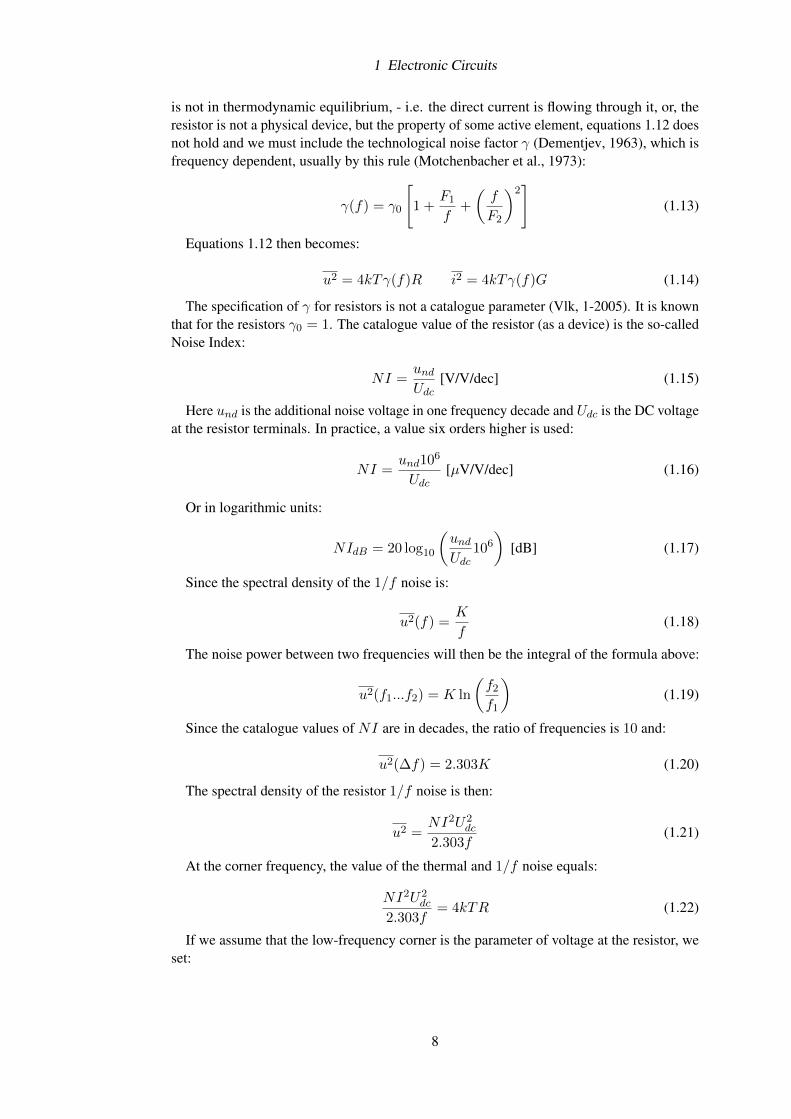
is not in thermodynamic equilibrium, - i.e. the direct current is flowing through it, or, theresistor is not a physical device, but the property of some active element, equations 1.12 doesnot hold and we must include the technological noise factor γ (Dementjev, 1963), which isfrequency dependent, usually by this rule (Motchenbacher et al., 1973):
γ(f) = γ0
[1 +
F1
f+
(f
F2
)2]
(1.13)
Equations 1.12 then becomes:
u2 = 4kTγ(f)R i2 = 4kTγ(f)G (1.14)
The specification of γ for resistors is not a catalogue parameter (Vlk, 1-2005). It is knownthat for the resistors γ0 = 1. The catalogue value of the resistor (as a device) is the so-calledNoise Index:
NI =undUdc
[V/V/dec] (1.15)
Here und is the additional noise voltage in one frequency decade and Udc is the DC voltageat the resistor terminals. In practice, a value six orders higher is used:
NI =und106
Udc[µV/V/dec] (1.16)
Or in logarithmic units:
NIdB = 20 log10
(undUdc
106
)[dB] (1.17)
Since the spectral density of the 1/f noise is:
u2(f) =K
f(1.18)
The noise power between two frequencies will then be the integral of the formula above:
u2(f1...f2) = K ln
(f2
f1
)(1.19)
Since the catalogue values of NI are in decades, the ratio of frequencies is 10 and:
u2(∆f) = 2.303K (1.20)
The spectral density of the resistor 1/f noise is then:
u2 =NI2U2
dc
2.303f(1.21)
At the corner frequency, the value of the thermal and 1/f noise equals:
NI2U2dc
2.303f= 4kTR (1.22)
If we assume that the low-frequency corner is the parameter of voltage at the resistor, weset:
8

1 Electronic Circuits
F1 = φU2dc (1.23)
And get:
φ =NI2
9.212kTR[Hz/V2] (1.24)
If we start with catalogue values, it is better to use the simplified formula:
φ =10
NIdB10
3.69 · 10−8R(1.25)
The noise indices of resistors of some technologies depend slightly on the resistor value.Since computing the noise factor includes division by the resistor value it may be possiblethat the noise factor φ of resistors of different values made with the same technology mayhave a smaller span. Typical noise of manufactured resistors is shown in the graph 1.15:
Figure 1.15: Noise of resistors (Motchenbacher et al., 1973)
The noise parameters of active circuits are slightly more complicated. The situation canbe simplified by using a unilateral model in fig. 1.16, which has the same topology for allactive devices, only the parameters of the devices change somewhat.
9

1 Electronic Circuits
Figure 1.16: Noisy active element
Note that when the left-down input node is grounded, the nullor down transforms intoshort. The operational amplifier is the only element where this node has sense, otherwise,it is grounded. The next table (Vlk, 1-2005) summarizes the noise properties of severalelectronic devices. The values there are only for illustration, and precise values must becomputed in every case for given DC operating point of the device from the catalogue data.Since modern devices are designed to shape transfer characteristics to a given purpose, i.e.linear or logarithmic amplification, theoretical formulas do not hold exactly for them.
Element R1 γ1 R2 γ2 L R3 γ3
Triode 0.1Ig
1K 3√Ia
2.5 1gsD
Pentode 2.5+20Is/S1+Is/Ia
JFET Up
2√IdsId
0.66 K√Id
BJT β40Ic
(0.2) 140Ic
(10) UeIc
NE5534 5 · 104 1.8 0.12 6.8 · 103 38 · 10−6 3 · 103
Operational amplifier is described by model similar to the model of simple transistor. Theonly difference is that resistances of the equivallent circuit have very high noise factor inboth input1 and transconductance elements 2 These devices are not generaly suitable forinput stages of ultra low noise amplifiers3.
1.3 Low-noise electronic systems
A slightly simpiler circuit is a little more interesting.
1Input circuit of modern bipolar operational amplifiers are normally of "bias cancellation" type, what serves asan bootstrap. Hence, input impedance is made greater at the cost of input noise current enlargement (OP27)
2Transcon noise factor is determined by the input stage current. This can be modified in some types of"programmed" operational amplifiers (LM381)
3Recent advances in the semiconductor technology reduced low-frequency noise corner of so-called videooperational amplifiers to infrasonic band. Example of this part is LME49990. These parts are not suitablefor general using in low-noise audio - frequency systems, mainly because special grounding methodology(ground - plane layout) is recommended by the manufacturer, what is in contradiction with normally usedstar grounding Ott (1976). When these parts are used in non-appropriate layout, UHF frequency oscillationsmay occur. They can be detected sometimes by measurement of DC power consumption of the part andusing human finger as "damping volume", or (better) by using HF voltmeter with random-sampling head i.e.HP3406.
10

1 Electronic Circuits
Zin 1/g m Cl
Cf
Figure 1.17: Amplifier
The input impedance of this circuit has the form:
Zin =1
p(Cl‖Cf )‖Cf + ClCfgm
(1.26)
This is the parallel combination of resistor and capacitor. Let us see how noisy this resistoris. One description of noise in electronic circuits originates from the so-called technologicalnoise quotient γ. This constant tell us how the element differs in noise temperature from theordinary resistor:
i2n = 4kTγGB (1.27)
Since electronic systems are not in thermodynamic equilibrium, this quotient tell us howthe noise power of the “electronic resistor” differs from that of the resistor (the resistor cannot exists as a device) in the thermodynamic equilibrium. To calculate how the noise factor ofthe synthetic element differs from the noise factor of the real element requires performing theenergetic sum of current noises of all amounts from the noisy circuit elements. The situationin this case is simple: we have only one noisy element in the circuit, transistor transadmittancegm. We must determine the current transfer from gm to the input synthetic resistance. Thecurrent transfer computation can be transformed to input impedance computation by addingseveral circuit elements:
Zin-1 1/g m
Cf
Cl
Figure 1.18: Current transfer to impedance circuit
After computation, the current transfer yields:
Zin =Cf
Cf + Cl(1.28)
The noise current at the input reads:
i2n = (Cf
Cf + Cl)24kTγmgmB (1.29)
But the value of the input real conductance:
11

1 Electronic Circuits
g′m =Cf
Cf + Clgm (1.30)
Comparison with formula 1.27 yields:
γ′
= γCf
Cf + Cl(1.31)
One can see, that the noise factor decreased by a large amount. If the noise factor issmaller than one, it has the same effect as cooling the circuit to a lower temperature, we mayrefer to it as electronic cooling (or cooled termination). Practically we are limited by othernoise sources and also system headroom and cooling under 1/10 of the ambient temperaturehas no sense.As an example of practical application of this topology, the author describes the simplephonograph pick-up amplifier.
Out
9V
2x2SK170
680n
10n560
2x1M
2x1u
150p
IHF moving armature
pick-up equivallent
mechanical part electrical part
Figure 1.19: Pick-up amplifier
The moving armature pick-up (in the form of a moving magnet or moving permalloy cross)is the most common in low-end HiFi vinylite record players. The problem of this design aretwo resonances which lie in the higher part of the acoustical band due to the resonance ofthe needle with its gymbal and the groove material (Miller, 1950). These two mechanicalresonances can not be damped from the electrical side. The only thing that can be doneis to maintain the electrical resonance properly damped to linearize the overall frequencyresponse. Damping the impedance by simple shunt resistor degrades noise performanceof the system in the high-frequency part of the audio band (Sýkora, 1990). Sýkora usedparallel resistance feedback to achieve cooled termination; his circuit in minimal form hasthree operational amplifiers. Our circuit is much simpler, it uses a single dynamically loadedtransistor stage. This stage is loaded with a shunt RIAA corrector. This forms an integratorin the high-frequency band where cooled termination of the pick-up is needed. Enlarging ofthe Miller transistor capacity allow us to set the input resistance at the prescribed value.
12

1 Electronic Circuits
9V
2x2SK170
2x1M
2x1u
electrical part
Magnetophone head
90p
3x1k
220
1n5
160p
Out
- -
NE5532
50M
Figure 1.20: Tape-recorder preamplifier
It is possible to realise the loading capacitor via a feedback circuit. This solution isadvantageous for tape-recorder preamplifier where the noise has a different character, andbad transient - intermodullation distortion (Otala, 1972) of the operational amplifier is not anissue.Using cooled termination in baseband amplifiers is not as advantageous than using it inamplifiers which use amplification at pure reactance - parametric amplifiers.
1.4 Parametric Amplifiers
The basic form of the parametric amplifier (PARAMP)1 used in the microwave frequencyrange has the form of one branch. This one branch is realised as a non-linear capacitor(varactor diode) to which pumping power (normally higher than amplified frequency) iscoupled, and which has resonant loading at combinational frequencies of pump and signal ofhigher frequencies (so-called idlers). Input and output waves are decoupled by circulator.
IN
OUT
TERMsignalcavity
(3GHz)
(12GHz)pump
idlercavity
(9GHz)
DC bias(-2V)
Figure 1.21: HF PARAMP
The theoretical behaviour of these circuits depends only on the energy conservation law,and is independent of their nonlinearity shape (Manley, 1956). It also holds that the reactancepower rises with frequency which means that gain is proportional to the pump-to-signalfrequency ratio. Microwave amplifiers have now been mostly replaced by HEMT transistor
1Mathematical tool for analysis of the parametric systems is Mathieu (1868) equation in form: y + (a +16q cos 2x)y = 0 . Electronic systems are nonlinear- simply described by Van der Pol (1927) equation foroscillator with limited output amplitude in form: y − µ(1− y2)y + y = 0. Real parametric amplifier can bedescribed by proper combination of both equations like this: y−µ(1−y2)y+(1−ry2)(a+16q cos 2x)y = 0
13
1 Electronic Circuits
stages and there are only a few niches where survives i.e. radar input amplifiers (PARAMPswithstand high input overload)
CCs (x)
pumpfp fx
Rl
L
idler
b
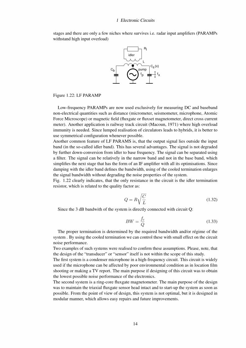
Figure 1.22: LF PARAMP
Low-frequency PARAMPs are now used exclusively for measuring DC and basebandnon-electrical quantities such as distance (micrometer, seismometer, microphone, AtomicForce Microscope) or magnetic field (fluxgate or fluxset magnetometer, direct cross currentmeter). Another application is railway track circuit (Macoun, 1971) where high overloadimmunity is needed. Since lumped realisation of circulators leads to hybrids, it is better touse symmetrical configuration whenever possible.Another common feature of LF PARAMS is, that the output signal lies outside the inputband (in the so-called idler band). This has several advantages. The signal is not degradedby further down-conversion from idler to base frequency. The signal can be separated usinga filter. The signal can be relatively in the narrow band and not in the base band, whichsimplifies the next stage that has the form of an IF amplifier with all its optimisations. Sincedamping with the idler band defines the bandwidth, using of the cooled termination enlargesthe signal bandwidth without degrading the noise properties of the system.Fig. 1.22 clearly indicates, that the only resistance in the circuit is the idler terminationresistor, which is related to the quality factor as:
Q = R
√C
L(1.32)
Since the 3 dB bandwith of the system is directly connected with circuit Q:
BW =fcQ
(1.33)
The proper termination is determined by the required bandwidth and/or régime of thesystem . By using the cooled termination we can control these with small effect on the circuitnoise performance.Two examples of such systems were realised to confirm these assumptions. Please, note, thatthe design of the “transducer” or “sensor” itself is not within the scope of this study.The first system is a condenser microphone in a high-frequency circuit. This circuit is widelyused if the microphone can be affected by poor environmental condition as in location filmshooting or making a TV report. The main purpose if designing of this circuit was to obtainthe lowest possible noise performance of the electronics.The second system is a ring-core fluxgate magnetometer. The main purpose of the designwas to maintain the triaxial fluxgate sensor head intact and to start-up the system as soon aspossible. From the point of view of design, this system is not optimal, but it is designed inmodular manner, which allows easy repairs and future improvements.
14

2 High-frequency condensermicrophone
2.1 Convergence of multimedial technology
In today information technology we use unified physical-logical layer to transfer, process andstorage of all the real - world signals. It is now common that radio, television, telephones andmany other equipments can be substituted by special programs in the computer connected tothe computer network (INTERNET). This process is called convergence. Further general-ization for the audio technology is, that all professional audio input and output equipments(microphones, speakers) could be viewed like computer network devices and special studioequipments (mixing consoles, audio effect processors and recorders) could be viewed ascomputer programs. Such that system would be free from dynamic and bandwidth limitationof today analogue systems. The barrier which is still not been overcame is analogue natureof electroacoustic transduction. In department of radioelectronics of the Czech TechnicalUniversity in Prague research focused on analog to digital and digital to analog conversionbased on transduction phenomenon have been started a couple years ago (Husník, 2003),(Kovár, 2004) ,(Motl, 2005). The goal of this part is to complement this research with trans-ducers which does not work in base frequencies. Transducers constructed in this way doesoperation of spectral transposition and we will call them parametric transducers. Spectraltransposition (under some circumstances (Manley, 1956)) is the origin of power gain, whichis theoretically noiseless. This is especially useful for parametric microphones because itcould works closer to theoretical noise minimum than other microphone types.
2.2 Condenser microphone as parametric elecroacousticsystem
In typical1 condenser microphone all acoustical system is concentrated to the part - capsule2
Typical capsule is in fig. 2.1
1Somewhat different are line transducers, where body of the microphone creates acoustical waveguide to obtainhigh degree of sensitivity. Sometimes are to pressure capsule attached pieces in the form of a disc with a holefor capsule or short tube of capsule diameter - these members can modify high-frequency characteristics atthe cost of directional characteristics
2Capsules in the studio microphones are usually replaceable as spare parts when microphone is repaired
15

2 High-frequency condenser microphone
Figure 2.1: Microphone capsule
For modelling of the capsule, non-standard analogy is presented, where voltage equalsthe displacement and current equals the force. This analogy origins from energy equation ofthe electrostatic transduction, which is eq. 6.9 in the appendix A. At the mechanical side itresembles mobility analogy (Lenk, 1973). Difference is in operational form, that eleastor ismodelled by resistor, mechanic resistor is modelled by capacitor1 and inertor is modelledby a double capacitor, what directly resembles the second Newton law f = ma = mxElectromechanical conversion is modelled by two arbitrary current sources (eqs. 6.12 and6.13 in the appendix A) At the electrical side mutator is included serving as integratinggyrator which transforms charge to current2 . The microphone creates one arm of a bridge,fed by symmetrical voltage source and loaded by a resistor matched by a series inductor.Reference arm of the bridge is shunt capacitor (fig. 2.2).
G1
1
G2
1
G3
-1
L1
1
Rser=1e-32
V1
0
V2
20e-6
V3
SINE(0 100 8meg 0 0 0 1000000)
V4
SINE(0 100 8meg 0 0 0 1000000)
C1
17p
L2
11.6µ
R1
1000
R2
2e-5
R3 0.08
G4
-1000
C2
.025
C3
.025R4 1e-5
C4
100
I1
SINE(0 0.1 10000 0 0 0 100)
N004
N003N005
G5 N005 N004 value=V(N003,N004)*V(N003,N004)*(2.5e+14)
G6 N003 N004 value=V(N003,N004)*V(N005,N004)*(5e+14)
.tran 10
Figure 2.2: Model of HF condenser microphone
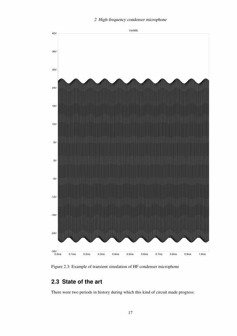
Because SPICE simulator does not allow using of singular circuit elements, we will usevoltage-controlled current source (VCCS) to model unilateral voltage - to current converters(fig.1.16 with only R2). Tables to translate circuit blocks with singular elements to blockswith controlled sources are given in Kvasil (1981) and Vágó (1985). Typical transientsimulation is in fig. 2.3
1It may cause problem in the noise simulation, but simulation of the acoustic resistor can be done via mutatorloaded by resistor. There is one condition, that cascade of mutators (on the electrical side and the second onthe mechanical side before resistors must be symmetrical (Vlk, 9-2008))
2This nonlinear model can be also used for modelling of capacitor microphone in regime with constantcharge for evaluation of transducer-based nonlinear distortion. Frederiksen (1994) showed, that distortionof microphone increases with increasing of the load electric capacity what is in contradiction with Pastille(2001). Problematics is discussed in (Vlk, 5-2008)
16
2 High-frequency condenser microphone
0.0ms 0.1ms 0.2ms 0.3ms 0.4ms 0.5ms 0.6ms 0.7ms 0.8ms 0.9ms 1.0ms-30V
-24V
-18V
-12V
-6V
0V
6V
12V
18V
24V
30V
36V
42VV(n008)
Figure 2.3: Example of transient simulation of HF condenser microphone
2.3 State of the art
There were two periods in history during which this kind of circuit made progress:
17

2 High-frequency condenser microphone
1. The 1920s when thermo-ionic tubes made rapid progress. These tubes had poorvacuum, and the conventional cathode follower suffered a noise and stability (gridleak) problem. These microphones have the form of a mere simple resonant circuit,the microphone playing the role of a capacitor, which was excited by a stable oscillatorwith quartz filter, and the resulting AM signal was envelope detected. This kind ofcircuit is referred to Reiger (Weynmann, 1944) and at the time belonged to the verylow- noise microphones. Another circuit had the form of an untuned transformerbridge. It is not particurlarly interesting at this point to comment on these historicalcircuits, only should be mentioned that the microphone connected in the oscillator aspart of a frequency modulated circuit was rejected at the time because of the notable1/f part of the circuit noise.1
2. In the 1960s, when bipolar transistors became relatively common, and the sortimentof JFETs suitable for the input follower stage was limited. In this period two basiccircuits were perfected and given to routine use: the transformer bridge (untuned andtuned) and ratio detector.
3. In the 1990s when end-user digital media set-up a new standard of dynamic range inthe recording industry. The development of the HF microphone circuit paradoxicalyconcentrated on low-cost circuits rather than on performance.
1It is paradoxical situation, that nearly all newer papers on parametric microphone describes this false idea:(Pedersen, et al., 1998), (Mueller, et al., 2004), (Soel et al., 2007)
18
2 High-frequency condenser microphone
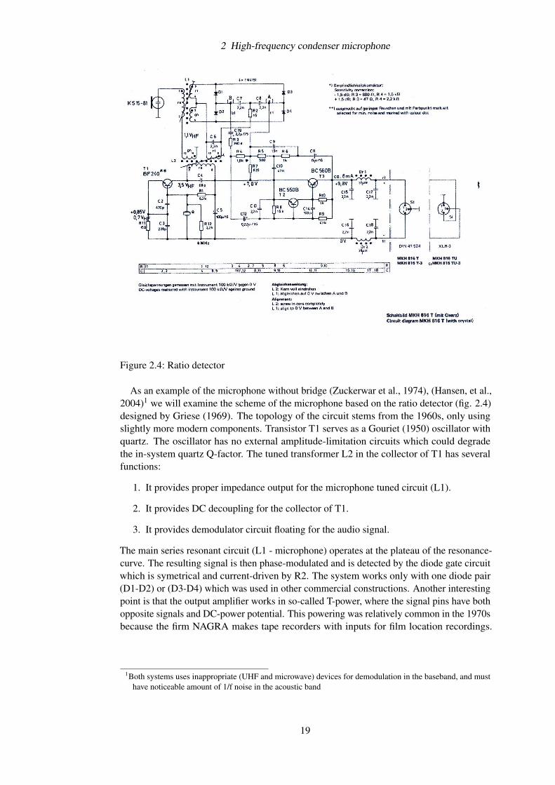
Figure 2.4: Ratio detector
As an example of the microphone without bridge (Zuckerwar et al., 1974), (Hansen, et al.,2004)1 we will examine the scheme of the microphone based on the ratio detector (fig. 2.4)designed by Griese (1969). The topology of the circuit stems from the 1960s, only usingslightly more modern components. Transistor T1 serves as a Gouriet (1950) oscillator withquartz. The oscillator has no external amplitude-limitation circuits which could degradethe in-system quartz Q-factor. The tuned transformer L2 in the collector of T1 has severalfunctions:
1. It provides proper impedance output for the microphone tuned circuit (L1).
2. It provides DC decoupling for the collector of T1.
3. It provides demodulator circuit floating for the audio signal.
The main series resonant circuit (L1 - microphone) operates at the plateau of the resonance-curve. The resulting signal is then phase-modulated and is detected by the diode gate circuitwhich is symetrical and current-driven by R2. The system works only with one diode pair(D1-D2) or (D3-D4) which was used in other commercial constructions. Another interestingpoint is that the output amplifier works in so-called T-power, where the signal pins have bothopposite signals and DC-power potential. This powering was relatively common in the 1970sbecause the firm NAGRA makes tape recorders with inputs for film location recordings.
1Both systems uses inappropriate (UHF and microwave) devices for demodulation in the baseband, and musthave noticeable amount of 1/f noise in the acoustic band
19

2 High-frequency condenser microphone
AF amplifiers (T2,T3) have also built-in frequency corrections1. As an example of themicrophone with bridge(Arends, 1963), (Baxandall, 1963), (Paerschke, 1965)) we shallexamine a typical actual product of the firm Senheiser (fig. 2.5). The circuit is designed byHibbing (1996). Solo-oscillator T1 is stabilised by T2 and drives a Blumlein (1928) bridgewith a symmetrical microphone capsule. The output from the bridge is tuned by L3 and fedto transformer L2. L2 has the function of DC and audio decoupling of the detector part andfunctions as an HF-pad if needed. D1 and D2 work as a gate. The peak current is stabilisedby the (R6 + R7)‖C3 leak, and thus a series resistor is not needed. Also the situation of thegate is reversed when compared with the ratio detector, because the input wave propagatesto the winding middle point instead of the switching wave. The microphone has a standardphantom power and the AF amplifier has a relatively uncommon series topology with respectto DC power.
Figure 2.5: Tuned transformer bridge - solooscillator
2.4 New development
From this point of view, the modern HF microphone would have these properties:
• Source of pump frequency: high stable quartz oscillator.
• Circuit topology: resonant loaded transformer bridge with synthetical resistor loading.
• DSP signal processing at the idler frequency.
• Some form of peak elimination and restauration system (PERS) must be included.
Since only a part of the circuit was finished, we shall describe it.1Critical damping of the diaphragm is needed for the flat frequency characteristics on an acoustic side. Damping
is controlled by variing of the mechanical resistance of the air gap between the diaphragm and back electrode(by means of holes or slots in the backplate). This resistance (as all dissipative element) adds noise to thesystem. Common trade-off in the low-noise capsule manufacturing is to leave the capsule under-damped andto correct the frequency characteristics by an additional filter in the electronic circuit.
20

2 High-frequency condenser microphone
Figure 2.6: Block diagram of developed HF condenser microphone
A Pierce quartz oscillator of ordinary single-transistor construction oscillates at 40 MHz.After the decoupling stage, a synchronous ring counter is used as a generator of non-overlapping impulses for power MOSFETs. The speciality of the counter is a diode matrixwith current output which uses the input part of S-TTL invertors as current-to-voltageconverters.
Q0
Q7
&
&
&
CLK
Out A
Out B
74HC164
74S04 13 X BAT42
Figure 2.7: Synchronous divider - non-overlapping outputs
The drivers are of classical half bridge topology using Elantec circuits. The power stage(PA) is based on complementary MOSFET topology, which is relatively commonly used inclass-D PA stages. The speciality of the power stage is dominant induction loading, whichlowers the switching noise of the stage and allows the phase-to-amplitude conversion modeof the stage that is essential for PERS function. The power stage requires power consumptionwhich is (although the system deals with pure reactances) fudamental for the low-noiseswitched regime at relatively high frequencies. This power is mainly composed of switching
21

2 High-frequency condenser microphone
losses and, using MOSFETs of a newer generation could reduce it. In experimental set-up2 A 7 V consumption was noted. The power dissipation of 14 W per stage needs a properheater. Simple passive heater will suffice. A double inductive balun is used for transformingthe impedance of the PA and for balancing the output between the microphone and dummyload. An ordinary tube ceramic capacitor worked best as the dummy load.
EL7242
+12V
EL7242
+12V
In
In
Out
4x 100k4x BAT42
4x 100n
+Udd
+Udd
2x 100n
2x 30p
30p
2x AT5201
4x SK52
Figure 2.8: Microphone PA
The input amplifier (fig.2.9) is a folded cascode with FET in the first stage in CS and BJTin the CB at second stage. The second stage is loaded by a shunt capacitor 30 pF. 1 pF ofthe paralel feedback capacitor forms the synthetic resistor to terminate the bridge. The thirdand fourth stages form the decoupling stage needed for further processing. The CE-CE BJTcascade with 100% parallel voltage feedback is used instead of the CC stage because thistype of circuit provides better stability for a strong signal. It is application of circuit withcontrolled input impedance to avoid parasitic oscillator structure (fig. 1.6).
+5V
1p
BF506
2x1N4148
2x2SK170
BF199
22p
-5V
2k2
-12V
2x5k 2x50k
1M
-
LM2900
2N3904
2N3906
Out
+5V
-5V
10n
M5*
Figure 2.9: Microphone input amplifier
For experimental purposes, only a synchronous detector is used (fig.2.10). This typeof detector provides supporting output suitable for experimenting with the circuit without
22

2 High-frequency condenser microphone
needing of high-resolution high-frequency A/D converter. The coherent digital signal neededfor detection is given by an additional row of diodes in the divider diode matrix.
2N3904
2N3906
+5V
2SK170
In 1k
to divider BAT42M1
100n
1M
10n
to audiorecorder
2x20k
2x 100n
2x 1N4148ITT!
-5V
Figure 2.10: Synchrodetector for experiments
Since the dynamic range of modern condenser microphones for recording purposes can goup to 130 dB of the peak sound pressure level, microphone must have a peak eliminationand restauration system (PERS). Since a high purity power source is used for the PA supply,the only way to achieve PERS is to use a phase-to-amplitude bridge (Chireix, 1935). Thesystem consists of a synchronous shifter and comparator. The disadvantage of this system isthe need for high frequency of the master oscillator. Cellular asynchronous logic can handlethese requirements without a problem in modern FPGA RTL designs. An example of such asystem is in fig. 2.11 .
Figure 2.11: Divider
This system is a systolic synchronous divider with a comparator. The output of the sectionof the divider is delayed by the number of the sections, the output from the comparator isdelayed by twice the number of the sections. The circuit consists of several cells connectedin series, one cell serving as phase shifter of one bit. Consider a 200 MHz SAW oscillator,which FPGA divides by 200/25 = 6.25 MHz. There is also the possibility of using adifferent modulus to obtain 5 MHz exactly as with a quartz oscillator, and using an analoguecircuit without modification. A five-bit system yields a shift of 32 positions which yields aheadroom of 6×5 = 30 dB The next part of the dynamics must be created by the decimationstructure.Another solution of the fine shift which does not depends on the frequency of the mainoscillator is based on a Delay Lock Loop.
The DLL system (fig.2.12), originaly developped by Combes (1994) is commonly used asa frequency-multiplier in the modern digital devices i.e. microprocessors. It is based on theRC lumped delay-line with constant delay per step (thus it does not have equal components
23

2 High-frequency condenser microphone
1
A
D...
MUX
Q
Fineshift
CLK
OUTCLK
IN
-
Q
Q
S
R
S
R
...
Figure 2.12: DLL fine shifter
values) and where C is realised by a varactor. Total delay of the line is stabilised by a phasesensitive detector which compares input and output and varies varactor bias to align the inputand the output pulse. Main advantage of this solution is that jitter property of the outputsignal is dependent on the main oscillator and not on the VCO as in the case of PLL. Whenan additional noise source is added to the varactor bias, spread-spectrum of the output wavecan be made what is useful to reduce EMI problems in the digital system1. Because nosuch systems was accesible for author in time of construction of the microphone circuit,simple shifter was developped using standard logic circuits. This system is on fig. 2.13. It isbinary-weighted time shifter based on dissimilarity of the two RC integrators connected tothe one input of the CMOS XOR. Full shift of the circuit is period of oscillator (25 ns). It ishighly reccomended, that significant bits are weighted in unary (thermometer) code to obtainlow jitter.
Figure 2.13: Phase shifter with standard logic
2.5 Realisation
Function of discussed circuit function was proved by breadboarding. The breadboardingitself gives the direction in the circuit modification to obtain best signal to noise ratio forgiven microphone AC HF voltage and defined capacitance change. This is figure of merit of
1Analogic system is known in the acoustics over 50 years in the form of vibrato unit of the famous Hammond(1946) organs.
24

2 High-frequency condenser microphone
the electronic circuit. Functionality was also tried with improvised capsule as can be seen atthe pictures.
Figure 2.14: Microphone circuit blocks
On the fig. 2.14 is photograph of buiding blocks of the microphone. From bottom: PAwith small discrete CMOS inverters (BS170 and BS250). Its performance was bad. In themiddle are HF bridge constructed of two-hole core from ferite material N05 (EPCOS). Inthe left is air tunning capacitors for reference and preamplifier. Low noise preamplifier ison the opposite part of the breadboard PCB. In the top is PA form complementar powerMOSFETS with discrete elements driver. It was replaced by integrated high-speed IC driversfrom Elantec discussed in the work.
On the fig .2.15 is complete microphone set-up. On the left-low corner is improvisedmicrophone. the first plate is preamplifier. in the middle is PA with discrete driver and inthe right-lower corner is oscillator, divider and RC phase circuit simillar to that discussedon fig. 2.13. On the upper left-middle part is stabiliser with main filter capacitor Thestabiliser is very similar to one used in 120V source of the fluxgate. On the upper-right partis synchronnous detector for testing. The blue coaxial cable (from preamplifier to detector)is decoupled for signal with the balun.
2.6 Conclusion
The noise property was estimated by dummy microphone (fig. 2.16). The dummy micro-phone was constructed as a T - circuit, the purpose of which is to create a capacity jump of20 fF over and above the basic capacity of 30 pF. A mercury-wetted relay (Hermeyer St57)was used for this purpose.
The comparison of the recording of the step to noise at 1 kHz, reduced to the audiobandwidth of 20 kHz and the sensitivity of an ordinary 50 V DC polarised recording capsuleyields 7 dB of unweighted self noise of the electronics over the audio band.Although the project of the digital microphone has not been finished, The developed codes
25

2 High-frequency condenser microphone
Figure 2.15: Microphone test setup
30p
1p 3p2
10p
St57
Figure 2.16: Dummy microphone
were used to create the background of the digital fluxgate described in the next section.The only difference of DSP between the microphone and the fluxgate is in fact, that thefrequencies used in the digital microphone are two orders higher than frequencies usedin the fluxgate. A pure software radio system, based on the ANSI-C code, is then usedfor processing the fluxgate data. RTL logics must be synthetised in FPGA to process themicrophone data. Although the author has all the needed cods written at the RTL level inthe VHDL and has simulated it in MODELSIM software, dedicated hardware must be madeto make these codes run. The cost of developing the hardware in small quantity with BGAbased parts was the main limiting factor. Because analogue part is finished and its maindisadvantage - big switching losses of the pump PA with MOSFETs can be solved by today’spower GaN HEMTs - it is possible, that the research will continue.
26

3 Second-harmonic fluxgate
3.1 Geomagnetic Survey instruments
Surveys of the geomagnetic field have great history. The oldest instrument the compass,has been known since old China. The compass is a primitive form of declinometer. Itmeasures only the direction of the horizontal component of the magnetic induction vector.Typically the horizontal component in the Czech Republic is 20000 nT and the verticalcomponent 44000 nT. A typical compass is a rod magnet suspended from a point axis (inthis case the vertical force must be balanced by additional mass) or floating in a fluid. Moremodern instruments (known since Gauss) use wire suspension. The wire can be made oforganic material like silk, or gold alloy, platinum - irridium alloy and fused silica. Thelater are the most stable and are still being used in survey instrument. A typical property ofthe geomagnetic field is that rapid phenomena (pulsations) are usually of small amplitude.Phenomena of high amplitude are the daily variation and magnetic storm. The ltter occursonly sporadically. A typical recording apparatus is the La Cour variometer (fig. 3.1). Itis named after its inventor, the Danish physicist Dan La Cour (1876-1942), son of theco-inventor of telephone, Poul la Cour (1846-1908).
DCL LM
P
BLW
S
V
N
Figure 3.1: La Cour variometer
An incadescent lamp with straight wire W is shielded by S so that its light can pass onlythrough prisms P where it is multiplied, to the line mirror LM, and is then reflected to thevariometer V, consisting of a rod magnet with a mirror fixed on it and suspended on a fusedsilica wire. The variometer reflects lamp images through lens BL onto rotating drum Dwith photopaper, where only one image is selected by the collimator and focused by thecylindrical lens CL. The position of the CL is changed in steps synchronised with thedrum’s rotation by mechanism N.The main purpose of this system is to perform “peak elimination and restauration” strategyoptically. Since the sensitivity of the paper is limited, sensitivity of the system must be high(in terms of nT/mm). However on a 24-hour record made on generally available paper one
27
3 Second-harmonic fluxgate
hour of record represents a few centimetres. The solution is to have the record composed ofseveral lines which are equidistant, only one is being displayed on the paper at one moment.The actual La Cour system is somewhat more complicated: it has a total of 50 prisms anduses three variometers, line mirrors, collimators and cylindrical lenses. Quartz variometerswere improved continually over several centuries and modern types of the Bobrov (1962)apparatus when aged have an annual stability of 3 nT, noise level of 10 pT/
√Hz and are
used with a proper digitalisation unit as survey instruments comparable to the best fluxgates,in terms of 1/f noise and EMC even better. Quartz magnetometers are fragile and needa stable optical bench several metres long and are thus impractical for mobile and spaceresearch.Space research in the 1960s accelerated the development of fluxgate magnetometers, becausethey are insensitive to vibrations. The noise of top instruments are now of the order of1 pT/
√Hz@1Hz. The peak-to-peak drift error is under 5 nT/year which is sufficient to
meet international standards for the observatory run. /newline Better noise can be obtainedtheoretically with cryogenic magnetometers, SQUIDs, but they needs cryostat and thereforeare not suitable for observatory operations where instruments are used over periods of severaldecades. SERF optically-pumped (Setzler et al., 2004) potassium vapour -gas masers couldhave better noise performance than fluxgates, but such instruments are still in development.Their noise level is in parts of 1 fT/
√Hz which can be degraded by eddy currents in
conventional permalloy shielding. An inner ferrite shield layer is thus recommended. TheSERF magnetometer also needs heating to approx. 200C which need not be great problemin the observatory, but is a problem at distant stations where power for heating is limited.SERF magnetometers are based on laser-diode pumping, and the semiconductor industry maypossibly produce cheaper laser diodes, thus bringing the price of the SERF magnetometerbelow that of the high-quality fluxgate magnetometer. Technological noise now dominates inthe construction of vector SERF which decreases its performance to 10 pT/
√Hz, comparable
to or worse than the ordinary fluxgate. Also solid-state organic-quartz laser-cooled masersare being developed in laboratories (Oxborrow et al., 2012) and could be rivals of the SERFsin the future because they work at laboratory temperature without oven heating.
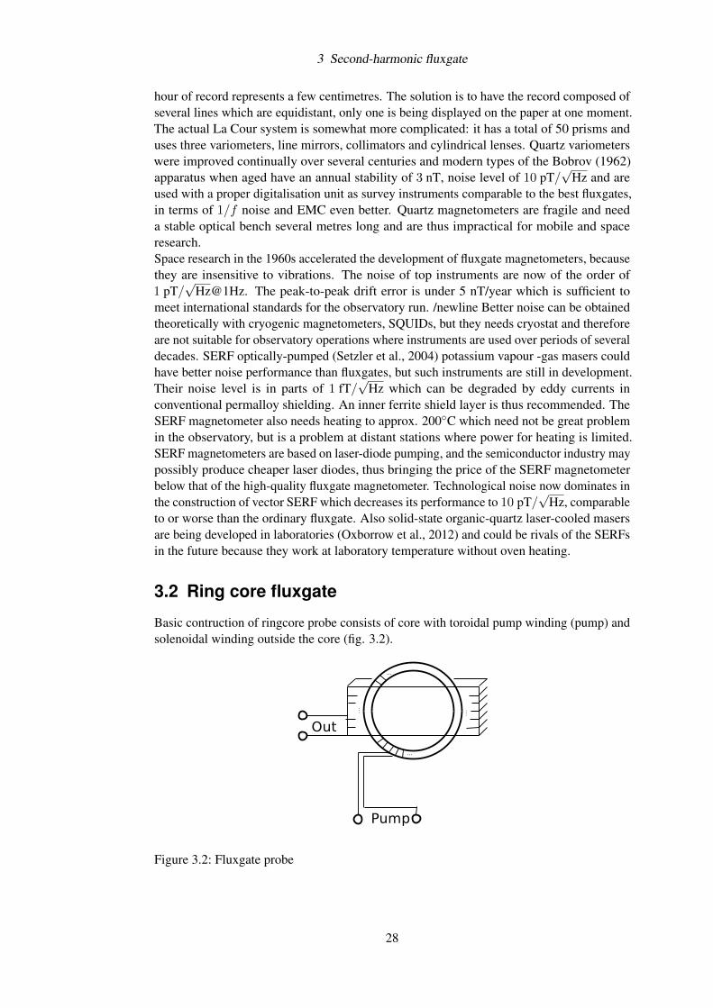
3.2 Ring core fluxgate
Basic contruction of ringcore probe consists of core with toroidal pump winding (pump) andsolenoidal winding outside the core (fig. 3.2).
Figure 3.2: Fluxgate probe
28

3 Second-harmonic fluxgate
Pump winding is usually driven by ferroresonant system, originally usued in power elec-trical engineering for decreasing mains electromagnetic pollution and for rough voltagestabilisation. It has been shown that ferroresonant principle have number of advantages inapplication to fluxgate pump circuit (Korepanov et al., 2013). One of them is fine stabilisationof the pump current, second one is a fact, that probe can not be damaged due to any failurein the electronic part of pump circuit. This fact is of great importance - price of good triaxialprobe set is 30k USD and its manufacturing is not a simple task (Narod, 2014), (Gordon etal., 1968), (Sery, et al., 1968) For proper design of this circuit good model is helpful.The most penetrating modelling system is SPICE. It is part of many CAD systems i.e. CA-Dence ORCAD, and it is also distributed as freeware, as PSpice or LTSpice - SwitcherCAD.The design of the simulation circuit does not need to be straightforward, mainly if there areseveral phenomena in the analysed system and only the dominant one need to be modelled.The ferroresonant system is in its basic concept a resonant circuit with non-linear inductance.It is relatively hard to imagine non-linear inductance, because non-linearity is basically drivenby current. It is much simpler to imagine a non-linear capacitor. But there is the gyratorwhich transforms capacity into inductance. Gyrator is in fact an anti-parallel connectionof voltage controlled current sources. It is not difficult to draw a model of the non-linearinductor using the gyrator (fig. 3.3).
G1
1000
G2 -0.001
C1
100m
R2
10
E3 1
D1
D
D3
DE41
PULSE(-0.001 0.001 0 10n 10n 25u 50u 1000)
I1
C2
1n
R1
10k
.tran 10
Figure 3.3: Nonlinear L model with gyrator
The result of the simulation for the stationary state is in fig. 3.4.
29

3 Second-harmonic fluxgate
24.07ms 24.08ms 24.09ms 24.10ms 24.11ms 24.12ms 24.13ms 24.14ms 24.15ms 24.16ms 24.17ms 24.18ms 24.19ms 24.20ms-10mA
-8mA
-6mA
-4mA
-2mA
0mA
2mA
4mA
6mA
8mA
10mAI(G2)
Figure 3.4: result of L model with gyrator
Note here, that all dissipative phenomena, like copper and iron losses, are included in R1.Without this, simulation usually hardly converges.The model with the gyrator includes a total of four controlled sources. It is thus relativelycomplicated. Let us redraw the non-linear part of the circuit using a unilateral voltage
30

3 Second-harmonic fluxgate
follower (which is in fact gamma cascade of a series nullator and shunt norator (fig. 3.5)).
Figure 3.5: Nonlinear C model with nullors
This model describes the non-linear capacitor. The non-linear inductor can be modelled asa dual circuit from the model of the non-linear capacitor. The dual circuit can be producedfrom every planar circuit in the folowing:
1. The node of the dual graph is drawn in the centre of every area, into which the plane isdivided by a circuit graph. (In analogy with the complex analysis, the exterior is alsoconsidered to be an area.)
2. Every pair of dual nodes in neighbouring areas is connected by one or more branches.The new branch always crosses the old branch between two nodes.
Dual pairs (Mitra, 1963) are inductance - capacitance, resistance - conductance. The nonlineardual elements have the same characteristics as swapped I - U axes. The nullator and noratorare their own duals1 When the dual model has been constructed, it is rather complicatedto make inverse characteristics of anti-parallel diodes. But because this part is used onlyas a nonlinear divider, it is possible to swap diodes and resistor in the divider to obtain therequired dual characteristics (fig. 3.6).
Figure 3.6: Non-linear L model with nullors
1Constructing dual circuit cannot be interchanged with constructing adjoint circuit. These circuit synthesis stepsleaves operational transfer characteristics unchanged, but in the dual circuit topological graph of the circuit ischanged, what can be done only for circuits with planar topology. In the adjoin circuit: (voltage driven) inputis changed to (current) output, (voltage) output is changed to (current) input and each nullator is changed tonorator and vice versa. Adjoint circuit can be used as part of network synthesis or computationally-efficientnoise analysis - i.e. noise analysis in SPICE software is realised by this way. Spice noise analysis as part offrequency domain analysis can not work for circuits with principal nonlinearity - parametric amplifiers - andall noise computations must be computed using transfer parameters computed from the all noisy sourcesvia time-domain analysis. For each (uncorrelated) noise source, one run of the analysis must be done andresulting output noise must be quadratically superposed via the energetic sum. In case of correlated noise,matrix of corellation is needed. It is recomended to avoid this case with equivallent circuits of noisy elementswhere uncorellated noises are used. It can be done simply using of singullar elements and noise factors.
31

3 Second-harmonic fluxgate
After redrawing the unilateral voltage follower to a controlled voltage source, we get thefinal model of non-linear inductance (fig. 3.7).
PULSE(-0.03 0.03 0 10n 10n 25u 50u 1000)
I1
C2
1n
R1
50kE1
1
E2
1
L1
90m
R2
10
D1
D
D2
D
.tran 10
Figure 3.7: Nonlinear L model with controlled sources
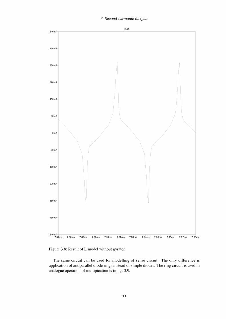
The resulting model is simpler: it has only two controlled sources, but this is hard tounderstand at the first glance. The results are similar (fig. 3.8):
32
3 Second-harmonic fluxgate
7.87ms 7.88ms 7.89ms 7.90ms 7.91ms 7.92ms 7.93ms 7.94ms 7.95ms 7.96ms 7.97ms 7.98ms-540mA
-450mA
-360mA
-270mA
-180mA
-90mA
0mA
90mA
180mA
270mA
360mA
450mA
540mAI(E2)
Figure 3.8: Result of L model without gyrator
The same circuit can be used for modelling of sense circuit. The only difference isapplication of antiparallel diode rings instead of simple diodes. The ring circuit is used inanalogue operation of multipication is in fig. 3.9.
33

3 Second-harmonic fluxgate
Figure 3.9: Diode ring modullator
One disadvantage of the circuit in fig. 3.9 is limitation of signal amplitude to twice ofdiode theshold voltage (Jagoš, 1989). Better circuit - switched modullator (fig. 3.10) wasused in frequency-divided telephone chanell multiplexing units constructed by companyEricsson
Figure 3.10: Diode ring modullator improved
Maximal signal amplitude was enlarged to level of carrier generator amplitude. Inputtransformer can be removed at the cost of added diodes (fig. 3.11).
Figure 3.11: Switched diode modullator
Inherent dynamic limitation of the ring circuit can be an advantage in modelling of thetuned fluxgate sensing circuit.
34

3 Second-harmonic fluxgate
E1
1
1
E2
L1
90m
R2
10
D1
D
D2
D
D3
D
D4
D
D5
D
D6
D
D7
D
D8
D
G11
V1
PULSE(0 1m 0 10n 10n 100u 200u 1000)
C1
50n
I1
1p
.tran 10
Figure 3.12: Fluxgate loaded by capacitor
35

3 Second-harmonic fluxgate
0ms 10ms 20ms 30ms 40ms 50ms 60ms 70ms 80ms 90ms 100ms 110ms-15V
-12V
-9V
-6V
-3V
0V
3V
6V
9V
12V
15VV(n003)
Figure 3.13: Output voltage of fluxgate loaded by capacitor
36

3 Second-harmonic fluxgate
86.0ms 86.4ms 86.8ms 87.2ms 87.6ms 88.0ms 88.4ms 88.8ms 89.2ms 89.6ms 90.0ms 90.4ms-18V
-15V
-12V
-9V
-6V
-3V
0V
3V
6V
9V
12V
15V
-0.2mA
-0.1mA
0.0mA
0.1mA
0.2mA
0.3mA
0.4mA
0.5mA
0.6mA
0.7mA
0.8mA
0.9mA
1.0mA
1.1mAV(n003) I(G1)
Figure 3.14: Output voltage of fluxgate loaded by capacitor: detail with +1 pA disturbingcurrent
37

3 Second-harmonic fluxgate
86.0ms 86.4ms 86.8ms 87.2ms 87.6ms 88.0ms 88.4ms 88.8ms 89.2ms 89.6ms 90.0ms 90.4ms 90.8ms-18V
-15V
-12V
-9V
-6V
-3V
0V
3V
6V
9V
12V
15V
-0.1mA
0.0mA
0.1mA
0.2mA
0.3mA
0.4mA
0.5mA
0.6mA
0.7mA
0.8mA
0.9mA
1.0mA
1.1mAV(n003) I(G1)
Figure 3.15: Output voltage of fluxgate loaded by capacitor: detail with -1 pA disturbingcurrent
38

3 Second-harmonic fluxgate
In fig. 3.12 is model of fluxgate based on previous model of the inductor and antiparalelring-modulators pumped by rectangullar current1. Fluxgate is disturbed by signal 1 pA;pumped by an unipolar rectangular signal 2 and tuned by a Capacitor. Signal wave (voltageon C1) have amplitude independent on disturbing signal and is in fig. 3.13. Fluxgate worksin parametric resonance regime and its amplitude is limited by ferroresonance which occursin signal circuit.
On the detail (fig. 3.14) we can see phase relationship of output voltage and pump current.When the disturbing signal (I1) is inverted, output signal is also inverted(fig. 3.15).
This phenomenon is analogical to superregenerative receivers and can be used in simple,sensitive, non-continuously operated devices. Example of this system is Double pumpedmagnetometer constructed by Baltag (2013).
For maintaining amplitude of output signal depended to disturbing signal, we can partiallydamp the parametric resonance what is shown in fig. 3.16.
E1
1
1
E2
L1
90m
R2
10
D1
D
D2
D
D3
D
D4
D
D5
D
D6
D
D7
D
D8
D
G11
V1
PULSE(0 1m 0 10n 10n 100u 200u 1000)
C1
50n
I1
100n
R1
10k
.tran 10
Figure 3.16: Fluxgate damped by resistor
Results of voltages on C1 for 100nA and 200nA are on fig. 3.18 and 3.19 respectively.Noiseless damping, discussed before, ane depicted on fig. 3.17 have the same effect as ansimple resistor (fig. 3.20).
1Due to inherent symetry of the antiparalel ring circuits it is not important wether pump signal is unipolaror bipolar. Bipolar pump signal have advantages that ferroresonant circuit is simple LC passive circuit.For unipolar ferroresonant circuit some form of switched electronic circuit must be used as in TelevisionCathode Ray Tube flyback generator (Zworykin, 1954). Another advantage of bipolar pumping is, thatpump frequency and signal frequency occupies different frequency bands (signal frequency is typicaly oddharmonic of the pump one), what simplifies construction of the instrument. The only advantage of unipolarpumping is that Barkhausen noise is typically weaker. Unipolary pumped fluxgates have also strong spurioussignals (offsetts) which may be caused by unsuitable shape of known units (Sasada, 2002); simple longwire with cyllindrical magnetic layer, with one terminal return astatised by nonmagnetic wire - frame (asused in ribbon microphones) may give better results. Author’s opinion is, that offset in case of ring-corefluxgate is caused by nonhomogenity of the core. Preliminary experiments showed, that tertial windingconnected in series with the pump sources, when properly adjusted so that have zero coupling to sense coil,can cancell offsett in the unipolary pumped ring core fluxgate. This type of offsett is usally supressed bybipollar pumping (Musmann and Anfassiev, 2010) p.4 .
2Effect of rectangullar pump signal duty factor on fluxgate performance was discussed by simplified analysisof Mathieu equation by Russell el al. (1983) and Player (1988). These papers contradicts.
39

3 Second-harmonic fluxgate
E1
1
1
E2
L1
90m
R2
10
D1
D
D2
D
D3
D
D4
D
D5
D
D6
D
D7
D
D8
D
G11
V1
PULSE(0 1m 0 10n 10n 100u 200u 1000)
C1
50n
I1
200n
-0.02
G2C2
10n
C3
100p
R1
100k
.tran 10
Figure 3.17: Fluxgate with noiseless damping
40

3 Second-harmonic fluxgate
0ms 3ms 6ms 9ms 12ms 15ms 18ms 21ms 24ms-20µV
-16µV
-12µV
-8µV
-4µV
0µV
4µV
8µV
12µV
16µV
20µV
24µVV(n003)
Figure 3.18: Output voltage of fluxgate damped by resistor and 100 nA disturbing current
41

3 Second-harmonic fluxgate
0ms 2ms 4ms 6ms 8ms 10ms 12ms 14ms 16ms-40µV
-32µV
-24µV
-16µV
-8µV
0µV
8µV
16µV
24µV
32µV
40µV
48µVV(n003)
Figure 3.19: Output voltage of fluxgate damped by resistor and 200 nA disturbing current
42

3 Second-harmonic fluxgate
0.0ms 0.9ms 1.8ms 2.7ms 3.6ms 4.5ms 5.4ms 6.3ms 7.2ms 8.1ms 9.0ms-35µV
-28µV
-21µV
-14µV
-7µV
0µV
7µV
14µV
21µV
28µV
35µV
42µVV(n003)
Figure 3.20: Output voltage of fluxgate with noiseless damping
43

3 Second-harmonic fluxgate
3.3 Coupled systems approach
More straight deduction can be done from energy equation of inductor 6.36 described withgeneralised coordinate Φ and force I . Definition of magnetic flow U = ∂Φ
∂t defines themutator which transforms resistive element group to reactive element group1. Becausefluxgate’s core (like every magnetic amplifier) equivallent circuit have form of nonliearsymmetrical lattice (Guillemin, 1953) and its realisation with diodes are antiparalel diodering, this element with addded resistor gamma network on each side (to simulate magneticleak) and bracketted by two nongyrating mutators gives model of complete magnetic amplifier(fig. 3.21). Note, that magnetostatic circuit (Heaviside, 1922) on the left side of the mutatorhas dual form (resistance corresponds to permeance Pm); This is standard meaning ofmagnetostatic analogy, because Hopkinson’s law for a reluctance resembles inverse of theOhm’s law:
Rm =ImΦ
R =U
I(3.1)
And for permeance holds analogy of Ohm’s law directly:
Pm =1
RmPm =
Φ
Im(3.2)
D1
D
D2
D
D3
D
D4
D
D5
D
D6
D
D7
D
D8
D
G1
11
G2
-1
G3
-1
G4
1
G5 G6
1
G7
-1
1G8
1G9 G10
-1
R1
1k
R2
1k
R31k
R4
10L1
1
L2
1C1
50n
C2
100n
PULSE(-0.05 0.05 0 10n 10n 5m 10m 10000)
I1
I2
200µ
.tran 10
Figure 3.21: Magnetic amplifier: Coupled system model
Nongyrating mutators can be simutated as cascade of normal mutator (three VCCS) andgyrator (two VCCS). Hence total number of controlled surces needed for simulation is ten(instead of two used in fig. 3.12). These models can be useful for simulation of cross-couplingphenomena in the ferroresonant parametric transformers in power electronics (Hannemann,et al., 1977). Figure resembles model of the condenser microphone (fig. 2.2), with onlyone difference that both branches are in the electric domain. In the case of microphonemodel, one branch is in the acoustical domain and the next one is in the mechanical oracoustical domain. In semiconductor physics modelling there are also circuits where somebranches believes to the electron / hole concentration in the semiconductor. These modelswere introduced by Linvill (1963). Another interesting fact is, that model is (excludingresistor) symmetric. This resembles, that pump and sense winding of the fluxgate sensor (fig.3.2) can be interchanged. Because of different magnetic leak, this “reciprocal” fluxgate hasbig spurious signal and can be used as an sensitive indicator of quality of manufacturing ofthe sensor unit.
1Mutators in combination with nonlinear elements can be used for modelling of more exotic elements as thememristor (resistor with the charge memory) as described by Chua (1971)
44

3 Second-harmonic fluxgate
3.4 State of the art
Fluxgate magnetometers are based on magnetic amplifiers. Magnetic amplifiers was used inpower electrical engineering (Zell, 1899) 1 power radio electronics (Alexanderson, 1916)and telecommunications since the beginning of the 20-th century (Petterson, 1929). They useferromagnetic material which changes its permeability inside a sensing coil and thus pumpsup parametric resonance in the sensing coil - capacitor system. The construction of thepumping coil determines the type of magnetometer (Primdahl, 1970). The orthogonal fluxgatemagnetises the material perpendicular to the measured field. Other types of magnetometer(Vacquier, Foertster, ring-core (Aschenbrenner et al., 1936), rat-race) magnetise the materialin the direction of the measured field, hence the balancing of pumping coil(s) causes nocoupling of the pump signal into the sensing coil. Ring-core, rat-race and orthogonalfluxgates works without an air-gap in the pump circuit and allow saturation of the core,which is analogous to power-cooling in varactor parametric amplifiers (Penfeld et al., 1962)and is fundamental for low-noise performance. The construction of fluxgate magnetometershas improved somewhat in time. Serson et al. (1957) used a tuned sensing coil. Acuna(1974) used ferroresonant pumping. Temperature stability was also solved by the thermistor(Primdahl, 1970) or by the temperature dependence of sense winding of the sensor using aHoward current source in the field-compensation mechanism (sometimes augmented withplatinum wire thermometers) (Narod, 1987). A diagram of a typical thermally uncompensatedfluxgate is shown in fig.3.22.
2:
RfRb
Cl Rl
OUT-
Figure 3.22: Fluxgate magnetometer typical schematics
Classical design of Acuna et al. (1978) is highly accepted till today (Connerney, 2012) asa very low-noise instrument and facsimile of his drawing are on figs. 3.23 and 3.24.
1It is interesting, that simplier apparatus - transductor - was patented lately by Lahmeyer (1902)
45

3 Second-harmonic fluxgate
Figure 3.23: Acuna’s magnetometer: pump unit
46

3 Second-harmonic fluxgate
Figure 3.24: Acuna’s magnetometer: preamplifiers
This type of magnetometer has several noisy elements which can be omitted or reduced:
• Pump oscillator and dividers must be low noise - (part of 1/f noise depends on it) -use low noise topology of Quartz oscillator and synchronous divider;
• Core driver must be low-noise (use switched MOS PA with external commutation);
• Load resistor Rl can be realised by reactance-feedback with low noise.
• Tuned notch can be removed by using different circuit topology;
47
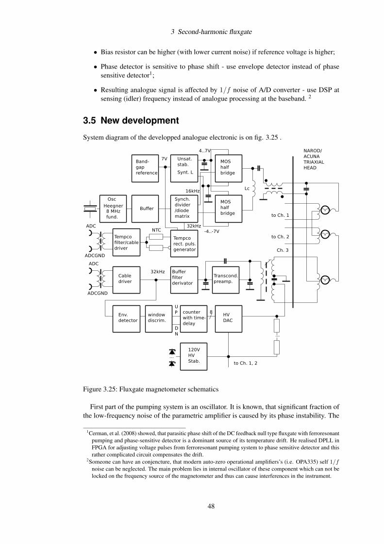
3 Second-harmonic fluxgate
• Bias resistor can be higher (with lower current noise) if reference voltage is higher;
• Phase detector is sensitive to phase shift - use envelope detector instead of phasesensitive detector1;
• Resulting analogue signal is affected by 1/f noise of A/D converter - use DSP atsensing (idler) frequency instead of analogue processing at the baseband. 2
3.5 New development
System diagram of the developped analogue electronic is on fig. 3.25 .
Figure 3.25: Fluxgate magnetometer schematics
First part of the pumping system is an oscillator. It is known, that significant fraction ofthe low-frequency noise of the parametric amplifier is caused by its phase instability. The
1Cerman, et al. (2008) showed, that parasitic phase shift of the DC feedback null type fluxgate with ferroresonantpumping and phase-sensitive detector is a dominant source of its temperature drift. He realised DPLL inFPGA for adjusting voltage pulses from ferroresonant pumping system to phase sensitive detector and thisrather complicated circuit compensates the drift.
2Someone can have an conjencture, that modern auto-zero operational amplifiers’s (i.e. OPA335) self 1/fnoise can be neglected. The main problem lies in internal oscillator of these component which can not belocked on the frequency source of the magnetometer and thus can cause interferences in the instrument.
48

3 Second-harmonic fluxgate
oscillator noise in the older magnetometer design was so drastic that they worked in thefeedback mode, in which the noise of the oscillator is partially attenuated. Since feedbackmode processing is hard to digitise, we decided to improve the parameters of the pumpcircuit to fall be below the noise of the sensor.
1MM1
10k
56k M1
10k
8MHz
10k
56k
BAT52
-12V
+12V
-12VOUT
160 160
4k7
680
4k7
10k
BF506
3xBF199
Figure 3.26: Heegner oscillator
The designed oscillator (fig. 3.26) uses 8.448 MHz fundamental mode (first-harmonic)quartz in rather uncommon Heegner topology. It is known that the in-system Q-factor of apieso-electric resonator can be much lower than its physical Q-factor, which is of the orderof millions for the best units. The main degradation is caused by the resistive part of “what isseen by quartz”. To decouple the resistive part, it is best to load the unit with large capacitors.Also the resistive part can be artificially augmented by limitation of the oscillation at thestage near the quartz. The limitation of this amplitude is prevented in the second stage byamplitude dependent negative feedback. Clockmakers know that the oscillator (pendulum)must be affected by clock mechanism for as short a time as possible. This is the electricalrealisation of this fact. The circuit starts oscillations as a normal A-class oscillator and, whenthe amplitude increases, it goes to class C. The next stage is the shaping circuit (fig. 3.27).
680
200
10k
4x1k
150k
BAT42
+5V
Out (TTL)
IN
BSV24
2xBSV72
Figure 3.27: Shapper
The shaping circuit is a two-stage CE amplifier, the first stage being emitor coupled toCB helper transistor, which completes the positive feedback loop into the input stage andwhat helps to shape the output rectangullar wave. The second stage CE amplifier has adesaturation diode and couples the output signal to the Schottky logic buffer. After the buffersignal has been divided by the synchronous divider by 26 (cascaded two 74HC163) to obtainthe frequency of 132 kHz, the next divider by 23 is shown in fig. 3.28:
49

3 Second-harmonic fluxgate
Q0
Q7
&
&
&
CLK
74HC164
74S04 15 X BAT42
Direct out
Delayed out
Figure 3.28: Divider with overlapping output
The divider generates two 16.5 kHz rectangular slightly shifted waves. The reason isthat the ferroresonant circuit, where pumping is realised by rectangular voltage and a seriesreactor does not have the autocommutation property needed for low noise run of switchedMOSFET PA (fig. 3.29). The external reactor between the amplifiers is used only for thecommutation. This property was confirmed by before PA circuit design. The power amplifierrespects the design of the very small VLF transmitter, in which the IC normally used as apower transistor driver is used as a power element.
PUMP
PUMP
2x 100n 2x BAT42
2x M1
2M2
+7V
-7V
M1
Sensor Head
EL7242
Direct
Delayed
Figure 3.29: Power Amplifier
The ferroresonant circuit uses a transformer instead of choke which symmetrises somewhatthe output signal. Since the pump signal must have low second-harmonic content, thesymmetry of the rectangular wave is critical. To obtain the symmetry, the power supply tothe switched PA is made of two complementary sections and is stabilised by a proprietaryunsaturable stabiliser (fig. ).
--
3k3
+12V
+7V+
2x10k
5k10k
2xOP07AD589
2x1k
4x5k
2x2M2
2x100n
4xBC550
2x10k
4xBC560
-12V
-7V
BD830
BD829
+
Figure 3.30: PA Stabiliser
There is only one pump section in the triaxial magnetometer. The signal sections are three.There is one complete system for each axis. The system is modular, which simplifies repair.It is easy to repair the module in the axis where the signal can be cancelled mechanically by
50

3 Second-harmonic fluxgate
turning of the arretation knob of the Ascania stand for axis D,I. In the Axis-F, the workingunit is a must for beginning the operation. The signal induced in the sensing coil is fed intoan amplifier (fig. 3.31).
1M 10k 10k
1M
2x 2SK170M1
M1
820 820 820 820
1k 270
33k 33k
82
1k2
1k8
3k6
10k
50
M1 1M
M1 M14xAuGe
2X10k
TL062
2xBAT52
LT10103xOP27
- - -
- -
+ + +
+ +
ADC
ADCGND
MORE LESS
PUMPGNDPUMP
FDBCK
FDBCKGND
2x3V0
-12V
-12V
+12V
Figure 3.31: Input amplifier
The input transformer has a splitt primary winding for using symmetrical shielded inputcables (this is called T-power in microphone technique). In the middle of the splitt primarywinding there is a capacitor, which serves as an untuned decoupling element for the PERSSystem to be described below. The transformer is also constructed with an air gap, whichallows some DC current to flow through it, and which is used for zeroing the geomagneticfield component in the case of the F axis. The secondary winding of the input transformer isloaded with a highly stable polystyrol capacitor. The shunt resistor is replaced by a specialconstruction of input amplifier: inverting integrator bridged by a capacitor. The bridgecapacitor is realised by the Miller capacity of the input transistor. The input impedanceof this system behaves like resistor cooled to low temperature and it was described in theintroduction of this thesis. Since the first stage works as an integrator, the remaining circuitmust work as an derivator in the frequency band of interest to obtain flat frequency transfer.The filter-derivator was synthetised with leaky synthetic L building blocks with somewhatnon-standard input and output. For the purpose of design, the whole input amplifier wassimulated to determine its sensitivity to component variation. The simulated circuit is shownin fig. 3.32.
G1
1
C1
100n
AC 1 0
V1E1
1000
E2
1000
C4
33n
C3
1n
R1
820
R2
820
C5
33n
E3
1000
C6
270p
R5
1k2
R6
1k2C2
270p
R3
820
R4820
C7
10p
G2
1
.ac oct 100 10k 70k
Figure 3.32: Model of input amplifier
Sensitivity of the derivator was checked-up by simulation using SPICE in the frequencydomain. The deformation of the frequency transfer curve due to the dominant pole of thefirst operational amplifier is in fig. 3.33:
51
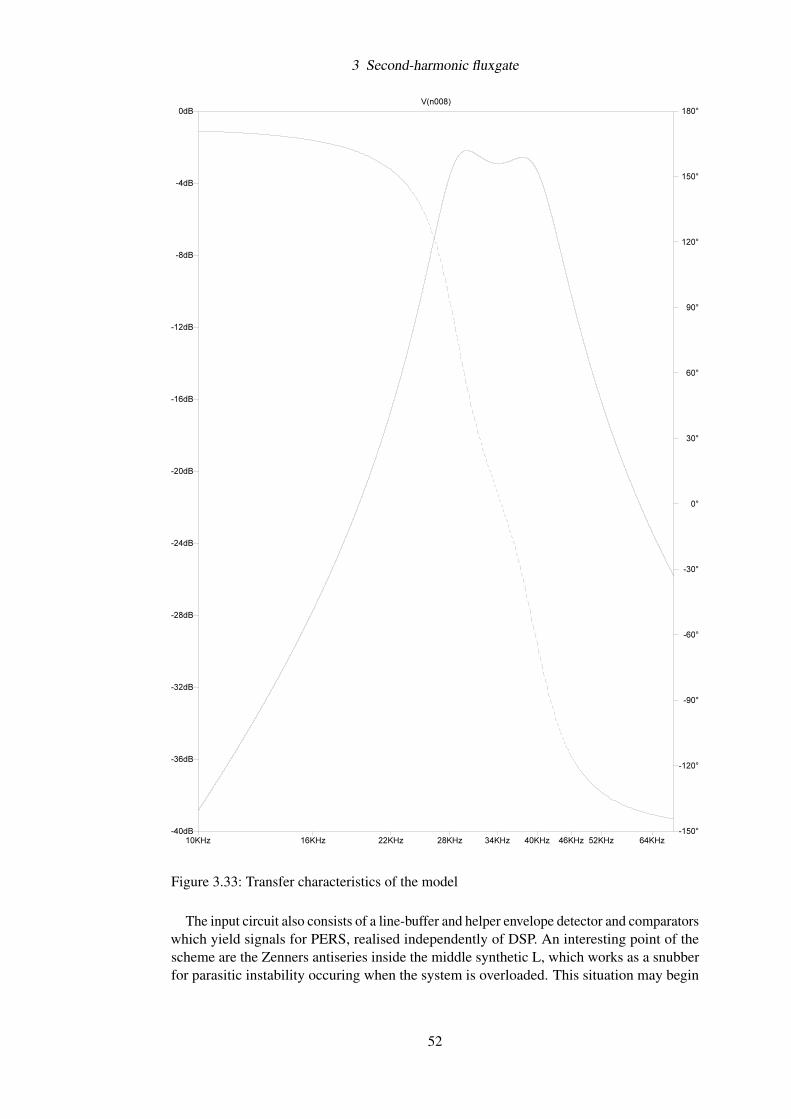
3 Second-harmonic fluxgate
10KHz 16KHz 22KHz 28KHz 34KHz 40KHz 46KHz 52KHz 64KHz-40dB
-36dB
-32dB
-28dB
-24dB
-20dB
-16dB
-12dB
-8dB
-4dB
0dB
-150°
-120°
-90°
-60°
-30°
0°
30°
60°
90°
120°
150°
180° V(n008)
Figure 3.33: Transfer characteristics of the model
The input circuit also consists of a line-buffer and helper envelope detector and comparatorswhich yield signals for PERS, realised independently of DSP. An interesting point of thescheme are the Zenners antiseries inside the middle synthetic L, which works as a snubberfor parasitic instability occuring when the system is overloaded. This situation may begin
52

3 Second-harmonic fluxgate
when the system is started and the PERS has not yet choosen the crude range - and workingas a counter.
&
&
&
&
TUP
DN
0123
C
B
TUP
DN
0123
C
B
M2
1
M2
1
1
...
...
...
+
+
-
-
-
-
+
+
-
- +
+
2xHC193
2xHC132
2xHC86
2xHC04
22xBS170
BC177
2xBC112
8x10k3x2M2
2x24k
22M
60M
30M
15M
7.5M
3.75M
1.875M
938k5
+120V
1M8
3xTL062
+2.5V
+2.5V
+2.5V
+5V
+5V
+5V
7xInGaN
FDBCK
FDBCKGND
MORE
LESS
Figure 3.34: PERS
The peak elimination circuit was inspired by the La Cour recorder described above. Thisapproach allowed us to use separate DSP for difference signal and analogue processing forPERS. The PERS circuit logics consists of the envelope detector, comparators, asynchronouscounter, set of weighted resistor chains and MOS switches in current mode. The designidea remains the same as in the AMOS stand-alone controller, but asynchronous hardwiredlogics is used instead of a microprocessor (for minimisation of interferences), and discreetesemi-conductor switches with resistor chains in wired assembly is used instead of D/Aconverters because of high voltage. High voltage was chosen because some reports rankedthe noise of Narod (1987) system worse that of the original instrument of Acuna (1974)(which was in fact a low-field space magnetometer). The only difference between the twosystems was the maximal measured field strength and, then, the value of the feedback resistor.If we want to use a bias resistor of the similar value like as Acuna’s (in the order of 100kOhms) for a high-field instrument, we must use high voltage. To achieve low 1/f noise ofthe resistor, chains are used instead of simple devices for lowering the device terminal DCvoltage. A deeper analysis is in Appendix E. The PERS for D,I has a current-mode MOSFETcommutator, The PERS for F has a bias resistor chain.
The PERS units use a 120 V precision source. It use a Zener diode chain - thermistorbridge in the feedback instead of the classical topology (reference - feedback divider compar-ison). The advantage of this topology is that we can use a chain of low-voltage Zener diodesin series which can decrease the noise (by 3 dB per doubled components). Also the propertiesof the Zener diode, instead of the avalanche diode, may be interesting if noise induced bycosmic radiation is the issue. It is today’s trend it electronics to omit avalanche devices inelectronic and opto-electronic systems. In fibre-optical networks, avalanche photodiodeswere replaced by cascade EDFA - PIN photodiods for better noise performance. In referencesources, avalanche diodes are replaced by Widlar band-gap reference although the noiseperformance is limited by a current mirror.Temperature sensing unit uses 32 kHz output from diode matrix of the synchronnous di-vider.Switched MOS circuit is used to generate rectangullar pulses to fed symetric line bufferconnected as an invertor. First harmonic from the termistor half-bridge is filtered by resonator.
53

3 Second-harmonic fluxgate
22k
+200V
1k 22M
10k
10k
1N4148100k 10k
10k
10k
+12V
+120V
10M 200
M1
4x10k
5xOP07
2x2k2
M1
12k
BS170
...
...68k
68k
68k
80xBZX85 3V0
-Ï
-Ï
2xBF421
-12V
+
++++
- - - -
-
BF462
BF465
4x1N4148
Figure 3.35: HV source
Signal is then fed via normal AC power cable to the acquisition house (with the distance of60 m from the sensor) and processed by the same way as the fluxgate signal.
Figure 3.36: Temperature sensor
3.6 Solid state power amplifiers in switched mode
Circuit diagram in fig. 3.29 is small solid-state ultra low wave transmitter. Solid-statetransmitters have several construction problems which must be properly handled to makeconstruction reliable. Semiconductor devices are usually used outside the manufacturer-guaranteed regime, and good knowledge of technological device limitations is necessary.There also exist classical solutions, which are reliable and display well-known behaviour,but have difficulties in system design. Let us illustrate the situation on a simple half-bridgeconfiguration.
Figure 3.37: Two forms of half- bridge
Let us examine the circuit on the left-hand side of fig. 3.37. If the load is pure - resistive,
54

3 Second-harmonic fluxgate
the duty cycle of φ has direct impact on the output power. But when the load is losslessfilter-loaded resistance, behaviour of the output power depends also on the property of thefilter. The impedance, which loads the filter at its input side, depends, on the polarity of theinput current when φ is in the closed state. The circuit in the right-hand part (half-bridge)has no such difficulty at first glance, but when the switching frequency increases and thetransistors do not have equal times of switch-on and switch-off, driving impulses φ and φmust then have a dead time betwen them to prevent short-circuit of the power supply.
During the dead-time, the impedance at the input of the filter is also indefinite. Anotherproblem is that the substrate diodes of the transistor have relatively slow recovery times andit is paramount to filter circuit to make conductive the diode of the transistor, which willbecome conductive after the dead-time ends. This property is called external commutation. Ifthis property is maintained, the transistor switches to the zero voltage regime which decreasesits switching losses and noise. It also makes the reliability higher, because the situation, inwhich lower diode is conducting and the upper transistor switches on, does not occur. Somecircuits have the autocommutation property: i.e. Class D audio power amplifier half-bridgesusually feeds the output series L shunt C gamma filter. Since the transition frequency ofthat ‘filter’ is far below the switching spectrum, autocommutation occurs. Other circuits arePWM modulators made for different reasons.The typical construction of a general solid-state transmitter is in fig. 3.38.
Figure 3.38: Solid-state transmitter
Amplitude modulation is effected by switching on the units. When better signal propertiesare required, part of the units in the transmitter are realised in binary-weighted scale ofamplitude, normally up to 9 bits of resolution.
Figure 3.39: Swanson unit PA
55

3 Second-harmonic fluxgate
Commutation is done by tuning of the output circuit, which is a series-L shunt-C gammaimpedance transformer followed by a Zobel-type constant-impedance low-pass filter. Theconstruction of the output circuits affects both transmitter reliability (commutation) anddistortion of modulation (impedance properties of the unit in the off-state). The outputcircuits and their tuning procedure is then the know-how of the manufacturer. Evidently, thatfor the carrier frequency, the unit corresponds with the left-hand part of fig. 3.37 for DC.A problem occurs when the commutation conditions of the external circuit cannot be fulfilled.Example of this situation is the narrow aerial in the ULW transmitter. Such that transmittersare used typically for military purposes as hot-swap for GPS/GLONASS/IRRIDIUM systems,because these systems can have drop-outs due to atmospheric and ionospheric disturbances.For optimal output-pulse forming of a typical LORAN transmitter, several ‘negative’ unitsare required in the combiner chain (fig. 3.40).
Figure 3.40: Loran - pulse modulation sequence (Hardy, 2008)
This can be done by adding additional units with an antiphased combinational transformer.But this solution will not work with Swanson units, because other units which are switched-off will behave as diodes in the opposite direction and decouple these negative units from theantenna. There is only one solution: to change the switching strategy of the elements in theH-bridge (fig. 3.41).
This principle does not only work correctly from its output impedance view, but it alsoallows outphasing modulation. This is so, because the commutation circuits are designedindependently for each half-bridge, thus commutation is nearly independent of the loadand thus also of the outphasing of the halves of the H-bridge. One disadvantage of thissolution of the VLW transmitter is that the required commutation inductance is impracticallybulky. Also the commutation inductance depends on the output frequency which maybe a disadvantage when the transmitter must be retuned fast. It is better to create highercommutation frequencies by time-shift between two half-bridges which makes another half-bridge that forms the final H-bridge (fig. 3.42). This solution is rather fractal and it ispossible that it will dominate in the future when the price of the transistors will be lower thanthe price of the capacitors.
56

3 Second-harmonic fluxgate
Figure 3.41: Westberg unit PA
Figure 3.42: Variation on Westberg unit PA
3.7 Digital signal processing
Further processing of the signal is purely digital. The signal is digitised by an ordinary HDaudio soundcard (Creative SB0570) at a sampling frequency of 96 kHz and bit depth of 16bits. This soundcard has buggy UNIX drivers (both OSS and ALSA). When the card is usedunder UNIX at 96 kHz, its A/D converter operates at 48 kHz samplerate and the soundcardinterpolates the signal to 96 kHz, which was established by measurement. When the MSwindows driver was used, the card behaved correctly. The solution was to write software forUNIX with a platform independent library (portaudio.h) and to cross-compile the code witha MINGW32 cross-compiler to windows. The code is relatively compact and it is given inAppendix C. The code presented on the acquisition computers (there are two because thereis no possibility to run two soundcards in a windows computer without device conflict andthree channels are needed for the triaxial fluxgate instrument). Its output is a 187.5 Hz rawdata binary hourly file. The acquisition computer is also connected to the local NTP (stratum3) server via a dedicated LAN.The sampled signal is band-pass filtered by a 200 Hz filter centered at 33 kHz. The reasonfor this is removing the power-line and A/D converter noise. The signal is then fed through a
57

3 Second-harmonic fluxgate
first-order allpass filter whose quadrature is at 33 kHz.
Z-
In Out
0.3
-1
Figure 3.43: Allpass filter
The result approximates the Hilbert transform for the signal with a narrow spectrum. Sincethe Hilbert transform of the harmonic signal has this property:
H sin(t) = − cos(t) (3.3)
And the required information is presented in the envelope:
A sin(t) (3.4)
The addition of the squares of the quadrature signal will be:
(A sin(t))2 + (−A cos(t))2 = A2(sin2(t) + cos2(t)) = A2 (3.5)
By square-rooting the resulting signal, we get the envelope. Note, that this simple thing,linear envelope detector, is hardly realisable in the analogue domain. As a result we have asignal which corresponds to the residual magnetic field (which is not compensated by thePERS). This residual magnetic field can never reach zero, because at this point the noise candominate over the signal and this noise, after envelope detection, has a finite DC component.This is the dis advantage of the envelope detector as compared with the coherent detector.But the coherent detector is sensitive to the parasitic phase shift between the signal andreference wave, which can enlarge offset in a tuned-output tuned-pump fluxgate. The resultmust be decimated to obtain the required sampling frequency. A cascade of IIR filters isused:
Z-2
0.4
-
Z
Z-2
--1
In
Out
.85
Figure 3.44: Decimation filter
This filter is used rather regularly in today’s sigmadelta A/D chips. Nine such units areincluded in the cascade to obtain a 187.5 Hz sample rate signal. The crude data are saved inthe file in an i ntel-float binary format. After the one-hour block is finished, The precise timewhen the last used sample was picked up is recorded at the end of the file also as a floatingnumber. This is needed in the post-processing routine, which can remove part of the jitterinduced in the NTP chain.
58

3 Second-harmonic fluxgate
The postprocessing code is given in Appendix D. It is run as post-processing routine and itsoutput is the IAGA2002 second data file. Firstly, the last data file of the preceding, wholeprocessed day and the first data file of the next day are loaded into the memory. The timemarks and data amounts for each instrument are then unwrapped, and a straight line is fittedto the points using the RMS algorithm. The parameters of the line define plesiochronousresampling. It is needed because each axis has its own time-scale driven by a free-runningquartz oscillator in the soundcard. All data are firstly resampled by 24 by the same decimatingchain as used in the acquisition system. The data from each equipment are then resampledplesiochronously (Strnad, 2013) according to the computed straigh line parameters. Theresulting data are on a time scale given by the NTP server at a rate of 13 Hz.
3.8 Plesiochronous interpolation
Complex electronic systems are commonly divided into small autonomous parts - blocks.This improves construction and reliability. If each block has its own clock, there need beno central clock distribution - construction is simpler. Also a quality free-running clockwith quartz resonator performs better from the jitter-point of view than a voltage controlledquartz oscillator, mainly because the varicap, which is needed to retune the quartz resonator,significantly reduces the in- system resonator quality factor. Also resonator aging cancomplicate the VCXO design, because the required in-system Q factor limits the tuningrange. But when the quartz ages, the central frequency shifts and the useful range decreases.This is a problem of high-quality OVCXO units used in atomic standards, and the resultis, that the designed lifetime of these units is 10 years. When part of the system is realisedin the software, some kind of buffering is used for maintaining the stability of the code ina given operating system. From this point of view, fast response of the buffered system isimpossible, and the plesiochronous system is a rule.Let us study the general parametric system:
y(t) =
∫ ∞−∞
H(t, q)x(q) dq (3.6)
This transforms signal x to signal y. The function of two variables H(t, q) is called the‘kernel’ of the transformation.
The simple kernel is the identity:
H(t, q) = δ(t− q) (3.7)
Another kernel is the linear time-invarian system (filter):
H(t, q) = h(t− q) (3.8)
where the function of one variable h(t) is called the ‘impulse response’.A special case of the filter is time shift:
δ(t− q + d) (3.9)
A system similar to identity (Eq.: 3.7) is the time stretch:
δ(kt− q) (3.10)
This system is parametric: if the input is a periodic signal, the period of the output signaldiffers by k.
59

3 Second-harmonic fluxgate
If the time-discrete signal is processed numerically, some kind of time discretisation mustbe performed. The most simplified discretisation procedure is equidistant sampling. It canbe modelled as multiplication of the signal by a pulse train:
y(t) = x(t)∞∑
n=−∞δ(t− nTs) (3.11)
Since the pulse train is invariant for the Fourier transformation, its image in the frequencydomain will be another pulse train with distances:
Ω =2π
Ts(3.12)
Since multiplication in the time-domain is transformed into convolution, the frequencyrange the signal x(t) must be limited to Ω/2 to prevent bands not overlapping.
There is a class of time-discrete filters which have a continuous prototype. These filtersmust have the same limitation to frequency contents as signals - their power spectrum mustbe sufficiently low at frequencies higher than Ω/2 before they are sampled.
When we have a continuous prototype of filter with impulse response
y(t) = FIR(t) (3.13)
We can then set up an interpollator kernel
y(t) =∞∑
n=−∞FIR(kTst− nTsq)x(q) (3.14)
Suitable low-pass filters can be made by multiplying function:
sin(απn
Ts)/απn
Ts(3.15)
and window:
1.0− (0.35875− 0.48829 cos(Q) + 0.14128 cos(2.0Q)− 0.01168 cos(3.0Q)) (3.16)
where α is smaller than 1 and represents the transient bandwidth of the filter (can bemade narrower wether filter have more coefficients). Used Blackmann-Harris window givesyelds good results and is noticeably simple (Q lies in the interval 0..2π). One practicalimplementation of such interpolator is routine in the appendix C.
The last decimation step must be linear-phase, because data are classified visually. Anintermagnet-approved (5 sec to 1 min) Gaussian FIR filter is chosen. Since the range of thesignal processing system is about 120 nT (range of peak elimination circuit is 3.8 µT), theresulting magnetograms resemble La Cour records if the day is not quiet.
3.9 Realisation
The Narod-Acuna triaxial set was modifiet without dismounting (all platinum thermal sensingresistors were shorted by a tin drop) and attached to Ascania stand for possibility of arretationin two angles (declination and inclination)(Fig. 3.45).
All described circuits were made on universal PCB breadboard plate and mounted intoaluminium-alloy Schroff rack modified to be non-magnetic (fig. ). From the left: Pump unit,
60

3 Second-harmonic fluxgate
Figure 3.45: Ascania stand
Figure 3.46: Schroff rack
HV stabiliser, F PERS unit with bias resistor on the teflon ring, F preamp, I PERS, I preamp,D PERS and D preamp.
On fig. 3.47 is preamplifier. In upper-right part of the plate is precision polystyrol capacitorwhat makes parametric resonance with the tuned input transformer/fluxgate system. Theonly element to tune is input transformer.
On fig. 3.47 is 120 V precision zener chain voltage source. Porcelain members were usedwhere necessary. Teflon insulation CuAg wires were used for wiring. Reference diodes weresealed into wax.
On fig. 3.49 is PERS. In the left part is delayed counter, in the right part is HV resistorchains with MOS switches what is in fact current - mode high-voltage D/A converter
61

3 Second-harmonic fluxgate
Figure 3.47: Preamp breadboard
Figure 3.48: HV stabiliser
3.10 Measured values
Analogue part of the system was finished in the november of the year 2012. Since this time,nearly continual data series is logged. Digital data processing (1 sec datas to IAGA2002files) was developped in the may of the year 2013. During lighting - caused failure in the may2014 thermal sense system was developped, which allow us to compensate instability in theF axis. Since 14.5.2014, thermally compensated data are logged on. Thermal compensationis achieved by adding of next gauss - filter and time-delay implemented digitally on theone-second temperature data to the F axis data. Instrument have name AMOS (AdvancedMagnetic Observatory System). Intercomparsion of F channell is done with two instruments:high sampling - rate Overhauser proton precession magnetometer (GSM90F1) with resolution
62

3 Second-harmonic fluxgate
Figure 3.49: PERS
of 10 pT and sampling rate of 1 Hz. This instrument is registering since 1.4.2014 and is placedin the underground variometric room with themperature control. Next instrument is DMIsuspended orthogonal ferite - core triaxial fluxgate variometer with custom PSU for low-noise1 Hz data. Its configuration was unchanged since june 2011 and it is part od main acquisitionunit GDAS (developped in BGS Edinburgh on ARM processor platform) The GDAS unit isbattery powered for highest data reliability. Sensor of this instrument is oriented in HDZdirection, then data was recomputed to DIF direction to make intercomparsion. Firstly, thetrue horizontal intensity was determined by the vector sum:
H∗ =√H2 +D∗2 (3.17)
Where H is prebased value of DMI horisontal intensity, D* is value of DMI declination (E)without prebasing and H* is true horisontal intensity. Total intensity was determined by thevector sum:
F =√H2 +D ∗2 +Z2 =
√H ∗2 +Z2 (3.18)
Where F is total intensity and Z is prebased value of vertical intensity. Intercomparsion oftotal intensity of all observatory instruments is on fig. 3.50 (baseline values of AMOS andDMI was artificialy enlarged for clarity)
Intercomparsion of declination (E) is simple, because this axis is common to both instru-ments. It is (with base enlarged for AMOS) on fig. 3.51 .
Value of inclination (V)
is computed according figure in the left.
V = F sin (arctan√H2 +D2/Z − Φ)
(3.19)Baseline of AMOS is enlarged for clarity. In-tercomparsion is on fig. 3.52. On the nextfigure (fig. 3.53) is hour detail of the inter-comparsion V.
63
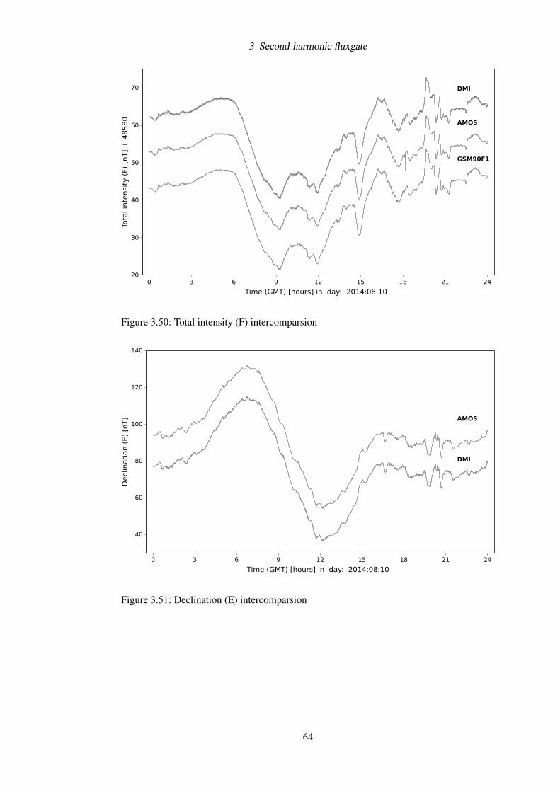
3 Second-harmonic fluxgate
0 3 6 9 12 15 18 21 24
Time (GMT) [hours] in day: 2014:08:10
20
30
40
50
60
70
Tota
l in
tensit
y (
F)
[nT]
+ 4
8580
GSM90F1
AMOS
DMI
Figure 3.50: Total intensity (F) intercomparsion
0 3 6 9 12 15 18 21 24
Time (GMT) [hours] in day: 2014:08:10
40
60
80
100
120
140
Declinati
on (
E)
[nT] AMOS
DMI
Figure 3.51: Declination (E) intercomparsion
64

3 Second-harmonic fluxgate
0 3 6 9 12 15 18 21 24
Time (GMT) [hours] in day: 2014:08:10
60
70
80
90
100
110
120
130
AMOS
DMI
Figure 3.52: Inclination (V) intercomparsion
0 10 20 30 40 50 60
Time [min] in day: 2014:08:10 5:00 (GMT)
96
98
100
102
104
106
108
110
AMOS (187.5 Hz)
AMOS (1Hz)
DMI
Figure 3.53: Inclination (V) intercomparsion: detail
3.11 Frequency-domain processing
Because high-frequency record is highly contaminated by power electricity (230/400V ∼50 Hz), what is variable due to temperature regullation in the variometric hut, it is betterto perform spectral analysis. The analysis was done for one hour datas of the instrument“AMOS” (fig. 3.53) and are on fig. 3.54
65

3 Second-harmonic fluxgate
0 10 20 30 40 50 60 70 80 90
Fr
1E2
1E3
1E4
1E5
1E6
Figure 3.54: Inclination (V): energy spectrum
Spectral analysis was done with 2048 samples blocks, Blackmann-Harris window and1000 samples step from the one-hour 187.5 Hz inclination data. DC level and slope of eachblock are deprecated by RMS method. Result is on fig. 3.54. The big peak is contaminationby 50 Hz power electricity network, the small peak left from the 80 Hz mark is alias of thesecond harmonic of the 50 Hz. Interesting is the peak left from the 20 Hz mark, what ispossibly frequency of austrian and german railways traction what is 16.7 Hz. Observatoryhave no other instrument to make intercomparsion in the ELF band.It is possible to estimate energetic spectra of noise of the instrument in the case of havingthree instruments which measures the same quantity. The menthod is analogical to themethod of reciprocity calibration of microphones (Ballantine, 1929). Let us have threeinstruments measuring the same quantity (fig. 3.55).
Figure 3.55: Three noisy instruments
The instruments have uncorellated noise and there is no coupling between them. Measuredvalues (F ) are contaminated by noise:
66

3 Second-harmonic fluxgate
F1 = F + n1
F2 = F + n2
F3 = F + n3 (3.20)
Then for the diferences of the output signals holds:
F1 − F2 = F + n1 − (F + n2) = n1 n2
F1 − F3 = F + n1 − (F + n3) = n1 n3
F2 − F3 = F + n1 − (F + n2) = n2 n3 (3.21)
Where AB =√A2 +B2 is quadratic superposition. Squaring eqs. 3.21 gives set of
linear equations, which can be solved to give noise parameters of all three instruments:
(F1 − F2)2 = n21 + n2
2
(F1 − F3)2 = n21 + n2
3
(F2 − F3)2 = n22 + n2
3 (3.22)
First step of data processing is determination of equivallent noise bandwidth of usedspectral analyser (it depends on used window and overlap ratio). the simple way is to useMLS sequence with unity RMS value, generated by this code1:
for(m=1;;)int b=0b11010001111010101; // MLS 17m=(m>>1)^((m&1)*b);out=(((m&1)*(-2)+1));
Due to Plancherel et al. (1910) theorem and knowledge, that MLS have flat energeticspectrum (Schroeder, 2009), we can calibrate the analyser in terms of pT/
√Hz Result of
processing of datas from fig. 3.50 is on fig. 3.56 The analyser is the same as in the case offig. 3.54, only the input sample rate is 1 Hz
1Author uses MLS sequence also for time-varied coeficients of digital filters. It can overcame problems withcoeficient quantisation in fixed length arithmetics
67

3 Second-harmonic fluxgate
0 100 200 300 400 500
Frequency [mHz]
20
40
60
80
100
120
140
160
180
200
Nois
e [
pT/
Hz]
DMI-AMOS GSM90-AMOS GSM90-DMI
Figure 3.56: Noise of three noisy instruments
The frequency range 350 to 450 mHz is free from artefacts (the waves on the left areresidues of discontinuous thermal regulation of AMOS instrument (which is thermallyunshielded), peak near 310 mHz from DMI is unknown) and was used for estimation ofnoise of instruments in the F axis. Constructed instrument (AMOS) has noise 13.8 pT/
√Hz.
Noise of standard observatory equipments was also estimated: Overhauser PPM GSM90F1:11.4 pT/
√Hz and DMI fluxgate: 61.3 pT/
√Hz. This method of noise intercomparsion
is used instead of usually used direct measurement. Because constructed instrument usesenvelope detection, does not work in the zero field and can not be tested in the magneticshield.
68

4 Conclusions
In this thesis, methods of singular elements, developed for filter synthesis in the 1970s, wereused to solve an acoustical problem (non-linear electrostatic transducer) and the problemof the magnetostatic circuit (fluxgate magnetometer). Both problems are so simillar thatthe author believes that they both can be considered electro-acoustical problems. Thefirst problem - parametric microphone - was solved only partially. Only the analoguepart was designed and breadboarded. For future development, some form of the digitalsystem must be constructed. Problems with electromagnetic compatibility of the NARODmagnetometer (based closely on the Acuna design) led the author to develop electronics forthe magnetometer, whose desighwas simillar to the previously constructed microphone. Sincethe magnetometer for observatory use is basically a very low-frequency instrument, someadditional parts were needed, including a highly stable thermally compensated referencevoltage source and precision temperature measurement unit. The digital part was based onDSP codes of plesiochronnous signal processing developed originally for the digital exciterof a MW transmitter in TESLA Hloubetín. It was shown that magnetometer electronics,constructed with specially designed input amplifiers, have a better SNR (fig. 3.53) achievedby the good EMI properties of the designed systems and lower physical noise sources. Thiswas compared with clasicall equipment constructed with low-noise operational amplifiers andswitched-circuit analogue processing (DMI Fluxgate). The author believes that DSP routines,used in constructing the digital magnetometer, can be used as a basis for constructing studioor measurement system based on the discussed parametric microphones, where no analogueaudio signal in the baseband and no global synchronisation circuit will be present in therecording chain, and with some parameters (EMC, dynamic range) exceeding today’s bestanalogue technology.The author’s original work:
• Model of nonlinear electrostatic transduction based on mutator and nonlinear VCCSs(fig. 2.2), published in (Vlk, 7-2008)
• Model of magnetostatic circuits based on singular elements graph manipulation,(fig.3.8), published in (Vlk, 2014).
• DSP technique of plesiochronous interpolation based on sampled continuous prototypefilter (Eg. 3.14) , published in (Vlk, 2005).
• Circuit of folded cascode with reactor powering used as low-noise input amplifier forparametric microphone (fig. 2.9 ), published in (Vlk, 2010).
• Commutation of VLF H-bridge trasmitter based on additional phase delayed H-bridgeand used in fluxgate low-noise pump circuit.
69

5 References
5.1 Cited documents
Aschenbrenner, H.; Goubau, G.: Eine Anordnung zur Registrierung rascher magnetischerStoerungen Hochfrequenz-technik und Electroakustik Vol. 47 (1936) No. pp. 177-181
Acuna, M.: Fluxgate magnetometers for outer planets exploration; IEEE Trans. Mag. Vol. 10(1974) No. 3 pp. 519-523
Acuna, M. H; Scearce, C. S.; Seek, J. B.; Scheifele, J. : The MAGSAT vector magnetometer -a precision fluxgate magnetometer for the measurement of the geomagnetic field NASATechnical memorandum No. 79656 Greenbelt, Maryland 1978
Arends, G.F.J.: De codensatormocrofoon met halfgleiders; Polytechnisch Tijdschrift, UitgaveE, Vol. 18(1963) No. 7 pp. 241-247
Alexanderson, E.F.W.; Nixdorf, S.P.: A Magnetic Amplifier for Radio Telephony Proc. IREVol. 4 (1916) No. 2 pp. 101-120
Ballantine, Stuart: Reciprocity in electromagnetic, mechanical, acoustical, and intercon-nected systems; Proc. IRE Vol. 17 (1929) No. 6 (June) pp. 929-951
Baltag, O.: Double Pumping Fluxgate Magnetometer Sensor Letters Vol. 11 (2013) No. 1 pp.149-152
Baxandall, P.J.: New Low-noise Transistor Circuit for Electrostatic Microphone WirelessWorld (1963) No. 11-12, pp. 538-542;593-597
Blumlein, Alan Dower: Alternating Current Bridge Circuits; British pat. 323037 filled:13.9.1928
Bobrov, V.N.: Serija kvarcevych magnitnych variometrov Geomagnetizm i aeronomija 2(1962) No. 2 p.348
Braun, Jaromír: Kombinatorické metody v analýze a modelování elektronických soustav;Prague: Academia 1990
Braun, K. : Elektroakustische Vierpole; TFT Bd. 33 (1944), H. 5 pp. 84-95
Castigliano, A.: Intorno ai sistemi elastici Turin 1873 dissertation
Cerman, A.; Merayo, J.M.G.; Brauer, P.; Primdahl, F.: Self-Compensating Excitation ofFluxgate Sensors for Space Magnetometers I2MTC - IEEE International Instrumentationand Measurement Technology Conference Victoria, Vancouver Island 12.-15.5.2008
Charkevic, Aleksandr Aleksandrovic: Teorija elektroakusticeskych preobrazovatelej; Vol-novyje processy; Moscow: Nauka 1973
70
References
Chireix, H.: High Power Outphasing Modulation Proc. IRE Vol. 23 (1935) No. 11 pp.1370-1392
Chua, L. O.: Memristor-the missing circuit element, IEEE Transaction on Circuit and SystemVol. 18 (1971) No. 5 pp. 507-519
Combes, Michel: Un générateur paramétrable de multiplieur de fréquence utilisant destechniques numeriques Paris: Université de Paris 06 1994 - Doctoral thesis
Connerney Jack, et al.: Mars Atmosphere and Volatile Mission (MAVEN) - MagnetometerInvesatigation (MAG) University of Colorado: Community meeting, 2.12.2012
Dement’jev, Jevgenij Petrovic: Elementy obšcej teorii i rasceta šumjašcich linejnych cepej;Moscow: Gosenergoizdat 1963
Fakhfakh, Mourad -ed.: Design of Analog Circuits through Symbolic Analysis; Benthame-books 2012
Feussner, W.: Zur Berechnung der Stromstarke in netzformigen Leitern Annalen der PhysikVol. 15 (1904) No. 12 pp. 385-394
Frederiksen, Erling: A method and a coupling for reducing the harmonic distortion of acapacitive transducer World patent WO 94/23547 published 13.10.1994
Gabler, Miloš; Haškovec, Jirí; Tománek, Evžen: Magnetické zesilovace Prague: SNTL 1950
Gayford, M.L.: Acoustical Techniques and Transducetrs London: STC 1961
Gordon, D.I. ; Sery, R.S.: Effects of charged particles and neutrons on magnetic materialsIEEE Trans. Comm. Electr. Vol. 83 (1964) No. 73 pp. 357-361
Gordon, D.I. ; Sery, R.S.: Irradiation of Iron and 5-79 Mo Permalloy with 2-MeV ElectronsJournal of Applied Physics Vol. 35 (1964) No. 3 pp. 879-880
Gordon, D.I. ; Sery, R.S. : Uniaxial anisotropy by "radiomagnetic" treatment; controllingfactors in a new process IEEE Trans. Magn. Vol. 1 (1965) No. 4 pp. 277-280
Gordon, D.I. ; Sery, R.S. : Uniaxial Anisotropy Induced by a Low-Temperature MagneticAnneal Following Electron Irradiation Journal of Applied Physics Vol. 37 (1966) No. 3pp. 1219-1217
Gordon, D. I.; Lundsten, R. H.; Chiarodo, R. A.; Helms, H. H. Jr.: A fluxgate sensor ofhigh stability for low field magnetometry IEEE Trans. Mag. vol. MAG-4(1968) No. 3,pp.397-401
Gouriet, G. G.: High-Stability Oscillator Wireless Engineer (Apr. 1950)
Griese, Hans Joachim: US. Pat. 3422225 pub. 1969 (compare with firm literature to addcapacitor to complete Clapp circuit)
Guillemin, Ernst Adolph: Theorie der Frequenzvervielfachung durch EisenkernkoppelungMuenchen: Sc.D. Thesis 1926
Guillemin, Ernst Adolph: Introductory Circuit Theory New York: J. Willey 1953
71

References
Gyimesi, M.; Avdeev, I.; Ostergaard, D.: Finiteelement simulation of micro-electromechanical systems (MEMS) by strongly coupled electromechanical transducersIEEE Transactions on Magnetics vol. 40(2004) no. 2 (march) pp. 557-560
Hammond, Laurens; Hanert, John M. : Vibrato apparatus US Patent: 2560568 (1946)
Hannemann, Dennis M; Huang, Kwang, Ta ; Shiroma, M.: Parametric energy coupledunitnterruptible power supply US Patent: 4115704 (filled: 19.9.1977)
Hansen, S.T.; Ergun, A.S.; Liou, W.; Alud, B.A.; Khuri-Jakub, B.T.: Wideband microma-chined capacitive microphones with radio frequency detection JASA Vol. 116 (2004), No.2 (August) pp.828-842
Hardy, Tim: Next Generation LF Transmitter Technology for (e) Loran Systems Unpublishedreport Nautel 2008
Harris, Frederic J.: On the Use of Windows fo Harmonic Analysis with the Discrete FourierTransform Proc. IEEE Vol.66 (1978) No. 1 pp. 172-205
Heaviside, Oliver: Electromagnetic Theory, vol. 1-3 London: Benn Brothers 1922
Hibbing, Manfred: Deutsche patent 4300379 publ.1996 (Compare with firm literature tocomplete gamma LC with series inductor to tune the bridge.)
Hunt, Frederick V.: Electroacoustics: The Analysis of transduction, and its historicalbackground; Cambridge: Harvard University Press 1954
Husník, L.: Influence of Transfer Functions of Transducers Constituting the Loudspeakerwith the Direct D/A Conversion on the Performance of the System, 115-th convention ofAES, New York, 2003 Paper No.: 6519
Jagoš, M.: Zmiešavac v spínacom režime Súbor prednsšok z celoslovenského seminárarádioamatérov zväzarmu Vysoké Tatry 1989
Korepanov, V.; Marusenkov, A.: Flux-Gate Magnetometers Design Peculiarities Surveys inGeophysics Vol.33 (2012) No. 5 pp. 1059-1079
Kovár, D.: Typy elektrod pro mikrofony s prrímou A/D premenou, Proceedings of the ATP,Brno, 2004
Kvasil, Josef: Mikroelektronické transformacní bloky; Prague: SNTL 1981
Lahmeyer, W: Transformator mit Sekundaerwickelungen auf verschiedenen SchenkelnGerman Pat. DE149761 (26.8.1902)
Lamb, H.: Higher Mechanics; London: Cambridge at the University Press 1920
Lenk, Arno: Elektromechanische Systeme Bd. 1: Systeme mit konzentrieren parameternBerlin: VEB Verlag Technik 1973
Lenk, Arno: Elektromechanische Systeme Bd. 2: Systeme mit verteilten parametern Berlin:VEB Verlag Technik 1974
Lenk, Arno: Elektromechanische Systeme Bd. 3: Systeme mit hilfenergie Berlin: VEB VerlagTechnik 1975
72

References
Linvill, John G.: Models of transistors and diodes New York: McGraw-Hill 1963
Macoun, Zbynek; Nádvorník, Bohumil: Liniový vlakový zabezpecovac LS H, LS III, LS IVPrague: NADAS 1971
Manley, J.M.; Rowe, H.E.: Some general properties of nonlinear elements- part 1. Generalenergy relations Proc. IRE 44 (1956) pp. 904-913
Marie, G.: Amplificateurs paramétriques basses fréquences à commande magnétique orthog-onale; Acta Electronica, Vol.8 (1964), No. 1 pp 7-81.
Mason, W.P.: Electromechanical transducers and wave filters New York: D. Van NostrandComp.1942
Mathieu E.: Mémoire sur Le Mouvement Vibratoire d’une Membrane de forme Elliptique;Journal de Mathématiques Pures et Appliquées pp 137-203
Miller, G.: Stylus-Groove Relations in Phonograph Records Cambridge: Harvard University1950 - Doctoral thesis
Mitra, S.K.: Analysis and Synthesis of Linear Active Networks, New York: J.Wiley 1963
Motchenbacher,C.D; Fitchen, F.C.: Low-noise electronic design New York: J.Wiley 1973
Moos, Petr: Nulorové modely kvazilineárních a nelineárních elektronických prvku; Prague:Academia 1983
Musmann, G.; Anfassiev, Y.: Fluxgate Magnetometers for Space Research Norderstedt:Books on Demand 2010
Motl, K.: Elektroakustický vysílac s prímou D/A premenou, Proceedings of the ATP Prague,2005
Mueller, R.; Holstein, P.: About a Digital RF-Condenser microphone; Convention Paper6130 116-th Convention AES Berlin: May 8-11 2004
Narod, B; Russell, R.D.: Steady-State Characteristics of the Capacitively Loaded Flux GateSensor; IEEE Trans. Mag. Vol. 20 (1984) No. 4 pp 592-597.
Narod, B. NGL S-100 service manual; Vancouver: Narod Geophysics Ltd. 1987
Narod, B.: The origin of noise and magnetic hysteresis in crystalline permalloy ring-corefluxgate sensors Geosci. Instrum. Method. Data Syst. Discuss. (2014) No. 4 pp. 319-352
Otala, Matti: Circuit Design Modifications for Minimizing Transient Intermodulation Distor-tion in Audio Amplifiers JAES 20 (1972) No. 5 (June) pp. 396-399
Ott,H.W.: Noise reduction techniques in electronic systems New York: Wiley-Bell Tel. lab.1976
Oxborrow, Mark; Breeze, Jonathan D.; Alford, Neil M.: Room-temperature solid-state maserNature 488 (2012) pp. 353-356
Paerschke, R.: Ein Hf- Kondensatormikrofon mit Transistoren Funkschau 1965 No. 2 pp.113-114
73

References
Parten, Michael E.: Linear network analysis by Nullator-Norator residual networks Lubbock:Texas Tech University(1972) - Doctoral thesis
Pastille, Holger: Ueber die Nichtlinearitaeten am Kondensatormikrofon unter besonderenBeruecksichtigung der Membran; Berlin, III. Fakultaet, 2011 - Doctoral thesis
Pedersen, M.; Olthuis, W.; Bergveld, P.: An integrated silicon capacitive microphone withfrequency-modulated digital output Sensors and Actuators vol. A69 (1998) pp. 267-275
Penfield, Paul; Rafuse, Robert P.:Varactor Applications Cambridge: The MIT Press 1962
Petterson, E.: Magnetic wave amplifiing repeater US PAT. 1884844 1929
Pimonow, Léonid: Les Infra-sons Paris: CNRS 1976
Player, P.A.: Parametric amplification in fluxgate sensors Journal of Physics D: Vol. 21(1988) No. pp. 1473-1480
Plancherel, Michel; Mittag-Leffler: Contribution à l’étude de la représentation d’une fonctionarbitraire par les intégrales définies Rendiconti del Circolo Matematico di Palermo Vol. 30(1910) No. 1 pp. 289-335
Primdahl, Fritz: Temperature compensation of fluxgate magnetometers IEEE Trans. Mag. 6(1970) No. 4 pp. 819-822
Radeka, V.: Signal, Noise and Resolution in Position-Sensitive Detectors; IEEE Trans. Nucl.Sci., Vol. 21 (1974), No. 1 pp 51-64.
Rieger, F. : Lineární Obvody; Prague: SNTL 1967
Ripka, Pavel : Magnetometry s feromagnetickou sondou; Prague: CVUT (Doctoral Thesis)1988
Russell, R.D.; Narod, B.B; Kollar, F.: Characteristics of the Capacitively Loaded Flux GateSensor IEEE Trans. Mag., Vol. MAG-19 (1983), No. 2 pp. 126-130
Sasada, I.: Symmetric response obtained with an orthogonal fluxgate operating in fundamen-tal mode IEEE Trans. Mag., Vol. MAG-38 (2002), No. 5 pp. 3377-3379
Sattinger, D. H: Lie Groups and Algebras with Applications to Physics,Geometry andMechanics New York : Springer 1986
Schroeder, Manfred R.:Number Theory in Science and Communication New York: Springer2009
Serson, P. H.; Mack, S.Z.; Whitham, K.: Publ. Dom. Obs. Ottawa, 19 (1957) pp. 15 - 97
Sery, R.S. ; Gordon, D.I.: Irradiation of Magnetic Materials with 1.5- and 4-MeV ProtonsJournal of Applied Physics Vol. 34 (1963) No. 4 pp. 1311-1312
Sery, R.S. ; Gordon, D.I. : Activation Energy and Annealing Kinetics of Remanence GrowthCaused by Low-Temperature Magnetic Anneal of Electron-Irradiated Nickel-Iron Journalof Applied Physics Vol. 39 (1968) No. 2 pp. 991-992
Seltzer, S. J.; Romalis, M. V. : Unshielded three-axis vector operation of a spin-exchange-relaxation-free atomic magnetometer Appl. Phys. Lett. 85 (2004) p. 4804
74

References
Soell, S.; Porr, B.: An Undersampling Digital Microphone Utilising Second Order NoiseShaping, 14-th. International conference MIXDES2007 Ciechocinek, Poland 21.-23. June2007
Sommerfield, A.: Vorlesungen ueber theoretische physik, band III-Elektrodynamik; Leipzig:Geest and Portig 1949 p.11
St-Louis, Benôit, ed.: Intermagnet Technical Reference Manual; Edinburgh: BGS 2011
Strnad, Ladislav: Synchronizace sítí; Prague: CVUT publishing house 2013
Sucksdorff, C.; Pirjola, R.; Häkkinen, L.: Computer production of K-indices based on linearelimination. Geophys. Trans. Vol. 36 pp. 333âAS345
Suesse, R.; Civelek, C.: Analysis of engineering systems by means of Lagrange and Hamil-ton formalisms depending on contravariant, covariant tensorial variables; Forschung imIngenieurwesen Bd. 68 (2003) pp. 66 - 74
Swanson, Hilmer Irvin: Amplitude modulator, European Patent: 0083727 1983
Sýkora, Bohumil; Dudek, Pavel: Predzesilovace pro prenosku s pohyblivým magnetemAmatérské radio A 68 (1990) No. 1 - 2 pp. 65-70,105-108
Tomlinson, G.H. ; Galvin, P.: Analysis of skewing in amplitude distributions of filtered msequences Proc. of the IEE Vol. 121 (1974) No. 12 pp. 1475-1479
Vackár, Jirí: Vysílace. 1., Teoretické základy Prague: SNTL 1960
Vágó, István: Graph Theory : Application to the calculation electrical networks; Budapest:Akadémiai Kiadó 1985
Van der Pol, B.; Van der Mark, J.: Frequency demultiplication Nature, 120 (1927), pp.363-364
Vorperian, Vatché: Fast Analytical Techniques for Electrical and Electronic Circuits; London:Cambridge University Press 2002
Westberg, Jerry: Phase to amplitude H-bridge switching circuit, US Patent: 7092269 2006
Weynmann, G.: Di Messung kleinster Schalldruecke mit dem kondensatormikrophon Elek-trische Nachrichtentechnik Vol. 20 (1944) No. 6, p. 149-158
Whittaker, Edmund Taylor; Robinson, George: The Calculus of Observations: A Treatise onNumerical Mathematics London: Blackie and Son Limited 1937
Yoshida, Kosaku : Operational Calculus: A Theory of Hyperfunctions Berlin: Springer-Verlag 1984
Zell, Clemens: Einrichtung zur Umwandlung von ein- oder mehrphasigen Wechselstromin Gleichstrom und umgekehrt mit Hilfe von Selbstinduktionsspulen mit polarisirtemEisenkern German patent DE113992 (25.4.1899)
Van der Ziel, A.: Noise Prentice-Hall 1954
Zuckerwar, A.;S hope, W.W.: A Solid-State Converter for Measurement of Aircraft Noiseand Sonic Boom IEEE Trans. Instrum. and Meas. Vol. IM-23 (1974) No.1 p. 23-27
75

References
Zworykin, V.K.: Television; the electronics of image transmission in color and monochromeNew York: J. Wiley 1954
5.2 Author’s document
Vlk, Michal: Blumleinuv mustek Czech patent CZ 302207 granted: 5. 11. 2010
Vlk, Michal: Šumové vlastnosti páskového rychlostního mikrofonu Master thesis, Prague:CVUT-FEL 2005
Vlk, Michal: Plesiochronní prevodník vzorkovací frekvence Proceedings of the regional AESmeeting ‘ATP’ Prague 2005
Vlk, Michal: A Novel Analogy for Time-Domain Simulation of the Nonlinear ElectrostaticTransducer Procedings of the conference Poster Prague 15.5. 2008
Vlk, Michal: Condenser microphone as parametric electroacoustic system and its time-domain modelling via equivallent electrical circuit in SPICE software Proceedings of theconference Acoustics 08 Paris 29.6-4.7. 2008
Vlk, Michal: Kondenzátorový mikrofon jinak Proceedings of the 77-th Acoustic seminary ofthe Czech Acoustical Society Zlenice 7.-9.10. 2008
Vlk, Michal: Koncové stupne digitálních vysílacu Proceedings of the conference Radioko-munikace Pardubice 4.-6.11. 2009
Vlk, Michal: Modernisation of the Narod fluxgate electronics at Budkov Geomagneticobservatory Poster presented at EGU General Assembly Wien 7.-12.4. 2013
Hejda,P.; J. Horácek, J.; Vlk, M.; Bayer, T.: ON THE THUNDERSTORM OF 10 JULY 2011AT MAGNETIC OBSERVATORY BUDKOV Boletin ROA San Fernando No.3 2013;
Vlk, Michal: Obvodové modely indukcnostního teslametru Proceedings of the 89-th Acousticseminary of the Czech Acoustical Society Šlovice 7.-9.10. 2014
76

6 Appendix A: Electromechanicaltransduction as anenergy-conservative system
Assume the system to have n degrees of freedom and q1, ...qn are generalized co-ordinates(Lamb, 1920). The partial derivatives of the generalized co-ordinates with respect to timeare generalized velocities qi = ∂qi
∂t . Assume the energy of th system to be a function ofco-ordinates only:
V = V (q1, ...qn) (6.1)
This energy is called the potential energy and its partial derivative with respect to the i-thco-ordinate is called the generalized force:
Fi = ∂V (q1, ...qn)/∂qi (6.2)
Assume the kinetic energy of system to be a function of only generalized velocity:
T = T (q1, ...qn) (6.3)
Its partial derivative with respect to the i-th generalized velocity is then the generalizedmomentum:
pi = −∂T (q1, ...qn)/∂qi (6.4)
Equations 6.2 and 6.4 are dual. The minus sign must be in one of them. It is the author’sdecision to include it in the equation 6.4. Sometimes it may be useful to differentiate 6.4with respect to time. We the get:
Fi = − d
dt(∂T (q1, ...qn)/∂qi) (6.5)
We can add energetic functions freely, i.e. as Lagrange functions of the system:
L = T − V (6.6)
Or to construct equations with them:
d
dt
∂L
∂qj− ∂L
∂qj= 0 (6.7)
The equation is merely a transcription of the commutativity properties of some differentialoperators:
d
dt
∂A
∂(dqdt )=
d
dt
∂Addt∂q
=∂A
∂q(6.8)
The reader can find further generalization in the Lie groups theory (Sattinger, 1986). We canalso use alternative Hamilton equations for some problems or add the Helmholtz functionin case of dissipative systems, but problems solved here are too simple to do that. Herewe shall need only eq. 6.2 from classical mechanics. But electro-acoustics is rather more
77

6 Appendix A: Electromechanical transduction as an energy-conservative system
electrodynamic than mechanics alone and thus we need to use mechanical and electrodynamicvariables together. The natural way of combining them is to use energetic functions: Themathematical description of the energy conservation law. There are pairs of variables in thegeneral electrodynamics called - ‘energetic influentia’ (Sommerfield, 1949). Electrodynamicones are: 1/2(HB), 1/2(DE), jE, [EH] and mechanic ones are: 1/2(Fx) and 1/2(σε)We can partially differentiate the energetic function by one variable from the pair to getanother variable, i.e.: if we differentiate the energy function partially by F or x, we get xor F, respectively (In mechanics, it is used in solving elasticity problem as the Castigliano(1873) method). We can generalize this for mechanical and electrodynamic variables, butunder the condition that the processes are reversible. For irreversible processes, we musttake into account the entropy concept, and the interested reader in that can find informationin every textbook of physical chemistry.The potential energy of an electrostatic system is described by equation (Charkevic, 1973):
V =1
2
q2
C(6.9)
where C is capacity and q is charge. If the transducer is simple (capacitor with infiniteequidistant plates), the capacity is:
C =εA
x(6.10)
Here A is the plate area , x is the distance between plates, and ε is the dielectric constant ofair. for the potential energy of a simple transducer the following holds:
V =xq2
2εA(6.11)
Eq. 6.11 indicates, that the generalized co-ordinates are x and q. The correspondinggeneralized forces are then F and U :
F =∂
∂xV =
q2
2εA(6.12)
U =∂
∂qV =
xq
εA(6.13)
Equations 6.12 and 6.13 are fundamental nonlinear equations of condenser transducer.They can be used for simulation in Spice-like software as discussed by the author in thethessis. It also holds:
I =∂q
∂t(6.14)
The behaviuor of every non-linear function can be expanded via the Taylor series. The firsttwo terms are constant and linear term. The process to assuming all higher terms to be zerois called linearization. Let us do this it for the generalized co-ordinates:
q = q0 + ∂q (6.15)
x = x0 + ∂x (6.16)
Substitution 6.15 and 6.16 into 6.12 and 6.13 gives two linear equations:
∂F =q0
εA∂q (6.17)
78

6 Appendix A: Electromechanical transduction as an energy-conservative system
∂U =x0
εA∂q +
q0
εA∂x (6.18)
Consider two linear equations. The equations have the same form for all linear transducerswith two constants. The first constant is quasistatic electrical elastance (reciprocal value toquasistatic transducer electrical capacity):
S0 =1
C0=x0
εA(6.19)
The second constant is the transducer constant (corresponds to Mason’s constant inpiezoelectric transducer)
k =q0
εA=U0
x0(6.20)
Where U0 is the polarization voltage of the transducer and x0 is static the distance betweenthe electrodes. If the electrostatic transducer is loaded to short at the electrical side (This mayoccur in an electrostatic speaker or a parametric microphone), equation 6.18 transforms to:
x0
εA∂q = − q0
εA∂x (6.21)
After substitution of 6.17 into 6.21, we get:
∂F = −(U0
x0
)2
C0∂x = −k2C0∂x (6.22)
which describes negative compliance on the mechanical side in the form of transformedself-capacity. Let us write the equations of electrostatic conversion in the form of a matrixRieger (1967) (we shall write the variables as lower-case letters, because they are smallquantities in the linear model):
[fu
]=[q x
] q0εA 0
x0εA
q0εA
(6.23)
Since the low signal value has zero initial condition (all transients are assumed to befinished), we can put:
i =∂q
∂t∼= i = pq (6.24)
v =∂x
∂t∼= v = px (6.25)
Where p is the operator of the time derivative. After substituting of 6.24 and 6.25 into6.23, we get linear equations of electromechanical conversion in the form of a mixed matrix(mechanical and electrical variables are on one side). This form is known in piezo-electricityfrom the book of Mason (1942).
[fu
]=[i v
] q0εAp 0
x0εAp
q0εAp
(6.26)
We cannot describe the type of matrix in the classical circuit theory without appendingmechanical values to electrical in advance. In electrical circuit theory, there are only two
79

6 Appendix A: Electromechanical transduction as an energy-conservative system
variables: current and voltage. Nevertheless, there are many forms of two-branch matrices(Z,Y,H,K,A,B), but only two basic operations are performed to convert between them. Oneoperation (so-called matrix inversion) is commonly used everywhere, where general solvingof the linear equation system is needed. Let us introduce an example of matrix inversion inrecomputing of Z (impedance) and Y (admittance) matrices.
Z = Y −1 =
y22|Y | −y21
|Y |
−y12|Y |
y11|Y |
(6.27)
The reciprocal problem (Y and Z) is dual:
Y = Z−1 =
z22|Z| − z21
|Z|
− z12|Z|
z11|Z|
(6.28)
‘Partial inversion’ exists between the Z and H matrices. It probably has no counterpartin the general matrix theory. Let us illustrate this on an example of recomputing Z and Hmatrix:
Z = H−1(22) =
|H|h22
h12h22
−h21h22
1h22
(6.29)
The reciprocal problem (H and Z) is dual:
H = Z−1(22) =
|Z|z22
z12z22
− z21z22
1z22
(6.30)
We could do only partly invert matrix 6.26 over term (22). After doing so, we get thematrix in more convenient form, known from the book of Charkevic (1973):
[fv
]=[i u
] q0εAp 0
−x0q0
εApq0
(6.31)
The next step is to mirror the matrix over the u|i axis and add the sign at u (This is becauseof the conventions in the classical electro-acoustic analogy):
[fv
]=[−u i
] 0 q0εAp
− εApq0
−x0q0
(6.32)
Let us decompose matrix on the right-hand side of eq. 6.32 into two matrices:
0 q0εAp
− εApq0
−x0q0
=
0 q0εAp
− εApq0
0
1 x0
εAp
0 1
=
0(x0pU0
)−1
−x0pU0
0
1 1
pC0
0 1
(6.33)
80

6 Appendix A: Electromechanical transduction as an energy-conservative system
The first term of the product is the matrix of the reactance invertor (Kvasil, 1981) andthe second one is the series self-capacitance on the electrical side. This equivalent cir-cuit appears seldom in the literature (Hunt, 1954), The transformed variant with an idealtransformer is more common. There are methods to transform the PI or T two-branch intoan ideal transformer with series/parallel elemens. These methods are called ‘The nortontransformations’:
Figure 6.1: Norton transformations
A slightly modified method is applied to the gamma-type capacitor twobranch. Hint: Jointtwo series capacitors on the left, apply Norton transformation to the result with the shuntcapacitor. Then transform the series capacitor from the right-hand side and join it with theseries cap resulting from the previous step.
Figure 6.2: Linearised models of condenser transducer
The schematic representation of the reactance invertor has two equivalent forms. The firstone has positive series capacitors and a negative shunt capacitor. and the second one hasnegative series capacitor and a positive shunt capacitor. Note here, that the transducer matrixremains the same. Insertion of ideal transformer is only the realization part of transducermodel and this model is valid only with all the components.The general form of the two-branch equation is the so-called affine approach. It uses twosquare matrices to form two homogenous linear equations where all two-branch variablesare included. There is only one condition for the two-branch: to be autonomous (does notinclude independent sources).[
00
]=[U1 U2 I1 I2
] [M N
](6.34)
Matrices can be manipulated, i.e. via the Gauss elimination method. We can get classicalcircuit matrices as elements in some places, where other places have prescribed values:
81

6 Appendix A: Electromechanical transduction as an energy-conservative system
[M N
]≈
y11 y12 −1 0
y21 y22 0 −1
≈−1 0 z11 z12
0 −1 z21 z22
≈−1 h12 h11 0
0 h22 h21 −1
≈
≈
k11 0 −1 k11
h21 −1 0 k22
≈−1 a11 0 @a12
0 a21 −1 @a22
≈b11 −1 @b12 0
a12 0 @b22 −1
(6.35)
Note, that symbol @ represents a sign for circuit matrices defined by the IEC convention,but notrespecting this leads in this case to simpler systematism. Using the sign makestransformation of the matrices complicated if the type of matrix is not nown a-priori (as inelectroacoustics). This is the reason for putting signs in equation 6.32
There are other phenomena used for electromechanical transduction. They will be listedbriefly. Consider a moving armature transducer where one turn of wire without resistance ispresent. Different number of turns can be expressed by an ideal transformer in cascade withthe electrical part of the transducer. The potential energy of magnetostatic system reads:
V =1
2RmΦ2 (6.36)
WhereRm is the reluctance. For a simple form of transducer (magnetic gap) the reluctancereads:
Rm =x
µA(6.37)
where x is the gap width, A is the armature cross-section and µ is air permeability. Thesimple form of the transducer formula for potential energy is:
V =xΦ2
2µA(6.38)
Here, the generalised coordinates are x and Φ. The generalised forces will be F and I .
F =∂V
∂x=xΦ2
2µA(6.39)
I =∂V
∂Φ=xΦ
µA(6.40)
These are the fundamental equations of moving-reluctance transduction. It also holds:
U =∂Φ
∂t(6.41)
A secial kind of transducer is a transducer with linear energy transfer. Consider a generalsystem with two degrees of freedom (i.e. one mechanical and one electrical), which is linear:
L(aA+ bB) = aL(A) + bL(B) (6.42)
The energy function of this system is:
V (y1, y2) =1
2(c11y
21 + c22y
22) + c12y1y2 (6.43)
82
6 Appendix A: Electromechanical transduction as an energy-conservative system
For some kinds of conversion principles, some coefficients may be equal to zero, but thecoupling coefficient have one value. Here we can see the reciprocity and, from this pointon, we conjencture, that reciprocity is the function of degrees of freedom of the transductionphenomenon.
The energy for piezo-electrical transduction reads:
V (D, ξ) =1
2
(1
εD2 + Emξ
2
)+ fDξ (6.44)
where D is electrical induction, ξ is the relative enlargement and f is Mason’s constant.The partial derivatives with respect to variables D and ξ yields the piezo-electrical equations:
E =∂T
∂D=
1
εD + fξ (6.45)
σ =∂T
∂ξ= fD + Emξ (6.46)
Consider an ideal moving conductor transducer. Its kinetic co-energy (electrodynamicenergy) is:
T = BlIv (6.47)
Where Bl is the gyration factor (product of induction in the gap with perpendicularprojection of the wire length onto induction). I is the electric current flowing through the wireand v is the velocity of the wire. Generalised velocities are v and I ,the generalised momentaF and U . Note, that equation 6.47 is in bilinear form: it predicts that the fundamentaltransducer equations will be linear:
F = −∂T∂v
= @BlI (6.48)
U = −∂T∂I
= @Blv (6.49)
Where @ indicates that the signs are negative. In a particular example of the transducerthe signum convention should conform to the Ampère right-hand rule.
83

7 Appendix B: Circuit determinantcomputation code
/********************************************************** Determinant Computation
* via Extended Sparse Tableau
* Mapped as binary tree
* core finished 14.1.2009
* Memory allocated via garbage-collector
* translate with: gcc -Wl,--stack=500000000 sparse.c
* (C) Michal Vlk [email protected]
************************************************************/
#include <math.h>#include <stdio.h>#include <stdarg.h>#include <stdlib.h>#include <string.h>
typedef struct spm_struct spm_* left;struct spm_* right;int row;int col;int indx; // 0 = not_used, terminating,
//1 = -1, 2 = +1 (vars), 3... (string var) spm;
// global memoryint gcol = 0; // garbage collectorvoid* gnod;FILE* output; // output file
spm* spmalloc()void * c;void * d;if(gcol == 0)
c = (void*)malloc(sizeof(spm));return(((spm*)c));
elsegcol--;c = ((void**)gnod)[0];d = gnod;gnod = c;return(((spm*)d));
spfree(spm* nod)void** b;b = (void**)nod;b[0]=gnod;gnod=(void*)b;gcol++;
int ind(int nod, int val)int nos;nos=2*(nod%2)-1;if(val==1)
return((-1)*nos);
if(val==2)return(nos);
if(val>2)return((val-1)*nos);
int rdd(spm* a, spm* b)
if((*a).row>(*b).row)
return(1);
if((*a).row<(*b).row)return(0);
if((*a).col>(*b).col)return(1);
if((*a).col<(*b).col)return(0);
return(0); // resultativity conition
int sparprint(spm* root, int row, int col)
if((*root).row==row&&(*root).col==col)return((*root).indx);
if((*root).indx!=0)if((*root).row>row)
return(sparprint((*root).left,row,col));
if((*root).row<row)return(sparprint((*root).right,row,col));
if((*root).col>col)return(sparprint((*root).left,row,col));
if((*root).col<col)return(sparprint((*root).right,row,col));
elsereturn(0);
void spt(spm* root,int mmax)int i,j;printf("\n");for(i=0;i<mmax;i++)
for(j=0;j<mmax;j++)
printf(" %i",sparprint(root,i,j));
printf("\n");
void sds(spm* root) // destructorif((*root).indx!=0)
sds((*root).right);sds((*root).left);
spfree(root);
spm* smk(int row, int col, int indx) // structure make
84

7 Appendix B: Circuit determinant computation code
spm* nod;nod=spmalloc();(*nod).row=row;(*nod).col=col;(*nod).indx=indx;(*nod).left=spmalloc();(*nod).right=spmalloc();(*((*nod).right)).indx=0;(*((*nod).left)).indx=0;return(nod);
spm* sdc(spm* infile) // copyspm* outfile;outfile = smk(0,0,((*infile).indx));if((*infile).indx!=0)
(*outfile).row=(*infile).row;(*outfile).col=(*infile).col;(*outfile).right=sdc((*infile).right);(*outfile).left=sdc((*infile).left);
return(outfile);
void ldd(spm* root, spm* onenod) // one member addif((*root).indx==0)
(*root).left=smk(0,0,0); // structure make(*root).right=smk(0,0,0);(*root).indx=(*onenod).indx;(*root).row=(*onenod).row;(*root).col=(*onenod).col;elseif(rdd(root,onenod))
ldd((*root).left,onenod);elseldd((*root).right,onenod);
// one member add with conditionvoid mdd(spm* root, spm* onenod, int row, int col)
if((*root).indx==0)
(*root).left=smk(0,0,0); // structure make(*root).right=smk(0,0,0);(*root).indx=(*onenod).indx;(*root).row=((*onenod).row>row) ?
((*onenod).row)-1:((*onenod).row) ;(*root).col=((*onenod).col>col) ?
((*onenod).col)-1:((*onenod).col) ;elseif(rdd(root,onenod))
ldd((*root).left,onenod);elseldd((*root).right,onenod);
// add two arbitrary structures togethervoid kdd(spm* root, spm* anex)if((*anex).indx==0)
;elseldd(root,anex);kdd(root,(*anex).right);kdd(root,(*anex).left);
// add element to structurevoid sad(spm* root,int row, int col, int indx)kdd(root,smk(row,col,indx));
// removes and returns the last element of treespm* gle(spm* root)if(((*root).indx!=0)&&((*((*root).right)).indx==0))
spm* tmp;spm* rest;tmp=sdc(root); // copysds((*root).right);rest = (*root).left; // left annex of last(*root).indx=(*((*root).left)).indx;if((*root).indx!=0)
(*root).row=(*rest).row;(*root).col=(*rest).col;(*root).right=(*rest).right;(*root).left=(*rest).left;
return(tmp);else if(((*root).indx!=0)&&
((*((*root).right)).indx!=0))return(gle(((*root).right)));elsereturn(smk(0,0,0));
// get minor - analogic to copyspm* gmn(spm* infile, int row, int col)spm* out1;out1 = smk(0,0,0); // structure makeif(((*infile).row!=row)&&((*infile).col!=col))
if((*infile).indx!=0)
mdd(out1,infile,row,col);kdd(out1,gmn((*infile).left,row,col));kdd(out1,gmn((*infile).right,row,col));
elseif((*infile).indx!=0)
kdd(out1,gmn((*infile).left,row,col));kdd(out1,gmn((*infile).right,row,col));
return(out1);
// add value to output treespm* adv(spm* lastnod, int value)
spm* tmp;tmp=spmalloc();(*tmp).indx = value;(*tmp).left = lastnod;return(tmp);
// trace output treevoid ttr(spm* lastnod, int sgn)if((*lastnod).indx!=0)
if((*lastnod).indx==-1) ttr((*lastnod).left,-sgn);if((*lastnod).indx==1) ttr((*lastnod).left,sgn);if((*lastnod).indx<-1)fprintf(output,"z%i*",(-1)*((*lastnod).indx)-1);ttr((*lastnod).left,-sgn);if((*lastnod).indx>1)fprintf(output,"z%i*",(*lastnod).indx-1);ttr((*lastnod).left,sgn);elsefprintf(output,"(%i)+",sgn);
spm* dnd(spm* lastnod)
85

7 Appendix B: Circuit determinant computation code
spm* tmp;tmp = (*lastnod).left;spfree(lastnod);return(tmp);
// det. comp.void dct(spm* infile, spm* lastnod, spm* lastinf, int nmax)spm* a;spm* b;spm* c;spm* d;spm* e;spm* f;a = infile;//spt(lastinf,nmax);b = gle(lastinf); // This element will be operated.//printf(" -%i-, %i, %i ",(*b).indx,(*b).row,(*b).col);//fprintf(output," -%i- ",(*b).indx);//ttr(lastnod,1);if((*b).row==nmax-1) // matrix have some valid element
if((*b).row==0)
if((*b).row==0&&(*b).col==0&&
(nmax-1)==0&&(*b).indx>0)d=adv(lastnod,ind((*b).col,(*b).indx));
// zero det//printf("trace %i %i ",(*b).row,(*b).col);
ttr(d,1); // trace output treeelse
// zero det//printf("bad reminder %i %i ",(*b).row,(*b).col);
elsee=adv(lastnod,ind((*b).col,(*b).indx));c=gmn(a,(*b).row,(*b).col); //get minorf = sdc(c);dct(c,e,f,nmax-1); // computes minors determinantsds(c);sds(f);//blb;d = sdc(lastinf);b = gle(lastinf);if((*b).row==nmax-1)
//e=adv(lastnod,ind((*b).col,(*b).indx));
dct(a,lastnod,d,nmax); // computes restsds(b);sds(d);
main(int argv,char**argc)spm* root; // root of structurespm* rt;spm* rd;int i,j,k,l,a,b,c,d;
// nullators, norators, regulars, totalsint nul, nor, reg, tot;
// maximal number of nodes, dimension of matrixint nmax, mmax;FILE * inf;printf(" %i \n",argv);if(argv<2)printf("Extened sparse tableau analysis\n");printf("usage sta.exe infile\n");printf("input file struct: node node number\n");printf("\n");printf("when number is positive number,
symbol is regular imittance with that number\n");printf("nodes goes from 0 to NMAX, all node
No within interval must be used\n");printf("when number is 0, symbol is nullator\n");printf("when number is -8, symbol is norator\n");printf("outfile is symbolic formulla\n");printf("optimalised malloc\n");printf("output var: res\n");printf("After Braun, Vlach &t al. \n");printf("(c) Michal Vlk \n");printf("v. 1.0.2 14.01.2010\n");return(-1);nul=0;nor=0;reg=0;nmax=0;
inf = fopen(argc[1],"rt");// outfile = fopen(argc[2],"wt");
output = fopen("output.txt","wt");while(!feof(inf))
fscanf(inf,"%i",&a);fscanf(inf,"%i",&b);d=fscanf(inf,"%i",&c);if(d&&(!feof(inf)))
if(c==0)nul++;if(c==-8)nor++;if(c>0)reg++;if(a>nmax)nmax=a;if(b>nmax)nmax=b;
mmax=(nul+nor+reg)*2+nmax; // order of matrixif(nul!=nor)
printf("no nullor pair");exit;
rewind(inf);root=smk(0,0,0);for(i=0,j=reg+2*(nul+nor)+nmax;i<reg;i++,j++)
// partial tree ballancing// giving -1 to place of lower unity matrixsad(root,j,i,1);// giving +1 to place of upper unity matrixsad(root,i,i,2);
for(;i<(reg+nul+nor);i++)//giving +1 to rest of upper unity matrixsad(root,i,i,2);
for(i=reg,j=reg+nul+nor+nmax,k=0;k<nul;i++,j++,k++)//givin +1 to I place of nullatorsad(root,j,i,2);
for(i=2*reg+nul+nor,j=reg+nul+nor+nmax+nor,k=0;k<nul;i++,j++,k++)
//givin +1 to U place of nullatorsad(root,j,i,2);
i=reg+nul+nor;j=reg+2*(nul+nor)+nmax;while(!feof(inf))
fscanf(inf,"%i",&a);fscanf(inf,"%i",&b);d=fscanf(inf,"%i",&c);// impedance inputif(d)if(c>0)sad(root,j,i,(2+c));j++;i++;
rewind(inf);i=2*(reg+nul+nor);j=0;k=reg+nor+nul;l=reg+nor+nul;while(!feof(inf))
fscanf(inf,"%i",&a);fscanf(inf,"%i",&b);d=fscanf(inf,"%i",&c);if(d)if(c>0)if(a<b)c=a;a=b;b=c;
if(b==0)sad(root,j,(i+a-1),1);sad(root,(k+a-1),l,2);elsesad(root,j,(i+a-1),1);sad(root,(k+a-1),l,2);sad(root,j,(i+b-1),2);sad(root,(k+b-1),l,1);
j++;l++; // regularsrewind(inf);
while(!feof(inf))fscanf(inf,"%i",&a);fscanf(inf,"%i",&b);d=fscanf(inf,"%i",&c);if(d)if(c==0)if(a<b)c=a;a=b;b=c;
if(b==0)sad(root,j,(i+a-1),1);
86
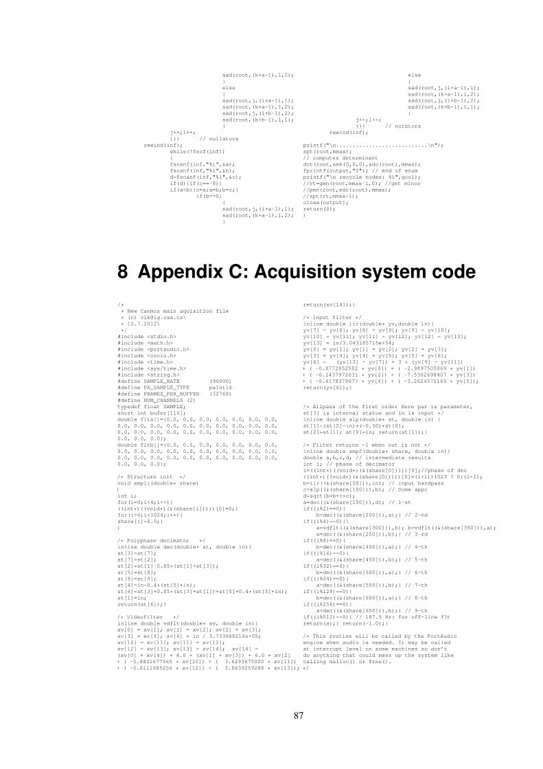
sad(root,(k+a-1),l,2);elsesad(root,j,(i+a-1),1);sad(root,(k+a-1),l,2);sad(root,j,(i+b-1),2);sad(root,(k+b-1),l,1);
j++;l++; // nullators
rewind(inf);while(!feof(inf))fscanf(inf,"%i",&a);fscanf(inf,"%i",&b);d=fscanf(inf,"%i",&c);if(d)if(c==-8)if(a<b)c=a;a=b;b=c;
if(b==0)sad(root,j,(i+a-1),1);sad(root,(k+a-1),l,2);
elsesad(root,j,(i+a-1),1);sad(root,(k+a-1),l,2);sad(root,j,(i+b-1),2);sad(root,(k+b-1),l,1);
j++;l++; // norators
rewind(inf);
printf("\n............................\n");spt(root,mmax);// computes determinantdct(root,smk(0,0,0),sdc(root),mmax);fprintf(output,"0"); // end of enumprintf("\n recycle nodes: %i",gcol);//rt=gmn(root,mmax-1,0); //get minor//pmn(root,sdc(root),mmax);//spt(rt,mmax-1);close(output);return(0);
8 Appendix C: Acquisition system code/** New Canmos main aquisition file
* (c) [email protected]\
* 15.7.2012\
*/#include <stdio.h>#include <math.h>#include <portaudio.h>#include <conio.h>#include <time.h>#include <sys/time.h>#include <string.h>#define SAMPLE_RATE (96000)#define PA_SAMPLE_TYPE paInt16#define FRAMES_PER_BUFFER (32768)#define NUM_CHANNELS (2)typedef float SAMPLE;short int bufer[110];double flta[]=0.0, 0.0, 0.0, 0.0, 0.0, 0.0, 0.0,0.0, 0.0, 0.0, 0.0, 0.0, 0.0, 0.0, 0.0, 0.0, 0.0,0.0, 0.0, 0.0, 0.0, 0.0, 0.0, 0.0, 0.0, 0.0, 0.0,0.0, 0.0, 0.0;double fltb[]=0.0, 0.0, 0.0, 0.0, 0.0, 0.0, 0.0,0.0, 0.0, 0.0, 0.0, 0.0, 0.0, 0.0, 0.0, 0.0, 0.0,0.0, 0.0, 0.0, 0.0, 0.0, 0.0, 0.0, 0.0, 0.0, 0.0,0.0, 0.0, 0.0;
/* Structure init */void smpli(double* share)int i;for(i=0;i<4;i++)((int*)((void*)(&(share[i]))))[0]=0;for(i=4;i<1024;i++)share[i]=0.0;
/* Polyphase decimator */inline double dec(double* st, double in)st[3]=st[7];st[7]=st[2];st[2]=st[1]-0.85*(st[1]+st[3]);st[5]=st[8];st[8]=st[4];st[4]=in-0.4*(st[5]+in);st[6]=st[3]+0.85*(st[3]+st[1])+st[5]+0.4*(st[5]+in);st[1]=in;return(st[6]);
/* Videofilter */inline double vdflt(double* xv, double in)xv[0] = xv[1]; xv[1] = xv[2]; xv[2] = xv[3];xv[3] = xv[4]; xv[4] = in / 3.733668216e+05;xv[10] = xv[11]; xv[11] = xv[12];xv[12] = xv[13]; xv[13] = xv[14]; xv[14] =(xv[0] + xv[4]) + 4.0 * (xv[1] + xv[3]) + 6.0 * xv[2]+ ( -0.8821677565 * xv[10]) + ( 3.6293675000 * xv[11])+ ( -5.6111685256 * xv[12]) + ( 3.8639259288 * xv[13]);
return(xv[14]);
/* input filter */inline double iir(double* yv,double in)yv[7] = yv[8]; yv[8] = yv[9]; yv[9] = yv[10];yv[10] = yv[11]; yv[11] = yv[12]; yv[12] = yv[13];yv[13] = in/3.043185715e+04;yv[0] = yv[1]; yv[1] = yv[2]; yv[2] = yv[3];yv[3] = yv[4]; yv[4] = yv[5]; yv[5] = yv[6];yv[6] = (yv[13] - yv[7]) + 3 * (yv[9] - yv[11])+ ( -0.8772852502 * yv[0]) + ( -2.9897505069 * yv[1])+ ( -6.1437972631 * yv[2]) + ( -7.5302698407 * yv[3])+ ( -6.4178379677 * yv[4]) + ( -3.2624571165 * yv[5]);return(yv[6]);
/* Allpass of the first order Here par is parameter,st[3] is internal status and in is input */inline double alp(double* st, double in) st[1]=(st[2]-in)*(-0.30)+st[0];st[2]=st[1]; st[0]=in; return(st[1]);
/* Filter returns -1 when out is not */inline double smpf(double* share, double in)double a,b,c,d; // intermediate resultsint i; // phase of decimatori=((int*)((void*)(&(share[0]))))[0];//phase of dec((int*)((void*)(&(share[0]))))[0]=(i+1)>1023 ? 0:(i+1);b=iir((&(share[50])),in); // input bandpassc=alp((&(share[100])),b); // Dome apprd=sqrt(b*b+c*c);a=dec((&(share[150])),d); // 1-stif((i%2)==0)
b=dec((&(share[200])),a); // 2-ndif((i%4)==0)\
a=vdflt((&(share[300])),b); b=vdflt((&(share[350])),a);a=dec((&(share[250])),b); // 3-rd
if((i%8)==0)b=dec((&(share[400])),a); // 4-th
if((i%16)==0)a=dec((&(share[450])),b); // 5-th
if((i%32)==0)b=dec((&(share[500])),a); // 6-th
if((i%64)==0)a=dec((&(share[550])),b); // 7-th
if((i%128)==0)b=dec((&(share[600])),a); // 8-th
if((i%256)==0)a=dec((&(share[650])),b); // 9-th
if((i%512)==0) // 187.5 Hz: for off-line fltreturn(a); return(-1.0);
/* This routine will be called by the PortAudioengine when audio is needed. It may be calledat interrupt level on some machines so don’tdo anything that could mess up the system likecalling malloc() or free().
*/
87
static int fuzzCallback(const void *inputBuffer, void *outputBuffer,
unsigned long framesPerBuffer,const PaStreamCallbackTimeInfo* timeInfo,PaStreamCallbackFlags statusFlags,void *userData )
(void*)outputBuffer;(void*) inputBuffer; /* Prevent unused variable warnings. */SAMPLE *in = (SAMPLE*)inputBuffer;(void) timeInfo; /* Prevent unused variable warnings. */(void) statusFlags;(void) userData;(((void**) (&(bufer[16])) ) )[0]=inputBuffer; // Databufer[10]=1; // semaphoreif(bufer[30]==1) \
struct timeval tv;gettimeofday(&tv, NULL);((float*)((void*)(&(bufer[40]))))[0]=
-1.0*((float)(tv.tv_sec % 3600 +(tv.tv_usec+1)/1000000.0));
bufer[30]=2;return paContinue;
/***********************************************/
int main(void)PaStreamParameters inputParameters, outputParameters;PaStream *stream;PaError err;SAMPLE* aa;int j, k, l, m;char ac=’ ’;time_t now, shifted, start;struct tm ts;struct tm tu;struct timeval tv;FILE* f1;FILE* f2;char fil1[200];char fil2[200];char filebuf[200];char* filebuff;char vocasout[]="C:\\\\data\\\\";int nex; //next inspection in 100 msecint i;double fa[1024];double fb[1024];double corr = 0.5;short int cp[70000];float ff[1800];float fta,ftb;double a,b,c;err = Pa_Initialize();if( err != paNoError ) goto error;inputParameters.device = Pa_GetDefaultInputDevice();if (inputParameters.device == paNoDevice)
fprintf(stderr,"Error: No default input device.\\n");goto error;
inputParameters.channelCount = 2; /* stereo input */inputParameters.sampleFormat = PA_SAMPLE_TYPE;inputParameters.suggestedLatency = Pa_GetDeviceInfo(inputParameters.device )->defaultHighInputLatency;inputParameters.hostApiSpecificStreamInfo = NULL;err = Pa_OpenStream(&stream,&inputParameters,NULL,
SAMPLE_RATE,FRAMES_PER_BUFFER, 0, /* paClipOff, */,fuzzCallback,NULL ); if( err != paNoError ) goto error;time(&now); ts=*gmtime(&now); strcpy(filebuf,vocasout);filebuff=&(filebuf[strlen(filebuf)]);strftime(filebuff,sizeof(filebuf),"%Y%m\\\\%Y%m%d%H.dat",&ts);f1=fopen(filebuf,"ab"); gettimeofday(&tv, NULL);ftb=-1.0*((float)(tv.tv_sec%3600 +(tv.tv_usec+1)/1000000.0));printf("_time: %f corr: %f\\n",ftb, ((float)corr));fta=ftb; nex=(int)(-1000.0*corr*(ftb));bufer[10]=0; bufer[5]=0; // Semaphoresmpli(fa); smpli(fb); // Decimators initbufer[30]=0;err = Pa_StartStream( stream );if( err != paNoError ) goto error;printf("Hit ‘a‘ to stop program.\\n");fflush(stdout);for(;ac!=’a’;)
if(bufer[10]==1)memcpy(((void*)cp),
( (((void**) (&(bufer[16])) ) )[0]),(4*32768));bufer[10]=0;for(i=0, j=0;i<32768;i++)a=smpf(fa,((double)(cp[2*i]+cp[2*i+1])));if(a>0.0)\ff[j]=a;j++;
bufer[5]=1;if(bufer[30]==2)bufer[30]=3;else if(bufer[5]==1)bufer[5]=0; printf("%f %f %i\\n",ff[0],corr,nex);fwrite((void*)ff,sizeof(float),(j),f1); //2*32768/512else if(bufer[30]==3)bufer[30]=0; fta = ftb;ftb = (((float*)((void*)(&(bufer[40]))))[0]);if(ftb<-1800.0) ftb+=3600.0;corr *= (3600.0+fta)/(3600.0+(fta-ftb)); // real/mach timenex=(int)(-1000.0*corr*(ftb)); // phase +1/2h in floatprintf("_time: %f corr: %f\\n",ftb,((float)corr));fwrite( (((void*)(&(bufer[40])))) ,sizeof(float),1,f1);fclose(f1); time(&now); ts=*gmtime(&now);now+=1800; tu=*gmtime(&now); strcpy(filebuf,vocasout);filebuff=&(filebuf[strlen(filebuf)]);strftime(filebuff,sizeof(filebuf),
"%Y%m\\\\%Y%m%d%H.dat",&tu);f1=fopen(filebuf,"ab");elsePa_Sleep(50); nex+=50;if(((float)nex)>(3600.0*1000.0*corr))
nex=0; bufer[30]=1;if(kbhit())ac=getche();
fclose(f1); err = Pa_CloseStream( stream );if( err != paNoError ) goto error;printf("Finished." );Pa_Terminate();return(0);error: Pa_Terminate();fprintf( stderr, "An error occured whileusing the portaudio stream\\n" );fprintf( stderr, "Error number: %d\\n", err );fprintf( stderr, "Error message: %s\\n",Pa_GetErrorText( err ) );return(-1);
9 Code D: Postprocessing system code/* ********************************** Extract files from list of
* hourly files & computes second IAGA files
* from AMOS channell datas
* Must be computed after 01 clock next day
* 29.10.2012
* (c) [email protected], rev. 2.0 20.1.2013
********************************** */#include <stdio.h>#include <math.h>#include <string.h>#include <time.h>
//decimatorinline double dec(double* st, double in)st[3]=st[7];st[7]=st[2];
st[2]=st[1]-0.85*(st[1]+st[3]);st[5]=st[8];st[8]=st[4];st[4]=in-0.4*(st[5]+in);st[6]=st[3]+0.85*(st[3]+st[1])+st[5]+0.4*(st[5]+in);st[1]=in;return(st[6]);
// init of decimator structurevoid smpli(double* share)int i;for(i=0;i<4;i++)((int*)((void*)(&(share[i]))))[0]=0;for(i=4;i<1024;i++)share[i]=0.0;
inline double smpl(double* share, double in)
88
9 Code D: Postprocessing system code
double a,b,c,d; // intermediate resultsint i; // phase of decimatori=((int*)((void*)(&(share[0]))))[0];((int*)((void*)(&(share[0]))))[0]=((i+1)>1023)?0:(i+1);a=dec((&(share[50])),in); // 10-thif((i%2)==0)b=dec((&(share[100])),a); // 11-thif((i%4)==0)a=dec((&(share[150])),b); // 12-thif((i%8)==0)b=dec((&(share[200])),a); // 13-thif((i%16)==0)return(b);return(-1.0);
//five second to minute intermagnet filterdouble fivesecflt[]= 0.12578865, 0.11972085,0.10321785, 0.08061140, 0.05702885, 0.03654680,0.02121585, 0.01115655, 0.00531440, 0.00229315;
// one value of filter - len is half-lengthinline double knev(double* infeld,double* coefs,int len) int i,j,k,l;double a[len];
a[0]=infeld[0]*coefs[0]; for(i=1,j=-1;i<len;i++,j--)
a[i]=(infeld[j]+infeld[i])*coefs[i];for(i=1;i<len;i<<=1) for(j=0;j<(len-i);j+=i<<1)
a[j]+=a[j+i]; return(a[0]);
// Plesiochronous interpolationdouble interp(double* a, double where)int i,j,k,l,m;double bb=0.907; // filter roll-ofint wh;double instp;double whd;int N = 128; // Length of filterdouble c[128];wh = (int)where; // integer partwhd = where - (double)wh; // fractional partwh -=N/2; // start of the filterinstp = whd;for(i=0;i<N;i++)
if((i+instp)!=((double)(N/2)))c[i]=a[wh+i]*(0.42-0.5*cos(2.0*PI*(i+instp)/N)+0.08*
cos(4.0*PI*(i+instp)/N))*sin(PI*bb*(i-N/2+instp))/(PI*(i-N/2+instp)); else
c[i]=a[wh+i]*(0.42-0.5*cos(2.0*PI*(i+instp)/N)+0.08*cos(4.0*PI*(i+instp)/N))*bb; //next - RDX2sumfor(l=1;l<N;l<<=1) for(m=0;m<(N-l);m+=l<<1) c[m]+=c[m+l];return(c[0]);
// Header of YAGA2002void baba(FILE* outf)fprintf(outf,"%s\n"," Format IAGA-2002
|\0");fprintf(outf,"%s\n"," Source of Data NAROD core CZE00001,proprietar electronics |\0");fprintf(outf,"%s\n"," Station Name Budkov
|\0");fprintf(outf,"%s\n"," Geodetic Latitude 49.072
|\0");fprintf(outf,"%s\n"," Geodetic Longitude 14.019
|\0");fprintf(outf,"%s\n"," Elevation 496
|\0");fprintf(outf,"%s\n"," Reported
|\0");fprintf(outf,"%s\n"," Sensor orientation DIF
|\0");fprintf(outf,"%s\n"," Digital Sampling 1 Hz
|\0");fprintf(outf,"%s\n"," Data Interval Type 1-second
|\0");fprintf(outf,"%s\n"," Data type variation
|\0");fprintf(outf,"%s\n","DATE TIME DOY BDVF BDVT BDVE BDVI |\0");
inline double hp() return(20396.957);
// Parametrised Gaussian filtervoid gsn(int n, double a, double* fl)int i;double b,c,e,f;e=((double)n);f=3.141592653/((double)n);
for(i=0;i<n;i++)c=(double)i;
fl[i]=exp(((c*c)/(-2*a)))*(1.0-(0.35875-0.48829*cos(f*(e+c))+0.14128*cos(2.0*f*(e+c))-0.01168*cos(3.0*f*(e+c))));
// RMS Line fit computationrms(int i,double* x,double* y,double* a, double* b)double xm,ym,sx,sxy;double pom[i];int j,k,l,m;for(j=0;j<i;j++) pom[j]=x[j]/((double)i); // preprocessingfor(l=1;l<i;l<<=1) for(m=0;m<(i-l);m+=l<<1) pom[m]+=pom[m+l];xm=pom[0]; // mean of xfor(j=0;j<i;j++) pom[j]=y[j]/((double)i); // preprocessingfor(l=1;l<i;l<<=1) for(m=0;m<(i-l);m+=l<<1)pom[m]+=pom[m+l]; ym=pom[0]; // mean of yfor(j=0;j<i;j++) pom[j]=(x[j]-xm)*(x[j]-xm);for(l=1;l<i;l<<=1) for(m=0;m<(i-l);m+=l<<1)pom[m]+=pom[m+l]; sx=pom[0];for(j=0;j<i;j++) pom[j]=(x[j]-xm)*(y[j]-ym);for(l=1;l<i;l<<=1) for(m=0;m<(i-l);m+=l<<1)pom[m]+=pom[m+l]; sxy=pom[0];
*b=sxy/sx;
*a=ym-(sxy/sx)*xm;
int main(int argc, char** argv)//double res1[(60*60*10)]; // second output datas//double res2[(60*60*10)];double *res1;double *res2;double *res3;double *res4;double *res5;
int i,j,k,l,m,n,o,p;
float g[4];float h[2];double a,b,c,d,e,f; // buffer variablesFILE *in; // output variablesFILE *outf;double fa[1024]; // filter termporaliesdouble fb[1024];double fc[1024];double fd[1024];
double gs[1024]; // Gaussian filter approx.
double amid[27];int acnt[27];double bmid[27];int bcnt[27];double rx[27];double ry[27];double rc[4]; // regression coefficients a1,b1,a2,b2time_t tme, start, now;struct tm ts;// infile name parts.
char *inf[]=" "," "," " ;\char anf[2000];char actfn[800];char actfm[800];char actfo[800];char dock[20];char *vock;
char vocasin[]="\0";char vocasout[]="\0";char filout[800];char filerow[500];char datestamp[200];char year[200];
a = atoi(argv[1]);//return(0);anf[1900]=’\0’;time(&now);now+=60*60*24*(a-1);now/=(60*60*24);now*=(60*60*24);start = now;//return(0);
for(i=0;i<3;i++,start+=60*60*24)
89

9 Code D: Postprocessing system code
ts=*gmtime(&start);strftime(&(anf[200*i]),50,"%Y%m/%Y%m%d\0",&ts);
start = now;start+=60*60*24;ts=*gmtime(&start);strftime(&(anf[600]),50,"%Y/%Y%m%d\0",&ts);sprintf(filout,"%s%s.txt",vocasin,&(anf[600]));
smpli(fa);smpli(fb);smpli(fc);smpli(fd);
res1=malloc((60*60*28*40)*sizeof(double));res2=malloc((60*60*28*40)*sizeof(double));res3=malloc((60*60*28*40)*sizeof(double));res4=malloc((60*60*28*40)*sizeof(double));res5=malloc((60*60*28*40)*sizeof(double));
// day, file, sampleA, sampleBfor(i=0,l=0,o=0,p=0;i<3;i++)
if(i==0)
j=23;k=24;vock=&(anf[0]);
if(i==1)j=0;k=24;vock=&(anf[200]);
if(i==2)j=0;k=1;vock=&(anf[400]);
for(;j<k;j++,l++)m=sizeof(vocasin);dock[0]=48+j/10;dock[1]=48+j%10;dock[2]=’\0’;sprintf(actfn,"%sd/%s%s.dat",vocasin,vock,dock);sprintf(actfm,"%sf/%s%s.dat",vocasin,vock,dock);printf("%s %i\n",actfn,l);if((in=fopen(actfn,"rb"))==NULL) return(-1);n=0;for(m=0;m<4;m++) ((char*)((void*)g))[m]=getc(in);for(;g[0]>=0.0;n++)for(m=0;m<4;m++) ((char*)((void*)h))[m]=getc(in);a=(double)(g[0]); b=(double)(h[0]);c=smpl(fa,a);d=smpl(fb,b);if(c>0.0)res1[o]=c; res2[o]=d;o++;for(m=0;m<4;m++) ((char*)((void*)g))[m]=getc(in);
amid[l]=(double)(g[0]);acnt[l]=n;fclose(in);if((in=fopen(actfm,"rb"))==NULL) return(1);n=0;for(m=0;m<4;m++) ((char*)((void*)g))[m]=getc(in);for(;g[0]>0.0;n++)
for(m=0;m<4;m++) ((char*)((void*)h))[m]=getc(in);a=(double)(g[0]); b=(double)(h[0]);c=smpl(fc,a);d=smpl(fd,b);if(c>0.0) res3[p]=c; res4[p]=d;p++;
for(m=0;m<4;m++) ((char*)((void*)g))[m]=getc(in);
bmid[l]=(double)(g[0]); bcnt[l]=n;fclose(in); // end of one day
// end of three days// *****************PROCESSING*********************for(l=0;l<26;l++) ry[l]=(l>0)?(ry[l-1]+(double)acnt[l]):((double)acnt[l]);for(l=0;l<26;l++) rx[l]=(3600.0*((double)l))+
((amid[l]<-1500.0)?(-(amid[l]+3600.0)):(-amid[l]));rms(26,rx,ry,(&(rc[0])),(&(rc[1]))); // regresion of d,efor(l=0;l<26;l++) ry[l]=(l>0)?(ry[l-1]+(double)bcnt[l]):((double)bcnt[l]);for(l=0;l<26;l++) rx[l]=(3600.0*((double)l))+((bmid[l]<-1500.0)?(-(bmid[l]+3600.0)):(-bmid[l]));for(l=0;l<26;l++) printf("%f ",((float)rx[l]));for(l=0;l<26;l++) printf("%f ",((float)ry[l]));rms(26,rx,ry,(&(rc[2])),(&(rc[3]))); // regression of fa=rc[1]/16.0/12.0; // step of d,ib=rc[0]/16.0; // position of zero time in irr. smpl)printf("%f %f\n",((float)a),((float)b));for(i=0,b-=20*a;i<(12*60*60*25);i++,b+=a) res5[i]=interp(res1,b);for(i=0,j=20;i<(60*60*24);i++,j+=12) res1[i]=0.000004*knev(&(res5[j]),fivesecflt,10);b=rc[0]/16.0;for(i=0,b-=1300*a;i<(12*60*60*25);i++,b+=a) res5[i]=interp(res2,b);for(i=0,j=20;i<(60*60*25);i++,j+=12) res2[i]=0.000004*knev(&(res5[j]),fivesecflt,10); // Temperature filteringgsn(1200,10000.0,gs); for(i=0,j=1201;i<(60*60*25);i++,j++)res5[i]=knev(&(res2[j]),gs,1200);for(i=0,j=1300-1201-20;i<(60*60*25);i++,j++) res2[i]=0.1*res5[j];a=rc[3]/16.0/12.0; // step of fb=rc[2]/16.0; // position of fprintf("%f %f\n",((float)a),((float)b));for(i=0,b-=20*a;i<(12*60*60*25);i++,b+=a) res5[i]=interp(res3,b);for(i=0,j=20;i<(60*60*24);i++,j+=12) res3[i]=0.000004*knev(&(res5[j]),fivesecflt,10); b=rc[2]/16.0;for(i=0,b-=20*a;i<(12*60*60*25);i++,b+=a) res5[i]=interp(res4,b);for(i=0,j=20;i<(60*60*24);i++,j+=12) res4[i]=0.000004*knev(&(res5[j]),fivesecflt,10);// *********** OUTPUT ROUTINE***********************//strftime(datestamp,sizeof(datestamp),"%Y-%m-%d",&ts);strftime(year,sizeof(year),"%j",&ts);outf=fopen(filout,"wt");baba(outf);for(j=0;j<60*60*24;j++)
// clockdatestamp[10]=’ ’;datestamp[11]=48+((j/60)/60)/10;datestamp[12]=48+((j/60)/60)%10;datestamp[13]=’:’;datestamp[14]=48+((j/60)%60)/10;datestamp[15]=48+((j/60)%60)%10;datestamp[16]=’:’;datestamp[17]=48+(j%60)/10;datestamp[18]=48+(j%60)%10;datestamp[19]=’.’;datestamp[20]=’0’;datestamp[21]=’0’;datestamp[22]=’0’;datestamp[23]=’ ’;sprintf(&(datestamp[24]),"%s",year);// Blank fillfor(k=27;k<70;k++) datestamp[k]=’ ’;datestamp[k+1]=’\0’;// processingfor(k=0;k<4;k++)
sprintf(filerow,"%5.3f\0",((k==0)?((float)res1[j]):((k==1)?((float)res2[j]):((k==2)?((float)res3[j]):((float)res4[j])))));i=(k==0)?30:((k==1)?40:((k==2)?50:60));sprintf(&(datestamp[i]),"%s",filerow);
datestamp[(i+strlen(filerow))]=’ ’;datestamp[70]=’\0’;fprintf(outf,"%s\n",datestamp);fclose(outf);return(0);
90