disintegration of single orifice and coaxial supercritical jets

DISINTEGRATION OF SINGLE ORIFICE AND COAXIAL SUPERCRITICAL JETS

By

SHAUN DESOUZA

A DISSERTATION PRESENTED TO THE GRADUATE SCHOOL OF THE UNIVERSITY OF FLORIDA IN PARTIAL FULFILLMENT

OF THE REQUIREMENTS FOR THE DEGREE OF DOCTOR OF PHILOSOPHY

UNIVERSITY OF FLORIDA

2016

To my wife, Danielle

4

ACKNOWLEDGMENTS

I would like to thank my advisor, Professor Corin Segal, for this work would not

have been possible without his guidance and expertise. I would also like to thank my

friends and colleagues in the Mechanical and Aerospace Engineering Department for

their technical advice towards my work but also for the great conversations about issues

of the day. I’d like to thank my friend, Matthew Carver, for always inspiring me to push

myself towards higher academic achievement. I would like to thank my family for their

continued love and support throughout my academic career. Finally, I would like to

thank my wife, Danielle, who has been my greatest support during the most difficult

times of my studies. You have brought the joy to the long nights and stressful days.

5

TABLE OF CONTENTS page

ACKNOWLEDGMENTS .................................................................................................. 4

LIST OF TABLES ............................................................................................................ 7

LIST OF FIGURES .......................................................................................................... 8

NOMENCLATURE ........................................................................................................ 12

ABSTRACT ................................................................................................................... 14

CHAPTER

1 INTRODUCTION .................................................................................................... 16

1.1 Theoretical Background .................................................................................... 16

1.2 Jet Breakup Theory........................................................................................... 16 1.3 Single Nozzle Subcritical Jet Experiments ........................................................ 22 1.4 Single Nozzle Supercritical Jet Experiments ..................................................... 25

1.4.1 Qualitative Studies of the Jet Surface ...................................................... 26 1.4.2 Spreading Angle Investigations ............................................................... 27

1.4.3 Core Length Measurements .................................................................... 30 1.4.4 Mapping of Jet Thermodynamic Profiles ................................................. 32

1.5 Coaxial Nozzle Subcritical Jet Experiments ...................................................... 33 1.5.1 Qualitative Behavior ................................................................................ 33 1.5.2 Core Length Investigations ...................................................................... 35

1.6 Coaxial Nozzle Supercritical Jet Experiments ................................................... 38 1.6.1 Qualitative Studies of the Jet Surface ...................................................... 39

1.6.2 Core Length Measurements .................................................................... 40 1.6.3 Jet Spreading Angle Investigations ......................................................... 41 1.6.4 Mapping of Jet Thermodynamic Profiles ................................................. 42

2 EXPERIMENTAL SETUP ....................................................................................... 60

2.1 High Pressure Chamber ................................................................................... 60

2.2 Injector Configuration ........................................................................................ 61 2.2.1 Single Injector .......................................................................................... 61

2.2.2 Coaxial Injector ........................................................................................ 62 2.3 Instrumentation, Experimental Control and Data Acquisition ............................ 62

2.3.1 Instrumentation ........................................................................................ 62 2.3.2 Experimental Control and Data Acquisition ............................................. 63

2.4 Working Fluid Photophysics and PLIF implementation ..................................... 64

2.5 Shadowgraphy Implementation ........................................................................ 67

3 SINGLE ORIFICE INJECTION ............................................................................... 75

6

3.1 Experimental Conditions ................................................................................... 75

3.2 Jet Morphology and Flow Visualization Analysis .............................................. 75 3.3 Jet Spreading Angle Analysis ........................................................................... 76

3.4 Droplet Size and Distribution Analysis .............................................................. 78 3.5 Conclusions ...................................................................................................... 79

4 COAXIAL INJECTION ............................................................................................ 85

4.1 Experimental Conditions ................................................................................... 85 4.2 Jet Morphology and Density Map Analysis ....................................................... 85

4.3 Core Length Analysis ........................................................................................ 87 4.4 Inner Jet Spreading Angle Analysis .................................................................. 88 4.5 Conclusions ...................................................................................................... 90

5 RECOMMENDED STUDIES .................................................................................. 99

APPENDIX

A FLUORESCENCE THEORY AND CALIBRATION ............................................... 100

A.1 Gas Phase Calibration .................................................................................... 103 A.2 Liquid Phase Calibration ................................................................................. 105

A.3 Conclusions .................................................................................................... 107

B SHADOWGRAPH EXPERIMENTAL CONDITIONS ............................................. 116

C MATLAB SCRIPTS FOR DATA PROCESSING ................................................... 118

D LABVIEW CODE FOR EXPERIMENTAL CONTROL ........................................... 172

LIST OF REFERENCES ............................................................................................. 180

BIOGRAPHICAL SKETCH .......................................................................................... 187

7

LIST OF TABLES

Table page B-1 Table of experimental conditions for all cases represented in spreading angle

data in Figure 3-5. ............................................................................................ 116

8

LIST OF FIGURES

Figure page 1-1 Criteria of cylindrical liquid jet disintegration regimes ......................................... 44

1-2 Cylindrical jet behavior ....................................................................................... 44

1-3 Classification of disintegration modes at fixed thermodynamic conditions. ........ 45

1-4 Three distinct regimes of a turbulent submerged jet ........................................... 45

1-5 Subcritical jet injected into a subcritical environment .......................................... 46

1-6 Influence of gas composition on jet behavior ...................................................... 46

1-7 Influence of gas temperature on jet behavior. .................................................... 47

1-8 Influence of chamber pressure at a supercritical temperature. ........................... 47

1-9 Back-illuminated images of a single nitrogen jet injected into nitrogen ............... 48

1-10 Software magnified images of the jets in Figure 1-9 ........................................... 48

1-11 Spreading or growth rate of single jets ............................................................... 49

1-12 Jet spreading angle plotted as a function of chamber-to-injectant density ratio. ................................................................................................................... 49

1-13 Theoretical dependence of the spray angle of surface, viscous and aerodynamic forces. ........................................................................................... 50

1-14 Ratio of the dark-core, intact-core, or potential-core length, depending on the case, divided by the density ratio for single jets.................................................. 50

1-15 Core lengths plotted as a function of chamber-to-injectant density ratio ............ 51

1-16 Figure of experimental conditions performed by Roy et al. ................................. 51

1-17 Scaled images of a supercritical jet injected into subcritical chamber conditions ........................................................................................................... 52

1-18 Scaled images of a supercritical jet injected into supercritical chamber conditions ........................................................................................................... 52

1-19 Simultaneous fluorescence, phosphorescence, and superimpose image of both of a liquid acetone jet .................................................................................. 53

1-20 Breakup modes of coaxial jets ............................................................................ 53

9

1-21 Air-assisted cylindrical jet atomization regimes .................................................. 54

1-22 Breakup regimes in the parameter space Rel – We for coaxial jets .................... 54

1-23 Correlations for the characteristic length of air-assisted liquid jets ..................... 55

1-24 Images of a coaxial jet at approximately the same inner-jet mass flow rates ..... 56

1-25 Figure shows comparison of the present coaxial- jet dark-core length measurements with all other relevant core length data available ....................... 57

1-26 Spreading rate of the shear layer versus the chamber/injectant or chamber/inner-jet density ratio for single and coaxial jets .................................. 57

1-27 Maximum baseline spread angles as a function of momentum flux ratio ............ 58

1-28 Hydrogen density for a coaxial LN2/H2 injection ................................................ 58

1-29 Radial N2 density profile for single jet. ............................................................... 59

2-1 Schematic of Liquid/Fuel supply system ............................................................. 69

2-2 Section view of the high pressure chamber. ....................................................... 70

2-3 Injector tip with honeycomb structure. ................................................................ 70

2-4 Chamber top assembly depicting the coaxial injector, chamber top thermocouple, and plugged NPT passageways. ................................................ 71

2-5 Coaxial injector schematic with dimensions ....................................................... 71

2-6 Schematic of the data acquisition system. .......................................................... 72

2-7 Schematic of optical and test bench setup ......................................................... 72

2-8 Variation of the number of excited electrons with the number of exciting photons. .............................................................................................................. 73

2-9 The result of correcting for the non-linear fluorescence signal. .......................... 73

2-10 Optical bench Shadowgraphy setup. .................................................................. 74

3-1 Experimental conditions for selected binary single orifice jet disintegration experiments ........................................................................................................ 81

3-2 Shadowgraph images of case 1 from Figure 3-1 ................................................ 81

3-3 Shadowgraph image and PLIF density map of case 2 from Figure 3-1 .............. 82

10

3-4 Shadowgraph images for case 3 reported in Figure 3-1 ..................................... 82

3-5 Plot of jet spreading angle versus chamber to injectant density ratio for fluoroketone/nitrogen single orifice jets .............................................................. 83

3-6 Plot of number of particles versus geometric mean of reduced injection and chamber temperature ......................................................................................... 83

3-7 Plot of normalized drop diameter versus the geometric mean of injection and chamber temperature ......................................................................................... 84

4-1 Experimental conditions for binary coaxial jet disintegration experiments .......... 91

4-2 Density and density gradient maps of cases 1 and 2 from Figure 4-1. ............... 92

4-3 Density and density gradient map of cases 3 and 4 from Figure 4-1 .................. 93



4-6 Plot of normalized core length as a function of momentum flux ratio of the outer-to-inner jet ................................................................................................. 96

4-7 Theoretical core length correlations .................................................................... 97

4-8 Plot of inner jet spreading angle versus momentum flux ratio for fluoroketone/nitrogen coaxial jets ....................................................................... 98

A-1 Plot of excited molecules versus the number of exciting photons..................... 108

A-2 Plots of fluorescence intensity variation of the laser sheet profile as it passes through the chamber ........................................................................................ 109

A-3 Plot of fluorescence signal intensity versus vapor density. ............................... 110

A-4 Fluorescence intensity as a function of laser power ......................................... 110

A-5 Plots of vertical and horizontal laser sheet intensity variation.. ......................... 111

A-6 Plot of normalized fluorescence intensity versus the length traversed by the laser in pixels.. .................................................................................................. 112

A-7 Calibration line for the absorption coefficient as a function of the fluoroketone vapor density. A linear dependence is noted from the plot. .............................. 112

A-8 Plot of normalized fluorescence intensity versus length traversed by the laser in pixels at 1.25 atm and 17oC. ......................................................................... 113

11

A-9 Plot of normalized fluorescence intensity versus length traversed by the laser in pixels at 12.7 atm and 145oC. ....................................................................... 113

A-10 Plot of normalized fluorescence intensity versus length traversed by the laser in pixels at various liquid densities. ................................................................... 114

A-11 Plots comparing the coefficients obtained from the gas curve fit and liquid sum of exponents fits. ....................................................................................... 115

D-1 LabVIEW wiring diagrams for the control of the gas valves and the temperature and pressure monitoring charts. ................................................... 173

D-2 LabVIEW wiring diagram for the gas flow data, shutdown of valves at the end of experiment, and control of the gas heater. ................................................... 174

D-3 LabVIEW wiring diagram for the control of the liquid and chamber heaters. .... 175

D-4 LabVIEW wiring diagrams for the closure of valves at the end of an experiment. ....................................................................................................... 176

D-5 LabVIEW wiring diagram for the closure of valves and bypass solenoid valve control. .............................................................................................................. 177

D-6 LabVIEW wiring diagram for the processing and saving of data....................... 178

D-7 LabVIEW wiring diagram for closing all valves in event of experiment termination. ....................................................................................................... 179

12

NOMENCLATURE

Latin Symbols A Nozzle geometric factor

L core length, [mm]

M 𝜌𝑔𝑢𝑔2

𝜌𝑙𝑢𝑙2 , Momentum flux ratio

P Pressure [atm]

Pr Reduced Pressure

T Temperature [K]

Tr Reduced Temperature

ug gas velocity at origin, [m/s]

ul liquid velocity at origin, [m/s]

VR 𝑢𝑔

𝑢𝑙, Velocity Ratio

Y 𝜌𝑙

𝜌𝑐ℎ(

𝑅𝑒𝑙

𝑊𝑒𝑙)2, Non-dimensional Taylor parameter for the jet growth rate

Greek Symbols ν kinematic viscosity (m2/s)

ρ Density (kg/m3)

σ surface tension (N/m)

Dimensionless Numbers Re 𝑢𝑙𝐷𝑙

𝜈, Reynolds number

We 𝜌𝑔𝑢𝑔𝐷𝑙

𝜎, Weber number

Subscripts

ch chamber gas properties

FK fluoroketone properties

g gas properties, annulus flow for coaxial injection

13

l liquid properties, central flow for coaxial injection

N2 nitrogen properties

r reduced properties

14

Abstract of Dissertation Presented to the Graduate School of the University of Florida in Partial Fulfillment of the Requirements for the Degree of Doctor of Philosophy

DISINTEGRATION OF SINGLE ORIFICE AND COAXIAL SUPERCRITICAL JETS

By

Shaun DeSouza

December 2016

Chair: Corin Segal Major: Aerospace Engineering

Two separate experimental studies were undertaken to characterize the behavior

of single orifice and coaxial supercritical jets injected into environments varying from

sub-to supercritical conditions. It was determined that the chamber-to-injectant density

ratio had a dominant effect on the visual breakdown of the jet as well as the mixing

behavior. The outer-to-inner momentum flux ratio was found to be the dominant factor in

the case of coaxial injection.

The study of single orifice jets covered a broad range of density ratios. The data

was compared to previous single orifice injection studies performed in the same facility

under similar conditions. The jet disintegration process was observed from

shadowgraph images and the jet lateral spreading angle was measured. An agreement

was found between the shadowgraph data and previous shadowgraph studies and the

differed from the PLIF quantitative results. The results show a square root dependence

of the jet spreading angle with respect to the density ratio. The study further evaluated

the effect of thermodynamic conditions on droplet production and quantified droplet size

and distribution. The results indicate an increase in normalized drop diameter and a

15

decrease in droplet population with increasing chamber temperatures. Droplet size and

distribution were found to be independent of chamber pressure.

Density distribution was quantified for coaxial jets injected in an inert gaseous

atmosphere under a range of subcritical and supercritical conditions. Density gradient

profiles were inferred from the experimental data. A novel method was applied for the

detection of detailed structures throughout the entire jet center plane. Core lengths were

measured for each of the cases and correlated with previous visualization results. An

eigenvalue approach was taken to determine the location of maximum gradient, hence,

systematically determining the core length. The results show a significant influence of

the outer-to-inner momentum flux ratio on the core length. Furthermore, the inner jet

spreading angle was calculated by detecting the jet boundary and applying a linear fit

through the contour. The jet spreading angle was found to increase to a maximum and

then decay with increasing momentum flux ratio.

16

CHAPTER 1 INTRODUCTION

1.1 Theoretical Background

Practical application when fluids in a supercritical state are injected in an

environment of various thermodynamic conditions and chemical composition are

numerous, ranging from propulsion applications to manufacturing industry and drug

delivery. There is a need to expand the current understanding of species transport in

shear layers under supercritical conditions as well as the bulk mass transfer at a

macroscopic scale when fluids of supercritical and/or subcritical state participate in the

mixing process. For this purpose, in this work coaxial jets are injected in a quiescent

atmosphere and their disintegration and mixing are observed.

In what follows, a background of current state of knowledge is presented;

beginning with single jets of subcritical and supercritical states followed by coaxial jets

studied both experimentally and theoretically. The experimental method used here

provides information of quantitative data previously not available, and thus, it

complements results obtained elsewhere.

1.2 Jet Breakup Theory

The early theoretical work by Plateau [1] and Rayleigh [2] laid the foundation for

the understanding of the jet breakup process. Plateau suggested that the surface

energy of a cylindrical column of fluid was not minimized for its given volume and hence

it must breakup into droplets. Rayleigh approached the problem by neglecting gravity,

viscosity of the jet, and the effects of the ambient fluid to conclude that disturbances

greater than the circumference of the jet are the cause of instability. Once the

wavelength of the surface disturbance has grown to the radius of the jet, a pinch point

17

appears and droplet formation occurs. His conclusion was that hydrodynamic instability

was the cause of jet breakup. Further work was conducted to expand upon these

theories by accounting for effects that were once neglected. Viscosity and density

effects were evaluated by Chandrasekhar [3]; it was found that droplet size was

increased and breakup rate was reduced by viscosity.

The effect of the ambient fluid on the jet breakup process was first considered by

Weber [4] and tested experimentally by Sterling & Sleicher [5]. Weber concluded that

ambient environment assisted in the growth of disturbances on the surface of the fluid

column. The presence of the ambient fluid provided a resistance to the jet and the result

is the growth and amplification of disturbances on the surface of the fluid column. The

experimental results of Sterling & Sleicher did not confirm Weber’s theory but a modified

semi-empirical relationship was proposed and reported in Figure 1-1. Taylor further

developed the hydrodynamic instability theory by accounting for the density effects of

the ambient fluid. It was suggested that droplets much smaller than jet diameter were

able to form at the liquid-gas interface if the force of the gas inertia was sufficiently high

[6]. This mode of breakup is known as atomization.

The works of Rayleigh, Weber, and Taylor have contributed to the theoretical

understanding and prediction of the jet breakup phenomenon. The breakup of a round

liquid jet is further influenced by internal nozzle effects, surface tension, inertia,

aerodynamic forces, and the thermodynamic state of the liquid and gas. The

development of the linear stability theory has allowed researchers to deduce the

qualitative behavior of the breakup phenomena and predict the existence of the five

currently accepted jet breakup regimes, illustrated in Figure 1-2, as follows:

18

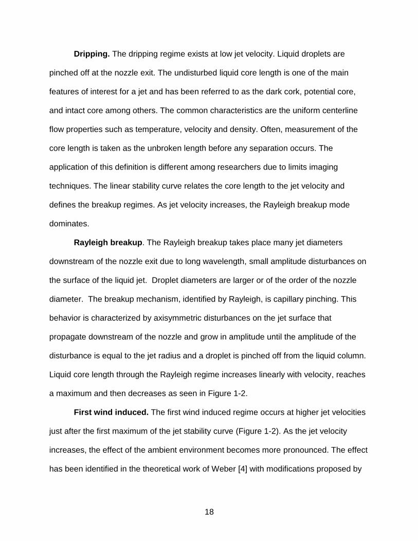
Dripping. The dripping regime exists at low jet velocity. Liquid droplets are

pinched off at the nozzle exit. The undisturbed liquid core length is one of the main

features of interest for a jet and has been referred to as the dark cork, potential core,

and intact core among others. The common characteristics are the uniform centerline

flow properties such as temperature, velocity and density. Often, measurement of the

core length is taken as the unbroken length before any separation occurs. The

application of this definition is different among researchers due to limits imaging

techniques. The linear stability curve relates the core length to the jet velocity and

defines the breakup regimes. As jet velocity increases, the Rayleigh breakup mode

dominates.

Rayleigh breakup. The Rayleigh breakup takes place many jet diameters

downstream of the nozzle exit due to long wavelength, small amplitude disturbances on

the surface of the liquid jet. Droplet diameters are larger or of the order of the nozzle

diameter. The breakup mechanism, identified by Rayleigh, is capillary pinching. This

behavior is characterized by axisymmetric disturbances on the jet surface that

propagate downstream of the nozzle and grow in amplitude until the amplitude of the

disturbance is equal to the jet radius and a droplet is pinched off from the liquid column.

Liquid core length through the Rayleigh regime increases linearly with velocity, reaches

a maximum and then decreases as seen in Figure 1-2.

First wind induced. The first wind induced regime occurs at higher jet velocities

just after the first maximum of the jet stability curve (Figure 1-2). As the jet velocity

increases, the effect of the ambient environment becomes more pronounced. The effect

has been identified in the theoretical work of Weber [4] with modifications proposed by

19

various researchers based on experimental results. The mechanism is similar to the

Rayleigh regime but droplet production is now on the order of the jet diameter. The

difference lies in the relative effect of the ambient environment with the first wind

induced regime characterized by the magnitude of the inertia force being a significant

percent of the surface tension force.

Second wind induced. Continuing to increase the jet velocity results in a

transition to the second wind induced breakup regime where capillary pinching is no

longer the main breakup mechanism. Short wavelength disturbances grow on the jet

surface causing the instability and resulting jet breakup a short distance downstream of

the nozzle after an initially smooth profile. At this point along the jet stability curve, the

breakup length is not well defined as theories by researchers are often contradictory as

will be reported in Section 3.

Atomization. Finally, with sufficiently high jet velocity, the jet begins to atomize

at the injector exit. Tiny droplets, much smaller than the jet diameter, form a dense

spray such that a core does not exist, or it is difficult to characterize. Hence, spray

characteristics are often evaluated such as the mean droplet diameters, droplet

trajectories, and spreading angles.

Ohnesorge [7] attempted to categorize the breakup regimes based on

nondimensional numbers to resolve the effects of the competing fluid dynamic forces.

The Reynolds (Re), Weber (We), and Ohnesorge (Oh) numbers have been used to

segregate, numerically, the breakup regimes. They are defined as follows:

𝑅𝑒 = 𝜌𝑢𝐷

𝜇 𝑊𝑒 =

𝜌𝑢2𝐿

𝜎 𝑂ℎ =

𝜇

√𝜌𝜎𝐿

20

The Reynolds number is a balance between the viscous and inertial forces and is

indicative of the level of turbulence present in the flow. The Weber number is a measure

of the inertial force relative to the surface tension at the interface between two fluids.

The Ohnesorge number combines the Reynolds and Weber numbers to weigh the

dominance of the inertia, viscous, and surface tension forces present in the flow. Figure

1-3 shows a plot of Ohnesorge number versus Reynolds number.

Figure 1-1 shows the results of several studies on the jet disintegration regimes

as compiled by Dumouchel [8]. Ranz [9] performed a theoretical analysis to quantify the

point at which the effect of the ambient fluid had a dominating effect on the jet breakup

process. The first condition at which the surface tension force is great enough to sustain

a fluid column corresponds to the end of the dripping regime. Considering the

interaction between the ambient fluid and the jet surface tension, Ranz [9] further

proposed that effect the of the surrounding fluid (WeG) was no longer negligible when

the inertia force of the surrounding fluid reached 10% of the surface tension force of the

liquid column.

Sterling and Schleicher [5] sought to define the maximum in the jet breakup

length as a point of dominance for the aerodynamic forces imposed on the jet. Their

result is reported in Figure 1-1 in the transition from the Rayleigh to first wind induced

regimes. Ranz [9] also sought to determine the point at which the aerodynamic forces of

the surrounding fluid were the same order of magnitude as the jet surface tension force,

marking the transition from first wind to second wind induced breakup modes. The

transition to the atomization breakup mode was considered by Miesse [10] as the point

at which breakup occurred directly at the nozzle exit. A modification of the previous

21

correlations was proposed by Reitz [11], seeking to quantify the nozzle effects on the

atomization process. The proposed empirical model accounts for the effects of

turbulence, cavitation, and other nozzle internal flow phenomena that affect the breakup

process. Taylor [6] considered the effects of the density ratio between the liquid and gas

interface by analyzing high speed images of jets. A mass balance was performed to

quantify the rate of droplet production, and hence mass loss from the liquid column. His

results are reported in Figure 1-1 with the numerical evaluation of the function f(T)

performed by Dan et al. [12].

The understanding of the transition from one breakup mode to next becomes

more complex when considering the thermodynamic state of the injected fluid.

Atomization can be considered a purely subcritical process dependent on the breakup

of a fluid surface. Jet disintegration, conversely, occurs when there exists is no fluid

surface tension forces to overcome. An example of such behavior is the turbulent

submerged jet.

The turbulent submerged jet structure, as described by Abramovich [13], consists

of three main regions as depicted in Figure 1-4. The potential core exists just after

injection where centerline properties such as temperature, density, and velocity are all

constant. Immediately following the potential core is the transition region where

turbulent mixing and entrainment occur. This relatively short-lived region quickly

develops into a fully turbulent self-similar profile. It has been shown that the turbulent

submerged jet behavior is analogous to that of a supercritical jet [14].

There has been a large scale effort to experimentally validate and improve the

theoretical understanding of the jet breakup process. The work of Lefebvre [15]

22

documents the experimental and theoretical development of theories on atomization

and sprays. The spray characteristics such as the core length, spray angle, and droplet

size distribution have been measured experimentally to validate and improve the

theoretical understanding of the liquid jet breakup process. The following is a review of

those efforts as they pertain to high pressure flows in the subcritical to supercritical

regime.

1.3 Single Nozzle Subcritical Jet Experiments

The study of a single round jet ejecting into a quiescent environment has relevant

combustion applications for diesel sprays in the high We number range (We > 13) and

hence experimental efforts on high speed jets are considered.

The work of Reitz and Bracco [16] sought to determine the mechanism causing

atomization and quantifying these effects in a theoretical model. Proposed mechanisms

of atomization include liquid turbulence, liquid/gas aerodynamic interaction effects, jet

velocity profile rearrangement effects, and oscillations in the supply pressure. Fourteen

L/D nozzle geometries were tested with a constant exit diameter. Surface finishes and

different nozzle contours were also considered to fully explore internal nozzle effects.

The working fluid was a mixture of water and glycerol while the chamber gas was varied

between helium, nitrogen, and xenon. Experiments were performed at room

temperature and three subcritical pressures. The vast experimental results reported by

this study concluded that spray angle increased with increased chamber pressure,

increased viscosity results in an increase in the core length of the jet, divergence angle

is decreased as L/D is increased, and noted stabilizing effects of rounding and

lengthening nozzles.

23

Experimental studies exploring nozzle geometric effects were also conducted by

Ohrn et al. [17] who also varied nozzle L/D while maintaining a constant nozzle

diameter. Surface finishes and inlet geometries were also varied with the conclusion the

sharp-edged inlets were most sensitive to perturbations. The discharge coefficient was

measured and found to increase with an increase in the inlet radius. Nozzle L/D ratio

was found to a have a weak effect in comparison to the nozzle inlet condition.

Further studies exploring nozzle effects were performed by Karasawa et al. [18]

who sought to relate the droplet sizes with the nozzle L/D ratio, nozzle inlet shape, and

nozzle diameter. The influence of the nozzle L/D ratio and inlet shape were negligible

and it was determined that the nozzle diameter had the most dominating influence on

droplet diameter.

Wu et. al [19] utilized shadowgraphy and holography to perform an experimental

study of turbulent gas/liquid mixing layers. Water, glycerol, and n-heptane jets with

nozzle diameters between 3.6-9.5 mm were injected into still air at one atm. The Sauter

mean diameter (SMD) of the droplets were calculated and agreed well with the

universal root normal distribution proposed by Simmons [20]. Wu and Faeth [21] also

performed a study to characterize the aerodynamic effects on the jet breakup process. It

was determined that aerodynamic effects were less pronounced for liquid-to-gas density

ratios less than 500. Experimental images were used to deduce the location of primary

breakup as well as droplet size as a function of downstream location of the injector. It

was found that the aerodynamic effects assisted in primary breakup and merged the

primary and secondary breakup locations when Rayleigh breakup times of ligaments

were longer than secondary breakup times of droplets. Faeth et al. [22] continued to

24

explore the multiphase mixing layer and determined that secondary breakup must occur

because the downstream region of the dense liquid spray was still dilute.

Smallwood and Gulder [23] performed an extensive review of jets where they

document the development of the diagnostic techniques used to study the dense core

structure of jets. In that regard, they detail the usefulness of each technique in

extracting the desired information. The consideration of the various breakup

mechanisms and their application to diesel sprays is reported.

High temporal resolution x-ray absorption images were used to determine the

mass distribution profile of diesel sprays by Yue et al. [24] A Gaussian radial distribution

was observed in the near nozzle region. Furthermore, it was found that a dense liquid

core was not detected over a pressure range of 20-80 MPa. Insead, a liquid/vapor

mixture with a volume fraction not exceeding 50% was observed in the vicinity of the

nozzle.

A jet disintegration study was performed by Sallam et al. [25] where three

breakup modes were observed for non-cavitating jets. Mean and fluctuating breakup

lengths were reported over a Reynolds number range of 5,000-200,000 for water and

ethanol jets injected into air at STP. The Rayleigh, primary, and bag-shear breakup

modes were observed under low, moderate and high We numbers, respectively. Droplet

size distribution and breakup length trends were in agreement with existing theoretical

models for both modes of disintegration.

Paciaroni et al. [26] developed an imaging technique that allowed the detection of

small scale features near the jet surface in very short exposure times. Ballistic imaging

was used to obtain high spatial resolution images at six different downstream locations

25

of the nozzle. The analysis of these images report droplet formation and spatially

periodic behavior.

Roy [27] utilized the planar laser induced fluorescence diagnostic technique to

image subcritical jets injected into subcritical environments. The analysis of these

resulted in detailed density and density gradient maps as seen in Figure 1-5.

Experiments performed in the subcritical regimes are only an extension of PLIF based

work done by Roy. The focus of Roy’s work was primarily in the supercritical regime.

The application of this technique to the supercritical regime will be discussed in the next

section.

1.4 Single Nozzle Supercritical Jet Experiments

The wide array of industrial applications makes the study of liquid injections into

supercritical environments of great importance. The coating of pharmaceuticals,

extraction of plant based oils, and power production all utilize supercritical fluid

technology all with the goal of efficiently dispersing a liquid into an extreme environment

relative to the critical point. The thermodynamic conditions in modern thrust chambers

have been increasing with higher chamber pressures driving liquid rocket engines to

gain higher specific impulse. Similarly, gas turbines and diesel engines have seen an

increase in efficiency and power output as a result of operating at exceedingly high

chamber pressures. This has motivated experimental efforts to understand liquid jet

injection into supercritical environments.

A supercritical fluid exhibits several interesting features that influence the way a

liquid jet will breakup and disintegrate. Supercritical fluids have no surface tension to

assist in droplet formation or cohesion of the liquid column. It also experiences a large

fluctuation in density at the critical point, has no latent heat, specific heat becomes very

26

large, and there is no longer a distinction between a liquid and gas. This study is further

complicated by the issue of solubility of liquids and gases at high chamber pressures

[28]. With the fuel and oxidizer mixing and dissolving at elevated pressures, the critical

point begins to shift dynamically. The critical mixing temperature must be exceeded for

a supercritical state to be realized under these conditions [29].

Newman and Bruzstowski reported the first experimental efforts on injection of

CO2 into an N2 environment at supercritical pressures [28]. The result of their work

determined that an increase in CO2 concentration and the resulting density increase in

the N2 filled chamber formed a fine atomized spray at supercritical pressure (Figure 1-

6). This increase in chamber-to-injectant density ratio caused a widening of the jet

profile. Furthermore, an increase in chamber temperature at fixed concentration and

pressure results in gas density to decrease, surface tension becomes nonexistent as

critical point is approached, and evaporation rates increase with constant injection

temperature (Figure 1-7 and 1-8). The visual length scale decreased as a consequence

of decrease in both radial and axial profiles. With the decrease in surface tension comes

a decrease in droplet formation and the atomization behavior the jet may have exhibited

under subcritical conditions now begins to behave like a turbulent variable density

gaseous jet. The confirmation of these findings and expansion on the available theories

will be presented further.

1.4.1 Qualitative Studies of the Jet Surface

Chehroudi et al. [30] studied LN2 jets injected into a gaseous N2 environment and

phenomenological effects of varying the chamber pressure from subcritical to

supercritical values while maintaining a supercritical injection temperature. The

27

experimental results are shown in Figure 1-9. The back-illuminated images confirm the

trends reported by Reitz and Bracco [31].

Classical liquid breakup behavior can be seen at subcritical chamber pressures

in frames 1-4 of Figure 1-9. Second wind induced breakup trends are apparent with

droplet and ligament formation downstream of the injector. The first magnified image in

Figure 1-10 further illustrates the subcritical jet breakup behavior. Frame 5 in Figure 1-9

and the central image in Figure 1-10 are classified as the transcritical regime by

Chehroudi who reported the formation of “finger-like” entities at the jet interface. Droplet

formation no longer occurs above a reduced pressure of 1.03 with surface tension and

enthalpy of vaporization diminishing. The jet interface begins to smoothen as the liquid

column dissolves before droplet formation occurs. Finally, when the chamber pressure

far exceeds the critical pressure of the working fluid, all classical jet breakup behavior is

subdued and the jet behaves as a turbulent gaseous jet. Confirmation of this behavior

was provided by Chehroudi in his fractal analysis of the jet boundary. It was found that

the fractal dimension of the jet resembled that of a turbulent gas jet for supercritical

pressures and liquid sprays for subcritical pressures [32].

1.4.2 Spreading Angle Investigations

The development of sophisticated image diagnostic techniques has played a

major role in making quantitative measurements of spray characteristics. The jet

spreading angle is an indicator of how well the jet has mixed with the surroundings.

Determination of the spreading angle first requires identification of the jet boundaries.

The various optical diagnostic techniques and results of their analysis are considered.

Chehroudi was the first to make quantitative measurements of jet spreading

angles and determined the criteria necessary for such a measurement [30]. Once it was

28

confirmed that the jet was inertially dominated, measurements of the spreading angle

were taken near the injector ensuring that a classical two dimensional mixing layer

existed. Chehroudi utilized the images taken by back-light illumination and the

calculated angles were compared with theories of liquid jets emanating into gaseous

environments and gaseous jets into gaseous environments due the existence of both

behaviors when varying the thermodynamic conditions about the critical point. Figure 1-

11 is the plot generated by Chehroudi with various theories plotted alongside the data.

Chehroudi’s findings were in agreement with Dimotakis’ theory [33] and found decent

agreement with the experimental trends reported by Papamoschou & Roshko [34] as

well as Brown & Roshko [35]. The work reported by Chehroudi [36] was the first

qualitative evidence of the behavioral similarities of supercritical jets and turbulent

submerged jets beyond physical appearance.

The work of Chehroudi continued with the application of the Raman scattering

diagnostic technique for characterization of the jet behavior. Although the goal of

applying this technique was to quantify the density distribution within the jet, spreading

angles were also inferred from the data set and compared to the back-illuminated

images originally analyzed. It was concluded that different definitions of mixing layer

thickness exist as reported by Brown and Roshko [35]and that the same criteria used

for the back-illuminated images did not yield the same results as the two-dimensional

Raman images. It was determined that twice the full-width half-maximum Raman

intensity profile yielded results in agreement with the diffuse lighting technique [37] and

was later confirmed by Oschwald and Micci [38] for 15 < x/D < 32. Oschwald and Micci

also reported that little agreement was found outside of this range and therefore not a

29

universal trend [38]. To justify their findings, they considered that Raman scattering

correlated to the density profile and shadowgraphy measured gradients in the density

distribution and hence, the two techniques were not directly comparable but some

correlation can be made.

The Planar Laser Induced Fluorescence (PLIF) technique was the next major

development in quantifying jet density profiles but is once again used to assess jet

spreading angles as well. Segal and Polikov [39] as well as Roy and Segal [40] utilized

a perfluoronated ketone injected into a gaseous nitrogen environment while varying the

chamber conditions about the critical point. The application of this diagnostic technique

required extensive calibration to account for the nonlinear fluorescence signal and

determination of the absorption coefficient [41]. The result of this calibration is a

corrected image that properly identifies the boundaries on both sides of the jet as the

laser is absorbed in the direction of propagation. The jet growth rate correlation

determined by Roy for single and binary species systems lies directly between the Reitz

and Bracco correlation for liquid sprays and Chehroudi’s correlation for supercritical jets

[40] as seen in Figure 1-12.

Mie scattering is utilized simultaneously with shadowgraphy by Lamanna et al.

[42] to classify the behavior of three different disintegration regimes for n-hexane jets

injected into argon. Detection of a liquid core is possible by the presence of a strong Mie

signal which allows for confirmation of the thermodynamic state of in the near nozzle

region. Liquid-gas aerodynamic interactions and nozzle geometry effects were

accounted for in a model based off of the linear stability analysis of Taylor [6] and the

correlation proposed by Reitz and Bracco [16]. The correlation included parameter, Y,

30

which accounts for surface tension, viscous, and aerodynamic forces and is plotted

along the abscissa of Figure 1-13. The function f(Y), represented on the ordinate axis,

accounts for the influence of dominant forces on the lateral growth rate. The constant,

A, was determined from experiment and accounts for the effects of the nozzle

geometry. Experimental data as well as the growth rate model are illustrated in Figure

1-13. The findings show that the thermodynamic state of the fluid has a direct influence

on the lateral spreading rate of the jet and the inclusion of the Y parameter provides an

accurate description of the jet growth rate. The analysis shows that the model proposed

by Reitz and Bracco [16] can accurately predict the growth rate of near critical jets. The

discrepancy in model in predicting the spreading angle for jets at T=505 K in Figure 1-

13 was determined in the thermodynamic analysis of the jets. The nozzle outflow

conditions for these tests were sonic, thus no longer obeying classical atomization

theory [42].

1.4.3 Core Length Measurements

The varying definitions of the physical characteristics of jets such as potential

core length, intact core length, unbroken length, and dark core length create a

discrepancy in the way this feature is measured and once again it is the development of

diagnostic imaging techniques that lead to improvement in the quantification of this

property of jets. Chehroudi’s analyzed back illuminated images by considering the dark

region near the injector as being representative of the potential core region of the jet

[30], [36]. Branam and Mayer [43] applied the Raman scattering technique and used the

centerline intensity profile to quantify the potential core length. This lead to reasonable

agreement with a model proposed by Chehroudi as well as a correlation developed by

Branam and Mayer as seen in Figure 1-14.

31

Roy’s [40] analysis of PLIF data lead to a new method of quantifying the potential

core length. With a detailed view of the jet core structure provided by the PLIF images,

Roy developed an algorithm that systematically analyzed the core. The image was

scaled by the most intense pixel and correlated to density measurement. The jet was

then sectioned into blocks equal to its diameter for which a corresponding density matrix

is also formed. The density fluctuations were analyzed by comparing the determinants

of the eigenvalue matrices of the gridded sections. It should be noted that this technique

is sensitive to separation of core structures. Measurements were taken before any

separation to negate this issue and also verified visually to be sure that the true core

length was recorded [40]. Cases have been discarded where the core length was

overestimated by an error in approximating the inflexion points of the polynomial curve

fit. A comparison of Roy’s data with the predictions of Abramovich [13] and Chehroudi is

represented in Figure 1-15. Abramovich reported core lengths between 6 and 10 for

cold turbulent submerged gas jets. Roy reported a constant core length of 11.5 across

an order of magnitude range of density ratios. His findings are in agreement with the

theoretical analysis of Abramovich and conclude that a jet injected at supercritical

conditions behaves like a gas jet injected into a gaseous environment. The core length

measurement is independent of the initial state of the jet as there is no variation in core

length with density ratio. It is worth noting that the findings presented on subcritical

diesel sprays by Chehroudi do not show agreement with the data presented by Roy.

Chehroudi’s correlation shows a dependence on the density ratio and the jet diameter

while no such dependence is supported by Roy’s findings.

32

1.4.4 Mapping of Jet Thermodynamic Profiles

The use of high powered lasers to apply Raman scattering, Mie Scattering,

Planar Laser Induced Fluorescence and Phosphorescence techniques as well as the

development of sophisticated image processing techniques has allowed researchers to

map the density and temperature distribution through a planar section of a jet.

Oschwald and Schik first reported radial density profiles by means of Raman scattering

[44]. Temperature fields were then calculated using an appropriate equation of state.

Oschwald and Schik reported normalized radial density and temperature profiles. Their

findings suggest that the behavior of the temperature profile represents the

thermophysical properties of the fluid. Behavior similar to liquid boiling is reported when

the fluid reaches a maximum in specific heat causing an expansion of the fluid without

an increase in temperature.

Chehroudi explored the self-similarity of turbulent jet density profiles in his

Raman scattering investigations. Success was found in the near and supercritical

regimes with a breakdown of the model as subcritical pressures are approached. In

addition, Chehroudi measured the FWHM of the radial density profiles and compared

them with the results of other researchers [37]. The nozzle configurations and Reynolds

numbers varied between researchers with So et al [45] and Richards and Pitts [46]

reporting results for subcritical pressures only.

Segal and Polikov [39] as well as Roy and Segal [47] measured the density

distribution and calculated density gradients of fluoroketone jets in single and binary

species systems. The intensity of the fluorescence signal is correlated to the density of

the working fluid by means of the PRSV equation of state and principles of fluorescence

photophysics. This allows for calculation of the density within two percent uncertainty.

33

The detailed correction procedure for the absorption coefficient and nonlinear

fluorescence signal showed positive results with a uniform density profile and no

preferential weighting that should be seen in the direction of propagation of the laser

due to absorption effects. Figure 1-16 reports test cases performed by Roy et al. [48].

Figure 1-17 and Figure 1-18 shows density and density gradient profiles obtained

by the PLIF diagnostic technique. The detection of droplets, bulges, and ligaments are

observed in the magnified density gradient images of the jet interface.

Further expansion of the available image diagnostic techniques is reported by

Tran who developed acetone Planar Laser Induced Fluorescence and

Phosphorescence (PLIFP) imaging to study jet mixing behavior. This technique requires

acquiring the fluorescence and phosphorescence signals simultaneously and

accounting for the shift in emission wavelength and lifetime. Acetone jets were injected

into air at subcritical and supercritical conditions. Phosphorescence was used to

determine if the location of the shear layer was detectable as the jet moved from less

diffusive to highly diffusive. Acetone density and mixture fraction are reported in Figure

1-19 from [49].

1.5 Coaxial Nozzle Subcritical Jet Experiments

1.5.1 Qualitative Behavior

The study of jet disintegration under the influence of a coaxial gas stream has

been considered due to the provided increase in atomization quality. The ability to

maintain this mode of operation is ideal for airblast atomizers and coaxial fuel injectors.

The influence of the co-flowing stream assists in peeling droplets from the central jet

interface, thus increasing the rate at which the fuel can evaporate, mix with the

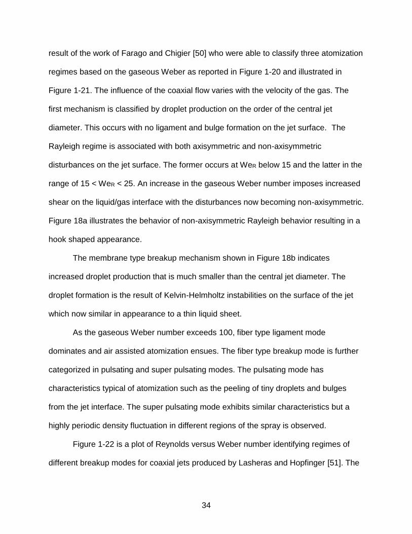
surroundings, and combust. The characterization of coaxial jet disintegration was a

34

result of the work of Farago and Chigier [50] who were able to classify three atomization

regimes based on the gaseous Weber as reported in Figure 1-20 and illustrated in

Figure 1-21. The influence of the coaxial flow varies with the velocity of the gas. The

first mechanism is classified by droplet production on the order of the central jet

diameter. This occurs with no ligament and bulge formation on the jet surface. The

Rayleigh regime is associated with both axisymmetric and non-axisymmetric

disturbances on the jet surface. The former occurs at WeR below 15 and the latter in the

range of 15 < WeR < 25. An increase in the gaseous Weber number imposes increased

shear on the liquid/gas interface with the disturbances now becoming non-axisymmetric.

Figure 18a illustrates the behavior of non-axisymmetric Rayleigh behavior resulting in a

hook shaped appearance.

The membrane type breakup mechanism shown in Figure 18b indicates

increased droplet production that is much smaller than the central jet diameter. The

droplet formation is the result of Kelvin-Helmholtz instabilities on the surface of the jet

which now similar in appearance to a thin liquid sheet.

As the gaseous Weber number exceeds 100, fiber type ligament mode

dominates and air assisted atomization ensues. The fiber type breakup mode is further

categorized in pulsating and super pulsating modes. The pulsating mode has

characteristics typical of atomization such as the peeling of tiny droplets and bulges

from the jet interface. The super pulsating mode exhibits similar characteristics but a

highly periodic density fluctuation in different regions of the spray is observed.

Figure 1-22 is a plot of Reynolds versus Weber number identifying regimes of

different breakup modes for coaxial jets produced by Lasheras and Hopfinger [51]. The

35

fiber type atomization mechanism characteristic of coaxial jet disintegration exists at

exceedingly high Weber and Reynolds numbers. A range of momentum flux ratios are

reported for water-air coaxial jets as well as the operating regimes of rocket engines

denoted by the hash lines in the regime 104-105 for both the Reynolds and Weber

numbers. The identification of such regimes, although qualitative in nature, assists in

the classification and verification of breakup modes of visual data. The fiber type

breakup regime is most common in rocket engines exhibits features similar to second

wind and atomization breakup modes, i.e. short wavelength disturbances. The jet

atomization characteristics include the shedding of fibers and their subsequent breakup

into droplets much smaller than the nozzle diameter in near nozzle region. Ligament

formation is see further downstream as the jet begins to take on a wavy appearance.

These ligaments eventually breakup into droplets larger than the droplets observed in

the near nozzle region [52]. The identification of qualitative breakup behavior is an

important first step in characterizing the qualitative and geometric features of the jet.

1.5.2 Core Length Investigations

A great deal of experimental effort has been made to develop models of the core

lengths of single phase and two phase coaxial jets. Figure 1-23 has been compiled by

Dumouchel [8] which documents different core length correlations developed by various

researchers.

The work done by Eroglu et al. sought to measure the core length of coaxial jets

and develop a correlation as reported in Figure 1-23. Over 1500 shadowgraph images

were analyzed with membrane and fiber type breakup modes observed for water/air

coaxial jets.

36

Woodward et al. implemented x-ray radiography to quantify the liquid core length

of coaxial jets consisting of water and either helium or nitrogen. The effects of liquid and

gas velocities as well as ambient pressure and gas density all influenced the liquid core

length. The Z parameter in the correlation account for the effects velocity ratio between

the liquid and gas streams.

Engelbert et al. [53] sought to quantify the effects of momentum flux ratio and

velocity and reported that the relation between momentum flux ratio and potential core

length is inversely proportional. Rehab et al. [54] utilized fluorescence imaging to

classify two regimes of coaxial flow with respect to the velocity ratio. They argued that a

critical velocity ratio existed that defined two regimes of flow behavior. This theory

confirmed the behavior of inverse proportionality proposed by Engelbert for velocity

ratios below the critical value. For values exceeding the critical velocity ratio, the

potential core of the central jet is reduced and followed by a recirculation bubble with

low frequency oscillation [54].

The near-field and far-field breakup mechanisms were investigated for water/air

coaxial jets by Lasheras [55]. Models were developed to quantify the behavior of the

driving mechanisms at each location. Entrainment was determined to be the driving

force in the shedding droplets, masses, and ligaments from the liquid surface and the

model developed quantified the shedding frequency as a function of momentum ratio.

The secondary breakup mechanism in the far field assists in the breakup and

coalescence of droplets. The model developed for the secondary breakup mechanism

considers the local turbulent dissipation rate of the gas since the kinetic energy of the

gas stream was found to be the primary driver of secondary atomization.

37

Pocheron et al. considered the coaxial gas density effects on the core length.

Studies of water/air and LOX/inert gas were performed at atmospheric pressure. A

probe was used to detect whether a liquid or gas was present on the tip. Using the

probe to scan the length of the jet, the location where there was a 100% probability of

the jet existing was determined. The liquid core length was then defined as the distance

at which there was only a 50% chance of detecting the jet.

Leroux et al. explored the nozzle effects on the breakup lengths of coaxial jets.

Five working fluids were used in conjunction with air in the annular passage providing a

wide range of operating conditions. Shadowgraph images were collected and analyzed.

The map of momentum ratio versus Reynolds number was explored to determine the

momentum ratio limits of the different breakup regimes. The Rayleigh and super

pulsating regimes were isolated and it was assumed that the membrane and fiber type

breakup behavior existed between the range of 7 x 106/ReG1.9 < M < 2 x 105/ReG

1.1. The

Rayleigh and super pulsating regime exist below and above those limits respectively.

The map of M vs Re was successful in delineating the Rayleigh and super pulsating

modes but not appropriate for dissociating the membrane and fiber behavior.

The effect of momentum flux ratio was further explored by Villermaux [56] who

demonstrated that surface tension and viscosity played no role in the breakup process

above a momentum ratio of 35. Therefore, the breakup length was independent of any

such effects. Additionally, the vorticity thickness of the gas stream at the nozzle exit

was shown to be proportional to the initial wavelength of the disturbance at the onset of

instability.

38

The effect of large area ratios (100-1000) was considered by Varga [57]. For

comparison, the area ratio of the SSME preburner injector is 2.81. The jet breakup

process was accelerated by the large aerodynamic forces provided by the gas stream

with primary breakup occurring in the first few gas-jet diameters. The Kelvin-Helmholtz

instability has been shown to be the dominant cause of primary breakup with the

Rayleigh-Taylor instability driving the secondary breakup process. The droplet sizes at

the onset of secondary atomization have been shown to correlate with the wavelength

of the most unstable Rayleigh-Taylor wave.

1.6 Coaxial Nozzle Supercritical Jet Experiments

The coaxial fuel injector can be found in the Space Shuttle Main Engine (SSME)

as well as many other liquid rocket engines as it is an ideal design for delivering the fuel

and oxidizer to the thrust chamber. The central post is supplied with liquid oxidizer and

the annular flow is gaseous fuel. The central jet disintegration is assisted by the shear

gas flow and mixing of the fuel and oxidizer is accelerated in the shear layer before

eventual combustion. The outer-to-inner jet velocity and momentum flux ratio are

common operating parameters considered in the design of shear coaxial injectors. The

operating conditions of the Space Shuttle Main Engine is roughly 1.2 <M<3.4, and 10

<Vr<11.5 as reported by Vivek [58]. Velocity ratios above 10 are reported to improve

combustion stability for LOX/GH2 injector configurations [59]. The conditions that exist in

the thrust chamber of liquid rocket engines are commonly above the thermodynamic

critical point of the fuel and hence the atomization phenomena that would have existed

at subcritical conditions no longer exist.

The study of shear coaxial jets is categorized into two types of injection

conditions: single phase and two phase. Single phase coaxial injection involves

39

gas/gas, liquid/liquid, and supercritical/supercritical injections into the same respective

environment. Two phase injections involve a liquid central flow with a gaseous annulus

flow and chamber. Widespread experimental effort has supported the development of

fuel injector design for liquid rocket engines with the efforts in the single and two phase

regimes necessary for a full understanding of the nature of coaxial injection from

subcritical to supercritical conditions.

1.6.1 Qualitative Studies of the Jet Surface

The experimental effort toward classifying the behavior of coaxial jets begins with

Telaar who conducted experiments with LN2 and gaseous He coaxial jets [60]. Telaar

sought to determine the effect of ambient pressure on the jet breakup process for sub-to

supercritical conditions. Shadowgraphy was used as the flow visualization technique to

image the jet boundary and qualitatively discern the jet behavior. The core flow

experienced the expected behavior in its transition from subcritical to supercritical

pressure, namely, a reduction in surface tension. The influence of the coaxial flow, as

discussed by Davis and Chehroudi [61], is to accelerate the liquid breakup process for

subcritical jets and to enhance mixing for supercritical turbulent jets.

The typical fuel and oxidizer delivery system for a liquid rocket engine generally

utilizes the fuel as a coolant for the nozzle prior to injection into the combustion

chamber. This leads to a significant temperature differential between the fuel and

oxidizer and hence the annular flow provides heat transfer to assist in the evaporation of

the liquid oxidizer inside the nozzle and the along the shear layer. Figure 1-24 illustrates

the effect of annulus mass flow rate at constant central flow rate. These images confirm

the trend of accelerated breakup and enhanced mixing in the subcritical and

supercritical regimes, respectively.

40

The images reported in Figure 1-24 illustrate the effect of outer jet mass flow rate

and pressure. The effect of increasing the annular mass flow rate is apparent from

frame 1 to 9. A noted decrease in core length and droplet size along with an increase in

droplet production is apparent. The near critical and supercritical regime in Figure 1-24

in frames 9-15 exhibit the same core length trend as annular mass flow rate in

increased. The turbulent gas jet behavior is still apparent at supercritical conditions with

the annular flow serving to accelerate the mixing process instead of being the source of

droplet production.

1.6.2 Core Length Measurements

The core length plays a major role in determining the degree to which the jet has

mixed with its surroundings. The coaxial jet, like the single round jet, exhibits many of

the same features when it comes to core length measurements but the core length is

now dependent on the outer-to-inner jet momentum flux ratio, velocity ratio, density

ratio, Reynolds number, and Weber number.

Woodward [62] sought the measure the potential core length of a LOX stimulant

over a broad range of Reynolds number, Weber number, and density ratios via x-ray

radiography and flow visualization. Two techniques were used to analyze the data with

no quantification of the uncertainty in the measurement. A correlation was developed for

the potential core breakup length as a function of Reynolds number, Weber number,

and density ratio.

Chehroudi and Davis [61] performed studies on subcritical to supercritical coaxial

LN2/GN2 jets into supercritical chamber pressures. They reported the core lengths as a

function of momentum flux ratio due to the difficulty in defining the Weber number when

surface tension reduced to zero at supercritical conditions. Core lengths were reported

41

as being small or nonexistent at supercritical conditions. The definition of core length,

dark core length, and potential core length continue to create confusion in the study of

coaxial jets as seen in the single jet case. Davis and Chehroudi [63] defined the core

length of coaxial jets as the connected dark fluid region before the first break in the

core. They employed an adaptive thresholding technique to make their measurements.

Chehroudi and Davis further concluded that supercritical coaxial jets behaved as single

phase variable density turbulent gaseous jets and subcritical coaxial jets behaved like

two phase mixing layers. The data obtained by Davis and Chehroudi is illustrated in

Figure 1-25 along with data from other researchers. A correlation is drawn through the

subcritical data while the near and supercritical data are grouped together. The behavior

of gas/gas and liquid/liquid coaxial jets confirms the single phase behavior. Subcritical

jets follow the two phase mixing layer trends as will be more apparent in the spreading

angle analysis. The range of experimental data covers three orders of magnitude with

the behavior of coaxial and single jets converging as M approaches zero. The trends for

single phase and two phase behavior are consistent among researchers.

1.6.3 Jet Spreading Angle Investigations

Jet spreading angles for coaxial injection allow for determination of the mixing

efficiency just like the single injection case. The jet growth rate for a coaxial jet is

defined as the spreading angle of the inner and outer jet combined. The spreading

angle is plotted against the chamber to inner jet density ratio along with correlations and

single jet investigations as reported by Davis and Chehroudi [64]. The plot along with

the data obtained by Chehroudi and Davis further support the trend of subcritical jets

behaving like two phase mixing layers and supercritical jets to behave like turbulent

variable density gaseous jets (Figure 1-26).

42

Gautam and Gupta [65] explored the effects of annular gas flow rate on the

spreading angle of coaxial liquid nitrogen and helium jets. They reported a decrease in

lateral spreading angle with an increase in gas flow rate. The increase in helium in the

surrounding air decreased the local density and hence a decrease in the spreading

angle should be expected. Their data was compared with correlations by Chehroudi et

al. [30] and Reitz and Bracco [16].

Rodriguez et al. [66] sought to classify the inner jet spreading angle of non-

reacting LN2/GN2 coaxial jets. Back-lit images were acquired in the sub-, near-, and

supercritical regimes in the velocity and momentum flux ratio ranges: 0.25 < VR < 23,

0.02 < M < 23, respectively. The use of a single species allowed for the existence of a

single critical point. Measurements of the inner jet spreading angle were made on the

basis of the inner jet core length since the inner jet density is much high than the

surrounding gas, therefore, producing a much darker signal in the experimental images.

The contour of the inner jet was detected and the spreading angle measurement was

made for the right and left boundaries of the jet. The jet spreading angle was defined as

the sum of both angle measurements. The spreading angle of the subcritical jets

showed a relatively constant value over a wide range of momentum flux ratios. Data for

the near-critical and supercritical exhibited a similar trend with the spreading angle

increasing to a maximum value and subsequently decaying at increased momentum

flux ratios as seen in Figure 1-27.

1.6.4 Mapping of Jet Thermodynamic Profiles

LN2 and GH2 coaxial injection under sub-to supercritical conditions was

investigated experimentally by Oschwald et al. [44] with the goal of mapping density

profiles of both streams. Density profiles have been generated by two dimensional

43

Raman scattering and utilizing a filtering technique to isolate the individual Raman

signals of the LN2 and H2. Difficulties arise at the shear layer interface where a large

density gradient, and hence gradient in index of refraction, was a source of

experimental error. Two dimensional species distribution images were reconstructed

from the individual radial density profiles and are represented in Figure 1-28. Radial

density profiles are reported in Figure 1-29. Oschwald [67] sought to classify the

evolution of the mixing process by tracking the maximum in the radial density profile in

the axial direction. The study of this behavior showed that there was a plateau in the

density profile that was associated with the far field density.

Coupling the radial density profile information with the far field plateau density

made it possible to compare the single injection and coaxial flow case. It was

determined that the co-flowing gas forced the evolution of the jet towards the plateau in

the density profile much quicker than the single injection case, confirming the enhanced

mixing behavior of the annular flow. Finally, the effect of the thermodynamic state was

explored by varying the temperature of the central jet to values above and below the

pseudo-boiling point, the temperature and pressure at which the specific heat is a

maximum and thermal diffusivity is at a minimum. Injection above the pseudoboiling

temperature led to densities similar to the gaseous phase while injection below the

pseudoboiling temperature exhibited liquid-like densities. In either case, it was found

that the coaxial gas velocity had a weak effect on the jet breakup process compared to

the thermodynamic state.

Schumaker and Driscoll [68] utilized acetone PLIF to produce instantaneous and

averaged images of mixture fraction fields. They injected acetone seeded air through

44

the central jet and helium or hydrogen through the annulus but report results based on

using pure oxygen as the working fluid in the central jet in an effort to directly compare

the results with reacting O2/H2 systems. Mixing lengths were inferred from the

experimental data by spanning a range of velocity ratios, density ratios, injector

diameters, and Reynolds numbers. A dependence on the outer-to-inner momentum flux

ratio was reported.

Figure 1-1. Criteria of cylindrical liquid jet disintegration regimes. aRanz [9], bSterling and Sleicher [5], cMiesse [10], dReitz [11], eDan et al. [12], f Taylor [6]

Figure 1-2. Cylindrical jet behavior. Left – jet stability curve, Right – example of visualizations (from left to right): Rayleigh regime (region B) ReL = 790, WeG = 0.06; first wind induced regime (region C) ReL = 5,500, WeG = 2.7; second wind induced regime (region D) ReL=16,500, WeG = 24; atomization regime (region E) ReL = 28,000, WeG = 70 (Images from Leroux [69])

45

Figure 1-3. Classification of disintegration modes at fixed thermodynamic conditions. The disintegration modes are highly dependent on jet velocity and thermodynamic conditions. Increasing the ambient gas density or increasing the jet velocity leads to increased droplet production and transition to the atomization regime. Baumgarten [70]

Figure 1-4. Three distinct regimes of a turbulent submerged jet

46

Figure 1-5. Subcritical jet injected into a subcritical environment. A) Density map of subcritical jet. Droplet formation is apparent around 20 jet diameters. B) Density gradient map.

Figure 1-6. Influence of gas composition on jet behavior. The jet is initially at Tr =0.97 is injected into the chamber at Tr =0.97, Pr =1.04 with injection velocity = 3.7 m/sec. Partial pressure ratio of CO2 is 0, 0.5 atm, and saturation value respectively.

47

Figure 1-7. Influence of gas temperature on jet behavior. The jet is initially at Tr =0.97 is injected into the chamber at Pr =1.228 and Tr = 0.97, 1.05 and 1.10 respectively with injection velocity = 2 m/sec. Initial CO2 partial pressure = 0 atm.

Figure 1-8. Influence of chamber pressure at a supercritical temperature. The jet is initially at Tr =0.97 is injected into the chamber at Tr=1.05 and Pr = 0.85, 1.04 and 1.228 respectively with injection velocity = 3.35 m/sec.

48

Figure 1-9. Back-illuminated images of a single nitrogen jet injected into nitrogen at a fixed supercritical temperature of 300K but varying sub- to supercritical pressures (For N2: Pcritical = 3.39MPa; Tc = 126.2K). From lower right to upper left: Pch/Pcritical (frame no.) = 0.23 (1), 0.43 (2), 0.62 (3), 0.83 (4), 1.03 (5), 1.22 (6), 1.62 (7), 2.44 (8), 2.74 (9). Reynolds’ number (Re) was from 25,000 to 75,000. Injection’ velocity: 10–15 m/s. Froude’ number: 40,000 to 110,000. Injectant temperature: 99 to 120 K. Chehroudi et al. [30].

Figure 1-10. Software magnified images of the jets in Figure 1-9 at their outer boundaries showing transition to the gas-jet-like appearance starting at just below the critical pressure of the injectant. Images are at fixed supercritical chamber temperature of 300 K. Chehroudi et al. [30].

49

Figure 1-11. Spreading or growth rate of single jets as a tangent of the visual spreading angle versus the chamber-to-injectant density ratio. Data taken by Chehroudi

are indicated by an asterisk (∗) in the legend. Chehroudi et al. [30].

Figure 1-12. Jet spreading angle plotted as a function of chamber-to-injectant density ratio. Roy’s data points and proposed model lie between those proposed by Reitz and Bracco for diesel sprays (L/D = 85) and Chehroudi’s model for N2 injected into supercritical N2 environment. The single species mixing cases produce higher spreading angles than the binary species cases. Both have been indicated.

50

Figure 1-13. Theoretical dependence of the spray angle of surface, viscous and aerodynamic forces, while the on the parameter Y and comparison with experimental function f(Y) reflects their impact on the growth data.

Figure 1-14. Ratio of the dark-core, intact-core, or potential-core length, depending on the case, divided by the density ratio for single jets. Chehroudi et al. [36], determined by analysis of shadowgraphs, for an injector L/D = 200.

51

Figure 1-15. Core lengths plotted as a function of chamber-to-injectant density ratio. Our data points and proposed model lie slightly above the theory of Abramovich for turbulent submerged cold gas jets but follow a similar trend. The core length stays relatively constant at about 11.5 jet diameters.

Figure 1-16. Figure of experimental conditions performed by Roy et al. [48]. Reduced temperatures and pressures are reported for Novec 649. Critical Temperature: 441K, Critical Pressure: 18.4 atm.

52

Figure 1-17. Scaled images of a supercritical jet injected into subcritical chamber conditions. Test conditions correspond to cases 1-4 in Figure 1-16. (a–d) density images; (e–h) magnified density gradient images. [48]

Figure 1-18. Scaled images of a supercritical jet injected into supercritical chamber conditions. Test conditions correspond to cases 5–8 in Figure 1-16: (a–d) density images; (e–h) magnified density gradient images. [48]

53

Figure 1-19. Simultaneous fluorescence, phosphorescence, and superimpose image of both of a liquid acetone jet at 450 K and 59 atm in 575 K air. 0 mm is at jet center. Mass flow rate – 8.34 g/s. Vjet – 13.45 m/s. Vgas ~ 1.0 m/s.

Figure 1-20. Breakup modes of coaxial jets

54

Figure 1-21. Air-assisted cylindrical jet atomization regimes. A) Non-axisymmetric Rayleigh regime, B) membrane-type regime, C) fiber-type regime, D) superpulsating submode, Farago and Chigier [50].

Figure 1-22. Breakup regimes in the parameter space Rel – We for coaxial jets. Lines of constant M are calculated for water/air coaxial jets by Lasheras and Hopfinger [51]. Here, Rel = (UlDl/νl), We = (ρgUg

2Dl/ σ) ; M = ρgUg2 / ρlUl

2.

55

Figure 1-23. Correlations for the characteristic length of air-assisted liquid jets

56

Figure 1-24. Images of a coaxial jet at approximately the same inner-jet mass flow

rates (∼275 mg/s). Columns are at about the same outer- annular-jet mass flow rates. For each row, the annular mass flow rate starts at a zero value to 2800 mg/s and increases from the left column to the right. The chamber

pressure levels for images 1–5 are subcritical (∼1.41MPa), for 6–10 are near-critical (∼3.46MPa), and for 11–15 are supercritical (∼4.77MPa). Inner-and outer-tube flow average temperatures at injector exit are 170K and 112 K, respectively. Davis and Chehroudi [63]

57

Figure 1-25. Figure shows comparison of the present coaxial- jet dark-core length measurements with all other relevant core length data available in the literature versus momentum flux ratio. Data reported by Eroglu et al. [71], Englebert et al. [53], and Woodward [72]are two-phase flows and the rest are single phase. The range of core length for cryogenic single jet (LN2/GN2) is also shown at the left margin. This figure was compiled by Davis and Chehroudi [63], [64].

Figure 1-26. Spreading rate of the shear layer versus the chamber/injectant or chamber/inner-jet density ratio for single and coaxial jets compared with different predictions for planar shear layers. For the coaxial data, the chamber pressure increases from sub- to near- and to supercritical conditions in the direction of the arrow.

58

Figure 1-27. Maximum baseline spread angles as a function of momentum flux ratio for sub-, near-, and supercritical conditions as reported by Rodriguez et al. [66] for coaxial without an external acoustic excitation source.

Figure 1-28. Hydrogen density for a coaxial LN2/H2 injection (TN2 = 140 K, TH2 = 270 K). Oschwald et al. [67]

59

Figure 1-29. Radial N2 density profile for single jet (VN2 = 5 m/s, TN2 = 140 K), 2mm (x/D = 1.05) downstream of the coaxial injector exit. (b) Radial N2 and H2 density profiles for coaxial LN2/H2 injection for a coaxial jet (VN2 = 5 m/s, TN2 = 140K, VH2 = 60 m/s, TH2 = 270 K), 2mm (x/D = 1.05) downstream the injector exit. Laser beam direction is from left to right. Oschwald et al. [67].

60

CHAPTER 2 EXPERIMENTAL SETUP

A detailed summary of the experimental setup can be found in Polikov [73] and

Roy [27]. Therefore, only a brief description of important features is included with details

on any major changes included for completeness. Figure 2-1 shows a schematic of the

experimental facility as described by Polikov [73]. Nitrogen is supplied via an industrial

supply tank to the high pressure chamber and the annulus of the coaxial injector after

being electrically heated. Fuel is pressurized in a stainless steel storage tank with an

additional nitrogen supply. The fuel supply utilizes a smaller version of the electric heat

exchanger used in the gas supply system to preheat the fuel prior to injection.

2.1 High Pressure Chamber

The design of the high pressure chamber must allow for safe operation above the

critical point of the working fluid while allowing optical access for image acquisition. The

high pressure chamber can be safely operated at pressures up to 70 atm (1000psi) and

300 oC (572 oF) with a maximum operating limit of 150 atm (2200 psi) and 350 oC (662

oF). Figure 2-2 depicts a section view of the high pressure chamber. Visible in the

diagram are the coaxial injector, thermocouples at the top and bottom of the chamber,

and quartz windows for optical access.

The chamber was constructed of brass due to its ability to operate at elevated

pressures while providing fast enough heat transfer to provide uniform temperature

distribution from the injection plane to the exhaust at the bottom of the chamber. The

chamber temperature is controlled by four cartridge heaters inserted into slots drilled

into the corner of the chamber body. Omega CIR-1060 cartridge heaters are used with

an effective total power output of 0.4 kW. The chamber pressure is monitored using

61

Omega PX303-1KG10V pressure transducers while the chamber temperature is read

using Omega K-type thermocouples at the top and bottom of the chamber.

Internal chamber dimensions are 1.8”x1.8”x9” to prevent liquid deposition on the

window caused by splashing from the bottom of the chamber and flapping of the liquid

jet. In addition, the windows on the chamber must provide maximum field of view to

allow for near injector studies as well as late stage breakup studies. Quartz windows

were selected for their high transmittance and ability to operate at temperatures up to

1000 oC and pressures up to 70 atm with a safety factor of seven. The windows are

flush mounted onto flanges and sealed using high temperature RTV and a silicon o-ring.

The effective field of view is 3.3” x0.84”; which allows studies between 0 and 40 jet

diameters for a 2 mm injector. To simplify facility maintenance, dummy flanges were

fabricated and used where optical access wasn’t necessary. The windowed flanges and

dummy flanges are sealed using a graphite gasket between the chamber body and the

flange.

2.2 Injector Configuration

2.2.1 Single Injector

The single injector configuration (Figure 2-38) utilizes a 2 mm diameter injector

which allows for near field and late stage breakup studies given the effective field of

view. Laminar flow exiting the injector is achieved by keeping the length to diameter

ratio of the injector at 2.5. A honeycomb structure is welded to the injector near the tip to

reduce post vibration and straighten the gas flow during coaxial injection. The coaxial

passageway is closed off during single injection studies by replacing the NPT plug on

the bottom of the chamber lid assembly to an NPT plug matching the outer dimensions

of the 2mm injector. The chamber is pressurized via four holes drilled in the body of the

62

chamber lid. The holes are in the direct vicinity of the windows which prevents liquid/gas

interaction and helps protect the windows from splashing.

2.2.2. Coaxial Injector

Coaxial injection is achieved by replacing the NPT plug on the bottom of the

chamber lid assembly with a new plug. The injector selected for this experimental

campaign was designed to the SSME pre-burner dimensions to simulate the area ratio

of a rocket engine coaxial injector. The passageways used to pressurize the chamber

during single injection are now sealed using four ¼ NPT pipe plugs as seen in Figure 2-

4. A detailed view of the coaxial injector is presented in Figure 2-5.

2.3 Instrumentation, Experimental Control and Data Acquisition

2.3.1 Instrumentation

The instrumentation on the test facility consists four main pieces of hardware: six

thermocouples, three pressure transducers, two flow meters, and two electric heaters.

The precise location of each piece of hardware can be located in Figure 2-1.

The six Omega K-type thermocouples monitor the fuel and gas supply

temperatures, the electric heater cores, and the chamber top and bottom. Omega

PX303-1KG10V pressure transducers are used to monitor pressure in the chamber as

well as the fuel and gas lines. The operational range is 0-1000 psi with a linear output

voltage in the range of 0-10 volts. The flow rate in the gas line is measured via an

Omega FLMG 12050SS-MA flow meter. Operational limits are 1-100 atm and 0-50

SCFM with a voltage output of 0-5 V. Pressure is monitored downstream of the flow

meter to assist in calibration and correction of gas flow rate from SCFM to ACFM. The

liquid flow rate is measure with a Sponslor Lo-Flo precision flow meter. The operational

range is 5-100 cc/s with +/- 0.25% linearity.

63

Two heating elements were constructed to regulate the temperature in the fuel

and gas lines. The gas heat exchanger was constructed using six Omega CIR-2121/240

cartridge heaters with an effective power output of 6kW. The nitrogen gas passes

through a threaded passageway within the heating element providing temperature

control of the gas flow prior to injection. Omega K-type thermocouples monitor the

temperature of the heater core and the temperature of the liquid after heating.

Temperature control of the fuel is provided by a similar cartridge heater element used in

the gas supply system with the exception of a 3kW power output. This ensures a

constant injection temperature for 30s at 50cc/s. The temperature of the heater core

and temperature of the liquid prior to injection as also monitored.

2.1.2 Experimental Control and Data Acquisition

The experimental control and data acquisition is best summarized in Figure 2-6.

A computer equipped with a National Instruments AT-MIO-64E-3 data acquisition board

and LabVIEW is utilized for controlling the experiment and acquiring data. The various

sensors and solenoid vales are wired into their respective terminal blocks, multiplexers,

signal conditioners, and the NI SCXI-1000 chassis connected to the computers onboard

DAQ.

Control of the experimental parameters is performed through the LabVIEW GUI.

The temperature of the chamber and heaters are set and allowed to reach their

operating points. The control of the gas and liquid flow are achieved through the use of

Omega SV-128 solenoid valves. Once the desired experimental parameters are

achieved, the LabVIEW program can begin to acquire the sensor data and write it to an

output file. The acquisition of all sensor channels is unnecessary and therefore limited

to the liquid and gas temperature, pressure, and flow rate as well as the chamber

64

temperature and pressure. The voltage output from the image acquisition system is also

recorded to facilitate synchronizing the sensor and image data.

2.4 Working Fluid Photophysics and PLIF implementation

The working fluid utilized in all studies is a perfluorinated ketone commonly

referred to as fluoroketone with the technical name, 2-trifluoromethyl-1,1,1,2,4,4,5,5,5-

nonafluoro-3-pentanone, or also simplified as FK-5-1-12. It is ideal for use in studies of

jet disintegration and mixing in the supercritical regime due to its low critical temperature

and pressure of 168 oC and 18.4 atm, respectively. Comparatively. water (374 oC, 218

atm) and acetone (235oC, 47.4 atm) which are common working fluids used in

supercritical experiments, require stricter design standards due to increased pressure

requirements and the potential for volatile reactions, respectively. With fluoroketone, the

facilities can be designed with cheaper materials due to lower thermodynamic

requirements with no risk of volatile behavior experienced with acetone. Fluoroketone is

also inert making it compatible with common construction materials and safe to use in

large quantities. In addition, it has low toxicity, is environmentally acceptable, and

experiences no thermal decomposition in air below 500 oC [27].

Further utilizing the material properties of the working fluid, it produces a strong

fluorescence signal with broadband excitation that can be achieved with many common

high power lasers. Fluoroketone experiences a strong absorption in the near ultraviolet

range with peak absorption at 307 nm. The laser selected is a Continuum Surelite

Nd:YAG laser tuned to its third harmonic with a wavelength of 355 nm. The average

energy per pulse is 150 mJ with pulse duration of 10 ns and frequency of 10 Hz. The

absorption cross section is 3.81 x10-19 cm2/molecule as determined by Roy [27].

65

Figure 2-7 is a schematic of the optical bench and test facility setup. The laser

beam is steered through three dichroic mirrors to remove any residual 532nm light

which results in a beam that is 99.998% pure 355 nm light. A laser sheet must then be

formed by passing the beam through three cylindrical lenses. The laser sheet is 25mm

wide and 0.1 mm thick. The beam is directed through the center of the jet and a PI MAX

II ICCD (Intensified Charge Coupled Device) camera is placed perpendicular to the

propagation direction of the laser sheet to capture the fluorescence signal. A bandpass

filter centered at 420 nm +/- 10 nm FWHM is mounted after the camera lens to eliminate

any elastic light scattering and isolate the fluorescence signal. Camera spatial resolution

is 44μm/pixel on 1024x1024 chip that has been cropped to 381x1024. Cropping of the

CCD chip increases the camera frame rate from 7 Hz to 10 Hz to match the laser

frequency. The camera, laser, and data acquisition system are all synchronized using a

Stanford Instruments DG-535 delay generator.

The Planar Laser Induced Fluorescence (PLIF) diagnostic technique utilizing

Fluoroketone as the working fluid has been well documented by Roy et al. [41]. A brief

discussion is included in this chapter with a more detailed analysis included in Appendix

A. The technique corrects for the nonlinear fluorescence signal caused by the high

power laser and the dense absorbing medium. Temperature and pressure effects have

been found to be negligible on the fluorescence signal [73].

Figure 2-8 is a plot of the excitation of electrons by photons which indicates that

a threshold of electron output exists for a given photon input. A linear regime can be

approximated but all experiments performed are in the nonlinear regime. The

66

fluorescence theory as derived by Roy [27] yields an equation for the electron output

versus photon input as indicated by Figure 2-8.

𝑁𝑒 = 𝑁𝜎𝑔

𝜎𝑔 + 𝜎𝑒[1 − 𝑒

−𝑁𝑝ℎ(𝜎𝑔+𝜎𝑒)

𝐴 ] (2-1)

The terms in this equation 1 are as follows:

N: total number of molecules

Ne: number of excited molecules

Nph: number of photons

σg, σe: absorption cross section of ground state and excited state

molecules

A:laser sheet area

The electron output is related to the signal intensity measured on the CCD chip

by considering the fluorescence yield (φ), as well as the optics efficiency and solid angle

of collection which have been grouped into a single term, F, in equation 2.

𝑆(𝑝𝑥, 𝑝𝑦) = 𝐹𝜌(𝑥, 𝑦)𝜑[1 − 𝑒−𝐼(

𝜆ℎ𝑐

)𝜎] (2-2)

The number density of the total electron output is directly proportional to the local

density in the flow field and thus the spatial pixel intensity is a function of the spatial

density distribution. In addition, the laser intensity drop through the absorbing medium is

accounted for by applying the Beer-Lambert law. All resulting constants have been

grouped into a single term, k.

𝑆(𝑝𝑥, 𝑝𝑦) = 𝐹𝜌(𝑥, 𝑦)𝜑[1 − 𝑒−𝑘𝑒−𝜎𝑛𝑥] (2-3)

Finally, the fluorescence intensity can be directly correlated to the local density

using the PRSV equation of state and the experimental sensor data.

67

𝑝 = 𝑅𝑇(𝑉 − 𝑏) − 𝑎𝛼(𝑉(𝑉 + 𝑏) + 𝑏(𝑏 − 𝑉)) (2-4)

The well documented thermodynamic properties can be predicted within 2%

uncertainty within the range of 0.1-100 atm and 150-600K. The coefficients a, b, and α

have been reported for Novec 649 (fluoroketone) by Polikov and Segal [74]. A

background image, laser sheet intensity profile, and experimental image of the jet are all

required to accurately map the density and gradient distributions. Core lengths and

spreading angles can also be inferred and measured. Figure 2-9 shows the result of

weighting the image by the laser sheet profile and removing the background signal. The

image on the left shows preferential weighting of the vapor density in the direction of

propagation of the laser (left to right). The image on the right shows an evenly weighted

density distribution as well as a more symmetric density profile. This technique was

implemented by Roy [48] and is the basis of the image processing method that will be

utilized in this study.

2.5 Shadowgraphy Implementation

Figure 2-10 depicts the optical bench setup for the parallel light shadowgraphy

technique. Flow visualization was accomplished using a 1,000W halogen lamp source,

providing 2,700 lumens with a color temperature of 3,200 K. The diffuse light was

focused and collimated through a bi-convex lens with a focal length of 20 cm. The

parallel light was then directed through the high pressure chamber using a mirror and

the light was captured with a PCO 1200s high speed CMOS camera. An effective

spatial resolution of 28 μm/pixel and frame rate of 1000 Hz was achieved by cropping

the chip to 511x1130. This simple flow visualization technique was used to measure

spreading angles for comparison with PLIF results.

68

The image processing technique is much simpler for the processing of the

shadowgraphy data. Two images are required: a background and the experimental

image. Seven hundred frames are acquired per test run and one hundred background

images. The background image is averaged and subtracted from each individual

experimental image. The processed image can now be averaged or used for further

processing.

The goal of image processing is to increase the signal to noise ratio. Dark noise

and background noise are sources of noise introduced into the experimental image. By

removing these through background subtraction, we obtain a much better signal to

noise ratio. The following two sections report the results of the single orifice

shadowgraphy experimental campaign as well as the coaxial jet PLIF study.

69

Figure 2-1. Schematic of Liquid/Fuel supply system. Gas supply line: 1 = gas bottle, 2 = pressure regulator, 3 = solenoid valve, 4 = needle valve, 5 = shop air supply check valve, 6 = gas flow=meter, 7 = pressure transducer, 8 = heater, 9 = heater core thermocouple, 10 = gas temperature thermocouple. Liquid supply line: 12 = gas bottle, 13 = pressure regulator, 14 = ball valve, 15 = fuel tank, 16 = ball valve, 17 = needle valve, 18 = liquid flow-meter, 19 = shop air supply check valve 20 = main liquid line solenoid valve, 21 = bypass liquid line solenoid valve, 22 = main line needle valve, 23 = bypass line needle valve, 24 = liquid line pressure transducer, 25 = liquid line heater, 26 = liquid line heater core thermocouple, 27 = liquid recuperation tank, 28 = ball valve, 30 = liquid temperature thermocouple. Chamber: 11 = chamber, 31 = chamber upper temperature thermocouple, 32 = chamber bottom thermocouple, 33 = pressure relief valve, 29 = exhaust needle valve, 34 = chamber pressure transducer. [73]

70

Figure 2-2. Section view of the high pressure chamber.

Figure 2-3. Injector tip with honeycomb structure.

71

Figure 2-4. Chamber top assembly depicting the coaxial injector, chamber top thermocouple, and plugged NPT passageways.

Figure 2-5. Coaxial injector schematic with dimensions. The image on the left depicts the NPT plug with the coaxial passage as well as the central post injector with the honeycomb structure for straightening the gas flow. The injector has been fabricated to the dimensions of the SSME preburner injector.

72

Figure 2-6. Schematic of the data acquisition system.

Figure 2-7. Schematic of optical and test bench setup

73

Figure 2-8. Variation of the number of excited electrons with the number of exciting photons.

Figure 2-9. The result of correcting for the non-linear fluorescence signal. The image on the left shows preferential weighing of the density distribution in the direction of propagation of the laser (left to right). The image on the right shows a more uniform density distribution on the left and right hand side of the jet. In addition, the jet appears slightly more symmetric.

74

Figure 2-10. Optical bench Shadowgraphy setup.

75

CHAPTER 3 SINGLE ORIFICE INJECTION

3.1 Experimental Conditions

The current study of single orifice jets injected into a chamber of sub-to

supercritical temperatures and pressures was focused on the effect of the chamber-to-

injectant density ratio on the jet disintegration process. Forty-eight tests were run in the

density ratio range of 0.0035-0.1280 with the all experimental conditions reported in the

appendix. Spreading angles were measured from the visualization data and reported in

the section to follow.

The experimental conditions for the selected images are presented in Figure 3-1.

The cases have been selected to correspond with similar injection conditions from the

previous PLIF studies. These cases are used for comparison between the PLIF and

shadowgraph data. The first case represents subcritical injection into a subcritical

environment, the second is supercritical injection into an environment of supercritical

pressure while chamber temperatures are subcritical and all conditions are supercritical

in the final case.

3.2 Jet Morphology and Flow Visualization Analysis

The images for case 1 represented in Figure 3-1 are reported in Figure 3-2. All

thermodynamic conditions are subcritical and the injection velocity is low compared to

the supercritical cases. A dense liquid jet is observed with low amplitude disturbances

apparent on the surface of the jet. The breakup mode is in the Rayleigh regime. The

high density region of the jet persists beyond 10 jet diameters as determined from the

PLIF image.

76

Case 2 represented in Figure 3-3 exhibits the effect of increasing the chamber

pressure and injection temperature beyond the critical point with the chamber

temperature held at a subcritical value. Droplets and ligaments are seen forming on the

jet surface. With the injection temperature supercritical and the chamber temperature

subcritical, there exists local subcritical conditions resulting in the reassertion of surface

tension and condensation of the supercritical phase. Droplet formation is seen at

downstream locations of x/D > 10. Droplet sizes appear to increase with increasing

downstream location. The high density region in the PLIF images are roughly the same

in magnitude as the fully subcritical case.

The effect of elevating both the temperature and pressure beyond the critical

point produces the behavior reported in Figure 3-4. Droplet production has ceased and

surface tension has become non-existent with the appearance of gas/gas-like mixing

behavior present in the images. Finger-like threads are still apparent on the jet surface.

There is a reduction in the jet penetration length as determined from the PLIF density

map. The lateral spreading rate has increased as expected with an increase in

chamber-to-injectant density ratio. The findings of the spreading analysis are reported in

the following section.

3.3 Jet Spreading Angle Analysis

The results of the jet spreading angle analysis are presented in Figure 3-5. The

result of an increase in chamber-to-injectant density ratio is an increase in the lateral jet

spreading angle. A wide spreading angle is indicative of increased mixing. In addition,

the need for evaporation and break down of surface tension is no longer necessary in

the supercritical regime. The correlation for the presented data follows the trends of the

flow visualization study by Reitz & Bracco [31] closely. According to the data, the

77

spreading angle of a fluoroketone jet injected into a N2 environment in subcritical and

supercritical conditions follows the trend:

𝜃 = 0.3(𝜌𝑁2

𝜌𝐹𝐾)

12

(3-1)

The above equation was obtained using a power curve fit through all of the data

points extending from subcritical to supercritical test conditions in the density ratio range

of 0.0035- 0.1280. The correlation found in the present dataset differ from the findings

of Roy [27] and Reitz and Bracco [31] by a small difference in the coefficient. Otherwise,

all datasets show a square root dependence on the chamber-to-injectant density ratio.

The variation between the data presented in this study and the findings of Roy which

were obtained in the same facility can be justified by the different imaging techniques

employed in each study. The integrative nature of the shadowgraph flow visualization

technique captures an average throughout the jet unlike the PLIF technique which

images a single plane through the center of the jet. The data from the back-lighting

technique employed in this study and the work by Reitz and Bracco [31] show

agreement. The method of finding the jet boundaries in each study differed as well with

the present study utilizing a thresholding technique to convert the image to a binary

image of black or white and then detecting the contour of the jet profile. The spreading

angle was found by drawing a linear fit through the left and right jet contour in the near

nozzle momentum dominated region. The image processing techniques differed

between all three studies and thus another uncertainty is introduced into the data.

The plot shows that beyond the density ratios where either the jet or the ambient

environment is at supercritical conditions with respect to the injectant critical properties,

the images of the jets exhibit liquid and gas-like properties. In the supercritical regime,

78

the images of the jets exhibit gas jet-like appearance and show similar behavior with

respect to spreading angle.

3.4 Droplet Size and Distribution Analysis

The droplet size and distribution were further measured from shadowgraph

visualization data with the results of the droplet distribution and mean size is reported in

Figures 3-6 and 3-7, respectively. When injection temperatures are supercritical and

chamber conditions are subcritical, condensation of the supercritical fluid occurs and

droplet formation is apparent. This has been attributed to the reassertion of surface

tension that was also observed in previous studies [75]. As chamber temperatures

approach the critical point and the injection temperature is supercritical, the rate of

droplet production decreases significantly due to the loss of surface tension even under

subcritical chamber pressures. Analysis of the normalized droplet diameters and droplet

population shows no dependence on chamber pressure. A decreasing trend relative to

increasing chamber temperature is seen in the droplet population data. The trend

observed in the plot of normalized mean diameter and normalized Sauter mean

diameter versus the geometric mean of the injection and chamber temperature show a

linear increase in droplet size with increasing injection and chamber temperature. This

is attributed to evaporation of smaller droplets occurring much quicker than larger

droplets relative to their residence time in the field of view. The appearance of larger

droplets is the result of the inability to undergo breakup due to higher surface tension

relative to the aerodynamic forces experienced in the chamber. The increase in the

mean droplet sizes can be attributed to the decrease in the overall number of droplets

present. The uncertainty in the droplet data is a result of the spatial resolution of the

79

images. Droplets that are much smaller than the spatial resolution of the images difficult

to quantify using image analysis software.

3.5 Conclusions

A flow visualization study of a subcritical and supercritical jets injected into

environments in the sub-to-supercritical range was undertaken to compare quantitative

spreading angle data obtained by two different imaging techniques in the same facility.

The images were obtained using high speed parallel light shadowgraphy and compared

to previously obtained PLIF data.

The selected images from the shadowgraph and PLIF studies show a decrease

in surface tension with increased injection temperature and pressure and complete

breakdown of the jet surface at supercritical conditions where surface tension no longer

plays a role in the disintegration process. In cases where the chamber temperatures are

subcritical, local subcritical conditions exist and thus condensation and droplet formation

occurs in those regions. The appearance of gas/gas mixing behavior is observed when

all chamber and injectant conditions are supercritical with droplet formation no longer

occurring and a much smoother appearance of the jet boundary. A widening of the jet

lateral profile is also observed which is indicative of increased mixing.

The visualization data obtained in the present study was used to measure the jet

spreading angle over the density ratio range of 0.0035-0.1280. The trend reported

shows a square root dependence of the jet spreading angle with respect to the

chamber-to-injectant ratio. Thus, the jet lateral spreading rate shows an increase with

increased density ratio. The trend found in the present study shows agreement with

previous studies performed in the same facility under similar conditions with the same

working fluid. The difference in the magnitude is attributed to the different imaging

80

technique utilized in each study. While the magnitude of the data closely agrees with

that of Reitz & Bracco, the shadowgraph technique is integrative through the entire jet

while the PLIF diagnostic technique images a single jet plane. Thus, the PLIF data

should more closely represent the magnitude of the spreading angle of the jet.

The results of the droplet distribution study show a decreasing number of

particles with an increase in the chamber temperature approaching the critical point.

The size of these particles increase in size as the critical point is approached. This is

attributed to the smaller diameter droplets evaporating much quicker than the larger

droplets as well as the inability of the larger droplets to breakup due to their higher

surface tension. The appearance of droplets under supercritical injection temperatures

is a direct result of condensation of the supercritical fluid under subcritical chamber

temperatures. Uncertainty in measuring small droplet diameters are present when

droplet diameters are much smaller than the spatial resolution of the experimental

images.

81

Figure 3-1. Experimental conditions for selected binary single orifice jet disintegration experiments. MFR represents mass flow rate in kilograms per second. The reduced temperatures and pressure are reported with respect to the critical point for fluoroketone (FK). Critical properties of fluoroketone (FK) are 441 K and 18.4 atm. Figure subscripts are for fluoroketone (FK), nitrogen (N2), and chamber (ch).

Figure 3-2. Shadowgraph images of case 1 from Figure 3-1. Surface instabilities are amplified downstream of the nozzle and the breakup mode is within the Rayleigh regime. The high density region of the jet persists beyond 10 jet diameters as determined from the PLIF density map.

82

Figure 3-3. Shadowgraph image and PLIF density map of case 2 from Figure 3-1. In case 2, the supercritical jet is in injected into a chamber of subcritical temperature and thus condensation of the jet should be expected where local subcritical conditions exist.

Figure 3-4. Shadowgraph images for case 3 reported in Figure 3-1. Chamber temperatures are supercritical. Fully supercritical behavior is observed. Single phase turbulent gas/gas jet mixing is observed in the shadowgraph and PLIF images.

83

Figure 3-5. Plot of jet spreading angle versus chamber to injectant density ratio for fluoroketone/nitrogen single orifice jets. An increase in jet spreading angle is apparent with an increase in the chamber-to-injectant density ratio. The results follow similar trends reported by Reitz & Bracco [76] as well as Roy [27].

Figure 3-6. Plot of number of particles versus geometric mean of reduced injection and chamber temperature. The reduction in overall number of particles can be attributed to evaporation of smaller droplets occurring much quicker than larger droplets.

84

Figure 3-7. Plot of normalized drop diameter versus the geometric mean of injection and chamber temperature. The increase in normalized drop diameter can be attributed to the evaporation of smaller droplets with increasing chamber temperature. This results in the remaining larger droplets increasing the mean droplet size due to their inability to evaporate within the frame of view.

85

CHAPTER 4 COAXIAL INJECTION

4.1 Experimental Conditions

The current study of coaxial jets injected into a chamber of supercritical pressure

was focused on the effect of the momentum flux ratio on the jet disintegration process.

The selected experimental conditions are listed in Figure 4-1. Each case was selected

to increase in momentum ratio with subcritical injection temperatures and supercritical

chamber pressures with the exception of the first case which was taken as a reference

for the condition with no annular flow, hence M = 0.

The momentum ratio ranged from 0.13 – 4.3 to overlap results of previous

studies. Density of the jet center plane were obtained for all cases listed below.

Measurement of the core length was performed based on the technique previously

developed. The threshold for determining the core length was taken as the point of

maximum gradient as in Roy [40]. Fluoroketone injection velocities were kept constant

at 2 m/s. Figure 4-1 subscripts are for fluoroketone (FK), nitrogen (N2), and chamber

(ch). Spreading angle measurements were determined by finding the boundary of the jet

and fitting a line through the contour for the length of the jet core.

4.2 Jet Morphology and Density Map Analysis

Density and density gradient maps as shown in Figure 4-2 represent the first and

second case in Figure 4-1. In the first case, the central jet momentum is unaffected by

the annulus flow and the behavior observed is typical of a single nozzle configuration.

Surface instabilities are amplified downstream of the nozzle. The formation of ligaments

and droplets is apparent on the jet surface and droplets are ejected from the core

structure. Case 2 in Figure 4-2 represents an increase in the momentum flux ratio to M

86

= 0.13. The results from the dimensionless number analysis shows that the flow

conditions exist at the beginning of the fiber type atomization regime with We > 500.

Droplet and ligament production have decreased in size under these conditions as the

fluid inertia dominates the surface tension forces.

Continuing to increase in the annular flow rate shows further signs of its influence

in the breakup process. Figure 4-3 shows these results indicating earlier separation of

core structures, i.e. a decrease in the core length. Case 3 shows droplet production on

a much smaller scale and Case 4 continues these trends with the appearance

approaching the wavy behavior characteristic of fiber type atomization. Its core length

has further decreased and core separation has accelerated due to the imparting of

momentum of the annular flow on the central jet.

With the momentum ratio exceeding unity, the dominance of the annular jet is

fully realized in cases 6-8. The jet core length is reduced to nearly a single nozzle

diameter and the fiber type breakup mechanism is apparent with detection of ligaments

and droplets. A smoothing of the density gradient profile is also observed in Figure 4-4

with the transition to increased momentum flux ratios.

The Reynolds and aerodynamic Weber numbers have been calculated for the

data points reported in Figure 4-1. The behavior of the jet approaching a momentum

flux ratio of zero is in the wind stress induced regime when compared with Figure 1-22

and confirms the wind assisted and Rayleigh type breakup for Weg < 15 [52]. The

remainder of the data points are in the fiber type atomization regime as expected by

Reynolds and Weber number analysis. This behavior is reported for Weg> 70 with the

super pulsating fiber type behavior reported when ReL/We1/2 < 100 [52]. Case 6-8 nearly

87

meet this condition and exhibit early visual characteristics such as a short core length, a

wavy appearance, and large detached masses, droplets, and ligaments. The core

length and inner jet spreading angle are measured using the results of the visual data

and are reported in the following section.

4.3 Core Length Analysis

The results of the core length analysis are shown in Figure 4-6. The data show a

reduction in core length with an increase in momentum flux ratio as also noted in

previous studies [77], [53], [63]. The image-to-image variation in core length can be

attributed to the stability of the jet with stable operation reported at velocity ratios above

10 [59].

The varying definitions of core length among researchers make comparison of

the experimental data, at times, imprecise. Therefore, the trends reported at similar

operating conditions are of more interest. The results presented in Figure 4-7 show an

agreement with the trends of various previous studies as reported by Chehroudi in

Figure 1-25. The magnitude of the core length measurements in the present study are

considerably lower owing to the systematic definition of the core length adopted here,

but the role played in explaining the mixing and disintegration process remains the

same. The large error bars are likely due to unstable behavior and flapping of the jet.

Further difficulties arise when comparing single phase and two phase coaxial jets.

Single phase coaxial jets (liquid/liquid or gas/gas) exhibit a much quicker decay in core

length than two-phase jets as indicated in Figure 1-25.

There are several correlations available for the liquid core length of coaxial jets

proposed by different studies. The trends in these correlations indicate an inverse

dependence on M in for form:

88

𝐿

𝐷=

𝐴

𝑀𝑛

(4-1)

Correlations of this form generally report n to be in the range 0.2 < n < 0.67 with

the experimental constant, A. Correlations by Mayer [77], Eroglu [71], and Raynal [51]

even attempt to include the effects of surface tension with limited success in predicting

the core length as surface tension vanishes. The core lengths reported in the study

show good agreement with the trends reports by Mayer [77] and Engelbert et al. [53]

particularly in the range of M > 1. These findings are shown in Figure 4-7. Agreement

with other correlations found limited success in predicting the magnitude of the core

length, likely due to the applied definition of core length in each study. Mayer [77]

developed a semi empirical expression using capillary wave theory to include the

surface tension and density ratio effects. Engelbert et al. [53] measured core lengths

from high speed images, thus, applying a different definition of the core length to the

study. In fact, when considering the accuracy of these measurements the previous

correlations seem to indicate the same results.

4.4 Inner Jet Spreading Angle Analysis

The inner jet spreading angle was based here on a criterion similar to Rodriguez

et al. [66] measuring on the fluorescence of the liquid core. The boundaries of the inner

jet were detected and the jet spreading angle was calculated for the jet core length.

The results are compared to the results of Rodriguez et al. [66] from Figure 1-27. The

outer-to-inner jet density ratios reported in this study were relatively unchanged so that

the thermodynamic conditions remain constant between test cases. Thus, when

comparing the effects of the density ratio on the inner jet spreading angle, the trends

differ from the results reported by Chehroudi in the previous studies [78]. This could be

89

due to the applied definition of spreading angle (combined outer and inner jet). The

momentum flux ratio dependence proved to have a much stronger effect with a trend

similar to Rodriguez et al. [66] observed.

A plot of inner jet spreading angle versus momentum flux ratio is reported in

Figure 4-8. An increase in jet spreading angle to a maximum value is noted with a quick

decay with increasing momentum flux ratio. Rodriguez et al. [66] found that the thick

inner post results in a delayed interaction between the inner and outer jet. A

recirculation zone is formed near the injector exit. Two-dimensional planar jets assume

immediate contact between the two jets and this discrepancy is apparent by the

behavior observed in the experimental results [66]. In the present study, the post

thickness is large compared to the central and annular flow areas results in a similar

behavior observed by Rodriguez et al. [66]. Shear is dominant at low momentum ratios

leading to large spreading angles; with increased momentum inertia dominates shear

effects resulting in a decay of the spreading angle.

90

4.5 Conclusions

This study evaluated the effects of the outer-to-inner momentum flux ratio on the

mixing characteristics of coaxial jets. PLIF was applied to measure density in coaxial

jets and provide density gradients of the central jet. The behavior observed in the

images were characteristic of the effects of varying the momentum flux ratio, namely,

the shedding of masses and formation of droplets, acceleration of the mixing process

and a reduction in core length. The behavior of jets with momentum flux ratios less than

one approaches the point where the regimes of coaxial and single round jets converge.

The jet in case 1 exhibits classic Rayleigh breakup behavior with the formation of

droplets and the growth of surface instabilities downstream of the injector as M

approaches zero and with Weg < 15. As the velocity of the annulus flow is increased, it’s

effect on the jet disintegration process becomes more pronounced. The amplitude and

frequency of the surface disturbances increases considerably with increased

momentum flux ratio. The Weber number of the remaining cases in this study exist in

the fiber type breakup mode. Furthermore, a smoothening of the density gradient profile

becomes more apparent as the rate of mixing increases due to the annular flow. The

accelerated mixing behavior is ideal in hot fire tests where adequate mixing is

necessary before combustion.

The core length and inner jet spreading angle were measured from the imaging

data and compared to experimentally derived correlations and theoretical models. The

core length data showed an inversely proportional relationship between the core length

and momentum flux ratio which agrees with trends reported by various studies. In

addition, the trends observed in the spreading angle analysis showed an increase in the

inner jet spreading angle to a maximum and subsequent decay at elevated momentum

91

flux ratios. Accelerated destruction of the liquid core and a wide jet spreading angle are

characteristic of enhanced mixing. Stable operation of the coaxial has been reported in

the range of velocity ratios greater than 10. Cases 6-8 with operating conditions in the

range, 1.28 < M < 4.32 and 9.97 < VR < 17.14, most closely resemble the ideal

simulated operating conditions for this injector geometry. Enhanced mixing features, i.e.

short core length, wide spreading angle, and a smoothening of the density gradient

profile, are observed under these conditions. The maximum and decay behavior

observed in the spreading angle data shows a transition in the dominance between

shear and inertia forces.

Figure 4-1. Experimental conditions for binary coaxial jet disintegration experiments. MR and VR represent the momentum and velocity ratios. The reduced temperatures and pressure are reported with respect to the critical point for fluoroketone (FK). Critical properties of fluoroketone (FK) are 441 K and 18.4 atm. Fluoroketone injection velocities are constant at 2 m/s. Figure subscripts are for fluoroketone (FK), nitrogen (N2), and chamber (ch).

92

Figure 4-2. Density and density gradient maps of cases 1 and 2 from Figure 4-1. In Case 1, the central jet momentum is unaffected by the annulus flow and the behavior observed is typical of a single nozzle configuration. Surface instabilities are amplified downstream of the nozzle. The formation of ligaments and droplets is apparent on the jet surface and droplets are ejected from the core structure. Case 2 represents an increase in the momentum flux ratio to M = 0.13. The results from the dimensionless number analysis shows that the flow conditions exist at the beginning of the fiber type atomization regime with We > 500. Droplet and ligament production have decreased in scale.

93

Figure 4-3. Density and density gradient map of cases 3 and 4 from Figure 4-1. Increasing in the annular flow rate shows further signs of its influence in the breakup process. The results indicate earlier separation of core structures, i.e. a decrease in the core length. Case 3 shows droplet production on a much smaller scale and Case 4 continues these trends with the appearance approaching the wavy behavior characteristic of fiber type atomization.

94

Figure 4-4. Density and density gradient map of cases 5 and 6 from Figure 4-1. The momentum flux ratio in case 5 is below 1 while case 6 is above 1. A nominal decrease in core length is observed. The core length is case 6 is almost a single nozzle diameter. A transition to fiber type atomization is apparent.

95

Figure 4-5. Density and density gradient map of cases 7 and 8 from Figure 4-1. Full fiber type atomization is observed in case 7 and 8. The density gradient profile begins to smooth. Droplet formation has increased with droplet sizes decreasing significantly.

96

Figure 4-6. Plot of normalized core length as a function of momentum flux ratio of the outer-to-inner jet. Fluoroketone (inner jet) and gaseous nitrogen (outer jet) are injected into a chamber filled with gaseous nitrogen. The data point in red on the far left represents the case where there is no annulus flow and hence the behavior is characteristic of a jet emanating from a single round orifice. The remainder of the data show an inversely proportional dependence on the core length with respect to the momentum flux ratio. The large error bar for M = 0.57 is due to jet flapping in the set of images employed.

97

Figure 4-7. Theoretical core length correlations proposed by Mayer [77] and Engelbert et al. [53] compared with the measured core length values reported in Figure 45. Agreement between the measured data and correlations is seen above M = 1. The correlations and experimental data exhibit the same M inversely proportional dependence on the core length.

98

Figure 4-8. Plot of inner jet spreading angle versus momentum flux ratio for fluoroketone/nitrogen coaxial jets. An increase in jet spreading angle to a maximum value is noted with a quick decay with increasing momentum flux ratio. This behavior has been attributed to the transition from shear to inertia dominance of the annular jet on the central jet.

99

CHAPTER 5 RECOMMENDED STUDIES

The work presented in this study focused on the disintegration of single orifice

and coaxial jets injected into environments ranging from subcritical to supercritical

thermodynamic conditions. The study aimed to expand the database of reliable

experimental data and further characterize the operational facility under similar working

conditions as previous researchers while applying new diagnostic techniques and

expanding upon the injection configurations of previous studies.

For the single orifice injection shadowgraph studies, further work is needed to

increase the field of view of the images to measure the jet penetration length for

comparison with shadowgraph data from similar binary species injection studies. The

trend of decreased penetration length with increased density ratio is apparent in with the

current data set but quantification and of this trend is still necessary.

There are still many injection conditions worth exploring in the coaxial injection

configuration. A study over a wide range of momentum flux ratios with the chamber

temperature and pressure supercritical would be of great interest. Furthermore,

increasing the injection temperature beyond the critical point while varying the chamber

conditions from sub-to supercritical conditions over a range of momentum ratios would

consist of another study worth exploring.

100

APPENDIX A FLUORESCENCE THEORY AND CALIBRATION

Fluorescence is a radiative decay process by which an atom or molecule

is excited from its ground state to a higher singlet state by absorption of photons

and subsequently decays to a lower energy level. The decay process includes

both radiative and non-radiative transitions. The emitted visible radiation is at a

longer wavelength and lower energy level (i.e. Stokes shift) which includes

fluorescence and phosphorescence. The non-radiative processes result in heat

production by release of phonons.

The working fluid in this experiment, fluoroketone, has a broadband

excitation in the range of 260-355 nm with fluorescence emission in the range of

350-550 nm. The number of molecule excited can be calculated by considering a

differential volume of fluid, dV, and a differential length, dL, traversed by the laser

onto an area, A, perpendicular to the direction of laser propagation. Thus, the

number of molecules excited from the ground state can be calculated as:

𝛥𝑁𝑒 =𝑁𝑝ℎ

𝐴𝑁𝑔𝜎𝑔

(A-1)

The number of molecules excited from the ground state is shown to be

proportional to the number of incident photons, Nph, number of ground state

molecules, Ng, and the absorption cross sections of the ground and excited state,

σg and σe, respectively. An expression can also be formed for the number of

molecules removed from the excited state due to stimulated emission:

−∆𝑁𝑒 =𝑁𝑝ℎ

𝐴𝑁𝑒𝜎𝑒

(A-2)

101

This expression is independent of laser loss processes during excitation

such as intersystem crossing, internal conversion, and collisional quenching due

to the time scales necessary for such processes to occur relative to the short

laser pulse duration. The instantaneous rate of change of the population in the

excited state can be calculated as:

𝑑𝑁𝑒

𝑑𝑡=

𝑁𝑝ℎ

𝐴(𝑁𝜎𝑔 − 𝑁𝑒(𝜎𝑒 + 𝜎𝑔))

(A-3)

This formulation considers the total number of molecules, N=Ng+Ne, as a

constant with no photo dissociation effects taken into account. To determine the

number of excited molecules during saturation, the previous equation must be

equated to zero and yields:

𝑁𝜎𝑔 = 𝑁𝑒,𝑠𝑎𝑡(𝜎𝑔 + 𝜎𝑒) → 𝑁𝑒,𝑠𝑎𝑡 = 𝑁(𝜎𝑔

𝜎𝑔 + 𝜎𝑒)

(A-4)

Solving equation 3-4 with the initial condition Ne(0)=0 and expressing the

solution in terms of the number of photons delivered in one pulse yields:

𝑁𝑒 = 𝑁 (𝜎𝑔

𝜎𝑒 + 𝜎𝑔) [1 − 𝑒


𝐴 ] (A-5)

This function is plotted in Figure A-1 is used to approximate the linear

regime of the curve which begins at the origin and ends at the saturation line.

The linear regime exists when Nph << Nτph. Since all experiments performed are

in the non-linear regime we can express the number of fluorescing molecules as:

𝑁𝑓𝑙 = 𝑁𝜑 (𝜎𝑔

𝜎𝑒 + 𝜎𝑔) [1 − 𝑒


𝐴 ] (A-6)

Where φ, the fluorescence quantum yield, is the ratio of excited photons

emitted to the number of photons absorbed. The fluorescence yield is considered

102

here to be a function of pressure, temperature, laser intensity (I), and

wavelength. The number of incident photons, Nph, can be expressed as:

𝑁𝑝ℎ =𝐼

ℎ𝑐/𝜆𝐴

(A-7)

This substitution can be made into (3-10) and it is assumed that (σg +

σe)≈σg or just σ. The optics efficiency and solid of angle of collection can now be

taken into account and an expression can be formed for the number of

fluorescing molecules collected.

𝑁𝑓𝑙,𝑐𝑜𝑙𝑙 = 𝜂𝑜𝑝𝑡𝑖𝑐 (𝛺

4𝜋) 𝑁𝜑 [1 − 𝑒

−𝐼(𝜆

ℎ𝑐)𝜎

] (A-8)

Two further substitutions must be made into this equation to obtain an

expression for the signal recorded on a single pixel. The number of absorbing

molecules, N, is proportional to the fluoroketone density, ρ(x,y) and the Beer-

Lambert law is used to account for the drop in laser intensity due to absorption

when scattering is neglected. All constants are grouped into two constants, F,

and k in the exponent to obtain the final expression for the signal recorded on a

single pixel:

𝑆(𝑝𝑥, 𝑝𝑦) = 𝐹𝜌(𝑥, 𝑦)𝜑[1 − 𝑒−𝑘𝑒−𝜎𝑛𝑥] (A-9)

The determination of φ is necessary to obtain concentration

measurements from the fluorescence signal and has been performed by Roy

through the gas and liquid phase [27]. This is done by obtaining fluorescence

signals for various fluoroketone densities and laser intensities. The image

processing for density calculations are reliable only if both φ and σ are constants.

This results a fluorescence signal that is linearly dependent on the density. A

summary of the calibration procedure follows.

103

A.1 Gas Phase Calibration

To perform the calibration through the gas phase, the chamber is partially

filled with fluoroketone and the chamber walls are heated to increase the

temperature. A pressure increase occurs since the temperature change occurs at

constant volume. This effectively increases the vapor density inside the chamber.

Once a uniform vapor has formed, the laser sheet is passed through the

chamber and the fluorescence intensity signal is recorded. The results are

plotted in Figure A-2. The laser enters a column 1 and leaves at column 512. It is

apparent that the intensity variation is significant as the vapor density is

increased. A plot of intensity signal versus vapor density was obtained by

observing a region close the point where the laser entered the chamber. Figure

A-3 shows a weak second order dependence of laser intensity with vapor

density. It can be approximated as a straight line at low vapor densities with non-

linear behavior becoming more prominent as the critical point is approached. The

fluorescence signal is proportional to the density with fixed values of quantum

yield, laser intensity, optics efficiency, and absorption cross section at the point

x=0. Under this assumption, the quantum yield varies only slightly from a

constant as the critical point is approached.

The fluorescence intensity dependence on laser power is reported in

Figure A-4. This plot is obtained by fixing the vapor density, optics efficiency, and

absorption cross section while varying the laser power. Under these

assumptions, the expression for the fluorescence intensity signal yields:

𝑆(𝑝𝑥, 𝑝𝑦) = 𝑎[1 − 𝑒−𝑏𝐼(0,𝑦)] (A-10)

104

All constants have been grouped into the constants a and b. The curve fit

in Figure A-4 shows agreement with this expression for the laser intensity and

thus it can be assumed that φ is a constant in experiments under similar

conditions.

The final calibration is that of the absorption coefficient and its variation

with laser intensity through the length and width of the chamber. A sample

image is chosen and plots of the laser sheet fluorescence intensity is plotted

versus horizontal and vertical position is shown in Figure A-5. The plots are also

normalized by the maximum intensity for a given row and column and are also

shown. The top plots show the laser sheet profile from top to bottom in the

chamber while the plots on the bottom report the variation from left to right. It is

observed the plots of the horizontal profile that the variation in laser intensity from

left to right cannot be ignored as there is a decrease from 100% to 5% within 300

pixels of the origin. Since the sample image is that of a dense fluoroketone

vapor, the intensity drop can only be attributed to the absorption through the

gaseous phase. Hence, this effect must be taken into account for single species

mixing unlike binary mixing where laser absorption does not occur through the

nitrogen surroundings. Since it has been shown that φ is essentially a constant

over the range of thermodynamic conditions of interest, equation 3-17 has been

validated and can be expressed as such:

𝑆(𝑝𝑥, 𝑝𝑦) = 𝐴𝜌(𝑥, 𝑦)𝜑[1 − 𝑒−𝑘𝑒−𝜎𝑛𝑥] (A-11)

A new constant is introduced in this equation, A=Fφ. An analysis of the

normalized fluorescence signal versus horizontal displacement shows an

105

exponential decrease in signal intensity as shown in Figure A-6. A curve is fitted

to the experimental data points according to the equation obtained, 3-20. The

exponential coefficient in the curve fit equation is the absorption coefficient as

given by the Beer-Lambert law. The value of the absorption coefficient is only

valid at the given thermodynamic conditions. An increase in chamber

thermodynamic conditions results in an increase in chamber vapor density and

thus, a resulting increase in the value of the absorption coefficient. A calibration

curve of absorption coefficient versus vapor density is report in Figure A-7. The

result is a linear dependence of the absorption coefficient versus vapor density

and the slope is constant throughout the vapor phase. The absorption coefficient

can now be related to the absorption cross section in the form:

𝛼 = 𝜎×𝑛 = [𝜎×𝑁𝐴

𝑀] ×𝜌

(A-12)

The slope of the calibration curve is proportional to the absorption cross

section and can be approximated as a constant for the range of densities

reported in the Figure A-7. This analysis validates the assumption of a constant

absorption cross section through the vapor phase that was made earlier in the

analysis. The absorption cross section through the vapor phase is calculated to

be 3.81 x 10-19 cm2/molecule from this data and the known molecular weight of

fluoroketone (316 g/mol). The fluorescence yield is found to be a constant up to

vapor densities of 0.25 g/cm3.

A.2 Liquid Phase Calibration

A similar procedure is performed for the calibration through the liquid

phase. The chamber is filled with fluoroketone and heated to the desired

temperature but kept below the vapor pressure. After steady conditions were

106

met, the laser sheet was passed through the chamber and images of the laser

sheet profile were obtained. Figure A-8 shows the result of the curve fit obtained

for the normalized laser intensity versus horizontal distance in the chamber along

with the curve fit obtained through the gaseous phase. The curve fit obtained for

the liquid data utilizes the sum of exponents fit. It can be seen that the gas

calibration curve fit does not agree well with the sum of exponents curve fit. This

is attributed to several competing phenomena. Since the absorption is higher for

liquids than gases, there is a greater chance of fluorescence trapping. In

addition, the absorption cross section values may differ significantly and the

possibility of quenching can also occur. Quenching has been shown to occur in

the presence of oxygen for ketone fluorescence. It is shown to affect the

phosphorescence more significantly than fluorescence and it is assumed that a

similar phenomenon occurs for fluoroketone. To observe the difference between

the liquid and vapor absorption behavior, fluorescence data was obtained for a

range of thermodynamic conditions approaching the critical point. A single case

for a chamber pressure of 12.7 atm and chamber temperature of 145oC is

reported in Figure A-9. It can be seen that there is agreement between the

experimental data and the obtained curve fit. To understand these observations,

the coefficients must be analyzed. For the sum of exponents case, the coefficient

c was two orders of magnitude less than a. This observation shows that the

second exponent term becomes less significant and lower liquid densities.

Observations at higher liquid densities showed that the coefficients were of the

same order of magnitude which signifies that they are equally important at higher

liquid densities. Figure A-10 shows the fluorescence data obtained over a range

107

of thermodynamic conditions as well as the corresponding curve fits. An analysis

of this plot shows that the calibration curve for the vapor phase works well for

liquid densities below 1401.7 kg/m3 which occurs at 3 atm and 80oC. It is

concluded that the non-linear effects that observed between the liquid and vapor

fluorescence signal are less important as chamber thermodynamic conditions are

increased towards the critical point.

Since the sum of exponents curve fit agrees well with the liquid

fluorescence data, an observation is made between the primary calibration

variable, b, and the calibration for the gas curve fit, c. The result is plotted in

Figure A-11. The differences are observed at higher liquid densities as expected.

The values for the coefficients show agreement below liquid densities of 1350

kg/m3 and vary about 0.0045 in magnitude. There is a steep decline in the value

of the coefficients between the range of liquid densities of 1600 kg/m3 and 1350

kg/m3 after which the value of the coefficient is relatively independent of density.

It is concluded that other competing phenomena cannot be quantified with the

current data but the curve fits obtained can be used with the liquid exists in

experiments with similar thermodynamic conditions.

A.3 Conclusions

A study of the optical properties of fluoroketone was performed by Roy

and a summary of those results is reported in this Appendix. A theoretical

analysis of fluorescence behavior in the non-linear regime of excitation was

developed. He criteria developed to use fluoroketone for quantitative

measurements in PLIF applications were verified which included the linear

variation of fluorescence intensity with concentration for fixed laser intensity as

108

well as the exponential variation of fluorescence intensity with laser power at

fixed concentrations. These criteria were found to be true in the range of

fluoroketone vapor densities of 20 kg/m3 to 200 kg/m3 and laser intensities of 20

mJ/pulse to 140 mJ/pulse. This was done to justify the assumption that the

quantum fluorescence yield is a constant within the range of laser intensities and

concentrations that were used in the experiments performed. A vapor phase

calibration curve was obtained for the density range of 0.03-0.24 g/cm3. The

curve obtained was a straight line which verified that the slope of the line, i.e.

absorption cross section, is a constant as assumed in the beginning of the

analysis. A calibration curve could not be obtained for the liquid phase using a

similar technique employed in that gas phase calibration. The absorption cross

section was calculated to be 3.81 x 10-19 cm2/molecule and can be used for any

experiment utilizing fluoroketone under similar experimental conditions.

Figure A-1. Plot of excited molecules versus the number of exciting photons.

109

Figure A-2. Plots of fluorescence intensity variation of the laser sheet profile as it

passes through the chamber. The laser sheet enters at column 1 and exits at column 500. It can be seen from these plots that the intensity variation is significant as thermodynamic conditions are increased. A) 2.7 atm, 85oC. B) 5.9 atm, 110oC. C) 10.4 atm, 150oC. D) 14.7 atm, 165oC.

110

Figure A-3. Plot of fluorescence signal intensity versus vapor density. The curve

fit is nearly linear for low vapor densities and non-linearity become more important as the critical point of the fluid is approached.

Figure A-4. Fluorescence intensity as a function of laser power. A non-linear

dependence of fluorescence signal intensity is observed over the operating range of the current experiments.

111

Figure A-5. Plots of vertical and horizontal laser sheet intensity variation. The

plots on the left represent the actual intensity variation while the plots on the right have been normalized by the maximum intensity for each row or column. A significant variation of laser sheet intensity is seen in all plots.

112

Figure A-6. Plot of normalized fluorescence intensity versus the length traversed

by the laser in pixels. An exponential curve is fitted to the experimental data which is used to obtain the absorption coefficient given by the Beer-Lambert law.

Figure A-7. Calibration line for the absorption coefficient as a function of the

fluoroketone vapor density. A linear dependence is noted from the plot.

113

Figure A-8. Plot of normalized fluorescence intensity versus length traversed by

the laser in pixels at 1.25 atm and 17oC.


the laser in pixels at 12.7 atm and 145oC.

114


the laser in pixels at various liquid densities. The pressure and temperature for each experimental condition is noted in the legend.

115

Figure A-11. Plots comparing the coefficients obtained from the gas curve fit and

liquid sum of exponents fits. The difference is noted at higher densities while little variation is seen at lower densities.

116

APPENDIX B SHADOWGRAPH EXPERIMENTAL CONDITIONS

Table B-1. Table of experimental conditions for all cases represented in spreading angle data in Figure 3-5.

Case Tch Tinj Pch FK velocity

FK density [kg/m3]

N2 density [kg/m3]

Density Ratio

Mass flow rate [g/s]

1 0.68 0.98 0.80 24.33 300.90 30.74 0.10217 23.74

2 0.68 0.99 0.82 31.39 326.00 30.30 0.09293 33.19

3 0.72 0.99 0.85 34.73 308.00 30.41 0.09873 34.69

4 0.71 0.97 0.61 24.55 362.70 30.33 0.08362 28.88

5 0.71 1.00 0.60 29.84 296.60 29.65 0.09998 28.70

6 0.71 0.97 0.59 32.37 283.90 29.57 0.10416 29.80

7 0.71 0.96 0.60 37.08 257.10 29.69 0.11548 30.92

8 0.71 0.99 0.60 36.43 276.23 29.68 0.10745 32.63

9 0.69 0.80 0.53 29.96 271.10 29.26 0.10794 26.34

10 0.69 0.84 0.34 32.27 319.21 28.76 0.09008 33.41

11 0.69 0.83 0.23 23.20 413.80 39.16 0.09464 31.13

12 0.70 0.80 0.24 19.83 404.24 39.74 0.09831 26.00

13 0.69 1.15 1.49 20.92 407.40 39.91 0.09795 27.64

14 0.69 1.13 1.47 59.44 209.44 25.19 0.12028 40.37

15 0.69 1.14 1.48 49.97 213.18 24.95 0.11702 34.55

16 0.71 1.11 1.50 53.38 222.78 24.97 0.11209 38.56

17 0.70 1.15 1.46 29.47 353.59 41.15 0.11638 33.79

18 0.71 1.17 1.47 32.48 328.83 40.01 0.12168 34.64

19 0.71 1.20 1.48 37.82 320.42 41.04 0.12808 39.30

20 0.71 1.19 1.47 23.88 524.02 40.68 0.07762 40.57

21 0.71 1.19 1.46 39.58 246.42 16.76 0.06803 31.63

22 0.70 1.17 1.41 38.06 225.40 16.99 0.07538 27.82

23 0.70 1.18 1.92 27.81 415.15 16.70 0.04022 37.45

24 0.71 1.18 1.97 34.68 469.99 12.18 0.02592 52.86

25 0.70 1.18 1.97 56.19 140.99 12.15 0.08621 25.69

26 0.71 1.20 1.25 6.33 162.72 11.79 0.07244 3.34

27 0.71 1.18 1.23 10.78 839.47 12.15 0.01448 29.34

28 0.71 1.17 1.24 61.58 133.23 12.62 0.09472 26.61

29 0.70 1.24 2.02 35.57 128.74 12.01 0.09326 14.85

30 0.71 1.27 2.00 5.68 1414.04 10.95 0.00774 26.06

31 0.70 1.28 2.02 6.71 1320.16 7.03 0.00533 28.74

32 0.69 1.12 1.96 0.64 1339.11 4.69 0.00350 2.78

33 0.71 1.00 0.63 3.93 1397.17 5.01 0.00358 17.79

34 0.89 1.14 1.59 0.74 1162.38 4.21 0.00363 2.78

35 0.88 1.14 1.59 23.34 625.22 24.70 0.03951 47.31

36 0.87 1.12 1.59 26.42 514.69 24.64 0.04787 44.10

117

Table B-1: Continued.

Case Tch Tinj Pch FK velocity

FK density [kg/m3]

N2 density [kg/m3]

Density Ratio

Mass flow rate [g/s]

37 0.90 1.15 1.54 25.53 512.56 24.79 0.04836 42.44

38 0.90 1.16 1.55 23.64 488.17 25.52 0.05228 37.42

39 0.89 1.15 1.54 31.48 364.72 25.21 0.06913 37.23

40 1.03 1.12 1.54 34.94 350.88 25.62 0.07301 39.76

41 1.02 1.16 1.54 22.20 650.48 25.91 0.03983 46.83

42 1.02 1.14 1.55 39.68 314.56 24.07 0.07651 40.48

43 1.02 1.12 1.54 39.62 311.26 24.36 0.07827 40.00

44 1.02 1.15 1.56 40.46 312.76 24.44 0.07816 41.04

45 1.02 1.13 1.54 27.09 359.63 21.17 0.05887 31.59

46 1.03 1.07 1.52 31.30 310.40 21.29 0.06858 31.51

47 1.02 1.08 1.52 27.65 333.76 21.44 0.06423 29.93

48 1.02 1.07 1.53 27.89 369.14 21.22 0.05748 33.39

118

APPENDIX C MATLAB SCRIPTS FOR DATA PROCESSING

A description of the MATLAB codes used for data processing are

presented along with the annotated codes.

Beam_Correction.m: This program is used to calculate the variation of the

intensity of the laser sheet profile. The laser sheet profile is then corrected along

the direction of propagation of the laser as well as from top to bottom. The

calculated absorption coefficient for the gas phase and the user-defined liquid

absorption coefficients are used to correction for the absorption effects through

their respective mediums.

Core_Length.m: This function calculates the core length of the jet defined as the

length along the axial coordinate for which the largest change in density occurs

signifying the end of the unbroken length of the jet. This is accomplished by

dividing the jet into sub-matrices using the diameter of the nozzle to create

matrices along the jet axis. The average density and eigenvalues of these

matrices are calculated and the location of the largest change in density is

determined.

Data_Analysis.m: This program calls Core_Length.m and Spreading_Angle.m to

perform their respective measurements. The program calculates the average,

standard deviation and also corrects for outliers in the data set. The calculations

are then written to a user-defined location in an Excel workbook.

Divergence_Angle.m: This function calculates the spreading angle of the jet by

first detecting the boundaries of the jet. A linear fit is drawn through the boundary

along one third of the jets length and slope of this curve is used to determine the

divergence angle from the jet axis.

119

Goodeqn_liq.m: This function calculates the density of the working fluid using the

PRSV equation of state and utilizing the manufacturer provided constants. It

provides an accurate calculation of the density from the subcritical to supercritical

regime.

Idealgas.m: This function is used to calculated the density of the nitrogen gas in

the chamber and annular flow of the coaxial nozzle using the ideal gas equation

of state.

Image_Processor.m: The program calls Beam_Correction.m and the

background.mat file to correct the experimental image of the jet. Density images

are created by applying a colormap to the corrected intensity profile of the image.

Density gradients are then calculated from the density maps. Each individual

density and density gradient map is saved in the source folder.

Jet_Boundary.m: This function is used to detect the boundaries of the jet by first

taking into account the variation of the laser from top to bottom and detecting the

location of the boundary by finding a gradient in the positive and negative radial

direction along the center axis of the jet.

Lmu_jet_angle_UF_REV2.m: This program was written by Lukas Muser of the

German Aerospace Institute under the guidance of Steffen Baab. This program

calculates the jet spreading angle at various downstream locations of the jet.

LMU_ROTATEIMAGE_REV2.m: This function was written by Lukas Muser of the

German Aerospace Institute under the guidance of Steffen Baab. This function

rotates the image to correct for any skewness of the camera during image

acquisition.

120

Run_background.m: This program reads the background image and creates a

‘.mat’ file of the intensity profile. The background intensity profile will be used to

eliminate the noise associated with background emission from the experimental

image. This program must be run before any other image analysis can be done.

Run_Preview.m: This program reads the sensor data file written by LabVIEW

during an experiment and plots the relevant data to ensure the run was

successful. The program outputs the data to a text file.

Spreading_Angle.m: This function is called by the Data_Analysis.m program to

perform the jet spreading angle calculations.

Shadowgraphy_Processing.m: This program performs the image processing on

the shadowgraphy data. The test image and background image are provided and

the corrected image as well as the averaged image are produced.

Shadowgraphy_Sensor_Data_Processing: This program processes the sensor

data file produced by the LabVIEW experimental control program.

Test_Conditions.m: This program is used to perform the flow calculations from

the acquired sensor data and write the experimental conditions to an excel file.

The velocities, velocity ratio, and momentum flux ratio are determined.

121

Beam_Correction.m

%% Modified Laser Sheet Program

% Takes into account the loss of intensity through the jet

% This matrix has to be used for point-by-point division

with the Image

% Prepared by Arnab Roy on 20th October, 2011

% Modified by Shaun DeSouza on 30th March, 2016

function

[mod_laser,Origin_new,degree]=Beam_Correction(pathname,orig

in,Noz)

%% Defining the location of the Laser Sheet Profile and

Background Image

location=strcat(pathname(1:49),

'\Laser_Sheet_Profile\Laser_Sheet_Profile.TIF');

bckgrdlocate=[pathname(1:49) 'Background\background.mat'];

bckgrd=load(bckgrdlocate);

background=bckgrd.background;

size(background);

%% Creating an Average Laser Sheet Profile

know=imfinfo(location);

n=length(know);

sum1=0;

for i=1:n

X=double(imread(location,i));

X1=X;

X1=X1-background;

sum1=sum1+X1;

end

profile=sum1/n;

[row,col]=size(profile);

avgprof=mean(profile(:,1:25)')';

profile=avgprof/max(avgprof);

profile=profile(Noz:end);

%% Finding the start and the end points of the jet for each

row

location2=strcat(pathname, 'Test.TIF');

[start,finish,imgtemp]=Jet_boundary_latest(location,locatio

n2,origin,Noz);

clrimg=imgtemp*64/max(max(imgtemp)); % Creating a color

image

mymap=(load(strcat(location(1:end-23),'mymap.txt'))); %

Loading the color map

ans1='n';

while (ans1=='n')

degree= 0; %input('Angle of rotation (clockwise):');

clrimg1=imrotate(clrimg,-degree,'crop');

figure(3)

122

colormap(mymap);

image(clrimg1);

grid on;

grid minor;

ans1= input('Satisfied with image

rotation?(y/n):','s');

end

Origin_new= 150; %input('Enter new origin:');

%% Creating the Modified Laser Image with exponential

decays after the Jet

%% starts and ends

location3=strcat(pathname,'ProcessedData.txt');

Pdata=load(location3);

samples=length(Pdata);

TimeIndex=1;

gradflow=gradient(Pdata(:,8));

for l=1:samples

if (gradflow(l)==max(gradflow))

TimeIndex=l;

break;

end

end

LiqTemp=mean(Pdata(TimeIndex:end,2));

% LiqPres=mean(Pdata(TimeIndex:end,6));

% ChmTemp=mean(Pdata(TimeIndex:end,3));

ChmPres=mean(Pdata(TimeIndex:end,5));

Tl=mean(LiqTemp);

Pg=mean(ChmPres);

% alpha_gas=(goodeqn_vap(Tg,Pg)*4e-5)+0.00092;

%alpha_liq=(goodeqn_liq(Tl,Pg)*1.2e-6)+0.0029; % For heated

jet injection

alpha_liq=0.003; % For cold jet injection

alpha_gas=0; % For binary injection

ans2='n';

while (ans2=='n')

%% Using the newly derived non-linear formula for laser

absorption inside the jet and beyond it

for k=1:row-Noz

for i=1:start(k)

mod_laser(k,i)=profile(k)*4.55*(1-exp(-

.25*exp(-alpha_gas*i)));

end

end

for k=1:row-Noz

for i=start(k):finish(k)-1

123

mod_laser(k,i+1)=mod_laser(k,start(k))*(1-exp(-

.25*exp(-(alpha_liq*(i-start(k)))-alpha_gas*start(k))))/(1-

exp(-.25*exp(-alpha_gas*start(k))));

end

for i=finish(k)+1:col

mod_laser(k,i)=mod_laser(k,finish(k))*(1-exp(-

.25*exp(-(alpha_gas*(i-finish(k)))-(alpha_liq*(finish(k)-

start(k)))-(alpha_gas*start(k)))))/(1-exp(-.25*exp(-

(alpha_liq*(finish(k)-start(k)))-(alpha_gas*start(k)))));

end

end

mod_laser=mod_laser/max(max(mod_laser));

clrimg_new=clrimg(1:end-1,:)./mod_laser;

clrimg_new=imrotate(clrimg_new,-degree,'crop');

clrimg_new=clrimg_new/max(max(clrimg_new));

figure(3)

image(clrimg_new*64);

colormap(mymap);

count=1;

for l=1:25:row-Noz-24

avg_profile(count,:)=mean(clrimg_new(l:l+24,:));

grad_profile(count,:)=gradient(avg_profile(count,:));

count=count+1;

end

count=count-1;

xlimit1=round(0.15*col);

xlimit2=round(2*Origin_new-0.15*col);

figure(4)

plot((xlimit1:xlimit2),avg_profile(:,xlimit1:xlimit2)');

grid on;

hold on;

plot(ones(count,1)*Origin_new,(0:1/(count-1):1),'r');

hold off;

figure(5)

plot((xlimit1:xlimit2),grad_profile(:,xlimit1:xlimit2)');

grid on;

hold on;

plot(ones(count,1)*Origin_new,(0-

max(max(grad_profile)):2*max(max(grad_profile))/(count-

1):max(max(grad_profile))),'r');

hold off;

ans2= input('Satisfied with image quality?(y/n):','s');

alpha_liq=alpha_liq+0.0005;

end

124

disp(strcat('The alpha used for this injection case

was:',num2str(alpha_liq-0.0005)));

figure(6)

plot(mod_laser');

title('Corrected laser profile image');

xlabel('Length (Pixels)');

ylabel('Actual Intensity');

sum=0;

for i=1:length(mod_laser)

sum=sum+(mod_laser(i,:)/max(mod_laser(i,:)));

end

sum=sum/length(mod_laser);

figure(7);

plot(sum);

title('Mean normalized laser intensity from left to

right');

xlabel('Length (Pixels)');

ylabel('Normalized Intensity');

125

Core_Length.m

%% This program calculates the core length and standard

deviation of

%% measurements.

function core_std=Core_Length(location,count,origin)

%% Initializing variables

JetDia=0.223; %[cm]

per1=0.1;

diffeig1=0.9;

core(1:count)=0;

%% Calculating core lengths of individual images

for i=1:count

clear outline coremaybe length Density AVG H V D M gH

gHroots gHrootsr x y1 y2 y3 p1 p2 p3 limit r counter c j k

g r r1 start finish center l count1 count2;

img=load(location(i,:));

Density=img.DensMatrix;

mymap=load([location(1,1:end-22)

'Laser_Sheet_Profile\mymap.txt']);

[row col]=size(Density);

count1=0;

start=origin-25;

finish=origin+25;

width=50+1;

width2=50+1;

height2=10+1;

center=origin;

for r=1:length(Density)-width-1

M(1:width,1:width)=Density(r:r+width-1,center-

((width-1)/2):center+((width-1)/2));

M2(1:height2,1:width2)=Density(r:r+height2-

1,center-((width2-1)/2):center+((width2-1)/2));

AVG(r)=sum(M2(:))/numel(M2);

[V,D]=eig(M);

H(r)=abs(det(eye(size(D))+D));

if AVG(r)<0.5*max(AVG);

break

end

end

x=1:r;

p1=polyfit(x,log(H(1:r)),20);

y1=p1(1)*x.^20+p1(2)*x.^19+p1(3)*x.^18+p1(4)*x.^17+p1(5)*x.

^16+p1(6)*x.^15+

p1(7)*x.^14+p1(8)*x.^13+p1(9)*x.^12+p1(10)*x.^11+p1(11)*x.^

10+p1(12)*x.^9 +

126

p1(13)*x.^8+p1(14)*x.^7+p1(15)*x.^6+p1(16)*x.^5+p1(17)*x.^4

+p1(18)*x.^3 + p1(19)*x.^2+p1(20)*x.^1 + p1(21)*x.^0;

gH=gradient(y1);gHroots=roots([20*p1(1) 19*p1(2)

18*p1(3) 17*p1(4) 16*p1(5) 15*p1(6) 14*p1(7) 13*p1(8)

12*p1(9) 11*p1(10) 10*p1(11) 9*p1(12) 8*p1(13) 7*p1(14)

6*p1(15) 5*p1(16) 4*p1(17) 3*p1(18) 2*p1(19) 1*p1(20)]);

gHrootsr=floor(abs(gHroots));

counter=1;

g=length(gHrootsr);

while g>=1

if (g>1 && gHrootsr(g)==gHrootsr(g-1)&&(gHrootsr(g)<r))

coremaybe(counter)=gHrootsr(g);

counter=counter+1;

g=g-1;

else

if ((gHrootsr(g)>1)&&(gHrootsr(g)<r))

coremaybe(counter)=gHrootsr(g);

counter=counter+1;

end

end

g=g-1;

end

counter=counter-1;

H20=((y1(coremaybe(1:counter))-

min(y1(coremaybe(1:counter))))/max(y1(coremaybe(1:counter))

-min(y1(coremaybe(1:counter)))))';

%% Normalized eigen vector at the inflexion points.

core1=0;

diffeig=diffeig1;

while (core1<=0)&&(diffeig>=.025);

per=per1;

while (core1<=0)&&(per<=0.99)

for j=2:counter-2

if (abs(H20(j)-H20(j-1))>diffeig &&

AVG(coremaybe(j))/AVG(coremaybe(j-1))<per &&

coremaybe(j)>0.1*row)

core1=coremaybe(j);

break

end

end

per=per+.025;

end

diffeig=diffeig-.025;

end

core2=0;

per=per1;

while (core2<=0)&&(per<=0.99)

127

diffeig=diffeig1;

while (core2<=0)&&(diffeig>=.025);

for j=2:counter-2

if (abs(H20(j)-H20(j-1))>diffeig &&

AVG(coremaybe(j))/AVG(coremaybe(j-1))<per &&

coremaybe(j)>0.1*row)

core2=coremaybe(j);

break

end

end

diffeig=diffeig-.025;

end

per=per+.025;

end

%% Normalize with the injector diameter

core(i)=min(core1,core2)/(JetDia/0.0044);

figure(1);

colormap(mymap);

scale=64/max(max(Density));

image(Density*scale);

hold on;

plot(1:col,core(i)*(JetDia/0.0044));

end

%% Eliminating outliers and plotting %

cnt=1;

for i=1:count

if (abs(core(i)-mean(core))<std(core))

core_final(cnt)=core(i);

cnt=cnt+1;

end

end

%% Plotting core length measurements for each image and

writing to xls

plot(core,'o-');

hold on;

avg_core(1:count)=mean(core);

plot((1:count),avg_core,'g',(1:count),avg_core-

std(core),'r-.',(1:count),avg_core+std(core),'r-x');

avg_final=mean(core_final);

plot(avg_final*ones(1,cnt),'k');

xlabel('No. of images considered','Fontsize',14);

ylabel('Normalized Core Length (L/D_i_n_j)','Fontsize',14);

legend('All core lengths','Mean core length','Lower

standard deviation','Upper standard deviation','Modified

mean');

disp(strcat('Average core length is: ',num2str(avg_final),'

jet diameters'));

128

disp(strcat('Standard deviation is:

',num2str(std(core_final)),' jet diameters'));

core_std=[avg_final std(core_final)];

%xlswrite('D:\Shaun\Tests\Corelength.xlsx',core_std,'J37:K3

7');

129

Data_Analysis.m

%% This program calculates the core lengths and spreading

angle of each

%% image and writes the data to a spreadsheet

% Created by Arnab Roy on 14th June, 2010


clc

clear all;

close all;

hold off;

%% Finding images to be processed by picking the first and

last files

JetDia=0.223;

pathname='C:\Shaun\Tests\';

[filename1, pathname1] = uigetfile('*.mat','Pick first

image file to Process',pathname);

[filename2, pathname2] = uigetfile('*.mat','Pick last image

file to Process',pathname1);

start=str2double(filename1(1:2));

finish=str2double(filename2(1:2));

count=1;

for i=start:finish

if (i<10)

location(count,:)=[pathname1

strcat('0',num2str(i)),'d.mat'];

else

location(count,:)=[pathname1

strcat(num2str(i)),'d.mat'];

end

fid=fopen(location(count,:));

if (fid~=-1)

count=count+1;

end

end

count=count-1;

fprintf('There are the %d file locations you have

chosen:\n',count);

disp(location);

%% Calling functinons to calculate the Core Length and

Spreading Angle

Origin=input('Enter the origin:');

warning off;

core_std=Core_Length(location,count,Origin);

angle_std=Spreading_Angle(location,count,Origin);

core_angle=[core_std angle_std];

130

xlswrite('C:\Users\Shaun\Desktop\AIAA

Paper\Coaxial_PLIF_Logbook.xlsx',core_angle,'AIAA Data

Set','R11:U11');

131

Divergence_Angle.m %% Spreading angle calculation function

% Prepared by Arnab Roy on 1st April, 2012

% Modified by Shaun Desouza on 30th March, 2016

function [alpha1,alpha2] =

Divergence_Angle(clrimg,origin,row)

%% Storing the boundaries of the jet for each row

initial(1:row)=0;

for i=1:row

for j=1:origin

if ((clrimg(i,j)>0) && (clrimg(i,j+1)>0))

initial(i)=j;

break;

end

end

end

final(1:row)=0;

for i=1:row

for j=size(clrimg,2):-1:origin

if ((clrimg(i,j)>0) && (clrimg(i,j-1)>0))

final(i)=j;

break;

end

end

end

plot(final,1:row,'k');

plot(initial,1:row,'r');

%% Fitting a line through the left and right boundaries of

the jet

p2=polyfit((1:round(row)),initial(1:round(row)),1);

y2=p2(1)*(1:round(row))+p2(2);

p3=polyfit((1:round(row)),final(1:round(row)),1);

y3=p3(1)*(1:round(row))+p3(2);

plot(y2,(1:round(row)));plot(y3,(1:round(row)));

%% Calculating the divergence angle of the jet

alpha1=atan(p2(1));

alpha2=atan(p3(1));

132

Goodeqn_liq.m

function density=goodeqn_liq(To,Po)

%PRSV.m

%Peng-Robinson-Stryjek-Vera equation of state applied to

fluoro-

%ketone FK-5-1-12mmy2. Parameter values from Owens, J,

"PHYSICAL

%AND ENVIRONMENTAL PROPERTIES OF A NEXT GENERATION

EXTINGUISHING

%AGENT", Proceedings of HOTWC-2002 12th Halon Options

Technical

%Working Conference, Albuquerque, NM, April 30 – May 2,

2002

%Modified through introduction of kappa variable replacing

old

%variable alpha - now in accordance with original PRSV

model in

%Stryjek&Vera (1986)

T=(0:1:600)'+273.15;

R=8.3144;

Tc1=441.81; Pc1=18.646E5; rhoc1=639; omega1=0.471;

kappa11=0.052; Mw1=.316046; %FK properties molar weight

kg/m^3

Tc2=748; Pc2=40.5E5; rhoc2=315.29; omega2=0.30295;

kappa12=0.03297; Mw2=.12817;

x1=1; x2=0.0; % molar fractions

Mw=x1*Mw1+x2*Mw2;

rho=0.1:1:1800;

V=Mw./rho; %m3/mole

b1=0.077796*R*Tc1/Pc1;

b2=0.077796*R*Tc2/Pc2;

Tr1=T/Tc1;

Tr2=T/Tc2;

kappa01=0.378893+1.4897153*omega1-

0.17131848*omega1^2+0.0196554*omega1^3;

kappa02=0.378893+1.4897153*omega2-

0.17131848*omega2^2+0.0196554*omega2^3;

kappa1=kappa01+kappa11*(1+Tr1.^0.5).*(0.7-Tr1);

kappa2=kappa02+kappa12*(1+Tr2.^0.5).*(0.7-Tr2);

alpha1=(1+kappa1.*(1-Tr1.^0.5)).^2;

alpha2=(1+kappa2.*(1-Tr2.^0.5)).^2;

a1=alpha1*0.457235*(R*Tc1)^2/Pc1;

a2=alpha2*0.457235*(R*Tc2)^2/Pc2;

133

a=x1^2*a1+2*x1*x2*sqrt(a1.*a2)+x2^2*a2;

b=x1*b1+x2*b2;

p=R*T*(1./(V-b))-a*(1./(V.*(V+b)+b*(V-b)));

pb=p/10^5;

To=To+273.15;

[ vl ,Ind ]=min(abs(T-To));

for i=length(pb(Ind,:)):-1:1

if (pb(Ind,i)-Po)<0

break

end

end

density=rho(i)*.97;

%pb(i,Ind)

% % figure(1)

% [c,h]=contour(rho-.03*rho,T-273.15,pb,[0:1:60]);

% clabel(c,h);

% shading flat;

% xlabel('\rho, kg/m^3');

% ylabel('T, C');

% grid minor

% % figure(2)

% % C = contourc(rho,T,pb,[25]);

134

Idealgas.m function densityN2=idealgas(T,P)

Ru=8.314;

Mw=28;

Tch=T+273.15;

Tch=T+273.15;

Pch=P*101.325;

densityN2=(Pch*Mw)/(Ru*Tch);

135

Image_Processor.m % Modified `run_processor.m' Program for single component

injection

% Accounts for point-by-point division with the Laser Image

% Prepared by John Gaebler. Modified by Arnab Roy on 7th

April, 2010


clear all;

close all;

%% Declaration of Variables and Initialization

DataCols=9;

CamHz=10;

x=0.044; % mm per one pixel

y=0.044; % mm per one pixel

JetDia=2.235; % [mm]

JetDia=JetDia/1000; % [m]

TimeCol=1; % Col stands for column, in ProcessedData.txt

LiqTempCol=2;

ChmTempCol=3;

ExtSyncCol=4;

ChmPresCol=5;

LiqPresCol=6;

GasPresCol=7;

LiqFlowCol=8;

GasFlowCol=9;

ExtSyncSpikeLev=4;

%TotalFrames=25;

%% Choosing the Files to process

pathname='C:\Shaun\Tests\';

[filename, pathname] = uigetfile('*.*','Pick

ProcessedData.txt file for data run to Process',pathname);

% Loading the necessary files from their respective

locations

location=[pathname filename];

Pdata=load(location);

TotalFrames=round(length(Pdata)/1000);

samples=length(Pdata); % Total number of samples

step=Pdata(2,TimeCol); % This position is first step from

time(1)=0

%% Finding the jet boundary

Noz= 130; %input('\nEnter start of nozzle:');

Origin_init= 150; %input('Enter origin:');

[weight,Origin,degree]=Beam_Correction(pathname,Origin_init

,Noz);

[row,col]=size(weight);

xlimit=round(0.45*col);

ylimit=round(0.9*row);

136

weight=weight(1:ylimit,:);

hold off;

%% Loading background and laser sheet

location=[pathname(1:49) 'Background\background.mat'];

eval(['load ' location ' background']) % Loading the

background image

background=background(Noz:ylimit+Noz-1,:);

ImageLocate=[pathname 'Test.TIF'];

location=[pathname(1:49) 'Laser_Sheet_Profile\mymap.txt'];

mymap = load(location); % Loading the colormap to be used

for images

clear location fid

%% Finding the index of each image wrt 'ProcessedData.txt'

Frame=0;

LengthCounter=0;

check=0;

for k=1:samples

if Pdata(k,ExtSyncCol)>=ExtSyncSpikeLev

LengthCounter=LengthCounter+1;

IndexOfSpike(LengthCounter)=k;

check=1;

else

if check==1

Frame=Frame+1;

FrameIndex(Frame)=round(mean(IndexOfSpike));

check=0;

LengthCounter=0;

clear IndexOfSpike

end

end

end

% Calculation of the TimeIndex %

TimeIndex=1;

% for l=1:samples

% if (Pdata(l,LiqFlowCol)==max(Pdata(:,LiqFlowCol)))

% TimeIndex=l;

% break;

% end

% end

gradflow=gradient(Pdata(:,LiqFlowCol));

for l=1:samples


TimeIndex=l;

break;

end

end

clear LengthCounter check i

if Frame==0 % check if there are any images present

137

fprintf('There are no images associated with this

data.\n')

fprintf('Check test.TIF and External Sync Channel in

DAQ\n')

return

end

InitialFrame=1;

ScreenSize=double(imread(ImageLocate,1));

X=0:x:(length(ScreenSize(1,:))-1)*x; % converting pixels to

mm.

Y=0:y:(length(ScreenSize(:,1))-1)*y; % converting pixels to

mm.

clear ScreenSize

scrsz = get(0,'ScreenSize');

%% Analysing each image separately starts here

for pic=1:Frame

Current=InitialFrame+pic-1;

if Current>TotalFrames

break

end

ImageMatrix=double(imread(ImageLocate,Current));

ImageMatrix=ImageMatrix(Noz:ylimit+Noz-1,:);

ImageMatrix=ImageMatrix-background; % Image is weighted

point-by-

ImageMatrix=ImageMatrix./weight; % point using

LaserWeight matrix

% Check for need to process the file

ImageMatrix1=imrotate(ImageMatrix,-degree,'crop');

figure(1)

YZ=ImageMatrix1*64/max(max(ImageMatrix1));

Pdata(FrameIndex(pic),TimeCol);

colormap (mymap);

image(YZ);

% xz=input(`Do you want this image to be

processed?(y/n)(1/anything)');

% if xz~=1

% clear YZ

% close(figure(1))

% end

xz=1;

%% Image Processing starts here

% Converts each image from Intensity Matrix to Density

Matrix

if (xz==1)

clear YZ

close(figure(1))

count1=1;

high=0;

138

for m=1:5:length(ImageMatrix)/2

mat_avg(count1,:)=mean(ImageMatrix(m:m+4,:));

if (count1>1)

if (max(mat_avg(count1,:))>high)

pos=count1;

high=max(mat_avg(count1,:));

end

end

count1=count1+1;

end

top_avg=mat_avg(pos,:);

for m=1:length(top_avg)

if (top_avg(m)==max(top_avg))

loc=m;

end

end

if (max(top_avg)==0)

loc=Origin;

end

left=loc-5;

right=loc+5;

%% Defining reference intensity

RefInt=mean(top_avg(left:right));

imcv=sort(reshape(ImageMatrix,numel(ImageMatrix),1));

%sorts intensities from smallest to largest and reshaping

to 1D array

ima=numel(ImageMatrix)*x*y; %calculates the area of

the image in mm^2

%RefInt=imcv(round(length(imcv)*(1-1/ima))); %

Using Jonas' method of weighting the image - reference

intesity is 99.7% highest value but only 55% of highest

value

% Storing the Temperature, Pressure, Velocity and

Mass Flowrate %

%% Flow Calculations

Time=Pdata(FrameIndex(pic)+TimeIndex,TimeCol);

LiqTemp=mean(Pdata(:,LiqTempCol));

ChmTemp=mean(Pdata(:,ChmTempCol));

ChmPres=mean(Pdata(:,ChmPresCol));

LiqPres=mean(Pdata(:,LiqPresCol));

MassFlow=mean(Pdata(:,LiqFlowCol)); % g/s

RefDen=goodeqn_liq(LiqTemp,ChmPres); % Units

(kg/m^3)

Velocity=(MassFlow/1000)/(RefDen*(pi/4)*JetDia^2);

% Units (m/s)

n2mdot=mean(Pdata(:,GasFlowCol)); % N2 mdot

(g/s)

139

Pch=ChmPres*101325; % Chamber Pressure [Pa]

Tch=ChmTemp+273.15; %Chamber Temperature [K]

rhoinj= Pch/(296.8*Tch); % Injection Density

[kg/m^3]

D=5.03; % Outer diameter of annulus [mm]

d=3.76; % Inner diameter of annulus [mm]

A=(pi/4)*(D^2-d^2); % Area of annulus [mm^2]

Am=A*0.000001; % [m^2]

V=(n2mdot/1000)/(Am*rhoinj); % Nitrogen Injection

velocity [m/s]

Tchr=(ChmTemp+273.15)/441;

Tfkr=(LiqTemp+273.15)/441;

Pchr=ChmPres/18.4;

Pout=rhoinj*V^2;

Pin=RefDen*Velocity^2;

M=Pout/Pin;

Vr=V/Velocity;

ChmTempr=(ChmTemp+273)/441;

ChmPresr=ChmPres/18.4;

LiqTempr=(LiqTemp+273)/441;

%% Calibrating Image Intensity Matrix to Density

Matrix

DensitySlope=RefDen/RefInt; % Calibration number

DensMatrix=ImageMatrix*DensitySlope; % Matrix of

Densities

DensMatrix1=DensMatrix;

for k=1:length(DensMatrix(1,:))

DensMatrix1(:,k)=smooth(DensMatrix(:,k),5);

end % Smoothening the Density Matrix

for k=1:length(DensMatrix(:,1))

DensMatrix1(k,:)=smooth(DensMatrix1(k,:),5);

end

CutOff_low=0; % Setting the cutoffs for the density

CutOff_high=RefDen;

% if (ChmTemp>LiqTemp)

% CutOff_high=RefDen;

% else

% CutOff_high=goodeqn_liq(ChmTemp,ChmPres);

% end

for k=1:length(DensMatrix(1,:))

for j=1:length(DensMatrix(:,1))

if DensMatrix(j,k)<CutOff_low

DensMatrix(j,k)=0;

end

if DensMatrix(j,k)>CutOff_high

DensMatrix(j,k)=CutOff_high;

end

end

140

end

sf=64/max(max(DensMatrix));

clear i j ;

X=X-X(Origin);

Y=Y-Y(Noz);

%% Forming Density Gradient from to Density Matrix

[DX,DY] = gradient(DensMatrix1,x,y);

clear DensMatrix1

GradMatrix=sqrt(DX.^2+DY.^2); % Forming the

Gradient Matrix

clear DX DY

gmcv=sort(reshape(GradMatrix,numel(GradMatrix),1));

gma=numel(GradMatrix)*x*y;

RefGrad=gmcv(round(length(gmcv)*(1-1/gma)));

mingrad=0;

for k=1:length(GradMatrix(1,:))

for j=1:length(GradMatrix(:,1))

if GradMatrix(j,k)<mingrad

GradMatrix(j,k)=0;

end

if GradMatrix(j,k)>RefGrad

GradMatrix(j,k)=RefGrad;

end

end

end

sf2=64/max(max(GradMatrix));

DensMatrix=imrotate(DensMatrix,-degree,'crop');

GradMatrix=imrotate(GradMatrix,-degree,'crop');

trim=Noz+round(tan(degree*pi/180)*(col-Origin));

%% Plotting the image and saving the files

h=figure('Name','Density/Gradient Plot

Window','NumberTitle','off','Position',[2 2 scrsz(3)

scrsz(4)-70]);

image(X(Origin-

xlimit:Origin+xlimit),Y(trim:ylimit),DensMatrix(trim-

Noz+1:end,Origin-xlimit:Origin+xlimit)*sf);

grid off;

% grid minor;

% axis ij

% axis square

axis equal

axis tight

colormap (mymap);

colorbar;

xlabel('Distance (mm.)','Fontsize',16)

ylabel('Distance (mm.)','Fontsize',16)

bet=strcat('T_c_h_,_r = ',num2str(ChmTempr,2),',

T_l_i_q_,_r = ',num2str(LiqTempr,2),', P_c_h_,_r =

141

',num2str(ChmPresr,2),', Velocity Ratio, VR =

',num2str(Vr,'%.1f'),' Momentum flux ratio, M =

',num2str(M,'%.2f'));

title(bet,'Fontsize',16)

k=get(gcf,'Children');

set(k(1),'YLim',[1 64]);

set(k(1),'YTick',1:63/8:64);

set(k(1),'YTicklabel',num2str(roundn((0:63/8:64)'./sf,1)),'

Fontsize',16);

set(k(2),'XTick',-6:2:6,'Fontsize',16);

set(get(k(1),'YLabel'),'String','\rho (kg/m^3)');

set(get(k(1),'YLabel'),'Fontsize',16);

if Current<10

saveloc=strcat(pathname,'ProcessedFiles\',int2str(0),int2st

r(Current),'d.fig');

saveas(h,saveloc)


r(Current),'d.emf');

saveas(h,saveloc)

eval(['save ' pathname 'ProcessedFiles\'

int2str(0) int2str(Current),'d.mat DensMatrix X Y']);

else

saveloc=strcat(pathname,'ProcessedFiles\',int2str(Current),

'd.fig');

saveas(h,saveloc)


'd.emf');

saveas(h,saveloc)


int2str(Current),'d.mat DensMatrix X Y']);

end

close(h)

clear DensMatrix

h=figure('Name','Density/Gradient Plot

Window','NumberTitle','off','Position',[2 2 scrsz(3)

scrsz(4)-70]);

image(X(Origin-

xlimit:Origin+xlimit),Y(trim:ylimit),GradMatrix(trim-

Noz+1:end,Origin-xlimit:Origin+xlimit)*sf2);

grid off;

% grid minor;

% axis ij

% axis square

142

axis equal

axis tight

colormap (mymap);

colorbar;

title(bet,'Fontsize',16)

xlabel('Distance (mm.)','Fontsize',16);

ylabel('Distance (mm.)','Fontsize',16);

m=get(gcf,'Children');

set(m(1),'YLim',[1 64]);

set(m(1),'YTick',1:63/8:64);

set(m(1),'YTicklabel',num2str(roundn((0:63/8:64)'./sf2,1)),

'Fontsize',16);

set(m(2),'XTick',-6:2:6,'Fontsize',16);

set(get(m(1),'YLabel'),'String','d\rho/dx(kg/m^4)');

set(get(m(1),'YLabel'),'Fontsize',16);

if Current<10


r(Current),'g.fig');

saveas(h,saveloc)


r(Current),'g.emf');

saveas(h,saveloc)


int2str(0) int2str(Current),'g.mat GradMatrix']);

else


'g.fig');

saveas(h,saveloc)


'g.emf');

saveas(h,saveloc)


int2str(Current),'g.mat GradMatrix']);

end

if Current<10

fid =

fopen(strcat(pathname,'ProcessedFiles\',int2str(0),int2str(

Current),'t.txt'), 'w');

fprintf(fid, bet);

fclose(fid);

else

143

fid =

fopen(strcat(pathname,'ProcessedFiles\',int2str(Current),'t

.txt'), 'w');

fprintf(fid, bet);

fclose(fid);

end

close(h)

clear GradMatrix

end

end

clear Frame FrameIndex scrsz

144

Jet_Boundary.m %% Jet boundary calculation function

% Prepared by Arnab Roy on 14th June, 2010

% Modified by Shaun DeSouza on 30th Marth, 2016

function [initial,final,imgtemp] =

Jet_boundary_latest(location1,location2,origin,Noz)

%% Creating an Average Laser Sheet Profile

bckgrdlocate=[location2(1:48)

'\Background\background.mat'];

bckgrd=load(bckgrdlocate);

know=imfinfo(location1);

n=length(know);

sum1=0;

for i=1:n

X=double(imread(location1,i));

X1=X;

X1=X1-bckgrd.background;

sum1=sum1+X1;

end

profile=sum1/n;

profile=profile(Noz:end,:);

[row,col]=size(profile);

%% Creating a laser weighting profile considering the top

to bottom variation in intensity

sum2=0;

for i=1:length(profile)

sum2(i)=sum(profile(i,:));

end

weight=sum2/max(sum2);

% plot(weight);

%% Choosing the images of the jet to be averaged and

averaging them

Pdatalocate=[location2(1:49) 'ProcessedData.txt'];

Pdata=load(Pdatalocate);

camcol=Pdata(:,4);

tot=length(camcol);

for i=1:tot

if (camcol(i)>4)

start=i;

break;

end

end

for i=tot:-1:1

if (camcol(i)>4)

finish=i;

break;

end

145

end

Frames=round((finish-start)/1000);

% InitialFrame=round(tot/1000)-Frames+1;

InitialFrame=1;

shuru=InitialFrame; % starting frame number

shesh=Frames; % ending frame number

sum3=0;

for i=shuru:shesh

X=double(imread(location2,i));

X=X-bckgrd.background;

sum3=sum3+X;

end

imgtemp=sum3/(shesh-shuru);

imgtemp=imgtemp(Noz:end,:);

%% Weighing the jet vertically and creating a colored image

for i=1:length(imgtemp)

img(i,:)=imgtemp(i,:)./weight(i);

end

clrimg=(img/max(max(img)))*64;

%% Setting the color of the jet surroundings to white

halfnoz=0; % Half width of nozzle

for i=1:row

for j=1:col

if ((j<(origin-halfnoz)) && (clrimg(i,j)<25)) %20

clrimg(i,j)=0;

end

if ((j>(origin+halfnoz)) && (clrimg(i,j)<20)) %15

clrimg(i,j)=0;

end

end

end

% clrimg(:,1:(origin-50))=0; % Anything 50 pixels away

% clrimg(:,(origin+50):end)=0; % from the origin is set to

white

figure(2);

image(clrimg);

colormap(load([location1(1:48)

'\Laser_Sheet_Profile\mymap.txt']));

%% Storing the boundaries of the jet for each row

initial(1:row)=origin;

final(1:row)=origin;

for i=1:row

for j=1:origin

if ((clrimg(i,j)>0) && (clrimg(i,j+1)>0))

initial(i)=j;

break;

end

end

146

end

for i=1:row

for j=col:-1:origin

if ((clrimg(i,j)>0) && (clrimg(i,j-1)>0))

final(i)=j;

break;

end

end

if ((final(i)==origin) && (i>1))

final(i)=final(i-1);

end

end

hold on;

plot(final,1:length(final),'k.');

plot(initial,1:length(initial),'r.');

147

lmu_jet_angle_UF_REV2.m %% SCRIPT HEADER FOR lmu_jet_angle

% SUPERIOR: none

% INFERIOR: LMU_ROTATEIMAGE_REV2

%

%

% LAST MODIFICATION: 09.01.2015

% AUTHOR: Lukas Muser

% DESCRIPTION: This script determines jet angles in the

near nozzle

% region in shadowgraphic images.

%% Input

close all

clear all

clc

%range in pixel (size of interval in which the angle is

determined)

n=50;

%x/D evaluation start (distance between nozzle exit and

point to start with

%evaluation)

xstart = 3; %in x/D

%nozzle diameter in mm

D=2.032;

%image size calibration in mm/pixel, if available

% im_calib=0.000984183;

%set fontsize

fontsize=14;

%% load image

%get directory of experimental data

% path = uigetdir('D:\','Select folder experimental data');

path = 'Averages\';

%get names of experiments

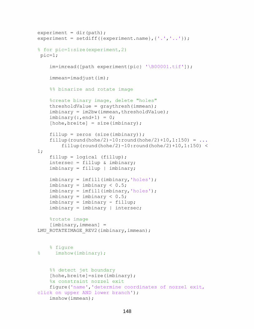
148

experiment = dir(path);

experiment = setdiff({experiment.name},{'.','..'});

% for pic=1:size(experiment,2)

pic=1;

im=imread([path experiment{pic} '\B00001.tif']);

immean=imadjust(im);

%% binarize and rotate image

%create binary image, delete "holes"

thresholdValue = graythresh(immean);

imbinary = im2bw(immean,thresholdValue);

imbinary(:,end+1) = 0;

[hohe,breite] = size(imbinary);

fillup = zeros (size(imbinary));

fillup(round(hohe/2)-10:round(hohe/2)+10,1:150) = ...

fillup(round(hohe/2)-10:round(hohe/2)+10,1:150) <

1;

fillup = logical (fillup);

intersec = fillup & imbinary;

imbinary = fillup | imbinary;

imbinary = imfill(imbinary,'holes');

imbinary = imbinary < 0.5;

imbinary = imfill(imbinary,'holes');

imbinary = imbinary < 0.5;

imbinary = imbinary - fillup;

imbinary = imbinary | intersec;

%rotate image

[imbinary,immean] =

LMU_ROTATEIMAGE_REV2(imbinary,immean);

% figure

% imshow(imbinary);

%% detect jet boundary

[hohe,breite]=size(imbinary);

%x constraint nozzel exit

figure('name','determine coordinates of nozzel exit,

click on upper AND lower branch');

imshow(immean);

149

[x0 ynozzlerand]=ginput(2);

close

x0=round((x0(1)+x0(2))/2);

% % columns=sum(imbinary(1:1200,:),1);

% % x0=find(columns==min(columns),1,'first');

if exist('im_calib','var') == 0

im_calib = D/abs(ynozzlerand(1)-ynozzlerand(2));

end

%y value middle of nozzle

ynozzle=(ynozzlerand(1)+ynozzlerand(2))/2;

% % %y constraint upper branch

% % y0_up=find(imbinary(1:1200,x0),1,'first');

% %

% % %y constraint lower branch

% % y0_low=find(imbinary(1:1200,x0),1,'last');

% detect jet boundary

bound = bwtraceboundary(imbinary,...

[find(imbinary(:,floor(x0+xstart*D/im_calib)),1,'first')

floor(x0+xstart*D/im_calib)]...

,'S',8,inf,'clockwise');

%detect upper and lower boundary seperately (of bound)

% % x_ind=find(bound(:,2)==x0);

% % bound=bound(1:x_ind(2),:);

xbound_up=[];

ybound_up=[];

xbound_low=[];

ybound_low=[];

for i=1:size(bound,1)

if (bound(i,1)>ynozzle) && (bound(i,1)<hohe) &&

(bound(i,2)>x0+xstart*D/im_calib) && (bound(i,2)<breite)

xbound_low(end+1,1)=bound(i,2);

ybound_low(end+1,1)=bound(i,1);

elseif (bound(i,1)<ynozzle) && (bound(i,1)>1) &&

(bound(i,2)>x0+xstart*D/im_calib) && (bound(i,2)<breite)

xbound_up(end+1,1)=bound(i,2);

ybound_up(end+1,1)=bound(i,1);

end

150

end

%% jet angle with least squares method

%upper branch

Aeq_up=[1 x0];

beq_up=min(ynozzlerand);

gradient2_up=[];

for i=xbound_up(1):n:xbound_up(end)

if (xbound_up(end)-i)/n >= 1 || (xbound_up(end)-

i)/n == 0

%fill Vandermonde-matrix V2_up

xint_up=[];

upy2_sel=[];

for m=1:size(xbound_up,1)

if xbound_up(m) >= i && xbound_up(m) < i+n

xint_up(end+1,1)=xbound_up(m);

upy2_sel(end+1,1)=ybound_up(m);

end

end

V2_up=[ones(size(xint_up,1),1) xint_up];

%solve upper jet angle (gradient2_up)

p2_up = lsqlin(V2_up, upy2_sel, [], [], Aeq_up,

beq_up);

gradient2_up(end+1)=p2_up(2);

end

end

%lower branch

xbound_low=flipud(xbound_low);

ybound_low=flipud(ybound_low);

Aeq_low=[1 x0];

beq_low=max(ynozzlerand);

gradient2_low=[];

for i=xbound_low(1):n:xbound_low(end)

if (xbound_low(end)-i)/n >= 1 || (xbound_low(end)-

i)/n == 0

%fill Vandermonde-matrix V2_low

xint_low=[];

upy2_sel=[];

for m=1:size(xbound_low,1)

if xbound_low(m) >= i && xbound_low(m) <

i+n

xint_low(end+1,1)=xbound_low(m);

upy2_sel(end+1,1)=ybound_low(m);

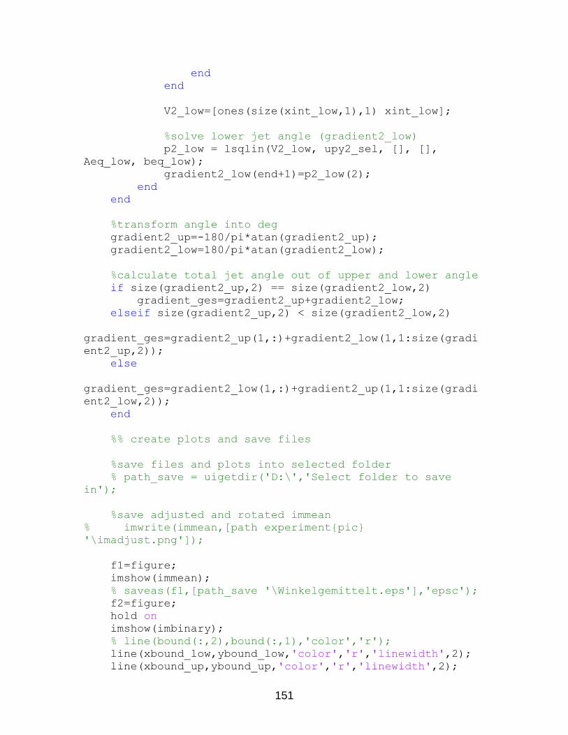
151

end

end

V2_low=[ones(size(xint_low,1),1) xint_low];

%solve lower jet angle (gradient2_low)

p2_low = lsqlin(V2_low, upy2_sel, [], [],

Aeq_low, beq_low);

gradient2_low(end+1)=p2_low(2);

end

end

%transform angle into deg

gradient2_up=-180/pi*atan(gradient2_up);

gradient2_low=180/pi*atan(gradient2_low);

%calculate total jet angle out of upper and lower angle

if size(gradient2_up,2) == size(gradient2_low,2)

gradient_ges=gradient2_up+gradient2_low;

elseif size(gradient2_up,2) < size(gradient2_low,2)

gradient_ges=gradient2_up(1,:)+gradient2_low(1,1:size(gradi

ent2_up,2));

else

gradient_ges=gradient2_low(1,:)+gradient2_up(1,1:size(gradi

ent2_low,2));

end

%% create plots and save files

%save files and plots into selected folder

% path_save = uigetdir('D:\','Select folder to save

in');

%save adjusted and rotated immean

% imwrite(immean,[path experiment{pic}

'\imadjust.png']);

f1=figure;

imshow(immean);

% saveas(f1,[path_save '\Winkelgemittelt.eps'],'epsc');

f2=figure;

hold on

imshow(imbinary);

% line(bound(:,2),bound(:,1),'color','r');

line(xbound_low,ybound_low,'color','r','linewidth',2);

line(xbound_up,ybound_up,'color','r','linewidth',2);

152

set(gca,'position',[0 0 1 1],'units','normalized');

% saveas(f2,[path experiment{pic}

'\binaryimage.tif'],'tif');

% subplot(3,3,1);

% imshow(immean);

% % Maximize the figure window.

% set(gcf, 'Position', get(0, 'ScreenSize'));

% % Force it to display RIGHT NOW (otherwise it might

not display until it's all done, unless you've stopped at a

breakpoint.)

% drawnow;

%

% % Just for fun, let's get its histogram.

% [pixelCount grayLevels] = imhist(immean);

% subplot(3, 3, 2);

% bar(grayLevels,pixelCount); title('Histogram of

original image');

% xlim([0 grayLevels(end)]); % Scale x axis manually.

%

%

% % Display the binary image.

% subplot(3, 3, 3);

% imagesc(imbinary); colormap(gray(256)); title('Binary

Image, obtained by thresholding');

%

% subplot(3,3,4);

% imshow(imbinary);

% line(bound(:,2),bound(:,1),'color','r');

% hold on

xD_up=xstart+n*size(gradient2_up,2)*im_calib/D;

xD_low=xstart+n*size(gradient2_low,2)*im_calib/D;

xD_end=(breite-x0)*im_calib/D;

figure1=figure;

set(figure1,'defaultTextInterpreter','Latex');

xvec2_up=(xstart+n*im_calib/(2*D):n*im_calib/D:xD_up-

n*im_calib/(2*D));

xvec2_low=(xstart+n*im_calib/(2*D):n*im_calib/D:xD_low-

n*im_calib/(2*D));

xvec_ges=(xstart+n*im_calib/(2*D):n*im_calib/D:min(xD_up,xD

_low)-n*im_calib/(2*D));

153

plot(xvec2_up,gradient2_up,'b.',xvec2_low,gradient2_low,'g.

',xvec_ges,gradient_ges,'r.')

set(gca, 'XTick', 0:2:ceil(xD_end), 'YLim', [0

20],'fontsize',fontsize);

% if max(gradient_ges) <= 85

% set(gca, 'XTick', 0:0.5:xD_end, 'YLim', [0 90]);

% else

% set(gca, 'XTick', 0:0.5:xD_end, 'YLim', [0

max(gradient_ges)+5]);

% end

xlabel('$x/D$');

ylabel('Winkel [$\circ$]');

I=legend('$\alpha_{oben}$','$\alpha_{unten}$','$\alpha_{ges

}$');

set(I,'interpreter','Latex','fontsize',fontsize);

%save jet angle data

result=cell(2,size(gradient_ges,2)+1);

result{1,1}='x-coordinate(x/D)';

result{2,1}='spray angle [deg]';

for q=1:size(gradient_ges,2)

result{1,q+1}=xvec_ges(q);

result{2,q+1}=gradient_ges(q);

end

% save([path experiment{pic} '\result'],'result');

versuch=experiment{pic}(13:26);

resultstruct.(sprintf(['Experiment_' versuch]))=result;

% saveas(figure1,[path_save '\winkel_' versuch

'.eps'],'epsc');

% xlswrite(['jet_angle.xls'],{versuch},'Sheet1',['A'

num2str(pic*2)]);

% xlswrite(['jet_angle.xls'],result,'Sheet1',['B'

num2str(pic*2)]);

close all

% end

% save('result_all','resultstruct');

154

LMU_ROTATEIMAGE_REV2.m function [imbinary,immean] =

LMU_ROTATEIMAGE_REV2(imbinary,immean)

%% FUNCTION HEADER FOR LMU_ROTATIONANGLE

% SUPERIOR: various

% INFERIOR: none

%

%

% LAST MODIFICATION: 19.01.2015

% AUTHOR: Lukas Muser

% DESCRIPTION:

% detects the rotation angle for tilted near nozzle spray

images

% INPUT: imbinary - binary image

% immean - average image

%

% OUTPUT: imbinary - rotated binary image

% immean - rotated average image

%

%

%%

[m,n] = size(imbinary);

imbin = imbinary(ceil(0.1*m):floor(0.8*m),ceil(0.2*n):n-1);

columns = sum(imbin,1);

%detect rotation angle

symLine = [];

ind = [];

for i=1:size(imbin,2)

if columns(1,i) ~= 0

ind(1,end+1) = find(imbin(:,i),1,'first');

symLine(1,end+1) = i;

symLine(2,end) = ind(1,end) + 0.5*columns(1,i);

end

end

V = [ones(size(symLine,2),1) symLine(1,:)'];

gradient = lsqlin(V,symLine(2,:)',[],[]);

angle = 180/pi * atan(gradient(2));

%rotate images

155

immean = imrotate(immean,angle);

imbinary = imrotate(imbinary,angle);

%delete "rotation boundary"

im_size = size(immean);

row_del = (im_size(2) * tan(pi/180 * -angle) - im_size(1) *

tan(pi/180 * -angle)^2) / (1 - tan(pi/180 * -angle)^2);

col_del = (im_size(1) - row_del) * tan(pi/180 * -angle);

immean(1:ceil(row_del)+1,:) = [];

immean(end-ceil(row_del):end,:) = [];

immean(:,1:ceil(col_del)+1) = [];

immean(:,end-ceil(col_del):end) = [];

imbinary(1:ceil(row_del)+1,:) = [];

imbinary(end-ceil(row_del):end,:) = [];

imbinary(:,1:ceil(col_del)+1) = [];

imbinary(:,end-ceil(col_del):end) = [];

end

156

Run_Background.m

clear all

[filename, pathname] = uigetfile('*.*','Find background

image','C:\Shaun\Tests\');


if filename==0

fprintf('No file was selected!\n')

return

end

X=double(imread(location,1));

vert=length(X(:,1))

horz=length(X(1,:))

sum=zeros(vert,horz);

know=imfinfo(location);

nimg=length(know);

total=0;

for k=1:nimg

X = double(imread(location,k));

sum=sum+X;

total=total+1;

end

background=sum/total;

figure(1);

image(background*64/max(max(background)));

doit=input('Would you like to save this image y/n?','s');

if doit=='y'

eval(['save ' pathname(1:end) '\background.mat

background']);

else

fprintf('This was not saved.\n');

end

157

Run_Preview_Coaxial.m % Shaun DeSouza

% 03/11/16

%

% Shows graphs of sensory data to check that experiental

conditions

% have been hit

% Saves data in proceessed and meaningful form to

'ProcessedData.txt'

% This program must be run before full processing can be

done

% Folders must be organized prior to running this program

% 1 time [s]

% 2 liquid temperature [C]

% 3 chamber temperature [C]

% 4 ext sync [V]

% 5 chamber pressure [atm]

% 6 liquid pressure [atm]

% 7 gas pressure [atm]

% 8 flow liquid [V]

% 9 gas flow [V]

%% Importing Data File

clear all

[filename, pathname] = uigetfile('*.*','Find run to

process','D:\Shaun\Tests\Data_03_24_16');


fid = fopen(location);

data = fscanf(fid,'%f %f %f %f %f %f %f %f %f',[9 inf]); %

It has nine rows now.

data = data'; % transpose to 9 columns

fclose(fid); % close the file, all relavant data has been

stored

%% Data Timing

samples=length(data); % total number of samples

time=data(:,1); % first column of data represents time

in steps

step=time(2); % this position is first step from

time(1)=0

fs=1/step; % sample rate

%% Processing Liquid Flow Data

[num1,den1]=butter(6,0.1);

f_data=filter(num1,den1,data(:,8));

158

NofB=20; % number of blocks that will be fit in total

time

delta=step*floor((samples-1)/NofB); % length in time of

block

chunk=floor((samples-1)/NofB); % indexed size of

block

for i=1:NofB

Block(:,i)=data(chunk*(i-1)+2:chunk*i+1,8);

BlockTime(i)=delta*(i-1/2); % at center of

block

end

for i=1:NofB

[Pxx,f] = pwelch(Block(:,i),[],[],[],fs);

[val,ind]=max(Pxx);

domfreq(i)=floor(f(ind));

end

% liqflow=6.545151*(0.0054*domfreq+0.2483); %[cm^3/s]

% liqflow2=6.545151*(0.0069*domfreq+0.0087); %[cm^3/s]

% liqflow3=6.545151*(0.0842*domfreq+2.1921); %[cm^3/s]

% liqflow4=0.0808*domfreq+1.5095; %[cm^3/s]

% liqflow5=0.081*domfreq+1.2899;

% liqflow=(1.6251609933+0.0353438154*domfreq); %Labview

% liqflow=0.0082*domfreq+1.1009; %[cc/s] calibration data

with zero 4/11/16

liqflow=0.0057*domfreq+1.2794; %[cc/s] calibration data

4/11/16

for q=1:NofB

data(chunk*(q-1)+1:chunk*q,8)=liqflow(q);

end

data(chunk*q:end,8)=liqflow(q); % save processed liquid

flow data to file

%% Processing Temperature Data

Fc = fs/200; % carrier frequency

F = Fc/fs; % change F to vary the filter's cutoff

frequency.

[num,den] = butter(6,F); % design butterworth filter.

scrsz = get(0,'ScreenSize');

h=figure('Name','Sensor output

plots','NumberTitle','off','Position',[2 2 scrsz(3)

scrsz(4)-70]);

%Filter Liquid Temperature

spot1=filter(num,den,data(:,2)); % temporary variable to

filter data

data(:,2)=spot1; % save processed liquid temperature to

data file [C]

159

%Filter Chamber Temperature

spot2=filter(num,den,data(:,3));

data(:,3)=spot2; % save processed chamber temperature to

data file [C]

%Plot Temperature Data

subplot(2,2,1);plot(time,spot1)

hold on % all temperature's appear on same plot

plot(time,spot2,'r')

title('Temperature Readings')

xlabel('Time (s)')

ylabel('Temperature ({\circ} C)')

legend('Liquid','Chamber top',1)

%% Process Pressure Data

%Filter Pressure Data

[num2,den2]=butter(6,F);

f_data_1=filter(num2,den2,data(:,5)); % Chamber Pressure

f_data_2=filter(num2,den2,data(:,6)); % Liquid Pressure

f_data_3=filter(num2,den2,data(:,7)); % Gas Pressure

data(:,5)=f_data_1; % save processed pressures to data file

data(:,6)=f_data_2;

data(:,7)=f_data_3;

%% Plotting Pressure Data

subplot(2,2,2);plot(time,data(:,5),'r')

hold on % All pressures appear on the same plot

plot(time,data(:,6),'b')

plot(time,data(:,7),'g')

title('Pressure Readings')

xlabel('Time (s)')

ylabel('Pressure (atm)')

tempmax=max(data(:,6)); % following finds max pressure

so to scale axis START

if max(data(:,5))>tempmax

tempmax=max(data(:,5));

end

ymax=1.1*tempmax; % max found so axis is pretty END

axis([0 1 0 ymax])

axis 'auto x'

legend('Chamber','Liquid',1)

%% Processing Gas Data

g_data=filter(num2,den2,data(:,9));

% Standard Calibration Flow Rate

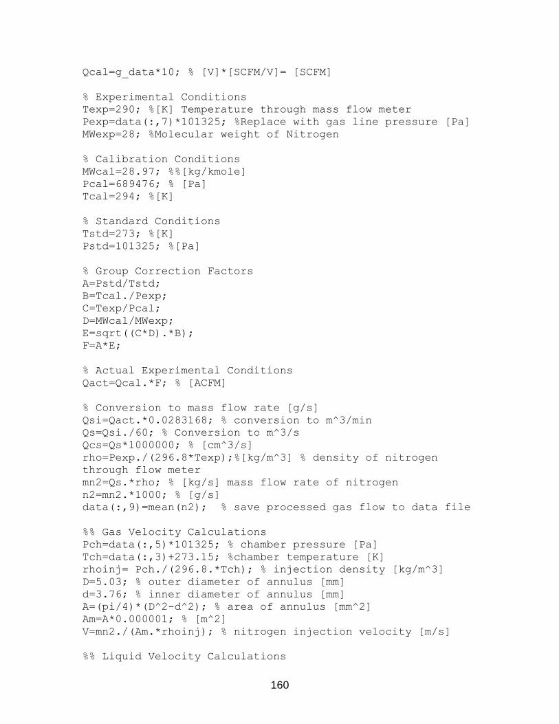
160

Qcal=g_data*10; % [V]*[SCFM/V]= [SCFM]

% Experimental Conditions

Texp=290; %[K] Temperature through mass flow meter

Pexp=data(:,7)*101325; %Replace with gas line pressure [Pa]

MWexp=28; %Molecular weight of Nitrogen

% Calibration Conditions

MWcal=28.97; %%[kg/kmole]

Pcal=689476; % [Pa]

Tcal=294; %[K]

% Standard Conditions

Tstd=273; %[K]

Pstd=101325; %[Pa]

% Group Correction Factors

A=Pstd/Tstd;

B=Tcal./Pexp;

C=Texp/Pcal;

D=MWcal/MWexp;

E=sqrt((C*D).*B);

F=A*E;

% Actual Experimental Conditions

Qact=Qcal.*F; % [ACFM]

% Conversion to mass flow rate [g/s]

Qsi=Qact.*0.0283168; % conversion to m^3/min

Qs=Qsi./60; % Conversion to m^3/s

Qcs=Qs*1000000; % [cm^3/s]

rho=Pexp./(296.8*Texp);%[kg/m^3] % density of nitrogen

through flow meter

mn2=Qs.*rho; % [kg/s] mass flow rate of nitrogen

n2=mn2.*1000; % [g/s]

data(:,9)=mean(n2); % save processed gas flow to data file

%% Gas Velocity Calculations

Pch=data(:,5)*101325; % chamber pressure [Pa]

Tch=data(:,3)+273.15; %chamber temperature [K]

rhoinj= Pch./(296.8.*Tch); % injection density [kg/m^3]

D=5.03; % outer diameter of annulus [mm]

d=3.76; % inner diameter of annulus [mm]

A=(pi/4)*(D^2-d^2); % area of annulus [mm^2]

Am=A*0.000001; % [m^2]

V=mn2./(Am.*rhoinj); % nitrogen injection velocity [m/s]

%% Liquid Velocity Calculations

161

di=2.235; % injector diameter [mm]

dm=di/1000; % injector diameter [m]

Ai=(pi/4)*(dm^2); % injector area [m^2]

LiqTemp=mean(data(:,2)); % liquid temp [C]

ChmPres=mean(data(10000:end,5)); % chamber pressure [atm]

MassFlow=1.64.*liqflow; % [g/s]

data(:,8)=mean(MassFlow); % [g/s] save processed liquid

flow rate to data file

LiqDen=goodeqn_liq(LiqTemp,ChmPres); % [kg/m^3]

U=(MassFlow/1000)/(LiqDen*Ai); % [m/s]

%% Momentum Flux and Velcity Ratios

Pout=mean(rhoinj)*(mean(V))^2; % outer jet momentum

Pin=mean(LiqDen)*(mean(U))^2; % inner jet momentum

M=Pout/Pin; % momentum flux ratio

Vr= mean(V)/mean(U); % velocity Ratio

%% Group Experimental Conditions

Vm=mean(V); %nitrogen velocity m/s

Um=mean(U); %fk velocity m/s

n2mdot=mean(mn2); %nitrogen flowrate g/s

fkmdot=mean(MassFlow); %fk flow rate g/s

Pchm=mean(f_data_1); %chamber pressure atm

Tchm=mean(spot2); %chamber temperature C

n2den=mean(rhoinj);

exp_cond=[M Vm Um LiqDen n2den LiqTemp Tchm Pchm fkmdot

n2mdot];

%% Plotting Liquid and Gas Data

subplot(2,2,3);plot(BlockTime,liqflow);hold

on;plot(BlockTime,liqflow,'r.');hold off;%spot)

hold on

plot(time, Qcs);

title('Flow Meter Data')

xlabel('Time (s)')

ylabel('Flow (cc/s)')

plot(time, data(:,9));

legend('Gas','Liquid',1);

ymax=1.1*max(Qcs);

axis([0 1 0 ymax])

axis 'auto x'

%% Plotting Camera Sync Data

subplot(2,2,4);plot(time,data(:,4),'g')

title('Camera Sync output') % Camera Sync Output is

connected to the Not Scan output of the ST-133 (Ch 1

labeled).

162

xlabel('Time (s)')

ylabel('Voltage (V)')

%% Saving Data and Plots

hgsave([pathname 'PDI_' filename(9:end) '.fig']);

newloc=[pathname 'ProcessedData.txt'];

eval(['save ' newloc ' data -ascii -tabs']);

163

Shadowgraphy_Processing.m

%% Shadowography image processing

%% Call test image

test = 'exp_2.tif';

info = imfinfo(test);

frames = numel(info);

test_img=[];

for k = 1:frames

t_img = imread(test, k, 'Info', info);

t_img = im2double(t_img);

test_img(:,:,k)=t_img;

end

%% Call background image

bckgrnd='background_1.tif';

know=imfinfo(bckgrnd);

n=length(know);

X=zeros(size(test_img(:,:,1)));

for i=1:n

X=X+im2double(imread(bckgrnd,i));

end

bckgrnd_avg=X/n; % average background image

%% Image adjustmest

for j = 1:frames

a_img=bckgrnd_avg-test_img(:,:,j); % background

subtraction

a_img(a_img<0)=0; % adjusted image

adj_img(:,:,j)=a_img;

end

imshow(imadjust(adj_img(:,:,10)))

sum =zeros(size(adj_img(:,:,1)));

for i = 1:size(adj_img,3)

sum = sum + adj_img(:,:,i);

end

adj_av = sum / size(adj_img,3); % averaged image

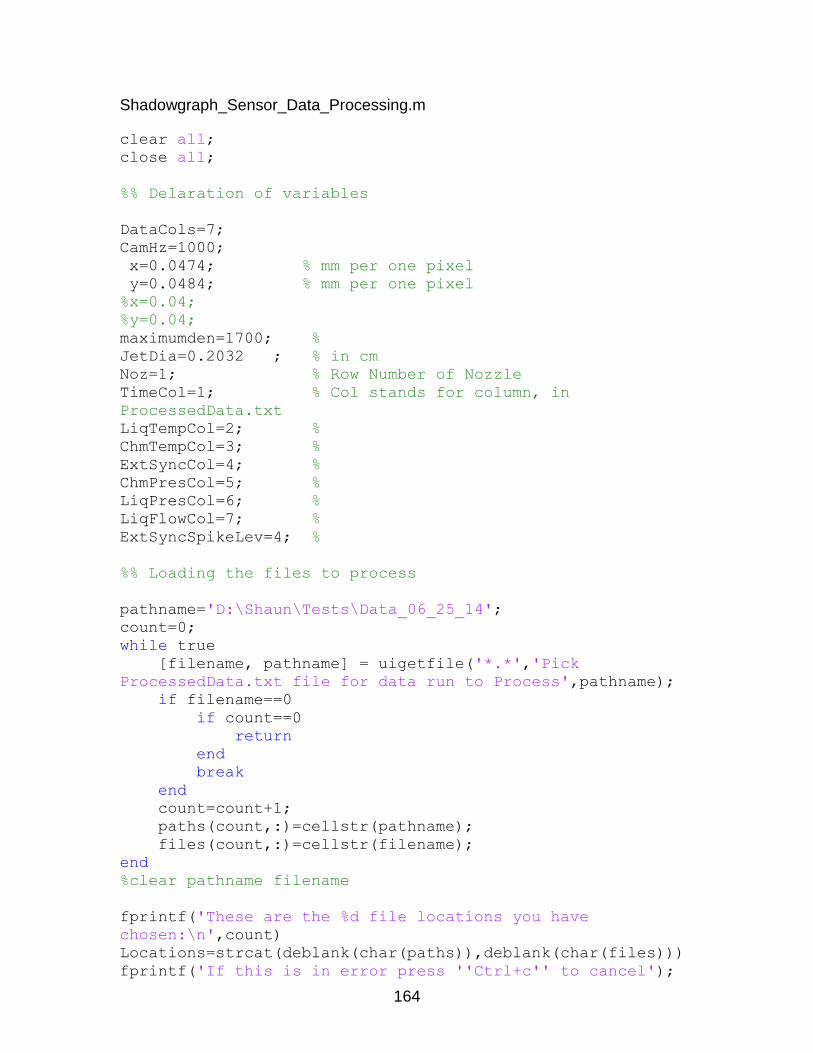
164

Shadowgraph_Sensor_Data_Processing.m

clear all;

close all;

%% Delaration of variables

DataCols=7;

CamHz=1000;

x=0.0474; % mm per one pixel

y=0.0484; % mm per one pixel

%x=0.04;

%y=0.04;

maximumden=1700; %

JetDia=0.2032 ; % in cm

Noz=1; % Row Number of Nozzle

TimeCol=1; % Col stands for column, in

ProcessedData.txt

LiqTempCol=2; %

ChmTempCol=3; %

ExtSyncCol=4; %

ChmPresCol=5; %

LiqPresCol=6; %

LiqFlowCol=7; %

ExtSyncSpikeLev=4; %

%% Loading the files to process

pathname='D:\Shaun\Tests\Data_06_25_14';

count=0;

while true

[filename, pathname] = uigetfile('*.*','Pick

ProcessedData.txt file for data run to Process',pathname);

if filename==0

if count==0

return

end

break

end

count=count+1;

paths(count,:)=cellstr(pathname);

files(count,:)=cellstr(filename);

end

%clear pathname filename

fprintf('These are the %d file locations you have

chosen:\n',count)

Locations=strcat(deblank(char(paths)),deblank(char(files)))

fprintf('If this is in error press ''Ctrl+c'' to cancel');

165

clear Locations

for i=1:count

pathname=deblank(char(paths(i)));

filename=deblank(char(files(i)));



TotalFrames=round(length(Pdata)/1100);

%TotalFrames=100

samples=length(Pdata); % Total

number of samples

step=Pdata(2,TimeCol); % This position is first step

from time(1)=0

% Finding the index of each image wrt

'ProcessedData.txt'

Frame=0;

LengthCounter=0;

check=0;

count=0;

for i=1:samples

if Pdata(i,ExtSyncCol)>=ExtSyncSpikeLev

count=count+1;

LiqTemp(count)=Pdata(i,LiqTempCol);

ChmTemp(count)=Pdata(i,ChmTempCol);

ChmPres(count)=Pdata(i,ChmPresCol);

LiqPres(count)=Pdata(i,LiqPresCol);

MassFlow(count)=1.64*Pdata(i,LiqFlowCol); %

Units (g/s)

RefDen(count)=goodeqn_liq(LiqTemp(count),ChmPres(count));

% Units (kg/m^3)

velocity(count)=10*MassFlow(count)/(RefDen(count)*(pi/4)*Je

tDia^2);

LengthCounter=LengthCounter+1;

IndexOfSpike(LengthCounter)=i;

else

if check==1

Frame=Frame+1;

FrameIndex(Frame)=round(mean(IndexOfSpike));

check=0;

LengthCounter=0;

clear IndexOfSpike

end

end

166

end

end

%% Average conditions during experiment

LiqTempavg=mean(LiqTemp)

ChmTempavg=mean(ChmTemp)

ChmPresavg=mean(ChmPres)

LiqPresavg=mean(LiqPres)

MassFlowavg=mean(MassFlow)

RefDenavg=mean(RefDen)

velocityavg=mean(velocity)

167

Spreading_Angle.m

function angle_std=Spreading_Angle(location,count,origin)

sprangle(1:count,1:2)=0;

totspread(1:count)=0;

thres(1:count)=0;

%% Calculating the threshold density for jet boundary using

peak density

%% gradients

for k=1:count

current=char(location(k,:));

colormap(load([current(1:49)

'Laser_Sheet_Profile\mymap.txt']));

img=load(current);

clrimg=round(64*img.DensMatrix/max(max(img.DensMatrix)));

if (k==1)

image(clrimg);

inp=input('Do you want to input threshold value

manually? (y/n)','s'); inp='n';

if (inp=='n')

ans1=input('Supercritical Test? (y/n)','s');

ans1='y';

ans2=input('Single Species? (y/n)','s');

ans2='n';

if (ans2=='n')

lower=10;

upper=30;

end

if (ans1=='y') && (ans2=='y')

lower=35;

upper=45;

end

if (ans1=='n') && (ans2=='y')

lower=20;

upper=35;

end

else

lower=input('Enter lower threshold value for

jet boundary:');

upper=input('Enter upper threshold value for

jet boundary:');

end

disp(strcat('Lower threshold=',num2str(lower)));

disp(strcat('Upper threshold=',num2str(upper)));

close all;

end

grad=abs(gradient(img.DensMatrix(50,:)));

[peak,locs]=findpeaks(grad);

168

nozwidth=40;

for l=1:length(locs)

if (locs(l)>(origin-nozwidth)) &&

(locs(l)<(origin+nozwidth))

if ((clrimg(50,locs(l))>lower) &&

(clrimg(50,locs(l))<upper))

thres(k)=clrimg(50,locs(l));

break;

end

end

end

end

%% Forcing a non-zero threshold condition

cnt=1;

for i=1:count

if (thres(i)~=0)

thresh(cnt)=thres(i);

cnt=cnt+1;

end

end

threshold=min(thresh);

%% Calculating the jet spreading angle

for k=1:count

current=char(location(k,:));

img=load(current);

clrimg=round(64*img.DensMatrix/max(max(img.DensMatrix)));

%% Setting the color of the jet surroundings to white

row=length(clrimg);

col=size(clrimg,2);

for i=1:row

for j=1:col

if clrimg(i,j)<threshold

clrimg(i,j)=0;

end

end

end

clrimg(:,1:(origin-100))=0;

clrimg(:,(origin+100):end)=0; % Anything 70 pixels away

from the origin is set to white

figure(1);

image(clrimg);

hold on;

plot(clrimg(50,:));

plot(grad,'k');

colormap(load([current(1:49)

'Laser_Sheet_Profile\mymap.txt']));

[alph1,alph2]=Divergence_Angle(clrimg,origin,row);

169

sprangle(k,1)=(alph1)*180/pi;

sprangle(k,2)=(alph2)*180/pi;

totspread(k)=abs(sprangle(k,2)-sprangle(k,1));

end

cnt=1;

for i=1:count

if (abs(totspread(i)-mean(totspread))<std(totspread))

angle_final(cnt)=totspread(i);

cnt=cnt+1;

end

end

figure(100)

clf

plot(totspread,'o-');

hold on;

avg_spr(1:count)=mean(totspread);

plot((1:count),avg_spr,'g',(1:count),avg_spr-

std(totspread),'r-.',(1:count),avg_spr+std(totspread),'r-

x');

avg_final=mean(angle_final);

plot(avg_final*ones(1,cnt),'k');

xlabel('No. of images considered','Fontsize',14);

ylabel('Spreading Angle','Fontsize',14);

legend('All angles','Mean spreading angle','Lower standard

deviation','Upper standard deviation','Modified mean');

disp(strcat('Average spreading angle is:

',num2str(avg_final),' degrees'));

disp(strcat('Standard deviation is:

',num2str(std(angle_final)),' degrees'));

angle_std=[avg_final std(angle_final)];

170

Test_Conditions.m

%% This program prints the test conditions to the logbook

close all

clear all

%% Initialize variables

JetDia=2.235; % mm

LiqTempCol=2;

ChmTempCol=3;

ExtSyncCol=4;

ChmPresCol=5;

LiqPresCol=6;

GasPresCol=7;

LiqFlowCol=8;

GasFlowCol=9;

pathname='D:\Shaun\Tests\';

count=0;

while true

[filename, pathname] = uigetfile('*.fig','Pick PDI file

to Process',pathname);

if filename==0

if count==0

return

end

break

end

count=count+1;

paths(count,:)=cellstr(pathname);

files(count,:)=cellstr(filename);

end

fprintf('These are the %d file locations you have

chosen:\n',count)

Locations=strcat(deblank(char(paths)),deblank(char(files)))

fprintf('If this is in error press ''Ctrl+c'' to cancel');

clear Locations

%% Flow meter correction

flowmeter=input('Does flowmeter work for this

case(s)?(y/n)','s');

for i=1:count

pathname=deblank(char(paths(i)));

filename=deblank(char(files(i)));

location=[pathname 'ProcessedData.txt'];


samples=length(Pdata);

TimeIndex=1;

if (flowmeter=='y')

gradflow=gradient(Pdata(:,LiqFlowCol));

171

for l=1:samples


TimeIndex=l;

break;

end

end

else

gradtemp=gradient(Pdata(5000:end-5000,LiqTempCol));

for k=5000:samples-5000

if (gradtemp(k-5000+1)==max(gradtemp))

TimeIndex=k;

break;

end

end

end

LiqTemp(i)=mean(Pdata(TimeIndex:end,LiqTempCol));

LiqPres(i)=mean(Pdata(TimeIndex:end,LiqPresCol));

ChmTemp(i)=mean(Pdata(TimeIndex:end,ChmTempCol));

ChmPres(i)=mean(Pdata(TimeIndex:end,ChmPresCol));

MassFlow(i)=mean(Pdata(TimeIndex:end,LiqFlowCol));

mn2(i)=mean(Pdata(TimeIndex:end,GasFlowCol));

RefDen=goodeqn_liq(LiqTemp(i),ChmPres(i));

end

%% Flow Calculations

LiqTemp=mean(LiqTemp); % [C]

LiqPres=mean(LiqPres); % [atm]

ChmTemp=mean(ChmTemp); % [C]

MassFlow=mean(MassFlow); % [g/s]

mn2=mean(mn2); % [g/s]

RefDen=mean(RefDen); % [kg/m^3]

dm=JetDia/1000; % [m]

U=(MassFlow/1000)/(RefDen*(pi/4)*dm^2); % [m/s]

Pch=ChmPres*101325; % chamber pressure [Pa]

Tch=ChmTemp+273.15; %chamber temperature [K]

rhoinj= Pch/(296.8*Tch); % injection density [kg/m^3]

D=5.03; % outer diameter of annulus [mm]

d=3.76; % inner diameter of annulus [mm]

A=(pi/4)*(D^2-d^2); % area of annulus [mm^2]

Am=A*0.000001; % [m^2]

V=(mn2/1000)/(Am*mean(rhoinj)); % nitrogen injection

velocity [m/s]

Pout=mean(rhoinj)*(mean(V))^2; % outer jet momentum

Pin=mean(RefDen)*(U)^2; % inner jet momentum

M=Pout/Pin; % momentum flux ratio

TestMatrix=[M V U RefDen rhoinj LiqTemp ChmTemp ChmPres

MassFlow mn2];

xlswrite('D:\Shaun\Tests\Coaxial_PLIF_Logbook.xlsx',TestMat

rix,'F33:O33');

172

APPENDIX D LABVIEW CODE FOR EXPERIMENTAL CONTROL

The LabVIEW code used to facilitate the control of experiments and

recording of sensor data is included in this section. The overall architecture of the

wiring and block diagrams are mostly unchanged from the description and details

reported by Polikov [73]. The only changes made to the code is the range of

channels being recorded to the experimental data file. The gas pressure and

temperature as well as the gas flowmeter data are now set to record to the data

file. This allows calculation of the gas velocity as well as the outer-to-inner

velocity ratio, and momentum flux ratio. Images of the block diagram and wiring

diagram follow.

173

Figure D-1. LabVIEW wiring diagrams for the control of the gas valves and the temperature and pressure monitoring charts.

174

Figure D-2. LabVIEW wiring diagram for the gas flow data, shutdown of valves at the end of experiment, and control of the gas heater.

175

Figure D-3. LabVIEW wiring diagram for the control of the liquid and chamber heaters.

176

Figure D-4. LabVIEW wiring diagrams for the closure of valves at the end of an experiment.

177

Figure D-5. LabVIEW wiring diagram for the closure of valves and bypass solenoid valve control.

178

Figure D-6. LabVIEW wiring diagram for the processing and saving of data.

179

Figure D-7. LabVIEW wiring diagram for closing all valves in event of experiment termination.

180

LIST OF REFERENCES

[1] J. Plateau, "Statique Experimentale et Theorique des Liquids Soumie aux Seules Forces Moleculaire," Paris: Cauthier Vil- lars, vol. 1, no. 2, pp. 450-495, 1873.

[2] Rayleigh, "On the instabililty of jets," Proceedings of the London Mathematical Society, pp. 4-13, 14 November 1878.

[3] S. Chandrasekhar, Hydrodynamic and Hydromagnetic Stability, New York: Dover, 1961.

[4] C. Weber, "Disintegration of Liquid Jets," Journal of Applied Mathematics and Mechanics, vol. 11, p. 136, 1931.

[5] A. Sterling and C. Sleicher, "The instability of capillary jets," Journal of Fluid Mechanics, vol. 68, pp. 477-495, 1975.

[6] G. Taylor, Scientific Papers of G.I. Taylor, Cambridge: Cambridge University Press, 1962.

[7] W. Ohnesorge, "Formation of drops by nozzles and the breakup of liquid jets," Journal of Applied Mathematics, vol. 16, pp. 355-358, 1936.

[8] C. Dumouchel, "On the experimental investigation on primary atomization of liquid streams," Experiments in Fluids, vol. 45, no. 3, pp. 371-422, 2008.

[9] W. Ranz, On Sprays and Spraying, Pennsylvania State University, Department Of Engineering Research, Bulletin No. 65., 1956.

[10] C. Miesse, "Correlation of experimental data on the disintegration of liquid jets," Industrial and Engineering Chemistry, vol. 47, no. 9, pp. 1960-1701, 1955.

[11] R. Reitz, "Atomization and other breakup regimes of a liquid jet. PhD Thesis," Princeton University, Princeton, 1978.

[12] T. Dan, T. Yamamoto, J. Senda and H. Fujimoto, "Effect of nozzle configurations for characteristics of non-reacting diesdel fuel sprays," SAE Technical Paper 970355, pp. 259-274, 1997.

[13] G. Abramovich, Theory of Turbulent Jets, Cambridge: MIT Press, 1963.

181

[14] W. Mayer and H. Tamura, "Propellant Injection in a Liquid Oxygen/Gaseous Hydrogen Rocket Engine," Journal of Propulsion and Power, vol. 19, pp. 155-1602, 1971.

[15] A. Lefebvre, Atomization and Sprays, Routledge: CRC Press, 1988.

[16] R. Reitz and F. Bracco, "Mechanism of atomization of a liquid jet," Physics of Fluids, vol. 25, no. 10, pp. 1730-1742, 1982.

[17] T. Ohrn, D. Senser and A. Lefebvre, "Geometrical effects on discharge coefficients for plain-orifice atomizers," Atomization and Sprays, vol. 1, no. 2, pp. 137-153, 1991.

[18] T. Karasawa, M. Tanaka, K. Abe, S. Shiga and T. Kurabayashi, "Effect of nozzle configuration on the atomization of a steady spray," Atomization and Sprays, vol. 2, no. 4, pp. 411-426, 1992.

[19] P. Wu, T. Tseng and G. Faeth, "Primary breakup in gas/liquid mixing layers for turbulent liquids," in 30th Aerospace Science Meeting and Exhibit, Reno, NV, USA, 1992.

[20] H. Simmons, "The correlation of drop size distributions in fuel nozzle sprays," Journal of Engineering for Gas Turbines and Power, vol. 99, no. 3, pp. 309-314, 1977.

[21] P. Wu and G. Faeth, "Aerodynamic effects on the primary breakup of turbulent liquids," Atomization and Sprays, vol. 3, no. 3, pp. 265-289, 1993.

[22] G. Faeth, L. Hsiang and P. Wu, "Structure and breakup properties of sprays," International Journal of Multiphase Flow, vol. 21, pp. 99-127, 1995.

[23] G. Smallwood and O. Gulder, "Views on the structure of transient diesel sprays," Atomization and Sprays, vol. 10, no. 3-5, pp. 355-386, 2000.

[24] Y. Yue, C. Powell, R. Poola, J. Wang and J. Schaller, "Quantitative measurements of diesel fuel spray characteristics in the near-nozzle region using x-ray absorption," Atomization and Sprays, vol. 11, no. 4, pp. 471-490, 2001.

[25] K. Sallam, Z. Dai and G. Faeth, "Liquid breakup at the surface of turbulent round liquid jets in still gases," International Journal of Multiphase Flow, vol. 45, no. 3, pp. 427-449, 2002.

182

[26] M. Paciaroni, M. Linne, T. Hall, J. Delplanque and T. Praker, "Single-shot two-dimensional ballistic imaging of the liquid core in an atomizing spray," Atomization and Sprays, vol. 16, no. 1, pp. 51-70, 2006.

[27] A. Roy, "Subcritical and supercritical fuel injection and mixing in single and binary species systems," University of Florida, PhD Thesis, Gainesville, FL, USA, 2012.

[28] J. Newman and T. Brzustowski, "Behavior of a Liquid Jet near the Thermodynamic Critical Region," AIAA Journal, vol. 9, no. 8, pp. 1595-1602, 1971.

[29] T. Bruno and J. Ely, Supercritical Fluid Technology: Review in Modern Theory and Applications, CRC Press, 1991.

[30] B. Chehroudi, D. Talley and E. Coy, "Initial growth rate and visual characteristics of a round jet into a sub-to supercritical environment of relavence to rocket, gas turbine, and diesel engines," in Proceedings of the 37th AIAA Aerospace Science Meering and Exhibit, Reno, NV, USA, 1999.

[31] R. Reitz and F. Bracco, "On the dependence of spray angle and other spray parameters on nozzle design and operating condition," in Proceedings of the SAE International Congress of Exposition, Detroit, MI, USA, 1979.

[32] B. Chehroudi and D. Talley, "The fractal geometry of round turbulent cryogenic nitrogen jets at subcritical and supercritical pressures," Atomization and Sprays, vol. 14, no. 1, pp. 81-91, 2004.

[33] P. Dimotakis, "Two-Dimensional Shear-Layer Entrainment," AIAA Journal, vol. 24, no. 11, pp. 1791-1796, 1986.

[34] D. Papmoshou and A. Roshko, "The compressible turbulent shear layer: an experimental study," Journal of Fluid Mechanics, vol. 197, no. 1, pp. 453-477, 1988.

[35] G. Brown and A. Roshko, "On density effects and large structure in turbulent mixing layers," Journal of Fluid Mechanics, vol. 64, no. 4, pp. 775-816, 1974.

[36] B. Chehroudi, D. Talley and E. Coy, "Visual characteristics and initial growth rates of round cryogenic jets at subcritical and supercritical pressures," Physics of Fluids, vol. 14, no. 2, pp. 850-861, 2002.

[37] B. Chehroudi, R. Cohn, D. Talley and A. Badakhshan, "Raman scattering measurements in the initial region of sub-and supercritical jets," in Proceedings of the 36th Joint Propulsion Conference, Huntsville, AL, USA, 2000.

183

[38] M. Oschwald and M. Micci, "Spreading angle and centerline variation of density of supercritical nitrogen jets," Atomization and Sprays, vol. 12, no. 1-3, pp. 91-106, 2002.

[39] C. Segal and S. Polikov, "Subcritical to supercritical mixing," Physics of Fluids, vol. 20, no. 5, 2008.

[40] A. Roy, C. Segal and C. Joly, "Spreading Angle and Core Length Analysis of Supercritical Jets," AIAA Journal, vol. 51, no. 8, pp. 2009-2014, 2013.

[41] A. Roy, J. Gustavsson and C. Segal, "Spectroscopic properties of a perfluorinated ketone for PLIF applications," Experiments in Fluids, vol. 51, no. 5, pp. 1455-1463, 2011.

[42] G. Lamanna, E. Oldenhof, S. Baab, I. Stotz and B. Weigand, "Disintegration Regimes Near the Critical Point," in 18th AIAA/3AF International Space Planes and Hypersonic Systems and Technologies Conference, International Space Planes and Hypersonic Systems and Technologies Conference, Tours, FR, 2012.

[43] R. Branam and W. Mayer, "Characterization of cryogenic injection at supercritical pressure," Journal of Propulsion and Power, vol. 19, no. 3, pp. 342-355, 2003.

[44] W. Oschwald and A. Schik, "Supercritical nitrogen free jet investigation by spontaneous Raman scattering," Experiments in Fluids, vol. 27, no. 6, pp. 497-506, 1999.

[45] R. So, J. Zhu, M. Otugen and B. Hwang, "Some Measurements in a Binary Gas Jet," Experiments in Fluids, vol. 9, no. 5, pp. 273-294, 1990.

[46] C. Richards and W. Pitts, "Global density effects on the self-preservation behavior of turbulent free jets," Journal of Fluid Mechanics, vol. 254, pp. 417-435, 1993.

[47] A. Roy and C. Segal, "Experimental Study of Fluid Jet Mixing," Journal of Propulsion and Power, vol. 26, no. 6, pp. 1205-1211, 2010.

[48] A. Roy, C. Joly and C. Segal, "Disintegrating supercritical jets in a subcritical environment," Journal of Fluid Mechanics, vol. 717, pp. 193-202, 2013.

[49] T. Tran, "Acetone Planar Laser-Induced Fluorescence and Phosphorescence," Georgia Institue of Technology, PhD Thesis, Atlanta, GA, USA, 2008.

[50] Z. Farago and N. Chigier, "“Morphological Classification of Disintegration of Round Liquid Jets in a Coaxial Air Stream," Atomization and Sprays, vol. 2, no. 2, pp. 137-153, 992.

184

[51] J. Lasheras and E. Hopfinger, "Liquid jet instability and atomization in a coaxial gas stream," Annual Review of Fluid Mechanics, vol. 32, no. 1, pp. 275-308, 2000.

[52] N. Chigier and R. Reiz, "Regimes of Jet Breakup and Breakup Mechanismcs (Physical Aspects)," in Recent Advances in Spray Combustion: Spray Atomization and Drop Burning Phenomena, American Institute of Aeronautics and Astronautics, 1995, pp. 109-133.

[53] C. Engelbert, Y. Hardalupas and J. Whitelaw, "Breakup phenomenona in coaxial airblast atomizers," Proceedings Mathematical and Physical Sciences, vol. 451, no. 1941, pp. 189-229, 1995.

[54] H. Rehab, E. Villermaux and E. Hopfinger, "Flow regimes of large velocity ratio coaxial jets," Journal of Fluid Mechanics, vol. 347, no. 1, pp. 357-381, 1997.

[55] J. Lasheras, E. Villermaux and E. Hopfinger, "Break-up and atomization of a round water jet by a high-speed annular air jet," Journal of Fluid Mechanics, vol. 357, pp. 351-379, 1998.

[56] E. Villermaux, "Mixing and spray formation in coaxial jets," Journal of Propulsion and Power, vol. 14, no. 5, pp. 807-817, 1998.

[57] C. Varga, J. Lasheras and E. Hopfinger, "Intialy breakup of a small-diameter liquid jet by a high speed gas stream," Journal of Fluid Mechanics, vol. 497, pp. 405-434, 2003.

[58] G. Vivek, "Flow and atomization characteristics of a cryogenic fluid from a coaxial rocket injector," Proquest, Ann Arbor, MI, USA, 2014.

[59] J. Hulka and J. Hutt, "Instability Phenomena in Liquid Oxygen/Hydrogen Propellant Rocket Engines," in Liquid Rocket Engine Combustion Instability, AIAA Progress in Astronautics and Aeronautics, 1995, pp. 39-71.

[60] J. Telaar, G. Schneider and W. Mayer, "Experimental investigation of breakup of turbulent liquid jets," in ILASS-Europe, Darmstadt, Germany, 2000.

[61] D. Davis and B. Chehroudi, "The effects of pressure and acoustic field on a cryogenic coaxial jet," in Proceedings of the 42nd AIAA Aerospace Sciences Meeting and Exhibit, Reno, NV, USA, 2004.

[62] R. Woodward, S. Pal, S. Farhangi and G. Jensen, "LOX/GH2 shear coaxial injector atomization studies:effects of recesss and non-concentricity," in Proceedings of the 45th AIAA Aerospace Sciences Meeting and Exhibit, Reno, NV, USA, 2007.

185

[63] D. Davis and B. Chehroudi, "The effects of pressure and acoustic field on a cryogenic coaxial jet," in Proceedings of the 42nd AIAA Aerospace Sciences Meeting and Exhibit, Reno, NV, USA, 2004.

[64] D. Davis and B. Chehroudi, "Behaviour of a rocket-like coaxial injector in an acoustic field," in Proceedings of the 19th Annual Conference on Liquid Atomization and Spray Systems, Toronto, Canada, 2006.

[65] V. Gautam and A. Gupta, "Cryogenic Flow and Atomization from a Coaxial Injector," Journal of Propulsion and Power, vol. 25, no. 1, pp. 33-39, 2009.

[66] J. Rodiguez, J. Graham, I. Leyva, H. Lyu and D. Talley, "On the inner jet spread angles of coaxial jets from subcritical to supercritical conditions with preliminary numerical results," in 55th JANNAF Propulsion/4th LPS/3rd SPS/6th MSS Joint Meeting, Orlando, FL, USA, 2008.

[67] M. Oschwald, A. Schik, M. Klar and W. Mayer, "Investigation of coaxial LN2/GH2-injection at supercritical pressure by spontaneous raman scattering," in Proceedings of the 35th AIAA/ASME/SAE/ASEE Joint Propulsion Conference and Exhibit, Los Angeles, CA, USA, 1999.

[68] S. Schumaker and J. Driscoll, "Mixing Lengths of Coaxial Jets in a Rocket Combustor," in 43rd AIAA/ASME/SAE/ASEE Joint Propulsion Conference & Exhibit , Cincinnati, OH, USA, 2007.

[69] S. Leroux, C. Dumouchel and M. Ledoux, "The stability curve of Newtonian liquid jets," Atomization and Sprays, vol. 6, no. 6, pp. 623-647, 1996.

[70] C. Baumgarten, Mixture Formations In Internal Combustion Engines, Friedrichshafen: Springer, 2006.

[71] C. Eroglu, N. Chigier and Z. Farago, "Coaxial atomizer liquid intact lengths," Physics of Fluids, vol. 3, no. 2, pp. 303-308, 1991.

[72] R. Woodward, "Primary atomization of liquid jets issuing from rocket engine coaxial injectors [PhD Thesis]," Pennsylvania State University, Department of Mechanical Engineering, University Park PA, USA, 1993.

[73] S. Polikov, "Experimental study of subcritical to supercritical mixing," University of Florida, PhD Thesis, Gainesville, FL, USA, 2007.

[74] S. Polikov and C. Segal, "Characterization of a Perfluorinated Ketone for LIF Applications," in AIAA, Reno, NV, USA, 2008.

186

[75] A. Roy, C. Joly and C. Segal., "Disintegrating supercritical jets into subcritical environments," Journal of Fluid Mechanics, vol. 717, pp. 193-202, 2013.

[76] R. Reitz and F. Bracco, "On the Dependence of Spray Angle and Other Spray Parameters on Nozzle Design and Operating Condition," in SAE International Congress and Exposition, Detroit, MI, USA, 1979.

[77] E. Mayer, "Theory of liquid atomization," ARS, vol. 31, no. 12, pp. 1783-1785, 1961.

[78] B. Chehroudi, "Recent experimental efforts on high-pressure supercritical injection for liquid rockets and their implications," International Journal of Aerospace Engineering, vol. 2012, no. 2012, p. 31, 2012.

187

BIOGRAPHICAL SKETCH

Shaun DeSouza was born in Port of Spain, Trinidad and Tobago and grew up

Wesley Chapel, Florida where he completed high school in 2006. He attended the

University of South Florida and earned a Bachelor of Science in Mechanical

Engineering with a minor in Physics in 2011. He began his graduate work in Aerospace

Engineering at the University of Florida in 2012 and joined the Combustion and

Propulsion Laboratory in 2013 under the advisement of Professor Corin Segal. He

received his Ph.D. from the University of Florida in Fall 2016.

disintegration of single orifice and coaxial supercritical jets

Documents

Transcript of disintegration of single orifice and coaxial supercritical jets