IEEE/ACM TRANSACTIONS ON COMPUTATIONAL BIOLOGY AND BIOINFORMATICS, VOL. ?, NO. ?, MONTH-MONTH 2010 1

Disease liability prediction from large scalegenotyping data using classifiers with a reject

optionJose R. Quevedo, Antonio Bahamonde, Miguel Perez-Enciso and Oscar Luaces

Abstract—Genome-wide association studies (GWA) try to identify the genetic polymorphisms associated with variation in phenotypes.However, the most significant genetic variants may have a small predictive power to forecast the future development of commondiseases. We study the prediction of the risk of developing a disease given genome-wide genotypic data using classifiers with a rejectoption, which only make a prediction when they are sufficiently certain, but in doubtful situations may reject making a classification. Totest the reliability of our proposal, we used the Wellcome Trust Case Control Consortium (WTCCC) data set, comprising 14,000 casesof 7 common human diseases and 3,000 shared controls.

Index Terms—Genome-wide analysis, classification with a reject option, risk of common human diseases.

F

1 INTRODUCTION

THE aim of genome-wide association (GWA) studiesis to identify the genetic variants associated with

variation in phenotypes that are, hopefully, reasonablyclose to the actual causal mutations. There is a fastincreasing literature employing this approach, typicallyapplied to case/control studies, although also to quan-titative traits; see for instance the references quotedin Table 2. However, it has been acknowledged that,compared with clinical risk factors alone, those geneticsignals associated with the risk of some common dis-eases may have a small predictive power to anticipatetheir future development. See for instance [1] for a recentreview, [2] with respect to cardiovascular disease risk,and [3] for type 2 diabetes. This lack of predictive powerwould be due to loci of small effects that are not detectedin GWAS and/or rare variants. Recently [4] have shownthat this is indeed the case for human height, a trait withhigh heritability but where few individual genetic effectshave been uncovered.

In this paper we study the prediction of phenotypesfrom genome-wide genotypic data from a different per-spective. We are primarily interested in the predictionof liability, i.e. the risk of developing a disease givencertain genotype data, rather than in the associationof genotype with phenotype per se. For this purpose,we extend the binary classification task into a more

• J.R. Quevedo, A. Bahamonde and O. Luaces are with the ArtificialIntelligence Center, University of Oviedo, 33204 Gijon, Spain.E-mail: {quevedo,antonio,oluaces}@aic.uniovi.es

• M. Perez-Enciso is with the Departament of Food and Animal Science,Veterinary School. Universitat Autonoma de Barcelona, 08193 Bellaterra,Spain and also with the Institut Catala de Recerca i Estudis Avancats,08010 Barcelona, Spain.E-mail: miguel.perez@uab.es

relaxed formulation of 3 classes: positive (case), negative(control), and uncertain. The goal is to build classifiersthat return only one class when they are sufficiently sure,but which may opt for returning both classes in doubtfulsituations, in other words, the classifiers may assign anuncertain tag to an individual. Therefore, the user canchoose the level of risk in misclassification by modifyingan appropriate threshold as detailed below.

These types of classifiers have received differentnames in the literature. In [5] the authors present an al-gorithm to learn set-valued classifiers called Naıve Credal;this is an extension of the Naıve Bayes classifier toimprecise probabilities. In [6], [7] these classifiers arecalled nondeterministic; the aim is to predict a set ofclasses that is as small as possible, while still containingthe true class.

In binary classification tasks, nondeterministic or set-valued classifiers have been presented as classifiers witha reject option [8], [9]. In [10] these classifiers are usedto handle microarray data. In this approach, the entriesthat are likely to be misclassified are rejected, they arenot classified and can be handled by other procedures:a manual classification, for instance.

In addition to build classifiers with a reject option,in this paper we propose a new method to select thefeatures to be used. Taking into account the high dimen-sionality of data, first we employ a filter instead of othertime-consuming procedures. One important quality ofthe filter used, FCBF [11], is that it is able to removeredundant features from genotype descriptions. The fea-ture selector is completed with the use of a grid search.The whole feature selector is a fully scalable methodsuitable for dealing with large genetic data sets.

To validate the method, we report a set of experi-mental results. We use the Wellcome Trust Case ControlConsortium (WTCCC) data set presented in [12]. This is

2 IEEE/ACM TRANSACTIONS ON COMPUTATIONAL BIOLOGY AND BIOINFORMATICS, VOL. ?, NO. ?, MONTH-MONTH 2010

a collection of 14,000 cases of 7 common diseases and3,000 shared controls.

About 500,000 single nucleotide polymorphisms(SNPs) were genotyped in the British individuals, pro-viding a comprehensive coverage of the genome.

We compare the prediction scores obtained using theentire collection of SNPs with those obtained usingonly a reduced set of SNPs, namely those reported inrecently published GWA studies. We confirm that areliable predictive model cannot be constructed usingonly highly associated SNPs to a given disease. Whilethe prediction scores obtained from the entire set arequite promising, the prediction power of the SNPs withdocumented association signals are quite modest. Ourresults therefore highlight the fact that ascertaining themain genetic causes of the disease may not suffice whenit comes to predicting disease liability.

2 METHODS

2.1 Data descriptionWe used the data employed in the genome-wide asso-ciation study (GWA) carried out by the Wellcome TrustCase Control Consortium (WTCCC) and reported in [12].Said database is publicly available on request1.

The data comprises genotype information from 17,000individuals distributed as 2,000 cases and 3,000 sharedcontrols for 7 complex, common human diseases: bipolardisorder (BD), coronary artery disease (CAD), Crohn’sdisease (CD), hypertension (HT), rheumatoid arthritis(RA), type 1 diabetes (T1D), and type 2 diabetes (T2D).

All 17,000 samples were genotyped with the GeneChip500K Mapping Array Set (Affymetrix chip), which com-prises 500, 568 SNPs. These numbers are approximate,since we excluded the same samples and SNPs that werealso excluded in the WTCCC study. More precisely, weexcluded 809 samples and 31,011 SNPs from the fulldatabase, keeping 469,557 SNPs in 16,191 samples withthe following distribution of cases by disease: 1,962 casesof BD, 1,882 of CAD, 1,698 of CD, 1,950 of HT, 1,834 ofRA, 1,819 of T1D, and 1,915 of T2D. The final number ofcontrols shared among the seven diseases was 2,938. Theresulting data presented 0.8% of missing values in SNPsof cases and controls. We used the following imputationmethod to handle these missing values: for an individualwith a missing value in the i-th SNP, we imputed themost probable value conditioned to the value of his/her(i + 1)-th SNP. In other words, if an individual X hasa missing value in the i-th SNP, we impute the mostfrequent value present in other individuals whose valuefor the (i + 1)-th SNP coincides with that of X . For thelast SNP of each chromosome, we used the precedingone instead of the next one.

The experimental design used in this paper was thesame as described in [12]. We constructed for each of

1. At the time of writing this paper, individual-level genotype dataand summary genotype statistics for these collections are held withinthe European Genotype Archive, http://www.ebi.ac.uk/ega.

the 7 diseases a binary classification task with about5,000 individuals; the corresponding cases were labeledas class +1 and the shared controls were labeled as −1.

The codification of the data to be handled by thealgorithms detailed in the following subsections is ofmajor importance. For any given individual and locus,there are four possible combinations of nucleotides: twofor a homozygote and two for a heterozygote. If weignore the order in the heterozygous case, the numberof combinations is reduced to 3; thus, a SNP couldbe codified by 3 different integer values, say {0, 1, 2}.This codification makes sense from a biological point ofview, because it separates homozygous from heterozy-gous genotypes, and it is an appropriate codification foralgorithms able to deal with symbolic data. However,algorithms that take into account the numerical relationsof the input values can be biased depending on the codi-fication selected. A common technique to avoid such biasconsists in transforming each input variable (in this case,a SNP) into the same number of binary (0/1) features aspossible values the original variable can take (three inour case); then the newly created feature correspondingto the value of the original variable is coded as 1, whilethe rest are coded as 0. We employed both codificationsin this paper: the former to apply a filter and selecta reduced number of SNPs, and the latter to learn anumerical model aimed at predicting the probability ofsuffering a given disease.

2.2 The learner

The learner used in this paper is a regularized logisticregressor, LibLinear [13], [14]. To describe the kind oftasks this learning algorithm is able to deal with, let{(xi, yi) : i = 1, . . . , l} be a binary classification problem,where inputs xi are real vectors of dimension n, xi ∈ Rn,and xji ∈ R for j ∈ {1, . . . , n}. In our case, xji ∈ {0, 1} con-tains the genotypic data, since the SNPs are binarized.The classes may have two possible values, yi ∈ {1,−1},representing the disease status. In this context, LibLinearassumes the following probability model

Pr(y = ±1|x) =1

1 + e−y(wTx+b), (1)

where w and b are learning parameters. The deterministicclassifier learned is then given by

hDET(x) = sign(Pr(class = +1|x)− 0.5). (2)

The parameters w ∈ Rn, and b ∈ R, are learned minimiz-ing the negative log-likelihood

minw,b

l∑i=1

log(

1 + e−yi(wTxi+b)

). (3)

To obtain good generalization abilities, the authorsof LibLinear added a regularization term, 1

2 [w; b]T [w; b],used in the formulation of Support Vector Machines(SVM) to incorporate the maximum margin principle.

QUEVEDO et al.: DISEASE LIABILITY PREDICTION FROM LARGE SCALE GENOTYPING DATA USING CLASSIFIERS WITH A REJECT OPTION 3

LibLinear thus solves the following convex optimizationproblem

minw,b

1

2[w; b]T [w; b] + C

l∑i=1

log(

1 + e−yi(wTxi+b)

). (4)

The value of parameter C is decided by users so thatthe two terms in (4) are balanced.

2.3 Classification with a reject optionOne possible implementation of nondeterministic classi-fiers uses a threshold τ in addition to posterior proba-bilities. The idea is that when an individual representedby x has, for both classes, posterior probabilities belowτ , we assume that the individual has a doubtful clas-sification. We then reject the classification of x, or weexpress this fact by predicting both classes. In symbols,

hND(x) =

{−1} if η(x) < τ{−1,+1} if τ ≤ η(x) ≤ (1− τ){+1} if (1− τ) < η(x),

(5)

where we are representing by η(x) the posterior proba-bility:

η(x) = Pr(y = +1|x).

Two approaches have been used in the literature tolook for an optimum classifier of this type. One ofthese is presented in [6], [7], in which a loss functionis defined considering the classification task as a kind ofinformation retrieval. Although it is possible to handlebinary classification tasks, the natural application fieldsfor nondeterminism are multi-class classification tasks.

The straightforward approach related to the decisionrule given in (5) is the classification with a reject option.Here, the core assumption is that the cost of making awrong decision is 1, while the cost of using the rejectoption is given by some d, 0 < d < 1. In this context,provided that posterior probabilities are exactly known,the classifier defined in (5) is the optimum if τ = d [8],[9]. In fact, when the probability of error for both classesis higher than τ , the decision is to reject the individual,since τ = d is the loss for predictions of two classes.Notice that d must be smaller than 0.5.

2.4 The selection of SNPsEach SNP may have up to 3 different values codifiedby the integers in {0, 1, 2}. Given that these codes haveno strict numerical semantics, we must use a selectionalgorithm devised for symbolic data.

Since the dimensionality of data is so high, we employa filter instead of other time-consuming procedures. Wechose the filter FCBF [11]. It is very fast and performedvery well in this case. In fact, this filter has been fre-quently used for dealing with genetic data; see [15].

FCBF proceeds in two steps: relevance and redun-dancy analysis, in this order. For both steps the filter useswhat is known as symmetrical uncertainty: a normalizedversion of the mutual information.

Let us recall the formulation of this measure. It isbased on a nonlinear correlation, entropy, a measure ofthe uncertainty that is defined for an input variable Xj

(the columns of the data matrix) as follows

H(Xj) = −l∑

i=1

Pr(xji ) log2(Pr(xji )), j = 1, . . . ,m, (6)

where m is the number of SNPs. Additionally, the en-tropy of a variable, Xj , after observing the values ofanother variable, Xk, is defined as

H(Xj|Xk)=−l∑

r=1

Pr(xkr )l∑

s=1

Pr(xjs|xkr ) log2(Pr(xjs|xkr )), (7)

where Pr(xkr ) denotes the prior probabilities for all pos-sible values of the variable Xk, while Pr(xjs|xkr ) denotesthe posterior probabilities.

The mutual information (MI) of Xj given Xk is definedas the difference between the entropy prior and posteriorto the observed values of Xj . In symbols,

MI(Xj |Xk) = H(Xj)−H(Xj |Xk) (8)

which can also be expressed as the Kullback-Leiblerdivergence of the product Pr(Xj) × Pr(Xk) of themarginal distributions of the two random variables, Xj

and Xk, and the random variables’ joint distribution:Pr(Xj ,Xk). In symbols,

MI(Xj |Xk)=DKL(Pr(Xj,Xk)||Pr(Xj) Pr(Xk)). (9)

The mutual information is a symmetrical measure;however, in order to normalize it, the symmetrical un-certainty (SU) is defined by

SU(Xj ,Xk) = 2

[MI(Xj |Xk)

H(Xj) +H(Xk)

]. (10)

Using this measure, FCBF removes those variables(SNPs) whose SU with respect to the class to be pre-dicted is lower than or equal to a given δ, then orders theremaining attributes in descending order of SU and ap-plies an iterative redundancy elimination process basedon approximate Markov blankets. In the experimentsreported below, we shall use δ = 0. We are thus, in fact,using only the redundancy analysis of FCBF to discardinput variables.

We applied FCBF separately for each chromosome,thus obtaining a more efficient processing from thecomputational point of view. The selected SNPs foreach chromosome, i.e. those not removed by the FCBFfilter, are then joined together in a single data set andordered according to their SU values. We then selectedthe t% best. More sophisticated strategies could obtainbetter results, but the computational effort would beunaffordable in the classification tasks handled in thispaper.

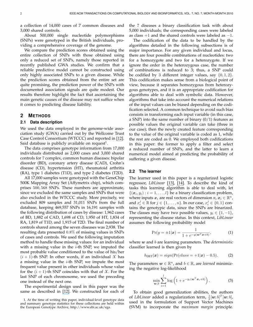
The choice of t should be carefully decided, as it has amajor impact on final results. To illustrate this, Figure 1shows the evolution of the estimated classification error

4 IEEE/ACM TRANSACTIONS ON COMPUTATIONAL BIOLOGY AND BIOINFORMATICS, VOL. ?, NO. ?, MONTH-MONTH 2010

10.0%

12.5%

15.0%

17.5%

20.0%

1% 10% 19% 28% 37% 46% 55% 64% 73% 82% 91% 100%

Error vs. % of SNPs (T1D)

% of SNPs

Fig. 1. Evolution of the estimation of the 0/1 classificationerror on the type 1 diabetes (T1D) disease varying thepercentage of SNPs selected from the ranking obtainedby FCBF

in a predictive model for the type 1 diabetes (T1D) dis-ease in the WTCCC data set (see Section 2.1). The scoresare estimated using a 5-fold cross validation for differentvalues of t. Starting with just the top 1% of the SNPsranked by FCBF, we iteratively add subsequent SNPs insteps of 1%. This experiment shows that adding moreinput variables to the model decreases the error up to apoint at which it increases again. This effect, known asthe peaking phenomenon and recently revisited in [16],is due to the addition of excessive (possibly irrelevant)information that disturbs the learning process.

In the experiments described in the next section, weshall use a grid search to search for good t values.

3 RESULTS AND DISCUSSION

3.1 Experimental setting

In this section we report the prediction performance ofour method in the 7 classification tasks. In order tounderscore the role played by the selection of SNPs,we compared our scores with those achieved using theSNPs reported recently by a collection of GWA studies(including [12]). The dramatic differences in the scoresso-obtained highlight the contrast between the aims ofGWA and prediction studies.

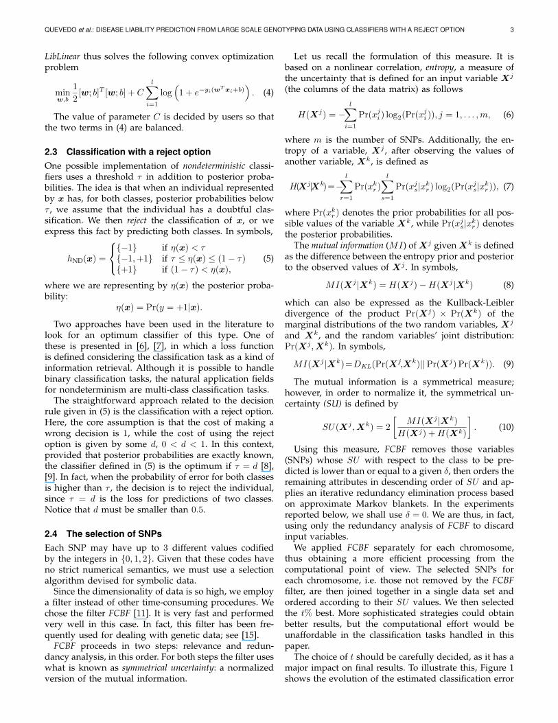
Let us first describe the procedure to induce a predic-tion model from training data, which is depicted in thepseudocode included in Figure 2. Our proposed methodstarts from a data set d with the controls and cases ofa given disease, described by all the SNPs provided inthe WTCCC data sets. Before training LibLinear (line 20),input data is filtered by FCBF one chromosome at a time(lines 2 – 7) for efficiency reasons and the SNPs notremoved are joined together, constructing a new dataset (d′). To estimate the best value for parameter t, thepercentage of top ranked SNPs, we used a standardstratified hold-out approach; thus, the data set is split(line 8) in two subsets: e, with 75% of cases and controlsof d′, and v with the remaining 25%. Then, by varyingthe value of t, we construct et and vt which will contain

1: function GETRISKPREDICTOR(d)2: d′ ← ∅3: for each chromosome c do4: s← GETCHROMOSOMESNPS(c, d)5: d′ ← d′ ∪ FCBF(s)6: end for7: d′ ← SORTBYSU(d′)8: [e, v]← RANDOMSPLIT(d′, 25%)9: tbest ← 0; lbest ←∞

10: for t = 10 to 100 in steps of 10 do11: et ← GETTOPRANKEDSNPS(t, e)12: vt ← GETTOPRANKEDSNPS(t, v)13: ht ← TRAINLIBLINEAR(et)14: lt ← TESTMODEL(ht, vt)15: if lt < lbest then16: lbest ← lt; tbest ← t17: end if18: end for19: d′′ ← GETTOPRANKEDSNPS(tbest, d

′)20: h← TRAINLIBLINEAR(d′′)21: return h22: end function

Fig. 2. Pseudo-code describing the proposed approachto obtain a disease risk predictor based on filtering SNPsand training LibLinear to obtain a probabilistic model

only the t% top ranked SNPs (according to their SUvalue with respect to the disease status); for each value,we train LibLinear on et and validate the 0/1 error ofthe obtained model ht on the corresponding vt, finallyselecting the value for t yielding the lowest estimationerror, i.e. tbest (lines 9 – 18). This procedure is used toestimate the 0/1 classification error without overfitting.Finally, we construct d′′ containing only the tbest topranked SNPs and we obtain the model h (line 20) thatwill be returned by the algorithm. The regularizationparameter C of the logistic regression (4) was left to itsdefault value (C = 1).

The predictive performance of our procedure wasestimated using a 5-fold stratified cross validation. Thus,for each disease we randomly split the data availablein the 5 partitions while maintaining the distributionof cases and controls (class +1 and −1) as in the fulldata set. Each partition is then used as a test set fora hypothesis induced using the algorithm depicted inFigure 2 on a training set formed by the remaining 4partitions.

The quality of each induced model is assessed usingboth the classification error (0/1 loss), the area under theROC curve (AUC), and the Sensitivity and the Specificity.The classification error of a model h on a test set S iscomputed as

∆0/1(h, S) =1

|S|

|S|∑i=1

[[h(xi) 6= yi]], (11)

where the output of h is given by (5), and [[p]] is evaluated

QUEVEDO et al.: DISEASE LIABILITY PREDICTION FROM LARGE SCALE GENOTYPING DATA USING CLASSIFIERS WITH A REJECT OPTION 5

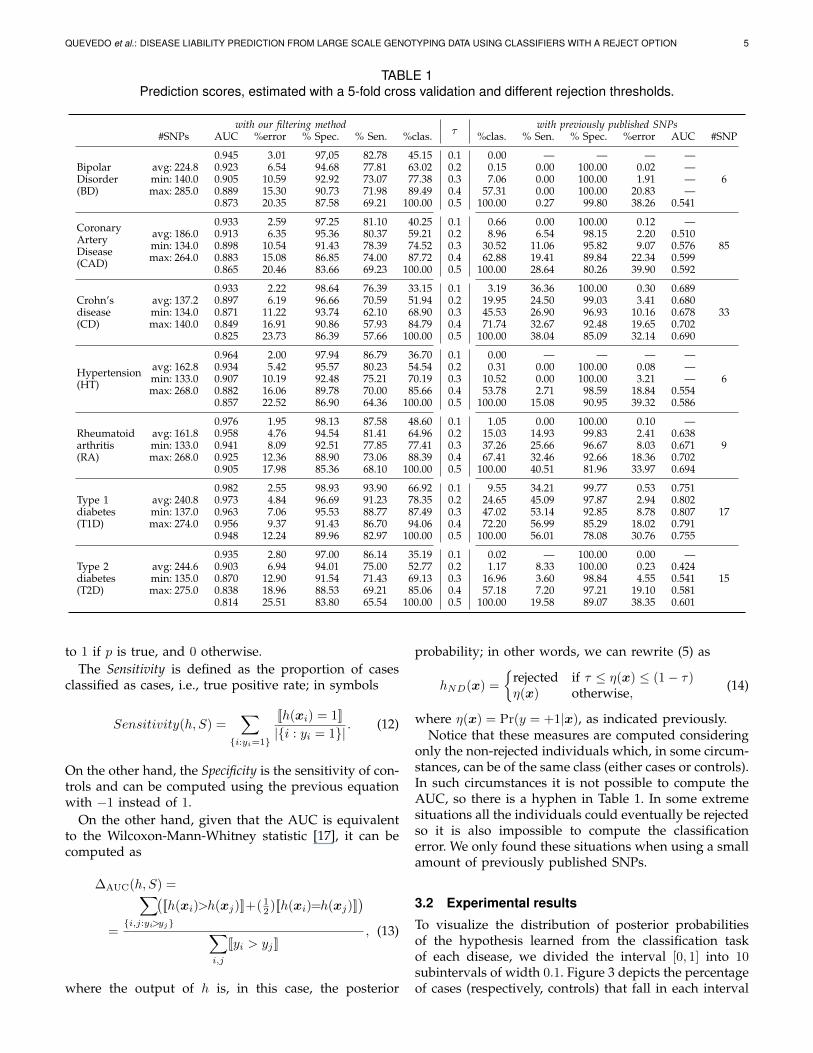
TABLE 1Prediction scores, estimated with a 5-fold cross validation and different rejection thresholds.

with our filtering methodτ

with previously published SNPs#SNPs AUC %error % Spec. % Sen. %clas. %clas. % Sen. % Spec. %error AUC #SNP

BipolarDisorder(BD)

0.945 3.01 97,05 82.78 45.15 0.1 0.00 — — — —avg: 224.8 0.923 6.54 94.68 77.81 63.02 0.2 0.15 0.00 100.00 0.02 —min: 140.0 0.905 10.59 92.92 73.07 77.38 0.3 7.06 0.00 100.00 1.91 — 6max: 285.0 0.889 15.30 90.73 71.98 89.49 0.4 57.31 0.00 100.00 20.83 —

0.873 20.35 87.58 69.21 100.00 0.5 100.00 0.27 99.80 38.26 0.541

CoronaryArteryDisease(CAD)

0.933 2.59 97.25 81.10 40.25 0.1 0.66 0.00 100.00 0.12 —avg: 186.0 0.913 6.35 95.36 80.37 59.21 0.2 8.96 6.54 98.15 2.20 0.510min: 134.0 0.898 10.54 91.43 78.39 74.52 0.3 30.52 11.06 95.82 9.07 0.576 85max: 264.0 0.883 15.08 86.85 74.00 87.72 0.4 62.88 19.41 89.84 22.34 0.599

0.865 20.46 83.66 69.23 100.00 0.5 100.00 28.64 80.26 39.90 0.592

Crohn’sdisease(CD)

0.933 2.22 98.64 76.39 33.15 0.1 3.19 36.36 100.00 0.30 0.689avg: 137.2 0.897 6.19 96.66 70.59 51.94 0.2 19.95 24.50 99.03 3.41 0.680min: 134.0 0.871 11.22 93.74 62.10 68.90 0.3 45.53 26.90 96.93 10.16 0.678 33max: 140.0 0.849 16.91 90.86 57.93 84.79 0.4 71.74 32.67 92.48 19.65 0.702

0.825 23.73 86.39 57.66 100.00 0.5 100.00 38.04 85.09 32.14 0.690

Hypertension(HT)

0.964 2.00 97.94 86.79 36.70 0.1 0.00 — — — —avg: 162.8 0.934 5.42 95.57 80.23 54.54 0.2 0.31 0.00 100.00 0.08 —min: 133.0 0.907 10.19 92.48 75.21 70.19 0.3 10.52 0.00 100.00 3.21 — 6max: 268.0 0.882 16.06 89.78 70.00 85.66 0.4 53.78 2.71 98.59 18.84 0.554

0.857 22.52 86.90 64.36 100.00 0.5 100.00 15.08 90.95 39.32 0.586

Rheumatoidarthritis(RA)

0.976 1.95 98.13 87.58 48.60 0.1 1.05 0.00 100.00 0.10 —avg: 161.8 0.958 4.76 94.54 81.41 64.96 0.2 15.03 14.93 99.83 2.41 0.638min: 133.0 0.941 8.09 92.51 77.85 77.41 0.3 37.26 25.66 96.67 8.03 0.671 9max: 268.0 0.925 12.36 88.90 73.06 88.39 0.4 67.41 32.46 92.66 18.36 0.702

0.905 17.98 85.36 68.10 100.00 0.5 100.00 40.51 81.96 33.97 0.694

Type 1diabetes(T1D)

0.982 2.55 98.93 93.90 66.92 0.1 9.55 34.21 99.77 0.53 0.751avg: 240.8 0.973 4.84 96.69 91.23 78.35 0.2 24.65 45.09 97.87 2.94 0.802min: 137.0 0.963 7.06 95.53 88.77 87.49 0.3 47.02 53.14 92.85 8.78 0.807 17max: 274.0 0.956 9.37 91.43 86.70 94.06 0.4 72.20 56.99 85.29 18.02 0.791

0.948 12.24 89.96 82.97 100.00 0.5 100.00 56.01 78.08 30.76 0.755

Type 2diabetes(T2D)

0.935 2.80 97.00 86.14 35.19 0.1 0.02 — 100.00 0.00 —avg: 244.6 0.903 6.94 94.01 75.00 52.77 0.2 1.17 8.33 100.00 0.23 0.424min: 135.0 0.870 12.90 91.54 71.43 69.13 0.3 16.96 3.60 98.84 4.55 0.541 15max: 275.0 0.838 18.96 88.53 69.21 85.06 0.4 57.18 7.20 97.21 19.10 0.581

0.814 25.51 83.80 65.54 100.00 0.5 100.00 19.58 89.07 38.35 0.601

to 1 if p is true, and 0 otherwise.The Sensitivity is defined as the proportion of cases

classified as cases, i.e., true positive rate; in symbols

Sensitivity(h, S) =∑

{i:yi=1}

[[h(xi) = 1]]

|{i : yi = 1}|. (12)

On the other hand, the Specificity is the sensitivity of con-trols and can be computed using the previous equationwith −1 instead of 1.

On the other hand, given that the AUC is equivalentto the Wilcoxon-Mann-Whitney statistic [17], it can becomputed as

∆AUC(h, S) =

=

∑{i,j:yi>yj}

([[h(xi)>h(xj)]]+( 1

2 )[[h(xi)=h(xj)]])

∑i,j

[[yi > yj ]], (13)

where the output of h is, in this case, the posterior

probability; in other words, we can rewrite (5) as

hND(x) =

{rejected if τ ≤ η(x) ≤ (1− τ)η(x) otherwise, (14)

where η(x) = Pr(y = +1|x), as indicated previously.Notice that these measures are computed considering

only the non-rejected individuals which, in some circum-stances, can be of the same class (either cases or controls).In such circumstances it is not possible to compute theAUC, so there is a hyphen in Table 1. In some extremesituations all the individuals could eventually be rejectedso it is also impossible to compute the classificationerror. We only found these situations when using a smallamount of previously published SNPs.

3.2 Experimental results

To visualize the distribution of posterior probabilitiesof the hypothesis learned from the classification taskof each disease, we divided the interval [0, 1] into 10subintervals of width 0.1. Figure 3 depicts the percentageof cases (respectively, controls) that fall in each interval

6 IEEE/ACM TRANSACTIONS ON COMPUTATIONAL BIOLOGY AND BIOINFORMATICS, VOL. ?, NO. ?, MONTH-MONTH 2010

0%

10%

20%

30%

40%

50%

60%

70%

< 0.1 [0.1,0.2) [0.2,0.3) [0.3,0.4) [0.4,0.5) [0.5,0.6) [0.6,0.7) [0.7,0.8) [0.8,0.9) ! 0.9

BD paper

Predicted probability of disease

cases (1962)controls (2938)BD

0%

10%

20%

30%

40%

50%

60%

70%

< 0.1 [0.1,0.2) [0.2,0.3) [0.3,0.4) [0.4,0.5) [0.5,0.6) [0.6,0.7) [0.7,0.8) [0.8,0.9) ! 0.9

CAD paper

Predicted probability of disease

cases (1882)controls (2938)CAD

0%

10%

20%

30%

40%

50%

60%

70%

< 0.1 [0.1,0.2) [0.2,0.3) [0.3,0.4) [0.4,0.5) [0.5,0.6) [0.6,0.7) [0.7,0.8) [0.8,0.9) ! 0.9

CD paper

Predicted probability of disease

cases (1698)controls (2938)CD

0%

10%

20%

30%

40%

50%

60%

70%

< 0.1 [0.1,0.2) [0.2,0.3) [0.3,0.4) [0.4,0.5) [0.5,0.6) [0.6,0.7) [0.7,0.8) [0.8,0.9) ! 0.9

HT paper

Predicted probability of disease

cases (1950)controls (2938)HT

0%

10%

20%

30%

40%

50%

60%

70%

< 0.1 [0.1,0.2) [0.2,0.3) [0.3,0.4) [0.4,0.5) [0.5,0.6) [0.6,0.7) [0.7,0.8) [0.8,0.9) ! 0.9

RA paper

Predicted probability of disease

cases (1834)controls (2938)RA

0%

10%

20%

30%

40%

50%

60%

70%

< 0.1 [0.1,0.2) [0.2,0.3) [0.3,0.4) [0.4,0.5) [0.5,0.6) [0.6,0.7) [0.7,0.8) [0.8,0.9) ! 0.9

T1D paper

Predicted probability of disease

cases (1819)controls (2938)T1D

0%

10%

20%

30%

40%

50%

60%

70%

< 0.1 [0.1,0.2) [0.2,0.3) [0.3,0.4) [0.4,0.5) [0.5,0.6) [0.6,0.7) [0.7,0.8) [0.8,0.9) ! 0.9

T2D paper

Predicted probability of disease

cases (1915)controls (2938)T2D

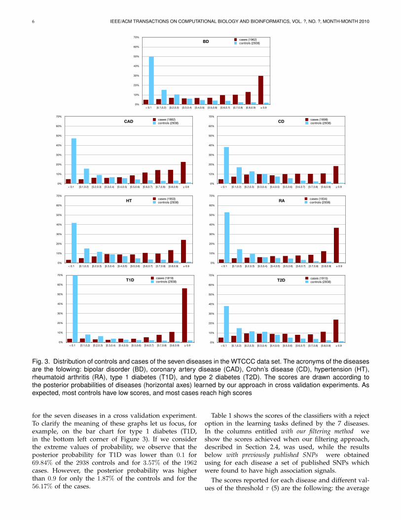
Fig. 3. Distribution of controls and cases of the seven diseases in the WTCCC data set. The acronyms of the diseasesare the folowing: bipolar disorder (BD), coronary artery disease (CAD), Crohn’s disease (CD), hypertension (HT),rheumatoid arthritis (RA), type 1 diabetes (T1D), and type 2 diabetes (T2D). The scores are drawn according tothe posterior probabilities of diseases (horizontal axes) learned by our approach in cross validation experiments. Asexpected, most controls have low scores, and most cases reach high scores

for the seven diseases in a cross validation experiment.To clarify the meaning of these graphs let us focus, forexample, on the bar chart for type 1 diabetes (T1D,in the bottom left corner of Figure 3). If we considerthe extreme values of probability, we observe that theposterior probability for T1D was lower than 0.1 for69.84% of the 2938 controls and for 3.57% of the 1962cases. However, the posterior probability was higherthan 0.9 for only the 1.87% of the controls and for the56.17% of the cases.

Table 1 shows the scores of the classifiers with a rejectoption in the learning tasks defined by the 7 diseases.In the columns entitled with our filtering method weshow the scores achieved when our filtering approach,described in Section 2.4, was used, while the resultsbelow with previously published SNPs were obtainedusing for each disease a set of published SNPs whichwere found to have high association signals.

The scores reported for each disease and different val-ues of the threshold τ (5) are the following: the average

QUEVEDO et al.: DISEASE LIABILITY PREDICTION FROM LARGE SCALE GENOTYPING DATA USING CLASSIFIERS WITH A REJECT OPTION 7

percentage of classified (i.e. not rejected) individuals (%clas.), the average classification error (%error), the AUC,the sensitivity (Sen.) and the specificity (Spec.). Note thatwhen τ = 0.5, the hypotheses behave like a classicalprobabilistic classifier that labels an individual either asa case, when the posterior probability is higher or equalthan 0.5, or as a control, otherwise. The percentage ofindividuals classified is then 100%.

The errors for τ = 0.5 are notably lower than thosereported in recent studies [18]. One reason that mayexplain this discrepancy is that we carry out a thoroughselection of the SNPs that are going to be involved inthe learning process. The second reason is the learningalgorithm used, a logistic regression instead of a decisiontree.

Our results also outperform other risk assessmentalgorithms that were recently published [19], [20], andwhose quality was estimated in terms of AUC. Worthof mention is the discussion in [20] about the possiblebias of the estimations obtained by a cross-validationexperiment. To avoid an optimistic estimation of theperformance in risk assessment, the authors suggestto use independent data sets obtained from differentsources to validate the induced models. Although weagree with their claim, in the present work we did notvalidate with independent data sets, so a comparison canonly be established on the cross-validation results.

However, despite the accuracy improvement consider-ing the standard classification approach (when τ = 0.5),we would like to highlight that higher scores can beobtained at the cost of rejecting to classify an acceptablylow percentage of cases. The goodness of our methodcan be found when the threshold, τ , has lower values.For instance, for τ = 0.3, the percentage of individualsclassified across the 7 diseases is on average 75.00%, withan average error of only 10%; the Specificity is over 90%while the Sensitivity is over 70% with the exception ofCD where it only reaches 62%.

Furthermore, we detect notable differences betweendiseases. Thus, in concordance with [18], T1D is morepredictable in our experiments than the other diseases:using a τ = 0.2, it is possible to return a classification for78.35% of the individuals with an error of just 4.84%.

We also report in Table 1 the number of SNPs used ineach task, which is indicated as the average, minimumand maximum values of the 5-fold cross-validation whenour filtering approach was used. We have observedthat all chromosomes have SNPs in these collections,which emphasizes the importance of making genome-wide explorations. More details can be found on thewebsite of supplementary data2 to this paper.

3.3 Comparison with other SNPsIn Table 2, we list a number of references comprising acollection of SNPs in which association signals with thediseases were found. We considered only those SNPs

2. http://www.aic.uniovi.es/disease prediction

TABLE 2Bibliographic references used to obtain a joint list of

relevant SNPs for each disease. The last two columnsreport the number of SNPs from each paper, and of the

union of them, included in the WTCCC data set.

#SNPs

Disease Reference Paper WTCCC Union

BD Ferreira et al. (2008) [21] 2 1 6Sklar et al. (2008) [22] 2 2Baum et al. (2007) [23] 11 2WTCCC (2007) [12] 1 1

CAD Samani et al. (2007) [24] 30 30 85Willer et al. (2008) [25] 59 36Aulchenko et al. (2009) [26] 161 37WTCCC (2007) [12] 1 1

CD Parkes et al. (2007) [27] 12 12 33Barrett et al. (2008) [28] 30 17WTCCC (2007) [12] 9 9

HT WTCCC (2007) [12] 6 6 6

RA Thomson et al. (2007) [29] 1 1 9Barton et al. (2008) [30] 3 3Plenge et al. (2007) [31] 9 1WTCCC (2007) [12] 4 4

T1D Todd et al. (2007) [32] 15 14 17Hakonarson et al. (2007) [33] 14 0WTCCC (2007) [12] 6 6

T2D Zeggini et al. (2007) [34] 11 9 15Cornelis et al. (2009) [3] 17 7WTCCC (2007) [12] 3 3

included in the WTCCC data set, adding the SNPsmentioned in [12] with high association measures, i.e.those with p < 5 ·10−7, except in HT, where we used the6 SNPs with 5 · 10−7 < p < 2 · 10−5. The union of SNPsso-gathered is finally considered for each disease. Thelast column in Table 2 shows the number of SNPs so-obtained. Note that these SNPs are considerably fewerthan those selected by our method. The list of such SNPsis available on the website of supplementary data.

The scores below the label with previously publishedSNPs in Table 1 were obtained with the SNPs listedin Table 2 in the experimental setting described at thebeginning of this section. The discriminatory power ofthese SNPs can be seen to be very modest. The predic-tion scores are similar to a baseline predictor that willalways return the most frequent class, thus labeling anyindividual as a control; this baseline has errors of around40%. This is the case, for instance in BD where theSensitivity is only 0.27% while the Specificity is 99.80%.In general, when all individuals are classified (τ = 0.5),the Sensitivity is below 50% with the exception of T1Dwhere the sensitivity is 56.01%.

These results confirm the conclusions regarding themodest predictive power of a small collection of SNPspresented in [2], [3].

8 IEEE/ACM TRANSACTIONS ON COMPUTATIONAL BIOLOGY AND BIOINFORMATICS, VOL. ?, NO. ?, MONTH-MONTH 2010

3.4 DiscussionAssessing the genetic risk of a patient to develop adisease is a very important target from a medical point ofview. In this sense, the approach presented in this paperaims at finding in this work useful prediction modelsbased on hundreds of SNPs instead of a few ones. Thismethod could be helpful to improve the assessmentsof disease risk only based on the absence or presenceof alleles associated to a given disease status, which isactually offered by some commercial personal genomicservices.

In addition, the performance of risk predictors canbe improved if we allow to reject the classification ofsome individuals with an uncertain prediction. Rejec-tion makes sense in this context since it is much moreadequate to tell patients that their genotype does notconvincingly predict their risk for a particular diseasethan to venture an untrustworthy prognosis.

In the classification tasks studied, the main difficulty isthe extremely high dimensionality of the data. We used amaximum margin learner preceded by a nonlinear corre-lation based filter to overcome the curse of dimensionality.

Using posterior probabilities we identified an averageof 25.00% individuals with uncertain predictions in theWTCCC data, while in the remaining individuals theclassification error was only around 10%. Our methodthus provides not only a prediction of disease status,but also a risk ranking represented by probabilities.

In addition to the accuracy, the performance of theclassifications was measured using the Sensitivity, theSpecificity, and the AUC. In all diseases studied, specifi-ties were quite high, over 83% in the worst case, whereassensitivity was 57% at least. The latter contrasts withsensitivities obtained with the most associated SNPs,which were much lower (Table 1).

Our approach considerably outperforms the predic-tions that can be obtained using only loci found fromgenome-wide association approaches. The classifiersbuilt with the SNPs reported in recent papers thatembrace the association approach, for τ = 0.3, onlycover a small proportion of individuals, 27.84%; thus,the reduced average error rate achieved, 6.53%, is not souseful. To obtain classifications for an average of 63.21%individuals, we need to fix τ = 0.4, the average errorthen increases to 19.59%.

One of the possible reasons why the approach pre-sented here far outperforms classifiers using only themost associated SNPs is that common diseases are likelyto be caused by numerous loci with small to modesteffects. These loci are usually discarded in GWA becauseof the strict significance thresholds normally employed.Our method, in contrast, implicitly employs all geno-typic information. For all these reasons, together withthe careful tuning of the algorithm, we are able to ob-tain larger AUCs than previously reported for complexdisease genetic prediction risk.

In [19], the authors have reported lower AUC thanours using the same data set, ranging from 0.66 to 0.79.

The differences are due to the different approach used.In fact, the approach of [19] is similar to the methodemployed here to obtain the results with previouslypublished SNPs; a p-value thresholding selects a subsetof SNPs to be used in a logistic regression learner.However, the codification of SNPs uses values {0, 1, 2}instead of the binarization proposed in this paper. In anycase, [19] results in a low discriminative power for alldiseases but Type 1 Diabetes (T1D). These results agreewith the AUC scores reported in the last column of ourTable 1, none of them is above 0.69.

Interestingly, the AUC reported here are close to themaximum AUC predicted by Wray et al. [35] for thediseases analyzed here. The ranking of their AUCs forthe different diseases is also, grossly, in agreement withours. For instance, they predict a higher AUCmax forT1D than for T2D, as we do obtain. As Wray et al.showed, maximum AUC depends on both incidenceand heritability in the underlying scale (they assumed athreshold model). The fact of discarding samples difficultto classify is, certainly, an indirect method to increaseheritability.

4 CONCLUSIONS

Prediction and association are related though still dis-tinct objectives. From a purely computational point ofview, the reason is that associations are searched aimingat the goodness of fit considering the available markersone by one. The consequence is that there are interac-tions that are unaccounted in GWA studies. Instead ofsearching for individual markers, the method proposedhere searches for subsets of SNPs whose joint values areuseful for prediction, but which one by one may notreflect association signals.

The reported results thus suggest that the geneticcauses of the diseases considered here are complex:there are many SNPs (along all chromosomes) whoseindividual effect cannot be detected, but which still addup to make an overall impact on disease risk.

ACKNOWLEDGMENTS

This study makes use of data generated by the Well-come Trust Case-Control Consortium. A full list of theinvestigators who contributed to the generation of thedata is available from www.wtccc.org.uk. Funding forthe project was provided by the Wellcome Trust underaward 076113. The research reported in this paper wassupported in part by grants from the Spanish Ministeriode Ciencia e Innovacion [TIN2008-06247] to JRQ, AB,and OL, and [AGL2007-65563-C02-01/GAN] to MPE.

REFERENCES

[1] D. De los Campos, D. Gianola, and D. B. Allison, “Predictinggenetic predisposition in humans: the promise of whole-genomemarkers,” Nature Reviews Genetics, vol. 11, pp. 880–886, 2010.

QUEVEDO et al.: DISEASE LIABILITY PREDICTION FROM LARGE SCALE GENOTYPING DATA USING CLASSIFIERS WITH A REJECT OPTION 9

[2] N. P. Paynter, D. I. Chasman, J. E. Buring, D. Shiffman, N. R. Cook,and P. M. Ridker, “Cardiovascular Disease Risk Prediction Withand Without Knowledge of Genetic Variation at Chromosome9p21.3,” Ann Intern Med, vol. 150, no. 2, pp. 65–72, 2009.

[3] M. C. Cornelis, L. Qi, C. Zhang, P. Kraft, J. Manson, T. Cai, D. J.Hunter, and F. B. Hu, “Joint Effects of Common Genetic Variantson the Risk for Type 2 Diabetes in U.S. Men and Women ofEuropean Ancestry,” Ann Intern Med, vol. 150, no. 8, pp. 541–550,2009.

[4] J. Yang, B. Benyamin, B. P. McEvoy, S. Gordon, A. K. Henders,D. R. Nyholt, P. A. Madden, A. C. Heath, N. G. Martin, G. W.Montgomery, M. E. Goddard, and P. M. Visscher, “Common snpsexplain a large proportion of the heritability for human height,”Nat Genet, vol. 42, no. 7, pp. 565–9, Jul 2010.

[5] G. Corani and M. Zaffalon, “Learning Reliable Classifiers FromSmall or Incomplete Data Sets: The Naive Credal Classifier 2,”Journal of Machine Learning Research, vol. 9, pp. 581–621, 2008.

[6] J. Alonso, J. J. del Coz, J. Dıez, O. Luaces, and A. Bahamonde,“Learning to predict one or more ranks in ordinal regressiontasks,” in Machine Learning and Knowledge Discovery in Databases,ser. LNAI, W. Daelemans, B. Goethals, and K. Morik, Eds., vol.5211. Springer, 2008, pp. 39–54.

[7] J. J. del Coz, J. Dıez, and A. Bahamonde, “Learning nondetermin-istic classifiers,” Journal of Machine Learning Research, To appear in2009.

[8] C. Chow, “On optimum recognition error and reject tradeoff,”IEEE Transactions on Information Theory, vol. 16, no. 1, pp. 41–46,1970.

[9] P. Bartlett and M. Wegkamp, “Classification with a reject optionusing a hinge loss,” Journal of Machine Learning Research, vol. 9,pp. 1823–1840, 2008.

[10] B. Hanczar and E. Dougherty, “Classification with reject optionin gene expression data,” Bioinformatics, vol. 24, no. 17, pp. 1889–1895, 2008.

[11] L. Yu and H. Liu, “Efficient feature selection via analysis ofrelevance and redundancy,” Journal of Machine Learning Research,vol. 5, pp. 1205–1224, 2004.

[12] WTCCC, “(Wellcome Trust Case-Control Consortium). Genome-wide association study of 14,000 cases of seven common diseasesand 3,000 shared controls,” Nature, vol. 447, no. 7145, pp. 661–678,06 2007.

[13] C.-J. Lin, R. C. Weng, and S. S. Keerthi, “Trust region newtonmethod for logistic regression,” J. Mach. Learn. Res., vol. 9, pp.627–650, 2008.

[14] R. Fan, K. Chang, C. Hsieh, X. Wang, and C. Lin, “LIBLINEAR: Alibrary for large linear classification,” J. Mach. Learn. Res., vol. 9,pp. 1871–1874, 2008.

[15] Y. Saeys, I. Inza, and P. Larranaga, “A review of feature selectiontechniques in bioinformatics,” Bioinformatics, vol. 23, no. 19, pp.2507—2517, 2007.

[16] C. Sima and E. R. Dougherty, “The peaking phenomenon in thepresence of feature-selection,” Pattern Recognition Letters, vol. 29,no. 11, pp. 1667 – 1674, 2008.

[17] J. Hanley and B. McNeil, “The meaning and use of the area undera receiver operating characteristic (ROC) curve,” Radiology, vol.143, no. 1, pp. 29–36, 1982.

[18] M. A. Schaub, I. M. Kaplow, M. Sirota, C. B. Do, A. J. Butte,and S. Batzoglou, “A Classifier-based approach to identify geneticsimilarities between diseases,” Bioinformatics, vol. 25, no. 12, pp.i21–i29, 2009.

[19] D. M. Evans, P. M. Visscher, and N. R. Wray, “Harnessing theinformation contained within genome-wide association studies toimprove individual prediction of complex disease risk,” Hum MolGenet, vol. 18, no. 18, pp. 3525–31, Sep 2009.

[20] Z. Wei, K. Wang, H.-Q. Qu, H. Zhang, J. Bradfield, C. Kim,E. Frackleton, C. Hou, J. T. Glessner, R. Chiavacci, C. Stanley,D. Monos, S. F. A. Grant, C. Polychronakos, and H. Hakonarson,“From disease association to risk assessment: An optimistic viewfrom genome-wide association studies on type 1 diabetes,” PLoSGenet, vol. 5, no. 10, 2009.

[21] M. A. R. Ferreira, M. C. O’Donovan, Y. A. Meng, I. R. Jones,D. M. Ruderfer, L. Jones, J. Fan, G. Kirov, R. H. Perlis, E. K.Green, J. W. Smoller, D. Grozeva, J. Stone, I. Nikolov, K. Chambert,M. L. Hamshere, V. L. Nimgaonkar, V. Moskvina, M. E. Thase,S. Caesar, G. S. Sachs, J. Franklin, K. Gordon-Smith, K. G. Ardlie,S. B. Gabriel, C. Fraser, B. Blumenstiel, M. Defelice, G. Breen,M. Gill, D. W. Morris, A. Elkin, W. J. Muir, K. A. McGhee,

R. Williamson, D. J. MacIntyre, A. W. MacLean, D. St Clair,M. Robinson, M. Van Beck, A. C. P. Pereira, R. Kandaswamy,A. McQuillin, D. A. Collier, N. J. Bass, A. H. Young, J. Lawrence,I. Nicol Ferrier, A. Anjorin, A. Farmer, D. Curtis, E. M. Scolnick,P. McGuffin, M. J. Daly, A. P. Corvin, P. A. Holmans, D. H.Blackwood, H. M. Gurling, M. J. Owen, S. M. Purcell, P. Sklar, andN. Craddock, “Collaborative genome-wide association analysissupports a role for ank3 and cacna1c in bipolar disorder,” NatureGenetics, vol. 40, no. 9, pp. 1056–1058, 09 2008.

[22] P. Sklar, J. W. Smoller, J. Fan, M. Ferreira, R. Perlis, K. Chambert,V. Nimgaonkar, M. McQueen, S. Faraone, A. Kirby, P. de Bakker,M. Ogdie, M. Thase, G. Sachs, K. Todd-Brown, S. Gabriel,C. Sougnez, C. Gates, B. Blumenstiel, M. Defelice, K. Ardlie,J. Franklin, W. Muir, K. McGhee, D. MacIntyre, A. McLean,M. VanBeck, A. McQuillin, N. Bass, M. Robinson, J. Lawrence,A. Anjorin, D. Curtis, E. Scolnick, M. Daly, D. Blackwood, H. Gurl-ing, and S. Purcell, “Whole-genome association study of bipolardisorder,” Molecular Psychiatry, vol. 13, no. 6, pp. 558–569, 2008.

[23] A. E. Baum, N. Akula, M. Cabanero, I. Cardona, W. Corona,B. Klemens, T. G. Schulze, S. Cichon, M. Rietschel, M. M. Nothen,A. Georgi, J. Schumacher, M. Schwarz, R. Abou Jamra, S. Hofels,P. Propping, J. Satagopan, S. D. Detera-Wadleigh, J. Hardy, andF. J. McMahon, “A genome-wide association study implicatesdiacylglycerol kinase eta (dgkh) and several other genes in theetiology of bipolar disorder,” Mol Psychiatry, vol. 13, no. 2, pp.197–207, 05 2007.

[24] N. J. Samani, J. Erdmann, A. S. Hall, C. Hengstenberg,M. Mangino, B. Mayer, R. J. Dixon, T. Meitinger, P. Braund, H.-E.Wichmann, J. H. Barrett, I. R. Konig, S. E. Stevens, S. Szymczak,D.-A. Tregouet, M. M. Iles, F. Pahlke, H. Pollard, W. Lieb, F. Cam-bien, M. Fischer, W. Ouwehand, S. Blankenberg, A. J. Balmforth,A. Baessler, S. G. Ball, T. M. Strom, I. Braenne, C. Gieger, P. De-loukas, M. D. Tobin, A. Ziegler, J. R. Thompson, H. Schunkert,the WTCCC, and the Cardiogenics Consortium, “GenomewideAssociation Analysis of Coronary Artery Disease,” N Engl J Med,vol. 357, no. 5, pp. 443–453, 2007.

[25] C. J. Willer, S. Sanna, A. U. Jackson, A. Scuteri, L. L. Bonnycastle,R. Clarke, S. C. Heath, N. J. Timpson, S. S. Najjar, H. M. Stringham,J. Strait, W. L. Duren, A. Maschio, F. Busonero, A. Mulas, G. Albai,A. J. Swift, M. A. Morken, N. Narisu, D. Bennett, S. Parish,H. Shen, P. Galan, P. Meneton, S. Hercberg, D. Zelenika, W.-M.Chen, Y. Li, L. J. Scott, P. A. Scheet, J. Sundvall, R. M. Watanabe,R. Nagaraja, S. Ebrahim, D. A. Lawlor, Y. Ben-Shlomo, G. Davey-Smith, A. R. Shuldiner, R. Collins, R. N. Bergman, M. Uda,J. Tuomilehto, A. Cao, F. S. Collins, E. Lakatta, G. M. Lathrop,M. Boehnke, D. Schlessinger, K. L. Mohlke, and G. R. Abecasis,“Newly identified loci that influence lipid concentrations and riskof coronary artery disease,” Nature Genetics, vol. 40, no. 2, pp. 161–169, 02 2008.

[26] Y. Aulchenko, S. Ripatti, I. Lindqvist, D. Boomsma, I. Heid,P. Pramstaller, B. Penninx, A. Janssens, J. Wilson, T. Spector et al.,“Loci influencing lipid levels and coronary heart disease risk in16 european population cohorts,” Nature Genetics, vol. 41, no. 1,pp. 47–55, 01 2009.

[27] M. Parkes, J. C. Barrett, N. J. Prescott, M. Tremelling, C. A. An-derson, S. A. Fisher, R. G. Roberts, E. R. Nimmo, F. R. Cummings,D. Soars, H. Drummond, C. W. Lees, S. A. Khawaja, R. Bagnall,D. A. Burke, C. E. Todhunter, T. Ahmad, C. M. Onnie, W. McArdle,D. Strachan, G. Bethel, C. Bryan, C. M. Lewis, P. Deloukas,A. Forbes, J. Sanderson, D. P. Jewell, J. Satsangi, J. C. Mansfield,L. Cardon, and C. G. Mathew, “Sequence variants in the au-tophagy gene irgm and multiple other replicating loci contributeto crohn’s disease susceptibility,” Nature Genetics, vol. 39, no. 7,pp. 830–832, 07 2007.

[28] J. C. Barrett, S. Hansoul, D. L. Nicolae, J. H. Cho, R. H. Duerr, J. D.Rioux, S. R. Brant, M. S. Silverberg, K. D. Taylor, M. M. Barmada,A. Bitton, T. Dassopoulos, L. W. Datta, T. Green, A. M. Griffiths,E. O. Kistner, M. T. Murtha, M. D. Regueiro, J. I. Rotter, L. P.Schumm, A. H. Steinhart, S. R. Targan, R. J. Xavier, C. Libioulle,C. Sandor, M. Lathrop, J. Belaiche, O. Dewit, I. Gut, S. Heath,D. Laukens, M. Mni, P. Rutgeerts, A. Van Gossum, D. Zelenika,D. Franchimont, J.-P. Hugot, M. de Vos, S. Vermeire, E. Louis, L. R.Cardon, C. A. Anderson, H. Drummond, E. Nimmo, T. Ahmad,N. J. Prescott, C. M. Onnie, S. A. Fisher, J. Marchini, J. Ghori,S. Bumpstead, R. Gwilliam, M. Tremelling, P. Deloukas, J. Mans-field, D. Jewell, J. Satsangi, C. G. Mathew, M. Parkes, M. Georges,and M. J. Daly, “Genome-wide association defines more than 30

10 IEEE/ACM TRANSACTIONS ON COMPUTATIONAL BIOLOGY AND BIOINFORMATICS, VOL. ?, NO. ?, MONTH-MONTH 2010

distinct susceptibility loci for Crohn’s disease,” Nature Genetics,vol. 40, no. 8, pp. 955–962, 08 2008.

[29] W. Thomson, A. Barton, X. Ke, S. Eyre, A. Hinks, J. Bowes,R. Donn, D. Symmons, S. Hider, I. N. Bruce, A. G. Wilson, I. Mari-nou, A. Morgan, P. Emery, A. Carter, S. Steer, L. Hocking, D. M.Reid, P. Wordsworth, P. Harrison, D. Strachan, and J. Worthington,“Rheumatoid arthritis association at 6q23,” Nat Genet, vol. 39,no. 12, pp. 1431–1433, 12 2007.

[30] A. Barton, W. Thomson, X. Ke, S. Eyre, A. Hinks, J. Bowes,D. Plant, L. J. Gibbons, A. G. Wilson, D. E. Bax, A. W. Morgan,P. Emery, S. Steer, L. Hocking, D. M. Reid, P. Wordsworth, P. Harri-son, and J. Worthington, “Rheumatoid arthritis susceptibility lociat chromosomes 10p15, 12q13 and 22q13,” Nature Genetics, vol. 40,no. 10, pp. 1156–1159, 10 2008.

[31] R. M. Plenge, M. Seielstad, L. Padyukov, A. T. Lee, E. F. Remmers,B. Ding, A. Liew, H. Khalili, A. Chandrasekaran, L. R. Davies,W. Li, A. K. Tan, C. Bonnard, R. T. Ong, A. Thalamuthu, S. Pet-tersson, C. Liu, C. Tian, W. V. Chen, J. P. Carulli, E. M. Beckman,D. Altshuler, L. Alfredsson, L. A. Criswell, C. I. Amos, M. F.Seldin, D. L. Kastner, L. Klareskog, and P. K. Gregersen, “TRAF1-C5 as a Risk Locus for Rheumatoid Arthritis – A GenomewideStudy,” N Engl J Med, vol. 357, no. 12, pp. 1199–1209, 2007.

[32] J. A. Todd, N. M. Walker, J. D. Cooper, D. J. Smyth, K. Downes,V. Plagnol, R. Bailey, S. Nejentsev, S. F. Field, F. Payne, C. E. Lowe,J. S. Szeszko, J. P. Hafler, L. Zeitels, J. H. M. Yang, A. Vella, S. Nut-land, H. E. Stevens, H. Schuilenburg, G. Coleman, M. Maisuria,W. Meadows, L. J. Smink, B. Healy, O. S. Burren, A. A. C. Lam,N. R. Ovington, J. Allen, E. Adlem, H.-T. Leung, C. Wallace,J. M. M. Howson, C. Guja, C. Ionescu-Tirgoviste, M. J. Simmonds,J. M. Heward, S. C. L. Gough, D. B. Dunger, L. S. Wicker, and D. G.Clayton, “Robust associations of four new chromosome regionsfrom genome-wide analyses of type 1 diabetes,” Nature Genetics,vol. 39, no. 7, pp. 857–864, 07 2007.

[33] H. Hakonarson, S. F. A. Grant, J. P. Bradfield, L. Marchand, C. E.Kim, J. T. Glessner, R. Grabs, T. Casalunovo, S. P. Taback, E. C.Frackelton, M. L. Lawson, L. J. Robinson, R. Skraban, Y. Lu, R. M.Chiavacci, C. A. Stanley, S. E. Kirsch, E. F. Rappaport, J. S. Orange,D. S. Monos, M. Devoto, H.-Q. Qu, and C. Polychronakos, “Agenome-wide association study identifies kiaa0350 as a type 1diabetes gene,” Nature, vol. 448, no. 7153, pp. 591–594, 08 2007.

[34] E. Zeggini, M. N. Weedon, C. M. Lindgren, T. M. Frayling, K. S.Elliott, H. Lango, N. J. Timpson, J. R. B. Perry, N. W. Rayner,R. M. Freathy, J. C. Barrett, B. Shields, A. P. Morris, S. Ellard, C. J.Groves, L. W. Harries, J. L. Marchini, K. R. Owen, B. Knight, L. R.Cardon, M. Walker, G. A. Hitman, A. D. Morris, A. S. F. Doney,T. W. T. C. C. C. (WTCCC), M. I. McCarthy, and A. T. Hattersley,“Replication of Genome-Wide Association Signals in UK SamplesReveals Risk Loci for Type 2 Diabetes,” Science, vol. 316, no. 5829,pp. 1336–1341, 2007.

[35] N. R. Wray, J. Yang, M. E. Goddard, and P. M. Visscher, “Thegenetic interpretation of area under the ROC curve in genomicprofiling,” PLoS Genet, vol. 6, no. 2, 2010.

Jose R. Quevedo received the MSc and thePhD degrees in Computer Science from theUniversity of Oviedo, Gijon, Spain, in 1997 and2000, respectively. He is currently an AssistantProfessor in the Department of Computer Sci-ence and a member of the Artificial IntelligenceCenter of the University of Oviedo. His currentresearch interest has a practical side in bioinfor-matics, and a theoretical side in learning frommulti-label and ordinal data.

Antonio Bahamonde received the MSc andPhD degrees in Mathematics from the Universityof Santiago de Compostela, Spain, in 1979 and1982 respectively. He is currently a Full Profes-sor of Artificial Intelligence in the University ofOviedo at Gijon, Spain. He is the Director of theArtificial Intelligence Center of his University, andsince 2007 presides the Spanish Associationfor Artificial Intelligence (AEPIA). His researchinterest includes Machine Learning applicationsin livestock, sensory analysis, and genetics.

Miguel Perez-Enciso is a biologist (PhD in Ge-netics, Universidad Complutense, Madrid, 1990)with a keen interest in the computational andstatistical problems appearing in agriculture, pri-marily in animal breeding and genetics. He hasworked in a variety of topics, ranging from op-timization of breeding schemes in small popu-lations to advanced Bayesian statistical meth-ods. He has been working in methods to utilizemolecular information into animal breeding forthe last 10 years and has recently become in-

terested in the challenges posed by massive parallel sequencing. He iscurrently ICREA professor at the Universidad Autonoma of Barcelona,Spain.

Oscar Luaces received the MSc and PhD de-grees in Computer Science from the Universityof Oviedo, Spain, in 1994 and 1999 respectively.He is currently an Assistant Professor in the Uni-versity of Oviedo at Gijon. He is the Secretary ofthe Artificial Intelligence Center of his University,and the Secretary of the Spanish Associationfor Artificial Intelligence (AEPIA). His researchinterest focuses in Machine Learning techniquesfor intelligent data analysis, including feature se-lection, support vector machines and preference

learning, with applications in sensory analysis, intensive care medicineand genetics.