econstor www.econstor.eu

Der Open-Access-Publikationsserver der ZBW – Leibniz-Informationszentrum WirtschaftThe Open Access Publication Server of the ZBW – Leibniz Information Centre for Economics

Nutzungsbedingungen:Die ZBW räumt Ihnen als Nutzerin/Nutzer das unentgeltliche,räumlich unbeschränkte und zeitlich auf die Dauer des Schutzrechtsbeschränkte einfache Recht ein, das ausgewählte Werk im Rahmender unter→ http://www.econstor.eu/dspace/Nutzungsbedingungennachzulesenden vollständigen Nutzungsbedingungen zuvervielfältigen, mit denen die Nutzerin/der Nutzer sich durch dieerste Nutzung einverstanden erklärt.

Terms of use:The ZBW grants you, the user, the non-exclusive right to usethe selected work free of charge, territorially unrestricted andwithin the time limit of the term of the property rights accordingto the terms specified at→ http://www.econstor.eu/dspace/NutzungsbedingungenBy the first use of the selected work the user agrees anddeclares to comply with these terms of use.

zbw Leibniz-Informationszentrum WirtschaftLeibniz Information Centre for Economics

Wiebelt, Manfred; Herrmann, Roland; Schenck, Patricia; Thiele, Rainer

Book

Discrimination against agriculture in developingcountries?

Kieler Studien, No. 243

Provided in Cooperation with:Kiel Institute for the World Economy (IfW)

Suggested Citation: Wiebelt, Manfred; Herrmann, Roland; Schenck, Patricia; Thiele, Rainer(1992) : Discrimination against agriculture in developing countries?, Kieler Studien, No. 243,ISBN 3161459202

This Version is available at:http://hdl.handle.net/10419/458

Kieler StudienInstitut fur Weltwirtschaft an der Universitat Kiel

Herausgegeben von Horst Siebert

243

Manfred Wiebelt et al.

, Discrimination Against Agriculturein Developing Countries?

Authors:Roland Herrmann, Patricia Schenck,

Rainer Thiele, Manfred Wiebelt

ARTIBUS

is

I "8 - 0 - 1

J.C.B. MOHR (PAUL SIEBECK) TUBINGEN

ISSN 0340-6989

Die Deutsche Bibliothek - CIP-Einheitsaufnahme

Discrimination against agriculture in developing countries? /Manfred Wiebelt et al. Autoren: Roland Herrmann ...-Tubingen : Mohr, 1992

(Kieler Studien ; 243)ISBN 3-16-145920-2 brosch.ISBN 3-16-145921-0 Gewebe

NE: Wiebelt, Manfred; GT

Schriftleitung: Hubertus M u l l e r - G r o e l i n g

Institut fur Weltwirtschaft an der Universitat KielJ. C. B. Mohr (Paul Siebeck) Tubingen 1992

Alle Rechte vorbehaltenOhne ausdruckliche Genehmigung des Verlages ist es auch nicht

gestattet, den Band oder Teile darausauf photomechanischem Wege (Photokopie, Mikrokopie) zu vervielfaltigen

Printed in GermanyISSN 0340-6989

Ill

Contents

List of Tables v i

List of Figures and Synoptical Tables ix

Abbreviations and Acronyms x

Preface x in

A. Background and Objectives of the Study 1

B. Measurement of Agricultural Protection: A Survey of the Concepts

and the Empirical Literature 6

I. Introduction 6

II. Concepts to Measuring Agricultural Protection 6

1. Nominal Protection 8

2. Producer Subsidy Equivalents 19

3. Effective Protection 27

4. Domestic Resource Costs 33

5. True Protection 366. Nominal Protection of the Price Ratio between Agri-

culture and Nonagriculture 44

7. Other Measures of Agricultural Protection or ProtectionEffects 47

III. Review of Empirical Studies on Agricultural Protection . . . . 49

1. The Empirical Evidence 50

a. Agricultural Support in LDCs as Opposed to DCs . . . 51

b. The Structure of Agricultural Support in LDCs:Export Crops versus Food Crops 54

c. The Relative Importance of Direct and Indirect Agri-cultural Policies for Agriculture in LDCs 55

d. The Widespread Existence of Food Subsidization inLDCs 57

IV

e. Does Agricultural Policy in LDCs Tax or SubsidizeFood Production? 58

f. On the Stabilizing Influence of Agricultural Policy inLDCs 67

g. On the Isolating and Stabilizing Influence of LimitedSubstitution in Agricultural Markets 68

2. Deficiencies in the Empirical Literature and the Addi-tional Benefit of the Following Quantitative Analysis . . . . 77

C. Magnitude and Structure of Protection 79

I. Introduction 79

II. Data and Procedures 80

III. Estimates of the Nominal Rates of Agricultural Protection 84

1. Survey of Protection Levels for Wheat 84

2. Survey of Protection Levels for Rice 90

3. Survey of Protection Levels for Coffee 94

IV. Instability of Protection Levels 98

1. Measurement of Causes of Protection Instability in theWorld Wheat Sector 99

2. Measurement of Causes of Protection Instability in theWorld Rice Sector 107

3. Measurement of Causes of Protection Instability in theWorld Coffee Sector 112

V. Comparison of the Results for Wheat, Rice and Coffee 118

D. The Impact of Sector-Specific and Economy-Wide Policies onAgriculture: The Cases of Malaysia, Peru and Zimbabwe 121

I. Introduction 121

II. Agriculture in the Three Economies 122

1. Agricultural and Macroeconomic Performance 122

a. Recent Economic Trends 122

b. Structure and Performance of Agriculture 127

2. Agricultural, Trade and Macroeconomic Policies 131

a. Agricultural Pricing Policies 131

b. Trade and Macroeconomic Policies 133

III. The Incidence of Industrial Import Protection on Agri-cultural Exports in Malaysia, Peru and Zimbabwe 136

1. The Analytical Framework 136

2. Empirical Results 140

a. The Incidence of Protection 140

b. True Incentives 143

TV. The Effects of Agricultural and Macroeconomic Policies onAgricultural Incentives in Malaysia 146

1. Measures of Intervention 147

a. Direct Effects on Output Prices: Nominal Rates'ofProtection 147

b. Indirect and Total Effects 148

2. Magnitude, Structure and Instability of AgriculturalIncentives 151

a. Output Price Effects 151

b. Effective Rates of Protection 158

V. Comparison with Other Studies 162

1. The Impact of Agricultural and Economy-Wide Policies . . 162

2. Food-Crop Protection versus Cash-Crop Discrimination? 168

E. Summary and Conclusions 171

I. Summary and Major Findings 171

II. Implications for Policy Reform 175

III. Open Questions for Further Research 178

Appendix Tables I8i

Bibliography 203

VI

List of Tables

Table 1 - Real Prices Received by Farmers, 1968-1970 53

Table 2 - Direct, Indirect and Total NRPs for Exportables andImportables within Agriculture, 1975-1984 56

Table 3 - NPCs for Bread Consumption in LDCs, 1980-1982 59

Table 4 - Estimated and Adjusted NPCs for Wheat Producers in31 Countries, 1980-1982: On the Sensitivity of theByerlee/Sain Results 60

Table 5 - Cross-Country Results on Incentives for Food Pro-duction in LDCs, 1980-1986 66

Table 6 - Ratio of Standard Deviations of Deflated Producer andBorder Prices, 1960-1984 67

Table 7 - Sensitivity Analysis on the Price and Welfare Effectsof Rice Market Interventions in Malaysia, Average1982-1986 73

Table 8 - Means and CVs with and without Intervention in

Malaysia, 1982-1986 76

Table 9 - Gross and Net NPCs for Wheat Producers, 1969-1985 . . . 86

Table 10 - Gross and Net NPCs for Rice Producers, 1969-1985 . . . . 91

Table 11 - Gross and Net NPCs for Coffee Producers, 1969-1985 . . 96

Table 12 - Instability of Gross and Net NPCs for Wheat Producersand Their Components, 1969-1985 100

Table 13 - Instability of Producer Prices for Wheat in US$ andTheir Components, 1969-1985 101

Table 14 - Instability of Gross and Net NPCs for Rice Producersand Their Components, 1969-1985 108

Table 15 - Instability of Producer Prices for Rice in USS andTheir Components, 1969-1985 110

Table 16 - Instability of Gross and Net NPCs for Coffee Producersand Their Components, 1969-1985 114

Table 17 - Instability of Producer Prices for Coffee in USS andTheir. Components, 1969-1985 115

Table 18 - Comparison of Gross and Net NPCs in the World Wheat,Rice and Coffee Market 118

VII

Table 19 - Comparison of the Instability of Gross NPCs and Pro-ducer and Border Prices in the World Wheat, Rice andCoffee Market 119

Table 20 - Macroeconomic Indicators of Malaysia, Peru andZimbabwe, 1971-1989 124

Table 21 - Balance of Payments of Malysia, Peru and Zimbabwe,

1980-1987 125

Table 22 - Main Indicators of Agricultural Development, 1965-1989 128

Table 23 - Average NRPs for Major Agricultural Commodities,1963-1989 132

Table 24 - Real Exchange Rate Movements, 1980-1989 135

Table 25 - Estimates of the Incidence Parameter o for Total Ex-ports, Total Agricultural Exports and IndividualAgricultural Exports in Malaysia, Peru and Zimbabwe,1969-1987 142

Table 26 - The Sensitivity of the Incidence Parameter u toDifferent Model Specifications, 1960-1987 143

Table 27 - Estimates of True Tariffs and Subsidies for Malaysia,Peru and Zimbabwe, 1980-1987 145

Table 28 - Direct, Indirect and Total Nominal Protection to Pro-ducers of Agricultural Commodities in Malaysia,1960-1988 152

Table 29 - Value-Added Ratios 1971, 1978 and 1983 159

Table 30 - Direct, Indirect and Total Effective Protection to Pro-ducers of Agricultural Commodities in Malaysia,1960-1988 161

Table 31 - CVs of Relative Producer Prices in Malaysia, 1960-1988 162

Table 32 - Estimates of True Tariffs and Subsidies Resulting fromImport Changes on Manufactures 166

Table 33 - Direct, Indirect and Total Nominal Protection to Agri-cultural Producers in Malaysia and a Sample of 18LDCs, 1975-1984 167

Table 34 - Direct and Total Nominal Protection of AgriculturalExports and Imported Food Crops, 1965-1985 169

VIII

Table Al - PSEs in OECD Countries, by Country or Country Groupand by Commodities, 1979-1990 181

Table A2 -Unadjusted NPCs for 32 Wheat-Producing Countries,1969-1985 182

Table A3 -NPCs for Wheat-Producing Countries Adjusted for Ex-change Rate Distortions, 1969-1985 184

Table A4 -Unadjusted NPCs for 29 Rice-Producing Countries,1969-1985 186

Table A5 - NPCs for Rice-Producing Countries Adjusted for Ex-change Rate Distortions, 1969-1985 188

Table A6 - Unadjusted NPCs for 22 Coffee-Producing Countries,1969-1985 190

Table A7 - NPCs for Coffee-Producing Countries Adjusted for Ex-change Rate Distortions, 1969-1985 191

Table A8 -Average Exchange Rate Distortion Factors, 1969-1985 . . 192

Table A9 - Variance Decomposition of Gross NPCs for Wheat-Producing Countries, 1969-1985 193

Table A10 -Variance Decomposition of Net NPCs for Wheat-Producing-Countries, 1969-1985 194

Table All - Variance Decomposition of Gross NPCs for Rice-Producing Countries, 1969-1985 195

Table A12 - Variance Decomposition of Net NPCs for Rice-Producing Countries, 1969-1985 196

Table A13 - Variance Decomposition of Gross NPCs for Coffee-Producing Countries, 1969-1985 197

Table A14 - Variance Decomposition of Net NPCs for Coffee-Producers, 1969-1985 198

Table A15 - Variance Decomposition of Producer Prices for Wheatin US$, 1969-1985 199

Table A16 - Variance Decomposition of Producer Prices for Ricein USS, 1969-1985 200

Table A17 - Variance Decomposition of Producer Prices for Coffeein USS, 1969-1985 201

Table A18 -Production of Main Agricultural Commodities, 1970-1988 202

IX

List of Figures and Synoptical Tables

Figure 1 - Primary Effects of Import Protection in the Non-agricultural Sector 37

Figure 2 - Impacts of Nonagricultural Import Protection on theExchange Rate 38

Figure 3 - Effects of Nonagricultural Import Protection on theAgricultural Import Sector (Food Crops) 39

Figure 4 - Impacts of Nonagricultural Import Protection on theAgricultural Export Sector 40

Figure 5 - Impacts of Nonagricultural Import Protection on the

Nontradable Sector 40

Figure 6 - Welfare Effects of Liberalization 70

Figure 7 - Ratio of the Equilibrium Exchange Rate to the Nominal

Exchange Rate (e*/eQ), 1960-1988 153

Figure 8 - Producer and Parity Prices, 1960-1988: Paddy 154

Figure 9 - Producer and Parity Prices, 1960-1988: Estate Rubber 156

Figure 10 - Producer and Parity Prices, 1960-1988: Smallholder

Rubber 156

Figure 11 - Producer and Parity Prices, 1960-1988: Palm Oil 157

Figure 12 - Producer and Parity Prices, 1960-1988: Cocoa 158Synoptical Table 1 - Measurement Concepts of Agricultural Pro-

tection, Their Orientation and TypicalPolicy Coverage 7

Synoptical Table 2 - Important Findings on the Incidence of Pro-tection: Evidence from Country Studies inLDCs 164

Abbreviations and Acronyms

ADBACSEacseAPSEapseBAEBML

BOTcifCNACCPICSECVDCDRCdrcECECLA(net) EPC(net) ERPFAO

fobGATTGDPGMPIMFIRRIkgLDCmtNACNEP(gross, net) NPC(gross, net) NRPOECD

OLSPEGPNACPSERinggitSAFERSMUtTDETUUDIUKUNCTAD

Asian Development Bankabsolute value of the consumer subsidy equivalentconsumer subsidy equivalent per consumed unitabsolute value of the producer subsidy equivalentproducer subsidy equivalent per produced unitbias against exportsBundesministerium fur Ernahrung, Landwirtschaftund Forstenbalance of tradecost, insurance, freightconsumer nominal assistance coefficientconsumer price indexconsumer subsidy equivalentcoefficient of variationdeveloped country, industrialized countrydomestic resource costdomestic resource cost per unitEuropean CommunityEconomic Commission for Latin America(net) effective protection coefficient(net) effective rate of protectionFood and Agriculture Organization of the UnitedNations --free on boardGeneral Agreement on Tariffs and Tradegross domestic productgaranteed minimum priceInternational Monetary FundInternational Rice Research Institutekilogramless developed country, developing countrymetric tonnominal assistance coefficientnominal economic policy(gross, net) nominal protection coefficient(gross, net) nominal rate of protectionOrganisation for Economic Co-Operation and Devel-opmentordinary least squareproducer entitlement garanteeproducer nominal assistance coefficientproducer subsidy equivalentMalaysian currency (Malaysian dollar, MS)Southern African Foundation for Economic Researchsupport measurement unittontrade distortion equivalentTheil's inequality coefficientUnilateral Declaration of IndependenceUnited KingdomUnited Nations Conference on Trade and Development

XI

UNIDO United Nations Industrial Development OrganizationUSA United States of AmericaUSAID US Agency for International DevelopmentUSDA US Department of AgricultureUSSR Union of Soviet Socialist Republics

XIII

Preface

With the increasing importance of structural adjustment programs in

developing countries, more attention has been paid to the effects that

macroeconomic policies have on the structure of incentives for different

sectors of the economy. In this context, the domestic agricultural terms

of trade that result from industrial protection and from exchange rate,

fiscal and monetary policies emerge as a key issue, as they affect the

composition of agricultural output and trade as well as the balance of

payments and growth. A major consideration in structural adjustment

programs is, therefore, the degree of discrimination that has to be offset

in order to assure the long-run viability of the sector.

It is the purpose of this study to analyze how macroeconomic

policies and agricultural pricing policies have affected the magnitude and

structure of agricultural incentives in developing countries. From a

methodological point of view, this involves an up-to-date review of

various protection concepts and a discussion of the pros and cons of

these concepts for measuring overall agricultural incentives. Empirically,

the study follows a dual approach that combines new cross-country and

time series evidence on agricultural protection for two important food

crops, wheat and rice, and one important cash crop, coffee, with ad-

ditional evidence on agricultural protection in three developing countries,

Malaysia, Peru and Zimbabwe. In each case, the overall level of agri-

cultural protection is measured and decomposed in order to quantify the

relative importance of macroeconomic and agricultural policies.

This study is an outcome of a research project entitled "Discrimi-

nation against Agriculture in Developing Countries? Magnitude, Struc-

ture and the Role of General Economic Policy", which was financed by

the Volkswagen-Stiftung. Its financial support is gratefully acknow-

ledged. The study is a joint effort of the Kiel Institute of World

Economics (Manfred Wiebelt, Rainer Thiele) and the Institute of Agri-

cultural Policy and Market Research at the University of GieBen (Roland

Herrmann, Patricia Schenck). The study also benefitted from preparatory

work by partners in Malaysia and Zimbabwe.

The partner in Malaysia was Dr. Abdul Aziz Abdul Rahman from the

Faculty of Economics and Management, Agricultural University of Malay-

XIV

sia, Serdang. He prepared two highly appreciated analyses on agri-

cultural protection in Malaysia which influenced the chapter on Malaysia

in this study significantly. The partners in Zimbabwe were Dr. Norman

Reynolds, Southern Africa Foundation for Economic Research (SAFER)

and Andrew Rukovo and Tobias Takavarasha, both at the Ministry of

Lands, Agriculture and Rural Resettlement, Harare. The Zimbabwean

component of this study benefitted from their joint investigation of

agricultural protection in Zimbabwe. At the Kiel Institute of World

Economics, Angela Husfeld, Michaela Rank and Christine Schulte assisted

in the computations, Mar lies Thiessen carefully typed successive drafts,

and Bernhard Klein and Susanne Rademacher made many helpful sug-

gestions when preparing the text for publication. Thanks are due to all

of them.

Kiel, February 1992 Horst Siebert

A. Background and Objectives of the Study

For more than three decades, it has been a central issue in development

economics which role agriculture plays in economic development and

which role it should play. With regard to the actual incentives for the

sector, it is a stylized fact that many developing countries (less

developed countries, LDCs) discriminate against agriculture, whereas the

industrialized countries (developed countries, DCs) favor their farmers

[World Bank, 1986]. Concerning the desired treatment of agriculture,

there was and still is severe dissension on the appropriate strategy of

development policy. The first view is in line with the economic theory of

distortions and stresses that it is crucial to reverse existing distortions.

Consequently, . the proposal is to change the existing price ratio between

agriculture and nonagriculture in favor of the agricultural sector

[Valdes, 1986; World Bank, 1986]. The second and opposite view is in

the tradition of dualistic development models as presented by Lewis

[1954], Fei and Ranis [1964] and others. According to this view, it is

necessary to foster a transition from agriculture to industry in order to

stimulate the long-run economic growth of a country. Agriculture is

regarded here as the traditional and more static sector of an economy,

whereas industry is seen as the modern and more dynamic sector.

Hence, a taxation of agriculture in the early stages of development is

regarded as necessary for restructuring the economy. A core parameter

within this view is the price elasticity of supply in agriculture. If it is

very low, and proponents of the second view argue along these lines,

taxation of agriculture can be realized with relatively low costs for the

economy as a whole.

Recent economic contributions and policy actions have stimulated the

discussion on the desired as well as the actual role of agriculture in

economic development. In an often cited theoretical contribution, Sah and

Stiglitz [ 1984] have utilized a dual-economy model to derive that govern-

ments can increase economic growth by setting the terms of trade be-

tween agriculture and industry in favor of the industrial sector.

Similarly, Rodrik [ 1986] argues that overvalued exchange rates in LDCs

For a survey of the role of agriculture in dualistic development mod-els, see Ghatak and Ingersent [1984, Chapter 5].

may be a welfare-increasing device by promoting structural change from

agriculture towards the more dynamic manufacturing sector.

Quite differently, Adelman [ 1984, p. 26] concluded from an analysis

of world income distribution and its determinants that "an agriculture-

driven, open-development strategy, is preferable to an industrial export-

driven strategy" for most LDCs. This is valid, according to Adelman,

under redistribution and growth aspects. Moreover, quantitative studies

on the agricultural supply elasticity have challenged the view that agri-

culture is a relatively static sector. Peterson [ 1979] came up with the

finding that the long-run supply elasticity and the social costs of low

agricultural prices are much higher than previously expected. Similarly,

but with a different methodology, Mundlak et al. [ 1989] showed that

agriculture clearly does respond to price changes when agricultural

supply is properly modelled and that a positive climate for investment in

agriculture leads to more investment in the nonagricultural sector, too.

This may explain the empirical observation that countries with a relative-

ly high growth rate in agriculture have a relatively prosperous general

economy, too [Hwa, 1988]. Actual incentive policies as contained in the

development strategies of the International Monetary Fund (IMF) and the

World Bank stress the important role of agriculture for development.

Crucial elements of structural adjustment programs are to reduce food

subsidies, to increase agricultural output prices and to rely upon out-

ward orientation, i. e. , by reducing disincentives against agricultural and

nonagricultural exports [Commander, 1989].

New evidence has also appeared in recent years on the actual in-

centives for agriculture in LDCs. Quantitative studies indicate that many

LDCs discriminate against agriculture compared with the nonagricultural

sector [e.g., Bale, Lutz, 1981; Scandizzo, Bruce, 1980; Bale, 1985].

They suggest further that agricultural producer prices in LDCs are

much lower than in DCs [Peterson, 1979]. However, there seem to be

major differences within agriculture as a deeper analysis on the

structure of incentives shows. From an analysis of gross-domestic-

product-based and agricultural output-based purchasing power parity

estimates for the years 1975 and 1980, Prasada Rao et al. [ 1990]

conclude that agricultural output prices have not been held as low in

LDCs as has been commonly believed but that distinct trends indicate a

faster rate of growth of nonagricultural prices relative to agricultural

prices. From a regional perspective, agricultural price levels are

relatively higher in Asia than in Africa. Over the 1975-1980 review

period, agricultural prices declined in Asia but rose marginally in

Africa. In a market study for wheat based on cross-country data, it is

also argued by Byerlee and Sain [ 1986] that producer prices in LDCs

are not as low as is often argued. They conclude that there is no

systematic discrimination against food producers, although consumer

prices are clearly subsidized compared with world market conditions.

Recent results of the World Bank's project on the "Political Economy of

Agricultural Pricing Policy" show on the" basis of country studies that

disincentives tend to be much larger for export crops than for food

crops. Additionally, they show that disincentives induced by general

economic and commercial policies are mostly larger than those generated

by direct agricultural policies [Krueger et al. , 1988].

The previous discussion is the background of our study. It is the

objective of our analysis to deepen the knowledge on the magnitude, the

structure and the variability of agricultural protection in LDCs. Based

on this broadened information on agricultural protection, policy im-

plications of the measured levels of protection will be elaborated. Major

questions to be answered in this study are the following:

(1) How do LDCs treat their agricultural sectors?

(2) Do they treat different sub-sectors differently? In particular: are

export crops favored or disfavored compared with food crops?

(3) Do policymakers stabilize agricultural producer prices in the

presence of volatile world market prices?

(4) Do general economic policies, in particular trade restrictions and

macroeconomic policies, matter for the measured degree of protection?

(5) What are the transmission mechanisms by which general economic

policies might affect agricultural incentives?

(6) Does the empirical evidence suggest a reorientation of agricultural

policy as opposed to policies towards the manufacturing sector?

(7) Does the empirical evidence suggest a resetting of agricultural price

ratios, especially between food crops and export crops?

The study is organized as follows. In Chapter B, an up-to-date

survey of the economic literature on measurement concepts and on the

extent of agricultural protection is aimed at. Traditional and non-

traditional concepts to measuring agricultural protection will be reviewed,

and their advantages and disadvantages will be investigated. The empiri-

cal literature on the magnitude and structure of agricultural protection

in LDCs will be presented and evaluated. It will be one result of the

review that a comprehensive cross-country information on protection

levels for important food and export crops is lacking, whereas an

impressive number of quantitative country studies on agricultural

protection has become available in recent years. Another result that

follows from the review is that economy-wide policies have usually been

neglected in these country studies.

After having identified the neglected areas in the literature on

agricultural protection, the main focus of Chapter C will be a quan-

titative analysis of the magnitude, structure and instability of protection

for two important food crops, wheat and rice, and one major export

crop, coffee. This quantitative analysis will be rather comprehensive

country- and period-wise. As DCs are important suppliers on the world

markets in wheat and rice, protection levels in LDCs and DCs will be

considered on those markets. In any case, a relatively large number of

LDCs will be covered for each commodity, and the protection levels will

be computed for a rather long period of time: 1969-1985. Important

measurement issues like exchange rate overvaluation and transport costs

will explicitly be taken into account. The measurement concept that is

implementable and most suitable for the problem at hand will be explained

first. Then, the magnitude and the time series behavior of protection

levels for the three important commodities will be investigated in detail.

Finally, conclusions on incentives for food crops as opposed to export

crops in LDCs will be drawn.

Whereas the cross-country studies in Chapter C concentrate on

agricultural protection vis-a-vis foreign competitors, Chapter D focuses

on domestic agricultural protection vis-a-vis the rest of the economy.

Based on the general finding of Chapter C that economy-wide policies

have a tremendous influence on agricultural incentives in LDCs, we will

investigate how and to what extent these policies affect the relative

profitability of agricultural production in three LDCs - Malaysia, Peru

and Zimbabwe. After a short survey of the economic situation and the

policy environment, we will elaborate the link between industrial import

protection and agricultural incentives for the most important export

crops in the respective countries. In addition, a more comprehensive

analysis of indirect effects, covering trade policy as well as macro-

economic measures, will be conducted for Malaysia's major agricultural

commodities. Finally, we take up again the "food-crop protection versus

cash-crop discrimination" question, but now based on a broader com-

modity basis.

In Chapter E, the major findings of the study are summarized and

policy conclusions are drawn.

B. Measurement of Agricultural Protection: A Survey of the Con-cepts and the Empirical Literature

I. Introduction

This chapter sets the stage for the empirical analysis of agricultural

protection in LDCs that follows in Chapters C and D. In Section B. II,

major concepts for measuring agricultural protection are surveyed and

their strengths and weaknesses are elaborated. It is discussed there

which problems can be treated with the measurement concepts selected

and which issues cannot. After this, empirical results based on the

discussed measurement concepts are presented. An overview of quanti-

tative studies on agricultural protection and their major findings are also

given. The content of Section B. Ill is as follows. Important results

concerning the degree of agricultural protection in LDCs as opposed to

DCs are summarized there. Additionally, findings on the magnitude of

protection of food versus export crops in LDCs are discussed. The

survey will also stress where the empirical literature on agricultural

protection has been insufficient and where the additional benefit of our

quantitative analysis is located.

II. Concepts to Measuring Agricultural Protection

Synoptical Table 1 lists the measurement concepts of agricultural

protection to be discussed in this section. It shows, too, which policies

are typically covered by those concepts and at which economic variables

they are oriented.

There are three traditional measurement concepts arising from inter-

national trade theory and policy which are discussed in all standard

Surveys of the methodology to measure agricultural protection and itsimpacts include Scandizzo and Bruce [1980], Scandizzo [1989] andTsakok [ 1990, Chapters 3 and 4]. The traditional concepts ofmeasuring agricultural protection are also surveyed in Strak [1982].An unconventional approach to measuring protection, or openness, ispresented by Learner [1988]. Openness is derived by comparing actualtrade as modelled on the basis of the Heckscher/Ohlin theory. Theapproach is an interesting alternative to the mainstream approach to bediscussed below.

Synoptical Table 1 - Measurement Concepts of Agricultural Protection,Their Orientation and Typical Policy Coverage (a)

Orientation Concept Policy coverage

Output price

Producer earnings

Value added

Comparativeadvantage

Relative pricesbetween sectors

Relative pricesbetween sectors

*- Nominal protection

Producer subsidy*- equivalent policies *•

policies

*- Effective protection ••

Domestic resourcecosts

- True protection

Nominal protectionof the price ratiobetween agricultureand nonagriculture

Support policy onoutput markets

Various directagricultural

Output and inputmarket policies

No policy; modell-ing of the freemarket case

Trade policies inthe nonagriculturalsector

Direct and indirect*• agricultural poli-

cies

(a) Direct agricultural policies are economic policies which are tar-geted at the agricultural sector. Indirect agricultural policies arethose economic policies which affect agriculture without being targetedat the sector.

studies on protection [ Corden, 1971; Balassa et al. , 1971; Michaely,

1977; Krueger, 1984]: nominal protection, effective protection and

domestic resource costs (DRCs). The relationship between these concepts

and important theorems of trade theory is well-elaborated, and all these

standard approaches have been extensively used in quantitative studies

on agricultural protection.

Apart from these standard approaches, additional concepts have

gained importance in the recent past. There are, in particular, three

concepts which either originated from agricultural economics research or

have been primarily applied to the agricultural sector. The first one is

the producer subsidy equivalent (PSE) which is now widely used in com-

parative studies on agricultural protection done by international organi-

zations and the US Department of Agriculture (USDA) [OECD, a, 1991;

b; USDA, 1990]. The basic idea of the PSE concept is to introduce more

governmental agricultural policies than in typical nominal protection

studies and to stress producer earnings rather than producer prices.

The second and the third of the new concepts emphasize the fact that a

comparative analysis of incentives for agriculture in LDCs has to in-

corporate direct and indirect agricultural policies arising from the

general macroeconomic policy. The concept of true protection is built

upon general equilibrium analysis and stresses the importance of

measures in one sector for the relative prices in an economy. Although

not being necessarily related to agriculture, this concept was applied in

many empirical studies to the implicit taxation of agricultural exports in

LDCs arising from nonagricultural import protection [Greenaway, Milner,

1987]. The third new concept may be defined as the measurement of

nominal protection of the price ratio between agriculture and non-

agriculture, ft was created as the common measure of policy impacts on

relative output prices within the World Bank's project on "The Political

Economy of Agricultural Pricing Policy" [Krueger et al. , 1988; Schiff,

1989].

We survey all six concepts in the following sections. The basic

theory behind the concepts is presented, the definitions for the

measurement approaches are given, and their past applications in the

measurement of agricultural protection or agricultural protection effects

are indicated. Additionally, we discuss how far they can be utilized for

quantitative inter-country comparisons of agricultural protection.

1. Nominal Protection

In many cases, the policy discussion on protectionism in agriculture has

concentrated on the question how policy affects prices compared with a

free-market situation without policy. The nominal rate of protection

(NRP) measures this aspect. It expresses the absolute difference be-

tween the domestic price (p.) and the world price (p ) as a percentage

of the world price:

[1] NRP = 100 • (P i - Pw)/Pw

A NRP of 20 percent indicates, e.g., that domestic prices exceed the

world market price by 20 percent. The r

(NPC) is often used, too, and is defined as

world market price by 20 percent. The nominal protection coefficient

[2] NPC = P i /p w .

If the NRP is positive or the NPC is above unity, one concludes

that agricultural prices are supported compared with a situation without

national policy interventions. A taxation of agriculture, on the other

hand, is inferred from a negative NRP or a NPC below unity.

NPCs or NRPs are often used in cross-country analyses on agri-

cultural protection showing how differently countries insulate agriculture

from free-trade conditions [FAO, a; Byerlee, Sain, 1986; Taylor, 1989].

It is a major reason for the use of nominal protection measures in cross-

section analyses that information on producer prices and on border

prices is often available on a comparative basis and even over time.

Hence, nominal protection measures are much easier to quantify for a

large country sample than alternative measures of protection such as a

PSE or measures of effective protection.

Although there are weaknesses of the concept of nominal protection,

there is no doubt that nominal protection covers one central issue of

agricultural protection, i. e. , the policy impact on agricultural output

prices. The ingredients of the NRP or the NPC are crucial for more ad-

vanced measures of protection as well as for policy evaluation. First,

domestic and border prices enter into the PSE and the effective pro-

tection, too. Second, the comparison between domestic and world prices

underlies virtually all welfare-economic analyses on agricultural pro-

It has to be considered, however, that the NRP must be distinguishedfrom the nominal tariff rate. The reason is that the NRP does not onlycover tariff-induced price differences between the domestic and theworld price. Those price differences that are caused by quotas orother nontariff barriers can also be taken into account. For themeasurement of tariff equivalents of nontariff trade barriers, seeMilner [1985, pp. 131 ff. ] and Deardorff and Stern [1984, pp. 23 ff. ].How a tariffication of nontariff barriers can occur within agriculturaltrade liberalization is discussed in Riethmuller et al. [ 1990, Section4.1]. Moschini [1991] elaborates, however, that nontariff barriers andtariffs are nonequivalent in many cases and that the measurement of anequivalent tariff is then not straightforward.

10

tection and all normative approaches to agricultural policy [Just et al. ,

1982; Houck, 1986; Gardner, 1987; Monke, Pearson, 1989].

The computation of solid NRPs is difficult. In particular, it has

been shown that the following aspects have to be taken into account

[Westlake, 1987]:

(1) When price distortions are to be measured via NRPs, it is essential

that those rates are measured at one point of the marketing channel.

(2) The computation of NRPs implies that prices are compared which are

denominated in differential currencies. Shadow exchange rates have

to be utilized for an undistorted comparison.

(3) An additional argument that is frequently put forward refers to the

price volatility observed in international agricultural markets. It is

argued that NRPs should be computed on the basis of "normal"

rather than actual world prices. Actual world prices are seen as

being too unstable for a rational planning of domestic economic and

agricultural policies.

Westlake's first argument means that marketing costs have to be

considered in order to present undistorted levels of protection.

Transport costs must be introduced for the computation of the free-trade

price at a specified point of the marketing chain, whereas it is often

possible to observe the domestic price including transport costs at the

relevant point. In several of the earlier empirical studies, rather crude

protection levels were calculated and transport costs were ignored.

Often, producer prices at the farm level were related to international

prices at the border, because both series were readily available. Inter-

national prices were then measured as fob (free on board) unit values

for exportables and as cif (cost, insurance, freight) unit values for

importables. This procedure is inappropriate, however, since a bias is

introduced in the measurement of distortions. Export parity prices have

to be computed for export goods and import parity prices for import

goods in order to receive "correct" NRPs taking transport costs into

consideration. The export parity price is the free-trade price of an ex-

portable at any point of the marketing channel. Or, put differently: the

export parity price is the price at which the export good would be

available at a certain point of the marketing chain in the hypothetical

situation without policy. It can be defined as the fob export price less

the total marketing and processing cost occurring between the defined

11

point of the marketing channel and the border. The NPC of an export-

able X at the farmgate (NPC_) is then computed as

[3] NPcJ=p£/(p$-CFB)

X Xwith p p = producer price of the exportable at the farmgate; p _ = fob

export price; Cpj-, = marketing cost between the farmgate and the

border. Analogously, one can calculate the NPC at the border (NPCj,)

by introducing the fob export price for p and by recalculating the

domestic price p. at the border. Marketing cost Cp», have to be added

then to the farmgate price. The NPC of the exportable at the border(NPC^S) is thus defined asis

[4] NPC* = <pj + CFB)/p£.

Suppose now that nominal protection is to be computed for an im-

portable. The self-sufficiency ratio is not zero, i. e. , the product is

produced domestically, too. An undistorted computation of nominal pro-

tection necessitates introducing import parity price into Equations [1] or

[2] for p . The import parity price is the free-trade price of an im-

portable at any point of the marketing channel. Or, put differently: the

import parity price is the price at which the import good would be

available at a certain point of the marketing chain in the hypothetical

situation without policy. It is equal to the cif import price plus the total

marketing cost between the border and the defined point of the market-

ing channel. The NPC of the importable M at the retail level is then

measured as

[5] NPC^=p^/(p^+CB R )

with P p = domestic price of the importable at the retail level; p R = cif

import price at the border; C R R = marketing cost between the border

and the retail level.

An undistorted measurement of nominal protection affords that equa-

tions like [3] or [4] replace Equation [2] for agricultural exportables

and that an equation like [5] replaces Equation [2] for an agricultural

importable. Additional care has to be taken if agricultural protection

12

affects a country's trade status or if the trade status changes over time.

Then, the use of either the export or import parity price based on the

actual or the usual trade status may give misleading results [Byerlee,

Morris, 1990]. In the past, crude protection levels were often shown

based on a direct comparison of pp and p_ ignoring marketing costs. It

has been convincingly shown in recent studies that transport costs

matter for the measured level of protection, in particular in LDCs.

Westlake [1987], e.g., shows that uncorrected protection coefficients of

the type NPC = Pp/pR indicate that domestic maize prices in Kenya were

clearly below the international level. An improved computation including

transport and marketing costs revealed the reverse at all important

points in the marketing channel. Westlake's results suggest that the

measurement of price distortions on the basis of uncorrected coefficients

of protection are highly misleading for LDCs. Transport facilities are

often underdeveloped, so that uncorrected protection levels underesti-

mate the true level of protection or overestimate the true level of price

discrimination against the producers. Furthermore, Westlake's findings

indicate that protection levels vary strongly between the different points

in the marketing chain. It might be helpful, therefore, to compute and

to compare protection levels at more than one point of the marketing

channel in order to identify price distortions.

Westlake's second argument stresses that a solid computation of

protection levels has to be based on shadow exchange rates. What is the

rationale for this argument? In Equations [1] and [2], nominal protection

has been defined without reference to an exchange rate. In empirical

applications of the equations, however, it is necessary to utilize an

exchange rate in order to express domestic prices and world prices in

one currency. This is so because official statistics exhibit domestic

prices in a country's domestic currency (say A) and world prices in an

international currency (say B), which is most often the US dollar. The

easiest way to solve the problem is to use official exchange rates for the

price comparison. Then, the NPC according to Equation [2] is implement-

ed as a gross nominal protection coefficient (gross NPC). It is defined

[2'] gross NPC = p^/(pB • e)

13

[2"] gross NPC

depending on whether prices are expressed in the domestic or the inter-

national currency, e is the official exchange rate, defined as the price

of one unit of the international currency in domestic currency units. The

argument that the use of a shadow exchange rate or an equilibrium ex-

change rate is superior to the official exchange rate is based on the

following reasoning. Protection measurement aims at a comparison of the

existing situation with protection and the hypothetical free-trade situ-

ation. Under free trade, however, it might well be that the equilibrium

exchange rate would differ from the actual exchange rate. This could be

due to macroeconomic policies like an import substitution strategy for the

manufacturing sector leading to an overvaluation of the domestic cur-

rencies in LDCs. Hence, the measurement of net protection, which takes

overvaluation or undervaluation of exchange rates into account, is

superior to the measurement of gross protection. It pictures the free-

trade situation more completely and provides a more solid concept for

measuring the actual policy incentives or disincentives for producers. In

the practical implementation, the net nominal protection coefficient (net

NPC) would use the equilibrium exchange rate (e*) to express world

market prices in terms of the domestic currency, i. e. ,

[6] net NPC = P /̂(p® • e*),

or to express domestic prices in terms of the international currency,

i. e.,

[6'] net NPC = (p*

Obviously, the relationship between the net NPC and the gross NPC is

[7] net NPC = gross NPC • (e/e*).

A gross versus a net approach to measuring the NRP may be distin-

guished, too. When Equation [ 1] is implemented by the use of the official

14

exchange rate, the gross nominal rate of protection (gross NRP) can be

measured as

A Bp. - p • e[8] gross NRP = (—j ) • 100

DPr., ' e

[8 1 ] gross NRP = (gross NPC - 1) • 100.

When the free-trade situation is modelled properly with the free-

trade exchange rate, e* rather than e has to be introduced. The net

nominal rate of protection (net NRP) is then defined as

p A - PB • e*

[9] net NRP = (—^-r— ) • 100pB • e*

[ 9 ' ] ne t NRP - (net NPC - 1) • 100.

The net NRP can also be reformulated as a function of the world price,

the tariff equivalent of the agricultural policy measures related to the

product and the ratio between the official and equilibrium exchange rate.

The actual domestic price, p ., can be defined as

[10] p* = p* • e • (1 + t)

where t stands for the tariff equivalent of tariff and nontariff measures

separating the domestic from the international price. Introducing Equa-

tion [10] into Equation [9] yields

The computation of net protection as well as the possibilities toestimate the extent of overvaluation within a structural economic modelare presented in Balassa et al. [ 1971, pp. 324 ff. ].

15

[11] net NRP - ( ^ • (1 + t ) - 1) • 100.

There is no dissension in the economic literature that the

measurement of net protection is superior to that of gross protection.

There are considerable difficulties, however, in the modelling of

equilibrium exchange rates, and very different approaches to the

problem do exist. Basically, three different approaches have been used

in the measurement of agricultural protection.

The first approach is based on purchasing power theory. According

to that theory, the percentage change of the exchange rate is equal to

the differential in the rates of inflation [Officer, 1976]. Inflation

differentials have been used in the agricultural economics literature, too,

in order to compute exchange-rate-adjusted NRPs [Byerlee, Sain, 1986].

There are some important objections against the modelling of equilibrium

exchange rates via the purchasing power parity theory. In particular, it

is argued that equilibrium exchange rates are not only determined by

sales of goods and services, on which the purchasing power parity

theory rests, but also by other transactions on the capital market. The

second and the third approach implicitly or explicitly cover such ad-

ditional transactions.

The second approach utilizes the widespread existence of parallel

markets for foreign exchange in LDCs for the modelling of equilibrium

exchange rates. It is argued that official exchange rates are strongly

affected by restrictions on exports, imports and foreign exchange in

many LDCs, thus leading to an overvalued exchange rate. Hence, black

market exchange rates rather than offical exchange rates are seen as a

reliable indicator of the equilibrium exchange rates. Black market ex-

change rates are determined by actual transactions on the parallel and

unregulated market for foreign exchange. In the agricultural economics

literature, this approach has been used in the cross-country analysis of

agricultural protection by Taylor [1989], and it will also be used in this

study. There are counterarguments against this procedure, too. The

Surveys on the theory of exchange rate determination are available inKrueger [1983], Jacque [1978] and Edwards [1989]. Measures of realexchange rate misalignments and the linkage between those misalign-ments and economic performance in 11 African countries are investi-gated in Schafer [1989].

16

economics of parallel markets have shown that a black market exchange

rate coincides with the free-trade exchange rate only in a special case.

The unification of official and parallel markets for foreign exchange will

often lead to an equilibrium exchange rate that lies somewhere between

the official and the parallel rate. Although this argument is valid,

empirical observations have shown that black market exchange rates are

often in the same order as equilibrium rates modelled with a structural

economic model [Taylor, 1989, p. 40]. If this argument is valid, black

market rates have the strong advantage that they are readily available

for a rather large country sample as time series.

The third approach is to model equilibrium exchange rates within a2

structural model of the foreign exchange market. This approach has

often been adopted by the World Bank in detailed country studies. The

method can be related directly to the protective measures of an indi-

vidual country, more so than the purchasing power parity or the black

market approach can. It may be used to model the changes in import

demand and export supply resulting from a removal of trade barriers.

Thus, the shifts in the demand and supply schedules for foreign

exchange due to trade policy can be specified. Consequently, it is

possible with this method to model the equilibrium exchange rate for the

situation without trade barriers. This procedure has been extensively

used within the 18 country studies of the World Bank's project on "The

Political Economy of Agricultural Pricing Policy". Equilibrium exchange

rates in the absence of trade and exchange rate policies are derived

there along these lines [Krueger et al., 1988].

Westlake's third argument is that the measurement of agricultural

price protection should employ longer term world prices instead of actual

world prices. The rationale for this argument is that actual world prices

of agricultural products fluctuate heavily and cannot serve as a reliable

benchmark for policy decisions in LDCs. Consequently, the basic

Equations [4] and [2] for the NRP should be altered to

This point is made in Roemer [1986]. For a further discussion of im-portant issues concerning parallel markets in LDCs, see Jones andRoemer [ 1989] and other contributions in the same issue of "WorldDevelopment".

2Examples for such a structural analysis of the equilibrium exchangerate include Dornbusch [1982] and Stockman [1987].

17

[12] NRP = 100 • (P i - P*)/P*.

p* measures a normal world price that takes longer term developments

into account. It can be calculated on the basis of trend analysis or a

structural model of the world price. If Equation [12] is supposed to

capture the way a decisionmaker forms his price expectations, one would2

wish to picture exactly these expectations in modelling p* .

It remains doubtful, however, whether long-term world prices are

generally superior to actual world prices in measuring agricultural

protection. It crucially depends on the objectives of the analysis. When

the measurement of actual price protection or actual welfare effects due

to protection in individual years is aimed at, p has to be used rather

than p* . If the goal is to show how price expectations are affected by

policy measures, Westlake's argument is well taken, and normal instead

of actual prices should be utilized. One might extend the argument,

however, and introduce normal domestic prices (p*), too. In many LDCs,

especially in those with hyperinflation and without a full indexation of

agricultural prices, income support policies are also not easy to predict.

Discretionary agricultural policies may lead to a rather high volatility of

domestic prices. With normal domestic prices. Equation [12] for the NRP

can be substituted by

[13] NRP = 100 • (p* - P*)/p*.

When the measurement of protection serves descriptive purposes, it could

also be argued that Equation [13] is superior to Equation [1]. This is a

valid argument if an unbiased model of normal prices can be developed

The study of Byerlee and Sain [ 1986] models normal world prices witha trend model and it is shown in Herrmann et al. [1991] how the waynormal prices are modelled does affect the quantitative and qualitativeresults.

2This point is made in Herrmann and Kirschke [ 1987 ], where it isargued that the modelling of price uncertainty depends on the in-dividual market participant's point of view on the determinants of priceformation.On domestic agricultural policies under high rates of inflation, seeGoldin and de Rezende [1990, Chapter HI] and Dias [1991].

18

and if the description focuses on one or very few years. Within a de-

scription of the longer run time series pattern of agricultural protection,

the argument is not valid. A possibility will exist in that case to

elaborate representative means of protection levels on the basis of

Equations [1] and [2]. Special features of protection in individual years

will tend to balance out over time.

Even when NRPs are computed in an undistorted fashion, limitations

of the concept certainly remain. One important limitation is that policy-

induced changes in the NRP are only under specific circumstances an

indicator for the resulting changes in producers' income. An introduction

of a nominal protection level of 10 percent in agriculture leads to an

increase of agricultural income by 10 percent only if

- the input share is zero and

- production does not respond to price changes, i. e. , is absolutely

price-inelastic.2

This argument can be shown easily. Under the specific assumptions

indicated, it follows that agricultural income and earnings are identical

(Y=E), and income can be decomposed into its price and quantity com-

ponents :

[14] Y = p • q

Equation [ 14] can be rewritten in relative changes as

[15] dY/Y = dp/p + dq/q

or, if the price elasticity of supply is supposed to be zero, as

[16] dY/Y = dp/p.

A similar argument is put forward by the EC Commission in saying thatthe use of PSEs on the basis of actual world prices cannot serve as anacceptable guideline for trade liberalization. The reason is thatexogenous changes in world prices or exchange rates might affect theprotection level without a change in agricultural policy measures. Thisleads to the EC's aggregate measurement of support which is presentedin Section B. II. 7. See Christen [1990, Chapter VI] for details.

2The derivation of Equation [16'] follows Koester [1980].

19

Regarding the introduction of an agricultural price policy on an other-

wise liberalized world market, Equation [ 16] can be reformulated to

[16*] dY/Y - <Pl - Pw)/Pw-

Equation [ 16' ] indicates that the change in the sectoral income due to a

change in agricultural price policy is fully determined by the NRP in the

no-input case and a zero price elasticity of supply. Obviously, the two

assumptions are very unrealistic. First, the price elasticity of aggregate

supply in agriculture is certainly not zero, and it is even doubtful

whether it is relatively low [Peterson, 1979; 1988]. Second, the input

share is definitely not zero in agriculture, although it is lower than in

the manufacturing sector. There are two common ways of dealing with

insufficiencies in the concept of nominal protection:

(1) The underlying output price distortions are used within economic

models to derive impacts of price policy on earnings, income, private

and governmental expenditure, or economic welfare.

(2) The measurement of protection concentrates more on value added and

income than on output prices.

We will follow the second path now and introduce measures of pro-

tection that are more closely oriented at agricultural income.

2. Producer Subsidy Equivalents

The concept of PSEs is a measure of protection which came from agri-

cultural economics research. Most other important approaches to measure

protection originate from trade theory and trade policy and were applied

to agricultural protection at a later stage.

The measurement of PSEs dates back to a study by Josling for the

Food and Agricultural Organization of the United Nations (FAO) [FAO,

b] and was applied again in later studies by the same author [Josling,

1979; 1980]. The PSE concept was revitalized during the last years and

has been used extensively in order to observe and to compare agri-

cultural policies across countries and over time [OECD, a, 1988, 1989,

1990, 1991; b; c; USDA, 1987; 1988a; 1988b; 1990]. Beyond the

measurement of support for agriculture, PSEs have been advocated by

20

agricultural economists as a concept at which agricultural trade liber-

alization under the Uruguay Round could be oriented [ Tangermann et

al., 1987; Josling, Tangermann, 1989; Wissenschaftlicher Beirat beim

BML, 1988]. Consequently, a debate was stimulated on the pros and cons

of PSEs as measures of agricultural protection [Peters, 1988; Hertel,

1989a; 1989b; Christen, 1990].

A PSE indicates which part of producers' earnings is induced by

agricultural policy. A PSE of 15 percent indicates that 15 percent of

producers' earnings are caused by the instruments of agricultural policy.

Hence, a positive value of the PSE stands for an income support for

producers, whereas a negative PSE indicates a taxation of producers.

There is a consensus on the verbal definition of PSEs among the

major users of the concept, i. e. , the FAO, the Organisation for Economic

Co-Operation and Development (OECD) and the USDA. However, various

analytical definitions of the concept do exist. The major difference is

which kinds of policies are considered. The FAO study of Josling

referred to product-specific agricultural policies for which price equi-

valents could be calculated. Those policies are market price support,

deficiency payments and subsidies of inputs, storage, and transport. A

major advantage of recent definitions of the PSE is that additional poli-

cies were taken into account that are not product-specific. The OECD

[b] extended the definition by introducing direct income transfers and

indirect measures of income support like budgetary expenses for agricul-

tural research, extension and structural policy. The USDA [ 1990]

utilizes a similar and broad PSE definition which considers overvalued

exchange rates in LDCs additionally. This reveals the main advantage of

the concept: PSEs are an aggregate measure for the impact of a broad

variety of agricultural policies on earnings in agriculture. They are not

restricted to price policies but cover a whole range of other policies like

factor market policies, trade restrictions, direct income transfers, and

government outlays for total agriculture rather than for individual

agricultural products.

The OECD distinguishes three different analytical versions of the

PSE concept. First, the absolute value of the producer subsidy equiva-

lent (APSE) is defined as

21

[17] APSE - q^- (p1 - pw) + D - L + B.

gq. indicates the quantity supplied, and p. and p are again the domestic

1 l w

producer price and the world price, respectively. The first component

on the right-hand side of Equation [ 17] is also called market price

support. D stands for direct income transfers, L for producer levies and

fees, and B indicates other budget payments to agriculture, either in

direct or in implicit form.

Additionally, the OECD calculates a producer subsidy equivalent per

produced unit (apse):

[18] apse = APSE/q^

as well as in percent of the producers' actual earnings including policy-

induced income transfers (PSE):

[19] PSE = (APSE • 100)/(q? • p. + D - L)

If Equation [19] is contrasted with Equation [1], it can be seen that

PSEs cannot readily be compared with the NRP. Actual earnings of the

producers enter into the denominator of Equation [19], and the hypo-

thetical free-trade price is in the denominator of Equation [1] . In order

to allow for a direct comparison between both concepts, Tangermann et

al. [ 1987] have introduced a further PSE concept. It shows the PSE as a

percentage of domestic production evaluated at world market prices.

Equation [ 19] can then be modified to

[19'] PSE = (APSE • 100)/(q^ • p + D - L).

This modified PSE concept includes the NRP as a special case. Like the

USDA and OECD concepts, it starts from a given level of production.

The quantity supplied under the existing policy and under world market

This is not the case, however, for the early Josling approach pre-sented in FAO [b] . Josling stressed the impacts of agricultural policieson producers' earnings and used price elasticities of supply anddemand for computing those impacts.

22

s sconditions is assumed to be equal (q. = q ), i.e., the price elasticity of1 v̂

supply is zero. Starting from this assumption and given that only price

policies exist, the PSE according to Equation [19'] is identical with the

NRP as defined in Equation [1]. It is also equal to the percentage

policy impact on producers' earnings in this special case.

In several respects, the monitoring of PSEs by the OECD and the

USDA has yielded further progress over time. Starting from Equations

[17]-[19] in OECD [b], the difference between net PSEs and gross PSEs

was introduced in OECD [a, 1988, Part III, Annex 1]. This distinction

has nothing to do with exchange rate corrections which cause the2

difference between net and gross nominal protection. Net PSEs and

gross PSEs are computed for livestock products, since incentives are

obviously affected in this sector by output-oriented as well as input-

oriented policies. Gross PSEs, as shown in OECD [b], consider output-

oriented policies alone. Net PSEs are calculated by subtracting the

taxation of certain inputs from the gross PSEs of livestock production.

The amount of input taxation or subsidization is called "farm feed ad-

justment". Net PSEs are computed along these lines for milk, beef and

veal, pigmeat, poultry, sheepmeat, wool, eggs, and total livestock pro-

duction. Analogous to Equations [17]-[19], net total PSEs, net unit PSEs

and net percentage PSEs are exhibited. More recently, the monitoring of

PSEs has included PSEs per farmer and PSEs per cropped area [ OECD,

a, 1989, Annex 2]. A further refinement of PSE calculations was

introduced and explained in OECD [a, 1990, Part IV]. Components of

PSEs and changes in PSEs were elaborated. PSEs were decomposed ac-

cording to whether the assistance is due to transfers from consumers,

transfers from taxpayers or budget revenues. Furthermore, net total

PSEs were broken down into a production volume component and several

unit value components: market price support, direct payments and farm

feed adjustment. Further decompositions are applied to these unit value

components. Additionally, individual researchers have tried to dis-

aggregate the OECD's PSEs into PERTs and PESTs [Rausser, de Gorter,

In the case that only agricultural price policies exist, it holds thatS S

D = L = B = O. A zero price elasticity of supply yields q. = q . Equa-

tion [19'] reduces then to PSE = 100 • (pj - pw>/pw = NRP.2

See Equations [6]-[11] in this chapter.

23

1991]. PERTs can be described as productive policies which are designed

to provide public goods and PESTS as predatory policies which are

primarily intended to affect redistribution [Rausser, 1982]. PSE estimates

have also been introduced into the OECD's ministerial trade mandate

model and a Walrasian general equilibrium model in order to compute the

impacts of a removal of agricultural protection in DCs [ Huff, Moreddu,

1990; Lienert, 1990; Burniaux et al. , 1990].

A major change has been introduced by the OECD [a, 1991]. Anal-

ogous to the idea of NPCs, nominal assistance coefficients (NACs) have

been introduced and computed. The purpose is to measure the price

wedge explicitly that various agricultural policies drive between domestic

and border prices. Although this seems like a return to nominal pro-

tection, the NAC concept incorporates as many policy instruments as

does the OECD's PSE approach. Hence, due to a rather comprehensive

policy coverage, the NAC concept can be regarded as an improvement

compared with many traditional applications of nominal protection. The

producer nominal assistance coefficient (PNAC) measures the price wedge

for producers and is defined formally as

[20] PNAC = (p + apse)/p .

If the PSE per unit is positive, i. e. , producers are supported, the

PNAC is above unity. Analogously, the PNAC is below unity if the PSE

per unit is negative.

The analysis of PSEs by the USDA has also developed further, and

the data basis covers now a wide range of countries and their major

commodities in the period 1982-1987 [USDA, 1990]. PSEs are presented in

percent of the value of production, per ton in local currency and in US

dollars. Moreover, the policy transfers to producers are decomposed into

the major agricultural policies of the countries which cause the trans-

fers.

By now, there is a vast empirical evidence on PSEs in DCs [ OECD,

a, 1988, 1989, 1990, 1991; b] and also on PSEs in DCs compared with

LDCs [USDA, 1987; 1988a; 1988b; 1990; OECD, a, 1991] for the last

decade. This evidence allows for the 1980s a cross-country comparison of

agricultural income support and of income support for individual agri-

24

cultural products. It further allows a cross-commodity comparison within

individual countries and an analysis of agricultural protection over time.

The advantages of the PSE concept have been addressed very

clearly by those who are engaged in the PSE estimation: "First, despite

the data problems, the PSE methodology can be implemented for a wide

range of countries, commodities and policies . . . Second, by aggregating

a wide range of government policies into a single indicator, PSEs improve

our ability to make the extent of government subsidies more transparent

to policymakers and the public. PSEs illustrate the relative importance of

total government assistance in different countries and commodity mar-

kets. PSEs help to show which forms of government assistance are most

important in individual countries or in specific commodity markets. When

examined over time, PSEs indicate changing government involvement in

agricultural sectors" [ Chattin, 1989, pp. 354-355].

Although it is generally appreciated that PSEs go beyond all other

measures of protection in their policy coverage, there is an ongoing

discussion on the pros and cons of the concept. Criticisms of the PSE

refer to remaining insufficiencies of the concept, to some simplifying

assumptions and the conceptual limitations. The first argument is that

there are still insufficiencies left if a comprehensive analysis of all in-

come-relevant policies is aimed at. Several agricultural policies are still

excluded from the computation of PSEs like implicit transfers in the

social security system or the impacts of most instruments of general

economic policy. Hence, PSEs are still limited due to an incomplete

coverage of policies, and the missing policies are designed rather differ-

ently across countries. However, it has to be borne in mind that these

insufficiencies in policy coverage are much more important in most ap-

plications of the other concepts of protection measurement.

The second argument refers to the assumptions of the concept. In

its implemented form, some strong assumptions were introduced which re-

strain the capabilities of the concept to model correctly the income ef-

fects of agricultural policies. Cases in point are that the price elasticity

of supply is assumed to be zero, that cross-country effects in supply

Empirical studies suggest that hidden income transfers towards agri-culture within the social security system may be significant in indi-vidual countries. This is shown (e.g., for Germany) in Scheele[1990].

25

and demand are ignored and that the small-country case is posited.

Thus, the computation of PSEs along the lines of the OECD or the USDA

cannot substitute for a detailed and careful modelling of income effects of

agricultural policy within a more realistic framework.

The third argument refers to limitations of the concept as such. It

is argued by several authors that it depends on the objectives of

analysis whether PSEs are a suitable indicator of policy interventions. It

has been proposed, e.g., to use PSEs as a guideline for trade liber-

alization under the auspices of the General Agreement on Tariffs and

Trade (GATT). The measurement of PSEs is income-oriented and not

oriented at the trade effects of agricultural policies. Therefore, one can

show that there are other indicators which are superior to PSEs in

serving this end. Very different agricultural policies may be equivalent

PSE-wise but may have crucially different trade effects [ de Gorter,

Harvey, 1990]. It is a major argument of DCs relying upon quotas that

they provide income support to their farmers without affecting trade

compared with a free-trade scenario. On the basis of this reasoning,

trade distortion equivalents (TDEs) have been introduced into the dis-2

cussion as a superior measure. A TDE is defined as

T T T[21] TDE = 100 • (q -

T T

q is the traded quantity under policy-induced distortions, and q is

the hypothetical traded quantity under free-trade conditions.

In a further refinement of the same idea, de Gorter and Harvey

[ibid.] suggest the measurement of nominal and effective rates of distor-

tion. They stress that it is crucial to distinguish between protection,

support and distortion and to concentrate on distortions within the agri-

A detailed analysis on the pros and cons of PSEs is given in Peters[1988]. Differences between PSEs, NRPs and effective rates of pro-tection (ERPs) are elaborated in Schwartz and Parker [1988]. Hertel[ 1989a; 1989b] elaborates limitations of the PSE concept showing thatincome changes and changes in trade distortions may differ from PSEchanges within a realistic modelling framework. For a comprehensiveoverview of the concept and its potential use, see Cahill and Legg[1990].

2On implementation issues of the various concepts within the GATTnegotiations, see Tangermann et al. [1987], McClatchy and Cahill[1989] and Sarris [1989].

26

cultural trade liberalization debate. The measurement of these rates of

distortion is closely linked with the recommendation to introduce pro-

ducer entitlement guarantees (PEGs) into agricultural policy [Blandford

et al., 1989]. According to the proponents, PEGs are supposed to be an

acceptable compromise for a distortion-free or nearly distortion-free

agricultural policy under the GATT negotiations. They would allow

individual countries to support farm income while reducing or eliminating

international trade distortions. Price support would be allowed for a PEG

quantity and would range below the quantity supplied under multilateral

free trade. All other support measures would be eliminated, so that do-

mestic prices would be equal to the world price and, hence, the world

price would guide the domestic production decisions.

Our discussion has focused on producer-oriented policies up to

now. A counterpart measure to the PSE is the consumer subsidy equiv-

alent (CSE). CSEs are computed by the OECD and the USDA in addition

to PSEs [OECD, b, Annex II]. The CSE is defined as the implicit tax on

consumption resulting from given policy measures. The measures included

are market price support and any subsidies to consumption. Analogous to

Equations [17]-[19] for PSEs, CSEs are expressed in three different

analytical versions. First, the absolute value of the consumer subsidy

equivalent (ACSE) is defined as

[22] ACSE = -q^ • (p£ - pj + G.

q. indicates the quantity demanded, and p . and p are the domestic

consumer price and the world price, respectively. G stands for budget

payments to consumers.

Additionally, the OECD calculates a consumer subsidy equivalentper consumed unit (acse)

[23] acse = ACSE/q°

as well as in percent of the actual consumer expenditures including the

policy-induced income transfers

[24] CSE = (ACSE • 100)/(q° • p^).

27

In general, a positive value of the CSE indicates that consumers are

subsidized due to policy measures, and a negative value means that they

are taxed. The calculation of CSEs provides important additional in-

formation for an inter-country comparison of agricultural and food pol-

icies since many countries utilize a two-tier price policy for consumers

and producers. Separate measures are in force for consumers leading to

an ambiguous connection between PSEs and CSEs across countries.

As PSEs were utilized recently in order to calculate NACs, the same

approach was introduced by the OECD [a, 1991] for CSEs. A consumer

nominal assistance coefficient (CNAC) measures the price wedge for

consumers. It relates the difference between the border price and the

CSE per unit to the border price:

[25] CNAC = (p - acse)/p

According to Equation [25], a taxation of consumers and, thus, a nega-

tive CSE per unit drives the CNAC above unity. Analogously, a sub-

sidization of consumers implies a positive CSE per unit, thus leading to a

CNAC below unity.

3. Effective Protection

The NRP and the PSE do not yet provide a sufficient indication of the

policy-induced income protection in a sector when inputs are used in the

production process. The effective protection is then the superior con-

cept. Policy may not only affect output prices but may influence input

prices, too. A typical example in agriculture is livestock production,

where input costs are often raised by a market price support for feed

grains. Whereas the NRP neglects this issue, the ERP takes policy

impacts on input costs into account.

The ERP is defined as the difference between the value added (VA)

of a sector in the situations with and without protection as a percentage

of the value added under free-trade conditions (VA ):

[26] ERP = 100 • (VA.-VA )/VA

28

As in the case of nominal protection, it is also common to work with

an effective protection coefficient (EPC):

[27] EPC = VA /VA

The ERP is a widespread instrument of policy analysis mostly used

in detailed country studies that has its origin in studies of Balassa and

Corden [Balassa et al. , 1971; Corden, 1971]. When ERPs are available

for all sectors of an economy, it can be derived whether the agricultural

sector is discriminated against or supported compared with other sectors.

In case that disaggregated ERPs are available for subsectors of agri-

culture, those parts of agriculture can be identified that are favored or

taxed as compared to others. As far as NRPs as well as ERPs are avail-

able for agriculture, one can conclude whether total protection is over-

estimated or underestimated when concentrating the analysis on output

protection.

It is a straightforward exercise to show under which conditions

NRPs and ERPs are equal or unequal. Suppose that one output 0 is pro-

duced with one input I. Quantities are again assumed to be constant,

i.e., unaffected by the move from free trade to protection. This as-

sumption is in line with the common definitions of PSEs, but given

quantities refer here to inputs, too. Let us express now the ERP in

relative rather than percentage terms (tp = ERP/100). It follows then

that

[27'] tE = (VAi - VAw)/VAw.

We posit that a tariff exists on the output (t_) and on the input

(t.). Let the output as well as the input be tradable, so that prices

under world market conditions can be figured out easily. Those world

prices are p for the output and r for the input. The linkage betweenw w

On the theoretical foundation of the concept of effective protection,see Balassa et al. [ 1971, Appendix A] and on its applicability, seeibid. [pp. 21 ff. ]. Besides these classical studies of Balassa andCorden, there are very comprehensive studies available on effectiveprotection, e.g., Hiemenz, von Rabenau [1973], Michaely [1977,Chapter 4] and ten Kate [1987]. See also the survey of Donges[1975].

29

the prices under the influence of policy and those in the hypothetical

situation without policy is then

[28] p± 0 w

on the output side and

[29] r£ = (I+4) • rw

on the input side. Denominating the output quantity with q and the in-

put quantity with x yields

[30'] WAi = P l • q - r± • x

for the value added in the existing situation with policy or

[30] VA± = (l+t0) • pw • q -

The value added in the hypothetical situation without policies, i. e. ,

under world market conditions, is

[31] VA = p • q - r • x.

Introducing Equations [30] and [31] into Equation [27'] gives the

following expression for the ERP:

[32][(1+V • Pw • q - (I+4) • rw • x] - (pw • q - rw • x)

Let us now introduce a new parameter a. This parameter a stands

for the share of input costs in the production value under free-trade

conditions:

[33] a = <rw • x)/(pw • q)

Dividing the right-hand side of Equation [30] by (p • q) leads,

after some reformulations, to

30

[32*] t £ = (tQ - t j

Various interesting conclusions can be drawn from Equation [32']:

(1) If the output sector does not use inputs, it follows that a = 0 and

tg = tQ. The effective protection in the output sector is equal to the

nominal protection.

(2) If a uniform tariff is applied to the input and the output (t_ = t . ) ,

the effective protection is again identical with the nominal protection.

This can easily be shown with a numerical example. Let t~ = t . = 0. 2

and a = 0.5, it follows then that t£ =- (0.2 - 0.2 • 0 .5) / ( I - 0 . 5 ) =

0.2.

(3) If the tariff on the final product is higher than the respective tar-

iff on the raw product (t_ > t . ) , the effective protection of the final

product is higher than its nominal protection: t p > t n (or ERP >

NRP).

(4) If the tariff on the final product, however, is smaller than the re-

spective tariff on the raw product (tQ < t . ) , the effective protection

of the final product is lower than its nominal protection: t p < t_ (or

ERP < NRP).

(5) If t_ < t . • a, the effective protection of the final product is nega-

tive. t_ may be negative even if tn is positive.1

(6) It is possible to interpret the ERP as a goal variable. Suppose,

e .g . , that a and t- are constant and known. It is possible then to

compute that tariff on the final product which would lead to an ERP

of zero. This is to compute the compensating tariff on the final

product (tX) which treats the sector equally as under free-trade

conditions in value-added terms. In order to realize tp = 0, it must

hold true that

(tQ -

Such an interpretation dominates in Gans [ 1985].

31

or

t* i t j • a.

tJ is the compensating tariff on the final product. Analogously,

NRP* (= t* • 100) is the compensating NRP.

The theory on ERPs has been developed further in various direc-

tions. When more than one input is utilized in production, the algebra

must be modified without changing the bottomline of the argument. Sup-

pose that n inputs I. with i = 1, . . . , n enter into the production

process. The effective protection of the output good can then be

measured as

n n[34] t = ( t - 2 a t ) / ( l - 2 a . ) .

i = l i = l

a. is the share of input costs for input i in the production value. From

the individual input tariffs, a weighted tariff on all n inputs can be

calculated as

n n[35] t •= < 2 a t ) / ( 2 a ) .

i l 1 L1 i l

nSolving Equation [35] for 2 a . t . and introducing this into Equation

i = l x

[ 3 4 ] y i e l d s

n n[ 3 4 1 ] t = ( t - t • 2 a ) / ( l - 2 a ) .

It can be seen from Equation [34'] that the effective protection is

identical with the nominal protection of the output good if the tariff on

the output is equal to the weighted tariff on the inputs (t_ = t.).

Analogously, t £ is higher (lower) than t_ if t» > I. (t_ < I.).

Extensions include, e.g., the application of ERPs on the case of inputsubstitution [Ethier, 1972].

32

When the concept of effective protection is applied to LDCs and a

cross-country comparison of effective protection is aimed at, it is again

important to take exchange rate misalignments into account. All equations

above refer to gross effective protection. It is possible, however, to

introduce the following exchange rate adjustments as it was done in the

case of nominal protection. The net effective protection coefficient (net

EPC) is defined as

[36] net EPC = gross EPC • (e/e*)

and the net effective rate of protection (net ERP) as

[37] net ERP = (net EPC - 1) • 100.

e and e* are 'again the actual and the equilibrium exchange rate, re-

spectively.

It is undoubted that the ERP is superior to the NRP and to the PSE

on theoretical grounds. It has been applied on agricultural protection in

various country studies but less so in comparative analyses across

countries. That the concept is primarily used in country studies rather

than cross-country studies is due to the fact that very detailed in-

formation on input-output coefficients is needed for a solid analysis of

effective protection in agriculture. This information is often not available

for LDCs on a recent basis and, in particular, it is not available in the

form of time series. Hence, effective protection is an important tool of

policy analysis within a country study where an input-output matrix is

available for a certain point of time. It can then fruitfully be used to

evaluate the structure of protection within a country and to draw con-

clusions for a welfare-increasing change of that structure. The use of

ERPs for cross-country comparisons of agricultural protection will, how-

ever, remain limited due to data constraints. Measurement concepts,

The first detailed country studies aiming at a comprehensive analysisof incentives for agriculture in LDCs were based on the concept ofeffective protection. Studies by Gotsch and Brown [ 1980] on Pakistan,Reca [ 1980] on Argentina, Cuddihy [ 1980] on Egypt, Bertrand [ 1980]on Thailand, and Bovet and Unnevehr [ 1981] on Togo are cases inpoint.

33

which are easier to quantify, have to be utilized for that purpose,

especially NRPs or PSEs. Moreover, there is ample evidence for the

agricultural sector in LDCs that nominal protection indicates ap-2

proximately the same pattern of protection as does effective protection.

4. Domestic Resource Costs

The concept of DRCs is closely linked to a central element of trade

theory, i. e. , the theorem of comparative advantage. More precisely, it is

the objective of the DRCs approach to measure the comparative

advantage or disadvantage a country or region has in the production of

a certain commodity.

Theory suggests that a country has a comparative advantage in the

production and the export of a commodity, if the macroeconomic opportu-

nity costs of producing an additional unit of the commodity are lower

than the country's export price. In an algebraic formulation, this implies

that

[38] f* • e + d <: p* • e

with

f* = costs of foreign inputs per unit of output,

e = exchange rate (price of one unit of foreign exchange in domestic

currency),

d = opportunity costs of domestic inputs per unit of output in domestic

currency,

p* = international price of the commodity in foreign currency.

Equation [ 38] can be reformulated to

A recent study by Con way and Bale [ 1988] indicates that EPCs may beapproximated quite easily by regression techniques using informationon NRPs for outputs and inputs and on macroeconomic data.

2This finding was confirmed recently in the country study by Doroshand Valdes [1990] on Pakistan.

34

d <: (p* • e - f* • e)

[39] drc = d/(p* - f*) <: e.

drc stands for the domestic resource costs per unit of earned or saved

foreign exchange. Equation [39] is the formulation of DRCs originating

from Bruno [1972]. The bottomline of Equation [39] is the following: a

country has a comparative advantage in the production of an exportable,

if the macroeconomic opportunity costs of earning an additional unit of

foreign exchange are lower than the exchange rate.

Some assumptions must be fulfilled so that DRCs actually express

comparative advantage:

(1) The homogeneity assumption is fulfilled; there are no quality

differentials.

(2) Shadow exchange rates rather than official exchange rates are

utilized.

(3) The markets are undistorted by governmental interventions.

Bruno used Equation [39] in order to study the differences in

comparative advantage across sectors for Israel. In this sense, Bruno's

DRC approach is similar to the concept of effective protection which has

been used primarily for intersectoral comparisons within an economy.

An interesting reformulation of the concept was utilized in agri-

cultural economics. This analysis focused there on international compari-2

sons of comparative advantage [Pearson, Meyer, 1974; Murphy, 1989].

One can easily rearrange Equation [39] to

[40] */<p;-f»> k i

For the differences between DRCs and effective protection, see Bruno[1972] and Krueger [1972].

2Monke and Pearson [ 1989] discuss DRCs as an integral part of policyanalysis for agricultural development.

35

[40-] (drc/e) <: 1.

The ratio (drc/e) is then used for investigating the relative efficiency

of individual countries in producing and exporting an exportable. If this

ratio is smaller for country A than for country B, it is argued that

country A has a larger comparative advantage than country B to export

the commodity. Other reformulations of Equation [ 40] are

[40") (d • q)/((p-f) • q) k 1

[ 4 0 " ' ] (DRC/DVA) i. 1.

q is the produced quantity of the commodity, p is the price of the com-

modity in domestic currency, and f indicates the costs of foreign inputs

per output unit in domestic currency. DRC stands for total domestic

resource costs of producing output q, and DVA is the domestic value

added in the respective sector. The approach of one of Equations [40]-

[40'"] can be used to show which country has the strongest comparative

advantage in the export of a commodity and which countries would pos-

sibly survive in case of trade liberalization.

Equations [40] and [40'"] were applied by Pearson and Meyer

[ 1974] to African coffee exporters and by Murphy [ 1989] to milk pro-

duction in the European Community (EC). Both studies exhibited clear

differences between countries. In the first study, all four countries -

Ethiopia, Ivory Coast, Tanzania, and Uganda - had coefficients below

unity indicating a comparative advantage for coffee production. The

second study, however, revealed coefficients below and above unity

saying that some EC countries have a comparative advantage and others

a comparative disadvantage in milk production.

Although the concept of DRCs is well-founded in trade theory, it

cannot be used directly for the problem at hand. First, time series and

cross-country data on the macroeconomic opportunity costs are not avail-

able. Second, the concept aims at the measurement of comparative ad-

vantage in an intervention-free world, whereas this study is targeted at

the impacts of policy on production incentives.

36

5. True Protection

The measures of protection discussed up to now have one common fea-

ture: they are usually computed in order to picture the degree of inter-

vention or the impacts of intervention in one sector. Often, they addi-

tionally aim at providing guidelines for policy changes within this sector.

Consequently, NRPs, PSEs and ERPs have been used extensively to show

agricultural price intervention effects.

Thus, agricultural economics research has nearly exclusively dealt

with the impact of direct agricultural policy on agricultural incentives.

When the incentives or disincentives for agriculture which face agri-

culture as a consequence of the total set of government policies are to

be worked out, this approach remains unsatisfactory. This is especially

true for LDCs where agriculture is an important sector of the economy

and where the influence of general economic policies on agriculture has

been stressed for many years. Various recent studies emphasize that

trade and exchange rate policies in LDCs affect agriculture heavily, in

several cases more than direct agricultural policies. One important reason

for this phenomenon is that many LDCs protect their manufacturing sec-

tors against foreign competition within a strategy of import substitution.

This raises factor costs for agriculture, since wages increase as well as

prices of imported inputs like fertilizer. Moreover, the value of the

domestic currency improves, and this will implicitly tax agricultural

exports. Agricultural exports, however, make up a large proportion of

total value added in many LDCs, and this implicit taxation may place a

heavy burden on the overall economy. In general, it holds true that the

described policy discriminates against agriculture and against exportables

within agriculture, whereas the manufacturing sector is favored.

As these arguments on relative incentives capture the basic idea of2 3

true protection, we will show them in more detail within a few graphs.

This argument is, of course, not valid for studies which dealt withexchange rate misalignments and where net nominal protection, neteffective protection or PSEs on the basis of equilibrium exchange rateswere computed.

2The concept rests upon the seminal work of Dornbusch [ 1974] andSjaastad [ 1980]. See also the survey article of Greenaway and Milner[ 1987] and the extension of the concept in Greenaway and Milner[1988a].The following presentation draws heavily upon Herrmann [ 1990a].

37

Figure 1 - Primary Effects of Import Protection in the NonagriculturalSector

Suppose that any LDC taxes manufacturing imports in order to protect

the domestic industry. The country follows a strategy of import sub-

stitution. Figure 1 shows how the tariff affects the market of the

protected manufactured product.

The import demand function of the importing country is ID, and the

country imports are q_ at the given world price in the benchmark situ-

ation without protection. The introduction of the import tariff shifts the

import demand curve to the left, from ID to ID'. This leads to a de-

crease of imports, from q_ to q... The domestic price of the manufac-

tured good rises to p., and it lies now by the import tariff t above the

world price. Hence, the incentive increases to produce the imported good

domestically.

Lower imports of the manufactured good imply a decreasing demand

for foreign exchange. The country's expenditure for the imports of the

manufactured good decline from (p • qn) to (p • q1). When import

protection covers all manufacturing imports or a large share thereof, this

effect will matter in quantitative terms, and the declining demand for

foreign exchange will affect the exchange rate. Figure 2 shows the

impact on the market for foreign exchange.

The basic equilibrium on the free market for foreign exchange is

given at the exchange rate e_ where the supply function for foreign

exchange (S) intersects the demand function for foreign exchange (D).

Decreasing imports in the manufacturing sector lower the demand for

foreign exchange from D to D', and the exchange rate falls to e.. We

38

Figure 2 - Impacts of Nonagricultural Import Protection on the ExchangeRate

Exchangerate

D'

US$

define the exchange rate as the price of one foreign currency unit in

domestic currency units, and, therefore, a falling exchange rate implies

an appreciation of the domestic currency. This currency appreciation

induces important consequential effects on agriculture, i.e., the agricul-

tural import as well as the agricultural export sector. Figure 3

illustrates first how the appreciation of the domestic currency affects the

agricultural import sector which is often represented in LDCs by food

crops.

On the left-hand side of Figure 3, the domestic market is shown

with the domestic supply function (S) and the domestic demand function

(D). This yields the surplus or import demand function ID in the right-D S

hand diagram. In the basic situation, q „ is consumed, q_ is produced,

and qn is imported at the price p _. p 0 indicates the equilibrium market

price denominated in the domestic currency, and it arises from the inter-$

national price denominated in US dollars (p ), multiplied by the base-

period nominal exchange rate (e ). Suppose now that the policy-induced

appreciation of the domestic currency follows. The price of the agricul-

tural importable in domestic currency falls to p . , since the exchange

rate lowers to e... Thus, it becomes more attractive to import foods. Im-

ports rise to qn , consumption increases also to q.. , and productionIDlowers to q1 . Obviously, the importing countries are getting more

dependent upon agricultural imports due to the import substitution

strategy in the manufacturing sector.

39

Figure 3 - Effects of Nonagricultural Import Protection on the Agri-cultural Import Sector (Food Crops)

Domestic Market International Market

Figure 4 captures impacts of the currency appreciation on agricul-tural exports. The export supply curve of the country is ES and it ex-

ES Dports q_ at the market equilibrium price p _ . The appreciation of the

domestic currency reduces the price which a coffee producer, e .g . , re -

ceives in domestic currency: from p to p 1 . If producers plan in theo ES

domestic currency, export supply lowers to q1 . It follows that exportD ES D ES

earnings fall, too, from (p_ • q_ ) to (p.. • q1 ). An implicit taxation

of the agricultural export sector occurs.

The impacts shown above can be summarized as a rise of the price

ratio between manufactured and agricultural products, i. e. , the relative

price between urban and rural goods. Thus, rural-urban migration is

favored, and consequential effects on markets for nontradables like

services, construction and housing are induced. The major impacts on

the market for nontradables are presented in Figure 5. In the basic

equilibrium, demand for nontradables (D«) is equal to the supply of non-

tradables (SQ) at the price p-.. The quantity of nontradables supplied

and demanded is q_. Rural-urban migration due to the changed rural-

urban price ratio increases demand for nontradables to D-. We can think

of increased demand for housing, construction and services in the urban

areas. Nontradable sectors have to compete with the manufacturing

sector which is booming due to import protection. Hence, factor prices in

the nontradable sector are raised, and the supply curve for nontradables

shifts to the left: from S- to S-. This increases prices for nontradables

from p 0 to p , . It can be concluded that import-substitution policy in the

40

Figure 4 - Impacts of Nonagricultural Import Protection on the Agricul-tural Export Sector

Figure 5 - Impacts of Nonagricultural Import Protection on the Nontrad-able Sector

manufacturing sector will cause prices to rise not only in the protected

but also in the unprotected nontradable sector.

Some important findings can be derived from the simple graphical

analysis shown above:

(1) If the nonagricultural sector in a LDC is insulated from the world

market and domestic production is protected by tariffs, the produc-

tion of agricultural tradables is implicitly taxed.

(2) Food imports are stimulated as a consequence of an import substitu-

tion strategy in the manufacturing sector. Domestic production of

food crops is hindered by the industrialization policy and the macro-

41

economic framework. Import substitution in the nonagricultural sector

thus leads to an increasing import dependence in agriculture.

(3) Agricultural exports suffer from an import substitution policy in the

nonagricultural sector. The price of agricultural exportables drops in

domestic currency. In relative terms, it falls compared with prices of

the protected manufacturing products and of nontradables.

The concept of true protection is suitable to analyze the intersec-

toral linkages presented above. It captures implications of trade policy

measures in one sector on relative prices between sectors of the econo-

my. With this approach, true protection is clearly different from nominal

or effective protection. Whereas NRPs or ERPs are applied to individual

markets or sectors, often within partial equilibrium approaches, the

concept of true protection is by definition a concept of general

equilibrium analysis.

In the theoretical foundation of the true protection concept [Dorn-

busch, 1974; Sjaastad, 1980], an importable, an exportable and a non-

tradable are produced and consumed. True protection is related to the

question how policy changes the price of exportables relative to those of

importables and nontradables. Or, put differently: true protection

measures how the burden of import protection is shifted on to export-2

ables and nontradables. Dornbusch has shown that an import tariff

raises the price ratios between the importable and the nontradable and

also between the nontradable and the exportable. Hence, import tariffs

imply that nontradables are taxed compared with importables. Additional-

ly, it is discriminated against exportables relative to both importables

and nontradables. It depends on the substitutive relationship between

This is not to say that NRPs and ERPs cannot be used in generalequilibrium analyses. They certainly can, but they were mostly usedwithin partial equilibrium analyses, and the definition of NRPs andERPs are related to one sector. On the differences between true andeffective protection, see Greenaway and Milner [ 1987].

2It is also possible to study the effects of trade liberalization or finan-cial market liberalization within general equilibrium models of the trueprotection type. For such analyses, see Sell [ 1988; 1990].The analysis is based on the assumption that the cross price elastici-ties of surplus demand for nontradables with regard to the prices ofthe tradables are positive, whereas the corresponding cross priceelasticities between the tradables are zero. See Dornbusch [ 1974, pp.179 and 181].

42

the products in supply and demand how strong these impacts actually

are.

Standard measures of true protection are the true tariff rate (t*)

and the true subsidy (s*). The definitions rely upon the assumption that

import tariffs and export subsidies exist as trade-regulating devices.

The true tariff rate measures the change of the price ratio between the

import sector (M) and the nontradable or home goods sector (H):

[41] t* = A (PM/PH) = (l+t)/(l+d) - 1 = (t-d)/(l+d)

t stands for the tariff on the aggregate import good, and d indicates the

price increase for the nontradable good. Thus, t* describes how strong-

ly the import sector is actually protected through an import tariff

relative to the nontradable sector. The true subsidy is defined as a

change of the. price ratio between the exportable (X) and the nontrad-

able sector:

[42] s* = A (PX/PH) = (s-d)/(l+d)

s is the nominal subsidy rate, and the true subsidy shows how strongly

the export sector is actually taxed compared with the nontradable sector.

Empirical studies utilizing the concept of true protection often work

with Sjaastads incidence parameter a [Sjaastad, 1980]. This parameter

expresses the percentage change of the -price ratio between nontradables

and exportables due to a one percent change of the price ratio between

importables and exportables:

Empirical studies with the concept of true protection are available forCameroon [Milner, 1990], Colombia [Garcia, 1981], Ivory Coast[Greenaway, 1989], Ghana [Miethbauer, 1990], Mauritius [Greenaway,Milner, 1986], Nigeria [Oyejide, 1986; Zachaus, 1990], Pakistan[Dorosh, Valdes, 1990], the Philippines [Bautista, 1987], Zimbabwe[Mlambo, 1989; Wiebelt, 1992], Zaire [Tshibaka, 1986], and in a com-parative analysis for Peru and Malaysia [Herrmann et al. , 1990].

43

u ranges between 0 and 1. The magnitude of <o provides information to

which extent the burden of import protection is transmitted to the export

sector. This is all the more the case, the more <o approaches unity.

o = l implies that the prices of importables and home goods rise by the

same rate, whereas prices in the exportable sector remain unchanged.

There is a tendency of o to approach unity when importables and non-

tradables are close substitutes and when nontradables and exportables

are not substitutes or the substitutional relationship is very weak.

Alternatively, o will converge towards zero when nontradables and ex-

portables are close substitutes, whereas importables and nontradables are

not. Then, p.. is not closely following the changes in p.,.

The following interpretation of empirical estimates of the incidence

parameter u is possible:

- In case of o = o, the burden of import protection is imposed equally on

the nontradable and the export sector.

- If co = 1, the export sector alone is burdened with the consequences of

import protection.

- If co ranges between 0 and 1 and if it is significantly higher than zero,

import protection places a heavier burden on the export sector than on

the nontradable sector.

It must be added that the incidence parameter u has to be combined

with additional information on protection levels when true tariff rates and

true subsidy rates shall be derived. Suppose that the true subsidy rate

for total agricultural exports is searched for. From Equation [42], the

true subsidy rate is the result of

- direct subsidies for agricultural exports (s) and

- indirect taxes resulting from the appreciating effect (d) of both export

subsidies and import taxes on manufactures.

The latter effect is given by

[44] d = co • t + (l-co)s

where t and s are the weighted average implicit import taxes on manu-

factures and export subsidies on agricultural exportables, respectively.

By now, the concept of true protection has been successfully

applied in empirical studies to show how import substitution strategies in

favor of the manufacturing sector, overvalued exchange rates or booms

44

in other sectors tax agriculture and, in particular, agricultural exports.

The empirical evidence reveals that the estimates of o are relatively

high. They are in nearly all cases above 0.5 and approach unity for

some countries and commodities. This implies that the implicit taxation

of agricultural exports via macroeconomic policies is strong. Starting

from individual inter-country comparisons, the evidence suggests that an

inter-country comparison of incidence parameters is insufficient when

differential incentives for production in various countries are to be

elaborated. It seems that the NRPs in the agricultural sector and in the

manufacturing sector vary widely across countries, whereas this is not

the case for the incidence parameter o [ Herrmann et al. , 1990].

6. Nominal Protection of the Price Ratio between Agriculture and Non-agriculture

This concept has been developed as a major element of 18 country stud-

ies within the World Bank's project on "The Political Economy of Agri-

cultural Pricing Policy" [Krueger et al. , 1984; 1988; Krueger, 1989;2

Schiff, 1989]. The computation of net NRPs is combined with a generalequilibrium approach. Policy impacts on agricultural incentives in a coun-

try are measured by the NRF of the price ratio between agriculture and

nonagriculture. Consequential policy impacts like those on production,

trade and economic welfare are based upon this measurement of pro-

tection.

For a critical discussion of the magnitude of o and some other featuresof the concept, see Singh [1988], Smeets [1989] and Greenaway andMilner [1988b; 1990].

2Published country studies include Avillez et al. [ 1988] on Portugal,Jansen [ 1988] on Zambia, Dethier [ 1989] on Egypt, Garcia and Llamas[1989] on Colombia, Greene and Roe [1989] on the Dominican Republic,Jenkins and Lai [1989] on Malaysia, Moon and Kang [1989] on SouthKorea, Siamwalla and Setboonsarng [ 1989] on Thailand, Tuluy andSalinger [ 1989] on Morocco, Intal and Power [ 1990] on the Philippines,Stryker [ 1990] on Ghana, Valdes et al. [ 1990] on Chile, Sturzeneggerand Otrera [ 1990] on Argentina, and Hamid and Nabi [ 1990] onPakistan. Forthcoming are the studies on Brazil (Carvalho, Brandao),Ivory Coast (Atsain et al. ), Sri Lanka (Bhalla), and Turkey (Olgun,Kasnakoglu). Preliminary results of the Turkey study are included inOlgun [1989].

45

A distinctive feature of the approach is that the measure of total

agricultural protection (NRP_) can be decomposed into one component

that indicates protection due to direct agricultural policies (NRP—) and

another component that captures protection due to indirect agricultural

policies (NRPJ:

[45] NRP = NRP + NRP

The measure of total agricultural protection, NRP™,, can be defined more

precisely as

pi/pNA

[ 4 6 ] H R ? T = (p!7pNA"

Agricultural protection due to direct agricultural policies, NRP .̂, is de-

fined as

Pi'PNA " P i / PNA( g 'Agricultural protection due to indirect agricultural policies, NRP,, is

pi/pNA[48] MPl = lWn~'X)'100'NRP is in each case defined for an agricultural/nonagricultural price

ratio, p. is the domestic producer price of a tradable agricultural

product i, and p. ' is the border price of this product evaluated at the

official nominal exchange rate (p.* = p. • e ). p* marks the border price

of the product evaluated at the equilibrium exchange rate (p? = p.

e*). p,.T. is the nonagricultural sector price index in domestic currency

defined as

PNA = a PNAT

46

with a tradable share a and a nontradable share (1-a) and the respective

prices P j , , _ and PvjAtp PKTA *S * n e nonagricult-ural price index where

the price index of the tradable part is evaluated at the equilibrium

exchange rate and in the absence of trade policy measures affecting

nonagricultural tradables (indicated by a tariff t ^ . ) . Let the equilibrium

price of the tradable component be defined as p*, ,_. Then, p*,, can be

written as

[50] p*A =a

itself *s ecIual to the world market price of nonagricultural trad-

ables, denominated in foreign currency, multiplied by the equilibrium

exchange rate:

PNAT • e *

together with the official exchange rate and the

existing trade policy, the actual price index for nonagricultural tradables

as follows:

["I P NAT " PNAT * 6o • (1+tA)

Introducing Equations [51] and [52] into Equation [50] yields the follow-

ing reformulation of the equilibrium price index for the nonagricultural

sector:

PNAT) - P Ne / ( 1 - a ) PNAH

Four aspects make the approach of the World Bank's project

especially attractive:

(1) The total magnitude of agricultural protection originating from direct

and indirect agricultural policies can be analyzed with the approach.

Direct agricultural policies cover those policies that are directed

towards agriculture, like market price policies, export taxes or input

subsidies within the sector. Indirect agricultural policies are those

47

instruments of general economic policy which have consequential

effects on agriculture, like trade or exchange rate policy.

(2) The contributions of direct and indirect agricultural policies on total

agricultural protection can be determined precisely on the basis of

the algebra shown above.

(3) The analysis of price protection is the basis for detailed studies of

the impacts on production, consumption, trade, the budget, and

economic welfare.

(4) The World Bank's approach goes beyond the true protection analysis

with regard to the policies covered. General macroeconomic policies,

e.g., fiscal policies, can be captured in addition to trade, exchange

rate and price .policies.

Given the broad country and commodity coverage of the World

Bank's project, innovative new results were produced on the magnitude,

structure and causes of agricultural protection in LDCs.

Although being attractive conceptually, the approach is much more

suitable for detailed country analyses than for combined cross-country

and time series analyses of agricultural protection. Data requirements

are usually too demanding for realizing detailed country studies for a

sufficiently long time period on a broad country basis.

7. Other Measures of Agricultural Protection or Protection Effects

The preceding analysis provided an overview of some commonly used

measures of agricultural protection or of agricultural protection effects.

Other measures have been emphasized in the literature and were used in

quantitative studies. They will be reviewed here only briefly.

Another measure used by Balassa et al. [ 1971, pp. 331 ff. ] con-

siders the fact that production for domestic markets in LDCs may be

treated differently by policy than production for exports. This measure

is called the bias against exports (BAE) and is defined as follows:

An interesting extension of the World Bank's concept is provided bySchmitz [ 1989] who distinguishes three components of the total NRP:the internal direct effect, the internal indirect effect and the externaleffect. The first two effects are those considered in Equation [ 45].The external effect arises from agricultural policies in DCs.

48

[53] BAE - 100 • (VAD - VAX)/VAX

It captures the percentage excess of value added obtainable from pro-

ducing for domestic markets (VAD) over that obtainable in exporting

(VAX). Value added is in both cases defined for the existing situation

with protection. As far as BAE is positive, there is a policy-induced

BAE and an incentive to produce for the domestic market. If BAE is

negative, the reverse holds true.

There is an additional measurement concept which did not receive

general acceptance but was used in an important empirical study of

agricultural protection by Peterson [1979], whose results will be dis-

cussed later. Peterson addressed the issue whether the pattern of agri-

cultural protection differs crucially between DCs and LDCs. Within a

cross-section approach, he measured for each country a relative price

(p ) between an aggregate output price for the agricultural sector (p)p

and a weighted fertilizer price (p ) as a proxy for agricultural input

prices:

[54] pR = p/pF

In Equation [54], the agricultural price level p is computed as follows:

D[55] p ?

Pi/PWH

D Wwhere p . is the domestic price of the commodity i, p . the world market

1 W 1

export price in US dollars of the commodity i, Pwrr the world marketexport price for wheat in US dollars, and w. the share of the commodity

i in total output of each country in wheat equivalent units, p can be

interpreted as the overall wheat equivalent price for a country. Based

on Equations [54] and [55], Peterson compared the relative incentives

for agricultural production across countries.

Individual measures of protection have gained importance in the

discussion around the liberalization of international agricultural trade.

This holds especially true for the support measurement unit (SMU)

introduced by the EC Commission [ Riethmuller et al. , 1990]. It was

49

proposed as an instrument at which agricultural reform should be

orientated. The concept of the SMU is similar to that of the PSE; it is

supposed to be an aggregate measurement of support which would cover

the protective impact of various agricultural policy instruments. The

SMU would be computed as the price difference per unit of output.

Although the concept has never been defined precisely by the EC, there

are differences to the PSE concept which are stressed by the EC Com-

mission. In particular, the SMU shall be based on the world price in a

fixed period rather than on the actual price as a reference price. The

reason for this is that fluctuations in markets and exchange rates shall

be kept outside of the measure. The EC argues that those fluctuations

have nothing to do with protection and, hence, should not be treated as

an element of protection in the measurement concept.

Finally, when impacts of agricultural protection are derived within

modelling approaches, many important economic variables are covered

which have not been discussed up to now. Depending on the objective of

the analysis, policy impacts on output, on trade, on government revenue

or expenditures, on the welfare of economic groups within an economy,2

and on aggregate welfare are analyzed.

III. Review of Empirical Studies on Agricultural Protection

There is a famous traditional hypothesis saying that price policy in LDCs

discriminates against agriculture. Most agricultural economists, e.g.,

Schultz , profess to this view and stress the negative economic con-

sequences of the discrimination. They argue that policy-induced distor-

tions cause insufficient investments in agriculture of LDCs, a low adap-

A more precise interpretation of the concept is given in Christen[ 1990, pp. 113 ff. ].

2For a detailed analysis of agricultural policy or welfare economics, seeBoadway and Bruce [1984], Gardner [1987], Houck [1986], Just et al.[1982], and Tsakok [1990, pp. 131 ff. ].See Schultz [ 1978, pp. 5 ff. ]. There are similar arguments in Brown[1978] and Hayami and Ruttan [1985, pp. 383 ff. ]. A comprehensivequalitative analysis of the urban bias, or anti-rural bias, in LDCs'policies is given in Lip ton [1977]. A very detailed analysis ofincentives for agriculture and price distortions in world agriculture isprovided in World Bank [1986].

50

tion of technical change and an increasing dependence on imported food.

Wrong price signals on output and input markets and economic welfare

losses due to this policy are emphasized as well as their unintended side

effects on rural-urban migration and on urban poverty.

Up to the early 1980s, the traditional hypothesis was investigated

empirically only for some countries. Since then, however, quite a few

cross-country studies on agricultural price incentives or distortions in

LDCs have appeared. In the following, we will give a brief summary of

the recent empirical literature on agricultural protection in LDCs. The

current knowledge on the issue will be elaborated first. Then, it will be

worked out where deficiencies of the available studies exist and what our

own quantitative analysis, which follows in the next chapter, adds to the

available literature.

1. The Empirical Evidence

The results of recent empirical analyses on agricultural protection and

food policy in LDCs give rise to the following stylized facts:

(1) The degree of agricultural support is much higher in DCs than in

LDCs.

(2) Within the agricultural sector in LDCs, it is discriminated against

export crops as opposed to food crops.

(3) In many cases, direct agricultural policies in LDCs are less important

than indirect agricultural policies for agricultural incentives.

(4) Food consumption in LDCs tends to be heavily subsidized by food

policy.

(5) There is no clear-cut evidence whether direct agricultural policies in

LDCs discriminate against food crops.

(6) Direct agricultural policies in LDCs tend to insulate domestic

producer prices from world prices and often stabilize prices.

See Bale and Lutz [1981], where the traditional hypothesis isconfirmed for Argentina, Egypt, Thailand, and Pakistan for the year1976. The same result occurred for Kenya which is additionally coveredin Lutz and Scandizzo [ 1980]. The conventional hypothesis of ataxation of agriculture is elaborated in further country studies, too,e.g., in Reca [1980] for Argentina. A somewhat more mixed result ispresented for Pakistan in Gotsch and Brown [ 1980].

51

a. Agricultural Support in LDCs as Opposed to DCs

By now, there is a wide empirical evidence available showing that DCs

protect their agricultural sectors. Table Al gives an overview of the

pattern of protection in this country group. Recent PSE estimates for

the OECD countries are summarized there by country and by product

[OECD, a, 1990]. Percentage PSEs for total agriculture were positive in

all periods between 1979 and 1989. The percentage PSE according to

Equation [ 19] amounted to 37 percent in the period 1979-1986 and to 44

percent in 1990, on average, for the OECD countries. Additionally, the

average PSE across OECD countries for individual products were in all

cases positive. Within this general pattern, there are remarkable

structural differences, however. The inter-country comparison shows

that the agricultural protection of Switzerland and Norway ranked

highest in all years. Besides this, it can be summarized that percentage

PSEs for total agriculture were in each period in Japan higher than in

the EC, in the EC higher than in the USA and in the USA higher than

in Australia and New Zealand. The latter two countries have the lowest

level of agricultural protection among the OECD countries. Scandinavian

countries, in particular Norway and Finland, rank very high in the scale

of agricultural protection. Percentage PSEs are not far from those of

Japan, i. e. , clearly above average. When average PSEs in the OECD are

compared across agricultural products, it is striking that percentage

PSEs fluctuate strongly from year to year. This is primarily due to

variations in the world price, in particular in crop production. Among

the crops, rice and sugar were the most heavily protected products in

all years. In livestock production, net percentage PSEs are in all years

highest for either milk production or sheepmeat, followed by beef and

veal. When PSEs for crops are compared with those for livestock pro-

ducts, no consistent pattern is visible over the years. The results

reveal that PSEs for crops vary stronger over time, mostly due to

fluctuating world market prices. Consequently, PSEs for crops were

higher than those for livestock production in the period 1986-1989, but

slightly lower before.

In any case, Table Al shows clearly how strongly agriculture is

supported in the most important DCs. Additionally, there are some

52

cross-country studies available dealing with the comparison of agri-

cultural incentives in DCs versus LDCs.

A direct comparison of real agricultural prices across countries was

provided for 1968-1970 in a study by Peterson [1979]. Based on real

producer prices as defined in Equation [54], Peterson computed the pro-

tection levels shown in Table 1. The major finding is that real prices

received by farmers in DCs were clearly higher than those in LDCs.

Although there are a few exceptions like South Korea or Pakistan, this

major result is very pronounced. The highest level of protection, in

Japan, was more than seven times higher than the lowest level of pro-

tection, in Niger. And: "Prices received in the top ten countries

averaged 3.7 times larger than prices in the lowest ten" [ibid., p. 14].

A further important element of the Peterson study is that he used

the real prices received by farmers for estimating an international

agricultural supply function. A main result of this analysis is that the

estimated price elasticities of agricultural supply ranged between 1.25

and 1.66. Thus, they were way beyond traditional estimates of the price

elasticity of agricultural supply. Peterson argues first that the cross-

sectional analysis rather yields the long-run supply elasticity, whereas

traditional time series approaches capture the short-run elasticity, and

second that the high magnitude of the supply elasticity indicates that a

discriminatory price policy in LDCs places a much higher burden on the

overall economy than previously expected.

Although the price data and the conclusions of the Peterson study2

were criticized, especially in their relevance for Africa, other recent

studies seem to support the major findings of Peterson. Various empirical

studies reveal that the degree of agricultural protection rises with eco-

nomic development [Balisacan, Roumasset, 1987; de Haen, Schafer, 1988;

Skully, 1990] or with other variables that are correlated with economic

Kislev [ 1981, p. 280] adds the argument that Peterson's relative pricescan be viewed as effective exchange rates and that his supply equation"can be interpreted more generally as a response function to effectiveexchange rate distortions".

2See Mclntire [1983] and the response of Peterson [1983].It is also shown in commodity-related studies for wheat and rice thatprotection increases with economic development [ Herrmann, 1989;Thiele, 1990; Schenck, 1991]. Some empirical evidence is also given

53

Table 1 - Real Prices Received by Farmers, 1968-1970 (a)

JapanHungarySwitzerlandFinlandUSASouth KoreaNorwayFranceSwedenBelgiumWest GermanyUKPolandDenmarkIrelandAustriaYugoslaviaPakistanSpainTurkeyNetherlandsItalyIsraelSri LankaCanadaCyprusMexico

(a) Real prices arewith 100 kg of wheat

52.551.945.544.544.043.843.341.240.437.638.036.736.335.935.935.532.432.231.229.829.429.228.527.927.827.825.8

kilogramsequivalents

ChileColombiaMoroccoGreeceTunisiaPortugalKenyaGhanaPanamaJordanSenegalGuatemalaIraqCameroonIvory CoastPeruUruguayPhilippinesBurkina FasoArgentinaBeninBurmaGuyanaKampucheaParaguayNiger

of fertilizer that could(see Equation [54]).

25.425.425.223.123.022.020.820.719.919.719.118.218.016.115.915.815.515.014.313.413.012.210.810.28.47.1

be purchased

Source: Peterson [1979, p. 14].

development [Honma, Hayami, 1986]. There is ample evidence, too, that

the price elasticity of agricultural supply is positive and relatively high

in the medium and long run [Cavallo, 1989; Mundlak et al. , 1989]. This

and explained in political economy terms by Anderson and Tyers[1989].Price elasticities of agricultural supply derived within a comparativestatic framework are usually smaller. See, e .g . , Binswanger et al.[1987] or Bond [1983]. Surveys of these traditional estimates of supplyelasticities are given in Askari and Cummings [1976], Ghatak andIngersent [1984, Chapter 7] and Rao [1989]. A discussion of theimportance of price versus nonprice factors in determining agriculturalsupply response can be found in Krishna [ 1982] and Beynon [ 1989] forSub-Saharan Africa.

54

implies that the distortion of price incentives for agriculture as opposed

to nonagriculture places a heavy burden on the overall economy [Valdes,

1986]. By utilizing a sectoral growth model, Cavallo [1989] and Mundlak

et al. [ 1989] show in the context of Argentina that a freer trade regime

combined with monetary and fiscal discipline would have produced sub-

stantially better economic performance. The price ratio would have

changed strongly in favor of agriculture, and agricultural output would

have increased significantly.

It has to be borne in mind, however, that the stronger policy-

induced support of agriculture in DCs than in LDCs does not imply that

agricultural prices relative to nonagricultural prices are also higher in

DCs. Quite the opposite is true. Prasada Rao et al. [1990, p. 221]

elaborate in a cross-country study for 1975 and 1980 that "agricultural

prices relative to nonagricultural prices are lower in high-income devel-

oped economies relative to low-income developing economies". This

finding is based on a comparison between agricultural output-based and

gross-domestic-product-based purchasing power parities. It can be ex-

plained by the fact that agricultural prices tend to deteriorate more with

economic development. This is a consequence of relatively high rates of

technical change in agriculture, relatively small changes in food demand

due to a low income elasticity and rather low price elasticities of supply

and demand thus favoring relative strong price changes.

b. The Structure of Agricultural Support in LDCs: Export Crops versus

Food Crops

A further empirical result which is rather safe in the light of empirical

analyses is that many LDCs discriminate against their export crops as

opposed to their food crops. The most important recent findings on this

issue come from the World Bank's project on "The Political Economy of

Agricultural Pricing Policy" [ Krueger et al. , 1988; Schiff, 1989]. As was

argued in Section B. II. 6, the measurement approach of this project in-

corporates the incentives and disincentives from direct as well as

indirect agricultural policies and disaggregates total protection of

agriculture accordingly.

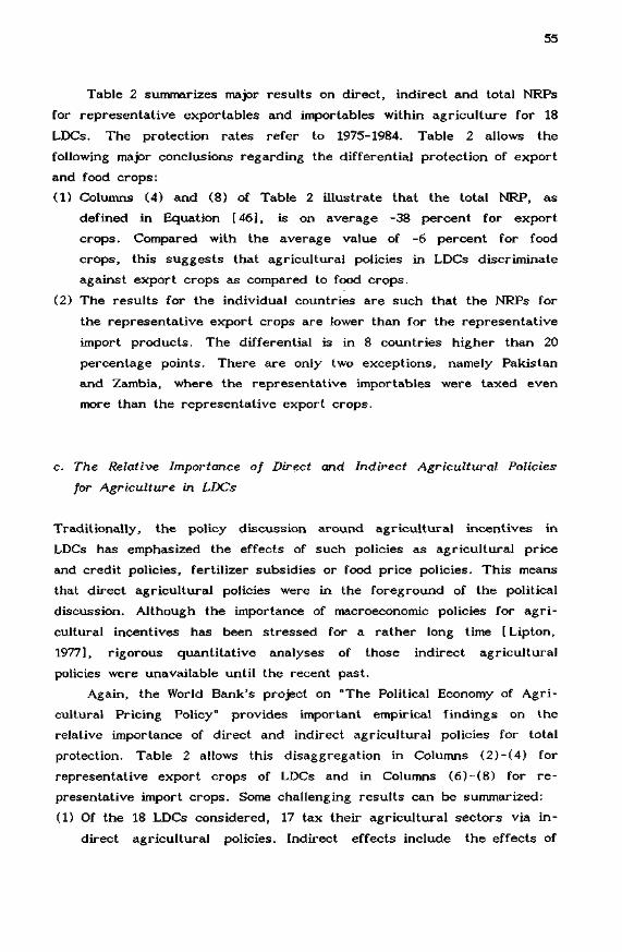
55

Table 2 summarizes major results on direct, indirect and total NRPs

for representative exportables and importables within agriculture for 18

LDCs. The protection rates refer to 1975-1984. Table 2 allows the

following major conclusions regarding the differential protection of export

and food crops:

(1) Columns (4) and (8) of Table 2 illustrate that the total NRP, as

defined in Equation [46], is on average -38 percent for export

crops. Compared with the average value of -6 percent for food

crops, this suggests that agricultural policies in LDCs discriminate

against export crops as compared to food crops.

(2) The results for the individual countries are such that the NRPs for

the representative export crops are lower than for the representative

import products. The differential is in 8 countries higher than 20

percentage points. There are only two exceptions, namely Pakistan

and Zambia, where the representative importables were taxed even

more than the representative export crops.

c. The Relative Importance of Direct and Indirect Agricultural Policies

for Agriculture in LDCs

Traditionally, the policy discussion around agricultural incentives in

LDCs has emphasized the effects of such policies as agricultural price

and credit policies, fertilizer subsidies or food price policies. This means

that direct agricultural policies were in the foreground of the political

discussion. Although the importance of macroeconomic policies for agri-

cultural incentives has been stressed for a rather long time [ Lipton,

1977], rigorous quantitative analyses of those indirect agricultural

policies were unavailable until the recent past.

Again, the World Bank's project on "The Political Economy of Agri-

cultural Pricing Policy" provides important empirical findings on the

relative importance of direct and indirect agricultural policies for total

protection. Table 2 allows this disaggregation in Columns (2)-(4) for

representative export crops of LDCs and in Columns (6)-(8) for re-

presentative import crops. Some challenging results can be summarized:

(1) Of the 18 LDCs considered, 17 tax their agricultural sectors via in-

direct agricultural policies. Indirect effects include the effects of

Table 2 - Direct, Indirect and Total NRPs for Exportables and Importables within Agriculture,(percent) (a)

1975-1984

Exportables

product

(1)

protection rates

direct

(2)

indirect

(3)

total

(4)

Importables

product

(5)

protection rates

direct

(6)

indirect

(7)

total

(8)

ArgentinaBrazilChileColombiaDominican RepublicEgyptGhanaIvory CoastMalaysiaMoroccoPakistanPhilippinesPortugalSouth KoreaSri LankaThailandTurkeyZambia

WheatSoybeansGrapesCoffeeCoffeeCottonCocoaCocoaRubber-(b)CottonCopraTomatoes-(b)RubberRiceTobaccoTobacco

Average

-19-141-6-23-2930

-26-22

-9-1817-(b)-30-22-134

-11

-27-23

7-30-19-16-78-30-7-10-42-28-9-15-33-17-38-50

-27

46378364245485629(b)51468(b)63395146

-(c)WheatWheatWheatRiceWheatRiceRiceRiceWheatWheatMaizeWheatRiceRice-(c)WheatMaize

-(c)141072320991253-41722218915-(c)1311

-27-237

-30-19-16-78-30-7-10-42-28-9-15-33-17-38-50

-38 21 -27

-917-234

-3621

-1846-14-59-61274

-18-(c)

-25-61

-6

(a) Direct, indirect and total NRPs are computed according to Equations [45]-[48] in Section B.II.6. -(b) South Korea and Morocco's main agricultural products are all imported. - (c) Argentina and Thailand'smain agricultural products are all exported.

Source: Schiff [1989, p. 11].

57

trade and macroeconomic policies on the real exchange rate and on

the extent of protection granted to nonagricultural products. The

only exception is Chile, where indirect agricultural policies slightly

favor agricultural protection. The average indirect NRP with -27

percent is rather remarkable.

(2) For the agricultural exportables, disincentives via indirect agri-

cultural policies strengthen the disincentives due to direct agri-

cultural policies which exist in all but three cases. On average, a

stronger taxation of agriculture stems from indirect rather than

direct agricultural policies. The average direct NRP is -11 percent

and, combined with the average indirect NRP of -27 percent, adds

up to a total NRP of -38 percent.

(3) For the agricultural importables, the picture is somewhat different.

In 12 out of 16 countries, the direct NRP is positive. On average,

the NRP is 21 percent. Concentrating on direct agricultural policies

alone would yield the result that agricultural importables, i. e. , food

crops, experience policy-induced subsidies. When the impacts of

indirect agricultural policies are also taken into account, however,

this subsidization is overcompensated, and an average total nominal

protection of -6 percent can be observed. Total NRPs are negative

in 10 out of 16 countries.

We can summarize that indirect agricultural policies are in most

countries more important than direct agricultural policies for overall in-

centives in agriculture. They tend to increase taxation of agricultural

exportables in LDCs and tend to reverse subsidization due to direct

agricultural policy for importables into a net taxation.

d. The Widespread Existence of Food Subsidization in LDCs

A stylized fact in the agricultural protection literature is that LDCs tend

to subsidize food consumption [Byerlee, 1987]. This stylized fact is con-

firmed by cross-country analyses in which consumer prices of food are

compared with "world prices". One of these studies is of Byerlee and

The importance of economy-wide measures is also visible in a study ongovernment intervention in agriculture of the six largest LatinAmerican economies by Roberts and Trapido [ 1991 ].

58

Sain [ 1986], and some of its results are presented in Table 3. For 1980-

1982, the authors argue that bread prices in wheat-importing countries

should have amounted to about US$0.75/kg, an estimate confirmed by-

consumer prices in Singapore and Panama where wheat was traded free-

ly. The computed NRP suggest that a widespread policy of subsidizing

bread consumption existed. The magnitude of subsidization was fairly

important. Byerlee and Sain demonstrated that the average price was 22

percent below the world price, or 27 percent if exchange rate over-

valuation is considered.

e. Does Agricultural Policy in LDCs Tax or Subsidize Food Production?"

It has been shown that many LDCs favor food crops rather than export

crops in their agricultural policies. Empirical evidence has proven, too,

that important export crops are taxed in many LDCs compared with free-

trade price levels. It is much less clear, however, whether agricultural

policy subsidizes or taxes the production of food crops compared with

world prices.

It is a stylized fact in the traditional literature on agricultural

policies in LDCs that food production is taxed due to economic and agri-

cultural policies [Brown, 1978; Lutz, Scandizzo, 1980; Schultz, 1978;

Lutz, Saadat, 1988]. The urban population has been believed to be

favored at the direct expense of the rural population. Again, Byerlee

and Sain [ 1986] contributed to this issue by a cross-country analysis of

wheat producer prices in 1980-1982. Based on the results contained in

Column (1) of Table 4, Byerlee and Sain came up with the challenging

result that producer prices for wheat in LDCs approached long-run

trend prices in the world wheat market during 1980-1982 and showed no

consistent evidence of price disincentives to wheat producers. Un-

expectedly, this basic result remains valid when exchange rate overvalu-

ation is taken into account. Column (3) in Table 4 shows this with ad-

The cross-country study of Mergos [ 1987] indicates a similar result forwheat, rice and maize in 1972 and 1978, but is one of the studies thatrelates directly farmgate and border prices without correcting fortransport costs and exchange rate distortions.

59

Table 3 - NPCs for Bread Consumption in LDCs, 1980-1982 (a)

ColombiaNigeriaBurmaCameroonKenyaChileNepalTanzaniaUruguayEcuadorParaguayLesothoBangladeshPeruBoliviaPakistanSudanIndiaBrazilMexicoTurkeyJordanMoroccoAfghanistanTunisiaEgypt

NPC

2.011.461.411.381.061.040.97

- 0.950.870.860.780.770.770.700.620.610.600.540.520.410.390.380.330.310.300.12

(a) NPCs are related here to consumer prices

Adjusted NPC

1.680.802.401.211.020.821.200.660.630.690.610.610.740.780.450.530.220.760.620.340.480.220.37na

0.380.05

Countries are ranked ac-cording to the unadjusted NPC. Adjusted NPCs take exchange rate mis-alignments into account. - na = not available

Source: Byerlee, Sain [ 1986, Appendix].

justed NRPs. The findings of the Byerlee/Sain study are rather re-

markable, since the authors' approach goes beyond several earlier

quantitative studies in three respects:

(1) NPCs are calculated at one point of the marketing chain. Transport

costs are taken into account.

(2) NPCs are not only computed with official exchange rates but also

with corrected exchange rates that are supposed to incorporate

exchange rate overvaluation in many LDCs.

(3) NPCs are based on "normal" world prices. This is done in order to

avoid a comparison of domestic prices with fluctuating world prices.

60

Table 4 - Estimated and Adjusted NPCs (a) for Wheat Producers in 31Countries, 1980-1982: On the Sensitivity of the Byerlee/SainResults

NigeriaSudanBurmaColombiaJordanAlgeriaBrazilMoroccoEthiopiaEcuadorBoliviaCameroonParaguayChileChinaLesothoBangladeshSyriaArgentina(b)KenyaTunisiaUruguayNepalMexicoTanzaniaPakistanAfghanistanIndiaTurkey(b)PeruEgypt

Producers taxed(NPC < 0.85) (percent)

No significant taxationor subsidization(0.85 < NPC < 1.15) (percent)

Producers subsidized(NPC > 1.15) (percent)

All countries (percent)Average NPC (percent)Median (percent)

(a) On the definitions of NPCj

NPC

(1)

2.602.372.051.671.661.501.351.351.321.241.211.191.081.071.061.021.001.001.000.890.840.800.790.760.730.710.680.660.650.510.41

35

26

391001.131.02

L, NPC2, aNP(

NPC2

(2)

2.402.191.891.541.531.38

, 1.251.251.221.141.121.101.000.990.980.940.920.921.000.820.770.740.730.700.670.660.630.610.650.470.38

39

32

291001.050.94

Z^ and aNPC2

aNPCl

(3)

aNPC2

(4)

1.43 1.320.90 0.833.49 3.221.40 1.290.98 0.901.52 1.401.67 1.541.55 1.431.05 0.970.99 0.910.88 0.811.05 0.970.85 0.780.85 0.781.25 1.150.81 0.750.96 0.890.91 0.840.60 0.600.86 0.791.06 0.980.59 0.540.98 0.900.66 0.610.50 0.460.62 0.57na na

0.92 0.850.79 0.790.58 0.540.19 0.18

37 50

40 27

23 23100 1001.03 0.950.92 0.84

see Section B.II.l. -

(b) Net exporters; the calculation of Byerlee and Sain were not changed for thesetwo countries as a different method for computing international prices was usedthere. - na = not available.

Source: Byerlee, Sain [1986, Table All; own computations.

61

The basic economic result of Byerlee and Sain has been challenged

in the literature due to two reasons [Herrmann et al. , 1991; Taylor,

1989]. First, the major result seems to be sensitive to the modelling

approach. Second, the findings seem to be very period- and product-

specific, and a comprehensive and well-founded protection analysis for

food crops should extend the period as well as the product coverage.

Concerning the first point, it can be put forward that the modelling of

the normal world price affects the economic result. Byerlee and Sain

compute their NPC, which we call NPC.., as follows:

[56] HPC1 = Pi/p*

Like in Equation [12] of the methodological survey, p. indicates the

domestic producer price of wheat and p * the normal world wheat price.

The latter price variable is measured by a linear time trend regression

of world prices over the period 1960-1982, and both prices are evaluated

at the consumption point. The rationale for using a normal rather than

the actual world price is that p * is an indicator of expected world

prices, whereas actual world prices include a stochastic component u:

[57] p = p* + u

Hence, the approach of Byerlee and Sain can be interpreted as one

which deals with price uncertainty, whereas the traditional approach

does not. The issue to be raised here is: Does the method which is used

to eliminate the stochastic component affect the economic results? In

order to answer this question, a reduced-form econometric model of the

world wheat market was developed. The estimated world wheat price from

this econometric model (p **) was introduced as a normal price into the

calculation of the NPCs. The resulting NPC, which we call NPC differs

from the Byerlee/Sain approach by the way the normal world price is

calculated:

[58] NPC2 = pD/p**

62

The econometric model is based on a stylized representation of

import demand and export supply in the world wheat market. The ex-

port supply function is

[59] Xt «• a + b p + c Y + d PIL + e PR^ + f POP

and the import demand function

[60] M = g + h p + i p r + j Y + k PRut + 1 PRMt + m POPMT*

X is exports and M is imports of wheat. P stands for the world wheat

price, Pp for the world rice price, PR for production of wheat, and POP

for population. Y is an income variable. The subscript X indicates ex-

porting and the subscript M importing countries, t and t-1 are the two

periods considered. Actual and lagged production are taken into account,

since a time lag between production and exports is realistic for many

exporting countries. The hypotheses on the signs of the coefficients are:

b>0, c<0, d>0, e>0, f<0, h<0, i>0, j>0, k<0, l<0, m>0. In an equilibrium

situation, exports are equal to imports:

[61] Xt = Mt

Introducing Equations [59] and [58] into Equation [61] yields the

reduced form of the world wheat model:

[62] p ^ = (g-a)/(b-h) + i/(b-h) • p R t + j /

- c/(b-h) • Yxt + k/(b-h) • ^ ^t_x

- d/(b-h) • PR^ - e/(b-h) • PRxt_1 + m/(b-h) • POPMt

- f/(b-h) • POPxt.

Equation [62] was the starting point of the econometric model. In order

to save degrees of freedom and to avoid multicollinearity problems, how-

ever, the production of the exporting and importing countries was ag-

Detailed and much more disaggregated econometric models of the worldwheat economy are available in the studies of Schiff [ 1985] andHarwood and Bailey [ 1990].

63

gregated. This seems acceptable, since it was not the goal of this

analysis to identify the underlying supply and demand Equations [59]

and [ 60]. It was also experimented with current and lagged income vari-

ables, and the income variables were constructed as weighted variables

for the major countries.

The following regression model performed best in the specification

search:

[63] In p = 5.9305 + 0.3544* In p,,,,, + 0.0848 In Y_ .Wt 1.32 2.76 RT 1.20 M t " 1

(0.38) _ (0.22)

+ 0.8681** In Y - 0.8433* In PR - 0.9077** In PR5.07 * -2.63 Z -3.07

(-0.45)

PXt-l

(1

- 0 .- 0 .

( -0 .

(R2

• 17)

20897214)

= 0.

In

96;

POP

DW

Mt-1

= 1.

( -0

+ 02

( 0 .

6 3 ;

.42)

.7687*

.8023)

F = 83

In

.31)

The price of American Red Hardwinter 2, cif Rotterdam, in USS/mt was

used as p , . p _ _ was measured as the price of American long corn

rice, cif Northsea ports in US$/mt. Both series are from the Stati-

stischen Bundesamt [various issues]. Y-, is the weighted gross

domestic product (GDP) of five major wheat-importing countries -

China, India, Japan, UK, and Brazil - in million US dollars. The GDP

is purchasing-power-partiy-corrected and in current prices. As there

were no GDP data available in current prices for China, the real GDP

was taken from Summers and Heston [ 1988] and corrected by the

Chinese national income deflator shown in IMF [1987]. The countries'

shares in wheat imports were used as weights. Y v is the weighted.A.

GDP of five major wheat-exporting countries - France, Canada, USA,

Argentina, and Australia - in million US dollars. It is again

purchasing-powei—parity-corrected and in current prices. The coun-

tries' shares in wheat exports were used as weights. The data for thecalculation of Y,. and Y v are from Summers and Heston [1988], andM Xthe trade shares are calculated from FAO [e] . PR, the world pro-

duction of wheat, is measured with data from FAO [c] . POP,, andM

POPV are trade-weighted population variables calculated with

population data from IMF [1987].

64

The values below the coefficients are t-values and the values in pa-

rentheses are beta coefficients. * indicates the 1 percent level of_2

statistical significance and ** the 5 percent level. R is the corrected

coefficient of determination, F the F-value and DW the Durbin/Watson

coefficient. Given the common test statistics, the overall performance of

the econometric model is quite good. 96 percent of the variation in the

logarithm of world prices can be explained with the model and major

hypotheses are confirmed. The world wheat price rises with an in-

creasing world rice price, with a growing income in exporting countries,

with a reduced world wheat production in the same year and in the

previous year, and with a rising population in the exporting countries.

The sign of the income variable Y...., indicates also that the world

wheat price is raised by a growing purchasing-power-parity-corrected

GDP in major wheat-importing countries with a one-year time lag. The

coefficient of the production variable can be interpreted as price

flexibility. An increase of world wheat production by 1 percent reduces

the world wheat price by 0.84 percent in the same period and by

another 0.91 percent in the next period.

Moreover, a comparison of simulation errors indicates that the actual

world wheat price can be much better explained with this model than

with a linear trend model as used by Byerlee and Sain. The root mean

square error over the estimation period 1960-1982 is 23.9 US$/mt with

the trend model and 6.9 US$/mt with the econometric model. Theil's in-

equality coefficient (TU) shows with 1.20 that the time trend model

performs worse than a naive simulation on the basis of previous years'

values, whereas the econometric wheat model clearly outperforms the

naive simulation (TU = 0.34). The antilog of In p according to Equation

[63] was now calculated for 1980-1982 and introduced into the denomi-

nator of NPC«. This allows to compare the NPCs of Byerlee and Sain

with those on the basis of an econometric world wheat model.

Table 4 shows NPC- and NPC_ for the 31 LDCs in Columns (1) and

(2). The results are summarized in the lower part of Table 4 in Columns

(1) and (2) for 1980-1982. It follows that, due to the better explanation

of movements in world wheat prices, the normal price according to the

structural model is closer to the actual world price than the linear trend

price. P™ is 197.4 US$/mt as opposed to p ^ with 182.11 US$/mt. This

65

means that NPC_ is by 7.7 percent lower than NPC. for all countries.

Table 4 shows that this makes a significant difference for the frequency

distribution of the NPCs. Whereas more LDCs subsidized than taxed

wheat production according to Byerlee and Sain, the reverse is true

when world price uncertainty is eliminated with a different method. The

median NPC is now 0.94 compared with 1.02, and it indicates that the

typical LDC taxes wheat producers.

The result becomes even more pronounced when exchange rate mis-

alignments are taken into -account. The coefficients aNPCL and aNPC_ in

Columns (3) and (4) of Table 4 capture this point by an adjustment of

NPC1 and NPC-, respectively. The comparison of aNPC. and aNPC2

shows that the median falls from 0.92 to 0.84. This means that the

frequency distribution exhibits a clear shift towards countries which tax

producers when price uncertainty is excluded with a structural economic

model - rather than with a trend model. According to our modelling

approach, the typical LDC clearly did tax wheat producers when ex-

change rate overvaluation is taken into account.

We can conclude on the sensitivity of the results of Byerlee and

Sain: the way how normal world prices are modelled matters to the

measured protection level. Put differently: the computed degree of

agricultural protection depends upon the modelling of price uncertainty

when normal rather than actual world prices are used.

Besides the importance of the modelling approach, another criticism

of the Byerlee/Sain findings is that they are too period- and product-

specific. A broader analysis of food price protection was provided by

Taylor [ 1989] who extended the analysis from 1980-1982 to 1980-1986 and

the product coverage by maize and rice. Additionally, the Taylor study

is based on national border prices rather than a uniform unit value of

imports, on actual rather than normal border prices and an exchange

rate correction via black market exchange rates. Table 5 presents her

major findings.

Taylor's results show that farmgate prices for wheat, maize and rice

were clearly below border price equivalents when exchange rate distor-

tions are taken into account. This pattern is valid for all subperiods

distinguished in Table 5. Maize prices, were on average, above and rice

66

Table 5 - Cross -Country Results on Incentives for Food Production inLDCs, 1980-1986 (a)

Wheat (31 countries)NPCAverageStandard deviation

Adjusted NPCAverageStandard deviation

Maize (36 countries)NPCAverageStandard deviation

Adjusted NPCAverageStandard deviation

Rice (23 countries)NPCAverageStandard deviation

Adjusted NPCAverageStandard deviation

1980-1982 1982-1983

1.10 1.070.32 0.43

0.83 0.670.30 0.29

1.37 2.83(b)1.72 7.93(b)

0.89 1.01(b)0.51 0.82(b)

0.74 0.840.34 0.49

0.61 0.610.33 0.34

(a) On the definitions and measurement of the NPC and thesee Taylor [1989, Chapter 3(d) 1983-1985.

. - (b) 1982-1984. - (c)

1984-1985

1.200.52

0.740.37

1.30(c)0.52(c)

0.93(c)0.56(c)

0.85(d)0.41(d)

0.600.16(d)

adjusted NPC,1985-1986. -

Source: Taylor [1989, Tables 4.1 and 4.4].

prices below border price equivalents when unadjusted NPCs are

measured. The average NPC for wheat ranged between 1.07 and 1.20.

Given possible data errors, Taylor evaluated this as being neither higher

nor lower than border price equivalents.

Given the still limited period covered and the differential results in

the empirical literature, we must conclude that the evidence on price

incentives for food crops in LDCs is still inconclusive. In particular,

this holds true on a broad cross-country basis using more comprehensive

time series data.

67

/ . On the Stabilizing Influence of Agricultural Policy in LDCs

The presented empirical evidence has substantiated the view that

economic and agricultural policies in LDCs tend to discriminate against

agriculture. This refers to the influence of policies on the level of

agricultural prices. There is, however, some evidence available

indicating that agricultural policy might have stabilized real producer

prices and, thus, might have created some risk benefits for farmers.

Table 6 presents some empirical results from the World Bank's project on

"The Political Economy of Agricultural Pricing Policy" on this issue. It is

revealed that, on average, producer price fluctuations were smaller than

border price fluctuations. This result is valid for representative agri-

cultural exportables as well as agricultural importables. It suggests that

Table 6 - Ratio of Standard Deviations of Deflated Producer and BorderPrices, 1960-1984 (a)

ArgentinaBrazilChileColombiaDominican RepublicEgyptlory CoastMalaysiaMoroccoPakistanPhilippinesPortugalSouth KoreaSri LankaThailandTurkeyZambia

Average

(a) The border price

Exports

crop ratio

Wheat 0.37Soybeans 0.80Grapes 0.94Coffee 0.87Coffee 0.84Cotton 0-42Cocoa 0.42Rubber 1.02NoneCotton 0.62Copra 0.94Tomatoes 1.13NoneRubber 0.44Rice 0.26Tobacco 1.16Tobacco 0.83

0.73

Imports

crop

NoneWheatWheatWheatRiceWheatRiceRiceWheatWheatCornWheatRiceRiceNoneWheatCorn

was measured at the official exchangedeflator was the price index of the nonagricultural sector.

ratio

0.410.730.930.660.301.200.470.630.170.271.001.580.65

0.560.75

0.69

rate. The

Source: Krueger et al. [1988, Table 3].

68

a price-stabilizing impact of most policies existed in the period 1960-

1984.

Table 6 also indicates, however, that there is a large dispersion in

the stabilization success of domestic agricultural policies. This as well as

the dominating stabilizing impact is confirmed in recent studies by

Knudsen and Nash [1990] and Guillaumont [1991]. Knudsen and Nash

provide empirical results for 15 crops across 37 LDCs, mostly for the

period 1967-1981, and find out that producer prices and producer

earnings were in most cases more stable than under world market

conditions. This pattern, however, is much more distinct for grains than

for beverages and fibers. The percentage of cases with stabilizing

effects were clearly higher for the typical food crops than for the

typical export crops. Guillaumont presents additional evidence on the

degree of stabilization of real producer prices for export crops in the

period 1979-1988. He concludes that there was a slight stabilization

impact, by 7 percent, on average, although destabilizing existed in

several cases.

g. On the Isolating and Stabilizing Influence of Limited Substitution in

Agricultural Markets

All studies on protection discussed so far used world market prices -

however measured - as the relevant reference prices against which to

judge domestic price policy. However, few countries look at the prevail-

ing world prices when setting their domestic prices for agricultural

goods. Instead, farm and consumer prices are administered and restric-

tions are placed on international trade to defend the domestic policies

[Timmer, 1986]. As a result of trade restrictions, the relevant free-

trade reference prices are unknown. Substitutions in both production

and consumption in the face of foreign competition will bring a new

equilibrium in farm output, consumption and trade, which is not easily

predictable on the basis of historical evidence before trade was openly

permitted.

Moreover, a large country's new agricultural policy may have a

significant effect on prices in world markets which have to be recognized

when estimating the protective effects of the former policy. A different

69

result is also obtained, if imported and domestically produced agri-

cultural commodities cannot be regarded as close substitutes because of

consumer preferences. If the cross price elasticity of domestically

produced agricultural products with respect to changes in the price of

imported products is relatively low, trade liberalization and the ac-

companying changes in the domestic price of imports will induce quantity

adjustments in the market for the domestic product which are not suf-

ficiently large to induce an equal percentage change in the domestic

price. This also implies that the protective effect [ Hiemenz, von

Rabenau, 1973, p. 83] and, consequently, the welfare effects are over-

estimated if import parity prices are used to evaluate agricultural policy.

There is enough empirical evidence to reject the assumption of

homogeneous agricultural markets found in standard welfare analyses of

agricultural markets. In fact, two-way trade in any sector, which is

ruled out by the "law of one price", can be found in agricultural trade

statistics at the most disaggregated commodity level [e.g. , FAO, e;

IRRI, 1988]. Furthermore, empirical evidence from Asia [e.g. , ADB,

1988] shows that there exists a wide spectrum of domestic prices indi-

cating limited substitution possibilities between different varieties, even

for such a narrowly defined market as that for rice. Finally, the law of

one price was rejected quite uniformly for various agricultural markets in

a recent study by Ardeni [1989].

In the following, we will first show how limited substitution can be

introduced into a model of an agricultural market and then discuss how

this influences the protection, welfare and stabilizing outcome of gov-

ernment-imposed interventions. We shall discuss these issues more

specifically with reference to rice in Malaysia. Limited substitution

implies that domestic consumers demand a composite commodity, C, which

is a function of imported quantities, M, and domestically produced

quantities, D:

[64] C = C(M, D)

Since total expenditure on the composite commodity must equal ex-

penditure on its imported and domestic components, we have the follow-

ing budget constraint:

70

[65] p-C = pM-M + pD-D

where p, p M and p^. stand for the composite commodity price, the import

price and the price for the domestic import substitute, respectively.

Assuming that consumers minimize the cost of purchasing a givenamount of the composite good, the demand for imported and domestic ricewill be functions of both the domestic price and the import price. Thesupply, S, of domestic rice will be a function of its own price:

[66] M = M(pM, pD)

D = D(pD, pM)

S = S(pD)

Now consider two varieties of rice that are substitutes in demand.

The supply of imported rice is perfectly elastic under the small-country

assumption, while the supply of domestic rice is upward sloping. As a

result of government-imposed distortions, the domestic prices of both

varieties are above the border price, and the welfare gains of free trade

are to be calculated. The situation is depicted in Figure 6. The demand

curves for imported and domestic rice are each conditional on the other's

price, i .e . , M(p_) and D(p-,). The demands are also conditional on in-

come, but this income is assumed to be constant with respect to the

policy change considered.

Figure 6 - Welfare Effects of Liberalization

M° M2 M1

71

Now let the price for M decrease from p.. to p. . as a result of0 1

liberalization. Initially, consumers attempt to increase M from M to M ,

but because of substitution in demand the lower price for M causes a

decrease in consumers' demand for D. This shift in demand for D from

D(pM) to D(pw) causes a change in p D from p~ to p.- which, in turn,

leads to a shift in demand for M from M(p_) to M(p_). The new equilib-1 2

rium finally occurs at price p., and quantity M .

Thus, the demand relationship M*, which takes account of adjust-

ments in the market for domestic rice, is obtained and this relationship

is less elastic than the movement along M(p_).

The total welfare gain generated by liberalization is the shaded

triangle under M*. As shown by Just et al. [1982, pp. 188-192], that

triangle measures consumer gains in the import market net of the loss of

government revenues as well as the gains to consumers and losses to

producers in the market for the domestic substitute.

What, then, determines the price adjustment in the domestic market?

Assuming a constant-elasticity-of-substitution (CES) function for Equa-

tion [62], de Melo and Robinson [1985] derive an expression which

relates percentage changes in the domestic price (p_) to percentage

changes in the domestic price for imports ( p j :

where a is the elasticity of substitution between imports and domestically

produced substitutes, 6 the price elasticity of demand for the composite

commodity, 9 the import share, and e the price elasticity of domestic

supply.

As can be seen from Equation [67], the price adjustment in the

market for domestic rice depends crucially on the elasticity of sub-

stitution. Thus, the higher the elasticity of substitution, the larger the

price adjustment of domestic supply.

Furthermore, it can be seen from Equation [ 67] that for any elasti-

city of substitution the responsiveness of the domestic price depends on

the import share. Thus, even if imported and domestic rice are close

substitutes in demand, the response of the domestic price to a change in

the import price will be small if the import share is low.

72

Finally, the derived nature of demand for domestic rice is shown by

the presence of the supply elasticity in Equation [67]. Thus, the higher

the elasticity of supply, the smaller the adjustment in the domestic price

necessary to bring equilibrium back to the market. The same can be said

of the role of the price elasticity of demand for the composite good.

These theoretical considerations are reflected in Table 7 which

summarizes the results from a sensitivity analysis on Malaysian rice

policy. The methodology involved the systematic elimination of distortions

from existing price levels to obtain a picture on prices, supply and

demand under a nonintervention scenario. In order to do this, the

theoretical model above was calibrated for prices and quantities on the

rice market for the period 1982-1986 given in Tamin and Meyanathan

[ 1988] and solved for the no-intervention prices and quantities. The

supply, demand and substitution elasticities, as reported in Tamin and

Meyanathan [ibid.] and Ahluwalia and Lysy [1983], were used as a

central estimate. However, because elasticity estimates differ widely from

researcher to researcher and because we wished to demonstrate the

sensitivity of the results to changes in elasticities, the supply, demand

and substitution elasticities actually used are the central estimate ± 0.5

times the point elasticities given by the sources. Thus, the results are

providing orders of magnitude rather than exact measures. The detailed

results for 1982-1986 are presented in Herrmann et al. [1991]. Table 7

shows averages over 1982-1986. The effects of rice market interventions

are evaluated in terms of nominal protection afforded, net social ef-

ficiency loss, the welfare trade-off between producers and consumers,

and changes in government revenue and expenditures.

If imported and domestically produced rice are perfect substitutes,

the welfare trade-off depends on the price elasticities of supply and

demand and the difference between the intervention prices and the

border price. Between 1982 and 1986, the domestic consumer and pro-

ducer prices in Malaysia have always been above the border price with

nominal protection being slightly higher for producers than for con-

sumers. With perfect substitutability apparent protection equals actual

protection, because arbitrage quickly equates goods prices internationally

under free trade. Assuming low supply and demand elasticities, producer

gains from intervention are estimated to average MS508. 5 million and gov-

ernment expenditures are MS145.5 million. However, consumers suffered

Table 7 - Sensitivity Analysis on the Price and Welfare Effects of Rice Market Interventions in Malaysia,Average 1982-1986 (a)

Reference solutionElasticity of supply (£)Elasticity of demand (<S)Elasticity of substitution (a)

Border price (p°) (M$ mil.)

Consumer price (p_) (M$ mil.)

Producer price (p ) (M$ mil.)

Apparent protection

NPCc(p°/p°)

NPCp(p°/p°)

No interventions outcomes

Producer price (p ) (M$ mil.)

Consumer price (pr) (M$ mil.)

Actual protection

NPCc(p°/pJ)

NPCp(p°/pJ)

Welfare results (M$ mil.)Producer gain/lossConsumer gain/lossGovernment revenue/expenditures

Total deadweight loss

(a) Low and high supply and demand

Perfect

low

0.100.15

508.5-383.2

-145.520.2

substitutability

CD

662

913

1123

1.4

1.7

662

662

1.4

1.7

elasticities.

high

0.300.45

486.0-401.3

-145.560.8

Strong

low

0.100.15

753

700

1.3

1.5

395.0-325.0

-83.713.8

substitutability

high

0.300.45

4.5

662

913

1123

1.4

1.7

865

746

1.3

1.2

259.0-262.7

-19.222.9

Weak

low

0.100.15

865

746

1.3

1.2

280.2-254.5

-33.47.6

ubstitutability

high

0.300.45

1.5

662

913

1123

1.4

1.7

1007

804

1.1

1.1

123.8-168.6

37.37.5

Source: Herrmann et al. [1991]. j

oo

74

an average loss of MS383. 2 million due to government intervention. Thus,

the average net social welfare loss (i.e., the deadweight efficiency loss)

amounted to M$20.2 million. Comparing these results with those of the

high elasticity case shows that the losses depend linearly on the assumed

supply and demand elasticities.

If imported and domestically produced rice is not perfectly sub-

stitutable in consumption, the no-intervention outcomes change drasti-

cally. As a result of product differentiation in demand, the fall in

domestic prices will be smaller than in the case of perfect substitutability

and will never equal border prices. As can be seen from Table 7,

domestic consumer and producer prices in the free-trade situation are

always above the border price with consumer prices being a consump-

tion-share-weighted average of the border and producer prices. Actual

protection coefficients relating the initial domestic prices to the free-

trade domestic prices are less than the apparent protection coefficients

relating domestic prices to border prices. As a result, the welfare

effects are much lower than in the case of perfect substitutability.

This is best illustrated by comparing the previous results with

those calculated under the assumption of weak substitutability and high

supply and demand elasticities. In this case, producers realize an aver-

age welfare gain of only MS123.8 million, which is only one-fourth of

producers' surplus estimated under the assumption of perfect substitu-

tability. This result is intuitively clear, because domestic producers

would benefit from some kind of "natural protection" with weak sub-

stitutability, even in a free-trade situation. Furthermore, consumers

suffer an average loss of MS168.6 million which is below 50 percent of

the previous case. These consumer losses are mainly attributable to the

implicit tax on imports. As a result, government expenditure for pro-

ducer subsidies are less, on average, than revenues from implicit taxes

on imports leaving net government revenues of M$37.3 million as

compared to net expenditures of MS145.5 million with perfect substi-

tutability. Thus, the average deadweight losses amount to only M$7.5

million.

Our results indicate that limited substitution possibilities can play

an important role in determining the final welfare effects of government

intervention in the Malaysian rice market. Assuming stronger substitut-

ability (a = 4.5) changes only the quantitative results leaving the

75

qualitative conclusions from the comparison of the two extreme cases

unaffected. In any case, limited substitution drives a wedge between

domestic prices and border prices, the extent of which depends on the

degree of substitutability on the consumer side, the share of imports in

total domestic supply and the supply and demand conditions in the

domestic market.

Some other observations which can be made are summarized in Table

8. There, the mean and the coefficient of variation (CV) of selected

variables over 1982-1986 in the free-trade situation and for various

elasticity assumptions are confronted -with those in the distorted

situation. The results can be summarized as follows:

(1) In terms of magnitude, the supply mean is raised (though not sub-

stantially) with intervention, while demand is reduced compared to

intervention. Imports, on the other hand, were in fact reduced over

the period.

(2) The changes in quantities increase with increasing substitutability

and increasing supply and demand elasticities. The same holds true

for producer and consumer prices. Thus, limited substitutability

diminishes the need to support producer prices in order to increase

producer income.

(3) Limited substitution in connection with high supply and demand

elasticities has a stabilizing effect on both producer and consumer

prices. This result also suggests that there is less need for inter-

vention if substitution possibilities are limited.

Although the above welfare calculations are not based on an econo-

metric estimation of the substitution elasticity for rice in Malaysia, they

provide nevertheless useful insights into the impact of agricultural

pricing policies. Perhaps the most important result that emerges from our

findings is the importance of the import share in determining domestic

price changes. Standard trade theory would predict that, even for a

large market such as the rice market in Asian countries, price liberal-

ization would exert strong pressure on domestic prices. On the contrary,

the Armington specification implies that a large market with a low import

share has substantial price autonomy. From the government point of

view, another interesting result is the fact that expenditures to support

the guaranteed minimum price (GMP) would need to be much lower than

is predicted under traditional assumptions.

76

Table 8 - Means and CVs with and without Intervention in Malaysia,1982-1986 (a)

With inter-vention

meanCV(per-cent)

Without intervention

perfect sub-stitutability

mean

Low supply and demand elasticities

Production 1135Consumption 1504Imports 370Border priceConsumer price 913Producer price 1123

High supply and demand

Production 1135Consumption 1504Imports 370Border priceConsumer price 913Producer price 1123

5.977.23

22.62

0.281.78

10881566478662662662

elasticities

5.977.23

22.62

0.281.78

9961689693662662662

CV(per-cent)

6.516.96

19.2415.6515.6515.65

8.147.49

20.0515.6515.6515.65

strong sub-stitutability

mean

10981557459662700753

10571628571662746865

CV(per-cent)

6.407.10

20.4515.6512.7411.18

7.087.68

22.4815.659.737.53

weak sub-stitutability

mean

11091546437662746865

11001585485662804

1007

(a) Production, consumption and imports in lOOOt. Prices in M$/tthe coefficient of variation. It is equal to the •the respective variable divided by the meanMean is the arithmetic mean.

of the

CV(per-cent)

6.287.20

21.5915.659.737.53

6.457.58

23.3615.656.273.84

CV isstandard deviation ofvariable, times 100.

Source: Herrmann et al. [1991].

The question remains whether the assumption of product differen-

tation at the micro level is reasonable. There may be disagreement on

the correct specification of the substitution elasticity, but one certainly

does not observe the degree of substitutability found in standard trade

theory.

77

2. Deficiencies in the Empirical Literature and the Additional Benefit ofthe Following Quantitative Analysis

The survey has shown that our knowledge on the international pattern of

agricultural protection has significantly developed further during the

1980s. In particular, many more country studies have become available in

which the extent, the structure and the causes of agricultural protection

have been measured and analyzed in detail. Important findings of coun-

try studies include that macroeconomic and trade policies are often more

important than direct agricultural policies for agricultural incentives in

LDCs. The results of country studies indicate in most cases that overall

incentives work against agriculture and that policy discriminates against

agriculture. Despite these important findings, the quantitative literature

on agricultural incentives in LDCs is in some important aspects in-

sufficient:

(1) The information on agricultural protection at the commodity level is

much more limited than at the country level. Country studies refer

to those commodities that are relevant from the individual countries'

points of view. Comprehensive cross-country comparisons of price

protection for important export and food crops are much more rare.

The study of Byerlee and Sain [ 1986] is limited to the period

1980-1982 and the wheat sector, and the results of Taylor [ 1989]

refer to 1980-1986 and wheat, maize and rice. Similar cross-country

results for important export crops are not available at all.

(2) Within the given literature on agricultural protection, the discussion

has focused on the level of agricultural protection. There exists no

analysis of the longer run time series pattern of agricultural pro-

tection, i. e., of trends and instabilities in agricultural protection.

(3) Most country studies on agricultural protection still focus on pro-

tection vis-a-vis foreign competitors neglecting policy-induced

distortions in the domestic terms of trade between individual

agricultural commodities and nonagriculture. This holds also true for

protection analyses on Peru and Zimbabwe. For Malaysia, Jenkins

and Lai [ 1989] investigate the relative protection afforded to

producers of rubber, palm oil and rice, but neglect another

promising cash crop, i. e. , cocoa. Moreover, the analysis does not

78

include the periods of structural adjustment (1985-1986) and re-

covery (1987-1988).

(4) Existing analyses of indirect agricultural protection do not dif-

ferentiate between^ indirect protection which is attributable to trade

policies on nonagricultural tradables and indirect protection resulting

from macroeconomic policies. Such a differentiation, however, is

necessary when it comes to policy recommendations. The recommen-

dations for policy reform may be quite different depending on the

source of agricultural discrimination.

The empirical analysis in the following parts will deal with these

significant shortcomings of the quantitative literature on agricultural

protection. To begin with, a rather comprehensive data basis on com-

modity-specific protection levels will be presented for wheat, rice and

coffee. Comprehensiveness will be attempted in terms of the countries

covered and the period of analysis: 1969-1985. In computing the pro-

tection levels, transport costs will explicitly be considered as well as

exchange rate distortions. The magnitude, the development and the in-

stability of protection levels will be measured, and the components of the

instability of protection rates will be elaborated for the three major food

and export crops of LDCs. This information will then be used to draw

conclusions on various policy-relevant issues like the relative importance

of direct and indirect agricultural policies for agricultural incentives, its

developments over time, relative incentives for coffee compared with

wheat and rice, or the policy impacts on price stability.

Next, we analyze the effects of trade restrictions and macroeconomic

policies on the agricultural sector in Malaysia, Peru and Zimbabwe. In a

first step, true protection resulting from agricultural pricing policies and

nonagricultural pricing policies are measured and contrasted with nominal

protection. This analysis covers the most important export crops in the

three countries. Following is an in-depth analysis of indirect protection

in Malaysia. Here, the focus is on different sources of indirect pro-

tection. Finally, the results on indirect protection are compared with

those on other countries and the question whether food crops are subsi-

dized and cash crops are taxed is discussed on a broad commodity basis.

79

C. Magnitude and Structure of Protection

I. Introduction

The literature survey in the previous chapter revealed that a number of

country studies on protective measures in the agricultural sector are

available, whereas comprehensive cross-country analyses for specific

goods are still lacking. In this part of the present study, it is the ob-

jective to provide a contribution to fill this gap by establishing a broad

data set on an individual commodity basis.' We examine the extent of pro-

tection, the change in protection over time and its variation across a

wide range of countries for three important agricultural commodities,

namely wheat, rice and coffee.

The chapter is organized as follows: Section C. II introduces the

measurement concept applied in our analysis and describes the data base

used in the calculations. After this, the quantitative results for all three

crops will be presented and interpreted. In the cases of wheat (see

Section C. III. 1) and rice (see Section C. III. 2), the samples comprise

DCs as well as LDCs. This enables us to investigate in how far the con-

clusion drawn in Section B. Ill that DCs generally protect their agri-

cultural sectors as opposed to LDCs is also valid for specific agricultural

commodities. Furthermore, we make a distinction between net importers

and net exporters, because one would expect government authorities to

behave differently in either case, emphasizing self-sufficiency goals in

the first and tax revenues or the maintenance of world market shares in

the second situation. With respect to coffee (see Section C. III. 3), how-

ever, the sample does only consist of LDCs for which coffee is a major

cash crop. In Section C. IV, the instability of protection and its possible

causes, domestic or border price fluctuations, are examined. The main

goal of this analysis is to elaborate whether producer prices are

successfully stabilized in the presence of volatile world market prices.

Finally, Section C. V contains a comparison of the results obtained for

the individual commodities. We address the question there whether gov-

ernment authorities treat food crops (in this case wheat and rice) more

favorably than export crops (in this case coffee), as is often suggested

in the literature [e.g., Krueger et al., 1988] but which has not yet

80

been demonstrated for specific commodities by broad cross-country

analyses.

II. Data and Procedures

In the following, the NPC serves as a measure of agricultural price

policies with two alternatives to be considered.

First, the gross NPC" is calculated as the ratio between domestic

prices and border prices, the latter being regarded as the opportunity

costs facing domestic producers (see Section B. II. 1). Data for producer

prices of various agricultural commodities are available from FAO sta-

tistics on prices that farmers received [FAO, d]. They were converted

into US dollars at the prevailing official exchange rate. For the calcu-

lation of border prices, we distinguish between net-exporting and net-

importing countries. The appropriate price for the former is measured

fob at the local port. In the latter case, cif prices are used. The

respective data are obtained as unit values from FAO [e]. For two wheat

importers (South Africa, Poland) the reported data were fob for both

imports and exports. In these cases the import values were converted

into cif using a standard conversion factor of 112 percent [ibid.]. With

respect to rice and coffee, produced and traded quantities are not di-

rectly comparable. Since rice production is reported in paddy units and

rice trade in milled rice units, the former was transformed into milled

rice units by applying the standard conversion factor 0.65 (1 paddy unit

= 0.65 rice units). Border prices for coffee refer to green or roasted

coffee and coffee substitutes containing coffee, whereas prices received

by farmers relate to green coffee. As coffee is mainly exported in the

form of green coffee, border prices as reported by the FAO are deter-

mined to a high degree by green coffee exports. Therefore, the bias

between the two reference quantities is rather small and can be

neglected.

The term "green coffee" is a synonym for "raw coffee" and iscommonly used by coffee traders for beans which are only preparedfor storage and transport. In 1980/81, about 90 percent of all coffeeexports were unprocessed. In earlier years, this share was evenlarger [ International Coffee Organization, various issues ].

81

Since producer prices and border prices should be brought to a

single marketing point in order to be comparable (see Section B. II. 1),

we, first, carried out an adjustment for internal transportation costs

between the farm gate and the local port to obtain export and import

parity prices, respectively. The transport margins are taken for some

countries from Taylor [1989]. For all other countries of our sample, in-

formation about major production regions for the respective commodities

is taken from the World Atlas Agricultural Committee [1973], and internal

transportation costs are computed along the lines suggested by Taylor

[1989].

Second, a factor correcting for exchange rate distortions was in-

cluded to account for indirect effects resulting from general economic

policies like commercial, exchange rate, monetary, and financial policies.

Currency overvaluations are widespread in LDCs, because governments

have often failed to adjust exchange rates when expansionary monetary

policies have produced higher inflation at home than abroad. Such a

policy implicitly results in import subsidization of food or taxation of

agricultural export commodities, i. e., agriculture is discriminated

against. Hence, using the official exchange rate to convert domestic

producer prices into US dollars may lead to severe overes timations of the

protection level. More realistic NPCs adjusted for exchange rate

distortions (net NPCs) were calculated by multiplying the unadjusted

protection coefficient by the ratio of the published black market rate

[Cowitt, 1986; Pick, 1978] to the official exchange rate [IMF, 1990],2

both expressed in US dollars per home currency. We posit that the

black market exchange rate is an acceptable estimate of the unobservable

free-market price for foreign exchange, although black market rates

certainly include a risk premium given the illegality of transactions on

those markets.

In order to assess the variability of NPCs and to quantify in how

far this variability was due to instabilities in domestic and world market

prices, respectively, we finally conducted a variance decomposition of

Taylor [ 1989, p. 32] provides a detailed description of the calculationof internal transportation costs.

2This method of considering exchange rate distortions is discussed inSection B. II. 1.

82

the protection coefficient for each single country. In a second step, we

also decomposed the variance of the domestic prices in US dollars into

price and exchange rate components to answer the question whether gov-

ernment authorities achieved the goal of stabilizing agricultural producer

prices in home currency.

The variance decomposition procedure can formally be derived as

follows: since the NPC is defined as the domestic price (P. ) divided by1 $the border price (P ), log NPC equals the difference between log P.

^V 1

and log P . For the variance of this difference holds the following

equation [e.g., Mood et al. , 1974, p. 179]:

[68] Var(log NPC) = Var(log P? - log P ) = Var(log P?)

+ Var(log P ) - 2 • Cov(log P?, log P )

According to Equation [ 68], instabilities in the protection levels either

reflect movements in domestic dollar prices or in world market prices.

Moreover, the joint effect of both components as measured by the co-

variance term does affect the variance of the protection coefficient. A

positive covariance indicates that both prices move in the same direction

and - since we analyze a quotient - offset each other, thereby lowering

the variability of the NPC compared to a situation in which domestic and

world market prices would vary independently.

Alternatively, the equation may also be formulated for variations of

the variables around log linear trends. In order to decide which of both

versions is appropriate in a special application, one has to test initially

whether the trend function of the variables in use is significant. In al-

most all cases, at least two out of three time series showed significant

trend functions. We then calculated standard deviations from a log linear

trend. In particular, this holds true for prices and exchange rates.

There were only a few exceptions in which standard deviations from the

mean had to be calculated.

This method was previously used, e.g., for isolating the contributionsof price and quantity effects to revenue instabilities in the agriculturalsector [Murray, 1978/79; Herrmann, Schmitz, 1984].

83

From Equation [68], the percentage contributions of instabilities in

domestic and world market prices to variations in NPCs can easily be

derived as

[69] CP̂ = 100 • Var(log P?)/Var(log NPC),

[70] CP = 100 • Var(log P )/Var(log NPC)

and

[71] CP?P = 100 • 2 • Cov(log P?, log P )/Var(log NPC).

$CP. denotes the contribution of domestic price movements to protection

instabilities, CP the respective contribution of world price fluctuations$ W

and CP. P the joint effect of both prices.The variance decomposition of the domestic price follows the same

$principle. Since the dollar price (P. ) equals the price in home currency(P.) multiplied by the exchange rate in US dollars per domestic currency

unit (E), it follows that

[72] Var(log p|) = Var(log P i + log E) =

Var(log P.) + Var(log E) + 2 • Cov(log P., log E).

Hence, exchange rate fluctuations or price changes in home cur-

rency may be the reason for dollar price variations. The covariance

term, which now refers to a product, has to be interpreted differently

from Equation [68]: a positive (negative) sign indicates that price and

exchange rate movements intensify (neutralize) each other in their effect

on dollar prices. The respective percentage shares in the variance of log

VarQog P.)/Var(log P?),

Var(log E)/Var(log P.)

P.* are

[73]

[74]

CP.

CE

= 100

= 100

and

[75] CP.E = 100 • 2 • Cov(log P., log E)/Var(log P?)

84

where CP. is the contribution of price changes in home currency to

dollar price instabilities, CE the contribution of the exchange rate

component and CP.E the joint effect of both exchange rates and home

prices.

The instability analysis enables us to assess in how far producer

prices for wheat, rice and coffee are successfully stabilized by

comparing the variations of world market prices and domestic prices in

home currency. A successful stabilization requires that

[76] Var(log Pi) < Var(log P )

The greater the difference between VarOog P ) and Var(log P.), the

more producer prices in home currency are stabilized.

III. Estimates of the Nominal Rates of Agricultural Protection

1. Survey of Protection Levels for Wheat

Wheat is the major traded food grain in the world. The world wheat

market is dominated by four exporters: Australia, Canada, France, and

the USA. Argentina is the only other country which has a considerable,

regular wheat export trade. On the other hand, China and the former

USSR have been the world's largest producers and importers of wheat,

apart from the old established importers Japan and the UK. Furthermore,

LDCs have become importers on a steadily increasing scale, particularly

in Asian market economies, North Africa and the Middle East [Josling,

1980, p. 15; Harwood, Bailey, 1990, p. 11]. Wheat has become the most

important agricultural product concerning world food security. The

ability of the world to feed its growing population rests heavily on the

production and the international trade flows of wheat. Hence, conditions

in the wheat market are the most significant single determinant of world

food security [Josling, 1980, p. 15]. Having this importance of wheat as

foodgrain in mind, one would expect that domestic policies at least in

Byerlee [1987, pp. 307-328], investigated the political economy of in-creasing wheat imports by LDCs.

85

import-dependent countries tend to favor wheat producers rather than to

discriminate against them in order to improve self-sufficiency.

The structure of protection in the world wheat sector is now

analyzed by means of NPCs which are calculated for the period 1969-

1985. The sample of wheat-producing countries is divided into net im-

porters and net exporters, since it can be expected that price policies

are different depending upon the self-sufficiency ratio in each country

(see Section C. I). With these countries, 57 percent of the world wheat

production is captured, on average, during the period considered. The

sample covers 20 net importers (including 6 typical poorer LDCs, 10

richer LDCs and 4 DCs) and 12 net exporters (including 5 richer LDCs

and 7 DCs). The classification of countries resulted from the dominating

trade status in the years under consideration. The NPCs for individual

years, however, were calculated according to the trade situation in the

respective year. A detailed list of NPCs for all countries is presented in

Tables A2 and A3.

Table 9 gives an overall impression of the distribution of alternative

NPCs for wheat producers across countries and over time. In Column

(1), traditionally measured coefficients are shown. Over the whole period

and across the total sample of wheat-producing countries, gross NPCs

are clearly above unity, thus indicating that wheat producers do not

face direct price discrimination in the long run. Hence, the wheat sector

is protected by direct agricultural price policies worldwide, which may

be explained by the particular role of this product as a staple food.

In individual years, however, protection coefficients diverge from the

average values depending upon the movement of border prices and the

degree of price transmission in each country. Particularly, this became

obvious during the world food crisis in 1974/75, when world market

prices for cereals more than doubled because of a worldwide supply

shortage and a boom in world demand. In these two years, NPCs

differed significantly from those in other years and were below unity in

most country groups except in importing DCs. This suggests a wide-

spread strategy of insulating domestic markets from world market

conditions.

Moreover, the difference between the average coefficients for the

total period as opposed to the two years of the food crisis are a rough

indicator of how world prices are transmitted into domestic markets. The

86

Table 9 - Gross and Net NPCs for Wheat Producers, 1969-1985

All countries1969-19851974-1975LDCs1969-19851974-1975DCs1969-19851974-1975

Net importers1969-19851974-1975Poorer LDCs(c)1969-19851974-1975

Richer LDCs(d)1969-19851974-1975

DCs(e)1969-19851974-1975

Net exporters1969-19851974-1975Richer LDCs(f)1969-19851974-1975

DCs(g)1969-19851974-1975

Measures of protection(a)

gross NPC

(1)

1.230.86

1.140.79

1.411.00

1.270.89

1.170.86

1.270.86

1.441.02

1.170.80

0.910.59

1.400.99

(a) Aggregated by the unweighted geometric mean. -exchange rate distortions.Tanzania, India, Pakistan(d) Brazil, Chile, Mexico,Yugoslavia, Poland. - (e)(f) Argentina, Uruguay, SouthCanada, USA, France, Greece,

net NPC(b)

(2)

0.980.72

0.820.61

1.390.99

0.930.71

0.780.62

0.860.68

1.431.00

1.090.74

0.790.50

1.400.98

(b) Adjusted for(c) Egypt, Kenya, Morocco, Nigeria,

(GDP per capita 1980 < US$1,200). -Algeria, Tunisia, South Korea, Syria,West Germany, Italy,

Africa, Turkey, Hungary.Spain, Sweden.

UK, Japan.- (g) Australia,

Source: Own computations with data from World Bank [ 1982] and TablesA2 and A3.

greater the reduction of NPCs due to extremely high world market

prices, the lower the price transmission is, and the higher the degree of

87

insulating domestic markets is. Regarding the various country groups,

there is a remarkable distinction. While the difference between both

periods is only 0.35 percentage points in LDCs, DCs show a much

greater deviation from the average in 1974/75, notably a difference of

0.41 percentage points. Hence, in LDCs the degree of insulating

domestic wheat production is greater than in DCs. This implies that not

only the level of wheat subsidization is higher in DCs than in LDCs but

also the degree of protecting domestic producer prices from world price

variability.

Net-importing and net-exporting countries differ in the level of

support. On average, net importers show higher protection coefficients

than net exporters. This indicates that self-sufficiency might be a major

objective of wheat pricing policies in net-importing countries. While high

income exporting countries also clearly protect wheat producers, export-

ing LDCs even tend to discriminate against them. This suggests that

wheat exports in these countries are often taxed in order to raise gov-

ernmental revenues. Another important finding which can be derived

from Column (1) is the fact that protection levels rise with economic

development in importing as well as in exporting countries. While gross

NPCs in DCs are clearly above the average levels of the two samples,

importing and exporting LDCs exhibit lower values. That is, LDCs do

not favor wheat production as much as DCs do.

One country stands out from the whole sample with an average un-

adjusted NPC of 3.40: Japan. This extremely high protection coefficient

rests on the fact that agricultural imports into Japan are more restricted

quantitatively and by means of import tariffs than in any other OECD

country. With relatively poor endowments of arable land, Japan heavily

relies on imports of foodstuffs. The self-sufficiency rate for wheat was

only 10-12 percent in the early 1980s. Therefore, domestic farmers are

highly protected from import competition in order to stimulate domestic

food production [OECD, b, p. 18; Vincent, 1989, p. 173].

In Column (2) of Table 9, NPCs adjusted for exchange rate distor-

tions are shown. These net NPCs were calculated by multiplying unad-

justed coefficients by the ratio of the black market exchange rate to the

For a detailed analysis of the background of agricultural protection inJapan, see Hayami [ 1988] and Australian Bureau of Agricultural andResource Economics [1988].

88

official exchange rate in US dollars per home currency. Assuming that

black market exchange rates represent the true demand price for foreign

currency on free capital markets [Taylor, 1989, p. .39], the indirect

impact of macroeconomic conditions on agriculture can be captured with

this exchange rate adjustment.

Table A8 presents average exchange rate factors which measure

exchange rate distortions. Most countries show factors lower than 1,

implying that black market exchange rates are lower than official rates,

thus indicating widespread policies of exchange rate overvaluation. In^ 16

out of 32 countries, factors range below 0.9 and in 8 countries, factors

are even lower than 0.75. The 11 DCs of the sample present no distinct

exchange rate distortions. Hence, overvalued exchange rates are typical

for LDCs. Table 9 shows that the overall protection level decreases in

importing as well as in exporting countries due to exchange rate

distortions. In comparing country groups, one can recognize that the

degree of exchange rate distortion varies considerably. While in all DCs

the differences between gross and net NPCs are negligible, the pro-

tection level decreases from above to below unity in importing LDCs.

Among the net exporters, LDCs show a significant reduction of the

protection coefficient, too. It becomes clear that the wheat sector is

heavily discriminated against in low-income countries when exchange rate

overvaluation is taken into account. Hence, indirect macroeconomic

policies affect agriculture seriously and often reduce production in-

centives for farmers. This is one reason why self-sufficiency particularly

in African countries could not be improved substantially, although it is a

major goal of producer price policy as it is indicated by the results of

Column ( I ) . 1

Summing up, the main results of Table 9 are the following. On the

one hand, producer prices for wheat are by and large favorable not

only in DCs but also in LDCs. The only exception is constituted by the

net-exporting LDCs that tend to discriminate against wheat production

directly. On the other hand, macroeconomic policies like overvalued ex-

For a detailed description of the influence of macroeconomic policies onagriculture in general and of currency overvaluation on the perform-ance of African agriculture in particular, see Valdes [ 1986, pp. 161-183] and Lofchie [1987, pp. 95-97]. An analysis of the politicaleconomy of rapidly increasing wheat imports into LDCs is provided byByerlee [1987, pp. 307-328].

89

change rates have a major indirect impact on agriculture in LDCs causing

unfavorable production conditions for wheat producers. Hence, these

policies are responsible for a poor performance of the wheat sector in

many low-income countries and for the high import dependence those

countries are facing.

The results of our study confirm the findings of Byerlee and Sain

[ 1986] and Taylor [ 1989] for a much longer period. The two earlier

studies also analyzed gross and net nominal protection for wheat in LDCs

(see Section B. III. l .e). Contrary to the traditional hypothesis that

producers in LDCs are discriminated against by low farm prices for food

crops, they also found out that wheat producers in LDCs, on average,

did not face direct price discrimination in the early 1980s. Indirect

taxation caused by exchange rate distortions, however, appeared to be

widespread in LDCs and to offset direct protection often. One limitation

at least of the Taylor study is the fact that general statements about the

treatment of agriculture should not be based on short-run measurements

of protection, since extreme world market prices in single years

produce protection coefficients which differ significantly from those in

"normal" years. Our analysis presents evidence that direct price pro-

tection and indirect discrimination of wheat production in LDCs did not

only occur in the 1980s but in most of the earlier years from 1969 on,

too.

Moreover, the demonstrated importance of indirect as opposed to

direct agricultural policies for the overall performance of agriculture in

LDCs is in line with the findings of the World Bank's project on "The

Political Economy of Agricultural Pricing Policy" (see Section B. III.l.c).

Finally, our study provides the additional benefit that the pattern of

agricultural protection in the world wheat sector can be analyzed, since

typical LDCs as well as typical DCs are taken into account, and pro-

tection levels can be compared directly across countries and country

groups as well as over time because of the uniform measurement of pro-

tection.

Byerlee and Sain compared producer prices with a so called normalworld market price which represented a long-run trend price calculatedby a linear time trend regression of world prices over the period 1960-1982 [Byerlee, Sain, 1986] (see Section B. III. 1. e).

90

2. Survey of Protection Levels for Rice

Rice is a very important commodity for human nutrition in the developing

world, especially in Asia and West Africa. In some Asian countries

(Bangladesh, Burma, Kampuchea, Laos, Thailand), the rice calory

supply accounts for more than two third of the total calory supply

[IRRI, 1988, p. 112]. Asia contributes about 90 percent to the world

rice production, the most important producers being China (including

Taiwan), India, Indonesia, and Bangladesh. Most of the rice is grown

for domestic consumption, while only a small fraction of about 5 percent

is sold in the world market, predominantly by China, Thailand,

Pakistan, and the USA. The direction of trade has changed during the

period under consideration [USDA, 1986]: Asian countries like India,

Indonesia and South Korea, which heavily relied on rice imports during

the 1970s, became more or less self-sufficient in the early 1980s, where-

as the African share in world rice imports increased significantly.

Against this background, price incentives in the rice sector are

examined by means of gross and net NPCs. Protection coefficients for

each individual country are presented in Tables A4 and A5. Table 10

provides a condensed survey of the level of protection across different

country groups covering the time period 1969-1985. The whole sample2

consists of 29 rice producers including 5 DCs and 24 LDCs. Theaverage traditional NPC that reflects only direct price policies was

slightly above unity for the total country sample, thus indicating a

moderate overall price support in the world rice market. As one would

expect, DCs were, on average, more protectionist than LDCs.

Significant deviations from the general pattern of protection

occurred in two subperiods. First, between 1970 and 1972 depressed

world market prices corresponded with above average NPCs. Second,

NPCs were comparatively low during the commodity price boom in 1974

and 1975. Both peculiarities indicate that fluctuations in world prices are

not entirely transmitted to the domestic market (see Section C. III. 1).

Childs [ 1990] points out that the low trade flows are, among otherthings, a result of very restrictive policies like import bans in Japanand South Korea.

2Some socialist countries, which are important rice suppliers (China,Laos, Kampuchea, South Korea, Vietnam), are excluded from thesample due to a lack of data.

91

Table 10 - Gross and Net NPCs for Rice Producers, 1969-1985

All countries1969-19851970-19721974-1975LDCs1969-19851970-19721974-1975DCs1969-19851970-19721974-1975

Net importers'1969-1985Poorer LDCs(c)Richer LDCs(d)AsiaAfrica

Net exporters1969-1985LDCs(e)DCs(f) (except Japan)Japan

(a) Aggregated by the unweightecexchange rate distortions.

Measures of protection(a)

gross NPC

(1)

1.091.300.75

1.01-1.190.67

1.602.011.46

1.120.991.661.201.00

1.040.731.264.14

I geometric mean. -

net NPC(b)

(2)

0.851.000.61

0.740.870.53

1.591.991.45

0.870.731.500.980.73

0.830.481.254.13

(b) Adjusted for(c) Cameroon, Kenya, Ivory Coast,

Madagascar, Nigeria, Senegal, Tanzania, Bangladesh,Philippines, Sri Lanka (GDP perKorea, Malaysia, Mexico, TurkeyThailand, Argentina, Colombia. -

capita 1980 < US$1- (e) Egypt, Burnt(f) USA, Australia,

India, Indonesia,200). - (d) Southi, Nepal, Pakistan,Italy, Spain.

Source: Own computations with data from World Bank [ 1982] and TablesA4 and A5.

With respect to the degree of price transmission, an interesting asym-

metry between DCs and LDCs becomes evident: while the former showed

larger deviations from the average in the period 1970-1972 than during

the world food crisis, the opposite was true for the latter. That is, the

DCs tended to insulate their domestic markets more effectively against

declining world prices as compared to the LDCs, but let the rice farmers

more likely gain from international price increases.

92

The disaggregation of the sample according to the trade status re-

veals that net rice importers as well as net rice exporters were slightly

protected, on average. The different composition of each group, how-

ever, does not allow a direct comparison of the respective NPCs. All 17

net importers are LDCs, whereas the 12 net exporters are divided into 5

DCs and 7 LDCs (see footnotes in Table 10).

Among the net importers, protection levels vary strongly with dif-

ferent stages of economic development. On the one hand, newly industri-

alized economies like Malaysia and South Korea pay heavy subsidies for

their rice farmers. This behavior supports the view that self-sufficiency

goals force governments to protect the domestic food production. On the

other hand, an average protection coefficient around unity for the

poorer rice importers does not confirm the self-sufficiency hypothesis.

Within this group, in turn, there are countries like Nigeria, Senegal and

Ivory Coast, the governments of which followed protective price policies

in most years, and others like Tanzania, Zambia, Kenya, and Indonesia,

where policy discriminated systematically against rice farmers (see Table

A4). The latter might be explained by the fact that cheap food prices

guaranteed by public marketing boards are common in many LDCs [ see

Titnmer, 1988] and that the boards would run severe losses if they ad-

ditionally granted high producer prices. As another possible reason for

the observed discriminatory policies, one can mention that rice is of

lower importance for human nutrition in these countries (except2

Indonesia), whereas it is a food staple in West Africa.

The results for the net exporters reveal how differently agricultural

producers are treated by policymakers in DCs and LDCs. On average,

the rice farmers of the LDCs faced a substantial discrimination. In Egypt

and in the Asian exporting countries (Burma, Nepal, Pakistan,

Thailand), the protection coefficient was below unity throughout the

period under consideration (see Table A4), i.e., rice exports served as

a source of taxation to raise public revenues. It is remarkable that more

The subsidization of rice farmers is well documented for South Koreaby Anderson [1989] and for Malaysia by Jenkins and Lai [1989].

2In Indonesia, the government grants high fertilizer subsidies to ricefarmers [Titnmer, 1989]. This may explain that the country becameself-sufficient in the early 1980s, although producer prices were belowtheir world market equivalents.

93

favorable price incentives were given by the Latin American countries

included in the sample, namely Argentina and Colombia. Among the in-

dustrial rice exporters, one has to look separately at Japan because of

its extreme policy of insulating domestic markets from international

competition that is not limited to the rice sector (see Section C. III. 1).

An average gross NPC of 4. 14 illustrates impressively the price distor-

tions in the Japanese rice market. The remaining DCs, however, showed

rather modest rice price protection as compared, for example, to the

newly industrialized Asian economies.

The additional consideration of exchange rate overvaluations result-

ing from trade and macroeconomic policies changes the measured struc-

ture of incentives fundamentally. When direct as well as indirect effects

are included, the world rice economy can be characterized by a domi-

nance of discriminatory agricultural policies. Since overvalued currencies

are a widespread phenomenon in LDCs but very rarely in the developed

world, protection levels for the former are significantly overestimated by

the traditional NPC. Only for the richer net rice importers, the ad-

justed protection coefficients remain above unity. For the low-income net

importers, however, exchange rate distortions were considerable and led

to a net taxation of the rice producers. Furthermore, the exporters in

LDCs were taxed by both direct and indirect policies, which is reflected

in a very low average net NPC of 0.48. In several countries, e.g.,

Nigeria and Sri Lanka, policy inconsistencies became evident: rice

farmers were subsidized by direct agricultural policies, but adverse

macroeconomic conditions counteracted these incentives. From this ob-

servation, one can conclude that agricultural planning should take into

account the effects of general economic policies in order to be effective.

Summing up, the world rice sector can be characterized as being

slightly protected from a cross-country point of view when only direct

agricultural policies „ are considered. Different country groups show

significant deviations from this pattern: while governments in richer net-

importing LDCs and - to a lower extent - in DCs grant generous sub-

sidies to their rice farmers, it is discriminated against rice exports in

LDCs. The additional consideration of indirect effects caused by general

Average exchange rate distortion factors for all countries included inour study are given in Table A8.

94

economic policies leads to an overall taxation of the rice sector. Partic-

ularly in poorer LDCs, overvalued exchange rates contribute substantial-

ly to negative production incentives.

There are only limited possibilities to compare these results to other

studies dealing with price protection in the rice sector. The only cross-

country study that applies the same methodology as we do is provided

by Taylor [1989] (see Section B. III. 1. e). Taylor does, however, only

consider LDCs, and the investigation is limited to the period 1980-1986.

Her general conclusions are similar to ours referring to LDCs: net rice

importers (excluding aid recipients) are protected by direct agricultural

policies and disprotected when exchange rate overvaluations are taken

into account, while net rice exporters are discriminated against by both

direct and indirect effects [ ibid. , pp. 55 ff. ]. The present investigation

shows that this outcome is also valid for the 1970s and that agricultural

price policies in DCs as opposed to LDCs subsidize rice exporters.

3. Survey of Protection Levels for Coffee

Coffee is produced in many LDCs which have a natural production

monopoly because of their climatic conditions, whereas coffee processing

and consumption is mainly located in DCs. Production levels vary strong-

ly from year to year according to weather conditions. A number of coun-

tries in Latin America, Africa and Asia rely heavily on coffee exports in

terms of foreign exchange. It is often argued that coffee co es next to

oil in political and economic importance. The outstanding contributor to

world coffee supply is Brazil. Hence, weather conditions in Brazil are an

important determinant of world prices. Cold weather reported from there

in July will cause a price rise, even when world stocks are sufficiently

on hand. The second largest coffee producer is Colombia. Its influence

in the market has steadily grown since 1970. Coffee is very important to

Colombia, because it is responsible for 50 percent of export income in

many years and sometimes a great deal more [Marshall, 1983, p. 8].

Having the importance of coffee export earnings for many countries

in mind, it is interesting to investigate in more detail domestic policies

which affect coffee production. Analogously to rice and wheat, the

structure of protection in the world coffee sector is analyzed for the

95

period 1969-1985. The sample includes 22 coffee-producing nations, not-

ably 8 African, 11 Latin American and 3 Asian countries. During the

period considered, these countries were responsible for 84 percent of the

world coffee production, on average, for 1969-1985. Table 11 surveys

the situation for several country groups and over time. In Column (1),

gross NPCs are shown. The overall result in the first line reveals a

serious direct price discrimination against coffee producers. The

geometric mean of protection levels indicates that domestic coffee prices

only amount to 63 percent of world prices. This result confirms the

stylized fact that cash crop exports are, often controlled by marketing

boards in LDCs and are heavily taxed possibly in order to raise govern-

mental revenues. Another reason might be the fact that it is easier for

politicians to implement taxes on export crops than on food crops

because only the supply side is affected and not urban consumers with

their greater 'political influence [Mellor, Ahmed, 1988]. Finally, many

countries try to support domestic processing of coffee by implementing

higher export taxes on green coffee than on roasted or soluble coffee. It

is remarkable that protection levels do not differ between poorer and

richer LDCs. Independent of a country's stage of development, coffee

producers face relatively low producer prices. With respect to regions,

however, a significant difference can be stated. While African countries

show clearly lower protection coefficients, indicating a much stronger

price discrimination compared with the other regions, farmers in Asia get

higher prices than elsewhere. This finding must be explained by the

long history of the marketing board system in Africa which was origi-

nated during the colonial era. Already the colonial governments viewed

the export sector as a source of tax revenue and foreign exchange.

After becoming independent, marketing boards dealing with export crops

were the principal source of hard currency for financing Africa's new

industries in most countries. Since much of the industrial sector in

Africa is governed by an import substitution strategy, it depends

heavily on foreign exchange to finance the import of the necessary in-

puts. "The operative idea was that the difference between the prices

that marketing boards paid their farmer clientele and the prices they

received on world markets would be used as venture capital for the new

industrial sector" [Lofchie, 1987, p. 99]. Nowadays, agricultural

marketing boards in Africa, which meanwhile exist for almost every crop

96

Table 11 - Gross and Net NPCs for Coffee Producers, 1969-1985

All countries1969-19851977Poorer LDCs(c)1969-19851977

Richer LDCs(d)1969-19851977

Africa1969-19851977

Latin America1969-19851977

Asia1969-19851977

Measures of ;

gross NPC

0.630.40

0.620.40

0.640.40

0.570.27

0.640.46

0.800.69

jrotection(a)

net NPC(b)

0.470.30

0.450.29

0.540.36

0.360.16

0.520.40

0.690.58

(a) Aggregated by the unweighted geometric mean. - (b) Adjusted forexchange rate distortions. - (c) Cameroon Ivory Coast, Kenya,Madagascar, Rwanda, Tanzania, Uganda, Zaire, Colombia, Dominican Repub-lic, El Salvador, Guatemala, Honduras, Peru,Sri Lanka (GDP per capita 1980 < US$1,200). -Ecuador, Mexico, Venezuela.

Indonesia, Philippines,d) Brazil, Costa Rica,

Source: Own computations with data from World Bank [ 1982] and TablesA6 and A7.

of economic significance, seem in most cases to be characterized by

waste, inefficiency, mismanagement, and corruption, and, hence, must

be regarded as the major reason for the continent's agricultural decline

[Lofchie, 1987]. One important exception - not only among the African

countries - is Kenya. Contrary to all other nations, coffee growers

receive prices which nearly reach the world price level in most years

(see Table A6). Over the whole period, a gross NPC of 0.99 was

measured. This relatively favorable treatment of coffee production in

Kenya is due to the fact that the state, the exporters, the whole

For additional background information about the agricultural per-formance in Africa, see also Bates [1981].

97

industry preparing and handling the coffee, and in particular the

growers, benefit from the central auctions organized by the Kenya

Coffee Board in Nairobi. Here, buyers from all over the world compete

to buy the coffee assuring themselves of the best possible price on the

day. Moreover, contrary to most other countries, it is the explicit policy

of the Kenyan Marketing Board to maximize returns to growers. Hence,

coffee growers in Kenya are in a position to get a higher proportion of

the international value of coffee than in other countries [Marshall, 1983,

pp. 87-88; UNCTAD, 1983, p. 10]. As in the case of wheat and rice,

protection coefficients diverge significantly from the average values in

individual years because of strong world price variability. In the world

coffee sector, 1977 was a year of extremely high world prices due to

large supply shortages in Brazil in the year before. Only a few hours of

frost in one night had affected some 75 percent of trees to some degree

[Marshall, 1983-, p. 42]. As a result, protection levels in all countries

heavily declined in this year. Moreover, the difference between the

values in this year and in the whole period reveals that the degree of

price transmission of world prices into domestic markets is lower in

poorer than in richer LDCs and greater in Asian and American nations

than in Africa. That is, most African coffee growers do not only face

absolutely low domestic price levels but also do not participate in high

world prices.

In Column (2) of Table 11, average NPCs adjusted for exchange

rate distortions (net NPCs) are presented. The adjustment procedure is

the same as for rice and wheat. Table A8 indicates that exchange rate

overvaluation is widespread in coffee-producing countries, because

values of below unity are given in most countries meaning that official

exchange rates are higher than black market rates. In 15 out of 22

countries, the average exchange rate factor is lower than 0.9, and in 9

countries it is even lower than 0.75.

The comparison with Column (1) of Table 11 reveals that net pro-

tection is clearly lower than gross protection in most coffee-producing

countries. That is due to the fact that currency overvaluation directly

affects agricultural exports, since producer prices of export crops are

determined by the conversion factor between foreign and domestic cur-

rency. Consequently, the greater the overvaluation, the fewer units of

local currency per unit sold are realized by agricultural producers.

98

Hence, world coffee production is taxed twofold: on the one hand by

direct price policies and on the other hand by indirect macroeconomic

policies. Regarding the difference between gross and net NPCs, the

degree of currency overvaluation is higher in poorer LDCs than in

richer ones and in African countries again stronger than in other

regions. As a result, many of Africa's export-oriented agricultural

marketing boards experience severe cash constraints, since their income

in local currency is also a function of the exchange rate. It has been

the general tendency of marketing parastatals, however, to pass the

systematic penalty on to the farmers by. making either partial or late

payments for their crops. Moreover, African governments, which are

normally rather interested in the political loyalty of parastatal personnel

than of poor farmers, often provide supplemental budgetary appropria-

tions for parastatal operating deficits. Hence, the final result is that

only the producers really suffer from currency overvaluation, since their

prices remain low [Lofchie, 1987, pp. 95-96].

Summing up, the main message of Table 11 is the worldwide un-

favorable treatment of coffee production, particularly in African coun-

tries. Contrary to wheat and rice, the strong taxation occurs already

due to direct agricultural policies. Although earnings from coffee exports

are very important for many countries, coffee production has not been

protected during the period considered but is heavily taxed in order to

finance governmental expenditures. As in the cases of rice and wheat,

indirect macroeconomic policies like currency overvaluation have a strong

negative impact on the overall protection level and on the poor per-

formance of the agricultural sector in many LDCs.

IV. Instability of Protection Levels

In the following, we analyze how NPCs for rice, wheat and coffee pro-

ducers as well as their components, notably producer and border prices,

vary over time. We investigate by means of variance decomposition what

the contribution of components to the variation of protection coefficients

is (see Section C.I). Moreover, we try to find out whether the instabil-

ity of producer prices in US dollars is due to variations of domestic

99

prices or to fluctuations of exchange rates. In this way, we want to dis-

cover the main causes of protection instability.

This analysis shall give a deeper insight into the structure and the

development of protection levels in world agriculture. It is a stylized

fact that many countries insulate domestic markets from world market

conditions in order to stabilize producer prices. In such countries,

domestic price stabilization are typically obtained by a buffer stock

system and government monopoly of the country's foreign trade together

with the enforcement of price targets for producers and consumers.

Moreover, the stability of food prices is a politically sensitive issue in

most LDCs. Hence, one would expect that in DCs as well as in LDCs

domestic price variability is relatively lower than world market price

instability [Bautista, 1990].

1. Measurement of Causes of Protection Instability in the World WheatSector

The instability of protection coefficients for wheat producers as well as

of prices and exchange rates is measured by the percentage standard

deviation from a loglinear trend line. Table 12 presents in Columns (1)-

(3) a summary of results of instability measures for the NPC and its

components, the domestic producer price and the world price, for

various country groups. In Columns (4) and (5), the mean percentage

contributions of the trend-corrected variances of producer and border

prices to the trend-corrected variances of NPCs, i. e. , the aggregated

results of the variance decomposition, are shown. The country-specific

results are given in Tables A9 and A10. Table 13 surveys the instability

of producer prices in US dollars and of its components, producer prices

in domestic currency and exchange rates. Furthermore, it shows the

average contributions of the components to the variation of producer

prices in US dollars for different country groups. Table 13 gives addi-

tional information about the causes of protection instability. Hence, both

tables have to be analyzed simultaneously. Standard deviations of pro-

ducer prices in US dollars differ slightly between both tables, because

transportation costs were not considered in Table 13.

100

Table 12 - Instability of Gross and Net NPCs for Wheat Producers andTheir Components, 1969-1985

Gross NPC

All countries(c)DCsLDCs

Net importersDCs(d)LDCs(e)

Net exportersDCs(f)LDCs(g)

Excludedcountries(c)

Net NPC

All countries(c)DCsLDCs

Net importersDCsLDCs

Net exportersDCsLDCs

Excludedcountries

Mean(a) of

standard deviation fromloglinear trend (per-cent)

NPC

(1)

23.220.524.823.717.025.624.622.522.1

35.1

23.220.724.723.517.425.322.522.522.6

52.6

(a) Arithmetic mean. -fined in Section

P$l

(2)

16.917.716.415.819.414.819.816.821.9

26.4

20.317.721.920.419.420.720.016.725.9

49.1

(b) The

Pw

(3) -

27.828.327.426.825.127.229.430.228.1

28.1

28.028.327.927.225.127.829.430.228.1

28.1

method ofC.II. Var stands for the

and P are domestic andgentina, Braziltreme inflation

borderand Chile wererates. - (d)

prices inexcluded

contribution of componentsto Var(NPC) (percent)(b)

CP?i

(4)

81.4118.758.669.1

153.245.1101.598.9

105.9

55.7

102.5117.093.690.5

137.077.2

122.0105.5150.6

78.4

decomposing

CPw

(5)

176.6249.5132.1153.7267.1121.2214.2239.4170.2

70.9

192.8246.7159.9159.8235.4138.2246.9253.1236.1

55.6

CP?P1 W

(6)

158.0268.290.7

122.8320.366.3

215.7238.3176.0

26.6

195.3263.7153.5150.3272.4115.4269.9258.6286.7

34.0

variances is de5

trend-corrected variance, P*US$, respectively. - (c) Ar-as outliers

Italy, Japan, UK,(e) Egypt, Algeria, Kenya, Morocco, Nigeria, TanzaniaSouth Korea, Pakistan, Syria,(f) Australia, France, Greece,Africa, Uruguay, Hungary , Turkey

Yugoslavia Poland,Spain, Sweden, Canada,

•

because of ex-West Germany., Tunisia, India,ChileUSA.

Mexico. -- (g) South

Source: Own computations with data from Tables A9 and A10.

101

Table 13 - Instability of Producer Prices (a) for Wheat in US$ and TheirComponents, 1969-1985

Mean(b) of

standard deviation fromloglinear trend (per-cent)

(1) (2) (3)

contribution of components

to Var(P.) (percent)(c)

CP.

(4)

CE

(5)

CP±E

(6)

All countries(d)DCsLDCsNet importersDCs(e)LDCs(f)

Net exportersDCs(g)LDCs(h)Excludedcountries(d)

19.422.017.917.621.516.422.822.423.2

15.712.A17.515.611.716.715.812.920.3

191621.018.515.419.420.616.626.4

99.332.9

136.2127.032.6

154.049.533.074.1

138.774.8

174.2152.354.4

180.2114.288.4

153.1

-138.-7.

-210-179

13.-234-63-21.

31.7 107.5 103.6 1132.0 1106.5

-127.2

-2158.5

(a) Producer prices without transportation costs. - (b) Arithmeticmean. - (c) The method of decomposing variances is defined in Section

g

C.II. Var stands for the trend-corrected variance, PT and P. are pro-

ducer prices for wheat in US$ and local currency, respectively. E in-

dicates the exchange rate between US$ and the local currency. - (d) Ar-

gentina, Brazil and Chile were excluded as outliers because of extreme

inflation rates. The USA were not considered, as P. and PT are the

same. - (e) Italy, Japan, UK, West Germany. - (f) Egypt, Algeria,Kenya, Morocco, Nigeria, Tanzania, Tunisia, India, South Korea, Paki-stan, Syria, Yugoslavia, Poland, Mexico. - (g) Australia, France,Greece, Spain, Sweden, Canada. - (h) South Africa, Uruguay, Hungary,Turkey.

Source: Own computations with data from Table A15.

Regarding the gross NPC in Table 12, the hypothesis is confirmed

that the variability of border prices around the loglinear trend (27.8

percent) is stronger than that of producer prices in US dollars (16.9

percent). This indicates that producer prices in US dollars are stabilized

102

in most countries. With 176.6 percent compared with 81.4 percent, the

contribution of world price variations to the instability of gross NPCs is

much greater than that of producer price variations (see Columns (4)

and (5)). The positive covariance term in Column (6) indicates that

world market prices being above the trend often go along with producer

prices which are above their trend values, too, and vice versa. Hence,

both effects neutralize each other, thus reducing the instability of gross

NPCs. Therefore, the mean variation of protection coefficients is smaller

than that of border prices. Table 13 shows that producer prices in US

dollars vary mainly as a result of exchange rate fluctuations (see

Columns (4) and (5)). For all countries, the absolute instability of

producer prices in US dollars is slightly higher than that of producer

prices in domestic currency. It can be concluded that domestic prices for

wheat producers are indeed stabilized, on average, because variations of

border prices (27.8 percent) are much stronger than fluctuations of

producer prices in domestic currency (15.7 percent). The negative co-

variance term in Column (6) of Table 13 indicates that the fluctuations of

producer prices in domestic currency and exchange rates are negatively

correlated. Hence, both effects again neutralize each other resulting in

lower variations of producer prices in US dollars than of the com-

ponents .

In LDCs, protection levels for wheat vary stronger than in DCs

(24.8 percent as against 20.5 percent), although the instability of pro-

ducer prices and border prices is rather similar (see Table 12). This im-

plies that the instability of protection coefficients is not only determined

by the absolute variations of the components but also by the correlation

between both price series. In DCs the covariance term is much higher

than in LDCs (268.2 percent as against 90.7 percent). This suggests

that both price series move more synchronously in DCs than in LDCs.

From this, one might conclude that producer price policies in DCs are

more closely linked to border price fluctuations than in LDCs. By

comparing Tables 12 and 13, however, we obtain the additional result

that prices in domestic currency (12.4 percent) vary much less than

producer prices in US dollars (22.0 percent) and border prices (28.3

percent) in DCs. Hence, wheat farmers in high-income countries actually

enjoy highly stabilized prices. As there is only little covariance between

producer prices in domestic currency and exchange rates in DCs (-7.7

103

percent), the instability of producer prices in US dollars is rather

strong. The opposite is true in LDCs. While producer prices in domestic

currency and exchange rates fluctuate more heavily in these countries,

both effects tend to neutralize each other. This is indicated by a high

negative covariance term, thus reducing the instability of producer

prices in US dollars. It can be concluded that the variation of producer

prices in LDCs, denominated in foreign currency, does not only result

from domestic price policies but is determined to a higher degree by

fluctuating exchange rates. That explains why producer prices in US

dollars and border prices develop less synchronously in LDCs compared

with DCs. The overall conclusion can be drawn that policies to stabi-

lizing producer prices are more effective in DCs than in LDCs.

With regard to the comparison between net-importing and net-ex-

porting countries, the overall protection instability presented in Table 12

is rather similar (23.7 percent and 24.6 percent). Border price vari-

ations obviously contribute more to the variations of NPCs than producer

price variations (see Columns (4) and (5)). But again, there are some

remarkable differences between DCs and LDCs. As in the whole sample,

in net-importing countries, the fluctuations of the gross NPC are lower

in DCs (17.0 percent) than in LDCs (25.6 percent). Net-importing DCs

even show the lowest protection instability. This is due to the fact that

producer prices in US dollars and border prices are closely correlated as

indicated by the high positive covariance value. Moreover, Table 13

shows that industrialized net importers experience the lowest instability

of producer prices in domestic currency (11.7 percent). In these coun-

tries, price stabilizing policies seem to be very effective. Furthermore,

the fluctuations of producer prices in domestic currency and exchange

rates are positively correlated (see Column (6)). Hence, both series

reinforce each other concerning their effects on producer prices in US

dollars. Although somewhat weakened, similar statements hold true for

industrialized net exporters. Although the protection instability is nearly

the same in DCs and LDCs (22.5 percent and 22.1 percent), Table 13

shows that domestic prices are more stable in net-exporting DCs than in

net-exporting LDCs (12.9 percent against 20.3 percent). That is, DCs

strongly protect wheat producers from price fluctuations independent of

their trade status in order to stabilize the agricultural income.

104

The main distinction between importers and exporters among the

LDCs arises from different producer price variations in US dollars,

whereas the protection instability is nearly the same. While fluctuations

of producer prices in US dollars are rather small in net-importing coun-

tries (14.8 percent), they are the highest in net-exporting nations (21.9

percent). This can be explained by the results in Table 13. Net-im-

porting LDCs not only show smaller fluctuations of producer prices in

domestic currency compared with those of net-exporting LDCs but also

present a lower exchange" rate variability. Moreover, the covariance

values between producer prices in domestic currency and exchange rates

are highly negative in importing LDCs (see Column (6)). Both effects

strongly neutralize each other resulting in a low instability of producer

prices in US dollars. The comparison with the fluctuations of border

prices (27.2 percent) reveals that domestic prices are also strongly

stabilized in these countries.

As mentioned above, producer prices in domestic currency and ex-

change rates fluctuate rather heavily in net-exporting LDCs. The

negative covariance term again indicates that both series are negatively

correlated. Therefore, the instability of producer prices in US dollars

(23.2 percent) is much smaller than the variations of exchange rates

(26.4 percent) but still higher than variations of producer prices in

domestic currency (20.3 percent). It follows that in net-exporting LDCs

domestic producer prices are also stabilized against heavily fluctuating

border prices but to a lower degree than in net-importing LDCs. Hence,

we can conclude that domestic policies of stabilizing prices are most

effective in DCs and more effective in net-importing than in net-ex-

porting LDCs. Protection instabilities mainly result from border price

variations, while instabilities of producer prices in US dollars are

strongly affected by exchange rate fluctuations.

Three countries, notably Argentina, Brazil and Chile, were ex-

cluded from the sample because of extremely high inflation rates in many

years which increase the instability of price series (see Table A15) and

produce a bias in the aggregated values of domestic price and exchange

rate series. The mean results for these three countries which are

presented in the last line of Table 13 show that instabilities differ

significantly from the values in other countries.

105

Table A9 gives some additional information on the movement of pro-

tection levels for wheat producers over time. The indices +, - indicate

whether the series follow a significant positive or negative loglinear

trend. It is interesting that NPCs move in only 15 out of 32 countries

significantly upwards or downwards. In 6 countries, protection levels

rise over time, while 9 countries show declining coefficients. In the

group of the DCs, an upward-moving coefficient occurs only for Japan,

while protection levels in Italy, Canada, France, and the USA decline

significantly during the period considered. In LDCs, the structure is

ambiguous. From the results shown in Table A9, the conclusion can be

drawn that protection levels for wheat producers do not follow a homo-

genous pattern across LDCs, whereas DCs tend to reduce direct wheat

price protection.

Regarding the net NPC in Table 12, the conclusion can be drawn

that protection coefficients, which were adjusted for exchange rate dis-

tortions, vary rather similarly to unadjusted NPCs. While currency over-

valuation does not affect border prices at least in the small-country

case, it has a strong impact on producer prices in US dollars or ex-

change rates, respectively. As exchange rate factors vary strongly over

time, the instability of producer prices in US dollars and of exchange

rates is higher than in the case of official exchange rates. Therefore,

percentage standard deviations of producer prices in US dollars are

higher in case of net NPCs than of gross NPCs. Prices in domestic

currency, however, remain unchanged.

Furthermore, Columns (4) and (5) of Table 12 show that the contri-

bution of producer price fluctuations to the instability of net NPCs

across all countries has increased compared to the results of gross

NPCs. A comparison of DCs and LDCs, however, reveals that the dif-

ferences between the alternative measures of protection only arise from

changes in LDCs. That is due to the fact that exchange rate overvalu-

ation is widespread in low-income countries alone (see Section C. III).

Moreover, the impact of the adjustment procedure is stronger for net-

importing LDCs than for net exporters, since the instability of producer

prices in US dollars has increased more in these countries. This sug-

gests that exchange rate overvaluation is more frequent and stronger in

net-importing countries compared with net exporters. That might be due

to the fact that the group of developing net importers includes even

106

poorer countries than the sample of developing net exporters, since ex-

change rate overvaluation is particularly typical for low-income coun-

tries.

Furthermore, Columns (4) and (5) of Table 12 show that the contri-

bution of border price fluctuations to instabilities of net NPCs are still

higher than the contribution of producer price variations. The positive

covariance terms in Column (6) indicate that both price series often move

together and therefore more or less neutralize each other.

Table A10 presents the country-specific results. Compared with

Table A9, some changes can be recognized within the group of LDCs.

While in the case of gross NPCs 10 LDCs showed significantly upward-

or downward-moving protection coefficients, now the number amounts to

13 countries. 6 nations, Algeria, Nigeria, Poland, Tanzania, Hungary,

and Uruguay, join this group, whereas the trends in protection coeffi-

cients become insignificant for 3 nations, Egypt, Syria and Argentina. 9

LDCs show significantly declining net protection coefficients, 4 LDCs

show increasing ones. When all countries are taken into account, net

protection levels moved downwards in 13 out of 32 countries, while only

5 nations showed upward-moving coefficients. Hence, the broad country

sample shows that the degree of net protection for wheat tends to

decline rather than to increase over time.

Summing up, it can be stated that protection coefficients for wheat

producers vary over time mainly as a result of border price fluctuations.

Hence, policies of stabilizing producer prices are widespread. This

finding gets even more distinct when the variation of producer prices in

US dollars is decomposed, because in most cases the instability of pro-

ducer prices in domestic currency is indeed much lower than the price

instability in US dollars. Moreover, the efficiency of stabilization policies

increases with a rising stage of development and is higher in net-import-

ing than in net-exporting countries. Exchange rate overvaluation, which

almost exclusively occurs in LDCs, causes increasing variations of pro-

ducer prices in US dollars, while producer prices in domestic currency

remain unchanged. Nevertheless, net protection in LDCs varies more

heavily over time than gross protection. The contribution of the in-

stability of border prices to fluctuating NPCs, however, is still stronger

than the variations of producer prices.

107

Our results confirm basically the findings of Krueger et al. [ 1988]

(see Section B. III. 1). For a smaller sample of countries and for their

main commodities, they also found out that domestic producer prices for

agricultural products in many LDCs have been more stable than their

border prices based on calculated standard deviations. Moreover, they

also discovered that the domestic price variability is significantly larger

for exported than for imported products. That might be explained by the

theory of collective action. With respect to imported food crops like

wheat, there is a pressure for price stability not only from producers

(as in the case of exports) but also from politically more influential

urban consumers because of the impact of food price variability on real

wages [ibid.]. As a result, politicians in LDCs rather provide stabi-

lization policies for staple crops than for export crops.

2. Measurement of Causes of Protection Instability in the World Rice

Sector

As in the case of wheat, variations of protection coefficients, prices and

exchange rates were quantified for each single rice-producing nation of

our sample. The results of the variance decomposition of NPCs into pro-

ducer and border price components are documented in detail in Tables

All and A12. The instabilities of dollar prices and its possible causes,

i.e., variations of domestic prices in home currency and exchange rate

fluctuations, are shown in Table A16. Tables 14 and 15 provide a sum-

mary of the aggregated results for different country groups.

Table 14 shows in Columns (2) and (3) that producer prices for

rice fluctuated to a lesser extent (21.8 percent standard deviation) than

its world market equivalents (31.1 percent), on average, thus indicating

a trend towards granting rice farmers stable prices in US dollars. As a

consequence, volatile border prices contributed more to instabilities of

the gross NPC than varying producer prices (see Columns (4) and

(5)). The positive covariance between producer and border prices (see

This result is confirmed by various studies examining the determinantsof nominal rice price protection [David, 1990; Timmer, 1990; Thiele,1990]. In all these studies, world price fluctuations were identified asan important source of variations in NPCs, thus indicating that pro-ducer prices were insulated from world market price movements.

108

Table 14 - Instability of Gross and Net NPCs for Rice Producers andTheir Components, 1969-1985

Gross NFC

All countries(c)DCsLDCs

Net importersRicher LDCsPoorer LDCs

Net exportersDCsLDCsExcluded countries

Net NFC

All countries(c)DCsLDCs

Net importersRicher LDCsPoorer LDCs

Net exportersDCsLDCs

Excluded countries

(a) Arithmetic mean.

Mean(a) of

standard deviation fromloglinear trend (per-cent)

NPC

(1)

25.220.127.228.733.427.621.920.123.735.9

27.520.929.130.433.929.623.420.929.341.5

(2)

21.821.022.024.127.723.318.621.016.422.8

25.421.126.427.827.328.021.721.122.131.7

- (b) The method

fined in Section C.II. Var !stands for

and P are domestic and border pricesw

Pw

(3)

31.127.231.932.130.132.529.727.231.739.0

31.127.231.932.130.132.529.727.231.739.0

contribution of componentsto Var(NPC)

CP?

(4)

92.0121.585.289.982.191.795.1

121.573.041.6

114.8117.1114.2111.777.8

119.5119.4117.1121.269.5

(percent)(b)

CPw

(5)

181.6197.7178.0161.386.2

178.6183.5197.7222.3127.8

157.7185.1151.4144.683.3158.8176.6185.1169.7153.6

CP?P1 W

(6)

173.6219.2163.2191.268.3

169.3178.6219.2195.369.4

172.5202.2165.6156.361.1

178.3196.0202.2123.1123.1

of decomposing variances is de-

the trend-corrected variance, P.

in US$, respectively. •

gentina and New Mexico were excluded as outliers becauseflation rates.

- (c) Ar-

of extreme in-

Source: Own computations with data from Tables All and A12.

109

Column (6)) expresses that both prices tended to move parallel during

the period considered. Put differently: producer price changes partly

offset variations in world market prices and, thus, the variability of

protection coefficients was below that of border prices.

Until now, we have only investigated whether producer prices in US

dollars were stabilized, on average. For a strategy which intends to

stabilize the revenues of farmers, however, the producer price in home

currency is the relevant goal variable. Therefore, in a second step, the

decomposition of the dollar price into its home price and exchange rate

components is necessary. The results of this variance decomposition are

reported in Table 15. Table 15 shows that producer prices in domestic

currency were indeed stabilized, because their standard deviation (16.9

percent) was lower than that of the dollar price (24 percent) which in

turn appeared to be less variable than the border price (see Table 14).

Home price and exchange rate variations contributed equally to insta-

bilities of the dollar price. Dollar price instabilities, in turn, were

higher than the fluctuations of its components, although the negative

covariance term signals that home price and exchange rate fluctuations

should tend to offset each other. The covariance term, however, was

comparatively low, i. e. , producer prices in home currency and exchange

rates moved rather independently.

Differences between LDCs and DCs are most striking with regard to

the variability of NPCs which was substantially lower in the latter group

as a consequence of a strong correlation between producer and border

prices. Price stabilization seems to prevail independent of the stage of

economic development: in developed as well as developing economies,

producer prices in US dollars varied to a lesser extent than border

prices and dollar prices, in turn, were less stable than prices in home

currency. The rather high variation of the dollar prices as compared to

exchange rates and prices in home currency is again due to the fact that

the components, although being negatively correlated in most countries,

moved more or less independently, particularly in DCs where the average

covariance was near zero.

As was already pointed out in Section III. 2, the results for net-im-

porting and net-exporting countries are not directly comparable. Never-

theless, it can be stated that both subgroups followed the general pat-

tern, i. e. , border price variations lay above those of dollar prices and

110

Table 15 - Instability of Producer Prices (a) for Rice in US$ and TheirComponents, 1969-1985

All countries(d)DCsLDCs

Net importersRicher LDCsPoorer LDCs

Net exportersDCsLDCs

Excludedcountries(e)

Mean(b)

standard deviation fromloglinear trendcent)

(1)

24.022.624.226.728.426.320.022.618.3

28.4

Pi

(2)

16.913.417.618.016.918.215.313.416.5

65.5

(per-

E

(3)

16.816.316.617.923.816.514.316.313.0

73.6

of

contribution of components

to Va

CP.

(4)

63.737.371.364.434.671.368.837.389.7

528.

(a) Producer prices without transportationmean. - (c) The method of decomposing variances

C.II. Var stands for the

ducer prices for rice indicates the exchange rategentina and Mexico were

trend-corrected

r(P$) (perce

CE

(5)

59.560.962.063.379.659.459.660.958.8

2 659.0

costs. - (b)is defined

gvariance, P. and

nt)(c)

CPiE

(6)

-231

-33-27-14-30-281

-48

-1137

.2

.8

.3

.7

.2

.7

.4

.8

.5

.1

Arithmeticin Section

P. arel

US$ and local currency, respectively, Ebetweenomitted

US$ and the local currencyas outliers

flation rates. The USA were not considered, as P

- (e) Mexico and Argentina.

because of

. and P. are

. - (d)extreme

pro-

in-Ar-in-

identical.

Source: Own computations with data from Table A16.

those above variations of prices in home currency. Among the net im-

porters, the richer LDCs showed higher average variability in NPCs,

dollar prices and exchange rates than the poorer LDCs. The opposite

was true for the producer price in home currency, mainly because of the

very low instability of Malaysian and South Korean producer prices (see

Table A16).

I l l

Within the group of net-exporting countries, NPCs varied to a

lesser extent in DCs than in LDCs. The opposite was true for producer

prices in US dollars due to two reasons (see Table 15). First, average

exchange rate fluctuations were higher in DCs. This may be explained

by a tendency in some LDCs like Egypt to fix their currencies to the US

dollar, while the currencies of the DCs included in the sample have been

floating towards the US dollar since 1973. Second, home price and ex-

change rate variations in the LDCs were negatively correlated, i. e. , off-

setting each other, thus reducing the instability of producer prices in

US dollars. The producer prices in home currency, in turn, were effec-

tively stabilized in net-exporting DCs as well as in net-exporting LDCs.

Although one would expect government authorities to tax exports with

frequently changing rates, the developing net exporters showed more

stability, on average, than the group of net importers with regard to

both dollar prices and prices in domestic currency.

Two highly inflationary economies, namely Argentina and Mexico,

were considered separately in the variance decomposition because of

extreme fluctuations in domestic prices and exchange rates (see Table

15). Since producer prices in home currency and exchange rates moved

strongly parallel in these countries, dollar prices did not show con-

siderable deviations from the average. The high variability of home

prices in the inflationary countries may be explained by the fact that

future movements of macroeconomic variables like exchange rates and

inflation can hardly be forecasted, and government authorities thus

adjust producer prices in a very discretionary way.

The additional consideration of exchange rate overvaluations, which

were considerable in a number of LDCs (see Table A8), changes parts of

the results obtained until now. While border prices and producer prices

in domestic currency per definition remained unaffected by distorted

exchange rates, the NPCs and the producer prices in US dollars became

more volatile. The instability of producer prices, however, was still

below that of border prices, i.e., the price stabilization hypothesis is

again confirmed. Since overvaluations are generally limited to LDCs,

differences in the variability of NPCs between DCs and LDCs become

more pronounced when the net NPCs are regarded (see Table 14). More-

over, adjusted dollar prices varied stronger in LDCs than in DCs in

112

contrast to unadjusted dollar prices which had roughly the same stand-

ard deviation in both groups.

From the detailed country specific results reported in Tables All

and A12, one obtains the additional information that in a number of the

countries considered the level of protection did not follow a significant

trend over time. Only in 13 (15) out of 29 cases the gross NPC (net

NPC) carried a trend. 5 (6) countries showed increasing values and 8

(9) countries decreasing values of the gross NPC (the net NPC) between

1969-1985. That is, no common trend of price protection among the rice

producers could be ascertained for that -period. Remarkably, all DCs

included in the sample, except for Japan, exhibited decreasing protection

levels, particularly the USA and Australia.

Altogether, the previous analysis revealed within a broad cross-

country comparison that volatile border prices contributed more to pro-

tection instabilities than varying producer prices. Producer prices in US

dollars, in turn, varied stronger than producer prices in home cur-

rency. Hence, it can be concluded that a general tendency towards price

stabilization in favor of domestic rice farmers does exist in the world

rice economy. This policy is observable independent of the stage of

economic development. Only some highly inflationary economies (Mexico,

Argentina) showed no successful stabilization. In these countries,

producer prices in home currency were more volatile than world market

prices.

3. Measurement of Causes of Protection Instability in the World Coffee

Sector

After having investigated the instability of protection coefficients for two

important food crops, now one typical export crop shall be analyzed:

coffee. According to earlier considerations (see Section C. IV. 1), it can

be expected that domestic coffee prices are less stabilized by policy than

prices for food crops. The reason is that urban consumers are hardly

affected by coffee price policies and, hence, will not stand up for price

stabilization measures in this case. It follows that political pressure for

price stability must solely be generated by influential coffee growers who

are often not sufficiently influential in the decision-making process.

Bibliof hek113

Again, the instability of protection coefficients, prices and exchange

rates is measured by the percentage standard deviation from a log linear

trend function. Moreover, the contribution of the trend-corrected var-

iances of producer and border prices to the trend-corrected variance of

NPCs is measured by means of variance decomposition. The summarized

results are presented in Table 16. Additionally, we analyze whether

variations of producer prices in US dollars are due to fluctuations of

prices in domestic currency or to exchange rate instability. Table 17

surveys these results. The" country-specific results are given in Tables

A13, A14 and A17.

Columns (l)-(3) in Table 16 show again that the instability of the

gross NPC for all countries mainly results from border price rather than

producer price variations. But there is only a slight difference between

the fluctuations of producer prices in US dollars and border prices (31. 5

percent as against 33.3 percent). Furthermore, the extremely high co-

variance terms in Column (6) indicate that variations of producer and

border prices are positively correlated in many cases. It follows that

both effects neutralize each other, thus reducing the instability of gross

NPCs. Therefore, fluctuations of protection coefficients are significantly

smaller than the variations of the components. Table 17 shows that

prices in domestic currency vary strongly in the total sample and even

contribute more to the instability of producer prices in US dollars (67. 1

percent) than exchange rate movements (42.5 percent). Hence, coffee

producers have to face highly unstable prices, on average, across coun-

tries. But it can be recognized, too, that producer prices in domestic

currency fluctuate less than in US dollars and even fluctuate less than

border prices. This suggests that the instability of world market prices

was not as much transmitted into domestic markets as producer price

fluctuations in US dollars imply. That is, in the world coffee sector

domestic producer prices are also stabilized to some degree. The rather

small covariance terms in Column (6) of Table 17 indicate that variations

of producer prices in domestic currency and exchange rates are hardly

correlated.

Dividing coffee producers into richer and poorer LDCs provides

some differences in the case of gross NPCs. In richer LDCs, the in-

stability of protection coefficients is slightly higher than in poorer

LDCs, although border price fluctuations are lower. Moreover, the vari-

114

Table 16 - Instability of Gross and Net NPCs for Coffee Producers andTheir Components, 1969-1985

Gross NFC

All countries(c)Poorer LDCs(d)Richer LDCs(e)AfricaLatin AmericaAsiaExcludedcountries(c)

Net NFC

All countries(c)Poorer LDCsRicher LDCsAfricaLatin AmericaAsiaExcludedcountries(c)

standardloglinearcent)

NPC

(1)

22.722.124.924.722.419.6

48.5

24.523.030.023.826.021.5

63.2

(a) Arithmetic mean. - (b) The

fined in Section

Mean(a) of

deviation fromtrend (per-

P$I

(2)

31.531.332.124.034.736.9

41.7

36.636.138.429.139.941.7

52.2

Pw

(3)

33.334.628.934.131.238.1

42.5

33.534.828.932.831.241.7

42.6

method of

C.II. Var stands

and P are domestic and borderw

da, Zaire, Peru,

for the

-

contribution of componentsto Var(NPC)

CP?l

(4)

706.7675.5815.9767.3634.6802.0

110.9

396.7419.6316.5328.8358.9645.9

130.7

(percent)(b)

CPw

(5)

716.7647.7958.3828.5656.0675.0

120.8

317.3343.7224.9309.7254.8519.9

82.4

decomposing variances

CPTP1 W

(6)

1323.41223.21674.21495.81190.61377.0

131.7

612.5661.4441.4534.1513.81065.8

113.1

• is de-

§trend-corrected variance, P.

prices in US$, respectively. -

and Brazil wererates. - (d) Cameroon, Colombia,temala, Kenya, Madagascar,

omitted

c) Ugan-

because of extreme inflationIvory Coast, Dominican Republic, Gua-

Rwanda, Tanzania, El Salvador, Honduras,Indonesia, Philippines, Sri LankaVenezuela.

• - (e) Costa Rica, Ecuador Mexico,

Source: Own computations with data from Tables A13 and A14.

115

Table 17 - Instability of Producer Prices (a) for Coffee in USS and TheirComponents, 1969-1985

All countries(d)Poorer LDCs(e)Richer LDCs(f)AfricaLatin AmericaAsiaExcludedcountries(d)

(a) Producer pr:mean. - (c) The me

C.II. Var stands

ducer prices in USexchange rate bettPeru, and Brazil(e) Cameroon, Co]Kenya, MadagascarPhilippines, Sri I

Mean(b) of

standard deviation fromloglinear trend (per-cent)

4-(i)

Pi

(2)

E

(3)

contribution of components

gto Var(PT) (percent)(c)

CPi

(4)

CE

(5)

c V

(6)

32.4 26.8 17.0 67.1 42.5 -9.632.4 26.2 14.2 64.7 33.0 2.332.7 28.8 27.1 75.4 76.0 -51.425.6 17.9 16.7 53.0 56.7 -9.735.5 33.0 21.9 89.2 63.2 -52.436.8 32.7 14.4 77.6 16.9 5.5

48.4 65.0 72.1 188.9 246.9 -335.8

ces without transportation costs. - (b) Arithmeticithod of decomposing variances is defined in Section

gfor the trend-corrected variance, P* and P. are pro-

5$ and local currency, respectively. E indicates thereen US$ and the local currency. - (d) Uganda, Zaire,were omitted because of extreme inflation rates. -

.ombia, Ivory Coast, Dominican Republic, Guatemala,Rwanda, Tanzania, El Salvador, Honduras, Indonesia,

^anka. - (f) Costa Rica, Ecuador, Mexico, Venezuela.

Source: Own computations with data from Table A17.

ance decomposition of producer prices in US dollars shows that prices in

domestic currency and exchange rates vary less in poorer LDCs than in

richer LDCs (see Table 17). The comparison of producer prices in do-

mestic currency and border prices reveals that producer price stabi-

lization is more frequent in poorer LDCs, whereas richer LDCs show

more or less the same fluctuations of both price series.

When the data basis is disaggregated into regions, it can be seen

from Table 16 that fluctuations of protection coefficients vary strongly

across different regions of the world. The greatest instability of the

116

gross NPC occurs in African countries, although producer prices in US

dollars fluctuate the least there, whereas the lowest variations of protec-

tion coefficients occur in Asia, where producer prices in US dollars vary

the most. This shows again that the joint effects of both price series

must be examined in order to explain the movement of protection levels.

In Latin American and Asian countries, the degree of variations of

producer and border prices is rather similar. Furthermore, the high

covariance values indicate that the course of both series is positively

correlated and, hence, fluctuations of the gross NPC are dampened. In

Africa, however, border prices vary much stronger than producer prices

in US dollars and even very much stronger than producer prices in do-

mestic currency (see Table 17). This suggests that in contrast to other

country groups, producer prices for coffee in Africa are clearly

stabilized, thus intensifying the instability of the gross NPC. Moreover,

Table 17 shows that prices in domestic currency fluctuate much stronger

in Asian and American countries than in Africa. Therefore, the con-

clusion can be drawn from Tables 17 and 11 that coffee producers in

Africa face rather stable but low prices, while producers in Latin

American and Asian countries more or less face world market conditions.

Four countries, notably Uganda, Zaire, Peru, and Brazil, were excluded

from the sample, because they had extremely high inflation rates in many

years which raise the variances of the price series. It follows that mean

values would be biased if these countries remained in the sample. Tables

16 and 17 show that the mean variations of protection levels, prices and

exchange rates are significantly stronger in these four countries than in

the rest of the sample.

Table A13 shows that 10 out of 22 countries have significantly de-

clining protection coefficients. It is noteworthy that no country showed

rising NPCs. This indicates increasingly unfavorable conditions for coffee

producers worldwide. Moreover, it can be recognized that the percentage

contributions of the components and the covariance terms vary strongly

across countries. This suggests that there is no uniform pattern of

producer price policies in the world coffee sector.

As in the case of wheat, net NPCs vary stronger than gross NPCs

(see Table 16). As border prices remain unaffected by exchange rate

117

policies, this must be due to the fact that corrected rather than un-

corrected exchange rates produce a greater instability of producer prices

in US dollars. Columns (4) and (5) show that the contribution of pro-

ducer price fluctuations in US dollars to the instability of the net NPC is

now even greater than the contribution of border price variations. Since

exchange rate factors vary over time, too, producer prices in US dollars

are not only affected by fluctuations of prices in domestic currency and

exchange rates but also by changing degrees of overvaluation in the

case of the net NPC. Hence, the instability of producer prices in US

dollars increases when exchange rate distortions are taken into account

and thus leads to stronger fluctuations of the net NPC. This general

result is also valid for the different country groups. Again, the ex-

cluded countries show significantly stronger variations of the net NPC

and components than the other groups.

Table A14 presents the country-specific results for the net NPC;

11 out of 22 countries show significantly declining protection coefficients

and the others follow no significant loglinear trend. Hence, the adjust-

ment for exchange rate distortions does not affect the general state-

ments.

Altogether, the conclusion can be drawn that highly unstable bor-

der prices are often transmitted into domestic markets resulting in

strong variations of producer prices. As both price series are positively

correlated to a high degree, the instability of NPCs is smaller than the

variations of the components. Moreover, the variance decomposition of

producer prices in US dollars had shown that prices in domestic cur-

rency vary rather strongly but compared with border price fluctuations

appeared to be stabilized to some degree. Differences between poorer

and richer LDCs are rather small, whereas differences between country

groups are considerable. Africa showed the lowest instability of prices in

domestic currency, while fluctuations in Latin America and Asia are

nearly twice as much and are of the same order as border price fluctua-

tions. Hence, Latin American and Asian coffee producers are exposed to

world market conditions, while African farmers get more or less stabi-

lized but low prices.

118

V. Comparison of the Results for Wheat, Rice and Coffee

In this chapter, we have investigated the extent and instability of

nominal protection in the world wheat, rice and coffee economy across a

number of countries for the period 1969-1985. Major results of the

analysis are summarized in Tables 18 and 19. As can be seen from Table

18, wheat producers and, to a lesser extent, rice producers were, from

a cross-country point of view, protected by output price policies, while

coffee was heavily discriminated against. At first glance, this confirms

the hypothesis of a food crop subsidization and cash crop taxation (see

Section B. I l l . l .b) . Does this conclusion, however, remain valid when the

samples are disaggregated? In the case of coffee, the decomposition into

richer and poorer LDCs reveals that producers were taxed independently

of the stage of economic development. This result appears to be very

stable, as only one out of 22 countries analyzed, namely Kenya, showed

average gross NPCs approaching unity (Table A6). With respect to wheat

and rice, the samples are much more heterogenous, containing DCs and

LDCs as well as net importers and net exporters. As one would expect

(see Section B. Ill . l .a), rice and wheat farmers in DCs generally re-

ceived prices exceeding world market equivalents. LDCs were, on aver-

Table 18 - Comparison of Gross and Net NPCs in the World Wheat, Riceand Coffee Market

WheatAll countriesDCsLDCs

RiceAll countriesDCsLDCs

CoffeeAll countriesRicher LDCsPoorer LDCs

Measures of protection

gross NPC net NPC

1.27 0.981.41 0.981.14 0.82

1.09 0.851.60 1.591.01 0.74

0.63 0.470.62 0.540.64 0.45

Source: Tables 9, 10 and 11.

119

Table 19 - Comparison of the Instability of Gross NPCs and Producer andBorder Prices in the World Wheat, Rice and Coffee Market

Wheat(a)All countriesDCsLDCs

Rice(a)All countriesDCsLDCs

Coffee(a)All countriesRicher LDCs'Poorer LDCs

Mean of standard deviation from loglinear trend(percent)

gross NPC

23.220.524.8

25.220.127.2

22.724.922.1

19.422.017.9

24.022.624.2

32.432.732.4

Pi

15.712.417.5

16.913.417.6

26.828.826.2

Pw

27.828.327.4

31.127.231.9

33.328.934.6

(a) Some highly inflationary countries are excluded (see notes inTables 12-15).

Source: Tables 12-17.

age, slightly protected in the wheat sector and treated neutrally in the

rice sector. Moreover, the trade status matters in LDCs: net wheat and

rice exporters were discriminated against, the latter more heavily than

the former, while average NPCs for net rice and wheat importers were

above unity (see Sections C. III. 1 and C. III. 2). Thus, one can put for-

ward the following statement: import-competing wheat and rice farmers in

LDCs tend to be protected by direct agricultural policies as opposed to

exporters of the two food crops and of coffee, the typical cash crop.

The inclusion of indirect effects resulting from general economic

policies changes the results fundamentally. The net NPCs indicate that

LDCs, which are net importers in the rice and wheat market, move from

The average nominal protection for rice importers in LDCs, however,is rather low (12 percent), reflecting that there are also countries inthis group in which rice farmers are taxed. Moreover, the results ob-tained here should be generalized with caution, because we analyzeonly two food crops and one export crop.

120

protection to disprotection, with a few exceptions like South Korea. Ex-

porters, in turn, are taxed by both direct and indirect policies. This

outcome, although obtained by application of another methodology, is

very much in line with the results reported in Krueger et al. [1988].

The most interesting conclusion that can be drawn from the in-

stability analysis is that price stabilization seems to be a very wide-

spread phenomenon. Table 19 shows the average variability of world

market prices as measured by the standard deviation from a loglinear

trend exceeded the variability of producer prices in domestic currency in

all three agricultural markets considered and in DCs as well as in LDCs.

However, some qualifications of this general statement have to be made:

first, prices granted to coffee producers were substantially less stable

than the respective prices for wheat and rice farmers. This observation

fits well into the view that government authorities treat food crops more

favorably than export crops and provides an extension of the findings in

Krueger et al. [ibid. ], who did obtain only very weak evidence support-

ing the hypothesis that price stabilization policies depend on the trade

status. Second, in some highly inflationary countries, which are

excluded from the figures in Table 19, price stabilization was not suc-

cessful, i. e., the variation of producer prices exceeded that of border

prices. Third, producer prices for wheat and rice were slightly more

effectively stabilized in DCs than in LDCs.

Summing up, import-competing producers in LDCs receive higher

and more stable prices than exporters. DCs, in turn, grant the highest

and most stable prices to farmers.

The effects of trade and macroeconomic policies on agriculture will bediscussed more thoroughly in Chapter D.

121

D. The Impact of Sector-Specific and Economy-Wide Policieson Agriculture: The Cases of Malaysia, Peru and Zimbabwe

I. Introduction

So far the question whether the agricultural sector is actually taxed or

subsidized has been analyzed in a partial equilibrium setting, con-

centrating on the distortionary impact of agricultural policy and ex-

change rate policy on individual agricultural tradables. However, the

size of agriculture in LDCs implies that any policy directed towards this

sector inevitably affects other parts of the economy profoundly. Con-

versely, measures to promote and protect other sectors can severely

hamper agricultural development. In this context, the domestic terms of

trade between agriculture and the rest of the economy, which result

from agricultural and macroeconomic policies, emerge as a key issue. By

changing the relative prices of importables, exportables and home goods,

trade and exchange rate policies alter the structure of incentives

throughout the economy, thereby affecting the sectoral allocation of in-

vestment, the level and composition of agricultural output and trade and

the migration of labor from farms to urban areas. These issues are

particularly important for LDCs, where governments in the 1970s and

1980s have failed to adjust their exchange rates despite acute foreign

exchange shortages and have relied instead on increasing import

restrictions.

This chapter discusses the extent to which agricultural policies -

such as trade duties, subsidies, administered prices etc. - and macro-

economic policies - such as overall trade policy and exchange rate policy

- affect the level and structure of incentives of agriculture vis-a-vis

other sectors and, within agriculture, the structure of incentives of cash

crops relative to food crops in three LDCs: Malaysia, Peru and

Zimbabwe.

The importance of agriculture to the three economies and the policy

environment is discussed first, in Section D. II. Then, we analyze the

The terms macroeconomic policies and economy-wide policies are usedinterchangeable in this study. They are defined to encompass all thosepolicies which have a significant influence on resource allocationwithout being intentionally directed towards agriculture.

122

extent to which the foreign trade regime has affected the relationship

between tradable and home goods prices in the three countries, based on

a general equilibrium model of exportables, importables and home goods

(see Section D. III). The empirical analysis further distinguishes between

different categories of export goods in the determination of the relative

price effects vis-a-vis home goods. Following the framework of Krueger

et al. [ 1988] in its approach to analyzing the effects of agricultural

price policies (direct effects) and trade and exchange rate policies

(indirect effects) on agriculture, Section D. IV examines the level of

overall protection in Malaysia. This analysis extends earlier work of

Jenkins and Lai [ 1989] in several areas, as will be shown below. Finally,

Section D. V compares the results obtained here with those of other

studies which applied the same methodology. The question whether food

crops are treated more favorably than export crops, which was already

raised in the cross-section analysis of Chapter C, is discussed again,

now covering a much broader set of agricultural commodities on an

individual country basis.

II. Agriculture in the Three Economies

1. Agricultural and Macroeconomic Performance

a. Recent Economic Trends

The three countries analyzed in our study have shown fundamentally

different economic performances during the last two decades. On the one

hand, Malaysia's economy appeared to be quite dynamic. Real GDP grew

steadily - apart from a short recession in 1985-1986 - at fairly low in-

flation rates. On the other hand, Peru and Zimbabwe are characterized

by a sequence of ups and downs rather than stable economic develop-

ment.

Malaysia, as an open and resource-rich economy, gained from the

price boom for petroleum and other primary commodities in the 1970s,

As a result, palm oil production, for example, increased from 400,000tons in 1970 to more than 2.5 million tons in 1980 [Rahman, 1990b].

123

which is reflected in high growth of real GDP at an average rate of

about 8 percent between 1970 and 1980 (see Table 20). The development

in the 1980s can be divided into three subperiods: the economic ex-

pansion of 1981-1984, the adjustment period 1985-1986 and the recovery

beginning in 1987. At the turn of the decade, the Malaysian economy

faced a sharp deterioration in the terms of trade because of a

simultaneous reduction in prices for important export goods like

petroleum, palm oil, rubber, sawlogs, tin, and cocoa [World Bank,

1988]. The subsequent decline in private investment was compensated by

an ambitious heavy industrialization program launched by the govern-

ment. Although protecting the economy from the global recession of

1981-1982, the costs of this policy were severe budget and current ac-

count deficits (see Table 21) which were mainly financed by foreign

borrowing, and thus caused the Ringgit (Malaysian dollar, MS) to

appreciate.

To remove the imbalances, the government initiated a process of

structural adjustment which started to bear fruits in 1985. Despite a

further decline in the terms of trade, the current account improved due

to a sharp reduction in imports of investment and intermediate goods

which overcompensated the downturn in commodity and manufactured

exports. Furthermore, a program of external debt refinancing was

instituted. Internal developments, however, were considerably less

favorable. Real GDP stagnated for two years, the worst performance

since independence in 1957. Main factors that contributed to the re-

cession were significant public expenditure cuts, the adverse terms of

trade and the loss of international competitiveness as a result of an

overvalued currency and real wage increases exceeding productivity

growth [ibid.]. A significant real depreciation of the Malaysian dollar

against the currencies of the major trading partners in 1986 and an

improvement of the terms of trade were main causes for an export-led

economic recovery in 1987. The upswing continued in 1988 and 1989 with

growth rates of 8.7 and 8.5 percent, respectively, now being mainly

investment-driven [UNIDO, 1991].

Peru's economic performance in the 1970s was determined by the

strictly inward-looking development strategy of the military government.

After a short period of fairly satisfactory growth, a combination of

stagnant exports, a decline in export prices, heavy dependence on food

124

Table 20 - Macroeconomic Indicators of Malaysia, Peru and Zimbabwe1971-1989 (a)

Malaysia1971-19751976-19801981-19841985-19861987-1989

Peru1971-19751976-19801981-19851986-19871988-1989

Zimbabwe1971-19751976-19801981-19851986-1988

Real GDP Real GDP per capita

(1985 prices)

7.58.66.70.17.5

5.32.00.08.9

-10.2

3.90.63.42.6

4.45.54.1-2.84.8

2.8-0.8-2.66.2

-12.9

1.4-1.70.7-0.1

Consumer price index(CPI)

(1985=100)

6.34.55.80.51.9

10.0(b)48.8(b)91.6(b)82.0(b)

2032.5

5.110.115.111.4

(a) Average annual growth rates. - (b) 1980=100.

Source: IMF [1990].

imports and industrial intermediate goods, and a rapid increase in the

burden of foreign debt caused a balance-of-payments crisis in 1975 and a

subsequent recession from 1976-1978 [Thiele, 1991b]. By mid-1978, the

government embarked on a stabilization program supported by the IMF

and the World Bank which led to a slight economic recovery and a rapid

improvement of the balance of payments.

President Belaunde, who was elected in 1980, continued the import

liberalization program of his predecessor. On the other hand, public

investment was increased, especially for infrastructural projects [ Mann,

Pastor, 1989]. In 1980 and 1981, the Peruvian GDP grew by 4.7 and 5.5

percent, respectively. Declining terms of trade, the worldwide recession,

an overvalued exchange rate and limited access to external funds as a

result of the Peruvian debt overhang led to an economic stagnation in

1982. In the following year, the situation was further aggravated by the

"El Nino" stream that caused floods in the North and droughts in the

125

Table 21 - Balance of Payments of Malaysia, Peru and Zimbabwe, 1980-1987 (USS mil. )

Malaysia19801982i9851987

Peru1980198219851987Zimbabwe1980198219851987

Trade balance(a)

2406-75335775839

826-4281172-521

106-160201381

(a) Minus sign indicates debit. -

Current account(a)

-285-3601-6132633

-101-1612135

-1481

-244-709-7648

Change inreserves(b)

-475390

-1204-1419

-60965

-124855

2624-54-113

(b) Minus sign indicates increase.

Source: IMF [1990].

South of Peru [ World Bank, 1989]. Consequently, GDP declined by 12.3

percent in 1983. In addition, inflation rose steadily. The government

reacted with a reversal of the import liberalization efforts and took

measures to stabilize the economy, particularly a currency depreciation

and a reduction of public expenditures. It achieved a recovery of the

current account via a sharp decrease of imports (see Table 21) but could

not overcome inflationary pressures and had to accept low economic

growth.

In 1985, the new Garcia government adopted a heterodox policy mix

to stabilize the economy [Corsepius, 1989; Foders, 1987]. To break

inflationary expectations, the exchange rate was devalued and then

fixed and prices were frozen. Real wages and - later on - agricultural

incomes were raised and public work programs initiated in order to

achieve demand-led growth. Additionally, a wide range of imports were

banned to encourage the use of slack capacities in local industry.

Foders [ 1987] contrasts this heterodox policy with the orthodox policyoption and concludes that the latter would be superior in the Peruviancontext.

126

Finally, Garcia announced a limit for debt service payments amounting to

10 percent of export revenues. At the beginning, the heterodox package

seemed to be very successful. Real GDP grew by 10 percent in 1986 and

7. 8 percent in 1987, and the inflation rate was reduced from 158 percent

in 1985 to 63 percent in 1986. However, the fiscal deficit could not be

controlled, which forced the inflation rate to increase again in 1987.

Moreover, the exchange rate freeze led to a real appreciation of the Inti.

The trade balance and the current account deteriorated, and inter-

national reserves became scarce as a result of very low fresh capital

inflows which could not offset the current account deficit (see Table 21).

The economy fell back into a deep recession - GDP declined by 8. 5 per-

cent and 12 percent in 1988 and 1989, respectively - accompanied by

accelerated inflation.

The Zimbabwean economy experienced a period of moderate growth

after the Unilateral Declaration of Independence (UDI) in 1970 and then

- being subject to international sanctions since 1975 - fell into a

recession that continued from 1976 to 1979 [Robinson, 1990]. When the

country achieved independence in April 1980, the new government in-

herited an economy which was - as a result of the sanctions - diversified

and industrialized and had a rather well-developed physical and ad-

ministrative infrastructure, not only by African standards [ Rukovo et

al. , 1991]. On the other hand, economic policymakers faced a number of

difficulties like a very skewed distribution of income and a high degree

of regulation. The "growth-with-equity" program introduced at inde-

pendence achieved important early successes in terms of double-digit

growth rates in 1980 and 1981 which were caused by expansionary

monetary and fiscal policies, the lifting of sanctions, increasing world

market prices for Zimbabwe's major agricultural and mining exports, and

the inflow of foreign assistance [ ibid. ]. In 1982, real GDP growth slowed

dramatically as a result of several factors: the global recession reduced

the demand for Zimbabwe's exports and thus caused the balance-of-

payments deficit to increase; measures to improve social services and to

remove income inequalities as well as heavy subsidies to parastatals

widened the budget deficit without generating growth; and finally, a

severe drought cut into the country's ability to export agricultural

commodities and necessitated food imports [World Bank, 1985]. Moreover,

increased wages, rapid expansion of government spending and increased

127

domestic credit fueled inflation. In the following years, the economic

performance was mixed. Low or negative growth rates in 1983, 1984 and

1987 again coincided with droughts and, the other way round, short

booms in 1985 and 1988 profited from favorable weather conditions. This

illustrates the close relationship between economic growth and agri-

cultural performance and the heavy dependence of the latter on the

climate. Obviously, policymakers were not able to overcome this

dependence despite the relatively large and diversified manufacturing

sector the country possesses.

b. Structure and Performance of Agriculture

Agriculture is still an important sector for all three economies, although

its role is declining as in most LDCs. In 1987, about one third of the

Peruvian and Malaysian workforce and even more than two thirds of the

Zimbabwean workforce were employed in the agricultural sector (see

Table 22). In terms of contribution to real GDP, agriculture still has a

prominent position in Malaysia, where it was only recently overtaken by

manufacturing. The share of Peruvian agriculture in real GDP (8 percent

in 1989), by contrast, has rapidly fallen as a result of the strong bias

against the sector caused by import substitution policies (see Sections

D. II. 2 and D. III). The priority given to industrialization also becomes

apparent from the fact that most Peruvians (70 percent in 1989) live in

urban areas, particularly in Lima. In the Zimbabwean economy, the

agricultural share in GDP is rather low, but agricultural exports are still

a main source of foreign exchange earnings and thus largely determine

the country's ability to carry out essential imports like capital goods.

Malaysia's agricultural sector is predominantly export-oriented.

Presently, about three quarters of agricultural output are attributable to

the perennial export crops rubber, palm oil and cocoa [Rahman, 1990b].

Malaysia is the world's largest producer of natural rubber and the third

largest producer of palm oil and cocoa. Whereas its world market share

Exact production figures for major Malaysian, Peruvian and Zimbabweanagricultural commodities for the period 1970-1987 are presented inTable A18. A comprehensive analysis of the cocoa industry is providedby Rahman [ 1990a].

128

Table 22 - Main Indicators of Agricultural Development, 1965-1989

Share of agriculture inreal GDP (percent)19651989

Share of agriculture inemployment (percent)19701987

Share of urban populationin total population (percent)19651989

Average annual growth ofreal GDP (percent)1965-1989

Average annual growth ofagricultural production(percent)1965-1987

Average annual growth of foodproduction (percent)1965-1987

Average growth of population(percent)1965-1987

Agricultural trade balance(US$ mil.)1965/67(a)1986/88(a)

Share of agricultural exportsin total exports (percent)1965/67(a)1986/88(a)

Share of agricultural importsin total imports (percent)1965/67(3)1986/88(3)

Daily cslory supply (per capita)19651988

Malaysia

2819

5432

2642

6.5

3.1

3.4

2.5

+285.5+2654.2

54.123.7

29.711.4

23072686

(a) Average values for the three years.avsilsble.

Peru

188

4736

5270

2.5

1.3

1.6

2.6

+229.5-303.8

49.811.8

17.019.2

23252269

(b) 1970/72

Zimbabwe

1813

7770

1427

4.1

2.0

2.4

3.3

+87.6+512.4(b)

na40.8

na3.9

20442232

na = not

Source: FAO [c; e ] ; World Bank [1990; 1991]; own computations.

in rubber has declined from 50 percent in 1970 to 41 percent in 1987,

world market shares in palm oil and cocoa have risen sharply in the same

129

period from 43 to 63 percent and from 1 to 9 percent, respectively. Rice

is Malaysia's single most important food crop, the production of which

has been subject to heavy public support since the First Malaysia Plan

1966-1970 in order to achieve a high degree of self-sufficiency. However,

increasing costs of paddy production in the early 1980s, especially in

marginal areas, led the government to concentrate paddy production in

selected granary areas. As a consequence, output decreased in recent

years and the self-sufficiency ratio was scaled down to about 60 percent

[Rahman, 1990b].

From an aggregate viewpoint, the performance of Malaysia's agri-

cultural sector can be regarded as rather satisfactory. In the period

1965-1987, overall output grew by 3. 1 percent, on average, and the

growth of food production exceeded population growth, thus indicating

an increase in per capita domestic food supply (see Table 22). The

improved nutritional standard of the country is also reflected in a higher

daily calory supply per capita. The external position of the agricultural

sector is characterized by an increasing surplus in the trade balance, as

exports have grown far more rapidly than imports.

The agricultural indicators for Peru sharply contrast with those for

Malaysia. Production expanded slowly during the period considered; in

particular, food production could not keep pace with population growth.

Output figures for all major Peruvian foodstuffs - potatoes, rice, maize,

and wheat - almost stagnated between 1970 and 1987 (see Table A18).

Even heavy food imports did not raise the food supply: in 1988, the

daily per capita supply of calories was below its 1965 level and signif-

icantly below the average of all middle-income LDCs. Moreover, the

increasing dependence on food imports has turned the agricultural trade

balance into deficit. Opposite to what one would expect in an in-

dustrializing economy, the share of agricultural imports in total imports

rose between 1965/67 and 1986/88. The agricultural trade situation was

further exacerbated by a sluggish export performance. Sugar and

cotton, Peru's most important export crops of the 1960s, experienced a

dramatic decline during the last two decades. In 1983, Peru became a net

importer of sugar. Since then, sugar exports were only made in order to

take advantage of the premium prices offered within the US sugar quota

[Boiling, 1989]. The world market share of cotton decreased from 4 per-

cent in 1963 to 1.5 percent in 1986. Only coffee, which emerged as a

130

new export crop in the 1960s, somewhat increased its world market share

from 1.2 percent to 1.9 percent [Herrmann et al. , 1990].

Zimbabwe's agricultural performance has been mixed since 1965. On

the one hand, total agricultural as well as food production growth fell

short of the (very high) population growth, which may partly be ex-

plained by repeated droughts that caused extreme temporary output

reductions for certain commodities, particularly maize (see Table A18).

On the other hand, Zimbabwe's reliance on food imports is very weak.

The country has achieved self-sufficiency for its main staple, maize, and

does even produce a significant exportable, surplus if weather conditions

are favorable. Wheat is the only major foodstuff that has to be imported

regularly. Zimbabwe's single most important export crop, tobacco,

currently accounts for about 50 percent of total agricultural export

revenues and reached a world market share of 6.5 percent in 1987.

Other major cash crops are cotton, sugar, tea, and coffee. Considerable

agricultural exports together with low food imports are responsible for a

surplus in Zimbabwe's agricultural trade balance.

A common feature of the agricultural sectors in all three economies

is a certain degree of dualism. Such dualistic structures are most

prominent in Zimbabwe as a result of the racial discrimination before

independence. One can clearly distinguish two subsectors in that

country: a modern, technologically advanced sector, comprising about

4,200 large-scale commercial farmers who own about 12.8 million hectares

of land; and the traditional smallholder's sector, comprising over 800,000

farm families who account for about 16. 4 million hectares of land [ Rukovo

et al. , 1991]. Similar differentiations are possible in Peru between

irrigated coastal agriculture and subsistence farming in the Highlands

and, to a lesser extent, in Malaysia between the growing of rubber,

palm oil and cocoa on estates and by smallholders, respectively.

A comparison of the agricultural and the general economic per-

formance in the three countries reveals as an interesting peculiarity that

the ranking is the same in both categories. Malaysia shows the highest

growth rates of agricultural production and real GDP, followed by

Zimbabwe and Peru (see Table 22). This result adds to the evidence that

Only in 1984, Zimbabwe had to import maize as a result of anextremely bad harvest caused by a drought.

131

agriculture is an important sector in economic development and that

industrialization at the expense of agriculture - like in Peru - can

hardly be successful.

2. Agricultural, Trade and Macroeconomic Policies

Against the background of the general economic and agricultural

indicators presented in the previous subsection, we will now provide a

short survey of the policies adopted in the three economies which

directly or indirectly affect the agricultural sector.

a. Agricultural Pricing Policies

Government interventions directed towards agricultural prices are wide-

spread in DCs as well as LDCs and are justified by several reasons like

food security and the securing of sufficient and stable farm incomes (see

Chapter C).

In Malaysia, rubber and palm oil exporters have to pay a pro-

gressive export tax that is collected for revenue purposes and also2

smoothes out price fluctuations. Moreover, both commodities are subject

to a research cess, and an additional cess is imposed on rubber for

replanting. Since these cesses are earmarked, they are, however, of

indirect benefit to the rubber and palm oil sector. The NRPs reported in

Table 23 thus overestimate the actual discrimination against the two

export crops which appears to be rather modest, especially in the 1980s.

The price of cocoa, Malaysia's third most important agricultural export

commodity, is fully determined by world market conditions. By contrast,

strict price regulations are at work in the rice market. Paddy farmers

receive a GMP that usually lies above the world market equivalent, thus

Hwa [ 1988] shows for a cross section of countries that there exists asignificant linkage between agricultural and industrial development andthat agricultural growth induces productivity increases and therebyfacilitates overall economic growth.

2Jenkins and Lai [ 1989] provide a detailed description of the pricingpolicies towards Malaysia's major agricultural commodities.

132

Table 23 - Average NRPs for Major Agricultural Commodities, 1963-1989(percent)

MalaysiaRiceSmallholder rubberEstate rubberPalm oilCocoa

PeruMaizeWheatRiceCottonCoffee

ZimbabweMaizeWheatCottonGroundnutsSoyabeansBeefRed sorghumWhite sorghum

1970-1980+22-22-17-130

1963-1980+2+23-45-72-53

1972-1979-22+11-9-22-7

+53+18+18

1981-1988+154-12-11-100

1981-1985+18+31-49-66-65

1980-1989+30+6-4

-15-24

+100+111+169

Source: Herrmann [1990b]; Rahman [1990b]; Rukovo et al. [1991].

reflecting the country's striving for self-sufficiency with regard to this

staple food crop. In addition, the GMP is a means of poverty eradication

among paddy farmers who are almost all Malays. The price subsidization

of rice production has steeply increased in the 1980s compared to the

1970s (see Table 23). Apart from the GMP, Malaysian paddy farmers also

gain from input subsidies like cheap fertilizer and public drainage and

irrigation projects.

Peru has continuously taxed its major export crops, coffee and

cotton, since the beginning of the import substitution policy in the early

1960s. Although producer prices are generally intervention-free, they

are dropped far below world market prices through high export duties.

Moreover, export prices are closely related to volatile world market

The improvement of the living standard, especially for the indigenousMalayan population, is a key objective of the new economic policy(NEP) which was implemented in 1970.

133

prices, while food prices are more effectively stabilized [Herrmann,

1990b]. Peru's food price policy has made use of consumer subsidies and

a system of guaranteed producer prices. The price system is ad-

ministered by two public enterprises that have generally granted favor-

able prices to wheat and maize farmers while taxing rice producers.

During the 1980-1985 period, some steps were taken to eliminate price

controls and food subsidies [Boiling, 1988]. In 1985, regulations were

sharpened again. Producer prices for the major food crops were sig-

nificantly raised in order to encourage import substitution in agriculture.

In addition, production costs were kept- low via subsidized credits and

fertilizer. This policy mix could not be financed any longer in late 1988,

so that prices were freed [see Corsepius, 1989].

The Zimbabwean government has treated the agricultural sector

rather favorable, on average, at least compared to other countries in

Subsaharan Africa. All agricultural prices, for consumers as well as pro-

ducers, are fixed by state-owned marketing boards and do more likely

reflect the bargaining power of the groups involved in the decision

process than efficiency considerations [Jansen, 1982]. Extensive con-

sumer subsidies together with sharply raised producer prices for some

commodities (maize, beef, sorghum) led to severe losses of the marketing

boards in the 1980s which had to be financed by the government and

thus exacerbated the Zimbabwean budget deficit.

b. Trade and Macroeconomic Policies

Nonagricultural import protection as well as macroeconomic instruments

like fiscal, monetary and exchange rate policies indirectly affect the

agricultural sector via changes in the real exchange rate, either

measured as the relative price between tradables and nontradables or as

the relation of domestic to foreign inflation. Import tariffs raise the

relative price of nontradables (see Section D. Ill), while expansionary

public expenditure programs fuel domestic inflation. Both policies end up

in a real appreciation and discriminate against agriculture, especially

In 1984/85, for example, subsidies for the marketing boards accountedfor 3.6 percent of the total government budget [Thomson, 1988].

134

agricultural exports, if they are not accompanied by sufficient nominal

devaluations.

Malaysia initiated a first phase of import substitution in the mid-

1960s. As a result, the average ERP for manufacturing rose from 25 per-

cent in 1965 to 44 percent in 1970 [Ariff, Semudram, 1990]. After this

early stage of import substitution was almost completed in the mid-1970s,

the system of protection was curtailed stepwise, but it is still in force

and works against exports except in the free trade zones, where pro-

ducers have duty-free access to imported inputs and machinery and ad-

ditionally receive several export incentives [ibid. ].

Recent macroeconomic policies in Malaysia have to be viewed as a

consequence of the resource boom in the 1970s. A large proportion of

the windfall profits was spent on nontradables, e.g., in the construction

sector whose relative price rose in the early 1980s. Moreover, the for-

eign exchange inflow led to a credit expansion that fueled inflation, and

the heavy industrialization program widened the fiscal deficit which was

mainly financed by foreign borrowing. Both effects contributed to a sig-

nificant real appreciation of the Malasian dollar between 1980 and 1984

(see Table 24). At the end of 1984, the Malaysian dollar was estimated to

be overvalued by 20 percent [ ibid. ]. The adjustment package in 1985-

1986 contained a fiscal and monetary restraint as well as a nominal de-

valuation. Consequently, the real exchange rate depreciated. In the

following years, monetary policies were directed at the maintenance of

price stability, the size of the public sector was reduced, and the ex-

change rate was geared to market forces [UNIDO, 1991]. For the agri-

cultural sector, this meant a considerable reduction of indirect taxation

(see Section D. IV).

Peru's economic policies since the 1960s have been dominated by an

inward-looking industrialization strategy based on heavy import pro-

tection. Especially the military regime of General Velasco insulated the

Peruvian economy from world markets. In 1978, the average tariff rate

for imports amounted to 66 percent [World Bank, 1989]. After a short

liberalization phase, that brought about a tariff reduction to 32 percent

in 1981, balance-of-payments problems caused a return to more protec-

tionist policies in 1984. This trend was continued by the Garcia ad-

This rate does, of course, not include nontariff barriers like thecomprehensive import licensing scheme that restricts exports to Peru.

135

Table 24 - Real Exchange Rate Movements, 1980-1989

Real exchange rate index

1980 1981 1982 1983 1984 1985 1986 1987 1988 1989

Malaysia(a)

Peru(b)ImportsExports

Zimbatrwe(c)

90.6 91.0 96.7 101.3 105.3 100.0 83.9 79.6 72.2 70.9

100.0 83.8 87.1 89.9 86.8 109.7100.0 85.5 89.2 92.9 89.3 102.6

89.4 72.290.5 91.7

100.0 83.7 72.6 71.5 76.0 72.3 67.4 64.3

(a) Real effective exchange rate as calculated by the IMF. An Increase ofthe index indicates an appreciation. - (b) Real effective exchange rate ascalculated by the Economic Commission for Latin America (ECLA) for exportsand imports, respectively [see Corsepius, 1989]. An increase of the indexindicates a depreciation. - (c) Real exchange rate defined as the relat iveprice between tradables (approximated by the trade unit value index) andnontradables (approximated by the building materials price index). An in-crease of the index indicates a depreciation.

Source: Corsepius [1989] for Peru; IMF [1991] for Malaysia; Masters[1991] for Zimbabwe.

ministration, so that the average legal tariff rate had risen back to the

1978 level in 1987.

An important instrument of Peru's macroeconomic policy is the ex-

change rate. Between 1978 and 1985, the Sol was gradually devalued

under a crawling peg system. However, a real appreciation of the cur-

rency could not be avoided, because expansionary demand policies fueled

inflation (see Table 24). The Garcia administration devalued the official

exchange rate drastically and held it fixed after that. Moreover, the

government introduced a system of multiple exchange rates which had

the objective to support nontraditional exports and to subsidize priority

imports, including the staples maize and wheat. With respect to agri-

culture, the multiple exchange rates caused a further discrimination

against the traditional export crops and counteracted the endeavors to

reduce the dependence on imported food. In view of a dramatic real ap-

preciation of the Inti (see Table 24), the government returned to a

crawling peg in December 1986 and carried out several discretionary

The Inti substituted the Sol as the Peruvian currency in 1986.

136

devaluations but could not offset the accelerated inflation that resulted

from the demand-led growth model.

In the case of Zimbabwe, Masters [ 1991] has shown for the period

1966-1988 that the inflation differential between Zimbabwe and its major

trading partners was almost fully compensated by nominal exchange rate

changes, thus keeping purchasing power parity roughly constant.

During the UDI period, the nominal exchange rate was more or less

constant, while the money supply grew faster than nominal GDP and the

government deficit exploded. The resulting inflationary pressure was

suppressed by strict price controls and the rationing of imports. After

independence, the now open inflation was stopped by fiscal and monetary

restraints. In addition, the Zimbabwean dollar was substantially devalued

in 1982 to regain the country's international competitiveness. However,

the new government also introduced a national minimum wage. The

following steep real wage increase pushed up the relative price of non-

tradables. The nominal devaluation had only a temporary effect and could

not stop this real appreciation (see Table 24) that led to a significant

transfer out of the agricultural sector [ ibid. ].

III. The Incidence of Industrial Import Protection on AgriculturalExports in Malaysia, Peru and Zimbabwe

1. The Analytical Framework

The starting point for the empirical investigation of the incidence of

protection is a simple general equilibrium model [Dornbusch, 1974] based

on the following assumptions:

(1) A small open economy with constant factor endowment and real in-

come that produces and consumes three different types of goods -

importables (M), exportables (X) and nontradables (N).

(2) Home goods and both tradables are substitutable in production and

consumption, whereas substitution possibilities between exportables

and importables are ruled out.

This assumption can be relaxed, as is shown by Greenaway and Milner[1988a], who discuss the case of intra-industry trade, where import-ables and exportables are substitutable.

137

(3) In the initial (free-trade) situation, the trade balance is in

equilibrium, and all prices (Pw. P-y, PKI) are set equal to unity.

(4) Uniform import tariffs (t) and uniform export subsidies (s) are

regarded as possible commercial policy instruments.

(5) The exchange rate is fixed, but the relative prices of both traded

goods in terms of home goods are flexible, i. e., market clearing is

guaranteed.

According to the small country assumption, the prices of the trad-

ables in domestic currency are determined by the world market price,

the exchange rate and the policy interventions applied at home. The

price for nontradables, however, is a function of domestic supply and

demand, but is also affected by commercial policies.

Let us now suppose the introduction of a uniform tariff that

disturbs the initial equilibrium via an increase in the relative prices

pM/pN and pM'/p.,. This change in relative prices causes adjustments on

the supply and demand side. On the one hand, firms in the import-

competing sector get incentives to increase their production and thereby

divert resources from the other sectors. On the other hand, consumers

shift from now more expensive import goods to nontradables and export-

ables. As a consequence of these substitution processes, the home good

sector faces an excess demand and a subsequent price increase. To what

extent must the price for nontradables rise in order to induce a new2

equilibrium? Since the market for nontradables was initially cleared, a

new general equilibrium requires an equiproportional change of both

demand and supply, i. e.,

["] BN = sN.

Such changes in demand and supply are,. in turn, a function of

(relative) price movements. Thus,

The price and quantity movements in response to the introduction ofan import restriction are shown graphically in Section B. II. 5 for allindividual markets.

2Dornbusch [ 1974] has shown that equilibrium in the market for non-tradables coincides with balanced trade. Hence, it is sufficient toinvestigate the equilibrium properties of either the home good or thetradable sector.

138

[78]

a n d

[79]

where E and <J are the compensated supply and demand price elasticities

for nontradables with respect to X, N and M, and a hat "*" denotes a

proportionate change. By setting Equation [78] equal to Equation [79],

solving for p . . and making use of the homogeneity constraint

[80] 2 6± - 2 d± = 0,i i

one obtains the price increase that is necessary to clear the home good

market as

[81] pN = opM + (l-o) px

where

rN

The ultimate change of p. . thus depends on the substitutability between

home goods and importables in supply and demand. The more (less)

elastic consumers and producers react to relative price changes, the

higher (lower) must be p., to remove the disequilibrium in the market

for nontradables. Apart from the two corner solutions, which are dis-

cussed in Section B. II. 5, the new equilibrium has the following charac-

teristics: the domestic price of importables has increased relative to the

price of exportables by the full amount of the tariff. It has also risen

relative to the price of home goods but by less than the full amount of

the tariff. Finally, the price of exportables has declined relative to both

other prices. In other words: only a part of the tariff turns out to be

of advantage for the import substitution sector, the rest is shifted to

the producers of exportables as an implicit tax. The extent of the shift

139

is measured by means of the incidence parameter, o, that ranges

between zero and unity and is the higher the closer the substitution of

relationship between importables and home goods is (see section B. II. 5).

Having estimated the incidence parameter, it is possible to calculate

true tariff and true subsidy rates [Greenaway, Milner, 1987]. The true

tariff is defined as the change in the price of importables relative to

home goods (A(p../pVI)). Hence, it measures the incentives for resourceM IN

reallocations between the import-competing and the nontradable sector

but not the protection against foreign competitors which is analyzed by

the conventional concepts like NPC and EPC.

Since the prices of importables and nontradables have increased to

1+t and 1+d, respectively, where d equals pN> the true tariff (t*) is

given by

where

[84] d - pN - U P M + (l-o) px

= ot + (l-o) s.

Analogously, the true subsidy (s*) measures the relative price change of

exportables in terms of nontradables ((Atp-Vp^)). It is defined as

The true tariff equals the nominal tariff (t) if importables and non-

tradables are not substitutable. In all other cases, it is lower and can

even become zero if home goods and importables are perfect substitutes.

Import protection also leads to true subsidies ranging below nominal sub-

sidies (s) via an increase in the price of nontradables apart from the

According to assumption (3), both prices were initially equal to unity.This implies, of course, that the relative price Pi//Pvi w a s also unity.

140

situation where home goods and importables cannot be substituted. Putdifferently: the import substitution policy does, in general, only partlyachieve its objective of creating incentives in the protected industriesand, over and above that, discriminates against exports.

2. Empirical Results

Based on these theoretical considerations, we estimated incidence

parameters and true incentives for Malaysia, Peru and Zimbabwe by

applying the Equations [81], [83] and [85].

a. The Incidence of Protection

In order to obtain the appropriate regression equation, we rewrite

Equation [81] as

[86] ( P N - ; X ) = O ( ; M . ; X ) .

Since the theoretical model focuses on changes in relative prices,

Equation [86] is further transformed into the double logarithmic form

[87] ln(pN/px) t = constant + u ln(pM/px)t + ufc

where u, is a stochastic disturbance term. Equation [87] shows that the

incidence parameter has to be interpreted as the elasticity of the price

of nontradables relative to exportables with respect to the price of

importables relative to exportables. u could now be estimated from

Equation [83]. One must keep in mind, however, that the regression is

based on time series data and thus the theoretical assumptions of

constant real income and balanced trade appear to be unrealistic.

Consequently, income (Y) - as measured by GDP per capita - and the

balance of trade (BOT) are additionally included into the regression.

That is,

[88] ln(pN/px) t = constant + u ln(pM/px)t + a BOTt + 0 lnYt + ufc

141

Moreover, as shown by Garcia [1981], the regression equation may

be disaggregated to account for subsectors among exportables and

importables. Then, the following specification is valid:

[89] ln(PN/PxA) t = constant + ^ i n C p ^ p ^ + «2 i n C p ^ / p ^

+ a BOT + |3 lnY + u

where py , either denotes the price index for individual agricultural

export commodities or a price index for all agricultural exports, and

F>XNA is a price index for all exportables not included in p ^ . All

export price indices are weighted by the export shares.

The results for the shift parameters, obtained by estimating

Equations [88] and [89], are presented in Table 25. In each case, the

Cochrane/Or cutt iterative procedure was used, because the ordinary

least square (OLS) estimates suffered from positive autocorrelation. The

coefficient of determination was always satisfactory, and the incidence

parameters appeared to be statistically different from zero at least at the

10 percent significance level.

The high values of the incidence parameters reported in Table 25

indicate that - with the exception of beef in Zimbabwe - a major part of

import tariffs is shifted to the export sector as an implicit tax. This

result holds true for all countries considered and for total exports as

well as individual agricultural exports. It implies that home goods and

importables are, in general, fairly close substitutes in production and

consumption, while the relationship between exportables and home goods

is weak. The imposition of a one percent uniform tariff on Malaysian im-

ports, for example, would raise the pricq ratio between nontradables and

total exports by 0.78 percent, the relative price of home goods in terms

of palm oil even by 0.91 percent, thus creating strong incentives to

divert resources from the export sector. Significant resource movements

between the import substitution and the home good sector are, by con-

The complete results of the regressions, including goodness of fitstatistics and detailed information on the data sources applied, areprovided by Herrmann et al. [ 1990] for Malaysia and Peru and byWiebelt [ 1990b] for Zimbabwe. These authors also tested the sensitivityof the incidence parameter u with respect to different model speci-fications.

142

Table 25 - Estimates of the Incidence Parameter o (a) for Total Exports,Total Agricultural Exports and Individual Agricultural Exportsin Malaysia, Peru and Zimbabwe, 1960-1987

Total exportsTotal agriculturalexportsIndividual agriculturalexportsRubberPalm oilCocoaFishmealCoffeeCottonMaizeTobaccoBeef

(a) The incidence parameter[41]. - (b) The regressionsbalance-of-trade variables.

Malaysia(b)

1960-1985

Peru

1970-1985

Zimbabwe

1966-1987

0.78 0.88 0.76

0.65

0.680.910.79

0.880.88 0.760.85 0.65

0.650.680.43

a is defined in Section B.II.5, Equationfor Malaysia were run without income and

Source: Herrmann et al. [1990, Tables 2 and 4]; Wiebelt [1990a,Table 1].

trast, rather unlikely, because the import tariff does only slightly

change the respective relative price.

The results discussed so far are all based on the regression

Equations [88] and [89]. It may be, however, that the estimates for o

depend on the model specification chosen [see Smeets, 1989; Meester,

1986]. We, therefore, tried several alternative specifications: the

balance-of-trade and income variables were omitted, different lag

structures were introduced, the weights for the export price index for

nonagricultural commodities (PVVTA) were changed, and various proxies

were used for the home good price index [see Herrmann et al. , 1990;

Wiebelt, 1990a].

As can be seen from Table 26, which shows the range of o esti-

mates, the incidence parameters are fairly stable across different model

specifications. Except for beef in Zimbabwe, they always rank above 0. 5

and in some models even lie around unity. Hence, the sensitivity analy-

143

Table 26 - The Sensitivity of the Incidence Parameter o to DifferentModel Specifications, 1960-1987

Total exportsTotal agriculturalexports

Individual agriculturalexportsRubberPalm oilCocoaFishmealCoffeeCottonMaizeTobaccoBeef

Malaysia

1960-1985

Peru

1970-1985

Zimbabwe

1966-1987

0.78 0.72-0.92 0.66-0.82

0.53-0.70

0.68-0.860.91-1.030.75-1.12

0.57-1.010.55-1.07 0.65-0.840.64-1.05 0.59-0.68

0.57-0.760.55-0.730.29-0.47

Source: Wiebelt [ 1990a, Table 3].

sis confirms our conclusion that total exports and individual agricultural

exports bear a major burden of import protection in Malaysia, Peru and

Zimbabwe.

b. True Incentives

The similarity of the incidence parameters for all three countries does

not imply that agricultural exports are treated similarly. In order to

assess whether, and to what extent, agricultural exports are discrimi-

nated against, we must additionally know the nominal protection for

manufacturing and the agricultural export crops. The estimated shift

parameters can then be combined with nominal tariffs and nominal export

subsidies to calculate true tariffs and true subsidies according to

Equations [83] and [85].

The true protection concept focuses on relative price changes of

importables and exportables caused by trade restrictions, both in terms

of nontradables. Import tariffs as well as export subsidies can raise the

price of nontradables. In our analysis, however, we assume the in-

144

troduction of an import tariff at given export subsidies, thus ruling out

repercussions from export subsidies or export taxes on home good

prices. As a consequence, Equation [84] reduces to

[90] d = ot.

The true tariffs and true subsidies calculated in this way reflect

upper bounds - in the presence of nominal export subsidies - or lower

bounds - in the presence of nominal export taxes - for the actual

incentives.

Table 27 contains average true tariff and true subsidy rates for

Malaysia, Peru and Zimbabwe. Peru exhibits by far the highest industrial

protection level which reflects the country's strong priority given to an

inward-looking development strategy. In Malaysia and Zimbabwe, import

protection appears to be rather moderate in the period considered. With

regard to the true incentives for manufacturing, the difference between

the three countries almost disappears: in each case, import protection is

followed by a price increase for nontradables which is nearly as large as

the price increase for importables. The close substitutability between

home goods and importables thus prevents the intended creation of sig-

nificant incentives for resource reallocations between both sectors, as is

indicated by very low true tariffs. An impressive example for this

phenomenon is given by Peru, where a nominal tariff of 71 percent turns

into a true tariff of 7 percent only.

Government interventions with regard to agricultural exports are2

extremely different in the three countries considered: Malaysia, tra-

ditionally being export-oriented, taxes its major export crops, rubber

and palm oil, but on a rather low level. Cocoa, the third important

Malaysian agricultural export commodity, is not subject to government

interventions. Zimbabwean policymakers tend to subsidize the agricultural

For a discussion of the conflict arising from simultaneous importprotection and export promotion, see Greenaway and Milner [ 1987] orGreenaway [1989].

2The values in Table 27 are unweighted averages and thus do not coverthe variations of export subsidies from year to year. Yearly figuresare provided by Wiebelt [ 1990a] for Zimbabwe and by Herrmann et al.[ 1990] for Malaysia and Peru.The policy instruments used are surveyed in Section D. II.

145

Table 27 - Estimates of True Tariffs and Subsidies for Malaysia, Peruand Zimbabwe, 1980-1987 (percent) (a)

Nominal protection on manu-facturing (t)(b)Incidence parameter (o)True tariff (t*)(c)Nominal subsidies (s)Estate rubberSmallholder rubberPalm oilCocoaCoffeeCottonMaizeBeef

True subsidies "(s*)(c)Estate rubberSmallholder rubberPalm oilCocoaCoffeeCottonMaizeBeef

(a) Unweighted averages.

Malaysia

1980-1985

170.783.5

-15-16-90

-24-25-21-13

- (b) The NRP is

Peru

1980-1985

Zimbabwe

1981/82-1986/87

710.84

7

-60-77

-75-86

an unweighted

280.75

6

-246108

-172186

average of im-plicit import tariffs for total manufactures as calculated by Erzan etal. [1989] and includes all import charges- (c) The true tariff rate and the trueEquations [83] and [85].True subsidies and

but no nontariff barriers.subsidy ratetrue tariffs

with the incidence parameters reported in Table 25.

are defined inare calculated

Source: Thiele [1991a, Table 4]; Wiebelt [1990a].

sector. There is, however, an enormous range of protection for individ-

ual goods running from moderate taxation to heavy subsidization. By

contrast, Peru is characterized by a very unfavorable treatment of its

major export crops, coffee and cotton, which must be viewed as a con-

sequence of the country's industrialization strategy.

The true subsidies lie substantially below nominal subsidies, thus

reflecting that import restrictions do not only, for the most part, miss

their original objective of changing relative prices in favor of import-

substituting activities but also impose an implicit tax on agricultural

146

exports. The tax on Malaysian palm oil, for example, more than doubles

when indirect effects resulting from import protection are included.

Malaysian cocoa and Zimbabwean cotton, which are neither taxed nor

subsidized by agricultural price policies, receive significant negative

true subsidies. These two examples illustrate that there may occur in-

consistencies between sector-specific and economy-wide policies. Hence,

successful agricultural planning is hardly possible without consideration

of commercial policies, as is indicated by the high incidence of import

protection. Along the same lines, one can argue that an improvement of

the production incentives for agricultural export commodities in Peru, for

example, requires both price adjustments and a trade liberalization.

IV. The Effects of Agricultural and Macroeconomic Policies on Agri-cultural Incentives in Malaysia

The import substitution bias in Malaysian industrial policy and the

resulting appreciation of the real exchange rate (measured as the rela-

tive price between tradables and home goods) discussed in the previous

sub-section indirectly affected the prices of agricultural commodities

relative to nontradable goods. Moreover, the "export boom" of the 1970s,

reflecting massive increases in foreign exchange inflows from the export

of petroleum, palm oil, electronics, textiles and timber, and the more

traditional commodities (rubber, tin, etc. ), has also caused important

shifts in the expenditure patterns, resource flows, employment, and the

structure of domestic production and imports. Evidence suggests that

the failure of the exchange rate to adjust appropriately has had adverse

effects on agriculture and, with escalating costs in the sector, may have

lowered returns for a major part of traditional agricultural commodity

production. This, in turn, has led to a fall-off in investment in the

sector and to the initiation of specific interventions to offset the biased

structure of macroeconomic incentives. Because the domestic terms of

trade have moved strongly against agriculture as a result of macro level

The export boom of the 1970s is described in World Bank [1984]. Thetransmission mechanisms by which the oil boom and trade policyaffected agricultural incentives in Malaysia are investigated by Wiebelt[ 1991a; 1991b] using a multisectoral, general equilibrium model.

147

developments, it is possible that a number of micro level policy inter-

ventions would be redundant, once corrective actions are taken to the

government's overall macro stance.

This question will be investigated more thoroughly in this sub-

section. Following the framework set forth in Krueger et al. [1988],

which is outlined in Section B. II. 6, the effects of agricultural trade and

pricing policies (direct effects) are quantified in terms of NRPs and

ERPs for major agricultural commodities, calculated using historical

nominal exchange rates in determining border prices. The (indirect)

effects of overall trade policy and appreciation of the real exchange rate

are then included in measures of the total effects on prices and value

added by using free-trade equilibrium real exchange rates. The analysis

extends earlier work on Malaysia by Jenkins and Lai [ 1989] in several

areas.

The period of investigation is extended to include the total macro-

economic expansion period 1981-1984 as well as the adjustment period

1985-1986 and the recovery period 1987-1988. The commodity coverage is

also extended to include cocoa as another important cash crop. Moreover,

variable input coefficients from different input-output tables are used to

compute ERPs. And finally, an attempt is made to isolate the indirect

effects resulting from trade policy and those emanating from macro pol-

1. Measures of Intervention

a. Direct Effects on Output Prices: Nominal Rates of Protection

Agricultural trade and price policies (including trade taxes, quotas, ad-

ministered prices, and marketing and processing subsidies) have a direct

effect on output prices. NRPs measure these direct effects on output

prices by comparing actual domestic prices with free-trade prices that

would prevail in the absence of government intervention, i. e. ,

[91] e [1] NRPi = (Pi - P|)/P.[

148

where NRP. is the NRP on good i, p. is the domestic producer price of

good i, and p. ' is the border or world market price of good i adjusted

for transport and other marketing costs. Since the interest in this

section is in incentives at the producers' level, NRPs are calculated

based on prices received by farmers. For the export crops - rubber,

palm oil and cocoa - p. is derived by adjusting the fob prices by all

relevant charges between the farm gate and the point where the fob

price is quoted. These include local marketing and transport costs and

export taxes. For paddy, the only food crop included, the producer

price is the GMP. In general, for an exportable good, the border price

measured at the farmgate (export parity price) is defined as the fob

price less the cost of export handling, transport and marketing. For

paddy, the border (import parity) price is obtained by deducting the

estimated miller's overhead costs and profits from the cif price and

converting it to paddy equivalents using the conversion factor of 0.65

for paddy/rice. The cost of milling and drying the paddy and t rans-

porting the wet paddy to the drying centre are then deducted.

b. Indirect and Total Effects

NRPs, calculated using the official exchange rate, measure only the

direct effects of agricultural policy. However, trade policies and ex-

change rate policies affect border prices and the opportunity costs of

production and consumption. In order to capture these indirect effects of

misalignment of the exchange rate, the indirect effects of trade on non-

agriculture and of exchange rate policies on farm prices can be measured

as (see Section B. II. 6):

roo, * r /« , HPP PI/PNA , P1/PNA . e0

/PNA ,[92] M48] ^ - - ^ - x - ^ , ^ . , ^ - ! - ^ -X

where p. ' is the border price of a commodity evaluated at the official

exchange rate and p? at the equilibrium exchange rate. P»JA is the actual

A more detailed description of the price calculations together with therelevant data sources is provided by Rahman [1990b].

149

price index of nonagriculture as defined in Equation 149]. Pxi* *s *-he

price index of nonagricultural products evaluated at the equilibrium

exchange rate and in the absence of trade policy measures affecting

nonagricultural tradables. This price index is defined as (see Section

B.II.6):

PNAT ' e *[93] • [50] p*A = a • ( 1 + w . e o + d-a) • PNAfJ

In Equations [92] and [93], e*/e_ measures the exchange rate adjustment

necessary to eliminate any prevailing current account imbalances and any

impact on the exchange rate of trade and pricing policies. The

exchange rate adjustment is estimated as follows:

V\J

where e* and e_ are defined as above.

Q_ = unsustainable deficit in the current account,

I)— = the elasticity of demand for foreign exchange (the elasticity of

demand for imports),

Q_ = the demand for foreign exchange (the level of import demand),

e_ = the elasticity of supply of foreign exchange (the elasticity of

supply of exports),

Q_ = the supply of foreign exchange (the level of exports),

tj, = the average implicit tariff rate,

t., = the average implicit export tax rate.

The above measure of indirect protection (Equation [92]) ignores

changes in the price of agricultural tradables. However, long-term in-

vestments in agriculture are a function of the relative prices of agri-

cultural and nonagricultural goods (the domestic terms of trade of agri-

For the definition of the other variables and parameters of Equation[93], see Section B.II.6.

150

culture). Thus, the ratio of the output price of a commodity to the price

of nonagricultural goods is the appropriate measure of the incentives:

P.-/PNAfi [ 4 6 ] NRPm - . " A - 11 J T it* /it*

This equation measures the combined effect of sectoral and economy-wide

price interventions on agricultural prices and is a measure of the price

incentives used in the empirical analysis; the total effect on output

prices can thus be interpreted as foreign protection adjusted by sectoral

and economy-wide policies. The difference between Equations [95] and

[92] yields another direct protection rate (see Section B. II. 6)

[96] s [ 4 7 ]

Pi/PNA " Pi/PNA

measuring the impact of direct policies as a percentage of the relative

price which would prevail in the absence of all interventions.

Finally, for an in-depth analysis of the impact of economy-wide

policies it may be useful to separate the effects of indirect protection in

Equation [92] into those arising from

- trade policy with respective to nonagricultural goods and from

- those policies which cause the unsustainability of the current account.

Analogously to Equation [92], the indirect effect of exchange rate

misalignment can be derived from Equation [92] as

where

PNAT%AH

captures only those effects on the price index for nonagricultural goods

which result from nonagricultural trade policies, while ignoring the ad-

151

justment of the exchange rate. Subtracting Equation [90'] from Equation

[90] yields

P1/PNA~ P1/PNA P1/PNA " P!/pNAtQ9"1 HBP = NTJP NTfP = M 1 NA =

1 W A X ™i[92 ] NRPIT NRPj - NRPIQ ^ ^

6O/PNA " V P NNA

which measures that part of indirect protection resulting from non-

agricultural trade policies. From the last expressions of the right-hand

side of Equations [92], [92'] and [92"], it is clear that the indirect

effects are the same for all tradables.

2. Magnitude, Structure and Instability of Agricultural Incentives

a. Output Price Effects

In estimating the direct and total NRPs caused by agricultural, trade,

and exchange rate policies, import parity prices are used as world

market prices for paddy (rice converted into paddy equivalents) and

export parity prices for rubber, palm oil and cocoa. The producer prices

are measured at the farmgate. In the case of paddy, the relevant

producer price is the GMP. For exportables, farmgate prices have been

calculated from the relevant fob prices by subtracting marketing and

transport cost as well as the different export taxes. Details of the

calculations are given in Rahman [1990b].

Table 28 presents the results of

- the effect of agricultural policies on nominal protection: NRP.;

- the direct effect of agricultural policies on nominal protection of

agricultural exportables relative to paddy: NRPp.;

- the direct effect of agricultural policy on the relative protection of

agricultural tradables to nonagriculture: NRPp..;

- the indirect effect of nonagricultural protection on the relative pro-

tection of agricultural tradables to nonagriculture: NRP._;

152

Table 28 - Direct, Indirect and Total Nominal Protection to Producers ofAgricultural Commodities in Malaysia, 1960-1988 (percent)

NRP.: PaddyEstate rubberSmallholder rubberPalm oilCocoa

NRP .: Estate rubberSmallholder rubberPalm oilCocoa

NRP : Paddy1 Estate rubber

Smallholder rubberPalm oilCocoa

NRP : NRPNRP"NRP*°

NRPTi: PaddyEstate rubberSmallholder rubberPalm oilCocoa

Annual average

1960-1969

10-8

-15-80

-13-20-14-6

9-7-14-70

-4-5-9

0-16-23-16-9

1970-1975

1-10-18-130

-9-17-122

1-9-16-12

0

-4-6

-10

-19-26-22-10

1976-1980

48-26-27-130

-49-50-39-31

46-25-26-12

0

-3-1-4

43-29-30-16-4

1981-1984

112-14-15-80

-56-57-51-49

101-12-13-70

-2-8

-10

91-22-23-17-10

1985-1988

196-8-8-13

0

-68-68-67-65

188-8-8

-120

-3-1-4

184-12-12-17-4

1960-1988

54-12-17-10

0

-32-36-30-23

51-11-15-10

0

-4-4-8

43-19-23-17-8

Source: Own computations based on Rahman [1990b].

- the indirect effect of exchange rate over-/undervaluation on the

relative protection of agricultural tradables to nonagriculture: NRP..-.;

- the total indirect effect: NRP- = NRPJT + JQJ

- the total (direct and indirect) effect of agricultural price, non-

agricultural trade and exchange rate policies on the relative protection

of agricultural tradables to nonagriculture: NRP_. = NRPJJJ + NRPj-

From Equations [92], [92'] and [92"], it is clear that the indirect

effects are the same for all tradables. For every year from 1960 to 1988,

the total indirect effects of trade policies (NRP.) have been detrimental

to the domestic relative price of the agricultural tradables (Table 28).

153

Figure 7 - Ratio of the Equilibrium Exchange Rate to the Nominal Ex-change Rate (e*/e0), 1960-1988

1970 1975

Fiscal Yeor

1985 1988

Source: Derived from basic data in Rahman [ 1990b].

This has arisen for two reasons. First, the impact of the exchange rate

overvaluation in Malaysia has a greater impact on the agricultural

sector, which is entirely traded, than it has on the nonagricultural

sector which is only partially traded. This indirect effect (NRP.Q) was

most pronounced in 1981-1984, when an expansive fiscal policy created

severe fiscal and external imbalances that were financed mainly by heavy

foreign borrowing, thereby leading to a drastic appreciation of the

Malaysian dollar (Table 28, Figure 7). Second, trade restrictions in the

nonagricultural sector have served to make investment in nonagriculture

relatively more attractive than it would have been otherwise. The

indirect effects of trade restrictions (NRP™) on nonagricultural imports

were more important during the import substitution phase 1960-1975

(Table 28). More recently, these indirect effects on the real exchange

rate decreased substantially as a result of the marked depreciation of the

Malaysian dollar and additional measures to curb inflation.

Summing up, the indirect effect of exchange rate policy and trade

policy was negative for all agricultural tradables over the period 1960-

154

1988. Whether individual agricultural tradables are ultimately taxed or

subsidized then depends on the direct effects of agricultural policies.

These direct effects together with the total effects will now be in-

vestigated for the most important agricultural commodities.

Paddy

The direct effect of agricultural price policy (NRP.) on paddy was small

in the 1960s and the first half of the 1970s which comprises also the

1973-1975 period of the world food crises when world rice prices were

abnormally high (Table 28, Figure 8). On average, domestic producer

prices exceeded import parity prices by 10 percent in 1960-1969 and 1

percent in 1970-1975 when evaluated at the official exchange rate. If

evaluated with respect to nonagricultural prices, this effect drops to 9

and 1 percent, respectively. Including the indirect effects of the ap-

preciation of the real exchange rate, however, the total effect of gov-

ernment policy on farmgate prices (NRP~.) of paddy averaged zero in

Figure 8 - Producer and Parity Prices, 1960-1988: Paddy

Producer Prio

Import Parity

1960 1965 1970 1975 1980 1985 1988

Fiscal Year

Source: Derived from basic data in Rahman [1990b].

155

1960-1969 and even became negative (-9 percent) in the 1970-1975

period.

After the mid-1970s and particularly during the 1980s, the GMP was

kept substantially above import parity prices measured at the official

exchange rate (Figure 8). The direct effect of rice policy is slightly

lower when measured as a percentage of the relative price which would

prevail in the absence of all interventions. Even if the negative indirect

effects of the overvaluation of the real exchange rate are taken into ac-

count, total protection, on average, exceeds 100 percent indicating sub-

stantial assistance through the paddy price support. Although the GMP

was reduced from M$698/mt to M$661/mt after 1983, total subsidization

increased over the 1985-1988 period as a result of decreasing world

prices and diminishing indirect discrimination against tradables.

Except for 1968-1970 and 1974-1975 - when import parity prices

were abnormally high (Figure 8) - the effect of direct pricing policies on

exportables and paddy has been to provide negative relative protection

to producers of exportables (NRPp.). In the 1960s, the relative dis-

protection was in the range of -6 percent for cocoa producers to -20

percent for rubber smallholders. This ratio of disincentives increased

steadily from the mid-1970s to reach a peak of over -65 percent in 1985-

1988.

Rubber

Rubber production has been discriminated against by direct and indirect

policies over the whole period of investigation. The direct impact of the

various export taxes (duty and cess payments) was the largest during

the commodity price boom of the late 1970s and early 1980s (Table 28,

Figures 9 and 10). The nominal discriminatioin was higher for smallholder

rubber than for estate rubber due to higher marketing and transport

costs and the replanting cess which was collected only from smallholdings

before 1975. The total export taxes paid by estates for 1960-1974 did not

include the replanting cess, because this cess was refunded to the

estates without any proof of replanting being required for refunding.

However, this practice was changed in 1975, and estates like small-

holdings were required to submit proof of replanting to qualify for the

refund. As a result, NRPs differ only slightly after 1975.

156

Figure 9 - Producer and Parity Prices, 1960-1988: Estate Rubber

19S0 1965 1970 1975 1980 1985 1988

Source: Derived from basic data in Rahman [1990b].

Figure 10 - Producer and Parity Prices, 1960-1988: Smallholder Rubber

1960 1965 1970 1975Fiscal Year

1985 1988

Source: Derived from basic data in Rahman [1990b].

157

The indirect effect of the appreciation of the real exchange rate

augmented the direct effect of trade policy, so that farmgate prices for

estate rubber and smallholder rubber were, on average, only 81 and 77

percent of the equilibrium exchange rate border prices from 1960 to

1988.

Palm Oil

Palm oil received negative nominal protection over the entire period

under study. This was due to the progressive export duty and the sur-

charge that were levied against exports up to 1988. On average, do-

mestic producer prices were 10 percent lower than the export parity

prices when evaluated at the official exchange rate (Table 28, Figure

11). If the indirect effects of the appreciation of the real exchange rate

are taken into account, average total discimination against palm oil

producers is raised to 17 percent. It is interesting to note that in the

1960s the indirect effect caused by overvaluation (-9 percent) dominated

the direct effect caused by export taxation (-8 percent).

Figure 11 - Producer and Parity Prices, 1960-1988: Palm Oil

Producer Price

Export Parity

1960 1965 1970 1975 1980 1985 1988

Fiscol Year

Source: Derived from basic data in Rahman [1990b].

158

Cocoa

Cocoa is the only export commodity which is not discriminated against by

direct agricultural policies (Figure 12), yet, the indirect effects of trade

and exchange rate policy resulted in average total negative protection of

-9 percent in 1960-1988 (Table 28).

Figure 12 - Producer and Parity Prices, 1960-1988: Cocoa

1985 1988

Source: Derived from basic data in Rahman [1990b].

b. Effective Rates of Protection

Trade and exchange rate policies do not only affect the relative prices of

final goods but also the prices of tradable inputs and, therefore, value

added in agricultural and nonag r icul tur al activities. The direct effects on

value added per unit of output of commodity i (value of output less

value of nonf actor inputs) relative to free-trade value added are

measured by the ERP (see Section B. II. 3), defined as

[97] ^ [26] ERP± = (VA± - VAI)/VA:

159

where VA is the value added. Total effects (including indirect effects of

trade and exchange rate policies) can be measured as

[98] - VA*/VA*A) / (VA*/VA*A)

where Vj.. represents value added in the nonagricultural sector and the

asterisks indicate that the value added is measured using border prices

evaluated at the equilibrium exchange rate. One common approach to

measure the impact of government policies on value added is to derive

the value-added ratios for the individual product categories from the

input-output tables and to multiply them by the actual and distortion-

free prices to generate series for value added. In order to calculate the

indirect effects of policies on relative effective protection of agricultural

tradables and nonagricultural goods, free-trade series of value added

need to be calculated similarly to the procedure above.

In order to measure the effective protection of rubber, palm oil and

paddy, Jenkins and Lai [ 1989] have taken the value-added coefficients of

the respective sectors from the 1971 input-output table for Malaysia

[Malaysia, 1973]. These coefficients are kept constant for the entire

1960-1988 period. The adoption of fixed value-added shares appears

rather stringent, especially given the availability of three mutually

consistent tables for 1971, 1978 and 1983. A cursory review of the three

comparable tables reveals that the value-added ratios have changed over

time (see Table 29).

It may be discerned that the value-added shares of estate and

smallholder rubber tended to increase over the 1970s and subsequently

Table 29 - Value-Added Ratios 1971, 1978 and 1983

Estate rubberSmallholder rubberPalm oilEstate cocoaSmallholder cocoaPaddyNonagricul ture

1971

0.8450.8550.8430.8500.8410.9020.526

1978

0.8710.8690.7860.8620.8440.8640.505

1983

0.8730.8630.7770.8690.8630.8290.449

Source: Malaysia [1973; 1982; 1988].

160

stagnated. In the case of palm oil, the value-added coefficient has shown

a gradual, albeit small, decline since 1971. This could have had a damp-

ening impact on the growth of the sector. On the other hand, the pro-

ductivity increase, which has occured in both estate and smallholder

cocoa as a result of intensified research and technology development, has

obviously led to an improved value-added share over time. To a large

extent, this could have been responsible for the strong expansion of this

sector over time. In the case of paddy, there has been a clear deterio-

ration in its value-added ratio since 1971. Indeed, it is widely accepted

that the labor and land productivity of paddy has declined sharply,

especially in recent years, owing to ageing labor force and deteriorating

irrigation facilities, especially outside the granary areas. The above set

of value-added ratios has been applied in the empirical analysis of

effective protection to approximate the value-added coefficients for the

periods 1960-1977, 1978-1982 and 1983-1988.

Table 30 presents results of calculations of the direct, indirect and

total ERPs for paddy, estate rubber, smallholder rubber, palm oil, and

cocoa. The estimates of the direct effects are qualitatively the same as

those for the nominal rates. The trend in effective protection over the

period 1960-1988 is also similar to that of nominal protection. Because

value added of rice at world prices was small in the second half of the

1980s, the ERPs estimated are extremely large. During the whole period,

the indirect effects tended to provide a negative effective protection to

the agricultural sector of approximately 9 percent. In recent years, this

negative protection diminished as a result of the macroeconomic adjust-

ment measures.

The total effective protection viv-a-vis the nonagricultural sector

was negative for rubber, palm oil and cocoa, but positive for local

paddy. Total effective protection for estate rubber varied between -9

and -36 percent and averaged -21 percent. The effective discrimination

against smallholder rubber was slightly larger and the discrimination

against palm oil was somewhat lower.

Evidently, agricultural pricing policies have not produced any

direct effect on the prices of estate and smallholder cocoa relative to

border prices and to nonagricultural goods. This is simply because there

is no export tax imposed on cocoa. Consequently, the total effects of

policy interventions, though negative, have tended to remain fairly low

161

Table 30 - Direct, Indirect and Total Effective Protection to Producers ofAgricultural Commodities in Malaysia, 1960-1988

ERP.: PaddyEstate rubberSmallholder rubberPalm oilCocoa

ERP .: Paddy1 Estate rubber

Smallholder rubberPalm oilCocoa

ERP : All commodities

ERPTi: PaddyEstate rubberSmallholder rubberPalm oilCocoa

1960-1969

11-9-17-90

10-8

-16-80

-8

2-17-24-17-8

1970-1975

1-12-21-150

1-10-18-130

-13

-12-23-31-26-13

Annual

1976-1980

58-29-30-150

49-27-28-140

-6

42-33-35-21-6

average

1981-1984

212-15-16-100

115-12-14-90

-12

103-24-26-21-12

1985-1988

480-9

-10-16

0

261-9

-10-15

0

-5

256-14-15-20-5

1960-1988

110-14-19-120

64-12-17-11

0

-9

55-21-26-20-9

Source: Own computations based on Rahman [1990b].

over time. It may be inferred that government policies have not intended

to discriminate cocoa since 1960. Nevertheless, these policies have

provided a deliberate support for nonagriculture, thereby discriminating

against cocoa producers. However, though cocoa production may not be

attractive when compared with the production of nonagricultural goods,

it is relatively more lucrative than either rubber or palm oil. This could

have explained the rapid investment in cocoa and, concomitantly, the

significant disinvestment in rubber since the early 1970s.

While the direct and total ERPs were negative for the export com-

modities, they were in turn extremely positive for local paddy. Protec-

tion was negative only during the world food crisis. In more recent

years, the total effective protection reached very high levels, as

reported in Table 30. After 1984, the total ERP averaged about 250 per-

cent, with a rate of 423 percent in 1987, primarily due to the fact that

the price of rice in the world was severely depressed.

162

Apart from the objective of influencing investment decisions, one of

the reasons why the Malaysian government intervenes in agricultural

markets is to provide greater year-to-year price stability for both pro-

ducers and consumers. Table 31 presents the coefficients of variation for

real agricultural prices (nominal prices deflated with an index of non-

agricultural prices, p ^ . or Pxr*)- Agricultural trade and price policies

have resulted in greater stability only for paddy producers, whereas the

coefficients of variation of border prices, which were calculated by use

of equilibrium exchange rates, are approximately the same or lower than

the coefficients of variation of actual domestic prices for all exportables.

It can be concluded that agricultural pricing policies not only dis-

criminated against cash crops relative to paddy but also were ineffective

in stabilizing producer prices of exports.

Table 31 - CVs of Relative Producer Prices in Malaysia, 1960-1988

PaddyEstate rubberSmallholder rubberPalm oilEstate cocoaSmallholder cocoa

P /Pi' NA

P' /Pi' NA

P*/P*i' NA

12.55 38.60 39.2625.15 25.50 25.0926.00 27.07 26.6822.78 25.81 25.4146.18 46.65 41.8046.76 46.76 41.91

Source: Own computations.

V. Comparison with Other Studies

1. The Impact of Agricultural and Economy-Wide Policies

A number of studies have endeavored to estimate shift parameters for

LDCs' exports using the type of methodology described in Section D. III.

A summary of results from these studies is presented in Synoptical Table

2. The time periods covered are usually quite extensive. In the cases of

Malaysia, Peru and Zimbabwe, we used yearly data, whereas in many

other cases quarterly (e .g . , for Cameroon) or monthly data (e .g . , for

163

Colombia) were taken. Conventions with respect to the construction of

price indices also vary from study to study. In many cases, single

product indices are relied upon, in others, multi-product indices are

deployed. Also, exportables refer in some cases to traditional exports

and nontraditional exports, agricultural exports and industrial exports,

in others to a composite of both. The results encompass a variety of

countries and time periods and rely upon alternative data bases.

As can be seen from Synoptical Table 2, estimates of the proportion

of import protection, which is shifted in the form of an implicit export

tax, vary from 48 percent (in the case of Pakistan lower estimate) to 100

percent (in the cases of Ghana and Zimbabwe upper estimate) with the

unweighted mean being 74 percent. Our results for Malaysia, Peru and

Zimbabwe are not crucially different from these findings. The estimated

(unweighted average) shift parameters for total exports are slightly

higher than the mean in Malaysia (0.80) and Peru (0.82) and equal to

the mean in Zimbabwe (0.74). The studies consistently indicate in fact

that a substantial proportion (at least three quarters) of the protection

conferred on import-substituting activities is shifted in the form of an

implicit export tax.

Generally, the shifting of protection is higher for traditional ex-

ports as well as for total agricultural and individual agricultural ex-

portables than for nontraditional exports, reflecting the lower sub-

stitutability in production between these resource-based activities and

nontradables. By contrast, the estimated ranges of incidence parameters

for total exports (0.66-0.83) are higher than those for total agricultural

exports (0.53-0.70) and individual agricultural exportables (0.36-0.84) in

Zimbabwe [Wiebelt, 1990a]. This implies that a tariff will decrease the

relative price of total exports, but the relative price of agricultural

(nonagricultural) exports will fall marginally less (more) than total ex-

ports. Obviously, technological and demand characteristics are such that

there is less substitutability between nonagricultural exportables and

home goods than between agricultural exportables and home goods. This

pattern of incidence contrasts with empirical evidence for other LDCs in

Synoptical Table 2, where agricultural exportables exhibit a larger

degree of incidence than nonagricultural exportables. It accords well

with a priori theorizing, since production in nonagricultural sectors is

164

Synoptical Table 2 - Important Findings on the Incidence of Protection:Evidence from Country Studies in LDCs

Estimates of Sjaastad's incidence parameter o

Cameroon:Kilner [1990]

Colombia:Garcia [1981]

Ghana:Miethbauer [1990]

Ivory Coast:Greenaway [1989]

Malaysia:Herrmann et al.[1990]Mauritius:Greenaway, Milner[1987]

Nigeria:Oyejide [1986];ZachSus [1990]

Pakistan:Dorosh, Valdes[1990]Peru:Herrmann et al.[1990]Philippines:Bautista [1987]

Zaire:Tshibaka [1986]

Zimbabwe:Mlambo [1989];Wiebelt [1992]

0.73-0.96 (agricultural exports), 0.62-0.81 (indus-trial exports) for I/1976-I/1984 with quarterly data

0.93-0.97 (total exports), 0.95-0.98 (coffee), 0.96-1.00 (nontraditional exports) for the period March1970-October 1979 with monthly data

0.64-1.00 (total exports), 0.68-0.95 (cocoa) for1969-1980

0.65-0.82 (traditional exports), 0.55-0.69 (non-traditional exports) for 1960-1984

0.80 (total exports), 0.68-0.86 (rubber), 0.91-1.03(palm oil), 0.75-1.12 (cocoa) for 1960-1985

0.85 (traditional exports), 0.59 (nontraditional ex-ports for July 1976-December 1982 and with monthlydata

0.55-0.90 (total exports), 0.82-0.84 (agriculturalexports), 0.83-0.86 (cocoa), 0.61-0.82 (groundnuts),0.66-0.79 (palm kernels) for 1960-1982; 0.65-0.73(total exports), 0.56-0.98 (total agricultural ex-ports), 0.37-0.67 (cocoa), 0.54-0.87 (palm kernels),0.36-0.44 (groundnuts) for 1960-1988

0.48-0.68 (total exports) for 1972-1987 withquarterly data

0.72-0.92 (total exports), 0.55-1.07 (coffee), 0.57-1.01 (fishmeal), 0.64-1.05 (cotton) for 1970-1985

0.85-0.87 (total exports), 0.66 (traditional agri-cultural exports) for 1950-1980

0.52 (total exports), 0.41 (agricultural exports),0.72 nonagricultural exports) for 1970-1982

0.79-1.00 (total exports), 0.83 (coffee), 0.88(beef) 0.97 (maize), 0.90 (cotton), 0.71 (tobacco),0.66-0.83 (total exports), 0.53-0.70 (agriculturalexports), 0.57-0.76 (maize), 0.66-0.84 (coffee),0.36-0.68 (cotton), 0.55-0.73 (tobacco) for 1966-1987

Source: Compiled from the sources given in the synoptical table.

165

more import-dependent, and adjustment is hampered by the rigid foreign

exchange allocation system dominating in Zimbabwe.

If for illustrative purposes we take the unweighted average total

import charges as calculated by Erzan et al. [ 1989] for most of the LDCs

contained in Synoptical Table 2 as a proxy for the appropriately

weighted implicit nominal tariff and the unweighted average of the shift

parameters, and neglect interventions on export markets, then the

average true tariffs and subsidies can be calculated from Equations [83],

[85] and [90]. Since the direct and indirect effects of export price

policies on agricultural producer prices and nontradables prices are

suppressed, the true incentive measures indicate only the indirect

effects of industrial import substitution policies. The major results can

be summarized as follows (Table 32):

(1) Import charges on manufactures are high in Cameroon, Colombia,

Mauritius, Pakistan, and Peru. This observation is a qualified one,

however, since nontariff measures are excluded from the analysis

due to data considerations and the actual application of nontariff

measures, and their restrictiveness could vary significantly across

countries.

(2) The average true tariffs on manufactures are substantially below the

nominal tariff rates depending on the size of the incidence para-

meter. The discrepancy is the largest in Colombia, where manufac-

tures are truly protected by only 2.5 percent despite nominal pro-

tection of 88 percent. By contrast, the discrepancy is the lowest in

Mauritius and Pakistan. This observation is also a qualified one,

however, since incentives for exportables were neglected in the

calculation of true tariffs. Where export subsidies (taxes) are

quantitatively important, the true tariffs are overestimated (under-

estimated).

(3) Of course, exportables, whether agricultural or nonagricultural, are

indirectly taxed by import protection. In some cases, these indirect

taxes may be more than offset by direct subsidization. However,

because export subsidies also induce negative indirect effects, these

export subsidies have to be large to compensate for indirect effects.

Peru, one of our case studies and a country with a poorly perform-

ing agricultural export sector, protected its manufacturing sector much

more strongly than most other countries. With an incidence parameter

166

Table 32 - Estimates of True Tariffs and Subsidies Resulting from ImportChanges on Manufactures (a)

Cameroon

Colombia

Ghana

Ivory Coast

Malaysia

Mauritius

Nigeria

Pakistan

Peru

Philippines

Zaire

Zimbabwe

Unweighted averagetotal import chargeson manufactures(b)

70

88

30

27

17

86

38

93

71

39

35

28

Unweighted truetariffs onmanufactures(c)

10.0

2.5

4.4

6.3

3.5

23.7

8.2

25.3

8.2

4.1

14.4

6.2

Unweighted true subsidieson categories of exports(d)

-37.2 (agricultural exports),-33.4 (industrial exports)

-45 (total exportB), -46.0(coffee), -46.4 (nontraditionalexports)

-19.7 (total exports), -19.7(cocoa)

-16,5 (traditional exports),-14.5 (nontraditional exports)

-12.3 (total exports), -11.9(rubber), -14.2 (palm oil),-13.8 (cocoa)

-42.2 (traditional exports),-33.8 (nontraditional exports)

-21.6 (total exports), -24.0(agricultural exports), -24.5(cocoa), -21.0 (groundnuts),-21.6 (palm kernels)

-35.1 (total exports)

-36.7 (total exports), -36.5(coffee), -35.7 (fishmeal),-37.5 (cotton)

-25.1 (total exports), -20.6(traditional agricultural ex-ports)

-15.3 (total exports), -12.3(agricultural exports), -20.0(nonagricultural exports)

-17.0 (total exports), -14.9(coffee), -15.6 (beef), -16.7(maize), -12.7 (cotton), -14.9(tobacco)

(a) True tariffs and true subsidies are calculated on the basis of an unweighted averageincidence parameter calculated from the extreme values given in Synoptical Table 2. -(b) The implicit tariff rate is an unweighted average of the total import chargeson total manufactures as calculated by Erzan et al. [i989] except for Mauritius andCameroon, where tariffs are taken from Greenaway and Milner [1987] and Milner [1990],respectively. - (c) Calculated with Equation [83]. - (d) Calculated with Equation [85]under the assumption of no nominal subsidies/taxes on exports.

Source: Own computations based on Erzan et al. [1989], Greenaway andMilner [ 1987] and the results given in Synoptical Table 2.

167

above the mean of the total sample, this implies that the indirect dis-

crimination against exports is heavier than the average. As shown in

Section D. Ill, agricultural exportables are also heavily taxed by direct

policies, thereby aggravating the discriminatory effects of trade policy.

The Zimbabwean trade policy also leads to an indirect taxation of agri-

cultural exportables. However, as shown in Section D. Ill, this negative

indirect effect is more than offset by direct subsidies in the case of

maize and beef. Malaysia shows the lowest NRP on manufactures. With an

incidence parameter near the mean of the total sample, this implies that

the indirect discrimination in Malaysia is lower than in all other countries

considered.

This result is reconfirmed if the more comprehensive estimates of

direct and indirect protection undertaken in Section D. IV are compared

with those for a sample of 18 LDCs (including Malaysia) of the World

Bank [ Krueger et al. , 1988]. Table 33 summarizes the results from the

individual country studies and contrasts them with our results for

Malaysia's most important agricultural commodities from Section D. IV. 2.

From Table 33, it can be seen that all agricultural exportables except

cocoa have been taxed directly more heavily than the average of the

total sample in the period 1975-1979. However, since indirect taxation in

Table 33 - Direct, Indirect and Total Nominal Protection to AgriculturalProducers in Malaysia and a Sample of 18 LDCs, 1975-1984(percent)

Average of 18 LDCs(a)ExportablesImportables

MalaysiaSmallholder rubberEstate rubberPalm oilCocoaRice

(a) Including Malaysis

1975-1979

direct

-1120

-24-23-15038

i.

indirect

-25-25

-4-4-4-4-4

total

-36-5

-28-27-19-434

1980-1984

direct

-1121

-15-15-6086

indirect

-29-27

-10-10-10-10-10

total

-40-6

-25-25-16-1076

Source: Krueger et al. [1988]; Rahman [1990b].

168

Malaysia was substantially below the average, total taxation of all

Malaysian agricultural exportables was below the average. The picture

somewhat changed in the period 1980-1984. As a result of expansionary

fiscal policy and increasing foreign borrowing, the indirect effect more

than doubled in Malaysia. Although direct taxation was reduced, total

taxation remained nearly constant and was substantially below the

average for the sample of 18 LDCs.

Food policy in Malaysia always favored rice producers. Direct sub-

sidies in both periods were substantially above the average. Moreover,

indirect taxation caused by trade policies for nonagricultural commodities

and macro policies only had a marginal impact if compared to rice policy.

As a result, total nominal protection of rice was substantially above the

average for the most important imported food products in the 18 LDCs.

2. Food-Crop Protection versus Cash-Crop Discrimination?

One of the major results of the cross-country analysis in Chapter C was

that both food producers (of wheat and rice) and exporters (of coffee)

are discriminated against in LDCs if the indirect effects of overvalued

exchange rates are taken into account. To measure the indirect and total

effects of agricultural trade and macro policies for food and cash crops

was also a major objective in the individual country studies of the World

Bank's project on "The Political Economy of Agricultural Pricing Policy"

[Krueger et al. , 1988].

Table 34 summarizes the results of these country studies for im-

portant food and cash crops. Several findings are noteworthy. First and

foremost, whereas import-competing food crops were protected by agri-

cultural policies, on average, these direct policies discriminated against

agricultural exports over most of the period investigated. Indeed, the

degree of discrimination against exportables and the protection of import-

substituting crops is remarkable even for the same commodities: contrast

rice exporters who are taxed at the equivalent of 14, 37 and 27 percent

over the three time periods, with rice importers, receiving the equiva-

lent of 8, 24 and 59 percent nominal protection (relative to nonagri-

cultural products). Second, the impact of indirect interventions is even

stronger than the direct ones for both exportables and importables. In

169

Table 34 - Direct and Total Nominal Protection of Agricultural Exportsand Imported Food Crops, 1965-1985 (percent)

Product(a)

Agricultual exports(b, c)CoffeeCottonRiceCocoaSugarRubberImported food crops(b, d)WheatRiceMaize

1965-1970

direct

6-11-13-142

81-1010278-5

total

-15-20-35-44-2868

-20-142

-11-33

1971-1979

direct

-16-12-19-3710-18-184-724-6

total

-47-33-47-61-28-40-27-16-196

-35

1980-1985

direct

-9-15-10-27124

-1821-95912

total

-39-46-47-54-37-23-28-11-2328-39

(a) Only those commodities were included which are produced in at least2 of the 18 co'untries; not recognized are commodities which are pro-duced in Argentina, Brazil, Ivory Coast, Morocco, Sri Lanka, andTurkey either because the studies are not published yet or because thecountry's products appear only once in one of the above categories. -(b) Calculated as an unweighted average of the protection rates for in-dividual crops. - (c) The countries included are for the individualcommodities: coffee (Colombia, Dominican Republic), cotton (Colombia,Egypt, Pakistan, Zambia), r ice (Colombia, Egypt, Pakistan, Thailand),cocoa (Ghana, Malaysia), sugar (Dominican Republic, Pakistan, Philip-pines, Thailand), rubber (Malaysia, Thailand). - (d) The countries in-cluded are for the individual commodities: wheat (Chile, Colombia,Egypt, Pakistan, Portugal), rice (Dominican Republic, Ghana, SouthKorea, Malaysia, Philippines, Portugal), maize (Egypt, Ghana, Philip-pines, Portugal, Thailand, Zambia).

Source: Computed from Avillez et al. [1988], Dethier [1989], Garcia andLlamas [1989], Greene and Roe [1989], Hamid et al. [1990],Intal and Power [1990], Jansen [1988], Jenkins and Lai [1989],Moon and Kang [1989], Rahman [1990b], Siamwalla andSetboonsarng [1989], Stryker [1990], and Valdes et al. [1990].

the case of agricultural exports, the effective taxation by indirect

policies exacerbates the negative direct protection, often resulting in

extremely large total negative protection equivalents. Rice exporters, for

example, are estimated to receive about one third the price they would

have received in a free-trade regime at realistic exchange rates with no

direct intervention in 1971-1979 and about half in 1980-1985.

In the case of imported food crops where the governments' in-

tention, as may be concluded from the direct effects, was to protect

170

domestic producers, the impact of indirect policies was sufficiently

strong to overcompensate direct protection. On average, the most im-

portant food crops are effectively discriminated against by government

policy. One remarkable exception is rice, where direct protection is very

high and the impact of indirect policies in net-importing countries like

South Korea and Malaysia is not large by comparison.

Overall, the results from these country studies reconfirm the

findings of Section C. Ill that exportables are directly taxed, whereas

food crops are subsidized in LDCs. They also confirm that individual

crops are directly taxed in net-exporting countries and directly sub-

sidized in net-importing countries. Most importantly, however, they

stress once again the quantitatively important negative effect of trade

and macroeconomic policies on relative incentives for agriculture.

This holds also true for wheat exports in Argentina, the direct NRPsbeing -10 (1965-1970), -32 (1971-1979) and -13 (1980-1985).

171

E. Summary and Conclusions

I. Summary and Major Findings

It is a central issue in development economics which role agriculture

plays in economic development and which role it should play. There is a

wide consensus that agriculture is a key sector in the early stages of

development with regard to its contribution to income, employment and

foreign exchange. There is a severe dissension, however, on the appro-

priate agricultural development strategy. Beyond this normative issue,

not many quantitative studies on agricultural incentives appeared up to

the very recent past which were either comprehensive as detailed coun-

try studies for total agriculture or as cross-country studies for indi-

vidual important agricultural products.

The main focus of our analysis has been on the positive rather than

normative analysis of agricultural policy in LDCs. This study is sup-

posed to contribute to a sounder and more comprehensive empirical

evidence on agricultural incentives in LDCs, The magnitude, the

structure, the development, and the instability of agricultural protection

in LDCs have been elaborated. In particular, the focus of our study has

been

(1) to provide an up-to-date survey of the different concepts that can

be applied to measure agricultural protection and to discuss the pros

and cons of these concepts;

(2) to review the empirical literature which is available on agricultural

protection in LDCs and to elaborate its strengths and weaknesses;

(3) to contribute to the quantitative literature on agricultural protection

in two respects:

- by quantifying the extent and the variability of agricultural price

protection in the wheat, rice and coffee markets on a broad data basis

covering a wide cross section of producer countries and a rather long

time period;

- by elaborating in case studies for Malaysia, Peru and Zimbabwe how

and to what extent economy-wide policies influence the agricultural

sector and whether those indirect agricultural policies are more or

less important than direct agricultural policies.

172

The survey of the measurement concepts has shown that various

techniques have been developed in order to measure the level of agri-

cultural protection as well as the influence of direct agricultural policies

and macroeconomic policies on agricultural incentives. The review of the

empirical evidence has revealed two key results. First, LDCs seem to

discriminate against export crops compared with food crops. Second,

indirect agricultural policies seem to dominate direct agricultural policies

in their importance for agricultural incentives. These important results

were derived recently in 18 country studies of the World Bank's project

on "The Political Economy of Agricultural" Pricing Policy" [Krueger et

al., 1988]. There is, however, a lack of cross-country studies for im-

portant agricultural products as well as of country studies utilizing other

methodologies which support this evidence.

In our empirical analysis, the main emphasis has been put on the

comparison of policies towards food crops and cash crops and on the dis-

tinction of direct and indirect policies affecting agriculture. The results

may serve as a basis for policy recommendations to reduce the distor-

tions within agriculture and between agriculture and the rest of the

economy.

In the cross-section analysis, we calculated gross and net NPCs for

major wheat, rice and coffee suppliers for the period 1969-1985. Net

NPCs were obtained by adjusting gross NPCs for exchange rate

distortions, and transport costs were explicitly taken into account. Ex-

change rate distortions were measured as the ratio between official and

black market rates and were regarded as a proxy for the effects of ex-

change rate policies. In order to assess whether producer prices were

stabilized in view of volatile world market prices, we first conducted a

variance decomposition of the NPCs into its components, producer and

world price variations, both measured in US dollars. In a second step,

dollar price variations were decomposed into exchange rate fluctuations

and movements of producer prices in home currency. Stabilization efforts

were regarded as successful if producer prices in domestic currency

varied less than world market prices. The results with respect to the

level and instability of nominal protection can be summarized as follows:

(1) On average, producer prices for both food crops and wheat and rice

were above world market equivalents, thus indicating a subsidization

173

of the farmers, while producer prices for coffee, a typical cash

crop, were generally below world market prices.

(2) When exchange rate distortions were taken into account, producer

prices for wheat were neither higher nor lower than border prices,

on average, whereas prices granted to rice and coffee farmers were

below world market prices.

(3) In net rice and wheat importing LDCs, producer prices exceeded

world market prices, on average, but were dropped below them as

soon as exchange rate distortions were taken into account.

(4) Net rice and wheat exporters received lower prices, on average,

than they would have reached in the world market. Prices diverged

further when exchange rate overvaluations were considered.

(5) The DCs included in our sample generally subsidized their wheat and

rice farmers independent of the trade status. Furthermore, exchange

rate distortions could almost be neglected in the DCs.

(6) In most cases, the variance of producer prices in home currency lay

below the variance of border prices, thus indicating a widespread

tendency to stabilize producer prices.

(7) Stabilization efforts were, on average, more successful towards the

two food crops than towards coffee. Among the food producers,

those in DCs received the most stable prices.

(8) Only in some highly inflationary countries, producer prices varied

even more than world market equivalents.

In the country studies, we analyzed the effects of import re-

strictions on the agricultural export sector by means of the concept of

true protection. This concept focuses on relative price changes between

tradables and nontradables and thus measures the incentives for

resource reallocations between domestic sectors rather than protection

against foreign competition. Incidence parameters, which quantify the

proportion of an import tariff that is shifted to exportables as an implicit

tax, were calculated for total exports as well as individual agricultural

exports of Malaysia, Peru and Zimbabwe. The incidence parameters were

then combined with nominal import tariffs for manufacturing and nominal

agricultural subsidy rates in order to obtain "true tariffs" and "true

subsidies" which measure the price changes of importables and export-

ables, respectively, both relative to nontradables. Major findings of this

analysis are:

174

(1) A large proportion of import tariffs - generally more than 50 percent

and in some cases even about 100 percent - was shifted to export -

ables as an implicit tax due to a close substitutability between im-

port-competing manufactured goods and nontradables.

(2) "True tariffs" were in all three countries significantly below nominal

rates, thus indicating that the intended incentives for resource re-

allocations in favor of the manufacturing sector were only partly

effective.

(3) "True subsidies" were always lower than nominal subsidies reflecting

the discriminatory effects of trade policy on agricultural exports. In

some cases, e.g., Malaysian cocoa, the indirect effects resulting

from import restrictions counteracted the incentives given by agri-

cultural policies.

For Malaysia, we finally adopted a more comprehensive measure of

protection including the contributions of agricultural as well as trade and

macroeconomic policies. Following the methodology of the World Bank's

project on "The Political Economy of Agricultural Pricing Policy" [Schiff,

1989], direct, indirect .and total NRPs and ERPs relative to nonagri-

culture were calculated for the major Malaysian agricultural commodities.

Moreover, the indirect effects were split up into one part that is due to

trade policies and another part that reflects macroeconomic policies. In

order to assess the relative incentives between food crops and export

crops, direct NRPs for exports were also calculated relative to paddy.

The analysis led to the following main results:

(1) Paddy farmers have been subsidized so heavily since the mid-1970s

that the negative indirect effects have been overcompensated by far.

(2) The weights of indirect and direct effects in the total NRPs of the

export crops varied over time largely depending on the government's

macroeconomic policy stance but also because of fluctuating export

taxes and cesses, especially for rubber. The overall taxation of

Malaysia's export crops has significantly decreased since 1985 due to

a reduction in both direct and indirect taxation.

(3) The relative prices within agriculture have continuously changed in

favor of paddy.

175

II. Implications for Policy Reform

The analysis of this study suggests that agricultural price distortion is

not only a result of agricultural policies but also of economy-wide

policies. Trade, exchange rate and other macroeconomic policies all have

a significant negative influence on the domestic relative price between

agriculture and nonagriculture in most LDCs. However, the costs of

adopting policies that discriminate against agriculture are not borne by

that sector alone. Ironically, it is those countries such as South Korea

and Malaysia, which did not or did only slightly discriminate against

agriculture relative to industry, that experienced very high industrial

growth rates. By contrast, the low-growth syndrome has been ex-

emplified by many countries in Sub-Saharan Africa and some in Latin

America and South Asia, where taxation of the agricultural sector is a

widespread phenomenon.

Since it has been revealed that economy-wide distortions are pre-

valent in many LDCs, agricultural pricing reforms should first and

foremost begin with macroeconomic policy reforms to correct for the real

overvaluation resulting from inappropriate macro policies. Monetary

policies, public sector policies and exchange rate and trade policies are

indeed a very significant element in many of the reform programs re-

commended by the World Bank and the IMF [IMF, 1986].

A devaluation of the official exchange rate will reduce most of the

discriminatory effects facing LDCs' agricultural producers. By increasing

the price in domestic currency terms of traded goods relative to non-

traded goods (the real exchange rate), a nominal devaluation will induce

a reallocation of resources from nontraded goods producing sectors to

import-substituting and export-oriented activities. Since agricultural

goods are mostly traded, a devaluation will benefit agricultural

producers. The argument for devaluation is particularly appealing in

view of the price and wage rigidities which normally prevail in markets,

limiting the scope for absolute decreases in the nominal price of non-

traded goods. Given these circumstances, the only practical means of

securing a real devaluation is often an upward adjustment of the price

for traded goods. Of course, the ultimate success of the strategy

depends on sufficient monetary restraint to prevent the erosion of the

176

devaluation-induced change in relative prices by subsequent increases in

the prices of nontraded goods.

Once the exchange rate reforms were achieved, such that net NPCs

and gross NPCs, discussed in Chapter C, were made equivalent, the

next step would be to reform direct government interventions in agri-

cultural and nonagricultural price determination. The interesting

observation from our cross-country analysis on wheat, rice and coffee is

that once exchange rates are realigned to their true values, NPCs for

the two food crops are above 1.0 in the group of LDCs indicating that

direct price protection policies vis-a-vis- foreign competitors prevail.

Thus, recommendations for increased agricultural prices may not be

necessary if exchange rate reforms are successful. In fact, if the

objective is to achieve efficiency in resource allocation, policymakers may

wish to lessen direct support programs, once exchange rates have been

devalued.

Whereas a devaluation more than offsets overall disprotection in the

cases of wheat and rice, it is insufficient to eliminate overall dis-

crimination against coffee producers. To the extent that demand for a

country's coffee exports is inelastic, the domestic producers may be

successful in shifting the burden of the export duty to the foreign

consumers of coffee. More commonly, however, coffee-exporting countries

are price takers in the international market, and coffee producers must

bear the tax. In such a case, domestic prices for coffee should be raised

from an efficiency point of view.

This highlights that agricultural producer price distortions cannot

be corrected by blanket policy reform. For many countries, the trade

categories differ between agricultural commodities which create in-

consistent distortions and sources of distortion. Moreover, trade policies

in nonagriculture affect the relative prices between traded agricultural

and nonagricultural goods and between traded and nontraded goods. In

general, given undistorted exchange rates and liberalized nonagricultural

markets, wheat and rice would require a lessening of support to achieve

border price equivalents, whereas coffee would require an increase in

domestic prices to achieve border price equivalents.

A final implication of the cross-country analysis on wheat and rice,

which can be generalized [see World Bank, 1986], is that DCs and LDCs

tend to follow exactly opposite policies. DCs protect their agricultural

177

sector and produce too much, LDCs discriminate against agriculture and

produce too little from a worldwide efficiency point of view. The patterns

of world agricultural production and exports would change in favor of

LDCs if both groups of countries followed efficient policies. Just as a

country gains by allocating its resources to where they can be most pro-

ductive, the world as a whole would certainly gain if more were pro-

duced in LDCs for both domestic use and exports. This would require

much freer trade and domestic policies not only in LDCs but also in

DCs.

Much of the bias against agriculture in Peru and Zimbabwe arises

from policies to promote industry behind high trade barriers. Inward-

looking industrialization strategies accelerated the shift of resources out

of agriculture by lowering agriculture's profitability vis-a-vis the in-

dustrial sector in both countries. Agricultural exports suffered, as did

food production that competes with imports. This is not just because do-

mestic agricultural prices became lower relative to the prices of protected

industrial products but also because the protectionist policies resulted in

an appreciation of the real exchange rate. As a result, traded agri-

cultural goods also became less profitable than nontraded goods. Given

the need to raise export earnings in these countries and agriculture's

potential in this respect, as well as the dependence of the rest of the

economy on the performance of the agricultural sector, it would seem

advisable to continue and reinforce the currently adopted devaluation

policy combined with a reduction of import restrictions.

Since the prices of most agricultural commodities in the two coun-

tries are controlled through marketing and stabilization boards, this

policy must be supported by direct pricing policies. For the agricultural

producer, the relevant real exchange rate is the ratio of the prices for

agricultural goods to the prices of nontraded goods. Therefore, the

producer price of the affected commodity must be raised - in principle,

pari passu with the currency depreciation - in order to facilitate the re-

quired drop in the real exchange rate. Recent experience with adjust-

ment policy in Peru seems to indicate that an important factor in the fai-

lure of the depreciation to increase (agricultural) export supply is the

inability of the authorities to ensure that the real exchange rate falls

significantly and remains at its depreciated rate for a period long enough

to permit adjustment of supply. Invariably, this is due to a failure to

178

pass on price increases to exporters and import-substituting activities -

where such prices are regulated - or an incapacity for various social and

political reasons to restrain budgetary deficits and monetary expansion

sufficiently to abate domestic inflation.

In Malaysia, the general thrust of government agricultural policy

has been to encourage self-sufficiency in rice and diversification in ex-

ports. Indirect effects, which, by definition, had the same net impact on

rice and exports, were remarkable low by international comparison.

During the import-substituting phase (1965-1975), indirect discrimination

was largely a result of industrialization policy, whereas indirect dis-

crimination in the 1980s largely stemmed from expansive fiscal policies.

Consistency in output pricing has not yet been adopted as a

principle of policy in agriculture in all three countries, as witnessed in

the variations observed both in levels of protection afforded different

crops in different years and protection for the same crop over time.

Partly, the cause of this variation is the use of inappropriate in-

struments (e.g., administered prices) to provide product incentives, and

partly it is the result of the numerous ad hoc interventions that were

introduced over time without an adequate consideration of the multiple

consequences that would result. Consequently, the task policymakers are

facing is to modify the pricing policy requirements, so that more con-

sistent long-term signals are given to producers, while at the same time

correcting for specific distortions that lower returns to particular crops.

III. Open Questions for Further Research

As argued above, the results of this study suggest that welfare-increas-

ing economic policies should

(1) dismantle the indirect and invisible burden arising from exchange

rate distortions for agricultural incentives and

(2) reverse the distorted price ratio between export and food crops to

the favor of export crops.

Beyond this general conclusions, it was not possible to answer all

related questions, and our study raises some issues for future research.

A first and important point is that this study has not been intended

to provide an optimal agricultural development strategy. Only some im-

179

portant policy conclusions have been drawn which can be immediately

derived from our results with the theory of economic distortions. In

order to design optimal strategies, analytical studies for individual

countries remain necessary which might utilize the theory of optimal

taxation as derived in modern public finance. Additional aspects would

have to be covered in such studies, like differential price and income

elasticities for rural and urban goods or the equity efficiency trade-off

in the social welfare functions.

A second area for further research is the importance of nonprice

factors for agricultural incentives. Such nonprice factors are infra-

structure, the functioning of credit markets in rural areas or the

adoption of technology. It has been shown in several studies [Krishna,

1982; Beynon, 1989] that the supply response in agriculture is strongly

dependent of nonprice factors as well as of the price factors which are

often stressed' within the "getting-prices-right" argument [Timmer,

1986]. A comprehensive policy analysis and proposal would have to

identify important nonprice factors limiting a successful agricultural

development strategy in an individual country.

The third point is also a major topic in the context of structural

adjustment [ Panagariya, Schiff, 1990; Imran, Duncan, 1988; Koester et

al., 1990]. It was elaborated above that price incentives within

agriculture in LDCs are distorted against export crops to the favor of

food crops and argued that this price ratio should be changed. A major

argument against a joint liberalization of LDCs' policies towards export

crops is that world prices would be depressed and total earnings would2

be reduced. A comprehensive analysis of optimal policies in individual

LDCs would have to judge the validity of the price-decreasing impact for

the relevant export markets of the countries under consideration. This is

a task for further research. It has to be borne in mind in such

analyses, however, that a major difference exists between the aggregate

view of all exporters and the individual country's point of view. Export

demand for the individual country's products will usually be much more

price elastic than aggregate world demand, and the individual country

Important contributions along these lines include the papers of Stern,Newbery, Atkinson, Heady and Mitra, and Sah and Stiglitz inNewbery and Stern [1987].

2Some evidence is provided by Mabbs-Zeno and Krissoff [1990].

180

may well find it attractive to expand even on a market which seems to be

"saturated" from a world market point of view.

181

Appendix Tables

Table Al - PSEs in OECD Countries, by Country or Country Group andby Commodities, 1979-1990 (a)

Percentage PSEs

1979-1986 1987 1988 1989(b) 1990(c)

PSEs for all agricultural products In various OECD countries(a)

AustraliaAustriaCanadaECFinlandJapanNew ZealandNorwaySwedenSwitzerlandUSA

Average

1232323758662572446828

37

1148494972761476578041

50

947424673747

76527834

46

103937417071575527329

41

1146414872685

77597830

44

Average PSEs for individual agricultural products in the OECD(a)

WheatCoarse grainsRiceOilseedsSugar (refined sugarequivalents)

MilkBeef and vealPigmeatPoultrySheepmeatWoolEggs

CropsLivestock production

31287415

4960411315491411

3637

61569033

7370441526637

11

6243

46438527

626249172367517

5143

30358227

4760441419636

17

4340

47398331

53684312206499

4942

(a) The PSE estimates are based on net percentage PSEs for livestockproduction and on gross percentage PSEs as defined by Equation [19] forcrops. Net PSEs are computed by subtracting the amount of input tax-ation, i.e., the farm feed adjustment, from the gross PSEs of livestockproduction. - (b) Estimated. - (c) Provisional.

Source: OECD [c].

182

Table A2 -Unadjusted NPCs for 32 Wheat-Producing Countries, 1969-1985

Net importers

BrazilChileMexico

ItalyUKWest Germany

AlgeriaEgyptKenyaMoroccoNigeriaTanzaniaTunisia

IndiaJapanPakistanSouth KoreaSyria

PolandYugoslavia

Net exporters

Australia

ArgentinaCanadaUruguayUSA

FranceGreeceSpainSweden

South Africa

Turkey

Hungary

1969

2.230.882.58

1.511.171.02

1.331.011.831.251.411.181.51

2.592.321.531.261.23

0.931.37

1.30

0.742.570.822.41

1.431.842.351.72

1.10

1.63

0.98

1970

2.310.841.67

1.591.211.15

1.501.291.801.201.741.291.38

2.802.462.501.180.91

0.931.19

1.40

0.683.06na

2.55

1.411.692.701.68

1.41

1.39

0.93

1971

2.021.162.50

1.551.191.10

1.580.991.681.292.561.561.42

2.442.602.531.270.88

0.971.86

1.51

0.612.930.732.40

1.241.911.091.59

1.40

1.00

0.75

1972

1.830.962.32

1.491.321.17

2.180.971.001.361.931.571.62

2.543.161.241.451.05

1.032.13

1.48

0.443.110.942.56

1.352.012.531.82

1.22

1.42

0.74

1973

1.290.251.71

1.241.401.09

1.310.890.681.191.610.911.06

1.572.260.990.771.01

1.050.76

2.67

0.603.100.862.27

1.081.221.351.33

1.01

1.21

0.52

1974

0.990.511.21

0.980.720.91

0.850.480.580.911.050.660.89

1.671.500.650.720.50

0.870.87

1.20

0.441.480.611.42

0.920.820.710.72

0.95

0.83

0.44

1975

1.800.781.31

0.980.740.89

0.680.621.021.161.240.781.20

1.331.910.620.900.69

0.660.90

0.86

0.241.400.731.43

1.080.910.561.01

0.84

0.84

0.44

1976

1.510.680.72

1.200.900.97

0.850.680.621.141.300.991.28

1.242.260.801.230.80

0.831.26

0.84

0.491.490.781.37

1.091.420.781.13

0.82

1.08

0.52

1977

2.391.472.04

1.351.021.38

1.190.891.082.081.301.171.54

1.254.770.941.641.06

1.091.44

1.04

0.851.961.071.62

1.011.901.061.58

1.08

1.62

0.58

183

Table A2 continued

Net Importers

'BrazilChileMexico

ItalyUKWest Germany

AlgeriaEgyptKenyaMoroccoNigeriaTanzaniaTunisia

IndiaJapanPakistanSouth KoreaSyria

PolandYugoslavia

Net exporters

Australia

ArgentinaCanadaUruguayUSA

FranceGreeceSpainSweden

South Africa

Turkey

Hungary

1978

1.741.131.65

1.250.971.04

1.600.991.011.911.801.121.46

0.895.491.111.821.37

1.001.24

1.57

1.072.220.851.64

1.002.001.051.39

1.06

1.52

0.57

na = not available.

1979

1.280.961.43

1.221.021.38

1.650.560.651.832.211.011.14

0.814.420.871.531.37

0.711.35

1.44

0.961.831.051.51

1.072.042.191.26

1.30

1.39

0.51

1980

0.821.061.41

1.141.011.17

1.440.610.821.972.100.890.96

0.873.840.822.201.25

0.531.39

1.21

1.021.621.351.38

1.061.720.941.12

1.52

0.91

0.59

1981

1.161.151.61

1.090.970.93

1.090.520.911.942.331.211.04

1.193.860.782.101.24

0.831.66

1.06

0.981.451.891.32

1.071.261.091.14

1.30

0.87

0.56

1982

1.411.071.14

1.101.001.31

1.450.480.901.411.881.251.25

1.383.930.662.272.29

0.871.54

1.15

2.821.521.381.38

1.121.601.521.34

1.44

0.85

0.63

1983

1.141.241.65

1.091.041.24

1.650.770.901.570.921.311.20

1.324.180.792.421.67

1.381.26

1.07

na1.631.031.44

1.121.371.491.28

1.48

0.80

0.66

1984

1.301.322.13

1.061.011.14

1.84na

0.961.491.721.461.16

na4.350.592.271.87

1.161.39

1.16

2.651.571.041.47

0.981.280.911.16

1.32

0.87

0.64

1985

1.651.383.12

1.041.020.86

2.18na

1.011.621.971.861.35

na4.480.682.172.08

1.031.31

1.00

1.961.460.571.47

1.011.231.001.20

1.07

0.82

0.66

Source: Own computations with data from FAO [d] for domestic prices,FAO [e] for border prices and Taylor [1989] as well as WorldAtlas Agricultural Committee [ 1973] for internal transportationcosts.

184

Table A3 - NPCs for Wheat-Producing Countries Adjusted for ExchangeRate Distortions, 1969-1985

Net importers

BrazilChileMexico

ItalyUKWest Germany

AlgeriaEgyptKenyaMoroccoNigeriaTanzaniaTunisia

IndiaJapanPakistanSouth KoreaSyria

PolandYugoslavia

Net exporters

Australia

ArgentinaCanadaUruguayUSA

FranceGreeceSpainSweden

South Africa

Turkey

Hungary

1969

2.000.602.58

1.471.161.03

0.860.491.351.121.120.831.13

1.552.300.701.041.05

0.281.27

1.30

0.732.580.812.41

1.351.762.271.70

1.06

1.26

1.06

1970

2.070.431.67

1.551.201.15

1.040.621.351.131.380.931.11

1.692.431.120.980.78

0.281.09

1.40

0.663.07na

2.55

1.401.632.621.65

1.27

1.08

1.11

1971

1.770.252.50

1.541.191.10

1.160.521.261.261.800.961.25

1.432.561.011.080.75

0.351.72

1.51

0.452.940.391.80

1.271.861.041.58

1.27

0.95

1.08

1972

1.600.092.32

1.451.311.17

1.360.520.761.271.540.741.34

1.833.150.881.370.93

0.452.04

1.48

0.313.110.572.40

1.381.952.511.78

1.10

1.38

0.99

1973

1.170.031.71

1.141.401.10

0.820.530.441.131.270.440.94

1.332.250.780.730.97

0.450.78

2.67

0.503.100.742.56

1.071.181.351.30

0.90

1.21

0.71

1974

0.870.361.21

0.890.720.91

0.530.300.480.880.750.330.86

1.451.500.550.580.49

0.340.85

1.18

0.231.480.402.27

0.920.780.700.71

0.85

0.80

0.62

1975

1.450.661.31

0.930.730.89

0.420.350.861.090.860.281.14

1.161.910.550.860.68

0.220.88

0.86

0.121.400.611.43

1.080.870.551.00

0.74

0.77

0.62

1976

1.150.600.70

1.110.890.97

0.480.360.551.080.970.371.14

1.062.260.731.210.76

0.231.20

0.83

0.271.490.681.37

1.081.370.771.12

0.59

0.99

0.58

1977

1.921.311.99

1.331.031.39

0.560.491.051.970.820.461.52

1.114.770.731.561.01

0.291.36

1.04

0.811.951.051.62

0.981.801.511.02

0.87

1.37

0.64

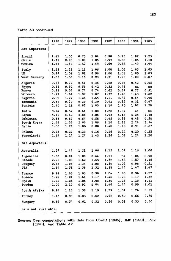
185

Table A3 continued

Net importers

BrazilChileMexico

ItalyUKWest Germany

AlgeriaEgyptKenyaMoroccoNigeriaTanzaniaTunisia

IndiaJapanPakistanSouth KoreaSyria

PolandYugoslavia

Net exporters

Australia

ArgentinaCanadaUruguayUSA

FranceGreeceSpainSweden

South Afrika

Turkey

Hungary

1978

1.411.111.63

1.230.971.05

0.730.550.931.770.990.671.40

0.745.490.831.691.30

0.281.17

1.57

1.052.200.831.64

0.991.921.371.00

0.94

1.16

0.65

na = not available.

1979

1.060.931.42

1.221.021.38

0.720.520.571.641.270.701.11

0.674.420.671.331.24

0.271.24

1.44

0.941.831.051.51

1.061.941.252.10

1.16

0.89

0.54

1980

0.731.001.37

1.131.011.16

0.510.560.741.871.260.390.87

0.613.840.642.001.08

0.201.24

1.21

1.001.621.341.38

1.031.611.060.92

1.38

0.83

0.61

1981

1.041.051.49

1.060.960.93

0.350.420.741.871.550.391.03

1.083.860.581.890.80

0.161.43

1.06

0.641.451.881.32

0.981.171.081.04

1.19

0.62

0.52

1982

0.980.930.69

1.081.001.31

0.420.320.621.321.110.411.16

1.203.930.452.161.48

0.161.26

1.15

1.151.521.301.38

1.041.461.301.46

1.29

0.62

0.56

1983

0.750.860.82

1.061.031.23

0.460.480.671.480.370.351.10

1.074.180.552.231.10

0.221.08

1.07

na1.631.021.44

1.001.231.251.44

1.31

0.59

0.53

1984

1.021.061.49

1.051.001.08

0.42na

0.771.430.410.311.02

na4.350.452.240.91

0.201.24

1.16

1.041.570.981.47

0.961.171.150.90

1.24

0.66

0.53

1985

1.251.101.94

1.051.030.87

0.45na

0.911.620.460.471.28

na4.480.582.340.67

0.251.20

1.00

0.901.450.511.47

1.021.121.211.01

0.99

0.70

0.50

Source: Own computations with data from Cowitt [1986], IMF [1990], Pick[1978], and Table A2.

186

Table A4 -Unadjusted NPCs for 29 Rice-Producing Countries, 1969-1985

Net importers

CameroonIvory CoastKenyaMadagascarNigeriaSenegalTanzaniaZambia

BangladeshIndiaIndonesiaMalaysiaPhilippinesSouth KoreaSri LankaTurkey

Mexico

Net exporters

BurmaEgyptJapanNepalPakistanThailand

ArgentinaColombiaUSA

Australia

ItalySpain

1969

0.721.460.481.253.031.460.780.57

0.770.950.491.591.311.011.231.51

1.42

0.380.741.631.350.850.68

0.941.251.60

1.29

1.621.34

1970

0.451.480.431.942.691.621.030.74

0.921.120.601.961.381.191.651.51

2.49

0.680.923.311.451.370.74

1.002.001.69

1.40

2.371.58

1971

0.681.860.432.061.351.801.000.86

1.031.080.382.401.711.441.601.92

1.91

0.690.973.451.120.970.77

1.201.001.75

1.31

2.621.62

1972

0.781.600.632.151.451.770.950.89

1.621.090.482.121.981.832.091.72

1.66

0.740.943.711.111.380.78

1.341.481.85

1.55

2.031.68

1973

0.520.780.491.651.181.480.830.89

3.480.800.721.211.451.221.381.28

1.25

0.770.523.291.020.660.57

0.540.981.78

1.62

1.351.45

1974.

0.340.880.430.861.140.480.310.72

2.090.830.460.480.910.640.821.49

1.34

0.380.202.850.770.710.38

0.770.821.02

1.23

1.001.08

1975

0.430.800.381.141.200.680.460.71

0.920.830.510.980.710.911.341.62

0.88

0.290.283.280.750.650.52

0.250.851.02

0.88

1.150.97

1976

0.651.280.661.431.431.710.620.91

0.680.750.801.520.981.781.632.62

1.05

0.600.523.420.800.740.68

0.880.971.22

0.99

1.381.38

1977

1.291.380.520.971.121.110.660.88

0.720.580.861.511.432.541.463.28

1.37

0.570.786.710.710.910.65

1.031.431.40

1.15

1.311.17

187

Table A4 continued

Net importers

CameroonIvory CoastKenyaMadagascarNigeriaSenegalTanzaniaZambia

BangladeshIndiaIndonesiaMalaysiaPhilippinesSouth KoreaSri LankaTurkey

Mexico

Net exporters

BurmaEgyptJapanNepalPakistanThailand

ArgentinaColombiaUSA

Australia

ItalySpain

1978

1.741.580.570.941.060.940.720.82

1.090.570.861.361.351.860.752.31

1.18

0.400.695.260.650.780.45

1.021.090.98

1.22

1.261.05

na = not available.

1979

2.021.750.620.941.451.740.800.82

1.170.820.891.260.782.470.742.82

1.65

0.460.606.520.660.780.80

0.920.821.29

1.12

1.321.25

1980

2.001.600.780.821.661.280.680.83

1.220.830.911.470.802.181.062.08

1.57

0.370.584.890.600.780.74

0.881.001.26

1.18

1.311.23

1981

1.780.940.740.751.621.120.880.78

1.340.750.911.200.802.230.861.83

1.48

0.290.514.89na

0.780.57

na1.030.88

1.08

1.281.00

1982

2.001.180.750.941.711.291.311.08

1.050.971.001.640.752.101.001.91

1.86

0.400.605.02na

0.750.80

na1.141.00

0.82

1.281.05

1983

na1.220.571.002.141.321.030.98

1.430.970.742.341.683.241.031.20

2.12

0.450.826.37na

0.890.83

na1.031.06

1.18

1.381.28

1984

na1.43na

0.852.091.311.110.74

1.001.000.802.441.082.700.741.31

2.15

0.43na

5.08na

0.820.88

na1.381.00

0.88

1.321.25

1985

na1.49na

0.691.891.851.050.32

1.081.110.972.661.372.041.141.40

2.68

0.37na

4.71nana

0.85

na0.921.00

0.94

1.251.25

Source: Own computations with data from FAO [d] for producer prices,FAO [e] for border prices and IMF [1990] for official exchangerates.

188

Table A5 - NPCs for Rice-Producing Countries Adjusted for ExchangeRate Distortions, 1969-1985

Net importers

CameroonIvory CoastKenyaMadagascarNigeriaSenegalTanzaniaZambia

BangladeshIndiaIndonesiaMalaysiaPhilippinesSouth KoreaSri LankaTurkey

Mexico

Net exporters

BurmaEgyptJapanNepalPakistanThailand

ArgentinaColombiaUSA

Australia

ItalySpain

1969

0.711.450.351.002.401.450.550.42

0.450.570.481.591.260.840.551.17

1.42

0.110.351.620.800.380.68

0.921.051.60

1.29

1.571.29

1970

0.451.460.321.552.141.600.740.54

0.540.680.581.961.340.990.741.17

2.49

0.180.453.260.850.620.74

0.971.681.69

1.40

2.311.54

1971

0.681.880.321.650.951.820.620.58

0.600.630.382.401.571.210.571.83

1.91

0.180.513.400.660.380.77

0.880.881.75

1.31

2.601.55

1972

0.801.630.481.721.151.820.450.43

0.950.780.462.121.881.720.851.68

1.66

0.250.513.690.800.980.78

0.921.381.85

1.55

i;981.66

1973

0.520.780.321.320.941.460.400.46

1.980.680.711.211.351.160.751.28

1.25

0.230.313.280.980.520.58

0.450.941.78

1.62

1.251.45

1974

0.340.880.350.690.820.480.150.40

1.080.720.450.480.860.510.511.45

1.34

0.120.122.850.820.600.38

0.400.721.02

1.23

0.911.06

1975

0.430.800.320.910.830.680.170.38

0.540.720.480.980.650.870.661.48

0.88

0.090.153.280.630.570.51

0.120.781.02

0.88

1.090.95

1976

0.651.290.581.141.061.720.230.35

0.480.650.781.520.921.740.972.38

1.02

0.180.283.420.740.680.65

0.480.911.22

0.98

1.281.35

1977

1.291.380.510.770.711.110.260.31

0.460.520.851.511.352.410.942.78

1.34

0.120.436.710.650.710.63

0.981.421.40

1.15

1.291.12

189

Table A5 continued

Net importers

' CameroonIvory CoastKenyaMadagascarNigeriaSenegalTanzaniaZambia

BangladeshIndiaIndonesiaMalaysiaPhilippinesSouth KoreaSri LankaTurkey

Mexico

Net exporters

BurmaEgyptJapanNepalPakistanThailand

ArgentinaColombiaUSA

Australia

ItalySpain

1978

1.821.660.520.750.580.980.430.31

0.490.480.821.361.281.720.571.77

1.17

0.090.385.260.570.580.45

1.001.080.98

1.22

1.251.00

na = not available.

1979

1.981.720.540.750.831.710.550.45

0.490.680.881.260.722.150.521.82

1.63

0.080.556.520.580.600.80

0.910.801.29

1.12

1.321.20

1980

2.021.620.710.651.001.290.290.49

0.570.580.891.470.751.980.801.88

1.52

0.060.544.890.580.620.77

0.860.981.26

1.18

1.291.20

1981

1.660.880.520.520.971.050.290.55

0.780.660.861.200.722.150.651.28

1.32

0.090.354.89na

0.550.54

na0.940.88

1.08

1.281.00

1982

1.861.110.490.461.031.200.420.74

0.620.850.911.640.661.980.751.45

1.12

0.120.405.02na

0.490.85

na1.031.00

0.82

1.281.05

1983

na1.030.460.481.281.080.230.65

0.950.720.662.340.862.930.770.86

1.46

0.140.496.37na

0.650.82

na0.751.06

1.18

1.381.28

1984

na1.28na

0.551.261.170.230.31

0.660.780.752.440.882.890.551.06

1.54

0.12na

5.08na

0.650.80

na1.021.00

0.88

1.321.25

1985

na1.75na

0.661.142.170.310.11

0.340.980.892.661.522.230.861.23

1.42

0.11na

4.71nana

0.89

na0.691.00

0.94

1.251.25

Source: Own computations with data from Cowitt [1986], IMF [1990], Pick[1978], and Table A4.

190

Table A6 -Unadjusted NPCs for 22 Coffee-Producing Countries, 1969-1985

CameroonIvory CoastKenya

MadagascarRwandaTanzaniaUgandaZaire

BrazilColombiaCosta RicaDominicanRepublicEcuadorEl SalvadorGuatemalaHondurasMexicoPeruVenezuela

IndonesiaPhilippinesSri Lanka

CameroonIvory CoastKenyaMadagascarRwandaTanzaniaUgandaZaire

BrazilColombiaCosta RicaDominicanRepublicEcuadorEl SalvadorGuatemalaHondurasMexicoPeruVenezuela

IndonesiaPhilippinesSri Lanka

na ° not available.

1969

0.820.S91.03

0.701.080.810.840.85

0.620.730.86

0.660.760.910.780.830.850.610.88

0.97nana

1978

0.370.450.990.300.360.330.20na

0.610.420.71

0.980.490.800.710.780.610.450.71

0.930.880.77

1970

0.590.470.96

0.710.620.970.810.85

0.500.650.81

O.SO0.540.910.680.810.730.501.05

0.601.24na

1979

0.470.401.030.340.600.320.380.53

.0.490.470.71

na0.43na

0.831.130.620.420.81

0.600.820.67

1971

0.600.500.99

0.730.771.100.730.87

0.700.700.82

0.580.530.890.740.680.780.511.10

0.460.82na

1980

0.470.481.000.360.800.360.360.71

0.480.440.75

0.850.74na

0.670.650.600.430.68

0.700.860.71

1972

0.690.581.05

0.730.791.180.820.64

0.750.700.83

0.550.580.930.830.620.740.550.78

0.450.92na

1981

0.600.590.850.530.740.410.450.93

0.670.560.60

1.07nana

0.730.670.800.410.87

1.090.830.79

1973

0.610.561.02

0.780.831.220.660.59

0.690.630.78

0.890.780.900.630.710.720.510.81

0.840.961.03

1982

0.520.550.990.470.650.560.341.51

0.380.500.70

0.81na

0.540.680.630.480.310.88

1.100.690.71

1974

0.550.540.96

0.770.860.860.550.73

1.190.680.75

0.910.470.810.700.670.690.460.33

0.740.691.16

1983

0.500.441.010.320.760.620.141.01

0.270.510.77

0.80na

0.600.640.620.450.311.10

1.020.750.65

1975

0.720.651.08

0.871.002.020.690.36

2.860.580.78

0.990.880.620.890.800.840.570.41

1.160.870.85

1984

0.400.380.930.250.760.610.110.55

0.250.450.73

nana

0.660.650.600.410.470.40

0.940.770.62

1976

0.570.391.08

0.480.570.810.360.11

0.710.520.72

0.950.461.030.830.481.290.220.39

0.540.911.07

1985

0.410.320.920.290.760.850.12na

0.530.400.72

0.35na

0.610.950.560.99na

0.64

1.000.590.72

1977

0.360.230.94

0.250.290.450.160.08

0.280.330.69

0.930.370.920.800.230.460.340.30

0.301.001.11

Source: Own computations with data from FAO [d] for domestic prices,FAO [e] for border prices and World Atlas AgriculturalCommittee [ 1973] for internal transportation costs.

191

Table A7 - NPCs for Coffee-Producing Countries Adjusted for ExchangeRate Distortions, 1969-1985

CameroonIvory CoastKenya

MadagascarRwandaTanzaniaUgandaZaire

BrazilColombiaCosta RicaDominicanRepublicEcuadorEl SalvadorGuatemalaHondurasMexicoPeruVenezuela

IndonesiaPhilippinesSri Lanka

CameroonIvory CoastKenyaMadagascarRwandaTanzaniaUgandaZaire

BrazilColombiaCosta RicaDominicanRepublicEcuadorEl SalvadorGuatemalaHondurasMexicoPeruVenezuela

IndonesiaPhilippinesSri Lanka

na ° not available.

1969

0.800.580.76

0.56na

0.570.590.66

0.550.610.72

0.530.620.770.630.830.850.540.87

0.94nana

1978

0.390.470.910.240.300.200.02na

0.490.410.68

0.710.470.660.520.780.600.430.71

0.880.830.58

1970

0.590.470.72

0.57na

0.690.570.68

0.450.540.80

0.410.450.770.540.810.730.361.04

0.581.20na

1979

0.460.390.910.270.500.220.040.18

0.410.460.65

na0.38na

0.561.130.610.370.81

0.590.760.47

1971

0.600.500.74

0.58na

0.680.480.60

0.610.620.67

0.460.480.760.590.680.780.331.09

0.460.76na

1980

0.470.490.900.280.670.150.030.31

0.430.360.59

0.620.66na

0.420.650.590.370.68

0.690.810.54

1972

0.700.590.80

0.58na

0.550.450.41

0.66 -0.650.48

0.450.530.790.670.620.740.330.78

0.440.87na

1981

0.570.550.690.400.620.130.110.33

0.600.520.47

0.79nana

0.600.670.740.340.87

1.060.770.71

1973

0.610.560.67

0.63na

0.590.220.37

0.620.600.50

0.730.760.760.500.710.720.300.81

0.820.890.56

1982

0.480.520.680.280.420.190.130.48

0.270.460.45

0.54na

0.280.550.630.290.240.85

1.020.620.63

1974

0.550.540.79

0.62na

0.430.140.43

1.040.600.65

0.750.470.690.560.670.690.300.33

0.710.660.72

1983

0.440.390.750.160.500.170.060.28

0.170.420.54

0.45na

0.300.440.620.220.210.69

0.910.520.51

1975

0.720.650.91

0.70na

0.740.090.18

2.300.540.72

0.780.860.520.710.800.840.340.41

1.090.800.42

1984

0.350.330.740.140.450.130.080.30

0.200.330.58

nana

0.330.370.600.290.280.17

0.860.510.45

1976

0.570.390.95

0.380.270.300.040.04

0.540.480.63

0.700.420.850.680.481.250.160.42

0.530.850.64

1985

0.430.330.830.240.540.220.08na

0.400.300.58

0.22na

0.210.360.560.62na

0.30

0.930.570.63

1977

0.360.230.91

0.200.270.180.020.03

0.230.330.63

0.690.340.690.640.230.450.300.30

0.300.940.71

Source: Own computations with data from Cowitt [1986], IMF [1990], Pick[1978], and Table A6.

192

Table A8 -Average Exchange Rate Distortion Factors, 1969-1985 (a)

AlgeriaArgentinaAustraliaBangladeshBrazilBurmaCameroonCanadaChileColombiaCosta RicaDominicanRepublicEcuadorEgyptEl SalvadorFranceGreeceGuatemalaHondurasHungaryIndiaIndonesiaItalyIvory CoastJapanKenyaMadagascar

0.48130.72410.99830.55910.82360.27340.98220.99920.69920.88820.8124

0.74660.91430.62540.72760.97780.94520.73661.00001.11070.78660.95910.97110.98360.97110.81130.7530

MalaysiaMexicoMoroccoNepalNigeriaPakistanPeruPhilippinesPolandRwandaSenegalSouth AfricaSpainSri LankaSwedenSyriaTanzaniaThailandTunisiaUgandaUKUSAVenezuelaWest GermanyYugoslaviaZaireZambia

1.00000.89680.94600.82600.61870.72090.74230.90460.29800.73550.98240.88760.97510.71400.98130.80850.45510.99330.90870.37460.99861.00000.91341.00000.92370.51010.6355

(a) The distortion factor was computed by dividing black market ex-change rates by official exchangefrom unity, theunity indicate

i stronger exchangerates. The more therate distortions are.

exchange rate overvaluations.

factor differsFactors below

Source: Own computations with data from Cowitt [1986], IMF [1990] andPick [1978].

193

Table A9 - Variance Decomposition of Gross NPCs for Wheat-ProducingCountries (a), 1969-1985

Importers

Italy

Japan

UKWest Germany

AlgeriaBrazil

Chile

EgyptIndia

KenyaMexico

Morocco

Nigeria

PakistanPoland

South Korea

SyriaTanzaniaTunisia

Yugoslavia

Exporters

Australia

CanadaFrance

Greece

Spain

SwedenUSA

ArgentinaHungary

South AfricaTurkey

Uruguay

(a) The method

Percentage standard deviation

from loglinear trend(b)

NPC

10.95—

26.46++16.12

14.49

30.1725.50-

36.47+

23.24-24.08—

30.3334.3518.97+

27.75

29.66--21.68

24.49++

27.57++

25.10

15.8125.10

24.0820.25—

9.49—26.27

42.1920.49

21.21—

43.37++

20.7418.17

21.45-

28.11

16.12++

22.58++20.25++

18.71+

10.95++17.89++

27.93++

15.49++6.32++

15.81++18.17++

28.11++11.83++

16.12++

12.25++20.00++

11.40++

9.49++

12.25++18.97++

23.24++

13.42++17.89++

17.32++16.43++14.83++

14.14++

33.40++

10.95++

21.45++

25.69+29.50++

of decomposing variances is

trend-corrected variance, P. and P

(b) Defined as

+,- indicatestandard deviation

the 95 percent level

Pw

22.58++

27.93++

28.28++21.68+

31.30++26.65++

27.02++

25.69++24.90++

31.78++38.99+27.57++

25.10++

25.69++

16.43++

29.33++25.69++

25.50++

23.66++29.83+

28.28++26.65++

23.24++32.09++

46.15+28.64++

27.39++

30.48++

27.93++

23.02++32.25++

29.33++

defined

are domestic and

from theand ++,

estimated loglinear trend. Moreover, they

a positive or negative sign. - (c) cpf, CP W

loglinear— the 99

Contribution of components to

Var(NPC)

211.6472.90

158.14170.27

13.60

49.1258.87

43.87

5.9527.11

28.03217.53

18.6129.25

31.86

67.2116.63

14.1160.66

57.02

93.4142.90

358.11

42.5614.92

51.4144.81

59.3028.65

138.50

145.79110.60

(percent)(c)

CPw

421.39

111.56

308.83226.73

107.61

108.4254.77

121.77

107.19109.64

128.00206.9782.87

75.1457.70

142.6087.80

102.95

225.14

141.96

137.34174.26

599.12149.06

119.32195.56

168.11

49.41182.09

161.61228.05

108.69

in Section C.II. Var stand:

border prices

CF»PW

533.03

84.46

366.97297.00

21.2157.54

13.64

65.6413.1436.75

56.03324.50

1.484.39 .

-10.44

109.814.43

17.06

185.80

98.98

130.75

117.16

857.23

91.6234.24

146.97

112.92

8.71

110.74200.11

273.84

119.29

s for the

in US$, respectively. -

trend multiplied by 100. The indicespercent level of significance of the

show whether the estimated coefficients carry

and CP|P W are defined ir Section C.II

Source: Own computations with data from FAO [d; e ] , IMF [1990] andTable A2.

194

Table A10 -Variance Decomposition of Net NPCs for Wheat-ProducingCountries (a), 1969-1985

Importers

ItalyJapanUKWest Germany

AlgeriaBrazilChileEgyptIndiaKenyaMexico(d)MoroccoNigeriaPakistanPolandSouth KoreaSyriaTanzaniaTunisiaYugoslavia

Exporters

AustraliaCanadaFranceGreeceSpainSwedenUSA

ArgentinaHungarySouth AfricaTurkeyUruguay

Percentage standard deviationfrom loglinear trend(b

NPC

13.04-26.46++16.1214.14

25.30—23.66—78.55+20.7423.02—31.3039.8718.44+35.64—17.32—21.91—24.49++26.0831.62-15.1722.80

24.2920.25—8.94—

26.6541.9520.4921.21—

55.6212.65—21.9118.97—36.74+

'I

15.49++22.80++20.25++18.97+

16.7317.03+85.09++14.14++14.14++23.02++30.0027.75++27.9318.17++17.0317.89++25.69++23.02+16.43++17.89++

23.24++13.42++17.61++17.61++16.73++14.14++14.14++

45.03++18.1722.36++26.4636.61++

Pw

22.58++27.93++28.28++21.68+-

31.30++26.65++27.02++25.69++24.90++31.78++46.6927.57++25.10++25.69++16.43++29.33++25.69++25.50++23.66++29.83+

28.28++26.65++23.24++32.09++46.15+28.64++27.39++

30.48++27.93++23.02++32.25++29.33++

Contribution of components toVar(NPC)

cpf

135.8874.56156.78181.01

42.9052.18117.4046.2037.6254.1756.71

226.2561.29

111.2459.8152.8197.0052.82

120.8161.69

91.3443.40

407.8543.7716.1547.1144.82

65.54203.58103.75195.9699.39

(percent)(c)

CPw

293.85112.21303.80231.56

152.99124.9511.84151.88117.69103.56137.22222.3849.87

219.5756.50

142.1797.0065.47

246.36171.20

135.47175.00696.17146.17121.14196.93168.11

30.03481.61110.12289.0863.41

(a) The method of decomposing variances is defined in Section C.II. Var stands

corrected variance

and border prices

in most cases (for exceptions see annotation (d))

in USS, respectively. - (b)linear trend multiplied by 100. The indices +,99 percent level of significance of

the estimated coefficients carry a

defined in Sectionof three components

Defined as standard- indicate

P? and P

deviationthe 95 percent level

cpipw

329.7386.77360.58312.57

95.8977.1329.2498.0855.3157.7393.93

348.6311.16

230.8116.3194.9894.0018.29

267.17132.89

126.81118.401004.0289.9437.29

144.04112.93

-4.43585.19113.87385.0462.80

for the trend-

are domestic

from the log-and ++,— the

the estimated loglinear trend. Besides they show whether

positive or negative sign. - (c)CP*. CPw

oand CPTP are

C.II. - (d) Variance decomposition with uncorrected variances, as two outshowed no significant trend

Source: Own computations with data from FAO [ d; e ] , IMF [ 1990] andTable A3.

195

Table Al l - Variance Decomposition of Gross NPCs for Rice-ProducingCountries (a), 1969-1985

Importers

Bangladesh(b)CameroonIndiaIndonesiaIvory CoastKenyaMadagascarMalaysia(b)Mexico(b)NigeriaPhilippinesSenegalSouth KoreaSri LankaTanzaniaTurkeyZambia

Exporters

ArgentinaAustraliaBurmaColombiaEgyptItalyJapanNepalPakistanSpainThailandUSA

(a) All notes

Percentage standard deviationfrom loglinear trend(a)

NPC Pi

38.86 36.0539.12++ 27.20++19.75 13.78++18.44++ 24.70++26.27 39.62+16.12++ 22.80++21.11— 20.4942.54 23.45++29.33 20.00++29.83 13.78++30.00 21.45++35.50 20.25++29.66++ 27.02++24.90-- 23.8732.71 13.78++28.11 32.56++25.69 24.70+

42.54 25.50++14.14-- 19.49++25.88- 25.8822.36 15.17++42.31 13.04++20.00- 16.12++23.45++ 28.63++7.75-- 8.94

19.75 13.78++26.27- Z1.68++21.68 21.90++16.73-- 19.24+

Pw

33.62+29.66+25.69++19.49++51.12+26.27++33.32++32.7137.6837.42++41.35+37.94+33.02+32.86++28.28++24.70++25.30++

40.25++22.80++41.83+24.90++44.50++30.98++29.33+14.83++26.83++28.81++37.82++24.29++

of Table A9 are again valid. -with uncorrected variances, as two out ofsignificant trend.

Contribution of com-ponents to Var(NPC)(percent)(a)

cpi

85.6948.0448.73

179.20227.50202.4492.3430.1546.9921.4250.7332.8282.7993.1218.16

133.1792.03

36.02193.3299.5347.199.66

63.42149.74130.6649.7968.12

101.39133.11

CPw

74.8757.22169.78110.59379.75268.52243.4758.75

165.93157.59189.17153.68123.44175.5674.3976.4496.97

89.76263.66260.97124.18110.96237.68156.71350.26183.96120.29303.82209.98

CP?Pl w

60.565.25

118.51189.79507.25370.95235.81-11.10112.9279.00

139.8986.50

106.23168.68-7.45

109.6189.00

25.78356.88260.5071.3720.62

200.68206.45380.92133.7588.41305.20243.08

(b) Variance decompositionthree components showed no

Source: Own computations with data from FAO [d; e ] , IMF [1990] andTable A4.

196

Table A12 -Variance Decomposition of Net NPCs for Rice-ProducingCountries (a), 1969-1985

Importers

Bangladesh(b)CameroonIndiaIndonesiaIvory CoastKenyaMadagascarMalaysia(b)Mexico(b)NigeriaPhilippinesSenegalSouth KoreaSri LankaTanzaniaTurkeyZambia

Exporters

ArgentinaAustraliaBurmaColombiaEgyptItalyJapanNepalPakistanSpainThailandUSA

(a) All notes

Percentage standard deviationfrom loglinear trend(a)

NPC

40.9939.24++15.81+19.24++28.4617.89++22.36--42.5423.2332.5629.33-37.0130.82++20.0040.12-28.2841.71

59.7514.14--32.71-21.68-42.0722.1423.45++11.83--21.2128.14-22.3616.73--

of Table A9

P.i

35.3627.93++20.25++25.69++40.50+29.49++27.0223.45++22.1415.17++28.98+22.58++25.69++27.39++24.29++32.71++39.50+

41.23++19.49++30.3320.98++13.41++16.12++28.63++19.75+26.08++22.32++21.91++19.23+

are againwith uncorrected variances, as twosignificant trend.

Pw

33.62+29.66++25.69++19.49++51.12+26.27++33.32++32.7137.6837.42++41.35++37.94+33.02+32.86++28.28++24.70++25.30++

40.25++22.80+41.83+24.90++44.50++30.98++29.33+14.83++26.83++28.81++37.82++24.29++

valid. -out of 1

Contribution of com-ponents to Var(NPC)(percent)(a)

CP.l

74.5550.71

163.98175.63204.58271.42145.7230.1591.2921.3296.9637.0969.46

185.6937.00

133.8089.34

47.68186.6886.1794.2810.1052.71

150.30288.36151.8862.9196.30

133.11

CPw

67.3556.72266.89101.22325.54214.96220.8058.75

261.83131.47197.57141.68115.05268.0449.6275.9421.20

45.38259.15163.53132.67112.33194.81156.59161.92160.78104.82286.67209.88

CPTP1 W

41.907.42

330.86176.85430.12386.38266.52-11.10253.1252.79

194.5378.7784.51353.73-13.37109.7410.54

-6.94345.83149.70126.9722.43147.51206.89350.27212.6567.73

282.94243.08

(b) Variance decomposition:hree components showed no

Source: Own computations with data from Cowitt [1986], FAO [e ; f ] , IMF[1990], Pick [1978], and Table A5.

197

Table A13 - Variance Decomposition of Gross NPCs for Coffee-ProducingCountries (a), 1969-1985

CameroonIvory CoastKenyaMadagascarRwandaTanzaniaUgandaZaire

Brazil(b)ColombiaCosta RicaDominicanRepublicEcuadorEl SalvadorGuatemalaHondurasMexicoPeruVenezuela

IndonesiaPhilippinesSri Lanka

(a) All notes

Percentage standard deviationfrom loglinear trend(a)

NPC

17.03-- 20.25++ 29.50++23.24 25.10++ 32.71++5.48 35.07++ 34.64++

27.57-- 18.97+ 32.09++31.62 13.78++ 38.47++43.24- 30.50 37.28++37.01-- 34.50 33.91++76.94 41.71++ 42.54++

57.88 57.01 57.1015.49-- 18.71++ 30.66++6.32-- 33.47++ 36.88++

30.33 52.06++ 31.30++25.10 17.32++ 25.50++13.04-- 44.05+ 34.93++11.83 32.25++ 31.78++31.14 36.61++ 36.61++26.65 37.68++ 33.17++22.14- 33.47++ 36.33++41.35 40.00++ 20.00++

34.21 26.83++ 39.12++12.25-- 43.01+ 36.74++12.25-- 40.74 38.47+

of Table A9 are again valid. -

Contribution of com-ponents to Var(NPC)(percent)(a)

CP|

141.79115.88

4229.3048.0718.8449.9787.3829.37

96.96147.122924.90

293.8247.46

1118.00750.19138.14197.96229.8693.32

61.611208.301136.00

CPw

301.33196.16

4115.60136.03147.7674.1083.8430.51

97.40398.57

3552.90

105.94102.87704.38723.78138.47153.79271.3923.51

131.35879.88

1013.90

cpfpi w

343.12212.04

8244.9084.1066.6024.0771.22

-40.12

94.36445.696377.90

299.7550.33

1722.381374.97176.62251.76401.2616.83

92.961988.182049.90

(b) Variance decompositionwith uncorrected variances, as two out of three components showed nosignificant trend.

Source: Own computations with data from Cowitt [1986], FAO [d; e ] , IMF[1990], Pick [1978], and Table A6.

198

Table A14 - Variance Decomposition. of Net NPCs for Coffee-Producers(a), 1969-1985

CameroonIvory CoastKenyaMadagascarRwanda(b)TanzaniaUgandaZaire(b)

BrazilColombiaCosta RicaDominicanRepublicEcuadorEl SalvadorGuatemalaHondurasMexicoPeruVenezuela

IndonesiaPhilippinesSri Lanka(b)

(a) All notes

Percentage standard deviationfrom loglinear trend(a)

NPCi

15.81— 22.14++22.80- 27.02++11.40 42.54++28.98-- 26.8333.17 30.3330.82-- 25.5084.32-- 54.4192.52 53.94

50.89- 54.8614.49-. 25.10++14.14 42.66+

32.40 53.85+26.27 14.83++20.98-- 51.9615.17-- 38.21+31.14 36.61++33.17-- 48.2724.90 45.39+46.26 47.96+

32.56 27.39++14.14-. 46.04+17.89 51.58

pw

29.50++32.71++,34.64++32.09++30.3337.28++33.91++61.73

38.34++30.66++36.88++

31.30++25.50++34.93++31.78++36.61++33.17++36.33++20.00++

39.12++36.74++49.30

of Table A9 are again valid. -with uncorrected variances, as two out ofsignificant trend.

Contribution of com-ponents to Var(NPC)(percent)(a)

CP?l

194.85141.68

1399.5085.0083.6768.1541.6434.00

116.01295.92915.68

274.4431.77613.52642.06138.14211.34331.03107.27

70.951039.54827.18

CPw

347.73206.89952.84121.8283.32145.9316.1344.52

56.73440.68686.94

92.6694.04

278.02444.23138.4799.81

212.2618.80

144.20661.23754.15

CP?P1 W

442.58248.57

2225.34106.8266.99

114.08-42.23-21.48

72.74636.60

1502.62

267.1025.81791.55986.29176.61211.15443.2926.07

115.151600.771481.33

(b) Variance decompositionthree components showed no

Source: Own computations with data from Cowitt [1986], FAO [d; e ] , IMF[1990], Pick [1978], and Table A7.

199

Table A15 - Variance Decomposition of Producer Prices for Wheat in USS(a), 1969-1985

Importers

ItalyJapanOKWest Germany

AlgeriaBrazilChileEgyptIndiaKenyaMexicoMoroccoNigeriaPakistanPolandSouth KoreaSyriaTanzaniaTunisiaYugoslavia

Exporters

AustraliaCanadaFranceGreeceSpainSwedenUSA

ArgentinaHungarySouth AfricaTurkeyUruguay

(a) The method

trend-corrected

Percentage standard deviationfrom loglinear trend(b)

19.57++22.59++21.81++21.86++

12.05++22.92++38.86++15.41++9.98++20.31++18.09++28.18++11.94++18.98++12.26++20.44++11.21++12.01++13.85++25.30++

27.89++32.67++20.24++19.76++19.24++14.71++29.91++

33.40++12.41++21.39++25.78+33.37++

Pi

10.38++15.85++14.92++5.56++

10.82++78.64++149.52++10.11++12.14++12.63++37.76++11.24++11.19++11.09++31.90++20.30++11.31++19.22++7.88++

26.01++

16.80++29.63++4.72++

11.00++7.35++7.90++

29.91++

94.35++3.75++

10.10++31.75++35.53++

of decomposing variances is

variance, PT and

tively. E indicates the exchange

E

17.75—14.11++11.43 —18.17+

9.6584.84—126.82—17.52—5.OS-IS.17—47.76—21.90-10.5917.34—29.91—16.09—1.29—

15.50—19.24-44.56—

12.54—5.18—

19.32-23.06—21.08—18.62-0.00

99.29—14.69++17.67—47.91—25.52—

defined it

P. are producer price:

Contribution of components to

Var(P°) (percent)(c)

CPi

28.1449.2146.816.46

80.511177.501480.2043.09148.1138.69

435.5315.9087.8534.16

676.9298.67101.83256.1432.43

105.69

36.2682.235.44

30.9514.5828.85

100.00

798.249.13

22.29151.69113.38

Section C.II

CE

82.2838.9827.4569.06

64.111370.801064.80129.3226.0455.83

696.6960.3978,7283U6

595.1061.991.32

166.48193.09310.28

20.232.51

91.21136.11120.00160.180.00

883.89140.1768.26

345.4058.46

CP.E

-10.4211.8125.7424.48

-44.62-2448.30-2445.00

-72.41-74.15

5.48-1032.22

23.71-66.57-17.62

-1172.02-60.66-3.15

-322.62-125.52-315.97

43.5115.263.35

-67.07-34.58-89.040.00

-1582.13-49.309.45

-397.09-71.84

Var stands for the

in USS and local currency, respec-

rate between USS and the local currency. - (bstandard deviation from the loglinear trencthe 95 percent

multiplieclevel and ++,— the 99 percent level of

linear trend. Moreover, they show whether

negative sign. - (c) CP?, CPw and CP*Pw are

l by 100. Thesignificance

the estimated coefficient.

defined in Section C.II.

indices ^Defined as

>•,- indicateof the estimated log-; carry a positive or

Source: Own computations with data from FAO [d] and IMF [1990].

200

Table A16 - Variance Decomposition of Producer Prices for Rice in USS(a), 1969-1985

Importers

BangladeshCameroonIndiaIndonesiaIvory CoastKenyaMadagascarMalaysiaMexicoNigeriaPhilippinesSenegalSouth KoreaSri LankaTanzaniaTurkeyZambia

Exporters

ArgentinaAustraliaBurmaColombiaEgyptItalyJapanNepalPakistanSpainThailandUSA

(a) All notes

Percentage standard deviationfrom loglinear trend

-I

38.86+28.10++15.17++25.14++41.99++23.45++30.17++23.45++24.29++31.94++17.61++21.91++27.03++28.11++16.12++34.64+31.14++

32.56++21.91++23.88+16.43++15.81++17.61++28.63++10.4914.83++22.49++28.11++24.49+

Pi

31.14++21.14++12.25++13.04++28.10++16.73++14.83++11.83++38.86++10.49++18.17++12.65++14.83++18.71++26.46++24.08++12.25++

92.16++16.12++23.45++11.83++10.00++11.83++14.49++7.75++21.91++10.95++24.29++24.49+

E

11.83—19.23-7.75—13.41—19.23-15.20—26.26—7.07—47.85—10.4818.44—19.23-16.10—14.83—15.17—48.27 —24.29++

99.35—12.65—8.37--12.25—17.60—17.70—14.10++4.47—17.89—20.73—17.61—0.00

of Table A15 are valid again.

Contribution of components

to Var(P!

CP.

63.9673.3264.3434.2221.9656.6323.5525.45255.06110.24111.5932.9030.1044.26271.8248.0715.32

801.2754.1496.9353.5339.0945.6025.6161.37

214.0223.7173.37

100.00

) (percent)

CE

9.1359.1325.7837.2447.6350.2375.379.09

386.77105.11106.7075.9835.4827.0791.07

194.1761.95

931.1733.3412.6655.44124.17101.0624.2514.52141.8184.963.930.00

CP E

26.91-32.45

9.8828.5330.41-0.861.09

65.46-541.83-113.35-118.29

-8.8734.4228.67

-262.89-142.2422.73

-1732.4412.52-9.58-8.97

-63.76-46.6650.1424.11

-255.83-8.6722.700.00

Source: Own computations with data from FAO [d] and IMF [1990].

201

Table A17 -Variance Decomposition of Producer Prices for Coffee in USS(a), 1969-1985

CameroonIvory CoastKenyaMadagascarRwandaTanzaniaUgandaZaire

BrazilColombiaCosta RicaDominicanRepublicEcuadorEl SalvadorGuatemalaHondurasMexicoPeruVenezuela

IndonesiaPhilippinesSri Lanka

(a) All notes

Percentage standard deviationfrom loglinear trend

P. E

Contribution of components

to Var(PT) (percent)

CP. CE CP.E

20.75++ 8.47++ 19.30- 16.67 86.50 -3.1725.89++ 10.40++ 19.30- 16.14 55.56 28.3036.21++ 29.48++ 15.10-- 66.25 17.40 16.3521.58+ 8.14++ 26.51-- 14.23 150.84 -65.0716.69++ 15.16++ 4.57 82.49 7.49 10.0232.52 35.95++ 15.31-- 122.25 22.18 -44.4345.23 59.91++ 91.36-- 175.41 408.01 -483.4257.06++ 87.78++ 56.25-- 236.70 97.18 -233.88

56.48 58.92++ 84.76-- 108.82 225.20 -234.0220.69++ 14.33++ 12.46-- 47.96 36.26 15.7835.27++ 24.00++ 37.29-- 46.28 111.77 -58.05

52.82++ 41.02++ 24.91 60.33 22.23 17.4417.65++ 12.62++ 7.69- 51.17 19.00 29.8345.06+ 45.06+ 0.00 100.00 0.00 0.0033.34++ 28.72++ 8.77 74.20 6.91 18.8937.09++ 31.73++ 8.77 73.20 5.59 21.2138.02++ 40.87++ 47.81-- 115.54 158.10 -173.6434.95++ 53.53++ 56.07-- 234.53 257.37 -391.9039.97++ 37.62++ 15.56- 88.59 15.17 -3.76

27.44++ 20.87++ 13.32-- 57.87 23.58 18.5542.03++ 36.05++ 18.52-- 73.59 19.42 6.9941.01 41.30++ 11.39-- 101.44 7.72 -9.16

of Table A15 are again valid.

Source: Own computations with data from FAO [d] and IMF [1990].

Table A18 - Production of Main Agricultural Commodities, 1970-1988 (1000 tons) s

1970

1971

1972

1973

1974

1975

1976

1977

1978

1979

1980

1981

1982

1983

1984

1985

1986

1987

1988

na =

Malaysia

rubber

1263

1318

1304

1542

1524

1459

1612

1588

1582

1570

1529

1510

1494

1563

1530

1469

1541

1581

1660

palmoil

431

580

719

812

1045

1258

1391

1612

1785

2188

2575

2824

3514

3018

3715

4133

4543

4533

5030

not available

cocoa

2

4

5

9

10

13

15

17

18

27

37

45

66

69

88

103

131

191

230

paddy

1679

1817

1837

1980

2095

2013

1995

1898

1590

2095

2171

2177

1832

1818

1755

1895

1948

1623

1796

Peru

sugar

8050

8758

8612

8772

9184

8958

8792

8816

7970

7034

5598

5129

6509

6381

6988

7329

5273

6099

5948

cotton

248

233

225

236

257

227

165

173

199

244

256

286

256

105

203

291

304

202

275

coffee

65

71

70

70

70

65

65

65

88

106

95

95

90

91

91

91

96

98

99

potatoes

1929

1968

1713

1713

1722

1639

1667

1615

1695

1695

1380

1705

1799

1200

1463

1557

1658

1709

2108

rice

587

615

482

484

494

537

570

587

468

560

420

712

776

798

1156

878

726

1169

1129

wheat

125

122

120

123

127

126

128

115

104

102

77

119

101

76

84

92

121

133

153

maize

615

616

628

600

606

635

726

734

590

631

453

587

631

585

776

702

876

914

908

Zimbabwe

maize

980

1809

2267

968

2125

1747

1787

1655

1619

1149

2813

2729

1785

844

1283

2952

2486

958

2034

wheat

56

88

82

86

90

130

147

175

204

162

191

201

213

124

99

210

232

198

242

cotton

86

139

165

130

190

170

142

144

166

145

158

171

135

147

222

274

247

237

279

tobacco soya-beans

55 9

65 9

67 10

69 9

75 22

86 32

109 45

84 50

83 79

108 87

120 97

69 73

89 92

94 81

117 99

108 87

na 72

na 95

na 120

ground-nuts

36

29

35

34

206

127

192

141

114

108

78

119

111

33

26

67

73

76

139

sorghum

na

na

na

na

161

109

135

51

73

49

82

125

67

52

54

127

131

49

169

Source: Rahman [1990b]; Rukovo et al. [1991]; Thiele [1991b].

203

Bibliography

ADELMAN, Irma, The World Distribution of Income. Referat auf derJahrestagung "Probleme und Perspektiven der weltwirtschaftlichenEntwicklung" des Vereins fur Socialpolitik, Travemiinde, 17.-19.September 1984, mimeo.

AHLUWALIA, Montek S. , Frank J. LYSY, The Workings of ComputableGeneral Equilibrium Models: With Special Reference to a Model onMalaysia. N. P. 1983, mimeo.

ANDERSON, Kym, "Korea: A Case of Agricultural Protection". In: TerrySICULAR (Ed. ), Food Price Policy in Asia: A Comparative Study.Ithaca 1989, pp. 109-153.

—, Rod TYERS, "Agricultural Protection Growth in Advanced and NewlyIndustrialized Countries". In: Allen MAUNDER, Alberto VALDES(Eds. ), Agriculture and Governments in an Interdependent World.Proceedings of the Twentieth International Conference of Agri-cultural Economists held at Buenos Aires, 24-31 August 1988.Aldershot 1989, pp. 175-186.

ARDENI, Pier G. , "Does the Law of One Price Really Hold for CommodityPrices?". American Journal of Agricultural Economics, Vol. 71,1989, pp. 661-669.

ARIFF, Mohamed, Muthi SEMUDRAM, "Country Study Malaysia". In:Sheila PAGE (Ed. ), Trade, Finance and Developing Countries.Strategies and Constraints in the 1990s. New York 1990, pp. 23-55.

ASIAN DEVELOPMENT BANK (ADB), Evaluating Rice Market InterventionPolicies. Manila 1988.

ASKARI, Hossein, John T. CUMMINGS, Agricultural Supply Response. ASurvey of the Econometric Evidence. New York 1976.

AUSTRALIAN BUREAU OF AGRICULTURE AND RESOURCE ECONOMICS,Japanese Agricultural Policies. A Time of Change. Canberra 1988.

AVILLEZ, Francisco, Timothy J. FINAN, Timothy JOSLING, Trade, Ex-change Rates, and Agricultural Pricing Policy in Portugal. WorldBank Comparative Studies, The Political Economy of AgriculturalPricing Policy, Washington 1988.

BALASSA, Bela et al. , The Structure of Protection in Developing Coun-tries. Baltimore 1971.

BALE, Malcolm D. , Agricultural Trade and Food Policy: The Experienceof Five Developing Countries. World Bank Staff Working Papers,724, Washington 1985.

204

BALE, Malcolm D. , Ernst LUTZ, "Price Distortions in Agriculture andTheir Effects: An International Comparison". American Journal ofAgricultural Economics, Vol. 63, 1981, pp. 8-22.

BALISACAN, Arsenio M. , James A. ROUMASSET, "Public Choice ofEconomic Policy: The Growth of Agricultural Protection". Weltwirt-schaftliches Archiv, Vol. 123, 1987, pp. 232-248.

BATES, Robert H. , Markets and States in Tropical Africa. Berkeley,L. A. , 1981.

BAUTISTA, Romeo M. , Production Incentives in Philippine Agriculture:Effects of Trade and Exchange Rate Policies. International FoodPolicy Research Institute, Research Reports, 59, Washington 1987.

—, "Price and Trade Policies for Agricultural Development". The WorldEconomy, Vol. 13, 1990, pp. 89-109.

BERTRAND, Trent, Thailand - Case Study of Agricultural Input andOutput Pricing. World Bank Staff Working Papers, 385, Washington1980.

BEYNON, Jonathan G. , "Pricism v. Structuralism in Sub-SaharanAfrica". Journal of Agricultural Economics, Vol. 40, 1989, pp. 323-335.

BINSWANGER, Hans P. , Maw-Cheng YANG, Alan BOWERS, YairMUNDLAK, "On the Determinants of Cross-Country Aggregate Agri-cultural Supply". Journal of Econometrics, Supplement on "Speci-fication Testing in Limited and Discrete Dependent Variable Models",Vol. 34, 1987, pp. 111-131.

BLANDFORD, David, Harry de GORTER, David HARVEY, "Farm IncomeSupport with Minimal Trade Distortions". Food Policy, Vol. 14,1989, pp. 268-273.

BOADWAY, Robin W. , Neil BRUCE, Welfare Economics. Oxford 1984.

BOLLING, Christine H. , "Price and Exchange Rate TransmissionRivisited: The Latin America Case". In: Colin A. CARTER, WalterH. GARDINER (Eds.), Elasticities in International AgriculturalTrade. Boulder 1988, pp. 163-194.

—, Peru: An Export Market Profile. USDA, Agriculture and TradeAnalysis Division, Economic Research Service, Washington 1989.

BOND, Marian E. , "Agricultural Responses to Prices in Sub-SaharanAfrican Countries". IMF Staff Papers, Vol. 30, 1983, pp. 703-726.

BOVET, David, Laurian UNNEVEHR, Agricultural Pricing in Togo. WorldBank Staff Working Papers, 467, Washington 1981.

205

BROWN, Gilbert T. , "Agricultural Pricing Policies in Developing Coun-tries". In: Theodore W. SCHULTZ (Ed.), Distortions of AgriculturalIncentives. Bloomington 1978, pp. 84-113.

BRUNO, Michael, "Domestic Resource Costs and Effective Protection:Clarification and Synthesis". Journal of Political Economy, Vol. 80,1972, pp. 16-33.

BURNIAUX, Jean-Marc, Franpois DELORME, Ian LIENERT, John P.MARTIN, "Walras - A Multi-Sector, Multi-Country Applied GeneralEquilibrium Model for Quantifying the Economy-Wide Effects of Agri-cultural Policies". In: Organisation for Economic Co-Operation andDevelopment (OECD) (Ed. ), Modelling the Effects of AgriculturalPolicies. (OECD Economic Studies, 13), Paris 1990, pp. 69-102.

BYERLEE, Derek, "The Political Economy of Third World Food Imports:The Case of Wheat". Economic Development and Cultural Change,Vol. 35, 1987, pp. 307-328.

--, Michael L. MORRIS, Calculating Measures of Protection: Is It AlwaysAppropriate to Use World Reference Prices? Paper presented at theAnnual Meeting of the American Agricultural Economics Associationheld 5-8 August 1990 in Vancouver, mimeo.

--, Gustavo SAIN, "Food Pricing Policy in Developing Countries: Biasagainst Agriculture or for Urban Consumers?" American Journal ofAgricultural Economics, Vol. 68, 1986, pp. 961-969.

CAHILL, Carmel, Wilfrid LEGG, "Estimation of Agricultural AssistanceUsing Producer and Consumer Subsidy Equivalents: Theory andPractice". In: Organisation for Economic Co-Operation and Devel-opment (OECD) (Ed. ), Modelling the Effects of AgriculturalPolicies. (OECD Economic Studies, 13), Paris 1990, pp. 13-43.

CAVALLO, Domingo, "Agriculture and Growth: The Experience ofArgentina, 1913-84". In: Allen MAUNDER, Alberto VALDES (Eds.),Agriculture and Governments in an Interdependent World. Pro-ceedings of the Twentieth International Conference of AgriculturalEconomists held at Buenos Aires, 24-31 August 1988, Aldershot1989, pp. 122-138.

CHATTIN, Barbara, "Discussion of the paper 'Measuring Levels of Pro-tection in Agriculture: A Survey of Approaches and Results' by T.Josling and S. Tangermann". In: Allen MAUNDER, Alberto VALDES(Eds. ), Agriculture and Governments in an Interdependent World.Proceedings of the Twentieth International Conference of Agri-cultural Economists held at Buenos Aires, 24-31 August 1988.Aldershot 1989, pp. 353-355.

CHILDS, Nathan W. , The World Rice Market - Government Interventionand Multilateral Policy Reform. USDA, Economic Research Service,Staff Reports, AGES 9060, Washington 1990.

CHRISTEN, Peter, Die Bedeutung der PSE/CSE fur die internationaleHandelsordnung dargestellt am Beispiel der Agrarpolitik. Diss. No.1197, Hochschule St. Gallen, Grusch 1990.

206

COMMANDER, Simon, Structural Adjustment and Agriculture: Theory andPractice in Africa and Latin America. Surrey 1989.

CONWAY, Patrick J. , Malcolm BALE, "Approximating the Effective Pro-tection Coefficient without Reference to Technological Data". TheWorld Bank Economic Review, Vol. 2, 1988, pp. 349-363.

CORDEN, W. Max, The Theory of Protection. Oxford 1971.

CORSEPIUS, Uwe, Peru at the Brink of Economic Collapse: CurrentProblems and Policy Options. Institut fur Weltwirtschaft, KielDiscussion Papers, 153, September 1989.

COWITT, Peter (Ed.), World Currency Yearbook 1985. Brooklyn, N. Y. ,1986.

CUDDIHY, William, Agricultural Price Management in Egypt. World BankStaff Working Papers, 388, Washington 1980.

DAVID, Christina C. , Determinants of Rice Price Protection in Asia.IRRI Social Science Division Papers, 90-22, Manila 1990.

DEARDORFF, Alan V. , Robert M. STERN, Methods of Measurement ofNontariff Barriers. University of Michigan, Department of Eco-nomics, Research Seminar in International Economics, Ann Arbor1984.

DETHIER, Jean-Jaque, Trade, Exchange Rate, and Agricultural PricingPolicies in Egypt. Vol. I: The Country Study. Vol. II: Appendixes:Data and Methodology. World Bank Comparative Studies, ThePolitical Economy of Agricultural Pricing Policy, Washington 1989.

DIAS, Guilherm L. S. , Inflation and Agriculture: Ten Years of Inflationand Government Debt. Invited Paper, XXI International Conferenceof Agricultural Economists, Tokyo, August 22-29, 1991, mimeo.

DONGES, Juergen B. , "Zur Theorie der effektiven Protektion". Zeit-schrift fur die gesamte Staatswissenschaft, Vol. 131, 1975, pp. 231-254.

DORNBUSCH, Rudiger, "Tariffs and Nontraded Goods". Journal of Inter-national Economics, Vol. 4, 1974, pp. 177-185.

—, "Equilibrium and Disequilibrium Exchange Rates". Zeitschrift furWirtschafts- und Sozialwissenschaften, Vol. 102, 1982, pp. 573-599.

DOROSH, Paul, Alberto VALDES, Effects of Exchange Rate and TradePolicies on Agriculture in Pakistan. International Food PolicyResearch Institute, Research Reports, 84, Washington 1990.

EDWARDS, Sebastian, Real Exchange Rates, Devaluation, and Adjust-ment: Exchange Rate Policy in Developing Countries. Cambridge,Mass. , 1989.

207

ERZAN, Refik, Hiroaki KUWAHARA, Seratino MARCHESE, ReneVOSSENAAR, "The Profile of Protection in Developing Countries".UNCTAD Review, Vol. 1, 1989, pp. 29-49.

ETHIER, Wilfred, "Input Substitution and the Concept of the EffectiveRate of Protection". Journal of Political Economy, Vol. 80, 1972,pp. 34-47.

FEI, John C. , Gustav RANIS, Development of the Labour SupplyEconomy: Theory and Policy. Homewood, 111. , 1964.

FODERS, Federico, Resisting Orthodoxy in a Highly Distorted Economy:Economic Policy in Peru. Institut fur Weltwirtschaft, Kiel WorkingPapers, 303, November 1987.

FOOD AND AGRICULTURE ORGANIZATION OF THE UNITED NATIONS(FAO) [a] , Agricultural Price Policies. Issues and Proposals. Rome1987.

-- [b ] , Agricultural Protection and Stabilization Policies: A Framework ofMeasurement in the Context of Agricultural Adjustment. C75/LIM/2,Rome 1975.

— [c] , Production Yearbook. Rome, various issues.

— [d ] , Statistics on Prices Received by Farmers. Rome, various issues.

— [e] , Trade Yearbook. Rome, various issues.

— [f], World Crop and Livestock Statistics. Rome 1987.

GANS, Oshar, Das Konzept der effektiven Protektion als Analyse- undPlanungsinstrument. Forschungsstelle fur Internationale Agrarent-wicklung e. V. , Diskussionsschriften, 4, Heidelberg 1985.

GARCIA, Jorge G. , The Effects of Exchange Rates and Commercial Policyon Agricultural Incentives in Colombia: 1953-1978. InternationalFood Policy Research Institute, Research Reports, 24, Washington1981.

—, Gabriel M. LLAMAS, Trade, Exchange Rate, and Agricultural PricingPolicies in Colombia. World Bank Comparative Studies, The PoliticalEconomy of Agricultural Pricing Policy, Washington 1989.

GARDNER, Bruce L. , The Economics of Agricultural Policy. New York1987.

GHATAK, Subrata, Ken INGERSENT, Agriculture and Economic Develop-ment. Baltimore 1984.

GOLDIN, Ian, Gervasio de REZENDE, Agriculture and Economic Crisis:Lessons from Brazil. OECD, Development Centre Studies, Paris1990.

208

de GORTER, Harry, David HARVEY, Agricultural Policies and theGATT: Reconciling Protection, Support and Distortion. ContributedPaper, Sixth European Congress of Agricultural Economists,"European Agriculture in Search of New Strategies", The Hague,3-7 September 1990, mimeo.

GOTSCH, Carl, Gilbert BROWN, Prices, Taxes and Subsidies in PakistanAgriculture, 1960-1976. World Bank Staff Working Papers, 387,Washington 1980.

GREENAWAY, David, "Commercial Policy and Policy Conflict: An Evalu-ation of the Incidence of Protection in a Non-IndustrializedEconomy". The Manchester School of Economic and Social Studies,Vol. 57, 1989, pp. 125-141.

—, Chris MILNER, "Estimating the Shifting of Protection across Sectors:An Application to Mauritius". Industry and Development, 1986, No.16, pp. 1-22.

—, —, "'True Protection' Concepts and Their Role in Evaluating TradePolicies in LDCs". The Journal of Development Studies, Vol. 23,1987, pp.- 200-219.

—, — [1988a], "Intra Industry Trade and the Shifting of Protectionacross Sectors". European Economic Review, Vol. 32, 1988, pp.927-945.

—, — [1988b], "Some Features of 'True Protection': A Reply". TheJournal of Development Studies, Vol. 24, 1988, pp. 122-125.

—, —, "The Estimation of 'True Protection': A Comment on the SmeetsProcedure". The Journal, of Development Studies, Vol. 26, 1990,pp. 330-334.

GREENE, Duty D. , Terry L. ROE, Trade, Exchange Rate, and Agri-cultural Pricing Policies in the Dominican Republic. Vol. I: TheCountry Study. Vol. II: Appendixes: Data and Methodology. WorldBank Comparative Studies, The Political Economy of AgriculturalPricing Policy, Washington 1989.

GUILLAUMONT, Patrick, Adjustment Policy and Agricultural Develop-ment. Plenary Paper, XXI International Conference of AgriculturalEconomists, Tokyo, August 22-29, 1991, mimeo.

de HAEN, Hartwig, Hans-Bernd SCHAFER, "Agrarpolitische Ziel-Mittel-Systeme in Entwicklungslandern - Versuch einer Systematisierung".In: Wilhelm HENRICHSMEYER, Cay LANGBEHN (Eds.) , Wirtschaft-liche und soziale Auswirkungen unterschiedlicher agrarpolitischerKonzepte. (Schriften der Gesellschaft fur Wirtschafts- und Sozial-wissenschaften des Landbaues e. V. , 24), 1st edition, Mvinster-Hiltrup 1988, pp. 417-432.

209

HAMID, Naved, Ijaz NABI, Anjum NASIM, Trade, Exchange Rate, andAgricultural Pricing Policies in Pakistan. World Bank ComparativeStudies, The Political Economy of Agricultural Pricing Policy,Washington 1990.

HARWOOD, Joy L. , Kenneth W. BAILEY, The World Wheat Market - Gov-ernment Intervention and Multilateral Policy Reform. USDA,Commodity Economics Division, Economic Research Service, StaffReports, AGES 9007, Washington 1990.

HAYAMI, Yujiro, Japanese Agriculture under Siege. The PoliticalEconomy of Agricultural Policies. Houndmills 1988.

--, Vernon W. RUTTAN, Agricultural Development: An International Per-spective. Revealed edition, Baltimore 1985.

HERRMANN, Roland, "Agricultural Price Protection, Import Dependenceand Economic Development: The Case of Wheat". Journal of Agri-cultural Economics, Vol. 40, 1989, pp. 152-167.

— [1990a], " Interdependenzen zwischen makrookonomischer Planung undAgrarentwicklungsplanung in Entwicklungs landern". Agrarwirt-schaft, Vol. 39, 1990, pp. 109-116.

— [1990b], "Wirkungen nationaler Agrarpolitiken auf den Agrarhandelder Entwicklungslander und Moglichkeiten der Handelsliberalisie-rung". In: Hermann SAUTTER (Ed. ), Konsequenzen neuerer han-delspolitischer Entwicklung en fur die Entwicklungslander. (Schriftendes Vereins fur Socialpolitik, N. F. , Vol. 197), Berlin 1990.

—, Dieter KIRSCHKE, "The Analysis of Price Uncertainty: TheoreticalIssues and Empirical Measurement on the World Coffee Market".Asian Economies, 1987, No. 62, pp. 24-44.

—, Peter M. SCHMITZ, "Stabilizing Producers' Revenues by Fixing Agri-cultural Prices within the EC?" European Review of AgriculturalEconomics, Vol. 11, 1984, pp. 395-414.

—, Patricia SCHENCK, Manfred WIEBELT, "On the Measurement of Agri-cultural Protection: How Price Uncertainty and Limited SubstitutionMatter". Oxford Agrarian Studies, Vol. 19, 1991, No. 1, pp. 21-40.

—, Nasarudin SULAIMAN, Manfred WIEBELT, "How Non-AgriculturalImport Protection Taxes Agricultural Exports: A 'True Protection'Analysis for Peru and Malaysia". Quarterly Journal of InternationalAgriculture, Vol. 29, 1990, No. 1, pp. 38-60.

HERTEL, Thomas W. [1989a], "Negotiating Reductions in AgriculturalSupport: Implications of Technology and Factor Mobility". AmericanJournal of Agricultural Economics, Vol. 71, 1989, pp. 559-573.

— [1989b], "PSEs and the Mix of Measures to Support Farm Incomes".The World Economy, Vol. 12, 1989, pp. 17-27.

210

HIEMENZ, Ulrich, Kurt von RABENAU, Effektive Protektion: Theorie undempirische Bedeutung fur die westdeutsche Industrie. Tubingen1973.

HONMA, Masayochi, Yujiro HAYAMI, "Structure of Agricultural Pro-tection in Industrial Countries". Journal of International Economics,Vol. 20, 1986, pp. 115-129.

HOUCK, James P. , Elements of Agricultural Trade Policies. New York1986.

HUFF, H. Bruce, Catherine MOREDDU, "The Ministerial Trade MandateModel". In: Organisation for Economic Co-Operation and Devel-opment (OECD) (Ed.), Modelling the Effects of AgriculturalPolicies. (OECD Economic Studies, 13), Paris 1990, pp. 45-67.

HWA, Erh-Cheng, "The Contribution of Agriculture to Economic Growth:Some Empirical Evidence". World Development, Vol. 16, 1988, pp.1329-1339.

IMRAN, Mudassar, Ron DUNCAN, Optimal Export Taxes for Exporters ofPerennial Crops. World Bank, Commodity Markets Division, DivisionWorking Papers, WPS 10, Washington 1988.

INTAL, Ponciano S. , John H. POWER, Trade, Exchange Rate, and Agri-cultural Pricing Policies in the Philippines. World Bank ComparativeStudies, The Political Economy of Agricultural Pricing Policy,Washington 1990.

INTERNATIONAL COFFEE ORGANIZATION, Quarterly Statistical Bulletin.London, various issues.

INTERNATIONAL MONETARY FUND (IMF), Fund-Supported Programs,Fiscal Policy, and Income Distribution. Occasional Papers, 46,Washington 1986.

—, International Financial Statistics Yearbook 1987 (1990, 1991).Washington 1987 (1990, 1991).

INTERNATIONAL RICE RESEARCH INSTITUTE (IRRI), World Rice Sta-tistics 1987. Manila 1988.

JACQUE, Laurent L. , Management of Foreign Exchange Risk. Theory andPraxis. 4th printing, Lexington, Mass. , 1978.

JANSEN, Doris, Agricultural Prices and Subsidies in Zimbabwe: Benefits,Costs and Trade-Offs. USAID/Zimbabwe Library, Harare 1982.

—, Trade, Exchange Rate, and Agricultural Pricing Policies in Zambia.World Bank Comparative Studies, The Political Economy of Agri-cultural Pricing Policy, Washington 1988.

JENKINS, Glenn P. , Andrew LAI, Trade, Exchange Rate, and Agri-cultural Pricing Policies in Malaysia. World Bank ComparativeStudies, The Political Economy of Agricultural Pricing Policy,Washington 1989.

211

JONES, Christine, Michael ROEMER, "Editors' Introduction: Modeling andMeasuring Parallel Markets in Developing Countries". World Develop-ment, Vol. 17, 1989, pp. 1861-1870.

JOSLING, Timothy, "Agricultural Protection and Stabilization Policies:Analysis of Current Neomercantilist Practices". In: Jimmye S.HILLMAN, Andrew SCHMITZ (Eds. ), International Trade and Agri-culture: Theory and Policy. (Westview Special Studies in Inter-national Economics and Business), Boulder 1979, pp. 149-162.

—, Developed-Country Agricultural Policies and Developing-CountrySupplies: The Case of Wheat. International Food Policy ResearchInstitute, Research Reports, 14, Washington 1980.

—, Stefan TANGERMANN, "Measuring Levels of Protection in Agri-culture: A Survey of Approaches and Results". In: AllenMAUNDER, Alberto VALDES (Eds. ), Agriculture and Governmentsin an Interdependent World. Proceedings of the Twentieth Inter-national Conference of Agricultural Economists held at BuenosAires, 24-31 August 1988. Aldershot 1989, pp. 343-352.

JUST, Richard E. , Darrell L. HUETH, Andrew SCHMITZ, AppliedWelfare Economics and Public Policy. Englewood Cliffs, N. J. , 1982.

ten KATE, Adriaan, Measuring Nominal and Effective Protection: TheCase of Mexico. Aldershot 1987.

KISLEV, Yoav, "International Farm Prices and the Social Cost of CheapFood Policies: Comment". American Journal of AgriculturalEconomics, Vol. 63, 1981, p. 280.

KNUDSEN, Odin, John NASH, "Domestic Price Stabilization Schemes inDeveloping Countries". Economic Development and Cultural Change,Vol. 38, 1990, pp. 539-558.

KOESTER, Ulrich, Theorie der Agrarmarktpolitik. Kiel 1980, mimeo.

—, Hartwig SCHAFER, Alberto VALDES, Demand-Side Constraints andStructural Adjustment in Sub-Saharan African Countries. Inter-national Food Policy Research Institute, Washington 1990.

KRISHNA, Raj, "Some Aspects of Agricultural Growth, Price Policy andEquity in Developing Countries". Food Research Institute Studies,Vol. 18, 1982, pp. 219-260.

KRUEGER, Anne O. , "Evaluating Restrictionist Trade Regimes: Theoryand Measurement". Journal of Political Economy, Vol. 80, 1972, pp.48-62.

—, Exchange Rate Determination. Cambridge Surveys of EconomicLiterature, Cambridge 1983.

—, "Trade Policies in Developing Countries". In: Ronald W. JONES,Peter B. KENEN (Eds. ), Handbook of International Economics. Vol.I. Amsterdam 1984, pp. 519-569.

212

KRUEGER, Anne O. , "Some Preliminary Findings from the World Bank'sProject on the Political Economy of Agricultural Pricing Policy". In:Allen MAUNDER, Alberto VALDES (Eds. ), Agriculture and Govern-ments in an Interdependent World. Proceedings of the TwentiethInternational Conference of Agricultural Economists held at BuenosAires, 24-31 August 1988. Aldershot 1989, pp. 162-171.

--., Maurice SCHIFF, Alberto VALDES, A Comparative Study of thePolitical Economy of Agricultural Pricing Policies. A Framework forthe Country Studies. Washington 1984.

—, —, —, "Agricultural Incentives in Developing Countries: Measuringthe Effect of Sectoral and Economywide Policies". The World BankEconomic Review, Vol. 2, 1988, pp. 255-271.

LEAMER, Edward E. , "Measures of Openness". In: Robert E. BALDWIN(Ed. ), Trade Policy Issues and Empirical Analysis. National Bureauof Economic Research, Chicago 1988, pp. 147-200.

LEWIS, W. Arthur, "Economic Development with Unlimited Supplies ofLabour". Manchester School, Vol. 22, 1954, pp. 139-191.

LIENERT, Ian, "Quantifying Agricultural Policies in the Walras Model".In: Organisation for Economic Co-Operation and Development(OECD) (Ed. ), Modelling the Effects of Agricultural Policies. (OECDEconomic Studies, 13), Paris 1990, pp. 103-130.

LIPTON, Michael, Why Poor People Stay Poor. A Study of Urban Bias inWorld Development. London 1977.

LOFCHIE, Michael F. , "The Decline of African Agriculture: An Inter-nalist Perspective". In: Michael H. GLANTZ (Ed.) , Drought andHunger in Africa: Denying Famine a Future. Cambridge 1987, pp.85-109.

LUTZ, Ernst, Yasmin SAADAT, "Issues Relating to Agricultural PricingPolicies and Their Analysis in Developing Countries". AgriculturalEconomics, Vol. 2, 1988, pp. 19-37.

—, Pasquale L. SCANDIZZO, "Price Distortions in Developing Countries:A Bias against Agriculture". European Review of AgriculturalEconomics, Vol. 7, 1980, pp. 5-27.

MABBS-ZENO, Carl, Barry KRISSOFF, "Tropical Beverages in theGATT". In: Ian GOLDIN, Odin KNUDSEN (Eds.) , AgriculturalTrade Liberalization. Implications for Developing Countries. OECD,Paris 1990, pp. 181-198.

MALAYSIA, Department of Statistics, 1978 (1983) Input-Output Tablesfor Malaysia. Kuala Lumpur 1982 (1988).

—, Economic Planning Unit, 1971 Input-Output Table for Malaysia. KualaLumpur 1973.

Bibhothekdes Instituts fur WeltwirtschalJ 2i3

MANN, Arthur J . , Manuel PASTOR, "Orthodox and HeterodoxStabilization Policies in Bolivia and Peru: 1985-1988". Journal ofInteramerican Studies and World Affairs, Vol. 31, 1989, No. 4, pp.163-192.

MARSHALL, C. F . , The World Coffee Trade. Cambridge 1983.

MASTERS, William A. , "Trade Policy and Agriculture: Measuring the RealExchange Rate in Zimbabwe". Quarterly Journal of InternationalAgriculture, Vol. 30, 1991, pp. 21-36.

McCLATCHY, Donald, Sean CAHILL, "Cross-Commodity Trade Effects ofAgricultural Policies: Some Implications for the GATT". In: AllenMAUNDER, Alberto VALDES (Eds. ), Agriculture and Governmentsin an Interdependent World. Proceedings of the Twentieth Inter-national Conference of Agricultural Economists held at BuenosAires, 24-31 August 1988. Aldershot 1989, pp. 293-301.

McINTIRE, John, "International Farm Prices and the Social Cost of CheapFood Policies: Comment". American Journal of AgriculturalEconomics, Vol. 65, 1983, pp. 823-826.

MEESTER, Gerrit, "Discussion Opening on Contributions of Y. Mundlakand A. Valdes". In: Allen MAUNDER, Ulf RENBORG (Eds. ), Agri-culture in a Turbulent World Economy. Proceedings of the Nine-teenth International Conference of Agricultural Economists held atMalaga, 26 August-4 September 1985. Aldershot 1986, pp. 633-635.

MELLOR, John W. , Raisuddin AHMED, "Agricultural Price Policy for Ac-celerating Growth". In: John W. MELLOR, Raisuddin AHMED(Eds. ), Agricultural Price Policy for LDCs. Baltimore 1988, pp.265-291.

de MELO, Jaime, Sherman ROBINSON, Product Differentiation and TradeDependence of the Domestic Price System in Computable GeneralEquilibrium Trade Models. World Bank, Development ResearchDepartment, Economics and Research Staff Reports, DRD127,Washington 1985.

MERGOS, George, "Relative Distortions of Agricultural Incentives: ACross-Country Analysis for Wheat, Rice and Maize". AgriculturalAdministration and Extension, Vol. 24, 1987, pp. 195-211.

MICHAELY, Michael, Theory of Commercial Policy. Trade and Protection.Chicago 1977.

MIETHBAUER, Thomas, Exportorientierung versus Importsubstitution:Chancen und Erfahrungen einer Neuorientierung am BeispielGhanas. Diplomarbeit, Christian-Albrechts-Universitat zu Kiel, 1990,unpublished.

MILNER, Chris, "Empirical Analyses of the Costs of Protection". In:David GREENAWAY (Ed. ), Current Issues in International Trade.Theory and Policy. Houndmills 1985, pp. 119-137.

214

MILNER, Chris, "Identifying and Quantifying Anti-Export Bias: TheCase of Cameroon". Weltwirtschaftliches Archiv, Vol. 126, 1990, pp.142-155.

MLAMBO, Kuphukile, "Exchange Rate Overvaluation and AgriculturalPerformance in Zimbabwe: 1965-85". In: Godfrey MUDIMU, RichardH. BERNSTEN (Eds.), Household and National Food Security inSouthern Africa. (University of Zimbabwe, Department of Agri-cultural Economics and Extension, UZ/MSU Food Security Researchin Southern Africa Project), Harare 1989, pp. 243-258.

MONKE, Eric A. , Scott R. PEARSON, The Policy Analysis Matrix forAgricultural Development. Ithaca 1989.

MOOD, Alexander M. , Franklin A. GRAYBILL, Duane C. BOES, Intro-duction to the Theory of Statistics. McGraw-Hill Series in Probabil-ity and Statistics, 3rd edition, Singapore 1974.

MOON, Pal-Yong, Bong-Soon KANG, Trade, Exchange Rate, and Agri-cultural Pricing Policies in the Republic of Korea. World BankComparative Studies, The Political Economy of Agricultural PricingPolicy, Washington 1989.

MOSCHINI, Giancarlo, "Economic Issues in Tariffication: An Overview".Agricultural Economics, Vol. 5, 1991, pp. 101-120.

MUNDLAK, Yair, Domingo CAVALLO, Rafael DOMENECH, Agriculture andEconomic Growth in Argentina, 1913-84. International Food PolicyResearch Institute, Research Reports, 76, Washington 1989.

MURPHY, Eithne, "Comparative Advantage in Dairying. An IntercountryAnalysis within the European Community". European Review ofAgricultural Economics, Vol. 16, 1989, pp. 19-36.

MURRAY, David, "Export Earnings Instability: Price, Quantity, Supply,Demand?" Economic Development and Cultural Change, Vol. 27,1978/79, pp. 61-73.

NEWBERY, David, Nicholas STERN (Eds.), The Theory of Taxation forDeveloping Countries. A World Bank Research Publication, 2ndpaperback printing, New York 1987.

OFFICER, Lawrence H. , "The Purchasing Power Parity Theory of Ex-change Rates: A Review Article". IMF Staff Papers, Vol. 23, 1976,pp. 1-60.

OLGUN, Hasan, "Some Aspects and Consequences of the AgriculturalPrice Interventions in Turkey". European Review of AgriculturalEconomics, Vol. 16, 1989, pp. 391-410.

ORGANISATION FOR ECONOMIC CO-OPERATION AND DEVELOPMENT(OECD) [a ] , Agricultural Policies, Markets and Trade. Monitoringand Outlook --. Paris, various issues.

215

ORGANISATION FOR ECONOMIC CO-OPERATION AND DEVELOPMENT(OECD) [b ] , National Policies and Agricultural Trade. Paris 1987.

— [c] , Tables of Producer Subsidy Equivalents and Consumer SubsidyEquivalents 1979-1990. OECD/GD (91) 128, Paris 1991.

OYEJIDE, T. Ademola, The Effects of Trade and Exchange Rate Policieson Agriculture in Nigeria. International Food Policy ResearchInstitute, Research Reports, 55, Washington 1986.

PANAGARIYA, Arvind, Maurice W. SCHIFF, Commodity Exports and RealIncome in Africa. World Bank, Country Economics Department,Policy, Research and External Affairs, Working Papers, WPS 537,Washington 1990.

PEARSON, Scott R. , Ronald K. MEYER, "Comparative Advantage amongAfrican Coffee Producers". American Journal of AgriculturalEconomics, Vol. 56, 1974, pp. 310-313.

PETERS, George, "The Interpretation and Use of Producer SubsidyEquivalents". Oxford Agrarian Studies, Vol. 17, 1988, pp. 188-218.

PETERSON, Willis L. , "International Farm Prices and the Social Cost ofCheap Food Policies". American Journal of Agricultural Economics,Vol. 61, 1979, pp. 12-21.

—, "International Farm Prices and the Social Cost of Cheap FoodPolicies: Reply". American Journal of Agricultural Economics, Vol.65, 1983, pp. 827-828.

—, "International Supply Response". Agricultural Economics, Vol. 2,1988, pp. 365-374.

PICK, Franz (Ed. ), Pick's Currency Yearbook 1976-1977. New York1978. __

PRASADA RAO, D. S. , William F. SHEPHERD, K. C. SHARMA, "A Com-parative Study of~~ National Price Levels, Agricultural Prices andExchange Ra tes \ World Development, Vol. 18, 1990, pp. 215-229.

RAHMAN, Abdul A. A. [1990a], The Cocoa Industry in Malaysia. Institutfur Weltwirtschaft, Kiel Working Papers, 449, November 1990.

— [1990b], Magnitude and Structure of Agricultural Price Protection inMalaysia. Institut fur Weltwirtschaft, Kiel Working Papers, 455,November 1990.

RAO, Mohan J. , "Agricultural Supply Response: A Survey". AgriculturalEconomics, Vol. 3, 1989, pp. 1-22.

RAUSSER, Gordon C. , "Political Economic Markets: PERTs and PESTs inFood and Agriculture". American Journal of Agricultural Economics,Vol. 64, 1982, pp. 821-833.

216

RAUSSER, Gordon C. , Harry de GORTER, "The Political Economy ofCommodity and Public Good Policies in European Agriculture: Im-plications for Policy Reform". European Review of AgriculturalEconomics (Special Issue "Proceedings of the Sixth Congress of theEuropean Association of Agricultural Economists" held in TheHague, 3-7 September 1990, edited by Y. Leon), Vol. 18, 1991, pp.485-504.

RECA, Lucio G. , Argentina: Country Case Study of Agricultural Prices,Taxes and Subsidies. World Bank Staff Working Papers, 386,Washington 1980.

RIETHMULLER, Paul, Ivan ROBERTS, L. Paul O'MARA, Graeme TIE,Vivek TULPULE, Mahabub HOSSAIN, Nico KLIJN, ProposedStrategies for Reducing Agricultural Protection in the GATTUruguay Round. A Synthesis and Assessment. Australian Bureau ofAgricultural and Resource Economics, Discussion Papers, 90.6,Canberra 1990.

ROBERTS, Donna, Paul TRAPIDO (Eds.), Government Intervention inLatin American Agriculture, 1982-87. USDA, Agriculture and TradeAnalysis Division, Economic Research Service, Staff Reports, ACES9152, Washington 1991.

ROBINSON, Peter, "Zimbabwe". In: Sheila PAGE (Ed.), Trade, Financeand Developing Countries: Strategies and Constraints in the 1990s.New York 1990, pp. 165-211.

RODRIK, Dani, "'Disequilibrium' Exchange Rates as IndustrializationPolicy". Journal of Development Economics, Vol. 23, 1986, pp.89-106.

ROEMER, Michael, "Simple Analytics of Segmented Markets: What Casefor Liberalization?" World Development, Vol. 14, 1986, pp. 429-439.

RUKOVO, Andrew, Tobias TAKAVARASHA, Rainer THIELE, ManfredWIEBELT, The Profile of Agricultural Protection in Zimbabwe.Institut fur Weltwirtschaft, Kiel Working Papers, 457, January 1991.

SAH, Raaj K. , Joseph E. STIGLITZ, Taxation and Pricing of Agri-cultural and Industrial Goods. National Bureau of EconomicResearch, Working Papers, 1338, Cambridge, Mass. , 1984.

SARRIS, Alexander, "Discussion of the paper 'Cross-Commodity TradeEffects of Agricultural Policies: Some Implications for the GATT' byD. McClatchy and Sylvester Cahill". In: Allen MAUNDER, AlbertoVALDES (Eds. ), Agriculture and Governments in an InterdependentWorld. Proceedings of the Twentieth International Conference ofAgricultural Economists held at Buenos Aires, 24-31 August 1988.Aldershot 1989, pp. 301-303.

SCANDIZZO, Pasquale L., Measures of Protection: Methodology, EconomicInterpretation and Policy Relevance. Lanham, Md. , 1989.

217

SCANDIZZO, Pasquale L. , Colin BRUCE, Methodologies for MeasuringAgricultural Price Intervention Effects. World Bank Staff WorkingPapers, 394, Washington 1980.

SCHAFER, Hartwig, Real Exchange Rates and Economic Performance: TheCase of Sub-Saharan Africa. Ph.D. Thesis, North Carolina StateUniversity, Department of Economics and Business, Raleigh 1989.

SCHEELE, Martin, Die politische Okonomie landwirtschaftlicher Einkom-menspolitik im Rahmen der Agrarsozialpolitik in der BundesrepublikDeutschland. Kiel 1990.

SCHENCK, Patricia, Bestimmungsgrunde der Protektion im Agrarbereich- Eine internationale Querschnittsanalyse fur Weizen und Kaffee.Referat auf der 32. Jahrestagung der Gesellschaft fur Wirtschafts-und Sozialwissenschaften des Landbaues e. V. , " InternationaleAgrarpolitik und Entwicklung der Weltagrarwirtschaft", Gottingen,30. 9. -2. 10. 1991, mimeo.

SCHIFF, Maurice W. , An Econometric Analysis of the World Wheat Marketand Simulation of Alternative Policies, 1960-80. USDA, EconomicResearch Service, Staff Reports, AGES 850827, Washington 1985.

—, "Sector-Specific and Economywide Policies and Agricultural Incentivesin LDCs". In: Bruce GREENSHIELDS, Mar got BELLAMY (Eds.),Government Intervention in Agriculture. Cause and Effect.(IAAE Ocassional Papers, 5), Aldershot 1989, pp. 9-14.

SCHMITZ, Peter M. , How to Measure the Bias against Agriculture inDeveloping Countries? Plenary Session Paper presented at theNineteenth Seminar of the European Association of AgriculturalEconomists on "Producers and Consumers versus Agricultural andFood Policies in Africa", Montpellier, May 29-June 2, 1989, mimeo.

SCHULTZ, Theodore W. , "On Economics and Politics of Agriculture". In:Theodore W. SCHULTZ (Ed. ), Distortions of Agricultural Incen-tives. Bloomington 1978, pp. 3-23.

SCHWARTZ, Nancy, Stephen PARKER, "Measuring Government Inter-vention in Agriculture for the GATT Negotiations". AmericanJournal of Agricultural Economics, Vol. 70, 1988, pp. 1137-1145.

SELL, Friedrich L. , "'True Exposure': The Analysis of Trade Liber-alization in a General Equilibrium Framework". WeltwirtschaftlichesArchiv, Vol. 124, 1988, pp. 635-652.

—, "True Financial Opening Up": The Analysis of Capital AccountLiberalization in a General Equilibrium Framework. University ofGieBen, Faculty of Economics, Discussion Papers in DevelopmentEconomics, 9, GieBen 1990.

SIAMWALLA, Ammar, Suthad SETBOONSARNG, Trade, Exchange Rate,and Agricultural Pricing Policies in Thailand. World BankComparative Studies, The Political Economy of Agricultural PricingPolicy, Washington 1989.

218

SINGH, Harsha V., "A Comment on Some Features of 'True Protection'".The Journal of Development Studies, Vol. 24, 1988, pp. 117-121.

SJAASTAD, Larry A. , "Commercial Policy, 'True' Tariffs and RelativePrices". In: John BLACK, Brian HINDLEY (Eds.) , Current Issuesin Commercial Policy and Diplomacy. Papers of the Third AnnualConference of the International Economics Study Group. London1980, pp. 26-51.

SKULLY, David W. , Government Intervention in Agriculture: ARegulatory Approach. USDA, Agriculture and Trade AnalysisDivision, Economic Research Service, Staff Reports, AGES 9039,Washington 1990.

SMEETS, Heinz-Dieter, "The 'True Protection' Concept - A Comment onGreenaway and Milner". The Journal of Development Studies, Vol.25, 1989, pp. 401-407.

STATISTISCHES BUNDESAMT, Reihe 5: Preise und Preisindizes imAusland. Wiesbaden, various issues.

STOCKMAN, Alan C. , "The Equilibrium Approach to Exchange Rates".Economic Review, Vol. 73, 1987, pp. 12-30.

STRAK, John, Measurement of Agricultural Protection. Trade PolicyResearch Centre, Commercial Policy Issues, 6, London 1982.

STRYKER, J. Dirck, Trade, Exchange Rate, and Agricultural PricingPolicies in Ghana. World Bank Comparative Studies, The PoliticalEconomy of Agricultural Pricing Policy, Washington 1990.

STURZENEGGER, Adolfo, Wylian OTRERA, Trade, Exchange Rate, andAgricultural Pricing Policies in Argentina. World Bank ComparativeStudies, The Political Economy of Agricultural Pricing Policy,Washington 1990.

SUMMERS, Ronald, Alan HESTON, "A New Set of International Com-parisons of Real Product and Price Levels, Estimates for 130Countries, 1950-1985". The Review of Income and Wealth, Vol. 34,1988, pp. 1-25.

TAMIN, Mokhtar, Sahatharan MEYANATHAN, "Rice Market InterventionSystem in Malaysia: Scope, Effects and the Need for Reform". In:ASIAN DEVELOPMENT BANK (ADB)(Ed. ), Evaluating Rice MarketIntervention Policies. Manila 1988.

TANGERMANN, Stefan, Timothy E. JOSLING, Scott PEARSON, "Multi-lateral Negotiations on Farm-Support Levels". The World Economy,Vol. 10, 1987, pp. 265-281.

TAYLOR, Daphne S. , A Cross-Country Analysis of Food Grain Price Dif-ferentials. University of Guelph, Department of AgriculturalEconomics and Business and the Centre for Food Security, Guelph,Ont. , 1989.

219

THIELE, Rainer, Structure and Determinants of Price Protection in theRice Sector. Institut fur Weltwirtschaft, Kiel Working Papers, 448,November 1990.

— [1991a], "Diskriminierung des Agrarsektors in Entwicklungslandern -Ausmafi und wirtschaftspolitische Implikationen". Die Weltwirtschaft,1991, H. 1, pp. 197-210.

— [1991b], Peruvian Agriculture: Recent History, Present Performanceand the Effects of Agricultural and General Economic Policies.Institut fur Weltwirtschaft, Kiel Working Papers, 474, April 1991.

THOMSON, Anne M. , "Country Case Study Zimbabwe". In: CharlesHARVEY (Ed. ), Agricultural Pricing Policy in Africa: Four CountryCase Studies. London 1988, pp. 187-219.

TIMMER, C. Peter, Getting Prices Right: The Scope and Limits of Agri-cultural Price Policy. Ithaca 1986.

--, "Analyzing Rice Market Interventions in Asia: Principles, Issues,Themes, and Lessons". In: ASIAN DEVELOPMENT BANK (ADB)(Ed. ), Evaluating Rice Market Intervention Policies. Manila 1988,pp. 323-368.

—, "Indonesia: Transition from Food Importer to Exporter". In: TerrySICULAR (Ed. ), Food Price Policy in Asia. Ithaca 1989, pp. 22-64.

—, How Does Indonesia Set Its Rice Price? The Role of Markets andGovernment Policy. Paper presented at the International Conferenceon the Economic Policy-Making Process in Bali, Indonesia,September 6-9, 1990, mimeo.

TSAKOK, Isabelle, Agricultural Price Policy. A Practioner's Guide toPartial-Equilibrium Analysis. Ithaca 1990.

TSHIBAKA, Tshikala B. , The Effects of Trade and Exchange RatePolicies on Agriculture in Zaire. International Food Policy ResearchInstitute, Research Reports, 56, Washington 1986.

TULUY, Hasan, B. Lynn SALINGER, Trade, Exchange Rate, and Agri-cultural Pricing Policies in Morocco. World Bank ComparativeStudies, The Political Economy of Agricultural Pricing Policy,Washington 1989.

UNITED NATIONS CONFERENCE ON TRADE AND DEVELOPMENT(UNCTAD), Sekretariat, Marketing and Processing of Coffee: Areasof International Co-Operation. Geneva 1983.

UNITED NATIONS INDUSTRIAL DEVELOPMENT ORGANIZATION(UNIDO), Malaysia: Sustaining the Industrial Investment Momentum.Industrial Development Review Series, Oxford 1991.

US DEPARTMENT OF AGRICULTURE (USDA), Rice Situation and OutlookReport. Washington 1986.

220

US DEPARTMENT OF AGRICULTURE (USDA), Government Interventionin Agriculture. Measurement, Evaluation, and Implications for TradeNegotiations. Economic Research Service, Foreign AgriculturalEconomic Reports, 229, Washington 1987.

— [1988a], Estimates of Producer and Consumer Subsidy Equivalents:Government Intervention in Agriculture, 1982-86. Agriculture andTrade Analysis Division, Economic Research Service, Staff Reports,AGES 880127, Washington 1988.

— [1988b], Global Review of Agricultural Policies. Agriculture and TradeAnalysis Division, Economic Research Service, Staff Reports, AGES880304, Washington 1988.

—, Estimates of Producer and Consumer Subsidy Equivalents: Govern-ment Intervention in Agriculture, 1982-87. Agriculture and TradeAnalysis Division, Economic Research Service. Statistical Bulletins,803 (edited by Alan J. Webb, Michael Lopez and Renata Penn),Washington 1990.

VALDES, Alberto, "Impact of Trade and Macroeconomic Policies on Agri-cultural Growth: The South American Experience". In: Inter-American Develoment Bank (Ed. ), Economic and Social Progress inLatin America. 1986 Report. Washington 1986, pp. 161-183.

—, Eugenia MUCHNIK, Hernan HURTADO, Trade, Exchange Rate, andAgricultural Pricing Policies in Chile. Vol. I: The Country Study.Vol. II: Appendixes: Data and Methodology. World Bank Com-parative Studies, The Political Economy of Agricultural PricingPolicy, Washington 1990.

VINCENT, David, "Effects of Agricultural Protection in Japan: An Econ-omywide Analysis". In: Andrew B. STOECKEL, David VINCENT,Sandy CUTHBERTSON (Eds. ), Macroeconomic Consequences of FarmSupport Policies. Durham 1989.

WESTLAKE, M. J. , "The Measurement of Agricultural Price Distortion inDeveloping Countries". The Journal of Development Studies, Vol.23, 1987, pp. 367-381.

WIEBELT, Manfred [1990a], The Shifting of Protection in DevelopingCountries: A Comparative Analysis for Zimbabwe, Malaysia andPeru. Institut fur Weltwirtschaft, Kiel Working Papers, 441,September 1990.

— [1990b], Some Preliminary Findings on the Sectoral Incidence ofProtection in Zimbabwe. Institut fur Weltwirtschaft, Kiel WorkingPapers, 419, May 1990.

— [1991a], Boomende Exportmarkte und landwirtschaftliche Entwicklung:Eine allgemeine Gleichgewichtsanalyse fur Malaysia. Referat auf der32. Jahrestagung der Gesellschaft fur Wirtschafts- und Sozialwis-senschaften des Landbaues e. V., "Internationale Agrarpolitik undEntwicklung der Weltagrarwirtschaft", Gottingen, 30.9.-2.10.1991,mimeo.

221

WIEBELT, Manfred [1991b], "The Impact of Industrial Protection onAgriculture: A General Equilibrium Analysis for PeninsularMalaysia". European Review of Agricultural Economics, Vol. 18,1991, pp. 61-83.

—, "The Sectoral Incidence of Protection and Zimbabwean Agriculture".Journal of Agricultural Economics, Vol. 43, 1992, pp. 205-217.

WISSENSCHAFTLICHER BEIRAT BEIM BUNDESMINISTERIUM FUR ERNAH-RUNG, LANDWIRTSCHAFT UND FORSTEN (BML), Aktuelle Frag ender Ordnung des internationalen Agrarhandels. Schriftenreihe desBML, Reihe A: Angewandte Wissenschaft, H. 362, Miinster-Hiltrup1988.

WORLD ATLAS AGRICULTURAL COMMITTEE, World Atlas of Agriculture.Vols. 1-4, Novara, Italy, 1973.

WORLD BANK, World Development Report 1982 (1986). Washington 1982(1986).

—, Malaysia: Incentive Policies in Agriculture. Report No. 4792-MA, 3vols. , Washington 1984.

—, Zimbabwe Country Economic Memorandum: Performance, Policies andProspects. Report No. 5458-ZIM, Washington 1985.

—, Malaysia: Matching Risks and Rewards in a Mixed Economy. ReportNo. 7208-MA, Washington 1988.

—, Peru: Policies to Stop Hyperinflation and Initiate Economic Recovery.A World Bank Country Study. Washington 1989.

—, World Development Report 1990 (1991). Oxford 1990 (1991).

ZACHAUS, Peter H. , Der Agrarsektor Nigerias unter dem EinfluB ge-samtwirtschaftlicher Entwicklungen und des Strukturanpassungspro-grammes der Weltbank. Diplomarbeit, Universitat GieBen, Institutfur Agrarpolitik und Marktforschung, 1990, unpublished.