Discrete-time modeling and control of a boost converter

by means of a variational integrator and sliding modes

Jorge Riveraa, Florentino Chaviraa, Alexander Loukianovb, SusanaOrtegab, Juan J. Raygozaa

aCentro Universitrio de Ciencias Exactas e Ingenierıas, Universidad de GuadalajarabCentro de Investigacion y Estudios Avanzados del I.P.N. Unidad Guadalajara

Abstract

This work deals with the discrete-time modeling of a boost DC-to-DC power

converter by means of a discrete Lagrangian formulation based on the mid-

point rule integration method. Then in the basis of this model, a discrete-

time sliding mode regulator is designed in order to force the boost circuit

to track a DC-biased sinusoidal signal. Simulations and experimental tests

are carried on where the great performance of the proposed methodology is

verified.

Keywords: DC-DC power converter, discrete-time control, sliding modes

1. Introduction

Switched mode DC-to-DC converters [37] are mainly used as constant

current sources for LED, LED flashlights, industry lighting, mobile phones,

among other commercial devices. Among the well known converter topolo-

gies as buck, boost, buck-boost and cuk converters, the last three mentioned

topologies result to be non-minimum phase with respect to the output capac-

itor voltage variable [21]. Therefore, these topologies constitute a challenging

area for the nonlinear control design point of view. So far, various control

Preprint submitted to Journal of the Franklin Institute September 4, 2013

techniques either linear or nonlinear to regulate these converters have been

proposed, such as I/O feedback linearization [7], linear designs [13], sliding

mode control [30], [10], [20], current-mode-control [12], [6], [1], artificial neu-

ral networks [16], fuzzy logic control [32], passivity-based control [14], [8],

among others.

With respect to DC-to-AC power conversion, a boost inverter was intro-

duced in [4] as two individual boost converters. These converters produce

a DC - biased sine wave output, so that each converter only produces an

unipolar voltage. The modulation of each converter is 180 degrees out of

phase with the other which maximizes the voltage excursion over the load.

The load is connected differentially across the converter. Thus, whereas a

DC bias appears at each end of the load with respect to ground, the dif-

ferential DC voltage over the load is zero. After the work by Caceres and

Barbi [4], several researchers were only interested in solving the tracking of

a DC-biased sinusoidal signal problem for only one converter of the boost

inverter. In [38], two solution approaches were proposed. The first one re-

duces the AC generation problem to the tracking of a Fourier series solution

of an Abel type of differential equation. In the second approach proposes a

backstepping controller for the tracking task. In the work presented by Sira

in [30], a sliding mode controller based on a boost circuit is proposed and the

flatness property of the system is exploited. An indirect tracking approach of

the capacitor voltage is used in order to avoid the underlying non-minimum

phase internal stability problem, where the reference capacitor voltage signal

is generated on the basis of a suitable inductor current reference signal deter-

mined in an iteratively fashion. Moreover, the convergence of the capacitor

2

voltage to its corresponding reference signal was not stablished. In the work

presented in [28] a direct tracking sliding mode control for the boost power

converter is developed based on a state transformation to the canonical form,

where the reference signal for the internal state is generated by an equation

of stable system centre as a solution of the linearized internal dynamics.

Meanwhile in [27] based in the same state transformation as in [28], a direct

tracking sliding mode control for the boost power converter is addressed via

dynamic sliding manifold where the existence of the sliding mode is locally

provided. In both works the simulation studies are carried out for the trans-

formed states where it would have been preferable to show the real behavior

of the inductor current and output voltage capacitor. In [9] the obtaining of

a uniformly convergence sequence of Galerkin approximations of the inductor

current reference, but two main handicaps appear. On the one hand, only

the first Galerkin approximation is available in closed-form, and therefore,

useful for dynamic compensation. On the other hand, the efectiveness of the

control scheme depends on a number of hypotheses for which sufficient con-

ditions are not provided. All of the above mentioned works are characterized

by cumbersome designs in the continuous-time setting.

On the other hand, the sliding mode control [33], [3], is a popular tech-

nique among control engineer practitioners due to the fact that introduces

robustness to unknown bounded perturbations that belong to the control

sub-space. The residual dynamics under the sliding regime i.e., the sliding

mode dynamics can easily be stabilized with a proper choice of the sliding

surface. The chattering phenomenon (small oscillations of finite frequency

at the output signal) can be caused by the deliberate use of classical sliding

3

mode control technique. Electrical and electromechanical systems become

vulnerable when the output tracking signals present the chattering problem.

The chattering problem is harmful because it leads to low control accuracy;

high wear of moving mechanical parts and high heat losses in power cir-

cuits. When fast dynamics are neglected in the mathematical model such

phenomenon can appear. Another situation responsible for chattering is due

to implementation issues of the sliding mode control signal in digital de-

vices operating with a finite sampling frequency, and then, the ideal infinite

switching frequency of the control signal cannot be fully implemented, [24].

This problem has motivated in the last decades the work of various re-

searchers; with the aim of improving the control performance by designing

the controller directly on the basis of the digital model, see for instance

[18], [19]. If a the digital model has been obtained, various important issues

regarding the controller performance can be faced, such as parameter vari-

ations, observer design, determination of the sampling period, modeling of

the actuator’s dynamics, etc. Clearly, the quality of the solutions given in

this way depends on the accuracy of the digital model. In this regard, un-

fortunately the problem of sampling continuous time systems is not trivial.

In fact, in general a sampled closed representation of the sampled dynam-

ics does not exist: while for linear systems a sampled model in closed form

can be easily obtained [2], for nonlinear systems in general the sampled data

representations are given in form of infinite series [18]. Hence in practice,

truncated models are used such as those due to Euler (backward or forward),

Tustin, etc., along with the design of the control law in the digital setting,

with the disadvantage that the accuracy of the resulting approximate discrete

4

time system decreases as the sampling period increases.

An alternative approach is presented in the work by [31], where a geomet-

ric approach to the problem of time integration was presented. Considering

mechanics from a variational point of view goes back to Euler, Lagrange

and Hamilton. The form of the variational principle is due to Hamilton,

and it is often called Hamilton’s principle or the least action principle that

simply states that a dynamical system always finds an optimal course from

one position to another. Therefore, the path followed by the object has op-

timal geometric properties. Geometric integrators are a class of numerical

time-stepping methods that exploit this geometric structure of mechanical

systems. Of particular interest within this class, variational integrators dis-

cretize the variational formulation of mechanics we mentioned above, pro-

viding a solution for most ordinary and partial differential equations that

arise in mechanics. The main idea behind discrete geometric mechanics is to

leverage the variational nature of mechanics and to preserve this variational

structure in the discrete setting. In fact, very few integrators have a varia-

tional nature: the explicit and implicit Euler methods discussed above are

not variational. Instead of simply approximating the final equations of mo-

tion, the variational principle behind them can directly be discretized. That

is, if a discrete equivalent of the Lagrangian is designed, then discrete equa-

tions of motion can be easily derived from it by paralleling the derivations

followed in continuous case. In essence, good numerical methods will come

from discrete analogs to the Euler-Lagrange equations that truly derive from

a variational principle.

Therefore, in this work it is proposed to derive a sampled model for

5

the boost converter by means of a variational integrator. For that reason,

a Lagrangian formulation for the DC-to-DC boost converter must be first

established in order to discretize the Hamilton’s principle. Then, on the

basis of the obtained sampled model a discrete-time sliding mode controller

is designed in order to force the DC-to-DC boost converter to track a DC-

biased sinusoidal signal. Finally, simulation and experimental results are

shown.

2. Mathematical background

In this section, the basic principles of Lagrangian mechanics and of dis-

crete Lagrangian mechanics are reviewed from a variational point of view, as

in the work presented by [31].

2.1. Lagrangian mechanics

Consider a finite-dimensional dynamical system parameterized by the

state variable q, i.e., the vector containing all degrees of freedom of the

system. In mechanics, a function of a position q and a velocity q called

the Lagrangian function L, is defined as the kinetic energy K (usually, only

function of the velocity) minus the potential energy U of the system (usually,

only function of the state variable):

L(q, q) = K(q)− U(q).

2.1.1. Variational principle

The action functional is then introduced as the integral of L along a path

q(t) for time t ∈ [0, T ]:

S(q) =

∫ T

0

L(q, q) dt.

6

With this definition, the main result of Lagrangian dynamics, Hamilton’s

principle, can be expressed quite simply: this variational principle states that

the correct path of motion of a dynamical system is such that its action has a

stationary value, i.e., the integral along the correct path has the same value

to within first-order infinitesimal perturbations. As an integral principle this

description encompasses the entire motion of a system between two fixed

times (0 and T in our setup). In more ways than one, this principle is very

similar to a statement on the geometry of the path q(t): the action can be

seen as the analog of a measure of curvature, and the path is such that this

curvature is extremized (i.e., minimized or maximized).

2.1.2. Euler-Lagrange Equations

How do we determine which path optimizes the action, then? The method

is similar to optimizing an ordinary function. For example, given a function

f(x), it is known that its critical points exist where the derivative δf(x) = 0.

Since q is a path, we cannot simply take a derivative with respect to q;

instead, we take something called a variation. A variation of the path q is

written δq, and can be thought of as an infinitesimal perturbation to the path

at each point, with the important property that the perturbation is null at

the endpoints of the path. Computing variations of the action induced by

variations δq of the path q(t) results in:

δS(q) = δ

∫ T

0

L(q(t), q(t)) dt =

∫ T

0

[

∂L

∂qδq +

∂L

∂qδq

]

dt

=

∫ T

0

[

∂L

∂q− d

dt

(

∂L

∂q

)]

δq dt+

[

∂L

∂qδq

]T

0

,

where integration by parts is used in the last equality. When the endpoints of

q(t) are held fixed with respect to all variations δq(t) (i.e., δq(0) = δq(T ) = 0),

7

the rightmost term in the above equation vanishes. Therefore, the condition

of stationary action for arbitrary variations δq with fixed endpoints stated in

Hamilton’s principle directly indicates that the remaining integrand in the

previous equation must be zero for all time t, yielding what is known as the

Euler-Lagrange equations:

∂L

∂q− d

dt

(

∂L

∂q

)

= 0. (1)

For a given Lagrangian, this formula will give the equations of motion of the

system.

2.1.3. Forced Systems

To account for non-conservative forces or dissipation F , the least action

principle is modified as follows:

δ

∫ T

0

L(q(t), q(t)) dt+

∫ T

0

F (q(t), q(t)) · δq dt.

This is known as the Lagrange-d’Alembert principle.

2.2. Discrete lagrangian mechanics

The main idea is to discretize the least action principle directly rather

than discretizing (1). To this end, a path q(t) for t ∈ [0, T ] is replaced by a

discrete path qk : t0 = 0, t1, ..., tk, tN = T where k,N ∈ N. Here, qk is viewed

as an approximation to q(tk).

2.2.1. Discrete Lagrangian

The Lagrangian L is approximated on each time interval [tk, tk+1] by a

discrete Lagrangian Ld(qk, qk+1, h), with h being the time interval between

8

two samples h = tk+1 − tk (chosen here to be constant for simplicity):

Ld(qk, qk+1) ≈∫ tk+1

tk

L(q, q) dt.

Now, the right-hand side integral can be approximated through a generalized

one-point quadrature, i.e., the length of the interval times the value of the

integrand evaluated somewhere between qk and qk+1 and with q replaced by

(qk+1 − qk)/h:

Ld(qk, qk+1, h) = hL

(

(1− α)qk + αqk+1,qk+1 − k

h

)

(2)

where α ∈ [0, 1]. For α = 1/2, the quadrature is second-order accurate and

is known as the standard midpoint rule, while any other value leads to linear

accuracy.

2.2.2. Discrete Stationary Action Principle

Given the discrete Lagrangian, the discrete action functional becomes

simply a sum:

Sd := Sd(qii=0...N) =

N−1∑

k=0

Ld(qk, qk+1) ≈∫ b

a

L(q, q) dt = S(q).

Taking fixed-endpoint variations of this discrete action Sd, we obtain:

δSd =

N−1∑

k=0

[D1Ld(qk, qk+1)δqk +D2Ld(qk, qk+1)δqk+1],

where D1Ld and D2Ld denote partial derivatives with respect to the first and

second argument of Ld. Reindexing the rightmost terms, and using the fixed

endpoint condition δq0 = δqN = 0, it is obtained:

δSd =N−1∑

k=1

[

D1Ld(qk, qk+1) +D2Ld(qk−1, qk)]

· δqk

9

Setting this variation equal to 0 and noting that each δqk is arbitrary, we

arrive at the discrete Euler-Lagrange (DEL) equations

D1Ld(qk, qq+1) +D2Ld(qk−1, qk) = 0. (3)

Notice that this condition only involves three consecutive positions. There-

fore, for two given successive positions qk and qk+1, Eq. (3) defines qk+2.

That is, these equations of motion are actually the algorithm for an integra-

tor! And since the DEL equations derive from the extremization of a discrete

action, such an algorithm enforces the variational aspect of the motion nu-

merically.

2.2.3. Update Rule in Phase Space

In mechanics, the initial conditions are typically specified as a position

and a velocity or momentum rather than two positions, therefore it is bene-

ficial to write (3) in a position-momentum form [36]. To this end, define the

momentum at time tk to be:

pk := D2Ld(qk−1, qk) = −D1Ld(qk, qq+1)

where the second equality holds due to (3). The position-momentum form

of the variational integrator discussed above is then given by:

pk = −D1Ld(qk, qk+1) (4)

pk+1 = D2Ld(qk, qk+1) (5)

For (qk, pk) known, Eq. (4) is an implicit equation whose solution gives qk+1.

qk+1 is then substituted in Eq. (5) to find pk+1. This provides an update rule

in phase space.

10

2.2.4. Forced Systems

In case of forcing and/or dissipation, the discrete action can be modified

by adding the non-conservative force term and using the discrete Lagrange-

d’Alembert principle as in [17]:

δSd =N∑

k=0

[

F−d (qk, qk+1) · δqk + F+

d (qk−1, qk) · δqk+1

]

= 0.

where F−d (qk, qk+1) and F+

d (qk, qk+1) are discrete external forces acting respec-

tively on the right of qk and on the left of qk+1. In other words, F−d (qk, qk+1) ·

δqk + F+d (qk−1, qk) · δqk+1 can be seen as a two-point quadrature of the con-

tinuous forcing term∫ k+1

tk

F · δqdt.

The forced discrete Euler-Lagrange equations can be expressed in a conve-

nient, position-momentum form as follows:

pk = −D1Ld(qk, qk+1)− F−d (qk, qk+1),

pk+1 = D2Ld(qk, qk+1) + F+d (qk, qk+1). (6)

This variational treatment of energy decay, despite its simplicity, has also

been proven superior to the usual time integration schemes that often add

numerical viscosity to get stability [36].

2.3. Discrete-time sliding mode control

This section deals with the discrete-time sliding mode control for linear

systems, [34]. Let us consider the following system:

xk+1 = Axk +Buk +Drk (7)

sk = Cxk

11

where xk ∈ ℜn is the state vector, uk ∈ ℜm is the input control vector, rk

is a reference input signal, sk is the sliding function and A, B, D and C are

constant matrices of proper dimension. In accordance to [34], the discrete-

time sliding mode exists if the matrix CB has an inverse and control uk is

designed as a solution of

sk+1 = CAxk + CDrk + CBuk = 0, (8)

that is, uk should be chosen as

uk = −(CB)−1(CAxk + CDrk). (9)

By analogy with continuos-time systems, the control (9) yielding motion

in the manifold sk = 0, will be referred as ’equivalent control’. Now, the

equivalent control will be presented as the sum of two linear functions:

uk,eq = −(CB)−1sk − (CB)−1((CA− C)xk + CDrk) (10)

and the difference equation for sk as well:

sk+1 = sk + (CA− C)xk + CDrk + CBuk. (11)

Let us suppose that the control can vary within ‖uk‖ ≤ u0 and the available

control resources are such that

‖(CB)−1‖ · ‖(CA− C)xk + CDrk‖ < u0. (12)

Note that otherwise, the control resources are insufficient to stabilize the

system. The control

uk =

uk,eq for ‖uk,eq‖ ≤ u0

u0uk,eq

‖uk,eq‖ for ‖uk,eq‖ > u0

(13)

12

complies with the bounds on the control resources. As shown above, uk =

uk,eq for ‖uk,eq‖ ≤ u0 yields motion in the sliding manifold sk = 0. In order

to prove convergence to this domain, consider the case ‖uk,eq‖ > u0, but in

compliance with condition (12). From (10) to (13) it follows that

sk+1 = (sk + (CA∗ − C)xk + CD∗rk)

(

1− u0

‖ukeq‖

)

with u0 < ‖ukeq‖.(14)

Therefore,

‖sk+1‖ = ‖(sk + (CA− C)xk + CDrk)‖(

1− u0

‖uk,eq‖

)

≤ ‖sk‖+ ‖(CA− C)xk + CDrk‖ −u0

‖(CB)−1‖≤ ‖sk‖

(15)

due to (12). Hence ‖sk‖ decreases monotonically and, after a finite number

of steps, ‖uk,eq‖ < u0 is achieved. Discrete-time sliding mode will take place

from the next sampling point onwards. Control (13) guarantees sk = 0 only

at the sampling instants, in contrast to a discrete-time implementation of

the classical sign function. Similar to the case of continuous-time systems,

the equation sk = Cxk = 0 enables the reduction of system order, and the

desired system dynamics in sliding mode can be designed by an appropriate

choice of matrix C.

3. Discrete-time modeling for a boost power converter

In this section, a Lagrangian approach is used for deriving the discrete-

time model for the boost power converter. The Lagrangian modeling is based

on a suitable parametrization, in terms of the switch position parameter, of

the EL functions describing each intervening system and subsequent appli-

cation of the Lagrange formalism.

13

3.1. Discrete-time Euler-Lagrange modeling for a boost power converter

Let us define Tu(qL) and Vu(qC) as the kinetic and potential energies of

the circuit respectively. One can denote by Fu(q) as the Rayleigh dissipa-

tion function of the circuit and by Vu,nc(q) as the non-conservative potential

function. These quantities are taken from [21] where readily found to be:

Tu(qL) =1

2Lq2L, Vu(qC) =

1

2Cq2C ,

Fu(q) =1

2R((1− u)qL − qC)

2, Vu,nc(q) = −µT q

where qL and qC are the circulating charge in the inductor and the electrical

charge stored in the output capacitor respectively, with q = (qL, qC)T ; in

this way, qL and qC are the corresponding currents with q = (qL, qC). The

constant parameters are L as the inductance, C as the capacitance and R

as the resistance.. The vector µ is defined as µ = (E, 0)T , where E is the

DC power supply value. Fig. 1 shows an electric diagram of a boost power

converter circuit. Now, a non-conservative Lagrangian can be formulated as

Figure 1: Boost converter circuit.

follows

Lnc(q, q) = Lc(q, q) +

∫ T

0

F(q)dt− Vnc(q)

14

where Lc(q, q) is the conservative Lagrangian defined as usual

Lc(q, q) = Tu(qL)− Vu(qC) =1

2Lq2L − 1

2Cq2C .

Following equation (2) one can obtain the discrete-time version of the con-

servative Lagrangian as in [23]

Lc,d = h

(

1

2L

(

qL,k+1 − qL,kh

)2

− 1

2C

(

(1− α)qC,k + αqC,k+1

)2)

.

The discrete external forces, F−d (qk, qk+1) and F+

d (qk, qk+1) appearing in (6)

are as follows

F−d (qk, qk+1) = h

(

Qd(qk, qk+q) + µTd

)

(1− α)

F+d (qk, qk+1) = h

(

Qd(qk, qk+q) + µTd

)

(α)

where µd = (E, 0)T and Qd are the sampled version the external generalized

forces of control input forces and dissipation forces respectively. The vector

of dissipation forces is obtained of the following form

Q = −∂Fu(q)

∂q

where its sampled results in

Qd =

∫ tk+1

tk

Qdt

where again, the right-hand side integral can be approximated through a

one-point quadrature, resulting as follows:

Qd =

−R

(

(1− u)(qL,k+1−qL,k

h

)

−( qC,k+1−qC,k

h

)

)

(1− u)

R

(

(1− u)(qL,k+1−qL,k

h

)

−(qC,k+1−qC,k

h

)

)

.

15

After some algebraic steps and assigning α = 1/2, i. e., the variational in-

tegrator known as the midpoint Euler method is obtained (in [23] a value of

zero is assigned to α, yielding to the variational integrator known as the sym-

plectic Euler method); then, the update rule for position shown in equation

(6) yields to

Pk = Aqk+1 −Aqk +Bqk − V (16)

where Pk = (PL,k, PC,k)T , qk = (qL,k, qC,k)

T ,

A =

Lh+ R(1−u)2

2−R(1−u)

2

−R(1−u)2

R2+ h

4C

, B =

0 0

0 h2C

, V =

hE2

0

.

Then, solving equation (16) for qk+1 results in

qk+1 = qk + A−1Pk − A−1Bqk + A−1V, (17)

and finally in scalar form

qL,k+1 = qL,k −2R(1− u)h2

βkqC,k +

2(2RC + h)h

βkPL,k +

(2RC + h)h2E

βk

qC,k+1 = qC,k −2(2L+Rh(1− u)2)h

βkqC,k −

4R(1− u)hC

βkPL,k −

2R(1− u)h2CE

βk

where βk = 4LRC + 2Lh+Rh(1− u)2.

Now, the update rule for momentum shown in equation (6) yields to

Pk+1 = −Aqk+1 + Aqk − Bqk + Bqk+1 + V, (18)

where

B =

2Lh

2Lh

0 0

.

16

Then, subtituting (17) in (18) yields to

PL,k+1 = −PL,k −4LR(1 − u)h

βkqC,k +

4L(2RC + h)

βkPL,k +

2L(2RC + h)hE

βk

PC,k+1 = −PC,k.

The variables qL,k and PC,k can be omitted since do not enter in the main

difference equations, i. e., qC,k and PL,k+1. In Appendix A, the classical

continuous-time model for the boost power converter is revisited where the

first state variable is defined as the derivative of the circulating charge qL, i.e.,

the input current represented as x1 = qL. The second state variable is defined

as the output voltage capacitor and is represented as x2 = qC/C where qC is

the electrical charge stored in the output capacitor. Therefore, one obtains

an approximated discrete-time model for the boost power converter of the

following form

x1,k+1 = −x1,k +α11,k

βk

x1,k −α12,k

βk

x2,k +α10,k

βk

x2,k+1 = x2,k +α21,k

βkx1,k −

α22,k

βkx2,k −

α20,k

βk

x1,k =x1,k

L

x2,k =x2,k

C

where x1,k = PL,k, x2,k = qC,k, x1,k ≈ x1(kh) is the sampled version of the

input current, x2,k ≈ x2(kh) is the sampled version of the output voltage

capacitor,

α11,k = 4(2RC + h)L, α12,k = 4RvkhL, α10,k = 2(2RC + h)hLE

α21,k = 4RvkhC, α22,k = 2h(2L+Rhv2k), α20,k = 2Rvkh2CE

with vk = 1− uk and βk = 4LRC + 2Lh +Rh2v2k.

17

4. Discrete-time control design for a boost converter

The control problem consists in forcing the output capacitor voltage vari-

able x2,k to track a desired reference signal x2r,k, so, let us suppose that

the reference signal for the input current x1,k is available, i. e., x1r,k (see

Appendix A).

Let us now define the steady state error as

zk = (z1,k, z2,k)T = xk − xr,k (19)

where xk = (x1,k x2,k)T and xr,k = (x1r,k x2r,k)

T , with x1r,k = Lx1r,k and

x2r,k = Cx2r,k. Then, the dynamic equation for (19) can be obtained by

taking one step ahead:

z1,k+1 = −x1,k +α11,k

βk

x1,k −α12,k

βk

x2,k +α10,k

βk

− x1r,k+1

z2,k+1 = x2,k +α21,k

βk

x1,k −α22,k

βk

x2,k −α20,k

βk

− x2r,k+1. (20)

Now one defines the sliding function as

sk = z2,k + c1z1,k, (21)

and taking one step ahead, i. e., sk+1 results in

sk+1 = x2,k +α21,k

βk

x1,k −α22,k

βk

x2,k −α20,k

βk

− x2r,k+1

+ c1

(

− x1,k +α11,k

βkx1,k −

α12,k

βkx2,k +

α10,k

βk− x1r,k+1

)

.

The equivalent control veq,k is calculated from sk+1 = 0, for that, the right-

hand side of last expression equalized to zero is multiplied by βk, and after

making some simplifications yields to:

akv2eq,k + bkveq,k + ck = 0 (22)

18

where

ak = −Rh2x2r,k+1 − Rh2x2,k + c1(

−Rh2x1,k − Rh2x1r,k+1

)

,

bk = −2Rh2CE − 4 c1RhLx2,k + 4RhCx1,k,

ck = (4LRC + 2Lh) x2,k − (4LRC + 2Lh) x2r,k+1 − 4Lhx2,k

+ c1 (− (4LRC + 2Lh) x1,k − (4LRC + 2Lh) x1r,k+1 + 4 (2RC + h)Lx1,k)

+ c1 (2 (2RC + h)hLE) .

Equation (22) has been dealt in the work presented by [5], where the following

equivalent control solution has been proposed:

veq,k =

− bk2ak

±√∆k

2akif ak > 0 and ∆k ≥ 0

− bk2ak

if ak > 0 and ∆k < 0

− ckbk

if ak ≤ 0

(23)

with ∆k = b2k − 4akck.

According to the results in [29] and [30]

0 < veq,k < 1,

therefore, one proposes the following control action:

vk =

veq,k if 0 < veq,k < 1,

12+ 1

2

veq,k|veq,k| if 0 > veq,k > 1.

(24)

When 0 > veq,k > 1, the control action is saturated (24), but as shown in

subsection 2.3, the sliding function (21) and the equivalent control (23) are

decreasing monotonically and after a finite number of steps, 0 < veq,k < 1

19

is achieved. When 0 < veq,k < 1, it follows that vk = veq,k, and the sliding

function is zeroed in one or more steps or tends asymptotically to zero [5].

After the sliding mode occurs, one has z2,k = −c1z1,k (see (21)), and

considering only the linear part of the first equation of (20) along with (23)

as in [35], then, the motion of the linearized closed-loop system (sliding mode

motion) will be governed by

z1,k+1 = (a11 − a12c1)z1,k + φ1,s,k (25)

with φ1,s,k as a function of higher order terms that vanish at the origin with

their first derivative, a1,j = ∂f1,k/∂xj,k|(b,b2/(RE)) with j = (1, 2), f1,k is the

right hand of the first equation in (20). Note that the terms a11 and a12

explicitly depends on the constant c1, therefore, one can assign a desired

eigenvalue and solve for c1, i.e., a11 − a12c1 = λ1, with |λ1| < 1. With this

choice it is easy to realize that the linear approximation of z1,k in the sliding

regime (25) is asymptotically stable, i. e., z1,k → 0 =⇒ x1,k = π1,k and

z2,k → 0 =⇒ x2,k = π2,k as k → ∞.

Remark 1. Due to the complexity of the equivalent control (23), the sliding

mode dynamic (25) must be determined for all of the three conditions pre-

sented in (23), where the design parameter c1 must stabilize the sliding mode

dynamic for all cases. Therefore, such parameter design will be determined

by a trial and error method for the simulation and experimental studies.

5. Simulations and Experimental Studies

5.1. Open-loop simulations

Open-loop simulations were carried out in order to verify the performance

of the obtained discrete-time model. The following two figures show the com-

20

parison of the continuous-time model of the boost power converter simulated

with a sampling time of 10 µs and the discrete-time model with a sampling

time of 100 µs. The switch input value was set to v = 1. Fig. 2 shows

the performance of the inductor current and Fig 3 shows the performance

of the output capacitor voltage. In both figures can be appreciated that the

discrete-time model can accurately track the corresponding continuous-time

signals.

0 0.01 0.02 0.03 0.04 0.05 0.06 0.07 0.08−2

−1

0

1

2

3

4

5

6

7

8

s

(a)

A

0 5

x 10−3

0

1

2

3

4

5

6

(b)

Figure 2: (a) Open-loop current comparison, continuous-time model (dashed

line), discrete-time model (solid line). (b) Zoom of the same variables in (a).

5.2. Comparison of two control schemes

The continuous-time controller designed in [15] (see Appendix B) is dis-

cretized by means of the explicit Euler method and compared with the

controller here designed. It is worth mentioning that the discretization of

21

0 0.01 0.02 0.03 0.04 0.05 0.06 0.07 0.08−5

0

5

10

15

20

25

30

35

s

(a)

V

0 5

x 10−3

−1

0

1

2

3

4

5

6

(b)

Figure 3: (a) Open-loop voltage comparison, continuous-time model (dashed

line), discrete-time model (solid line). (b) Zoom of the same variables in (a).

22

continuous-time controllers via this method is a common practice among

control engineer practitioners.

The initial conditions for the exosystem (A.2) are set to a = 1.06, b = 7.5

in order to generate a sinusoidal shape signal with a peak value of 1.5 and a

bias value of 7.5. The parameters of the boost converter are L = 0.098 H ,

C = 0.47 µF , R = 4.8 Ω, E = 5 V . The design parameter c1 was determined

with a trial and error method with help of Fig. 4. It was fixed to a value

of −1.02 which corresponds to an eigenvalue λ1 = 0.12 when ∆k ≥ 0, λ =

−0.993 when ∆k < 0 and λ = −0.1415 when ak ≤ 0 according to Fig. 4.

And for the sampled controller c1 was set in −1800.

−20 −10 0

−1

−0.8

−0.6

−0.4

−0.2

0

0.2

0.4

0.6

0.8

1

c1

λ 1

−1.5 −1

−1

−0.8

−0.6

−0.4

−0.2

0

0.2

0.4

0.6

0.8

1

c1

λ 1

−10 0 10

−1

−0.8

−0.6

−0.4

−0.2

0

0.2

0.4

0.6

0.8

1

c1

λ 1

Figure 4: Sliding mode dynamics eigenvalues for all cases in (23). (a) When

∆k ≥ 0. (b) When ∆k < 0. (c) When ak ≤ 0.

23

In the following, simulation results for the tracking of a sinusoidal signal

with a frequency of α = 377 rad/s, i. e., 60 Hz will be shown. Fig. 5

shows the performance of the output capacitor voltage with a sample time of

1 µs. In this figure one observes that both controllers have a good tracking

performance. Fig. 6 shows the simulation with a sample time of 50 µs.

In this figure one can observe that the proposed controller still performs

well (Fig. 6(b)), meanwhile, the sampled controller (Fig. 6(a)) is full of

chattering. Finally, Fig. 7 shows simulation results where the sample time

is incremented to 140 µs. Here, one can appreciate the difference between

the sampling of continuous-time controllers and the discrete time control

law design based on a good sampled model. There is a slight deviation in

the output voltage capacitor for the proposed controller as can be seen in

Fig. 7(c), but with the sampled controller, the output voltage capacitor

signal is distorted (see Fig. 7(a)). This is the intention of this simulation

exercise, to show the degradation of the discretized controller with larger

sampling periods and at the same time to show that the proposed controller

can still perform better even with the larger sampling periods. It is worth

mentioning that the sampled and discrete-time control laws were simulated

with the continuous-time plant model.

5.3. Simulations with parameter variations

Simulations under plant parameter variations are carried out in order to

verify the performance of the proposed controller. The nominal parameters

are the same of subsection 5.2. At time instant 0.4 s, a 20% increment in R is

introduced and at time instant 0.7 s a 20% increment in E is also introduced.

Fig. 8 shows the sliding function where it can be appreciated the finite-time

24

0 0.02 0.04 0.06 0.08 0.10

2

4

6

8

10

s

(a)

V

0 0.005 0.010

2

4

6

8

10

(b)

0 0.02 0.04 0.06 0.08 0.10

2

4

6

8

10

s

(c)

V

0 0.005 0.010

2

4

6

8

10

(d)

Figure 5: Comparison of discrete-time controllers with a sample time of 1 µs.

Output capacitor voltage (continuous line), Reference signal (dashed line).

(a) Output capacitor voltage obtained with sampled controller. (c) Output

capacitor voltage obtained with proposed controller. (b) and (d) are zoom

of same variables on the left.

25

0 0.02 0.04 0.06 0.08 0.10

2

4

6

8

10

s

(a)

V

0 0.005 0.010

2

4

6

8

10

(b)

0 0.02 0.04 0.06 0.08 0.10

2

4

6

8

10

s

(c)

V

0 0.005 0.010

2

4

6

8

10

(d)

Figure 6: Comparison of discrete-time controllers with a sample time of

50 µs. Output capacitor voltage (continuous line), Reference signal (dashed

line). (a) Output capacitor voltage obtained with sampled controller. (c)

Output capacitor voltage obtained with proposed controller. (b) and (d) are

zoom of same variables on the left.

26

0 0.02 0.04 0.06 0.08 0.10

2

4

6

8

10

s

(a)

V

0 0.005 0.010

2

4

6

8

10

(b)

0 0.02 0.04 0.06 0.08 0.10

2

4

6

8

10

s

(c)

V

0 0.005 0.010

2

4

6

8

10

(d)

Figure 7: Comparison of discrete-time controllers with a sample time of

140 µs. Output capacitor voltage (continuous line), Reference signal (dashed

line). (a) Output capacitor voltage obtained with sampled controller. (c)

Output capacitor voltage obtained with proposed controller. (b) and (d) are

zoom of same variables on the left.

27

convergence. The output tracking result of the voltage capacitor is shown in

0 0.02 0.04 0.06 0.08 0.1−0.03

−0.02

−0.01

0

0.01

s

(a)

0 2 4

x 10−3

−0.03

−0.02

−0.01

0

0.01

(b)

0 0.01 0.02 0.03 0.04 0.05 0.06 0.07 0.08 0.09 0.1−5

0

5x 10

−3

(c)

Figure 8: (a) Sliding function. (b) and (c) zoom of (a).

Fig. 9. The first 0.4 s of simulation is under nominal parameters where it

can be appreciated a good performance of the closed-loop system. With the

introduction of the increment in the resistance R at 0.4 s, the system still

performs well until the increment of the input voltage at 0.7 s, the output is

considerably deviated from its reference.

Fig. 10 shows the sliding mode dynamics performance that corresponds to

the inductor current. This variable is commonly known to be unstable when

directly controlling the capacitor voltage [21], but with an adequate sliding

function design, its stabilization was possible. It is worth mentioning that the

performance of the inductor current is practically not affected by parameter

28

0 0.01 0.02 0.03 0.04 0.05 0.06 0.07 0.08 0.09 0.10

2

4

6

8

10

s

(a)

V

0 0.01 0.02 0.03 0.04 0.05 0.06 0.07 0.08 0.09 0.1

−8

−6

−4

−2

0

s

(b)

V

Figure 9: (a) (Dashed) Voltage capacitor reference x2r,k and (solid) output

voltage capacitor x2,k. (b) Output tracking error z2,k.

29

variations, due to the fact that reference signal (B.2) relies on the nominal

parameters. Hence, for compensating the deviations of the output voltage

capacitor, the parameters in the reference signal (B.2) must be updated.

This problem is out of scope, since the main aspects for this work are the

discrete-time modeling of the boost circuit and the control law formulation

in the digital setting.

0 0.01 0.02 0.03 0.04 0.05 0.06 0.07 0.08 0.09 0.10

1

2

3

4

s

(a)

A

0 0.01 0.02 0.03 0.04 0.05 0.06 0.07 0.08 0.09 0.1−3

−2

−1

0

1

s

(b)

A

Figure 10: (a) (Dashed) Inductor current reference x1r,k and (solid) inductor

current x1,k. (b) Tracking error z1, k.

5.4. Experimental Study

The nominal parameters are the same of subsection 5.2. The experimental

setup consists of a VARIAC, which is a three-phase variable transformer fed

30

from a three-phase voltage source. By rotating the knob of the VARIAC,

the amplitude of the three-phase voltage source is regulated. These voltages

are fed to the power module (Semikron) that incorporates a three-phase

rectifier and a single switching transistor that is connected to the boost power

converter elements; in that way, a regulated DC input voltage is available

for the boost power converter. The control algorithm and PWM generation

are programmed in Simulink and implemented with a DSP board (dSPACE

DS1104). This board comes along with a library that easily incorporates with

Simulink. Analog-to-digital converters included in the DSP board acquire

the signals from the inductor current and capacitor voltage. Once the DSP

executes the control algorithm in each sampling step, it generates one digital

signal for switching the insulated-gate bipolar transistor (IGBT). This digital

signal is TTL level and is converted to a CMOS level of 15 V. This voltage

level is the required one for switching on the IGBT. A block diagram of this

setup is shown in Fig. 11.

VARIAC ACDC

LEMHX-10P

b

b

b

b

b

b

Semikron IGBT Power

LEM

LV25-P

PWMOUTPUT

dSPACE DS1104

A/DA/D

Electronics Teaching System

b b

b

b

b

b

b

Figure 11: Block diagram of the experimental setup.

31

The inductor current and the output voltage capacitor are measured by

means of hall-type sensors, as the HX 10-P and LV 25-P respectively; both

manufactured by LEM. A first-order Butterworth low-pass filter having an

100 rad/s edge frequency was used for filtering the inductor current and

the output voltage capacitor in order to attenuate the measurement noise.

The Butterworth filter is chosen because its frequency response is flat in the

passband and rolls off towards zero in the stopband. The sampling period

has been fixed at a value of h = 60 µs. The DC input voltage E was open-

loop calibrated (v was set to 1) to a value of 6 V in order to introduce an

increment (the nominal value is 5 V ). As in simulations, the the output

voltage capacitor is forced to track a sinusoidal signal with a peak value of

1.5 V and bias value of 7.5 V . The real time results for a frequency value

of 377 rad/s or equivalently 60 Hz are shown in Fig. 12 and 13, and for a

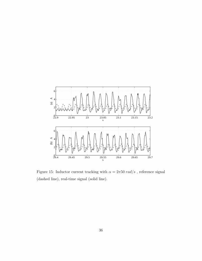
value of 50 Hz are shown in Fig. 14 and 15. In general, it can be appreciated

a good output tracking performance in the presence of uncertainties in the

input voltage E, for both cases. On the other hand, the tracking of the

inductor current shows noisy signals in both cases, where the first order filter

introduces the appreciated delay.

Remark 2. The tracking of the inductor is noisy and not so accurate due

to the effect of the PWM switching which is correct since the system is not

regulating the inductor current, but the capacitor voltage.

6. Conclusions

A discrete-time sliding mode control scheme has been designed for the

tracking of a DC-biased sinusoidal signal in a boost power converter. The

32

22.95 23 23.05 23.1 23.15 23.20

2

4

6

8

10

(a)

V

s

29.25 29.3 29.35 29.4 29.45 29.55

6

7

8

9

10

(b)

V

s

Figure 12: Output tracking of the voltage capacitor with α = 2π60 rad/s ,

reference signal (dashed line), real-time signal (solid line).

33

22.95 23 23.05 23.1 23.15 23.20

2

4

6

(a)

A

s

29.25 29.3 29.35 29.4 29.45 29.50

2

4

6

(b)

A

s

Figure 13: Inductor current tracking with α = 2π60 rad/s , reference signal

(dashed line), real-time signal (solid line).

34

22.9 22.95 23 23.05 23.1 23.15 23.20

2

4

6

8

10

(a)

V

s

29.4 29.45 29.5 29.55 29.6 29.65 29.75

6

7

8

9

10

(b)

V

s

Figure 14: Output tracking of the voltage capacitor with α = 2π50 rad/s ,

reference signal (dashed line), real-time signal (solid line).

35

22.9 22.95 23 23.05 23.1 23.15 23.20

2

4

6

(a)

A

s

29.4 29.45 29.5 29.55 29.6 29.65 29.70

2

4

6

(b)

A

s

Figure 15: Inductor current tracking with α = 2π50 rad/s , reference signal

(dashed line), real-time signal (solid line).

36

discrete-time model was obtained by means of a variational integrator scheme

based on the discrete Lagrangian formulation of the boost power converter,

that uses the midpoint rule integration method. The reference signal for

the inductor current was proposed as a polynomial of order 3 that solves

with a good accuracy the corresponding solution of one of the correspond-

ing FIB equations in the continuous-time setting. The sliding mode based

controller can stabilize non-minimum phase system dynamics with a proper

choice of a sliding surface as in the case of the inductor current. Simulation

and experimental results illustrate the good performance of the boost power

converter closed-loop with the discrete-time sliding mode regulator strategy

when tracking a DC-biased sinusoidal signal. Some interesting issues as the

robustness of the controller with respect to plant parameter variations are

currently under study.

Appendix A. Calculation of reference signals

The mathematical model of the Boost converter is given by the following

equations [15]:

x1 = −vx2

L+

E

L

x2 =vx1

C− x2

RC(A.1)

e = x2 − x2,r

with x1 as the inductor current, x2 is the output voltage capacitor, the control

input v represents the switch position and can only take a value of 0 or 1, e

as the output tracking error, x2,r as the output reference signal, E is the DC

37

input voltage. The constant parameters are the resistance R, the inductance

denoted by L, and the capacitance denoted by C.

The reference signals are supposed to be generated by an autonomous

exosystem given by

w1 = −αw2

w2 = αw1

w3 = 0 (A.2)

with initial conditions w1(0) = w2(0) = a and w3(0) = b, with the following

output

q(w) = w1 + w3. (A.3)

where w1 is a sinusoidal shape signal with an amplitude of√2a and a fre-

quency equal to α, w3 provides a bias value equal to b, w = (w1, w2, w3)T .

Using concepts of output regulation theory [11], the steady state functions

x1r = π1(w) and x2r = π2(w) for x1 and x2 respectively can be calculated

as a solution of the following PDEs (FIB equations) which are obtained by

using (A.1):

∂π1(w)

∂ws(w) = −c(w)π2(w)

L+

E

L(A.4)

∂π2(w)

∂ws(w) =

c(w)π1(w)

C− π2(w)

RC(A.5)

0 = π2(w)− q(w) (A.6)

with s(w) = (−αw2, αw1, 0)T . From (A.3) and (A.6) one can determine

π2(w) = w1 + w3. Then, one can calculate c(w) from (A.5) as follows:

c(w) =C

π1(w)

∂π2(w)

∂ws(w) +

π2(w)

Rπ1(w)

38

and substituing it in (A.4) yields to

∂π1(w)

∂ws(w) = −Cπ2(w)

Lπ1(w)

∂π2(w)

∂ws(w)− π2

2(w)

LRπ1(w)+

E

L. (A.7)

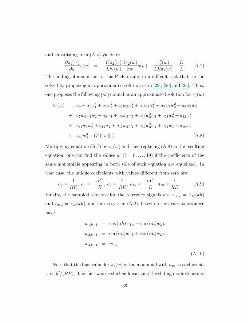
The finding of a solution to this PDE results in a difficult task that can be

solved by proposing an approximated solution as in [22], [26] and [25]. Thus,

one proposes the following polynomial as an approximated solution for π1(w)

π1(w) = a0 + a1w31 + a2w

21 + a3w2w

21 + a4w3w

21 + a5w1w

22 + a6w1w2

+ a7w3w1w2 + a8w1 + a9w3w1 + a10w23w1 + a11w

32 + a12w

22

+ a13w3w22 + a14w2 + a15w3w2 + a16w

23w2 + a17w3 + a18w

23

+ a19w33 +O4(‖w‖1). (A.8)

Multiplying equation (A.7) by π1(w) and then replacing (A.8) in the resulting

equation, one can find the values ai (i = 0, . . . , 19) if the coefficients of the

same monomials appearing in both side of such equation are equalized. In

that case, the unique coefficients with values different from zero are:

a2 =1

RE, a6 = −αC

E, a9 =

2

RE, a15 = −αC

E, a18 =

1

RE. (A.9)

Finally, the sampled versions for the reference signals are x1r,k = x1r(kh)

and x2r,k = x2r(kh), and for exosystem (A.2), based on the exact solution we

have

w1,k+1 = cos (αh)w1,k − sin (αh)w2,k

w2,k+1 = sin (αh)w1,k + cos (αh)w2,k

w3,k+1 = w3,k

(A.10)

Note that the bias value for π1(w) is the monomial with a18 as coefficient,

i. e., b2/(RE). This fact was used when linearizing the sliding mode dynamic.

39

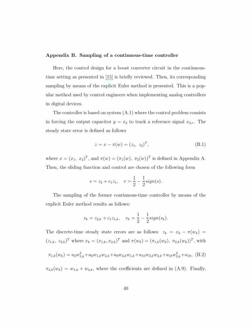
Appendix B. Sampling of a continuous-time controller

Here, the control design for a boost converter circuit in the continuous-

time setting as presented in [15] is briefly reviewed. Then, its corresponding

sampling by means of the explicit Euler method is presented. This is a pop-

ular method used by control engineers when implementing analog controllers

in digital devices.

The controller is based on system (A.1) where the control problem consists

in forcing the output capacitor y = x2 to track a reference signal x2,r. The

steady state error is defined as follows

z = x− π(w) = (z1, z2)T , (B.1)

where x = (x1, x2)T , and π(w) = (π1(w), π2(w))

T is defined in Appendix A.

Then, the sliding function and control are chosen of the following form

s = z2 + c1z1, v =1

2− 1

2sign(s).

The sampling of the former continuous-time controller by means of the

explicit Euler method results as follows:

sk = z2,k + c1z1,k, vk =1

2− 1

2sign(sk).

The discrete-time steady state errors are as follows: zk = xk − π(wk) =

(z1,k, z2,k)T where xk = (x1,k, x2,k)

T and π(wk) = (π1,k(wk), π2,k(wk))T , with

π1,k(wk) = a2w21,k+a6w1,kw2,k+a9w3,kw1,k+a15w3,kw2,k+a18w

23,k+a19, (B.2)

π2,k(wk) = w1,k + w2,k, where the coefficients are defined in (A.9). Finally,

40

exosystem (A.2) is approximated of the following form

w1,k+1 = w1,k − αhw2,k

w2,k+1 = w2,k + αhw1,k

w3,k+1 = w3,k.

[1] Al-Mothafar, M. R. D., 2012. Small-signal modelling of current-

programmed n-connected parallel-input/series-output bridge-based

buck dcdc converters. Journal of the Franklin Institute 349 (1), 260–

283.

[2] Astrom, K. J., Wittenmark, B., 1990. Computer-Controlled Systems.

Prentice-Hall, Englewood Cliffs, NJ.

[3] Basin, M., Rodriguez-Ramirez, P., 2012. Sliding mode controller design

for linear systems with unmeasured states. Journal of the Franklin In-

stitute 349 (4), 1337 – 1349.

[4] Caceres, R., Barbi, I., 1996. Sliding mode controller for the boost in-

verter. In: Power Electronics Congress, 1996. Technical Proceedings.

CIEP ’96., V IEEE International. pp. 247–252.

[5] Castillo-Toledo, B., Di Gennaro, S., Loukianov, A., Rivera, J., 2008.

Hybrid control of induction motors via sampled closed representations.

Industrial Electronics, IEEE Transactions on 55 (10), 3758 –3771.

[6] Choi, B., Lim, W., Choi, S., Sun, J., may 2008. Comparative perfor-

mance evaluation of current-mode control schemes adapted to asym-

metrically driven bridge-type pulsewidth modulated dc-to-dc converters.

Industrial Electronics, IEEE Transactions on 55 (5), 2033 –2042.

41

[7] Ciezki, J., Ashton, R., may 1998. The design of stabilizing controls

for shipboard dc-to-dc buck choppers using feedback linearization tech-

niques. In: Power Electronics Specialists Conference, 1998. PESC 98

Record. 29th Annual IEEE. Vol. 1. pp. 335 –341 vol.1.

[8] Cormerais, H., Buisson, J., Richard, P. Y., C., M., 2008. Modelling and

passivity based control of switched systems from bond graph formalism:

Application to multicellular converters. Journal of the Franklin Institute

345 (5), 468–488.

[9] Fossas, E., Olm, J., 2007. Galerkin method and approximate tracking

in a non-minimum phase bilinear system. Discrete and Continuous Dy-

namical Systems. Series B 7 (1), 53–76.

[10] Gee, A., Robinson, F., Dunn, R., 30 2011-sept. 1 2011. Sliding-mode

control, dynamic assessment and practical implementation of a bidirec-

tional buck/boost dc-to-dc converter. In: Power Electronics and Appli-

cations (EPE 2011), Proceedings of the 2011-14th European Conference

on. pp. 1 –10.

[11] Isidori, A., Byrnes, C., feb 1990. Output regulation of nonlinear systems.

Automatic Control, IEEE Transactions on 35 (2), 131 –140.

[12] Jang, J., Choi, S., Choi, B., Hong, S., 30 2011-june 3 2011. Average cur-

rent mode control to improve current distributions in multi-module eso-

nant dc-to-dc converters. In: Power Electronics and ECCE Asia (ICPE

ECCE), 2011 IEEE 8th International Conference on. pp. 2312 –2319.

42

[13] Kassakian, J., Schlecht, M., Verghese, G., 1991. Principles of power elec-

tronics. Addison-Wesley series in electrical engineering. Addison-Wesley.

URL http://books.google.com.mx/books?id=k4YoAQAAMAAJ

[14] Linares Flores, J., Avalos, J., Espinosa, C., march 2011. Passivity-based

controller and online algebraic estimation of the load parameter of the

dc-to-dc power converter cuk type. Latin America Transactions, IEEE

(Revista IEEE America Latina) 9 (1), 784 –791.

[15] Loukianov, A., Rivera, J., Chavira, F., Ortega, S., Sept. Discontinuous

output regulation for a dc-to-ac boost converter. In: Electrical Engi-

neering, Computing Science and Automatic Control (CCE), 2012 9th

International Conference on. pp. 1–6.

[16] Marie-Francoise, J.-N., Gualous, H., Berthon, A., aug. 2004. Dc to dc

converter with neural network control for on-board electrical energy

management. In: Power Electronics and Motion Control Conference,

2004. IPEMC 2004. The 4th International. Vol. 2. pp. 521 –525 Vol.2.

[17] Marsden, J. E., West, M., 2001. Discrete mechanics and variational

integrators. Acta Numerica 10, 357–514.

[18] Monaco, S., Normand-Cyrot, D., 2001. Issues on nonlinear digital sys-

tems. Eur. J. Control 7, 160–178.

[19] Monaco, S., Normand-Cyrot, D., 2007. Advanced tools for nonlinear

sampled-data systems analysis and control. Eur. J. Control 13 (2), 221–

241.

43

[20] Na, W., sept. 2011. Ripple current reduction using multi-dimensional

sliding mode control for fuel cell dc to dc converter applications. In:

Vehicle Power and Propulsion Conference (VPPC), 2011 IEEE. pp. 1

–6.

[21] Ortega, R., 1998. Passivity-based Control of Euler-Lagrange Systems:

Mechanical, Electrical, and Electromechanical Applications. Communi-

cations and Control Engineering. Springer.

URL http://books.google.com.mx/books?id=GCVn0oRqP9YC

[22] Ramos, L., Castillo-Toledo, B., Alvarez, J., apr 1997. Nonlinear regula-

tion of an underactuated system. In: Robotics and Automation, 1997.

Proceedings., 1997 IEEE International Conference on. Vol. 4. pp. 3288

–3293 vol.4.

[23] Rivera, J., Chavira, F., Loukianov, A., 2013. On the discrete-time mod-

eling of a dc-to-dc power converter and control design with discrete-time

sliding modes. Mathematical Problems in Engineering 2013, 1–17.

[24] Rivera, J., Garcia, L., Mora, C., Raygoza, J. J., Ortega, S., 2011. Slid-

ing Mode Control. InTech, Rijeka, Croatia, Ch. Super-Twisting Sliding

Mode in Motion Control Systems.

[25] Rivera, J., Loukianov, A., Castillo-Toledo, B., 2008. Discontinuous out-

put regulation of the pendubot. In: Proceedings of the 17th world

congress The international federation of automatic control.

[26] Sanposh, P., Tarn, T., Cheng, D., 2002. Theory and experimental re-

44

sults on output regulation for nonlinear systems. In: American Control

Conference, 2002. Proceedings of the 2002. Vol. 1. pp. 96 – 101 vol.1.

[27] Shtessel, Y., Zinober, A., Shkolnikov, I., dec. 2002. Boost and buck-

boost power converters control via sliding modes using dynamic sliding

manifold. In: Decision and Control, 2002, Proceedings of the 41st IEEE

Conference on. Vol. 3. pp. 2456 – 2461 vol.3.

[28] Shtessel, Y., Zinober, A., Shkolnikov, I., dec. 2002. Boost and buck-

boost power converters control via sliding modes using method of stable

system centre. In: Decision and Control, 2002, Proceedings of the 41st

IEEE Conference on. Vol. 1. pp. 340 – 345 vol.1.

[29] Sira-Ramırez, H., 1988. Differential geometric methods in variable-

structure control. International Journal of Control 48 (4), 1359–1390.

URL http://www.tandfonline.com/doi/abs/10.1080/00207178808906256

[30] Sira-Ramırez, H., 2001. Dc-to-ac power conversion on a ‘boost’converter.

International Journal of Robust and Nonlinear Control 11 (6), 589–600.

URL http://dx.doi.org/10.1002/rnc.575

[31] Stern, A., Desbrun, M., 2006. Discrete geometric mechanics for vari-

ational integrators. In: Proc. of the 33rd International Conference

and Exhibition on Computer Graphics and Interactive Techniques SIG-

GRAPH.

[32] Taeed, F., Salam, Z., Ayob, S., 29 2010-dec. 1 2010. Implementation of

single input fuzzy logic controller for boost dc to dc power converter.

45

In: Power and Energy (PECon), 2010 IEEE International Conference

on. pp. 797 –802.

[33] Utkin, V., 1992. Sliding Modes in Control and Optimization. Commu-

nications and Control Engineering Series. Springer-Verlag.

URL http://books.google.com.mx/books?id=uzNmQgAACAAJ

[34] Utkin, V., Guldner, J., Shi, ., 1999. Sliding mode control in electrome-

chanical systems. CRC Press.

[35] Utkin, V. I., Loukianov, A. G., Castillo-Toledo, B., Rivera, J., 2004.

Sliding mode regulator design. In: Sabanovic, A., Fridman, L. M., Spur-

geon, S. (Eds.), Variable Structure Systems: from principles to imple-

mentation. Vol. 66 of IET Control Engineering Series. Institution of

Engineering and Technology, pp. 19–44.

[36] West, M., 2003. Variational integrators. Ph.D. thesis, California Insti-

tute of Technology, USA.

[37] Wu, X., Liu, C., 1993. A unified method for fast modelling of dc-dc

switching converters. Journal of the Franklin Institute 330 (6), 1017–

1049.

[38] Zinober, A. S. I., Fossas-Colet, E., Scarratt, J. C., 1998. Two sliding

mode approaches to the control of a boost system. In: 6th IEEE Mediter-

ranean Conference on Control and Systems.

46