Discovering Excitatory Networks from Discrete Event Streamswith Applications to Neuronal Spike Train Analysis

Debprakash PatnaikDepartment of Computer Science

Virginia Tech, VA 24061, USAEmail: patnaik@vt.edu

Srivatsan LaxmanMicrosoft Research

Bangalore 560080, IndiaEmail: slaxman@microsoft.com

Naren RamakrishnanDepartment of Computer Science

Virginia Tech, VA 24061, USAEmail: naren@vt.edu

Abstract—Mining temporal network models from discreteevent streams is an important problem with applications incomputational neuroscience, physical plant diagnostics, andhuman-computer interaction modeling. We focus in this paperon temporal models representable as excitatory networks whereall connections are stimulative, rather than inhibitive. Throughthis emphasis on excitatory networks, we show how they canbe learned by creating bridges to frequent episode mining.Specifically, we show that frequent episodes help identify nodeswith high mutual information relationships and which canbe summarized into a dynamic Bayesian network (DBN). Todemonstrate the practical feasibility of our approach, we showhow excitatory networks can be inferred from both mathemat-ical models of spiking neurons as well as real neurosciencedatasets.

Keywords-Frequent Episodes; Dynamic Bayesian Network;Computational Neuroscience; Spike train analysis; TemporalData Mining

I. INTRODUCTION

Discrete event streams are prevalent in many applications,such as neuronal spike train analysis, physical plants, andhuman-computer interaction modeling. In all these domains,we are given occurrences of events of interest over a timecourse and the goal is to identify trends and behaviors thatserve discriminatory or descriptive purposes.

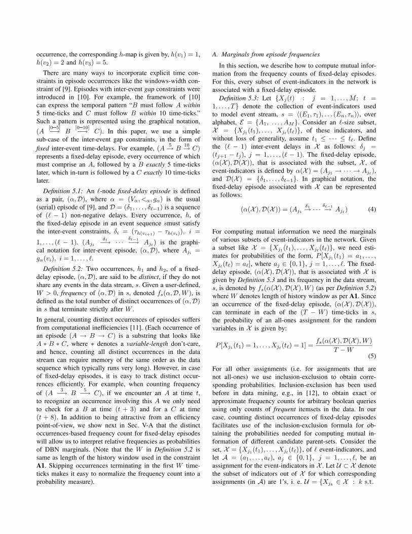
A Multi-Electrode Array (MEA) records spiking actionpotentials from an ensemble of neurons which after variouspre-processing steps, yields a spike train dataset providingreal-time, dynamic, perspectives into brain function (seeFig. 1). Identifying sequences (e.g., cascades) of firingneurons, determining their characteristic delays, and recon-structing the functional connectivity of neuronal circuits arekey problems of interest. This provides critical insights intothe cellular activity recorded in the neuronal tissue.

Similar motivations arise in other domains as well. Inphysical plants the discrete event stream denotes diagnosticand prognostic codes from stations in an assembly line andthe goal is to uncover temporal connections between codesemitted from different stations. In human-computer inter-action modeling, the event stream denotes actions taken byusers over a period of time and the goal is to capture aspectssuch as user intent and interaction strategy by understandingcausative chains of connections between actions.

Beyond uncovering structural patterns from discreteevents, we seek to go further, and actually uncover a

generative temporal process model for the data. In particular,our aim is to infer dynamic Bayesian networks (DBNs)which encode conditional independencies as well as tem-poral influences and which are also interpretable patterns intheir own right. We focus exclusively on excitatory networkswhere the connections are stimulative rather than inhibitoryin nature (e.g., ‘event A stimulates the occurrence of event B5ms later which goes on to stimulate event C 3ms beyond.’)This constitutes a large class of networks with relevance inmultiple domains, including neuroscience.

Our main contributions are three-fold:1) New model class of excitatory networks: Learning

Bayesian networks (dynamic or not) is a hard problemand to obtain theoretical guarantees we typically haveto place restrictions on network structure, e.g., assumethe BN has a tree structure as done in the Chow-Liu algorithm. Our focus on excitatory networks placesrestrictions on the nature of the conditional probabilitytables (CPT) instead of network structure and we showhow this leads to a tractable formulation.

2) New methods for learning DBNs: We demonstratethat DBNs can be learnt by creating bridges to frequentepisode mining literature. In particular, the focus on ex-citatory networks allows us to relate frequent episodesto parent sets for nodes with high mutual information.This enables us to predominantly apply fast algorithmsfor episode mining, while relating them to probabilisticnotions suitable for characterizing DBNs.

3) New applications to spike train analysis: We demon-strate a successful application of our methodologies toanalyzing neuronal spike train data, both from math-ematical models of spiking neurons and from realcortical tissue.

The paper is organized as follows. Sec. II gives a briefoverview of DBNs and Sec. III presents our formalismfor modeling event streams using DBNs. Sec. IV definesexcitatory networks and develops the theoretical basis forefficiently learning such networks. Sec. V introduces fixed-delay episodes and relates frequencies of such episodes withmarginal probabilities of a DBN. Our learning algorithm ispresented in Sec. VI, experimental results in Sec. VII andconclusions in Sec. VIII.

Figure 1. A multi-electrode array (MEA; left) produces a spiking event stream of action potentials (middle top). Mining cascaded firings (middle bottom)in the event stream helps uncover excitatory circuits (right) in the data.

II. BAYESIAN NETWORKS: STATIC AND DYNAMIC

Formal mathematical notions are presented in the nextsection, but here we wish to provide some backgroundcontext to past research in Bayesian networks (BNs). As iswell known, BNs use directed acyclic graphs to encode prob-abilistic notions of conditional independence, such as thata node is conditionally independent of its non-descendantsgiven its parents (for more details, see [1]). The earliestknown work for learning BNs is the Chow-Liu algorithm [2].It showed that, if we restricted the structure of the BN to atree, then the optimal BN can be computed using a minimumspanning tree algorithm. It also established the tractabilityof BN inference for this class of graphs.

More recent work, by Williamson [3], generalizes theChow-Liu algorithm to show how (discrete) distributions canbe approximated using the same general ingredients as theChow-Liu approach, namely mutual information quantitiesbetween random variables. Meila [4] presents an acceler-ated algorithm that is targeted toward sparse datasets ofhigh dimensionality. The approximation thread for generalBN inference is perhaps best exemplified by Friedman’ssparse candidate algorithm [5] that presents various greedyapproaches to learn (suboptimal) BNs.

DBNs are a relatively newer development and best ex-amples of them can be found in specific state space anddynamic modeling contexts, such as HMMs. In contrast totheir static counterparts, exact and efficient inference forgeneral classes of DBNs has not been studied well.

III. MODELING EVENT STREAMS USING DBNS

Consider a finite alphabet, E = {A1, . . . , AM}, ofevent-types (or symbols). Let s = 〈(E1, τ1), (E2, τ2),. . . , (En, τn)〉 denote a data stream of n events over E . EachEi, i = 1, . . . , n, is a symbol from E . Each τi, i = 1, . . . , n,takes values from the set of positive integers. The eventsin s are ordered according to their times of occurrence,τi+1 ≥ τi, i = 1, . . . , (n−1). The time of occurrence of thelast event in s, is denoted by τn = T . We model the datastream, s, as a realization of a discrete-time random process

X(t), t = 1, . . . , T ; X(t) = [X1(t)X2(t) · · ·XM (t)]′, whereXj(t) is an indicator variable for the occurrence of eventtype, Aj ∈ E , at time t. Thus, for j = 1, . . . ,M andt = 1, . . . , T , we will have Xj(t) = 1 if (Aj , t) ∈ s, andXj(t) = 0 otherwise. Each Xj(t) is referred to as the event-indicator random variable for event-type, Aj , at time t.

Example 1: The following is an example event sequenceof n = 7 events over an alphabet, E = {A,B,C, . . . , Z},of M = 26 event-types:

〈(A, 2), (B, 3), (D, 3), (B, 5), (C, 9), (A, 10), (D, 12)〉 (1)

The maximum time tick is given by T = 12. Each X(t), t =1, . . . , 12, is a vector of M = 26 indicator random variables.Since there are no events at time t = 0 in the examplesequence (1), we have X(1) = 0. At time t = 2, we willhave X(2) = [1000 · · · 0]′. Similarly, X(3) = [0101 · · · 0]′,and so on.

A DBN [6] is a DAG with nodes representing randomvariables and arcs representing conditional dependency re-lationships. We model the random process X(t) (or equiv-alently, the event stream s), as the output of a DBN. Eachevent-indicator, Xj(t), t = 1, . . . , T and j = 1, . . .M ,corresponds to a node in the network, and is assigned aset of parents, which is denoted as π(Xj(t)) (or simplyπj(t)). A parent-child relationship is represented by an arc(from parent to child) in the DAG. In a DBN, nodes areconditionally independent of their non-descendants giventheir parents. The joint probability distribution of X(t)under the DBN model, can be factorized as a product ofP [Xj(t) |πj(t)] for various j, t. In this paper we restrict theclass of DBNs using the following two constraints:

A1 [Time-bounded causality] For user-defined param-eter, W > 0, the set, πj(t), of parents for the node,Xj(t), is a subset of event-indicators out of the W -length history at time-tick, t, i.e. πj(t) ⊆ {Xk(τ) :1 ≤ k ≤M, (t−W ) ≤ τ < t}.

A2 [Translation invariance] If πj(t) = {Xj1(t1),. . . , Xj`(t`)} is an `-size parent set of Xj(t) forsome t > W , then for any other Xj(t′), t′ > W ,

its parent set, πj(t′), is simply a time-shifted ver-sion of πj(t), and is given by πj(t′) = {Xj1(t1 +δ), . . . , Xj`(t` + δ)}, where δ = (t′ − t).

While A1 limits the range-of-influence of a random variable,Xk(τ), to variables within (a user-defined) W time-ticks ofτ , A2 is a structural constraint that allows parent-child re-lationships to depend only on relative (rather than absolute)time-stamps of random variables. Further, we also assumethat the underlying data generation model is stationary, sothat joint-statistics can be estimated using frequency countsof suitably defined temporal patterns in the data.

A3 [Stationarity] For every set of event-indicators,Xj1(t1), . . . , Xj`(t`), and for every time-shift δ,we have P [Xj1(t1), . . . , Xj`(t`)] = P [Xj1(t1+δ),. . . , Xj`(t` + δ)].

Learning network structure involves learning the map,πj(t), for each Xj(t), j = 1, . . . ,M and t > W . LetI[Xj(t) ; πj(t)] denotes the mutual information betweenXj(t) and its parents, πj(t). DBN structure learning can beposed as a problem of approximating the data distribution,P [·], by a DBN distribution, Q[·]. Let DKL(P ||Q) denotethe KL divergence between P [·] and Q[·]. Using A1, A2 andA3, and following the lines of [2], [3], it is possible to showthat for parent sets with sufficiently high mutual informationto Xj(t), DKL(P ||Q) will be concomitantly lower [7].In other words, a good DBN-based approximation of theunderlying stochastics (i.e. one with small KL divergence)can be achieved by picking, for each node, a parent-setwhose corresponding mutual information exceeds a user-defined threshold.

However, picking such sets with high mutual information(while yields a good approximation) falls short of unearthinguseful dependencies among the random variables. This isbecause mutual information is non-decreasing as more ran-dom variables are added to a parent-set (leading to a fully-connected network always being optimal). For a parent-set tobe interesting, it should not only exhibit sufficient correlation(or mutual information) with the corresponding child-node,but should also successfully encode the conditional inde-pendencies among random variables in the system. This canbe done by checking if, conditioned on a candidate parent-set, the mutual information between the corresponding child-node and all its non-descendants is always close to zero. (Weprovide more details later in Sec. VI-C).

IV. EXCITATORY NETWORKS

The structure-learning approach described in Sec. III isapplicable to any general DBN that satisfies A1 and A2.In this paper, we focus on a further specialized class of net-works, called excitatory networks, where only certain kindsof conditional dependencies among nodes are permitted. Ingeneral, each event-type has some baseline propensity inthe data which is small and less than 0.5 (This corresponds

to a sparse-data assumption). A collection, Π, of randomvariables is said to have an excitatory influence on anevent-type, A ∈ E , if occurrence of events correspondingto the variables in Π, increases the propensity of A togreater than 0.5. We define an excitatory network as onein which nodes can only exert excitatory influences onone another. For example, in an excitatory network it ispossible that “if B, C and D occur (say) 2 time-ticks apart,the probability of A increases.” By contrast, in excitatorynetworks, it is not possible to model relationships like “whenA does not occur, the probability of B occurring 3 time-tickslater increases.” Similarly, excitatory networks cannot modelinhibitory relationships like “when A occurs, the probabilityof B occurring 3 time-ticks later decreases.” Excitatorynetworks are natural in neuroscience, where one is interestedin unearthing conditional dependency relationships amongneuron spiking patterns. Several regions in the brain areknown to exhibit predominantly excitatory relationships [8]and our model is targeted toward unearthing these.

Table IEXAMPLE OF A CONDITIONAL PROBABILITY TABLE IN AN EXCITATORY

NETWORK.

ΠP [XA = 1 | aj ]XB XC XD

a0 0 0 0 ε < 12

a1 0 0 1 ε1 ≥ εa2 0 1 0 ε2 ≥ εa3 0 1 1 ε3 ≥ ε, ε1, ε2a4 1 0 0 ε4 ≥ εa5 1 0 1 ε5 ≥ ε, ε1, ε4a6 1 1 0 ε6 ≥ ε, ε2, ε4

a7(a∗) 1 1 1 φ > ε, 12, εj∀j

The excitatory assumption manifests as a set of constraintson the conditional probability tables associated with theDBN. Consider a node1 XA (an indicator variable for event-type A ∈ E) and let Π denote a parent-set for XA. In excita-tory networks, the probability that A occurs, conditioned onthe occurrence of all the events associated with Π, should beat least as high as the corresponding conditional probabilitywhen only some (though not all) of the events of Π occur.Further, the probability of A is less than 0.5 when none ofthe events of Π occur and greater than 0.5 when all theevents of Π occur. For example, let Π = {XB , XC , XD}.The conditional probability table for A given Π is shown inTable I. The different conditioning contexts come about bythe occurrence or otherwise of each of the events in Π. Theseare denoted by aj , j = 0, . . . , 7. So while a0 representsthe all-zero assignment (i.e. none of the events B, C or Doccur), a7 (or a∗) denotes the all-ones assignment (i.e. allthe events B, C and D occur). The last column of the tablelists the corresponding conditional probabilities along withthe associated excitatory constraints. The baseline propensity

1To facilitate simple exposition, time-stamps of random-variables aredropped from the notation in this discussion.

of A is denoted by ε and the only constraint on it is thatit must be less than 1

2 . Conditioned on the occurrence ofany event of Π, the propensity of A can only increase, andhence, εj ≥ ε ∀j and φ ≥ ε. Similarly, when both C and Doccur, the probability must be at least as high as that wheneither C or D occurred alone (i.e. we must have ε3 ≥ ε1 andε3 ≥ ε2). Finally, for the all-ones case, denoted by Π = a∗,the conditional probability must be greater than 1

2 and mustalso satisfy φ ≥ εj ∀j.

In the context of DBN structure learning, excitatorynetworks ensure that event-types will occur frequently aftertheir respective parents (with suitable delays). This willallow us to estimate DBN structure using frequent patterndiscovery algorithms (which have been a mainstay in datamining for many years). We now have a simple necessarycondition on the probability (or frequency) of parent-sets inan excitatory network.

Theorem 4.1: Let XA denote a node in the DynamicBayesian Network corresponding to the event-type A ∈ E .Let Π denote a parent-set with excitatory influence onA. Let ε∗ be an upper-bound for conditional probabilitiesP [XA = 1 | Π = a] for all a 6= a∗ (i.e. for all butthe all-ones assignment in Π). If the mutual informationI[XA ; Π] exceeds ϑ(> 0), then the joint probability ofan occurrence of A along with all events of Π satisfiesP [XA = 1,Π = a∗] ≥ PminΦmin, where

Pmin =P [XA = 1]− ε∗

1− ε∗(2)

Φmin = h−1

[min

(1,h(P [XA = 1])− ϑ

Pmin

)](3)

and where h(·) denotes the binary entropy function h(q) =−q log q− (1− q) log(1− q), 0 < q < 1 and h−1[·] denotesits pre-image greater than 1

2 .Proof: Under the excitatory model we have P [XA = 1 |Π =a∗] > P [XA = 1 | Π = a] ∀a 6= a∗. First we apply ε∗ toterms in the expression for P [XA = 1]:

P [XA = 1] = P [Π = a∗]P [XA = 1 |Π = a∗]

+∑a 6=a∗

P [Π = a]P [XA = 1 |Π = a]

≤ P [Π = a∗] + (1− P [Π = a∗])ε∗

This gives us P [Π = a∗] ≥ Pmin (see Fig. 2). Next, sincewe are given that mutual information I[XA ; Π] exceeds ϑ,the corresponding conditional entropy must satisfy:

H[XA |Π] = P [Π = a∗]h(P [XA = 1 |Π = a∗])

+∑a6=a∗

P [Π = a]h(P [XA = 1 |Π = a])

< H[XA]− ϑ = h(P [XA = 1])− ϑ

Every term in the expression for H[XA |Π] is non-negative,and hence, each term (including the first one) must be lessthan (h(P [XA = 1]) − ϑ). Using (P [Π = a∗] ≥ Pmin) in

Curve B: H[X]- θ

Curve A: H[XA]

h(ε*)

h(φ)

ε* φ

H[XA]

P[XA=1]

H[XA] - θ

θ

1

Pmin

1-Pmin

Line B

Line A

Line C

Figure 2. An illustration of the results obtained in Theorem 4.1. x-axisof the plot is the range of P [XA = 1] and y-axis is the correspondingrange of entropy H[XA]. For the required mutual information criteria, theconditional entropy must lie below H[XA] − ϑ and on line A. At theboundary condition [φ = 1], Line A splits Line B in the ratio Pmin :(1− Pmin). This gives the expression for Pmin.

the above inequality and observing that P [XA = 1 |Π = a∗]must be greater than 0.5 for an excitatory network, we nowget (P [XA = 1 | Π = a∗] > Φmin). This completes theproof. �

V. FIXED-DELAY EPISODES

In the framework of frequent episode discovery [9] thedata is a single long stream of events over a finite alphabet(cf. Sec. III and Example 1). An `-node (serial) episode, α,is defined as a tuple, (Vα, <α, gα), where Vα = {v1, . . . , v`}denotes a collection of nodes, <α denotes a total order2 suchthat vi <α vi+1, i = 1, . . . , (`− 1). If gα(vj) = Aij , Aij ∈E , j = 1, . . . , `, we use the graphical notation (Ai1 → · · · →Ai`) to represent α. An occurrence of α in event stream,s = 〈(E1, τ1), (E2, τ2), . . . , (En, τn)〉, is a map h : Vα →{1, . . . , n} such that (i) Eh(vj) = g(vj) ∀vj ∈ Vα, and(ii) for all vi <α vj in Vα, the times of occurrence of theith and jth events in the occurrence satisfy τh(vi) ≤ τh(vj)

in s.Example 2: Consider a 3-node episode α = (Vα, <α,

gα), such that, Vα = {v1, v2, v3}, v1 <α v2, v2 <α v3and v1 <α v3, and gα(v1) = A, gα(v2) = B andgα(v3) = C. The graphical representation for this episode isα = (A→ B → C), indicating that in every occurrence ofα, an event of type A must appear before an event of type B,and the B must appear before an event of type C. For exam-ple, in sequence (1), the subsequence 〈(A, 1), (B, 3), (C, 9)〉constitutes an occurrence of (A → B → C). For this

2In general, <α can be any partial order over Vα. We focus on onlytotal orders here and show how multiple such total orders can be used tomodel DBNs of arbitrary -arity. In [9], such total orders are referred to asserial episodes.

occurrence, the corresponding h-map is given by, h(v1) = 1,h(v2) = 2 and h(v3) = 5.

There are many ways to incorporate explicit time con-straints in episode occurrences like the windows-width con-straint of [9]. Episodes with inter-event gap constraints wereintroduced in [10]. For example, the framework of [10]can express the temporal pattern “B must follow A within5 time-ticks and C must follow B within 10 time-ticks.”Such a pattern is represented using the graphical notation,(A

[0–5]−→ B[0–10]−→ C). In this paper, we use a simple

sub-case of the inter-event gap constraints, in the form offixed inter-event time-delays. For example, (A 5→ B

10→ C)represents a fixed-delay episode, every occurrence of whichmust comprise an A, followed by a B exactly 5 time-tickslater, which in-turn is followed by a C exactly 10 time-tickslater.

Definition 5.1: An `-node fixed-delay episode is definedas a pair, (α,D), where α = (Vα, <α, gα) is the usual(serial) episode of [9], and D = (δ1, . . . , δ`−1) is a sequenceof (` − 1) non-negative delays. Every occurrence, h, ofthe fixed-delay episode in an event sequence smust satisfythe inter-event constraints, δi = (τh(vi+1) − τh(vi)), i =

1, . . . , (` − 1). (Aj1δ1−→ · · · δ`−1−→ Aj`) is the graphi-

cal notation for inter-event episode, (α,D), where Aji =gα(vi), i = 1, . . . , `.

Definition 5.2: Two occurrences, h1 and h2, of a fixed-delay episode, (α,D), are said to be distinct, if they do notshare any events in the data stream, s. Given a user-defined,W > 0, frequency of (α,D) in s, denoted fs(α,D,W ), isdefined as the total number of distinct occurrences of (α,D)in s that terminate strictly after W .

In general, counting distinct occurrences of episodes suffersfrom computational inefficiencies [11]. (Each occurrence ofan episode (A → B → C) is a substring that looks likeA ∗ B ∗ C, where ∗ denotes a variable-length don’t-care,and hence, counting all distinct occurrences in the datastream can require memory of the same order as the datasequence which typically runs very long). However, in caseof fixed-delay episodes, it is easy to track distinct occur-rences efficiently. For example, when counting frequencyof (A 3−→ B

5−→ C), if we encounter an A at time t,to recognize an occurrence involving this A we only needto check for a B at time (t + 3) and for a C at time(t + 8). In addition to being attractive from an efficiencypoint-of-view, we show next in Sec. V-A that the distinctoccurrences-based frequency count for fixed-delay episodeswill allow us to interpret relative frequencies as probabilitiesof DBN marginals. (Note that the W in Definition 5.2 issame as length of the history window used in the constraintA1. Skipping occurrences terminating in the first W time-ticks makes it easy to normalize the frequency count into aprobability measure).

A. Marginals from episode frequencies

In this section, we describe how to compute mutual infor-mation from the frequency counts of fixed-delay episodes.For this, every subset of event-indicators in the network isassociated with a fixed-delay episode.

Definition 5.3: Let {Xj(t) : j = 1, . . . ,M ; t =1, . . . , T} denote the collection of event-indicators usedto model event stream, s = 〈(E1, τ1), . . . (En, τn)〉, overalphabet, E = {A1, . . . , AM}. Consider an `-size subset,X = {Xj1(t1), . . . , Xj`(t`)}, of these indicators, andwithout loss of generality, assume t1 ≤ · · · ≤ t`. Definethe (` − 1) inter-event delays in X as follows: δj =(tj+1 − tj), j = 1, . . . , (` − 1). The fixed-delay episode,(α(X ),D(X )), that is associated with the subset, X , ofevent-indicators is defined by α(X ) = (Aj1 → · · · → Aj`),and D(X ) = {δ1, . . . , δ`−1}. In graphical notation, thefixed-delay episode associated with X can be representedas follows:

(α(X ),D(X )) = (Aj1δ1→ · · · δ`−1→ Aj`) (4)

For computing mutual information we need the marginalsof various subsets of event-indicators in the network. Givena subset like X = {Xj1(t1), . . . , Xj`(t`)}, we need esti-mates for probabilities of the form, P [Xj1(t1) = a1, . . . ,Xj`(t`) = a`], where aj ∈ {0, 1}, j = 1, . . . , `. The fixed-delay episode, (α(X ),D(X )), that is associated with X isgiven by Definition 5.3 and its frequency in the data stream,s, is denoted by fs(α(X ),D(X ),W ) (as per Definition 5.2)where W denotes length of history window as per A1. Sincean occurrence of the fixed-delay episode, (α(X ),D(X )),can terminate in each of the (T − W ) time-ticks in s,the probability of an all-ones assignment for the randomvariables in X is given by:

P [Xj1(t1) = 1, . . . , Xj`(t`) = 1] =fs(α(X ),D(X ),W )

T −W(5)

For all other assignments (i.e. for assignments that arenot all-ones) we use inclusion-exclusion to obtain corre-sponding probabilities. Inclusion-exclusion has been usedbefore in data mining, e.g., in [12], to obtain exact orapproximate frequency counts for arbitrary boolean queriesusing only counts of frequent itemsets in the data. In ourcase, counting distinct occurrences of fixed-delay episodesfacilitates use of the inclusion-exclusion formula for ob-taining the probabilities needed for computing mutual in-formation of different candidate parent-sets. Consider theset, X = {Xj1(t1), . . . , Xj`(t`)}, of ` event-indicators, andlet A = (a1, . . . , a`), aj ∈ {0, 1}, j = 1, . . . , `, be anassignment for the event-indicators in X . Let U ⊂ X denotethe subset of indicators out of X for which correspondingassignments (in A) are 1’s, i. e. U = {Xjk ∈ X : k s.t.

Procedure 1 Overall ProcedureInput: Alphabet E , event stream s = 〈(E1, τ1), . . . ,

(En, τn = T )〉, length W of history window, condi-tional probability upper-bound ε∗, mutual informationthreshold, ϑ

Output: DBN structure (parent-set for each node in thenetwork)

1: for all A ∈ E do2: XA := event-indicator of A at any time t > W3: Set fmin = (T −W )PminΦmin, using Eqs. (2)-(3)4: Obtain set, C, of fixed-delay episodes ending in A,

with frequencies greater than fmin (cf. Sec. VI-B,Procedure 2)

5: for all fixed-delay episodes (α,D) ∈ C do6: X(α,D) := event-indicators corresponding to (α,D)7: Compute mutual information I[XA ; X(α,D)]8: Remove (α,D) from C if I[XA ; X(α,D)] < ϑ9: Prune C using conditional mutual information cri-

teria to distinguish direct from indirect influences(cf. Sec. VI-C)

10: Return (as parent-set for XA) event-indicators corre-sponding to episodes in C

ak = 1 in A, 1 ≤ k ≤ `}. Inclusion-exclusion is used tocompute the probabilities as follows:

P [Xj1 = a1, . . . , Xj` = a`]

=∑Y s.t.

U ⊆ Y ⊆ X

(−1)|Y\U|(fs(Y)T −W

)(6)

where fs(Y) is short-hand for fs(α(Y),D(Y),W ), thefrequency (cf. Definition 5.2) of the fixed-delay episode,(α(Y),D(Y)).

VI. ALGORITHMS

A. Overall approach

In Secs. III-V, we developed the formalism for learning anoptimal DBN structure from event streams by using distinctoccurrences-based counts of fixed-delay episodes to computethe DBN marginal probabilities. The top-level algorithm(cf. Sec. III) for discovering the network is to fix any timet > W , to consider each Xj(t), j = 1, . . . ,M , in-turn, andto find its set of parents in the network. Due to the translationinvariance assumption A2, we need to do this only once foreach event-type in the alphabet.

The algorithm is outlined in Procedure 1. For each A ∈ E ,we first compute the minimum frequency for episodesending in A based on the relationship between mutualinformation and joint probabilities as per Theorem 4.1 (line3, Procedure 1). Then we use a pattern-growth approach(see Procedure 2) to discover all patterns terminating in A

Procedure 2 pattern grow(α,D,L(α,D))

Input: `-node episode (α,D) = (Aj1δ1→ · · · δ`−1→ Aj`)

and event sequence s = 〈(E1, τ1), . . . , (En, τn = T )〉,Length of history window W , Frequency thresholdfmin.

1: ∆ = W − span(α,D)2: for all A ∈ E do3: for δ = 0 to ∆ do4: if δ = 0 and (Aj1 > A or ` = 1) then5: continue6: (α′,D′) = A

δ→ α; L(α′,D′) = {}; fs(α′,D′) = 07: for all τi ∈ L(α,D) do8: if ∃(Ej , τj) such that Ej = A and τi − τj = δ

then9: Increment fs(α′,D′)

10: L(α′,D′) = L(α′,D′) ∪ {τj}11: if fs(α′,D′) ≥ fmin then12: Add (α′,D′) to output set C13: if span(α′,D′) ≤W then14: pattern grow(α′,D′,L(α′,D′))

(line 4, Procedure 1). Each frequent pattern corresponds toa set of event-indicators (line 6, Procedure 1). The mutualinformation between this set of indicators and the node XA

is computed using exclusion-exclusion formula and only setsfor which this mutual information exceeds ϑ are retained ascandidate parent-sets (lines 5-8, Procedure 1). Finally, weprune out candidate parent-sets which have only indirectinfluences on A and return the final parent-sets for nodescorresponding to event-type A (lines 9-10, Procedure 1).This pruning step is based on some conditional mutualinformation criteria (to be described later in Sec. VI-C).

B. Discovering fixed-delay episodes

We employ a pattern-growth algorithm (Procedure 2)for mining frequent fixed-delay episodes because, unlikeApriori-style algorithms, pattern-growth procedures allowuse of different frequency thresholds for episodes endingin different alphabets. This is needed in our case, since, ingeneral, Theorem 4.1 prescribes different frequency thresh-olds for nodes in the network corresponding to differentalphabets. The recursive procedure is invoked with (α,D) =(A, φ) and frequency threshold fmin = (T −W )Pminφmin(Recall that in the main loop of Procedure 1, we look forparents of nodes corresponding to event-type A ∈ E).

The pattern-growth algorithm listed in Procedure 2 takesas input, an episode (α,D), a set of start times L(α,D), andthe event sequence s. L(α,D) is a set of time stamps τi suchthat there is an occurrence of (α,D) starting at τi in s. Forexample, if at level 1 we have (α,D) = (C, φ), then L(C,φ)

= {1, 4, 5, 8, 9} in the event sequence s shown in Fig 3.The algorithm obtains counts for all episodes like (α′,D′)

1 2 3 4 5 6 7 8 9 10

A

B

C

Figure 3. An event sequence showing 3 distinct occurrences of the episodeA

1→ B2→ C.

generated by extending (α,D) e.g. B 1→ C, . . ., A 5→ C etc.For an episode say (α′,D′) = B

2→ C, the count is obtainedby looking for occurrences of event B at times τj = τi − 2where τi ∈ L(C,φ). In the example such B’s at τj ∈ L

B2→C

= {2, 3, 6}. The number of such occurrences (= 3) gives thecount of B 2→ C. At every step the algorithm tries to growan episode with count fs > fmin otherwise stops.

C. Conditional MI criteria

The final step in determining the parents of a node XA

involves testing of some conditional mutual informationcriteria (cf. line 10, Procedure 1). The input to the stepis a set C of (frequent) fixed-delay episodes ending in A.Each episode in C is associated with a set of event-indicatorswhose mutual information with XA exceeds ϑ. Consider twosuch sets Y and Z , each having sufficient mutual informationwith XA. Our conditional mutual information criterion is:remove Y from the set of candidate parents (of XA), ifI[XA ; Y | Z] = 03. We repeat this test for every pair ofepisodes in C.

To understand the utility of this criterion, there are twocases to consider: (i) either Y ⊂ Z or Z ⊂ Y , and (ii) bothY 6⊂ Z and Z 6⊂ Y . In the first case, our conditional mutualcriterion will ensure that we pick the larger set as a parentonly if it brings more information about XA than the smallerset. In the second case, we are interested in eliminating setswhich have a high mutual information with XA because ofindirect influences. For example, if the network were suchthat C excites B and B excites A, then XC can have highmutual information with XA, but we do not want to reportXC as a parent of XA, since C influences A only throughB. Our conditional mutual information criterion will detectthis and eliminate XC from the set of candidate parents (ofXA) because it will detect I[XA ; XC |XB ] = 0.

VII. EXPERIMENTAL RESULTS

We present results on data gathered from both mathemat-ical models of spiking neurons as well as real neurosciencedatasets.

A. Neuronal network model

The approach here is to model each neuron as an inho-mogeneous Poisson process whose firing rate is a function

3We use a small threshold parameter to ascertain this equality.

of the input received by the neuron is recent past [13]:

λi(t) =λ

1 + exp(−Ii(t) + δ)(7)

Eq. (7) gives the firing rate of the ith neuron at time t.The network inter-connect allowed by this model gives itthe amount of sophistication required for simulating higher-order interactions. More importantly, the model allows forvariable delays which mimic the delays in conduction path-ways of real neurons.

Ii(t) =∑j

βijYj(t−τij)+. . .+∑ij...l

βij...lYj(t−τij) . . . Yl(t−τil)

(8)In Eq. (8), Yj(t−τij) is the indicator of the event of a spikeon jth neuron τij time earlier and the β(.)s are the weightparameters for the interactions. The higher order terms inthe input contribute to the firing rate only when the ith

neuron received inputs from all the neurons in the term withcorresponding delays. With suitable choices of parametersβ(.), one can simulate a wide range of networks.

B. Types of Networks

In this section we demonstrate the effectiveness of ourapproach in unearthing different types of networks. Each ofthese networks was simulated by setting up the appropriateinter-connections, of suitable order, in our mathematicalmodel.

Causative chains and higher order structures: A higher-order chain is one where parent sets are not restricted to beof cardinality one. In the example network of Fig. 4(a), thereare four disconnected components with two of them havingcycles. (Recall this would be ‘illegal’ in a static Bayesiannetwork formulation.) Also the component consisting ofnodes 18, 19, 20, 21 exhibits higher-order interactions. Thenode 20 fires with high probability when node 18 has fired4 ms before and node 18 has fired 5 ms before. Similarlynode 21 is activated by node 18, 19, 20 firing at respectivedelays. The complete network consists of 100 nodes (withthe remainder of the nodes firing independently). Spike traindata is generated for runs of 60 sec using the multi-neuronalsimulator. The base firing rate for neurons is set at 20Hz andthe activation probability of a child node (i.e. the conditionalprobability that the child node fires given its parents) isvaried form 0.6 to 0.8 (by suitably selecting βij’s). Ouralgorithm reports good precision and recall over a rangeof ϑ (0.05 ≤ ϑ ≤ 0.5) and ε∗ (0.02 ≤ ε∗ ≤ 0.04). Forlower values of (simulation) conditional probability, recallgradually drops but precision remains high (100%). Detailsare shown in Table II.

Overlapping causative chains: The graph shown inFig. 4(a) (b) has two chains 0 → 1 → 2 → 3 and12 → 1 → 13 → 14 → 15 → which share the node 1.Here 1 can be independently excited by 0 or 12. Also 2is activated by 0, 1 together and 13 is activated by 13, 1.

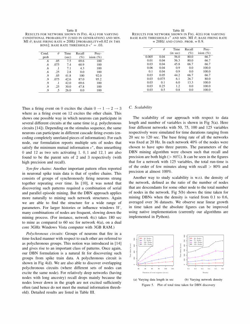
Table IIRESULTS FOR NETWORK SHOWN IN FIG. 4(A) FOR VARYING

CONDITIONAL PROBABILITY (USED IN GENERATION) AND MIN.MI ϑ; BASE FIRING RATE = 20HZ [PROBABILITY=0.02 IN 1MS

BINS]; BASE RATE THRESHOLD ε∗ = .03.

Cond. ϑ Time Recall Prec-prob (sec) (%) ision (%)

.6 .05 7.5 69.6 100

.6 .075 7.4 60.9 100

.6 .1 7.1 4.3 100

.6 .25 2.8 0.0 100

.9 .05 41.8 100 92.0

.9 .075 42.6 87.0 95.2

.9 .1 42.0 69.6 100

.9 .25 30.0 47.8 100

.9 .5 26.0 0.0 100

Thus a firing event on 0 excites the chain 0→ 1→ 2→ 3where as a firing event on 12 excites the other chain. Thisshows one possible way in which neurons can participate inseveral different circuits at the same time (e.g. polychronouscircuits [14]). Depending on the stimulus sequence, the sameneurons can participate in different cascade firing events (en-coding completely unrelated pieces of information). For eachnode, our formulation reports multiple sets of nodes thatsatisfy the minimum mutual information ε∗, thus unearthing0 and 12 as two sets activating 1. 0, 1 and 12, 1 are alsofound to be the parent sets of 2 and 3 respectively (withhigh precision and recall).

Syn-fire chains: Another important pattern often reportedin neuronal spike train data is that of synfire chains. Thisconsists of groups of synchronously firing neurons strungtogether repeating over time. In [10], it was noted thatdiscovering such patterns required a combination of serialand parallel episode mining. But the DBN approach appliesmore naturally to mining such network structures. Againwe are able to find the structure for a wide range ofparameters. For larger histories or influence windows W ,many combinations of nodes are frequent, slowing down themining process. (For instance, network 4(c) takes 180 secto mine as compared to 60 sec for network 4(a), on a dualcore 3GHz Windows Vista computer with 3GB RAM.)

Polychronous circuits: Groups of neurons that fire in atime-locked manner with respect to each other are referred toas polychronous groups. This notion was introduced in [14]and gives rise to an important class of patterns. Once again,our DBN formulation is a natural fit for discovering suchgroups from spike train data. A polychronous circuit isshown in Fig 4(d). We are also able to discover overlappingpolychronous circuits (where different sets of nodes canexcite the same node). For relatively deep networks (havingnodes with long ancestry) recall drops mainly because thenodes lower down in the graph are not excited sufficientlyoften (and hence do not meet the mutual information thresh-old). Detailed results are listed in Table III.

Table IIIRESULTS FOR NETWORK SHOWN IN FIG. 4(D) FOR VARYING

BASE RATE THRESHOLD ε∗ AND MIN. MI ϑ; BASE FIRING RATE= 20HZ AND COND. PROB. = 0.9.

ε∗ ϑ Time Recall Prec-(in sec) (%) ision (%)

0.005 0.04 56.0 80.0 66.70.01 0.04 56.3 80.0 66.70.03 0.04 45.8 66.7 66.70.06 0.04 0.9 0.0 100.00.1 0.04 0.9 0.0 100.0

0.03 0.05 44.2 66.7 66.70.03 0.075 6.1 26.7 80.00.03 0.1 6.0 13.3 100.00.03 0.25 1.2 0.0 100.00.03 0.5 0.8 0.0 100.0

C. Scalability

The scalability of our approach with respect to datalength and number of variables is shown in Fig 5(a). Herefour different networks with 50, 75, 100 and 125 variablesrespectively were simulated for time durations ranging from20 sec to 120 sec. The base firing rate of all the networkswas fixed at 20 Hz. In each network 40% of the nodes werechosen to have upto three parents. The parameters of theDBN mining algorithm were chosen such that recall andprecision are both high (> 80%). It can be seen in the figuresthat for a network with 125 variables, the total run-time isof the order of few minutes along with recall > 80% andprecision at almost 100%.

Another way to study scalability is w.r.t. the density ofthe network, defined as the ratio of the number of nodesthat are descendants for some other node to the total numberof nodes in the network. Fig 5(b) shows the time taken formining DBNs when the density is varied from 0.1 to 0.6,averaged over 36 datasets. We observe near linear growthin time taken and the absolute figures can be improvedusing native implementation (currently our algorithms areimplemented in Python).

20 40 60 80 100 120

020

040

060

080

0

Duration of event sequence (in sec)

Tim

e ta

ken

(in

sec

)

50−Nodes75−Nodes100−Nodes125−Nodes

(a) Varying data length in sec

0.1 0.2 0.3 0.4 0.5 0.6

010

020

030

040

050

060

0

Density

Tim

e ta

ken

(in

sec

)

50−Nodes75−Nodes100−Nodes125−Nodes

(b) Varying network density

Figure 5. Plot of total time taken for DBN discovery

(a) Higher-order causative chains (b) Overlappingcausative chains

(c) Syn-fire Chains (d) Polychronous Circuits

Figure 4. Four classes of DBNs investigated in our experiments.

D. Sensitivity

Finally, we discuss the sensitivity of the DBN miningalgorithm to the parameters ϑ, ε∗ and cond. mutual infor-mation threshold (used to check for MI=zero). To obtainprecision-recall curves for our algorithm applied to data se-quences with different characteristics, we vary the parameterϑ in the range [0.04-0.06] and repeat for different cond.mutual information threshold values. The data sequence forthis experiment is generated from the multi-neuronal simu-lator using different settings of base firing rate, conditionalprobability, number of nodes in the network, and the densityof the network.

The set of precision-recall curves are shown in Fig 6.The general trends observed here show that for a range ofsettings of the conditional probability, base firing rates, andnetwork topology, both high precision and high recall canbe obtained. As the stringency of the conditional mutualinformation threshold is increased (compare Fig. 6 (top) toFig. 6 (bottom), we observe a deterioration of performanceonly w.r.t. the base rate threshold.

E. Cortical cultures

Multi-electrode arrays provide high throughput recordingsof the spiking activity in neuronal tissue and are hence richsources of event data where events correspond to specificneurons being activated. We use data from dissociated corti-cal cultures gathered by Steve Potter’s laboratory at GeorgiaTech [15] which gathered data over several days. The miningis done with mutual information threshold ϑ = 0.001 withDBN search parameter ε∗ = 0.02.

In order to establish the significance of the networksdiscovered we run our algorithm on several surrogate spiketrains generated by replacing the neuron labels of spikes inthe real data with randomly chosen labels. These surrogatesbreak the temporal correlations in the data and yet preservethe overall summary statistics. No network structure wasfound in such surrogate sequences. We are currently in theprocess of characterizing and interpreting the usefulness of

Figure 7. DBN structure discovered from first 15 min of spike trainrecording on day 35 of culture 2-1 [15].

such networks found in real data. An example network isshown in Fig. 7, reflecting the sustained bursts observed inthis culture by Wagenaar et al [15].

VIII. DISCUSSION

Our work marries frequent pattern mining with probabilis-tic modeling for analyzing discrete event stream datasets.DBNs provide a formal probabilistic basis to model rela-tionships between time-indexed random variables but areintractable to learn in the general case. Conversely, frequentepisode mining is scalable to large datasets but does notexhibit the rigorous probabilistic interpretations that are themainstay of the graphical models literature. We have pre-sented the beginnings of research to relate these two diversethreads and demonstrated its potential to mine excitatorynetworks with applications in spike train analysis.

Two key directions of future work are being explored.The excitatory assumption as modeled here posits an orderover the entries of the conditional probability table butdoes not impose strict distinctions of magnitude over theseentries. This suggests that, besides the conditional indepen-dencies inferred by our approach, there could potentially

0 20 40 60 80 100

020

40

60

80

100

Pre

cisi

on

Recall

Pre

cisi

on

minimum MI = 0.04 − 0.06

Cond. MI threshold = 1e−04

Density

0.20.40.60.8

0 20 40 60 80 100

020

40

60

80

100

Pre

cisi

on

Recall

Pre

cisi

on

minimum MI = 0.04 − 0.06

Cond. MI threshold = 0.001

Density

0.20.40.60.8

0 20 40 60 80 100

020

40

60

80

100

Pre

cisi

on

Recall

Pre

cisi

on

minimum MI = 0.04 − 0.06

Cond. MI threshold = 1e−04

N

5075100125

0 20 40 60 80 100

020

40

60

80

100

Pre

cisi

on

Recall

Pre

cisi

on

minimum MI = 0.04 − 0.06

Cond. MI threshold = 0.001

N

5075100125

0 20 40 60 80 100

020

40

60

80

100

Pre

cisi

on

Recall

Pre

cisi

on

minimum MI = 0.04 − 0.06

Cond. MI threshold = 1e−04

Base.Rate

0.010.020.040.06

0 20 40 60 80 100

020

40

60

80

100

Pre

cisi

on

Recall

Pre

cisi

on

minimum MI = 0.04 − 0.06

Cond. MI threshold = 0.001

Base.Rate

0.010.020.040.06

0 20 40 60 80 100

020

40

60

80

100

Pre

cisi

on

Recall

Pre

cisi

on

minimum MI = 0.04 − 0.06

Cond. MI threshold = 1e−04

Cond.Prob

0.60.80.9

0 20 40 60 80 100

020

40

60

80

100

Pre

cisi

on

Recall

Pre

cisi

on

minimum MI = 0.04 − 0.06

Cond. MI threshold = 0.001

Cond.Prob

0.60.80.9

Figure 6. Precision-recall curves for different parameter values in the DBN mining algorithm.

be additional ‘structural’ constraints masquerading insidethe conditional probability tables. We seek to tease outthese relationships further. A second, more open, questionis whether there are other useful classes of DBNs that haveboth practical relevance (like excitatory circuits) and whichalso can be tractably inferred using sufficient statistics of theform studied here.

ACKNOWLEDGMENT

This work is supported in part by General Motors Re-search, NSF grant CNS-0615181, and ICTAS, Virginia Tech.Authors thank V. Raajay and P. S. Sastry of Indian Instituteof Science, Bangalore, for many useful discussions and foraccess to the neuronal spike train simulator of [13].

REFERENCES

[1] M. I. Jordan, Ed., Learning in Graphical Models. MIT Press,1998.

[2] C. Chow and C. Liu, “Approximating discrete probabilitydistributions with dependence trees,” IEEE Transactions onInformation Theory, vol. 14, no. 3, pp. 462–467, May 1968.

[3] J. Williamson, “Approximating discrete probability distribu-tions with bayesian networks,” in Proc. Intl. Conf. on AI inScience & Technology, Tasmania, 2000, pp. 16–20.

[4] M. Meila, “An accelerated chow and liu algorithm: Fittingtree distributions to high-dimensional sparse data,” in Proc.ICML’99, 1999, pp. 249–257.

[5] N. Friedman, K. Murphy, and S. Russell, “Learning thestructure of dynamic probabilistic networks,” in Proc. UAI’98.Morgan Kaufmann, 1998, pp. 139–147.

[6] K. Murphy, “Dynamic Bayesian Networks: representation,inference and learning,” Ph.D. dissertation, University ofCalifornia, Berkeley, CA, USA, 2002.

[7] D. Patnaik, S. Laxman, and N. Ramakrishnan, “Inferringdynamic bayesian networks using frequent episode mining,”CoRR, vol. abs/0904.2160, 2009.

[8] F. Rieke, D. Warland, R. Steveninck, and W. Bialek, Spikes:Exploring the Neural Code. The MIT Press, 1999.

[9] H. Mannila, H. Toivonen, and A. Verkamo, “Discovery offrequent episodes in event sequences,” Data Mining andKnowledge Discovery, vol. 1, no. 3, pp. 259–289, 1997.

[10] D. Patnaik, P. S. Sastry, and K. P. Unnikrishnan, “Inferringneuronal network connectivity from spike data: A temporaldata mining approach,” Scientific Programming, vol. 16, no. 1,pp. 49–77, January 2007.

[11] S. Laxman, “Discovering frequent episodes: Fast algorithms,connections with hmms and generalizations,” Ph.D. disserta-tion, IISc, Bangalore, India, September 2006.

[12] J. K. Seppanen, “Using and extending itemsets in data min-ing: Query approximation, dense itemsets and tiles,” Ph.D.dissertation, Helsinki University of Technology, 2006.

[13] V. Raajay, “Frequent episode mining and multi-neuronal spiketrain data analysis,” Master’s thesis, IISc, Bangalore, 2009.

[14] E. M. Izhikevich, “Polychronization: Computation withspikes,” Neural Comput., vol. 18, no. 2, pp. 245–282, 2006.

[15] D. A. Wagenaar, J. Pine, and S. M. Potter, “An extremelyrich repertoire of bursting patterns during the development ofcortical cultures,” BMC Neuroscience, 2006.