LAPPEENRANTA UNIVERSITY OF TECHNOLOGY

SCHOOL OF INDUSTRIAL ENGINEERING AND MANAGEMENT

Master’s Thesis

Jari Lirkki

VALIDATION AND SELECTION OF TRANSPORTATION

COST DRIVERS WITH ADVANCED METHODS

Lappeenranta 14.2.2014

Examiners: Professor Timo Kärri, Professor Hannu Rantanen

ABSTRACT

Author: Jari Lirkki

Title: Validation and Selection of Transportation Cost Drivers with Advanced

Methods

Year: 2014 Location: Lappeenranta

Master’s Thesis. Lappeenranta University of Technology

School of Industrial Engineering and Management, Cost Management

86 pages, 24 figures, 5 tables, 7 appendices

Examiners: Professor Timo Kärri, Professor Hannu Rantanen

Keywords: Cost driver, selection, cost driver analysis, validation, correlation,

regression analysis, practicality analysis, wholesaler, transportation, activity-

based costing, cost driver combination

In today's logistics environment, there is a tremendous need for accurate cost

information and cost allocation. Companies searching for the proper solution

often come across with activity-based costing (ABC) or one of its variations

which utilizes cost drivers to allocate the costs of activities to cost objects. In

order to allocate the costs accurately and reliably, the selection of appropriate

cost drivers is essential in order to get the benefits of the costing system.

The purpose of this study is to validate the transportation cost drivers of a

Finnish wholesaler company and ultimately select the best possible driver

alternatives for the company. The use of cost driver combinations as an

alternative is also studied. The study is conducted as a part of case company's

applied ABC-project using the statistical research as the main research method

supported by a theoretical, literature based method. The main research tools

featured in the study include simple and multiple regression analyses, which

together with the literature and observations based practicality analysis forms

the basis for the advanced methods.

The results suggest that the most appropriate cost driver alternatives are the

delivery drops and internal delivery weight. The possibility of using cost driver

combinations is not suggested as their use doesn't provide substantially better

results while increasing the measurement costs, complexity and load of use at

the same time. The use of internal freight cost drivers is also questionable as

the results indicate weakening trend in the cost allocation capabilities towards

the end of the period. Therefore more research towards internal freight cost

drivers should be conducted before taking them in use.

TIIVISTELMÄ

Tekijä: Jari Lirkki

Työn nimi: Kuljetusten kustannusajureiden arviointi ja valinta edistyksellisten

menetelmien avulla

Vuosi: 2014 Paikka: Lappeenranta

Diplomityö. Lappeenrannan teknillinen yliopisto.

Tuotantotalouden tiedekunta, kustannusjohtaminen

86 sivua, 24 kuvaa, 5 taulukkoa, 7 liitettä

Tarkastajat: Professori Timo Kärri, Professori Hannu Rantanen

Avainsanat: Kustannusajuri, valinta, ajuri analyysi, validointi, korrelaatio,

regressioanalyysi, käytännöllisyys analyysi, tukkumyyjä, kuljetus,

toimintolaskenta, ajuriyhdistelmä

Tämän päivän logistiikan toimintaympäristössä on suuri tarve tarkalle

kustannustiedolle sekä niiden allokoinnille. Yrityksille, jotka etsivät sopivaa

ratkaisua usein päätyvät usein valitsemaan toimintolaskennan tai jonkin sen

sovelluksista, mitkä hyödyntävät kustannusajureita kustannusten jakamisessa

toiminnoilta laskentakohteille. Jotta kustannukset saadaan jaettua tarkasti ja

luotettavasti, on kustannusajurien valinnalla erittäin suuri merkitys laskennan

onnistumisen kannalta.

Tämän tutkimuksen tarkoituksena on arvioida suomalaisen tukkumyyntiä

harjoittavan yrityksen kuljetustoimintojen kustannusajureita ja valita niistä

yritykselle sopivimmat vaihtoehdot. Ajuriyhdistelmiä hyödyntävän vaihtoehdon

soveltuvuutta on myös tutkittu. Tutkimus on toteutettu osana kohdeyrityksen

sovellettua toimintolaskentahanketta käyttäen päätutkimusmenetelmänä

tilastollista tutkimusta ja tukevana menetelmänä teoreettista, kirjallisuuteen ja

havaintoihin pohjautuvaa arviointia. Tutkimustyökaluina on käytetty yhden ja

useamman selittäjän regressioanalyysejä, mitkä käytännöllisyysanalyysin

kanssa luovat pohjan työssä käytettäville edistyksellisille menetelmille.

Tulosten perustella parhaat ajurivaihtoehdot ovat toimitustapahtuma sekä

sisäinen toimituspaino. Tulokset eivät suosittele ajuriyhdistelmien käyttöä, sillä

ne eivät anna merkittävästi parempia tuloksia kuitenkin samalla kasvattaen

mittauksen kustannuksia, kuormittavuutta sekä käytön monimutkaisuutta.

Lisäksi tulokset kyseenalaistavat sisäisiä kuljetuksia mittaavien ajurien

luotettavuuden niiden tarkkuustrendin ollessa laskeva tarkastelujakson loppua

kohti. Ennen toimituspainon ottamista käyttöön, tulisinkin tehdä lisää

tutkimuksia sisäisten kuljetusten ajureista.

FOREWORD

Writing these last chapters of my master's thesis feels absolutely surreal. I can't

believe that the journey that began almost exactly five years ago has now

culminated into these few last chapters. These five years have, most definitely,

been the best five years of my live… so far and it wouldn’t be the so without all

the friends and people that I have met during my stay here in Lappeenranta.

In order to reach the final peak of my studies, I wish to thank the case company

for giving me the opportunity to do this thesis along with all the employees that

have helped me during this process. Special thanks go to my supervisor in the

company. Without his advices, knowledge and support that I have been given, I

could not have done this. On the academic side, I would like to thank my

supervisor Professor Timo Kärri for all the advices, guidance and enthusiasm and

also for making time to listen my concerns about the project and the thesis itself.

A special acknowledgement goes to my lovely girlfriend Anna. Without her

patience, support and understanding, finishing this thesis would have been a lot

more difficult. Thank you for sharing this journey together and being there when

needed the most.

Last but not least, I also want to thank my family: mum, sisters and dad for the

interest, encouragement and support towards my studies. Without them and my

dad especially, I would not be here writing this.

Lappeenranta, February 2014

Jari Lirkki

TABLE OF CONTENTS

ABSTRACT

TIIVISTELMÄ

FOREWORD

1 INTRODUCTION ........................................................................................... 1

1.1 Background ............................................................................................... 1

1.2 Objectives and Study Approach ................................................................ 2

1.3 Restrictions and Key Definitions .............................................................. 3

1.4 Structure of the Thesis .............................................................................. 4

2 COST DRIVERS IN ACTIVITY-BASED COSTING SYSTEMS ................ 7

2.1 Evolution and Definitions ......................................................................... 7

2.2 Classifications of Cost Drivers ................................................................. 9

2.2.1 Resource Drivers ............................................................................... 9

2.2.2 Activity Drivers ............................................................................... 10

2.3 Cost Allocation Process and Stages ........................................................ 12

2.4 Benefits of Cost Drivers' Use .................................................................. 14

3 ADVANCED COST DRIVER SELECTION METHOD ............................. 17

3.1 Introduction to Advanced Selection ........................................................ 17

3.2 Statistical Estimation of Cost Drivers through Cost Functions .............. 18

3.3 Estimating Cost Drivers with Regression Analysis ................................ 23

3.3.1 Simple Linear Regression ................................................................ 24

3.3.2 Multiple Linear Regression ............................................................. 26

3.4 Statistical Selection Criterions ................................................................ 27

3.4.1 Economic Plausibility ...................................................................... 28

3.4.2 Goodness of Fit ................................................................................ 29

3.4.3 Significance of Independent Variable ............................................. 31

3.4.4 Specification Analysis of Estimation Assumptions ......................... 33

3.5 Practical Issues in Cost Driver Selection ................................................ 36

3.5.1 Measurability ................................................................................... 37

3.5.2 The Amount of Cost Drivers ........................................................... 39

4 COST DRIVER VALIDATION IN THE WHOLESALER COMPANY .... 41

4.1 Introduction to the Case Company ......................................................... 41

4.1.1 Description of the Used Resource Cost mass .................................. 43

4.1.2 Description of the Activities ............................................................ 46

4.1.3 Estimated Cost Drivers .................................................................... 47

4.2 Background and Purpose of the Study .................................................... 49

5 VALIDATION OF SINGLE COST DRIVER APPROACH ........................ 52

5.1 Cost Drivers of Sales Freight Activity .................................................... 52

5.1.1 Cost driver D1 – Delivery lines ........................................................ 53

5.1.2 Cost driver D2 – Delivery drops ...................................................... 55

5.1.3 Cost driver D3 – Delivery volume ................................................... 57

5.1.4 Cost driver D4 – Delivery weight .................................................... 58

5.2 Cost Drivers of Internal Freight Activity ................................................ 60

5.2.1 Cost driver D5 – Internal delivery lines ........................................... 60

5.2.2 Cost driver D6 – Internal delivery drops .......................................... 62

5.2.3 Cost driver D7 – Internal delivery volume ....................................... 64

5.2.4 Cost driver D8 – Internal delivery weight ........................................ 66

6 VALIDATION OF COMBINATIONS APPROACH .................................. 68

6.1 Combinations of Sales Freight Cost drivers ........................................... 68

6.1.1 Sales Freight Combination Models 1-6 ........................................... 69

6.1.2 Sales Freight Combination Models 7-10 ......................................... 71

6.1.3 Sales Freight Combination Model 11 .............................................. 71

6.2 Combinations of Internal Freight Cost drivers ....................................... 72

6.2.1 Internal Freight Combination Models 1-6 ....................................... 72

6.2.2 Internal Freight Combination Models 7-10 ..................................... 73

6.2.3 Internal Freight Combination Model 11 .......................................... 74

6.3 The Practicality Issues in Case Company’s Cost Driver Selection ........ 75

7 RESULTS AND CONCLUSIONS OF THE STUDY .................................. 78

7.1 Validation Results ................................................................................... 78

7.2 Suggestions and Future Proceedings ...................................................... 81

8 SUMMARY ................................................................................................... 84

REFERENCES

APPENDICES

1

1 INTRODUCTION

1.1 Background

In today’s logistics environment, there is a tremendous need for accurate cost

information. In a relationship with both suppliers and customers, the knowledge

of cost behavior is essential. The need is caused by an increasing competition in

global economy along with the increasing cost levels that drive companies to

streamline their logistics operations and reduce the costs to maximum. (Everaert

et al. 2008, p. 173; Lyly-Yrjänäinen et al. 2000, p. 484; FTA 2012, p. 19,56-58)

The ongoing financial crisis has also increased the significance of the issue

throughout the field of logistics (Bokor 2010, p. 14).

Because of the prevailing situation, the need for accurate and detailed cost

information along with overall cost efficiency is expected to increase significantly

in the near future especially in the field of logistics, making the accuracy and

specification of cost models and cost accounting an important factors (Varila et al.

2007, p. 184; Everaert et al. 2008, p. 173). Varila et al. (2004, p. 1-2) further

states, that cost efficiency of processes is expected to be one of the main

competitive advantages and the key to achieve the desired level of cost efficiency

is proper cost control. Bokor (2012, p. 515) also agrees that the control of logistics

costs will become increasingly important for firms seeking competitive advantage.

Companies seeking for the proper solution often come across with activity-based

costing (ABC) or a one of its variations (Bokor et al. 2010, p. 13). The ABC

refines a costing model first by identifying individual activities in all functions of

companies’ value chain. The model then assigns costs to cost objects such as

products or services according to certain allocation coefficient, known as cost

driver on a basis of the mix of activities needed to produce each product or

service. (Horngren et al. 2009, p. 170; Sheng 2009, p. 47)

2

In the implementation of ABC and determining the occurrence of costs and the

consumption of resources, the identification and selection of the appropriate cost

drivers is the key in assigning the cost of a product or service accurately thereby

achieving the benefits of ABC-systems (Sheng 2009, p. 47; Bokor 2010, p. 13).

Meng & Tian (2013, p. 49) adds that choosing the relevant cost drivers can greatly

improve the accuracy of costing.

On the other hand, making wrong choices and choosing an inappropriate cost

drivers can lead to misallocated costs upon cost objects and ultimately to flawed

costs that are not reflecting the reality (Cokins & Câpusneanu 2010, p. 11). Alhola

(2008, p. 44) further adds that finding and selecting the cost drivers is also one of

the most critical stages in ABC.

1.2 Objectives and Study Approach

The purpose of this thesis is to estimate and select the proper cost driver

alternatives for a Finnish wholesaler company. The cost drivers presented in this

study consists of logistics cost drivers related to the transportation activity of the

company in question. The objective of the study is reached by evaluating how

well the validated cost drivers meet the designated selection criterions.

The main output for the company is to be able to provide evidence based, well-

justified summary about the estimated cost drivers and specifically which cost

driver alternative is best for the company to choose and why. Moreover, the study

will provide an alternative for the use of a single cost driver by bringing forward

an option of using a combination of cost drivers instead. The research questions of

this study are introduced below.

“Which cost driver alternatives meet the designated selection criterions best and

therefore should be selected by the company?”

3

“Does the use of cost driver combinations provide better results in terms of more

accurate cost allocation without sacrificing practicality issues at the same time?"

The study is carried out using statistical and normative, case based study

approaches. More specifically, the methods include statistical research in a form

of regression analysis and empirical research in form of literature and observation

based practicality studies. The study and the thesis itself were conducted as a part

of the case company’s applied ABC-project. The results and conclusions of the

study rely on the findings of both of the research methods used. However the

main emphasis is on the statistical method whereas practical method acts in a

much smaller role supporting the findings of the statistical method.

Normative research is used in the last phase of the study which will, based on the

results propose suggestions for the case company about the estimated cost drivers.

In addition to simply answering to the research questions, the conclusions part

will also provide a point of view related to cost driver’s practicality issues such as

data validity, measurability and usability. Other issues regarding to cost driver's

use in the case company is also brought up.

1.3 Restrictions and Key Definitions

The main emphasis of this thesis is restricted around cost drivers. More

specifically, the literature featured in this thesis deals with the classifications, use

and benefits of cost drivers along with their different estimation and selection

methods. The deeper literature insight about ABC has been mostly left out of the

thesis and it is covered only as much as it is required to reveal the necessary

contexts of the topic in hand.

The cost drivers that the study deals with diverge from the typical ABC cost

drivers. In this study, the drivers can't be defined specifically under neither of the

typical ABC-driver categories (resource or activity driver). However they lean

more towards the resource drivers as they act as a mediate component between the

4

resource cost-mass and the cost object. In more detail, the cost drivers deal with

the contribution of the quantity of the determined transportation cost mass used to

cost an activity. As the cost drivers feature characteristics from both ABC driver

categories, they're both presented in the literature. As the study focuses on cost

driver selection specifically, the further inspection of the cost allocation of costs

upon cost objects is excluded from this study.

In order to narrow the scope of the study even further, the used selection methods

are categorized under a single concept that is named as advanced selection

method. The concept of advanced method refers to cost driver’s selection method

that takes attributes from both quantitative and qualitative selection methods. In

the quantitative method, the relationship between the cost driver and the cost mass

is being estimated using linear regression analyses. The qualitative method on the

other hand focuses on the cost drivers’ practicality issues which are evaluated

based on observations and the suggestions presented in the literature.

The term validation in the context of this study refers to assessing the degree to

which a cost driver accurately measures what it purports to measure that in this

case are, the changes in the predetermined cost mass of the transportation

activities. The validation also includes the evaluation of how well the cost drivers

fit for the needs of the case company by comparing the cost drivers against the set

of validation criterions.

1.4 Structure of the Thesis

The thesis first introduces the related literature and backgrounds of cost drivers

along with their use in ABC-systems. In this section, the definitions,

classifications and the use of cost drivers are presented along with the benefits

that cost drivers’ use may provide. After the introduction, the literature content

takes a more detailed look into cost drivers’ estimation and selection methods and

criterions which is the key content of the literature part. The section includes

theory for the advanced selection methods introducing the statistical and practical

5

cost driver selection methods. Also theory related to cost estimation processes and

different selection criterions of both method categories is introduced.

The study part itself consists of the estimation and selection of case company’s

cost drivers by utilizing the methods and selection criterion presented in the

literature. The study begins with an introduction to the case company, its

transportation process and the industry it operates in. The purpose of the case

study along with the methodology and structure are also introduced at this stage in

more detail. The introduction also features the set of validated cost drivers, cost

masses and activities along with a brief review of the factors behind them.

The research itself is divided into two separate sections based on the different

approaches. In the first section, the cost drivers are estimated one at the time using

simple regression analysis. The validation at this stage is conducted by comparing

the cost drivers against the set of statistical selection criterions measuring the

reliability and precision. In the second section, the cost drivers are estimated in

combinations of two, three and four. The set of criterions differs slightly from first

section’s criterions focusing only on measurement accuracy. The both approaches

also include analysis focusing on the practicality issues.

The last part of the thesis features the results and conclusions. This section

concludes the purpose of the thesis by summing up the regression results under

the validation results. Based on the results and conclusions, suggestions and future

proceeding regarding to the issue of the most appropriate cost driver alternatives

are presented. Also notes for the future cost driver selection processes are

introduced. The summary section also answers the research questions of this

study. The full structure of the thesis and the interrelations of different

components are introduced in the figure 1.

6

Cost drivers in

ABC

Selection

methods

Statistical method

Practical method

1. Single driver

approach

2. Combinations

approach

Validation

results

Introduction & Background Study part Results &

Conclusions

Literature review Regression &

Practical analysis Suggestions

Figure 1. Structure of the thesis and interrelations of components

Supportive

theory

Advanced

methods

Classifications

Utilization

Benefits

Definitions

7

2 COST DRIVERS IN ACTIVITY-BASED COSTING

SYSTEMS

2.1 Evolution and Definitions

Before the emergence of activity-based costing (ABC), cost drivers were typically

broadly selected factors such as the amount of sales, number of units produced or

direct labor input hours. These so called pre-cost drivers or cost allocation bases

represented the traditional cost driver approach. (Cokins & Câpusneanu 2010, p.

8; Meng & Tian 2013, p. 42-43) However due to the lack of proper causal

relationship between the allocated indirect and shared expenses and because of the

chosen allocation bases were non-causal, the cost information was often

inaccurate and sometimes completely wrong (Cokins & Câpusneanu 2010, p. 8-

9). Also the improved technology, more customers oriented attitude, along with

more complicated products and services have altered the cost structures thereby

acting as a reason for companies to seek for new costing systems alternatives

(Alhola 2008, p. 16). The main problem however, was that the conventional cost

models were incomprehensible to allocate the overhead costs (Gríful-Miquela

2001, p. 134).

In response to the need for more accurate and useful cost information, the ABC-

system was developed in the 1980’s to make use of multiple cost drivers and

replace the traditional standard-cost systems (Schniederjans & Garvin 1997, p. 72;

Kaplan & Anderson 2007, p. 5-6). As the ABC emerged, the traditional terms of

cost allocation base and cost factor were gradually replaced with the term cost

driver. Since then, the cost drivers have become a well-known concept and

method for accurate overhead cost assignment and they have been defined in

various different ways by the specialists in the field with many definitions being

similar. However the most significant definitions of cost drivers apply to the

concept of ABC. (Cokins & Câpusneanu 2010, p. 8-9; Bokor 2010, p. 13)

8

In the ABC, cost drivers measure the utilization of overhead resources by cost

objects by assigning indirect costs to profit objects such as products or services.

Overhead costs are then allocated to cost objects in proportion to their cost driver

demand. (Bokor 2010, p. 13; Homburg 2001, p. 197) Cokins & Câpusneanu

(2010, p. 9) adds that assigning and tracing of resource expenses is based on the

consumption that cost objects place demands on resources. He further states that

any factor that causes a change in the cost of an activity or how much of an

activity's cost is consumed can be defined as a cost driver.

According to Bhattacharyya (2006, p. 353), cost drivers are variables those

explain the behavior of activity costs. Moreover, a cost driver is the factor which

causes or produces a change at the cost level. This definition can also be called as

the strategic purpose of a cost driver (Cokins & Câpusneanu 2010, p. 8). Sheng

(2009, p. 48) specifies that when the occurrence of fixed cost is closely related to

corporate strategic decisions, the cost driver in that matter is called as the strategic

cost driver.

Horngren et al. (2009, p. 58) adds that cost driver is a variable, such as the level of

activity or volume that causally affects costs over a given time period. That is, if a

cause-and-effect relationship between a change in the level of activity or volume

and a change in total costs exist. Bokor (2010, p. 13) also agrees and mentions

that cost drivers can be any factors that have a cause-effect relationship with costs.

In general, cost drivers can be any factor that can cause a change in the cost of

work performed or simply cost to incur in an organization (Schniederjans &

Garvin 1997, p.72; Fong 2011, p. 1).

Another point of view for cost drivers, and especially their definition in a context

of direct costs, is given by Singh (2010, p. 2-4). According to him, direct costs do

not need cost drivers as they are cost drivers themselves. Therefore they can be

traced directly to the products without the use of any specific driver. All other

costs such as factory or manufacturing costs need cost drivers. (Singh 2010, p. 2-

4)

9

2.2 Classifications of Cost Drivers

Based on the traditional principle and calculation procedure of ABC, cost drivers

can be divided into two main types of drivers, resource and activity cost drivers

(Sheng 2009, p. 48; Singh 2010, p. 5). Both driver types functions as a mediate

components either between the cost-object, its related activity or its relevant

resource and they can be derived directly from companies’ technology processes

(Bokor 2010, p. 15). The role of cost drivers in the cost allocation process of ABC

is featured in the figure 2.

2.2.1 Resource Drivers

A resource driver is the contribution of the quantity of resources used to cost an

activity (Fong 2011, p. 1). It is the driving factor that can lead to consume

resources as they are used for assigning cost of resources to activities (Alhola

2008, p. 44). Due to the fact that resources are consumed when performing

activities, resource drivers are therefore often recognized as resource consumption

cost drivers (Blocher et al. 2010, p. 129).

Emblemsvag (2010) further specifies that resource driver keeps track of how the

subsequent activity levels effects the resource consumption by measuring the

consumption of work activities on resources. In fact, resource driver is recognized

as the best single measure of quantity of resources consumed by an activity.

Examples of a resource cost drivers are machine and labor hours, number of tools,

items or sales orders used, usage hours and percentage of total square feet

occupied by an activity (Fong 2011 p. 1; AllBusiness 2013; Bokor 2010, p. 15).

Resource cost drivers are usually more general and less company specific which

makes them suitable to use especially for most logistics or transportation

companies. Also resource drivers related to transport and logistics can often be

adapted from manufacturing costing models as they are likely to be connected to

10

general business management practices like human resource management, facility

management or information services. (Bokor 2010, p. 16)

2.2.2 Activity Drivers

The second type of cost driver that is used to allocate overhead costs is the

activity driver. Activity drivers refer to the cost incurred by the activities required

to complete a specific task (Fong 2011, p. 1). In other words, activity drivers

measure the consumption of specific cost objects on activity costs which is why

they are generally considered more company and technology specific than

resource drivers (Bokor 2010, p. 16; Cokins & Câpusneanu 2010, p. 10).

Varila et al. (2007, p. 186) states that activity drivers can be considered as the key

innovation of ABC systems. On the other hand, defining the activity cost drivers

is in many cases the most difficult and expensive part in the ABC-project

(Lahikainen & Paranko 2001, p. 1). Since the activity cost drivers are more

company and technology specific they can therefore be categorized under many

classes. One of the most widely used and logical classification of activity drivers

is presented by Kaplan & Atkinson (1998, p. 108-110) and Bhattacharyya (2006,

p. 353-354) in which the activity drivers are divided into the following three

classes.

Transaction driver

Duration driver

Intensity (or direct charging) driver

Transaction drivers determine the number of times an activity is performed. They

are based on assumption that the same quantity of resources is required each time

an activity is performed. In real life however, an equal consumption of resources

is very seldom the case which thereby questions the credibility of the transaction

drivers. (Varila et al. 2007, p. 187)

11

Examples of the transaction cost drivers are number of products, set-ups or rows

handled (Kaplan & Anderson 2007, p. 17). Transaction drivers are the least

expensive type of cost driver compared to others, but they also dramatically lack

in accuracy of accounting. (Bhattacharyya 2006, p. 354) Varila et al. (2004, p. 1)

agrees by saying that in companies with wide variety of products with different

characteristics, transactional drivers may not be as accurate as duration drivers

when assigning costs of logistics activities. Still they are typically used when

costing logistics activities. Kaplan & Anderson (2007, p. 17) adds that the reason

why transactional drivers are often applied by the ABC-users is because they are

less expensive compared to durational drivers.

Duration drivers are used in situations where resource consumption is directly

proportional to time. They are most useful in situations where the capacity of a

resource is measured in terms of time availability. (Varila et al. 2004, p. 3)

Bhattacharyya (2006, p. 354) adds that duration drivers represent the amount of

time required to perform an activity with one example being the set-up hours.

Even though the duration drivers surpass transaction drivers in accuracy they

come second in the cost of use (Kaplan & Anderson 2007, p. 17; Bhattacharyya

2006, p. 354). The accuracy compared to transaction drivers comes from better

capabilities to be used in situations where a wide variety of products with

different characteristics and needs is eminent (Varila et al. 2004, p. 1).

Despite the obvious benefits of durational drivers, transactional drivers are in

many cases still the more commonly used driver. The problem with the duration

or time-based drivers in general, is that the measurement of durations is either too

laborious or in some cases impossible. For this reason, when seeking the optimal

driver that provides both, the decent accuracy and cost of measurement, many

users choose a coarse driver in between. (Varila et al. 2007, p. 188)

In situations where different products consume different amounts of resources, the

use of weight indexes is a simple way to increase accuracy of the cost assignment

phase. In this method, an individual activity is divided into different levels and

12

weighted using weight factors that indicate the usage of each activity. This driver

type is called an intensity driver and it is often used in situations where the actual

data is unavailable or when other driver alternatives fail to provide accurate

results. The use is also justified in cases when resources associated with

performing an activity are both expensive and variable each time the activity is

performed. (Varila et al. 2007, p. 187; Bhattacharyya 2006, p. 354)

Intensity drivers directly charge for the resource each time an activity is

performed. An example of intensity driver is repair and maintenance activity

where because of its complexity the consumption of resources cannot be

measured accurately by a single driver. (Bhattacharyya 2006, p. 354) Varila et al.

(2004, p. 3) specifies that especially in the logistics environment where the

number of different items and alternative ways to handle products grow, the use of

weight indexes may oversimplify the situation. Themido et al. (2000, p. 1148-

1149, 1153,) suggests that in order to avoid the oversimplification, the use of

statistical techniques such as simple or multiple regression models is not unusual.

2.3 Cost Allocation Process and Stages

The essence in ABC is that the costs are being allocated to cost objects instead of

dividing, distributing or separating them (Alhola 2008, p. 41). The process in

which the previously mentioned cost driver types are involved is called the cost

assignment process and it usually consists of at least two individual allocation

stages (Schniederjans & Garvin 1997, p. 73; Lyly-Yrjänäinen et al. 2000, p. 486;

Blocher et al. 2010, p. 130; Bhattacharyya 2006, p. 353).

In this chapter however, a more detailed, three-stage allocation process is used to

represent the use and purpose of cost drivers because in most real-world cases, the

use of two-stage allocation model is often not consistent enough (Homburg 2001,

p. 198). The process along with the components and stages it include are featured

in the figure 2.

13

Figure 2. Three-stage cost allocation process in ABC (Lyly-Yrjänäinen et al.

2000, p. 486).

The process starts by identifying the organizational activities and the cost factors

those form the basis of resources. The cost factors of this stage can be different

functions of the company that have individual cost accounts recorded in the

departmental or general ledger accounts. The basis of the resources comprises of

the contents of these accounts. After the determination of the cost factors, they are

assigned to the resources. (Lyly-Yrjänäinen et al. 2000, p. 486; Schniederjans &

Garvin 1997, p. 73).

At the second stage, the costs of resources are further assigned to activities based

on the activities that use or consume resources using the resource drivers (Blocher

et al. 2010, p. 129). The allocation using the resource drivers can be conducted

either directly from the resource level or through designated resource cost pools

(Alhola 2008, p. 44). The second phase of the process is often called as the first-

stage or first level allocation and the resource drivers therefore the first-stage cost

drivers (Baykasoglu & Kaplanoglu 2008, p. 310) However in this presented

process with three individual stages, this takes place in the second stage.

At the third and last stage, the activities are assigned to the ultimate cost-objects

using the second-stage drivers (activity drivers) which reflect each product’s or

service's consumption of the activity cost. This stage is often recognized as the

most difficult stage of the process especially in product costing. (Lyly-Yrjänäinen

et al. 2000, p. 486; Lahikainen & Paranko 2001, p. 1) Pirttilä & Hautaniemi

Activity Cost object Resource Cost factor

Cost assignment Resource driver Activity driver

II I III

1-stage driver 2-stage driver

14

(1995, p. 328) adds that before the third allocation stage, it must be clear and

measured how much activities the cost objects use.

2.4 Benefits of Cost Drivers' Use

In this chapter the benefits of cost drivers' use is illustrated in a way of a three

stage process chart. The process along with the benefits and relations are

presented in the figure 3 below.

The use of contemporary cost drivers is beneficial for many reasons. First of all,

they enable companies to improve their performance by producing more realistic,

accurate, reliable, informative and authentic cost information (Cokins &

Câpusneanu 2010, p. 15; Blocher et al. 2010, p. 133). The cost drivers of ABC are

typically utilized to reach as fair cost assignment capabilities as possible which is

further used to reduce costs, thus guiding the interests of the company to the right

targets. (Varila et al. 2007, p. 186)

Secondly, cost drivers can increase the cost awareness throughout the

organization. The increased awareness benefits in a way that employees and

managers can become aware of the benefits that the knowledge of the causes of

costs have on performance. Therefore based on cost drivers, the management of

performance can contribute to individual increases in salaries or other bonuses

and premiums related. Understanding the cost drivers and their effect on how the

costs behave can also be useful for the analyzation of the production costs.

Companies can for example examine their resource expenses to determine if some

of them are adjustable in terms of long term performance improvement. (Cokins

& Câpusneanu, 2010, p. 15)

When searching for cost reduction options, the better understanding of cost-cause

relationship help managers to make the right decisions and reduce the costs from

the correct function. Sheng (2009, p. 48) specifies that especially resource cost

drivers are used to improve and reduce the activity costs. In overall, cost drivers

15

can also help managers to find the non-value-adding activities and shift their focus

on eliminating them instead of the profitable ones. (Cokins & Câpusneanu, 2010,

p. 15) The ABC system as a whole can help managers to identify the process areas

where improvement is needed and also to spot and cost the possible unused

capacity (Blocher et al. 2010, p. 133).

The new contemporary approaches, advanced management accounting and cost

calculation methods along with the ABC can also provide companies valuable

cost information that can serve as the basis for intermediate and ultimately for

long-term decision making (Cokins & Câpusneanu, 2010, p. 15). The more

accurate measurements can help managers to improve product and process values

by making better decisions for product design, customer support and value-

enchantment projects (Blocher et al. 2010, p. 133).

Through the increase in cost awareness, the cost drivers can provide an insight

into better overall cost controlling and cost calculations. The increased control is

based on the acknowledgement that in order to control the costs, the causing

factors, namely the cost drivers must be controlled. Reducing the quantity,

frequency or intensity of a cost driver will lower its related activity. (Cokins &

Câpusneanu, 2010, p. 15)

Third and often the most important advantage gained through the use of cost

drivers compared to non-causal cost allocation methods is more accurate

calculation of total and unit costs of products, channels and customers. Ultimately

the accurate cost determination provides great advantages for the user in terms of

evaluating selling prices or profit margins to strategically important types of

products, channels or customers. (Cokins & Câpusneanu 2010, p. 15-16) Blocher

et al. (2010, p. 133) also agrees and adds that enhanced profitability measures lead

not only to better customer profitability capabilities but in the end to better-

informed strategic decision making about prices, product lines and market

segments. Schniederjans & Garvin (1997, p. 74) also agrees that enterprises

should pick cost drivers that encourage them towards improved performance.

16

Bokor (2010, p. 16) adds that cost drivers play an important role especially in the

management practices of transport and logistics companies as they contribute to

make decision making procedures in costing issues more precise.

Figure 3. Impact and benefits of the use of ABC and cost drivers’ for companies

Improved Cost Calculation Capabilities

• Accurate

• Reliable

• Relevant

• Informative

Increased Cost Awareness

• Enhanced understanding of cost behaviour and cause-effect relationship

• Improved product and process value

• Cost of unused capacity

Improved Performance

• Decision making capabilities (e.g. pricing, margins, negotiations)

• Overall cost control

• Enhanced cost reduction capabilities

17

3 ADVANCED COST DRIVER SELECTION METHOD

3.1 Introduction to Advanced Selection

Despite the obvious benefits that the use of cost drivers can provide, many

challenges regarding to their selection and use are also imminent. In order to make

the ABC systems work and gain the benefits that their use may provide,

organizations must undertake the process of selecting the appropriate cost drivers.

The careful selection of cost drivers is the key in achieving the benefits of any

ABC-system. (Bokor 2010, p. 13-14)

The aim of cost driver selection is to choose the appropriate drivers that reflect the

real consumption of resources as closely as possible (Varila et al. 2007, p. 187). In

other words, the proper cost driver should reflect the causal relationship between a

specified activity and the cost incurred (Way 2013). An important factor in the

cost driver selection processes is to also to choose the drivers those are the most

relevant alternatives to describe the activity they are supposed to measure. A good

guideline for finding those drivers is to select the ones with the best capabilities to

reflect the activity-cost relationship and also ask the people performing the

activity how much time it will take. (Gríful-Miquela 2001, p. 137) In most cases,

at least one cost driver and often a set of multiple cost drivers is selected among

the possible candidates (Bokor 2010, p. 13).

Traditionally the selection of appropriate cost drivers from the larger set of

candidates is mainly based on human judgment supported by analyses using

simple accounting techniques or more sophisticated techniques such as correlation

coefficients and regression counting. However, usually both methods should be

used when selecting the cost drivers. However there are no uniform methods for

selecting the drivers. The process involves an examination of costs and their

causes in order to identify the possible candidate drivers quantify the cost-driver

relationship and further to explain it. The determination process can also be called

as cost driver analysis which consists of examination, quantification and

18

explanation of the cause-effect relationship between the cost driver and the

indirect cost of an operation. (Bokor 2010, p. 13-14; Schniederjans & Garvin

1997, p. 72-73)

Bokor (2010, p. 17) further argues that cost driver selection that is only based on

experience of the staff may contain several subjective considerations that might

prevent reaching a high level of accuracy. As a solution he suggests using

additional quantitative methods such as correlation and regression counting to

ensure that the most appropriate drivers are chosen. The use of both methods

simultaneously is recognized as a better solution than using either of them alone.

According to various authors, the best choice of a cost driver is aided substantially

by understanding both the operations and simple cost accounting techniques such

as correlation techniques from statistics. (Horngren et al. 2009, p. 375;

Schniederjans & Garvin 1997, p. 74)

Despite the many earlier studies suggesting the use of quantitative methods in cost

driver selection, only a handful of studies in which the statistical methods have

actually been implemented exist. One of the most recent studies is presented by

Wang et al. (2010, p. 367-378) in which the cost drivers are studied and selected

for Chinese oil well cementing company using a series of regression models. The

other three that will also provide most of the literature support for this study are

Horngren et al. (2009, p. 363-411), Blocher et al. (2010, p. 274-326) and Hirsch

(2006, p. 157-179).

3.2 Statistical Estimation of Cost Drivers through Cost Functions

The basis for quantitative validation and selection is to estimate cost drivers and

cost behavior through cost functions. A cost function is a mathematical

description of how a cost changes with the changes in the level of an activity

relating to that cost (Horngren et al. 2009, p. 363). The development process

where the relationship between the cost driver and the cost object is defined for

19

the purpose of cost prediction is called the cost estimation process (Blocher et al.

2010, p. 275).

The estimation of cost drivers through the estimation process is a simple way to

test them for causality or in other words, the cause-and-effect relationship which

is one of the selection criterions that companies with any interest of understanding

the economic cost of the cost object should investigate (Geiger 1999, p. 35).

Blocher et al. (2010, p. 275) adds that the relationships between the costs and cost

drivers can often best fit by the linear cost estimation methods because these

relationships are at least approximately linear within the relevant range. However

not all cost functions are linear and thereby can't be explained by using a just a

single driver. (Horngren et al. 2009, p. 363-364)

The process for estimating cost functions and further the cost drivers is known as

quantitative analysis method. In the analysis, the past relationship between the

cost and the cost driver is being estimated using formal mathematical method to

fit cost functions to the past data observations. The estimation process itself

comprises of three to six steps depending on how specifically the steps are

presented. In this study, a following a six step process model is being used.

(Horngren et al. 2009, p. 369-372; Sheng 2009, p. 48-49; Blocher et al. 2010, p.

276-277)

1. Choosing the dependent variable (cost object)

2. Identifying the independent variable (cost driver)

3. Collecting data for the cost object and the cost driver

4. Plotting the data

5. Estimating the cost function

6. Evaluating the cost driver of the estimated cost function

The first step of the process includes determining and choosing the dependent

variable which means the cost object to be predicted and managed. The choice of

the dependent variable will depend on the estimated cost function and it may be at

20

very aggregate level like maintenance costs for the entire firm or in more detail,

the costs of a specific department. (Horngren et al. 2009, p. 370) Blocher et al.

(2010, p. 281) adds that in the end, the choice of level depends on the objectives

for the cost estimation, data availability, reliability and cost/benefit

considerations.

At the second step, the independent variable, or in other words the estimated cost

driver, is identified. Identifying the cost drivers is the most crucial step in

developing the cost estimate (Blocher et al. 2010, p. 276). The independent

variable is the factor that is used to predict the changes in the dependent variable.

Terms of cost driver, level of activity or cost-allocation base are often used to

describe the independent variable. Although each of these terms is commonly

used, the term of cost driver is used in most cases. The identified cost driver

should be relevant, measurable and have an economically plausible relationship

with the dependent variable which means that the changes in the cost driver lead

to changes in the costs being considered. Also the cost driver should not duplicate

other independent variables. (Horngren et al. 2009, p. 370-371; Blocher et al.

2010, p. 281)

The third step of the process is the data collection step which is considered as the

most difficult step in the process and the reason for that often is that many

companies seriously underestimate the magnitude and time-consumption of the

data gathering (Horngren et al. 2009, p. 371; Lahikainen & Paranko, 2001, p. 1).

Sullivan et al. (2008, p. 81-82) lists that the sources of cost information can be

companies’ accounting records and other sources inside or outside the company.

He also mentions that in cases where the data is not available, research and

development may have to be conducted in order to generate it. The collected data

must be consistent and accurate which means that each period of data is calculated

using the same accounting basis and all the transactions are properly recorded.

The accuracy depends most heavily on the source as in most cases, the

companies’ management policies and procedures. (Horngren et al. 2009, p. 367,

371)

21

The collection period must also be reasonable. If it is too short, there is a chance

of mismatch between the variables. On the other hand if the period is too long,

important short-term relationships in the data might be averaged out therefore

sacrificing the accuracy of the estimate. Horngren et al. (2009, p. 367) agrees that

the data should be gathered through long enough period because some of the costs

may be fixed in a short run during which time they haven’t got a cost driver.

However in a long run the costs will usually become variable at some point and

thereby have a cost driver. (Blocher et al. 2010, p. 276-277; Horngren et al. 2009,

p. 371, 384) Bokor (2010, p. 14) further argues that the longer the time period is,

the more accurate estimations of cost-performance relations can be achieved.

The fourth step is the data plotting step in which the collected data of both the

cost driver and the dependent variable is observed in a form of a graphical

representation. Through the graph the basic relations between both variables can

be seen (Sheng 2009, p. 49). The plotting also makes the spotting of the extreme

observations (outliers), those diverge from the general pattern, possible which is

one of its objectives. The unusual data should be excluded when developing the

estimate or at least the analyst should compensate for it. (Blocher et al. 2010, p.

277)

Read (1998) underlines that before removing any data points, the user must have

very strong evidence indicating, that the data is unreliable. The compensation can

be done by dividing each cost by a price index on the date the cost was incurred or

at least decreasing the affect of inflation from the study. Moreover the plotting

provides an insight into whether the relationship between the costs and cost driver

is somewhat linear and what the relevant range of the cost function is. (Horngren

et al. 2009, p. 371-372, 385) Figure 4 shows the plotting of 12 data points along

with the regression line, relevant range, outlier data point and the altered

regression line (dotted) affected by the outlier data point.

22

Figure 4. Linear regression model describing the independent and dependent

variables, the relevant range, outlier data point, regression line and the altered

regression line (dotted) caused by the outlier point. (modified from Horngren et al.

2009, p. 373, Blocher et al. 2010, p. 281)

At the fifth step, the cost function is being estimated by using a suitable method.

In this thesis, the introduced advanced methods include estimation by using the

regression analysis which along with the high-low methods are both recognized as

two of the most frequently described forms of quantitative analysis. (Horngren et

al. 2009 p. 368, 372) Users with enough available resources can even use

statistical modeling to estimate the function (Freedman 2008).

The last and sixth step in estimation process is the evaluation of the cost driver of

the estimated cost function (Horngren et al. 2009, p. 372). At this stage, it is

critical to consider the potential for error which involves considering the selection

factors such as cost drivers capabilities, data accuracy and reliability, data

observations and selection methods presented in the earlier steps. A common and

yet simple way to do so, is to compare the estimates to the actual results over

time. (Blocher et al. 2010, p. 277) Horngren et al. (2009, p. 370) further adds that

in most cases the user of the six-step estimation model has to cycle through the six

steps several times in order to identify a cost driver that fits best with the data.

0

20000

40000

60000

80000

100000

120000

140000

0 200 400 600 800 1000 1200

Dep

enden

t var

iable

(co

st o

bje

ct)

Independent variable (cost driver)

Relevant range y

x xn xm x0 y0

Outlier

23

3.3 Estimating Cost Drivers with Regression Analysis

Regression analysis method is used to evaluate the cost driver of the estimated

cost function (Horngren et al. 2009, p. 372). It is a statistical cost estimation

method for obtaining the unique cost-estimation equation that fits best with the set

of data points by minimizing the sum of squares of the estimation errors. Each

error refers to the distance measured between the regression line and one data

point. (Blocher et al. 2010, p. 280)

The regression analysis along its variations and derives is one of the most applied

and used statistical cost estimation method and arguably also one of the most

important. (Horngren et al. 2009, p. 374; Mellin 2006, p. 267-268) Blocher et al.

(2010, p. 277) adds that the advantages of the regression analysis method are

precision and reliability whereas disadvantages are the required effort, price, time,

data collection and expertise necessary to utilize it properly.

Dizikes (2010) adds that regression analysis establishes a correlation between

phenomena but it does not mean that it would reflect the real relationship. Instead,

critical analysis and careful studies should be made in order to validate the true

nature of the relationship. He further summarizes that the regression analysis only

helps to establish the existence of connections for closer investigation. (Dizikes

2010)

The regression models can further be divided into four categories based on their

functional form and the number of equations used (Mellin 2006, p. 268, Blocher

et al. 2010, p. 280).

Linear regression

Non-linear regression

Simple regression

Multiple regression

24

The functional regression model comprises of linear and non-linear regression

models which describe the shape. In the linear regression model, the cost function

in which the graph of dependent variable versus independent variable related to

that dependent variable is a straight line within the relevant range whereas with

the non-linear models, it is not. The regression analysis can also be divided into

two individual approaches, simple and multiple regressions, based on the number

of variables in the cost function. (Blocher et al. 2010, p. 280; Horngren et al.

2009, p. 363-364, 378; Mellin 2006, p. 268-275)

Blocher et al. (2010, p. 299) adds that the partition can also be based on the type

of data used, which divides the regressions into time-series regression and cross-

sectional regression. The time-series regression uses data collected prior to the

measurement period to predict future amounts. Literature also commonly uses the

name ordinary least squares (OLS) regression analysis when the estimating linear

cost relationships from the past data (Constas 2011, p. 8). Cross-sectional

regression on the other hand estimates the costs for a particular cost object based

on the information on other variables where the information is taken from the

same measurement period. (Blocher et al. 2010, p. 299)

3.3.1 Simple Linear Regression

Simple linear regression analysis estimates the relationship between the dependent

variable and one independent variable, or cost driver (Horngren et al. 2009, p.

374; Blocher et al. 2010, p. 280). With the simple regression analysis, the

relationship of the two distinct variables can be analyzed in situations where the

dependence is statistical instead of exact. The statistical dependency provides a

possibility to use one variables value to forecast and predict the values of the

other. (Mellin 2007, p. 5) The typical form of the cost function of a simple

regression model is introduced in the equation 1 below according to Blocher et al.

(2010, p. 280)

25

Y = a + biXi + e i = 1,2, ... , n (1)

where,

Y = the amount of dependent variable, the cost to be estimated

a = a fixed quantity, also called as intercept or constant term

Xi = the value for the independent variable, the estimated cost driver

bi = the unit variable cost, also called as coefficient for cost driver

e = the estimation error, the amount by which the regression

prediction differs from the data point

The analysis is used to find and determine the true cause-effect relationship

between the independent variable (cost driver) and the dependent variable

(relevant cost) and also to explain its nature. The regression analysis can also be

used to predict the changes of the dependent variable through the independent

variable. The overall purpose is to be able to have a control over the dependent

variable. In the case with cost drivers and indirect costs, the changes in the driver

values can explain the changes in the indirect costs which will provide better cost

control of the specific cost batch. The dependency and distance between the

dependent and independent variables are estimated by using a regression model

(Mellin 2006, p. 240, 267-270; Lin et al. 2001, p. 709; Blocher et al. 2010, p. 280,

293).

The basic tool for analyzing the cost driver-cost relationship using the regression

analysis method is the measurement of correlation coefficient (r). In the field of

statistics, the correlation means a (linear) statistical dependency between two

variables. The correlation coefficient varies in the range between -1 to +1, that is -

1 < r < +1. Different r values represent different correlation relationship between

variables. (Sheng 2009, p. 48) Mellin (2007, p. 6) adds that correlation coefficient

is also used to measure the strength of dependence of the statistical characteristics.

The categorization of different r-values is presented below. Also the plotting

together with the r-value examples are featured in the figure 5.

26

r = 1, means that there is a perfect positive correlation relationship

r = 0, means that no linear correlation relationship exists

r = -1, means that there is a perfect negative correlation relationship

0 < r < 1, means that there is a certain degree of positive correlation relationship

-1 < r < 0, means that there is a certain degree of negative correlation

relationship

Figure 5. Data plotting and correlation coefficient (r) values (Mellin 2006, p. 251)

3.3.2 Multiple Linear Regression

Multiple regression approach is used in cases with two or more independent

variables and a dependent variable (Blocher et al. 2010, p. 280). The use of

multiple regressions is more economically plausible and accurate than using the

simple regression approach and it can be used to examine how independent

variables affect the dependent variable with a diminished forecasting error

(Horngren et al. 2009, p. 394; Varila et al. 2007, p. 189).

The multiple linear regressions can be used by testing the various different

combinations and compare the overall results. In many practical applications, the

use of multiple regressions is a logical extension of simple linear regression

models. The purpose in those cases is to be able to compare if the results are

27

better than with the simple regression models. (Hirsch 2006, p. 175-179) The

equation for multiple variable regressions is featured in the equation 2 below.

Y = a + biXi + ... bi+1Xi+1+ e i = 1,2, ... , n (2)

where,

Y = the amount of dependent variable, the cost to be estimated

a = a fixed quantity, also called as intercept or constant term

Xi = the value for the independent variable, the estimated cost driver

bi = the unit variable cost, also called as coefficient for cost driver

e = the estimation error, the amount by which the regression

prediction differs from the data point

Traditionally the use of multiple regressions provides more realistic image about

the relationship than simple regression and it is therefore more often used in the

field of statistics (Mellin 2007, p. 3). Varila et al. (2004, p. 1) further adds that in

addition to the increase in accuracy, the use of multiple variables in regression

analysis increases the overall accuracy of the accounting however increasing the

effort made for the data collection at the same time.

As stated earlier, the regression model graph or plotting consists of two

components, a dependent and an independent variable. Mellin (2006, p. 241)

further adds that because the creation of scatter graphs for three or more

dimensional models is not practically possible, the graphical comparison for

multiple regressions is therefore conducted by using the pair wise comparison

where a set of pairs from the variables of multiple regression is designated.

3.4 Statistical Selection Criterions

After the relationship between the cost object and the cost driver has been

recognized, the company can evaluate the results of the regression equation based

on the designated selection criterions or measures. According to Horngren et al.

(2009, p. 376-377, 390-393) and Blocher et al. (2010, p. 293-298) the selection

28

criterions through which the cost drivers should be evaluated can be divided

roughly under the following categories: economic plausibility, goodness of fit,

significance of independent variable(s) and the specification analysis of

estimation assumptions. The criterions along with their sub-measures are

introduced in the figure below 6.

Figure 6. Statistical selection criterions and sub-measures of cost drivers

3.4.1 Economic Plausibility

The selected cost driver should have an economically plausible relationship with

the dependent variable. Economic plausibility means that the relationship between

the cost driver and the costs is based on a physical relationship, a contract or

knowledge of operations while making economic sense. Economic plausibility

gives managers and analyst confidence that the relationship between cost and the

cost driver will appear again in other sets of data from the same situation. It will

also give managers confidence that reducing the driver quantity will reduce the

costs as well. (Horngren et al. 2009, p. 367) At simplest, the test for cause-and-

effect relationship, thus for the economic plausibility can be estimated by a simple

STATISTICAL SELECTION

CRITERIONS

Economic

plausibility Goodness of fit

Significance of

Independent

variable(s)

Specification analysis

of estimation

assumptions

R-square (R2, R2a) t-value

Linearity within the

relevant range

Standard Error of

regression (S)

Constant variance of

residuals

Independence of residuals

Normality of residuals

p-value

29

test: does more cost driver increase cost in the cost object and less cost driver

decrease cost in the cost object (Geiger 1999, p. 35).

3.4.2 Goodness of Fit

Goodness of fit measures how well the predicted y-axis values based on the cost

driver (x-axis) match the actual cost observations. In other words, how well the

regression line approximates the real data points. The closer the data points are to

the regression line, the better the fit (Read 1998). At simplest of definitions,

goodness of fit measures the strength of the relationship between the cost and the

cost driver. (Horngren et al. 2009, p. 390)

The goodness of fit is often called as the coefficient of determination and it is

described with a term R-square (or R-squared) (R2) or adjusted R-square (R

2a),

those measure the percentage of variation of the data explained by the fitted line.

The difference between the normal and the adjusted R-square is that the adjusted

R-square is not as sensitive to the number of points within the data. (Horngren et

al. 2009, p. 390; Read 1998) Constas (2011, p. 9) adds that the adjusted R-square

is often used especially with multiple regressions because it adjusts the R2 value

for the number of explanatory variables.

Blocher et al. (2010, p. 295) adds that the variance of data can be said in other

words as the explanatory power of the regression. Read (1998) adds that for linear

regression with one explanatory variable, the R-square is the same as the square of

correlation coefficient (r). The formula for R2 is introduced below in the equation

3 according to Horngren et al. (2009, p. 390) and Hirsch (2006, p. 167).

(3)

The range of values for R2 varies between 0 and 1, where 0 implies no explanatory

power and 1 a perfect explanatory power. Generally the higher the R2-value is, the

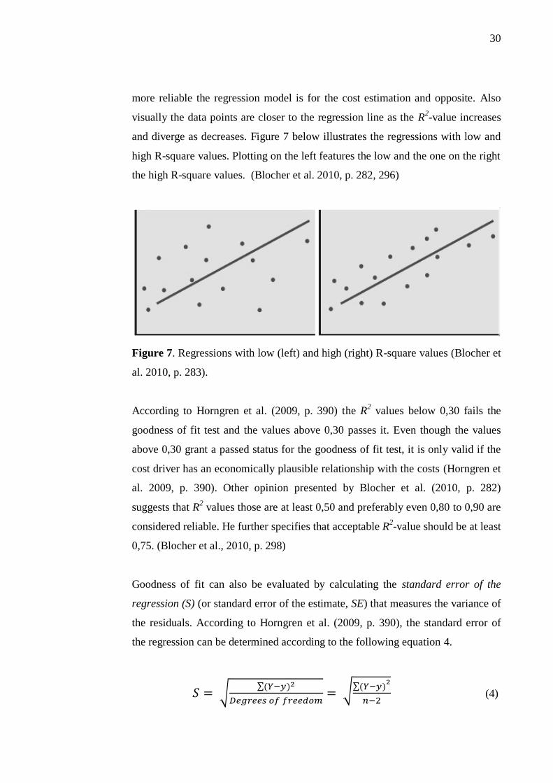
30

more reliable the regression model is for the cost estimation and opposite. Also

visually the data points are closer to the regression line as the R2-value increases

and diverge as decreases. Figure 7 below illustrates the regressions with low and

high R-square values. Plotting on the left features the low and the one on the right

the high R-square values. (Blocher et al. 2010, p. 282, 296)

Figure 7. Regressions with low (left) and high (right) R-square values (Blocher et

al. 2010, p. 283).

According to Horngren et al. (2009, p. 390) the R2 values below 0,30 fails the

goodness of fit test and the values above 0,30 passes it. Even though the values

above 0,30 grant a passed status for the goodness of fit test, it is only valid if the

cost driver has an economically plausible relationship with the costs (Horngren et

al. 2009, p. 390). Other opinion presented by Blocher et al. (2010, p. 282)

suggests that R2 values those are at least 0,50 and preferably even 0,80 to 0,90 are

considered reliable. He further specifies that acceptable R2-value should be at least

0,75. (Blocher et al., 2010, p. 298)

Goodness of fit can also be evaluated by calculating the standard error of the

regression (S) (or standard error of the estimate, SE) that measures the variance of

the residuals. According to Horngren et al. (2009, p. 390), the standard error of

the regression can be determined according to the following equation 4.

(4)

31

Where the degrees of freedom is the number of total observations or data points

minus the number of coefficients estimated in the regression model. The Y and y

have the same meaning as with the determination of the R2, where Y refers to the

actual observation values and y to the predicted ones. The S-value tells how much

on average, the actual and predicted values differ. The standard error is illustrated

in the figure 8 where a plotting with wide (poor) S-value is on the left, and narrow

(good) S-value on the right. The middle line represents the regression line and the

two outliers the approximate line drawn through the data points. The smaller the

S-value is, the better the fit and the predictions for different cost driver values is.

(Horngren et al. 2009, p. 390)

Figure 8. Regressions with wide (poor, left) and narrow (good, right) standard

error values (Blocher et al. 2010, p. 284)

Blocher et al. (2010, p. 295) mentions that the precision and accuracy of the

regression increases as the variance for standard error reduces and as the number

of data points increases because the number of degrees of freedom increases. He

further adds that S-value is indirectly proportional to R2-value. He argues that as

R2 increases the S decreases. In fact, if R

2 equals 1, then S value must equal zero.

Blocher et al. (2010, p. 282, 286)

3.4.3 Significance of Independent Variable

The significance of independent variable criterion evaluates how likely the cost

driver is to be affected by random factors. More specifically, the significance is

32

measured through the standard error of the estimated coefficient (t). The

measurement is conducted by estimating the t-value of slope coefficient, which

measures how large the value of the driver is relative to its standard error. In other

words the t-value equals the ratio of the coefficient of the independent variable to

the standard error of the coefficient for that independent variable. (Horngren et al.

2009, p. 390) The t-value (or t-stat) can be determined by dividing the estimated

coefficient (b) by the standard error or the regression (S) according to equation 5

below (Princeton University 2007).

(5)

According to Blocher et al. (2010, p. 283, 296) the t-value is a measure of

reliability of each cost driver that is, the degree to which a cost driver has a valid,

stable long-term relationship with the dependent variable. A relatively small t-

value speaks for little or non-existent statistical relationship and thereby a cost

driver with low t-value should be removed from the regression. (Blocher et al.

2010, p. 296) A t-value that is around 2,0 or higher at the 5 % significance level is

considered to be acceptable and therefore the variable it is measuring is usable.

Values lower than 2,0 are indicators of low reliability of the coefficient and a

variable with t-value < 2,0 should be removed from the regression analysis in

order to simplify the model and to lead to more accurate cost estimates.

(Allbusiness 2005; Blocher et al. 2010, p. 283, 296; University of Turku 2007, p.

10) Constas (2011, p. 9) points out that if a multiple regression results give a high

R2a value and low t-value, the model is good, but the cost drivers are related.

In those cases of multiple regression models with two or more cost drivers, this

kind of situation signals for multicollinearity, which means that two or more cost

drivers are supposed to be independent of each other, not correlated. Therefore as

one of these variables changes, the other(s) tend to change predictably in the same

or opposite direction. The cost drivers are therefore not independent and

unreliable. (Blocher et al. 2010, p. 283)

33

Another measure of cost driver's reliability is the p-value. It measures the risk that

a cost driver has only a chance relationship to the costs it measures and that there

is no significant statistical relationship between the variables. Salonen (2012) adds

that the p-value is the probability that causes the same results to occur randomly.

For example a p-value of 0,50 refers to 50 % chance that the similar results can be

generated by random. A small p-value, ranging from 0,05 to 0,1 or less indicates

small risk and is often set as a standard guide value. The p-value is also closely

related to t-value and therefore they should be evaluated together. The t-values

over two should have low p-values. (Blocher et al. 2010, p. 284) Generally if t-

value gets a value of 2,0, then the p-value should not be less than 0,05 (5 %). If

not, the model should be refitted as the coefficient may "accidentally" be

significant. (Duke University 2012)

3.4.4 Specification Analysis of Estimation Assumptions

The specification analysis is the testing of the four assumptions of the regression

analysis which include (1) linearity within the relevant range, (2) constant

variance of residuals, (3) independence of residuals, and (4) normality of

residuals. The general idea is to test if all four assumptions hold. If so, then the

regression model gives reliable coefficient values. If the assumptions are not

satisfied, more complex regression procedures are necessary to obtain the best

estimates. (Horngren et al. 2009, p. 391)

The first assumption of linearity within the relevant range is commonly used in

many business applications due to its reasonability. It assumes that there is a

linear relationship between the cost driver and the cost within the relevant range.

The easiest way to test it is to study the data plotted in a scatter diagram. A linear

cost function follows a straight line whereas non-linear cost functions not. An

example of cost behavior in non-linear cost function would be such case when the

level of production increases, but by lesser amounts than would occur with a

linear cost function. (Horngren et al. 2009, p. 391-392)

34

The second assumption that deals with the constant variance of the residuals

measures vertical deviation of the observed value Y from the regression line

estimate y and it is measured with residual term or error term. The basis of the

assumption is that the residual terms are unaffected by the level of the cost driver.

At simplest, in the nonconstant variance, higher outputs have larger residuals.

(Horngren et al. 2009, p. 392-393) In the case of nonconstant variance, the

variance of errors is not constant over the range of independent variable which is

the case when for example the relationship between the costs and the cost driver

becomes less stable over time. If the nonconstant variance occurs, the standard

error of the regression (S) is not uniformly accurate over the over the range of

independent variable. As a solution, the analyst using the regression should

compensate the cost driver data with log or square root. Figure 9 illustrates the

constant and non constant variances, where on the x-axis is the cost driver and the

costs on the y-axis. (Blocher et al. 2010, p. 297)

Figure 9. Plotting of data illustrating constant (left) and nonconstant (right)

variances (Horngren et al. 2009, p. 393).

The independence of residuals assumption assumes that the residual term for any

one observation is not related to the residual term for any other observation. The

nonindependence of errors occurs when the amount and direction of each error

term (residual) is related to those around it. A pattern such where a certain

residual conveys information about other residuals in the observation. The serial

correlation can be observed from the data plotting where the scatter and the

variance of the data points tends to be more non-constant where higher outputs

have larger residuals. Another indicator is also when all data points are below the

35

regression line for the large values of the independent variable. The scatter

illustrating the nonindependence of residuals (serial correlation) is featured in the

figure 10. (Horngren et al. 2009, p. 392-393; Blocher et al. 2010, p. 297)

Figure 10. Plotting describing the independence (left) and nonindependence of

errors (right) (Horngren et al. 2009, p. 394)

Blocher et al. (2010, p. 297) adds that the Durbin-Watson statistic (DW) is a

common measure that can be used to detect the nonindependence of errors (or

serial correlation). He mentions that DW-value falls between zero and 4,0 with 20

or more data points and values between ~1,0 to ~3,0 indicates little chance of

nonlinearity. On the other hand values less than 1,0 or greater than 3,0 indicate the

need for evaluate the data and choose the relevant fixes to compensate for it.

Horngren et al. 2009 (p. 392) further specifies that for a sample of 10 to 20

observations, a DW-value in the 1,10 to 2,90 range indicates that the residuals are

independent. Blocher et al. (2010, p. 299) adds that the nonindependence of errors

can only be applied to the regressions where the past data is used, in other words,

in time-series regression.

The fourth and final assumption deals with the normality of residuals. It means

that the residuals are distributed normally around the regression line. The

assumption is usually satisfied when using real cost information as the dependent

variable or cost object in the regression analysis. Moreover even when the

assumption may not hold, the users of the regression analysis can still generate

accurate cost estimates based on the regression equation. On the other hand, the

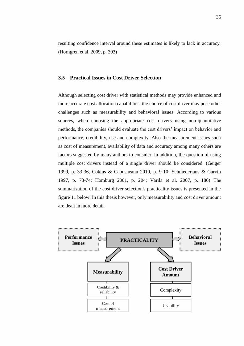
36

resulting confidence interval around these estimates is likely to lack in accuracy.

(Horngren et al. 2009, p. 393)

3.5 Practical Issues in Cost Driver Selection

Although selecting cost driver with statistical methods may provide enhanced and

more accurate cost allocation capabilities, the choice of cost driver may pose other

challenges such as measurability and behavioral issues. According to various

sources, when choosing the appropriate cost drivers using non-quantitative

methods, the companies should evaluate the cost drivers’ impact on behavior and

performance, credibility, use and complexity. Also the measurement issues such

as cost of measurement, availability of data and accuracy among many others are

factors suggested by many authors to consider. In addition, the question of using

multiple cost drivers instead of a single driver should be considered. (Geiger

1999, p. 33-36, Cokins & Câpusneanu 2010, p. 9-10; Schniederjans & Garvin

1997, p. 73-74; Homburg 2001, p. 204; Varila et al. 2007, p. 186) The

summarization of the cost driver selection's practicality issues is presented in the

figure 11 below. In this thesis however, only measurability and cost driver amount

are dealt in more detail.

PRACTICALITY

Measurability Cost Driver

Amount

Credibility &

reliability

Cost of

measurement

Complexity

Usability

Behavioral

Issues

Performance

Issues

37

Figure 11. Practicality issues to consider in the cost driver selection.

3.5.1 Measurability

The measurement viability in cost driver selection is an important aspect to

consider because of the possibility to misstate a cost view that is specified.

Several issues considering the measurement issues of cost drivers’ fitness

including homogeneity, causality and saliency are involved. These include

specific factors like measurement credibility and reliability and the costs of

measurement. (Geiger 1999, p. 33-35)

The driving factor behind the credibility and reliability of measurement lies within

the information and the data itself. Ideally the companies need the data to be

accurate and relevant thus being fast and easy to generate at the same time

(Lahikainen & Paranko 2001, p. 1). Most companies often go overboard with the

data collection ending up gathering excruciatingly detailed information, which

overwhelms both their people and the computer systems they are using (Lyly-

Yrjänäinen et al. 2000, p. 486).

Another issue that comes along especially with the ABC cost drivers and cost

estimates is that the cost drivers assume homogeneity: that the average cost per

unit of cost driver is a credible measurement. This creates a situation where

instead of providing accurate and therefore credible measurement, the cost drivers

reflects the nature of costs behavior based on averages. This creates a situation

where the cost reflection isn’t reasonable and fair for everyone. The practicality

issue that the users of ABC cost drivers must therefore consider is whether the

average is close enough for the purpose of what the cost drivers are used for.

(Geiger 1999, p. 35)

38

One factor that may cause problems to reliability of the data is the possible

distortions or interruptions in the data collection. The data collection flow may be

interrupted by many reasons such as malfunctions in the information systems or

other breaks. This often causes outliers to the data that may weaken the

explanatory power of the model. A way to diminish the corruption of the data is to

either visually or on the basis on indexes eliminate the data points where the

results are unusual. Another solution is to use robust regression methods which

are designed to tolerate diverging observations. (Varila et al. 2004, p. 10)

Horngren et al. (2009, p. 384-385) adds that a problem regarding to the reliability

often arises if the accounting records are not kept on the accrual basis. According

to him, these kind of records present an inaccurate picture of what is actually

taking place. Therefore he suggests that the analysts should use methods of

accrual accounting to better match costs with the cost driver. Varila et al. (2004, p.

2) agrees and adds that when the needed data is available the costs of acquiring

data also decrease which increases the accuracy of the cost accounting.

As the cost drivers themselves must be measurable, the measurement itself comes

with a cost. Different cost drivers have different cost of measurement. A driver

that is highly complex and frequently updated may not be worth to maintain. On

the other hand, a driver that is affordable and readily available may be non-

homogeneous and improperly motivating. As each choice related to possible cost

driver options may distribute cost differently, pose a different measurement

challenge and make different assumptions about behavioral response they all cost

different amounts to measure. Furthermore the amount of available resources

ultimately sets the bar to the complexity and the cost of measurement. (Geiger

1999, p. 32,36)

Geiger (1999, p. 36) sums up that a cost driver that is not credible or is extremely

costly is not a good selection. A credible driver that is easy to measure, but not

managerially useful, or is costly to measure is not fit. Also a cost driver that is

inexpensive, but not useful or credible is not fit. Instead, appropriate cost drivers

39

create a desired and useful motivation through credible measurement that is not

prohibitively expensive. (Geiger 1999, p. 36)

3.5.2 The Amount of Cost Drivers

Schniederjans & Garvin (1997, p. 73-74) proposes that in addition to the

behavioral and measurement issues, companies should evaluate the amount of

used cost drivers. He argues that at least one cost driver and often a set of multiple

cost drivers can be selected.

Cokins & Câpusneanu (2010, p. 10-11) states that usually 3-7 cost drivers is

enough to trace the majority of the total indirect costs. According to them, if too

few drivers are selected, it is likely that some products or services will be over-

costed while the others must be under-costed. If too many are selected, then the

extra amount of effort to collect the necessary driver data may not offset the

informational value from the incremental increase in accuracy of the product cost.

(Cokins & Câpusneanu 2010, p. 10-11)

As a solution, Homburg (2001, p. 198) suggests that instead of reducing the

amount of cost drivers, the use of cost driver combinations reduces the danger of

overweighting the selected cost drivers. He further adds that using only simple

replacement of cost drivers is often an unnecessary restriction which may result in

a high loss of accuracy. Instead, considering all the relevant cost drivers to

allocate the overhead costs is considered as a more reasonable approach. The use

of cost driver combinations will also generally yield better accuracy and cause-

and-effect relationships between the overhead costs of an eliminated cost driver

and its corresponding cost driver volume than driver reduction or replacement

procedures. (Homburg 2001, p. 198)

Homburg (2001, p. 197) further argues that in order to allocate overhead costs

with high accuracy a high number of cost drivers is required. Varila et al. (2007,

40

p. 186) supports this by mentioning that the increasing number of cost drivers can

in most cases lead to more accurate results. On the other hand, they both agree

that a small number of cost drivers are often desirable to achieve acceptable

information cost and to make the activity-based-costing systems easier to

understand. Bokor (2010, p. 14) states however, that grouping of cost drivers will

probably result in worse correlation values than using a single cost driver.

Management must also consider whether the cost measurement provided by a

potential cost driver is both accurate and easy to use. For example when adding

another dimension to cost measurement to provide more accuracy, the cost

allocation might end up being harder to implement. Therefore it may be better to

use limited rather than devoting more resources to develop complex cost

measurements that would increase the measurement costs. (Way 2013) As the

amount of cost drivers’ increase, so do the costs of acquiring the needed

information. It can be said that the selection of proper cost driver amount reflects

a subjective trade-off between accuracy and the cost of measurement. (Varila et

al. 2007, p. 186; Varila et al. 2004, p. 3)

A related usability issue is also the upgradability of the cost drivers and the

frequency of the upgrade process. In ideal situation a cost driver should be

updated in every accounting period. However due to the fact that it usually comes

costly, it is rarely the case. Geiger (1999, p. 36) mentions that when the cost

driver is reasonably stable, the cost drivers for future periods are often taken from

history. The same principal applies to forecasting or prediction of future cost

distributions. (Geiger 1999, p. 36)

41

4 COST DRIVER VALIDATION IN THE WHOLESALER

COMPANY

4.1 Introduction to the Case Company

The case company of this study is a Finnish wholesaler company known as Alpha.

Alpha operates in wholesale business which includes importing and purchasing of

consumer goods to be sold either straight from the manufacturers or other

suppliers and selling them to the end customers.

Alpha has three warehouses (WH) in the region, one of which (WH2) functions as

a central warehouse. From the WH2, the other two warehouses are replenished

from time-to-time. WH1 also does internal replenishment back to WH2 but its

magnitude compared to the WH2’s replenishment is minimal. Each warehouse

WH1, WH2 and WH3 are also physically separated into warehouse and

distribution center sections. From these centers, Alpha delivers thousands of

different kinds of products with product life cycles varying from a few months to

years to hundreds of different customers around the region of Finland. Due to the

fact that Alpha has a wide range of customers and products, it finds it difficult to

value and charge the provided logistical services from the customers and hence

settling the delivery contracts appropriately.

For the improvement of the current system, the logistics process of the company

and the list of relevant resources, activities, cost objects and cost drivers have

been identified and determined. Based on the observations and interviews, the

following process chart (featured in the figure 12) with all the sub-processes

considering the transportation activities has been identified. The highlighted

dashes in the figure represent Alpha’s main supply streams related to customer-

delivery of goods. The dotted lines describe the internal transfers taken place

between Alpha’s warehouses.

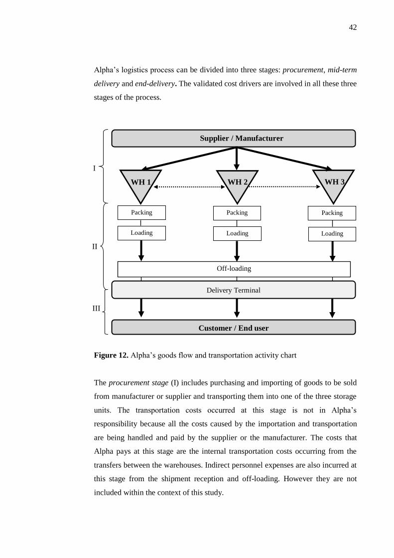
42

Alpha’s logistics process can be divided into three stages: procurement, mid-term

delivery and end-delivery. The validated cost drivers are involved in all these three

stages of the process.

Figure 12. Alpha’s goods flow and transportation activity chart

The procurement stage (I) includes purchasing and importing of goods to be sold

from manufacturer or supplier and transporting them into one of the three storage

units. The transportation costs occurred at this stage is not in Alpha’s

responsibility because all the costs caused by the importation and transportation

are being handled and paid by the supplier or the manufacturer. The costs that

Alpha pays at this stage are the internal transportation costs occurring from the

transfers between the warehouses. Indirect personnel expenses are also incurred at

this stage from the shipment reception and off-loading. However they are not

included within the context of this study.

Loading

Packing

Customer / End user

Supplier / Manufacturer

I

II

III

WH 1 WH 2 WH 3

Delivery Terminal

Off-loading

Packing Packing

Loading Loading

43

The second stage (II) of the delivery process, named as the mid-term delivery

stage consists of packing, loading and transporting the goods to the delivery

terminal owned by the designated logistics service provider (LSP). When the

goods arrive at the terminal, they are off-loaded from their secondary

transportation vehicles, prepared and moved into the primary vehicles those are

responsible for placing the end customer delivery. This marks as the third and last

stage of the process and it is handled completely by the LSPs.

4.1.1 Description of the Used Resource Cost mass

The resource cost masses used in the study are based on a predefined cost mass

determined for the costing model's transportation activity by the models creator

working in the company. The mass is a combination of each warehouses’ actual

transportation costs summed together. The study uses two individual cost masses

first of which consists of the transportation costs accumulated in the mid-term and

end-customer delivery stages and the second from the trans-warehouse

transportation taking place in the procurement stage. The first of the mentioned

cost masses is determined as sales freight cost mass and the latter as internal

freight cost mass.

The sales freight and internal freight costs are the main cost batches associated

with Alpha’s transportation activities. Together they form one of the most

significant cost batches for Alpha, covering around 15 % share of Alpha’s total

annual costs being the second largest cost batch after the 43 % portion of labor

expenses. Of the 15 %, 2 % comes from the internal and 13 % from the sales

freight costs.

The cost data was obtained from Alpha's accounting systems and the collection

was made with an assistance of the employees of the finance department utilizing

the available data mining platforms. The data was gathered for a period of two full

financial years of 2011 and 2012. Instead of using the cost information provided

by the standard cost center reports, the methods of accrual accounting was used as

44

suggested by the literature. Therefore a more reliable and accurate cost data were

able to be obtained. Also the cost index for road transportation of goods provided

by Statistics Finland (2013) was used to further compensate the yearly costs

differences in order to get more reliable measurement. One noticeable factor that

is also that fixed delivery fees are not being included in the cost mass. The idea is

to be able to compare the pure occurred transportation costs against the

corresponding activity as genuinely as possible.

Naturally, a big part of the costs occurred is based on mutual negotiations and

agreements between Alpha and the LSP. In order to understand the factors those

affects the cost-mass and thereby to identify the possible drivers that affects to it,

interviews were conducted with Alpha’s transportation manager. The interviewee

was asked about the factors affecting the transportation costs and the results were

collected to the figure 13 below.

Figure 13. The factors affecting the transportation cost mass

Based on the interviews, the cost of services provided follows the measures that

are often based on the amount, weight or volume of goods transported or the

TRANSPORT COST MASS

Weight

Volume

Item Quality

Quantity of

Deliveries Distance

Delivery Route

Index values

45

quantity of transportation events occurred. Also the location factors such as

distance, route and the location of customer affect the costs. The quality and

characteristics of the products also increases the cost-mass due to the fact, that

some items require different transportation conditions than others. In Alpha’s

case, some of the products also take more space than others which decreases the

overall amount of items that the transportation vehicle can carry thereby

increasing the number of deliveries and further the costs that occur.

Because the cost of service is affected by a variety of factors, some LSPs use a

combinational measure such as volume-weight (m3/kg). Also a costing system

which comprises of standard price per pallet or transportation event plus an

additional weight or volume based fee is commonly used especially with the

LSP’s responsible for internal freights. The distance factor is also taken into

account by setting up different prices for different delivery routes.

Alpha places deliveries daily no matter how full or empty the delivery vehicles

are. The varying fullness of cargo affects the fees slightly. The basic idea is that

case company pays for the whole space. However, the transportation company

uses different coefficients depending on how full the cargo space is. For example,

the standard price for full load is higher than the price for half-full load. On the

other hand the unit cost of products transported increases as the volume of cargo

decreases.

The internal freight costs and their accumulation differ from transportation costs

related to costs of sales freight activity. In the case of internal freight, the elements

behind the cost incurrence are not related to distance or location. Instead, the

variance of internal freight costs is mostly based on the number of pallets

transported. The other cost elements, such as distance related costs and fuel costs

are fixed. The internal freight costs also include an additional cost batch which

consists of special deliveries occurred between WH1 and WH2. During the years

2011-2012 a total of ten special deliveries occurred.

46

4.1.2 Description of the Activities

As mentioned earlier, the activities of this study include two different kinds of

transportation activities, transportation from warehouses to customers and

transportation between the warehouses. Even though both activities accumulates

transportation cost mass, Alpha’s accounting system has two individual accounts

for both activities. As the accounting systems use the term sales freight to describe

the costs accumulated in customer delivery, the activity where the goods are being

transported from Alpha’s warehouses to customers is named as sales freight

activity. On the other hand the transportation activity taking place between

Alpha’s warehouses is named accordingly as internal freight activity.

The sales freight activity consists of stage II and III transportations (see Figure

12) which start with the loading of the transportation vehicles (stage II vehicles)

that handle the mid-term delivery from Alpha’s warehouse to LSPs terminal. At

the terminal, the cargo is being offloaded from the stage II vehicles and moved

into the primary transportation vehicles (stage III vehicles) which are responsible

for the end-delivery to customers. In most cases, the LSPs also use secondary

terminals where the cargo is off-loaded and moved further into secondary

transportation vehicles. This activity and the costs occurred are also included in

the context of this study.

The internal freight activity takes place in stage I of Alpha’s process (see Figure

12). The activity can also be described as a replenishment or internal transfer

activity. The need for the replenishment of warehouses occurs when the stock

levels of the warehouses reaches the point of replenishment. Usually activity

follows the predetermined replenishment schedule according to which the transfer

is conducted. As the need for replenishment occurs, a certain amount of goods are

being transported from the replenishing warehouse to the warehouse that needs

restocking.

47

4.1.3 Estimated Cost Drivers

The cost drivers estimated in the study are selected based on both the opinions and

suggestions of the cost management accountants and through the observations and

interviews conducted with the relevant personnel. The study features four

different kinds of cost drivers that have been used in cases of both activities.

Therefore the total amount of estimated drivers is eight, four of which are related

to sales freight and four to internal freight activity. The context of these cost

driver foursomes are similar, however the difference comes with the different

activity amounts, costs and the activity that they measure. The cost drivers have

been named with the symbol D and using an extension numbering from one to

eight to separate the drivers of each other. The full list of the cost drivers is

presented in the table 1 below.

Table 1. Cost drivers of sales and internal freight activities

Sales Freight (to customers)

Internal Freight (between warehouses)

Symbol Cost driver Symbol Cost driver

D1 Delivery lines D5 Internal delivery lines

D2 Delivery drops D6 Internal delivery drops

D3 Delivery volume D7 Internal delivery volume

D4 Delivery weight D8 Internal delivery weight

Delivery lines cost driver (D1) is a commonly used transactional measure in Alpha

that is set to describe the amount of goods ordered and delivered. At simplest, one

delivery line is one row of one product in the purchase order list. The amount of

the specific product ordered can vary without resulting in a new delivery line.

However if another type of product is ordered, it will automatically result in a

delivery line of its own. In other words, the amount of different products ordered

results usually equals to the same amount of delivery lines.

Alpha follows a FEFO-principal (first expired-first out) in its warehouse

management. Therefore it sometimes leads to a situation where an order of the

48

same product may cause more than one delivery line to occur. The reason behind

those cases is that products are categorized and delivered based on the expiration

date. Therefore if a customer orders a batch of product that comprises of products

whose best-before dates are from separate date categories, will it result in two

separate delivery lines instead of one. A corresponding version for internal

deliveries is the internal delivery lines cost driver (D5) whose meaning is the same

as D1's. The destination of delivery remains as the only distinguishing factor.

The delivery drops (D2) is a cost driver for the delivery activity that takes place in

the mid-term and end-term delivery stages of Alpha’s process (see Figure 12).

The cost driver is a typical transaction cost driver that measures the changes in the

delivery activity registering how many times certain delivery takes place from the

warehouse to the designated customer. In this study, the amount of drops is being

estimated in monthly basis for a total period of two fiscal years.

The cost driver is also partly related to specific route. However, the delivery drops

those are involved in this study consist of the combination of all the Alpha’s sales

freight routes. The D2 cost driver measures the number of drops made from

Alpha’s warehouses to customers within the selected time-range. The similarity

and relation of cost drivers D2 and D1 can be visualized as follows; one delivery

drop can include a multiple amount of delivery lines in it but one delivery line

doesn’t inform anything about the amount of drops.

The D2 driver does not include the drops, thus the transportation activity rate

between the case company’s warehouses since it is determined as other, individual

activity with an own cost driver. The cost driver that represents the internal

transfers between the warehouses is determined as the internal delivery drops cost

driver (D6). The characteristics of the cost driver are otherwise similar to delivery

drops (D2) driver with an exception that D6 measures the number of drops made in

the internal freight routes from one Alpha’s warehouse to another. Since the

replenishment takes only place from WH1 and WH2, the D6 –driver only

measures the drops taking place from the two warehouses.

49

The last four cost drivers measures the volume and weight of the goods

transported. The relevance of both of the cost drivers were pointed out through the

interviews conducted with Alpha’s transportation manager. As it turned out, both

the volume and weight are factors that affect the pricing of the LSPs which

thereby affects the accumulation of the transportation cost mass. In the selection

of the most appropriate cost driver estimating the potential of volume and weight

as the possible driver choices is therefore included in this study.

The delivery volume cost driver (D3) measures the total volume of goods

transported. The measurement unit for the cost driver is a cubic meter (m3) per

delivery and in this study it is set to measure the monthly volume of transported

goods. The volume also takes pallet’s volume into account. The final cost driver

to be estimated is the delivery weight (D4). As it was with the delivery volume

driver, the delivery weight driver measures quantity of goods transported through

kilogram (kg) per delivery. The internal freight versions of the cost drivers follow

the same principals as D3 and D4 driver pairs. The internal delivery volume and

internal delivery weight are described with symbols D7 and D8.

4.2 Background and Purpose of the Study

The roots of this study are in the applied ABC-project carried out in the case

company Alpha whose objective was to develop an updated version of the

customer’s profitability costing model. The impulse to start the project was that

the previous model had become obsolete making its upgrading and maintenance

not worthwhile to continue. Also the need for more accurate and visible costing

system along with the enhanced user-friendliness and minimized error occurrence,

were key reasons for the creation of the new model. Another reason was to create

a costing model that would support a new trend of activity-based pricing which is

the trend that Alpha is moving towards. Ultimately the new model is expected to

prove ground as one of Alpha's main tools for analyzing customers’ profitability.

50

Before bringing the project to the conclusion, one of the most important part of

the model, the cost drivers, are being analyzed. The case company wants to be

certain about their cost drivers’ suitability and especially the ones related to the

transportation. The purpose and the outlines of this study are therefore narrowed

around Alpha's transportation and delivery activity related the eight cost drivers

presented earlier in the table 1. The validation and ultimately the selection are

conducted by using the statistical methods introduced in the literature supported

with the practicality issue evaluation. Based on the results, the most appropriate

cost driver alternative will be selected for both activities. The validation process

along with the different components is featured in the figure 14

Figure 14. Cost driver’s validation process and components

Sales Freight

Delivery lines

Delivery drops

Delivery volume

Delivery weight

Internal Freight

Int. delivery lines

Int. delivery drops

Int. delivery volume

Int. delivery weight

D1 - D4 D5 - D8

Practicality Issues Statistical Analysis

Measurability Simple Regression

Driver Amount Multiple Regression

Validation Results

Top Alternative

D1-D4

Top Alternative

D5-D8

AL

TE

RN

AT

IVE

S

VA

LID

AT

ION

S

EL

EC

TIO

N

1.

2.

Combination models 1-11 (D1-D8)

51

The statistical analysis evaluates the relationship between the cost drivers and the

cost mass through simple linear regression and multiple regression analyses. It

forms the basis for the cost driver validation by estimating the regression models

through the measures and criterions presented in the literature. The models

themselves are created with Microsoft Excel’s regression analysis tool. The data

output sheets can be found in the appendices I to VII at the end of this thesis. The

relevant range for the regressions is set to cover primarily both of the financial

years 2011 and 2012 and the measurement is done in monthly basis resulting in 24

data points in total. However the study features also 23 and 12(11 for some

drivers) data point evaluations.

The practicality issues part acts in a supportive role evaluating the measurability

aspects of the cost drivers. Also the driver amount is evaluated in the case of cost

driver combinations created in the multiple regressions. The measurability can

further be divided into evaluation of cost driver data reliability, credibility and

costs of measurement while the driver amount analyzes the complexity and

usability aspects of the combinations. The criterions linkage to the performance

and behavior is also brought up. The section of practical validation can be found

in the end of combinations approach chapter.

52

5 VALIDATION OF SINGLE COST DRIVER APPROACH

5.1 Cost Drivers of Sales Freight Activity

The first part of the validation with simple regression focuses on Alpha’s sales

freight activity’s cost drivers D1 – D4. The relationship between the sales freight

cost mass and the cost drivers is estimated through the created regression models.

Each driver is estimated based on their reliability and precision. The validations

criterions for the drivers include the following: specification analysis of

estimation assumptions, economic plausibility, goodness-of-fit and the

significance of the independent variable. The economic plausibility, significance

of independent variable and estimation assumption criterions are used to evaluate

the reliability and the goodness of fit criterion to evaluate the drivers' precision

against each other and finding the one with the best cost-driver relationship. The

simple regression results can be found from the appendix I.

Figure 15. Content and criterions of the simple regression approach

The criterions mentioned above are further divided into second tier measures. The

specification assumption evaluates the linearity, constant variance and

RELIABILITY

Linearity within the relevant range

Constant variance of residuals

Independence of residuals (DW)

Normality of residuals

t-value

p-value

Slope coefficient (b)

PRECISION

Adjusted coefficient of determination (R2a)

Standard error of regression (S)

Correlation coefficient (r)

Economic plausibility

Significance of independent variable

Estimation assumptions

Goodness of fit

53

independency and normality of residuals. The independence of residuals is

evaluated with Durbin-Watson statistic (DW). The economic plausibility focuses

and states whether the relationship is plausible. Also the steepness of the slope

through slope coefficient (b) is used to estimate the relationship. The significance

of the independent variable (cost driver) is evaluated through the t-value at 5 %

level of significance. Also in comparison, the p-value is therefore evaluated as it

should reach values < 0,05. The precision evaluation with goodness of fit is

estimated through the adjusted coefficient of determination (R2a) and the standard

error of regression (S) criterions. The acceptable R2a values follow the suggestions

presented in the literature. The full listing of the validation criterions and the

validation content of the simple regression approach is illustrated in the figure 15

above.

5.1.1 Cost driver D1 – Delivery lines

The regression model for delivery lines cost driver (D1) along with the key

statistical figures is featured in the figure 16. The plotting of the data indicates a

positive linear relationship between the sales freight cost mass and the number of

lines. The plot reveals that as the number of lines increases, the sales freight costs

increase by a multiplier of 0,226. At first the slope coefficient (b) value 0,226

indicates the regression line to be seemingly flat. However it should be noted that

the number of lines varies between 1,45 and 1,78 million lines per month which

means that in order to get higher b-values, the sales freight costs should

proportionally also be much higher.

The vertical differences between the sales fright costs and the regression line are

also constant creating a uniform scatter around the line. Therefore the variance of

residuals assumption stands. The independence of residuals and thereby the serial

correlation is measured through the Durbin-Watson statistics (DW). The

calculated DW-value of 1,36 for D1 indicate that the residuals are independent

stating that the independence of residuals assumption is reasonable assumption

for the model. The plotting also confirms the fourth assumption that the residuals

54

are normally distributed around the regression line because the sales freight costs

are based on actual cost data. Based on the plotting and the steepness of the slope,

it is safe to say that the relationship between delivery lines cost driver and sales

freight cost mass is economically plausible.

Figure 16. Regression model for delivery lines cost driver

The t-value for the regression line is 3,07 which means that at the 5 %

significance level there is less than 5 % probability that the delivery lines cost

driver is affected by the random factors. The 3,07 is higher than the acceptable

value of 2,0 at 5 % significance which means that the t-value is significant and the

measurement relationship between the D1 -driver and sales freight cost mass is

considered as reliable. Also the p-value of 0,01 stays below the guide value of

0,05 suggesting that the significance is not accidental. The delivery lines cost

driver thereby passes the significance of the independent variable criterion and

along with the standing assumptions, the cost driver is viable.

The correlation coefficient (r) and the adjusted coefficient of determination (R2a)

get values 0,55 for r and 0,27 for R2a. They both indicate for a moderate positive

correlation on the scale from 0 to 1, where 1 refers to perfect correlation. However

as the acceptable value for R2a is approximately 0,75 (according to Blocher et al.

y = 0,226x + 66 017

R²a = 0,27

0

100 000

200 000

300 000

400 000

500 000

600 000

1 300 000 1 400 000 1 500 000 1 600 000 1 700 000 1 800 000

Sal

es F

reig

ht

cost

mas

s (E

UR

)

Number of lines

Delivery lines (D1)

Data Points

Regression line

r = 0,55

S = 27 044

t-value = 3,07

p-value = 0,01

DW = 1,36

55

2010, p. 298), the delivery lines cost driver do not pass the goodness of fit

criterion. Also based on the Horngren et al. (2009, p. 390) acceptable level of 0,30

for R2, the D1 stays slightly below it. The standard error of regression (S) for the

delivery lines is also 27 044 which means that the variance of data points is on

average 27 044 EUR on the y-axis. This high variance indicates relatively weak

cost prediction capabilities for the D1 driver. An indicator of poor precision is also

the low R2a value as they are with S-value inversely proportional against each

other. The yearly differences between R2a values of 2011 and 2012 are also

similar which shows that no radical changes in accuracy (see appendix I). The S-

value for the year 2011 is 20 541 which is slightly better compared to 27 731 of

2012.

5.1.2 Cost driver D2 – Delivery drops

The regression model for delivery drops cost driver (D2) is presented in the figure

17. The plot shows a positive linear relationship between the number of drops and

sales freight costs. The regression slope coefficient (b) value of 8,85 also speaks

for a positive relationship between the variables. Compared to D1 driver, the

difference seems to be much more significant. However the number of drops is

measured in tens of thousands compared to the millions in the number of lines

which explains the big difference in the coefficient values. The plotting also

confirms that the variance of residuals is constant and the residuals are

independent and normally distributed around the regression line. The

independence of residuals assumption is further confirmed by the DW-value of

2,21 which indicate strong independence between the residuals. All four

assumptions are therefore confirmed.

The t-value for D2 regression coefficient is measured as 10,39 which at the 5 %

significance level is very high indicating that the delivery drops driver is highly

reliable and usable cost driver. Also the p-value is close to zero which indicates a

minimal risk for the residuals being significant by chance. The selection criterion

56

of independent variable's significance is therefore passed and along with the

proved economic plausibility.

Figure 17. Regression model for delivery drops cost driver

The goodness of fit for D2 driver is strong according to the R2a value of 0,82 and

r-value of 0,91 which together with more than twice as small S-value of 13 306

indicate an excellent fit for the D2-driver. The regression line therefore seems to

follow the data points nearly perfectly. Each data point also seem to be near the

regression line with minimal amount of extreme observations which means that

the number of drops explains the changes in sales freight cost mass very precisely.

The R2a passes the goodness of fit limit value of 0,75 and thereby can be accepted

as a possible alternative surpassing the delivery lines driver clearly.

When taking a more detailed look into the yearly correlation values, it can also be

seen that the goodness of fit criterion values are better for the year 2012 than 2011

which speaks for an increasingly positive accuracy trend for the D2 cost driver

with the R2a value 0,92 for 2012 and 0,61 for 2011. The S-values of 9 794 (2012)

and 15 429 (2011) along with other measures can be seen in more detail from the

appendix I.

y = 8,85x + 27 776

R²a = 0,82

0

100 000

200 000

300 000

400 000

500 000

600 000

35 000 40 000 45 000 50 000 55 000

Sal

es F

reig

ht

cost

mas

s (

EU

R)

Number of drops

Delivery drops (D2)

Data Points

Regression line

r = 0,91

S = 13 307

t-value = 10,39

p-value = 0,00

DW = 2,21

57

5.1.3 Cost driver D3 – Delivery volume

The third cost driver alternative, the delivery volume (D3) is featured in the model

presented in figure 18. Compared against the previously presented model of D2-

driver, the data points vary more in this case. Especially, the plotting is not as

linear and progressive which can be seen as an increased variance between the

data points. The regression slope coefficient (b) value of 0,038 also verifies the

weaker relationship between the driver and the cost mass. It can be stated though

that as the volume of goods delivered increases so does the sales freight cost

mass, however not by a great margin. As it was with the D1 cost driver, the small

b-value can by its half be explained by the quantity of the cost driver which in the

case of delivery volume is measured in millions.

The assumption regarding constant variance holds. However there are few data

points those are slightly outside the uniform scatter. The Durbin-Watson statistic

value of 1,61 is within the 1,10-2,90 range indicating that the residuals are

independent confirming the independency assumption. As the data is based on

actual data, the normality assumption also holds. The t-value of delivery volume

cost driver regression is 3,87 which is higher than the minimum acceptable value

of 2,0 indicating reliable long term relationship between the variables.

Furthermore the p-value of 0,0008 is well within the suggested values. Therefore

the significance criterion along with the economic plausibility hold but not as

clearly as with the delivery drops or even delivery lines cost drivers.

On the other hand, based on the R2a-value of 0,38 and r-value of 0,64, the

goodness of fit for delivery volume cost driver ranks higher than D1-driver’s.

However the as stated earlier, the variance of some of the data points is greater

than with drivers D1 and D2. The observations is also supported by the S-value,

which in delivery volume’s case is 24 938 EUR. Based on the R2a and r values,

R2a does not reach high enough values in order to pass the goodness of fit

criterion. The R2a value however on the scale, where 0,30 is the limit, passes the

58

test and thereby can be recognized as an economically plausible alternative even

though the goodness of fit is moderate compared to D2 driver.

Figure 18. Regression model for delivery volume cost driver

The yearly differences between 2012 and 2011 are more visible with the delivery

volume than with the previous two alternatives. Compared to D2 driver, the

correlation with the cost mass is better with the year 2011 cost data than 2012 by

almost a half. The R2a for 2011 is 0,49 whereas for 2012 it is only 0,17. Also the

S-values 17 596 (2011) and 30 976 (2012) speaks for significantly greater

variance between the periods. The weakening trend in correlation capabilities

questions the reliability and use of the D3 as the possible alternative.

5.1.4 Cost driver D4 – Delivery weight

The last of the sales freight cost drivers is the delivery weight cost driver (D4).

The plotting and the key figures presented in the figure 19 indicate that delivery

weight and sales freight costs have a positive, yet weak linear relationship. The b-

value gets similar value than delivery lines cost driver with 0,183 as the weight of

delivered goods is measured in millions. It should be noted though, that as the

original plotting of 24 data points included one extreme observation, the model

y = 0,038x + 129 898

R²a = 0,38

0

100 000

200 000

300 000

400 000

500 000

600 000

6 000 000 7 000 000 8 000 000 9 000 000 10 000 000

Sal

es F

reig

ht

cost

mas

s (E

UR

)

Volume of goods delivered (m3)

Delivery volume (D3)

Data Points

Regression line

r = 0,64

S = 24 938

t-value = 3,87

p-value = 0,0008

DW = 1,61

59

presented in figure 19 was modified to include only 23 data points. The

assumptions regarding to constant variance therefore holds as the one extreme

observation has been removed from the model. However there are still two data

points those are slightly outside the uniform scatter. The Durbin-Watson statistic

1,85 means that serial correlation is minimal and the residuals are therefore

independent. As all the assumptions hold and the positive relationship exists, the

delivery weight is economically plausible.

The t-value for delivery weight cost driver is 3,08 which is higher than two and

therefore within acceptable range when it comes to measurement reliability.

Compared to other driver alternatives, the D4 driver's t-value gets similar results

than the D1 driver still passing the significance of independent variable criterion.

As the p-value is 0,01 that is well within the acceptable range, the delivery weight

can therefore be stated as a reliable alternative.

Figure 19. Regression model for delivery weight cost driver

The D4 cost driver gets moderate goodness of fit ratings according to the

correlation coefficient (r) and R2a-values. The R

2a and r-values are almost in line

with the delivery lines cost driver with the values of 0,28 for R2a and 0,56 for r. In

y = 0,183x + 180 825

R²a = 0,28

0

100 000

200 000

300 000

400 000

500 000

600 000

1 000 000 1 200 000 1 400 000 1 600 000 1 800 000

Sal

es F

reig

ht

cost

mas

s (E

UR

)

Weight of goods delivered (kg)

Delivery weight (D4)

Data points

Regression line

r = 0,56

S = 25 195

t-value = 3,08

p-value = 0,01

DW = 1,85

60

addition, the overall data point variance is slightly smaller with S-value of 25 195

EUR. The cost driver passes the goodness of fit test with poor cost prediction

capabilities as R2a-value remains under the suggested limit values of 0,75 and

0,30. Also the yearly differences indicate that the correlation is almost nonexistent

especially when looking into the year 2012 with R2a value of -0,05 and S-value of

34 836 EUR. Compared to other sales freight cost drivers the delivery weight

ranks third, even with the 23 data points which should act as an increase of

precision, only trailing by delivery lines with slightly weaker results.

5.2 Cost Drivers of Internal Freight Activity

The second part of the simple regression approach deals with the cost drivers

related to the internal freight activity. The cost drivers presented in this section

include cost drivers from D5 to D8. As it was the case with sales freight activity,

the characteristics of the cost drivers are similar with internal freight activity as

well. Also the selection criterions remain the same. The difference compared to

sales freight cost drivers’ validation is that the used cost mass comprises of

internal freight costs instead of sales freight costs and the drivers’ measure the

changes in the internal freight activity.

5.2.1 Cost driver D5 – Internal delivery lines

The regression model for the internal delivery lines cost driver (D5) is presented

in the figure 20. The plotting of the data and the slope coefficient b value of 2,63

indicate that the relationship between the cost driver (D5) and the cost mass is

positive and linearly increasing with the multiplier of 2,63 as the number of lines

increases. Even though the pattern seems to increase linearly, the variance of

residuals is high being closer to non-constant than constant. Although the variance

does not affect the precision of the measurement, it reveals that the data behind it

may be unreliable.

61

The independence of residuals measured with the Durbin-Watson statistic gets a

value 1,48 which with the sample of 24 data points indicate that the residuals are

independent and the assumption of independence is reasonable for the estimated

residuals for this model. The residuals are also normally distributed around the

regression line which makes the normality assumption stand. As the relationship

with the D5 driver and the cost mass is positive and all the assumptions hold, the

driver is economically plausible and therefore a viable alternative.

The t-value 4,51 of the regression line also indicate that the cost driver is reliable

and thereby the relationship between D5 driver and internal freight costs is reliable

in a long term. As it clearly surpasses the acceptable value of 2,0, the significance

criterion also holds. The p-value is 0,0002 is also acceptable thereby confirming

the significance criterion.

Figure 20. Regression model for internal delivery lines cost driver

Based on the adjusted coefficient of determination (R2a) and the correlation

coefficient values (r) of 0,46 and 0,69, and the standard error (S) value of 4 654

EUR, the internal delivery lines seem to predict the changes in the internal freight

costs well. However as the internal freight costs are measured in tens of

thousands, the S-value of 4 654 indicate that the variance is on average quite high

y = 2,63x + 4371,2

R²a = 0,46

0

10 000

20 000

30 000

40 000

50 000

60 000

70 000

10 000 12 000 14 000 16 000 18 000 20 000 22 000

Inte

rnal

fre

ight

cost

mas

s (E

UR

)

Number of lines

Internal delivery lines (D5)

Data points

Regression line

r = 0,69

S = 4 654

t-value = 4,51

p-value = 0,0002

DW = 1,48

62

thereby questioning the accuracy of the driver. Also even though the r-value

indicates that a certain degree of positive correlation exists between variables, the

R2a-value does not reach the value high enough in order to surpass the 0,75 mark.

It passes the 0,30 marking however meaning that the goodness of fit criterion is

passed with moderate grades. Having said that, there definitely is a connection

between internal delivery lines and the internal freight costs but using it alone as a

cost allocator doesn’t provide reliable measurement.

When the relevant range is split into two separate 12 month periods, the results

reveal that the correlation capabilities are much better with the year 2011 than

2012. The R2a value for year 2011 is 0,87 and for 2012 only 0,40. Also the other

values such as standard error S advocates that the trend of accurate cost prediction

is much weaker in 2012 with S-value of 4 810 compared to 2 188 of 2011. Even

though the data covers only 12 data points, the results still raises a question

whether the internal delivery lines is an appropriate measure of internal freight

costs for Alpha as the trend is towards poorer reliability and precision.

5.2.2 Cost driver D6 – Internal delivery drops

The internal delivery drops (D6) regression model is presented in the figure 21.

Based on the plotting, the variance between the cost driver and the cost mass is

non-constant and uniform data point pattern is hard to define. Also the linearity of

the regression is questionable based on the plotting. The slope coefficient (b) of

the regression line is 67,9 which indicate that each drop made increases the costs

by a multiplier of that amount. However the high b-value compared to D5 driver

can be explained by the fact that the number of drops is measured in hundreds

whereas the delivery lines, weight and volume are measured in tens of thousands.

The independence assumption is passed with the DW value of 1,88 which indicate

that the residuals are independent. The residuals are also normal as the cost mass

consists of the actual cost data. The t-value for D6 driver is 2,82 and the p-value

0,01 both pass the significance criterion thereby proving that the internal delivery

63

drops is a reliable cost driver alternative. Based on the slope coefficient, the

relationship between the variables is still positively correlated and therefore along

with the fact that as the number of drops increases, so does the costs, the

relationship is economically plausible.

The internal delivery drops get 0,23 for R2a-value and 0,51 for r-value which tells

that the D6-driver’s goodness of fit is poor. Also the R2a stays below the 0,30 mark

which would indicate that the driver does not pass the goodness of fit criterion.

The standard error value of 5 537 EUR and the extreme observations suggests that

D6 is also poorer alternative than D5 to measure the changes of internal freight

costs. The outlier value (x,y) (341, 49 506) is not deleted since during the period,

the deliveries included a lot of half full deliveries between the warehouses. The

data itself was recorded correctly.

The results from the 12 data points’ validation also question the D6's suitability.

The correlation coefficients r for years 2011 and 2012 are 0,43 and 0,22 which

indicate positive correlation between the driver and cost mass. However at the

same time the R2a values are 0,10 and -0,05 which indicate that the relationship

between the internal delivery drops and internal freight costs is almost nonexistant

even compared to the D5. Also the 12 month inspection (appendix I) questions the

driver's economic plausibility. However the S-values of 5 517 (2012) and 5 407

(2011) are not significantly different. Thereby the precision trend stays seemingly

normal between the years.

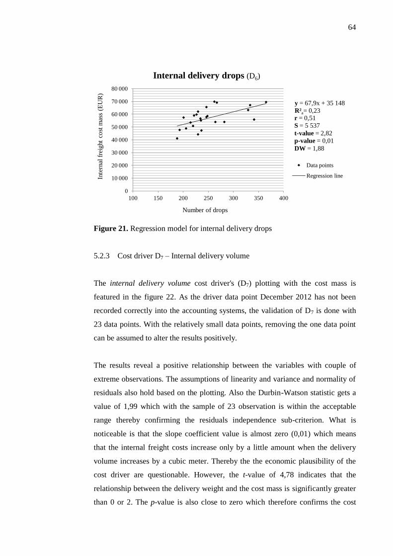
64

Figure 21. Regression model for internal delivery drops

5.2.3 Cost driver D7 – Internal delivery volume

The internal delivery volume cost driver's (D7) plotting with the cost mass is

featured in the figure 22. As the driver data point December 2012 has not been

recorded correctly into the accounting systems, the validation of D7 is done with

23 data points. With the relatively small data points, removing the one data point

can be assumed to alter the results positively.

The results reveal a positive relationship between the variables with couple of

extreme observations. The assumptions of linearity and variance and normality of

residuals also hold based on the plotting. Also the Durbin-Watson statistic gets a

value of 1,99 which with the sample of 23 observation is within the acceptable

range thereby confirming the residuals independence sub-criterion. What is

noticeable is that the slope coefficient value is almost zero (0,01) which means

that the internal freight costs increase only by a little amount when the delivery

volume increases by a cubic meter. Thereby the the economic plausibility of the

cost driver are questionable. However, the t-value of 4,78 indicates that the

relationship between the delivery weight and the cost mass is significantly greater

than 0 or 2. The p-value is also close to zero which therefore confirms the cost

y = 67,9x + 35 148

R²a= 0,23

0

10 000

20 000

30 000

40 000

50 000

60 000

70 000

80 000

100 150 200 250 300 350 400

Inte

rnal

fre

ight

cost

mas

s (E

UR

)

Number of drops

Internal delivery drops (D6)

Data points

Regression line

r = 0,51

S = 5 537

t-value = 2,82

p-value = 0,01

DW = 1,88

65

driver's reliability. The contrast between the slope coefficient and t-value can

further be explained by the fact that internal freight costs are measured in tens of

thousands compared to delivery volume which is measured in millions cubic

meters. The D7 is thereby proven to be economically plausible and reliable.

Figure 22. Regression model for internal delivery volume

The delivery volume ranks reasonable well in the goodness of fit category

compared to the two previous cost drivers with the R2a value of 0,50, r-value of

0,72 and standard error (S) of 4 572 EUR. The coefficient value R2a doesn't reach

the suggested acceptable value of 0,75, but the 0,50 still indicate for a moderate

goodness of fit thereby passing the criterion. Also the 4 572 EUR S-value

confirms that the data points are relatively close to the regression line compared to

the previous two cost drivers. As mentioned earlier however, the missing data

point alters the regression values positively. If all the 24 data points would be

used, the precision values would be slightly worse.

The yearly difference in the correlation is as significant with the D7 driver as it

was with the D5. For the year 2011 the r value 0,91 advocate nearly perfect

positive correlation between the variables whereas the value 0,51 for 2012 speaks

y = 0,01x + 32 223

R²a = 0,50

0

10 000

20 000

30 000

40 000

50 000

60 000

70 000

80 000

0 1 000 000 2 000 000 3 000 000 4 000 000 5 000 000

Inte

rnal

fre

ight

cost

mas

s (E

UR

)

Volume of goods delivered (m3)

Internal delivery volume (D7)

Data points

Regression line

r = 0,72

S = 4 572

t-value = 4,78

p-value = 0,00001

DW = 1,99

66

for a moderate or poor correlation. Even though the goodness of fit for the 23 data

point period indicate excellent fit, the 12 data point evaluation suggests the same

weakening trend in measurement precision with S-values 2 443 EUR (2011) and 4

871 EUR (2012) as in D5's case.

5.2.4 Cost driver D8 – Internal delivery weight

The last of the validated cost drivers is the internal delivery weight (D8). The

regression model along with the key figures is featured in the Figure 23. As it was

the case with D7, the regression model for D8 also includes only 23 data points

because the data for the 24th data point has not been recorded correctly into the

accounting systems thereby distorting the results greatly.

The plotting of the data and the regression slope coefficient b show that the

relationship between the delivery weight and internal freight cost mass is positive,

linear and increasing the internal freight costs by a multiplier of 0,03 as the weight

of the goods increases. The variance of residuals is also constant and normally

diverged around the regression line. The DW value of 2,00 suggests that the

residuals are independent which confirms the validity of the D8 driver.

The significance of independent variable criterion for delivery weight cost driver

is also passed with the t-value of 5,34 and the acceptable p-value of 0,00002 It

should be noted though, that the decreased number of data points affects the t-

value also as the regression slope coefficient (b) value is higher. Compared to

other t-values of the internal freight cost drivers, the D8 driver surpasses the

second highest value of 4,78 of the cost driver D7. As the relationship is positive

and increases linearly while all the assumptions along with the significance

criterion hold, D8-driver is therefore economically plausible and can be compared

equally against the other alternatives.

67

Figure 23. Regression model for the internal delivery weight

The adjusted coefficient of determination (R2a) value 0,56 and correlation

coefficient r value of 0,75 indicates that around two thirds of the variance in the

internal freight cost mass can be explained by the changes in the internal delivery

weight. Also the standard error (S) value 4 304 EUR being more than 150 EUR

lower than the next best cost driver (D7) describing the internal freight activity

indicate that internal delivery weight has an excellent goodness of fit. The r-value

of 0,75 ranks high in the correlation scale from 0 to 1 and the R2a also gets

significantly better results than with the other internal cost driver alternatives.

The same trend where the correlation capabilities weaken from 2011 to 2012 is

also the case with the D8 cost driver (appendix I). The difference compared to

other internal freight drivers is narrower but the R2a values of 0,75 (2011) and

0,35 (2012) along with other measures shows that the cost measurement

capabilities for the D8 is inferior in 2012 than 2011. The S-value for 2011 is 3 101

EUR and 4 419 EUR of 2012.

y = 0,03x + 27 138

R²a = 0,56

0

10 000

20 000

30 000

40 000

50 000

60 000

70 000

80 000

0 500 000 1 000 000 1 500 000

Inte

rnal

fre

ight

cost

mas

s (E

UR

)

Weight of goods delivered (kg)

Internal delivery weight (D8)

Data points

Regression line

r = 0,75

S = 4 304

t-value = 5,34

p-value = 0,00002

DW = 2,00

68

6 VALIDATION OF COMBINATIONS APPROACH

6.1 Combinations of Sales Freight Cost drivers

The simple regression results presented earlier shows that all of the estimated cost

drivers have certain degree of correlation with the dependent variable. Even

though some drivers qualify better than the others, each alternative is still

economically plausible as an individual and thereby a possibility for Alpha to

select from. Therefore accepting only one and rejecting the others may be harmful

for the accuracy and overall performance of cost allocation.

This section includes multiple regression analysis in which all of the validated

sales freight cost drivers from the previous single driver approach will be

estimated. The purpose is to reveal if the use of cost driver combinations can

provide more accurate cost prediction capabilities compared to the single use of

cost drivers without compromising the reliability and practicality aspects at the

same time. More specifically the criterions include the adjusted R-square (R2a)

and standard error of the regression (S). Also the t-value is used to evaluate the

combinations reliability of use. In addition, the practicality issues of combinations

and also their comparison to single cost driver approach is investigated.

Figure 24. Comparison process chart and components for the combinations

PRECISION

Adjusted coefficient of determination (R2a)

Standard error of regression (S)

Significance of cost drivers (t-value)

MODELS

1-11

PRACTICALITY

RESULTS

69

The comparison process along with the different components that will be used in

both cases of sales freight and internal freight combinations is presented in the

figure 24. The models 1-11 comprises of three set of model categories based on

the number of variables in the models. The grouping of first six models estimates

the regressions of the cost driver pairs. After that the number of variables is

increased to three and further to four cost drivers. The total amount of different

regression models is thereby 11. The estimated cost driver combinations along

with their unit markings are presented in more detail in the table 2 below and the

multiple regression results in appendices II to IV.

Table 2. Cost driver combinations in the multiple regression models

Model No. of

Variables Units Cost Drivers in Model

1 2 D1,D2 D. lines & Drops

2 2 D2,D3 Drops & Volume

3 2 D3,D4 Volume & Weight

4 2 D4,D1 Weight & D. lines

5 2 D3,D1 Volume & D. lines

6 2 D2,D4 Drops & Weight

7 3 D1,D2,D3 D. lines, Drops & Volume

8 3 D2,D3,D4 Drops, Volume & Weight

9 3 D3,D4,D1 Volume, Weight & D. lines

10 3 D2,D4,D1 Drops, Weight & D. lines

11 4 D1,D2,D3,D4 D. lines, Drops, Volume & Weight

6.1.1 Sales Freight Combination Models 1-6

The multiple regression models from 1 to 6 comprises of cost driver combinations

those include two cost drivers each. The models along with the regression

statistics measures and values can be found in the Appendix II.

The combination approach yield generally higher R-square values compared to

the single use of cost driver. The R2a value of 0,83 for model 1 surpasses the

highest simple regression value of 0,82. Also the standard error of the regression

(S) decreases slightly down to 13 108 from the lowest simple regression

counterpart’s 13 306 indicating slightly less variance between the variables. For

the model 2, the results also indicate excellent goodness of fit with the R2a value

70

of 0,82 that matches the highest value of the simple regression approach results.

The S-value of 13 564 EUR also supports the observation.

For models 3 and 4, the R2

a values are still better on-average than the drivers

alone, however not as greatly as with the first two models. The R2a value of 0,59

for model 3 and 0,26 for model 4 still speaks for a moderate goodness of fit.

However the variance of residuals (S) almost doubles compared to models 1 and 2

reaching the values of 20 351 (model 3) and 27 243 (model 4). The last two cost

driver pairs in models 5 and 6 feature R2a values of 0,35 and 0,82 and S-values of

25 482 EUR and 13 317 EUR.

Based on the results, the best goodness of fit of the first six models is with models

1, 2 and 6. When taking a more detailed look into the pairings, it can be seen that

each of the three models reaching the highest values of measures include the

delivery drops cost driver (D2). On the other hand, the models with the poorest

goodness of fit (models 4 and 5) both include delivery lines cost driver (D1). The

rest of the pairings including delivery weight and volume seem only to have a

moderate impact on the R-square and S-values. However the coefficient values for

delivery volume surpasses the delivery weight’s values slightly indicating better

correlation with the sales freight cost-mass. The yearly differences with the two-

variable combinations also show that the measurement precision is better in 2012

than in 2011 which give a positive insight for future measurement accuracy.

The t-values for the models show that only for cost driver D2 the values are

positive in every model it appears. On the other hand, the other drivers get

negative values in every other model except for model 5. This also questions the

reliability of the other cost drivers’ use in the two-variable combinations as the

drivers D3 and D1 get t-values of 1,94 and 0,27 which means that D3 passes the

criterion and D1 not.

71

6.1.2 Sales Freight Combination Models 7-10

The multiple regression models including three variables are featured in models

from 7 to 10 (see appendix III). The R2a values for the models varies between 0,57

(model 9) and 0,82 (model 7) and the standard error between 20 854 (model 9)

and 13 343 (model 7). The goodness of fit therefore reaches on average slightly

better results when using the three-variable combinations compared to single cost

drivers or pairings. The results shows again that the combinations 7, 8 and 10,

those gets the highest R2a and S-values, each include the delivery drops cost driver

whereas the model 9 including everything but the delivery drops driver gets the

worst values.

When taking a more detailed look into the coefficients of each cost driver in the

multiple regression equations, it can be seen that delivery drops has also the

highest and the most significant t-values in each model compared to the others as

it was the case with two-variable combinations. On the other hand, the delivery

lines and delivery weight has slightly negative t-values in each model it appears.

Therefore it can be assumed that in case of the three-variable combinations, the

delivery drops (D2) acts as the main factor that drives the costs and the lines (D1)

and weight (D4) with the low t-values indicate multicollinearity which means that

the D1 and D4 are not correlated or independent and therefore not reliable

measures in the combination.

6.1.3 Sales Freight Combination Model 11

The last multiple regression model includes the combination of all four cost driver

alternatives (appendix IV). The model gets the best goodness of fit capabilities of

all the combinations reaching R2a value of 0,82 and S-value of 13 251 EUR.

However the difference compared to two or three-variable combinations is not

that significant. In fact, the difference between the model 11 and the next best

model is only 0,01 (R2a) and 144 EUR (S). Once again, the main driver behind the

good correlation capabilities is the delivery drops cost driver where as the other

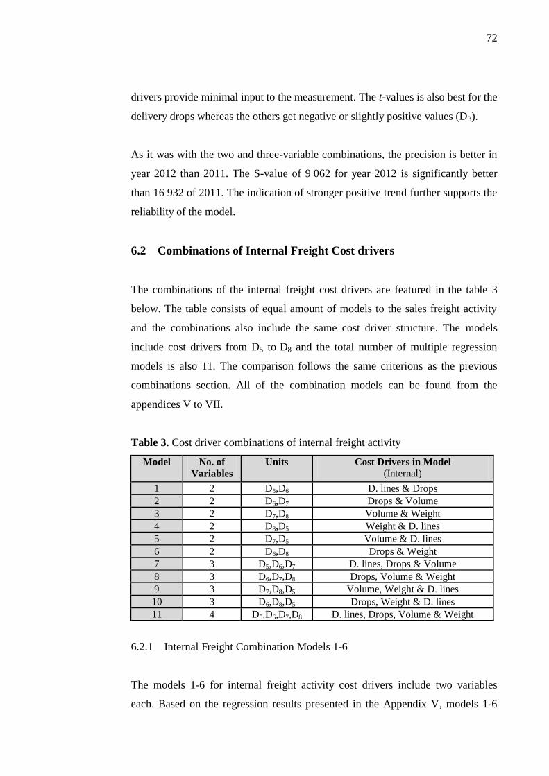
72

drivers provide minimal input to the measurement. The t-values is also best for the

delivery drops whereas the others get negative or slightly positive values (D3).

As it was with the two and three-variable combinations, the precision is better in

year 2012 than 2011. The S-value of 9 062 for year 2012 is significantly better

than 16 932 of 2011. The indication of stronger positive trend further supports the

reliability of the model.

6.2 Combinations of Internal Freight Cost drivers

The combinations of the internal freight cost drivers are featured in the table 3

below. The table consists of equal amount of models to the sales freight activity

and the combinations also include the same cost driver structure. The models

include cost drivers from D5 to D8 and the total number of multiple regression

models is also 11. The comparison follows the same criterions as the previous

combinations section. All of the combination models can be found from the

appendices V to VII.

Table 3. Cost driver combinations of internal freight activity

Model No. of

Variables

Units Cost Drivers in Model

(Internal)

1 2 D5,D6 D. lines & Drops

2 2 D6,D7 Drops & Volume

3 2 D7,D8 Volume & Weight

4 2 D8,D5 Weight & D. lines

5 2 D7,D5 Volume & D. lines

6 2 D6,D8 Drops & Weight

7 3 D5,D6,D7 D. lines, Drops & Volume

8 3 D6,D7,D8 Drops, Volume & Weight

9 3 D7,D8,D5 Volume, Weight & D. lines

10 3 D6,D8,D5 Drops, Weight & D. lines

11 4 D5,D6,D7,D8 D. lines, Drops, Volume & Weight

6.2.1 Internal Freight Combination Models 1-6

The models 1-6 for internal freight activity cost drivers include two variables

each. Based on the regression results presented in the Appendix V, models 1-6

73

provide increased goodness of fit capabilities in terms of on-average better R2a

and S-values compared to the simple regression approach.

The results show that best cost-combination relationship can be achieved with the

model 1 with the (R2a) value of 0,58 and standard error (S) value of 5 433 EUR.

The worst correlation is with model 5 with R2a-value 0,45 and S-value of 6 153

EUR. The rest of the models can be designated between these two models. The

values still don’t indicate improved or excellent goodness of fit compared to the

simple regression results as the R2a won’t surpass the 0,67 value of internal

delivery weight cost driver.

Unlike it was the case with the combinations of sales freight cost drivers, a

general pattern that would designate a single cost driver that would determine the

ranking by itself is harder to define with the internal freight cost drivers. What is

noticeable is that the t-values of the models 1-6 gets negative or significantly low

only with model 3. The model 1 with the best precision values also gets high t-

values which speak for independence of cost drivers and therefore reliable

measurement of the combinations. However, when looking the combinations in

more detail the general trend in yearly differences in precision goes to the

opposite way than with the sales freight combinations.

6.2.2 Internal Freight Combination Models 7-10

The three-variable regression models 7-10 provide similar results in terms of

measurement precision when compared against the models including two cost

drivers. The models are featured in the appendix VI. The R2a -values ranges from

0,56 to 0,58 and standard errors (S) between 5 500-5 600 EUR. Model 8 gets the

lowest R2a value (0,56) while others get equally high (0,58). Again, the coefficient

for D6 gets the highest t-values followed by D5 while D7 and D8 get the lowest.

Therefore increasing the cost drivers in the combinations from two to three does

not seem provide significantly better results in terms of cost allocation

74

capabilities. Also the t-values for D7 gets significantly weaker results compared to

the R2a which questions its reliability and usefulness in the combinations.

The difference between years 2011 and 2012 is also as drastic with models 7 to 10

as it was with the two-variable combinations. Especially with models 7, 9 and 10

the yearly differences in standard error values are more than two times greater

indicating significantly poorer precision for year 2012 compared to 2011.

6.2.3 Internal Freight Combination Model 11

For the last combination including all four cost drivers, the goodness of fit gets

also similar results than the previous models (see appendix VII). The model 11

gets the R2a value of 0,59 which improves only by 0,01 when adding the fourth

variable into the combination. The standard error also remains nearly unchanged

with the value of 5 605 EUR. As it has been the case with the previous models,

the cost driver D5 seems to be the two main drivers in the regression equation

while D7 and D8 only have a moderate impact on the combination-cost

relationship.

What is also noticeable with the model 11 as well as the other combinations is that

if the relevant range is divided into two separate 12 month parts, the first part

covering the fiscal year 2011 gets significantly better results in terms of goodness

of fit and thereby the cost allocation capabilities. In fact, the R2 for model 11

indicates nearly perfect correlation with value of 0,94 and standard error (S) of

2 023 EUR for the year 2011. However, the latter period covering the year 2012

gets the opposite, yet still better results than the full 24 month period with R2 of

0,61 and S-value of 4 758 EUR. The same goes for the combinations of two and

three cost drivers.

75

6.3 The Practicality Issues in Case Company’s Cost Driver Selection

As the amount of variables increases so does the complexity and the costs of

measurement. For Alpha, the use of cost driver combinations increases the

amount of variables in the regression equations making the measurement more

complex and also increasing the time and effort in order to acquire the necessary

data. It will also make the maintenance and updating more time consuming and

further more costly. For example in four-driver combinations’ case, Alpha would

need to collect four times more driver data compared to use of single cost driver.

In Alpha’s case, all the driver data is not directly obtainable from the information

systems. Instead, it has to be manually refined into a usable form by the user. Also

currently the user of the costing model is not the same person who’s generating

the data. Instead, IT-department or another specialist must be asked to run the

reports. The data for delivery lines (D1), volume (D3) and weight (D4) especially

are more easily obtainable than the data for delivery drops (D2). However filtering

and refining the data is still required with all the cost drivers in order to get

reliable data.

According to various interviews, the reliability of the data and therefore the cost

drivers primarily depends on the user itself. In order to get reliable results, the

user must know exactly what kind of driver data he wants and to what kind of

purposes he wants it to use for. Therefore if the user of the model does not know

exactly what he wants, the generated data may be incorrect and thereby unreliable.

This can cause issues especially when updating the cost drivers or in cases if the

employee responsible for the driver’s updating gets reassigned.

Also in cases when totally new kinds of data are needed, the workload to get it

naturally is much greater. On the other hand if the data for the new driver already

exists, then it is just a matter of searching it from the systems and refining it to

desirable form. The interviewees also states that the most time consuming and

therefore most costly are situations where the user of the model and the data

76

generator are both having difficulties understanding what kind of new information

is needed. In those cases, meetings and clearances must be conducted which takes

time and costs.

The increased amount of data required also increases the error occurrence which

further affects the reliability of measurement. For the combinations featured in

this study, the required data needs to be at least two times greater than with the

use of single cost drivers. Therefore the chance of error occurrence increases in

same proportion which decreases the overall measurement reliability. On the

opposite, the use of a single cost driver reacts more sensitively to the

measurement and data collection errors. Especially with the relevant range of only

24 months, even one missing month of data can alter the results significantly as

evaluated with the D4, D7 and D8 drivers in earlier regression analysis chapters.

A big issue regarding to the selection between the combination and single cost

driver are the resources. In order to use to cost driver combinations, Alpha should

use more advanced information systems and programs to run and update the cost

drivers. Currently as the models and thereby the cost drivers are run on an Excel-

based platform, the resource consumption would increase if combinations were

selected. The use of single cost driver is manageable with the current platform,

but if using the combinations, a more enhanced system should be used.

Another issue of the use of combinations compared to single use is the

understandability. For example the use of combinations such as models 11 makes

them also more difficult to understand especially if used manually. Thereby in

order to enhance the understandability, the combination could be set to have a

mutual name consisting of the names of the cost drivers of the combination. For

combinations with two drivers the names could be for example drop-weight

(model 6) or volume-weight (model 3) which would be understandable. However

as the amount of variables increases, the naming, thus the understandability gets

difficult. This may distract the management and other decision makers when the

purpose or content of combinations may not be clear.

77

The combinations also average the measurement where some cost drivers increase

while others decrease the measurement accuracy. This can be seen for example

with sales freight combination models 7-10 where clearly the delivery drops cost

driver provides the most reliable and accurate measurement out of the two other

drivers. On the other hand, the delivery weight and volume acts the opposite. This

averaging decreases the overall accuracy of the model. For Alpha’s case when the

purpose of the model is to provide more accurate cost measurement, the model’s

reflection of costs may not be accurate enough. The results also indicate that the

overall accuracy of the combinations is not significantly better than with the best

single cost driver alternative.

78

7 RESULTS AND CONCLUSIONS OF THE STUDY

7.1 Validation Results

The table 4 features the summarized validation results of the simple regression

approach. The results reveal that all four sales freight cost drivers are viable

alternatives for Alpha to use. However based on the results of the comparison, the

vertical differences between the actual and predicted sales freight costs are

smallest for the delivery drops cost driver (D2). Also the other statistical criterions

get the best ratings compared to the other three alternatives. Even when the

relevant range is diminished to 12 months, the correlation coefficient r, adjusted

coefficient of determination R2a, standard error S remains at excellent levels. The

assumptions, slope coefficient b, t-value and p-value along with the Durbin-

Watson statistic (DW) all indicate an excellent reliability for the delivery drops

cost driver. The other cost driver alternatives are also possible to use however

they do not get as good results compared to the delivery drops.

The cost allocation capabilities of the sales freight cost drivers have also kept their

form during the full two fiscal year period. Especially delivery lines (D1) and

delivery drops (D2) cost drivers get similar results on both 12 month periods. Both

cost drivers thereby provides reliable measurement since the relationship between

them and sales freight costs seem to be long-lasting. The relationships of delivery

volume (D3) and delivery weight (D4) cost drivers on the other hand varies more

in-between the years thereby questioning their long term cost prediction

capabilities.

For the internal freight, the results show that internal delivery volume (D7) and

weight (D8) measure the changes in the internal freight cost mass most accurately.

The difference compared to sales freight cost drivers is clearer as the values of r,

R2a, S and t are lower with every cost driver alternative. Also the difference

between years 2011 and 2012 is more drastic with the internal freight cost drivers

compared to the sales freight drivers. This tells that even though the 24 month

79

results show relatively good cost allocation capabilities, the internal freight cost

drivers can't be seen as reliable long term measures. Especially the fact that, the

year 2012 gets worse values than 2011 indicates that Alpha should seek for a new

cost driver alternative when it comes to the single use of internal freight cost

drivers.

Table 4. Simple regression results and cost driver ranking (24 month period)

Activity Dx Cost driver b r R2

a S t p DW Rk.

Sale

s

Fre

igh

t

D1 Delivery lines 0,23 0,55 0,27 27 044 3,08 0,001 1,36 4.

D2 Delivery drops 8,85 0,91 0,82 13 307 10,4 0,000 2,21 1.

D3 Delivery volume 0,04 0,64 0,38 24 938 3,41 0,001 1,61 2.

D4 Delivery weight* 0,18 0,56 0,28 25 195 3,08 0,01 1,85 3.

Inte

rnal

Fre

igh

t

D5 Delivery lines (i) 2,63 0,69 0,46 4 654 4,51 0,00.. 1,48 3.

D6 Delivery drops (i) 67,9 0,51 0,23 5 537 2,82 0,01 1,88 4.

D7 Delivery volume* (i) 0,01 0,72 0,50 4 572 4,78 0,00.. 1,74 2.

D8 Delivery weight* (i) 0,03 0,76 0,56 4 304 5,34 0,00.. 1,84 1.

* = 23 out of 24 data points were used in the regression models.

The results from the multiple regression approach featured in the table 5 reveal

that using a combination of cost drivers for the sales freight activity provides

similar results for Alpha in terms of cost allocation accuracy than the use of the

best single cost driver alternative, the delivery drops. The results are also

supported by the fact that the main driver behind the combinations is the delivery

drops cost driver which also gets the best rating out of the simple regression

results. On the other hand the other cost drivers and especially the delivery lines

(D1) weaken the combinations results. Out of the 11 combinations, the

combination model 1 with cost drivers delivery drops (D2) and delivery lines (D1)

results in the best ratings while the model 4 with delivery weight (D4) and

delivery lines (D1) gets the weakest.

80

The combination results also indicate that if the delivery lines cost driver (D1) is

used together with any other cost driver than the delivery drops, the cost

allocation capabilities of that specific model reduce more than with any other

alternative. The reason why the model 1 gets the best ratings is that the other cost

driver alternatives would reduce the correlation ratings of the D2 driver more in

proportion which would result in slightly weaker R2a and S-values.

Table 5. Combination approach results and model ranking

Sales freight combinations Internal freight combinations

Model No. R2a S Rank Model No. R

2a S Rank

Model 1 0,83 13 108 1.

Model 1 0,53 4 345 1.

Model 2 0,82 13 564 7. Model 2 0,40 4 874 11.

Model 3 0,59 20 351 8. Model 3 0,45 4 681 7.

Model 4 0,26 27 243 11. Model 4 0,47 4 603 6.

Model 5 0,35 25 482 10. Model 5 0,44 4 725 8.

Model 6 0,82 13 317 3. Model 6 0,43 4 777 9.

Model 7 0,82 13 343 4. Model 7 0,50 4 452 4.

Model 8 0,82 13 443 6. Model 8 0,42 4 795 10.

Model 9 0,57 20 854 9. Model 9 0,51 4 421 2.

Model 10 0,82 13 398 5. Model 10 0,50 4 449 3.

Model 11 0,82 13 252 2. Model 11 0,49 4 513 5.

For the combinations of the internal transfer, out of the 11 models, the model 1

gets the best rating. When comparing the adjusted coefficient values (R2a) and

standard error values (S) to the results from the simple approach, the cost drivers

D7 and D8 get higher values than the drivers D5 and D6 of best combination

(model 1). Therefore the use of cost driver combinations would result in worse

overall ratings than the use of a single cost driver. Also the highest R2a and S-

values of model 1 did not surpass the best single internal freight cost driver (D8).

However, as the simple regression models of D7 and D8 include only 23 data

points and the total amount of data points in the study is only 24, the adjusted

81

coefficient R2a can't compensate the lack of one data point well enough thereby

indicating better results for the D7 and D8 than should have. The overall results

from the internal freight combinations average higher than the use of single cost

driver, but even the best correlation capabilities of the model 1 do not reach the

values of single use of drivers D7 or D8.

The results from the both combinations suggests that adding more variables won't

significantly improve the measurement capabilities as it could be predicted based

on the literature. In fact, in cases of both the sales freight and internal freight

combinations, the best results can be achieved by using combinations of two cost

drivers. The reason is that as the number of variables increases, so does the

possibility of including a variable that causes more variance instead of increasing

the accuracy. The increasing number of variables also makes the practicality

issues such as data collection and updating more time consuming and the use of

combinations more complicated. Also the use of only two cost drivers enables

Alpha to keep the measurement understandable and simple without straining both

the user and the measurement platform too much. The benefits of simplicity can

be turned into savings in working time and thereby in the personnel costs savings

as the time needed to maintain a single cost driver takes less effort than using a

two, three or four-variable combinations.

7.2 Suggestions and Future Proceedings

As for the sales freight activity, the delivery drops cost driver (D2) correlates very

well with the sales freight cost mass. The extra work to be done in order to use

combination is not worthwhile because the accuracy increases only marginally.

Therefore Alpha should select the delivery drops cost driver to measure the

changes in sales freight cost mass as it is reliable and gets the best precision

ratings compared to the other driver alternatives measuring the sales freight

activity. However as the data collection behind the delivery drop’s data is more

difficult than with other alternatives, Alpha should also focus on making it more

automated. This would greatly decrease the time required for the model user to

82

use and update the model which would in the end decrease the costs of

measurement.

The use of cost driver combination to measure the sales freight activity is not

suggested even though the results showed that the accuracy and precision would

increase slightly when using a two-variable combination (Model 1). At the same

time however, the complexity and measurement costs would increase also, which

compared to the 0,01 difference in R2a and 199 EUR S-value (see tables 4 and 5)

is not worthwhile. However if the available resources towards the costing model

increases in the future that would lead into the use of new measurement platform

or system, the use of two-variable combinations would provide slightly better

accuracy and therefore be the best alternative.

With the case of internal freight cost drivers the difference between the internal

delivery weight (D8) cost driver results in better accuracy than any of the

combinations. The use of a single cost driver is also more understandable alone

and its maintenance and upgrading takes less effort than with any combination.

However despite the D8 gets the best ratings, it doesn't meet the 0,75 value

goodness of fit criterion with the R2a of 0,65 and gets a 0,82 as the r-value. Also

the yearly differences between 2011 and 2012 questions whether D8 or any of the

cost driver alternatives presented in this study are usable in a long term. As the set

of data include only 24 data points (23 for some alternatives), the reliability of the

measurement is also questionable. In order to further confirm the ranking of the

internal freight drivers, more analysis should be made by taking in more data to

see the accuracy trend better.

Alpha should for now find more suitable alternatives, which means that more

studies should be conducted. Possible alternatives for internal freight cost drivers

could be taken from the measures used by the LSPs such as delivery distance or

product specifics or quantity. Therefore, Alpha should not select any of the four

internal cost driver alternatives as the results aren’t reliable and consistent enough

to be used in the model for long period of time. For the improvement of the

83

consistency, the cost drivers’ suitability could be evaluated when the contracts

with the LSP’s are being negotiated. This may be time-consuming, but in order to

provide reliable and accurate long term measurement and decision making it is

suggested.

As a side product, the study also surfaced an alternative use for the cost drivers

that Alpha might consider in the future. Currently, there is a big difference

between the actual and budgeted transportation costs as a result from not having

an accurate cost prediction tool. As the cost drivers measure the changes in the

transportation costs seemingly accurate, they could be used to predict the future

cost behavior. Therefore the cost drivers those provides the most accurate measure

such as delivery drops could be used for future cost prediction that can be used for

monthly accruals and ultimately even in transportation costs budgeting. Also as

the delivery drops are being recorded into the information systems as a delivery

takes place, the needed information is already there to be used.

Another area of future study lies in the transportation cost mass itself. In order to

get more accurate and veracious cost allocation results related to transportation

activities, Alpha may want to reconsider the content of the currently used cost

mass. The current cost mass does not include all the indirect labor costs that are

associated with the transportation activities. For example the work that is done at

the delivery reception and dispatch offices including the clearances and other

work related to transportation planning is not currently taken into account even

though the work is done by Alpha’s employees. To support the more accurate cost

mass determination, Alpha may consider using more durational or intensity based

cost drivers especially with the case of internal freight activity. By measuring the

time and frequency, Alpha could be able to allocate the resource consumption

even more reliably and accurate. Currently as the measurement lacks in both, the

use of time or weight indexes may help to adjust the yearly differences better. In

order to do this, Alpha could start supervising the warehouse employees those

work with the chosen activities to keep track on their tasks and measure how long

it will take.

84

8 SUMMARY

The selection of cost drivers is often based on decisions of the relevant staff

members that have enough experience to recognize the suitable measures.

However, this solution may contain several subjective considerations which

prevent reaching the high level of accuracy. Therefore it is reasonable to use

additional methods such as quantitative methods in a form of correlation and

regression analysis along with other empirical methods to ensure that the most

appropriate cost drivers are chosen. The comprehensive cost driver validation

provides the company the tools for reliable cost allocation that in future will turn

into valuable tools of accurate cost management.

The main emphasis of this study was to validate and further to select best cost

driver alternative for the case company Alpha. The study was conducted as a part

of case company's applied activity-based costing (ABC) project and it included

the evaluation of eight cost driver alternatives four of which measures the

consumption of sales freight and four the internal freight activity's costs. The

methods used in the study included statistical regression analysis and literature

and observation based practical evaluation. The data behind the analyses covered

the fiscal years 2011 and 2012 lasting 24 months in total and in order to make it

reliable, the methods of accrual accounting and price indexing was used to

diminish the monthly and yearly differences in costs.

“Which cost driver alternatives did meet the designated selection criterions best

and therefore were selected by the company?”

The results revealed that out of the four possible cost driver alternatives, the

delivery drops cost driver was the best alternative for sales freight activity and

therefore selected as the top alternative for Alpha. For the internal freight activity,

the best option was the internal delivery weight cost driver. However the

measurement precision of the internal delivery weight cost driver did not reach the

acceptable values. Therefore the cost driver was not suggested to the case

85

company to choose. Instead, more research and analysis towards finding an

alternative cost driver options for the internal freight activity was suggested.

“Did the use of cost driver combinations provide better results in terms of more

accurate cost allocation without sacrificing practicality issues at the same time?"

The study also evaluated the possibility of using a cost driver combination an

alternative as presented in the research question above. The results showed that

the combinations of both activities provided slightly, but not substantially, better

cost allocation capabilities when it came to measurement accuracy compared to

the use of single cost drivers. The best results for both activities were gained with

the use of two-variable combinations including the delivery drops and delivery

lines cost drivers for sales freight and internal drops and lines for internal freight

activity.

On the downside, the use of combinations would have also made the measurement

and usability more complex and costly. Therefore were they not suggested for

Alpha to choose. Also the delivery drops was noticed to act as the main driver in

the combinations which on its behalf suggests that delivery drops is an appropriate

alternative as well on its own. Another reason was that use of combinations would

have strained the current measurement platform too much compared to the

benefits. However the possibility of using the two-variable combinations could

still be considered in the future when Alpha next time decides to upgrade their

programs and measurement platforms.

The study also surfaced an alternative uses for the cost drivers. In the future, the

case company could also utilize the most accurate measurement alternative, like

the delivery drops cost driver or the two-variable combination models, to predict

the future transportation costs. This information also can be used, in addition to

their original purpose of acting in the costing model, for future budgeting

processes.

86

For companies looking for a solution to improve their current costing system, the

use of ABC and cost driver combinations provide the most accurate measurement.

However the complexity of the use increases as the amount of drivers increases.

Therefore companies should first determine the available resources and the

desired level of accuracy. After that, the selection between a single and cost driver

combination alternatives can be made accordingly. The desired level of accuracy

ultimately sets the bar on how much resources the company should put on.

Companies with minimal available resources may select the single driver

alternative as it is easier to run even with non-ERP platforms and programs. On

the other hand companies with more resources the combination alternative should

be selected. It can also be summarized that even the recognition and studying of

cost drivers can lead to better overall performance even without using them in any

specific costing model.

REFERENCES

Alhola, K. 2008. Toimintolaskenta – Perusteet ja käytäntö. The 4th Edition. Juva,

WSOY. 119 p.

AllBusiness.com. 2013. [online-document]. [referred 23.8.2013]. Available at:

http://www.allbusiness.com/glossaries/resource-cost-driver/4954100-1.html.

AllBusiness.com. 2005. [online-document]. [referred 20.1.2014]. Available at:

http://www.allbusiness.com/glossaries/t-statistic/4942069-1.html.

Baykasolu, A. Kaplanoglu, V. 2008. Application of activity-based costing to a

land transportation company: A case study. International Journal of Production

Economics. Vol. 116. pp. 308-324.

Bhattacharyya, A.K. 2006. Principles and Practice of Cost Accounting. The 3rd

Edition. New Delhi, Prentice-Hall India Limited. 1084 p.

Blocher, E. Stout, D. Cokins, G. 2010. Cost Management – A Strategic Emphasis.

5th Edition. New York, The McGraw-Hill/Irwin Companies. 961 p.

Bokor, Z. 2010. Cost drivers in transport and logistics. Transportation

Engineering. Periodica Polytechnica. Vol. 38, No. 1, pp. 13-17.

Bokor, Z. 2012. Cost Calculation Model for Logistics Service Providers. Promet –

Traffic & Transportation. Vol. 24, No. 6, pp. 515-524.

Cokins, G. Câpusneanu, S. 2010. Cost Drivers. Evolution and Benefits.

Theoretical and Applied Economics. Vol. 17, No. 8(549), pp. 7-16.

Constas, M. 7.4.2011. Cost Behavior. [online-document]. [referred 11.2.2014].

Available at: http://www.csulb.edu/~mconstas/acct310/notes/n02.pdf. 13 p.

Dizikes, P. 2010. Explained: Regression analysis. MIT News Office. [online-

document]. [referred 4.2.2014]. Available at:

http://web.mit.edu/newsoffice/2010/explained-reg-analysis-0316.html.

Duke University. 2012 The Fuqua School of Business: What to look for in

regression model output. [online-document]. [referred 4.2.2014]. Available at:

http://people.duke.edu/~rnau/411regou.htm.

Emblemsvag, J. 2010. [Last updated 17.2.2010]. Activity-based-costing (ABC).

[online-document]. [referred 1.10.2013]. Available at:

http://www.emblemsvag.com/abc.htm.

Everaert, P. Bruggeman, W. Sarens, G. Anderson, S.R. Levant, Y. 2008. Cost

modeling in logistics using time-driven ABC – Experiences from a wholesaler.

International Journal of Physical Distribution & Logistics Management. Vol. 38,

No. 3, pp. 172-191.

Fong, C.C. Steve. 27.11.2011. Cost Drivers and Company Activities. [online-

document]. [referred 7.6.2013]. AAT Examination Paper 3: Management

Accounting. pp. 1-4. Available at:

http://www.hkiaat.org/images/uploads/articles/AAT_Paper_3_Cost_drivers_and_

company_activities.pdf.

Freedman, J. 2008. [online-document]. [referred 23.9.2013]. Available at:

http://smallbusiness.chron.com/cost-estimation-methods-accounting-52025.html.

FTA, 2012. The Logistics Report. United Kingdom.

Geiger, D.R. 1999. Practical Issues in Cost Driver Selection for Managerial

Costing Systems. The Government Accountants Journal. Vol. 48, No. 3, pp. 32-

45.

Gríful-Miquela, C. 2001. Activity-Based Costing Methodology for Third-Party

Logistics Companies. International Advances in Economic Research. Vol. 7, No

1. pp. 133-146.

Hirsch, M.L., Jr. 2006. Advanced Management Accounting. The 2nd Edition.

Thomson Learning. Singapore, Seng Lee Press. 706 p.

Homburg, C. 2001. A note on optimal cost driver selection in ABC. Management

Accounting Research. Vol. 12. pp. 197-205.

Horngren, C., Foster, G., Rajan, M., Ittner, C., Datar, S.M. 2009. Cost

Accounting: A Managerial Emphasis. The 13th Edition. New Jersey: Prentice

Hall. 896 p.

Kaplan, R. Anderson, A. 2007. Time-Driven Activity-Based Costing – A Simpler

and More Powerful Path to Higher Profits. Boston, Harvard Business School

Publishing Corporation. 266 p.

Kaplan, R.S Atkinson A.A, 1998. Advanced Management Accounting. The 3rd

Edition. Upper Saddle River, New Jersey, Prentice Hall. 798 p.

Lahikainen, T. Paranko, J. 2001. Easy method for assigning activities to products

– an application of ABC. Tampere University of Technology, Industrial

Management. 13 p.

Lin, B. Collins, J. Su, R.K. 2001. Supply chain costing: an activity-based

perspective. International Journal of Physical Distribution & Logistics

Management. Vol. 31, No. 10. pp. 702-713.

Lyly-Yrjänäinen J., Kulmala, H., Paranko J. 2000. A Practical Activity-Based

Costing Application in Logistics Business. The Second Conference on New

Directions in Management Accounting: Innovations in Practice and Research. pp.

483-500.

Meng, X. Tian, S. 2013. Application Analysis of Activity-Based Costing in

Logistics Cost Management: In Comparison with Traditional Costing. The 19th

International Conference of Industrial Engineering and Management:

Engineering Management. pp. 41-49

Mellin, I. 2007. Tilastolliset menetelmät - Osa 4: Regressioanalyysi, tilastollinen

riippuvuus ja korrelaatio. [online-document]. [referred 5.10.2013]. TKK. 116 p.

Available at: http://math.aalto.fi/opetus/sovtoda/luennot/TILRI100.pdf.

Mellin, I. 2006. Tilastolliset menetelmät, lineaarinen regressioanalyysi. [online-

document]. [referred 6.10.2013]. TKK. pp. 231-433. Available at:

http://math.aalto.fi/opetus/sovtoda/oppikirja/Regranal.pdf.

Pirttilä, T. Hautaniemi, P. 1995. Activity-based costing and distribution logistics

management. International Journal of Production Economics. Vol. 41. pp. 327-

333.

Princeton University. 2007. Interpreting Regression Output. [online-document]

[referred 4.2.2014] Available at:

http://dss.princeton.edu/online_help/analysis/interpreting_regression.htm.

Read, J. 1998. Linear Regression. University of Leicester. [referred 10.2.2014]

[Last updated May 2000] Available at:

http://www.le.ac.uk/bl/gat/virtualfc/Stats/regression/regr1.html

Salonen, J. 2012. Mikä on p-arvo ja miten sitä mitataan? [last updated 17.9.2012].

[online-document] [referred 5.3.2014]. Available at: http://blite.iki.fi/artikkelit/p-

arvo/.

Schniederjans, M, J. Garvin, T. 1997. Using the Analytical Hierarchy Process and

multi-objective programming for the selection of cost drivers in activity-based

costing. European Journal of Operational Research. Vol. 100. pp. 72-80.

Sheng, Y. 2009. Research on selection methods of cost driver. Journal of Modern

Accounting and Auditing. Vol. 5, No. 9(52). pp. 47-49

Singh, R. 2010. Cost drivers & Cost behavior. [online-document]. [referred

7.11.2013]. Available at: http://www.slideshare.net/ranasingh0820/cost-driver#.

37 p.

Statistics Finland, 2013. Cost Index for Road Transportation of Goods, June 2013.

Helsinki, Finland. Available from: kui.tilastokeskus(at)tilastokeskus.fi.

Sullivan, W.G. Wicks, E.M. Koelling, C.P. 2008. Engineering Economy. The

14th Edition. New Jersey, Prentice Hall. 598 p.

Themido, I. Arantes, A. Fernandes, C. Guedes, A.P.2000. Logistics costs case

study – an ABC approach. Journal of Operational Research Society 51. pp. 1148-

1157.

University of Turku. 2007. Regressioanalyysi. [online-document]. [referred

11.12.2013] Available at: http://moniviestin.jyu.fi/vanhat/sosnet/sosnet5/3/2007-

08-21.2174458245/view.

Varila, M. Seppänen, M. Suomala, P. 2004. Automatic Data Collection in

Logistics Costing: Analysing the Causes and Effects of Variation. Tampere

University of Technology, Cost Management Center, Institute of Industrial

Management. 16 p.

Varila, M. Seppänen, M. Suomala, P. 2007. Detailed cost modelling: a case study

in warehouse logistics. International Journal of Physical Distribution & Logistics

Management. Vol. 37, No. 3. pp. 184-200.

Wang, P. Du, F. Lei, D. Thomas, W.L. 2010. The Choice of Cost Drivers in

Activity-Based Costing: Application at a Chinese Oil Well Cementing Company.

International Journal of Management. Vol. 27, No. 2. pp. 367-380.

Way, J. 2013. How to Determine Cost Drivers. [online-document]. [referred

10.8.2013] The Houston Chronicle. Available at:

http://smallbusiness.chron.com/determine-cost-drivers-40992.html.

APPENDICES (1/3)

APPENDIX I. Simple regression results.

COST DRIVER D1 - DELIVERY LINES

Regression statistics Symbol 2012-2011 2012 2011

Multiple R-Square

R-Square

Adjusted R-Square

Standard Error

Observations

Intercept

Variable X1

t-value (X1)

p-value (X1)

Durbin-Watson statistic

r

R2

R2a

S

Amount

a

b

t

p

DW

0,55

0,30

0,27

27 044

24

66 017

0,23

3,08

0,01

1,36

0,63

0,39

0,33

27 731

12

-51 988

0,31

2,54

0,03

1,91

0,61

0,37

0,31

20 541

12

139 926

0,17

2,42

0,04

1,61

COST DRIVER D2 - DELIVERY DROPS Regression statistics Symbol 2012-2011 2012 2011

Multiple R-Square

R-Square

Adjusted R-Square

Standard Error

Observations

Intercept

Variable X1

t-value (X1)

p-value (X1)

Durbin-Watson statistic

r

R2

R2a

S

Amount

a

b

t

p

DW

0,91

0,83

0,82

13 307

24

27 776

8,85

10,39

5,97*10-10

2,21

0,96

0,92

0,92

9 794

12

6 995

9,36

11,05

6,36*10-7

2,00

0,80

0,64

0,61

15 429

12

103 301

7,10

4,26

0,002

2,14

COST DRIVER D3 - DELIVERY VOLUME

Regression statistics Symbol 2012-2011 2012 2011

Multiple R-Square

R-Square

Adjusted R-Square

Standard Error

Observations

Intercept

Variable X1

t-value (X1)

p-value (X1)

Durbin-Watson statistic

r

R2

R2a

S

Amount

a

b

t

p

DW

0,64

0,41

0,38

24 938

24

129 898

0,04

3,87

0,001

1,61

0,49

0,24

0,17

30 976

12

119 199

0,04

1,79

0,10

1,86

0,73

0,54

0,49

17 596

12

181 690

0,03

3,41

0,007

1,50

(Continues)

(Continued 2/3)

APPENDIX I. Simple regression results.

COST DRIVER D4 - DELIVERY WEIGHT Regression statistics Symbol 2012-2011 2012 2011

Multiple R-Square

R-Square

Adjusted R-Square

Standard Error

Observations

Intercept

Variable X1

t-value (X1)

p-value (X1)

Durbin-Watson statistic

r

R2

R2a

S

Amount

a

b

t

p

DW

0,56

0,31

0,28

25 195

23

180 825

0,18

3,08

0,01

1,85

0,38

0,15

0,05

25 860

11

284 612

0,12

1,24

0,52

2,36

0,52

0,27

0,20

22 109

12

215 736

0,15

1,92

0,08

1,46

COST DRIVER D5 - INTERNAL DELIVERY LINES

Regression statistics Symbol 2012-2011 2012 2011

Multiple R-Square

R-Square

Adjusted R-Square

Standard Error

Observations

Intercept

Variable X1

t-value (X1)

p-value (X1)

Durbin-Watson statistic

r

R2

R2a

S

Amount

a

b

t

p

DW

0,69

0,48

0,36

4 654

24

4 371

2,63

4,51

0,0002

1,48

0,67

0,45

0,40

4 180

12

23 699

1,72

2,88

0,02

3,02

0,93

0,87

0,85

2 188

12

-37 613

4,84

8,05

0,0002

2,15

COST DRIVER D6 - INTERNAL DELIVERY DROPS

Regression statistics Symbol 2012-2011 2012 2011

Multiple R-Square

R-Square

Adjusted R-Square

Standard Error

Observations

Intercept

Variable X1

t-value (X1)

p-value (X1)

Durbin-Watson statistic

r

R2

R2a

S

Amount

a

b

t

p

DW

0,51

0,26

0,23

5 537

24

35 148

67,95

2,82

0,01

1,88

0,22

0,05

-0,05

5 517

12

47 941

26,07

0,71

0,49

3,14

0,43

0,18

0,10

5 407

12

17 503

144,97

1,50

0,16

0,88

(Continues)

(Continued 3/3)

APPENDIX I. Simple regression results.

COST DRIVER D7 - INTERNAL DELIVERY VOLUME Regression statistics Symbol 2012-2011 2012 2011

Multiple R-Square

R-Square

Adjusted R-Square

Standard Error

Observations

Intercept

Variable X1

t-value (X1)

p-value (X1)

Durbin-Watson statistic

r

R2

R2a

S

Amount

a

b

t

p

DW

0,72

0,52

0,50

4 571

23

32 223

0,01

4,78

0,0001

1,74

0,51

0,26

0,18

4 871

11

46 396

0,003

1,87

0,09

3,23

0,91

0,83

0,82

2 443

12

-3 204

0,02

7,08

0,00003

2,09

COST DRIVER D8 - INTERNAL DELIVERY WEIGHT

Regression statistics Symbol 2012-2011 2012 2011

Multiple R-Square

R-Square

Adjusted R-Square

Standard Error

Observations

Intercept

Variable X1

t-value (X1)

p-value (X1)

Durbin-Watson statistic

r

R2

R2a

S

Amount

a

b

t

p

DW

0,76

0,58

0,56

4 304

23

27 138

0,03

5,34

0,000002

1,84

0,65

0,42

0,36

4 419

11

32 233

0,02

2,56

0,03

3,31

0,86

0,73

0,70

3 102

12

-11 579

0,08

5,22

0,0004

1,56

(1/2)

APPENDIX II. Multiple variable regression results for sales freight models 1-6.

COMBINATION MODEL 1 - D1 & D2

Regression statistics Symbol 2012-2011 2012 2011

Multiple R-Square

R-Square

Adjusted R-Square

Standard Error

Observations

Intercept

Variable X1 (D2)

Variable X2 (D1)

t-value (X1, D2)

t-value (X2, D1)

r

R2

R2a

S

Amount

a

b1

b2

t1

t2

0,92

0,84

0,83

13 108

24

84 328

9,88

-0,06

8,52

-1,29

0,96

0,92

0,91

10 316

12

-22,60

9,27

0,01

7,95

0,12

0,81

0,66

0,59

15 828

12

136 581

9,05

-0,07

2,80

-0,71

COMBINATION MODEL 2 - D2 & D3

Regression statistics Symbol 2012-2011 2012 2011

Multiple R-Square

R-Square

Adjusted R-Square

Standard Error

Observations

Intercept

Variable X1 (D2)

Variable X2 (D3)

t-value (X1, D2)

t-value (X2, D3)

r

R2

R2a

S

Amount

a

b1

b2

t1

t2

0,91

0,83

0,82

15 564

24

36 205

9,23

-0,003

7,31

-0,42

0,96

0,93

0,91

9 969

12

42 484

9,84

-0,01

9,36

-0,81

0,81

0,65

0,58

16 069

12

105 138

5,77

0,01

1,73

0,47

COMBINATION MODEL 3 - D3 & D4

Regression statistics Symbol 2012-2011 2012 2011

Multiple R-Square

R-Square

Adjusted R-Square

Standard Error

Observations

Intercept

Variable X1 (D3)

Variable X2 (D4)

t-value (X1, D3)

t-value (X2, D4)

r

R2

R2a

S

Amount

a

b1

b2

t1

t2

0,79

0,62

0,59

20 351

24

168 472

0,07

-0,23

5,64

-3,47

0,92

0,84

0,80

15 029

12

115 982

0,10

-0,35

6,69

-5,79

0,78

0,60

0,51

17 232

12

239 884

0,05

-0,15

2,73

-1,19

(Continues)

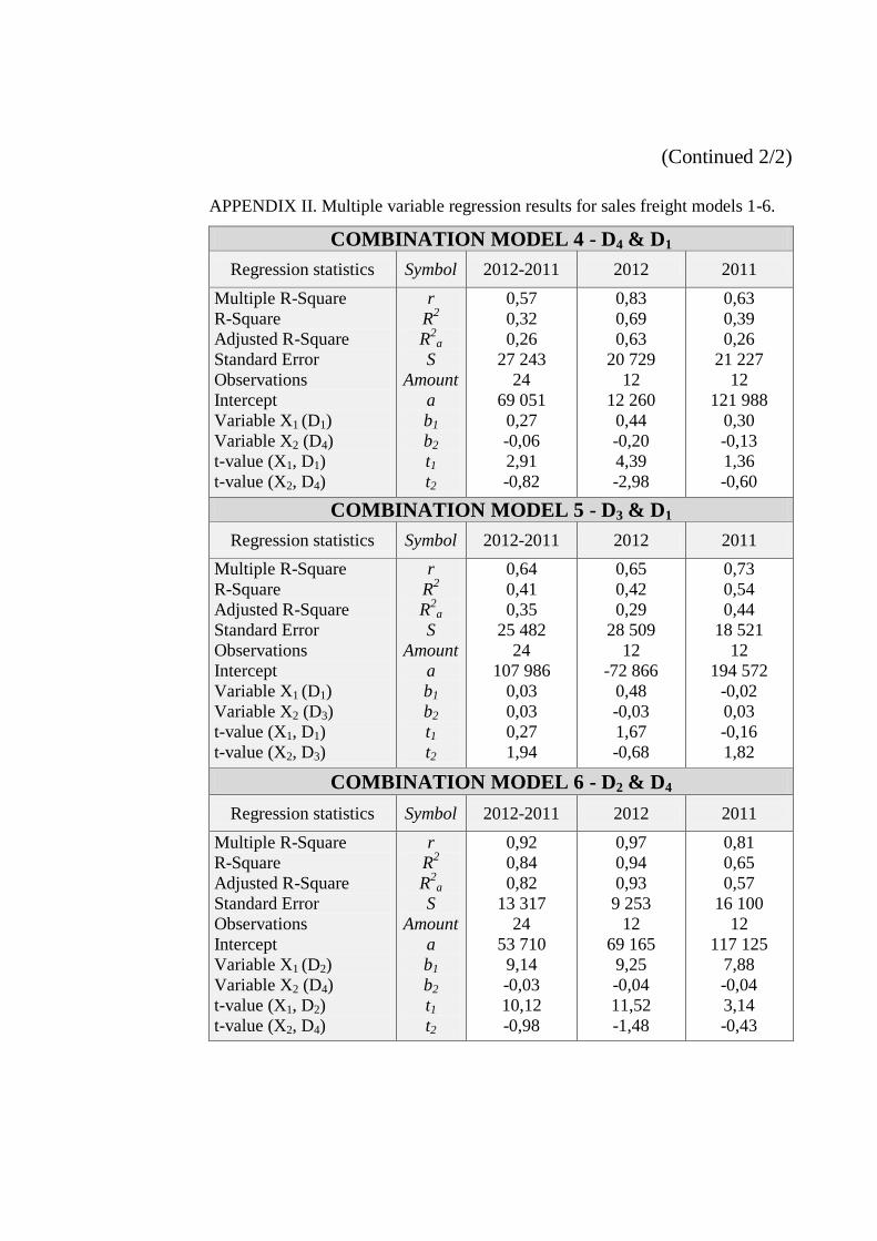
(Continued 2/2)

APPENDIX II. Multiple variable regression results for sales freight models 1-6.

COMBINATION MODEL 4 - D4 & D1

Regression statistics Symbol 2012-2011 2012 2011

Multiple R-Square

R-Square

Adjusted R-Square

Standard Error

Observations

Intercept

Variable X1 (D1)

Variable X2 (D4)

t-value (X1, D1)

t-value (X2, D4)

r

R2

R2a

S

Amount

a

b1

b2

t1

t2

0,57

0,32

0,26

27 243

24

69 051

0,27

-0,06

2,91

-0,82

0,83

0,69

0,63

20 729

12

12 260

0,44

-0,20

4,39

-2,98

0,63

0,39

0,26

21 227

12

121 988

0,30

-0,13

1,36

-0,60

COMBINATION MODEL 5 - D3 & D1

Regression statistics Symbol 2012-2011 2012 2011

Multiple R-Square

R-Square

Adjusted R-Square

Standard Error

Observations

Intercept

Variable X1 (D1)

Variable X2 (D3)

t-value (X1, D1)

t-value (X2, D3)

r

R2

R2a

S

Amount

a

b1

b2

t1

t2

0,64

0,41

0,35

25 482

24

107 986

0,03

0,03

0,27

1,94

0,65

0,42

0,29

28 509

12

-72 866

0,48

-0,03

1,67

-0,68

0,73

0,54

0,44

18 521

12

194 572

-0,02

0,03

-0,16

1,82

COMBINATION MODEL 6 - D2 & D4

Regression statistics Symbol 2012-2011 2012 2011

Multiple R-Square

R-Square

Adjusted R-Square

Standard Error

Observations

Intercept

Variable X1 (D2)

Variable X2 (D4)

t-value (X1, D2)

t-value (X2, D4)

r

R2

R2a

S

Amount

a

b1

b2

t1

t2

0,92

0,84

0,82

13 317

24

53 710

9,14

-0,03

10,12

-0,98

0,97

0,94

0,93

9 253

12

69 165

9,25

-0,04

11,52

-1,48

0,81

0,65

0,57

16 100

12

117 125

7,88

-0,04

3,14

-0,43

(1/2)

APPENDIX III. Multiple variable regression results for sales freight models 7-10.

COMBINATION MODEL 7 - D1, D2 & D3

Regression statistics Symbol 2012-2011 2012 2011

Multiple R-Square

R-Square

Adjusted R-Square

Standard Error

Observations

Intercept

Variable X1 (D2)

Variable X2 (D1)

Variable X3 (D3)

t-value (X1, D2)

t-value (X2, D1)

t-value (X3, D3)

r

R2

R2a

S

Amount

a

b1

b2

b3

t1

t2

t3

0,92

0,85

0,82

13 343

24

90 177

9,63

-0,09

0,01

7,52

-1,30

0,52

0,97

0,95

0,93

9 066

12

-18 978

9,22

0,17

-0,03

9,00

1,70

-1,91

0,83

0,70

0,58

15 975

12

164 001

7,47

-0,13

0,02

2,02

-1,05

0,91

COMBINATION MODEL 8 - D2, D3 & D4

Regression statistics Symbol 2012-2011 2012 2011

Multiple R-Square

R-Square

Adjusted R-Square

Standard Error

Observations

Intercept

Variable X1 (D2)

Variable X2 (D3)

Variable X3 (D4)

t-value (X1, D2)

t-value (X2, D3)

t-value (X3, D4)

r

R2

R2a

S

Amount

a

b1

b2

b3

t1

t2

t3

0,92

0,84

0,82

13 443

24

57 540

8,17

0,01

-0,06

5,30

0,78

-1,17

0,97

0,95

0,93

8 887

12

61 799

7,22

0,03

-0,12

4,21

1,33

-1,82

0,84

0,70

0,59

15 848

12

160 788

5,38

0,03

-0,13

1,63

1,14

-1,12

(Continues)

(Continued 2/2)

APPENDIX III. Multiple variable regression results for sales freight models 7-10.

COMBINATION MODEL 9 - D3, D4 & D1

Regression statistics Symbol 2012-2011 2012 2011

Multiple R-Square

R-Square

Adjusted R-Square

Standard Error

Observations

Intercept

Variable X1 (D3)

Variable X2 (D4)

Variable X3 (D1)

t-value (X1, D3)

t-value (X2, D4)

t-value (X3, D1)

r

R2

R2a

S

Amount

a

b1

b2

b3

t1

t2

t3

0,79

0,62

0,57

20 854

24

169 727

0,07

-0,23

-0,002

3,98

-3,37

-0,02

0,92

0,84

0,78

15 870

12

136 858

0,11

-0,36

-0,05

2,71

-4,59

-0,27

0,81

0,66

0,53

16 830

12

171 102

0,05

-0,33

0,21

2,51

-1,70

1,20

COMBINATION MODEL 10 - D2, D4 & D1

Regression statistics Symbol 2012-2011 2012 2011

Multiple R-Square

R-Square

Adjusted R-Square

Standard Error

Observations

Intercept

Variable X1 (D2)

Variable X2 (D4)

Variable X3 (D1)

t-value (X1, D2)

t-value (X2, D4)

t-value (X3, D1)

r

R2

R2a

S

Amount

a

b1

b2

b3

t1

t2

t3

0,92

0,84

0,82

13 398

24

84 791

9,82

-0,05

-0,01

8,17

-0,86

-0,31

0,98

0,95

0,94

8 480

12

16 143

7,79

-0,07

0,11

6,77

-2,31

1,65

0,82

0,67

0,55

16 591

12

147 624

9,76

0,09

-0,17

2,59

0,44

-0,69

APPENDIX IV. Multiple variable regression results for sales freight model 11

COMBINATION MODEL 11 - D1, D2, D3 & D4

Regression statistics Symbol 2012-2011 2012 2011

Multiple R-Square

R-Square

Adjusted R-Square

Standard Error

Observations

Intercept

Variable X1 (D2)

Variable X2 (D1)

Variable X3 (D3)

Variable X4 (D4)

t-value (X1, D2)

t-value (X2, D1)

t-value (X3, D3)

t-value (X4, D4)

r

R2

R2a

S

Amount

a

b1

b2

b3

b4

t1

t2

t3

t4

0,92

0,86

0,82

13 252

24

108 184

8,61

-0,08

0,02

-0,06

5,53

-1,26

1,20

-1,13

0,98

0,95

0,93

9 062

12

19 055

7,69

0,10

0,003

-0,08

4,19

0,83

0,08

-1,00

0,84

0,70

0,53

16 932

12

163 160

5,83

-0,03

0,02

-0,11

0,95

-0,09

0,83

-0,35

(1/2)

APPENDIX V. Multiple variable regression results for internal freight models 1-6.

COMBINATION MODEL 1 - D5 & D6

Regression statistics Symbol 2012-2011 2012 2011

Multiple R-Square

R-Square

Adjusted R-Square

Standard Error

Observations

Intercept

Variable X1 (D5)

Variable X2 (D6)

t-value (X1, D5)

t-value (X2, D6)

r

R2

R2a

S

Amount

a

b1

b2

t1

t2

0,75

0,57

0,53

4 345

24

1 374

2,24

41,5

3,83

2,06

0,67

0,45

0,33

4 403

12

22 953

1,70

3,77

2,59

0,12

0,94

0,90

0,87

2 039

12

-33 966

5,51

-72,58

7,83

-1,58

COMBINATION MODEL 2 - D6 & D7

Regression statistics Symbol 2012-2011 2012 2011

Multiple R-Square

R-Square

Adjusted R-Square

Standard Error

Observations

Intercept

Variable X1 (D6)

Variable X2 (D7)

t-value (X1, D6)

t-value (X2, D7)

r

R2

R2a

S

Amount

a

b1

b2

t1

t2

0,68

0,46

0,40

4 874

24

31 286

39,4

0,004

1,66

2,72

0,53

0,28

0,12

5 061

12

41 837

17,42

0,002

0,51

1,69

0,91

0,84

0,80

2 557

12

-5 795

17,76

0,02

0,35

5,98

COMBINATION MODEL 3 - D7 & D8

Regression statistics Symbol 2012-2011 2012 2011

Multiple R-Square

R-Square

Adjusted R-Square

Standard Error

Observations

Intercept

Variable X1 (D7)

Variable X2 (D8)

t-value (X1, D7)

t-value (X2, D8)

r

R2

R2a

S

Amount

a

b1

b2

t1

t2

0,71

0,50

0,45

4 681

24

27 683

-0,01

0,06

-1,36

2,18

0,67

0,45

0,32

4 438

12

33 866

-0,01

0,05

-1,30

1,75

0,92

0,84

0,80

2 534

12

855

0,03

-0,02

2,45

-0,54

(Continues)

(Continued 2/2)

APPENDIX V. Multiple variable regression results for internal freight models 1-6.

COMBINATION MODEL 4 - D8 & D5

Regression statistics Symbol 2012-2011 2012 2011

Multiple R-Square

R-Square

Adjusted R-Square

Standard Error

Observations

Intercept

Variable X1 (D8)

Variable X2 (D5)

t-value (X1, D8)

t-value (X2, D5)

r

R2

R2a

S

Amount

a

b1

b2

t1

t2

0,72

0,51

0,47

4 605

24

13 511

0,01

1,63

1,21

1,61

0,68

0,46

0,34

4 385

12

20 103

-0,004

2,13

-0,29

1,40

0,93

0,87

0,84

2 272

12

-36 000

0,01

4,20

0,52

3,10

COMBINATION MODEL 5 - D7 & D5

Regression statistics Symbol 2012-2011 2012 2011

Multiple R-Square

R-Square

Adjusted R-Square

Standard Error

Observations

Intercept

Variable X1 (D7)

Variable X2 (D5)

t-value (X1, D7)

t-value (X2, D5)

r

R2

R2a

S

Amount

a

b1

b2

t1

t2

0,70

0,49

0,44

4 725

24

9 772

0,001

2,13

0,59

2,07

0,70

0,49

0,37

4 275

12

14 563

-0,002

2,58

-0,75

1,99

0,95

0,91

0,89

1 933

12

-27 362

0,01

2,93

1,95

2,63

COMBINATION MODEL 6 - D6 & D8

Regression statistics Symbol 2012-2011 2012 2011

Multiple R-Square

R-Square

Adjusted R-Square

Standard Error

Observations

Intercept

Variable X1 (D6)

Variable X2 (D8)

t-value (X1, D6)

t-value (X2, D8)

r

R2

R2a

S

Amount

a

b1

b2

t1

t2

0,70

0,48

0,43

4 777

24

30 026

24,65

0,018

0,96

2,92

0,59

0,34

0,20

4 831

12

40 625

5,67

0,01

0,16

2,01

0,86

0,74

0,68

3 227

12

-8 260

-34,61

0,08

-0,48

4,36

(1/2)

APPENDIX VI. Multiple variable regression results for internal freight models 7-

10.

COMBINATION MODEL 7 - D5, D6 & D7

Regression statistics Symbol 2012-2011 2012 2011

Multiple R-Square

R-Square

Adjusted R-Square

Standard Error

Observations

Intercept

Variable X1 (D5)

Variable X2 (D6)

Variable X3 (D7)

t-value (X1, D5)

t-value (X2, D6)

t-value (X3, D7)

r

R2

R2a

S

Amount

a

b1

b2

b3

t1

t2

t3

0,75

0,57

0,50

4 452

24

1 514

2,21

41,41

0,0034

2,27

1,91

0,015

0,70

0,49

0,30

4 534

12

14 654

2,59

-1,10

-0,002

1,79

-0,03

-0,69

0,96

0,92

0,89

1 893

12

-26 576

3,76

-52,38

0,01

2,90

-1,18

1,57

COMBINATION MODEL 8 - D6, D7 & D8

Regression statistics Symbol 2012-2011 2012 2011

Multiple R-Square

R-Square

Adjusted R-Square

Standard Error

Observations

Intercept

Variable X1 (D6)

Variable X2 (D7)

Variable X3 (D8)

t-value (X1, D6)

t-value (X2, D7)

t-value (X3, D8)

r

R2

R2a

S

Amount

a

b1

b2

b3

t1

t2

t3

0,71

0,50

0,42

4 795

24

27 685

-5,23

-0,01

0,06

-0,13

-0,91

1,30

0,74

0,55

0,38

4 251

12

38 293

-62,31

-0,02

0,10

-1,34

-1,90

2,18

0,92

0,86

0,80

2 537

12

-2 012

68,01

0,04

-0,06

0,99

2,56

-1,07

(Continues)

(Continued 2/2)

APPENDIX VI. Multiple variable regression results for internal freight models 7-

10.

COMBINATION MODEL 9 - D7, D8 & D5

Regression statistics Symbol 2012-2011 2012 2011

Multiple R-Square

R-Square

Adjusted R-Square

Standard Error

Observations

Intercept

Variable X1 (D7)

Variable X2 (D8)

Variable X3 (D5)

t-value (X1, D7)

t-value (X2, D8)

t-value (X3, D5)

r

R2

R2a

S

Amount

a

b1

b2

b3

t1

t2

t3

0,76

0,57

0,51

4 421

24

4 552

-0,01

0,05

1,83

-1,66

1,99

1,88

0,73

0,53

0,36

4 317

12

15 920

-0,01

0,03

1,86

-1,13

0,90

1,23

0,97

0,94

0,91

1 699

12

-22 529

0,02

-0,06

3,59

2,84

-1,91

3,47

COMBINATION MODEL 10 - D6, D8 & D5

Regression statistics Symbol 2012-2011 2012 2011

Multiple R-Square

R-Square

Adjusted R-Square

Standard Error

Observations

Intercept

Variable X1 (D6)

Variable X2 (D8)

Variable X3 (D5)

t-value (X1, D6)

t-value (X2, D8)

t-value (X3, D5)

r

R2

R2a

S

Amount

a

b1

b2

b3

t1

t2

t3

0,75

0,57

0,50

4 449

24

2 983

39,22

0,001

2,08

1,58

0,16

2,05

0,68

0,46

0,26

4 645

12

19 061

4,84

-0,004

2,12

0,15

-0,29

1,31

0,95

0,90

0,87

2 090

12

-31 615

-76,7

0,016

4,71

-1,62

0,75

3,67

APPENDIX VII. Multiple variable regression results for internal freight model

11.

COMBINATION MODEL 11 - D5, D6, D7 & D8

Regression statistics Symbol 2012-2011 2012 2011

Multiple R-Square

R-Square

Adjusted R-Square

Standard Error

Observations

Intercept

Variable X1 (D5)

Variable X2 (D6)

Variable X3 (D7)

Variable X4 (D8)

t-value (X1, D5)

t-value (X2, D6)

t-value (X3, D7)

t-value (X4, D8)

r

R2

R2a

S

Amount

a

b1

b2

b3

b4

t1

t2

t3

t4

0,76

0,58

0,49

4 513

24

2 811

1,98

17,96

-0,007

0,031

1,89

0,44

-0,66

0,68

0,78

0,61

0,39

4 219

12

22 452

1,59

-54,57

-0,01

0,08

1,06

-1,17

-1,64

1,49

0,97

0,94

0,90

1 815

12

-22 695

3,65

-6,53

0,02

-0,055

2,93

-0,12

1,89

-1,30