lappeenranta university of technology - LUTPub

LAPPEENRANTA UNIVERSITY OF TECHNOLOGY

LUT School of Energy Systems

LUT Mechanical Engineering

Juho Venäläinen

IMPROVING PRODUCTIVITY IN VALVE BALL GRINDING WITH CERAMIC

ABRASIVES

Examiners: Prof. Juha Varis

M.Sc. Jari-Antero Sivula

ABSTRACT

Lappeenranta University of Technology


LUT Mechanical Engineering

Juho Venäläinen

Improving productivity in valve ball grinding with ceramic abrasives

Master’s Thesis

2017

98 pages, 34 figures, 8 tables and 7 appendices

Examiners: Prof. Juha Varis

M.Sc. (Tech.) Jari-Antero Sivula

Keywords: Valve ball grinding, factorial experiment, sol-gel aluminium oxide, grinding

fluid

This thesis aims to improve the ball grinding process by increasing material removal rate.

Improvement is pursued through modern grinding tools for which optimal grinding

parameters are determined and the achieved outputs are compared to each other. To

familiarize the process and recognize the important components in valve ball grinding, a

literature review is performed on grinding process and its components. To compare the tool

alternatives, systematical experimentation is required for which Design of Experiments

method is used after introducing it through literature review. Each tool is experimented

equipping different factorial designs where the material removal rate and tool wear are

measured. Based on the results of the experiments, the optimal parameters are determined

and the respective outputs are used for comparison. In the experiments, the alternative tools

were noted to be very different from the currently used tool and to require additional fluid

delivery in order to perform satisfactorily. The tool performance was noticed to be more

dependent on the suitability of the specification in the particular application, than on the

grain type. Experiments lead to conclusions based on which the tool specifications are

altered, but the final results are yet to be determined in the forthcoming experiments.

TIIVISTELMÄ

Lappeenrannan teknillinen yliopisto


LUT Kone

Juho Venäläinen

Venttiilipallojen hionnan tuottavuuden parantaminen keraamisella abrasiivilla

Diplomityö

2017

98 sivua, 34 kuvaa, 8 taulukkoa and 7 liitettä

Tarkastajat: Prof. Juha Varis

DI Jari-Antero Sivula

Hakusanat: Venttiilipallojen hionta, teollinen koe, sol-gel alumiinioksidi, hiontaneste

Tämän diplomityön tavoitteena on tehostaa venttiilipallojen hiontaprosessia kasvattamalla

materiaalinpoistonopeutta. Parannuksia haetaan moderneilla hiontatyökaluilla, joille

etsitään optimaaliset hiontaparametrit. Prosessin oppimiseksi ja tärkeimpien osatekijöiden

tunnistamiseksi, näistä suoritetaan kirjallisuuskatsaus. Työkalujen systemaattiseen

vertailuun käytetään teollista koesuunnittelua, joka esitellään osana kirjallisuuskatsausta.

Työkaluille suoritetaan teolliset kokeet, joissa mitataan materiaalinpoistonopeutta ja

työkalun kulumaa. Koetulosten perusteella määritellään työkalukohtaiset optimaaliset

työstöparametrit ja näillä saavutettavia tuloksia vertaillaan keskenään. Kokeiden aikana

vaihtoehtoisten työkalujen huomattiin olevan hyvin erilaisia nykyiseen työkaluun verrattuna

ja näiden tarvitsevan lisänestettä toimiakseen kunnolla. Työkalun tehokkuuden havaittiin

olevan riippuvaista enemmän työkalun muiden ominaisuuksien sopivuudesta

käyttökohteeseen, kuin abrasiivin tyypistä. Kokeista tehtyjen johtopäätösen perusteella

työkalujen ominaisuuksia muutetaan, mutta lopulliset tulokset ovat nähtävissä vasta tulevien

kokeiden jälkeen.

ACKNOWLEDGEMENTS

When starting my first summer job at Metso in 2008, I could not have imagined writing my

master’s thesis for the company almost nine years later. I have enjoyed working for the

company for all the internships and now for the single biggest project in my life so far. Thank

you for all the people I have worked with during my time with the company and special

thank you to Pekka Lappalainen who believed in me enough to hire me for my very first job

in 2008.

I want to express my deepest gratitude to my advisor Jari-Antero Sivula who provided me

with an interesting subject and guided me through the project. I also want to give special

thanks to grinding machine operators Jone Tolsa and Jyrki Kiema for patiently running the

experiments with me, making the study possible.

I want to thank all the teachers and professors at both LUT and Universität Paderborn and

in particular professor Juha Varis for examining my thesis.

Thank you to all my friends and family for supporting me through all the school years.

Finally, thank you to my lovely wife Jessica for your unconditional support in whatever I

do.

Juho Venäläinen

Vantaa, 3.4.2017

5

TABLE OF CONTENTS

ABSTRACT

TIIVISTELMÄ

ACKNOWLEDGEMENTS

TABLE OF CONTENTS

LIST OF ABBREVIATIONS AND SYMBOLS

1 INTRODUCTION ..................................................................................................... 10

1.1 Introduction of the Company ............................................................................... 10

1.2 Research Problem and Questions ........................................................................ 10

1.3 Research Methods ................................................................................................ 11

1.4 Limitations ........................................................................................................... 11

2 GRINDING AS A PROCESS ................................................................................... 12

2.1 Grinding Operations ............................................................................................ 12

2.1.1 Grinding Parameters ........................................................................................ 14

2.2 Basics of the Grinding Process ............................................................................ 15

2.2.1 Material Removal Mechanisms ....................................................................... 17

2.2.2 Chip Formation in Ductile Materials ............................................................... 18

2.3 Formation of Cutting Edges ................................................................................. 20

2.3.1 Tool Fracture Mechanics ................................................................................. 22

2.4 The Effect of Parameters on Material Removal Rate .......................................... 23

2.5 Grinding Errors .................................................................................................... 24

2.5.1 Excessive Heat Generation .............................................................................. 25

2.5.2 Tool Loading .................................................................................................... 26

3 GRINDING OF VALVE BALLS ............................................................................. 27

3.1 Basic Operation of Ball Valve ............................................................................. 27

3.2 Requirements for Valve Balls .............................................................................. 28

3.3 Ground Materials and Grindability ...................................................................... 30

4 GRINDING TOOLS .................................................................................................. 31

4.1 Tool Specification ................................................................................................ 31

4.2 Abrasives ............................................................................................................. 34

6

4.2.1 Aluminium Oxide ............................................................................................ 34

4.3 Bond Material ...................................................................................................... 36

4.3.1 Vitreous Bonds ................................................................................................ 37

4.3.2 Bond Material Additives .................................................................................. 37

5 GRINDING FLUID ................................................................................................... 39

5.1 Fluid Types .......................................................................................................... 40

5.1.1 Fluid Additives ................................................................................................ 43

5.2 Fluid Delivery ...................................................................................................... 44

5.2.1 Nozzle Design .................................................................................................. 45

6 DESIGN OF EXPERIMENTS AS A TOOL ........................................................... 46

6.1 Process Model ...................................................................................................... 46

6.2 Purpose of Experiments ....................................................................................... 47

6.3 Experiment Strategies .......................................................................................... 48

6.3.1 The Best-guess Approach ................................................................................ 48

6.3.2 One Factor at a Time ....................................................................................... 48

6.3.3 Factorial Designs ............................................................................................. 49

6.4 Principles of Experimenting ................................................................................ 51

6.4.1 Replication ....................................................................................................... 51

6.4.2 Randomization ................................................................................................. 51

6.4.3 Blocking ........................................................................................................... 52

6.5 Planning an Experiment ....................................................................................... 52

6.6 Empirical Model .................................................................................................. 54

6.6.1 Multiple Linear Regression Model .................................................................. 55

7 DESIGN OF THE GRINDING EXPERIMENTS .................................................. 56

7.1 Pre-planning the Experiments .............................................................................. 56

7.1.1 Stating the Problem .......................................................................................... 56

7.1.2 Design Factors ................................................................................................. 57

7.1.3 Response Variables .......................................................................................... 62

7.1.4 Choosing the Designs ...................................................................................... 64

7.2 Running the Experiments ..................................................................................... 65

7.2.1 Test Machine .................................................................................................... 66

7.2.2 Test Workpiece ................................................................................................ 67

7.2.3 Tool Alternatives ............................................................................................. 68

7

7.3 Data Analysis ....................................................................................................... 69

8 DISCUSSION ............................................................................................................. 70

8.1 Key Results and Tool Evaluations ....................................................................... 70

8.1.1 Tyrolit .............................................................................................................. 71

8.1.2 Theleico ........................................................................................................... 74

8.1.3 Diprotex ........................................................................................................... 78

8.1.4 Norton Grades F, H & J ................................................................................... 78

8.2 Observations and Findings on the General Process ............................................. 81

8.2.1 Observations on Fluid Delivery ....................................................................... 81

8.2.2 Fluid Content and Concentration ..................................................................... 85

8.2.3 Bending of the Segment ................................................................................... 87

8.3 Development Possibilities .................................................................................... 89

8.4 Further Research Topics and Experiments .......................................................... 91

8.5 Validity and Reliability ........................................................................................ 93

9 CONCLUSIONS ........................................................................................................ 94

REFERENCES ................................................................................................................... 95

APPENDICES

APPENDIX I: Experiment report, Tyrolit

APPENDIX II: Experiment report, Theleico

APPENDIX III: Experiment report, Diprotex

APPENDIX IV: Experiment report, Norton grade F

APPENDIX V: Experiment report, Norton grade H

APPENDIX VI: Experiment report, Norton grade J

APPENDIX VII: Grinding fluid test report

8

LIST OF ABBREVIATIONS AND SYMBOLS

AW Anti Wear

DMAIC Define, Measure, Analyze, Improve, Control

DOE Design of Experiments

EP Extreme Pressure

FM Friction Modifier

G-ratio Grinding Ratio

MRR Material Removal Rate

OFAT One-Factor-at-a-Time

PEP Passive Extreme Pressure

SG Seeded-gel

WP Workpiece

α Clearance angle

β Regression coefficient

γ Rake angle

ε Experimental error

η Effective cutting speed angle

ρs Cutting edge radius

λ Head conductivity

cp Specific heat capacity

hcu Undeformed chip thickness

hcu eff Effective chip thickness

P Grinding power

Q’ Specific removal rate

9

r Heat evaporation

Tµ Critical cutting depth

v Viscosity

vc Cutting speed

Vc Cylinder volume

Vcbs Volume of bearing mount caps

Vcfp Volume of flowport caps

Vt Sphere total volume

x Design factor

y Response variable

Al2O3 Aluminium Oxide

CBN Cubic Boron Nitride

SiC Silicon Carbide

TiO2 Titanium Dioxide

WC-Co Tungsten Carbide Cobalt

10

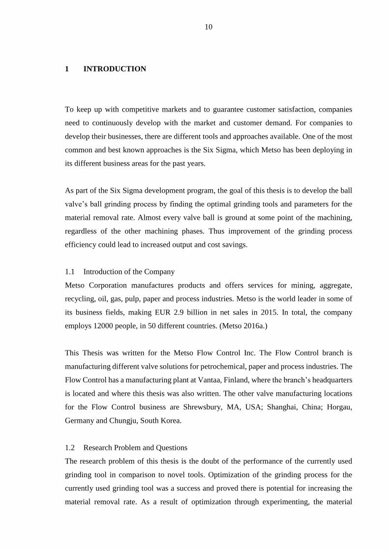
1 INTRODUCTION

To keep up with competitive markets and to guarantee customer satisfaction, companies

need to continuously develop with the market and customer demand. For companies to

develop their businesses, there are different tools and approaches available. One of the most

common and best known approaches is the Six Sigma, which Metso has been deploying in

its different business areas for the past years.

As part of the Six Sigma development program, the goal of this thesis is to develop the ball

valve’s ball grinding process by finding the optimal grinding tools and parameters for the

material removal rate. Almost every valve ball is ground at some point of the machining,

regardless of the other machining phases. Thus improvement of the grinding process

efficiency could lead to increased output and cost savings.

1.1 Introduction of the Company

Metso Corporation manufactures products and offers services for mining, aggregate,

recycling, oil, gas, pulp, paper and process industries. Metso is the world leader in some of

its business fields, making EUR 2.9 billion in net sales in 2015. In total, the company

employs 12000 people, in 50 different countries. (Metso 2016a.)

This Thesis was written for the Metso Flow Control Inc. The Flow Control branch is

manufacturing different valve solutions for petrochemical, paper and process industries. The

Flow Control has a manufacturing plant at Vantaa, Finland, where the branch’s headquarters

is located and where this thesis was also written. The other valve manufacturing locations

for the Flow Control business are Shrewsbury, MA, USA; Shanghai, China; Horgau,

Germany and Chungju, South Korea.

1.2 Research Problem and Questions

The research problem of this thesis is the doubt of the performance of the currently used

grinding tool in comparison to novel tools. Optimization of the grinding process for the

currently used grinding tool was a success and proved there is potential for increasing the

material removal rate. As a result of optimization through experimenting, the material

11

removal rate grew several times over. Now it is estimated, that by finding an optimal tool

and corresponding parameters for it, the material removal rate could be increased even

further.

The main research question that the thesis is aiming to answer is: can the material removal

rate be increased without impairing the surface quality, and how. Without investing in new

machinery and by leaving out the human factor, the question can ultimately be split into two

parts: what is the optimal grinding tool and what are the optimal corresponding grinding

parameters?

1.3 Research Methods

The thesis consists of a theory part and empirical part where the introduced theories are

applied. The theory covers the basic principles of grinding and the mechanics of chip

formation, and it also gives an introduction to grinding tools and abrasives. The theory part

also introduces Design of Experiment (DOE) practice in a depth that it is necessary for

running experiments and analyzing its results. To bring out the importance of grinding for

the operation of a rotary valve, a short description on the principle of operation of rotary

valves is included.

The theory is based on a literature review from each subject’s respective field. The empirical

research, following the principles of DOE, is based on the data collected from the test runs

that are performed with a grinding machine. A regression model is composed from the

collected results, based on which the optimal grinding parameters are selected and finally

verified with a confirmation test as a part of the DOE process.

1.4 Limitations

As mentioned earlier in the research questions, the research is focused solely on the grinding

event with the current machinery. New machine investments and human factors are

eliminated from this research. The experiments are limited to five different ceramic abrasive

tools from three different abrasive manufacturers. The research is limited only to grinding

austenitic stainless steel in a state prior to possible chromium or other coatings.

12

2 GRINDING AS A PROCESS

The abrasive processes date back to the times people used to rub rocks against each other to

make tools and weapons, making abrasive processes one of the earliest methods of working

materials. Even the grinding of metal dates backs to the 2000 BCE, when Egyptians utilized

it to sharpen tools. The basic principle of the material removal has remained the same ever

since, even though everything else in the modern process has more or less changed. What

we consider machining with abrasives these days, started in the 18th century. Later on 1891

abrasives took a big step forward as producing the first synthetic abrasive, silicon carbide

was discovered. Finally, development has led to today’s extremely hard synthetic abrasives

that are crucial in modern grinding processes, on which the tools experimented in this thesis

also rely on. (Malkin & Guo 2008, pp. 3–4; Klocke 2009, p. 1.)

Abrasive processes have few specific features in comparison to other conventional

machining processes. Cutting edges are much smaller and there is a numerous amount them

participating in the cutting process simultaneously. As a result of numerous small cutting

edges and hardness of the grain, the abrasive processes have some advantages over other

machining processes. The extreme hardness typical for the abrasives, makes the machining

of very hard materials possible, materials such as hardened steel, carbides or ceramics.

Moreover, fine surfaces as well as close dimensional and geometrical tolerances can be met.

In some applications where the materials are extremely hard, machining with abrasives is

the only practical option as the use of other methods is either impossible or inefficient. (Black

& Kohser 2012, p. 715; Malkin et al. 2008, pp. 1–2.)

The usual abrasive processes can be split into two groups depending on the abrasive type.

Grinding, that this thesis is focused on, and honing represent machining with bonded

abrasives. Lapping and polishing then are examples of the usual processes done with free

abrasive particles. (Marinescu et al. 2013, pp. 3–4, 7; Klocke 2009, p. 1.)

2.1 Grinding Operations

Grinding is a machining process performed with a tool where hard abrasive grains are

bonded together. It is usually considered as precision machining process, where material

13

removal rates are low, but which with high surface quality and tight tolerances can be met.

However, grinding is also used as heavy duty process for example for cleaning billets at

foundries, where material removal rates are high and other factors such as surface roughness

are not the primary interest. The grinding method that this thesis regards, can be considered

as precision process, as measures and geometry of the ball are crucial for the valve’s

operation. (Klocke 2009, p. 1; Malkin et al. 2008, pp. 1–2.)

Grinding operations can be grouped based on the tool shape, kinematics, workpiece and

grinding head. The basic operations can be grouped on four different categories that are

represented in Figure 1. (Marinescu et al. 2007, p. 6.)

Figure 1. Four common grinding operations (modified from Marinescu et al. 2007, p. 6).

The principle of operation of ball grinding machine used at Metso is illustrated in Figure 2.

It is a special application and is not directly part of any of the four groups but has similarities

with several. Despite the difference in principle of operation, on a grain level the process

still follows the same basic principles introduced in the second chapter.

14

Figure 2. The principle of operation of ball grinding machine.

2.1.1 Grinding Parameters

Grinding is often considered complex and unpredictable process because of numerous of

small, randomly shaped and scattered cutting edges. However, with correct equipment the

process control is fairly easy and the number of parameters that need to be controlled is fairly

low. (Marinescu et al. 2007, p. 9.) The following parameters cover only an extent that

concerns the ball grinding application and are used in the experiments or theory. The

experiments are interested mainly in material removal and tool wear, therefore other

parameters such as calculations for surface roughness are not covered.

The main input parameters that the ball grinding machine users adjust, are feed rate, wheel

(rotational) speed and workpiece (rotational) speed. The feed rate expresses the amount of

feed motion per time unit, which is on the test machine set as mm/min. Wheel speed on the

machine is set to desired RPM, which can be converted to velocity with a simple formula

taking the wheel diameter into account. Like the wheel speed, the workpiece speed is set as

RPM and the actual workpiece speed depends on the ball diameter. The actual wheel speed

and workpiece speed are important to calculate for safety reasons. Grinding tools have

maximum speed rating within which the tool is safe to use and exceeding the limit increases

the risk of the wheel to shatter. (Marinescu et al. 2007, p. 11, 60.)

15

The output variables that the ball grinding machines gives, are not directly applicable to

precise experimenting, instead they tell the information that is useful for the machine user in

normal production. The machine measures the diameter of the ball which is used to calculate

the volume of the ball that is required for calculating the material removal. The way the

diameter is applied in calculating valve ball volume, is covered more thoroughly in chapter

7.1.3 Response variables.

To express material removal rate in grinding, the specific removal rate Q’ is often used. The

specific removal rate expresses the removal rate as material removal rate per width of tool

contact. So, the unit for Q’ is mm3/mm/s. (Marinescu et al. 2007, pp. 12–13.)

To express tool wear, the ball grinding machine gives out the length of the tool. Its values

are compared before and after the runs to get the change in tool length. It could be used to

evaluate tool wear on its own, but long tool life itself does not mean that the tool is any good,

so it is better to relate to material removal rate. Grinding ratio, or G-ratio, expresses the ratio

between the volume of material removed from the workpiece and the volume removed from

the tool and is often used as a main criteria evaluating the tool wear. Since it’s a ratio, both

sides of the equation have similar units and the output is unitless. (Marinescu et al. 2007, pp.

17–18; Rowe 2013.)

Specific grinding energy is not a factor of interest in grinding experiments, however it is

used in theory and therefore its definition is given here. It measures the energy that is needed

for removing a certain volume of material from the workpiece and accordingly its unit is

J/mm3. (Marinescu et al. 2007, p. 12.)

2.2 Basics of the Grinding Process

The material removal principle in grinding seems to differ from many other machining

processes such as turning or milling. In these processes, the chip is removed by an insert of

which size, shape and location is known. But in grinding, the material removal is a sum of

countless small, randomly placed, cutting edges removing tiny particles from the workpiece.

However, from a point of a single cutting edge, the material removal follows the same

method as in milling or turning and the difference is in grinding’s clearly negative rake angle.

With countless slightly different cutting edges, the grinding tool has very complex structure

16

which makes the forming of the single chip unpredictable. Instead of analyzing the material

removal on a single grain scale, the approach is more often statistical by building up a model

of an average grain, based on all the measured cutting edge profiles. An illustration of such

model, representing an average abrasive grain on grinding tool, is seen on Figure 3.

(Marinescu et al. 2007, p. 24; Klocke 2009, p. 3; Aurich et al. 2013, p. 81.)

Figure 3. An illustration of an average cutting edge on grinding tool, where α is the clearance

angle and γ the rake angle. The rake angle is clearly negative which is typical for abrasive

cutting edges. (Marinescu et al. 2007, p. 25.)

To understand the material removal principle, it is necessary to look into the process on a

grain scale. The Figure 4 represents a simplified image of a grinding tool on a workpiece

surface. The dark gray abrasive grains are bonded together with light gray bond material.

These abrasive grains, numbered from 1 to 5, protrude from the surface of the bond material,

on random sizes, shapes and locations. The grains protruding the most and reaching the

machined surface are the ones participating in the cutting process. These are called kinematic

cutting edges and are marked with red circles. The yellow squares mark the static cutting

edges, which are not part of the machining process yet. As a result of the tool wear, kinematic

edges wear and new static edges constantly turn into new kinematic edges, becoming part of

the grinding process. (Klocke 2009, p. 4.)

17

Figure 4. A simplified image of abrasive grains in bonding material (modified from Klocke

2009, p. 4).

2.2.1 Material Removal Mechanisms

The material removal mechanisms of a single grain are shown in the Figure 5. As numerous

of grains protruding differently from the bond cut the workpiece simultaneously, all of the

three mechanisms can occur on the workpiece surface at the same time. Whether the main

mechanism is microplowing, microchipping or microbreaking, is mainly determined by the

workpiece material. Ductile materials are more prone to microplowing and microchipping,

where brittle-hard materials, such as ceramics are apt to microbreaking. (Marinescu et al.

2007, p. 31.)

Figure 5. Illustrations of different material removal mechanisms in grinding (Marinescu et

al. 2007, p. 32).

On a single grain scale, microplowing is not particularly effective material removal

mechanism. The most of the energy goes to continuous plastic, or elastoplastic deformation

of the material’s surface. Finally, as the microplowed area gets hit enough times by various

18

cutting edges, the part tends to break from its trace borders leading to material removal. The

second mechanism, microchipping, occurs together with microplowing. The relation of these

two mechanisms depends on grinding parameters as well as the suitability of the parts

associating in the process, such as grinding fluid and tool. The material removal in ductile

materials such as many steels, usually happens through these two mechanisms. (Marinescu

et al. 2007, p. 31.)

The microbreaking is a mechanism that occurs mainly on brittle-hard materials, like

ceramics. Prior to material removal, the material surface cracks and the crack spreads leading

to chip removal. As seen on the Figure 5, the chips removed by microbreaking, can be very

large in comparison to grinding trace. (Marinescu et al. 2007, p. 31.)

2.2.2 Chip Formation in Ductile Materials

As stated earlier, the material removal in grinding of ductile materials is mainly based on

microplowing and microchipping mechanisms. Figure 6 shows a three stage model of

material removal in ductile material. The effective cutting speed angle η, between the

workpiece surface and the effective cutting speed ve, that the abrasive approaches and

penetrates the workpiece surface, is typically small. So, the travel path is rather flat, which

leads to a certain behavior of the material, or to the three phases of the model. (Marinescu et

al. 2007, pp. 32, 262-263; Klocke 2009, pp. 8–9.)

Figure 6. A basic three stage model of grinding process of ductile materials (modified from

Marinescu et al. 2007, p. 32).

19

In the area of the first phase, the material deforms elastically which is often referred as

rubbing or sliding. After the phase of elastic deformation starts the plastic deformation,

sometimes called ploughing. In this phase the material flows underneath and aside of the

cutting edge, forming material outbursts. Finally, in the third phase, when the undeformed

chip thickness hcu reaches the critical cutting depth Tµ, the chip formation begins.

(Marinescu et al. 2007, p. 32; Klocke 2009, pp. 8–9; Rowe 2013.)

The actual volume of removed material is determined by the effective chip thickness hcu eff,

so by the portion of the uncut chip thickness hcu that is actually removed as a chip. This

relation depends on different factors in grinding process, such as the cutting edge radius ρs,

effective cutting speed angle η, cutting speed vc, material properties and friction. The friction

between the cutting edge and the workpiece has significant effect on hcu eff and Tµ. Basically

higher friction equals more efficient material removal, so on a grain scale, any lubrication

such as cutting fluid lowers the material removal rate of a single grain. By lowering the

friction, the grain cutting depth Tµ increases, but so does the portion of deformed sections,

thus resulting in decrease in the effective chip thickness. On macroscale, the use of cutting

fluids makes possible the use of higher grinding parameters and has several other benefits

explained later on, so in practice they are often used nevertheless. (Marinescu et al. 2007, p.

32, 195; Klocke 2009, pp. 8–9; Rowe 2013.)

The previous three stage model for chip formation illustrates a situation where grinding is

performed with wheel periphery. In the model, single grain follows a circular path of the

wheel and the penetration depth into the workpiece changes with the revolving motion of

the wheel. In the grinding application used at Metso, the depth of the grains penetrating the

surface increases slowly and the single grain is in contact with the workpiece the majority

of the time, so the contact length becomes much longer. Despite the different grinding

method, similar three stages can still be recognized where the grains go through the three

stages with increasing feed rate. The kinematic cutting edges not participating in the cutting,

slowly turn into to active cutting edges with feed rate. At first they are barely touching the

surface and they are in the first phase of the model. With feed motion they move on first to

the second phase and then third, before fracturing and starting the cycle over.

20

2.3 Formation of Cutting Edges

A key factor in efficient grinding is the formation of new cutting edges on the grinding tool

surface. Friability is a factor that describes the fracturing tendency of a grain under strain.

Practically, the tendency of the grain to break and form new cutting edges. The higher the

friability, more apt the grain is to fracture. For the optimal process efficiency and quality,

the friability of the grain plays an important role. Too tough of a grain, does not break in

time, but dulls instead. The dull grains rubbing the workpiece surface can cause thermal

damage through the elevated surface temperature caused by increased friction. A grain too

friable remains sharp, but then wears unnecessarily quickly, shortening tool life and thus

increasing the tooling costs. (Marinescu et al. 2013, p. 247.)

Ultimately, the formation of new cutting edges depends on both the properties of the grain

and the bond. When the cutting edges on the grain get too dull, grain should break creating

new cutting edge and finally when the grain is worn out the bond should release the grain,

making room for new grains to surface. (Marinescu et al. 2007, pp. 111–112; Badger 2012,

p. 1118.)

On top of the tool properties, formation of new cutting edges also depends on other factors,

of which the grinding parameters are a major one. Wrong tool does not work well with any

parameters and the optimal tool with unsuitable grinding parameters unlikely works any

better.

The Figure 7 illustrates the three different wear regimes of the tool that depend on so-called

“aggressiveness”. Badger (2012, p. 1118) defines the aggressiveness in a following manner:

“The aggressiveness is simply the factors in the calculation for chip thickness that are under

immediate control of the machine operator with the cutting-point density and chip width

ratio removed.” So, the grinding parameters affecting the aggressiveness are the feed rate,

depth of cut, wheel speed and equivalent wheel diameter and they should be selected in a

way that the aggressiveness is optimal resulting in optimal wear of the wheel. (Badger 2012,

p. 1118.)

21

Figure 7. For an optimal grinding process, it is important to find the sweet spot between

different wear mechanisms by using suitable grinding parameters (Badger 2012, p. 1118).

In the ball grinding application, not all of the parameters listed by Badger apply. The

parameters controlled by the operator that define the aggressiveness are the feed rate and

tool and workpiece speed.

In the area of regime I, the parameters are not aggressive enough. Not enough stress is

addressed to the abrasive grains for them to fracture and self-sharpen, resulting in dulling.

Dulling of the grains leads to inefficient cutting process as the portion of rubbing increases,

leading to increased heat generation. The dulling of the grains eventually leads to large

chunks of wheel to break off as the force towards the area of dull grains exceeds the retaining

strength of the surrounding bond. (Badger 2012, p. 1118.)

In the area of regime II, the stresses addressed towards the grain are in proportion so there

is no excessive dulling nor excessive bond wear due to large forces on grains. In the regime

II both the specific energy and wheel wear are moderate and the tool wear occurs optimally,

meaning that the grains and bond fracture when meant to. (Badger 2012, p. 1118.)

The area of regime III represents grinding with overly aggressive parameters, where the

specific energy is low but the stresses addressed towards the tool surface are high. The grains

on the tool remain sharp because of the excessive fracturing constantly bringing about new

22

cutting edges. However, such overly aggressive parameters lead to catastrophic wheel wear.

(Badger 2012, p. 1118.)

2.3.1 Tool Fracture Mechanics

As stated earlier, the formation of new cutting edges as the old dull, is the premise to material

removal. The tool wear and generation of new cutting edges occurs through four different

means, shown on Figure 8. The mechanism of tool wear and thus the generation of a new

cutting edge, depends on several factors such as the grinding parameters and the type of the

abrasive. (Rowe 2013.)

Figure 8. The different wear types of abrasive grains (Rowe 2013).

When the stresses addressed towards the grain are not high enough, fracturing does not

occur. In this case the wear type is rubbing, also known as attritious wear, that leads to

dulling of the grains. Despite the volume of the tool wear through attritious wear being

almost negligible, it is perhaps the most important factor determining the overall wheel wear.

The wear flats caused by the attritious wear determine the grinding forces to a high extent,

which the probability of the bond fracture and then the overall wheel wear depends on. So,

eventually rubbing results in parts of the tool surface breaking off, as explained earlier in the

part regarding aggressiveness. (Malkin et al. 2008, p. 296; Rowe 2013.)

Micro-fracturing is a preferred type of grain fracture, where only a small volume of grain is

lost. This results in longer tool life and grain maintaining its sharp cutting edges, keeping

23

the grinding forces low. In macro-fracturing, the fracture usually happens along the fracture

plains. This results into a loss of larger volume of the grain than in event of micro-fracture.

The relation between the two fracture types is mainly dependent on the crystalline structure

of the grain. (Rowe 2013; Klocke 2009, p. 29.)

In bond fracture the whole grain, or bigger chunk of bond with several grains, breaks off

from the tool. The bond fracture is a wear mechanism that the overall wheel wear ultimately

depends on, as the wheel can only wear as fast as the bond fractures. The event of bond

fracture is highly dependent on the grinding forces addressed to the grain and the retention

strength of the bond. The optimal bond fracture occurs when the grain is worn out and dull,

releasing the grain and making room for new grains. The grinding forces that are too high

cause unwanted and premature bond fracturing. An example of an effect of such event is

seen in Figure 7, regime III, where bigger chunks of bonding material might break off

causing excessive tool wear. (Rowe 2013; Badger 2012, p. 1118; Malkin et al. 2008, p. 294.)

In grinding processes with high conformity, such as the ball grinding application, the

grinding pressure spreads over to large area. This means lower forces addressed towards

single grain, reducing the fracturing and increasing the risk of the grain dulling and glazing.

(Rowe 2013.)

2.4 The Effect of Parameters on Material Removal Rate

Every grinding tool specification has its own set of parameters it works optimally with, as

well as limits when it comes to material removal rate. These practical limits for increasing

the material removal rate can be process and quality related due to for example surface

roughness, heat generation and chatter. Depending on the application, the limit for heat

generation is different. In precision grinding the limit is often low due to accuracy problems

that the heat expansion causes. In addition to quality related factors, the limit for material

removal rate can be set by the machine, for instance just by lacking required power. (Rowe

2013.)

The parameters listed earlier, regarding the aggressiveness and tool fracturing, were the feed

rate, tool speed and workpiece speed. As expected, the same parameters determine also the

material removal rate. To increase the material removal rate, these parameters need to be

24

changed in relation to each other. Ultimately, the material removal depends on the feed rate,

as it sets the maximum theoretical value for the material removal. The portion that of the

theoretical maximum value is achieved, depends on other factors. (Rowe 2013.)

Increasing feed rate while keeping two other variables constant, results in increased grinding

forces and roughness, and reduces specific energy. With reduced specific energy the

grinding becomes more energy efficient but a feed rate too high results in high wheel wear,

reducing the G-ratio. (Rowe 2013.)

Tool speed has somewhat opposite effects from feed rate. Increasing tool speed, while other

factors remain constant, reduces grinding forces and roughness and increases specific energy

and tool life (Rowe 2013). Increasing the tool speed has its limit which comes from the speed

the tool is rated for. For example, the grinding segments compared in the experiments are

rated for 32 m/s.

The workpiece speed has usually smaller effect on material removal rate than the two other

variables. However, the workpiece speed affects the probability of thermal damage, as with

low workpiece speed the tool and thus the energy is focused on a single area for longer time.

So in some applications, increasing workpiece speed can possibly allow the other parameters

to be increased and this way increase the removal rate. (Rowe 2013.)

Despite increasing the nominator in the formula for G-ratio, G-ratio will decrease by

increasing the material removal rate. The decrease in G-ratio is linear until reaching the

maximum removal rate of the tool. Increasing the removal rate over the limit of the tool

causes the G-ratio to drop exponentially. (Marinescu et al. 2007, p. 20.)

2.5 Grinding Errors

Defects caused by grinding are often very problematic. In many cases, grinding is one of the

last machining phases, meaning that the value added to the workpiece prior to grinding is

significant. If the product needs to be scrapped after grinding, it can be very expensive. In

this chapter few of the known errors and their causes are introduced.

25

2.5.1 Excessive Heat Generation

High temperatures are known to cause several problems in grinding. The problems can occur

either directly from the heat in a form of thermal damage or indirectly from the effects of

heat. In ball grinding, clearly increased workpiece temperature leads to poor accuracy due

to heat expansion.

The problems caused by the high grinding temperature include discoloration, tensile residual

stress, surface hardening, sub-surface softening. The type of thermal damage and its severity

depends on the temperature the surface is exposed to. Further issue with some of the damage

types is that they are invisible to bare eye and thus difficult to recognize. (Rowe 2013.)

Low temperature grinding is to be preferred, not only because of its lower tendency to cause

issues but also due to its positive effect on ground surface. Grinding with low temperature

generates compressive residual stresses on the ground surface, which has positive effect on

the fatigue life of the workpiece. (Rowe 2013.)

Most of the means for lowering the temperatures and avoiding thermal issues culminate on

lowering the heat generation caused by friction and rubbing. This can be achieved by

dressing the tool to get fresh and sharp cutting surface or by changing the tool specification

altogether. Softer tool with more open structure has better self-sharpening abilities, keeping

the cutting surface sharp. (Rowe 2013.)

Other mean for reducing the workpiece temperature is to improve the fluid delivery or

change the grinding fluid (Rowe 2013). Grinding fluid has a significant effect in reducing

the grinding temperatures as it works in two ways. It both lubricates the surfaces, reducing

friction and also conveys the heat away. (Marinescu et al. 2013, p. 148.)

The last option for reducing the heat generation is to adjust the parameters so that the material

removal rate is reduced. Other methods are usually priority as lowering the material removal

rate is directly lowering the output. (Rowe 2013.)

26

2.5.2 Tool Loading

Tool loading, or clogging, can severely impair the output of grinding. In particular, it is a

problem in high conformity applications with long contact length, because of their higher

tendency for tool loading. The long contact length results in long chips, that get trapped

between the tool and the workpiece surface, filling the pores of the tool. (Rowe 2013.)

A clogged tool impairs the grinding performance by different means. Tool loading reduces

the available pore space, meaning less space for fluid and thus weakened fluid delivery to

contact area. Friction increases due to weakened lubrication, leading to increased

temperature and grinding forces. Ultimately, clogging leads to poor surface quality and

lowered tool life. (Klocke 2009, p. 152; Rowe 2013.)

The cure for tool loading can often be found in grinding fluid. To prevent clogging of the

tool, a sufficient coolant delivery using a coolant with good lubrication abilities is essential.

In applications where clogging is a problem, additional coolant nozzles rinsing the tool

surface can provide help targeted specifically to this problem. Other means for preventing

clogging can be changing the wheel specification or adjusting the grinding parameters for

example by increasing the tool speed. (Klocke 2009, p. 153; Rowe 2013.)

27

3 GRINDING OF VALVE BALLS

The end customer’s constant demand for more efficient processes require more from the

used valve system as well. This includes tightening requirements for valve sealing

properties, where the quality of valve parts plays a major role. Due to certain advantages of

grinding, it is often the only machining operation able to reach the set requirements. Valve

balls are not an exception.

3.1 Basic Operation of Ball Valve

A ball valve is one of the valve types that bases its operation on rotation. In a ball valve, of

which an example is seen in Figure 9, the valve ball rotates in valve body, controlling the

flow through the valve. In the figure, the ball flowport is aligned with piping, letting the flow

through thus the valve is open. By rotating the ball by 90°, the valve is shut.

Figure 9. An example of basic metal seated valve (Metso 2016b).

28

The three main parts of a ball valve are seats, body and a ball, on which this thesis is focused

on. In the Figure 9, the ball seats are marked with A and B, the valve ball with C, and together

they are mounted in the valve body, forming the main pressure retaining parts of the valve.

The first rotary valves were equipped with soft rubber seats that based their sealing ability

on local elastic and plastic deformation of the seat. Ball valves with metal seats came first

on the market in the 1960’s and have been gaining share of the market from soft seated

valves. The metal seated valves have several benefits over the soft seated, which is why they

the only option in some applications. For example, the operating temperature of metal seated

valve is much wider, all the way from -200 to 800 °C and they are also fire safe. Ball valves

are often used as backup valves that shutdown the process in case of emergency, a case

where fire safety is a crucial feature. (Kivipelto, 1990, p. 81; Wright & Bregman, 1990, pp.

95–97.)

3.2 Requirements for Valve Balls

Unlike the soft seats, the metal seats do not base their sealing property on material

deformation to the same extent. The sealing ability of metal seated ball valve depends largely

on how well the seat and ball surfaces match each other. The sealing principle and an ideal

contact is illustrated in Figure 10.

Figure 10. The ball surface and its matching seat surface forming a sealing pair (Kivipelto,

1990, p. 88).

29

To ensure smooth operation and tight sealing of the valve, the seats can be lapped together

with the ball to form a well matching pair. Lapping, however, is a slow process and thus is

avoided. The need for lapping ultimately depends on the success of grinding, or how well

the parts meet their dimensional and geometrical tolerances. In many cases, the dimensional

tolerances could be achieved with even faster processes than grinding. However, many of

these processes cannot match grinding in the two factors that are important to sealing ability

of the valve: the surface roughness and circularity.

The surface roughness depends on both the used grinding tool and the parameters used with

it (Malkin et al. 2008, p. 258). The usual Ra value requirement for surface roughness for

spherical surfaces of valve balls is 0.4 μm. In addition to meeting the required surface

roughness and tolerances, a certain visual appearance of the ball surface is traditionally

preferred. The machine users aim to have grinding marks crossing like on the ball surface in

Figure 11. Cross marking has generally been visual evaluation criterion for sphere

circularity. Although, the lack of cross scratches does not mean that the ball does not meet

the set requirements. Vice versa, a clear cross scratching does not mean that the ball meets

the requirements.

Figure 11. An example of desired cross marking on the ball surface after roughing.

30

3.3 Ground Materials and Grindability

Generally, all the valve balls are ground at least once at some point of their machining.

Depending on the application and the customer’s desire, different base materials and

coatings are available, and thus are ground. The number of different ground materials is

limited to rather few, but their material properties differ with large margin, changing their

grindability.

The base materials are usually different grades of steel which are, based on the application,

either coated or not. The ground materials can vary for example from hard WC-Co (Tungsten

Carbide Cobalt) coating, that is ground with superabrasives, to basic austenitic steel. One of

the most common base materials, and the material of the workpieces used in the experiments,

is ASTM grade A351 CF8M austenitic steel which is a cast equivalent of wrought grade

AISI 316.

Despite the fact that an exact definition of the term grindability does not exist, the term is

still commonly used. It describes how difficult the material is to grind with certain tools in a

certain environment. Practically, it measures the required grinding energy; the lower energy

requirement equals easier grinding and thus better grindability. The required grinding energy

can be calculated by diving the grinding power P with the specific removal rate Q’, so it is

the same as specific cutting energy in machining in general. The main factors affecting the

energy are the workpiece hardness and wheel sharpness. (Rowe 2013.)

In general, the harder material equals higher grinding forces, thus lower grindability. Even

though softer materials are technically easier to grind, they bring about their own problems.

The soft ductile materials tend to generate long chips that lead to increased risk of clogging

the tool surface. (Marinescu et al. 2013, pp. 523–524.)

Austenitic stainless steels, such like in the experiments, are considered ductile and therefore

follow the typical behavior for ductile materials. They are a prime example of material that

is prone to generate long chips. In addition, stainless steels have tendency to work-harden,

resulting in high grinding forces and tool wear. (Klocke 2009, p. 92, Marinescu et al. 2007,

p. 263.)

31

4 GRINDING TOOLS

The basis of all abrasive processes is understanding and controlling the relations between

the abrasive grains, bonding material and the workpiece. The most important of these is

between the abrasive and workpiece as it is the premise of material removal. The abrasives

have to retain their hardness above the workpiece hardness throughout the whole grinding

event, regardless of the temperature raise in the process. Otherwise the result is opposite

from wanted and the material is removed mainly from the tool. However, the tool cannot be

selected by simply making sure it is harder than the ground material. Excessive hardness will

lead to other problems such as thermal damage. Thus, understanding all the parts of the

process and how they are related is crucial in selection of the right grinding tool. (Marinescu

at al. 2013, pp. 5–6.)

Grinding tools come in numerous different shapes and material combinations for different

grinding applications. Often the grinding tools are wheel shaped but different shapes such as

cups exist. Taking different shapes, abrasives and bond materials into account, the grinding

tool companies might offer tens of thousands of slightly different products to fit every need.

(Malkin et al. 2008, pp. 11–12.)

For ball grinding at Metso, few different tool specifications are used for different materials.

The shape of the tool depends on the type of abrasive and workpiece size. The superabrasive

tools are small, about 10 mm in diameter, bits attached to grinding head. Tools with

conventional abrasives are cup shaped for small ball sizes. For larger valve balls, the tool

consists of segments in a grinding head, essentially forming a cup with gaps between the

segments. This tool related chapter focuses on the type of tools that are compared in the

experiments, aluminium oxide in vitreous bond.

4.1 Tool Specification

Grinding tool consists of abrasive grains that are fixed together with bonding matrix. In

addition to these two main components, different fillers and grinding aid substances can be

added to the tool. The variation in grinding tools does not stop just at the ingredients, but for

example, the grain size and porosity vary depending on the application and have a significant

32

effect on the grinding process. To perceive often invisible differences in grinding tools and

to be able to compare them, standardized marking systems for grinding tools have been

developed. Conventional and superabrasives have both their own marking systems, of which

different standardization organizations have their own slightly different versions. An

example of standardized marking system for conventional grinding tools is the American

National Standard Institute’s ANSI B74.13, which is shown on the Figure 12. Other marking

systems, like German DIN-standard 69 100 are quite similar to it. (Malkin et al. 2008, p. 12;

Klocke 2009, pp. 45–46.)

Figure 12. An example specification of a certain aluminium oxide tool according to ANSI

standard (Marinescu et al. 2007, p. 109).

The tool specification, consisting of series of numbers and letters, tells the main components

of the tool, as well as features of the wheel. Explanations behind each letter and number in

marking system for conventional abrasives are given below.

The prefix is reserved for use of the manufacturer. The use of it is optional, but several

manufacturers use it to differentiate their abrasive variants. The first actual character

33

expresses the type of the abrasive material, which is traditionally either A for aluminium

oxide or C for silicon carbide. (Malkin et al. 2008, p. 12; Klocke 2008, p. 46.) However,

manufacturers seem to digress from the standard and use other letters or letter-number

combinations to represents their specific kind of grain, for example the initials of the trade

name.

The number after the abrasive type determines the grain size of the abrasive, which is

measured a bit differently, depending on the standard. In the commonly used ANSI-standard,

the grain size is reported as the mesh size of the sieve the grains were sorted with, thus the

nominal grain size actually has a range of different grain sizes. Some manufacturers use an

additional number after the grain size specification, to express whether the tool has various

grain sizes. The number 1 usually entails that the tool consists only the indicated grain size,

where the other numbers represent certain mixtures of different grain sizes. (Malkin et al.

2008, pp. 12–15; Klocke 2008, p. 47, Rowe 2013.)

Third actual character, a letter ranging from A to Z, expresses the grade of the tool, from soft

to hard in respective order. The tool grade is a general determination of the strength of the

tool, in other words the resistance of grits breaking from bond. This is directly related to tool

wear as the softer tools tend to wear quicker. The tool grade can be defined in different ways,

but a common one is based on porosity. The harder grade has more bond material and is less

porous. The hardest grade of Z having about 2% porosity, Y having 4% porosity and so on.

However, the scale is not universal and there is diversity between the manufacturers. (Malkin

et al. 2008, pp. 15–16; Klocke 2008, p. 47; Rowe 2013.)

The fourth character indicates the volume of abrasive in the tool. The tool structure varies

between dense and open, where higher number means less abrasive, resulting in more open

packing density of grains. The scale for structure is not universal between the manufacturers,

so the structure numbers and what they represent vary. On a commonly used scale from 0 to

25, a low end number for structure such as 4 or lower can be considered very dense. In terms

of volume it equals almost 60% abrasive, resulting in tight packing. Generally, lower

packing density gives grinding fluid a better access to the surface and results in more

efficient swarf removal. (Malkin et al. 2008, p. 16; Rowe 2013.)

34

The last character before the suffix indicates the used bond material. These days, the most

common bond materials are either vitrified (V) or resinoid (B) and the other types are used

quite rarely. After the letter for bond material, manufacturers may use an optional suffix to

further differentiate the product. (Malkin et al. 2008, p. 16.)

4.2 Abrasives

Abrasives used in grinding tools can be either natural or man-made, synthetic materials.

Regardless of the origin of the abrasive, their use is based on their hardness, which is why

grinding was earlier done with hard materials found from nature, such as natural corundum,

garnet or diamond. These days, corundum and diamond are still widely used but are mainly

synthetic. (Malkin et al. 2008, pp. 19–20.)

The abrasive materials are split into two groups: conventional and superabrasives.

Corundum, or aluminium oxide (Al2O3) and silicon carbide (SiC) are considered as

conventional abrasives, where cubic boron nitride (CBN) and diamond are called

superabrasives, because of their superior hardness. (Klocke 2008, p. 19; Rowe 2013.) The

experimented tools equip different types of aluminium oxide grains, on which differences

this chapter is focused on.

4.2.1 Aluminium Oxide

Aluminium oxide goes by with many names, including corundum, alumina and aloxide. It

is a widely used abrasive for grinding of different ferrous metals. Aluminium oxides can be

grouped further to fused and sintered based on a matter how they are made. Prior to 1904

and the invention of the Higgins furnace, natural corundum was used in the form of minerals

emery and corundum. These days, only the emery is still in used in coated papers. After the

invention of Higgins electric arc furnace, production of various fused alumina started, which

are still used widely in precision grinding processes. However, more recently founded

ceramic aluminium oxides have taken a significant share of the market. (Jackson &

Hitchiner. 2013, p. 20.)

Differences of Two Grain Types

Nowadays, this more novel grain comes in different variations and goes by with several

general and trade names such as: ceramic, sintered, sol-gel, seeded-gel (SG) and Cubitron.

35

Yet, when the ceramic grain was first introduced in 1981 by company 3M coming out with

their Cubitron grain, it wasn’t used in grinding wheels at all. The potential of ceramic grains

in grinding was discovered later, after Norton had launched their similar ceramic SG grain

in 1986. It took time before the industry learned how to apply this new kind of grain. It was

tougher than the conventional corundum and without altering the grinding parameters for

the new kind of tool, it usually led to dulling of the wheel. To avoid excessive grinding forces

resulting from the toughness and ensure required hardness, at first the sol-gel grains were

mixed with the conventional grains as little as 5% of the total grain volume. These days the

common mixtures of SG are 10%, 30% and 50%. (Marinescu et al. 2007, p. 80; Badger 2012,

p. 1115, Rowe 2013.)

Being the same material as the conventional alumina, many of the material properties of sol-

gel grain are about the same, but the different production method results in some advantages.

The properties such as shape and size of the grain vary less, making sol-gel grains more

homogenous. (Nadolny 2014, p. 85.) When correctly used, sol-gel grains can provide higher

material removal rate with lower grinding forces and thus lowered temperature, but often the

biggest benefit is its longer tool life. Because of these features, sol-gel alumina can be

considered as an option to much more expensive superabrasive CBN in certain applications.

(Webster & Tricard 2004, p. 598.)

The benefit of ceramic grains, over the conventional fused alumina grains, comes from their

different fracturing mechanism explained earlier in the chapter 2.3.1 Tool fracture

mechanisms. The both grains types have the same basic behavior, requiring enough force

for the grain to fracture and self-sharpen. The biggest difference between the two is in the

volume the grain loses when a fracture occurs. The ceramic grains have tendency to micro-

fracture where the conventional aluminium oxide macro-fractures along the fracture plains,

leading to bigger volume lost and often duller grain. (Badger 2012, p. 1116, 1122.)

As stated earlier, the fused grains are apt to macro-fracture where the sol-gel grains micro-

fracture. The different fracture behavior is explained by looking at their structure more

closely. A fused alumina grain is usually a single crystallite, that consists of crystallographic

planes like in the illustration in Figure 13. Forces addressed to the grain in the grinding event

cause cracks to advance parallel to these planes, resulting in a significant loss of volume and

36

in the grain. This form of cracking also leads to duller cutting edges than micro-cracking of

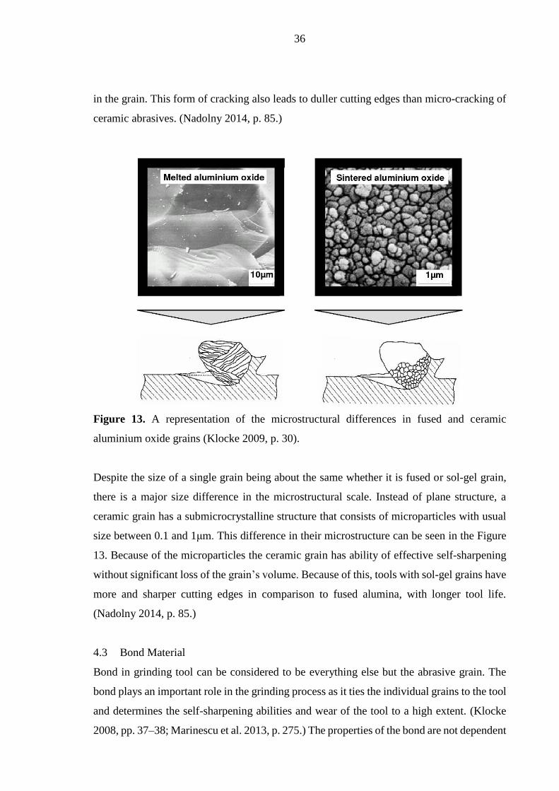
ceramic abrasives. (Nadolny 2014, p. 85.)

Figure 13. A representation of the microstructural differences in fused and ceramic

aluminium oxide grains (Klocke 2009, p. 30).

Despite the size of a single grain being about the same whether it is fused or sol-gel grain,

there is a major size difference in the microstructural scale. Instead of plane structure, a

ceramic grain has a submicrocrystalline structure that consists of microparticles with usual

size between 0.1 and 1μm. This difference in their microstructure can be seen in the Figure

13. Because of the microparticles the ceramic grain has ability of effective self-sharpening

without significant loss of the grain’s volume. Because of this, tools with sol-gel grains have

more and sharper cutting edges in comparison to fused alumina, with longer tool life.

(Nadolny 2014, p. 85.)

4.3 Bond Material

Bond in grinding tool can be considered to be everything else but the abrasive grain. The

bond plays an important role in the grinding process as it ties the individual grains to the tool

and determines the self-sharpening abilities and wear of the tool to a high extent. (Klocke

2008, pp. 37–38; Marinescu et al. 2013, p. 275.) The properties of the bond are not dependent

37

just on the bonding agent, but the tool grade and structure. In general, the more porous bonds

provide less retaining strength. (Marinescu et al. 2007, p. 109.)

The most important task of the bond is to retain the grain until it gets dull and then release it

to make room for new grains. In addition to this main task, bonding agent has other important

functions as well, such as transferring the forces from the machine spindle to workpiece and

dissipating the heat generated by the grinding process. (Marinescu et al. 2013, p. 275.)

Generally, there are six different bonding agent types used in grinding tools with

conventional abrasives: resin, shellac, oxychloride, rubber, silicate and vitrified. The most

common ones are resin and vitrified bonds, vitrified representing about a half of the market.

All the grinding tools compared in the experiments, are also vitrified, therefore the bonding

material chapter is focused only on vitrified bonds. (Malkin et al. 2008, p. 27.)

4.3.1 Vitreous Bonds

The vitreous bonds have multiple advantages, which is why they are so popular. One of the

main advantages is the very porous structures that the vitreous bonds make possible. They

are also stabile in high temperatures, brittle, rigid and resistant to oil and water. (Marinescu

et al. 2007, p. 108; Klocke 2009, p. 40.)

The usual base materials for vitreous bonds are clay, feldspar and frit. The ingredients are

mixed and molded in room temperature, after which the blank is fired in a kiln, transforming

it into a glasslike material. To achieve highly porous structure without sacrificing too much

of the structural integrity, sometimes additional ingredients are added to the mixture. They

can be hollow particles such as bubble alumina, that remain in the structure and break open

in the grinding event, opening up a pore. They can as well be combustible materials, such as

sawdust. The combustible material burns away in the firing process, leaving behind a pore.

(Marinescu et al. 2007, p. 108, 112.)

4.3.2 Bond Material Additives

In addition to materials that are mixed in the bond for production reasons, further additives

may also be added to bond matrix to modify the properties of the tool and improve its

performance. The additives can be added to either the bond mixture before kilning process

38

or after the kilning as fillers by impregnating the tool. (Klocke 2009, p. 41; Marinescu et al.

2013, p. 278.)

The necessity and use of additives and fillers depend on the requirements set by the

application. They can fulfill different tasks such as improve the tool strength, increase the

heat resistance or act as a lubricant. (Klocke 2009, p. 41.)

Common lubricating agents added to grinding tools are sulfur, wax or resin. They are added

to a tool by impregnating it, so that the tool pores are filled with the substance. For example,

in internal grinding in bearing industry, where the contact lengths are usually long, wheels

are often impregnated with sulfur which is an effective extreme pressure (EP) lubricant.

(Marinescu et al. 2013, p. 278.)

An exact mechanism how sulfur effects the process is not very well known. However, it is

believed that sulfur chemically reacts with the ground metal, forming a lubricating sulfide

film. Sulfur additions to the ground metal are known to have significant increase on the G-

ratio and similar effects are witnessed with sulfur additions in the grinding tool. Despite the

advantages of sulfur additives in grinding, the sulfur impregnated wheels have been losing

popularity due to their downside of being a possible source for health and environmental

issues. (Marinescu et al. 2007, p. 113; Malkin et al. 2008, p. 306.)

39

5 GRINDING FLUID

The grinding fluid is often a crucial part in many of the grinding processes, as it can have

significant effect on the output. The fluid is largely responsible for lubricating and cooling

in the process, which are the two of its main tasks. By reducing friction between the

workpiece and the tool with a lubricative film in between, grinding forces drop. Lowering

the grinding forces leads to decreased the wheel wear and lowers the amount of heat that is

generated in the process. (Klocke 2009, p. 113; Marinescu et al. 2013, p. 214.)

In many instances, the grinding fluid is simply referred as coolant, which derives from the

second of its main functions. The grinding fluid works as a coolant in two ways, both by

cooling down the contact area and by bulk cooling the workpiece by transporting the heat

away. (Klocke 2009, p. 113; Marinescu et al. 2013, p. 214.)

In addition to lubrication and cooling, grinding fluid has some secondary tasks and benefits.

With correctly directed and powerful enough spray, the tool surface can be flushed, cleaning

out the swarf and thus preventing clogging of the tool. Grinding fluid also works also a

corrosion inhibitor for both the workpiece and the machine. (Klocke 2009, p. 113, 125.)

The primary requirements for effective grinding fluid are good lubrication, cooling and

flushing properties as well as good corrosion protection. These requirements for functional

properties are set by the main tasks of the fluid and are related to the performance of the

grinding process. The secondary requirements for grinding fluid are related to operational

behavior, or efficient and safe use of the fluids. The most important of these requirements is

the safety for human health and environment. The same reason why some grinding fluids or

their additives have lost popularity despite fulfilling the performance requirements. Further

requirements for operational behavior are for example easy filtration and recycling, bacteria

resistance, low flammability and suitability for the machine and its tools. (Marinescu et al.

2007, pp. 195–196.)

40

5.1 Fluid Types

On a broad level the fluids can be split based on if there is water present when the fluid is

applied. Straight oils (water-immiscible) do not contain water, where soluble oils (water-

miscible) and synthetic fluids (water composite fluids) are water based. Different fluid types

have their own basic properties which are altered with series of additives. (Malkin et al.

2008, p. 304; Marinescu et al. 2007, p. 196.) The optimal grinding fluid for each application

is different and therefore selection should be done after weighing which of the fluid’s tasks

are the most crucial and which fluid fulfills them the best. (Klocke 2009, p. 113.)

Customarily, straight oils provide the best lubrication out of grinding fluids. The low friction,

due to good lubricative properties of oil, contributes to high G-ratios, low grinding forces

and good surface finish. The lubrication performance of oil is linked to its ability to reduce

attritious wear and wear-flats it causes. The Figure 14 shows an area of wear-flats on a

function of material removal and it compares nothing but air, two oil-water solutions with

different concentrations and straight oil. The superiority of an oil as a lubricant can be clearly

seen, particularly with higher material removal rates. The total area of wear flats remains

rather constant with oil, where in dry grinding or with emulsion its starts to increase quickly

with material removal. Between the two emulsions, increasing the oil content decreases the

area of wear-flats caused by attritious wear and lowers the grinding forces. (Malkin et al.

2008, p. 304.) Besides the superior lubrication, oils are very effective corrosion inhibitors

and are resistant to bacteria even without additives, therefore oils have longer lifespan than

water-based fluids (Klocke 2009, pp. 116–117).

41

Figure 14. The area of wear flats versus material removal in certain grinding process with

different grinding fluids (Malkin et al. 2008, p. 305).

The oils come with their downsides, which is why in practice the water-based fluids are used

more often. The most substantial of functional downsides of oil is its poor cooling ability.

From the Table 1, a comparison between the thermal properties of oil and water can be seen.

The specific heat capacity of water is more than two times over the oil and the heat

conductivity is more than four times higher in favor of water. The same table also shows the

major difference in viscosities that explains the superior lubrication properties of oil in

comparison to water. (Klocke 2009, p. 117.)

Table 1. Comparison of properties of oil and water (modified from Klocke 2008, p. 117).

Mineral oil Water

Specific heat capacity cp [J/(g*K)] 1.9 4.2

Heat conductivity λ [W/(m*K)] 0.13 0.6

Heat of evaporation r [J/g] 210 2260

Viscosity (40°C) v [mm2/s] 5…20 0.66

42

Due to the inferior thermal properties of oil in comparison to water, its ability to transfer the

generated heat away is significantly lower. However, by using oil, there is less heat generated

to begin with. Thus, the most suitable grinding fluid from lubrication and cooling perspective

depends on the application. In high heat generation processes, such as creep feed grinding,

where effective cooling is crucial, water-based fluids are often considered as an only option.


Rest of the disadvantages of the oil are related to operational behavior and safety. The oil’s

tendency to form mist is problematic and causes different issues. If the machine is not fully

enclosed, the machine user might be exposed to respirable oil mist, causing a possible health

hazard. The oil mist is also highly flammable, posing another safety risk. A major increase

in the workpiece temperate, caused for example by a sudden loss of the fluid delivery, can

be enough to ignite the mist. As a preparation it is necessary to have a fire exhaust system

and safety guards for the temperature. (Klocke 2009, p. 117.)

Soluble, or emulsifiable oils are concentrates that are mixed with water and emulsifier in

certain ratios to create emulsions. The water content in emulsions is usually high, which is

why their properties are usually more water-like. By increasing the oil content, the properties

and behavior becomes more oil-like, increasing the lubrication performance while reducing

the cooling abilities. The effect of increased oil content and how it affects attritious wear can

be seen from the Figure 14. (Marinescu et al. 2007, p. 198.)

Much like emulsions, synthetic grinding fluids, or aqueous solutions, are water-based fluids.

The main difference to emulsions is the absence of oil. To compensate this and to improve

the properties, just like in other fluid types, different additives are added in the mixture.


The grinding fluid used in ball grinding at Metso was earlier straight oil, but was changed to

water-based emulsion in the 1990’s. One of the reasons for the change was the better cooling

performance that helped in reaching the geometrical tolerances. The cooling ability of the

oil was insufficient to keep the valve ball cool enough during the grinding, causing the heat

to distort the ball and not meet the tolerances.

43

5.1.1 Fluid Additives

The properties of grinding fluid are enhanced by using different additives. Additives can be

split on three groups based on their function. They can serve as changing the physical

properties of the fluid, such as viscosity. They can serve as changing the chemical properties

of the fluid, for example corrosion inhibitors. Finally, they can work as tribologically active

substances, that alter the friction conditions. Tribologically active additives include polar

additives, friction modifiers (FM), anti-wear (AW) and extreme pressure (EP) additives.

(Klocke 2009, p. 119–120.) The main additive types, that affect the material removal, and

their modes of actions are listed in the Table 2.

Table 2. The additive types associated with cutting performance (modified from Brinksmeier

et al. 2015, p. 608).

Additive type Substances Mode of action, function

Anti-wear additive

(AW)

Acid and nonionic

phosphoric acid ester, zinc

dialkyldithio-phosphate

Reduces abrasive wear of

rubbing surfaces by

physisorption

Extreme pressure

additive (EP)

Chlorineparaffine,

sulphurous ester,

phosphoric acid ester,

polysulphide

Protection against wear by

formation of adsorption or

reaction layers, prevent

microfusing of metallic surfaces

Friction modifier (FM) Glycerol mono oleate,

whale oil, natural fats, oils,

synthetic ester

Lowers friction and wear,

improve adhesion of lubricating

film

Passive extreme

pressure additive (PEP)

Overbased sodium or

calcium sulfonate

Kind of solid lubricant, forms a

film between the surfaces

Tribologically active additives is likely the group with the most significant effect on cutting

performance as they improve the lubrication properties. The different additives of grinding

fluid work on different operational areas. The polar additives, that are mostly fatty

substances from plants and animals or synthetic esters, form a lubricating film on the

workpiece surface due to their polarity. The film lubricates the process effectively until about

150 °C. (Klocke 2009, p. 120; Marinescu et al. 2007, p. 199.)

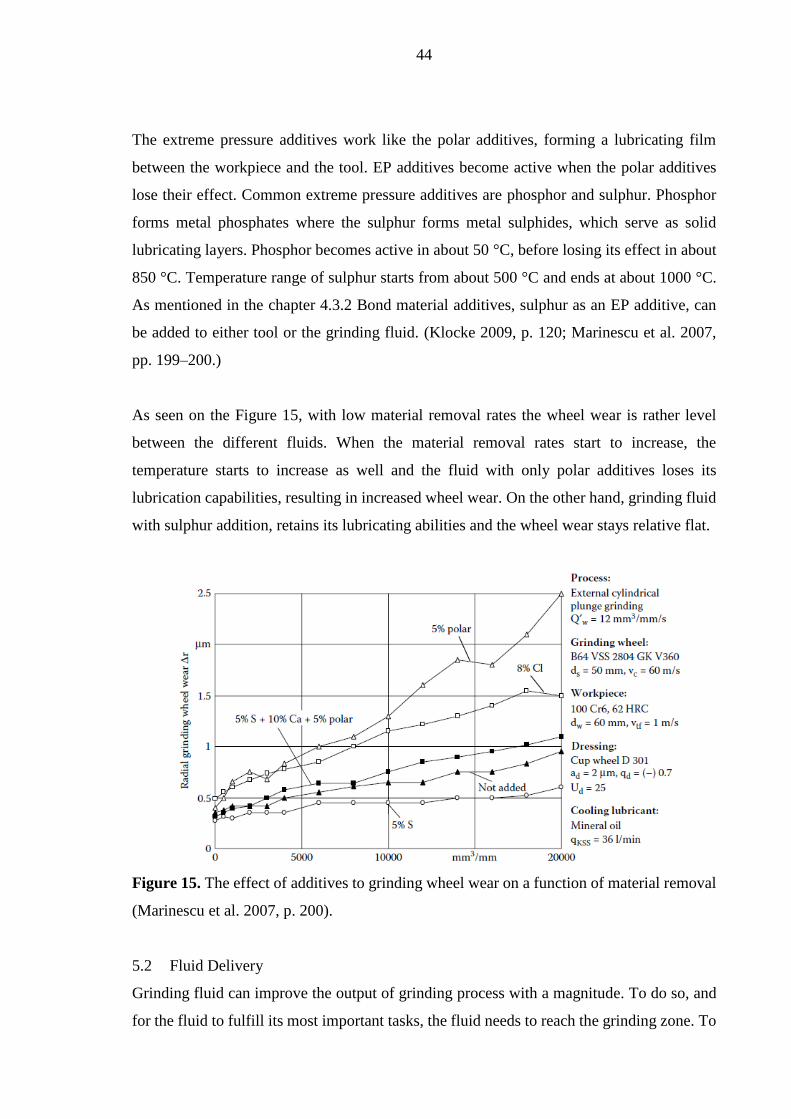
44

The extreme pressure additives work like the polar additives, forming a lubricating film

between the workpiece and the tool. EP additives become active when the polar additives

lose their effect. Common extreme pressure additives are phosphor and sulphur. Phosphor

forms metal phosphates where the sulphur forms metal sulphides, which serve as solid

lubricating layers. Phosphor becomes active in about 50 °C, before losing its effect in about

850 °C. Temperature range of sulphur starts from about 500 °C and ends at about 1000 °C.

As mentioned in the chapter 4.3.2 Bond material additives, sulphur as an EP additive, can

be added to either tool or the grinding fluid. (Klocke 2009, p. 120; Marinescu et al. 2007,

pp. 199–200.)

As seen on the Figure 15, with low material removal rates the wheel wear is rather level

between the different fluids. When the material removal rates start to increase, the

temperature starts to increase as well and the fluid with only polar additives loses its

lubrication capabilities, resulting in increased wheel wear. On the other hand, grinding fluid

with sulphur addition, retains its lubricating abilities and the wheel wear stays relative flat.

Figure 15. The effect of additives to grinding wheel wear on a function of material removal

(Marinescu et al. 2007, p. 200).

5.2 Fluid Delivery

Grinding fluid can improve the output of grinding process with a magnitude. To do so, and

for the fluid to fulfill its most important tasks, the fluid needs to reach the grinding zone. To

45

ensure this, the fluid nozzles need to be selected and directed accordingly. To maximize the

benefits from grinding fluid, the fluid also needs to fulfill its secondary tasks such as cleaning

swarf from the tool surface and bulk cooling around the contact area. In many cases, just one

nozzle or nozzle design cannot fulfill all the tasks and it is necessary to have several nozzles

each for different purposes. (Marinescu et al. 2007, p. 206; Marinescu et al. 2013, pp. 214–

215.)

5.2.1 Nozzle Design

A revolving tool generates an air barrier around itself, of which effect gets stronger with

increasing tool speed. For the fluid to reach the contact area, the air barrier needs to be

overcome. In order to do so, the fluid flow needs high enough velocity, for which a common

recommendation is to match the wheel peripheral speed. Ultimately, the grinding fluid

reaching the contact zone depends on the nozzle. After all, the nozzle determines the fluid

flow, including the velocity, to a great extent. (Marinescu et al. 2007, p. 204, Marinescu et

al. 2013, p. 228.)

The optimal design of the nozzle depends on its task. For main tasks, lubricating and cooling

the contact zone, correctly directed high pressure is needed and the nozzle design should be

selected correspondingly. The contact zone lubrication is not necessarily as much matter of

the fluid volume as it is the fluid entering the zone. Thus, to ensure the fluid reaching the

contact area, the pressure can be increased by reducing the opening of the nozzle while

keeping the flowrate constant. To achieve high enough velocity with nozzles with large

openings, more powerful pumps producing more heat are needed. Since it is waste of energy

to accelerate higher quantities of fluid than necessary, nozzle types with limited openings

are often used to deliver fluid to the contact zone. (Marinescu et al. 2013, p. 214, 230.)

For secondary tasks of the fluid, such as bulk cooling, the efficiency is not based on the

pressure, but the flowrate. Even if the extra fluid from the main nozzles serves in bulk

cooling, it is often more practical to have the separate nozzles for the purpose. For bulk

cooling purposes, simple flood nozzles with low pressure are enough and are the most

efficient solution. (Marinescu et al. 2013, p. 214, 230.)

46

6 DESIGN OF EXPERIMENTS AS A TOOL

Development techniques like Six Sigma use various of statistical tools on a path towards

improvement, one of these tools is experimentation. The DMAIC improvement model of

above mentioned Six Sigma consists of phases for Define, Measure, Analyze, Improve and

Control, where it also derives its name from. Design of Experiments is a commonly used

method in the analyze phase, in transition to improve. (Pyzdek 2003, p. 3.)

Experimentation is a tool that aims for better understanding and improvement of the process

that it is performed on. It is widely used on all fields, but is particularly important in product

design and process improvement on technical field. (Pyzdek 2003, p. 3.) In short, the usual

goal of DOE is to recognize the critical process factors, measure their effect on the output

and give out their optimal values for desired output (Meran et al. 2013, p. 7).

6.1 Process Model

A process, like grinding in this case, can be anything from chemical to machining processes

or to something from a whole different field. As seen from the Figure 16, process is a

combination of input, process factors and output. In a process, various factors working on

the input, turn it into output. The input and factors can be anything from machines to

materials to people. Often, the input is a material that machine and other factors turn into

finished or semi-finished products. The process factors taking a part in the process can be

either controllable or uncontrollable, depending on if they can be altered by the process

controller or not. For example, in machining operation, the feed rate or the spindle speed can

be directly controlled but the cutting fluid temperature often not. (Montgomery 2012, pp. 1–

3.)

47

Figure 16. An example of a process model (modified from Montgomery 2012, p. 3).

6.2 Purpose of Experiments

The purpose of each experiment varies and the ultimate goal is not necessarily the obvious,

maximizing the output. The purpose of an experiment might be to discover the most

influential factors for the output or to determine the optimal factor levels in a way that the

output is as close as possible to desired one. The reason for running an experiment might as

well be to determine the factors in a way, that results to least variation in the output.

(Montgomery 2012, p. 3.)

Some of the above-mentioned common reasons for running an experiment are often referred

with specific names depending on the type of the experiment. An experiment aiming to

identify the most significant factors and familiarize the process is often referred as screening

experiment. It is usually a start point of experimenting for unknown processes and further

testing follows once the process is more familiar to the experimenter. Optimization

experiment commonly follows the screening experiment. Once the significant factors are

known, their optimal levels for desired output are determined with optimization.


As the name suggests, confirmation experiments aim to confirm that the certain process

behaves in expected manner. Confirmation experiments are commonly used in situations

48

where some previously used part of the process is replaced with a new corresponding one or

the production is moved from plant to another. It is verified that changing the factor with

equivalent one or changing the site does not affect the output. (Montgomery 2012, p.14.)

Many other types of experiments do exist, such as discovery experiment used to resolve the

outcome of adding something new to the process. Ultimately, the type of experiment depends

on what kind of questions it is aiming to answer. (Montgomery 2012, p.14.)

6.3 Experiment Strategies

The experiment can be performed with different strategies such as best-guess approach, one

factor at a time (OFAT) or different factorial designs. The most suitable design depends on

the available recourses as well the experience of the experimenter. (Montgomery 2012, p.

4.)

6.3.1 The Best-guess Approach

The simplest of the methods, which can also be the most time consuming, is the so called

best-guess approach. In this method one or a few factors are changed at a time, based on the

best guess of the experimenter observing the process. The method is often used and works

fairly well, owing to the prior experience and knowledge of the experimenter. However, the

method has two major weaknesses. If the initial guess is far from the desired outcome, the

experimenter might have to take numerous runs without a guarantee of any sort of success.

Another disadvantage of the method is its uncertainty. After the experimenter has reached

the level he is happy with, there is still no guarantee that it would be the best possible level.


6.3.2 One Factor at a Time

The OFAT approach is another widely used, slightly more complex method than the best-

guess approach. In beginning of OFAT, each factor is set on its baseline. Then each factor

is varied while the others are kept on the baseline. After the test runs, series of graphs are

composed of the test results. The graphs show the direction that changing each of the factors

lead to. The optimal combination of parameters is determined by selecting the level for each

parameter that lead closer to desired output. The major downside of the OFAT method is its

inability to bring out possible interaction between the factors. It is possible, and quite usual,

49

that the effect of a certain factor depends on the level of some other factor. (Montgomery

2012, pp. 4–5; Pyzdek 2003, p. 607.) Interactions between two factors are quite usual,

however three and higher order interactions are rather rare in engineering sciences (Mathews

2005, pp. 213–214).

An example of interaction between two factors is shown on Figure 17. On the left side, no

interaction is present as the lines B+ and B- run parallel. On the right side, a clear interaction

of the factors can be seen. The effect of the factor B highly depends on the level of the factor

A. Recognizing interactions is very important as they might have more significant effect on

the response than the main effects themselves. In cases with significant interaction, the

interaction can mask the real significance of the main effects. It seems that one of the factors

does not have an effect, when in reality it just depends on the other factor. (Montgomery

2012, pp. 184–186.)

Figure 17. An example of factors that are not interacting (left) and interacting (right)

(Montgomery 2012, p. 184).

6.3.3 Factorial Designs

The advantages of factorial designs are clear, thus its often the best practice for performing

an experiment. As mentioned previously, factorial designs take interactions into account but

they are also more efficient than OFAT method. Due to an experimental error, OFAT method

is often necessary to replicate and for example in two factor two level experiment, the

factorial design lowers the number of required runs from six to four. (Montgomery 2012, p.

187.)

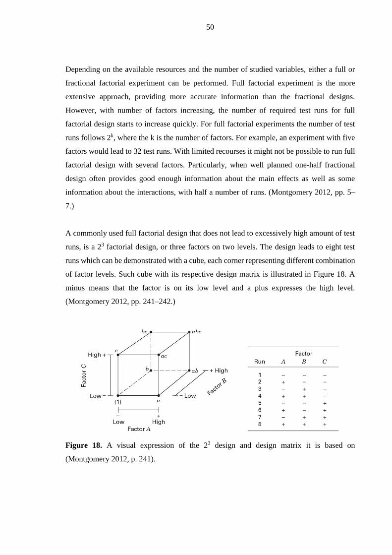
50

Depending on the available resources and the number of studied variables, either a full or

fractional factorial experiment can be performed. Full factorial experiment is the more

extensive approach, providing more accurate information than the fractional designs.

However, with number of factors increasing, the number of required test runs for full

factorial design starts to increase quickly. For full factorial experiments the number of test

runs follows 2k, where the k is the number of factors. For example, an experiment with five

factors would lead to 32 test runs. With limited recourses it might not be possible to run full

factorial design with several factors. Particularly, when well planned one-half fractional

design often provides good enough information about the main effects as well as some

information about the interactions, with half a number of runs. (Montgomery 2012, pp. 5–

7.)

A commonly used full factorial design that does not lead to excessively high amount of test

runs, is a 23 factorial design, or three factors on two levels. The design leads to eight test

runs which can be demonstrated with a cube, each corner representing different combination

of factor levels. Such cube with its respective design matrix is illustrated in Figure 18. A

minus means that the factor is on its low level and a plus expresses the high level.

(Montgomery 2012, pp. 241–242.)

Figure 18. A visual expression of the 23 design and design matrix it is based on


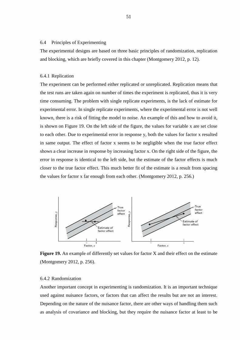
51

6.4 Principles of Experimenting

The experimental designs are based on three basic principles of randomization, replication

and blocking, which are briefly covered in this chapter (Montgomery 2012, p. 12).

6.4.1 Replication

The experiment can be performed either replicated or unreplicated. Replication means that

the test runs are taken again on number of times the experiment is replicated, thus it is very

time consuming. The problem with single replicate experiments, is the lack of estimate for

experimental error. In single replicate experiments, where the experimental error is not well

known, there is a risk of fitting the model to noise. An example of this and how to avoid it,

is shown on Figure 19. On the left side of the figure, the values for variable x are set close

to each other. Due to experimental error in response y, both the values for factor x resulted

in same output. The effect of factor x seems to be negligible when the true factor effect

shows a clear increase in response by increasing factor x. On the right side of the figure, the

error in response is identical to the left side, but the estimate of the factor effects is much

closer to the true factor effect. This much better fit of the estimate is a result from spacing

the values for factor x far enough from each other. (Montgomery 2012, p. 256.)

Figure 19. An example of differently set values for factor X and their effect on the estimate


6.4.2 Randomization

Another important concept in experimenting is randomization. It is an important technique

used against nuisance factors, or factors that can affect the results but are not an interest.

Depending on the nature of the nuisance factor, there are other ways of handling them such

as analysis of covariance and blocking, but they require the nuisance factor at least to be

52

known. If the nuisance is unknown and uncontrolled, or so called noise factor, randomizing

both the allocation of experiment material and the order of test runs spreads its effect

between different runs and results in less biased experiment. (Pyzdek 2003, p. 611;

Montgomery 2012, p. 12, 139.)

6.4.3 Blocking

Blocking is a technique that can eliminate the effects of a nuisance factor, but in order to use

blocking, the nuisance factor must be both known and be controllable. In blocking, test runs

are divided into blocks based on some criterion that is expected to cause variation in results.

For example, if an experiment is run on several days, each day forms its own block.

(Montgomery 2012, p. 12, 219.)

6.5 Planning an Experiment

Before rushing to the experiment, it is important to answer some basic question about the

experiment and the process on which to base the experiment on. For example, the purpose

of the experiment and what does it study and how to collect the data should be clear in mind

before starting. Montgomery (2012, p. 14) has put together the following seven step

guideline for planning, running and analyzing the experiment, which is illustrated in the

Figure 20.

Figure 20. Steps of experimenting.

53

In the phase of recognizing and stating the problem, the questions that the experiment is

aiming to answer, need to be determined. The objectives of the experiment are based on the

questions and thus the type of the experiment, whether it is screening, confirmation or some

other type. (Montgomery 2012, pp. 14–15.)

Selection of response variable, or variables, is often done together with choosing the factors.

It is important that the selected response variables provide desired and usable information

about the process and they are to be selected accordingly. After the response variables are

selected, their measurement needs to be planned and possible issues with it given a thought.

If the measurement system is known to be inaccurate, only large effects can be identified

with confidence. However, if the measurement errors and inaccuracies are considered early

enough in this phase, they can be at least partially compensated by replicating, for example.

(Montgomery 2012, pp. 15–16.)

The factors in experiments can first be divided to potential design factors and to earlier

mentioned nuisance factors. In the phase of choosing factors and their levels, the potential

design factors and its subdivisions of design, held-constant and allowed-to-vary factors, are

determined. The design factors are the group of factors that the experimenter has decided to

study in the experiment. Despite their possible effect on the response, the held-constant

factors are not an interest in the experiment and thus are held at constant level. Allowed-to-

vary factors are often assumed to have small effect on the response, therefore their variation

is often ignored and the randomization is expected to balance their effect. Such factors are

often, for instance, materials. The nuisance factors should be dealt with the earlier explained

ways, depending if the factor is controllable, uncontrollable or noise factor. (Montgomery

2012, p. 16.)

Once the design factors are selected, their levels for the experiment need to be determined.

Usually the selection of the design factor levels is based on previous process knowledge that

the experimenter has. If the process is not well known and the optimal region for response

is unclear, particularly in screening experiments, the spacing between the levels should be

wide. As the process becomes more familiar and the optimal region is better known, the

spacing of the levels can be narrowed down. (Montgomery 2012, pp. 16–17.)

54

After the three pre-experimental planning steps, the experimental design is to be selected.

Selection is very obvious if the pre-experimental phases are done properly as they determine

the number of factors and levels. Moreover, the use of techniques to be equipped such as

replication or blocking is determined in this phase and a tentative model for expressing the

results is selected. (Montgomery 2012, pp. 18–19.)

On the fifth phase, the actual experiment takes place. During the experiment, in addition to

measuring just the output, it is important to monitor the process for any deviation from the

usual. Errors in following the plan or unwanted occurrences in the process without corrective

measures, such as re-running the faulty test run, leads to poor validity. Sometimes it wise to

perform couple trial runs before starting the experiment, particularly in cases where the

process is not well known. By doing so, the chosen factors and their levels can be tested

before starting the experiment and possibly wasting time on badly planned experiment.

(Montgomery 2012, pp. 19–20.)

In data analyzing phase, statistical methods are equipped for interpretation of results and

drawing of conclusions. Graphical methods such as diagrams and plots are a useful and easy

way of expressing the results. However, expressing the results with an additional empirical

model is often helpful, as it has further purposes like estimating the response with desired

parameters. (Montgomery 2012, p. 20.)

Finally, based on the analyzed data, the experimenter comes up with a conclusion and gives

recommendations of actions to follow. To verify the conclusions from the experiment,

confirmation testing should be performed. In confirmation experiments the, the experimenter

verifies that the process runs as is expected. For example, verifies that the estimates from

the empirical model are accurate. (Montgomery 2012, p. 20.)

6.6 Empirical Model

After the experiment, responses with other than the experimented factor values are often an

interest. The empirical model compiled in the data analysis phase, can be used for estimating

the response or optimizing and controlling the process. Fitting a model on an experiment

data is universally called regression model, which has different variants with own their

names and features. (Montgomery 2012, p. 89, 450.)

55

6.6.1 Multiple Linear Regression Model

The multiple linear regression model is a regression model with two or more variables. The

general form of it is (Montgomery 2012, p. 19, 450),

𝑦 = 𝛽0 + 𝛽1𝑥1 + 𝛽2𝑥2 + ⋯ + 𝛽𝑘𝑥𝑘 + 𝜀 (1)

where y is the response variable, β’s are the regression coefficients determined by the

experiment, x’s are the design factors and ε is the experimental error. The parameters as well

as significance of different factors, whether they should be included in the model, can be

calculated manually or as well with various computer software, such as Minitab that is used

in these experiments. (Montgomery 2012, p. 457.)

56

7 DESIGN OF THE GRINDING EXPERIMENTS

To find the optimal tool for grinding, the tool alternatives need to be compared. In order to

do the comparison reliably and accurately, systematic experimentation is needed. For fair

comparison between the tool alternatives, each tool should be performing fairly close to its

optimal level. To determine the optimal region for each of the tools, the parameters are

determined by equipping experimental designs introduced in the previous chapter. The main

interests are material removal rate and its relation to tool wear. Advantages, as well as

disadvantages that surface during the experiments for each tool, are noted and used as

additional means for comparison.

The Montgomery’s seven step guideline for experimenting can be separated into before,

during and after the experiment phases. This chapter introduces the design used in the

grinding experiments, following the phases in the guideline. This chapter does not

concentrate on experiments on individual level but gives an overview of the experiments.

The more detailed individual reports of the experiments are found in the appendices.

7.1 Pre-planning the Experiments

The company has earlier conducted similar experiments to determine the optimal parameters

for the currently used Tyrolit grinding tool. These experiments were studied and used as a

help for planning the experiments for new tool alternatives.

7.1.1 Stating the Problem

The base problem in experiments for each new grinding segment was the same. Apart from

their specification and visual appearance, not much was known about them. Due to such

specific application, the grinding tool manufacturers were not able provide recommendations

for the parameters to start with. Since the tools and their behavior was unfamiliar, the

experiments were started with a broad screening approach. After getting more familiar with

the tools, more accurately targeted experiments were conducted.

57

7.1.2 Design Factors

Based on the theory as well as the results from the earlier experiments, the main factors

contributing to the output are the feed rate and tool speed. Out of the three basic factors that

the machine users adjust on regular basis, the workpiece speed is expected to have only little

effect on the outputs that are measured in the experiments. Nevertheless, for the first

screening experiments, the workpiece speed was included in the design factors. If varying

this or other some factor turns out to be insignificant in the experiment by not having an

effect on the response, the extra runs caused by the factor work as a replicate.

After discovering the significance of fluid delivery for some of the tools, the factor for

workpiece speed was replaced with factor for fluid delivery in some experiments. So, the

feed rate and tool speed were used as design factors in all of the conducted experiments and

the third factor, if needed, varied. The design factors used in each experiment are listed in

the beginning of each experiment in the report sheets. The report sheets for all the tools are

found from the appendices.

Held-constant Factors

Following the principles of DOE, the factors that are not design factors are to be held

constant. Some of the listed factors are more likely to cause variation in response than others,

if not controlled. Such factors are for example grinding time and different factors related to

grinding fluid. Some of the held-constant factors, like guideway lubrication and headstock

pressure, are less likely to affect the output even if they varied. The held-constant factors

were following:

Workpiece surface

Tool surface

Grinding fluid

Grinding time

Machine power output limits

Guideway lubrication

Headstock pressure

Temperature

58

The workpiece surface was ground clear of irregularities if any were witnessed prior to

starting the experiment. This procedure ensures an even start between the first and following

test runs. A similar practice was done for the grinding tool surface, which can often be done

together with clearing the workpiece surface. The tool surface must have total conformity

with the workpiece surface when starting the experiment. If not, the contact area between

the tool and workpiece changes with tool wear until the total conformity is reached.

The used grinding fluid is Henkel Bonderite 49-2 DF, a synthetic cutting fluid emulsified

with water to form 3% concentration. Both the concentration and filtration were untouched

during each experiment. The filters of the central system are changed and cleaned based on

the normal maintenance schedule, possibly causing minor variation between different days

and experiments. The fluid concentration is measured with refractometer on a weekly basis,

and if it differs from the 3% level, it is regulated by either adding water or fluid concentrate.

However, the method causes variation in long run which is covered in the discussion part.

Standard grinding fluid delivery is through four low pressure flood nozzles. Three of the

four nozzles are seen in Figure 21 and are marked with red circles. The additional fluid

nozzles that were added for most of the later experiments, are marked with yellow arrows.

The nozzles remained untouched during experiments, but were adjusted or even removed

between the experiments due to needs of normal production. The angle, direction and

distance of the nozzles were attempted to maintain identical between the experiments, but

the assessment was merely visual, so minor variation occurred unavoidably.

59

Figure 21. The standard fluid delivery setup with two additional higher pressure nozzles.

The material removal is compared in a time unit and thus could be calculated regardless of

the run time of each run. But determining and sticking to certain grinding time is important

for experiment’s validity and setting the run time high enough is crucial for couple reasons.

If the grinding time is too short, the temperature might not reach its peak level. Reaching the

maximum temperature is important as it can be a major rejecting factor. Setting the run time

high enough also ensures that unwanted variation is smaller, for example resulting from

uneven starts between the runs. On the other hand, setting the grinding time too high is waste

of resources. The machine is out of production longer and more workpieces are needed

because more material is removed.

After considering the above mentioned factors, the grinding time was set to 900 seconds, or

15 minutes. It should be enough for the process to reach its maximum temperature, as well

as to balance the effects of uneven starts. The 15 minutes is measured with a manual stop

watch and consists of only the roughing phase. Finishing and spark out phases are not part

of the experiments and are skipped over.

The machine has limiters for spindle power outputs, which can be set how the user wants. If

the power exceeds the upper limit set by the user, the machine stops the feed motion. The

60

tool spindle continues to rotate with the set speed and once the lower limit of the power is

reached, the feed motion starts again. For the experiments, the power output levels were

increased from the usual level, since the power limiter was not wanted to be affecting the

output. Based on previous knowledge, high power output with currently used Tyrolit

segments usually leads to burn marks on the workpiece surface. Since the behavior of each

grinding tool was unknown, instead of using the power limiter to prevent burn marks, the

surface of the ball was visually examined after each run. The upper limit for the tool spindle

power output for the experiment was set to 75% and the lower limit to 70%. The total power

output of the machine was set to 90%.

The usual power limit for tool spindle for recognizing contact, two percent, lead the machine

to assume that the tool had solid contact with workpiece even if it was not one. The

percentage expresses how much the power output needs to increase from an idle level, when

the machine is looking for a contact to workpiece. Once the limit is reached, the machine

accelerates the spindle to desired speed and starts the feed motion. In the first experiments

for example with Theleico, the machine assumed it had a contact and started feed motion,

after which it took several minutes for power to reach the level of showing a solid contact.

After few experiments with uneven contacts between the runs, the limit was decided to be

set at 10%. Setting the limit high enough makes sure that the start for each run is even and

the tool is actually fed into the workpiece for the whole 15 minutes.

Guideway lubrication is very unlikely to cause error to test results, but just in case a

lubrication run on the machine is performed on morning of every test day. Headstock

pressure is also rather insignificant factor, especially since the workpiece is fixed in place

from splines. As a precaution, the headstock pressure is set to 26 bar for each test.

Even though the grinding fluid temperature is attempted to retain constant during the

experiment, it is one of the factors that is difficult hold constant in practice in production

environment. The fluid temperature, is cooled down to 17 °C in the central fluid system

throughout all of the experiments. However, the incoming fluid temperature is somewhat

higher and hard to control accurately. The exact temperature of incoming grinding fluid

depends on the ambient temperature, as well as the use of the other machines connected to

61

the central system. Small changes in grinding fluid temperature are not likely to effect the

response, but since its effects are not well known, it poses as a possible nuisance factor.

The machine temperature likely has no effect on the response factors and was not observed

or measured in the experiments. Regardless, the machine was run before a start of each

experiment, to ensure fairly similar temperature between the first and following runs.

The temperature of the workpiece during the grinding is difficult to measure or control, but

being an important quality related factor, the ball temperature cannot be ignored. Since it is

not possible to hold the ball temperature constant, the workpiece temperature is evaluated

with human senses instead of setting a specific limit for the temperature. The main limiting

and rejecting factors are burn marks on the workpiece surface and fluid vaporizing from the

surface of the workpiece after run. Like the machine power output, the workpiece

temperature and is not a factor that is held constant, instead both are only limiting factors

and in well prepared experiments these limits should not be met. In most cases, to make sure

that the parameters are within usable area, they were trialed before the start of the

experiment.

Nuisance Factors

The known nuisance factors in the experiments are tool bending and variation in fluid

delivery, temperature and concentration. Other nuisance factors possibly exist, but their

sources or effects on the response are not known. From the known factors, tool bending has

the largest effect on single experiment as the other nuisance factors do not vary as much

within short periods of time and are more of a nuisance between different experiments.

Following the laws of mechanics, the longer tool means higher torque that leads to more

bending. So, the bend is at its most when the tool is new and on its maximum length. As the

tool wears, the lever arm shortens, resulting the segment to hold its form better. The bending

of the tool results in power losses, as some of the forces intended to grinding process go to

tool bending. Although the cause and effect of tool bending are known, the extent of its effect

to response is not known and would require experiments of its own. To deal with tool

bending in the experiments, randomization and replication balance its effects between the

runs.

62

Before the first experiments where the fluid delivery was varied, its magnitude as a possible

nuisance factor was not realized. As mentioned earlier, the fluid delivery was untouched

during the experiment and thus it remained about the same within an experiment, not causing

significant variation. But between the experiments, for example screening experiment and

confirmation runs, the fluid delivery can cause significant variation. The extent and direction

of the variation it causes is not known before the experiment.

Fluid temperature is likely not a major nuisance factor as it seemed to vary only a little in

the experiments. However, its effects have not been experimented and the measuring method

used in the experiment does not tell the temperature of incoming fluid reliably. The effect of

fluid content and concentration is not known, but poses as possible nuisance factor over

longer period of time.

7.1.3 Response Variables

As stated in the chapter 2.1.1 Grinding parameters, the measured outputs in the experiment

were the change in workpiece diameter and the change in tool length. These two outputs

were used to calculate more accurate and applicable responses, material removal rate and

grinding ratio.

The change in workpiece diameter should not be used as a response variable, since it does

not consider in the changes in ball volume. In other words, it does not take into account that

grinding a millimeter off from a small sphere is not the same as grinding a millimeter off

from a bigger sphere. To factor in this difference, a diameter before and after each run are

used to calculate the sphere volume, however this is not accurate on its own. Since the valve

ball is not a complete sphere and the ball is ground with feed motion only from one direction,

the geometry of the ball changes as it is ground, causing the ball so to say, flatten. The

flowport length, marked with the red arrow in Figure 22, decreases but its diameter remains

the same. So, the height of the spherical cap removed from the ends of the flowport changes

as well, but the diameter remains the same. And the height of the spherical cap removed

from the bearing sides remains the same, but its diameter, marked with the yellow arrow,

changes.

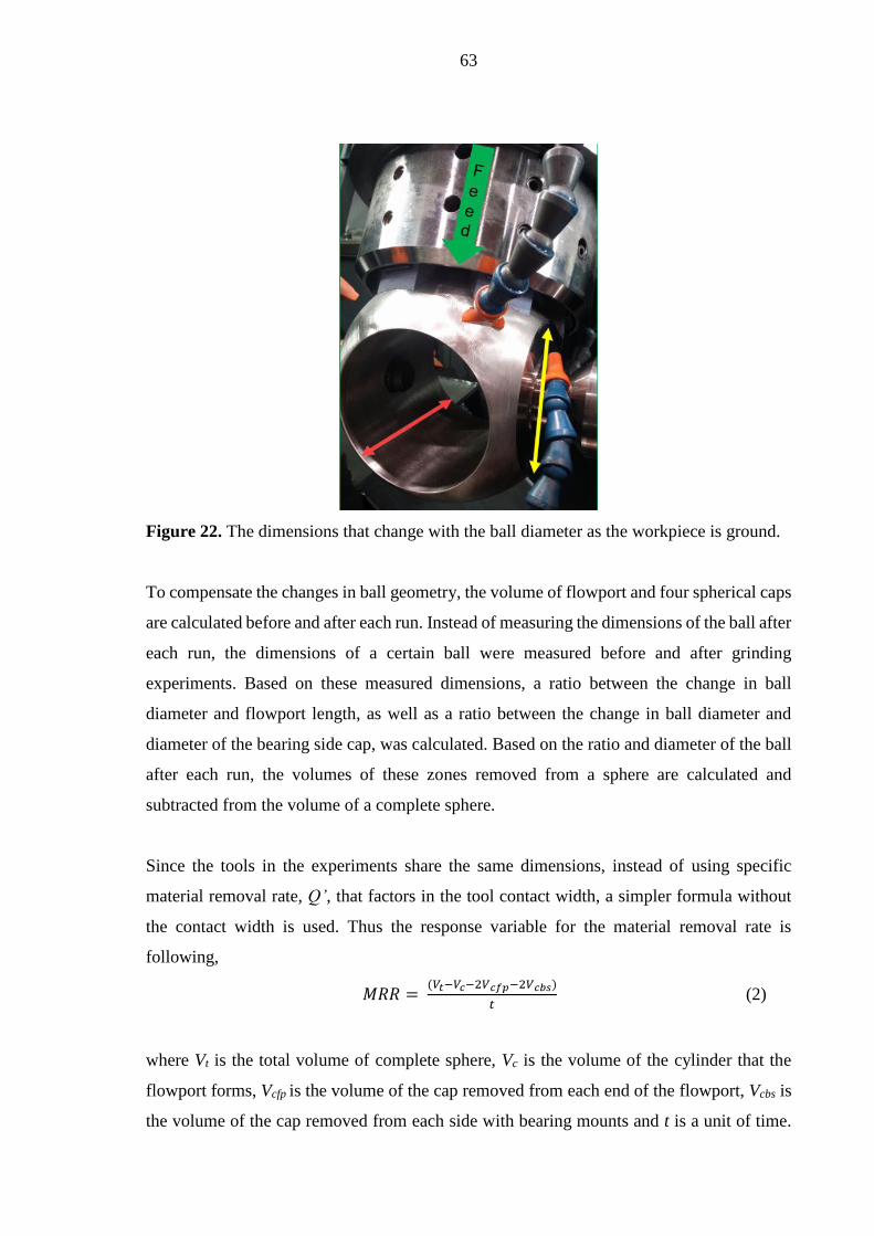
63

Figure 22. The dimensions that change with the ball diameter as the workpiece is ground.

To compensate the changes in ball geometry, the volume of flowport and four spherical caps

are calculated before and after each run. Instead of measuring the dimensions of the ball after

each run, the dimensions of a certain ball were measured before and after grinding

experiments. Based on these measured dimensions, a ratio between the change in ball

diameter and flowport length, as well as a ratio between the change in ball diameter and

diameter of the bearing side cap, was calculated. Based on the ratio and diameter of the ball

after each run, the volumes of these zones removed from a sphere are calculated and

subtracted from the volume of a complete sphere.

Since the tools in the experiments share the same dimensions, instead of using specific

material removal rate, Q’, that factors in the tool contact width, a simpler formula without

the contact width is used. Thus the response variable for the material removal rate is

following,

𝑀𝑅𝑅 = (𝑉𝑡−𝑉𝑐−2𝑉𝑐𝑓𝑝−2𝑉𝑐𝑏𝑠)

𝑡 (2)

where Vt is the total volume of complete sphere, Vc is the volume of the cylinder that the

flowport forms, Vcfp is the volume of the cap removed from each end of the flowport, Vcbs is

the volume of the cap removed from each side with bearing mounts and t is a unit of time.

64

The used dimensions were in millimeters and the used time unit was a minute, making the

unit of equation mm3/min.

As stated above, the experimented tools share the same dimensions. Since the dimensions

are the same, the tool wear of each run could be simply expressed by comparing the tool

lengths before and after the run. But, using G-ratio to evaluate the tool wear is much better

option since it relates the wear to material removal. The volume lost from single segment

was calculated by multiplying the area of front face of the segment with difference in tool

length before and after the run. To get the total volume needed to calculate G-ratio, the

volume lost from a single segment was multiplied with number of segments in the grinding

head, so by six in the experiments. Finally, the total volume lost is divided by grinding time,

15 minutes, to get the same unit as in MRR.

In addition to two response variables, data was gathered about few factors that are not

constant during the experiments, fluid temperature and machine power output. The factors

were not a particular interest and further analyzed, but were monitored because they could

give away something about the process. Measuring of the fluid temperature took place about

half way in each test run and was measured from a collector tank with handheld infrared

thermometer. The value for power output of the tool spindle was written down about every

two minutes throughout each test run.

7.1.4 Choosing the Designs

Experimentation of each tool alternative was started with full factorial design. Since the

factors were determined in the pre-experimental planning, the design came to be 23-form,

resulting in eight runs in each experiment. Most of the following experiments were

conducted with full factorial designs, with either the 23 or 22 -form. Design matrixes for each

of the experiments are found in the report sheets in the appendices I through VI.

For confirmation runs, few combinations in- and outside of the experimented range were

hand selected to test the fit of the model. The test matrixes for confirmation runs as well as

evaluations of the models are found from the same report sheets as the above mentioned

screening runs.

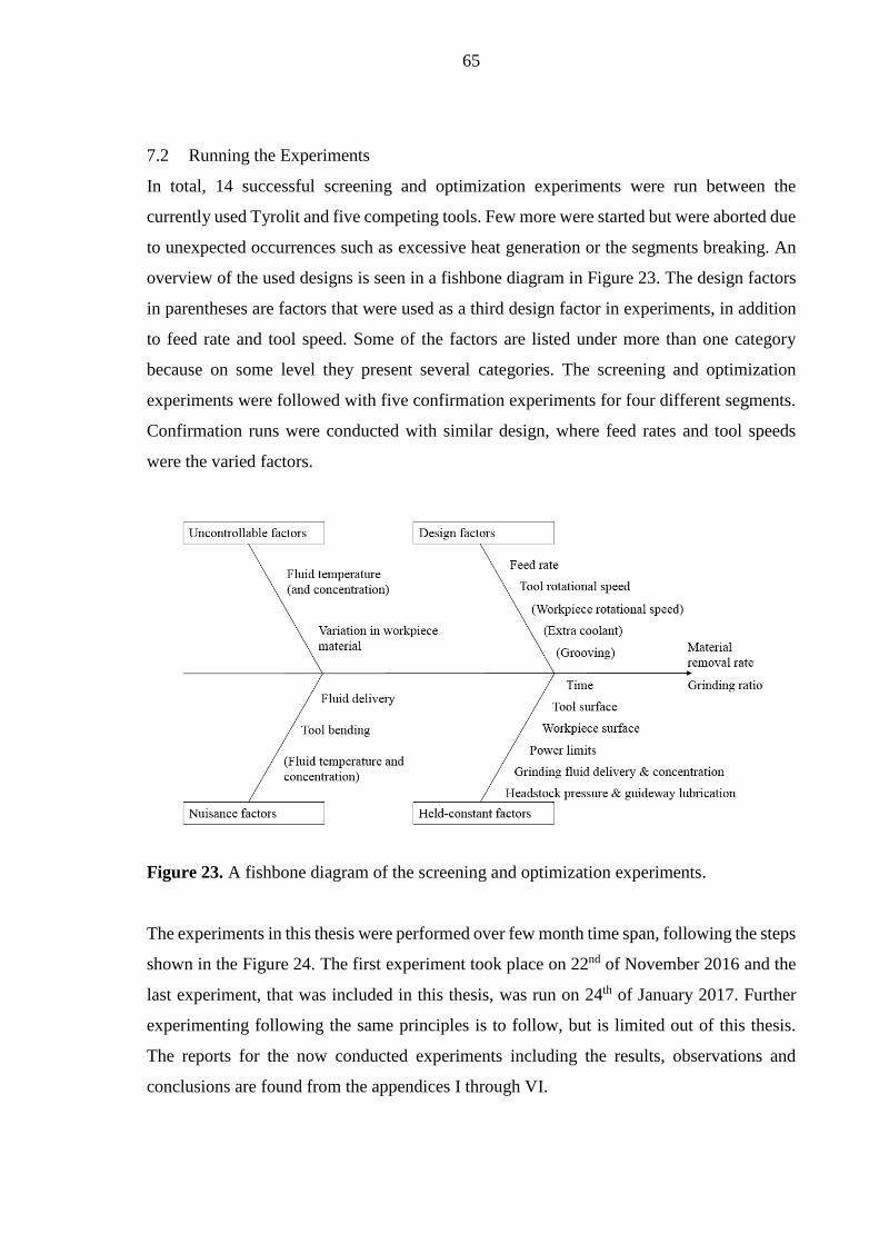
65

7.2 Running the Experiments

In total, 14 successful screening and optimization experiments were run between the

currently used Tyrolit and five competing tools. Few more were started but were aborted due

to unexpected occurrences such as excessive heat generation or the segments breaking. An

overview of the used designs is seen in a fishbone diagram in Figure 23. The design factors

in parentheses are factors that were used as a third design factor in experiments, in addition

to feed rate and tool speed. Some of the factors are listed under more than one category

because on some level they present several categories. The screening and optimization

experiments were followed with five confirmation experiments for four different segments.

Confirmation runs were conducted with similar design, where feed rates and tool speeds

were the varied factors.

Figure 23. A fishbone diagram of the screening and optimization experiments.

The experiments in this thesis were performed over few month time span, following the steps

shown in the Figure 24. The first experiment took place on 22nd of November 2016 and the

last experiment, that was included in this thesis, was run on 24th of January 2017. Further

experimenting following the same principles is to follow, but is limited out of this thesis.

The reports for the now conducted experiments including the results, observations and

conclusions are found from the appendices I through VI.

66

Figure 24. Progress of the grinding experiments.

7.2.1 Test Machine

The platform for testing is a Plantool BGM 600 ball grinding machine with spindle power

of 22 kW. The machine is used for grinding spherical surfaces of different shutter elements

used in valves, up to around 24 inch, or 600 mm in diameter. (Danobat 2017a.) Such shutter

elements may be spherical segments, valve balls with a stem or stemless valve balls. Metso

uses the machine to grind above mentioned shutter elements mainly from flowport sizes of

4 to 12 inches, or respective ball diameters of 165 to 470 mm.

The machine is one of the more modern grinding machines in the factory, so it is a good

platform for experimentation. The parameters are easily changeable for testing purposes and

the machine gives out more information about the grinding process than the older machines.

For example, the spindle power outputs and their changes are displayed on the control panel,

which can give out certain tool behavior such as excessive tool fracturing. The machine also

measures the ball diameter with a built-in measurement probe and gives out the tool length,

based on which the material removal rate and tool wear is calculated.

67

The workpiece is mounted to workpiece spindle from bearing mounts and is locked in place

from splines. The ball rotates around the same center as it does in operation of valve and its

speed can be adjusted between 1 and 500 RPM. (Puska 2013.)

As seen in the Figure 25, the grinding head consists of grinding segments on the grinding

head periphery, essentially forming a cup wheel with gaps. The number of segments in the

grinding head depends on the workpiece size; larger workpiece means more segments. The

grinding head for the ball size of six inches, consists of six segments. The grinding head with

segments is fed towards the center axis of the workpiece with adjustable speed of 0.001 to 2

mm/minute. The rotation speed of the tool spindle can be adjusted between 3 and 4500 RPM.

(Puska 2013.)

Figure 25. The grinding head type used in the experiments. In the particular experiment, the

effect of grooving the segments was experimented. Two of the grooves are marked with the

red arrows.

7.2.2 Test Workpiece

The inputs in the experiments, the workpieces, were valve balls made of AISI 316 grade

steel. The experiments were decided to be conducted with valve balls with flowport size of

six inches, since they represent about the midpoint of the most commonly ground valve ball

range. Use of six inch balls keeps the experimentation costs reasonable when compared to

larger ball sizes. The tool costs are lower since the larger grinding heads require more

segments. The material costs also remain lower, since on start of an experiment the ball is

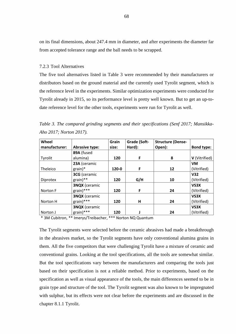
68

on its final dimensions, about 247.4 mm in diameter, and after experiments the diameter far

from accepted tolerance range and the ball needs to be scrapped.

7.2.3 Tool Alternatives

The five tool alternatives listed in Table 3 were recommended by their manufacturers or

distributors based on the ground material and the currently used Tyrolit segment, which is

the reference level in the experiments. Similar optimization experiments were conducted for

Tyrolit already in 2015, so its performance level is pretty well known. But to get an up-to-

date reference level for the other tools, experiments were run for Tyrolit as well.

Table 3. The compared grinding segments and their specifications (Senf 2017; Mansikka-

Aho 2017; Norton 2017).

The Tyrolit segments were selected before the ceramic abrasives had made a breakthrough

in the abrasives market, so the Tyrolit segments have only conventional alumina grains in

them. All the five competitors that were challenging Tyrolit have a mixture of ceramic and

conventional grains. Looking at the tool specifications, all the tools are somewhat similar.

But the tool specifications vary between the manufacturers and comparing the tools just

based on their specification is not a reliable method. Prior to experiments, based on the

specification as well as visual appearance of the tools, the main differences seemed to be in

grain type and structure of the tool. The Tyrolit segment was also known to be impregnated

with sulphur, but its effects were not clear before the experiments and are discussed in the

chapter 8.1.1 Tyrolit.

Wheel manufacturer: Abrasive type:

Grain size:

Grade (Soft-Hard):

Structure (Dense-Open): Bond type:

Tyrolit 89A (fused alumina) 120 F 8 V (Vitrified)

Theleico 23A (ceramic grain)* 120-0 F 12

VM (Vitrified)

Diprotex 3CG (ceramic grain)** 120 G/H 10

V32 (Vitrified)

Norton F 3NQX (ceramic grain)*** 120 F 24

VS3X (Vitrified)

Norton H 3NQX (ceramic grain)*** 120 H 24

VS3X (Vitrified)

Norton J 3NQX (ceramic grain)*** 120 J 24

VS3X (Vitrified)

* 3M Cubitron, ** Imerys/Treibacher, *** Norton NQ Quantum

69

As stated above, all of the five alternatives have ceramic grains mixed with conventional

fused alumina grains. The exact proportions of grain types in Theleico and Diprotex

segments are not known and Norton tools are known to have 30% ceramic grain (Norton

2017). In addition to possible differences in grain type content, the properties of ceramic

grains from different manufacturers are known to have minor differences. The 3M Cubitron,

that is used in Theleico’s segment, is stated to be less tough and in certain applications easier

to apply than Saint-Gobain’s SG grain. (Badger 2011, p 6.) On the other hand, SG’s higher

hardness of 21GPa versus Cubitron’s 19GPa can provide a longer tool life in right

application (Marinescu et al. 2007, p. 81).

More recently Saint-Gobain has introduced the Quantum grain, which is slightly modified

version of the SG family. Quantum grain has similar submicron crystallite size and hardness

as the SG but the micro-fracturing properties are different. (Jackson et al. 2013, pp. 36–37.)

The experimented segments from Norton equip the Quantum grain. The ceramic abrasive

that is used in the Diprotex’s segment is manufactured by Imerys but the grain’s properties

in comparison to two other grains are not known.

7.3 Data Analysis

Data analysis was performed using Minitab 16 software and DOE and regression analysis

tools it includes. Each screening and optimization experiment was analyzed to discover the

significant variables and more importantly, their effect on the response. Generally speaking,

there were no surprises in significant variables, and the feed rate with tool speed determines

the outputs to a high extent, just like the theory entails.

The main objective in data analysis was to build models for outputs of different tools. In

most cases the model consisted of feed rate, tool speed and possibly their interaction. In few

of the experiments, some of the variables did not show up as statistically significant or the

results were inconsistent with the other experiments. In these cases, few competing models

were built and their fit was tested in the confirmation experiments. After all the goal of the

experiments was to find out the practical limit for material removal rate of each tool, not to

build mathematically perfect models.

70

8 DISCUSSION

This chapter first covers the final results of each of the tool alternatives and discusses about

the tool specific observations and findings. Later on, in the chapter 8.2 Observations and

Findings on the General process, results are discussed on more general level, focusing on

other than tool related factors found in the experiments.

8.1 Key Results and Tool Evaluations

Evaluation of each tool is mainly based on the maximum outputs it reached in the

experiments. Other than numerical evaluation of the two responses, material removal rate

and grinding ratio, if the tool was noted to have any advantages or disadvantages in the

experiment, they are discussed.

The final values for outputs are listed in Table 4. The listed values for material removal rates

are not necessarily the maximum values that were achieved in the experiments nor the

absolute maximum that the tool can reach, but the maximum values that were reached in the

experiments while considering quality factors. The following material removal rates did not

lead to burn marks or the workpiece temperature raising to a level that the machine user or

experimenter found problematic.

Table 4. The overall results and their respective parameters.

Feed rate (mm/min)

Tool speed (RPM)

Additional fluid

delivery

Material removal rate (mm3/min)

G-ratio (MRR/Tool

wear)

Tyrolit

89A120F8AV217T3 0.18 2000 No 5281 5.90

Theleico

23A120-0F12VM4200 0.16 3000 Yes 3464 4.74

Norton

3NQX120F24VS3X 0.2 2000 Yes 3397 3.04

3NQX120H24VS3X 0.15 1000 Yes 1449 1.55

Diprotex

3CG120G/H10V32 0.16 3000 Yes 3301 3.87

71

Since the ceramic grain was supposed to lead to improved process, at the very least through

lowered tool wear and thus increased G-ratio, question is: why did this not happen. In fact,

why did the process efficiency go down by both measures. It seems that between the five

alternative tools and Tyrolit, the performance of the tool was not dependent on the type of

grain. Instead, the performance depended on the other factors of the specification and

whether they were suitable. To determine these differences and their effects, the differences

between Tyrolit and other segments need to be looked closer at.

8.1.1 Tyrolit

Despite not having the more novel ceramic grain, couple decades ago selected Tyrolit

segment still achieved the highest material removal with highest G-ratio. So, the key to its

success must be in other factors than the abrasive itself.

Main Differences to Other Segments

Looking at the specification, Tyrolit is not that much different from the other segments. The

main difference seems to be in structure, but because of the differences between

manufacturers, this cannot be stated with absolute confidence. However, the noticeably

different appearance and larger mass of the Tyrolit segments support the hypothesis, and

based on these it is fair to say that Tyrolit likely has tighter packing of grains. Tighter packing

of grains means more kinematic cutting edges and thus is one of the explanations to Tyrolit’s

higher cutting rate. This should also mean more heat generation, but with Tyrolit segments

the heat generation seems to be in control.

Another difference, the Tyrolit’s sulphur treatment, is not directly noticeable from the

specification. However, this difference is a major one and likely the reason behind Tyrolit’s

performance. Lubrication from the sulphur impregnation helps in keeping the friction low,

that keeps the temperature in the contact zone in control. The process runs well without extra

coolant delivered to contact zone and the sulphur treatment seems to provide enough

lubrication.

The key to Tyrolit’s performance is likely the combination of both the higher density and

sulphur impregnation. Higher density means more cutting edges resulting in more heat

generation, but the lubrication coming from the sulphur impregnation keeps the heat

72

generation in control and makes the use of higher density possible. This hypothesis is to be

tested later as a follow-up to these experiments, by experimenting similar segment without

sulphur impregnation.

The Effects of Extra Fluid Delivery with Tyrolit Segment

When experimenting the effect of additional fluid delivery with Tyrolit segment, the

response variables were expected to increase, just like in the experiments with other

segments. But instead, an interesting observation was made of the extra fluid delivery

lowering the responses. The reason behind this is not clear and would require further studies

and experimenting. Few hypotheses are however made based on concepts found from

literature.

The most likely cause is hydroplaning that is linked particularly to dense wheels. The

structure of Tyrolit’s segment is dense in comparison to other experimented segments, which

the sulphur impregnation further incites. In hydroplaning, or hydrodynamic lift, the fluid

film between the tool and the workpiece can cause the tool to hydroplane, particularly in

systems where stiffness is known to be a problem (Irani, Bauer & Warkentin 2005, pp. 1700–

1701). Taking into account the dense structure of the segment and their tendency to bend,

this is likely at least part of the reason for weakened results with extra grinding fluid. The

effect of adding the grinding fluid on Tyrolit’s performance is seen in the Figure 26.

Figure 26. Material removal rates from the experiment determining the effects of extra

coolant nozzles with Tyrolit segments.

0

1000

2000

3000

4000

5000

6000

0,12/1600 0,18/1600 0,12/2000 0,18/2000

Mat

eria

l rem

ova

l rat

e

The effect of extra coolant on Tyrolit

Without extra coolant With extra coolant

73

In the experiment to determine the effect of extra fluid delivery, the run order was not

randomized to keep the fluid delivery as constant as possible between the runs. By not

randomizing the run order, the risk of biased experiment increases. As seen from the

experiment report in the Appendix I, 2, the runs without extra coolant were taken first and

the runs with extra coolant formed the latter half of the experiment. Since the tool bending

is known to be at its maximum in the beginning of the test and decrease with tool wear, it is

a nuisance factor that can distort the results and impair the validity of the experiment.

The runs without the coolant were taken first, when the effect of bending is at its most, and

still resulted in higher output. It proves that the bending was not the direct cause for the

decreased output with the extra fluid. Looking at the last two runs of the experiment, so the

red columns on the right side of the Figure 26, it can be noticed that the outputs between

runs with and without the fluid are getting closer to each other. Keeping in mind that the

hydroplaning was stated to be a problem in systems where stiffness is a problem, the

responses getting closer to each other could be explained with tool length and its effect on

the stiffness of the system. On runs seven and eight, the tool is worn to a point that the

bending hardly occurs anymore and the fluid film between the tool and workpiece does not

lead to hydroplaning to a same extent as with longer tool. So, based on this theory the

weakened output is a result of bending, caused by the additional fluid.

Other possible theory is related to chemical reactions on the workpiece surface. Some

chemical substances are known to compete on the workpiece surface, weakening each

other’s effects. Whether the additives in the grinding fluid interfere with the sulphur additive

on the grinding tool is not known and therefore remains as a possible factor for impairing

the results. (Meyer & Wagner 2016, p. 315.)

Follow-up to Experiments with Tyrolit

To verify the hypothesis of the benefits originating from sulphur, identical segments without

sulphur impregnation have been ordered. If the hypothesis is correct, grinding with similar

parameters without additional coolant nozzles should not be possible because of the heat

generation resulting from the lack of lubrication. To experiment the direct effect of sulphur

for material removal, the segment without treatment is experimented with certain parameters

that the grinding is possible and seems to work with. This is followed with an experiment

74

with similar parameters and sulphur treated segment. If the responses are better with sulphur

treated segment, the hypothesis can be verified.

In addition to experimenting the significance of sulphur, segment with ceramic abrasive and

sulphur impregnation has been ordered from Tyrolit and is to be experimented. Being similar

to currently used segment from rest of the specification, but equipping the more novel grain,

the segment holds high potential to lead to improvement.

Based on the hypothesis of advantages of sulphur working as a solid lubricant, another solid

lubricant is to be experimented as an alternative to using sulphur. Similar segment to sulphur

impregnated one has been ordered from Tyrolit, but instead of sulphur impregnation, the

segment is impregnated with wax. If the wax impregnated segment matches the performance

of the sulphur treated, it is considered as a replacement for the sulphur impregnated segment

because of the health and environmental problems related to sulphur.

Grooving the segments’ contact surfaces was experimented with Theleico, for which it did

not result in improvement. Since the Tyrolit segment is likely suffering from hydroplaning

when the additional fluid is used, grooving could be beneficial. It could reduce the segment’s

tendency to hydroplane, in similar manner as in threads on car tires. If the grooves would

work on alleviating the hydroplaning, the fluid could be used without drawbacks and the

fluid would lower the contact zone temperature. Lower temperature would either reduce the

time needed for finishing and spark out phases through better geometrical integrity after

roughing or it would allow increase in material removal rate. This hypothesis of advantages

of grooves on Tyrolit’s segment would have to be confirmed with an experiment.

8.1.2 Theleico

Theleico turned out to be the best contender for the current Tyrolit segment. After

discovering the benefits of the extra grinding fluid delivered to the contact zone, the material

removal rate grew about 2.5 times over and the G-ratio increased even more. Without the

additional coolant nozzles, the segment was clearly lacking lubrication and wearing out

really quick.

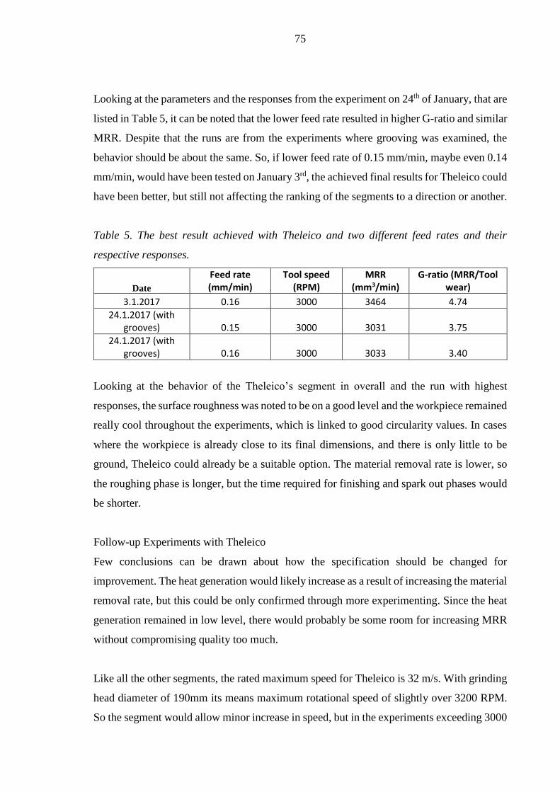
75

Looking at the parameters and the responses from the experiment on 24th of January, that are

listed in Table 5, it can be noted that the lower feed rate resulted in higher G-ratio and similar

MRR. Despite that the runs are from the experiments where grooving was examined, the

behavior should be about the same. So, if lower feed rate of 0.15 mm/min, maybe even 0.14

mm/min, would have been tested on January 3rd, the achieved final results for Theleico could

have been better, but still not affecting the ranking of the segments to a direction or another.

Table 5. The best result achieved with Theleico and two different feed rates and their

respective responses.

Date

Feed rate (mm/min)

Tool speed (RPM)

MRR (mm3/min)

G-ratio (MRR/Tool wear)

3.1.2017 0.16 3000 3464 4.74

24.1.2017 (with grooves) 0.15 3000 3031 3.75

24.1.2017 (with grooves) 0.16 3000 3033 3.40

Looking at the behavior of the Theleico’s segment in overall and the run with highest

responses, the surface roughness was noted to be on a good level and the workpiece remained

really cool throughout the experiments, which is linked to good circularity values. In cases

where the workpiece is already close to its final dimensions, and there is only little to be

ground, Theleico could already be a suitable option. The material removal rate is lower, so

the roughing phase is longer, but the time required for finishing and spark out phases would

be shorter.

Follow-up Experiments with Theleico

Few conclusions can be drawn about how the specification should be changed for

improvement. The heat generation would likely increase as a result of increasing the material

removal rate, but this could be only confirmed through more experimenting. Since the heat

generation remained in low level, there would probably be some room for increasing MRR

without compromising quality too much.

Like all the other segments, the rated maximum speed for Theleico is 32 m/s. With grinding

head diameter of 190mm its means maximum rotational speed of slightly over 3200 RPM.

So the segment would allow minor increase in speed, but in the experiments exceeding 3000

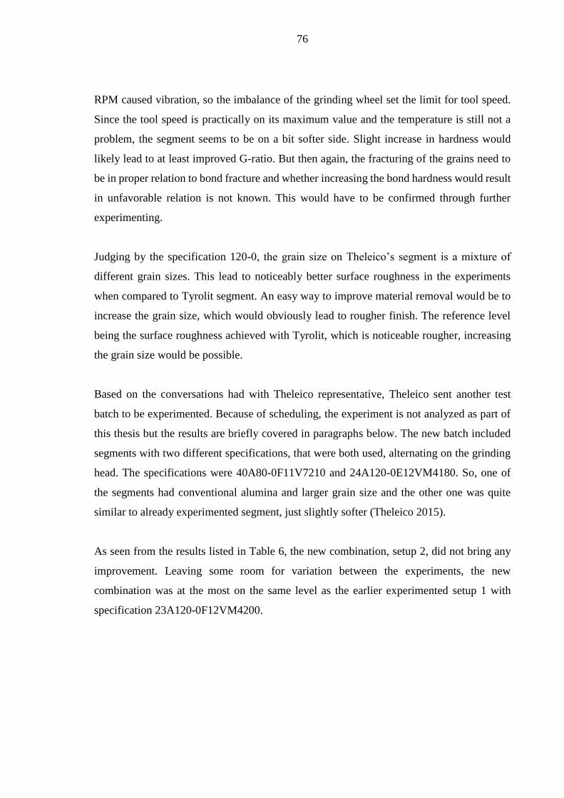
76

RPM caused vibration, so the imbalance of the grinding wheel set the limit for tool speed.

Since the tool speed is practically on its maximum value and the temperature is still not a

problem, the segment seems to be on a bit softer side. Slight increase in hardness would

likely lead to at least improved G-ratio. But then again, the fracturing of the grains need to

be in proper relation to bond fracture and whether increasing the bond hardness would result

in unfavorable relation is not known. This would have to be confirmed through further

experimenting.

Judging by the specification 120-0, the grain size on Theleico’s segment is a mixture of

different grain sizes. This lead to noticeably better surface roughness in the experiments

when compared to Tyrolit segment. An easy way to improve material removal would be to

increase the grain size, which would obviously lead to rougher finish. The reference level

being the surface roughness achieved with Tyrolit, which is noticeable rougher, increasing

the grain size would be possible.

Based on the conversations had with Theleico representative, Theleico sent another test

batch to be experimented. Because of scheduling, the experiment is not analyzed as part of

this thesis but the results are briefly covered in paragraphs below. The new batch included

segments with two different specifications, that were both used, alternating on the grinding

head. The specifications were 40A80-0F11V7210 and 24A120-0E12VM4180. So, one of

the segments had conventional alumina and larger grain size and the other one was quite

similar to already experimented segment, just slightly softer (Theleico 2015).

As seen from the results listed in Table 6, the new combination, setup 2, did not bring any

improvement. Leaving some room for variation between the experiments, the new

combination was at the most on the same level as the earlier experimented setup 1 with

specification 23A120-0F12VM4200.

77

Table 6. Results from the latest experiments with new Theleico segments.

Feed rate (mm/min)

Tool speed (RPM)

Material removal

rate (mm3/min)

G-ratio (MRR/Tool

wear) Specification

Tyrolit

89A120F8AV217T3 0.18 2000 5281 5.9

Theleico

23A120-0F12VM4200

0.16 3000 3464 4.74

SETUP 1

24A120-0E12VM4180 + 40A80-0F11V7210 0.14 3100 2502 3.32

SETUP 2 0.16 3100 3034 3.51

0.18 3100 3143 3.19

23A120-0F12VM4200 + 40A80-0F11V7210 0.16 3100 4408 5.47

SETUP 3 0.18 3100 3776 3.9

With the combination of new specifications, the workpiece was noticed to remain as cool as

in the earlier experiments with the setup 1. Since increasing the hardness was earlier

hypothesized to lead to improvement and slight increase in temperature would not be a

problem, the new harder segment was decided to be experimented by alternating it on the

grinding head with the first specification 23A120-0F12VM4200, which is harder than the

now delivered 24A120-0E12VM4180.

This setup 3 resulted in two of the highest responses for material removal rate, excluding

Tyrolit’s results. As expected, the temperature increased from the setup 2, but only to about

similar level as with Tyrolit. Lowering the feed rate from 0.18 to 0.16 mm/min shows a trend

of increasing responses towards lower feed rate. If lowering the feed rate to 0.14 mm/min is

beneficial, would have to be experimented to confirm its effects. But looking at the segment

surface after the run with 0.16 mm/min, the bottom half of the segment with conventional

grain was quite badly glazed, and lowering the feed rate would likely lead to less fracturing

and thus worse glazing and temperature increase.

The newly found results and observations were passed to Theleico and possible further

changes to specifications are being discussed.

78

8.1.3 Diprotex

Diprotex segment was quite similar to Theleico’s segment from the visual appearance as

well as behavior and results. In the first experiments without additional coolant nozzles, the

segment was fracturing excessively and the responses were poor. After the introduction of

the additional coolant to the process, the excessive fracturing stopped and the responses

increased by an order of a magnitude, but are still far from the Tyrolit’s level.

As seen from the results in Table 7, much like with Theleico, slightly lowering the feed rate

from 0.16 mm/min could possibly lead to minor increase in responses. Judging from the

surface of the segment after the run however, lowering the feed rate would cause the surface

of the segment to glaze even more and increase temperature. Even if lowering the feed rate

would result in higher feed rate or increased G-ratio, it would not match the Tyrolit’s

performance.

Table 7. Two of the best runs with Diprotex segment.

Feed rate (mm/min) Tool speed (RPM) MRR (mm3/min) G-ratio (MRR/Tool wear)

0.16 3000 3301 3.87

0.18 3000 3160 3.04

The conclusions from the experiments are similar to ones drawn from experiments with

Theleico. But with Diprotex, the route of changing the segment specification is different.

Based on the results and observations made on the experiments conducted with both

Diprotex and Tyrolit, as a follow-up to Diprotex experiments, new specification with sulphur

impregnation is ordered. Once the new segment arrives, it is experimented in the similar way

as the other segments in this thesis.

8.1.4 Norton Grades F, H & J

Of the three segments from Norton, the softest one with grade F turned out to be the most

suitable. Like other segments, excluding Tyrolit, Norton segments benefitted from additional

coolant nozzles. But the behavior of Norton’s segments before adding the fluid nozzles was

very different from Theleico or Diprotex, which hints towards very different bond

hardnesses.

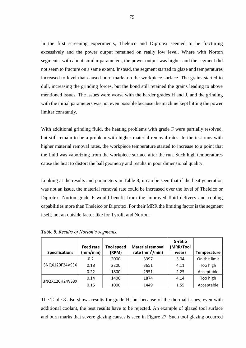
79

In the first screening experiments, Theleico and Diprotex seemed to be fracturing

excessively and the power output remained on really low level. Where with Norton

segments, with about similar parameters, the power output was higher and the segment did

not seem to fracture on a same extent. Instead, the segment started to glaze and temperatures

increased to level that caused burn marks on the workpiece surface. The grains started to

dull, increasing the grinding forces, but the bond still retained the grains leading to above

mentioned issues. The issues were worse with the harder grades H and J, and the grinding

with the initial parameters was not even possible because the machine kept hitting the power

limiter constantly.

With additional grinding fluid, the heating problems with grade F were partially resolved,

but still remain to be a problem with higher material removal rates. In the test runs with

higher material removal rates, the workpiece temperature started to increase to a point that

the fluid was vaporizing from the workpiece surface after the run. Such high temperatures

cause the heat to distort the ball geometry and results in poor dimensional quality.

Looking at the results and parameters in Table 8, it can be seen that if the heat generation

was not an issue, the material removal rate could be increased over the level of Theleico or

Diprotex. Norton grade F would benefit from the improved fluid delivery and cooling

capabilities more than Theleico or Diprotex. For their MRR the limiting factor is the segment

itself, not an outside factor like for Tyrolit and Norton.

Table 8. Results of Norton’s segments.

Specification: Feed rate (mm/min)

Tool speed (RPM)

Material removal rate (mm3/min)

G-ratio (MRR/Tool

wear) Temperature

3NQX120F24VS3X

0.2 2000 3397 3.04 On the limit

0.18 2200 3651 4.11 Too high

0.22 1800 2951 2.25 Acceptable

3NQX120H24VS3X 0.14 1400 1874 4.14 Too high

0.15 1000 1449 1.55 Acceptable

The Table 8 also shows results for grade H, but because of the thermal issues, even with

additional coolant, the best results have to be rejected. An example of glazed tool surface

and burn marks that severe glazing causes is seen in Figure 27. Such tool glazing occurred

80

throughout the experiment and as expected, with lower feed rate and higher tool speed it was

worst. The burn marks seen on right side of the figure, was more extensive when the ball

was rotating slower, however occurred with higher workpiece speed as well.

Figure 27. Glazed tool surface and its effect on workpiece surface from screening

experiment with Norton grade H.

Since both the grade F and in particular the grade H had thermal issues, the hardest of the

Norton segments was not experimented further from the initial screening experiment and

was simply declared to be too hard.

Follow-up to Experiments with Norton

Further experiments with Norton segments have not been planned so far, but by analyzing

the test results, conclusions about the direction of changes can be drawn. The grade F

showing the most potential, points to direction of softer grades. Even the grade F tends to

glaze when increasing the material removal rate and thus experiment softer grade, such as

E, would be an interest. If segments with lubricative additives like sulphur are available, its

effect together with increasing grain content would be a possible route to improvement.

Further, the grain size could be changed to larger as the surface roughness seemed to be on

better level than with Tyrolit.

81

8.2 Observations and Findings on the General Process

Even if the five segments failed to bring improvement to material removal or tool wear, the

experiments conducted with them provide a good reference point and indicated the direction

of change. After the completion of this thesis, follow-up experiments with altered tool

specifications continue. In addition to tool specific observations made in this thesis, several

other interesting observations about the process were made. Some of the observed

phenomena are discussed in this chapter and the recommended actions are covered in

chapters 8.3 Development possibilities and 8.4 Further research topics and experiments.

8.2.1 Observations on Fluid Delivery

On the test machine, Tyrolit segments have been used for years with just four low pressure

flood nozzles. The low pressure, alignment and distance of the nozzles from the contact zone

likely results in very little of grinding fluid actually reaching the contact zone and the fluid

works mainly as cooling the workpiece. There has been no need for additional nozzles and

as discussed earlier, this is based on the hypothesis of the effects of the sulphur impregnation.

Because there was no need for the additional nozzles earlier and the effects and whole reason

of the sulphur impregnation of Tyrolit segment were unclear, the poor performance of the

alternative segments was not linked to shortage of lubrication at first. This was recognized

after couple experiments in when the additional nozzles were first added in.

All the alternatives were already experimented without additional fluid before the nozzles

were added and their benefits were discovered. As a result, experiments for each tool,

excluding the Norton grade J, had to be started all over with the additional nozzles as a part

of the process. Adding the nozzles was beneficial for all of the alternative segments as seen

from the Figure 28, more comparisons between runs with and without fluid can be found in

the reports in the appendices. In the case of Theleico and Diprotex, fluid applied directly to

the contact zone stopped excessive fracturing and the G-ratio increased by a magnitude. With

Norton’s segments, the introduction of fluid reduced the heat generation and made the use

of wider parameter scale possible.

82

Figure 28. Some of the directly comparable responses between runs with and without

additional fluid delivery. The number values below the names of the segments represent the

grinding parameters, first being the feed rate and the latter the tool speed.

After the fluid delivery was discovered to have such large impact on the responses and being

a difficult factor to retain constant between experiments, its high possibility of acting as a

nuisance factor was realized. The Figure 29 shows the difference in responses between three

identical runs, taken with Diprotex’s segment, apart from the fluid delivery.

Figure 29. Variation in responses between three runs with identical grinding parameters.

0,000,501,001,502,002,503,003,504,004,505,00

0

500

1000

1500

2000

2500

3000

3500

4000

Theleico0.1/2500

Theleico0.1/2800

Diprotex0.05/2600

Diprotex0.15/2600

Norton F0.2/2500

Norton F0.08/1200

G-r

atio

MR

RThe effects of additional nozzles

MRR without add. nozzles MRR with add. nozzles

G-ratio without add. nozzles G-ratio with add. nozzles

0

0,5

1

1,5

2

2,5

3

3,5

0

500

1000

1500

2000

2500

3000

1 2 3

G-r

atio

MR

R

Feed rate: 0.15 mm/minTool speed: 2600 RPM

Variation in responses between similar runs

MRR G-ratio

83

The other known nuisance factor, tool bending, might explain some of the poor response of

run 1 as the tool was significantly longer than on runs 2 and 3. But the difference between

runs 2 and 3 cannot be explained with tool bending, since on run 2 the tool was actually

longer. The run number one is taken from screening experiment conducted day earlier than

runs 2 and 3 that were part of confirmation experiment. Between the two experiments, the

machine was used for normal production and the fluid hoses were removed. The factors from

the screening experiment were tried to be replicated for the confirmation experiment, but

there was clearly difference in fluid delivery as the responses between runs 1 and 2 are so

far off. For the last couple confirmation runs, including the number 3 in the Figure 29, the

fluid flow and pressure were decreased and the nozzles were re-aligned and the response

was much closer to run 1 from the previous day. This can be also seen by looking at the

model and its fit to confirmation runs on the Appendix III, 13 and 14.

Since the fluid delivery is so important, in particular with segments without after treatments,

a new and improved hose and nozzle setup has been ordered. Needle nozzles that have

several small openings are to be used to deliver the fluid to contact zone with high pressure.

Using high enough pressure could possibly improve the flushing of the tool and help with

the phenomenon that started after the additional nozzles were added. The Figure 30, shows

the surface of a segment and a ball after a run with additional coolant nozzles in use.

Figure 30. By using the additional nozzles to deliver fluid to contact zone, two distinct

surfaces start to generate on the segment’s surface, which the segment starts to replicate on

the ball surface.

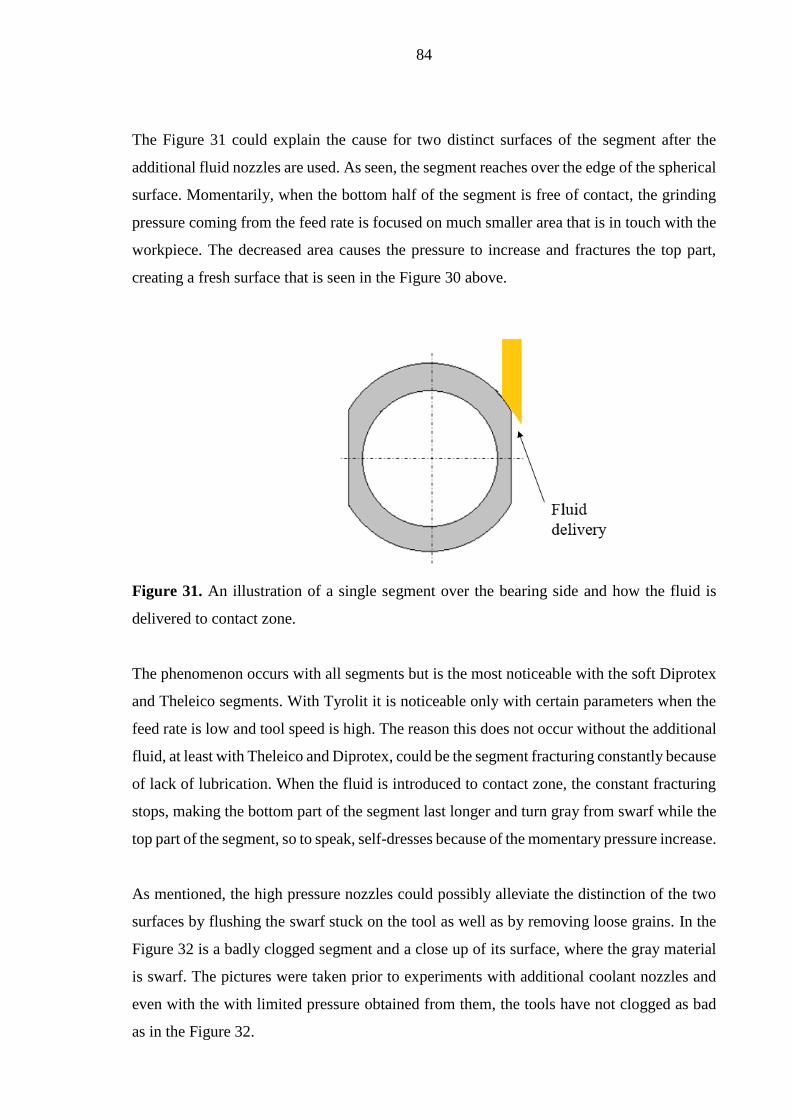
84

The Figure 31 could explain the cause for two distinct surfaces of the segment after the

additional fluid nozzles are used. As seen, the segment reaches over the edge of the spherical

surface. Momentarily, when the bottom half of the segment is free of contact, the grinding

pressure coming from the feed rate is focused on much smaller area that is in touch with the

workpiece. The decreased area causes the pressure to increase and fractures the top part,

creating a fresh surface that is seen in the Figure 30 above.

Figure 31. An illustration of a single segment over the bearing side and how the fluid is

delivered to contact zone.

The phenomenon occurs with all segments but is the most noticeable with the soft Diprotex

and Theleico segments. With Tyrolit it is noticeable only with certain parameters when the

feed rate is low and tool speed is high. The reason this does not occur without the additional

fluid, at least with Theleico and Diprotex, could be the segment fracturing constantly because

of lack of lubrication. When the fluid is introduced to contact zone, the constant fracturing

stops, making the bottom part of the segment last longer and turn gray from swarf while the

top part of the segment, so to speak, self-dresses because of the momentary pressure increase.

As mentioned, the high pressure nozzles could possibly alleviate the distinction of the two

surfaces by flushing the swarf stuck on the tool as well as by removing loose grains. In the

Figure 32 is a badly clogged segment and a close up of its surface, where the gray material

is swarf. The pictures were taken prior to experiments with additional coolant nozzles and

even with the with limited pressure obtained from them, the tools have not clogged as bad

as in the Figure 32.

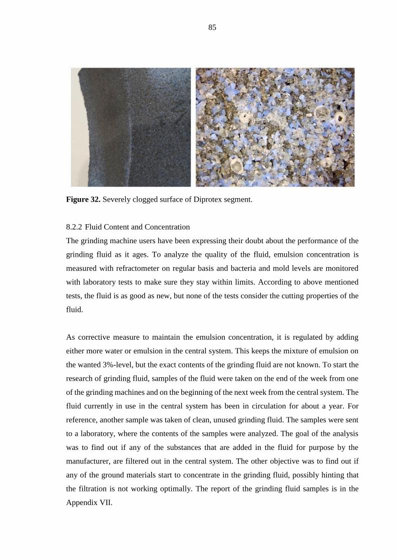
85

Figure 32. Severely clogged surface of Diprotex segment.

8.2.2 Fluid Content and Concentration

The grinding machine users have been expressing their doubt about the performance of the

grinding fluid as it ages. To analyze the quality of the fluid, emulsion concentration is

measured with refractometer on regular basis and bacteria and mold levels are monitored

with laboratory tests to make sure they stay within limits. According to above mentioned

tests, the fluid is as good as new, but none of the tests consider the cutting properties of the

fluid.

As corrective measure to maintain the emulsion concentration, it is regulated by adding

either more water or emulsion in the central system. This keeps the mixture of emulsion on

the wanted 3%-level, but the exact contents of the grinding fluid are not known. To start the

research of grinding fluid, samples of the fluid were taken on the end of the week from one

of the grinding machines and on the beginning of the next week from the central system. The

fluid currently in use in the central system has been in circulation for about a year. For

reference, another sample was taken of clean, unused grinding fluid. The samples were sent

to a laboratory, where the contents of the samples were analyzed. The goal of the analysis

was to find out if any of the substances that are added in the fluid for purpose by the

manufacturer, are filtered out in the central system. The other objective was to find out if

any of the ground materials start to concentrate in the grinding fluid, possibly hinting that

the filtration is not working optimally. The report of the grinding fluid samples is in the

Appendix VII.

86

The substances that were looked for from the samples were the additives that were known

to be added in the fluid based on the fluid’s safety manual and substances that were known

to be used in fluid as friction modifiers such as EP additives. Additionally, the concentrations

of substances coming from ground coatings, base materials and what could originate from

the grinding segment were analyzed. Nearly all of the analyzed substances had very high

concentrations in comparison to fresh sample.

The sulphur content was a particular interest since it is known to be used as an additive in

both the grinding tools and fluid. And because of the information found from the literature,

such as research conducted by Nadolny et al. (2013, p. 118), where sulfur from grinding tool

liquefied as a result of high temperature in the grinding contact zone. The temperature in the

contact zone in ball grinding is not known, but sulfur becoming liquid in certain conditions

cannot be ruled out.

The above mentioned possible liquidation of sulphur is just one way of certain substances

concentrating in the grinding fluid. Looking at the report in the Appendix VII, concentrations

of many other substances are elevated as well. Based on the concentrations of chlorine, boron

and sulfur in the fresh sample, they are all used as additives in the fluid in different forms.

But comparing their concentrations between fresh and currently used sample, the

concentrations in the used sample are several times higher. This is very likely a result of

regulating the emulsion concentration by adding emulsion concentrate. It has not been

known whether their concentrations change in relation to emulsion’s concentration and

judging by the report they do not. By adding in more of the emulsion, the fluid starts to

accumulate with substances that do not evaporate from the fluid.

Researches reveal extensively high concentrations of certain chemical substances, that are

added in the fluid as beneficial additives, increasing the grinding forces and wear

(Brinksmeier et al. 2015, p. 614). Whether the concentrations in the grinding fluid samples

are high enough to be disadvantageous is not known, but the findings from the literature

would back up the machine users’ complaints about slowly deteriorating performance of the

fluid.

87

The other substances, mainly metallic materials, do not have as high concentrations, but

comparing to fresh sample, they likely should not be in the fluid. In particular, nickel and

chromium concentrations are high and could be a sign of ineffective filtration. The difference

in grinding performance that the substances cause between the fresh and used sample, could

be determined with experiments. Changing the grinding fluid in the system has been

discussed and experiments before and after are planned to discover the real impact of

grinding fluid. Based on the results of experiments with new and used fluid, a schedule for

future grinding fluid changes could be estimated.

As the concentrations of different substances likely accumulate with time as the fluid is used

and the effects of the substances or their extent are not known, grinding fluid causes variation

between experiments in the long run. The experiments in this thesis were conducted over the

time span of couple months. Although, the fluid is not estimated to be a severe nuisance

factor within this time, its effects cannot be ruled out, thus slightly harming the reliability of

the experiments and the research.

8.2.3 Bending of the Segment

The grinding head design that is used with six inch balls and several other ball sizes, is robust

and thus very stable and unsusceptible to chatter. The design however has some drawbacks,

of which the tool bending is the most crucial for experimenting. The other drawbacks and

possible improvements are discussed more closely in the chapter 8.3 Development

possibilities.

The machine users were aware of the tool bending slightly when the segment is new and on

its full length. But its extent was not known before the experiment with Theleico, where

grooving of the segments was experimented. In such experiments, where the run order was

not randomized, the bending poses as a serious nuisance factor that can distort the results of

the experiment. Prior to the grooving experiment, the bending was not considered a nuisance

factor.

The effect of tool bending and how it can lead to false conclusions can be seen by looking

at the experiment more closely. The initial conclusion from the experiment with grooves was

that grooving the segments is beneficial for material removal rate. Looking at the two

88

leftmost blue columns in the Figure 33, the grooving seems to have increased the MRR and

the same applies to two of the leftmost red columns. After six runs with three different

parameter combinations, all pointing to same direction, the grooving was stated to be

beneficial. To confirm this, another three test runs were taken: the rightmost blue column

and the two rightmost red columns. Now with the parameter combination one and without

grooving, the material removal rate was on the similar level to earlier run with grooving. The

same happened with the parameter combination two. The run without grooving resulted in

rather identical MRR. The last run of the experiment, the rightmost red column was taken

with grooving again and it resulted in even slightly lower MRR than the earlier run without

grooving.

Figure 33. Material removal rates from experiment where the effect of grooving was

determined. Yes or no stating whether the segment was grooved and the value below it

expressing the tool length after the run.

The experimentation of grooving finally proved two things. Grooving is not advantageous

for Theleico and unlikely for any of the segments that are porous enough to not to be prone

to hydroplaning. The experiment also proved the effect of bending, how it depends on the

tool length and how it can lead to false conclusions if not taken into consideration.

0

500

1000

1500

2000

2500

3000

3500

No(217,364)

Yes(212,311)

No(202,429)

No(213,54)

Yes(208,615)

No(200,473)

Yes(198,474)

MR

R

1 Feed rate: 0.1 mm/min 2 Feed rate: 0.16 mm/minTool speed: 2500 RPM Tool speed: 3000 RPM

Effect of tool bending on MRR

89

8.3 Development Possibilities

This chapter covers mainly improvements and changes for the grinding machine. Some of

these proposals would be mainly to help in the future experiments and some of the proposals

are based on the machine user’s feedback and would be beneficial in the everyday production

as well.

The most significant single improvement would be changing the design of the grinding head.

There are several issues related to it, of which the tool bending was already touched on. To

eliminate bending or to at least reduce it, the distance of the segment contact area from the

support point would have to be reduced. When the segments are worn and they are shorter,

the lever arm is shorter like on the right side of the Figure 34, leading to less bending.

Figure 34. The current grinding head design.

Which takes us to the second issue with the grinding head design: fastening the grinding

segments. The machine users say that fastening method of the segments is unnecessarily

complex, requiring either two screws to be tightened at the same time or by tightening them

alternately little by little. The tight fit of the segments without a possibility to disassemble

the grinding head to clean the swarf causes segments to get stuck. In few of the experiments

the method of fixing the segments to grinding head was also noticed to cause point loads on

the segment surface, inducing splits on the segment surface and causing them to break.

90

The design of the grinding head has also a third major flaw. Only about half of the segment

can be used, after which the segment cannot be fastened to grinding head securely. Once the

top of the segment reaches about the halfway between the fastening points, the segment is

changed to new. The half used segments can be still put to use in the older grinding machine

with different grinding head design, but that does not make the drawback of the grinding

head any less justified.

For an improved grinding head, the machine users have been proposing a design where the

segments are fastened in place with a band surrounding the periphery. The design is still on

idea level and requires work but could reduce the time needed for change or adjustment of

the segments, while providing support for the segment in grinding, reducing the bending

phenomenon. In production that is constantly moving towards smaller batch sizes, reducing

the setup times is becoming more and more crucial and could be achieved with better

grinding head design.

Another suggested improvement for the machine, also originating from the machine users,

would be dressing possibilities for the segments. Self-sharpening seems to work rather well

in production when grinding uncoated workpieces like in the experiments. Chromium

coating is however problematic and sometimes the machine users are required to manually

dress the surfaces by using another segment to scrape the contact area surface. Built-in

dressing tool would speed up the process but the characteristic extremely long contact length

of the application would likely lead to very frequent need of dressing. So, the primary interest

is to find a separate grinding segment for chromium coating and eliminate the need for

dressing altogether.

In the experiments so far, the power output has been monitored from the control screen of

the grinding machine and collecting the data has simply been writing down the power output

value every two minutes. The information about the power output is really valuable in

predicting the tool behavior because the power output and its changes can tell what is

happening in the contact zone, where the eye cannot see. A data logging feature on the

machine would be more accurate and easier method to collect the data, without necessarily

leading to huge investments.

91

Some of the other grinding machines at Metso have a fluid delivery inside the grinding head,

through the spindle. The feature is helpful in getting the fluid to reach the contact zone evenly

during the rotation of the tool, as long as the fluid is correctly directed and the velocity is

high enough. Before investing in changes that would be required on the fluid delivery system

and the machine, the benefits of the fluid delivery through spindle would have to be

experimented, which more about in the next chapter 8.4 Further research topics and

experiments.

8.4 Further Research Topics and Experiments

Various segment specifications have been and are being ordered based on the experiments

conducted in this thesis. The follow-up experiments for these segments are going to continue

in similar manner to determine their performance and whether they bring an improvement.

In addition to these follow-up experiments already discussed in evaluation of each tool, few

other experiments would be highly beneficial to determine the effects of certain factors.

These additional experiments and further research topics are covered in this chapter.

The steel base material, that is ground in the experiments in this thesis, represents only some

of the ground material range. Titanium dioxide (TiO2) and hard chromium coatings are also

ground with the same Tyrolit segment. In particular, grinding the chromium coating has been

an issue as described earlier. The chromium coating has always been ground with a sharp

edge on the segment, keeping the contact area between the workpiece and the segment small.

Once the segment would wear, starting to contour the spherical shape, the tool would have

to be cut to obtain a sharp edge with small contact area again. To eliminate the need for

earlier mentioned manual scraping of the tool surface, that the machine users are required to

do, and perhaps to make possible the use of the whole surface area of the segment, new

specifications for grinding chromium coating are experimented. To start the grinding

experiments with chromium coating, a modified specification of the Tyrolit segment has

been ordered based on the Tyrolit’s recommendation.

For grinding titanium dioxide coating, specification with silicon carbide abrasive was in use

years ago. According to machine users, the specification worked much better on TiO2 than

the Tyrolit with aluminium oxide grain. The manufacturer of the segments closed down and

few substituting segments have been tried years ago with poor results. Now to start the search

92

for a better tool for grinding titanium dioxide, a specification based on the Tyrolit’s

recommendation has been ordered.

On top of reducing the thermal issues, increasing the workpiece speed seemed to result in

minor increase in material removal rate in most of the experiments. Since the workpiece

speed seems to be limited only by the quality related factors, such as vibration and its effects,

and the higher speed is otherwise beneficial, the limits for the workpiece speed would be

beneficial to determine. If the thermal issues can be reduced by increasing the workpiece

speed, this could possibly allow increase in material removal rate. Practical limits for the

workpiece speed could be determined with experiments where the responses would be

quality related, such as dimensional and geometrical integrity.

After the grinding fluid in the central system is changed, the effect of the fluid can be

determined by running experiments prior and after the change. Furthermore, these

experiments should be conducted regularly as the grinding fluid ages, for example every

couple months. This practice would help in understanding the connection between the aging

of the fluid and its performance. Even better, if the experiments are done together with

collecting and analyzing samples of the grinding fluid, a possible correlation between the

contents of the fluid and the cutting performance can be determined.

Another grinding fluid related factor of which effect would need to be determined through

experimenting, is the emulsion concentration. Currently, the concentration is kept at 3%, so

at the lower limit of the fluid manufacturer’s recommendation (Henkel 2013). As shown in

the Figure 14, increase in oil content shifts the properties closer to oil from water. Whether

increasing the emulsion concentration would lead to improvement in this application could

only be confirmed with an experiment.

The experiments proved the additional grinding nozzles to be beneficial for all the alternative

segments with aluminium oxide grains. Since superabrasives, diamond and CBN, are also

widely used, the effect of introducing extra fluid in a process would have to be determined

through experimentation.

93

The way of grinding valve balls with high conformity cup or segmented wheels is not the

only available method; grinding machines with other principles do exist. For example, a

machine in which the tool is a traditional grinding wheel oscillating on the ball surface. The

machine would be also capable of grinding for example valve seats and thus having its own

advantages. The advantages and disadvantages of the currently used grinding machinery are

rather well known, but how they compare to other grinding principles and machines in the

market is unclear. Research on other machinery would be highly valuable for future

investments which is why its listed here on the further research topics. (Danobat 2017b.)

8.5 Validity and Reliability

This thesis was able to answer the main research questions about the grinding tools and the

parameters by using statistical methods where randomization and confirmation tests

equipped, leading to valid results. The questions raised during the experiments and writing

of the thesis are discussed based on the literature, however many hypotheses requiring

further experimenting are left open, and therefore slightly hindering the overall validity of

the research.

Despite the validity and reliability being on fairly good level, there are several factors that

harm the reliability and in particular replicability of the experiments. Some of their effects

are known better after this thesis and can be prepared for in the forthcoming experiments.

The factors are:

Tool bending causing experimental error

Fluid delivery causing experimental error

Evaluating the workpiece temperature with human perception

The same factors are the nuisance factors in the experiments and their impact is covered in

the chapter 7.1.2 Design factors.

94

9 CONCLUSIONS

The goal of this still ongoing research is to find a grinding segment that would improve the

grinding process. The main interest is in increasing the material removal rate while not

giving up on quality. The experiments conducted for the five segments that were initially

recommended by the grinding tool manufacturers, proved that the combination of the factors

in tool specification ultimately determines the material removal rate. Potential benefits from

single factors, from a more novel grain in this case, are not realized unless the other factors

are suitable.

Despite that the five initial tool alternatives failed to bring improvement to the process,

valuable knowledge and observations were gathered from the experiments. This knowledge

is now used to alter the tool specification of the initially recommended tools towards more

suitable. The first experiments with altered specifications show an improvement to initial

level and the performance is closing the minimum target level set by the currently used

segment.

The importance of lubrication that the correctly set-up fluid delivery brings, was noted in the

experiments. With the alternative segments, the material removal rates grew up to four times

the level that was achieved without additional fluid delivery. The introduction of fluid

delivery directly to the contact zone through the additional nozzles was a crucial find for the

performance of the segments that do not have lubricating additives in the tool itself and

remains in use in the future experiments.

Using design of experiments approach with full factorial designs proved to be an effective

method for optimization tasks. However, once the experimenter is familiar with the tool

behavior, one-factor-at-a-time method can be used as effectively.

95

REFERENCES

Aurich, J. C., Bouabid, A., Steinmann, P. & Kirsch, B. 2013. [Chapter 4:] High-Performance

Surface Grinding. In: Denkena, B. & Hollman, F. Process Machine Interactions: Prediction

and Manipulation of Interactions between Manufacturing Processes and Machine Tool

Structures. Heidelberg, Germany: Springer-Verlag. Pp. 81–100.

Badger, J. A. 2012. Microfracturing Ceramic Abrasive in Grinding. ASME 2012

International Manufacturing Science and Engineering Conference, held at Notre Dame, IN,

USA 4–8 June, 2012. Pp. 1115–1123.

Black, J. T. & Kohser, R. A. 2012. DeGarmo’s Materials and Processes in Manufacturing.

Eleventh Edition. Hoboken, NJ, USA: John Wiley & Sons, Inc.. 1143 p.

Brinksmeier, E., Meyer, D., Huesmann-Cordes, A.G. & Herrmann, C. 2015. Metalworking

fluids–Mechanisms and Performance. CIRP Annals – Manufacturing Technology, Vol. 64,

Iss 2. Pp. 605–628.

Danobat. 2017a. BGM – Radius grinding machine. [Danobat webpage]. [Referred 5.3.2017].

Available: http://www.danobatusa.com/bgm-radius-grinding-machine

Danobat. 2017b. Ball valve balls - up to 10". [Danobat webpage]. [Referred 24.3.2017].

Available: http://www.danobatusa.com/oil-and-gas-ball-valve-balls-up-to-10

Henkel. 2013. Bonderite L-MR 49-2 DF - Technisches Dateblatt [web document].

Düsseldorf, Germany: December 2013. [Referred 20.3.2017]. Available in PDF-file:

http://www.csc-jaekle.com/fileadmin/MeBl/751/MeBl_751344_DE.pdf.

Irani, R. A., Bauer, R. J. & Warkentin, A. 2005. A review of cutting fluid application in the

grinding process. International Journal of Machine Tools & Manufacture, Vol. 45, Iss 15.

Pp. 1696–1705.

96

Jackson, M. J. & Hitchiner, M. P. 2013. High Performance Grinding and Advanced Cutting

Tools. New York, NY, USA: Springer Science+Business Media. 100 p.

Kivipelto, P. 1990. [Chapter 8:] Neles-Jamesbury Metal Seating Technology. In: Sparig, P.

The valve book. Helsinki, Finland: Neles-Jamesbury. Pp. 80–91.

Klocke, F. 2009. Manufacturing Processes 2: Grinding, Honing, Lapping. Berlin, Germany:

Springer-Verlag. 433 p.

Malkin, S. & Guo, C. 2008. Grinding Technology: Theory and Applications of Machining

with Abrasives. Second Edition. New York, NY, USA: Industrial Press, Inc.. 375 p.

Mansikka-Aho, A. 2016. Diprotexin kivet [private e-mail]. Receivers: Juho Venäläinen, Jari

Sivula (cc). Sent 21.11.2016, 08.53 (GMT +0200).

Marinescu, I. D., Rowe, W. B., Dimitrov, B. & Ohmori, H. 2013. Tribology of Abrasive

Machining Processes. Second Edition. Norwich, NY, USA: William Andrew Publishing.

586 p.

Marinescu, I. D., Hitchiner, M., Uhlmann, E., Rowe, W. B. & Inasaki, I. 2007. Handbook of

Machining with Grinding Wheels. Boca Raton, FL, USA: CRC Press. 629 p.

Mathews, P. G. 2005. Design of Experiments with MINITAB. Milwaukee, WI, USA: ASQ

Quality Press. 499 p.

Meyer, D. & Wagner, A. 2016. Influence of Metalworking Fluid Additives on the Thermal

Conditions in Grinding. CIRP Annals – Manufacturing Technology, Vol. 65, Iss. 1. Pp.313–

316.

Meran, R., John, A., Roenpage, O. & Staudter, C. 2013. Six Sigma + Lean Toolset. Edited

by Lunau, S. Second Edition. Heidelberg, Germany: Springer-Verlag. 400 p.

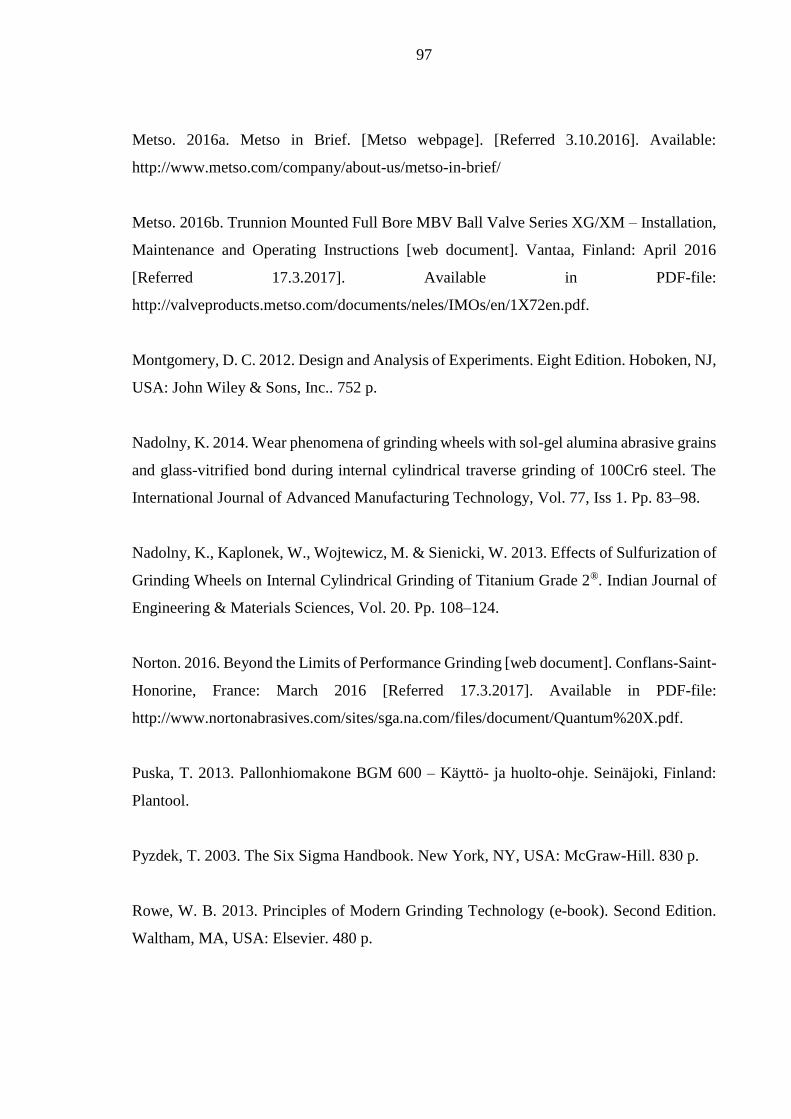
97

Metso. 2016a. Metso in Brief. [Metso webpage]. [Referred 3.10.2016]. Available:

http://www.metso.com/company/about-us/metso-in-brief/

Metso. 2016b. Trunnion Mounted Full Bore MBV Ball Valve Series XG/XM – Installation,

Maintenance and Operating Instructions [web document]. Vantaa, Finland: April 2016

[Referred 17.3.2017]. Available in PDF-file:

http://valveproducts.metso.com/documents/neles/IMOs/en/1X72en.pdf.

Montgomery, D. C. 2012. Design and Analysis of Experiments. Eight Edition. Hoboken, NJ,

USA: John Wiley & Sons, Inc.. 752 p.

Nadolny, K. 2014. Wear phenomena of grinding wheels with sol-gel alumina abrasive grains

and glass-vitrified bond during internal cylindrical traverse grinding of 100Cr6 steel. The

International Journal of Advanced Manufacturing Technology, Vol. 77, Iss 1. Pp. 83–98.

Nadolny, K., Kaplonek, W., Wojtewicz, M. & Sienicki, W. 2013. Effects of Sulfurization of

Grinding Wheels on Internal Cylindrical Grinding of Titanium Grade 2®. Indian Journal of

Engineering & Materials Sciences, Vol. 20. Pp. 108–124.

Norton. 2016. Beyond the Limits of Performance Grinding [web document]. Conflans-Saint-

Honorine, France: March 2016 [Referred 17.3.2017]. Available in PDF-file:

http://www.nortonabrasives.com/sites/sga.na.com/files/document/Quantum%20X.pdf.

Puska, T. 2013. Pallonhiomakone BGM 600 – Käyttö- ja huolto-ohje. Seinäjoki, Finland:

Plantool.

Pyzdek, T. 2003. The Six Sigma Handbook. New York, NY, USA: McGraw-Hill. 830 p.

Rowe, W. B. 2013. Principles of Modern Grinding Technology (e-book). Second Edition.

Waltham, MA, USA: Elsevier. 480 p.

98

Senf, P. 2017. Application engineer, Theleico Schleiftechnik GmbH & Co. KG. Vantaa,

Metso Flow Control Hakkila factory: interview 20.12.2016. Interviewer Juho Venäläinen.

Notes are occupied by the interviewer.

Theleico. 2015. Grinding Wheels and Bonded Abrasives – Product Range [web document].

Meschede, Germany: July 2015 [Referred 20.3.2017]. Available in PDF-file:

http://www.theleico.de/fileadmin/masterTemplate/Resources/Public/Files/downloads/ueber

sichtsprospekt-en.pdf.

Webster, J. & Tricard, M. 2004. Innovations in Abrasive Products for Precision Grinding.

CIRP Annals – Manufacturing Technology, Vol. 53, Iss 2. Pp. 597–617.

Wright, J. & Bregman, A. 1990. [Chapter 9:] Neles-Jamesbury Soft Seating Technology.

In: Sparig, P. The valve book. Helsinki, Finland: Neles-Jamesbury. Pp. 94–118.

Appendix I, 1

Results and analysis: Tyrolit – 89A120F8V217T3

Tyrolit’s segment has already been experimented in 2015 and the optimal parameters for it are known.

To get more recent and thus fair reference for the other segments, Tyrolit was decided to be

experimented as well.

EXPERIMENT 1: 15.12.2016

The optimized parameters for Tyrolit’s segment were known to be:

Feed rate: 0.15 mm/min

Tool speed: 1800 RPM

Workpiece (WP) speed: 50 RPM

These parameters were used as a middle point for the parameter setting for the experiment.

The test matrix for Tyrolit was following:

StdOrd RunOrd Feedrate

Tool

RPM

WP

RPM

Tool L

1

Tool L

2 WP D 1 WP D 2

Fluid

temp. MRR

G-

ratio

5 1 0,12 1600 80 225,476 224,093 245,966 245,24 18,8 2825 4,44

3 2 0,12 2000 20 224,093 222,894 245,24 244,225 18,9 3936 7,14

8 3 0,18 2000 80 222,894 220,948 244,225 242,857 19,1 5281 5,90

7 4 0,12 2000 80 220,94 219,682 242,857 241,857 19,4 3842 6,64

4 5 0,18 2000 20 219,682 217,791 241,857 240,402 19,1 5561 6,39

6 6 0,18 1600 80 217,791 215,715 240,402 239,222 18,9 4485 4,70

2 7 0,18 1600 20 215,715 213,621 239,222 238,037 18,6 4481 4,65

1 8 0,12 1600 20 213,621 212,263 238,037 237,186 18,4 3204 5,13

Observations:

Run: Ball temperature: Segment surface: Power (%): Additional details:

1 OK, slightly warm Normal 21-35

2 Hot, fluid vaporizing Slightly glazed 25-44



5 Hot, fluid vaporizing Slightly glazed 29-44

6 Cool Normal 26-38


8 Cool Normal 24-35

Overall observations:

No problems occurred during the experiment. In overall, the parameters seemed to be close to optimal,

as the response was on rather high level on every run. Higher workpiece speed helped to keep the

workpiece temperature lower.

Analysis:

Naturally, increasing the feed rate and tool speed show an increase in MRR, as seen from the Figure

1. The effect of workpiece speed is small, as expected. No interaction between the feed rate and tool

speed was present, likely due to narrow parameter range. Surprisingly the feed rate and workpiece

speed seem to be about as significant for G-ratio, both showing decrease towards the higher values.

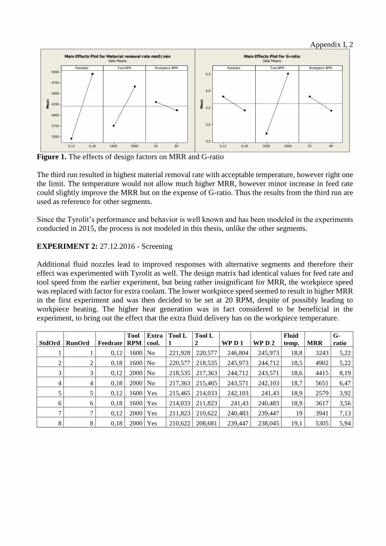
Appendix I, 2

0,180,12

5000

4750

4500

4250

4000

3750

3500

20001600 8020

Feedrate

Me

an

Tool RPM Workpiece RPM

Main Effects Plot for Material removal rate mm3/minData Means

0,180,12

6,5

6,0

5,5

5,0

4,5

20001600 8020

Feedrate

Me

an


Main Effects Plot for G-ratioData Means

Figure 1. The effects of design factors on MRR and G-ratio

The third run resulted in highest material removal rate with acceptable temperature, however right one

the limit. The temperature would not allow much higher MRR, however minor increase in feed rate

could slightly improve the MRR but on the expense of G-ratio. Thus the results from the third run are

used as reference for other segments.

Since the Tyrolit’s performance and behavior is well known and has been modeled in the experiments

conducted in 2015, the process is not modeled in this thesis, unlike the other segments.

EXPERIMENT 2: 27.12.2016 - Screening

Additional fluid nozzles lead to improved responses with alternative segments and therefore their

effect was experimented with Tyrolit as well. The design matrix had identical values for feed rate and

tool speed from the earlier experiment, but being rather insignificant for MRR, the workpiece speed

was replaced with factor for extra coolant. The lower workpiece speed seemed to result in higher MRR

in the first experiment and was then decided to be set at 20 RPM, despite of possibly leading to

workpiece heating. The higher heat generation was in fact considered to be beneficial in the

experiment, to bring out the effect that the extra fluid delivery has on the workpiece temperature.


Tool

RPM

Extra

cool.

Tool L

1

Tool L

2 WP D 1 WP D 2

Fluid

temp. MRR

G-

ratio

1 1 0,12 1600 No 221,928 220,577 246,804 245,973 18,8 3243 5,22

2 2 0,18 1600 No 220,577 218,535 245,973 244,712 18,5 4902 5,22

3 3 0,12 2000 No 218,535 217,363 244,712 243,571 18,6 4415 8,19

4 4 0,18 2000 No 217,363 215,465 243,571 242,103 18,7 5651 6,47

5 5 0,12 1600 Yes 215,465 214,033 242,103 241,43 18,9 2579 3,92

6 6 0,18 1600 Yes 214,033 211,823 241,43 240,483 18,9 3617 3,56

7 7 0,12 2000 Yes 211,823 210,622 240,483 239,447 19 3941 7,13

8 8 0,18 2000 Yes 210,622 208,681 239,447 238,045 19,1 5305 5,94

Appendix I, 3

Observations:




3 Hot, fluid vaporizing Normal 16-36

4 Hot, fluid vaporizing Normal 21-38

5 Cool Normal 25-46

6 Cool Normal 24-42

7 OK, warm Top half clearly open,

bottom half normal

25-60

8 OK, warm Normal 33-63


The additional fluid seemed to result in lowered responses and cause the power output to go up

significantly. It did keep the workpiece cooler however and the fluid seemed to be warmer in runs with

the extra delivery, since more heat was conveyed in it.

Analysis:

As seen from the Figure 2, for MRR the extra coolant shows a clear downwards slope towards the

extra coolant and the effect is naturally similar on the G-ratio.

0,180,12

5000

4750

4500

4250

4000

3750

3500

20001600 YesNo

Feedrate

Me

an

Tool RPM Extra coolant


0,180,12

7,0

6,5

6,0

5,5

5,0

4,5

20001600 YesNo

Feedrate

Me

an



Figure 2. The effects of design factors on MRR and G-ratio.

In overall, the extra coolant impaired the responses, however the difference between runs with and

without extra coolant seemed to balance out towards the end of the experiment. The experiment does

not change the evaluation of the segment and it the reference level is still the run number three from

the first experiment.

Appendix II, 1

Results and analysis: Theleico – 23A120-0F12VM4200


The test matrix was then decided to be set based on the screening experiment conducted for Diprotex

segment. With high feed rates the Diprotex segment was wearing out quickly, so the feed rate was

lowered. Also, the output seemed to increase by increasing tool speed, so the experiment with Theleico

was decided to be started with higher tool speed. For which different tool speeds were cautiously tested

prior the start. The highest tested tool speed was 2500 RPM, with which no problems occurred.

The test matrix for the first screening of Theleico was finally following:


Tool

RPM

WP

RPM

Tool L

1

Tool L

2

WP D

1

WP D

2

Fluid

temp. MRR G-ratio

1 1 0,03 1200 20 214,216 213,771 244,497 244,445 18,3 201 0,98

7 2 0,03 2500 80 213,771 213,496 244,445 244,243 18,3 782 6,18

2 3 0,1 1200 20 213,496 211,987 244,243 244,197 17,9 178 0,26

3 4 0,03 2500 20 211,987 211,682 244,197 244,046 18,4 584 4,16

4 5 0,1 2500 20 211,682 210,327 244,046 243,855 18,2 738 1,18

8 6 0,1 2500 80 210,327 209,076 243,855 243,503 18,8 1359 2,36

5 7 0,03 1200 80 209,076 208,626 243,503 243,468 18,5 135 0,65

6 8 0,1 1200 80 208,626 207,101 243,468 243,416 18,6 201 0,29


No problems occurred in the first screening experiment of Theleico. Like with every other segment,

the higher tool speeds seemed to result in higher outputs. The performance was still far from the goal

set by Tyrolit but after the first round of screening experiments, Theleico showed the most promise.

The ball surface quality seemed good after every run and no heating problems occurred.

EXPERIMENT: 20.12.2016 - Confirmation

Regression models were composed of the first screening experiment and the accuracy of the models

was tested in confirmation experiment, with a following test matrix:


Tool

RPM

WP

RPM

Tool L

1

Tool L

2

WP D

1

WP D

2

Fluid

temp. MRR G-ratio

x 1 0,04 2500 80 219,45 219,015 246,914 246,749 19,1 645 3,22

x 2 0,06 2000 80 216,933 216,158 246,749 246,624 19,1 488 1,37

x 3 0,06 2500 80 214,16 213,453 246,624 246,434 19,3 742 2,28

x 4 0,08 2000 80 213,453 212,363 246,434 246,314 18,6 468 0,93

x 5 0,08 2500 80 212,363 211,364 246,314 246,093 18,6 862 1,88

x 6 0,1 2500 80 211,364 210,056 246,093 245,867 18,6 881 1,46

x 7 0,1 2800 80 207,861 206,542 244,834 244,604 18,8 892 1,47

Appendix II, 2

The models follow the changes in actual tested values sufficiently as seen from the Figures 1 and 2,

but the tested output is much below the estimated throughout the test matrix. The error is emphasized

on the G-ratio as the lacking material removal basically transforms to tool wear. The estimates could

be corrected by adjusting the constant in the model, by doing so the MRR predictions reach a 90

percent prediction interval. However, by correcting the constant in the G-ratio model, the predictions

are still far off. This kind of constant error hints towards variation in conditions between the screening

and confirmation experiment. After realization of the major influence that the fluid has, the difference

was likely in delivery of the coolant. Even though the both tests are conducted with just flood nozzles,

their alignment was probably different, leading to different amount of fluid reaching the contact area.

Figure 1. The fit of the MRR model to confirmation runs, with 10% error bars.

Figure 2. The fit of the G-ratio model to confirmation runs, with 10% error bars.

400

500

600

700

800

900

1000

1100

1200

0 1 2 3 4 5 6 7 8

Tested/model MRR

Tested MRR Model MRR

0,5

1

1,5

2

2,5

3

3,5

4

4,5

5

0 1 2 3 4 5 6 7 8

Tested/model G-ratio

Tested G-ratio Model G-ratio

Appendix II, 3

EXPERIMENT 3: 20.12.2016 – Screening

After the confirmation runs for the regression models, the introduction of extra coolant nozzles was

experimented for the first time and the results were promising. Since the outputs were greatly

enhanced, the evaluation of the segment was decided to be based on a setup with extra coolant nozzles.

Thus a screening experiment was conducted with a setup with additional fluid nozzles.

The test matrix for the screening experiment was following:


Tool

RPM

WP

RPM

Tool L

1

Tool L

2

WP D

1

WP D

2

Fluid

temp. MRR G-ratio

x 1 0,1 2500 80 210,056 208,907 245,867 245,409 18,6 1782 3,37

x 2 0,1 2800 80 208,907 207,861 245,409 244,834 18,9 2233 4,64

x 3 0,15 2500 80 204,464 202,611 243,328 242,733 19,1 2292 2,69

x 4 0,15 2800 80 202,611 200,848 242,733 241,962 18,9 2962 3,65

Observations:


1 Cool Normal/slightly glazed 32-38


3 Cool Normal/slightly glazed 31-41 Distinct surfaces of the

segment start to

replicate to the ball

surface

4 Cool Normal/glazed 39-49


The additional coolant nozzles resulted in a new unseen phenomenon on the segment surface where

the surface had two clearly distinct sections to it. The bottom half looked normal like before adding

the nozzles. The top part then was clear, the color was bright and there was visibly less swarf clogging

the surface.

Analysis:

Based on the earlier experiments, the workpiece speed was already left out from the test matrix by

setting it to 80 RPM. Therefore, the design factors were feed rate, tool speed. Neither of the terms or

their interaction come up as statistically significant, as seen from the Figure 3. Based on the previous

tests however, all of the three terms will be included in the regression models and the suitability and

fit of the models are verified through confirmation experiment.

AB

B

A

120001000080006000400020000

Te

rm

Effect

10680

A Feedrate

B Tool RPM

Factor Name

Pareto Chart of the Effects(response is Material removal rate mm3/min, Alpha = 0,05)

Lenth's PSE = 840,520 Figure 3. Statistical significance of the terms with α=0.05

Appendix II, 4

The material removal rate improves by increasing the feed rate and the tool speed, as seen from the

Figure 4. Looking at the interaction plot, also very minor interaction can be seen. The small effect of

interaction can likely be explained with the narrow scale of the tool speed. For the interaction to be

more influential, the difference in tool speed, or the feed rate, would have to be large enough to cause

the tool behavior to change.

0,150,10

2700

2600

2500

2400

2300

2200

2100

2000

28002500

Feedrate

Me

an

Tool RPM


28002500

3000

2800

2600

2400

2200

2000

1800

Tool RPMM

ea

n

0,10

0,15

Feedrate

Interaction Plot for Material removal rate mm3/minData Means

Figure 4. The effects of design factors on MRR.

The significance of terms for the G-ratio is similar to MRR. The initial model will include the main

factors and their interaction and the fit of the model is verified with confirmation experiment.

As seen from the Figure 5, the slopes for effects follow the trend from the previous experiments. The

higher tool speed increases the G-ratio and the increase in feed rate goes more towards the tool wear.

The interaction for G-ratio is minor but noticeable.

0,150,10

4,2

4,0

3,8

3,6

3,4

3,2

3,0

28002500

Feedrate

Me

an

Tool RPM


28002500

4,5

4,0

3,5

3,0

2,5

Tool RPM

Me

an

0,10

0,15

Feedrate

Interaction Plot for G-ratioData Means

Figure 5. The effects of design factors on G-ratio.

Conclusions:

The high and low values for the variables were quite close to each other on the screening run, but all

the values are relatively close to the area where the segment seems to work. Based on the observations

made during and after the screening experiment, none of the value combinations caused unwanted

event such as excessive fracturing or thermal damage. The parameters that are set close together

increase the risk of fitting the regression model to noise but the responses are far enough from each

other to rule this out. Also, the parameters set close to optimal area should provide an accurate model,

as the tool behavior has not drastically changed during the screening experiment.

Appendix II, 5

The primary models for the both outputs are based on feed rate, tool speed and their interaction. Models

without interaction are also composed and compared to primary models with the interaction term.

The coefficients for the primary model for MRR with the interaction term in place:

Estimated Coefficients for Material removal rate mm3/min using data in uncoded

units

Term Coef

Constant 653,685

Feedrate -26288,2

Tool RPM 0,0437612

Feedrate*Tool RPM 14,5925

The coefficients for the primary model for G-ratio with the interaction term in place:

Estimated Coefficients for G-ratio using data in uncoded units

Term Coef

Constant -10,9379

Feedrate 37,3363

Tool RPM 0,00627072

Feedrate*Tool RPM -0,0204009

EXPERIMENT 4: 3.1.2017 – Confirmation

For the confirmation test, parameter combinations within the screened area as well as outside of it were

selected. Based on the screening experiment, the optimal parameters were likely to be found over 2800

RPM tool speed as long as the temperature does not become a problem. For estimates outside the

screened area, the model was extrapolated. The test matrix for the confirmation experiment was

following:


Tool

RPM

WP

RPM

Tool L

1

Tool L

2

WP D

1

WP D

2

Fluid

temp. MRR G-ratio

x 1 0,08 2200 80 226,633 225,819 243,561 243,232 18,8 1269 3,39

x 2 0,12 2500 80 225,819 224,584 243,232 242,671 18,5 2160 3,80

x 3 0,16 2200 80 224,584 222,665 242,671 242,199 18,9 1814 2,05

x 4 0,08 3000 80 222,665 222,1 242,199 241,648 18,8 2113 8,13

x 5 0,16 3000 80 222,1 220,511 241,648 240,742 18,6 3464 4,74

x 6 0,15 2800 80 220,511 218,972 240,742 239,944 18,8 3040 4,29

Observations:


1 Cool Normal (distinct colors) 27-39



4 Cool Normal/slightly glazed 42-51 Distinct surfaces

replicate to workpiece

5 Cool Normal/glazed 45-61 Distinct surfaces

replicate to workpiece

6 Cool Normal/glazed 45-56 Minor streakiness due

to distinct surfaces

Appendix II, 6


On test runs with high tool speeds, the power output reached rather high levels. Despite the high power

output, the workpiece surface remained cool throughout the tests. The material removal rate achieved

on the fifth run was the highest the alternative segment has reached so far. The distinct surface of the

segment started to replicate to the ball surface on some of the test runs, but not to a problematic extent.

Conclusions:

The model for material removal rate with terms for feed rate, tool speed and their interaction was

confirmed to be accurate, as seen from the Figure 6. The parameters for runs 1, 3, 4 and 5 were outside

the screened area to which the regression model was fit. Despite that the model was extrapolated for

these runs, the accuracy is still on good level. From 10% error bars on the tested values it can be seen

that almost all the estimates for MRR reach more than 90 % prediction interval.

Figure 6. The fit of the MRR model to confirmation runs, with 10% error bars.

The model for G-ratio is not as accurate as the model for MRR. Both the models with and without the

interaction term for the feed rate and tool speed were compared. The model without the interaction fit

the tested output better and is presented in the Figure 7. By adjusting the constant in the model, all the

estimates except the number four can be fit within the 90 % prediction interval. The right value for the

constant seems to depend on the day and how well the conditions are replicated from the experiment

the model is based on.

1000

1500

2000

2500

3000

3500

4000

0 1 2 3 4 5 6 7

Tested/model MRR


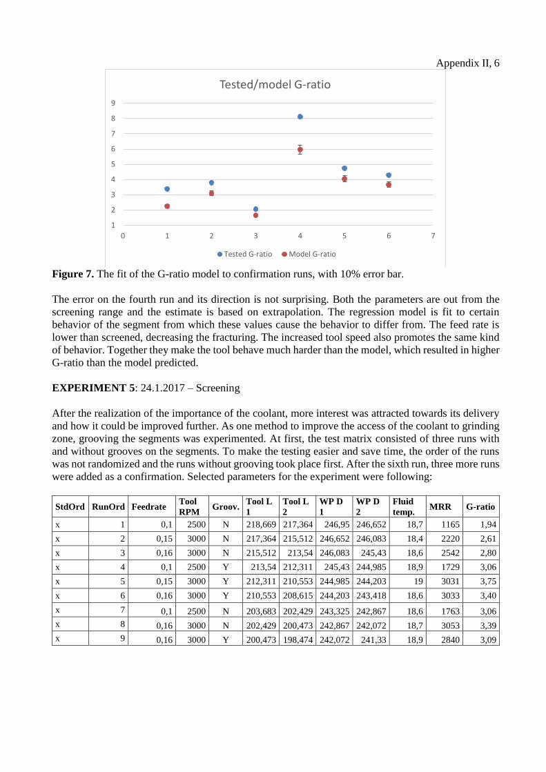
Appendix II, 6

Figure 7. The fit of the G-ratio model to confirmation runs, with 10% error bar.

The error on the fourth run and its direction is not surprising. Both the parameters are out from the

screening range and the estimate is based on extrapolation. The regression model is fit to certain

behavior of the segment from which these values cause the behavior to differ from. The feed rate is

lower than screened, decreasing the fracturing. The increased tool speed also promotes the same kind

of behavior. Together they make the tool behave much harder than the model, which resulted in higher

G-ratio than the model predicted.


After the realization of the importance of the coolant, more interest was attracted towards its delivery

and how it could be improved further. As one method to improve the access of the coolant to grinding

zone, grooving the segments was experimented. At first, the test matrix consisted of three runs with

and without grooves on the segments. To make the testing easier and save time, the order of the runs

was not randomized and the runs without grooving took place first. After the sixth run, three more runs

were added as a confirmation. Selected parameters for the experiment were following:

StdOrd RunOrd Feedrate Tool

RPM Groov.

Tool L

1

Tool L

2

WP D

1

WP D

2

Fluid

temp. MRR G-ratio

x 1 0,1 2500 N 218,669 217,364 246,95 246,652 18,7 1165 1,94

x 2 0,15 3000 N 217,364 215,512 246,652 246,083 18,4 2220 2,61

x 3 0,16 3000 N 215,512 213,54 246,083 245,43 18,6 2542 2,80

x 4 0,1 2500 Y 213,54 212,311 245,43 244,985 18,9 1729 3,06

x 5 0,15 3000 Y 212,311 210,553 244,985 244,203 19 3031 3,75

x 6 0,16 3000 Y 210,553 208,615 244,203 243,418 18,6 3033 3,40

x 7 0,1 2500 N 203,683 202,429 243,325 242,867 18,6 1763 3,06

x 8 0,16 3000 N 202,429 200,473 242,867 242,072 18,7 3053 3,39

x 9 0,16 3000 Y 200,473 198,474 242,072 241,33 18,9 2840 3,09

1

2

3

4

5

6

7

8

9

0 1 2 3 4 5 6 7



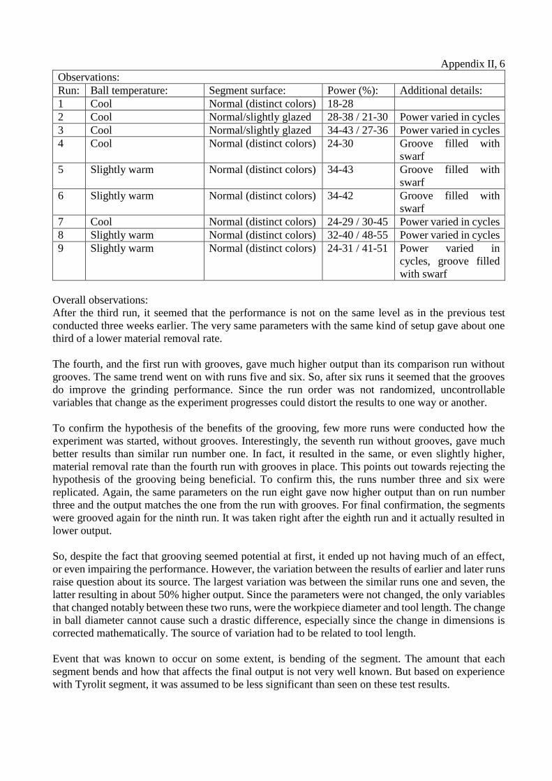
Appendix II, 6

Observations:


1 Cool Normal (distinct colors) 18-28

2 Cool Normal/slightly glazed 28-38 / 21-30 Power varied in cycles

3 Cool Normal/slightly glazed 34-43 / 27-36 Power varied in cycles

4 Cool Normal (distinct colors) 24-30 Groove filled with

swarf

5 Slightly warm Normal (distinct colors) 34-43 Groove filled with

swarf

6 Slightly warm Normal (distinct colors) 34-42 Groove filled with

swarf

7 Cool Normal (distinct colors) 24-29 / 30-45 Power varied in cycles

8 Slightly warm Normal (distinct colors) 32-40 / 48-55 Power varied in cycles

9 Slightly warm Normal (distinct colors) 24-31 / 41-51 Power varied in

cycles, groove filled

with swarf


After the third run, it seemed that the performance is not on the same level as in the previous test

conducted three weeks earlier. The very same parameters with the same kind of setup gave about one

third of a lower material removal rate.

The fourth, and the first run with grooves, gave much higher output than its comparison run without

grooves. The same trend went on with runs five and six. So, after six runs it seemed that the grooves

do improve the grinding performance. Since the run order was not randomized, uncontrollable

variables that change as the experiment progresses could distort the results to one way or another.

To confirm the hypothesis of the benefits of the grooving, few more runs were conducted how the

experiment was started, without grooves. Interestingly, the seventh run without grooves, gave much

better results than similar run number one. In fact, it resulted in the same, or even slightly higher,

material removal rate than the fourth run with grooves in place. This points out towards rejecting the

hypothesis of the grooving being beneficial. To confirm this, the runs number three and six were

replicated. Again, the same parameters on the run eight gave now higher output than on run number

three and the output matches the one from the run with grooves. For final confirmation, the segments

were grooved again for the ninth run. It was taken right after the eighth run and it actually resulted in

lower output.

So, despite the fact that grooving seemed potential at first, it ended up not having much of an effect,

or even impairing the performance. However, the variation between the results of earlier and later runs

raise question about its source. The largest variation was between the similar runs one and seven, the

latter resulting in about 50% higher output. Since the parameters were not changed, the only variables

that changed notably between these two runs, were the workpiece diameter and tool length. The change

in ball diameter cannot cause such a drastic difference, especially since the change in dimensions is

corrected mathematically. The source of variation had to be related to tool length.

Event that was known to occur on some extent, is bending of the segment. The amount that each

segment bends and how that affects the final output is not very well known. But based on experience

with Tyrolit segment, it was assumed to be less significant than seen on these test results.

Appendix III, 1

Analysis: Diprotex - 3CG120G/H10V32

The experiments were started with Diprotex segment. The first tests took place on 22nd of November

2016.

Diprotex segment was noted to be very porous and open in comparison to currently used Tyrolit

segment. The segment also feels much lighter.


Without better knowledge, the test parameters were set according to optimized parameters for Tyrolit

segment. The optimized parameter values for this size with Tyrolit are 0.15 mm/min for the feedrate,

1800 RPM for the tool speed and 50 RPM for the workpiece speed. These were selected as midpoints

for the test parameters, so the test matrix for Diprotex segment was following:

StdOrder RunOrder Feedrate Tool RPM Workpiece RPM

3 1 0,1 2200 20

8 2 0,2 2200 80

7 3 0,1 2200 80

5 4 0,1 1400 80

2 5 0,2 1400 20

4 6 0,2 2200 20

6 7 0,2 1400 80

1 8 0,1 1400 20

In the second test run with all the parameters set to high value, one of the segments broke three minutes

into the test. The test had to be stopped for further examination. The cause for the breakdown of the

segment was examined and was very likely the lack of support plate behind the segment. Two out of

six segments on the opposite sides of the grinding head were left without such plates. The plates are

not meant to come off from the grinding head and are difficult to put back. Without the support plate,

the distance of the support point from the grinding area increases, which increases the torque addressed

towards the segment. Without the plate, the fastening screws are also digging in the segment, possibly

causing the segment to fracture. To continue testing, all the plates were put in place despite the

difficulties. As in further precaution, the tool speeds were also reduced by 200 RPM.

Appendix III, 2


After failure of one of the segments, the test matrix with reduced tool speeds was following:


Tool

RPM

WP

RPM Tool L 1 Tool L 2 WP D 1 WP D 2

Fluid

temp.

MR

R

G-

ratio

3 1 0,1 2000 20 223,396 222,098 243,803 243,693 18,6 425 0,71

6 2 0,2 1200 80 222,098 219,136 243,693 243,637 18,5 216 0,16

4 3 0,2 2000 20 219,136 216,335 243,637 243,477 18,9 618 0,48

5 4 0,1 1200 80 216,335 214,862 243,477 243,431 18,9 178 0,26

1 5 0,1 1200 20 214,862 213,37 243,431 243,396 18,9 135 0,20

8 6 0,2 2000 80 213,37 210,521 243,396 243,244 18,8 586 0,45

2 7 0,2 1200 20 210,521 207,515 243,244 243,209 18,4 135 0,10

7 8 0,1 2000 80 207,515 206,142 243,209 243,096 18,4 436 0,69

Observations:


1 Slightly glazed Power varied in cycles

2 Clearly open Power remained low

3 Normal Power varied in cycles

4 Normal Power remained low

5 Normal Power remained low


7 Clearly open Power remained low



The segment seemed to fracture excessively in all of the test runs. In every run with the tool speed of

1200 RPM, the power output remained very low, likely signing that the tool was fracturing as it was

fed into the workpiece. The runs with higher tool speed of 2000 RPM, the power output varied in

cycles. As the theory entails, this is clearly the right direction for the tool speed, as the constant

fracturing stopped. The fact that the power output still varied, reaching virtually an idle level before

building up again, is still a sign that there is still too much fracturing.

Analysis:

The Figure 1 shows the statistically significant factors for MRR. Since the parameter placement is

quite wide and the tool behavior and performance changes depending on the parameter combination’s

fit to each other, the interaction term between feed rate and tool speed shows up as statistically

significant with significance level of 0.05.

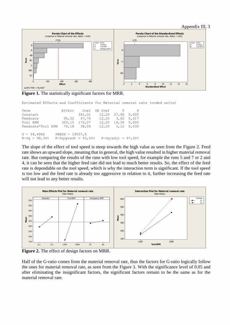
Appendix III, 3

AC

ABC

C

BC

AB

A

B

4003002001000

Te

rm

Effect

174,8

A Feedrate

B Tool RPM

C Workpiece RPM

Factor Name

Pareto Chart of the Effects(response is Material removal rate, Alpha = 0,05)

Lenth's PSE = 46,4267

AB

A

B

1614121086420

Te

rm

Standardized Effect

2,78

A Feedrate

B Tool RPM

Factor Name

Pareto Chart of the Standardized Effects(response is Material removal rate, Alpha = 0,05)

Figure 1. The statistically significant factors for MRR. Estimated Effects and Coefficients for Material removal rate (coded units)

Term Effect Coef SE Coef T P

Constant 341,01 12,20 27,96 0,000

Feedrate 95,52 47,76 12,20 3,92 0,017

Tool RPM 350,15 175,07 12,20 14,36 0,000

Feedrate*Tool RPM 76,18 38,09 12,20 3,12 0,035

S = 34,4942 PRESS = 19037,6

R-Sq = 98,30% R-Sq(pred) = 93,20% R-Sq(adj) = 97,02%

The slope of the effect of tool speed is steep towards the high value as seen from the Figure 2. Feed

rate shows an upward slope, meaning that in general, the high value resulted in higher material removal

rate. But comparing the results of the runs with low tool speed, for example the runs 5 and 7 or 2 and

4, it can be seen that the higher feed rate did not lead to much better results. So, the effect of the feed

rate is dependable on the tool speed, which is why the interaction term is significant. If the tool speed

is too low and the feed rate is already too aggressive in relation to it, further increasing the feed rate

will not lead to any better results.

0,20,1

550

500

450

400

350

300

250

200

150

20001200 8020

Feedrate

Me

an


Main Effects Plot for Material removal rateData Means

20001200

600

500

400

300

200

100

Tool RPM

Me

an

0,1

0,2

Feedrate

Interaction Plot for Material removal rateData Means

Figure 2. The effect of design factors on MRR.

Half of the G-ratio comes from the material removal rate, thus the factors for G-ratio logically follow

the ones for material removal rate, as seen from the Figure 3. With the significance level of 0.05 and

after eliminating the insignificant factors, the significant factors remain to be the same as for the

material removal rate.

Appendix III, 4

ABC

AC

C

BC

AB

A

B

0,40,30,20,10,0

Te

rm

Effect

0,1784

A Feedrate

B Tool RPM

C Workpiece RPM

Factor Name

Pareto Chart of the Effects(response is G-ratio, Alpha = 0,05)

Lenth's PSE = 0,0473845

AB

A

B

181614121086420

Te

rm

Standardized Effect

2,78

A Feedrate

B Tool RPM

Factor Name

Pareto Chart of the Standardized Effects(response is G-ratio, Alpha = 0,05)

Figure 3. The statistically significant factors for G-ratio. Estimated Effects and Coefficients for G-ratio (coded units)


Constant 0,38037 0,01219 31,20 0,000

Feedrate -0,16925 -0,08463 0,01219 -6,94 0,002

Tool RPM 0,40323 0,20162 0,01219 16,54 0,000

Feedrate*Tool RPM -0,06805 -0,03403 0,01219 -2,79 0,049

S = 0,0344799 PRESS = 0,0190218


The tool speed has an obvious positive effect for the G-ratio as seen from the Figure 4. If the feed rate

is kept the same, and there is more removed from the workpiece by increasing the tool speed, it means

that there must be less removed from the tool. So, increasing the tool speed basically transforms the

volume removed from the tool to volume removed from the workpiece, making it to have an “double”

effect on the G-ratio. The higher feed rate showed somewhat positive effect for material removal rate

but same cannot be said for the G-ratio. As mentioned earlier, looking at the run pairs 5 & 7 and 2 &

4, the increase in feed rate went straight to the tool wear. Naturally, the G-ratio is then influenced by

the interaction of the feed rate and the tool speed.

0,20,1

0,6

0,5

0,4

0,3

0,2

20001200 8020

Feedrate

Me

an



20001200

0,7

0,6

0,5

0,4

0,3

0,2

0,1

Tool RPM

Me

an

0,1

0,2

Feedrate


Figure 4. The effect of design factors on G-ratio.

Conclusions from the first screening experiment

The parameters were clearly unsuitable for the segment and new experiment is needed for fitting a

regression model. Based on the observations at machine and the results of the analysis, it is clear that

the feed rate was overly aggressive in relation to other parameters.

Appendix III, 5

The tool would very likely benefit from increasing the tool speed further than 2000 RPM as the high

tool speed value resulted in clearly better output. By increasing the tool speed, the material removal

rate should go up, as the tool wear would go down. The effect for workpiece speed is rather small for

both outputs, higher resulting in slightly better results.

To adjust the process closer to the optimal parameters for the next experiment, higher tool speed

combined with lower feed rate should be experimented.


The results from the first screening experiment with Diprotex segment were disappointing, but pointed

out the direction the parameters should be changed to. The first experiment showed that the parameters

that are close to optimal for Tyrolit segment, are far from optimal for Diprotex.

Before the third experiment for Diprotex, visually quite similar segment from Theleico was also

experimented. For the third experiment, the test matrix was set similarly to the experiment conducted

with Theleico.

The feedrate was reduced significantly. The new high value was now the old low value, because even

with the low value in the previous test, the segment was fracturing excessively. To spread out the

parameters enough, the new low value for feed rate was set to 0,03 mm/min. The new high value for

tool speed was set to 2500 and the low value was kept the same.

The test matrix for the third screening experiment was following:


Tool

RPM

WP

RPM

Tool L

1

Tool L

2

WP D

1

WP D

2

Fluid

temp. MRR G-ratio

1 1 0,03 1200 20 223,688 223,239 243,305 243,272 17,6 127 0,62

6 2 0,1 1200 80 223,239 221,743 243,272 243,234 18,3 147 0,21

5 3 0,03 1200 80 221,743 221,288 243,234 243,214 18,3 77 0,37

7 4 0,03 2500 80 221,288 221,026 243,214 243,107 18,2 412 3,42

4 5 0,1 2500 20 221,026 219,735 243,107 242,896 18,8 813 1,37

2 6 0,1 1200 20 219,735 218,229 242,896 242,858 18,4 146 0,21

8 7 0,1 2500 80 218,229 216,965 242,858 242,592 18,9 1023 1,76

3 8 0,03 2500 20 216,965 216,668 242,592 242,495 18,1 373 2,73

Observations:


1 OK Slightly glazed 8-16

2 OK Normal 9-16


4 Warm Slightly glazed 20-30* See Figure 5

5 OK Slightly glazed 10-36** Power varied in cycles

6 OK Normal 7-13


8 Warm Glazed and clogged 13-33*** See Figure 5

*Took four minutes to reach the 10%-level, ** Took two minutes to reach the 10%-level, *** Took

over five minutes to reach the 10% level.

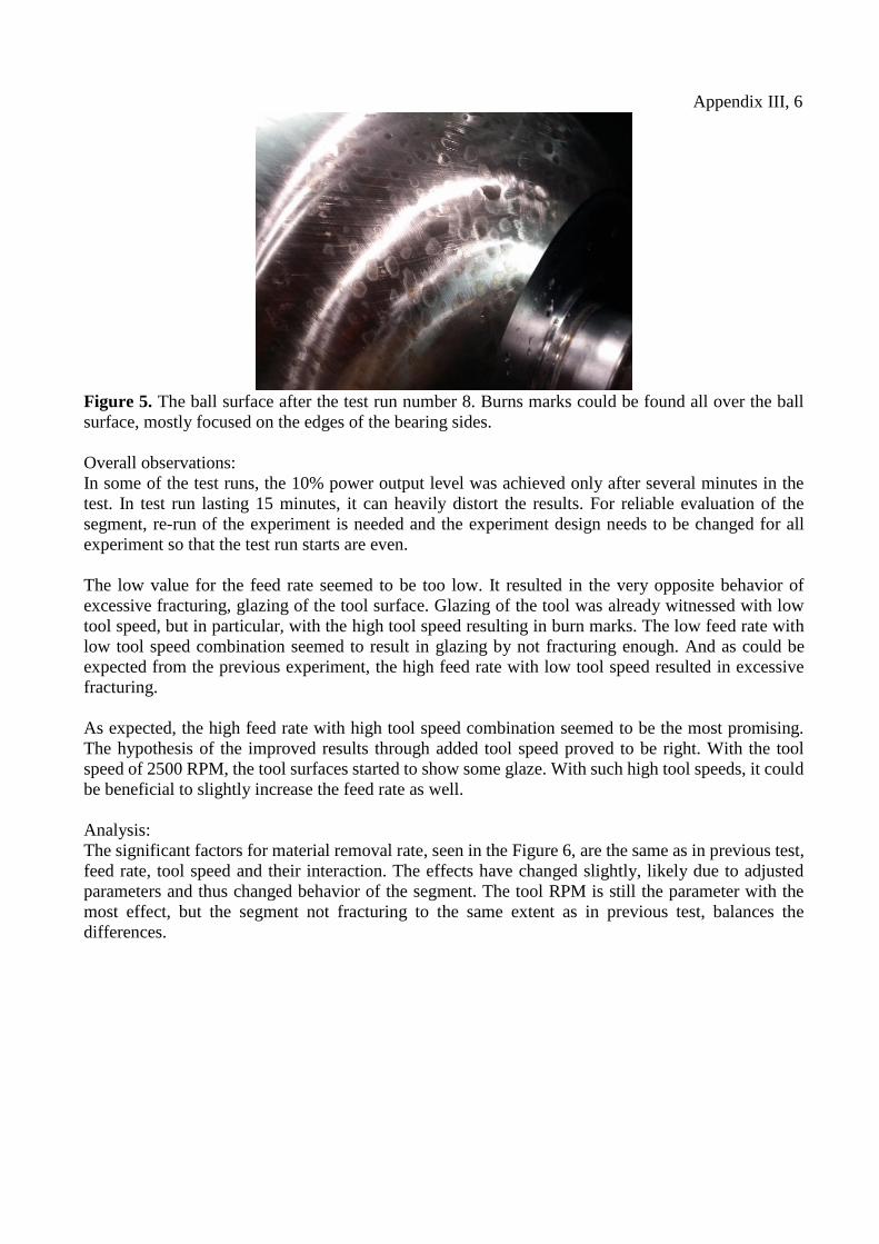
Appendix III, 6

Figure 5. The ball surface after the test run number 8. Burns marks could be found all over the ball

surface, mostly focused on the edges of the bearing sides.


In some of the test runs, the 10% power output level was achieved only after several minutes in the

test. In test run lasting 15 minutes, it can heavily distort the results. For reliable evaluation of the

segment, re-run of the experiment is needed and the experiment design needs to be changed for all

experiment so that the test run starts are even.

The low value for the feed rate seemed to be too low. It resulted in the very opposite behavior of

excessive fracturing, glazing of the tool surface. Glazing of the tool was already witnessed with low

tool speed, but in particular, with the high tool speed resulting in burn marks. The low feed rate with

low tool speed combination seemed to result in glazing by not fracturing enough. And as could be

expected from the previous experiment, the high feed rate with low tool speed resulted in excessive

fracturing.

As expected, the high feed rate with high tool speed combination seemed to be the most promising.

The hypothesis of the improved results through added tool speed proved to be right. With the tool

speed of 2500 RPM, the tool surfaces started to show some glaze. With such high tool speeds, it could

be beneficial to slightly increase the feed rate as well.

Analysis:

The significant factors for material removal rate, seen in the Figure 6, are the same as in previous test,

feed rate, tool speed and their interaction. The effects have changed slightly, likely due to adjusted

parameters and thus changed behavior of the segment. The tool RPM is still the parameter with the

most effect, but the segment not fracturing to the same extent as in previous test, balances the

differences.

Appendix III, 7

ABC

C

AC

BC

AB

A

B

6005004003002001000

Te

rm

Effect

312,8

A Feedrate

B Tool RPM

C Workpiece RPM

Factor Name



AB

A

B

1086420

Te

rm

Standardized Effect

2,78

A Feedrate

B Tool RPM

Factor Name

Pareto Chart of the Standardized Effects(response is Material removal rate mm3/min, Alpha = 0,05)

Figure 6. The statistically significant factors for MRR. Estimated Effects and Coefficients for Material removal rate mm3/min (coded

units)


Constant 389,8 27,52 14,17 0,000

Feedrate 284,8 142,4 27,52 5,17 0,007

Tool RPM 531,1 265,5 27,52 9,65 0,001


S = 77,8374 PRESS = 96938,6


For the material removal rate, the main effects plot shows the same direction as before. Increasing the

feed rate is beneficial as well as increasing the tool speed, which can already be assumed based on

theory and previous experiments. The fact that the slope, on the Figure 7, is really steep, points out

that increasing the tool speed even further could be beneficial, but with low feed rate, the temperature

limit has been reached because the tool glazes and the feed rate should be obviously increased.

0,100,03

700

600

500

400

300

200

100

25001200 8020

Feedrate

Me

an



25001200

900

800

700

600

500

400

300

200

100

0

Tool RPM

Me

an

0,03

0,10

Feedrate



The interaction term between the feed rate and tool speed seems to have major effect. The severe

interaction can likely be explained with very different behavior between high and low tool speeds

combined with high feed rate. With the low feed rate, the difference between high and low tool speed

is more moderate since in either case the segment does not fracture, causing the surface to glaze and

likely dulling of the grains. Where with high feed rate, the low tool speed output starts about from the

same level as it does low feed rate, even though the behavior is the opposite, excessive fracturing. But

with increasing the tool speed, the behavior changes from excessive fracturing to actual cutting, while

showing only minor glazing on the tool surface.

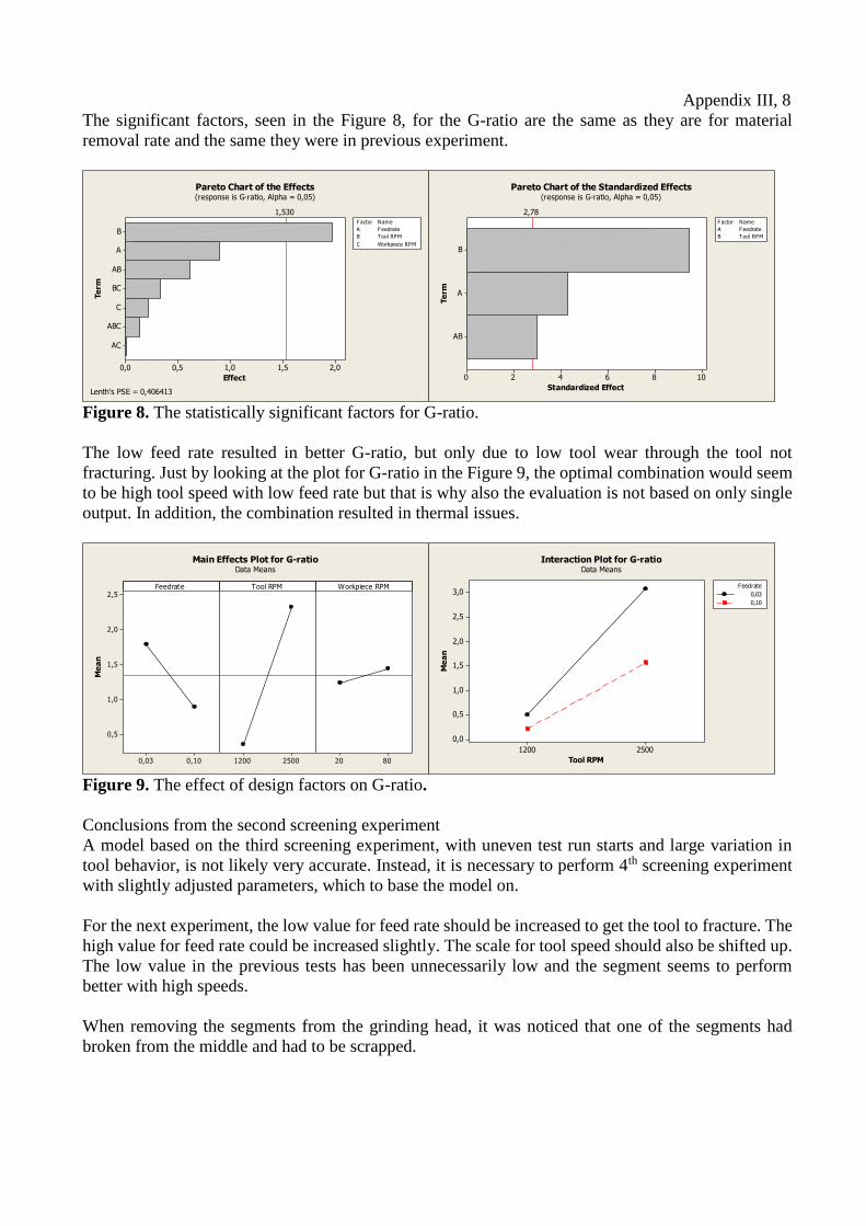
Appendix III, 8

The significant factors, seen in the Figure 8, for the G-ratio are the same as they are for material

removal rate and the same they were in previous experiment.

AC

ABC

C

BC

AB

A

B

2,01,51,00,50,0

Te

rm

Effect

1,530

A Feedrate

B Tool RPM

C Workpiece RPM

Factor Name



AB

A

B

1086420

Te

rm

Standardized Effect

2,78

A Feedrate

B Tool RPM

Factor Name


Figure 8. The statistically significant factors for G-ratio.

The low feed rate resulted in better G-ratio, but only due to low tool wear through the tool not

fracturing. Just by looking at the plot for G-ratio in the Figure 9, the optimal combination would seem

to be high tool speed with low feed rate but that is why also the evaluation is not based on only single

output. In addition, the combination resulted in thermal issues.

0,100,03

2,5

2,0

1,5

1,0

0,5

25001200 8020

Feedrate

Me

an



25001200

3,0

2,5

2,0

1,5

1,0

0,5

0,0

Tool RPM

Me

an

0,03

0,10

Feedrate



Conclusions from the second screening experiment

A model based on the third screening experiment, with uneven test run starts and large variation in

tool behavior, is not likely very accurate. Instead, it is necessary to perform 4th screening experiment

with slightly adjusted parameters, which to base the model on.

For the next experiment, the low value for feed rate should be increased to get the tool to fracture. The

high value for feed rate could be increased slightly. The scale for tool speed should also be shifted up.

The low value in the previous tests has been unnecessarily low and the segment seems to perform

better with high speeds.

When removing the segments from the grinding head, it was noticed that one of the segments had

broken from the middle and had to be scrapped.

Appendix III, 9


Before conducting another screening experiment for the Diprotex segment, a modified cooling setup

was experimented first with Theleico and then with Norton grade F. It provided a major increase in

the performance in both cases and made the use of higher parameters possible. So, the similar setup

was tested with Diprotex segment as well.

The run order of the tests was not randomized, instead, the runs with extra coolant were first, followed

by the runs without coolant. The valves used on the fluid delivery for extra hoses are simple shut off

type and thus maintaining the fluid volume and velocity constant is difficult if the handle needs to be

adjusted to anything between either fully open or closed. Since the current hose setup prevents keeping

the valve fully open, the runs with the extra coolant took place first so the handle could remain

untouched before closing it for the final four runs.

To keep the number of requires test runs reasonable, instead of adding another factor, one was replaced.

In any of the previous experiments, the workpiece speed has not raised to be a significant factor and

was thus replaced by the factor for extra coolant. Since the high workpiece speed in previous

experiments has proven to result in higher output, the workpiece speed was set to 80 RPM.

The test matrix for the screening experiment with extra coolant nozzles was following:


Tool

RPM

Extra

cool

Tool L

1

Tool L

2

WP D

1

WP D

2

Fluid

temp. MRR G-ratio

1 1 0,05 1800 Yes 225,894 225,204 246,73 246,614 18,9 453 0,95

2 2 0,15 1800 Yes 225,204 223,033 246,614 246,429 19 722 0,33

3 3 0,05 2600 Yes 223,033 222,485 246,429 246,18 18,9 971 1,68

4 4 0,15 2600 Yes 222,485 220,552 246,18 245,715 19,3 1812 0,88

5 5 0,05 1800 No 220,552 219,822 245,715 245,633 18,6 319 1,43

6 6 0,15 1800 No 219,822 217,656 245,633 245,549 18,3 327 0,72

7 7 0,05 2600 No 215,746 215,052 245,549 245,411 18,3 537 3,85

8 8 0,15 2600 No 215,052 213,014 245,411 245,199 18,4 824 2,04

Observations:


1 OK Normal/glazed 12-25 Distinct surfaces

replicate to ball

2 OK Normal/slightly glazed 13-25

3 OK Normal/badly glazed 24-35 Distinct surfaces

replicate to ball

4 OK Normal/slightly glazed 34-41 Distinct surfaces

replicate to ball

5 OK Normal 8-15

6 OK Normal 8-13

7 OK Normal 14-18

8 OK Normal 15-19

Appendix III, 10


The additional coolant nozzles seemed to have positive effect on the performance of the Diprotex

segment as well. The introduction of the additional nozzles does bring the similar effect as it does with

the Theleico’s segment. The surface of the segment is clearly open and bright blue from the top part,

but the bottom part is darker and in some occasions glazed. The disparity of the tool surface then starts

to show on the ball surface in a form of alternating streaks.

The segment surfaces seemed less glazed with high feed rate runs as they were fracturing more. This

also resulted in less visible streaks on the ball surface. The power output seemed to be lower on the

runs without the extra coolant.

Analysis:

The three main effects come up as having the most effect on the output, as seen from the Figure 10.

After removing the factors with lesser significance and keeping just the main effects, only the tool

speed comes up as statistically significant with significance level of 0.05. However, looking at the

results extra coolant is obviously significant and the feed rate has to be included in the model whether

it comes up statistically significant or not.

ABC

AC

AB

BC

A

C

B

1400120010008006004002000

Te

rm

Effect

1260

A Feedrate

B Tool RPM

C Extra coolant

Factor Name



Feedrate

Extra coolant

Tool RPM

3,53,02,52,01,51,00,50,0

Te

rm

Standardized Effect

2,776


Figure 10. The statistically significant factors for MRR.

Despite the extra coolant not coming up statistically significant, it was proven to have a major

performance boost in this experiment, as seen from the effect plot in the Figure 11. For that reason,

any further testing as well as the model will be conducted with the extra coolant nozzles.

0,150,05

1100

1000

900

800

700

600

500

400

26001800 YesNo

Feedrate

Me

an




Appendix III, 11

The first four runs are analyzed separately, forming its own two factor, two level full factorial design.

The regression model for the segment performance will be based on that half of the experiment.

After taking out the coolant variable from the process, leaving the feed rate and the tool speed are the

only variables. Their significance from statistical point of view drops like the Figure 12. Less

surprisingly, introducing the extra coolant to the process, does not change the direction how different

variables influence the output. Increasing feed rate and tool speed improve the material removal rate

and are somewhat dependent on each other like in experiments before. Although, the interaction of the

feed rate and the tool speed is far from being statistically significant, clear interaction can be seen on

the interaction plot in the Figure 13.

AB

A

B

120001000080006000400020000

Te

rm

Effect

10573

A Feedrate

B Tool RPM

Factor Name


Lenth's PSE = 832,091 Figure 12. The statistically significant factors for MRR.

0,150,05

1400

1300

1200

1100

1000

900

800

700

600

500

26001800

Feedrate

Me

an

Tool RPM


26001800

2000

1750

1500

1250

1000

750

500

Tool RPM

Me

an

0,05

0,15

Feedrate



Like for the material removal rate, any of the terms for G-ratio do not appear to be statistically

significant with significance level of 0.05, as seen from the Figure 14. To make even the closest to

significant factor, the tool speed, statistically significant, the significance level needs to be increased

to over 0.50.

Appendix III, 12

AB

A

B

2520151050

Te

rm

Effect

24,02

A Feedrate

B Tool RPM

Factor Name


Lenth's PSE = 1,89060 Figure 14. The statistically significant factors for G-ratio.

The main effects and the interaction term for G-ratio, in the Figure 15, follow the same logical trend

as before. The increase in feed rate lowers the G-ratio as more of the increase goes to tool wear than

to material removal rate. The tool speed has the same influence by increasing the material removal rate

and decreasing the tool wear.

0,150,05

3,0

2,5

2,0

1,5

1,0

26001800

Feedrate

Me

an

Tool RPM


26001800

4,0

3,5

3,0

2,5

2,0

1,5

1,0

Tool RPM

Me

an

0,05

0,15

Feedrate



Conclusions from the third screening experiment:

The introduction of extra coolant to the process improved the tool performance with a large margin.

Like with other segment alternatives, the further tests will be conducted with the additional coolant

nozzles in place.

From statistical point of view, the terms for both material removal rate and G-ratio would have to be

rejected from the regression model as statistically insignificant. Nevertheless, the model will be

compiled from these terms and its accuracy will be confirmed with confirmation test. If the model

turns out to be too inaccurate, another screening experiment, perhaps replicated, might be in order.

Like in the previous experiment with Diprotex segments, when removing them from the grinding head,

one of the segments was noticed to be broken.


For the confirmation experiment of the model, different parameter combinations were selected mixing

higher and lower feed rate and tool speed parameters. To find the optimal parameters for the

performance of the segment, the model was also interpolated outside the parameter range of the

screening experiment.

Appendix III, 13


Tool

RPM

Extra

cool

Tool L

1

Tool L

2

WP D

1

WP D

2

Fluid

temp. MRR G-ratio

x 1 0,06 2000 Yes 214,745 213,987 244,335 244,092 19 940 2,70

x 2 0,12 2000 Yes 213,987 212,37 244,092 243,773 19 1233 1,66

x 3 0,1 2300 Yes 212,37 211,123 243,773 243,311 19,2 1783 3,11

x 4 0,14 2000 Yes 211,123 209,206 243,311 242,963 18,8 1341 1,52

x 5 0,15 2600 Yes 209,206 207,309 242,963 242,289 18,6 2592 2,97

x 6 0,16 3000 Yes 207,309 205,457 242,289 241,428 18,6 3301 3,87

x 7 0,18 3000 Yes 205,457 203,201 241,428 240,601 19,1 3160 3,04

x 8 0,15 2600 Yes* 203,201 201,226 240,601 240,054 19,3 2084 2,29

x 9 0,1 2300 Yes* 201,226 199,914 240,054 239,707 19,1 1319 2,19

x 10 0,06 2000 Yes* 199,914 199,126 239,707 239,477 18,9 873 2,41

*Nozzle alignment was re-adjusted

Observations:



replicate to ball


replicate to ball


replicate to ball


replicate to ball


replicate to ball

6 Slightly warm Normal/glazed 53-65 Distinct surfaces

replicate to ball

7 Slightly warm Normal/glazed 49-64 Distinct surfaces

replicate to ball


replicate to ball


replicate to ball


replicate to ball


The segment performance seems to be highly dependent on the fluid delivery. Two runs with same

machine parameters in this confirmation test, as well as one the runs from the earlier screening test

resulted in very different material removal rate. The material removal rate changed from 1812 to 2592

mm3/min between the screening experiment and the run number five. After the nozzles were re-aligned

the MRR dropped closer to screening experiment level, 2084 mm3/min that was achieved on run

number eight.

Comparing the runs six and seven, it is noted that the lower feed rate resulted in higher MRR. The

higher feed rate of run seven takes the segment over its limit and the MRR starts to decrease. The run

number six will be used to compare the segment to others.

Appendix III, 14

Evaluating the model:

The regression model for material removal rate, with feed rate, tool speed and their interaction as terms,

is:

Estimated Coefficients for Material removal rate mm3/min using data in uncoded units

Term Coef

Constant -205,006

Feedrate -10158,4

Tool RPM 0,290901


The Figure 16 shows that the model with interaction term follows the changes in actual material

removal rate rather well, but the model is way below the real value. Some of such constant error can

be corrected by increasing the constant term or adding an error term. The main cause for error is

probably the difference in fluid delivery in screening and confirmation experiments. For the runs 8 to

10, the fluid delivery was adjusted by redirecting the nozzles. Redirecting the nozzles caused the output

to go down but took the tested values closer to model, which can be seen by comparing, for example,

runs four and nine. The difference in fluid delivery could also explain the increasing error towards the

higher tool speeds in runs 4, 5 and 6. Based on the interaction of the extra coolant term with the tool

speed term, that is seen in the Figure 17, the influence of the fluid delivery is emphasized on higher

speeds.

Figure 16. The fit of the MRR models to confirmation runs.

YesNo

1500

1250

1000

750

500

Extra coolant

Me

an

1800

2600

Tool RPM


Figure 17. The interaction between fluid delivery and tool speed.

500

1000

1500

2000

2500

3000

3500

0 2 4 6 8 10 12

Tested/model MRR

Tested MRR Model with interact. tem Model w/o interact. term

Appendix III, 15

The model for G-ratio is separate from the model for MRR, but both are based on the same test runs,

thus showing similar kind of error. As seen in the Figure 18, the model for G-ratio follows the changes

of the actual G-ratio. But the higher than expected MRR on the test runs increases the numerator while

lowering the denominator, which has a major effect of lowering the G-ratio and causing constant error

on the model. The model without interaction seems to give a better estimate than the one with the

interaction.

Figure 18. The fit of the G-ratio models to confirmation runs.

The regression models for the segment proved to be pointing out in the right direction, but the output

estimates were on a much lower level than tested. This is caused by variation in conditions and terms

that are hard to standardize, mainly the fluid delivery. Different test runs between various fluid delivery

setups have proved that the placing of the nozzle and the fluid flow characteristics have major influence

on the output.

1,00

1,50

2,00

2,50

3,00

3,50

4,00

0 2 4 6 8 10 12


G-ratio Model with interact. term Model w/o interact. term

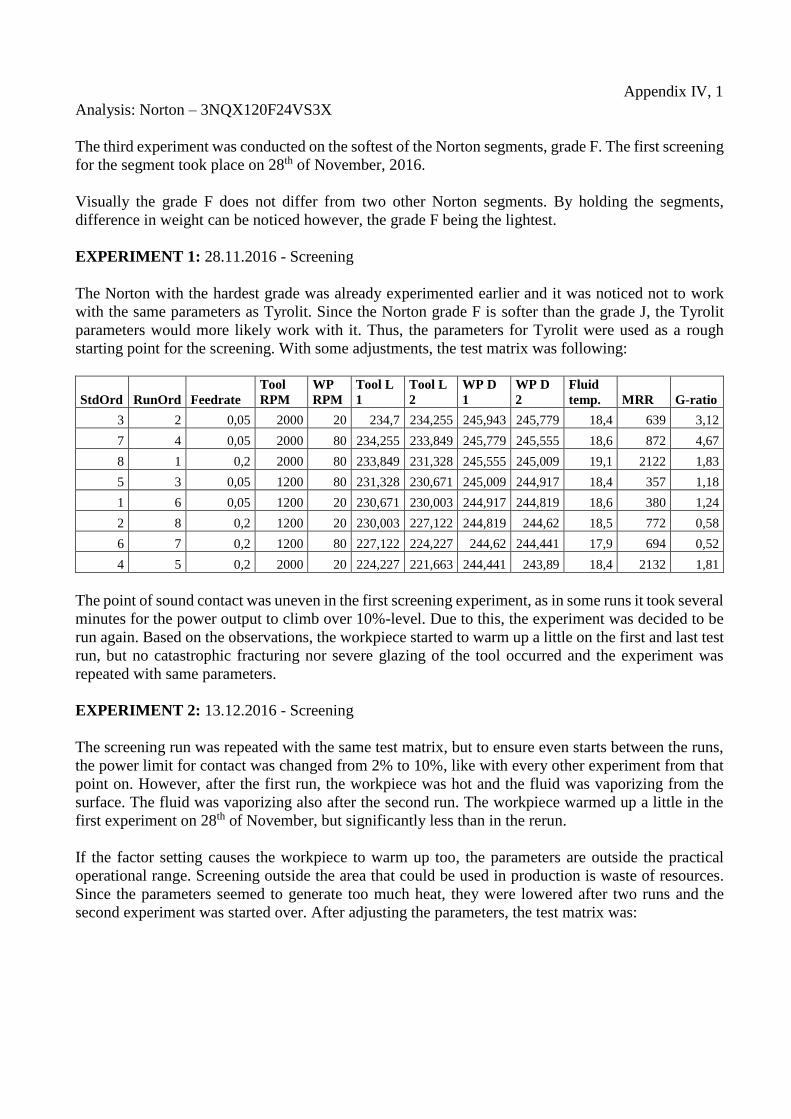
Appendix IV, 1

Analysis: Norton – 3NQX120F24VS3X

The third experiment was conducted on the softest of the Norton segments, grade F. The first screening

for the segment took place on 28th of November, 2016.

Visually the grade F does not differ from two other Norton segments. By holding the segments,

difference in weight can be noticed however, the grade F being the lightest.


The Norton with the hardest grade was already experimented earlier and it was noticed not to work

with the same parameters as Tyrolit. Since the Norton grade F is softer than the grade J, the Tyrolit

parameters would more likely work with it. Thus, the parameters for Tyrolit were used as a rough

starting point for the screening. With some adjustments, the test matrix was following:


Tool

RPM

WP

RPM

Tool L

1

Tool L

2

WP D

1

WP D

2

Fluid

temp. MRR G-ratio

3 2 0,05 2000 20 234,7 234,255 245,943 245,779 18,4 639 3,12

7 4 0,05 2000 80 234,255 233,849 245,779 245,555 18,6 872 4,67

8 1 0,2 2000 80 233,849 231,328 245,555 245,009 19,1 2122 1,83

5 3 0,05 1200 80 231,328 230,671 245,009 244,917 18,4 357 1,18

1 6 0,05 1200 20 230,671 230,003 244,917 244,819 18,6 380 1,24

2 8 0,2 1200 20 230,003 227,122 244,819 244,62 18,5 772 0,58

6 7 0,2 1200 80 227,122 224,227 244,62 244,441 17,9 694 0,52

4 5 0,2 2000 20 224,227 221,663 244,441 243,89 18,4 2132 1,81

The point of sound contact was uneven in the first screening experiment, as in some runs it took several

minutes for the power output to climb over 10%-level. Due to this, the experiment was decided to be

run again. Based on the observations, the workpiece started to warm up a little on the first and last test

run, but no catastrophic fracturing nor severe glazing of the tool occurred and the experiment was

repeated with same parameters.


The screening run was repeated with the same test matrix, but to ensure even starts between the runs,

the power limit for contact was changed from 2% to 10%, like with every other experiment from that

point on. However, after the first run, the workpiece was hot and the fluid was vaporizing from the

surface. The fluid was vaporizing also after the second run. The workpiece warmed up a little in the

first experiment on 28th of November, but significantly less than in the rerun.

If the factor setting causes the workpiece to warm up too, the parameters are outside the practical

operational range. Screening outside the area that could be used in production is waste of resources.

Since the parameters seemed to generate too much heat, they were lowered after two runs and the

second experiment was started over. After adjusting the parameters, the test matrix was:

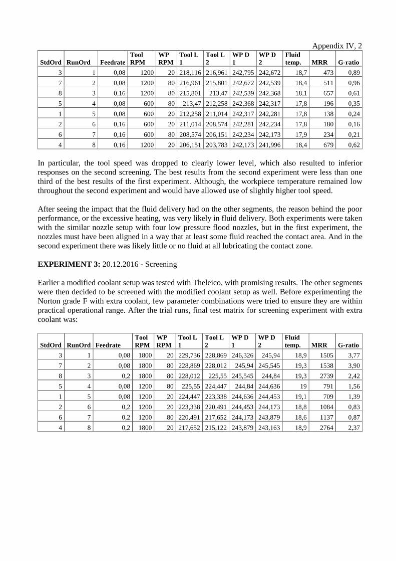
Appendix IV, 2


Tool

RPM

WP

RPM

Tool L

1

Tool L

2

WP D

1

WP D

2

Fluid

temp. MRR G-ratio

3 1 0,08 1200 20 218,116 216,961 242,795 242,672 18,7 473 0,89

7 2 0,08 1200 80 216,961 215,801 242,672 242,539 18,4 511 0,96

8 3 0,16 1200 80 215,801 213,47 242,539 242,368 18,1 657 0,61

5 4 0,08 600 80 213,47 212,258 242,368 242,317 17,8 196 0,35

1 5 0,08 600 20 212,258 211,014 242,317 242,281 17,8 138 0,24

2 6 0,16 600 20 211,014 208,574 242,281 242,234 17,8 180 0,16

6 7 0,16 600 80 208,574 206,151 242,234 242,173 17,9 234 0,21

4 8 0,16 1200 20 206,151 203,783 242,173 241,996 18,4 679 0,62

In particular, the tool speed was dropped to clearly lower level, which also resulted to inferior

responses on the second screening. The best results from the second experiment were less than one

third of the best results of the first experiment. Although, the workpiece temperature remained low

throughout the second experiment and would have allowed use of slightly higher tool speed.

After seeing the impact that the fluid delivery had on the other segments, the reason behind the poor

performance, or the excessive heating, was very likely in fluid delivery. Both experiments were taken

with the similar nozzle setup with four low pressure flood nozzles, but in the first experiment, the

nozzles must have been aligned in a way that at least some fluid reached the contact area. And in the

second experiment there was likely little or no fluid at all lubricating the contact zone.


Earlier a modified coolant setup was tested with Theleico, with promising results. The other segments

were then decided to be screened with the modified coolant setup as well. Before experimenting the

Norton grade F with extra coolant, few parameter combinations were tried to ensure they are within

practical operational range. After the trial runs, final test matrix for screening experiment with extra

coolant was:


Tool

RPM

WP

RPM

Tool L

1

Tool L

2

WP D

1

WP D

2

Fluid

temp. MRR G-ratio

3 1 0,08 1800 20 229,736 228,869 246,326 245,94 18,9 1505 3,77

7 2 0,08 1800 80 228,869 228,012 245,94 245,545 19,3 1538 3,90

8 3 0,2 1800 80 228,012 225,55 245,545 244,84 19,3 2739 2,42

5 4 0,08 1200 80 225,55 224,447 244,84 244,636 19 791 1,56

1 5 0,08 1200 20 224,447 223,338 244,636 244,453 19,1 709 1,39

2 6 0,2 1200 20 223,338 220,491 244,453 244,173 18,8 1084 0,83

6 7 0,2 1200 80 220,491 217,652 244,173 243,879 18,6 1137 0,87

4 8 0,2 1800 20 217,652 215,122 243,879 243,163 18,9 2764 2,37

Appendix IV, 3

Observations:


1 Slightly warm Normal/glazed 29-51


3 Slightly warm Normal/slightly glazed 36-60





8 Warm Normal/glazed 37-62


The Norton grade F benefitted from the extra coolant nozzles. Based on the human perception, the

temperatures remained lower, but unquestionable sign was the increase in material removal rate. The

first screening experiment shares two runs with similar parameter with the now conducted screening.

The MRR in test runs 6 and 7 increased from the screening experiment without extra coolant by about

40% in the run 6 and over 60% in the run 7.

The extra coolant generating two different surfaces on the segment continues with Norton grade F.

However, despite the segment having clearly distinctive surfaces, on this screening experiment it did

not seem to be replicating to the ball surface.

Analysis:

As seen in the Figure 1, the feed rate, tool speed and their interaction show up as statistically significant

for the MRR with significance level of 0.05.

AB

A

B

50403020100

Te

rm

Standardized Effect

2,78

A Feedrate

B Tool RPM

Factor Name



Appendix IV, 4 Estimated Effects and Coefficients for Material removal rate mm3/min (coded

units)


Constant 1533,4 13,23 115,89 0,000

Feedrate 795,1 397,6 13,23 30,05 0,000

Tool RPM 1206,0 603,0 13,23 45,57 0,000


S = 37,4224 PRESS = 22407,0


The difference between the low and high value of feed rate being so wide, the effect of feed rate is the

expected one and having a rather significant effect, as seen in the Figure 2. The slope for effect of

workpiece speed is rather flat, not having much of an effect with Norton grade F either. The slopes on

the interaction plot show the parameters being clearly dependent on each other.

0,200,08

2200

2000

1800

1600

1400

1200

1000

18001200 8020

Feedrate

Me

an



18001200

3000

2500

2000

1500

1000

Tool RPM

Me

an

0,08

0,20

Feedrate



With significance level of 0.05, the workpiece speed becomes close to being statistically significant

for G-ratio. Regardless, the workpiece speed is left out from the initial regression model for the G-

ratio.

C

AB

A

B

706050403020100

Te

rm

Standardized Effect

3,18

A Feedrate

B Tool RPM

C Workpiece RPM

Factor Name


Figure 3. The statistically significant factors for G-ratio.

Appendix IV, 5 Estimated Effects and Coefficients for G-ratio (coded units)


Constant 2,1395 0,02755 77,67 0,000

Feedrate -1,0331 -0,5166 0,02755 -18,75 0,000

Tool RPM 1,9549 0,9775 0,02755 35,48 0,000


S = 0,0779133 PRESS = 0,0971278


The effects plot in the Figure 4 looks similar to every other screening experiment conducted so far.

Increasing the feed rate has more effect on tool wear as it does on the material removal rate, thus having

negative slope towards the higher feed rate. The increase in tool speed results in higher material

removal rate on expense of the tool wear, leading to higher G-ratio.

0,200,08

3,0

2,5

2,0

1,5

1,0

18001200 8020

Feedrate

Me

an



18001200

4,0

3,5

3,0

2,5

2,0

1,5

1,0

Tool RPM

Me

an

0,08

0,20

Feedrate



The extra coolant has positive effect on material removal rate both directly and indirectly. On

comparative test runs, the extra coolant has resulted in higher MRR while lowering the tool wear.

Indirect benefit from the extra coolant is the possibility to use higher parameters.

The workpiece speed was statistically insignificant for both the measured outputs. In all the

experiments conducted so far, including this one, its effect has been a minor positive slope towards the

higher value of 80 RPM. For the confirmation experiment, the workpiece speed is set to 80 RPM.

The regression model for material removal rate consists of terms for feed rate, tool speed and their

interaction. The material removal rate can be estimated with a model with following coefficients:


units

Term Coef

Constant 126,671

Feedrate -11487,4

Tool RPM 0,319363


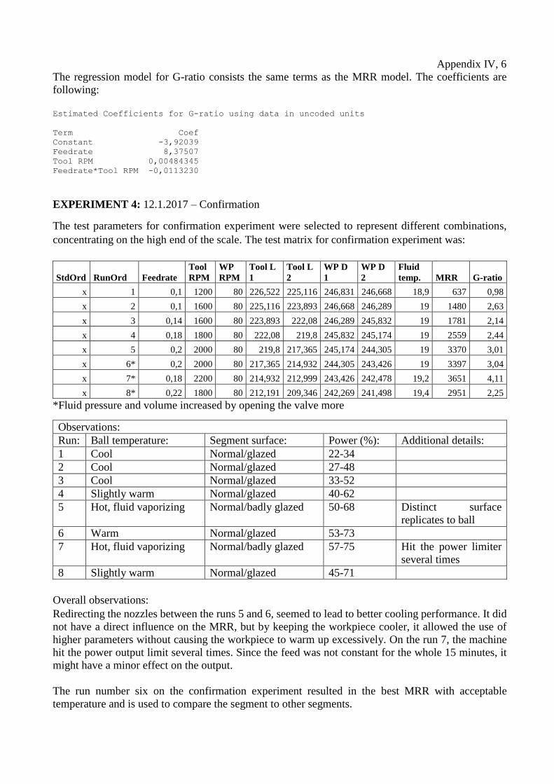
Appendix IV, 6

The regression model for G-ratio consists the same terms as the MRR model. The coefficients are

following:


Term Coef

Constant -3,92039

Feedrate 8,37507

Tool RPM 0,00484345



The test parameters for confirmation experiment were selected to represent different combinations,

concentrating on the high end of the scale. The test matrix for confirmation experiment was:


Tool

RPM

WP

RPM

Tool L

1

Tool L

2

WP D

1

WP D

2

Fluid

temp. MRR G-ratio

x 1 0,1 1200 80 226,522 225,116 246,831 246,668 18,9 637 0,98

x 2 0,1 1600 80 225,116 223,893 246,668 246,289 19 1480 2,63

x 3 0,14 1600 80 223,893 222,08 246,289 245,832 19 1781 2,14

x 4 0,18 1800 80 222,08 219,8 245,832 245,174 19 2559 2,44

x 5 0,2 2000 80 219,8 217,365 245,174 244,305 19 3370 3,01

x 6* 0,2 2000 80 217,365 214,932 244,305 243,426 19 3397 3,04

x 7* 0,18 2200 80 214,932 212,999 243,426 242,478 19,2 3651 4,11

x 8* 0,22 1800 80 212,191 209,346 242,269 241,498 19,4 2951 2,25

*Fluid pressure and volume increased by opening the valve more

Observations:






5 Hot, fluid vaporizing Normal/badly glazed 50-68 Distinct surface

replicates to ball


7 Hot, fluid vaporizing Normal/badly glazed 57-75 Hit the power limiter

several times



Redirecting the nozzles between the runs 5 and 6, seemed to lead to better cooling performance. It did

not have a direct influence on the MRR, but by keeping the workpiece cooler, it allowed the use of

higher parameters without causing the workpiece to warm up excessively. On the run 7, the machine

hit the power output limit several times. Since the feed was not constant for the whole 15 minutes, it

might have a minor effect on the output.

The run number six on the confirmation experiment resulted in the best MRR with acceptable

temperature and is used to compare the segment to other segments.

Appendix IV, 7

Evaluation of the model:

As the Figures 5 and 6 show, the models fit the tested values well, especially the model for MRR. A

relatively small error can be seen on G-ratio’s model but most of the runs in the confirmation

experiment fit in the 90% prediction interval illustrated with the error bars.

Figure 5. The fit of the MRR models to confirmation runs.

Figure 6. The fit of the MRR models to confirmation runs

500,00

1000,00

1500,00

2000,00

2500,00

3000,00

3500,00

4000,00

0 1 2 3 4 5 6 7 8 9

Tested/model MRR


0,5

1

1,5

2

2,5

3

3,5

4

4,5

0 1 2 3 4 5 6 7 8 9



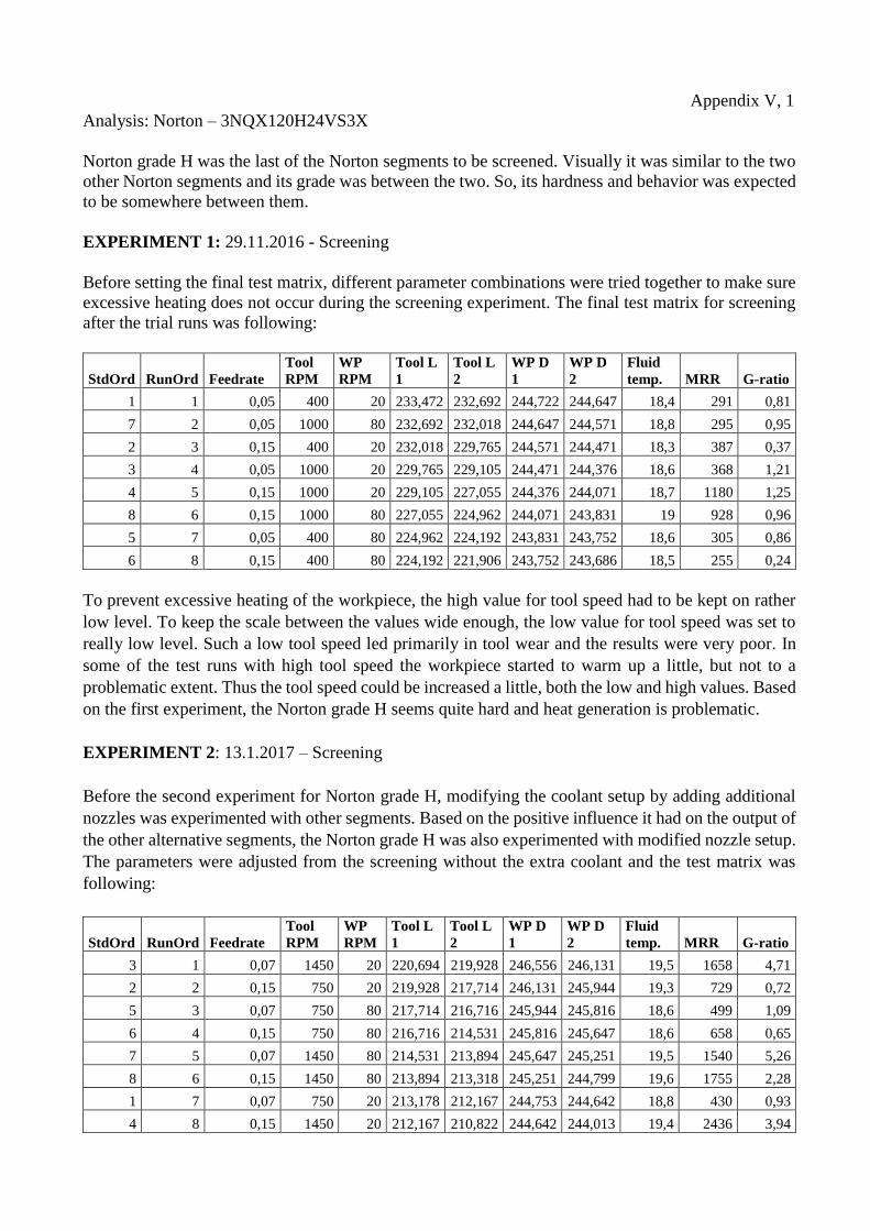
Appendix V, 1

Analysis: Norton – 3NQX120H24VS3X

Norton grade H was the last of the Norton segments to be screened. Visually it was similar to the two

other Norton segments and its grade was between the two. So, its hardness and behavior was expected

to be somewhere between them.


Before setting the final test matrix, different parameter combinations were tried together to make sure

excessive heating does not occur during the screening experiment. The final test matrix for screening

after the trial runs was following:


Tool

RPM

WP

RPM

Tool L

1

Tool L

2

WP D

1

WP D

2

Fluid

temp. MRR G-ratio

1 1 0,05 400 20 233,472 232,692 244,722 244,647 18,4 291 0,81

7 2 0,05 1000 80 232,692 232,018 244,647 244,571 18,8 295 0,95

2 3 0,15 400 20 232,018 229,765 244,571 244,471 18,3 387 0,37

3 4 0,05 1000 20 229,765 229,105 244,471 244,376 18,6 368 1,21

4 5 0,15 1000 20 229,105 227,055 244,376 244,071 18,7 1180 1,25

8 6 0,15 1000 80 227,055 224,962 244,071 243,831 19 928 0,96

5 7 0,05 400 80 224,962 224,192 243,831 243,752 18,6 305 0,86

6 8 0,15 400 80 224,192 221,906 243,752 243,686 18,5 255 0,24

To prevent excessive heating of the workpiece, the high value for tool speed had to be kept on rather

low level. To keep the scale between the values wide enough, the low value for tool speed was set to

really low level. Such a low tool speed led primarily in tool wear and the results were very poor. In

some of the test runs with high tool speed the workpiece started to warm up a little, but not to a

problematic extent. Thus the tool speed could be increased a little, both the low and high values. Based

on the first experiment, the Norton grade H seems quite hard and heat generation is problematic.


Before the second experiment for Norton grade H, modifying the coolant setup by adding additional

nozzles was experimented with other segments. Based on the positive influence it had on the output of

the other alternative segments, the Norton grade H was also experimented with modified nozzle setup.

The parameters were adjusted from the screening without the extra coolant and the test matrix was

following:


Tool

RPM

WP

RPM

Tool L

1

Tool L

2

WP D

1

WP D

2

Fluid

temp. MRR G-ratio

3 1 0,07 1450 20 220,694 219,928 246,556 246,131 19,5 1658 4,71

2 2 0,15 750 20 219,928 217,714 246,131 245,944 19,3 729 0,72

5 3 0,07 750 80 217,714 216,716 245,944 245,816 18,6 499 1,09

6 4 0,15 750 80 216,716 214,531 245,816 245,647 18,6 658 0,65

7 5 0,07 1450 80 214,531 213,894 245,647 245,251 19,5 1540 5,26

8 6 0,15 1450 80 213,894 213,318 245,251 244,799 19,6 1755 2,28

1 7 0,07 750 20 213,178 212,167 244,753 244,642 18,8 430 0,93

4 8 0,15 1450 20 212,167 210,822 244,642 244,013 19,4 2436 3,94

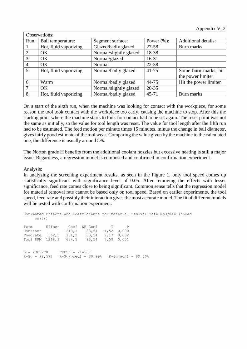
Appendix V, 2

Observations:


1 Hot, fluid vaporizing Glazed/badly glazed 27-58 Burn marks


3 OK Normal/glazed 16-31

4 OK Normal 22-38

5 Hot, fluid vaporizing Normal/badly glazed 41-75 Some burn marks, hit

the power limiter

6 Warm Normal/badly glazed 44-75 Hit the power limiter


8 Hot, fluid vaporizing Normal/badly glazed 45-71 Burn marks

On a start of the sixth run, when the machine was looking for contact with the workpiece, for some

reason the tool took contact with the workpiece too early, causing the machine to stop. After this the

starting point where the machine starts to look for contact had to be set again. The reset point was not

the same as initially, so the value for tool length was reset. The value for tool length after the fifth run

had to be estimated. The feed motion per minute times 15 minutes, minus the change in ball diameter,

gives fairly good estimate of the tool wear. Comparing the value given by the machine to the calculated

one, the difference is usually around 5%.

The Norton grade H benefits from the additional coolant nozzles but excessive heating is still a major

issue. Regardless, a regression model is composed and confirmed in confirmation experiment.

Analysis:

In analyzing the screening experiment results, as seen in the Figure 1, only tool speed comes up

statistically significant with significance level of 0.05. After removing the effects with lesser

significance, feed rate comes close to being significant. Common sense tells that the regression model

for material removal rate cannot be based only on tool speed. Based on earlier experiments, the tool

speed, feed rate and possibly their interaction gives the most accurate model. The fit of different models

will be tested with confirmation experiment.

Estimated Effects and Coefficients for Material removal rate mm3/min (coded

units)


Constant 1213,1 83,54 14,52 0,000

Feedrate 362,5 181,2 83,54 2,17 0,082

Tool RPM 1268,3 634,1 83,54 7,59 0,001

S = 236,278 PRESS = 714587


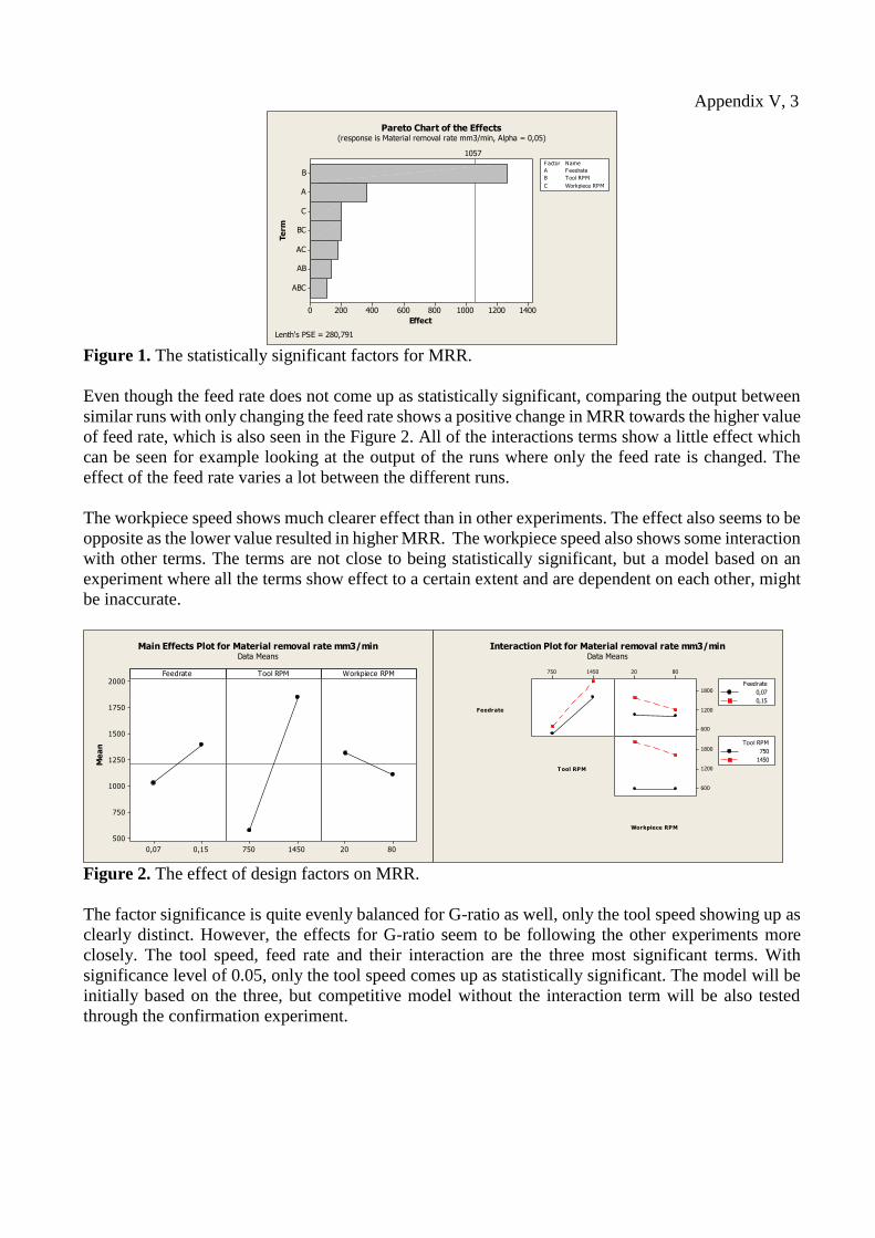
Appendix V, 3

ABC

AB

AC

BC

C

A

B

1400120010008006004002000

Te

rm

Effect

1057

A Feedrate

B Tool RPM

C Workpiece RPM

Factor Name


Lenth's PSE = 280,791 Figure 1. The statistically significant factors for MRR.

Even though the feed rate does not come up as statistically significant, comparing the output between

similar runs with only changing the feed rate shows a positive change in MRR towards the higher value

of feed rate, which is also seen in the Figure 2. All of the interactions terms show a little effect which

can be seen for example looking at the output of the runs where only the feed rate is changed. The

effect of the feed rate varies a lot between the different runs.

The workpiece speed shows much clearer effect than in other experiments. The effect also seems to be

opposite as the lower value resulted in higher MRR. The workpiece speed also shows some interaction

with other terms. The terms are not close to being statistically significant, but a model based on an

experiment where all the terms show effect to a certain extent and are dependent on each other, might

be inaccurate.

0,150,07

2000

1750

1500

1250

1000

750

500

1450750 8020

Feedrate

Me

an



1450750 8020

1800

1200

600

1800

1200

600

Feedrate

T ool RPM

Workpiece RPM

0,07

0,15

Feedrate

750

1450

Tool RPM



The factor significance is quite evenly balanced for G-ratio as well, only the tool speed showing up as

clearly distinct. However, the effects for G-ratio seem to be following the other experiments more

closely. The tool speed, feed rate and their interaction are the three most significant terms. With

significance level of 0.05, only the tool speed comes up as statistically significant. The model will be

initially based on the three, but competitive model without the interaction term will be also tested

through the confirmation experiment.

Appendix V, 4 Estimated Effects and Coefficients for G-ratio (coded units)


Constant 2,4449 0,2193 11,15 0,000

Feedrate -1,0970 -0,5485 0,2193 -2,50 0,067

Tool RPM 3,1989 1,5995 0,2193 7,29 0,002


S = 0,620317 PRESS = 6,15668


C

BC

ABC

AC

AB

A

B

3,53,02,52,01,51,00,50,0

Te

rm

Effect

3,115

A Feedrate

B Tool RPM

C Workpiece RPM

Factor Name



AB

A

B

876543210

Te

rm

Standardized Effect

2,776

A Feedrate

B Tool RPM

Factor Name



The effects for G-ratio are as usual and shown in the Figure 4. The feed rate increases the tool wear,

resulting in weaker G-ratio. The tool speed reduces the wear and increases the MRR, improving the

G-ratio. In the interaction plot of feed rate and tool speed below, the slopes for two feed rates are not

parallel, thus showing some interaction.

0,150,07

4,0

3,5

3,0

2,5

2,0

1,5

1,0

1450750 8020

Feedrate

Me

an



1450750

5

4

3

2

1

Tool RPM

Me

an

0,07

0,15

Feedrate



The initial regression model for material removal rate consists of terms for feed rate and tool speed.

Output estimates are also calculated with models consisting other terms. If some other model proves

to be more accurate, it will be used instead. The primary model consists of following coefficients:


units

Term Coef

Constant -1278,27

Feedrate 4530,65

Tool RPM 1,81179

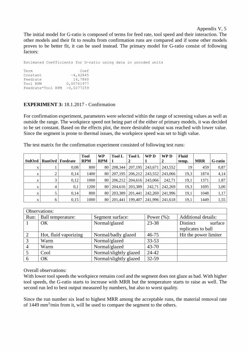
Appendix V, 5

The initial model for G-ratio is composed of terms for feed rate, tool speed and their interaction. The

other models and their fit to results from confirmation runs are compared and if some other models

proves to be better fit, it can be used instead. The primary model for G-ratio consist of following

factors:


Term Coef

Constant -4,42845

Feedrate 16,7860

Tool RPM 0,00761977


EXPERIMENT 3: 18.1.2017 - Confirmation

For confirmation experiment, parameters were selected within the range of screening values as well as

outside the range. The workpiece speed not being part of the either of primary models, it was decided

to be set constant. Based on the effects plot, the more desirable output was reached with lower value.

Since the segment is prone to thermal issues, the workpiece speed was set to high value.

The test matrix for the confirmation experiment consisted of following test runs:


Tool

RPM

WP

RPM

Tool L

1

Tool L

2

WP D

1

WP D

2

Fluid

temp. MRR G-ratio

x 1 0,08 800 80 208,344 207,195 243,671 243,552 19 459 0,87

x 2 0,14 1400 80 207,195 206,212 243,552 243,066 19,3 1874 4,14

x 3 0,12 1000 80 206,212 204,616 243,066 242,71 19,1 1371 1,87

x 4 0,1 1200 80 204,616 203,389 242,71 242,269 19,3 1695 3,00

x 5 0,14 800 80 203,389 201,441 242,269 241,996 19,1 1048 1,17

x 6 0,15 1000 80 201,441 199,407 241,996 241,618 19,1 1449 1,55

Observations:


1 OK Normal/glazed 23-38 Distinct surface

replicates to ball

2 Hot, fluid vaporizing Normal/badly glazed 46-75 Hit the power limiter






With lower tool speeds the workpiece remains cool and the segment does not glaze as bad. With higher

tool speeds, the G-ratio starts to increase with MRR but the temperature starts to raise as well. The

second run led to best output measured by numbers, but also to worst quality.

Since the run number six lead to highest MRR among the acceptable runs, the material removal rate

of 1449 mm3/min from it, will be used to compare the segment to the others.

Appendix V, 6

Evaluation of the models:

The estimates given by the model and their fit to tested values are shown in the Figure 5. The estimates

for first two runs are rather accurate but for the remaining four, the estimates are on average 280 units

lower than the tested values. With several factors showing some level of significance, the model could

be expected to have some inaccuracy.


The model for G-ratio, shown in the Figure 6, is the total opposite of the model for MRR. For G-ratio,

the biggest error appears to be on two of the first runs and the rest of the estimates seem to be following

the tested values nicely.


400,0

600,0

800,0

1000,0

1200,0

1400,0

1600,0

1800,0

0 1 2 3 4 5 6 7

Tested/model MRR


0,5

1

1,5

2

2,5

3

3,5

4

4,5

0 1 2 3 4 5 6 7



Appendix VI, 1

Analysis: Norton – 3NQX120J24VS3X

The second experimented alternative was the hardest of the Norton segments and very likely the

hardest of all the tested alternatives. The testing of the Norton grade J was started on 24nd of November,

2016.


Like with the Diprotex segment, not much was known about the segments that Norton had provided

for the test. The testing had to be started somewhere and the parameters would have to be corrected

based on the results and observations. Visually, the Norton segments are closer to Tyrolit than the

other alternatives. So with once again, without better knowledge, the testing was started with

parameters that work with Tyrolit segment. The experiment was conducted before discovering the

benefits of the additional coolant nozzles. The test matrix for screening the Norton J segment was

following:

StdOrder RunOrder Feed rate Tool RPM Workpiece RPM

2 1 0.2 1200 20

5 2 0.1 1200 80

4 3 0.2 2000 20

8 4 0.2 2000 80

7 5 0.1 2000 80

1 6 0.1 1200 20

3 7 0.1 2000 20

6 8 0.2 1200 80

The first run was stopped at two minutes due to the machine reaching the set limit for power output.

The surface of the ball had severe burn marks and the fluid on the workpiece surface was vaporizing.

It was clear after just two minutes that the bond on Norton J is much harder than Tyrolit or Diprotex

and the parameters would have to be adjusted.

Before starting the experiment over, the effect of dropping the feed rate to half was tested. With feed

rate of 0.10 mm/min, combined with tool speed of 1200 RPM and workpiece speed of 20 RPM, the

power output limit was no longer reached. After few quick test runs, the test matrix parameters for the

first screening experiment were set to:


Tool

RPM

WP

RPM Tool L 1 Tool L 2 WP D 1 WP D 2

Fluid

temp. MRR G-ratio

2 1 0,1 400 20 239,224 237,813 245,866 245,776 18,1 350 0,54

5 2 0,03 400 80 237,813 237,399 245,776 245,728 17,7 187 0,98

4 3 0,1 1200 20 237,399 236,456 245,728 245,411 19,1 1233 2,84

8 4 0,1 1200 80 236,456 235,602 245,411 245,09 19,3 1247 3,18

7 5* 0,03 1200 80 235,602 235,552 245,09 245,015 18,7 291 12,66

1 6** 0,03 400 20 235,552 235,171 245,015 244,979 18,8 140 0,80

3 7** 0,03 1200 20 235,171 234,977 244,979 244,903 18,4 295 3,31

6 8 0,1 400 80 234,977 233,592 244,903 244,826 18,4 299 0,47

*A solid contact after 11 minutes, **Contact after several minutes into the test run

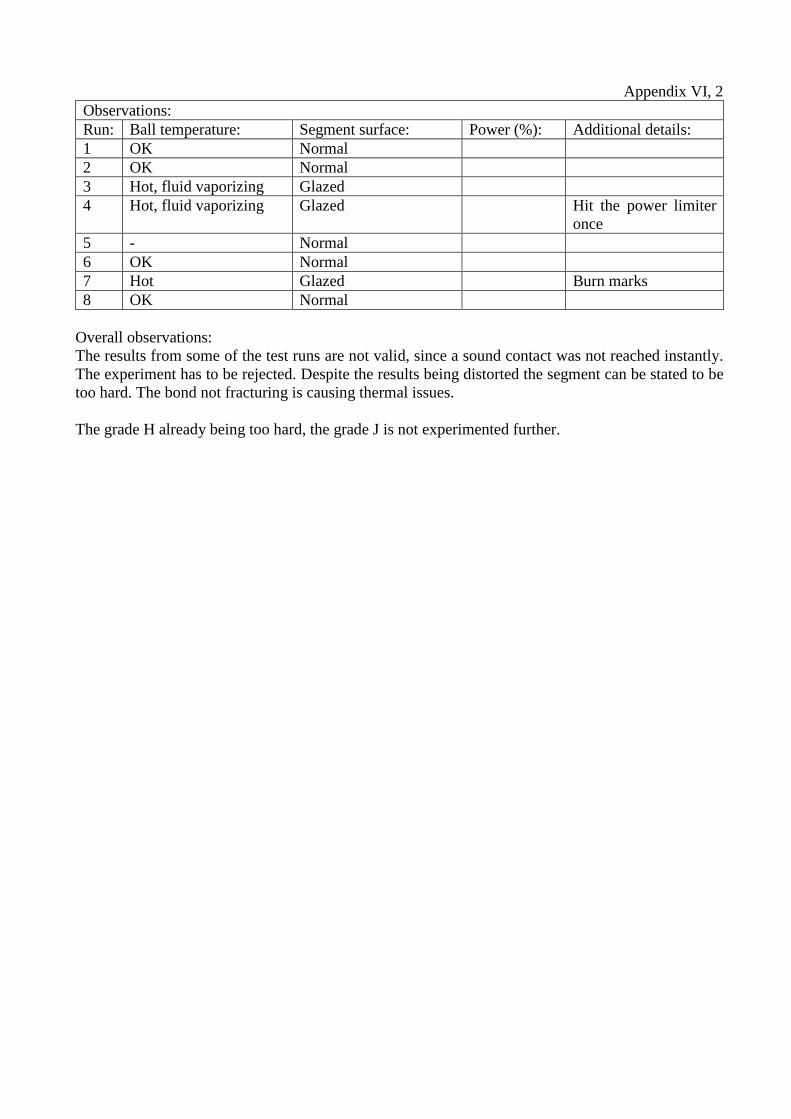
Appendix VI, 2

Observations:


1 OK Normal

2 OK Normal

3 Hot, fluid vaporizing Glazed

4 Hot, fluid vaporizing Glazed Hit the power limiter

once

5 - Normal

6 OK Normal

7 Hot Glazed Burn marks

8 OK Normal


The results from some of the test runs are not valid, since a sound contact was not reached instantly.

The experiment has to be rejected. Despite the results being distorted the segment can be stated to be

too hard. The bond not fracturing is causing thermal issues.

The grade H already being too hard, the grade J is not experimented further.

Appendix VII

Concentrations of certain substances in grinding fluid

Analysis Method Fresh

sample Sample 1 Sample 2 Unit Uncertainty

(%)

Chlorine, Cl 11 000 100 000 78 000 μg/l 10

Boron, B, total EN ISO 11885:2009 62 000 460 000 460 000 μg/l 20

Boron, B, soluble EN ISO 11885:2009 57 000 370 000 370 000 μg/l 20

Sulfur, S, total EN ISO 11885:2009 8 800 72 000 70 000 μg/l 20

Sulfur, S, soluble EN ISO 11885:2009 8 400 57 000 56 000 μg/l 20

Phosphorus, P, total EN ISO 11885:2009 < 50 440 440 μg/l 20

Phosphorus, P, soluble EN ISO 11885:2009 < 50 270 260 μg/l 20

Cobolt, Co, total EN ISO 11885:2009 < 15 220 130 μg/l 20

Cobolt, Co, soluble (0.45 μm) EN ISO 11885:2009 < 15 47 39 μg/l 20

Chromium, Cr, total EN ISO 11885:2009 < 20 240 1200 μg/l 20

Chromium, Cr, soluble (0.45 μm) EN ISO 11885:2009 < 20 110 110 μg/l 20

Manganese, Mn, total EN ISO 11885:2009 < 3 30 71 μg/l 20

Manganese, Mn, total (0.45 μm) EN ISO 11885:2009 < 3 14 22 μg/l 20

Molybdenum, Mo, total EN ISO 11885:2009 < 15 270 390 μg/l 20

Molybdenum, Mo, soluble (0.45 μm) EN ISO 11885:2009 < 15 180 180 μg/l 20

Nickel, Ni, total EN ISO 11885:2009 < 30 390 3700 μg/l 20

Nickel, Ni, soluble (0.45 μm) EN ISO 11885:2009 < 30 < 30 < 30 μg/l 20

Titanium, total EN ISO 11885:2009 < 10 100 110 μg/l 20

Titanium, soluble EN ISO 11885:2009 < 10 73 72 μg/l 20

Hydrocarbons, C10-C40

EN ISO 9377-2:2001 mod

C10-C21 58 690 49 μg/l 40

C21-C40 860 3500 2400 μg/l 40

Hydrocarbons, C10-C40, total 920 4200 2400 μg/l 40

lappeenranta university of technology - LUTPub

Documents

Transcript of lappeenranta university of technology - LUTPub