Effect of Coating-thickness on the Formability of Hot Dip Aluminized Steel
Upload
independentCategory
view
0download
0
! !
Digital Image Processing & Machine Vision ! ! Enrolment No.: 11012041034!
!INDEX !
Sr. No.
Title Date
Page No.
Signature of
Instructor
Remarks
1 Introduction to MATLAB 2/7/14 1 13
2 Study of Different Matlab Commands in Image Processing
9/7/14 14 28
3 Study of imread and imshow Function 23/7/14 29 29
4 Study Basic Matlab Function 6/8/14 30 32
- Study subplot and title function
- Study plot, xlabel and ylabel function
- Study imcrop function
- Study imrotate function
5 Study of Images in MATLAB 20/8/14 33 36
- Binary image,
- Monochrome/ Gray level image
- RGB/Color image.
- Indexed image
6Study Programs Related to Enhancement – Point Processing
10/9/14 37 44
- Study Program related to Image negative
- Study of imadjust function
- Study of effect of gamma in power law transformation
- Development of algorithm for image histogram for monochrome image and study of imhist function.
!B.TECH VII SEM MECHATRONICS ENGINEERING !!
!
! !
Digital Image Processing & Machine Vision ! ! Enrolment No.: 11012041034!
- Development of algorithm for histogram equalized image and study of histeq function.
- Study program to verify the contribution of each bit plane to monochrome.
- Study of image subtraction.
- Study of image multiplication.
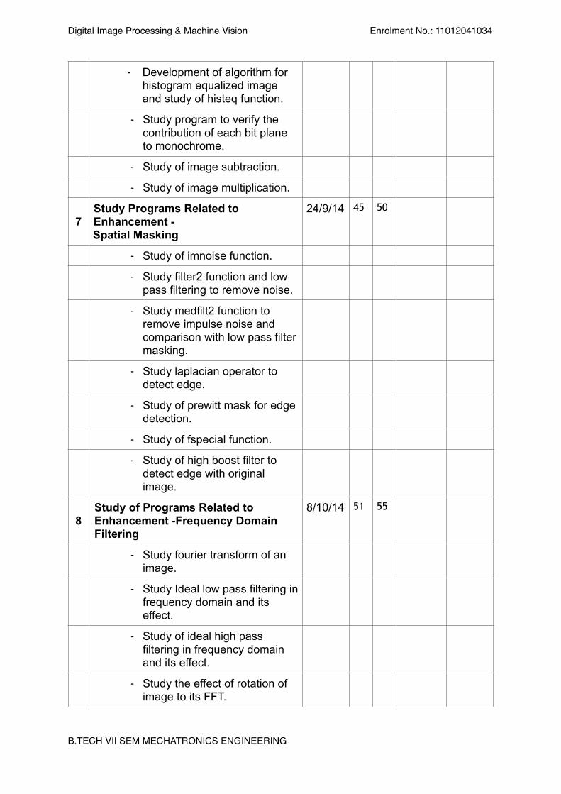
7Study Programs Related to Enhancement - Spatial Masking
24/9/14 45 50
- Study of imnoise function.
- Study filter2 function and low pass filtering to remove noise.
- Study medfilt2 function to remove impulse noise and comparison with low pass filter masking.
- Study laplacian operator to detect edge.
- Study of prewitt mask for edge detection.
- Study of fspecial function.
- Study of high boost filter to detect edge with original image.
8Study of Programs Related to Enhancement -Frequency Domain Filtering
8/10/14 51 55
- Study fourier transform of an image.
- Study Ideal low pass filtering in frequency domain and its effect.
- Study of ideal high pass filtering in frequency domain and its effect.
- Study the effect of rotation of image to its FFT.
!B.TECH VII SEM MECHATRONICS ENGINEERING !!
!

! !
Digital Image Processing & Machine Vision ! ! Enrolment No.: 11012041034!
!!!!!!!!!!
!
!
!
!
PRACTICAL-1!AIM : Introduction to Matlab.
!!!!
!B.TECH VII SEM MECHATRONICS ENGINEERING !!
!

! !
Digital Image Processing & Machine Vision ! ! Enrolment No.: 11012041034!
!!!!!
!
!
Introduction to MATLAB
What is MATLAB?
MATLAB is a high performance language for technical computing. It integrates computation, visualization, and programming in an easy to use environment where problems and solutions are expressed in a familiar mathematical notation. Typical uses include:
• Math and computation • Algorithm development • Modeling, simulation and prototyping • Data analysis, exploration and visualization • Scientific and engineering graphics • Application development, including graphic user interface building !
MATLAB is an interactive system whose basic data element is an array that does not require dimensioning. This allow you to solve many technical computing problems, especially those with matrix and vector formulation, in a fraction of time it would take to write a program in scalar non interactive language such as C of FORTRAN. !
DEPARTMENT OF MECHANICAL & MECHATRONICS ENGINEERING Shri. U.V.Patel College of Engineering, Ganpat Vidyanagar
Sub: Digital Image Processing & Machine Vision (MC 705)
Exp No: -01 Date: - 08/07/10
!B.TECH VII SEM MECHATRONICS ENGINEERING !!
!

! !
Digital Image Processing & Machine Vision ! ! Enrolment No.: 11012041034!
The name MATLAB stands for matrix laboratory. MATLAB was originally written to provide easy access to matrix software developed by the LINPACK and EISPACK projects. Today, MATLAB uses software developed by the LINPACK and ARPACK projects, which together represent the state of the art in software for matrix computation. !MATLAB has evolved over a period of years with input from many users. In university environments, it is the standard instructional tool for introductory and advanced courses in mathematics, engineering and science. In industry, MATLAB is the tool of choice for high productivity research, development and analysis. !MATLAB feature a family of application specific solution called toolboxes. Very important to most users of MATLAB, toolboxes allow you to learn and apply specialized technology. Toolboxes are comprehensive collections of MATLAB function (M-files) that extend the MATLAB environment to solve particular classes of problems. Areas in which toolboxes are available include signal processing, control system, neural networks, fuzzy logic, wavelets, simulation, and many others. !The MATLAB System:-
The MATLAB system consists of five main parts:
Development environment: - This is the set of tools and facilities that help you use MATLAB function and files. Many of these are graphical user interfaces; it includes the MATLAB desktop and Command Window, a command history, and browser for viewing help, the workspace, files and the search path.
The MATLAB Mathematical Function Library:- This is a vast collection of computational algorithms ranging from elementary function like sum, sine, cosine, and complex arithmetic, to more sophisticated functions like matrix inverse, matrix eigenvalues, Bessel function, and fast Fourier transforms.
The MATLAB Language: - This is a high-level matrix/array language with control flow statement, function, data structure, input/output, and object-oriented programming feature. It allows both "programming in the small" to rapidly create quickly and dirty throwaway programs, and "programming in the large" to create complete large and complex application programs.
Handle Graphics: - This is the MATLAB graphics system. It includes high-level commands for two-dimensional and three-dimensional data visualization, image processing, animation, and presentation graphics. It also includes low-level commands that allow you to fully
!B.TECH VII SEM MECHATRONICS ENGINEERING !!
!
! !
Digital Image Processing & Machine Vision ! ! Enrolment No.: 11012041034!
customize the appearance of graphics as well as to build complete graphics user interface on your MATLAB applications.
The MATLAB Application Programming Interface (API):- This is a library that allows you to write C and FORTRAN programs that interface with MATLAB (dynamic linking), calling MATLAB as computational engine, and for reading and writing MAT-files.
Entering Matrices:-
The best way for you to get started with MATLAB is to learn how to handle matrices. Start MATLAB and follow along with each example.
You can enter matrices into MATLAB in several different ways:
➢ Enter an explicit list of elements.
➢ Load matrices from external data files.
➢ Generate matrices using built-in function.
➢ Create matrices with your own function in M-files.
Start by entering Duper’s matrix as a list of its elements. You have only to follow a few basic conventions: !
➢ Separate the elements of a row with blanks or commas.
➢ Use a semicolon (;), to indicate the end of each row.
➢ Surround the entire list of elements with square brackets [ ].
To enter Durer’s matrix, simply type in the command window.
A = [16 3 2 13; 5 10 11 8; 9 6 7 12; 4 15 14 1]
MATLAB displays the matrix you just entered.
A = 16 3 2 13 5 10 11 8 9 6 7 12 4 15 14 1 This exactly matches the number the numbers in the engraving. Once you have entered the matrix, it is automatically remembered in the MATLAB workspace. You can refer to it simply as A. Now that you have A in the workspace; take a look at what makes it so interesting.
!!B.TECH VII SEM MECHATRONICS ENGINEERING !!
!

! !
Digital Image Processing & Machine Vision ! ! Enrolment No.: 11012041034!
Sum, Transpose, and Diag.
You’re probably already aware that the special properties of a magic square have to do with the various ways of summing its elements. If you take the sum along any row or column, or along either of the two main diagonals, you will always get the same number. Let’s verify that using MATLAB. The first statement to try is
Sum (A)
MATLAB replies with
Ans = 34 34 34 34
When you don’t specify an output variable, MATLAB uses the variable Ans, short for answer, to store the results of a calculation. You have computed a row vector containing the sums of the columns of A. sure enough; each of the columns has the same sum, the magic sum, and 34.
How about the row sums? MATLAB has a preference for working with the columns of a matrix, so the easiest way to get the row sums is to transpose the matrix, compute the column sums of the transpose, and then transpose the result. The transpose operation is denoted by an apostrophe or single quote (‘). It flips a matrix about its main diagonal and it turns a row vector into a column vector. So
!A’
Produces Ans =
16 5 9 4 3 10 6 15 2 11 7 14 13 8 12 1
And sum (A’)’
Producing a column vector containing the row sums
Ans = 34 34 34 34
The sum of the elements on the main diagonal is easily obtained with the help of the diag function, which picked off that diagonal.
!B.TECH VII SEM MECHATRONICS ENGINEERING !!
!

! !
Digital Image Processing & Machine Vision ! ! Enrolment No.: 11012041034!
Diag (A) produces
Ans = 16 10 7 1
And
Sum (diag (A)) produces
Ans = 34
The other diagonal, anti diagonal, is not so important mathematically, so MATLAB does not ready made function for it. But function originally intended for use in graphics, fliplr, flips matrix from left to right.
Sum (diag (flipper (A)))
Ans = 34
Deleting Rows and Columns You can delete rows and columns from a matrix from a matrix using just a pair of square brackets. Start with
X=A;
Then to delete the second column of X, use
X (: 2) = []
This changes X to
X= 16 2 13 5 11 8 4 14 1 !If you delete a single element from a matrix, the result isn’t a matrix anymore. So expressions like X (1, 2) = []
Result is an error. However, using a single subscript deletes a single element or sequence of elements, and reshapes the remaining elements into a row vector. So
X (2:2:10) = []
Results in
!B.TECH VII SEM MECHATRONICS ENGINEERING !!
!
! !
Digital Image Processing & Machine Vision ! ! Enrolment No.: 11012041034!
X= 16 9 2 7 13 12 1
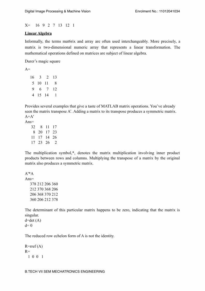
Linear Algebra
Informally, the terms mat6rix and array are often used interchangeably. More precisely, a matrix is two-dimensional numeric array that represents a linear transformation. The mathematical operations defined on matrices are subject of linear algebra.
Durer’s magic square
A=
16 3 2 13 5 10 11 8 9 6 7 12 4 15 14 1 !Provides several examples that give a taste of MATLAB matrix operations. You’ve already seen the matrix transpose A’. Adding a matrix to its transpose produces a symmetric matrix. A+A' Ans= 32 8 11 17 8 20 17 23 11 17 14 26 17 23 26 2 !The multiplication symbol,*, denotes the matrix multiplication involving inner product products between rows and columns. Multiplying the transpose of a matrix by the original matrix also produces a symmetric matrix. !A'*A Ans= 378 212 206 360 212 370 368 206 206 368 370 212 360 206 212 378 !The determinant of this particular matrix happens to be zero, indicating that the matrix is singular. d=det (A) d= 0 !The reduced row echelon form of A is not the identity. !R=rref (A) R= 1 0 0 1 !B.TECH VII SEM MECHATRONICS ENGINEERING !!
!
! !
Digital Image Processing & Machine Vision ! ! Enrolment No.: 11012041034!
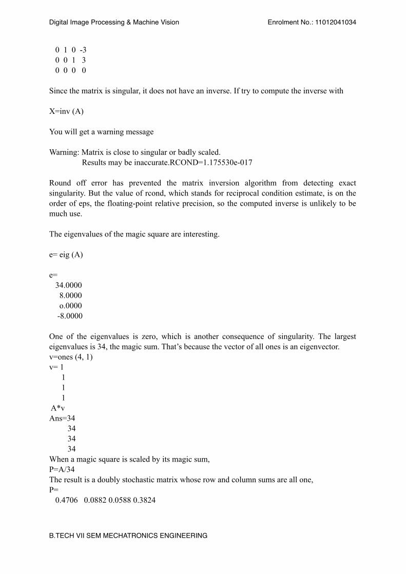
0 1 0 -3 0 0 1 3 0 0 0 0 !Since the matrix is singular, it does not have an inverse. If try to compute the inverse with !X=inv (A) !You will get a warning message !Warning: Matrix is close to singular or badly scaled. Results may be inaccurate.RCOND=1.175530e-017 !Round off error has prevented the matrix inversion algorithm from detecting exact singularity. But the value of rcond, which stands for reciprocal condition estimate, is on the order of eps, the floating-point relative precision, so the computed inverse is unlikely to be much use. !The eigenvalues of the magic square are interesting. !e= eig (A) !e= 34.0000 8.0000 o.0000 -8.0000 !One of the eigenvalues is zero, which is another consequence of singularity. The largest eigenvalues is 34, the magic sum. That’s because the vector of all ones is an eigenvector. v=ones (4, 1) v= 1 1 1 1 A*v Ans=34 34 34 34 When a magic square is scaled by its magic sum, P=A/34 The result is a doubly stochastic matrix whose row and column sums are all one, P= 0.4706 0.0882 0.0588 0.3824
!B.TECH VII SEM MECHATRONICS ENGINEERING !!
!
! !
Digital Image Processing & Machine Vision ! ! Enrolment No.: 11012041034!
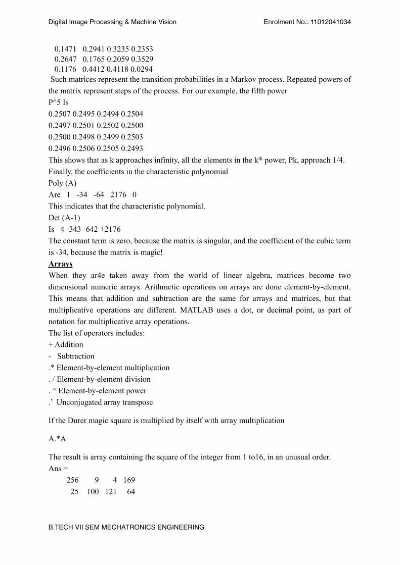
0.1471 0.2941 0.3235 0.2353 0.2647 0.1765 0.2059 0.3529 0.1176 0.4412 0.4118 0.0294 Such matrices represent the transition probabilities in a Markov process. Repeated powers of the matrix represent steps of the process. For our example, the fifth power P^5 Is 0.2507 0.2495 0.2494 0.2504 0.2497 0.2501 0.2502 0.2500 0.2500 0.2498 0.2499 0.2503 0.2496 0.2506 0.2505 0.2493 This shows that as k approaches infinity, all the elements in the kth power, Pk, approach 1/4. Finally, the coefficients in the characteristic polynomial Poly (A) Are 1 -34 -64 2176 0 This indicates that the characteristic polynomial. Det (A-1) Is 4 -343 -642 +2176 The constant term is zero, because the matrix is singular, and the coefficient of the cubic term is -34, because the matrix is magic! Arrays When they ar4e taken away from the world of linear algebra, matrices become two dimensional numeric arrays. Arithmetic operations on arrays are done element-by-element. This means that addition and subtraction are the same for arrays and matrices, but that multiplicative operations are different. MATLAB uses a dot, or decimal point, as part of notation for multiplicative array operations. The list of operators includes: + Addition - Subtraction .* Element-by-element multiplication . / Element-by-element division . ^ Element-by-element power .’ Unconjugated array transpose
If the Durer magic square is multiplied by itself with array multiplication
A.*A
The result is array containing the square of the integer from 1 to16, in an unusual order. Ans = 256 9 4 169 25 100 121 64
!B.TECH VII SEM MECHATRONICS ENGINEERING !!
!
! !
Digital Image Processing & Machine Vision ! ! Enrolment No.: 11012041034!
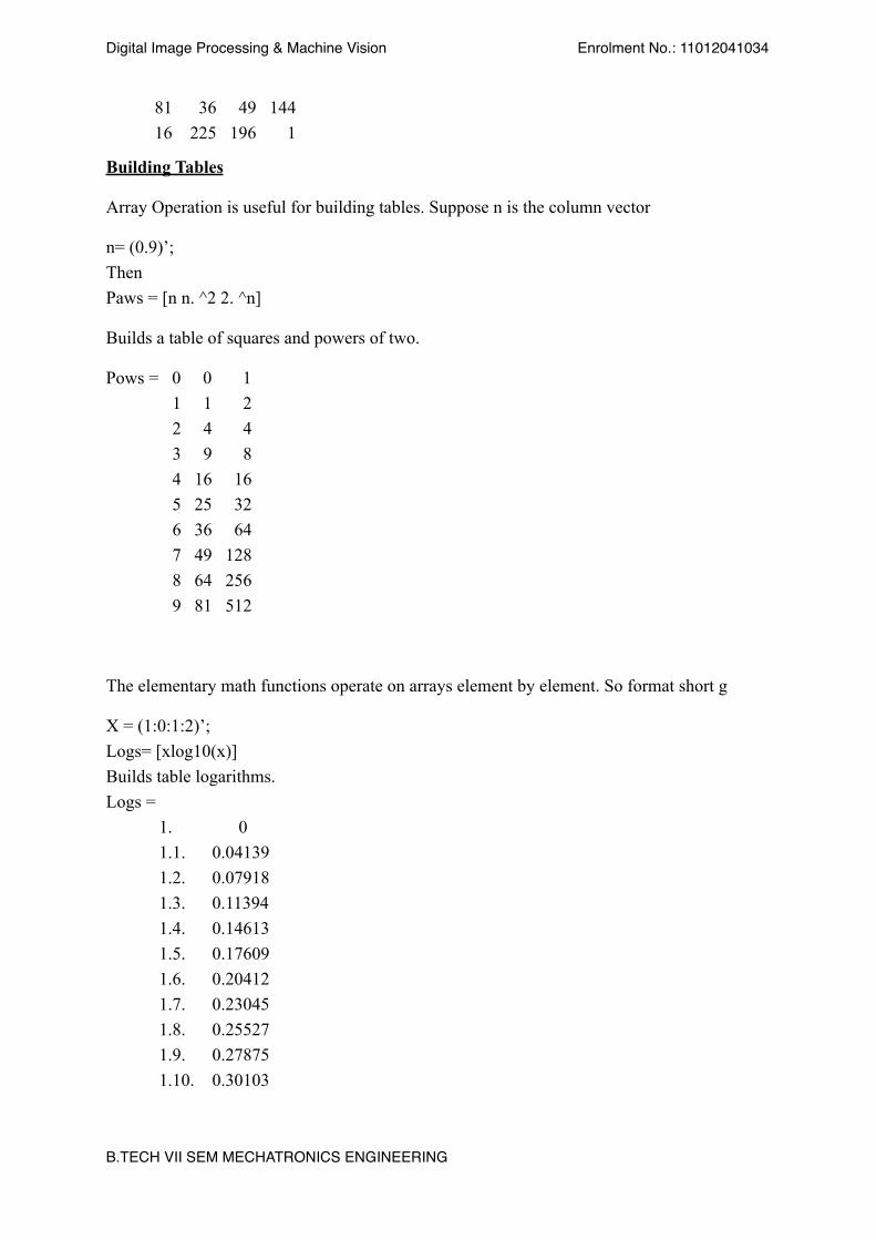
81 36 49 144 16 225 196 1
Building Tables
Array Operation is useful for building tables. Suppose n is the column vector
n= (0.9)’; Then Paws = [n n. ^2 2. ^n]
Builds a table of squares and powers of two.
Pows = 0 0 1 1 1 2 2 4 4 3 9 8 4 16 16 5 25 32 6 36 64 7 49 128 8 64 256 9 81 512
!The elementary math functions operate on arrays element by element. So format short g
X = (1:0:1:2)’; Logs= [xlog10(x)] Builds table logarithms. Logs =
1. 0 1.1. 0.04139 1.2. 0.07918 1.3. 0.11394 1.4. 0.14613 1.5. 0.17609 1.6. 0.20412 1.7. 0.23045 1.8. 0.25527 1.9. 0.27875 1.10. 0.30103
!B.TECH VII SEM MECHATRONICS ENGINEERING !!
!

! !
Digital Image Processing & Machine Vision ! ! Enrolment No.: 11012041034!
Desktop Tools: This section provides as introduction to MATLAB’s desktop tools. You can also use MATLAB functions to perform most of the features found in the desktop tools. The tools are: 1.Command Window
Use the command window to enter variables and run functions and M-files. For more information on controlling input and output, see Controlling Command Window Input and Output.
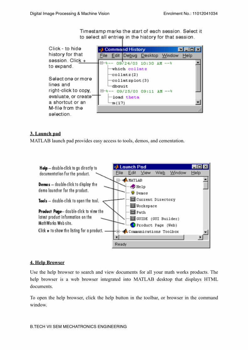
! !!2. Command History
Lines you enter in the Command Window are logged in Command History Window. In the Command History, you can view previously used functions and copy and execute selected lines. To save the input and output from a MATLAB session to a file, use the diary function. !!
!B.TECH VII SEM MECHATRONICS ENGINEERING !!
!
! !
Digital Image Processing & Machine Vision ! ! Enrolment No.: 11012041034!
! !3. Launch pad MATLAB launch pad provides easy access to tools, demos, and cementation. !
! 4. Help Browser
Use the help browser to search and view documents for all your math works products. The help browser is a web browser integrated into MATLAB desktop that displays HTML documents.
To open the help browser, click the help button in the toolbar, or browser in the command window.
!B.TECH VII SEM MECHATRONICS ENGINEERING !!
!

! !
Digital Image Processing & Machine Vision ! ! Enrolment No.: 11012041034!
!Running the external programs
You can run the external programs from the MATLAB command window. The exclamation point character! Is a Shell escape and indicates that the rest of the input line command to the operating system. This is useful for invoking utilities of running other programs without quitting MATLAB on Linux for example, lemacs magilk.m. When you quit the external programs, the operating returns control to MATLAB.
The help browser consist of two planes, the help navigator, which you see to find information, and display pane, where you view the information.
Help navigator Use to help navigator to find information. It includes:
➢ Product filter- Set filter to show documentation only for the products specify.
➢ Contents tab- View the title and content of the tables of documentation for your products.
➢ Index tab- Find specific entries in the math works documentation for your products.
➢ Search tab- Look for specific phrase in the documentation. To get help for a specific function set the search type to function name.
➢ Favorites tab- View a list of documents you previously designed as favorites.
Display Pane After finding documentation using the help navigator, view it in the display pane. While viewing the documentation, you can !
➢ Browse to other pages- Use the arrows at the top and bottoms of the pages, or use the backward and forward buttons in toolbar.
➢ Bookmark pages- Click to add the favorite’s button in the toolbar.
➢ Print pages- Click the print button in the toolbar.
➢ Find a term in the page - Type a term in the find in page fiddle in the toolbar and click go Other feature available in the display pane are :copying information ,evaluating the selection , and viewing web pages. !!
For More Help
!B.TECH VII SEM MECHATRONICS ENGINEERING !!
!
! !
Digital Image Processing & Machine Vision ! ! Enrolment No.: 11012041034!
In addition to the help brow, you can use help function, use doc. For example, doc format displays help for the format function in the help browser. Other means for getting help include contacting Technical support (http://www.mathworks.com/support) and participating in the newsgroup for METLAB user, comp.soft-sys.matlab.
5. Current directory browser:
MATLAB file operation use the current directory and search path as reference points. Any file you want to run must either be in the current directory or on the search path. A quick way to view or change the current directory is by using the current directory field in the desktop tool bar as shown below.
To search for, view, open, and make to changes to MATLAB-related directories and files use the METLAB current directory browser. Alternatively, you can use the function dir, cd, and delete.
Search Path
To determine how to execute functions you call. MATLAB user is a search path to find M-files and other MATLAB-related files, which are organized in directories on your file system. Any file you want to run In MATLAB must reside in the current directory or in a directory that is in the search path. By default, the files supplied with MATLAB and Math Works toolboxes are included in the search path.
To see which are on the search path or to change, select set path from the file menu in the desktop, and use the set path dialog box. Alternatively, you can use the path function to view the search path, add path to add directories to the path, and rmpath to remove directories from the path.
6. Workspace browser
The MATLAB workspace consists of the set of variables (named arrays) build up during a MATLAB session and stored in the memory. You add variables to the workspace by using function, running M-files, and loading saved workspaces. To view the workspace and information about each variable, use the workspace browser, or use the function who and whos.
!!!!!!!B.TECH VII SEM MECHATRONICS ENGINEERING !!
!

! !
Digital Image Processing & Machine Vision ! ! Enrolment No.: 11012041034!
!!!!!!!!!
!
!
!
!
!
!
PRACTICAL-2!AIM : Study of Different Matlab Commands in
Image Processing.
!!!B.TECH VII SEM MECHATRONICS ENGINEERING !!
!

! !
Digital Image Processing & Machine Vision ! ! Enrolment No.: 11012041034!
!!!!!!!!!!!!!!!!!!!!!!!!!!!!!
!B.TECH VII SEM MECHATRONICS ENGINEERING !!
!

! !
Digital Image Processing & Machine Vision ! ! Enrolment No.: 11012041034!
!Study of different matlab commands in image processing. !➢ imread !Read image from graphic file. !Syntax A= imread (filename, fmt) [X, map] = imread (filename.fmt) !Description !The imread function supports four general syntaxes; described below the imread function also supports several other format- specific syntaxes. See special Case Syntax for information about these syntaxes. A=imread (filename, fmt) reads a gray scale or color image from the file specified by the string filename, where the string fmt specifies the format of the file. If the file is not in the current directory or in a directory or in a directory in the MATLAB path, specify the full pathname of the location on your system. For a list of all the possible values for fmt, see supported formats. If imread cannot find a file named filename, it looks for a file named filename.fmt. Imread returns the image data in the array A. If the file contains a gray scale image, A is a two-dimensional (M-by-N) array. If the file contains a color image, A is a three dimensional (M-by-N-by-3) array. The class of the returned array depends on the data types used by the file format. For most file formats the color image data returned uses the RGB color spaces.
[X, map] = imread (filename, fmt) reads the indexed image in filename into X and its associated color map into map. The color map values are rescaled to the range [0, 1]. !➢ imshow !Display an image !Syntax
DEPARTMENT OF MECHANICAL & MECHATRONICS ENGINEERING Shri U.V.Patel College of Engineering, Ganpat Vidyanagar
Sub: Digital Image Processing & Machine Vision (MC 705)
Exp. No: -02 Date: - 22/07/10
!B.TECH VII SEM MECHATRONICS ENGINEERING !!
!
! !
Digital Image Processing & Machine Vision ! ! Enrolment No.: 11012041034!
!imshow (I, n) imshow (I,[low high]) imshow (BW) imshow (X, map) Description !imshow (I, n) displays the intensity image I with n discrete levels of gray. If you omit n. imshow uses 256 gray levels on 24 bit displays, or 64 gray levels on other systems imshow (I,[low high]) display I as a gray scale intensity image, specifying the data range for I. The value low (and any values less than low) displays as black; the value high (and any value greater than high) displays as white. Values in between are displayed as intermediate shades of gray, using the default number of gray levels. If you use an empty matrix ([]) for [low high], imshow uses [min (I (: )) max (I (: )]; that is the minimum values in I is displayed as black, and the maximum value is displayed as white.
imshow (BW) displays the binary image BW. imshow displays pixels with the value 0 (zero) as black and pixels with the value I as white imshow (X map) displays the indexed image X with the color map.
imshow (RGB) displays the true-color image RGB. imshow (…displays option) displays the image, where displays option specifies how imshow handles the sizing of the image. A display option is a string that can have either of these values. Option strings can be abbreviated. !Values descriptions ‘notruesize’ Do not call the true size function. !‘truesize’ call the truesize function. !The truesize function maps each pixel in the image to one screen pixel. If you do not supply these arguments, imshow refers to the setting of the ‘Imshow Truesize’ preference to determine whether to call truesize or not, by default, imshow calls truesize if there are no other objects in the resulting figure besides the image and its axes. !➢ clear !Remove items from workspace, freeing up system memory Graphical Interface As an alternative to the clear function, uses Clear Workspace in the MATLAB desktop Edit menu. !Syntax !!B.TECH VII SEM MECHATRONICS ENGINEERING !!
!

! !
Digital Image Processing & Machine Vision ! ! Enrolment No.: 11012041034!
Clear Clear name Clear name1 name2 name3… Clear global name Clear –regexp expr1 expr2… Clear global –regexp expr1 expr2… Clear keyword Clear (‘name1’, ‘name2’, ’name3’…) !!Description
clear
removes all variables from the workspace. This frees up system memory.
clear name
Removes just the m-file or MEX-file function or variable name from the workspace. You can wildcards (*) to remove items selectively. For example, clear my* removes any Variable whose name begins with the string my. It removes debugging breakpoints in M- Files and reinitializes persistent variables, since the break points for function and persistent Variables are cleared whenever the M-file is changed or cleared. If name is global, it is removed from current workspace, but left accessible to any functions declaring it global. If name has been locked by mlock, it remains in memory.
clear name 1 name2 name3 … removes name 1, name 2, and name3 from the workspace.
clear global name removes the global variable name. If name is global, clear name Removes name from the current workspace, but leaves it accessible to any functions declaring it global. Use clear global name to completely remove a global variable.
clear -regexp expr 1 expr 2…clears all variables that match any of the regular expressions expr 1, expr 2, etc. this option only clears variables
➢ close
Delete specified figure
Syntax close close (h) close name close all
!B.TECH VII SEM MECHATRONICS ENGINEERING !!
!
! !
Digital Image Processing & Machine Vision ! ! Enrolment No.: 11012041034!
close all hidden Status =close (…) !Description Closedeletes the current figure or the specified figure(s). It optionally returns the status of the close operation, and close deletes the current figure (equivalent to close (gef)), Close (h) deletes the figure identified by h. if h is a vector or matrix. Close deletes all figures identified by h. Close name deletes the figure with the specified name. Close all deletes the figure whose handles are not hidden. Close all hidden deletes all figures including those with hidden handles. !!!➢ subplot !Create and control multiple axes. !Syntax subplot (m, n, p) !Description !subplot divides the current figure into rectangular panes that are numbered row wise. Each pane contains axes. Subsequent plots are output to the current plane.
subplot (m, n, p)
Creates an axis in the path pane of figure divided into an m-by-n matrix of rectangular Panes. The new axis becomes the current axis. If p is a vector, it specifies axes having a position that covers all the subplot position listed in p. !➢ imcrop !Crop an image Syntax I2 = imcrop (I) X2 = imcrop (x, map)
RGB2 = imcrop (RGB)
!!B.TECH VII SEM MECHATRONICS ENGINEERING !!
!

! !
Digital Image Processing & Machine Vision ! ! Enrolment No.: 11012041034!
I2 = imcrop (I, rect)
X2 = imcrop(x, map, rect)
RGB = imcrop (RGB, rect)
![…] = imcrop (x, y)
[A, rect] = imcrop (…)
[x, y, A, rect] = imcrop (…)
!Description imcrop corps an image to a specified rectangle. In the syntaxes below, imcrop displays the input image and waits for you to specify the crop rectangle with the mouse. !I2=imcrop (I) X2=imcrop(x, map) RGB2=imcrop (RGB) !If you omit the input arguments, imcrop operates on the image in the current axes. To specify the rectangle, for a single button mouse, press the button and drag to define the crop rectangle. finish by releasing the mouse button. for a two-or –three- button mouse, press the left mouse button and drag to define the crop rectangle. finish by releasing the mouse button .if u hold down the shift key while dragging , or if you press the right mouse button on a two-or –three- button mouse imcrop constraints the bounding rectangle to be a square, when you release the mouse button, imcrop returns the cropped image in the supplied output argument. If you do not supply an output argument, imcrop corps displays the output image in a new figure.
You can also specify the cropping rectangle none interactively, using these syntheses !I2=imcrop (I, rect) X2=imcrop(x, map, rect) RGB2=imcrop (RGB, rect) !rect is a four-element vector with the form [xmin ymin width height]; these values are specified in spatial coordinates. !➢ plot !B.TECH VII SEM MECHATRONICS ENGINEERING !!
!

! !
Digital Image Processing & Machine Vision ! ! Enrolment No.: 11012041034!
!Linear 2-D plot SyntaxY plot(Y) plot(X1, Y1 …) plot(X1, Y1, linespac…) plot (…,’property name’, propertyvalue…) plot (axes_handle…) h=plot (…..) hlines =plot (‘v6’,) !Description !plot(Y) plots column of y versus their index if y is a real number. If y is complex, plot(Y) is equivalent to plot (real(Y), image(Y)). In all other uses of plot, the imaginary component is ignored. plot(X1, Y1,) plots all lines defined by Xn versus Yn pairs. If only Xn or Yn is a matrix, the vector is plotted versus the rows or columns of the matrix, depending on whether the vector’s row or column dimension matches the matrix. plot(X1, Y1, Line Space…) plots all lines defined by the Xn, Yn, Line Spec triples, where Line Spec is a line specification that determines line type, marker symbol, and color of the plotted lines. You can mix Xn, Yn, Line Spec triples with Xn, Yn pairs: plot(X1, Y1, X2, Y2, Line Spec, X3, Y3). Note See Line Spec for a list of line style, marker and color specifies.
plot (…,’Property Name’, Property Value…) sets properties to specified property values for all line series graphics objects created by plot. !!!➢ imnoise !Add nose to an image !Syntax J = imnoise (I, type) J = imnoise (I, type, parameters) !Description !
!B.TECH VII SEM MECHATRONICS ENGINEERING !!
!

! !
Digital Image Processing & Machine Vision ! ! Enrolment No.: 11012041034!
J = imnoise (I, type) adds noise of given type to the intensity image I. type is a string that can have one of these values
J = imnoise (I, type, parameters) accepts an algorithm type plus additional modifying parameters particular to type of algorithm chosen. If you omit these arguments imnoise uses default values for the parameters.
J = imnoise (I,’ Gaussian ’, m, v) It adds Gaussian white noise of mean m and variance v to the image I. The default is zero mean noise with 0.01 variance.
J = imnoise (I, ’localvar’ ,V) adds zero-mean, Gaussian white noise of local variance V to the image I. V is an array of the same size as I.
J = imnoise (I, ’localvar’, image _intensity, var) adds zero-mean, Gaussian noise to an image I, where the local variance of the noise, var, is a function of the image intensity values in the I. The image_intensity and var arguments are vectors of the same size, and plot (image_intensity, var) plots the functional relationship between noise variance and image intensity. The image_intensity vector must contain normalized intensity values ranging from 0 to 1.
J = imnoise (I, ’Poisson’) generates Poisson noise from the data instead of adding artificial noise to the data, In order to respect Poisson statistics, the intensities of uint8 and uint16 images must correspond to the number of photons (or any other quanta of information). Double-precision images are used when the number of photons per pixel can be much larger than 65535 (but less than 10^12); the intensity values vary between 0and 1 and correspond to photons divided by 10^12. !J= imnoise (I, ’salt & pepper’, d) adds salt and pepper noise to the image I, where d is the noise density. This affects approximately d*prod (size (I)) pixels. The default is 0.05 noise density. J= imnoise (I, ’speckle’, v) adds multiplicative noise to the image I, using the equation J=I+n*I, where n is uniformly distributed random noise with mean 0 and variance v. The default for v is 0.04. !!!➢ imhist !Display a histogram of image data !Syntax
!B.TECH VII SEM MECHATRONICS ENGINEERING !!
!
! !
Digital Image Processing & Machine Vision ! ! Enrolment No.: 11012041034!
imhist (I, n)
imhist(X, map)
[Counts, x]= imhist (…) !Description
imhist (I) displays a histogram for the intensity image I above a gray scale color bar. The number of bins in the histogram is specified by the image type. If I is a gray scale image, imhist uses a default value of 256 bins. If I is a binary image, imhist uses 2 bins.
imhist (I, n) displays histogram where n specifies the number of bins uses in the histogram. N also specifies the length of the color bar. If I is a binary image, n can only have the value 2.
imhist (X, map) displays a histogram for the indexed image X. This histogram shows the distribution of pixel values above a color bar of the color map. The color map must be at least as long as the largest index in X. The histogram has one bin for each entry in the color map.
[counts, x]= imhist (…) returns the histogram counts in counts and the bin locations in x so that stem(x, counts) shows the histogram. For indexed images, it returns the histogram counts for each color map entry; the length of counts is the same as the length of the color map.
➢ histeq Enhances contrast using histogram equalization algorithm.
Syntax
J = histeq(I, hgram) J = histeq(I, n) [J, T] = histeq(I,...) newmap = histeq(X, map, hgram) newmap = histeq(X, map) [newmap, T] = histeq(X,...)
Description
histeq enhances the contrast of images by transforming the values in an intensity image, or the values in the color map of an indexed image, so that the histogram of the output image approximately matches a specified histogram.
J = histeq(I, hgram) transforms the intensity image I so that the histogram of the output intensity image J with length (hgram) bins approximately matches hgram. The vector hgram should contain integer counts for equally spaced bins with intensity values in the appropriate range: [0, 1] for images of class double, [0, 255] for images of class uint8, and [0, 65535] for images of class uint16. histeq automatically scales hgram so that sum (hgram)=prod (size (I)). The histogram of J will better match hgram when length (hgram) is much smaller than the number of discrete levels in I.
!B.TECH VII SEM MECHATRONICS ENGINEERING !!
!

! !
Digital Image Processing & Machine Vision ! ! Enrolment No.: 11012041034!
J = histeq (I, n) transforms the intensity image I, returning in J an intensity image with n discrete gray levels. A roughly equal number of pixels is mapped to each of the n levels in J, so that the histogram of J is approximately flat. (The histogram of J is flatter when n is much smaller than the number of discrete levels in I.) The default value for n is 64.
[J, T] = histeq (I,...) returns the gray scale transformation that maps gray levels in the image I to gray levels in J. !➢ medfilt2 !Performs 2-D median filtering. !Syntax B = medfilt2 (A, [m n]) B = medfilt2 (A) B = medfilt2 (A, ‘indexed’ ...) B = medfilt2 (..., padopt) !Description !Median filtering is a nonlinear operation often used in image processing to reduce "salt and pepper" noise. A median filter is more effective than convolution when the goal is to simultaneously reduce noise and preserve edges.
!B = medfilt2 (A, [m n]) performs median filtering of the matrix A in two dimensions. Each output pixel contains the median value in the m-by-n neighborhood around the corresponding pixel in the input image. medfilt2 pads the image with 0s on the edges, so the median values for the points within [m n]/2 of the edges might appear distorted.
!B = medfilt2 (A) performs median filtering of the matrix A using the default 3-by-3 neighborhood.
!B = medfilt2 (A, 'indexed', ...) processes A as an indexed image, padding with 0s if the class of A is uint8, or 1s if the class of A is double. B = medfilt2 (..., padopt) controls how the matrix boundaries are padded. padopt may be 'zeros' (the default), 'symmetric', or 'indexed'. If padopt is 'symmetric', A is symmetrically extended at the boundaries. If padopt is 'indexed', A is padded with ones if it is double; otherwise it is padded with zeros. !!B.TECH VII SEM MECHATRONICS ENGINEERING !!
!

! !
Digital Image Processing & Machine Vision ! ! Enrolment No.: 11012041034!
!!➢ imrotate !Rotate an image !Syntax !B = imrotate (A, angle) B = imrotate (A, angle, method) B = imrotate (A, angle, method, box) !Description
B=imrotate (A, angle) rotates the image a by angle degrees in a counterclockwise direction, using the nearest -neighbor interpolation. To rotate the image clockwise, specify a negative angle.
B=imrotate (A, angle, method) rotates the image by angle degrees in a counterclockwise direction, using the interpolation method specify by method.
Method is a string that can have one of these values. The default value enclosed in braces ({}). !{‘Nearest’}- Nearest- neighbor interpolation ‘Bilinear’- bilinear interpolation ‘bicubic’- bicubic interpolation
B=imrotate (A, angle, method, box) !Rotates the image A through angle degrees .The bbox argument specify the bounding box Of the returned image .bbox is a string that can have one of these values. The default value is enclosed in braces ({}).
‘crop’- output image B includes only the central portion of the rotated image and is the same Size as A.
{‘loose’}- output image B includes the whole rotated image and is generally larger than the Input image A. imrotate sets pixels in areas outside the original image to zero. !!➢ conv2 !!B.TECH VII SEM MECHATRONICS ENGINEERING !!
!
! !
Digital Image Processing & Machine Vision ! ! Enrolment No.: 11012041034!
Two –dimensional convolution !Syntax C= conv2 (A, B) C=conv2 (hcol, hrow, A) C=conv2 (…,’shape’) Description
C=conv2 (A, B) computes the two-dimensional convolution of matrices A and B. If oneof these matrices describes a two-dimensional finite impulse response (FIR.) filter, theother matrix is filtered in two dimensions.
The size of C In each dimension is equal to the sum of the corresponding dimensions of the Input matrices, minus one. That is, if the size of A is [ma, na] and the size of B is[mb, nb], then the size of C is [ma+mb-1, na-nb-1].
C = conv2 (hcol, hrow, A) convolves A first with the vector hcol along the rows and then with the vector hrow alongthe columns.If hcol is a column vector and hrow is a rowvector, this case is the same as C = conv2 (hcol*hrow, A).
C = conv2 (...,'shape')returns a Subsection of the two-dimensional convolution, as specified by the shape parameter:
Full- Returns the full two-dimensional convolution (default).
Same - Returns the central part of the convolution of thesame size as A.
Valid - returns only those parts of the convolution that arecomputed without the zero-padded edges. Using this option, C has size [ma-mb+1, na-nb+1] when all (size (A) >= size (B)). Otherwise conv2 returns [].
!➢ fspecial Create 2-D special filters
Syntax
h = fspecial (type)
h = fspecial (type, parameters)
!Description
!B.TECH VII SEM MECHATRONICS ENGINEERING !!
!

! !
Digital Image Processing & Machine Vision ! ! Enrolment No.: 11012041034!
h = fspecial (type) creates a two-dimensional filter h of the specified type. fspecial returnsh as a correlation kernel, which is the appropriate form to use with imfilter.
h = fspecial (type, parameters) accepts a filter type plus additional modifying parameters particular to the type of filter chosen. If you omit these arguments, fspecial uses default values for the parameters. The following list shows the syntax for each filter type. Where applicable, additional parameters are also shown.
h = fspecial ('average', hsize) returns an averaging filter h of size hsize. The argument size can be a vector specifying the number of rows and columns in h, or it can be ascalar, in which case h is a square matrix. The default value for hsize is[3 3]. H= fspecial ('dlsk', radius) returns a circular averaging filter (pillbox) within the square matrix of siderradius+1. The default radius is 5.
!h=fspecial (gaussian, hsize, sigma) returns a rotational symmetric gaussian low pass filter of size hsize with standard deviation sigma (positive) hsize can be a vector specifying the no of rows and columns in h, or it can be scalar, in which case h is a square matrix. The default value for hsize is [3 3] the default value for sigma is 0.5.
h=fspecial (log, hsize, sigma) returns a 3-by-3 filter approximating the shape of two -dimensional laplacian operator. The parameter alpha controls the shape of the laplacian and must be in the range 0.0 to 1.0.The default value fot alpha is 0.2.
h=fspecial (motion, len, theta) returns a filter to approximate, once convoked with an image, the linear motion of the camera by Len pixels, with an angle of theta degrees in a counter clock direction. The filter becomes a vector for horizontal and vertical motions. The default Len is 9 the default theta is 0, which corresponds to horizontal motion of nine pixels.
h=fspecial ('prewitt') returns a 3-by-3 filter h (shown below) that emphasizes horizontal edges by approximating a vertical gradient. If you need to emphasize vertical edges, transpose the filter 'h'. [1 1 1 0 0 0 -1 -1 -1] !To find vertical edges, or for x-derivation use 'h'.
h=fspecial ('sobel') returns a 3-by-3 filter h (shown below) that emphasizes horizontal edges using the smoothing effect by a approximating a vertical gradient. If you need to emphasize vertical edges transpose the filter 'h'. [1 2 1 0 0 0 -1 -2 -1]
h=fspecial ('unsharp', alpha) returns a 3-by-3 unsharp contrast enhancement filter. fspecial creates the unsharp filter from the negative of the laplacian filter with parameter alpha. Alpha
!B.TECH VII SEM MECHATRONICS ENGINEERING !!
!
! !
Digital Image Processing & Machine Vision ! ! Enrolment No.: 11012041034!
controls the shape of the laplacian and must be in the range 0.0 to 1.0 .The default value fot alpha is 0.2. !➢ filter2 !Two-dimensional digital filtering !Syntax !Y=filter2 (h, x) Y=filter2 (h, x, shape)
Description Y = filter2 (h, X) filters the data in X with the two-dimensional FIR filter in the matrix h. It computes the result, Y, using two dimensional correlations, and returns the central part of the correlation that is the same size as X. !Y = filter2 (h, X, shape) returns the part of Y specified by the shape parameter, shape is a string with one of these values:
‘full’ – Returns the full two dimensional correlation. In this case, Y is larger than X.
‘same’ – (default) returns the central part of the correlation. In this case, y is the same size as X.
‘valid’- Returns only those parts of the correlation that are computed with zero-padded edges. In this case, Y is smaller than X. ➢ bitget Get bit
Syntax
C = bitget (A, bit)
Description
C = bitget (A, bit) returns the value of the bit at position bit in A. Operand A must be an unsigned integer, and bit must be a number between 1 and the number of bits in the unsigned integer class of A (e.g., 32 for the unit32 class). !➢ fft2 Two-dimensional discrete Fourier transform
Syntax
!B.TECH VII SEM MECHATRONICS ENGINEERING !!
!
! !
Digital Image Processing & Machine Vision ! ! Enrolment No.: 11012041034!
Y = fft2(X) Y = fft2(X, m, n)
Description
Y = fft2(X) returns the two-dimensional discrete Fourier transform (DFT) of X, computed with a fast Fourier transform (FFT) algorithm. The result Y is the same size as X. ifft2 Two-dimensional inverse discrete Fourier transform Syntax Y=ifft2(X) Y=ifft2(X, m, n) Y=ifft2 (…,’non symmetric’) Y=ifft2 (…,’non symmetric’) Description Y=ifft2(X) returns the two-dimensional inverse discrete Fourier transform (DFT) of X, computed with a fast transform (FFT) algorithm. The result Y is The same size as X.
ifft2 tests X to see whether it is conjugate symmetric. If so, the computation is faster and the output is real. An M-by-N matrix X is conjugate symmetric if,
X(I,j)=conj(X(mod(M i+1,M)+1,mod(N-j+1,N)+1)) for each element of X. and
Y=ifft2(X, m, n)returns the m-by –n inverse fast Fourier transform of matrix X.
y=ifft2 (…,’symmetric’) causes ifft2 to treat X as conjugate symmetric. This option is useful when X is not exactly conjugating symmetric. merely because of round-off error.
y=ifft2 (…,’non symmetric’) is the same as calling ifft2 (…) without the argument ‘non symmetric’. For any X, ifft2 (fft2(X)) equals X to within round off error. !➢ edge !Find edges in an intensity image !Syntax BW=edge (I, ’sobel ’) BW=edge (I,’ sobel’, thresh) BW=edge (I, ’sobel’, thresh, direction) [BW, thresh] = edge (I, ’sobel’,) !BW=edge (I, ’prewitt’) BW=edge (I, ’prewitt’, thresh)
!B.TECH VII SEM MECHATRONICS ENGINEERING !!
!

! !
Digital Image Processing & Machine Vision ! ! Enrolment No.: 11012041034!
BW=edge (I, ’prewitt’, thresh, direction) [BW, thresh]=edge (I, ’prewitt’,…) !BW=edge (I, ’roberts’) BW=edge (I, ’roberts’, thresh) [BW, thresh]=edge (I, ’roberts’,…) !BW=edge (I, ’log’) BW=edge (I, ’log’, thresh) BW=edge (I, ’log’, thresh, sigma) [BW, threshold]=edge (I, ’log’, …) !BW=edge (I, ’zero cross’, thresh) [BW, thresh]=edge (I, ’zero cross’…) !BW=edge (I, ’canny’) BW=edge (I, ’canny’, thresh) BW=edge (I, ’canny’, thresh, sigma) [BW, threshold]=edge (I, ’canny’) !Description
edge takes an intensity image I as its input, and returns a binary image BW of the same size as I, with 1’s where the function finds edges in I and 0’s elsewhere. Edge supports six different edge-finding methods:
The sobel method finds edges using the sobel approximation to the derivative. It returns edges at those points where the gradient of I is maximum.
The Prewitt method finds edges using the Prewitt approximation to the derivative. It returns edges at those points where the gradient of I is maximum.
The Roberts method finds edges using the Roberts approximation to the derivative. It returns edges at those points where the gradient I is maximum.
The Laplacian of Gaussian method finds edges by looking for zero crossings after filtering I with a Laplacian of Gaussian filter.
The zero-cross method finds edges by looking for zero crossings after filtering I with a filter you specify.
The Canny method finds edges by looking for local maxima of the gradient of I. The gradient is calculated using the derivative of a Gaussian filter. The method uses two thresholds, to detect strong and weak edges, and includes the weak edges in the output only if they are
!B.TECH VII SEM MECHATRONICS ENGINEERING !!
!

! !
Digital Image Processing & Machine Vision ! ! Enrolment No.: 11012041034!
connected to strong edges. This method is therefore less likely than the others to be fooled by noise, and more likely to detect true weak edges.
The parameters you can supply differ depending on the method you specify. If you do not specify a method, edge uses the Sobel method. !Example !Find the edges of an image using the Prewitt method and canny methods. !I= imread (‘circuit.tif’); BW1=edge (I, ‘prewitt’); BW2=edge (I, ‘canny’); imshow (BW1) ; figure , imshow (BW2); !!!!!!!!!!!!!!!!!!
PRACTICAL-3!!B.TECH VII SEM MECHATRONICS ENGINEERING !!
!

! !
Digital Image Processing & Machine Vision ! ! Enrolment No.: 11012041034!
AIM : Study of imread and imshow function. !!!!!!!!!!!!!!!!!!!!!!!!!!!!!!!B.TECH VII SEM MECHATRONICS ENGINEERING !!
!

! !
Digital Image Processing & Machine Vision ! ! Enrolment No.: 11012041034!
DEPARTMENT OF MECHATRONICS & MECHANICAL ENGINEERING
U. V. Patel College of Engineering, Ganpat Vidyanagar
Subject: - Digital Image Processing & Machine Vision (MC 705)
Exp. No.: 03 Date:-
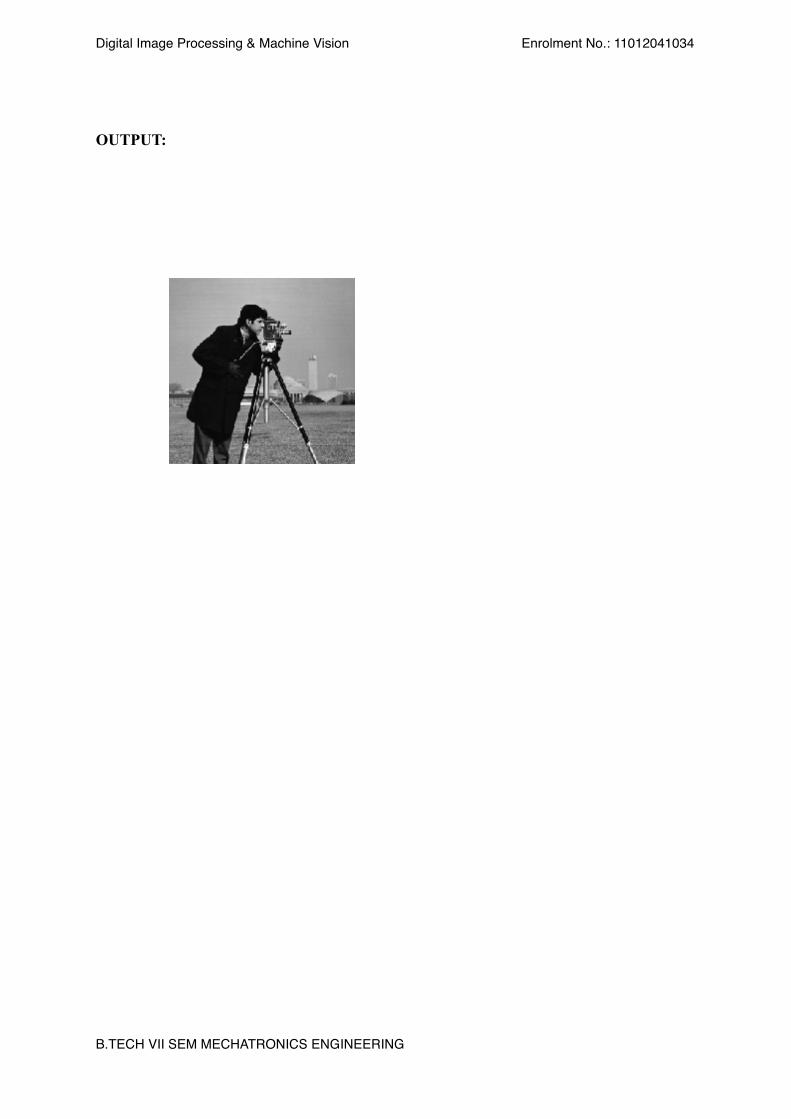
Aim: Study of imread and imshow Function.
PROGRAM
!clc;
clear all;
I=imread('cameraman.tif');
I1=imread('rice.png');
subplot(1,2,1);
imshow(I);
title('Title:Pout');
subplot(1,2,2);
imshow(I1);
title('Title:Rice');
!!OUTPUT:
!
!B.TECH VII SEM MECHATRONICS ENGINEERING !!
!
! !
Digital Image Processing & Machine Vision ! ! Enrolment No.: 11012041034!
!
!!!!!!!!!!!!!
Title:Pout Title:Rice
!B.TECH VII SEM MECHATRONICS ENGINEERING !!
!
! !
Digital Image Processing & Machine Vision ! ! Enrolment No.: 11012041034!
!!!!
!
!
PRACTICAL-4!AIM : Study of basic Matlab function.!
!
!B.TECH VII SEM MECHATRONICS ENGINEERING !!
!
! !
Digital Image Processing & Machine Vision ! ! Enrolment No.: 11012041034!
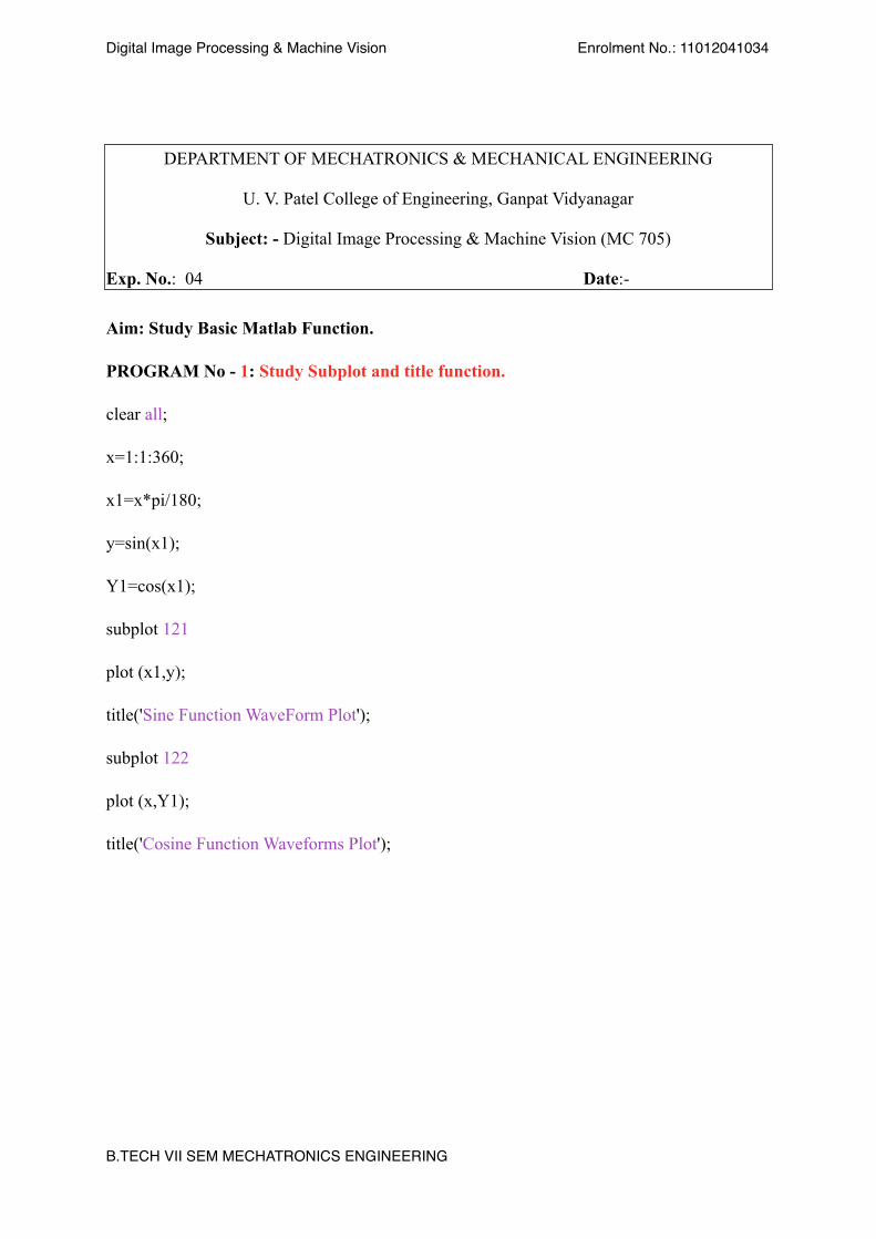
!DEPARTMENT OF MECHATRONICS & MECHANICAL ENGINEERING
U. V. Patel College of Engineering, Ganpat Vidyanagar
Subject: - Digital Image Processing & Machine Vision (MC 705)
Exp. No.: 04 Date:-
Aim: Study Basic Matlab Function.
PROGRAM No - 1: Study Subplot and title function.
clear all;
x=1:1:360;
x1=x*pi/180;
y=sin(x1);
Y1=cos(x1);
subplot 121
plot (x1,y);
title('Sine Function WaveForm Plot');
subplot 122
plot (x,Y1);
title('Cosine Function Waveforms Plot');
!
!B.TECH VII SEM MECHATRONICS ENGINEERING !!
!

! !
Digital Image Processing & Machine Vision ! ! Enrolment No.: 11012041034!
:OUTPUT
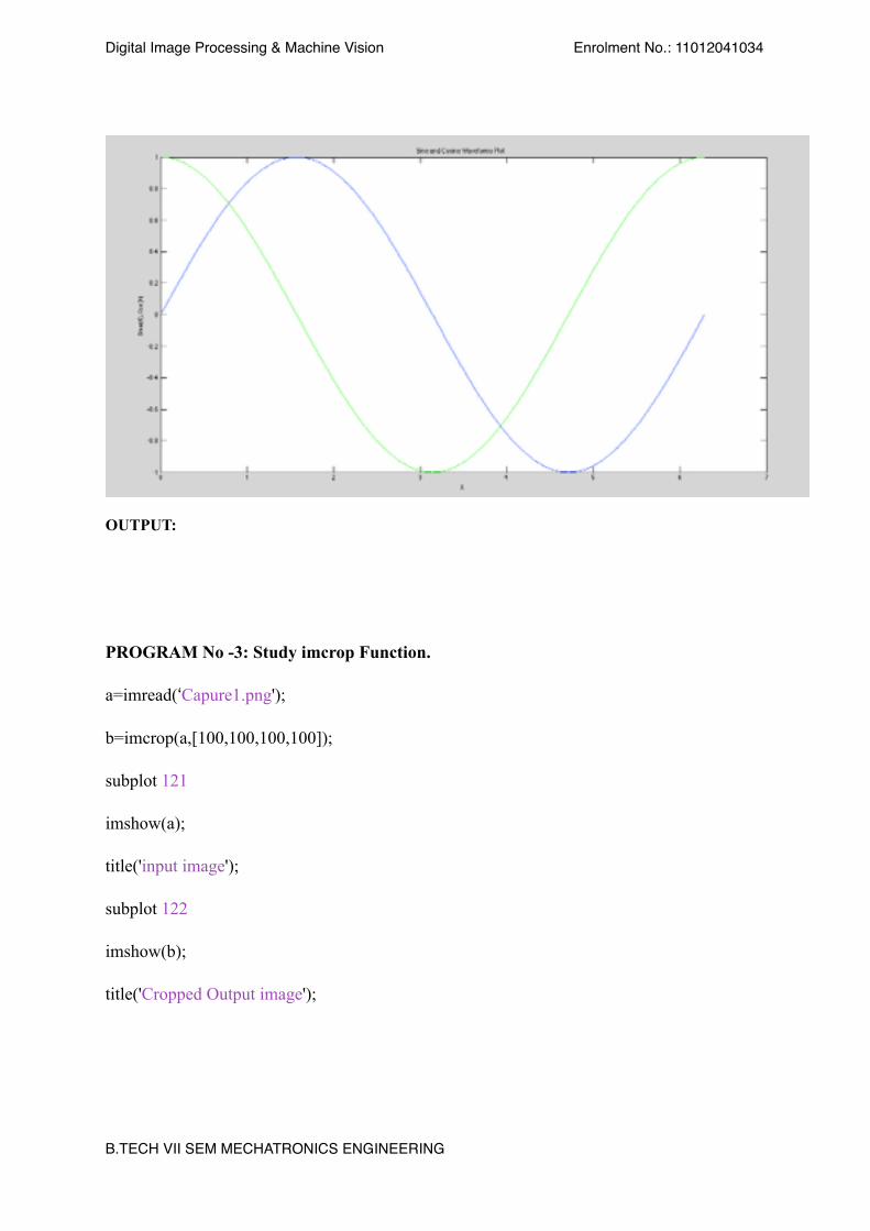
PROGRAM No - 2: Plot, xlabel, ylabel function.
clear all;
x=1:1:360;
x1=x*pi/180;
y=sin(x1);
Y1=cos(x1);
plot(x1,y,'b',x1,Y1,'g');
title('Sine and Cosine Waveforms Plot');
xlabel('X');
ylabel(‘Sine(X),Cos(X)');
!
!B.TECH VII SEM MECHATRONICS ENGINEERING !!
!
! !
Digital Image Processing & Machine Vision ! ! Enrolment No.: 11012041034!
OUTPUT:
!!PROGRAM No -3: Study imcrop Function.
a=imread(‘Capure1.png');
b=imcrop(a,[100,100,100,100]);
subplot 121
imshow(a);
title('input image');
subplot 122
imshow(b);
title('Cropped Output image');
!!!B.TECH VII SEM MECHATRONICS ENGINEERING !!
!

! !
Digital Image Processing & Machine Vision ! ! Enrolment No.: 11012041034!
!!
!B.TECH VII SEM MECHATRONICS ENGINEERING !!
!

! !
Digital Image Processing & Machine Vision ! ! Enrolment No.: 11012041034!
!OUTPUT:
!PROGRAM No -4: Study imrotate Function.
a=imread(‘pout.tif');
b=imrotate(a,45,'nearest','crop');
subplot 121
imshow(a);
title ('input image');
subplot 122
imshow(b);
title(‘rotate image’);
title ('rotate output image');
input image Cropped Output image
!B.TECH VII SEM MECHATRONICS ENGINEERING !!
!
! !
Digital Image Processing & Machine Vision ! ! Enrolment No.: 11012041034!
!!!!!output :
!
!
!!!!!!!
input image rotate image
!B.TECH VII SEM MECHATRONICS ENGINEERING !!
!
! !
Digital Image Processing & Machine Vision ! ! Enrolment No.: 11012041034!
!!!!!!!!!!!!
PRACTICAL-5! AIM :Study of matlab images.!
!!!!!!!!B.TECH VII SEM MECHATRONICS ENGINEERING !!
!

! !
Digital Image Processing & Machine Vision ! ! Enrolment No.: 11012041034!
!!!!!!! DEPARTMENT OF MECHATRONICS & MECHANICAL ENGINEERING
U. V. Patel College of Engineering, Ganpat Vidyanagar
Subject: - Digital Image Processing & Machine Vision (MC 705)
Exp. No.: 05 Date:-
Aim: Study of Images in Matlab.
Program No-1: Study the Binary Image.
a=zeros(256,256,'uint8');
for i=1:50;
for j=1:50;
a(i,j)=255;
end
end
for i=1:50;
for j=206:256;
a(i,j)=255;
end
!B.TECH VII SEM MECHATRONICS ENGINEERING !!
!
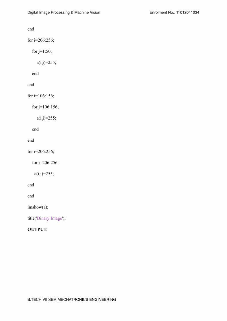
! !
Digital Image Processing & Machine Vision ! ! Enrolment No.: 11012041034!
end
for i=206:256;
for j=1:50;
a(i,j)=255;
end
end
for i=106:156;
for j=106:156;
a(i,j)=255;
end
end
for i=206:256;
for j=206:256;
a(i,j)=255;
end
end
imshow(a);
title('Binary Image');
OUTPUT:
!B.TECH VII SEM MECHATRONICS ENGINEERING !!
!

! !
Digital Image Processing & Machine Vision ! ! Enrolment No.: 11012041034!
!
PROGRAM No-2: Study of Monochrome/Grey Level Image.
a=zeros(256,256,'uint8');
a(:,:)=255;
for i=1:1:256;
for j=1:1:256;
if(i<=j)
a(i,j)=i;
else
a(i,j)=j;
end
end
end
imshow(a);
title('GreyLevel Image’);
Binary Image
!B.TECH VII SEM MECHATRONICS ENGINEERING !!
!

! !
Digital Image Processing & Machine Vision ! ! Enrolment No.: 11012041034!
!!Output:
!
PROGRAM No-3: Study of RGB/Color Image.
clc;
clear all;
a=zeros(500,500,3);
[x,y,z]=size(a);
radius=140;
xr=round(x/2-radius/(2*sqrt(3)));
yr=round(y/2-radius/2);
xg=round(x/2-radius/(2*sqrt(3)));
yg=round(y/2+radius/2);
xb=round(x/2+radius/sqrt(3))
yb=round(y/2);
!B.TECH VII SEM MECHATRONICS ENGINEERING !!
!

! !
Digital Image Processing & Machine Vision ! ! Enrolment No.: 11012041034!
for i=1:x;
for j=1:y;
d=sqrt((i-xr)^2+(j-yr)^2);
if(d<=radius)
a(i,j,1)=255;
end
d=sqrt((i-xg)^2+(j-yg)^2);
if(d<=radius)
a(i,j,2)=255;
end
d=sqrt((i-xb)^2+(j-yb)^2);
if(d<=radius)
a(i,j,3)=255;
end
end
end
imshow(a);
title('RGB Circle');
OUTPUT:
!B.TECH VII SEM MECHATRONICS ENGINEERING !!
!
! !
Digital Image Processing & Machine Vision ! ! Enrolment No.: 11012041034!
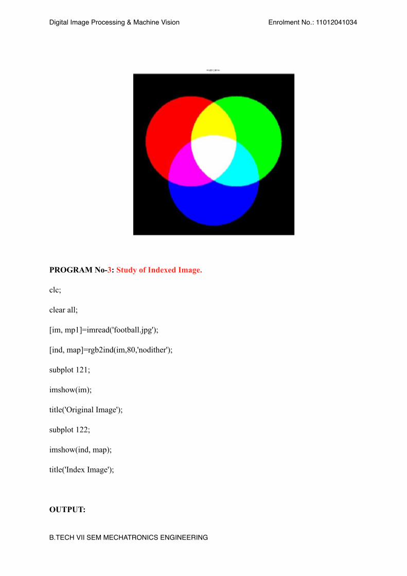
!PROGRAM No-3: Study of Indexed Image.
clc;
clear all;
[im, mp1]=imread('football.jpg');
[ind, map]=rgb2ind(im,80,'nodither');
subplot 121;
imshow(im);
title('Original Image');
subplot 122;
imshow(ind, map);
title('Index Image');
!OUTPUT: !B.TECH VII SEM MECHATRONICS ENGINEERING !!
!

! !
Digital Image Processing & Machine Vision ! ! Enrolment No.: 11012041034!
!
!!!!!!!!!!!
!
!!B.TECH VII SEM MECHATRONICS ENGINEERING !!
!
! !
Digital Image Processing & Machine Vision ! ! Enrolment No.: 11012041034!
!
!
!
PRACTICAL-6!AIM : Study programs related to enhancement- point
processing.
!!
!!!!!!!!!!B.TECH VII SEM MECHATRONICS ENGINEERING !!
!

! !
Digital Image Processing & Machine Vision ! ! Enrolment No.: 11012041034!
!! DEPARTMENT OF MECHATRONICS & MECHANICAL ENGINEERING
U. V. Patel College of Engineering, Ganpat Vidyanagar
Subject: - Digital Image Processing & Machine Vision (MC 705)
Exp. No.: 06 Date:-
Aim: Study Programs related to Enhancement - Point Processing.
PROGRAMNo.1: -Study Program related to Image Negative.
a=imread(‘onion.png’);
b=255-a;
subplot 121;
imshow(a);
title('Original Image’);
subplot 122;
imshow(b);
title('Inverted Image’);
!OUTPUT:
!B.TECH VII SEM MECHATRONICS ENGINEERING !!
!

! !
Digital Image Processing & Machine Vision ! ! Enrolment No.: 11012041034!
!PROGRAMNo.2: -Study of imadjust Function.
clear all;
a=imread('rice.png');
b=imadjust(a);
subplot 121;
imshow(a);
title('Original Image');
subplot 122;
imshow(b);
title ('High Contrast Image');
OUTPUT:
!B.TECH VII SEM MECHATRONICS ENGINEERING !!
!

! !
Digital Image Processing & Machine Vision ! ! Enrolment No.: 11012041034!
!
PROGRAMNo.2: -Study effect of gamma in Power Law Transformation.
a=imread('rice.png');
a=im2double(a);
[rowi coli]=size(a);
r=0:1:255;
gamma=0.8;
c=1.5;
s=c*r.^gamma;
out=zeros(rowi,coli);
for k=1:256
for i=1:rowi
for j=1:coli
if a(i,j)==a(k);
out(i,j)=s(k);
end
!B.TECH VII SEM MECHATRONICS ENGINEERING !!
!
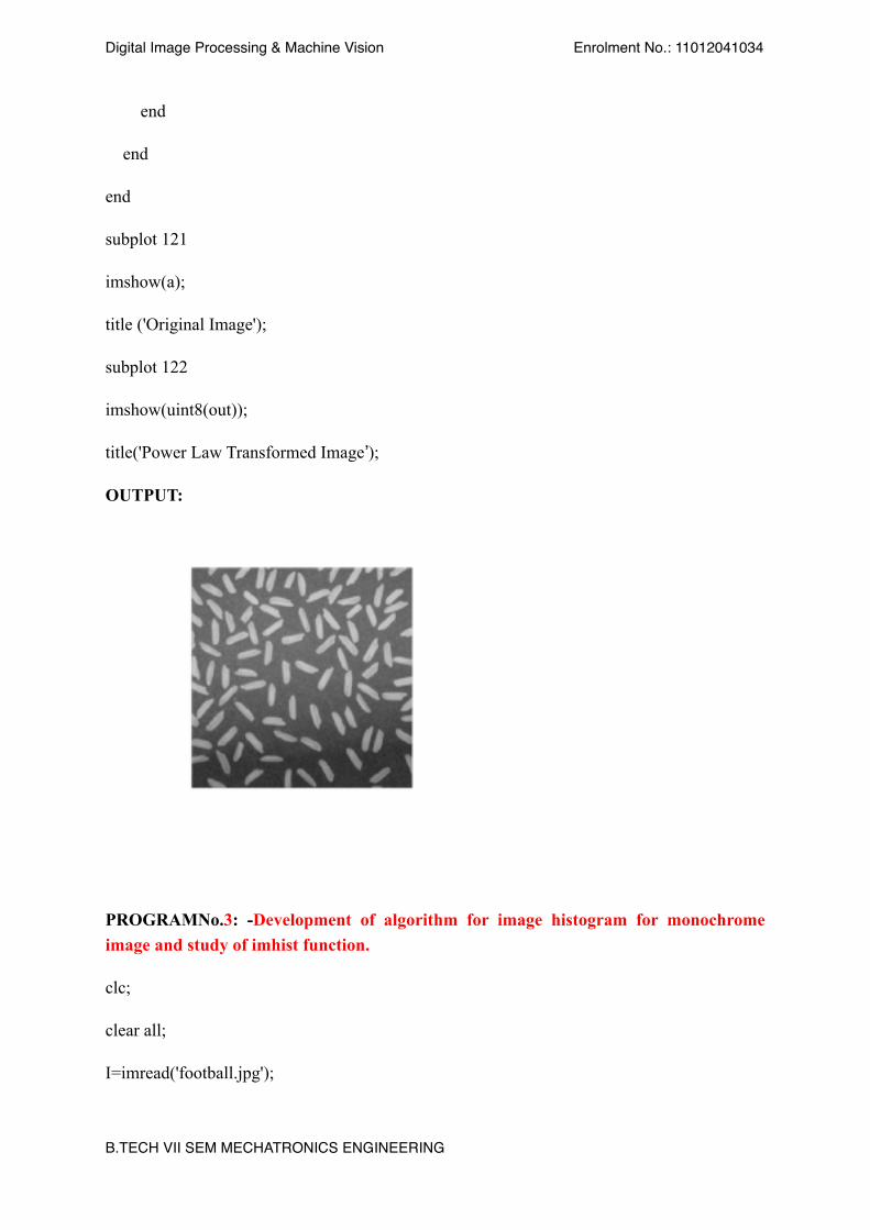
! !
Digital Image Processing & Machine Vision ! ! Enrolment No.: 11012041034!
end
end
end
subplot 121
imshow(a);
title ('Original Image');
subplot 122
imshow(uint8(out));
title('Power Law Transformed Image’);
OUTPUT:
!
!PROGRAMNo.3: -Development of algorithm for image histogram for monochrome image and study of imhist function.
clc;
clear all;
I=imread('football.jpg');
!B.TECH VII SEM MECHATRONICS ENGINEERING !!
!

! !
Digital Image Processing & Machine Vision ! ! Enrolment No.: 11012041034!
a=rgb2gray(I);
subplot 321
imshow(a);
title('Original Image');
subplot 322;
imhist(a);
title('Histogram of Original Image');
xlabel('intensity form 0-255’);
ylabel('no. of Occurance');
a=im2double(a);
[m,n]=size(a);
for i=1:m;
for j=1:n;
b(i,j)=a(i,j)^1.5;
end
end
subplot 323;
imshow(b);
title('Darker Image');
subplot 324;
imhist(b);
title('histogram of Darker Image ');
xlabel('Intensity from 0-1');
!B.TECH VII SEM MECHATRONICS ENGINEERING !!
!

! !
Digital Image Processing & Machine Vision ! ! Enrolment No.: 11012041034!
ylabel('No. of Occurance');
for i=1:m;
for j=1:n;
b(i,j)=a(i,j)^0.5;
end
end
subplot 325;
imshow(b);
title('Lighter Image');
subplot 326;
imhist(b);
!title('histogram of lighter Image ');
xlabel('Intensity from 0-1');
ylabel('No. of Occurance');
!OUTPUT:
!B.TECH VII SEM MECHATRONICS ENGINEERING !!
!

! !
Digital Image Processing & Machine Vision ! ! Enrolment No.: 11012041034!
!
PROGRAMNo.4: -Development of algorithm for histogram equalised image and study of histeq function.
Program:
clc;
clear all;
a=imread('rice.png');
[m,n]=size(a);
b=a;
r=zeros(1,256);
for i=1:m;
for j=1:n;
r(a(i,j)+1)=r(a(i,j)+1)+1;
end
end
!
Original Image
0
500
1000
Histogram of Original Image
intensity form 0-255
no. of Occurance
0 50 100 150 200 250
Darker Image
0
500
1000
1500
histogram of Darker Image
Intensity from 0-1
No. of Occurance
0 0.1 0.2 0.3 0.4 0.5 0.6 0.7 0.8 0.9 1
Lighter Image
0
500
1000
histogram of lighter Image
Intensity from 0-1
No. of Occurance
0 0.1 0.2 0.3 0.4 0.5 0.6 0.7 0.8 0.9 1
!B.TECH VII SEM MECHATRONICS ENGINEERING !!
!

! !
Digital Image Processing & Machine Vision ! ! Enrolment No.: 11012041034!
subplot 321;
imshow(a);
title('original image');
subplot 322
plot(r);
title('Histogram of original Image through Plot');
xlabel('Gray Level');
ylabel('No. of Occurance');
!d=m*n;
e=255/d;
s=zeros(1,256);
for k=0:255
for h=0:k
s(1,k+1)=s(1,k+1)+r(1,h+1);
end
end
!s=s.*e;
for i=1:m
for j=1:n
b(i,j)=s(1,a(i,j)+1);
end
!B.TECH VII SEM MECHATRONICS ENGINEERING !!
!

! !
Digital Image Processing & Machine Vision ! ! Enrolment No.: 11012041034!
end
subplot 324
plot(s);
title('Histogram Equalization oe Original Image through Plot');
xlabel('Gray Level');
ylabel('No. of occurance');
subplot 325
imshow(b);
title('New histogram Equalized Image');
subplot 326
imhist(b);
title('Histogram of New Equalized Image through command')
xlabel('Gray Level');
ylabel('No. of occurance');
Output:
!B.TECH VII SEM MECHATRONICS ENGINEERING !!
!

! !
Digital Image Processing & Machine Vision ! ! Enrolment No.: 11012041034!
!
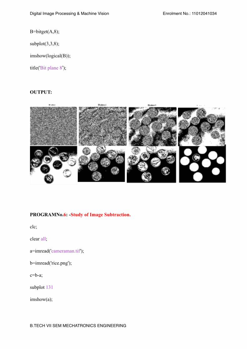
!!ROGRAMNo.5: -Study program to verify the contribution of the each bit plane to monochrome.
A=imread('coins.png');
B=bitget(A,1);
figure,
subplot(3,3,1);
imshow(logical(B));
title('Bit plane 1');
B=bitget(A,2);
subplot(3,3,2);
original image
0 100 200 3000
1000
2000Histogram of original Image through Plot
Gray Level
No. o
f Occ
uran
ce
0 100 200 3000
200
400Histogram Equalization oe Original Image through Plot
Gray Level
No. o
f occ
uran
ceNew histogram Equalized Image
0
500
1000Histogram of New Equalized Image through command
Gray LevelNo. o
f occ
uran
ce
0 100 200
!B.TECH VII SEM MECHATRONICS ENGINEERING !!
!
! !
Digital Image Processing & Machine Vision ! ! Enrolment No.: 11012041034!
imshow(logical(B));
title('Bit plane 2');
B=bitget(A,3);
subplot(3,3,3);
imshow(logical(B));
title('Bit plane 3');
B=bitget(A,4);
subplot(3,3,4);
imshow(logical(B));
title('Bit plane 4');
B=bitget(A,5);
figure,
subplot(3,3,5);
imshow(logical(B));
title('Bit plane 5');
B=bitget(A,6);
subplot(3,3,6);
imshow(logical(B));
title('Bit plane 6’);
B=bitget(A,7);
subplot(3,3,7);
imshow(logical(B));
title('Bit plane 7');
!B.TECH VII SEM MECHATRONICS ENGINEERING !!
!
! !
Digital Image Processing & Machine Vision ! ! Enrolment No.: 11012041034!
B=bitget(A,8);
subplot(3,3,8);
imshow(logical(B));
title('Bit plane 8’);
!OUTPUT:
!!PROGRAMNo.6: -Study of Image Subtraction.
clc;
clear all;
a=imread('cameraman.tif');
b=imread('rice.png');
c=b-a;
subplot 131
imshow(a);
!B.TECH VII SEM MECHATRONICS ENGINEERING !!
!

! !
Digital Image Processing & Machine Vision ! ! Enrolment No.: 11012041034!
title('Image 1');
subplot 132
imshow(b);
title('Image 2');
subplot 133
imshow(c);
title('Subtracted Image’);
!OUTPUT:
!
PROGRAMNo.6: -Study of Image Multiplication.
clc;
clear all;
a=imread('moon.tif');
b=imread('rice.png');
a=imresize(a,[256,290]);
!B.TECH VII SEM MECHATRONICS ENGINEERING !!
!

! !
Digital Image Processing & Machine Vision ! ! Enrolment No.: 11012041034!
b=imresize(b,[256,290]);
e=im2double(a);
f=im2double(b);
g=f.*e;
subplot 131;
imshow(a);
title('Coins');
subplot 132;
imshow(b);
title('Rice')
subplot 133
imshow(g);
title('Multiplied Image’);
!OUTPUT:
!
!B.TECH VII SEM MECHATRONICS ENGINEERING !!
!

! !
Digital Image Processing & Machine Vision ! ! Enrolment No.: 11012041034!
!!!!!!!!
PRACTICAL-7!AIM : Study programs related to enhancement -
Spatial Masking.
!!!!!!!!!!
!B.TECH VII SEM MECHATRONICS ENGINEERING !!
!
! !
Digital Image Processing & Machine Vision ! ! Enrolment No.: 11012041034!
!!!!!
!DEPARTMENT OF MECHATRONICS & MECHANICAL ENGINEERING
U. V. Patel College of Engineering, Ganpat Vidyanagar
Subject: - Digital Image Processing & Machine Vision (MC 705)
Exp. No.: 07 Date:-
Aim: Study Programs related to Enhancement - Spatial Masking.
PROGRAM No: 1 -Study of imnoise function.
a=imread('moon.tif');
b=imnoise(a,'gaussian');
c=imnoise(a,'poisson');
d=imnoise(a,'salt & pepper',0.06);
f=imnoise(a,'speckle');
subplot 231
imshow(a);
title('Original Image');
subplot 232
imshow(b);
title('Gaussian Noise Image');
subplot 233
!B.TECH VII SEM MECHATRONICS ENGINEERING !!
!

! !
Digital Image Processing & Machine Vision ! ! Enrolment No.: 11012041034!
imshow(c);
title('Poisson Noise Image');
subplot 234
imshow(d);
title('Salt & Pepper Noise Image’);
subplot 235
imshow(f);
title('Speckle Noise Image’);
!!!!OUTPUT:
!B.TECH VII SEM MECHATRONICS ENGINEERING !!
!

! !
Digital Image Processing & Machine Vision ! ! Enrolment No.: 11012041034!
!PROGRAM No: 2 -Study filter2 function and low pass filtering to remove noise.
a=imread('rice.png');
b=imnoise(a,'salt & pepper',0.06);
c=ones(3);
d=ones(5);
i=filter2(c,b);
j=filter2(d,b);
subplot 131
imshow(b,[]);
title('Noisy Image');
subplot 132
imshow(i,[]);
Original Image Gaussian Noise Image Poisson Noise Image
Salt & Pepper Noise Image Speckle Noise Image
!B.TECH VII SEM MECHATRONICS ENGINEERING !!
!

! !
Digital Image Processing & Machine Vision ! ! Enrolment No.: 11012041034!
title('3x3 Masked Filter Image');
subplot 133
imshow(j,[]);
title('5x5 Masked Filter Image');
Output:
!PROGRAM No: 3 -Study medfilt2 function to remove impulse noise and comparison with low pass filter masking.
a=imread('moon.tif');
b=imnoise(a,'salt & pepper',0.05);
c=medfilt2(b,[5 5]);
subplot 131
imshow(b);
title('Noisy Image');
subplot 132
imshow(c);
title('Median Filtered Image');
!B.TECH VII SEM MECHATRONICS ENGINEERING !!
!

! !
Digital Image Processing & Machine Vision ! ! Enrolment No.: 11012041034!
m=1/9.*ones(3);
d=filter2(m,b);
subplot 133
imshow(d,[]);
title('3x3 Masked Low Pass filtered Image’);
!!OUTPUT:
!PROGRAM No: 4 -Study Laplacian Operator for Edge Detection.
clear all;
a=imread('cameraman.tif');
h=[-1 -1 -1; -1 8 -1 ;-1 -1 -1];
c=filter2(h,a);
subplot 121
imshow(a);
title('original Image');
!B.TECH VII SEM MECHATRONICS ENGINEERING !!
!

! !
Digital Image Processing & Machine Vision ! ! Enrolment No.: 11012041034!
subplot 122
imshow(c,[]);
OUTPUT:
!
!PROGRAM No: 5 -Study Laplacian Operator for Edge Detection.
clc;
clear all;
a=imread(‘moon.tif');
h=[-1 -1 -1; 0 0 0; 1 1 1];
b=filter2(h,a);
subplot 121
imshow(a);
title('Original Image');
subplot 122
imshow(b,[]);
OUTPUT:
!B.TECH VII SEM MECHATRONICS ENGINEERING !!
!

! !
Digital Image Processing & Machine Vision ! ! Enrolment No.: 11012041034!
!
PROGRAM No: 6 -Study of fspecial function.
a=imread('pout.tif’);
b1=fspecial('sobel');
c1=filter2(b,a);
subplot 121
imshow(a);
title('Original Image');
subplot 122
imshow(c1,[]);
title('Sobel Operator via Fspecial Function’);
OUTPUT:
!B.TECH VII SEM MECHATRONICS ENGINEERING !!
!

! !
Digital Image Processing & Machine Vision ! ! Enrolment No.: 11012041034!
!
PROGRAM No-7 : Study of High Boost Filter to detect the edge with original Image.
clc;
clear all;
a=imread('cameraman.tif');
m=1/8.*[-1 -1 -1; -1 100 -1; 1 1 1];
b=filter2(m,a);
subplot 121
imshow(a);
title('Original Image');
subplot 122
imshow(b,[]);
title('Boosted Image');
!
!B.TECH VII SEM MECHATRONICS ENGINEERING !!
!
! !
Digital Image Processing & Machine Vision ! ! Enrolment No.: 11012041034!
!OUTPUT:
!
!!!!!!!!!
Original Image Boosted Image
!B.TECH VII SEM MECHATRONICS ENGINEERING !!
!

! !
Digital Image Processing & Machine Vision ! ! Enrolment No.: 11012041034!
!!!
!
!
PRACTICAL-8!AIM : Study of programs related to enhancement -
Frequency domain. !!!!!!!!!!!!!
!B.TECH VII SEM MECHATRONICS ENGINEERING !!
!

! !
Digital Image Processing & Machine Vision ! ! Enrolment No.: 11012041034!
!DEPARTMENT OF MECHATRONICS & MECHANICAL ENGINEERING
U. V. Patel College of Engineering, Ganpat Vidyanagar
Subject: - Digital Image Processing & Machine Vision (MC 705)
Exp. No.: 08 Date:-
Aim: Study of Programs related to Enhancement - Frequency Domain Filtering.
PROGRAM No-1: Study the Fourier Transformed of an Image.
clc;
clear all;
a=imread('coins.png');
b=fft2(a);
c=log(1+abs(b));
d=fftshift(c);
subplot 221
imshow(a);
title('Original Image');
subplot 222
imshow(b);
title('Fast Fourier Transformation')
subplot 223
imshow(c,[]);
title('Fourier Trasformed and Enhanced Image');
subplot 224
imshow(d,[]); !B.TECH VII SEM MECHATRONICS ENGINEERING !!
!

! !
Digital Image Processing & Machine Vision ! ! Enrolment No.: 11012041034!
title('Shifted Fourier Transformed Image')
!!!!!!OUTPUT:
!
PROGRAM No-2: Study the Ideal low pass filtering in Frequency domain and its effect.
clc;
clear all;
a=imread('cameraman.tif');
[x y]=size(a);
b=fft2(a);
b=fftshift(b);
!B.TECH VII SEM MECHATRONICS ENGINEERING !!
!
! !
Digital Image Processing & Machine Vision ! ! Enrolment No.: 11012041034!
h=zeros(x,y);
for i=1:x
for j=1:y
d=sqrt((i-x/2)^2+(j-y/2)^2);
if (d<=100)
h(i,j)=1;
end
end
end
c=h.*b;
d=ifft2(c);
d=abs(d);
d=log(1+d);
%gamma Enhancemet
for i=1:x
for j=1:y
d(i,j)=d(i,j).^2;
end
end
subplot 121
imshow(a);
title('Original Image');
subplot 122
!B.TECH VII SEM MECHATRONICS ENGINEERING !!
!
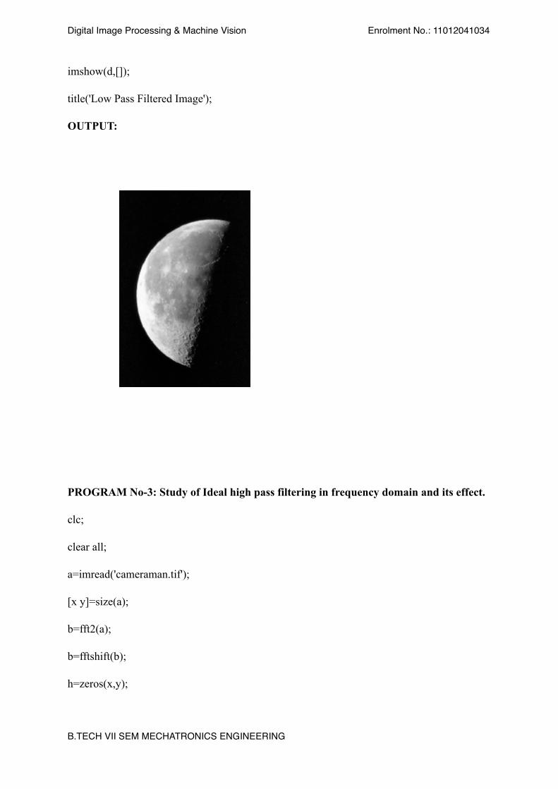
! !
Digital Image Processing & Machine Vision ! ! Enrolment No.: 11012041034!
imshow(d,[]);
title('Low Pass Filtered Image');
OUTPUT:
!
!PROGRAM No-3: Study of Ideal high pass filtering in frequency domain and its effect.
clc;
clear all;
a=imread('cameraman.tif');
[x y]=size(a);
b=fft2(a);
b=fftshift(b);
h=zeros(x,y);
Original Image Low Pass Filtered Image
!B.TECH VII SEM MECHATRONICS ENGINEERING !!
!

! !
Digital Image Processing & Machine Vision ! ! Enrolment No.: 11012041034!
for i=1:x
for j=1:y
d=sqrt((i-x/2)^2+(j-y/2)^2);
if (d<=40)
h(i,j)=1;
end
end
end
h=1-h;
c=h.*b;
d=ifft2(c);
d=abs(d);
d=log(1+d);
%gamma Enhancemet
for i=1:x
for j=1:y
d(i,j)=d(i,j).^2;
end
end
subplot 121
imshow(a);
title('Original Image');
subplot 122
!B.TECH VII SEM MECHATRONICS ENGINEERING !!
!

! !
Digital Image Processing & Machine Vision ! ! Enrolment No.: 11012041034!
imshow(d,[]);
title('High Pass Filtered Image’);
OUTPUT:
!
PROGRAM No-4: Study the effect of Rotation of an image to its FFT.
clc;
clear all;
a=imread('pout.tif');
b=imrotate(a,45,'crop');
d=fft2(b);
d=log(1+abs(d));
d=fftshift(d);
f=fft2(a);
f=log(1+abs(f));
f=fftshift(f);
subplot 221
!B.TECH VII SEM MECHATRONICS ENGINEERING !!
!
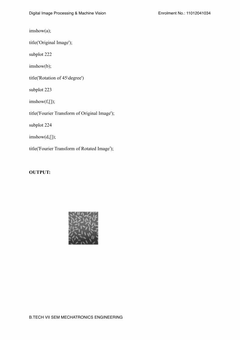
! !
Digital Image Processing & Machine Vision ! ! Enrolment No.: 11012041034!
imshow(a);
title('Original Image');
subplot 222
imshow(b);
title('Rotation of 45\degree')
subplot 223
imshow(f,[]);
title('Fourier Transform of Original Image');
subplot 224
imshow(d,[]);
title('Fourier Transform of Rotated Image’);
!OUTPUT:
!!
!
!B.TECH VII SEM MECHATRONICS ENGINEERING !!
!

! !
Digital Image Processing & Machine Vision ! ! Enrolment No.: 11012041034!
!B.TECH VII SEM MECHATRONICS ENGINEERING !!
!
Copyright © 2022 FDOKUMEN