arX

iv:0

707.

0298

v2 [

hep-

th]

30

Oct

200

7

Preprint typeset in JHEP style - HYPER VERSION

CERN-PH-TH/2007-099

IFT-UAM/CSIC-07-34

LMU-ASC 41/07

MIT-CTP 3846

MPP-2007-76

PUPT-2238

Dimers and Orientifolds

Sebastian Franco1, Amihay Hanany2, Daniel Krefl3,4, Jaemo Park5,6,

Angel M. Uranga7,8 and David Vegh9

1 Joseph Henry Laboratories, Princeton University

Princeton NJ 08544, USA2 Perimeter Institute for Theoretical Physics

31 Caroline Street North, Waterloo Ontario N2L 2Y5 Canada3 Max-Planck-Institut fur Physik

Fohringer Ring 6, 80805 Munich, Germany4 Arnold Sommerfeld Center for Theoretical Physics,

Ludwig-Maximilians-Universitat, Theresienstr. 37, 80333 Munich, Germany5 Department of Physics, Postech, Pohang 790-784 Korea6 Postech Center for Theoretical Physics (PCTP), Pohang 790-784, Korea7 PH-TH Division, CERN

CH-1211 Geneva, Switzerland8 On leave from Instituto de Fısica Teorica, Facultad de Ciencias, Madrid, Spain9 Center for Theoretical Physics, Massachusetts Institute of Technology,

77 Massachusetts Avenue, Cambridge MA 02139, USA

Abstract: We introduce new techniques based on brane tilings to investigate D3-

branes probing orientifolds of toric Calabi-Yau singularities. With these new tools,

one can write down many orientifold models and derive the resulting low-energy

gauge theories living on the D-branes. Using the set of ideas in this paper one recovers

essentially all orientifolded theories known so far. Furthermore, new orientifolds of

non-orbifold toric singularities are obtained. The possible applications of the tools

presented in this paper are diverse. One particular application is the construction of

models which feature dynamical supersymmetry breaking as well as the computation

of D-instanton induced superpotential terms.

Contents

1. Introduction 2

2. Some background on dimers and on orientifolds 3

2.1 Quiver gauge theories and dimer diagrams 3

2.2 Orientifolds 5

2.3 Orientifolding dimers 6

3. Orientifolds from dimers with fixed points 8

3.1 Orientifold rules 8

3.1.1 Example: Orientifolds of C3 10

3.1.2 A comment on tadpoles/anomalies and extra flavors 11

3.2 Geometric action 12

3.2.1 On the orientifolds of C3 13

3.2.2 Example: Orientifolds of the conifold 15

3.2.3 Example: C2/Z2 × C 17

3.3 The global sign rule and Higgsing 20

3.4 The global constraint for the fixed point signs revisited 21

3.5 Further examples 22

3.5.1 Orientifolds of C3/Z3 22

3.5.2 Orientifolds of the Conifold/ZN 23

3.5.3 Orientifolds of SPP 24

3.5.4 Orientifolds of L1,5,2 25

4. Orientifolds from dimers with fixed lines 26

4.1 Generalities 26

4.2 Few examples and the geometric action 27

4.2.1 Line orientifolds of C3 27

4.2.2 C2/ZN × C, even N 28

4.2.3 C2/ZN × C, odd N 30

4.2.4 The geometric action 30

4.3 Further examples 31

4.3.1 General Laba theories 31

4.3.2 Orbifolds of the conifold 33

– 1 –

5. The mirror perspective 35

5.1 Review of the mirror picture 35

5.2 Orientifolds in the mirror system 40

5.3 Classes of orientifold involutions 43

5.3.1 Involutions mirror to orientifold dimers with fixed points 43

5.3.2 Involutions mirror to orientifold dimers with fixed lines 44

5.4 Tadpole cancellation 47

5.5 Calibration 49

6. Applications 49

6.1 Dynamical supersymmetry breaking 49

6.2 D-brane instantons 53

7. Conclusions 54

A. From quivers to dimers and shivers 55

B. Mnemonics: Orientifolded Harlequin diagrams 59

C. Laba theories 62

1. Introduction

The study of D-branes at singularities and the gauge theories on them is interesting

for a variety of reasons. On the one hand, branes at singularities give rise to interest-

ing extensions of the original AdS/CFT correspondence to theories with a reduced

amount of (super)symmetry [1, 2]. This front has witnessed remarkable progress in

recent years: in the conformal case, with the precision matching of geometric prop-

erties of new infinite families of Sasaki-Einstein metrics and their gauge theory duals

[3, 4, 5, 6, 7]; in the presence of fractional branes, with the dictionary between geo-

metric properties of the singularity and strong infrared dynamics in the dual gauge

theories [8, 9, 10, 11, 12].

On the other hand, they provide a natural setup for a bottom-up approach to

string phenomenology, allowing for local constructions of Standard Model-like gauge

theories [13, 14, 15]. Many features of the resulting models depend only on the local

structure of the singularity and can be investigated without a detailed knowledge of

the full compactification manifold.

Orientifolds are an interesting new twist in these constructions, with possibly

novel features. To name a few, they can be used to produce interesting spectra

– 2 –

(with new kinds of gauge factors and representations), they naturally lead to non-

conformal theories (with orientifold charges arising as 1/N corrections), easily lead

to supersymmetry breaking in the infrared (with or without runaway), and lead to

models with interesting non-perturbative superpotential interactions (since orien-

tifolding eliminates superfluous zero modes on certain D-brane instantons). Thus,

the construction of orientifolds of D-branes at singularities is an interesting direction

worth being pursued.

Unfortunately, the techniques to construct such orientifolds are very rudimentary.

So far, only a very limited number of orientifolds of non-orbifold singularities has been

constructed. Orientifolds of orbifold singularities are in principle amenable to direct

construction using worldsheet techniques, although in practice only a few families of

models have been constructed. For orientifolds of non-orbifold singularities, partial

resolution of orientifolds of orbifolds can be used to derive a few new models, but

the approach becomes non-practical for singularities beyond the simplest ones. A

simple classification of orientifolds is also possible for the very restricted subset of

singularities that are T-dual to simple Hanany-Witten (HW) setups [16].

The problem of finding the gauge theory on a set of branes probing an arbitrary

toric CY singularity M was fully solved with the introduction of dimer model meth-

ods [17, 18].1 One of the main virtues of dimers is its computational simplicity, in

sharp contrast with pre-existent alternatives such as partial resolution.

Given the striking success of dimer models in the study of branes at singularities,

it is natural to ask how to expand their range of applicability. A natural problem is

the classification of orientifolds of toric singularities. This paper extends the success

of dimer models in the study of toric singularities to their orientifolds, providing a

general method and explicit construction of them.

The organization of the paper is as follows. In §2, we review some basics of

dimers, quivers and orientifolds. The main results are presented in §3 and §4, where

we explain how to obtain orientifolds of arbitrary toric singularities corresponding to

involutions with fixed points and fixed lines, respectively. The mirror perspective is

discussed in §5. In §6 we present some applications of our framework and conclude

in §7. We collect additional related material in appendices.

2. Some background on dimers and on orientifolds

2.1 Quiver gauge theories and dimer diagrams

In this section we give several aspects of quiver gauge theories that live on D3-

branes at toric Calabi-Yau singularities and their construction in terms of dimer

diagrams (a.k.a. brane tilings). Brane tilings give the most efficient construction

1For a recent review, see [19].

– 3 –

of such quiver gauge theories and in the math literature one can find them under

the name of periodic bipartite tilings of the two dimensional plane. For the physical

application of dimers to D-branes at singularities, see e.g. [17]-[30]. A review of the

mathematical aspects of dimers can be found in [31, 32].

The gauge theory living on D3-branes probing a toric threefold singularity M is

determined by a set of unitary gauge factors (vector multiplets with a unitary gauge

group), chiral multiplets in bi-fundamental representations, and a superpotential

given by a sum of traces of products of such bi-fundamental fields. The gauge group

and matter content of such gauge theories can be encoded in a quiver diagram,

with nodes corresponding to gauge factors, and arrows to bi-fundamentals.2 The

superpotential terms are gauge invariant operators and hence correspond to closed

oriented loops of arrows in the quiver, however not all such loops in the quiver are

superpotential terms.

A powerful tool that encodes all the gauge theory information, including the

gauge group, the matter content and the superpotential, is given by the so-called

brane tiling or dimer diagrams [17, 18]. This is a tiling of T2 defined by a bipartite

graph, namely one whose nodes can be colored black and white, with no edges

connecting nodes of the same color. There is a dictionary between the tiling data

and the gauge theory data that associates faces in the dimer diagram to gauge factors

in the field theory, edges with bi-fundamental fields (fields in the adjoint in the case

that the same face is at both sides of the edge), and nodes with superpotential

terms. The bipartite character of the diagram is important in that it defines an

orientation for edges (e.g. from black to white nodes), which determines the chirality

of the bi-fundamental fields (for example, going clockwise around white nodes and

counter-clockwise around black ones). The color of a node determines the sign of

the corresponding superpotential term, by convention +(−) sign for a white (black)

node.

The inverse procedure, of computing the dimer from the gauge theory data, was

discussed in detail in [21] and is given a new light with a recipe which is provided in

§A. Different techniques allow to systematically construct the dimer diagram (and

hence recover the gauge theory) for any given toric singularity [20, 21, 27]. One can

also directly obtain the geometry of the singularity from the information of the dimer

diagram (i.e. of the gauge theory) [21, 22]. A novel way to achieve this is introduced

in Appendix A.

Mesonic operators and paths in the dimer

A set of objects which are of interest below are the gauge invariant BPS mesonic

operators. These objects, which are elements of the chiral ring are the simplest

2It is also possible to encode adjoint fields in quiver diagrams. They are represented by arrows

starting and ending at the same node.

– 4 –

gauge invariant operators in the gauge theory. They are naturally defined in the

dimer diagram and encode the interplay between the gauge theory and the singular

geometry. There is a special subset of the mesonic operators which generate the

chiral ring and they are used in the algebraic description of the manifold. In this

paper they are sometimes called “fundamental mesons”. See Figure 2 for a simple

example of such fundamental mesons. As discussed since the early days of D-branes

at singularities [33, 34], the geometry transverse to a D-brane can be regarded as the

(mesonic) moduli space of the gauge theory living on its world-volume. The gauge

invariant mesonic operators are then good complex coordinates on the Calabi-Yau

singularity at which the D-branes are located. The full set of mesonic operators,

recently studied in [35, 36, 37, 38], has a natural realization in the dimer diagram.

They correspond to closed oriented paths in the dimer, with orientation determined

by the orientation of the edges.

Since each mesonic operator corresponds to an algebraic function on the sin-

gular geometry, the complete set of gauge invariant mesonic operators provides the

complete set of algebraic functions, which in the spirit of algebraic geometry is an

equivalent description of the geometry itself. The use of mesonic operators as coor-

dinates of the singular geometry are exploited in §3.2.

A last important comment concerns the global symmetries of the gauge theory.

In general, gauge theories living on D3-branes at toric singularities have a generic

U(1)3 global symmetry, associated to the toric action on the geometry.3 This includes

the U(1)R symmetry, and two global symmetries, which are sometimes called “flavor

symmetries” in the literature. The charges of the different fields under U(1)R can be

represented geometrically in the dimer diagram as the angles of the corresponding

edges when the dimer diagram is drawn in the so-called isoradial embedding [21].

The two remaining global symmetries are associated to the non-trivial 1-cycles in the

two-torus of the dimer diagram. A possible convention for these two global flavor

charges can be as follows: given a gauge invariant mesonic operator, represent it in

the universal cover of the dimer as an open path between one fundamental domain

to another, assign lattice coordinates which specify the position of each fundamental

domain, and assign the lattice difference between the starting fundamental domain

to the ending fundamental domain as the two global flavor charges.

2.2 Orientifolds

In this paper we are interested in studying systems of D3-branes that probe a (toric)

CY singularity M in the presence of orientifold quotients. Namely, we consider the

quotient of the system by the orientifold action

ωσ(−1)FL, (2.1)3In the absence of fractional branes this symmetry is not broken by quantum effects. In the

presence of fractional branes, the symmetry is still present but may be broken by quantum effects.

In addition, there are also baryonic U(1) symmetries which are not used in this paper.

– 5 –

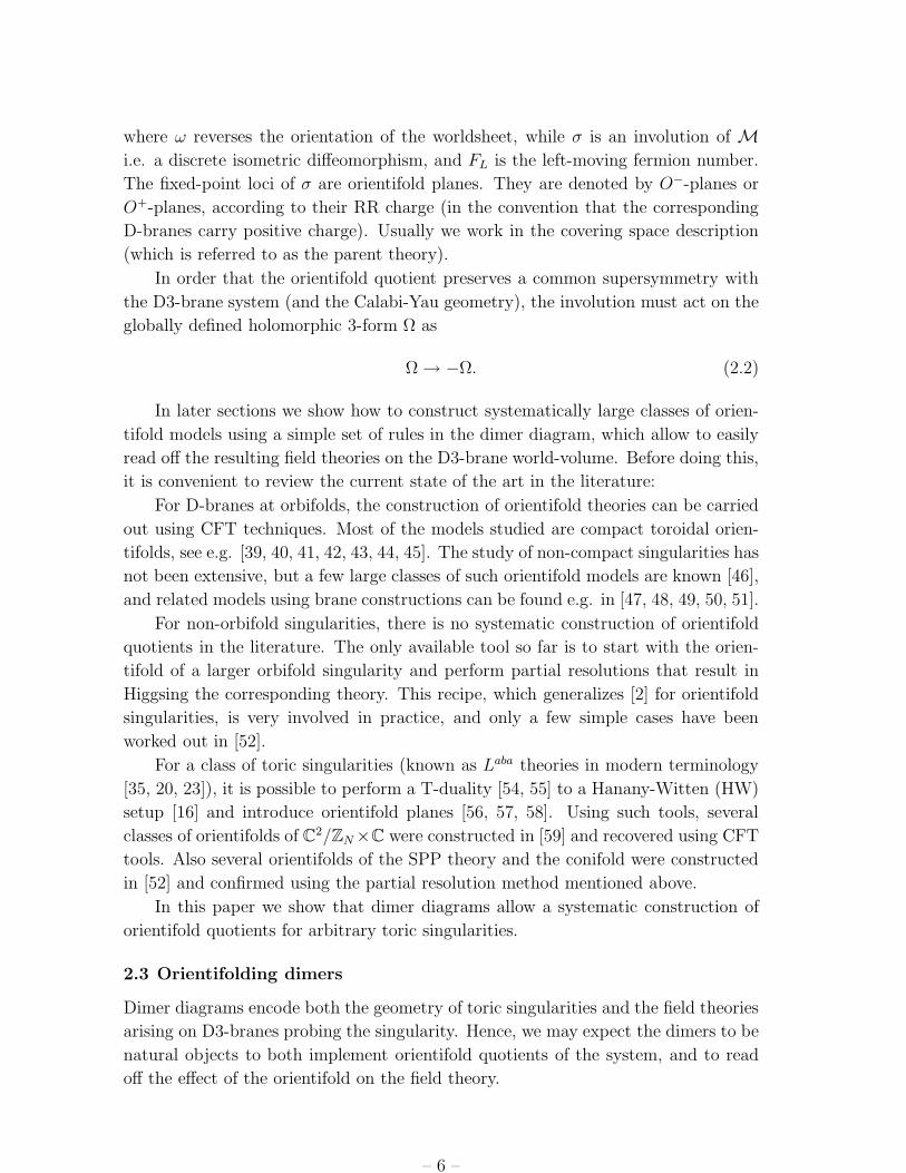
where ω reverses the orientation of the worldsheet, while σ is an involution of M

i.e. a discrete isometric diffeomorphism, and FL is the left-moving fermion number.

The fixed-point loci of σ are orientifold planes. They are denoted by O−-planes or

O+-planes, according to their RR charge (in the convention that the corresponding

D-branes carry positive charge). Usually we work in the covering space description

(which is referred to as the parent theory).

In order that the orientifold quotient preserves a common supersymmetry with

the D3-brane system (and the Calabi-Yau geometry), the involution must act on the

globally defined holomorphic 3-form Ω as

Ω → −Ω. (2.2)

In later sections we show how to construct systematically large classes of orien-

tifold models using a simple set of rules in the dimer diagram, which allow to easily

read off the resulting field theories on the D3-brane world-volume. Before doing this,

it is convenient to review the current state of the art in the literature:

For D-branes at orbifolds, the construction of orientifold theories can be carried

out using CFT techniques. Most of the models studied are compact toroidal orien-

tifolds, see e.g. [39, 40, 41, 42, 43, 44, 45]. The study of non-compact singularities has

not been extensive, but a few large classes of such orientifold models are known [46],

and related models using brane constructions can be found e.g. in [47, 48, 49, 50, 51].

For non-orbifold singularities, there is no systematic construction of orientifold

quotients in the literature. The only available tool so far is to start with the orien-

tifold of a larger orbifold singularity and perform partial resolutions that result in

Higgsing the corresponding theory. This recipe, which generalizes [2] for orientifold

singularities, is very involved in practice, and only a few simple cases have been

worked out in [52].

For a class of toric singularities (known as Laba theories in modern terminology

[35, 20, 23]), it is possible to perform a T-duality [54, 55] to a Hanany-Witten (HW)

setup [16] and introduce orientifold planes [56, 57, 58]. Using such tools, several

classes of orientifolds of C2/ZN ×C were constructed in [59] and recovered using CFT

tools. Also several orientifolds of the SPP theory and the conifold were constructed

in [52] and confirmed using the partial resolution method mentioned above.

In this paper we show that dimer diagrams allow a systematic construction of

orientifold quotients for arbitrary toric singularities.

2.3 Orientifolding dimers

Dimer diagrams encode both the geometry of toric singularities and the field theories

arising on D3-branes probing the singularity. Hence, we may expect the dimers to be

natural objects to both implement orientifold quotients of the system, and to read

off the effect of the orientifold on the field theory.

– 6 –

a) b)

1 1

11 1

1 1

1 1

111

1

1 1

1

2

22

2 2

2

2

2 222

22

2 2

2

Figure 1: The two basic examples of possible reflections as applied to the dimer of the

conifold: a) A point reflection. b) A line reflection. The dotted box marks the unit cell of

the periodic tiling and defines the T2 of the dimer. The red crosses mark the fixed points

under the point reflection in the T2, while the red lines mark the fixed lines under the line

reflection. Under point reflections white nodes are exchanged with black nodes, indicating

arrow (orientation) reversal in the quiver.

Given a system of D-branes at singularities, the orientifold field theory is obtained

from the parent theory by a certain Z2 identification of gauge groups, chiral multiplets

and superpotential couplings (for detailed descriptions see §3). This implies that the

orientifold operation should be manifest as a Z2 symmetry of the dimer diagram.

The mapping of the faces give the gauge group identifications and the mappings of

the edges give the chiral multiplet identifications while the mapping of the vertices

give identifications of the superpotential monomials.4

We may consider several kinds of such involutions, with different sets of fixed

points. A given theory may admit several (or none) of such symmetries, correspond-

ing to different possible orientifolds of the system. We consider two main classes:

• A possible involution corresponds to an inversion of the two T2 coordinates of

the dimer diagram, as shown in Figure 1a for the conifold dimer diagram. This

is a reflection with respect to a point. It has several features:

1. This involution commutes with the U(1)3 Cartan subgroup of the mesonic

flavor symmetry of the theory: It preserves the angles in the dimer and it

preserves distances between different fundamental domains.

2. This involution exists for T2 of arbitrary complex structure, hence we may

expect it to exist for large classes of dimer diagrams.

4Although sometimes equivalent, this procedure should not be confused with the naıve quotient

of a Z2 symmetric quiver. As explained in §3 and §4, various constraints follow from the dimer

construction. Direct orientifolding of the quiver usually leads to theories without interpretation as

quotients by a geometric action and a Chan-Paton action.

– 7 –

This kind of orientifold projection is discussed in detail in §3.

• A second possible involution corresponds to an inversion of one of the T2 direc-

tions. This is a reflection with respect to a fixed line. An example is shown in

Figure 1b. The two features listed above for point reflection are now different:

1. This involution does not commute with global symmetries and differs from

the action in the case of point reflections. The parent theory has two

mesonic flavor U(1) symmetries. This involution breaks the two mesonic

U(1)’s into a U(1) subgroup which is some linear combination of the two.

2. Such a Z2 symmetry exists only for specific T2 complex structures, hence

we may expect it to exist for a more restricted class of dimers (a necessary

requirement is that the dimer, described in the isoradial embedding in

[21], defines a T2 with a complex structure that is compatible with the Z2

action).

This kind of orientifolds are a special case of involutions which keep a linear

combination of global U(1) symmetries intact and is presented in §4.

3. Orientifolds from dimers with fixed points

3.1 Orientifold rules

In this section we consider systems of D3-branes at singularities in the presence of

orientifold actions which commute with the U(1)3 subgroup of the mesonic flavor

symmetry. As described above, they should be manifest as Z2 symmetries of the

dimer diagram corresponding to reflections of the two T2 coordinates.5 A description

in terms of the mirror geometry is provided in §5.

There are four points in the dimer diagram which are fixed under such Z2 actions,

and which correspond to objects (gauge factors or chiral multiplets) of the field

theory which are mapped to themselves under the orientifold action. Using the

interpretation of the dimer diagram as a brane tiling [18, 20], namely as a physical

configuration of D5-branes suspended on open discs with boundaries given by the

faces of a web of NS-branes, such fixed points correspond to orientifold planes in the

configuration. This interpretation introduces a possible sign, which can be assigned

to each orientifold plane, which determines the specific orientifold projection on the

vector multiplets or chiral multiplets as they are mapped to themselves. We refer

5An additional requirement is that these reflections of the dimer diagram must map black to

white nodes and viceversa. Since the color of nodes determines the orientation of arrows (bi-

fundamentals), such reflections produce the orientation revearsal expected from an orientifold. Fur-

ther, this implies that about half of the superpotential terms would appear in the orientifolded

theory.

– 8 –

to them as positive or negative orientifold planes, denoted as O+, O−. As is argued

later, there is a global constraint (related to supersymmetry) which restricts the

number of orientifold planes of same sign to be either even or odd, depending on the

dimer diagram under consideration. This constraint is similar to a global constraint

on signs of orientifold planes as in [60, 61]

Let us set notation by denoting a face with an index a and its image face under

the orientifold action by a′ (a = a′ for faces on top of an orientifold plane). The

orientifold field theory is read out from the parent field theory and the orientifold

action according to the following rules:

• Each face a 6= a′ gives a gauge factor U(Na) (with the face a′ being its image)

• Each face a = a′ on top of an O+ or O− plane gives a gauge factor SO(Na) or

Sp(Na/2), respectively (clearly one needs even Na in the latter case).

• A bi-fundamental chiral multiplet ( a, b) of the parent theory, for b 6= a′,

gives a bi-fundamental ( a, b) of the orientifold theory (with its image

( b′, a′) ).

• A bi-fundamental chiral multiplet ( a, b′) of the parent theory gives a bi-

fundamental ( a, b) of the orientifold theory. Similarly a bi-fundamental

( a′ , b) gives a ( a, b).

• An edge with a = a′ leading to bi-fundamentals ( a, a′) on top of an O+

or O− plane, is projected down to a representation a or a, respectively.

Similarly bi-fundamentals ( a′ , a) lead to the conjugate representations,

a or , respectively.

• In some cases additional (anti)fundamental fields are added in order to cancel

chiral anomalies. An example of such a case is given in §3.2.2.

• The superpotential of the orientifold theory is obtained from the parent su-

perpotential by projecting out half of the terms and replacing in the surviving

terms the parent fields by their images under the orientifold projection.

The two rules providing the orientifold projection on elements mapped to them-

selves under the orientifold action are not independent. They are related to each

other by removing/adding an edge on top of an orientifold plane, see §3.3. This op-

eration is well known and corresponds to Higgsing/unHiggsing in the parent theory

[18].

– 9 –

3.1.1 Example: Orientifolds of C3

Explicit examples of orientifold field theories obtained using this procedure are de-

scribed in coming sections, but it may be convenient to illustrate the concepts with

a simple example. Let us consider the set of all possible point reflection orientifolds

for the system of D3-branes on C3. The dimer diagram is shown in Figure 2. There

is one orientifold plane on top of the face (denoted a in the figure), while the other

three (b, c, d in the figure) are on top of edges. The different cases are as follows:

1. Consider the configuration where the signs of the orientifold planes are chosen

to be (a, b, c, d) = (+ −−−). Using our rules above, the gauge group projects

down to SO(N) while each of the three chiral multiplets projects down to the

antisymmetric (adjoint) representation. There are two superpotential terms

which are inherited from the parent theory and give rise to a commutator term.

The resulting theory corresponds to the N = 4 supersymmetric orientifold

theory with gauge group SO(N) obtained from D3-branes in flat space sitting

on top of an O3− plane. Denote the three antisymmetric fields by A1,2,3, then

the projected superpotential is given by

W = A1A2A3. (3.1)

2. Similarly, the configuration with (a, b, c, d) = (− + ++) reproduces the orien-

tifold with N = 4 supersymmetry and a gauge group Sp(N/2), obtained by

placing N/2 D3-branes on top of an O3+ plane. The superpotential is as in

Equation (3.1) with the antisymmetrics replaced by symmetric representations.

3. The choices (a, b, c, d) = (+ − ++), (+ + −+), (+ + +−) lead to an SO(N)

gauge theory, one chiral multiplet in the antisymmetric (adjoint) representa-

tion, and two chiral multiplets in the symmetric representation. Denote the

adjoint representation by Φ and the two fields in the symmetric representation

by S1,2. Then the superpotential is

W = S1ΦS2. (3.2)

This reproduces the N = 2 supersymmetric orientifold field theory living on

N D3-branes in C3 that sit on an O7+ plane.

4. Similarly the choices (a, b, c, d) = (− + −−), (− − +−), (− − −+) lead to

the N = 2 supersymmetric Sp(N/2) field theory that lives on a stack of N

D3-branes sitting on top of an O7− plane.

In cases 3 and 4 the direction transverse to the O7-plane is related to the location of

the adjoint chiral multiplet (− sign for case 3 and + sign for case 4). The relation

– 10 –

between the geometric action of the orientifold and the sign choices in the dimer is

discussed in §3.2.

The 4 cases above refer to 8 out of 16 possible orientifold sign assignments. Other

sign choices, with an even number of orientifold planes of the same sign, do not lead

to consistent supersymmetric orientifolds of D3-branes on C3. Hence we encounter

for the first time a global constraint that seems to constrain the set of possible

consistent orientifolds. In further examples it turns out that this is a general feature of

orientifold dimers. For a given dimer diagram, consistent supersymmetric orientifolds

are obtained for sign choices that have a fixed parity for the number of orientifold

planes with the same sign. Henceforth, we refer to the even/odd character of the

number of orientifold planes of the same sign as the ‘sign parity’ of the configuration.

We are now ready to state the Sign Rule. The sign parity is determined by the number

of the superpotential terms NW in the parent theory (i.e. the number of nodes in

the unit cell of the parent dimer diagram) according to:

Sign rule : The sign parity of a given orientifold is equal to NW/2 mod 2. That is,

the number of orientifold planes with the same sign is even(odd) for NW /2 even(odd).

This statement is supported in §3.4, after studying the orientifold action on

mesonic operators and using observations made there. NW is even for every toric

singularity. From the dimer point of view, this is a result of the bipartiteness of the

dimer graph. An alternative way to determine the correct sign parity that reproduces

all the consistent orientifolds of a given dimer diagram uses the Higgsing/unHiggsing

procedure, see §3.3.

3.1.2 A comment on tadpoles/anomalies and extra flavors

Using the above rules one can construct large classes of orientifold field theories,

as we describe in examples below. An important point is that the resulting field

theories are in general chiral (even in cases where the parent theory is non-chiral,

see the following examples) and have potential gauge anomalies. As usual (see [62]

for the orbifold case), they are canceled as a consequence of cancellation of RR

tadpoles (with mixed U(1) anomalies involving a Green-Schwarz mechanism [46]).

The tadpole conditions can be analyzed by following the procedures in [63, 64].

This is discussed in some detail in the mirror geometry perspective in §5. For the

rest of this section and the next we ignore this issue and assume that a suitable

choice of ranks for the gauge groups, and a possible addition of extra ingredients

like non-compact D7-branes leading to fundamental flavors, are sufficient to render

the systems consistent. It is straightforward to determine the choice that leads to a

consistent theory with a simple gauge theory analysis. In some cases, more than one

of these alternatives are possible.

– 11 –

Let us give a more explicit description of the introduction of extra D7-branes and

fundamental flavors. D7-branes wrapped on holomorphic 4-cycles passing through

the singularity can be added in the parent theory as described in the appendix of

[65]. The D7-branes are naturally associated to the bi-fundamental edges in the

dimer. Namely, for each bi-fundamental Xij it is possible to introduce a D7-brane,

whose D3-D7 open string sectors lead to flavors Qi, Qj in the representations i,

j, respectively, with a cubic superpotential coupling QiXijQj . In the orientifold

theory, cancellation of tadpoles/anomalies may require the introduction of D7-branes

associated to bi-fundamentals mapped to themselves under the orientifold action.

In such situation, the gauge factors i, j are identified, the flavors Q are identified

with the flavors Q, and the bi-fundamental Xij projects down to a two-index tensor

representation X. The superpotential is XQQ. It is important to point out that the

addition of D7-branes may break some of the global symmetries of the parent theory

preserved by the orientifold quotient.

3.2 Geometric action

In the previous subsection we provided tools to construct different orientifold quo-

tients of a given system of D3-branes at singularities. These correspond to quotients

ωσ(−1)FL with different geometric actions σ on the CY manifold. In this subsection

we describe how to relate σ to the corresponding orientifold quotient which is given

by the choice of signs in the dimer diagram.

Our strategy is to propose a set of rules for computing σ by looking at a series

of examples of increasing complexity. As a corollary, we derive the sign rule in §3.4.

The discussion shows a clear correlation between the sign rule and the condition on

having supersymmetry.

In order to compute the action of the orientifold on the parent geometry, we

describe the geometry as the moduli space of vacua for the parent theory. It is enough

to consider the orientifold action on the set of mesonic generators of the moduli

space. The action on other mesonic operators is then inferred by the way they are

represented in a product form. For a systematic discussion of mesonic operators and

dimer diagrams, see [35, 36, 37, 38]. Mesonic operators are transparent to the action

on Chan-Paton (gauge) indices, since all fundamental indices are contracted with

anti-fundamental indices. This implies that sign choices which differ by an overall

flip of the Chan-Paton projection should correspond to the same orientifold action.

As mentioned in §2.3 the orientifold quotient preserves the mesonic flavor symmetries.

As a result this orientifold action usually corresponds at most to picking up a ±1

sign. This is interpreted as the transformation of the corresponding coordinate in

the geometry under the orientifold action.

We begin our discussion with the simplest example: The orientifolds of C3.

– 12 –

3.2.1 On the orientifolds of C3

The gauge theory for C3 has N = 4 supersymmetry. The mesonic operators, which

correspond to the coordinates of the geometry are the adjoint fields6

x = Φ1, y = Φ2, z = Φ3. (3.3)

The fundamental dimer cell and the fixed points under the involution are shown

in Figure 2.

z

y x

1

1

1

1

Φ2 Φ2

Φ3

Φ3

Φ1

a

b c

d

Figure 2: Left: The dimer of C3 and the four fixed points under the point reflection.

Right: The three fundamental mesons (edges crossed by the blue lines) assocciated to

coordinates of C3.

As described in §3.1.1, the gauge group and three adjoints are mapped to them-

selves. The possible orientifold sign choices and the resulting spectra are summarized

in the first three columns of Table 1, where signs for the four orientifold planes are

ordered in a clockwise fashion (abcd). Henceforth this ordering convention will be

used throughout the paper. The action on the mesons is given in the fourth column

of Table 1. The fifth column denotes the number of supersymmetry of the theory at

each row.

Sign choice Gauge group Matter σ(x, y, z) N

(− + ++) Sp 3 (−x,−y,−z) 4

(+ −−−) SO 3 (−x,−y,−z) 4

(− + −−) Sp 1 + 2 (+x,−y, +z) 2

(+ − ++) SO 2 + 1 (+x,−y, +z) 2

Table 1: Some possible orientifolds of the C3 theory. Additional (but obviously iso-

morphic) examples are obtained by permuting the signs of the b, c, d orientifolds and the

geometric actions on x, y, z, giving one of the gauge theories in this table.

As expected the mesons are mapped to themselves under the Z2 action but with

possible signs. We propose the following rule to determine the sign of a meson under

the orientifold action:

6We consider only single-trace operators, and the trace is implicit in the discussions.

– 13 –

Rule 1 : A meson passing through two orientifold planes, picks up a sign equal to the

product of the signs of these orientifold planes: It is even (odd) if the two orientifold

planes have equal (opposite) sign.

This rule produces the geometric actions shown in the fourth column of Table

1. This agrees with the geometric actions of O3-planes (the N = 4 theories) and the

geometric actions of O7-planes (N = 2 theories), which lead to the orientifold field

theories with spectra given in the second and third column.

The holomorphic 3-form which is preferred by the D3-branes is given by

Ω = dx ∧ dy ∧ dz. (3.4)

Indeed the condition for unbroken supersymmetry in equation (2.2) is consistent

with the geometric actions in Table 1. Furthermore, configurations with an even

number of orientifold planes of equal sign would lead to geometric actions where

two coordinates flip sign, hence leaving Ω invariant. Such orientifolds (which have

either O9-planes or O5-planes) do not preserve any common supersymmetry with

the D3-branes. Hence, as indicated above, we see a close relation between the sign

rule and supersymmetry.

In fact Ω transforms as the meson xyz or the meson xzy, both are odd under the

Z2 action. These mesons are special, since they are terms in the superpotential. Such

mesons always exist in more general theories. It is a general fact that in order to have

a supersymmetric orientifold, mesons in the superpotential must be odd under the

orientifold action. Formally, this follows from the fact that W is a complex quantity

which is determined by Ω in some string theory constructions.7 Furthermore, mesons

in the superpotential can be written as the product of all the GLSM fields in the toric

description [25]. This product transforms under the orientifold in the same way as

the holomorphic 3-form, as one can check directly in many examples. This is because

Ω can be expressed in the GLSM description as the contraction of the holomorphic

n-form Ωn = dp1∧· · ·∧dpn with the (n−3) Killing vectors iKagenerating the (C∗)n−3

holomorphic quotient symmetries

Ω = iK1· · · iKn−3

Ωn. (3.5)

We can promote these observations to a new rule:

Rule 2 : A mesonic operator appearing as a superpotential term (surrounding a

node in the parent dimer diagram) is odd under the orientifold action.

7 In the mirror viewpoint the coefficients of the superpotential are given by the integral of

e(J+iB) over a disk worldsheet instanton. Mirror symmetry exchanges e(J+iB) and Ω and hence the

connection between terms in W and the holomorphic form Ω.

– 14 –

More generally, a mesonic operator defined by a homologically trivial loop in the

dimer diagram picks up a sign given by (−1)k, where k is the number of nodes it

encloses. Since the total number of nodes in the dimer is even, this sign is independent

of the choice of the enclosed region.

3.2.2 Example: Orientifolds of the conifold

As the next example, let us consider the conifold singularity. The corresponding

dimer diagram is illustrated in Figure 3.

wz

y

x11

1

2

22

X(1)12

X(2)21

X(1)21

X(1)12

X(2)21

X(1)21

X(2)12

Figure 3: Left: The fundamental cell of Figure 1 for the conifold with fixed-points of the

orientifold action. Right: The mesonic operators.

As for the C3 example, the number of superpotential terms is 2 and therefore,

using the sign rule, for this configuration the total number of orientifold planes with

equal sign is odd. Using the Higgs mechanism one can show that the sign rule for

both these theories should be the same. This is discussed in §3.3. Some possible

orientifolds are shown in Table 2. Other sign choices lead to isomorphic models

related by a relabeling of fields and mesons and are not shown in the table.

Charges Gauge group Matter σ(x, y, z, w)

(+ − ++) U + + 2 + 8 (+x,−y,−z, +w)

(− + −−) U + + 2 + 8 (+x,−y,−z, +w)

Table 2: Two examples of orientifolds of the conifold theory. Other sign choices lead

to isomorphic models related by permutations of x, y, z, w. We have added eight chiral

multiplets in the fundamental or respectively anti-fundamental representation to make the

theory anomaly free.

In both cases, a set of 8 (anti)fundamentals are added to cancel the chiral

anomaly associated with the + ( + ) combination. In a string theory

construction with D3 branes on the conifold this follows from uncanceled contribu-

tions of the orientifold planes to tadpoles of RR fields localized at the singularity.

They are cancelled by the introduction of additional D7-branes, which contribute

additional fields from the D3-D7 sector. We come back to this point in the mirror

perspective in §5.4.

– 15 –

We can write down the superpotential following the discussion in §3.1.2. Let us

denote the different fields by A, S, S1, S2, Qi, i = 1 . . . 8. Then the superpotential of

the first model takes the form

W = SS1AS2 − S1QiQi. (3.6)

where we have chosen to introduce the flavors by using the D7-brane naturally as-

sociated to S1 (there exist other consistent choices). A similar superpotential exists

for the second model.

In order to obtain the geometric action, let us consider the basic mesonic oper-

ators in the parent theory, given by

x = X(1)12 X

(1)21 , y = X

(2)12 X

(2)21 , z = X

(1)12 X

(2)21 , w = X

(2)12 X

(1)21 , (3.7)

which in this case are in one-to-one correspondence with zigzag paths of the dimer

and fulfill the usual relation xy = wz.

Using rule 1 we can infer the geometric actions on x, y, z, w, as shown in the last

column of Table 2. The holomorphic 3-form can be locally written as

Ω =dx ∧ dy ∧ dz

z. (3.8)

Hence it is odd under the orientifold action, as expected from a supersymmetric

orientifold quotient. One can show that this directly follows from the sign rule

(global constraint on sign parity).

Orientifolds of the conifold can be studied using the T-dual HW setup, which

involves D4-branes suspended between one NS and one NS′-brane. It is possible to

orientifold this configuration by introducing O6-planes: one is on top of the NS-

brane (leading to an N = 2 subsector), namely two chiral multiplets in conjugate

two-index representations ( or depending on the O6-plane charge); the second

is on top of the NS′-brane, which cuts it in two halves with opposite signs (leading

to fields in + or + ). The latter configuration has been dubbed a

‘fork’ [47] due to its shape as a musical fork and was used in [52]. Cancellation of

world-volume tadpoles on the NS′ requires the introductions of eight half-D6 branes

[53], which lead to additional flavors. Notice that any orientifold quotient of this

configuration necessarily contains one (and only one) fork. The geometric action of

the orientifold quotient in these models were determined in [52], using the partial

resolution method.

Our construction in this section reproduces the orientifold field theories obtained

from the HW dual and which contain a fork configuration. The appearance of just

one fork follows from the global constraint on sign parity. The geometric action

on mesons as in Table 2, obtained from the orientifold, is in agreement with the

geometric action in the dual HW setup [52].

– 16 –

3.2.3 Example: C2/Z2 × C

Let us consider orientifolds of the C2/Z2 × C orbifold. The dimer diagram with the

orientifold planes and the basic mesons are shown in Figure 4. They satisfy the

relation xy = w2, with z free. There is also a meson u corresponding to a closed

loop around a node, which is not explicitly shown since it is not basic. It can be

expressed in terms of the others as u = zw.

This example illustrates an additional situation that we might encounter. Our

rules above allow to read the orientifold action on mesons that pass over orientifold

planes and hence are mapped to themselves, such as x, y and z, or the meson

corresponding to a superpotential term u. In this example, there is a new type of

meson w that is not mapped to itself but rather to another path that is labeled w′′.

xy w’ w"z w

X(1)21X

(2)21

X(1)12X

(2)12

Φ1 Φ1

Φ2

Φ2

1

1

1

1

2

Figure 4: Left: C2/Z2 × C dimer with fixed-points. Center and right: The mesonic

operators. We show two equivalent representations w and w′′ of the same meson, and an

intermediate path w′.

The path w can be transformed into its image w′′ using some number of F-term

relations (in this case one). At some intermediate stage(s), labeled w′ in this example,

the path can go over two orientifold planes. This pair of orientifold planes can be

in any of the combinations contemplated by rule 1. The total sign picked by w is

the product of signs dictated by rule 1 for each pair of nodes that are transversed at

intermediate steps, times one minus sign for each F-term equation used coming from

rule 2. Another way of interpreting this procedure is that we can deform both w and

w′′ into w′ by moving them to the right and left, respectively. Both paths become

identical and the sign can be determined using rule 1. The combined displacements

of w and w′′ to an intermediate path can be viewed as the total displacement from

w to w′′, which involves one F-term equation. This reasoning applies to any other

theory. We can summarize our conclusions as:

Rule 3 : Consider a mesonic operator corresponding to a path which is not invari-

ant under the orientifold action, but mapped to another path representing the same

mesonic operator. The two paths define a strip8 enclosing 2k nodes, and orientifold

planes, of charges qi = ±1. Then, the sign picked up by the operator is∏

i qi (−1)k.

8In fact, they define two stripes. Either of them can be used. In the next section we discuss how

this freedom can be used to constrain sign parity.

– 17 –

Note that rule 3 is not an additional independent rule, but a combination of rules

1 and 2 in a practical form to deal with mesons that are not mapped to themselves.

The sign rule on orientifold charges implies in this case that there is an even num-

ber of orientifold planes with equal charge. Different orientifold models of this system

are shown in Table 3. Other choices amount to overall sign flips, corresponding to

overall flips of the Chan-Paton actions.

Charges Gauge group 2-index tensors σ(x, y, w, z)

(− + −+) Sp × Sp 1 + 2 (+x, +y, +w,−z)

(− + +−) Sp × SO 1 + 2 (−x,−y, +w,−z)

(−−−−) Sp × Sp 1 + 2 (+x, +y,−w, +z)

(−− ++) Sp × SO 1 + 2 (−x,−y,−w, +z)

Table 3: Some possible orientifolds of the C2/Z2 × C theory. Other choices amount to

overall sign flips. The indices 1 and 2 refer to the adjoint fields of the parent theory. Only

the two-index tensor representations in the matter sector are listed. There are 2 additional

bi-fundamental fields.

It is straightforward to check that sign(u) = sign(z)sign(w) = −1 in all cases,

in agreement with rule 2.

To write down the superpotential e.g. for the first model let us introduce the

notation S1, S2, X(1,2) for the two symmetric fields and the two bi-fundamental fields,

and note that the four terms in the parent theory are mapped to two in the orien-

tifolded theory. We get

W = S1X(1)X(2) − S2X

(2)X(1). (3.9)

Similar superpotentials can be written for the other three models. D3-branes at

C2/Z2×C can be T-dualized to a Type IIA configuration with D4-branes suspended

between two NS-branes. The introduction of orientifold planes in these configurations

was described in [58], and the geometric actions in the Type IIB geometry have been

constructed in [66, 59] using CFT techniques. Hence we can compare our results

with these constructions.

In fact the four models in Table 3 correspond to orientifolds in these references,

where in Type IIA language the different projections follow from the relative orien-

tation of the O-planes and the two NS-branes. The four models correspond to: two

O6-planes with positive charge, two O6-planes with opposite charges, two O6′-planes

with opposite charges and two O6′-planes with positive charge, respectively. Also,

the geometric actions in Table 3, obtained using our rules for orientifold action on

mesons, agree with the ones previously derived using other methods [66, 59]. Note

that in configurations with O6′-planes, the vector multiplet and the adjoint chiral

multiplet for each group have opposite projections. This is nicely reproduced by the

dimer, and is ultimately implied by the global constraint on orientifold signs.

– 18 –

Other orientifolds of C2/Z2 × C

We can consider other possible orientifolds of C2/Z2 × C which are obtained by a

different embedding of the dimer diagram into the T2. Figure 5 shows the dimer

diagram with the orientifold planes and the basic mesons. Recall that we also have

the meson u corresponding to a closed path around a node.

x

x

yz wX(1)21

X(1)21X

(2)21

X(2)21

X(1)12

X(1)12X

(2)12

Φ1

Φ21

1

2

2

Figure 5: Left: C2/Z2×C dimer with fixed-points for a different orientifold action. Right:

The mesonic operators.

Our rules above allow to read the orientifold action on mesons. We use rule 3

for z. Table 4 shows the spectrum and geometric action for some choices of signs.

Charges Gauge group 2-index tensors σ(x, y, w, z)

(+ + ++) U 1 Adj. + 2 + 2 (+x, +y, +w,−z)

(+ + −−) U 1 Adj. + + + + (−x,−y, +w,−z)

(+ − +−) U 1 Adj. + + + + (+x, +y,−w, +z)

(+ −−+) U 1 Adj. + 2(

+)

+ 16 (−x,−y,−w, +z)

Table 4: Some possible orientifolds of the C2/Z2 × C theory.

Once again, we can immediately verify that sign(u) = sign(z)sign(w) = −1 in

all cases. Other choices amount to overall flip of the signs, and thus produce the

same geometric actions. As in the conifold example, we have added fundamental

fields when necessary to cancel the chiral anomaly. This corresponds to the addition

of non-compact D7-branes.

Once again, these models can be T-dualized to Hanany-Witten Type IIA setups.

In this case, the NS-branes are on top of O6-planes. These theories have been studied

from that perspective in [66, 59, 52] and correspond to having two O6-planes with

positive charge, two O6-planes with opposite charges, two forks and two oppositely

oriented forks, respectively.

The superpotential for the first model can be written as follows: Denote the

fields in the adjoint and two-index tensors and conjugates as Φ, S1,2, S1,2. Then we

have

W = ΦS1S1 − ΦS2S2, (3.10)

– 19 –

with similar terms for the other model that has no fork. The superpotential for

models with extra fundamental flavors can be calculated as described in §3.1.2, giving

contributions of the form

W = S1QiQi + S2Q′

iQ′

i, (3.11)

where we have chosen to introduce the flavors by using 8 D7-branes associated to

S1 and 8 to S2. Other consistent choices are possible, whose superpotentials are

obtained similarly.

3.3 The global sign rule and Higgsing

It is illustrative to consider how the above construction of orientifold theories inter-

plays with the Higgs mechanism. We argue below that using the Higgs mechanism

one can fix the global constraint on the number of orientifold planes of equal sign

in arbitrary dimer diagrams. Another simpler derivation for the prescription is de-

scribed in §3.4.

Higgsing in the parent theory corresponds to removal of edges associated with

the fields acquiring vevs in the dimer diagram [18]. In the presence of orientifold

quotients, removal of an edge should be accompanied by the removal of its orientifold

image, since both correspond to a single field in the orientifold theory. There are two

important points to consider in this procedure:

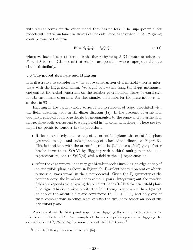
• If the removed edge sits on top of an orientifold plane, the orientifold plane

preserves its sign, and ends up on top of a face of the dimer, see Figure 6a.

This is consistent with the orientifold rules in §3.1 since a U(N) gauge factor

breaks down to an SO(N) by Higgsing with a chiral multiplet in the

representation, and to Sp(N/2) with a field in the representation.

• After the edge removal, one may get bi-valent nodes involving an edge on top of

an orientifold plane as shown in Figure 6b. Bi-valent nodes represent quadratic

terms (i.e. mass terms) in the superpotential. Given the Z2 symmetry of the

parent theory, the bi-valent nodes come in pairs. Integrating out the massive

fields corresponds to collapsing the bi-valent nodes [18] but the orientifold plane

flips sign. This is consistent with the field theory result, since the edges not

on top of the orientifold plane correspond to + , and only one of

these combinations becomes massive with the two-index tensor on top of the

orientifold plane.

An example of the first point appears in Higgsing the orientifolds of the coni-

fold to orientifolds of C3. An example of the second point appears in Higgsing the

orientifolds of C3/(Z2 × Z2) to orientifolds of the SPP theory.9

9For the field theory discussion we refer to [52].

– 20 –

+ +

+ −

a)

b)

Figure 6: a) Behavior of orientifold plane (red cross) upon removal of edges. b) Behavior

of orientifold plane upon integrating out matter.

The above rules allow to fix the global constraint on the number of orientifold

planes of equal sign in arbitrary dimer diagrams by Higgsing them down to a known

dimer diagram. Some examples are discussed in following sections.

3.4 The global constraint for the fixed point signs revisited

In all the models considered in the previous sections, we are able to determine which

parity of the fixed point signs leads to supersymmetric orientifolds. This is consistent

with (un)Higgsing to known theories. It is in principle possible, although generally

much more involved, to use one of these approaches for a generic toric singularity.

The transformation rules of mesonic operators under the orientifold action, de-

rived in the previous section, offer a simpler method for fixing the signs. For an

arbitrary dimer, the parity of orientifold plane signs can be determined by requiring

consistency among the sign assignments that follow from the three rules.

With a reasoning similar to the one used to arrive at rule 3, we can derive a

compact principle fixing the sign parity. Take any mesonic operator and move it

once around the torus until it comes back to itself. It picks up a sign given by

(−1)SP (−1)#F = (−1)SP (−1)NW /2, (3.12)

where SP denotes the overall sign parity and F the number of F-term relations

required to move the path once around the torus. In detail, when moving around the

torus, the path representing the meson passes over all the orientifold planes and pick

their signs. This gives rise to the (−1)SP factor in (3.12). The (−1)#F factor comes

from the F-term relations required to move the path around the torus and return

to its original position. All the NW superpotential terms are used in this process.

Since every field in the quiver is present in exactly two superpotential terms, we take

care of all of them by using the F-term equations for NW /2 fields. Since the meson

should not pick up a sign in this process, (3.12) has to be equal to one. Hence, we

conclude that the sign parity is equal to the parity of NW /2. This is precisely the

sign rule announced in §3.1.

– 21 –

3.5 Further examples

3.5.1 Orientifolds of C3/Z3

Let us consider C3/Z3 which can be also seen as the orbifold point of OP2(−3), i.e.

the complex cone over dP0. The dimer and the fixed-points under the point-reflection

involution as well as the mesonic operators corresponding to the coordinates of the

geometry are depicted in Figure 7. Under the involution one gauge group stays fixed

y

x

z

z

z

x

x

X(2)23

X(1)31

X(3)23

X(2)12

X(1)23X

(3)31

X(2)23

X(1)12

X(3)23

X(2)31

X(1)23 1

22

23 3

3

Figure 7: Left: The dimer of the orbifold C3/Z3 with fixed-points. Right: The mesonic

operators.

while two are identified. Three bi-fundamentals are mapped to themselves while the

remaining ones are identified. The holomorphic 3-form survives from the parent C3

theory. The mesonic operators show identical behavior as in C3, i.e. they have only

one common fixed-point. Hence, the same considerations apply, i.e. only an odd sign

parity leads to an N = 1 supersymmetric theory. Some possible sign choices and

the resulting theories are listed in Table 5. The orientifolds of the first and second

Charges Gauge group Matter

(+ + −+) Sp × U 3 2 + 3 ( , )

(−− +−) SO × U 3 2 + 3 ( , )

(+ −−−) Sp × U 1 2 + 2 2 + 3 ( , )

(− + ++) SO × U 2 2 + 1 2 + 3 ( , )

Table 5: Some possible N = 1 orientifolds of C3/Z3.

model of Table 5 are closely related to the orientifold projection introduced in [41],

see e.g. [67, 68, 13, 69] for its construction using D3-branes.

All the spectra shown in Table 5 are anomalous unless the ranks of the gauge

groups are restricted or additional (anti)fundamental matter is added. It is instruc-

tive to discuss this example in more detail, since similar considerations apply to the

rest of the models in the paper. Contrary to what happens for the models we have

discussed so far, there is more than one way to render them consistent. For example,

for the first model in Table 5 with gauge group Sp(n1) × U(n2), the most general

anomaly-free spectrum reads

– 22 –

3 2 + 3 ( , ) + 3 (4 − n1 + n2) , (3.13)

where a negative number of is understood as a positive number of . All these

choices translate to branes wrapping compact or non-compact cycles. It would be

interesting to reproduce this constraint along the lines of [63].

3.5.2 Orientifolds of the Conifold/ZN

In this section we consider orientifolds of certain orbifolds of the conifold, introduced

in [54], and corresponding to Laaa geometries with a = N . The tools should be

familiar by now, so our discussion is sketchy.

Let us start with the Z2 orbifold of the conifold obtained by the following geo-

metric action:

x → x, y → y, z → −z, w → −w. (3.14)

This orbifold has been discussed in detail in [93]. The holomorphic 3-form Ω of the

conifold is invariant under this orbifold action as can be inferred from (3.8). The

dimer and the mesonic operators are drawn in Figure 8. The basic structure of

y

z wx

11

12

23

34

4

4

Figure 8: Left: Dimer of the conifold/Z2. Right: The mesonic operators.

mesonic operators and their relation with the orientifold points is similar to that of

the conifold. The sign parity of the model is positive, though. Hence the number of

negative orientifold planes is even.

The structure of the possible orientifold models is as follows. The resulting gauge

group is U(N1) × U(N2) and there are two antisymmetric and two symmetric rep-

resentations (two among the four are conjugated). The chiral combinations require

additional flavors, as in fork configurations. This can be obtained upon introduction

of extra non-compact branes in the system. The models can be described using a T-

dual HW setup with two NS and two NS′-branes. The non-chiral models correspond

to HW models with e.g. the NS-branes on top of O6-planes (of different possible

signs) and the NS′-branes mapped to each other by the orientifold action. The chiral

models correspond to HW models with the NS′-branes on top of O6-planes. These

O6 planes are split in halves, and lead to a chiral matter content as in a fork config-

uration. The NS-branes are mapped to each other.

– 23 –

It is easy to generalize this to any ZN orbifold of the conifold. The dimers for

odd as well as for even N are given in Figure 9. Some basic possible orientifolded

1

1

11

1

1

2

2

2

2

3

3

N

N

N

N

N+1

N+1

N+1

N+1

N+2

N+2

N-1

N-1

2N

2N

2N

2N

2N

2N

2N-1

2N-1

2N-1

2N-1

2N-2

2N-2

Figure 9: Top: Dimer of the conifold/ZN for odd N . Bottom: For even N .

theories are given in Table 6. For all these models we have N factors of gauge

group U(Ni) with i = 1...N and bi-fundamentals∑N−1

i=1 ( i, i+1) + ( i, i+1).

The remaining matters are specified in Table 6. The different geometric actions are

straightforwardly obtained from our rules.

Charges G. g. Matter

(+ + +−)∏N

i=1 U(Ni) 1 + 1 + N + N + 8 N

(+ −−−)∏N

i=1 U(Ni) 1 + 1 + N + N + 8 1

(+ + ++)∏N

i=1 U(Ni) 1 + 1 + N + N

(+ − +−)∏N

i=1 U(Ni) 1 + 1 + N + N + 8 1 + 8 N

Table 6: Basic N = 1 orientifolds of the conifold/ZN . The first two rows correspond to

orbifolds with odd N , while the last two rows correspond to orbifolds with even N .

3.5.3 Orientifolds of SPP

As another example, consider the real cone over the first member of the Laba family,

L1,2,1. This is also known as the complex cone over the suspended pinch point, for

short SPP. The dimer and the mesonic operators corresponding to the coordinates

of the geometry are shown in Figure 10.

Using the rules one can easily extract the spectra and action on coordinates for

various sign choices as listed in Table 7. In addition to the fields listed, all the models

contain a ( 1, 2)+ ( 1, 2) pair. The last two models also require the addition

of antifundamentals to cancel gauge anomalies.

– 24 –

xz w w

y

Φ3

X31

X13X23

X32

X21

X12

1

1

1

2

2

2

3

Figure 10: Dimer of SPP and the mesonic operators.

Charges Gauge group Matter σ(x, y, z, w)

(+ + ++) SO × U 1 + 2 + 2 (+x, +y, +z,−w)

(−−−−) Sp × U 1 + 2 + 2 (+x, +y, +z,−w)

(−− ++) SO × U 1 + 2 + 2 (−x,−y, +z,−w)

(+ + −−) Sp × U 1 + 2 + 2 (−x,−y, +z,−w)

(+ − +−) SO × U 1 + 2 + 2 + 8 2 (+x,−y,−z, +w)

(− + −+) Sp × U 1 + 2 + 2 + 8 2 (+x,−y,−z, +w)

Table 7: Some possible orientifolds of the SPP.

Hence, we easily recover the orientifolds derived via field-theory techniques in

[52].

It is straightforward to use our rules to systematically construct orientifolds

of general Laba theories. Some technical details of these theories can be found in

Appendix C. Since the basic ingredients have already been discussed, we refrain from

a detailed classification and instead proceed to the construction of new examples.

3.5.4 Orientifolds of L1,5,2

Finally, in order to illustrate the power of our methods, we close this section with

an example that was not amenable to the techniques previously available in the

literature. Figure 11 shows the dimer diagram for L1,5,2 [20].

1

1

1

1

2

2

2

2

3 4

5

5

6

6

Figure 11: Dimer diagram for L1,5,2.

– 25 –

The parent theory has 10 superpotential terms. Hence, the sign rule determines

that the sign parity must be odd. The resulting gauge group is U(n1)×U(n3)×U(n5),

with matter content

( 1, 3)+( 1, 3)+( 1, 5)+2 ( 3, 5)+( 3, 5)+R1+S3+T5+V5. (3.15)

R1, S3, T5 and V5 are two-index tensor representations determined by the signs of

the orientifold planes.

Charges 2-index tensors

(+ + +−) 1 + 3 + 5 + 5

(+ + −+) 1 + 3 + 5 + 5

(+ − ++) 1 + 3 + 2 5

(− + ++) 1 + 3 + 2 5

Table 8: Two-index representations for some possible orientifolds of the L1,5,2 theory.

Other choices amount to overall sign flips.

As in previous examples, gauge anomalies are canceled by constraining the ranks

of gauge groups and adding (anti)fundamental fields.

4. Orientifolds from dimers with fixed lines

After discussing in detail the large class of involutions preserving the mesonic U(1)2

flavor symmetries, in this section we consider a different type of involution preserving

a linear combination of them. As pointed in §2.3, they are described in the dimer

diagram as symmetries which leave fixed lines.

4.1 Generalities

Orientifolds with fixed lines are obtained for dimer diagrams which are invariant

under a line reflection.10 Symmetries with fixed lines exist for dimer diagrams with

unit cell of two possible kinds, as shown in Figure 12. As in Figure 12a, the unit cell

can be a ‘rectangle’, in which case it has two independent orientifold lines. Or as in

Figure 12b it can be a ‘rhombus’, in which case there is a single orientifold line.11

Using the interpretation of the dimer diagram as a brane tiling of NS-branes with

suspended D5-branes [18, 20], such orientifold lines are physical orientifold planes.

10An additional constraint is that the symmetry should map black to black nodes and white to

white nodes.11In the orientifold literature it is well known that tori with line symmetries exist only for two

possible complex structures (rectangular and rhombus). This issue has been discussed in detail e.g.

in [70, 71]. It corresponds to the fact that in Type I the orientifold flips the B-field so only two

choices are left: B = 0 and B = 1/2 (dual to rectangular and rhombus unit cell, respectively)

– 26 –

Hence, for the case in Figure 12a we can consider independent sign choices (charges)

for the two orientifold lines. The structure of the unit cell depends only on the dimer

diagram under consideration.

a) b)

Figure 12: The two possible unit cell geometries for orientifolds with fixed lines: rectangle

and rhombus.

For each choice of orientifold signs, the rules to read out the spectrum are similar

to the case of fixed points, see §3.1. Our description here is thus more sketchy.

• Faces mapped to themselves by the orientifold action have their gauge factors

projected down to SO or Sp for positive or negative orientifold line charge,

respectively. Faces paired up by the orientifold action are identified, and give

rise to a single unitary gauge factor.

• Edges mapped to themselves correspond to chiral multiplets in the two-index

symmetric or antisymmetric tensor representations for positive or negative ori-

entifold line charge, respectively. Edges paired up by the orientifold action are

identified, and give rise to a single bi-fundamental field.

• Nodes mapped to themselves give rise to interaction terms in the superpoten-

tial.

4.2 Few examples and the geometric action

In this section we consider several examples of orientifold with fixed lines. We also

describe the geometric action on mesons, which can be obtained using rules similar

to those of fixed point orientifolds.

4.2.1 Line orientifolds of C3

As a little warmup, let us come back to C3. But this time, let us consider the

line-reflection symmetry as depicted in Figure 13.

Clearly, The orientifold line passes through the face and depending on the sign of

the single O-plane, we obtain a SO/Sp gauge theory. One of the fields is mapped to

itself and projects down to the adjoint of the SO/Sp gauge group, which is denoted

– 27 –

x

zy

1

1 1

1

Φ2 Φ2

Φ3

Φ3

Φ1

Figure 13: Left: The dimer of C3 with line reflection. Right: The three fundamental

mesons.

by Φ. The other two fields are exchanged and lead to one two-index symmetric and

one antisymmetric representation, denoted by S, A respectively.

The superpotential can be obtained from the parent theory by simply replacing

the original fields by the components surviving the projection:

W = ΦAS − ΦSA. (4.1)

The superpotential in coming examples can be found similarly.

Concerning the geometric action, we anticipate that the line reflection exchanges

the mesons y and z and keeps the meson x fixed:

y ↔ z, x → x. (4.2)

This agrees with the fact that the model corresponds to the introduction of an O7-

plane in a system of D3-branes in flat space. The sign transformation of the mesons

will be more systematically discussed in §4.2.4.

4.2.2 C2/ZN × C, even N

Let us consider the example of C2/ZN ×C, distinguishing the even and odd N cases.

The geometry has a T-dual realization as a HW setup with N parallel NS5-branes.

Since these models are orbifolds, we can also construct the orientifolds we are to

discuss using CFT techniques. Both descriptions can be found in [72, 73]. Thus, the

models provide a good starting point to derive the rules for the construction of the

orientifolds in terms of dimer diagrams with fixed lines.

Consider the even N case, for example C2/Z4 × C shown in Figure 14a. The

unit cell has a geometry such that the two orientifold lines are independent, so their

signs can be chosen independently. This leads to the four possible orientifold models

whose gauge group and two-index tensor structure is given in Table 9. Here and

in the following examples we take as convention that we label the fixed lines from

bottom to top, i.e. (+−) means that the lower fixed line has positive charge while

the upper line has negative charge. Note that all models presented in Table 9 possess

– 28 –

a) b)

11

11

1

1

1

1 1

1

111

2

2 2

2

2

2

22

3 3

3

3

3

3

3

4

4

4

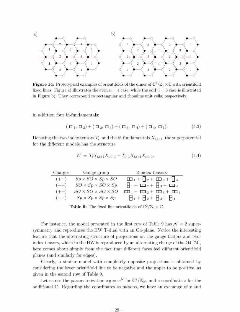
Figure 14: Prototypical examples of orientifolds of the dimer of C2/Zn×C with orientifold

fixed lines. Figure a) illustrates the even n = 4 case, while the odd n = 3 case is illustrated

in Figure b). They correspond to rectangular and rhombus unit cells, respectively.

in addition four bi-fundamentals:

( 1, 2) + ( 2, 3) + ( 3, 4) + ( 4, 1). (4.3)

Denoting the two-index tensors Ti, and the bi-fundamentals Xi,i+1, the superpotential

for the different models has the structure

W = TiXi,i+1Xi,i+1 − Ti+1Xi,i+1Xi,i+1. (4.4)

Charges Gauge group 2-index tensors

(+−) Sp × SO × Sp × SO 1 + 2 + 3 + 4

(−+) SO × Sp × SO × Sp 1 + 2 + 3 + 4

(++) SO × SO × SO × SO 1 + 2 + 3 + 4

(−−) Sp × Sp × Sp × Sp 1 + 2 + 3 + 4

Table 9: The fixed line orientifolds of C2/Z4 × C.

For instance, the model presented in the first row of Table 9 has N = 2 super-

symmetry and reproduces the HW T-dual with an O4-plane. Notice the interesting

feature that the alternating structure of projections on the gauge factors and two-

index tensors, which in the HW is reproduced by an alternating charge of the O4 [74],

here comes about simply from the fact that different faces feel different orientifold

planes (and similarly for edges).

Clearly, a similar model with completely opposite projections is obtained by

considering the lower orientifold line to be negative and the upper to be positive, as

given in the second row of Table 9.

Let us use the parameterization xy = wN for C2/ZN , and a coordinate z for the

additional C. Regarding the coordinates as mesons, we have an exchange of x and

– 29 –

y. The meson z crosses two orientifolds of opposite signs, suggesting it is odd, the

same holds for w.

Let us consider the case of both orientifold lines with positive sign. The corre-

sponding models can be found in the third and fourth row of Table 9.

The theory has N = 1 supersymmetry and reproduces the HW T-dual with an

O8-plane, described in [73]. One can also infer that the geometric action exchanges

the mesons x and y while the meson z crosses two orientifolds of same sign, suggesting

it is even, similar for w.

4.2.3 C2/ZN × C, odd N

Let us consider the odd N case, for instance the case C2/Z3×C shown in Figure 14b.

The unit cell has a geometry such that there is only one orientifold line. Notice that

this automatically forbids the analogs of the N = 2 orientifolds described above for

the even N case. This is in complete agreement with the impossibility to introduce

O4-planes in HW configurations with an odd number of NS-branes.

The two possible models are given in Table 10, where we show the gauge group

and two-index tensor structure. There we use the notation (++), (−−) for positive

and negative orientifold lines (to keep the analogy with the previous case).

Charges Gauge group 2-index tensors

(++) SO × SO × SO 1 + 2 + 3

(−−) Sp × Sp × Sp 1 + 2 + 3

Table 10: The fixed line orientifolds of C2/Z3 × C.

In addition, both models possess three bi-fundamentals

( 1, 2) + ( 2, 3) + ( 3, 1). (4.5)

The structure of the superpotential is as in (4.4)

The models correspond to N = 1 theories, in agreement with the T-dual HW

setup with O8-planes described in [73]. Notice that in these HW models the O8-plane

does not have any alternating structure, so they really exist for odd N as well.

4.2.4 The geometric action

As for fixed point orientifolds, the simplest way to specify the geometric action of

the orientifold quotient is by providing rules for the action on the gauge invariant

mesonic operators. These can be easily obtained from simple examples (for which

the geometric action is known via other techniques) and extended to general validity.

We simply state them as follows

– 30 –

Rule 1 : A meson mapped to itself under the orientifold action picks a sign (−1)k

where k is the intersection number (counted with orientation) with negative orien-

tifold lines.

Rule 2 : Two mesons mapped to each other under the orientifold action are related

without any relative sign.

A simple consequence of these rules is that mesons corresponding to superpotential

terms associated to nodes on top of orientifold lines are even under the orientifold

action. This does not contradict the fact that the complete superpotential is odd (cf.

footnote 7), since in general different terms in the superpotential are swapped under

the orientifold action.12

For instance, consider C3 with the orientifold action y ↔ z, x → x as discussed

in §4.2.1. The operators t1 = tr(Φ1Φ2Φ3) and t2 = tr(Φ2Φ1Φ3) are exchanged, so

the meson (modulo F-terms) t ≡ t1 ≡ t2 is even. Still, the complete superpotential

W = t1 − t2 is odd.

It is straightforward to apply the above rules to obtain the geometric action for

the orientifolds constructed in the previous subsections. Let us use the parameteri-

zation, familiar from previous sections, xy = wN for C2/ZN , and a coordinate z for

the additional C. Regarding the coordinates as mesons, we have an exchange of x

and y. The meson z is mapped to itself and crosses two orientifold lines. Finally, the

same holds for w. From the above rules we obtain the action

x ↔ y, z → εz, w → εw. (4.6)

With ε = −1 for the models with one positive and one negative orientifold line (and

ε = +1 for the other examples). This precisely agrees with the geometric actions

proposed in [72] for the T-dual of the HW with O4-planes, and in [73] for the T-dual

of the HW with O8-plane. Notice that in all cases, the meson associated to the

superpotential terms (which can be regarded as xw) is even.

We hope that this examples suffice to illustrate the rules to construct orientifolds

of dimers with fixed lines. In the next section we apply these rules to construct further

families of examples.

4.3 Further examples

4.3.1 General Laba theories

It is straightforward to construct orientifolds with fixed lines for the entire Laba

family. In this section we illustrate it with a few examples.

12The explanation in the mirror picture is as follows: These involutions switch the orientation of

paths bounding the faces in the dimer. Hence, the corresponding 1-cycles in the mirror Riemannian

surface do so. Thus, the superpotential terms are mapped to themselves, but an additional sign

flip comes in due to the orientation change (for illustration compare Figures 23 and 26).

– 31 –

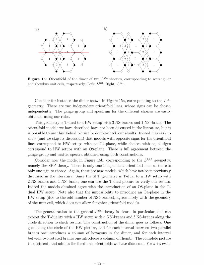
a) b)

111

11

1 1

1

11

11 1

2

2

2

2

2

2

2

2

33

3

3

3

3

3

4

4

4

Figure 15: Orientifold of the dimer of two Laba theories, corresponding to rectangular

and rhombus unit cells, respectively. Left: L131, Right: L121.

Consider for instance the dimer shown in Figure 15a, corresponding to the L131

geometry. There are two independent orientifold lines, whose signs can be chosen

independently. The gauge group and spectrum for the different choices are easily

obtained using our rules.

This geometry is T-dual to a HW setup with 3 NS-branes and 1 NS′-brane. The

orientifold models we have described have not been discussed in the literature, but it

is possible to use this T-dual picture to double-check our results. Indeed it is easy to

show (and we skip its discussion) that models with opposite signs for the orientifold

lines correspond to HW setups with an O4-plane, while choices with equal signs

correspond to HW setups with an O8-plane. There is full agreement between the

gauge group and matter spectra obtained using both constructions.

Consider now the model in Figure 15b, corresponding to the L1,2,1 geometry,

namely the SPP theory. There is only one independent orientifold line, so there is

only one sign to choose. Again, these are new models, which have not been previously

discussed in the literature. Since the SPP geometry is T-dual to a HW setup with

2 NS-branes and 1 NS′-brane, one can use the T-dual picture to verify our results.

Indeed the models obtained agree with the introduction of an O8-plane in the T-

dual HW setup. Note also that the impossibility to introduce an O4-plane in the

HW setup (due to the odd number of NS5-branes), agrees nicely with the geometry

of the unit cell, which does not allow for other orientifold models.

The generalization to the general Laba theory is clear. In particular, one can

exploit the T-duality with a HW setup with a NS′-branes and b NS-branes along the

circle direction to check results. The construction of the dimer goes as follows. One

goes along the circle of the HW picture, and for each interval between two parallel

branes one introduces a column of hexagons in the dimer, and for each interval

between two rotated branes one introduces a column of rhombi. The complete picture

is consistent, and admits the fixed line orientifolds we have discussed. For a+b even,

– 32 –

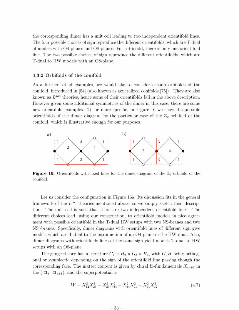
the corresponding dimer has a unit cell leading to two independent orientifold lines.

The four possible choices of sign reproduce the different orientifolds, which are T-dual

of models with O4-planes and O8-planes. For a + b odd, there is only one orientifold

line. The two possible choices of sign reproduce the different orientifolds, which are

T-dual to HW models with an O8-plane.

4.3.2 Orbifolds of the conifold

As a further set of examples, we would like to consider certain orbifolds of the

conifold, introduced in [54] (also known as generalized conifolds [75]) . They are also

known as Laaa theories, hence some of their orientifolds fall in the above description.

However given some additional symmetries of the dimer in this case, there are some

new orientifold examples. To be more specific, in Figure 16 we show the possible

orientifolds of the dimer diagram for the particular case of the Z2 orbifold of the

conifold, which is illustrative enough for our purposes.

a) b)

1

1

1

1

1

1

1

1

22

3

3 3

3

44

Figure 16: Orientifolds with fixed lines for the dimer diagram of the Z2 orbifold of the

conifold.

Let us consider the configuration in Figure 16a. Its discussion fits in the general

framework of the Laba theories mentioned above, so we simply sketch their descrip-

tion. The unit cell is such that there are two independent orientifold lines. The

different choices lead, using our construction, to orientifold models in nice agree-

ment with possible orientifold in the T-dual HW setups with two NS-branes and two

NS′-branes. Specifically, dimer diagrams with orientifold lines of different sign give

models which are T-dual to the introduction of an O4-plane in the HW dual. Also,

dimer diagrams with orientifolds lines of the same sign yield models T-dual to HW

setups with an O8-plane.

The gauge theory has a structure G1 × H2 × G3 × H4, with G, H being orthog-

onal or symplectic depending on the sign of the orientifold line passing though the

corresponding face. The matter content is given by chiral bi-fundamentals Xi,i+1 in

the ( i, i+1), and the superpotential is

W = X212X

223 − X2

23X234 + X2

34X241 − X2

41X212. (4.7)

– 33 –

Describing the geometry as xy = znwn, with the basic mesons defined as in

Figure 8, the geometric actions correspond to

x ↔ y, z → εz, w → εw, (4.8)

with here and later on ε is given by the product of orientifold line signs (negative for

opposite signs, positive for equal sign).

Consider now the configuration in Figure 16b. Again there are two independent

orientifold lines, whose signs can be chosen independently. The structure of the

orientifold theory on ZN orbifold of the conifold is as follows. The gauge group reads

G1 × U(n2) × . . . × U(nN ) × GN+1, (4.9)

with Gi given by SO/Sp for O+/− respectively.

For the N = 2 case in the figure, we have G1 × U(n2) × G3, and the matter

content is given by

( 1, 2) + ( 1, 2) + ( 2, 3) + ( 2, 3), (4.10)

with superpotential

W = X212X

221 − X12X23X32X21 + X2

23X232. (4.11)

Using our techniques, the geometric action of the orientifold can be obtained as

z ↔ w, x → εx, y → εy. (4.12)

The above orientifold corresponds under T-duality to a HW model with O6-

planes away from the NS- and NS′-branes, and mapping them to each other (thus the

orientifold planes are at 45 degrees with the NS-branes in the 48 and 59 directions).

This orientifold has been briefly considered in [52].

Notice that for the particular case of the conifold the two orientifolds described

above (with horizontal or vertical fixed lines) are isomorphic (up to a relabeling of

coordinates). This is related to the enhanced global symmetries of the conifold,

which lead to a very symmetric dimer diagram.

Thus we have two possible HW T-dual interpretations for the orientifold of xy =

zw by the orientifold ωσ(−1)FL, with σ acting as

x ↔ y, z → εz, w → εw. (4.13)

This is in fact correct, as one can see as follows: One can regard the conifold as a

C∗ , parameterized by x, y, fibered over z, w and degenerating at z = 0 an w = 0.

T-dualizing along the circle in this C∗ (namely the orbit of x → eiθx, y → e−iθy) gives

one NS along z and one NS′ along w. In this T-dual picture the orientifold action

– 34 –

reproduces an O4-plane for ε = −1 and an O8-plane for ε = +1. On the other hand,

one can regard the same equation as describing a C∗ fiber parameterized by z, w

fibered over x, y. T-dualizing along the circle in this fibration, one gets one NS along

x and one NS′ along y. In this T-dual, the orientifold action introduces and O6-

plane at 45 degrees with the NS- and NS′-branes. Hence the two HW configurations

are correct T-dual descriptions of the orientifold model. It is amusing that the

dimer representation is clever enough to realize this and make manifest that the two

orientifolds are actually the same!

5. The mirror perspective

The physical realization of the dimer diagram has been shown to be quite manifest

upon use of mirror symmetry [22]. The different gauge factors arise from D6-branes

wrapped on 3-cycles in the mirror geometry, with the bi-fundamental multiplets

arising from their intersection and the superpotential couplings arising from open

string disk worldsheet instantons. The dimer diagram is moreover recovered from

the mirror geometry by a certain projection on a two-torus.

We may therefore expect that there is a natural interpretation of the orientifold

action in the mirror geometry, and that some aspects of the previous discussion

receive a new light from this viewpoint. In this section we provide a description of

orientifolding in the mirror geometries, and its interplay with our previous dimer

diagram description. Although we do not achieve a systematic understanding of all

aspects of orientifolding, we recover many interesting results.

5.1 Review of the mirror picture

The mirror configuration

Under local mirror symmetry, a system of D3-branes located at the singular point of

a non-compact toric Calabi-Yau 3-fold M are mapped to a set of D6-branes wrapping

supersymmetric 3-cycles in the mirror Calabi-Yau M [76, 77]. The mirror manifold

M can be seen as a double fibration over the complex plane [78, 79]:

z = uv,

z = P (x1, x2),

where x1, x2 ∈ C×, u, v, z ∈ C and P (x1, x2) is the Newton polynomial of the toric

diagram of the singularity. Note that one can read off P directly from the correspond-

ing toric diagram [82, 76]. More specifically, for a singularity whose toric diagram is

given by a set of points (ni, mi), we have

P (x1, x2) =∑

i

xni

1 xmi

2 . (5.1)

– 35 –

For instance, for the conifold we have P = 1+x1 +x2 +x1x2. Note that the SL(2, Z)

freedom in choosing the basis of the toric lattice corresponds to a redefinition of

coordinates in the mirror geometry.

The first fiber defines a C∗ fibration, degenerating at the origin of the base

z = 0, where the S1 in C∗, denoted S1c , shrinks to zero. The second fiber describes a

punctured Riemannian surface, which is denoted as Σ. Its genus g equals the number

of internal points of the toric diagram. The fiber over z = 0, denoted Σ0, is important

for our purposes. It corresponds to a smooth Riemann surface which can be thought

of as a thickening of the web diagram dual to the toric diagram [80, 81, 82]. At

certain critical points z∗i on the base, certain 1-cycles [ci] of Σ pinch off. In detail,

the critical points z∗i can be obtained by solving

∂x1P = 0, ∂x2

P = 0, (5.2)

for x1, x2 and substituting back into the fiber defining Σ.

The geometry has a non-trivial compact 3-homology. We can define a set of

3-cycles [Ci] by taking the segment [0, z∗i ] on the base and fibering the two-torus

S1c × [ci] over it. Since S1

c shrinks to zero at z = 0 and [ci] shrinks to zero at z∗i ,

this defines a 3-cycle with the topology of S3. The mirror image of the D3-branes

at the singularity correspond to D6-branes wrapped on these 3-cycles. Namely, the

fractional D3-brane giving rise to the ith gauge factor is mapped to a D6-brane

wrapped on the 3-cycle [Ci]. The bi-fundamental chiral multiplets ( i, j) arise

from open strings stretching between the ith and jth D6-branes, at their intersections.

That is, there are Iij = [Ci] · [Cj] bi-fundamentals ( i, j) in the gauge theory.

Notice from the above description that the 3-spheres intersect only on the fibers

above z = 0. Hence, the geometry of the D6-brane cycles and their intersections is

encoded in Σ0.

The close relation between Σ0 and the gauge theory works in the reverse way,

and in fact it is easy to recover Σ0 and the geometry of the D6-branes in terms of the

dimer diagram. Given a dimer diagram, one can define zigzag paths (these, along

with the related rhombi paths, were introduced in the mathematical literature on

dimers in [31, 32], and applied to the quiver gauge theory context in [21]), as paths

composed of edges, and which turn maximally to the right at e.g. black nodes and

maximally to the left at white nodes. They can be conveniently shown as oriented

lines that cross once at each edge and turn at each vertex, as shown in Figure 17.

We denote the colorful diagram corresponding to the set of such zigzag-lines as the

Harlequin diagram.13 Notice that at each edge two zigzag paths must have opposite

orientations. For dimer models describing toric gauge theories, these zigzag paths

13Any graph has an associated Harlequin diagram consisting of its zigzag paths. In short, we will

introduce a tiling of the Σ0 that we denote shiver diagram. Both the dimer and shiver diagrams

have associated Harlequins. We are confident that the reader can distinguish between the two

constructions based on the context.

– 36 –

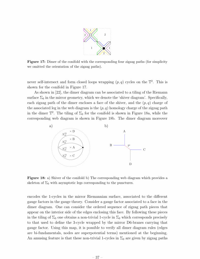
1

11

2

2

2

Figure 17: Dimer of the conifold with the corresponding four zigzag paths (for simplicity

we omitted the orientation of the zigzag paths).

never self-intersect and form closed loops wrapping (p, q) cycles on the T2. This is

shown for the conifold in Figure 17.

As shown in [22], the dimer diagram can be associated to a tiling of the Riemann

surface Σ0 in the mirror geometry, which we denote the ‘shiver diagram’. Specifically,

each zigzag path of the dimer encloses a face of the shiver, and the (p, q) charge of

the associated leg in the web diagram is the (p, q) homology charge of the zigzag path

in the dimer T2. The tiling of Σ0 for the conifold is shown in Figure 18a, while the

corresponding web diagram is shown in Figure 18b. The dimer diagram moreover

A

A

B

B

C

C

D

D

X(1)12

X(1)21

X(2)12

X(2)21

P1

a) b)

Figure 18: a) Shiver of the conifold b) The corresponding web diagram which provides a

skeleton of Σ0 with asymptotic legs corresponding to the punctures.

encodes the 1-cycles in the mirror Riemannian surface, associated to the different

gauge factors in the gauge theory. Consider a gauge factor associated to a face in the

dimer diagram. One can consider the ordered sequence of zigzag path pieces that

appear on the interior side of the edges enclosing this face. By following these pieces

in the tiling of Σ0 one obtains a non-trivial 1-cycle in Σ0 which corresponds precisely

to that used to define the 3-cycle wrapped by the mirror D6-branes carrying that

gauge factor. Using this map, it is possible to verify all dimer diagram rules (edges

are bi-fundamentals, nodes are superpotential terms) mentioned at the beginning.

An amusing feature is that these non-trivial 1-cycles in Σ0 are given by zigzag paths

– 37 –

of the tiling of Σ0. The non-trivial 1-cycles in the mirror Riemann surface for the

case of the conifold are shown in Figure 19.

A

B

C

D

Figure 19: Harlequin diagram of the conifold shiver. The two zigzag paths of the conifold

shiver corresponding to the 1-cycles in Σ0 the D6-branes are wrapped which give rise to

the two gauge groups.

A direct construction of the shiver diagram from the knowledge of the toric gauge

theory and its superpotential is explained in detail in §A.

The amoeba and alga maps

There exists certain projections of the Σ fibration which turn out to be useful in

relating the mirror configuration to the dimer diagram [22]. Consider the amoeba

projection, given by the map Σ → R2:

(x1, x2) ∈ Σ → (s = log(|x1|), t = log(|x2|)) ∈ R2, (5.3)

It has been widely studied in mathematics, and it has the useful property that the

punctures of Σ map to ”tentacles” perpendicular to the convex polyhedron associated

to the toric variety of M [83]. Namely, it provides a smooth version of the web

diagram for the toric singularity. For example, the amoeba of the conifold and a Z2

orbifold thereof are illustrated in Figure 20.

Let us consider a different projection. Namely, the projection of Σ onto the

phases of x1 = |x1|eiΦ and x2 = |x2|eiΘ. This projection was dubbed alga map in

[22], and provides a natural map Σ → T2:

(x1, x2) ∈ Σ → (Φ, Θ) ∈ T2, (5.4)

Moreover, at least for certain cases, it is possible to identify this T2 with the dimer

T2 and recover the dimer diagram from the image of the alga [22]. As is discussed in

§5.3, this map turns out to be useful for translating the orientifold action from the

dimer to an involution on Σ.

– 38 –

s

t

st

Figure 20: Left: Amoebae of the conifold. Right: Amoebae of conifold/Z2.

Tadpole cancellation

An important consistency condition of systems of D-branes at singularities is cancel-

lation of RR tadpoles of compact support. This condition is manifest in the mirror

geometry, as cancellation of compact homology charge of the wrapped 3-cycles, see

[76, 69]. Given that the set of 3-cycles [Ci] in the mirror geometry provides a basis of

the compact 3-homology, an equivalent definition is as follows: the total homology

class of the system must have zero intersection number with any of the basic 3-cycles

[Ci]. As usual, this implies cancellation of gauge anomalies for the four-dimensional

field theory.

The simplest solution to these constraint is to consider an equal number of D-

branes corresponding to each gauge factor (the conformal case of D3-branes at a

singularity). In the mirror geometry, it is possible to see that the set of 3-cycles [Ci]

can recombine into a single 3-cycle with the topology of T3. This is the mirror of

the statement that in this situation the different fractional branes can form a bound

state corresponding to a dynamical D3-brane able to move off the singular point.

In the presence of orientifold planes, the orientifold plane has a contribution to

RR charge, proportional to the compact 3-homology class of the 3-cycle it wraps.

This implies that the set of D6-branes required to cancel RR tadpoles is different

from those in unorientifolded system (and in particular that no recombination into

a T3 cycle is possible). An example is discussed in §5.4.

Supersymmetry and calibrations

In order that the D6-branes and O6-planes in the mirror geometry preserve a com-

mon supersymmetry, they need to wrap special Lagrangian submanifolds. This is

made more explicit in §5.5, where a (local) calibration condition is given for the

embedding of the D6-branes and O6-planes to fulfill.

– 39 –

A subtlety for genus 0

We would like to conclude this section with a clarification regarding the genus 0

case. As already mentioned in [22], for Σ of genus 0 it may happen that the mirror

fibration has fewer critical points than needed to explain the number of gauge factors.

For instance for the mirror of C3 there are no critical points, and for the conifold

there is only a single critical point.

Looking at these examples in detail one however finds no paradox. For instance,

the mirror of the D3-branes in C3 is given by a D6-brane wrapped on a smooth T

3

in the mirror geometry (given by fibering S1c times a 1-cycle in Σ over a 1-cycle in

the base encircling the origin).

Similarly, a single critical point for the conifold is not necessarily a problem. The

Σ fibration in this case is given by14

1 + x1 + x2 − x1x2 − z = 0, (5.5)

Clearly, there is only a single critical point at z = 2, above which the fiber is

(1 − x1)(1 − x2) = 0. (5.6)

This describes two complex planes given by x1 = 1, x2 arbitrary and x2 = 1,

x1 arbitrary. Under the amoeba projection (5.3) they reproduce the web diagram of

the conifold (cf. Figure 20), with the interior shrunk to a point. This implies that

the two 1-cycles associated to the two gauge factors shrink at this point, and can be

used to construct two 3-spheres. This fits with the picture in [76].

We conclude this review section by noting that one can nicely visualize many

of the properties of the mirror geometry by drawing the mirror surface Σ0 with the

1-cycles wrapped by the D6-branes as illustrated in Figure 21a.

5.2 Orientifolds in the mirror system

In this section we would like to consider the introduction of orientifold quotients in

the mirror configurations. As described above the mirror configuration is given by

a set of D6-branes wrapped on special lagrangian 3-cycles in the mirror Calabi-Yau

geometry. The natural orientifolding operation in this system is the introduction of

O6-planes on the 3-cycles fixed under an antiholomorphic action, that is modding

out by ωσ(−1)FL, where ω is worldsheet parity and σ is an antiholomorphic action

on the mirror geometry (hence acting as Ω → Ω on the holomorphic 3-form).15

Notice that this implies that the orientifold preserves a common supersymmetry

14To avoid confusion, note that we switched on a non-trivial B-field. As is clear, without B-field

the mirror interpretation breaks down at the conifold point.15Systems of D6-branes in the presence of O6-planes have been extensively studied in compact

setups in the intersecting brane model literature, see e.g. [84, 85, 86, 87] for reviews.

– 40 –

a) b)

Figure 21: a) The C3 shiver Harlequin on the Riemann sphere with three punctures.

The darkly shaded faces mark the world-sheet disk instantons. b) Heuristic picture of the

C3 shiver Harlequin diagram. There is one self-intersecting cycle, with three intersection

points giving the three adjoint fields of N = 4 SYM.

with the D6-brane system. Different choices of the orientifold geometry corresponds

to different orientifolds of the D-brane systems (as is studied in Type IIB using

the dimer diagram). Since on the mirror side one has to deal with the (in general

complicated) geometry of Σ, a systematic classification of possible orientifolds is

beyond the scope of this work. Our aim is rather to present how different ingredients

of the orientifold arise in the mirror picture.

It is illustrative to describe at this stage some general features of the orientifold

mirror geometries. The antiholomorphic action on the geometry (5.1) can be defined

by specifying antiholomorphic actions on the base and fibers. Namely, the O6-

planes in the geometry span a real dimension on the base, and on each of the fibers.

Clearly, given that essentially all the information of the gauge theory is encoded on

the Riemann surface Σ0 over z = 0, much of the information of the orientifold is

encoded in the antiholomorphic action on Σ0. In Figure 22 we show a prototypical

example of such involution, for the case of the mirror of the SPP singularity.

The anti-holomorphic action on Σ0 can more practically be visualized on the

shiver diagram of the system. This allows a direct interpretation of the action of the

orientifold on the gauge theory data. The action in Figure 22 is shown on the shiver

of the SPP in Figure 23.

Note that the fixed set contains a set of non-compact branches escaping to infinity

along punctures. In principle these orientifold branches correspond to disconnected

O6-planes in the geometry, and hence can have different RR charges and thus im-

ply different orientifold projections. We expect that the freedom in choosing these

charges (along with other discrete choices on how the involutions act on the rest of

the mirror geometry) reproduce the different orientifolds of a given system. However

we have not achieved such a complete understanding, and here simply restrict to

well-understood aspects of the mirror orientifold.

– 41 –

Figure 22: Orientifold action on the mirror Riemann surface Σ0 of the SPP singularity.

The red lines are the non-compact 1-cycles wrapped by the O6-planes, while the other

colored lines are the 1-cycles wrapped by the D6-branes.

X21

X32X13

Φ3

X31

X12

X23

Figure 23: Left: Antiholomorphic involution acting on the shiver of SPP. Right: Action

on the corresponding Harlequin diagram.

In either of these pictures it is easy to read out the effect of the orientifold on

the gauge theory. For instance, the gold D6-branes are mapped to themselves, while

the green and blue are mapped to each other.16 This implies that the gauge group

of the orientifold field theory is

G1 × U(N2), (5.7)

with G1 corresponding to SO/Sp depending on the sign of the orientifold branch

16Of course this statement is valid for an appropriate action of the orientifold on the z-base,

which is easy to construct and whose details we skip for the moment.

– 42 –

crossing the gold D6-brane. Concerning the matter content, the orientifold action on

the intersections implies that it is given by

( , ) + (1, R) + (1, S) + (T, 1), (5.8)

where R, S, T are two-index tensor representations determined by the RR charge of

the O6-plane branches passing through the corresponding intersection (and possibly

the relative geometry of the D6-branes and O6-plane in the complete geometry).

These pictures of the mirror construction provide a good understanding of the

orientifold action on the gauge theory ingredients. However, we have not found a

proper general explanation of detailed projections of the gauge groups to orthogonal

and symplectic factors, and of the chiral multiplets mapped to themselves to two-

index symmetric and antisymmetric representations. Leaving this more detailed

understanding for future work, we proceed with the description of several classes of

involutions and their effect on the gauge theory.

5.3 Classes of orientifold involutions

It is possible to use the alga projection to find the involutions of the mirror geometries

that correspond to the orientifold of the dimer diagrams studied in §2.3. The main

idea to achieve this is to start from the action on the coordinates (Φ, Θ) of the dimer

T2, and infer an action on the variables x1 and x2 of the curve Σ0. By demanding

invariance of Σ under the action, one can infer an extension to the whole double

fibration given in (5.1), i.e. infer an action on u, v and z.17

5.3.1 Involutions mirror to orientifold dimers with fixed points

Let us start with the orientifolds that act as a point reflection on the dimer dia-

gram. Using the alga map (5.4) it follows that point reflection in the dimer diagram

corresponds to complex conjugation of x1 and x2.

This can be extended to an antiholomorphic involution of the Σ fibration by

specifying the additional action z → z. Note that this maps the fiber over z to the

fiber over z. Note also that this in general exchanges the degeneration points z∗i of

the fibration.

In most examples (see later for examples), supersymmetry of the O6-plane with

respect to the D6-branes fixes that the latter should span the S1c circle in the C∗

fibration. This implies that the anti-holomorphic action on the C∗ fibration is

(u, v) → (v, u). (5.9)

Note that the phase in this action is fixed by requiring that the S1c is mapped point-

wise to itself (so that the orientifold planes really exist).

17It is implicitly understood that we are at special points in moduli space such that the involution

exists.

– 43 –

Given the above action on the geometry, one can obtain the action on the 3-

spheres the D6-branes are wrapped on, namely Ci → Ci, where i denotes the complex

conjugate of the critical point. This allows to obtain the effect of the orientifold on

the gauge theory, as illustrated in the following concrete example:

Consider the orientifolds of C3/Z3, studied in §3.5.1 from the viewpoint of the

dimer diagram. The mirror of the geometry and the system of D-branes has been

discussed in detail in [78, 88, 76]. The mirror geometry is given by

z = uv,

z = P (x1, x2) = x1 + x2 + x 21 x 2

2 , (5.10)

The degenerations of the Σ fibration can be obtained by solving (5.2). They are

located at

z∗k = r e2πi k/3, (5.11)

with r a constant not relevant to the discussion below.

The structure of the Σ fibration is drawn in Figure 24. It allows to immediately

read off the structure of the orientifold field theory. We see that S31 is mapped to

itself while S32 and S

33 are exchanged under the involution, yielding the gauge group

G1 × U(n2), (5.12)

with G1 an orthogonal or symplectic factor. Concerning the matter content, one

can directly read out the intersections mapped to themselves or exchanged by the

orientifold action and obtain the spectrum

3 [ ( 1, 2) + (1, R2) ], (5.13)

where R2 is a two-index tensor. This agrees with the structure obtained in §3.5.1.

For later discussion it is convenient to focus on a concrete choice. Consider

the three orientifold branches to have negative RR charge. This corresponds to the

representation R2 corresponding to the two-index antisymmetric representation, and

should correspond to G1 being an orthogonal SO(n1) factor. Other choices should

reproduce the different orientifolds classified in §3.5.1.

Clearly many other examples can be worked out similarly. We leave them as

exercises for the interested reader.

5.3.2 Involutions mirror to orientifold dimers with fixed lines

Here we would like to consider other kinds of involutions, that correspond to ori-

entifolds of the dimer with fixed lines, which exist for particular geometries. For

concreteness, we consider two examples. Namely, the non-trivial orientifolds of C3

– 44 –

1

2

3

z

Figure 24: The mirror Σ fibration for the dP0 theory. On the left we show the elliptic

fiber Σ0, with the shiver and with punctures shown as crosses. On the right the red dots

correspond to the critical points of the elliptic fibration, while the blue dot correspond to

the critical point of the circular fibration over the base z. The blue, green and gold lines

correspond to the cycles wrapped by the D6-branes, while the red line corresponds to the

orientifold plane (which splits into three branches).

and of the conifold as discussed in §4.2.1 and §4.3.2. Generalization to other examples

should be clear.

Let us start with the mirror geometry of C3, where the Σ fibration is given by

z = 1 + x1 + x2. (5.14)

Via the alga map, we can translate the action on the dimer T2 to an involution on

Σ:

x1 → x2, x2 → x1. (5.15)

Hence, the base and the circular fibration transform as in §5.3.1.

It is easy to deduce that the corresponding fixed-point set corresponds to a 1-

cycle that runs from a puncture back to the same puncture, as illustrated in Figure

25a. We infer that we obtain a SO/Sp gauge group with a single adjoint, one

a) b)

Figure 25: a) Σ0 of C3 with the fixed-line involution (red line). b) Action on the Harlequin

diagram.

symmetric and one anti-symmetric tensor, as expected from §4.2.1.

– 45 –

As another example, let us consider the mirror of the conifold. The action

with fixed lines in the dimer diagram of the conifold corresponds to a reflection of

one circular coordinate leaving the other invariant. Recalling that the alga map

interprets these circles as phases of coordinates in the mirror geometry, we infer the

following action on the variables x1 and x2:

σ(x1) = x1, σ(x2) =1

x2. (5.16)

This can indeed be extended to a symmetry of the Σ fibration by requiring that the

coordinate z on the base transforms as

z →z

x2. (5.17)

Notice that this is indeed an involution, given the specific transformation of x2 in

(5.16). Similarly, it can be extended to an involution of the C∗ fibration (with the

circle on its fixed point set) by introducing the action

u → v ; v →u

x2. (5.18)

The fixed point set is given by two components x1 ∈ R, x2 = +1, z ∈ R, u = v and

x1 ∈ R, x2 = −1, iz ∈ R, u = −v. This suggests that the fixed set in the Riemann

surface Σ0 passes through two punctures. Indeed, the effect of this involution on Σ0

can be captured by using the amoeba map (5.3). In detail, the action on the amoeba

image, namely the web diagram, is given by

σ(s, t) = (s,−t). (5.19)

It corresponds to a Z2 reflection keeping two punctures (t = 0, s → ±∞) fixed, while

mapping the other two (s = 0, t → ±∞) to each other.

The O6-plane has two branches, which can in principle have either sign.

In Figure 26 we see the action on the conifold shiver diagram. One can imme-

diately obtain the effect of the orientifold on the gauge theory. Each of the 1-cycles

associated to the D6-branes are mapped to themselves under the orientifold action,

hence the gauge group is

G1 × G2, (5.20)

with Gi and orthogonal or symplectic gauge factor, determined by the sign of the

orientifold branch crossing the corresponding 1-cycle. Concerning the matter content,

no intersection is invariant under the orientifold action, rather any intersection is

mapped to an image. Hence, the matter content is

2 ( 1, 2). (5.21)

The resulting theories are in precise agreement with the construction in terms of

dimer diagrams in §4.3.2.

– 46 –

X(1)12

X(1)21

X(2)12

X(2)21

Figure 26: Left: The action of the involution on the shiver of the conifold. Right: Action

on the corresponding Harlequin diagram.

5.4 Tadpole cancellation

An advantage of the mirror description of these systems is that it makes it manifest

the RR charges carried by the D6-branes and O6-planes in terms of the 3-homology

classes of the 3-cycles they wrap. In this language, cancellation of RR tadpoles

corresponds to the condition that the compactly supported homology classes of the

different objects add up to zero. Since this point has already been discussed in the

literature (see e.g. [76, 69]), we simply sketch the general idea and provide a simple

example.

Consider first the situation in the absence of orientifold planes. We have stacks

of Na D6-branes wrapped on 3-cycles [Πa]. The total homology charge of the system

should cancel in compact homology. This is equivalent to demanding the vanishing

of its intersection with the elements [Cb] of a basis of compact homology:

∑

a

Na[Πa] · [Cb] = 0 ∀b. (5.22)

For branes at singularities, the 3-cycles wrapped by the branes are themselves ele-

ments of the basis. The conditions∑

i Na[Ca] · [Cb] = 0 are then equivalent to the

conditions of cancellation of non-abelian gauge anomalies on the D6-brane wrapped

on [Cb]. We thus recover the equivalence between cancellation of compact RR tad-

poles and cancellation of gauge anomalies.

As a simple illustrative example, consider the dP0 theory, whose mirror geometry

is described in §5.3.1. The gauge theory on the D6-brane system is∏

i U(Ni) with

matter 3∑

i( i, i+1). The condition of cancellation of anomalies requires N1 =

N2 = N3. This is in agreement with the fact that the total homology class N( [C1] +

[C2] + [C3] ) has zero intersection number with any of the basis 3-cycles [Ca] (and

hence is zero in compact homology).

A similar result holds in the presence of orientifold planes, as has been described

in the intersecting brane literature. Focusing to the case of D6-branes wrapping

– 47 –

basis cycles, we consider a set of Na D6-branes on 3-cycles [Ca] and their orientifold

images on [Ca′]. The O6±-planes wrap 3-cycles with total compact homology class

±4[ΠO6± ], where the factor of 4 comes from the O6-plane charge. Cancellation of

compact homology charge requires

[Πtot] =∑

a

Na [Ca] +∑

a′

Na′ [Ca′ ] + 4 ([ΠO6+ ] − [ΠO6−]) = 0. (5.23)

Equivalently, one may require [Πtot] · [Ca] = 0 for all basis 3-cycles:∑

b

Nb[Cb] · [Ca] +∑

b′

Nb′ [Cb′ ] · [Ca] + 4 ([ΠO6+] − [ΠO6− ]) · [Ca] = 0. (5.24)

These conditions are equivalent to the cancellation of anomalies on the D6-brane

wrapped on [Ca]. This is easily shown by noticing that the field content on such

brane is as follows:

• [Ca] · [Cb] chiral multiplets in the ( a, b),

• [Ca] · [Cb′ ] in the ( a, b),

• [Ca] · [CO6±] fields in the a, respectively a representation from aa′ inter-

sections on top of orientifold planes,

• 12[Ca] · ([Ca′ ]− [CO6+]− [CO6−]) fields in the a + a from aa′ intersections

away from orientifold planes.

Hence we conclude that cancellation of RR tadpoles is equivalent to cancellation

of gauge anomalies on D6-branes on all possible basis 3-cycles. It is important

that in configuration where some multiplicity Na is zero, one still needs to impose

[Πtot] · [Ca] = 0. In this sense, one needs to require cancellation of anomalies, even

for gauge factors absent in the specific model at hand. In fact this condition is not

satisfied by some models in the literature.

Cancellation of RR tadpoles in coming examples are carried out by checking can-

cellation of anomalies on the D6-branes. To illustrate with an example, let us again

consider the orientifold of the dP0 theory in §5.3.1. The geometry of the D6-branes

and O6-planes is shown in Figure 24. As discussed, in the case where all orientifold

plane branches carry negative charge it leads to a gauge theory with gauge group

SO(n1) × U(n2) and chiral multiplets 3( 1, 2) + 3(1, 2). Here n1 correspond

to the number of D6-branes in the 3-cycle [C1], and n2 is the number of D6-branes

on [C2] and [C3] (which must be equal due to the orientifold symmetry). Cancella-

tion of tadpoles corresponds to cancellation of SU(n2) anomalies (since SO(n1) is

automatically anomaly free), and leads to the condition n1 + 4 = n2.

Other examples can be discussed similarly. Notice that in general it may not be

possible to satisfy the RR tadpoles with compact D6-branes. In such situations, it

may be possible to satisfy them by introducing non-compact D6-branes. These are

mirror to D7-branes in the Type IIB picture.

– 48 –

5.5 Calibration

In the introduction of O6-planes in the system, we have implicitly used a constraint

that we would like to make explicit at this point. In order that the various D6-

branes and O6-planes preserve a common supersymmetry, they need to wrap special

lagrangian 3-cycles, i.e. the phase of Ω must be constant on the volume of the

wrapped 3-cycle. This calibration condition for the geometries at hand can be made

explicit as follows (cf. [69]). Let us introduce a local coordinate w on Σ0 near an

intersection locus of D6-branes and an O6-plane. Then the holomorphic 3-form is

locally given by

Ω = dz ∧ dw ∧du

u. (5.25)

Parameterizing the 3-spheres [Ci] as

z = |z∗i |eiθi, u =

√|z∗i |e

iν , v =√

|z∗i |e−iνeiθi, w = |w|eiφ, (5.26)

we obtain that Ω restricted to the D6-brane volume is given by

Ω|D6 = iei(θ+φ)d|z| ∧ d|w| ∧ dν. (5.27)

We thus conclude that the 3-cycles are special lagrangian for

θ = −φ. (5.28)

In other words, the angle in the base must be aligned with the angle in Σ0.

The non-compact O6-planes (as well as possible) non-compact D6-branes can be

parameterized similarly. Namely, considering they wrap the S1c circle in the C∗ fibra-

tion, their angles in the elliptic fibration should obey (5.28). This kind of constraint

has been implicitly used in §5.3.2 to require that the O6-plane spans the S1c in the

C∗ fiber. Namely, the angle between the O6-plane and the D6-branes in Σ0 can be

argued to be π/2, while the angle on the z-plane is −π/2; hence it is calibrated only

if it wraps S1c .

6. Applications

In this section we discuss several possible physical applications of models of the kind

studied in this paper. They correspond to diverse systems where the presence of

orientifold planes is crucial in the physics.

6.1 Dynamical supersymmetry breaking

One of the most interesting applications of systems of D-branes at singularities is to

study the dynamics of gauge theories on fractional branes. This can lead to the strong

dynamics phenomena of confinement [8, 9] or to supersymmetry breaking [10, 11, 12]

– 49 –

with runaway to infinity [11, 89, 90]. Upon the addition of flavor D7-branes, this can

also lead to metastable vacua [65, 91].18

One also expects rich strong dynamical phenomena on systems of D-branes at

orientifold singularities. A full classification and study is beyond the scope of the

present paper, but we would like to mention the existence of configurations of D-

branes leading to dynamical supersymmetry breaking in the vacuum.

The model we like to present is based on the C3/Z′

6 geometry, where the Z′

6 is

generated by

zi → e2iπvizi, (6.1)

with v = (1, 2,−3)/6. The orientifolded dimer diagram is shown in Figure 27, where

we also show some of the basic mesons, which are related to the C3 coordinates by

x = z 61 , y = z 3

2 , z = z 23 . (6.2)

x

z

y

1

2

23

4

4 5

5

0

0

0a

d

c

b

Figure 27: Dimer diagram for an orientifold of the C3/Z

′6 theory.

As extensively discussed in §3, one can obtain different models by choosing differ-

ent signs for the orientifold points. Each choice of sign setup corresponds to a different

orientifold action. Consider the choice of orientifold signs (a, b, c, d) = (+ + −−).

Using our rules, the gauge theory for general ranks can be obtained as

SO(n0) × U(n1) × U(n2) × Sp(n3)

( 0, 1) + ( 1, 2) + ( 2, 3)+

+( 0, 2) + ( 1, 3) + 2 + 1+

+[ ( 0, 3) + ( 1, 2) + ( 1, 2) ] . (6.3)

As described in §5.4, the requirement of cancellation of non-abelian gauge anoma-

lies is equivalent to the requirement of cancellation of compact RR tadpoles. The

18For other realizations of metastable vacua using D-branes at singularities see [92, 93].

– 50 –

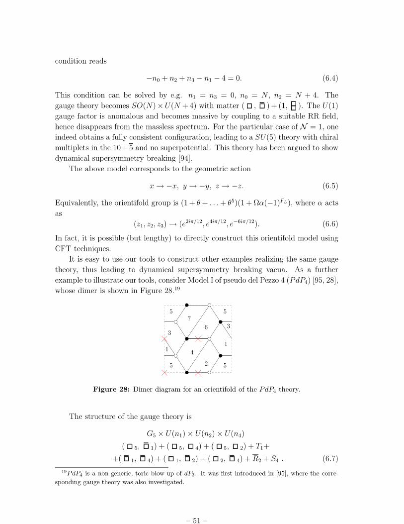
condition reads

−n0 + n2 + n3 − n1 − 4 = 0. (6.4)

This condition can be solved by e.g. n1 = n3 = 0, n0 = N , n2 = N + 4. The

gauge theory becomes SO(N)×U(N + 4) with matter ( , ) + (1, ). The U(1)

gauge factor is anomalous and becomes massive by coupling to a suitable RR field,

hence disappears from the massless spectrum. For the particular case of N = 1, one

indeed obtains a fully consistent configuration, leading to a SU(5) theory with chiral

multiplets in the 10+5 and no superpotential. This theory has been argued to show

dynamical supersymmetry breaking [94].

The above model corresponds to the geometric action

x → −x, y → −y, z → −z. (6.5)

Equivalently, the orientifold group is (1 + θ + . . . + θ5)(1 + Ωα(−1)FL), where α acts

as

(z1, z2, z3) → (e2iπ/12, e4iπ/12, e−6iπ/12). (6.6)

In fact, it is possible (but lengthy) to directly construct this orientifold model using

CFT techniques.

It is easy to use our tools to construct other examples realizing the same gauge

theory, thus leading to dynamical supersymmetry breaking vacua. As a further

example to illustrate our tools, consider Model I of pseudo del Pezzo 4 (PdP4) [95, 28],

whose dimer is shown in Figure 28.19

11

2

33

4

5 5

5 5

6

7

Figure 28: Dimer diagram for an orientifold of the PdP4 theory.

The structure of the gauge theory is

G5 × U(n1) × U(n2) × U(n4)

( 5, 1) + ( 5, 4) + ( 5, 2) + T1+

+( 1, 4) + ( 1, 2) + ( 2, 4) + R2 + S4 . (6.7)

19PdP4 is a non-generic, toric blow-up of dP3. It was first introduced in [95], where the corre-

sponding gauge theory was also investigated.

– 51 –

The signs of the orientifold points determine the orientifold projections on the gauge

factor G5 and the two-index tensor representations T1, R2 and S4, respectively. The

dimer diagram contains 8 superpotential couplings, hence the sign parity is even.

For the choice of signs (+−+−), we have G5 = SO(n5), T1 = 1, R2 = 2 and

S4 = 4. The tadpole/anomaly cancellation conditions for the theory are simply

n5 − n1 − n2 + n4 + 4 = 0, (6.8)

which we can satisfy by taking n2 = n4 = 0, n5 = N , n1 = N + 4. The resulting

theory is SO(N) × U(N + 4) with matter ( , ) + (1, ). Thus for N = 1 it

reproduces the dynamical supersymmetry breaking theory of interest.

Note that there have been several proposals of orientifold models in the literature

which claim to realize the above SU(5) gauge theory [96, 97]. Although insightful in

suggesting orientifold models to reproduce dynamical supersymmetry breaking, the

proposals show technical problems in the specific models presented, as one can show

using our new tools.

The model in [96] is based on an orientifold of C3/(Z3 × Z3) corresponding to

a dimer with fixed lines. The orientifold projection on gauge factors and two-index

tensors in the reference is not compatible with the existence of a single orientifold

fixed line for this model.20

The orientifold model proposed in [97] is based on C3/Z′

6 with an orientifold

action (z1, z2, z3) → (z1, z2,−z3). This corresponds to the action

x → x, y → y, z → z, (6.9)

and can be described with the dimer diagram with fixed points given above. The

corresponding sign setup leading to this geometric action is (+ + ++) or (−−−−).

Thus, the resulting spectra do not agree with the theory of interest since there is no

model with orthogonal gauge factor and matter in two-index antisymmetric tensor

representations.

Since these models are based on orbifolds, we have also double-checked our results

by direct computations using CFT techniques.

It is remarkable that our new tools facilitate the construction of orientifolds in

a simple and systematic way. We expect them to be extremely useful in the study

of infrared dynamics of systems of D-branes at orientifold singularities.

It is almost suggestive that one can find whole families of orientifold models

yielding dynamical supersymmetry breaking. We leave a detailed investigation and

classification of these models for future work.

20Note that other models in this reference, for instance the 3-2 model realized on dP5 are non-toric

and we cannot use our tools to check their consistency.

– 52 –

6.2 D-brane instantons

In Type II compactification, many important non-perturbative effects arise from Eu-

clidean D-brane instantons. In configurations with 4d spacetime filling D-branes

leading to a gauge sector, such D-brane instanton can induce superpotentials corre-

sponding to non-trivial field theory operators. This can correspond to a field the-

ory instanton effect (when the structure of the Euclidean D-brane instanton in the

Calabi-Yau geometry is the same as that of one of the 4d spacetime filling branes), see

[98, 99, 100, 101] for recent discussions, or to a D-brane instanton without such field

theory interpretation (stringy D-brane instantons), see [102, 103, 99, 104, 105, 106]

for recent discussions. Focusing in the latter case, the D-brane instanton typically

has fermion zero modes αa, βb transforming in the a, b under the 4d gauge

factors a, b. If there is a coupling αaOabβb where Oab is a 4d chiral operator in the

( a, b), integration over the fermion zero modes leads to insertions of O in the

superpotential [107].

As discussed in general in [106] and in particular cases in [108, 101, 105], stringy

D-brane instantons in perturbative Type II compactifications without fluxes gener-

ically have four uncharged fermion zero modes, and cannot generate superpotential

couplings. In the presence of orientifold planes, the orientifold projection on instan-

tons with O(1) world-volume gauge group removes two fermion zero modes, thus

allowing the possibility of non-perturbative superpotentials.

This observations make orientifolds of D-branes at singularities a natural setup

to study this non-perturbative effects. In fact, some concrete examples have already

appeared in [93, 105]. It is clear that the techniques developed in this paper provide

many additional examples of D-brane instantons in this kind of systems. Namely,

one can consider D-brane instantons with the internal structure corresponding to

one of the faces of the dimer diagram (and on top of an O−-plane to have O(1)

symmetry).21 This instanton is stringy if there are no 4d spacefilling branes for the

corresponding face. Edges between the instanton face and faces of 4d spacefilling

branes correspond to instanton fermion zero modes, and nodes correspond to their

interactions. Thus one easily obtains the structure of the induced superpotentials.

In Figure 29 we show several examples of stringy D-brane instantons (shown as

shaded faces) generating non-perturbative superpotentials. Figure 29a shows a D-

brane instanton in the orientifold of C3/(Z2×Z2) studied in [105]. The magenta faces

correspond to 4d spacefilling D-branes, while the green face corresponds to a D-brane

instanton. Notice the fermion zero modes of the latter α31, β23 (and their orientifold

images) arising from edges between magenta and green faces, and their cubic coupling

αΦ12β to the 4d chiral multiplet Φ12. Figure 29b shows a D-brane instanton in the

orientifold of the Laba geometry considered in [93]. Notice the fermion zero modes

21Note the sign flip in the orientifold action on the gauge group of D-brane instantons as compared

with 4d spacefilling D-branes.

– 53 –

α54, β45, and the coupling αX43X34β.

replacemen

a) b)

1

1

1

2

2

2

2

2

2

33

4

4

5

6

6

7

8

8

9

Figure 29: D-brane instantons in systems of D-branes at orientifolded singular geometries.

Figure a) shows an instanton (filling the green face) in an orientifold of C3/(Z2×Z2). Figure

b) shows an instanton in an orientifold of a generalized conifold.

It is straightforward to use our techniques to obtain many other examples of

stringy D-brane instantons generating superpotentials in systems of D-branes at sin-

gularities with orientifold actions. We leave a more detailed discussion for future

work.

7. Conclusions

We have introduced dimer model techniques that allow an easy determination of the

gauge theory on D-branes over orientifolds of general toric singularities. As in the

unorientifolded case, dimers provide the most comprehensive available classification

of such theories.

The rules have been presented as a heuristic extrapolation of some simple fami-

lies of examples. However, it is important to emphasize that they are automatically

consistent with partial resolution (and its inverse process of un-Higgssing) and there-

fore extend by induction to arbitrary toric singularities. This constitutes a proof of

the rules we have presented.

Under the new light, the pre-existing examples based on worldsheet computations

for orbifolds and theories with T-dual Hanany-Witten setups become trivial.

We explained how to extract the geometric action of the orientifold using mesonic

operators. We also explored in detail the orientifolds from the point of view of the

mirror geometry.

To give a flavor of some possible applications of our ideas, we chose dynamical

supersymmetry breaking and D-brane instantons. We are confident that our tools

will permit a systematic investigation of large families of models and fuel considerable

progress in model building.

– 54 –

We also expect other exciting directions to profit from our work. To name one,

it is natural to expect that they will help extending recent progress in the combina-

torics of quiver gauge theories (counting of chiral BPS gauge invariant operators) to

orientifold theories.

Acknowledgments

We thank R. Argurio, M. Bertolini, M. Buican, I. Garcia-Etxebaria, S. Kachru, J. Mc-

Greevy and M. Wijnholt for useful discussions. S.F. is supported by the DOE under

contract DE-FG02-91ER-40671. D.K. likes to thank D. Lust for support and CERN-

TH for hospitality during part of the project. A.U. thanks Ecole Polytechnique and

SISSA for hospitality during part of this project. The work of J. P. is supported by

the Science Research Center Program of KOSEF through the Center for Quantum

Spacetime (CQUeST) of Sogang University with the grant number R11-2005-021. J.

P. appreciates the hospitality of CERN-TH and of theoretical particle physics group

of University of Pennsylvania during his stay. The work by A.U. has been supported

by CICYT (project FPA-2003-02877), Comunidad de Madrid (project HEPACOS),

the EU networks MRTN-CT-2004-503369, MRTN-CT-2004-005104, and partially by

the European Union Excellence Grant MEXT-CT-2003-509661. D.V. is supported

by the U.S. Department of Energy under cooperative research agreement #DE-FC02-

94ER40818.

A. From quivers to dimers and shivers

The authors of [22] constructed the dimer and shiver of a given toric quiver gauge

theory via a 2- or respectively 3-step procedure. Firstly, they glued the superpotential

terms appropriately together to obtain the periodic quiver, then they graph dualized

the periodic quiver to obtain the dimer and finally performed an untwisting procedure

to arrive at the shiver. In the following, we give a more practical algorithm to obtain

the dimer as well as the shiver, which in principal follows the same steps but without

the need to draw the intermediate graphs. Especially, the given algorithms are more

suitable for a computer implementation. The main ingredient we use are D(imer)-

and respectively S(hiver)-chains. These are chains of bi-fundamental fields which

correspond to fundamental cells of the dimer or respectively of the shiver.22

S-chains

A S-chain is constructed in the following way: Take an arbitrary bi-fundamental field

contained in a monomial of the superpotential as the first field in the S-chain. The

22In fact, the fields need not necessarily be bi-fundamentals. For example, adjoint fields may

occur in the superpotential as well. However, one can interpret such fields as bi-fundamentals of

the same group and hence are sometimes referred to as bi-fundamentals.

– 55 –

next field is the field right of it in the same monomial. If the field is the last one in

the monomial, take the first field of the monomial as the next field. Then jump to

the unique other monomial containing this field.23 Take the right field of it as the

next one in the S-chain and again jump to the unique monomial containing also this

field. Iterate until the chain closes.24

Actually, a S-chain is nothing else than a zigzag path of the corresponding dimer.

In order to see this, let us translate the S-chain defining algorithm into the

language of the periodic quiver: Each monomial of the superpotential corresponds to

a set of nodes of the quiver connected by a closed path of arrows of one orientation

(clockwise or anti-clockwise). Hence, each monomial term can be seen as a closed cell

with an orientation given by the orientation of the arrows. Cells which are formed

by a closed loop of clockwise arrows we assign a positive sign and call them positive

cells, while cells which are formed by anti-clockwise arrows we assign a negative sign

and denote them as negative cells. The periodic quiver is constructed by gluing these

cells together along the edges, i.e. bi-fundamental fields, they have in common. Since

each bi-fundamental field occurs in a toric quiver exactly twice, once in a monomial

with plus, and once in one with minus sign, the gluing gives a totally periodic graph,

there positive and negative cells alternate (the graph dual is the dimer). The fact that

our algorithm only visits two fields of a monomial, one while entering the monomial,

and one to exit to the next monomial, corresponds in the periodic quiver to entering

a cell and leaving it in the next step.25 Leaving a positive cell corresponds to make a

step right while leaving a negative cell corresponds to make a step left. Since always

cells of different sign are glued together, our algorithm actually follows a zigzag path

in the periodic quiver which under graph dualization goes over to a zigzag path in

the dimer.

Recalling the untwisting procedure of [22], we conclude that in order to obtain

the shiver we simply need to glue the S-chains at there common fields appropriately

together.

Further, since an S-chain encircles a puncture in the shiver, it can also be iden-

tified as the difference of two perfect matchings of the corresponding dimer (cf.

[21, 27]).

As an illustrative example of this algorithm, consider the conifold. The super-

23Since the quiver is assumed to be toric, each bi-fundamental can only occur twice and the jump

to the next monomial is uniquely determined.24Since a S-chain encloses a puncture in the mirror Riemannian surface, the number of S-chains

equals the number of punctures and further it can not intersect itself up to multiple windings.25Actually, the meaning of entering and leaving a cell is a bit confusing since an edge always

belongs to two different cells. In fact, we mean by leaving a cell that the next edge followed is in

a different cell, while by entering we understand that the edge followed before belonged to another

cell.

– 56 –

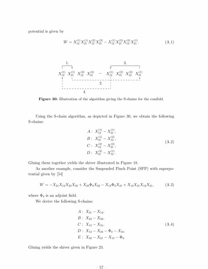
potential is given by

W = X(1)12 X

(1)21 X

(2)12 X

(2)21 − X

(1)12 X

(2)21 X

(2)12 X

(1)21 . (A.1)

X(1)12 X

(1)21 X

(2)12 X

(2)21

− X(1)12 X

(2)21 X

(2)12 X

(1)21

1.

2.

3.

4.

Figure 30: Illustration of the algorithm giving the S-chains for the conifold.

Using the S-chain algorithm, as depicted in Figure 30, we obtain the following

S-chains:

A : X(1)12 − X

(1)21 ,

B : X(1)21 − X

(2)12 ,

C : X(2)12 − X

(2)21 ,

D : X(2)21 − X

(1)12 .

(A.2)

Gluing them together yields the shiver illustrated in Figure 18.

As another example, consider the Suspended Pinch Point (SPP) with superpo-

tential given by [54]

W = −X21X12X23X32 + X23Φ3X32 − X13Φ3X31 + X13X31X12X21, (A.3)

where Φ3 is an adjoint field.

We derive the following S-chains:

A : X21 − X12,

B : X23 − X32,

C : X13 − X31,

D : X12 − X23 − Φ3 − X31,

E : X32 − X21 − X13 − Φ3.

(A.4)

Gluing yields the shiver given in Figure 23.

– 57 –

D-chains

A D-chain is defined as follows: Take an arbitrary bi-fundamental field in a monomial

of the superpotential as the first field in the D-chain. The next field is the field right

of it in the same monomial. If the field is the last one in the monomial, take the first

field of the monomial as the next field. Then jump to the unique other monomial

containing this field. Take the field left of it as the next field. If the field is the first

one in the monomial, take the last field of the monomial as the next field. Jump to

the other monomial containing this field and iterate until the chain closes.26

A D-chain encloses a face of the dimer.

Again, this can be most easily seen in the language of the periodic quiver. In

contrast to the S-chain algorithm, we change the orientation we follow once we enter

a new cell, since the algorithm alternates between taking the left or right one as

the next field. Hence, we simply collect the edges conneted to a single vertex in a

clockwise or anti-clockwise fashion. Thus, under graph dualization the D-chain goes

over to a fundamental cell of the dimer. Obviously, the number of D-chains equal

the number of gauge groups.

The untwisting procedure then shows that the D-chain corresponds to a zigzag

path in the shiver.

Note that the orientation of the zigzag paths is neither fixed in the dimer nor

in the shiver. Both algorithms work fine as well if one exchanges left and right.

This is as expected, since the orientation of zigzag paths in a bipartite graph is pure

convention.

There is one potentially source of failure in both algorithms one must be aware

of. Namely, it is crucial that the fields in the monomials of the superpotential are in

correct order. This is clear since the fields are in general matrices which can not be

permuted freely. Note that this is something not always being taken care of in the

superpotentials which can be found in the literature.

As an example for this algorithm, the D-chain algorithm applied to the super-

potential of the conifold is depicted in Figure 31. We obtain the following D-chains:

1 : X(1)21 − X

(2)12 − X

(2)21 − X

(1)12 ,

2 : X(1)12 − X

(1)21 − X

(2)12 − X

(2)21 .

(A.5)

Gluing them together yields the well known dimer illustrated in Figure 1.

As another example, let us apply the D-chain algorithm to the SPP:

We obtain the following D-chains:

1 : X21 − X12 − X31 − X13,

2 : X12 − X23 − X32 − X21,

3 : X23 − X32 − Φ3 − X31 − X13 − Φ3.

(A.6)

26Care must be taken, since the D-chain may also possess self-intersections.

– 58 –

X(1)12 X

(1)21 X

(2)12 X

(2)21

− X(1)12 X

(2)21 X

(2)12 X

(1)21

1.

2.

3.

4.

5.

6.

7.

8.

Figure 31: Illustration of the algorithm defining the D-chains applied to the conifold.

Note that one of the D-chains possesses a self-intersection, implying that the respec-

tive face in the dimer is glued to itself. The corresponding dimer is given in Figure

10.

B. Mnemonics: Orientifolded Harlequin diagrams

The purpose of this Appendix is to introduce yet another practical point of view for

orientifold quotients, namely orientifolded versions of the Harlequin diagrams of the

dimer. We focus on orientifolds with fixed points. The resulting Harlequin diagrams

live on a 2-sphere with punctures.

Let us consider the Z2 symmetry which acts on the dimer torus with four fixed

points. Modding-out by this action gives a sphere with four singular points. The

zigzag paths of the original dimer map to lines on this sphere. There are two possible

types of zigzags in the dimer graph:

• Closed zigzags which avoid the singular points. They map to closed lines on

the sphere with nontrivial homotopy between the four punctures.

• Open zigzags that pass through singular points. They occur when the orien-

tifold is lying on top of a bi-fundamental edge in the dimer diagram. In the

vicinity of the orientifold point a local complex z coordinate can be chosen for

which the Z2 action is z 7→ −z. Modding-out this action eliminates half of the

zigzag that passes through the origin. As a result such zigzags become open

lines stretched between two singular points on the sphere.

Let us apply these ideas to some concrete models. First, consider the simple

example of C3. Figure 32 shows the three steps from the tiling to the sphere Harlequin

diagram. C3 has three zigzags, represented in blue, green and yellow lines. All of

– 59 –

*

*

*

*1

1

1

1

* *

***

**

*

(i) (ii) (iii)

Figure 32: (i) C3 tiling with zigzags. (ii) Orientifold tiling of the sphere. (iii) C

3 orientifold

Harlequin diagram. The three open zigzags create a single loop.

them cross orientifold points, therefore they become open zigzags. Modding-out the

involution gives (ii), with the three zigzags ending on three singular loci. The tiling

here is drawn with a grey vertex to indicate that black and white nodes were mapped

to one another. One can consider this graph as a “tiling” of the sphere by one face

which contains the fourth orientifold point. The Harlequin diagram can be drawn on

a plane, which gives (iii). The grey triangle corresponds to the superpotential term

in the orientifolded theory. The three lines are the open zigzags. The (infinite) white

face corresponds to the gauge group. In this case, the group is SO/Sp depending on

the charge of the fixed point in it.

In general, the orientifolded Harlequin diagram will contain open and closed

zigzags. Since zigzags come in pairs for every fixed point, we are left with a set

of closed loops after combining them. Whenever an open zigzag crosses a singular

point it changes color (this is for instance the case in Figure 32, where the loop

touches three orientifold points). After drawing the zigzag lines, we can shade every

other face. The shaded faces correspond to superpotential terms. The remaining

white faces are the gauge groups. Whenever there is a fixed point in the middle of

a white face, the corresponding gauge group is SO/Sp, depending on the charge.

Bifundamentals arise from intersections of lines. (Anti)symmetric fields are present

whenever two zigzags touch at a singular point. Henceforth we follow the convention

that the infinite face is white. One can always draw the diagram in this way. The sign

parity of the configuration is simple equal to the number of shaded faces modulo two

(this is in agreement with the sign rule of §3.1.1, which states that the sign parity is

equal to the parity of half the number of superpotential terms in the parent theory).

Anomaly cancellation can be ensured by adding extra chiral multiplets if necessary.

We conclude by listing the orientifolded Harlequin diagrams for the examples in

§3.2.3.

– 60 –

**

* *

Figure 33: The conifold. The (infinite) white face contains no orientifold, and thus it

corresponds to a U(N) gauge group. The intersections of the four open zigzags give four

(anti)symmetric fields as listed in Table 2.

***

*

**

*

*

(i) (ii)

Figure 34: (i)-(ii) Two different orientifolds of C2/Z2 × C. They correspond to Figure 5

and Figure 6, respectively.

*

*

*

*

Figure 35: C3/Z3. There are two white faces and one of them contains an orientifold.

Thus, the gauge group is SO/Sp × U . The matter content can also be read off from the

diagram: three bi-fundamentals from the intersections and three (anti)symmetric fields

from the orientifolds as in Table 5.

**

* *

*

*

**

Figure 36: Left: The Suspended Pinch Point theory. We simply add one more loop to the

C3 diagram. Right: The L1,5,2 Harlequin diagram. There is a single loop which intersects

itself six times and crosses the four orientifold points.

– 61 –

C. Laba theories

In this Appendix, we consider the generically singular Laba spaces.27 These are in the

Labc family for which explicit metrics are known [109, 110]. Probing a real cone over

Laba spaces with D3-branes gives interesting gauge theories [35, 20, 23]. The T-dual

theory is an elliptic model, i.e. Type IIA N = 1 Hanany-Witten setup [16] which

contains a NS5-branes with world-volume along 012345 and b NS5’-branes along

012389. D4-branes (along 01236) are suspended between the five-branes. There

are 2× (a + b) bi-fundamental fields. There are also adjoints whenever two adjacent

fivebranes are parallel. We have referred to these Type IIA constructions extensively.

In this appendix we explain how they can be translated into harlequin and shiver

diagrams, which can then be orientifolded following the rules we have presented in

the paper.

Figure 37 shows two simple examples.

NS’

NS’

NS

NS’

NS’

NSNS

45

89 6

(i) (ii)

Figure 37: (i) L1,2,1 = the Suspended Pinch Point. (ii) L2,2,2 = conifold/Z2.

Since we have been discussing orientifolds from the dimer point of view, the

question immediately arises: can this Type IIA picture be easily translated to the

language of brane tilings? The answer is yes. In order to show this, we work with

Harlequin diagrams (of the dimer). The simple rules for constructing the diagrams

are the following:

• Start with an empty box for the fundamental cell of the tiling torus. In the

following, we heuristically identify the horizontal circular direction with x6 of

the elliptic models.

• Draw a horizontal line. We choose the convention that it is directed to the left.

• Draw vertical lines for the NS5-branes. The direction should be upward for NS

and downward for NS′ branes.

• Draw another horizontal line going to the right. It should go around the non-

trivial vertical torus cycle whenever two adjacent five-branes are parallel.

27a and b are positive integers with a ≤ b.

– 62 –

To illustrate our ideas, this is demonstrated for the SPP in Figure 38. The

resulting tiling can be seen in Figure 39.

6x NS NS’ NS’

Figure 38: Constructing the Harlequin diagram (of the dimer) of SPP. (i) First step: a

horizontal blue line. (ii) Second step: adding NS and NS′ branes. (iii) Last step: another

“horizontal” green line which wraps the vertical cycle between two identical NS′-branes.

Figure 39: The Harlequin diagram and the tiling of SPP.

Elliptic models can be orientifolded by including O6-planes. The Z2 symmetry

acts on the x6 direction and reduces it to an interval with two orientifold planes at the

ends. Several orientifolds from this class were constructed in [56, 57, 58, 59]. There

are two fixed points on the x6 circle, which determine the horizontal coordinates of

the fixed points in the dimer diagram. As an example, we take the orientifold of SPP

in Figure 40. This has been discussed in detail in [59] (see Figure 3 there). The four

fixed points in the tiling are presented in Figure 40. We immediately see that a and

b are related to the O6-plane passing through the NS-brane in Figure 40. Similarly,

c and d correspond to the O6 between the two NS′-branes.

Intuitively, the fork configuration corresponds to the case when we set opposite

charges for those orientifolds in the tiling which then become the same O6 in the

Type IIA picture after T-duality (i. e. they are at the same horizontal position).

Finally, we briefly describe an alternative perspective on these theories, given

shivers in the mirror. The toric diagram contains no internal points, and thus the

– 63 –

NS’

NS’

NS

O6

O6

NS NS’ NS’

*b

c

d

a**

*

Figure 40: Left: Orientifolding SPP. Right: Four fixed points in the Harlequin diagram.

Riemman surface Σ0 of the mirror is a sphere. The azimuthal angle of this sphere

can be identified with x6.

The shiver is an even sided polygon with double lines. It looks like a ring with

“bubbles” (see Figure 41). There is one bubble for each NS and NS′ brane. The

parity of the position of the bubble on the polygon distinguishes between the two

fivebranes. The conifold shiver (Figure 18) consists of two bubbles. On the other

hand, the SPP shiver (Figure 23) has three bubbles and an empty place. Seiberg

duality moves the bubbles around while keeping the number of each type fixed. This

nicely matches the Type IIA picture where the NS5-branes are moving.

Orientifolding the shiver is relatively straightforward: the orientifold line cuts the

ring into two identical pieces. This can only be achieved if the bubbles are arranged

via Seiberg duality in a symmetric fashion. We leave the details to the interested

reader.

6x

NS

NS

NS’

NS’

NS’

NS’

emptyempty

empty

empty

Figure 41: Shiver for a generic Laba. The diagram contains a + b “bubbles”.

– 64 –

References

[1] I. R. Klebanov and E. Witten, “Superconformal field theory on threebranes at a

Calabi-Yau singularity,” Nucl. Phys. B 536 (1998) 199 [arXiv:hep-th/9807080].

[2] D. R. Morrison and M. R. Plesser, “Non-spherical horizons. I,” Adv. Theor. Math.

Phys. 3, 1 (1999) [arXiv:hep-th/9810201].

[3] J. P. Gauntlett, D. Martelli, J. Sparks and D. Waldram, “Sasaki-Einstein metrics

on S(2) x S(3),” Adv. Theor. Math. Phys. 8, 711 (2004) [arXiv:hep-th/0403002].

[4] J. P. Gauntlett, D. Martelli, J. F. Sparks and D. Waldram, “A new infinite class of

Sasaki-Einstein manifolds,” Adv. Theor. Math. Phys. 8, 987 (2006)

[arXiv:hep-th/0403038].

[5] J. P. Gauntlett, D. Martelli, J. Sparks and D. Waldram, “Supersymmetric AdS

backgrounds in string and M-theory,” arXiv:hep-th/0411194.

[6] D. Martelli and J. Sparks, “Toric geometry, Sasaki-Einstein manifolds and a new

infinite class of AdS/CFT duals,” Commun. Math. Phys. 262, 51 (2006)

[arXiv:hep-th/0411238].

[7] S. Benvenuti, S. Franco, A. Hanany, D. Martelli and J. Sparks, “An infinite family

of superconformal quiver gauge theories with Sasaki-Einstein duals,” JHEP 0506,

064 (2005) [arXiv:hep-th/0411264].

[8] I. R. Klebanov and M. J. Strassler, “Supergravity and a confining gauge theory:

Duality cascades and χSB-resolution of naked singularities,” JHEP 0008, 052

(2000) [arXiv:hep-th/0007191].

[9] S. Franco, A. Hanany and A. M. Uranga, “Multi-flux warped throats and cascading

gauge theories,” JHEP 0509, 028 (2005) [arXiv:hep-th/0502113].

[10] D. Berenstein, C. P. Herzog, P. Ouyang and S. Pinansky, “Supersymmetry breaking

from a Calabi-Yau singularity,” JHEP 0509, 084 (2005) [arXiv:hep-th/0505029].

[11] S. Franco, A. Hanany, F. Saad and A. M. Uranga, “Fractional branes and dynamical

supersymmetry breaking,” JHEP 0601, 011 (2006) [arXiv:hep-th/0505040].

[12] M. Bertolini, F. Bigazzi and A. L. Cotrone, “Supersymmetry breaking at the end of

a cascade of Seiberg dualities,” Phys. Rev. D 72, 061902 (2005)

[arXiv:hep-th/0505055].

[13] G. Aldazabal, L. E. Ibanez, F. Quevedo and A. M. Uranga, “D-branes at

singularities: A bottom-up approach to the string embedding of the standard

model,” JHEP 0008, 002 (2000) [arXiv:hep-th/0005067].

[14] D. Berenstein, V. Jejjala and R. G. Leigh, “The standard model on a D-brane,”

Phys. Rev. Lett. 88, 071602 (2002) [arXiv:hep-ph/0105042].

– 65 –

[15] H. Verlinde and M. Wijnholt, “Building the standard model on a D3-brane,” JHEP

0701, 106 (2007) [arXiv:hep-th/0508089].

[16] A. Hanany and E. Witten, “Type IIB superstrings, BPS monopoles, and

three-dimensional gauge dynamics,” Nucl. Phys. B 492, 152 (1997)

[arXiv:hep-th/9611230].

[17] A. Hanany and K. D. Kennaway, “Dimer models and toric diagrams,”

arXiv:hep-th/0503149.

[18] S. Franco, A. Hanany, K. D. Kennaway, D. Vegh and B. Wecht, “Brane dimers and

quiver gauge theories,” JHEP 0601 (2006) 096 [arXiv:hep-th/0504110].

[19] K. D. Kennaway, “Brane Tilings,” arXiv:0706.1660 [hep-th].

[20] S. Franco, A. Hanany, D. Martelli, J. Sparks, D. Vegh and B. Wecht, “Gauge

theories from toric geometry and brane tilings,” JHEP 0601, 128 (2006)

[arXiv:hep-th/0505211].

[21] A. Hanany and D. Vegh, “Quivers, tilings, branes and rhombi,”

arXiv:hep-th/0511063.

[22] B. Feng, Y. H. He, K. D. Kennaway and C. Vafa, “Dimer models from mirror

symmetry and quivering amoebae,” arXiv:hep-th/0511287.

[23] A. Butti, D. Forcella and A. Zaffaroni, “The dual superconformal theory for

L(p,q,r) manifolds,” JHEP 0509, 018 (2005) [arXiv:hep-th/0505220].

[24] A. Butti and A. Zaffaroni, “R-charges from toric diagrams and the equivalence of

a-maximization and Z-minimization,” JHEP 0511, 019 (2005)

[arXiv:hep-th/0506232].

[25] S. Franco and D. Vegh, “Moduli spaces of gauge theories from dimer models: Proof

of the correspondence,” JHEP 0611, 054 (2006) [arXiv:hep-th/0601063].

[26] A. Hanany, C. P. Herzog and D. Vegh, “Brane tilings and exceptional collections,”

JHEP 0607, 001 (2006) [arXiv:hep-th/0602041].

[27] I. Garcia-Etxebarria, F. Saad and A. M. Uranga, “Quiver gauge theories at resolved

and deformed singularities using dimers,” JHEP 0606 (2006) 055

[arXiv:hep-th/0603108].

[28] A. Butti, “Deformations of toric singularities and fractional branes,” JHEP 0610,

080 (2006) [arXiv:hep-th/0603253].

[29] A. Butti, D. Forcella and A. Zaffaroni, “Deformations of conformal theories and

non-toric quiver gauge theories,” JHEP 0702, 081 (2007) [arXiv:hep-th/0607147].

– 66 –

[30] Y. Imamura, H. Isono, K. Kimura and M. Yamazaki, “Exactly marginal

deformations of quiver gauge theories as seen from brane tilings,”

[arXiv:hep-th/0702049].

[31] R. Kenyon, “An introduction to the dimer model,” arXiv:math/0310326 [math.CO]

[32] R. Kenyon, A. Okounkov and S. Sheffield, “Dimers and Amoebae,”

[arXiv:math-ph/0311005].

[33] M. R. Douglas and G. W. Moore, “D-branes, Quivers, and ALE Instantons,”

[arXiv:hep-th/9603167].

[34] M. R. Douglas, B. R. Greene and D. R. Morrison, “Orbifold resolution by

D-branes,” Nucl. Phys. B 506, 84 (1997) [arXiv:hep-th/9704151].

[35] S. Benvenuti and M. Kruczenski, “From Sasaki-Einstein spaces to quivers via BPS

geodesics: L(p,q|r),” JHEP 0604, 033 (2006) [arXiv:hep-th/0505206].

[36] S. Benvenuti and M. Kruczenski, “Semiclassical strings in Sasaki-Einstein manifolds

and long operators in N = 1 gauge theories,” JHEP 0610, 051 (2006)

[arXiv:hep-th/0505046].

[37] S. Benvenuti, B. Feng, A. Hanany and Y. H. He, “Counting BPS operators in gauge

theories: Quivers, syzygies and plethystics,” [arXiv:hep-th/0608050].

[38] B. Feng, A. Hanany and Y. H. He, “Counting gauge invariants: The plethystic

program,” JHEP 0703, 090 (2007) [arXiv:hep-th/0701063].

[39] G. Pradisi and A. Sagnotti, “Open String Orbifolds,” Phys. Lett. B 216, 59 (1989).

[40] G. Pradisi and A. Sagnotti, “Orbifolds and Open Strings,”

[41] C. Angelantonj, M. Bianchi, G. Pradisi, A. Sagnotti and Y. S. Stanev, “Chiral

asymmetry in four-dimensional open- string vacua,” Phys. Lett. B 385, 96 (1996)

[arXiv:hep-th/9606169].

[42] E. G. Gimon and J. Polchinski, “Consistency Conditions for Orientifolds and

D-Manifolds,” Phys. Rev. D 54, 1667 (1996) [arXiv:hep-th/9601038].

[43] A. Dabholkar and J. Park, “An Orientifold of Type IIB Theory on K3,” Nucl.

Phys. B 472, 207 (1996) [arXiv:hep-th/9602030].

[44] E. G. Gimon and C. V. Johnson, “K3 Orientifolds,” Nucl. Phys. B 477, 715 (1996)

[arXiv:hep-th/9604129].

[45] G. Aldazabal, A. Font, L. E. Ibanez and G. Violero, “D = 4, N = 1, Type IIB

orientifolds,” Nucl. Phys. B 536, 29 (1998) [arXiv:hep-th/9804026].

[46] L. E. Ibanez, R. Rabadan and A. M. Uranga, “Anomalous U(1)’s in Type I and

Type IIB D = 4, N = 1 string vacua,” Nucl. Phys. B 542, 112 (1999)

[arXiv:hep-th/9808139].

– 67 –

[47] I. Brunner, A. Hanany, A. Karch and D. Lust, “Brane dynamics and chiral

non-chiral transitions,” Nucl. Phys. B 528, 197 (1998) [arXiv:hep-th/9801017].

[48] J. Erlich, A. Hanany and A. Naqvi, “Marginal deformations from branes,” JHEP

9903, 008 (1999) [arXiv:hep-th/9902118].

[49] A. Hanany and A. Zaffaroni, “Issues on orientifolds: On the brane construction of

gauge theories with SO(2n) global symmetry,” JHEP 9907, 009 (1999)

[arXiv:hep-th/9903242].

[50] B. Feng, A. Hanany and Y. H. He, “The Z(k) x D(k’) brane box model,” JHEP

9909, 011 (1999) [arXiv:hep-th/9906031].

[51] B. Feng, A. Hanany and Y. H. He, “Z-D brane box models and non-chiral dihedral

quivers,” arXiv:hep-th/9909125.

[52] J. Park, R. Rabadan and A. M. Uranga, “Orientifolding the conifold,” Nucl. Phys.

B 570 (2000) 38 [arXiv:hep-th/9907086].

[53] A. Hanany and A. Zaffaroni, “Chiral symmetry from type IIA branes,” Nucl. Phys.

B 509 (1998) 145 [arXiv:hep-th/9706047].

[54] A. M. Uranga, “Brane configurations for branes at conifolds,” JHEP 9901, 022

(1999) [arXiv:hep-th/9811004].

[55] K. Dasgupta and S. Mukhi, “Brane constructions, conifolds and M-theory,” Nucl.

Phys. B 551, 204 (1999) [arXiv:hep-th/9811139].

[56] K. Landsteiner, E. Lopez and D. A. Lowe, “N = 2 supersymmetric gauge theories,

branes and orientifolds,” Nucl. Phys. B 507, 197 (1997) [arXiv:hep-th/9705199].

[57] K. Landsteiner and E. Lopez, “New curves from branes,” Nucl. Phys. B 516, 273

(1998) [arXiv:hep-th/9708118].

[58] A. M. Uranga, “Towards mass deformed N = 4 SO(n) and Sp(k) theories from

brane configurations,” Nucl. Phys. B 526, 241 (1998) [arXiv:hep-th/9803054].

[59] J. Park, R. Rabadan and A. M. Uranga, “N = 1 Type IIA brane configurations,

chirality and T-duality,” Nucl. Phys. B 570, 3 (2000) [arXiv:hep-th/9907074].

[60] A. Keurentjes, “Classifying orientifolds by flat n-gerbes,” JHEP 0107, 010 (2001)

[arXiv:hep-th/0106267].

[61] A. Hanany, B. Julia, A. Keurentjes, “Non Simply Laced Scalar Manifolds,”

unpublished

[62] R. G. Leigh and M. Rozali, “Brane boxes, anomalies, bending and tadpoles,” Phys.

Rev. D 59, 026004 (1999) [arXiv:hep-th/9807082].

– 68 –

[63] Y. Imamura, “Anomaly cancellations in brane tilings,” JHEP 0606, 011 (2006),

arXiv:hep-th/0605097.

[64] Y. Imamura, “Global symmetries and ’t Hooft anomalies in brane tilings,” JHEP

0612, 041 (2006) [arXiv:hep-th/0609163].

[65] S. Franco and A. M. Uranga, “Dynamical SUSY breaking at meta-stable minima

from D-branes at obstructed geometries,” JHEP 0606 (2006) 031

[arXiv:hep-th/0604136].

[66] J. Park and A. M. Uranga, “A note on superconformal N = 2 theories and

orientifolds,” Nucl. Phys. B 542, 139 (1999) [arXiv:hep-th/9808161].

[67] J. D. Lykken, E. Poppitz and S. P. Trivedi, “Chiral gauge theories from D-branes,”

Phys. Lett. B 416, 286 (1998) [arXiv:hep-th/9708134].

[68] J. D. Lykken, E. Poppitz and S. P. Trivedi, “M(ore) on chiral gauge theories from

D-branes,” Nucl. Phys. B 520, 51 (1998) [arXiv:hep-th/9712193].

[69] A. M. Uranga, “Local models for intersecting brane worlds,” JHEP 0212 (2002)

058 [arXiv:hep-th/0208014].

[70] C. Angelantonj and R. Blumenhagen, “Discrete deformations in type I vacua,”

Phys. Lett. B 473, 86 (2000) [arXiv:hep-th/9911190].

[71] R. Blumenhagen, B. Kors and D. Lust, “Type I strings with F- and B-flux,” JHEP

0102, 030 (2001) [arXiv:hep-th/0012156].

[72] A. M. Uranga, “A new orientifold of C**2/Z(N) and six-dimensional RG fixed

points,” Nucl. Phys. B 577, 73 (2000) [arXiv:hep-th/9910155].

[73] B. Feng, Y. H. He, A. Karch and A. M. Uranga, “Orientifold dual for stuck NS5

branes,” JHEP 0106, 065 (2001) [arXiv:hep-th/0103177].

[74] N. J. Evans, C. V. Johnson and A. D. Shapere, “Orientifolds, branes, and duality of

4D gauge theories,” Nucl. Phys. B 505, 251 (1997) [arXiv:hep-th/9703210].

[75] M. Aganagic, A. Karch, D. Lust and A. Miemiec, “Mirror symmetries for brane

configurations and branes at singularities,” Nucl. Phys. B 569, 277 (2000)

[arXiv:hep-th/9903093].

[76] A. Hanany and A. Iqbal, “Quiver theories from D6-branes via mirror symmetry,”

JHEP 0204, 009 (2002) [arXiv:hep-th/0108137].

[77] B. Feng, A. Hanany, Y. H. He and A. Iqbal, “Quiver theories, soliton spectra and

Picard-Lefschetz transformations,” JHEP 0302 (2003) 056 [arXiv:hep-th/0206152].

[78] K. Hori, A. Iqbal and C. Vafa, “D-branes and mirror symmetry,”

arXiv:hep-th/0005247.

– 69 –

[79] K. Hori and C. Vafa, “Mirror symmetry,” arXiv:hep-th/0002222.

[80] O. Aharony and A. Hanany, “Branes, superpotentials and superconformal fixed

points,” Nucl. Phys. B 504, 239 (1997) [arXiv:hep-th/9704170].

[81] O. Aharony, A. Hanany and B. Kol, “Webs of (p,q) 5-branes, five dimensional field

theories and grid diagrams,” JHEP 9801, 002 (1998) [arXiv:hep-th/9710116].

[82] N. C. Leung and C. Vafa, “Branes and toric geometry,” Adv. Theor. Math. Phys.

2, 91 (1998) [arXiv:hep-th/9711013].

[83] G. Mikhalkin, “Amoebas of algebraic varieties,” arXiv:math.AG/0108225

[84] A. M. Uranga, “Chiral four-dimensional string compactifications with intersecting

D-branes,” Class. Quant. Grav. 20, S373 (2003) [arXiv:hep-th/0301032].

[85] R. Blumenhagen, M. Cvetic, P. Langacker and G. Shiu, “Toward realistic

intersecting D-brane models,” Ann. Rev. Nucl. Part. Sci. 55, 71 (2005)

[arXiv:hep-th/0502005].

[86] R. Blumenhagen, B. Kors, D. Lust and S. Stieberger, “Four-dimensional String

Compactifications with D-Branes, Orientifolds and Fluxes,” arXiv:hep-th/0610327.

[87] F. Marchesano, “Progress in D-brane model building,” arXiv:hep-th/0702094.

[88] F. Cachazo, B. Fiol, K. A. Intriligator, S. Katz and C. Vafa, “A geometric

unification of dualities,” Nucl. Phys. B 628 (2002) 3 [arXiv:hep-th/0110028].

[89] K. Intriligator and N. Seiberg, “The runaway quiver,” JHEP 0602, 031 (2006)

[arXiv:hep-th/0512347].

[90] A. Birini and D. Forcella, “Comments on the non-conformal gauge theories dual to

Y p,q manifolds,” JHEP 0606, 050 (2006) [arXiv:hep-th/0603245].

[91] I. Garcia-Etxebarria, F. Saad and A. M. Uranga, “Supersymmetry breaking

metastable vacua in runaway quiver gauge theories,” arXiv:0704.0166 [hep-th].

[92] R. Argurio, M. Bertolini, S. Franco and S. Kachru, “Gauge/gravity duality and

meta-stable dynamical supersymmetry breaking,” JHEP 0701 (2007) 083

[arXiv:hep-th/0610212].

[93] R. Argurio, M. Bertolini, S. Franco and S. Kachru, “Metastable vacua and

D-branes at the conifold,” arXiv:hep-th/0703236.

[94] I. Affleck, M. Dine and N. Seiberg, “Dynamical Supersymmetry Breaking In

Supersymmetric QCD,” Nucl. Phys. B 241, 493 (1984).

[95] B. Feng, S. Franco, A. Hanany and Y. H. He, “Unhiggsing the del Pezzo,” JHEP

0308, 058 (2003) [arXiv:hep-th/0209228].

– 70 –

[96] M. Wijnholt, “Geometry of particle physics,” arXiv:hep-th/0703047.

[97] Y. E. Antebi and T. Volansky, “Dynamical supersymmetry breaking from simple

quivers,” arXiv:hep-th/0703112.

[98] M. Haack, D. Krefl, D. Lust, A. Van Proeyen and M. Zagermann, “Gaugino

condensates and D-terms from D7-branes,” JHEP 0701 (2007) 078

[arXiv:hep-th/0609211].

[99] B. Florea, S. Kachru, J. McGreevy and N. Saulina, “Stringy instantons and quiver

gauge theories,” arXiv:hep-th/0610003.

[100] N. Akerblom, R. Blumenhagen, D. Lust, E. Plauschinn and

M. Schmidt-Sommerfeld, “Non-perturbative SQCD Superpotentials from String

Instantons,” JHEP 0704 (2007) 076 [arXiv:hep-th/0612132].

[101] M. Bianchi, F. Fucito and J. F. Morales, “D-brane Instantons on the T 6/Z3

orientifold,” arXiv:0704.0784 [hep-th].

[102] R. Blumenhagen, M. Cvetic and T. Weigand, “Spacetime instanton corrections in

4D string vacua - the seesaw mechanism for D-brane models,” Nucl. Phys. B 771

(2007) 113 [arXiv:hep-th/0609191].

[103] L. E. Ibanez and A. M. Uranga, “Neutrino Majorana masses from string theory

instanton effects,” JHEP 0703 (2007) 052 [arXiv:hep-th/0609213].

[104] M. Cvetic, R. Richter and T. Weigand, “Computation of D-brane instanton induced

superpotential couplings: Majorana masses from string theory,”

arXiv:hep-th/0703028.

[105] R. Argurio, M. Bertolini, G. Ferretti, A. Lerda and C. Petersson, “Stringy

Instantons at Orbifold Singularities,” arXiv:0704.0262 [hep-th].

[106] L. E. Ibanez, A. N. Schellekens and A. M. Uranga, “Instanton Induced Neutrino

Majorana Masses in CFT Orientifolds with MSSM-like spectra,” arXiv:0704.1079

[hep-th].

[107] O. J. Ganor, “A note on zeroes of superpotentials in F-theory,” Nucl. Phys. B 499

(1997) 55 [arXiv:hep-th/9612077].

[108] M. Bianchi and E. Kiritsis, “Non-perturbative and Flux superpotentials for Type I

strings on the Z3 orbifold,” arXiv:hep-th/0702015.

[109] M. Cvetic, H. Lu, D. N. Page and C. N. Pope, New Einstein-Sasaki spaces in five

and higher dimensions, arXiv:hep-th/0504225.

[110] D. Martelli and J. Sparks, Toric Sasaki-Einstein metrics on S2 X S3, Phys. Lett. B

621, 208 (2005) [arXiv:hep-th/0505027]

– 71 –