Digital Computer Calculation of Power System Short Circuit

and Load Flow Utilising Diakoptics and Sparsity Techniques

by

W.A. Prebble, B.Sc., B.E.

submitted in fulfilment of

the requirements for the degree of

Master of Engineering

UNIVERSITY OF TASMANIA

HOBART

3 October 1975

The thesis contains no material which has been accepted for

the award of any other degree or diploma in any university,

and that, to the best of my knowledge and belief, the thesis

contains no copy or paraphrase of material previously

published oritten by another person, except when due

reference is made in the text of the thesis.

1

SUMMARY

In part A a non-singular connection matrix is used to combine

the self and mutual impedance matrix of a group of mutually coupled

elements with a network bus impedance matrix; the resulting impedance

matrix is then reduced by eliminating rows and columns if necessary,

to give the bus impedance matrix of the interconnected network. The

self impedances of the mutually coupled group of elements are added

to the network bus impedance matrix in the same way as uncoupled

elements, then the mutual impedances Are added followed by matrix

reduction. By considering examples of the connection matrix 'applied

to adding a single element, then to adding groups of uncoupled and

coupled elements to a network, rules are devised for combining the

celf impedances of branch and loop elements and group mutual imped-

ances with the network bus impedance matrix.

From the bus impedance matrix of power system sequence networks

fault parameters are derived by simple arithmetic operations. It is

shown that rules for adding a group of mutually coupled loop elements

can be applied to modify a bus impedance matrix when element self and

mutual impedances are changed. The derivation of an equivalent network

from the bus impedance matrix is noted; the addition of two network

bus impedance matrixes is considered and shown to be a special case

of the more general problem of adding a self and mutual impedance

matrix to a bus impedance matrix. A numerical example involving the

calculation and modification of the bus impedance matrix, deriving an

equivalent circuit and adding bus impedance matrixes is included.

An outline of a digital computer power system short circuit

programme which calculates fault parameters from the bus impedance

matrix derived from randomly ordered lists of network element self

and mutual impedances is given.

The inverse of the connection matrix discussed in part A is

used in part B to combine a network bus admittance matrix with the

self and mutual admittance matrix of a group of mutually coupled

elements. From this the Well known method of forming the bus admit-

tance matrix from uncoupled element self admittances follows and is

ii

extended to cover self and mutual admittances of coupled elements.

For a group of mutually coupled elements, the diagonal terms of the

group admittance matrix are added to the bus admittance matrix in the

same way as self admittances of uncoupled elements while the off-

diagonal terms are added in a matrix operation either before or after

the diagonal terms. A relationship is indicated between the admit-

tance connection matrix and the group element bus incidence matrix.

Although the presence of mutual coupling results in some loss

of spal-sity, it is shown that for power systems the bus admittance

matrix still has a large proportion of zero terms. By eliminating

terms below the main diagonal in an optimal order, a "factored inverse"

of the admittance matrix is derived which has considerably fewer non-

zero terms than the corresponding bus impedance matrix. Terms of the

Impedance matrix can be obtained from the inverse as required. The

numerical calculation of the bus admittance matrix of a. power system

zero sequence network is set out and derivation of fault impedance

and current distribution factors included.

A digital computer programme using the bus admittance matrix

and factored inverse method for power system short circuit studies is

described and a tabulation indicates the affect on computer storage

requirements of the optimal factoring procedure.

In part C Newton's method of power system load flow calculation

using Gaussian elimination to solve the voltage correction equations

is discussed. The network and problem parameters are specified in

rectangular cartesian co-ordinates. As the voltage correction equation

matrix has the same form as the bus admittance matrix, a preferred

order for the Gaussian elimination which preserves sparsity is devised

by analogy with network reduction.

A digital computer load flow programme is outlined and a tab-

ulation included which shows that, for typical power system networks,

the preferred elimination order retains sparsity in the matrix.

Algol listings of the digital computer short circuit and load

flow programmes are included in the supplement with data and corres-

ponding calculated results for power system studies.

CONTENTS

General Introduction 1

List of Symbols 5

A. The Bus Impedance Matrix for Power System Fault Calculations

A.1. Introduction 7

A.2. Combination of Group Impedance and Bus Impedance Matrixes 9

A.2.1. Current Connection Matrix 11

A.2.2. Voltage Connection Matrix 13

A.2.3. Impedance Matrix of Interconnected Network 14

A.2.4. Rules for Forming Bus Impedance Matrix 16

A.3. Step-by-Step Calculation of Bus Impedance Matrix 17

A.3.1. Single Branch Element 17

A.3.1.1. Group of Branch Elements 20

A.3.2. Single Loop Element 21

A.3.2.1. Group of Loop Elements 24

A.3.3. Group of Branch and Loop Elements 29

A.3.4. Group of Mutually Coupled Elements 31

A.A • Fault Calculations Using the Bus Impedance Matrix 37

A.5. Modification of Bus Impedance Matrix 38

A.6. Derivation of Equivalent Network 39

A.7. Example of Bus Impedance Matrix Calculation 40

A.7.1. Examples of Bus Impedance Matrix Modi -riation 46

A.7.2. EquiValent Network and Partial Network Matrix

Combination 48

A.8. Combination of Network Bus Impedance Matrixes 52

A.9. Digital Computer Short Circuit Programme 54

B. The Bus Admittance Matrix and Power System Fault Caaculations

B.1. Introduction 58

3.2. Connection Matrix Relations 59

3.3. Step-by-Step Calculation of Bus Admittance Matrix 62

B.31. Groups or Mutually Coupled Elements 67

3.4- Example of Bus Admittance Calculation 70

B.5. Derivation of Factored Inverse 72

13.6. Digital Computer Short Circuit Programme 74

13.7. Effectiveness of Sparsity Technique - Example 76

C. Ordered Gaussian Elimination for Power System Load Flow

Cl. Introduction 79

C.2. Derivation of Voltage Correction Equations 80

0.3. Gaussian Elimination Procedure 84

C.4. Optimal Ordering Scheme ""or Elimination 86

C.5. Efect of OptImal Ordering on Power System Matrixes 94

C.6.1. Data Preparation -or Computer Programme 94

C.6.2. Digital Computer Programme 9 7 C.7. Example of Rate of Convergence 100

Conclusion 101

References 103

SUPPLEMENT ^

S.1. The Digital Calculation or Sequence Networks Including Mutual

Impedances. Proc.I.E.E.,Vol.112,April 1965,p.711.

5.2, The Calculation of the Transfer and Driving Point Impedance

Matrix by Digital Computer. Matrix and Tensor Quarterly, Vol.15,

June 1965, p.126,

5.3. Digital Calculation of Short-Circuit Networks. Elect.Engg.Trans.

I.E.Aust., Vol.EE2, No.2, 1966, p.62.

3.4. The Digital Solution of the Load Flow Problem by Elimination.

Elect.Engg.Trans.I.E.Aust., Vol.EE4, No.1, 1968, p.23,

5.5. Discussion on paper by Tinney,W.F. and Hart,C.E. - Power Flow

Solution by Newton's Method. IEEE Trans. on Power Apparatus and

Systems, Vol.PAS-86, Nov. 1967, p.1449.

5.6. Letter from W.F.Tinney of Bonneville Power Administration dated

October 3, 1967.

5.7. Discussion on paper by Freris,L.L. and Sasson,A.M. - Investig-

ation of the Load Flow Problem. Proc.IEE, Vol.1 1 7, 1 9 70, p.397.

S.8. Digital Computer Programme HEI 2a Short Circuit - Algol Listing

and Example or Network Calculation.

3.9. Digital Computer Programme HEI 13 Short Circuit - Algol Listing

and Example or Network Calculation.

3.10. DigitL1 Computer Programme HEI 8g Complex Load Flow - Algol

Listing and Examples of Network Calculations.

1

GENERAL INTRODUCTION

The paper, concerning the digital computer solution of power

system short circuit and load flow problems using a nodal represen-

tation of the revelent network,is divided into three parts. In part A

a method, based on Kron's diakoptics (Ref.]. and 2), of deriving the

nodal or bus impedance matrix from randomly ordered lists of element

self and mutual impedances is discussed. The method which has par-

ticular relevance to the inclusion of mutual coupling between network

elements may be described as a "geometric" approach in contrast to the

algorithms derived by El-Abiad (Ref.23). Subsequent amendments to the

digital computer programme HEI 2, which has been usal since 1964 for

power system short circuit studies, have been to make use of increased

computer storage, removal or the option of excluding element resis-

tance and replacing the procedure for grouping mutual impedances by

a simplified version. Publications relevent to part A are :-

1. Prebble,W.A. - The Digital Calculation of Sequence Networks

Including Mutual Impedances. Proc.I.E.E.,Vol.112,April 1965,

p.711. (Awarded the Institution of Electrical Engineers Overseas

Premium for 1965).

. Prebble,W.A. - The Calculation of the Transfer and Driving Point

Impedance Matrix by Digital Computer. Matrix and Tensor Quar-

terly, Vol.15, June 1965, p.126.

3. Prebble,W.A. - Digital Calculation of Short-Circuit Networks.

Elect.Engg.Trans.I.E.Aust., Vol.EE2, No.2, 1966, p.62.

(Presented at the Institutions Annual Conference, Newcastle,

March 1966).

In part B the formation of the network nodal or bus admittance

matrix (the reciprocal of the bus impedance matrix) including mutual

coupling between network elements is discussed. By applying diakoptics

it is shown that in the formation of the admittance matrix from ran-

domly ordered lists or element self and mutual admittances, processing

of the mutual can he separated from that of the self admittances with

each group or mutual admittances being added at any time during or

after the addition of element self admittances to the matrix. The

reciprocal relationship between the connectionmatrixes used in the

derivation of the bus impedance and admittance matrixes and their

relation to the bus incidence matrix is noted. This method of con-

structing the network bus admittance matrix is used in the digital

computer programme HEI 13 which has been in use since 1968 for power

system short circuit calculations. Sparsity techniques are utilised

in this programme together with triangularisstion of the admittance

matrix, as outlined by Tinney and Walker (Ref.116), to derive one row

at a time of the bus impedance matrix and thus solve problems invol-

ving networks too large 'or the programme HEI 2.

Part C is concerned with the elimination (or Newton's) method

of solving power system load flow problems with particular reference

to exploiting sparsity of the bus admittance matrix. The order for

Gaussian elimination o' the voltage correction equations is derived

from a consideration of network connections, i.e. the "geometry" of

the network, and is suited to the rectangular co-ordinate form in differs

which the equations are written. This procedure/from that of Tinney

et al (Ref.45, 46 and 47) who use polar co-ordinates and matrix tri-

angularisation, but the optimal processing order derived is similar

to Method 2 of Tinney and Hart (Ref.47). The digital computer pro-

gramme HEI 8 at present in use for solving power system load flow

problems by ordered elimination is, with the exception of minor amend-

ments, the same as that first used in 1966. Publications relevent to

part C are :-

1. Prebble,W.A. - The Digital Solution of the Load Flow Problem

by Elimination. Elect.Engg.Trans.I.E.Aust., Vol.7E4, No.1, 19C)8,

p.23. (Presented at the Institution's Power Systems Conference,

Melbourne, August 1967).

2. Prebble,W.A. - Discussion on paper by Tinney,W.F. and Hart,C.E. -

Power Flow Solution by Newton's Method. IEEE Trans. on Power

Apparatus and Systems, Vol.PAS-86, Nov. 1967, p.1449.

3. Prebble,W.A.- Discussion on paper by Freris,L.L. and Essson,A.M.

- Investigation of the Load Flow Problem. Proc.IEE, Vol.117,

Feb. 1970, p.397,

Included in the list of references are books and papers relevant

to the subject matter of parts A, B or C which have been published

subsequent to the developement of the computer programmes HEI 2,

HEI 13 and HEI 8 and the following comments refer to these publications.

3

(a) The book by Stagg and El-Abiad (Ref.5, 1968) has become a sten-

reference for digital computer application to short circuit, load

flow and transient stability problems. It contains en extensive dis-

cussion of network mesh and nodal matrixes including the application

to three phase networks, also the derivation of the bus impedance

matrix from randomly ordered lists of element self and mutual imped-

ances by the algorithms given in previously published works (Ref.23).

The Gauss-Seidel and elimination (Newton's) methods of solving the

load flow problem are considered in detail but the important tech-

niques for preserving matrix sparsity are not discussed. Brameller,

John and Scott (Ref.6, 1969) in their book apply diskoptics to mesh

and nodal analysis of power system networks including assembly of the

bus impedance and admittance matrixes from network element lists but

mutual coupling between elements is not considered.

(b) Tarsi (Ref.28, 1970) and Dy Liacco and Flamers() (Re'.29, 1970)

extend El-Abiad's algorithms for deriving the bus impedance matrix to

include the end-fault case. Storry and Brown (Re".27, 1970) and Daniels

and Chen (Ref.30, 1971) suggest first forming the bus impedance matrix

of element self impedances, then in a separate operation adding the

mutual impedances. In Storry and Brown's method mutual couplings are

dealt with one at a time in a two step process associated with network

reduction, while Daniels and Chen add all mutual impedances in one

operation followed by matrix reduction. The method developed in Part A

for separate processing of self and mutual impedances has advantages

over both of these procedures as the mutual impedances are added dir-

ectly into the appropriate matrix terms and no extra matrix reductions

are necessary.

(c) Although the formation of the bus admittance matrix from lists

of network element self admittances is well known from the load flow

problem (e.g. Ref.36), the inclusion of mutual coupling between net-

gork elements has not been covered in earlier literature. Nagappen

(Ref.32, 1970) develops a step-by-step procedure in which as each

element is added allowance is made for mutual coupliag with Previously

processed elements. This is analogous to El-Abiad's method for for-

ming the bus impedance matrix, but is unnecessarily complicated and,

as shown in Part B, the concept of branch and loop elements has no

relevance when applied to the bus admittance matrix. Anderson, Bowen

A

and Shah (Re 1 .33, 1970) derive simple rules for adding mutual admit-

tances, calculated from the inverse of group mutual impedance matrixes,

directly to the bus admittance matrix thereby avoiding any multipli-

cation with a bus incidence matrix. Tinney (Ref.34, 1972) extends the

use of the factorised inverse formed from the admittance matrix by

showing how to incorporate network modifications, including that of

varying mutual coupling between network elements, without changing

the factorisation.

(d) Many different methods of solving power system load flow prob-

lems have been devised and a large number of papers on this subject

published; Gupts, and Davies (Ref.39, 1961) giving a comprehensive list

of those appearing prior to 1961. Although new procedures are still

being suggested, it is now recognised that the elimination (Newton's)

method method combined with an optimum order of processing the equa-

tions such as that developed in Part C or that of Tinney and Hart

(Ref.A7, 1967) iF the best way of solving power system load flow pro-

1 ems.

Vk Ik

ek fk

ak bk

Ied

ca l Icb A 1

A l

zeqivi

1 Zdiag i

5

LIST OF SYMBOLS

= denotes a matrix.

[Zil] = network nodal or bus impedance matrix.

pe:• = network nodal or bus admittance matrix.

Zlj yij = term i-j of El = real, imaginary components of IT

Glj Bij = term i-j of 1-61,11.

Nid [Nd= group impedance, admittance matrix.

e z zml = self, mutual impedance component of lz

qP l

= resistive, reactive components of

= equivalent self, mutual admittance components of [y cip

= impedance, admittance matrix of partial network combined

with group self impedances, admittances.

[Z1 = impedance, admittance matrix of partial network combined

• with group self and mutual impedances, admittances.

VA = nodal voltage matrix.

= nodal current matrix.

= nodal voltage, current matrix for partial network.

1r x s

Ye ii z'

I ' 1

Iz e I

= nodal voltage, current at node "k".

= real, imaginary components of Vic ,

= real, imaginary components of Ik.

= current in element e-d (e>d).

= nodal power matrix.

= nodal power at node "k".

= real, reactive components of FE]. = real, reactive components of Sk .

= specified power and components at node "k".

= specified voltage magnitude at node "k".

= sub-matrixes of the impedance connection matrix.

= sub-matrixes of the admittance connection matrix.

= matrix formed by discarding columns of Ab

= bus incidence matrix.

= bus impedance matrix of equivalent network.

= bus admittance matrix of equivalent network.

= lower diagonal matrix of Z" I corresponding to group

elements,

a

IV -V q Pi

6

factor = factored inverse form of Ei derived from Y

ci

= voltage correction equation matrix.

F-1 sub-matrixes of

Uti Hii

W. T = term i-j of the sub-matrixes of

= subscript denoting matrix transpose.

= superscript denoting complex conjugate.

= denotes incremental value.

= denotes summation.

= denotes modulus of a complex quantity.

= matrix of currents in group elements (q>0.

= matrix of voltages applied to group elements.

7

A. THE BUS IMPEDANCE MATRIX FOR POWER SYSTEM FAULT CALCULATIONS

Al. INTRODUCTION

Before the advent of the digital computer, short circuit cal-

culations on small power system networks were done by hand using

familiar network reduction techniques and neglecting element resis-

tance. Disadvantages of this method are :-

(a) separate network reductions are required for each fault;

(b) inclusion of resistance and mutual coupling between elements

makes the calculatin too laborious for any but the simplest networks;

(c) derivation of element fault currents and node voltages involves

"beck-tracking" through the network reduction. These disadvantages

were overcome by representing the network on a plugging board which

allowed simulation of faults at all nodes.

Early digital computer methods (Ref.3) used a loop or mesh rep-

resentation of the network (Ref.18-21) which requires matrix inversion

or, alternatively iterative procedures were used (Ref.14-17). However,

it was recognised that the nodal or bus impedance matrix provided the

best approach (Ref.3) as all fault calculations can be done by simple

arithmetic operations on the matrix terms thus avoiding inversion or

iterative procedures and network coding is simpler than for the mesh

approach. Brown and Person (Ref.24) have shown that the bus impedance

matrix can be formed automatically from randomly ordered element im-

pedance lists and this has been extended to include mutual coupling

between elements by El-Abiad (Ref.23). The method of including mutual

coupling involves inverting matrixes and applying corrections to the matrix

impedance/row and column corresponding to the coupled element to allow

for its direct and indirect coupling to network elements already in-

cluded in the matrix.

By processing all elements directly and indirectly coupled to-

gether, it is shown that mutual impedances can be added into the im-

pedance matrix, thus avoiding matrix inversion and calculating term

corrections. The self impedances of the coupled elements are added,

applying the rules for processing uncoupled elements, to the impedance

matrix followed by the addition of the group mutual impedances. The

rules are extended to the modification of a given bus impedance matrix

when network element self and mutual impedances are changed. It is

8

shown that an equivalent circuit for a given network can be derived

from the network bus impedance matrix and also, that adding the bus

impedance matrix of one network to that of a second network (forming

the bus impedance matrix of the combined network) is a special case

of adding the self end mutual impedance matrix of a group of mutually

coupled elements to the bus impedance matrix of a partial network.

A digital computer programme for calculating the bus impedance

matrix of sequence networks by this method is outlined.

where . VA a FITA1 are column matrixes of the n node voltages and Iii • • • •

• (1 )

z o.P the rra ,am

9

A.2. COMBINATION 07 GROUP IMPEDANCE AND BUS IMPEDANCE MATRIXES.

Fig. 1

Fig. 1(a) repreeents a network with n+1 nodes, one of which ' to

is chosen_as reference or base nso whiph the voltages V at the other

n nodes are referred. The relatibn between these n voltages and the

corresponding: n currents I nal:awing into the network at the nodes

is given by the equation written in matrix notation ;-

(a)

currents and ZA is the square nn transfer and driving point

impedance matrix of the network. In the follOwing it is shown how

, which, for simplicity is referred to as the bus impedance

matrix, is built up in .a step by step procedure from lists of self

and mutual impedances of the network elements.

Fig. 1(b) represents a group of m lines or elements, at

this stage not physically connected, between any pair of which there

may be mutual coupling. For this group the matrix equation

V -V P Zqp

holds where V -V q P

and. i qp i across and m currents flowing in each element, and

are column matrixes of the m voltages

matrix with. the self. impedances KNXXXXPXXXXXXINIXIM of the elements

as diagonal terms and the mutual impedances between the elements as

the 'off-diagonal terms. Vq, VP are the voltages, referred to a common

reference, at the nodes of the element q-p and Iqp is the current

in this element assuming the positive direction of flow from q to p,

where q is numerically greater than p.

Combining eqns.(1) and (2) into one matrix equation :-

• • (3)

VA

Z

0 zclP

V -V P

The group of elements (b) are connected together and

and connected to the network (a) to form the interconnected network

1 Ca

0 cb

A

Iv

IA

I B • •

1 IA are column matrixes with n+m rows and

where

IA

and

I cip

IS

. (4 )

10

shown in Fig. l(c). The bus impedance matrix of the interconnected

network (c) will be derived from eqn (3).

The group of elements (b) are connected together and to the

network (a) in such a way that the power flowing into the nodes before

and after interconnection is unchanged, i.e. the references for (a)

and (b) are connected together, the node voltages are the same and

the current flowing in each element is the same berore and after

interconnection.

The equations relating the currents before and after

interconnection can be written :-

Ca

is the square connection matrix with n+m rows and columns. 1 Ca

0 Cb

In eqn (4) the connection matrix is sub-divided into four sub -matrixes:

a unit matrix of order n, a zero matrix with m rows and n columns,

with n rows and m columns and Ca square matrix with m rows oi

and columns. The terms of LCA andlCid are +1, -1 or 0. It is shown in

eqns.(183 and 204) that LFbIL C;lare related to the incidence matrix

for the group of lines (b).

The connecting of the elements of (b) to network (a)

forming the interconnected network (c) can be considered as a step-

by-step procedure - firstly element d-e is connected establishing

a new node e in the interconnected network, then elements e-f, k-h

and h-g in that order establishing new nodes f, h and g .respectively

and finally element f-g which connects established nodes f and g. In

eqn. (4) the n terms I IA are the node currents at nodes in (c)

corresponding to nodes in (a) while the m terms II B1 are node currents at new nodes established by the elements (b) and element currents

for elements of (b) which connect established nodes.

In this discussion of eqn. (4) mutual coupling between

the elements (b) has been ignored. It is shown below that the bus

impedance matrix of network (c) is formed from that for network (a)

by firstly processing the self impedances of the elements (b) and

11 then adding in the mutual impedances.

The discussion also shows that in the step-by-step formation

of the bus impedance matrix of the interconnected network (c), an element

of (b) cannot be added unless at least one of its nodes is establiehed

in the network - this node may be the reference node. Thus in the

formation of the interconnected network and its bus impedance matrix

from a partial network and a group of elements or, simply from a group

of elements, two types of element arise :-

(1) a branch element i.e. one which connects a new node to an

established node thus forming a new node in the interconnected

network; and

(2) a loop element i.e. one which connects two established nodes

in the network.

A.2.1. CURRENT CONNECTION MATRIX.

From eqn.(4) the relation between the element currents of

the group of elements (b) and the node and element currents of the

interconnected network (c) is given by :-

cIP = Cb 1.1±31 • • • • • • • . (5)

If in Fig. 1 it is assumed that the group of elements (b) are added to

the network (a) so that the branch elements d-e, e-f, k-h,and h-g form

new nodes e,f,h and g respectively in the inuerconnected network (c)

while loop element g-t connects nodes g and f, also if e>d, f>e, k>h,

h>g and g>f then the terms of eqn.(5) for the branch elements are :-

I ed = I e + I f + Igf • • • • • (6)

I re = I f + Igf .• • • • • (7)

Ikh = -(Ih 1g Igf ) = -Ih - 1g Igf • (8)

Ihg = -(Ig Igf ) = -Ig + I sf • • • (9)

and for the loop element g-f is :-

Igf = Igf • • •• (101

Combining eqns.(6) to (10 into one matrix equation corres-

ponding to eqn.(5)

1 1 0 0 1 I e

Ife 0 1 0 0 1 If

ikh 0 0 -1 -1 1 Ih • (11)

'hg 0 0 0 -1 1 1g 0' 0 0 0 1

Because the element currents are listed in the order inwhich the

11 00 1

0 0 1 1 -1

Id

Lik (15 )

I d

Ik

I e

I f

Ih

1g

12

corresponding elements of (b) are added to form the interconnected

network (c) and the node currents are listed in the order in which the

corresponding nodes are established in (c) with the loop currents last,

the terms below the main diagonal of the connection sub-matrix 1C10 1 in

eqn.(11) are zero. Consider the addition of branch element e-f to the

Interconnected network :- as node e is established, the element current

I fe does not depend on the node current I e and hence the term to the

left of the main diagonal in the second row of the connection sub-

matrix in eqn.(11) is zero. Similarly the terms to the left of the main

diagonal in all rows corresponding to branch elements are zero, while

for loop elements all the terms in the corresponding rows except the

main diagonal terms are zero.This is a general property of IC131

and is

used in deriving this sub-matrix in the calculation of the bus

impedance matrix by digital computer (page 9, section A.3.).

From eqn.(4) the relation between the node currents of

network (a) and the node and element currents of the interconnected

* network (c) is given by

= IA + Ca 1 BI • • • • • (12)

For nodes d and k of the network Fig.1(a) to which elements of the

group (b) are connected in forming the interconnected network (c),

the terms of eqn.(12) are :-

Id = Id + Ied = Id le If le • (13) yl y Lk = 'k Ikh = Ik + Ih + If; Igf . (14)

Combining eqns.(13) and (14) into one matrix equation :-

Writing eqns.(11) and(15) as one equation which relates the node and

branch currents of networks (a) and (b) in Fig.1 to the currents in

the interconnected network (c)

Ik

Ie (16) If

Ih 1g Igf.

13 •

10 11 0 01

0 1 0 0 1 1 -1

0011 0 01

0001 0 01

0 0 0 0 -1 -1 1

0 0 0 0 0 -1 1

0000 0 01

Id

Ik

Ied I fe

Ihg I gr

Eqn. (16-) is eqn. (4) written out in full omitting the rows and columns

corresponding to node currents such as I .) of Fig.1(a) which are the

same before and after interconnection of (a) and (b) to form the network

Fig.1(c), i.e. pti is written out in full but the rows of

which all terms are zero are omitted.

Ca in

A.2.2. VOLTAGE CONNECTION MATRIX.

From eqn.(3) the voltages before interconnection are

Vq_Vp

and if the voltages after connecting networks Flg.1 (a ) and (b) to form

(c) are VA , then the equation relating these voltages is derived on

VB the basis of constant power before and aftevinterconnection as follows :-

(V -VP ) 1 1 11*

I * qP • • . (17)

where • denotes the conjugate of the complex current terms and the

subscript t the transpose of the voltage matrix terms. From eqn. (4) :- • IA (vq-vp ) t

I t VAt VBt

• (18)

1 Ca 0 cb

as there are no complex terms in the connection matrix. Hence, from

eqn. (18) and after transposing the relation between the voltages before

and after connecting the group of lines Fig.1(b ) to the network (a) to

form (c) is :- VA 1 0 VA VB Cat bt V -V P 0 • • .

From eqn.(19)

VA • • •.

i.e. the voltages at the nodes of the partial network Fig.1(a) remain

unchanged when connected with the group of elements (b) to form the

network (c) - this follows from the specified condition of constant

power before and after interconnection.

(19)

(20)

sr vA

vAt VBt I * A vit 1g

Cat I cbt I V -V q P VB

1 0

1 0

1 0

1 0

1 -1

Cat

V -V e d

Vf -Ve

Vk —Vh Vh—Vg Vg _V

.( 24 )

Vd

Vk

Ve

Vf

Vg

0

From eqns.(19) and (20) :-

14

From eqn.(11)

140 0 0 0

1.1 0 00

0 0 -1 0 0

0 0 -1 -1 0

11 1 1].

cbt

and from eqn.(15)

. (23)

On substituting eqns.(22) and (23) into eqn.(19), Writing in the terms

of Vq -V

P and using eqn.(20) but omitting the terms of VA f not

common to the networks Fig.1(a) and (b) then multiplying out the left

hand side gives :-

1 00 0 0 bO

o 1 0 0 0 00

1 010 0 00

1 0 1 1 0 0 0

0 100-1 00

0 1 0 0 -1 -1 0

1 -1 1 1 1• 1 1

From the right hand side of eqn.(24), which gives the voltages in the

interconnected network Fig.1(c), it follows that the terms of

corresponding to branch elements from the group Fig.1(b) are node

voltages of the new nodes eg. Ve for branch element d-e, and zero

corresponding to loop elements eg. loop element g-f.

A.2.3. IMPEDANCE MATRIX OF INTERCONNECTED NETWORK.

The matrix equation relating the node voltages and currents

of the interconnected network Fig.1(c) is now formed using eqn.(3)

which relates voltages and currents before the group of elements

Fig.1(b) are connected to the partial network Fig.1(a). Premultiplying

VB

Cat Cbt

ZA ZACa

Cat ZA CatZACa ObtzqPCb

• . (25)

•

•

. (26)

• •

▪

. (27)

the matrix equation :-

0 1

Cbt at

ZA

0

0

qP

=

where

IA VA

VB

z'

VA VB

ZA ZAC6

OatZA CatZACa+Cbtz4pCb

il

• . ( 28 )

15 '

both sides of eqn.(3) by 1 0 and using eqns.(19) and (4) gives

From eqn.(27) it follows that is symmetrical provided

that si and T-1 are symmetrical, because the product 1. (111) 1

transpose of the product IZACal and the products [CatZACa and Cat ZA is the

cb qpcb are symmetrical. In general I z -q-pl is symmetrical as it is a

matrix of self and mutual couplings of a group of elements - when

there are no mutual couplings it is a diagonal matrix - and it can be

shown that ZA is symmetrical by applying the above argument to

building up a network starting with an element connected to the

reference node for which [Z,"41 has one term, namely the impedance of the

element. Hence IZ1 is, in general, symmetrical which is important for computation as only its upper or lower triangular part is required for

ca,lculation and storage.

From egns.(25) and (27) the equation relating the voltages

and currents of the interconnected network Fig.1(c) is :-

The impedance matrix in eqn.(28) has n+m rows and columns, namely a

row and column corresponding to each node of the network Fig.1(a) and

to each element of the group Fig.1(b) ie. there is a row and column

corresponding to each node of the interconnected network Fig.1(c) with

an additional row and column for the element of the group which forms

a loop. As the term of IVB corresponding to the loop element is zero,

egn.(24), the row and column of the impedance matrix in eqn.(28) can

be eliminated by Kron's rule (ref. 1 ) leaving a matrix with a row

and column for each node, excluding the reference node, of the network

Fig.1(c) ie.the bus impedance matrix of this network.

For a group of elements Fig.1(b) the matrixin cIP

ZA ZACa

9atZA Cat ZACa* Cbt z s Cb* Cbt zmCb

. (31)

. (32) r-* 0 0 0 Cbt zmCb

1 6 •

can eqn.(28) A be written as the sum of two matrixes :-

lzql)

1 = I I za l

+ 1

• • . (29)

where z s is a diagonal matrix with diagonal terms equal to the self

impedances of the elements of Fig.1(b) and z m is the matrix of the

mutual impedances coupling these elements ie. a matrix with zero

diagonal. Thus the term obtzcipab may be written :-

ICbizotp Cb = Cbt z sabi * Clot zmCb • • . (30)

In the discussion leading to eqns.(16) and (24) which respectively

relate the currents and voltages in Fige.1(a) and (b) before inter;

connection to those in Fig.1(c) after interconnection, it is assumed

that there are no mutual couplings in the. group of elements (b), i.e.

= 0, and on this assumption eqn.(27), the impedance matrix for

the interconnected network Fig.1(c), is derived. However, inspection

of eqns.(6)-(10) and (13)-(14) relating node and element currents

shows that this restriction is unnecessary, i.e.

the same with and without mutual couplings.Hence, when mutual couplings

are present eqn.(30) shows that eqn.(27) may be written :-

lel=

and Cal are

where g is the matrix formed from

of the partial network Fig.1(a), and

ZA 1 , the bus impedance matrix

z s , the self impedances of the

group of elements Fig.1(b). Eqn.(32) shows that the impedance matrix

can be formed by first calculating and then adding the matrix

product jcbti zm cb formed from the mutual couplings between the

elements of the group and the partial connection matrix b This

is important in the digital calculation of a network bus impedance

matrix, as z 5 is a diagonal matrix and simple rules can be derived

for augmenting the bus impedance matrix of a partial matrix with

rows and columns corresponding to the branch and loop elements of a

group being added to the network.

A.2.4. RULES FOR FORMING BUS IMPEDANCE MATRIX.

Summarising, the bus impedance matrix 1Z of an intercon-

nected network formed by combining a partial network having a bus

and a group of elements of self impedance riT31 impedance matrix A

17

and mutual impedance [] is calculated in three steps :-

(a) the matrix IZA I is augmented by rows and columns corresponding

firstly to the branch elements and secondly to the loop elements of the

group, i.e. the matrix products ZACa # 1CatZA and CatZACt+Clot z e Cb

of eqn.(31) are formed using the element self impedances only. With

the digital computer the group elements are processed one at a time

instead of calculating matrix products;

(b) the terms of the matrix product [Cbt zmCb calculated from

the group mutual coupling impedances zm and the partial connection

matrix Cb are added into the augmented rows and columns formed in (a)

and as indicated in eqn.(31); and

(6) the augmented rows and columns which correspond to loop computer

elements are eliminated by Kron's rule -.using the digital/it is

convient to eliminate the rows and columns one at a time.

STEP-B:/-STEP CALCULATION 07 BUS IMPEDANCE MATRIX.

A.3.1. SINGLE BRANCH ELEMENT.

Starting with the bus impedance matrix I zAl of a given network

simple rules are now derived for calculating the bus impedance matrix

of the network formed by :-

(a) adding a branch element to the original network; and

(b) adding a loop element to the original network.

It is shown that these rules apply when adding any number of branch

elements, or any numberof loop elements, or a group of branch and

loop elements to the given network. Also, rules for forming the partial

connection matrix 1%

I of eqn.(32) for a group of mutually coupled

elements are'derived, and thus the bus impedance matrix of an

interconnected network formed by adding a group of mutually coupled

'elements to'the given network can be calculated.

Ied • -4---- e

-

Id s

(a)

Id /t le t (b)

Fig.?

and V -V e d • • (34)

• • • • •

• Zjj . lid .

• • • • •

• Zdj . Zdd .

• • • • .

• • (33)

d.

Ied zed

vi

1

10

• • • S . (38) Ca

18

Fig.2(a) and (b) represent respectively conditions before and after

the addition of a branch element e-d to node "d" of the network shown

in Fig.1(a). If "j" is any node in this network, then the equations

corresponding to eqns.(1) and (2) before the branch element is added

to the network are :-

d.

The equations corresponding to eqns.(6) and (13) for adding the

branch element e-d to the network are :-

and

Ied = /e • • • • •

•

• (35)

I I = Id ed +I = Id + e • • I . (36) d

By comparing eqns.(35) and (36) with eqns.(5) and (12) respectively it

follows that the connection sub-matrixes for adding the branch element

e-d to the network are :-

1 • • • • • • I . (37)

^

i.e. 10b1 is a unit matrix of order 1 and ICal is a column matrix in

which all rows are zero except for row "d" which has the value +1. The

impedance matrix for the interconnected network is now found by cal-

culating the matrix products shown in eqn.(27). Using eqn.(38) and from eqn.(33) it follows that the products ZACa and CatZA are

respectively column and row matrixes having terms equal to corres-

ponding terms in column and row "d" of I Hence, the product

is the diagonal term of IZA 1

CatZA 0a n row "d", i.e.

eat ZA-8-al = Zdd • • • • • • I . (39)

From egns.(34) and (37) :-

ZA1

cbtzcipab • • • •

▪

• (40) zed

ZACe and matrix idib is +1. Hence eqn.(40) applies but, all terms of

=0 • •

I catiA . (45)

are zero and

CetZACe.

ponding row and column in the bus impedance matrix

sub-matrix has all terms zero for a branch element ,e-d and sub-

, the connection

Ca

ZA

19 .

as zqpi is a matrix with one term, z ed .

Hence is formed by augmenting ZA I with one row and column :-

= j

• • • • • •

• Zji • Z jd . Zjd

• • $ • • 0

• Zdj • zad • Zdd

• • . . • .

• Zdj • Zdd • Zdezed

• • • • • (41)

It follows from A.2.3.thatl Z i l is the bus impedance matrix of the

interconnected network formed by adding the branch element e-d to the

network Fig.1(a).

If d>e then eqns.(35) and (36) become respectively :-

'de = -1e• • • • . (42) • •

and IA = Id-Ide = Id+Ie • • • • • (43)

i.e. the connection sub-matrix riTsi is the same as eqn.(38) and -1 • (44) • • •

It follows that the matrix products ZACa and CatZA are the same as

in the previous case and, as eqns.(39) and (40) also apply, the bus

impedance matrix is given by eqn.(41).

If node "d" is the reference node then, as there is no corres-

Therefore the bus impedance matrix after adding a brahch element

connected from node "e" to the reference node is :-

• • • •

• Zji • 0

• • • •

• 0 • led

• • • • • • • • (46)

Note that this follows directly from the relation between current and

voltage for an element connected only from node "e" to the reference

node, i.e. Ve = . (47) zedIed = die • • • • • •

Ve-Vd = zed 0 Ied

Vf-Ve 0 zfe I fe

• • • • (51)

I e

•

20 ' Eqn.(41) shows that the bus impedance matrix of the interconnected

network formed by adding a branch element e-d to node "du of a given

network is formed by adding a new row and column "e" to the bus imped-

ance matrix of the given network; the off-diagonal terms of row and

column "e" being equal to the corresponding terms of row and column term

"d" and the diagonal/being equal to the diagonal term of row "d" plus

the self impedance of the branch element. If the branch element connects

node "e" to the reference node, then the new row and column "e" of the

bus impedance matrix have all terms zero except the diagonal term which

is equal to the self impedance of the element.

A.3.1.1. GROUP 07 BRANCH ELEMENTS.

The addition of two branch elements e-d and f-e is now considered

where e-d is connected to the existing node "d" of a network and f-e

is connected to the newly established node "e".

Ied Ire e ■ f

- - - -• -.A v6 •

I (a) Id! (b)

l e t If!

Fig.3

In Fig. 3(a) and (b) the two branch elements e-d and f-e are connected

to node "d" of the network shown in Fig.1(a); Fig.3(a) showing con-

ditions before and Fig.3(b) conditions after interconnection. Before

interconnection eqn.(33) holds for the network while the following

equation applies to the branch elements :-

• • • • . (48)

For the connection of the two branch elements to the network the

equations corresponding to eqns.(6) and (13) are :-

I ed = I e+I f Ife = I f • • (49)

and

= Id+Ied = Id+IefIr • • • • (50)

These equations may be written :-

I ed

Ire

and =

Comparing eqns.(51) with (5) and (52) with(12) the connection sub-

1 I e • (52)

If

are :-

1. • • . (53)

1

matrixes Cb and.

Zde/ed Zde .zed

Zdezed Zdeleezfe

zdiag • • 157)

21

a rid. • (54)

of eqn.(33) it follows that the products

consist respectively of two identical columns and rows

From eqn.(54) and zA ZACa and CatZA

•

0

•

1 1

with terms equal to the corresponding terms in column and row "d" of

i ZAI. Hence the product CatZACa = • Zdd Zdd . (55)

Zdd Zdd From eqn.(53) and 11,7-Q from eqn.(48)

zed zed

zed zeez e

CbtzqpCb . (56)

Adding eqns.(55) and (56) gives the diagonal term for the rows and

columns "e" and "f" which are added to IZA]

Therefore the matrix s : -

• • • • • • .

• Zjj • Zjd • Z

• . . . • • .

• Zdj • Zdd . iZ, A i ‘., Zdd

• • • • • • .

• Zdj • Zdd • , "diag

• Zdi • Zdd •

• • 6, . ( 58)

which is the bus impedance matrix of the interconnected network.

Eqn.(58) shows that the off-diagonal terms of row and column "f"

are equal to the corresponding terms of row and column "e", while the

diagonal NNW term is equal to the diagonal term in row "e" plus the

self-impedance of the element f-ie. Hence, the rule for adding a single'

branch element can be extended to a group of branch elements provided

that the order in which the individual elements are processed follows

the rule before adding an element one of its nodes is established.

A.3.2. SINGLE LOOP ELEMENT.

•

Id

Ik

. (59)

• S. • • • • • (61)

• • • • • (62)

• • • • . (63)

/kd = Ikd •

IA = Id+ ikd

= Ik-Ikd

IA

•--.."..ws---./

I ikd I- - •---",-.."\---• k

T 1 / 4.k

(a)

22

Ikd

Fig.4

Figs.4(a) and (b) represent respectively conditions before and

after the addition of a loop element k-d, k>d, connecting nodes "k"

and "d" of the network shown in Fig.1(a). If "j" is any node in this

network, then the equations corresponding to eqns.(1) and(2) before

the loop element is added to the network, i.e. Fig.4(a), are :-

j • • • • • • •

• Zjj . lid . Z jk .

• • • • • • •

• Zdj • Idd • Zdk •

• • • • • • •

• Zkj • .Zkd . Zior ... •

• • • • • • •

vi

•

Vd

•

Vk

•

zkal Ikd • • • • • • • a • ( 60)

For adding the loop element k-d to the network the equations

corresponding to eqns.(10), (13) and (14) are :-

Writing eqns.(62) and (63) as a matrix equation :-

• (64)

Id

•. • • •

Ik

Comparing eqns.(61) and (64) with eqns.(5) and (12) respectively :-

K1 =El. • • •

and

•

1

•

. (66) • •

i .e. is a column matrix with zero terms except rows "d" and "k"

• S S • .

• Zjj,' • .Zid . Zik . Zid■Zik

• •.. • . • . . . .

• ZdJ • Z,dd • Zdk • Zdd-Zdk • . S • . . . .

• Zkj • Zkd zkk • ZIEd-Zkk • . . • . • .

• Zdj -ZkJ • Zdd-Zkd • Zdk-Ikk 0 Zdiag

= j

d.

• (67)

3

which are +1 and -1 respectively. It follows from eqn.(65) and LZAJ

from eqn.(59) that ZACa and [Cat A are column and row matrixes

with terms equal to the difference between corresponding terms of

columns and rows "d" and "k" respectively. Hence [Z t i for the inter-

connected network formed by adding loop element k-d to the network

Fig.].(a) is 1ZA] augmented by a row and column :-

. The product CatZA0a is the difference between terms in rows

•

and "k" of ZACal, i.e.

Fa-aTZACa 1= Zdd-Zdk-ZkeZkk while from eqns.(60) and (65) :-

• • • • • • (68)

Cbt ZaoCb zkd • • • • . ( 69) From eqn.(27) Zdiag is the sum of eqns.(68) and (69), i.e.

Zdiag =

•

. (70) zdd-zdk-Zkehlezkd • • • •

From A.2.3. the bus impedance matrix of the interconnected network is

found by eliminating the last row and column from m using Kron's

rule, i.e. Zjd in eqn.(67) is replaced by Z ejd etc. where

• • • Zld = Zjd.-.(Z jd-.1jk)(Z deZkd)/Zdiag (71)

If "d" is the reference node, then eqn.(66) becomes :-

• • • • 5 • (72): Ca 0

-1

i.e. all terms are zero except for the term in row "k" which is -1.

TherefOre the off-diagonal terms of the augmenting column and row

formed by-the products pw and N-tZA1 are the negative of the

corresponding terms in column and row "k" respectively of Z A and

• . • • •

• Zji . Zik .

• Zkj • Zkk • -Zkk

• - Zki •

- Zkk • Zdiag

I el •

▪

. (74)

24 from eqn.(70) the diagonal term is :-

Zdiag = Zkezkd • • •

•

. (73)

Therefore in this case the matrix Z is :-

Finally the bus impedance matrix i Zit ] is formed by eliminating the last

row and column of

Summarising, when adding a loop element to .a network its bus

impedance matrix is augmented by a row and column with terms equal to

the difference between corresponding terms of the rows and columns

corresponding to the nodes of the loop element and diagonal term equal

to the self impedance of the element plus the difference between terms

of the augmenting row (or column) corresponding to the nodes of the

loop element. If one node of the loop element is the reference node,

then the terms of the augmenting row and column are the negative of

the corresponding terms in the row and columi, corresponding to the

other node of the element and the diagonal term is equal to the

element self impedance plus the negative of the term of the augmenting

row (or column) corresponding to the other node of the loop element.

Finally the augmenting row and column are eliminated by Kronls rule

to give the bus impedance matrix of the new network.

A.3.2.1. GROUP OF LOOP ELEMENTS.

extended The rule for adding a single loop element to a network is/to a

number of loop elements added as a group.

Id 1

d - - e

I kd ihe

/ k

(a)

Fig. 5

Id Ie

d e

Ikd

• • • • • • • • • • .

• Zjj Zjd • Zje • Zjh • Z jk •

• • • • • • • • • • •

• Zdj • Zdd • ;le • Zdh • kik s

• • • • • • • • • • •

• Ze j . Zed . Zee . Zeh . Zek .

• • • • • • • • • • .

• Zhj • Zhd • Zile • Zhh • Zhk •

• • • • • • • • • • .

• Zkj • Zkd . Zke • Zkh • Zkk '

• • • • • • • • • • •

zA I • . (75)

25

Figs.5(a) and (b) show the relevant parts of a network in which

d, e, k and h are established nodes and shows loop elements k-d (k>d)

and h-e (h>e) before and after adding to the network. If zA i s the

bus impedance matrix of the network and

the loop elements, then :-

.1

IzciP the impedance matrix of

where °P4 is any other node in the network; and

zqp 1 zkd 0

0 zhe

• • • . (76)

For the loop elements k-d and h-e the equations corresponding to

eqns.(10), (13) and (14) relating currents before and after connecting

to the network are :-

Ikd = Ikd /he = /he . (77) T e

IA = Id+Ikd IeIhe • • (78)

= /k-Ikd To • • = Ih-Ihe • (79)

Writing eqns (77) in matrix form :-

Ikd 10 Ikd • S • • • • (8o)

'he 0 1 'he

and combining eqns.(78) and (79) into one matrix equation :-

I 41 Id 1 0 Ikd • (81) I s I e 0 1 ' he

Ih Ih 0 -1 I

j.k Ik -1 0

then comparing eqns.(5) and (80) gives :-

Ob 1 • • • • • • 5 • (82)

0 0

•

1 0

0

•

0

-1 0

Ca • • • (83)

26

and comparing eqns.(12) and (81) gives ;-

From eqns.(75) and (83) it follows that the products ZACe and[Cet ZAI

are matrixes of two columns and two rows respectively, with terms in

the first column and row equal to the difference between the corres-

ponding terms of columns and rows "d" and "k" of ZA and in the

second column and row equal to the difference between the corres-

ponding terms of columns and rows "ell and "h". The terms of the

column matrix are indicated below :-

d.

•

Zjd-Zik Zje-Zjh

Zdd-Zdk Zde-Zdh

. .

Zed-Zek Zee-Zeh

• •

Zhd-Zhk Zhe-Zhh

• .

Zkd-ZIck Zke-Z1ch

. .

• • • (84)

From eqns.(83), (84), (82) and (76) the sum of the matrix

products CetZACa and. Obtzqp 0b is a square matrix of order 2 as

given below :-

Zdiag CatZACa+Cbt zqp 0b

Zdd-Zdk-ZkeZkk"kd Zde-Zdh-Zkehh

Zed-Zek-ZheZhk Zee-Zeh-Z + 4. he Zhh zhe

• (85)

.

• kid • ;le • Zdh • Zdk • Zdd-Zdk ;le -Zdh

.

• Zed • Zee • Zeh • Zek • Zed-Zek Zee-Zeh

• Zhd • Zile • Zhh • Zhk • Zhd-Zhk Zhe-Zhh

•

• Zkd • Zke • Zkh • Zkk • Zkd-Zkk Zke-Zkh

. •

CatZA Zdiag

Ii

• ( 86 )

27

The matrix

for the interconnected network is forned by aug-

menting ZA of eqn.(75) with two columns and rows given by zAca ICatZA and zdiagl

The bus impedance matrix of the interconnected network is then

calculated by eliminating the last two rows and columns of zt •

From eqn.(85) it follows that the off-diagonal terms of Zdiag

can be determined by applying the rule stated in section A.3.2.

for adding a loop element to the matrix ZA , i.e. by repeated

application of the rule the matrix pci is augmented by a row and column corresponding to loop element k-d, then the matrix so formed

is augmented by a further row and column corresponding to loop

element h-e.

Two special cases involving loop elements are now considered :-

(a) two parallel loop elements, i.e. elements having two common

nodes.

IkdlIIIIIkd2 Ikdl Ikd2

k

(a)

(b)

Fig.6

Fige.6(a) and (b) represent the addition of .two parallel loop elements

to a network of bus impedance ZA before and after interconnection

Zdd-Zdk-zkeZkezkdl Zdd-Zdk-ZkeZkk

Zdd-Zdk-ZkeZkk Zdd-Zdk-ZkeZkezkd2

• . (8 7) diag

Zdd-Zdk-Zkelkezkd Zde-Zke-ZdeZkk

Zed-Zak ""Zkd*Zkk Zee-Zek-ZkeZkezke

28

respectively. In this case the two columns of Z C A al and the two rows

of CatZA are identical having terms equal to the difference between

the Corresponding terms in columns and rows "d" and "k" of ZA . The

terms of zdiag are found by replacing the subscripts "e" and "h"

by "d"and "k" respectively in eqn.(85)

CatZAca

The four terms of zdiag formed by the product are iden-

ticalwith the self-impedances of the two loop elements being added

to the diagonal terms.

(b) two loop elements with one common node.

I s Id

d

e

e d • —

Ikd I t

-

Fig.7

Figs.7(a) and (b) represent the addition of 'cwo loop elements k-e and

k-d to a network having bus impedancel ZA] before and after inter-

connection respectively. If element Ic-Ki is added first the terms of

the first augmenting row and column are the same as in eqn.(86) and

the terms of the last row and column of Z l i are found by replacing

subscript "h" by "k" in this row and column in eqn.(86). The terms of

zdiag for this case are as indicated :-

Zdiag (88)

It is seen that the off-diagonal terms in eqn.(88) are the difference

between the "k" and "e" terms of the corresponding row and column.

Summarising the rules for modifying the bus impedance matrix

of a network when adding a number of loop elements are :-

(a) take the elements one at a time augmenting I ZA with a new row and column for each element, the off-diagonal terms being equal

to differences between existing row and column terms (as determined

by element node numbers) and with a diagonal term equal to the

(b ) (a)

29

difference between the two terms which correspond to the element node

numbers in the new column (or row) plus the element self-impedance; and

(b) eliminate the augmenting rows and columns by Kron's rule eqn.(71).

A.3.3. GROUP OF BRANCH AND LOOP ELEMENTS.

The rules for adding separate groups of branch orjoop elements

can be applied to adding a mixed group of branch and loop elements to

a given network.

'Ik Ike e \ Ike 1/4 I: \

Fig.8

Figs.8(a) and (b) show, before and after interconnection respectively,

a branch element k-d (k>d) and a loop element k- (k>e) which are

joined to nodes "du and H e° of a network having bus impedance matrix

given by :-

• • • • • • •

• .., . A,jj . Zjd • Zj e .

• • • • • • •

• Zdj • Zdd . Zde •

• • • • • • •

• Z . ej . Z . Zed . • Zee. •

• • • • • • •

The impedance matrix of the elements is :-

zkd

zke

The equations corresponding to eqns.(6), (10), (13) and (14) for

connecting k-d and k-e to the network are :-

Ikd = I k-Ike

Ike = Ike • • . (91 )

41. = Ielkd = 'elk -Ike

= Ie+Ike • • (92)

Writing eqns.(91) in matrix form :-

ZAI

izA =

Zqpi

d.

• • •

• (89)

(90)

ZACa and CatZA1 From eqns.(89) and (96) it is seen that the products

•

•

below :- "e". These products are indicated in

is 1Zdiag l From eqns.(90) (94), (96) and (97) the square sub-matrix

30

Ikd 1 -1 Ik • • • . (93) Ike 0 1 Ike

and compa:•ing this with eqn.(5) gives :-

Cb 1 -1 • • • • (94) 0 1

Writing eqns.(92) as a matrix equation :-

Id 1 -1 Ik . (95) I e 0 1 Ike

and comparing with eqn.(12) gives :-

are matrixes of two columns and two rows respectively having terms

in the first column and row equal to the corresponding terms of IZAI

in column and row "d ° and in the second column and row equal to the

difference between corresponding terms of columns and rows "d" and

• • • . • 4..

• • . . --7

• Z JJ • Zjd • Z je . Z • . • • . • • .

• Zd.) • Zdd • ;le • Zd.d. Zde-Zdd • • • . • • • . , Zej • zed

• Zee • Zed Zee-Zed • . • . . • • • • • z

dJ • Zdd • Zde • Zdiag • Z ej -ZA4 LI-J • Zed-Zdd • Zee-Zde •

(97)

CatZA 0a+ Cbt zqp Cb

Zdezkd Zde-Zdd-zkd

Zed -Zdd -zkd Zee -Zed-ZdeZde .gke zke

. (98)

iz'

z'

• •

0 0

•

1 -1

• •

0 1

• (96 )

31

Inspection of eqns.(97) and (98) shows that for element k-d a new row

and column "k", with terms derived by applying the rule for adding a -

branch element, is added to 1ZA and for element . k-e-this matrix is

then augmented by a row and. column with terms calculated by the rule

for adding a loop element. The augmenting row and column are then

eliminated to give the bus- impedance matrix of the interconnected

network. •

In the examples discussed above of adding branch, loop or groups

of branch and loop elements to a given network, it is shown that the

bus impedance matrix for the interconnected network is derived from

of the.original.network by the application of simple rules. These

rules which involve repeating, adding or subtracting matrix terms

apply generally to any combination of branch and loop elements, because

(a) the terms of the connection sub-matrixes Ca and Cb are 0

+1 or -1 depending on the type of element, its node numbers and mode

of connection to. the existing network, i.e. direct or indirect through

other group elements; and

(b) the group impedance matrix .qp is a diagonal matrix having terms

equal to the element self- impedance values.

It is also necessary to process the group elements in a specified

order with branch elements first and loop elements last.

A.3.4. GROUP OF MUTUALLY COUPLED ELEMENTS.

For an interconnected network formed by adding branch and loop

elements to an existing network having bus impedance matrix ZAI, it

has been shown that the matrix 12 1 1 may be derived from zA l by

simple rules without formally setting up the connection sub-matrixes

and However, for adding a group of mutually coupled

elements the connection sub-matrix Cb is required in the calculation

of the produot 1ld1-3-t zmCb basically because lzm consists of off-

diagonal terms whereas Jz sl has diagonal terms only and hence the

simple rules for adding the self-impedance values cannot be extended

to adding mutual impedances.

From consideration of a number of cases in which, for convienoe,

nodes are identified by integers instead of alphabetical letters as

previously, rules depending on the relationships between integer

magnitudes, types and interconnections of elements and having a

Ca

3 • : 4

(a) - 1 43 131

2-1

4-3

2-1 4-3

• • . (loo) 1 0 1 21 0 1 43

=

143

0

I5/

4 4

/ 3 5

2 L_ _

(c) hf

32

general application for setting up ran, are derived. As the purpose is to derive rules for a computer programme applicable to any network

having nodes numbered in any regular or irregular pattern and elements

listed in any order, these cases of which some may seem artificial

can arise during processing of power system networks.

In the following diagrams the relevant part of the established

network and the group of mutually coupled elements being added are

shown for various combinations of branch and loop elements. For each

case the associated equations- corresponding to eqn.(5) - relating

element currents before to network currents after interconnection,

are written in full showing I cb 1 for the correct processing order of

the elements. The reference node is denoted by 0 0" in the diagrams.

0 0

(a) Two mutually coupled branch elements 3-1 and 4-2 connected to

established network nodes 1 and 2 respectively. 34

131

4-21 14

31 ••• • . (99) = 3-1 1

142

(b) Two mutually coupled loop elements 2-1 and 4-3 connected to the

network at nodes 1,2 and 3,4 respectively.

'32

1 3 / (d)

Fig_. 9

31.0 _04' 4

3 / /14

(e)

0

(f)

33

Fig.9(c). Two branch elements 2-1 and 4-3 connected to the network

at nodes 2 and 3 respectively with a third branch element 5-4 connected

indirectly to node 3 through element 4-3.

= 2.01

4-3

5-4

14 5

• . (101) 1 21 -1 0 0 Ii

1 43 0 1 1 14

1 54 0 0 1 15

Fig.9(d). A branch element 3-1 connected to the network at node 1

and a loop element 3-2 connected directly to network node 2 and linked

through element 3-1 to node 1.

3-1

3-2

1 3-2

• • . (102) 1 31 1 1 3

132 0 1 132

Fig.9(e) Two branch elements 3-1 and 4-2 connected to network

nodes 1 and 2 respectively and loop element 4-3 linked to nodes 1 and

2 through group elements 3-1 and 4-2.

3 4 4-3

1 31 = 3-1 1 0 1 1 3 , (103)

42 4-2 0 1 -1 1 4

1 43 4-3 0 0 1 143

Fig. (9) (g)

Fig.9(f). Two branch elements 2-1 and 3-1 both connected to network

node 1 with loop element 2-1 connected to network node 1 and linked

through parallel group element 2-1 to network node 2.

2 3 2-1

121a = 2-1 1 0 -1 12 . (104)

1 31 3-1 0 1 0 1 3

121b 2-1 0 0 1 121b

•

34

Fig.9(g). Branch elements 3-1 and 2-1 respectively connected directly

and indirectly through element 3-1 to network node 3 and loop element

2-1 having node I linked via element 3-1 to network node 3 and node 2

linked via parallel element 2-1 and element 3-1 to node 3. This is the

same group of elements as in 9(f) but with network node 3 instead of

node 1 established so that element 3-1 must be processed first to

establish node 1 whereas in 9(f) either element 3-1 or one of the

parallel elements 2-1 can be processed

1 22-1

first.

1 31 3-1 -1 -1 0 Ii • • (105)

1 21a 2-1. 1 -1 12

I21b 2-1 0 0 1 1 2lb

From eqns.(99) to (105) it can be seen that each row in Cb .

corresponds to a group element while columns correspond to new nodes

in the case of branch elements and to the element itself for loop

elements, i.e. as each group element is processed a new row and column

is added to Cb The diagonal term in the new row and column is +1

for a loop element and", depending on whether the new node is greater

or lesser in magnitude than the established node is +1 or -1 respect-

ively for a branch element (the follows from the assumption that the

element current flows from the higher to the lower numbered node).

Because the current in the element being processed may affect currents

in previously processed group elements but is itself not affected by

those currents, the off-diagonal terms in the corresponding column of

are +1, -1 or zero and those in the corresponding row are zero,

i.e. all terms below the main diagonal are zero.

The column terms of Cb are found by tracing element connections

back through the group to the network taking into account relations

between node numbers. If the element is connected directly to the

network then the corresponding column terms are zero, e.g. in Fig.O(a)

as branch element 4-2 is connected to network node 2 the off-diagonal

term in column 4 of eqn.(99) is zero; in Fig.9(b) loop element /1-3

is connected is connected to network nodes 4 and 3 there fore the off-

diagonal term in column 4-3 of eqn.(100) - Is zero; similarly for element

4-3 of Fig .9(c) the term in column 4 of eqn.(101) is zero, for element

4-2 of Fig.9(e) the term in column 4 of eqn.(103) is zero and for

eb

35

element 3-1 of Fig.9(f) the term in column 3 oP eqn.(104) is zero. For

a branch element connected indirectly to the original network, the

column term corresponding to an element linking the branch to the

network is the same as the diagonal term for the link element, e.g. in

Fig.9(c) branch element 5-4 is linked to the network via element 4 -32

hence the term in column 5 row 4-3 of abl in eqn.(101) is +1, which

is the same as the diagonal term in row 4-3; similarly for branch

element 2-1 and linking element 3-1 in Fig.9(g) the term in column 2

row 3-1 of eqn.(105) is the same as the row 3-1 diagonal term. Thus

the sign of the column term is dependant on the node numbering of the

'corresponding link element, but is independant of the node numbering

of the branch element concerned - this is illustrated for example in

Fig.9(c) if nodes 4 and 5 are interchanged the current in the link

element is unaltered at I4+I

5.

For a loop element it is necessary to examine the mode of con-

nection from both nodes to the original network. If it is indirectly

connected from the higher and, or the lower numbered nodes then the

column terms corresponding to linking elements are found in the same

way as for a branch element, except that the sign of the diagonal term

is reversed for elements linking the higher !lumbered node of the loop

element;-in Fig.9(d) node 3 of loop element 3-2 is linked to network

node 1 via element 3-1 hence the term in column 3-2 row 3-1 of eqn.(102)

is -1 which is the diagonal term in row 3-1 with sign reversed; sim-

ilarly for cb I in eqn.(103) the terms of column 4-3 are -1 in row

4-2 and +1 in row 3-1 being the reverse and the same sign respectively

as the corresponding diagonal terms. In Fig.9(g) element 3-1 links

both nodes of loop element 2-1 to network node 3, hence in eqn.(105)

the term in column 2-1 row 3-1 is -1+1=0.

Summarising, the connection sub- matrix PiTt: has a row and column

corresponding to each group element with diagonal term +1 for loop

elements and +1 or .7.1 for branch elements depending respectively on

whether the new node being established is the greater or the lesser

of the branch nodes. The off-diagonal terms are zero except for elements

connected indirectly, - i.e. linked through, other group elements, to the

network in which ease the term in the element column and linking

element row is :-

(a) for a branch elementplus the link element diagonal term; and

36

(b) for a loop element - minus or plus the link element diagonal

term or zero depending respectively on whether the link element connects

the higher or the lower numbered node or both nodes of the loop element

to the network.

As shown in eqns.(99) - (105) all terms below the main diagonal

of [Cbl are zero when this matrix is set up in the order in which the

group elements are processed.

CbtzmCb After

has been found the triple matrix product,

is calculated to give the mutual coupling values which are added into

forming Z as in eqn.(32). Because matrix ICI) is a real matrix,

the triple matrix product can be separated into real and imaginary

parts which may be calculated separately :-

CbtzmCb

ObtrmCb

Cbtxm Cb .1 • . (106)

Hence when adding a group of mutually coupled elements to a

network, the network bus impedance matrix is modified in a step

by step procedure as follows :-

(a) the group elements are sorted into a list with branch elements,

in the order in which they are added to the network, first and loop

elements last;

(h) z' is formed using the element self-impedances in processing

the elements one at a time in the listed order, adding a corresponding

row and column to ZA for each branch element and an augmenting row

and column for each loop element according to the branch and loop

element rules respectively;

(c) the connection sub-matrix Cb and the matrix of mutual imped-

ances I zmi are set up using the group element list from (a); the

product CbtzmCb calculated and the result added to I Z i l to give

z "i and

(d) the augmenting rows and columns are eliminated from one

at a time by Kron's rule giving the bus impedance matrix for the

interconnected network.

In steps (b) and (c) only addition and subtraction of matrix and

impedance terms are involved so the real and imaginary parts of the

matrixes can be calculated separately, but as step (d) and z" involves multiplication and division both parts of the matrix

are used in these calculations.

. (107)

•

I i

I i •

Ik

37

A.4. FAULT CALCULATIONS USING THE BUS IMPEDANCE MATRIX.

In power system analysis, an important application of the bus

impedance matrix is in fault calculations for which the positive,

negative and zero sequence networks are used with mutual coupling

between network elements taken into account in the zero sequence

network only. Because a power system has components such as trans-

mission lines operating at different voltages connecting generators

and transformers having different power ratings, all element sequence

impedances are convgrted to per unit values on a suitable power base

such as 100 MVA before calculating the bus impedance matrix. Let the

relation between node voltages and currents and bus impedance matrix

of a power system sequence network be given by :-

• Zii . Zij . Zik .

• • • • • • •

• Zji . Z jj . Z jk .

• • • • • • •

• Zki • Zkj' • 1kk •

•

vi

Vj

•

Vk

where i, j and k are network nodes.

If all currents except that at node s i s are zero, then 1-

Vi = ZiiIi . • • (108)

and Vj = ZjiIi Vk = ZkiIi . (109)

From eqn.(108) it follows that Zil is the sequence network driving

point impedance in per unit for node s i s and the per unit power is

V V* i i 1 ViIt = . . • • . (110)

Zti Zti

if Vi is 1 per unit voltage - in the case of the positive sequence

network this is the fault power for a three phase fault on node "i s ,

i.e. fault power base MVA

Zti

From eqn.(109), Z ji and Zki are the sequence transfer imped-

ances in per unit between nodes s i s s i ft and ° i s - sk s respectively.

If ' 1=1, i.e. unit current flowing into the network at node si n , then

given by :

. . • • (111)

new

Yfic or

• bold lYfic]

• Yold Ynewl are the inverse of 15roldl and l Ynewl where znew I and zold

the voltages appearing on nodes "j" and "k" are :-

Vj = Z ji Vk • • (112)

The current flowing in an element k-j, which is not mutually coupled

to any other network element, is :-

yk- V i Zki-Zji Ikj = = • • . (113)

zkj zkj

where zkj is the element self impedance. Ikj is the "current distrib-

ution factor"

If e-d

the relation

for the element k-J.

and g-f form a group

between element currents

of mutually coupled elements, then

and node voltages is :-

Ve-Vd zed Zmi Ied • • • • . (114)

Vg -Vf Zml Zgf Igf

where zed, zgf are the element self impedances and zmi the mutual

coupling impedance. Inverting the impedance matrix in eqn,(114)

Ied Yed Yml I Ve-Vd • • (115)

Igf Yml Ygf Vg-Vf

The current distribution factor for element e-d when unit current is

flowing into node "1" is, from eqns.(115) and (112) :-

Ied = Y d(Ve-Vd) *Yml(Vg-Vf)

= Yed(Zei-adi)+Ymi(Zgi-Zfi) (116)

Similarly Igf = Yml(Zeroadi)+Ygf(Zgr'afi) • • . (117)

A.5. MODIFICATION Or BUS IMPEDANCE MATRIX.

Consider a network having bus impedance matrix ZA and in which

there is a group of mutually coupled elements with self and mutual

impedances given by the matrix z -old'. If one or more of the imped-

ances in the group are modified so that the matrix of self and mutual

impedances becomes z new l, then the bus impedance matrix incorpor-

ating this modification can be found by adding a group of fictitious

elements with self and mutual impedances given by

is such that the result of paralleling impedances

is rici d, i.e.

Z fi e where z fic

zold and Z fle

pectively. From eqn.(119) 2,fie is calculated as the inverse of Yfic

Zii Zu Zik

Zji h i Z jk

Zki Zkj , Zkk

zeqlv = • • (123)

39

—1

i.e. z fic I Yfic • • • • . (120)

The diagonal terms of i-zfic, are the self impedances of, and the

off-diagonal terms the mutual couplings between the fictitious elements

to be added to ZA forming the bus impedance matrix of the modified

hetwork. All elements in the fictitious group are loop elements as

they connect established nodes, hence from eqn.(100) the connection

sub-matrix cb As a unit matrix of order equal to the number of

elements in the group.

The equations derived above can be applied to the particular

case of modifying an element which is not mutually coupled to any

other element; in this case the matrixes in eqns.(118)-(120) degen-

erate into the self admittance and self impedance of the single

element.. When changing the impedance of a network element from z old

to znew , it follows from eqns.(119) and (120) . that the fictitious

self impedance for adding in parallel to z nid is :-

toldznew = zrie . • • • (121) 'old-znew

When an uncoupled element is switched out of the network, i.e.

ynew=0 , it follows from eqns.(119) and (120) that :-

z fic 7 —zold • . . • • (122)

A.G. DERIVATION Or EQUIVALENT NETWORK.

Consider a network having bus impedance matrix given by .

eqn.(107), then the partial matrix formed by selecting the terms

indicated in this equation is the bus impedance matrix of a network

with nodes "1", "j" and "k" which is equivalentto the original

network, i.e.

Inspection of eqn.(123) shows that the terms of the matrix are the

transfer and driving point impedances of the original network for

nodes "i", "j" and "k", hence all properties of the original network

relevant to these nodes can be derived from IZegivl.

As the partial bus impedance matrix IZeqiv represents the effect of the original network at the selected nodes, it can be used

40

in the calculation of the bus impedance matrix for a second network

which is connected to one or more of the selected nodes. The calcul-

ation may start with Zeqiv then adding elements of the second

network - uncoupled elements one at a time and coupled elements by

groups - until all elements are processed or, alternatively the

impedance zeqiv can be added to the bus impedance of the second

network by considering it to represent elements 1-0, J-0 and k-O

having self impedances Zii, Zjj and Zkk respectively and mutual

impedances Zij, Zik and Z jk • The final tt.s impedance matrix is that

of the second network including the effect of the original network.

If required the impedances of the equivalent network elements

can be found by inverting the corresponding admittance values

obtained from Yeqiv, the inverse of Zeqiv

1Yegiv zeqiv -1

Yii Yij Yik

Yii YJJ IA

Yki Ykj Ikk

( 1 24 )

From Yeqiv the admittances of the elements are easily derived; the

off-diagonal terms are the negative Of the admittances between nodes

and the sum of the terms in each row (or column) is the admittance

between node and reference, i.e. -Yli is the admittance of element

1-J and Yii+Yij+Yik is the admittance of element 1-0, etc.

An example of an equivalent circuit and network modification

are included in the following numerical example.

A.7. EXAMPLE OP BUS IMPEDANCE MATRIX CALCULATION.

The rules which have been derived are now applied to the

calculation of the bus impedance matrix for the sample network shown

in Fig.10 in which all the self and mutual impedance values are in

per unit and, for ease of calculation, element resistances are neg-

lected - a common practice in power system fault studies before use

of digital computers became general. By using tables, all network

information is set out in a simple systematic form which,for the

digital computer programme, are data for calculating the bus imped- matrix

ancei element current distribution factors, etc.

41

0.30 0.01 0.10

"Irrinnr

Fig. 10

The first step is coding the network, a procedure which simply

involves assigning zero to the reference node and a positive integer

to all other nodes, thus identifying network nodes by integers and

network elements by two node numbers. Three tables are used to list

all the network information; the first giving basic data, i.e.

numbers of nodes (excluding the reference node), network elements and

mutual couplings; the second element node connections and self im-

pedances and the third mutually coupled elements together with their

mutual impedances. For the network in Fig.10 the three tables are :-

TABLE 1. BASIC DATA.

Number of nodes 4

Number of elements 7 Number of mutual couplings 3

TABLE 2. ELEMENT DATA.

Element Number Node Connections Self Impedance

1 0 1 0.04

2 0 2 0.08

3 1 2 0.08

4 0 3 0.10

5 1 3 0.30

6 3 4 0.20

7 2 3 0.40

TABLE 3. MUTUAL COUPLING DATA.

Coupling Number Elements Linked Mutual Impedance

1 5 6 -0.01

2 5 7 0.10

3 6 7 -0.05

In Table 2, each element is assigned a number which is used in

Table 3 for identifying mutually coupled elements - a simpler pro-

cedure than using the two node numbers which also avoids the

z m = 3-1

4-3

3-2

0 -0.01 0.10

-0.01 0 -0.05

0.10 -0.05 0

• . (125)

z' zA i 0.04 = 1 . (126)

Is = '1

2

0. 04 0

0

0.08

. (127)

42

difficulty of distinguishing between parallel elements as these have

the same node numbers. The mutual impedance value is listed with a

positive or a negative sign determined by the directions of current

flow in the coupled elements relative to one another which follow

from network geometry and node numbering, e.g. from Fig.10 the

directions from higher to lower numbered nodes in elements 3-1 and

3-2 is parallel, hence the corresponding mutual impedance value is

entered in Table 3 with a positive sign, but for the mutually coupled

elements 4-3, 3-2 and 4-3, 3-1 the directions from higher to lower

numbered nodes is anti-parallel, hence the corresponding impedances

appear in Table 3 with negative signs.

The calculation commences with the formation of group mutual

impedance matrixes from Table 3 and in this example there is only

one group for which zm is set up in the order in which the coupled

elements are listed in Table 3 :-

3-]. 4-3

3-2

The calculation of the network bun impedance matrix begins with

a branch element connected to the reference node (a "generator"

element) because initially no network nodes are established. In

Table 2 the first element listed is in this category so the cal-

culation starts with element 1-0 establishing node 1. Applying the

branch element rule for an element connected to the reference node,

eqn.(46)

1

As node 1 is now established, the next element processed could be a

branch element connected to either the reference or node 1, or a

loop element parallel to node 1. Inspection of Table 2 shows that the

next listed element, 2-0, is a branch connected to the reference

node and application of eqn.(46) gives :-

1 2

0.04 0 0.04

0.08 -0.08

0.04 -0.08 0.20

2

2-1

▪ (128)

0.032 ro.016 .

0.016 0.048

ZA

2

. (129)

ZA 0.032 0.016 0

0.016 0.048 0

_ 0 0 0.10

• (130) 1

2

3

0.032 0.016 0 0 0.032 0.016

0.016 0.048 0 0 0.016 0.048

0 0 0.10 0.10 -0.10 -0.10

0 0 0.10 0.30 -0.10 -0.10

0.032 0.016 -0.10 -0.10 0.432 0.116

0.016 0.048 -0.10 -0.10 0.116 0.548

1.

2

3

4

3-1

3-2

( 1 31 )

43

The third element in Table 2, 2-1, forms a loop connecting estab-

lished nodes 1 and 2. Applying the rules for adding a loop element,

eqns. (67) and (70) :-

1

2

2-1

= 1

2

2-1

0.04 0 0.04

0 0.08 -0.08

0.04 -0.08 0.04+0.08+0.08

1

2

2-1

Elimining the augmenting row and column, 2-1, by Kronts rule, eqn.(71)

1 2

This is the bus impedance matrix for the network formed by the three

elements 1-0, 2-0 and 2-1. Inspection of Table 2 shows that the next

listed element 3-0 is a branch element establishing node 3; by

application of egn.(46) :-

1

The remaining three elements in Table 2 form a mutually coupled group

in which 41-3 is a branch element from node 3, and 3-1 and 3-2 are

loop elements. To the impedance matrix in eqn.(130) element 4-3 is

added by the branch element rule, eqn.(41), and then elements 3-1,

3-2 by the loop element rule, egna.(67) and (70) :-

1 2 3 4 -1 -2

0 -0.01 -0.05

-0.01 0 0.10

-0.05 0.10 0

z m i = 4-3 3-1

3-2

• •

•

(133)

0 -0.01 -0.05

-0.01 0 0.10

-0.05 0.10 0

•

•

• .(134 ) CbtzmCb it

3-1

3-2

0.032 0.016 0 o 0.032 0.016

0.016 0.048 0 o 0.016 0.048

o o 0.10 0.10 -0.10 -0.10

0 o 0.10 0.30 -0.11 -0.15

0.032 0.016 -0.10 -0.11 0.432 0.216

0.016 0.048 -0.10 -0.15 0.216 0.548

1

2

3

4 3-1

3-2

.(135)

44

The connection sub-matrix cb for the group is - from eqns.(99)

and (1004 :-

4 3-1 3-2

1 0 0

0 1 0

0 0 1

0b = 4-3 3-1

3-2

▪ .(132)

The group mutual impedance matrix is obtained by rearranging the terms

in eqn.(125) to correspond with the order in which the elements are

processed :-

4-3 3-1 3-2

The triple matrix product cbtzmcb is now calculated, a trivial

calculation in this case as I ab l is a unit matrix :- 4 3-1 3-2

and z" for the interconnected network it; derived from eqns.(32),

(131) and (134) :-

z

Z I + CbtzmOb

1 2

3

4 3-1 3-2

The bus impedance matrix for the network in Fig. 10 is now found by

eliminating the last two rows of Z N one at a time by Kronte rule;

eliminating the row and column corresponding to loop element 3-2 :-

ZA 0.0296 0.0148 0.0074 0.0082

0.0148 0.0438 0.0082 0.0127

0.0074 0.0082 0.0712 0.0638

0.0082 0.0127 0.0638 0.2515

•. (136) = 1

2

3

4

45

1

2

3

4

3-1 0.0315 0.0146 0.0029 0.0044 0.0257

0.0146 0.0438 0.0087 0.0131 -0.0029

0.0029 0.0087 0.0818 0.0727 -0.0606

0.0044 0.0131 0.0727 0.2590 -0.0510

0.0257 -0.0029 -0.0606 -0.0510 0.3470

and then the row and column corresponding to loop element 3-1 :-

1

2 3 4

1

2

3

4

3-1

This is the imaginary part of the complex bus impedance matrix, the

real part being zero as element resistance has been neglected.

If 1 3 = 1 and = 12 = 14 = 0 . . ( 1 37)

then, from eqns.(112) and (136) the voltages at the network nodes

are : - 1,1 =, 0.0074 1/2 = 0.0082

1/3 . 0,0712 1/4 = 0.0638 • • . (138)

From eqn.(113) the current distribution factors for the uncoupled

elements connected to node 1 are :-

110 = V1 = 0.0074 = 0.185 (139) -

zio 0.04

121 = V2-V1 = 0.0082-0.0074 = 0.010 . (140)

221 0.08

As element 3-1 is mutually coupled to elements 4-3, 3-2 the inverse

of the group self and mutual impedance matrix, qP is required

for calculating its current distribution factor.

4-3 3-1 3-2

= 4-3

3-1

3-2

cIP

Inverting :-

0.2 -0.01 -0.05

-0.01 0.3 0.10

-0.05 0.10 0.4

4-3

3-1 ,3-2

= 4-3

3-1

3-2

5.1619 -0.0469 0.6570

-0.0469 3.6368 -0.9151

0.6570 -0.9151 2.8109

. (141)

. (142)

0.0296 0.0148 0.0074 0.0082 0.0148

0.0148 0.0438 0.0082 0.0127 -0.0290

0.0074 0.0082 0.0712 0.0638 -0.0008

0.0082 0.0127 0.0638 0.2515 -0.0045

0.0148 -0.0290 -0.0008 -0.0045 0.1238

z' 1

2

3

4

2-1

. (145)

0.0278 0.0183 0.0075 0.0087

0.0183 0.0370 0.0080 0.0116

0.0075 0.0080 0.0712 0.0638

0.0087 0.0116 0.0638 0.2513

. (146) El = 1 2

3

4

46 Therefore, as in eqn.(116) :-

'31 = -0.0469(V4-V3)+3.6368(V3-V1)-0.9151( 113-V2)

Substituting the voltage values from eqn.(138) :-

131 = -0.0469(-0.0074)+3.6368(0.0638)-0.9151( 0 . 0630 )

= 0.1748 • • • • • • . . (143)

Checking, from eqns.(140) and ( 143) 1 21+ 131 = 0.1848 which, within

the degree of accuracy of the calculations, is equal to 110 from

eqn.(139).

A.7.1. EXAMPLES OF BUS IMPEDANCE MATRIX MODIFICATION.

The bus impedance matrix for two examples of modifications to the

network in Fig.10 is now calculated.

(a) The self impedance of uncoupled element 2-1 is changed from

0.08 to 0.04 per unit.

From eqn.(121) :-

zfic = 0.08 . • • • • • . (144)

i.e. add an element having impedance 0.08 in parallel with element

2-1. As this element forms a loop, an augmenting row and column is

added to the bus impedance matrix of eqn.(136); applying eqns.(67)

and (70) :-

1

2

3

4

2-1

The augmenting row and column 2-1 are eliminated.leaving the bus

impedance matrix of the modified network :-

1

2 3 4

(b) The self and mutual impedances of the mutually coupled group

of elements 4-3, 3-1 and 3-2 are modified as follows :-

self impedance of element 4-3 changed from 0.2 to 0.4 per unit,

47

self impedance of element 3-1 changed from 0.3 to 0.5 per unit,

self impedance of element 3-2 changed from 0.4 to 0.2 per unit,

and mutual impedance between elements 4-3, 3-1 reduced to zero

and similarly between elements 4-3, 3-2.

The new impedance matrix for the group of elements is :-

4-3 3-1 3-2

0.4 0

0 0.5 0.1

0.1 0.2

z new = A-3

3-1

3-2

• • • (147)

Inverting :-

4-3 3-1

3-2

2.5 0 0

0 2.2222 -1.1111

0 -1.1111 5.5556

7newl = 4-3

3-2

• • . (148).

7old for the group of mutually coupled elements is given by eqn.(142)

and hence from eqn.(119)

= mew

5rold

4-3 3-1 3-2

-2.6619 0.0469 -0.6570

0.0469 -1.4146 -0.1960

-0.6570 -0.1960 2.7447

. (149)

4-3 3-1 3-2

zricl = 4-3

3-1

3-2

-0.3547 o -0.0849

o -0.7000 -0.0500

-0.0849 -0.0500 0.3404

(150)

= 4-3

3-1

3-2

Inverting :-

The diagonal terms of lZfic

are self impedances and the off-diagonal

terms mutual impedances of loop elements 4-3, 3-1 and 3-2 which are

now added to the bus impedance matrix, eqn.(136). As all group

elements form loops the corresponding connection sub-matrix is,

from eqn.(100), a unit matrix and hence applying the loop element

rule and eqn.(32) :-

0.0303 0.0144 0.0063 0.0064

0.0144 0.0410 0.0127 0.0128

0.0063 0.0127 0.0683 0.0684

0.0064 0.0128 0.0684 0.4686

= 1

2

3

4

(152)

48

1 2 3 4 4-3 3-1 3-2

0.0296 0.0148 0.0074 0.0082 -0.0008 0.0222 0 . 0074

0.0148 0.0438 0.0082 0.0127 -0.0045 0.0066 0.0356

0.0074 0.0082 0.0712 0.0638 0.0074 -0.0638 -0.0630

0.0082 0.0127 0.0638 0.2515 -0.1877 -0.0556 -0.0511

-0.0008 -0.0045 0.0074 -0.1877 -0.1596 -0.0082 -0.0968

0.0222 0.0066 -0.0638 -0.0556 -0.0082 -0.6140 0.0204

0.0074 0.0356 -0.0630 -0.0511 -0.0968 0.0204 0.4390

. (151)

Eliminating the three augmenting rows and columns leaves the bus

impedance matrix of the modified network :-

1 2 3 4

4-3

3 -3.

0.0295 0.0142 0.0085 0.0091 0.0008 0.0219

0.0142 0.0409 0.0133 0.0168 0.0033 0.3049

0.0085 0.0133 0.0621 0.0564 -0.0065 -0.0609

0.0091 0.0168 0.0564 0.2455 -0.1990 -0.0532

0.0008 0.0033 -0.0065 -0.1990 -0.1810 -0.0037

0.0219 0.0049 -0.0609 -0.0532 -0.0037 -0.6150

1

2

3

4

4-3

0.0303 0.0144 0.0063 0.0072 0.0007

0.0144 0.0409 0.0128 0.0164 0.0033

0.0063 0.0128 0.0681 0.0617 -0.0061

0.0072 0.0164 0.0617 0.2501 :0.1987

0.0007 0.0033 -0.0061 -0.1987 -0.1810

1

2

3

4

1

2

3

4

4-3

3-1

3-2

1

2

3

4

4-3

3-1

1

2

3

4

4-3

A.7.2. EQUIVALENT NETWORK AND PARTIAL NETWORK MATRIX COMBINATION.

Fig.11 shows the network of Fig.10 divided at nodes 1 and 2

into two sub-networks "A" and "B". For sub-network "A" the bus imped-

ance matrix ZAI is given in eqn.(129)

0.032 0.016

0.016 0.048

. (153) = 1

2

A

ZA

00 0

00 0

0 0 0.10

• • • . (154) ZB = 1

2

3

0.40 0.10 0.10 0.10

0.10 0.50 0.10 0.10

0.10 0.10 0.10 0.10

0.10 0.10 0.10 0.30

•(155) z' = 1

2

3

4

3-1

4-3

3-2

14 2

• • -1 0 0

0 1 0

0 0 -1

. (156) = abI

1

4

2

1 4 2

0 0,01 0.10

0.01 0 0.05

0.10 0.05

Cbt zmCb = (157)

1 2

49

0. 04 0.10

3

Fig. 11

The bus impedance matrix zB I of sub-network "B" Is calculated

commencing with generator element 3-0 :-

1 2 3

The group of three mutually coupled elements 3-1, 4-3 and 3-2 which

form branches establishing nodes 1, 4 and 2 respectively are now

added to eqn.(154) by the branch element rule, eqn.(41) :-

1 •2 3 4

The group mutual impedance matrix I z m I is given in eqn.(125) and from eqns.(99) arid (101) the connection sub-matrix ch..D is :-

and the triple matrix product :-

Z 1 1 + ZB

0.40 0.20 0.10 0.11

0.20 0.50 0.10 0.15

0.10 0.10 0.10 0.10

0.11 0.15 0.10 0.30

2

3

4

. (158)

zeqlv = 1

2

Inverting :-

Yeqiv = 1

2

• • . (159) 0.40 0.20

0.20 0.50

2

3.125 -1.25

-1.25 2.50

(1 6 0 )

50

As all group elements are branches, adding eqn.(157) to eqn.(155)

according to eqn.(32) gives the bus impedance matrix of sub-network

cbt zmeb

1

2

3

4

From this equation the bus impedance matrix for B's equivalent network

retaining nodes 1 and 2 is derived :-

.1 2

Hence the per unit admittances of the elements of the equivalent

circuit are :-

Y21 ' 1.25 Y10 = 3.125-1.25 = 1.875

Y20 = 2.5-1 . 25 ' 1.25 • • . (161)

Inverting these admittances gives the per unit impedances :-

z21 = 0 . 8 zlo = 0-5333 z20 = 0 . 8 • • . (162)

and the equivalent circuit is shown below in Fig.12 :-

Fig. 12

The bus impedance matrix of sub-network "A" including the effect of

sub-network "B" is now calculated by two methods :-

(a) elements 2-0, 1-0 and 2-1 with self impedances given by

eqn.(162) are added to the bus impedance matrix of sub-network "A",

eqn.(153). Startinewith element 2-0 and applying the rules for

adding a loop element connected to the reference node, eqns.(73)

0.032 0.016 -0.016

1 0.016 0.048 -0.048

-0.016 -0.048 0.848

z` 1

2

2-0

• . (163)

0.0317 0.0151 -0.0317

0.0151 0.0453 -0.0151

-0.0317 -0.0151 0.5650

1

2

• . (164)

0.0299 0.0143 0.0156

0.0143 0.0449 -0.0306

0.0156 -0.0306 0.8462

• • (165)

2

0.0296 0.0149

0.0149 0.0438

• • (166)

I t

1

2

1-0

2-0

0.032 0.016 -0.032 -0.016

0.016 0.048 -0.016 -0.048

-0.032 -0.016 0.432 0.016

-0.016 -0.048 0.016 0.548

• . (167)

and (74) :-

1

2-0

Eliminate row and column 2-40 and add loop element 1-0 by eqns.(73)

and (74) :-

1-0

Eliminate row and column 1-0 and add element 2-1 by the loop element

rules, eqns.(67) and (70) :-

1

2-1

Z I

2

2-1

Eliminating the augmenting row and column 2-1 gives the required

.bus impedance matrix :-

2

(b)It is assumed that Z egiv i given in eqn.(159) is the impedance

matrix for a group of two generator elements 1-0 and 2- 0 having per

unit self impedances 0.40 and 0.50 respectively and mutual coupling

impedance 0.20. Applying eqns.(73) and (74) to add the two loop

elements 1-0 and 2-0 to ZA from eqn.(153) :-

2 1-0 2-0 1

As the two loop elements connect established nodes, the connection'

sub-matrix rai--;] is a unit matrix and hence the product :-

1-0 2-0

1-0 0 0.20 • •

2-0 0.20 0 l ebtzmcio

= . . . (168)

0.032 0.016 -0.032 -0.016

0.016 0.048 -0.016 -0.048

-0.032 -0.016 0.432 0.216

-0.016 -0.048 0.216 0.548

. (169) I z" 1

2

1-0

2-0

52

Combining eqns.(167) and (168) according to eqn.(32) :-

1 2 1-0 2-0

Eliminate row and column 2-0 :*

1 2 1-0

0.0315 0.0146 -0.0257

0.0146 0.0438 0.0029

-0.0257 0.0029 0.3470

Eliminating row and column 1-0 leaves the bus impedance matrix of

sub-network "A" including the effect of sub-network "B e :-

1 2

0.0296 0.0148 = 1 . .

2

Eqns.(166) and (170) are both equal to the bus impedance matrix of

the equivalent circuit retaining nodes 1 and 2 for the network shown

in Fig.10 and which can be derived from eqn.(136) by inspection.

A.8. COMBINATION OF NETWORK BUS IMPEDANCE MATRIXES.

The addition of the bus impedance matrixes zeqiv in eqn.(159)

1

2

1-0

0.0148 0.0438

. (170)

and FiTi in eqn.(153) to give I z I in eqn.(170) is an example of adding the bus impedance matrixes of networks joined at two nodes; a

procedure which can be extended to networks joined at one or more

nodes. A

0

0. 04

0.20

1

0,08

0,08

0, 01 0. 30

0, 10

Fig. 13

5 1 2

ZA = 1

2

5

When adding network "A" to network 'B",

Cb mutual impedances (noting that

for the combined network is :-

1 2

3

z" is a unit matrix) the matrix

1-0 4 5 2-0

1-0 5 4

Eliminating row and column 2-0 :-

1 2 3

53

Consider the two networks "A"and-"B" shown in Fig.13 which are to be

connected together at nodes 1 and 2. The bus impedance matrix of

network "B" is given in eqn.(158) and that for network "A" is found

by adding branch element 5-1, self impedance 0.2 per unit, to the

bus impedance matrix given in eqn.(153), i.e. :-

(171)

can be considered

0.032 0.016 0.032

0.016 0.048 0.016

0.032 0.016 0.232

as the impedance matrix of an equivalent group of mutually coupled

generator elements 1-0, 2-0 and 5-0, i.e. the diagonel and off-

diagonal terms are respectively self and mutual impedances of these

equivalent elements. As nodes 1 and 2 are common to both networks,

elements 1-0 and 2-0 form loops with element 5-0 forming a branch,

hence starting with (ZEll and adding the equivalent element self

impedances bY the generator branch and loop rules followed by the

0.40 0.20 0.10 0.11 0 -0.40 -0.20

0.20 0.50 0.10 0.15 0 -0.20 -0.50

0.10 0.10 0.10 0.10 0 -0.10 -0.10

0.11 0.15 0.10 0.30 0 -0.11 -0.15

0 0 0 0 0.232 0.032 0.016

-0.40 -0.20 -0.10 -0.11 0.032 0.432 0.216

-0.20 -0.50 -0.10 -0.15 0.016 0.216 0.548

(172)

0.3270 0.0175 0.0635 0.0553 0.0058 -0.3212

0.0175 0.0438 0.0088 0.0131 0.0146 -0.0029

0.0635 0.0088 0.0818 0.0726 0.0029 -0.0606

10.0553 0.0131 0.0726 0.2589 0.0044 -0.0509

0.0058 0.0146 0.0029 0.0044 0.2315 0.0257

-0.3212 -0.0029 -0.0606 -0.0509 0.0257 0.3470

1

2

3

4

5

1-0

1

2

3

4

5

1-0

2-0

0.0296 0.0148 0.0074 0.0082 0.0296

0.0148 0.0438 0.0083 0.0127 0.0148

0.0074 0.0083 0.0712 0.0637 0 . 0074

0.0082 0.0127 0.0637 0.2514 0.0082

0.0296 0.0148 0.0074 0.0082 0.2296

3

4

5

. (173)

54

then row and column 1-0 leaves the bus impedance matrix of the

connected networks :-

1 2

3

4

5

Comparing this with eqn.(136) shows that the bus impedance matrix

of the connected networks is the same as that derived from the bus

impedance matrix given in eqn.(136) by adding a branch element 5-1,

self impedance 0.2, to the network in Fig.10. Hence, if two networks

having bus impedance matrixes

nodes, then the impedance matrix

given by (Ref. 2): -

are joined at one or more

of the combined network is

ZAI and ZB

branch loop

Z B 0 -Zcol

0 ZA+Zegiv

-Zrow

branch

loop

• (174)

where Zcol and Z row are respectively the column and row terms of

the sub-matrix of

, impedance matrix

is

ZB corresponding to the common nodes. The bus

of the combined networks is derived from z"

1Z—B1 corresponding to nodes common to both networks and

zeqiv

by eliminating the "loop" rows and columns.

The impedance matrix FZ-19 of eqn.(174) resulting from the combination of two network bus impedance matrixes has the simple form

shown because the added bus impedance matrix is assumed to be the

self and mutual impedance matrix of a group of generator elements

which form loops in the case of nodes common to both networks,other-

wise branches, and for which the connection sub-matrix cb I is a unit

matrix.

A.9. DIGITAL COMPUTER SHORT CIRCUIT PROGRAMME.

In the digital computer programme (HEI 2a) the network bus

impedance calculation set out in the above example is generalised for

application to any power system network with any combination of node

numbering and listing orders for element self and mutual coupling

read element data convert impedances to per unit

yes mutual coupling no

read mutual coupling data convert impedances to per unit

sort into groups form mutual impedance .matrixes

no used element

yes mutual coupling

loop element

branch element

add self and mutual impedances to matrix

eliminate loops no all elements

used

yes

record used aliments

print unused elements

print node impedances and current distrir. bution factors

I - counter N - number of elements 4

end

Fig. 14

read basic data

55

56

impedances. The flow diagram for the computer programme is given in

Fig.14. Because power system transmission line impedances are usually

given in ohms, provision is made for listing element self and mutual

impedances either in ohms or per unit by including the base MVA in

Table 1, Basic Data, and nominal voltages (in kV) for each impedance

in Tables 2 and 3. As each line of data is read, the impedance is

converted to per unit and stored together with node numbers for the

self impedances and element numbers for the mutual impedances.

The next step in the calculation is sorting the mutual couplings

into groups, i.e. each set of elements directly or indirectly coupled

together is listed with its associated matrix of mutual impedances. As

this matrix is symmetrical only the lower triangular part is stored.

After this preliminary re-organisation of the data, the cal-

culation of the network bus impedance matrix starts with the first

generator element from the list (mutual coupling to generator elements

is not permitted in the programme, a minor restriction with power

system networks). Thus a network node, other than the reference, is

now established and the next element processed may be connected to

the reference or to this node.

The network bus impedance matrix is formed in a step-by-step

procedure involving the repeated searching, until all elements are

used, of the Tist for an element or a group of mutually coupled

elements which can be processed. During the calculation only the

lower triangular part of the bus impedance matrix is stored and used

as it is symmetrical. If the element being processed is a branch then

a corresponding row is formed in the matrix using the rule in eqn.(41)

or (46), if a loop then an augmenting row is formed using the rule

in eqns.(67) and (70) or eqns.(73) and (74) which is then eliminated

by application of Kron's rule.

When a group of mutually coupled elements is found, it is

examined to determine whether there is an order in which these elements

can be processed at this stage of the calculation; if so they are

listed in the processing order with branch elements first and loop

elements last. The self impedances of the group elements are added

to the impedance matrix according to the branch and loop element rules

followed by derivation of the group connection sub-matrix Cip which

57

is built up by examining the group elements one at a time in the

processing order and forming a corresponding row and column - row

terms zero, column terms found by tracing the connections from element

nodes to an established network node taking account of relative node

magnitudes as shown in eqns.(99) to (105). The matrix of group mutual

impedances is set up by rearranging the the terms of the matrix

formed in the initial sorting to correspond with the processing order,

the triple matrix product cbtzinGb calculated and added to the net-

work impedance matrix and then augmenting rows corresponding to loop

elements are eliminated.

As mentioned above mutual coupling with generator elemnts is

not permitted in the computer programme - in power system networks

this is not a significant restriction which can be overcome by using

a "dummy" node to divide the element into two parts and lumping the

mutual impedance in the part remote from the reference node - no

error is introduced by this procedure as all self and mutual imped-

ances are lumped in any case.

When all listed elements are used, the calculation of the bus

impedance matrix is complete but before printing results the group

self and mutual impedance matrixes are inverted as the admittances

I YqPi are required in the calculation of current distribution factors.

For each network node or busbar the current distribution factors for

elements connected to that node are calculated and printed, the per

unit driving point impedance and the base MVA divided by this imped-

ance are also printed. In addition, current distribution factors for

other specified elements may be obtained and the impedance matrix

terms for anequivalent network retaining specified nodes punched on

paper tape in a form that can be used as data for a computer pro-

gramme for calculation of the elements of the equivalent network.

58

B. THE BUS ADMITTANCE MATRIX AND POWER SYSTEM FAULT CALCULATIONS.

B.1. INTRODUCTION.

In contrast with the bus impedance matrix which is full, i.e.

every term has a value other than zero, the bus admittance matrix

reflects network structure and, as in power systems usually there are

few connections between nodes or busbars, it is sparse, i.e. most

off-diagonal terms are zero. Hence, if the admittance instead of the

impedance matrix could be used for power system fault studies, a

considerable saving in computer storage requirements would be possible

with a large network by storing only non-zero terms. Also there would

be a reduction in the number of arithmetic operations during com-

putation thus reducing computer running time and possibly round-off

errors, although the latter is not likely to be significant.

However in power system fault studies, terms of the bus imped-

ance matrix are required for calculating fault powers and current

distribution factors - eqns.(111), (113) and (116) - and if complete matrix

inversion of the admittance/is necessary the adveatages of sparsity

are lost. W.F.Tinney and J.W.Walker (ref.46 ) of the Bonneville

Power Administration have devised a method for calculating terms of

the bus impedance matrix from a factored inverse derived from the

bus admittance matrix by Gaussian elimination of terms below the main

diagonal and show also that by selecting a preferred elemination

order, the resulting factored inverse has almost as meay zero terms

as the original admittance matrix. In a power system the preferred

order is determined by the number of network connections to the nodes,

excluding connections to the reference node, 1.e. the number of off-

diagonal terms in the corresponding row or column. The elimination

starts with nodes connected to one other node only, followed by those

with connections to two other nodes, then those connected to three,etc.

While this is not necessarily the optimum order it has the advantage

of simplicity and, in general does produce for power systems a fac-

tored inverse which reflects the sparsity of the admittance matrix.

From the factored inverse it is easy to derive one row at a time, or

only part of a row if all the terms in the row are not required, of

Vq-Vp ciP

Yqp

59 '

the bus impedance matrix from which fault powers and current dis-

tribution factors can be calculated.

B.2. CONNECTION MATRIX RELATIONS

For the network shown in Fig.1(a) the relation between node

currents and voltages is given by the equation :-

YA IvA l • (175)

where IYA1 is the bus admittance which like the bus impedance matrix

has a row and column corresponding to each network node except the

reference node, IA are the currents flowing into the nodes and VA

the node voltages referred to the reference. Comparing with eqn.(1)

-1

YA zA •

. (176)

The equation connecting element currents and node voltages for the

mutually coupled group of elements shown in Fig.1(b) can be written :-

• (177)

where I;!, the group self and mutual admittance matrix, is the

inverse of the self and mutual impedance matrix Iz cip l of eqn.(2)

Yqpj= IzqP1-1 • • ( 178)

Corresponding to eqn.(29), piTciii may be considered as the sum or a diagonal matrix ly s and a matrix rd having zero diagonal terms :-

f I-Y rn • (179) Yqp

Ye

The terms of [71-3-1 are "equivalent" self admittances or the group

elements and are not reciprocals of the corresponding element self

impedance's in iz a l while rici ] are "equivalent" mutual admittances

between group elements. In general lyul is a full matrix with "equiv-

alent" mutual admittances between each pair of group elements even if

is sparse and all pairs are not directly coupled.

Combining eqns.(175) and (177) into one equation :-

• • • . (180) 1

IA 0 VA

cIP 0 cIP V -V P If the network shown in Fig.1(a) and the group of elements

Fig.1(b) are connected together so that the power before and after

interconnection is unchanged, i.e. the current flowing in each element

is unaltered by interconnection, then the relationship between the

currents before and after interconnection is given by the equation :-

Zqp

1 Aat I * A VAt VBt

Aat and -1 ieb Abti

1 Aat -1 • • • . (181)

IB 0 Abt qP

where IA are currents at the nodes of network (a) after interconnec-

tion and I B 1 are, after interconnection, node currents corresponding

to branch elements of group (b) and element currents corresponding to

and. Abt

respectively which are related to the bus incidence matrix as shown

in eqn.(204). Comparing eqn.(181) with eqn.(4) ;-

1 Aat = 1 Ca -1 = 1 -cac;1

•

. (182)

0 Abt 0 Cb 0 et-1 vb

Therefore, equating sub-matrixes on both sides of the equation :-

loop elements. Each term of the connection sub-matrixes Aat

is 0, +1 or -1 and they are the transpose of matrixes Aal and

ob i -1

▪

. (183) 1

IMO 10..1 Abt and Cb are square matrixes of size equal to the number of

elements in the group Fig.1(b). As the sub-matrix can be expres-

sed in the form having zero for all terms below the main diagonal and

+1 or -1 for its diagonal terms, its determinant is equal to the

product of the diagonal terms, i.e. +1 or -1, and hence it has an

inverse. The relation between the connection matrixes shown in

eqns.(182) and (183) holds in general for connecting any group of

mutually coupled elements to a network as no restrictions have been

placed on the network and group shown in Figs.1(a) and (b).

Assuming that power is invariant when the group of elements

Fig.1(b) is connected to the network Fig.1(a) then the 'relation

between voltages and currents before and after interconnection is :-

I vAt I vstiIA1 = VAt (Vq-vp ) t • *

•

•

. (184)

ig qp where "t" denotes the transposed matrix and '*" the complex conjugate.

Substituting for I * A from eqn.(181)

I (Vq—Vp ) t

0 Abt I * cIP qP

Cancelling the current terms and transposing :-

1 0 VA VA

Aa Ab VB Vq-Vp

• • • . (185)

In this equation VA are voltages at the nodes of network (a) and

corresponding to is found by discarding the rows and columns of

these loop elements, i.e. :-

YA0 1 0

0 yq . Aa A.

Ey] = 1

0 At

'hat l

61

VB are voltages at the nodes established in the interconnected

network shown in Fig.1(c) by branch elements of group (b) and zero

corresponding to loop elements of the group.

Premultiplying both sides of eqn.(180) by 1 Aat and

0 Abt

substituting for currents and voltages from eqns.(181) and ( 185) :- 1 A 0 1 0 VA

0 Abt 0 Yqp A a A , b V B

• . . (186) 'Al =

IB

From this equation it follows that the admittance matrix of the

network formed by connecting the group of elements shown in Fig.1(b)

to the network Fig.1(a) is

Yd

1 Aat 0 0

0 Abt 0 Yqp Aa

0 Aat ycipAa AatYcipAb

AbtYcipAa AbtYcipAb

Aat Frc;31 Aa Ab • . (187)

Abt

From eqns.(186) and (187) it follows that :-

(a) as the terms of and VB corresponding to loop elements

are respectively element currents and zero, the bus admittance matrix

[Yl relating node currents and voltages of the interconnected network

YA Yqpi

Abt

a • . (188)

with columns corresponding to loop elements omitted.

where Ab

For comparison this is a simpler procedure thanthat for obtaining the

bus impedance matrix 1- which requires the elimination of rows and

columns from lz "I corresponding to loop elements ;

YA . (b) in forming I " I the terms of are modified by the addition

of Aat ycipAa l calculated from the group admittance matrix as compared

with the the formation of 1Z], eqn.(31), in which ZA is unchanged;

(c) in r Y the terms in the rows and columns augmenting YA are

calculated from the group admittance matrix Yqp whereas the rows

and columns augmenting IZ401 in eqn.(31) contain terms of IZA I;

(c)

62

(d) from eqns.(179) and (187) it follows that group equivalent

mutual admittances are in all four sub-matrixes of

, whereas in

eqn.(31) the group mutual impedances appear only in the lower diagonal

sub-matrix of z"I (e) as, in general, for a group with mutual coupling Yqp is a

full matrix, the bus admittance matrix for a network with mutual

coupling is not as sparse as that for the corresponding network without

mutual coupling; and

(f) as 111 is determined by adding to terms calculated from

and the connection sub-matrixes lAaland I Ab I and the

bus admittance matrix El derived from

columns corresponding to group loop elements, the order in which the

group elements are processed is immaterial. This is in contrast to

forming the bus impedance matrix where group elements are processed

in a definite order as new rows and columns are formed from existing

rows and columns, eqn.(31), and elimination of loop rows and columns

products of yrJ

I e I by discarding rows and

modifies the terms of giving the bus impedance matrix 13 •

A v A at.qp a Note - As yqp is symmetrical, the diagonal sub-matrixes

and AbtYqpAb are symmetrical and the off-diagonal sub-matrix

AatycipAbl Is the transpose of off-diagonul sub-matrix AbtYcIpAal

hence

is IYAI plus a symmetrical matrix; and as YA has been

built up from groups of elements and is therefore symmetrical it

follows that Y I and El are symmetrical.

B.3. STEP-BY-STEP CALCULATION OF BUS ADMITTANCE MATRIX.

Fig.15

Fig.15 is Fig.1 repeated and from eqn.(181) the relation between

element currents I I qpl and the currents I B after interconnection is :-

• (189)

• . (195) I ed

I fe

Ikh

' hg

Igf

63

From Fig. 15 assuming that e>d, f>e, k>h, h>g and g>f and that when

the elements of (b) are added to network (a) e-d, f-e, k-h and h-g

form branches and g-f forms a loop then the terms of the matrix

eqn.(189) are :-

Ie = Ied-/fe • . . .

,

.

I f = Ife-Igf . . . .

.... (((11111999990123j)

Ih = /hg-Ikh . . . .

Ig = Igf-Ihg . . . .

Igf= Igf • . . . .

or, writing as one matrix equation corresponding to eqn.(189) :-

e-d f-e k-h h-g g-f

1 -1 0 0 0

0 1 0 0 -1

0 0 -1 1 0

0 0 0 -1 1

0 0 0 0 1 '

I e

Ih

1g

Igf g-f

The product of pcti from this equation and unit matrix as in eqn.(183).

From eqn.(181)

Gb from eqn.(11) is a

IA

IA

II 1 . ( 196) ciP1

For nodes "d" and "k" of the network shown in Fig.15(a), and to which

elements of group (b) are connected to form the interconnected

network Fig.15(c), the terms of this equation are :- 1

Id = Id-l ed

Ik = 111c+ /kh

and writing in matrix form :-

Id

Ik

Ik

Combining eqns.(195) and (199) into one equation relating currents in

the interconnected network to node currents in network (a) and

element currents in group (b)

1-10

• • . (197)

• . (198)

0 I ed • (199)

1 Ikh

rAbt of eqn.(181) omitting the rows of I As d in which all terms are

Aal in which all terms are zero have

I Aa I Ab from eqn.(201) into

In this equation the columns of

been omitted.

Substituting the connection matrix

1 0 0 0 0 0 0

01 0 0 0 0 0

-1 0 1 0 0 0 0

0 0 -1 1 0 0 0

0 1 0 0 -1 0 0

00 0 01-1 0

0 0 0 -1 0 1 1

e-d

f-e

k-h

h-g

g-f

. (201) Vd

Vk

Ve

Vf

vh Vg

0

Vd

Vk

Ve -Vd

Vf•-•Ve

VkVh -- Vh-Vg

V -V, g

admittance matrix IYA] 4

of network (a) in finding Jy for the inter-

connected network Fig.15(c) is :-

Aat

Abt

Ye Aa Ah

1 d I k

Ie

Ih

1g Igf

Ii

64

d k e-d f-e k-h h-g g-f

1 0 -1 0 0 0 0

01 0 0 1 0 0

0 0 1 -1 0 0 0

0 0 0 1 0 0 -1

00 0 0-1 1 0

0 0 0 0 0 -1 1

00 0 0 0 0 1

1,1 Ik Ied

I fe

Ikh

'hg

I gr

lAatlThe connection matrix in this equation gives the terms in and

zero, i.e. omitting rows and columns corresponding to nodes not

common to network (a) and group (b). The equation connecting the node

voltages before and after connecting the network and group of elements

shown in Vigs.15(a) and (b) given in eqn.(185) is found by transposing

the connection matrix in eqn.(200) :-

dkefhgg-f

eqn.(187) and using eqn.(179), the matrix of equivalent group self

admittancesfor the elements shown in Fig.15(b) which is added to the

• • (200)

Yed ° -Yed 0 0 0 0

° Ykh 0 0 -Ykh 0 0

-Yed ° Yed+ Yfe -Yfe 0 0 0

0 0 -Yre Yfe+Ygf 0 -Ygf -*Ygf

o "'Ykh 0 0 Ykh+ Yhg -Yhg 0

0 0 0 -ygf -Yhg YheYgf Ygf

0 0 0 "'Ygf 0 Y r g Ygf g-f

(203)

g-f

65

-10 0 0 0 v -ed 0 0 0 0

0 0 1 0 0 0 yfe 0 0 0

1 -1 0 0 0 0 0 Ykh 0 0

0 1 0 0 -1 0 0 0 yhg 0

0 0 -1 1 0 0 0 0 0 ygf

0 0 -1 1

0 0 0 0 1

d k e f h g g-f

-1 0 1 0 0 0 0

0 0 -1 1 0 0 0

0 1 0 0 -1 0 0

0 0 0 0 1 -1 0

0 0 0 -1 0 1 1

. (202)

Multiplying the three matrixes on the right hand side gives the

matrix of equivalent self admittances :-

A at

Abt

I Ye Aa I Abl

g-f

To find the admittance matrix

of the interconnected net-

work shown in Fig.15(c), the matrix in eqn.(203) is added to YA

the bus admittance matrix of network (a) followed by the addition of

group mutual admittances from the product Aat lAa Ab l The bus

Abt

admittance matrix Fyi of the interconnected network Fig.15(c) is then found by discarding the row and column of Y " I corresponding to the

loop element g-f.

From eqn.(201) it follows that the connection matrix

is the bus incidence matrix of the group of elements, Fig.15(b),

augmented by a column for loop element g-f, i.e. disregarding column

▪ . (204) Aa Ab = •

66

g-f, the row corresponding to each elemant has two non-zero terms -1

in the column for the lower and +1 in the column for the higher

numbered node. Hence, the connection matrixes in eqn.(181) are trans-

poses of matrixes IAa l and lAbl. As shown in eqns.(187) and (188) rows

and columns of

corresponding to loop elements are discarded to

give the bus admittance matrix r-1, therefore the column of the connection matrix in eqn.(201) and the row of its transpose in eqn.(200)

which correspond to loop element g-f can he omitted leaving the bus

incidence matrix and its transpose. Writing :-

where IAI is the bus incidence matrix of the group of elements,

eqn.(188) may be written :-

= At Yqp Al

At i ya I Al + t ' I A 1 lYrni FA- • (205)

splitting NPI

into components as in eqn.(179).

Note It follows from eqns.(187) and (188) that the discarded rows and

columns of Lel involve terms of only, and from eqn.(201) that

the the column omitted from lAbi has +1 for the diagonal and zero

for all other terms.

Omitting row and column g-f from the matrix in eqn.(203) it

follows that the rule for adding the equivalent self admittance y ji

Of a mutually coupled element j-i to the bus admittance matrix is :-

add y ji into the diagonal terms jj and ii corresponding to the element

nodes and -yji into the off-diagonal terms ji and ij. This is the

same as the well known rule for forming a bus admittance matrix from

uncoupled network elements; also inspection of eqn.(203) shows that

the rule applies to both branch and loop elements of the group and,

as only addition is involved, the order in which group elements are

processed is immaterial. As the bus admittance matrix does not have

a row and column corresponding to the reference node, if the group

element is a generator its equivalent self admittance is added to the

diagonal term corresponding to its other node.

As there is no row and column in IX] for the reference node,

the column of IA I, eqn.(205), corresponding to the reference node can

be omitted when the group contains a generator element, i.e. the row

0 1 -,

0

0 -1 0 1

LI = 3-1

4-2

• . (206)

67

Of 13 corresponding to a generator element has the one entry +1 in

the column for the node other than the reference. After the elememt

self, or equivalent self admittances have been added as above, the

equivalent group mutual admittances are added in accordance with

eqn.(205) from the product

Ym

Thus in contrast to the bus impedance matrix calculation, the

bus admittance matrix is formed by taking the network elements in any

order and adding the appropriate self admittance values into row and

column terms, while group mutual admittance values may be added after-

wards or at any stage of the calculation. Also, as it is immaterial

whether group elements form branches or loops, the triple matrix

product At y mA can be set up taking the group elements in any order,

in contrast to the mutual impedance product Cbt z m abl which is formed

from the group elements in a definite order.

B.3.1. GROUPS OF MUTUALLY COUPLED ELEMENTS.

Typical examples of calculating the matrix product

I A v A t- m for

groups of mutually coupled elements are set out below.

0

(a) (b)

Fig.16

Fig.16(a). Two mutually coupled elements 3-1 and 4-2.

1 234

For this group the mutual admittance matrix is :-

3-1 4-2

yrn i = 3-1

4-2

0 Yml

Ym1 0

. (207)

and the right hand term of eqn.(205) for the mutual coupling is :-

-1 0 0 Yml 0 -1 Yml 0

1 0

0 1

-1 0 1 0

0 -1 0 1

1

2

3

4

0 ymi 0 -ymi

Yml 0 -yra 0

0 -ymi 0 yo.

-Yml 0 Yml 0

mutually coupled elements 3-1 and 4-3 with a common

=1

2

3

4 Fig.16(b). Two

node.

(208)

1 34 -1 0 0 Yml -1 1 0

1 -1 Yml 0 0 -1 1

0 1

At ymAl 1

3

4

0 Yml -Yml

Yml -2Yml Yml

-Yml Yml 0

1

3

4

(210)

68

1 234

1

2

3

4

1 34 = 3-1 -1 1 0

4-3 0 -1 1 • • • • (209)

The mutual coupling product for the two element group is :-

1

3

4

(d)

Fig. 16

Fig.16(c). Two mutually coupled parallel elements 3-1.

At ymA] = 1

3

2ymi -2ymi

-2Yrill 2ymi

▪ (212) = 1

3

-1 -1

1 1

0 Yml

Yml 0

-1 1

-1

69

• A = 3-1

3-1

-1 1

-1 1

▪ (211)

The group mutual coupling product is :-

1 3 1 3

Fig.16(d). Two mutually coupled generator elements 1-0 and 2.0.

12

Fil = 1-0 1 0 . . . . (213)

2-0

The mutual coupling product for the two generator elements is :-

0 1

12 1 2

At ymA • = 1 Ii 0 0 Yml 1 0 = 1 0 Yml 20 1 Yml 0 1 2 Yml 0

. (214)

From the above examples it is seen that besides being symmet-

rical, the triple matrix product of mutual admittances has rows and

columns which sum to zero except when one or more of the group

elements is a generator, e.g. eqn.(214), but unless two or more

elements have nodes, other than the referenz!e node, in common,

eqns.(210) and (212), the diagonal terms are zero. As is well known,

the row and column sums of the bus admittance matrix formed from

element self, or equivalent, admittances using the product At y sA

are zero except when generator elements are included, but the

diagonal term is not zero, e.g.- eqn.(203) omitting row and column

g-f, - this rule has been used for deriving the self admittances,

eqn.(161), from eqn.(160). Thus the form of the bus admittance matrix

is unchanged when there is mutual coupling between network elements,

but some sparsity is lost because mutual admittances appear in terms

which otherwise would be zero, e.g. in eqn.(21U) a value appears in

terms 4-1, 1-4 due to mutual coupling between elements 4-3 and 3-1,

similarly mutual coupling between elements 2-0 and 1-0 causes terms

1-2 and 2-1 in eqn..(214) to have a value other than zero.

0 -0.0469 0.6570

-0.0469 0 -0.9151

0.6570 -0.9151 0

. (215) = 4-3

371

3-2

Ym

70

B.4. EXAMPLE OF BUS ADMITTANCE MATRIX CALCULATION.

Consider the network shown in Fig.17 which is the network given

in Fig. 10 repeated and for which the bus impedance matrix is given by

eqn.(136).

Fig. 17

The per unit self and mutual impedances listed in Tables 2 and 3 are

are converted to admittances.

TABLE 4. Element self and equivalent self admittances. Element Number Node Connections Admittance

1 0 1 25.0

2 0 2 12.5

3 1 2 12.5

4 o 3 10.0

5 1 3 3.6368

6 3 4 5.1619

7 2 3 2.8109

The admittances for elements 1 to 4 are obtained by inversion

of the impedances listed in Table 2 while the equivalent admittances

for elements 5, 6 and 7 are obtained from the mutual admittance

matrix for the group given in eqn.(142). This equation also gives

the group mutual admittance matrix :-

4-3 3-1

3-2

The formation of the network bus admittance matrix starts by

taking the element admittances one at a time from Table 4 in the

listed order. The first element is a generator connected to node 1,

El = 1

2

25. 0

0

0

12.5

(217)

41.1368 -12.5 -3.6368 o

-12.5 27.8109 -2.8109 0

-3.6368 -2.8109 21.6096 -5.1619

o 0 -5.1619 5.1619

• (220) Y I = 1

2

3

4

71

so the admittance value adds into the diagonal term only :-

1

125.01

El = 1 • • (216)

The next element 2-0 is also a generator :-

1 2

As the third listed element connects nodes 2 and 1, its admittance

is added to the two diagonal terms and subtracted from the two off-

diagonal terms :-

1

2

LYJ = 1

2

37.5 -12.5

-12.5 25.0

• (218)

Element 3-0 is another generator :-

1 2

37.5 -12.5 0 = 1 . (219)•

2

3

The bus admittance matrixes for partial networks of Fig.17 given in

eqns.(216) to (219) are respectively inverses of the bus impedance

matrixes in eqns.(126),(127), (129) and (130).

The equivalent self admittances of the three mutually couplel

-12.5 25.0 0

0 0 10.0

elements 3-1, 4-3 end 3-2 are added to

1 2

El in eqn.(219) :-

3 4

The bus incidence matrix for the group of mutually coupled elements

is :-

1 2 34

0 0 —1

-1 0 1

0 -1

• (221)

From this and eqn.(215) the triple matrix product is derived :-

lAt YmA l = 1

2

3

4

41.1368 -13.4151 -2.7686 0.0469

-13.4151 27.8109 -1.2388 -0.6570

-2.7686 -1.2388 18.5592 -4.5518

0.0469 -0.6570 -4.5518 5.1619

= 1

2

3

4

. (223)

72

1

2

3

4

o -0.9151 0.8682 0.0469

-0.9151 o 1.5721 -0.6570

0.8682 1.5721 -3.0504 0.6101

0.0469 -0.6570 0.6101 o

. (222)

which is added to

, eqn.(220), giving the bus admittance matrix

of the network shown in Fig.17

1 2

3

171 is the inverse of the bus impedance matrix in eqn.(136). Compar-

ison of eqn.(220), which includes all element self admittances, with

eqn.(223) shows that sparsity of the bus admittance matrix for the

network, Fig.17, is lost when the mutual couplings are included. In

general, for power systems the bus admittance matrix of the zero

sequence network is less sparse than that for the corresponding

positive or negative sequence network because mutual coupling between

network elements is included in the zero sequence but not in the

positive or negative sequence network.

B.5. DERIVATION OF FACTORED INVERSE.

The factored inverse of the bus admittance matrix in eqn.(223)

is now calculated by taking each row and column in turn, dividing the

row terms by the diagonal, then eliminating the column terms below

the diagonal by Gaussian elimination and finally replacing the

diagonal term by its reciprocal (Ref. 46). Starting with row and

column 1 :-

1

2

3

4

0.0243 -0.3261 -0.0673 0.0011

0 23.4361 -2.1417 -0.6417

o -2.1417 18.3729 -4.5486

o -0.6417 -4.548 6 5.1618

followed by row and column 2 :-

2

3

4

1

2

3

4

then row and column 3 and finally replacing the diagonal term in the

0.0243 -0.3261 -0.0673 0.0011

0 0.0427 -0.0914 -0.0274

0 18.1772 -4.6072

0 0 -4.6072 5.1442

0.0243 -0.3261 -0.0673 0.0011

0 0.0427 -0.0914 -0.0274

0 0 0.0550 -0.2535

0 0 0 0.2515

. (224) Zfactor = 1

2

3

4

7 3 1

2

3

fourth row by its reciprocal gives the factored inverse

1 2

3

A

As the bus admittance matrix for power system networks is

symmetrical, the upper triangular part only is required for cal-

culation of the factored inverse thus reducing storage requirements

for the matrix and inverse. If the factored inverse for a power

system network is calculated by operating on rows and columns of the

bus admittance matrix in a preferred order - commencing with columns

having one term below the diagonal, then those with two, three, etc.

until all columns are processed - the resulting inverse is almost as

sparse as the original matrix, thereby minimising the number of

arithmetic operations during computation and apace required for

storing the inverse.

The bus impedance matrix can be calculated one row at a time

from the factors in eqn.(224), e.g. the terms of row 3 are :-

234 = 0.2535x0.2515 = 0.0638

z33

= 0.0550+0.2535x0.0638 = 0.0712

2 32 = 0.0914x0.0712+0.13274K0.0638 = 0.0083

231 = 0.326ix0.0083+0.0673x0.0712-0.0011xo.0638 = 0.0074

. (225)

As the terms for each row are calculated progressively commencing

with that in the last column, the calculation may therefore be

stopped when all the required terms are derived. Comparison with

eqn.(136) shows that the terms calculated in eqn.(225) are the same

as the row three terms of the bus impedance matrix. Hence the fault

powers, eqn.(111), and current distribution rectors, eqns.(113), (116)

and (117), for the network can now be derived

read element data convert impedances to per unit

mutual coupling

yes

read mutual coupling data convert impedances to per unit

sort into groups form mutual admittance matrixes

convert impedance of uncoupled elements to admittance

no

form factored inverse

read basic data

form bus admittance matrix

simulate elimination of matrix terms below main diagonal

74

using element self admittances and group admittance matrixes which

have been used in calculating the bus admittance matrix.

B.h. DIGITAL COMPUTER SHORT CIRCUIT PROGRAMME.

I calculate rows of bus impedance matrix

print node impedances and current distribution factors

end I

Fig.18

The flow chart of the digital computer programme HEI 13 for

calculating power system short circuit problems by the bus admittance

and factored inverse method is shown in Fig.18. The data for this

programme while basically the same as for the bus impedance-matrix

75

programme HE1 2 allows for more flexibility in node numbering and

network elements are given specific numbers for use in all studies.

As the element self and mutual impedance data is read from

Tables 2 and 3, the impedances are converted to per unit if in ohms

before storing with the element and node numbers. Then the mutual

impedances are sorted into groups setting up as each group is formed

which is the corresponding self and mutual impedance matrix Zqp

inverted to give the admittance matrix cIP and the upper triangular

part of this is retained in storage. The matrix cIP is inverted

by first calculating its factored inverse, then one row at a time of

Yqp using the same programme procedures as are used for deriving

the bus impedance matrix from the network admittance matrix. In this

programme there is no restriction on mutual couplings as any element,

including a generator, may be mutually coupled to any other element.

The next step in the programme is to replace the per unit self

Impedances of elements without mutual coupling by their corresponding

self admittance values and commence calculating the bus admittance

matrix. As each element is processed, the appropriate admittance value

is added to the diagonal and off-diagonal lists and, at the same time,

recording row and column numbers of off-diagonal terms. Then the

mutually coupled groups of elements are processed by :-

(a) adding "equivalent" self admittances to the diagonal and off-

diagonal lists as for uncoupled elements; and

(b) forming the group bus incidence matrix A , calculating the

triple matrix product At ycipA and adding the result to the diagonal

and off-diagonal lists keeping a record of the number and location

of the terms in the bus admittance matrix.

On completion of the bus admittance matrix calculation, a

simulated elimination is carried out to determine the order in which

matrix rows and columns are processed and the storage requirements

for the real and imaginary parts of the factored inverse. The rows

are listed in order so that at each step of the elimination the row .

operated on is the one with the fewest number of non-zero terms

(Ref. 46)- as the original matrix is symmetrical, this corresponds

to the column with the fewest number of non-zero terms below the main

diagonal. The process starts by searching for a row with one off-

76

diagonal term, simulating elimination of the corresponding column

term and continuing with the next row having one off-diagonal term,

When no row with one off-diagonal term remains, the first row with two

off-diagonal terms is selected, elimination of the column terms sim-

ulated and the process continued until all rows with two off-diagonal

terms are used. Next those with three, then those with four, etc. off-

diagonal terms are processed.until all rows are used. During the

simulated elimination new non-zero terms may be formed; the location

of these is recorded and their effect, if any, on the elimination

order taken into account. The last row processed has one term only,

namely the diagonal term and the second last has one off-diagonal term.

Resulting from the simulation lists of the node processing order

(essentially a node renumbering) and of the non-zero terms in each

row of the factored inverse are formed.

The factored inverse of the admittance matrix is then calculated

followed by computation of the network bus impedance matrix terms row

by row. In the determination of the row terms, only non-zero terms of

the factored inverse are used thus reducing the number of arithmetic

operations in the calculation.

Finally, from the terms of each row of the impedance matrix, the

per unit system impedance to the node is derived and current distrib-

ution factors for network elements when unit current is flowing into

the node are calculated and printed. In the computer programme, element

admittances and mutual admittance matrixes used in deriving the bus

admittance matrix are used in calculating current distribution factors

applying eqns.(113) and (116).

EFFECTIVENESS OF SPARSITY TECHNIQUE - EXAMPLES.

The effect on computer storage requirements of using the bus

admittance matrix - factored inverse instead of the bus impedance

matrix method for power system fault studies is illustrated by the

figures in Table 5 which lists factored inverse and matrix sizes for

typical power system networks with and without mutual coupling. The

numbers of nodes, elements and mutual couplings are from the network

input data, while the numbers of coupled elements, groups, terms in=

the bus admittance matrix and factored inverse are found by the corn-

77

TABLE 5

Network 1 2 3 4 5

Number of

15 40 40 23 67 89 99 nodes

elements 21 61 61 117 143 177

mutual couplings 0 0 29 20 55 129 139

mutually coupled elements 0 0 27 15 35 75

, 89

mutually coupled groups 0 0 6 2 7 16 22

terms in upper triangle of bus admittance matrix 30 86 149 105 221 362 427

terms in factored inverse 30 92 152 105 241 370 436

terms in upper triangle of bus impedance matrix 120 820 820 276 2278 4005 4950

puter during the short circuit calculation. The numbers or terms in

the bus impedance matrix for each network are for a full matrix.The

figures listed for the factored inverse, bus admittance and imped-

ance matrixes apply to single matrixes; for power systems having

complex element and mutual impedances the computer storage require-

ments for these items would. be double the figures shown.

From Table 5 the following conclusions can be drawn for power

system networks :-

(a) the sparsity of the admittance matrix is modified by mutual

coupling between network elements, e.g. the number of terms in the

upper triangle of the bus admittance matrix for network 2 increases

from 86 to 149 when there are 29 mutual couplings (network 3). How-

ever the matrix remains sparse withover 80% of its terms zero;

(b) over 90% of the terms in the bus admittance matrixes for large

networks are zero, e.g. network 7 with 99 nodes and mutual coupling

between 89 of the 177 elements 7 the number of non-zero terms is

approximately proportional to the number of nodes whereas the total

number of terms is proportional to the number of nodes squared; and

(c) generally the method of forming the factored inverse is effec-

tive in preserving sparsity, in most cages, the number or terms in the in

factored inverse is less than 3% more than/the admittance matrix.

78

C. ORDERED GAUSSIAN ELIMINATION FOR POWER SYSTEM LOAD FLOW.

C.1. INTRODUCTION.

For power system fault studies by digital computer the derivation

of the bus impedance and admittance matrixes for the positive, negative

and zero sequence networks has been discussed, and it has been shown

that the required fault powers and current distribution factors can

be calculated directly from the bus impedance matrix. In contrast,

for power system load flow studies the network nodal equations cannot

be solved directly because at most nodes the known information is

power, a product of voltage and current, and hence the equations are

solved by an iterative process.

Although the bus impedance matrix form of the network equations :-

= Ft]

cra . (226)

has been used for load flow studies (Ref. 43), the network nodal

equations :-

= . • • . (227)

involving the bus admittance matrix are generally used (Ref. 3 6 , 38 )

and have the advantages that the admittance matrix is sparse and easier

to derive than the impedance matrix.

The three types of network busbars or nodes in load flow studies

are :-

(a) the slack node where voltage is specified in magnitude and

phase angle. There is one node, usually a generator, of this type in

power system networks as transmission line losses are unknown init-

ially and therefore the total generation cannot be specified;

(b) generator or voltage regulated nodes where real power and

voltage magnitude are specified. Upper and lower limits of reactive

power generation are also specified; when either limit is exceeded

the node concerned reverts to type (c); and

(c) load or unregulated nodes at which real and reactive powers are

specified. Generally most nodes are of this type .7. for a generator it

is often more convient to specify real and reactive power than use a

type (b) node.

The iterative procedure chosen for solving the load flow problem

79

was the Newton-Raphson or Ward-Hale method, described in Ref. 36

using rectangular co-ordinates for the components of IV I and Fil • Initially a voltage or 1+.0 per unit is assumed at all nodes and

eqn.(227) solved at node "k" for the nodal current I k ; a correction

factor is then calculated for the assumed voltage V k such that the

calculated current and corrected voltage give the specified power 4

- at a generator node the specified voltage magnitude and real power

are used to obtain a voltage correction. When the voltages have been

molfied at all nodes except the slack node, thus completing one

itryation, the ',rocess is repeated until the voltage correction at

all nod e s Is 1 PSF then a snecified value or, until the maximum number

of iterations Is reache d .

has been 'nund in practice that the convergence process is

slow but may, in many rases, be improved by acceleration, i.e. over

co--opting the nolF1 voltages during the first few iterations. However,

80P1' Flo ,er system studies still required a large number of iterations

before a satisfactory result was achieved end in a few cases the

calcult'on stopped at the specified maximum number or iterations

without conve-ging. zone 'actors chat adversely affect the rate or

converi-'er,ce are an open type network configuration having loads

supoliea from raiial feeders or a slack node situated remote f'ro' the

centre of the etwo-k.

From a stuey or the large amount of literature bvalltble (1965)

on the load. low problem, It appears( that adoption of the elimin-

ation method oroposed by Van Ness and Griffen (Fee. 44) would lead to

solutions in -ewer Iterations and might also provide solutions to

some of the nrob7ers which were not converging by the Ward-Hale method_

On testing the elimination method by the simple expedient of replacing,

in the existing Toad flow programme, the Ward-Hale iteraton pro-

cedures by corresponding elimination procedures, it was found that an

accurate solution to most problems is obtained in 3 or A. iterations,

including ones that required several hundred iterations by the Ward.-

Hale method. However a major disadvantage of the elimination method

Is that for storing the voltage correction equations a matrix approx-

imately twice the size of the bus admittance matrix, i.e. four times

80

as many terms, is required. Hence, for the success of the .elimination,

or Newton's method as it is now known it is essential to retain

sparsity of the matrix during solution of the correction equations

thus minimising computer storage requirements and computation time.

. The procedure devised is based on the analogy between network reduction

and elimination of columns in the matrix storing the terms of the

voltage correction equations.

C.2. DERIVATION OF VOLTAGE CORRECTION EZUATIONS.

The network bus admittance matrix IYI, which is formed from the

transmission line per unit admittances and susceptances of the nominal

pi representation, may be plit into real and imaginary parts

1Y1 = EQ1 FB-1 • • • •

•

( 228)

where the term In row k, column m is :-

Ykm = Gkm + 'Plikm • • • • . (229)

From eqn.(227), if admittances and voltages are in per unit, the per

unit current is :-

Ik =1-YkmVm • • • • • (230)

where the summation is from m=1 to m=n, n being the number of nrOes

in the network. The components of the nodal cnrrent Ik and nodal

voltage Vk at node "k" are :-

Ik = ak +jbk • •

•

. (231)•

and

Vk = ek +jfk • • (232)

The calculated Power at node "k" is :-

5k = Pk

= VkI; = (ek+jfk )(a k-jbk) . (233)

If the correct nodal voltages for the problem differ from those

assumed by LVI and the correct. nodal current's differ by

from

those calculated using en. (227), then the equation for the solution

to the problem is :-

Ii+AI

V+aV

or = oV • • • •

•

(234)

Subtracting eqn.(227) gives :-

&If = rfiav

(235)

for the equation relating the current and voltage corrections. From

81 •

this equation the current correction at node "k" is :-

°Ik YkmOm • •

and the components or the voltage and current corrections at

"k" are :-

. (2 36 )

node

AVk = Aek + k . . • • . (237)

tak = 6 ak + j Abk

The specified power at node. "k"

• • •

is :-

• • . (238)

.5. = Pliz + jqc = (Vk+AVk )(I11+44) . . (239)

may be expressed in terms of the calculated power c- k a and nor- Sk -

rection ASk 1

Sk ' ";kt°Sk . . . . . . (240)

Hence, from eqns.(233), (239) and (240) the power correction at node

"k" is :-

.6 sk 31scsk

= AVkIi*c+( Vk+AVk).6.I; • • • . (241)

pak can also be written in terms of the real and retntive components

of powe-

t• = P liAl+ .1 Q1!; -(PeNk )

= Pk+ j 6 Q4: • • •

•

(242)

where . (243) 412k ' Pk-Pk • •

. (244) and Q.k = • •

.Substituting ror Aq from eqn.(236) in eqn.(241)

= . .(245) Athk AVkI;+(Vk+AVk44 mAV; • •

In this equation, Yilzm is known from the bus admittance matrix, the

value of Vk is assumed, I is calculated from eqn.(227) and at load

nodes 4Sk is derived from the difference in specified power S and

power Gk calculated from eqn.(233), but at generator nodes only the

real component of 621k is known. However at a generator node "k" an

equation connecting the magnitude of the assumed voltage with

that specified can be written down :-

1 /1 1 12_1 12 = Vk kkkkk-

= VkLifcc+Ork (Vil+,e11k )

•

(246)

Hence by equating real and Imaginary parts on each side of eqn.(245)•

ror load nodes and equating the real parts of eqn.(245) and using

eqn.(246) for generator nodes two equations for the unknown voltage

corrections AV k can be derived at each of the (n-1) load and generator

82

nodes, i.e. a set of simultaneous second order equations in the com-

ponents ofl&Vican be written down. As power system vo7tages normally

do not differ from nominal by more than a few per cent, then if all

voltages are assumed initially to be 1 per unit the corrections &V

will be small and a reasonable approximation to their values obtained

by solving the simultaneous linear equations that result when squares

and products in eqns.(245) and (246) are neglected. The digital. com-

puter can be programmed to solve these linear equations for the voltage

corrections which are then applied to the assumed nodal votages and.

the process repeated until the voltage corrections at all nodes are

negligible.

Neglecting second order terms in AV eqns.(245) and (246) are:-

&Sk = aliiI.VY&V. . . . (247)

and = VkpV;+&Vk Vil (243)

substituting for Ykm , 1k , Vk , &Vk , plim and.6..Sk from eons. (229), (231),

(232), (237) and (2A2) in eqn.(247)

aPk+ j 6Qk (Aek+ j°fk )(ak- J bk )+(ek+ i fk )(Gkm- i Bkm )(6Pm- JArm ) (249)

which on equating real and imaginary parts gives the two equations :-

4Pk ak°ek"k4f1l ( ekGkm+fkBkm )4em+(-ekBkm+ f0-km )‘4fm • • (250)

-bkzek+aktAfk +.7"5 (-ekBkm+fkGk m )&e mi(ekGk m+fkBk m )af yr • (251)

Substituting for Vk and aVk from eqns.(232) and (237) in eqn.(248) :.-

1141 2 - 1 Vk l 2 = (ek+jfk)(t•ek-jAfk)+( 6 ek+Wk)(ek-ifk)

= 2 ek&e k+2fkofk • (2 7-2)

For a load node ens. (250) and (251) hold and at a generator node

eqns.(20)and (252) hold.

Eqns.(250) - (252) may be written as one matrix equation :-

(253) W Q,

LP

for the (n-1) voltage correltions, where IUI, 1-7 and T I are

matrixes with (n-1) rows. For simplicity eqn.(253) will be written :-

M ILIT1 s •

. (254)

square matrixes of size (n-1) and

, 16Q1 and

A l' are column

where FIT! is a square matrix of size 2(n-1) and

the voltage and power components as in eqn.(253).

4 V ,

lAs

represent

For load nodes, the terms ris- cli and API in eqn.(253) are given

by eqne.(243) and (244), while for generator nndes PI is given by

83

eqn.(243) and from eqn.(248) the term IAQ. is :-

Laik = IVIIc12-1Vki2

(255) From eqns.(252) and (251) the diagonal terms of the sub-matrixes I U and are for a generator node :-

•

•

•

•

•

•

•

•

•

•

•

•

.

.

•

.

(256)

(257)

(258)

(259)

Ukk = 2ek

W = 2f kk - k

and for a load node :-

Ukk = -bk-ekB- XX fkGkk

Wkk = A ficEkk

The diagonal terms of sub-matrixes rif!

nodes are from eqn.(250)

e

:-

Hkk = aekGkk+fkBkk .

Tick = bk-ekB., A+- Z fkGkk •

The off-diagonal terms of the four sub-matrixes

and IT for load and generator

.

.

( 26

. . 2 • • 2 601

are from eqn.(252) for

.

•

a generator node :-

Ukm = W 0 . • •

from eqn.(251) for a load node :-

(262)

Ukm = -ekBkm+fkGkm • . (263)

Wkm = -ekGkm-fk Bkm . • •

and from eqn,(250) for a load and generator node :-

. (264)

Hkm = ekGkm+fkBkm . • • • • . (26 5)

Tkm -ekBkm+fkCrkm • • • . (266)

From eqns.(256) - (266) it follows, that in general sub-matrixes

114], IHj and [T have the same degree of sparsity as the network

bus admittance matrix when the row and column corresponding to the

slack node are omitted, i.e. for a non-zero term in the admittance

matrix there is a corresponding non-zero term in each of the sub-

matrixes except for rows of U and WI when eqm.(262) applies and all

off-diagonal terms are zero. However, it is convient to retain all

terms in the sub-matrixes which correspond to non-zero terms in the

network bus admittance matrix thus keeping the symmetrical form of

the four sub-matrixes and,because there are only a few generator nodes

the number of zero terms retained in IU I and 1WI is small. By symmetry.

from eqns.(263) - (266) the in-k off-diagonal terms are :-

TI = -emBmk+fmGmk . • • . (267)"

Wmk = -emGmk-fmBmk • • • . (268)

. (271) • • aVI

AV2

6 v3

A 51

.6s2

1 :

m12 1

m13

m21 m22 m23 •

m31 m32 m33 •

• • • •

• • . (272) •

AV2

A113

Asi

A 52

653

84

Hmk = emGmk+fmBmk . • • . (269)

Tmk = -emBmk+fmGmk . . .• • . (270)

Comparing with eqns.(263) . - (266) it Is seen that because the

voltage components ek and e m , fk and fm are equal except for the first

iteration when all voltages are 1+JO, corresponding off-diagonal terms

Ukm and Umk, etc., are not equal although their values will not be

very different (the admittance matrix terms Bk m and Bmk, Gkm and Gmk

are equal). Hence the sub-matrixes El El and are not

symmetrical in value even when all nodes, other than the slack node,

are load nodes; therefore all terms of the matrixes must be stored in

the computer calculation.

C.3. GAUSSIAN ELIMINATION PROCEDURE.

As outlined below, eqn.(253) is solved by Gaussian elimination

using the main diagonal terms as pivots. Writing down the terms of

eqn.(254)

mll m12 mI3 •

m21 m22 m23 •

m31 m32 m33 •

• • •

Starting with the first row and column divide the terms on both sides

of eqn.(271) in row 1 by the diagonal term m il ;-

1 1 1 where m12 =

m12/m1 1 m13 = m13/m11 A51 = 651/1511 . (273)

The off-diagonal terms in column I are now eliminated giving :-

1 m12 (Or]. aSi

0 m22 152 3 • AV2 AB2 0 m32 m33 AV

3 AS I 3

•. (274)

_1 _ m22-m21m12

, 1 m23 = m23-m21m13 m22 -

1 _ t m32 - ,,, m32-m31m12 m -33 - m33-m31 mi3 452 = 652-m21651 AS' = AS -m a 3 3 31 SI • . (275)

This completes pivoting on the first diagonal term m11 so the

where

AVi 1 0

0 A112 1

0 0 AV3 1

•

• . (276) • to

= S1 AS" 2

85

the second diagonal term from eqn.(274) is now used as a pivot and

the off-diagonal terms in column 2 elimlnated, after which the re-

maining diagonal terms are used in turn as pivots and all the off-

diagonal terms eliminated leaving a unit matrix :-

fl ThereforeA =

d .61/2

2 AV3 = AS3

• • . (277) Vi Si • = .6S

. and the solution of the eqn.(271) is complete.

As it is assumed initially that ek = 1 an fk = 0 at all nodes

It follows from eqns.(256) and (257) that

Ukk 7 2 . W = kk

for a generator node "k". Hence the diagonal terms or the sub-matrix

Lai cannot be used as pivots and the equations for the voltage cor-rections are written in the form given in eqn.(253) using the • -nag-

°nal terms Ukk and Tkk as pivots.

From eqns.(258), (260), (267) and (269) with e k = 1 and fk = 0 :-

ukk -bk-Bkk• • •

•

. (279)

1.1kk = ak*Gkk • • • • • (280)

Umk = -Bmk • . (281) • • • • •

Hmk = Gmk . • • •

▪

. (232)

and from eqn.(230) :-

Ik = ak+jbk = 11.1cm = li (Gkm+jBkm ) •

▪

• (283) •

In power systems the sum of the terms in a row or column of the bus

admittance. matrix is equal to the admittance between the corresponding

node and reference which, in most cases is the nominal pi susceptance

of the transmission lines connected to the node. Hence in eqn.(283)

ak =fr"...Gkm = 0 and bk =B small compared with Bkk. Because in

high voltage networks, the transmission line reactance is generally

greater than the resistance, the terms Bkk , Bmk are greater than Gkk ,

Gmk respectively and also Bkk , being the sum of Bmk for node "k", is

. greater than or equal to Bmk . Hence it follows rrlm eqns.(279) - (232)

that the diagonal term Ukk is the greatest in absolute magnitude in

its row or column of 141 fora load node. If "k" is a generator node .

Ukk may not be the largest term in column "k", but in this case all

• . (278)

86

other terms., as shown in eqns.(262) and (279), are zero. After the

first iteration, ek.and fk are still 1 and 0 approximately as the

voltage corrections are small, hence eqns.(279) - (293) remain true

to a first approximation and the above conclusions regarding the

relative absolute magnitudes of row and column terms hold 'or subse-

quent iterations. Similarly it can be shown that in general, Tkk is

the term or greatest absolute magnitude in its row and column of

in eqn.(254). Thus the put and 1-F1' diagonal terms should be suitable

pivots for solving eon. (253) and, in practice this has been 'ound to

hold for power system networks.

C.4. OPTIMAL OFO.TRING SCHEME FOR ELIMINATION.

Flom eqnE.(27,6) - (266) it is seen that, as the terms or the

sub-matrixes in eqn.(253) depend on voltage components e k , fk which

vary 'rom teration to iteration, the equations must be set up anew

for each iteration. It has also been shown that the suh-matrixes

51, IHI and I T have the same degree of sparsity as the bus admit-

Lance matrix of the network omitting the slack node. The fundamental

requirement for success in . using the elimination method for solving

load flow problems Is a. preferred order of eliminating the off„ -liagonal

column terms of matrix 'MI that preserves sparsity, thereby minimLeIng

complIter storage and number of arithmetic operations.

As the sub-matrixes reflect the network strI:eture or geometry,

1.e. if there is no network connection between nodes "i" and "J" then

corresponlIng terms I-J and j-i are zero in each sub-matriN, elimin-

ation or column terms in M is analogous to network reduction! '.4hen,

In the network, nodes at the end of branches are eliminated no new

connections are formel; similarly eliminating a column with one off-

diagonal term In the sub-matrixes of 'MI does not form any new terms

in the matrix. Elimination of a node connected to two other network

nodes introduces one new connection which may be parallel to an exist-

ing connection; limilarly eliminating a column with two of'-diagonal

terms in the sub-matrixes creates a new pair of off-diagonal terms

which may modify existing terms. Elimination of a network node con-

nected to three other nodes forms three new connections (a star-delta

transformation) some or all of which may be parallel to existing con-

nections; similarly eliminating a column with three off-diagonal

87

terms in the sub-matrixes of 113 creates or modifies three pairs of

matrix terms. In practice the number of terms formed or modified is

less than that indicated because columns in which some of these terms

appear have already been eliminated.

The application of this to eqn.(25j) takes the form of elimin-

ating columns of the matrix in pairs, pivoting first on the fii] then

on the corresponding ITI diagonal terms. At each step the pair of

columns with the fewest number of off-diagonal terms is selected for

elimination and if more than one pair satisfies this criterion, then

the first listed pair is selected.

Starting with matrix columns corresponding to nodes at the end

of radial lines in the network, the one off-diagonal term in the

HI

and EI-1 sub-matrixes and the diagonal terms in the [WI and HI matrixes are eliminated. As no new terms are formed in this process the sparsity of 1m is unaffected. When all such columns have been processed, the first column with two off-diagonal terms In the sub-

matrixes is selected and elimination of its terms may form a new pair

of terms in each sub-matrix or , may add to existing terms. Thus after

,.=:U columns with one and two off-diagonal terms in the sub-matrixes

are processed the sparsity of mi is not affected to any great extent. When all columns with two off-diagonal terms in the sub-matrixes

have been processed those with three are processed in turn, then those

with four, five, etc. until all the off-diagonal terms of PTO are eliminated. As processing columns with two, three, or more of-diag-

onal terms can form new terms in El, the record of the number of

terms per column must be modified during the elimination,e.g. a column

with two may become a column with three off-diagonal terms in the sub-

matrixes.

The elimination procedure is detailed for the 9 node network

shown diagrammatically in Fig.19 for which connections to the slack

node are made in broken lines.

X X

x X x x

X X x X x X

x X X X

X X X

X x,x

2

3

4

5

6

7

8

9

• • • (284)

88

Fig. 19

The alb-matrix lUI for this network is indicated below :- 2 3 4 5 6 7 8 9

term having a value and a blank indicates zero. where IIXII denotes a

The columns with one off-diegonal term are 2 and 4. Dividing row 2 by

its diagonal term and eliminating term 5-2 involves modification t6

terms 2-5 and 5-5, while elimination of the term 9-A requires division

of term A-9 by diagonal term 4-4 and modification of term 9-9, after

which has the form :-

2 3 4 5 678 9

1 X

x x x x

x

xix-I

I I

x IxIx1

1 1 7-

41x1xi

x

x

x

x

x

= 2

3

4

5

6

7

8

9

(285)

lx

X X

1 X

X 1

X ix

X X

X 1 X

X

El = 2

3

4 5 6

7 8

9

(287)

89

The first column, 5, with two off-diagonal terms is now selected.

Dividing row 5 by the diagonal term 5-5 modifies term 5-3 and elimin-

ating terms 2- 5 and. 3-5 modifies term 3-3 and adds one new term 2-3 as

the off-diagonal term in column 2 has already been eliminated-The matrix

now has the form :-

2 3 4 5 6 7 8 9

9

lx

X X X

1 X

X 1

X X X

X X X X

X X X

X

= 2

3 4

5 6

7

• • (286)

Column 3 now has four off-diagonal terms and 6 is the next column with

two terms plus the diagonal. Dividing row 6 by the diagonal term 6-6

modifies terms 6-3 and 6-7 while eliminating terms 3-b and 7-6 results

in modification to terms 3-3, 3-7, 7-.3 and 7-7 without forming new

terms. The next column with two off-diagonal terms is 8 and after'

dividing row 8 terms 8-7 and 8-9 by the diagonal 8-8 eliminating term

7-8 modifies 7-7 and forms a new term 7-9, while elimination of term

9-8 results in modification of 9-9 and formation of a new term 9-7. At

this stage the matrix has the form :-

2 3 4 5 6 7 8 9

So far 8 terms have been eliminated, 3 new terms formed and

modifications made to 16 terms leaving no columns with two off-diagonal

terms and only one column, 9, with 3. Dividing row 9 by its diagonal

9-9 modifies term 9-7, eliminating term 4-9 forms a new term 4-7;

eliminating terms 7-9 and 8-9 modifies terms 7-7 and 8-7 leaving the

1 x

1 X

1 x

1 X

1X

x

X 1

X 1

= 2

3

4

5

6

7

8

9

. (289 )

matrix with the form :-

90

2 3 4 5 6 7 8 9

lx

X X

X

X 1

X 1

X X

X 1

X

= 2

3

4

5

6

7

8

9

. (288)

Only two columns remain, 3 with 4 off-diagonal terms and 7 with 5 and

processing column 3 involves dividing term 3-7 by the diagonal term

373, forming new terms 2-7 and 5-7, modifying terms 6-7 and 7-7. This

leaves the matrix with one full column, 7 :-

2 3 4 5 6 789

On eliminating the off-diagonal terms co .P column 7 a unit matrix

is left. Hence during the elimination process 6 new terms are formed

in the ER matrix and modifications to 22 terms are required, i.e. the

number of terms used during the elimination is 30 compared with 24 in

the original Egi matrix and 64 terms in the full matrix.

Elimination in the preferred order - 2, 4, 5, 6, 8, 9, 3 and 7 -

is now compared with processing the columns in numerical order - 2, 3,

4, 5, 6, 7, 8 and 9. Commencing with column 2, as above 2 terms are

modified and no new terms are formed, then elimination of the 3 off-

diagonal terms in column 3 creates 4 new terms 5-6, 5-7, 6-5 and 6-7

and modifies 8 terms 3-5, 3-6, 3-7, 5-5, 6-6, 6-7, 7-6 and 7-7 leaving

the sub-matrix in the form :-

1 x 1 X X X

X

X X

X X X

XX XX

X X X

X X X

2

3

4

5

6

7

8

9

(290) .

1 X X

1 X X

1 X

1 X X

X X

X X X

X x

x X

= 2

3

4

5

6

7

9

(291)

x

1 x

1 X

1 X

1 X

lx

x X

X X

= 2

3

4

5

6

7

8

9

(292)

91

2 3 4 5 6 7 8 9

.Column 4 is processed in the same way as in the preferred system, i.e.,

no new terms are formed and two-terms 4-9 and 9-9 'are modified, while

.elimination of the 4 off-diagonal terms in column 5 creates 2.new .

terms 2-6 and 2-7 and modifies 8 terms 5-6, 5-7, 3-6, 3-7, 6-6,:6-7,

7-6 and 7-7 'giving the sub-matrix the form :-

2 3 4 5 6 7 8 9

Eliminating the 4 off-diagonal terms in column 6 does not form any new

terms, but the 5 terms 6-7, 2-7, 3-7, 5-7 and 7-7 are modified and

elimination of the 5 off-diagonal terms in column 7 creates 4 new terms

278, 3-8, 5-8 and 6-8 and modifies the two terms 7-8 and 8-8 so that

the sub-matrix now has the form :-

2 3 4 5 6 7 8 9

92

Processing column 8 to eliminate the 6 off-diagonal terms forms 5 new

terms 2-9, 3-9, 5-9, 6-9 and 7-9 and modifies 2 terms 8-9 and 9-9. and

leaves column 9 full. Hence by processing columns in numerical order

15 new terms are formed and 29 terms are modified during the elimin-

ation, i.e. the number of terms used is 39. Thus comparing the pre-

ferred order of processing columns with processing in numerical order,

there is a significant saving in storage and in arithmetic operations -

120 terms in the I3 matrix as against 156 terms and 22+6=28 as against -

29+15=46 arithmetic operations on matrix terms by the former com-

pared with the latter process. This saving is achieved in each iter-

ation in the computer programme and could be considerable for a large

power system network.

The preferred elimination order is not necessarily the optimum

for all power system networks, but is easy to apply as it is based on

a simple rule - . at each stage the column pair of

chosen for pro-

ceasing is the one with the least number of terms and if more than one

pair satisfies this criterion then select that first listed. The pro-

cedure discussed for the preferred elimination order of the ITJ1 matrix is applied, with slight alterations, to the F1 Matrix, eqn.(254), by processing columns in pairs and pivoting first on the rill diagonal term, then on the corresponding diagonal term.

Consider the 'MI matrix corresponding to Fig.19 - when pivoting

on U22 to eliminate U52 , H22 and H52 the terms U25' W22 and W25 are

divided by U22 and the terms u55 , w52 , w55 , H25 , T 22 ,T25 , H55 , T 52 and

T 55 are modified; then pivoting on T22 to eliminate T r,2 , W22 and W52

the terms H2 and T 25 are divided by T 22 and the terms U25, W25 , u 5 ,

w55' H55

and T55

are modified, i.e. no new terms are formed but 20

terms are modified. Comparing this with pivoting on U 22 , discussed

above, in the iii] matrix alone when 2 terms are modified highlights the increased number of operations due to Ej being twice the size of

E and emphasises the importance of the preferred elimination order.

After pivoting on U22, T22 the column pairs are processed in the order

4, 5, 6, 8, 9, 3 and 7 - note that where one new term is formed in the

matrix 4 new terms are formed in pl, e.g. pivoting on u55 , T55

. forms the new terms u23 , W23 , H23 and T23 .

As in each iteration the error in the nodal voltage corrections

93

ae and Lf is proportional to their squares, the procedure is quad-

ratically convergent and for most power system problems the values of

6e and Af are 10-4 or less after 3 or 4 iterations. This corresponds

to differences of less than 0.005MW and 0.005MVAr between the calcul-

ated and specified real and reactive powers at all nodes, i.e. for

practical purposes the problem is solved.

Summarising, a procedure for solving eqn.(253) which - retains

sparsity in the matrix is :-

(a) processing in numerical order the column pairs having one oft-

diagonal term in T1 and ill, these correspond to network nodes with one connection in the network; no new terms are formed in by their

elimination;

(1-) processing in. numerical order the column pairs having two off-

diagonal terms in lUi and IT 1. These correspond to network nodes con-nected to two other nodes and the elimination of each pair forms none,

one or two new terms in the sub-matrixes of 1M! depending on network

connections and columns (or nodes) already eliminated;

(c) processing in order the column pairs with three off-diagonal

terms in 71 and pq. These correspond to star-clelta transformations in the network with the possibility o forming up to six new terms in

each of the sub-matrixes , of FR]. However, in practice not more than two or three new terms are likely and existing terms will be modified,

also columns in which new terms could appear have already been elimin-

ated, e.g. eliminating the three off-diagonal terms in column 9,

egn(287), forms the one new term, 4-7, in the sub-matrixes; and

(d) processing in order the column pairs with four , then those with -

five, etc., off-diagonal terms in 11.11 and Large numbers of new

matrix terms could be formed, but in practice this is unlikely because

at this stage many columns where new terms might appear have been

eliminated, e.g. eliminating the four off-diagonal terms in column 3

of eqn.(288) results in only two new terms 2-7 and 5-7 in the sub-

matrixes of I M I.

M I

94

C.5. EFFECT OF OPTIMAL ORDERING ON POWER SYSTEM MATF1XES.

TABLE 6

Network. 1 2 3 4 AEP14 AEP30 AEP57

Number of

C" 10 36 83 14 30 57 nodes

lines and regulators 14 1 5 -, 43 94 20 41 78

network connections 11 12 A2 94 20 41 78

terms in bus admittance matrix excluding the slf, ck node 2 /1 31 111 269 49 107 206

terms in ffil matrix used in elimination 30

c'J 175 518 71 193 531

terms In a matrix of size (n-T) 64 81 1225 6724 169 8 41 3 1 3 6

Table 6 lists computer • storage required for the 1.1J sub-instrix

for typical power system networks including the thr ee IEEE Standard

Test Systems with, for comparison the numbers of terms in the bus

admittance matrix and the total including zero terms. The figures for

lines and regulators differs from that for network connections in some

cases because there are parallel lines. The initial number df terms in

the P1,. IHI and rT-1 sub-matrixes is given in the row for the bus

admittance matrix excluding the slack node, while the corresponding

figure allowing or terms formed during the elimination is given in

the row labelled "number of terms inIUI matrix used in elimination" -

this latter figure being derived by the computer during solution of

the problem.

Examination of Table 6 shows that the preferred elimination

order is effective in maintaining sparsity, e.g. for the 83 node sys -

tem more than 911 of terms in the pq matrix remain zero throughout

the calculation leading to a considerable saving in storage require-

ments and by opereting only on non-zero terms, keeping computation

time down.

C.6.1. DATA PREPARATION FOR COMPUTER PROGRAMME.

In preparing for a digital computer load flow study, the

95

Fig. 20,

power system network is coded by numbering the active nodes sequen-

tially commencing with 1, the same as for short circuit studies except

that the reference node is not referred to directly. The data for a

load flow study is in three lists

(a) the basic data giving the numbers of nodes, transmission lines,

generators, etc.;

(b) the network data detailing node, connections and impedances of

transmission lines, voltage regulators and transformers; and

(c) the problem data listing the generation and leading at the net-

work nodes.

For the sample system shown in Fig.20 Tables 7, 8 and 9 list the

basic, network and problem data respectively.

TABLE 7. BASIC DATA.

MVA base 100.0

Number of nodes 9

Number of transmission lines 12

Number of regulators 1

Number of generators 2

Number of loads 7

Number of shunt capacitors 0

Number of adjustable regulators 0

The slack node is included in the generator nodes and all those for

which real and reactive powers are specified are included in the load

96

nodes. Adjustable regulators are those for which upper and lower volt-

age limits are specified, the tap being automatically adjusted during

computation to bring the voltage at the node concerned within these

limits.

TABLE 8. TRANSMISSION LINE AND VOLTAGE REGULATOR DATA.

Line Connection Resistance Reactance Total Shunt Susceptance

Nominal Voltage

1 5 2 1.25 3.4 42.0 110.0

2 2 1 1.34 3.85 48.0 . 110.0

3 1 6 10.36 18.25 230.0 110.0

4 1 7 29.34 40 .68 134.0 110.0

5 7 6 7.2 44.3 15.0 110.0

7 8 0.18 0.69 5.0 110.0

7 3 11.25 19.72 252.0 110.0

8 6 3 18.21 45. 09 102.0 110.0

9 8 9 0.0 0.04 0.0 1.0

10 9 4 4.83 19.37 233.0 220.0

11 1 7 29.34 40.68 134.0 110.0 ,

12 7 6 7.2 44.3 15.0 110.0

Regulator Tap

501 1 3 5 0.0 2.45 1.08 110.0

The nominal voltage is used to convert the resistance, react-

ance (which are in ohms) and susceptance (which is in micromhos) to

per unit; but these may be entered on the data list in per unit and

1.0 entered under nominal voltage. For voltage regulators the tap,

entered in per unit, is assumed to act at the higher numbered node,

the regulator be1ng represented in the computer programme by the

equivalent circuit given in Ward.and Hale (Ref.36).

97

TABLE 9 . GENERATOR AND LOAD DATA.

Generator node

Voltage magnitude

Real power

Reactive power limits minimum maximum

Nominal voltage

1 110.0 110.0

3 110.0 212.0 80.0 110.0 110.0

Load node Real power Reactive power Nominal voltage

2 32.0 0.0 110.0

4 122.0 48.0 220.0

5 0.0 0.0 110.0

6 -31.0 -10.0 110.0

7 -229.0 -104.0 110.0

8 0.0 0.0 110.0

9 0.0 0.0 220.0

Thi slack node, for which only voltage magnitude is specified, is

listed first in Table 9 and for generator nodes besides voltage mag-

nitude and real power limits for reactive power generation are spec-

ified; if it is impossible 'to achieve reactive power generation within

the limits then the node concerned is converted from a generator to a

load allowing the voltage to vary. The sign convention adopted is that

power flowing into a node is positive.

C.6.2. DIGITAL COMPUTER PROGRAMME.

The outline of the flow diagram for the digital computer pro-

gramme HEI 8, calculation of power system load flows by the elimin-

ation method using a preferred column processing order, is given in

Fig.21. After reading the sets of data and converting impedances, etc.

to per unit, voltages at all nodeaare set to 1+.30 per unit except at

generator nodes where the real component is set to the per unit value

of the specified voltage magnitude. The transmission line and regul-

ator lists are examined, the diagonal terms of the bus admittance mat-

rix formed and stored, line admittances stored and those of parallel

lines combined thus making all terms of the bus admittance matrix

available. Lists are set up giving row and.column numbers of off-

diagonal terms and the location of the corresponding values in the

line list.

After the ° formation" of the bus admittance matrix, a simulated

eliminatA.on of the voltage correction equations is performed taking

set nodal voltages calculate diagonal and locate off-

dLn.gonal terms of bus admittance matrix

r1= 0 1

1=1+1

set up and solve voltage correction equations and adjust nodal vc.ltages

no yes

adjur, no voltage tape

MVAr generation outside limits

'output

Fig. 21

I-counter

yes

smulate solution of voltage correction equations by elimination

read more data change loads and modify network

98

read basic datal

read network data !convert to per unit admittances

V

I read problem data"

99

into consideration omission of the slack node and its connections.

Firstly the nodes at the ends of radial lines, i.e. those corresponding

to one off-diagonal term in the sub-matrixes of Ware listed in

numerical order and corresponding storage requirements for 10 recorded.

Next the effect of eliminating the first listed node with two

network connections is examined and if new terms are formed in r-1 their location is recorded before proceeding to the remaining nodes

having two network connections. When the elimination of all nodes

corresponding to columns in Ei with two off-diagonal terms has been examined, those with three, then those with four, etc., are processed

until finally all nodes are eliminated. As a result of this simulation,

a processing order for the columns of is established and lists

formed of the storage required, and terms used, in each column of its

sub-matrixes.

The voltage correction equations are set up and solved, the

nodal voltages adjusted and the process repeated using the corrected

voltage values. Before calculating the next set of voltage corrections,

the voltage at tap changing transformers is examined and any required

tap changes made and the MVAr at generator nodes is calculated and if

outside the specified limits the node concerned is converted to a load.

After a minimum of four iterations, or two following an adjustment to

taps or conversion of a generator to a load, the output procedure is

entered. The results consist of listing for every node MW and MVAr

generation or load, voltage in kV and per unit and its angle relative

to that of the slack node and the MVAr line charging while for trans-

mission lines, transformers and regulators the power flows at each

node, MW and MVAr losses and tap settings for regulators are listed.

In addition the total generation, line charging and. losses are printed. .

The calculation is then repeated for modifications such as changing

loads or altering transmission impedances (including line switching).

The accuracy of the solution to the problem is determined by

the difference between specified and calculated parameters at the

network nodes and in most cases calculated real and reactive powers

are within 0.005 MW and 0,005 MVAr respectively of the specified values

at all nodes, which for practical purposes is an exact solution.

100

C.7. EXAMPLE OF RATE OF CONVERGENCE.

TABLE 10. VOLTAGE CORRECTIONS.

Node Iteration 1 Iteration 2 Iteration 3

2 0.0395+J0.0396 -0.0041-j0.0004 -0.00003-30.00004

3 0.0000+j0.0872 -0.0033-j0.0061 -0.00001-J0.00014

A 0.0069+j0.0723 -0.0297+j0.0060 -0.00097+ja.00030

5 0.0715+j0.0652 -0.0072-J0.0006 -0.00005-J0.00008

6 -0.0392-j0.0091 -0.0104-J0.0007 -0.00029+j0.00002

7 -0.0629-j0.0253 -0.0226-j0.0009 -0.00070+J0.00003

8 -0.0571-J0.0194 -0.0230-j0.0004 -0.00072+J0.00005

9 -0.0290+J0.0294 -0.0267+j0.0024 -0.00085+j0.0u016

Table10 lists the components of the Per unit voltage corrections

calculated in three iterations of the power system network shown in

Fig.20 using the data in Tables 7, 8 and 9. As on the fourth iteration

all voltage corrections are 0.000001 or less, it follows that every

nodal voltage has been corrected in three iterations. The pattern of

convergence shown in Table 10, i.e. an error of the came magnitude in

both components of all nodal voltages after three or four iterations,

holds generally for power system networks.

101

CONCLUSION

By considering the combination of a network with a group of

mutually coupled elements using a connection matrix and its inverse

rules, suitable for digital computer programmtng, have been devised

for forming network bus impedance and admittance matrixes from ran-

domly ordered lists of element self and mutual impedamces.

In calculating the bus impedance matrix, an uncoupled element

self impedaace is added to the diagonal term of a new row and column

which, for a branch element correspond to the branch node and for a

loop element augment the matrix. The new row and column are derived

from existing matrix terms by repetition or subtraction and augmenting

terms are eliminated by matrix reduction. For a mutually coupled group

element self impedances are added to the bus impedance matrix as

uncoupled branch or loop elements, then the group mutual Impedances

are added to the appropriate matrix terms and finally any augmenting

rows and columns are eliminated by matrix reduction.

A given network bus impedance matrix can be modified to allow

for variations in element self and mutual impedances by adding loop

element impedances which when parallelled with the existing impedances

give the required new values. Power system fault parameters are cal-

culated by arithmetic operations on sequence network bus impedance

matrix terms and a desired equivalent network can be derived from the

appropriate matrix terms. Because a network bus impedance matrix can

be considered as the self and mutual impedance matrix of a group of

coupled generator elements, the rules for adding the impedances of a

group of mutually coupled elements to a bus impedance matrix can be

applied to combine two bue impedance matrixes.

The method of forming a network bus admittance matrix from ran-

domly ordered l liste of element self admittances has been extended to

elements with mutual coupling. For a mutually coupled group of elements,'

the diagonal terms of its self and mutual admittance matrix are added

in the same way as uncoupled element self admittances and the result

of the triple matrix product of the off-diagonal terms with the group

element bus incidence matrix and its transpose is added. As well as

being simpler to construct than the bus impedance matrix, the admit-

102

tance matrix is sparse and from it, by an optimal ordering procedure,

a sparse factored inverse is derived which is suitable for digital

computer fault studies. This method has the advantage of requiring

less storage than the bus impedance matrix method.

To solve power system load flow problems on the digital computer

using Newton's method, an optimal order for solving the voltage cor-

rection equations has been devised which is based on the anology bet-

ween network reduction and the Gaussian elimination procedure. Init-

ially the voltage correction matrix has the same form as the bus

admittance matrix and, for typical power system networks, by this

ordering scheme sparsity is retained during the elimination. Most power

system load flog problems are solved in four iterations by this pro-

cedure.

1 03

REFERENCES.

Books.

1. Kron,G. - Tensor Analysis of Networks. New York, Wiley, 1937.

2. Kron,G. - Diakoptics - The Piecewise Solution of Large Scale Systems.

London, Macdonald, 1963.

3. George,E.E. - Matrix Handbook for Electrical Engineers. Ebasco

Services Inc., U.S.A., 1958.

4. Bickley,W.G. and Thompson,R.S.H.G. - Matrixes, Their Meaning and

Manipulation. London, English UnivereiGies Press, 196A.

5. Stagg,G.W. and El-Abiad,A.H. - Computer Methods in Power System

Analysis. New York, McGraw-Hill, 1968.

6. Brameller,A., John,M.N. and Scott,M.R. - Practical Diakoptics for

Electrical Networks. London, Chapman & Hall, 1969.

Short Circuit - General.

7. Glimm,A.F., Haberman,R., Henderson,J.M. and Kirkmayer,L.K. -

Digital Calculation of Network Impedances. Trans.A.I.E.E., Pt.III,

Vol.74, Dec.1955, p.1285.

8. Hale,H.W. and Ward,J.B. - Digital Computation of Driving Point and

Transfer Impedances. Trans.A.I.E.E., Pt.III, Vol.76, 1957, P.476.

9. Byerly,R.T., Long,R.W. and King,C.W. - Logic for Applying Topo-

logical Methods to Electric Networks. Trans.A.I.E.E., Pt.I, V01.77,

Nov.1958, p.657.

10. Converti,V. - Application of Row-by-Row Matrix Inversion to Power

System Problems. Trans.A.I.E.E., Pt.IIIA, Vol.78, June 1959, p.A13.

11. Shipley,R.B. and Coleman,D. - A New Direct Matrix Inversion Method.

Trans.A.I.E.E., Pt.I, Vol.78, Nov.1959, p.568.

12. Sato,N. - Digital Calculation of Network Inverse and Mesh Trans-

formation Matrixes. Trans.A.I.E.E., Pt.III, Vol.79, Oct.1960,

p.719.

13. Hale,H.W. - A Logic for Identifying the Trees of a Graph. A.I.E.E.

Power Apparatus and Systems, June 1961, p.195.

Short Circuit - Nodal Iterative.

Coombe,L.W. and Lewis,D.G. - Digital Calculation of Short Circuit

Currents in Large Complex Impedance Networks. Trans.A.I.E.E.,

Pt.III, Vol.75, 1956 (Feb.1957), p.1394.

104

15. Siegel,J.C. and Bills,G.W. - Nodal Representation of Large Complex

Element Networks Including Mutual Reactances. Trans.A.I.E.E.,

Pt.III, Vol.77, 1958(Feb.1959), p.1226.

16. Taylor,G.E., Carter,G.K. and MacDonald,E.H. - New Digital Computer

Short Circuit Programme for Relay Studies. Trans.A.I.E.E., Pt.III,

Vol.79, 1960(Feb.1961), p.1257.

17. Shipley,R.B., Coleman,D. and Nason,W.L. - Short Circuit Comparison

Study. A.I.E • E. Power Apparatus and Systems, Feb.1962, p.1162,

Short Circuit - Loo Matrix.

18. Lantz,M.J. - Digital Short Circuit Solution of Power System Net-

works Including Mutual Impedance. Trans.A.I.E.E., Pt.III, Vol.76,

1957(Feb.1958), p.1230.

19. Byerly,R.T., Long,R.W., Baldwin,C.J. and King,C.W. - Digital Cal-

culation of Power System Networks Under Faulted Conditions. Trans.

A.I.E.E., Pt.III, Vol.77, 1958(Feb.1959), p.1296.

20. Tinney,W.F. and McIntyre,C.M. - A Digital Method for Obtaining a

Loop Connection Matrix. Trans.A.I.E.E., Pt,III, Vol.79, Oct.1960,

21. Rindt,L.J. and Long,R.W. - New Short Circuit Provides Many Auto-

matic Feetures. I.E.E.E. Trans. on Power Apparatus and Systems,

Special Supplement, 1963, P.740 .

Short Circuit - Bus Impedance Matrix.

22. Toalston,A.L. - Digital Solution of Short Circuit Currents for

Networks Including Mutual Impedances. Trans.A.I.E.E., Pt.IIIB,

Vol.78, 1959(Feb.1960), p.1720,

23. El-Abiad,A.H. - Digital Calculation of Line-to-Ground Short Cir-

cuits by Matrix Met hod. Trans.A.I.E.E., Pt.III, Vol.79, June 1960,

p.323.

21. Brown,H.E. and Person,C.E. - Digital Calculation of Single Phase-

to-Ground Faults. Trans.A.I.E.E., Pt.III, Vol.79, Oct.1960, p.657.

25. Brown,H.E., Person,C.E., Kirkmayer,L.K. and Stagg,G.W. - Digital

Calculation of 3-Phase Short Circuits by Matrix Method. Trans.

A.I.E.E., Pt.III, Vol.79, 1960(Feb.1961), p.1277.

26. El-Abied,A.H., Guidone,R. and Stagg,G.W. - Calculation of Short

Circuits Using a High Speed Digital Computer. A.I.E.E. Power

Apparatus and Systems, Dec.1961, p.702.

105

27. Storry,J.0. and Brown,H.E. - An Improved Method of Incorporating

Mutual Couplings in Single Phase Short Circuit Calculations.

I.E.E.E. Trans. on Power apparatus and Systems, Vol.PAS 89, Jan.

1970, p.71.

28. Tarsi,D.C.- Simultaneous Solution of Line-Out and Open-End Line-

to-Ground Short circuits. I.E.E.E. Trans. on Power Apparatus and

Systems, Vol.PAS 89, July/Aug.1970, p.1220.

29. Dy Liacco,T.E. and Bamarao,K.A. - Short Circuit Calculations for

Multiline Switching and End Faults. I.E.E.E. Trans. on Power App-

aratus and Systems, Vol.PAS 89, July/Aug.1970, p.1226.

30. Daniels,H.A. and Chen,M. - Compensation of Mutual Coupling in the

Formation of the Bus Impedance Matrix. I.E.E.E. Trans. on Power

Apparatus sad Systems, Vol.PAS 90, May/June 1971, p.1207.

31. Gonzalez,F.A. and Gastineau,E.L. - A Complete 500 Bus Short Cir-

cuit Program for Use with a Small Computer. I.E.E.E. Trans. on

Power Apparatus and Systems, Vol.PAS 91, May/June 1972, p.1259.

Short Circuit - Bus Admittance Matrix.

32. Nagappan,K. - Step-by-Step Formation of the Bus Admittance Matrix.

I.E.E.E. Trans. on Power Apparatus and Systems, Vol.PAS 8 9,

May/June 1970, p.812,

33. Anderson,P.M., Bowen,D.W. and Shah,A.P. - An Indefinite Admittance

Network Description for Fault Computation. I.E.E.E. Trans on Power

Apparatus and Systems, Vol.PAS 89, July/Aug.1970, p.1215,

3G. Tinney,W.F. - Compensation Methods for Network Solutions by Op-

timally Ordered Triangular Factorisation. I.E.E.E. Trans. on Power

Apparatus and Systems, Vol.PAS 91, Jan./Feb.1972, p.123.

Power System Load Flow.

35. Laughton,M.A. and Davies,M.W.H. - Numerical Techniques in Solution'

of Power System Load Flow Problems. Proc.I.E.E., Vol.111, Sept.

1964, p.1575.

36. Ward,J.B. and Hale,H.W. - Digital Computer Solution of Power Flow

Problems. Trans,A.I.E.E., Vol.75, June 1956, p.398.

37. Furst,G.B. and Heal,N.F. - Digital Load Flow Studies. The SNOCOM

Load Flow Programme. Jour.I.E.Aust., Vol.34, Dec.1962, p.333.

38. Glimm,A.F. and Stagg,G.W. - Automatic Calculation of Load Flows.

Trans.A.I.E.E., Vol.76, 0ct.1957, p.817.

1o6

39. Gupta,P.P. and Davies,M.W.H. - Digital Computers in Power System

Analysis. Proc.I.E.E., Pt.A, Vol.108, Oct.1961, p.383.

40. John,M.N. - A General Method of Digital Network Analysis Partic-

ularly Suitable for Use with Low Speed Computers. Proc.I.E.E.,

Pt.A, Vol.108, Oct.1961, p.369.

41. Brameller,A. and Denmead,J.K. - Some Improved Methods for Digital

Network Analysis. Proc.I.E.E., Pt.A, Vol.109, Feb.1962, p.109.

02. Hale,H.W. and Goodrich,R.W. - Digital Computation or Power Flow -

Some New Aspects. Trans.A.I.E.E., Pt.IIIA, Vol.78, Oct.1959, p.919.

43. Brown,H.E., Carter,G.K., Happ,H.H. and Person,C.E. - Power Flow

Solution by Impedance Matrix Iterative Method. I.E.E.E. Trans. on

Power apparatus and Systems, April 1963, p.l.

Van Nees,J.E. and Griffin,J.H. Elimination Methods for Load Flow

Studies. A.T.E.E. Power Apparatus and Systems, June 1961, p.299.

A5. Sato,N. and Tinney,W.F. - Techniques or Exploiting the Sparsity

of the Network Admittance Matrix. I.E.E.E. Trans. on Power Appar-

atus end Systems, Dec.1963, p.944.

46. Tinney,W.F. and Walker,J.W. - Direct Solutions or Network Equations

by Optimally Ordered Triangular Factorisation. Proc.I.E.E.E.,

Vol.55, Nov.1967, p.1801.

47. Tinney,W.F. and Hart, .E. - Power Flow Solution by Newton's Method.

I.E.E.E. Trans. on Power Apparatus and System s, Vol.PAS 86, Nov.

1967, p.1449.

48. Wallach,Y. and Even,R.K. - Application of Newton's Method to Load

Flow Calculations. Proc.I.E.E., Vol. 114, Mar. 1967, p.372.

Freris,L.L. and Sasson,A.M. - Investigation of the Load Flow Prob-

lem. Proc.I.E.E., Vol.115, Oct.1968, p.1459.

50. Jgbuobiri,E.0., Tinney,W.F. and Walker,J.W. - Sparsity Directed

Decomposition for Gaussian Elimination on Matrixes. I.E.E.E. Trans.

on Power apparatus and Systems, Vol.PAS 89 , Jan.1970, p.141.

51. Peterson,N.M. and Meyer,W.S. - Automatic Adjustment of Transformer

and Phase Shifter Taps in the Newton Power Flow. I.E.E.F. Trans.

on Power Apparatus and Systems, Vol.PAS 90, Jan./Feb.1971, p.1459.

52. Stott,B. and Hobson;E. - Solution of Large Power System Networks

by Ordered Elimination. A comparison of Ordering Schemes. Proc.

I.E.E., Vol.118, Jan.1971, p.125.

107

53. Sasson,A.M., Trevino,C. and Aboytes,F. - Improved Newton's Load

Flow Through a Minimisation Technique. I.E.E.E. Trans. on Power

Apparatus and Systems, Vol.PAS 90, Sept./Oct.1971, b. 1 9 74.

54. Stott,B. - Decoupled Newton Load Flow. I.E.E.E. Trans. on Power

Apparatus and Systems, Vol.PAS 91, Sept./Oct.1972, p.1955.

55. Psterson,N.M., Tinney,W.F. and Bree,D.W. - Iterative Lineer AC

Power Flow Solution for Fast Approximate Outage Studies. I.E.E.E.

Trans. on Power Apparatus and Systems, Vol.PAS 91, Sept./Oct.1972,

p.2048.

PROCEEDINGS THE INSTITUTION OF ELECTRICAL ENGINEERS

Volume 112 Power

Digital calculation of sequence networks including mutual impedances W. A. Prebble, B.Sc., BE., A.M.I.E.E.

Synopsis

A method of including mutual impedances in the bus-impedance matrix by addition and matrix reduction is derived. It is shown how this procedure can be extended, to take into account the modification of an established matrix when the impedance of network elements is changed, and to the calculation of the matrix of a subnetwork which is part of a larger network system. A sample calculation of a four-bus network with three mutually coupled line elements, showing the derivation and modification of its bus-impedance matrix and the derivation of the matrixes when it is divided into two networks, is included in the Appendix.

List of symbols vp = voltage of bus p above reference bus lp = current injected into network at bus p

Zpq = term of bus-impedance matrix in row p and column q

I, V. Z = nodal-current, voltage and bus-impedance matrixes (primed quantity refers to value before interconnection of partial networks)

= current in element p-q zpq = self impedance of element p-q z„, = mutual impedance between elements z = self-impedance and mutual-impedance matrix of

coupled elements y = inverse of matrix z

y„, = terms of y C = connection matrix (all terms zero, plus or minus

one) C, = transpose of matrix C Cm = part of matrix C involving mutually coupled

elements In all cases, reference bus is number 0

1 Introduction Until recent years, problems involving short circuits

on transmission systems have been solved mainly by the use of symmetric components and the short-circuit board; so far, this approach has proved satisfactory. As the 3-phase method requires a more complicated system arrangement if mutual impedances, earthing conditions and phase relations are to be represented, symmetric components have continued to be used for the digital-computer solution of these problems. This

Paper 4700 P, first received 27th August and in revised form 8th December 1964 Mr. Prebble is with the Hydro-Electric Commission, Hobart, Tasmania PROC. IEE, Vol. 112, No. 4, APRIL 1965

34 P9

has the added advantage that network parameters, such as impedances, are readily available.

The two most important conditions for the computer programme are:

(a) the representation of mutual couplings between the trans-mission lines; this can exist in any of the phase networks, or between them, but is taken into account only in the zero-phase-sequence system. This has proved one of the most difficult aspects of solving short-circuit problems on a digital computer

(b) flexibility in representing the opening and closing of circuit breakers, to simulate various fault conditions.

Other important conditions are ease of coding and pro-gramming, the inclusion of resistances and negative impe-dances and the accuracy of the calculation with low impedances.

Bearing these conditions in mind, a digital-computer programme should be automatic, accepting any network configuration and doing the equivalent of plugging up the network on a calculating board; i.e. it should construct a mathematical model of the network which contains all the information for the complete solution of the network equa-tions, the model to be formed from a list of impedances and bus connections.

The procedures developed for solving this problem on a digital computer can be classified as:

(a) the mesh methodl (b) the nodal method. 2

The mesh or loop-equation approach has the disadvantages of being more difficult to code than the nodal method and of involving a matrix inversion, which increases the storage space required and introduces rounding errors. The earlier nodal methods required an iteration procedure, but these

711

of self impedances z 31 , z42 and mutual impedance z„„ which are to be added to the partial network, establishing the new buses 3 and 4. Fig. lc represents the final interconnected network.

The nodal equations for the partial network of Fig. la are

v,2] r,, [v z21 z2

2 ZI2] [11d

where VI , V2 are the voltages appred to the nodes and 1, are the currents flowing into the nodes 1 and 2; the Zs are the terms of the bus-impedance matrix.

The equations for the network of Fig. lb are

[V3 — V12] [5 31 z„,] [ 131] . ( 2)

V4 — V Z. Z4

2

/4

2

where V3 — 111, 1/4 — V2 are the voltages applied and 131 , 142 are the resulting currents in elements 3-1, 4-2, respectively.

Combining eqns. 1 and 2 into one matrix equation:

equations 1; = l i + 13 , = 12 + 14 , 131 = 13 and 142 = 14 , which may be written as a single matrix equation:

_[`o 131 0

142 0

[Il] /2 /3

14

(4)

From this it fo lows that the voltages of the interconnected network are given bys

and the bus-impedance matrix by

On multiplying out expression 6 by the rules of matrix algebra, the become5

VI) 1

V3 V4

• • • • (7 ) PROC. FEE, Vol. 112, No. 4, APRIL 1965

equations for

Zz i ZI2

Z22 Zi 1 Z12 Z21 Z22

the interconnected

Z11 ZI 2 I Z2I Z22

Z Z12 + Z. Z11 + _31 Z21 + Zm Z22 z42

[

network

1 1

/12 3

V3— 111 0 0 /31 Z. 131

V4 — V2 0 0 Z. 4

2 142

The networks of Figs. la and b are now connected at the common buses so that the power in each element is the same before and after interconnection. For this to be so, the currents before and after interconnection are related by the

VI Zil Z12 0 0 1 1 .

[V2 Z21 Z22 0 0 11: 1 ][

(3)

O 0 1 O 0 I 0 O 1

[ VI V2 = V2 V3 — V3 I • 1/4 — V2 114

. (5)

Zii Z12 0

Z.

0

Z42

101 010 001 000

10 00 01 00

[ Z21 Z22 0

10 10 0 0 0 0

Z31 0 I 01 Zm

(6)

V2 v4

1 1 31 3

z,”

2 142 4

v2/

have now been superseded by the driving-point- and transfer-impedance matrix or, more simply, the bus-impedance-matrix 3 approach. In this method, the matrix is formed automatically, without matrix inversion or iterative techniques, and all fault calculations are done by simple arithmetic operations on related portions of the matrix. Furthermore, the matrix can be easily and simply modified to represent changes in the transmission network, without having to construct a new matrix, and it is therefore possible to programme for the automatic solution of all fault conditions.

Present methods of handling mutual couplings involve inverting a small matrix and applying corrections to each term of the new row and column that are being added to the matrix of the established partial network.4 These corrections allow for the direct and indirect couplings of the new element with elements of the established partial network. It is the purpose of this paper to show how this somewhat involved procedure can be replaced by simple addition; the key to this being adding each group of mutually coupled lines to the partial-network matrix, and closing loops after all the elements of the group have been added.

2 Derivation of equations

2.1 Equations for construction of bus-impedance matrix

These are derived from the consideration of two simple basic cases.

2.1.1 Adding to partial network mutually coupled elements which establish new buses

Fig. la represents a partial network in which buses 1 and 2 are established; Fig. lb represents a pair of elements

Fig. 1

Adding mutually coupled elements which establish new buses a Initial network b Two mutually coupled line elements

Final network 712

and

r

10 0 000 rV1

01 0 000 v

00 1 00 0 V3 =

0 0

0 100 V4

1 0 —1 0 1 0 V3 —

0 1 0 —1 0 1 V4 —V2

Vi I

V3

V4 0

0

. . . . (13)

2.1.2 Adding mutually coupled elements which complete loops in the established partial network

This includes adding elements in parallel with elements of the partial network. Fig. 2a represents a partial network with established buses 1, 2, 3 and 4; Fig. 2b the mutually coupled elements which are to be added to the partial network,

Multiplying eqn. 8 by C, and substituting in eqns. 10 and 11 gives

V = Z/ (14)

where Z = CiZ'C

After multiplying these three matrixes, Z is given by

Z31

Z„, 1 .Z11 ZI2 2.13 Z14

Z21 Z22 Z23 Z24 Z31 Z32 Z33 2.34

Z4I Z42 ,Z43 Z44

zIl — Z31 .Z12 — Z32 Z13 — Z33 Zi4 — Z34

Z2I Z41 Z22 — Z42 Z23 — 2.43 Z24 — Z44

ZI1 ZI3

Z2I Z23

Z31 — Z3 3

Z41 — Z43 Z11 — Zi3 — Z31 + Z33

Z21 — Z23 — Z41 + Z43

ZI2 ZI4

Z22 — Z24 Z32 Z34

Z42 Z44

Z12 Zi 4 Z32 4- Z34 + 2„,

Z22 — Z24 — Z42 ± Z44 4- z42

. . (15)

resulting in the final network of Fig. 2c. The equations for the networks of Figs. 2a and b can be written as a single equation

V' = Z'/' (8)

where V', Z' and /' are the following matrixes:

v1

V2

V3

1/4

V3 — VI 0 0 0 0 Z31 Z„,

V4 -- V2 0 0 0 0 Z Z m -42 _

r /1 I

1; 14 (9)

131

142

When these two networks are connected together at the common buses and the power is maintained constant, the relation between currents and voltages before and after interconnection is given by

/' = C/ (10)

and C,V' = V (11)

Writing out in full the corresponding matrixes for these two equations:

0 0 0 1 0 —1

0 0 0 0 1 0

0 0 1 0 —1 0 13

0100 0 1

[

0 0 0 0 0 1 142

/ I

131

PROC. FEE, Vol. 112, No. 4, APRIL 1965

0

'2 1

1

■

3

r -t_

4 V2 V1

z n,

L

V3 V4

a I '4

Fig. 2

Adding mutually coupled elements which form loops a Initial network b Two mutually coupled line elements c Final network

As the last two terms of the voltage matrix set out in eqn. 13 are zero, the last two rows and columns of the matrix in expression 15 can be eliminated one at a time by Kron's method; i.e. if r is the last row and column, the term Z,,,7 is replaced by Zpq — (Z,„.Z„/Z„). This procedure is the mathe-matical equivalent of closing the loops in the network, and, in this case, the final bus-impedance matrix has four rows and columns.

Eqns. 7 and 15 show that the bus-impedance matrix for any network including mutual couplings can be built up by simple addition, followed by closing of loops after all the elements of the group have been added. The elements of the group which establish new buses are added first into their correct rows and columns; e.g. for an element connected between buses p and q, where q is a new bus, make the offdiagonal terms of row and column q equal to the corre- sponding terms of row and column p, and the diagonal term qq equal to the diagonal term pp plus the self impedance of

713

I

1 Z11 Z12 Z I 3 Z14 0 0

Z21 Z22 Z23 Z24 0 0

= Z31 Z32 Z33 Z34 0 0

Z41 Z42 Z43 Z44 0 0

1

/4

131

142

(12)

• 2.3 interconnection of networks 9

Fig. 3a represents two established subnetworks, and Fig. 3b two line elements which connect these two networks, as shown in Fig. 3c. As in Sections 2.1.1 and 2.1.2, the matrix equation for the networks of Figs. 3a and b is

– Z/1 Z12 0 0 Zi

V2 Z2I Z22 0 0 Z2I V3 0 0 2'33 Z34 — Z33

V4 0 0 Z43 Z44 0 Zil Z12 — Z33 — Z34 Z11 -4- Z33 ± /31

0 Z21 Z22 Z43 — Z44 Z2I Z43

V1 1

V2

V3

V4

V3 —

Z1

Z2I

Z i 2

Z22

0

0

0

0 0

- 1; -

0 0 Z33 Z34 0 (18) 0 0 Z43 Z44 0

0 0 0 0 /31 13 1

0 0 0 0 0 z42 142 _

Z12 /11

Z22 — Z34 13

(19) Z44

Z12 + Z34 131

Z22 + Z44 4" z42 142

the element. For a generator element, i.e. p = 0, the terms of this row and column are zero. If the element being added is coupled to another element of the group which has already been added to the bus-impedance matrix, the mutual coupling between these elements is added to the appropriate terms; e.g. if this element establishes a new bus r, this Mutual impedance is added into terms rq and qr.

When all the elements of the group which establish new buses have been added, those elements which complete loops are added, forming rows and columns outside the established matrix. For an element connected between the established buses p and q, the offdiagonal terms of row r and column r are the differences between the corresponding terms of the rows and columns p and q; the diagonal term is the difference between the terms pr and qr plus the self impedance of the new element. For a generator element, the terms of one of the rows and columns p and q are zero. If the element being added forms a new row and column s and has mutual coupling to the element which formed row and column r, this mutual impedance is added into terms rs and Sr.

When all the elements of the group have been added to the matrix, the loops are closed by eliminating one row and column for each loop. If the element which has been added has no mutual coupling to any other element and forms a loop in the network, the corresponding row and column of

V4 — V2

If the networks of Figs. 3a and b are so connected that the power in each element remains constant, the matrix equation for the resulting network (Fig. 3c) is

the matrix are eliminated immediately following the addition of this element to the partial network.

2.2 Modification of established network 6 . 7

The bus-impedance matrix of an established network can easily be modified when the impedance of its elements is altered. If zaa represents the impedance matrix of a group of coupled elements, and z, their impedance matrix after changes in one or more of the group,

Y — Ynew Yold (16)

where Yne. = 1/z„,„ and Yold = liZo id is first determined. A group of coupled lines with self and mutual impedances given by the terms of the matrix

z = 1 /y (17)

is then added to the existing bus-impedance matrix. Because all the buses are established, each element of this group therefore makes a loop in the network. When removing a line with mutual coupling from the network, a very high self impedance and zero mutual impedance are put in the corresponding terms of the matrix z new. For studying the effects of switching operations in a network, a partial matrix for selected buses is formed from the complete matrix, and modifications are carried out on this smaller matrix.

To change the impedance of an element which has no mutual couplings, add a parallel element of admittance equal to the difference between the new and the old admittances.

In calculating a bus-impedance matrix, this is the only occasion that a matrix inversion is required, and the inversion of the small matrixes involved can be done by division by the major diagonal terms. 8

V2

3

V3 V4 V2 V3 V4

2 4

1 2 a 4

2 4

Fig. 3 Interconnection of two networks a Initial networks b Two line elements c Final network

714 PROC. IEE, Vol. 112, No. 4, APRIL 1965

read next element

read line and generator elements starting from first listed element

calculate faults

yes

add element to matrix

yes

add element to matrix .

yes

read next element add elements which establish new buses to matrix

add to established- bus list

close loop

I odd elements which form loops to matrix

add mutual impedances to matrix

!close loops

ladd to used-element list'

read all elements in group

read data and rearrange to form mutual-impedance matrixes

add to established-bus and used-element lists

The matrix equation for the left subnetwork of Fig. 3a, which includes the effect of the right subnetwork, is therefore given by

Vt zit Z12 Z1i ZI2 [1 I

V2 Z2I Z22 Z2I Z22 /2 o Z11 Z12 Z11 4" Z33 Z12 Z34 131 CO Z2I Z22 Z2I Z43 Z22 ± Z44 142

. . . . (20)

The final bus-impedance matrix for this subnetwork is found by eliminating the last two rows and columns of the matrix Z in eqn. 20. From this can be derived the rule for so cutting a large network into smaller subnetworks that the bus-impedance matrix of each subnetwork includes the effect of the complete network. The network is cut at specified buses into smaller networks A, B, C etc., and the bus-impedance matrix for each of these is calculated. The bus-impedance matrix of the subnetwork A, including the effect of the sub-network B, is found by selecting the partial matrix of the

common buses from B's bus-impedance matrix and adding this as a group of mutually coupled elements, between the reference and common buses, to A's matrix. The bus-impedance matrix for A, including the effect of B, is formed by eliminating the rows and columns so added.

In this way short-circuit studies of, for example, proposed generation and transmission arrangements can be performed without calculating the complete bus-impedance matrix for each arrangement. The matrix for the basic network is established, followed by those for each additional subnetwork. The required short circuits are calculated from appropriate combinations of the subnetworks with the basic network.

Computer calculation of network faults Fig. 4 outlines the main steps for calculating the bus-

impedance matrix of a network, using a digital computer, from a list of line-and-generator self-and-mutual impedances and bus identifications. Before an element can be added to the bus-impedance matrix, it must be connected at one or

Fig. 4 Basic flow diagram for calculation of bus-impedance matrix PROC. IEE, Vol. 112, No. 4, APRIL 1965 715

bus fault power

voltage on bus 1

fault current in line 4-3

fault current in line 3-1 -

— (2:23 — 2.24)/Z22z43 per unit

-= Y31(,721 Z23)/Z22 Yra(Z22 Z24)/Z22 per unit

— 1/Z22 per unit

1 — Z21 1Z22 per unit

both terminals to an already established bus (the reference bus being considered established). The formation of the matrix is commenced with the first element of the list con-nected to the reference bus. In general, the matrix is symmetric about the main diagonal, and so one half only is stored in the computer.

At the beginning of the programme, the mutual impedances are sorted into groups; a list of the elements in each group is stored and a matrix z, of their mutual impedances is set up. When an element with mutual coupling is read from the line-and-generator list, all the elements of its group are tested to determine whether they can be added to the bus-impedance matrix being formed, and the order in which they will be added is established (those which form new buses first). During this test, the mutual-impedance connection matrix C„, is formed as shown in Section 7.2. If the test is successful, the elements of the group are added one at a time to the bus-impedance matrix, then mutual impedances found from the product C„„zi,C,„ are added and the loops closed by reduction. If all the elements of the group cannot be added at this stage of the calculation, the next listed element is read.

4 Network-fault power and line currents The calculation of the fault power at a bus and the

resulting sequence currents in the elements of a network is illustrated with reference to Fig. 2c. Assuming that all impedances are expressed per unit, and that the calculated bus-impedance matrix for the network is

(21)

24 1 242 244

where Z11 , Zi2 etc. do not have the same values as Zii , Z12

etc. in eqn. 15 but are the values after the last two rows and columns of that equation have been eliminated; then, for a fault on bus 2,

where y31 and y„, are terms of the admittance matrix y, the inverse of the mutual-impedance matrix z involving the coupled lines 3-1 and 4-2. The phase powers and currents for different types of fault are then found by combinations of the sequence networks.

5 Conclusion The problem of calculating system short circuits has

been analysed by Kron's tensor methods and translated into matrix operations which can easily be programmed for a digital computer. From the final bus-impedance matrix, the faults at any point in the network (with any modifications such as opening or closing of lines) can be determined by simple arithmetic. The method also has the advantage of simplicity of coding, and hence the data preparation is no more complex than for a short-circuit-board study; further, it can be programmed to provide a complete record of the short-circuit power at all locations, and the resulting current in every element of the network.

716

6 References LANTZ, M. J.: 'Digital short-circuit solution of power system networks including mutual impedance', Trans. Amer. Inst. Elect. Engrs., 1958, 77, Pt. III, p. 1230

2 COOMBE, L. w., and LEWIS, D. G.: 'Digital calculation of short-circuit currents in large complex impedance networks', ibid., 1957, 76, Pt. III, p. 1394

3 BROWN, H. E., PERSON, C. E., KIRCHMAYER, L. K., and STAGG, G. W.: 'Digital calculation of three-phase short-circuits by matrix method', ibid., 1960, 79, Pt. 111, p. 1277

4 EL-ABIAD, A. H.: 'Digital calculation of line-to-ground short-circuits by matrix method', ibid., 1960, 79, Pt. III, p. 323

5 KRON, G.: 'Tensor analysis of networks' (Wiley, 1939) 6 BFtAMELLER, A., and DENMEAD, J. 'Some improved methods for

digital network analysis', Proc. lEE, 1962, 109 A, p. 109 7 LAUGHTON, M. A., and DAVIES, M. W. H.: 'Numerical techniques in

solution of power-system load-flow problems', ibid., 1964, 111, (9), p. 1575

8 SHIPLEY, R. o., and COLEMAN, D.: 'A new direct matrix inversion method', Trans. Amer. Inst. Elect. Engrs., 1959, 78, Pt. I, p. 568

9 KRON, G.: 'Diakoptics—the piecewise solution of large scale systems' (Macdonald, 1963)

7 Appendix

7.1.1 Calculation of bus-impedance matrix for small network

No account is taken of prefault conditions in the network (Fig. 5), and the numerical work is simplified by neglecting the resistance of the line and generator elements.

Start with generator elements 1-0:

[0.04]

Add generator element 2-0, establishing a new bus 2:

[0.04 0

L 0 0.08j

Fig, 5

Sample network with mutually coupled line elements

Add line element 2-1, which closes a loop:

r0-04 0 0.041

0 0.08 —0.08

-04 —0.08 0.20

Elim .nate the last row and column and add generator element 3-0, establishing a new bus 3:

Z24

1

0.032 0.016 0

0.016 0.048 0

0 0 0. 100

PROC. IEE, Vol. 112, No. 4, APRIL 1965

I ZI1 ZI2 ZI3 Z I4

Z2I Z22 Z22

ZM Z22 Z23 Z24

242

10 - 0320 - 016 0-016 0-048

0

0

4-3 0 0

3-1 3-2

0-032 0-016

0-016 0-048 0 0 0-100 0.100 -0.100 -0-100

4-3 [ 0 0 0-100 0-300 -0-110 -0-150 3-1 0.032 0-016 -0.100 -0-110 0.432 0-216 3-2 0-016 0.048 -0-100 -0.150 0-216 0.548

The term in row 4 and column 4 is 0-100 +0-200 = 0-300 the term in row 4 and column 5 is 0 - 0-100 - 0.010

0-110 the term in row 6 and column 6 is 0-048 - (- 0-100) +

+ 0.400 = 0-548 etc.

Eliminate row 6 and column 6:

0.032 0-015 0.003 0-004 0.026 0.015 0-044 0.009 0.013 -0-003 0.003 0-009 0-082 0-073 -0.061 0-004 0-013 0.073 0.259 -0-051 0-026 -0.003 -0.061 -0.051 0-347

Elinfnating row 5 and column 5 gives the bus-impedance matrix of the sample network:

1 0.030 0-015 0.007 0.008 0-015 0.044 0.008 0.013 0-007 0-008 0.071 0-064 0-008 0-013 0.064 0-251

(22)

4-3 3-1 3-2 4-3 -2-662 0-047 -0-657

Y Y new Yold 3-1 0.047 -1.415 -0-196

3-2 -0-657 -0.196 2.745

4-3 3-1 3-2

Inverting z„,v gives = 3-1 0 -

4-3 2-500

2-222 1.111

0 0 I

3-2{ 0 -1-111 5.556

Add the mutually coupled group of lines, 4-3 being added 4-3 3-1 3-2 first, establishing a new bus 4, then 3-1 and 3-2, which close 4-3 5-162 -0.047 0.657 loops: Inverting zom

gives yom = 3-1 -0.047 3.637 -0.915

3-2 0-657 -0-915 2.811

4-3 4-3 [ 0-40

z„,,,, = 3-1 0

3-2

3-1 0

3-2 0 1

0.50 0-10 0-10 0.20

4-3 3-1 3-2 4-3 -0.355 0 -0-085

Invert y to give z = 3-1 0 -0-700 -0-050

3-2 -0-085 -0.050 0.340

. . (23)

Adding a group of coupled lines 4-3, 3-1 and 3-2, with self and mutual impedances given by eqn. 23, to the bus-impedance matrix 22 calculated in Section 7.1.1:

0.030 0-015 0-007 0-008

4-3 -0-001 3-1 0.023 3-2 _ 0-008

0-015 0.007 0.008

4-3

--0.001

3-1

0.023

3-2

0-008 -- 0.044 0.008 0-013 -0-005 0.007 0-036 0-008 0.071 0.064 0.007 -0-064 -0-063 0 013 0.064 0-251 --0-187 -0-056 -0-051

-0-005 0-007 -0-187 -0-161 -0.008 -0-097 0-007 -0-064 -0-056 -0-008 -0-613 0-021 0-036 -0-063 -0.051 -0.097 0.021 0-439 _

The term in row 2 column 5 is 0.008 - 0.013 = -'0-005, the term in row 6 column 7 is 04007 - (-0-064) - 0-050 = 0.021 the term in row 6 column 6 is 0-023 - (-0-064) - 0-700 = - 0.613 etc.

7.1.2 Modification of bus-impedance matrix

The self and mutual impedances of the group of coupled lines in the network of Fig. 5 are changed as follows:

self impedance of line 4-3 from 0-20 to 0.40 self impedance of line 3-1 from 0-30 to 0-50 self impedance of line 3-2 from 0.40 to 0-20 mutual impedance between lines 4-3 and 3-1 from -0.01

to 0 mutual impedance between lines 4-3 and 3-2 from -0-05

to 0

4-3 3-1 3-2 I 4-3 -

0.20 -0.01 0-05

zom = 3-1 -0-01 0.30 0-10

3-2-0-05 0.10 0-40

PROC. IEE, Vol. 112, No. 4, APRIL 1965

Eliminating row 7 and column 7: 0-014 0.008 0.009 04301 0.022

0-014 0.041 0.013 0-017 0-003 0.005 0-008 0-013 0-062 0.056 -0-006 -0.061

[

0-030

0.009 0-017 0-056 0.246 -0-199 -0-053 0.001 0-003 -0.006 -0-199 -0.181 -0.004 0-022 0-005 -0.061 -0.053 -04304 -0-615

Eliminating row 6 and column 6: 0.014 0.006 04307 0.001

0-014 0-041 0-013 0.016 0-003

[

0-030

0-006 0-013 0.068 0.062 -0-006 0-007 0-016 0-062 0-250 -0.199 0-001 0-003 -0-006 -0-199 -0.181

717

F 0.400 0.200

0200. 0.500

0-100 0.100

0.110 0.150

0.400 0200.

0200. 0.500

0.100

0-100

0-100

0.100

0-100

0.100

0.110

0-150

0.100

0.300

0.110

0.150

0.400

0200.

0.100

0-110

0.432

0.216

0200.1

0.500

0.100

0.150

0.216

0.548

Eliminating row 6 and column 6:

0-327

0.018

0-064

0.055

0-321

0.018

0.044

0.009

0-013

0-003

0.064

0-009

0.082

0.073

0.061

0.055

0.013

0-073

0.259

0.051

0.016 0.032 0.016

0.016 0.048 0.016 0-048

[

0-032

0-032 0.016 0.432 0-216

0.016 0.048 0-216 0.548

Fig. 6

Sample network divided into subnetworks a and b

adding elements 1-0 and 2-0 of self and mutual impedances 0.400, 0.500 and 0.200, respectively, to the matrix 25 for a:

Eliminating row 5 and column 5 gives the bus-impedance matrix for the modified network:

and 2-0, of self and mutual impedances 0.032, 0.048 and 0.016, respectively, to the matrix 26 for b:

[

0.030

0.014

0-006

0-006

0.014

0.041

0-013

0-013

0-006

0-013

0.068

0-068

0-006

0-013

0.068

0.468

(24)

7.1.3 Network subdivision

The network of Fig. 5 is cut at buses 1 and 2 into two subnetworks a and b (Fig. 6). The bus-impedance matrix for the subnetwork of Fig. 6a is:

I-0-032 0.0161

L0-016 0.048 j

and that for subnetwork

[

0.400 0200.

0200. 0.500

0-100 0-100

0.110 0.150

b is

0-100

0.100

0.100

0-100

0.1101

0-150

0.100

0.300

(25)

. (26)

The bus-impedance matrix for the subnetwork of Fig. 6a, which includes the effect of subnetwork b, is formed by

a

0.3211

0.003

0-061

0.051

0.346

Eliminating row 5 and column 5 gives the bus-impedance matrix for subnetwork b including the effect of a (this is the same matrix as that calculated in Section 7.1.1):

[

0.030

0-015

0-007

0.008

0-015

0.044

0.008

0.013

0.007

0-008

0-071

0.064

0.008

0.013

0.064

0.251

(28)

7.2 Derivation of the mutual-impedance connection matrix Cm In Fig. 7a, buses 2 and 3 have been established, and the

group of mutually coupled lines are added to the bus-impedance matrix in the order:

2-1 establishing a new bus 1

4-3 establishing a new bus 4

5-4 establishing a new bus 5.

Eliminating row 4 and column 4:

[

0.032 0-015 0.0261

0.015 0-044 -0-003

0-026 --0.003 0.347

a Fig. 7

Adding mutually coupled elements to networks a Elements which establish new buses b Elements which establish new bus and form loop

Eliminating row 3 and column 3 gives the bus-impedance matrix for subnetwork a, including the effect of b:

r0.030 0.0151 (27)

1_0.015 0-044]

The bus-impedance matrix for subnetwork b, which includes the effect of subnetwork a, is formed by adding elements 1-0

The matrix Cm for this group of

2-1 4-3 5-4

2-1 1-1 0 0

C 1

„, = 4-3 0 1 1

5-4 0 0 I

coupled lines is:

(29)

718 PROC. IEE, Vol. 112, No. 4, APRIL 1965

In Fig. 7b, buses 1 and 2 have been established, and the mutually coupled lines are added to the bus-impedance matrix in the order:

3-1 establishing a new bus 3 3-2 closing a loop.

The matrix Cm for these coupled lines is:

3-1 3-2

Cm = 3-1 [1 -1] (30 )

The matrix Cm is derived by examining the bus connection

numbers of each element of the group in the order in which it is added to the bus-impedance matrix. Cm has the properties:

Its order is equal to the number of elements in the group. In general, it is asymmetric. The major diagonal terms are +1 for loop elements and +1 or -1 for new bus elements, depending on the relation between the element bus connection numbers.

All terms below the major diagonal are zero, but terms above the major diagonal are +1 or —1 if an element of the group is connected to a new bus already established by the group, the sign depending on the relation between the bus connection numbers.

3-210 1

PROC. FEE, Vol. 112, No. 4, APRIL 1965 719

126 THE MATRIX AND TENSOR QUARTERLY JUNE

Thut, the Cauer realization may be developed from purely algebraic considerations. Frank M. Brown, Captain U.S.A.F.,

Department of Electrical Engineering, Air Force institute of Technology,

Wirght-Patterson A.F.B., Ohio, U.S.A.

REFERENCES

1. L. M. Milne-Thomson The Calculus of Finite Differences, London, Macmillan and Co., Ltd., 1933, PP. 108— 110.

The Calculation of the Transfer and Driving Point Impedance Matrix by Digital Computer

The transfer and driving point impedance matrix is important for digital computer studies of power system networks. By examining the connection matrix simple rules are derived for the construction of this matrix; in particular, each line in a mutually coupled group of lines is initially considered as uncoupled the necessary mutual imped-ance values being derived separately for the whole group. These rules involve imped-ance values and node numbers only and are therefore suitable for digital computer prog- ramming.

ref ref

S2

• A

Fig. 1: Network A and group of coupled lines B.

In the following discussion all impedances are lumped, as is usual in power sys-tem studies.

In Fig. I, A represents a network of n + 1 nodes, one of which is chosen as the reference. The relation between the node voltages, referred to the reference, and the node currents is given by the matrix equation

[VA] = [ZA]{4] (1) •

where [ZA ] is the n xn transfer and driving point impedance matrix of the network A. In Fig. 1, B represents a group of m mutually coupled lines and a reference node

for which the m equations •

[I'd - ' [Zs ] [ id. ]

(2)

hold, I/d , V, are the node voltages, referred to the reference, of line d — e, Id, the line

1965 THE MATRIX AND TENOR QUARTERLY 127

current and [2 8 ] the m xm matrix of line self and mutual impedances (the convention assumed for the direction of current flow is from the higher to the lower numbered node).

Combining equations (1) and (2):

VA [

v_vi.r

.

A ae E] [Idel

0

It is required to find the transfer and driving point impedance matrix of the inter-connected network formed when the lines B are added to the network A. Connect the group of lines B to the network A so that the voltage of each node is the same before and after interconnection, i.e., the current is unchanged in each branch and the power in the connected network is the same as in the two parts A and B. The equation relat-ing the currents before and after interconnection:

^

(4)

where [IA ] are the currents at the nodes in the interconnected network represented by A and [IB] are node currents when a line of B establishes a node in the interconnected network and line currents otherwise.

The terms of the n x m matrix [C] and the m x m matrix [C9 ] are +1, -1 and 0. Consider the line k of B with nodes d and e. In the interconnected network two cases arise:

1. A node is established by this line; let this node be e. If p is the node of A to which d is connected either directly (in which case p = d) or indirectly through other lines of B, then the term pk of [C] is +1 and the otber terms in column k zero. The diagonal term kk of [Cg ] is +1 if e > d, -1 if e < d. The remaining column k terms of

[C p ] are zero unless there are lines k i , k s , netween nodes d and p in v.hich case the terms k ik, k 2 k, ... are +1, if in the path from d to p the higher numbered node occurs first, -I if the lower numbered node occurs first.

2. The line connects two nodes which have already been established. Let p, q be the nodes of A to which d, e are either directly or indirectly connected, then if c > d the terms pk and qk of [C.] are +1 and -I respectively, the other terms in column k are zero. The diagonal term kk of [Cil is +1. For direct connection of the line k to A the remaining column k terms of [C9 ) are zero; otherwise there are terms +1 or -1 det-ermined as in 1 for lines between nodes d and p, but with the opposite sign for lines between nodes e and q.

The voltages before and after interconnection are related by the equation:

[1 0 VA [VAl (5)

Ct Cpti [Vd - 1/61 = V a

'where [V B] are node voltages when the line of B establishes a node in the intercon-nected network, otherwise zero.

The impedance matrix after interconnection is given by:

(3)

[

fA 1 c IA

Ide = 0 c 9 ia

Z A

0

0

ZB

1 1

0

C C l C , = Z A

C,ZA

Z AC

C gZAC+CoZBC, (6)

128 THE MATRIX AND TENSOR QUARTERLY JUNE

The matrix [Z B ] can be expressed as the sum of two matrices:

[Z,9] = [Z s ] + [z„,] (7)

where [Z s ) is the matrix of the self-impedances of the lines B, i.e., all off-diagonal terms zero, and [Z m ] is the matrix of the mutual impedances between the lines.

It follows from equations (6) and (7) that the impedance matrix for the intercon-nected network can be derived in three steps.

1. Add the lines d—e one at a time. If the node d is already established then repeat row and column d in row and column e, the principal diagonal term ee is the self-imped-ance of the line plus the term de. If both nodes d and e are established then form a new row and column f with terms (e > d) row d minus row e, column d minus column e and principal diagonal term li the self-impedance of the line plus term di minus term el. In the case in which d is the reference node its row and column terms are taken as zero.

2. The mutual impedance values are then added into the matrix. These are determined by the matrix product [CotZ,,,Cg 3 , where [C„], [C9 ] are derived from the order in which the lines B are added and the relation between their node numbers.

3. The rows and columns f are eliminated by matrix reduction, as the voltage terms in equation (5) which correspond to lines of B added between establisked nodes, are zero.

W. A. Prebble, Hydro-Electric Commission,

Hobart, Tasmania.

REFERENCES

1. G. Kron Tensor Analysis of Networks, Wiley, 1939. 2. G. Kron Diakoptics—the Piecewise Solution of Large Scale Systems, MacDonald. 3. A. H. El-Abiad Digital Calculation of Line-to-Ground Short-Circuits by Matrix Method.

Transactions American Institute of Electrical Engineers, 1960, Vol. 79. Part III, p. 323.

4. M. A. Laughton and M.W.H. Davies Numerical Techniques in Solution of Power-System Load-Flow Problems, Proceedings I.E.E., 1964, Vol. III, p. 1575.

5. W. A. Prebble Digital Calculation of Sequence Networks Including Mutual Impedances, ibid., (to be published).

Matrices or Tensors?*

Since there are thousands of Journals that publish papers on the application of matrices, but only one Quarterly that publishes on the application of tensors, it strikes me that the Tensor Quarterly should give preference to tensorial papers. As a matter of fact serious thought should be given to a change in the title to 'Tensor Quarterly' instead of the present 'Matrix and Tensor Quarterly'. • Editor's Note : Matrices can exist without tensors whilst tensors cannot exist without matrices. This

summarizes the title ana policy of the Quarterly.

5.3.

11111111111111111111111 lllll 1111111111111 lllllllllllllll 11111,1111111111 ■ 1111111111111111111 llllllllllll 11111111111 lllllll 11111111111 llllllllllll 111 llllllll 1111 lllll 1111111111111 llllllllllllll 1111111111 lllll 111131111111111 llllllll 111111.1111111111111111111111 llllllllll 11111111111 llllll lllllllll 1111111 lllll 11111 lllll 111111111111 11

Reprint of Paper published in

THE ELECTRICAL ENGINEERING TRANSACTIONS

OF

THE INSTITUTION OF ENGINEERS, AUSTRALIA

1111

11

MII

IIM

IIM

IMIIM

UI1

1,1

11

,,,,,,11111111111111111111111111111111111111111111111. 1111 11111 111 . 11 / 1111111 1 111111 . 1 lllllll 11111111111.111111111111111111111111111111111111111111111111111111111,111111111111111111111111111111111111111111111111111111111111111111111111111111111111111111111111111111111111111111111111101111111111111111/1111111111111111111111111/10

62 DIGITAL CALCULATION OF SHORT-CIRCUIT NETWORKS—Prebbk.

Digital Calculation of Short-Circuit Networks By W. A. PREBBLE, B.Sc., B.E.

(Associate Member)*

Surnmary.—It is shown how a power system network is coded by means of node numbers and lists of self and mutual impedances assembled for input to the computer. After reading, sorting and reorganising these data, the computer calculates the bus impedance matrix for any sequence network by start-ing with the reference bus and establishing, one by one, the network busses. The calculation processes, according to simple rules, one element or one group of mutually coupled elements at a time, until all the listed elements are used.

The output consists of the sequence impedance for every bus in the sequence network solved plus current distribution factors in selected line and generator elements. When a network is too large for solution with the available computer storage, it is divided into sub-networks and information is printed nut to derive their equivalent circuits. These are then combined in the appropriate way to obtain the required information about the original network.

The mathematical rules for calculating line flows and equivalent circuits are summarised in the Appendix together with information on computer running times.

A bibliography relating to digital computer programmes for fault studies is included.

List of Principal Symbols. = Connection matrix for group of coupled lines. = Transpose of C,. = Mutual impedance matrix for group of coupled lines. = Self and mutual impedance matrix for group of coupled

lines. Inverse of Self impedance of network element 1. Mutual impedance between two lines.

= Bus impedance matrix term in row i, column j. = Voltage of node i above reference. = Current in line connecting nodes i and j.

In the flow diagrams : N = Number of line and generator elements. M = Number of mutual impedances. R, G = Number of lines in a group, group number.

K, L, P Line elements. D, E = Busses of line y. I = A counting integer.

1.—Introduction. During the past few years a number of papers have been

published on the application of digital computers to power system short-circuit problems. The methods derived for solving these problems can be divided into two principal groups :

(i) those which use an iterative procedure (Refs. 9 to 13), and (ii) those in which an impedance matrix is calculated directly. Method (i) has the disadvantage that an iterative solution of

the complete network for each fault condition is required. Method (ii) can be sub-divided into :

(a) the mesh or loop equation approach (Refs. 15 to 18), and (6) the nodal approach (Refs. 19 to 26). The mesh method requires a matrix inversion and is more

difficult to code than the nodal method. The computer programme described in this paper is based on the nodal method which has been developed in recent years and described in other publications (Refs. 8, 20 and 26). In this programme the computer calculates the transfer and driving point impedance matrix, referred to more simply as the bus impedance matrix directly from lists of sequence impedances identified by node numbers by making simple logical decisions followed by arithmetic operations.

'Taper No. 2039, presented before the Engineering Conference, 1966, in Newcastle from 21st to 25th March, 1965.

The author is a Section Leader in the Electrical Investigations Division, The Hydro-Electric Commission, Tasmania.

The programme is written in the Algol language and all input and output to the computer are in the form of paper tapes. All data must be in the form of numbers except for strings which are input and output without being operated on by the computer and are used for headings. The nodal method is particularly suited to this type of data input because the network can be simply and easily coded with numbers. It has the added advantage that the data are kept to a minimum and are easily arranged in tables.

All calculations during the running of the programme are with per unit values of impedance, etc.

' provision being made for the

selection of any convenient mVA base; the voltage base is the nominal kV of the various sections of the system. As the bus im-pedance matrix is symmetrical, only the lower triangular part is stored during the calculation.

The computer programme is considered under the three parts into which it naturally divides :

(1) the reading and sorting of data, (2) the calculation of the bus impedance matrix, and (3) the output.

2.—Reading and Sorting Data. An essential preliminary to the calculation of the bus im-

pedance matrix is the sorting and re-organising of the input data. By making the computer do this, the rules for coding the network and listing the data are reduced to a minimum. The generator or source bus is numbered zero and the remaining busses or nodes distinguished by positive integers which need not be consecutive although the omission of any number leads to the non-utilisation of allocated storage. In addition to the actual system busses, dummy busses may be placed at any desired location, e.g., along a line element.

Fig. 1 is a diagram showing the coding of a small zero sequence network with mutual impedances ; Tables I, II and III list the data as presented to the computer for solving this network. Note that only the figures are read by the computer during the data input, the remaining letters, etc., punched on the tape are ignored. 2.1 Basic Data :

This consists of an ordered set of positive integers as shown in Table I for the network of Fig. 1. The first number is used in converting any resistance and reactance values listed in ohms in Tables II and III to the per unit values required for the computer calculations. The second and third numbers tell the computer how many items of data are in Tables II and III and, hence, the amount of storage to allocate ; if the third number is zero, then there

The Institution of Engineers, Australia

215

C--1 Zr Ze

8

km3i 11

2 ,3

Z

Hi I 25

6

0 li

Z-

216

Mutual Element Voltage Element Voltage Resistance Reactance

N N

N't N

1■

11 oi■

li

220 3 110 4.40 16.39 110 15 220 6.69 28.80 110 13 88 -3.24 -16.21 88 15 220 -3.24 -12.13

220 14 110 6.81 27.59 220 4 110 4.40 16.63 110 4 110 8.21 51.89

mVA base 100

Number of line and generator elements 16

Number of mutual impedances 7

Highest bus number 10

DIGITAL CALCULATION OF SHORT-CIRCUIT NETWORKS-Prebble. 63

Fig. 1.-Partial System Zero Sequence Network.

are no mutual couplings and Table III is omitted. • The highest bus number is required to allocate storage for the bus impedance matrix. The last number in Table I controls the arithmetic operations in the programme ; if zero, the resistance columns in Tables II and III are omitted and the working is with real numbers; if greater than zero the working is with complex numbers. This arises because in the past sequence calculations have been done using reactances only ; thus the required resistance values are not always available.

TABLE I. Basic Data.

permitting the impedance to be entered in ohms when the line voltage is entered in kV or in per unit when the integer one is entered under voltage.

TABLE II. Line and Generator List.

Element Bus connections Resistance Reactance Voltage 0

01

•-•,tr 0

I .C1 0

CD

0 ts

‘0 0

0 0

, 0 0

0.0 0.198 1 15.42 94.63 220 24.53 82.59 110 24.53 82.59 110 15.42 94.63 220 0.0 0.052 1 0.0 0.085 1 0.0 0.085 1 0

, 0.0 0.108 1 0.0 5.353 1 0.0 -0.603 1

10.47 57.28 110 9.67 89.98 88

12.27 55.10 110 16.67 93.96 220 0.0 0.15 1

TABLE III. Mutual Impedance List.

Number of resistances

2.2 Line and Generator Data : The line and generator elements are listed in any order, each

being distinguished by the numbers of the busses which it connects. Table II gives this data list for the network of Fig. 1. The number-ing of each element of the list is used to check the total number of elements and to distinguish those which are mutually coupled to other elements. The column for voltage allows the resistance and reactance to be listed in ohms or in per unit by entering the nominal voltage in kV or the integer one respectively. As the data for each element are read, the following operations are performed.-

(1) the bus connection numbers are stored in order, the lower number first, and

(2) if necessary, the resistance and reactance are converted to per unit using the kV voltage and mVA base, then the per unit values are stored.

This does not slow down the reading process as the computer makes the decisions and performs the calculations much faster than the numbers are read.

In general, line elements are entered in the table with resist-ance and reactance in ohms while generator and transformer elements are entered with per unit reactances which may be negative for a transformer represented by an equivalent circuit. 2.3 Mutual Coupling Data :

At present the programme allows for mutual coupling between any network elements except generator elements, i.e., those con-nected to the reference bus. These may be listed in any order as shown in Table III, each mutual impedance being distinguished by the two line numbers from the line list. Each impedance is numbered as a check on the total number of entries. As in the line and generator list, there are columns for line voltage thus

Electrical Engineering Transactions, September, 1966

The sign of the mutual impedance depends on the network geometry and is found by examining the direction along the lines from the higher to the lower numbered busses in the network diagram. If these directions in two mutually coupled lines are the same, then the mutual impedance is listed as positive ; if these directions are opposite then the mutual impedance is negative ; e.g., if in Fig. 1 busses 7 and 8 are interchanged then the mutual couplings 3 and 4 in Table III would be positive.

During the reading of the data, two operations are performed for each mutual impedance.-

(1) the two line numbers are sorted into order and stored temporarily with the lower number first, and

(2) after conversion to per unit, if necessary, the impedance value is placed in temporary storage.

After this preliminary working the data are not in a form which is suitable for use in the programme and hence the data must be re-arranged. The basic flow diagram by which the computer carries out this re-arrangement is given in Fig. 2. Starting with the first element from the line and generator list, the mutual line list is searched for coupling with this element ; if no coupling is found then the process is repeated with the second element, and so on until a pair of mutually coupled lines are located. These two lines commence a group and the mutual line list is searched until all the other lines directly, or indirectly, coupled to these two lines are found and listed in the group. If all the mutually coupled lines are grouped the calculation proceeds to the next part of the programme, otherwise the search continues for another group of coupled lines.

During the sorting, the lower triangular matrix of mutual impedance values for each group is derived and these are st )red one after the other in linear arrays. For reference during subse-quent calculations it is necessary to store the number of lines in each group and the total number of groups, in addition to the locations of each group of lines and impedance values.

64 DIGITAL CALCULATION OF SHORT-CIRCUIT NETWORKS—Prebble.

P.J7.0

1-11

"Art group wilh AC and terpeciance

Fig. 2.—Basic Flow Diagram for Sorting the Mutually Coupled Lines into Groups.

3.—Calculation of the Bus Impedance Matrix. The first step in the calculation of the bus impedance matrix

is the setting of the controls which direct the working of the pro-gramme. These consist of:

a used element indicator in which each element is marked when the calculation adding it to the matrix is finished ; an established bus indicator in which each bus is marked as the calculation establishes it in the matrix ;

(3) the mutual element indicator has been set up during the procedure of grouping the mutual impedances. This indicates which elements have mutual coupling and into which group the element has been sorted ; and

(4) an integer variable which has, as the calculation proceeds, the value of the highest established bus thus controlling the use, when working with elements referred to below as type (b), of the space allotted for the storage of the bus impedance matrix.

The bus impedance matrix is calculated by establishing the network busses, one at a time, and closing loops as they are formed. The mathematical rules for these operations have been covered in the literature, e.g., Refs. 8, 20, 22, 23, 24, 25 and 26; the explana-tions below refer to the following matrix :

z„

For clarity the complete matrix is shown, but, in practice, for sequence networks it is symmetrical and only the lower triangular part is stored by the computer.

In the calculation of the bus impedance matrix, outlined in the basic flow diagram, Fig. 3, two types of element are recognised :

(a) a bra.:ch element, i.e., one from an established bus and therefore establishing a new bus, and

(b) a loop element, i.e., one connecting two established busses. As the network elements are listed in any order and, therefore,

are not necessarily processed in this order, the basis for the pro-gramme is repeated searches of the list for, elements of type (a) or (b) until all the elements are used and the calculation of the impedance matrix is complete. The computer selects the first unused element / from the list and places it in one of the following three categories.—

(i) A generator element, i.e., one connected to the reference bus. If this is a type (a) element establishing a new bus k then a new row and column k are formed in the impedance matrix having off-diagonal terms zero and diagonal term equal to the self impedance of the element.

— — 0 (2) Z kk = (3)

Initially the only bus established is the reference bus, hence the first network element processed will be in this category.

For a type (b) element connected from the reference to the established bus i then a dummy row and column k are formed with the off-diagonal terms equal to the corresponding terms of the row and column i and the diagonal term equal to the element self-impedance plus the diagonal term of row i.

ZA, = 4; Z51 = Zij (4)

Zkk (3) The dummy row and column k are eliminated by replacing

each term of the matrix by : ZilZki

(6)

(1)

(2)

(1)

The hydration of Engineers, Australia

1711.17.,01.1

I,eod ono, so-, CI0 ,71

Th Ist frols

p7-r/ r•en",-,

,tred

1 0...m... ■ I

DIGITAL CALCULATION OF SHORT-CIRCUIT NETWORKS—Prebble. 65

read box

1 1-eac/ h,ve one geneeoFor data

Fig. 3.—Basic Flow Diagram for Calculating the Bus I npedance Matrix.

Fig. 4.—Basic Flow Diagram Determining if a Mutually Coupled Group of Lines can be Processed.

Electrical Engineering Transactions, September, 1966

.000100.st• 04, $ -rb•-t

,

00*-0.00:43

00.0.3)

;3i,;;...• ;97.; leb4-0.0000.1•

P. ■ • 7 2.0,00.141,

*

:•.41.0.1:700.*

"-0.09•0-0.*rt!

..,...1*(•r::0•711].

••.046

: 0,00,0005)

66 DIGITAL CALCULATION OF SHORT-CIRCUIT NETWORKS—Prebb/e.

(ii) A line element without mutual coupling. If neither bus of this element is established the programme proceeds to the next unused element in the line list. For a line from an established bus i to a new bus k then a new row and column k are formed with the off-diagonal terms equal to the corresponding terms of row and column i and the diagonal term equal to the self impedance of the element plus the diagonal term of row 1.

Zu; Z = Zu (7) Zkk = Zig (8)

When the line is of type (b), connecting the established busses i and j, then a dummy row and column k are formed in the impedance matrix with the off-diagonal terms equal to the difference between the corresponding terms in the rows and columns i and j while its diagonal term is the self impedance of the element plus the difference between the i and j terms of row k.

= Zjj; Zkj = Zri — (9) Zkk = Zki — Zi (10

The dummy row and column k are eliminated by the rule of Eq (6). (iii) A line with mutual coupling, in which case a more com-

plicated procedure is entered because all elements of the group, i.e., all elements either directly or indirectly coupled to this element, must be processed together. The basic flow diagram for this procedure is set out in Fig. 4 and this does the following :

(I) determines whether all elements of the group can be processed at this stage, the order in which they are to be processed (those which establish new busses first) and whether they establish new busses or loops ; and

(2) derives the group impedance matrix C, which has + 1 or — 1 in the main diagonal, zero for all terms below the main diagonal and depending on the bus numbers of the elements and the way they are connected together and to the partial established network, zero, + 1 or — 1 for terms above the main diagonal.

The elements of the group are separated into two lists, those which establish new busses and those which form loops. The programme starts by testing the group elements to find the first one which can be added to the bus impedance matrix and putting it into one of the two lists. The elements are then searched again to find the next element of the group which can be added to the bus impedance matrix assuming that the first element has been added. The procedure is then repeated until it has been deter-mined in what order the elements of the group are to be added to the bus impedance matrix or that they cannot be added in any possible way. In the latter case, the programme proceeds to the next element in the list which is not in the group just tested.

On completion of the above two steps the elements are pro-cessed in the order determined and the group mutual impedance matrix Z. formed. This latter operation is simply a re-arrange-ment of the group mutual impedances which are not necessarily stored in the order in which the line elements have been pro-cessed. The matrix product Ca tZ.C, is then derived and the values from this product added into their respective terms of the bus impedance matrix. Finally, any loops formed by the group are closed one at a time using Eq. (6). In the Appendix, this process is outlined with reference to the network of Fig. 1.

4.-Output. Because of the present storage limitations on the computer,

the storing of the complete programme leaves insufficient working space for solving system problems. It has therefore been divided into two separate programmes, the first of which ends with the determination of the bus impedance matrix and the output on paper tape of the terms of the matrix plus all the sorted self and mutual impedance data. The input to the second programme consists of the output from the first programme plus the numbers of specified elements for which line flows are wanted and specified busses if an equivalent network is required.

The second programme firstly inverts the self and mutual impedance matrix, Z, m, of each group of coupled line elements. The inversion is by the method of pivotal condensation, the succes-sive pivots being the main diagonal terms (Refs. 5 and 14). This

Fig. 5.—Part Print-up of Results for the Network, Fig. 1.

gives an inverse to the required degree of accuracy because, in general, the self impedance diagonal terms have a greater modulus than the off-diagonal mutual impedance terms. The symmetry of the matrices is utilised to save space and operations during the inversion process. The lower triangular parts of the resulting admittance matrices, Ys., are then stored one after the other as calculated and called when required for the calculation of the current distribution factors.

Taking the busses one at a time, in the order of their numbers, a list of all the elements connected to the bus under consideration plus any other specified elements is set up. The per unit sequence impedance of the system to the bus and the mVA base divided by this impedance are printed. The latter represents the three-phase fault power at the bus when the positive phase sequence network is solved. The magnitude and direction of the current distribution factors (considering unit current flowing out of the bus and in at the reference bus, no current into or out of any other bus) are then calculated and printed out for the listed elements. The rules for these calculations are given in Eqs. (14), (16) and (17). The output is punched on paper tape by the computer and is then printed on a flexowriter ; part of the flexowriter print-up for the network of Fig. 1 is shown in Fig. 5.

If required the terms of the partial bus impedance matrix for selected network busses are also printed and can be used to derive an equivalent circuit for the network. On inverting this matrix, the resulting off-diagonal terms are minus the admittances of lines between busses and the sum of the terms in a row or a column is the admittance of an element connected to the reference bus.

Fig. 6.—Equivalent Circuit for the Network, Fig. 1. Impedance values in:per unit.

The Institution of Engineers, Australia

DIGITAL CALCULATION OF SHORT-CIRCUIT NETWORKS—Prebbie. 67

Fig. 6 is the equivalent circuit for the network of Fig. 1 re-taining busses 4 and 5. As the partial bus impedance matrix represents the effect of the complete network at the selected busses, it can be used in the calculation of the matrix for a second network connected to the first network at one or more of the selected busses. The calculation starts with this matrix, the final bus impedance matrix being that for the second network including the effect of the first network.

5.-1Frogramme Running. The computer running time for solving a network depends

on a number of factors such as the presence of resistance and mutual coupling, the coding of the network, and the order in which the line and generator elements are listed. While the programme solves a problem coded in any way with the self and mutual im-pedances listed in any order, it is more efficient if the node numbers follow regularly round the network starting at a generator element and the elements with the lowest node numbers listed first. It is also better from the aspect of programme running time, if the line elements with mutual couplings are listed in such a way that all those in a group can be processed as soon as one element of the group is read. The actual order in which the mutual impedances are listed is not significant as these are sorted by the computer in any case ; the speed of sorting is improved slightly by listing line elements with mutual coupling early in the line and generator list.

By varying the network coding and data listing, the network elements are processed in a different order which may cause a difference in the fourth significant figure of the resulting impedances and distribution factors. As the data are not known to any higher degree of accuracy, there is no advantage in varying the coding or listing for the purpose of obtaining more accurate results.

6.—Conclusion. The direct calculation of the bus impedance matrix by the

computer leads to simple rules for coding the network with node numbers. By making the computer organise and sort the data the input is kept to easily understood lists of self and mutual im-pedances which can be assembled with little experience and a minimum chance of error.

The computer automatically calculates the bus impedance matrix by simple arithmetical operations and logical decisions based on the node numbers and finally calculates impedances and line flows for all busses of the sequence network. At present the sequence networks are solved independently, but the programme could be extended to combine these networks to determine line-to-line, line-to-ground faults, etc., and resulting power flows anywhere on the system.

Acknowledgments. The author acknowledges the permission of the Hydro-Elec-

tric Commissioner, Mr. A. W. Knight, C.M.G., B.Sc., M.E., B.Com., M.I.E.Aust., to publish this paper. He is also indebted to Mr. R. W. Wadsley, B.E., M.I.E.Aust., Deputy Chief Electrical Engineer, for helpful criticism of the subject-matter.

References. The papers referring to short-circuit problems have been divided

into sections and include some on load flow analysis where these contain relevant material. Also included are some books and papers on matrix methods which are used in electrical network analysis.

General : 1. Gumisr, A. F., HABERMANN, R., HENDERSON, J. M. and KnoimarER,

L. K.—Digital Calculation of Network Impedances. Trans. A.I.E.E. Pt. III, Vol. 74, Dec., 1955, p. 1285, (Paper No. 55-680).

2. HALE, H. W. and WARD, J. B.—Digital Computation of Driving Point and Transfer Impedances. Trans. A.I.E.E. Pt. III, Vol. 76, Aug., 1957, p. 476, (Paper No. 57-146).

3. BYERLY, R. T., LONG, R. W. and Knsm, C. W.—Logic for Applying Topological Methods to Electric Networks. Trans. A.I.E.E. Pt. h Vol. 77, Nov., 1958, p. 657, (Paper No. 58-826).

Electrical Engineering Transactions, September, 1966

4. CONVER11, V.—Application of Row-by-Row Matrix Inversion to Power System Problems. Trans. A.I.E.E. Pt. Vol. 78, June, 1959, p. 413, (Paper No. 59-99).

5. SHIPLEY, R. B. and CoulmApi, D.—A New Direct Matrix Inversion Method. Trans. A.LE.E. Pt. I, Vol. 78, Nov., 1959, p. 568, (Paper No. 59-502).

6. Sm.°, N.—Digital Calculation of Network Inverse and Mesh Trans-formation Matrices. Trans. A.I.E.E. Pt. III, Vol. 79, Oct., 1960, p. 719, (Paper No. 60-780).

7. HALE, H. W.—A Logic for Identifying the Trees of A Graph. A.LE.E. Power Apparatus and Systems, No. 54, June, 1961, p. 195, (Paper No. 61-54).

8. PREBBLE, W. A.—The Calculation of the Transfer and Driving Point Impedance Matrix by Digital Computer. Matrix and Tensor Quarterly, Vol. 15, June, 1965, p. 126.

Nodal Iterative : 9. COOMBE, L. W. and Lswis, D. G.—Digital Calculation of Short-

Circuit Currents in Large Complex-Impedance Networks. Trans. A.I.E.E. Pt. III, Vol. 75, 1956, (Feb., 1957), p. 1394, (Paper No. 56-920).

10. SIEGEL, J. C. and Buis, G. W.—Nodal Representation of Large Complex-Element Networks Including Mutual Reactances. Trans. A.I.E.E. Pt. III, Vol. 77, 1958, (Feb., 1959), p. 1226, (Paper No. 58-1023).

11. TAYLOR, G. E., CARTER, G. K. and MACDONALD, E. H.—New Digital Computer Short Circuit Programme for Relay Studies. Trans. A.I.E.E. Pt. III, Vol. 79, 1960, (Feb., 1961), p. 1257, (Paper No. 60-1388).

12. SHIPLEY, R. B., COLEMAN, D. and NASON, W. L.—Short-Circuit Comparison Study. A.I.E.E. Power Apparatus and Systems, No. 58, Feb., 1962, p. 1162, (Paper No. 61-932).

13. Joins, M. N.—A General Method of Digital Network Analysis Par-ticularly Suitable for Use with Low-Speed Computers. Proc. I.E.E. Pt. A, Vol. 108, Oct., 1961, p. 369, (Paper No. 3259S).

14. BRAMELLER, A. and DENMEAD, J. K.—Some Improved Methods for Digital Network Analysis. Proc. 1.E.E. Pt. A, Vol. 109, Feb., 1962, p. 109, (Paper No. 3778S).

Loop : 15. LArTrz, M. J.—Digital Short-Circuit Solution of Power System Net-

works including Mutual Impedance. Trans. A.LE.E. Pt. III, Vol. 76, 1957, (Feb., 1958), p. 1230, (Paper No. 57-796).

16. BYERLY, R. T., LONG, R. W., BALDWIN, C. J. and Kam, C. W.— Digital Calculation of Power System Networks under Faulted Condi-tions. Trans. A.LE.E. Pt. III, Vol. 77, 1958, (Feb., 1959), p. 1296, (Paper No. 58-1099).

17. TINNEY, W. F. and MchrrYkir, C. M.—A Digital Method for Ob-taining a Loop Connection Matrix. Trans. A.I.E.E. Pt. III, Vol. 79, Oct., 1960, p. 740, (Paper No. 60-781).

18. Rpm; L. J. and LONG, R. W.—New Short Circuit Provides Many Automatic Features. I.E.E.E. Trans. on Power Apparatus and Systems, Special Supplement, 1963, p. 740, (Paper No: T-151).

Nodal : 19. TOAIBTON, A. L.—Digital Solution of Short-Circuit Currents for

Networks Including Mutual Impedances. Trans. A.I.E.E. Pt. III-B, Vol. 78, 1959, (Feb., 1960), p. 1720, (Paper No. 59-1164).

20. EL-ABIAD, A. H.—Digital Calculation of Line-to-Ground Short Circuits by Matrix Method. Trans. A.I.E.E. Pt. III, Vol. 79, June, 1960, p. 323, (Paper No. 60-180).

21. BROWN, H. E. and PERSON, C. E.—Digital Calculation of Single-Phase-to-Ground Faults. Trans. A.LE.E. Pt. III, Vol. 79, Oct., 1960, p. 657, (Paper No. 60-255).

22. BROWN, H. E., PERSON, C. E., ICIRCHMAYER, L. K. and STAGG, G. W.— Digital Calculation of 3-Phase Short Circuits by Matrix Method. Trans. A.LE.E. Pt. III, Vol. 79, 1960, (Feb., 1961), p. 1277, (Paper No. 60-181).

23. EL-ABIAD, A. H., GUIDONE, R., and STAGG, G. W.—Calculation of Short Circuits Using a High-Speed Digital Computer. A.LE.E. Power Apparatus and Systems, No. 57, Dec., 1961, p. 702, (Paper No. 61-797).

24. BROWN, H. E., CARTER, G. K., HAPP, H. H. and PERSON, C. B.—Power Flow Solution by Impedance Matrix Iterative Method. I.E.E.E. Trans. on Power Apparatus and Systems, No. 65, April, 1963, p. 1, (Paper No. 62-214).

25. LAUGHTON, M. A. and DAVIES, M. W. H.—Numerical Techniques in Solution of Power-System Load-Flow Problems. Proc. LE.L., Vol. 111, Sept., 1964, p. 1575, (Paper No. 4511P).

26. PREBBLE, W. A.—The Digital Calculation of Sequence Networks Including Mutual Impedances. Proc. I.E.E., Vol. 112, April, 1965, p. 711, (Paper No. 4700P).

Textbooks and Reports : 27. KRON, G.—Tensor Analysis of Networks. New York, Wiley, 1939,

635 p. 28. KRote, G.—Diakoptics—The Piecewise Solution of Large-Scale Systems.

London, Macdonald, 1963, 166 p. 29. GEORGE, E. E.—Matrix Algebra Handbook for Electrical Engineers.

Ebasco Services Inc., U.S.A., 1958, 234 p. 30. Srto/ukrr, S. A.—Matrix and Tensor Analysis in Electrical Network

Theory. London, Macdonald, 1964, 505 p.

APPENDIX. r. Addition of Mutually Coupled Elements to the Bus Impedance

Matrix : This will be discussed with reference to Fig. 1 and Tables II and III.

After rearranging, the mutual impedances are held in storage in two groups, in the first of which are lines 2, 3, 4, in that order, and in the second four lines 12, 15, 13, 14. The first element read establishes bus 1, the second element is mutually coupled and the computer determines that the group can be added in the order : element 2 establishing bus 3, element 3 establish- ing bus 2, and element 4 set up for this group by the

3 -- 1

2 - -1

2-1

forming a loop. computer is :

3-1 2-1

1 0

0 1

0 0

2-1

0

-1

1 1

The connection matrix C„

11)

where the numbers outside the matrix refer to the bus connections of the lines 2, 3 and 4. These line elements are then processed in accordance with Eqs. (7) to (10) forming the matrix :

1 2 3 4

2

--Z 11

Z21

Z,,

Z22

Z13

Z22

ZI4

Z24 (12)

3 Z2, 42 Z22 Z22

4 _Z41 Z42 Z Z44

The matrix product C,,Z,„C„ is calculated :

68 DIGITAL CALCULATION OF SHORT-CIRCUIT NETWORKS—Prebble.

3. Equivalent Circuit : The equivalent circuit retaining busses 4 and 5 in the network of Fig. I

has the bus impedance matrix :

4 5

4[ 0.00056 + j0.03366 0.00043 -I- j0.01648

5 0.00043 + j0.01648 0.00066 + j0.04750

which inverted gives the equivalent circuit admittance matrix :

4 5

4 r 0.441 —j35.778 —0.002 -I j12.415

5 [-0.002 -I- j12.415 0.242 —j25.354

From this is derived the per unit admittance of each element :

4 — 0 0.439 —j23.364

5-0 0.240 —j12.939 (21)

4-5 0.002 + j12.415

and inversion of these gives the per unit impedances of Fig. 6.

4. Computer Running Times : The times quoted refer to the Elliot 503 computer installed in the

Hydro-University computing centre. Because of the size of the two programmes there is insufficient storage

space in the computer to hold the Algol compilers together with the trans-lated programme. Hence, as the programme is compiled a version in machine code is output on paper tape. This has the advantage that the programme does not have to be compiled again and the machine code version is more rapidly translated into the machine than the Algol version. The times for the input of the two machine code versions of the programmes are 25 and 20 sec., respectively, compared with several minutes for trans-lating the original Algol versions.

The following times apply to a 33-bus system with 54 line and generator elements, 47 mutual couplings, but not including any resistance. The time for reading in the data and calculating the bus impedance matrix by the first programme is 30 sec. followed by 2 min. to punch out all the terms of this matrix and the sorted self and mutual impedance data for the second programme. The reading in of the data and the inversion of the mutual impedance matrices by the second programme takes 15 sec. while the calculation of the line flows, etc., and punching out the results takes another 35 sec. If more line flows are required, these can be calculated and punched out at the rate of 4 a second. The overall computer time, allowing for winding tapes, etc., is 5 to 6 min. and the time to print up the results en the flexowriter is 10 mm.

If the network has resistance the time to punch out the results of the first programme is doubled while that for punching the results of the

(13) second programme and printing on the flexowriter is increased by about 25 per cent. It is seen from these times that not a great deal is to be gained by coding the network and listing the data for optimum calculation time.

3—I 2 - -1

0

0

_ — Z„, Z„, „ Z„,,

3-1

2-1

2-1

(19)

(20)

and then the result Z„ i added to Z32 , Z23 Z„,,, added to Z43 Z„; Z„., added to Z,,, , Z, 4 and — 2Z„, added to Z„. Finally, row and column 4 are eliminated by the rule of Eq. (6) and the calculation proceeds to the next element in the line list.

2. Fault Power and Current Distribution Factors : From Eq. (1) for a fault on bus i

mVA base fault power — — (14)

Zji

Consider unit current flowing in at the reference bus and out of the network at bus i, then

V. =

V, = Zi , etc. (15) Hence the current distribution factor for a line j — k, of impedance

Z,, with a fault on bus i is : Zki

(16) z,

If the lines j — k and g — h are a mutually coupled group : Y/t(Z.,. — ZIA.) — Z„) (17)

where Y,,, Y,„ are terms of the admittance matrix obtained by inverting the matrix :

I p

1 r z, (18)

p LZ,„, Z,

where Z„,, is the mutual impedance coupling lines I and p.

Discussion Mr. J. W. Phillips (Associate Member, Sydney Divi-

sion).—This paper constitutes a worthy addition to the growing literature of computer application to the problems encountered in the planning, design and operation of electricity supply systems. The author set out to develop a programme for the determination ol short-circuit currents using a computer just acquired by his organisa-tion and in doing so adopted the nodal approach whereby, by solving the three sequence networks, he obtains the positive, negative and zero sequence impedances for each busbar. This in turn enables him to determine the short-circuit currents at the busbars and in the various lines connected to these busbars. This method is more sophisticated than, for instance, the nodal iterative approach which is in common use. The author should be complimented on the vast amount of study and the quality and simplicity of the exposition of the subject matter. I would think that his method would serve well for a fault study of a large existing system with a view to deciding on protective settings, but would it be as suitable for the purpose of forward system planning as an adequate A.C. network analyser ? As is known the system designer has no control over the study once it is put into the computer, whereas with network analyser he retains this control throughout the exercise and could change the course of study at any point. How would the time taken in preparing and carrying out a computer study by the proposed method compare with that required for a similai

The Institution of Engineers, Australia

DIGITAL CALCULATION OF SHORT-CIRCUIT NETWORKS—Prebble. 69

network analyser study ? I also note that the programme is written in the " Algol " language. Could it be readily translated into the popular " Fortran " language ?

Mr. R. K. Edgley (Associate Member, Sydney Division). —I would support Mr. Phillips's comments concerning the relative convenience and utility of computers and network analysers for power-system fault studies. Some years ago I had to assist my Company in deciding which of the two to adopt for this purpose, and although it was realised that a computer could carry out studies much more quickly, and with greater accuracy, than a network analyser, our decision was to build a network analyser. The main reasons for the decision were

(a) The network analyser could have sufficient accuracy, consistent with that of the available data, for the purpose ;

(b) As an analogue device, it enabled the engineers concerned to follow a study closely, and to see and understand what was being done.

The decision was made at a time when commercially available computers were in their infancy, but even though a wide range of versatile computers is now available we still prefer the network analyser for fault and power flow studies. This preference could be conditioned by the fact that many of our studies are carried out for other organisations whose engineers in general are not familiar with computing techniques ; in this our usage differs from the author's.

The author mentioned that the application of his method was complicated by lack of sufficient computer capacity. In this con-nection, my Company has been using computer methods (for other than power system studies) for some years, although it is only just installing a computer. This was made possible by the existence in U.K. of a countrywide high-speed data-transmission network, which among other things allows users to " talk " to computers, and computers to " talk " to one another by Telex methods.

In a recent paper* by S. Dossing, I note mention of the nucleus of such a network, allowing data transmission at a rate approximately 50 times higher than by the P.M.G. Telex network, already in existence in Australia, although it is operated I believe exclusively for the American National Aeronautics & Space Adminis-tration. Has the author considered the possibility of extending his computer capacity by " talking " to another computer, and does he know whether there are any plans to establish in Australia a high-speed data-transmission network, either in conjunction with, or separate from, the N.A.S.A. network ?

Mr. P. J. Hoare (Associate Member, Brisbane Divi-sion).—The author is to be commended for a clear explanation of the inclusion of mutuals in the impedance matrix solution of short-circuit studies.

Can the programme allow for loads, differing machine voltages, off-nominal transformer taps and line end faults ? The Northern Electric Authority has developed a Fortran short-circuit programme for an IBM 1620 Computer at the University College of Townsville which can allow for these refinements and for mutuals, although in fact they are seldom used. This procedure has been extended with a second programme to calculate total and selected feeder sequence and phase currents and voltages for earth faults, utilising as input data punched card output of the short-circuit programme. This method is simpler, and considered preferable to one in which fault currents are calculated directly from all sequence impedances since a check can be made on the intermediate results, and very little additional computer time is involved.

Would it be possible to develop the bus matrix to include only busbars on which faults are applied or metered lines connected, and what is the procedure for changing fault location or a feeder outage ?

The use of the bus impedance matrix as described would definitely result in faster calculating time than the nodal iterative method used by the Authority. However, with the latter method, ease of programming and saving in programme storage (for example, the one developed by the Authority has only about 200 Fortran

• DOSSING, S.—Data Transmission. Elec. Engg. Trans. I.E.Aust., March, 1966, p. 21.

Electrical Engineering Transactions, September, 1966

instructions including the refinements mentioned above) may offer advantages with a small, reasonably fast computer and small systems of less than 30-50 busbars.

The Author in Reply : The author appreciates the comments submitted by the

discussers. The question of using an A.C. network analyser or a digital computer for solving power system problems is raised. In the past, the network analyser has been used extensively and, depending on factors such as its availability, the type of problem and the training and preferences of the engineers concerned, it will no doubt continue in use. However, the digital computer is now applied, in an increasing extent, to power system analysis ; if the best is to be obtained from this new tool it should not be compared directly with the analyser. In methods of analysis and computation, the computer has brought about a revolution re-quiring a new approach to power system problems and to the assembling of accurate data. It is doubtful if, at present, any organisation would buy an analyser because the computer has many applications in addition to electrical network problems.

To Mr. Phillips : The programme is particularly suitable for the extensive, detailed short-circuit calculations necessary in determining circuit breaker ratings and protective relay settings required by the existing power system and for its planned extensions. Because many mutual transformers are required, the representation on the analyser of network sections with several parallel transmission lines can present difficulties which do not arise in the digital com-puter programme.

The initial problem preparation, i.e., drawing a circuit dia-gram and listing the self and mutual impedances, is similar for the analyser and computer studies, but with a computer no further work is done by the engineer. The preparation of data tapes, running of the programme on the computer and printing the results takes about a day (irrespective of problem size) depending on the work-load. The programme could be written in " Fortran " from the flow diagrams ; a direct translation from the " Algol " probably would not be satisfactory.

To Mr. &Vey: The recent addition of a unit of core backing store (16,1'.34 words) has overcome programme limitations caused by insufficient computer storage space. Now a study of the com-plete power system is possible without division into sub-networks and deriving equivalent circuits ; in addition, programme running time is reduced because the punching of intermediate results is not necessary. The author believes that high speed links are available from the P.M.G. for transmitting data direct to a computer but, to date, little use has been made of this facility. When the distances involved and the services provided by the airlines are considered, the sending of large amounts of data on magnetic tape could be satisfactory as well as more economical than a data-transmission link.

To Mr. Hoare : The author agrees that the nodal method does lead to some simplifications, e.g., the admittance matrix is easy to calculate, has many zero terms and the inclusion of mutual coupling between lines (a difficult problem with the impedance matrix) is relatively simple. However, an iterative solution of the network is necessary for each fault, whereas in the bus impedance method, the fault mVA and sequence current distributions are automatically calculated, by simple arithmetic operations, for all busbars.

The effect of constant impedance loads can be included by listing an equivalent impedance, and off-nominal taps by the impedances for an equivalent circuit (Ref. DD. Different machine voltages, transformer tap changes, feeder outages and line end faults can be included by the following procedure. The bus impedance matrix for the basic network is calculated and held in storage ; from this a sub-matrix for the buses close to the circuit change is selected and modified (e.g., in the case of a line outage, a new line with impedance equal to minus that of the original line, is added as a loop element to the sub-matrix). From the modified

70 DIGITAL CALCULATION OF SHORT-CIRCUIT NETWORKS—Prebble.

sub-matrix, the effect of this line outage on the selected busbars is easily determined.

A line end fault is then derived by adding the self-impedance of this line to the fault impedance of the busbar, to which it is connected, in the modified sub-matrix. For a line end fault on a line with mutual coupling, the corresponding procedure is to remove the group from the sub-matrix, then add them in again with the line concerned establishing a new bus. However, a better method in this case is to place a dummy bus, in the basic network, at a suitable location on the line and lump the mutual impedances

in one section, so that the second section is a line without mutual coupling.

By this process, selecting the sub-matrix for any number of busbars from the network bus impedance matrix, the effect of line outages, tap changes, loads, etc. can be calculated at specified busbars.

Reference. Dl. CLARK, E.—Circuit Analysis of A.C. Power Systems. New York,

Wiley, 1943 and 1950, Vol. 1, 540 p., Vol. 2, 396 p.

The Institution of Engineers, Australia.

.11111MOIMMUMIli iiiii MOUHR8,11111111.11M1111 llllll .111111111411.111111 lllll MOURIM1111 llllllll OMMUMMMUMMUMMUUROUWORMUMUORMIUMMOUHRIMUMMUUMMIHUR lllll nummummonnuunimunnumnumminummour.

Reprint of Paper published in

THE ELECTRICAL ENGINEERING TRANSACTIONS

OF

THE INSTITUTION OF ENGINEERS, AUSTRALIA

MIIMMIMMIIMOMMIIMOMMWM.HMMUMIIHMRIIIIIMMUMIIMUMUMUUMWM lllllll 1111116111MMUMMUMHUMMM lllll MMMUUMMUWWW.MMIIIIMMUMMIMMUMMUMMMUMMMMIIMUUMMOSIMMIIMM.m..mmb

DIGITAL LOAD FLOW BY ELIMINATION—Prebbk. 23

The Digital Solution of the Load Flow Problem by Elinkation BY W. A. PREM.% B.Sc., B.E.

(Associate Member)*

Summary.—This paper first sets out the requirements of a digital programme for solving the load flow problem and briefly describes, with its limita-tions, an iterative method.

Then a programme, based on the solution by elimination of a set of linear equations for the voltage corrections at each busbar, is described. This method has advantages in that all practical load flow problems are solved in three or four elimination cycles, there is no difficulty solving problems which fail to converge using the iterative technique, and the resulting solution approaches the specified conditions at all busbars with the same degree of accuracy.

As the voltage correction equations differ from cycle to cycle, a reduction in the number of arithmetic operations and storage required by the com-puter is achieved by establishing, for the elimination process, the order of column pivoting. From an examination of network connections, it is shown that this is achieved by the selection for pivoting, at each stage in the calculation, of the column with the least number of non-zero terms ; when a number of columns satisfy this criterion simultaneously, then the first such column is selected.

A description of the computer programme is illustrated by the solution of a small power system network. The Appendices include the derivation of the voltage correction equations, their solution by column pivoting and arrangement to limit round-off errors,

the calculated busbar voltage corrections for the small network and problem solving times on the computer.

List of Principal Symbols. V = e-I-jf= node voltage. I = a + jb = node current. Y G - jB = admittance. Z = impedance. S = P jQ = complex power. M = voltage correction matrix. N = number of network busbars. U, W, H, T = sub-matrixes of matrix M. Matrixes are identified in the text by [ J. Subscripts identify particular martix elements and a primed element

denotes a specified quantity. * = complex conjugate.

= incremental value.

= summation from m = I to m = N.

= modulus of a complex quantity.

1.—Introduction. In planning extensions to an existing network, many load flow

studies are necessary for determining the most economical trans-mission line arrangement to transmit power from the generators to the loads under all anticipated operating conditions. The trans-mission lines are required to carry the power under all conditions of generation and load, maintaining busbar voltages within specified limits even when some lines are out of service. Also required from these studies are the tapping ranges of transformers or regulators, and the size and location of any capacitors or reactors necessary to ensure an acceptable flow of reactive power in the network.

In the past, a network analyser was used exclusively by the H.E.C. for load flow studies. With the growth of the system, the capacity of the analyser has been exceeded and the digital computer is now used for solving the larger network problems. The computer also has advantages (e.g., the production of a complete printed record of the study, data tapes can be kept and easily altered for repeating, at a later date, studies with changed system conditions) ; in addition, features such as regulator tap changing, load variations and line switching can be included in the programme.

'Paper No. 2293, presented at The Institution's Power Systems Conference, held in Melbourne on 15th and 16th August, 1967.

The author is a Section Leader in the Electrical Investigations Division, The Hydro-Electric Commission, Tasmania.

Electrical Engineering Transactions, March, 1968

With the installation of the Hydro-University digital computer in 1964, system load flow studies commenced using an iterative procedure for solving problems (Ref. 1). This method was chosen because of its successful use by other authorities (Ref. 2), it is easily understood and programme writing is straightforward. However, after about a year unsatisfactory features of this programme had become apparent (e.g., some problems took too long to solve while others did not converge to the required tolerance) therefore, a pro-gramme using the elimination method was developed.

2.—Formulation of the Problem. Although some of the early digital load flow studies used mesh

equations to describe the relation between the voltages and currents in a transmission network, it is now accepted that the nodal equations are superior. For a particular node k, the nodal equation is

)

while the system nodal equations are

or, their inverse 1/1 = (2)

[V] = [Z][1]. With these equations the network can be simply coded ; each

busbar is identified by a number and each transmission line, trans-former or regulator by the two numbers of the busbars which it connects. Any shunt capacitors or reactors are identified by a busbar number.

For the solution of the problem sets of conditions are specified at each busbar which, therefore, can be classified into one of three types.—

(1) the slack or floating busbar, k, at which the voltage is specified, i.e., ek --- voltage magnitude and fk = 0. There is one busbar, usually a generator, of this type required in the network because the transmission losses have to be found and hence the total generation is unknown ;

(2) voltage regulated or generator busbars at which the voltage magni-tude and the real power are specified ; and

(3) unregulated or load busbars at which the real and reactive / „over are specified.

In addition, the solution may be required to satisfy restraints such as a limit on the reactive power generated at a type (2) busbar, or limits on the voltage of a busbar controlled by a tap changing transformer.

24

DIGITAL LOAD FLOW BY ELIMINATION—Prebbfe.

3.—Iterative Solution. For solving the problem, the H.E.C.'s initial programme was

based on the Newton-Raphson iterative technique developed by Ward and Hale (Ref. 1) using Eq. (1) and rectangular voltage co-ordinates, i.e.,

4.—More Direct Solution. From an examination of the various methods (Ref. 3) of solving

the load flow problem it appeared that a direct method would result in the solution of problems that have proved difficult and, apparently, impossible to solve by the iterative technique.

These methods may be classified into three groups.— (1) using the admittance matrix (Ref. 4) ; (2) using the impedance matrix (Refs. 5 and 6); and (3) using a hybrid matrix, i.e., a matrix with mixed impedance and

admittance elements, which is really a combination of direct and iterative methods (Ref. 7).

The main disadvantage of methods (2) and (3) is that the im-pedance matrix has, in general, no zero terms, therefore the whole matrix must be stored for use in the calculations. Also more calcu-lation is involved in setting up the impedance matrix than for the admittance matrix ; in Refs. 5, 6 and 7 a matrix inversion is used but, this can be avoided (Ref. 8) by assembling directly from the network line impedance and connection list. These disadvantages are not so important on a modern computer with a large fast access store.

In method (1) a voltage, usually 1 +j0, is assumed for all busbars, then 2(N — 1) linear equations for the voltage corrections, i.e., the difference between the assumed and the true voltages at all except the slack busbar, are set up and solved (Appendix I). The corrections so obtained are applied to the busbar voltages but, because the true equations are non-linear, the result is an approxi-mation to the true answer, therefore the cycle is repeated until all corrections are less than a specified limit.

As the existing digital load flow programme used the admittance matrix, it was decided to test method (1) by copying this programme but replacing the Newton-Raphson iterative procedures with ones

for setting up and solving, by elimination (Appendix II), the voltage correction equations. So that the process could be examined in detail, facilities for printing the equations and the resulting voltage corrections after each cycle were also included.

This programme was tried with several small networks (up to 20 busbars) ; in particular ones that had proved difficult to solve by the iterative technique. The main features of the results obtained are as follows.—

(1) the number of cycles required for a satisfactory result is indepen-dent of the number of busbars, the presence of radial loads, or the location of the slack busbar (in one case this was at the end of a radial line) ;

(2) the voltage correction on the fourth cycle is less than 0.00005 per unit for both voltage co-ordinates at all busbars ;

(3) after the first couple of cycles, the voltage correction is of a similar order for both co-ordinates at all busbars (Appendix IV). This is in contrast to the iterative method, where convergence to the correct voltage is slower at busbars loosely coupled to the slack busbar ; and

(4) usually after three and certainly after four cycles the computed power differs by less than 0.005 MW and 0.005

cycles, from the

specified power at all busbars. With an iterative solution, this difference is as high as 0.8 MW, occasionally higher, at some bus-bars even with a convergence limit of 0.00005 per unit for the voltage co-ordinates.

Following these successful tests a programme based on the admittance matrix and using the elimination method to solve the correction equations, was developed. The principal difficulty with the programme is in devising techniques for the efficient storing of the admittance and correction matrixes. Although the size of these matrixes depends on the square of the number of network busbars, most of their terms for large systems are zero (Ref 9). Thus by storing and operating on the non-zero terms only, a con-siderable saving in computer storage space and operating times can be expected.

The admittance matrix presents no difficulties in this respect and, furthermore, is symmetrical and constant for a particular net-work. As the terms of the correction matrix depend on the busbar voltages, which vary between cycles, this matrix must be recalculated for each cycle. For this reason, and also because it is unsymmetrical and terms initially zero are assigned values during the elimination, it is desirable to determine for the correction matrix of each problem

(1) the order of eliminating columns (Appendix II) which ensures that a minimum number of locations are assigned values during the calculation ; and

(2) the storage requirements for all the terms used during the elimina-tion; in particular, that for each column so that the terms can be stored in their right relationship to avoid shifting and facilitate indexing during the calculation.

While the scheme used to achieve these objectives may not be the optimum, it does, however lead to considerable savings in space and arithmetic operations by the computer.

5.—Voltage Correction Equations. The equations for the busbar voltage corrections can be

written [AS] = [MP

[-AQ 1 ru 1V [4e

LPj LH T Ltlf j The expressions for the terms of Eq. (5), set out in Eqs. (6)

to (17) below, are derived in Appendix I. In the following equa-tions, k and m are two busbars, other than the slack busbar, connected in the network by a transmission line, transformer or regulator. At a load busbar k:

4 Qk Qk (6)

Ukk = bk ekBkk fkUlk

(7) Wkk = ak — ekUkk fkBLk

At a generator busbar k: (9)

Ukk = 2ek (10) Wkk = 2fk (11)

The butitutiolitf Engineers, Australia

Vk 4 + jfk (3) This method has advantages in that the network admittance matrix is

(1) easy to derive (Refs. 1 and 2) which leads to a simple computer programme for its construction from a list of line impedances and connections ; and

(2) for power systems, mainly empty ; hence computer space and time are saved by storing and operating only on the non-zero terms.

In each iteration voltage corrections at each busbar, except the slack busbar, are computed sequentially with, at this point in the calculation, the voltages at all the other busbars considered correct. The iterations are repeated until the voltage corrections at all busbars are less than a specified tolerance.

Alternatively, the calculation is stopped if this tolerance is not reached in a prescribed number of iterations. Thus the solution is, at best, an approximation, the tolerance determining the degree of accuracy attained. The rate of convergence depends on several factors, e.g., the number of busbars, the choice of slack busbar and the presence or absence of radial lines remote from the slack busbar are some of the more important. The number of iterations required for convergence to a solution is considerably reduced, if; for a given number of iterations depending on the size of the network, both components of the calculated voltage correction are multiplied by a linear acceleration factor (Ref. 3).

Using a linear acceleration factor of 1.6 and reliable estimates, obtained from system operating conditions and previous studies, for the specified busbar powers and voltages, load flow problems

0 with as many as 44 busbars have converged to a tolerance of 0.00005 per unit voltage in 90-100 iterations. However, some problems (including ones with fewer busbars) require 200-300 iterations even with an increased tolerance ; while others apparently do not con-verge at all. This applies aprticularly with networks representing system emergency operating conditions such as line outages, especially when the resulting network has a radial type configuration.

or, (4)

(5)

= I rkit — I vI 2

/ /

/ / /

/

0 Fig. 1.—Outline of Network Connections.

Electrical Engineering Transactions, March, 1968

DIGITAL LOAD FLOW BY ELIMINATION—Prebb/e. 25

At a load or generator busbar k: AP, = rk — Pk (12)

Hkk ak + ekGkk + fkBkk (13) Tkk = bk — ekEikk fkGkk (14)

U.„, = Tk,k — e3133„, + fkGk„, (15)

except that fora generator busbar k: (16)

= = 0 (17) Hence, it follows that LIQ, t1P, de and df are column matrixes each with (N — 1) terms, while U, W, H and T are (N — 1) by (N — 1) square matrixes.

It is seen from Eqs. (6) to (17) that, excluding the slack bus-bar, for each network connection there corresponds a term in the U, W, H and T matrixes (including the zero terms of Eq. (17)). As in general Uk,„ is not equal to U,99 , etc., the matrixes are not symmetrical, but corresponding terms on either side of their main diagonals have values and these terms correspond with those of the network admittance matrix, Y, when the row and column for the slack bushbar are excluded. This symmetry, and the correspon-dence with the admittance matrix, provide clues for the efficient solution of Eq. (5) by elimination (Refs. 9 and 10) and for setting up a system to store and locate all the terms of the connection matrix used in the calculations.

2 3 4 5 6 7 8 2 U's

3 U33 Us6 U36 U37

4 U44

5 U,, U63 U„

6 U63 U66 Ug7

7 U„ U,, U,, U7e

8 U87 U. g

9 U,, 113 ,

where the terms indicated are assigned values by Eqs. (6) to (17). In the following discussion, the elimination method of solving Eq. (5), set out in Appendix II, is discussed with reference to Fig. 1

0 0 0 /I //

I- I I

and its corresponding U-matrix Eq. (18). In Eq. (18), column! numbered 2 and 4 each have one off-diagonal term correspondini to a connection in Fig. 1. The elimination of the terms U 52 and U94 introduces no new terms in the U-matrix, just as a networl reduction which eliminates busbars at the end of radial lines intro-duces no new network branches. The first column with two off-diagonal terms is 5, and the elimination of U„ U„ introduces f new term U23, but not a term U32 as U3 2 in column 2 has already been eliminated. The equivalent operation in the network reduc-tion is the elimination of busbar 5 with the formation of the nem branch 2-3.

Column 6 is the next one with two off-diagonal terms and as the terms U37 and U73 are already present, the elimination M. U3, and U76 introduces no new matrix terms. This is equivalent in the network reduction, to eliminating busbar 6 which introduce! a branch in parallel with the existing branch 3-7. The eliminatior of the off-diagonal terms of column 8 introduces the new term: U73 and U„, and as this results in three off-diagonal terms ir column 9, all the remaining columns have three or more terms At this stage of the elimination, Eq. (18) has the form :

2 3 4 5 6 7 8 9 21 Ups

3 U., U. 7

1 U.17

5 U.. 1 19:

6 U.. 1 U57

7 U 7 . U77 U„

8 U87 1 U8 ,

9 U„ 0 U„ _

The values of the terms U„ , U„, etc. of Eq. (19) will, in general, be different from those of corresponding terms in Eq. (18). So far the calculation has resulted in the elimination of eight, and the introduction of three off-diagonal terms, i.e., a net loss of five terms from the U-matrix. The remaining columns are processed in the order 9 (introducing a term U„), 3 (introducing terms U„ and U57) and finally 7 which completes the calculation.

From the above discussion it follows that an efficient elimina-tion procedure for solving Eq. (5) is as follows.--

(1) processing, in order, the columns with one off-diagonal term. These correspond to busbars with one network branch connection and introduce no new terms in the matrix ;

(2) processing, in order, the columns with two off-diagonal terms. These correspond to busbars with two network branch connec-tions and introduce none, one or two new terms in the matrix depending on the network connections and the columns eliminated under (1). Note that the processing of one column may add a term to another column in this category which then becomes a column with three off-diagonal terms ; processing, in order, the columns with three off-diagonal terms, i.e., those corresponding to bttsbars with three network branch connections. This is equivalent, in a network reduction, to a star-delta transformation and could result in as many as six new matrix terms corresponding to three branches. However, in practice not more than two or three new terms are likely, because (a) network connections are usually such that some of the tenns already exist in the matrix ; and (b) columns where new terms could appear have been processed under (1) and (2). This is illustrated in Eq. (19) when the three off-diagonal terms of column 9 are eliminated resulting in one new term U, 7 ; and

(4) processing, in order, the columns with four, then those with five, etc., 'off-diagonal terms until the elimination is complete. Theore-tically, large numbers of new matrix terms can occur ; but, in practice this is unlikely because of existing network connections and, at this stage, many columns where new terms might appear have been processed, e.g., from Eq. (19) the elimination of the four off-diagonal terms in column 3 results in two new s ms U3 , and U,,.

The elimination scheme, discussed above for the U-matrix, can be applied, with slight modifications, to the M-matrix. In this case, the colomns are processed in pairs, i.e., referring to Fig. 1

6.—Elimination Scheme. Fig. 1 represents, in outline, the connections of a small power

system network ; those to the swing busbar being indicated with broken lines. The U-matrix corresponding to this network is

9

U„

(18)

U„

U„ _

(3)

EN READ MORE DATA MODIFY Y- MATRIX

I I.

1 T 3 YES

YET

I COMBINE PARALLEL LINES CALCULATE Y-MATRIX DIAGONAL TE

DETERMINE ORDER AND STORAGE FOR CORRECTION EOUATIONS

IREAD NerwoRK DATAI

IREAD PRO8LE4I DATA

26 DIGITAL LOAD FLOW BY ELIMINATION—Prebb/e.

and its M-matrix, the off-diagonal terms U52, H22, W55, W52 and T52 , in the column corresponding to busbar No. 2, are eliminated first followed, in order, by the off-diagonal terms in the columns corresponding to busbar Nos. 4, 5, 6, 8, 9, 3 and 7. There-fore, after processing the columns corresponding to busbars Nos. 2, 4, 5, 6 and 8, the H-, W- and T-matrixes have terms in correspond-ing locations to that of the U-matrix, as indicated in Eq. (19), except that the diagonal terms in these columns of the H- and W-matrixes are zero.

The preferred elimination scheme above is now compared with that of eliminating the off-diagonal matrix terms, column by column, in the order of the busbar numbers, i.e., 2, 3, 4, 5, etc. Using the latter order of elimination, 15 new terms appear and 29 terms are modified in the U-matrix of Eq. (18), whereas only 6 new terms and 22 modifications occur with the preferred scheme. It therefore follows that, if these two elimination schemes are applied to the correction equations for Fig. 1 (i.e., Eq. (5)) then the preferred scheme leads to a reduction in the number of M-matrix terms used during the calculation and, also in the number of arithmetic opera-tions on terms of the M- and A S-matrixes.

7.—Computer Programme. In Fig. 2, the flow diagram for the load flow programme is

given. The calculation commences by reading in the system data which is in two parts. The first part is basic data listing the number of modifications, MVA base, numbers of busbars, trans-mission lines (including transformers), regulators, generator busbars (including the slack busbar), load busbars, shunt reactors or capaci-tors and busbars with voltage limits. The second part is the line data which, for the network of Fig. 3, are set out in Table I.

Any regulators are listed last and given numbers commencing with 501 to distinguish them from the transmission lines and fixed ratio transformers ; the tap refers to the higher numbered busbar, i.e., in Table I busbar 5 has an 8 per cent boost. As the data for each line are read, the busbar connections are stored, the resistance and reactance converted to per unit admittance, the shunt suscept-ance to per unit and these three values stored. For regulators the

Fig. 2.—Power System Network.

TABLE L Line and Regulator Data.

Line No.

Busbar Connections

Resistance (ohms)

Reactance (ohms)

Shunt Susceptance (micromhos, or Tap %)

Nominal Voltage

(kV) 1

ev -■

o r- v

) co en el e

n

1.25 3.4 42.0 110 1.34 3.85 48.0 110

10.36 18.25 230.0 110 14.67 20.34 268.0 110 3.6 22.15 30.0 110

,0

C. 0.18 0.69 5.0 110 11.25 19.72 252.0 110 18.21 45.09 102.0 110 0.0 0.04 0.0 1 4.83 19.37 233.0 220 0.0 2.45 1.08 110

per unit admittance multiplied by the tap is stored, together with the tap setting. Hence the list of admittances stored represents the off-diagonal terms of the admittance matrix, and can be used directly in calculating terms of the M-matrix.

Following the reading of the system data, the problem:data are read. Tables II and III set out these data for the network of Fig. 3.

Fig. 3.—Basic Diagram for Load Flow Study.

TABLE IL Generator Busbar Data.

Busbar No.

Voltage (kV)

Real Power (MW)

Reactive Power Limits (MVAr)

Nominal Voltage

(kV)

1 3

110.0 110.0 212.0 80.0 110.0

110 110

The first busbar listed is the slack busbar for which the voltag_ - magnitude and nominal voltage only are specified, but it may be assigned any number. For the remaining generator busbars the real power and upper and lower reactive powei limits are also specified.

The Institution of Engineers, Australia

DIGITAL LOAD FLOW BY ELIMINATION-Prebb/e. 27

TABLE M. Load Busbar Data.

Busbar No.

Real Power (MW)

Reactive Power (MVAr)

Nominal Voltage (kV)

32.0

0 .2

0000

2

122.0 0.0

-31.0 -229.0

0.0 0.0

This list includes all busbars at which the voltage magnitude is not specified ; the sign indicates whether the nett power flow is into the system (positive), or out of the system (negative) at the busbar.

Further problem data such as shunt reactors and capacitors, voltage limits at regulator busbars can also be included at this stage. This is followed by system modifications which can be either line switching or load changing.

After reading all the data, the line list is searched and any parallel lines combined, thus determining the number of network connections which is useful in setting up the correction matrix.

Next, the diagonal terms of the admittance matrix are calculated and stored, and two lists, one showing the number of connections to each busbar, the other indicating where the corresponding ad-mittance is stored, are set up to give easy access to non-zero matrix terms. terms. The initial per unit voltage of each load busbar is set at 1 +10 and of each generator busbar at e +10 where e is the specified per unit voltage magnitude.

Following this, lists showing the number of terms in each column and row of, and their locations in, the U-matrix are set up. The numbers of the busbars corresponding to columns with one off-diagonal term are listed and the row list modified by removing terms relating to these columns. Next listed is the first busbar correspond-ing to a column with two off-diagonal terms. The elimination of these two terms is then examined to determine whether it results in new terms for any column not listed. If so, the necessary lists are amended before removing the related terms from the row list and proceeding to the next column with two off-diagional terms. This procedure is continued through columns with two, three, etc., off-diagional terms until all (N - 1) busbars are listed. The result is three lists, the first of busbar numbers, the remaining two giving the maximum number of terms which appear in each column and row when the elimination proceeds according to the first list

The calculation now enters the elimination cycle. The cor-rection matrix is set up using the column and row lists to allocate storage space for each set of terms, thus avoiding term shifting

BUS MW MVAr VOLTAGE kV per unit degrees

1 -90.39 -19.04 110.00 +0.00j 110.00 1.0000 0.0000

2 32.00 -0.00 113.89 +4.30j 113.97 1.0361 2.1622

3 212.00 90.87 109.64 +8.91j 110.00 1.0000 4.6469

4 122.00 48.00 2111.78 +17.301 215.47 0.9794 4.6059

5 0.00 0.00 117.06 +7.10j 117.28 1.0662 3.4731

6 -31.00 -10.00 104.51 -1.08j 104.51 0.9501 -0.5909

7 - 229.00 -104.00 100.52 -2.88j 100.57 0.9142 -1.6427

8 0.00 -0.00 101.12 -2.171 101.14 0.9194 -1.2298

9 0.00 -0.00 20756 +7.04j 207.67 0.9440 1.9429

LINE NO BUS MW MVAr BUS MW MVAr MW LOSS MVAr LOSS TAP

1 2 114.79 67.61 5 -116.50 -72.26 1.708 4.646

2 1 144.08 60.99 2 -146.79 -68.78 2.711 7.789

3 1 -19.13 -22.25 6 18.39 20.95 0.737 1.298

4 1 -34.57 -26.31 7 32.28 23.14 2.288 3.173

5 6 -11.45 -16.84 11.31 16.00 0.137 0.841

6 7 119.79 51.95 8 -120.09 -53.11 0.303 1.163

7 3 -70.47 -15.80 7 65.62 7.30 4.849 8.500

8 3 -25.03 -4.34 6 24.06 1.94 0.971 2.405

9 8 120.09 53.06 9 -120.09 -61.21 0.000 8.156

10 4 -122.00 -58.82 9 120.09 55.16 1.908 7.653

501 3 -116.50 -75.01 5 116.50 71.68 0.000 3.333 1.080

TOTAL LINE LOSS = 15.61 MW

48.96 MVAr TOTAL LINE CHARGING = 43.12 MVAr

BUS MISMATCH MW MVAr LINE CHARGING MVAr

1 -0.0000 0.0000 6.61

2 0.0000 0.0000 1.17

3 0.0000 0.0000 4.28

Fig. 4.-Partial Prim of Results for Load Flow Study.

Electrical Engineering Transactions, March, 1968

28 DIGITAL LOAD FLOW BY ELIMINATION—Prebbk.

during the calculation. After two cycles the results are examined, and if necessary, regulator taps adjusted and generator busbars which have exceeded their reactive power limits converted to load busbars. The elimination cycle is then continued until there are no further adjustments or until four cycles have been completed.

When this stage is reached the results are punched out on paper tape for printing. These are

(I) at each busbar—the MW and MVAr power flowing into, or out of, the network ; the voltage components and magnitude in kV and per unit ; the voltage angle referred to the swing busbar ; the line charging lumped at the busbar ; the reactive flow in any shunt reactors or capacitors ;

(2) for each line, transformer or regulator—the MW and MVAr flowing into or out of each busbar ; the MW and MVAr loss ; and

(3) the total MW line loss and MVAr line charging for the network. Any required network modifications are then carried out and

the elimination cycle re-entered, otherwise the calculation is complete.

,Fig. 4 is a portion of the printed results for a load flow study of the network shown in Fig. 3.

8.—Conclusion. For solving the load flow problem, the more direct method of

using a set of linear equations to calculate voltage corrections at all network busbars simultaneously is superior to the iterative method of sequentially determining busbar voltage corrections. Only three or four correction calculations are required to obtain an accurate solution of any practical load flow problem.

It has disadvantages in that the correction equations require considerable storage space and are recomputed for each cycle. By taking advantage of the sparsity of the admittance matrix, these can be overcome and a scheme established for the elimination pro-cess based on the network connections when the slack busbar is excluded. This leads to a considerable saving of computer storage space and to a reduction in the number of arithmetic operations during computation.

The computer programme developed using these techniques efficiently solves system load flow problems.

Acknowledgments. The author is indebted to the Hydro-Electric Commissioner,

Mr. A. W. Knight, C.M.G., B.Sc., M.E., B.Comm., M.I.E.Aust., for permission to publish this paper. He is grateful to colleagues in the Electrical Investigations Division for useful comments regarding the working of the load flow programmes.

References. 1. WARD, J. B. and HALE, H. W.—Digital Computer Solution of Power-

Flow Problems. Trans. A.LE.E. Pt. III, Vol. 75, June, 1956, p. 398, (Paper No. 56-164).

2. FURST, G. B. and HEAL, N. F.—Digital Load Flow Studies. The SNOCOM Load Flow Programme. Jour. I.E.Aust., Vol. 34, No. 12, Dec., 1962, pp. 333-41.

3. LAUGHTON, M. A. and DAVIES, M. W. H.—Numerical Techniques in Solution of Power-System Load-Flow Problems. Proc. LE.E., Vol. 111, No. 9, Sept., 1964, p. 1575 (Paper No. 4511P).

4. VAN NESS, J. E. and GRIFFIN, J. H.—Elimination Methods for Load-Flow Studies. A.I.E.E. Power Apparatus and Systems, No. 54, June, 1961, p. 299, (Paper No. 61-51). (Trans. A.I.E.E. Pt. III, No. 80.)

5. Glwra, P. P. and DAVIES, M. W. H.—Digital Computers in Power System Analysis. Proc. I.E.E. Pt. A, Vol. 108, No. 41, Oct., 1961, p. 383 (Paper No. 3484S).

6. BRAMELLER, A. and DENMEAD, J. K.—Some Improved Methods for Digital Network Analysis. Proc. I.E.E. Pt. A, Vol. 109, No. 43, Feb., 1962, p. 109, (Paper No. 3778S).

7. HALE, H. W. and GOODRICH, R. W.—Digital Computation of Power Flow—Some New Aspects. Trans. A.I.E.E. Pt. Vol. 78, Oct., 1959, p. 919, (Paper No. 59-224).

8. BROWN, H. E., CARTER, G. K., HAPP, H. H. and PERSON, C. E.— Power Flow Solution by Impedance Matrix Iterative Method. LE.E.E. Trans. on Power Apparatus and Systems, No. 65, April, 1963, p. 1, (Paper No. 62-214).

9. Sam, N. and TINNEY, W. F.—Techniques for Exploiting the Sparsity of the Network Admittance Matrix. I.E.E.E. Trans. on Power Appa-ratus and Systems, No. 69, Dec., 1963, p. 944 (Paper No. 63-201).

10. Cam, B. A.—The Partitioning of Network Equations for Block Iteration. The Computer Journal, Vol. 9, May, 1966, p. 84.

11. BICRLEY, W. G. and THOMPSON, R. S. H. G.—Matrices, Their Meaning and Manipulation. London, English Universities Press, 1964, 168 p.

APPENDIX L Derivation of Equations.

From Eq. (1), the current Ik at busbar k, is calculated from the net-work constants and the assumed voltages. The following equation is then used to calculate a power at the busbar :

Sk V5I* 5 (20) However, as the correct problem voltage differs from the assumed voltage [V] by a quantity [AV] the correct current will differ from [I] by [Al], therefore, the equation for the problem is :

[I + Al] = [Y][V + AV] (21) and the specified power at busbar k is:

5'. = S. + AS.= (Vi i- 4V1,)(15.+ Al*.) (22) From Eqs. (1) and (21)

EYHAV] (23) Combining Eqs. (20) and (22) and substituting for ak from Eq. (23),

AS. 4V, I', + (V,, 4V,) 17*„, (24)

Equating the real and imaginary terms on both sides of this equation, results in 2(N — 1) second-order equations in the unknown voltage correc-tions—there will not be an equation at the slack busbar as the voltage correc-tions are zero. At the load busbars all the other terms in Eq. (24) can be calculated from the network and problem data, but at the generator busbars the reactive power is unknown and hence one of the two equations contains another unknown. However, as at a busbar k of this type the voltage magnitude V'k = Vk 41', is specified, the following equation can be written

IV' sI' — IVsl i = (V. + AVO(V* APP.) — V.V*.

V.AV*,, AV.(V". 4 V*0 (25) Theoretically it is possible to solve, for the unknown voltage correc-

tions, the 2(N — 1) equations derived from Eqs. (24) and (25). But, as it is easier to solve linear equations, an approximate solution is obtained by neglecting the terms involving powers and products of the voltage correc-tions. In a power system network, the busbar voltages do not differ greatly from nominal, in most cases less than 10 per cent, therefore the corrections are small. A result for the load flow problem which is, for practical pur-poses, exact can be found by repeating, three or four times, the set up and solution of Eqs. (24) and (25) neglecting second-order terms.

Neglecting second order terms, Eq. (24) becomes

AS. = I*. AV,„*

Or, AP. ± jAQ. = (Ae. — ib.) (ek Jr.) x

X l(G„,. — jB„,.)(de,„ — jAf„,) ...(26)

Equating the real and imaginary parts of Eq. (26) :

AP. = a.4e. bedf. + 2 + + 2 (—e,Br,5 + (27)

4 (2k = — b.Ae. a.df. + 2 (— + fkG,,,k)tle„,

.1113.04.h. (28)

Similarly from Eq. (25) : — 'VW = V.AV*. AV.V",,

2e.Ae. 21k4f„ (29) Eqs. (6) to (17) follow from Eqs. (27), (28) and (29).

APPENDIX H. Digital Solution of Equations.

The procedure used for solving a set of linear equations is outlined briefly. Consider the set of equations

The Irutitution of Engineers, Australia

DIGITAL LOAD FLOW BY ELIMINATION-Prebbk. 29

[00:1 5 act: ao r I

,

X5 = ]

.2 3. x

c.

a., a,. C. in which it is required to determine x 1 , x 5 , and x., assuming that the a-matrix is not singular. The procedure on the computer is to use the main diagonal terms as pivots and eliminate the off-diagonal terms in successive columns (Ref. 11). For example, starting with column 2, all terms in row two of the a- and c-matrixes are divided by a l, . The term ai , is then eliminated by subtracting 012031/02, from ; 0 120.3/032 from 013 and a uc,/a., from C1 . In a similar way, a,. is eliminated modifying the row 3 terms ; then the off-diagonal terms in columns 1 and 3 are eliminated using first a, then a. 3 as the pivot. With this procedure, no additional storage is required by the computer and the final c-matrix terms are the solution to the equa-tions.

TABLE IV. Busbar Voltage Corrections.

Busbar First Cycle Second Cycle Third Cycle

2 0.0395 -Fj0.0396 -0.0041 -j0.0004 -0.00003 -j0.00004 3 0.0000 +j0.0872 -0.0033 -j0.0061 -0.00001 -j0.00014 4 0.0069 -I-j0.0723 -0.0297 -Fj0.0060 -0.00097 +j0.00030 5 0.0715 -I-j0.0652 -0.0072 -j0.0006 -0.00005 -j0.00008 6 -0.0392 -j0.0091 -0.0104 -j0.0007 -0.00029 +j0.00002 7 -0.0629 -j0.0253 -0.0226 -j0.0009 -0.00070 +j0.00003 8 -0.0571 -j0.0194 -0.0230 -j0.0004 -0.00072 +10.00005 9 -0.0290 +j0.0294 -0.0267 -1-j0.0024 -0.00085 +10.00016

(30)

Ukk = - bk - Bkk

Hkk = a k Gkk

APPENDIX III. ' Accuracy of Method of Solution.

In the above method, it can be shown (Ref. 11) that the result is satis-factory and not subject to round-off errors if the element of greatest absolute value in each column is used as the pivot. Assuming that e = 1 and f = 0 at all busbars, then from Eqs. (7) and (13) :

puting time of 1 min. 45 sec. for the study. The overall computing time, including winding of tapes, is about 4 min. and the time taken for printing the results on the flexowriter is 17 min.

Discussion Mr. J. A. Callow (Member, Sydney Division).-The

32) author is kind enough to refer to work by the Snowy Mountains Authority in Ref. 2, the load flow programme for the SNOCOM computer. That was our first attempt at producing a load flow programme, and we have since produced programmes for the National Elliott 405 and for the GE225, the latter machine being in use at present. In writing the later programmes, we made various modifications to reduce preparation and computing times and improve convergence. We have established clearly that for any particular system the best result will be obtained by a programme which is to some extent tailored to suit the system. For instance, we found that for the particular configuration of the interconnected 330-kV system the package GE225 programme was not satisfactory. Our present programmes include various options that permit a degree of" tailoring ".

We considered the elimination method for the GE225 pro-granune but found that for an extensive system with a large number of busbars the large matrices required an amount of fast access storage which was not available to us. Could the author indicate how many busbars his computer can handle ?

In view of the author's recent experience with both network analysers and computers, could he comment on whether he finds it possible to get the feel of a new problem on the computer as quickly as on the network analyser ? We have recently been trying to simulate the interconnected system as a three-machine system in which the machines would have the same voltages and angles behind transient reactance as selected machines in the full representation. This requires the shifting of impedance from one line section to another line section (i.e., to either side of critical loads) and a step-by-step process is required with the computer because of the need to check the results, particularly the voltages at the loads, before proceeding with the punched cards for the next adjustment. We had the feeling that we could have achieved the required result in less time on a network analyser. However, for the following stability studies, the punched cards for several different fault locations could be produced in one batch, and left with the operator.

The Author in Reply : Resulting from the growth and interconnection of power

systems, the need has arisen to solve load flow problems for large complicated networks which has led to a great deal of effort being expended on the improvement of existing, and the development of more sophisticated computer programmes. Such programmes are made possible by improvements in computers such as the con-struction of large random access core storages, a considerable increase in the speed of arithmetic and logic operations and the introduction of languages like " Algol " by means of which the power system engineer (without becoming a skilled programm, r) can communicate directly with the digital computer in a language in which he can think.

For the successful application of the elimination (or Newton's) method to the load flow problem, it is essential to determine a

(31)

From Eq. (1) ak ft/. = (G,,,k PLO

(33)

For a network of lines having resistance, reactance and shunt suscept-ance Gmk is zero and / B.,, is small, being the summation of the shunt

TT

susceptances at the busbar, k. Hence from Eq. (33), a,, is zero and b k is small. As in power system networks the reactance of a line is usually greater than its resistance, it follows that Bk

k is greater than Gkk and hence,

from Eqs. (31) and (32), U kk is higher in absolute value than Hkk

From Eqs. (15) and (16) : Um k = Ara 34)

= 35) For a power system, the diagonal term Bkk is, in general, greater than

the off-diagonal terms /3„,. , G.,, of the Y-matrix. Hence, from Eqs. (31), (34) and (35), Ukk is greater than U„,k and H,„k . If k is a generator busbar, then from Eq. (10)

Ukk = 2 36) This, in general, is not greater than other terms in column k of the U- and H-matrixes, but in this case all other terms in row k are zero.

Similarly it can be shown that, in general, T.,, is the largest element in column k of the W- and T-matrixes. After the first elimination, ek and f,, will not differ greatly from one and zero respectively, therefore the con-clusions of the above analysis still hold. Therefore, in the majority of power system networks, 1 -F j0 as the starting busbar voltage ensures that each time the correction matrix M is set up, its main diagonal terms are the elements of greatest absolute value in their respective columns (except as mentioned above for generator busbars).

In lower voltage networks of the distribution type, the resistance of a line may be greater than its reactance and the presence of any cables increases the shunt susceptance at the busbars concerned. As can be seen from Eqs. (7) to (16) for busbar k, the elements of [M] depend not only on network admittances and susceptances but also on e,, and f. ; and it can be shown that for this type of network, a starting busbar voltage of 0.6 + j0.8 usually ensures that [M] has a dominant major diagonal.

APPENDIX IV. Voltage Corrections.

Table IV lists the per unit voltage corrections calculated for the net-work given in Fig. 3 and the data listed in Tables I, II and III.

For the fourth cycle, the maximum value of the corrections to any busbar voltage is - 10-6 per unit for the in-phase component of the voltage at No. 4 busbar.

APPENDIX V. Computer Running Times.

The programme is written in Algol and takes 58 sec. to compile on the Hydro-University Elliott 503 computer. For a load flow study of a 35-busbar system, the time taken from starting to read the data until pun-ching of the output commences is 37 sec. Although the M- and LIS-matrixes are held in the core backing store, thus requiring transfers to and from this store during computation, only 25 sec. is required for setting up and solving the elimination equations four times. The calculation and punching on paper tape of the busbar voltages and loads, the line losses, charging and power flows takes a further 1 min. 8 sec. giving a total corn-

Electrical Engineering Transactions, March, 1968

30 DIGITAL LOAD FLOW BY ELIMINATION—Prebble.

preferred order of solving the voltage correction equations and this is achieved by using the logical versatility of the computer to, in effect renumber the network busbars. By this preliminary network analysis the necessity of storing large matrixes is avoided, thereby increasing the size of the problem that can be handled by the com-puter and also decreasing the computation time by limiting the number of arithmetic operations required. As it is becoming recog-nised that Newton's is one of the best and most reliable methods for solving load flow problems, many organisations can be expected to adopt it as techniques for controlling the size of the matrixes used are developed.

Using the H.E.C.'s programme which occupies some 6,500 locations of the 8K core store in the Elliott 503 computer, problems with 70 busbars have been solved. For a problem of this size, the remainder of the core store plus about 2,000 locations in the 16K core backing store are used, leaving plenty of space available for solving larger networks.

There is a physical correspondence between the system parameters and controls and their representation on a network analyser, which is therefore suitable for experimentation and an excellent educational instrument enabling an engineer to readily acquire a knowledge of the operating characteristics of a small system. However

' engineers using a digital computer soon become

familiar with the effect on system behaviour of altering various parameters and tend to plan studies in a systematic and disciplined way ; furthermore the computer's powerful logical facilities can be used to incorporate engineering decisions in programmes.

The author would agree that the network analyser is as fast as the digital computer for studies on small systems, but it is a specia-lised item of equipment which would not be bought today because the digital computer can do all the work of the analyser and have time available for solving other problems. As Mr. Callow has mentioned, punched cards or tape can be produced by a computer thus making it easy to interrupt a study or, at some time in the future, do subordinate studies not originally contemplated.

The Institution of Engineers, Australia

Iev " AP s

S.

TINNEY AND SART: POWER FLOW soLuTios BY NEWTON'S hik7CROD 1459

TABLE X

automatically, with print-out of overloaded, lines only, takes three minutes and six seconds using a flat voltage start for each case, and takes 26 seconds longer using voltages from the previous case. It is believed that the 11 percent savings in computer time is not worth risking, a possible convergence to a wrong solution.

The main disadvantages of Newton's method are: 1) the program-ming logic is considerably more complex, and 2) the memory require-ments dictate a computer with at least 32K memory.

The advantages of Newton's method include greater speed and accuracy, and the ability to solve a wider variety of ill-conditioned systems than ever before. The authors are to be commended for their work in presenting this method to the industry.

W. A. Prebble (The Hydro-Electric Commission, Hobart, Tasmania, Australia): The following comments refer to the program, based on the elimination method suggested by Van Ness and Griffin,' de-veloped and tested early in 1966 and now used for solving the Com-mission's load flow problems.

Using rectangular Cartesian coordinates, i.e.,

V = e jf (11)

the network voltage correction equations, written in matrix form, are

in which there are no rows or columns corresponding to the slack busbar. The values used in the U, W, S and T submatrixes are given by equations (14) and (15) of Van Ness and Griffin;' for generator busbars the equation for voltage magnitude is included in aQ, U and Jr. Equation (12) is solved by column pivoting, with the main diagonal U and 7' terms as the pivots.

As, for a particular problem, (12) is set up and solved more than (awe, it. is advantageous to predetermine the order of column pivoting which keeps the number of arithmetic operations (also the storage requirements) to a minimum for this problem. The network connec-tions are examined and a" list, establishing the circler of colunut pivots, is set tip so that at each stage of the calculation, the pivot is the one in the column with the least number of off-diagonal terms; when several columns satisfy this requirement. simultaneously, the first of these is used.

Manuscript received February 28, 196V1 J. E. Van Ness and J. H. Griffin, "Elimination methods for load-

flow studies," Trans. Al EE (Power Apparatus and Systems), vol. 80, pp. 209-304, June 1961.

Type of Problem

,Yslettis

Systems 0,110611nm- itegative reactance, such as 3-winding transformers or series capacitors

Systems with slack bus at a desired loca-tion

Long and short lines terminating on same bus

Long radial type system

'Acceleration factors

Gauss-Seidel Method

Usually cannot solve SySiC1118 With PIIIISC shift. beyond 70 degrees linable to solve

Often requires trial-and-error to find a slack bus location which will yield a solu-tion Usually cannot solve a system with a long-to-short line ratio at any bus beyond 1000 to 1 Difficulty in solving Number of iterations depends on choice of acceleration factors

Newton's Mel ISS

S■ dyes systems with phase shifts up to 90 I kgrves Solves with ease

More tolerant of slack bus location

Can solve a system with a long-to-short line ratio at any bus of 1 000 000 to I

Solves a wider range of such problems

None required

From the network, omitting the slack busbar and the connections to it, indexes are set up for locating the off-diagonal terms of the T matrix. The columns with one off-diagonal term (corresponding to busbars at the end of radial lines) are listed first, because when used as pivotal columns no new terms are introduced into the matrix. Next, the first column with two off-diagonal terms is listed and the result of using it as the pivotal column examined; if this introduces new terms in the matrix, then the indexes are modified. The pro-cedure is repeated with the remaining columns having two off-diagonal terms, then those with three, etc., until all the columns are

Equation (12) is then set up and solved by pivoting on the U and T diagonal terms pairs according to the order list, the indexes giving the storage location of the terms used during the calculation.

It is interesting to note that with rectangular voltage coordinates the U, W, S, and 7' submatrix terms depend directly on the values of e and f chosen. In a high-voltage system, the choice of 1 + j0 for the initial busbar voltages makes the U and T diagonal terms the ones of greatest magnitude in their respective columns each time (12) is set up (except for generator busbars where the U diagonal term is initially two and all other terms in this U and W row zero). For low-voltage distribution line and cable networks, in which the resistance may be greater than the reactance, a starting voltage such as 0-6 50.8 causes dominance of the major diagonal terms. However, in practice no advantage has been found for starting with a voltage other than 1 50; the solution is obtained just as quickly and accurately even when the main diagonal is not dominant.

From the experience gained with the program, which is written in Algol for the Elliott 503 computer, it is concluded that:

1) Any load flow problem can be solved accurately, i.e., within (12) 0.005 MW, 0.005 Mvar of the speCified real, reactive powerat load

busbars and 0.005 MW, 0.005 kV of the specified real power, voltage magnitude at generator busbars; for practical problems this requires two or three elimination cycles.

2) The choice of slack busbar is not important: radial type net-works with slack busbar at the beginning have been solved success-fully.

3) It is faster than the nodal iterative method using linear acceler-ation.

P. L. Dandeno (Hydro-Electric Power Commission, Toronto. Ont., Canada): The authors have presented examples which give con-vincing evidence of extremely high accuracies for load flow solut ions. There may not be the need for such high accuracy for .normal load flow cases; however, this discusser believes that the authors met hod could be used to great advantage in stability calculation:. This was hinted at in their comments about related developments in the paper.

Manuscript received February 24, 1967.

UNITED STATES DEPARTMENT OF THE INTERIOR

BONNEVILLE POWER ADMINISTRATION

PORTLAND, OREGON 97208

3.6.

October 3, 1967

In reply refer to: ESBIL

Mr. Allen Prebble The Hydro-Electric Commission Box 355D G.P.O. Hobart, Tasmania, Australia

Dear Mr. Prebble:

Thank you for the papers and information which you sent to me in your letter of May 4, 1967. Although you may be isolated by geography, you certainly are keeping up with developments in your field.

During this last year it has become widely recognized that Newton's Method is the best way to solve the power flow problem and most of the major U. S. companies either have adopted this method or have plans to do so. You were years ahead of most everyone in this effort.

I am enclosing a copy of our latest paper. We recognize that it probably is too brief for easy reading but there was a 10-page limitation. We intend to write more on this subject later. Although the problem formu-lation is in terms of the polar form of solution, it could be adqpted to the rectangular form which you use. We expect that the optimal power flow will eventually replace the present cut and try solutions.

Our organization is acquiring a CDC 6400 computer that will enable us to solve power flow problems of 2000 busses. With this computing power many new applications should be possible.

I was also interested in your paper on short circuit calculations. Our present program is similar, but we are considering the possibilities of using the impedance matrix in factored form with sparsity techniques when we rewrite the program.

. I would appreciate maintaining our correspondence and exchange of papers.

Sincerely yours,

William F..Tinney, Head Methods Analysis Group

Enclosure .

5.

- as far as possible, the best features of previous methods into one process, with the accent on the rapid solution of the larger modern systems.

Today, there is a widely held view that the N.R. algorithm with ordered elimination constitutes the best general-purpose load-flow solver currently available, for well and ill condi-tioned systems of all sizes.

My own experience strongly confirms these conclusions, and the following example may be of interest. Having developed a number of different production programs in FORTRAN (coded efficiently within the limitations of the language), I ran the 118 busbar test system used by the author of paper 5830 P on the Manchester University Atlas machine, in order to compare tlieir total execution times. The result for the A.G.S. method was similar to that given in the paper. The N. R. solution converged with a maximum mismatch of less than 0.01 NA VA in 23 of the A.G.S. time, at a commeicial cost of 1:2. Much better comparative per-formances can be obtained with machine-orientated N. R. programs. In addition, the method is generally highly successful on ill-conditioned systems, and has nonrestrictive computer-memory requirements.

The 118 busbar system could not be accommodated in the Atlas 16k core store using the nodal Zmatrix program, but a rough calculation established that one iteration cycle would have taken virtually as long . as the complete N.R. solution, ignoring the time required to obtain the Zmatrix. This is in keeping with the trend that, for most purposes, power-system-network solutions using nonsparse inverse network matrices arc rapidly becoming obsolete.

For adjusted solutions, the advantages of the N.R. method over the A.G.S. or the author's new boosted G.S. (B.G.S.) method may become even more marked than for unadjusted solutions. Hence, for the larger systems and with machine-orientated programs, the margin of superiority of the N.R. method will still be considerable, and much more marked than indicated in the example.

A. Brameller: It is very interesting to see that some attempt has been made to compare the nodal and mesh approach. For commercial purposes, it is important that the total time of computation is a minimum. Could the authors give us a cost or total-time comparison for the different methods they propose?

The standard AEP networks (on which the authors of Paper 5639 P have based their conclusions) are highly inter-connected systems and relatively well conditioned. There is a class of networks which display mathematical ill-conditioning effects. Among such systems are those in which 1.v. and h.v. networks are interconnected through relatively high-im-pedance transformers and also h.v. transmission systems Which carry bulk power over several hundreds of miles. Such rest systems are available, and I wonder whether the authors investigated their proposed methods to such networks and, if so, what are the results?

In the G.S. or direct solution, whether based on mesh or nodal analysis, the selection of a reference/slack busbar can in general affect the convergence rate. Work carried out in America° and confirmed by results obtained at UMIST, suggest that the applications of N.R. methods gives con-vergence in about four to eight iterations for the most difficult networks. The convergence is virtually independent of the choice of the reference/slack busbar. Could the authors compare their methods with the N.A. methods, bearing in mind that highly efficient topologically controlled elimination processes are available which take advantage of the sparsity 6f the admittance matrix both in computation and storage requirement.

D. W. Wells: I have tried to compare the convergence rates of the examples quoted in the paper with some results which I obtained using the N.R. method. For the convergence rate p. I have used the log of the largest eigenvalue of the iteration matrix which I estimated from the convergence obtained. After n iterations, the residuals are reduced by a factor of about exp p. For the various methods, p is as follows:

A.G.S. p = 0.005-0-05 B.G.S. p = 0.01-0 -1 N.R. p = 2-2-5-0

398

This means that the B.G.S. method will take at least 20 times as many iterations as the N.R. method to produce a result of the same accuracy. The relative times taken for an iteration are less easy to estimate, but if the Jacobian in the N.R. method is factorised, each iteration will take con-siderably less than 20 times as long as a B.G.S. iteration. Even allowing for the time taken to form the Jacobian, the N.R. method is faster but the program is more complex.

W. A. Prebble (communicated): The hybrid method, shown by the authors of Paper 5639 P to have advantages with regard to the number of iterations, the choice of slack busbar etc., has the disadvantages that the system impedance and admittance matrixes are required, and two iterative procedures must be programmed. For solving load-flow problems in the Hydro-Electric Commission of Tasmania, the variational matrix, or Newton's method, is used, and this experience. together with the following remarks, indicates that it could be superior to the authors hybrid method.

Table A summarises the results of solving by Newton's method (startlng with a voltage of I + j0p.u. at all except the slack busbar) the IEEE standard test systems described in Appendixes 9.6.1, 9.6.3, and 9.6.4 of the paper.

Table A

CONVERGENCE USING NEWTON'S METHOD

System Iterations

Number of nodes for which the error is greater than:

0-0005 MW

0. 0005 MVAr

0. 001 MW

0.001 MVAr

AEP 14 busbar AEP 30 busbar AEP 57 busblr

3 3 3

0 4 9

0 4 8

0

2

0 1 2

For each of the test systems, the error in the voltage magnitude at the generator busbars is less than 0.00005p.u. after three iterations, and a fourth iteration reduces the errors at all busbars in the two larger systems to less thin 0.0005 MW and 0.0005MVAr. From Table A, it is seen that the system size has very little effect on the number of iterations required, and for practical purposes these systems are solved in three iterations.

Table B, which lists the voltage corrections calculated in

Table B PER-InsaT VOLTAGE CORRECTIONS

Iteration I x10-2 Node Iteration 2

x10-3 Iteration 3

x 10-2

NM

■n,0NW0 0

,-,NMV

0.00 — 8-56j —3.91 — 4.99j —0-34— 1.72J 0.00 — 22•16] —2514— 500] —3-60 --I - 34J 2-79 — 17.64j —22.74 — 676j —4.99 — 1-04j 2.90 — 14.91j —18-67 — 6-85] —4.07 — 1.391 0.00 — 25.96j —32-17— 2.871 —5-60 — 2.27j 7.11 —2319J —3583— 13-79] —9-95— 199j 0•00 — 25.28j —29.17 + 0-61j —3-88 + 0.55j 6.51 — 26.18j —42.21 — 10-99j — 11 - 84 — 0.38j 5.89 — 26.39j —41.83 — 10-291 —11.51 — 0.58j 6.29 — 25-55j —39.28 — 14.111 —11-01 — 3 - 32j 5.91 — 25-86j —38-95 — 15.221 —11-02 — 4.51j 5•44 — 26.06] —39.17 — 13-5Ij —10-81 — 3-75j 4•19 — 28•04j —44-53 — 6.06] —12.06 + 1.08j

each iteration for the AEP 14-busbar system, shows that all voltages converge quadratically at about the same rate to their final values. For a fourth iteration, all corrections are of a magnitude 10-6 or less.

From the practical point of view, Newton's method has the advantages that (a) no acceleration is required and no testing for convergence

is necessary (b) the choice of slack busbar is not critical (c) it is extremely reliable in solving problems that fail to

converge using the nodal-admittance technique. However, it does have the disadvantage that, for a system of it nodes, 2(n — 1) linear equations are set up and solved in

PROC. IEE, Vol. 117, No. 2, FEBRUARY 1970

each iteration, but, by taking advantage of network geometry to solve these in a preferred order,c•D large systems can be handled on a medium-sized computer in times proportional to the number of nodes.

All the methods (including Newton's) mentioned by the authors are basically that of the network analyser adapted for digital comptitation; it would seem that real progress can now be made only by devising new techniques.

J. A. Treece (in reply): All contributors to the dis-cussion have asserted that the N.R. technique has made G.S.

. obsolete for load-flow calculations; so I will address my remarks to them all.

In my opinion the G.S. technique will continue to survive for sonic years. Special-purpose programs, built around a basic G.S. load flow, cannot be easily reprogrammed. Al-though the N.R. technique can be programmed efficiently, with some difficulty, it is not known if it can stand up to a normal production environment. Long-term studies alone amount to over 300 a year, of which 40% exceed 400 nodes in size. These studies sometimes contain 300 program-controlled tap changers, and some have d.c. links built onto the a.c. system; the d.c. link is extremely sensitive to voltage changes. A technique as reliable as the G.S. technique is absolutely essential. The execution times quoted in Table G show that, for large cases, the bootstrap method is superior to G.S. by a factor of up to three times.' However, only iteration times are compared. The input-output time has become more significant, as iteration times have fallen, so a new technique has to be extremely fast to produce a reasonable 'pay off'. The only way to improve this situation is to con-centrate on a technique which will handle outage cases very quickly. l'Aamples are frequently run with over so outages to establish security of the network. It is in this area that both (LS. and N.B. techniques need to he developed; yet nothing scents to IlaVe heen done. Perhaps this aspect of the problem is not sufficiently glamorous to attract interest.

In comparing techniques, only mismatches provide a reliable guide. The results quoted in many papers using voltage

Table C

MISMATCH *PLOT (ACCELERATION)

Nodes Iterations Mismatch Acceleration

IEEE 118 148 •63 •60 134 •58 .64 123 -57 •67 112 •56 -70 104 •60 •72 97 •57 -74*

400$ 7-0 •75

CEGB 276 325 6-9 •60 285 6.8 •65* - - -70:

CEGB 515 900 18-5 •60 838 17.0 -65 747 16.2 .70* 920$ - -725

• Near-optimum

9 Not converged

Diverging

Table D

MISMATCH P LCiT (BOOST)

Nodes Iterations Mismatch Boost

IEEE 118 161 0.37 0.75 130 0-27 0-80 89 0.13 0.85 78 0-07 0.86 67 0.15 0•87' 78 0.11 0.88

CEGB 276 360 3-5 0•70 251 2.4 0•80 121 1.8 0.90' 247$ 0.4 0•95

CEGB 515 684 3.6 0•85 456 I - 1 0-92* - - 0-95:

- - ear-optimum 9 Diverging Unstable

PROC. IEE, Vol. 117, No. 2, FEBRUARY 1970

Table E

RATE OF CONVERGENCE (TWO POINTS)

Nodes NI MI N2 M2 t 'rZsk," 1 "'n

IEEE 118 40 23.0 97 1.57 1.74A 49 1.05 67 0-15 0.8713

CEGB 276 200 20.0 285 6-8 1-65 A 80 11-0 121 1 • 8 0.9011

CEGB 515 300 98.0 747 16.2 I • 70 A 300 5.8 456 1- I 0. 92 B

NI, N2 number of iterations A/1, M2 = mismatches

Table F

ITERATIONS FOR SAME MISMATCH SOLUTION

Nodes Acceleration Extrapolation* Boost

IEEE 118 97 - 45 , CEGB 276 285 200 95 CEGB 515 747 410 200

• Combined with acceleration

Table G

COMPUTING TIME IN SECONDS (CEGB CASES)

Time in reach Nodes Time (A) Time (III I Rao° of time.

Voltage 276 40 21 4.0A/1)* tolerances . 515 175 131 13 . 5 A/Il •

1(8) iterations 276 515

14 . 6 23.4

17. 3 28.8

1 • 191S/1 1 • 2314/A

Same 276 40 15-6 2-6A/B mismatches 515 175 57.5 3.0A/13

• Mismatch ratio A - acceleration B = boost

tolerances only are of little value. I have taken the trouble to provide mismatch values for the test examples used in my paper. They are shown in Table C (A.G.S.) and Table D (B.G.S.). These mismatches are the maximum errors obtained when convergence to the conventional voltage tolerance of 0.0001 p.u. is used. Near-optimum boost values can be obtained using the simple formula B = 0-94 - (10/N) for a network of N nodes. I see no point in further. complicating the choice of B. The bootstrap method is applied by simply adding -A V: Y 7s.V,. to a running mismatch sum at each node r (connected to s) during iteration on node s. The successor nodes r> s are ignored during the s iteration, and the partial products in this calculation are already available in the normal G.S. procedure. Consequently B.G.S. iterations only cost about 20°/0 more than A.G.S. iterations as shown in Table G. The inherent simplicity of the G.S. technique is thus seen to be preserved. Table E shows two points on each of the linear convergence curves (obtained by plotting log against N) for several test examples. However, comparisons based on convergence rates alone are suspect, since they take no account of the logic required ICY program the processes. We have some experience of techniques which, in terms of number of operations, seemed superior, until they were pro-grammed. Table F shows the number of iterations necessary to reach the same mismatch solutions, regardless of voltage tolerance, and results for the massive extrapolation technique (Reference 4 in Paper 5830 P) are included. For large values, the B.G.S. technique is clearly superior to the other methods when the increased cost of the iterations are taken into account. Only 200 iterations are required, compared . with 747 (near-optimum A.G.S.) for the 515 node case,. and the iteration time has been reduced by 66%. These networks are not particularly easy to solve, but they are not ill conditioned for the G.S. technique-such cases do not often arise.'

L. L. Freris and A. M. Sasson (in reply): The authors agree with Mr. Cory's statement that methods implicitly

. 399

5. a .

****-**************************-****** .4 itit*************####**************1-11, 414

10/07/75 ALGOL LPRES

SEGMENT AREA 1 SIZE 94 SEGMENT AREA 1 SIZE 337 SEGMENT AREA 1 SIZE 357 SEGMENT AREA 1 SIZE 464 SEGMENT AREA 1 SIZE 124 HEI2A SHORT CIRCUIT

rqr-E STORE MS 2230 BS 7226

TR()G4RA?t'1E 1

NFTwoRK- PA -rA (F/G10) 10

Coke. PUT aol_ 17fUNTooT 11

HEI2a Short circuit; begin comment calculates the bus impedance matrix for a network with or without mutual couplings;

integer A,D,I,J,K,L,Q,m,n,p,C5,C6,C9; real a; integer array str[1:40]; I:=1; instring(str,I); read apn,m1P;

. comment mva base, number of lines, number of mutuals,highest bus number; K:= if m<5 then 5 else m;

begin, integer array connec, :n,1 :2],busind[1 :p],mutind [ 1 :K,1 :3],muline[1:3*K, 1 :2]; array react,resis[1:n],remat,immat[1:(p+4)*(p+5) div 23,reimped,imimped[1:3*K]; • comment maximum of four loops if the highest numbered bus is established,more than four if it is not established; switch s:=11,12,13,14,15; comment insert procedures start,grouping,radial line ldummy bus,mutuals,

reorder,generator,reduce matrix,invert,lineflow,finish; procedure start;

comment uses global variables a tmo l p,connec t resis o react; begin comment segment[1]; integer i,j,k,q,t; real r,x,y,v ;

t:=D; for i:=1 step 1 until n do

begin read q,j,k,r,x,v; ii j=k or j>p or k>p or 3<0 or ic<0 then

begin print EE1?line data error?,q,j,k; t:=t+1

end; connec[i,1]:=if j>k then k else j; connec[i,2]:=if j>k then j else k; y:=if v>1,1 then a/(v*v) else v; resis[i]:=r*y; react[i]:=x*y end reading of line data,storing line connections in connec with lower numbered bus first,per unit values of reactance and resistance in react and resis;

if t>0 then stop end t will have a positive value if there is a mistake in the bus numbers, in this case the numbers of

the line and its buses are printed and the program stops; procedure grouping; comment uses global variables a,m,C5,C6,C9,mutind,muline l react,resis t reimped,imimped,linind;

begin comment segment[1]; integer d l f,g,h,i,j,k,q,r,t; real u,v o x,y,z; integer array fircon,secon t ind[1:10; real array ristce reatce[1:m]; switch ss:=111,112,113,114,115,116; h:=0; for i:=1 sap 1 until m do

begin read g,j,u,k,v,x,y; if j=k or j>n or k>n or j<1 or k<1 then

begin print EE1?mutual data error?,g,j,k; h:=h+1 end;

fircon[i]:=j; secon[i]:=k; ind[i]:=0; z:=if abs(u-1.0)>0.1 then a/(u*v) else 1.0; ristce[i]:=x*z; reatce[i]:=y*z

end reading mutual coupling data storing line numbers and per unit values of resistance and reactance; if h>0 then stop; C6:=C9:=i:=0;

111: i:=1+1; if i>m then goto 116; if ind[i]W then zoto 111; C5:=C5+1; ind[i]:=C5;

• j:=fircon[i]; k:=secon[i]; linind[j,2]:=C5; linind[k,2]:=C5; muline[C6+1,1]:=j; muline[C6+2,1]:=k;

d:=2; g:=1; h:=C9+g+(d-1)*(d-2) div 2; reimped[h]:=ristce[i]; imimped[077reatce[i];

112: 113: k:=k+1; if k>m then goto 114;

2

if ind[k)WI then goto 113; q:=fircon[k]; r:=secon[k]; if q=j or r=j then

begin switch sss:=1111,1112; Tiinkl:=C5; t:=if q=j then r else q; :=g;

1111: f:=f+1; if f>d then

begin d:=d+1; muline[C6+d,1]:=t; linind[t,2]:=C5; goto 1112 end storing line number;

if 4mu1ine[C6+f,1] then goto 1111; 1112: h:=C9+g+(1-1)*(f-2) div 2; reimpecl[h]:=ristce[k]; imimped[h]:=reatce[k]

end storing resistance and reactance in group impedance matrix; goto it3;

114: g:=g+1; if g>d then goto 115; j:=muline(C6+g,I]; goto 112;

115: mutind[C5,1]:=d; mutind(C5,2]:=C6+1; mutind[C5,3]:=C9+1; C6:=C6+d; C9:=C9+d*(d-1) div 2; goto 111;

116: for i:=1 step 1 until C6 do muline[i,2]:=0 end grouping Which sorts mutual impedances into groups, C5 number of groups, mutind gives the number of lines in

each group, the location of these lines in muline and the location of the mutual impedance values in imimped and reimped;

procedure radial line; comment uses global variables I,J,K,A,resis,react,remat, immat,busind ;

begin integer i,j,k,q,r; q:=J*(J-1) div 2; r:=K*(K-1) div 2; for i:=1 step 1 until A do

begin j:=if i>J then J+i*(i-1) div 2 else i+q; k:= if i>K then K+i*(i-1) div 2 else i+r; if busind[J]=0 then

begin immat[j]:=immat[k]; ramat[j]:=realat[k] end else begin immat[k]:=immat[j]; remat[k]:=remat[j] end

end; if busind[J]=0 then

begin immat[q+J]:=immst[r+K)+react[I]; remat(q+J]:=remat[r+K]+resis[I]; busind[j]:=1

end else begin immat[r+K]:=immat[q+J]+react[I]; rematEr+K]:=remat[q+J]+resis[I];

busind[K]:=1 end;

if K>A then A:=K; linindfI l l1:=1 end radial line which adds a line from an established bus to a new bus, initiates an established bus

and a used line, updates A if necessary; procedure, dummy bus; comment uses global variables I 9 J,K,A,D,resispreact,immat,remat,linind;

begin integer i,j,k,q,r,t; q:=(A+D)*(A+D+1) div 2; r:=J*(J-1) div 2; t:=K*(K-1) div 2; for i:=1 1112 1 until A+D do

begin j:= if i>J then J+i*(i-1) div 2 else i+r; k:= if i>K then K+i*(i-1) div 2 else i+t; imast[q+i]:= immat[j]-immat[k]; remat[q+i]:=rematlj]-remat[k]

end; immat[q+A+D+1]:=immat[q+.1]-immat[q+K]+react[i]; remat (q+A+D+1]:=remat[q+J]-remat[q+K]+resisrIl; D:=D+1; 1inind[I,1]:=1

end dummy bus which adds an element forming a loop in the network, initiates a used element and adds one to D;

Procedure mutuals(E,R,U,V,W,X,Y); comment uses global variables I,J,K,immat t remat,connec and procedures dummy bus,radial line; value E,R,W,X,Y; integer E,R; ,integer array U,V,W; real array X,Y;

begin comment segraent[1]; integer i l j,k,t,u,v,w; integer array ind [1:R,1 :2 ] ; real array improd ,reprod [1 : R] ; switch ss:=111,112,113,114,115,116,117;

procedure product(T,G,H,Z); value T,G,H; integer T; integer array G; real array H,Z;

begin real z; for i:=1 step 1 until T do for j:=1 sap 1 until T do

begin Z[i,j]:3„0; for k:=1 step 1 until T do

begin z:=3.0; for t:=1 Step 1 until T do z:=z+H[k,t]*G[t,j]; Z[i,j]:=Z[i,j]+G[kvi]*z

end end Z is a second order matrix of size T and is the product transpose of matrix G

times matrix H times matrix G and holds the mutual resistances or reactances to be added end product;

for i:=1 step 1 until R do if i>E then

begin I:=V[i-E,2]; J:=connec[1,1]; K:=connec[I,2]; dummy bus end else begin I: =U[i,2 ; J: =connec [ I, 1 ] ; K:=connec [1,2 ]; radial line end adds first elements which establish new buses to imaat and reraat,

then adds elements which form loops, no mutual impedances added at this stage; product(R,W,X,improd); product(R,W,Y,reprod); for i:=1 step 1 until R do

begin ind[i,1]:=i; ind[i,2]:= if i>E then A-E+i else U[i t 3] end at this stage the second location of ind lists the new

buses in the order in which they have been established and also the dummy bus numbers;

i•3; 111: i:=i+1; if i>E then goto 114; j:=i; 112: j:=j+1; if j>E then goto 111;

if ind[i,2]<ind[j,2] then goto 112; t:Co; 113: t:=t+1; k:=ind[i,t)-ind[j,t]; ind[i l t]:=ind[i,t]-k;

ind[j,t]:=ind[j,t]+k; if t=1 then goto 113; goto 112; Comment the second location of ind now the bus numbers in ascending order and the first

location gives the order in which the bus was established; 114: 115: w:=ind[i,2]; u:=ind[i.,1]; k:=w*(w+1) div 2;

immat[k]:=immat[k]+ improd[u,u]; remat[k]:=remat[k]+ reprod[u,u]; if i=1 then goto 117; j:=i;

116: j:=j-1; if j=0 then begin i:=i-1; got°, 115 end;

t:=ind[j,2]; v:=ind[j,1]; k:=w*(w-1) div 2+t; immat[k]:=immat[1d+improd[u,v]; remat[k]:=remat[k]+reprod[u t v]; goto 116; comment adds group mutual impedances to inunat and remat;

117: end mutuals; .procedure reorder(lab); comment uses global variables 1,Q,linind,busin:d,muline,mutind,reimped,imimped

and requires procedure mutuals declared first; label lab;

begin integer d,e,f,g,h,i,j,k,q,r,t,u,v,w;

Q:=1inindbe[ gI i,211 ; r: =nutind [Q,1]; k: =mutind [ Q,2]-1 ; integer array new[ 1 :r,1 :4 ],loop[1 , 1 :2 ],mat[ 1 :r, real array immumat,remumat[1:r,1:r]; switch ss:=111,112,113,114,115,116,117,118,119,11 for i:=1 step 1 until r (12•

begin for j:=1 ,step 1 until r ao! immumat[i, for j:=1 step I until 2*r sic) mat[i,j]

I:2*r];

10,1111,1112,1113,1114,1115;

j]:=remumat[ j]:3 :=0

end; 111:i:=11:=0; 112:1 :=i+1; i>r . then

begin for i:=1 step 1 until r do muline[k+i,2]:; got o lab end exits as group cannot be added at this stage;

if muline[k+i,211=0 then goto 112; q:=mu1ine[k+i,1]; w:=connec[q,1]; t:=connec[q 2]; if busind[w]1=0and busind[t]1=0 then goto 114; comment this is a loop between established buses w and t; if busind[wTh 0 and busind[t]=0 then

begin switch sss:=again; again: j:=j+1; ifj>e then goto 116;

• if tnew[j,3] then goto again; g:=-1; goto 113 end this is a new bus t from established bus w or a loop

between established bus w and new bus t; if busind[w]=0 and busind[t]1=0 then —

begin switch sss:=again; again: j:=j+1; if j>e then goto 115;

if wi=new[j,3] then goto again; g:=1; goto 113 end this is a new bus w from established bus t or a loop

between established bus t and new bus w; begin switch sss:=again;

j:=j+1; if j>e then goto 112; if w=new[j $ 3] then

begin switch ssss:=repeat; v:=j; h:= repeat: j:=j+1; • j>e then goto 116;

•••■•• if 'thiew[j,3] then goto repeat; g:=-1; goto 113 end this is a new bus t from a new bus w or a loop

between new bus t and new bus w; begin _switch ssss:=repeat; if 'anew[j 3] then goto again; v:=j; h:=I

repeat: j:=j+1; if j>e then goto 115; if w new[j,3] then Loa repeat; g:=1; goto 113

end this is a new bus w from a new bus t or a loop between new bus w and new bus t

again:

end;

11 1143:: hf: +3; ==hf+1; loop[f,1]:=i; loop[f,2 115: e:=e+I; new[e,3]:=w; new[e,4] 116: e:=e+I; new[e,3]:=t; new[e,4] 117: new[e,I]:=i; new[e,2]:=q; d:=e 118: if h=0 then goto 1112; 119: mat[ j o d] :=mat[ j,d]+( if new ti ,4]<new[j,3] then g else -g); u:=j;

7!;11;m:::+f; sato 118; ,e]:=-1; goto 117;

:=w; mat[e s e]:=1; ; g:=I ; if h=1 then begin u:=i; „gat„2 1110 end;

1110: j:=J-1 ; if j=0 then goto 1111 ; if new [u,41=new[j,3] then goto 119 else goto 1110; 1111 if h=1 then goto 1112; g:=-g; h:=h-1; j:=v; goto 119; comment Updates loop or new bus count, records the order of the line in the group and

its number in the line list in the first and second locations of loop or new, if a new bus records the bus numbers in third and fourth locations of new, the new bus number being in the third location, puts plus or minus one if necessary in the r+f or e columns of mat;

1112: muline[k+i,21:=1; if e+f <r then goto 111;

for i:=1 an 1 until f do begin for j:=1 step 1 until e do mat[j,e+i]:=mat[j,r-fi];

mat[e+i,e+i]:=1 end completes connection matrix mat and shifts column r+f to column e+f

making a square matrix of order r; v:=mutind[Q,3]-1; i:=0;

1113: i:=i+1; if i=r then goto 1115; if i>e then w:=loop[i-e,1] else w:=new[i,1]; j:=i;

1114: j:=j+1; if j>r then goto 1113; if j>e then t:=1;77j-e,1] else t:=new[j,1]; if w>t then u:=(w-1)*(w-2) div 2+t else u:=(t-1)*(t-2) div 2+w; immumat[i, j] :=immumat[ i l l] :=imimped[u+v] ; remumatti,j]:=reaktanat[i t i]:=reimped[u+v]; goto 1114; comment forms square matrices immumat and remumat of order r, main diagonal terms zero,

off diagonal terms equal to the mutual impedances between the elements of group Q in the order in which these are to be added to immat and remat;

1115: mutuals(e I r t new,loop,mat o immumat o remumat) end

end reorder; • procedure generator;

comment uses global variables,I,A,D,connec,resis t react,busind,linind,immat,remat; begin integer i,j,k,q,r;

k:=connec[I,2]; q:=k*(k-1) div 2; if busind[k]=0 then

begin immat[q+k]:=react[I]; reraat[q+k]:=resis[I]; if k>A then A:=k; busind[k]:=I

end else begin r:=A*(A+1) div 2;

for i:=1 step 1 until A do begin j:= if i>k then . k+i*(i-1) div 2 else i+q;

immat[r+i]:=immat[j]; remat[r+i]:=remat[j] end;

immat[r+A+1]:=immat[q+k]+react[I]; remat[r+A+1]:=remat[q+k]+resis[I];

end; linind[I,1]:=1

end generator which adds an element from the reference bus either establishing a new bus in which case an established bus is initiated and A updated if necessary, or forms a loop in which case D is updated, in either case a used line is initiated;

procedure reduce matrix; comment uses global variables A,D,immat,remat;

begin integer i,j,k,h; real e,f,g,r,t,x,y,x1,y1; switch ss:=111,112,113,114; k:=(A+D)*(A+D+1)div 2; x:=remat[k]; y:=immat[k]; e:=x*x+y*y; g:=y/e; f:7:x/e; k:=(A+D)*(A+D-1) div 2; i:=1;

112: j:=1; h:=i*(i-1) div 2; 113: y:=immat[k+j]; yl:=immat[k+i]; x:=remat[k+j]; xl:=remat[k+i];

r:=x*xl-y*y1; t:=x*yl+xl*y; remat[j+h]:=remat[j+h]-r*f-t*g; immat[j+h]:=immat[j+h]+r*g-t*f;

j .:=j+1; if j>i then begin i:=i+1; if i=A+D then goto 114 else goto 112 end;

goto 113;

114:' for i:=1 step- 1 until A+D do begin immat[k+i]:=0.0;.remat[k+i]:=0.0 end.

D=D-11—if D>0 then goto 111

6

end this procedure eliminates the last D rows of the complex matrix stored as remat and immat; procedure invert(G,H,x,Y); value G,H; integer G,H; real array X,Y; comment uses global variables mutind,muline,resis,react, imimped,reimped;

begin integer d,g,h,ij,k; real Z; d:mutind[G,1]; g:mutind[G,2J-1 ; h:=mutind[G,3]-1 ;

begin real array S,R[1:d,1:d]; switch ss:=llI,l12,113,114,115,l16; for i:=1 step I until d do

begin k:=muline[g+i,Ji; S[i,iJ:=react[kJ; R[i,i]:=resis[k]; k:(i_I)*(i_2) div 2-i-h; j.2 j:=I step I until i-I do

begin s[i,j):=S[j,i]:=imimped[k+jl; R[i ,j]:=R[j,iJ:=reimped[k+j]

end

for i:1 step untii d begin z:=1 .0/(R[i,i]*R[i,i].sS[i,i1*Sti,i]);

R(i,i):=_z*R[i,i]; S[i,i]:=z*S[i,i]; j:O;

ill: j:=j-i-I j ji then goto 111 ; if j>d then goto 112; g:=if j<i then I else j; h:if j'Zi then j else i; R[ g ,h]: =Ri,i]*R{h, g ]_S[i,i]*S[h,g] ;

goto 111; 112: 113: j:=j+1 ; if j=i then goto 113;

if j>d then begin if i=d then goto 116; goto 115 end;

k : =0; 114: k:=k+1;

if k=i then goto 114; if k>j then goto 113; g:=if j<i then i else j; h:=if j<i then j else i; R[j,kJ :=j k<i then R[j,kJ+R[i,k]*R[h ,g]_S[i,k]*S[h,g]

Se R[j,k]+R[j,i]*R[i,k]_S[j,i]*S[i,k]; Sj,k):=j k<i then S[j,k)+R[i,k]*S[h,g]+S[i,k]*R[h,g]

else S[j,.k]+R[j,i]*S[i,kJ+S[j,i]*R(i,k]; .goto 114;

115: for j:=I step I until d-I do for k:j+I step I until d do

begin S[j,k]:=s[k,j]; Rj,k]:=R[k,j]. end

116: i:3 step 1 until d do begin k:i*(i+I) 2+H-1 ; x[k]:=-s[ii]; Y[k]:-R[i,i);

k:=i*(i_I) div 2+11-3 ; for j:3 step 1 untIl i-I do

begin XElj~k):=-S{i,j]; Y[j+k]:=-R(i,j] end

end end

invert which inverts in situ using diagonal pivots the complex matrix R+jS using the properties that the matrix is symmetrical and has no zero main diagonal terms;

procedure lineflow(N,I,E,G,H,F); value N,I; integer N,I; integ.array E; real G,H,F;

comment uses global variables muline, mutind,connec,linind,immat,remat; begin integer i,j,k,r,s,t,q,w;

r:=linind[N,2]: t:=Inutind[r,1]; begin real Array T[1:t,1:2]; switch sss:=1111;

• q:=1*(I-1) div 2; • for i:=1 step 1 until t do

begin j:=muline[mutindfr,21+i-1,1); w:=connec[j,1]; s:=connec[j,2]; j:=if w>1 then wqw-1) div 2+1 else q+w; k:=if s>1 then s*(s-1) div 2+1 else q+s; Tii,1):=rematf.k]-remat[j]; Ili,2]:==immat[k]-immat[j];

end; F[1]:=F[2]:=3.0; s:=0; s:=s+1; if muline[mutind[r,2]+s-1,1MN then goto 1111; comment s gives the position of line N in mulime; q:7•=1.-1's-1) div 2; for i:=1 step 1 until t do

begin j:=if i>s then i*(i-1) div 2+s else q+i; k:=j+E[r]-1; F[1]:=P[1]+T[i,1]*akl-T[i,2]*H[k];

FE21:=F[2]+T[i,1]*H[k]4-T[i,2]*G[k] end calculation of per unit current in line N for a fault on bus

end end lineflow;

procedure finish; comment uses global variables a,n,m,p,C5,L,connec,linind,mutind,resis,:react,imimped,reimped,

remat,immat and requires procedures invert and linef low declared first; begin integer i,j,k,d,e,f,g,h,t,w,I,J,K,M,P,q; real u,v,x,y,z,x1,y1,x2,y2;

switch sss:=1111; k:=01; for i:=1 step 1 until n do if linind[i,1]=0 then

begin, print E£1?error line not used?,i; k:=k+1 end;

if k>0 then stop;

if m>0 then for i:=1 sap 1 until C5 do g:=g+mutind[i,1]*(mutind[i,1 1+1 div 2; read p;

' begin comment segment[1]; integer array indic[0:C5],buslin[0:p,1:2],line[1:10]; real array imaftit,readmit[0:0,cur[1:2]; switch ss:=111,112,113,114,115,116,117 418,119,1110 ;- for i:=1 step 1 Until P do read'buslin[i,1],buslin[i,2]; if m>0 then

begin j:=1; for i:=1 step 1 until C5 do begin indic[i]:=j;

invert(i,j,imadmit,readmit); j:=j+mutincl[i,1]*(mutirmd[i,1]+1) div 2

end end inverts the mutual impedance matrices and stores the values in imadmit

and readmit the location of each set being given by indic; f:=0; for i:=1 step 1 until p do

• begin k:=i*(i+1) div 2; if immat[k]=0,0 then goto 1110; I:=J:=K:=1;

111: e:=0; if VI then goto 112; • commentiTumber=lines connected to bus i less than ten;

for j:=1 step 1 until n do if connec j,1]=i or connecfj,2]=i then

begin e:=e+1; line[e]:=j end;

112: if P>f then for j:=J step 1 until P do if buslin[j,1]=i then

begin e:=e+1; if e>10 then begin J:=j; K:=K+1; e:=e-1 goto 113 end;

f:=f+1; line[e]:=buslin[j,2] end stores in sets of ten the lines connected to bus

and the additional lines for which the line flows are required; 113: if M=0 then goto 114;

if L4e<56 then goto if I;s1 then 116 else 115; top of form;

114: M:=M+1; print, 2212s60?PAIDE?,M;

print 2E12? BUS LINE FROM BUS TO BUS CURRENT IMPEDANCE FAULT MVA?; L:=if M=1 then 5 else 3; if I>1 then goto 116;

115: x:=remat[k]; y:=immat[k]; z:=1.0/(x*x+y*y); x2:=x*z; y2:=y*z; 116: print 2212??,i;

q:=i*(i-1) div 2; for j:=1 step 1 until e do

begin d:=1ine[j]; w:=connec[c1,1]; t:=connec[d,2]; h:=if t>i then t*(t-1) div 2+i else q+t; if w=0 then

begin u:=remat[h]; v:=immat[h]; gotR 118

end; if m=0 then gotc 117; if linind[d,2]=0 then goto 117; lineflow(d,i,indic,readmit,imadmit,cur); goto 119;

117: g:=if w>i then wqw-1) div 2+i else q+w; u:=remat[h]-remat[g];

v:=immat[h]-immat[g]; 118: xl:=resis[d]; yl:=react[d]; z:=x1*x1+y1*y1;

cur[1]:=(u*xl+v*y1)/z; cur[2]:=(v*xl-u*y1)/z; comment flaw is positive from lower to higher numbered bus;

119: if j>1 then print 2E1? ?; print prefix( 2 ?),d,w,t; print 2 ?,cur[1],specia1(2),cur[2],2j?; if j=1 then begin print 2 ?,x, special (2),y,Ey?; print 2 ?,aligned(4,1), x2*a, special(2), y2*a,ej?

end end; L:=L+e+1;

I:=I+1; if K=I then gato 111; 1110:end

end; read P; if P=0 then goto 1111; scaled (9); punch (2); prefix(221??);

begin comment segment[1]; integ array row[1:13 ]; for i:=1 21E2 1 until p do read row [ii; print 21 Eq?equivalent circuit ?; i:=1; outstring(str,i); print 2Eu? ?,P,P*(P+1) div 2,2 1 1 3 3?; for i:=1 step 1 until p do

begin k:=row[i]; g:=k*(k-1) div 2; • for j:=1 step 1 until p do if row [j]< k then.

. 12EiE d:= row[j]; h:= g+d;. print d,k,remat[h],immat[h]

end end print out of terms for equivalent circuit;

..print LEND? end;

1111: end print out of fault at each. bus in mva, per unit-imepdance to each bus,mva flow in each line connected to the faulted bus and in specified linesalso specified terms of the . bus impedance matrix;.

for I:=-1 step I until n do linind[I,1]:=1inind[1 )2]1=0; for I:= step. .1 until 'p do busind[I]:=0; . Q:=3*IC; for I:=1 step I until Q do reimped [I]:=imimped[I):=0.0; Q:=p*(p+1) div 2; for I:=1 step 1 until Q , do

begin immat[I]:=0.0; remat[I]1=0,0 end;

samelinel digits(3); sligned(I,4); I:=1; outstring(str,I); C5:=0; start; if m>0 then grouping; A::=0;

11: I:=I; Q:=I000; 12:- if linind[I,1]=1 then

begin I:=I+I; if I>n then

begin finish; goto 15 end;

goto 12 end if element has been used then next element is read,if all elements used then

goes to finish;- 13: if connec[I,1]=0 then

begin generator; if D>0 then reduce matrix; ,goto 11

if linind[I,21>0 then begin reorder(14);

.if D>0 then reduce matrix; goto 11 end line element with mutual coupling,all lines of the group are tested to determine

whether and in what order they can be added to the matrix,if all cannot be added exits to next element;

j:=c0unec[I,1); K:=connec[I,2]; if busind(J]=0 and busind[10=0 then gotc 14; comment element cannot be added to the matrix as neither bus established; if busind[J]=1 and busind[K]=1 then

begin dummy bus; reduce matrix; goto 11 end line element for which both buses are established and therefore makes a loop

in the network;

g1:1)11 1;17 ; comment line element for which one bus is established and which therefore establishes a new bus;

14: I:=I+I; if I>n then begin finish; goto 15

•end;

if linind[I,11=1 then goto if gt loirld[I,2)=Q then goto 14;

• comment next element read and tested to determine whether it has been used or whether it • belongs to a group of which all the elements cannot be added at this stage;

15: end end;

e S AMPLE NETWORK WITH MUTUAL COUPLING? Basic Data base mva 100.0 number of elements 7 number of mutual couplings 3 number of nodes 4 Element Data number node connections self impedance voltage 1 0 1 0,0 0,04 1,0 2 0 2 0,0 0,08 1,0 3 1 2 0.0 0,08 1.0 4 0 3 0.0 0,10 1,0 5 1 3 0.0 0,30 1.0 6 3 4 0,0 0,20 1.0 7 2 0.0 0,40 1.0 Mutual Coupling Data number element voltage element voltage mutual impedance 1 5 1,0 6 1,0 -0,0 -0,01 2 5 1,0 7 3,0 0.0 0,10 3 6 ' 1,0 7 1.0 -0,0 -0,05 Additional Element Current Distribution Factors 17 1 2 1 4 1 6 1 7 2 1 2 4 2 5 2 6 3 1 3 2 3 3 4 1 4 2 4 3 4 4 4

7 - Equivalent Circuit 0 END

11

SAMPLE NETWORK WITH

BUS LINE

MUTUAL COUPLING

FROM BUS To Bus CURRENT

PAGE . 1

IMPEDANCE FAULT mvA

1 0 1 0.7407+0.0000J 0.0000+0.0296J 0.0+3375.0J

3 1 2 -0.1852+0.0000J 5 1 3 -0.0741+0.00D0J 2 0 2 0.1852+0.0000J 4 0 3 0.0741+0.D000J 6 3 4 0.0000+0.D000J 7 2 3 -0.0000+0.0000J

2 n 2 0.5471+0.0000J 0.0000+0.0438J 0.0+2284.6J 3 1 2 0.3620+0.0000J 7 2 3 -0.0909+0.0000J

1 0 1 0.3704+0.0000J 4 0 3 0.0825+0.0000J

5 1 3 0.0084+0.0000J 6 3 4 0.0000+0.0000J

4 0 3 0.7117+0.0000J 0.0000+0.0712J 0.0+1405.1J

5 •1 3 0.1747+0.0000J 6 3 4 -0.0000+0.0000J 7 2 3 0.1136+0.0000J

2

0.1852+0.0000J

0.1031+0.0000J 3 0.0105+0.0000J

6 3 4 1.0000+0.0000J 0.0000+0.2515J 0.0 +397.6J

1 _ 1 _0. 2037+0 .0 09 0 J 2 2 0.1589+0.0000J 3 1 2 0.0570+0.0000J 4 P 3 0.6374+0.0000J 5 3 0.1467+0.0000J 7 2 3 0.2159+0.0000J

END-

' 3.9.

15/07/75 ALGOL EDIT LPRES

SEGMENT AREA 1 SIZE 110 SEGMENT AREA 1 SIZE 467 SEGMENT AREA 1 SIZE 439 SEGMENT AREA 1 SIZE 697 SEGMENT AREA 1 SIZE 594 HEI13 SHORT CIRCUIT .

FREE STORE MS 3038 BS 60 4 0

'PRA) CtRP= !Am Lis -r- tHer

74ETWoRk_ )7P./Am

N uto }<- PATA

CoMP OTEP- riktNToUT

HEI13 Short Circuit;

begin comment solves sequence network including resistance and mutual coupling by means of the factorised impedance matrix. Sequence impedance and fault mva calculated for each bus together with current factors for specified lines; integer I,m,n,p,C2,C3,C4,C5,C6,C7,C8,C9; real a; integer array str[1:30]; I:=1; instring(str r I) read a,m,p,n; comment base mva tnumber of lines,mutuals and highest bus number; C3:= if p>0 then p+m+m else m; CB:= if p>6 then p else 6;

begin comment CBS:; integer array, linnum,linind[l :m] ,connec[l :m, 1 :2] ,lnbus,busind t order,rowpon, term[l :n] mutind[0:p0:3],muline[0:p+p],buslines,conlines[1:C3+C3]; comment CBS:; real array admitt( 1 :m, 1 :2],busmat[l :n, 1 :2] ,linel 1 C3,1 :2],reped,imped[l :n],reimped,imimped[l :4*CB] ; comment insert procedures start l organise,factor,impedance,renumber,mutualtadmat;

procedure start; comment uses global variables a,m,n,linnum,admitt e connec t linind;

begin comment segment[1]; integer g o h l i,j,k; real voc,y,z; h:=0; •

for i:=1 step 1 until m do begin read g,j,k,x,y,v;

if j>n or k>n or j<0 or k<0 then begin print EE1?line data error? t g,j,k; h:=h+1 end;

linnum[i]:=g; linind[i]:=0; connec[i.,1]:=if j>k then k else j; connec[i,2]:=if j>k then j else k; z:= if abs(v-1,0)>0,1 then a/(v*v) else 1,0; admitt[i.,1]:=x*z; admitt[i,2]:=y*z

end; if hU) then stop

end start; procedure organise(D); value D; integer D; comment uses global variables C8,C2,C4,1nbus,conlinesporder,

upper triangular matrix formed by elimination operat begin comment segment[1]; ,integer d t e,f,g,h,i,j,k,p,q,

integer array linebus11:D],row[1:C8+20]; switch C4:=d:=1; ltcol:=C8; C2:=10; for i:=1 step 1 until Dap. linebus[i]:=1nbus[i]; for i:=1 step 1 until.ltcoldo row[i]:=conlines[ for i:=1 step 1 until D do if linebus[i]=0 then

■■••■• =WNW*

begin busind[i]:=1000; C2:=C2-1

busind,rowpon,„Renumbers network busbars so that ing in order on rows with fewest remaining terms; r,t,ltcol,nlone; boolean b; ss:=111,112,113;

i]; if D=2 then goto 113;

tal • nlone:=Q2-1;

111: i:=0; j:=1; 112: i:=i+1;

if i>D then begin i:=0; j:=j+1; gato 112

2n4; if jW.inebus[i] then goto 112; order[d]:=i; busind[i]:=d; rowpon[d]:=CA; C4:=C4+j+1; d:=d+1;

begin integer array number[1:j]; switch sss:=1111,1112; k:=e:=0; for q:=1 step 1 until ido e:=e+linebus[q]; f:=e-j+1; ltcol:=1tcol-j; iinebus[i]:=0; for q:=f step 1 until e L19.,

begin k:=k+1; number[k]row[q] end the j busbars connected to i are stored in number and will now be removed from row;

2

for q:=f step 1 until ltcol do row[q]:=row[q+j); for q:=1 1,122 1 until j do

begin g:=number[q]; for p:=q+1 step 1 until j do

begin h:=number[p]; e:D; comment search busbar h for a connection to busbar g; for k:=1 step 1 until h do

begin if k=h then f:=e+1; e:=e+linebus[k] end;

for k:=f step 1 until e do if g=row[k] then goto 1111; comment if connection then exit else make connection g to h; b:= false; e:=1tcol:=1tcol+2; for k:=1D step -1 until I do

begin f:=1inebus[k]; if k=g or k=h then

begin linebus[k]:=f+I; row[e]:= if k=g then h else g; if b then goto 1111; b:= true; e:=e-1 ;

end; r:=e-f+1; for t:=e sap -1 until r do row[t]:= if b then row[t-1] else row[t-2]; e:=e-f

end k; end p now remove connection i from busbar g;

e:=0; ltcol:=1tcol-1; for k:=1 step 1 until g do

begin r:=linebus[k]; if k=g then

beg linebus[k]:=r-1; f:=e end;

e:=e+r end;

1112: if row[f]ji then gEto 1112; for k:=f stex 1 until ltcol do row[k]:=row[k+1]

end q end block;

if anlone then goto 111; 113:

for i:=1 step 1 until D do begin j:=1inebus[i];

if jW0 then begin order[d]:=i; busind(i3:=d; rowpon[d]:=C4;

d:=d+1; if d=C2 then C4:=C4+2; if .*1 then

begin print ££1?error in organise?,d,i,j,ltcol t raw[e]; e:=e-1

end end

end i; if e2 then stop

end organise;

procedure factor(D,cmn,rmt,imt); value D; integer D; integer array cmn; real arrl ay rmt,imt ; comment sets up table of factors with renumbered network busbars. Uses global variables 2,busmat,1ine,lnbus,

buslines,conlines,order,busind,rowpon,term; begin comment segment[1]; integer d,e,f,g,h,i,j,k,p,q,t;

real u,v,w,x,y,z; switch ss:=111,112,113; e:=0; for i:=1 Ian 1 until D do

begin d:=1nbus[i]; if d=0 then goto 113; f:=e+1; e:=e+d; k:=busind[i]; j:=rawpon[k]; rmt[j]:=busmat[i,1]; imt[j]:=busmat[i,2]; d:=O; t:=k+1; for q:=f step 1 until e do

begin g:=conlines[q]; for p:=t lila 1 until 2 do if g=order[p] then

begin j:=j+1; cmn[j]:=p; d:=d+1; h:=buslines[q]; rmt[j]:=1ine[h,1]; imt[i]:=1ine[h,2]; goto 111

end p; 111: end q; term[k]:=d;

113: end i upper half of admittance matrix stored with renumbered busbars,terms below the main diagonal are now eliminated and new terms stored in the allotted spaces;

i:41; 112: i:=i+1;

j:=rowpon[i]; x:=rmt[j]; y:=imt[j]; z1=x*x+y*y; x:=x/z; y:=-y/z; rmt[j]:;tx; imt[j]:=y; d:=term[i]; comment x+jy inverse, of diagonal term;

begin, integer array . bus,loc[0:d]; switch ems:=1111,1112 . 1113; for k:=1 119.2 1 until d do

begin, g:=e:=k+j; f:=cmn[e]; h:=0;

1111: h:=h+1; if h=k then goto 1112; p:=bus[h]; if p<f then goto, 1111; bus[h]:=f; f:=p; e:= loc[h]; loc[h]:=g; g:=e; gotO 1111;

1112: bus[k]:=f; loc[k]:=g end bus lists the column numbers of row i terns in ascending order, loc lists their locations;

for k:=1 2122, 1 until d do begin e:=loc[k]; f:=bus[k];

• u:=rmt[e]; v:=imt[e]; z:=t*u-y*v; w:=2c*v+y*u;

• rmt[e]:=z; imt[e]:=w; comment u+jv is the off-diagonal term in raw f which will be eliminated,z+jw is the corresponding term in row i divided by the diagonal term o the diagonal term in row f is now modified; j:=rowpon[f]; rmt[j]:=rmt[j]-u*z+v*w; imt[j]:=imt[j]-u*w-v*z; comment row f now searched for terms in same column as remaining terms in row i; h:=term[f]; t:=h+j; for q:=k+1 step 1 until d do

begin g:=bus[q]; e:=loc[q]; u:=rmt[e]; v:=imt[e]; for p:=j+1 step 1 until t do if g=cmn[p] then

begin rmt[p]:=rmt[p]-u*z+v*w; imt[p]:=imt[p]-10.w-v*z; goto 1113

end modifying row f tenn t if no term then add new term; t:=t+1; h:=h+1; term[f]:=h; cmn[t]:=g; rmt[t]:=-u*z+v*w;. imt[t]:u*viv*z;

1113: end q end k

end block; if i<C2 then :goto 112

• end factor;

procedure impedance(D,E,F,G,cmn,rmt,imt); value D,E,F,G; integer, D,E,F,G; integer array cmn; real array rmt,imt; comment calculates reped+j imped i.e. row D of the impedance matrix from the table of factors. Uses global variables C2,

122an rowpon,term,reped,imped; integer d o e,f,g,i,j,k; real u,v,w,x,y,z; switch ss:=111,112; if G=2 then goto 112;

for i:=k sap 1 until C2 do begin reped[i]:=0.0; imped[i]:=0,0 end;

e:=rowpon[D]; d:=term[D]; reped[D]:=rmt[e]; imped[D]:=imt[e]; for i:=1 step 1 until d do

begin f:=e+i; g:=cmn[f]; reped[g]:=-rmt[f]; imped[g]:=-imt[f]

end; for i:=k step 1 until C2 do

begin x:=i;i5gari]; 7=imped[i]; if x=0,0 and y=101.0 then goto 111; d:=term[i]; e:=rowpon[i]; for j:=1 step 1 until d do

begin f:=e+j; g:=cmn[f]; u:=-rmt[f]; v:=-imt[f]; reped[g]:=reped[g]+x*u-y*v; imped[g]:=imped[g]+x*v+y*u

end; u:=rmt[e]; v:=imt[e]; reped[i]:=x*u..y*v; imped[i]:=x*v+y*u;

111: end; 112: for i:=E-1 step -1 until E do

begin x:= if i<D then 0.0 else reped[i]; y:= if i<D then 0,0 else imped[i]; e:=Towpon[i]; d:=term[i]; for j:=1 step 1 until d do

begin f:=e+j; g:=cmn[f]; u:=,-rmt[f]; v:=-imt[f]; z:=reped[g]; w:=imped[g]; x:=x+u*z-v*w; y:=y+u*w+v*z

end j; reped[i]:=x; imped[i]:=y

end i end impedance;

procedure renumber(D,N); comment uses global variables m,linnum; value D; integer D; integer array N;

begin integer i,j,k; switch ss:= 111; for i:=1 step 1 until D do

begin k:= 1-41717 for j:=1 step 1 until m do if k=linnum[j] then goto 111;

111: N[i]:= j end

end renumber;

procedure mutual; comment uses global variables a,p,C3,04 ,C5,C6, C7,C8',C9,1innum l linind,mutind,muline, line,reimped, imimped admitt,busmat, lnbus,

buslines,conlinesporder,busind,rowpon,term p reped,imped and requires procedures renumber, organise, factor and impedance; begin integer d,e,f,g,h,i,j,k,cl o r t t; real u,v,x,y,z;'

integer array fircon,secon,ind,M717:0;

real array resis,react[ 1:p] ; switch ss:=111 412,113,114,115,116,117 ; for i:=1 step 1 until p do

begin read g,j,u,k,v,x,y; fircon[i]:=j; secon[i]:=k; ind[i]:=0; z:= if abs(u-1.0)>0 0 1 then a/(u*v) else 1.0; resis[i]:=x*z; react[i]:=y*z

end reading mutual coupling data,converting to per unit and storing for sorting; renumber(p,fircon); renumber(p,secon); i:=C9:=0;

111: i:=i+1; if i>p then goto 117; if ind[iM0 then goto 111; C5:=C5+1; ind[i]:=C5; jl= fircon[i]; k:= seconti4 linind[j]:=C5; linind[k]:=C5; mut[1]:=i; . muline[C6+1]:=j; muline[C6+2]:=k; d:=2; C3:=g:=1;

112: k:=i; 113: k:=k+1; if k>p then goto 1141

if ind[k]Ol then goto 113; q:= fircon[k];• r:= secon[k]; if q=j or r=j. then

begin switch sss:=1111; . ind[k]:=C5; C3:=C3+1; mut[C3]:=k;

t:= if q=j then r else q; f:=g; 1111: f:=f+1; .

if f>d then beRin, d:=d+1; muline[C6+d]:=t; linind[t]:=C5; Kato 113 end;

•if tmu1ine[C6+f] then goto . 1111 end; agstle 113; .

114: g:=g+1; if Od then gotn 115; ,j:=muline[C6+g]; goto. 112;

115: mutind[C5,1]:=d; mutind[C5,2]:=C6; Mutind[C5,3]:=C9; 613: 11, C3; e:=10; for j:=1 step 1 until d do

begin.h:=muline[C6+j]; t:=0; • for k:=1 ,step 1 until C3 do.

begin, q:=mut[k]; i77 fircon[q]; g:= secon[q]; if h=f or h=g then

begin. e:=e+1; t:=t+1; buslines[e]:=k; r:= if h=f then, g else f; for q:=1 ,step 1 until d do if r=muline[C6+q] then

begin, conlines[e]:=q; goto 116 . end

end; 116: end k; lnbus[j]:=t; busmat[j,1]:=admitt[h,1]; busmat[j,2]:=admitt[11,2]

end j; for j:=1 s122 1 until C3 do

begin h:=mut[j]; line[j,1]:=resis[h]; line[j,2]:=react[h] end setting up impedance matrix for inverting; organise(d); begin integer array column[1:04]; real array remat,imat[1 :C4]; factor(d,column,remat,tmat);

for j:=1 step 1 until d do begin h:=busind[j]; k:=j*(j-1) aiv 2;

iMpedance(h,1101 1 1,column,remat,tmat); for q:=h step 1 until d do

begin g:= if h=q then j else order[q]; f:= if g>j then g*(g-1) div 2+j else k+g; g:=c9+f; reimped[g]:=reped[q]; imimped[g]:=imped[q]

end end

end storing admittance matrix of mutual couplings; C9:=C9+d*(d+1) div 2; c6:=C6+d; if d>c7 then C7:=d; goto 111;

117: end mutual;

procedure admat; qomment uses global variables C3,C5,C7,C8,m,n,1iflind,mutind,mulifle,reimPed,imimPed,mitt,

connec,busmat,line,lnbus,bUSlifleS,COflhifleS,reped, iinped; begin comment segment[1]; integer d,e,f,g,h,i,j,k,q,r,t,gr,tr,fp,jp,kp,tp,SW; real x,y,z;

integer array loc[1:n],at(O:C8,O:C71,bus[O:C8]; switch ss:=1l1,112,113,114,1l5,ll6,l17,1l8,119,111O,lllJ ,1112,].113,1l14; for i:=1 step I ntil n

begin loc[i]:=O; lnbus[i]:; j2 j:=,2 do busmat[i,j]:.O

i:=C3:=C8:= 0; sw:1 111: i:=i+I ; if i>ni then goto 114;

if 1inind[i] then goto 111; x:=admitt(i,I]; y:admitt[i,2J; z:x*x+y*y; xX/Z; y:=-y/z; admitt[i,I):=x; admitt[i,2]:=y; j:=connec[i,1); k:=connec[i,2];

112: for q:=k,j do begin if q then goto ss{sw];

busmat[q,I]:=busmat[q,I]+x; busmat[q,2]:=busmat[q,2J+y

113: f:=lnbustj]; g:1oc[j]; q:=1 step I until I do if k=conlines(q-i-g] then

begin d:buslines(q-i-g]; line[d,I]:=line[d,1]-x; line[d,2]:=line[d,2]-y; goto ss[sw]

; C3:=C3+I; C8:= C8+2; C3>p+m-i-m then print £1?admat error?,C3,i,sw;

line[C3,I):=-x; line(C3,2]:=-y; q:=n step -1 until j do begin f:=lnbus[q]; g:=loc[q];

t:= if q>k then g+2 else g+1; if qI:j then

begin for r:f step -1 until 1 begin gr:=g~r; tr=t+r;

buslines[tr] :buslinestgr]; conlines[tr]:conlines[gr]

loc[q] :=t

if qk or q=j then begin lnbus(q]:f+I ; tr=t+( j q=j f else 1+1);

busljnes(tr):C3; conljnes[tr]:= if qk then jelse k

end endq;

goto 114: 115: i:=i+I; if i>c5 then goto 1111 ;

sw:7; h:=mutind[i,1); gr:2*h; tp:=mutindEi,3]; . jp=l step I until gr do for kp:1 stp 1 until h do at[jp,kp):=O; fp:=mutind(i,2]; e:= jp:=O;

117: jp:= jp + I; j jp>h then goto 1112; f:mulinetfp+jp]; j:connec[f,1); k:=connec[f,2

for tr:j,k do if trI the beginTr kp:1 sfp 1 until e do if trbus[kpJ then goto 116;

6

7

kp:=e:=e+1; bus[e]:=tr; 116: at[kPpjP]:= if tr=j then -1 else 1

end tr forming bus list and incidence matrix; tr:=tp+jp*(jp+1) div 2; x:=reimped[tr]; y:=imimped[tr]; gots 112; comment adding self admittance terms;

1112: sw:= 10; jp:= 0; 1113: jP+1 ;

for kp:=1 step 1 until h do begin x:=y:=0.0; k:=kp*(kp-1) div 2;

for tr:=1 step 1 until h do begin if tr=kp then goto 118;

d:=at[jp,tr]; if d:11 then goto 118; gr:=tp+( if tr>kp then tr*(tr-1) div 2+kp else k+tr); x:=x+( if d=1 then reimped[gr] else -reimped[gr]); y:=y+( if d=1 then imimped[gr] else -imimped[gr]);

118: end; reped[kp]:=x; imped[kp]:=y

end kp; fp:= bus[jp]; kp:= jp-1; 1114: kp:= kp+1; x:=y:3.0;

for tr:=1 sap 1 until h do begin d:=at[kp,tr]; if d=0 then goto 119;

x:=x+( if d=-1 then reped[tr] else -reped[tr]); y:=y+( if d=-1 then imped[tr] else -imped[tr]);

119: end sign changed so that positive value added to admittance matrix; g:=bus[kp]; if jp=kp then

begin busmat[g o 1]:=busmat[g,1]-x; hummat[g,2]:=busmat[g 23-y end else begin j:= if fp>g then g else fp;

k:= if fp>g then fp else g; goto 113 end;

1110: if kp<e then goto 1114 else if jp<e then goto 1113 elsepoto 115; 1111: end adMat;

sameline; digits(3); aligned(1,4); start; C5:=C6:=C7:D; if p>0 then mutual; C8:=C7+C7; admat; organise(n); I:=1; outstring(str,I);

begin comment CBS:; integer array cOlumn[1:C4]; comment CBS:; real array remat o imat[1:C4]; comment insert procedures lineflow and output;

procedure lineflow(E,F,D,J,X,Y); value E,F,J; integer E,F,D,J; real X,Y; comment uses global variables mutind,muline,reimped,imimped,connec,reped o imped o busind and procedure impedance;

begin integer d,e,f,g,i,j,k,q,r,pi,pk; real u o v o x o y; switch ss:=111; d:=mutind[E,1]; e:=mutind[E,2); comment d o e number and location of lines in group; j:J;

111: j:=j+1; if muline[e+j]*:F then goto 111; comment j is position of line in group; X:=Y:=0.0; pi:=mutind[E,3]; pk:=j*(j-1) div 2; for i:=J stu 1 until d do

begin q:=muline[e+i]; f:=connec[q,1]; g:=connec[q 12]; q:= if f=0 then 1000 else busind[f]; r:=busind[g]; for k:=q,r do if k<D then

begin impedance(J,k,D,2,column o remat,imat); D:=k end;

u:=reped[r]-( if 1=0 then 0.0 else reped[q]); v:=imped[r]-( if f=0 then 0.0 else imped[q]);

q:= if i>j then i*(i-1) div 2+j else pk+i; x:=reimped[pi+c1]; V=inlimPed[Pi+cl]; X:=X+u*x-v*y; y:=Y+u*y+v*x

end i end lineflaw;

procedure output; Comment uses global variables a,m,n,C2,1innum,linind,admitt,connec,busind,order,reped,imped,column,

remat o imat and procedures renumber, impedance and lineflaw; begin comment segment[1]; integer d,e,f,g,i,j,k,q,r,t,lh,bh,sw,lin.es,bus,L,M; real u t v,woc r y,z,u1,v1,x1,y1; boolean b;

read lines,bus; if bus>0 then print punch(2),E1 £q?equivalent circuit value admittance£u??,bus tbus*(bus+1) div 2. £ 1 1 3 3?;

begin integer ,array buses i lin [ 0 : lines],raw[0:bus]; switch ss:=111,112,113,1 14,115,116,117,118,1190.110; for i:=1 step 1 until lines do read buses[i],lin[i]; for i:=1 step 1 until bus do read row[i]; for i:=1 step 1 until bus do

begin d:=raw[i]; k:=11= if i=1 then busind[d] else d; for j:=i+1 step 1 until bus 'do

begin d :=row[ j] ; g:= if i=1 then . busind[d] else.d; if g<f then

begin f:=g; q:=j end else if i=1 then row[j]:=g

end; if Ickf then

begin row[i]:=f; row[q]:=k end else if i=1 then row[i]:=f

end sorting re-ordered bus numbers o lowest number first; renumber(lines p lin);

bh:.=M:=1; print ££12??; for i:=1 step 1 until n do

begin j:=busind[i]; if 3=1000 then goto 119; sw:=4; if M=1 then goto 112; if L<52 then goto 113;

111: top of form; 112: print ££860?PiCE?,M; M:=M+1;

Print ££12? BUS LINE FADM BUS TO BUS CURRENT IMPEDANCE FAULT MVA?; L:= if M4 then 5 else 3;

113: print ££12??,i; b:= true; goto ss[sw]; 114: impedance(j j ,C2 , 1, coluran , remat , imat ) ; d:=j;

u:=reped[j]; v:=imped[j]; z:=u*u+v*v; x:=u/z; y:=v/z; sw:=5 ; k:= 0;

115: k:= k+1 ; if k<m then .012 117; if 1ines=111 then goto 1110; sw:= 6; e:= 0;

116: e:= e+1 ; if e> lines then goto 1110; if i buses [e] then goto 116; lh:= lh+1; k:= lin[e]; gate 117;

1110: goto if bh> bus then 119 else 118; 117: f:=connec[k o i];

if sw=5 and f>i then goto 115; g:=connec[k,2]; if sw=5 and fi and gi then goto 115; 0=linind[k]; if q0 then

begin q:= if f=0 then 1000 else busind[f]; r:=busind[07-- for t:=q,r do if t<d then

begin impedance(jTE,d,2,column,remat,imst); d:=t

end; ul:=reped[r]-( if f=0 then 0.0 else reped[q]); v1:=imped[r]-( if f=0 then 0.0 else imped[q]); z:=admitt[k,1]; w:=admitt[k,2]; xl:=ul*z-vl*w; yl:=v1*z+ul*w

end else lineflaw( q,k,d,j,x1,y1);

if not b then print ££1? ?; Print prefix( £ ?),linnum[k],f,g; print £ ? Ix1,special(2),y1 t Ej?; if b then

begin print £ ?t ut special(2),v,EJ?;

Print £ ?,aligned(4,1),x*a,specia1(2),y*a,£j? end;

L:=L+( if b then 2 else 1); if 1,>58 then

begin if sw=8 and lines-lh>4 then 2212 111 end;

if b then b:= false; goto ss[sw]; 118: if row[bh]=j then

begin for k:=bh step 1 until bus do begin d:=row[k]; f:=order[d];

print punch(2),Prefix(E£1??),i,f,sca1ed(9),reped[d],imped[d] end; bh:=bh+1

end printing terms for equivalent circuit; 119: end i; if bus>0 then print punch(2),EEND?

end block end output;

factor(ni column e rematimat); . output:

end end

end. shortcircuit;

tr, ■.11.

■■■••■•••••■

t

P.%

4" *

4.

•■••••■■•■ 44%

-- N

;N.

0

cr%

co

0

1, •

27,KRe SEQUENCE

MVA base No of lines No of mutuals Highest bus .

1968 MAXIMUM PLANT SAMPLE REDUCED NETWORK? 100.0 77 52 45

Line data 1 1 4 0,0 0.105 1,0 9 1 3. 16.748 91.349 2200, 3 1 8 -21,39 98.83 220,0 4 1 35 24.73 98.53 220.p

. 5 2 5 )0.382 57.22 110.0 6 2 21 20.53 71,78 1:o.o 7 2 43 11,0 40.4 130,0

. 8 3 8 - 14,13 91,4 220.0 9 8 6 0.0 0,1 1,0 10 8 10 12.43 59.24 220,0 11 p 11 14.13 59•g )10.0 12 9 16 13,23 25,24 111%0

. 13 9 . 12 13,92 59.11 110.0 14 0 '7 0.0 0,055 1.0 15 •11 . 12 0,403 3,72 110,0 16 11. 13. 23,68. 79.;0' 110.0 17 11• 15 22.95 76.7 18 13 15 0.706 2.36 110.0 IP . 17 14 13,22 48.65 22,0 20 18 . 19 0.086- 0,349 110.0 21 18 24. 4,65 26.71 110.0 22 18 25 4,65 26.71 110,0 23 18 43 -7. „82 25.42 110,0

. 24 19 26 19.18 • 72,63 310,0 .25 19 29 94,98 106,22 110,0 26 19 30 25,005 111,636 110,0 27 20 24 0.57 1.83 110,0 28 20 25 0.57 . 1,83. 110,0 99- -93 24 5,37 25.29 110.0

. 30 21 95 5,37, 25,29 110,0 31 23 32 25,636 121.645 110,0 32 21 32 28,986 121,719 110.0 33 21 43 8,05 26.13 110,0 .34 • 42 44 11,53 22.07 88.0 .35 26 28 6.62 37.34 110,0 36 . 27 28 1,43 5.4 )10,0 37 27 29 1.43 5,4 110,0 38 28 . 30 5,94 28.55 110.0 39 29 30 5,94 28,55 110,0 40 30 31 0,663 3,99 110.0 41 30 33 0,425 2,435 110.0 42 44 23 16.7 32.84 88.0

- 43 31 . 32 0,573 3,025 110,0 44 33 22 •0.0 -0,003 1.0 45 . 33 41 9.6 45.08 110.0 46 34 35 22.72 108.49 220,0 47 34 36 16,34 85.5 220.0 48 35 36 6.,38 22,99 220.0 .49 35 ' 39 4,23 2,43 220.0 •50 36 37' 1,05 6,04 920,0 51 37 38 0,61 3.54 220.0 52 39 40 4,45 3,62 220,0

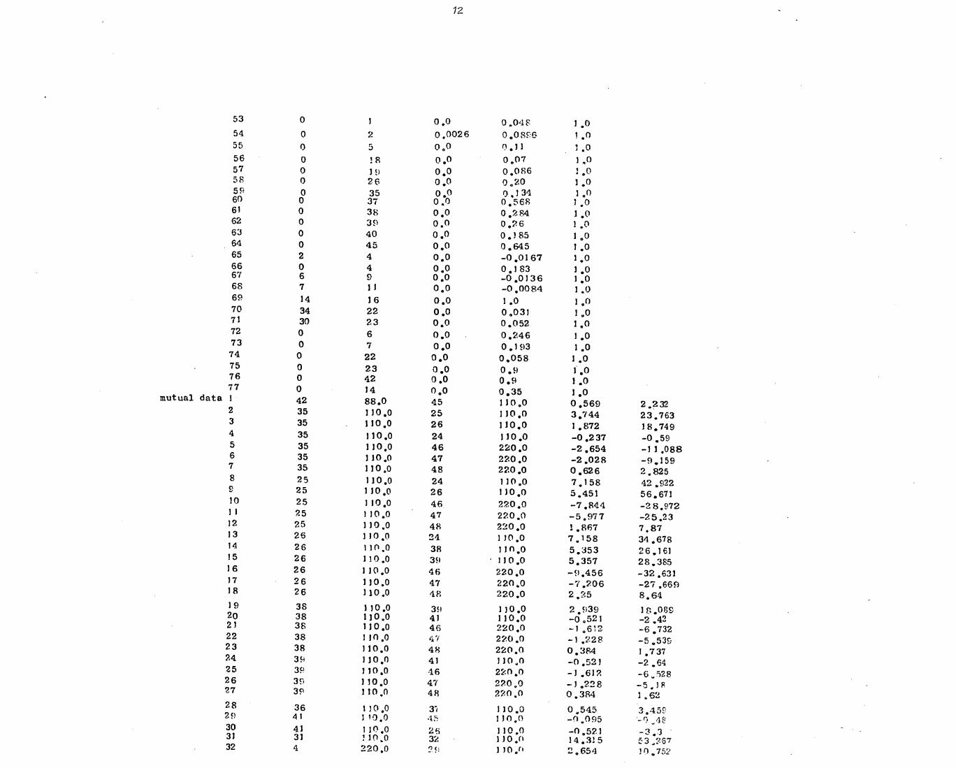
mutual data

53 0 1 0,0 0.048 1.0 54 0 2 0,0026 0.0896 1,0 55 0 5 0,0 0,11 1 .0 56 0 18 0,0 0,07 1,0 57 0 19 0.0 0.086 1 • 0 58 0 26 0,0 0 0 20 1,0 59 0 35 0.0 0,134 1,0 60 0 37 0.0 0,568 1,0 61 0 38 0,0 0,284 1,0 62 0 39 0.0 0,26 1.0 63 0 40 0,0 0.185 1.0 64 0 45 0,0 0,645 1,0 65 2 4 0,0 -0,0167 1,0 66 0 4 0,0 0,183 1,0 67 6 9 0,0 -0.0336 1,0 68 7 13 0.0 -0,0084 1,0 69 14 16 0,0 1,0 1.0 70 34 22 0,0 0,031 1.0 71 30 23 0,0 0,052 1,0 72 0 6 0,0 0,246 1,0 73 0 7 0,0 0.193 1,0 74 0 22 0,0 0,058 1.0 75 0 23 0,0 0,9 3,0 76 0 42 0,0 0,9 1.0 77 0 14 0,0 0,35 1,0 1 42 88.0 45 110,0 0,569 2,232 2 35 110,0 25 110,0 3,744 23,763 3 35 110,0 26 110,0 1,872 18,749 4 35 110,0 24 110.0 -0 .237 -0 .59 5 35 110,0 46 220,0 -2,654 -11 .088 6 35 110,0 47 220,0 -2.028 -9,159 7 35 110,0 48 220,0 0,626 2,825 8 25 110,0 24 110.0 7,158 42,922 9 25 110,0 26 110,0 5,451 56,671 10 25 110,0 46 220,0 -7,844 -28,972 11 25 110.0 47 220,0 -5.977 -25.23 12 25 110,0 48 220,0 1,867 7.87 13 26 110,0 24 110,0 7.158 34,678 14 26 110,0 38 110.0 5,353 26,161 15 26 110.0 39 110,0 5,357 28,385 16 26 110,0 46 220,0 -9,456 -32,631 17 26 110,0 47 220,0 -7,206 -27,669 18 26 110,0 48 220,0 2,25 8.64 19 38 110,0 39 110,0 2,939 1 ,089 20 38 1 3 0 .0 41 110,0 -0,521 -2,42 21 38 110,0 46 220,0 -1 .612 -6,732 22 38 110,0 47 220.0 -1.228 -5,539 23 38 110,0 48 220,0 0.384 1,737 24 39 10,0 41 110,0 -0,521 -2,64 25 39 110,0 46 220.0 -1,612 -6.528 26 39 110,0 47 220,0 -1,228 27 39 110,0 48 220,0 0,384 1,62 28 36 1,0,0 31 1 3 0 ,0 0,545 3,459 29 41 110,0 45 110,0 -0,095 '-0 30 41 110,0 26 110,0 -0.521 -3.3 31 31 110,0 32 110.0 14.315 53267 32 4 220,0 f.' 110, 2,654 3 0 ,752

33 4 220.0 30 110.0 2.654 12.88 34 4 220.0 21 110.0 -0.37.C: -1,53C 35 4 220.0 22 - 110.0 -0.379 -1,84 36 27 110.0 28 110.0 0.19 0.96 37 23 110.0 29 110.0 -0.64 -3.24 38 7 110.0 6 110.0 4.171 22.84 39 7 110.0 4 220.0 4.171 16.965 40 11 110.0 15 110.0 -0.428 -2.705 41 16 110.0 17 110.0 7.74 48.85 42 16 110,0 18 110,0 -0.238 -1.504 43 6 110.0 33 310.0 -0,735 -0.359 44 6 110.0 4 220,0 4,835 /7.61 45 33 110.0 4 220.0 -2.702 -10.26 46 5 110.0 2 220.0 4•55 744 47 24 110.0 46 220,0 -5,19 -19,386 48 24 110.0 47 220.0 -3.956 -17.853 49 24 110,0 48 220,0 1.234 - 5.58 50 46 220.0 47 220.0 9.483 49.64 51 46 220.0 48 220.0 -1.96 -15.5 52 31 110.0 13 110.0 6.806 42.97

Additional 'Element Current Distribution Factors 8 Equivalent Circuit 0 Elements 19 21 19 22 19 23 19

8 4 8 1 8 2 8 56 53E

ZERO

SUS

SEQUENCE 1968

LINE

MAXIMUM

FROM PUS

PLANT REouci-i , NI:TwORK

TO BUS CURRENT

PAGE 1

IMPEDANCE FAULT MVA

1 1 1 4 -0.1844+0.0053J 0.0011+0.0289J 129.6+3458.4J 2 1 3 -0.0297-0.0006J 3 1 8 -0.0633-0.0057J 4 1 35 -0.1210-0.0215J

53 0 1 0.6015-0.0226J

2 5 2 5 -0.0581-0.0072J 0.0012+0.0334J 103.4+2993.8J 6 2 21 -0.0251-0.0052J 7 2 43 -0.0263-0.0055J

54 0 2 0.3724-0.0020J 65 2 4 -0.5181+0.0158J

3 2 1 3 0.6362+0.0145J 0.0177+0.1115J 138.8 +874.9J* 8 3 8 -0.3638+0.0145J

4 1 1 4 n.211 8 -0.0119J 0.0018+0.0317J 175.7+3140.0J 65 2 4 0.6147+0.0216J 66 0 4 0.1735-0.0097J

5 5 2 5 0.1931+0.0286J 0.0031+0.0888J 39.8+1125.3J 55 0 5 0.8069-0.0286J

9 6 8 -0.4187-0.0038J 0.0052+0.0955J 57.2+1044.0J 67 6 9 -0.1931-0.0175J 72 0 6 0.3882-0.0213J

7 14 7 10 -0.3240-0.01 9 6J 0.0068+0.1026J 64.2 +970.6J 68 7 11 -0.1444-0.0155J 73 0 7 0.5315-0.0351J

8 3 1 8 0.3158+0.0246J 0.0084+0.0813J 125.6+1217.5J 8 3 8 0.2001+0.0094J 9 6 8 0.2764-0.0278J

10 8 10 -0.2076+0.0063J 4 1 35 -0.0667-0.0169u 1 1 4 -0.1223-0.0056J 2 1 3 0.2001+0.0094J

53 0 1 0.3269+0.0115J

9 11 9 11 -0.0588-0.0078J 0.0048+0.0868J 63.7+1149.2J 12 9 16 -n.0996-0.0008J 13 9 12 -0.0497-0.0048J 67 6 9 0.8359-0.0135J

1 0 10 8 10 0.4668+0.0361J 0.0098+0.1141J 75.1 +870.0J 14 7 10 0.5332-0.0361J

1 5

BUS LINE FROM Bus TO BUS CURRENT

PAGE 2

IMPEDANCE FAULT MVA

11 11 9 11 0.0707+0.00831 0.0065+0.0965J 69.9+1031.6J 15 11 12 -0.059A-0.0049J 16 11 13 -0.0000+0.11000J 17 11 15 -0.0non+0.0000J 68 7 11 0.8696-0.0132J

12 13 9 12 0.1125+0.0042J 0.0127+0.1188J 89.1 +832.0J 15 11 12 0.8875-0.0042J

13 16 11 13 0.5003+0.0004J 0.1373+0.6311J 32.9 +151.3J 18 13 15 -0.4997+0.0004J

14 19 14 17 0.0000+0.0000J 0.0051+0.2761J 6.7 +362.0J 69 14 16 -0.2110-0.0146J 77 0 14 0.7890-0.0146J

15 17 11 15 0.5146-0.0004J 0.1353+0.6186J 33. 7 +154.3J 18 13 15 0.4854+0.0004J

16 12 9 16 0.8140+0.0564J 0.0761+0.2510J 110.6 +364.8J 69 14 16 0.1860-0.0564J

17 19 14 17 1.0000+0.0000J 2.7365+1 ic.+01J 2.4 +9.0J

18 20 18 19 -0.4263-0.0004J •0.0010+0.0327J 95.7+3057.5J 21 18 24 -0.034 8 -0.0063J 22 18 25 -0.0351-0.0063J 23 18 45 -0.0370 - 0.0016J 56 0 18 0.4668-0.0146J

19 20 18 19 0.5518+0.0043J n .0011+0.0330J 100.7+3023.3J 24 19 26 -0.0251-0.0047J 25 19 29 -0.0128+0.0010J 26 19 30 -0.0761-0.0048J 57 0 19 0.3842-0.0128J 21 18 24 -0.0333-0.0063J 22 18 25 -0.0336-0.0064J 23 18 45 -0.0356-0.0019J 56 0 18 0.4492-0.0103J

20 27 20 24 -0.4968+0.0006J 0.0199+0.1144J 147.9 +848.7J 28 20 25 -0.5032-0.0006J

21 6 2 21 0.1479+0.0065J 0.0264+0.1314J 147.1 +731.5J 29 21 24 -0.2667+0.0091J 30 21 25 -0.2628+0.0094J 31 21 32 -0.0785+0.0003J 32 21 32 -0.0777-0.0034J 33 21 43 -0.1664-0.0088J

rUIT9F+9•9IT

r6•096+ COSI

rw*O0E1.+o•901

ree2o.o+LToo . o

rtiui . o+eoto - o

T8T$100+6600

r0000•o+uouro rgoTo*0-9999•0 r5o10'0+o22I*0

r9600*0-999'0 re900•0+2950'0 c9200•0+1L50 . 0

c1600•0-o900- r1600*.0-9116o

To

22 22

F2 F2 e2

F2

-T2

22 FF 02

12

TF TF

T2

02

50 o0 TO

90 F2 12

20

Oo

22

22

12

12T00 -0-5v9V0 rLeivo+sLee•o-

.02

.92 2e 02

11 TO

• rscovo-9gsvo- 12 .02' • Oo • coeoo.*.o+e -rwo

r000vu+9ge•.o •

.02

' .o2 6?, se:

62 92

IG*6179T+T'e91 . CL2G0'D+000•0 rFU0v0+9000 -0-

r000ti'o-g -rts*o- roLoo'o+e2ov*0

02

02 6?

61-

6? Le

9?

6S 12

02

re'voL+ 5'5If CZ921'0+9ZE0'0 r6uT0'0-S500'0

r9e00•0+L2oo*O- rZLTO*0+1O52'0

6?

02 9e

61

se a

se

92 92

6?

rfrozt+ 9111 r552T'0+01aU*0 r9oTv0-zeuvo

cTsovo-sgwo-

97,

6?

9?

a

52

12

92

1'0'295+ 2'56 r6991*0+21EO'0 r -coo . o+sowo-

rT6t70•0-5165 - u r0ie00-os9e*0-

9?

96 se

0 9?

92

95

52

te

C9629+ 969 r29T10+9600•0 ri9F0'0+920T'0

r99000+96910 C2900•0+629t'0

9e

5F ge

61

TZ

oe

oe

02

se

9?

CT'5T6+ ti'951 re9OT'0 4. C9Tu'O rO2TO*0-, 59920

rs100Po+ee9 -v0 1'5L00'0+o0Lo'0

se

oe oe

91

Te oe

U

66 Le

ge

r2o16+ L951 r2901*04-F9TO*0 1'6eTo•0-ot920

rosovo-2o -co reo00•0+0109*0-

oe

2? 02

91

22 0

Te

IL

oz

CO'ZL01+0'95 r0260•0+6o00•0 1'96uu'0-9550•0-

1'0'120'0-2969U rT5I:0'0-995T'O-

oo

?,?. o2

2?

0 ee

ot OL

2?

ro'ILoa+0•011. r000vo+sTou'o r6cL0*0-15l7T*0- 22 ee oo ee

VAN 110VJ dJi\JVUdWI 11\1388(13 snH 01 snH wOeH '11\11 -1

.71UtIci

91-

1 -1

BUS L 1lE FROM BUS TO BUS CURRENT

RAGE 4

IMPEDANCE FAULT MVA

34 46 34 35 -0.1334-0.0160J 0.0032+0.0576J 95.2+1732.0J 47 34 36 -0,1539-0.0129J 70 22 34 0.7127-0.0290J

35 4 1 35 0.1742+0.0204J 0.0033+0.0351J 266.9+2827.7J 46 34 35 0.0800-0.0016J 48 35 36 -0.1367-0.0042J 49 35 39 -0.2979-0.0016J 59 0 35 0.2616-0.0247J

36 47 34 36 0.1852-0.0147J 0.0069+0.0516J 255.5+1905.4J 48 35 36 0.5629+0.0451J 50 36 37 -0.2519+0.0304J

37 50 36 37 0.7022+0.0358J 0.0071+0.0573J 211.8+1718.5J 51 37 38 -0.1969+0.0234J 60 0 37 0.1009-0.0124J

38 51 37 38 0.7829+0.0262J 0.0074+0.0617J 192.8+1598.3J 61 0 38 0.2171-0.0262J

39 49 35 39 0.6556+0.0459J 0.0061+0.0380J 413.9+2566.4J 52 39 40 -0.1984+0.0223J 62 0 39 0.1461-0.0236J

. 40 52 39 40 0.7677+0.0581J 0.0108+0.0430J 548.1+2189.7J 63 0 40 0.2323-0.0581J

41 45 33 41 1.0000+0.0000J 0.0807+0.4083J 46.6 +235.7J

42 34 42 44 -0.5036-0.1087J 0.0979+0.446RJ 46.R +213.6J 76 0 42 0.4964-0.1087J

43 7 2 43 0.5444+0.0089J 0.0484+0.1928J 122.5 +487.8J 33 21 43 0.4556-0.0089J

44 34 42 44 0.3190-0.0598J 0.1184+0.3691J 78.8 +245.7J 42 23 44 0.6810+0.0598J

45 23 18 45 0.7249+0.0534J 0.0345+0.1774J 109.9 +543.1J 64 0 45 0.2751-0.0534J

END

* * ** ** ** ** ** ** * ** * ** ** ** *4

23/07/75 ALGOL LPRES

1 1

SIZE SIZE

404 411

SEGMENT SEGMENT

AREA AREA

SEGMENT AREA 1 SIZE 547 SEGMENT AREA 1 SIZE 582 SEGMENT AREA 1 SIZE 378 SEGMENT AREA 1 ..SIZE .393 HEI 8G COMPLEX LOAD FLOW

FREE STORE MS 2955 BS 5632

Pfko CI-R. A M L./Sr/NC, 1

02.,/kiN PI_E N FT N,-1012-K- PAT (F16.20 11

ComPu -rerk. FR/Nr LIT

%nip RV._ 14

NE-TwoRK. PPTA 15

CoN\Pu-rP-- PR-IN -rot); 19

HEI 8g Complex Load Flow;

begin comment calculates voltage and load or generation at each bus, power flow in lines, line losses and line charging for a given network;

integer 1001 ,L,M,m,n,o,mo,mo10,m11 ,t1 ,t2 ,t3,t4 ,C1 ,C2,C3,C4,C5,C6,C7 ,C8,C9; real R,T,a; integer array, str[1:30]; I:=1; instring(str,I); read C9,a,n,m,o,t1,t2,t3,t4; comment number of load flows, mva base, number of buses, lines, regulators, generators, loads, shunt

loads and special regulators; mo:= m+o; mo10:= mo+10; m11:=m+11;

begin integer array spgen[1:t1,1:2], spreg[0:t4], spbus[0:t3],modn[1:20,1:2]; comment CBS:; integer array connec[1:mo10,1:2],paralle1[1:m], buslines ,conlines(1 :2*mo] ,colposn,rowposn, junct,order,linebusEl :n]; real array gen[1:t1,1:2], reg[0:t1,1:2], shunt[0:t3,1:2Lvalue[1 :20,1:3]; comment CBS:; real array load,puvolt,busmat[1:n0:2], nomvol[ 1 :n] ,line[ 1 :mo10, 1 :3] , correction( 1 :2*n] ,diagonal [ 1 :2*n , 1 :2 ] ; switch s:= 11,12; comment insert procedures input, admat f organise ,solve ' current, corvol ,page,

output,modify,ailjust; procedure input; comment Uses global variables nomvol,load,connec,line,junct o gen t reg I spreg o spbus t shunt,spgen,a,m,n,mo o mo10,

t1,t2,t3,t4,C1; begin comment segment[1]; ,integer e v f,h,i,j,k; real x,y,z,g,v,w;

h:3; for i:=1 step 1 until mo do

begin read k,e,f,x,y,z,g; if e=f or e<1 or f < 1 or e>n or f>n then

begin h:= h+1; print EE1?data error?,k,e,f end;

j:= if i>m then i+10 else i; connec[j,1]:=if e>f then f else e; connec[j,2]:=if e>f then e else f; w:= if abs(g-1,0)<0,1 then 1,0 else a/g/g; v:= (x*x+y*y)*w; line[j,1]:= if x=0,0 and y=0,0 then 0,0 else if i>m then x*z/v else x/v; line[j,2]:= if x=0,0 and y=0,0 then 0,0 else if i>m then -y*z/v else -y/v; line[j,3]:= if i>m or abs(g-1,0)<0,1 then z else z*10-6/w

end reading line and regulator data, storing bus numbers in adjacent locations with lower number first, per unit admittance for lines or tap times this for rags in first two locations, per unit shunt susceptance or tap in location three;

read j,x,g; junct[j]:= C1:= j; load[j,2]:= x/g; nomvol[j]:= g; for i:=2 step 1 until ti do

begin read j,x,y,v,w,g; junct[j]:= j; load[j,1]:= y/a; load[j,2]:= x/g; gerai,1]:= v/a; gen[1,2]:= w/a; nomvol[j]:= g ; spgen[i,1]:= j; spgen[i,2]:= 0

end reading generator data, per unit power and voltage in load , bus number in junct, nominal voltage in nomvol, per unit reactive limits in gen, setting spgen;

for i:=1 sap 1 until t2 do begin read j,x,y,g; junct[j]:= 500+j; nomvol[j]:= g;

load[j,1):= x/a; load[j,2]:= y/a end reading load data, per unit real and reactive power in load, nominal voltage in

nomvol, 000 plus bus number in junct; for i:=1 step 1 until t3 do

begin read j,x,y,g;

1

2.

spbus[i]:= j; w:= abs(g-1.0)<0.1 then 1.0 else a/g/g; v:= (x*x+y*y)ft; shunt[i,1]:= x/v; shunt[i,2]:= -y/v

end reading impedances at busses, per unit admittance in shunt, bus number in spbus; for i:=I step I until t4 do

begin read j,x,y; k:= j+m-490; f:=connec[k,2]; g:= redi,1]:= x/g;

end reading voltage limits if h>0 then stop

spreg[i]:= k; nomvol[f];

reg[i,2]:= y/g on regulators, per unit limits in reg, setting spreg;

•■■••• end input;

procedure admat; comment uses global variables parallel,busmat ,buslines,conlines,linebus ' connec t spbus * shunt,

moo mo,molOpm11,t3,C2,C3; begin comment segment[I]; integer i,j,k,d,e,f,g; real x,y,z;

switch ss:= 111,112,113,114; for i:=I step I until m do parallel[i]:= 0;

d:= m+1; C3:= mo; C2:= m; 111: i:= i+1;

if i>m then gots! 112; if parallel[i]=0 then

begin f:=connec[i,I]; g:=connec[i,2]; x:= y:=z:= 0.0; k:= 0; for j:= i+1 2112 I until in do begin if f=connec[j,1] and g=connec[j,2] then

begin k:= k+I; parallel[j]:= d; x:= x +line[j,I]; y:= y+line[j,2]; z:=z+liwa[j,3)

end end; if k>0 then

begin connec[d,I]:=f; connec[d,2]:=g; line[d,1]:=1ine[i,1]+x; line[d02]:=1ine[i,2]+y; lima[d,3]:=1ineli,3]+z; parallel[i]:=d; d:=d+1; C2:= C2+1; 3:= C3-k

end combining parallel lines and storing in locations after m, C2 gives in plus the sets of parallel lines, C3 number of connections between busses

end; sato 111;

112: for i:=I step I until n do busmat[i,1]:= busmat[i,12]:= 0.0; i:=k:= d:= 0;

113: i:= i+I; e:=D; for j:= I sap I until C2,mI1 step 1 until mol0 do

begin if j <m then begin if para1lel[j]f4 then goto 114 end; f:=connec[j,I]; g:=connec[j,2]; if f=i or g=i then

begin d:= d+I; buslines[d]:=j; conlines[d]:= if f=i then g else f; e:=e+I; x:=1ine[j,1]; y:=1ine[j,2]; z:=1ine[j,3]; busmat[i,1]:= busmat[i,1]+(if ISC2 then x else if f=i then x*z else x/z); busmat[i,2]:= busmat[i,2] + (if j<C2 then y else if f=i then y*z else y/z); if j<C2 then busmat[i,2]:=busnat[i,2]+z

end forming diagonal terms of admittance matrix in busmat, listing lines in order of bus connections and number of connections to each bus;

114: end; linebus[i]:=e; if e=0 then

begin print 9£1?no connections to bus?,i; k:=k+1 en ;

if i<n then goto 113; for i:=1 step 1 until t3 do

begin, j:= sphus[i]; busmat[j,1]:= busmat[j,1] + shunt[i,1]; busmat[j,2]:= busmst[j,2] + shunt[i,2]

end adding admittances at busses to diagonal terms of matrix; if k>0 then stop

end admat;

procedure organise;

comment uses global variables linebus,conlines, C1,C4,C5,C6,n,mo setting up the global arrays colposn,rowposn,order;

begin comment segment[1]; integer d,e,f,g,h,i,j,k,q,ltcol,ltrow,rkci,rich,cpi,ropi,cpch; integer array colterm,rowtermainterm,busind [ 1 :n] ,row,column[ 1 :3*mol0]; switch ss:= 111,112,113,114,115; k:=1; f:=D; for i:=1 step 1 until n do

begin d:= f+1; f:= f +linebus[i]; if i=C1 then Eau 112; j:=0; colposn[i]:= rawposn[i]:= k; for q:= d step 1 until f do

begin g:=conlines[q]; if g=ci then goto 111; column[k]i= row[k]:=g; k:= k+1; j:= j+1;

111: end; if j=0 then

begin,print'Eslack'bus4s the only bus connected to bus? i; stop

colterm[i]:= rowterm[i]:=finterm[i]:=j; busind[i]:=0;. _

112: end column lists.rcf* number of terms,.in.eachcolumn,.rollt..lists column. number of terms in each roW,:colterm and colposn - give number. of terms and location in column, rowterm and rOwposn in . rOw,.finterm stores maximum value of rowterM;

busind[C1]:=1; ltcol:=1trow:=k-1; j::=1;

113: i:=0; 114: i:=i+1;

if i>n then begin. d:=d+1; goto 113 end;

if busind[i]=1 then goto 114; if colterm[i]W then sotq 114; order[j]:=i; busind[i]:=1; cpi:=colposn[i]; f:= cpi+d-1; for k:=cpiatE2 1 until f do

begin rkci:=column[k]; comment row number of term in column i which is to be eliminated; ropi:= rowposn[i]; g:= ropi + rowterm[i]-1; for h:= ropi step 1 until g do

begin. rich: = row[h]; comment column number of term in row i; if rkci= rich then goto 115; cpch:= colposn[rich]; e:= cpch + colterm[rich]-1;

4

=1 step until n d

o q:= cpch sap I until e do if rkci= column[q] then rate 115; comment a new term to be added in column rich and row rkci; colterm[rich]:= colterm[rich]+1; for q:= rich+1 1 until n do if qtCI then colposn[q]:= colposn[q]+1; e:= e+2; ltcol:= ltcol+1; for q:= ltcol sap -1 until e do column[q]:= column[q-1]; column[e-1]:= rkci; if rich <i then

begin f:= 1+1; k:= k+1 end;

romterm[rkci]:= e:= rowterm[rkci]+1; if e>finterm[rkci] then finterm[rkci]:=e; for q:= rkci+1 219.2 1 until n do if q Cl then rowposn[q]:= rowposn[q]+1; e:=e+ rowposn[rkci]; ltrow:= ltraw+1; for q:= ltrow 1122 -1 until e do row[q]:= row[q-1]; row[e-1]:= rich; if rkci<i then

begin g:= g+1; h:= h+1 end;

115: end adding new term and modifying column,colposn,colterm, row,rowposn,rowterm,finterm;

rowterm[rkci]:= rowterm[rkci]-1; for q:= rkci+1 1122 1 until n do if OC1 then rowposn[q]:= rowposn[q]-1; ltrow:= ltrow-1; g:= 0; for q:= rowposn[rkci] .2112 1 until ltrow do

begin if row[q]=i then g:=1; if g=1 then row[q]:= row[q+1]

end elimination of column i from row rkci end;

j:= j+1; if On then

i: it i*C1 then

ltcol:= ltcol-d; for q:=colposn[i]stpx 1 until ltcol do column[q]:= column[q+d]; for q:= i+1 step 1 until n do if busind[q]=0 then colposn[q]:= colposn[q]-d; Eat2 114

for 1 2

end col umn from column; C6:= j= : =I

rowposn[i]:= k; j:=j+colterm[i]; g:= finterm[i]; if g>C6 then c6:= g

end setting ma717176 values in colposn and rowposn; C4:=j-

end organise;

procedure solve (CTM,CMN,RTM,RW,ave,b1w); comment uses global variables colposn, rowposn,C6,order,correction,diagonal,n Eliminates

pairs of columns in the prescribed order using the extra space in ave lblw, CTM,CMN,RT1W and RW to avoid shifting terms;

ABItgAr.RE.Key CTM,CMN' RTM RW; real array ave,b1w;

begin integer

begin

:k;

k:= k+g;

1; C5 : =k-1

de f 9 h 9 9 pg, ,T737k,p,q,n1,rt,rp,rw,ct,cp,u,ew; real x,y,z,z1,z2,cor,diag; integer array loc coll[1:c6]; riTir array usterms, wtterms[1:C6]; WITZE-ss:=111,112,113,114,115; d:=1; n1:=n-i;

111: i:=order[d]; rt:=RTM[i]; if rt=0 then goto 113; comment number of terms in row i; rp:= rowposn[i];

112: j:= RW[rp+f]; cp:=colposn [j]; g:=cp+CTM[j]-1; for k:=cp 2122 1 until g do if CMN[10=i then

begin f:=f+1; loc[f]:=k; coll[f]:=j; if f = rt then goto 113 else goto 112

end storing the locations and columns of row i off diagonal terms; 113: f:= if u=0 then i else i+n;

x:= if u=0 then diagonal[f,1] else diagonal[f,2]; if u=0 then

begin diag:=diagonal[f,27/x; diagonal[f,2]:=diag

cor:=correction[f]/x; correction[f]:=cor; comment division of correction and semi-diagonal terms by diagonal pivot; for j:=1 sap 1 until rt do

begin k:= loc[j]; for g:=1,2 do

begin y:=(if u=0 then ave[k,g] else blw[k,g])/x; if u=0 then ave[k,g]:=y else blw[k,g]:=y; if g=1 then usterms[j]:=y else wtterms[j]:=y

end end division of off-diagonal row i terms by diagonal pivot and storing;

f:= if u=0 then i+n else i; y:= if u=0 then diagonal[f,1] else.dieg;. for j:=1 2122 1 until rt do

begin k:=loc[j]; for g:=1,2 do

begin z:= y*(if g=1 then usterms[j] else wtterms[j]); if u=0 then blw[k,g]:=b1w[k,g]-z (aim ave[k,g]:=ave[k,g] -z

end end modifying off-diagonal terms in corresponding row;

if u=0 then diagonal[1,2]:=diagonal[f41-y*diag; correction[f]:=correction[f]-y*cor; comment corresponding semi-diagonal term is eliminated; uw:=e:=0; f:=if u=0 then 1 else 21 cp:=colposn[i]; . ct:=CTM[i];

114: g:=cp+e; rw:=CMN[g]; comment term in row rw and column i; y:=if uw=0 then ave[g,f] else blw[g,f]; if u=0 then

begin if uw=0 then ave[g,2]:=ave[g,2]-y*diag else blw[g,2]:=b1w[g,2]-y*dieg end modifying term in column i-i-n;

g:= if uw=0 then rw else rw+n; correction[g]:=correction[g]-y*cor; comment modifying correction terms; for j:=1 2122 1 until rt do

begin h:=coll[j]; z1:=y* usterms[j] . ; z2:=y*wtterms[j]; if h=rw then

_begin diagonal[g,1]:=diagonal[g,1] -z 1 ; diagonal[g,2]:=diagonal[g,2]-z2; got(' 115 end otherwise search fora term in row rw and column h;

p:= colposn[h]; rp:=CTm[h] .;,k:=p+rp-1; • for q:=p ,step 1 until k do if CMN[q]='m then

• begin if uw=0 then 'begin avelq,1]:=ave[q,11-z1; ave[q,2]:=ave[q,2]-z2 encl. else , begin blw[q,1]:=b1w[q,1]-z1; blw[q,2]:=1D1w[q,2]-z2

6

end; goto 115 end otherwise add a new term in row rw and column h;

k:=k+I; if uw=0 then

begin ave[k,1]:=-z1; ave[k,2]:=-z2 end else begin blw(k,1]:=-z1; blw[k,2]:=-z2 end;

if uw=1 then begin CTM[h]:=rp+1; CMN[k]:=rw; k:=RTM[rw]; RTM[rw]:=k+I

RWfk+ rowposn[rw]]:=h end;

115: end elimination of term in row rw and column i; if u=I and uw =1 and 1:1:11 then

begin rp:= rowposn(rw]; k:=RTM[rw]; RTM[rw]:=k-1; k:=k+rp -2; g:=0; for q:=rp step 1 until k do

begin if RW[q]=i then g:=1; if g=I then RW[q]:= RW[ 0:1+ 1 ]

end elimination of i from row rw end;

uw:=uw+1; if uw =1 then got°, 114; e:= e+I; if e<ct then

begin uw:=0; end;

u:=u+I; if u=I then goto 113; if d<n then gots! 111

end solve; procedure current(X,Y,U,V); comment used for calculating current at a bus and requires global variables R,T; value X,Y,U,V; real X,Y,U,V; begin R:= R+X*U-Y*V;

T:= T+X*V+Y*U end current;

.procedure . corvol; comment sets'up . correetion equations:and corrects bus volteges, requires .

• procedures current and. solve,uses global variables'colposn,roWposn n,R,T,C4,.d5i .junct t load tbusmat r correction t diagonal,puvOit,line t linebus,buslines,cOnlines; • integer, die4f I g,i4 j,k,q,busi

-real u o vocair,t,w,z;.coMment CB5.:; real ,Itrriv . above,be1ow[1:C4 I:2]; integer array rawtermp colterm[kin],column[liC41, row[1.:C51:. switch.ss:= 111,,112;•

step 1 until n do colterm[i]:=6; . for i:=I . step. 1 until n dO.

begin dl=f+1; f:= f4linebus[i]; if i=CI then x2s22 112;' bus:=junct[i]; comment if bus > 500 then load otherwise generator; u:=puvolt[i,1]; v:=puvolt[i,2]; x:=busmat(i,1); y:=busmat(i,2); R:= T:= 0,0; current(X,y,u,V).; w:= -u*y+v*x; z:= u*x+v*y; for q:= d,step 1 until f do •

begin j:=buslines[q]; g:=conlines[q]; r:=-1ine(j,1]; t:=-1ine[j,23: current(r o t'ouvolt[g,1],puvolt[g,2]);

if g=CI then alto 111; x:= -u*C7.1747; y:= u*r+v*t; e:= colterm[g];

-7

j:= colposn[g]+e; k:= rowposn[g]+e; colterm[g]:= e+1; column[j]:= row[k]:=i; below[j,1]:=y; below[j,2]:=x; above[j,1]:=if bus>500 then x else 0,0; above[j 12]:=if bus>500 then -y else 0,10;

111: end; e:= n+i; correction[e]:=load[i,1]-40R-v*T; diagonal[e,1]:=R+z; diagonal[e,2]:=T+w; x:=load[i,2]; if bus >500 then

begin. correction[i]:=x+u*T-v*R; diagonal[i,1]:=-T+w; diagonal[i,2]:=R-z

end else begin correction[i]:=x*x-u*u-v*v;

diagonal[i,1]:=2,0*u; diagonal[ip2]:=2,0*v end calculation of terms in row i;

112: end setting up correction equations; for i:=1 step 1 until n do rowterm[i]:= colterm[i]; solve(colterm,column,rowterm,row,above,below); for i:=1 step 1 until n do if iC1 then

begin puvolt[i,1]:=puvolt[i l l]+correction[i]; puvolt[i,2]:=puvolt[i42]+correction[i+n]

end correcting voltages at each bus end corvol;

procedure, page (u,v); comment prints page numbers and headings, uses global variables LOW; value u,v; integer, u,v;

begin, switch ss:=111,112,1131 114,115; goto ss[u];

111: top of form; 112: print ££860?PAGEP,M,E£12??;

M:=M+1; goto ss[v]; 113: print £ BUS MW MVAR VOLTAGE KV PER UNIT DEGREES MVAR LINE CHARGING?;

if t 3>0 then print £ SHUNT MW MVAR?; goto 115; 114: print ELINE NO BUS MW MVAR MVA BUS MW MVAR WA MW LOSS MVAR LOSS TAP?;

115: L:=0 end page;

procedure output; comment uses global variables a,m,n,mo10,m11 ,t3 ,R,T,L,C2 ,nomvol ,busmat, line ,linebus ,buslines ,

conlines,puvolt,connec t spbus,shunt o requires procedures page and current; becin comment segment[1]; ,integer d,e,f,g,i,j,k,r,q; real uoi,w,x,y,z,z1,z2,z3,z4,suml,suna,sum3,1inch;

real array volt[1:n]; print ££12??; r:=5; page(2,3); aligned(4,2); suml:=sum2:=sum3:=1inch:0 4,0; f:=k:01; for i:=1 step 1 until n do

begin r:=r+1; if r=6 then begin r:=1; if L = 9 then page(1,3); E:=L+1; print ££1?? end;

u:=puvolt[i,1]; v:=puvolt[i,2]; volt[I]:=w:=u*u+v*v; R:=T:=z3:=0,0; current(busmat[i I] ,busmat [ 12 ] ,u,v) ; d:=f+1; f:=f+linebus[i]; for q:=d step 1 until f do

begin e:zbuslines[q]; g:=conlines[q]; current(-1ine[e , 1 ] ,-line[e 9 2], puvolt[g, 1 ] ,puvolt[g,2 ]) ; if e<C2 then z3:=z3+1ine[e$3]

end calculation of current and susceptance at bus i; z2:=z3*w*a; linch:=1inch+z2;

x:=a*(u*R+v*T); y:=a*(v*R-u*T); if x>1 •0 then

begin suml:=suml+x; sum2:=sum2+y; sum3:=sum3+sqrt(x*x+y*y)

end adding generation; z:= if u>0 •0 then arctan(v/u) else if abs(v):00.0 then sign(v)*1.57079633-arctan(u/v) else 3.14159265; w:=sqrt(w); z1:=nomvol[i]; print 221??,i,E ?,x,2 ?,y 1 2 ?,u*z1,special(2) print prefix( 2 ?) ,w*z1 ,aligned(2,4),w,z*57 .2957795, if

k <bte:inhef:r j:=1 step 1 until t3 do if spbus[j]=i begin k:=k+1; z:=volt[ii*a;

print aligned(3,2),prefix(2

,v*z 1 tEr; aligned(3,2),z2;

then

?),-shunt[j,I)*z,shunt[j,2j*z end

••■■■••■•■•

end end printing generation,loads,bus voltages, angles, line charging and shunt loads;

print 2212?TOTAL GENERATION=?,freepoint(4),sum1,2 MW ?,stm2,2 MVAr ?,sum3,2 MVA?; r:=5; sum1:=sum2:=0.0; aligned(3,2); 122: i:=1 step 1 until m,m11 step 1 until mo10 do

begin w:=1ine[i,2]; if wi=0.0 then begin r:=r+1; if r=6 then

begin r:=1; if L=9 or i=1 then page(1,4); L:=L+1; ,print £21?? end;

f:=connec[i,1]; g:=connec[i,2]; IL i>m then sum3:=1ine[i,3]; u:=puvolt[1,1]; v:=puvolt[f,2]; z:=1ine[i,1]; x:=puvolt[g,1]; y:=puvolt[g,2]; z1:=u*x+v*y; z2:=u*y-v*x; u:=z2*z; v:=z2*w; x:=z14 if i>m then volt[f]*sum3 else volt[f]); y:=z1-( i>m then volt[g]/sum3 else volt[g]); zl:=(x*z-v)*a; z3:=(y*z+v)*a; z2:=(-x*w-u)*a; z4:=(-y*w+u)*a; x:=sqrt(zl*z1+z2*z2); if z1<0.0 then x:=-x; zyi f:: == zq> rmi z3h 3e; n* z w3

print

+: =z z* 2z zE) :Os u met then ; yp r: =si -n yt ; ?? w; ;

print prefix( 2 ?),f,z1,z2,x,g,z3,z4,y,aligned(2,3),z,w; if i>m then print 2 ?,aligned(1,3),sum3

end printing, line flaws and losses end;

print 2212?TOTAL LINE LOSS=?,freepoint(4),som1,2 MW ?,sum22,2 MVAr ?,TOTAL LINE CHARGING=?,linch,E MVAr? 422....id output;

Procedure, modify; comment uses global variables a,C7,C8,value,modn,reads and stores network modifications; Iman comment segment[1]; integer e,f,q,j,i,,k; real g,r,v,w,x,y,z; Procedure change(u); comment uses global variables modn,value,connec,line,parallel,busmat,load,C8. If u=1 restores original

network, if u=2 sets up new network and stores old values; value u; integer u; begin for 1:=1 step 1 until C8 112

begin j:= modn[i,2]; modn[i,1]=2 then

begin if u2 then begin x:=load[j,1]; y:=load[j,2] end;

load[j,1]:=value[i,1]; load[j,2]:=value[i,2]; if u=2 then

begin value[i,1]:=x; value[i,2]:= y

9

end end changing loads else begin e:=connec[j,1]; f:=connec[j,2];

x:= value[i l l); r:=1.ine(j,1); y:= value[i,27; v:=1ineU,2]; z:= value[i,31; w:=line[j,31; line[j,11:=x; line(j•2):=y; line[j,37:=z; k:=parallel(j); if k>0 then

begin line(k,1 :=line[k,17+x-r; line[k,2]:=1ine[k,2]+y-v; lineEk,33:=1ine(k,37+z-w end;

if u=2 then begin value[i, h=r; value[i '2] :=v; value [i ,37:=w end;

for q:= e t f do begin busmat[q, 1 ] :=busmat [q, 1 7+x-r ; busmat Eq,2 : =busmat ,2 7+y-v+z-v/ end

end changing lines end

ana change; C7;.1 then change( 1) ;

2:212,a C8; i:=1 step I until C8 do

begin read k,e,modn[i,2],x,y; if e=1 then read z,g; modn[i,1]:= e; IL then

begin value[i,1]:=x/a; valuea,27:=y/a end storing new loads else begin w:= abs(g-1„0 X0,1 then 1,0 else a/g/g;

v:= (x*x+yloy)*Fw; value[i l l]:= x4.0 juLd y=0,0 then 0,0 else x/v; value(i,2):=21. x4,0 _end y=0,0 then 0,0 else -y/v; vaitietio]:=It abs(g-1,0)<0,1 then z else z*icr-6/w

Ind storing new line data end reading and storing modifications;

change(2) end modify; procedure, ad bceoammein,nctommuseens

q; real t segment[17; integer d,e,f,g,h,i,j,k

just; global variables tht4,R,T,J,J1,spgen,gen t spreg,reg o busmat,load,

puvolt,line,connec and requires procedure current declared first;

for i:4 ate/ 1 until t1 dolt spgen[i,2)=0 then begin j:=spgen[i,17; d:= j-I;

u:=puvolt[j, ; v:=puvolt[j,2]; R::-- T:= 0,0; f:= 0 c urrent(busmat U, 1 ,busmat j,27 u, v) ; for q:=1 2.122 1 until d do f:= f+linebus[q]; d:= f+1; f:= f+linebus[j]; for q:= d sae 1 until f do

begin e:=buslines[q]; g:=conlines[q]; current(-line[e , ],-1 ine[e ,2],puvol t[g ,1

end calculation of current at bus j; w:= v*R-u*T; u:= gen[i,17; gen[i,27; if u>w or v(w then

begin if u>w then begin spgenri,2 ; gen( , 1 3:=load[j,2] ; load[j,27:=u end else begin spgen[i,27:= 2; gen[i,21:=load(j,2]; load[j,2]:=v

;

junct o linebus,buslines,conlines 9

r,u,v,w,x,y,z,x1,y1;

;

puvol t [g,2 3)

junct[j]:=500+j; h:= h+1 end changing generator to load if either MVA limit exceeded

end; for i:=1 step 1 until t4 do

begin j:= spreg[i]; k:=connec[j,2]; u:=puvolt[k $ 1]; v:=puvolt[k,2]; z:=1ine[j,3]; w:= sqrt(u*u+v*v); u:= reei,1]; v:= redi,21; if ( u>w and abs(z-1,15)>%0055) or ( v<w and abs(z-0.9)>0,0055) then

begin x:=1ine[j,1]; y:=1ine[j,2]; if JI=2 then

begin xI:= entier(100.0*(if u>w then w-u else v-w))/100,0; v:= z + (if u>w then -xl else xl); if v>1,1555 then v:= v-entier(100,0*(1,-1,145))/100,0; if v<0,8945 then v:= v + entier(100J3*(0,905 - v))/I00,0

end else v:= z+ (if u>w then 0,01 else -0,01); r:= v/z; x*r; yl:= y*r; f:=connec[j 1 1]; line[j,I]:=x1; line[j,2]:=y1; line[j,3]:=v; busmat[f,1]:=busmat[f,17-x*z+xl*v; busmat[f,2]:=busmat[f,2]-y*z+yI*v; h:= h+1

end changing tap, line and bmat if either voltage limit exceeded end;

if hig-0 then J:=2 end adjust;

sameline; digits(3); input; admat; for I:=I step 1 until n do

begin puvolt[I,1]:= if junct[I]>500 then 1,0 else load[I,2]; puvolt[I,2]:=0,0 end;

organise; noflo; J:=J1:=C7:=0;

11: I:=M:=I; outstring(str,I); 12: J:=J+1; J1:=J1+1; corvol;

if J>1 and (' -..1>1 or t4>0) then adjust; if J<5 then gotn 12; C7:= C7-I; output; if C7<C9 then

begin top of form; I:=I; instring(str,I); modify; J:=2; jgoto 11

end end

end load flow;

9LLAAD FLOW FUR SAMPLE nTwury? Number of studiet; 1 mva base 100.0 number of busbars 0 number of liner; 12 number of regulatJ , rs number of ',.encrators 2 number of loads 7 number of shunts 0 number of tap c""angers 0 line connection resistance reactance total shunt

husbar bushar susceptance 1 c 2 1.25 3.4 42.0 2 2 1 1.34 3.85 48.0 3 1 6 10.36 . 18.25 230.0 4 1 7 29.34 40.68 134.0 5 7 6 7.2 44.3 15.0

6 7 8 0.18 0.69 5.0 7 7 3 11.n5 19.72 252.0 E.! 6 3 18.21 45.09 102.0 9 8 9 0.0 0.04 0.0 10 c 4 4.83 19.37 233.0 11 1 7 29.34 40.68 134.0 12 7 6 7.2 44.3 15.0 regulator tap 501 3 5 0.0 2.45 1.08 generator voltage MW MVAr limits nominal busbar magnitude minimum maximum voltage 1 110.0 110.0 3 110.0 212.0 80.0 110.0 110.0 load MW MVAr nominal busbar voltage 2 32.0 0.0 110.0 4 122.0 48,0 220.0 ' 5 0.0 0.0 110.0 6 -31.0 -10.0 110.0 7 -229.0 -104.0 110.0 8 0.0 0.0 110.0 9 0,0 0.0 220.0 E

nominal voltage 110.0 110.0 110.0 110.0 110.0 110.0 110.0 110 .0 1.0 220.0 110 .0 110 .0

110 .0

12

LOAD

BUS

FLOW FOR SAMPLE

MW

NETWORK

MVAR VOLTAGE

PAGE

KV

1

PER UNIT DEGREES MVAR LINE

1 -90.39 -19.04 110.00 +0.00J 110.00 1.0000 0.0000 6.61

2 32.00 0.00 113.89 +4.30J 113.97 1.0361 2.1622 1.17

3 212.00 90.87 109.64 4.8.91J 110.00 1.0000 4.6469 4.28 4 122.00 48.00 214.78 +17.30J 215.47 0.9794 4.6059 10.82 5 - 0.00 - 0.00 117.06 +7.10J 117.28 1.0662 3.4731 0.58

6 -31.00 -10.00 104.51 -1.08J 104.51 0.9501 -0.5909 3.95

7 -229.00 -104.00 100.52 -2.88J 100.57 0.9142 -1.6427 5.61 8 -0.00 0.00 101.12 -2.17J 101.14 0.9194 -1.2298 0.05 9 0.00 -0.00 207.56 +7.04J 207.67 0.9440 1.9429 10.05

CHARGING

TOTAL GENERATION= 366.0 MW 138.9 MVAR

393.8 MVA

LANE- NO-8W 'MVA

1 2 114.79 67.61 133.22 2 1 144.08 60.99 156.46 3 1 -19.13 -22.25 -29.34 4 1 -17.28 -13.16 -21.72 _ _ _ 5 6 -5.72 -8.42 -10.18

6 7 119.79 51.95 130.57 7 3 -70.47 -15.80 -72.22 8 3 -25.03 -4.34 -25.40 9 _ 8 120.09 53.06 _ _ 131.29

•10 4 ;122.00 -58.82 -135.44

11 1 717.28 -13.16 -21.72 12 6 -5.72 -8.42 - 10.18

501 3 -116.50 -75.01 -138.56

8 7 '6

-120.09 65.62 24.06

-120.09 -120.09

PAGE

"fiOTAL •LINE LOSS= 15,61 MW END

MVAR

-72.26 -68.78

20.95 •11.57

8.00

-53.11 7.30 1.94

-61.21 51.16

11.57 8.00

71.68

MVA

-137.09 -162.11

27.88 19.86 9.80

-131.31 66.03 24.14

7134.79 130.54

19.86 9.80

136.79

MW LOSS

1.708 2.711 0.737 1.144 0.068

0.303 4.849 0.971

•0•000 . 1.908

1.144 0.068 n.000

MVAR LOSS

4.646 7.789 1.298 1..5_8.6. 0.421

1.163 8.5.00 2.405 8.156._ 7.653

1.586

3.133

TAP

1.080

BUS MW

5 -116.50 2 -146.79 6 18.39 7 16.14 7 5.66

16.14 5.66

116.50

48.96 MVAR TOTAL LINE CHARGING= 43.12 MVAR

B • 0

00 =l•

00

0 4- V;

LI

El

ta

CSYSTEM IC/ID FLOW 1973 LOADINGS? number of studies 1 mva base 100.0 number of busbars 83 number of lines 86 number of regulators 8 number of generators 1 number of loads 82 number of shunts 0 number of tap changes 0 line connection resistance reactance total shunt nominal

busbar busbar susceptance voltage 10 23 6.41 11.12 523.0 110.0

2 12 36 3.0 8.18 27.0 110.0 3 8 36 14,0 30,7 99.0 110,0 4 8 12 11 .1 6 20.26 245.0 110.0 . 5 9 38 1,18 3,36 42,0 110,0 6 8 15 11.78 21.56 70.0 110,0 7 15 35 2,61 11.3 37,0 110,0 8 12 13 0,13 0,49. 17,0 110,0 9 11 12 0,16 0,66 10.0 110,0 10 2 13 0,0009 0,028 0,0 1.0 11 2 3 8,24 33,84 116,0 220.0 12 1 3 7,93 34,44 108,0 220,0 13 3 4 1,96 8.53 27,0 220,0 14 4 2 6,28 25.85 89,0 220,0 15 1 19 7,71 33,49 105,0 220,0 16 1 7 4,14 16.39 242,0 220,0 17 10 24 13,25 22,0 65,0 110,0 18 1 24 0,0029 0,089 0,0 1,0 19 24 25 3,41 9.11 125,0 110,0 20 41 28 0,175 1,1 2,0 110,0 21 21 32 7,3 18,0 61,0 110,0 22 6 19 4,57 19,8 62,0 220,0 23 5 32 15,13 22.2 68.0 110.0 24 20 33 3,8 9,52 36,0 110,0 25 11 23 0,197 0,528 7.0 110,0 26 33 32 9,1 24,0 82,0 110,0 27 10 34 5,37 8,25 23.0 110,0 28 14 36 0,5 13,97 3,0 110,0 29 14 35 0,5 13,97 3,0 110,0 30 8 16 5,25 8,08 23,0 110,0 31 16 17 19,22 2 9,0 3 85.0 110,0 32 17 18 10,03 15.4 43.0 110.0 33 21 22 3,43 7,24 22,0 110,0 34 24 34 6.89 12,49 37,0 110,0 35 29 39 2,75 6,7 21,0 110,0 36 21 39 1,24 3,05 31,0 110,0 37 31 32 0.45 1,11 4,0 110,0 38 29 31 4,03 9,9 32,0 110,0 39 22 82 3,8 11.3 78,0 110,0 40 7 19 4,21 26,4 95.0 220.0 41 12 35 3,0 8,18 27,0 110,0 42 21 30 1,25 6.0 22,0 110,0 43 5 40 0,47 0,69 2,0 110,0 44 32 40 14,7 23,5 66.0 110,0 45 40 37 6,04 8,9 27,0 110,0 46 10 38 1.35 3,88 48,0 110,0

47 _

3 44 0,0069 0,135 0 00 1.0 48 15 43 0,0081 0,197 0,0 1,0 49 46 48 0,61 2,66 9,0 220,0 50 3 46 0,58 2,52 8,0 220,0 51 50 57 0,21 1,17 4.0 220,0 52 4 50 0,36 1,99 6.0 220,0 53 54 55 5,91 8.3 28,0 110,0 54 53 54 0,61 0,89 3,0 110.0 55 13. 54 4,93 12,58 46,0 110,0 56 51 52 13,3 10,58 28,0 88,0 57 56 57 0,0144 0,286 0.0 1,0 58 49 50 0,0246 0,568 0,0 •1,0 59 45 46 0,0152 0,26 0.0 1,0 60 47- 48 0,0098 0,185 0,0 1.0 61 39 61 0 000897 0,211 0,0 1,0 62 63 64 30,54 28,73 156,0 88,0 63 64 65 3,58 2,82 15,0 88,0 64 64 66 11,02. 10,06 54,0 88,0 65 42 . 62 0,006 0,096 0,0 1,0 66 26 63 0,0 0,145 0.0 1 0 0 67 8 58 0,0054 0,0666 0,0 1,0 68 8 59 0,0061 0,092 0,0 1,0 69 16 60 0.052 0,647 0,0 1,0 70 21 67 0,26 1,71 7.0 110,0 71 67 68 0,00448 0,105 0,0 1,0 72 24 69 0,00212 0.0815 0.0 1.0 73 24. 70 18.56 33,26 1.58,0 110,0 74 28 71 0.722 1,25 . 4.0 110,0 75 28 72 0,05 0,18 2,0 110,0 76 19 74 1,79 9,26 . 33,0 220,0 77 19 76 1,75 9,07 32,0 220,0 78 19 78 2,68 13.98 44.0 220.0 79 80 •81 0,008 0,21 0,0 1,0 80 80. 79 0,036 0.273 0,0 1,0 81 73 74 0,0156 0,324 0.0 •1,0 82 75 76 0,006 0,11 0,0 • 1,0 83 77 78 0,008 0.162 0,0 1,0 84 19 . 80 3,42 18,15 62.0 220,0 85 1 83 0,00232 0,0875 0,0 1,0 86 30 82 1.86 4,84 34.0 110,0 regulator tap 501 8 9 0,0665 2,42 1.03 110,0 502 25 26 . 0,072 2,62 0,96 110,0 503 6 32 0,201 5,7 1,0 110,0 504 19 21 0.27 10,5 0,98 110,0 505 7 - 28 0,145 • 5,05 0,978 110,0 506 26 42 0,81 13.4 0,98 110,0 507 27 41 0,005 0,103 1,07 1,0 508 . 12 51 0,0024 0,0206 1,03 1,0 generator voltage magnitude .nominal voltage

.83 16.05 14,70 load MW MVAR 1 0,0 0,0 220.0 2 -42,0 -21,0 220.0 3 00 0,0 220,0 4 0,0 0,0 220.0 5 -14.0 -7.0 110,0 6 0,0 0,0 220.0

13

7 -76.0 -39.0 220.0 8 0,0 0,0 110,0

9 0,0 0,0 110,0

10 -1.5 -0.6 110,0 11 -1 65 .0 -82 .0 110,0 12 -48.0 -24.0 110.0 13 0,0 0,0 110,0 14 -53,0 -16.0 110,0 15 0,0 0,0 110,0 16 0,0 0,0 110.0 17 -16.0 -2.0 110,0 18 -25.0 -4.0 110,0 19 0,0 0,0 220.0 20 -28.0 -14.0

•

110,0 21 0,0 0,0 110,0 22 -20,0 -10.0 110,0 23 -34.0 -17.0 110,0 24 -3.0 -1.0 110,0 25 0,0 0.0 110,0 26 0,0 0,0 110,0 27 114.0 70.0 14,0 28 -12,0 -6.0 110,0 29 -5.0 -2.0 110,0 30 -32.0 -16.0 110.0 31 -30,0 -15.0 110,0 32 -30,0 -15.0 110,0 33 0,0 0,0 110.0 34 -6,0 -2.0 110,0 35 0,0 0,0 110,0 36 0,0 0,0 110.0 37 -10,0 -4.0 110,0 38 30,0 10.0 110,0 39 0,0 0,0 110,0 40 0,0 0,0 110,0 41 0,0 0,0 110,0 42 -96.0 -30.0 22 ,0 43 39.0 12.0 10,52 44 83,0 40,0 10,5 45 38,0 16,0 10,5 46 0,0 0,0 220,0 47 48.0 20.0 10,5 48 0.0 0,0 220.0 49 21.0 2,0 10,5 50 0,0 0,0 220,0 51 0,0 0,0 88,0 52 -17.0 -7.0 88.0 53 -6,0 -2.0 110.0 54 0,0 0,0 110.0 55 -14.0 -6.0 110,0 56 28.0 12,0 10 ,5 57 0,0 0,0 220,0 58 125.0 20.0 10,76 59 90,0 12,0 10,76 60 9.0 4,6 10,76 61 26.0 16.0 10,2 62 80,0 48.0 10,75 63 0,0 0,0 88,0

64 0 .0 0 ,0 88 ,0 65 -4.0 -2.0 88,0 66 -5.0 -2.0 88.0 67 0,0 0,0 110.0 68 60.0 40,0 10,2 69 50,0 15.0 14.7 70 -13.0 -6.0 88.0 71 -50,0 -25.0 110,0 72 -118,0 -58.0 11 0 .0 73 30.0 10,0 10,3 74 0,0 0,0 220,0 75 80,0 30,0 10,1 76 0,0 0,0 220,0 77 50.0 20.0 10,3 78 0 00 0.0 220,0 79 6.0 0,0 21,1 80 0.0 0.0 22 0 .0 81 44.0 15,0 10,1 82 -18,0 -6.0 110.0E

18

-

SYSTEM

BUS

LOAD FLOW 1973

MW

LOADINGS

mVAR VOLTAGE

PAGE

KV

1

PER UNIT DEGREES mvAR LINE

1 -0.00 0.00 233.48 +4.66J 233.53 1.0615 1.1443 24.61 2 -41.99 -21.00 217.73 +5.64J 217.81 0-9900. 1.4840 9.73 _ _ 3 0.00 0.00 229.02 +14.86J 229.50 1.0432 3.7133 13.64 4 0.00 0.00 226.95 +13.87J _22 7 -3 7 1.0335 3.4967 6.31 5 -14.00 -7.00 111.36 -3.68J 111.42 1.0129 -1.8912 0.87

6 0.00 0.00 231.85 +2.88J 231.87 1.0540 0.7125 3.33 7 -76.00 -39.00 230.66 +0.26J 230.66 1.0485 0.0642 17.93 8 ----:0.0 -0 -0.00 111 :04----+fo- : - Cf-- 111.51 1.0138 5.3022 5.43 9 0.00 0.00 114.53 +9.38J 114.91 1.0446 4.6825 ("55

10 -1.50 -0.60 113.11 +4.58J 113.20 1.0291 2.3204 8.44

- 11 -164.97 -81.98 104.47 -1.59J 104.48 0.9498 -0.8721 0.19 12 -47.99 -23.99 105.04 -0.92J _ _ _ _ 105.04 0.9549 -0.5018

-0.00 105.58 -0.62J 105.58 0.9598 -0.3342 0.70 14 -52.99 -15.99 104.25 -2.83J 104.29 0.9481 -1.5562 0.07 15 0.00 0.00 108.35 +6.92J 108.57 0.9870 3.6535 1.26

16 -0.00 -0.00 109.03 +7.77J 109.31 0.9937 4.0742 1.29 17 -16.00 -2.00 99.02 -3.09J ._ _ 99.07 0.9006 -1.7883 1.26,,

0.39 -724.99 - -3.99 95.58 -6.51J 95.80 0.8709 -3.8943 19 - 0.00 - 0.00 236.30 +8.24J 236.44 1.0747 1.9969 24.21_ 20 -28.00 -14.00 105.94 -8.65J 106.30 0.9663 -4.6663 0.41

21 0.00 -0.00 116.24 +1.00J 116.24 1.0567 0.4916 1.66 22 -20.00 -10.00 114.79 11 4 . 79 1..0 4 36 - 0.'2517 ___ 1.32 23 -33.99 -17.00 104.67 -1.42J 104.68 0.9516 -0.7762 5.81 24 -3.00 -1.00 115.93 +2.89J 115.97 1.0543 1.4272 5.18 25 -0.00 0.00 116.00 +0.55J 116.00 1.0545 0.2709 1.68

26 0.00 -0.00 111.55 -0.09J 111.55 1.0141 -0.0451 0.00 27 113.99 70.00 14.10 +1.24J 14.16 1.0112 5.0164 0.00 28 -12.00 -6.00 110.97 -2.84J 111.01 1.0091 -1.4656 0.10 29 -5.00 -2.00 115.21 -0.43J 115.21 1.0473 -0.2135 0.70 30 -32.00 -16.00 114.76 . 96J 114.77 1.0433 -0.4794 0.74

31 -30.00 -15.00 113.78 -2.031 113.80 1.0345 -1.0230 0.47 32 -30.00 -15.00 113.89 -1.98J 113.90 1.0355 -0.9965 3.65 33 0.00 0.00 108.32 -6.81J 108.53 0.9867 -3.5990 1.39 34 -6.00 -2.00 114.03 +3.61J 114.08 1.0371 1.8112 0.78 35 -0.00 0.00 105.82 +1.12J 105.83 0.9621 0.6038 0.75

36 -0.00 0.00 105.26 0.17J 105.26 0.9569 0.0951 1.43 37 -10.00 -4.00 110.51 -4.24J 110.59 1.0054 -2.1990 0.33 38 30.00 10.00 114.18 +7.59J 114.43 1.0403 3.8013 1.18 39 0.00 -0.00 116.37 +0.91J 116.37 1.0579 0.4494 0.43 40 0.00 -0.00 111.38 -3.67J 111.44 1.0131 -1.8883 1.18

41 • -0.00 -0.00 111.70 -1.82J 111.71 1.0156 -0-.9340 0.02 42' -95.99 -29.99 22.08 -0.44J 22.09 1.0040 -1.1327 0.00 43, 38.99 12.00 10.53 +1.48J 1 0 -63 1.0107 : 8.0142, 0.00 44 82.99 40.00 11.3 +1 .H4J 11.48 1.0930 9.2128 0.00, 45 38.00 16.00 11.26 +1.74.1 11.4n 1.0855 8.7988 0.00'

CHARGING

--BUT-- " H V Al:- . VOLTAGE

PAGE

k.v .

2

PER UNIT DEGREES MVAVLINE CHARGING

. 46 -0.00 -0.00 229.50 +15.76J . 230.04 1.0456 3.9287 0.90 • 47 . 48•00 _20..._00.... _11.24 +1.67„/ . .11.37. 1.0825 8..4492... .0...0.0 - ...

48 -0.00 ' -0.00 229.77 +16.29J 23 .0.35 1.0470 4.0554 0.48 - 49 -------07.- •

.21.00 7-0..00

2.00 _10.8.0 . ; +1 ....89J . ..._.

-0.00 227..09 +.14.29J .10.96,..,.

227.54 . 1.03-43 . 1.0438

3.6002 0..52 ........ ..._..

. 51 • -0.00 .0,00 86.38 -1.07J 86.38 0.981.6 -0 ..7074 0.21 . 52 ‘. -17.00 . 77..00 82.75 72.06J 82.78 ...0.9406 -1.42.30.. . 0.19.

53 . • -6..00 -2..00 103.66 -2.71J 103.70 0.9427 -1.4996 0.03 . 54• .. . .0.00 -0.00 .103, 4 7.1 . „... 72.._68,1_ ._ .,._... ....1 . 0 .... 3.75

••-.14.00 -6.00 102442 -3.44J 102.48 0.9316 . -1..9220 . 0..29

. 56 •..28.00 12.00 .. . 11 . .11 • +1.50J • 11421 79 . 1.06 7.7001 0.00 57 . .. .. • ....0.00 0.00 • .227• ..16 :+14.43) _22.7.61.. 1.0346_ 3.6.34.0 0.21

• • 58 124.98 20.01 .. 10.92 +1.89J .• 11.08. 1.0301 .9.8146 . 0.00 " •59 ., - 89.99 12..01 . 10..89 +1.88J ..... Al . 05 , 1.0267

. 60 - •9.00 4.00' ..• 10.91 + . 1.39J 11.00' . 1.0221 7.2427 0.00 -..,

' .61 - 26...00 16.00 ,11.10 .4-0.60J 1.1,12. , 1.0.899 3.1049 ' 0.01 ... ..62 . • _79.99 48.00 11.2 . 7 +0.57J. 11.29. .. 1.0.5 . 00 .2.887.7. 0.00.

63 -0.00 -0.00 89...09." .•-1425,1 . 89.10 1.0125 -0.8067 • 1..24 .• •64 •-...,..0.00 ....... .,...... .. 0.00 . ..a..5•14,..: - 3.46J ._ _..... f15.1...5 . 0.90_79 .. -2...3.271,... ....1......,63,...... .7 65 . .... • -4..00 -2.00 . 84.88, 73.50J 84.95 0.9653. 2.362 . 8 : •0.1.1

66 . .5 .. .00 -2.0 . 0 . .8 -4.25: --3..81J. 84.33 . . •0.9583 . .-2.5863 . 0.3 . 8 •.:67.... ... .0400 -0..00 . .116.88 +1...80J . 116.89 1.0627 .. 0..8838 0.1.0..

•': • 68 • . 60-40.0 40.00 . • . + . 0.76J ..11.21 11.24 1.10 , 18 .. 3.8804 0.00 6 .?....i. :. ,.. .. 00. . 15.00 2 . .. _15...OA__ 0.95J _• 15..67 . . 10.661 . _.3 ...,.4:a87.. .0....0_0 .

:-. 70 . : . -13 00 .. -6.00• . . . 90 .4 -08 -0.23J • 90.08. . . 1.02-3.7 - . 0.1445 2..00

.. 71 . . ..5.0....00 • .• ••-25...00 - '..110 .35- . -3 22J . .110 . .40' :1.0.03 . 6 -71.6736 • 0.05. .,• ; .7.2, .' ... =117..99 .. -5.7.99 . 110 .82 • -3 .00J . 11.0;86 ': 1.00 78 - .-1...5510 . 0.02

••' , .73 .' . . -3.0.00 10..00 . 11.32 +1.36J 11.41 ; 1.10.74 - • 6 ..8603 . 0..00 •• • 74 • 0.00 -0.00 - • 236..84. +9..36J 237.03 .• . 1.0774 1...' - , 2.2628.... ..:1..85 ... • '75 . • 8.0.00 . 30 . .00 .11.16 +1 ..33J 11.24 1.11.29 6.7932. ••0.00 .

.76 r0.00 0.00 237.72 +11.16J 237.98 . 1.0817 . 2..6873 . 1.81 77 . •50.0.0 20.00 . 11.39 +1.28J 11.46 . .1.11 26 .....__.6.43.55_..._ 1 ..00. ... 78 . . -0.00. 0.00 237.83 +11.03J . 238.09 • 1.082.2 "2.6546 2.49

. 79... 6.00 . 0.00 22.84 +1.46) 22.89 1408 , 49.„ 80 . : 0.00 -0.00 237.96 +11.91J 238.26 - 1.0830 • 2.8657, . 3.52

. 81.• 44.00 '. 15.00 . 11.14 +.1.41,1 . 1122 1.1114 7.2111 . -n.00 • 82 -18.00 -6.00 114.44 -1.30J 114..45 4.04 04 .-.0.6518 . _ _1.17_

. 83 . 725.42. 38.79 16:05 +0.00J 16.05 1.0918 0.00.00 0.00

, . TOTAL, .0E.NERATI , ONL: 105-1 .. tot • 41:24 m.voi . 1142 .MVA

LINE NO BUS MW MVAR MVA BUS

PAGE

MW .

3

MVAR MVA MW LOSS MVAR LOSS

1 10 -81.42 -41.38 -91.33 23 77.25 34.15 84.46 4.173 7.239 2 12 13.29 -2.16 13.46 36 -13.34 2.02 -13.49 0.049 0.134 3 8 -37.90 -7.02 -38.54 36 36.23 3.35 36.38 1.672 3.667 4 8 -61.16 -4.90 -61.36 12 57.79 -1.24 57.80 1.379 6.134 5 9 -58.86 3.76 -58.98 38 58.55 -4.65 58.74 0.311 0.885

6 8 -18.95 -5.11 -19.62 15 18.58 4.44 19.1.1 0.365 0.668 7 15 -57.44 -14.49 -59.24 35 56.67 11.13 57.75 0.777 3.365 8 12 90.30 90.81 128.07 13 -90.50 -91.54 -128.72 0.193 0.728 9 11 121.77 58.95 135.28 12 -122.03 -60.06 -136.01 0.268 1.106

10 2 -111.05 -105.07 -152.88 13 110.83 98.39 148.21 0.215 6.676

11 2 71.29 56.80 91.15 3 -72.73 -62.72 -96.04 1.443 5.926 12 1 59.93 -42.68 73.57 3 -60.71 39.26 -72.30 0.787 3.418 13 3 -34.48 -49.44 -60.28 4 34.35 48.85 59.72 0.135 0.588 14 2 81.75 59.55 101.14 4 -83.11 -65.12 -105.58 1.354 5. 574 15 1 27.70 13.75 30.92 1 9 -27.83 -14.34 -31.31 0.135 0.587

16 1 -68.08 -24.26 -72.28 7 67.68 22.69 71.39 0.397 1.570 17 10 - 0.56 14.52 -14.53 24 0.34 -14.88 14.88 0.218 0.362 18 1 5.92 -8.83 10.63 24 -5.92 8.74 -10.56 0.003 0.089 19 24 -26.11 9.85 -27.91 25 25.91 -10.38 27.92 009 7 0.,528 _

- 20 28 113.01 52.89 124.77 41 -113 ..23 -54.28 -125.57 0.221 1.390

21 21 -21.75 -6.52 -22.7n 32 21.47 5.84 22.25 0.279 0.687 22 6 70.50 36.56 79.42 19 -71.04 . -38.88 -80.98 0.536 2,123_ 23 5 11.87 4.32 12.63 32 -12.06 -4.61 -12.91 0.194 0.285 24 20 28.00 ,13.59 31.12 33 -28.32 -14.41 ....-31.7.8._ 0...3.2.6_ ___11.1116._ 25- 11 43.21 22.84 48.87 23 -43.25 -22.96 -48.97 0.043 0.116

_ __ 26 32 -29.07 -15.00 -32.71 33 28.32 13.02 31.17 0.751 - 1.980 27 lo -4.26 14.83 -15.43 34 4.16 -14.98 15.55 n...J.0 0 __ ____ o_d5.3 _ 28 14 22.86 6.08 23.66 36 -22.89 -6.80 -23.88 0.026 0.719 29 . 14 30.13 9.85 . 31.70 35 - 30.18 - .1. -_32A_Z____ J1,0_46.... 30 8 -36.79 -6.86 -37.42 16 36.19 5.95 36.68 0.591 - 0.910

31 16 -45.14 -10.64 -46.38 17 41.68 5.41 42.03 3.460 5.226 32 17 -25.69 -4.67 -26.11 18 24.99 3.60 25.25_ 0.697_ tall__ 33 21 -28.59 -9.89 -30.25 22 28.36 9.40 29.88 0.232 0..490 34 24 - 1.98 -16.46 -16.57 34 1.84 16.20 1640 .0.141_ _0.'255_ 35 29 26.81 8.92 28.26 39 -26.98 -9.32 -28.54 0.165 0.403

36 21 -1.05 5.45 -5.55 39 1.05 -5.45 5.55 0.003 0.007 37 31 8.35 7.31 11.09 32 - 8.35 -7.32 -11.10 0.004 0.011 38 29 -21.81 -7.62 -23.11 31 21.65 7.23 22.82 0.162 0.398 39 22 -8.36 -0.72 -8.39 82 8.34 0.66 8.37 0.020 0.060 40 7 75.62 37.28 84.31 19 -76.18 -40.80 -86.42 0.562 3.527

41 12 26.30 0.23 26.30 35 -26.49 -0.74 -26.50 0.188 0.513 42 21 -41.87 -20.14 -46.46 30 41.67 19.18 45.87 0.200 0.959 43 5 2.13 1.81 2.79 40 -2.13 -1.81 -2.79 0.000 0.000 44 32 -12.38 - 4.67 -13.24 40 17.18 4.38 1 2 .95 0.198 0.290 45 37 10.00 3.67 1 0.65 40 -10.06 -3.75 -10.73 0.056 0.083

TAP

PAGE

LINE NO BUS • mw mvAR mvA BUS mw mvAR

MVA

MW LOSS

MVAR LOSS TAP

46 10 87.74 4.19 87.84 38 -88.55 -6.53 -88.79 0 .813 2.336 47 3 82.50 30.41 87.93 44 -82.99 -40.0n _ -92.13 O .490 _ _9,591 48 15 38.86 8.79

•

39.84 43 -38.99 -12.00 -40.80 0 .132 3.210 49 46 47.74 16.08 50.38 _ 48 -47.77 -16.21 n _4_1128_

- 50 - 3 85.43 28.84 90.17 46 -85.52 -29.23 -90.38 .090 0.389 ,

51 50 27.88 9.86 29.57 57 -27.88 -9.88 -29.58 0 .004 0.020 52 4 48.76 9.96 49.76 50 -48.77 -10.06 -49.80 . 017 0.095 53 54 -14.13 -5.88 -15.30 55 14.00 5.70 15.12 0 .129 0.181 54 53 6.00 1.97 6.31 54 -6.00 -1.97 -6_02_ 0.002 0.003,

- 55 - 13 -20.34 -21.69 54 20.13 7.03 21.32 0.208 0.531

56 51 -17.65 -7.32 - 19.11 52 17.00 6.81 18.31 0 .651 57 56 -28.00 -12.00 -30.46 57 27.88 9.67 29.51 0.117 _ _2.327 58 49 -21.00 -2.00 -21.09 50 20.90 -0.32 20.90 o .too 2.319 59 45 2. 38.00 -16.00 _ _ -41.23 46 37.78 12,25 3 9 .71 3.751,

- 6-0 47 -48.00 -20.00 -52.00 48 47.77 15.73 50.29 0 .226 4 ..268

61 39 25.93 14.34 29.63 61 -26.00 -16.00 -30.53 0.070 1.655' 6 2 63 -9.41 -2.26 -9.68 64 9.05 1.92 9.25 360_ 63 64 -4.01 -1.90 -4.44 •65 4.00 1.89 4.42 0 .010 0.008

. - 1.65 - 5.31 66 5.00 1.62 5.25 _ 65 42 79.52 40.42 89.20 62 -79.99 -48.00 -93.29 0 .474 7.578

_ 66 26 -9.41 -1.15 -9.48 63 9.41 1.02 9.47 n .000 0.127 67 S 8 124.17 9.95 124.57 58 -124.98 -20.01 126.57 __O 10.055_ 68 8 89.51 4.81 89.64 59 -89.99 -12.01 -90.78 . fl 477 7.193

_ 6 9 16 8.95_ 3.40 9.57 60 7.9.00 -4.00 -9.85 D 0.601 70 21 59.71 34.99 69.21 67 -59.80 -35.60 -69.60 0 .092 0.606

71 67 59.80 35.50 69.55 68 -60.00 -40.00 -72.11 0 .192 72 24 49.95 13.04 51.62 69 -50.00 -15.00 -52.20 0 .051 1.954 73 24 -13.27 -4.48 -14.01 70 13.00 4.00 13.60 0 .271. 0..485 74 28 -50.18 -25.27 -56.19 71 50.00 24.95 55.88 0 .185 0,320

- 75 28 -118.06 -58.22 -131.64 72 117.99 57.97 131.46 .07t 0.254 _ 76 19 29.84 9.05 31.18 74 -29.87 -9.21 -31.26 0 .031 0.161 77 19 79.43 24.21 83.03 76 -79.64 -25.33 -83.57 0 .216 1.119 78 19 49.68 18.00 52.84 78 -49.81 -18.70 -53.20 .134 0.698 79 80 43.86 11.33 45.30 81 -44.00 -15.00 -46.48 O .140 3.674 80 79 -6.00 -0.00 -6.00 80 5.99 -0.08 5.99 O .01i 0.083

81 73 -30.00 -10.00 -31.62 74 29.87 7.36 30.76 0.127 2.642 82 75 -80.00 -30.00 - 8 5 .4 4 76 79.64 23.52 83.04 0-. 354 6.483 83 77 -50.00 -20.00 -53.85 78 49.81 16.20 52.38 O .187 3.795 84 19 49.68 13.90 51.59 80 -49.85 -14.76 -51.99 0 .163 0.864 85 1 -25.46 37.21 -45.09 83 25.42 -38.79 46.38 O .047 1.579

86 30 -9.67 -3.92 -10.44 82 9.66 3.88 10.41 O .015 0.040 501 8 -58.88 3.68 -59.00 9 58.86 -4.32 59.02 O . 018 0.639 1.030 502 25 -25.91 8.70 -27.33 26 25.91 -8.86 27.38 O . 004 0.158 0.960 503 6 -70.50 -39.89 -91.01 32 70.40 37.11 79.58 0 .098 2.783 1.000 504 19 -33.57 4.65 -33.89 21 33.55 -5.55 34.01 .023 0.899 0.980 ,r

PAGE 5

LINE NO BUS MW MVAR MVA BUS MW -MVAR MVA MW LOSS MVAR LOSS TAP

505 7 -67.31 -38.90 -77.74 28 67.24 36.50 76.51 0.069 2.399 0.978 506 26 -16.50 10.01 -19.29 42 16.47 -10.42 19.49 0.025 0.417 0,980 507 27 -113.99 -70.00 -133.77 41 113.23 54.25 125.56 0.764 15.743 1.070 508 12 -17.66 -7.19 -19.06

V

51 17.65 7.11 1?,(1.1_0.009_ ____0477_______1_,030_

TOTAL LINE LOSS= 34.09 MW 182.8 MVAR TOTAL LINE CHARGING= 173.6 MVAR END