Diffuse optical correlation tomography of cerebral blood flow during cortical spreading depression...

Diffuse optical correlation tomographyof cerebral blood flow during cortical

spreading depression in rat brain

Chao Zhou1, Guoqiang Yu1, Daisuke Furuya2, Joel H. Greenberg2,Arjun G. Yodh1, Turgut Durduran1

1Department of Physics and Astronomy, 2Cerebrovascular Research Center, Department ofNeurology, University of Pennsylvania, Philadelphia, PA, 19104

[email protected]

Abstract: Diffuse optical correlation methods were adapted for three-dimensional (3D) tomography of cerebral blood flow (CBF) in small animalmodels. The image reconstruction was optimized using a noise model fordiffuse correlation tomography which enabled better data selection andregularization. The tomographic approach was demonstrated with simulateddata and during in-vivo cortical spreading depression (CSD) in rat brain.Three-dimensional images of CBF were obtained through intact skull intissues deep (∼ 4 mm) below the skull surface.

© 2006 Optical Society of America

OCIS codes: (170.3010) Image reconstruction techniques; (170.3660) Light propagation in tis-sues; (170.3880) Medical and biological imaging; (170.6960) Tomography; (170.0110) Imag-ing systems.

References and links1. A. Zauner and J. P. Muizelaar, Head Injury, Chapter 11 (Chapman and Hall, 1997).2. R. S. J. Frackowiak, G. L. Lenzi, T. Jones, and J. D. Heather, “Quantitative Measurement of Regional Cere-

bral Blood-Flow and Oxygen-Metabolism in Man Using O-15 and Positron Emission Tomography - Theory,Procedure, and Normal Values,” J. Comput. Assist. Tomogr. 4, 727–736 (1980).

3. D. S. Williams, J. A. Detre, J. S. Leigh, and A. P. Koretsky, “Magnetic resonance imaging of perfusion using spininversion of arterial water.” Proc. Natl. Acad. Sci. U. S. A. 89, 212–216 (1992).

4. J. A. Detre and D. C. Alsop, “Perfusion magnetic resonance imaging with continuous arterial spin labeling:methods and clinical applications in the central nervous system,” Eur. J. Radiol. 30, 115–124 (1999).

5. G. Zaharchuk, J. Bogdanov, A. A., J. J. Marota, M. Shimizu-Sasamata, R. M. Weisskoff, K. K. Kwong, B. G.Jenkins, R. Weissleder, and B. R. Rosen, “Continuous assessment of perfusion by tagging including volume andwater extraction (CAPTIVE): a steady-state contrast agent technique for measuring blood flow, relative bloodvolume fraction, and the water extraction fraction,” Magn. Reson. Med. 40, 666–678. (1998).

6. A. K. Dunn, H. Bolay, M. A. Moskowitz, and D. A. Boas, “Dynamic imaging of cerebral blood flow using laserspeckle,” J. Cereb. Blood Flow Metab. 21, 195–201 (2001).

7. A. K. Dunn, A. Devor, H. Bolay, M. L. Andermann, M. A. Moskowitz, A. M. Dale, and D. A. Boas, “Si-multaneous imaging of total cerebral hemoglobin concentration, oxygenation, and blood flow during functionalactivation,” Opt. Lett. 28, 28–30 (2003).

8. T. Durduran, M. G. Burnett, G. Yu, C. Zhou, D. Furuya, A. G. Yodh, J. A. Detre, and J. H. Greenberg, “Spa-tiotemporal Quantification of Cerebral Blood Flow During Functional Activation in Rat Somatosensory CortexUsing Laser-Speckle Flowmetry,” J. Cereb. Blood Flow Metab. 24, 518–525 (2004).

9. C. Ayata, H. K. Shin, S. Salomone, Y. Ozdemir-Gursoy, D. A. Boas, A. K. Dunn, and M. A. Moskowitz, “Pro-nounced hypoperfusion during spreading depression in mouse cortex,” J. Cereb. Blood Flow Metab. 24, 1172–1182 (2004).

10. A. N. Nielsen, M. Fabricius, and M. Lauritzen, “Scanning laser-Doppler flowmetry of rat cerebral circulationduring cortical spreading depression,” J. Vasc. Res. 37, 513–522 (2000).

#9712 - $15.00 USD Received 23 November 2005; revised 18 January 2006; accepted 30 January 2006

(C) 2006 OSA 6 February 2006 / Vol. 14, No. 3 / OPTICS EXPRESS 1125

mailto:[email protected]

11. A. Yodh and B. Chance, “Spectroscopy and Imaging with Diffusing Light,” Phys. Today 48, 34–40 (1995).12. A. G. Yodh and D. A. Boas, Biomedical Photonics (CRC Press, 2003). Chapter Functional Imaging with Diffus-

ing Light.13. D. A. Boas, M. A. Franceschini, A. K. Dunn, and G. Strangman, “Non-Invasive imaging of cerebral activation

with diffuse optical tomography,” in Optical Imaging of Brain Function, R. Frostig, ed. (CRC Press, 2002).14. A. P. Gibson, J. C. Hebden, and S. R. Arridge, “Recent advances in diffuse optical imaging,” Phys. Med. Biol.

50, R1–R43 (2005).15. A. H. Hielscher, “Optical tomographic imaging of small animals,” Curr. Opin. Biotechnol. 16, 79–88 (2005).16. A. Villringer and B. Chance, “Non-invasive optical spectroscopy and imaging of human brain function,” Trends

Neurosci. 20, 435–442 (1997).17. G. Gratton, M. Fabiani, P. M. Corballis, D. C. Hood, M. R. Goodman-Wood, J. Hirsch, K. Kim, D. Friedman, and

E. Gratton, “Fast and localized event-related optical signals (EROS) in the human occipital cortex: comparisonswith the visual evoked potential and fMRI.” Neuroimage 6, 168–180 (1997).

18. B. W. Pogue and K. D. Paulsen, “High-resolution near-infrared tomographic imaging simulations of the ratcranium by use of apriori magnetic resonance imaging structural information,” Opt. Lett. 23, 1716–1718 (1998).

19. D. A. Benaron, S. R. Hintz, A. Villringer, D. Boas, A. Kleinschmidt, J. Frahm, C. Hirth, H. Obrig, J. C. vanHouten, E. L. Kermit, W. F. Cheong, and D. K. Stevenson, “Noninvasive functional imaging of human brainusing light,” J. Cereb. Blood Flow Metab. 20, 469–477 (2000).

20. D. A. Boas, D. H. Brooks, E. L. Miller, C. A. DiMarzio, M. Kilmer, R. J. Gaudette, and Q. Zhang, “Imaging thebody with diffuse optical tomography,” IEEE Signal Process. Mag. 18, 57–75 (2001).

21. D. M. Hueber, M. A. Franceschini, H. Y. Ma, Q. Zhang, J. R. Ballesteros, S. Fantini, D. Wallace, V. Ntziachristos,and B. Chance, “Non-invasive and quantitative near-infrared haemoglobin spectrometry in the piglet brain duringhypoxic stress, using a frequency-domain multidistance instrument,” Phys. Med. Biol. 46, 41–62. (2001).

22. A. Bluestone, G. Abdoulaev, C. Schmitz, R. Barbour, and A. Hielscher, “Three-dimensional optical tomographyof hemodynamics in the human head,” Opt. Express 9, 272–286 (2001).

23. J. C. Hebden, A. Gibson, R. M. Yusof, N. Everdell, E. M. C. Hillman, D. T. Delpy, S. R. Arridge, T. Austin, J. H.Meek, and J. S. Wyatt, “Three-dimensional optical tomography of the premature infant brain,” Phys. Med. Biol.47, 4155–4166 (2002).

24. M. A. Franceschini and D. A. Boas, “Noninvasive measurement of neuronal activity with near-infrared opticalimaging,” Neuroimage 21, 372–386 (2004).

25. T. Wilcox, H. Bortfeld, R. Woods, E. Wruck, and D. A. Boas, “Using near-infrared spectroscopy to assess neuralactivation during object processing in infants,” J. Biomed. Opt. 10, 011,010 (2005).

26. E. Gratton, V. Toronov, U. Wolf, M. Wolf, and A. Webb, “Measurement of brain activity by near-infrared light,”J. Biomed. Opt. 10, 011,008 (2005).

27. J. Choi, M. Wolf, V. Toronov, U. Wolf, C. Polzonetti, D. Hueber, L. P. Safonova, A. Gupta, R. Michalos, W. Man-tulin, and E. Gratton, “Noninvasive determination of the optical properties of adult brain: near-infrared spec-troscopy approach,” J. Biomed. Opt. 9, 221–229 (2004).

28. J. P. Culver, T. Durduran, T. Furuya, C. Cheung, J. H. Greenberg, and A. G. Yodh, “Diffuse optical tomographyof cerebral blood flow, oxygenation, and metabolism in rat during focal ischemia,” J. Cereb. Blood Flow Metab.23, 911–924 (2003).

29. T. Durduran, G. Yu, M. G. Burnett, J. A. Detre, J. H. Greenberg, J. Wang, C. Zhou, and A. G. Yodh, “Diffuseoptical measurement of blood flow, blood oxygenation, and metabolism in a human brain during sensorimotorcortex activation,” Opt. Lett. 29, 1766–1768 (2004).

30. C. Cheung, J. P. Culver, K. Takahashi, J. H. Greenberg, and A. G. Yodh, “In vivo cerebrovascular measurementcombining diffuse near-infrared absorption and correlation spectroscopies,” Phys. Med. Biol. 46, 2053–2065(2001).

31. G. Q. Yu, T. Durduran, C. Zhou, H. W. Wang, M. E. Putt, H. M. Saunders, C. M. Sehgal, E. Glatstein, A. G.Yodh, and T. M. Busch, “Noninvasive monitoring of murine tumor blood flow during and after photodynamictherapy provides early assessment of therapeutic efficacy,” Clin. Cancer Res. 11, 3543–3552 (2005).

32. G. Q. Yu, T. Durduran, G. Lech, C. Zhou, B. Chance, R. E. Mohler, and A. G. Yodh, “Time-dependent bloodflow and oxygenation in human skeletal muscles measured with noninvasive near-infrared diffuse optical spec-troscopies,” J. Biomed. Opt. 10, 024,027–1–12 (2005).

33. T. Durduran, R. Choe, G. Yu, C. Zhou, J. C. Tchou, B. J. Czerniecki, and A. G. Yodh, “Diffuse Optical Measure-ment of Blood flow in Breast Tumors,” Opt. Lett. 30, 2915–2917 (2005).

34. J. Li, G. Dietsche, D. Iftime, S. E. Skipetrov, G. Maret, T. Elbert, B. Rockstroh, and T. Gisler, “Noninvasivedetection of functional brain activity with near-infrared diffusing-wave spectroscopy,” J. Biomed. Opt. 10, 1–12(2005).

35. D. A. Boas and A. G. Yodh, “Spatially varying dynamical properties of turbid media probed with diffusingtemporal light correlation,” J. Opt. Soc. Am. A-Opt. Image Sci. Vis. 14, 192–215 (1997).

36. M. Heckmeier, S. E. Skipetrov, G. Maret, and R. Maynard, “Imaging of dynamic heterogeneities in multiple-scattering media,” J. Opt. Soc. Am. A-Opt. Image Sci. Vis. 14, 185–191 (1997).

37. D. A. Boas, L. E. Campbell, and A. G. Yodh, “Scattering and Imaging with Diffusing Temporal Field Correla-



tions,” Phys. Rev. Lett. 75, 1855–1858 (1995).38. A. A. P. Leao, “Spreading depression of activity in cerebral cortex,” J. Neurophysiol. 7, 359–390 (1944).39. A. Gorji, “Spreading depression: a review of the clinical relevance,” Brain Res. Rev. 38, 33–60 (2001).40. G. G. Somjen, “Mechanisms of spreading depression and hypoxic spreading depression-like depolarization,”

Physiol. Rev. 81, 1065–1096 (2001).41. G. Maret and P. Wolf, “Multiple light scattering from disordered media. The effect of brownian motion of scat-

terers,” Z. Phys. B. 65, 409–413 (1987).42. D. Pine, D. Weitz, P. Chaikin, and Herbolzheimer, “Diffusing-wave spectroscopy,” Phys. Rev. Lett. 60, 1134–

1137 (1988).43. D. Boas, “Diffuse Photon Probes of Structural and Dynamical Properties of Turbid Media: Theory and Biomed-

ical Applications,” Ph.D., University of Pennsylvania (1996).44. R. C. Haskell, L. O. Svaasand, T. Tsay, T. Feng, M. S. McAdams, and B. J. Tromberg, “Boundary conditions for

the diffusion equation in radiative transfer,” J. Opt. Soc. Am. A-Opt. Image Sci. Vis. 11, 2727–2741 (1994).45. C. Menon, G. M. Polin, I. Prabakaran, A. Hsi, C. Cheung, J. P. Culver, J. F. Pingpank, C. S. Sehgal, A. G.

Yodh, D. G. Buerk, and D. L. Fraker, “An integrated approach to measuring tumor oxygen status using humanmelanoma xenografts as a model,” Cancer Res. 63, 7232–7240 (2003).

46. T. Durduran, “Noninvasive measurements of tissue hemodynamics with hybrid diffuse optical methods,” Ph.D.,University of Pennsylvania (2004).

47. G. Yu, T. F. Floyd, T. Durduran, C. Zhou, J. J. Wang, J. M. Murphy, and A. G. Yodh, “Concurrent Optical-MRIMeasurement of Limb Blood Flow/Perfusion,” Opt. Lett. in prep (2005).

48. S. Rice, “Mathematical analysis of random noise,” in Noise and Stochastic Processes, N. Wax, ed., p. 133 (Dover,New York, 1954).

49. A. Kak and M. Slaney, Principles of Computerized Tomographic Imaging (IEEE Press, New York, 1988).50. S. R. Arridge, “Optical Tomography in medical imaging,” Inverse Probl. 15, R41–R93 (1999).51. B. W. Pogue, T. O. McBride, J. Prewitt, U. L. Osterberg, and K. D. Paulsen, “Spatially variant regularization

improves diffuse optical tomography,” Appl. Optics 38, 2950–2961 (1999).52. M. A. Oleary, D. A. Boas, B. Chance, and A. G. Yodh, “Refraction of diffuse photon density waves,” Phys. Rev.

Lett. 69, 2658–2661 (1992).53. D. A. Boas, M. A. Oleary, B. Chance, and A. G. Yodh, “Scattering and Wavelength Transduction of Diffuse

Photon Density Waves,” Phys. Rev. E 47, R2999–R3002 (1993).54. D. A. Boas, M. A. Oleary, B. Chance, and A. G. Yodh, “Scattering of diffuse photon density waves by spherical

inhomogeneities within turbid media - analytic solution and applications,” Proc. Natl. Acad. Sci. U. S. A. 91,4887–4891 (1994).

55. K. Schatzel, “Noise in photon-correlation and photon structure functions,” Optica ACTA 30, 155–166 (1983).56. The solution to the correlation diffusion equation, i.e., Eq. (2), is a more accurate description for g 1(τ ). However,

when the delay time τ is small (τ � 3µaµ ′

sk20α Db

), g1(τ ) can be simplified as an exponential decay function. On the

other hand, we have compared the noise calculated from Eq. (8) assuming exponential decay and the noisecalculated numerically using exact the semi-infinite solution as input. No significant difference was observed.

57. D. E. Koppel, “Statistical accuracy in fluorescence correlation spectroscopy,” Phys. Rev. A 10, 1938–1945 (1974).58. K. Schatzel, M. Drewel, and S. Stimac, “Photon-Correlation Measurements at Large Lag Times - Improving

Statistical Accuracy,” J. Mod. Opt. 35, 711–718 (1988).59. U. Meseth, T. Wohland, R. Rigler, and H. Vogel, “Resolution of fluorescence correlation measurements,” Bio-

phys. J. 76, 1619–1631 (1999).60. T. Wohland, R. Rigler, and H. Vogel, “The standard deviation in fluorescence correlation spectroscopy,” Biophys.

J. 80, 2987–2999 (2001).61. S. H. Friedberg, A. J. Insel, and L. E. Spence, Linear algebra, 3rd ed. (Prentice Hall, 1997).62. P. Hansen, “Analysis of discrete ill-posed problems by means of the L-curve,” SIAM Rev. 34, 561–580 (1992).63. J. P. Culver, R. Choe, M. J. Holboke, L. Zubkov, T. Durduran, A. Slemp, V. Ntziachristos, B. Chance, and A. G.

Yodh, “Three-dimensional diffuse optical tomography in the parallel plane transmission geometry: Evaluation ofa hybrid frequency domain/continuous wave clinical system for breast imaging,” Med. Phys. 30, 235–247 (2003).

64. X. M. Song, B. W. Pogue, S. D. Jiang, M. M. Doyley, H. Dehghani, T. D. Tosteson, and K. D. Paulsen, “Au-tomated region detection based on the contrast-to-noise ratio in near-infrared tomography,” Appl. Optics 43,1053–1062 (2004).

65. M. A. O’Leary, “Imaging with diffuse photon density waves,” Ph.D., Unversity of Pennsylvania (1996).66. C. Zhou, T. Durduran, G. Yu, and A. G. Yodh, “Optimizing Image reconstruction of tissue blood flow by diffuse

correlation tomography,” in Photonics West, SPIE, vol. 4955-43, pp. 287–95 (San Jose, CA, 2003).67. P. E. Greenwood and M. S. Nikulin, A guide to chi-squared testing, Wiley series in probability and statistics.

Applied probability and statistics (New York : John Wiley & Sons, 1996).68. M. Kohl, U. Lindauer, U. Dirnagl, and A. Villringer, “Separation of changes in light scattering and chromophore

concentrations during cortical spreading depression in rats,” Opt. Lett. 23, 555–557 (1998).69. R. D. Hoge, J. Atkinson, B. Gill, G. R. Crelier, S. Marrett, and G. B. Pike, “Investigation of BOLD signal

dependence on cerebral blood flow and oxygen consumption: the deoxyhemoglobin dilution model,” Magn.



Reson. Med. 42, 849–63 (1999).70. M. Lauritzen and M. Fabricius, “Real time laser-Doppler perfusion imaging of cortical spreading depression in

rat neocortex,” Neuroreport 6, 1271–1273 (1995).71. A. Mayevsky and H. R. Weiss, “Cerebral Blood-Flow and Oxygen-Consumption in Cortical Spreading Depres-

sion,” J. Cereb. Blood Flow Metab. 11, 829–836 (1991).72. A. Mayevsky and B. Chance, “Repetitive Patterns of Metabolic Changes During Cortical Spreading Depression

of Awake Rat,” Brain Res. 65, 529–533 (1974).73. J. Sonn and A. Mayevsky, “Effects of brain oxygenation on metabolic, hemodynamic, ionic and electrical re-

sponses to spreading depression in the rat,” Brain Res. 882, 212–216 (2000).74. L. D. Lukyanov and J. Bures, “Changes in PO2 Due to Spreading Depression in Cortex and Nucleus Caudatus

of Rat,” Physiologia Bohemoslovaca 16, 449–455 (1967).75. W. B. Davenport and W. L. Root, Random Signals and Noise (McGraw-Hill, 1958).76. C. D. Cantrell, “N-Fold Photonelectric counting statistics of gaussian light,” Phys. Rev. A 1, 672–685 (1970).77. P. A. Lemieux and D. J. Durian, “Investigating non-Gaussian scattering processes by using nth-order intensity

correlation functions,” J. Opt. Soc. Am. A-Opt. Image Sci. Vis. 16, 1651–1664 (1999).

1. Introduction

Normal brain function depends on delivery of oxygen and glucose, and on clearance of theby-products of metabolism. Thus, an understanding of the normal and pathologic conditions ofoxygen supply and consumption, and measurement of blood flow is important for clinical ap-plications [1]. To this end a variety of tools have been developed to image cerebral blood flow,but all of these techniques have limitations. For example, PET-based [2] and MRI-based [3–5]cerebral blood flow measurements are expensive and sometimes lack the spatio-temporal res-olution important for animal studies. Laser speckle imaging [6–9] and scanning laser-Dopplerflowmetry [10] have high spatial resolution, but are limited to two-dimensional (2D) mappingof cerebral blood flow and require the skull to be removed or thinned during the study.

The focus of this paper is the diffuse optical method. Diffuse optical imaging and spec-troscopy is a growing subfield of biomedical optics whose aim is to investigate physiology mil-limeters to centimeters below the tissue surface [11–15]. Thus far diffuse optical methods havebeen used in research and clinical settings for measurement of blood volume, blood oxygen sat-uration [16–29], and, to a lesser extent, blood flow [28–34]. The basics of diffuse correlation to-mography (DCT) have already been developed and tested in phantom studies [35–37], and two-dimensional image slices have been obtained below the tissue surface in a three-dimensional(3D) rat brain ischemia model [28]. However, to our knowledge, 3D in-vivo images of dynamicchanges in cerebral blood flow using the diffuse correlation method have not been demon-strated.

The principle of diffuse correlation tomography is similar to that of diffuse optical tomog-raphy (DOT), which is well established for mapping three-dimensional tissue optical proper-ties [11, 14]. However, in practice, blood flow imaging using DCT is harder to obtain due to itssensitivity to measurement noise and data selection. In this contribution we describe an analy-sis to optimize data selection and image reconstruction for DCT, and we use this optimizationscheme to derive 3D tomographic images of flow dynamics from an in-vivo model of corti-cal spreading depression (CSD). CSD is a wave of excitation and depolarization of neuronalcells that spreads radially with a speed of 2-5 mm/min over the cerebral cortex [38]. It leadsto temporary loss of specific cell function and is involved in some clinical disorders, includ-ing migraine, cerebrovascular disease, head injury and transient global amnesia. Its mechanismand physiology have recently been reviewed by Gorji [39] and Somjen [40]. Cortical spreadingdepression is also accompanied by robust blood flow changes [9, 10], making it a good modelfor testing the feasibility of diffuse optical imaging of blood flow.

The paper is structured as follows. In Section 2, we describe the basic theory of diffuse corre-lation spectroscopy (DCS) and the image reconstruction algorithm we use for three-dimensional



tomography of blood flow. In Section 3, we introduce a noise model for the DCS measurementsand test its validity with experiment (readers not interested in the noise model can skip this sec-tion without loss of continuity). After we show explicitly how an optimal data set and regular-ization parameters can be obtained (Section 4), computer simulated data is generated and usedto determine optimal parameters for the image reconstruction (Section 5). Our findings are thenemployed to reconstruct three dimensional (3D) in-vivo images of relative cerebral blood flow(rCBF) in a rat brain CSD model (Section 6). A discussion of the results follows these sections.

2. DCS theory and Image reconstruction method

In the near infrared wavelength range (∼ 650-950 nm range), the propagation of the unnormal-ized electric field temporal auto-correlation function, G1(r,τ ) = 〈E(r, t)E∗(r, t + τ )〉t , insidetissue can be accurately described using a diffusion equation [37]:

∇ · (D∇ G1(r,τ ))−(

vµa +13

vµ ′sk

20α 〈∆r2(τ )〉

)G1(r,τ ) = −vSδ3(r− rs). (1)

Here, E(r, t) is the electric field at position r and time t, ∗ denotes complex conjugate, τ is thecorrelation delay time and 〈〉t denotes time average. µa and µ ′

s are the absorption and reducedscattering coefficients of the tissue respectively, v is the light speed in the media, D ∼= v/3µ ′

s isthe light diffusion constant, k0 is the optical wave-vector, α is the percentage of light scatteringevents from moving scatterers (e.g., blood cells), 〈∆r2(τ )〉 is the mean-square displacementof the moving scatters in time τ , and Sδ3(r− rs) is the point source term located at rs. Thisdifferential equation approach [37] is formally equivalent to the original integral formulation(termed diffusing-wave spectroscopy [41, 42]), but is particulary attractive for investigation ofheterogeneous media [35–37]. Its solution in the semi-infinite homogeneous geometry is [43],

G1(r,τ ) =vSe−K(τ )r1

4πDr1− vSe−K(τ )r2

4πDr2, (2)

where K2(τ ) = 3µaµ ′s + µ ′2

s k20α 〈∆r2(τ )〉, r1 = |r− rs + ztrn|, r2 = |r− rs − (ztr + 2zb)n|, n is

the unit normal to the boundary pointing away from the turbid medium, ztr = 1/µ ′s is the dis-

tance into the media where the collimated source is considered isotropic, zb is the extrapolationdistance from the sample boundary as determined by the mismatch in the indices of refraction;here we use zb = 2/3µ ′

s to be consistent with literature [44]. For the important case of randomballistic flow in the tissue vasculature, 〈∆r2(τ )〉 = V 2τ 2. Here V 2 is the second moment of thecell velocity distribution. For the case of diffusive motion, 〈∆r2(τ )〉 = 6Dbτ , where Db is aneffective diffusion coefficient of the moving scatterers. Generally, we have found that both ofthese models fit our in-vivo data [30], but the latter model often provides better quality fits. Fur-thermore, we have found that relative changes in α Db correspond quite well to relative changesin blood flow measured by other techniques [31, 32, 45–47].

In experiments, the temporal field auto-correlation function is not measured directly. Instead,the intensity fluctuations within a single speckle area are detected using a single mode fiber anda photon counting detector. A custom made correlator board then uses the output from thedetector to calculate the temporal intensity auto-correlation functions of the scattered light,g2(r,τ ) = 〈I(r,0)I(r,τ )〉/〈I(r,0)〉2. The normalized temporal field auto-correlation functiong1(r,τ ) = G1(r,τ )/G1(r,0), in turn, is linked to g2(r,τ ) through the Siegert relation [48]:

g2(r,τ ) = 1+β |g1(r,τ )|2. (3)

β is a parameter that depends on the detection optics and is approximately inversely propor-tional to the number of speckles within the detection area.



Diffuse correlation tomography uses DCS measurements from many source-detectorpairs to construct a blood perfusion image. When the dynamic properties of the me-dia are heterogeneous, the measured auto-correlation functions contain contributions fromall volume elements inside the medium. Within the Rytov approximation [35], we writeg1(rs,rd,τ ) = g1,0(rs,rd,τ ) exp(φs(rs,rd,τ )), where g1,0(rs,rd,τ ) is the contribution ofthe homogeneous background, and φs(rs,rd,τ ) accounts for perturbations due to the hetero-geneities of dynamic and static optical properties. Then, following the procedure of Kak andSlaney [49], and assuming, for simplicity, that changes in absorption, ∆µa = 0 cm−1, and scatte-ring, ∆µ ′

s = 0 cm−1, are negligible, we can derive a matrix equation, which relates the measuredperturbations in g1(r,τ ) to the heterogeneous blood flow variations, i.e.

φs(rsi,rdi,τ ) = lng1(rsi,rdi,τ )

g1,0(rsi,rdi,τ )=

N

∑j=1

Wi j(rsi,rdi,rj,τ )∆(α Db(rj)). (4)

Here N is the number of sample voxels, i is from 1 to M (M is the number of measurements), Wi j

links the flow perturbation in the jth voxel (∆(α Db(rj))) to the ith source-detector measurementpair (φs(rsi,rdi,τ )). Wi j can be calculated analytically from the correlation propagation model[35, 37], i.e.

Wi j(rsi,rdi,rj,τ ) = −2vµ ′sk

20τG1(rsi,rj,τ )H(rj,rdi,τ )

DG1(rsi,rdi,τ ), (5)

here, H(rj,rdi,τ ) is the Green’s function for the homogeneous correlation diffusion equation.By solving this inverse problem, the spatial distribution of the heterogeneous flow properties,∆(α Db(r)), can be obtained. Generally, the inverse problem is ill-posed. Therefore, in order tostabilize the image reconstruction of ∆(α Db(r)), regularization is necessary. We use Tikhonovregularization [50] as follows:

∆(α Db(r)) = W T (W ·W T +λ · I)−1 ·φs, (6)

where T indicates a transpose. The regularization parameter λ is made spatially variant toreduce source-detector artifacts at the surface plane, i.e.

λ (z) = λc +λe · (e(z−zmax)/zmax −1), (7)

where z is the depth of each voxel, zmax is the maximum depth in the reconstruction geometry,λe = 10λc is chosen to produce even image noise as a function of depth [51]. The inverse(W ·W T +λ · I)−1 is obtained by Singular Value Decomposition (SVD). In order to achieve thebest image quality, we carefully have studied the optimization of delay time τ and regularizationparameter λc for the diffuse correlation problem. This is discussed in detail in Section 4.

3. Noise model for DCS

In order to derive meaningful optimization schemes to guide applications of DCT, a properestimate of experimental noise must be made. However, in contrast to the problem of diffusivewaves [52–54], which measures light intensity and phase shift variations caused by propagationof photon fluence rate through tissues, the noise model for correlation experiments is non-trivial. A noise model suitable for photon correlation measurements was previously developedfor the single scattering limit [55, 57]. Here, we have adapted the noise model developed byKoppel [57] for fluorescence correlation spectroscopy (FCS) in the single scattering limit andtested its feasibility in diffuse correlation experiments, wherein photons experience multiplescattering.



Single Mode Laser

Detector Fiber(Single-Mode)

Source Fiber(Multi-Mode)

Optical Attenuator

1cm

Photon Counting APD

Correlator Board

PC

Fig. 1. Experimental setup used to test the accuracy of the noise model. One source-detectorpair, with a 1 cm separation, is placed into an Intralipid phantom. A long coherence lengthlaser (∼ 50 m) is provides light to the phantom. In order to test the noise-model underdifferent signal-to-noise ratio conditions, the input power is adjusted manually using anoptical attenuator connected to the input fiber. The light is detected by a photon countingAPD the output of which is fed into a correlator board to calculate the normalized intensityauto-correlation function g2(τ ). g2(τ ) is then collected and saved in a desktop computer.A hundred g2(τ ) curves are measured under the same conditions. The measurement noise,plotted in Fig. 2(a), is calculated as the standard deviation of the fluctuation at each delaytime τ .

In a typical DCS experiment, the normalized field auto-correlation function decays approx-imately exponentially, i.e. g1(τ ) = exp(−Γτ ) [56]. The experiment and experimental configu-ration is characterized by the decay rate Γ, the correlator bin time interval T , the bin index mcorresponding to the delay time τ , the average number of photons 〈n〉 within bin time T (i.e.〈n〉= IT , where I is the detected photon count rate), the total averaging time t and the parameterβ as described in Section 2. Following the steps in reference [57] (see Appendix), the standarddeviation (σ(τ ), noise) of the measured correlation function (g2(τ )−1) at each delay time (τ )is estimated to be

σ(τ ) =

√Tt[β2 (1+ e−2ΓT )(1+ e−2Γτ )+2m(1− e−2ΓT )e−2Γτ

(1− e−2ΓT )

+ 2〈n〉−1β(1+ e−2Γτ )+ 〈n〉−2(1+βe−Γτ )]1/2. (8)

We designed a simple experiment to test the accuracy of this noise model (Fig. 1). A singlesource-detector pair, separated by 1 cm, is placed into an Intralipid phantom. A long coherencelength (∼ 50 m) laser provides light to the phantom. The input power is then adjusted manu-ally using an optical attenuator in order to test the noise-model under different signal-to-noiseratio (SNR) conditions. The light was detected by a photon counting avalanche photo-diode(APD) whose output was fed into a correlator board to calculate the normalized intensity auto-correlation function g2(τ ). The instrument is described in further detail in Section 6.

One hundred DCS curves were collected for each input power, and the standard deviationof the fluctuations at each τ was calculated and plotted (dots in Fig. 2(a)). The solid linesin Fig. 2(a) are the calculated noise using equation 8 with all the input parameters obtainedfrom experiments: β was obtained from the intercept of the correlation curve; Γ was obtainedby fitting the experimental data with the exponentially decaying function; the averaging timet = 1 s was kept constant for all measurements; photon count rates were recorded by thecorrelator board; the binning time interval T and bin index m were fixed on the correlator board.As shown in Fig. 2(a), the measured noise decreases as the delay time τ increases. The “steps”in the figure are due to the multi-tau arrangement of the correlator [58]. On our correlator board,



10−7

10−6

10−5

10−4

10−3

10−2

10−1

100

τ (s)σ(

τ)

I=10kcps

I=59kcps

I=416kcps

I=1623kcps

(a)

10−6

10−4

0

50

100

150

τ (s)

SN

R

I=10kcps

I=59kcps

I=416kcps

I=1623kcps

(b)

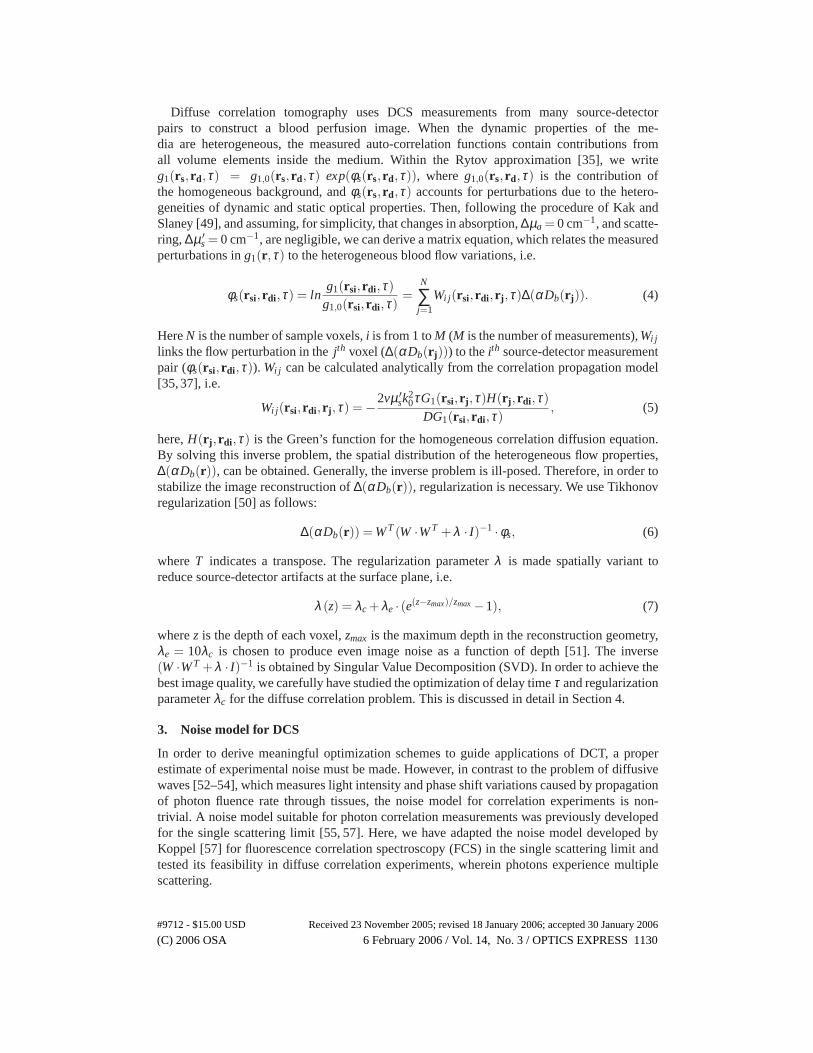
Fig. 2. (a) Comparison of measured noise (dots) and calculated noises using the model(solid lines). All input parameters for the noise model are obtained from experiments.Measurement noise decreases as the delay time τ increases. The “steps” are due to themulti-tau arrangement of our correlator. (b) Signal-to-Noise Ratio (SNR) comparison of themeasured correlation curves and the model predictions. Although the measurement noisedecreases as the delay time τ increases, the SNR of the DCS measurements also decreasesbecause the “signal” drops even faster as τ increases. (kcps = kilo-counts per second)

the bin time interval is T = 160 ns for the first 32 channels and is doubled every 16 channelsthereafter. Figure 2(a) shows that noise drops when the detected light intensity increases, asexpected from equation 8. On the timescales of interest (τ ∈ {10−6 s, 10−3 s}), the noise modelprovides a good estimate of the measurement noise in DCS, although it slightly overestimatesthe noise at large τ when the photon count rate is high. The failure of the noise model at largedelay time has also been observed in FCS studies [59, 60].

Figure 2(b) shows the signal-to-noise ratio (SNR) of the measured correlation curves,SNR = (g2(τ )− 1)/σ(τ ), at different light intensities. In Fig. 2(a) we see that the DCSmeasurement noise decreases as the delay time τ increases. However, the “signal” drops evenfaster as τ increases. As a result, the signal-to-noise ratio of the DCS measurement still de-creases as the delay time increases. The signal-to-noise ratio can be improved by increasingthe light intensity collected by the detector, as well as increasing the averaging time t (data notshown), but the SNR curves will have same general form.

After studying the noise in (g2(τ )−1), we have developed a technique to estimate the noisein the perturbation φs(rsi,rdi,τ ) for our image optimization. The noise of φs can be derived fromthe relations in equations 3, 4 and 8 as:

σφs(rsi,rdi,τ ) =12

σ(rsi,rdi,τ )(g2(rsi,rdi,τ )−1)

=12

1SNR

. (9)

This results in a perturbation noise that is higher at large delay time τ . We will use equation 9in the following section to derive the upper limit of the normalized image noise.

4. Optimization Criteria

In this section we describe in detail how to optimize data selection for the image reconstructionand how to choose the optimal regularization parameter to reduce image artifacts.

4.1. Choosing the optimal data set

Generally, we collect the entire correlation curve for each DCS measurement, which has∼ 200 data points, each corresponding to a different delay time, τ . DCT uses DCS measure-ments at different source-detector pairs; usually one data point from each correlation curve



10−7

10−6

10−5

10−4

10−30

0.2

0.4

0.6

0.8

1

τ (s)

g 1(τ)

n=4 n=1

n=0.25

Fig. 3. Example of the field auto-correlation function g1(τ ). Points corresponding to dif-ferent values of n are notated. n is defined as the point where g1(τ ) decreases to exp(−n)of its initial value (i.e. we write g1(τ ) = exp(−n)g1(0)).

is picked for the image reconstruction. Here, we introduce a parameter n, which defines thepoint where the field auto-correlation function decreases to exp(−n) of its initial value, i.e.g1(τ ) = exp(−n)g1(0) (shown in Fig. 3). From Eq. (2), it is easy to show that τ and n have thefollowing relationship,

τ =1

µ ′2s k2

0α Db(

n2

|rs − rd|2 − 2n√

3µaµ ′s

|rs − rd| ). (10)

For each n, the delay time τ is calculated using the above formula for each source-detectorpair, and is used to calculate the elements in the weight matrix W . The condition number of W(i.e. Nc = ϕmax/ϕmin, where ϕmax is the largest singular value of W and ϕmin is the smallest) isoften used to characterize the weight matrix. The larger the condition number, the bigger theerror amplification after the system is inverted. It can be shown that [61],

‖σ∆(α Db)‖‖∆(α Db)‖ ≤ ‖σφs‖

‖φs‖ ·Nc, (11)

where ‖ ‖ denotes the two-norm of a vector, i.e. ‖φs‖ =√

∑i φ2si. The upper limit of the nor-

malized image noise (‖σ∆(α Db)‖/‖∆(α Db)‖) can be estimated by computing the product of thenormalized measurement noise (‖σφs‖/‖φs‖) and the condition number of the weight matrix(Nc). Therefore, by calculating the upper limit of the normalized image noise for different n,the minimal point can be determined and the set of these minimal points defines the optimaldata set for image reconstruction.

4.2. Choosing optimal regularization parameter

The optimization of the regularization parameter λc is achieved by conducting a standard L-Curve analysis [62]. After a data set is chosen, a perfusion image ∆(α Db(r)) can be recon-structed with regularization parameter λc. The solution norm η (λc) = ‖∆(α Db(r))‖, whichprovides a measure of the fluctuation in the reconstructed images, and the normalized residualnorm, ξ (λc) = ‖W ·∆(α Db(r))−φs‖/‖φs‖, which shows the quality of the data fit, are thencalculated. Generally, we want to minimize both of these values to reduce image fluctuationsand obtain a good fit. If we calculate η (λc) and ξ (λc) for different λc and plot them on thex- and y-axis, an “L” shape curve will be obtained as shown in Fig. 5. The optimized λc isobtained at the elbow of the L-curve as the best compromise between improved data fitting and



Z

X

Yz=0.2cm

z=0.6cm

z=0.4cm

r=0.2cm, (0.4cm, 0.2cm, 0.4cm)

Sources and Detectors

(a)

−0.6 −0.3 0 0.3 0.6 −0.6

−0.3

0

0.3

0.6

x (cm)

y (c

m)

25 sources, 16 detectors

SourcesDetectors

(b)

Fig. 4. Simulation geometry: (a) A spherical object with a radius of 0.2 cm is placed ina homogeneous background at three distances from the source/detector plane (0.4 cm,0.2 cm, 0.4 cm). The dynamic property of the object is 10% lower than the background(α Db = 0.9× 10−8 cm2/s, α Db0 = 1× 10−8 cm2/s). The static optical properties of thesphere and background are the same (µa = 0.1 cm−1, µ ′

s = 8 cm−1). (b) 25 sources and16 detectors are placed at the z = 0 cm plane and cover a region ranging from -0.6 cm to0.6 cm in both the x and y dimensions. An analytical solution is used for the simulation.Measurement noise is calculated and added to the simulated data with a normal distribution.

0.1 1 10

106

107

108

n

Nc ⋅

||∆φ s||

/ ||φ

s||

(a)

0 0.5 1x 10

−7

0.5

0.6

0.7

0.8

0.9

1

ξ(λ c)

η(λc)

n=0.25n=1n=4Optimal λ

1=0.0052

Optimal λ2=0.0008

Optimal λ3=0.0176

(b)

Fig. 5. Choice of the optimal data set and optimal regularization parameter: (a) The nor-

malized image noise ‖σφs‖‖φs‖ ·Nc plotted as a function of n. The optimal data set is obtained

at n = 1, where the upper limit of the normalized image noise is a minimum. (b) L-Curveswith noisy data at different n are plotted to identify the optimal regularization parameter λ .The n = 1 curve is the closest to the origin, which also indicates the advantage of using adata set with n = 1 for image reconstruction.

reduced image noise (minimizing the norm of the reconstructions). In our study, the curvatureat each point of the L-Curve was calculated, the maximum curvature point was found and wasconsidered as optimal.

5. Simulation Results

In this section, we use simulated data to compare the image quality using different data sets anddifferent reconstruction schemes. The simulation geometry is on the same scale as our smallanimal models. Thus our conclusions can be directly used to improve image quality for ourin-vivo small animal studies.

As shown in Fig. 4, a spherical object with radius of 0.2 cm, whose center is located at(0.4 cm, 0.2 cm, 0.4 cm), sits in a homogeneous background. The dynamic property of the ob-



z=0cm z=0.2cm z=0.4cm z=0.6cm z=0.8cm

−0.8 0 0.8

0.8

0

−0.8

−10% −5 % 0 % 5 %

y x

cm

(a) Sim

(b) DRR

(c) SFR

(d) NFR

Fig. 6. Reconstructed images using data with n = 1. Reconstructed 3D images cover theregion (x: -0.8 cm - 0.8 cm, y: -0.8 cm - 0.8 cm, z: 0 cm - 0.8 cm) with 1 mm3 voxels. Im-ages at every 2 mm along the z direction are shown (from left to right). The depth for eachlayer is marked for each column. (a) Simulation (Sim) geometry. (b) Reconstructed im-ages using data directly from the noisy raw data (Direct Raw-data Reconstruction, DRR).The object is found at a displaced layer (z=0.6 cm). (c) Images using data from the fit-ted curve (by minimizing ‖g2m(τ )−g2c(τ )‖) to reconstruct the images (Smoothed FittingReconstruction, SFR). Image artifacts are greatly reduced. (d) Using noise information in

the fitting process (by minimizing ‖ g2m(τ )−g2c(τ )σ(τ ) ‖) can further improve the image quality

(Noise Fitting Reconstruction, NFR).

DRR SFR NFR Sim0

1

2

3

4

Nor

mal

ized

volu

me

wei

ghte

d rC

BF

(a)

DRR SFR NFR0

0.1

0.2

Loca

tion

Err

or (

cm)

(b)

DRR SFR NFR0

1

2

3

4

CN

R

(c)

Fig. 7. Quantitative comparison of different image reconstruction schemes: (a) Volumeweighted rCBF for the reconstructed object normalized to the simulation (Sim). Noise Fit-ting Reconstruction (NFR) gives the most accurate value compared to the simulation. (b)Distance from the center of the simulation to the center of the reconstructed object. NFRprovides the best location accuracy (∼ 1 mm). (c) Contrast to noise ratio (CNR) of thereconstructed images. NFR gives the highest CNR over the three reconstruction schemes.

ject is 10% lower than the background (i.e. α Db = 0.9×10−8cm2/s, α Db0 = 1×10−8 cm2/s),while the static optical properties of the sphere and background are the same (µa = 0.1 cm−1,µ ′

s = 8 cm−1). Twenty-five sources and 16 detectors are placed in the z = 0 cm plane and covera region ranging from -0.6 cm to 0.6 cm in both x and y dimensions. The analytical solutionfor a spherical perturbation [35, 54] is used to simulate noise-free measurement data for eachsource-detector pair. DCS measurement noise is then calculated based on Eq. (8) and added tothe noise free data with a normal distribution.

The noise in φs is estimated using Eq. (9) and‖σφs‖‖φs‖ ·Nc at different n, and is plotted in



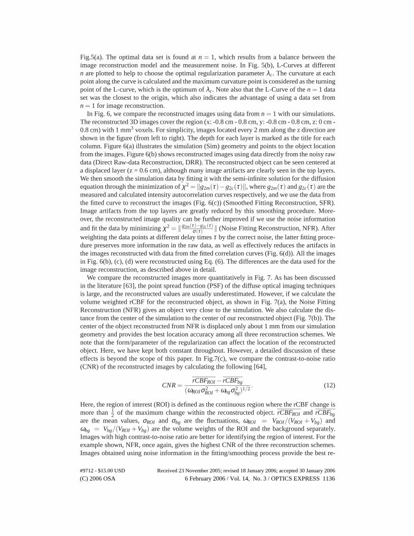
Fig.5(a). The optimal data set is found at n = 1, which results from a balance between theimage reconstruction model and the measurement noise. In Fig. 5(b), L-Curves at differentn are plotted to help to choose the optimal regularization parameter λc. The curvature at eachpoint along the curve is calculated and the maximum curvature point is considered as the turningpoint of the L-curve, which is the optimum of λc. Note also that the L-Curve of the n = 1 dataset was the closest to the origin, which also indicates the advantage of using a data set fromn = 1 for image reconstruction.

In Fig. 6, we compare the reconstructed images using data from n = 1 with our simulations.The reconstructed 3D images cover the region (x: -0.8 cm - 0.8 cm, y: -0.8 cm - 0.8 cm, z: 0 cm -0.8 cm) with 1 mm3 voxels. For simplicity, images located every 2 mm along the z direction areshown in the figure (from left to right). The depth for each layer is marked as the title for eachcolumn. Figure 6(a) illustrates the simulation (Sim) geometry and points to the object locationfrom the images. Figure 6(b) shows reconstructed images using data directly from the noisy rawdata (Direct Raw-data Reconstruction, DRR). The reconstructed object can be seen centered ata displaced layer (z = 0.6 cm), although many image artifacts are clearly seen in the top layers.We then smooth the simulation data by fitting it with the semi-infinite solution for the diffusionequation through the minimization of χ2 = ‖g2m(τ )−g2c(τ )‖, where g2m(τ ) and g2c(τ ) are themeasured and calculated intensity autocorrelation curves respectively, and we use the data fromthe fitted curve to reconstruct the images (Fig. 6(c)) (Smoothed Fitting Reconstruction, SFR).Image artifacts from the top layers are greatly reduced by this smoothing procedure. More-over, the reconstructed image quality can be further improved if we use the noise informationand fit the data by minimizing χ2 = ‖ g2m(τ )−g2c(τ )

σ(τ ) ‖ (Noise Fitting Reconstruction, NFR). Afterweighting the data points at different delay times τ by the correct noise, the latter fitting proce-dure preserves more information in the raw data, as well as effectively reduces the artifacts inthe images reconstructed with data from the fitted correlation curves (Fig. 6(d)). All the imagesin Fig. 6(b), (c), (d) were reconstructed using Eq. (6). The differences are the data used for theimage reconstruction, as described above in detail.

We compare the reconstructed images more quantitatively in Fig. 7. As has been discussedin the literature [63], the point spread function (PSF) of the diffuse optical imaging techniquesis large, and the reconstructed values are usually underestimated. However, if we calculate thevolume weighted rCBF for the reconstructed object, as shown in Fig. 7(a), the Noise FittingReconstruction (NFR) gives an object very close to the simulation. We also calculate the dis-tance from the center of the simulation to the center of our reconstructed object (Fig. 7(b)). Thecenter of the object reconstructed from NFR is displaced only about 1 mm from our simulationgeometry and provides the best location accuracy among all three reconstruction schemes. Wenote that the form/parameter of the regularization can affect the location of the reconstructedobject. Here, we have kept both constant throughout. However, a detailed discussion of theseeffects is beyond the scope of this paper. In Fig.7(c), we compare the contrast-to-noise ratio(CNR) of the reconstructed images by calculating the following [64],

CNR =rCBFROI − rCBFbg

(ωROIσ2ROI +ωbgσ2

bg)1/2

. (12)

Here, the region of interest (ROI) is defined as the continuous region where the rCBF change ismore than 1

2 of the maximum change within the reconstructed object. rCBFROI and rCBFbg

are the mean values, σROI and σbg are the fluctuations, ωROI = VROI/(VROI + Vbg) andωbg = Vbg/(VROI +Vbg) are the volume weights of the ROI and the background separately.Images with high contrast-to-noise ratio are better for identifying the region of interest. For theexample shown, NFR, once again, gives the highest CNR of the three reconstruction schemes.Images obtained using noise information in the fitting/smoothing process provide the best re-



sult.We have tried the optimization and reconstruction procedures for different simulation scales,

different optode configurations and different perturbations location and values. The optimiza-tion results were found to be consistent with the findings reported here. We have also triedusing multiple data points simultaneously from the correlation curve measured at each source-detector pair for the image reconstruction, but it has not as yet lead to any significant improve-ment in the image quality.

In summary, from computer simulations we find that the data set from n = 1 is optimalfor the image reconstruction. We also find that use of data from the fitted correlation curvescan improve image quality, and use of noise information in the fitting process gives a betterfit and further improves the image quality. These findings are applicable to cases wherein arelative image is reconstructed by comparison to a secondary measurement (e.g. a baseline or areference sample), and when reconstructing absolute images using numerical solutions from ahomogeneous background as the reference.

6. In-vivo 3D flow imaging of cortical spreading depression on rat brain

A portable, relatively fast (several seconds per frame), large field of view instrument was con-structed for imaging blood flow changes during cortical spreading depression (CSD) in therat [28, 30]. A non-contact probe with a grid-like pattern of source/detector fibers was devel-oped for this purpose (Fig. 8). The probe was mounted on the film-plane of a regular 35 mmcamera body, which acted as a light sealed, robust box to hold the lens system and probe. Thedepth-of-focus of the camera lens reduces the motion artifacts along the optical axis of thelens. This non-contact probe enabled manipulations to the animal without movement of theprobe, thereby avoiding some common experimental artifacts. Furthermore, crossed-polarizers(OFR Inc., NJ, USA) were used to reduce surface reflections from the tissue. Light from acontinuous wave, long coherence length laser source (Model TC40, SDL Inc., San Jose, CA,USA) operating at 800 nm was coupled to the non-contact probe through optical switches (Di-Con, CA, USA) in order to time-share the source positions. Eight fast, photon-counting APDs(SPCMAQR-14, Perkin-Elmer, Canada) with low dark current were used in parallel as DCSdetection units. The output of the APDs were fed into a custom built, fast, 9-channel corre-lator board (Correlator.com, Bridgewater, NJ, USA) to calculate the intensity auto-correlationfunction g2(τ ). The whole system was automated and controlled by a desktop computer. Threesource and eight detector positions were used for DCT measurements and a full frame wasacquired every ∼ 6.5 seconds.

Adult male Sprague-Dawley rats weighing 300-325 g were fasted overnight with free accessto water. They were anesthetized with a 1 - 1.5% halothane in a 70% nitrous oxide, 30% oxygenmixture. Catheters were placed into the femoral artery for monitoring of arterial blood pressure.Body temperature was maintained at 37±0.5oC by a controlled heating pad. The animals weretracheotomized, mechanically ventilated, and the head was fixed on a custom stereotaxic frame.Blood gases were obtained frequently and the respirator was adjusted in order to keep theblood gases within the normal physiological range. The scalp was retracted to avoid additionalcomplications due to the fur. A 2 mm burr-hole was made over the frontal cortex of the righthemisphere leaving the dura intact. CSD was evoked by placing a 1 mm3 filter paper soakedin 2 mol/L potassium chloride (KCl) onto the dura for the duration of the desired inductionof CSD waves (∼ 30 min). The paper was changed rapidly every 15 minutes. The setup isillustrated in Fig. 9. After measuring 5 - 10 CSD waves, the KCl was removed and the brainwas washed with saline. A total of six animals were studied and gave similar results, but wepresent here reconstructed images from one representative animal.

In order to reconstruct rCBF images during CSD, baseline measurements from each source-



Fig. 8. System setup for the in-vivo rat brain CSD study. A grid-like pattern ofsource/detector fibers (3 sources, 8 detectors) was mounted on the back of a 35 mm camerabody. The light was sent to and detected from the tissues through a relay lens avoidingcontact with the tissue. Light from a CW, long coherence length laser operating at 800 nmwas connected to the non-contact probe through optical switches in order to time-share thesource positions. The output of the APDs was fed into a custom built correlator board whichcalculated the intensity auto-correlation function g2(τ ). The whole system was automatedand controlled by a desktop computer and a full frame was acquired every ∼ 6.5 seconds.

KCl placed on brain through burr hole

Fig. 9. Cortical Spreading Depresstion (CSD); During experiments, a rat was fixed on astereotaxic frame with the scalp retracted and the skull intact. CSD was induced by placingKCl solution on the rat brain through a small hole drilled on the skull. Periodic activationsand deactivations of the neurons then spread out radially on the cortex as shown on thesketch.

detector pair were used as references to calculate the perturbations using Eq. (4). Backgroundoptical properties were kept constant as µa = 0.1 cm−1 and µ ′

s = 15 cm−1, while averageα Db = 4.5× 10−8 cm−2/s was calculated from baseline measurements at different source-detector pairs as the background dynamic property (see Section 7 for the discussion about theinfluence of µa, µ ′

s changes during CSD to our image reconstructions). After the weight matrixW was built, reconstructed flow images were optimized following the descriptions in Sections 4and 5. Since blood flow changes during CSD were large, reconstructed images using the linearRytov approximation usually underestimated flow values, but the position mappings should beaccurate [65]. Thus, we scaled the rCBF images obtained directly from the reconstruction to



Skullz=0mm

0 s

(mm)

(mm

)

−1 0 1

−4

−2

0

2

26 s 45 s 65 s 84 s 104 s 123 s 143 s

z = 0mm

Cortexz=1mm

0 s

(mm)(m

m)

−1 0 1

−4

−2

0

2

26 s 45 s 65 s 84 s 104 s 123 s 143 s

z = 1mm

Cortex(Bottom)z=2mm

0 s

(mm)

(mm

)

−1 0 1

−4

−2

0

2

26 s 45 s 65 s 84 s 104 s 123 s 143 s

z = 2mm

WhiteMatterz=3mm

0 s

(mm)

(mm

)

−1 0 1

−4

−2

0

2

26 s 45 s 65 s 84 s 104 s 123 s 143 s

rCBF (%)

z = 3mm

0 50 100 150 200

Fig. 10. Reconstructed 3D rCBF images at different layers (from top to bottom) of therat brain during CSD. CSD is induced at the top, slightly to the left of the midline(∼ x = 0 mm). Images (from left to right) are shown about every 20 seconds from im-mediately before KCl was applied until the end of the first CSD peak. rCBF responsesare mainly localized to the cortex and spread across the cortex tangentially from the pointwhere KCl was applied. No significant activity is visible in the top panel, which corre-sponds to the skull, and in the bottom panel, which penetrates below the cortex, indicatingthat the activity is localized in the cortex. Images are oriented as shown in Fig. 8(b).

match the bulk rCBF changes obtained from spectroscopy measurements over the matchingbrain regions.

Figure 10 shows the reconstructed rCBF images in different layers of the rat brain duringCSD. The burr-hole is located at the top, slightly to the left of the midline (∼ x = 0 mm). Eachpanel shown is averaged over 0.5 mm in the depth direction (z) starting with the top of the skull(z = 0 mm), and at 1 mm, 2 mm and 3 mm from top to bottom, respectively. Images (fromleft to right) are shown roughly every 20 seconds from immediately before KCl was applied(t ≈ 26 s) until the end of the first CSD peak. The panel titles indicate the correspondingtime point in this figure. Along the surface of the cortex (∼ 1 mm deep), a strong increase inblood flow appears from the top and proceeds to the bottom. It is quite significant that minimalactivity is visible in the top panel (which corresponds mostly to the skull) and in the bottompanel (which penetrates below the cortex).



Cortexz=1mm

0 s 143 s

162 s 299 s

318 s

(mm)

(mm

)

−1 0 1

−4

−2

0

2

455 s

rCBF (%)0 50 100 150 200

time

time

time

123

Fig. 11. rCBF changes on the cortex of the rat brain during CSD. Images (from left to right,from top to bottom) are shown roughly every 20 seconds from immediately before KCl wasapplied until the end of the second CSD peak. The panel titles indicate the correspondingtime point. A strong increase in blood flow appears from the top and proceeds to the bottomof the image. After the peak, there is a sustained decrease in blood flow which covers mostof the image area. Three regions of interest (ROI) were selected and the time series of rCBFchanges from these ROIs are plotted in Fig. 12(a). A movie showing the rCBF changes atdifferent brain layers during CSD is also provided as supporting media (1.5MB).

The time series images for the layer at 1 mm depth illustrates the spreading of two CSD wavesin the cortex (Fig. 11. A movie showing the rCBF changes at different brain layers during CSDis also provided as supporting media.). After the first peak, there is a sustained decrease in bloodflow (∼ 3 min) which covers most of the image area. The sustained decrease has been observedpreviously [39] and is compatible with inhibition of neuronal activity. Three regions of interestwere selected and the rCBF changes within them are plotted in Fig. 12(a). The propagation ofthe CSD waves can be clearly identified from the delay between each curve. Figure 12(b) showsthe dependence of maximal rCBF changes on depth using the data from the second region ofinterest (ROI-2) as in Fig. 11. The maximal change occurs at 1 mm (just below the skull) whichcorresponds to the surface of the cortex. The peak spreads ∼ 0.5 mm above and below thecortical surface as expected from the broadening due to the diffuse nature of photons. There isno significant change at the surface (z = 0 mm) and in the deep region (z = 3 mm). Note thatthe in-vivo images appear to have less “cross-contamination” across layers at different depthscompared to the simulation results. We believe this effect is real and is due to the localizationof CSD blood flow responses to the thin two-dimensional layer of rat brain cortex. Clearly,three-dimensional tomographic in-vivo relative blood flow information is revealed.

7. Discussion

The measurement noise of DCS depends on only a few parameters which can be obtainedexperimentally, and therefore can be estimated based on the model discussed in Section 3.Furthermore, the upper limit of the reconstructed image noise in DCT can be estimated usingthe DCS noise information at each source-detector pair. This, in turn, can be minimized bycorrect selection of the data set for the image reconstruction. We have parameterized the auto-correlation curve (parameter n, see Section 4, we note here n does not have to be integer)



http://www.opticsexpress.org/viewmedia.cfm?id=87781&seq=1

0 200 400 60050

100

150

200

sec

rCB

F (

%)

ROI−1ROI−2ROI−3

(a)

0 1 2 3 4100

120

140

160

180

rCB

F (

%)

Depth (mm)

(b)

Fig. 12. (a) Time series of rCBF changes from three ROIs illustrated in Fig. 11. From thesecurves, the propagation of the CSD waves can be clearly identified. (b) Dependence ofmaximum rCBF on depth in the second region of interest. The maximal change is localizedat a depth of 1 mm below the skull. This corresponds to the surface of the cortex. The peakspreads ∼ 0.5 mm above and below the cortical surface as expected from the broadeningdue to the diffuse nature of photons (see text). There is no significant change at the surface(skull) or in deeper regions.

and n = 1, corresponding to g1(τ ) = exp(−1), was found to be the optimal data point for theimage reconstruction. Previously, we reported that the condition number of the weight matrixdecreased as we increase the parameter n [66]. By contrast, the noise model teaches that a dataset derived from small n (e.g. n = 0.25), where the noise in φs is low, does not improve imagequality because the condition number of the weight matrix is large, i.e. the measurement noiseis amplified to intolerable levels when the weight matrix is inverted; however, using a dataset derived from large n, where the condition number is small, does not help either, becausethe noise in the Rytov scattered data (φs) is increased in this regime. The interplay of thesetwo effects is balanced by using a data set from n = 1, i.e. both the condition number and themeasurement noise in φs are optimized. The development of this model was a key theoreticalaspect of the present work.

The noise model enabled us to calculate the theoretical signal-to-noise-ratio (SNR) of theDCS measurement, i.e. (g2(τ )− 1)/σ(τ ), which in turn provides practical guidelines for ex-perimental design. In contrast to diffuse optical near-infrared spectroscopy (NIRS) whereinfiber bundles can be used to increase detection area, diffuse correlation spectroscopy typicallyemploys single mode fibers with diameters ∼ 6 µm to detect intensity fluctuations within a sin-gle speckle area. This limits the amount of light that can be collected at large separations (e.g.> 3 cm) by the flow detectors. (Although it is possible to employ multiple detectors at nearlythe same position to improve signal-to-noise ratio.) As a result, the SNR of the DCS measure-ment is greatly reduced when the light intensity is low, as demonstrated in Fig. 2(b). Recently,the use of few-mode fibers for DCS detection have been reported [34]; in this case more lightcan be collected from a few speckles. However, the value of β (see Section 2, equation 3) is in-versely proportional to the number of speckles within the detection area, and so would decreaseby the same amount, and the product β〈n〉 is about the same as if a single-mode fiber was used.Therefore the noise model suggests that the SNR of the measurement would not improve whenmulti-mode/few-mode fibers are used. This observation was confirmed experimentally (data notshown). Ultimately, in order to increase the signal-to-noise ratio, it is necessary to adjust theaveraging time, the input light power, and/or the number of fibers/detectors working in parallel.

The development of the noise model also proved to be useful in fitting the DCS data. The bestfitting curves are derived when an error can be assigned to each data point from the collected



DCS curve. By weighting all the data points with the appropriate estimated measurement noisein the definition of χ2 [67], e.g. χ2 = ‖ g2m(τ )−g2c(τ )

σ(τ ) ‖, each data point from the curve is betterused in the fitting. We have shown that if the estimated noise information is considered, thereconstructed image quality is thus improved (see Section 5). From a phantom study, we alsoobserved a smaller standard deviation in fitted α Db when the estimated noise was used in thefitting (data not shown), especially when the measured DCS curves were noisy. This will beimportant when using more complex models to fit spectroscopy data, for example, in brainmeasurements where multiple layers should be considered [34, 43, 46].

Finally we examine some of the assumptions used for rCBF diffuse correlation tomographyimage reconstructions. One of our assumptions was that the static optical properties (µa, µ ′

s)do not change during activation. This assumption may be incorrect for in-vivo animal studies.Kohl et al reported in-vivo dynamic oxygenation and scattering changes during cortical spread-ing depression [68], for example, and found that the magnitude of the optical property changeswere relatively small (∆HbO2 ∼ +15 µM, ∆Hb ∼ -7 µM and ∆µ ′

s ∼ 1 cm−1). Compared tothe baseline brain optical properties we measured and used in our image reconstruction, theserelative changes in both µa and µ ′

s are less than 7%. To this end, we changed the global opticalproperties by the same amount during CSD, and no significant changes in the reconstructedrCBF images were observed (i.e. changes in the image voxels were less than 10 %). In practice,it is desirable to carry out frequency domain diffuse optical tomography measurements concur-rently with the diffuse correlation tomography measurement for in-vivo studies. It will then bepossible to reconstruct absorption and scattering images from DOT first, and use them for cal-culating DCT Green’s functions, thereby reducing the optical property influence on blood flowimage reconstructions. Furthermore, by combining the DOT and DCT images, it is possible toimage the cerebral metabolism rate of oxygen (CMRO2) in three dimensions [28, 69].

Over the past thirty years, there has been great interest in measuring cerebral blood flow, oxy-gen consumption and metabolic responses during cortical spreading depression [9, 10, 70–73].The optical imaging technique we describe in this paper provides reliable three-dimensionalin-vivo images of rCBF during CSD with a relatively fast frame rate (∼ 0.15 Hz) and moder-ate transverse and depth resolution (∼ 0.5 mm). The relative blood flow changes we observedduring CSD, an initial strong increase followed by a sustained decrease, is consistent with ob-servations from other techniques such as laser Doppler flowmetry (1D) [70], scanning laserDoppler imaging [10], and laser speckle imaging (2D) [9]. The strong increase of rCBF is be-lieved to be coupled to the increase of oxygen consumption [71, 74], which in turn can alsobe directly measured using the diffuse optical imaging methods as discussed above. On theother hand, in addition to its capability for providing three dimensional blood flow images, thenon-invasive nature of our technique is desirable for studying brain activity in-vivo. We haverecently extended this technique for local measurements of rCBF in adult human brain [29] andit is conceivable to adapt methods developed in this paper for regional imaging of relative bloodflow in a variety of human tissues.

8. Conclusion

In summary, we have demonstrated tomographic three-dimensional relative blood flow imagesusing diffuse correlation measurements. A noise model for DCS measurements was introducedand its accuracy in the multiple scattering regime was studied by experiment and simulation.Optimized data sets and regularization parameters for the image reconstruction were derived,and the optimal data set was achieved at time-points wherein the field auto-correlation functiong1(τ ) decreases to 1/e of its initial value. Our findings were then employed in the study of thecortical spreading depression in a rat brain, and three-dimensional in-vivo blood flow imagesduring CSD were obtained using the diffuse optical correlation tomography technique.



Acknowledgments

We thank Alper Corlu, Goro Nishimura, Joseph P. Culver, David A. Boas and Douglas J. Durianfor useful discussions and gratefully acknowledge funding from the National Institute of Healthgrants 2-RO1-HL-57835-04, and NS-033785.

Appendix

In this section, we briefly outline the derivation of the noise model for DCS measurements asin Eq. (8) following the steps in [57].

In reality, the measured intensity auto-correlation function G2(τ ) is calculated as

G2(τ ) =1N

N

∑i=1

n(iT )n(iT + τ ), (13)

where τ is the delay time, T is the correlator bin time interval, n(iT ) is the number of photoncounts in time iT , N is the total number of the measurements (exposure time t = NT ). Herein,we will use 〈〉 to represent the true value of a parameter, and ˆ to denote the experimentalestimate of the true value. We begin by defining a parameter

S(τ ) ≡ G2(τ )− n2, (14)

where n = ∑Ni=1 n(iT ), and

n2 = [〈n〉− (〈n〉− n)]2

≈ 〈n〉2(1−2〈n〉− n〈n〉 )

= 2〈n〉n−〈n〉2. (15)

The noise of the normalized intensity autocorrelation function (g2(τ )− 1) can be obtained bynormalizing the variance of S(τ ), as

σ(τ ) =

√var(S(τ ))

〈n〉4 . (16)

Using Eqs. (13), (14), and (15), the variance of S(τ ) can be written as

var(S(τ )) = var(G2(τ )−2〈n〉n)

= var(1N

N

∑i=1

n(iT )[n(iT + τ )−2〈n〉]). (17)

If we definex(iT ) ≡ n(iT )[n(iT + τ )−2〈n〉], (18)

Eq. (17) can be expanded as [75]

var(S(τ )) = N−1var(x)+2N−1N−1

∑k=1

[〈x(0)x(kT )〉−〈x〉2]× (1− kN−1). (19)

Using the fact in photon statistics [76],

〈 n(iT )!(n(iT )− l)!

〉 = 〈I(iT )l〉, (20)



where n(iT ) and I(iT ) are the photon count and the light intensity in time iT seperately, andwriting the higher order correlation functions as sums of products of the second order cor-relation functions [77], an analytical expression of the variance of S(τ ) can be derived forexponentially decayed (g2(τ )−1) = βe−2Γτ after tedious math,

var(S(τ )) =1N

[〈n〉4β2 (1+ e−2ΓT )(1+ e−2Γτ )+2m(1− e−2ΓT )e−2Γτ

(1− e−2ΓT )

+ 2〈n〉3β(1+ e−2Γτ )+ 〈n〉2(1+βe−Γτ )]. (21)

Consequently, the noise (σ(τ )) of the normalized intensity autocorrelation function (g2(τ )−1)can be expressed as

σ(τ ) =

√Tt[β2 (1+ e−2ΓT )(1+ e−2Γτ )+2m(1− e−2ΓT )e−2Γτ

(1− e−2ΓT )

+ 2〈n〉−1β(1+ e−2Γτ )+ 〈n〉−2(1+βe−Γτ )]1/2, (22)

as shown in Eq. (8). And in the limit of ΓT � 1, which is satisfied in most of our experiments,

σ(τ )=

√1Γt

[β2(1+e−2Γτ +2mΓTe−2Γτ )+2〈n〉−1βΓT (1+e−2Γτ )+〈n〉−2ΓT (1+βe−Γτ )]1/2.

(23)



Diffuse optical correlation tomography of cerebral blood flow during cortical spreading depression...

Documents

Transcript of Diffuse optical correlation tomography of cerebral blood flow during cortical spreading depression...