ChronoGeoGraph: An expressive spatio-temporal conceptual model
Upload
independentCategory
view
4download
0
Project SD/TA/08 - “Development of an integrated spatio-economic-ecological model methodology for the analysis of sustainability policy “ISEEM”
SSD - Science for a Sustainable Development – Transversal Actions 0
DEVELOPMENT OF AN INTEGRATED SPATIO-ECONOMIC-
ECOLOGICAL MODEL METHODOLOGY FOR THE
ANALYSIS OF SUSTAINABILITY POLICY
“ISEEM”
C. HEYNDRICKX, O. IVANOVA, A. VAN STEENBERGEN, I. MAYERES, B. HAMAIDE, T. ERALY, F. WITLOX

Transversal Actions
SCIENCE FOR A SUSTAINABLE DEVELOPMENT (SSD)
FINAL REPORT
DEVELOPMENT OF AN INTEGRATED SPATIO-ECONOMIC-ECOLOGICAL MODEL METHODOLOGY FOR THE ANALYSIS
OF SUSTAINABILITY POLICY
“ISEEM”
SD/TA/08A
Promotors Christophe Heyndrickx
Transport en Mobility Leuven (TML) Inge Mayeres
Federal Planning Bureau (FPB) Bertrand Hamaide
Facultés Universitaires Saint-Louis (FUSL) Frank Witlox
Ghent University (UGent) Authors
Christophe Heyndrickx (TML/UGent) Dr. Olga Ivanova (TML/TNO) Alex Van Steenbergen (FPB)
Dr. Inge Mayeres (FPB) Prof. Bertrand Hamaide (FUSL)
Thomas Eraly (FUSL) Prof. Frank Witlox (UGent)
February 2009

Rue de la Science 8 Wetenschapsstraat 8 B-1000 Brussels Belgium Tel: +32 (0)2 238 34 11 – Fax: +32 (0)2 230 59 12 http://www.belspo.be Contact person: Marie-Carmen Bex +32 (0)2 238 34 81 Neither the Belgian Science Policy nor any person acting on behalf of the Belgian Science Policy is responsible for the use which might be made of the following information. The authors are responsible for the content.
No part of this publication may be reproduced, stored in a retrieval system, or transmitted in any form or by any means, electronic, mechanical, photocopying, recording, or otherwise, without indicating the reference :
Christophe Heyndrickx, Olga Ivanova, Alex Van Steenbergen, Inge Mayeres, Bertrand Hamaide, Thomas Eraly, Frank Witlox. Development of an integrated spatio-economic-ecological model methodology for the analysis of sustainability policy “ISEEM” Final Report Brussels : Belgian Science Policy 2009 – 129 p. (Science for a Sustainable Development)

Project SD/TA/08 - “Development of an integrated spatio-economic-ecological model methodology for the analysis of sustainability policy “ISEEM”
SSD - Science for a Sustainable Development – Transversal Actions 3
Table of Contents
1. INTRODUCTION ....................................................................................................................................9 1.1 DESCRIPTION OF THE MODEL ................................................................................................................................ 9 1.2 DIFFERENCE BETWEEN RAEM AND ISEEM .................................................................................................... 11 1.3 WHAT ARE THE POSSIBLE APPLICATIONS OF ISEEM? ...................................................................................... 12 1.4 WHAT ARE THE DRAWBACKS OF ISEEM?........................................................................................................... 13
2. STRUCTURE OF THE MODEL........................................................................................................... 15 2.1 HOUSEHOLDS.......................................................................................................................................................... 16
2.1.1 Household income, savings and consumption budget ............................................................................................... 16 2.1.2 Household utility’................................................................................................................................................. 17 2.1.3 Household welfare ................................................................................................................................................ 18 2.1.4 Passenger trips for different purposes...................................................................................................................... 18 2.1.5 Housing stock and residential emissions ................................................................................................................ 19
2.2 FIRMS........................................................................................................................................................................ 19 2.2.1 Production technology............................................................................................................................................ 19 2.2.2 Energy inputs and sector emissions ........................................................................................................................ 21 2.2.3 Monopolistic competition....................................................................................................................................... 22 2.2.4 Business trips ....................................................................................................................................................... 23 2.2.5 Total factor productivity ............................................................................................................................. 23
2.3 GOVERNMENT ........................................................................................................................................................ 24 2.3.1 Government tax income and subsidies ................................................................................................................... 24 2.3.2 Government transfers............................................................................................................................................ 24 2.3.3 Government consumption ...................................................................................................................................... 25
2.4 TRADE ...................................................................................................................................................................... 26 2.4.1 Imports and interregional trade ............................................................................................................................. 26 2.4.2 Exports ............................................................................................................................................................... 27
2.5 LABOUR MARKET .................................................................................................................................................... 28 2.5.1 Vacancies, interregional commuting and unemployment .......................................................................................... 28 2.5.2 Labour supply and migration................................................................................................................................ 29 2.5.3 Regional wages ..................................................................................................................................................... 29
2.6 LAND AND BUILDINGS........................................................................................................................................... 30 2.7 INVESTMENTS.......................................................................................................................................................... 30 2.8 MARKET EQUILIBRIUM CONDITIONS................................................................................................................... 31 2.9 RECURSIVE DYNAMICS ........................................................................................................................................... 31
3. DATABASE AND CALIBRATION ....................................................................................................... 35 3.1 CONSTRUCTION OF THE SUPPLY AND USE TABLES AND SOCIAL ACCOUNTING MATRIX .............................. 35
3.1.1 The construction of the supply and use tables.......................................................................................................... 35 3.1.2 Contruction of the social accounting matrix............................................................................................................ 39
3.2 ACCOUNTS OF FEDERAL AND REGIONAL GOVERNMENTS ............................................................................... 41 3.3 TRANSPORT RELATED DATA ................................................................................................................................. 42
3.3.1 Freight flows and transport costs ........................................................................................................................... 42 3.3.2 Commuting and education trips............................................................................................................................. 42 3.3.3 Business, shopping and other trips ......................................................................................................................... 43
3.4 ELASTICITIES ........................................................................................................................................................... 43 3.5 LABOUR MARKET DATA ......................................................................................................................................... 43
3.5.1 Auxiliary data on population, unemployment........................................................................................................ 43 3.5.2 Vacancies ............................................................................................................................................................ 43 3.5.3 Wages and unemployment benefits......................................................................................................................... 44

Project SD/TA/08 - “Development of an integrated spatio-economic-ecological model methodology for the analysis of sustainability policy “ISEEM”
SSD - Science for a Sustainable Development – Transversal Actions 4
3.6 EMISSIONS DATA..................................................................................................................................................... 44 3.6.1 Source of data on different emission types ............................................................................................................... 44 3.6.2 Monetary valuation of the emission damages .......................................................................................................... 45
3.7 SOCIO-ECONOMIC DATA........................................................................................................................................ 45 3.7.1 Consumption by income decile ............................................................................................................................... 45 3.7.2 Income, transfers and taxes by income decile........................................................................................................... 46
3.8 DATA ON STRUCTURE OF FIRMS ........................................................................................................................... 47 3.8.1 Land and buildings as production factors............................................................................................................... 47 3.8.2 Number of firms .................................................................................................................................................. 47
4. INDICATORS.......................................................................................................................................... 49 4.1 INTRODUCTION................................................................................................................................................ 49 4.2 INDICATORS OF SUSTAINABILITY............................................................................................................ 49
4.2.1 Developing an indicator for sustainability .............................................................................................................. 49 4.2.2 The choice for traditional indicators rather than composite indexes .......................................................................... 50
4.3 LIST OF INDICATORS....................................................................................................................................... 51 5. POLICY SIMULATIONS AND RESULTS ........................................................................................... 53
5.1 TECHNICAL SIMULATION: LOWER COMMUTING TIMES WITH AN EXTENDED LABOUR MARKET
FORMULATION ....................................................................................................................................................................... 53 5.1.1 Calibration .......................................................................................................................................................... 53 5.1.2 The extended model .............................................................................................................................................. 54 5.1.3 Simulations.......................................................................................................................................................... 55
5.2 NOX-CHARGE ........................................................................................................................................................ 58 5.2.1 Introduction ......................................................................................................................................................... 58 5.2.2 Results................................................................................................................................................................. 59 5.2.3 Interpretation ....................................................................................................................................................... 61
5.3 FREIGHT CHARGE SIMULATION............................................................................................................................ 63 5.3.1 Introduction ......................................................................................................................................................... 63 5.3.2 Simulation set up and assumptions ....................................................................................................................... 64 5.3.3 Results................................................................................................................................................................. 65
5.4 TAX ON LAND VERSUS DECREASE IN LAND ENDOWMENTS ............................................................................. 74 5.4.1 Simulation description .......................................................................................................................................... 74 5.4.2 Results................................................................................................................................................................. 75 5.4.3 Introducing a land supply curve ............................................................................................................................. 79 5.4.4 Conclusions .......................................................................................................................................................... 82
6. ISEEM MODEL IMPLEMENTATION IN GAMS.............................................................................. 85 6.1.1 About GAMS.................................................................................................................................................... 85 6.1.2 Main structure of the code ..................................................................................................................................... 85 6.1.3 General rules when editing the code........................................................................................................................ 87 6.1.4 Model numeraire .................................................................................................................................................. 88 6.1.5 Closure of the model and exogenously fixed variables.............................................................................................. 88 6.1.6 How to implement simulations with the model ....................................................................................................... 89 6.1.7 Model reporting .................................................................................................................................................... 90 6.1.8 If the model does not run....................................................................................................................................... 90
7. BIBLIOGRAPHY .................................................................................................................................... 91 ANNEX I: ELASTICITIES ............................................................................................................................. 93 ANNEX II: MATHEMATICAL APPENDIX ................................................................................................ 95 ANNEX III: LIST OF INDICATORS USED IN THE MODEL................................................................113
Project SD/TA/08 - “Development of an integrated spatio-economic-ecological model methodology for the analysis of sustainability policy “ISEEM”
SSD - Science for a Sustainable Development – Transversal Actions 5
Index of figures Figure 2.1 Tree of nested CES production function, based on HERMES....................................................20 Figure 2.2 CES-tree for the international and interregional trade ...................................................................26 Figure 3.1 General structure of a Use Table .......................................................................................................35 Figure 3.2 Energy intensity across provinces for a number of industrial sectors (percentage of output).36 Figure 3.3 General structure of a Supply table....................................................................................................38 Figure 3.4 Expenditure shares on different goods, per income decile (low to high: D1-D10)...................46 Figure 5.1 Tax rates on energy use by industrial sectors ...................................................................................58 Figure 5.2 Percentage change in provincial and national GDP for 5 scenario’s ...........................................60 Figure 5.3 Percentage change in production for the energy sector .................................................................60 Figure 5.4 EV for the poorest decile (Decile 1)..................................................................................................61 Figure 5.5 EV for the richest decile (Decile 10) .................................................................................................61 Figure 5.6 % Change in total GDP from taxed (freight) and untaxed (serv) sectors ...................................68 Figure 5.7 Changes in GDP compared for BE scenario with and without redistribution ..........................69 Figure 5.8 Pollution reduction by sector..............................................................................................................73 Figure 5.9 GDP per sector, TAX and LEND scenarios...................................................................................77 Figure 5.10 Investments by sector of destination (TAX scenario) ....................................................................78 Figure 5.11 Effect on regional GDP in the TAX and LEND scenario............................................................78 Figure 5.12 Change in GDP by sector, TAX and LEND scenario ...................................................................79 Figure 5.13 Changes in GDP, comparison across scenarios ..............................................................................81 Figure 5.14 Regional welfare of lowest (D1) and highest (D10) income decile .............................................82

Project SD/TA/08 - “Development of an integrated spatio-economic-ecological model methodology for the analysis of sustainability policy “ISEEM”
SSD - Science for a Sustainable Development – Transversal Actions 6
Index of tables Table 2.1 Subscripts within the mathematical formulation .............................................................................15 Table 2.2 Commodities/sectors within the ISEEM model.............................................................................15 Table 3.1 Overview of data on Belgian Government.......................................................................................41 Table 3.2 Monetary value ammonia emissions based on (Zuidema T & Nentjes A, 2001) .......................45 Table 3.3 Intial distribution of income, benefits and taxes between household income deciles
(EUROMOD 2003) .............................................................................................................................46 Table 4.1 Overview of the basic indicators of ISEEM ....................................................................................51 Table 5.1 Labour commuting from and towards Brussels ..............................................................................54 Table 5.2 Percentual changes in job matches from and towards Brussels ....................................................56 Table 5.3 Percentual changes in job commuters from and towards Brussels ..............................................56 Table 5.4 Percentual changes in a number of variables. ..................................................................................56 Table 5.5 Percentage change in income and equivalent variation for a number of deciles........................57 Table 5.6 Employer’s payroll tax rate and Flemish tax credits initially and in 5 scenarios.........................59 Table 5.7 Percentage change in GDP due to a Flemish labour to capital tax swap ....................................62 Table 5.8 Taxes implemented within ISEEM....................................................................................................65 Table 5.9 Results from the BE and FL scenario on country level (% change from basecase). .................66 Table 5.10 Revenues from kilometer charge in different provinces ................................................................66 Table 5.11 Effect on budget of main regional governments.............................................................................67 Table 5.12 Main results on province level (GDP, consumption, unemployment and inflation) ................68 Table 5.13 Regional economic effects BE scenario with and without redistribution ...................................69 Table 5.14 Welfare changes, measure in equivalent variation (EV) .................................................................70 Table 5.15 Main results on province level (Gini coefficient and poverty gap)...............................................70 Table 5.16 Regional welfare BE scenario and BE redistribution scenario......................................................71 Table 5.17 Social indicators on regional level, BE and BE + redistribution ..................................................71 Table 5.18 Monetary value of emission damages. totals in million euro (absolute changes). ......................72 Table 5.19 Country level effects: main indicators ...............................................................................................76 Table 5.20: Results of SUPPLY simulation, compared with TAX and LEND scenarios.............................80 Table 5.21 Percentual change in land prices and land supply ...........................................................................81
Project SD/TA/08 - “Development of an integrated spatio-economic-ecological model methodology for the analysis of sustainability policy “ISEEM”
SSD - Science for a Sustainable Development – Transversal Actions 7
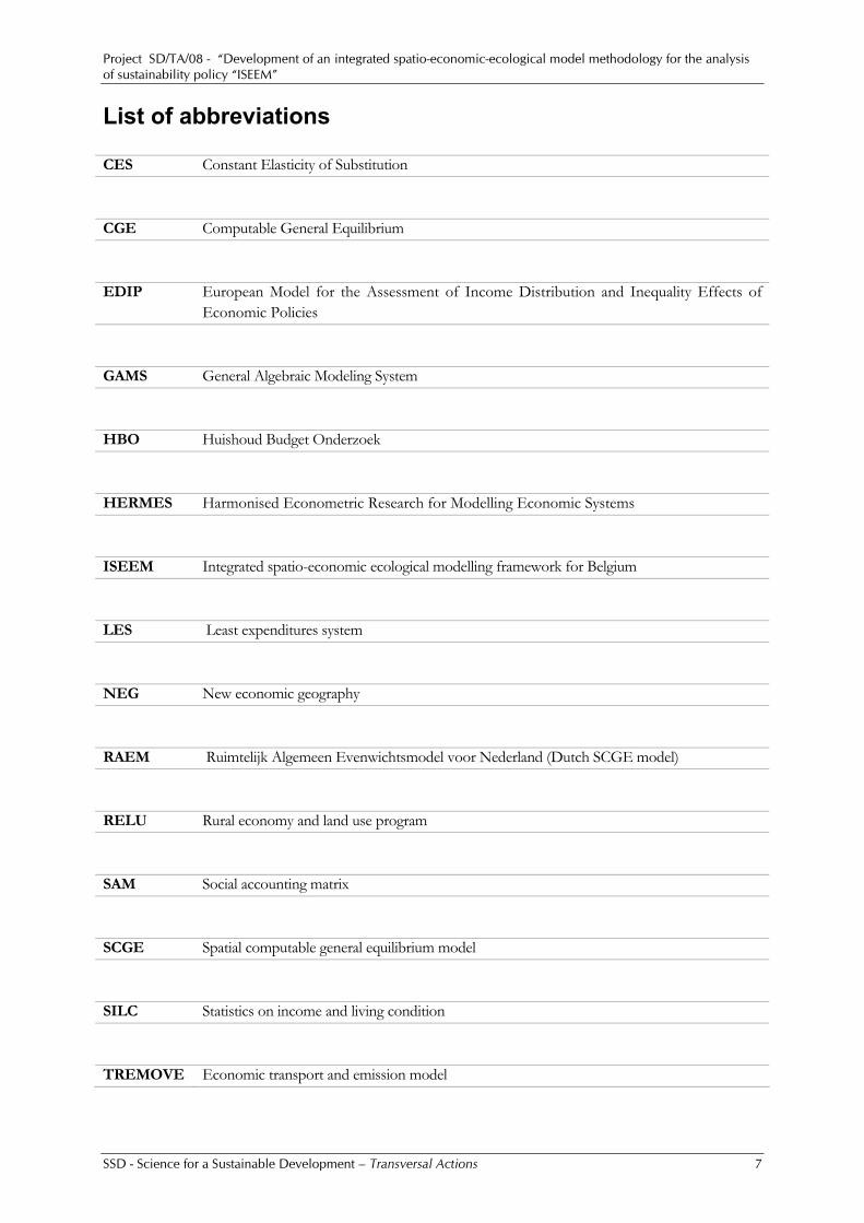
List of abbreviations CES Constant Elasticity of Substitution
CGE Computable General Equilibrium
EDIP European Model for the Assessment of Income Distribution and Inequality Effects of Economic Policies
GAMS General Algebraic Modeling System
HBO Huishoud Budget Onderzoek
HERMES Harmonised Econometric Research for Modelling Economic Systems
ISEEM Integrated spatio-economic ecological modelling framework for Belgium
LES Least expenditures system
NEG New economic geography
RAEM Ruimtelijk Algemeen Evenwichtsmodel voor Nederland (Dutch SCGE model)
RELU Rural economy and land use program
SAM Social accounting matrix
SCGE Spatial computable general equilibrium model
SILC Statistics on income and living condition
TREMOVE Economic transport and emission model

Project SD/TA/08 - “Development of an integrated spatio-economic-ecological model methodology for the analysis of sustainability policy “ISEEM”
SSD - Science for a Sustainable Development – Transversal Actions 9
1. Introduction
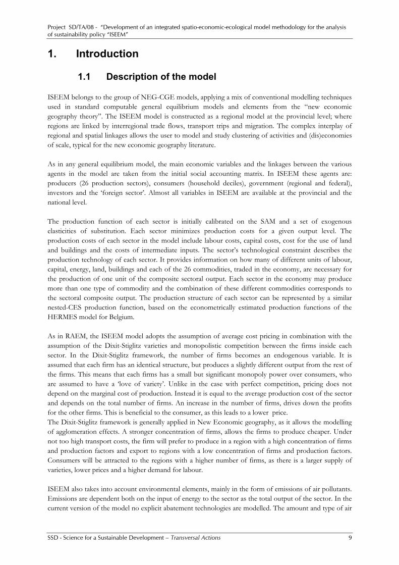
1.1 Description of the model ISEEM belongs to the group of NEG-CGE models, applying a mix of conventional modelling techniques used in standard computable general equilibrium models and elements from the “new economic geography theory”. The ISEEM model is constructed as a regional model at the provincial level; where regions are linked by interregional trade flows, transport trips and migration. The complex interplay of regional and spatial linkages allows the user to model and study clustering of activities and (dis)economies of scale, typical for the new economic geography literature. As in any general equilibrium model, the main economic variables and the linkages between the various agents in the model are taken from the initial social accounting matrix. In ISEEM these agents are: producers (26 production sectors), consumers (household deciles), government (regional and federal), investors and the ‘foreign sector’. Almost all variables in ISEEM are available at the provincial and the national level. The production function of each sector is initially calibrated on the SAM and a set of exogenous elasticities of substitution. Each sector minimizes production costs for a given output level. The production costs of each sector in the model include labour costs, capital costs, cost for the use of land and buildings and the costs of intermediate inputs. The sector’s technological constraint describes the production technology of each sector. It provides information on how many of different units of labour, capital, energy, land, buildings and each of the 26 commodities, traded in the economy, are necessary for the production of one unit of the composite sectoral output. Each sector in the economy may produce more than one type of commodity and the combination of these different commodities corresponds to the sectoral composite output. The production structure of each sector can be represented by a similar nested-CES production function, based on the econometrically estimated production functions of the HERMES model for Belgium. As in RAEM, the ISEEM model adopts the assumption of average cost pricing in combination with the assumption of the Dixit-Stiglitz varieties and monopolistic competition between the firms inside each sector. In the Dixit-Stiglitz framework, the number of firms becomes an endogenous variable. It is assumed that each firm has an identical structure, but produces a slightly different output from the rest of the firms. This means that each firms has a small but significant monopoly power over consumers, who are assumed to have a ‘love of variety’. Unlike in the case with perfect competition, pricing does not depend on the marginal cost of production. Instead it is equal to the average production cost of the sector and depends on the total number of firms. An increase in the number of firms, drives down the profits for the other firms. This is beneficial to the consumer, as this leads to a lower price. The Dixit-Stiglitz framework is generally applied in New Economic geography, as it allows the modelling of agglomeration effects. A stronger concentration of firms, allows the firms to produce cheaper. Under not too high transport costs, the firm will prefer to produce in a region with a high concentration of firms and production factors and export to regions with a low concentration of firms and production factors. Consumers will be attracted to the regions with a higher number of firms, as there is a larger supply of varieties, lower prices and a higher demand for labour. ISEEM also takes into account environmental elements, mainly in the form of emissions of air pollutants. Emissions are dependent both on the input of energy to the sector as the total output of the sector. In the current version of the model no explicit abatement technologies are modelled. The amount and type of air

Project SD/TA/08 - “Development of an integrated spatio-economic-ecological model methodology for the analysis of sustainability policy “ISEEM”
SSD - Science for a Sustainable Development – Transversal Actions 10
pollutants emitted is specific for each sector. Besides CO2, we distinguish several greenhouse gasses such as NO2, CH4, SF6 and several non greenhouse pollutants such as PM10, NOx, SOx, NH3. The outputs of the domestic sectors are either consumed inside the country or exported abroad. Domestic sales of each of the 26 types of commodities are composed of the commodities produced by the domestic sectors, those imported from the EU25 and those imported from the rest of the world. According to the Armington assumption, the same type of commodity produced by the domestic sectors, imported from the EU25 or imported from the rest of the world has different specifications and, hence, cannot be treated as a homogenous good. Domestic consumers have different preferences for these three specifications and can substitute between them in case the relative prices of the specifications change. The substitution possibilities between these three commodity specifications are represented by the Armington elasticity of substitution and vary between the types of commodities. The shares in which a commodity is bought from the domestic producers, from the EU25 and from the rest of the world are determined by the relative producer prices of the commodity inside the country, in the EU25 and in the rest of the world as well as by the Armington elasticity of substitution. The ISEEM model distinguishes multiple households in each province. These households are aggregate economic agents that represent the behaviour of a part of the population. Each household type represents one income decile, ordered from the poorest to the richest part of the population. The households vary in the composition of their consumption bundle, savings, income taxes, factor endowments, income from transfers and unemployment benefits. The main assumption made, is that the behaviour of the household can be characterized by the mean household income. Each household spends its consumption budget on services and goods in order to maximize its satisfaction from the chosen consumption bundle. The utility of the household is maximized under the budget constraint, where the household’s consumption spending is equal to its income minus income tax and the household’s savings. Households and domestic sectors use transport services in their consumption and production activities. The passenger transportation services in the model are used for different purposes, which are represented separately. These include business, commuting, shopping, education and travel. The number of trips associated with each of these purposes is generated by means of specific trip generation functions, which take into account the time and monetary costs of travel as well as a set of the attraction factors for the trips. Commuting is modelled in a different way, inspired by the Pissarides approach for modelling unemployment. It is assumed that each region posts a set of vacancies, based on the job destruction and vacancy generation rate within each region. An increase in the demand for labour leads to an increase in the amount of vacancies, which can be filled in by unemployed within the region as well as unemployed from the other regions. The probability that a match occurs between an unemployed and an open vacancy depends negatively on the time and monetary cost between the regions. In ISEEM the federal government structure of Belgium has been incorporated in detail. In ISEEM we distinguish, besides the Federal Government (which also includes the municipalities): the Flemish region,1 Walloon region, French language community, Brussels region and 3 smaller governments within Brussels. The income and expenditures of each regional government and the federal government are modelled
1 The model is constructed on the provincial level, or otherwise said the Belgian NUTS-2 level. We use region here to refer to the NUTS-1 level. The Flemish region is composed of the provinces of Antwerp, Limburg, Oost-Vlaanderen, West-Vlaanderen, Vlaams Brabant. The Walloon region is composed of Hainaut, Luxemburg, Liège, Namur and Brabant Wallon. The province of Brussel is equal to its NUTS-2 regional division.

Project SD/TA/08 - “Development of an integrated spatio-economic-ecological model methodology for the analysis of sustainability policy “ISEEM”
SSD - Science for a Sustainable Development – Transversal Actions 11
separately. The federal government collects the main part of the taxes and pays household transfers, such as unemployment benefits. A large part of the income of the federal state is transferred to the regional governments, who have different jurisdictions and mostly use the money for government consumption, transfers to households and subsidies. Transfers between the governments are determined using fixed factors, based on the basecase dataset. Transfers from one government to another are calculated relatively on the change in tax income of the donating government. The different jurisdiction of each government makes it necessary to distinguish government consumption at the provincial level. Government consumption is modelled in 2 stages, first it is assumed that each province gets a fixed part of the government consumption budget. Within each province, this fixed budget is spent on different products, based on a Cobb-Douglas utility function. This means that the share of the expenditures on each product, compared to the provincial budget, will remain the same. The model incorporates the representation of investment and savings decisions of the economic agents. Savings in the economy are made by households, government and the rest of the world. The model solves dynamically through the accumulation of non-mobile sector-specific capital. The stock of this capital in each period of time is equal to the last period stock minus depreciation plus the new capital accumulated during the previous period of time. The total investment into the sector-specific capital stock is spent on buying different types of capital goods such as machinery, equipment and buildings. The concrete mixture of the different capital goods used for physical investments is determined by the maximization of the utility of the investment agent. This is an artificial national economic agent responsible for buying capital goods for physical investments in all the domestic sectors.
1.2 Difference between RAEM and ISEEM The ISEEM model was not built from scratch. The RAEM 3.0 model, developed by the Dutch research institute TNO and TML, provided the basis for the first version of the ISEEM model code. Afterwards, the model was extended in some aspects, to make it possible to study issues more related to sustainability. For example, to study the effect of environmental policy, such as a tax on emissions or energy taxes or implement socially related policies, such as changes in labour taxes or redistribution of tax revenues.The different versions of the RAEM models are developed for the Netherlands. They distinguish 40 regions. The RAEM 2.0 version allows for agglomeration effects through migration. It has, for example, been applied to examine the spatial effects, such as job reallocation and of a new railway link from the Dutch Randstad (Amsterdam) to the province of Groningen. RAEM 3.0 extends its predecessor by incorporating dynamics, extending the government sector, introducing a foreign sector, making unemployment endogenous and introducing passenger trips in a more detailed way. ISEEM extends this work even further and in general experiments on how far the methodology of RAEM 3.0 can be extended. First of all, the dataset of ISEEM had to contain nearly the same elements as those used in RAEM. Next, data was sought to make a more detailed representation of the labour market, household income, and environmental aspects such as land use and pollution. The introduction of environmental aspects required a higher desaggregation of the industrial sectors and also of the input output structure of the sectors. Fossil fuels (causing emissions) had to be separated from the other industrial inputs and specific emission (coefficients) had to be sought for each type of industry (food sector, clothing, glass, metals,..) and the service sectors. The sectoral structure of ISEEM incorporates about as many primary and secondary industries as services, while RAEM focuses very much on the services sector. Next, the governmental structure of ISEEM had to be more disaggregated, as the Belgian government is much more complex than the Dutch one and contains several regional

Project SD/TA/08 - “Development of an integrated spatio-economic-ecological model methodology for the analysis of sustainability policy “ISEEM”
SSD - Science for a Sustainable Development – Transversal Actions 12
governments and a federal one. Government consumption and structure of income is also modelled in a more detailed way than in RAEM 3.0. The RAEM model contains quite a lot of exogeneous parameters that can be calibrated by the researcher and potentially lead to different results. For ISEEM we have tried to use as much of econometrically estimated parameters as possible. This resulted in the use of the econometrically estimated parameters from the HERMES model. The input-output structure and production technology in ISEEM was adapted to fit the estimated parameters of HERMES more closely. In ISEEM, a lot of variables related to household income and consumption which were calculated in RAEM on the regional level, are disaggregated by household type, using the socio-economic data available to us from statistics Belgium. This also allows a more detailed analysis of changes in household welfare. Unlike the earlier versions of RAEM, ISEEM uses land and buildings as a production factor of firms. This opens new dimensions for researchers that want to work on the modelling of land use policies. One important thing that was not realized in the ISEEM project was a revision of the dynamics of the model and the incorporation of endogeneous growth theory. The dynamics of the model have stayed identical to the RAEM 3.0 approach.
1.3 What are the possible applications of ISEEM? ISEEM is a model that simulates the Belgian economy on a regional (provincial level). It incorporates a detailed dataset of the production, consumption, government expenditures, taxation, transport sector, land use calibrated for the year 2006. Besides integrating all of these datasets in a consistent model, it is able to make predictions for a huge variety of policies, due to the resolution and the regional dimension of the model. In general, the model can handle any simulation which is related to one of its variables, provided that the simulation is implemented in the form of a monetary value or as a percentual change in initial endowments or costs. Most applications with the model done thus far were related to transport, as it has its origin in regional economics and transport economics. It can be used to study the economic effect of changes in regional transport costs, both for consumers and for firms. This can be done directly from the model, for example by modelling a new transport tax or subsidy, or changing the initial time and monetary costs of transport trips between the regions. However, often information from another source, like a transport model or a concrete calculation of a tax/subsidy will be necessary to back up the ISEEM simulation. For example, when studying the effect of an extension of the Brussels Ring, one should have information on the change in generalized cost (both time and monetary cost) within Brussels and between all the regions. Optimally this calculation should be done in a network model, where the change in monetary costs between provinces and for transport trips with different purposes is calculated. Results of this model can then be used to make assumption on the change in generalized costs within ISEEM. The model can also handle a variety of labour market policies, such as: changing the social contributions paid by employers and/or employees, changing the income tax rates for different income deciles, modifying the unemployment benefits or even paying back a part of the commuting costs made by employees. This can be related to social aspects within the model, as the model incorporates a limited amount of indicators to check the condition of the poorest income decile and the income inequality within and between provinces. ISEEM also makes predictions on the amount of commuters and business trips between the regions as a result of the simulation.
Project SD/TA/08 - “Development of an integrated spatio-economic-ecological model methodology for the analysis of sustainability policy “ISEEM”
SSD - Science for a Sustainable Development – Transversal Actions 13
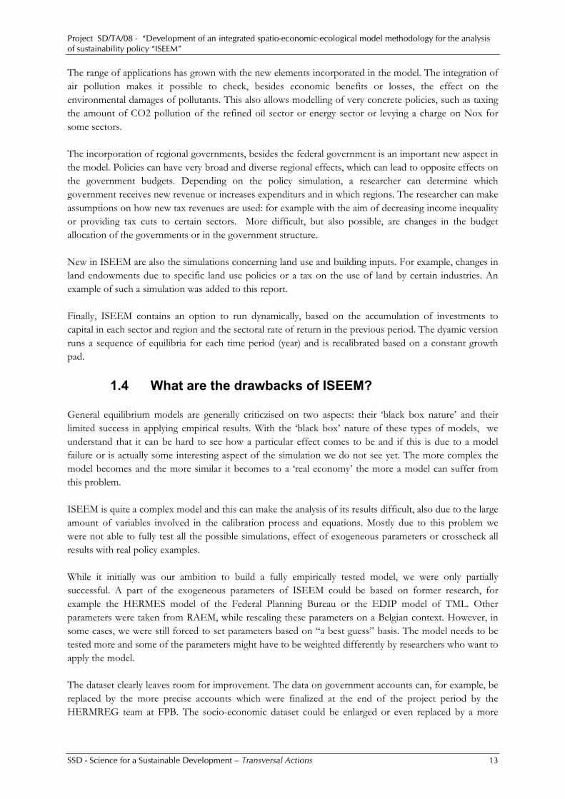
The range of applications has grown with the new elements incorporated in the model. The integration of air pollution makes it possible to check, besides economic benefits or losses, the effect on the environmental damages of pollutants. This also allows modelling of very concrete policies, such as taxing the amount of CO2 pollution of the refined oil sector or energy sector or levying a charge on Nox for some sectors. The incorporation of regional governments, besides the federal government is an important new aspect in the model. Policies can have very broad and diverse regional effects, which can lead to opposite effects on the government budgets. Depending on the policy simulation, a researcher can determine which government receives new revenue or increases expenditurs and in which regions. The researcher can make assumptions on how new tax revenues are used: for example with the aim of decreasing income inequality or providing tax cuts to certain sectors. More difficult, but also possible, are changes in the budget allocation of the governments or in the government structure. New in ISEEM are also the simulations concerning land use and building inputs. For example, changes in land endowments due to specific land use policies or a tax on the use of land by certain industries. An example of such a simulation was added to this report. Finally, ISEEM contains an option to run dynamically, based on the accumulation of investments to capital in each sector and region and the sectoral rate of return in the previous period. The dyamic version runs a sequence of equilibria for each time period (year) and is recalibrated based on a constant growth pad.
1.4 What are the drawbacks of ISEEM? General equilibrium models are generally criticzised on two aspects: their ‘black box nature’ and their limited success in applying empirical results. With the ‘black box’ nature of these types of models, we understand that it can be hard to see how a particular effect comes to be and if this is due to a model failure or is actually some interesting aspect of the simulation we do not see yet. The more complex the model becomes and the more similar it becomes to a ‘real economy’ the more a model can suffer from this problem. ISEEM is quite a complex model and this can make the analysis of its results difficult, also due to the large amount of variables involved in the calibration process and equations. Mostly due to this problem we were not able to fully test all the possible simulations, effect of exogeneous parameters or crosscheck all results with real policy examples. While it initially was our ambition to build a fully empirically tested model, we were only partially successful. A part of the exogeneous parameters of ISEEM could be based on former research, for example the HERMES model of the Federal Planning Bureau or the EDIP model of TML. Other parameters were taken from RAEM, while rescaling these parameters on a Belgian context. However, in some cases, we were still forced to set parameters based on “a best guess” basis. The model needs to be tested more and some of the parameters might have to be weighted differently by researchers who want to apply the model. The dataset clearly leaves room for improvement. The data on government accounts can, for example, be replaced by the more precise accounts which were finalized at the end of the project period by the HERMREG team at FPB. The socio-economic dataset could be enlarged or even replaced by a more

Project SD/TA/08 - “Development of an integrated spatio-economic-ecological model methodology for the analysis of sustainability policy “ISEEM”
SSD - Science for a Sustainable Development – Transversal Actions 14
sophisticated micro-dataset on household level. An application for this type of data was made, but we were unable to obtain and rework the dataset within the time-frame of the project. Some elements ISEEM are less worked out than was initially our goal. We planned to have a more extended housing markt and land use module, disaggregate the production of transport in a similar way as done in the model EDIP and have more elements in the model that can be linked to sustainability. In foreseen and unforeseen ways, we had to limit our ambitions, mostly due to the large preparatory work on the methodology of the model and the time needed to find and prepare data. One should also be careful when interpreting the results on welfare of the different household deciles, as this is modeled in a quite exogeneous way. The share of the total labour and capital income within a province, as well as the amount of unemployment benefits and other transfers going to different household types, are fixed by exogeneous shares based on the EUROMOD model. The model does not implicitely model different income earning abilities of each household type. It is also important to note that we used a more restricted set-up of the model to run our simulation. The reason for this is that in some cases the simulations took a very long time to give a solution. The variables that were fixed exogeneously are the ones related to government consumption and the equations related to migration. The fixing of government consumption is not unlogical, as we only have a limited idea on how governments decide on allocating government expenditures. We introduced a basic formulation in ISEEM, which uses a Cobb-Douglas based government utility for allocating government expenditures to the commodities. This part of the model is callibrated and functions, but can lead to a large effect on the price of certain commodities. The formulation of migration, which was taken over from the RAEM model, sometimes led to contradictory results in our simulations. We decided to leave this out of the simulations, to avoid inconsistencies. The results without migration are also more straightforward and easier to analyze. We were forced to stay closer to the original RAEM methodology. However, we feel that ISEEM offers a genuine progress in the field of economic modelling, certainly in the Belgian context. The model is complex enough to check the applicability of a large variety of different policies. It integrates and calibrates a very complete dataset on regional government income and expenditures, regional production, consumption, labour market issues, taxation, emissions data and data on land use. We think that this model can be used and improved by researchers interested in (regional) general equilibrium modelling and be applied to give more insight into policies concerning sustainability.
Project SD/TA/08 - “Development of an integrated spatio-economic-ecological model methodology for the analysis of sustainability policy “ISEEM”
SSD - Science for a Sustainable Development – Transversal Actions 15
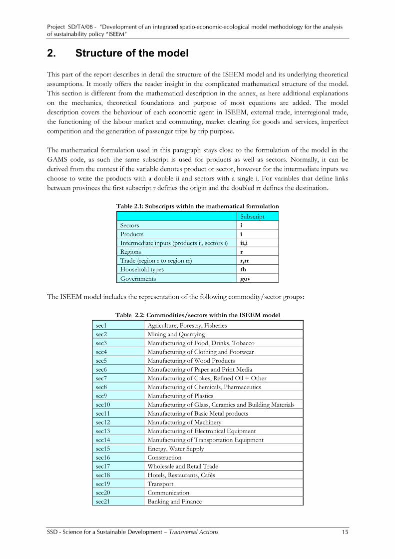
2. Structure of the model This part of the report describes in detail the structure of the ISEEM model and its underlying theoretical assumptions. It mostly offers the reader insight in the complicated mathematical structure of the model. This section is different from the mathematical description in the annex, as here additional explanations on the mechanics, theoretical foundations and purpose of most equations are added. The model description covers the behaviour of each economic agent in ISEEM, external trade, interregional trade, the functioning of the labour market and commuting, market clearing for goods and services, imperfect competition and the generation of passenger trips by trip purpose. The mathematical formulation used in this paragraph stays close to the formulation of the model in the GAMS code, as such the same subscript is used for products as well as sectors. Normally, it can be derived from the context if the variable denotes product or sector, however for the intermediate inputs we choose to write the products with a double ii and sectors with a single i. For variables that define links between provinces the first subscript r defines the origin and the doubled rr defines the destination.
Table 2.1: Subscripts within the mathematical formulation
Subscript Sectors i Products i Intermediate inputs (products ii, sectors i) ii,i Regions r Trade (region r to region rr) r,rr Household types th
Governments gov The ISEEM model includes the representation of the following commodity/sector groups:
Table 2.2: Commodities/sectors within the ISEEM model
sec1 Agriculture, Forestry, Fisheries sec2 Mining and Quarrying sec3 Manufacturing of Food, Drinks, Tobacco sec4 Manufacturing of Clothing and Footwear sec5 Manufacturing of Wood Products sec6 Manufacturing of Paper and Print Media sec7 Manufacturing of Cokes, Refined Oil + Other sec8 Manufacturing of Chemicals, Pharmaceutics sec9 Manufacturing of Plastics sec10 Manufacturing of Glass, Ceramics and Building Materials sec11 Manufacturing of Basic Metal products sec12 Manufacturing of Machinery sec13 Manufacturing of Electronical Equipment sec14 Manufacturing of Transportation Equipment sec15 Energy, Water Supply sec16 Construction sec17 Wholesale and Retail Trade sec18 Hotels, Restaurants, Cafés sec19 Transport sec20 Communication sec21 Banking and Finance
Project SD/TA/08 - “Development of an integrated spatio-economic-ecological model methodology for the analysis of sustainability policy “ISEEM”
SSD - Science for a Sustainable Development – Transversal Actions 16
sec22 Business Services sec23 Government Services sec24 Education sec25 Health sec26 Leisure Services
2.1 Households
2.1.1 Household income, savings and consumption budget The model incorporates the behaviour of 10 representative household types per province; these households are classified according to their income (income deciles). The total income of each household is calculated as the sum of its labour income and its capital income. Its capital income includes income from land endownments, buildings and other capital.
thrrrltp
rltprii
ri
thrrrrrth
NWYshareBDSPBDPLDLDSRKK
WYshareERLROWPWUNEMPLSY
_)(
_))((
,,,
,
⋅⋅+⋅+⋅+
⋅⋅−⋅−=
∑∑ (1)
The labour income of the regional household is calculated as the total endowment of labour in the region (LS) minus the regional unemployment multiplied by the region-specific wage rate minus the net amount of regional labour supplied abroad or LROW, multiplied by the exchange rate ER. The region specific wage rate PW, is a weighted average of the wages earned within the province and the wages earned by commuters. It is assumed that the return to capital used by all sectors located in the region is allocated to the regional household. This way the capital income of the regional household is calculated as the sum over all regional sectors of their capital inputs multiplied by the sector-specific rate of return to capital and the exchange rate/terms of trade between the country and the rest of the world. Households capital income also includes the total endowments of land of different types (LDS) and buildings (BDS), multiplied by their respective regional prices. Both labour income and capital income are distributed over the different household types using exogeneous shares, calculated from the results of the EUROMOD model (share_WY being the income from labour and share_NWY being the income from capital). The money received by the regional households are spent on consumption of goods and services, transportation trips, savings and income taxes. The consumption budget of the household is the amount of money spent on the purchase of goods and services, which contribute to the household’s utility. The higher the consumption of these services and goods is, the more utility the household receives. It is assumed that consumption of the transportation services does not directly contribute to the utility of the household. The consumption budget of the regional household (CBUD) is calculated as its net income (Y) plus the social transfers from the government (TRF) plus the unemployment benefits (UNEMPB) minus the households savings (SH) and spending on travel trips including commuting (LCM), education, shopping and other trips: The consumption of trips by household type are determined by multiplying the regional expenditures on trips with an exogeneous factor shareCONS.

Project SD/TA/08 - “Development of an integrated spatio-economic-ecological model methodology for the analysis of sustainability policy “ISEEM”
SSD - Science for a Sustainable Development – Transversal Actions 17
( )TRANSPORTii
iiiiiiiiii
rii
rrrrrrrrrrrr
rrrrrrrrrrr
rrrrth
govrthrthrththrthrth
exstvatctcscP
EDUMONTEDUTRIPSOTHMONTOTHTRIPS
SHOPMONTSHOPTRIPSLCMTmoneyshareCONS
UNEMPBSHGDPDEFTRFtyYCBUD
=
⎟⎠
⎞⎜⎝
⎛+++−⋅⋅
⋅+⋅+
⋅+⋅⋅−
+−⋅+−⋅=
∑
∑
∑
1
)
(
)1(
,
,,,,
,,,,,
,,,,,,
(2)
The savings of the regional household (SH) is calculated as a fixed proportion of its total disposable income that consists of the household’s net income plus the social transfers and unemployment benefits from the governments. This marginal propensity to save (mps) is different for each province and household type. It can also be negative, reflecting persistent debts for this type of household.
))1(((
,,,,,, ∑+⋅+−⋅⋅=
govrthrththithrthith UNEMPBGDPDEFTRFtyYmpsSH (3)
The total transfers to households are equal to the transfers from each government (TRFF)
∑=gov
govrthrth TRFFTRF ,,,
2.1.2 Household utility’
The amounts of the goods and services bought by the regional household types are determined according to a utility-maximization problem, where the household maximizes the following utility function. This is a 2-stage utility function with at the top level a Cobb-Douglas utility function and at the bottom level a LES function The top level aggregates utility derived from the consumption of housing stock in each region and the utility from the consumption of goods. The housing stock (HOUS) is weighted by the amount of households in each region and depends upon the activities of the construction sector, compared with the initial activities of the construction sector (intial value of production is indicated with a superscript 0).
)1(,,,,
,0
,,,
,,,,
,
))((
))/(()/(
rithrith
rth
alphaHOUSEalphaHrith
irith
alphaHOUSE
onConstructiiririrrthrth
muHC
XDXDPopHOUSU
−
=
−⋅
⋅=
∏
∑ (4)
The LES function is a variation on the Cobb-Douglas utility function, where we substract a fix part of the consumption of goods which is defined as ‘basic’ or ‘subsistence’ consumption (muH) from the total consumption of a good (C).The utility from consumption is associated only with the amount of good and service which is higher than its subsistence consumption level. The regional household defines its consumption levels such as to maximize the LES utility function under the budget constraint that the total expenditures of the household are equal to its consumption budget. This utility problem is solved by the following equation for its optimal consumption levels.
⎟⎠
⎞⎜⎝
⎛+++−⋅⋅−⋅+
⋅+++−⋅=⋅+++−⋅
∑ )1(
)1()1(
,,,,,,
,,,,,,
iiiirii
rithrithri
rithiiiiririthiiiiri
exstvatctcscPHCBUDH
HexstvatctcscPCexstvatctcscP
μα
μ (5)
Project SD/TA/08 - “Development of an integrated spatio-economic-ecological model methodology for the analysis of sustainability policy “ISEEM”
SSD - Science for a Sustainable Development – Transversal Actions 18
2.1.3 Household welfare The welfare of an individual regional household is calculated as the percentage share of the equivalent variation (EV) associated with a certain economic changes in the total income of the household.
1001
,,,
,
0,
, ⋅⋅⎟⎟
⎠
⎞
⎜⎜
⎝
⎛−⋅⎟
⎟⎠
⎞⎜⎜⎝
⎛=
rthrthrth
rth
rthrth Y
SIDSIIPEVPEV
EV (6)
The calculation of the equivalent variation measure according to this formula is based on the unit price of an additional household’s utility (PEV) and on the level of the household’s budget (SII) associated with the utility level. This budget does not include the spending necessary to pay for the subsistence levels of consumption determined from the LES function. The parameter SID represents the original amount of budget available to the consumer. The superscript ‘0’ refers to the initial baseline values of the utility price and the utility budget. The price of an additional unit of utility obtained by the household is derived according to the following equation.
( )( ) ri
productsiiiiirir exstvatctcscPPEV ,1,
α∏=
+++−⋅= (7)
The price of the unit of the household’s utility depends upon the after-tax prices of goods and services as well as the utility shares. The household’s budget associated with its utility level (SII) is calculated as the total household’s consumption budget minus the spending of the households on the provision of its subsistent levels of consumption, calculated as the parameter ri,μ .
( )( )∑ +++−⋅⋅−=
iiiiiririrr exstvatctcscPCBUDSII 1,,μ (8)
2.1.4 Passenger trips for different purposes
The generation and distribution of passenger trips such as shopping trips, education and other trips is based on a generation-distribution model which follows the structure of a constrained gravity model. It is assumed that a fixed part γ of the total real consumer income in the region of origin is spent on trips for non-commuting purposes (shopping, education and other). The trips are distributed across the different zone pairs based on the levels of the attraction variables at the regions of destination and on the transport costs. The choice of the attraction variables for the generation of the trips depends upon the type of the trip and is different for education, shopping and other passenger trips. We take total output of the corresponding service sector to be the major attraction variable. The total transport costs are calculated as the sum of the monetary and time costs associated with each pair of regions in the country. Increase in the transportation costs for a particular pair of regions negatively influences the number of the trips between these regions. However, this does not have a direct effect upon the total number of the passenger trips generated at the region of origin. The only factor that influences total trips is the total real consumer income. The next equation calculates the demand for shopping from region to region. The attractions for the shopping trips are based on the total output of the shopping sectors in each region. The equations for education trips and other trips are similar (cfr. Mathematical appendix), but use the output of the education sector and of the travel sectors as the major attraction variables respectively.
Project SD/TA/08 - “Development of an integrated spatio-economic-ecological model methodology for the analysis of sustainability policy “ISEEM”
SSD - Science for a Sustainable Development – Transversal Actions 19
( )
( )∑∑
∑∑
=
+−=
+−
⋅⋅
⋅⋅⋅⋅=
shopi
shopMONTshopTIMErrrirrrr
rrr
shopi
shopMONTshopTIMErirrr
r
rthth
rrrr rrrrrrrr
rrrrrr
eXDshop
eXDshop
INDEX
YshopSHOPTRIPS
,,
,,
(,,
(,,,
, β
βγ (9)
2.1.5 Housing stock and residential emissions The housing stock in each region has been fixed, calibrated on an initial dataset of the available housing stock in each province. The only factor that influences the amount of housing consumed in each region is the production of the construction sector. This can be seen in the utility function of each household (Equation 4). Residential emissions are coupled to the housing stock and hence also to the production of the construction sector. An increase in the activities of the construction sector increases air pollution origination from residential sources.
)/(_2_2 0,,,,, ∑
=
⋅⋅=CONSTRi
ririrthrthrth XDXDHOUSZRESPOLLCORESPOLLCO α (10)
)/(__ 0,,,,,,, ∑
=
⋅⋅=CONSTRi
ririrthremisthremisth XDXDHOUSZRESPOLLGHGRESPOLLGHG α (11)
)/(__ 0,,,,,,, ∑
=
⋅⋅=CONSTRi
ririrthremisthremisth XDXDHOUSZRESPOLLNGHGRESPOLLNGHG α (12)
2.2 Firms
2.2.1 Production technology ISEEM contains 26 regional production sectors using labour, capital, land, buildings, energy and intermediate goods in their production process. Inputs of the sectors are combined according to the Constant Elasticity of Substitution (CES) technology, whereas the intermediate goods are used in the fixed proportions of the aggregated materials nest, using Leontief technology. Figure 2.1 schematically represents the nested CES productions structure of the sectors. The amount of the inputs per unit of output are based on the cost minimization principle. The resulting amounts of capital, labour, land, buildings, energy and intermediate goods depend upon the production technology of the sectors and upon the prices of the sectoral inputs. The value of the top CES bundle is equal to the total domestic production, multiplied by a fix factor. It is essentially a leontief share of the total outputs.
ririri XDioBDLDKELMBDLDKELM ,,, ⋅= (13)
The composite price of this bundle is equal to the weighted average of the prices of the BDLD (buildings-land) and KELM (capital-energy labour-materials) bundle.
ririririri KELMPKELMBDLDPBDLDPBDLDKELM ,,,,, ⋅+⋅= (14)

Project SD/TA/08 - “Development of an integrated spatio-economic-ecological model methodology for the analysis of sustainability policy “ISEEM”
SSD - Science for a Sustainable Development – Transversal Actions 20
Figure 2.1: Tree of nested CES production function, based on HERMES
The demands for the 2 composite bundles (BDLD and KELM) are derived by the following 2 equations. Where parameters beginning with γ define a share parameter in the CES nest and a technological constants.
BDLDKELMBDLDKELM
riBDLDELM
aBDLDKELMPBDLDKELMPKELMKELM
BDLDKELMKELM riri
ririri
σσ
σγ −⋅⋅⎟
⎟⎠
⎞⎜⎜⎝
⎛⋅= 1
,,
,,,
,
(15)
BDLDKELMBDLDKELM
riBDLDELM
aBDLDKELMPBDLDKELMPBDLDBDLD
BDLDKELMBDLD riri
ririri
σσ
σγ −⋅⋅⎟
⎟⎠
⎞⎜⎜⎝
⎛⋅= 1
,,
,,,
,
(16)
The demands for the other composite inputbundles of the lower nests have a very similar structure as the equations (15) and (16) and will not be treated here, but are included in the mathematical description.The demand for labour and capital are somewhat different, due to the assumption of monopolistic competition and the addition of business trips and are treated below as equations (17) and (18). The variable expenditures on capital (Kv) are derived as a subnest from the Capital-Energy bundle, as a solution of the cost minization problem. The total expenditures on capital are a sum of the variable capital inputs and the fixed capital costs. This are the fixed cost of capital per firm (fcK), multiplied by the amount of firms (NF) in the sector.
riri
KvCapitalVariable
KEri
KEri
KE
ririi
ririri
fcKNF
aKEPKEPIRKtk
KKEK riri
ri
,,
)(_
1,,
,,
,,,
,,
,
)1(
⋅+
⎥⎥⎦
⎤
⎢⎢⎣
⎡⋅⋅⎟
⎟⎠
⎞⎜⎜⎝
⎛
⋅∂+⋅+⋅=
=
−σσ
σγ
(17)
BDLDKELM
BDLD KELM
KE LMBD LD
Kv E Lv MAT
CES
CES
CES
.. .. ..
Leontief
ELEC NONELEC
OIL COAL
CES
CES
CES

Project SD/TA/08 - “Development of an integrated spatio-economic-ecological model methodology for the analysis of sustainability policy “ISEEM”
SSD - Science for a Sustainable Development – Transversal Actions 21
The regional labour demand per sector (L) is derived in a similar way as the capital demand, as a subnest from the Labour-Materials bundle (which is equal to the variable labour inputs), plus the fixed labour costs for the sector. However, the fixed labour costs of an individual firm include the time costs of the business trips. The idea behind this assumption is to relate the number of the business trips to the number of the operating firms (NF) and not to the total output of the sector (2.2.1). It is assumed that the more firms operate in the sector, the more time is spent on business trips, such that the total time costs of the business trips per firm stays approximately the same.
rrrrr
rrririri
LvLabourVariable
LMri
LMri
LM
iiiri
ririri
BTIMEBTRIPSfcLNF
aLMPLMtltltlPL
LLML riri
ri
,,,,,
)(_
,,,
,,,
,,
,
))11(11(
⋅+⋅+
⎥⎥⎦
⎤
⎢⎢⎣
⎡⋅⋅⎟
⎟⎠
⎞⎜⎜⎝
⎛
⋅+++⋅⋅=
∑=
σσσ
γ
(18)
The total production costs of the sector is calculated as the sum of the capital costs, which include depreciation, labour costs, the costs of intermediate inputs, the monetary costs of the business trips and the total expenditures on land and buildings.
( ) ( )
rirrirltprr
rrrrrr
FUELiiii
riiiriririiririiiii
irirriririiriiiriri
BDPBDLDPLDltpBMONTBTRIPS
PFUELPELECELECPMATiotltl
tlLPLPIRKtkKsptxdTFPXDPD
,,,,,
,,,,,,,,
,,,,,,,
),(
)11(
11()1(1
⋅+⋅+⋅+
⋅+⋅+⋅⋅+⋅+
++⋅⋅+⋅∂+⋅+⋅=+−⋅⋅⋅
∑∑
∑ = (19)
2.2.2 Energy inputs and sector emissions
Each sector in ISEEM uses a composite energy bundle (ENER), consisting of fossil fuels and electricity. Demand for electricity inputs (ELEC) and nonelectricity inputs(NONELEC) are CES-subnests of the composite energy bundle and are given by the next equations.
1,,
,
,,,,
,,
,
−⋅⋅⎟⎟⎠
⎞⎜⎜⎝
⎛⋅= riri
ri
Eri
Eri
E
ri
regiiiriri aECNECPENERPNONELECNEC
ENERNONELEC σσ
σγ
(20)
1,,
,
,,,,
,,
,
−⋅⋅⎟⎟⎠
⎞⎜⎜⎝
⎛⋅= riri
ri
Eri
Eri
E
ri
regiiiriri aECNECPENERPELECEC
ENERELEC σσ
σγ
(21)
The demand for each type of fossil fuel is again a subnest of the NONELEC bundle, given by the next equation. We only distinguish 2 types of fuels: oil and a coal-gas bundle, as gas is not distinguished as a separate sector/product in our social accounting matrix.
1,,
,
,,,,,
,,
,
−⋅⋅⎟⎟⎠
⎞⎜⎜⎝
⎛⋅= riri
ri
NEri
NEri
NE
regii
regiiiriregiii aFUELPNONELEC
PFUEL
NONELECFUEL σσ
σγ
(22)
The greenhouse gas and non-greenhouse gas emissions are treated separately and are coupled partially to the total output of each sector and partially to the composite input bundle of fuels with fixed coefficients. It was not possible with the given statistical data to dissagregate the emissions per fuel type. Therefore emissions are linearily dependent on the use of fossil fuels (NONELEC) and the production of each sector. The next 3 equations treat the emissions due to fossil fuels (23)
riiri NONELECCOPOLLCOPOLL ,, 2_2_ ⋅= α (24)

Project SD/TA/08 - “Development of an integrated spatio-economic-ecological model methodology for the analysis of sustainability policy “ISEEM”
SSD - Science for a Sustainable Development – Transversal Actions 22
riiemisriemis NONELECGHGPOLLGHGPOLL ,,,, __ ⋅= α (25)
riiemisriemis NONELECNGHGPOLLNGHGPOLL ,,,, __ ⋅= α (26)
The following 3 equations treat the emissions coupled to the total output of each sector.
riiri XDPRODCOPOLLPRODCOPOLL ,, _2__2_ ⋅= α (27)
riiemisriemis XDPRODGHGPOLLPRODGHGPOLL ,,,, ____ ⋅= α (28)
riiemisriemis XDPRODNGHGPOLLPRODNGHGPOLL ,,,, ____ ⋅= α (29)
2.2.3 Monopolistic competition
The way to integrate agglomeration effects in an economic model is by dropping the assumption of perfect competition. Instead it is assumed that the production of the firms is characterised by increasing returns to scale and that the firms operate under the condition of monopolistic competition. Following the New Economic Geography (NEG) litterature, we assume that each regional (provincial) sector contains a certain number of firms, producing slightly differentiated goods and services. Given that there are no statistical data that describe the production process of each firm in the industry, all firms are assumed to be homogenous and have the same production technology, the same output size and the same fixed production costs. The fixed production costs of an individual firm are related to its initial establishment in the industry and include both labour and capital costs. Each new firm produces one particular type of the product type/variety. The firms charge prices higher than their marginal costs in order to be able to cover their fixed costs. Since consumers have widely differentiated preferences with respect to the types/varieties of goods and services produced by the firms, they purchase output of all the firms in the sector. The functional form of the consumer utility function is equivalent to the CES function, making it a concave function which positively depends on the number of firms (varieties!) in a region. This setup is generally called the Dixit-Stiglitz form of monopolistic competition. Given that the entry to all the industries is assumed to be free, the number of the monopolistic firms in each sector (NF) is determined by the condition that the total costs of the firms equal its total revenues. Once the firms in the industry starts making profits, several new firms enter the market and drive total profits down to zero again. The fixed capital and labour costs for each firm are assumed to be constant, making the total number of the firms operating in a sector endogenous, defined by the zero profit condition for the sector as a whole:
riri
riri
rrrrrrrri
ririri
PDTFPXD
fcKNF
BTIMEBTRIPSfcLgelasNF
,,
,,
,,,
,,, Re
⋅⋅=
⎟⎟⎟
⎠
⎞
⎜⎜⎜
⎝
⎛+
⋅+⋅⋅∑
(30)
The price of the goods or services produced by a monopolistically competitive sector (PDC) depend negatively on both the number of the operating firms and on the elasticity of substitution between the varieties of a good or a service produced by each firm. Under the assumption that the firms operating in a sector are identical, the price of a monopolistically competitive sector is derived according to the following formula:
Project SD/TA/08 - “Development of an integrated spatio-economic-ecological model methodology for the analysis of sustainability policy “ISEEM”
SSD - Science for a Sustainable Development – Transversal Actions 23
ririri AUXVPDPDC ,,, ⋅= (31)
which is the domestic production price (PD), multiplied by the auxiliary variable (AUXV)
rigelasriri NFAUXV ,Re11
,, −= (32)
The profits made by the monopolistical firms are identical to the sum of their fixed labour and capital costs.
( )riririri fcKfcLNFPROFITS ,,,, +⋅= (33)
2.2.4 Business trips
The total number of business trips of the sector is assumed to be linearly dependent upon the number of the operating firms:
ririri NFBTBRTRIPST ,,, ⋅= β (34)
The total number of the business trips generated by the sector is distributed between the destinations in other regions of the country according to the gravity equation below
( )
( )rrrrrr
rrrrrr
BTIMEBMONTrrrrrri
k
BTIMEBMONTrrrrrri
rrrirrri
eBTSHAREBTeBTSHAREBT
BTRIPSTBTRIPS
,,
,,
,,,
,,,
,,,,
+−
+−
⋅⋅
⋅⋅⋅
=
∑ αα
(35)
The number of the business trips from region (r ) to region ( rr ) depends on the amount of interregional trade (XDDE) between the 2 regions, compared to the total trade originating from region r. The share of the trade with the region j in the total trade of region i is calculated according to the following formula:
( )( )∑∑
∑+
+=
i krrkikrri
irrrirrri
rrr XDDEXDDE
XDDEXDDEBTSHARE
,,,,
,,,,
, (36)
2.2.5 Total factor productivity Total factor productivity in ISEEM is introduced, dependent on the production of the education sector. An increase in the production of education, leads to a proportional increase of the total factor productivity. When production of the education sector is doubled, compared to the basecase scenario, this leads to an additional growth of 2% of the total factor productivity.
∑∑ ∑
=
= =
−⋅=
−
reducationiri
reducationi reducationiriri
TFPZXD
TFPZXDXDTFP
,,
, ,,,
_
_02.0
1)1(
(37)

Project SD/TA/08 - “Development of an integrated spatio-economic-ecological model methodology for the analysis of sustainability policy “ISEEM”
SSD - Science for a Sustainable Development – Transversal Actions 24
2.3 Government ISEEM contains a disaggregated government structure with a federal government (FGOV) (which also includes the municipalities) and several regional governments with different jurisdictions. The government structure has been made to represent the complex Belgian institutional web.
2.3.1 Government tax income and subsidies Each government gets 2 types of income: tax revenues from the economic agents within the regions under its jurisdiction and income from intergovernment transfers. Not all regional governments have own tax income, as in Belgium the jurisdictions of the “governments of the region” and “language communities” are different, meaning that the “communities” cannot collect tax income. The federal government level is responsible for collecting the largest part of the tax revenues; this concerns the full income tax and social security benefits, as well as a large share of the other taxes. The tax revenues within each region (TAXRG) are calculated as the sum of the social security taxes paid by the employers (tl) and employees (tl1), profit taxes of the firms (tk), taxes on production (txd) and taxes on the total consumption (tc, vatc and exst), which include transport trips, investments and government consumption. The taxes on consumption are subdivided in: normal taxes on consumption, VAT and excise taxes. However, they are all modelled as a fixed percentage of the value of a good. This is necessary for the model to remain homogeneous. The taxrates are the same for all regions within Belgium, but regional governments get a different fixed share of the total tax revenues from each tax subtype. The total tax income for each government is equal to the sum of its tax revenues within each region.
( )
⎥⎥⎥⎥⎥⎥⎥⎥⎥⎥⎥⎥⎥
⎦
⎤
⎢⎢⎢⎢⎢⎢⎢⎢⎢⎢⎢⎢⎢
⎣
⎡
⋅⋅+
⎟⎟⎟⎟⎟⎟⎟⎟
⎠
⎞
⎜⎜⎜⎜⎜⎜⎜⎜
⎝
⎛
++
⎟⎟⎟
⎠
⎞
⎜⎜⎜
⎝
⎛
⋅+⋅+
⋅+⋅+
⋅⋅⋅+⋅+⋅+
⋅⋅⋅⋅+⋅⋅⋅+
⋅⋅++⋅⋅⋅
=
=
∑∑
∑
∑
govrthrth
riri
TRANSPORTrrrrrrrrrrrr
rrrrrrrrrrr
rrr
ithrith
irigovgovgovrigovri
ririgovririgovri
govrigovgovririr
rgov
govtytyY
CGI
EDUMONTEDUTRIPSOTHMONTOTHTRIPS
SHOPMONTSHOPTRIPSLCMTmoneyC
Pgovexstexstgovvatcvatcgovtctc
PDTFPXDgovtxdtxdRKKgovtktk
govtltltlgovtltlLPL
TAXRG
,,
,,
,,,,
,,,,
,,,
,,,
,,,,,
,,,
_
___
__
_)11(()_11(
(38)
The total subsidies of each government consist of subsidies on production and consumption. Subsidies are treated similarly as tax revenues. The national rates are fixed and equal for each province, but the share of the total subsidies paid by each government are different in each region. The equation can be found in the mathematical appendix.
2.3.2 Government transfers The governments transfer income to the households and to the other governments. For the transfers to the households a distinction is made between unemployment benefits and ‘other transfers’. Transfers to the households are partially fixed; the ‘other transfers’ are assumed to be constant, but the unemployment benefits depend on the wage level and on unemployment within each region. A fixed share of the unemployment benefits goes to each household decile. Unemployment benefits only partially compensate

Project SD/TA/08 - “Development of an integrated spatio-economic-ecological model methodology for the analysis of sustainability policy “ISEEM”
SSD - Science for a Sustainable Development – Transversal Actions 25
the loss in real wage (PW); the degree of compensation depends on the exogeneously fixed parameters trep (wage replacement rate) and a_lab (auxiliary parameter).
( ) govrrrrthgovregth UNEMPBindicPWlabatrepUNEMPTRFHHshareUNEMPB ___,, ⋅⋅⋅⋅⋅= (39)
Transfers from government to government are endogenous and are calculated in the following way. First, we assume that a fixed share of the total government income (tax revenues and income from transfers) is transferred.
)( govgovgovgov TRFGYTAXRGshareTRFGETRFGE +⋅= (40)
Next, we assume that each government gets a fixed share of the government transfer expenditures
govgovvgovgovvgov TRFGEaTRFGETRFGG ⋅= ,, (41)
The income from transfers is assumed to be the sum of the total transfers from each government
∑=gov
govvgovgovv TRFGGTRFGY , (42)
2.3.3 Government consumption
The consumption budget of each government (CBUD_GOV) consists of the total tax revenues (TAXRG) minus total subsidies (SUBSG), minus the unemployment benefits, minus the transfers to the households (TRFF), plus the income from intergovernmental transfers (TRFGY) minus the expenditures on intergovernmental transfers (TRFGE), and savings plus the transfers to the government from abroad (TREU25).
( )
GDPDEFSGERTREU
GDPDEFTRFGETRFGYUNEMPBGDPDEFTRFF
SUBSGTAXRGGOVCBUD
govgov
govgovrth
govrthgovrthrth
govgovgov
⋅−⋅+
⋅−+−⋅⋅
−=
∑∑25
)(
_
,,,,,
,
(43)
In our simulations with the model, we have supposed that the consumption of the government is fixed exogeneously. A change in the government revenues that is only redistributed via the government consumption (without any other assumption on redistribution) can lead to large price and consumption effects on education, government services and health. However, the ISEEM model contains some basic equations to model the government expenditures on commodities based on a 2 stage approach. In the first stage we assume that each region gets a fixed part of the government spendings on commodities.
govgovrgovr GOVCBUDGCGR _,, ⋅=α (44)
In the next stage, we assume that the consumption budget within each regions is distributed between the consumption of various regional commodities according to a Cobb-Douglas demand function.
govrgovrigovriiiiiri CGRaGCGGexstvatctcscP ,,,,,, )1( ⋅=⋅+++−⋅ (45)
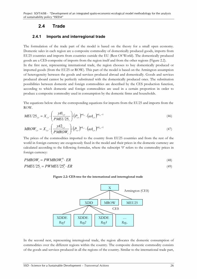
Project SD/TA/08 - “Development of an integrated spatio-economic-ecological model methodology for the analysis of sustainability policy “ISEEM”
SSD - Science for a Sustainable Development – Transversal Actions 26
2.4 Trade
2.4.1 Imports and interregional trade The formulation of the trade part of the model is based on the theory for a small open economy. Domestic sales in each region are a composite commodity of domestically produced goods, imports from EU25 countries and imports from countries outside the EU (Rest Of World). The domestically produced goods are a CES-composite of imports from the region itself and from the other regions (Figure 2.2). In the first nest, representing international trade, the region chooses to buy domestically produced or imported goods (from the EU25 or ROW). This part of the model is based on the Armington assumption of heterogeneity between the goods and services produced abroad and domestically. Goods and services produced aboard cannot be perfectly substituted with the domestically produced ones. The substitution possibilities between domestic and foreign commodities are described by the CES production function, according to which domestic and foreign commodities are used in a certain proportion in order to produce a composite commodity used in consumption by the domestic firms and households. The equations below show the corresponding equations for imports from the EU25 and imports from the ROW.
( ) ( ) 1,,
,,,
,,
251
25 −⋅⋅⎟⎟⎠
⎞⎜⎜⎝
⎛⋅= riri A
riA
rii
ririri aAPPMEUA
XMEU σσγ (46)
( ) ( ) 1,,
,,,
,,2 −⋅⋅⎟⎟
⎠
⎞⎜⎜⎝
⎛⋅= riri A
riA
rii
ririri aAPPMROWA
XMROW σσγ (47)
The prices of the commodities imported to the country from EU25 countries and from the rest of the world in foreign currency are exogenously fixed in the model and their prices in the domestic currency are calculated according to the following formulas, where the subscript ‘0’ refers to the commodity prices in foreign currency:
ERPWMROWPMROW ii ⋅= 0 (48)
ERPWMEUPMEU ii ⋅= 02525 (49)
Figure 2.2: CES-tree for the international and interregional trade
In the second nest, representing interregional trade, the region allocates the domestic consumption of commodities over the different regions within the country. The composite domestic commodity consists of the goods and services produced in all the regions of the country. Similar to the international trade part,
X
XDD MROW MEU25
XDDE Reg1
XDDE Reg2
XDDE Reg3
… Reg..
Armington (CES)
CES
Project SD/TA/08 - “Development of an integrated spatio-economic-ecological model methodology for the analysis of sustainability policy “ISEEM”
SSD - Science for a Sustainable Development – Transversal Actions 27
we assume heterogeneity between the goods and services produced in different domestic regions. The substitution possibilities between the commodities produced in different regions are described by the CES production function. The demand for the composite domestic commodity is determined in the first CES nest
( ) ( ) 1,,
,
,,,
,,3 −⋅⋅⎟
⎟⎠
⎞⎜⎜⎝
⎛⋅= riri A
riA
riri
ririri aAPPDDTA
XXDD σσγ (50)
The price of the composite domestic goods and services is derived as the weighted average of the prices of the commodities bought from all domestic regions. This weighted price includes the monopolistic competition price for domestically produced goods (PDDC) in each region, plus the relative transport costs.
( )∑ ⋅+⋅=⋅rr
irrrrirrririri trmPTMPDDCXDDEXDDPDDT ,,,,,,, (51)
The demand for domestic commodities by region is given by the next equation
11,
1,
1
,,,
,,,,
,,
,
14 −⋅⋅⎟
⎟⎠
⎞⎜⎜⎝
⎛
⋅+⋅= riri
ri
Ari
Ari
A
irrrrri
ririrrri aAPDDT
trmVPTMPDDCA
XDDXDDE σσ
σγ
(52)
The calculation of the transport costs of commodities deserves some additional explanation. Instead of using the commonly applied iceberg transportation costs, the model bases transport costs on the relative production and consumption of transport margins. The countrywide (!) price of trade margins (PTM) is a weighted sum of the production cost of transport margins relative to the sales price of some sectors. The sectors producing transport margins are the trade and retail sector (sec17) and the transport sector (sec19). The shares (atm) are exogenously fixed.
( )∑∑ ⋅=i r
riri PatmPTM ,, (53)
The consumption of trade margins is calculated relative to the value of the specific commodity transported. Like the relative production shares, the relative transport margin consumption (trm) is fixed exogenously. However, not all products consume transport margins, only the commodities using freight transport (commodities from sec1-sec14). While service sectors (sec15-sec26) use inputs that consume freight transport, the products of service sectors have zero transport margins.
2.4.2 Exports Domestic sectors have the possibility to export their production to the EU25 countries and to the rest of the world. Each sector decides upon the amount of commodities to be produced for export and their decisions depend upon their unit production costs, the price level in the domestic economy and the price elasticity. Increase in the production costs of the sector relative to the average price level in the economy leads to a decrease in the production activity of the sector and hence reduces the level of its exports.
ielasE
ri
iriri PDINDEXEEUEEU ⎟
⎟⎠
⎞⎜⎜⎝
⎛⋅=
,
0,, 2525 (54)
ielasE
ri
iriri PDINDEXEROWEROW ⎟
⎟⎠
⎞⎜⎜⎝
⎛⋅=
,
0,, (55)

Project SD/TA/08 - “Development of an integrated spatio-economic-ecological model methodology for the analysis of sustainability policy “ISEEM”
SSD - Science for a Sustainable Development – Transversal Actions 28
The price of regional goods PDDC is a leontief aggregator of different sectoral prices PDC
rjijri PDCiopsPDDC ,,, ⋅= (56)
2.5 Labour market
2.5.1 Vacancies, interregional commuting and unemployment The model makes use of search and matching function for unemployment, ressembling the Pissarides approach to define involuntary unemployment by frictions on the labour market. The idea is that labour demand in a region is followed by the posting of vacancies, which have a probability to be filled in by the regional labour force, or by the labour force of the other regions (labour which then has to commute). The underlying matching function is given in the equation below. The probability of a match between a vacancy in region rr and an unemployed person in region r, depends on the number of vacancies within the region of destination and the unemployment within the region of origin, but decreases exponentially with the time and monetary costs to commute between the regions.
( ) )()1(,,
,,,,, rrrrrrrrrrrrrrr TmoneyTtimebetaTMr
Mrrrrrrrr eUNEMPNVaMNM +⋅−− ⋅⋅⋅= αα (57)
The total amount of vacancies posted per sector depends on the difference between the present labour demand (L) and past year’s labour demand (LDD), plus the amount of jobs destroyed since last year ( depending on the exogenous job destruction rate ), divided by the probability to fill in a vacature.
( )r
rirriri QR
LDDLNVS
,0
,,
)1( ⋅−+=
ν (58)
The amount of vacancies in a region is simply the sum over all vacancies posted by each sector.
∑=i
rir NVSNV , (59)
The probability that a vacancy within a region is filled is equal to the total number of matches within one region divided by the number of vacancies within that region.
r
rrrrr
r NV
NMQR
∑=
,
(60)
Additionally we can calculate the chance that a person changes from unemployed to employed, as we assume that only unemployed people are looking for a new job. This is equal to the total number of matches within one region, divided by the total nationwide unemployment.
∑∑
=
rrrr
rrrrr
r UNEMP
NMPR
,
(61)
The labour force within one region is split up by the relative shares of labour demand origination from each region (including itself), resulting in the commuting matrix. The labour demand depends on last year’s labour demand between regions, minus the exogenous job destruction rate, plus the amount of new matches between regions..

Project SD/TA/08 - “Development of an integrated spatio-economic-ecological model methodology for the analysis of sustainability policy “ISEEM”
SSD - Science for a Sustainable Development – Transversal Actions 29
( )( )∑∑ +−⋅
+−⋅⋅=
rrrrrrrrrrrrr
rrrrrrrr
iirrr NMLCMD
NMLCMDLLCM
,,0
,,0
, 11
ηη
(62)
The total unemployment within one region is simply the total labour force, minus the commuters.
∑−=rr
rrrrr LCMLSUNEMP , (63)
2.5.2 Labour supply and migration
The total endowment of labour in the region is calculated as the initial labour endowment plus the sum of the net inflow of labour from the rest of the regions, minus the time spent on the commuting transportation trips. The regional labour supply is fixed and does not expand with the regional wage rate. In dynamic simulations, population growth should be modelled exogeneously.
( )∑∑ ⋅−−+=rr
rrrrrrrrrrr
rrrrr LCMTtimeLMIGLMIGLSLS ,,,,0 )( (64)
In our policy simulations with ISEEM, we have mostly worked without the modelling of migration, as the results obtained in this way were easier to generate and to analyze. The modelling of migration is present however, and is based on the regional utilities of the different consumers. The migration flow from region to region is derived according to the discrete choice migration generation function. The decision to move to another region of the’ country is split into two steps. At the first step, a household decides whether to move from the region or not. The choice to move, is based upon the region specific prefrences (Bmig) and the difference of the average regional household’s utility and the household’s utility of this particular region. At the second step the household decides to which region it is going to move. This choice is based on the regional attractions (Amig) and the level of the household’s utility in the destination region.
( )2
,,,
,,,
1
,
,
,,
)(
11
11
STEPrrrrrrthrrrrth
rrthrrrth
STEPrrrrrrr
rrrrth
rrrr
rrrr
rrrrth
rrrrrrrrrthrrr
UAmigUAmig
UUBmig
UUBmigLSshareCONSLMIG
=
=
⎥⎥⎥
⎦
⎤
⎢⎢⎢
⎣
⎡
++
⋅
⎥⎥⎥⎥⎥
⎦
⎤
⎢⎢⎢⎢⎢
⎣
⎡
⎟⎟⎠
⎞⎜⎜⎝
⎛⎟⎠
⎞⎜⎝
⎛−+
⎟⎟⎠
⎞⎜⎜⎝
⎛⎟⎠
⎞⎜⎝
⎛−+
⋅⋅=
∑
∑∑
∑∑
(65)
2.5.3 Regional wages
Households receive wages both from employment within their region as from other regions. The regional wage level is determined as a weighted average of the wages of the labour commuting between regions.
∑∑ ⋅
=
rrrrr
rrrr
rrr
r LCM
PLLCMPW
,
,
(66)
The regional price of labour is determined, based on the regional labour market. We apply a wage bargaining function based on the behaviour of a trade union. The trade union forces the firms to raise wages more than their marginal productivity. The equation contains both the change in unemployment
Project SD/TA/08 - “Development of an integrated spatio-economic-ecological model methodology for the analysis of sustainability policy “ISEEM”
SSD - Science for a Sustainable Development – Transversal Actions 30
wage (PLU), the firms profits, a share factor ( Bα ) and a factor determining the bargaining power of the trade union ( scalB ). An increase in profits, while the unemployment wage stays the same, increases the price of labour in the region.
∑∑∑ ⋅⋅−⋅⋅=⋅i
ri
riri
rir PROFTISscalBBLPLULPL )1(,, α (67)
The unemployment wage (PLU) is determined based on the replacement wage rate and the probability of finding a new job.
( ) rrrrrrr PLPRlabatrepPWPRPLU ⋅+⋅⋅=+⋅ _1 (68)
2.6 Land and buildings Land and buildings are used as inputs to the production processes of firms (cfr. 2.2.1). The expenditures on buildings and land cannot easily be separated, as often the prices of buildings hide the the value of the land a particular building occupies. We represent the joint use of buildings and land by a composite buildings-land nest within the CES demand function (Figure 2.1).
BDLDKELMBDLDKELM
riBDLDKELM
aBDLDKELMPBDLDKELMPBDLDBDLD
BDLDKELMBDLD riri
ririri
σσ
σγ −⋅⋅⎟
⎟⎠
⎞⎜⎜⎝
⎛⋅= 1
,,
,,,
,
(69)
The expenditures on this composite bundle depend on the composite land-buildings price, which is a weighted price given by the next equation.
rirriltp
rltpri BDPBDLDPLDPBDLD ,,,, ⋅+⋅=∑ (70)
There is only one type of composite buildings stock used by all sectors, as we did not have access to detailed statistical data to split up the building stock over different building types. However, it is easy to define new building types in the code, similar to the land types in the region. The relative yearly expenditures on land and buildings are subnests from the composite buildings-land bundle and are given by the following equations.
1,
,,,
,,
,
−⋅⋅⎟⎟⎠
⎞⎜⎜⎝
⎛⋅= riri
ri
BDLDBDLDri
BDLD
r
ririri aBDLDPBDLD
PBDBD
BDLDBD σσσγ
(71)
1,
,,,
,,
,
−⋅⋅⎟⎟⎟
⎠
⎞
⎜⎜⎜
⎝
⎛⋅=∑
riri
ri
BDLDBDLDri
BDLD
rltp
ririri aBDLDPBDLD
PLDLD
BDLDLD σσ
σ
γ (72)
The prices of land and buildings are dependent on the total stock of land (per type) and buildings within the province. It has been assumed that the stock of land per land type is completely fixed, moreover the land types do not change when the price of one land type increases.
2.7 Investments The total domestic savings consists of the savings made by all regional households, government and the regional sectors.. The savings of the regional sectors are assumed to be equal to their depreciation costs. The total domestic savings are calculated according to the following formula:
Project SD/TA/08 - “Development of an integrated spatio-economic-ecological model methodology for the analysis of sustainability policy “ISEEM”
SSD - Science for a Sustainable Development – Transversal Actions 31
PIKSGSHS rigov ri
rigovrth
rth ⋅⋅∂++= ∑ ∑∑ ,,
,,
, (73)
The total investments in the economy consist of domestic savings, the savings/investments received from the EU25 countries and from the rest of the world minus the total changes in stocks:
( )∑∑ ⋅−⋅+⋅+=i r
riri PSVERSROWERSEUSIT ,,25 (74)
The total investments are spent on buying physical investments goods from various domestic regions, where the demand for them is determined according to the Cobb-Douglas demand function:
( ) ( ) ITexstcvatctcscPI riiiiiriri ⋅=+++−⋅⋅ ,,, 1 α (75) The nominal rate of return in the economy is calculated as the average return to capital of all domestic sectors:
( )
∑∑ ⋅
=
iri
iriri
r K
KRKRGD
,
,,
(76)
The price of additional unit of the composite physical investment good is calculated in accordance to the Cobb-Douglas demand function and has the following form:
( ) ri
i r i
iiiiri exstvatctcscPPI
,1,α
α∏∏ ⎟⎟⎠
⎞⎜⎜⎝
⎛ +++−⋅= (77)
2.8 Market equilibrium conditions Markets for goods and services are in equilibrium in each region of the country. According to the market clearing condition the total supply of a certain commodity in each region is equal to the sum of the demand of the regional households, region-specific demands of the governments, region-specific demand for physical investment goods, changes in stocks, region-specific demand for commodities used for production of freight trade and transport margins, intermediate demands of the regional production sectors both of materials as energy inputs. The next equation calculates the total amount of goods or services sold in one region for all sectors except the transport sector.
∑∑∑ +⋅+++++=ii
riiiriiii
riiiririririth
rithri IOEMATioTMXSVICGCX ,,,,,,,,,,,, (78)
In order to write the equation for the demand for transport services we need to add an additional term related to the total amount of the passenger trips.
)
(
)(
,,
,,,,,,
,,,,,,,,,,,,,,,,
rrrrrr
rrrrrrrrrrrrrrrrr
rrr
ii rriirrrrrriiriiirii
iiriiiriririri
thrithri
EDUMONTEDUTRIPS
OTHMONTOTHTRIPSSHOPMONTSHOPTRIPSLCMTmoney
BMONTBTRIPSIOEMATioTMXSVICGCX
⋅
+⋅+⋅+⋅+
⋅++⋅+++++=
∑
∑ ∑∑∑(79)
2.9 Recursive dynamics ISEEM has a recursive dynamic structure composed of a sequence of several temporary equilibria. The first equilibrium in the sequence is given by the benchmark year 2006. In each time period, the model is

Project SD/TA/08 - “Development of an integrated spatio-economic-ecological model methodology for the analysis of sustainability policy “ISEEM”
SSD - Science for a Sustainable Development – Transversal Actions 32
solved for an equilibrium given the exogenous conditions assumed for that particular period. The equilibriums are connected to each other through capital accumulation. In the benchmark case, we assume that the economy is on a steady-state growth path, where all the quantity variables grow at the same rate and all relative prices remain unchanged. When a policy measure is implemented the economy enters on a transition path, until, after some time it has reached a new steady-state growth path (Ballard, Fullerton, Shoven and Walley, 1985). We are of course interested in the transition path induced by the policy measure and the characteristics of the new growth path. The endogenous determination of investment behavior is essential for the dynamic part of the model. Investment and capital accumulation in year t depend on expected rates of return for year t+1, which are determined by actual returns on capital in year t. This approach involves adaptive expectations. Thus, investment is not only a demand category in the model. In the dynamic economic processes a homogenous composite investment commodity is allocated between sectors according to the actual (year t) returns on capital in sector sec (subscript i). The equilibrium expected rate of return tiRK , by sector in
year t, is specified as an inverse logistic function (see Figure 1) of the proportionate growth in sector’s capital stock (Dixon and Rimmer, 2002):
)]maxln()minln()maxln(
))min[(ln()/1(
,,
,,,,,
,,,,0
,,,,
riri
riritriri
ritriritritri
KtrendKgKgKtrendKgKgKgKgBRKRK
−+
−−−−
−⋅+=
(80)
where 0,, triRK is the sector’s historically normal rate of return, triKg ,, is the actual capital growth rate in
the sector, riKg ,min and riKg ,max are the minimum and the maximum possible growth rates of
capital in the sector, riKtrend , is the sector’s historically normal growth rate and riB , is a positive
parameter. The minimum possible growth rate is set at the negative of the rate of depreciation in the sector, while the maximum rate is set at riKtrend , plus 0.062 in order to avoid unrealistically large
simulated growth rate (Dixon and Rimmer, 2002). Parameter riB , reflects the sensitivity of capital growth in sector sec to variations in its equilibrium
expected rate of return. It is derived by differentiating the above equation with respect to triKg ,, :
⎟⎟⎠
⎞⎜⎜⎝
⎛
−⋅−−
⋅=)min()max(
minmax
,,,,
,,,
riririri
ririri KgKtrendKtrendKg
KgKgSEAB (81)
where: 1
,,
,,
−
⎟⎟⎠
⎞⎜⎜⎝
⎛
∂∂
=tri
tri
KgRK
SEA (82)
The present value of purchasing a unit of capital to be used in the sector, in year t is defined as:
]1/[)]1([ ,11,,,, trittrittri RINTdeltaPIRRKPIPVK +−⋅++−= ++
2 The specification of the maximum possible growth rate implies that if the historically normal rate in a sector is 4 per cent, the upper limit in any year t would not exceed 10 per cent.
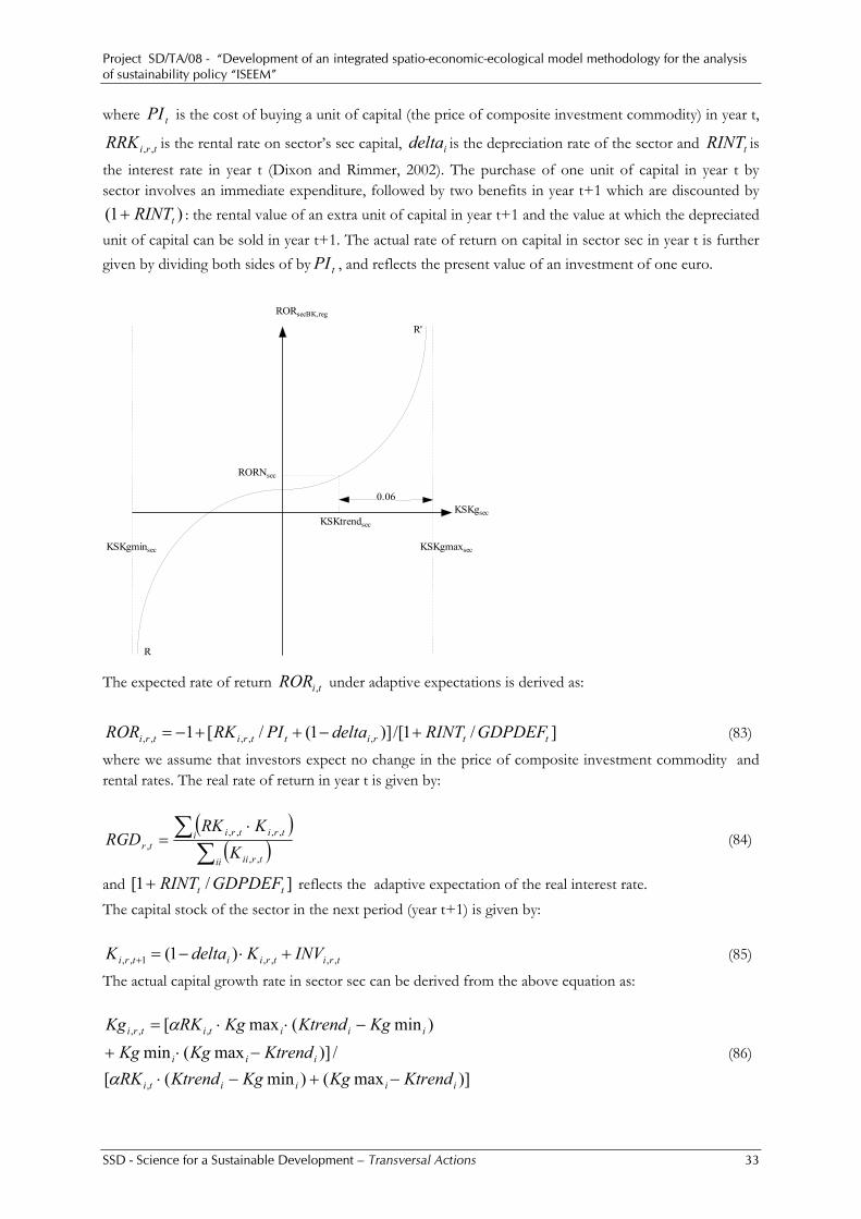
Project SD/TA/08 - “Development of an integrated spatio-economic-ecological model methodology for the analysis of sustainability policy “ISEEM”
SSD - Science for a Sustainable Development – Transversal Actions 33
where tPI is the cost of buying a unit of capital (the price of composite investment commodity) in year t,
triRRK ,, is the rental rate on sector’s sec capital, idelta is the depreciation rate of the sector and tRINT is
the interest rate in year t (Dixon and Rimmer, 2002). The purchase of one unit of capital in year t by sector involves an immediate expenditure, followed by two benefits in year t+1 which are discounted by
)1( tRINT+ : the rental value of an extra unit of capital in year t+1 and the value at which the depreciated unit of capital can be sold in year t+1. The actual rate of return on capital in sector sec in year t is further given by dividing both sides of by tPI , and reflects the present value of an investment of one euro.
RORsecBK,reg
RORNsec
0.06
KSKtrendsec
KSKgsec
KSKgmaxsecKSKgminsec
R
R'
The expected rate of return tiROR , under adaptive expectations is derived as:
]/1/[)]1(/[1 ,,,,, ttrittritri GDPDEFRINTdeltaPIRKROR +−++−= (83)
where we assume that investors expect no change in the price of composite investment commodity and rental rates. The real rate of return in year t is given by:
( )( )∑
∑ ⋅=
ii trii
i tritritr K
KRKRGD
,,
,,,,, (84)
and ]/1[ tt GDPDEFRINT+ reflects the adaptive expectation of the real interest rate. The capital stock of the sector in the next period (year t+1) is given by:
tritriitri INVKdeltaK ,,,,1,, )1( +⋅−=+ (85)
The actual capital growth rate in sector sec can be derived from the above equation as:
)]max()min([/)]max(min
)min(max[
,
,,,
iiiiti
iii
iiititri
KtrendKgKgKtrendRKKtrendKgKg
KgKtrendKgRKKg
−+−⋅−⋅+
−⋅⋅=
α
α (86)

Project SD/TA/08 - “Development of an integrated spatio-economic-ecological model methodology for the analysis of sustainability policy “ISEEM”
SSD - Science for a Sustainable Development – Transversal Actions 34
where: )(
,,
0,,,,, tritriti RKRKB
tri eRK −⋅=α (87)
and the capital growth rate in terms of capital stock in year t+1 and the capital stock in year t is given by:
1/ ,,1,,,, −= + tritritri KKKg (88)
From the previous equations we derive the investment carried out in the sector in year t:
)1()1)]max()min([
/)]max(min)min(max([
,,
,,,,,,
,,,
,,,,,,
itri
riririritri
ririri
iiitritritri
deltaKKtrendKgKgKtrendRK
KtrendKgKgKgKtrendKgRKKINV
−⋅−
+−+−⋅
−⋅+
−⋅⋅⋅=
α
α
(89)
The model is solved dynamically with annual steps. The simulation horizon of the model has been set up until 2020 but it can easily be extended. In between periods, some other variables like the transfers between firms, government and the rest of the world, and the balance of payments balance (foreign savings) are updated exogenously.
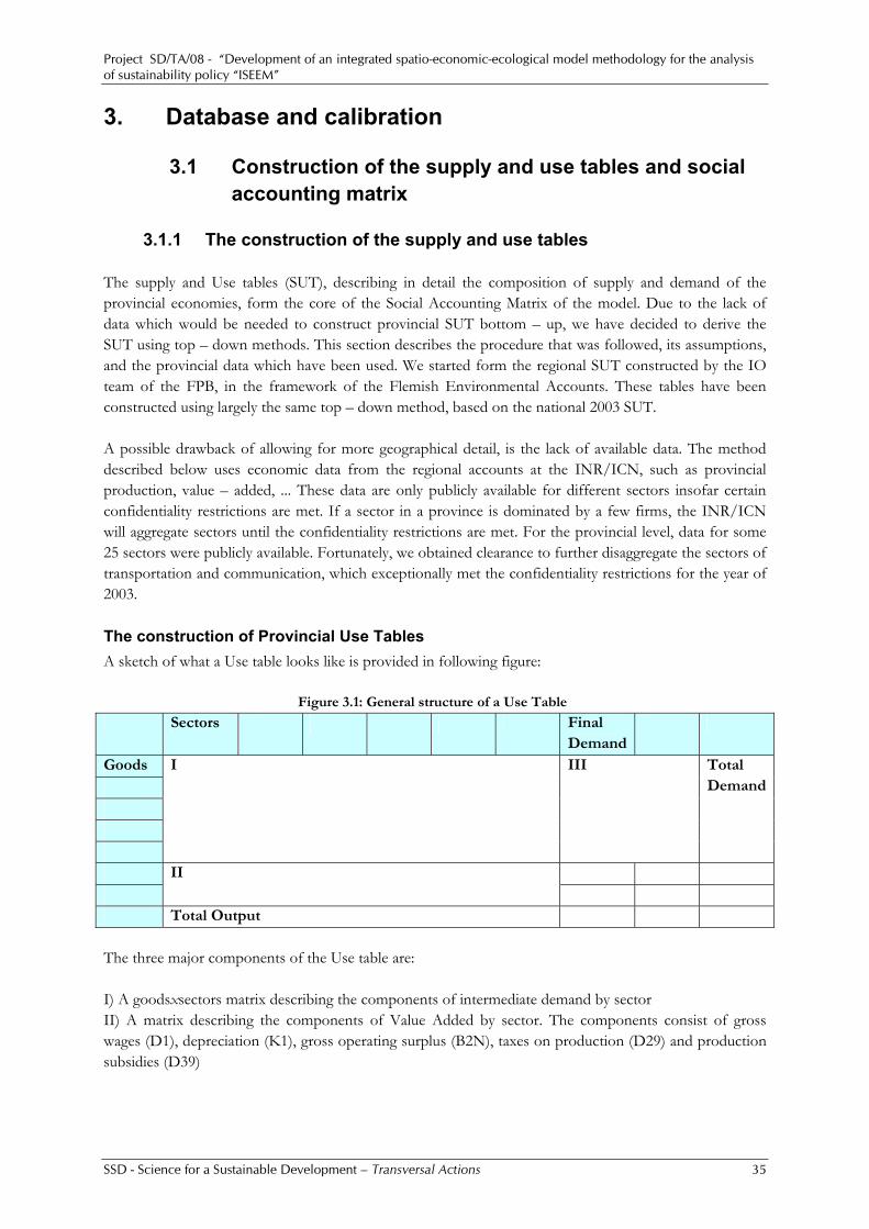
Project SD/TA/08 - “Development of an integrated spatio-economic-ecological model methodology for the analysis of sustainability policy “ISEEM”
SSD - Science for a Sustainable Development – Transversal Actions 35
3. Database and calibration
3.1 Construction of the supply and use tables and social accounting matrix
3.1.1 The construction of the supply and use tables
The supply and Use tables (SUT), describing in detail the composition of supply and demand of the provincial economies, form the core of the Social Accounting Matrix of the model. Due to the lack of data which would be needed to construct provincial SUT bottom – up, we have decided to derive the SUT using top – down methods. This section describes the procedure that was followed, its assumptions, and the provincial data which have been used. We started form the regional SUT constructed by the IO team of the FPB, in the framework of the Flemish Environmental Accounts. These tables have been constructed using largely the same top – down method, based on the national 2003 SUT. A possible drawback of allowing for more geographical detail, is the lack of available data. The method described below uses economic data from the regional accounts at the INR/ICN, such as provincial production, value – added, ... These data are only publicly available for different sectors insofar certain confidentiality restrictions are met. If a sector in a province is dominated by a few firms, the INR/ICN will aggregate sectors until the confidentiality restrictions are met. For the provincial level, data for some 25 sectors were publicly available. Fortunately, we obtained clearance to further disaggregate the sectors of transportation and communication, which exceptionally met the confidentiality restrictions for the year of 2003. The construction of Provincial Use Tables A sketch of what a Use table looks like is provided in following figure:
Figure 3.1: General structure of a Use Table
Sectors Final Demand
Goods
I III Total Demand
II
Total Output The three major components of the Use table are: I) A goodsxsectors matrix describing the components of intermediate demand by sector II) A matrix describing the components of Value Added by sector. The components consist of gross wages (D1), depreciation (K1), gross operating surplus (B2N), taxes on production (D29) and production subsidies (D39)

Project SD/TA/08 - “Development of an integrated spatio-economic-ecological model methodology for the analysis of sustainability policy “ISEEM”
SSD - Science for a Sustainable Development – Transversal Actions 36
III) A matrix giving the components of final demand, by good. The different components are household consumption, consumption of the non profit organisations, government consumption, collective government consumption, Investment, changes in inventories and exports. Summing intermediate consumption and value added by sector gives total production, while summing across products gives total provincial demand. Given data for production, gross value added and gross wages, plus data on provincial household disposable income and provincial population, the Use table can be disaggregated. Where possible, the data have been constructed, first using the maximum disaggregation level available (256 SUT categories). Summation to 26 sectors / goods has been done only at the end of the calculations to use the maximum amount of information available to us. Data processing and aggregation was therefore done inhouse at the FPB to protect confidentiality. In order to reconstruct Part I of the Use table, total intermediate consumption is calculated using data on gross production and value added. By sector this total is split into different intermediate goods using a same product mix assumption: the composition of provincial intermediate demand is assumed to consist of the same proportions of goods as in the regional (and a fortiori national table). It is clear that such an assumption imposes an important degree of uniformity on the data. Applied to environmental policy, it effectively asumes that firms of the same sector have similar energy intensities – as a proportion of total intermediates – across Belgian provinces. Differences in energy intensity as a a percentage of total production will continue to exist though for two reasons. First, the share in output of total intermediate consumption varies across provinces because we use data on output and value added. Second, since we disaggregated the tables at a much finer level of sectoral disaggregation then the 26 sectors of the model, we capture differences in sectoral composition of the various model sectors.
Figure 3.2: Energy intensity across provinces for a number of industrial sectors (percentage of output)
The value added block II is provincialized as follows. Since D1 is given by the data, only K1, D29, D39 and B2N needed to be reconstructed. K1, D29 and D39 have been partitioned using provincial Value Added (VA) as a precentage of regional VA as key. We thus assume a same tax and subsidy rate (and
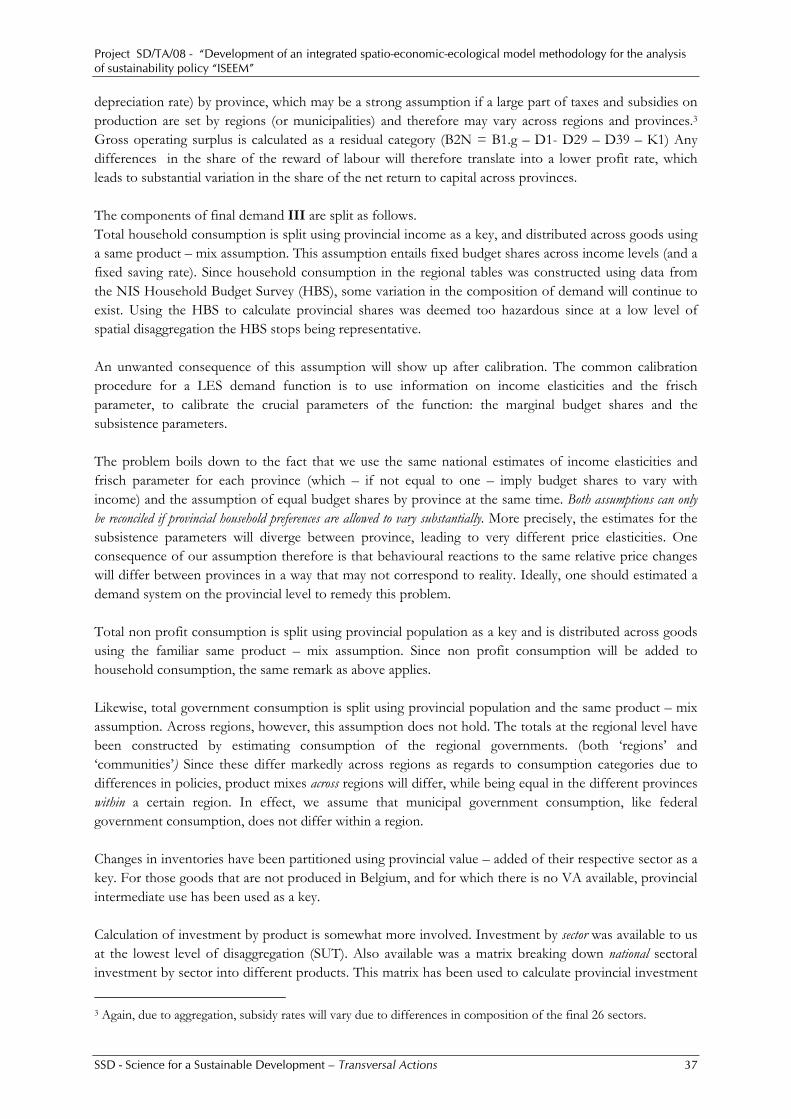
Project SD/TA/08 - “Development of an integrated spatio-economic-ecological model methodology for the analysis of sustainability policy “ISEEM”
SSD - Science for a Sustainable Development – Transversal Actions 37
depreciation rate) by province, which may be a strong assumption if a large part of taxes and subsidies on production are set by regions (or municipalities) and therefore may vary across regions and provinces.3 Gross operating surplus is calculated as a residual category (B2N = B1.g – D1- D29 – D39 – K1) Any differences in the share of the reward of labour will therefore translate into a lower profit rate, which leads to substantial variation in the share of the net return to capital across provinces. The components of final demand III are split as follows. Total household consumption is split using provincial income as a key, and distributed across goods using a same product – mix assumption. This assumption entails fixed budget shares across income levels (and a fixed saving rate). Since household consumption in the regional tables was constructed using data from the NIS Household Budget Survey (HBS), some variation in the composition of demand will continue to exist. Using the HBS to calculate provincial shares was deemed too hazardous since at a low level of spatial disaggregation the HBS stops being representative. An unwanted consequence of this assumption will show up after calibration. The common calibration procedure for a LES demand function is to use information on income elasticities and the frisch parameter, to calibrate the crucial parameters of the function: the marginal budget shares and the subsistence parameters. The problem boils down to the fact that we use the same national estimates of income elasticities and frisch parameter for each province (which – if not equal to one – imply budget shares to vary with income) and the assumption of equal budget shares by province at the same time. Both assumptions can only be reconciled if provincial household preferences are allowed to vary substantially. More precisely, the estimates for the subsistence parameters will diverge between province, leading to very different price elasticities. One consequence of our assumption therefore is that behavioural reactions to the same relative price changes will differ between provinces in a way that may not correspond to reality. Ideally, one should estimated a demand system on the provincial level to remedy this problem. Total non profit consumption is split using provincial population as a key and is distributed across goods using the familiar same product – mix assumption. Since non profit consumption will be added to household consumption, the same remark as above applies. Likewise, total government consumption is split using provincial population and the same product – mix assumption. Across regions, however, this assumption does not hold. The totals at the regional level have been constructed by estimating consumption of the regional governments. (both ‘regions’ and ‘communities’) Since these differ markedly across regions as regards to consumption categories due to differences in policies, product mixes across regions will differ, while being equal in the different provinces within a certain region. In effect, we assume that municipal government consumption, like federal government consumption, does not differ within a region. Changes in inventories have been partitioned using provincial value – added of their respective sector as a key. For those goods that are not produced in Belgium, and for which there is no VA available, provincial intermediate use has been used as a key. Calculation of investment by product is somewhat more involved. Investment by sector was available to us at the lowest level of disaggregation (SUT). Also available was a matrix breaking down national sectoral investment by sector into different products. This matrix has been used to calculate provincial investment
3 Again, due to aggregation, subsidy rates will vary due to differences in composition of the final 26 sectors.
Project SD/TA/08 - “Development of an integrated spatio-economic-ecological model methodology for the analysis of sustainability policy “ISEEM”
SSD - Science for a Sustainable Development – Transversal Actions 38
by product at the lowest level of disaggregation, and has only then been aggregated into coarser product categories. Exports, from EU countries as well as ROW, have been partitioned using provincial production by good (calculated by first constructing the domestic part of the supply tables). Exports for goods that are not produced in Belgium (re-exports of certain mining products) have been broken down according to provincial intermediate use. It is important to note that the provincial use tables that will show up in the SAM are expressed in purchase prices (PP), and therefore include productrelated taxes, subsidies and transport margins (in the case of goods). To obtain numbers for these categories, the same procedure has been used to construct tables in basic prices (BP). For each region, total demand in PP and BP has been calculated and the difference between both totals has been split into taxes, subsidies and margins according to national proportions. The construction of the provincial Supply Tables The general structure of a Supply table is presented in the following figure:
Figure 3.3: General structure of a Supply table Sectors Imports
Goods I II Total Supply
Total
Output
Block I breaks down the total output of each sector by good. This part of the table was easily reconstructed using the same market share assumption, which states that the same sectors in each province supply a same share of goods. Block II gives total imports of each good. Imports have been calculated with the help of the regional use tables of imports constructed by our colleagues at FPB. For each cell in the (regional) use table, a share of imports has been calculated, which was then applied to the provincial use tables described above. Imports could then be calculated by simply summing these provincial use tables of imports across sectors. Linkages between provinces After constructing the SUT, we need additional information to estimate the trade linkages between the different provinces. In general, information on interregional trade is very hard to come by. For trade in goods, we could resort to existing surveys on freight flows. One such dataset, based on a 1995 Stratec survey and supplemented by 2000 freight traffic data by NIS, is used by FPB. This dataset gives freight flows between Belgian so-called “arrondissements” (that is a sub-regional disaggregation) by mode and NSTR goods category. The simplest way to proceed with such data would be to calculate, by province, the

Project SD/TA/08 - “Development of an integrated spatio-economic-ecological model methodology for the analysis of sustainability policy “ISEEM”
SSD - Science for a Sustainable Development – Transversal Actions 39
share of each destination province in total provincial exports. These shares could then be applied to domestic production by province from the IO tables to obtain interregional trade flows. However, freight flow data do not necesseraly add up to trade data. Trade transactions may, for example, consist of different freight transactions (e.g. from factory gate to warehouse, from warehouse to store). If this phenomenon is prevalent, then it is likely that provinces containing major seaports may receive an unduly high share of ‘trade’, due to the presence of hidden exports. We therefore decided to estimate a gravity equation, relating freight flows on origin and destination GDP and trade costs, augmented with arrondissemental dummies to cleanse the equation from the errors mentioned above. Trade flows could then be imputed by taking predicted values for the dependent variable without the regional specific dummies. The specification of the equation was as follows: FFlowij = β0 + β1*ln(Yi/Ni) + β2*ln(Ni) + β3*ln(GDPj/Nj) + β4*ln(Nj) + β5*ln(GCij) + δij + di + dj + εij Yi/Ni : Production per capita of the good in origin region Ni : Population in origin region GDPj/Nj : Total production in destination region Nj : Population in destination region GCij : Generalized cost of transport between regions δij : A dummy representing the existence of a linguistic/regional border between i and j di : Origin dummy
dj : Destination dummy As it turned out, the equations produced biased estimates for the border effect dummy δij. In a regression without regional specific dummies, the border effect turned out to be prohibitively high. (regions separated by a linguistic border would trade only 0.5% the quantity of intraregional trade). In the literature, the existence of an inflated border effect in gravity equations has been amply documented. (e.g. McCallum, 1995) Nevertheless, including regional specific dummies might have been a sufficient remedy against this upward bias, as documented by Anderson and Van Wincoop (2003) In our estimations, even with such dummies the border effect remained more than likely grossly inflated. Due to these problems, we resorted to outside model databases. More particularly, we made use of the shares taken from the Transtools database for trade flows in goods. For trade flows in services lack of data is even more severe. As a last resort, we applied the shares for goods trade to the services sectors as well. Another approach would be to calibrate service flows using the technique described by Treyz and Bumgardner (2000).
3.1.2 Contruction of the social accounting matrix -Datafile: ISEEM-SAM-2006.xls, national level social accounting matrix - Datafile: ISEEM-SAM-auxiliary.xls, unbalanced social accounting matrices on regional level A SAM is a square matrix in which each transaction is recorded only once in a cell of its own – it is conventionally agreed that the entries made in rows represent incomes or receipts, whilst the entries made in columns represent outlays or expenditures - so, for each row there is a corresponding column, i.e. for every income there exists a corresponding expenditure, with their totals being equal. These figures will include both production and institutional accounts, which are subdivided into yet other accounts, defined in accordance with the goal of the study and the available information. Thus, the SAM consists of a set of interrelated subsystems that, on the one hand, give an analytical picture of the studied economy in a

Project SD/TA/08 - “Development of an integrated spatio-economic-ecological model methodology for the analysis of sustainability policy “ISEEM”
SSD - Science for a Sustainable Development – Transversal Actions 40
particular accounting period and, on the other hand, serve as an instrument for assessing the effects of changes on the particular flows represented by it (injections and leakages in the system), which might be the result of policy measures. Therefore, the SAM can be seen as a working instrument for quantifying the flows in the economic circuit and for simulating the effects resulting from any changes in such flows. A social accounting matrix is a useful tool for economic modellers as it can be used as a basecase dataset for a general equilibrium model. The social accounting matrix is already in equilibrium, so the calibration of the economic model then reduces to recreating the existing equilibrium of the social accounting matrix. In theory we could have used the regional supply and use tables to construct a SAM for the model (cfr. 3.1.1), however there were several problems when we tried to construct regional social accounting matrices out of the regional supply and use tables. The main problem when working with a SAM is the interrelatedness of all cells and elements within the matrix, this means that working with the data can get very time consuming and demanding on the researcher. Working with regional SAM adds the extra difficulty of interregional trade patterns. To circumvent the problem of spending too much time constructing balanced regional social accounting matrices, we first constructed a balanced social accounting matrix, based on national supply and use tables of 2003 from the EUROSTAT website. The construction of this matrix could be based on work of a former project of TML, namely the construction of the EDIP model for Europe. The social accounting matrix constructed for Belgium had to be aggregated from 60 sectors to 26 sectors. This is not a very difficult exercise. However, even when working with this more general data, several problems have been encountered and had to be solved. One of the serious problems is that exports and imports of supply and use tables include both own export and import as well as re-export. Inclusion of re-exports into supply and use tables leads to the situation where the total domestic output of the country seems smaller than the country’s export for several groups of products. In order to fix this problem we have used the study on re-export rates, provided to us by the Federal Planning Bureau. Next, commodity and sector classification used in the ISEEM model differs strongly from the commodity and sector classification in supply and use tables. First, we have constructed the SAM based on the commodity and sector classification from the available tables. This SAM was balanced and checked for consistency. Second, then the resulting matrix was aggregated to the sector disaggregation of the ISEEM model. This national level social accounting matrix is then disaggregated within the model code to the specific regions. To do this, we used the work we did formerly on constructing the regional social accounting matrixes, but instead of trying to construct a balanced social accounting matrix from the bottom-up, we parted from the balanced national level matrix and work our way down to the regions using the input-output coefficients of the (unbalanced) regional SAMs wherever possible. Sometimes we had to base the disaggregation on general value added or another measure to avoid inconsistencies: such as sectors in a permanent state of loss, or negative capital on regional level. While this can be correct in the accounts of a 1-year social accounting matrix it cannot be used as a basis for a long term equilibrium nor for the callibration of economic parameters. The only problem that remains then is the callibration of the trade flows, these are balanced to make sure regional demand equals regional supply by using a balancing procedure described in Canning and Wang (2005)
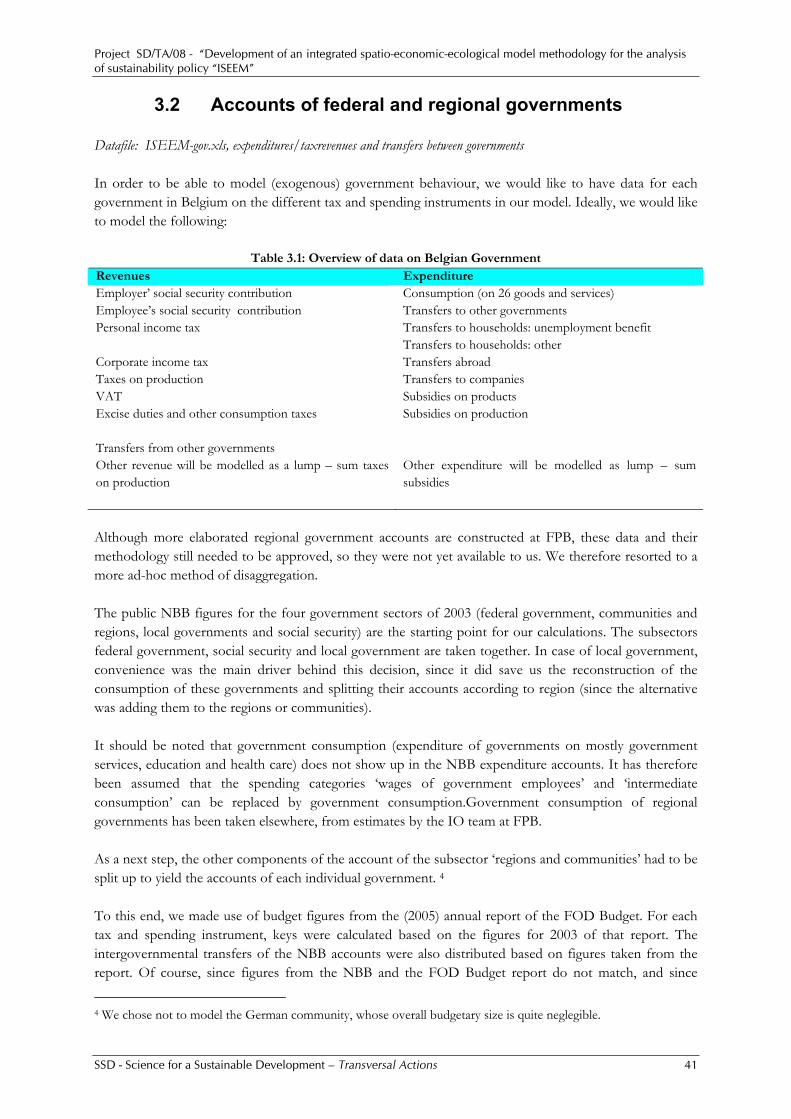
Project SD/TA/08 - “Development of an integrated spatio-economic-ecological model methodology for the analysis of sustainability policy “ISEEM”
SSD - Science for a Sustainable Development – Transversal Actions 41
3.2 Accounts of federal and regional governments Datafile: ISEEM-gov.xls, expenditures/taxrevenues and transfers between governments In order to be able to model (exogenous) government behaviour, we would like to have data for each government in Belgium on the different tax and spending instruments in our model. Ideally, we would like to model the following:
Table 3.1: Overview of data on Belgian Government Revenues Expenditure Employer’ social security contribution Consumption (on 26 goods and services) Employee’s social security contribution Transfers to other governments Personal income tax Transfers to households: unemployment benefit Transfers to households: other Corporate income tax Transfers abroad Taxes on production Transfers to companies VAT Subsidies on products Excise duties and other consumption taxes Subsidies on production Transfers from other governments Other revenue will be modelled as a lump – sum taxes on production
Other expenditure will be modelled as lump – sum subsidies
Although more elaborated regional government accounts are constructed at FPB, these data and their methodology still needed to be approved, so they were not yet available to us. We therefore resorted to a more ad-hoc method of disaggregation. The public NBB figures for the four government sectors of 2003 (federal government, communities and regions, local governments and social security) are the starting point for our calculations. The subsectors federal government, social security and local government are taken together. In case of local government, convenience was the main driver behind this decision, since it did save us the reconstruction of the consumption of these governments and splitting their accounts according to region (since the alternative was adding them to the regions or communities). It should be noted that government consumption (expenditure of governments on mostly government services, education and health care) does not show up in the NBB expenditure accounts. It has therefore been assumed that the spending categories ‘wages of government employees’ and ‘intermediate consumption’ can be replaced by government consumption.Government consumption of regional governments has been taken elsewhere, from estimates by the IO team at FPB. As a next step, the other components of the account of the subsector ‘regions and communities’ had to be split up to yield the accounts of each individual government. 4 To this end, we made use of budget figures from the (2005) annual report of the FOD Budget. For each tax and spending instrument, keys were calculated based on the figures for 2003 of that report. The intergovernmental transfers of the NBB accounts were also distributed based on figures taken from the report. Of course, since figures from the NBB and the FOD Budget report do not match, and since
4 We chose not to model the German community, whose overall budgetary size is quite neglegible.

Project SD/TA/08 - “Development of an integrated spatio-economic-ecological model methodology for the analysis of sustainability policy “ISEEM”
SSD - Science for a Sustainable Development – Transversal Actions 42
‘government consumption’ does not exactly equal wages and intermediatie consumption some error was bound to occur. To make sure total regional government revenue and expenditure add up to the figures from the NBB accounts, the ‘other’ categories were adjusted accordingly.
3.3 Transport related data
3.3.1 Freight flows and transport costs Datafile: ISEEM-auxiliary.xls ( tcosts_fr, aux_fr), sheets with freight transport costs based on transtools data Freight flows were estimated based on the database of the TRANSTOOLS model, aggregated to the provincial (NUTS-2) level. This is one of the only models that figures detailed transport data (NSTR classification, interregional transport, transport costs, etc.) on the provincial level for Belgium. As explained in 3.1.1 (linkages between provinces), it was chosen to use these data, afer an estimation of the freight flows using a gravity model failed. The data on freight flows in ISEEM is used in the calibration process of the interregional trade flows when the model is run for the first time with new data. This calibration procedure has to be initialized whenever some change is made to the intial social accounting matrices, both to the national as to the unbalanced regional social accounting matrices. The result from this calibration is saved in the ISEEM-SAM-2006.xls file (frt_new and interreg_trade_fr sheets). After running the calibration procedure this data is no longer used. The ISEEM dataset also contains an auxiliary dataset on freight (ISEEM-auxiliary.xls, aux_fr sheet). This data could be used for policy simulations, but is not used for any additional purposes within the model. The freight charge simulation which we treat in the Freight charge simulation (5.3) made use of this dataset.
3.3.2 Commuting and education trips Datafile: ISEEM-auxiliary.xl ( tcosts_comm, tcosts_edu) Raw data from weekly commuting trips, their average distance and speed have been obtained from the 2001 socio – economic survey. In the framework of the PLANET project this dataset has been cleaned of possible outliers. Money costs have been taken from Hertveldt e.a. (2006), while time costs are based on the VOT values found in Bickel e.a. (2006). Concerning commuting, one remark is in order. The dataset could be greatly improved if commuting could be broken down by income categories, since we could better track interprovincial flows over labour income that way. Right now the provincial wage bill net of social security contributions is divided across other provinces according to commuting flows, without taking into account the fact that commuters may on average earn higher wages. In other words, while the provincial wage bill in our model follows NBB data, take-home pay does not. The Brussels region is an interesting case. In the present model database Brussels residents earn an income that lies well above the national average, which in reality is quite the opposite case. Among others, this impairs our ability to endogenize intergovernmental transfers. Regional governments are financed – among others – according to a horizontal allocation formula which depends on regional per

Project SD/TA/08 - “Development of an integrated spatio-economic-ecological model methodology for the analysis of sustainability policy “ISEEM”
SSD - Science for a Sustainable Development – Transversal Actions 43
capita personal income tax revenues relative to the national average per capita revenues. Due to its relatively disadvantaged position the Brussels regional government currently enjoys a solidarity grant from the federal government, which in our model economy would not be the case.
3.3.3 Business, shopping and other trips Datafile: ISEEM-auxiliary.xls ( tcosts_buss, tcosts_shop and tcosts_oth), business, shopping and other trips The data for business, shopping and other trips was based on the TRANSTOOLS dataset on passenger flows within Belgium (NUTS-2 level) of the year 2001. However, the dataset had to be cleaned out as it only calculates the total trips between 2 links (region to region), but does not contain information on how the totals are split up by region of origin. This serious defect could only be corrected by applying the O/D shares of the commuting and education trips and applying these on the TRANSTOOLS dataset. This means that the total trips between two regions are the same as in the TRANSTOOLS dataset, but that the amount of flow origination from one province to another is based on the commuting and education flows described above.
3.4 Elasticities Datafile: ISEEM-elasticities.xls (production and consumption) Income elasticities, used to calibrate the household demand side of the model, and parameter estimates for the production function have been taken from the HERMES model at FPB. In both cases values are econometrically estimated, following procedures described in Bossier e.a. (2004). In the case of the production function, estimates were available for marginal coefficients. These are associated with new capital vintages, whereas subsititution possibilities with old capital is typically zero. Although these parameters may better describe the long run where all capital is substitutable, it has been chosen to half the original values for the base case run. Where applicable, results for full values of parameters will be shown. We note that in using the HERMES production function, we – somewhat – atypically assume substitutability of materials with other factors of production.
3.5 Labour market data Datafile: ISEEM-auxiliary.xls (labour market)
3.5.1 Auxiliary data on population, unemployment The data on population and households was based on the publicly available ECODATA database. Active labour is defined as the amount of people from 15 to 64, which can be easily determined via the ECODATA statistics on population by age group. Total unemployment and the unemployment rate are based on the same datasource. All data is based on the year 2006.
3.5.2 Vacancies Vacancies (average monthly job offers received by public employment agencies) are taken from data supplied to us by FOREM and VDAB. No information on job openings were available from Actiris for the Brussels capital region. Therefore we imputed numbers for Brussels on the assumption that the provincial job destruction rate (vacancies / employed persons) equals the national rate.
Project SD/TA/08 - “Development of an integrated spatio-economic-ecological model methodology for the analysis of sustainability policy “ISEEM”
SSD - Science for a Sustainable Development – Transversal Actions 44
3.5.3 Wages and unemployment benefits
Regional wages were taken from the regional statistics of the NBB (National Bank of Belgium). The data have a common problem, namely that they estimate the average wage, based on the place of work and not on the home location of the employee. Similarily as in other data, this leads to an overestimation of the wage in Brussel, compared with the other regions. In this case this problem is not overly important as the regional wages figuring in the auxiliary dataset only play a minor role in the model. They are used to balance the replacement wage of the governement when unemployment increases. The unemployment benefits figuring in the auxiliary dataset, are based on RSZ data from the year 2006. They were checked for consistency with the other provincial data (unemployment, wages).
3.6 Emissions data Datafile: ISEEM-emisssions.xls
3.6.1 Source of data on different emission types We distinguish between greenhouse gasses (GHG’s) and non-GHG’s and use diffent data sources to represent them in the ISEEM model. The data we initially use, is only available on the country level. The country level dataset, coupled to either production or energy input of a sector, is split-up within the model code by assuming that the emissions are the same relative on the production and input of fossil fuels of the industry, compared to the industries in the other regions. This means that we assume the same production technology (and emission coefficients) on regional level as on national level. For CO2 emission data, we used IEA as primary source. Their dataset include a database holding CO2 emissions by sector and by used product on country level. They distinguish 45 products (e.g. brown coal, naphtha, kerosene etc.) which were aggregated for use in the ISEEM model. Apart from different products, also 30 sectors are considered. Unfortunately the sector breakdown is not the same disaggregation as used for ISEEM, so we constructed a compatibility matrix. IEA also supplies emission data for non-CO2 greenhouse gasses and CO2 emissions which are released due to activities other then combustion (fugitive). The non-CO2 GHG considered are CH4, HFC, N2O, PFC and SF6. Sectoral detail for these emissions is very minimal, so a more simple way of allocating the emissions to the sectors is applied. Data is given in MT CO2 equivalent, so no extra conversion is needed. For non-GHG emission data, we used the dataset of EMEP. The EMEP program focuses on assessing the transboundary transport of acidification and eutrophication, the formation of ground level ozone and, more recently, of persistent organic pollutants (POPs), heavy metals and particulate matter. To this end EMEP constructed a large emission inventory database, which we (partially) used as input for EDIP. The pollutants considered for EDIP are CO, NH3, NMVOC, NOx, PM and SO2. Similar to the energy data of IEA, emission data is presented per country and per sector, yet no distinction is made between different inputs. As with the data from IEA, the sectoral breakdown of EMEP is not immediately linkable with the sectors of ISEEM, so, again, a compatibility matrix was constructed.
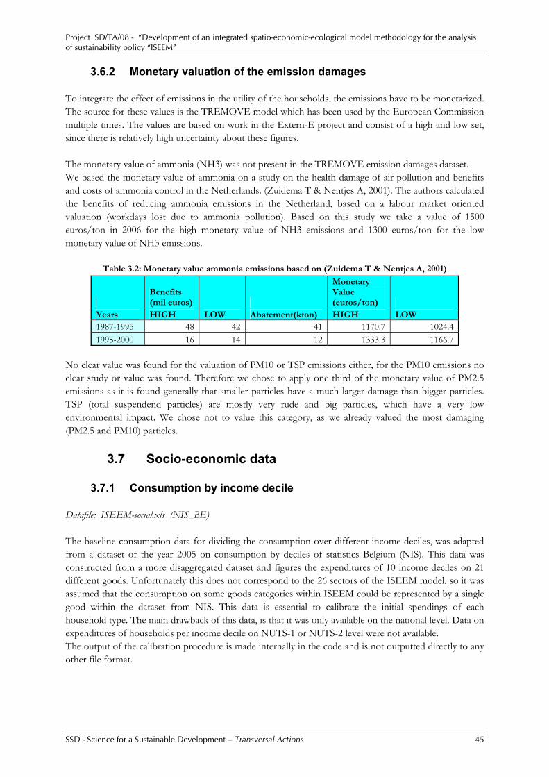
Project SD/TA/08 - “Development of an integrated spatio-economic-ecological model methodology for the analysis of sustainability policy “ISEEM”
SSD - Science for a Sustainable Development – Transversal Actions 45
3.6.2 Monetary valuation of the emission damages To integrate the effect of emissions in the utility of the households, the emissions have to be monetarized. The source for these values is the TREMOVE model which has been used by the European Commission multiple times. The values are based on work in the Extern-E project and consist of a high and low set, since there is relatively high uncertainty about these figures. The monetary value of ammonia (NH3) was not present in the TREMOVE emission damages dataset. We based the monetary value of ammonia on a study on the health damage of air pollution and benefits and costs of ammonia control in the Netherlands. (Zuidema T & Nentjes A, 2001). The authors calculated the benefits of reducing ammonia emissions in the Netherland, based on a labour market oriented valuation (workdays lost due to ammonia pollution). Based on this study we take a value of 1500 euros/ton in 2006 for the high monetary value of NH3 emissions and 1300 euros/ton for the low monetary value of NH3 emissions.
Table 3.2: Monetary value ammonia emissions based on (Zuidema T & Nentjes A, 2001)
Benefits (mil euros)
Monetary Value (euros/ton)
Years HIGH LOW Abatement(kton) HIGH LOW 1987-1995 48 42 41 1170.7 1024.4 1995-2000 16 14 12 1333.3 1166.7
No clear value was found for the valuation of PM10 or TSP emissions either, for the PM10 emissions no clear study or value was found. Therefore we chose to apply one third of the monetary value of PM2.5 emissions as it is found generally that smaller particles have a much larger damage than bigger particles. TSP (total suspendend particles) are mostly very rude and big particles, which have a very low environmental impact. We chose not to value this category, as we already valued the most damaging (PM2.5 and PM10) particles.
3.7 Socio-economic data
3.7.1 Consumption by income decile Datafile: ISEEM-social.xls (NIS_BE) The baseline consumption data for dividing the consumption over different income deciles, was adapted from a dataset of the year 2005 on consumption by deciles of statistics Belgium (NIS). This data was constructed from a more disaggregated dataset and figures the expenditures of 10 income deciles on 21 different goods. Unfortunately this does not correspond to the 26 sectors of the ISEEM model, so it was assumed that the consumption on some goods categories within ISEEM could be represented by a single good within the dataset from NIS. This data is essential to calibrate the initial spendings of each household type. The main drawback of this data, is that it was only available on the national level. Data on expenditures of households per income decile on NUTS-1 or NUTS-2 level were not available. The output of the calibration procedure is made internally in the code and is not outputted directly to any other file format.
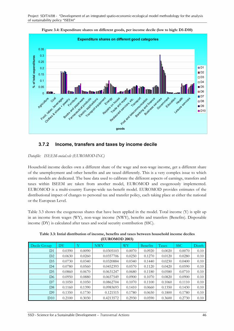
Project SD/TA/08 - “Development of an integrated spatio-economic-ecological model methodology for the analysis of sustainability policy “ISEEM”
SSD - Science for a Sustainable Development – Transversal Actions 46
Figure 3.4: Expenditure shares on different goods, per income decile (low to high: D1-D10)
Expenditure shares on different good categories
0
0.05
0.1
0.15
0.2
0.25
0.3
0.35
Agricu
lture
Coal
Food, ta
bac,
beve
rages
Clothes &
shoe
s + je
welry
Furnitu
re
Books
and pa
perw
are
Farmace
utical
products
Electric
applica
tions
Transport
equipm
ent
Energy
Repairs
on hou
se
Trade an
d repa
ir
Restaura
nt se
rvice
s, etc.
Transport
Post a
nd te
lecom
municatio
n
Bankin
g and
finan
ce
Busines
s serv
ices
Govern
ment
Educa
tion
Health
Leisu
re servi
ces
goods
% o
f tot
al e
xpen
ditu
res
D1D2D3D4D5D6D7D8D9D10
3.7.2 Income, transfers and taxes by income decile Datafile: ISEEM-social.xls (EUROMOD-INC) Household income deciles own a different share of the wage and non-wage income, get a different share of the unemployment and other benefits and are taxed differently. This is a very complex issue to which entire models are dedicated. The base data used to calibrate the different aspects of earnings, transfers and taxes within ISEEM are taken from another model, EUROMOD and exogenously implemented. EUROMOD is a multi-country Europe-wide tax-benefit model. EUROMOD provides estimates of the distributional impact of changes to personal tax and transfer policy, each taking place at either the national or the European Level. Table 3.3 shows the exogeneous shares that have been applied in the model. Total income (Y) is split up in an income from wages (WY), non-wage income (NWY), benefits and transfers (Benefits). Disposable income (DY) is calculated after taxes and social security contribution (SSC).
Table 3.3: Intial distribution of income, benefits and taxes between household income deciles (EUROMOD 2003)
Decile Group DY Y NWY WY Benefits Taxes SSC DistrhD1 0.0390 0.0090 0.0305103 0.0070 0.0920 0.0020 0.0070 0.10D2 0.0630 0.0260 0.0357706 0.0250 0.1270 0.0120 0.0280 0.10D3 0.0730 0.0340 0.0320884 0.0340 0.1440 0.0230 0.0400 0.10D4 0.0780 0.0560 0.0452393 0.0570 0.1120 0.0420 0.0590 0.10D5 0.0860 0.0670 0.0631247 0.0680 0.1180 0.0580 0.0710 0.10D6 0.0950 0.0880 0.0657549 0.0900 0.1070 0.0820 0.0900 0.10D7 0.1050 0.1050 0.0862704 0.1070 0.1100 0.1060 0.1110 0.10D8 0.1160 0.1390 0.0983693 0.1410 0.0660 0.1350 0.1430 0.10D9 0.1350 0.1730 0.121515 0.1780 0.0650 0.1800 0.1780 0.10
D10 0.2100 0.3030 0.4213572 0.2930 0.0590 0.3600 0.2730 0.10

Project SD/TA/08 - “Development of an integrated spatio-economic-ecological model methodology for the analysis of sustainability policy “ISEEM”
SSD - Science for a Sustainable Development – Transversal Actions 47
3.8 Data on structure of firms
3.8.1 Land and buildings as production factors Datafile: ISEEM-auxiliary.xls (land, aux_land, housing, buildings) In ISEEM, production sectors use both land and buildings as production factors. The total expenditures on land and buildings per firm are estimated based on values derived from the structure of enterprises survey of 2001, publicly available on the NIS website. The states the relative amount of the firms average capital that is used for expenditures on land and expenditures on buildings. These country level variables are applied on all regions. This means that we assume that each sector spends the same amount of money on land and buildings regionally as the country average. From the regional expenditures on land and buildings derived in this way, we determine the initial stock of land, for each land type. We assume that each sector only uses 1 type of land, dependent on it being an agricultural, industrial or service sector. An attempt was made to prepare additional data for the model and make calculations on both the availability of land and the value of land in 2006. This was done by combining datasets from the National Statistics Institute, EcoMod data and information from the Social accounting matrix. The result is given in the aux_land datasheet. Other datasets on housing and building stock were prepared as well, based on the same data sources. To our regret, the use of these datasets within ISEEM was kept very limited, as there was no time to implement and test the new methodology on land use, housing market and buildings.
3.8.2 Number of firms Datafile: ISEEM-auxiliary.xls (firms) absolute number of firms in each region This dataset was prepared, based on the ECODATA statistics on number of firms (NACE sector classificiation) within each region in the year 2006. The initial dataset was aggregated from 60 sectors to 26 sectors, in a similar way as done to aggregate the social accounting matrix on country level (cfr. 3.1.2 )


Project SD/TA/08 - “Development of an integrated spatio-economic-ecological model methodology for the analysis of sustainability policy “ISEEM”
SSD - Science for a Sustainable Development – Transversal Actions 49
4. Indicators
4.1 INTRODUCTION Indicators perform many functions. They can lead to better decisions and more effective actions by simplifying, clarifying and making information available to policy makers. They can help measure and calibrate progress toward sustainable development goals. In the first section, we will shortly review the concepts of sustainability indicators. Then we will talk about the different characteristics that indicators need so as to be effective. After that we will distinguish the three pillars and explain the choice for single and traditional indicators instead of composite indicators. In annex III on the final report we present a list of the different indicators proposed in the ISEEM project with additional explanations.
4.2 INDICATORS OF SUSTAINABILITY
4.2.1 Developing an indicator for sustainability The concepts of sustainability indicators Sustainability indicators may be viewed as toolkits to guide policy makers when choosing among various policy options taking sustainable development into account. They ought to build the foundation for improved information and data collection, and enable a comparative and national (or regional) specific analysis of the state of and progress towards sustainable development.5 Characteristics of an effective indicator An indicator is a quantitative or qualitative measure derived from a series of observed facts that can reveal positions in a given area. When evaluated at regular intervals, an indicator can point out the directions of change across different units and through time. In the context of policy analysis, indicators are useful in identifying trends and drawing attention to particular issues. They can also be helpful in setting policy priorities and in benchmarking or monitoring performance. There are several requirements that are important to choose indicators: Indicators should be: Scientific:
• Measurable and quantifiable: they should adequately reflect the phenomenon intended to be measured
• Meaningful: appropriate to the needs of the user • Clear in value: distinct indication which direction is good and which is bad • Clear in content: measure in understandable units that make sense
Functional: • Relevant: for all stakeholders involved • Leading: so that they can provide information to act on • Possible to influence: Indicators must measure parameters that may be modified
5 Spangenberg , J.H., Pfahl, S., Deller, K., 2002, Towards indicators for institutional sustainability: lessons from an analysis of Agenda 21, Ecological Indicators, 2, 2002, 61-77
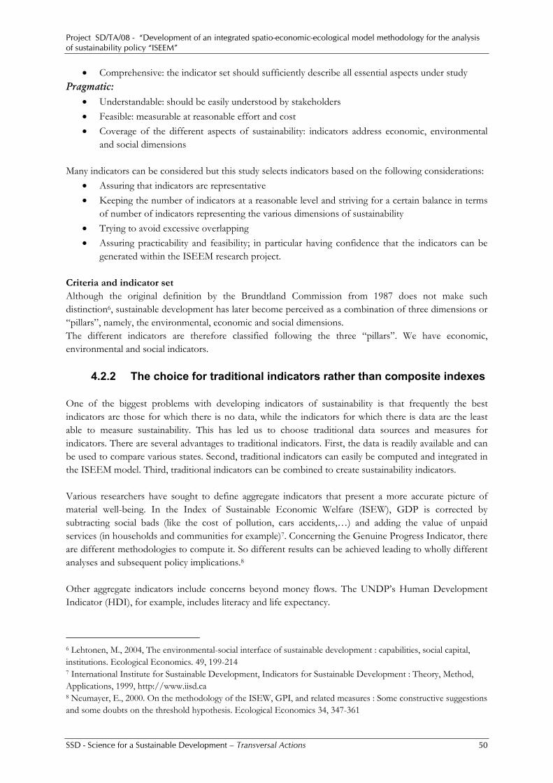
Project SD/TA/08 - “Development of an integrated spatio-economic-ecological model methodology for the analysis of sustainability policy “ISEEM”
SSD - Science for a Sustainable Development – Transversal Actions 50
• Comprehensive: the indicator set should sufficiently describe all essential aspects under study Pragmatic:
• Understandable: should be easily understood by stakeholders • Feasible: measurable at reasonable effort and cost • Coverage of the different aspects of sustainability: indicators address economic, environmental
and social dimensions Many indicators can be considered but this study selects indicators based on the following considerations:
• Assuring that indicators are representative • Keeping the number of indicators at a reasonable level and striving for a certain balance in terms
of number of indicators representing the various dimensions of sustainability • Trying to avoid excessive overlapping • Assuring practicability and feasibility; in particular having confidence that the indicators can be
generated within the ISEEM research project. Criteria and indicator set Although the original definition by the Brundtland Commission from 1987 does not make such distinction6, sustainable development has later become perceived as a combination of three dimensions or “pillars”, namely, the environmental, economic and social dimensions. The different indicators are therefore classified following the three “pillars”. We have economic, environmental and social indicators.
4.2.2 The choice for traditional indicators rather than composite indexes One of the biggest problems with developing indicators of sustainability is that frequently the best indicators are those for which there is no data, while the indicators for which there is data are the least able to measure sustainability. This has led us to choose traditional data sources and measures for indicators. There are several advantages to traditional indicators. First, the data is readily available and can be used to compare various states. Second, traditional indicators can easily be computed and integrated in the ISEEM model. Third, traditional indicators can be combined to create sustainability indicators. Various researchers have sought to define aggregate indicators that present a more accurate picture of material well-being. In the Index of Sustainable Economic Welfare (ISEW), GDP is corrected by subtracting social bads (like the cost of pollution, cars accidents,…) and adding the value of unpaid services (in households and communities for example)7. Concerning the Genuine Progress Indicator, there are different methodologies to compute it. So different results can be achieved leading to wholly different analyses and subsequent policy implications.8 Other aggregate indicators include concerns beyond money flows. The UNDP’s Human Development Indicator (HDI), for example, includes literacy and life expectancy.
6 Lehtonen, M., 2004, The environmental-social interface of sustainable development : capabilities, social capital, institutions. Ecological Economics. 49, 199-214 7 International Institute for Sustainable Development, Indicators for Sustainable Development : Theory, Method, Applications, 1999, http://www.iisd.ca 8 Neumayer, E., 2000. On the methodology of the ISEW, GPI, and related measures : Some constructive suggestions and some doubts on the threshold hypothesis. Ecological Economics 34, 347-361
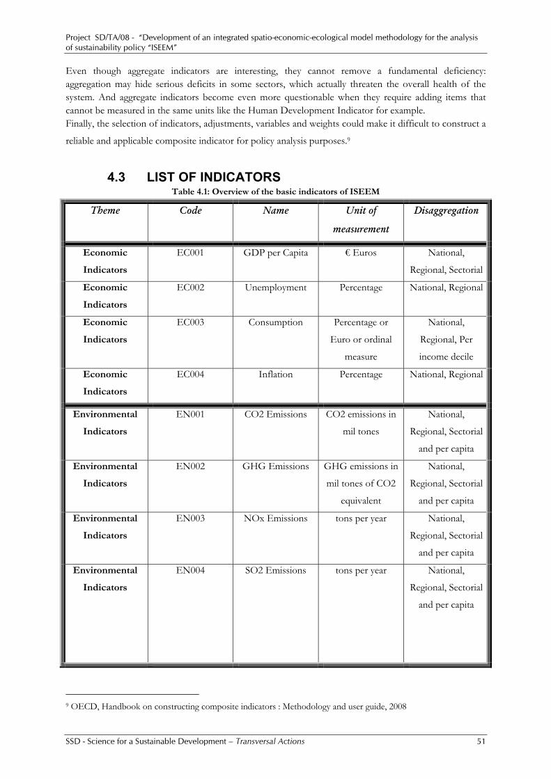
Project SD/TA/08 - “Development of an integrated spatio-economic-ecological model methodology for the analysis of sustainability policy “ISEEM”
SSD - Science for a Sustainable Development – Transversal Actions 51
Even though aggregate indicators are interesting, they cannot remove a fundamental deficiency: aggregation may hide serious deficits in some sectors, which actually threaten the overall health of the system. And aggregate indicators become even more questionable when they require adding items that cannot be measured in the same units like the Human Development Indicator for example. Finally, the selection of indicators, adjustments, variables and weights could make it difficult to construct a
reliable and applicable composite indicator for policy analysis purposes.9
4.3 LIST OF INDICATORS Table 4.1: Overview of the basic indicators of ISEEM
Theme Code Name Unit of
measurement
Disaggregation
Economic
Indicators
EC001 GDP per Capita € Euros National,
Regional, Sectorial
Economic
Indicators
EC002 Unemployment Percentage National, Regional
Economic
Indicators
EC003 Consumption Percentage or
Euro or ordinal
measure
National,
Regional, Per
income decile
Economic
Indicators
EC004 Inflation Percentage National, Regional
Environmental
Indicators
EN001 CO2 Emissions CO2 emissions in
mil tones
National,
Regional, Sectorial
and per capita
Environmental
Indicators
EN002 GHG Emissions GHG emissions in
mil tones of CO2
equivalent
National,
Regional, Sectorial
and per capita
Environmental
Indicators
EN003 NOx Emissions tons per year National,
Regional, Sectorial
and per capita
Environmental
Indicators
EN004 SO2 Emissions tons per year National,
Regional, Sectorial
and per capita
9 OECD, Handbook on constructing composite indicators : Methodology and user guide, 2008
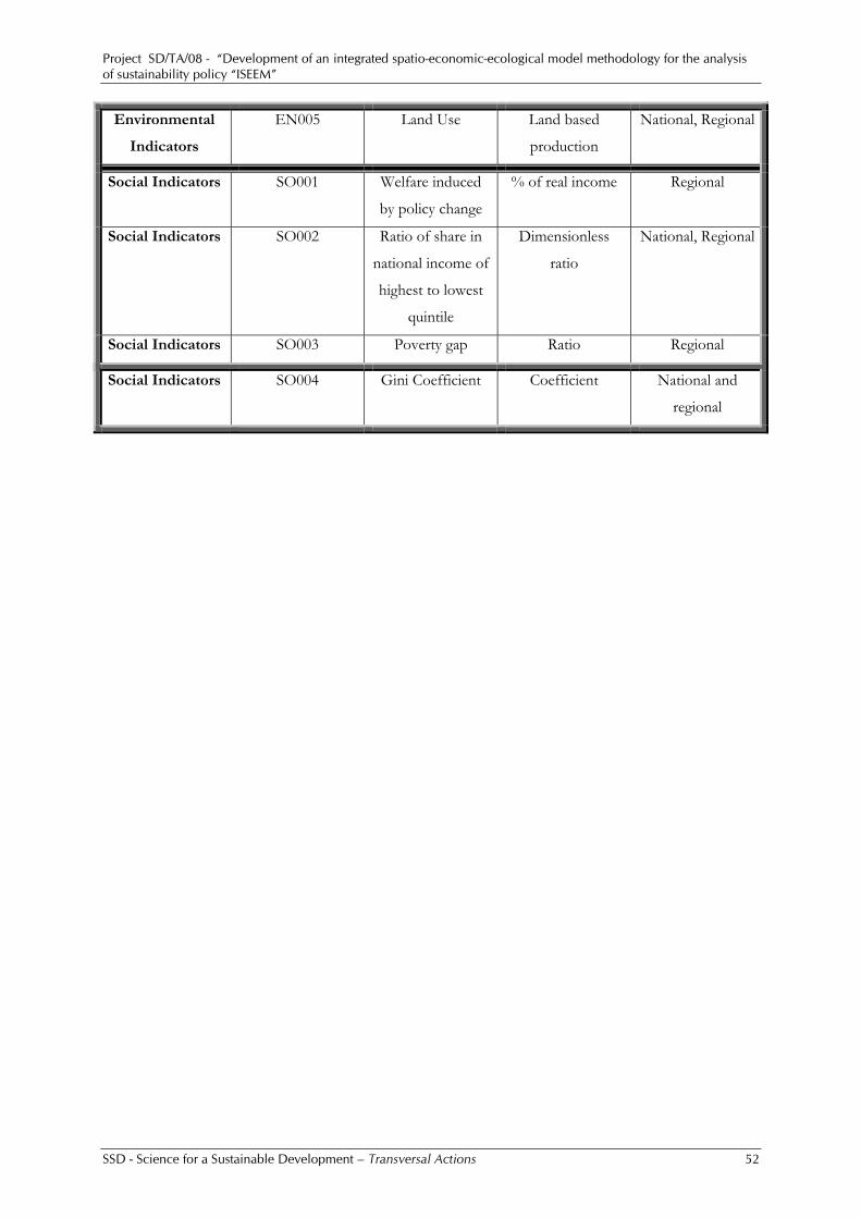
Project SD/TA/08 - “Development of an integrated spatio-economic-ecological model methodology for the analysis of sustainability policy “ISEEM”
SSD - Science for a Sustainable Development – Transversal Actions 52
Environmental
Indicators
EN005 Land Use Land based
production
National, Regional
Social Indicators SO001 Welfare induced
by policy change
% of real income Regional
Social Indicators SO002 Ratio of share in
national income of
highest to lowest
quintile
Dimensionless
ratio
National, Regional
Social Indicators SO003 Poverty gap Ratio Regional
Social Indicators SO004 Gini Coefficient Coefficient National and
regional

Project SD/TA/08 - “Development of an integrated spatio-economic-ecological model methodology for the analysis of sustainability policy “ISEEM”
SSD - Science for a Sustainable Development – Transversal Actions 53
5. Policy Simulations and results
5.1 Technical simulation: lower commuting times with an extended labour market formulation
At present, the representation of regional labour markets and commuting are represented by elements which have been borrowed from Pissarides’ theory of unemployment, without – however – incorporating some of its essential elements. In the literature, Pissarides’ theory has already been applied towards a regional dimension. Van Ommeren e.a. (2002) use the search framework to examine the effects of infrastructure improvements on regional labour markets. In a spatial CGE model tailored towards transport and the labour market, Pilegaard (2003) examines a wider range of issues using search theory, including the effects of commuting subsidies, a reduction in labour income taxes and vacancy subsidies on regional unemployment and transportation externalities. Ideally we would like to see our model to be able to answer the same set of questions. Unfortunately, the present formulation misses some crucial elements which drive the results underlying Pissarides’ theory and its spatial applications. In the following we will give the results of an exogenous transport improvement in ISEEM, explain their causes, and suggest how the model can be improved. To this end, two version of the model have been developed. One, the main version described above, only models interregional matching and commuting, with a classic wage equation and labour demand condition which contain no links to the Pissarides block. Another version does incorporate some richer theoretical effects, but is only developed as a test version.
5.1.1 Calibration Since pairwise matching via equation (x) is the main driver of the submodel, we will first explain a bit how its parameters are chosen or calibrated.
( ) )()1(,,
,,,,, rrrrrrrrrrrrrrr TmoneyTtimebetaTMr
Mrrrrrrrr eUNEMPNVaMNM +⋅−− ⋅⋅⋅= αα (1)
The value of the Cobb Douglas share parameter rrrM ,α of 0.4 is chosen in a standard way. A value below 0.5 indicates that in the matching process additional vacancies are more likely to decrease the probability of a match more for the firm then an extra unemployed would for workers. The intial number of matches rrrNMZ , is calculated as follows:
∑⋅⋅=r
rrrrrrrrrrrrr LCMZLCMZQRZNVZNMZ ,,, / (2)
Where the initial probability rrQRZ is assumed to equal 0.5. Not surpisingly the number of matches tracks commuting patterns very closely. The value of the crucial betaT – parameter is then obtained as follows. We took the initial number of matches, vacancies, unemployed and the betaT parameter to construct a new variable rrrX , :

Project SD/TA/08 - “Development of an integrated spatio-economic-ecological model methodology for the analysis of sustainability policy “ISEEM”
SSD - Science for a Sustainable Development – Transversal Actions 54
/ln( ,, rrrrrr NMZX = ( ) ))1( ,, rrrrrr Mr
Mrr UNEMPNV αα −⋅ (3)
This auxiliary variable is then regressed on time and monetary costs of commuting, obtaining an estimate of betaT of about 111. Given this value, the scaling parameter rrraM , should then subsume other
influences on commuting patterns, such as the linguistic barrier and other reasons for spatial mismatch. To enhance insight into the simulations below, we report actual commuting patterns from and towards Brussels, the corresponding matches and the scaling parameter.
Table 5.1: Labour commuting from and towards Brussels Region LCMZr,bru NMZr,bru aMr,bru LCMZbru,r NMZbru,r aMbru,r BRU 10.452 0.467 0.276 10.452 0.467 0.276 ANT 0.765 0.034 0.042 0.102 0.021 0.017 LIM 0.191 0.009 0.032 0.012 0.002 0.009 VBR 4.413 0.197 0.253 0.893 0.167 0.106 OVL 2.391 0.107 0.123 0.027 0.006 0.005 WVL 0.767 0.034 0.082 0.002 0.0005 0.001 HEN 1.657 0.074 0.089 0.070 0.004 0.012 WBR 1.693 0.076 0.185 0.278 0.058 0.081 NAM 0.443 0.020 0.061 0.027 0.004 0.013 LUI 0.394 0.018 0.042 0.014 0.001 0.007 LUX 0.030 0.001 0.019 0.002 0.0005 0.008
Despite their relative proximity to Brussels, Flemish Brabant (VBR), East-Flanders (OVL) and Walloon Brabant (WBR) retain the highest exogenous scaling parameter. Distance and transport costs alone (as measured by the exponential function) can therefore not account for the relatively high level of commuting towards Brussels from these provinces.
5.1.2 The extended model The base version of model lacks the most essential features of search models, and is as such not firmly grounded in theory, let alone into empirics on regional labour markets in Belgium. As a quick test of what may be achieved without having to change the basics of the labour market part10, we expanded the model to include two of the three essential ingredients of the Pissarides model: the job creation condition and the wage bargaining equation. The job creation condition is just a modification of the familiar labour demand equation. The firm is assumed to maximize a discounted stream of profits, treating the (variable!) labour input rsLv , as an asset, with the
number of vacancies as the control variable. In this problem wvi,r is a parameter for the total cost per vacancy. It has been arbitrarily set at 0.25 (following Pilegaard (2003)). r and rν (the job destrucion rate) are treated as parameters as well.
∫∞
=
− −−0
,,,,, ))((max,
tririririri
rtLv dtLvPLNVSwvLvYe
ri (4)
s.t. rirrirri LvNVSqrLv ,,, ν−=•
10 Like pairwise matching, a single wage rate, no Beverdige curve. Changing these features to a more theoretically sound model was not possible within the present timeframe.
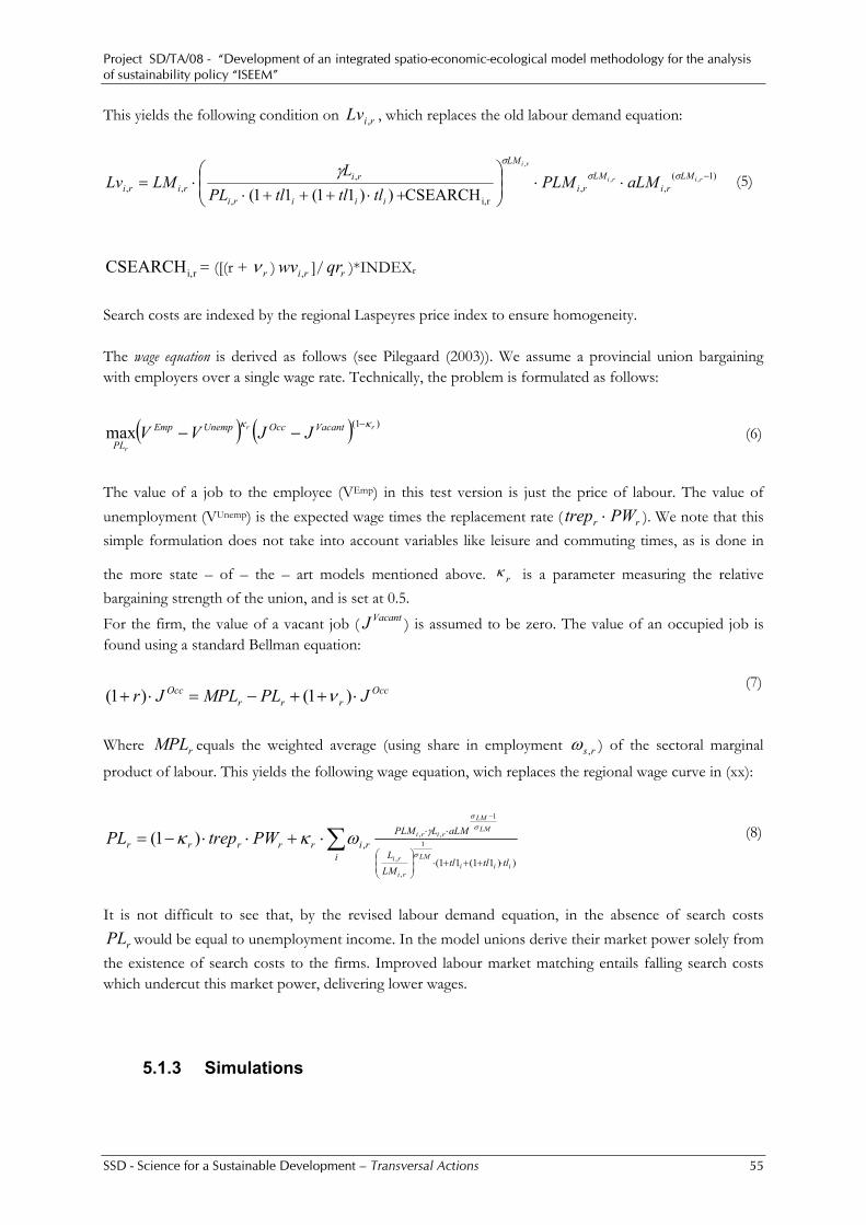
Project SD/TA/08 - “Development of an integrated spatio-economic-ecological model methodology for the analysis of sustainability policy “ISEEM”
SSD - Science for a Sustainable Development – Transversal Actions 55
This yields the following condition on riLv , , which replaces the old labour demand equation:
)1(,,
ri,,
,,,
,,
,
CSEARCH))11(11(−⋅⋅⎟
⎟⎠
⎞⎜⎜⎝
⎛
+⋅+++⋅⋅= riri
ri
LMri
LMri
LM
iiiri
ririri aLMPLM
tltltlPLL
LMLv σσσ
γ (5)
ri,CSEARCH = ([(r + rν ) riwv , ]/ rqr )*INDEXr
Search costs are indexed by the regional Laspeyres price index to ensure homogeneity. The wage equation is derived as follows (see Pilegaard (2003)). We assume a provincial union bargaining with employers over a single wage rate. Technically, the problem is formulated as follows:
( ) ( ) )1(max rr
r
VacantOccUnempEmp
PLJJVV κκ −
−− (6)
The value of a job to the employee (VEmp) in this test version is just the price of labour. The value of unemployment (VUnemp) is the expected wage times the replacement rate ( rr PWtrep ⋅ ). We note that this simple formulation does not take into account variables like leisure and commuting times, as is done in
the more state – of – the – art models mentioned above. rκ is a parameter measuring the relative bargaining strength of the union, and is set at 0.5. For the firm, the value of a vacant job ( VacantJ ) is assumed to be zero. The value of an occupied job is found using a standard Bellman equation:
Occrrr
Occ JPLMPLJr ⋅++−=⋅+ )1()1( ν (7)
Where rMPL equals the weighted average (using share in employment rs,ω ) of the sectoral marginal
product of labour. This yields the following wage equation, wich replaces the regional wage curve in (xx):
∑⋅+++⋅⎟
⎟⎠
⎞⎜⎜⎝
⎛
⋅⋅
−
⋅+⋅⋅−=i tltltl
LML
aLMLPLMrirrrrr
iiiLM
ri
ri
LMLM
ririPWtrepPL))11(11(
, 1
,
,
1
,,)1(σ
σσ
γωκκ (8)
It is not difficult to see that, by the revised labour demand equation, in the absence of search costs
rPL would be equal to unemployment income. In the model unions derive their market power solely from the existence of search costs to the firms. Improved labour market matching entails falling search costs which undercut this market power, delivering lower wages.
5.1.3 Simulations

Project SD/TA/08 - “Development of an integrated spatio-economic-ecological model methodology for the analysis of sustainability policy “ISEEM”
SSD - Science for a Sustainable Development – Transversal Actions 56
In both versions, we exogenously reduced the bilateral time cost of commuting between Antwerp and Brussels by 50%. In terms of the Pissarides model, such a change would decrease mismatch between job candidates and job offers between the two provinces. To keep attention focussed on the essentials, we suppressed the labour supply effect of changes in commuting time. Government budgets are closed by allowing the deficit to improve. Predictably, in the base version the policy only leads to a redistribution of the number matches and to a corresponding redistribution of commuting flows. It has hardly any influence on the total number of commuters and on national unemployment, or output. There is, however, a very large change in the number of vacancies within both regions and a correspondingly large change of the probability of filling a vacancy (QRr). By the definition of QRr, the number of matches towards Brussels does not change much. Correspondingly, labour demand does not change much either. This drop in vacancies is at the root of the redistribution effect noted above. Falling vacancies cause the number of matches to drop to and from brussels and other provinces, thereby serving as a harmless factor restoring equilibrium without affecting the other variables in the model. The reason is, of course, that Pissarides variables like vacancies and QRr hardly play any role in the model, other than in the stand – alone labour market submodel. In the extended version, both labour demand as well as wage setting will be influenced by changes in the labour market variables. We expect the policy to induce dropping search costs, reducing the wegde between wages and the marginal productivity of labour, leading to downward pressure on wages and rising labour demand. Some results of dropping time costs in the extended version are presented below.
Table 5.2: Percentual changes in job matches from and towards Brussels BXL ANT LIM VBR OVL WVL HEN WBR NAM LUI LUX From 0.20 31.37 -0.18 -0.14 -0.17 -0.18 -0.12 -0.14 -0.17 -0.17 -0.19 Towards 0.20 25.69 0.39 0.35 -0.37 0.38 0.38 0.35 0.38 0.39 0.39
Table 5.3: Percentual changes in job commuters from and towards Brussels BXL ANT LIM VBR OVL WVL HEN WBR NAM LUI LUX From 0.01 6.25 -0.04 -0.03 -0.03 -0.04 -0.007 -0.03 -0.03 -0.02 -0.04 Towards 0.05 1.13 0.02 0.02 0.02 0.02 0.02 0.02 0.02 0.02 0.02
Table 5.4: Percentual changes in a number of variables. BXL ANT LIM VBR OVL WVL HEN WBR NAM LUI LUX CSEARCHr -0.144 -0.010 0.021 0.122 0.054 0.023 0.120 0.121 0.049 0.031 0.007 NVr 0.983 0.053 0.019 0.114 0.057 0.024 0.176 0.130 0.058 0.042 0.007 UNEMPr -0.313 -0.219 -0.011 -0.071 -0.033 -0.016 -0.025 -0.067 -0.024 -0.010 -0.005 PLr -0.054 -0.013 0.004 0.004 0.002 0.002 -0.003 -0.0001 -0.003 -0.0001 -0.001 RGDr 0.091 0.028 0.011 0.011 0.014 0.012 0.016 0.014 0.012 0.012 0.010 PWr -0.047 -0.014 0.001 -0.016 -0.007 -0.002 -0.010 -0.022 -0.008 -0.003 -0.002 GDPr 0.030 0.009 0.003 0.003 0.004 0.003 0.005 0.005 0.004 0.003 0.003
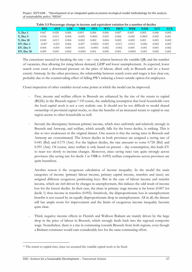
Project SD/TA/08 - “Development of an integrated spatio-economic-ecological model methodology for the analysis of sustainability policy “ISEEM”
SSD - Science for a Sustainable Development – Transversal Actions 57
Table 5.5 Percentage change in income and equivalent variation for a number of deciles BXL ANT LIM VBR OVL WVL HEN WBR NAM LUI LUX Yr Dec 1 0.067 0.020 0.006 0.003 0.006 0.006 0.007 0.005 0.005 0.006 0.005 Yr Dec 5 0.036 0.015 0.004 -0.002 0.0001 0.003 0.006 -0.002 0.0001 0.002 0.001 Yr Dec 10 0.045 0.013 0.004 -0.002 0.002 0.004 0.002 -0.002 0.001 0.003 0.002 EVr Dec 1 -0.007 -0.021 0.006 -0.007 -0.0003 0.005 -0.011 -0.012 -0.006 0.002 0.005 EVr Dec 5 0.004 -0.001 0.003 -0.003 -0.0001 0.002 -0.002 -0.005 -0.001 0.001 0.002 EVr Dec 10 0.009 0.005 0.002 -0.0001 0.001 0.002 0.001 -0.0001 -0.001 0.002 0.001
The extensions succeed in breaking the one – on – one relation between the variable QRr and the number of vacancies, thus allowing for rising labour demand, GDP and lower unemployment. As expected, lower search costs exert a downward pressure on the price of labour, albeit only in Brussels and (to a lesser extent) Antwerp. In the other provinces, the relationship between search costs and wages is less clear cut, probably due to the countervailing effect of falling PW’s inducing a lower outside option for employees. Closer inspection of other variables reveal some points at which the model can be improved.
- First, income and welfare effects in Brussels are enhanced by the rise of the return to capital (RGDr) in the Brussels region.11 Of course, the underlying assumption that local households own the local capital stock is not a very realistic one. It should not be too difficult to model shared ownership of provincial capital stocks, so that the benefits of an increased return to capital in one region accrue to other households as well.
- Second, the discrepancy between primary income, which rises uniformly and relatively strongly in
Brussels and Antwerp, and welfare, which actually falls for the lower deciles, is striking. This is due to two weaknesses in the original dataset. One reason is that the saving rates in Brussels and Antwerp are overestimated. The lowest deciles in both provinces are assigned a saving rate of 0.441 (Bxl) and 0.175 (Ant). For the highest deciles, the rate amounts to some 0.720 (Bxl) and 0.591 (Ant). Of course, since welfare is only based on present – day consumption, this leads EV to react too slowly to income changes. Moreover, since saving rates vary quite strongly across provinces (the saving rate for decile 1 in VBR is -0.093) welfare comparisons across provinces are quite hazardous.
Another reason is the exogenous calculation of income inequality. In the model the main categories of income (primary labour income, primary capital income, transfers and taxes) are assigned different exogenous partitioning keys. But in the case of labour income and transfer income, which are both driven by changes in unemployment, this induces the odd result of income loss for the lowest deciles. In their case, the share in primary wage income is far lower (0.007 for decile 1) then income in transfers (0.092). Intuitively, the disproportionate loss in unemployment benefits is not caused by an equally disproportionate drop in unemployment. All in all, the dataset still has ample room for improvement and the limits of exogenous income inequality become quite clear.
- Third, negative income effects in Flemish and Walloon Brabant are mainly driven by the large
drop in the price of labour in Brussels, which strongly feeds back into the regional composite wage. Nonetheless, there is a rise in commuting towards Brussels from both regions, even though a Brabant commuter would earn considerably less for the same commuting effort.
11 The return to capital rises, since we assumed the variable capital stock to be fixed.
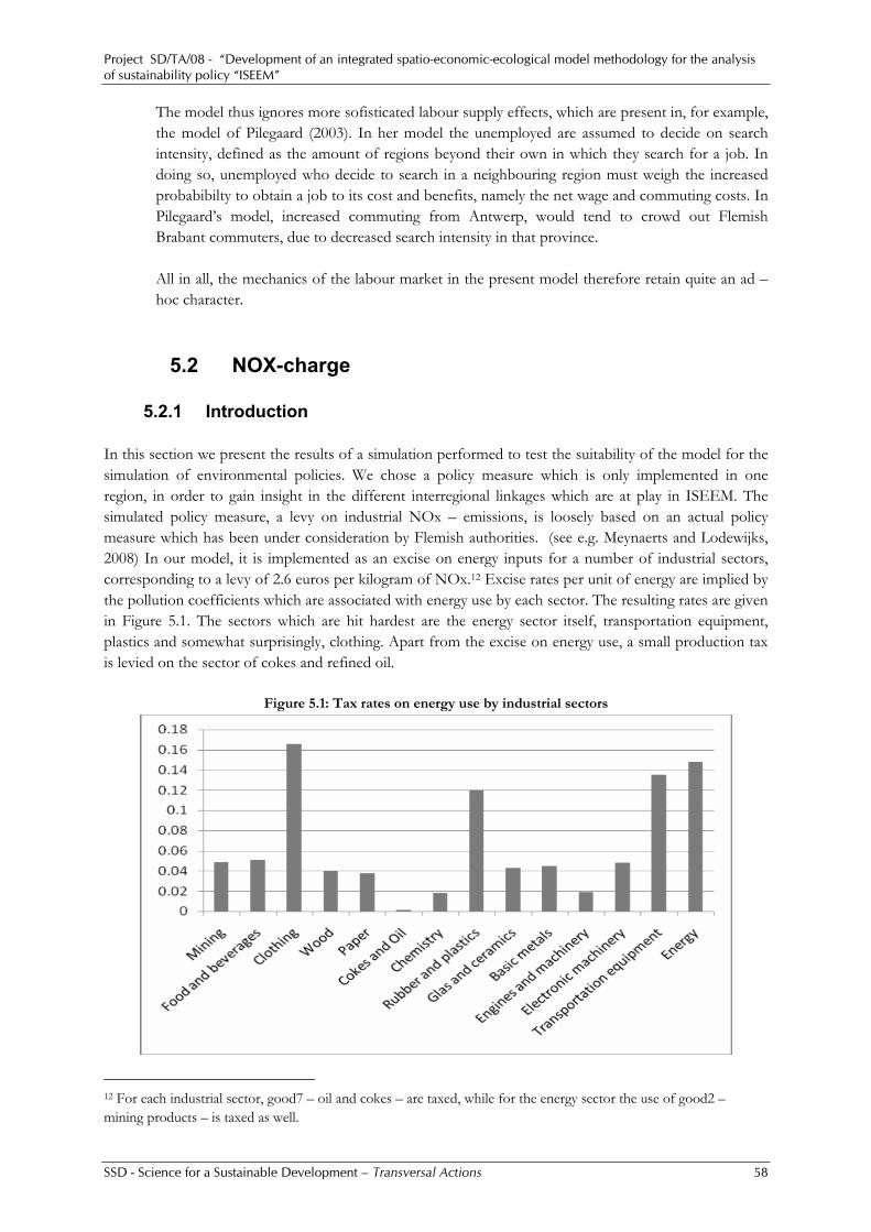
Project SD/TA/08 - “Development of an integrated spatio-economic-ecological model methodology for the analysis of sustainability policy “ISEEM”
SSD - Science for a Sustainable Development – Transversal Actions 58
The model thus ignores more sofisticated labour supply effects, which are present in, for example, the model of Pilegaard (2003). In her model the unemployed are assumed to decide on search intensity, defined as the amount of regions beyond their own in which they search for a job. In doing so, unemployed who decide to search in a neighbouring region must weigh the increased probabibilty to obtain a job to its cost and benefits, namely the net wage and commuting costs. In Pilegaard’s model, increased commuting from Antwerp, would tend to crowd out Flemish Brabant commuters, due to decreased search intensity in that province. All in all, the mechanics of the labour market in the present model therefore retain quite an ad – hoc character.
5.2 NOX-charge
5.2.1 Introduction In this section we present the results of a simulation performed to test the suitability of the model for the simulation of environmental policies. We chose a policy measure which is only implemented in one region, in order to gain insight in the different interregional linkages which are at play in ISEEM. The simulated policy measure, a levy on industrial NOx – emissions, is loosely based on an actual policy measure which has been under consideration by Flemish authorities. (see e.g. Meynaerts and Lodewijks, 2008) In our model, it is implemented as an excise on energy inputs for a number of industrial sectors, corresponding to a levy of 2.6 euros per kilogram of NOx.12 Excise rates per unit of energy are implied by the pollution coefficients which are associated with energy use by each sector. The resulting rates are given in Figure 5.1. The sectors which are hit hardest are the energy sector itself, transportation equipment, plastics and somewhat surprisingly, clothing. Apart from the excise on energy use, a small production tax is levied on the sector of cokes and refined oil.
Figure 5.1: Tax rates on energy use by industrial sectors
12 For each industrial sector, good7 – oil and cokes – are taxed, while for the energy sector the use of good2 – mining products – is taxed as well.
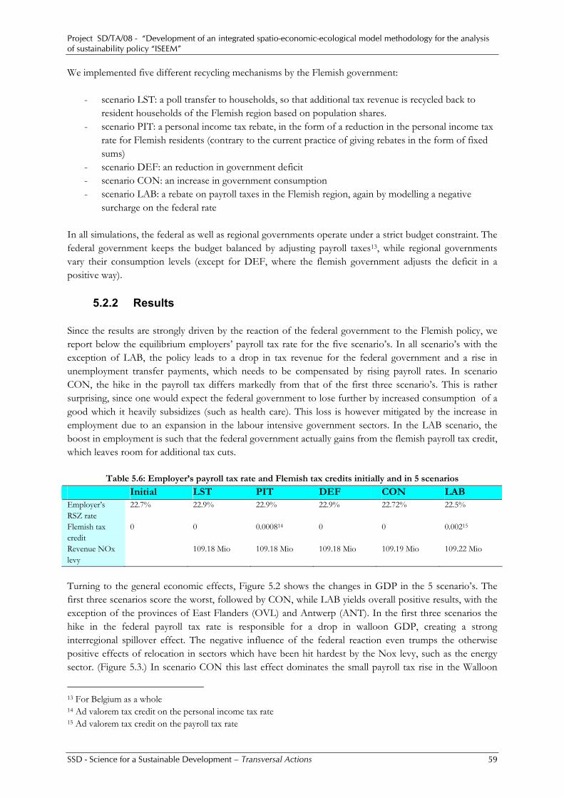
Project SD/TA/08 - “Development of an integrated spatio-economic-ecological model methodology for the analysis of sustainability policy “ISEEM”
SSD - Science for a Sustainable Development – Transversal Actions 59
We implemented five different recycling mechanisms by the Flemish government:
- scenario LST: a poll transfer to households, so that additional tax revenue is recycled back to resident households of the Flemish region based on population shares.
- scenario PIT: a personal income tax rebate, in the form of a reduction in the personal income tax rate for Flemish residents (contrary to the current practice of giving rebates in the form of fixed sums)
- scenario DEF: an reduction in government deficit - scenario CON: an increase in government consumption - scenario LAB: a rebate on payroll taxes in the Flemish region, again by modelling a negative
surcharge on the federal rate In all simulations, the federal as well as regional governments operate under a strict budget constraint. The federal government keeps the budget balanced by adjusting payroll taxes13, while regional governments vary their consumption levels (except for DEF, where the flemish government adjusts the deficit in a positive way).
5.2.2 Results
Since the results are strongly driven by the reaction of the federal government to the Flemish policy, we report below the equilibrium employers’ payroll tax rate for the five scenario’s. In all scenario’s with the exception of LAB, the policy leads to a drop in tax revenue for the federal government and a rise in unemployment transfer payments, which needs to be compensated by rising payroll rates. In scenario CON, the hike in the payroll tax differs markedly from that of the first three scenario’s. This is rather surprising, since one would expect the federal government to lose further by increased consumption of a good which it heavily subsidizes (such as health care). This loss is however mitigated by the increase in employment due to an expansion in the labour intensive government sectors. In the LAB scenario, the boost in employment is such that the federal government actually gains from the flemish payroll tax credit, which leaves room for additional tax cuts.
Table 5.6: Employer’s payroll tax rate and Flemish tax credits initially and in 5 scenarios
Initial LST PIT DEF CON LAB Employer’s RSZ rate
22.7% 22.9% 22.9% 22.9% 22.72% 22.5%
Flemish tax credit
0 0 0.000814 0 0 0.00215
Revenue NOx levy
109.18 Mio 109.18 Mio 109.18 Mio 109.19 Mio 109.22 Mio
Turning to the general economic effects, Figure 5.2 shows the changes in GDP in the 5 scenario’s. The first three scenarios score the worst, followed by CON, while LAB yields overall positive results, with the exception of the provinces of East Flanders (OVL) and Antwerp (ANT). In the first three scenarios the hike in the federal payroll tax rate is responsible for a drop in walloon GDP, creating a strong interregional spillover effect. The negative influence of the federal reaction even trumps the otherwise positive effects of relocation in sectors which have been hit hardest by the Nox levy, such as the energy sector. (Figure 5.3.) In scenario CON this last effect dominates the small payroll tax rise in the Walloon
13 For Belgium as a whole 14 Ad valorem tax credit on the personal income tax rate 15 Ad valorem tax credit on the payroll tax rate

Project SD/TA/08 - “Development of an integrated spatio-economic-ecological model methodology for the analysis of sustainability policy “ISEEM”
SSD - Science for a Sustainable Development – Transversal Actions 60
provinces leading to positive results in their GDP. In scenario LAB, the relocation effect in the energy sector dominates the positive effect of the payroll tax cut only in the Antwerp and East Flanders. Within Flanders, the NOx levy and its recycling scheme can be understood as a transfer from provinces with a high share of energy production towards provinces with a more balanced production structure.
Figure 5.2: Percentage change in provincial and national GDP for 5 scenario’s
Figure 5.3: Percentage change in production for the energy sector
Turning to welfare, the caveats noted in the paragraph above become evident again. For decile 1 (Figure 5.4) the high welfare gain in Flanders due to the lump – sum transfer, and the relatively low welfare loss for the top decile (Figure 5.5) in PIT are logical distributional effects (‘cents versus percents’).
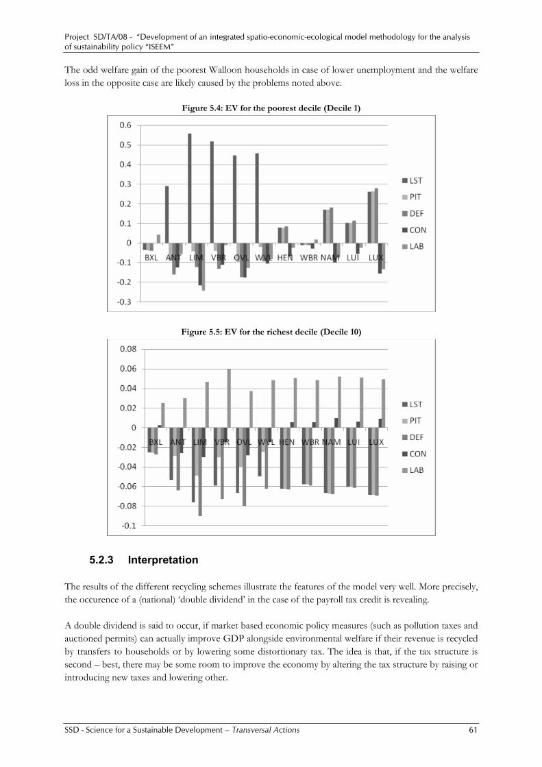
Project SD/TA/08 - “Development of an integrated spatio-economic-ecological model methodology for the analysis of sustainability policy “ISEEM”
SSD - Science for a Sustainable Development – Transversal Actions 61
The odd welfare gain of the poorest Walloon households in case of lower unemployment and the welfare loss in the opposite case are likely caused by the problems noted above.
Figure 5.4: EV for the poorest decile (Decile 1)
Figure 5.5: EV for the richest decile (Decile 10)
5.2.3 Interpretation The results of the different recycling schemes illustrate the features of the model very well. More precisely, the occurence of a (national) ‘double dividend’ in the case of the payroll tax credit is revealing. A double dividend is said to occur, if market based economic policy measures (such as pollution taxes and auctioned permits) can actually improve GDP alongside environmental welfare if their revenue is recycled by transfers to households or by lowering some distortionary tax. The idea is that, if the tax structure is second – best, there may be some room to improve the economy by altering the tax structure by raising or introducing new taxes and lowering other.
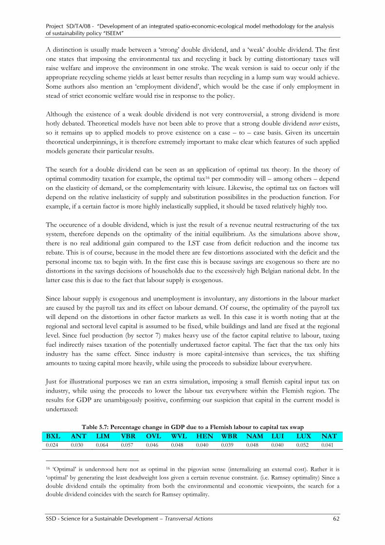
Project SD/TA/08 - “Development of an integrated spatio-economic-ecological model methodology for the analysis of sustainability policy “ISEEM”
SSD - Science for a Sustainable Development – Transversal Actions 62
A distinction is usually made between a ‘strong’ double dividend, and a ‘weak’ double dividend. The first one states that imposing the environmental tax and recycling it back by cutting distortionary taxes will raise welfare and improve the environment in one stroke. The weak version is said to occur only if the appropriate recycling scheme yields at least better results than recycling in a lump sum way would achieve. Some authors also mention an ‘employment dividend’, which would be the case if only employment in stead of strict economic welfare would rise in response to the policy. Although the existence of a weak double dividend is not very controversial, a strong dividend is more hotly debated. Theoretical models have not been able to prove that a strong double dividend never exists, so it remains up to applied models to prove existence on a case – to – case basis. Given its uncertain theoretical underpinnings, it is therefore extremely important to make clear which features of such applied models generate their particular results. The search for a double dividend can be seen as an application of optimal tax theory. In the theory of optimal commodity taxation for example, the optimal tax16 per commodity will – among others – depend on the elasticity of demand, or the complementarity with leisure. Likewise, the optimal tax on factors will depend on the relative inelasticity of supply and substitution possibilites in the production function. For example, if a certain factor is more highly inelastically supplied, it should be taxed relatively highly too. The occurence of a double dividend, which is just the result of a revenue neutral restructuring of the tax system, therefore depends on the optimality of the initial equilibrium. As the simulations above show, there is no real additional gain compared to the LST case from deficit reduction and the income tax rebate. This is of course, because in the model there are few distortions associated with the deficit and the personal income tax to begin with. In the first case this is because savings are exogenous so there are no distortions in the savings decisions of households due to the excessively high Belgian national debt. In the latter case this is due to the fact that labour supply is exogenous. Since labour supply is exogenous and unemployment is involuntary, any distortions in the labour market are caused by the payroll tax and its effect on labour demand. Of course, the optimality of the payroll tax will depend on the distortions in other factor markets as well. In this case it is worth noting that at the regional and sectoral level capital is assumed to be fixed, while buildings and land are fixed at the regional level. Since fuel production (by sector 7) makes heavy use of the factor capital relative to labour, taxing fuel indirectly raises taxation of the potentially undertaxed factor capital. The fact that the tax only hits industry has the same effect. Since industry is more capital-intensive than services, the tax shifting amounts to taxing capital more heavily, while using the proceeds to subsidize labour everywhere. Just for illustrational purposes we ran an extra simulation, imposing a small flemish capital input tax on industry, while using the proceeds to lower the labour tax everywhere within the Flemish region. The results for GDP are unambigously positive, confirming our suspicion that capital in the current model is undertaxed:
Table 5.7: Percentage change in GDP due to a Flemish labour to capital tax swap
BXL ANT LIM VBR OVL WVL HEN WBR NAM LUI LUX NAT 0.024 0.030 0.064 0.057 0.046 0.048 0.040 0.039 0.048 0.040 0.052 0.041
16 ‘Optimal’ is understood here not as optimal in the pigovian sense (internalizing an external cost). Rather it is ‘optimal’ by generating the least deadweight loss given a certain revenue constraint. (i.e. Ramsey optimality) Since a double dividend entails the optimality from both the environmental and economic viewpoints, the search for a double dividend coincides with the search for Ramsey optimality.

Project SD/TA/08 - “Development of an integrated spatio-economic-ecological model methodology for the analysis of sustainability policy “ISEEM”
SSD - Science for a Sustainable Development – Transversal Actions 63
Moreover, the fuel input is untaxed in the benchmark equilibrium while in reality it is one of few inputs which are subject to indirect taxation. In practice the distortions of taxing energy even more may be higher then the present model acknowledges. So, while it may be the case that labour is taxed too heavily, just how much ‘too much’ is from an economic perspective depends on the assumptions of the model for the other factor markets and the realism of the initial equilibrium. While the problem of intermediate fuel taxation is easily remedied by adjusting the database, the behaviour of (the different forms of) capital requires the modelling of capital mobility. Barring such an adjustment, it is best to interpret the current results as short to medium term results only. In the long run capital will be interregionally and internationally mobile, raising the elasticity of capital and making taxing capital intensive goods less attractive.
5.3 Freight charge simulation
5.3.1 Introduction This simulation is based on the the new Eurovignette guideline, which is essentially an agreement between European countries, to recover external costs for freight transport (especially heavy goods transport) by a common system of ‘vignets’ (road charges). These would be implemented in the form of a kilometer charge. Our simulation was based on a set of runs with TREMOVE, a partial equilibrium model of the transport market for 31 European countries constructed by TML. In these runs a new network tax, much like the Eurovignette was introduced, replacing other taxes on freight transport partially. The scenario we use from TREMOVE went further than the original Eurovignette proposal. It was assumed that a new tax would be implemented that aims to recover all external costs from freight traffic, including the costs of new investments in the road network. On average, the tax introduced amounted to about 0.231 euro per vehicle kilometer. ISEEM does not contain a network model of freight and does not calculate all external costs from the transport sector. Instead, we estimate the average tax revenue from the kilometer charge, based on the runs with TREMOVE. Originally, it was our intention to model the increase in transport costs from region to region directly within the model, based on the amount of freight kilometers driven between Belgian provinces and the tax revenues taken from TREMOVE. However, we were forced to drop a lot of ‘specificity’ for each region, as there were problems with the consistencies of our database on freight transport and the interregional trade matrix within ISEEM. Instead, we simplified our orginal kilometercharge scenario to a tax on goods. As such, it should better be rephrased as a consumption charge on goods that consume freight transport or a freight charge. The results of this simulation should thus be read with caution and mostly be seen as a test of the model. Essentially, we introduce a new consumption tax on producers and consumers, based on a generalization of the Eurovignette scheme. The ‘tax rates’ on these goods have been estimated, based on freight data for Belgium coming from the ETIS database. While this charge on consumption of goods mimicks the effects of a raise in transport costs between the regions due to the kilometer charge, it is not completely the same. For example, we noticed that the interregional trade between regions should probably be more repressed in a ‘real kilometer charging scheme’. There should also be differences in the regional effect of the tax, as we assumed the tax rates to be equal for each province.
Project SD/TA/08 - “Development of an integrated spatio-economic-ecological model methodology for the analysis of sustainability policy “ISEEM”
SSD - Science for a Sustainable Development – Transversal Actions 64
The simulation with ISEEM compares the effect of this tax, when implemented for the whole of Belgium (BE) or only for Flanders (FL). While this simulation serves principally as a test of the ISEEM model and as a thought experiment, a scenario where Flanders (possibly together with the Netherlands) would pursue a kilometer charging scheme is not impossible. We did not include a scenario where the tax would only be implemented in Wallony as this was not included in the original TREMOVE runs. Moreover, most of the external costs of freight traffic are located in the region of Flanders and Brussels. In the BE and FL scenarios, the income from the new network tax is redistributed to the regional governments of Belgium, generating a new and important source of revenues for the Belgian regions. The additional revenues are used to increase the government savings and public budget, while other taxes are kept at the same level. A so called ‘double dividend’ effect is not present in this way. To study the effect of a redistribution of the tax income, we propose an alternative set-up of the simulation. In the BE + redistribution scenario, we assume that the federal government collects the tax revenues and uses the tax revenues to decrease the social security contributions, paid by employers. It was calculated from ISEEM, that the full revenues of the freight charge could be used to decrease the employer social contributions in a uniform way (for all sectors and all regions) from 22.7 % to 21.3%. We choose this type of redistribution, because it should have an immediate positive effect on employment and production. We let the federal government collect the tax in the redistribution variant, as the regional governments only have a limited leverage to change taxes and start redistributional initiatives. This is also the reason why we only check redistribution in the BE scenario, as this type of policy is only realistic for a country wide charge. The possibility of redistribution on the regional level can be a legislative nightmare, so we leave the redistribution of the tax revenue in the middle for the FL scenario.
5.3.2 Simulation set up and assumptions Simplifications and the use of external data ISEEM and TREMOVE are very different models. While TREMOVE calculates the tax income and the changes in costs for the users of the transport network on country level, ISEEM is a regional-economic model. Therefore, it was necessary to split the effect over different regions and production sectors. This division was realized by using information from the ETIS database17. This database contains freight transport data, split up by O/D, for several products and on NUTS-2 (province) level. The ETIS data was already available to us as it was used to callibrate the basecase of ISEEM. However it was technically impossible to determine the effect of the freight charge for each sector, product and region separately. Instead, we had to simplify the problem, the total income from the tax on road freight was subdivided on different products, dependent on the amount of freight transport (in vehicle km) these products consume. This tax per product was subdivided by the total consumption (both intermediary and final). In the case of a kilometer charge on freight for the whole of Belgium, this relative tax on consumption was assumed to be equal for each province, but to differ by product. In the next simulation, the charge applies only to Flanders. The ETIS database was used to determine the amount of in- and outgoing freight transport between Flanders, Brussels and Wallonia. Then it was assumed that only the freight transport in Flanders would be taxed. The extra tax on products applies in 17 This database was developed under coordination of NEA in a European project: Core Database Development for the European Transport policy Information System (ETIS).
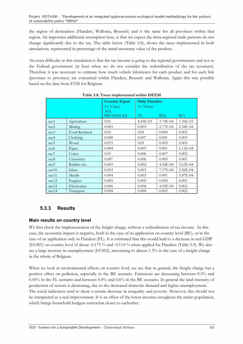
Project SD/TA/08 - “Development of an integrated spatio-economic-ecological model methodology for the analysis of sustainability policy “ISEEM”
SSD - Science for a Sustainable Development – Transversal Actions 65
the region of destination (Flanders, Wallonia, Brussels) and is the same for all provinces within that region. An important additional assumption here, is that we expect the intra-regional trade patterns do not change significantly due to the tax. The table below (Table 5.8), shows the taxes implemented in both simulations, represented in percentage of the initial monetary value of the product. An extra difficulty in this simulation is that the tax income is going to the regional governments and not to the Federal government (at least when we do not consider the redistribution of the tax revenues). Therefore it was necessary to estimate how much vehicle kilometers for each product and for each link (province to province) are consumed within Flanders, Brussels and Wallonia. Again this was possible based on the data from ETIS for Belgium.
Table 5.8: Taxes implemented within ISEEM
Country Equal Only Flanders (% Value) (% Value)
ALL PROVINCES VL BXL WA
sec1 Agriculture 0.01 8.45E-03 3.74E-04 1.56E-03 sec2 Mining 0.003 0.003 2.77E-04 2.34E-04 sec3 Food &related 0.01 0.01 0.004 0.002 sec4 Clothing 0.008 0.007 0.001 0.003 sec5 Wood 0.015 0.01 0.003 0.003 sec6 Paper 0.004 0.003 0.001 6.11E-04 sec7 Cokes 0.01 0.006 0.007 0.002 sec8 Chemistry 0.007 0.006 0.003 0.001 sec9 Rubber etc. 0.003 0.002 4.34E-04 5.63E-04 sec10 Glass 0.003 0.003 7.57E-04 2.56E-04 sec11 Metals 0.004 0.003 0.001 5.47E-04 sec12 Engines 0.005 0.005 0.002 0.001 sec13 Electronics 0.006 0.006 4.92E-04 0.002 sec14 Transport 0.004 0.004 0.002 0.002
5.3.3 Results Main results on country level We first check the implementation of the freight charge, without a redistribution of tax income. In this case, the economic impact is negative, both in the case of its application on country level (BE), or in the case of an application only in Flanders (FL). It is estimated that this would lead to a decrease in real GDP (EC001) on country level of about -0.175 % and -0.114 % when applied for Flanders (Table 5.9). We also see a large increase in unemployment (EC002), amounting to almost 1.5% in the case of a freight charge in the whole of Belgium. When we look at environmental effects on country level, we see that in general, the freight charge has a positive effect on pollution, especially in the BE scenario. Emissions are decreasing between 0.3% and 0.45% in the FL scenario and between 0.4% and 0.6% in the BE scenario. In general the land intensity of production of sectors is decreasing, due to the decreased domestic demand and higher unemployment. The social indicators tend to show a certain decrease in inequality and poverty. However, this should not be interpreted as a real improvement. It is an effect of the lower incomes troughout the entire population, which brings household budgets somewhat closer to eachother.

Project SD/TA/08 - “Development of an integrated spatio-economic-ecological model methodology for the analysis of sustainability policy “ISEEM”
SSD - Science for a Sustainable Development – Transversal Actions 66
The picture completely changes when a redistribution of the tax income is considered. In this case, we see a large positive impact on employment and production (goes up with 0.353%). There is also a positive influence on consumption, which also points to a higher income of households. The environmental picture is also positive. While the redistriubution scenario does not realize the same emission reductions as the BE scenario, it still manages to decrease the overall pollution. The redistribution version of the BE scenario manages to decrease the damages from pollution, while at the same time increasing employment and production. The changes in the land use coefficients show that most of the extra output is realized in the service sector and only partially in the industrial sector. The output of the agricultural sector decreases at about the same rate as in the BE scenario. The only indicators denoting ‘negative’ effects are the indicators of social (in)equality. These show that inequality and poverty increase in the population, probably because the increase in employment is mostly beneficial for higher income classes and not for lower. Mean income of the population goes up, but prices also increase on country level (EC004, Inflation), due to the tax.
Table 5.9: Results from the BE and FL scenario on country level (% change from basecase).
BASECASE FL BE BE
(redistribution)ECONOMY (%) (%) (%) GDP per household (euros) 69991.4799 -0.114 -0.176 0.353Unemployment (rate) 0.1139 1.021 1.540 -3.305Consumption per household (euros) 36644.0220 -0.148 -0.228 0.325Inflation 0.15 0.301 0.261ENVIRONMENT CO2 pollution (1000 mil euros) 3.8321 -0.263 -0.512 -0.287GHG pollution (1000 mil euros) 0.6525 -0.296 -0.572 -0.418NOx pollution (1000 mil euros) 4.1648 -0.351 -0.689 -0.386SOx pollution (1000 mil euros) 1.1027 -0.135 -0.251 0.022Output coefficient agricultural land (value / m2) 0.0048 -0.414 -0.632 -0.544Output coefficient industrial land (value / m2) 3.7494 -0.244 -0.377 0.052Output coefficient building land (value / m2) 5.3694 -0.070 -0.109 0.501SOCIAL Ratio high low 3.9444 -0.082 -0.130 0.178Poverty gap 11956.5376 -0.230 -0.353 0.543Gini coefficient 0.2945 -0.0757 -0.1056 0.1232 Main economic results on government level The first thing that can be shown is that the freight charge is generating a lot of revenue. It is estimated that the extra tax revenue would amount to 1986.5 million euros on country level, with 1321 million for Flanders, 605 million for Wallonia and 60.5 million for Brussels. In the FL scenario, the total tax revenues for Flanders are a little higher (+ 5.5 million euros). The redistribution of the tax does not have a large effect on the tax revenues from the charge.
Table 5.10: Revenues from kilometer charge in different provinces
(1000 mil euros) VL FGOV WG BHG TOTAL BE Road tax revenues 1.314199 0.60188 0.06 1.980 FL Road tax revenues 1.36394 0 0 0 1.361 BE +redist Road tax revenues 0 2.001 0 0 2.001

Project SD/TA/08 - “Development of an integrated spatio-economic-ecological model methodology for the analysis of sustainability policy “ISEEM”
SSD - Science for a Sustainable Development – Transversal Actions 67
The next table (Table 5.11:) shows the change in public budget of the main governments. As the charge leads to economic losses, it also affects the government revenues from different sources. While the regional governments of Flanders, Wallony and Brussels (VL, WG, BHG) see their budgets increasing considerably, the federal government (FGOV) is losing revenues. In total, government budget is only going up 779 million euros in the FL case and 1204 million euros in the BE case. When we implement the redistribution by decreasing the tax on labour, we see a different picture. The total public budget actually increases more in this case of a redistribution of tax revenues, than without the redistribution. The extra revenues amount to about 500 million euros. Actually, the revenues from the freight charge, the increase in tax income from other sources and the reduction of unemployment benefits, offset the decrease in tax income due to the decrease in employer social contributions. As it is now the federal government that collects the revenues, there are no negative side effects on the budgets of the other governments. The largest part of the tax revenue is collected from traffic in Flanders, which can be deduced from Table 5.10. This is only partially transferred to the Flemish regional government. The federal government pays the costs of the decrease in tax revenues from labour, but also receives the largest part of the new revenues.
Table 5.11: Effect on budget of main regional governments
FL BE BE+redistribution
Public budget FGOV (1000 mil euros) -0.179 -0.197 1.38 Public budget VL (1000 mil euros) 0.961 0.972 0.191 Public budget WG (1000 mil euros) -0.004 0.369 0.030 Public budget BHG (1000 mil euros) -0.001 0.047 0.01386 Public budget FG (1000 mil euros) 0.003 0.012 0.08405 TOTAL budget 0.779 1.204 1.704
Regional economic results’ No redistribution effects We will first check the regional economic effects, when we do not take into account redistribution. From the results in Table 5.12 it becomes clear that the provinces in Flanders are experiencing a relatively bigger decrease in regional production and consumption and a subsequent increase in unemployment. The relatively larger effect on the Flemish economy can be expected from the FL scenario as we explicitely assume that the tax is higher, but it is also more generally true, when the tax would apply to the whole of Belgium. The main reason for this is that the Flemish provinces have bigger economies that attract more interregional and international trade, which also leads to a larger consumption of goods related to freight transport.
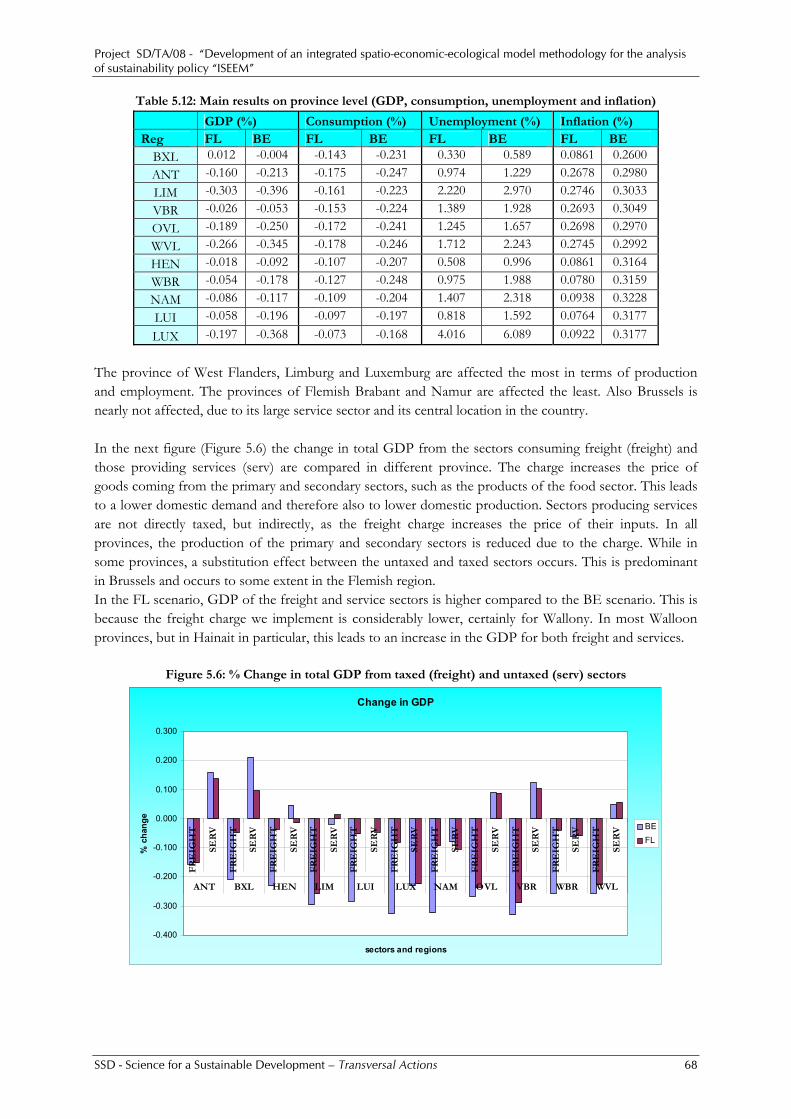
Project SD/TA/08 - “Development of an integrated spatio-economic-ecological model methodology for the analysis of sustainability policy “ISEEM”
SSD - Science for a Sustainable Development – Transversal Actions 68
Table 5.12: Main results on province level (GDP, consumption, unemployment and inflation)
GDP (%) Consumption (%) Unemployment (%) Inflation (%) Reg FL BE FL BE FL BE FL BE
BXL 0.012 -0.004 -0.143 -0.231 0.330 0.589 0.0861 0.2600 ANT -0.160 -0.213 -0.175 -0.247 0.974 1.229 0.2678 0.2980 LIM -0.303 -0.396 -0.161 -0.223 2.220 2.970 0.2746 0.3033 VBR -0.026 -0.053 -0.153 -0.224 1.389 1.928 0.2693 0.3049 OVL -0.189 -0.250 -0.172 -0.241 1.245 1.657 0.2698 0.2970 WVL -0.266 -0.345 -0.178 -0.246 1.712 2.243 0.2745 0.2992 HEN -0.018 -0.092 -0.107 -0.207 0.508 0.996 0.0861 0.3164 WBR -0.054 -0.178 -0.127 -0.248 0.975 1.988 0.0780 0.3159 NAM -0.086 -0.117 -0.109 -0.204 1.407 2.318 0.0938 0.3228 LUI -0.058 -0.196 -0.097 -0.197 0.818 1.592 0.0764 0.3177 LUX -0.197 -0.368 -0.073 -0.168 4.016 6.089 0.0922 0.3177
The province of West Flanders, Limburg and Luxemburg are affected the most in terms of production and employment. The provinces of Flemish Brabant and Namur are affected the least. Also Brussels is nearly not affected, due to its large service sector and its central location in the country. In the next figure (Figure 5.6) the change in total GDP from the sectors consuming freight (freight) and those providing services (serv) are compared in different province. The charge increases the price of goods coming from the primary and secondary sectors, such as the products of the food sector. This leads to a lower domestic demand and therefore also to lower domestic production. Sectors producing services are not directly taxed, but indirectly, as the freight charge increases the price of their inputs. In all provinces, the production of the primary and secondary sectors is reduced due to the charge. While in some provinces, a substitution effect between the untaxed and taxed sectors occurs. This is predominant in Brussels and occurs to some extent in the Flemish region. In the FL scenario, GDP of the freight and service sectors is higher compared to the BE scenario. This is because the freight charge we implement is considerably lower, certainly for Wallony. In most Walloon provinces, but in Hainait in particular, this leads to an increase in the GDP for both freight and services.
Figure 5.6: % Change in total GDP from taxed (freight) and untaxed (serv) sectors
Change in GDP
-0.400
-0.300
-0.200
-0.100
0.000
0.100
0.200
0.300
FR
EIG
HT
SER
V
FR
EIG
HT
SER
V
FR
EIG
HT
SER
V
FR
EIG
HT
SER
V
FR
EIG
HT
SER
V
FR
EIG
HT
SER
V
FR
EIG
HT
SER
V
FR
EIG
HT
SER
V
FR
EIG
HT
SER
V
FR
EIG
HT
SER
V
FR
EIG
HT
SER
V
ANT BXL HEN LIM LUI LUX NAM OVL VBR WBR WVL
sectors and regions
% c
hang
e
BEFL

Project SD/TA/08 - “Development of an integrated spatio-economic-ecological model methodology for the analysis of sustainability policy “ISEEM”
SSD - Science for a Sustainable Development – Transversal Actions 69
Effects of redistribution When the tax revenue is redistributed to decrease the taxes on labour, we see that all regional economic indicators show more positive results. Regional GDP, consumption and employment decrease and inflation is lower. The Walloon provinces of Luxemburg and Namur react very strongly on the policy. There is a large decrease in unemployment and increase in GDP. This is caused by an expansion of the services sectors in these provinces.
Table 5.13: Regional economic effects BE scenario with and without redistribution GDP (%) Consumption (%) Unemployment (%) Inflation (%)
reg BE BE + redist BE
BE + redist BE
BE + redist BE
BE + redist
ANT -0.213 0.123 -0.247 0.312 1.229 -2.172 0.298 0.265 BXL -0.004 0.314 -0.231 0.280 0.589 -1.646 0.260 0.225 HEN -0.092 0.553 -0.207 0.332 0.996 -2.584 0.316 0.271 LIM -0.396 0.307 -0.223 0.307 2.970 -4.965 0.303 0.260 LUI -0.196 0.530 -0.197 0.313 1.592 -3.441 0.318 0.260 LUX -0.368 1.021 -0.168 0.163 6.089 -14.776 0.318 0.258 NAM -0.117 1.010 -0.204 0.313 2.318 -6.545 0.323 0.266 OVL -0.250 0.207 -0.241 0.345 1.657 -3.018 0.297 0.265 VBR -0.053 0.493 -0.224 0.391 1.928 -4.490 0.305 0.265 WBR -0.178 0.751 -0.248 0.394 1.988 -5.031 0.316 0.267 WVL -0.345 0.173 -0.246 0.316 2.243 -3.992 0.299 0.266
In the next figure (Figure 5.7) we make a new comparison of the total GDP, originating from freight and service sectors in the BE and BE + redistribution scenarios. It is obvious that services are gaining in the redistribution case. Actually this stands to common sense as only inputs to services (freight), but not outputs are taxed, while at the same time the employer social contribution decrease uniformly in all regions and all sectors. This creates an important advantage for the service sectors.
Figure 5.7: Changes in GDP compared for BE scenario with and without redistribution
Change in GDP
-0.600
-0.400
-0.200
0.000
0.200
0.400
0.600
0.800
1.000
1.200
1.400
1.600
FR
EIG
HT
SER
V
FR
EIG
HT
SER
V
FR
EIG
HT
SER
V
FR
EIG
HT
SER
V
FR
EIG
HT
SER
V
FR
EIG
HT
SER
V
FR
EIG
HT
SER
V
FR
EIG
HT
SER
V
FR
EIG
HT
SER
V
FR
EIG
HT
SER
V
FR
EIG
HT
SER
V
ANT BXL HEN LIM LUI LUX NAM OVL VBR WBR WVLsectors and regions
% c
hang
e
BEBE + redistribution
Regional welfare No redistribution effects In the table below (Table 5.14), we measure welfare changes in equivalent variation, which corresponds to social indicator SO001. This index is based on the utility a household can attain, given its income and the
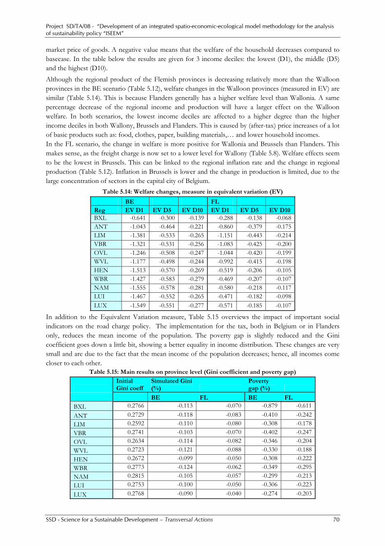
Project SD/TA/08 - “Development of an integrated spatio-economic-ecological model methodology for the analysis of sustainability policy “ISEEM”
SSD - Science for a Sustainable Development – Transversal Actions 70
market price of goods. A negative value means that the welfare of the household decreases compared to basecase. In the table below the results are given for 3 income deciles: the lowest (D1), the middle (D5) and the highest (D10). Although the regional product of the Flemish provinces is decreasing relatively more than the Walloon provinces in the BE scenario (Table 5.12), welfare changes in the Walloon provinces (measured in EV) are similar (Table 5.14). This is because Flanders generally has a higher welfare level than Wallonia. A same percentage decrease of the regional income and production will have a larger effect on the Walloon welfare. In both scenarios, the lowest income deciles are affected to a higher degree than the higher income deciles in both Wallony, Brussels and Flanders. This is caused by (after-tax) price increases of a lot of basic products such as: food, clothes, paper, building materials,… and lower household incomes. In the FL scenario, the change in welfare is more positive for Wallonia and Brussels than Flanders. This makes sense, as the freight charge is now set to a lower level for Wallony (Table 5.8). Welfare effects seem to be the lowest in Brussels. This can be linked to the regional inflation rate and the change in regional production (Table 5.12). Inflation in Brussels is lower and the change in production is limited, due to the large concentration of sectors in the capital city of Belgium.
Table 5.14: Welfare changes, measure in equivalent variation (EV)
BE FL Reg EV D1 EV D5 EV D10 EV D1 EV D5 EV D10 BXL -0.641 -0.300 -0.139 -0.288 -0.138 -0.068 ANT -1.043 -0.464 -0.221 -0.860 -0.379 -0.175 LIM -1.381 -0.533 -0.265 -1.151 -0.443 -0.214 VBR -1.321 -0.531 -0.256 -1.083 -0.425 -0.200 OVL -1.246 -0.508 -0.247 -1.044 -0.420 -0.199 WVL -1.177 -0.498 -0.244 -0.992 -0.415 -0.198 HEN -1.513 -0.570 -0.269 -0.519 -0.206 -0.105 WBR -1.427 -0.583 -0.279 -0.469 -0.207 -0.107 NAM -1.555 -0.578 -0.281 -0.580 -0.218 -0.117 LUI -1.467 -0.552 -0.265 -0.471 -0.182 -0.098 LUX -1.549 -0.551 -0.277 -0.571 -0.185 -0.107
In addition to the Equivalent Variation measure, Table 5.15 overviews the impact of important social indicators on the road charge policy. The implementation for the tax, both in Belgium or in Flanders only, reduces the mean income of the population. The poverty gap is slightly reduced and the Gini coefficient goes down a little bit, showing a better equality in income distribution. These changes are very small and are due to the fact that the mean income of the population decreases; hence, all incomes come closer to each other.
Table 5.15: Main results on province level (Gini coefficient and poverty gap)
Initial Gini coeff
Simulated Gini (%)
Poverty gap (%)
BE FL BE FL
BXL 0.2766 -0.113 -0.070 -0.879 -0.611 ANT 0.2729 -0.118 -0.083 -0.410 -0.242 LIM 0.2592 -0.110 -0.080 -0.308 -0.178 VBR 0.2741 -0.103 -0.070 -0.402 -0.247 OVL 0.2634 -0.114 -0.082 -0.346 -0.204 WVL 0.2723 -0.121 -0.088 -0.330 -0.188 HEN 0.2672 -0.099 -0.050 -0.308 -0.222 WBR 0.2773 -0.124 -0.062 -0.349 -0.295 NAM 0.2815 -0.105 -0.057 -0.299 -0.213 LUI 0.2753 -0.100 -0.050 -0.306 -0.223 LUX 0.2768 -0.090 -0.040 -0.274 -0.203

Project SD/TA/08 - “Development of an integrated spatio-economic-ecological model methodology for the analysis of sustainability policy “ISEEM”
SSD - Science for a Sustainable Development – Transversal Actions 71
Including redistribution effects The joint introduction of freight charges and a decrease in the tax of labour seems to be generally more positive than the non-redistribution case. However, the welfare change is often negative for the lower income deciles and is only slightly more positive for the higher income deciles. Still, this makes the case of redistribution superior in terms of welfare, to the non-redistribution case.
Table 5.16: Regional welfare BE scenario and BE redistribution scenario
BE BE + redistribution reg EV D1 EV D5 EV D10 EV D1 EV D5 EV D10 BXL -0.641 -0.3 -0.139 -0.067 0.03 0.028 ANT -1.043 -0.464 -0.221 -0.192 0.033 0.038 LIM -1.381 -0.533 -0.265 -0.038 0.037 0.067 VBR -1.321 -0.531 -0.256 0.038 0.113 0.104 OVL -1.246 -0.508 -0.247 -0.125 0.065 0.066 WVL -1.177 -0.498 -0.244 -0.143 0.036 0.051 HEN -1.513 -0.57 -0.269 -0.028 0.059 0.073 WBR -1.427 -0.583 -0.279 0.1 0.117 0.115 NAM -1.555 -0.578 -0.281 0.107 0.039 0.094 LUI -1.467 -0.552 -0.265 0.007 0.049 0.076 LUX -1.549 -0.551 -0.277 0.068 -0.108 0.034
The social indicators on the regional level show that the poverty and income inequality goes up. This is an effect of the increase in mean income, which is mostly beneficial for richer income groups.
Table 5.17: Social indicators on regional level, BE and BE + redistribution
Initial Gini coeff
Simulated Gini (%)
Poverty gap (%)
BE BE + redist BE BE + redist
BXL 0.2729 -0.113 0.116 -0.879 1.85 ANT 0.2766 -0.118 0.129 -0.41 0.759 LIM 0.2741 -0.11 0.135 -0.308 0.479 VBR 0.2815 -0.103 0.174 -0.402 0.477 OVL 0.2773 -0.114 0.147 -0.346 0.543 WVL 0.2768 -0.121 0.137 -0.33 0.581 HEN 0.2592 -0.099 0.139 -0.308 0.412 WBR 0.2753 -0.124 0.188 -0.349 0.439 NAM 0.2672 -0.105 0.155 -0.299 0.38 LUI 0.2634 -0.1 0.139 -0.306 0.411 LUX 0.2723 -0.09 0.078 -0.274 0.391
External effects and environmental impacts The ISEEM model can measure two external effects of taxing freight transport. The first is the time gain on the transport network. ISEEM contains a dataset and calculates transport trips for different purposes between regions. The changes in timecosts for different transport purposes (work, non-work and business) were calculated from TREMOVE and exogenously applied on transport trips within Belgium and Flanders for both scenarios. We want to note here, that this is based on a TREMOVE calculation and does only incorporate time gains for the consumers. From these results, the total gain in travel time (in 1 year) for consumers is calculated to be about 51.8 million Euros in the BE and 39.4 million euro in the FL scenario.
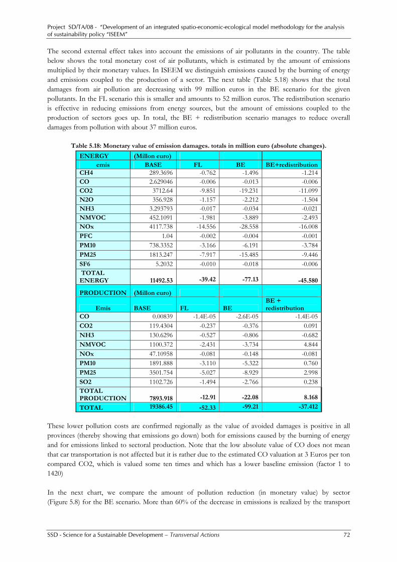
Project SD/TA/08 - “Development of an integrated spatio-economic-ecological model methodology for the analysis of sustainability policy “ISEEM”
SSD - Science for a Sustainable Development – Transversal Actions 72
The second external effect takes into account the emissions of air pollutants in the country. The table below shows the total monetary cost of air pollutants, which is estimated by the amount of emissions multiplied by their monetary values. In ISEEM we distinguish emissions caused by the burning of energy and emissions coupled to the production of a sector. The next table (Table 5.18) shows that the total damages from air pollution are decreasing with 99 million euros in the BE scenario for the given pollutants. In the FL scenario this is smaller and amounts to 52 million euros. The redistribution scenario is effective in reducing emissions from energy sources, but the amount of emissions coupled to the production of sectors goes up. In total, the BE + redistribution scenario manages to reduce overall damages from pollution with about 37 million euros.
Table 5.18: Monetary value of emission damages. totals in million euro (absolute changes).
ENERGY (Millon euro)
emis BASE FL BE BE+redistribution CH4 289.3696 -0.762 -1.496 -1.214 CO 2.629046 -0.006 -0.013 -0.006 CO2 3712.64 -9.851 -19.231 -11.099 N2O 356.928 -1.157 -2.212 -1.504 NH3 3.293793 -0.017 -0.034 -0.021 NMVOC 452.1091 -1.981 -3.889 -2.493 NOx 4117.738 -14.556 -28.558 -16.008 PFC 1.04 -0.002 -0.004 -0.001 PM10 738.3352 -3.166 -6.191 -3.784 PM25 1813.247 -7.917 -15.485 -9.446 SF6 5.2032 -0.010 -0.018 -0.006 TOTAL ENERGY 11492.53 -39.42 -77.13 -45.580
PRODUCTION (Millon euro)
Emis BASE FL BE BE + redistribution
CO 0.00839 -1.4E-05 -2.6E-05 -1.4E-05 CO2 119.4304 -0.237 -0.376 0.091 NH3 130.6296 -0.527 -0.806 -0.682 NMVOC 1100.372 -2.431 -3.734 4.844 NOx 47.10958 -0.081 -0.148 -0.081 PM10 1891.888 -3.110 -5.322 0.760 PM25 3501.754 -5.027 -8.929 2.998 SO2 1102.726 -1.494 -2.766 0.238 TOTAL PRODUCTION 7893.918 -12.91 -22.08 8.168
TOTAL 19386.45 -52.33 -99.21 -37.412
These lower pollution costs are confirmed regionally as the value of avoided damages is positive in all provinces (thereby showing that emissions go down) both for emissions caused by the burning of energy and for emissions linked to sectoral production. Note that the low absolute value of CO does not mean that car transportation is not affected but it is rather due to the estimated CO valuation at 3 Euros per ton compared CO2, which is valued some ten times and which has a lower baseline emission (factor 1 to 1420) In the next chart, we compare the amount of pollution reduction (in monetary value) by sector (Figure 5.8) for the BE scenario. More than 60% of the decrease in emissions is realized by the transport
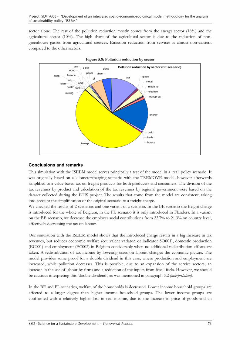
Project SD/TA/08 - “Development of an integrated spatio-economic-ecological model methodology for the analysis of sustainability policy “ISEEM”
SSD - Science for a Sustainable Development – Transversal Actions 73
sector alone. The rest of the pollution reduction mostly comes from the energy sector (16%) and the agricultural sector (10%). The high share of the agricultural sector is due to the reduction of non-greenhouse gasses from agricultural sources. Emission reduction from services is almost non-existent compared to the other sectors.
Figure 5.8: Pollution reduction by sector
Pollution reduction by sector (BE scenario)
agr glass
metal
machine
electron
transp eq
energy
build
trade
horecatransp
bank
food
oil
chem
plast
mining
financebuss
clothwood
paper
gov
edu
healthleisur
Conclusions and remarks This simulation with the ISEEM model serves principally a test of the model in a ‘real’ policy scenario. It was originally based on a kilometercharging scenario with the TREMOVE model, however afterwards simplified to a value-based tax on freight products for both producers and consumers. The division of the tax revenues by product and calculation of the tax revenues by regional government were based on the dataset collected during the ETIS project. The results that come from the model are consistent, taking into account the simplification of the original scenario to a freight charge. We checked the results of 2 scenarios and one variant of a scenario. In the BE scenario the freight charge is introduced for the whole of Belgium, in the FL scenario it is only introduced in Flanders. In a variant on the BE scenario, we decrease the employer social contributions from 22.7% to 21.3% on country level, effectively decreasing the tax on labour. Our simulation with the ISEEM model shows that the introduced charge results in a big increase in tax revenues, but reduces economic welfare (equivalent variaton or indicator SO001), domestic production (EC001) and employment (EC002) in Belgium considerably when no additional redistribution efforts are taken. A redistribution of tax income by lowering taxes on labour, changes the economic picture. The model provides some proof for a double dividend in this case, where production and employment are increased, while pollution decreases. This is possible, due to an expansion of the service sectors, an increase in the use of labour by firms and a reduction of the inputs from fossil fuels. However, we should be cautious interpreting this ‘double dividend’, as was mentioned in paragraph 5.2 (interpretation). In the BE and FL scenarios, welfare of the households is decreased. Lower income household groups are affected to a larger degree than higher income household groups. The lower income groups are confronted with a relatively higher loss in real income, due to the increase in price of goods and an

Project SD/TA/08 - “Development of an integrated spatio-economic-ecological model methodology for the analysis of sustainability policy “ISEEM”
SSD - Science for a Sustainable Development – Transversal Actions 74
increase in unemployment. In the redistribution variant of the BE scenario, changes in welfare balance on slightly negative for poor income groups, to slightly positive for the richer income groups. Generally, domestic production of all sectors is weakened due to the rise in costs in the BE and FL scenarios. The production of the primary and secondary industries is reduced more, relative to the service sectors. In the BE redistribution scenario, domestic production of most sectors increases, but with a general advantage for the service sectors. This is caused by a relatively lower impact of the freight charge on service sectors, while the taxes on labour are reduced uniformly in the country. We took into account two types of external effects: the decrease in time costs for consumers due to the lower freight traffic on the transport network and the decrease in emission damages by the transport sector and other sectors. The model results show that all scenarios are effective in reducing emissions from road transport, also in the case of redistribution of tax income. The freight charge simulation illustrates how the model can be used to analyze the indirect economic effects of transportation problems, at the regional level. However, we point the reader to some specific defaults. The simulation is a simplified version of a kilometercharging scheme and does not to claim to take into account all the effects of a ‘real kilometer charge for freight’. It is probable that the effects on interregional trade and international imports and exports are underestimated, as we do not directly increase transport costs of goods. The effects on unemployment are also particularily large, both in the redistribution and non-redistribution case. This is caused by the fixed regional capital assumption and our limited knowledge on the distance decay parameter of the matching function. This simulation could be improved by translating the original kilometercharge to a rise in transport costs of exports, imports, interregional trade between provinces and pass-through traffic through Belgium. This was not possible with the given data and time-frame of the project.
5.4 Tax on land versus decrease in land endowments
5.4.1 Simulation description This simulation was set up to test the land use part of the model. Basically, the model allows for two opposite types of land based simulations:
• change in the costs of land used for production purposes, due to the implementation of a charge, subsidy, tax or a similar market based mechanism
• change in land endowments due to the implementation of land based planning (for example a lower land availability for the agricultural or industrial sector)
We implement two general policies to illustrate how the model reacts in both cases. We compare the introduction of an ad valorem tax on the use of land as a production factor with a general decrease in land endowmnent for all land types. We refer to these scenarios as TAX (ad valorem tax on land) and LEND (land endowments decrease). Our main purpose is to show how the model reacts in both cases.

Project SD/TA/08 - “Development of an integrated spatio-economic-ecological model methodology for the analysis of sustainability policy “ISEEM”
SSD - Science for a Sustainable Development – Transversal Actions 75
The ad valorem tax is set at 15% of the total market price of land. We do not make any distinction between the regions or between the different types of land. The tax revenues are going to the federal government and are used to increase national savings. The logic behind this simulation, is the introduction of a tax on a factor with a low substitution elasticity (land) for budgetary purposes of the government. The effect of this tax is compared with a 1% decrease in land endowments for all land types. The value 1% was chosen, because it gives results of a similar scale as the ad valorem tax. It is assumed that the land cannot be used productively any more. A decrease in land endowments is quite an abstract measure. One could imagine that this land becomes unavailable due to flooding or excessive pollution, or that it is used to increase green space.
5.4.2 Results Results on country level The economic effects are (as expected) quite negative: decrease in GDP, increase in unemployment and lower consumption. In the LEND scenario, the effect on GDP and unemployment is considerably higher than in the TAX scenario, while the effect on consumption is lower. At first glance, the negative change in price level in the case of the TAX scenario is puzzling, as we would expect that firms pass on the land tax to consumers in the form of higher prices. These results can be explained by the way in which land use is modeled. The implementation of the land tax leads to a decrease in land prices of about 13%, meaning that the price effect on the production sector is limited. The reason is, that the land supply is fixed and that it is assumed that there is no ‘empty’ or ‘unused’ land. With a fixed supply of land, the price is determined by the demand of land by the sectors. This actually means that the firms are not bearing the land tax, but the land owners. We assume that all the endowments are held by the local consumers, so consumers are affected by a decrease in non-labour income. Thus, the tax on land we are implementing has a similar effect on the economy as an increase in non – labour income taxation. The decrease in consumer income and the subsequent decrease in consumer demand are relatively more important than the increase in costs at firm level. The LEND scenario makes land a scarcer commodity, which (for similar reasons as mentioned above) results in a 4% to 5% price increase of land. This leads to a higher income for land owners, as well as higher costs for firms using land as an input. In this scenario however, the firm level effect dominates the income effect of consumers, leading to lower overall consumption and higher prices. Hence, the effects of this scenario are somewhat closer to our intuition. The TAX scenario leads to an increase of 0.115% in the tax revenues at the country level. This amounts to about 210 million euro. This money is used for deficit reduction , which will increase country wide investments. The decrease in land endowments for firms only leads to lower revenues for the government, as we do not specify what happens to the land we take away from the production sector. When we consider the environmental results, we see that (mostly production based) pollution slightly decreases on country level. The overall pollution (greenhouse gasses and non-greenhouse gasses) is lower in the LEND scenario, which can be explained by the larger decrease in production. The production based indicators coupled to land use, show that the value of output per unit of land decreases for the agricultural sector, but increases for both the industrial and services sectors in the TAX

Project SD/TA/08 - “Development of an integrated spatio-economic-ecological model methodology for the analysis of sustainability policy “ISEEM”
SSD - Science for a Sustainable Development – Transversal Actions 76
scenario. In the LEND scenario, the land endowments go down by about 1%, while production only goes down by a fraction of this number. The result is that the value of output per unit of land increases for all types of land. The social indicators note a decrease in income inequality and poverty, which is due to a decrease in mean income. This brings income from all households a bit closer together, as no additional redistribution of the tax income is implemented. The TAX scenario leads to a more equal wage distribution than the LEND scenario. This can be explained from the effect of the land tax on the non-labour income of the (richer) land owners.
Table 5.19: Country level effects: main indicators
BASECASE TAX LEND
ECONOMIC Initial value (%) (%)
GDP (euros) 69995.000 -0.001 -0.009 Unemployment (rate) 0.114 0.007 0.045 Consumption (euros) 36644.022 -0.066 -0.002 Inflation (rate) -0.0026 0.0024 Tax revenues (euros) 144.058 0.115 -0.014
ENVIRONMENT CO2 pollution (1000 mil euros) 3.832 -0.002 -0.003 GHG pollution (1000 mil euros) 0.653 -0.003 -0.011 NOx pollution (1000 mil euros) 4.165 -0.002 -0.005 SOx pollution (1000 mil euros) 1.103 0.001 -0.004 Output coefficient agricultural land (value/m2) 0.005 -0.011 0.968 Output coefficient industrial land (value/m2) 3.749 0.001 1.004 Output coefficient building land (value/m2) 5.369 0.002 0.999 SOCIAL Ratio high low (rate) 3.944 -0.0431 -0.0065 Poverty gap (euros) 11956.53 -0.0755 -0.0128 Gini (rate) 0.2944 -0.039 -0.0026
In Figure 5.9 we show the change in GDP for each sector at the country level for the TAX and LEND scenarios. In the TAX scenario we get an irregular pattern of changes in GDP. There are negative values for some industrial sectors (food, clothes, paper, and chemicals), the transport sector and most of the services sectors (health, banking). At the same time, there is an important increase in production in the construction sector. These results are very difficult to interpret, if we do not take into account that they are caused by 2 important side-effects, which are different from the policy we actually wanted to introduce. The first effect is caused by the large decrease in land prices before taxes. As explained above, the inflexible way in which land was modeled leads to a considerable loss in real income of consumers. Instead of a tax on firms, we are taxing non-wage income, such that most of the negative changes in sector-level GDP for the TAX scenario are “demand-driven”.

Project SD/TA/08 - “Development of an integrated spatio-economic-ecological model methodology for the analysis of sustainability policy “ISEEM”
SSD - Science for a Sustainable Development – Transversal Actions 77
Figure 5.9: GDP per sector, TAX and LEND scenarios
Total GDP per sector
-0.08
-0.06
-0.04
-0.02
0
0.02
0.04
0.06
0.08
0.1
Agr MinFood
ClothWood
Paper
Coke
Chem Rub
Glass
Metal
EngElec
t
Transp
eq Ener
Constr
Trade
Hore
Transp Com
Bank
Bus GovEdu
Health Leis
Sectors
% C
hang
e
TAXLDS
The second side effect is caused by our assumption that the tax revenues are piled up as government savings. It is assumed that savings (including government savings) are equal to investments, meaning that all the extra tax revenues generated, are reinvested in the economy. The extra investments are assigned to different sectors according to a ‘representative investor’ with a Cobb-Douglas utility function. As is shown in Figure 5.10, the main investments are going to the construction, engines and electronics sectors. Moreover, the extra investments in the construction sector entail an increase in demand for the engines and electronics, as well as basic metals, glass and wood sectors, because these sectors provide inputs in the production process of the construction sector. The effect on the construction sector is so prominent, because the good ‘construction’ is hardly used directly by the consumers, but takes about 45% of the total investments. The ‘transport’ good is much more dependent on consumer demand, which explains why the reduction of the transport sector is falling, even when investments for transport are also increased Figure 5.10. The results of the LEND scenario are somewhat more intuitive. The sectors using a lot of land in their production process (agriculture, mining) are touched the hardest. But, also in the LEND scenario, results are driven by the investment function. The decrease in land endowments leads to a decrease in income for the federal and regional governments. This leads to lower government saving and lower investments. The results for the construction and related sectors are a mirror-image of the TAX scenario results.

Project SD/TA/08 - “Development of an integrated spatio-economic-ecological model methodology for the analysis of sustainability policy “ISEEM”
SSD - Science for a Sustainable Development – Transversal Actions 78
Figure 5.10: Investments by sector of destination (TAX scenario)
Engines
Electronic
Transport
Construction
Bussiness
AgricultureCokes
Leis Metals
Agriculture
Cokes
Metals
Engines
Electronic
Transport
Construction
Bussiness
Leis
Results on regional level We take a quick look at the effect of both scenarios on the regional GDP. In the TAX scenario the effect on GDP is limited, compared to the LEND scenario. This was already clear from the country level results. There is no significant difference between the results on country level and the ones on regional level. The regional difference in domestic production (Figure 5.11) can easily be explained by the sectoral make-up in each region (Figure 5.12).
Figure 5.11: Effect on regional GDP in the TAX and LEND scenario
-0.014
-0.012
-0.01
-0.008
-0.006
-0.004
-0.002
0
0.002
GDP GDP GDP GDP GDP GDP GDP GDP GDP GDP GDP
BXL ANT LIM VBR OVL WVL HEN WBR NAM LUI LUX
TAXLEND
In Figure 5.12, we disaggregate regional GDP in Industry (INDUST), Agriculture (AGR), Energy (ENER), Construction (CONSTR) and transport (TRANSP) for both scenarios in some provinces. Obviously, the changes in production of the construction sector have an important effect on the composite GDP indicator (Figure 5.11). As was explained above, this is caused by the change in government savings and investments. The regional GDP of the provinces of Namur and Luxemburg decrease more than other provinces in both scenarios. This is caused by their smaller relative importance in the construction sector (TAX scenario) and higher relative importance of the agricultural and industrial sectors (LEND scenario).
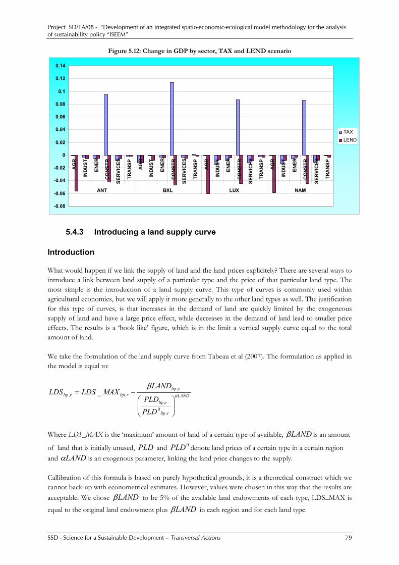
Project SD/TA/08 - “Development of an integrated spatio-economic-ecological model methodology for the analysis of sustainability policy “ISEEM”
SSD - Science for a Sustainable Development – Transversal Actions 79
Figure 5.12: Change in GDP by sector, TAX and LEND scenario
-0.08
-0.06
-0.04
-0.02
0
0.02
0.04
0.06
0.08
0.1
0.12
0.14A
GR
INDU
ST
EN
ER
CO
NST
R
SE
RVIC
ES
TRA
NSP
AG
R
INDU
ST
EN
ER
CO
NST
R
SE
RVIC
ES
TRA
NSP
AG
R
INDU
ST
EN
ER
CO
NST
R
SE
RVIC
ES
TRA
NSP
AG
R
INDU
ST
EN
ER
CO
NST
R
SE
RVIC
ES
TRA
NSP
ANT BXL LUX NAM
TAXLEND
5.4.3 Introducing a land supply curve Introduction What would happen if we link the supply of land and the land prices explicitely? There are several ways to introduce a link between land supply of a particular type and the price of that particular land type. The most simple is the introduction of a land supply curve. This type of curves is commonly used within agricultural economics, but we will apply it more generally to the other land types as well. The justification for this type of curves, is that increases in the demand of land are quickly limited by the exogeneous supply of land and have a large price effect, while decreases in the demand of land lead to smaller price effects. The results is a ‘hook like’ figure, which is in the limit a vertical supply curve equal to the total amount of land. We take the formulation of the land supply curve from Tabeau et al (2007). The formulation as applied in the model is equal to:
LAND
rltp
rltp
rltprltprltp
PLDPLD
LANDMAXLDSLDS α
β
⎟⎟⎠
⎞⎜⎜⎝
⎛−=
,0
,
,,, _
Where LDS_MAX is the ‘maximum’ amount of land of a certain type of available, LANDβ is an amount
of land that is initially unused, PLD and 0PLD denote land prices of a certain type in a certain region and LANDα is an exogenous parameter, linking the land price changes to the supply. Callibration of this formula is based on purely hypothetical grounds, it is a theoretical construct which we cannot back-up with econometrical estimates. However, values were chosen in this way that the results are acceptable. We chose LANDβ to be 5% of the available land endowments of each type, LDS_MAX is
equal to the original land endowment plus LANDβ in each region and for each land type.
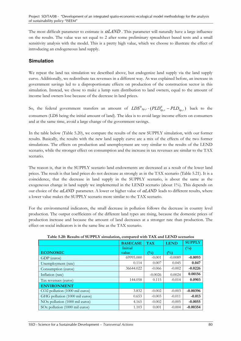
Project SD/TA/08 - “Development of an integrated spatio-economic-ecological model methodology for the analysis of sustainability policy “ISEEM”
SSD - Science for a Sustainable Development – Transversal Actions 80
The most difficult parameter to estimate is LANDα . This parameter will naturally have a large influence on the results. The value was set equal to 2 after some preliminary spreadsheet based tests and a small sensitivity analysis with the model. This is a pretty high value, which we choose to illustrate the effect of introducing an endogeneous land supply. Simulation We repeat the land tax simulation we described above, but endogenize land supply via the land supply curve. Additionally, we redistribute tax revenues in a different way. As was explained before, an increase in government savings led to a disproportionate effects on production of the construction sector in this simulation. Instead, we chose to make a lump sum distribution to land owners, equal to the amount of income land owners lose because of the decrease in land prices. So, the federal government transfers an amount of )( ,
0,,
0rltprltprltp PLDPLDLDS −⋅ back to the
consumers (LDS being the initial amount of land). The idea is to avoid large income effects on consumers and at the same time, avoid a large change of the government savings. In the table below (Table 5.20), we compare the results of the new SUPPLY simulation, with our former results. Basically, the results with the new land supply curve are a mix of the effects of the two former simulations. The effects on production and unemployment are very similar to the results of the LEND scenario, while the stronger effect on consumption and the increase in tax revenues are similar to the TAX scenario. The reason is, that in the SUPPLY scenario land endowments are decreased as a result of the lower land prices. The result is that land prices do not decrease as strongly as in the TAX scenario (Table 5.21). It is a coincidence, that the decrease in land supply in the SUPPLY scenario, is about the same as the exogeneous change in land supply we implemented in the LEND scenario (about 1%). This depends on our choice of the LANDα parameter. A lower or higher value of LANDα leads to different results, where a lower value makes the SUPPLY scenario more similar to the TAX scenario. For the environmental indicators, the small decrease in pollution follows the decrease in country level production. The output coefficients of the different land types are rising, because the domestic prices of production increase and because the amount of land decreases at a stronger rate than production. The effect on social indicators is in the same line as the TAX scenario.
Table 5.20: Results of SUPPLY simulation, compared with TAX and LEND scenarios
BASECASE TAX LEND SUPPLY
ECONOMIC Initial value (%) (%)
(%)
GDP (euros) 69995.000 -0.001 -0.0089 -0.0093
Unemployment (rate) 0.114 0.007 0.045 0.047
Consumption (euros) 36644.022 -0.066 -0.002 -0.0226
Inflation (rate) -0.0026 0.0024 0.00156
Tax revenues (euros) 144.058 0.115 -0.014 0.0903
ENVIRONMENT CO2 pollution (1000 mil euros) 3.832 -0.002 -0.003 -0.00396GHG pollution (1000 mil euros) 0.653 -0.003 -0.011 -0.013NOx pollution (1000 mil euros) 4.165 -0.002 -0.005 -0.0055SOx pollution (1000 mil euros) 1.103 0.001 -0.004 -0.00354

Project SD/TA/08 - “Development of an integrated spatio-economic-ecological model methodology for the analysis of sustainability policy “ISEEM”
SSD - Science for a Sustainable Development – Transversal Actions 81
Output coefficient agricultural land (value/m2) 0.005 -0.011 0.968 1.074Output coefficient industrial land (value/m2) 3.749 0.001 1.004 1.01Output coefficient building land (value/m2) 5.369 0.002 0.999 1.006
SOCIAL Ratio high low (rate) 3.944 -0.0431 -0.0065 -0.020
Poverty gap (euros) 11956.53 -0.0755 -0.0128 -0.0368
Gini (rate) 0.2944 -0.039 -0.0026 -0.0149
Table 5.21: Percentual change in land prices and land supply
TAX LEND SUPPLYPrice of Agricultural land -13.06 4.18 -9.19Price of Industrial space -13.04 4.87 -8.77Price of Service space -13.04 4.90 -8.76Agricultural land supply 0 -1 -1.063Industial land supply 0 -1 -1.008Building land supply 0 -1 -1.006
Figure 5.13 compares the change in domestic production of the land supply scenario with the other scenarios. As explained before, the results on domestic production are comparable to the LEND scenario. The redistribution of tax revenues to land owners, avoids large distortive effects caused by an increase in investments in the construction sector.
Figure 5.13: Changes in GDP, comparison across scenarios
-0.08
-0.06
-0.04
-0.02
0
0.02
0.04
0.06
0.08
0.1
Agr
Min
Food
Clo
th
Woo
d
Pape
r
Cok
e
Che
m
Rub
Gla
ss
Met
al
Eng
Elec
t
Tran
sp e
q
Ener
Con
str
Trad
e
Hor
e
Tran
sp
Com
Ban
k
Bus
Gov Ed
u
Hea
lth
Leis
TAXLENDSUPPLY
We do not take compare the results of GDP on regional level. The results do not give more information than Figure 5.13 and are very similar to Figure 5.11 and Figure 5.12. Instead, we conclude by showing the result on regional welfare for the TAX, LEND and SUPPLY scenarios in Figure 5.14. We take into account the change in equivalent variation of the highest and lowest income deciles in the different regions. The negative effect on regional welfare is the largest in the TAX scenario as it entails the largest decrease in household income. The LEND scenario hardly has any effect on regional welfare, as the decrease in income from land endowments is compensated by higher land prices. In some provinces,
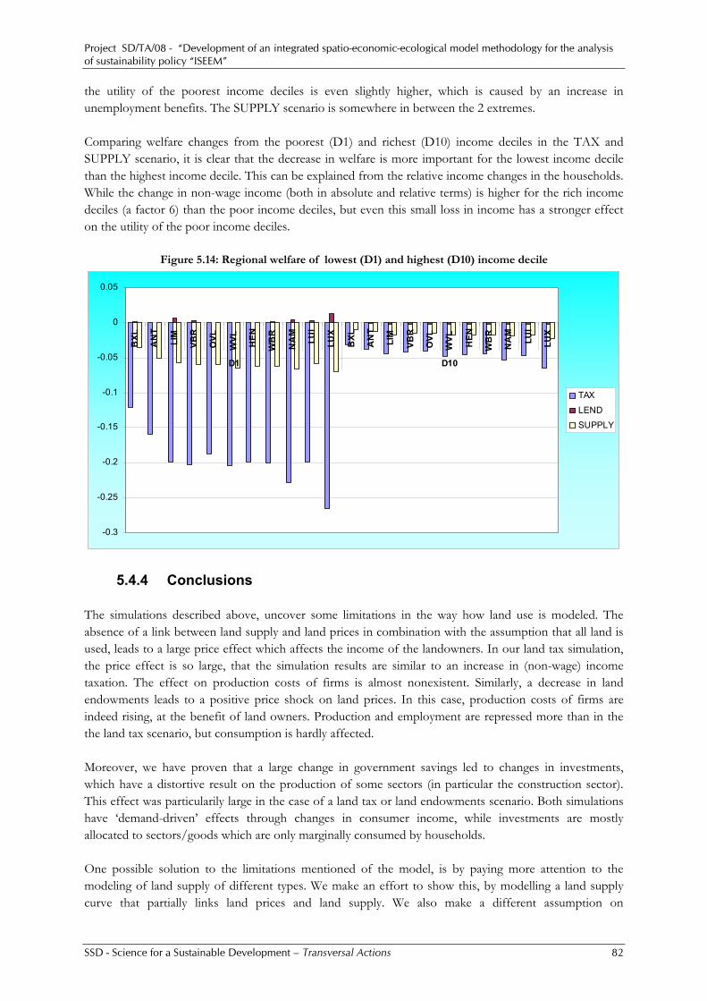
Project SD/TA/08 - “Development of an integrated spatio-economic-ecological model methodology for the analysis of sustainability policy “ISEEM”
SSD - Science for a Sustainable Development – Transversal Actions 82
the utility of the poorest income deciles is even slightly higher, which is caused by an increase in unemployment benefits. The SUPPLY scenario is somewhere in between the 2 extremes. Comparing welfare changes from the poorest (D1) and richest (D10) income deciles in the TAX and SUPPLY scenario, it is clear that the decrease in welfare is more important for the lowest income decile than the highest income decile. This can be explained from the relative income changes in the households. While the change in non-wage income (both in absolute and relative terms) is higher for the rich income deciles (a factor 6) than the poor income deciles, but even this small loss in income has a stronger effect on the utility of the poor income deciles.
Figure 5.14: Regional welfare of lowest (D1) and highest (D10) income decile
-0.3
-0.25
-0.2
-0.15
-0.1
-0.05
0
0.05
BXL
AN
T
LIM
VBR
OVL
WVL HEN
WB
R
NA
M
LUI
LUX
BXL
AN
T
LIM
VBR
OVL
WVL HEN
WB
R
NA
M
LUI
LUX
D1 D10
TAX
LENDSUPPLY
5.4.4 Conclusions The simulations described above, uncover some limitations in the way how land use is modeled. The absence of a link between land supply and land prices in combination with the assumption that all land is used, leads to a large price effect which affects the income of the landowners. In our land tax simulation, the price effect is so large, that the simulation results are similar to an increase in (non-wage) income taxation. The effect on production costs of firms is almost nonexistent. Similarly, a decrease in land endowments leads to a positive price shock on land prices. In this case, production costs of firms are indeed rising, at the benefit of land owners. Production and employment are repressed more than in the the land tax scenario, but consumption is hardly affected. Moreover, we have proven that a large change in government savings led to changes in investments, which have a distortive result on the production of some sectors (in particular the construction sector). This effect was particularily large in the case of a land tax or land endowments scenario. Both simulations have ‘demand-driven’ effects through changes in consumer income, while investments are mostly allocated to sectors/goods which are only marginally consumed by households. One possible solution to the limitations mentioned of the model, is by paying more attention to the modeling of land supply of different types. We make an effort to show this, by modelling a land supply curve that partially links land prices and land supply. We also make a different assumption on
Project SD/TA/08 - “Development of an integrated spatio-economic-ecological model methodology for the analysis of sustainability policy “ISEEM”
SSD - Science for a Sustainable Development – Transversal Actions 83
redistribution of tax revenues, where we partially neutralize both the large income effect on consumers and the increase in country-level investments. The results are in between our pure land tax scenario (TAX) and our pure land endowments scenario (LEND). Another way to introduce frictions in the land market, is by explicitly modeling the decisions of land owners to supply or not supply land of a particular type. This can be realized by implementing a discrete choice framework, similar to the one of the RELU model (cfr. Literature review). Also, we should make assumption on the ‘non-use’ of land by firms. For example, it could be considered to implement a land change function, which allows the interchange of land between land types based on the costs of land change and the land prices (or rents). The main problem with both of these approaches, which is also the reason why we did not implement this yet, is a lack of data and a lack of information on the necessary parameters. Another possibility (which does not require big changes to the model), is to use the results of a more detailed land use model. The most important (possible) drawback here is the compatability of our model with this hypothetical model. These simulations were principally aimed at land use modelling. However, the way how the buildings sector is implemented in the model is very similar to how we model land use. Similar problems arise when simulations with the building inputs are done. Again, modelling the link between price of building stock and the size of the stock in a better way, may improve the results of the model. The price of builings and the available building stock on short-run, behave very similarly to price changes as the stock of land. In the long-run however the stock of buildings is of course more price elastic than land supply.


Project SD/TA/08 - “Development of an integrated spatio-economic-ecological model methodology for the analysis of sustainability policy “ISEEM”
SSD - Science for a Sustainable Development – Transversal Actions 85
6. ISEEM model implementation in GAMS
6.1.1 About GAMS The ISEEM model is implemented using the General Algebraic Modeling System (GAMS). This software is widely used for general equilibrium modeling and has proved to be able to efficiently handle large scale economic models. More information about this software is available from www.gams.com. A manual to work with GAMS is freely available, as well as a test version of the model. However, ISEEM requires the use of a fully functional GAMS program, including a solver able to handle “Mixed Complementarity Problems” (MCP). The price of this software packet and the solver is considerable, but allows complex modelling on a large scale.
6.1.2 Main structure of the code
The main structure of the GAMS code consists of the following elements:
0) BASIC MODEL SETS
-Definition and naming of the sets
-Setting scaling parameters
I) IMPORTING DATA TO GAMS
-Reading in data for the social accounting matrices of the model
o Importing SAM to GAMS (ISEEM-SAM-2006.xls)
o Importing regional (unbalanced) SAM data to GAMS
o Importing other (ISEEM-SAM-auxiliary data for GAMS.xls)
-Constructing the indicators for the split of national SAM between the 11 Provinces
o Importing the data on model parameters estimated using time-series data
o Declaration of scalars and parameters used in the model
-Importing data on transport costs and transport trips (ISEEM-auxiliary.xls)
-Import data on regional governments (ISEEM-gov.xls)
-Constructing the indicators to split up the government accounts
-Reading in other auxiliary data
o Reading in data on regional labour market (ISEEM-auxiliary.xls)
o Reading in data on model parameters (based on HERMES) (ISEEM-elasticities.xls)
o Reading in data on land and building investments (ISEEM-auxiliary.xls)
o Reading in data on housing (ISEEM-auxiliary.xls)
-Reading in data for splitting up household to different types (ISEEM-social.xls)
-Constructing shares to split up household accounts
-Reading in data on emissions and calculating monetary damages of emissions per sector (ISEEM-emissions.xls)

Project SD/TA/08 - “Development of an integrated spatio-economic-ecological model methodology for the analysis of sustainability policy “ISEEM”
SSD - Science for a Sustainable Development – Transversal Actions 86
II) DECLARATION AND INTIALIZATION OF PARAMETERS
-Declaration of parameters, which denote initial values of model variables
-Assigning the initial (base year) values of model variables and checking that all the data is consistent. If this is not the case, the GAMS program is immediately terminated with a corresponding message. First the data from the SAM is read in. Then the auxiliary data on different aspects of the model is used to split up variable from the national SAM in corresponding variables of ISEEM.
-The variables determined from the national social accounting matrix are split up in the regional variables using the shares determined before.
-The expenditures on land and buildings are determined as a fix share of the firm budgets.
-Variables on regional level corresponding to households are split up in different household types.
-Variables on regional level corresponding to the government are split up in regional governments
-Assign values (mostly unity) to each initial price in the baseyear
-Assign functional (exogenous parameters) necessary for the model callibration
-Intitial variables are redefined as values net of taxes (in the SAM the consumption on goods includes the tax on these goods)
-Calculation of tax rates
-Determining variables related to the implementation of regional governments. such as intergovernmental transfers and parameters of government incomes.
III) CALIBRATION OF MODEL PARAMETERS
-Callibration of model parameters concerning the consumption side of the economy, investment, household expenditures, government expenditures, etc..
Estimating interregional trade flows with the nonlinear programming approach (Used under the first run of the program. Resulting data is saved in an Excel file. In further model runs this data is not estimated but read directly from Excel file.)
-Callibration of the labour market
-Callibraton of the monopolistic competition profits associated with Dixit-Stiglitz models
-Callibration of international and interregional trade
-Callibration of the parameters concerned with the production technology of sectors
-Callibration of labour market parameters matching function and wage curve,
-Associating monopolistic competition prices to the model
-Callibration of the commuting flows and migration
-Determining emission coefficients, based on monetary damages per region and per sector.
-Calculating initial values of socio-economic indicators such as the poverty gap, gini coefficients, land use coefficients. etc..
IV) MODEL VARIABLES AND EQUATIONS
-Declaration of model variables
-Declaration of model equations
-Formulation of model equations (cfr. Mathematical formulation)

Project SD/TA/08 - “Development of an integrated spatio-economic-ecological model methodology for the analysis of sustainability policy “ISEEM”
SSD - Science for a Sustainable Development – Transversal Actions 87
V) INITIALIZE VARIABLES
-Formulation of the ISEEM model in non-linear programming (the NLP and mixed complementarity MCP formats)
-Initialization of model variables (mostly to 1, as variables are multiplied with their initial values)
Setting lower bounds for the model variables’ (not when using MCP format)
Testing homogeneity of the model (by multiplying all prices and incomes with a contant value)
-Exogenously fix the variables which are initially equal to zero
VI) MODEL CLOSURE AND NUMERAIRE
-To have a ‘working model’ we have to fix a set of variables exogenously. These are generally initial endowments of different types. Here the modeler makes sure that the model is defined by a square matrix of variables.
VII) SIMULATION (optional)
- Reading in new data, changing the intial values of variables, introducing new tax rates and subsidies, exogeneously fixing a new variable, etc.
VIII) SET SOLVER OPTIONS
- Calling of the model and setting some basic options for the solver
- After this step the model is initialized
IX) MODEL REPORTING
-Declaration of parameters used for reporting of model results
-Calculation of indicators for the model
- Write the results to an Excel file
X) RECURSIVE DYNAMICS
-Declaration of the time periods set for the recursive dynamic part
-Declaration of investment related parameters
-Loop over the time periods
- Within the time loop: translate total savings into sector-specific investments, reinitialize model variables to the specific time period, call the solver and calculate the output parameters for each time period
-Write the results of the model into excel file
END OF CODE
6.1.3 General rules when editing the code When adding lines of code to the model, you should make sure that the general template of the model is still followed. When introducing a new parameter, the parameter has to be defined and an initial value for

Project SD/TA/08 - “Development of an integrated spatio-economic-ecological model methodology for the analysis of sustainability policy “ISEEM”
SSD - Science for a Sustainable Development – Transversal Actions 88
the parameter has to be set in the model calibration. It is important to follow the notational conventions that we have set, to avoid creating an unintelligible and therefore unusable code.
Basic conventions • New sets and aliases are introduced in the beginning of the code, before declaring initial
parameters. • Scalars, parameters and data are in lower case. For example Scal (scaling variable), sigma A1,.. • VARIABLES (and their initial levels) and EQUATION names are in CAPITAL letters are named
in the shortest and most logical way possible. • INDICATORS are called after their respective variables and should be named as short and clearly
as possible • EQUATION names always begin with EQ and are named after the variable that results from the
calculation, for example: EQP is the equation that calculates the price of a good; EQXD is the equation that calculates domestic production for each sector, in each region.
• Initial values of variables and parameters are indicated with Z added to their names, for example: PZ, XDZ, CZ. Respectively initial price level, intial domestic production and initial consumption.
• VARIABLES are initialized to 1 and are multiplied with their initial values in the model equations.
Within the code numerous comments are added on what happens within the model and why. GAMS forces the researcher to declare each parameter explicitly, together with the sets that each parameter uses. This can be very time demanding, but increases the readability of the code and makes it easier to debug. A comment is introduced by the $ontext/$offtext command or by putting an asterisk in the margin.
6.1.4 Model numeraire
A common assumption for a CGE model, which is also adopted here, is that the economy is initially in equilibrium with the quantities normalized in such a way that the prices are equal to unity. Due to the homogeneity of degree zero in prices the model can only determine relative prices. A particular price has been selected to provide the numeraire against which all the prices in the model will be measured. In the ISEEM model, the GDP deflator is chosen as the numeraire and exogenously fixed in the model. The ER equation is used to check the walras law.
6.1.5 Closure of the model and exogenously fixed variables The formal introduction of the concept of closure rule can be traced back to Sen (1963). Sen (1963), showed that the necessary ex-post equality between savings and investment cannot be fulfilled when all the following conditions are satisfied: the factors are paid at their marginal productivity, household consumption is a function of real income, real investment is fixed and the factors are fully employed. The equilibrium is achieved only by relaxing one of these constrains. The choice of the constraint to be dropped, represents in fact the choice of the closure rule. In mathematical terms, the model should consist of an equal number of independent equations and endogenous variables. The closure rule reflects the choice of the model builder of which variables are exogenous and which variables are endogenous, so as to achieve ex-post equality. The following variables are exogenously fixed in the ISEEM model and define its closure:
• Sector-specific capital endowments in each region • Endowments of land (by type) in each region

Project SD/TA/08 - “Development of an integrated spatio-economic-ecological model methodology for the analysis of sustainability policy “ISEEM”
SSD - Science for a Sustainable Development – Transversal Actions 89
• Governmental transfers to households and savings (optional) • Transfers from abroad • Price of labor in the rest of the world and Belgian labour supplied to the rest of the world • Labour supply in each region • Time and monetary costs of freight transport • Time and monetary costs of passenger transport by trip purpose • Migration (optional) • Public savings / Government consumption (one of these has to be fixed, government
consumption is fixed by default) The closure of the ISEEM model is thus defined by a particular set of the exogenously fixed variables. The model closure can be changed by the model user under the simulations given the needs of the particular policy analysis and the assumptions made under the simulation. The user should take care that the number of variables exogenously fixed in the model does not change. This ensures that the number of unknowns in the nonlinear system of equations is equal to the number of equations.
6.1.6 How to implement simulations with the model
The ISEEM model does not have a graphical interface. Implementing a simulation requires basic understanding of the GAMS language and some modelling knowledge. In the model one can change any of the exogenously fixed model parameters and variables, as well as introducing new variables or changing the endowments of capital, labour, land, buildings, etc. The set-up of the simulation can best be done after the model closure and before calling the solver. Here new data can be read in, the initial values of variables can be changed or a tax rate or subsidy rate can be applied. Whenever possible, it is best to avoid introducing unnecessary new variables and parameters and to stick to the variables that are already in the model. However, even then, a simulation can require introducing new variables (III) and changing the basic equations (IV) If the simulation involved changing equations and/or variables, it is important to check if the baseline of the model is still correct. This can be done by running the model without applying the simulation. The solver should initialize the model and then stop immediately with the notification of ‘solution found’. If debugging is necessary, it is best to set the iteration limit of the model to 0 (VIII). It is then possible to look for the equations that generate ‘infeasabilities’ in the output file (search for INFES in the .lst file). It is also important to check if the model still has a degree of homogeneity equal to zero after changing the equations of the model. This means that if all the prices, incomes and the numerair are are doubled (or multiplied with another fixed factor), this should not affect the consumption. A homogeneity check was built in to the model. The homogeneity of the model should be respected, because what matters in economic modelling are the relative prices of goods and factors. If these are multiplied with a constant factor and the real income is still the same, this should not lead to different results. After running the simulation the researcher should check the walras law. This states that if a model exists from a square system of n equations, each defining a unique parameter, a full solution of the model should allow determining the value of parameter n, out of the values of the other (n-1) parameters. Or otherwise said, the intial system of equations is overdefined. By leaving out one equation, it’s possible to crosscheck the results of the model, by calculating the value of the “left-out equation”.

Project SD/TA/08 - “Development of an integrated spatio-economic-ecological model methodology for the analysis of sustainability policy “ISEEM”
SSD - Science for a Sustainable Development – Transversal Actions 90
In ISEEM the Walras law is checked by the value of the exchange rate. In a correct simulation, the value of the walras check, should be very close to zero (E-8 or smaller). If Walras law does not hold, your simulation is incorrect and should be reprogrammed. In this case you should check if the new variable is introduced correctly. The ‘leakage’ introduced in the economy is often due to a mistake in the budget equation of the consumer or tax income equation of the government, or because of not introducing or misspecifying the new variable. ISEEM also contains the option to run your models in a dynamic way. The modeler or researcher will then need to specify this in the code. The dynamic simulation works as a loop over time periods. We specify these as years, but it is possible to see these as longer or shorter periods, depending on the set-up of the simulation. In the basecase scenario all variables (except prices) are inflated with a constant growth factor. This can be changed exogeneously, for example by inserting a basecase (prevision) scenario for the model, however this will require the model to solve a new basecase scenario first. When running the model without implementing a simulation, one can check if this generates a sequence of correct solution. This is tested in a similar way as for a static simulation, by setting the iteration limit of the solver to 0. Infeasabilities resulting from an incorrect basecase scenario should be solved before running any other simulation.
6.1.7 Model reporting Results from the ISEEM model are written to Excel sheets. We offer a full model report of ISEEM, both of the dynamic simulations as of the static simulations. This contains the percentual change in all variables and gives a very broad overview of the model results. Alternatively, ISEEM offers an output in the basic indicators which are grouped in Table 4.1. The basic indicators offer a general view on the results of the simulation, while the full report gives more information on how these results are generated. In general one should check both the indicators from the model as the full output to understand the effect of the policy run.
6.1.8 If the model does not run
...and the solver does not initialize - Check the error codes of the GAMS model and correct the problems one by one by clicking on
the error messages …while the solver initializes, but does not come to a solution - Check if you implemented the simulation in a correct way, often a failure to run is due to a model
misspecification. - Check if your model is homogeneous - Try other values for the exogeneous parameters (increase or decrease elasticities) - Try a different scaling of the model, especially if you changed something in the calibration
process (scalings are defined after the introduction of the sets and aliases) - Choose a different model closure (lock government spendings or budgets, fix migration, fix
transfers to households, etc.) - Check the solver options …while the model solves, but does not give sensible outputs - Again, check the setup of your simulation - Check walras law and homogeneity - Try to locate the source of the problem from the type of simulation you implemented. - Make changes to the model if necessary.
Project SD/TA/08 - “Development of an integrated spatio-economic-ecological model methodology for the analysis of sustainability policy “ISEEM”
SSD - Science for a Sustainable Development – Transversal Actions 91
7. Bibliography Bleys. B., 2008, Proposed changes to the Index of Sustainable Economic Welfare : An application to Belgium, Ecological Economics, 64. 741-751 Clarke. M.. Lawn. P., 2008, Is measuring genuine progress at the sub-national level useful ? Ecological Indicators. 8. 573-581 Dasgupta. P.. 2001. Human Well-being and the Natural Environment. Oxford University Press. p. 160 Dobbelaere S., 2007, Panel data estimates of the production function and product and labour market imperfections, ECB working papers no. 782 European Environment Agency, 2005, The European Environment : State and outlook 2005, European Environment Agency, Copenhagen Eurostat. 2003. « Laeken »indicators-Detailed Calculation Methodology. European Commission Eurostat Quality Profile. http://epp.eurostat.ec.europa.eu/portal Fane G.. Ahammad H., 2003, Alternative ways of measuring and decomposing equivalent variation, Economic Modelling, 21. 175-189 German System of socials indicators. http://www.gesis.org Hamilton. C., 1998, The Genuine Progress indicator methodological developments and results from Australia. Ecological Economics. 30. 13-28 Hanley. N., Moffatt. I.. Faichney. R., Wilson. M., 1999. Measuring sustainability : a time series of alternative indicators for Scotland. Ecological Economics 28. 55-73 Harberger A.C.. 1971. Three basic postulates for applied welfare economics : an interpretative essay. J. Economic L. 9. 785-797 Intergovernmental Panel on Climate Change. 1995. http://www.ipcc.ch/ipccreports/assessments-reports.htm Lasso de la Vega. M.C.. Urrutia. A.M.. 2001. HDPI : a framework for pollution-sensitive human development indicators. Environment. Development and Sustainability (3). 199-215 Lawn. P. 2003. A theoretical foundation to support the Index of Sustainable Economic Welfare (ISEW). Genuine Progress Indicator (GPI). and other related indexes. Ecological Economics. 44. 105-118 Lehtonen M., 2004, The environmental-social interface of sustainable development : capabilities, social capital, institutions, Ecological Economics. 49. 199-214 Meynaerts E., Lodewijks P., 2008, Ex ante evaluation of the costs and effects of an earmarked NOx charge for stationary sources in Flanders with the Environmental Costing Model.

Project SD/TA/08 - “Development of an integrated spatio-economic-ecological model methodology for the analysis of sustainability policy “ISEEM”
SSD - Science for a Sustainable Development – Transversal Actions 92
Morse. S., 2003, For better or for worse, till the human development index do us part ?. Ecological Economics. 45 (2) 281-296 Neumayer. E.. 2000, On the methodology of the ISEW, GPI and related measures : Some constructive suggestions and some doubts on the threshold hypothesis. Ecological Economics 34. 347-361 Nourry. M., 2008, Measuring sustainable development : Some empirical evidence for France from eight alternative indicators. Ecological Economics. 67 (3). 441-456 OECD. 2008. Handbook on constructing composite indicators : Methodology and user guide. OECD. 2004. Key environmental indicators. OECD Environment Directorate. Paris. France Sagar. A.D.. Najam. A.. 1998. The human development index : a critical review. Ecological Economics. 25 (3). 249-264 Sancho F., 2006, Callibration of CES function for real World multisectoral modelling, Department of economics, Universitat autonoma de Barcelona. Sen. A. (Ed.), 1997, On economic inequality. Oxford University Press. New-York. 280 pp. Solow. R., 1993. An almost practical step toward sustainability, Resources Policy 19, 162-172 Spangenberg . J.H.. Pfahl, S., Deller. K.. 2002, Towards indicators for institutional sustainability: lessons from an analysis of Agenda 21, Ecological Indicators. 2. 2002. 61-77 Tabeau A., Eickhout B. and Meil (van) H., 2007, the importance of land heterogeneity in long-term scenarios (GTAP based), Agricultural economics Research (LEI) and Netherlands environmental assessment agency (MNP), The Hague Netherlands. UN Department of Economic and Social Affairs, Division for sustainable development. http://www.un.org/esa/sustdev/csd/review.htm Vermeulen W., 2003, A model for dutch commuting, CPB working paper. World Bank, http://www.worldbank.org/poverty and the World Development Report 2006 : Equity and Development, the World Bank 2005. Ziemeser T., 2001, Monopolistic competition and search unemployment: A Pissarides-Dixit-Stiglitz model, Maastricht University. Zuidema T. and Andries N., 2002, Health damages from air pollution and benefits and costs of ammonia control in the Netherlands, University of Groningen

Project SD/TA/08 - “Development of an integrated spatio-economic-ecological model methodology for the analysis of sustainability policy “ISEEM”
SSD - Science for a Sustainable Development – Transversal Actions 93
ANNEX I: Elasticities
Table I.1: Income elasticities of ISEEM products (based on HERMES)
Description Sec elasY Agriculture good1 0.49 Mining good2 0.15 Food, Drink, Tobacco good3 0.49 Clothing and Footwear good4 0.98 Wood good5 0.32 Paper and print media good6 1.22 Cokes and Refined Oil + Miscellaneous good7 0.62 Chemistry, pharmaceutics good8 1.44 Rubber, plastics good9 0.32 Glas, ceramics good10 0.32 Metals, basic good11 0.32 Engines and Machinery good12 0.32 Electronic machinery good13 1.22 Transportation equipment good14 1.99 Energy good15 0.25 Construction good16 1.37 Trade and repair good17 1.37 Horeca good18 1.37 Transport good19 0.72 Communication good20 1.04 Banking and finance good21 1.37 Business services good22 0.65 Government good23 1.22 Education good24 1.22 Health good25 1.44 Leisure services good26 1.22
Table I.2: Elasticities of capital, energy and labour products (HERMES)
Description Sec sigmaKELM18 sigmaKE sigmaLM
Agriculture good1 0.475 0.23 0.4 Mining good2 0.475 0.2 0.35 Food, Drink, Tobacco good3 0.475 0.23 0.4 Clothing and Footwear good4 0.475 0.23 0.4 Wood good5 0.475 0.23 0.4 Paper and print media good6 0.475 0.23 0.4 Cokes and Refined Oil + Miscellaneous good7 0.475 0.145 0.27 Chemistry, pharmaceutics good8 0.475 0.2 0.35 Rubber, plastics good9 0.475 0.23 0.4 Glas, ceramics good10 0.475 0.2 0.35 Metals, basic good11 0.475 0.2 0.35 Engines and Machinery good12 0.475 0.25 0.515
18 In the original HERMES specification the upper Capital – Energy – Labour – Materials nest is Cobb – Douglas. We approximated this by using a CES nest with elasticity 0.95 instead.

Project SD/TA/08 - “Development of an integrated spatio-economic-ecological model methodology for the analysis of sustainability policy “ISEEM”
SSD - Science for a Sustainable Development – Transversal Actions 94
Electronic machinery good13 0.475 0.25 0.515 Transportation equipment good14 0.475 0.25 0.515 Energy good15 0.475 0.145 0.27 Construction good16 0.39 0.45 0.475 Trade and repair good17 0.445 0.52 0.425 Horeca good18 0.445 0.52 0.425 Transport good19 0.445 0.535 0.46 Communication good20 0.43 0.545 0.475 Banking and finance good21 0.43 0.705 0.43 Business services good22 0.45 0.89 0.475 Government good23 0.45 0.89 0.475 Education good24 0.45 0.89 0.475 Health good25 0.45 0.89 0.475
Leisure services good26 0.45 0.89 0.475
Table I.3 Other exogenous parameters
Description Parameter Value Frisch Frisch -1.1 International Armington Sigma 1.5 Interregional Armington sigmaA1 5 Substitution between varieties (equal for all goods) elasReg 10 Substitution between labour/land bundle and other capital (equal for each sector) sigmaBDLDKELM 0.3 Substitution labour/land bundle (equal for each sector) sigmaBDLD 0.2
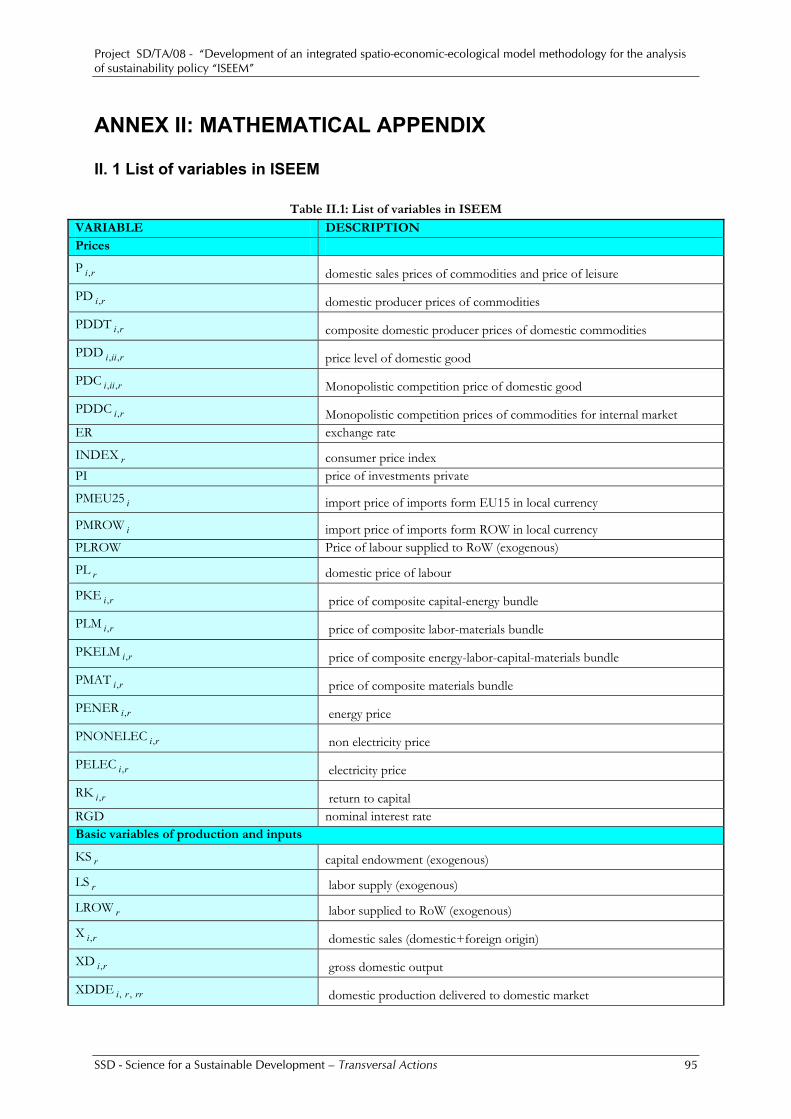
Project SD/TA/08 - “Development of an integrated spatio-economic-ecological model methodology for the analysis of sustainability policy “ISEEM”
SSD - Science for a Sustainable Development – Transversal Actions 95
ANNEX II: MATHEMATICAL APPENDIX II. 1 List of variables in ISEEM
Table II.1: List of variables in ISEEM
VARIABLE DESCRIPTION Prices
P ri, domestic sales prices of commodities and price of leisure
PD ri, domestic producer prices of commodities
PDDT ri, composite domestic producer prices of domestic commodities
PDD riii ,, price level of domestic good
PDC riii ,, Monopolistic competition price of domestic good
PDDC ri, Monopolistic competition prices of commodities for internal market ER exchange rate
INDEX r consumer price index PI price of investments private
PMEU25 i import price of imports form EU15 in local currency
PMROW i import price of imports form ROW in local currency PLROW Price of labour supplied to RoW (exogenous)
PL r domestic price of labour
PKE ri, price of composite capital-energy bundle
PLM ri, price of composite labor-materials bundle
PKELM ri, price of composite energy-labor-capital-materials bundle
PMAT ri, price of composite materials bundle
PENER ri, energy price
PNONELEC ri, non electricity price
PELEC ri, electricity price
RK ri, return to capital RGD nominal interest rate Basic variables of production and inputs
KS r capital endowment (exogenous)
LS r labor supply (exogenous)
LROW r labor supplied to RoW (exogenous)
X ri, domestic sales (domestic+foreign origin)
XD ri, gross domestic output
XDDE rrri ,, domestic production delivered to domestic market
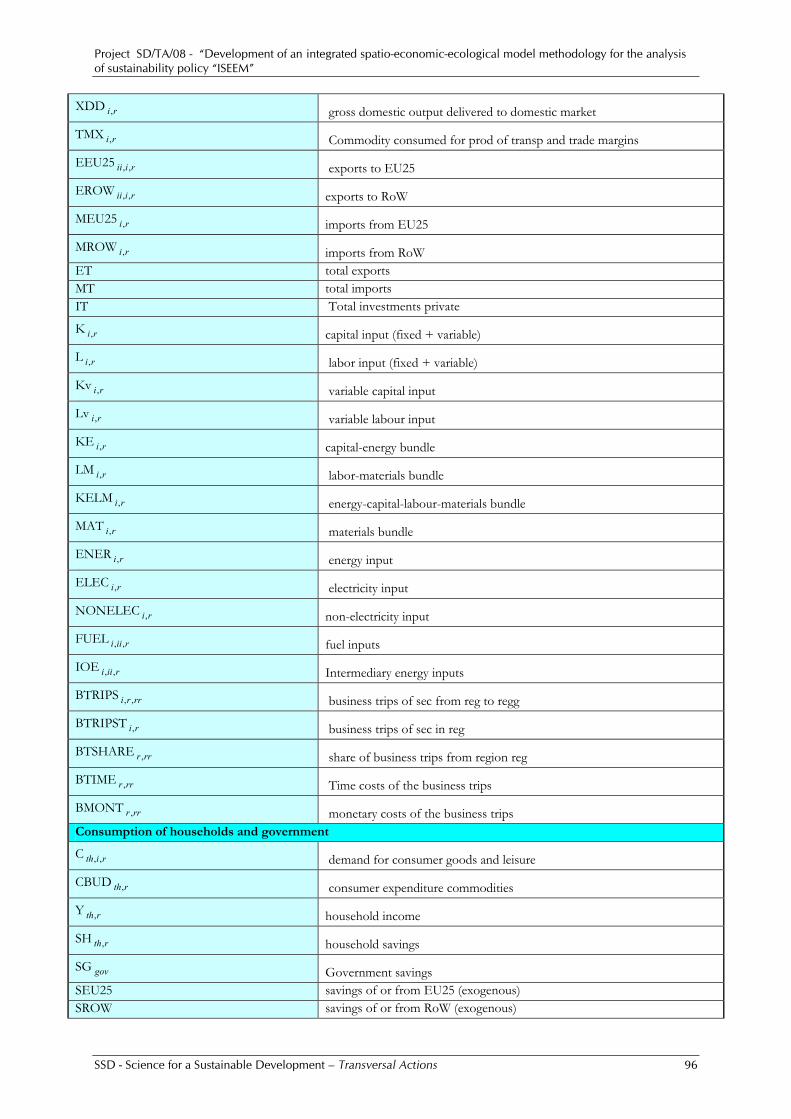
Project SD/TA/08 - “Development of an integrated spatio-economic-ecological model methodology for the analysis of sustainability policy “ISEEM”
SSD - Science for a Sustainable Development – Transversal Actions 96
XDD ri, gross domestic output delivered to domestic market
TMX ri, Commodity consumed for prod of transp and trade margins
EEU25 riii ,, exports to EU25
EROW riii ,, exports to RoW
MEU25 ri, imports from EU25
MROW ri, imports from RoW ET total exports MT total imports IT Total investments private
K ri, capital input (fixed + variable)
L ri, labor input (fixed + variable)
Kv ri, variable capital input
Lv ri, variable labour input
KE ri, capital-energy bundle
LM ri, labor-materials bundle
KELM ri, energy-capital-labour-materials bundle
MAT ri, materials bundle
ENER ri, energy input
ELEC ri, electricity input
NONELEC ri, non-electricity input
FUEL riii ,, fuel inputs
IOE riii ,, Intermediary energy inputs
BTRIPS rrri ,, business trips of sec from reg to regg
BTRIPST ri, business trips of sec in reg
BTSHARE rrr , share of business trips from region reg
BTIME rrr , Time costs of the business trips
BMONT rrr , monetary costs of the business trips Consumption of households and government
C rith ,, demand for consumer goods and leisure
CBUD rth, consumer expenditure commodities
Y rth, household income
SH rth, household savings
SG gov Government savings SEU25 savings of or from EU25 (exogenous) SROW savings of or from RoW (exogenous)

Project SD/TA/08 - “Development of an integrated spatio-economic-ecological model methodology for the analysis of sustainability policy “ISEEM”
SSD - Science for a Sustainable Development – Transversal Actions 97
S national savings
I ri, demand for investment goods private
CG ri, Intermediate public demand for goods
CGR govr , public spendings on regional level
CGG govri ,, Intermediate public demand regional governments TAXR tax revenues SUBS Total subsidies
TAXRG gov total tax revenue of regional goverment
SUBSG gov total subsidies of regional goverment
TRF rth, total transfers of government to households (exogenous)
TRFF govrth ,, total transfers of regional government to households
TREU25 gov total transfers to government from EU25 (exogenous)
GDP Gross domestic product (real) GDPC Gross domestic product (nominal) GDPDEF GDP deflator (exogenous-numeraire)
GDPR r regional gross domestic product (real)
GDPRC r regional gross domestic product (nominal) INDEXE price index for exports INDEXM price index for imports PTM composite price of trade and transport margin
PEV rth, equivalent variation price index
SII rth, equivvalent variation budget
EV rth, welfare change as a percentage of households income
U rth, regional utility level
SV ri, changes in stocks Monopolistic competition and labour market
NF ri, equilibrium number of monopolistic firms
AUXV ri, auxiliary variable
PROFITS ri, profits of the sectors
PW r composite regional wage
LCM rrr , job commuters
UNEMP r regional unemployment level
UNRATE r regional unemployment rate
UNEMPB govrth ,, unemployment benefits
LMIG rrrth ,, labor migration from reg to regg
Ttime rrr , travel costs between the regions (time)

Project SD/TA/08 - “Development of an integrated spatio-economic-ecological model methodology for the analysis of sustainability policy “ISEEM”
SSD - Science for a Sustainable Development – Transversal Actions 98
Tmoney rrr , travel costs between the regions (money)
trmV irrr ,, c freight transport costs
SHOPTRIPS rrr , shopping trips
SHOPTIME rrr , time costs of shopping trips
SHOPMONT rrr , monetary costs of shopping trips
OTHTRIPS rrr , other trips
OTHTIME rrr , Time costs of other trips
OTHMONT rrr , monetaty costs of other trips
EDUTRIPS rrr , education trips
EDUTIME rrr , Time costs of education trips
EDUMONT rrr , monetaty costs of education trips
PLU r reservation wage
PR r probability to find a job
QR r probability to fill in a vacancy
NVS ri, number of vacancies per sector
NV r number of vacancies
NM rrr , number of matches Regional governments TRFG total intra-government transfers
TRFGE gov outgoing transfers from government
TRFGY govvgov, incoming transfers from government
TRFGG govvgov, Intra government transfers gov to govv PB total public budget
CBUD_GOV gov regional consumption budget of government Land use and buildings
PLD rltp, Price of land used in a particticular sector
PBD rbtp, Price of buildings in a particular region
LDS rltp, supply of land
BDS rbtp, supply of buildings
PBDLD ri, Price of composite land-buildings bundle
PBDLDKELM ri, composite price of land labour and capital bundle
LD ri, demand for land
BD ri, demand for buildings

Project SD/TA/08 - “Development of an integrated spatio-economic-ecological model methodology for the analysis of sustainability policy “ISEEM”
SSD - Science for a Sustainable Development – Transversal Actions 99
BDLD ri, demand for composite land buildings bundle
BDLDKELM ri, composite land labour and capital bundle Emissions
POLL_CO2 ri, energy related CO2 pollution in mil tones
POLL_GHG riemis ,, energy related GHG (non-CO2)
POLL_NGHG riemis ,, energy related non GHG pollution in mil tones
POLL_CO2_PROD ri, output related CO2 pollution in mil tones
POLL_GHG_PROD riemis ,, output related GHG (non-CO2)
POLL_NGHG_PROD riemis ,, output related non GHG pollution in mil tones
POLL_CO2_RES rth, housing related CO2 pollution in mil tonnes
POLL_GHG_RES remisth ,, housing related GHG (non-CO2)
POLL_NGHG_RES remisth ,, housing related NGHG pollution in mil tonnes
II.2 List of parameters callibrated within the model
Parameters associated with taxation and government consumption
aTRFGOV govvgov, coefficient for initial intra-government transfers
shareTRFGE gov share of the government income going to transfers
aTRFGE govvgov, division of transfers between subgovernments
aG govri ,, Cobb-Douglas parameter for government spending on regional level
α G govr , Cobb-Douglas power in government utility function (goods
sp_gov govr , share of subsidies on production subgovernment
sc_gov govr , share subsidies on products subgovernment
tc_gov govr , share of tax products subgovernment
vatc_gov govr , share of VAT products subgovernment
exst_gov govr , share of of excise on products subgovernment
tk_gov govr , share of corporate tax rate subgovernment
tl_gov govr , share of tax employers contribution subgovernment
tl1_gov govr , share ofemployees contribution subgovernment
txd_gov govr , share of production tax subgovernment
ty_gov govvthr ,, income tax
sp i subsidies rate on production
sc i subsidies rate on products

Project SD/TA/08 - “Development of an integrated spatio-economic-ecological model methodology for the analysis of sustainability policy “ISEEM”
SSD - Science for a Sustainable Development – Transversal Actions 100
tc i tax rate on products
vatc i VAT tax rate on products
exst i tax rate of excise on products
tk i corporate tax rate
tl i tax rate on labor use employers contribution
tl1 i tax rate on labor use employees contribution
txd i tax rate on production
ty th tax rate on income by income decile Parameters of the labour market
scalB r bargaining power of workers by sector and region
aM rrr , scale parameter of the matching function
α M rrr , share parameter of the matching function related to vacancies
nu r job destraction rate
trep r replacement rate of unemployed
a_lab r parameter to balance unemployment and unemployment benefits Technical coefficients of production and input-output
trm irrr ,, trade and transport margins
io regiii ,, Technical coefficients intermediate inputs
iop regiii ,, technical coefficients outputs
iops regiii ,, technical coefficients outputs (production share in demand
ioBDLDKELM ri, Technical coefficients for BDLDKL bundle (land-building labour capital
σ BDLD ri, CES elasticity of substitution between land and building stock
σ BDLDKELM ri, CES elasticity of subsitutiton between land-buildings and capital-labor bundle
γ LD ri, CES share parameter for land
γ BD ri, CES share parameter for buildings
γ BDLD ri, CES share paramter for buildings and land bundle
γ KELM ri, CES share parameter for labor-capital bundle
aBDLD ri, scaling parameter of CES function buildings land
aBDLDKELM ri, scaling parameter of the CES function
σ KELM ri, CES elasticity of subsitutiton between capital and labor
γ KE ri, CES share parameter for capital and labour bundle
γ LM ri, CES share parameter for energy
aKELM ri, scaling parameter of the CES function
aECNEC ri, scaling parameter of CES function of energy
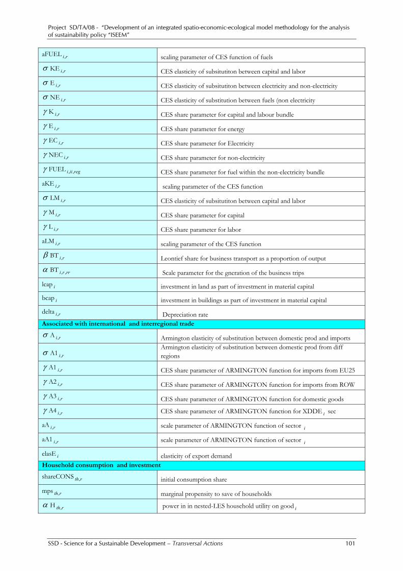
Project SD/TA/08 - “Development of an integrated spatio-economic-ecological model methodology for the analysis of sustainability policy “ISEEM”
SSD - Science for a Sustainable Development – Transversal Actions 101
aFUEL ri, scaling parameter of CES function of fuels
σ KE ri, CES elasticity of subsitutiton between capital and labor
σ E ri, CES elasticity of subsitutiton between electricity and non-electricity
σ NE ri, CES elasticity of substitution between fuels (non electricity
γ K ri, CES share parameter for capital and labour bundle
γ E ri, CES share parameter for energy
γ EC ri, CES share parameter for Electricity
γ NEC ri, CES share parameter for non-electricity
γ FUEL regiii ,, CES share parameter for fuel within the non-electricity bundle
aKE ri, scaling parameter of the CES function
σ LM ri, CES elasticity of subsitutiton between capital and labor
γ M ri, CES share parameter for capital
γ L ri, CES share parameter for labor
aLM ri, scaling parameter of the CES function
β BT ri, Leontief share for business transport as a proportion of output
α BT rrri ,, Scale parameter for the gneration of the business trips
lcap i investment in land as part of investment in material capital
bcap i investment in buildings as part of investment in material capital
delta ri, Depreciation rate Associated with international and interregional trade
σ A ri, Armington elasticity of substitution between domestic prod and imports
σ A1 ri, Armington elasticity of substitution between domestic prod from diff regions
γ A1 ri, CES share parameter of ARMINGTON function for imports from EU25
γ A2 ri, CES share parameter of ARMINGTON function for imports from ROW
γ A3 ri, CES share parameter of ARMINGTON function for domestic goods
γ A4 ri, CES share parameter of ARMINGTON function for XDDE i sec
aA ri, scale parameter of ARMINGTON function of sector i
aA1 ri, scale parameter of ARMINGTON function of sector i
elasE i elasticity of export demand Household consumption and investment
shareCONS rth, initial consumption share
mps rth, marginal propensity to save of households
α H rth, power in in nested-LES household utility on good i

Project SD/TA/08 - “Development of an integrated spatio-economic-ecological model methodology for the analysis of sustainability policy “ISEEM”
SSD - Science for a Sustainable Development – Transversal Actions 102
muH rith ,, subsistence household consumption quantity of good i
α HOUS rth, Cobb-Douglas power of the househond utility function associated with housing
α I ri, Cobb-Douglas power in investment production function
svs ri, inventory shares
atm ri, share of commodity for prod of transp and trade margins Parameters associated with the modelling of transport trips and migration
β SHOP rrr , scale parameter for the generation of the shopping trips
β EDU rrr , scale parameter for the generation of the education trips
β OTHER rrr , scale parameter for the generation of travel(other
γ SHOP r generation coefficient for the generation of the shopping trips
γ EDU r generation coefficient for the generation of the education trips
γ OTHER r generation coefficient for the generation of travel(other
Bmig rth, taste parameter for generation of migration flow
Amig rth, ,regg taste parameter for the distibution of the generated migration Parameters for determining the interregional trade flows α T parameter Parameter associated with the available labour force γ T Parameter associated with the distance between regions
scalarT rrr , scaling parameter calibrated on the initial data on commuting Parameters associated with pollution
α POLL_CO2 i share of energy related CO2 pollution in mil tones
α POLL_GHG iemis, share of energy related GHG (non-CO2
α POLL_NGHG iemis, share of energy related non GHG pollution in mil tones
α POLL_CO2_PROD i share of output related CO2 pollution in mil tones
α POLL_GHG_PROD iemis, share of output related GHG (non-CO2
α POLL_NGHG_PROD iemis, share of output related non GHG pollution in mil tones
α POLL_CO2_RES rth, share of residential stock coupled to CO2 pollution in mil tonnes
α POLL_GHG_RES iemisth ,, share or residential stock coupled to GHG (non-CO2)
α POLL_NGHG_RES iemisth ,, share of residential stock coupled to NGHG in mil tonnes II.3 List of equations
( )( )
riiii
rrrrririrrririri
MROWPMROWMEUPMEU
trmVPTMPDCXDDEXP
,
,,,,,,,
2525 ⋅+⋅+
⋅+⋅=⋅ ∑ (1)
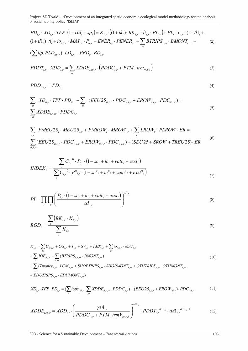
Project SD/TA/08 - “Development of an integrated spatio-economic-ecological model methodology for the analysis of sustainability policy “ISEEM”
SSD - Science for a Sustainable Development – Transversal Actions 103
( ) ( )
rirrirltp
rrrrrrrrriririiririiiii
irirriririiriiiriri
BDPBDLDPLDltp
BMONTBTRIPSPENERENERPMATiotltl
tlLPLPIRKtkKsptxdTFPXDPD
,,,
,,,,,,,,
,,,,,,,
),(
)11(
11()1(1
⋅+⋅
+⋅+⋅+⋅⋅+⋅+
++⋅⋅+⋅∂+⋅+⋅=+−⋅⋅⋅
∑
∑ (2)
( )∑ ⋅+⋅=⋅
rrirrrrirrririri trmPTMPDDCXDDEXDDPDDT ,,,,,,, (3)
ririii PDPDD ,,, = (4)
riii
rrri
riiiriiiriiiriiiii
riiriiii
PDDCXDDE
PDCEROWPDCEEUPDTFPXD
,,,
,,,,,,,,,, )25(
⋅
=⋅+⋅−⋅⋅
∑
∑∑ (5)
ERTREUSROWSEUPDCEROWPDCEEU
ERPLROWLROWMROWPMROWMEUPMEU
riiiriiiriiiriii
riii
rrriirii
ri
⋅+++⋅+⋅
=⋅⋅+⋅+⋅
∑
∑∑)2525()25(
2525
,,,,,,,,
,,
,,,
(6)
( )
( )∑∑
+++−⋅⋅
+++−⋅⋅=
iiiiiriri
iiiiiriri
r exstvatctcscPC
exstvatctcscPCINDEX
0000,
00,
,0
,
1
1
(7)
( )∏∏ ⎟
⎟⎠
⎞⎜⎜⎝
⎛ +++−⋅=
i r
I
ri
iiiiriri
IexstvatctcscP
PI,
,
, 1α
α (8)
( )
∑∑ ⋅
=
iri
iriri
i K
KRKRGD
,
,,
(9)
)
(
)(
,,
,,,,,,
,,,,,,
,,,,,,,,,,
rrrrrr
rrrrrrrrrrrrrrrrr
rrr
ii rriirrrrrriiriii
riiii
riiiririririth
rithri
EDUMONTEDUTRIPS
OTHMONTOTHTRIPSSHOPMONTSHOPTRIPSLCMTmoney
BMONTBTRIPSIOE
MATioTMXSVICGCX
⋅+
⋅+⋅+⋅+
⋅++
⋅+++++=
∑
∑ ∑
∑∑
(10)
riiiriiiriiiriirr
rrriiii
riiiriri PDCEROWEEUPDDCXDDEiopsPDTFPXD ,,,,,,,,,,,,, )25()( ⋅++⋅⋅=⋅⋅ ∑∑ (11)
11,
1,
1
,,,
,,,,
,,
,
14 −⋅⋅⎟
⎟⎠
⎞⎜⎜⎝
⎛
⋅+⋅= riri
ri
Ari
Ari
A
irrrrri
ririrrri aAPDDT
trmVPTMPDDCA
XDDXDDE σσ
σγ
(12)
Project SD/TA/08 - “Development of an integrated spatio-economic-ecological model methodology for the analysis of sustainability policy “ISEEM”
SSD - Science for a Sustainable Development – Transversal Actions 104
ielasE
ri
iriri PDINDEXEEUEEU ⎟
⎟⎠
⎞⎜⎜⎝
⎛⋅=
,
0,, 2525 (13)
ielasE
ri
iriri PDINDEXEROWEROW ⎟
⎟⎠
⎞⎜⎜⎝
⎛⋅=
,
0,, (14)
( ) ( ) 1,,
,
,,,
,,3 −⋅⋅⎟
⎟⎠
⎞⎜⎜⎝
⎛⋅= riri A
riA
riri
ririri aAPPDDTA
XXDD σσγ (15)
( ) ( ) 1,,
,,,
,,
251
25 −⋅⋅⎟⎟⎠
⎞⎜⎜⎝
⎛⋅= riri A
riA
rii
ririri aAPPMEUA
XMEU σσγ (16)
( ) ( ) 1,,
,,,
,,2 −⋅⋅⎟⎟
⎠
⎞⎜⎜⎝
⎛⋅= riri A
riA
rii
ririri aAPPMROWA
XMROW σσγ (17)
( )∑∑ ⋅−⋅+⋅+=
i rriri PSVERSROWERSEUSIT ,,25 (18)
riri
KEri
KEri
ririi
ririri
fcKNF
aKEPKEPIRKtk
KKEK riri
riKE
,,
1,,
,,
,,,
,,
,
)1(
⋅+
⋅⋅⎟⎟⎠
⎞⎜⎜⎝
⎛
⋅∂+⋅+⋅= −σσ
σ
γ (19)
rrrrr
rrririri
LMri
LMri
LM
iiiri
ririri
BTIMEBTRIPSfcLNF
aLMPLMtltltlPL
LLML riri
ri
,,,,,
1,,
,
,,,
,,
,
))11(11(
⋅+⋅+
⋅⋅⎟⎟⎠
⎞⎜⎜⎝
⎛
⋅+++⋅⋅=
∑
−σσ
σγ
(20)
1,,
,,,
,,
,
−
=
⋅⋅⎟⎟⎟
⎠
⎞
⎜⎜⎜
⎝
⎛⋅=∑
riri
riKE
KEri
KEri
ENERiiii
ririri aKEPKE
PE
KEK σσ
σ
γ (21)
1,,
,
,,,
,,
,
−⋅⋅⎟⎟⎠
⎞⎜⎜⎝
⎛⋅= riri
ri
LMri
LMri
LM
ri
ririri aLMPLMPMATMAT
LML σσ
σγ
(22)
( )
eleciregiiregiiiregiii ELECFUELIOE=
+= ,,,,, (23)
Project SD/TA/08 - “Development of an integrated spatio-economic-ecological model methodology for the analysis of sustainability policy “ISEEM”
SSD - Science for a Sustainable Development – Transversal Actions 105
1,,
,
,,,,,
,,
,
−⋅⋅⎟⎟⎠
⎞⎜⎜⎝
⎛⋅= riri
ri
NEri
NEri
NE
regii
regiiiriregiii aFUELPNONELEC
PFUEL
NONELECFUEL σσ
σγ
(24)
1,,
,
,,,,
,,
,
−⋅⋅⎟⎟⎠
⎞⎜⎜⎝
⎛⋅= riri
ri
Eri
Eri
E
ri
regiiiriri aEPENERPNONELECNEC
ENERNONELEC σσ
σγ
(25)
1,,
,
,,,,
,,
,
−⋅⋅⎟⎟⎠
⎞⎜⎜⎝
⎛⋅= riri
ri
Eri
Eri
E
ri
regiiiriri aEPENERPELECEC
ENERELEC σσ
σγ
(26)
1,,
,
,,,
,,
,
−⋅⋅⎟⎟⎠
⎞⎜⎜⎝
⎛⋅= riri
ri
KEri
KEri
KE
ri
regiriri aKEPKEPENERE
KEENER σσ
σγ
(27)
1,
,
,,,
,,
,
−⋅⋅⎟⎟⎠
⎞⎜⎜⎝
⎛⋅= riri
ri
KELMri
KELMKELM
ri
ririri aKELMPKELMPKEKE
KELMKE σσσ
γ (28)
1,
,
,,,
,,
,
−⋅⋅⎟⎟⎠
⎞⎜⎜⎝
⎛⋅= riri
ri
KELMri
KELMKELM
ri
ririri aKELMPKELMPLMLM
KELMLM σσσ
γ (29)
BDLDKELMBDLDKELM
riBDLDELM
aBDLDKELMPBDLDKELMPKELMKELM
BDLDKELMKELM riri
riri
σσ
σγ −⋅⋅⎟
⎟⎠
⎞⎜⎜⎝
⎛⋅= 1
,,
,,
,
(30)
( )
( )rrrrrr
rrrrrr
BTIMEBMONTrrrrrri
k
BTIMEBMONTrrrrrri
rrrirrri
eBTSHAREBTeBTSHAREBT
BTRIPSTBTRIPS
,,
,,
,,,
,,,
,,,,
+−
+−
⋅⋅
⋅⋅⋅
=
∑ αα
(31)
ririri NFBTBRTRIPST ,,, ⋅= β (32)
( )( )∑∑
∑+
+=
i krrkikrri
irrrirrri
rrr XDDEXDDE
XDDEXDDEBTSHARE
,,,,
,,,,
, (33)
( )∑∑ ⋅−−+=
rrrrrrrrrrr
rrrrrrr LCMTtimeLMIGLMIGLSLS ,,,,
0 )( (34)
Project SD/TA/08 - “Development of an integrated spatio-economic-ecological model methodology for the analysis of sustainability policy “ISEEM”
SSD - Science for a Sustainable Development – Transversal Actions 106
( )2
,,,
,,,
1
,
,
,,
)(
11
11
STEPrrrrrrthrrrrth
rrthrrrth
STEPrrrrrrr
rrrrth
rrrr
rrrr
rrrrth
rrrrrrrrrthrrr
UAmigUAmig
UUBmig
UUBmigLSshareCONSLMIG
=
=
⎥⎥⎥
⎦
⎤
⎢⎢⎢
⎣
⎡
++
⋅
⎥⎥⎥⎥⎥
⎦
⎤
⎢⎢⎢⎢⎢
⎣
⎡
⎟⎟⎠
⎞⎜⎜⎝
⎛⎟⎠
⎞⎜⎝
⎛−+
⎟⎟⎠
⎞⎜⎜⎝
⎛⎟⎠
⎞⎜⎝
⎛−+
⋅⋅=
∑
∑∑
∑∑
(35)
⎟⎠
⎞⎜⎝
⎛+++−⋅⋅−⋅+
⋅+++−⋅=⋅+++−⋅
∑ )1(
)1()1(
,,,,,,
,,,,,,
iiiirii
rithrithri
rithiiiiririthiiiiri
exstvatctcscPHCBUDH
HexstvatctcscPCexstvatctcscP
μα
μ (36)
( )TRANSPORTii
iiiiiiiiii
riirrrrrrrrr
rrrrrrrrrrr
rrrrth
govrthrthrththrthrth
exstvatctcscPEDUMONTEDUTRIPSOTHTRIPS
SHOPMONTSHOPTRIPSLCMTmoneyshareCONS
UNEMPBSHGDPDEFTRFtyYCBUD
=
⎟⎠
⎞⎜⎝
⎛+++−⋅⋅⋅+
+⋅+⋅⋅−
+−⋅+−⋅=
∑
∑
∑
1)
(
)1(
,,,,
,,,,,
,,,,,,
(37)
thrrrltp
rltprii
ri
thrrrrrth
NWYshareBDSPBDPLDLDSRKK
WYshareERLROWPWUNEMPLSY
_)(
_))((
,,,
,
⋅⋅+⋅+⋅+
⋅⋅−⋅−=
∑∑ (38)
))1(((
,,,,,, ∑+⋅+−⋅⋅=
govrthrththithithith UNEMPBGDPDEFTRFtyYmpsSH (39)
∑=rth
govrthrth TRFFTRF,
,,, (40)
PIKSGSHS rigov ri
rigovrth
rth ⋅⋅∂++= ∑ ∑∑ ,,
,,
, (41)
( ) ( ) ITexstcvatctcscPI riiiiiriri ⋅=+++−⋅⋅ ,,, 1 α (42)
( )
GDPDEFSGERTREU
GDPDEFTRFGETRFGYUNEMPBGDPDEFTRFF
SUBSGTAXRGGOVCBUD
govgov
govgovrth
govrthgovrthrth
govgovgov
⋅−⋅+
⋅−+−⋅⋅
−=
∑∑25
)(
_
,,,,,
,
(43)
∑=gov
govriri CGGCG ,,, (44)

Project SD/TA/08 - “Development of an integrated spatio-economic-ecological model methodology for the analysis of sustainability policy “ISEEM”
SSD - Science for a Sustainable Development – Transversal Actions 107
govgovrgovr GOVCBUDGCGR _,, ⋅=α (45)
govrgovrigovriiiiiri CGRaGCGGexstvatctcscP ,,,,,, )1( ⋅=⋅+++−⋅ (46)
∑=gov
govTAXRGTAXR (47)
∑=gov
govSUBSGSUBS (48)
( )
⎥⎥⎥⎥⎥⎥⎥⎥⎥⎥⎥⎥⎥
⎦
⎤
⎢⎢⎢⎢⎢⎢⎢⎢⎢⎢⎢⎢⎢
⎣
⎡
⋅⋅+
⎟⎟⎟⎟⎟⎟⎟⎟
⎠
⎞
⎜⎜⎜⎜⎜⎜⎜⎜
⎝
⎛
++
⎟⎟⎟
⎠
⎞
⎜⎜⎜
⎝
⎛
⋅+⋅+
⋅+⋅+
⋅⋅⋅+⋅+⋅+
⋅⋅⋅⋅+⋅⋅⋅+
⋅⋅++⋅⋅⋅
=
=
∑∑
∑
∑
govrthrth
riri
TRANSPORTrrrrrrrrrrrr
rrrrrrrrrrr
rrr
ithrith
irigovgovgovrigovri
ririgovririgovri
govrigovgovririr
r
gov
govtytyY
CGI
EDUMONTEDUTRIPSOTHMONTOTHTRIPS
SHOPMONTSHOPTRIPSLCMTmoneyC
Pgovexstexstgovvatcvatcgovtctc
PDTFPXDgovtxdtxdRKKgovtktk
govtltltlgovtltlLPL
TAXRG
,,
,,
,,,,
,,,,
,,,
,,,
,,,,,
,,,
_
___
__
_)11(()_11(
(49)
⎟⎟⎟⎟⎟⎟⎟⎟
⎠
⎞
⎜⎜⎜⎜⎜⎜⎜⎜
⎝
⎛
++
⎟⎟⎟
⎠
⎞
⎜⎜⎜
⎝
⎛
⋅+⋅+
⋅+⋅+
⋅⋅⋅+
⎟⎠
⎞⎜⎝
⎛⋅⋅⋅⋅=
=
∑
∑
∑
)
(_
_
,,
,,,,
,,,,
,,,,,
,,
riri
TRANSPORTrrrrrrrrrrrr
rrrrrrrrrrr
rrr
ithrithrigovri
ririgovr
i
gov
CGI
EDUMONTEDUTRIPSOTHMONTOTHTRIPS
SHOPMONTSHOPTRIPSLCMTmoney
CPgovscsc
PDTFPXDgovspsp
SUBSG
(50)
∑=r
rGDPRGDP (51)
∑=r
rGDPRCGDPC (52)

Project SD/TA/08 - “Development of an integrated spatio-economic-ecological model methodology for the analysis of sustainability policy “ISEEM”
SSD - Science for a Sustainable Development – Transversal Actions 108
( )
))
((
,,
,,
,,,,,
,,
,
0,,,
0,,
,,
0,,
0,,,
0,,
,
riri
rr TRANSPORTrrrrrr
rrrrrrrrrrrrrrr
rithiiii
irrTRANSPORTirrrrrri
iiriii
i iii irELECiiririiririiiririr
CGIEDUMONTEDUTRIPS
OTHMONTOTHRIPSSHOPMONTSHOPTRIPSLCMCscexstcvatctc
PBMONTBTRIPSPFUELFUEL
PELECPMATioTFPPDXDGDPR
rii
++
⋅+
⋅+⋅+
+⋅−+++
⋅⋅−⋅−
⋅−⋅⋅−⋅⋅=
∑
∑∑
∑ ∑ ∑
=
=
(53)
( )
))
((
,,
,,
,,,,,
,,
,,,,,,,
,,,,,,,,,
riri
rr TRANSPORTrrrrrr
rrrrrrrrrrrrrrr
rithiiii
irrTRANSPORTirrrrrri
iiriiriii
i iii irELECiiririiririiiririr
CGIEDUMONTEDUTRIPS
OTHMONTOTHRIPSSHOPMONTSHOPTRIPSLCMCscexstcvatctc
PBMONTBTRIPSPFUELFUEL
PELECPMATioTFPPDXDGDPRC
++
⋅+
⋅+⋅+
+⋅−+++
⋅⋅−⋅−
⋅−⋅⋅−⋅⋅=
∑
∑∑
∑ ∑ ∑
=
=
(54)
( )∑∑ ⋅=
i rriri PatmPTM ,, (55)
( )iiiiri
irithrthrth exstvatctcscPmUHCBUDSII +++−⋅⋅−= ∑ 1(,,,,, (56)
rthrthrth
rthrth SIDSII
PEVPEV
EV ,,,
0,
, −⋅⎟⎟⎠
⎞⎜⎜⎝
⎛= (57)
)1(,,,,
,,
,,,,
,
))((
).()/(
rithrith
rth
alphaHOUSEalphaHrith
irith
alphaHOUSE
onConstructiiirrthrth
muHC
LXDPopCHOUSU
−
=
−⋅
⋅=
∏
∑ (58)
riri XsvsSV ,, ⋅= (59)
riri
rriri
rrrrrrrri
ririri
PDTFPXD
INDEXfcKNF
BTIMEBTRIPSfcLgelasNF
,,
,,
,,,
,,, Re
⋅⋅=
⋅⎟⎟⎟
⎠
⎞
⎜⎜⎜
⎝
⎛+
⋅+⋅⋅∑
(60)
rigelasriri NFAUXV ,Re11
,, −= (61)
Project SD/TA/08 - “Development of an integrated spatio-economic-ecological model methodology for the analysis of sustainability policy “ISEEM”
SSD - Science for a Sustainable Development – Transversal Actions 109
( ) rririri INDEXfcKfcLNFPROFITS ⋅+⋅= ,,, (62)
( )( ) ENERiriririririiriri PENERKvZKPIRKtkKEPKE =⋅+⋅⋅⋅∂+⋅+=⋅ ,,,,,,, 1 (63)
( ) ririririiiirriri MATPMATLvZLtltltlPLLMPLM ,,,,,, )11(11 ⋅+⋅⋅⋅+++⋅=⋅ (64)
riririririri LMPLMKEPKEKELMPKELM ,,,,,, ⋅+⋅=⋅ (65)
ririiiriiii
riri MATioPMATPMAT ,,,,,, ⋅⋅=⋅ ∑ (66)
rrrr
rrrrr
rrrr PLLCMLCMPW ⋅=⋅ ∑∑ ,, (67)
∑∑
=
rrrr
rrrrr
r UNEMP
NMPR
,
(68)
r
rrrrr
r NV
NMQR
∑=
,
(69)
( )rirrirri LDDLQRNVS ,
0,, )1( ⋅−+=⋅ η (70)
∑=i
rir NVSNV , (71)
( ) )()1(,,
,,,,, rrrrrrrrrrrrrrr TmoneyTtimebetaTMr
Mrrrrrrrr eUNEMPNVaMNM +⋅−− ⋅⋅⋅= αα (72)
( )( )∑∑ +−⋅
+−⋅⋅=
rrrrrrrrrrrrr
rrrrrrrr
iirrr NMLCMD
NMLCMDLLCM
,,0
,,0
, 11
ηη
(73)
∑−=rr
rrrrr LCMLSUNEMP , (74)
rrr UNRATELSUNEMP ⋅= (75)
∑∑∑ ⋅⋅−⋅⋅=⋅i
ri
riri
rir PROFTISscalBBLPLULPL )1(,, α (76)
( ) rrrrrrr PLPRlabatrepPWPRPLU ⋅+⋅⋅=+⋅ _1 (77)

Project SD/TA/08 - “Development of an integrated spatio-economic-ecological model methodology for the analysis of sustainability policy “ISEEM”
SSD - Science for a Sustainable Development – Transversal Actions 110
( ) govrrrrthgovregth UNEMPBindicPWlabatrepUNEMPTRFHHshareUNEMPB ___,, ⋅⋅⋅⋅⋅= (78)
GDPDEFTRFGYTAXRGshareTRFGETRFGE govgovgovgov ⋅+⋅= )( (79)
govgovvgovgovvgov TRFGEaTRFGETRFGG ⋅= ,, (80)
∑=gov
govvgovgovv TRFGGTRFGY , (81)
( ) rltp
ltp iri LDSZLD ,, =∑∑ (82)
∑∑=
⋅=onConstructii
ririri
ri XDXDBDSZBD ))/( ,0
,, (83)
rirriltp
rltpri BDPBDLDPLDPBDLD ,,,, ⋅+⋅=∑ (84)
ririririri KELMPKELMBDLDPBDLDPBDLDKELM ,,,,, ⋅+⋅= (85)
1,
,,,
,,
,
−⋅⋅⎟⎟⎠
⎞⎜⎜⎝
⎛⋅= riri
ri
BDLDBDLDri
BDLD
r
ririri aBDLDPBDLDPBDBD
BDLDBD σσσγ
(86)
1,
,,,
,,
,
−⋅⋅⎟⎟⎟
⎠
⎞
⎜⎜⎜
⎝
⎛⋅=∑
riri
ri
BDLDBDLDri
BDLD
rltp
ririri aBDLDPBDLD
PLDLD
BDLDLD σσ
σ
γ (87)
BDLDKELMBDLDKELM
riBDLDELM
aBDLDKELMPBDLDKELMPBDLDBDLD
BDLDKELMBDLD riri
ririri
σσσ
γ −⋅⋅⎟⎟⎠
⎞⎜⎜⎝
⎛⋅= 1
,,
,,,
,
(88)
ririri XDioBDLDKELMBDLDKELM ,,, ⋅= (89)
∑∑ ∑
=
= =
−⋅=
−
reducationiri
reducationi reducationiriri
TFPZXD
TFPZXDXDTFP
,,
, ,,,
_
_02.0
1)1( (90)
riiri NONELECCOPOLLCOPOLL ,, 2_2_ ⋅= α (91)
riiemisriemis NONELECGHGPOLLGHGPOLL ,,,, __ ⋅= α (92)
riiemisriemis NONELECNGHGPOLLNGHGPOLL ,,,, __ ⋅= α (93)
Project SD/TA/08 - “Development of an integrated spatio-economic-ecological model methodology for the analysis of sustainability policy “ISEEM”
SSD - Science for a Sustainable Development – Transversal Actions 111
riiri XDPRODCOPOLLPRODCOPOLL ,, _2__2_ ⋅= α (94)
riiemisriemis XDPRODGHGPOLLPRODGHGPOLL ,,,, ____ ⋅= α (95)
riiemisriemis XDPRODNGHGPOLLPRODNGHGPOLL ,,,, ____ ⋅= α (96)
)/(_2_2 0,,,,, ∑
=
⋅⋅=CONSTRi
ririrthrthrth XDXDHOUSZRESPOLLCORESPOLLCO α (97)
)/(__ 0
,,,,,,, ∑=
⋅⋅=CONSTRi
ririrthremisthremisth XDXDHOUSZRESPOLLGHGRESPOLLGHG α (98)
)/(__ 0
,,,,,,, ∑=
⋅⋅=CONSTRi
ririrthremisthremisth XDXDHOUSZRESPOLLNGHGRESPOLLNGHG α (99)
II.3.2. Alternative labour market formulation
)1(,,
ri,,
,,,
,,
,
CSEARCH))11(11(−⋅⋅⎟
⎟⎠
⎞⎜⎜⎝
⎛
+⋅+++⋅⋅= riri
ri
LMri
LMri
LM
iiiri
ririri aLMPLM
tltltlPLL
LMLv σσσ
γ (20b)
∑⋅+++⋅⎟
⎟⎠
⎞⎜⎜⎝
⎛
⋅⋅
−
⋅+⋅⋅−=i tltltl
LML
aLMLPLMrirrrrr
iiiLM
ri
ri
LMLM
ririPWtrepPL))11(11(
, 1
,
,
1
,,)1(σ
σσ
γωκκ (76b)
( )[ ]{ } rrrir INDEXQRwvr ⋅⋅+= /CSEARCH ,ri, ν (100)
II.3.3. Alternative land supply formulation
LAND
rltp
rltp
rltprltprltp
PLDPLD
LANDMAXLDSLDS α
β
⎟⎟⎠
⎞⎜⎜⎝
⎛−=
,0
,
,,, _ (101)


Project SD/TA/08 - “Development of an integrated spatio-economic-ecological model methodology for the analysis of sustainability policy “ISEEM”
SSD - Science for a Sustainable Development – Transversal Actions 113
ANNEX III: LIST OF INDICATORS USED IN THE MODEL
EC001 : GROSS DOMESTIC PRODUCT PER CAPITA
1. Indicator
a. Name : Gross domestic product (GDP) per capita
b. Definition : Levels of GDP per capita are obtained by dividing GDP at current market prices by the
population. A variation of the indicator could be the growth in real GDP per capita. which is derived as
the percentage change in real GDP divided by the population.
c. Unit of measurement : € Euros
d. Placement in the indicator set : Economic indicators: Macroeconomic performance
2. Policy Relevance
a. Purpose : The indicator is a basic economic indicator and measures the level of total economic output
relative the population of a country. It reflects changes in total well being of the population.
b. Relevance to sustainable/unsustainable development: Growth in the production of goods and
services is a basic determinant of how the economy fares. GDP per capita shows the extent to which the
total production of a country (or a region) can be shared by its population and its growth indicates the
pace of income growth per person. As a single composite indicator it is a powerful summary indicator of
economic development. It does not directly measure sustainable development but it is a very important
measure for the economic and developmental aspects of sustainable development.
3. Disaggregation
National GDP per capita
Regional GDP per capita
4. Methodological description
a. Underlying definitions and concepts: GDP can be derived in three ways: Firstly, it is the sum total
added value of all production units including all taxes and subsidies on products which are not included in
the valuation of output. It is also equal to the sum of final uses of goods and services measured in
purchasers prices, less the value of imports of goods and services. Finally, it can be measured as the sum
of primary incomes distributed by resident producer units.
b. Measurement methods: In order to compare GDP data over years, real GDP is used instead of
nominal GDP.

Project SD/TA/08 - “Development of an integrated spatio-economic-ecological model methodology for the analysis of sustainability policy “ISEEM”
SSD - Science for a Sustainable Development – Transversal Actions 114
5. Calculation method
National GDP per capita= r
r
PopGDP∑
Regional GDP per capita= r
r
PopGDPR
where r stands for a region

Project SD/TA/08 - “Development of an integrated spatio-economic-ecological model methodology for the analysis of sustainability policy “ISEEM”
SSD - Science for a Sustainable Development – Transversal Actions 115
EC002: UNEMPLOYEMENT
1. Indicator
a. Name: Total unemployment level
b. Definition: The unemployment rate is the number of unemployed persons aged 15 to 65 as a
percentage of the total of those in employment (employed or self-employed) and the unemployed.
c. Unit of measurement: Percentage or change compared to basecase
d. Placement in the indicator set: Economic indicators: macroeconomic performance
2. Policy relevance
a. Purpose: This indicator is a basic economic indicator that enables to evaluate the level of the
workforces in a country, region or sector.
b. Relevance: Unemployment is very costly both to individuals and society. It has a financial impact but
it can also have impacts in terms of atrophy of skills and personal psychological well-being. It therefore
gives a picture of economic and social trends
3. Desagregation
Unemployment per country
Unemployment per region
4. Methodology
a. Underlying definitions and concepts: The unemployment is based on the number of unemployed
persons aged 15 to 65 as a percentage of the labour force of the same age bracket. The number of persons
in the labour force is the total sum of those in employment (employed or self-employed) and the
unemployed. The unemployed are persons outside of institutional households aged between 15 and 65
who are unemployed are available to take on a job at short notice, and are looking actively for
employment (i.e have been actively seeking work during the previous weeks or are no longer looking for a
job because they have already found work on which they will start working in the very near future).
5. Calculation method
Unemployment level:
rrr UNRATELSUNEMP ⋅= where LS means Regional labour endowment and UNRATE means
Regional unemployment rate
Project SD/TA/08 - “Development of an integrated spatio-economic-ecological model methodology for the analysis of sustainability policy “ISEEM”
SSD - Science for a Sustainable Development – Transversal Actions 116
EC003: CONSUMPTION PER CAPITA
1. Indicator
a. Name: Consumption per capita
b. Definition: The consumption per capita measures the utility of each consumer and households. their
abilities to buy goods and products.
c. Unit of Measurement: Euros, percentage and/or ordinal measure
d. Placement in the indicator set: Economic indicators: Macroeconomic
2. Policy Relevance
a. Purpose: The objective of this indicator is to give a vision of the level of consumption in a country or
a region.
b. Relevance: Consumption per capita is one measure of consumers’ utility and it has important
implications for the level and pattern of production and for related demands for natural resources.
3. Disaggregation
Consumption per capita per country
Consumption per capita per region
4. Calculation method
The calculation is simple and straightforward, consumption divided by the population.

Project SD/TA/08 - “Development of an integrated spatio-economic-ecological model methodology for the analysis of sustainability policy “ISEEM”
SSD - Science for a Sustainable Development – Transversal Actions 117
EC004: INFLATION
1. Indicator
a. Name: Inflation Rate
b. Definition: The inflation rate gives the information about the rise in the general price level of goods
and services in an economy over a period of time.
c. Units of measurement: Ratio
d. Placement in the indicator set: Economic indicators: Macroeconomic performance
2. Policy Relevance
a. Purpose: The objective of this indicator is to see the impacts of policies on the formation of prices in
the country or the region.
b. Relevance: Different policy decisions can lead to changes in the level of inflation in a country. A too
high or too low level of inflation could lead to some economic and social problems for the country. Thus.
it is important to keep an eye on inflation.
3. Disaggregation
National inflation rate
Regional inflation rate
4. Methodological description
a. Underlying definitions and concepts: For the calculation of inflation we use the consumer price
index, based on the consumption of the household in the baseyear.
5. Calculation method
Consumer price index
( )
( )∑∑
+++−⋅⋅
+++−⋅⋅=
iiiiiriri
iiiiiriri
r exstvatctcscPC
exstvatctcscPCINDEX
0000,
00,
,0
,
1
1
Inflation rate : 1,
1,,
−
−−
tr
trtr
INDEXINDEXINDEX where t represent the period of time

Project SD/TA/08 - “Development of an integrated spatio-economic-ecological model methodology for the analysis of sustainability policy “ISEEM”
SSD - Science for a Sustainable Development – Transversal Actions 118
EN001: CARBON DIOXIDE EMISSIONS
1. Indicator
a. Name: Carbon dioxide (CO2) emissions.
b. Definition: Anthropogenic emissions, less removal by sinks of carbon dioxide (CO2). In addition to
total emissions, sectoral or regional CO2 emissions can be considered.
c. Unit of Measurement: CO2 emissions in mil tones, change in CO2 emissions compared to basecase
d. Placement in the indicator set : Environmental indicators: Atmosphere/ Climate Change
2. Policy relevance
a. Purpose: This indicator measures the emissions of carbon dioxide which is known to be the most
important in terms of impact on global warming due to anthropogenic greenhouse gas (GHG).
b. Relevance: For about a thousand years before the industrial revolution the amount of greenhouse
gases in the athmosphere remained relatively constant. Since then the concentration of various gases has
increased. The emissions of carbon dioxide has increased by more than 30% since pre-industrial times and
is currently increasing at an unprecedented rate of about 0.4% per year.
The increasing of atmospheric carbon dioxide concentration has consequences on global temperatures
and the earth’s climate and potential consequences for ecosystems, human settlements and socio-
economic activities.
3. Disaggregation
Carbon dioxide emissions per region
Carbon dioxide emissions per sector
Carbon dioxide emissions per capita
4. Methodological description
a. Underlying Definitions and Concepts: Greenhouse gases contribute in varying degrees to global
warming depending on their heat absorptive capacity and their lifetime in the atmosphere. The global
warming potential (GWP) describes the cumulative effect of a gas over a time horizon (usually 100 years)
compared to that of CO2. For example, according to the IPCC Second Assessment Report. 199519, the
global warming potential of CH4 (methane) is 21 meaning that the global warming impact of one kg of
CH4 is 21 times higher than that of one kg of CO2. Howerver, although the GWP values for methane is
higher than for carbon dioxide, the volume of emissions is much greater for CO2.
19 Intergovernmental Panel on Climate Change, 1995, http://www.ipcc.ch/ipccreports/assessments-reports.htm

Project SD/TA/08 - “Development of an integrated spatio-economic-ecological model methodology for the analysis of sustainability policy “ISEEM”
SSD - Science for a Sustainable Development – Transversal Actions 119
b. Measurement Methods: CO2 emissions are estimated from data on emission sources, which are
mostly facilities where fuel is combusted to produce energy. Data on the amount of fuel used and
emission factors for each source are applied and estimated.
c. Limitations of the indicator: Carbon dioxide is only one of greenhouse gases and therefore CO2
emissions are smaller than the overall GHG emissions.
Project SD/TA/08 - “Development of an integrated spatio-economic-ecological model methodology for the analysis of sustainability policy “ISEEM”
SSD - Science for a Sustainable Development – Transversal Actions 120
EN002: EMISSIONS OF GREENHOUSE GASES
1. Indicator
a. Name: Emissions of Greenhouse Gases (GHG).
b. Definition: Anthropogenic emissions, less removal by sinks of carbon dioxide (CO2), methane (CH4).
nitrous oxide (N2O), hydrofluorocarbons (HFCs), perfluorocarbons (PFCs) and sulphur hexafluoride
(SF6).
c. Unit of Measurement: Annual GHG emissions in mil tones. Emissions of CH4. N2O. HFCs. PFCs
and SF6 can be converted to CO2 equivalents using the so-called global warming potentials (GWPs). So
the measurement unit is million tons of CO2 equivalent.
d. Placement in the indicator set : Environmental indicators: Atmosphere/ Climate Change
2. Policy relevance
a. Purpose: This indicator measures the emissions of the six main GHGs which have a direct impact on
climate change, less the removal of the main GHG CO2 through sequestration as a result of land-use
change and forestry activities.
b. Relevance: As explained in EN001, CO emissions and concentrations have skyrocketed since the
industrial revolution. The concentrations of methane and nitrous oxide are increasing as well due to
agricultural, industrial and other activities. Hydrofluorocarbons (HFCs), perfluorocarbons (PFCs) and
sulphur hexafluoride (SF6) do not occur naturally in the atmosphere but have been introduced by human
activities. They are strong greenhouse gases and have long atmospheric lifetimes.
The increase in atmospheric greenhouse gas concentrations has consequences on global temperatures and
the earth’s climate and potential consequences for ecosystems, human settlements and socio-economic
activities. GHG emissions are still very important in developed countries, despite some progress achieved
in de-coupling CO2 from GDP growth.20
3. Disaggregation
Greenhouse gas emissions on national level
Greenhouse gas emissions per region
4. Methodological description
20 OECD, 2004, Key environmental indicators, OECD Environment Directorate, Paris, France

Project SD/TA/08 - “Development of an integrated spatio-economic-ecological model methodology for the analysis of sustainability policy “ISEEM”
SSD - Science for a Sustainable Development – Transversal Actions 121
a. Underlying Definitions and Concepts: Emissions of various GHG are transferred into CO2
equivalent emissions, based on the Global Warming Potential, describing the cumulative effect of a gas
over a time horizon compared to that of CO2. of each gas.
b. Measurement Methods: In some cases. GHG emissions can be measured directly at the source.
More commonly, emissions are estimated from data on emission sources.
c. Limitations of the indicator: This indicator shows the net amount of GHGs entering the
atmosphere for each reporting country each year. It does not show how much the climate will be affected
by the increased accumulation of GHGs or the consequent effect of climate change on countries.

Project SD/TA/08 - “Development of an integrated spatio-economic-ecological model methodology for the analysis of sustainability policy “ISEEM”
SSD - Science for a Sustainable Development – Transversal Actions 122
EN003: NOx EMISSIONS
1. Indicator
a. Name: NOx Emissions
b. Definition: Emission of nitrogen oxides in the air coming from human activities.
c. Unit of measurement: tons per year
d. Placement in the indicator set: Environmental indicators: air pollution
2. Policy relevance
a. Purpose: NOx Emissions contribute to air pollution but they can be reduced without too many
difficulties with a good and shrewd policy as for example a tax on NOx emissions.
b. Relevance: Air pollution has effects on human health, ecosystems and buildings but also has
economic and social consequences. The problem is the concentration of fine particulates, toxic air
pollutants and acute ground-level (tropospheric) ozone pollution episode in both urban and rural areas.
3. Disaggregation
NOx Emissions per region
NOx Emissions per capita
NOx Emissions per unit of GDP

Project SD/TA/08 - “Development of an integrated spatio-economic-ecological model methodology for the analysis of sustainability policy “ISEEM”
SSD - Science for a Sustainable Development – Transversal Actions 123
EN004: SO2 EMISSIONS
1. Indicator
a. Name: SO2 Emissions
b. Definition: Emission of sulfur dioxide in the air coming from human activities.
c. Unit of measurement: tons per year
d. Placement in the indicator set: Environmental indicators: air pollution
2. Policy relevance
a. Purpose: The objective is to measure how high the concentration of sulfur dioxide in the atmosphere
is.
b. Relevance: Air pollution has effects on human health, ecosystems and buildings but also has
economic and social consequences. The problem is the concentration of fine particulates, toxic air
pollutants and acute ground-level ozone pollution episode in both urban and rural areas. In the particular
case of SO2, sulfur dioxide acts as an acid. It reacts with other chemicals in the air to form tiny sulfate
particles and hence contributes to acid rain.
3. Desagregation
SO2 Emissions per region
SO2 Emissions per capita
SO2 Emissions per unit of GDP
Project SD/TA/08 - “Development of an integrated spatio-economic-ecological model methodology for the analysis of sustainability policy “ISEEM”
SSD - Science for a Sustainable Development – Transversal Actions 124
EN005: LAND BASED PRODUCTION
• Indicator
a. Name: Land based production
b. Definition: Monetary output per square meter within a country or a region and for a sector
c. Unit of measurement: Euro
d. Placement in the Indicator set: Environmental indicators: Land use
• Policy relevance
a. Purpose: The purpose of this indicator is to assess the importance of regional and sectoral output in
terms of land use.
Relevance: Belgium is densely populated but density varies across regions and provinces. Also, sectoral
production varies across regions and provinces (in some areas, agriculture is dominant, in others, the
service industry is the most important sector and other areas are mostly industrial). Therefore, it may be
interesting to compare the use of land for a particular sectoral output disaggregated across regions. Such
information is useful to manage future land allocation and to estimate potential changes in future land
allocations that may be brought about by changes in regional and sectoral output trends.
• Disaggregation
By region and provinces
By sectors, namely, agriculture, industry and services
• Calculation methods
- for each region or province: regional GDP / square meters of regional land (alternatively, regional
GDP / value of regional land)
- for each sector per region: sector-specific regional GDP / square meters of regional land
(alternatively, sector-specific regional GDP / value of regional land)

Project SD/TA/08 - “Development of an integrated spatio-economic-ecological model methodology for the analysis of sustainability policy “ISEEM”
SSD - Science for a Sustainable Development – Transversal Actions 125
SO001: WELFARE EFFECTS INDUCED BY POLICY CHANGE 1. Indicator:
a. Name: Equivalent Variation of a policy change
b. Definition: The equivalent variation of a policy change is the change in the amount of income
(everything else held constant at benchmark levels). in order to make consumers equivalently worse off or
better off following a price change due the application of a particular policy
c. Unit of measurement: % of real income
d. Placement in the indicator set: Social indicators: Welfare
2. Policy relevance
a. Purpose: The aim of the Equivalent Variation of a policy change is to see which change in income. at
unchanged relative prices. would impact consumers as much as the policy change; or said differently.
which change in income that would allow consumers to reach the utility that they would reach as a result
of the reform.21
b. Relevance: Equivalent variation of a policy change could be useful to measure the impact of policies
in sustainable development.
3. Disaggregation
Equivalent Variation of a policy change per country
Equivalent Variation of a policy change per region
4. Methodology
b. Underlying definitions and concepts: The welfare analysis states that households gain benefits from
the allocation of their income between consumption and savings. Consequently, how well off a policy
change actually makes a household, depends on the effects of the policy change on prices, output, trade
flows, income and how the household evaluates the benefits from these changes. This is assessed by the
assumed utility function representing the consumer’s preferences. Comparing the utility level before and
after the policy change enables ot measure the welfare effects induced by that policy change. Equivalent
variation is the welfare measure most often used in CGE (computable general equilibrium) modelling.22
c. Measurement methods: The Equivalent Variation of a policy uses the money metric utility (MMU)
function23. This function gives the wealth (in monetary terms) required to reach a given level of utility
when prices are constant. Using this function. one can measure the welfare change expressed in monetary
unit (€ Euros) induced by a policy change. The Equivalent Variation expressed in MMU can be
21 FANE G., AHAMMAD H., 2003, Alternative ways of measuring and decomposing equivalent variation, Economic Modelling, 21, 175-189 22 Id. 23 Id.

Project SD/TA/08 - “Development of an integrated spatio-economic-ecological model methodology for the analysis of sustainability policy “ISEEM”
SSD - Science for a Sustainable Development – Transversal Actions 126
decomposed by an equation24 where each terms in this decomposition can be interpreted as the excess of
the marginal social benefit of an activity over its marginal social cost, multiplied by the increase in the level
of that activity in the change being analysed.25
24 HARBERGER A.C., 1971. Three basic postulates for applied welfare economics : an interpretative essay. J. Economic L. 9, 785-797 25 FANE G., AHAMMAD H., 2003, Alternative ways of measuring and decomposing equivalent variation, Economic Modelling, 21, 175-189
Project SD/TA/08 - “Development of an integrated spatio-economic-ecological model methodology for the analysis of sustainability policy “ISEEM”
SSD - Science for a Sustainable Development – Transversal Actions 127
SO002: RATIO OF SHARE IN NATIONAL INCOME OF HIGHEST TO LOWEST QUINTILE
1. Indicator
a. Name: Ratio of share in national income of highest to lowest quintile
b. Definition: Ratio of the share in national income of the highest 20 percent of the population to the
share of the lowest 20 percent.
c. Unit of measurement: Dimensionless ratio with higher values indicating a more unequal distribution
of income or consumption.
d. Placement in the indicator set: Social indicators: Inequality
2. Policy relevance
a. Purpose: The indicator shows the extent of inequality in income distribution within the country (or
regions).
b. Relevance: The impact of inequalities on long-term economic growth is important. And when initial
income inequality is lower, the impact of growth on poverty reduction is greater.26
3. Disaggregation
Income inequality per country
Income inequality per region
4. Methodology
a. Underlying Definitions and Concepts: The ratio of the share in national income of the highest to
the lowest quintile measures the extent of inequality in the distribution of income. The higher this ratio,
the larger the share of the country’s (or region) total income belonging to the richest quintile, compared to
the poorest quintile.
b. Measurement methods: This indicator is constructed by dividing the income of the richest quintile
of the population by the income of the poorest quintile of the population.
c. Limitations of the indicator: This ratio merely shows how much more the two wealthiest deciles of
the population earn compared to the two poorest deciles and does not provide a full picture of the income
distribution.
26 http://www.worldbank.org/poverty and the World Development Report 2006 : Equity and Development, the World Bank 2005.

Project SD/TA/08 - “Development of an integrated spatio-economic-ecological model methodology for the analysis of sustainability policy “ISEEM”
SSD - Science for a Sustainable Development – Transversal Actions 128
SO003: POVERTY GAP
1. Indicator
a. Name: Poverty gap
b. Definition: The poverty gap is a measure of the distance between poor households’ income and a
poverty line
c. Unit of measurement: Ratio
d. Placement in the indicator set: Socials indicators: Poverty
2. Policy relevance
a. purpose: Poverty is one of the most important defining characteristic of a country or a region. Poverty
rate is one of the core measures of living standards and it draws attention exclusively towards the poor.
b. Relevance: Poverty reduction is one of the key goals of many countries. Measuring and monitoring
the current level as well as the trend in poverty gaps provides useful information for the policy makers to
plan and implement pro-poor growth strategies.
c.
3. Disaggregation
National level poverty gap
Regional poverty gap
4. Methodological description
Underlying Definition: This indicator takes into account poor income and poverty line (based on a
percentage of global income) and aims at showing the social impact of policies on how far apart poor
houseolds are from the poverty line
b. Limitations of the Indicator: This income based poverty indicator does not fully reflect the other
dimensions of poverty such as inequality. For that reason, we have to use another indicator to have
information about inequality.
5. Calculation method
The poverty line is set at 60 percent of the mean income (it could however be set higher or lower as it is
user given in the model). This value is compared to the poor households mean income and the distance
between these two numbers yields the poverty gap index

Project SD/TA/08 - “Development of an integrated spatio-economic-ecological model methodology for the analysis of sustainability policy “ISEEM”
SSD - Science for a Sustainable Development – Transversal Actions 129
SO004: GINI COEFFICIENT
1. Indicator
e. Name: Gini coefficient
f. Definition: Measure of the inequality of incomes
g. Unit of measurement: Coefficient
h. Placement in the indicator set: Socials indicators: Poverty
2. Policy relevance
d. purpose: The purpose of the Gini coefficient is to see the impact of proposed policy measures on
income inequalities. The closer the coefficient is to 0, the closer we are to perfect equality and the closer
the Gini coefficient is to 1, the more unequal the income ditribution.
e. Relevance: Poverty reduction is one of the key goals of many countries. The Gini coefficient is a
complement to the other social indicators, like the poverty gap. It is frequently presented by the Lorenz
curve.
3. Disaggregation
National Gini coefficient
Regional Gini coefficient
4. Methodological description
Underlying Definition: Many policies have a potential impact on inequality. The Gini coefficient is
certainly a helpful measure when for example a change in income tax is considered as this may affect poor
people differently than more affluent people.
c. Limitations of the Indicator: The Gini coefficient is likely to be of minor importance for many
environmental policies in Belgium, but becomes important when changes income taxes and income
redistribution are considered.
5. Calculation method
The Gini coefficient is equal to the area between the line of perfect income equality, in the income and
household space in cumulative percent and the Lorenz curve, which is the leasure of the cumulative
distribution of income in the same space to to the total area below the line of perfect income equality.
It is calculated in the ISEEM code by the following formula, where μ denotes the mean income,
shareHH denotes the share of households in one province and INCOME denotes the total income of
households by type and region (including transfers from the government and taxes)
rrthhrthrrthh
rr
rth
r INCOMEINCOMEshareHHshareHHGINI ,,,, 10102
1−⋅⋅⋅= ∑∑μ
Copyright © 2022 FDOKUMEN