Tailoring spatio-temporal dynamics with DNA circuits
218
HAL Id: tel-00992096 https://tel.archives-ouvertes.fr/tel-00992096 Submitted on 16 May 2014 HAL is a multi-disciplinary open access archive for the deposit and dissemination of sci- entific research documents, whether they are pub- lished or not. The documents may come from teaching and research institutions in France or abroad, or from public or private research centers. L’archive ouverte pluridisciplinaire HAL, est destinée au dépôt et à la diffusion de documents scientifiques de niveau recherche, publiés ou non, émanant des établissements d’enseignement et de recherche français ou étrangers, des laboratoires publics ou privés. Tailoring spatio-temporal dynamics with DNA circuits Adrien Padirac To cite this version: Adrien Padirac. Tailoring spatio-temporal dynamics with DNA circuits. Agricultural sciences. Uni- versité Claude Bernard - Lyon I, 2012. English. NNT: 2012LYO10244. tel-00992096
-
Upload
khangminh22 -
Category
Documents
-
view
4 -
download
0
Transcript of Tailoring spatio-temporal dynamics with DNA circuits

HAL Id: tel-00992096https://tel.archives-ouvertes.fr/tel-00992096
Submitted on 16 May 2014
HAL is a multi-disciplinary open accessarchive for the deposit and dissemination of sci-entific research documents, whether they are pub-lished or not. The documents may come fromteaching and research institutions in France orabroad, or from public or private research centers.
L’archive ouverte pluridisciplinaire HAL, estdestinée au dépôt et à la diffusion de documentsscientifiques de niveau recherche, publiés ou non,émanant des établissements d’enseignement et derecherche français ou étrangers, des laboratoirespublics ou privés.
Tailoring spatio-temporal dynamics with DNA circuitsAdrien Padirac
To cite this version:Adrien Padirac. Tailoring spatio-temporal dynamics with DNA circuits. Agricultural sciences. Uni-versité Claude Bernard - Lyon I, 2012. English. �NNT : 2012LYO10244�. �tel-00992096�

THESE DE L’UNIVERSITE DE LYON
Délivrée par
l’Université Claude Bernard Lyon I
Ecole Doctorale de Chimie
DIPLOME DE DOCTORAT
(arrêté du 7 août 2006)
soutenu publiquement le 29 novembre 2012
par
M. Adrien PADIRAC
Tailoring spatiotemporal dynamics with DNA circuits
Jury: Arnaud BRIOUDE, président du jury
Anthony W. COLEMAN, directeur de thèse
Teruo FUJII
Ludovic JULLIEN, rapporteur
Yannick RONDELEZ, codirecteur de thèse
Masahiro TAKINOUE, rapporteur

Abstract
Biological organisms process information through the use of complex reaction networks. These can be
a great source of inspiration for the tailoring of dynamic chemical systems. Using basic DNA biochem-
istry –the DNA-toolbox– modeled after the cell regulatory processes, we explore the construction of
spatio-temporal dynamics from the bottom-up.
First, we design a monitoring technique of DNA hybridization by harnessing a usually neglected
interaction between the nucleobases and an attached fluorophore. This fluorescence technique –called
N-quenching– proves to be an essential tool to monitor and troubleshoot our dynamic reaction circuits.
We then go on a journey to the roots of the DNA-toolbox, aiming at defining the best design rules
at the sequence level. With this experience behind us, we tackle the construction of reaction circuits
displaying bistability. We link the bistable behavior to a topology of circuit, which asks for specific
DNA sequence parameters. This leads to a robust bistable circuit that we further use to explore the
modularity of the DNA-toolbox. By wiring additional modules to the bistable function, we make two
larger circuits that can be flipped between states: a two-input switchable memory, and a single-input
push-push memory. Because all the chemical parameters of the DNA-toolbox are easily accessible,
these circuits can be very well described by quantitative mathematical modeling. By iterating this
modular approach, it should be possible to construct even larger, more complex reaction circuits: each
success along this line will prove our good understanding of the underlying design rules, and each
failure may hide some still unknown rules to unveil.
Finally, we propose a simple method to bring DNA-toolbox made reaction circuits from zero-
dimensional, well-mixed conditions, to a two-dimensional environment allowing both reaction and
diffusion. We run an oscillating reaction circuit in two-dimensions and, by locally perturbing it, are
able to provoke the emergence of traveling and spiral waves. This opens up the way to the building of
complex, tailor-made spatiotemporal patterns.
2

Résumé
L’ADN est reconnu depuis longtemps comme une des molécules fondamentales des organismes vivants.
Support de l’information génétique, la molécule d’ADN possède aussi des propriétés qui en font un
matériel de choix pour construire à l’échelle nanométrique. Deux simples brins d’ADN complémentaires
et antiparallèles (c.à.d. de directivité opposée) peuvent, par exemple, s’hybrider s’ils se rencontrent en
solution, c’est à dire s’associer l’un à l’autre. La cohésion de la molécule « double-brin » ainsi formée
est maintenue par une série de liaisons faibles entre les bases complémentaires de chaque brin. Cette
réaction d’hybridation de l’ADN est réversible : un double-brin stable à basse température retrouvera
l’état simple-brin à plus haute température.
Notre capacité à lire (séquencer) et écrire (synthétiser) l’ADN est à l’origine de l’émergence du
domaine des nanotechnologies ADN. Cette capacité à prévoir quantitativement les interactions (ciné-
tiques et thermodynamiques) entre deux partenaires moléculaires quels qu’ils soient est propre à l’ADN
: on peut facilement synthétiser deux molécules de même taille et nature, de manière à ce qu’elles in-
teragissent – ou non – selon la séquence qui leur est propre. Il existe aussi toute une batterie d’enzymes
capables de catalyser différentes réactions au sein d’un brin d’ADN ou entre deux brins d’ADN, par
exemple : une polymérase catalyse la synthèse d’un brin d’ADN à partir de son complémentaire ; une
nickase coupe un seul des deux brins d’une molécule double-brin à un emplacement spécifique ; une
exonucléase hydrolyse un brin d’ADN en fragments plus courts, tandis qu’une ligase lie deux brins
courts en un brin unique, plus long.
En utilisant ces simples réactions (hybridation, polymérisation, coupe spécifique et hydrolyse), il
est possible de construire des réactions qui associent des brins d’ADN « input » à des brins d’ADN «
output » selon le modèle « input -> input + output ». Si l’output est de la même nature que l’input, il
peut servir d’input à une autre réaction. On définit alors qu’à chaque réaction est associé un « module
» : par exemple, le module AtoB encode la réaction A -> A + B. Lorsque A s’hybride à AtoB, il est
3

Résumé 4
allongé par une polymérase suivant la séquence du module AtoB, formant ainsi un brin constitué de
la séquence de A suivie de la séquence de B. Ce produit est alors coupé entre A et B par une nickase :
A et B peuvent alors se détacher du module AtoB. Montagne et al. (MSB, 2011) ont démontré qu’en
associant trois modules encodant les trois types de réaction « activation » (A -> A+ B), « autocatalyse
» (A -> 2A) et « inhibition » (B -> inhibiteur de A), complétées d’une exonucléase hydrolysant inputs
et outputs (mais pas les modules), il est possible d’obtenir un oscillateur qui fonctionne dans un tube
à essai, mais qui est entièrement constitué de matériel biologique : l’oligator.
Dans cette thèse, nous commençons par vérifier que les trois modules de l’oligator (activation,
autocatalyse et inhibition) peuvent être réarrangés de manière arbitraire, afin de créer différents circuits
de réactions dynamiques. Nous appellerons cette collection de réactions catalysées par trois enzymes
(polymérase, nickase et exonucléase) la boite à outils ADN. La construction et le contrôle de circuits
complexes nécessitent de pouvoir observer les modules désirés de manière spécifique et en temps réel.
A cette fin, nous mettons au point une nouvelle technique de fluorescence utilisant une interaction
– souvent négligée – entre les bases d’ADN et un fluorophore qui y est attaché : celui-ci émet une
fluorescence dont l’intensité dépend de l’état (simple ou double brin) et de la séquence à proximité du
fluorophore. Cette méthode, nommée N-quenching (pour nucleobase-quenching), a fait l’objet d’une
publication dans Nucleic Acids Research. A l’origine, les oscillations de l’oligator étaient observées
au moyen d’un agent intercalant de l’ADN dont la fluorescence dépend de la quantité totale d’ADN
présente en solution. En utilisant N-quenching, il est possible d’observer de manière spécifique les
différents composants de l’oligator, et d’en apprécier les oscillations déphasées : il suffit d’attacher un
fluorophore à un module afin d’observer la présence ou l’absence de l’input associé.
Ces outils en main, nous abordons l’assemblage de circuits de réactions plus complexes, en nous
intéressant plus particulièrement à la bistabilité. Le phénomène de bistabilité est extrêmement courant
au sein des systèmes de régulation de l’expression génétique, ainsi que dans divers systèmes chimiques.
Une fois déterminées les caractéristiques requises pour obtenir un système bistable avec notre boîte
à outils, nous construisons un circuit dont les deux états de stabilité correspondent à deux modules
autocatalytiques qui s’inhibent mutuellement par le biais de deux modules d’inhibition. N-quenching
s’avère être un outil indispensable pour discerner sans ambiguïté les deux états stables du bistable.
Nous avons ensuite montré qu’il est possible de donner de nouvelles fonctions au bistable en le connec-
tant à d’autres modules ou sous-circuits : c’est ainsi que nous avons assemblé un circuit « mémoire »
pouvant être mis à jour au moyen de deux « inputs » externes, puis une mémoire flip-flop capable de

Résumé 5
switcher entre ses deux états stables au moyen d’un unique input externe. Les résultats de ce travail
ont été publiés dans Proceedings of the National Academy of Sciences.
Les connections entre différents modules de nos circuits de réactions sont basées sur un système
d’adressage chimique: c’est la reconnaissance entre deux brins d’ADN qui structure le réseau et nous
travaillons donc dans l’espace des séquences. Il est aussi envisageable d’utiliser l’espace réel, c’est à
dire de passer d’un système en zéro dimension à un système – par exemple – en deux dimensions ou
chaque molécule possède désormais des coordonnées spatiales (en plus d’une adresse chimique). On
s’intéresse alors à l’évolution spatiale de nos réactions. Nous avons mis au point un dispositif fluidique
permettant d’enfermer hermétiquement nos circuits de réactions sous la forme d’une fine couche de
liquide de la forme désirée. Le système est alors observé au moyen d’un microscope pour résoudre
les composantes spatiales: nous y installons un oscillateur biochimique et montrons qu’en contrôlant
réaction et diffusion, il est possible d’observer l’émergence de motifs spatio-temporels complexes.
De par la nature du matériel les constituant (ADN et enzymes), nos systèmes se situent à l’interface
directe entre le vivant et le non-vivant. Notre boîte à outils s’inspire (quoique de manière très sché-
matique) de la régulation de l’expression génétique : elle forme par conséquent une sorte de modèle
expérimental permettant l’étude des relations entre la structure du circuit d’une part et sa fonction,
d’autre part, telles qu’elles pourraient être au sein du vivant. Ces circuits pourraient aussi être utilisés
pour diriger des nanorobots ADN in situ, supprimant ainsi le besoin de stimulus externe commandant
leurs mouvements. D’autres applications potentielles incluent le transfert de ces systèmes in vivo, à
des fins thérapeutiques par exemple (médicament intelligent). Cela reste cependant un défi, dont la
première étape sera d’améliorer la robustesse de ces circuits afin qu’ils puissent fonctionner dans des
milieux plus hostiles qu’un tube à essai.

Acknowledgments
First of all, I would like to express my gratitude to my supervisor, Yannick Rondelez, who was a
great mentor, and gave me a wonderful image of scientific research. Even in his busiest time, Yannick
was fully available, with a never exhausting battery of wise advices, clever ideas and great teachings.
I thank my Senpai (elder colleagues) of the Molecular Programming team: Kevin Montagne, who
taught me precious DNA techniques and gave me many advices for both experiments and english lan-
guage, Anthony Genot for his sharp but good writing advices, as well as my Kohai (junior colleagues):
Nathanael Aubert and Alexandre Baccouche who are as lucky as I was, to have Yannick as a supervisor.
I thank my thesis committee members: Arnaud Brioude, Anthony Coleman, Yannick Rondelez and
Teruo Fujii, as well as my two referees who carefully read this thesis, Ludovic Jullien and Masahiro
Takinoue.
Thanks also to all the Fujii Lab. members, who hosted me and were always available when I needed
advices. In particular, thanks to Christophe Provin, who first showed me around the lab, and taught
me micro-fabrication, Jiro Kawada, who started his PhD at about the same time as me, Shohei Kaneda
who countless times helped me out finding the reagents in the busy chemicals shelves, Soo Hyeon Kim
who taught me most of the microscopy techniques I used, and Hervé Guillou for good discussions about
important things in life and carefully reading our papers.
I am especially grateful to Dominique Collard for managing the 3-years stipend from the CNRS
that allowed me to do this thesis, and Teruo Fujii who hosted me in his laboratory all this time.
Thanks also to all the administrative staff of both LIMMS and Fujii Laboratory, who helped me much
with everyday administrative issues.
I would also like to thank two visiting researchers who helped me quite a bit in my research:
Kazuhito Tabata for teaching me enzyme expression and purification and André Estévez Torres for
motivating me spatializing our reaction circuits.
6

Acknowledgments 7
As a child, my father appealed me to Science, and nourished my curiosity with many unreachable,
mesmerizing examples. And there I was drawing Miller experiment without a clue of what was hap-
pening in this damn good-looking setup. I eventually went on studying systems that may also have
implications on our understanding of the Origin of Life, which is a mystery that fascinates me, as it
fascinates my father. So, thank you dad. And thanks also to all my family, friends and to my other
half, who were the best support - but scientific - during this thesis, and will be so for all what is to
come.

Contents
Abstract 2
Résumé 3
Acknowledgments 6
1 Overview 13
1.1 Introduction . . . . . . . . . . . . . . . . . . . . . . . . . . . . . . . . . . . . . . . . . . . 13
1.1.1 DNA . . . . . . . . . . . . . . . . . . . . . . . . . . . . . . . . . . . . . . . . . . . 13
1.1.2 DNA computing . . . . . . . . . . . . . . . . . . . . . . . . . . . . . . . . . . . . 14
1.1.3 Mimicking in silico computation . . . . . . . . . . . . . . . . . . . . . . . . . . . 17
1.1.4 Mimicking in vivo computation . . . . . . . . . . . . . . . . . . . . . . . . . . . . 20
1.1.5 Applications . . . . . . . . . . . . . . . . . . . . . . . . . . . . . . . . . . . . . . 25
1.1.6 Reaction-Diffusion . . . . . . . . . . . . . . . . . . . . . . . . . . . . . . . . . . . 26
1.2 Outline . . . . . . . . . . . . . . . . . . . . . . . . . . . . . . . . . . . . . . . . . . . . . 28
1.3 Glossary . . . . . . . . . . . . . . . . . . . . . . . . . . . . . . . . . . . . . . . . . . . . . 29
2 N-quenching 32
2.1 Abstract . . . . . . . . . . . . . . . . . . . . . . . . . . . . . . . . . . . . . . . . . . . . . 32
2.2 Introduction . . . . . . . . . . . . . . . . . . . . . . . . . . . . . . . . . . . . . . . . . . . 33
2.3 Materials and methods . . . . . . . . . . . . . . . . . . . . . . . . . . . . . . . . . . . . . 35
2.3.1 Oligonucleotides . . . . . . . . . . . . . . . . . . . . . . . . . . . . . . . . . . . . 35
2.3.2 Fluorescence shift measurement . . . . . . . . . . . . . . . . . . . . . . . . . . . . 36
2.3.3 Monitoring of DNA reaction circuits . . . . . . . . . . . . . . . . . . . . . . . . . 36
2.4 Results . . . . . . . . . . . . . . . . . . . . . . . . . . . . . . . . . . . . . . . . . . . . . . 37
8

CONTENTS 9
2.4.1 Characterization of nucleobase quenching . . . . . . . . . . . . . . . . . . . . . . 37
2.4.2 Environmental dependence . . . . . . . . . . . . . . . . . . . . . . . . . . . . . . 38
2.4.3 Monitoring an elementary DNA reaction circuit . . . . . . . . . . . . . . . . . . . 39
2.4.4 Monitoring a DNA-based oscillator . . . . . . . . . . . . . . . . . . . . . . . . . 41
2.5 Discussion . . . . . . . . . . . . . . . . . . . . . . . . . . . . . . . . . . . . . . . . . . . 42
2.5.1 N-quenching sensitivity and quantitative measurement . . . . . . . . . . . . . . 42
2.5.2 Non-invasive monitoring . . . . . . . . . . . . . . . . . . . . . . . . . . . . . . . 43
2.5.3 N-quenching as a general method to monitor position-specific hybridization . . . 44
2.6 Supplementary Information . . . . . . . . . . . . . . . . . . . . . . . . . . . . . . . . . . 45
2.7 Additional results . . . . . . . . . . . . . . . . . . . . . . . . . . . . . . . . . . . . . . . . 46
2.7.1 C11bt Oligator . . . . . . . . . . . . . . . . . . . . . . . . . . . . . . . . . . . . . 46
2.7.2 Impact of a single fluorophore on the production of inhibitor . . . . . . . . . . . 47
2.7.3 Indirect monitoring using N-quenching . . . . . . . . . . . . . . . . . . . . . . . . 48
2.7.3.1 Reporting module: design & test . . . . . . . . . . . . . . . . . . . . . . 48
2.7.3.2 Reporting module: use with an oligator . . . . . . . . . . . . . . . . . . 50
2.7.4 Tracking inhibitors with N-quenching . . . . . . . . . . . . . . . . . . . . . . . . 51
2.7.5 Quantification with N-quenching: calibration curves . . . . . . . . . . . . . . . . 52
2.7.6 Fluorophores tested with N-quenching . . . . . . . . . . . . . . . . . . . . . . . . 53
3 In vitro switchable memories 54
3.1 Abstract . . . . . . . . . . . . . . . . . . . . . . . . . . . . . . . . . . . . . . . . . . . . . 54
3.2 Introduction . . . . . . . . . . . . . . . . . . . . . . . . . . . . . . . . . . . . . . . . . . . 55
3.3 Materials and methods . . . . . . . . . . . . . . . . . . . . . . . . . . . . . . . . . . . . . 58
3.3.1 Oligonucleotides . . . . . . . . . . . . . . . . . . . . . . . . . . . . . . . . . . . . 58
3.3.2 Reaction assembly . . . . . . . . . . . . . . . . . . . . . . . . . . . . . . . . . . . 58
3.3.3 Fluorescence curve acquisition and normalization . . . . . . . . . . . . . . . . . 58
3.3.4 Simulations . . . . . . . . . . . . . . . . . . . . . . . . . . . . . . . . . . . . . . . 59
3.4 Results . . . . . . . . . . . . . . . . . . . . . . . . . . . . . . . . . . . . . . . . . . . . . . 59
3.4.1 DNA-toolbox: three basic modules . . . . . . . . . . . . . . . . . . . . . . . . . . 59
3.4.2 Bistable switch: designing the reaction circuit . . . . . . . . . . . . . . . . . . . . 60
3.4.3 Experimental building of the bistable circuit . . . . . . . . . . . . . . . . . . . . 62
3.4.4 Two-input switchable memory . . . . . . . . . . . . . . . . . . . . . . . . . . . . 65

CONTENTS 10
3.4.5 Push-push memory . . . . . . . . . . . . . . . . . . . . . . . . . . . . . . . . . . . 68
3.5 Discussion . . . . . . . . . . . . . . . . . . . . . . . . . . . . . . . . . . . . . . . . . . . . 69
3.6 Conclusion . . . . . . . . . . . . . . . . . . . . . . . . . . . . . . . . . . . . . . . . . . . 72
3.7 Supplementary Information . . . . . . . . . . . . . . . . . . . . . . . . . . . . . . . . . . 73
3.7.1 Workflow of network assembly with the DNA-toolbox . . . . . . . . . . . . . . . 73
3.7.2 Experimental building of the bistable circuit . . . . . . . . . . . . . . . . . . . . 73
3.7.2.1 Design rules . . . . . . . . . . . . . . . . . . . . . . . . . . . . . . . . . 73
3.7.2.2 Protection from ttRecJ . . . . . . . . . . . . . . . . . . . . . . . . . . . 74
3.7.2.3 DNA sequences . . . . . . . . . . . . . . . . . . . . . . . . . . . . . . . 77
3.7.2.4 Sequence space limitation . . . . . . . . . . . . . . . . . . . . . . . . . . 77
3.7.3 Model . . . . . . . . . . . . . . . . . . . . . . . . . . . . . . . . . . . . . . . . . . 78
3.7.3.1 Simple Model . . . . . . . . . . . . . . . . . . . . . . . . . . . . . . . . . 78
3.7.3.2 Minimal bistable circuit design: single autoloop . . . . . . . . . . . . . 80
3.7.3.3 Simple robustness . . . . . . . . . . . . . . . . . . . . . . . . . . . . . . 82
3.7.3.4 Detailed model construction . . . . . . . . . . . . . . . . . . . . . . . . 82
3.7.3.5 Perturbation of the bistable and switching threshold . . . . . . . . . . 84
3.7.3.6 Activation module . . . . . . . . . . . . . . . . . . . . . . . . . . . . . . 86
3.7.3.7 Push-push strategy . . . . . . . . . . . . . . . . . . . . . . . . . . . . . 86
3.7.4 Reamplification . . . . . . . . . . . . . . . . . . . . . . . . . . . . . . . . . . . . . 87
3.7.5 Push-push memory circuit . . . . . . . . . . . . . . . . . . . . . . . . . . . . . . . 88
3.7.6 Long-term experiments . . . . . . . . . . . . . . . . . . . . . . . . . . . . . . . . 90
4 Toward memory circuits 93
4.1 Enzymes activity . . . . . . . . . . . . . . . . . . . . . . . . . . . . . . . . . . . . . . . . 93
4.2 Bistable Switch: a design out-of-the-toolbox . . . . . . . . . . . . . . . . . . . . . . . . . 94
4.3 Bistable circuits with the DNA-toolbox . . . . . . . . . . . . . . . . . . . . . . . . . . . 96
4.3.1 Working with mesophilic RecJf . . . . . . . . . . . . . . . . . . . . . . . . . . . . 96
4.3.2 Trials with thermophilic cd-ttRecJ, purified in-house . . . . . . . . . . . . . . . . 97
4.3.3 Design and evaluation of autocatalytic modules . . . . . . . . . . . . . . . . . . . 98
4.3.4 Design rules for inhibitors . . . . . . . . . . . . . . . . . . . . . . . . . . . . . . . 101
4.3.5 Trials with unbalanced autocatalytic modules . . . . . . . . . . . . . . . . . . . . 104
4.3.6 Working with a new thermophilic exonuclease: full-length ttRecJ . . . . . . . . . 106

CONTENTS 11
4.3.7 On balancing the bistable circuit . . . . . . . . . . . . . . . . . . . . . . . . . . . 106
4.3.7.1 First: charge and inhibit to balance . . . . . . . . . . . . . . . . . . . . 107
4.3.7.2 Second: inhibit to balance . . . . . . . . . . . . . . . . . . . . . . . . . 109
4.4 On switching the bistable: switchable memory circuit . . . . . . . . . . . . . . . . . . . 111
4.4.1 Direct injection of inputs . . . . . . . . . . . . . . . . . . . . . . . . . . . . . . . 111
4.4.2 “Super-inputs” . . . . . . . . . . . . . . . . . . . . . . . . . . . . . . . . . . . . . 112
4.4.3 “Input-makers” . . . . . . . . . . . . . . . . . . . . . . . . . . . . . . . . . . . . . 116
4.5 Modeling of the circuit . . . . . . . . . . . . . . . . . . . . . . . . . . . . . . . . . . . . . 117
4.5.1 DNA melting experiment . . . . . . . . . . . . . . . . . . . . . . . . . . . . . . . 117
4.5.2 Enzymes kinetic parameters . . . . . . . . . . . . . . . . . . . . . . . . . . . . . . 118
4.5.2.1 Exonuclease parameters . . . . . . . . . . . . . . . . . . . . . . . . . . . 119
4.5.2.2 Nickase parameters . . . . . . . . . . . . . . . . . . . . . . . . . . . . . 119
4.6 Stability on the long-term . . . . . . . . . . . . . . . . . . . . . . . . . . . . . . . . . . . 120
4.6.1 Buffer additives . . . . . . . . . . . . . . . . . . . . . . . . . . . . . . . . . . . . . 121
4.6.2 Template degradation by ttRecJ. . . . . . . . . . . . . . . . . . . . . . . . . . . 121
4.6.3 Flattening the steady state . . . . . . . . . . . . . . . . . . . . . . . . . . . . . . 122
4.7 Others . . . . . . . . . . . . . . . . . . . . . . . . . . . . . . . . . . . . . . . . . . . . . . 123
4.7.1 Tristable circuit and three-switch oscillator . . . . . . . . . . . . . . . . . . . . . 123
4.7.2 Charge / Load . . . . . . . . . . . . . . . . . . . . . . . . . . . . . . . . . . . . . 125
4.7.3 Parasite . . . . . . . . . . . . . . . . . . . . . . . . . . . . . . . . . . . . . . . . . 127
5 Compartmentalization of the reactions 129
5.1 Microfabrication . . . . . . . . . . . . . . . . . . . . . . . . . . . . . . . . . . . . . . . . 129
5.2 Self-closing chambers . . . . . . . . . . . . . . . . . . . . . . . . . . . . . . . . . . . . . . 131
5.2.1 First design . . . . . . . . . . . . . . . . . . . . . . . . . . . . . . . . . . . . . . . 132
5.2.2 Comb design . . . . . . . . . . . . . . . . . . . . . . . . . . . . . . . . . . . . . . 132
5.2.3 Are the chambers closed? . . . . . . . . . . . . . . . . . . . . . . . . . . . . . . . 133
5.2.4 Improving the sealing of the chambers . . . . . . . . . . . . . . . . . . . . . . . . 134
5.3 The impossible compromises . . . . . . . . . . . . . . . . . . . . . . . . . . . . . . . . . . 136
5.3.1 PDMS and EvaGreen . . . . . . . . . . . . . . . . . . . . . . . . . . . . . . . . . 136
5.3.2 Coating and Sealing . . . . . . . . . . . . . . . . . . . . . . . . . . . . . . . . . . 136
5.4 Droplet microfluidics . . . . . . . . . . . . . . . . . . . . . . . . . . . . . . . . . . . . . . 137
CONTENTS 12
6 An ecological approach to spatiotemporal patterning 138
6.1 Technical notes . . . . . . . . . . . . . . . . . . . . . . . . . . . . . . . . . . . . . . . . . 139
6.2 Predator-Prey reaction circuit . . . . . . . . . . . . . . . . . . . . . . . . . . . . . . . . . 139
6.2.1 Basic functioning . . . . . . . . . . . . . . . . . . . . . . . . . . . . . . . . . . . . 139
6.2.2 Adjusting the parameters of the Predator-Prey circuit . . . . . . . . . . . . . . . 140
6.2.3 Long-term oscillator . . . . . . . . . . . . . . . . . . . . . . . . . . . . . . . . . . 142
6.3 Enable the reactions for working under the microscope . . . . . . . . . . . . . . . . . . . 144
6.4 A simple device to observe the reactions in two-dimensions . . . . . . . . . . . . . . . . 144
6.5 Stabilizing the reaction . . . . . . . . . . . . . . . . . . . . . . . . . . . . . . . . . . . . . 146
6.5.1 Double layer and coatings . . . . . . . . . . . . . . . . . . . . . . . . . . . . . . . 146
6.5.2 Delaying the divergence . . . . . . . . . . . . . . . . . . . . . . . . . . . . . . . . 147
6.5.3 A commercial alternative . . . . . . . . . . . . . . . . . . . . . . . . . . . . . . . 148
6.6 Paraframe . . . . . . . . . . . . . . . . . . . . . . . . . . . . . . . . . . . . . . . . . . . . 149
6.6.1 Tracking the foxes . . . . . . . . . . . . . . . . . . . . . . . . . . . . . . . . . . . 152
6.6.2 Spatiotemporal patterns . . . . . . . . . . . . . . . . . . . . . . . . . . . . . . . . 152
6.7 Mathematical modeling . . . . . . . . . . . . . . . . . . . . . . . . . . . . . . . . . . . . 153
6.8 Extension of this work . . . . . . . . . . . . . . . . . . . . . . . . . . . . . . . . . . . . . 154
Conclusion 156
Bibliography 158
A Expression, extraction and purification of cd-ttRecJ 176
B Working at lower temperature 182
C Two-dimensional Bistability 186
D Working in agarose 188
E Nucleic acids for the rational design of reaction circuits 191
F A microfluidic device for on-chip agarose microbead generation with ultralow reagent
consumption 199

Chapter 1
Overview
1.1 Introduction
Nucleic Acids may be the informational polymers that jump-started the emergence of life [1]. In the
“RNA world” hypothesis, RNA is considered as one of the most primitive informational polymers,
probably followed at some point by DNA [2] and proteins. In Life as we know it, Nucleic Acids are
the holders of genetic information, which makes them central to all biological organisms. Nucleic acids
are also extremely important from a biochemical point of view: DNA and RNAs are - together with
proteins - regulating and expressing the genetic information. But more than that, as a molecule, RNA
and DNA form an amazing biochemical tool to build things at the nanoscale or to assemble chemical
systems.
1.1.1 DNA
DNA stands for DeoxyriboNucleic Acid. The DNA polymer is built from nucleotide monomers. As
the fundamental building block of DNA, the nucleotide consists of a phosphate joined to a sugar
(deoxyribose), to which a base is attached. The phosphate group of a nucleotide is linked to the
sugar of the following nucleotide by a phosphodiester bond (Figure 1.1). Because of the chirality
of the sugar, the DNA molecule has a direction, noted 5’->3’. Each nucleotide contains one base:
a purine (Adenine or Guanine) or pyrimidine (Thymine or Cytosine). These four bases exhibit a
complementary characteristic: A pairs with T, and G pairs with C. Following these two characteristics
(directionality and complementarity), two antiparallel, complementary DNA strands (for instance,
13

CHAPTER 1. OVERVIEW 14
Figure 1.1: DeoxyriboNucleic Acid: DNA. (Left) Structure of a double-stranded DNA molecule show-ing Watson-Crick base pairing. A pairs to T with 2 hydrogen bonds, and C pairs to G with 3 hydrogenbonds. Circled P corresponds to a phosphate group. (Right) Corresponding schematic representationused in this study for two complementary, anti-parallel, hybridized DNA strands. The arrowheadindicates the 5’->3’ direction.
5’-GGTC-3’ and 5’-GACC-3’) can hybridize to each other. DNA hybridization is reversible: a double-
stranded DNA molecule can dissociate under mechanical force or high temperature. As such, each
DNA molecule carries information encoded in its sequence, and has the capability to recognize its
perfectly complementary sequence, as well as partially complementary sequences with a lower affinity.
With these properties, DNA (along with RNA) is a powerful biochemical tool that can be used to
engineer various nanoscale devices. Back in 1959, Richard Feymann pointed out that DNA uses as
little as about 50 atoms to store one bit of information (or 1 bit per cubic nanometer for Adleman [3],
2 gigabytes per micromol for Ouyang [4] or 455 exabytes per gram for Church [5]): is there any other
information storage more compact? Also, DNA molecules provide an immense address space that can
be explored at will. Our capacity to read (sequence) and write (synthesize) nucleic acids (NA) has
opened up a wide range of possible applications, and gave birth to the field of NA nanobiotechnology.
Researchers first focused on structural NA nanotechnology: 2D [6] and 3D [7] static structures. Then
came NA nanomachines [8, 9]: dynamic nanostructures capable of nanoscale movements in response
to external stimuli. In this thesis, we will focus on a third sub-field of NA nanobiotechnology: DNA
computing, also known as molecular programming.
1.1.2 DNA computing
In 1994, Leonard Adleman [3] showed that it was possible to compute directly with molecules, as he
used DNA to solve a Hamiltonian path problem (Figure 1.2). Such problem was known to require much

CHAPTER 1. OVERVIEW 15
computing power when solved in silico, because there exists no algorithm that can shortcut the search
of the solutions: one can only adopt a brute-force approach that consists in exploring all possibilities,
one by one. DNA appeared to be an alternative of choice in this specific case. Adleman’s in vitro
implementation of the problem took advantage of the massive parallelism of DNA hybridization: if
in a tube, one puts thousands of different DNA strands, all will find their complementary strand
and hybridize to it, simultaneously. In other words, instead of manually trying DNA strands one by
one to find the matching one, all can be thrown together in a tube, where each strand will find its
complementary upon annealing. This breakthrough brought much enthusiasm to the unconventional
computing communities and created the field of DNA computing. It was followed by other works
also using the parallelism of DNA chemistry to solve “search” type problems [10, 11, 12, 4, 13]. Some
were even predicting vast computation speedups over in silico computing for similar problems [10,
14]. Such computation however required numerous laboratory steps, resulting in long and laborious
processes to harness the computational power of DNA [13]. This issue was somewhat addressed by
autonomous DNA computers, which aimed at integrating these numerous steps in all-in-one protocols:
as an example, Sakamoto et al. [15] solved another “search” problem by using secondary structures of
DNA molecules, but this time in a one-step protocol. Advance in this direction was eventually hindered
by issues such as the fidelity of DNA hybridization or reactions kinetics, limiting the complexity of the
computable problems [16].
A few years later, Yurke et al. [9] came up with a DNA machine in which structural changes
were obtained by DNA hybridization, and made reversible by a strand-displacement DNA hybridiza-
tion. This DNA-made, DNA-fueled nano-machine gave a new breath to the field, bringing along the
“toehold-mediated DNA strand-displacement” [17, 18] (Figure 1.3). This great tool - thoroughly and
quantitatively analyzed by Zhang et al. [19] - brought a new dimension to the conception of molecular
programming: roughly speaking, an “input” DNA strand can release a related “output” DNA strand by
following the scheme of Figure 1.3. Input and output strands can be addressed through their specific
DNA sequence, potentially leading to an infinity of possible connections between inputs and outputs,
that is, offering the ability to encode various connectivities in circuits of reactions. This powerful
concept opened up the way to generalized computation using the DNA.

CHAPTER 1. OVERVIEW 16
Figure 1.2: Adleman’s DNA implementation of a Hamiltonian path problem. (A) Let the circlednumbers be cities, the arrows airplane flights. The problem is to find the path that goes from thestarting (0) city to the final (6) city, and stops only once in each city. (B) Cities and flights areencoded by DNA strands. a is complementary to a, b to b and so on. The left (3’) site of cities canbe considered as the airport arrival terminal, and the right (5’) as the departure terminal. (C) Flightstrands are connecting the city strands together, and a DNA ligase covalently binds two adjacent DNAstrands. The DNA molecule that encodes the Hamiltonian path then has the following properties:starts with the city strand 0, ends with the city strand 6 and contains all the cities: it can be extractedfrom the pool and read using conventional molecular biology procedures.
Figure 1.3: Toehold-mediated DNA strand-displacement. Toehold is colored in orange. (A) Irreversiblecase: the solid strand takes advantage of its toehold to displace the dashed strand from its location.Dashed strands does not have toehold, hence cannot displace the hybridized plain strand. (B) Re-versible case: “toehold exchange”. A toehold is included at both ends of the bottom DNA strand: bothsolid and dashed strands have a toehold that allows them to displace the hybridized strand.

CHAPTER 1. OVERVIEW 17
1.1.3 Mimicking in silico computation
Since the birth of the field, molecular computation using NA has taken various forms, from mimicking
in silico (logic gates) or in vivo (genes regulatory networks) computations to the exploration of more
DNA-specific, novel ways of computation, as first proposed by Adleman [3]. In 2002, Stojanovic and
coworkers [20] demonstrated logic gates (AND, NOT and XOR) based on deoxyribozymes (DNA-
based catalysts [21]). Despite the limitation in the number of gates that could run in parallel, they
demonstrated a brilliant molecular automaton capable of playing tic-tac-toe against a human opponent
[22], following 19 different game patterns. They later refined their automaton with a perfect strategy,
encompassing 76 different game patterns [23]. Other systems encoding logic gates were proposed
[24, 25], and soon took as a principle that both input and output were of the same nature, potentially
allowing chain reaction system, that is, cascading of logic gates [26, 27].
So far, the most advanced DNA logic gates circuits that have been made are based on toehold
sequestering / exchange technology (Figure 1.3-B). In 2006, Seelig et al. reported a complete set of
boolean logic gates (OR, NOT and AND) powered only by toehold sequestering [27]. Using short DNA
strands as inputs and outputs, these gates could be cascaded in a more complex 6-inputs forward circuit
(computing “a AND b AND (c OR d) AND (e OR f)”). They successfully performed the experiment at
37°C in presence of high concentration of mouse brain total RNA, suggesting that these logic circuits
could potentially be run in vivo. However, in order to form a robust cascading circuit, each gate
would require a complex signal restoration mechanism ([28] to overcome damping of the signal) and
signal thresholding (to avoid leak reactions), thus rapidly increasing the complexity of the circuit.
In their example, signal restoration was only introduced at the output of the circuit, a design which
would be incompatible with larger scale circuits (due to signal damping during the evolution of the
computation). Zhang et al. came up with a toehold exchange-based solution for the implementation
of catalytic reactions: an “entropy-driven catalytic gate”, which allowed the release of more than one
output per input [29], making signal restoration a routinely executable task. Such mechanism would
insure the modularity of the reactions, that is, the possibility to arbitrarily assemble logic gates in any
configuration, and to cascade them at will (Figure 1.5-A).
Then Qian and Winfree proposed the “seesaw” gate [30]: a simple modular gate motif featuring
both thresholding and catalytic signal restoration (Figure 1.4), opening the way to large-scale logic
circuits. They demonstrated that AND and OR logic gates could be both constructed with two
seesaw gates, and proposed a method to translate logic gate circuits into seesaw gate circuits [30].

CHAPTER 1. OVERVIEW 18
Figure 1.4: Seesaw gate for large-scale DNA logic circuits. Input has a higher affinity for the threshold,and get sequestrated by it. If the concentration of input exceeds that of the threshold, input goes tothe gate and displaces the output. In such configuration, the system should equilibrate with roughlythe same amount of free input and output (since the output can displace the input from the gate). Inthe case of cascaded logic gates, this would lead to a quick damping of the signal. However, in presenceof fuel, the input (the strand that displaced the output) is “recycled”, and can in turn displace anotheroutput: one input has the ability to release a number of output that depends on the initial amount offuel.
They demonstrated the modularity and scalability of the seesaw gate by constructing a 42-gates (plus
16 thresholds) circuit calculating the square root of a four-bit number [31], and a 48-gates (plus 12
thresholds) circuit elegantly mimicking neural network computation [32].
Current logic circuits based on toehold exchange are single-use processes, driven toward equilibrium:
once the final output (end-point concentrations of some DNA strands) is reached, the circuit is locked
in its thermodynamic trap (Figure 1.5-B). Genot et al. recently demonstrated reversible logic circuits
that are responsive to changes in their inputs concentrations [33]. They first built a reversible AND
gate based on a DNA hairpin that is opened upon cooperative binding of its two inputs. The opened
hairpin reveals the hybridization domain of a fluorescent probe, that consequently informs about the
current state of the gate. They assembled a logic circuit computing “(a AND b) OR (b AND NOT c)”
and demonstrated that it could be reused - if the inputs initially introduced were known: in this case,
adding their complementary strands would sequester them, resetting the system for a new computation.
However, such system needs to stay close to the equilibrium, which may limit the possibility to cascade
the reactions [34]. To maintain time-responsiveness, a system requires a source of energy. In a closed
setup, is also requires a kinetic trap to be kept out-of-equilibrium, that is, to be able to exhibit dynamic
behaviors [35, 36]. In other words, it needs to be continuously traversed by a flux of energy (Figure
1.5-B).
Despite their non-ideal behaviors [37], toehold exchange circuits have been proposed as a universal

CHAPTER 1. OVERVIEW 19
Figure 1.5: Modularity and Dynamism (A) In order to be modular, a reaction circuit needs that (i)its outputs are of the same nature as its inputs, so that they can themselves play the role of inputsand that (ii) an input triggers the production of one or more ouptut, so that the signal is not dampedas reactions are cascaded. (B) Irreversible system versus dynamic system. Left: from an initial state(0) and a set of inputs, an irreversible system evolves towards a low-potential equilibrium state thatcorresponds to the answer of the computation (A or B), and cannot be re-used. Right: a dynamicsystem continuously consumes energy. Upon reading of a set of inputs (that may be endogenous), ittransits from state to state, but does not get trapped in the equilibrium: it can be re-used or performrecursive tasks.
technology for dynamic biochemical circuits [38]. Soloveichik et al. demonstrated that, theoretically,
they could be used to build an infinity of dynamic behaviors, including limit cycle oscillator, 2-bit
counter and chaotic system [38]. The main issue with strand-displacement cascade based systems
is that they are driven by a finite number of gates (or gate-output duplexes, see Figure 1.4): as an
output is released from a gate, the gate itself becomes a waste. The depletion of gate-output complexes
inevitably impacts the kinetics of the system, until its kinetic death (as it runs out of all gate-output).
In their theoretical study, Soloveichik et al. set an initial amount of gates in regard to the expected
time of the reaction, so that it can be considered pseudo-constant during the whole reaction time [38].
This would however be difficult for practical reasons. Another way to overcome this issue in a closed
environment was proposed by Lakin et al., with the idea of keeping a constant amount of ready-to-
use, “active” gates [39]. They proposed an architecture that works as follows: when an active gate is
consumed, it is replaced by a buffered gate (i.e. inactive), which gets activated by an initializing strand
that is released when an active gate is consumed. Doing so, each consumed gate is replaced by a fresh
one. They theoretically demonstrated the efficiency of these buffered gates to support a long-running
three-phase oscillator. Another, more practical possibility to allow strand-displacement cascades to
run forever would be to set them up in an open reactor, with a constant flow of fresh gate-output
complexes.
CHAPTER 1. OVERVIEW 20
A way to achieve dynamic reaction circuits in a closed system is to harness the wonderful cat-
alytic properties of enzymes. For example, dynamic and modular logic computation was proposed
with RTRACS (Reverse-transcription and TRanscription based Autonomous Computing System): an
autonomous computer modeled after retroviral replication [40]. RTRACS uses RNA as both input
and output of a DNA-encoded software that is executed by an enzymatic hardware. It includes a
reverse transcriptase, a DNA polymerase, a RNA polymerase, and a RNase that plays the role of
chemical sink (to keep the system out-of-equilibrium). In the context of RTRACS, Takinoue et al.
first experimentally demonstrated an AND gate [40], that was later extended to a NAND gate [41].
Kan and coworkers recently built a general logic gate that should be capable of performing various
logic functions (such as AND, NAND, OR, NOR), thus expanding the possible computational power
of RTRACS [42]. Using the modularity of RTRACS, it should be possible to build oscillating reactions
[43], or even more complex cell-like systems that could be hosted, for instance, in liposomes [44].
1.1.4 Mimicking in vivo computation
Cellular information processing relies on dynamic networks of biochemical reactions [45] that contin-
uously recompute their state depending on some exogenous stimuli and the endogenous state of the
cell. In these out-of-equilibrium networks of reactions, genes and their products regulate each other in
huge assemblies of components and connections. Biological reaction networks seem to be among the
most sophisticated information-processing systems that we know, and finding the relations between
the cell’s function and the underlying reaction network is not an easy task. Characterization of even
the simplest systems (e.g. the lactose utilization network [46, 47] or the phage decision switch [48])
requires information that is extremely hard to obtain, including: macroscopic characteristics of the
function, molecular understanding of the underlying reaction network, chemical knowledge of the dif-
ferent elements and quantitative kinetic and thermodynamic information concerning their interactions.
Synthetic biology provides an other way to progress toward a better understanding of the underlying
rules of natural reaction networks. The strategy consists in following a bottom-up approach - that is,
to rationally design, construct, run and characterize such reaction networks in vivo [49, 50, 51].
Back in 2000, Elowitz and Leiber [52] and Gardner et al. [53] first harnessed the cell’s machinery to
compute synthetic reaction circuits. They showed that the cell could be used as a hardware to which
one could give a software - an artificially designed gene network - that would endow the cell with new,
non-natural functions. In contrast to standard genetic modifications, the function is engineered by

CHAPTER 1. OVERVIEW 21
Figure 1.6: Schematic building blocks of in vivo reaction networks and in vitro analogs. (A) Schematicgene regulation pathway in the cell: a gene is transcribed into RNA, in turn translated into proteinsthat regulate (activate or inhibit) the activity of another gene. (B) In vitro analogy proposed by Kimet al. [61]: a DNA “switch” is transcribed into RNA transcripts which sequester or release the DNAactivator of another switch. (C) In vitro analogy proposed by Montagne et al. [62]: a DNA “template”is replicated into DNA signal molecules that directly regulate the activity of another template.
rearranging a few of the cell’s known regulatory elements: by doing so, they constructed an oscillator
[52] and a bistable function [53]. Following the same approach, other small scale reaction networks
encoding elementary functions such as cascades [54], bistability [53, 55, 56, 57] or oscillations [52, 55]
have been successfully engineered. Synthetic biologists are however facing some major issues due to
the complexity of their platform - the cell. The shortage of known interoperable regulatory elements is
one of these issues, as well as the difficulty to harness the cell’s machinery: nonlinear effects [58, 51, 59]
and unintended interactions between the synthetic network and the cell’s housekeeping functions [60]
are frequent and difficult to pinpoint.
An attractive alternative is to engineer analogs of gene networks out of the cell, in purposely created
- and better controlled - in vitro environments [61, 63, 62, 64, 65, 66]. Such cell-free approach eliminates
unintended interactions with the natural functioning of the cell, and allows easier quantitative analysis
[67]. Figure 1.6 abstracts the in vivo gene regulation pathway mechanisms (Figure 1.6-A), as well as
two in vitro analogs implemented by Kim et al. ([61], Figure 1.6-B) and Montagne et al. ([62], Figure
1.6-C).
As straight as it can be, Noireaux et al. demonstrated cell-free genetic circuit elements in a
commercial (modified) transcription-translation extract [68]. They harnessed the full gene regulation
pathway (Figure 1.6-A), and showed that positive and negative regulatory elements could be produced
in vitro [68]. In later studies, Shin and Noireaux produced and characterized a cell-free expression
toolbox from E. Coli extracts, potentially giving access to many regulatory elements that could be
rearranged in in vitro synthetic gene circuits [69]. Using this system, they recently constructed a

CHAPTER 1. OVERVIEW 22
multiple stage cascades, an AND gate and a negative feedback loop [66]. This complete system stands
as the unique in vitro implementation allowing the study of transcription-translation reaction networks,
which are closely reproducing in vivo networks.
In 2006, Kim et al. proposed an in vitro analogy of gene regulation pathway [61] where, rather than
getting translated into protein, RNA transcripts directly regulate transcription from DNA gene analogs
(Figure 1.6-B). In their system, a “genelet” is a short double-stranded DNA that contains a nicked
promoter (Figure 1.7). The promoter needs to be completed by a DNA activator for the genelet to start
emitting RNA transcripts. RNA transcripts make the bridge between genelets, by either sequestering
or releasing DNA activators. One or two RNases keep the system out-of-equilibrium by specifically
digesting the RNA transcripts. As for the genes in natural in vivo reaction networks, genelets can
be cascaded: one can arbitrarily decide which genelets will be connected, and what will be their
interaction (activation or inhibition). In this way, Kim and Winfree have experimentally constructed a
bistable circuit [61], and a number of oscillators [63] by rearranging genelets following different network
topologies (Figure 1.7-B and C). As recently demonstrated [70], a single auto-activated genelet can
behave as a bistable switch, which is intrinsically autoregulated. They also investigated the load
effect, which happens when a genelet needs to load (and drive) a downstream process that uses its
RNA transcript [71].
Montagne et al. proposed in 2011 an even simpler in vitro biochemical implementation of reac-
tion networks [62], where DNA gene analogs (templates) produce DNA signal molecules that directly
regulate other DNA templates (Figure 1.6-C). Despite its simplicity, this system is able to reproduce
in vitro the main architectural features of gene regulatory networks. As a stripped-down in vitro ge-
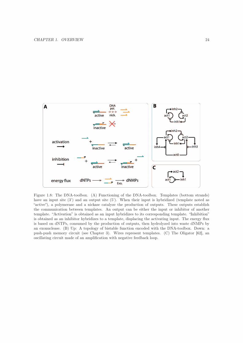
netic machinery, the DNA-toolbox is based on three enzymatic reactions (Figure 1.8-A): short DNA
signal molecules hybridize with stable DNA templates in a set of basic reactions that structures the
topology of the reaction circuits. Templates are composed of a 3’ input site and a 5’ output site.
Signal molecules come in two types: inputs activate templates whereas inhibitors block templates.
An exonuclease specifically degrades DNA signal molecules, thus providing the required chemical sink
to build out-of-equilibrium reaction circuits. Templates are fully modular: it is theoretically possible
to assemble them following complex reaction circuits topologies (Figure 1.8-B and C). Montagne et
al. first demonstrated an oscillator (Figure 1.8-C) made with this system [62]; in this thesis, we will
construct a bistable function (Figure 1.8-B), and show how the modularity of the reactions allows the
building of more complex memory functions.

CHAPTER 1. OVERVIEW 23
Figure 1.7: The genelet system. (A) Functioning of the genelet system. Genelets are short double-stranded DNA that contain a nicked promoter (in red). When the promoter is complete (geneletindicated as “active”), a RNA polymerase transcribes it into RNA transcripts (thin wavy strands)that establish the connection between genelets. A RNase degrades RNA transcripts, keeping thesystem out-of-equilibrium. “Activation” is obtained as the DNA activator of an inactive genelet (whichpromoter is incomplete because lacking its DNA activator) is released thanks the incoming RNAtranscript. “Inhibition” is obtained when the incoming RNA transcript sequester the DNA activatorof an active genelet, making it inactive. The system is traversed by an energy flux as NTPs are usedto produce RNA transcripts that are later on hydrolyzed into waste NMPs. (B) Two circuit topologiesthat experimentally showed a bistable behavior. Up: a single autoregulated genelet. Bottom: twocross-repressed genelets. (C) Two circuit topologies that experimentally produced oscillations. Up:Two-genelets negative feedback loop. Bottom: Amplification with negative feedback loop.
CHAPTER 1. OVERVIEW 24
Figure 1.8: The DNA-toolbox. (A) Functioning of the DNA-toolbox. Templates (bottom strands)have an input site (3’) and an output site (5’). When their input is hybridized (template noted as“active”), a polymerase and a nickase catalyze the production of outputs. These outputs establishthe communication between templates. An output can be either the input or inhibitor of anothertemplate. “Activation” is obtained as an input hybridizes to its corresponding template. “Inhibition”is obtained as an inhibitor hybridizes to a template, displacing the activating input. The energy fluxis based on dNTPs, consumed by the production of outputs, then hydrolyzed into waste dNMPs byan exonuclease. (B) Up: A topology of bistable function encoded with the DNA-toolbox. Down: apush-push memory circuit (see Chapter 3). Wires represent templates. (C) The Oligator [62], anoscillating circuit made of an amplification with negative feedback loop.

CHAPTER 1. OVERVIEW 25
Figure 1.9: Examples of applications of NA reaction circuits
1.1.5 Applications
In vitro NA reaction circuits are enabled to interfacing with all the other constructs of the widening
field of NA nanobotechnology. These include static as well as dynamic nanostructures: for example,
NA reaction circuits could be used to drive NA robots in situ, thus removing the need for exogenous
control (Figure 1.9). In this way, Franco et al. used a genelet-based oscillating circuit to sequentially
drive the opening and closing of DNA tweezers [71]. NA reaction circuits can also be used to drive
other processes such as the production of aptamer [71], organic synthesis [72, 73], DNA gels [74] or
optical devices [75].
Dynamic reaction circuits provide an experimental model to study the relationships between circuit
topology and functions. Because they are shaped by mimicking in vivo computation, they may affect
our understanding of the complex in vivo regulatory processes. Recent in vitro works have pointed
out the importance of two neglected phenomena on molecular circuits: the competition for enzymatic
resources (and complex couplings that may arise thereof) [59] and the “load” effect that appears when a
circuit has to drive a downstream process [71]. It is very probable that similar phenomena also happen
in natural reaction networks, however, they are generally not considered in the building of biological
models [59]. In this sense, engineering in vitro analogs is another way of exploring the underlying
design rules of the molecular circuits that control cells.
In vivo applications of NA reaction circuits are also burgeoning. Hybridization chain reaction -
by which a NA molecule triggers a chain hybridization of metastable hairpin molecules, eventually
releasing a final NA product [76] - was used for detection of specific mRNAs within biological samples
[77]. It was also successfully translated in vivo, and set up as a reaction circuit drug that mediated

CHAPTER 1. OVERVIEW 26
the cell death upon detection of a given combination of cancer-specific mRNAs markers [78].
However, it is not trivial to transfer NA circuits designed in vitro to a more challenging environment.
In recent works, much effort is put on improving the robustness of the circuits for subsequent imple-
mentation in non-pristine milieu, where various materials and reactions may interfere with the circuit
[79]. NA logic circuits showed to perform well in the presence of excess of random oligonucleotides [80],
or mouse brain total RNA [28]. Diehl and coworkers did a careful study of their strand-displacement
system in order to improve its robustness for application in situ [81]. This proved useful as they used
it with DNA-conjugated antibodies for the labeling of endogenous proteins [82]. Other works have
also focused on reaction robustness to impurities in the sequences [37], and hybridization robustness
over large ranges of temperature and salt conditions [83]. These works may prove extremely useful to
assist the transfer of complex NA circuits in vivo.
NA reaction circuits stand at the interface between the living and non-living matter: they form a
unique bridge that is both conceptual - as an operative model of in vivo information processing - and
material - as being capable of sensing and actuating in vivo functions - (Figure 1.9).
1.1.6 Reaction-Diffusion
Reaction-diffusion (RD) computers can be considered as a thin layer of liquid that is the receptacle
of programmed reactions; these reactions transform data; data takes the form of concentrations of
reagents. Such liquid computers are capable of amorphous computing: they can be considered as a
huge number of identical microvolume processors that are interconnected by diffusion, but do not have
any a priori knowledge of their spatial location [84]. These microvolume processors continuously and
simultaneously recompute their state (i.e. their concentration in reagents) depending on (i) their own
state, (ii) the state of their neighbors and (iii) possible external perturbations [85]. This is radically
different from regular computers, which are hard-wired assemblies of transistors computing in a serial
manner: if one transistor dies, chances are that the computer will also die. In contrast, RD computers
are fault-tolerant: if a single unit is damaged, it may not affect the main function of the computer. In
this sense, RD computing shares similarities with the distributed computing approach where multiple
computers connected over a network are executing different tasks in order to solve a common problem.
RD computers are relevant to biological / natural information processing which seems to be carried
out by highly parallel mechanisms [86]. The concept of amorphous computer fits well to local arrays
of identical cells that are capable of intercellular communication [87] (even though cells are themselves

CHAPTER 1. OVERVIEW 27
complex computing units). Also, neural networks can be considered as networks of simple units that
interact with each other, yielding a variety of collective behaviors [86]. Their case can be a bit trickier,
since neurons are not only connected to nearest neighbors, but can also have direct connections to more
distant areas [88]. Reaction-diffusion models have been proposed to describe various cases of biological
patterning phenomena [89] such as, for example, some anatomic features of Drosophila acquired during
morphogenesis [90, 91, 92], or the reorganizing stripe patterns on the skin of angelfishes [93].
In a different perspective, reaction-diffusion systems can also be used to explain various phenomena
such as the complex ecological patterns observed in nature [94], or the spread of infectious diseases
[95, 96]. In a more general vision, simple chemical reaction-diffusion systems [97] or cellular automata
such as Conway’s Game of Life [98] have shown that the key to the emergence of complex patterns lies
in the communication capability of simple units.
Note that amorphous computers are not meant to replace conventional, silicon-based computers,
and probably cannot [99]. However, our ability to program such systems would expand the list of
available substrates that are capable of information processing [84]. Then, one could imagine fantasy
applications such as smart materials of which each molecule (or single unit) would behave in conjunction
with its neighbors, and would have computational abilities so that the whole chunk of material would
sense and actuate in response to its environment.
Mathematically, a reaction-diffusion system can be obtained by simply adding a diffusion term to
a set of ordinary differential equations, given that these are of the first order in time [100]. Experi-
mentally, it consists in granting a chemical system the possibility to diffuse. In this way, the Belousov-
Zhabotinsky (BZ) oscillating reaction [101] has been extensively studied in zero (well-mixed), then
in two (thin layer of liquid) and three-dimensional environments. By setting the BZ reaction in 2D,
researchers first discovered traveling waves [102], then spiral waves [103] that emerged from breaking
traveling waves (e.g. by a physical perturbation of the front of an expanding wave).
In contrast with conventional chemistry, NA-based biochemistry proposes an easy access to the
scaling up of reaction circuits, mainly due to the chemical addressability of NA. We have seen that
NA-based chemical reaction circuits are able to emulate in vitro the behavior of many dynamic systems
with complex time trajectories [63, 62]. Yet, NA-based in vitro dynamic RD systems have, so far, not
been explored.

CHAPTER 1. OVERVIEW 28
1.2 Outline
Montagne et al. built a robust DNA-based biochemical oscillator (the Oligator) through a rational
network design [62]; we will demonstrate that the three basic building blocks they devised (the DNA-
toolbox) can be reused in a general and fully modular manner to build more complex DNA reaction
circuits.
The oscillations of the oligator could be observed by using a fluorescent intercalating dye reporting
on the total (oscillating) amount of DNA strands present in solution. When working with larger scale
reaction networks, it is necessary to be able to monitor the reactions at the desired locations in the
sequence space, that is in a sequence-specific manner. For instance, a bistable reaction circuit that
would output either a strand α or a strand β (but not both at the same time) would require a way to
differenciate between these two strands: it would otherwise be impossible to unambiguously check the
state of the system (i.e. state {α, β} = {1, 0} OR {0, 1}). Such reaction circuits thus require dedicated
monitoring technique: in Chapter 2, we will address this point by proposing N-quenching, a versatile
fluorescent technique for the monitoring of oligonucleotide hybridization.
With the DNA-toolbox and N-quenching in our hands, we will tackle the construction of more
complex reaction circuits, and more specifically circuits encoding for bistability and updatable memory
functions: we demonstrate in Chapter 3 the construction of a bistable reaction circuit, and improve
it into the first in vitro updatable memory circuit and 1-bit binary counter. The (long) road that
led to these working circuits is presented in Chapter 4, in which we also explore a few other circuit
assemblies.
The laboratory hosting us is specialized in microfluidics. Naturally, this spurred us on to combine
the possibilities brought by the microfluidic tool with our expertise of DNA biochemistry. First, the
idea was to enclose our reactions in tiny reactors - that is to compartmentalize our reactions - and
then connect them. In Chapter 5, we explore various (failed) approaches. Eventually, microdroplets
appeared to be the best compartmentalization method, if not the most practical in the purpose of
connecting them in assemblies of microreactors.
Finally, in Chapter 6, we explore the use of the DNA-toolbox made reaction circuits to build
reaction-diffusion systems. For this purpose, we engineer a very simple and cheap device that allows us
to observe our reaction circuits in two-dimensions. As a first step toward tailor-made spatio-temporal
patterns, we show that locally perturbing an oscillating reaction circuit provokes the emergence of
traveling and colliding waves.

CHAPTER 1. OVERVIEW 29
1.3 Glossary
• Closed system: is a system that does not exchange matter with its environment. If a flux of
energy is not provided, a closed system ultimately reaches its thermodynamic equilibrium. In
this study, we deal with closed systems which are emulating openness to allow out-of-equilibrium
behaviors for a certain lapse of time.
• DNA-toolbox: nickname refers to the modular DNA based chemistry introduced first by Mon-
tagne et al. [62]. It allows the construction of arbitrary networks of activation and inhibition
reactions.
• dNTPs: stands for deoxyribonucleotide triphosphate. dNTPs are activated DNA monomers that
are used by the DNA polymerase to polymerize the complementary DNA strand of a template.
• EvaGreen: is a DNA-binding dye (such as the SYBR Green I) that intercalates with double-
stranded DNA molecules, thus allowing to monitor DNA hybridization in a non-sequence specific
manner.
• Fluorophore: is a fluorescent compound (also referred to as dye) that emits light when excited
with a light of a shorter wavelength.
• Inhibitor: is the signal molecule produced by an inhibition module. A given inhibitor blocks a
target template (either an activation or an autocatalytic module) by hybridizing to it, overlapping
on its input site and output site. It is longer (hence more stable) than inputs and is able to
displace an input hybridized to its template.
• Input: are activating the production of other inputs, or inhibitors, by hybridizing to the input
site of the associated template.
• Melting temperature: For a stoichiometric mix of two complementary DNA strands (or a DNA
strand secondary structure, such as a hairpin), the melting temperature (Tm) is the temperature
at which half of the double-stranded complex is dissociated (i.e. in single-stranded form), given
its concentration and salt conditions.
• Modular: is said of a system which subunits (or modules) can be arbitrarily connected to other
subunits (or modules). Modularity requires that input and output of a subunit are of the same
nature, so that output can play the role of input for a separate subunit. It also requires the

CHAPTER 1. OVERVIEW 30
amount of produced output to be equal, or greater, than the amount of received input, so that
there is no damping of the signal throughout the reactions.
• N-quenching: is the fluorescence technique that we devised to monitor the hybridization of inputs
in a sequence-specific manner. This technique is detailed in Chapter 2.
• Out-of-equilibrium: refers to a system which is not allowed to relax to its thermodynamic equilib-
rium. Out-of-equilibrium conditions can be maintained by a flux of matter or energy traversing
the system, or by a kinetic trap existing on the thermodynamic track. In the context of the
DNA-toolbox, out-of-equilibrium conditions are maintained thanks to the slow spontaneous hy-
drolysis of dNTPs and the two-step enzymatic catalysis (polymerization-depolymerization) that
can accelerate this process.
• Phosphate: In the context of this study, the 3’ end of templates is modified with a phosphate
group, that prevents the DNA polymerase from extending them.
• Phosphorothioates: are backbone modifications of the DNA strand used to protect the template
from hydrolysis by the exonuclease. The 5’ end of templates is typically modified with three
phosphorothioates.
• Strand-displacement: DNA polymerases display two different modes of polymerization along a
template: normal (unobstructed) polymerization, when the template is unoccupied downstream,
and strand-displacement, when it has to displace a downstream DNA that occupies the template.
In the context of this study, strand-displacement happens when the output site of template being
processed is occupied by the output. In this case, the DNA polymerase has to displace the already
present output to polymerize a new output. This reaction is taken in account in the detailed
mathematical model, as well as the fact that the DNA polymerase we use has a lower activity
when working in strand-displacement.
• Template: In general, a “template DNA” is a DNA strand that is transcribed into RNA: it serves
as “template” for the RNA polymerase. In this study, a template designates the DNA strand
associated to a module of the DNA-toolbox. A template strand is composed of an input site and
an output site. Templates are modified in 5’ with phosphorothioate modifications, and in 3’ with
a phosphate of a fluorophore.

CHAPTER 1. OVERVIEW 31
• Thermocycler: to run DNA-toolbox made reaction circuits in bulk, we use real-time PCR ther-
mocyclers. These machines allow to incubate and monitor the fluorescence of up to 96 separate
reactions in parallel. We typically use reaction volumes ranging from 10 μl to 20 μl.
• Time-responsive: is said of a system that is reusable. Upon reading of a set of inputs, a time-
responsive system gives an answer that is only transient: once the inputs are removed, the system
is ready for another computation. Time-responsiveness requires a flux of energy to maintain the
system out-of-equilibrium. This is possible in our closed setup by the constant (for a given amount
of time) supply of precursors (dNTPs) that are consumed as signal molecules are produced. Signal
molecules are then degraded into inactivated waste monomers (dNMPs).
Chapter 2
N-quenching
The Oligator [62] was constructed by using three distinct modules (its functioning involves 3 dynamic
species, see Figure 1.8), which could potentially be rearranged in various reaction circuit topologies.
Yet, one would lack a way to monitor specifically the dynamic of each components of such circuit.
The work presented below is our answer to this problem: a fluorescence monitoring technique of DNA
hybridization, specific and specially tailored for the use with dynamic reaction circuits. We will present
how we came up with the idea of this technique, determined its usability in the context of DNA reaction
circuits, and used it to monitor the dephased oscillations of the different components of the Oligator in
real-time. The following work was published as: Adrien Padirac, Teruo Fujii, and Yannick Rondelez,
Quencher-free multiplexed monitoring of DNA reaction circuits in Nucleic Acids Research. We will also
explore a few practical applications of N-quenching, with notably a proposition about how to monitor
inhibitor species, that cannot be directly monitored with a straightforward use of N-quenching.
2.1 Abstract
We present a simple yet efficient technique to monitor the dynamics of DNA-based reaction circuits.
This technique relies on the labeling of DNA oligonucleotides with a single fluorescent modification.
In this quencher-free setup, the signal is modulated by the interaction of the 3’-terminus fluorophore
with the nucleobases themselves. Depending on the nature of the fluorophore’s nearest base pair, fluo-
rescence intensity is decreased or increased upon hybridization. By tuning the 3’-terminal nucleotides,
it is possible to obtain opposite changes in fluorescence intensity for oligonucleotides whose hybridiza-
32
CHAPTER 2. N-QUENCHING 33
tion site is shifted by a single base. Quenching by nucleobases provides a highly sequence-specific
monitoring technique, which presents a high sensitivity even for small oligonucleotides. Compared to
other sequence-specific detection methods, it is relatively non-invasive and compatible with the com-
plex dynamics of DNA reaction circuits. As an application, we show the implementation of nucleobase
quenching to monitor a DNA-based chemical oscillator, allowing us to follow in real time and quan-
titatively the dephased oscillations of the components of the network. This cost-effective monitoring
technique should be widely implementable to other DNA-based reaction systems.
2.2 Introduction
Various implementations of nucleic acid-based reaction circuits have been demonstrated since DNA
was first used as a substrate for in vitro computation of a Hamiltonian path in 1994 [3]. DNA was used
to encode complex systems such as interactive molecular automata [22, 23], as well as computation
mimicking neural networks [32], a square-root calculator [31] and robust chemical oscillators [62, 63].
These information processing systems are composed of many interacting DNA species and yield one
or more outputs, typically encoded in the dynamic [62, 63, 38] or end-point concentrations [22, 32, 31]
of some oligonucleotides. In order to read out the results of such molecular systems, as well as for
the purpose of rationally designing and troubleshooting these DNA reaction circuits, it is desirable
to distinguish their different components and monitor the evolution of their concentrations as the
reactions proceed.
Methods to observe nucleic acid-based reactions have evolved from post-experiment gel analysis
to real-time sequence-specific monitoring. Real-time monitoring of DNA based reactions is possible
thanks to the development of fluorescence techniques that allow detection and quantification of nucleic
acids. In the case of isothermal conditions - as generally used for DNA reaction circuits -, a further
constraint is that the monitoring technique does not interfere too much with the reaction that is
monitored. Ideally, the presence or absence of the fluorescent probe has no influence on the kinetics
and thermodynamics of the DNA-based reaction circuit under scrutiny.
DNA-binding fluorophores, such as the SYBR family, become highly fluorescent when bound to
single or double-stranded DNA. They can be used to monitor DNA amplification reactions such as
PCR (Polymerase Chain Reaction). Some of them, like SYBRGreen II or Evagreen [104], can also be
used to observe isothermal amplification (EXPAR [105, 106]). However, they only provide sequence-
unspecific monitoring; in many cases it is necessary to obtain more detailed information than the total

CHAPTER 2. N-QUENCHING 34
amount of double-stranded DNA in solution. Probes that are specific to a given, arbitrarily selected
sequence are then required.
Sequence-specific monitoring can be obtained with fluorescent probes that hybridize to target se-
quences, leading to a modification of the intensity of their fluorescence. Such fluorescent probes usually
consist in oligonucleotides that are dual-labeled with a “donor” and an “acceptor” fluorophore. Through
fluorescence resonance energy transfer (FRET [107]), the acceptor acts as a quencher of the donor,
and the quenching efficiency strongly depends on the distance between the two fluorophores. Probes
bear the complementary sequence of their target, which allow them to hybridize to it. Hybridization
and following reactions lead to the separation of donor and acceptor, subsequently dequenching the
fluorescence of the donor. For instance, in the case of PCR TaqMan probes [108], depolymerization
of the hybridized probe separates donor and acceptor. For Molecular Beacon [109], donor and accep-
tor are initially brought close to each other by the probe’s hairpin structure. The probe opens as it
hybridizes to its target, which increases the distance between donor and acceptor.
Besides classic DNA amplification techniques (such as real-time PCR [108] or EXPAR [105, 106]),
other types of DNA systems also require sequence-specific real-time monitoring. This work focuses
on DNA reaction circuits that are complex reactive assemblies of many DNA strands able to perform
some form of pre-encoded program [32, 62, 63]. Such systems generally require the design of custom
monitoring solutions. In some cases, it is still possible to readapt the conventional donor/acceptor
pair of fluorophores: DNA-based molecular automaton MAYA [22] uses a fluorogenic substrate with
a donor at one end and an acceptor at the other. Cleavage of this substrate separates donor and
acceptor, which produces an irreversible dequenching of the donor fluorescence. Also, most DNA-based
molecular machines [8, 9] use various donor/acceptor pairs of fluorophores to monitor the molecular
motions associated with the machine functioning [110].
Donor and acceptor can also be placed on two separate and complementary DNA molecules. In this
case, hybridization of the two strands brings donor and acceptor close to each other, which quenches
the fluorescence of the donor [111, 19, 31, 32]. However, this technique significantly impacts the
thermodynamics of the labeled complementary strands [112].
The most complex DNA reaction circuits are out-of-equilibrium systems that are able to display
emergent behaviors like oscillations [62, 63], multi-stability [61] or - theoretically - chaotic trajectories
[38]. Such circuits display non-monotonous concentration evolutions and generally require reversible
fluorescence reporting. Moreover, labeled probes can be difficult to use in these systems because some

CHAPTER 2. N-QUENCHING 35
DNA strands are continuously produced and destroyed [62]: therefore, a simple, general and non-
disruptive monitoring technique would be a welcome addition to the field of molecular programming.
Direct quenching by adjacent nucleobases is a somehow neglected effect where the fluorescence
of a single DNA-bound fluorophore is modulated by interactions with the neighboring DNA sequence
[110, 113, 112]. Each nucleoside has a different quenching effect on nearby fluorophores, with guanosine
exhibiting the highest quenching efficiency [113]. Moreover, the quenching ability of each base strongly
depends on its paired or unpaired status, leading to fluorescence changes upon duplex formation. Using
this property, DNA hybridization [114] and PCR [115, 116] have been monitored.
In this work, we show that nucleobase quenching (referred to as ’N-quenching’ hereafter) provides an
efficient method for real-time multiplexed monitoring of DNA reaction circuits with complex dynamics.
By labeling the 3’ end of a ’template’ oligonucleotide with a single fluorophore, hybridization and
separation of the complementary ’signal’ oligonucleotide can be monitored. N-quenching is highly
sequence-specific: a non-complementary sequence or a sequence hybridizing a few bases away from
the fluorophore is readily distinguished from the target sequence. Regarding short oligonucleotides,
N-quenching sensitivity is relatively high compared to DNA-intercalating fluorophores. It is a cost-
effective technique that only requires one fluorophore per target oligonucleotide, with no need for
additional probes. N-quenching is thus non-invasive and compatible with dynamic DNA reaction
circuits. As an implementation example, we monitored the signal oligonucleotides of an autonomous
DNA-based chemical oscillator by directly labeling the sequences of interest. N-quenching is a versatile
monitoring technique that should be easily implemented to various DNA-based reaction systems.
2.3 Materials and methods
2.3.1 Oligonucleotides
All DNA oligonucleotides were purchased from either Integrated DNA Technologies (IDT, Coralville,
IA, USA) or biomers.net (Ulm germany), with HPLC purification. Concentrations were determined by
measuring the absorbance at 260nm using a GeneQuant Pro RNA/DNA Calculator (GE Healthcare).
Using DinaMelt [117], we checked that all sequences used in this study did not display secondary
structures at the working temperatures.

CHAPTER 2. N-QUENCHING 36
2.3.2 Fluorescence shift measurement
For fluorescence intensity shift curves upon temperature-induced hybridization, oligonucleotides were
diluted in a buffer containing 100mM NaCl and 0.1% Synperonic F108 (Sigma-Aldrich) in TE buffer
(pH 8.0). Oligonucleotides were used at a concentration of 100nM for labeled 22-bases long ’templates’
and 300nM for 11-bases long ’signals’. Hybridization and separation were induced by alternating
between temperatures lower and higher than the duplexes’ melting temperatures. Temperatures were
determined so that NUPACK [118] predicts less than 5% of template strands hybridized at ’high’
temperature and more than 95% of template strands hybridized at ’low’ temperature. Fluorescence
of 20μL samples covered with 15μL of mineral oil was recorded using an IQ5 real-time thermocycler
(Bio-Rad).
For the experiment shown in Figure 2.1, a ’template’ oligonucleotide (5’ - AGATGACTCTC-
CTTAGACTCAG - 3’) bearing a 3’-terminal TAMRA NHS ester modification was used with either
a ’signal’ complementary sequence (5’-CTGAGTCTAAG-3’) or a non-complementary sequence (5’-
AACAGACTCGA-3’).
2.3.3 Monitoring of DNA reaction circuits
Reactions were assembled in a buffer containing 10mM KCl, 10mM (NH4)2SO4, 50mM NaCl, 2mM
MgSO4, 45mM Tris-HCl, 5mM MgCl2, 6mM DTT, 100μg/ml BSA (New England Biolabs), 410mM
Trehalose, 1x EvaGreen and dNTPs (100μM each). Bst DNA polymerase, large fragment, Nt.BstNBI
nickase and RecJf exonuclease were purchased from New England Biolabs, and used at 8, 40, 12 U/mL
respectively. Samples of 40μL were observed using an IQ5 real-time thermocycler (Bio-Rad) set at a
constant temperature of 38.5°C.
For monitoring the single steady state network, 50nM of template A (5’ - CTTAGACTCAG-
CTTAGACTCAG - 3’) with 3’-terminal TAMRA NHS ester modification was put in presence of
an initial concentration of 0.1nM of signal α. In the case of the oscillator, templates A, αtoβ (5’ -
AGATGACTCTC-CTTAGACTCAG - 3’) with 3’-terminal TAMRA NHS ester modification and βtoiα
(5’ - TTACTCAGCTTAGAC-AGATGACTCTC - 3’) with Alexa Fluor 594 NHS ester modification
were used at concentrations of 40, 5 and 20nM. All templates bore two phophorothioates backbone
modification at their 5’ end to protect them from hydrolysis by RecJf exonuclease [62].

CHAPTER 2. N-QUENCHING 37
2.4 Results
2.4.1 Characterization of nucleobase quenching
We initially observed that adding the complementary strand to a 3’-terminal fluorophore labeled
oligonucleotide in solution produced a shift of fluorescence intensity. To further characterize the phe-
nomenon and the possibility to use it in our assay, we selected a 22-bases long oligonucleotide ’template’
labeled with TAMRA at its 3’ end (Figure 2.1). This template was put either in the presence of a 11-
bases long ’signal’ complementary sequence or a 11-bases long non- complementary sequence. Signal
oligonucleotide hybridized adjacently to the template 3’-terminal dye. We induced hybridization and
separation of the strands by applying temperature cycles.
This allowed us to observe the effect of hybridization on the intensity of fluorescence emission of
the 3’-terminal dye. Figure 2.1 shows the fluorescence intensity shift obtained by cycling between
temperatures higher and lower than the duplex melting temperature. At ’low’ temperature, TAMRA
showed a 50% drop of fluorescence intensity in the presence of the complementary strand, whereas a
non-complementary sequence did not produce any significant shift of fluorescence intensity. Cycling
the temperature several times confirmed the reversibility of the phenomenon.
Figure 2.1: TAMRA fluorescence quenching upon temperature induced hybridization/separation. Flu-orescence intensity is expressed as a percentage of the fluorescence of TAMRA-labeled template putalone in solution. Presence of the complementary sequence (c.s.) induces a fluorescence shift (blackcurve) when the temperature is lower than the duplex melting temperature, whereas presence of anon-complementary sequence (n.c.s) does not have influence on the fluorescence of TAMRA (greycurve).
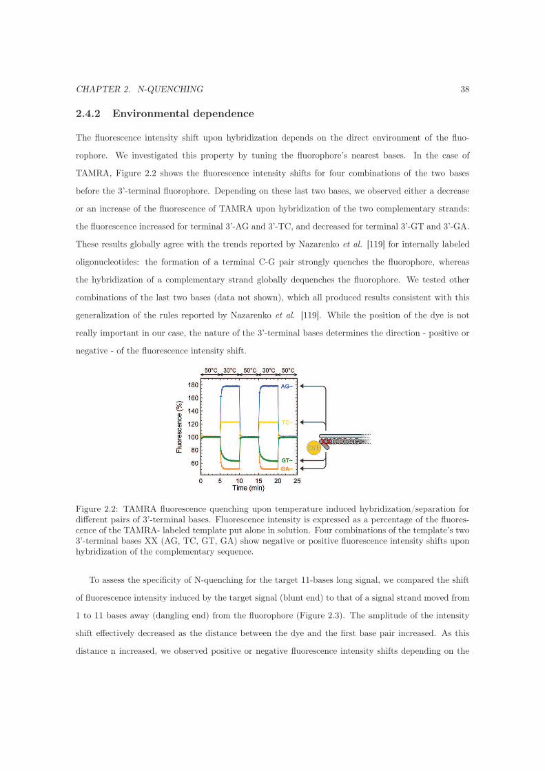
CHAPTER 2. N-QUENCHING 38
2.4.2 Environmental dependence
The fluorescence intensity shift upon hybridization depends on the direct environment of the fluo-
rophore. We investigated this property by tuning the fluorophore’s nearest bases. In the case of
TAMRA, Figure 2.2 shows the fluorescence intensity shifts for four combinations of the two bases
before the 3’-terminal fluorophore. Depending on these last two bases, we observed either a decrease
or an increase of the fluorescence of TAMRA upon hybridization of the two complementary strands:
the fluorescence increased for terminal 3’-AG and 3’-TC, and decreased for terminal 3’-GT and 3’-GA.
These results globally agree with the trends reported by Nazarenko et al. [119] for internally labeled
oligonucleotides: the formation of a terminal C-G pair strongly quenches the fluorophore, whereas
the hybridization of a complementary strand globally dequenches the fluorophore. We tested other
combinations of the last two bases (data not shown), which all produced results consistent with this
generalization of the rules reported by Nazarenko et al. [119]. While the position of the dye is not
really important in our case, the nature of the 3’-terminal bases determines the direction - positive or
negative - of the fluorescence intensity shift.
Figure 2.2: TAMRA fluorescence quenching upon temperature induced hybridization/separation fordifferent pairs of 3’-terminal bases. Fluorescence intensity is expressed as a percentage of the fluores-cence of the TAMRA- labeled template put alone in solution. Four combinations of the template’s two3’-terminal bases XX (AG, TC, GT, GA) show negative or positive fluorescence intensity shifts uponhybridization of the complementary sequence.
To assess the specificity of N-quenching for the target 11-bases long signal, we compared the shift
of fluorescence intensity induced by the target signal (blunt end) to that of a signal strand moved from
1 to 11 bases away (dangling end) from the fluorophore (Figure 2.3). The amplitude of the intensity
shift effectively decreased as the distance between the dye and the first base pair increased. As this
distance n increased, we observed positive or negative fluorescence intensity shifts depending on the

CHAPTER 2. N-QUENCHING 39
nature of the dye’s nearest base pair (i.e. the terminal base pair). The intensity shift was positive
for a terminal A-T, and negative for a terminal C-G base pair. Using the same assay, this trend was
confirmed on another sequence (Supplementary Figure 2.6). Following this observation, we could very
clearly discern a signal oligonucleotide hybridized at position n=0 (negative shift) from one located a
single base away, at position n=1 (positive shift).
We also explored the case of an imperfect match between the template and the 5’ end of the signal
molecule. As can be seen in Figure 2.3 (red marks), the fluorescence change still primarily depends
on the base pair nearest to the fluorophore. Only A-A and G-G mismatches appeared to depart from
this rule, with no obvious rationale.
From n=6 to n=11, we observed weak and position- independent fluorescence intensity shifts. We
tentatively attribute this to the rigidification of the DNA coil. Our target implementation (described
below) only requires distinction between signal molecules that hybridize at the 3’ end of the tem-
plate from those that hybridize 11 bases away. In this configuration, N-quenching provides a reliable
sequence- specific monitoring technique.
Figure 2.3: Fluorescence intensity shift upon hybridization of a signal oligonucleotide moved from n=0to n=11 bases away from the template 3’-terminal dye. Red marks show the fluorescence intensitiesfor a signal oligonucleotide hybridizing with a single 5’ mismatch (mA, mT, mC or mG). Fluorescenceintensity is expressed as a percentage of the fluorescence of the TAMRA-labeled template put alonein solution.
2.4.3 Monitoring an elementary DNA reaction circuit
We used N-quenching to monitor the evolution of an elementary DNA-based dynamic system encoding
homeostasis. As shown on Figure 2.4, this network consists of one template ’A’ that, in presence of
a polymerase and a nicking enzyme, encodes for an autocatalytic amplification of its signal α. In

CHAPTER 2. N-QUENCHING 40
the additional presence of an exonuclease that specifically degrades signal molecules α [62], but not
template A, this circuit becomes a dynamic, out-of-equilibrium system that possesses a single steady
state: as long as dNTPs are available, the concentration of α will always evolve toward a given constant
value.
To test N-quenching, template A was labeled at its 3’ end with TAMRA, allowing us to monitor the
concentration of α as it binds to the template. Hybridization of signal α (5’-CT-) on template A induces
a quenching of TAMRA fluorescence. Therefore, the template itself becomes a probe for measuring
the concentration of α. As a control, we simultaneously monitored the reaction in the presence of
an intercalating dye (EvaGreen) whose fluorescence increases when binding to double-stranded DNA.
In Figure 2.4, we observe that, as expected, the concentration of α evolves towards a steady state:
EvaGreen induced fluorescence increases, TAMRA fluorescence decreases and both eventually reach a
plateau that corresponds to the steady state. In this assay, the fluorescence intensity shift observed
with N-quenching has twice the amplitude observed for EvaGreen. Also, EvaGreen and N-quenching
yielded fluorescent recordings with similar shapes, suggesting that dynamic DNA reaction circuits can
be precisely monitored by using N-quenching only.
Figure 2.4: Monitoring an elementary DNA reaction circuit. (left) Template A encodes the autocat-alytic amplification of signal α, and bears a TAMRA dye at its 3’ end. As α hybridizes to the 3’ endof template A, it gets elongated by a polymerase. The upper strand of the duplex is then cut in itsmiddle by a nicking enzyme, and signal α and output α are released. The exonuclease specificallydegrades single-stranded α. (right) The reaction is triggered with 0.1nM of α and is monitored withboth EvaGreen intercalating dye and the 3’- terminal TAMRA of template A. EvaGreen fluorescenceintensity increases as α-A duplexes are formed, and TAMRA fluorescence is quenched as α hybridizesto the 3’-end of A. Both fluorescence intensities are normalized with respect to the maximal shift offluorescence intensity of EvaGreen for the reaction where the TAMRA modification of template A isreplaced by a phosphate.
CHAPTER 2. N-QUENCHING 41
2.4.4 Monitoring a DNA-based oscillator
N-quenching was then used to study a network containing more than one dynamic species. We previ-
ously reported a DNA-based oscillator [62] that uses the same enzymes cocktail but is encoded in the
sequences of three templates (Figure 2.5). Template A activates the autocatalytic production of signal
molecule α. Template αtoβ receives α as input, activating the production of β. Finally, template βtoiα
receives β as input, activating the production of iα. iα closes the negative feedback loop: it inhibits α
production by blocking the activity of template A. Overall, this chain of reactions produces oscillations
of the three signal molecules α, β and iα.
When this reaction circuit is monitored with EvaGreen as previously reported [62], one obtains
real time, but non- specific information about the total amount of duplex DNA in the system. In
fact, in this case, EvaGreen fluorescence is mainly induced by iα [62], which mostly prevents the
observation of α and β. However, because oscillations are produced by the interplay of the 3 dynamic
species, a complete characterization requires individual tracking of α and β concentrations as well.
This information is readily obtained using N-quenching: we respectively labeled αtoβ and βtoiα 3’
ends with TAMRA and Alexa Fluor 594, which enabled sequence-specific observation of both α and β.
Sequences of α (5’-CTGA-) and β (5’-GAGA-) produced a negative shift of fluorescence intensity upon
hybridization (with formation of a terminal C-G base pair). With these two labeled oligonucleotides,
we could directly observe the phase shifts between α, β and iα concentration peaks: as expected from
the structure of the network, peak of α came first, followed by β and then iα, before the cycle started
again. Using N-quenching, we could also extract quantitative information about the concentrations of
α and β throughout the reaction. To do so, we built calibration curves for αtoβ and βtoiα, showing
their fluorescence intensity shift as a function of known concentrations of respectively α and β. By
comparison with these calibration curves, we found that α and β concentrations do not exceed 30nM and
55nM, respectively, at their peak concentration (see Section 2.7.5 for more details). Also, assuming a
linear relationship between the quenching effect and the ratio of hybridized templates, we could deduce
that less than 20% of αtoβ and 25% of βtoiα are in double-strand form at the oscillation peaks.
CHAPTER 2. N-QUENCHING 42
Figure 2.5: Multiplexed monitoring of a DNA-based oscillator. (left) 3-nodes oscillator network andsequence encoding. A is the autocatalytic module of Figure 3. The second template, αtoβ, receives αas input, produces β as output and is labeled in 3’ with TAMRA. The third template, βtoiα, receives βas input, produces iα as output and is labeled in 3’ with Alexa Fluor 594. (right) Time evolution of theoscillator in three colors. α is seen with TAMRA, β with Alexa Fluor 594 and EvaGreen shows the totalduplex concentration, roughly corresponding to iα concentration [62]. Fluorescence of TAMRA andAlexa Fluor 594 is expressed as a percentage of their respective unquenched fluorescence. Fluorescenceof EvaGreen is normalized at 1 for the highest and 0 for the lowest fluorescence intensity. Verticallines show the peak of each species concentration.
2.5 Discussion
2.5.1 N-quenching sensitivity and quantitative measurement
Using N-quenching, dynamic DNA reaction circuits can be monitored by simply labeling sequences of
interest with a single fluorophore. Even though the shifts in fluorescence intensity (up to -50%/+80%)
are not as high as those obtained by using donor/acceptor pairs of fluorophores (almost 100% quench-
ing for some donor/acceptor pairs), they were sufficient to observe reactions on 20 or 40μL volumes
using a conventional real-time thermocycler (the signal-to-noise ratio in the experiment of Figure 2.1
is approximately 250). In the case of the simple DNA reaction circuit of Figure 2.4, the relative fluo-
rescence intensity shift produced by a 11- bases long oligonucleotide with TAMRA was higher than the
one obtained with EvaGreen. One may remark that in these conditions, the fluorescence of EvaGreen
is partially quenched by TAMRA [120]. Still, the shift of TAMRA fluorescence intensity is comparable
to the one of EvaGreen, using a non- labeled template. This result might be explained by the weak
affinity of EvaGreen for short double-stranded DNA [104], and the fact that EvaGreen fluorescence
intensity depends on the number of paired bases. Thus, in the case of short DNA strands - here, 11
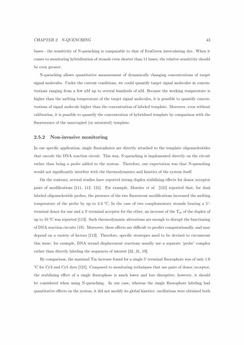
CHAPTER 2. N-QUENCHING 43
bases - the sensitivity of N-quenching is comparable to that of EvaGreen intercalating dye. When it
comes to monitoring hybridization of strands even shorter than 11 bases, the relative sensitivity should
be even greater.
N-quenching allows quantitative measurement of dynamically changing concentrations of target
signal molecules. Under the current conditions, we could quantify target signal molecules in concen-
trations ranging from a few nM up to several hundreds of nM. Because the working temperature is
higher than the melting temperature of the target signal molecules, it is possible to quantify concen-
trations of signal molecule higher than the concentration of labeled template. Moreover, even without
calibration, it is possible to quantify the concentration of hybridized template by comparison with the
fluorescence of the unoccupied (or saturated) template.
2.5.2 Non-invasive monitoring
In our specific application, single fluorophores are directly attached to the template oligonucleotides
that encode the DNA reaction circuit. This way, N-quenching is implemented directly on the circuit
rather than being a probe added to the system. Therefore, our expectation was that N-quenching
would not significantly interfere with the thermodynamics and kinetics of the system itself.
On the contrary, several studies have reported strong duplex stabilizing effects for donor/acceptor
pairs of modifications [111, 112, 121]. For example, Moreira et al. [121] reported that, for dual
labeled oligonucleotide probes, the presence of the two fluorescent modifications increased the melting
temperature of the probe by up to 4.3 °C. In the case of two complementary strands bearing a 5’-
terminal donor for one and a 3’-terminal acceptor for the other, an increase of the Tm of the duplex of
up to 10 °C was reported [112]. Such thermodynamic alterations are enough to disrupt the functioning
of DNA reaction circuits (19). Moreover, these effects are difficult to predict computationally, and may
depend on a variety of factors [112]. Therefore, specific strategies need to be devised to circumvent
this issue: for example, DNA strand displacement reactions usually use a separate ’probe’ complex
rather than directly labeling the sequences of interest [32, 31, 19].
By comparison, the maximal Tm increase found for a single 5’-terminal fluorophore was of only 1.6
°C for Cy3 and Cy5 dyes [121]. Compared to monitoring techniques that use pairs of donor/acceptor,
the stabilizing effect of a single fluorophore is much lower and less disruptive; however, it should
be considered when using N-quenching. In our case, whereas the single fluorophore labeling had
quantitative effects on the system, it did not modify its global kinetics: oscillations were obtained both
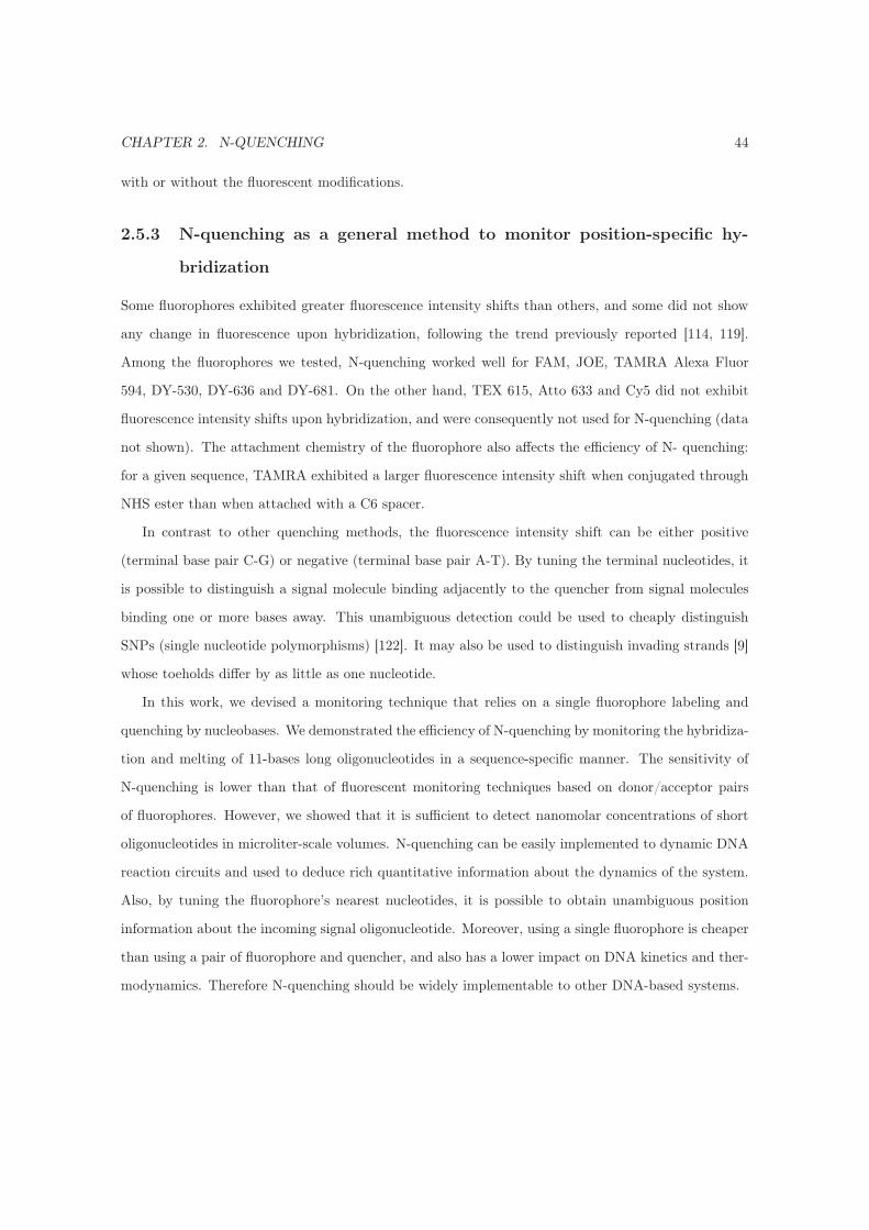
CHAPTER 2. N-QUENCHING 44
with or without the fluorescent modifications.
2.5.3 N-quenching as a general method to monitor position-specific hy-
bridization
Some fluorophores exhibited greater fluorescence intensity shifts than others, and some did not show
any change in fluorescence upon hybridization, following the trend previously reported [114, 119].
Among the fluorophores we tested, N-quenching worked well for FAM, JOE, TAMRA Alexa Fluor
594, DY-530, DY-636 and DY-681. On the other hand, TEX 615, Atto 633 and Cy5 did not exhibit
fluorescence intensity shifts upon hybridization, and were consequently not used for N-quenching (data
not shown). The attachment chemistry of the fluorophore also affects the efficiency of N- quenching:
for a given sequence, TAMRA exhibited a larger fluorescence intensity shift when conjugated through
NHS ester than when attached with a C6 spacer.
In contrast to other quenching methods, the fluorescence intensity shift can be either positive
(terminal base pair C-G) or negative (terminal base pair A-T). By tuning the terminal nucleotides, it
is possible to distinguish a signal molecule binding adjacently to the quencher from signal molecules
binding one or more bases away. This unambiguous detection could be used to cheaply distinguish
SNPs (single nucleotide polymorphisms) [122]. It may also be used to distinguish invading strands [9]
whose toeholds differ by as little as one nucleotide.
In this work, we devised a monitoring technique that relies on a single fluorophore labeling and
quenching by nucleobases. We demonstrated the efficiency of N-quenching by monitoring the hybridiza-
tion and melting of 11-bases long oligonucleotides in a sequence-specific manner. The sensitivity of
N-quenching is lower than that of fluorescent monitoring techniques based on donor/acceptor pairs
of fluorophores. However, we showed that it is sufficient to detect nanomolar concentrations of short
oligonucleotides in microliter-scale volumes. N-quenching can be easily implemented to dynamic DNA
reaction circuits and used to deduce rich quantitative information about the dynamics of the system.
Also, by tuning the fluorophore’s nearest nucleotides, it is possible to obtain unambiguous position
information about the incoming signal oligonucleotide. Moreover, using a single fluorophore is cheaper
than using a pair of fluorophore and quencher, and also has a lower impact on DNA kinetics and ther-
modynamics. Therefore N-quenching should be widely implementable to other DNA-based systems.

CHAPTER 2. N-QUENCHING 45
2.6 Supplementary Information
On the experiment of Figure 2.3, we observed a pattern of alternating negative and positive changes of
fluorescence as the signal molecule was shifted away from the template’s 3’ fluorophore. This pattern
is consistent with the trend observed for signal oligonucleotides hybridizing next to the fluorophore
(blunt end): decrease of fluorescence for a terminal C-G and increase of fluorescence for a terminal
A-T base-pair. Therefore we may conclude that the unpaired bases in-between the dye and the closest
base-pair have only a secondary effect on the quenching.
However, to check unambiguously this result, we performed another experiment with a different
sequence. This was done using the same assay as the experiment of Figure 2.3, but with another signal
oligonucleotide whose sequence displayed a different alternation of A-T and C-G bases. Supplementary
Figure 2.6 shows the results of this experiment: the direction of the fluorescence intensity shifts is not
regularly alternated anymore, but follows the pattern of A or T versus G or C in the sequence. As in
Figure 3, the shift intensity gradually decreases as the distance increases.
This confirms that as the signal molecule is shifted away from the fluorophore, the fluorescence
change upon hybridization still depends on the nature of the fluorophore’s nearest base-pair: decrease
of fluorescence for a terminal C-G and increase of fluorescence for a terminal A-T.
Figure 2.6: Fluorescence intensity shift upon hybridization of a signal oligonucleotide moved from n=0to n=6 bases away from the template 3’-terminal dye. Fluorescence intensity is expressed as a per-centage of the fluorescence of the TAMRA-labeled template put alone in solution. The full sequence ofthe labeled template is 5’- TTACTCAGCCAAGACAACAGACTCGA-3’, with a 3’-terminal TAMRANHS ester modification.
CHAPTER 2. N-QUENCHING 46
2.7 Additional results
2.7.1 C11bt Oligator
In this chapter, we worked with an Oligator made of sequences different from the ones used by Montagne
et al. [62]. The present oligator is based on an autocatalytic module called “C11bt” (hence “C11bt
Oligator”), amplifying the input called “T11bt” which was designed with a low melting temperature
(33.1 °C against 39.5 °C for “T11” of the original Oligator [62], hence the “bt” that stands for “low
temperature” in French). With this low Tm, we were expecting it to have the potential of oscillating
faster than the original Oligator. Or at least be able to oscillate at lower temperature, where RecJf
would be more stable. In practice, C11bt oscillator could run at descent speed at 37 °C (showing periods
of about 70 minutes). However, we weren’t able to make it run faster than the original Oligator. Figure
2.7 shows a collection of combinations of concentrations of C11bt and I11bttoinhT11bt.
Figure 2.7: C11bt Oligator for various combinations of [C11bt]-[I11bttoinhT11bt] (in nM), with a fixed[T11bttoI11bt] = 5 nM. Reactions are performed at 38 °C.
The C11bt Oligator is constituted of sequences that do not present any cross-talks with the original
Oligator, suggesting that they could potentially be run in the same tube. Due to their difference of de-
sign, these two Oligators were originally optimized for very different enzymatic conditions, at different
temperatures: finding conditions that would fit both of them required much tuning effort. We even-
tually managed to get them running together (Figure 2.8), monitoring the reactions with EvaGreen.
The resulting fluorescence time plot was not a simple sum of both oscillator running separately, which
suggested some complex couplings that may occur - for instance - through competition for enzymatic
resources [59]. Unfortunately, this work was done before the completion of N-quenching, which would
have provided us with precious hints about the coupling between these two Oligators.
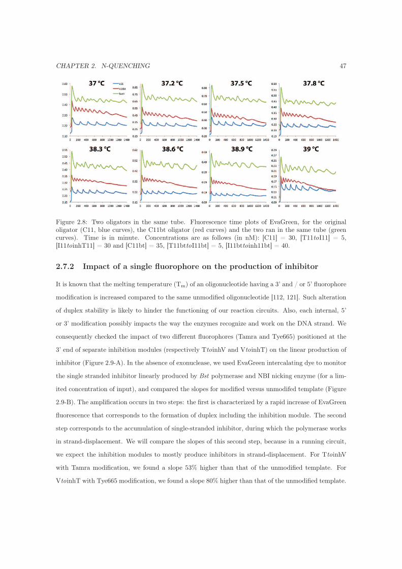
CHAPTER 2. N-QUENCHING 47
Figure 2.8: Two oligators in the same tube. Fluorescence time plots of EvaGreen, for the originaloligator (C11, blue curves), the C11bt oligator (red curves) and the two ran in the same tube (greencurves). Time is in minute. Concentrations are as follows (in nM): [C11] = 30, [T11toI11] = 5,[I11toinhT11] = 30 and [C11bt] = 35, [T11bttoI11bt] = 5, [I11bttoinh11bt] = 40.
2.7.2 Impact of a single fluorophore on the production of inhibitor
It is known that the melting temperature (Tm) of an oligonucleotide having a 3’ and / or 5’ fluorophore
modification is increased compared to the same unmodified oligonucleotide [112, 121]. Such alteration
of duplex stability is likely to hinder the functioning of our reaction circuits. Also, each internal, 5’
or 3’ modification possibly impacts the way the enzymes recognize and work on the DNA strand. We
consequently checked the impact of two different fluorophores (Tamra and Tye665) positioned at the
3’ end of separate inhibition modules (respectively TtoinhV and VtoinhT) on the linear production of
inhibitor (Figure 2.9-A). In the absence of exonuclease, we used EvaGreen intercalating dye to monitor
the single stranded inhibitor linearly produced by Bst polymerase and NBI nicking enzyme (for a lim-
ited concentration of input), and compared the slopes for modified versus unmodifed template (Figure
2.9-B). The amplification occurs in two steps: the first is characterized by a rapid increase of EvaGreen
fluorescence that corresponds to the formation of duplex including the inhibition module. The second
step corresponds to the accumulation of single-stranded inhibitor, during which the polymerase works
in strand-displacement. We will compare the slopes of this second step, because in a running circuit,
we expect the inhibition modules to mostly produce inhibitors in strand-displacement. For TtoinhV
with Tamra modification, we found a slope 53% higher than that of the unmodified template. For
VtoinhT with Tye665 modification, we found a slope 80% higher than that of the unmodified template.
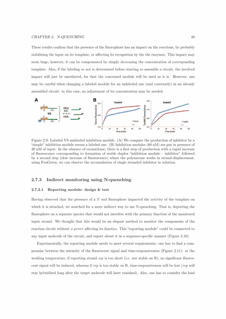
CHAPTER 2. N-QUENCHING 48
These results confirm that the presence of the fluorophore has an impact on the reactions, by probably
stabilizing the input on its template, or affecting its recognition by the the enzymes. This impact may
seem huge; however, it can be compensated by simply decreasing the concentration of corresponding
template. Also, if the labeling or not is determined before starting to assemble a circuit, the involved
impact will just be smothered, for that the concerned module will be used as it is. However, one
may be careful when changing a labeled module for an unlabeled one (and conversely) in an already
assembled circuit: in this case, an adjustment of its concentration may be needed.
Figure 2.9: Labeled VS unlabeled inhibition module. (A) We compare the production of inhibitor by a“simple” inhibition module versus a labeled one. (B) Inhibition modules (60 nM) are put in presence of20 nM of input. In the absence of exonuclease, there is a first step of production with a rapid increaseof fluorescence corresponding to formation of stable duplex “inhibition module : inhibitor” followedby a second step (slow increase of fluorescence) where the polymerase works in strand-displacement:using EvaGreen, we can observe the accumulation of single stranded inhibitor in solution.
2.7.3 Indirect monitoring using N-quenching
2.7.3.1 Reporting module: design & test
Having observed that the presence of a 3’ end fluorophore impacted the activity of the template on
which it is attached, we searched for a more indirect way to use N-quenching. That is, deporting the
fluorophore on a separate species that would not interfere with the primary function of the monitored
input strand. We thought that this would be an elegant method to monitor the components of the
reaction circuit without a priori affecting its kinetics. This “reporting module” could be connected to
any input molecule of the circuit, and report about it in a sequence-specific manner (Figure 2.10).
Experimentally, the reporting module needs to meet several requirements: one has to find a com-
promise between the intensity of the fluorescent signal and time-responsiveness (Figure 2.11): at the
working temperature, if reporting strand rep is too short (i.e. not stable on R), no significant fluores-
cent signal will be induced, whereas if rep is too stable on R, time-responsiveness will be lost (rep will
stay hybridized long after the target molecule will have vanished). Also, one has to consider the load

CHAPTER 2. N-QUENCHING 49
Figure 2.10: (Up) The reporting module receives target input α and produces rep. (Bottom) rephybridizes to template R that is labeled with a 3’ fluorophore. This results in a change of fluorescenceintensity, reflecting the presence of α. By changing only the template αtorep (to a template Xtorep),it is possible to connect the reporting module to another target input (X).
effect [71] on the reported system (see Section 4.7.2 for more details): in the example of Figure 2.10,
template αtorep will sequester some α, that consequently cannot play its role in the monitored reaction
circuit. Thus, the concentration of αtorep should be kept low in order to not impact significantly the
functioning of the reaction circuit under scrutiny. The presence of the reporting module represents
more DNA substrates for the enzymes to work on, which could lead to their saturation more easily.
Figure 2.11: Fluorescence change (quenching) of the TAMRA label of template R (60 nM) uponinjection of complementary strand rep (100 nM), for temperatures ranging from 38 °C to 46 °C. Athigh temperature, the injection of rep does not induce a big fluorescence change. At low temperature,the fluorescence takes a long time to get back to its initial level. Sequence of R is as follows: 5’-A*G*T*T*CTAGTGTGTC-3’-FAM. Duplex rep:R has a predicted (Dinamelt) Tm of 44.2 °C in theconditions of this experiment.

CHAPTER 2. N-QUENCHING 50
Figure 2.12: Reporting module plugged to the C11bt oligator. (A) Circuit of the oligator (in black)and plugged reporting module (in orange). (B) Fluorescence time plots of EvaGreen intercalating dyefor a ramp βtorep (0 to 30 nM) and (C) corresponding time plots of Tamra. Curves are offsetted forvisibility. The experiment was run at 38.5 °C, with concentrations of templates as follows: αtoα = 30nM, αtoβ = 5 nM, βtoiα = 35 nM and R = 30 nM. Sequence of R is 5’-C*A*A*GTCACATGG-3’-TAMRA. Duplex r:R has a predicted (Dinamelt) Tm of 40.3 °C.
2.7.3.2 Reporting module: use with an oligator
Following the results of Figure 2.11, we designed a new reporting module targeted at the working
temperature of the C11bt oligator (38.5 °C). By plugging it to the oligator (Figure 2.12-left), we
succeeded in monitoring the oscillating reaction (Figure 2.12-right). Even though the reporting module
worked, it only produced a low fluorescent signal. Interestingly, increasing the concentration of βtorep
seemed to stabilize the oscillations: this may be explained by the fact that βtorep slows down (i.e.
delays further) the negative feedback loop, which is known to increase the robustness of the oscillations
[123] - at the cost of the speed.
Note that the reporting module induces a delay between the monitored fluorescent signal and the
actual concentration of target molecule, which potentially makes the analysis more complex. Also, the
reporting module appeared to actually - indirectly - have an impact on the kinetics of the reaction
circuit under scrutiny - here, seemingly increasing the robustness of the oscillations. We consequently
turned toward the simple labeling of the templates with a single fluorophore, allowing a direct monitor-
ing of the target input. Doing so has an impact on the hybridization and kinetics of the corresponding
template: however, this impact is still low enough to not disrupt the functioning of the reaction circuits,
given some adjustments of the template concentrations. We took this as part of the DNA-toolbox, in
which we have many other handles to counterbalance the effect of a single fluorescent modification: for
instance, one can decrease the concentration of labeled template if this one seems to be more “active”
than the one without fluorescent modification.
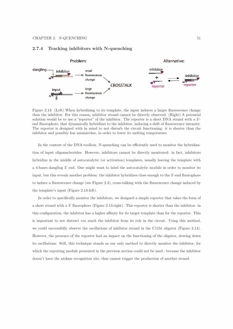
CHAPTER 2. N-QUENCHING 51
2.7.4 Tracking inhibitors with N-quenching
Figure 2.13: (Left) When hybridizing to its template, the input induces a larger fluorescence changethan the inhibitor. For this reason, inhibitor strand cannot be directly observed. (Right) A potentialsolution would be to use a “reporter” of the inhibitor. The reporter is a short DNA strand with a 3’-end fluorophore, that dynamically hybridizes to the inhibitor, inducing a shift of fluorescence intensity.The reporter is designed with in mind to not disturb the circuit functioning: it is shorter than theinhibitor and possibly has mismatches, in order to lower its melting temperature.
In the context of the DNA-toolbox, N-quenching can be efficiently used to monitor the hybridiza-
tion of input oligonucleotides. However, inhibitors cannot be directly monitored: in fact, inhibitors
hybridize in the middle of autocatalytic (or activation) templates, usually leaving the template with
a 4-bases dangling 3’ end. One might want to label the autocatalytic module in order to monitor its
input, but this reveals another problem: the inhibitor hybridizes close enough to the 3’-end fluorophore
to induce a fluorescence change (see Figure 2.3), cross-talking with the fluorescence change induced by
the template’s input (Figure 2.13-left).
In order to specifically monitor the inhibitors, we designed a simple reporter that takes the form of
a short strand with a 3’ fluorophore (Figure 2.13-right). This reporter is shorter than the inhibitor: in
this configuration, the inhibitor has a higher affinity for its target template than for the reporter. This
is important to not distract too much the inhibitor from its role in the circuit. Using this method,
we could successfully observe the oscillations of inhibitor strand in the C11bt oligator (Figure 2.14).
However, the presence of the reporter had an impact on the functioning of the oligator, slowing down
its oscillations. Still, this technique stands as our only method to directly monitor the inhibitor, for
which the reporting module presented in the previous section could not be used - because the inhibitor
doesn’t have the nickase recognition site, thus cannot trigger the production of another strand.

CHAPTER 2. N-QUENCHING 52
Figure 2.14: Monitoring C11bt oligator with the reporter of inhibitor. (Left) Circuit of the oligator.βtoiα is labeled with Alexa Fluor 594, thus reporting the presence of β. iα can hybridize to thereporter, which is labeled with FAM. (Middle) Looking at the Alexa channel: the presence of increasingconcentration of reporter seems to slow down the oligator (period = 113 min with reporter, 122 with 5nM and 148 with 10 nM of reporter). (Right) Looking at the FAM channel: the reporter successfullyreports on the presence of inhibitor iα. The experiment was run without EvaGreen, at 37.5 °C, and withαtoα = 30 nM, αtoβ = 3 nM and βtoiα = 30 nM. Duplex iα:reporter has a predicted Tm of 39.3 °C, to becompared with 46.7 °C for αtoα-iα. The sequence of reporter is as follows: 5’-C*T*C*AGCTTAGAC-3’-FAM.
Figure 2.15: Calibration curves of N-quenching for 20 nM of βtoiα labeled with Alexa 594.
2.7.5 Quantification with N-quenching: calibration curves
When monitoring a reaction circuit with N-quenching, it is easy to get quantitative information about
the ratio of hybridized templates if we assume a linear relationship with the quenching effect. Get-
ting further quantitative information, that is, about the actual total concentration of target input in
solution, requires to calibrate N-quenching for the reaction conditions (temperature, buffer and concen-
tration of labeled template). Figure 2.15 shows such calibration curves for template βtoiα at different
temperatures. At low temperatures, the fluorescence intensity shift quickly saturates, preventing the
quantification of high concentrations of target input. Working at higher temperature allows to mea-
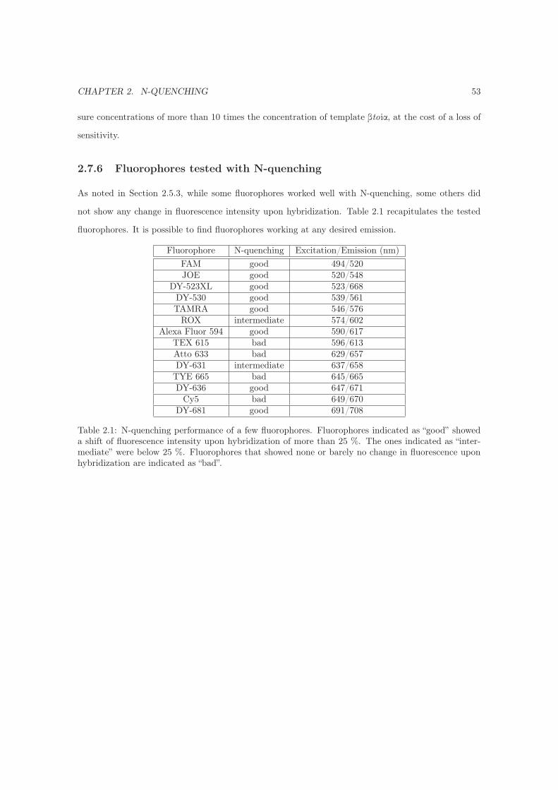
CHAPTER 2. N-QUENCHING 53
sure concentrations of more than 10 times the concentration of template βtoiα, at the cost of a loss of
sensitivity.
2.7.6 Fluorophores tested with N-quenching
As noted in Section 2.5.3, while some fluorophores worked well with N-quenching, some others did
not show any change in fluorescence intensity upon hybridization. Table 2.1 recapitulates the tested
fluorophores. It is possible to find fluorophores working at any desired emission.
Fluorophore N-quenching Excitation/Emission (nm)
FAM good 494/520JOE good 520/548
DY-523XL good 523/668DY-530 good 539/561TAMRA good 546/576
ROX intermediate 574/602Alexa Fluor 594 good 590/617
TEX 615 bad 596/613Atto 633 bad 629/657DY-631 intermediate 637/658
TYE 665 bad 645/665DY-636 good 647/671
Cy5 bad 649/670DY-681 good 691/708
Table 2.1: N-quenching performance of a few fluorophores. Fluorophores indicated as “good” showeda shift of fluorescence intensity upon hybridization of more than 25 %. The ones indicated as “inter-mediate” were below 25 %. Fluorophores that showed none or barely no change in fluorescence uponhybridization are indicated as “bad”.

Chapter 3
In vitro switchable memories
In the cell, memory is kept by various mechanisms, with bistability potentially being one of the most
robust of them [124, 125, 126]. Bistability and oscillations are also believed to be the two major
building blocks of the complex networks that carry cellular information processing [127]. In a more
general vision, bistability seems to be at the basis of the dynamic behaviors of many non-linear chemical
systems, including oscillators [128]. With N-quenching and the three modules of the DNA-toolbox
(Figure 1.8) in hands, we tackled this family of memory functions. In the work below, we focused on
switchable bistable memory reaction circuits in the context of the DNA-toolbox, and constructed three
successive circuits of increasing complexity. In this way, we explored the implementation of relatively
large scale dynamic circuits, culminating with a 8-modules circuit encoding for a 1-bit counter. This
work was published as: Adrien Padirac, Teruo Fujii, and Yannick Rondelez. Bottom-up construction
of in vitro switchable memories in Proceedings of the National Academy of Sciences.
3.1 Abstract
Reaction networks displaying bistability provide a chemical mechanism for long-term memory storage
in cells, as exemplified by many epigenetic switches. These biological systems are not only bistable,
but also switchable, in the sense that they can be flipped from one state to the other by application
of specific molecular stimuli. We have reproduced such functions through the rational assembly of
dynamic reaction networks based on basic DNA biochemistry. Rather than rewiring genetic systems
as synthetic biology does in vivo, our strategy consists in building simplified dynamical analogs in
54

CHAPTER 3. IN VITRO SWITCHABLE MEMORIES 55
vitro, in an artificial, well controlled milieu. We report successively a bistable system, a two-input
switchable memory element, and a single-input push-push memory circuit. These results suggest that
it is possible to build complex time-responsive molecular circuits, by following a modular approach to
the design of dynamic in vitro behaviors. Our approach thus provides an unmatched opportunity to
study topology/function relationships within dynamic reaction networks.
3.2 Introduction
Cellular information processing relies on dynamic networks of biochemical reactions [45]. For example,
genes and their products regulate each other in intricate assemblies that embrace numbers of compo-
nents and interactions. The function of these assemblies, i.e. the computation that they perform at
the molecular level, is encoded both in the structure and in the physical characteristics of the web of
chemical interactions that links their components. These in vivo networks are often difficult to identify
in their entirety. Indeed, a complete description requires (i) a detailed analysis of the macroscopic
dynamic behavior, (ii) a molecular understanding of the structure of the underlying biological network
sustaining the function and (iii) a chemical (thermodynamic and kinetic) knowledge of the reactions
at hand. For technical reasons, this information can be very hard to obtain, even in the simplest
biological cases [129, 130, 47, 48].
Rather than attempting a systematic analysis of natural reaction networks, synthetic biology har-
nesses cells as a receptacle –the hardware– to implement artificially designed networks [52, 53]. These
networks are typically engineered through the recycling of original biological parts, their modification
and their reassembly in non-natural architectures, which endow cells with additional functions [49, 50].
This strategy aims at understanding the cell regulatory processes through a bottom-up approach, which
is expected to reveal the underlying design rules [51]. In this way, small scale circuits encoding elemen-
tary functions such as cascades [54], counters [131], bistability [53, 56, 55, 57] or oscillations [52, 55]
have successfully been engineered.
The richness of the cell’s inner biochemistry provides a platform that theoretically allows the
engineering of an infinity of increasingly complex synthetic networks [132]. It also poses formidable
challenges to a rational designer. In practice, only small synthetic networks (compared to their natural
models) have been reported [133]. One reason is that synthetic biologists face a shortage of known
interoperable units [133, 134]. Also, harnessing the cell’s machinery is a complex task: nonlinear
effects [51, 59, 58] and unintended interactions between the synthetic circuit and the host housekeeping
CHAPTER 3. IN VITRO SWITCHABLE MEMORIES 56
functions [60] are frequent and difficult to pinpoint. Moreover, the lack of quantitative knowledge of
in vivo processes strongly constrains the predictive power of the in silico models used in the design
process [132, 134].
Engineering analogs of gene networks out of the cell, in purposely created and better controlled
in vitro environments, provides an attractive alternative [61, 62, 66, 38]. Going cell-free offers a
better control of the system parameters, minimizes unintended couplings and allows easier quantitative
analysis [67]. Like in vivo gene networks, in vitro analogs are constructed from elementary units,
but this time, one is freed from the constraints of the cellular machinery: various, possibly simpler
chemistries can be used; toxicity and host interference disappear and stochastic effects can be handled.
Still, in analogy with synthetic biology, it is possible to build basic functions like oscillators [62, 63],
bistable systems [61, 70] or logic gates [40, 27] through a rational bottom-up strategy. The expectation
is that it will be possible to assemble these elementary modules in a wealth of large-scale circuits
[31, 135], potentially with life-like behaviors [136].
This paper focuses on in vitro reaction circuits encoding memory functions. In the context of
biological circuits, memory refers to the ability to integrate a transient molecular stimulus into a
sustained molecular response [137]. In most cases, this information is digitized into a small number of
alternative states, which correspond to the multiple steady states of a dynamic chemical system. In the
cell, various mechanisms exist to keep memory of an event. Slowly changing protein levels can result in
memory-like behaviors transmitted over a few cell generations [138]. Phage-like genetic recombination
can be used to reversibly switch one bit of information on the DNA of engineered cells [139], making a
passive data storage that can be passed down through generations. Epigenetic switches use bistability
to carry a robust, heritable memory [124, 125, 126]. Other bistable switches naturally occur in gene
networks, and play important roles in fundamental cell functions [130, 47], cell cycle [129, 140], cell
commitment [48, 141] and signal transduction pathways [142].
Such biological memories based on multistability, also require the interfacing with upstream and
downstream molecular processes. This includes in particular the ability, given the correct stimuli,
to toggle reversibly and sensitively between the reciprocally exclusive stable states [47, 48]. From a
chemical point of view, the memory function therefore incorporates a form of antagonism. On the one
hand, robust information storage imposes stability against molecular perturbations or noise but, on the
other hand, the function also requires a sensitive mechanism to integrate environmental information
and – if appropriate – update its state. Synthetic bistable switches constructed so far in vivo have

CHAPTER 3. IN VITRO SWITCHABLE MEMORIES 57
not yet solved this dilemma: the host cells are typically forced on one state by exposition to strong
inducer drugs for the whole switching time [53, 56, 143]. Alternatively, non-molecular stimuli, such
as temperature or light, are used. For example, Lou et al. [57] have recently reported a synthetic
switchable “push-push” bistable circuit in which UV stimulation was used to switch the system back
and forth between its two stable states. However, such systems that use non-molecular inputs cannot be
cascaded, i.e. integrated in larger circuits. Additionally in this case, extreme photo-toxicity negatively
impacts the host cells.
Because the alternative states of a bistable system are all equally stable over time, thermodynamics
imposes that multistability is fundamentally an energy consuming, out-of-equilibrium process [144]:
switching to the new state requires the complete disappearance or degradation of the constituents
of the previous state. This poses a severe constraint for the design of in vitro analogs of biological
memory circuits. Nevertheless, a couple of batch bistable systems [61, 70] have been reported, thanks
to the use of an enzymatic sink to maintain the dynamic of the system. However, no attempt was
made to switch these basic bistable networks after they first reached one of their steady states.
Herein, we use enzyme-catalyzed, DNA-based reactions [62] to rationally construct various in vitro
memory circuits. We present a DNA-toolbox composed of 3 modules encoding elementary reactions:
activation, autocatalysis and inhibition. These modules can be arbitrarily connected in circuits encod-
ing desired behaviors (SI Appendix, Section 3.7.1). We use these modules to sequentially construct
three dynamic reaction circuits implementing memory functions of increasing complexity.
We start with a foundational bistable switch circuit, which always reaches one out of only two
possible steady states, depending on the initial conditions. This bistable switch is very robust to
perturbation, and making it switchable requires a specific strategy. We use the modularity of the
reactions to upgrade the bistable circuit to a two-input in vitro switchable memory circuit. This
system comprises 6 modules, and is able to flip between two stable states upon administration of a
small amount of the correct, exogenous input. Next, we construct and experimentally characterize a
push-push memory circuit that accepts a single external input: depending on its present state, the same
input flips it in one direction or the other. This push-push memory circuit culminates at 8 modules,
showing the ability of the DNA-toolbox to serve as a tool to rationally construct scaled-up in vitro
reaction circuits. All the experimental observations are rationalized by a quantitative mathematical
analysis.
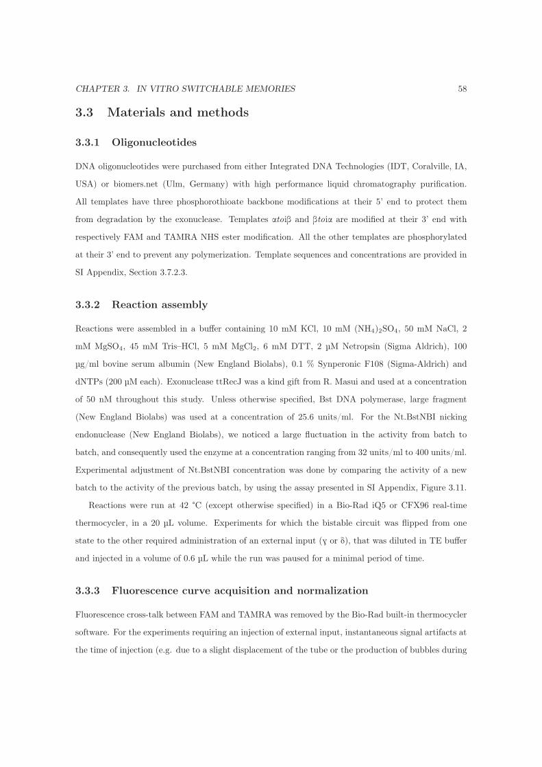
CHAPTER 3. IN VITRO SWITCHABLE MEMORIES 58
3.3 Materials and methods
3.3.1 Oligonucleotides
DNA oligonucleotides were purchased from either Integrated DNA Technologies (IDT, Coralville, IA,
USA) or biomers.net (Ulm, Germany) with high performance liquid chromatography purification.
All templates have three phosphorothioate backbone modifications at their 5’ end to protect them
from degradation by the exonuclease. Templates αtoiβ and βtoiα are modified at their 3’ end with
respectively FAM and TAMRA NHS ester modification. All the other templates are phosphorylated
at their 3’ end to prevent any polymerization. Template sequences and concentrations are provided in
SI Appendix, Section 3.7.2.3.
3.3.2 Reaction assembly
Reactions were assembled in a buffer containing 10 mM KCl, 10 mM (NH4)2SO4, 50 mM NaCl, 2
mM MgSO4, 45 mM Tris–HCl, 5 mM MgCl2, 6 mM DTT, 2 μM Netropsin (Sigma Aldrich), 100
μg/ml bovine serum albumin (New England Biolabs), 0.1 % Synperonic F108 (Sigma-Aldrich) and
dNTPs (200 μM each). Exonuclease ttRecJ was a kind gift from R. Masui and used at a concentration
of 50 nM throughout this study. Unless otherwise specified, Bst DNA polymerase, large fragment
(New England Biolabs) was used at a concentration of 25.6 units/ml. For the Nt.BstNBI nicking
endonuclease (New England Biolabs), we noticed a large fluctuation in the activity from batch to
batch, and consequently used the enzyme at a concentration ranging from 32 units/ml to 400 units/ml.
Experimental adjustment of Nt.BstNBI concentration was done by comparing the activity of a new
batch to the activity of the previous batch, by using the assay presented in SI Appendix, Figure 3.11.
Reactions were run at 42 °C (except otherwise specified) in a Bio-Rad iQ5 or CFX96 real-time
thermocycler, in a 20 μL volume. Experiments for which the bistable circuit was flipped from one
state to the other required administration of an external input (G or δ), that was diluted in TE buffer
and injected in a volume of 0.6 μL while the run was paused for a minimal period of time.
3.3.3 Fluorescence curve acquisition and normalization
Fluorescence cross-talk between FAM and TAMRA was removed by the Bio-Rad built-in thermocycler
software. For the experiments requiring an injection of external input, instantaneous signal artifacts at
the time of injection (e.g. due to a slight displacement of the tube or the production of bubbles during
CHAPTER 3. IN VITRO SWITCHABLE MEMORIES 59
mixing) were corrected to keep the curve continuity. “Charge levels” were normalized from fluorescence
data: to the high plateau (ON state of the autocatalytic module; if unavailable, a reference tube with
the same reacting mix set in the ON state was used) and low plateau (OFF state of the autocatalytic
module; if unavailable, the reaction was ran until depletion of dNTPs, thus revealing the OFF state
of the autocatalytic module).
3.3.4 Simulations
The simple model of the bistable reaction circuit was analytically analyzed using Mathematica (SI
Appendix, Section 3.7.3.1). Detailed models of the bistable circuit, switchable memory and the push-
push memory were done with a set of measured and predicted (DINAMelt) parameters, refined by
fitting on the experimental curves of the switching memory, using Mathematica (SI Appendix, Section
3.7.3.4). The set of refined parameters was used for all other model predictions.
3.4 Results
3.4.1 DNA-toolbox: three basic modules
Our constructions are based on a stripped-down in vitro genetic machinery based on three enzy-
matic reactions [62] (Figure 3.1-A): short DNA signal molecules hybridize with stable DNA template
molecules in a set of basic reactions that structures the topology of the reaction circuits. Templates
are 22 or 26 bases single-stranded deoxy-oligonucleotides composed of a 3’ input site and a 5’ output
site. Signal molecules come in two types: 11-bases long inputs activate templates; on the contrary,
15-bases long inhibitors block them. Reactions take place at a temperature (42 °C) where both inputs
and inhibitors are dynamically hybridizing and separating. Note that the short length of the inputs
(11 bases) limits the number of available sequences, but the construction of relatively large circuits is
still possible (SI Appendix, Section 3.7.2.4).
Templates encode basic reactions following the pattern input -> input + output. When an input
correctly hybridizes on the input site of a template, it is elongated by a DNA polymerase, leading to
the double-stranded form of the template. Next, a nicking endonuclease nicks the new strand, so that
input and output are released from the template. When free in solution, these short oligonucleotides
can be degraded by ttRecJ, a single-strand-specific 5’->3’ exonuclease [145, 146]. Templates are
protected from degradation by a few phosphorothioate backbone modifications located at their 5’ end
CHAPTER 3. IN VITRO SWITCHABLE MEMORIES 60
(SI, Section 3.7.2.2). If not degraded, the input can start another round of reaction, while the output
can, for instance, play the role of input for a separate reaction encoded by another template. Templates
are thus fully composable, and can be classified into the following three modules, depending on their
input and output:
• Activation module if input �= output (α -> α + β).
• Autocatalytic module if input = output (α -> α + α).
• Inhibition module if output = inhibitor (α -> α + inh).
Inhibitors are longer than inputs, hence more stable when fully hybridized. A given inhibitor targets
a template and strongly binds to it, overlapping on the input and output sites of the template. An
inhibitor noted iα will target the autocatalytic module αtoα and an inhibitor noted iαβ will target
the activation module αtoβ. Inhibitors do not have the recognition site for the nicking enzyme, hence
cannot be cut (SI, Section 3.7.2.1 and 3.7.2.3). They also possess two mismatched bases in 3’, which
prevents the polymerase from extending them. Therefore, they are able to block the production of
output by their target modules.
To observe the dynamics of these reactions, we use N-quenching [147], a versatile fluorescent tech-
nique for the monitoring of oligonucleotide hybridization: to follow a given input, the input site of the
corresponding template is labeled in its 3’ end with a single fluorophore. Hybridization of the corre-
sponding input produces a change in the fluorescence level, whereas hybridization of the templates’
output does not (Figure 3.1-B). Therefore, templates themselves serve as specific reporters of the pres-
ence of their inputs. This versatile technique eliminates the need for additional probes to monitor the
system –which could in turn affect the function of the network through the load effect [71].
Using this toolbox, it is possible to build time-responsive DNA reaction circuits of various topolo-
gies, and follow in real time the behavior of some specific sequences within these dynamic systems.
We demonstrate next the design and assembly of a bistable switch function.
3.4.2 Bistable switch: designing the reaction circuit
Bistability can be obtained from a variety of elementary motifs [148, 149], all including at least one
positive feedback loop, but only a couple of basic designs do not require cooperative binding [150]
(and SI Appendix, Section 3.7.3.2). We chose here a symmetrical design [53] where two autocatalytic
modules negatively regulate one another: when one autocatalyst is active, it dynamically represses the
CHAPTER 3. IN VITRO SWITCHABLE MEMORIES 61
Figure 3.1: The DNA-toolbox uses DNA templates to shape the reaction network performed by a setof three enzymes. (A) Templates (bottom strands) have an input site (3’) and an output site (5’) andreceive signal molecules (upper strands). When an input (α) hybridizes to a template, it is elongatedby a DNA polymerase (pol.). Inputs bear the recognition site (in grey) of a nicking enzyme (nick.)that cuts the elongated upper strand between input and output. Input α and output x then dissociateand are free to start another reaction, or be degraded by a single-strand specific exonuclease (exo.).Following this scheme, three types of modules can be obtained depending on the output sites of thetemplate. (B) Nucleobase quenching on the dye-labeled templates allows sequence-specific monitoringof the reactions.
activity of the other (Figure 3.2-A). Given this topology, we decided for two signal strands (α and β), and
designed two templates (respectively αtoα and βtoβ) responsible for their autocatalytic production. In
between αtoα and βtoβ are two inhibition modules that encode the cross-inhibition function: inhibition
module αtoiβ takes α as input and produces iβ. It therefore inhibits the production of β when α is
present; inhibition module βtoiα does the opposite job. By combining the 4 templates αtoα, βtoβ, αtoiβ
and βtoiα in appropriate ratios and conditions, we expect a system featuring bistability, i.e. where
either α or β, but not both, can exist at the steady state.
We started with the building of a simple model to first check the consistency of the design with a
bistable function, when implemented within the toolbox. In this coarse-grained model, four equations
express the life cycle (production and degradation) of the two inputs and two inhibitors (α, β, iα and
iβ, see SI Appendix, Section 3.7.3.1 for details about the model construction). In order to easily find
out the control parameters of this bistable circuit design, we put the model in a non-dimensional form
(Figure 3.2-B) where productions of inputs and inhibitors are described by Michaelis-Menten equations
with maximum rates (tα, tβ, tiα, tiβ) controlled by the concentration of the template encoding the

CHAPTER 3. IN VITRO SWITCHABLE MEMORIES 62
corresponding reaction. Sequestering of templates by the inhibitors tends to decrease the production
rate following a competitive mechanism (enzyme saturation, which would lead to cross coupling terms,
is not considered in this simple model). Parameters λ define the relative strength of an inhibitor
against the input it is competing with. Degradation is represented by a first order term, with the same
degradation rate for all four species.
When looking for the stable equilibria in the {tα, tβ} plane, the model suggests that the emergence
of bistability is favored by high λα and λβ (i.e. inhibitors stronger than inputs) (Figure 3.2-C). Ex-
perimentally, λα and λβ can be adjusted by increasing the binding constants of iα and iβ (for example,
making these inhibitors longer). In the case of a non-ideal system (e.g. non symmetrical λα and λβ),
the bistability domain in the {tα, tβ} plane shrinks (Figure 3.2-D): to be bistable, the circuit needs to
be adjusted by, for instance, changing the concentration of αtoα and βtoβ. Figures 3.2-E & F show the
basins of attraction of the two states A and B for an ideal and a non-ideal bistable circuit: for each
combination of initial {α, β}, the bistable circuit tends to one of the two states {α, β} = {0, 1} or {1,
0}. One notes that even in the cases where the system is bistable, the basins of attraction of the two
states can be very asymmetric.
3.4.3 Experimental building of the bistable circuit
Given these theoretical considerations, we selected the sequences of α and β so that their predicted
binding constants were close to each other at the working temperature. We then designed inhibitors
so that their predicted binding constants were approximately two orders of magnitude higher than the
ones of α and β, i.e. high enough to produce a large bistable state, but small enough to maintain a
dynamic binding equilibrium with their target templates (this insures the responsiveness of the circuit).
Templates αtoiβ and βtoiα are labeled at their 3’ end with two different fluorophores (respectively Fam
and Tamra), which allows specific and simultaneous monitoring of both α and β (Figure 3.3-A). More
details about the design rules are presented in SI Appendix, Section 3.7.2.1.
To assemble the experiment, we combined the four templates and the three enzymes in a consistent
buffer containing dNTPs, and incubated isothermally in a closed tube. We first checked for the presence
of two stable states, which should be selected depending on the initial conditions. Indeed we found
that, if the system is initiated with α only, it evolved to a stable state characterized by a strong shift in
Fam fluorescence, but no perturbation in Tamra fluorescence (called state A, see Figure 3.3-B). Initial
conditions containing only β produced the opposite fluorescent pattern (called state B). This suggests

CHAPTER 3. IN VITRO SWITCHABLE MEMORIES 63
Figure 3.2: Bistable circuit design. (A) A circuit encoding bistability. (B) Non-dimensionalizedequations of the simplified model. tx are the scaled template concentrations and λx the ratio ofactivator over inhibitor binding constant. Periods indicate multiplications. (C) Phase diagram of thebistable circuit in the {tα, tβ} plane. Yellow: bistable domain for {λα, λβ} = {20, 20}. Gray: bistabledomain for {λα, λβ} = {100, 100}; (D) the same with yellow: bistable domain for {λα, λβ} = {100,50}; and gray: bistable domain for {λα, λβ} = {100, 100}. (E) Plot of the calculated trajectories ofthe bistable circuit for different initial {α, β} (small black dots). The bistable circuit is evolving to astable state A (blue dot) or B (red dot). {λα, λβ} = {100, 100} and {tα, tβ}={20,20}, correspondingto the small circle in the gray area of C. (F) The same for {λα, λβ} = {100,50} and {tα, tβ} = {10,10} (small circle in the yellow area of D).
that the system possesses only two stable states. Note that working in a closed configuration imposes
a limited lifetime for the system: once all the dNTPs are consumed, it will simply die out, toward its
unique thermodynamic equilibrium.
To quantitatively assess the bistable behavior of the circuit (i.e. the convergence toward one of
these states at the exclusion of any other trajectory), we initiated the reactions with various mixtures
of α and β: we observed that, after some transients, the system always stabilized on either stable state
A or stable state B (Figure 3.3-C). These experiments also led to a matrix representing the basin of
attraction of each stable state, which were initially quite asymmetric (Figure 3.3-D). Even if templates
were present in the same concentration and sequences had similar thermodynamic constants (but are
still different: dissociation constant of α is more than twice that of β as seen on SI Appendix, Table
S3), side A tended to win as soon as α was initially present in significant quantities, irrespective of the
initial concentration of β. However, as suggested by the simple model, we could adjust this by tuning
the concentrations of templates αtoα and βtoβ (Figure 3.3-D). Figure 3.3-E shows the trajectories of
an adjusted system for different initial input combinations. While the behavior is still not ideal, both

CHAPTER 3. IN VITRO SWITCHABLE MEMORIES 64
states possess a reasonable basin of attraction.
Figure 3.3: Experimental building of the bistable circuit. (A) Topology and templates of the bistablecircuit. Templates αtoiβ and βtoiα are labeled with Fam and Tamra, respectively, allowing multiplexmonitoring of the hybridization status of these two templates. (B) Time plots of the “Charge level”of the bistable switch taking either state B (left) or A (right). “Charge level” is the normalizedfluorescence at 0 in the absence of the corresponding template’s input, and 1 at the steady state ofinput. (C) Time plots of the Charge level of the adjusted bistable switch for two different initial[α] and [β] combinations. (D) The bistable circuit picks its state (A or B) according to the initialcombination of α and β concentrations. With 20 nM of each template, the basin of attraction of stateB (grey domain) is small compared to that of state A. Decreasing the concentration of αtoα to 7.5 nMresults in an expansion of the basin of attraction of state B (yellow domain). Colored stars and dotsare experimental points for, respectively, the bistable with 20 nM of each template and the adjustedbistable with 7.5 nM of αtoα for 20 nM of βtoβ. Domain boundaries are drawn to facilitate the plotreading. (E) Experimental trajectories of the adjusted bistable for different combinations of initial αand β. For each trajectory, the X axis corresponds to the charge level of template αtoiβ, the Y axis tothe charge level of template βtoiα. After some transients, the bistable stabilizes in either state A (bluedot) or B (red dot).
To assess unambiguously and quantitatively the identity of the two states, aliquots were withdrawn
from the solution after the system, initiated with {α, β} = {10 nM, 0.1 nM} or {0.1 nM, 10 nM},
reached one or the other stable state. We analyzed the α and β content of these aliquots and found
a concentration of 55 nM of α for state A and 40 nM of β for state B (SI Appendix, Section 3.7.4).
This similitude between the steady levels of α and β further validates that both sides of the bistable
circuit are well balanced, thanks to the tuning of the concentrations of αtoα and βtoβ. At the same
time, we measured about 1000 times less of the output of the loosing state. The simple model predicts
that the losing side should evolve asymptotically toward 0, but leak reactions not considered therein

CHAPTER 3. IN VITRO SWITCHABLE MEMORIES 65
probably maintain a small basal level. Combining these results with the fluorescence measurement, we
conclude that after having taken a stable state depending on the initial α/β ratio, the bistable system
continuously and unambiguously delivers information about its current status.
The simple model predicts that the bistable circuit is robust to perturbations in concentration of
α and β as long as they do not exceed the concentration of input currently at the steady-state (SI
Appendix, Section 3.7.3.3). Experimentally, we found that the bistable circuit is much more robust
than this prediction: for example, when in the stable state A, an injection of a concentration of β
(100 nM) twice as large as the steady concentration of α is not enough to flip the bistable circuit to
the opposite state (Figure 3.4-A). This discrepancy could be attributed to the fact that the simple
model rests on immediate equilibria for all the hybridization reactions. Since the inhibitor strands
are stable enough to have slow dissociation constants, this assumption is probably not realistic. We
therefore built a detailed mathematical model that takes into account the full set of reactions taking
place in the system (SI Appendix, Section 3.7.3.4). Indeed, this new model predicts a higher resilience
of the bistable circuit (Figure 3.4-B): when the perturbation is introduced as a single Gaussian spike,
a ~20-fold concentration of the opposite input is predicted to be necessary to switch the system to its
opposite state (SI Appendix, Section 3.7.3.5). Since this did not appear as a very practical solution to
flip the system back and forth, we turned toward an alternative switching strategy.
Figure 3.4: Perturbation of the bistable at the steady state. The red dot (charge level {αtoiβ, βtoiα} ={0, 1}) corresponds to stable state B. The blue dot (charge level {αtoiβ, βtoiα} = {1, 0}) correspondsto stable state A. (A) Experimental and (B) calculated (using the detailed model) trajectories of thebistable perturbed by 100 nM of the opposite input.
3.4.4 Two-input switchable memory
To obtain an updatable memory circuit, we decorated the bistable circuit with two activation modules
that connect this bistable core to two different and specific external signals. Activation modules Gtoα
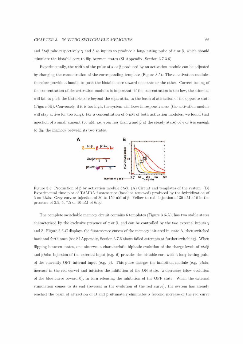
CHAPTER 3. IN VITRO SWITCHABLE MEMORIES 66
and δtoβ take respectively G and δ as inputs to produce a long-lasting pulse of α or β, which should
stimulate the bistable core to flip between states (SI Appendix, Section 3.7.3.6).
Experimentally, the width of the pulse of α or β produced by an activation module can be adjusted
by changing the concentration of the corresponding template (Figure 3.5). These activation modules
therefore provide a handle to push the bistable core toward one state or the other. Correct tuning of
the concentration of the activation modules is important: if the concentration is too low, the stimulus
will fail to push the bistable core beyond the separatrix, to the basin of attraction of the opposite state
(Figure 6B). Conversely, if it is too high, the system will loose in responsiveness (the activation module
will stay active for too long). For a concentration of 5 nM of both activation modules, we found that
injection of a small amount (30 nM, i.e. even less than α and β at the steady state) of G or δ is enough
to flip the memory between its two states.
Figure 3.5: Production of β by activation module δtoβ. (A) Circuit and templates of the system. (B)Experimental time plot of TAMRA fluorescence (baseline removed) produced by the hybridization ofβ on βtoiα. Grey curves: injection of 30 to 150 nM of β. Yellow to red: injection of 30 nM of δ in thepresence of 2.5, 5, 7.5 or 10 nM of δtoβ.
The complete switchable memory circuit contains 6 templates (Figure 3.6-A), has two stable states
characterized by the exclusive presence of α or β, and can be controlled by the two external inputs G
and δ. Figure 3.6-C displays the fluorescence curves of the memory initiated in state A, then switched
back and forth once (see SI Appendix, Section 3.7.6 about failed attempts at further switching). When
flipping between states, one observes a characteristic biphasic evolution of the charge levels of αtoiβ
and βtoiα: injection of the external input (e.g. δ) provides the bistable core with a long-lasting pulse
of the currently OFF internal input (e.g. β). This pulse charges the inhibition module (e.g. βtoiα,
increase in the red curve) and initiates the inhibition of the ON state. α decreases (slow evolution
of the blue curve toward 0), in turn releasing the inhibition of the OFF state. When the external
stimulation comes to its end (reversal in the evolution of the red curve), the system has already
reached the basin of attraction of B and β ultimately eliminates α (second increase of the red curve

CHAPTER 3. IN VITRO SWITCHABLE MEMORIES 67
and final decrease in the blue curve): the memory has flipped between states. These curves were used
to optimize the parameters of the detailed mathematical model (i.e. all other predictions use this same
set of parameters (SI Appendix, Section 3.7.3.4)). They are also plotted as calculated (Figure 3.6-D)
and experimental (Figure 3.6-E) trajectories in two dimensions, showing the good agreement between
the model and the experiments. The trajectories (from A to B and from B to A) appear to be crossing
only because they are a two-dimension projection of a higher dimensional system [151] (see Figure
3.20).
The bistable core takes around 200 minutes to flip between states. This duration is comparable
with the period of the oscillator previously reported [62]. Also, switching requires a concentration of
external input (30 nM) that is of the same scale as the produced α or β at the steady state (~50 nM).
This suggests that the switchable memory circuit could be connected with other circuits made with
the DNA-toolbox, in the quest for more complex reaction networks.
Figure 3.6: Switchable memory circuit. (A) Circuit and templates of the bistable switchable memory.(B) Trajectories of two attempts to flip the bistable memory from A to B, with δtoβ = 2.5 nM (black,failure) and δtoβ = 5 nM (grey, success). (C) Experimental (thick line) and fitted model (thin line)time plot of the charge levels of αtoiβ and βtoiα. The memory circuit is started in state A, flipped fromA to B, then from B to A. (D) Predicted and (E) experimental trajectories of the memory switchingreversibly from A to B (grey) and B to A (black).

CHAPTER 3. IN VITRO SWITCHABLE MEMORIES 68
3.4.5 Push-push memory
The push-push memory is another type of updatable memory element, in which a bistable system is
switched back and forth by a unique stimulus (hence the name push-push, in reference to a push-button
mechanical switch). A chemical implementation of this function can be obtained by further enriching
the previous memory circuit (Figure 3.7-A): the two activation modules (δtoα and δtoβ) now respond to
the same external input δ. To carry out the push-push functionality, two additional inhibition modules
(αtoiδα and βtoiδβ) feed the current state of the bistable core back to the activation modules: when
the bistable is in state A, they ensure that the corresponding activation module (δtoα) is inhibited,
and vice versa. In the presence of the four templates δtoα, δtoβ, αtoiδα and βtoiδβ, injection of δ will
only trigger the production of the input of the OFF state of the bistable core, whereas the input of
the currently ON state will not be produced. This strategy was theoretically validated by a model (SI
Appendix, Section 3.7.3.7).
The detailed model suggested that the full circuit would work with the same bistable core and
same concentration of activation modules as the memory circuit, in the presence of a few nanomolars
of αtoiδα and βtoiδβ (Figure 3.7-B). Before assembling the full circuit, we experimentally checked the
sub-parts encoding the push-push functionality. Figure 3.8 shows that indeed, a concentration of βtoiδβ
as low as 1 nM is efficiently regulating the pulse of β produced by δtoβ.
Figure 3.7: (A) Circuit of the push-push memory: a single external input δ controls the bistable core.(B) Calculated 3D trajectories in the space {Charge level of αtoiβ, Charge level of βtoiα, Normalizedtotal concentration of δ} for the push-push memory switching from A to B (blue) and B to A (red).Normalized values of δ (injected as a gaussian spike) from 0 to 1 are associated to a color gradientfrom blue/red to green. (C) Experimental trajectories of the push-push memory circuit showing twoindependent experiments: one where the system is initially set on the state A, then flipped to B uponinjection of 30 nM of δ, and another where the same system is set in state B, then flipped to A uponinjection of the same input. The charge level of βtoiα higher than 1 indicates that the amount of βtransiently produced by activation module δtoβ during switching exceeds the concentration of β at thestable state B.

CHAPTER 3. IN VITRO SWITCHABLE MEMORIES 69
Figure 3.8: Push-push negative feedback. (A) Circuit and templates. Upon injection of δ, productionof β is activated. Then, β hybridizes to βtoiα (resulting in an increase of TAMRA fluorescence) and toβtoiδβ that, in turn, produces the inhibitor of δtoβ, stopping the production of β. (B) Experimentaltime plot of the normalized TAMRA fluorescence (1 at the highest and 0 at the lowest) for differentconcentrations (0, 1, 2 and 4 nM) of inhibition module βtoiδβ.
When experimentally assembling the 8 templates of the push-push memory circuit, we had to
adjust the concentrations of δtoβ and βtoiδβ to strengthen the response of the B side to the exogenous
input δ. Note that in the bistable core, state B is less attractive than state A (Figure 3.3-C), which
may explain why switching toward B requires a stronger amplification of the external stimulus δ. We
therefore kept the concentrations of activation module δtoα and inhibition module αtoiδα proposed
by the model (respectively 5 nM and 4 nM), and adjusted the concentration of δtoβ to 10 nM. This
explains the large amount of β produced upon injection of δ (exceeding the concentration of β at the
steady state). After fine-tuning of the concentration of βtoiδβ (we settled on a concentration of 1 nM,
see SI Appendix, Section 3.7.5), the push-push circuit could be flipped from state A to B –and from
state B to A– by injection of 30 nM of its unique external input, δ (Figure 3.7-C). The corresponding
fluorescence time plots are shown on Figure 3.19.
3.5 Discussion
Bistability is a fundamental feature of dynamic systems. Bistable switches have been identified or
postulated in a number of important biological circuits [129, 130, 47, 48, 124, 125, 126, 140, 141, 142].
More generally, bistability seems to be at the basis of the dynamic behaviors of many non-linear
artificial chemical systems, such as oscillators [128, 152].
Molecular bistability can theoretically be obtained from a great variety of reaction network topolo-
gies [148, 149, 153], and the mechanistic requirements for this function have been explored in detail
[150, 154, 155]. The presence of a positive feedback loop is a necessary but not sufficient signature

CHAPTER 3. IN VITRO SWITCHABLE MEMORIES 70
[129, 47, 53, 150]: an isolated single autocatalysis provides bistability only if sufficient non-linearities
are included in the loop. In vivo, mechanisms such as ultrasensitivity or cooperative binding –proteins
that acquire new regulatory functions through the formation of multimers– typically provide these
sources of nonlinearity.
Bistable systems without cooperative nonlinearity can be obtained at the cost of a slightly increased
topological complexity of the network [150]. The in vitro toolbox that we use here does not provide
a mechanism to introduce cooperative effects; however, it allows easy assembly of relatively large
networks. Hence we decided for a robust and symmetrical design that contains two autocatalytic loops
responsible for the self-amplification of two cross-repressing species (another design compatible with
the chemistry at hand is discussed in SI Appendix, Section 3.7.3.2). The advantages of the present
design are twofold: first, both stable states correspond to a high concentration of one out of two species
(and not to the presence or absence of a single species), making the reading and interfacing easier;
second, the symmetry facilitates the identification of the control parameters for the network behavior.
In particular, even for not symmetrical sequences, one can theoretically tune the concentrations of
templates to obtain and balance the bistable domain. In practice, this proved to be a useful feature
for the construction of the more complex target behaviors.
The requirement to switch from one state to the other poses another design challenge. In the ideal
case of a system that adapts immediately to a perturbation, as in the simple model presented in Figure
3.2, flipping from A to B is obtained as soon as the concentration of β is pushed above that of α. This
reactivity should not be expected in systems constructed out of complex biochemical transformations,
which is typical of biological systems. Slow loops then increase the hysteresis found in the bistable
behavior [156]. However, while cellular bistable switches are self-contained and can be exposed to input
stimuli over long periods of time [53], it is not the case of our in vitro batch design: by construction,
inputs α and β are degradable species, and an injection of α or β will only produce a spike of limited
length (Figure 3.5). Therefore, we had to look for an alternative switching strategy: we introduced
an additional dimension in the sequence space to provide a switching pathway with a much lowered
concentration threshold (see Figure 3.5). The complete system provides a stable memory, able to
resist very strong transient fluctuations of its chemical signature, but which also specifically responds
to short and dilute spikes of external inputs. Steady state concentrations of outputs α and β (~50 nM)
are of the same scale as the external input required to flip the memory (~30 nM), which suggests that
the memory circuit is itself modular: it could be used as such in a plug&play manner for the building

CHAPTER 3. IN VITRO SWITCHABLE MEMORIES 71
of more complex reaction circuits.
The step-by-step assembly of large-scale systems –like the push-push memory circuit presented
here– rests heavily on the modularity of the molecular toolbox that we use. By modularity, we refer
here to the fact that a priori, any activating or inhibiting relation between two signal molecules (input
or inhibitor) can be implemented: one only needs to design the corresponding templates. However,
in practice this modularity may be limited by a number of design issues: load effect [71] arises when
a downstream module sequesters the product of an upstream module; enzyme saturation can lead to
unintended coupling between unconnected modules because of the competition for enzymatic resources
[59]; and spurious interactions between non complementary sequences may also lead to some extent
of cross-talk [157]. These effects become more prevalent when the size of the system increases [31].
However, their consequences can be circumvented through the emphasis on the robustness of the
design, which in turn is identified using toy mathematical models (SI Appendix, Section 3.7.3.1).
Then, a complete set of reactions (SI Appendix, Section 3.7.3.4) can be combined to provide a better,
quantitative understanding of the consequences of non-modular interactions, which generally lie beyond
our intuition. In the end, building and understanding the dynamics of these complex networks strongly
rests on the good agreement between the experimental result and the mathematical approach. While
this process can be time consuming, one may envision that, in the future, design rules similar to those
of engineering disciplines will emerge to directly mitigate or incorporate these complex effects. It is
also interesting to note that such design rules may have a direct impact on our understanding of in vivo
regulatory processes: for example, in vitro models suggest that competition for enzymatic resources
may be an important contribution to the dynamics of cellular circuits [51, 59].
In this paper, reaction circuits were assembled in a closed environment. This stands in contrast
to most chemical or biological bistable networks reported so far, which perform in open systems
[53, 56, 55, 57, 152]. This closeness imposes specific challenges, for example the presence of precisely
controlled internal source and sink energetic pathways. It also implies that each experiment has a
limited lifetime, and that true steady states cannot be obtained –because various reaction parameters
are modified over time: for instance, dNTP concentration decreases, and enzymes can loose activity.
Worse, even though the templates are protected from the exonuclease, they get slowly degraded (SI
Appendix, Section 3.7.2.2). These factors may pile up to modify the circuit behavior and explain the
loss of function that we have observed after long experimental times (SI Appendix, Section 3.7.6).
Still, we were able to obtain satisfying pseudo-steady states and to perform at least one complete cycle

CHAPTER 3. IN VITRO SWITCHABLE MEMORIES 72
of the two-input memory circuit through its alternative states. For the push-push memory circuit, the
longer time required for switching may explain that repetitive operations were not successful. Note
that an eventual breakdown is unavoidable considering our closed experimental set-up. We anticipate
that if the reactions were performed in an open system (e.g. in a reactor with a constant flow of fresh
precursors), they could be run for an infinite amount of time and switched continuously.
3.6 Conclusion
Biological behaviors are built from and controlled by assemblies of biochemical reactions connected
in complex networks. Despite the enormous molecular complexity of living systems, we may expect
that a correct characterization of the individual components will lead to a rational understanding of
the biological organization and dynamics. A critical test for this approach is the man-made rational
design of molecular systems reproducing non-trivial biological behaviors. The in vivo version of this
idea, synthetic biology, is based on the assumption that biological systems are built from modular,
interchangeable sub-elements: cells provide a platform in which exogenous genetic programs can be
run. Successes along this systematic line are interpreted as a proof of a correct understanding of
the molecular basis of complex, life-like behaviors. However, many studies in this direction have
resulted in a significant deviation from this idealized view of a cell as a universal platform. In many
cases, interference with the housekeeping functions cannot be neglected; modularity is not provided
for free but must be carefully enforced. Our results here suggest that the in vitro approach, which
reproduces some of the essential features of biological networks (including universality), but avoids
some of their limitations, mitigate these concerns and hence may provide a faster learning curve
regarding the potential of reaction networks. Here, the 8 “genes” push-push memory circuit already
compares favorably with the largest realizations of in vivo synthetic biology. Moreover, because it
is fully modular, it could theoretically be connected to other circuits. For instance, two push-push
circuits in series would give a 2-bit binary counter, and one push-push downstream of an oscillator
would perform frequency division, oscillating at half the driving frequency.
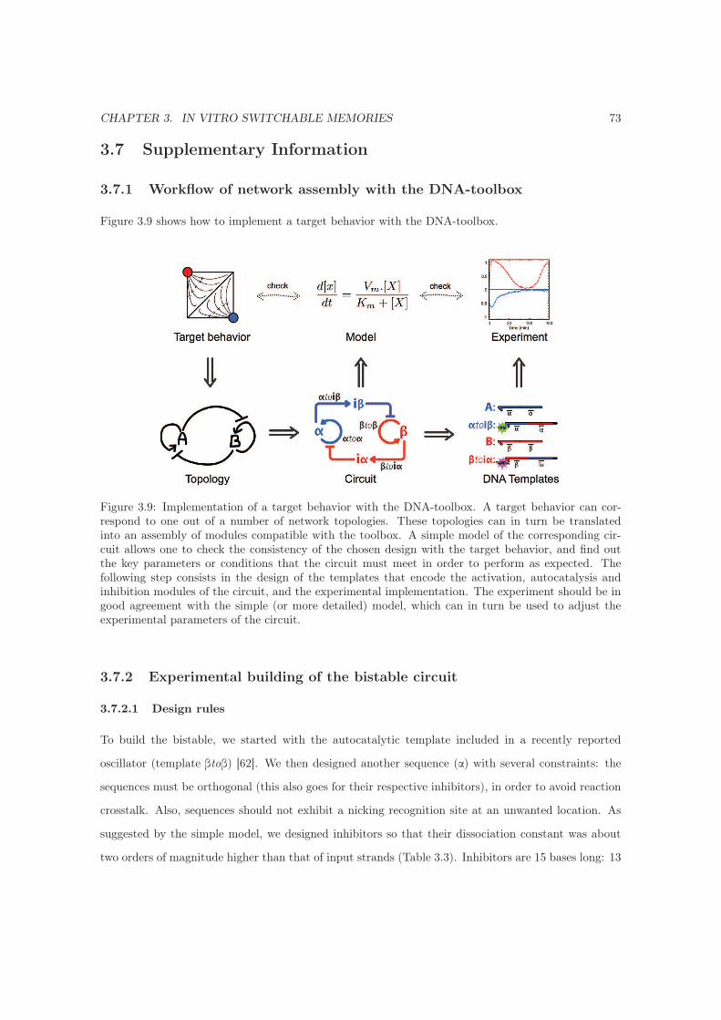
CHAPTER 3. IN VITRO SWITCHABLE MEMORIES 73
3.7 Supplementary Information
3.7.1 Workflow of network assembly with the DNA-toolbox
Figure 3.9 shows how to implement a target behavior with the DNA-toolbox.
Figure 3.9: Implementation of a target behavior with the DNA-toolbox. A target behavior can cor-respond to one out of a number of network topologies. These topologies can in turn be translatedinto an assembly of modules compatible with the toolbox. A simple model of the corresponding cir-cuit allows one to check the consistency of the chosen design with the target behavior, and find outthe key parameters or conditions that the circuit must meet in order to perform as expected. Thefollowing step consists in the design of the templates that encode the activation, autocatalysis andinhibition modules of the circuit, and the experimental implementation. The experiment should be ingood agreement with the simple (or more detailed) model, which can in turn be used to adjust theexperimental parameters of the circuit.
3.7.2 Experimental building of the bistable circuit
3.7.2.1 Design rules
To build the bistable, we started with the autocatalytic template included in a recently reported
oscillator (template βtoβ) [62]. We then designed another sequence (α) with several constraints: the
sequences must be orthogonal (this also goes for their respective inhibitors), in order to avoid reaction
crosstalk. Also, sequences should not exhibit a nicking recognition site at an unwanted location. As
suggested by the simple model, we designed inhibitors so that their dissociation constant was about
two orders of magnitude higher than that of input strands (Table 3.3). Inhibitors are 15 bases long: 13
CHAPTER 3. IN VITRO SWITCHABLE MEMORIES 74
bases are matched with the target template, and the last two 3’ bases are mismatched, preventing the
polymerase from extending the duplex. Inhibitors should not display the nicking enzyme recognition
site: to meet this requirement, 7 of the 13 matched bases are on the template input (3’) side and 6 on
its output (5’) side: two partial but no complete recognition sites are then included in these strands
(See Table 3.2).
Because of the symmetric topology of the bistable circuit, both autocatalytic modules should be of
equivalent “strength”. Thus, we designed α and β so that the predicted1 melting temperatures (Tm)
on their templates were as close as possible: even though the Tm alone is not enough to determine the
relative “strength” of α and β, it is an accessible parameter to balance the sequences before assembling
the circuit. Enzymes have a different affinity for each sequence, and this parameter is not predictable
(but has recently attracted interest in the context of isothermal DNA amplification and template
dependence [158]), nor controllable for a given sequence. A robust network design should then be
as little sensitive as possible to such unpredictable parameters in delivering the target function, and
also provide some adjustable control parameters that may be used to mitigate these effects, once the
sequences have been decided. Here we have shown that it is possible – in a certain extent – to tune the
concentrations of some templates to experimentally “balance” a non-perfect system in order to obtain
a robust bistable circuit.
Monitoring of α and β is done by using N-quenching [147]: a single fluorophore is attached at
the 3’ end of templates αtoiβ and βtoiα, where its fluorescence gets modified by the presence of the
template’s input (i.e. single-strand vs double-strand state). On the contrary, the binding of the
output doesn’t impact the fluorescence of the template 3’ fluorophore [147]. The fluorophores were not
attached to templates αtoα or βtoβ for the following reason: these two autocatalytic modules are the
target of inhibitors iα and iβ, which hybridize 4 bases away from the template 3’ fluorophore. In this
configuration, they might induce a slight fluorescence change when hybridizing [147]. To avoid this
unwanted effect, we attached the fluorophores on inhibition modules αtoiβ and βtoiα.
3.7.2.2 Protection from ttRecJ
In order to protect template from degradation by 5’->3’ exonuclease ttRecJ, templates have several
phosphorothioate backbone modifications (PT) at their 5’ end. Note that the RecJ exonuclease used
here is not the same as the commercially available enzyme from Escherichia coli used in Montagne et
1Using DINAMelt (http://mfold.rna.albany.edu/?q=DINAMelt)

CHAPTER 3. IN VITRO SWITCHABLE MEMORIES 75
Figure 3.10: Degradation of template βtoβ (400 nM) by ttRecJ in the same buffer, ttRecJ concen-tration (50 nM) and temperature (42 °C) as for the bistable switch, memory and push-push memoryexperiments. Template βtoβ has 0, 1, 2 or 3 consecutive phosphorothioate backbone modifications atits 5’ end.
al. [62]. Here we used thermophilic analog ttRecJ from T. thermophilus [145, 146]. This thermophilic
enzyme is more stable than its mesophilic counter part. Therefore it does not require the addition of
stabilizing additives in the buffer and extends the range of available working temperatures.
However the activities of the two enzymes are slightly different. Figure 3.10 shows the degradation
of 400 nM of template βtoβ in presence of the same concentration of ttRecJ as used in the switch
experiments reported here. Even with 2 PTs, βtoβ is rapidly degraded, which may prematurely disrupt
the functioning of a circuit containing it (this stands in contrast with the mesophilic RecJ, for which
two phophorothioates were found to provide a good protection [62]). Three terminal consecutive PTs
appear to be necessary to obtain a correct protection, but produce a problematic side-effect: the
nicking enzyme cutting speed is divided by roughly a factor of 4 in the presence of the third PT
(Figure 3.11-B).
We hypothesized that this was the consequence of a form of competitive inhibition, where the
nicking enzyme could bind –unproductively– the recognition sequence on the output side of the tem-
plate (even if for this pseudo-site, no DNA extends beyond the nicking position). Following this line
of thought, we searched for a way to decrease the affinity of the nicking enzyme for the output site.
We found that replacing the thymine of the recognition sequence by an uracil (GACUC instead of
GACTC) could indeed address the reduced cutting speed issue. In this case, a correct nicking rate
was recovered (Figure 3.11-C). In fact, we even observed an increase in the rate of the nicking process,
compared to template βtoβ with 2 PT and no dU.
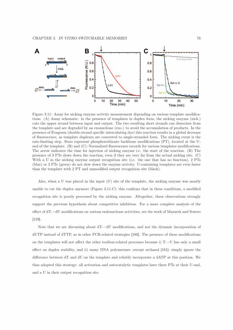
CHAPTER 3. IN VITRO SWITCHABLE MEMORIES 76
Figure 3.11: Assay for nicking enzyme activity measurement depending on various template modifica-tions. (A) Assay schematic: in the presence of templates in duplex form, the nicking enzyme (nick.)cuts the upper strand between input and output. The two resulting short strands can dissociate fromthe template and are degraded by an exonuclease (exo.) to avoid the accumulation of products. In thepresence of Evagreen (double-strand specific intercalating dye) this reaction results in a global decreaseof fluorescence, as template duplexes are converted to single-stranded form. The nicking event is therate-limiting step. Stars represent phosphorothioate backbone modifications (PT), located at the 5’-end of the template. (B) and (C): Normalized fluorescence records for various templates modifications.The arrow indicates the time for injection of nicking enzyme i.e. the start of the reaction. (B) Thepresence of 3 PTs slows down the reaction, even if they are very far from the actual nicking site. (C)With a U in the nicking enzyme output recognition site (i.e. the one that has no function), 2 PTs(blue) or 3 PTs (green) do not slow down the enzyme activity. U-containing templates are even fasterthan the template with 2 PT and unmodified output recognition site (black).
Also, when a U was placed in the input (3’) site of the template, the nicking enzyme was mostly
unable to cut the duplex anymore (Figure 3.11-C): this confirms that in these conditions, a modified
recognition site is poorly processed by the nicking enzyme. Altogether, these observations strongly
support the previous hypothesis about competitive inhibition. For a more complete analysis of the
effect of dT->dU modifications on various endonuclease activities, see the work of Mazurek and Sowers
[159].
Note that we are discussing about dT->dU modifications, and not the dynamic incorporation of
dUTP instead of dTTP, as in other PCR-related strategies [160]. The presence of these modifications
on the templates will not affect the other toolbox-related processes because i) T->U has only a small
effect on duplex stability, and ii) many DNA polymerases -except archaeal [161]- simply ignore the
difference between dT and dU on the template and reliably incorporate a dATP at this position. We
thus adopted this strategy: all activation and autocatalytic templates have three PTs at their 5’-end,
and a U in their output recognition site.

CHAPTER 3. IN VITRO SWITCHABLE MEMORIES 77
3.7.2.3 DNA sequences
Table 3.1: Templates and concentrations used in this study. Stars stand for phosphorothioate backbonemodifications. Templates are separated in two parts, corresponding to input and output bindingsequences, respectively. Nicking enzyme recognition sites are in bold. Uracilated pseudo-sites are ingray.
Table 3.2: Input and inhibitors used in this study. Inhibitors are overlapping on both input and outputsite of their target template. Nicking enzyme recognition sites are in bold, and partial recognition sites(on inhibitors) in gray.
DNA templates used in this study, and their concentrations, are shown in Table 3.1. Input and
inhibitors (i.e. the species that are dynamically produced and degraded) are shown in Table 3.2.
3.7.2.4 Sequence space limitation
With the DNA-toolbox, 11-bases long inputs and 15-bases long inhibitors can be arbitrarily wired in
reaction networks following any desired network topology. The shortness of these oligonucleotides is
limiting the available sequences: on the 11 bases of an input, 5 are required for the nicking enzyme
recognition site (in bold on Table S2), leaving 6 bases to choose among 4 nucleotides. That is 46 =
4096 combinations. With a conservative estimate of 2-5 % of them viable (to exclude sequences with

CHAPTER 3. IN VITRO SWITCHABLE MEMORIES 78
secondary structures, G repeats, cross-talks or other issues (e.g. parasitic nicking site)), this leaves
about 80-200 sequences. This last number should be compared with the 3 basic sequences needed to
build the push-push memory circuit, giving an idea of the maximal circuit complexity that one could
construct with the DNA-toolbox (in homogeneous, well mixed conditions).
In order to overcome this limitation, that is, to increase the number of viable input species, one
might consider working with longer oligonucleotides (and therefore at higher temperature to maintain
the dynamic exchanges). Also, it should be possible to work with another nicking enzyme having
a shorter recognition site: this would further increase the available bases for designing inputs with
orthogonal sequences.
3.7.3 Model
3.7.3.1 Simple Model
Assuming a Michaelis-Menten mechanism for the DNA amplification step of an activation template T
= xtoy :
we obtain:
dy
dt=
k2.T.x
Kx + x;Kx =
k−1 + k2k1
where T and x are the total concentrations of the corresponding species. Note that this is not
formaly valid: the second (k2) reaction involves two complex enzymatic reactions besides mutiple de-
hybridization, and thus barely corresponds to the classic Michaelis-Menten assumptions. However, for
modelling purposes with minimal mathematical complexity, we can still expect the Michaelis-Menten
expression to correctly describe the saturable production of y as a function of x. From the arguments
above, we would also expect k2 << k-1, and Kx becomes roughly equal to the dissociation constant of
x on the template T. Moreover, assuming that the inhibiting strand ixy acts as a competitive inhibitor,
and noting Kixy the dissociation constant of ixy and kx the k2 of activator x we obtain:
dy
dt=
kx.T.x
Kx(1 +xKx
+ixy
Kixy)

CHAPTER 3. IN VITRO SWITCHABLE MEMORIES 79
For the bistable system as shown in Figure 3.3-A, and assuming the same first order degradation
rate D for all species2, we can then generalize the previous equation (with obvious notations) to write
the complete system as:
dα
dt=
kα.Tα.α
Kα(1 +αKα
+ iαKiα
)−D.α
dβ
dt=
kβ .Tβ .β
Kβ(1 +βKβ
+iβKiβ
)−D.β
diαdt
=kiα.Tiα.β
Kβ(1 +βKβ
)−D.iα
diβdt
=kiβ .Tiβ .α
Kα(1 +αKα
)−D.iβ
We non-dimensionnalize by setting τ = t.D, α = α/Kα, β = β/Kβ , iα = iα/Kα, iβ = iβ/Kβ and
tα = kα.Tα/Kα.D, tβ = kβ .Tβ/Kβ .D, tiα = kiα.Tiα/Kα.D, tiβ = kiβ .Tiβ/Kβ .D, λα = Kα/Kiα and
λβ = Kβ/Kiβ .
˙α =tα.α
1 + α+ λαiα− α
˙β =tβ .β
1 + β + λβ iβ− β
˙iα =tiα.β
1 + β− iα
˙iβ =tiβ .α
1 + α− iβ
It can be checked that the fixed point {α, β} = {0, 0} is unstable as soon as one of the autocatalytic
templates reach a threshold concentration (tα >1 or tβ >1). The two fixed points that can give rise to
bistable behavior are then {α, β} = {tα−1, 0} and {0, tβ−1}. They obviously exist only for tα and tβ
superior to unity. Moreover, for the first point, the eigenvalues of the associated Jacobian matrix are
{−1, −1, (1−tα)/tα, −1+tα.tβ/(tα+λβ.tiβ.(tα−1))} so this point is stable for tα > λβ.tiβ/(1−tβ+λβ.tiβ).
Similarly, the second point is stable for tβ > λα.tiα/(−tα+1+ λα.tiα). In the case of a perfectly equili-
2This is, of course, not realistic, as inhibitors form more stable duplexes than activators, and are “protected” fromthe exonuclease when in duplex form. Also, note that the exonuclease has different Michaelis constants for inhibitorsand activators (SI Appendix, Section 3.7.3.4). However, in the non-dimensional form of the equations, introducing adifferent D would come down to scaling tiα and tiβ and the respective inhibitors concentrations. Therefore it would notchange the global dynamic behavior.

CHAPTER 3. IN VITRO SWITCHABLE MEMORIES 80
brated switch tα = tβ and λα.tiα = λβ.tiβ, they may coexist for λα.tiα = λβ.tiβ > 1. Then, the overlapping
areas of stability (i.e. the bistable range) will increase with increasing λα.tiα = λβ.tiβ. Finally, a fourth
root in the positive quadrant, corresponding to the coexistence of the two dynamic species, can be
stable when the two previous inequalities are simultaneously violated (and thus produces a monostable
system).
Therefore, the insights brought by this simple model are as follow (see also Figure 3.2):
• As soon as their templates reach a threshold concentration, both autocatalytic loops produce a
non-trivial steady state in α or β.
• Bistability can occur with asymptotic elimination of one species, but a minimum strength of
the inhibitory link is necessary, and the concentrations of the autocatalytic templates must both
be within a finite range (below which no species is produced and above which the system is
monostable with a single species or two coexistent species).
• The bistable area, which can be interpreted as a quantification of the robustness of the function,
increases with increasing inhibiting strength.
• This can be obtained both by increasing the binding constant of the inhibitor or the concentration
of the template that produces it. Note however that both cases could result in a breakdown of
the assumption used in the model (i.e. inhibitors would not dynamically hybridize anymore or
the enzymes would become limiting and the production rate of β would not linearly follow the
template concentration).
• The most robust behavior is given by the symmetric (ideal) system, as defined above. However,
chemical dissymmetry (for example kα �= kβ) can be compensated by adjusting the concentration
of the template responsible for the production of each species.
3.7.3.2 Minimal bistable circuit design: single autoloop
In a system lacking cooperative nonlinearities, bistability can still emerge in the presence of at least
one autocatalytic module [150, 153]. By using the simple model, we wanted to check if such compact
circuit design (one autocatalytic module instead of two) would be deemed feasible in the context of
the DNA-toolbox, and if so, how robust would it be compared to the design with two autocatalytic
modules.

CHAPTER 3. IN VITRO SWITCHABLE MEMORIES 81
Figure 3.12: (A) Single-autocatalytic module circuit encoding bistability. (B) Non-dimensionalizedequations of the simplified model. tx are the scaled concentrations of template producing x and λx theratio of activator over inhibitor binding constant. Periods indicate multiplications. (C) Phase diagramof the bistable circuit in the plane {tα, tβ}, with {tiα, tiηβ} = {0.3, 0.3} and η = 1. Yellow: bistabledomain for {λα, λβ} = {20, 20}. Gray: bistable domain for {λα, λβ} = {100, 100}. (D) Idem withyellow: bistable domain for {λα, λβ} = {50, 100}; and gray: bistable domain for {λα, λβ} = {100, 100}.
Experimentally, it should be possible to build a bistable circuit with a single autocatalytic module
(Figure 3.12-A), provided that the concentration of one input species (η) is kept constant (this could be
obtained by simply adding phosphorothioate backbone modifications at the 5’-end of η, thus protecting
it from degradation by the exonuclease). In the network of Figure 3.12-A, constant input η activates
the production of β, which in turn triggers the production of iα, inhibitor of αtoα. On the other side,
αtoα autocatalytically produces α, which triggers the production of inhibitor iηβ. The latter is targeting
template ηtoβ, thus inhibiting the production of β.
We constructed a simple model of this circuit (Figure 3.12-B) and analyzed it the same way as the
model of the bistable circuit with two autocatalytic modules (i.e. with the same values of tix, λx and
the same ranges of {tα, tβ}). The phase diagrams of this bistable circuit in the plane {tα, tβ} (Figure
3.12-C and D) suggest that in the context of the DNA-toolbox, and using similar design rules, this
single-autocatalytic module design is less robust than the design containing two autocatalytic modules
(analyzed in Figure 3.2). Moreover, it does not deliver a symmetric output to signal its current state.

CHAPTER 3. IN VITRO SWITCHABLE MEMORIES 82
3.7.3.3 Simple robustness
Figure 3.13: Assessing the response of the bistable switch: successive Gaussian spikes of increasingamount of ¯α are added to the system in the B state. β (red line) responds by a decrease as α (bluedashed line) is injected. Eventually, injected α transiently exceeds the amount of β at the steady state:the bistable flips from B to A. The parameters are tα = tβ = 20, tiα = tiβ = 0.3, λα = λβ = 100.
Using the simple nondimensionalized model, we assessed the response of the bistable switch to
perturbation in its input concentrations. In this simplified, “instantaneous” model (i.e. that strictly
relies on the instantaneous concentrations of dynamic species and does not incorporate hybridization
/ dehybridization dynamics), the bistable flips between states as soon as the injected OFF state input
exceeds the ON state input (Figure 3.13).
3.7.3.4 Detailed model construction
Whereas the simple model gives a good insight about the validity of a given circuit design and its
steady states, it fails to predict realistically the experimental circuit dynamics. Thus we built a more
detailed mathematical model that takes in account all the hybridization and enzymatic reactions that
happen in a toolbox-based DNA reaction circuit (as an example, see the detailed set of reactions for
a circuit constituted of one autocatalytic module on Figure 3.14), with the following assumptions:
• Association rate of ka = 0.06 nM-1.min-1 was taken, as proposed by Zhang and Winfree [19] for
short oligonucleotides.
• Also, inhibitors take advantage of a 7 bases (if hybridizing to template-output duplex) or 6
bases (if hybridizing to template-input duplex) toehold: at 25 °C, this should give them a full
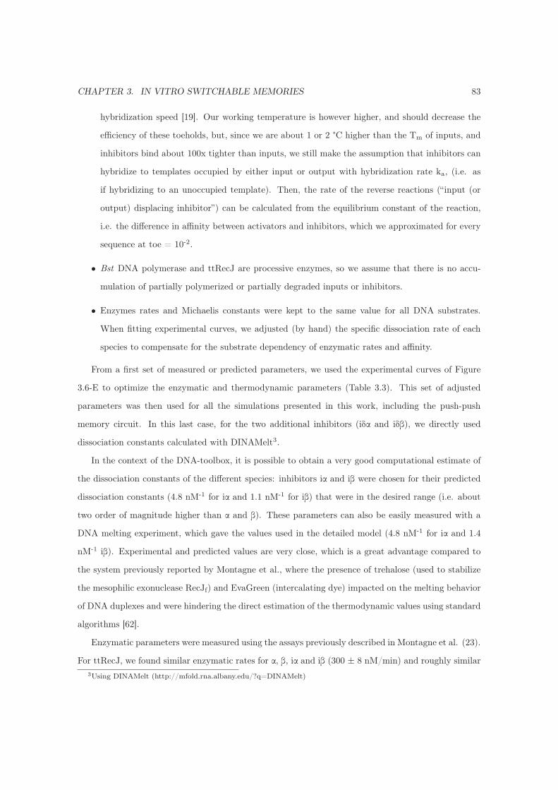
CHAPTER 3. IN VITRO SWITCHABLE MEMORIES 83
hybridization speed [19]. Our working temperature is however higher, and should decrease the
efficiency of these toeholds, but, since we are about 1 or 2 °C higher than the Tm of inputs, and
inhibitors bind about 100x tighter than inputs, we still make the assumption that inhibitors can
hybridize to templates occupied by either input or output with hybridization rate ka, (i.e. as
if hybridizing to an unoccupied template). Then, the rate of the reverse reactions (“input (or
output) displacing inhibitor”) can be calculated from the equilibrium constant of the reaction,
i.e. the difference in affinity between activators and inhibitors, which we approximated for every
sequence at toe = 10-2.
• Bst DNA polymerase and ttRecJ are processive enzymes, so we assume that there is no accu-
mulation of partially polymerized or partially degraded inputs or inhibitors.
• Enzymes rates and Michaelis constants were kept to the same value for all DNA substrates.
When fitting experimental curves, we adjusted (by hand) the specific dissociation rate of each
species to compensate for the substrate dependency of enzymatic rates and affinity.
From a first set of measured or predicted parameters, we used the experimental curves of Figure
3.6-E to optimize the enzymatic and thermodynamic parameters (Table 3.3). This set of adjusted
parameters was then used for all the simulations presented in this work, including the push-push
memory circuit. In this last case, for the two additional inhibitors (iδα and iδβ), we directly used
dissociation constants calculated with DINAMelt3.
In the context of the DNA-toolbox, it is possible to obtain a very good computational estimate of
the dissociation constants of the different species: inhibitors iα and iβ were chosen for their predicted
dissociation constants (4.8 nM-1 for iα and 1.1 nM-1 for iβ) that were in the desired range (i.e. about
two order of magnitude higher than α and β). These parameters can also be easily measured with a
DNA melting experiment, which gave the values used in the detailed model (4.8 nM-1 for iα and 1.4
nM-1 iβ). Experimental and predicted values are very close, which is a great advantage compared to
the system previously reported by Montagne et al., where the presence of trehalose (used to stabilize
the mesophilic exonuclease RecJf) and EvaGreen (intercalating dye) impacted on the melting behavior
of DNA duplexes and were hindering the direct estimation of the thermodynamic values using standard
algorithms [62].
Enzymatic parameters were measured using the assays previously described in Montagne et al. (23).
For ttRecJ, we found similar enzymatic rates for α, β, iα and iβ (300 ± 8 nM/min) and roughly similar
3Using DINAMelt (http://mfold.rna.albany.edu/?q=DINAMelt)

CHAPTER 3. IN VITRO SWITCHABLE MEMORIES 84
Figure 3.14: Schematic of the full set of reactions relative to a reaction circuit where input α onlyinteracts with template αtoα, and the corresponding set of ordinary differential equations. αtoα is notedA for simplicity of notation. Red arrows indicate enzymatic reactions. Periods indicate multiplications.Dissociation rates (in min-1) were calculated as kd = ka/Kd
Michaelis constant for inhibitors iα and iβ (150 ± 10 nM). However, we found Michaelis constant for
input α and β to be higher (440 ± 100 nM), suggesting a higher affinity of ttRecJ for longer substrates
(inhibitors). This was also the case for RecJf used in Montagne et al. [62]. We thus assigned two
different parameters for inputs and inhibitors. For Nt.BstNBI, we found Michaelis constants of 30 ±
10 nM for α and β. We however kept one single value for all input species, which would be compensated
by adjusting each input dissociation rate during the fitting process.
3.7.3.5 Perturbation of the bistable and switching threshold
As shown in Figure 3.13, the simple model fails to describe the actual resilience of the bistable to
perturbation in concentration of its inputs (α and β). We thus used the detailed model of the bistable,
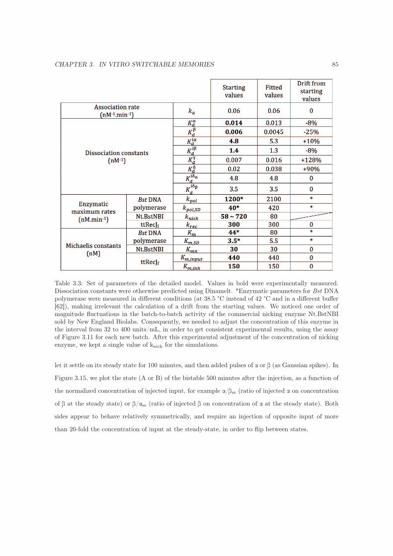
CHAPTER 3. IN VITRO SWITCHABLE MEMORIES 85
Table 3.3: Set of parameters of the detailed model. Values in bold were experimentally measured.Dissociation constants were otherwise predicted using Dinamelt. *Enzymatic parameters for Bst DNApolymerase were measured in different conditions (at 38.5 °C instead of 42 °C and in a different buffer[62]), making irrelevant the calculation of a drift from the starting values. We noticed one order ofmagnitude fluctuations in the batch-to-batch activity of the commercial nicking enzyme Nt.BstNBIsold by New England Biolabs. Consequently, we needed to adjust the concentration of this enzyme inthe interval from 32 to 400 units/mL, in order to get consistent experimental results, using the assayof Figure 3.11 for each new batch. After this experimental adjustment of the concentration of nickingenzyme, we kept a single value of knick for the simulations.
let it settle on its steady state for 100 minutes, and then added pulses of α or β (as Gaussian spikes). In
Figure 3.15, we plot the state (A or B) of the bistable 500 minutes after the injection, as a function of
the normalized concentration of injected input, for example α/βss (ratio of injected α on concentration
of β at the steady state) or β/αss (ratio of injected β on concentration of α at the steady state). Both
sides appear to behave relatively symmetrically, and require an injection of opposite input of more
than 20-fold the concentration of input at the steady-state, in order to flip between states.
CHAPTER 3. IN VITRO SWITCHABLE MEMORIES 86
Figure 3.15: Numerical simulation of the switching of the bistable with the detailed model. Thesystem, initially in state A (blue dot) or B (red dot) is perturbed by a Gaussian spike of input of theopposite species, from 0 to 30-fold the current steady concentration. The plot gives the state observed500 minutes after the injection.
3.7.3.6 Activation module
An activation module is a template that amplifies a short spike of its input into a long-lasting pulse of
its output. As an example, activation module δtoβ is activated by δ, but also acts as a “refuge” for δ:
in hybridized (and elongated) state, δ is protected from ttRecJ that specifically targets single-stranded
substrates. δ is thus able to stay in solution for longer than without “refuge” templates, and thus
activate the production of a long-lasting pulse of β. Figure 3.16 shows the predicted time plot of α
and β concentrations produced by 5 nM of the corresponding activation module, compared to a direct
injection of α and β.
3.7.3.7 Push-push strategy
In the push-push memory circuit, the current state of the bistable core is fed back to the two activation
modules. This allows the system to decide which internal specie (α or β) to produce upon reading of
the single external input δ, depending on its current state. We checked the validity of this strategy
with the detailed mathematical model. In the absence of autocatalytic modules αtoα and βtoβ (Figure
3.17-A), we impose a fixed concentration (40 nM) of non-degradable internal input α or β, and set a
spike of 30 nM of external input δ. Figure 3.17-B shows that the system responds with the production
of a large pulse of the species that is initially absent (i.e. β if the system is in A state, and conversely).

CHAPTER 3. IN VITRO SWITCHABLE MEMORIES 87
Figure 3.16: Predicted time plots of the concentration of α (left) and β (right) produced by theactivation module Gtoα or δtoβ (5 nM) upon injection of 30 nM of the corresponding input G or δ.These curves (plain lines) are compared to direct spike of 30 nM of α or β (dashed lines). Thesepredictions were generated with the detailed model.
Still, the model predicts that the charge level of βtoiα (for β imposed) and αtoiβ (for α imposed) is
transiently slightly exceeding 1, which indicates a small leak production of the current internal species.
Note that no switching is expected here since the state is externally imposed at all times (and no
autocatalytic module is present).
3.7.4 Reamplification
Table 3.4: Measured concentrations of α and β at the steady state of the bistable in state A and B.
Here, we used a previously reported method [62] to experimentally measure the concentrations of α
and β when the bistable switch is asymptotically converging toward one or the other of its two dynamic
stable states.
The system was initiated with {α, β} = {10 nM, 0.1 nM} or {0.1 nM, 10 nM}, and allowed 150
minutes to reach one of its steady states, respectively A or B (as judged by the fluorescence signals).
We then withdrew aliquots from the solutions and immediately quenched them by 10x dilution in 95
°C mQ water followed by a 5 minutes incubation at the same temperature. Dilution of these samples
were then amplified by isothermal amplification at 50 °C in presence of template αtoα (20 nM) or βtoβ

CHAPTER 3. IN VITRO SWITCHABLE MEMORIES 88
Figure 3.17: Structure and function of the injection layer for the push-push memory system. (A)Inhibition modules αtoiδα and βtoiδβ produce respectively iδα and iδβ, depending on the presence ofeither α or β. Inhibitors iδα and iδβ inhibit the activation modules δtoα and δtoβ. In the resultingcircuit, in the presence of α, δtoα is inhibited, and injection of the external input δ will only activateδtoβ, hence produce β. Conversely, in presence of β, only δtoα will be sensible to external input δ. (B)Theoretical time traces of the charge level of the templates βtoiα and αtoiβ either when the constantpresence of α is imposed and a short pulse of δ is applied (left), or when the constant presence of β isimposed and the same short pulse of δ is applied (right).
(30 nM) with Bst DNA polymerase (8 units/ml) and Nt.BstNBI nicking endonuclease (100 units/ml).
The reaction was performed in a thermocycler set at a constant temperature (50 °C) and monitored
with 1x EvaGreen intercalating dye as described. Using the built-in software, concentrations of α and
β were determined from the shape of the amplification curves by comparison with calibration curves
built from UV-calibrated concentrations of pure α or β. Results are displayed in Table S4.
3.7.5 Push-push memory circuit
Figure 3.18: Experimental trajectories (A) and time plots (B) of the push-push memory circuit withδtoα = δtoβ = 5 nM and αtoiδα = βtoiδβ = 4 nM. Upon addition of 30nM of δ, the circuit switchedfrom B to A, but failed to switch from A to B.

CHAPTER 3. IN VITRO SWITCHABLE MEMORIES 89
Table 3.5: Experimental result of the push-push memory circuit (with δtoβ = 10 nM, δtoα = 5 nMand αtoiδα = 4 nM) flipping between states for different concentrations of inhibition module βtoiδβ.
Figure 3.19: Experimental time plots (same data as Figure 3.7) of the push-push memory circuit withδtoα = 5 nM, δtoβ = 10 nM, αtoiδα = 4 nM, and βtoiδβ = 1 nM. Upon addition of 30nM of δ, thecircuit switched from A to B (left), and from B to A (right).
In the assembly of the push-push memory circuit, we kept the templates of the bistable core at the
same concentrations as for the memory circuit and the bistable circuit, and adjusted the concentration
of the 4 templates that encode the push-push function. The detailed model suggested that the full
circuit would work with concentrations of activation modules δtoα and δtoβ at 5 nM and inhibition
modules αtoiδα and βtoiδβ at 4 nM. In these conditions, upon addition of 30 nM of δ, the experimental
push-push circuit successfully switched from B to A, but failed to switch from A to B (Figure 3.18).
This result pointed out that a stronger amplification of input β was required to push the circuit (initially
in state A) to the basin of attraction of state B. We consequently adjusted the concentrations of δtoβ
(to 10 nM) and βtoiδβ to obtain a working point where the push-push memory circuit could switch
in both directions. Table 3.5 displays the experimental results of the fine-tuning of the concentration
of βtoiδβ, showing that the strength of the negative feedback (performed by βtoiδβ) must be carefully
adjusted in order to reach a reversible working point. Experimental trajectories of the push-push
memory circuit (Figure 3.7) are shown as time plots on Figure 3.19.
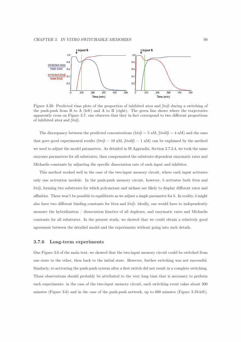
CHAPTER 3. IN VITRO SWITCHABLE MEMORIES 90
Figure 3.20: Predicted time plots of the proportion of inhibited αtoα and βtoβ during a switching ofthe push-push from B to A (left) and A to B (right). The green line shows where the trajectoriesapparently cross on Figure 3.7: one observes that they in fact correspond to two different proportionsof inhibited αtoα and βtoβ.
The discrepancy between the predicted concentrations (δtoβ = 5 nM, βtoiδβ = 4 nM) and the ones
that gave good experimental results (δtoβ = 10 nM, βtoiδβ = 1 nM) can be explained by the method
we used to adjust the model parameters. As detailed in SI Appendix, Section 3.7.3.4, we took the same
enzymes parameters for all substrates, then compensated the substrate-dependent enzymatic rates and
Michaelis constants by adjusting the specific dissociation rate of each input and inhibitor.
This method worked well in the case of the two-input memory circuit, where each input activates
only one activation module. In the push-push memory circuit, however, δ activates both δtoα and
δtoβ, forming two substrates for which polymerase and nickase are likely to display different rates and
affinities. These won’t be possible to equilibrate as we adjust a single parameter for δ. In reality, δmight
also have two different binding constants for δtoα and δtoβ: ideally, one would have to independently
measure the hybridization / dissociation kinetics of all duplexes, and enzymatic rates and Michaelis
constants for all substrates. In the present study, we showed that we could obtain a relatively good
agreement between the detailed model and the experiments without going into such details.
3.7.6 Long-term experiments
One Figure 3.6 of the main text, we showed that the two-input memory circuit could be switched from
one state to the other, then back to the initial state. However, further switching was not successful.
Similarly, re-activating the push-push system after a first switch did not result in a complete switching.
These observations should probably be attributed to the very long time that is necessary to perform
such experiments: in the case of the two-input memory circuit, each switching event takes about 200
minutes (Figure 3.6) and in the case of the push-push network, up to 600 minutes (Figure 3.19-left).
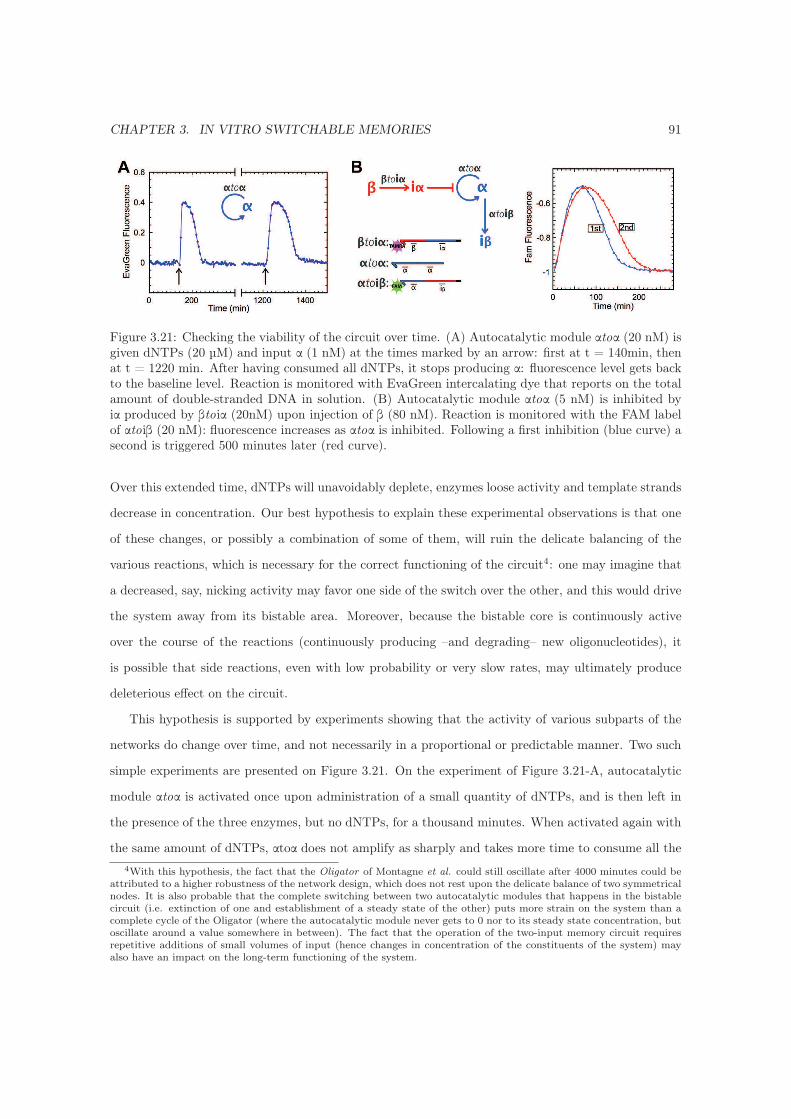
CHAPTER 3. IN VITRO SWITCHABLE MEMORIES 91
Figure 3.21: Checking the viability of the circuit over time. (A) Autocatalytic module αtoα (20 nM) isgiven dNTPs (20 μM) and input α (1 nM) at the times marked by an arrow: first at t = 140min, thenat t = 1220 min. After having consumed all dNTPs, it stops producing α: fluorescence level gets backto the baseline level. Reaction is monitored with EvaGreen intercalating dye that reports on the totalamount of double-stranded DNA in solution. (B) Autocatalytic module αtoα (5 nM) is inhibited byiα produced by βtoiα (20nM) upon injection of β (80 nM). Reaction is monitored with the FAM labelof αtoiβ (20 nM): fluorescence increases as αtoα is inhibited. Following a first inhibition (blue curve) asecond is triggered 500 minutes later (red curve).
Over this extended time, dNTPs will unavoidably deplete, enzymes loose activity and template strands
decrease in concentration. Our best hypothesis to explain these experimental observations is that one
of these changes, or possibly a combination of some of them, will ruin the delicate balancing of the
various reactions, which is necessary for the correct functioning of the circuit4: one may imagine that
a decreased, say, nicking activity may favor one side of the switch over the other, and this would drive
the system away from its bistable area. Moreover, because the bistable core is continuously active
over the course of the reactions (continuously producing –and degrading– new oligonucleotides), it
is possible that side reactions, even with low probability or very slow rates, may ultimately produce
deleterious effect on the circuit.
This hypothesis is supported by experiments showing that the activity of various subparts of the
networks do change over time, and not necessarily in a proportional or predictable manner. Two such
simple experiments are presented on Figure 3.21. On the experiment of Figure 3.21-A, autocatalytic
module αtoα is activated once upon administration of a small quantity of dNTPs, and is then left in
the presence of the three enzymes, but no dNTPs, for a thousand minutes. When activated again with
the same amount of dNTPs, αtoα does not amplify as sharply and takes more time to consume all the
4With this hypothesis, the fact that the Oligator of Montagne et al. could still oscillate after 4000 minutes could beattributed to a higher robustness of the network design, which does not rest upon the delicate balance of two symmetricalnodes. It is also probable that the complete switching between two autocatalytic modules that happens in the bistablecircuit (i.e. extinction of one and establishment of a steady state of the other) puts more strain on the system than acomplete cycle of the Oligator (where the autocatalytic module never gets to 0 nor to its steady state concentration, butoscillate around a value somewhere in between). The fact that the operation of the two-input memory circuit requiresrepetitive additions of small volumes of input (hence changes in concentration of the constituents of the system) mayalso have an impact on the long-term functioning of the system.

CHAPTER 3. IN VITRO SWITCHABLE MEMORIES 92
dNTPs. The experiment of Figure 3.21-B shows two successive inhibitions of αtoα: here also, αtoα is
more strongly inhibited during the second inhibition. On the one hand, this suggests a loss of activity
of αtoα, but on the other hand, this shows that βtoiα is still handling well its function. These two
experiments suggest that it may indeed be some variation in the relative “strength” of the subparts
that leads to the loss of function of the global system.
Below, we tentatively discuss one of the many mechanisms that may lead to such evolution over
time and possibly hinder the long-term performance of the circuit.
One issue may lay in the slow degradation of the templates by the exonuclease (Figure 3.10).
In Section 3.7.5 of the SI, we have seen that the push-push memory circuit was very sensible to a
variation in template concentration: the circuit worked for 1 nM of βtoiδβ, but its ability to switch in
both directions was lost when this value was increased or decreased by 20%. As a circuit is running,
the exonuclease may slowly degrade all the templates, potentially disrupting the ratios of templates
concentrations in the circuit; it turns out that we have not found a perfect protection against ttRecJ.
Besides, the actual behavior of ttRecJ with respect to phosphorothioate (PT) linkages (used to protect
the 5’ end of all templates) is not known.
PT linkages are inherently chiral: Yang et al. [162] reported that Exonuclease III stops on R
isomers, but digests S ones. If ttRecJ was to behave the same, we would have, roughly, 50% of intact
templates, 25% of templates with 1 base missing, 12,5% of templates with 2 bases missing, and 12,5% of
templates entirely digested. In the case where PT linkages would just slow down ttRecJ, all templates
would be degraded little by little throughout the reaction. Given the results of Figure S2, we might
be facing both behaviors at the same time: degradation curves for 2 PT and 3 PT display an initial
quick decrease, then a slower linear slope.
In any case, templates are likely to loose activity because of (i) decrease of their concentration,
(ii) loss of one or two bases in 5’, which would results in the production of truncated output (with
one or two bases missing in 3’), less stable on their target template (i.e. weaker activators). Then, an
explanation for the results shown on Figure 3.21-B (i.e. inhibition module βtoiα still properly handling
its function) would be that inhibition modules spend most of their time in duplex with the inhibitor
that they produce (iα has a predicted Tm of 51.3 °C on βtoiα): in this duplex form, they are protected
from the single-stranded specific exonuclease and consequently degrade more slowly.
Note however that the mechanism discussed above would not explain the difference in durability of
two similar templates like αtoα and βtoβ, but more a departure from the general balance of the system.
Chapter 4
Toward memory circuits
In this chapter, we present the progression that led to a better understanding and harnessing of the
tools forming the DNA-toolbox, and ultimately to the work presented in the previous chapter. This
progression was littered with challenges that ranged from hunting for the good exonuclease to finding
a good strategy to assemble circuits displaying bistability. Amongst others, we sought for different
designs of bistable circuit, as well as a good way to reversibly update their state, but also worked on
the roots of the DNA-toolbox, defining the design rules for autocatalytic and inhibiting sequences, and
tried to stabilize on the long-term these reactions occuring in a closed system.
4.1 Enzymes activity
Enzymes are able to catalyze a variety of reactions within a DNA strand or between two separate
DNA strands. The reactions of the DNA-toolbox are catalyzed by three enzymes: a polymerase (Bst
DNA Polymerase, Large Fragment), a nicking endonuclease (Nt.BstNBI) and an exonuclease (RecJf,
which we eventually replaced by ttRecJ). With the exception of ttRecJ, all enzymes are commercial
ones, and we noticed a large difference in activity from batch to batch (we experienced up to a 10x
difference for Nt.BstNBI and a 100x difference for RecJf). Our systems are very sensible to the activity
of enzymes, and the readjustment of enzymes conditions demanded numerous experiments. More than
just a variation in their activity, batches sometimes presented some not characterized parasitic activity
that hindered the global functioning of our systems. Figure 4.1 shows two example experiments: a
simple comparison between two batches of Nt.BstNBI for a simple amplification reaction, and a ramp
93
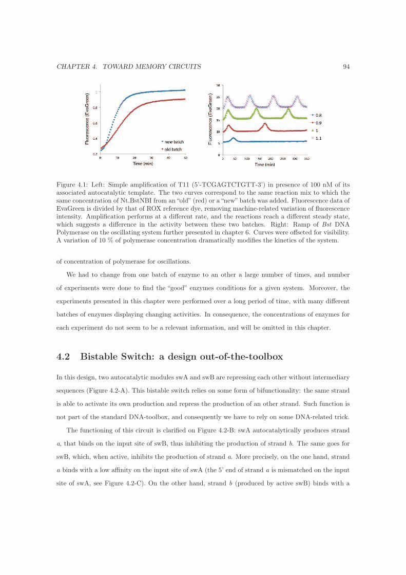
CHAPTER 4. TOWARD MEMORY CIRCUITS 94
Figure 4.1: Left: Simple amplification of T11 (5’-TCGAGTCTGTT-3’) in presence of 100 nM of itsassociated autocatalytic template. The two curves correspond to the same reaction mix to which thesame concentration of Nt.BstNBI from an “old” (red) or a “new” batch was added. Fluorescence data ofEvaGreen is divided by that of ROX reference dye, removing machine-related variation of fluorescenceintensity. Amplification performs at a different rate, and the reactions reach a different steady state,which suggests a difference in the activity between these two batches. Right: Ramp of Bst DNAPolymerase on the oscillating system further presented in chapter 6. Curves were offseted for visibility.A variation of 10 % of polymerase concentration dramatically modifies the kinetics of the system.
of concentration of polymerase for oscillations.
We had to change from one batch of enzyme to an other a large number of times, and number
of experiments were done to find the “good” enzymes conditions for a given system. Moreover, the
experiments presented in this chapter were performed over a long period of time, with many different
batches of enzymes displaying changing activities. In consequence, the concentrations of enzymes for
each experiment do not seem to be a relevant information, and will be omitted in this chapter.
4.2 Bistable Switch: a design out-of-the-toolbox
In this design, two autocatalytic modules swA and swB are repressing each other without intermediary
sequences (Figure 4.2-A). This bistable switch relies on some form of bifunctionality: the same strand
is able to activate its own production and repress the production of an other strand. Such function is
not part of the standard DNA-toolbox, and consequently we have to rely on some DNA-related trick.
The functioning of this circuit is clarified on Figure 4.2-B: swA autocatalytically produces strand
a, that binds on the input site of swB, thus inhibiting the production of strand b. The same goes for
swB, which, when active, inhibits the production of strand a. More precisely, on the one hand, strand
a binds with a low affinity on the input site of swA (the 5’ end of strand a is mismatched on the input
site of swA, see Figure 4.2-C). On the other hand, strand b (produced by active swB) binds with a

CHAPTER 4. TOWARD MEMORY CIRCUITS 95
Figure 4.2: A bistable switch out-of-the-toolbox. (A) Topology of the circuit: two templates (swAand swB) are autocatalytically producing signal molecules (respectively a and b) that directly re-press the activity of the opposite template. (B) Schematic of the reactions for swA (up) and swB(down). For swA, strand a can bind on the input site with a mismatched 5’ end. Through thework of a polymerase and a nickase, it allows the production of another strand a. Strand a canalso bind on the input site of template swB with a mismatched 3’ end, preventing the polymeraseto elongate this substrate. Template swB follows a symmetric scheme. These reactions should en-code for “if a then not b” and “if b then not a”. (C) Stability of the duplexes calculated (Dinamelt)for swA (5’-T*A*G*T*GACTCTGCC-TAGTGACTCTGGG-3’), swB (5’-A*T*G*T*GACTCTGGG-ATGTGACTCTGCC-3’), a (5’-GGCAGAGTCACTA-3’) and b (5’-CCCAGAGTCACAT-3’). Strandb is more stable than strand a on the input site of swA, in order to inhibit the production of a. (D)Calculated time plots of the bistable switch started with {[a], [b]}={1nM, 2nM} (left) and {4nM,1nM} (right). After some transient, the system finds a steady state of production of either a or b (butnot both). These time plots were calculated for a concentration of swA and swB of 20 nM, at 40 °C.
higher affinity than strand a on the input site of swA (Figure 4.2-C). Having its 3’ end mismatched
on swA, strand b is preventing the polymerase from producing strand a from template swA. In this
scheme, we expect strands a and b to be mutually exclusive: at the steady state, either a or b should
be produced, but not both.
A simple model (that did not take the saturation of enzymes into account) with the calculated
(Dinamelt) dissociation constant of a and b on swA and swB predicted that the system would exhibit
a bistable behavior (Figure 4.2-D), provided realistic enzymatic reaction rate, on however a narrow
window of carefully chosen concentrations of templates. Experimentally, we could confirm that b
was inhibiting the activity of swA and a was inhibiting the activity of swB (in the concentrations of
templates and temperature suggested by the model). Assembling the two templates did not, however,
produce the expected bistable behavior. Several hypothesis can be done about this failure:
• the model required precisely balanced concentrations of swA and swB to work, which can be
hard to obtain experimentally, considering an eventual asymmetry of the dissociation rates and

CHAPTER 4. TOWARD MEMORY CIRCUITS 96
enzymatic rates and affinities.
• both templates had 4 phosphorothioate backbone modifications in their 5’ end, and no U in the
output nickase recognition site. We observed later that 3 phosphorothioates were already enough
to dramatically decrease the nicking reaction speed (as discussed in Section 3.7.2.2). Four can
just be worse.
• the autocatalytically produced strands (a and b) are very stable on their output site because
they are matched on both sides (Figure 4.2-C). Thus, at the working temperature, we expect Bst
DNA Polymerase to only work in strand displacement (it has to displace the hybridized output
strand to polymerase a new output strand), making the autocatalytic production reaction slower.
• the relative strength of inhibitor vs activator might not be high enough (only about 5 °C of Tm
difference). Yet, we know that in the case of the oligator, a difference of about 10 °C is required.
It should be possible to address these points, and (maybe) make this bistable circuit work properly.
However, if ever working, it might still be hard to interface this system that uses some particularities
of the oligonucleotides (i.e. the bifunctionality) that are not part of the toolbox and might not be
cascadable or generalizable.
4.3 Bistable circuits with the DNA-toolbox
To construct a bistable with the DNA-toolbox, we selected a symmetric repressor-repressor design,
where two autocatalytic modules repress the activity of each other through two inhibitor modules
(Figure 3.2). We first designed a bistable switch circuit based on the autocatalytic templates of the
oligator designed to work at lower temperature (c11bt, also used in Figure 2.5: 5’-C*T*TAGACTCAG-
CTTAGACTCAG-3’), and another autocatalytic template, c11’ (5’-A*C*TTGACTCTC-ACTTGACTCTC-
3’).
4.3.1 Working with mesophilic RecJf
We started to work using the same enzymes (i.e. Bst DNA Polymerase Large Fragment, Nt.BstNBI
nicking endonuclease and RecJf exonuclease) and buffer as for the original oligator [62]. We designed
the two inhibition modules that make the link between c11bt and c11’, and tried to monitor the
reaction with a TAMRA fluorophore located on the autocatalytic templates, either c11bt or c11’ -
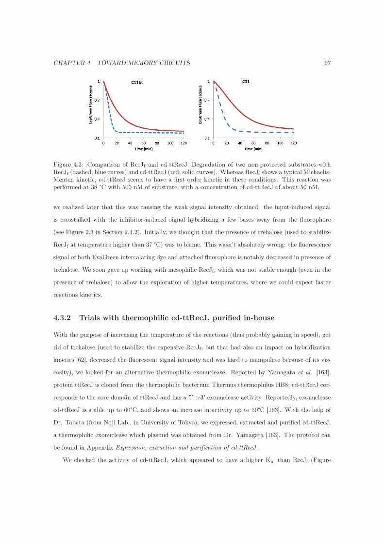
CHAPTER 4. TOWARD MEMORY CIRCUITS 97
Figure 4.3: Comparison of RecJf and cd-ttRecJ. Degradation of two non-protected substrates withRecJf (dashed, blue curves) and cd-ttRecJ (red, solid curves). Whereas RecJf shows a typical Michaelis-Menten kinetic, cd-ttRecJ seems to have a first order kinetic in these conditions. This reaction wasperformed at 38 °C with 500 nM of substrate, with a concentration of cd-ttRecJ of about 50 nM.
we realized later that this was causing the weak signal intensity obtained: the input-induced signal
is crosstalked with the inhibitor-induced signal hybridizing a few bases away from the fluorophore
(see Figure 2.3 in Section 2.4.2). Initially, we thought that the presence of trehalose (used to stabilize
RecJf at temperature higher than 37 °C) was to blame. This wasn’t absolutely wrong: the fluorescence
signal of both EvaGreen intercalating dye and attached fluorophore is notably decreased in presence of
trehalose. We soon gave up working with mesophilic RecJf, which was not stable enough (even in the
presence of trehalose) to allow the exploration of higher temperatures, where we could expect faster
reactions kinetics.
4.3.2 Trials with thermophilic cd-ttRecJ, purified in-house
With the purpose of increasing the temperature of the reactions (thus probably gaining in speed), get
rid of trehalose (used to stabilize the expensive RecJf, but that had also an impact on hybridization
kinetics [62], decreased the fluorescent signal intensity and was hard to manipulate because of its vis-
cosity), we looked for an alternative thermophilic exonuclease. Reported by Yamagata et al. [163],
protein ttRecJ is cloned from the thermophilic bacterium Thermus thermophilus HB8; cd-ttRecJ cor-
responds to the core domain of ttRecJ and has a 5’->3’ exonuclease activity. Reportedly, exonuclease
cd-ttRecJ is stable up to 60°C, and shows an increase in activity up to 50°C [163]. With the help of
Dr. Tabata (from Noji Lab., in University of Tokyo), we expressed, extracted and purified cd-ttRecJ,
a thermophilic exonuclease which plasmid was obtained from Dr. Yamagata [163]. The protocol can
be found in Appendix Expression, extraction and purification of cd-ttRecJ.
We checked the activity of cd-ttRecJ, which appeared to have a higher Km than RecJf (Figure
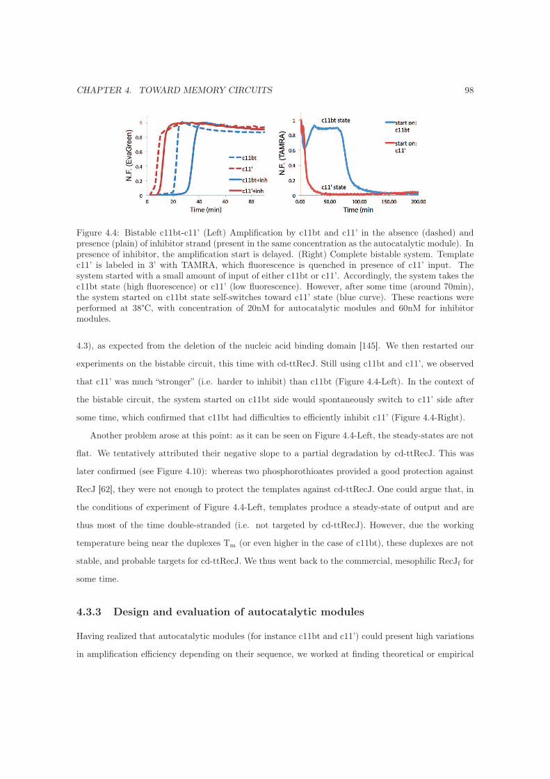
CHAPTER 4. TOWARD MEMORY CIRCUITS 98
Figure 4.4: Bistable c11bt-c11’ (Left) Amplification by c11bt and c11’ in the absence (dashed) andpresence (plain) of inhibitor strand (present in the same concentration as the autocatalytic module). Inpresence of inhibitor, the amplification start is delayed. (Right) Complete bistable system. Templatec11’ is labeled in 3’ with TAMRA, which fluorescence is quenched in presence of c11’ input. Thesystem started with a small amount of input of either c11bt or c11’. Accordingly, the system takes thec11bt state (high fluorescence) or c11’ (low fluorescence). However, after some time (around 70min),the system started on c11bt state self-switches toward c11’ state (blue curve). These reactions wereperformed at 38°C, with concentration of 20nM for autocatalytic modules and 60nM for inhibitormodules.
4.3), as expected from the deletion of the nucleic acid binding domain [145]. We then restarted our
experiments on the bistable circuit, this time with cd-ttRecJ. Still using c11bt and c11’, we observed
that c11’ was much “stronger” (i.e. harder to inhibit) than c11bt (Figure 4.4-Left). In the context of
the bistable circuit, the system started on c11bt side would spontaneously switch to c11’ side after
some time, which confirmed that c11bt had difficulties to efficiently inhibit c11’ (Figure 4.4-Right).
Another problem arose at this point: as it can be seen on Figure 4.4-Left, the steady-states are not
flat. We tentatively attributed their negative slope to a partial degradation by cd-ttRecJ. This was
later confirmed (see Figure 4.10): whereas two phosphorothioates provided a good protection against
RecJ [62], they were not enough to protect the templates against cd-ttRecJ. One could argue that, in
the conditions of experiment of Figure 4.4-Left, templates produce a steady-state of output and are
thus most of the time double-stranded (i.e. not targeted by cd-ttRecJ). However, due the working
temperature being near the duplexes Tm (or even higher in the case of c11bt), these duplexes are not
stable, and probable targets for cd-ttRecJ. We thus went back to the commercial, mesophilic RecJf for
some time.
4.3.3 Design and evaluation of autocatalytic modules
Having realized that autocatalytic modules (for instance c11bt and c11’) could present high variations
in amplification efficiency depending on their sequence, we worked at finding theoretical or empirical

CHAPTER 4. TOWARD MEMORY CIRCUITS 99
rules to design new - potentially better balanced - sequences, and finding a way to evaluate their
performance.
By comparing the melting temperature (Tm) of input sequences
Figure 4.5-Up displays the input sequences and experimental time plots of their amplification performed
by their respective autocatalytic modules, without exonuclease. In this assay, all sequences do not
appear to amplify identically: cS11 seems slower (compared to cZ11 that has a close Tm), cK11
diverges (unknown reason). Only looking at the stability of an input on its autocatalytic template is
not a good way to evaluate its amplification performance.
Turnover experiment
In order to easily evaluate the efficiency of a given autocatalytic module, we introduced the “turnover”
experiment. The idea is to put the autocatalytic module (with polymerase, nickase and exonuclease)
in presence of a given amount of dNTPs, and look at the time it needs to consume them all. As the
autocatalytic module runs out of dNTPs, it cannot sustain the steady state production of input/output:
fluorescence of EvaGreen returns to the baseline level as input/output degraded by the exonuclease
are not replaced by freshly produced ones. Then, using the same enzymatic and buffer conditions
(containing the same concentration of dNTPs) for various autocatalytic modules, we could directly
compare their turnover. Experiments of turnovers for cT11, cP11 and cZ11 are shown on Figure 4.5-
Bottom: not only it reveals different behaviors (cT11 steady-state is never really reached - this will be
discussed later on, in Section 4.6.3), but also allows to calculate the production rate of each templates
in the experiment conditions. For instance, in the case of Z11, the limiting dNTP is G (Figure 4.5-
Left): 5 dGTPs are used for each produced Z11. Thus, with 25 μM of dGTPs initially present, cZ11
can catalyze the production of 5 μM of Z11, that are mostly produced during the steady-state (plateau
of the fluorescence curve). The steady-state is kept for about 55 min in the case of 30 nM cZ11, which
leads to a production rate of roughly 90 nM/min. If the first order degradation rate (k1st) of the
exonuclease is known for this sequence, it is possible to directly extract the concentration of Z11 at
the steady state.
Designing a library of autocatalytic modules using rational “design rules”
We then designed new autocatalytic modules following a few rules, for a sequence Ω11 of 11 bases:

CHAPTER 4. TOWARD MEMORY CIRCUITS 100
Figure 4.5: (Left) Amplified sequences and calculated Tm. (Right) Fluorescence curves of amplification(self-start, i.e. without primer) at 38.5 °C, in the absence of exonuclease. Templates are present inconcentration of 60 nM. (Bottom) Turnovers for cT11, cP11 and cZ11 at 38.5 °C with 25 μM of dNTPs,and three different concentrations of autocatalytic modules.
1. Ω11 has to include the nicking enzyme recognition site.
2. Amplified sequence Ω11 should not end with a G in 3’, which would make an unwanted nickase
recognition site appearing on the inhibition module Ωtoinh? in the case of a 8-6 inhibitor (i.e.
an inhibitor forming 8 base-pairs on the input site and 6 base-pairs on the output site of the
target autocatalytic module).
3. Amplified sequence Ω11 should not end with GA, which would make an unwanted nickase recog-
nition site appearing on the inhibition module Ωtoinh? in the case of a 7-6 inhibitor (that is,
those that we adopted for the final version of the bistable circuit).
4. Ω11 (as well as the corresponding autocatalytic module) should not present any secondary struc-
tures (that could lead to self-triggering in the case of a self-fold with a matched 3’, or other
uncontrolled behaviors) or interactions between two Ω11 (to avoid primer dimer).
5. The melting temperature of Ω11 should be not too high nor too low (i.e. should not be composed
of too many C and G or A and T).
6. For the following sequences, we also avoided double C or double G, in order to limit the sequences
domain to search.
CHAPTER 4. TOWARD MEMORY CIRCUITS 101
Scrutinized sequences are shown on Figure 4.6 and 4.7.
Evaluating the new sequences
Evaluation of the new sequences was done by comparison with a previously designed (and efficiently
amplifying) autocatalytic module: cX11. We first performed a simple amplification (Figure 4.8-Left).
As all sequences seemed to amplify well, we checked their turnover (as defined previously) in presence
of 40 μM dNTPs (Figure 4.8-Right). The application of the few design rules presented before proved
to be successful: all autocatalytic modules amplified correctly (Figure 4.8-Left), contrarily to some of
the ones used in Figure 4.5-Right. These rules were however not sufficient to insure the efficiency of
all sequences: the turnover experiment (Figure 4.8-Right) helps finding out which sequences should be
discarded. To compare the autocatalytic modules, we can calculate their normalized plateau time with
regard to cX11: S = N.TNcX11.TcX11
with N the number of limiting dNTP per polymerized oligonucleotide
and T the plateau time. This gives ScW11 = 0.73 , ScE11 = 0.86, ScR11 = 0.87, ScX11 = 1, ScN11 =
1.21, ScD11 = 2.66. In the present case, one might want to avoid working with cD11 (which is slow)
or cR11 (which shows a tilted plateau).
Sequence dependence of DNA exponential amplification (EXPAR [105]) is still not well understood,
but has been the subject of a recent study [158], in which the Qian et al. characterized the performance
of about 400 templates. They notably observed that GA or AG dimers-rich sequences were poorly
performing. Interestingly, one of our “strongest” autocatalytic template (cP11, see Figure 4.5) has very
few AG dimer (i.e. a lot in the amplified sequence, as displayed in Figure 4.5). For future design of
autocatalytic templates, one may consider including the rules proposed by Qian et al. [158].
4.3.4 Design rules for inhibitors
Inhibitor strands are referred to as inhΩ11-ab where “Ω” is the autocatalytic module targeted, “a”
is the number of bases that will bind on the input site of the target template, and “b” the number
of bases that will bind on the output site. For instance, inhT11-76 targets cT11 and binds with 7
bases on its input site and 6 bases on its output site. Inhibitors should be more stable than inputs
in order to block autocatalytic modules. Montagne et al. [62] proposed that the Tm of an inhibitor
should be about 10 °C higher than that of the target input, which was the case for the oligator. In
the case of a bistable circuit, the importance of the inhibitor binding strength can be deduced from
the analysis of a simple model of the circuit (as described in Section 3.7.3.1). Roughly speaking, the

CHAPTER 4. TOWARD MEMORY CIRCUITS 102
Figure 4.6: Designing autocatalysts (first part). Sequences were chosen following the previously definedrules (xxxxx indicates the nickase recognition site, GACTC). All sequences were scanned to discard theones presenting too stable (or “dangerous”, such as a hairpin with a matched 3’) secondary structures(checked with Nupack). Among the remaining sequences, a few were chosen, after making sure thatthe Tm of the amplified sequence was between 37 and 39 °C (calculated with DinaMelt).

CHAPTER 4. TOWARD MEMORY CIRCUITS 103
Figure 4.7: Designing autocatalysts (second part).

CHAPTER 4. TOWARD MEMORY CIRCUITS 104
Figure 4.8: Evaluation of new autocatalytic modules (20 nM, 43°C). (Left) Amplification (self-start).All sequences seem to perform amplification efficiently. (Right) Turnovers in presence of 40 μM dNTPs.Limiting dNTP for each template (and number per polymerized oligo): cD11: G(5), cE11: G(4), cN11:A(4), cR11: G(4), cW11: A and G (4), cX11: A (4). Despite consuming more of the same dNTP perpolymerized oligo, template cD11 is by far the slowest. Template cR11 presents a tilted plateau: it isnever really flat.
stronger the inhibitors are, the larger will the bistability domain be. However, too strong inhibitors
are likely to impact the dynamic of the circuit: we are looking for an efficient dynamic inhibition to
insure a good responsiveness of the circuit. They would also result in a break-down of the hypothesis
of fast equilibrium used to build the simple model (see Section 3.7.3.1).
In the context of the DNA-toolbox, inhibitors must also meet two sequence requirements:
1. They must possess two 3’ mismatched bases to prevent the polymerase from extending them as
they are hybridized on their target template.
2. They should not present the nickase recognition site, which might lead to disastrous experiments
(Figure 4.9): as a consequence, inhibitors cannot cover more than 8 bases on the input site of
the target template, and 6 bases on the output site.
In an attempt to make stronger inhibitors that would not have the nickase binding site, we tried to
include a mismatch on the output-binding section of the inhibitor: this would allow us to have inhibitors
covering more that 6 bases on the output site of the target template, presenting a mismatch in the
nickase recognition site, which we hypothesized to be enough to distract the nickase from binding to the
mismatched substrate. In practice, the designed inhibitors were targeting cP11, which later appeared
to be a “too strong” autocatalytic module: these mismatch-bearing inhibitors did not work against it.
4.3.5 Trials with unbalanced autocatalytic modules
We tried to build bistable circuits with the autocatalytic modules of Figure 4.5-Bottom: cT11, cP11 and
cZ11. All three circuits (T-P, T-Z and P-Z) resulted in systems that would eventually set in one single

CHAPTER 4. TOWARD MEMORY CIRCUITS 105
Figure 4.9: Forbidden inhibitors. (Left) Sequence of P11 and three associated inhibitors: inhP11-67and inhP11-77 have the nickase recognition site (in bold). (Right) Turnover of cP11 (15 nM) alone or inpresence of 30 nM of inhP11-67 or inhP11-77 protected against degradation by ttRecJ. The experimentis run at 42 °C with 50 μM dNTPs. In presence of inhibitors that have the nickase recognition site,the reaction produces an unexplained fluorescence trajectory.
Figure 4.10: Degradation of template c11bt (400nM, 43°C) with 1, 2, 3 and 4 phosphorothioates(pt). Fluorescence intensity of EvaGreen was divided by that of ROX (1x) reference dye, then dividedby the fluorescence of the corresponding template in absence of exonuclease. Still, fluorescence levelare not perfectly quantitatively comparable, as 0 does not correspond to 0nM of template remaining.(Left) Degraded by ttRecJ (15% of 1/160). Templates with one and two phosphorothioates are quicklydegraded. (Right) Degraded by cd-ttRecJ (10%), which behaves quite differently. Interestingly (andunexpectedly), 2pt provide a better protection than 3pt. Also, 2pt and 4pt curves have similar profiles.
state, suggesting a lack of balance between the autocatalytic modules. These failures were also probably
due to other problems unrecognized at that time. We were still working with the commercial RecJf,
usually at temperature as low as 38.5 °C, using EvaGreen that was stabilizing duplexes, and trehalose
that was probably slowing down the hybridization kinetics [62]. It is possible that these conditions
were increasing the already important gap between the sequences amplification performances. We
realized later that cP11 as well as cZ11 were virtually unstoppable in the concentrations then used
(>20 nM), even at higher temperatures.

CHAPTER 4. TOWARD MEMORY CIRCUITS 106
original new
exonuclease RecJf ttRecJtemperature up to 40 °C up to 50 °C
stabilizing agentstriton X-100 (0.1 %), trehalose(400mM), BSA (0.1 mg/ml)
synperonic (0.1 %),BSA (0.1 mg/ml)
product inhibition bythe nicking enzyme
strong less
monitoring EvaGreen (non-specific)N-quenching (sequence-specific),
EvaGreen (non-specific)
template modifications5’: 2 phosphorothioates,
3’: phosphate5’: 3 phosphorothioates,
3’: fluorophore or phosphateinhibitors 8-6 7-6
Table 4.1: Status of the DNA-toolbox. The use of thermophilic ttRecJ allows to increase the temper-ature, and get rid of trehalose. Product inhibition: the use of a dU in the output site of the nickaserecognition site decreases the affinity of the nickase for this site (where it would bind without havinganything to cut, thus hindering the melting of the output). Monitoring: N-quenching allows to moni-tor the reactions in a sequence-specific manner, which was not possible with EvaGreen. Inhibitor: weadopted inhibitor 7-6 (with 7 bases hybridizing to the input site, and 6 bases hybridizing to the outputsite of the target template) instead of 8-6. While still efficiently inhibiting, shorter inhibitors (i.e. lessstable), allow a faster recovery of the target template from inhibition.
4.3.6 Working with a new thermophilic exonuclease: full-length ttRecJ
The purified full-length ttRecJ was a kind gift from Dr. Masui (Osaka university), and worked like a
charm. Exonuclease ttRecJ proved to be extremely stable, and seemed perfectly usable for our DNA
reaction circuits. It however brought a disturbing surprise: the two 5’ phosphorothioate backbone
modifications that provided a good protection against RecJf were not enough against ttRecJ (Figure
4.10-Left). Luckily, 3 or 4 phosphorothioates seemed better, as opposed to cd-ttRecJ for which 3 were
worse than 2 (Figure 4.10-Right, still unexplained).
We consequently ordered autocatalytic templates with 3 phosphorothioates instead of 2, but soon
found out that these were performing poorly compared to the ones with only 2 phosphorothioates.
These results and the solution to this issue are presented in Section 3.7.2.2. Once this problem was
solved, we adopted ttRecJ and redesigned our reaction circuits in order to work with this enzyme,
potentially at a higher temperature. At this point, the DNA-toolbox had evolved quite a bit (Table
4.1): we kept this status for the rest of this study.
4.3.7 On balancing the bistable circuit
Even carefully designed autocatalytic modules with very close Tm are far from being perfectly balanced:
some show a better amplification performance than others. The present symmetric design of bistable

CHAPTER 4. TOWARD MEMORY CIRCUITS 107
circuit however requires well balanced nodes: as seen in Figure 4.4-Right, two autocatalytic modules
of very different strength will result in a monostable rather than bistable system. Consequently, we
set out on searching for a way to quantify and compensate these differences, in the context of the
chemistry at hand (including buffer, temperature and enzyme conditions).
A first idea - given a working temperature and enzymes concentrations - was to use the turnover
experiment (see Figure 4.8), on the two autocatalytic modules, or on the two “semi-switches” (autocat-
alytic module + inhibition module), for ramps of concentration of autocatalytic module or inhibition
module. We would then select the concentrations for which the two sides were consuming dNTPs at
the same rate. The problem with this strategy is that it would not take in account a factor that is
critical for a proper balancing: the strength of inhibitors on their target autocatalytic module (i.e.
the inhibition strength). Still, such experiments revealed the “charge” or “load” effect (as shown by
Franco et al. [71] for a genelet-based circuit that has to “load” a downstream process): the greater the
concentration of inhibition module was, the slower the system was to consume dNTPs (i.e. the weaker
was the autocatalytic module that had to charge the following inhibition module, see also Section
4.7.2).
Another idea was to inhibit the semi-switches by using phosphorothoiated inputs (thus protected
from the exonuclease) to charge the inhibiting inhibition module, that would consequently produce a
steady amount of inhibitor (Figure 4.11-A and B). This would have been an elegant method to evaluate
the strength of the fully-charged inhibition module, and select its concentration so that the targeted
autocatalytic module would be (just) inhibited. It actually did not work: phosphorothioated inputs
were not able to activate the production of inhibitors efficiently (Figure 4.11-C). This may be due to
the phosphorothioate backbone modifications, which, as discussed in Section 3.7.2.2, are hampering
the work of the nickase: if the nickase is slowed down, the production of inhibitor is also slowed down,
which will result in a weaker inhibition of the target template. We tried to use phosphorothioated
inputs with longer 5’ end, in order to move the phosphorothioates away from the nickase recognition
site: this only had a (too) small positive impact. Consequently, this method was not deemed viable to
balance the bistable circuit.
4.3.7.1 First: charge and inhibit to balance
The next strategy was motivated by the idea of taking in account both the load on the autocatalytic
modules and the relative strength of inhibitors, while trying to have a system as sensitive as possible
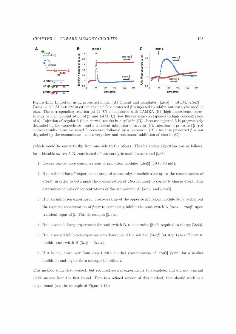
CHAPTER 4. TOWARD MEMORY CIRCUITS 108
Figure 4.11: Inhibition using protected input. (A) Circuit and templates. [αtoα] = 10 nM, [αtoiβ] =[βtoiα] = 30 nM. 250 nM of either “regular” β or protected β is injected to inhibit autocatalytic moduleαtoα. The corresponding reaction (at 42 °C) is monitored with TAMRA (B) (high fluorescence corre-sponds to high concentration of β) and FAM (C) (low fluorescence corresponds to high concentrationof α). Injection of regular β (blue curves) results in a spike in (B) - because injected β is progressivelydegraded by the exonuclease - and a transient inhibition of αtoα in (C). Injection of protected β (redcurves) results in an increased fluorescence followed by a plateau in (B) - because protected β is notdegraded by the exonuclease - and a very slow and continuous inhibition of αtoα in (C).
(which would be easier to flip from one side to the other). This balancing algorithm was as follows,
for a bistable switch A-B, constituted of autocatalytic modules αtoα and βtoβ:
1. Choose one or more concentrations of inhibition module: [αtoiβ] (10 to 30 nM).
2. Run a first “charge” experiment (ramp of autocatalytic module αtoα up to the concentration of
αtoiβ), in order to determine the concentration of αtoα required to correctly charge αtoiβ. This
determines couples of concentrations of the semi-switch A: [αtoα] and [αtoiβ].
3. Run an inhibition experiment: create a ramp of the opposite inhibition module βtoiα to find out
the required concentration of βtoiα to completely inhibit the semi-switch A (αtoα + αtoiβ) upon
transient input of β. This determines [βtoiα].
4. Run a second charge experiment for semi-switch B, to determine [βtoβ] required to charge [βtoiα].
5. Run a second inhibition experiment to determine if the selected [αtoiβ] (at step 1) is sufficient to
inhibit semi-switch B (βtoβ + βtoiα).
6. If it is not, start over from step 1 with another concentration of [αtoiβ] (lower for a weaker
inhibition and higher for a stronger inhibition).
This method somewhat worked, but required several experiments to complete, and did not warrant
100% success from the first round. Here is a refined version of this method, that should work in a
single round (see the example of Figure 4.12):
CHAPTER 4. TOWARD MEMORY CIRCUITS 109
1. For 10 nM and 20 nM concentrations of inhibition module, run the “charge” experiment, with a
ramp of autocatalytic module αtoα or βtoβ (Figure 4.12-A).
2. Pick one or more couple of [αtoα] and [βtoβ] that take about the same time to charge their
inhibition module.
3. For these concentrations of αtoα and βtoβ, do an inhibition experiment with a ramp of inhibition
module (Figure 4.12-B).
4. Pick concentrations of inhibition module αtoiβ and βtoiα that inhibit the opposite autocatalytic
module for about the same laps of time.
5. Assemble the bistable circuit.
This refined method worked well, yielding a balanced bistable circuit in two experiments. A remaining
problem was that the first charge experiment was done with a fixed concentration (10 or 20 nM) of
inhibition module: we have seen that after balancing, it is likely that the chosen concentration of
inhibition module will be different. If, for instance, an autocatalytic module has less inhibition module
to charge, it will become “stronger” (see Section 4.7.2), i.e. harder to inhibit, which would then require
an increased concentration of the opposite inhibition module, further de-balancing the system.
4.3.7.2 Second: inhibit to balance
We then searched for an even simpler way to balance the circuit: a single experiment that would point
out the concentrations of the four templates at once. With the insights from previous experiments,
we were aware of the load problem: basically, if an autocatalytic module has too much downstream
templates to charge, it gets weaker. Having too much to load will also negatively affect its resilience
against inhibition. The idea for this new balancing strategy was that if we were fixing the two con-
centrations of inhibition modules, the only fact of changing the autocatalytic modules concentrations
would be enough to balance both sides, while taking in account the load effect. All this, of course, for
sequences balanced as much as possible at the design level:
1. Set the same concentrations for the two inhibition modules [αtoiβ] and [βtoiα] (20 nM should be
enough)
2. Run in parallel these two symmetrical experiments, with [αtoiβ] = [βtoiα] = 20 nM: (i) ramp of
[αtoα] from 5 to 20 nM (no βtoβ) with a starting [α] = 1 nM, (ii) ramp of [βtoβ] from 5 to 20 nM

CHAPTER 4. TOWARD MEMORY CIRCUITS 110
Figure 4.12: Balancing a bistable circuit. Here, we use a different β: 5’-CAGAGTCCAAG-3’ whichproduces a negative fluorescence change as it hybridizes on the dy636-modified βtoiα. (A) Chargeof inhibition modules (20 nM) αtoiβ (up) or βtoiα (down) by respectively αtoα or βtoβ (ramp ofconcentration from 2 to 16 nM). In this system, 12 nM of αtoα seems to charge αtoiβ in the sameamount of time as 6 nM of βtoβ charges βtoiα. (B) Inhibition of αtoα (12 nM, up) or βtoβ (6 nM,down) by a ramp of concentration (from 8 to 20 nM) of the opposite inhibition module (respectivelyβtoiα and αtoiβ). Here, 10 nM of βtoiα inhibits αtoα for the same time as 20 nM of αtoiβ inhibits βtoβ.The concentrations to assemble this bistable circuit should then be [αtoα] = 12 nM, [βtoβ] = 6 nM,[αtoiβ] = 20 nM and [βtoiα] =10 nM. Reaction were performed at 43 °C, and started with 1 nM ofinput (either α or β)

CHAPTER 4. TOWARD MEMORY CIRCUITS 111
(no αtoα) with a starting [β] = 1 nM. The samples with concentrations of autocatalytic module
that are too low won’t reach the steady state before a long time (or might just fail to charge
their inhibition module): they should be discarded. When the steady state of production of α
or β is reached, inject 30 nM of the opposite input (respectively β or α), that will activate the
inhibition of the active autocatalytic module. This experiment will lead to fluorescence curves
similar to the ones of Figure 4.12-B: this time, low concentrations of autocatalytic module are
more strongly inhibited by the same concentration of inhibition module. Remains to choose the
concentrations of autocatalytic module αtoα and βtoβ that are inhibited for a moderate (and
similar) amount of time (i.e. that almost get fully inhibited, but manage to restart and find back
their steady state after that).
3. Then, the four concentrations are determined, and the full circuit is ready to be assembled.
This simplified balancing method proved to work nicely: by considering the system at a higher level
(i.e. by considering the bistable circuit as made of two “semi-switches” with an inhibitory link, rather
than made of four modules with complex interactions), we could abstract the parameters that are hard
to balance (in this case, the load problem, see Section 4.7.2), and easily - in a single step - fix the
concentrations of all modules. Note that in the case of sequences known to be unbalanced, starting
with asymmetric concentrations of inhibition module (i.e. lowering the one that is targeting a weaker
autocatalytic module) can prove to be fruitful.
4.4 On switching the bistable: switchable memory circuit
With a bistable circuit constructed and well balanced, the next step would be to give it the ability to
be updated. We explored different methods to flip the bistable between states, eventually adopting a
DNA-toolbox made solution.
4.4.1 Direct injection of inputs
As described in Sections 3.4.3 and 3.7.3.5, the bistable circuit is robust to perturbation in its input
concentration. It should however be possible to force it in one state or the other by successive injections
of α or β, given that both sides of the bistable circuit (shown again on Figure 4.13-A) are well balanced.
Managing to flip the bistable circuit with this brute-force method would also be a proof that it is
possible to update the memory held by the circuit. In the experiment of Figure 4.13-B and C, three

CHAPTER 4. TOWARD MEMORY CIRCUITS 112
Figure 4.13: Switching the bistable circuit. (A) Bistable circuit and templates. (B) Switching from Ato B and (C) from B to A. This experiment was run at 42 °C, with [αtoα] = 10 nM, [βtoβ] = 20 nM,[αtoiβ] = [βtoiα] =20 nM. The system was administered three shots of 80 nM of α or β before it wouldeventually switch between states.
successive injections of, respectively, β (to switch from A to B) or α (to switch from B to A) were
required to force the flipping of the bistable circuit. For the bistable circuit in state A: the first
injection of β primes the inhibition of αtoα, the second injection continues to inhibit αtoα, and the
third injection allows βtoβ to restart, and maintain the inhibited state of αtoα: the bistable circuit has
switched from {A, B} = {ON, OFF} to {OFF, ON}.
This was however far from being practical, and for sure incompatible with the idea of building
larger reaction circuits in which the bistable would be a sub-unit. As a matter of fact, the required
concentration of input is far larger than what the bistable circuit itself is capable to deliver: the
homogeneity between input and output concentrations is lost, and so is the modularity of the bistable
circuit.
4.4.2 “Super-inputs”
Consequently, we set on finding a method to switch the bistable memory with a “single shot” of dilute
DNA input. We would need to give a chance to the inhibited autocatalytic modules to get rid of the
inhibitor blocking them, so that they would start again. To this end, we introduced super inputs, which
are super-strong versions of the inputs of the bistable circuits: α and β. Super inputs are two bases
longer than inputs. With these two additional 5’ C or G, they bind about as strongly as inhibitors
on the input site of the autocatalytic module, which itself has two additional 3’ bases to receive them
(Figure 4.14-B). Moreover, these additional two bases make them having a 6-bases long toehold to
efficiently displace the hybridized inhibitors (Figure 4.14-C).
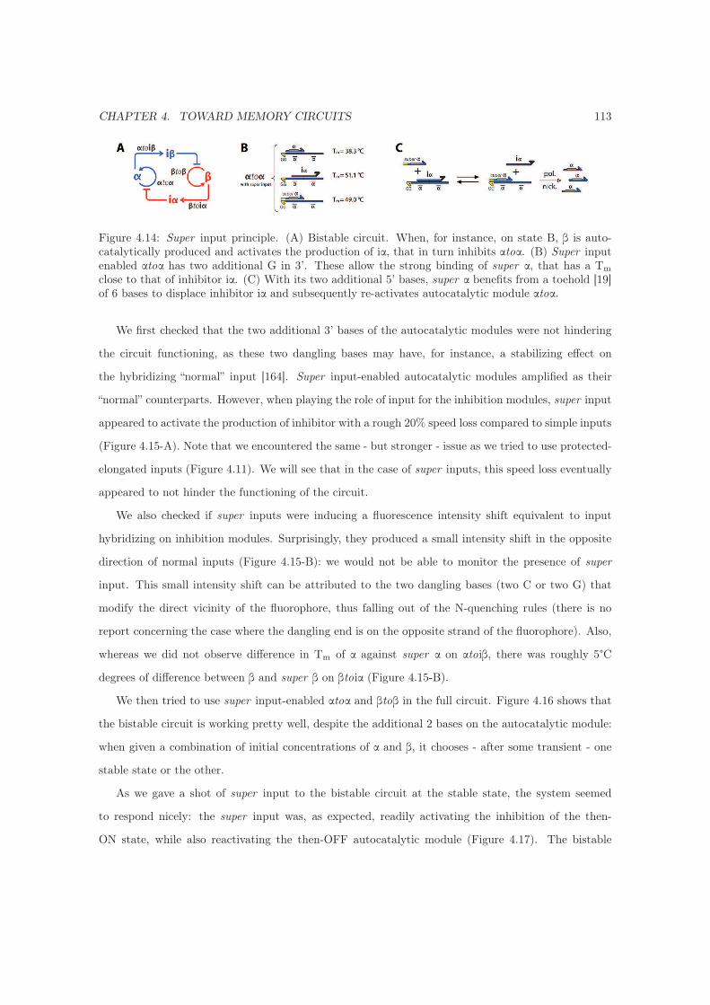
CHAPTER 4. TOWARD MEMORY CIRCUITS 113
Figure 4.14: Super input principle. (A) Bistable circuit. When, for instance, on state B, β is auto-catalytically produced and activates the production of iα, that in turn inhibits αtoα. (B) Super inputenabled αtoα has two additional G in 3’. These allow the strong binding of super α, that has a Tm
close to that of inhibitor iα. (C) With its two additional 5’ bases, super α benefits from a toehold [19]of 6 bases to displace inhibitor iα and subsequently re-activates autocatalytic module αtoα.
We first checked that the two additional 3’ bases of the autocatalytic modules were not hindering
the circuit functioning, as these two dangling bases may have, for instance, a stabilizing effect on
the hybridizing “normal” input [164]. Super input-enabled autocatalytic modules amplified as their
“normal” counterparts. However, when playing the role of input for the inhibition modules, super input
appeared to activate the production of inhibitor with a rough 20% speed loss compared to simple inputs
(Figure 4.15-A). Note that we encountered the same - but stronger - issue as we tried to use protected-
elongated inputs (Figure 4.11). We will see that in the case of super inputs, this speed loss eventually
appeared to not hinder the functioning of the circuit.
We also checked if super inputs were inducing a fluorescence intensity shift equivalent to input
hybridizing on inhibition modules. Surprisingly, they produced a small intensity shift in the opposite
direction of normal inputs (Figure 4.15-B): we would not be able to monitor the presence of super
input. This small intensity shift can be attributed to the two dangling bases (two C or two G) that
modify the direct vicinity of the fluorophore, thus falling out of the N-quenching rules (there is no
report concerning the case where the dangling end is on the opposite strand of the fluorophore). Also,
whereas we did not observe difference in Tm of α against super α on αtoiβ, there was roughly 5°C
degrees of difference between β and super β on βtoiα (Figure 4.15-B).
We then tried to use super input-enabled αtoα and βtoβ in the full circuit. Figure 4.16 shows that
the bistable circuit is working pretty well, despite the additional 2 bases on the autocatalytic module:
when given a combination of initial concentrations of α and β, it chooses - after some transient - one
stable state or the other.
As we gave a shot of super input to the bistable circuit at the stable state, the system seemed
to respond nicely: the super input was, as expected, readily activating the inhibition of the then-
ON state, while also reactivating the then-OFF autocatalytic module (Figure 4.17). The bistable

CHAPTER 4. TOWARD MEMORY CIRCUITS 114
Figure 4.15: Super input and inhibition modules. In these two experiments, we compare the produc-tion of inhibitor by “normal” input and “super” input, in absence of exonuclease. (A) Production ofinhibitor by inhibition module αtoiβ (left) and βtoiα (right). The reaction is monitored with EvaGreenintercalating dye. Inhibition modules (60 nM) are put in presence of 100 nM of input or super input.In the absence of exonuclease, there is a first step of production with a rapid increase of fluorescencecorresponding to formation of stable duplex “inhibition module : inhibitor” followed by a second step(slow increase of fluorescence) where the polymerase works in strand-displacement: we can observe theaccumulation of single stranded inhibitor in solution. (B) Melting the duplex (50 nM) “α : αtoiβ” (left)or “β : βtoiα” (right) reveals the fluorescence change upon separation of the duplex (hence opposite tothe fluorescence change upon hybridization). Curves show the fluorescence change per degree for theattached fluorophore of the corresponding inhibition module. The highest (or lowest) value roughly(but not exactly) corresponds to the Tm of the duplex.

CHAPTER 4. TOWARD MEMORY CIRCUITS 115
Figure 4.16: Matrix of initial concentrations of α and β on the super input-enabled bistable circuit.The experiment is only observed through the Tamra channel: high steady-state corresponds to βtoβON (and αtoα OFF) and baseline level corresponds to βtoβ OFF (and αtoα ON). As in Figure , it showsthe basins of attraction of both states. Concentrations of templates are as follows [αtoα] = [βtoβ] = 10nM, [αtoiβ] = [βtoiα] =20 nM

CHAPTER 4. TOWARD MEMORY CIRCUITS 116
Figure 4.17: Flipping the switch with super input. (A) Bistable circuit and templates: αtoα hastwo G (and βtoβ, two C) in 3’ to receive its super input. Fluorescence of TAMRA (B) and tye 665(C), respectively monitoring β (high fluorescence corresponds to high [β]) and α (low fluorescencecorresponds to high [α]). The same reaction mix is initiated with either α (red curve) or β (blue curve).At t = 150 min, an injection of 30 nM of either super α or β triggers the switching process. The systeminitially in state B (blue curve) flips to the A state: fluorescence of TAMRA decreases (inhibition ofβtoβ), that of tye 665 also decreases (reactivation of αtoα). However, the system initially in state A(red curve) doesn’t flip to state B, but seems to end up in an alternate state where both αtoα and βtoβare partially active. At t = 300 min, an injection of super β confirms that the system is not responsiveanymore.
circuit seemed to have flipped from one side to the other. When trying to switch backwards, however,
the bistable circuit did not behave as expected, and ended up in an intermediate state with both
states half active -which is of course forbidden by the bistable topology of the circuit. In other word,
once flipped using super inputs, the bistable circuit was somewhat stuck in a “super activated” state.
We tentatively attributed that to the slow melting of super inputs, which, once hybridized to the
autocatalytic modules, might not move much: the system is not responsive anymore. This system
might benefit from running at a higher temperature (it was only tried at 39 °C), where super input
should still be stable enough to do there job, while being unstable enough to eventually melt and be
digested by the exonuclease.
4.4.3 “Input-makers”
Our next attempt, and also the most successful, came straight out of the DNA-toolbox. It consisted
in using an activation module (say, xtoy), that would amplify an exogenous spike of its input (x) into
a long lasting pulse of its output (y). The latter would simply be connected to the bistable circuit (y
= α or β), stimulating the OFF side of the bistable to make it switch ON. More details are given in
Section 3.4.4. By connecting two activation modules to the two nodes of the bistable circuit, it became
a two-input switchable memory circuit, able to be switched from one state to the other, and directly
CHAPTER 4. TOWARD MEMORY CIRCUITS 117
connectable to other circuits made with the DNA-toolbox.
4.5 Modeling of the circuit
Mathematical modeling of the bistable circuit is explained in details in Section 3.7.3, for both “simple”
and “detailed” models. Construction of the detailed “realistic” model requires various parameters that
can be classified in two categories: oligonucleotides hybridization parameters and enzymes parameters.
In this section are presented the techniques used to determine these parameters.
4.5.1 DNA melting experiment
Each input and inhibitor has a different dissociation constant: as mentioned in Section 3.7.3.4, it
is possible, in the context of the DNA-toolbox, to obtain a very good computational estimate (for
instance using DINAMelt, knowing the concentrations of DNA strands and cations Mg2+ and Na+) of
the dissociation constant of each species. Nonetheless, chances are that the real value departs from the
computed one. Luckily, dissociation constants are easy to measure by doing a DNA melting experiment.
This experiment consists in putting two complementary strands in stoichiometric concentrations (in
the case of two separate strands, the melting temperature depends on the concentration of species) in
the desired buffer (in our case, the reaction buffer without dNTPs), anneal them, then “melt” them
by slowly increasing the temperature while measuring the absorbance at 260 nm: denaturation of a
duplex is accompanied by an increase of absorbance of about 15 to 20% (hyperchromism). We want to
be slow enough to leave time to the sample to reach the thermodynamic equilibrium between duplex
/ simplex, but avoid staying too long at high temperature (evaporation + DNA depurination).
As an example, we will take the melting temperature of the inhibitor of c11bt (inhbt3) on c11bt,
with and without EvaGreen intercalating dye. Curves were acquired with a V600bio spectrophotometer
(Jasco), with 1 μM of each oligonucleotide, in the reaction mix without dNTPs nor enzymes (total
volume: 700 μL), a stirrer (600 rpm), temperature sensor in the cell, which was closed with Parafilm
to avoid evaporation:
1. Denature: sample is brought to 50 °C.
2. Anneal: from 50 °C to 20 °C (slope: 2 °C / min). Low temperature: watch out for condensation!
3. Melt: from 20 °C to 80 °C (slope 0.6 °C / min). High temperature: watch out for evaporation!
CHAPTER 4. TOWARD MEMORY CIRCUITS 118
4. Plot raw curves (temperature in K). Extract upper (simplex) and lower (duplex) linear baselines
(Figure 4.18-A).
5. Plot the fraction of hybridized oligonucleotides: θ = baseline(simplex)−absorbance
baseline(simplex)−baseline(duplex) as a function
of the temperature in Kelvin (Figure 4.18-B).
6. Select 0.03 < θ < 0.97 and calculate the constant of affinity Ka = θ[concentration(Mol)].(1−θ)2 .
7. Plot ln(Ka) as a function of 1Temperature(K) (Figure 4.18-C).
8. Then we have the Gibbs Free Energy ΔG = −R.T.ln(Ka) = ΔH − T.ΔS which lead to the
following linear fit: slope = −∆H/R and Y intercept = ∆S/R with R = 1.985 cal/K/mol.
In the present case, we find with EvaGreen ΔH = -101 kcal/mol and ΔS = -284 cal/K/mol. Without
EvaGreen, ΔH = -119 kcal/mol and ΔS = -342 cal/K/mol.
Additional points of interest:
• Association rates: they are roughly constant for all oligonucleotides (inputs and inhibitors) used
in the context of the DNA-toolbox [62]. As detailed in Section ??, we used a single association
rate ka = 0.06 nM-1.min-1for mathematical modeling of reaction circuits.
• Derivative: the maximal value of the first derivative (is close to but) usually doesn’t correspond
to the Tm of the duplex, except for intramolecular denaturation (i.e. internal structure / self-
folding / hairpin). The Tm can however be accurately calculated from the extracted ΔH and ΔS
with the following formula: Tm(°C) = ∆H∆S+R.ln([oligo]) −273.15. Which, in the present case, leads
to a Tm of 46.5 °C with EvaGreen, and 45.0 °C without: this confirms that EvaGreen stabilizes
the duplexes.
• Stability: the most stable structure at a given temperature is not the one that has the highest
Tm, but the one that has the lowest ΔG at that temperature.
4.5.2 Enzymes kinetic parameters
In the context of the DNA-toolbox, enzyme kinetics can be satisfyingly described by the Michaelis-
Menten model. It is an approximation of the multi-step reaction that happens between an enzyme and
its substrate: for instance, an exonuclease first binds to its substrate, then cleaves nucleotides one by
one (for the construction of the simple model in Section 3.7.3.1, we further simplified the amplification

CHAPTER 4. TOWARD MEMORY CIRCUITS 119
Figure 4.18: Melt curve analysis of c11bt and its inhibitor. (A) Raw melt curve with and withoutEvaGreen. (B) Fraction of hybridized duplex as a function of the temperature. (C) The linear fit ofthese two lines contains ΔH and ΔS of the reaction.
mechanism - catalyzed by the polymerase and the nickase - in a single Michaelis-Menten equation).
Enzymes can have different rate and Michaelis-Menten constant for each substrate. These can be
experimentally measured by setting up a specific assay for each enzyme. By fitting the integrated form
of Michaelis-Menten equation to the experimental curves, one can extract kenz (Michaelis rate) and
Km (Michaelis constant) for a given substrate, in a given buffer, at a given temperature, given that the
measured enzymatic reaction is actually the rate-limiting reaction. In the case of first-order kinetics,
an exponential fit will give the k1st = kenz/Kmof the enzyme in given conditions.
4.5.2.1 Exonuclease parameters
The kinetic parameters of ttRecJ are the easiest to measure. One has to put the target signal species
(input or inhibitor) in presence of EvaGreen and a low concentration of ttRecJ, and monitor the de-
creasing fluorescence of EvaGreen that is due to the hydrolysis of target single-stranded species (Figure
4.19). Then plot the Time t (min) as a function of the Fluorescence x, and fit the integrated Michaelis-
Menten equation: − 1Vm
(
xr− [oligo] +Km.ln
(
xr.[oligo]
))
with r corresponding to the fluorescence units
per mole of oligonucleotide, and [oligo] the initial amount of oligonucleotide in mole.
4.5.2.2 Nickase parameters
The kinetic parameters of Nt.BstNBI can be measured for each template (activation, autocatalytic
and inhibition modules) using the following assay. The principle is to have a given amount of double-
stranded uncut substrate for the nickase, that will be cut and will consequently melt away. The two
separated signal strands will then be degraded by the exonuclease (and the template stays intact, see
Figure 4.20-A). The sine qua non is that the reaction is set up so that the cutting step is the rate-

CHAPTER 4. TOWARD MEMORY CIRCUITS 120
Figure 4.19: Digestion of (A) 2 μM of input t11 (blue) or v11 (red) and (B) 500 nM of inhT11-76(blue) or inhV11-76 (red), at 42 °C, with 1x EvaGreen and 0.4 % of ttRecJ/160. Baseline removed.
limiting step. This requires: a high concentration of exonuclease (so that as soon as they are cut and
melt, signal strands are degraded) and a low concentration of nickase (so that it does not cut faster
than the rate of the other reactions -melting and degradation). Figure 4.20-B shows curves for three
different concentrations of Nt.BstNBI. In order to make sure that we are looking at what we want, an
idea is to check the linear portion of the different curves: if the cutting reaction is the rate-limiting
one, then the slope should be double for a double concentration of nickase. This is what we can observe
in the inset of Figure 4.20-B for the red (0.05 % of Nt.BstNBI) and the green (0.025 % of Nt.BstNBI)
curves. These two can thus be used to fit the integrated Michaelis-Menten equation (as presented in
the previous section). This is not the case for the blue (0.1 % of Nt.BstNBI), which slope is not twice
that of the red curve: the cutting step might be too fast compared to the dissociation-degradation step
(or substrate inhibition may occur and slow down the nicking enzyme).
4.6 Stability on the long-term
Because we are working in a closed system, each experiment has a limited lifetime (typically driven by
the initial amount of dNTPs). Also, various reaction parameters are modified over time: enzymes can
loose activity, templates can be degraded and so on. These issues are discussed in Section 3.7.6; here
we present a few additional results to flesh out the discussion about the stability on the long-term of
circuits made with the DNA-toolbox in a closed setup.

CHAPTER 4. TOWARD MEMORY CIRCUITS 121
Figure 4.20: Measuring Nt.BstNBI parameters for cT11. (A) Schematic of the reaction: the templateand its complementary strand are initially hybridized. The nickase cuts the complementary strandin its middle, and since the two products are shorter, they melt and are then digested by ttRecJ,resulting in a decrease of fluorescence of EvaGreen. The presence of a U in the output site of thetemplate prevents the nickase to stick to it, which would hinder the melting of the output strand. (B)Experiment for cT11 (100 nM) with its complementary (110 nM) at 42 °C. Exonuclease is in excess(4 % of ttRecJ/160), and Nt.BstNBI is present in low concentration (0.1 % (blue), 0.05 % (red) and0.025 % (green)). The linear portion of the curves is also displayed in inset, with the correspondinglinear fit: slope of (0.05 %) is twice that of (0.025 %). However, the slope of (0.1 %) is lower thantwice that if (0.05 %), meaning that the cutting reaction is not the speed limiting one anymore: thiscurve cannot be used to extract the kinetic parameters of Nt.BstNBI.
4.6.1 Buffer additives
Reaction buffer contains several additives, such as BSA (Bovine Serum Albumin) used to stabilize
enzymes and their interactions with surfaces (we will see later on that the increase of the surface /
volume ratio requires an increased concentration of BSA), Synperonic F108 (a surfactant) and DTT
(Dithiothreitol), which is a reducing agent used to stabilize enzymes activity. As an example to
illustrate the need for these additives, Figure 4.21 shows a repetitive turnover reaction (such as the
one shown in Section 3.7.6) with and without DTT. Indeed, DTT is necessary for the reaction circuit
to still be viable after some time.
4.6.2 Template degradation by ttRecJ.
As detailed in Section 3.7.2.2, two phosphorothioate modifications were not enough to efficiently pro-
tect the templates against hydrolysis by ttRecJ. We found that putting three phosphorothioates was
providing a good protection: here we investigate this a little further. In the experiment of Figure 4.22,
autocatalytic module αtoα is inhibited by βtoiα after having been “aged” (i.e. left free in solution with
enzymes but without dNTPs) for 0, 2 or 4 hours. This experiment allows us to simulate the effect

CHAPTER 4. TOWARD MEMORY CIRCUITS 122
Figure 4.21: Repetitive turnovers of cT11 (20 nM) with 20 μM dNTPs at 42 °C. (Left) Low concentra-tion of DTT (1 mM): production of T11 by cT11 reaches the steady state, and requires more time toconsume the second shot of dNTPs (injected at 750 min). (Right) Intermediate concentration of DTT(6 mM): cT11 produces T11 faster, an doesn’t have the time to reach the steady state. The secondshot of dNTPs (injected at about 1200 min) is consumed in about the same laps of time as the firstone.
on long-term experiments of the slow degradation of the template by ttRecJ. It turns out that the
activity of αtoα does not significantly decrease upon 4 hours of aging. Note that even for the earliest
inhibition, αtoα does not recover from its inhibition as sharply as in Figure 4.12-B: this may mean
that in the present conditions, the “viable” amount of autocatalytic module is not the parameter that
limits the rate of amplification: one may want to perform this experiment again in different enzymes
conditions.
4.6.3 Flattening the steady state
All autocatalytic modules behave differently, for that enzymes have a different affinity for each se-
quence. Such phenomenon is usually hard to explain intuitively: still, we investigated this issue a little
further, for autocatalytic modules that we knew were free of defaults such as secondary structures
or unwanted nickase recognition site. When analyzing a turnover experiment (with a low amount of
dNTPs), some templates reach a nice (i.e. flat) steady state (for instance cP11 and cZ11 on Figure
4.5) whereas others (such as cT11 on Figure 4.5) show a not-flat steady state. It turns out that the
amplified sequences that have such problem are the ones for which dTTP is the limiting dNTP (i.e.
the one present in the biggest number in the sequence): for instance, cT11 (5 T) or cV11 (4 T). On
the contrary, amplified sequences having a low number of T (for instance cX11 (1 T), cP11 (2 T) and
cZ11 (2 T)) exhibit a nice steady state. Autocatalytic modules cV11 and cX11 are compared in Figure
4.23-Left. We found that adding dTTPs to the reaction mix is improving the flatness of the steady
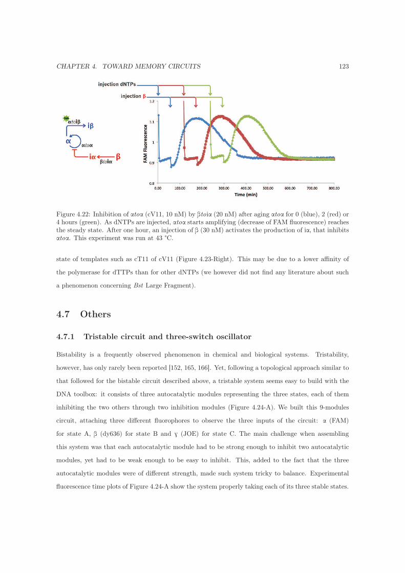
CHAPTER 4. TOWARD MEMORY CIRCUITS 123
Figure 4.22: Inhibition of αtoα (cV11, 10 nM) by βtoiα (20 nM) after aging αtoα for 0 (blue), 2 (red) or4 hours (green). As dNTPs are injected, αtoα starts amplifying (decrease of FAM fluorescence) reachesthe steady state. After one hour, an injection of β (30 nM) activates the production of iα, that inhibitsαtoα. This experiment was run at 43 °C.
state of templates such as cT11 of cV11 (Figure 4.23-Right). This may be due to a lower affinity of
the polymerase for dTTPs than for other dNTPs (we however did not find any literature about such
a phenomenon concerning Bst Large Fragment).
4.7 Others
4.7.1 Tristable circuit and three-switch oscillator
Bistability is a frequently observed phenomenon in chemical and biological systems. Tristability,
however, has only rarely been reported [152, 165, 166]. Yet, following a topological approach similar to
that followed for the bistable circuit described above, a tristable system seems easy to build with the
DNA toolbox: it consists of three autocatalytic modules representing the three states, each of them
inhibiting the two others through two inhibition modules (Figure 4.24-A). We built this 9-modules
circuit, attaching three different fluorophores to observe the three inputs of the circuit: α (FAM)
for state A, β (dy636) for state B and G (JOE) for state C. The main challenge when assembling
this system was that each autocatalytic module had to be strong enough to inhibit two autocatalytic
modules, yet had to be weak enough to be easy to inhibit. This, added to the fact that the three
autocatalytic modules were of different strength, made such system tricky to balance. Experimental
fluorescence time plots of Figure 4.24-A show the system properly taking each of its three stable states.

CHAPTER 4. TOWARD MEMORY CIRCUITS 124
Figure 4.23: Improving the flatness of the steady state. (Left) Turnover of cX11 (up) and cV11 (down)with a ramp of initial concentration of dNTPs (from 10 to 100μM). Whereas cX11 reaches a nicelyflat steady state, cV11 does not, especially for the low concentrations of dNTPs. (Right) Turnover ofcV11 for 40 μM of dNTPs. Adding dTTPs to the reaction mix improves the flatness of the steadystate. Experiments were run at 43 °C with 20 nM of autocatalytic module.

CHAPTER 4. TOWARD MEMORY CIRCUITS 125
States A and B had, however, very small basins of attraction: as soon as G was initially present in a
concentration of even a tenth of that of that of α or β, the system inevitably settled in state C.
By using only half of the inhibition modules on a clockwise pattern (αtoα inhibits βtoβ that inhibits
GtoG that inhibits αtoα) or a counterclockwise one (αtoα inhibits GtoG that inhibits βtoβ that inhibits
αtoα), one should obtain an oscillator in which autocatalytic modules get activated one after the
other (Figure 4.24-B). A mathematical model of the circuit for perfectly equilibrated sequences indeed
predicted a robust oscillating behavior. After some tedious balancing of the three sides, we managed
to experimentally obtain a single cycle of oscillations (Figure 4.24-C). Autocatalytic module GtoG
appeared, once again, to be stronger than the two others: the system eventually settled in a state
where GtoG only was active and leaving not chance to αtoα and βtoβ to restart.
4.7.2 Charge / Load
When working in the “right” conditions (i.e. for which the enzymes are not limiting the reaction speed),
the rate of amplification by an autocatalytic module is initially correlated to its own concentration
and the concentration of amplified input, as shown on Figure 4.25-A and B. Furthermore, when an
autocatalytic module has to provide input to a downstream module, it undergoes the “load” effect.
This is characterized by a weakened amplification of the module undergoing the load (Figure 4.25-C).
This can be intuitively explained by the fact that the module “to load” is sequestering outputs from
the “loading” module, and in the case of an autocatalytic module, outputs are also inputs: having a
lower concentration of input, the autocatalytic module is slowed down.
Such effect has to be considered during the assembly of circuits in which autocatalytic modules have
to charge one or more modules: this can be done by establishing an appropriate balancing strategy,
such as the one we have described for the bistable circuit in Section 4.3.7. This can however be
trickier for larger reaction circuits such as the the tristable circuit or the push-push memory circuit,
in which each autocatalytic module has to load two inhibition modules (for the push-push memory
circuit, one module inhibiting the opposite autocatalytic module, and another one feed-backing the
current state of the bistable core to the push-push function). In this latter case, the assembly of
the full circuit benefited from a robustly balanced bistable core. A strategy against the load effect
would be to introduce intermediate activation (amplification) modules (as “insulator” [71]). However,
increasing the total concentration of templates may also result in a problem by transferring the load
on the enzymes (i.e. moving the system in the saturated regime of the enzymes).

CHAPTER 4. TOWARD MEMORY CIRCUITS 126
Figure 4.24: Tristability and three-switch oscillator. (A) Tristable circuit. Templates αtoiβ and αtoiGare labeled with FAM to monitor α (negative fluorescence intensity shift upon charge); βtoiα and βtoiGare labeled with dy636 to monitor β (negative fluorescence intensity shift upon charge); Gtoiα and Gtoiβare labeled with JOE to monitor G (positive fluorescence intensity shift). The system initiated with1 nM of either α, β or G stabilizes in each corresponding state A, B or C, characterized by a shift offluorescence intensity of, respectively, FAM, dy636 or JOE, as one can observe in the fluorescence timeplots of each dye. Concentrations are: [αtoα] = [βtoβ] = 15 nM, [GtoG] = 10 nM, all inhibition modulesat 20 nM. (B) Three-switch oscillators oscillating counterclockwise (left) and clockwise (right). (C)Left: model (concentration of free α (blue), β (red) or G (green)) for perfectly equilibrated sequencesall present in a 20 nM concentration. Right: experimental fluorescence (normalized, and reversed forFAM and JOE whose fluorescence change upon hybridization is negative) time plot for a system with[αtoα] = 20 nM, [βtoβ] = 5 nM, [GtoG] = 5 nM, [αtoiβ] = 10 nM, [βtoiG] = 7.5 nM and [Gtoiα] = 5 nM.This latter concentration explain the poor signal induced by G. The reaction was initiated with [G] =5 nM and [α] = [β] = 1 nM. Colored arrows indicate the successive spikes of input species: first comesa spike of G, then β, then α, after which G reactivates and the system stalls forever. Sequences are asfollows: α: CTGAGTCTTGG, β: CAGAGTCCAAG, G: AGGAGTCACAC.
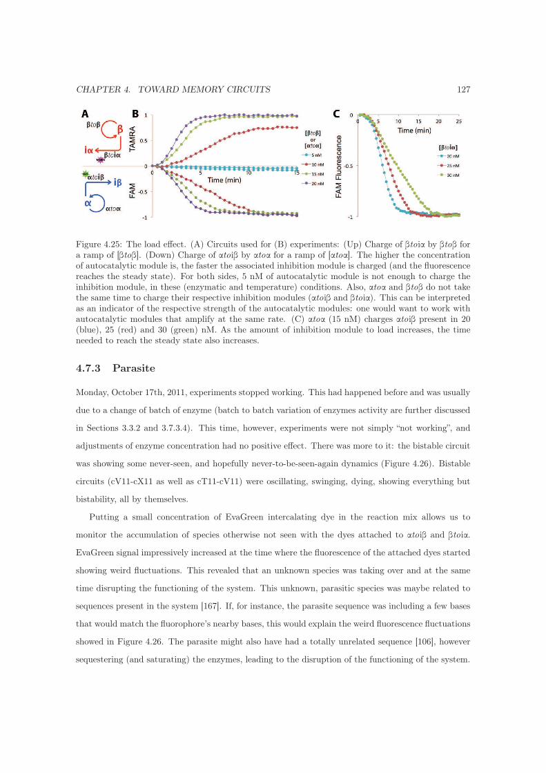
CHAPTER 4. TOWARD MEMORY CIRCUITS 127
Figure 4.25: The load effect. (A) Circuits used for (B) experiments: (Up) Charge of βtoiα by βtoβ fora ramp of [βtoβ]. (Down) Charge of αtoiβ by αtoα for a ramp of [αtoα]. The higher the concentrationof autocatalytic module is, the faster the associated inhibition module is charged (and the fluorescencereaches the steady state). For both sides, 5 nM of autocatalytic module is not enough to charge theinhibition module, in these (enzymatic and temperature) conditions. Also, αtoα and βtoβ do not takethe same time to charge their respective inhibition modules (αtoiβ and βtoiα). This can be interpretedas an indicator of the respective strength of the autocatalytic modules: one would want to work withautocatalytic modules that amplify at the same rate. (C) αtoα (15 nM) charges αtoiβ present in 20(blue), 25 (red) and 30 (green) nM. As the amount of inhibition module to load increases, the timeneeded to reach the steady state also increases.
4.7.3 Parasite
Monday, October 17th, 2011, experiments stopped working. This had happened before and was usually
due to a change of batch of enzyme (batch to batch variation of enzymes activity are further discussed
in Sections 3.3.2 and 3.7.3.4). This time, however, experiments were not simply “not working”, and
adjustments of enzyme concentration had no positive effect. There was more to it: the bistable circuit
was showing some never-seen, and hopefully never-to-be-seen-again dynamics (Figure 4.26). Bistable
circuits (cV11-cX11 as well as cT11-cV11) were oscillating, swinging, dying, showing everything but
bistability, all by themselves.
Putting a small concentration of EvaGreen intercalating dye in the reaction mix allows us to
monitor the accumulation of species otherwise not seen with the dyes attached to αtoiβ and βtoiα.
EvaGreen signal impressively increased at the time where the fluorescence of the attached dyes started
showing weird fluctuations. This revealed that an unknown species was taking over and at the same
time disrupting the functioning of the system. This unknown, parasitic species was maybe related to
sequences present in the system [167]. If, for instance, the parasite sequence was including a few bases
that would match the fluorophore’s nearby bases, this would explain the weird fluorescence fluctuations
showed in Figure 4.26. The parasite might also have had a totally unrelated sequence [106], however
sequestering (and saturating) the enzymes, leading to the disruption of the functioning of the system.

CHAPTER 4. TOWARD MEMORY CIRCUITS 128
Figure 4.26: Swinging Curves. These are a selection of “crazy” bistable circuits obtained during a fewmonths, seen through FAM, TAMRA of dy636 channels, depending on the bistable system (cV11-cX11or cT11-cV11).
This parasite first appeared in a separate system (using a different nicking endonuclease, see chapter
6, but soon contaminated all our reactions, as such “monster” is known to have the ability to [168].
In order to get rid of the parasite (or at least delay its emergence) we cleaned all our pipettes and
thermocyclers, threw away tubes, buffers, enzymes, and found that using Netropsin, an oligopeptide
binding to AT-rich double-stranded sequences [169], was effectively delaying the emergence of the
parasite in each reaction. From this time, Netropsin (2 μM) was added to the reaction buffer. We have
never sequenced the parasite, nor done any gel analysis (by fear of further spreading the parasite), and
maintain the habit to discard, without opening, any tube in which it is suspected to have appeared.
It would however be interesting to try and understand the features that make it appear and duplicate
that efficiently in our systems.

Chapter 5
Compartmentalization of the reactions
Compartmentalization in micro-reactors can be interesting for many applications. It can allow high-
throughput analysis of a given system in various conditions. If small enough, micro-reactors can be used
to study the statistical variations in molecule numbers between each units, as well as the dependency
of the reaction on its volume. Micro-reactors could then be connected together, allowing one to control
the diffusion - that is, the communication - between each computing unit.
By using microfluidic technologies, it is relatively easy to construct two-dimensional arrays of
micro-chambers. Remaining challenges are (i) to find a way to fill and close them properly (ii) to get
the reactions to work inside. These challenges do not have obvious solutions, as we will see in this
chapter. We will find more success with the use of micro-emulsions, that can be cleanly generated by
using microfluidic tools. This will allow us to set up a single-module reaction circuit in mono-disperse
micro-droplets, opening good perspectives for the study of our reaction circuits in tiny compartments.
5.1 Microfabrication
Using soft lithography to build a simple microfluidic device first consists in making the mould master
of the device:
• One has first to draw the design of the microfluidic device, using a vector drawing software (such
as Adobe Illustrator) or dedicated software (such as AutoCAD).
• The drawing is then patterned in positive photoresist (e-beam etching) spincoated on a chrome-
coated glass. After development of the photoresist, the exposed chrome is etched away (with a
129

CHAPTER 5. COMPARTMENTALIZATION OF THE REACTIONS 130
chrome etchant solution): this transfers the drawing of the device to the chrome coating. The
remaining photoresist is removed with acetone, thus revealing our chrome mask.
• The regular method then consists in using a silicon wafer as a substrate for the device mould
master. The silicon wafer can first be cleaned using a piranha solution (mixture of hydrogen
peroxide and sulfuric acid). This however makes the surface of the wafer hydrophilic, which is
not wanted for the following spincoating of photoresist. The hydrophobicity of the wafer can be
recovered by immersing it in BHF (Buffered Hydrofluoric Acid) for a few minutes. In the case
of a freshly produced wafer, this cleaning process is not required.
• Next, negative photoresist is spincoated on the wafer. The thickness of the film of photoresist
will roughly be the thickness of the microfluidic channels. Relationship between film thickness
and spincoating speed is given by the photoresist maker (for a new photoresist).
• Then, Soft Bake (SB) is carried out: temperature and time depend on the thickness, for a given
photoresist.
• The mould is then photo-exposed in the near UV, for a time that depends on the thickness and
lamp power.
• Next comes the Post Exposure Bake (PEB), for a time that depends on the thickness of pho-
toresist. This step is extremely important, since it controls the diffusion of the photo-activated
compounds that will trigger the reticulation of the resist. If the PEB is too short, there will
be a loss in sensitivity of the photoresist (not enough vertical diffusion of the photo-activated
compounds), whereas if it is too long, there will be a loss in resolution (too much lateral diffusion
of these same compounds).
• The negative photoresist is then developed: the UV-exposed areas, being reticulated, remain on
the silicon substrate. We have our mould master.
• This mould can be Hard Baked (HB, done at higher temperature than SB and PEB) in order to
remove eventual cracks present on the surface of the photoresist.
• Treating the mould master with a Teflon coating (CHF3) by RIE (Reactive Ion Etching) will
insure the resilience of the master mould to repetitive uses.
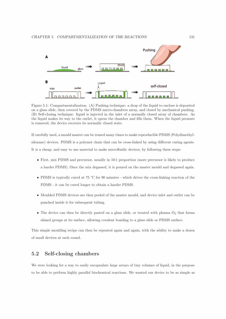
CHAPTER 5. COMPARTMENTALIZATION OF THE REACTIONS 131
Figure 5.1: Compartmentalization. (A) Pushing technique: a drop of the liquid to enclose is depositedon a glass slide, then covered by the PDMS micro-chambers array, and closed by mechanical pushing.(B) Self-closing technique: liquid is injected in the inlet of a normally closed array of chambers. Asthe liquid makes its way to the outlet, it opens the chamber and fills them. When the liquid pressureis removed, the device recovers its normally closed state.
If carefully used, a mould master can be reused many times to make reproducible PDMS (Polydimethyl-
siloxane) devices. PDMS is a polymer chain that can be cross-linked by using different curing agents.
It is a cheap, and easy to use material to make microfluidic devices, by following these steps:
• First, mix PDMS and precursor, usually in 10:1 proportion (more precursor is likely to produce
a harder PDMS). Once the mix degassed, it is poured on the master mould and degassed again.
• PDMS is typically cured at 75 °C for 90 minutes - which drives the cross-linking reaction of the
PDMS - it can be cured longer to obtain a harder PDMS.
• Moulded PDMS devices are then peeled of the master mould, and device inlet and outlet can be
punched inside it for subsequent tubing.
• The device can then be directly pasted on a glass slide, or treated with plasma O2 that forms
silanol groups at its surface, allowing covalent bonding to a glass slide or PDMS surface.
This simple moulding recipe can then be repeated again and again, with the ability to make a dozen
of small devices at each round.
5.2 Self-closing chambers
We were looking for a way to easily encapsulate large arrays of tiny volumes of liquid, in the purpose
to be able to perform highly parallel biochemical reactions. We wanted our device to be as simple as

CHAPTER 5. COMPARTMENTALIZATION OF THE REACTIONS 132
possible - that is, to avoid multilayer devices with complicated valve structures - because each device
would only be used once (to avoid contamination between separate experiments). A common way to
enclose liquid in arrays of micro-chambers [170] is to pattern them in PDMS, and press the patterned
PDMS array on a glass slide where the liquid to enclose is deposited (Figure 5.1-A). This would require
a device to keep the array pressed on the array of chambers.
We thought about a technique that wouldn’t need any additional tool: self-closing chambers (Figure
5.1-B). The idea was to set up normally closed chambers, that would get opened by the fluid injected
at the inlet of the device. As the liquid injection would stop, the chambers would find back their
normally closed state, compartmentalizing the liquid in small separated volumes.
5.2.1 First design
The first design is shown in Figure 5.2-A. We started with an array of about 20000 relatively big
chambers (40 μm diameter), patterned in between two inlets (for potential mixing of two reagents)
and one outlet. The PDMS layer was covalently bonded to the glass slide, but the chambers array,
so that the liquid could flow from the inlet to the outlet. This was done by protecting the chambers
array from O2 plasma with a thin plastic layer, removed before pasting to the glass slide. Using this
device was very simple: the liquid was injected in the device with a plastic syringe; when removing
the syringe, the chambers would close (Figure 5.1-B and 5.2-B).
This first design was not able to fill out all the chambers: once the injected liquid would have made
its way from one inlet to one outlet, the chambers located on the path followed by the liquid would be
filled. Then, the other inlets and outlets would stay closed. We tried replacing the inlets split in 5 by
a single large inlet, thinking that the whole array would then be filled at once. This however didn’t
work much better.
5.2.2 Comb design
The best working design (and the progression toward it) is shown on Figure 5.3, for 10 μM diameter
chambers. The main idea was to reduce the number of chambers to fill between the inlet and outlet
(in order to make sure they would be filled), while keeping a large number of chambers on the device.
In the present “comb” channels structure, only 15 to 20 chambers are separating the combs inlet and
outlet. The devices shown on Figure 5.3 are still able to hold about 15000 chambers. The main
improvement through the successive designs was the increased channels width, which would allow an

CHAPTER 5. COMPARTMENTALIZATION OF THE REACTIONS 133
Figure 5.2: First self-closing design. (A) Device layout, 3D view and zoom on the chamber array. Thelatter is protected from O2 plasma so that the liquid can make its way from the inlet to the outlet.(B) As the liquid flows from the inlet to the outlet, it fills the chambers.
Figure 5.3: Comb design. (1) Initial design, with 15 chambers between the channels that are 70 μmwide. (2) Increased channel width (100 μm). (3) Increased channel width (150 μm) and number ofchambers (20 between the channels). (4) XL channels (400 μm), 15 chambers between them and lessoutlets. (5) Best design: 200 μm wide channels, 15 chambers between them, less outlets than inlets.
easier filling and escape (to the inlets) of the liquid to enclose. For the two following designs, there
are less outlets than inlets: this leaves no “dead zone” where the liquid injected would not flow (in the
previous designs, the liquid was not able to flow at upper and lower extremities of the array, because
bordered by the PDMS rather than an outlet). The chambers array of these devices is about 4 mm
wide: this is small enough to allow the fabrication of 4 to 8 device per master mould. This device
worked well, allowing the efficient filling and closing of large array of tiny volumes of liquid (Figure
5.4).
5.2.3 Are the chambers closed?
In order to address this important point, we performed a photo-bleaching experiment for each filled
device. This test consists in including a fluorescent dye - for instance fluorescein - to the liquid to

CHAPTER 5. COMPARTMENTALIZATION OF THE REACTIONS 134
Figure 5.4: Large view of a portion of a filled device (Left). Zoom and bleaching of a single 10 μmchamber (Right).
Figure 5.5: Bleaching test with 20 μm chambers. Fluorescein (10 μM) in water is introduced in aself-closing device. After photo-bleaching of the chambers in the middle (using a pinhole, and settinga high UV intensity), the fluorescence recovery is recorded through time. Here, chambers are wellsealed: bleached ones do not recover any fluorescence during the 2-hours long time-lapse recording.
enclose; once the chambers seem closed, photo-bleaching one or more chambers - by exposing them to
a strong light - then checking if, through time, the bleached chambers recover or not their fluorescence.
If they do, this means that they are not properly sealed: there is diffusion of fluorescent dye from the
nearby chambers. If they stay dark, this proves that they are well sealed (Figure 5.5).
5.2.4 Improving the sealing of the chambers
Here are a few ideas we tried to improve the sealing of the chambers:
• Making a thicker PDMS layer -> this somewhat worked. While a layer too thin was not allowing
a good self-closing, a too thick one was rendering the device hard to fill. The best compromise
was a thickness of about 4 mm.

CHAPTER 5. COMPARTMENTALIZATION OF THE REACTIONS 135
Figure 5.6: Plasma sealing. The PDMS surface containing microchambers is activated with plasmaO2. The liquid to seal is then poured on the surface, and covered with an activated glass slide, thatshould covalently bind to the PDMS array, thus closing the chambers.
• Increasing the stiffness of the closing layer: this could be done by covalently binding a glass slide
on top of the PDMS layer -> this worked for thin PDMS layer, (of about 2 mm). The filling was
however quite harder.
• Once the self-closing chambers are filled, applying a constant and negative pressure on the inlet
and outlet: the channels will thus behave like suckers, sealing the chambers more efficiently ->
this worked. However, the encapsulated liquid dried up more quickly.
• Making smaller arrays of chambers -> this also proved useful, however reducing the number of
experiments possible to perform in parallel.
Another idea to close the chambers is presented in Figure 5.6. It consisted in taking a simple layer of
PDMS with patterned array of chambers, treating it with O2 plasma, which would make the surface
(and chambers) hydrophilic. A drop of liquid to enclose would then easily get inside the chambers, and
would be covered by a glass slide also treated with O2 plasma. We would then expect the glass slide
to covalently bind to the PDMS, efficiently closing the chambers. This technique worked well with
simple solution of fluorescein in water, given that the overload of liquid could flow out of the array
of chambers, before getting trapped by the covalent binding between the glass slide and the PDMS
layer. For that, one would have to start press the device from the middle of the array to the outer
sides. This technique however failed at enclosing samples “richer” (e.g. that contain proteins) than
just a fluorescent dye in water.

CHAPTER 5. COMPARTMENTALIZATION OF THE REACTIONS 136
Figure 5.7: Various fluorescence pictures of the PDMS layer after the experiment (after having flushedaway all the liquid)
5.3 The impossible compromises
5.3.1 PDMS and EvaGreen
As we started experiments with our reaction mix, we observed odd adsorption phenomena. EvaGreen
appeared to be sticking to PDMS (Figure 5.7) which was one major problem: at that time, we were
only using EvaGreen to monitor our reactions. We tried various surface treatments, coatings and
surfactants: treating the PDMS with O2 plasma was what appeared to work best. Which was a
problem, since the fabrication of the self-closing device required the chamber array to be protected
from O2 plasma.
Adsorption of EvaGreen on the PDMS surface was one of the reasons that motivated the investi-
gation of a different monitoring method: N-quenching. Another solution would have been to change
the PDMS for another material, or come up with a device fully made of glass.
5.3.2 Coating and Sealing
As the surface to volume ratio increases, one gets subject to various problems at the interface between
the liquid and the PDMS. We are working with chambers of sub-nanoliter volume, and want to enclose
in it a buffer that contains DNA and enzymes, which can both have a tendency to adsorb on the
surfaces. BSA (Bovine Serum Albumin) is commonly included in biological buffers to avoid DNA
and enzymes non-specific adsorption [171, 172, 173] by competitively sticking to the surface. MPC
(2-methacryloyloxyethyl phosphorylcholine) coating can also be used to prevent protein molecules
adsorption on the surfaces [174, 175, 176]. As well, other surfactants can also be included in the
reacting mix [177, 178].
While all these surfactants may be necessary for the reaction to perform in small volumes (in
PDMS), they appeared to hinder the sealing of the chambers. We tried combinations of MPC-coated
or raw surface with BSA, or BSA added to our reaction mix, and performed the photo-bleaching test

CHAPTER 5. COMPARTMENTALIZATION OF THE REACTIONS 137
to check if the chambers were properly sealed. We found that sealing was possible with BSA alone
(up to 0.5 mg/ml) or our reaction mix alone, but adding BSA to the reaction mix resulted in a failed
sealing. As well, MPC coating was negatively affecting the sealing of the chambers.
5.4 Droplet microfluidics
Another way to encapsulate reactions is to use water-in-oil micro-emulsion. Microfluidics is good at
producing microdroplets of desired size, in which it is possible to encapsulate things going from simple
DNA amplification mixture [179] to single cells [180]. Microdroplets have also been used to compart-
mentalize the Belousov-Zhabotinsky oscillator and study the coupling (by an inhibitory intermediate
of the reaction diffusing in oil) between oscillating droplets in 1D [181] and 2D [182]. Microfluidic
droplets technology are readily used in our laboratory, we had the chance to design and try one of
our simplest reaction circuits and monitor on-chip its functioning in agarose microdroplets by using
N-quenching.
Mono-disperse microdroplets can be generated by using a flow-focusing microchannel network
through which the aqueous phase is segmented by the oil phase. We used an innovative “push-pull”
technique to produce microdroplets: it consists in pushing the oil phase only, while applying suction
at the outlet of the device. By doing so, we could produce microemulsions by using a very low volumes
of reagents. Using this setup, we encapsulated a single autocalatytic module blocked by an inhibitor
strand (to prevent the reaction from starting during the droplets generation at room temperature),
and could perform the reaction it in microvolume droplets, monitored under the microscope. The
result of this work was published in Biomicrofluidics, and is present in Appendix as A microfluidic
device for on-chip agarose microbead generation with ultralow reagent consumption. It opens the way
to the high throughput analysis of DNA-toolbox made circuits: a next step may be to encapsulate
more interesting - such as oscillating - reaction circuits, and observe the possible statistical variations
between the encapsulated reactions.

Chapter 6
An ecological approach to
spatiotemporal patterning
Ecological systems display complex population fluctuations that can theoretically be described by the
century-old Lotka-Volterra Predator-Prey (PP) equations [183]. Also, spatial effects are believed to be
responsible for a large part of the dynamic complexity observed among animal populations [94]. In this
chapter, we will use a recently reported in vitro implementation of the PP relationship [184], and install
it in a purposely engineered two-dimensional milieu. Our setup can be considered as a micro-ecosystem,
which is able to emulate a two-dimensional in vitro PP ecosystem under a microscope. In nature, PP
systems are extremely hard to observe because of their large scale in both time and space [185, 186]; our
micro-ecosystem enables easy two-dimensional in vitro study of PP relationship and its extensive range
of dynamics arising, for instance, from environmental perturbations. It could be used to explore the
landscape-dynamics relationships for complex PP ecosystems, by implementing different environment
topologies (micro-ecosystem shape), or localizing some of the resources at particular positions of the
microchip (patchy systems [187]).
We also implemented the bistable circuit presented in Chapter 3 in a two-dimensional environment,
and could observe the two stable states “fighting” against each other in various system geometries.
These results are presented in Appendix Two-dimensional Bistability.
138

CHAPTER 6. AN ECOLOGICAL APPROACH TO SPATIOTEMPORAL PATTERNING 139
6.1 Technical notes
Otherwise indicated, all reactions were performed with the template G5dy530 (5’-CGGCCGAATG-
CGGCCGAATG-3’), refereed to as G (for grass). Reactions were monitored with N-quenching alone
(G is labeled with a dy530 in 3’, allowing the specific monitoring of rabbits), or completed by EvaGreen
intercalating dye (reporting both rabbit and fox concentrations).
For the two-dimensional experiments, we used an inverted IX-71 microscope (Olympus) with a
CoolLED light source (pE excitation system) associated with a Semrock Cy3-4040C filter cube (to
observe the fluorescence of dy530) . Reactions were monitored with an Andor XION camera, through
a 1.25x objective lens with a 0.5x camera adapter. Devices were incubated using a Tokai thermoplate.
Images were typically acquired every minute (using μmanager software) and post-treated as follows,
using ImageJ software:
• Optional: moving average on the whole stack, followed by the removal of half of the slices (great
gain in signal to noise ratio, for a slight loss in spatial-temporal resolution).
• Calculation of the mean image of the whole stack (from shortly after the beginning to before the
emergence of divergence) to get an estimate of the static background.
• Each image was normalized against the background.
• Kalman stack filter (used to reduce signal noise) was applied to the stack of images.
6.2 Predator-Prey reaction circuit
6.2.1 Basic functioning
Predator-Prey (PP) systems can be defined in terms of a set of reactions: preys autocatalytic repro-
duction (N -> 2N), predation of preys by predators (N + P -> 2P), and decay of both species (N or
P -> 0). Initially, Lotka studied this system using the following set of ordinary differential equations
[183]:
• For the prey: N = N −N.P (The growth of the prey is a function of its own population. Preys
are consumed by predators, in relation of the frequency of encounters)
• For the predator: P = N.P −P (The growth of predator is a function of its own population and
the population of rabbits. Predators decay by natural death.)

CHAPTER 6. AN ECOLOGICAL APPROACH TO SPATIOTEMPORAL PATTERNING 140
Figure 6.1: DNA-based Predator-Prey system. (A) In presence of the grass DNA template, rabbits au-tocatalytically reproduce. (B) Predation of rabbits by foxes. (C) Death of both rabbits and foxes. (D)Experimental curve in 0-dimensional milieu (test tube) using N-quenching [147], showing oscillationsof rabbit population: a decrease in fluorescence intensity indicates an increase in rabbit concentration.
By using the same set of DNA-based enzymatic reactions as in the DNA-toolbox (based on a poly-
merase, a nicking enzyme and an exonuclease), it is possible to implement the PP relationship for the
simplest ecological system consisting of a single prey and its predator. Predator (fox) and prey (rab-
bit) are both DNA species, and their DNA sequences define their trophic relationship. Experimentally,
DNA-foxes and DNA-rabbits interact in a closed environment: in the presence of grass template, rab-
bits autocatalytically reproduce (Figure 6.1-A). Grass template is labeled in 3’-end with a fluorescent
dye, which allows – through N-quenching [147] – the monitoring of the rabbits as they hybridize to
the grass. A fox finding a rabbit produces two foxes (Figure 6.1-B); both foxes and rabbits die (Figure
6.1-C), whereas the amount of grass stays constant across generations. In 0-dimensional (well mixed)
conditions, this system is an accurate chemical in vitro model of realistic PP equations [183], and
displays sustained oscillations of fox and rabbit populations (Figure 6.1-D). We will not get into the
detail of the DNA biochemistry behind this system (which is further presented in [184]), but keep in
mind that this system only needs a single template (called G) to oscillate, and is fully compatible with
the DNA-toolbox.
6.2.2 Adjusting the parameters of the Predator-Prey circuit
The Predator-Prey system can oscillate over a large range of parameters. In this section, we explore
its sensitivity to several parameters, from the concentration of enzymes to the temperature. These
experiments can then be reused as a calibration model when, for instance, one has to use a new batch

CHAPTER 6. AN ECOLOGICAL APPROACH TO SPATIOTEMPORAL PATTERNING 141
Figure 6.2: (A) Ramp of Bst/5 (percent of the total volume; 1 % corresponds to 16 units/ml) with[G] = 140 nM, T = 44.5 °C, dNTPs = 200 μM. (B) Ramp of Bsmi (percent of the total volume; 1 %corresponds to 100 units/ml) with [G] = 110 nM, T = 44.5 °C, dNTPs = 200 μM. (C) Ramp of [G](nM) at T = 44.5 °C, dNTPs = 200 μM. (D) Ramp of dNTPs (1 % corresponds to 100 μM of eachdNTP) with [G] = 140 nM, T = 46 °C. (E) Gradient of temperature with [G] = 140 nM.

CHAPTER 6. AN ECOLOGICAL APPROACH TO SPATIOTEMPORAL PATTERNING 142
of enzymes (with a different activity), or when one is searching for specific dynamics, such as slower but
more stable oscillations, faster and damped oscillations or coexistence of preys and predators. Typical
curves for ramps of polymerase concentration, nickase concentration, template concentration, dNTPs
concentration and temperature are shown in Figure 6.2.
Changing the concentration of Bst polymerase (Figure 6.2-A) gives dynamics ranging from ex-
tinction of both species (at low concentration) to damped oscillations followed by coexistence (high
concentration). Moving the concentration of Nb.BSMI nicking endonuclease goes reversely (Figure
6.2-B): at low concentration, the nicking enzyme works more slowly than the polymerase, resulting in
a too strong growth of both prey and predator, that end up coexisting. At high concentrations, the
nickase works too fast: in comparison, the polymerase is not fast enough to support the growth of
rabbits. Roughly, changing the concentration of template corresponds to changing the concentration of
polymerase (Figure 6.2-C). It is not shown on these curves, but at too low concentration of template,
we also observe the extinction of both species. Interestingly, changing the concentration of dNTPs
does more than just impacting the life span of the reaction (Figure 6.2-D): at too high concentration of
dNTPs, the reaction is initially slower, and accelerates as dNTPs are used throughout the experiment.
This can be explained by the binding of Mg2+ to dNTPs, making the concentration of free Mg2+
dependent on the concentrations of dNTPs. Yet, Mg2+ are required for the good functioning of the
enzymes. Each “percent” of dNTPs corresponds to 100 μM of each of the four dNTPs, that is, 400 μM.
Each percent thus sequesters 5 % of the 8 mM of Mg2+ contained in the reacting mix. Alternatively,
dNTPs may have a competitive effect by binding to DNA processing enzymes. The temperature also
has a complex impact on the kinetics of the reaction: among others, it modifies the activity of enzymes
and the stability of duplexes (Figure 6.2-E).
6.2.3 Long-term oscillator
When properly optimized, the Predator-Prey system oscillates for days (Figure 6.3). This proves that
we are able to maintain this closed system in quasi-stationary conditions far from equilibrium over a
long period of time. We tried to further increase the concentration of dNTPs, but the reactions did
not last longer (and actually got slower). After a week, the remaining enzyme activity may just be too
low for the reaction to go on. With respect to future applications, it is important that such molecular
computers can perform autonomously during such long periods.

CHAPTER 6. AN ECOLOGICAL APPROACH TO SPATIOTEMPORAL PATTERNING 143
Figure 6.3: An oscillator running for 8 days (showing about 112 oscillations). [G] = 140 nM, T = 45.4°C
CHAPTER 6. AN ECOLOGICAL APPROACH TO SPATIOTEMPORAL PATTERNING 144
6.3 Enable the reactions for working under the microscope
Our first fear when trying to work in a configuration with an increased surface-to-volume ratio (com-
pared to bulk 0D experiment) was that various components of the system would adsorb on the surfaces
of the two-dimensional milieu. During our investigation of PDMS microfluidic devices, we had big trou-
bles with EvaGreen. In consequence, we initially decided to get rid of it. However, EvaGreen is not
neutral to the functioning of the system: it is stabilizing the DNA duplexes, as observed in Section
4.5.1, and may also affect the binding of the enzymes to DNA, by competing for the grooves of the
helix. Working without EvaGreen, we found good oscillating conditions at 44 °C (which was about
2 °C below the reaction temperature with EvaGreen). N-quenching gave us a signal good enough to
monitor the oscillations (Figure 6.1). Enzymes might also adsorb to the surfaces: we could not get
rid of them, so we hoped that increasing the two blockers of our reacting mix (BSA and Synperonic)
would provide a working solution. In consequence, we checked if increasing the concentration of these
blockers was hampering the reactions or not (Figure 6.4). Too high concentrations of BSA or Syn-
peronic seemed to provoke a premature damping of the oscillations. We settled on a concentration
of 0.5 mg/mL of BSA (5 times our usual concentration in bulk) and an unchanged concentration of
Synperonic (0.1 %).
6.4 A simple device to observe the reactions in two-dimensions
The first device we used was proposed by André Estévez-Torres from CNRS/LPN: a flow-cell made
of a simple layer of Parafilm (127 μm) separating two glass slides. By baking the device a few tens of
seconds on a hot plate (around 65 °C), the Parafilm strongly attaches to the glass. The sample was
then introduced by the “inlet”, filling the chamber by capillarity. As initial perturbation, we slightly
touched one inlet with a tip filled with rabbit solution. Inlets were closed with grease in order to avoid
evaporation. The device was then incubated on the microscope hotplate, in a homemade setup to
keep a wet atmosphere: it consisted of a petri dish put upside down on a PDMS joint and sealed with
grease. An eppendorf cap filled with water was put next to the device to keep the air around saturated
with water. With this simple setup, we could observe three successive waves of rabbits (difficult to
distinguish from the background, see Figure 6.5). This was the first time we could observe traveling
waves that were emerging from the inlet initially perturbed, and moving toward the opposite inlet. We
found a temporal periodicity (when observing the oscillations at a given location) similar to that of

CHAPTER 6. AN ECOLOGICAL APPROACH TO SPATIOTEMPORAL PATTERNING 145
Figure 6.4: Increasing the concentration of BSA and Synperonic. Fluorescence time plots (X-axis: timein minutes, Y-axis: fluorescence of DY-530) for various couples of BSA and Synperonic concentrations.Usual conditions are: 0.1 % of Synperonic and 0.1 mg/mL of BSA. With increased concentrations ofBSA or Synperonic, the oscillations tend to damp earlier. The relationship is however not clearcut:there might be some interactions between synperonic and BSA. [G] = 80 nM, T = 44 °C.

CHAPTER 6. AN ECOLOGICAL APPROACH TO SPATIOTEMPORAL PATTERNING 146
Figure 6.5: Three waves of rabbits going from left to right, arbitrarily delimited for visibility. Theyare followed by the divergence, emerging from t = 210 min. [G] = 80 nM, T = 44 °C.
the bulk experiment (i.e. a period of about 80 minutes). However, the reaction diverged very quickly,
as it can be seen from t = 210 min on Figure 6.5.
In two dimensions, the divergence is characterized by a dark front that moves slowly and ineluctably.
It also appears in the bulk experiment - though not as early - and is characterized by a strong decrease of
the fluorescence of the attached dye (suggesting that all the templates become part of double-stranded
complexes). If EvaGreen is used, one can observe a huge increase of its fluorescence, which indicates an
accumulation of double-stranded species (and possibly single-stranded species). We still haven’t any
steady idea about the mechanism of this divergence, but as an easy example, if an uncut complementary
strand of template G was to melt away, it would itself become a template for the production of G. Then,
an increasing concentration of G might rapidly cause the system to be saturated with preys, taking
away the dynamic balance between the prey and the predator growths. A variety of other autocatalytic
mechanisms can be imagined, possibly yielding more complex and/or bigger DNA complexes. Note
also that in two-dimensions, the divergence front moves notably (about 4 times) more slowly than the
waves of preys, suggesting that its products are longer strands (or bigger complexes) than preys and
predators, thus diffusing more slowly.
6.5 Stabilizing the reaction
We set on finding out what was causing the divergence to come so early, as compared to the bulk
experiment.
6.5.1 Double layer and coatings
Whereas stable in tube, reactions had a tendency to diverge very quickly in the Parafilm device.
Moreover, we had a very bad contrast in the first experiments (Figure 6.5). We solved the bad
contrast issue by introducing the double layer device, for a double thickness (254 μm) of reacting mix.
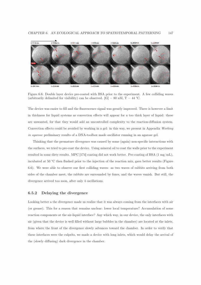
CHAPTER 6. AN ECOLOGICAL APPROACH TO SPATIOTEMPORAL PATTERNING 147
Figure 6.6: Double layer device pre-coated with BSA prior to the experiment. A few colliding waves(arbitrarily delimited for visibility) can be observed. [G] = 80 nM, T = 44 °C.
The device was easier to fill and the fluorescence signal was greatly improved. There is however a limit
in thickness for liquid systems as convection effects will appear for a too thick layer of liquid: these
are unwanted, for that they would add an uncontrolled complexity to the reaction-diffusion system.
Convection effects could be avoided by working in a gel: in this way, we present in Appendix Working
in agarose preliminary results of a DNA-toolbox made oscillator running in an agarose gel.
Thinking that the premature divergence was caused by some (again) non-specific interactions with
the surfaces, we tried to pre-coat the device. Using mineral oil to coat the walls prior to the experiment
resulted in some dirty results. MPC [174] coating did not work better. Pre-coating of BSA (1 mg/mL),
incubated at 50 °C then flushed prior to the injection of the reaction mix, gave better results (Figure
6.6). We were able to observe our first colliding waves: as two waves of rabbits arriving from both
sides of the chamber meet, the rabbits are surrounded by foxes, and the waves vanish. But still, the
divergence arrived too soon, after only 4 oscillations.
6.5.2 Delaying the divergence
Looking better a the divergence made us realize that it was always coming from the interfaces with air
(or grease). This for a reason that remains unclear: lower local temperature? Accumulation of some
reaction components at the air-liquid interface? Any which way, in our device, the only interfaces with
air (given that the device is well filled without large bubbles in the chamber) are located at the inlets,
from where the front of the divergence slowly advances toward the chamber. In order to verify that
these interfaces were the culprits, we made a device with long inlets, which would delay the arrival of
the (slowly diffusing) dark divergence in the chamber.

CHAPTER 6. AN ECOLOGICAL APPROACH TO SPATIOTEMPORAL PATTERNING 148
Figure 6.7: Long inlets. The delayed divergence (darker wave) arrives from both inlets. [G] = 80 nM,T = 44 °C.
The experiment of Figure 6.6 was performed in a 8 mm diameter chamber laying on a 24 mm long
glass slide, leaving less than 8 mm for the inlets. For the experiment of Figure 6.7, we made the same
8 mm diameter chamber on a 36 mm long glass slide, which resulted in inlets of about 14 mm. Indeed,
the divergence took quite longer to arrive in the chamber, where the reaction was otherwise properly
performing. We could observe two successive waves of rabbits colliding with the walls of the chambers:
in such case, the rabbits get cornered by the foxes that follow them, which results in the extinction of
the wave against the wall. After these two waves, the point of emergence of rabbits moved to an inlet,
until the eventual divergence of the reaction coming - once again - from the two inlets (Figure 6.7).
As a conclusion, getting rid of the divergence meant getting rid of the inlets.
6.5.3 A commercial alternative
Bio-Rad sells Frame-Seal (FS), two-dimensional incubation chambers adapted for PCR reactions, that
are vapor-tight and gas-tight up to 97 °C. The frame of FS is pasted on a regular glass slide, and is
closed by a plastic sheet. FS allows to set up 65 μL of reacting mix on a 15x15 mm surface (a bit larger
than what can be observed with our 1.25x objective lens and 0.5x camera adapter), which makes a
thickness of about 290μm. Set up in FS, the reaction got more stable, and we were able to observe
some nice spatio-temporal patterns (Figure 6.8). We started the reactions with one or more localized
populations of rabbits: this was done by depositing a drop (typically 0.3 μL of rabbits at 1 μM) on
the glass slide, and drying it up by heating on a hot plate.
Properly filling the Frame-Seal was tricky, and most experiments were launched with a few bubbles
on a side or a corner. Almost every time, the divergence seemed to come from those large bubbles.

CHAPTER 6. AN ECOLOGICAL APPROACH TO SPATIOTEMPORAL PATTERNING 149
Figure 6.8: An experiment in Frame-Seal. The experiment is started with a population of dry rabbitsin the middle of the FS and a smaller population a bit further up-right. (Top) Fluorescence time-plotsof 10x10 pixels squares located at their respective locations of the FS (up-left corner, up-middle, up-right corner, and so on) (Bottom) After some transient, the system settled in the pattern tentativelydepicted here. [G] = 80 nM, T = 44 °C.
Still, we were able to observe very nice spatio-temporal behaviors for various initial perturbations of
the system. We also found good working conditions with an increased concentration of template G
(140 nM) which resulted in a better fluorescent signal. FS are, however, all of the same square shape,
and mostly impossible to customize.
6.6 Paraframe
The shortcomings of Frame-Seal motivated us to think about a homemade solution. We would need a
device simple to produce with any desired shape, however avoiding PDMS (for that - as discussed in
the previous chapter - it is far from being a good material when it comes to working with enzymes, and
also EvaGreen intercalating dye). This device should avoid interfaces with air, since the premature
divergence was always emerging at theses interfaces. As with the Frame-Seal, we wanted to maintain
the possibility to localize the initial perturbation of rabbits and/or foxes.

CHAPTER 6. AN ECOLOGICAL APPROACH TO SPATIOTEMPORAL PATTERNING 150
Figure 6.9: Making of Paraframe chambers.
Inspired by Frame-Seal, we upgraded our Parafilm devices. We engineered “paraframe”, an ex-
tremely simple (and cheap) device that only requires two glass slides and some Parafilm - removing
the need for grease (Figure 6.9). Paraframe can be constructed in a few minutes, and only requires to
punch or cut the desired chamber shape in a Parafilm double-layer, paste it on a glass slide and bake a
few seconds at 50 °C. Then comes the eventual localization of dry rabbits, followed by the deposition
of the reacting mix (adding an excess of 1 or 2 μL, as compared to the 20 μl of a chamber of 10 mm
diameter). A second glass slide then sandwiches the reacting mix, and the device just needs to be
flipped and baked another few seconds on this other side to be firmly closed. Paraframe can then be
incubated on a hot plate without need of further closing (it has no inlet nor outlet) or wet atmosphere
to avoid evaporation (it holds up well at 46 °C for days). The first experiment was already a great
improvement over the “old” devices with inlets and outlets (Figure 6.10). Even in such a roughly
shaped device, the reaction showed about 14 oscillations before diverging. The experiment in Figure
6.11 ran for more than two days, demonstrating the ability of paraframe to hold a reaction for a long
time, preserved from evaporation.

CHAPTER 6. AN ECOLOGICAL APPROACH TO SPATIOTEMPORAL PATTERNING 151
Figure 6.10: First Parafilm device. (Left) Fluorescence image at t = 370 min. Dark area are whererabbits are numerous. Small dots (dark and light) are bubbles. (Right) Time plot of the meanfluorescence in the small square delimited in green on the left image. [G] = 110 nM, T = 44 °C
Figure 6.11: PP system with long period (about 200 min) in a round paraframe of 11 mm diameter.(Left) Fluorescence image (dy530) at t = 860 min. (Right) Time plot of the mean fluorescence on 900pixels (up, corresponding to the green square) and 10 pixels (down, corresponding to the red line).These curves present a global fluctuation of the signal, which period is about 24 hours, which was alsoobserved on longer experiments. We attributed these fluctuations - that mostly appeared in summer- to the variation of the temperature in the experimental room. [G] = 140 nM, T = 43 °C
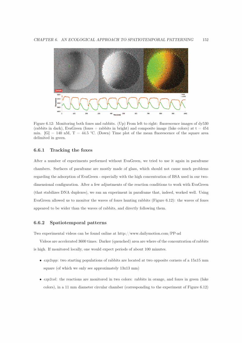
CHAPTER 6. AN ECOLOGICAL APPROACH TO SPATIOTEMPORAL PATTERNING 152
Figure 6.12: Monitoring both foxes and rabbits. (Up) From left to right: fluorescence images of dy530(rabbits in dark), EvaGreen (foxes + rabbits in bright) and composite image (fake colors) at t = 454min. [G] = 140 nM, T = 44.5 °C. (Down) Time plot of the mean fluorescence of the square areadelimited in green.
6.6.1 Tracking the foxes
After a number of experiments performed without EvaGreen, we tried to use it again in paraframe
chambers. Surfaces of paraframe are mostly made of glass, which should not cause much problems
regarding the adsorption of EvaGreen - especially with the high concentration of BSA used in our two-
dimensional configuration. After a few adjustments of the reaction conditions to work with EvaGreen
(that stabilizes DNA duplexes), we ran an experiment in paraframe that, indeed, worked well. Using
EvaGreen allowed us to monitor the waves of foxes hunting rabbits (Figure 6.12): the waves of foxes
appeared to be wider than the waves of rabbits, and directly following them.
6.6.2 Spatiotemporal patterns
Two experimental videos can be found online at http://www.dailymotion.com/PP-ad
Videos are accelerated 3600 times. Darker (quenched) area are where of the concentration of rabbits
is high. If monitored locally, one would expect periods of about 100 minutes.
• exp2opp: two starting populations of rabbits are located at two opposite corners of a 15x15 mm
square (of which we only see approximately 13x13 mm)
• exp2col : the reactions are monitored in two colors: rabbits in orange, and foxes in green (fake
colors), in a 11 mm diameter circular chamber (corresponding to the experiment of Figure 6.12)

CHAPTER 6. AN ECOLOGICAL APPROACH TO SPATIOTEMPORAL PATTERNING 153
6.7 Mathematical modeling
As described in [184], the kinetics of the Predator-Prey system is determined by the prey growth,
predation (by the predator) and degradation on one side, and by the predator predation (of the prey)
and degradation on the other side. As demonstrated in [184], these can be recapitulated in two non-
dimensional, coupled ordinary differential equations (for prey n and predator p):
dn
dτ=
g.n
1 + β.g.n− p.n− λ.δ
n
1 + p
dp
dτ= p.n− δ
p
1 + p
With the following parameters taken from [184]: β = 0.087, λ = 4.5, δ = 0.39, τ = t/tc with tc =
2.6min, g = G/G0 with G being the concentration of template with the scaling factor G0 = 53nM .
This mathematical model was shown to accurately describe the behavior of this PP system in 0D,
for various g (scaled concentration of grass template G). To describe a two-dimensional system, we
simply added a diffusion term to the above equations, following Fick’s laws of diffusion (with a constant
diffusion coefficient Dn for the prey, and Dp for the predator).
dn
dτ=
g.n
1 + β.g.n− p.n− λ.δ
n
1 + p+Dn
(
∂2n
∂x2+
∂2n
∂y2
)
dp
dτ= p.n− δ
p
1 + p+Dp
(
∂2p
∂x2+
∂2p
∂y2
)
Coefficient of diffusion of both species were approximated by following two different rules of thumb
found in the literature for short single stranded DNA in water [188, 189]. Both led to diffusion coefficient
around 10-2 mm2/min, and are - once again - approximations: we are not working in water, and at a
different temperature. Note also that in our setup, not only preys and predators diffuse, but also the
template G, as well as different double-stranded complexes (e.g. prey hybridized to G). Also, predators
may have secondary structures or form dimers. Nonetheless, we took Dn = 1 × 10⁻² mm2/min for
the 10-bases long prey and Dp = 0.8 × 10⁻² mm2/min for the 14-bases long predator. With regard
to our experimental setup, we set no-flux boundary conditions, and one or more starting populations

CHAPTER 6. AN ECOLOGICAL APPROACH TO SPATIOTEMPORAL PATTERNING 154
of preys, localized as gaussian peaks. The initial population of predators was set as an homogeneous,
low concentration on the whole surface. Using this simplified model, we were able to reproduce the
important features that we experimentally observed, such as traveling, colliding waves as well as spiral
waves.
Three videos of simulations, in a 10x10 mm square, are available online. Dark areas correspond to
areas of high rabbit concentration. All the starting populations of rabbits were localized slightly out
of the axis or center of symmetry
• simu1side: one starting population of rabbits on one side
• simu2opp: two starting populations of rabbits at two opposite corners
• simu3 : three starting populations of rabbits
These can be found at the following link: http://www.dailymotion.com/PP-ad
6.8 Extension of this work
So far, in our two-dimensional setup, all species are diffusing: rabbits and foxes, but also the grass.
It would be interesting to study systems for which some species do not diffuse (i.e. patchy systems)
by, for instance, localizing inhomogeneous concentrations of grass. In such configuration, the growth
of rabbits would be possible only in those patches of grass [187, 190]. A way to experimentally do this
is to attach the grass templates to beads, which could be fixed in an gel matrix, where rabbits, foxes
and enzymes would be allowed to diffuse. For the gel, agarose could be used: the system may however
need some readjustment of the enzymatic conditions, as suggested in Appendix Working in agarose.
DNA strands can easily be attached to beads through a biotin-streptavidin link (using streptavidin
beads linked to biotinylated DNA strands). We first checked if a biotin attached to the 3’ (coupled using
a TEG linker) or 5’ (coupled using a 2-aminoethoxy-ethoxyethanol linker) end of the grass template
was hindering the kinetic of the reactions (Figure 6.13). If performed at the same temperature, and
in the same enzymatic conditions as for the system without biotin modification, G with 5’ biotin (and
a dy530 in 3’) showed very fast, damped oscillations (one might try to decrease the concentration of
polymerase in order to find stable oscillations), and G with a 3’ biotin (and a dy530 in 5’) required an
increased concentration of template in order to show oscillations.
In conclusion, it should be possible to find optimized conditions for biotin modified templates.
The next step would be to attach the template to a streptavidin, then to a bead. Adding a spacer

CHAPTER 6. AN ECOLOGICAL APPROACH TO SPATIOTEMPORAL PATTERNING 155
Figure 6.13: Biotinylated G. Fluorescence time plot of the predator-prey circuit for a ramp of [G](displayed on the right of the curves, in nM), (Left) template G has a biotin in 5’ (and dy-530 in 3’).(Right) template G has a biotin in 3’ (and dy-530 in 5’). The experiment was performed at T = 46°C, in the same enzymatic conditions as for G without biotin.
between the template and the biotin modification should help to avoid unwanted interactions between
the template and the bead [191, 192]. This should also help the enzymes, which may be affected by
the presence of the (big) biotin-streptavidin modification.
Other strategies may also be envisaged on the way for patchy systems: templates could be attached
to agarose beads (PCR has been demonstrated in such configuration [193, 194]), or directly patterned
on the glass [195]. It may also be possible to localize the enzymes on surfaces [196] (thus preventing
their diffusion) or nanoparticles [197] (thus limiting their mobility).
Conclusion
The DNA-toolbox offers the possibility to assemble chemically modular systems that, just like their
in vivo models, are able to display a plethora of dynamic behaviors. By its relevance to biology,
the DNA-toolbox provides an experimental framework to study the network/function relationships
within dynamic reaction networks. In this thesis, we expanded the DNA-toolbox with an efficient
monitoring technique that was required to develop more complex reaction circuits. We then explored
the roots of the DNA-toolbox, improved its buffer and enzymatic machinery and defined several design
rules from the sequence level to the rational assembly of modules. By resting on this experience,
we tackled the assembly of reaction circuits displaying bistability and switchability. We successfully
assembled a robust bistable circuit and two switchable memory circuits. Using the easily accessible
DNA hybridization and enzymatic Michaelis-Menten parameters, we built a detailed mathematical
model that described extremely well these reaction circuits. Following this direction, it should be
possible to explore the construction of even larger circuits with more complex dynamics. Each success
along this line will improve our understanding of the underlying design rules of reaction networks, and
each failure may hide some still unknown rules to unveil [59].
Nonetheless, perfectly harnessing the DNA-toolbox still presents challenges. Even though its func-
tioning is simpler than the other existing in vitro implementations of dynamic behaviors [63, 42, 66],
the DNA-toolbox is still a complex molecular system with many unpredictable facets. For instance,
enzymes possess marvelous catalytic properties, but are also full of (irritating) surprises. Our circuits
are based on three generalist enzymes (e.g. the nicking enzyme is expected to cut every recognition
site), however, we extensively experienced their substrate dependence, and tried to compensate this
issue by a careful –empirical– selection of the DNA sequences and a robust design of our reaction
circuits. Yet, various surprises stay unanswered, or are still veiled: for instance, why does cd-ttRecJ
degrade more quickly templates with 3 phosphorothioates than the ones with only 2 (Figure 4.10)? Is
156
CONCLUSION 157
their any way to deal with the stickiness of Nt.BstNBI on its substrates (this issue was partially ad-
dressed, see Figure 3.11)? Incidentally, sequence dependence of DNA processing enzymes has recently
been the focus of a thorough study in the context of EXPAR DNA amplification ([158], using Bst DNA
polymerase Large Fragment and Nt.BstNBI nicking enzyme). Such study may prove precious on the
way to fully master the DNA-toolbox, with the purpose of building more complex reaction networks.
Another approach would be to develop enzymatic tools dedicated to the building of reaction networks,
instead of reusing not-so-well adapted, naturally occurring enzymes.
Reaction circuits assembled with the DNA-toolbox are starting to make their way towards two-
dimensional environments. We now have in our hands a microfluidic tool to make any desired 2D
shapes, and the possibility to assemble any desired dynamics: this control of both reaction and diffusion
opens up the way to tailor-made spatiotemporal patterning. Still, this is just a burgeoning approach
using the DNA-toolbox: perspectives are diverse, as are the technical points to tackle.
On the ecological side, while we observed the evolution of a single pair of predator-prey, many more
interesting, complex spatiotemporal patterns can be expected from setting up additional species with
arbitrarily chosen relationships in the food web. For instance, two pairs of predator-prey in a single
tube have been shown to display chaotic oscillations upon competition for enzymatic resources [184].
What kind of behaviors can we expect from such a system installed in two-dimensions?
On the pattern side, we could observe –in both experiments and simulations– the emergence of
spiral waves from the two-dimensional predator-prey oscillator. In the Belousov-Zhabotinsky oscillating
reaction, spiral waves are propagating from pacemakers, which are either due to a physical perturbation
(such as dust particles) or can emerge from breaking a traveling wave [103]. A technique to locally
perturb an already oscillating system would be a good addition to the DNA-toolbox. For instance,
we could use a method of photocontrol of DNA duplex formation [198] to locally induce the transient
hybridization of an otherwise inactive inhibitor strand.
On the circuit side, we implemented an oscillating and a bistable circuit in our reaction-diffusion
setup, but there is still a plethora of reaction circuits that could possibly result in interesting spa-
tiotemporal behaviors. Then, one could think about localizing each circuit in space, by –for instance–
attaching DNA templates to the surface, or to immobile beads. This may results in an integrated
circuit-like, or a cell array-like surface which computational ability would be driven by both its reac-
tion network components and its spatial arrangement. That is, an array of localized, communicating
amorphous computers.

CONCLUSION 158
(D)NA and amorphous computers are not meant to replace conventional, silicon-based computers.
Shortly after the seminal work by Adleman [3], enthusiasts proposed that molecular computers might
surpass silicon-based computers [10]. This eventually did not happen, and surely will not: to date, no
man-made molecular computer is capable of programmed calculations that cannot be trivially solved by
any notebook. Rather, molecular computers –and amorphous computers– can be seen as new substrates
capable of information processing [84]. These should be valued for their specific characteristics (e.g.
fault-tolerance, shape independency, massive parallelism), rather than suffer from the comparison of
their computational power with that of electronic computers. In this sense, amorphous computers
could be envisioned as “smart materials” and two-dimensional reaction-diffusion systems as “smart
surfaces”. These would be able to sense, compute and actuate in response to their environment.
As molecular computers, Nucleic Acid reaction circuits are wonderful because they form a unique
conceptual and material bridge between the living and the non-living matter. In this way, in vivo
applications of nucleic acid circuits are burgeoning: to this end, more and more effort is put on
improving the robustness of various systems [37, 81] and there has been reports of successful in vivo
implementation of simple systems [77, 78].
The perspective of engineering a minimal, artificial cell as a stripped-down form of life has attracted
much attention during the last decade [199, 64, 200]. It has been proposed that the de novo construction
of such cell could use a liposome as a compartment, membrane proteins to communicate with the
outside world, and would host a synthetic “DNA program” commanding its life-like behavior [44, 65].
However, this “DNA program” seems to remain the most complex hurdle of this project [65]. Other
approaches concerning the origin of life also emphasize the structuring of reaction networks, rather
than some peculiar physical characteristics [201, 202]. May the DNA-toolbox live up to the fascinating
challenge of defining the minimal requirements of life?
Bibliography
[1] Powner, M. W., Gerland, B. & Sutherland, J. D. Synthesis of activated pyrimidine ribonu-
cleotides in prebiotically plausible conditions. Nature (2009).
[2] Joyce, G. F. The antiquity of RNA-based evolution. Nature (2002).
[3] Adleman, L. M. Molecular computation of solutions to combinatorial problems. Science (New
York, NY) (1994).
[4] Ouyang, Q., Kaplan, P. D., Liu, S. & Libchaber, A. DNA solution of the maximal clique problem.
Science (New York, NY) (1997).
[5] Church, G. M., Gao, Y. & Kosuri, S. Next-generation digital information storage in DNA.
Science (New York, NY) (2012).
[6] Winfree, E., Liu, F., Wenzler, L. A. & Seeman, N. C. Design and self-assembly of two-dimensional
DNA crystals. Nature (1998).
[7] Chen, J. H. & Seeman, N. C. Synthesis from DNA of a molecule with the connectivity of a cube.
Nature (1991).
[8] Mao, C., Sun, W., Shen, Z. & Seeman, N. C. A nanomechanical device based on the B-Z
transition of DNA. Nature (1999).
[9] Yurke, B., Turberfield, A. J., Mills, A. P., Simmel, F. C. & Neumann, J. L. A DNA-fuelled
molecular machine made of DNA. Nature (2000).
[10] Lipton, R. J. Dna Solution of Hard Computational Problems. Science (New York, NY) (1995).
[11] Boneh, D., Dunworth, C. & Lipton, R. J. Breaking DES using a molecular computer. Proceedings
of 1st DIMACS Workshop on DNA Computing. (1995).
159

BIBLIOGRAPHY 160
[12] Guarnieri, F., Fliss, M. & Bancroft, C. Making DNA add. Science (New York, NY) (1996).
[13] Faulhammer, D., Cukras, A. R., Lipton, R. J. & Landweber, L. F. Molecular computation:
RNA solutions to chess problems. Proceedings of the National Academy of Sciences of the United
States of America (2000).
[14] Boneh, D., Dunworth, C., Lipton, R. J. & Sgall, J. On the computational power of DNA. Discrete
Applied Mathematics (1996).
[15] Sakamoto, K. et al. Molecular computation by DNA hairpin formation. Science (New York, NY)
(2000).
[16] Braich, R. S., Chelyapov, N., Johnson, C., Rothemund, P. W. K. & Adleman, L. Solution of a
20-variable 3-SAT problem on a DNA computer. Science (New York, NY) (2002).
[17] Simmel, F. C. & Yurke, B. Using DNA to construct and power a nanoactuator. Physical review
E, Statistical, nonlinear, and soft matter physics (2001).
[18] Simmel, F. & Yurke, B. A DNA-based molecular device switchable between three distinct
mechanical states. Applied Physics Letters (2002).
[19] Zhang, D. Y. & Winfree, E. Control of DNA strand displacement kinetics using toehold exchange.
Journal of the American Chemical Society (2009).
[20] Stojanovic, M., Mitchell, T. & Stefanovic, D. Deoxyribozyme-based logic gates. Journal of the
American Chemical Society (2002).
[21] Breaker, R. & Joyce, G. A Dna Enzyme with Mg2+-Dependent Rna Phosphoesterase Activity.
Chemistry & Biology (1995).
[22] Stojanovic, M. N. & Stefanovic, D. A deoxyribozyme-based molecular automaton. Nature
Biotechnology (2003).
[23] Macdonald, J. et al. Medium scale integration of molecular logic gates in an automaton. Nano
Letters (2006).
[24] Benenson, Y., Adar, R., Paz-Elizur, T., Livneh, Z. & Shapiro, E. DNA molecule provides a
computing machine with both data and fuel. Proceedings of the National Academy of Sciences
of the United States of America (2003).

BIBLIOGRAPHY 161
[25] Benenson, Y., Gil, B., Ben-Dor, U., Adar, R. & Shapiro, E. An autonomous molecular computer
for logical control of gene expression. Nature (2004).
[26] Takahashi, K., Yaegashi, S., Kameda, A. & Hagiya, M. Chain reaction systems based on loop
dissociation of DNA. In Dna Computing (2006).
[27] Seelig, G., Soloveichik, D., Zhang, D. & Winfree, E. Enzyme-free nucleic acid logic circuits.
Science (New York, NY) (2006).
[28] Seelig, G., Yurke, B. & Winfree, E. Catalyzed relaxation of a metastable DNA fuel. Journal of
the American Chemical Society (2006).
[29] Zhang, D. Y., Turberfield, A. J., Yurke, B. & Winfree, E. Engineering entropy-driven reactions
and networks catalyzed by DNA. Science (New York, NY) (2007).
[30] Qian, L. & Winfree, E. A simple DNA gate motif for synthesizing large-scale circuits. Journal
of The Royal Society Interface (2011).
[31] Qian, L. & Winfree, E. Scaling up digital circuit computation with DNA strand displacement
cascades. Science (New York, NY) (2011).
[32] Qian, L., Winfree, E. & Bruck, J. Neural network computation with DNA strand displacement
cascades. Nature (2011).
[33] Genot, A. J., Bath, J. & Turberfield, A. J. Reversible logic circuits made of DNA. Journal of
the American Chemical Society (2011).
[34] Chiniforooshan, E., Doty, D., Kari, L. & Seki, S. Scalable, time-responsive, digital, energy-
efficient molecular circuits using DNA strand displacement. DNA Computing and Molecular
Programming (2011).
[35] Nicolis, G. & Prigogine, I. Self-organization in nonequilibrium systems. Wiley (1977).
[36] Kjelstrup, S. & Bedeaux, D. Non-equilibrium thermodynamics of heterogeneous systems. World
Scientific (2008).
[37] Zhang, D. Y. & Winfree, E. Robustness and modularity properties of a non-covalent DNA
catalytic reaction. Nucleic Acids Research (2010).

BIBLIOGRAPHY 162
[38] Soloveichik, D., Seelig, G. & Winfree, E. DNA as a universal substrate for chemical kinetics.
Proceedings of the National Academy of Sciences of the United States of America (2010).
[39] Lakin, M. R., Youssef, S., Cardelli, L. & Phillips, A. Abstractions for DNA circuit design.
Journal of The Royal Society Interface (2012).
[40] Takinoue, M., Kiga, D., Shohda, K.-i. & Suyama, A. Experiments and simulation models of a
basic computation element of an autonomous molecular computing system. Physical review E,
Statistical, nonlinear, and soft matter physics (2008).
[41] Sakai, Y., Mawatari, Y., Yamasaki, K., Shohda, K. & Suyama, A. Construction of AND Gate
for RTRACS with the Capacity of Extension to NAND Gate. DNA Computing and Molecular
Programming (2009).
[42] Kan, A., Shohda, K. & Suyama, A. A DNA Based Molecular Logic Gate Capable of a Variety
of Logical Operations. DNA Computing and Molecular Programming (2012).
[43] Takinoue, M., Kiga, D., Shohda, K.-i. & Suyama, A. RNA Oscillator: Limit Cycle Oscillations
based on Artificial Biomolecular Reactions. In New Generation Computing (2009).
[44] Ayukawa, S., Takinoue, M. & Kiga, D. RTRACS: A Modularized RNA-Dependent RNA Tran-
scription System with High Programmability. Accounts of Chemical Research (2011).
[45] Hartwell, L. H., Hopfield, J. J., Leibler, S. & Murray, A. W. From molecular to modular cell
biology. Nature (1999).
[46] Novick, A. & Weiner, M. Enzyme induction as an all-or-none phenomenon. Proceedings of the
National Academy of Sciences of the United States of America (1957).
[47] Ozbudak, E. M., Thattai, M., Lim, H. N., Shraiman, B. I. & Van Oudenaarden, A. Multistability
in the lactose utilization network of Escherichia coli. Nature (2004).
[48] Arkin, A., Ross, J. & McAdams, H. Stochastic kinetic analysis of developmental pathway bifur-
cation in phage lambda-infected Escherichia coli cells. Genetics (1998).
[49] Hasty, J., McMillen, D. & Collins, J. J. Engineered gene circuits. Nature (2002).
[50] Guido, N. J. et al. A bottom-up approach to gene regulation. Nature (2006).
BIBLIOGRAPHY 163
[51] Nandagopal, N. & Elowitz, M. B. Synthetic biology: integrated gene circuits. Science (New
York, NY) (2011).
[52] Elowitz, M. B. & Leibler, S. A synthetic oscillatory network of transcriptional regulators. Nature
(2000).
[53] Gardner, T. S., Cantor, C. R. & Collins, J. J. Construction of a genetic toggle switch in
Escherichia coli. Nature (2000).
[54] Hooshangi, S., Thiberge, S. & Weiss, R. Ultrasensitivity and noise propagation in a synthetic
transcriptional cascade. Proceedings of the National Academy of Sciences of the United States of
America (2005).
[55] Atkinson, M. R., Savageau, M. A., Myers, J. T. & Ninfa, A. J. Development of genetic circuitry
exhibiting toggle switch or oscillatory behavior in Escherichia coli. Cell (2003).
[56] Kramer, B. P. et al. An engineered epigenetic transgene switch in mammalian cells. Nature
Biotechnology (2004).
[57] Lou, C. et al. Synthesizing a novel genetic sequential logic circuit: a push-on push-off switch.
Molecular Systems Biology (2010).
[58] Mather, W., Bennett, M. R., Hasty, J. & Tsimring, L. S. Delay-induced degrade-and-fire oscil-
lations in small genetic circuits. Physical review letters (2009).
[59] Rondelez, Y. Competition for catalytic resources alters biological network dynamics. Physical
review letters (2012).
[60] Tan, C., Marguet, P. & You, L. Emergent bistability by a growth-modulating positive feedback
circuit. Nature chemical biology (2009).
[61] Kim, J., White, K. S. & Winfree, E. Construction of an in vitro bistable circuit from synthetic
transcriptional switches. Molecular Systems Biology (2006).
[62] Montagne, K., Plasson, R., Sakai, Y., Fujii, T. & Rondelez, Y. Programming an in vitro DNA
oscillator using a molecular networking strategy. Molecular Systems Biology (2011).
[63] Kim, J. & Winfree, E. Synthetic in vitro transcriptional oscillators. Molecular Systems Biology
(2011).
BIBLIOGRAPHY 164
[64] Noireaux, V. & Libchaber, A. A vesicle bioreactor as a step toward an artificial cell assembly.
Proceedings of the National Academy of Sciences of the United States of America (2004).
[65] Noireaux, V., Maeda, Y. T. & Libchaber, A. Development of an artificial cell, from self-
organization to computation and self-reproduction. Proceedings of the National Academy of
Sciences of the United States of America (2011).
[66] Shin, J. & Noireaux, V. An E. coli Cell-Free Expression Toolbox: Application to Synthetic Gene
Circuits and Artificial Cells. ACS Synthetic Biology (2012).
[67] Simpson, M. L. Cell-free synthetic biology: a bottom-up approach to discovery by design.
Molecular Systems Biology (2006).
[68] Noireaux, V., Bar-Ziv, R. & Libchaber, A. Principles of cell-free genetic circuit assembly. Pro-
ceedings of the National Academy of Sciences of the United States of America (2003).
[69] Shin, J. & Noireaux, V. Efficient cell-free expression with the endogenous E. Coli RNA poly-
merase and sigma factor 70. Journal of biological engineering (2010).
[70] Subsoontorn, P., Kim, J. & Winfree, E. Ensemble Bayesian Analysis of Bistability in a Synthetic
Transcriptional Switch. ACS Synthetic Biology (2012).
[71] Franco, E. et al. Timing molecular motion and production with a synthetic transcriptional clock.
Proceedings of the National Academy of Sciences of the United States of America (2011).
[72] Milnes, P. J. et al. Sequence-specific synthesis of macromolecules using DNA-templated chem-
istry. Chemical communications (Cambridge, England) (2012).
[73] McKee, M. L. et al. Programmable one-pot multistep organic synthesis using DNA junctions.
Journal of the American Chemical Society (2012).
[74] Xing, Y. et al. Self-assembled DNA hydrogels with designable thermal and enzymatic respon-
siveness. Advanced materials (Deerfield Beach, Fla) (2011).
[75] Nishioka, H., Liang, X., Kato, T. & Asanuma, H. A photon-fueled DNA nanodevice that contains
two different photoswitches. Angewandte Chemie (International ed in English) (2012).
[76] Dirks, R. M. & Pierce, N. A. Triggered amplification by hybridization chain reaction. Proceedings
of the National Academy of Sciences of the United States of America (2004).

BIBLIOGRAPHY 165
[77] Choi, H. M. T. et al. Programmable in situ amplification for multiplexed imaging of mRNA
expression. Nature Biotechnology (2010).
[78] Venkataraman, S., Dirks, R. M., Ueda, C. T. & Pierce, N. A. Selective cell death mediated by
small conditional RNAs. Proceedings of the National Academy of Sciences of the United States
of America (2010).
[79] Hodgman, C. E. & Jewett, M. C. Cell-free synthetic biology: thinking outside the cell. Metabolic
engineering (2012).
[80] Zhang, D. Y. Cooperative hybridization of oligonucleotides. Journal of the American Chemical
Society (2011).
[81] Duose, D. Y. et al. Configuring robust DNA strand displacement reactions for in situ molecular
analyses. Nucleic Acids Research (2012).
[82] Schweller, R. M. et al. Multiplexed in situ immunofluorescence using dynamic DNA complexes.
Angewandte Chemie (International ed in English) (2012).
[83] Zhang, D. Y., Chen, S. X. & Yin, P. Optimizing the specificity of nucleic acid hybridization.
Nature chemistry (2012).
[84] Abelson, H. et al. Amorphous computing. Communications of the ACM (2000).
[85] Adamatzky, A., Costello, B. D. L. & Asai, T. Reaction-Diffusion Computers (Elsevier Science,
2005).
[86] Hopfield, J. J. Neural networks and physical systems with emergent collective computational
abilities. Proceedings of the National Academy of Sciences of the United States of America (1982).
[87] Danino, T., Mondragón-Palomino, O., Tsimring, L. & Hasty, J. A synchronized quorum of
genetic clocks. Nature (2010).
[88] Jirsa, V. K. & Kelso, J. A. Spatiotemporal pattern formation in neural systems with heteroge-
neous connection topologies. Physical review. E, Statistical physics, plasmas, fluids, and related
interdisciplinary topics (2000).
[89] Kondo, S. & Miura, T. Reaction-diffusion model as a framework for understanding biological
pattern formation. Science (New York, NY) (2010).
BIBLIOGRAPHY 166
[90] Bunow, B., Kernevez, J. P., Joly, G. & Thomas, D. Pattern formation by reaction-diffusion
instabilities: Application to morphogenesis in Drosophila. Journal of theoretical biology (1980).
[91] Lacalli, T. C. Modeling the Drosophila Pair-Rule Pattern by Reaction-Diffusion: Gap Input and
Pattern Control in a 4-Morphogen System. Journal of theoretical biology (1990).
[92] Papaseit, C., Vuillard, L. & Tabony, J. Reaction–diffusion microtubule concentration patterns
occur during biological morphogenesis. Biophysical chemistry (1999).
[93] Kondo, S. & Asai, R. A reaction-diffusion wave on the skin of the marine angelfish Pomacanthus.
Nature (1995).
[94] Briggs, C. J. & Hoopes, M. F. Stabilizing effects in spatial parasitoid-host and predator-prey
models: a review. Theoretical population biology (2004).
[95] Wilson, R. E. & Capasso, V. Analysis of a Reaction-Diffusion System Modeling Man–
Environment–Man Epidemics. SIAM Journal on Applied Mathematics (1997).
[96] Riley, S. Large-scale spatial-transmission models of infectious disease. Science (New York, NY)
(2007).
[97] Pearson, J. E. Complex Patterns in a Simple System. Science (New York, NY) (1993).
[98] Gardner, M. Mathematical games: The fantastic combinations of John Conway’s new solitaire
game “life”. Scientific American (1970).
[99] Agladze, K., Magome, N., Aliev, R., Yamaguchi, T. & Yoshikawa, K. Finding the optimal path
with the aid of chemical wave. Physica D: Nonlinear Phenomena (1997).
[100] Kuramoto, Y. Chemical Oscillations, Waves, and Turbulence (Dover Publications, 2003).
[101] Zhabotinsky, A. M. A history of chemical oscillations and waves. Chaos: An Interdisciplinary
Journal of Nonlinear Science (1991).
[102] Zaikin, A. N. & Zhabotinsky, A. M. Concentration wave propagation in two-dimensional liquid-
phase self-oscillating system. Nature (1970).
[103] Winfree, A. T. Spiral waves of chemical activity. Science (New York, NY) (1972).
BIBLIOGRAPHY 167
[104] Mao, F., Leung, W.-Y. & Xin, X. Characterization of EvaGreen and the implication of its
physicochemical properties for qPCR applications. BMC biotechnology (2007).
[105] Van Ness, J., Van Ness, L. & Galas, D. Isothermal reactions for the amplification of oligonu-
cleotides. Proceedings of the National Academy of Sciences (2003).
[106] Tan, E. et al. Specific versus nonspecific isothermal DNA amplification through thermophilic
polymerase and nicking enzyme activities. Biochemistry (2008).
[107] Stryer, L. & Haugland, R. P. Energy transfer: a spectroscopic ruler. Proceedings of the National
Academy of Sciences of the United States of America (1967).
[108] Holland, P., Abramson, R., Watson, R. & Gelfand, D. Detection of specific polymerase chain
reaction product by utilizing the 5’->3’exonuclease activity of Thermus aquaticus DNA poly-
merase. Proceedings of the National Academy of Sciences (1991).
[109] Tyagi, S. & Kramer, F. R. Molecular beacons: probes that fluoresce upon hybridization. Nature
Biotechnology (1996).
[110] Cooper, J. P. & Hagerman, P. J. Analysis of fluorescence energy transfer in duplex and branched
DNA molecules. Biochemistry (1990).
[111] Morrison, L. E. & Stols, L. M. Sensitive fluorescence-based thermodynamic and kinetic mea-
surements of DNA hybridization in solution. Biochemistry (1993).
[112] Marras, S., Kramer, F. & Tyagi, S. Efficiencies of fluorescence resonance energy transfer and
contact-mediated quenching in oligonucleotide probes. Nucleic Acids Research (2002).
[113] Seidel, C., Schulz, A. & Sauer, M. Nucleobase-specific quenching of fluorescent dyes. 1. Nu-
cleobase one-electron redox potentials and their correlation with static and dynamic quenching
efficiencies. The Journal of Physical Chemistry (1996).
[114] Torimura, M. et al. Fluorescence-quenching phenomenon by photoinduced electron transfer
between a fluorescent dye and a nucleotide base. Analytical sciences (2001).
[115] Crockett, A. O. & Wittwer, C. T. Fluorescein-labeled oligonucleotides for real-time pcr: using
the inherent quenching of deoxyguanosine nucleotides. Analytical biochemistry (2001).
BIBLIOGRAPHY 168
[116] Kurata, S. et al. Fluorescent quenching-based quantitative detection of specific DNA/RNA using
a BODIPY® FL-labeled probe or primer. Nucleic Acids Research (2001).
[117] Markham, N. R. & Zuker, M. DINAMelt web server for nucleic acid melting prediction. Nucleic
Acids Research (2005).
[118] Zadeh, J. N. et al. NUPACK: Analysis and design of nucleic acid systems. Journal of Compu-
tational Chemistry (2011).
[119] Nazarenko, I., Pires, R., Lowe, B., Obaidy, M. & Rashtchian, A. Effect of primary and secondary
structure of oligodeoxyribonucleotides on the fluorescent properties of conjugated dyes. Nucleic
Acids Research (2002).
[120] Howell, W. M., Jobs, M. & Brookes, A. J. iFRET: an improved fluorescence system for DNA-
melting analysis. Genome research (2002).
[121] Moreira, B., You, Y., Behlke, M. & Owczarzy, R. Effects of fluorescent dyes, quenchers, and
dangling ends on DNA duplex stability. Biochemical and biophysical research communications
(2005).
[122] Subramanian, H. K. K., Chakraborty, B., Sha, R. & Seeman, N. C. The label-free unambiguous
detection and symbolic display of single nucleotide polymorphisms on DNA origami. Nano Letters
(2011).
[123] Novák, B. & Tyson, J. J. Design principles of biochemical oscillators. Nature Reviews Molecular
Cell Biology (2008).
[124] Casadesus, J. & D’Ari, R. Memory in bacteria and phage. BioEssays : news and reviews in
molecular, cellular and developmental biology (2002).
[125] Veening, J.-W., Smits, W. K. & Kuipers, O. P. Bistability, Epigenetics, and Bet-Hedging in
Bacteria. Annual Review of Microbiology (2008).
[126] Robert, L. et al. Pre-dispositions and epigenetic inheritance in the Escherichia coli lactose operon
bistable switch. Molecular Systems Biology (2010).
[127] Tyson, J., Albert, R., Goldbeter, A., Ruoff, P. & Sible, J. Biological switches and clocks. Journal
of The Royal Society Interface (2008).
BIBLIOGRAPHY 169
[128] Tyson, J. J., Chen, K. C. & Novák, B. Sniffers, buzzers, toggles and blinkers: dynamics of
regulatory and signaling pathways in the cell. Current Opinion in Cell Biology (2003).
[129] Yao, G., Tan, C., West, M., Nevins, J. R. & You, L. Origin of bistability underlying mammalian
cell cycle entry. Molecular Systems Biology (2011).
[130] Monod, J. & Jacob, F. General Conclusions - Teleonomic Mechanisms in Cellular Metabolism,
Growth, and Differentiation. Cold Spring Harbor Symposia on Quantitative Biology (1961).
[131] Friedland, A. E. et al. Synthetic gene networks that count. Science (New York, NY) (2009).
[132] Lu, T. K., Khalil, A. S. & Collins, J. J. Next-generation synthetic gene networks. Nature
Biotechnology (2009).
[133] Purnick, P. E. M. & Weiss, R. The second wave of synthetic biology: from modules to systems.
Nature Reviews Molecular Cell Biology (2009).
[134] Ellis, T., Wang, X. & Collins, J. J. Diversity-based, model-guided construction of synthetic gene
networks with predicted functions. Nature Biotechnology (2009).
[135] Simpson, Z. B., Tsai, T. L., Nguyen, N., Chen, X. & Ellington, A. D. Modelling amorphous
computations with transcription networks. Journal of The Royal Society Interface (2009).
[136] Lincoln, T. A. & Joyce, G. F. Self-Sustained Replication of an RNA Enzyme. Science (New
York, NY) (2009).
[137] Xiong, W. & Ferrell, J. E. A positive-feedback-based bistable ’memory module’ that governs a
cell fate decision. Nature (2003).
[138] Sigal, A. et al. Variability and memory of protein levels in human cells. Nature (2006).
[139] Bonnet, J., Subsoontorn, P. & Endy, D. Rewritable digital data storage in live cells via engineered
control of recombination directionality. Proceedings of the National Academy of Sciences of the
United States of America (2012).
[140] Zhang, T., Schmierer, B. & Novák, B. Cell cycle commitment in budding yeast emerges from
the cooperation of multiple bistable switches. Open biology (2011).
[141] Dworkin, J. & Losick, R. Developmental Commitment in a Bacterium. Cell (2005).

BIBLIOGRAPHY 170
[142] Bhalla, U. S., Ram, P. T. & Iyengar, R. MAP kinase phosphatase as a locus of flexibility in a
mitogen-activated protein kinase signaling network. Science (New York, NY) (2002).
[143] Polynikis, A. et al. Design and construction of a versatile synthetic network for bistable gene
expression in mammalian systems. Journal of computational biology : a journal of computational
molecular cell biology (2011).
[144] Vellela, M. & Qian, H. Stochastic dynamics and non-equilibrium thermodynamics of a bistable
chemical system: the Schlögl model revisited. Journal of The Royal Society Interface (2009).
[145] Wakamatsu, T. et al. Structure of RecJ exonuclease defines its specificity for single-stranded
DNA. Journal of Biological Chemistry (2010).
[146] Wakamatsu, T. et al. Role of RecJ-like protein with 5’-3’ exonuclease activity in
oligo(deoxy)nucleotide degradation. Journal of Biological Chemistry (2011).
[147] Padirac, A., Fujii, T. & Rondelez, Y. Quencher-free multiplexed monitoring of DNA reaction
circuits. Nucleic Acids Research (2012).
[148] Ramakrishnan, N. & Bhalla, U. S. Memory Switches in Chemical Reaction Space. PLoS Com-
putational Biology (2008).
[149] François, P. & Hakim, V. Design of genetic networks with specified functions by evolution in
silico. Proceedings of the National Academy of Sciences of the United States of America (2004).
[150] Widder, S., Macía, J. & Solé, R. Monomeric Bistability and the Role of Autoloops in Gene
Regulation. PLoS ONE (2009).
[151] Epstein, I. & Pojman, J. A. An Introduction to Nonlinear Chemical Dynamics (2012).
[152] Boissonade, J. & De Kepper, P. Transitions From Bistability to Limit-Cycle Oscillations -
Theoretical-Analysis and Experimental-Evidence in an Open Chemical-System. Journal of Phys-
ical Chemistry (1980).
[153] Siegal-Gaskins, D., Mejia-Guerra, M. K., Smith, G. D. & Grotewold, E. Emergence of Switch-
Like Behavior in a Large Family of Simple Biochemical Networks. PLoS Computational Biology
(2011).

BIBLIOGRAPHY 171
[154] Cherry, J. L. & Adler, F. R. How to make a biological switch. Journal of theoretical biology
(2000).
[155] Ferrell, J. E. Self-perpetuating states in signal transduction: positive feedback, double-negative
feedback and bistability. Current Opinion in Cell Biology (2002).
[156] Brandman, O. & Meyer, T. Feedback loops shape cellular signals in space and time. Science
(New York, NY) (2008).
[157] Zhang, D. Y. & Seelig, G. Dynamic DNA nanotechnology using strand-displacement reactions.
Nature chemistry (2011).
[158] Qian, J. et al. Sequence dependence of isothermal DNA amplification via EXPAR. Nucleic Acids
Research (2012).
[159] Mazurek, M. & Sowers, L. The paradoxical influence of thymine analogues on restriction en-
donuclease cleavage of oligodeoxynucleotides. Biochemistry (1996).
[160] Pang, J., Modlin, J. & Yolken, R. Use of Modified Nucleotides and Uracil-DNA Glycosylase
(UNG) for the Control of Contamination in the PCR-Based Amplification of RNA. Molecular
and Cellular Probes (1992).
[161] Greagg, M. A. et al. A read-ahead function in archaeal DNA polymerases detects promutagenic
template-strand uracil. Proceedings of the National Academy of Sciences of the United States of
America (1999).
[162] Yang, Z., Sismour, A. M. & Benner, S. A. Nucleoside alpha-thiotriphosphates, polymerases and
the exonuclease III analysis of oligonucleotides containing phosphorothioate linkages. Nucleic
Acids Research (2007).
[163] Yamagata, A., Masui, R., Kakuta, Y., Kuramitsu, S. & Fukuyama, K. Overexpression, purifica-
tion and characterization of RecJ protein from Thermus thermophilus HB8 and its core domain.
Nucleic Acids Research (2001).
[164] Bommarito, S. & Peyret, N. Thermodynamic parameters for DNA sequences with dangling ends.
Nucleic Acids Research (2000).
BIBLIOGRAPHY 172
[165] Orban, M., Dateo, C., De Kepper, P. & Epstein, I. Systematic design of chemical oscillators.
11. Chlorite oscillators: new experimental examples, tristability, and preliminary classification.
Journal of the American Chemical Society (1982).
[166] Tockstein, A. Simple kinetic models for a tristable system in a continuously stirred tank reactor.
Chemical physics letters (1992).
[167] Bansho, Y. et al. Importance of parasite RNA species repression for prolonged translation-
coupled RNA self-replication. Chemistry & Biology (2012).
[168] Marshall, K. A. & Ellington, A. D. Molecular parasites that evolve longer genomes. Journal of
molecular evolution (1999).
[169] Zimmer, C. & Wähnert, U. Nonintercalating DNA-binding ligands: specificity of the interaction
and their use as tools in biophysical, biochemical and biological investigations of the genetic
material. Progress in biophysics and molecular biology (1986).
[170] Rondelez, Y. et al. Microfabricated arrays of femtoliter chambers allow single molecule enzymol-
ogy. Nature Biotechnology (2005).
[171] Nagai, H., Murakami, Y., Morita, Y., Yokoyama, K. & Tamiya, E. Development of a microcham-
ber array for picoliter PCR. Analytical chemistry (2001).
[172] Niu, Z., Chen, W., Shao, S., Jia, X. & Zhang, W. DNA amplification on a PDMS-glass hybrid
microchip. Journal of Micromechanics and Microengineering (2006).
[173] Giordano, B. C., Copeland, E. R. & Landers, J. P. Towards dynamic coating of glass microchip
chambers for amplifying DNA via the polymerase chain reaction. Electrophoresis (2001).
[174] Ishihara, K. et al. Why do phospholipid polymers reduce protein adsorption? Journal of
biomedical materials research (1998).
[175] Hirota, K., Murakami, K., Nemoto, K. & Miyake, Y. Coating of a surface with 2-
methacryloyloxyethyl phosphorylcholine (MPC) co-polymer significantly reduces retention of
human pathogenic microorganisms. FEMS microbiology letters (2005).
[176] Goda, T., Konno, T., Takai, M., Moro, T. & Ishihara, K. Biomimetic phosphorylcholine polymer
grafting from polydimethylsiloxane surface using photo-induced polymerization. Biomaterials
(2006).

BIBLIOGRAPHY 173
[177] Shin, Y. et al. PDMS-based micro PCR chip with parylene coating. Journal of Micromechanics
and Microengineering (2003).
[178] Fukuba, T., Yamamoto, T., Naganuma, T. & Fujii, T. Microfabricated flow-through device for
DNA amplification—towards in situ gene analysis. Chemical Engineering Journal (2004).
[179] Mazutis, L., Araghi, A., Miller, O. & Baret, J. Droplet-Based microfluidic systems for high-
throughput single DNA molecule isothermal amplification and analysis. Analytical chemistry
(2009).
[180] Edd, J. F. et al. Controlled encapsulation of single-cells into monodisperse picolitre drops. Lab
on a Chip (2008).
[181] Toiya, M., Vanag, V. K. & Epstein, I. R. Diffusively Coupled Chemical Oscillators in a Microflu-
idic Assembly. Angewandte Chemie International Edition (2008).
[182] Toiya, M., González-Ochoa, H. O., Vanag, V. K., Fraden, S. & Epstein, I. R. Synchronization
of Chemical Micro-oscillators. The Journal of Physical Chemistry Letters (2010).
[183] Lotka, A. Undamped oscillations derived from the law of mass action. Journal of the American
Chemical Society (1920).
[184] Rondelez, Y. Predator-Prey Molecular Ecosystems. Submitted (2012).
[185] Okubo, A., Maini, P. K., Williamson, M. H. & Murray, J. D. On the spatial spread of the grey
squirrel in Britain. Proceedings of the Royal Society of London. Series B, Containing papers of
a Biological character. Royal Society (Great Britain) (1989).
[186] Krebs, C. J. et al. Impact of food and predation on the snowshoe hare cycle. Science (New York,
NY) (1995).
[187] Wiens, J. A. Population responses to patchy environments. Annual Review of Ecology and
Systematics (1976).
[188] Lukacs, G. L. et al. Size-dependent DNA mobility in cytoplasm and nucleus. The Journal of
biological chemistry (2000).
[189] Stellwagen, E., Lu, Y. & Stellwagen, N. C. Unified description of electrophoresis and diffusion
for DNA and other polyions. Biochemistry (2003).

BIBLIOGRAPHY 174
[190] Michalski, J., Poggiale, J. C., Arditi, R. & Auger, P. M. Macroscopic dynamic effects of migra-
tions in patchy predator-prey systems. Journal of theoretical biology (1997).
[191] Nykypanchuk, D., Maye, M. M., van der Lelie, D. & Gang, O. DNA-guided crystallization of
colloidal nanoparticles. Nature (2008).
[192] Park, S. Y. et al. DNA-programmable nanoparticle crystallization. Nature (2008).
[193] Kumaresan, P., Yang, C. J., Cronier, S. A., Blazej, R. G. & Mathies, R. A. High-throughput
single copy DNA amplification and cell analysis in engineered nanoliter droplets. Analytical
chemistry (2008).
[194] Zeng, Y., Novak, R., Shuga, J., Smith, M. T. & Mathies, R. A. High-performance single cell
genetic analysis using microfluidic emulsion generator arrays. Analytical chemistry (2010).
[195] Zammatteo, N. et al. Comparison between different strategies of covalent attachment of DNA
to glass surfaces to build DNA microarrays. Analytical biochemistry (2000).
[196] Mateo, C., Palomo, J. M., Fernandez-Lorente, G., Guisan, J. M. & Fernandez-Lafuente, R.
Improvement of enzyme activity, stability and selectivity via immobilization techniques. Enzyme
and Microbial Technology (2007).
[197] Jia, H., Zhu, G. & Wang, P. Catalytic behaviors of enzymes attached to nanoparticles: the effect
of particle mobility. Biotechnology and bioengineering (2003).
[198] Asanuma, H., Liang, X., Yoshida, T. & Komiyama, M. Photocontrol of DNA duplex formation
by using azobenzene-bearing oligonucleotides. Chembiochem : a European journal of chemical
biology (2001).
[199] Szostak, J. W., Bartel, D. P. & Luisi, P. L. Synthesizing life. Nature (2001).
[200] Jewett, M. C. & Forster, A. C. Update on designing and building minimal cells. Current Opinion
in Biotechnology (2010).
[201] Eigen, M. & Schuster, P. Stages of emerging life—five principles of early organization. Journal
of molecular evolution (1982).
[202] Eigen, M. The origin of genetic information: viruses as models. Gene (1993).

BIBLIOGRAPHY 175
[203] Chan, S., Zhu, Z., Van Etten, J. & Xu, S. Cloning of CviPII nicking and modification system
from chlorella virus NYs-1 and application of Nt. CviPII in random DNA amplification. Nucleic
Acids Research (2004).

Appendix A
Expression, extraction and purification
of cd-ttRecJ
Reagents
10× TB salts (1 liter):
• 23.12 g KH2PO4
• 125.41 g K2HPO4
Dissolve to a final volume of 1 liter and autoclave.
Terrific Broth (TB) (1 liter):
• 12 g Tryptone
• 24 g Yeast Extract
• 4 ml Glycerol (5 g)
Dissolve to a final volume of 900 ml.
Autoclave and cool down.
Add 100 ml of 10× TB salts, glucose (if required) and ampicillin to 100 μg/ml.
176

APPENDIX A. EXPRESSION, EXTRACTION AND PURIFICATION OF CD-TTRECJ 177
Or, in the case of powder TB (in a 1 liter flask):
For 300 ml TB: mix 14,28 g TB + 300 ml milliQ water. Autoclave
Stock solutions (not sterilized):
• 1 M Tris-HCl pH 7.9
• 5 M NaCl
• 2 M imidazole pH 7.9 (adjust with HCl, watch out over volume)
• 500 mM PMSF in ethanol
• 500 mM EDTA
• 2 M KCl
Method for purification of cd-ttRecJ
Buffer A (200 ml)
• 20 mM Tris-Hcl pH7.9
• 500 mM NaCl
• 10 % glycerol
• 0.5 mM PMSF
Buffer B (50 ml) Next time, try 100 mM imidazole
• Buffer A + 20 mM imidazole
Elution buffer (each 5 ml) Next time, do 150.200.250.300 mM imidazole
• Buffer A + 50 mM imidazole
• + 100 mM imidazole
• + 150 mM imidazole
• + 200 mM imidazole

APPENDIX A. EXPRESSION, EXTRACTION AND PURIFICATION OF CD-TTRECJ 178
Buffer C (50 ml)
• 20 mM Tris-HCl pH 7.9
• 100 mM KCl
• 0.1 mM EDTA
• 10 % glycerol
60% Glycerol stock (50ml, autoclaved, kept at room temperature)
LB Agar + Ampicillin plates (2~3 dishes)
1. One pill of LB Agar for 50 ml of milliQ, autoclave.
2. Once cooled down (to ~60 °C), add Ampicillin at 0.1 mg/ml. (Watch out gelification at ~40 °C)
3. Pour in petri dishes.
4. Store upside-down to avoid condensation. Properly saran-wrapped, can be kept 6 months at 4
°C.
Procedure
Verification of expression
1. Plasmid transformed colonies are on a petri dish. Select 6 of them, number them. Number 6
tubes for culture with a large air volume (e.g. 50 ml falcon tubes).
2. Under the hood, with the flame on, insert in each falcon 3 ml of culture medium, 30 μl of IPTG
and 3 μl of ampicillin. Use sterile tips.
3. With one tip on a pipetman, pick each numbered colony and put in each numbered falcon tube.
Grow at 37 °C overnight.
4. Take 1ml of culture and put in an eppendorf. Centrifugate (~ 5 min at 6000g), remove super-
natant that contains a lot of proteins.
5. Freeze at -20 °C.
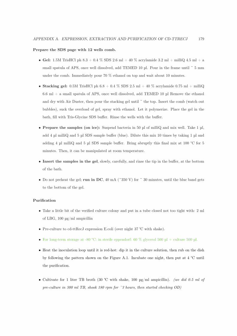
APPENDIX A. EXPRESSION, EXTRACTION AND PURIFICATION OF CD-TTRECJ 179
Prepare the SDS page with 12 wells comb.
• Gel: 1.5M TrisHCl ph 8.3 + 0.4 % SDS 2.6 ml + 40 % acrylamide 3.2 ml + milliQ 4.5 ml + a
small spatula of APS, once well dissolved, add TEMED 10 μl. Pour in the frame until ~ 5 mm
under the comb. Immediately pour 70 % ethanol on top and wait about 10 minutes.
• Stacking gel: 0.5M TrisHCl ph 6.8 + 0.4 % SDS 2.5 ml + 40 % acrylamide 0.75 ml + milliQ
6.6 ml + a small spatula of APS, once well dissolved, add TEMED 10 μl Remove the ethanol
and dry with Air Duster, then pour the stacking gel until ~ the top. Insert the comb (watch out
bubbles), suck the overload of gel, spray with ethanol. Let it polymerize. Place the gel in the
bath, fill with Tris-Glycine SDS buffer. Rinse the wells with the buffer.
• Prepare the samples (on ice): Suspend bacteria in 50 μl of milliQ and mix well. Take 1 μl,
add 4 μl milliQ and 5 μl SDS sample buffer (blue). Dilute this mix 10 times by taking 1 μl and
adding 4 μl milliQ and 5 μl SDS sample buffer. Bring abruptly this final mix at 100 °C for 5
minutes. Then, it can be manipulated at room temperature.
• Insert the samples in the gel, slowly, carefully, and rinse the tip in the buffer, at the bottom
of the bath.
• Do not preheat the gel; run in DC, 40 mA (~350 V) for ~ 30 minutes, until the blue band gets
to the bottom of the gel.
Purification
• Take a little bit of the verified culture colony and put in a tube closed not too tight with: 2 ml
of LBG, 100 μg/ml ampicillin
• Pre-culture to cd-ttRecJ expression E.coli (over night 37 ℃ with shake).
• For long-term storage at -80 °C: in sterile eppendorf: 60 % glycerol 500 μl + culture 500 μl.
• Heat the inoculation loop until it is red-hot: dip it in the culture solution, then rub on the dish
by following the pattern shown on the Figure A.1. Incubate one night, then put at 4 °C until
the purification.
• Cultivate for 1 liter TB broth (30 ℃ with shake, 100 μg/ml ampicillin). (we did 0.5 ml of
pre-culture in 300 ml TB, shook 180 rpm for ~3 hours, then started checking OD)

APPENDIX A. EXPRESSION, EXTRACTION AND PURIFICATION OF CD-TTRECJ 180
Figure A.1: Pattern to follow.
• Reach an optical density at 600 nm of 0.4 and add to IPTG 0.4 mM.
• Harvest after 3 hours. Induction by centrifugation (8000 rpm, 5 min). (we did 2 times 500 ml,
threw away liquid, then added about 20 ml of [20 mM Tris-HCl + 50 mM NaCl] in centrifuge
tube to get the pellet then a bit more to get the remains of the emulsion, put in 50 ml falcon,
re-centrifuge, remove liquid)
• Store the bacteria pellet at -20 ℃.
• Suspend frozen cell (about 10 g) in 80 ml of buffer A. (we did ~3 g in 20 ml)
• Sample n°1 for SDS page.
• Disrupt by sonication. (in beaker, put in ice+water in polystyrene box, ~5 min enough, pulse 1
s off 0.5 s, set amplitude according to sound, once done, set back to 1. Keep cold from now on)
do more than 5min next time
• Sample n°2 for SDS page.
• Heat at 65℃, 30min (skipped)
• Centrifuge 40000 rpm for 1 hour. (we did 70000 rpm 30min, to get a clear solution for his-tag
trapping. Be careful to fill the tube completely to avoid explosion. Wipe rotor.)
• Transfer supernatant and adjust to 5 mM final concentration by adding 2 M imidazole. (to limit
non specific binding)
• Equilibrate His-Trap column with 20 ml of buffer B. (don’t insert bubbles inside. use lock-type
syringe)
• Add the sample in the equilibrated column.

APPENDIX A. EXPRESSION, EXTRACTION AND PURIFICATION OF CD-TTRECJ 181
• Sample n°3 of trash start, n°4 of trash end for SDS page.
• Wash the column with 20 ml of buffer B.
• Sample n°5 at washing end for SDS page.
• Elute from the column with elution buffer (50mM→100mM→150mM→200mM). (2 samples of
1.5ml for each.) do 150.200.250.300 mM next time
• Check the eluting fraction by SDS page. Choose the good ones.
• Correct the cd-ttRecJ eluting fraction and (if needed) concentrate by ultrafiltration. (We took
150-2, 200-1, 200-2, first check that the columns membranes aren’t broken: put milliQ in two of
them, centrifuge, if mQ is filtered too quickly, that means there is a hole somewhere. We reduced
from 4.5 ml to 1 ml. 7500g, enter sample height ~50 mm)
• Equilibrate desalting column with 25ml of buffer C.
• Apply the sample (1.5 ml) in desalting column. (We added 0.5 ml of buffer C to get to 1.5 ml)
• Elute with 2 ml of buffer C. (exactly 2 ml or other things will get out)
• Measure the concentration of cd-ttRecJ by absorption at 278 nm (molar extinction coefficient
33400M-1). (We checked 1x and 1/10x concentrations, 50 μl each. 0.355218/0.0334 = 10.64
μM)
• Concentrate to (~ 10 mg/ml) by ultrafiltration. (We concentrated 4 times to ~40 μM)
• Store at -80℃ in 50% glycerol. Freeze small volumes with liquid nitrogen.
• Check the activity of cd-ttRecJ by digestion experiment.
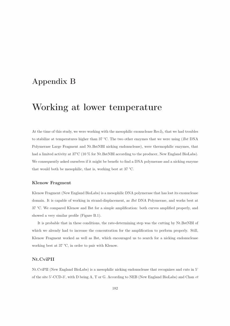
Appendix B
Working at lower temperature
At the time of this study, we were working with the mesophilic exonuclease RecJf, that we had troubles
to stabilize at temperatures higher than 37 °C. The two other enzymes that we were using (Bst DNA
Polymerase Large Fragment and Nt.BstNBI nicking endonuclease), were thermophilic enzymes, that
had a limited activity at 37°C (10 % for Nt.BstNBI according to the producer, New England BioLabs).
We consequently asked ourselves if it might be benefic to find a DNA polymerase and a nicking enzyme
that would both be mesophilic, that is, working best at 37 °C.
Klenow Fragment
Klenow Fragment (New England BioLabs) is a mesophilic DNA polymerase that has lost its exonuclease
domain. It is capable of working in strand-displacement, as Bst DNA Polymerase, and works best at
37 °C. We compared Klenow and Bst for a simple amplification: both curves amplified properly, and
showed a very similar profile (Figure B.1).
It is probable that in these conditions, the rate-determining step was the cutting by Nt.BstNBI of
which we already had to increase the concentration for the amplification to perform properly. Still,
Klenow Fragment worked as well as Bst, which encouraged us to search for a nicking endonuclease
working best at 37 °C, in order to pair with Klenow.
Nt.CviPII
Nt.CviPII (New England BioLabs) is a mesophilic nicking endonuclease that recognizes and cuts in 5’
of the site 5’-CCD-3’, with D being A, T or G. According to NEB (New England BioLabs) and Chan et
182

APPENDIX B. WORKING AT LOWER TEMPERATURE 183
Figure B.1: Amplification of T11 in absence of exonuclease. The reaction is performed at 37 °C, with0.08 unit/μl of either Bst DNA polymerase (blue curve) or Klenow Fragment (red curve). Nickingendonuclease Nt.BstNBI was used (2 %). Autocatalytic module cT11 (60 nM) was initially put inpresence of 0.1 nM of T11.
al. [203], the site CCT is cut less efficiently than CCA and CCG, and some CCT sites are not cut at all.
We confirmed this with an autocatalytic module (C12vi, amplifying T12vi: 5’-CCTAAGATGTAT-3’)
that did work, however very slowly. One would have to be careful to not use the site CCT.
We then tried with the recognition site CCG with two different autocatalytic modules:
• c11vi-sph, amplifying T11vi-sph 5’- CCGTCTGCATG*-3’, also enabled to work with SphI
(NEB), that cuts at the location marked by a star in the site 5’-GCATG*C-3’ (Figure B.2)
• c11vi, amplifying T11vi 5’-CCGAGATTGAA-3’ (Figure)
Figure B.2: Amplification of T11vi-sph ([c11vi-sph] = 60 nM) in absence of exonuclease. The reactionis performed at 37 °C, with Bst DNA Polymerase, and either nickase SphI (blue curve) or Nt.CviPII(red curve). Whereas the amplification worked well with Nt.CviPII, it did not with SphI.
Curves of c11vi exhibited a weird, sudden decrease of fluorescence after the initial amplification.
We investigated this by doing an acrylamide gel analysis of reaction samples taken before and after
this sudden decrease. We did the gel analysis for both cT11 (that we know amplify without artifact)

APPENDIX B. WORKING AT LOWER TEMPERATURE 184
Figure B.3: Amplification of T11vi ([c11vi] = 60 nM) in absence of exonuclease. The reaction isperformed at 37 °C, with Bst DNA Polymerase, and a ramp of Nt.CviPII from 0.5 % to 5 %. Left: thefirst 20 minutes. Amplification speed increases as the concentration of nickase increases. Right: after afew tens of minutes, the fluorescence decreases suddenly. This happens earlier for higher concentrationsof nickase.
and c11vi. Samples were quenched with EDTA 2 μl, then put on ice, and subsequently frozen until
gel analysis. For c11vi, a first sample was taken before the beginning of the amplification, (cycle 0),
then at the plateau (cycle 77), then right after the decrease of fluorescence (cycle 253) and finally later
on (cycle 403). We can clearly see the emergence of an unknown species (a new band appears on the
sample taken at cycle 253) whose concentration increases (the band at cycle 403 is bigger). This new
species is longer than T11vi, but shorter than c11vi. Also, it seems that between cycle 253 and 403, the
concentration of T11vi has not increased, whereas that of the new species has clearly increased. We
could not get to any conclusion with these results alone: T11vi or c11vi do not present any secondary
structure or interaction that may lead to unwanted behaviors. A possible star activity of Nt.CviPII
may result in such weird behavior; however, we did not find any references going in this direction.

APPENDIX B. WORKING AT LOWER TEMPERATURE 185
Figure B.4: Poly-acrylamide gel analysis of the amplification of cT11 (left) and c11vi (right). The high-est bands correspond to the templates cT11 or c11vi (both 22 bases long). The lower ones correspondto the produced T11 of T11vi (both 11 bases long). In the case of c11vi, a new band appears abovethat of T11vi, at cycle 253. It becomes darker at cycle 403, suggesting an increase of concentration ofthis new species.

Appendix C
Two-dimensional Bistability
Using Paraframe, we implemented our bistable circuit in a two-dimensional environment. We were
able to appreciate the difference in speed of the moving front in a given state when freely diffusing or
when confronting to a front in the opposite state.
Figure C.1: Bistable circuit in 2D. (A) Bistable circuit. (B) Time-frame of the experiment monitoredthrough Tamra channel. Fluorescence intensity was converted in three levels for visibility (dark, greyand bright). Bright corresponds to high concentration of β. The reaction was started with two localizedspots of β and one of α. (C) Fluorescence time-plot at three different locations. The global decreaseof intensity suggests that Tamra gets bleached throughout the reaction. The experiment was run at42 °C, with [αtoα] =10 nM and [βtoβ] = 20 nM.
186
APPENDIX C. TWO-DIMENSIONAL BISTABILITY 187
In a round chamber
We first tried to run the bistable circuit (Figure C.1-A) in a round paraframe, setting up localized [α]
and [β] dried on the glass surface prior to the experiment (Figure C.1-B). In order to get a fluorescence
signal high enough, we increased the concentrations of inhibitor modules from 20 nM to 40 nM. We also
increased the concentration of BSA to 5 mg/ml (corresponding to the concentration used in Chapter
6). Otherwise, the reaction conditions (enzymatic, temperature and concentrations of autocatalytic
modules) were kept the same as in Chapter 2. The front in state B (initiated at the localized spots
of β) diffused in tens of minutes to fill the upper part of the chamber, where it did not encounter any
resistance. However, front B was confronted to front A on the lower part of the chamber, and took
about 800 minutes to finally “kill” the areas in state A. This accounts for the good balancing between
both sides (A and B) of this bistable circuits: one would expect an immobile front in the ideal case of
a perfectly balanced bistable circuit.
Appendix D
Working in agarose
As detailed in Appendix A microfluidic device for on-chip agarose microbead generation with ultralow
reagent consumption, both Bst DNA polymerase and Nt.BstNBI nicking endonuclease are working well
in presence of agarose, gelified or not (we tested up to 2 % on a simple autocatalytic amplification).
However, we had trouble using RecJ (both mesophilic RecJf and thermophilic tt-RecJ) in agarose.
Oscillator c11bt in agarose: first try
We first tried to run the c11bt Oligator in usual conditions, with or without agarose. This simply
did not work (Figure D.1). Warm agarose (3 %) or water was added to the reaction mix, which was
then put on ice for gelification before starting the reaction. Note that we were careful not to heat the
agarose too much, in order to avoid damaging mesophilic RecJf.
Degradation by RecJf in agarose
We checked the activity of RecJf in agarose by doing a degradation experiment: the presence of agarose
– gelified or not – clearly impacted the kinetics of RecJf (Figure D.2): it decreases RecJf speed and
seems to increase its Km. By doing an exponential fit of the degradation curve with 1 % agarose, we
found that we would need roughly 5 times more RecJf in order to reach the same k1st = Vm/Km as
that of RecJf in absence of agarose.
188

APPENDIX D. WORKING IN AGAROSE 189
Figure D.1: Oligator c11bt with (red curve) or without (blue curve) agarose 1%. The reaction wasperformed at 38.4 °C. In presence of agarose, the initial amplification only performs properly. It seemsthat the exonuclease activity is lost.
Figure D.2: Degradation of 2 μM of inh11bt3 (5’-GTCTAAGCTGAGTAA-3’) by RecJf. (Left) Inpresence of 0, 0.2, 0.5 or 1 % of gelified agarose and (Right) in presence of 1 % of agarose, gelified ornot. The reaction was performed at 38.4 °C.
Oscillator c11bt in agarose: second try
We then tried again the c11bt Oligator in agarose, with a ramp of concentration of RecJf. We could
observe a few oscillations for higher concentrations of RecJf (Figure D.3), confirming that we need
to increase its concentration when working in agarose. Agarose probably is a form of competitive
substrate for both RecJf and tt-RecJ. Supporting this hypothesis, Wakamatsu et al. [145] observed
that RecJ possesses a domain that has structural similarities to an oligosaccharide-binding fold.

APPENDIX D. WORKING IN AGAROSE 190
Figure D.3: Degradation of 2 μM of inh11bt3 (5’-GTCTAAGCTGAGTAA-3’) by RecJf. (Left) Inpresence of 0, 0.2, 0.5 or 1 % of gelified agarose and (Right) in presence of 1 % of agarose, gelified ornot. The reaction was performed at 38.4 °C.

Appendix E
Nucleic acids for the rational design of
reaction circuits
191

Nucleic acids for the rational design of reaction circuits
Adrien Padirac1, Teruo Fujii1, Yannick Rondelez1,* 1LIMMS/CNRS-IIS, Institute of Industrial Science, The University of Tokyo, 4-6-1 Komaba, Meguro-ku,
Tokyo 153-8505,
*Correspondence to: [email protected]
Abstract
Nucleic acid-based circuits are rationally designed
in vitro assemblies able to perform complex pre-
encoded programs. They can be used to mimic in
silico computations. Recent works emphasized the
modularity and robustness of these circuits, which
allow their scaling-up. Another new development
has led to dynamic, time-responsive systems able
to display emergent behaviors like oscillations.
These are closely related to biological
architectures and provide an in vitro model of in
vivo information processing. NA circuits have
already been used to handle various processes for
technological or biotechnological purposes.
Future applications of these chemical smart
systems will benefit from the rapidly growing
ability to design, construct, and model nucleic acid circuits of increasing size.
Introduction
Nucleic Acid (NA) polymers provide a functional
substrate to encode information at the molecular level.
When this potential was first harnessed in
nanotechnology [1], researchers focused on immobile
2D [2] and 3D [3] nanostructures. These were followed
by NA nanomachines: dynamic nanostructures able to
perform nanoscale movements [4] upon the reception
of external stimuli. NA also proved to be a tool of
choice for a specific class of computation: in the mid
90s, Adleman came out with an innovative search
strategy for NP-complete problems by exploiting the
massively parallel process of molecular recognition inherent to NA hybridization [5].
Computation with NA eventually moved to a more
“universal” direction by taking the form of logic gates
[6]. Such an approach would allow one to build NA-
made Boolean circuits, thereby mimicking in silico computation.
In their natural role, NA are the groundwork of
biological information managing. DNA carries the
genetic information, which is processed within complex
reaction networks involving in particular RNA [7].
These in vivo circuits can also be taken as a model for
artificial NA-based computation. In 2006, Kim et al.
demonstrated an in vitro bistable circuit, modeled after in vivo gene regulatory networks [8].
For these various technological approaches, the critical
asset of NA is to offer a facilitated access to the
modular assembly of a molecular system: simple
hybridization rules [9] permit the rational design of
molecular recognition; and the polymeric structure of
NA allows one to physically link individual domains in
order to obtain multifunctional molecular components
(e.g. two-input gates [10,11], or input-output modules
[12]). Therefore, these modules can be rationally
organized into scaled-up reaction circuits. By
increasing the size of the circuits [13] –or expanding
the set of chemical rules [14-16]– researchers are now
addressing increasingly complex computations / behaviors.
In this review, we wish to emphasize the recent
breakthrough in the complexity and capabilities of
deterministic NA-based molecular circuits. We mostly
limit ourselves to experimentally demonstrated
systems. Therefore, we do not focus on a number of
theoretical works proposing intriguing computation
schemes based on stochastic chemical processes,
which are less amenable to wet-lab validation [17,18].
We first survey the most advanced irreversible
systems, single-use reactive assemblies whose final
state is a pre-encoded function of a set of inputs. We
then review dynamic systems, out-of-equilibrium
assemblies whose convoluted behaviors emerge from
the structural features of a designer reaction network.
Figure 1: Irreversible system versus dynamic system.
(Left) From an initial state (0) and a set of inputs, an
irreversible system evolves towards a low-potential
equilibrium state that corresponds to the answer of the
computation (A or B), and cannot be re-used. (Right) A
dynamic system continuously consumes energy. Upon
reading of a set of inputs (that may be endogenous), it
transits from state to state, but does not get trapped in
the equilibrium: it can be re-used or perform recursive
tasks.

Finally we discuss the place of these circuits within the
field of NA nanotechnology, and their possible links with the biological world.
Toehold based reaction circuits
The first addressable NA nanomachine –the DNA
tweezers of Yurke et al. [4]– brought the concept of
toehold-mediated strand-displacement (TMSD), by
which the displacement of an “output” strand, by an
invading “input” strand, is controlled by a small single-
stranded recognition sequence called “toehold”. In
2006, Seelig et al. demonstrated the computational
ability of TMSD by using it to power a complete set of
Boolean logic gates [19]. These hybridization-driven
logic gates could be cascaded, yet with several
limitations due to a damping of the signal after each
layer of logic gates. The authors had to introduce a
complicated amplification mechanism to mitigate this
effect. The concept of chemical signal restoration to
allow deeper cascading was later revisited by Zhang et al. [20].
The recent rise in the complexity of toehold-powered
reaction circuits was made possible by the “seesaw”
gate [11]. Qian and Winfree packed in this compact
gate motif the two important features allowing robust
modularity, and consequently the scaling-up of reaction
circuits: thresholding (robustness against noise) and
signal restoration (robustness against damping of the
signal). This was nicely demonstrated in two papers
showcasing various reaction circuits including up to 40
seesaw gates: one of them able to calculate the square
root of a four-bit binary number [13], and another elegantly mimicking neural network computation [21].
However, irrespective of the complexity of the
computation they perform, these experimental TMSD
cascades are still based on a small thermodynamic
driving force. This limits the evolutions of the
concentrations of their components to simple
trajectories. In other words, they are use-once
structures and a new “computer” is required for every
computation. Genot et al. demonstrated a reversible
logic gate design [22] that permanently responds to
changes in its inputs. However, such a strategy implies
that the system always remains close to the
equilibrium, which would forbid signal restoration and
limit the cascading of reactions [23]. For classic
(deterministic) chemical systems, the only route to non-
trivial behaviors -such as oscillations- involves the
creation of attractors other than the thermodynamic
branch. This is only possible in dissipative chemical
systems, i.e. those traversed by a continuous flux of energy [24-26].
Figure 2: Two systems allowing the rational assembly of dynamic reaction circuits from basic units. Genelets are double-
stranded DNA that contain a nicked promoter (in red). When the promoter is complete (genelet indicated as “active”), a
RNA polymerase transcribes it in RNA transcripts (thin wavy strands) that establish the communication between genelets.
“Activation” is obtained when the sequestered DNA activator of an inactive genelet is released by an activating RNA
transcript. “Inhibition” is obtained as an inhibiting RNA transcript binds and displaces the DNA activator of an active
genelet, thus inactivating it. A RNase degrades RNA transcripts into NMPs. In the DNA-toolbox, short DNA activators
activate DNA templates (bottom strands) that consequently produce other DNA activators or inhibitors and establish the
communication between templates. “Activation” is obtained as a DNA activator hybridizes to a DNA template and primes
polymerization. “Inhibition” is obtained as a DNA inhibitor hybridizes to a template, thus blocking activators. An
exonuclease degrades DNA activators and inhibitors into dNMPs. Both systems led to experimental implementations of various dynamic circuits encoding oscillations and bistability.

Dynamic reaction circuits
In the context of TMSD cascades, building oscillations,
chaos or recursive computations [26] would require a
theoretically constant concentration of fuel molecules.
This could be achieved by working in an open reactor –
rather than in a closed tube– with a constant resupply
of logic gates. Since closed system are experimentally
more practical, another idea would be to have a large
amount of “buffered” inactivated gates present in
solution, with one buffered gate getting activated as an
active gate is consumed [27]. This would allow the
system to run with a constant concentration of
activated gates, until it runs out of buffered gates.
Nonetheless, the building of dynamic or time-
responsive behaviors out of TMSD primitives remains an attractive challenge.
Enzymes, with their exquisite catalytic properties, offer
an easy access to the implementation of kinetic traps.
These provide the separation of time scales that is
necessary to turn a closed system into a pseudo-open
system [28]. By using catalytic mechanisms with
feedbacks to control their rates, it is possible to shape
dynamic systems that stay out-of-equilibrium until all precursors have been consumed [29].
RTRACS is an autonomous computer based on RNA
polymerase and RNase and modeled after retroviral
replication [30]. The modular, time-responsive logic
computations use RNA as both input and output of a
DNA-encoded software that is executed by the
enzymatic hardware. Kan et al. recently built a
generalized logic gate that should be capable of
performing various logic functions (such as AND,
NAND, OR, NOR), thus potentially allowing the wiring of larger logic gate circuits [31].
In 2006 Kim et al. [8] proposed an in vitro analog of
gene regulation circuits where, rather than getting
translated into proteins, RNA transcripts regulate their
own transcription from DNA gene analogs. These
genelets are short DNA duplexes that contain an
incomplete promoter: they require an additional DNA
single-stranded activator before they can initiate the
transcription of their RNA outputs. In turn, these RNA
transcripts will either release or sequester the labile
DNA activator of other genelets, hence establishing a
cross-regulation between different units (Figure 2).
One or two RNases [32] provide an internal chemical
sink by continuously degrading the RNA transcripts, thereby maintaining the system’s boundedness.
As for the genes of in vivo reaction networks [33],
genelets can be arbitrarily cascaded: one can freely
organize the topology of the network, as well as the
nature (activation or inhibition) of each vertex. Kim et
al. first constructed a bistable circuit in which two
genelets are mutually repressing each other [8]. It was
latter demonstrated that a single self-activating unit can
also behave as a bistable switch [32]. The modularity
of these constructs was further explored with several
oscillator designs [34], including an analog of the repressilator [35].
Montagne et al. abstracted one more step of the gene
regulation pathway by removing the need for RNA
transcription and described a DNA-only general
scheme for the implementation of dynamic circuits: the
DNA-toolbox (Figure 2). In this case, pseudo-genes
(single strand templates) directly regulate each other
by emitting small signal molecules [12]. These DNA
signals come in two types: inputs that activate DNA
templates and inhibitors that block them. A single-
strand specific exonuclease degrades signal
molecules, while templates are protected by DNA
backbone modifications. Despite its simplicity, this
implementation supported reaction circuits displaying
oscillations [12,36], bistability and switchable memory
[37], all rationally designed and assembled by using the modularity of the reactions.
Interface
In vitro dynamic reaction circuits provide an operative
model to study the network / functions relationships
with regard to what occurs in vivo. Dynamic processes
that may be blurred by biological complexity naturally
become apparent when one tries to construct in vitro
analogs [38]. For instance, recent studies have pointed
at the possible importance in cellular circuits of two
neglected phenomena: the competition for enzymatic
resources within a functional motif [39,40], and the
“load” effect that appears when a reaction circuit is connected to a downstream process [41].
Some systems that are built in vitro, but precisely
reproduce the biochemistry of transcription-translation
reaction networks, may also be instrumental to bridge
the gap with in vivo systems [29,42]. In this way,
Noireaux and coworkers are developing a cell-free
expression toolbox from E. Coli extracts [43,44]. Using
this toolbox, they recently constructed a multi-stage
cascade, an AND gate and a negative feedback loop [45].
Figure 3: Examples of technological and biological applications of NA reaction circuits.

By their nature, reaction circuits built from nucleic acids
are at the direct interface with biology. It is however not
trivial to transfer a NA circuit designed in vitro toward
an in vivo environment. Efforts in testing and improving
the robustness of the circuits are required in order to
work in a non-pristine milieu where various materials
may interfere with the function of the circuit [46]. Some
NA logic circuits have been shown to perform well in
the presence of cellular amount of RNA [19], or
random oligonucleotides [14,47]. Recent studies also
focused on reaction robustness to mutations or
impurities in the sequences [47], and hybridization
robustness in large range of temperature and salt
conditions [48]. Such works may prove precious with
respect to the possible implementation of complex NA circuits in vivo.
The resilience of strand displacement reactions was
specifically studied for in situ application [49], and
subsequently used with DNA-conjugated antibodies for
the labeling of endogenous proteins [50]. Choi and
coworkers demonstrated that the hybridization chain
reaction [51] –by which a specific DNA molecule
triggers a chain hybridization of metastable hairpin
molecules– could be implemented with RNA, and
tweaked for specific mRNAs detection purposes within
intact biological samples. Hybridization chain reaction
was also used in living cells, to build circuits that would
mediate the cell death upon detection of cancer-specific mRNAs [52].
NA circuits could also play the role of the software
controlling dynamic NA robots or motors by
sequentially producing the driving molecular stimuli in
situ, thus alleviating the need for exogenous control.
An insight of such application was recently published
by Franco et al., who used a genelet-based oscillator
to drive the opening-closing of DNA tweezers, as well
as the production of an RNA aptamer [41]. This
approach could be extended to the control of DNA gels
[53], organic synthesis [54,55] or optical devices
[56,57]. More complex NA nanorobots [58,59], possibly
oriented towards in vivo applications [60] could also
benefit from an integrated NA circuit-based sensing and driving.
Conclusion
Because they offer a handy solution to the problem of
chemical modularity, NA have dramatically accelerated
the development of man-made reaction networks with
precise structural organization enabling intricate
behaviors. Irreversible logic circuits will find
applications in therapeutics or smart cellular probes
[52,61]. Dissipative architectures have a richer
potential from a computational perspective [26].
Moreover their elaboration and study is backed by their
relevance to biological examples. Indeed, as regulatory
phenomena emerge more and more as the central
feature of living systems [62], in vitro and generic
reaction networking schemes reproducing biological
architectures and functions will form a unique
conceptual and material bridge between living and non-living matter [63].
1. Seeman NC: Nucleic acid junctions and
lattices. J Theor Biol 1982, 99:237–247.
2. Winfree E, Liu F, Wenzler LA, Seeman NC:
Design and self-assembly of two-
dimensional DNA crystals. Nature 1998,
394:539–544.
3. Chen JH, Seeman NC: Synthesis from DNA
of a molecule with the connectivity of a
cube. Nature 1991, 350:631–633.
4. Yurke B, Turberfield AJ, Mills AP, Simmel FC,
Neumann JL: A DNA-fuelled molecular
machine made of DNA. Nature 2000,
406:605–608.
5. Adleman LM: Molecular computation of
solutions to combinatorial problems.
Science 1994, 266:1021–1024.
6. Stojanovic M, Mitchell T, Stefanovic D:
Deoxyribozyme-based logic gates. J Am
Chem Soc 2002, 124:3555–3561.
7. Licatalosi DD, Darnell RB: RNA processing
and its regulation: global insights into
biological networks. Nat. Rev. Genet. 2010,
11:75–87.
8. Kim J, White KS, Winfree E: Construction of
an in vitro bistable circuit from synthetic
transcriptional switches. Mol Syst Biol
2006, 2:68.
9. Bindewald E, Afonin K, Jaeger L, Shapiro BA:
Multistrand RNA secondary structure
prediction and nanostructure design
including pseudoknots. ACS Nano 2011,
5:9542–9551.
10. Elbaz J, Lioubashevski O, Wang F, Remacle
F, Levine RD, Willner I: DNA computing
circuits using libraries of DNAzyme
subunits. Nat Nanotechnol 2010, 5:417–422.
11. Qian L, Winfree E: A simple DNA gate motif
for synthesizing large-scale circuits.
Journal of The Royal Society Interface 2011,
8:1281–1297.
12. Montagne K, Plasson R, Sakai Y, Fujii T,
Rondelez Y: Programming an in vitro DNA
oscillator using a molecular networking
strategy. Mol Syst Biol 2011, 7:466.

13. Qian L, Winfree E: Scaling up digital circuit
computation with DNA strand
displacement cascades. Science 2011,
332:1196–1201.
14. Zhang DY: Cooperative hybridization of
oligonucleotides. J Am Chem Soc 2011,
133:1077–1086.
15. Chen X: Expanding the rule set of DNA
circuitry with associative toehold
activation. J Am Chem Soc 2012, 134:263–
271.
16. Genot AJ, Zhang DY, Bath J, Turberfield AJ:
Remote Toehold: A Mechanism for
Flexible Control of DNA Hybridization
Kinetics. J Am Chem Soc 2011, 133:2177–
2182.
17. Qian L, Soloveichik D, Winfree E: Efficient
Turing-universal computation with DNA
polymers. DNA Computing and Molecular
Programming 2011, [no volume].
18. Cardelli L: Strand algebras for DNA
computing. Natural Computing 2011,
10:407–428.
19. Seelig G, Soloveichik D, Zhang D, Winfree E:
Enzyme-free nucleic acid logic circuits.
Science 2006, 314:1585.
20. Zhang DY, Turberfield AJ, Yurke B, Winfree
E: Engineering entropy-driven reactions
and networks catalyzed by DNA. Science
2007, 318:1121–1125.
21. Qian L, Winfree E, Bruck J: Neural network
computation with DNA strand
displacement cascades. Nature 2011,
475:368–372.
22. Genot AJ, Bath J, Turberfield AJ: Reversible
logic circuits made of DNA. J Am Chem
Soc 2011, 133:20080–20083.
23. Chiniforooshan E, Doty D, Kari L, Seki S:
Scalable, time-responsive, digital, energy-
efficient molecular circuits using DNA
strand displacement. DNA Computing and
Molecular Programming 2011.
24. Nicolis G, Prigogine I: Self-organization in
nonequilibrium systems. John-Wiley &
Sons: New York, 1977.
25. Kjelstrup S, Bedeaux D: Non-equilibrium
thermodynamics of heterogeneous
systems. Series on Advances in Statistical
Mechanics: Vol. 16 World Scientific: New
York, 2008.
26. Soloveichik D, Seelig G, Winfree E: DNA as a
universal substrate for chemical kinetics.
Proc Natl Acad Sci USA 2010, 107:5393–
5398.
27. Lakin MR, Youssef S, Cardelli L, Phillips A:
Abstractions for DNA circuit design.
Journal of The Royal Society Interface 2012,
9:470–486.
28. Li Y, Qian H, Yi Y: Oscillations and
multiscale dynamics in a closed chemical
reaction system: second law of
thermodynamics and temporal complexity.
J Chem Phys 2008, 129:154505.
29. Goda K, Ito H, Kondo T, Oyama T:
Fluorescence correlation spectroscopy to
monitor Kai protein-based circadian
oscillations in real time. Journal of
Biological Chemistry 2012, 287:3241–3248.
30. Ayukawa S, Takinoue M, Kiga D: RTRACS: A
Modularized RNA-Dependent RNA
Transcription System with High
Programmability. Accounts Chem Res 2011,
44:1369–1379.
31. Kan A, Shohda K, Suyama A: A DNA Based
Molecular Logic Gate Capable of a Variety
of Logical Operations. DNA Computing and
Molecular Programming 2012,
doi:10.1007/978-3-642-32208-2_7.
32. Subsoontorn P, Kim J, Winfree E: Ensemble
Bayesian Analysis of Bistability in a
Synthetic Transcriptional Switch. Acs
Synth Biol 2012, [no volume].
33. Purnick PEM, Weiss R: The second wave of
synthetic biology: from modules to
systems. Nat Rev Mol Cell Biol 2009,
10:410–422.
34. Kim J, Winfree E: Synthetic in vitro
transcriptional oscillators. Mol Syst Biol
2011, 7:465.
35. Elowitz MB, Leibler S: A synthetic
oscillatory network of transcriptional
regulators. Nature 2000, 403:335–338.
36. Padirac A, Fujii T, Rondelez Y: Quencher-
free multiplexed monitoring of DNA
reaction circuits. Nucleic Acids Res 2012,
doi:10.1093/nar/gks621.
37. Padirac A, Fujii T, Rondelez Y: Bottom-up
construction of in vitro switchable memories.
Submitted.
38. Schulman R, Yurke B, Winfree E: Robust
self-replication of combinatorial

information via crystal growth and
scission. Proc Natl Acad Sci USA 2012,
109:6405–6410.
39. Rondelez Y: Competition for catalytic
resources alters biological network
dynamics. Physical review letters 2012,
108:018102.
40. Genot AJ, Fujii T, Rondelez Y: Computing
with competition in biochemical networks.
Physical review letters. In Press.
41. Franco E, Friedrichs E, Kim J, Jungmann R,
Murray R, Winfree E, Simmel FC: Timing
molecular motion and production with a
synthetic transcriptional clock. Proc Natl
Acad Sci USA 2011, 108:E784–93.
42. Chen IA, Nowak MA: From Prelife to Life:
How Chemical Kinetics Become
Evolutionary Dynamics. Accounts Chem
Res 2012, doi:10.1021/ar2002683.
43. Shin J, Noireaux V: Efficient cell-free
expression with the endogenous E. Coli
RNA polymerase and sigma factor 70. J
Biol Eng 2010, 4:8.
44. Karzbrun E, Shin J, Bar-Ziv RH, Noireaux V:
Coarse-grained dynamics of protein
synthesis in a cell-free system. Physical
review letters 2011, 106:048104–.
45. Shin J, Noireaux V: An E. coli Cell-Free
Expression Toolbox: Application to
Synthetic Gene Circuits and Artificial
Cells. Acs Synth Biol 2012, 1:29–41.
46. Hodgman CE, Jewett MC: Cell-free
synthetic biology: thinking outside the
cell. Metab. Eng. 2012, 14:261–269.
47. Zhang DY, Winfree E: Robustness and
modularity properties of a non-covalent
DNA catalytic reaction. Nucleic Acids Res
2010, 38:4182–4197.
48. Zhang DY, Chen SX, Yin P: Optimizing the
specificity of nucleic acid hybridization.
Nat Chem 2012, 4:208–214.
49. Duose DY, Schweller RM, Zimak J, Rogers
AR, Hittelman WN, Diehl MR: Configuring
robust DNA strand displacement reactions
for in situ molecular analyses. Nucleic
Acids Res 2012, 40:3289–3298.
50. Schweller RM, Zimak J, Duose DY, Qutub AA,
Hittelman WN, Diehl MR: Multiplexed in situ
immunofluorescence using dynamic DNA
complexes. Angew Chem Int Ed Engl 2012,
51:9292–9296.
51. Dirks RM, Pierce NA: Triggered
amplification by hybridization chain
reaction. Proc Natl Acad Sci USA 2004,
101:15275–15278.
52. Venkataraman S, Dirks RM, Ueda CT, Pierce
NA: Selective cell death mediated by small
conditional RNAs. Proc Natl Acad Sci USA
2010, 107:16777–16782.
53. Xing Y, Cheng E, Yang Y, Chen P, Zhang T,
Sun Y, Yang Z, Liu D: Self-assembled DNA
hydrogels with designable thermal and
enzymatic responsiveness. Adv Mater
Weinheim 2011, 23:1117–1121.
54. Milnes PJ, McKee ML, Bath J, Song L, Stulz
E, Turberfield AJ, O'Reilly RK: Sequence-
specific synthesis of macromolecules
using DNA-templated chemistry. Chem.
Commun. (Camb.) 2012, 48:5614–5616.
55. McKee ML, Milnes PJ, Bath J, Stulz E,
O'Reilly RK, Turberfield AJ: Programmable
one-pot multistep organic synthesis using
DNA junctions. J Am Chem Soc 2012,
134:1446–1449.
56. Zhou M, Liang X, Mochizuki T, Asanuma H: A
light-driven DNA nanomachine for the
efficient photoswitching of RNA digestion.
Angew Chem Int Ed Engl 2010, 49:2167–
2170.
57. Nishioka H, Liang X, Kato T, Asanuma H: A
photon-fueled DNA nanodevice that
contains two different photoswitches.
Angew Chem Int Ed Engl 2012, 51:1165–
1168.
58. Gu H, Chao J, Xiao S-J, Seeman NC: A
proximity-based programmable DNA
nanoscale assembly line. Nature 2010,
465:202–205.
59. Lund K, Manzo AJ, Dabby N, Michelotti N,
Johnson-Buck A, Nangreave J, Taylor S, Pei
R, Stojanovic MN, Walter NG, et al.:
Molecular robots guided by prescriptive
landscapes. Nature 2010, 465:206–210.
60. Douglas SM, Bachelet I, Church GM: A logic-
gated nanorobot for targeted transport of
molecular payloads. Science 2012,
335:831–834.
61. Xie Z, Wroblewska L, Prochazka L, Weiss R,
Benenson Y: Multi-input RNAi-based logic
circuit for identification of specific cancer
cells. Science 2011, 333:1307–1311.
62. Gerstein MB, Kundaje A, Hariharan M, Landt
SG, Yan K-K, Cheng C, Mu XJ, Khurana E,
Rozowsky J, Alexander R, et al.:
Architecture of the human regulatory
network derived from ENCODE data.
Nature 2012, 489:91–100.
63. Jewett MC, Forster AC: Update on
designing and building minimal cells.
Current Opinion in Biotechnology 2010,
21:697–703.
Annotations
12
Montagne et al.
A potent strategy for the in vitro assembly of dynamic
reaction circuits is presented and demonstrated with a robust
oscillator showing tens of periods.
21
Qian et al.
The demonstration of large-scale circuits based the seesaw
gate motif, mimicking neural networks computation with
pattern recognition ability.
26
Soloveichik et al.
This theoretical paper proposes toehold-mediated strand-
displacement as a general mechanism to build dynamic
reaction circuits.
34
Kim et al.
A transcription-based in vitro scheme is wired into various
circuits with oscillatory behaviors.
41
Franco et al.
A nice demonstration of in vitro reaction circuits driving
downstream processes proposes the “load” effect as an
important feature of biomolecular reaction circuits.
52
Venkatararaman et al.
RNA circuits transfected into live cells detect mRNA cancer
marker and release a RNA drug to trigger cell death.

Appendix F
A microfluidic device for on-chip
agarose microbead generation with
ultralow reagent consumption
199

A microfluidic device for on-chip agarose microbead
generation with ultralow reagent consumption
1LIMMS/CNRS-IIS, Institute of Industrial Science, The University of Tokyo, 4-6-1 Komaba, Meguro-ku,
Tokyo 153-8505, Japan.
2Université Lille 2, Faculté de Médecine et CHRU Lille, Laboratoire de Virologie / EA 3610, Loos-lez-
lille, 59120, France.
* correspondence should be addressed to: [email protected]
Abstract
in situ
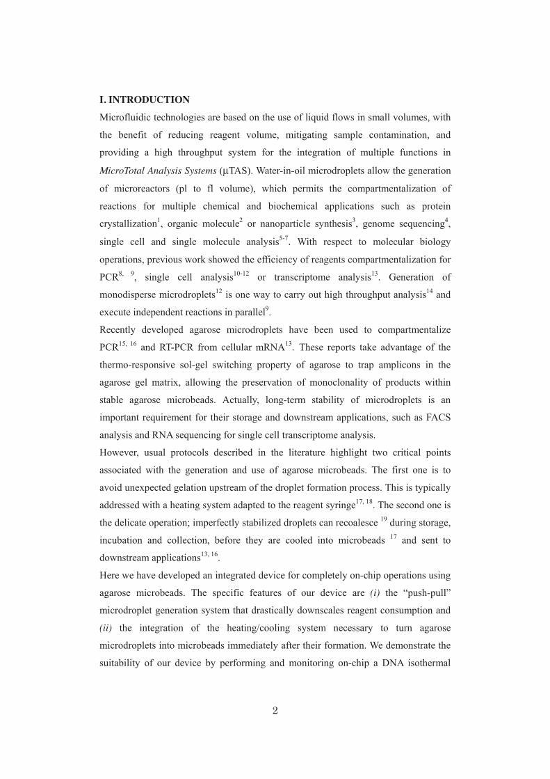
I. INTRODUCTION
MicroTotal Analysis Systems µ
(i)
(ii)

II. MATERIALS AND METHODS
A. Design and fabrication of the microfluidic device
µ
µ

B. Agarose microdroplet generation at room temperature (25 ºC)
µ
C. On-chip agarose microdroplet cooling into agarose microbeads

D. Temperature measurement in the device
E. DNA amplification reaction
Bst
F. DNA amplification monitoring and DNA amplification curve

III. RESULTS AND DISCUSSION
A. Agarose microdroplet generation at room temperature with an ultra low
volume of sample
Qo
Qe

Qa Qa = Qe − Qo

B. On-chip agarose microbead gelation
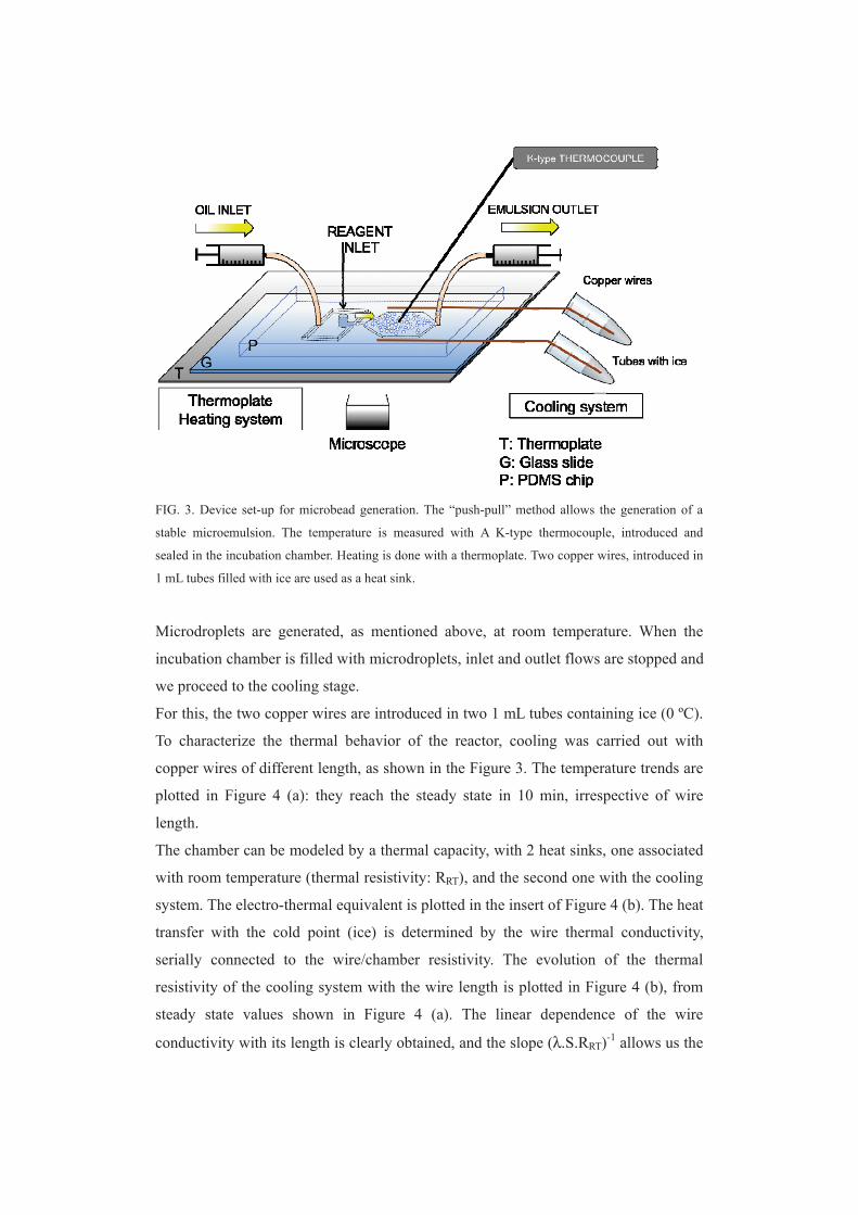
λ

λ

≤
C. DNA amplification and monitoring on-chip


IV. CONCLUSIONS
(i)
(ii) (iii)
ACKNOWLEDGMENTS
125
128
4
437
12
82
102
27
109
134
82
84
12
10
84
32
6
25
37
21

Chapter 14
5
109
89
40
7
[]

A. COMSOL simulation of the temperature in the incubation chamber
We made simulations of the variation of the temperature in the chamber using COMSOL
multiphysics software. We used the constants indicated in the Table SI. The ends of the wires
are set to 0 ºC. The device is immersed in air whose temperature away from the device is
26ºC.
The temperature, at the bottom of the chamber (300 μm below the copper wires) varies from
11.9 ºC (near the wall) to 13.1 ºC (4.1 mm away from the wall, i.e. in the middle of the
chamber) as shown in Figure S1.
The experimental temperature in the middle of the chamber (14.2 ºC) is in good agreement
with the simulation (13.1 ºC). The simulation also indicates that the temperature in the
chamber is homogeneous, with a variation of 1.2 ºC between the coldest (walls) and the
hottest (center of the chamber) part (Figure S2 (a)).
FIG. S1. Simulation of the variation of the temperature inside the chamber. (a) 3D view of the
temperature in the device (only the chamber is simulated). The slice shows the temperature at the
bottom of the device. (b) Cross section view of the device.
In order to find out the maximal chamber width that can be cooled with this method, we
investigate the maximal and minimal temperature at the bottom of the chamber as a function
of the chamber width, all other parameters being equal (Figure S2 (b)). The maximal
temperature ranges from 10.6 ºC for a 2 mm wide chamber, to 15.7 ºC for a 16 mm wide
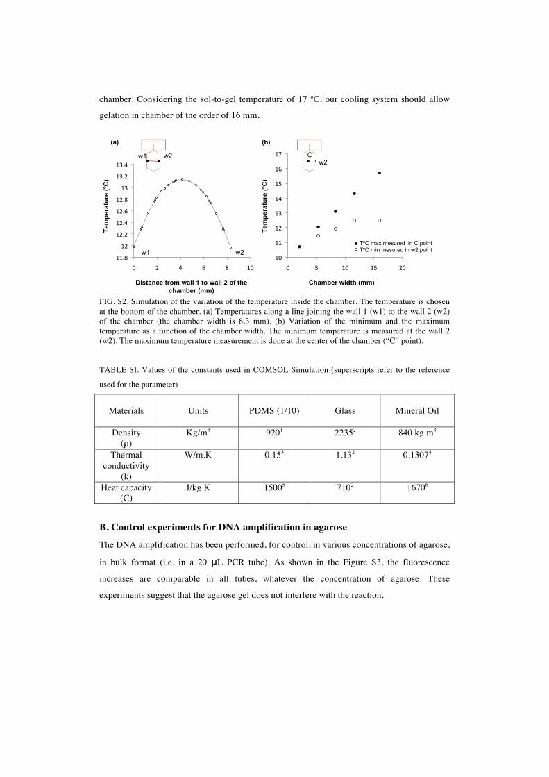
chamber. Considering the sol-to-gel temperature of 17 ºC, our cooling system should allow
gelation in chamber of the order of 16 mm.
FIG. S2. Simulation of the variation of the temperature inside the chamber. The temperature is chosen
at the bottom of the chamber. (a) Temperatures along a line joining the wall 1 (w1) to the wall 2 (w2)
of the chamber (the chamber width is 8.3 mm). (b) Variation of the minimum and the maximum
temperature as a function of the chamber width. The minimum temperature is measured at the wall 2
(w2). The maximum temperature measurement is done at the center of the chamber (“C” point).
TABLE SI. Values of the constants used in COMSOL Simulation (superscripts refer to the reference
used for the parameter)
Materials
Units
PDMS (1/10)
Glass
Mineral Oil
Density
(ρ)
Kg/m3
9201 22352 840 kg.m3
Thermal
conductivity
(k)
W/m.K 0.153 1.132 0.13074
Heat capacity
(C)
J/kg.K 15005 7102 16706
B. Control experiments for DNA amplification in agarose
The DNA amplification has been performed, for control, in various concentrations of agarose,
in bulk format (i.e. in a 20 µL PCR tube). As shown in the Figure S3, the fluorescence
increases are comparable in all tubes, whatever the concentration of agarose. These
experiments suggest that the agarose gel does not interfere with the reaction.
Chamber width (mm)
Tem
pera
ture
(ºC
)
Distance from wall 1 to wall 2 of the
chamber (mm)
Tem
pera
ture
(ºC
)
w1 w2
(a) (b)
w1 w2 w2
C
TºC max mesured in C point
TºC min mesured in w2 point

FIG. S3. DNA amplification reaction in the presence of various concentrations of agarose. The DNA
amplification mixtures have been prepared with various concentrations of agarose (from 0. 5% to 2 %).
They were then cooled at 4 ºC for a few minutes in order to gelify the agarose. After the cooling stage,
all tubes have been incubated in a thermal cycler at 43 ºC for DNA amplification. Whatever the
agarose concentration, the fluorescence signal increases as fast as the control, i.e. the DNA
amplification occurred in all tubes.
BIBLIOGRAPHY
1. D. Armani, C. Liu and N. Aluru, Twelfth IEEE International Micro Electro
Mechanical System Conference, 222-227 (1999).
2. I. Wong, S. Atsumi, W. C. Huang, T. Y. Wu, T. Hanai, M. L. Lam, P. Tang, J. A.
Yang, J. C. Liao and C. M. Ho, Lab Chip 10 (20), 2710-2719 (2010).
3. O. K. Bates, Ind Eng Chem 41 (9), 1966-1968 (1949).
4. L. H. Huang and L. S. Liu, J Food Eng 95 (1), 179-185 (2009).
5. A. Elliott, J. Schwartz, J. Wang, A. Shetty, J. Hazle and J. R. Stafford, Laser Surg
Med 40 (9), 660-665 (2008).
6. C. Xie and J. P. Hartnett, Int J Heat Mass Tran 35 (3), 641-648 (1992).
Flu
ore
sc
en
ce
(A
U)
Time (min)