This article appeared in a journal published by Elsevier. The attachedcopy is furnished to the author for internal non-commercial researchand education use, including for instruction at the authors institution

and sharing with colleagues.

Other uses, including reproduction and distribution, or selling orlicensing copies, or posting to personal, institutional or third party

websites are prohibited.

In most cases authors are permitted to post their version of thearticle (e.g. in Word or Tex form) to their personal website orinstitutional repository. Authors requiring further information

regarding Elsevier’s archiving and manuscript policies areencouraged to visit:

http://www.elsevier.com/copyright

Author's personal copy

Ecological Modelling 221 (2010) 1605–1619

Contents lists available at ScienceDirect

Ecological Modelling

journa l homepage: www.e lsev ier .com/ locate /eco lmodel

Development of an individual-based model to evaluate elk (Cervus elaphusnelsoni) movement and distribution patterns following the Cerro Grande Fire innorth central New Mexico, USA

Susan P. Ruppa,b,∗, Paul Ruppc,1

a Ecology Group (ENV-ECO), Los Alamos National Laboratory, TA-21, Bldg. 210, MS M887, Los Alamos, NM 87545, USAb Department of Range, Wildlife, and Fisheries Management, Box 42125, Texas Tech University, Lubbock, TX 79409-2125, USAc Acorp Computers, 4615 Albany Ct., Albuquerque, NM 87114, USA

a r t i c l e i n f o

Article history:Received 21 August 2009Received in revised form 15 February 2010Accepted 17 March 2010Available online 19 April 2010

Keywords:DistributionElkFireIndividual-based modelMovementSuccession

a b s t r a c t

Though studies have modeled the effects of fires on elk, no studies have related the effects of post-firelandscape succession on ungulate movements and distribution using dynamic modeling techniques. Thepurpose of this study was to develop and test a spatially-explicit, stochastic, individual-based model(IBM) to evaluate potential movement and distribution patterns of elk (Cervus elaphus nelsoni) in relationto spatial and temporal aspects of the Cerro Grande Fire that burned north central New Mexico in Mayof 2000. Following extensive literature review, the SAVANNA Ecosystem Model was selected to simulatethe underlying post-fire successional processes driving elk movement and distribution. Standard logisiticregression was used to analyze habitat-use patterns of ten elk from data collected using global positioningsystem radio collars while an additional five animals were used as an independent test set during modelvalidation. Static variables in the form of roads, buildings, fences, and habitual use/memory were used tomodify a map of impedance values based on the logistic regression of slope, aspect, and elevation. Integra-tion with SAVANNA came through the application of a habitat suitability index (HSI), which combinedmovement rules written for the IBM and variables modified and produced by the dynamic ecologicalprocesses run in SAVANNA. Overall pattern analysis indicated that realistic migrational processes andhabitat-use patterns emerged from movement rules incorporated into the IBM in response to advanc-ing and receding snow when compared to the independent test set. Primary and secondary movementpathways emerged from the collective responses of simulated individuals. Using regression analyses, nosignificant differences between simulated animals and animals used in either model development or anindependent test set revealed any differences in response to snow patterns. These considerations suggestthe model was adequately corroborated based on existing data and outlined objectives.

© 2010 Elsevier B.V. All rights reserved.

1. Introduction

Long-term studies on the movement and distribution patternsof species at local and regional scales are needed because those arethe scales at which conservation strategies are planned and imple-mented (Saunders and Hobbs, 1991). In early May 2000, the CerroGrande Fire (CGF) in north central New Mexico burned approx-imately 19,020 ha as well as 400 residences in the town of LosAlamos. That fire, coupled with the region’s unique fire historyand interagency collaborations, presented a unique opportunity to

∗ Corresponding author. Present address: South Dakota State University, Depart-ment of Wildlife and Fisheries Sciences, Northern Plains Biostress Lab 139B, Box2140B, Brookings, SD 57007, USA. Tel.: +1 605 688 4779; fax: +1 605 688 4515.

E-mail address: susan.rupp@sdstate.edu (S.P. Rupp).1 Present address: 610 12th Avenue, Brookings, SD 57006, USA.

study the long-term ecological consequences of large-scale fires onthe regional elk (Cervus elaphus nelsoni) herd. Consequently, a “Par-ticipating Agreement” was signed by the Santa Fe National Forest(USFS), U.S. Department of Energy’s Los Alamos National Labora-tory (LANL), and the National Park Service (BNM) to collaborate indata collection efforts to evaluate and mitigate potential changesin movement and distribution patterns of elk following the CerroGrande Fire.

Though many methods are available for modeling animal move-ments and distribution (e.g., path analysis, fractal analysis, randomwalks, structural equation modeling), there has been a growinginterest in the use of individual-based models (IBMs) in ecologi-cal applications. Individual-based approaches to modeling animalmovements address principles that are largely ignored in othermodeling environments. First, IBMs acknowledge that individu-als are behaviorally and physiologically distinct because of geneticand environmental influences and second, they acknowledge that

0304-3800/$ – see front matter © 2010 Elsevier B.V. All rights reserved.doi:10.1016/j.ecolmodel.2010.03.014

Author's personal copy

1606 S.P. Rupp, P. Rupp / Ecological Modelling 221 (2010) 1605–1619

interactions among individuals are inherently localized (Slothoweret al., 1996; Schank, 2001). An advantage to IBMs is that they donot require many of the simplifying assumptions and mathematicalderivations typically needed in more aggregated models (Railsbacket al., 1999) thus resulting in a more realistic representation ofreal-world phenomena.

Integrated models of disturbance and succession offer a meansof comparing long-term effects of fire events on forest vegetationand other ecosystem processes, including animal movement anddistribution that may otherwise be difficult to observe empirically(Keane et al., 1989; He and Mladenoff, 1999; Turner et al., 2001). Inaddition, successional models enable evaluation of the cumulativeeffects of management practices and ecosystem response in a spa-tial context over long time periods (Keane and Hann, 1998). Severalapproaches have been used to model post-fire succession (Keaneand Long, 1998; Barrett, 2001; Turner et al., 2001) but currentefforts are focused on stochastic approaches that examine the rela-tionship between fire regimes and landscape heterogeneity as wellas fire-affected landscape changes through time (He and Mladenoff,1999). The majority of post-fire successional models are designedspecifically for evaluating forest (i.e., tree) dynamics and not theunderstory component to the degree deemed critical for modelingelk movement and distribution. As a result, the temporal resolu-tion of such models is often in the range of years to decades—muchlonger than the daily or seasonal time step desired to evaluate elkmovement across the Jemez.

Though studies have evaluated the effects of fire scale andpattern on elk (C. elaphus) (Turner et al., 1994), no studies haverelated the effects of post-fire landscape succession on ungulatemovements and distribution using dynamic modeling techniques.Consequently, models linking the responses of herbivores to envi-ronmental heterogeneity and successional dynamics followinglarge-scale fires are needed (Turner et al., 1994). Therefore, thepurpose of this study was twofold: (1) to identify, calibrate, andvalidate a model that could simulate the underlying post-firesuccessional processes driving elk movement and distribution fol-lowing the CGF; (2) to develop and integrate into the post-firesuccessional model a spatially-explicit, stochastic, individual-based model to evaluate potential movement and distributionpatterns of elk in relation to spatial and temporal aspects of theCGF. Conceptualization, development, integration, and validationof the individual-based model are discussed here. Identification,development, and validation of the post-fire successional modelare described in Rupp (2005).

2. Area description

The Pajarito Plateau, located in the Jemez Mountains of northcentral New Mexico, was formed by an ash flow of volcanic activ-ity about 1.4 million years ago (Wilcox and Breshears, 1994). Theregion is classified as a wildland–urban interface and is politi-cally segmented, making natural resource management difficult.The most conspicuous and influential government entity is LosAlamos National Laboratory (11,200 ha). It is bordered by Bande-lier National Monument (13,290 ha) to the southwest, Santa FeNational Forest to the northwest, San Ildefonso Reservation to theeast, and Santa Clara Reservation to the far north. In addition,the federal government recently purchased 37,200 ha of privateland to the northwest that includes the Valles Caldera NationalPreserve (VCNP)—an ancient caldera grassland that serves as theprimary summering grounds for the region’s growing elk popula-tion.

The plateau is topographically complex, ranging in ele-vation from 1600 m near the Rio Grande to 3240 m nearthe summit of Cerro Grande. It is transected by a series of

smaller canyon systems and mesas making the terrain roughand virtually inaccessible in some places. Vegetative patternsare highly dependent on elevation and topography (Wilcoxand Breshears, 1994), but five main vegetative associationshave been described; pinon-juniper grassland (1600–1900 m),pinon-juniper woodland (1900–2100 m), ponderosa pinegrassland (2100–2300 m), mixed-conifer (2300–2900 m), andsubalpine grassland (2900–3200 m). Average annual pre-cipitation is 330–460 mm (Davenport et al., 1996; Wilcoxet al., 1996) of which about 45% occurs in July, August,and September. Average daytime temperatures range from32.2 ◦C in the summer (max. = 41.1 ◦C) to −9.4 ◦C in the winter(min. = −30.6 ◦C).

In the last 30 years the Jemez Mountain region has experiencedfour major fires—the La Mesa fire in 1977, the Dome fire in 1996,the Oso fire in 1998, and the Cerro Grande fire in 2000. Of these,the most prominent fires were the La Mesa and the Cerro Grandeburning 6180 and 19,020 ha, respectively. These fires were centeredin areas of dense, monotypic ponderosa pine forests which, in thecase of the earlier fires, were converted into a more productive anddiverse mosaic of grassland, shrubland, and forest communities.It is believed such conditions may have created prime winteringrange, which contributed to population increases in the regionalelk herd (Allen, 1996).

3. Methods

3.1. Model conceptualization

One of the primary objectives of the research was to analyzepotential movement pathways across the Jemez typically usedin “migration” and assess whether these pathways may changein response to spatial and temporal aspects of the Cerro GrandeFire. By definition, migration indicates a periodic shift from oneseasonal home range to another, which can be assessed throughan analysis of site fidelity within each range (Hooge, 2003, pers.comm.). The elk population in the Jemez Mountains, however, ismore properly referred to as “quasi-migratory” in that movementsare not periodic and seasonal home ranges are difficult to delin-eate, but animals move in response to the best resources (food,water, shelter) available at the time. Nevertheless, it was assumedthe factors that affect migratory patterns in other populations likelyaffect quasi-migratory behaviors as well. These may include pre-ferred ranges, weather, snow depth, forage availability, sex andage, habitual behavior, hunting pressure, and barriers to migration(e.g., roads, buildings, fences) (Adams, 1982). Similarly, factors thatinfluence habitat selection by elk (Table 1) irrespective of migrationmust also be considered given the quasi-migratory behavior of thispopulation.

Following a number of iterations, a conceptual diagram wasconstructed to identify the most parsimonious model among avariety of plausible models in which state variables, processes,driving variables, and dependent variables were depicted. This ini-tial conceptual model guided expert discussion, data needs andassessment, and further introspection that led to the conclusionthat numerous ecological models already existed to address var-ious components depicted in the conceptual model. Of particularinterest were models that could simulate the post-fire successionalprocesses driving elk movement and distribution.

Extensive literature review led to the selection of the SAVANNAEcosystem Model (Coughenour, 1993, 2002). SAVANNA is aspatially-explicit, process-oriented ecosystem model that inte-grates computer modeling, geographic information systems,remote sensing, and field studies. The model is composed of varioussubmodels (e.g., hydrologic, plant biomass production, plant pop-

Author's personal copy

S.P. Rupp, P. Rupp / Ecological Modelling 221 (2010) 1605–1619 1607

Table 1Factors that influence habitat selection by elk. Adapted from Skovlin (1982).

Category of variables Variable name Category of variables Variable name

Topographic Elevation Food AvailabilitySlope Quality

Gradient Cover Cover typePosition on slope ThermalAspect Hiding

Land features DensityMeteorologic Precipitation—snow Composition

Depth Site productivityCondition Structure

Temperature Successional stageSolar radiation Configuration

Radiation SpaceConvection Water and salt

Humidity Specialize habitats CalvingBarometric pressure WallowsWind Trails

VelocityDirection

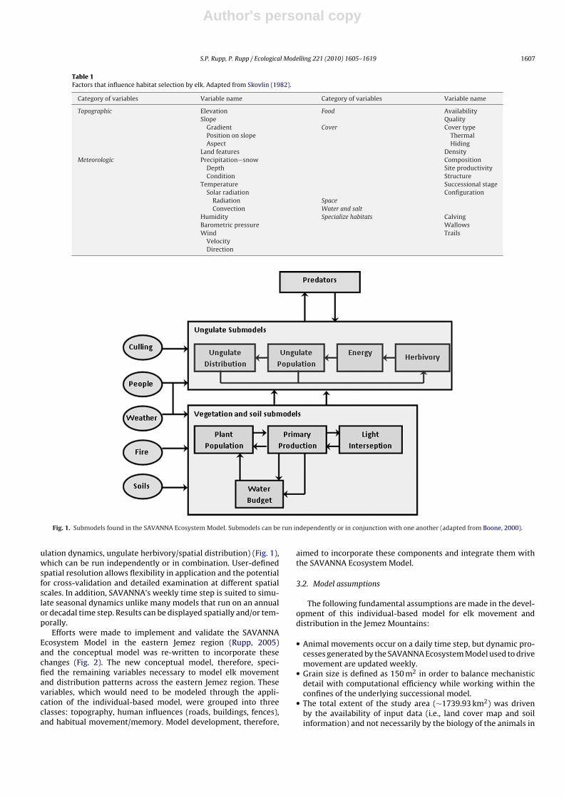
Fig. 1. Submodels found in the SAVANNA Ecosystem Model. Submodels can be run independently or in conjunction with one another (adapted from Boone, 2000).

ulation dynamics, ungulate herbivory/spatial distribution) (Fig. 1),which can be run independently or in combination. User-definedspatial resolution allows flexibility in application and the potentialfor cross-validation and detailed examination at different spatialscales. In addition, SAVANNA’s weekly time step is suited to simu-late seasonal dynamics unlike many models that run on an annualor decadal time step. Results can be displayed spatially and/or tem-porally.

Efforts were made to implement and validate the SAVANNAEcosystem Model in the eastern Jemez region (Rupp, 2005)and the conceptual model was re-written to incorporate thesechanges (Fig. 2). The new conceptual model, therefore, speci-fied the remaining variables necessary to model elk movementand distribution patterns across the eastern Jemez region. Thesevariables, which would need to be modeled through the appli-cation of the individual-based model, were grouped into threeclasses: topography, human influences (roads, buildings, fences),and habitual movement/memory. Model development, therefore,

aimed to incorporate these components and integrate them withthe SAVANNA Ecosystem Model.

3.2. Model assumptions

The following fundamental assumptions are made in the devel-opment of this individual-based model for elk movement anddistribution in the Jemez Mountains:

• Animal movements occur on a daily time step, but dynamic pro-cesses generated by the SAVANNA Ecosystem Model used to drivemovement are updated weekly.

• Grain size is defined as 150 m2 in order to balance mechanisticdetail with computational efficiency while working within theconfines of the underlying successional model.

• The total extent of the study area (∼1739.93 km2) was drivenby the availability of input data (i.e., land cover map and soilinformation) and not necessarily by the biology of the animals in

Author's personal copy

1608 S.P. Rupp, P. Rupp / Ecological Modelling 221 (2010) 1605–1619

Fig. 2. Revised conceptual model showing the integration of the SAVANNA Ecosystem Model and remaining components to be addressed through the application of movementrules in the individual-based model.

question. However, preliminary analysis of elk locations (Rupp,2005) collected through radio telemetry indicated 0.2% of totallocations used in model development and calibration fell outsidethe final study area. Therefore, it is assumed points outside theextent of the study area would not affect overall model resultsand/or conclusions.

• It is assumed that study area extent and grain are representativeof the scale over which elk use and select habitat.

• Factors that affect migratory patterns and habitat selection inmigratory populations likely affect quasi-migratory behaviors aswell and are considered in this analysis.

• Primary external variables driving elk movement and distribu-tion over time include precipitation, temperature, forage quantityand quality, and snow depth whose values are decided by theapplication of the SAVANNA Ecosystem Model. Therefore, anyunderlying assumptions and limitations of SAVANNA apply tothis IBM as well.

• Food intake by elk is determined by the quantity, quality, andavailability of forage in a given cell and can be influenced by thepresence of other elk in that cell.

• The effect of predators (mountain lions and hunters), thoughlikely to affect elk movement and distribution patterns, is notsimulated in this system due to insufficient data at time of modeldevelopment.

• Simulated elk do not have “vision” beyond the eight cells imme-diately surrounding their current location and, therefore, mustmove through each adjacent cell to a final destination point.

• It is assumed elk move in response to spatial and temporal vari-ation associated with calculated habitat suitability indices (HSIs)in a manner that will maximize fitness (i.e., the ability of an organ-ism to survive and reproduce viable offspring) based on howfitness varies among potential locations.

• It is assumed that migratory pathways are, in part, a habitualbehavior that may be influenced by immediate circumstances

encountered during migration (Adams, 1982) and are thereforemodeled accordingly.

• It is recognized that elk are a gregarious species and that socialinteractions and group size will vary throughout the year. Noattempt is made to adjust for seasonal social behaviors and nolimit is placed on density of animals within individual cells; how-ever, parameter files are capable of adjusting density of animalsper cell.

• No attempt is made to distinguish variability among individ-uals based on size, age, sex, or other distinguishing features.Population demographics and life cycles are ignored but can beincorporated at a future point in time when additional informa-tion becomes available that allows for such distinctions.

Data were collected from 54 Rocky Mountain elk (C. elaphusnelsoni) that were collared using Telonics, Inc., GEN-II “Store-on-Board” GPS collars equipped with Trimble LassenTM SK-2 or SK-8receivers and a VHF beacon transmitter. Collars were programmedto acquire GPS positions at intervals ranging from 15 min to 23 hwith more fixes purposefully taken during the fall and springmigration periods. Following a series of technical difficulties withpre-programmed release mechanisms and resulting discrepanciesin data collection, 10 animals were randomly selected for modeldevelopment and 5 were used as an independent test set duringmodel validation.

Preliminary tests of GPS collar accuracy indicated a strong effectof 2D fixes on position acquisition rates (PARs) depending on timeof day and season of year (Rupp, 2005). Position acquisition rateswere lower during mid-day hours and summer months indicatinga possible change in animal behavior during the hottest parts of theday/season. Slope, aspect, elevation, and land cover type affecteddilution of precision (DOP) values for both 2D and 3D fixes, althoughrelationships varied from positive to negative making it difficultto delineate the mechanism behind significant responses. Two-

Author's personal copy

S.P. Rupp, P. Rupp / Ecological Modelling 221 (2010) 1605–1619 1609

dimensional fixes accounted for 34% of all successfully acquiredlocations and may affect results in which those data were used.Nonetheless, mean DOP values were generally in the range of4.0–6.0, regardless of fix type, which was considered reasonablefor model development based on accuracy assessments outlinedby Trimble (1999).

3.3. Model development and calibration

3.3.1. Topographic featuresA comprehensive digital elevation model (DEM) was mosaicked

from sixteen 7.5-min digital elevation model quadrangles down-loaded from the United States Geological Survey (USGS) EarthResources Observation Systems (EROS) Data Center website(http://edc.usgs.gov/geodata/) and used in model development. All1:24,000 quadrangles were projected in Universal Transverse Mer-cator (UTM) coordinates, North American Datum (NAD, 1927) ata resolution of 10 m. Any errors inherent in the acquired datawere assumed minimal and not assessed in detail. The final DEMwas resampled to various resolutions (50 m, 100 m, 150 m, 250 m,and 500 m) using cubic convolution resampling methods avail-able through the Spatial Analyst extension in ArcView 3.2. Becauseinterpolation methods compute an average (Huber, 2004, pers.comm.), slope and aspect maps were generated from the resampledDEMs instead of resampling the slope and aspect maps gener-ated from the original 10 m DEM. Resultant slope and aspect maps,therefore, were also at 50 m, 100 m, 150 m, 250 m, and 500 m reso-lutions. Final maps used in model runs were at a grain of 150 m.

Logistic regression is often used in studies of wildlife habitatuse to predict the presence or absence of an animal using indepen-dent variables which can be either categorical and/or continuous.Regression coefficients in a logistic regression equation can be usedto estimate the odds ratios (Cody and Smith, 1997; Keating andCherry, 2004). The odds ratio is:

(x|xR) = exp(ˇ′x − ˇ0) = exp(ˇ1x1 + · · · + ˇpxp)where (x|xR) is the odds ratio and ˇ = (ˇ0, ˇ1, . . . ˇp) is a vectorof regression coefficients for the variables xi, i = 1, 2, . . ., p. Oddsratios can be used to approximate relative risk—the probability ofuse given x relative to the probability of use given a reference type,xR, that is,

�(x|xR) = P(y = 1|x)P(y = 1|xR)

where � is relative risk, P(y = 1|x) is the probability of occurrencegiven the independent variable(s) ‘x’, and P(y = 1|xR) is the prob-ability of occurrence given a reference type ‘xR’. The odds ratio isrelated to relative risk as:

(x|xR) = �(x|xR)[

1 − P(y = 1|x)1 − P(y = 1|xR)

]Thus, if use is assumed to be rare everywhere (i.e., P(y = 1|x) ≈ 0 forall x, including xR), then (x|xR) ≈ �(x|xR), and the odds ratio canthen be used to approximate relative risk in a case–control design(Keating and Cherry, 2004). Relative risk is simply the ratio of twoconditional probabilities. A relative risk of ‘1’ indicates an event isequally probable in both groups.

The case–control design (Keating and Cherry, 2004) was, there-fore, applied to calculate odds ratios for topographic variables(slope, aspect, and elevation) independently and in combinationbased on GPS locations obtained from the 10 elk used in modeldevelopment. Using the Spatial Analyst extension for ArcView3.2a, elk locations were overlaid on constructed slope, aspect,and elevation maps using the original DEM coverage and thenqueried to determine actual values (i.e., N1 used locations) foreach variable at each location. Because of the circular nature of

aspect readings, aspect values were converted into nine categoricalvariables as follows: north (337.5–22.5◦), northeast (22.5–67.5◦),east (67.5–112.5◦), southeast (112.5–157.5◦), south (157.5–202.5◦),southwest (202.5–247.5◦), west (247.5–292.5◦), and northwest(292.5–337.5◦) directions as well as a category representing noaspect (i.e., flat ground). A total of 55,782 locations were recordedfor the 10 animals used in model development.

For each animal the 95% fixed kernel home range (Worton, 1989)was used to define available habitat. Cells from the slope, aspect,and elevation maps that had been marked as “used” were removedand remaining cells (i.e., unused cells) were then exported fromArcView as ASCII text files and incorporated into a FORTRAN 90 pro-gram. Remaining cells were randomly sampled with replacement tocreate a data set for each animal that included N0 unused locationswith associated slope, aspect, and elevation values. Aspect valueswere converted into categorical variables as before. Therefore, foreach animal a complete data set that included N1 used locationsand an equivalent number of N0 unused locations. Data were thenimported into SAS (ver. 9.0) and analyzed using PROC LOGISTICwith a stepwise procedure and aspect as a class variable. Resultantregression coefficients (beta values) were used to estimate oddsratios (≈relative risk) for each cell at a final model resolution of150 m in the study area based on that cell’s topographic features.The product was a map of “impedance values” based on topographicfeatures where a value of ‘1’ indicated no preference, values lessthan ‘1’ indicated the cell was less likely to be used than a refer-ence cell, and values greater than ‘1’ indicate the cell was morelikely to be used.

3.3.2. Habitual movement (memory)The role that habitual behavior plays in elk migration and/or

movement patterns has not been clearly defined, but likely isan integral part of migration (Adams, 1982). Fall migrations areoften initiated in response to snow (Vales and Peek, 1996). Vari-ous authors have concluded elk utilize the same migration pathsyear after year (Altmann, 1952; Thomas and Toweill, 1982) dur-ing both the spring and fall migrations (Skinner, 1925; Compton,1975; Thomas and Toweill, 1982) and elk may even use the samecrossing-points at places such as streams even though alternativecrossings are nearby (Anderson, 1958). Seasonal affinity for spe-cific areas may be passed down from cow to calf (Murie, 1951) andsome research has shown the mother–offspring relationship to bea relatively stable assemblage that persists throughout the life ofthe animal (Franklin and Lieb, 1979). Thus, migratory routes arelikely established through some combination of topography andhabitual use passed down through maternal relationships. In addi-tion, one can argue that habitual migration – a learned behavior(proximate causation) that is genetically influenced and subject tonatural selection – evolved because it increased evolutionary fit-ness over time (ultimate causation). Habitual migration/memorythus serves as an important factor to consider in destination anddeparture rules for development of an IBM when considering elkbehavior.

Modeling habitual use/memory is a challenge. One method is toweight individual cells based on prior use and then test results withan independent data set. However, with this approach emergentbehaviors that may be elicited from an individual-based model can-not be revealed. This approach also limits the potential outcomesof model runs by restricting use to certain cells. A better approachallows patterns of potential use to emerge naturally through simu-lation runs based on factors that influence these movements and donot change over time. Given that migratory routes are likely estab-lished through a combination of topography and habitual use asdiscussed above, and given that the objective is to model habitualuse, topography remains the likely driver that influences elk mem-ory/habitual use over evolutionary time scales. Individual animals

Author's personal copy

1610 S.P. Rupp, P. Rupp / Ecological Modelling 221 (2010) 1605–1619

most likely selected the path of least-resistance based on topo-graphic features in an effort to maximize potential fitness and thesepaths were then passed down through each generation. Therefore,a new approach to modeling habitual habitat use is attempted here.

The map of impedance values generated through the analysis oftopographic features was used as a base map for running a MonteCarlo series of 50,000 simulated animals through the landscape inorder to create “memory”—a map of accumulated frequencies ofsimulated visits normalized between 0 and 1 that could be used asan independent variable in the final IBM. Based on actual locationdata from the 10 animals used in the logistic regression, 3 areason the Valles Caldera National Preserve were subjectively definedas potential destination areas and 3 areas on LANL and/or BNMwere defined as departure areas. In preliminary model runs, simu-lated animals randomly selected a given departure and destinationarea and were allowed to move freely until they reached a cho-sen destination regardless of the number of moves taken (i.e., no“kill cap” set). In addition, animals were not allowed to immedi-ately return to the cell from which they just departed (i.e., no “tagbacks”). The frequency of occurrence of animals within a given cellwas modeled under two scenarios: (1) frequencies reflected onlyone occurrence by a simulated animal even if the animal returnedto that cell multiple times (i.e., no “wandering”) therefore makingthe maximum possible value in a given cell the number of simu-lated animals run through the system, and (2) frequencies reflectedmultiple occurrences by a simulated animal if it returned to the cell(i.e., wandering).

Preliminary runs indicated there were three main barriers withwhich simulated elk had to contend. First, initial model runs indi-cated simulated animals were commonly crossing the Rio Grandebased solely on topographic features, which did not support pat-terns of actual movement. Second, an intermediate area known asthe “escarpment” contained a combination of slope, aspect and ele-vation values such that simulated animals would not traverse itwithout an incentive to reach more attractive summering groundon the VCNP. Finally, on occasion a simulated animal would finditself in a “dead-end” inhabiting a cell surrounded by cells that con-tained values of ‘0’ or ‘−9999’ (i.e., unusable) making it impossibleto find a way out and eventually crashing the program. The thirdproblem was easy to resolve by allowing animals to return to thecell from which they came (i.e., “tag backs”) in situations where allother cells were unattractive or by simply killing off those animals,but the first two issues required more thought.

To address the natural barrier posed by the Rio Grande, it wasdecided the river would be coded as an impassable barrier to elkmovement. In order to accomplish this at the 150 m resolutionof the model, the river needed to be widened slightly using the“expand” function in the Spatial Analyst extension of ArcView. Theriver was then reassigned values of “−9999,” which prevented sim-ulated elk from crossing the river.

The area of the escarpment was more difficult to address andrequired manipulation of animal movements in order to over-come this obstacle. A minimum amount of incentive (i.e., force)was applied to model runs to encourage animals to traverse theescarpment. This incentive would normally come as a response tothe receding snow line as animals moved toward more attractivevegetation at higher elevation summer ranges. Because snow andvegetation were not variables in the memory model, however, this“incentive” was modeled by applying a force in the direction ofthe end destination by taking the Euclidean distance between theanimal’s current location and the center of the chosen destinationarea. This distance was then compared to the Euclidean distancesof the surrounding eight cells and a pre-specified force was addedto the four cells with the lowest values. Simulated animals, there-fore, responded to a combination of topography and a slight forceto encourage them to move in the direction of the VCNP over less

attractive areas of the escarpment. However, a small amount ofstochasticity (i.e., “fractional stochasticity”) was still applied to eachmove made by a simulated animal by allowing the computer to ran-domly select a uniformly-distributed value between 0 and 1. Therandom number was then compared to the relative contributionof each cell of the surrounding eight cells, which were normalizedto ‘1’. The likelihood of a given cell being selected, therefore, wasa function of the normalized value (i.e., probability value) of thatcell. Cells with higher values were more likely to be selected thanthose with lower values, but through random chance a lower valuecell could still be selected.

Once the basic program was in place, simulation runs wereconducted. Animals were run through the matrix independentlyand cell counts were accumulated. Various simulations were runby modifying parameters and/or binary indicators associated withkill caps, wandering counts, tag backs, and the forced incentivevalue until an overriding pattern emerged that was consistentbetween simulations. The final map selected for incorporation intothe individual-based model as a “memory/habitual use” variable,which was normalized from 0 to 1 with higher values indicatingcells more likely to be used perpetually, resulted from a run of50,000 animals using a minimum incentive of 0.05 in the direc-tion of the VCNP with no “tag backs” and no “wandering.” Animalsthat got caught in a dead-end were simply “killed off” and a newsimulated animal was started.

3.3.3. Human influencesUnlike geographic barriers, most of which elk are capable of

negotiating, manmade obstacles such as roads, fences, and build-ings can alter migrational patterns and restrict elk access to winterrange (Adams, 1982). These obstacles are obviously more promi-nent in areas classified as “wildland–urban interfaces” as is thecase in the Pajarito Plateau. In addition, the diversity of governmentagencies in the region – many with conflicting mission statements– is reflected in the prominence and overall impact of human struc-tures and influences.

3.3.3.1. Fences. Elk behavior changes with the presence of fencelines. Bauman et al. (1999) found elk typically spend considerabletime at fences up to 122 cm engaged in pacing, rubbing, and lickingbehaviors before finally jumping the fence. In contrast, the fencespresent within the bounds of Los Alamos National Laboratory typi-cally are in the range of 228.6–243.84 cm and may (security fences)or may not (industrial fences) have an additional 61 cm of razor wirealong the top. Therefore, these fences are ultimately impermeableto elk movement and were modeled accordingly by assigning all150 m cells containing industrial or security fences a value of ‘0’.

3.3.3.2. Buildings. Though buildings themselves are barriers to elkmovement patterns, the presence of buildings is also positivelycorrelated with human activity in most cases. Just because a cellhas a building in it, however, does not mean it is impermeableto elk. Therefore, in order to model the effect of buildings on elkmovement, an assumption was made that the greater relative areaoccupied by buildings per m2 the greater impact to elk movementand distribution.

An ArcView shapefile coverage of building structures across LosAlamos County was obtained that included both residential areasand technical buildings present on LANL. The coverage was con-verted into grid format at a resolution of 1 m in order to preservethe presence of small buildings in the study area that might oth-erwise be lost in the conversion to larger cell sizes. A C++ programwas constructed to count the number of 1-m cells occupied by abuilding within larger grid cells at the final resolution of 150 m. Theresultant map of building frequencies (i.e., total area in m2 coveredby buildings) was then normalized from 0 to 1 and inverted so that

Author's personal copy

S.P. Rupp, P. Rupp / Ecological Modelling 221 (2010) 1605–1619 1611

cells with values closer to 0 (i.e., those cells with more buildings)were least likely to be used and those closer to 1 were more attrac-tive. The level of aversion or attraction to cells with these structureswas assumed constant regardless of time of day.

3.3.3.3. Roads. Roads may be one of the best predictors of elk dis-persion (Lyon, 1983; Thomas et al., 1988; Benkobi et al., 2004), butthe level of aversion depends on several factors including the kindand amount of traffic, quality of road, and density of cover adjacentto the road (Lyon and Ward, 1982). To complicate matters, the levelof aversion may vary with time of day and the spatial patterning ofroads may also have an effect.

In order to effectively model the effect of roads on elk move-ment and distribution in the Jemez Mountains, two questions hadto be addressed. First, given all roads are avoided according to theliterature, how much of an aversion is a particular type of road (i.e.,primary, secondary/paved, or tertiary/dirt)? Second, once a basic“aversion factor” is applied to a given type of road, can portions ofthat road be modified to account for locations where elk appear tocongregate or cross the road? Attempts were made to structure themodel and provide flexibility to address both questions.

An ArcView shapefile with primary, secondary, and tertiaryroads was converted into grid format at 150 m resolution. Locationsfrom the 10 animals used in model development were overlaid oneach grid and two measures were taken. First, the total numberof elk occupying a cell with a given type of road was recorded. Itwas assumed that road cells with more elk locations were rela-tively more attractive than other road cells with fewer elk locations.Second, using the Animal Movement Analyst Extension (AMAE) inArcView 3.2a (Hooge et al., 2001), movement pathways (i.e., poly-lines) were constructed for each animal by connecting consecutivelocations. Points at which these polylines crossed roads were iden-tified and frequencies of crossings were recorded for each road cellby differing road types. Though the time between consecutive loca-tions could affect the accuracy of road crossings, it was assumedthat a conglomeration of road crossings in a particular region wasindicative of a segment of road with greater relative use.

In order to develop a final “aversion factor” for each cell of thestudy area occupied by a primary, secondary, or tertiary road, twofinal steps were taken. First, the total number of elk locations in agiven road cell was cross-multiplied by the total number of roadcrossings for that same cell and normalized from 0 to 1. If cellshad neither elk nor crossings, a value of ‘1’ (i.e., a trace amountof use) was assigned to the cell prior to normalization to preventfuture divisions by ‘0’. The resultant value was a relative “attrac-tiveness index”, indicative of portions of each road that account forlocations where elk appear to congregate or cross the road. Sec-ond, the “attractiveness index” was re-normalized using a slidingscale based on road type. An associated parameter file containedmaximum and minimum aversion factors (with the potential to bemodified by the user) for primary, secondary, and tertiary roads.The maximum and minimum values were then used as the slid-ing scale to which the “attractiveness indices” were applied. Cellswith the lowest attractiveness were assigned the maximum aver-sion while cells with the highest attractiveness were assigned thelowest aversion. On the small chance that a given cell contained acombination of primary, secondary, and/or tertiary roads, primaryroads took precedence over secondary roads, which took prece-dence over tertiary roads. The final roads map was then importedfor use in the IBM.

3.3.4. Integration with SAVANNA: the HSIThe development of the individual-based movement model was

completed with the specific intention of providing the option toreplace SAVANNA’s existing ungulate distribution submodel. Thetrue integration of the IBM comes in the application of the habitat

suitability index values (U.S. Fish and Wildlife Service, 1981), whichintegrated movement rules written for the IBM and variables mod-ified and produced by the ecological processes run in SAVANNA.The HSI value was calculated in a two-step process. The first steprequired the development of a “cost” map, which designated thosevariables that potentially inhibit movement by simulated animals:

COST = impedance map × roads map × fences map

× buildings map

The “impedance map” – generated from the logistic regressionbased on elk use of topographic features (slope, aspect, eleva-tion) – was modified by applying the roads and buildings maps toincrease the aversion to applicable cells where buildings or roadswere found. The resultant map was further modified by maskingcells wherever a security or industrial fence occurred. The resultant“COST map” was then applied to the final HSI, which was the nor-malized 0–1 product of the following variables output by SAVANNAand cross-multiplied by “COST”:

HSIF = COST × P(snow) × P(diet) × P(forage) × P(ME) × P(temp)

× min(shrub/thicket) × P(green) × P(dead)

where P(snow) is the functional response of elk to snow at a givendepth, P(diet) is the preference-weighted forage biomass based ondietary preferences, P(forage) is based on total amounts of greenand dead herbaceous biomass, P(ME) is the potential metabolicenergy (MJ/kg/day) acquired by moving into a given cell, P(temp) isfunctional response of elk to temperature, min(shrub/thicket) usesthe “Law of the Minimum” to select the lowest value between shruband thicket cover, P(green) is the preference for green biomass, andP(dead) is the inverse-weighted avoidance of dead biomass. Eachvariable was controlled by a series of flags in the associated “IBM”parameter file, which allowed the user to decide whether or not toinclude the variable.

3.3.5. Movement rulesMovement rules are a critical component of spatially-explicit

IBMs because movement is an essential method used to adapt tochanging environmental conditions (Railsback et al., 1999). Theserules, which include both departure rules to determine when ananimal leaves a location and destination rules used by animalsto select a new location, are often based on some measure of“fitness”—the ability of an animal to survive and reproduce viableoffspring. Fitness measures are often identified from optimal forag-ing literature in which net energy intake is further adjusted by theassociated risk of mortality, which has the apparent advantage ofconsidering both survival and growth. Because no measure of riskwas identified for elk in the Jemez Mountains, fitness was assumedto be positively correlated with increasing HSI value.

3.3.5.1. Model initialization. Before individuals can begin to moveacross the landscape, the model was initialized by reading inappropriate maps and designating starting locations for each indi-vidual (Fig. 3). During the initial steps the model read in the costimpedance map created in the analysis of topographic features andthen modified it by overlaying maps created for roads, buildings,and fences, with each input controlled by a binary flag in the asso-ciated parameter file. Animals were initialized by designating thetotal number of individuals to be simulated across the landscapeusing SAVANNA. A separate parameter file was created to allowflexibility in individual animal’s starting locations, which was thenlinked to an associated parameter that specified the x–y coordinatesof each individual. Additional animals had the option of starting atrandom locations on the summering grounds (i.e., VCNP) or acrossthe landscape.

Author's personal copy

1612 S.P. Rupp, P. Rupp / Ecological Modelling 221 (2010) 1605–1619

Fig. 3. Initialization routine for the individual-based movement model.

3.3.5.2. Departure rules. Some models have been designed in whichanimals do not depart a location until after their fitness declines toless than their average on previous days (Van Winkle et al., 1998).This approach is disadvantageous in that such rules prevent indi-viduals from seeking locations that actually improve their fitness(Railsback et al., 1999). Railsback et al. (1999) and Railsback andHarvey (2001) apply departure rules that reflect an individual’sknowledge of surrounding cells within some maximum distance,but this is computationally intensive. Therefore, a simpler versionof these departure rules was applied to elk in the Jemez Mountains.Individuals were only given the “vision” to see the surroundingeight cells in their neighborhood, but a parameter allowed thetotal number of cells moved to be adjusted based on actual move-ment data of the 10 animals used in model development. They also

have the option of remaining in their current cell or traveling to anadjacent cell with a potentially higher HSI value resulting in morerealistic movement patterns throughout the course of a day. A deci-sion tree documenting the major steps used during the model runis shown in Fig. 4.

Given the quasi-migratory behavior of elk in the Jemez Moun-tains, a parameter to trigger migrational responses betweendistinct summer and winter ranges could not be modeled usinga robust measure such as a break in site fidelity. Migration datehas been defined in the literature as the median date between thelast location an animal was within its seasonal home range and thenext location when the animals was not on its seasonal home range(Vales and Peek, 1996). Therefore, migrational responses were trig-gered once a simulated animal decided to leave the perimeter of

Author's personal copy

S.P. Rupp, P. Rupp / Ecological Modelling 221 (2010) 1605–1619 1613

Fig. 4. Decision tree for the individual-based movement model. At the end of each move, the total elk count in a cell is either decremented or augmented accordingly.

the VCNP, which is considered the primary summering groundsof the Jemez Mountain elk population. Once outside the VCNP, amigration “flag” was turned on that allowed conditional modifiersto be applied to HSI values depending on the current location of asimulated animal and the conditions found in that cell. Fall migra-tions are often initiated in response to snow (Vales and Peek, 1996);therefore, if snow was present in the cell a force in the direction ofthe wintering grounds was applied to the HSI of the four cells inthe eight-cell neighborhood containing the shortest Euclidean dis-tance between the current cell location and a designated cell onthe wintering range. If snow was not present in the cell, a force was

applied in the direction of the summering grounds (i.e., VCNP) tothe four cells in the eight-cell neighborhood containing the shortestEuclidean distances to a designated cell on the VCNP. This approachwas used in an effort to model empirical observations that elk movein response to the advancing and receding snow line.

3.3.5.3. Destination rules. Destination habitat was selected usingcombinations of fractional stochasticity, exclusion of destinationsthat do not meet some habitat requirement (e.g., presence offences, snow depth exceeds tolerance), and optimization of habitatvariables through the application of the HSI. The fractional stochas-

Author's personal copy

1614 S.P. Rupp, P. Rupp / Ecological Modelling 221 (2010) 1605–1619

ticity, as described in Section 3.3.2 of the model, was applied insuch a way as to allow individuals to still select cells most likely tomaximize fitness while allowing for free will.

3.3.6. Model outputsIndividuals move a specified number of cells per day, but

SAVANNA updates its dynamic model components on a weeklybasis in order to maximize computational efficiency. Therefore,animals respond to resources available at the start of each week.All applicable spatial and temporal output files associated withSAVANNA still apply (e.g., herbaceous production, offtake, animaldistribution, current annual growth for woody species, and precip-itation patterns).

3.4. Model validation

Model validation acknowledges that models, as abstractions ofreal-world systems, can never be proven “true”, but can be ten-tatively accepted until proven false (Shenk and Franklin, 2001).The goal should be to establish how suitable the model is for itsintended purpose, not whether the model is suitable. In this sense,model validation can be viewed as assembling evidence for whythe IBM is valuable for its intended application. Model validation isclassified into four basic categories: subjective assessment, visualtechniques, measures of deviation, and statistical tests (Mayer andButler, 1993; Shenk and Franklin, 2001; Turner et al., 2001).

“There is little sense in analyzing an IBM’s system-level behav-ior before developing confidence that the model’s individual-levelbehavior is acceptable, and there is no reason to expect individualbehavior to be acceptable before the environmental processes thatdrive individual behavior have been tested” (Grimm and Railsback,2005, p. 317). By testing the underlying parts of an IBM, includingthe submodels representing the environment, validation proceedsfrom the bottom-up. Given that the SAVANNA Ecosystem Modeldrives the dynamic processes used in the calculation of HSI val-ues, which are in turn the basic building blocks of this IBM, criticalevaluation of the functioning of SAVANNA was a primary step indetermining the validity of this IBM. Model calibration and test-ing of SAVANNA indicated the underlying environmental processesdriving the variables used for development of the HSI were robust(Rupp, 2005). Weather patterns were functioning as intended andbiomass production showed no significant differences betweensimulated results and independent field data for a variety of landcover types (Table 2). In addition spatial interpolations of snowdepth were realistic, although simulated values may be low for theregion. Other model functions not specifically tested were assumedreliable given the long history behind SAVANNA’s development

and its presence in peer-reviewed literature (i.e., face validity—seeRykiel, 1996).

Uncertainty can occur in both model structure and parametervalues, but for IBMs the strategy of pattern-oriented modeling isuseful for separating analysis of structure from analysis of param-eter values by looking beyond random variation to the IBM’sunderlying structural validity (Grimm and Railsback, 2005). Usingpatterns as currency for analysis can supercede quantitative meth-ods for evaluating the precise fit of simulated or observed patternsas long as clear criteria for qualitative patterns are established andmet (Rykiel, 1996; Grimm and Railsback, 2005). This type of corrob-oration is well suited to mechanistic modeling approaches whoseaim is to identify underlying processes (such as migration) and isoften the primary step before more sophisticated methods of modelcorroboration are undertaken. Pattern-oriented modeling naturallyincorporates spatial and temporal scale, guidelines to aggregatebiological information, and serves as a tool by which to understandthe mechanisms underlying the pattern (Grimm et al., 1996).

Observation of real data used to construct the IBM revealedstark patterns in animal behavior that served as the preliminarybasis for model validation. For purposes of modeling the quasi-migratory behaviors of elk in the Jemez Mountains it was essentialfor the model to reproduce these individual- and population-levelresponses. In particular, four distinct patterns related to movementacross the eastern Jemez were identified and used for model vali-dation:

1. The overall pattern of habitat use by real animals shouldserve as the primary basis for model validation. Similar pat-terns of habitat use across the landscape should emerge frompopulation-level responses when simulated individuals areexposed to realistic scenarios that mimic real-life conditionsduring similar time periods (i.e., visual validation/time-seriesanalysis—see Rykiel, 1996). Stray activity by one or more indi-viduals can then be analyzed to determine if stochasticity mightaccount for the pattern or if an underlying mechanism in themodel is erroneous. Abstract patterns that emerge from modelruns that are not present in the real population may be revealedand guide further model development. For purposes of thismanuscript, patterns were analyzed by visually comparing over-all habitat use between real and simulated animals and analyzingdensity maps generated from actual locations and model results.

2. Using AMAE (Hooge and Eichenlaub, 2000) in ArcView 3.2a,movement pathways were constructed for the 10 animals usedin model development by connecting consecutive locations andprojecting them on landscape maps. Two primary and two sec-ondary movement corridors used to traverse the eastern Jemez

Table 2Mean aboveground biomass values (g/m2) comparing actual field plots to simulated results for a variety of land cover types. Levene’s test (Levene, 1960) tested for homogeneityof variances and means were adjusted using Welch’s (Welch, 1951) ANOVA if necessary. Means with the same letter are not statistically different within a given land covertype (˛= 0.05).

Land covera n Actual Simulated F-value P-value

Valles Caldera Grasslandsb 33 157.18 a (±8.7292) 157.48 a (±8.7292) F1,41.82 = 0.00 0.9807PIPO forestb 8 52.65 a (±14.3522) 5.90 a (±14.3522) F1,7 = 5.31 0.0547PIPO/other grass woodland 2 92.62 a (±30.6744) 51.70 a (±30.6744) F1,2 = 0.89 0.4451ABCO-PSME forestc 1 77.92 2.90 – –ABLA-PIEN forestc 1 66.60 1.00 – –BRCA-AGTR grasslandc 1 9.18 86.30 – –POTR forestc 1 88.92 24.90 – –RONE shrublandc 1 73.44 81.80 – –Sparse-bare groundc 1 0.00 11.20 – –

Overall 49 124.68 a (±10.4487) 113.38 a (±10.4487) F1,96 = 0.59 0.4461

a Acronyms for land cover types are as follows: PIPO = Pinus ponderosa, ABCO = Abies concolor, PSME = Pseudotsuga menziesii, ABLA = Abies lasiocarpa, PIEN = Picea engelmannii,BRCA = Bromus carinatus, AGTR = Agropyron trachycaulum, POTR = Populus tremuloides, and RONE = Robinia neomexicana.

b Heterogeneous variances required adjustment using Welch’s ANOVA.c Lack of replication prevented the use of statistical procedures to compare actual and simulated results.

Author's personal copy

S.P. Rupp, P. Rupp / Ecological Modelling 221 (2010) 1605–1619 1615

Fig. 5. Frequency of elk occurring on ≥1 cm snow based on 10 animals used in model development. Mean monthly snow depth (cm) was interpolated using an internalfunction in the SAVANNA Ecosystem Model and actual locations of elk were superimposed on resultant maps by month. Over 68% of elk were found on cells free of snow(i.e., snow depth = 0).

Mountains were identified. Primary corridors had ≥4 of the 10animals using them while secondary corridors had ≤2 animalsusing them. Emergent properties of the individual-based modelshould reveal use of these same corridors in roughly equal pro-portions to those seen in the real population.

3. When actual animal locations for the 10 animals used in modeldevelopment were superimposed on interpolated maps of meanmonthly snow depths generated by the SAVANNA EcosystemModel, >68% of locations were in cells free of snow. The remain-ing locations where snow depth was greater than or equal to 1 cmproduced a nonlinear response curve (Fig. 5). Ninety percent oflocations were in snow less than 8 cm. Simulations should revealsimilar patterns in response to snow (i.e., event validity—seeRykiel, 1996).

4. In conjunction with the pattern observed in #3, animals movedto the lower elevations of BNM and LANL during months withheavy snowfall (e.g., early 2001), but this pattern was not obvi-ous during months with little to no snowfall. Model simulationsshould show temporal and spatial patterns of habitat use thatmimic the real population.

One method of model validation is to compare the mean ofseveral replicate IBM runs to observed patterns (Wiegand et al.,1998, 2003). The strongest evidence of structural realism, how-ever, is independent predictions of system properties using data notinvolved in model construction or parameterization (Grimm andBerger, unpub. rep.; Rykiel, 1996). Therefore, an independent testwas run on five simulated animals to evaluate model performancecompared to real-life data collected on five animals which were notused in model parameterization or calibration over the 2001–2004period. Simulated animals were initialized on cells that containedthe actual starting location of the corresponding “real” animals andruns were conducted for the length of time for which data wereactually collected in the field. Animals were allowed to move up to86 cells (∼13,000 m/day) per day to mimic the maximum distancemoved by the 10 animals used in model development. The totalpopulation of elk was set to 3500—a conservative estimate of elkalong the eastern Jemez based on sightability estimates conductedby the New Mexico Department of Game and Fish (Kirkpatrick et

al., unpub. rep.). Actual weather data were used for 2001 and 2002and random weather was initiated in 2003. Patterns were analyzedas outlined above.

4. Results

Overall patterns of habitat use by simulated animals dur-ing 2001–2004 were consistently similar to patterns observed inthe independent test set. Because simulated animals were pro-grammed to follow the advancing and receding snow line, theyexhibited less movement down mesa tops than the real population.Overall habitat-use patterns were consistent with the real popula-tion, though simulated animal densities were higher than thoseof the real animals just south of the Cerro Grande burn area andnot as high in the southeast portion of the Valles Caldera NationalPreserve (Fig. 6). In addition, higher use was consistently exhib-ited by real animals in the southwest portion of the area burned bythe Cerro Grande Fire. Differences in density patterns, especially inareas burned by the Cerro Grande Fire, may be due to stochastic-ity in simulation runs, decreased resolution of the underlying landcover map, or movement rules related to topography.

Three of four pathways identified during model developmentwere used by the 5 independent test animals as well as the five sim-ulated animals. Movement pathways of the five simulated animalsfell within paths used by real animals in roughly equal propor-tions to those seen in the real population. Modeled movementswere not as linear as those exhibited by real animals, however.Simulated animals tended to display more exploratory behavior.Real animals traversed single mesa tops whereas simulated ani-mals crossed more canyon systems than their real counterparts.Therefore, movement pathways of simulated animals were not asclearly defined as in the real population though the same pathwaysused by the population clearly emerged.

Patterns of snow use were remarkably similar between simu-lated and real animals. Animals avoided cells with snow in themajority of cases (72.67% for simulated animals compared to 70.66%for the independent test set and 68.66% for animals used in modeldevelopment). Ninety-one percent of simulated animals’ locationswere found in cells containing <8 cm of snow compared to 90.30% ofthe independent test animals and 89.98% of animals used in model

Author's personal copy

1616 S.P. Rupp, P. Rupp / Ecological Modelling 221 (2010) 1605–1619

Fig. 6. Normalized density (number/km2) for: (a) the 10 animals used in model development, (b) the 5 independent test animals used in validation, and (c) 5 animalsgenerated through a single simulation run. Though simulated animals exhibited similar habitat-use patterns, densities were higher just south of the Cerro Grande burn area(hash marks) and not as high in the southeast portion of the Valles Caldera National Preserve. Differences in density patterns, especially in areas burned by the Cerro GrandeFire, may be due to stochasticity in simulation runs, decreased resolution of the underlying land cover map, or movement rules related to topography.

development. Though more simulated animals were found in cellscontaining >42 cm of snow, this is likely explained through theapplication of the underlying SAVANNA Ecosystem Model, whichmay deposit “instantaneous” snow on a weekly basis.

Patterns of use in relationship to snow depth (Fig. 7) were com-pared using regression analyses. The curvilinear relationships inFig. 7 were modeled with a power function Y = ˇ0Xˇ1 + e (where

Fig. 7. Percent of elk locations for snow depths ≥1 cm for simulated animals com-pared to an independent test set as well as animals used in model development.Overall patterns of use were remarkably similar.

Y is percent of elk locations and X is snow depth) which was lin-earized by taking logarithms of both Y and X; slopes were comparedbetween the modeled animals, the independent test set animals,and the simulated animals. Observations of snow depth >42 cmfor the simulated animals were removed from the data set; theseobservations were considered artifacts of SAVANNA snow gener-ation. Simulated animals and the 10 animals used to develop themodel responded similarly (F1,62 = 1.18, P > 0.1642) to snow depth.An even stronger test for validation involves a comparison betweensimulated animals and the 5 independent animals; in this compar-ison, simulated animals and real animals also responded similarly(F1,52 = 0.97, P > 0.1265) to snow depth. Interestingly, the 10 realanimals used for model development and the 5 real animals thatact as an independent data set with respect to model developmentresponded differently (F1,56 = 4.13, P < 0.0112) to snow depth. Thus,although different groups of real animals varied with regard to theirresponse to snow depth, the response of simulated animals to snowwas intermediate between the two. These results suggest that themodel was functioning properly in terms of animals’ response tosnow depth.

In conjunction with the above results, patterns of landscape useby simulated animals during periods of heavy snowfall appearedrealistic. In 2001 – the wettest year of the study period – simu-lated animals were at lower elevations in February and March andmore scattered in November and December. December showedthe greatest difference in habitat-use patterns between the sim-ulated animals and the independent test set. Simulated animalsremained on the VCNP whereas actual animals moved into areas

Author's personal copy

S.P. Rupp, P. Rupp / Ecological Modelling 221 (2010) 1605–1619 1617

of the escarpment just below the snowline. This difference in landuse was likely the result of “instantaneous snow” generated by theSAVANNA Ecosystem Model, which “trapped” simulated animals insnow-free areas of the VCNP.

5. Discussion and future research

Quantifying landscape connectivity requires spatially-explicitmethods that are sensitive to the possibility of complex interac-tions between the behavior of individual animals and landscapestructure (Pither and Taylor, 1998). Spatial simulation models thatevaluate interactions among cells in a raster-based environmentprovide a powerful approach to modeling spatial dynamics of com-plex systems based on individual-level properties (Wiens et al.,1993). However, simulation models are critically dependent onthe input values for model parameters and, therefore, have thegreatest value when they are coupled with field studies, both tocalibrate model parameters and to test or confirm model projec-tions (Turchin, 1998). It is rare to find empirical data that directlydescribe key parameters of landscape connectivity, such as habitat-specific movement patterns, rates, or capabilities of animals (Pitherand Taylor, 1998). Even more rare are data comparing movementbehaviors among landscapes that differ in structure or that describemovements occurring at spatial scales coincident with a givenspecies’ population dynamics (Pither and Taylor, 1998). A morethorough understanding of landscape connectivity – and, therefore,functional corridor design – could emerge from conducting empir-ical studies over sufficiently large spatial scales so as to encompassthe movement capabilities of the subject organisms (Pither andTaylor, 1998; Rosenberg et al., 1998). The model developed here hasattempted to address such issues. Its overall strength comes fromits dynamic nature, which will allow alternative management sce-narios to be explored with respect to temporal and spatial aspectsof the Cerro Grande Fire.

Uchmanski and Grimm (1996) proposed four criteria that dis-tinguish IBMs from other models:

1. The degree to which the complexity of an individual’s life cycleis modeled;

2. Whether or not the dynamics of resources used by individualsare explicitly represented;

3. Whether real or integer numbers are used to represent the sizeof the population;

4. The extent to which variability among individuals of the sameage/cohort is considered.

Using these criteria, even this IBM falls short of being considereda true IBM, although efforts were made to address each criterionand/or provide the flexibility in the program code to modify it at afuture point in time. The underlying ecosystem model (SAVANNA),used as the foundation for the integration of the IBM, modelsdynamic ecosystem processes (Criterion #2) that both respond toand affect simulated animals and, though not yet implemented,has the potential to look at life cycle dynamics (Criterion #1) basedon life table information already built into the population dynamicssubmodel. The newly incorporated IBM addresses Criterion #3 byfollowing the movements of specific individuals in the populationand it meets Criterion #4, in part, by allowing stochasticity in ani-mal movements and the ability to respond to other animals in theindividual’s immediate neighborhood. Future research and modeldevelopment will only make the IBM approach even stronger so itcan fully meet the criteria above.

In spite of these shortcomings, the model developed here isstill the first to relate the effects of post-fire landscape successionon ungulate movements and distribution using dynamic modeling

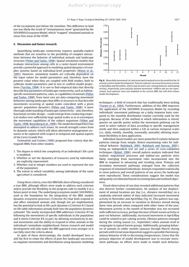
Fig. 8. Mean daily movement (m) and associated standard errors by month for the 10animals used in model development. Patterns indicate increased movement activityin April/May and November, which may be tied to pre-calving behavior and huntingactivity, respectively. June and July showed movement <1000 m and are not repre-sented. Such patterns were not modeled in the current IBM, but will drive futuremodel development.

techniques—a field of research that has traditionally been lacking(Turner et al., 1994). Furthermore, addition of this IBM improvesthe application of the SAVANNA Ecosystem Model by recordingindividuals’ movement pathways on a daily stepwise basis com-pared to the monthly distribution routine currently used by theprogram. Because of the method in which information is stored,queries on specific points within the movement pathway can beused to select subsets of data according to specific managementneeds and then analyzed within a GIS at various temporal scales(i.e., daily, weekly, monthly, seasonally, annually) allowing maxi-mum flexibility in data application.

Individual-based models are more powerful if realistic behaviorpatterns emerge from simple, fitness-maximizing rules for indi-vidual behavior (Railsback, 2001; Railsback and Harvey, 2001).Using an independent test set and a series of cross-validationtechniques (Rykiel, 1996), overall pattern analysis indicated thatrealistic migrational processes and habitat-use patterns werelikely emerging from movement rules incorporated into theIBM in response to advancing and receding snow. Primary andsecondary movement pathways emerged from the collectiveresponses of simulated individuals. Animals responded realisticallyto snow patterns and overall patterns of use across the landscapewere reproduced. These considerations suggest the model wasadequately corroborated based on existing data and outlined objec-tives.

Visual observation of raw data revealed additional patterns thatalso deserve further consideration. An analysis of net displace-ment of animal locations per day (i.e., distance moved/day) on arandomly-selected subset of data indicated increased movementactivity in November and April/May (Fig. 8). This pattern was sup-plemented by an increase in variation in distance moved duringthese time periods when compared with other times of the year.Movement activity in the month of November was not recreatedwith sufficient accuracy, perhaps because of hunt season activity orpost-rut behavior: additionally, increased movement in April/Maycould be related to pre-calving activity. Obvious patterns emergedduring the rutting season (i.e., September) when animals tend tocongregate in typical harem groups. Additionally, grouping behav-ior of animals in colder months (January through March) duringperiods with trivial snow deposition suggests a possible thermoreg-ulatory behavior of elk to decreasing temperatures. Given that theprimary objective of model development was to recreate move-ment pathways no efforts were made to model such behavior.

Author's personal copy

1618 S.P. Rupp, P. Rupp / Ecological Modelling 221 (2010) 1605–1619

Future research is necessary to evaluate such response mechanismsin order to sufficiently model these interactions.

Model performance could also be improved through additionaltesting of model assumptions, adjustments to fitness measures inthe form of mortality risks (i.e., predation), and fixing problem-atic factors such as “instantaneous snow.” Mortality risks could beincorporated by either implementing the predation submodel avail-able in SAVANNA after additional data for the Jemez Mountains aremade available through future studies or by possibly incorporat-ing existing HSIs for select predators known to occur in the JemezMountain region. Though sensitivity analyses have limited use foranalyzing complex IBMs because comprehensive analysis of allparameters is infeasible and techniques do not address how systemdynamics arise from individual traits (Grimm and Railsback, 2005),it is possible a sensitivity analysis on the snow factor could provideadditional information about its influence on other model param-eters or outputs. Finally, additional studies could address specifiedmodel assumptions by evaluating hierarchical habitat selection byelk, determining intra-specific interactions among individuals, orevaluating density in relation to mean individual fitness throughan intensive demographic study in a variety of habitats (Van Horne,1983) and then incorporating information gained to improve over-all model performance.

Acknowledgements

Our appreciation goes out to The Canon National Parks ScienceScholars Program and the Ecology Group at LANL for funding thisproject. We would also like to thank the Valles Caldera NationalPreserve, New Mexico Department of Game and Fish, U.S. For-est Service, Bandelier National Monument, Telonics, Inc., SantaClara Reservation, and Adventure Aviation for assistance with col-lar retrieval. Dr. Michael Coughenour, developer of the SAVANNAEcosystem Model, offered valuable insight and guidance in calibrat-ing that model for the Jemez Mountains. Drs. James Biggs and DavidWester provided technical and statistical guidance, respectively.

References

Adams, A.W., 1982. Migration. In: Thomas, J.W., Toweill, D.E. (Eds.), Elk of NorthAmerica: Ecology and Management. Stackpole Books, Harrisburg, PA, pp.301–321.

Allen, C.D., 1996. Elk response to the La Mesa Fire and current status in the JemezMountains. In: Allen, C.D. (tech ed.), Fire Effects In Southwestern Forests: Pro-ceedings of the Second La Mesa Fire Symposium. RM-GTR-286, USDA ForestService Rocky Mountain Forest and Range Experiment Station, Fort Collins, CO,pp. 179–195.

Altmann, M., 1952. Social behavior of elk, Cervus canadensis nelsoni, in the JacksonHole area of Wyoming. Behaviour 4, 116–143.

Anderson, C.C., 1958. The Elk of Jackson Hole. Bulletin 10. Wyoming Game and FishCommission, Laramie, 184 pp.

Barrett, T.M., 2001. Models of vegetative change for landscape planning: a com-parison of FETM, LANDSUM, SIMPPLLE, and VDDT. General Technical ReportRMRS-GTR-76-WWW, USDA Forest Service Rocky Mountain Research Station,Ogden, Utah, 14 pp.

Bauman, P.J., Jenks, J.A., Roddy, D.E., 1999. Evaluating techniques to monitor elkmovement across fence lines. Wildl. Soc. B 27, 344–352.

Benkobi, L., Rumble, M.A., Brundige, G.C., Millspaugh, J.J., 2004. Refinement of theArc-Habcap model to predict habitat effectiveness for elk. Research Paper,RMRS-RP-51, U.S. Department of Agriculture, Rocky Mountain Research Station,18 pp.

Boone, R.B., 2000. Integrated management and assessment system: balancing foodsecurity, conservation, and ecosystem integrity. Global Livestock CollaborativeResearch Support Program Training Manual, US Agency for International Devel-opment. 208 pp.

Coughenour, M.B., 1993. The SAVANNA Landscape Model—Documentation andUsers Guide. Natural Resource Ecology Laboratory, Colorado State University,Fort Collins, CO, 54 pp.

Coughenour, M.B., 2002. Elk in the Rocky Mountain National Park ecosystem—amodel-based assessment. Final report to the U.S. Geological Survey Biologicalresources Division and U.S. National Park Service, Washington, DC.

Cody, R.P., Smith, J.K., 1997. Applied Statistics and the SAS Programming Language,4th edition. Prentice-Hall, Inc., New Jersey, 445 pp.

Compton, T., 1975. Mule deer-elk relationships in the western Sierra Madre area ofsouthcentral Wyoming. Technical Report Number 1, Wyoming Game and FishDepartment, Laramie, 125 pp.

Davenport, D.W., Wilcox, B.P., Breshears, D.D., 1996. Soil morphology of canopy andintercanopy sites in pinon-juniper woodland. Soil Sci. Soc. Am. J. 60, 1881–1887.

Franklin, W.L., Lieb, J.W., 1979. The social organization of a sedentary population ofNorth American elk: a model for understanding other populations. In: Boyce,M.S., Harding, L.D. (Eds.), North American Elk: Ecology, Behavior, and Manage-ment: Proceedings of a Symposium on Elk Ecology and Management. Universityof Wyoming, Laramie, Wyoming, pp. 185–198.

Grimm, V., Berger, U. Seeing the woods for the trees and vice versa: pattern-orientedecological modeling. Unpublished report.

Grimm, V., Railsback, S.F., 2005. Individual-based Modeling and Ecology. PrincetonUniversity Press, Princeton, New Jersey, 480 pp.

Grimm, V., Frank, K., Jeltsch, F., Brandi, R., Uchmanski, J., Wissel, C., 1996. Pattern-oriented modeling in population ecology. Sci. Total Environ. 183, 151–156.

He, H.S., Mladenoff, D.J., 1999. Spatially explicit and stochastic simulation of forest-landscape fire disturbance and succession. Ecology 80, 81–99.

Hooge, P.N., 2003. Personal communication. In: Course in “The Analysis of TelemetryData in the GIS Environment”. U.S. Fish and Wildlife Service, National Conser-vation Training Center (NCTC), Shepherdstown, WV.

Hooge, P.N., Eichenlaub, B., 2000. Animal Movement Extension to Arcview. (ver.2.0). Alaska Science Center—Biological Science Office, U.S. Geological Survey,Anchorage, AK.

Hooge, P.N., Eichenlaub, W.M., Solomon, E.K., 2001. Using GIS to analyze animalmovements in the marine environment. In: Spatial Processes and Managementof Marine Populations. Alaska Sea Grant Program, AK-SG-01-02, 2001, pp. 37–51.

Huber, W., 2004. Personal communication. ESRI Technical Support List Serve.Keane, R.E., Hann, W.J., 1998. Simulation of vegetation dynamics after fire at mul-

tiple temporal and spatial scales—a summary of current efforts. In: Close, K.,Bartlette, R.A. (Eds.), Proceedings of the 1994 Interior West Fire Council Meetingand Symposium, 1994. Coeur d’Alene, Idaho, pp. 115–124.

Keane, R.E., Long, D.G., 1998. A comparison of coarse scale fire effects simulationstrategies. Northwest Sci. 72 (2), 76–90.

Keane, R.E., Arno, S.F., Brown, J.K., 1989. FIRESUM—an ecological process model forfire succession in Western conifer forests. USDA Forest Service, Intermount. For.Range Exp. Stn., Ogden, UT, Gen. Tech. Rep. INT-266, 76 pp.

Keating, K.A., Cherry, S., 2004. Use and interpretation of logistic regression in habitat-selection studies. J. Wildl. Manage. 68, 774–789.

Kirkpatrick, R.J., Kohlmann, S., Tierney, R. Elk management in the JemezMountains—a synopsis. New Mexico Department of Game and Fish, Unpublishedreport, 25 pp.

Levene, H., 1960. Robust tests for equality of variances. In: Olkin, I. (Ed.), Contribu-tions to Probability and Statistics. Stanford Univ. Press, Palo Alto, pp. 278–292.

Lyon, L.J., 1983. Road density models describing habitat effectiveness for elk. J. Forest.81, 592–595.

Lyon, L.J., Ward, A.L., 1982. Elk and land management. In: Thomas, J.W., Toweill,D.E. (Eds.), Elk of North America: Ecology and Management. Stackpole Books,Harrisburg, PA, pp. 443–477.

Mayer, D.G., Butler, D.G., 1993. Statistical validation. Ecol. Model. 68, 21–32.Murie, O.L., 1951. The Elk of North America. Stackpole Co., Harrisburg, PA.Pither, J., Taylor, P.D., 1998. An experimental assessment of landscape connectivity.

Oikos 83, 166–174.Railsback, S.F., 2001. Getting “Results”: the pattern-oriented approach to analyzing

natural systems with individual-based models. Nat. Resour. Model. 14, 465–475.Railsback, S., Harvey, B., 2001. Individual-based model formulation for cutthroat

trout, Little Jones Creek, California. General Technical Report, PSW-GTR-182,Pacific Southwest Research Station, Forest Service, U.S. Department of Agricul-ture, 80 pp.

Railsback, S.F., Lamberson, R.H., Harvey, B.C., Duffy, W.E., 1999. Movement rules forindividual-based models of stream fish. Ecol. Model. 123, 73–89.

Rosenberg, D.K., Noon, B.R., Megahan, J.W., Meslow, E.C., 1998. Compensatory behav-ior of Ensatina eschscholtzii in biological corridors: a field experiment. Can. J. Zool.76, 117–133.

Rupp, S.P., 2005. Ecological impacts of the Cerro Grande Fire: predicting elk move-ment and distribution patterns in response to vegetative recovery throughsimulation modeling. Ph.D. Thesis, Texas Tech University.

Rykiel, E.J., 1996. Testing ecological models: the meaning of validation. Ecol. Model.90, 229–244.

Saunders, D.A., Hobbs, R.J., 1991. The role of corridors in conservation: what dowe know and where do we go? In: Saunders, D.A., Hobbs, R.J. (Eds.), NatureConservation 2: The Role of Corridors. Surrey Beatty & Sons, pp. 421–427.

Schank, J.C., 2001. Beyond reductionism: refocusing on the individual withindividual-based modeling. Complexity 6, 33–40.

Shenk, T.M., Franklin, A.B. (Eds.), 2001. Modeling in Natural Resource Management.Island Press, p. 223.

Skinner, M.P., 1925. Migration routes in Yellowstone Park. J. Mammal. 6, 184–192.Skovlin, J.M., 1982. Habitat requirements and evaluations. In: Thomas, J.W., Toweill,

D.E. (Eds.), Elk of North America: Ecology and Management. Stackpole Books,Harrisburg, PA, pp. 369–413.

Slothower, R.L., Schwartz, P.A., Johnston, K.M., 1996. Some guidelines for implement-ing spatially-explicit, individual-based ecological models within location-basedraster GIS. In: Proceedings, Third International Conference/Workshop on Inte-grating GIS and Environmental Modeling, Santa Fe, NM, January 21–26, 1996.National Center for Geographic Information and Analysis, Santa Barbara, CA,http://www.ncgia.ucsb.edu/conf/SANTA FE CD-ROM/main.html.

Author's personal copy

S.P. Rupp, P. Rupp / Ecological Modelling 221 (2010) 1605–1619 1619

Thomas, J.W., Toweill, D.E. (Eds.), 1982. Elk of North America. Stackpole Books, Har-risburg, PA, p. 698.

Thomas, J.W., Leckenby, D.A., Henjum, M., Pederson, R.J., Bryant, L.D., 1988. Habitat-effectiveness index for elk on Blue Mountain winter ranges. General TechnicalReport, PNW-GTR-218, U.S. Department of Agriculture, Pacific NorthwestResearch Station, 28 pp.

Trimble Navigation Limited, 1999. LassenTM SK II GPS: System Designer ReferenceManual. Trimble Navigation Limited, Sunnyville, CA, 202 pp.

Turchin, P., 1998. Quantitative Analysis of Movement: Measuring and Modeling Pop-ulation Redistribution in Animals and Plants. Sinauer Associates, Inc. Publishers,Sunderland, MA, 396 pp.

Turner, M.G., Gardner, R.H., O’Neill, R.V., 2001. Landscape Ecology in Theory andPractice: Pattern and Process. Springer-Verlag, New York, Inc, 401 pp.

Turner, M.G., Wu, Y., Wallace, L.L., Romme, W.H., Brenkert, A., 1994. Simulating win-ter interactions among ungulates, vegetation, and fire in northern YellowstonePark. Ecol. Appl. 4, 472–496.

Uchmanski, J., Grimm, V., 1996. Individual-based modeling in ecology: what makesthe difference? Trends Ecol. Evol. 11, 437–441.

U.S. Fish and Wildlife Service, 1981. Ecological Services Manual—Standards forthe Development of Habitat Suitability Index Models (103 ESM). Division ofEcological Services, U.S. Fish and Wildlife Service, Department of the Interior,Washington, DC.

Vales, D.J., Peek, J.M., 1996. Responses of elk to the 1988 Yellowstone fires anddrought. In: Ecological Implications of Fire in Greater Yellowstone. InternationalAssociation of Wildland Fires, pp. 159–167.

Van Horne, B., 1983. Density as a misleading indicator of habitat quality. J. Wildl.Manage. 47, 893–901.

Van Winkle, W., Jager, H.I., Railsback, S.F., Holcomb, B.D., Studley, T.K., Baldrige, J.E.,1998. Individual-based model of sympatric populations of brown and rainbowtrout for instream flow assessment: model description and calibration. Ecol.Model. 110, 175–207.

Welch, B.L., 1951. On the comparison of several mean values: and alternativeapproach. Biometrika 38, 330–336.

Wiegand, T., Jeltsch, F., Hanski, I., Grimm, V., 2003. Using pattern-oriented modelingfor revealing hidden information: a key for reconciling ecological theory andapplication. Oikos 100, 209–222.

Wiegand, T., Naves, J., Stephan, T., Fernandez, A., 1998. Assessing the risk of extinc-tion for the brown bear (Ursus arctos) in the Cordillera Cantabrica, Spain. Ecol.Monogr. 68, 539–570.

Wiens, J.A., Stenseth, N.C., Van Horne, B., Ims, R.A., 1993. Ecological mechanisms andlandscape ecology. Oikos 66, 369–380.

Wilcox, B.P., Breshears, D.D., 1994. Hydrology and ecology of pinon-juniper wood-lands: conceptual framework. In: Shaw, D.W., Aldon, E.F., LoSapio, C. (tech.coords.), 1995. Desired Future Conditions for Pinon-Juniper Ecosystems. USDAForest Service General Technical Report, RM-258, Rocky Mountain Forest andRange Experiment Station, Fort Collins, CO, pp. 109–119.

Wilcox, B.P., Newman, B.D., Allen, C.D., Reid, K.D., Brandes, D., Pitlick, J., Daven-port, D.W., 1996. Runoff and erosion on the Pajarito Plateau: observations fromthe field. In: New Mexico Geological Society Guidebook: 47th Field Conference,Jemez Mountains Region, New Mexico Geological Society Guidebook, Albu-querque, NM, pp. 433–439.

Worton, B.J., 1989. Kernel methods for estimating the utilization distribution inhome-range studies. Ecology 70 (1), 164–168.