Development of an Angular Sensor for Shape Sensing ... - edoc

Development of an Angular Sensor for Shape Sensing of Medical Robots

Inaugural dissertation

to be awarded the degree of Dr. sc. med.

presented at

the Faculty of Medicine of the University of Basel

by Lorenzo Iafolla

from Monte Porzio Catone, Italy

Basel, 2021

Original document stored on the document server of the University of Basel edoc.unibas.ch

Approved by the Faculty of Medicine on application of Prof. Dr. Philippe Claude Cattin, University of Basel, First examiner

Prof. Dr. Georg Rauter, Second examiner

Prof. Dr. Gastone Ciuti, External expert

Basel, 28th May 2021

Prof. Dr. Primo Leo Schär Dean

Dedicated to my wife Marina, my children Sasha and Nikita, and my parents Nucciaand Valerio.

Contents

Acknowledgments vii

Foreword ix

Summary xi

1 Introduction 11.1 Contribution . . . . . . . . . . . . . . . . . . . . . . . . . . . . . . . . . 41.2 Outline . . . . . . . . . . . . . . . . . . . . . . . . . . . . . . . . . . . . 5

2 Medical and Technical Background 72.1 Examples of Orthopedic Surgeries . . . . . . . . . . . . . . . . . . . . . 72.2 Medical Robotics . . . . . . . . . . . . . . . . . . . . . . . . . . . . . . . 9

2.2.1 Image-Guided Intervention . . . . . . . . . . . . . . . . . . . . . 92.2.2 Surgical Robotics . . . . . . . . . . . . . . . . . . . . . . . . . . . 112.2.3 Tracking and Controlling Articulated and Continuum Robots . . 132.2.4 Mechanical Digitizer Tracking Systems . . . . . . . . . . . . . . . 142.2.5 Planar Kinematics of Mechanical Linkages Systems . . . . . . . . 17

2.3 Position and Angular Measuring Systems . . . . . . . . . . . . . . . . . 192.3.1 Rotary Encoders . . . . . . . . . . . . . . . . . . . . . . . . . . . 192.3.2 Lens-free Shadow Image Sensors . . . . . . . . . . . . . . . . . . 24

3 Apparatus and Method for Determining the Orientation and Position oftwo rigid Bodies 29

4 Proof of Principle of a Novel Angular Sensor Concept for Tracking Systems 61

5 Preliminary Tests of the Miniaturization of a Novel Concept of AngularSensors 71

6 Data Acquisition System for a Medical Tracking Device based on a NovelAngular Sensor 77

7 Proof of Concept of a Novel Absolute Rotary Encoder 83

8 Machine learning-based method for an absolute rotary encoder 95

9 Discussion, Outlook, and Conclusion 1079.1 Discussion . . . . . . . . . . . . . . . . . . . . . . . . . . . . . . . . . . . 107

v

9.2 Outlook . . . . . . . . . . . . . . . . . . . . . . . . . . . . . . . . . . . . 1079.3 Conclusion . . . . . . . . . . . . . . . . . . . . . . . . . . . . . . . . . . 110

Bibliography 111

Curriculum Vitae 119

Acknowledgments

The first person I want to thank is my supervisor Professor Dr. Philippe ClaudeCattin for giving me the opportunity to work at DBE, where I could greatly improvemy research and transferable skills. Beside providing a precious guidance and support,the inspirational conversation we had during these years have spread the seeds for allthe innovative content of this work. I have also appreciated the motivational spirit andenthusiasm that he demonstrated by believing in my ideas. For example, he proposedto invest in ASTRAS by filing a patent few months after I have started and, last year,he funded a new PhD project which is based on my work.

I would like to thank also my second supervisor Prof. Dr. Georg Rauter. Besideproviding valuable feedback to improve my work and inspiring new developments, suchASTRAS360, I have appreciated the encouraging words he always told me during ourconversations.

Dr. Sara Freund and Dr. Lilian Witthauer need a special acknowledgment becauseof their precious contributions to this dissertation and my publications. I particularlyappreciated the promptness with which they contributed to my works.

For his contribution to my publications, I must thank also Prof. Dr. Azhar Zam.Thanks to his positive attitude, it was always encouraging to discuss and share myideas with him.

Part of the results of this research work are certainly due to the productive collab-oration with Massimiliano Filipozzi. I am glad to know that he will be responsible forcontinuing my project within his PhD.

This PhD was carried on in the Planning and Navigation team of DBE within whichI spent pleasant, inspiring, and fun time; in particular, I want to thank: SamanehManavi, Marek Zelechowski, Balazs Faludi, Carlo Seppi, and Eva Schnider.

A special thought goes to all the colleagues of the MIRACLE and the CIAN groups,who are too many to be mentioned here, but I will always remember with pleasureabout all of them.

I need to thank also my wife Marina Popova. Without her, I might have not steppedout from my comfort zone in Italy and had this amazing experience in Switzerland.

This dissertation was written during the lock-down for the Covid-19 pandemic onspring 2020. Without the help of my parents, Ignazia Ragnedda and Valerio A. Iafolla,who took care of my two years old son, it would have not been possible to make it.

Finally, a thought goes to my son Alexander Iafolla (Sasha). His contribution hasbeen to force me taking some pauses, by time to time, during the writing of thisdissertation: I appreciated it! And I hope one day I will be able to teach him all theamazing things I have learned during these years at DBE.

P.S. During the finalization of this thesis, my son Nikita was born -7th of September2021- and I couldn’t resist from adding my best wishes for a happy life!

vii

Foreword

When I started this PhD, I was assigned to a project named opto-mechanical po-sition sensor. The idea of this research was to adapt an existing technology, calledshadow sensing, to the tracking of a robotic articulated medical endoscope. While Iwas studying the literature, I went through several images representing different im-plementations and applications of shadow sensors. By chance, my misinterpretationof one of these images inspired me to use the shadow sensing to accurately measurethe angle between the elements of an articulated device. Based on this novel idea, wesoon filed a patent application, which is currently pending in EU, USA, and Canada.

However, to implement this idea, there were, and still are, a lot of challenges toovercome. In this PhD project, I have laid the foundations to enable the designof a device that is applicable to a small medical endoscope. To do this, I used amultidisciplinary approach that made this project very interesting, instructive, andinspiring. For example, the project involved measurement/sensor science and opto-mechanics to understand and characterize the behavior of the device, electronics toacquire the data from the image sensors, image processing and machine learning toprocess the data, robotics to understand its applications and requirements, and, ofcourse, a medical background.

Through this thesis, I will provide an overview of all such diverse challenges.

ix

Summary

Tracking is a crucial need to control an endoscopic surgical tool accurately. Unfor-tunately, widely used solutions based on optical trackers cannot work in this casebecause the line-of-sight is blocked once the endoscope is inside the patient’s body.Other promising techniques are fiber Bragg grating, electromagnetic trackers, andintra-operative imaging-based shape sensing, but these still show some issues andfurther investigations are required. For this reason, this work aims to develop newsolutions to track the pose and to sense the shape of robotic articulated endoscopesfor minimally invasive surgery.

This thesis lays down the foundations for a new tracking and shape sensing methodbased on a novel, miniaturizable, angular measuring system, called ASTRAS (AngularSensor for TRAcking Systems). This is a shadow sensor able to generate a shadowimage with a one-to-one correspondence to an input angle. The tracking methodinvolves measuring the joints bending angles of the articulated endoscope by placingone ASTRAS in each of them. Subsequently, the position, the orientation, and theshape of the endoscope can be calculated from these angular measurements.

As ASTRAS is a novel concept, it was necessary to define and test the methods toachieve the required accuracy. Pursuing this, we developed 1) the measurement prin-ciple of the measuring system, 2) the measurement methods (i.e., image processingtechniques) to determine the input angle from the shadow image, 3) the methods toextend the angular range up to 360 degrees (ASTRAS360), 4) the machine learning-based methods to compensate for systematic errors (e.g., linearity error or imperfec-tions of the mechanics), 5) techniques based on FPGA electronic devices to acquire andprocess data in real-time. For each of these developments, we performed experimentsfor validation. For example, we demonstrated that ASTRAS is very precise (5 arcsec)even when using a miniaturized image sensor (e.g., NanEye, 1× 1× 0.5 mm3).

The result of this work is the know-how to design new versions of ASTRAS specif-ically for minimally invasive robotics. In particular, the miniaturized version of AS-TRAS has the potential to outperform the existing angular measuring systems (i.e.,rotary encoder). It will provide an alternative solution to the existing tracking andshape sensing technologies.

Furthermore, ASTRAS is prone to further developments, such as being used tomeasure over two degrees of freedom (i.e., two angles). This would enable further ap-plications in medical robotics, such as tracking of continuum (non-articulated) robots.

xi

1 Introduction

This thesis aims to investigate a novel method to track the pose (position and orienta-tion) and shape of medical robots for minimally invasive surgery (MIS). Pursuing thisaim, we proposed a novel concept of an angular measuring system, called ASTRAS(Angular Sensor for TRAcking Systems), that has the potential to be miniaturizedand used in the rotational joints of a medical robot. By measuring the bending anglesof the joints, it is possible to calculate pose and shape of the robot.

The importance of this topic is related to robotics in medicine and, in particular,MIS. In the last decades, robotics has significantly impacted our lives. For instance, ithas revolutionized the way things are manufactured in the automotive industry. Re-cently, robotics has also been applied to other fields such as agriculture, aerospace, andeducation. Driven by the success of several pilot projects, interest in robotics withinthe medical field keeps growing since the 1980s. For example, robotics can eliminatepart of the monotonous and repetitive work physicians and healthcare workers haveto perform. This is crucial considering the increasing labor shortage in healthcare andthe growing world population. Therefore, the demand for surgical- rehabilitation- andhospital-robotics keeps rising while the production costs keep declining [16, 59].

Earlier robots were not very popular in the surgical field. The reasons were techni-cal complications during the surgery, limited flexibility, cumbersome equipment, etc.However, the success of the da Vinci robot demonstrated that these issues can besolved and the surgical robotics market is projected to grow to 91.5 billions USD by2025 [24].

Orthopedic robots are an important category of medical robots and were introducedin the beginning of the 1980s. Indeed, non-robotic surgeries are characterized bymultiple challenges due to the use of manual instruments; consequently, human errorsare introduced and the outcomes are less predictable and reproducible. For example,bone removal and implant placement might be inconsistent thus, the best outcome forthe patient cannot be achieved. Using robots is beneficial to the clinical and the patientoutcomes for the three following reasons: accuracy, state monitoring, and safety. Inorthopedics, accuracy is crucial to achieving good bone remodeling resulting in betterpatient outcomes [40]. For example, robots outperform the freehand operations interms of location of the cut with respect to the planned one. The quality of the cut,i.e., its flatness, improves as well [13, 45] allowing the surgeon to perform cement-lessfixation with consequent longer lifespan of the implant [58].

The present work was conducted in the framework of a project called MIRACLE(Minimally Invasive Robot-Assisted Computer-guided LaserosteotomE), which aimsto develop a robotic endoscope to cut bones with laser light. The main applicationswould be in orthopedics, cranio-maxillofacial surgery, neurosurgery, otolaryngology,traumatology, and spine surgery. The advantages of using laser light are a quicker

1

1 Introduction

Figure 1.1: Functional cut of the right partially toothed mandible. Reprinted from [6](Figure 1) with permission from Elsevier.

recovery of the patient and less invasive procedures than conventional cutting toolssuch as a surgical saw [19]. For instance, thermal damage like carbonization can beavoided, the cut face is characterized by open porous, no damage was observed inthe sub-dermal soft tissues [7]. Another feature facilitating the healing is that lasercuts are typically as thin as the laser spot (a few hundred microns diameter); in[6], the authors experimentally achieved a cutting width of 0.5 mm. Furthermore,the cutting geometry is not limited to plane as with a saw. Consequently, it can bechosen with more freedom. This allows the surgeon to perform the so-called functionalcuts, as shown in Figure 1.1, that will enable types of surgeries not possible with theconventional cutting tools. This allows stable load-sharing connections and facilitatesthe cement-less fixation of the prosthesis. However, there are several open challenges inMIRACLE and the majority of them are related to the miniaturization (the diameterof the endoscope should be less than 10 mm) and to the accuracy of the navigationsystem. For example, to fully exploit the potential of laser osteotomy, the trackingand navigation systems have to assure an accuracy level comparable to the cuttingwidth (i.e., 0.5 mm). For this reason, an accurate tracking and shape sensing systemfor endoscopes is essential.

Navigating a medical robot involves controlling its pose and its shape with respectto the patient’s body; for this reason, tracking the pose and the shape of the robotis key. Several tracking technologies have already been studied and some have beencommercialized for a few decades [29].

For instance, optical systems are among the most widely used and accurate trackers.The measuring principle is based on capturing the position of optical markers attached

2

to the tracked device (e.g., the robot or the patient’s body) using two or more cameras.Employing the triangulation principle, it is possible to calculate the position and theorientation of the tracked devices within the operating room. They can reach a meanerror of robot shape (MERS) of less than 1 mm. However, sometimes the opticalsystems cannot operate because the line-of-sight between the cameras and the markersis blocked. This is the case in the MIRACLE robot where the markers would be insidethe body of the patient due to its MIS application [70].

For MIS applications, other technologies have to be used in combination or asalternatives. The most important examples are electromagnetic tracking systems(EMT), fiber-optic based sensors (e.g., fiber Bragg gratings, FBG), and intra-operativeimaging-based shape sensing.

Electromagnetic tracking systems consist of an electromagnetic field generator andtarget sensors embedded in the tracked device. As the generated field is known, theposition of the target sensors can be calculated from their output. The main limitationis due to the interference from the surrounding environment and the limited workingspace. Although in principle, the accuracy can be better than 0.5 mm, experimentsin application conditions demonstrated that the MERS is usually worse than 1 mm[69, 70].

Fiber Bragg gratings sensing uses optical fibers where Bragg gratings (FBG sensors)are written at specific locations into the fiber. These gratings reflect the light at avery specific wavelength that changes with some physical variables such as mechanicalstrain and temperature. By combining data from multiple FBG sensors, it is possibleto reconstruct the shape of the fiber. As the fibers are very thin, they are ideal tobe integrated in tiny robots such as robotic endoscopes. However, this technology isstill under investigation and current results are not yet satisfactory. A review of theexperiments done using this technique is presented in [69]; tracking a flexible robot,the MERS was worse than 4 mm [84].

Finally, intra-operative imaging-based shape sensing is based on capturing medicalimages in real-time during the surgery. Biplane fluoroscopy is one example and pro-vides the most accurate results: MERS lower than 0.5 mm were measured in phantomsand cadavers [80]. The measurement principle is based on capturing X-ray views ofthe subject at various poses and then using the triangulation principle to reconstructthe position and the shape of the robot. The limitations of the biplane fluoroscopymethod are mainly due to large dose of radiations, workspace constraints, and largecosts. Endoscopic stereo-cameras, monoplane C-arm and ultrasound imaging-basedshape reconstructions are alternative solutions to reduce the radiation dose, but at theprice of lower accuracy. Furthermore, most intra-operative imaging-based methodsrequire demanding computations to reconstruct the shape of the robot, consequently,real-time applications are still challenging [69].

In light of all the former considerations, there is no comprehensive technique avail-able to track and sense the shape of a robotic endoscope such as MIRACLE. Weinstead have a portfolio of solutions and the optimal one has to be chosen dependingon the application requirements. For this reason, there is still space for research eitherto improve the existing solutions or to develop new ones.

In the frame of MIRACLE, we proposed a solution based on measuring the bending

3

1 Introduction

angles at each joint of the robot (mechanical digitizer). Within macro-robotic systems,this is usually done using rotary encoders (REs). However, in miniaturized robotsfor MIS, the requirements for such a measuring system are more strict than those formacro robots. First, the RE has to be accurate and fast enough to allow the navigationsystem to drive the robot onto the target with high accuracy. Second, it has to besmall enough to fit in small robots for MIS. Third, it has to be absolute for safetyreasons, which means that it provides the correct output even after a power failure.It should be noticed that the first two requirements are contradicting goals. Indeed,the accuracy of a RE, particularly its resolution, is usually inversely proportional toits diameter. Consequently, small REs are typically not very accurate. Depending onthe technology, the absolute encoding might pose some limits to the minimum size aswell [21, 63, 23, 34, 26, 39].

The required size and accuracy have to be assessed depending on the specific ap-plication and architecture of the robot. For example, the maximum size of the REsdepends on the diameter of the robot. In the MIRACLE case, we assume a robotwith less than 10 mm diameter, consequently, the RE should occupy a volume muchsmaller than 10 × 10 × 10 mm3 (this is the size of the state of art smallest absoluteRE [68]), so that there would be still space for wires, optical fibers, rods, and all theother devices required inside the endoscope. Similarly, we mentioned that the positionof the laser spot has to be controlled with an accuracy better than 0.5 mm in laserosteotomy applications; for MIRACLE, we are targeting 0.2 mm. Combining theserequirements with the architecture of the robot, the required accuracy for the REscan be estimated. Indeed, the positioning error of the tip of the robot depends on itsdistance to the joints, the number of joints, and the accuracy of the REs. For instance,a 300 mm long a robot with three joints requires angular measurements with an errorsmaller than 40 arcsec (see Section 2.2.5).

The most used types of REs are magnetic encoders, Inductosyn (aka IncOder),and optical encoders [21] and are shortly reviewed in Section 2.3.1 and in Chapter 7.However, typically these types of REs are not accurate enough for MIRACLE whenthey are miniaturized.

1.1 Contribution

To propose an alternative to existing RE technologies for MIRACLE, we developedASTRAS. This is based on generating and capturing a shadow image whose shapecompletely determines the rotational angle. Specifically, ASTRAS is made of a rotorconsisting of a mirror and a stator consisting of an image sensor, a shadow mask, anda light source (e.g., an LED). The system is designed in a way that when the rotorrotates about the axis, the shadow cast onto the image sensor changes.

Despite its simple concept, a lot of know-how is necessary to make ASTRAS workingwith high accuracy. Our contribution addresses the following questions: a) how toanalytically model ASTRAS and, specifically, its sensitivity; b) how to accuratelyevaluate the rotation angles from the shadow images; c) how a miniature image sensorimpacts the accuracy; d) how to extend the range of measurement to a full 360 degrees

4

1.2 Outline

of rotation; e) how to improve the performance of the measuring system using machinelearning techniques; and f) how to acquire and process the data in real-time from atracking system made of several ASTRAS. To answer these questions, we have builtprototypes, performed experiments, developed data processing software, and analyzeda lot of experimental data. The result is a crucial know-how to create new versions ofASTRAS to be used in tracking systems. Specifically, we could validate an analyticalmodel of ASTRAS; test the methods to process the shadow images; demonstrate that,even using a miniature image sensor (NanEye, 1 × 1 × 0.5 mm3, [2]), ASTRAS isstill precise (down to 5 arcsec corresponding to a 6σ-resolution of 30 arcsec (16 bits));extend the range to 360 degrees (ASTRAS360); use machine learning to compensatefor systematic errors such as non-linearity, and play of the rotation axis; and showthat the acquisition and real-time processing is feasible using a Field ProgrammableGate Array (FPGA).

Using miniature components, in particular a miniature image sensor (e.g., NanEye)and a small ball bearing [74], we believe that ASTRAS can be made in form of a REsmaller than 10× 10× 10 mm3. Since we demonstrated that ASTRAS keeps its highresolution even with a miniature image sensor, we are confident that it can be used intracking systems for MIS robotics, like MIRACLE, outperforming the existing REs.Furthermore, ASTRAS can be integrated in a robotic endoscope with no need of theball bearing, thus optimizing and reducing the occupied space.

ASTRAS also has the potential to measure over two degrees of freedom (two angles).This means that the rotor would rotate about a pivot point rather than a single axis.In this case, the two angular measurements are independent and can be separatedentirely. Consequently, the methods developed for ASTRAS can be used separately foreach angle. Empowering the ASTRAS measuring system even for tracking continuumrobots where two degrees of freedom are expected between two contiguous elements.

Finally, besides the application in tracking technologies for medical robots, this workis also an advancement in measurement and sensor science.

1.2 Outline

In Chapter 2, we will introduce the reader to the medical and technical background ofthis thesis. In particular, we will describe some examples of orthopedic surgery, somebasic concepts of medical robotics, the mechanical digitizer tracking systems, and themeasuring systems which are relevant to ASTRAS: i.e., rotary encoders and lens-freeshadow sensors.

Chapters 3 to 8 comprise the patent and the publications resulting from this work.Specifically, Chapter 3 is the patent describing a novel idea to determine the anglebetween two rigid bodies; Chapter 4 describes the measuring model of ASTRAS andthe characterization of its first prototype; Chapter 5, the test of a partially miniatur-ized version of ASTRAS; Chapter 6, a concept for the data acquisition of a trackingsystem based on ASTRAS; Chapter 7, the measuring model of ASTRAS360 and theexperimental proof of its concept; and Chapter 8, the machine learning methods toprocess the data of ASTRAS360 and characterization of their performance.

5

1 Introduction

We will end this thesis with discussion, outlook, and conclusions in Chapter 9 whichalso includes the description of some integration concepts of ASTRAS in a roboticsendoscope.

6

2 Medical and Technical Background

2.1 Examples of Orthopedic Surgeries

The examples of surgeries presented in this section are from the orthopedic field forthree reasons. First, the characteristics of the bones provide the conditions for accu-rate procedures. For example, it is possible to define an accurate reference frame basedon the bones features; preoperative images are also reliable during the intra-operativephase as bones do not change significantly over short periods of time. Second, in ortho-pedic procedures accuracy is key and higher accuracy would enable new procedures.Lastly, this thesis was carried out in the framework of the project MIRACLE, whichis mainly dedicated to orthopedics.

Removal of a Tumor from a Femur. Figure 2.1 shows a femur and, as the surgicaltarget (dashed red area), a tumor. Reaching the tumor and removing it with a surgicaldrill is not easy because it is on the femoral head; consequently, it has to be accessedfrom the direction indicated by the arrow. Although the tumor is easily visible withinpreoperative imaging, for instance, using an MRI, it might be challenging to localizein the intra-operative phase. A C-arm can be used to perform X-ray imaging in the

Figure 2.1: In this picture of a femur (side of the hip), a tumor is represented with thered dashed area. The drill must enter from the direction indicated by thearrow to reach it. Courtesy of [67] (Figure 1.3), reprinted by permissionfrom Springer Nature: Springer, Medical Robotics by A. Schweikard andF. Ernst, ©2015. Original image from [33] (Figure 245).

7


Figure 2.2: Vertebra viewed from above. Pedicle screws must be inserted through thepedicles without touching the spinal canal. Courtesy of [67] (Figure 1.7),reprinted by permission from Springer Nature: Springer, Medical Roboticsby A. Schweikard and F. Ernst, ©2015. Original image from [33] (Figure82).

intra-operative phase, however, the accuracy is often not enough and the tumor mightnot be visible. For this reason, preoperative three-dimensional images have to bematched (registered) to the intra-operative situation to navigate the drill and removethe tumor. It is key that the drill is tracked and navigated with high accuracy toavoid damaging the surrounding tissues and to remain minimally invasive. Therefore,an accurate tracking system is necessary [67].

Insertion of Pedicle Screws. Figure 2.2 shows an example of spine surgery whereaccuracy is crucial. In this case, a vertebra has to be stabilized using fixation rods.These are held by screws, called pedicle screws, which go through the pedicles (whosediameter might be smaller than 5 mm, [15]) of the vertebra as shown by the red dashedlines. It should be noticed that the screws must not breach the pedicle body intothe spinal canal because this could potentially cause serious injuries to the patient.Therefore, the screws must be positioned and oriented very accurately before theirinsertion [60]. For this reason, a tracking system is key to reach a good outcome.

Corrective Osteotomy of a Femur. Corrective osteotomy is a further examplewhere accuracy is important for optimal outcome. To obtain a better positioning of thebone axis, a wedge is removed from the femur as shown in Figure 2.3. Small deviationsfrom the planned cutting angle might result in a badly aligned bone. Consequently,the cutting plane orientation, i.e., of the surgical saw, must be tracked and controlledwith high accuracy [67].

8

2.2 Medical Robotics

Figure 2.3: Corrective osteotomy. The cutting plane must be accurately located toachieve a good outcome. Courtesy of [67] (Figure 1.8), reprinted by permis-sion from Springer Nature: Springer, Medical Robotics by A. Schweikardand F. Ernst, ©2015. Original image from [33] (Figure 245).


2.2.1 Image-Guided Intervention

Image-guided intervention ([17], IGI) is a technique in use since 30 years and is key inmost minimally invasive surgeries. It relies on a combination of preoperative data (suchas tomographic images) and some technologies (such as displaying devices and, relevantfor this work, tracking systems) to use the position-data for controlling the surgicaltool during the intervention. As an instance, total knee arthroplasty is described in[77].

The counterpart of IGI are the image-free interventions where no preoperative orintra-operative image is acquired. In this case, the surgeon contacts anatomical ref-erence points with a special tool, like a rigid pointer, tracked by a tracking system.These points are then used to morph a virtual model of the target, e.g., a joint or abone, that provides guidance to execute the procedure. Other steps of the procedureare similar to those of IGI. As an instance, total knee arthroplasty is described in [72].

Image-guided interventions play a crucial role in MIS because the visibility of theanatomic target in these procedures, typically inside a patient’s body, is limited. Fur-thermore, it is straightforward to adapt IGI technology to robotics because it providesdigital data usable to navigate surgical tools. Anyway, it is important to notice thatin both IGI and non-IGI methods the tracking system is key.

To provide further insight of IGI and a better understanding of the role of the track-ing system, we will describe here, as an instance, the navigation based on computedtomography (CT) images. This method can be divided in five main steps, which are:preoperative imaging; planning; tracking; registration; and navigation [44, 77].

9


Preoperative Imaging. Three-dimensional CT images are obtained by a mathe-matical reconstruction of a series of X-ray images. CT is ideal to provide preopera-tive imaging for navigation, especially in orthopedics. Indeed, a CT image is three-dimensional, accurate, and bones are particularly easy to distinguish and segment fromthe background. Furthermore, bones do not change shape during the time between thepreoperative scan and the surgery. Although it is possible to use CT in intra-operativeimaging, it is usually not convenient because a CT scanner is very large and expensive[77].

Planning. Once the preoperative images are recorded, the surgeon can plan theprocedure. Several software packages to visualize and plan the surgery have been de-veloped over the years [71]. A common method relies on visualizing three-dimensionalrendered objects in perspective view from an arbitrary point of view. More recent sys-tems are based on virtual reality, where the surgeon can easily visualize and move thevirtual representation of the three-dimensional images [12]. Planning software usuallyoffer the possibility to define and to simulate the surgical procedure. To make thisplanned procedure usable during the operation, it is usually defined with respect to ananatomic coordinate system. Furthermore, when an implant is necessary, simulationsare also possible to verify and to avoid any impingement or restriction to the rangeof motion of articulations (e.g., the HipNav planner incorporated a range of motionsimulator [20, 44]).

Tracking. Tracking is key in navigation systems. It is based on determining accu-rately, and in real-time, the pose of the anatomical target (e.g., a bone of interest) andthe surgical tool (e.g., a robot or a surgical saw). The most relevant tracking methodshave been presented in the introduction and this thesis aims to further contribute tothis topic. A common challenge of tracking systems is the tool calibration and patientreferencing. This calibration involves determining the relative pose of the markers (orof the sensors) of the tracking system with respect to the surgical tool. For example,the position of the optical markers on the robot must be known to compute the poseof its tip [67].

Registration. Registration is required to correlate the surgical tools and patient’spose with the preoperative images. After registration, all data are represented inthe same reference system enabling the actuation of the planned surgical procedure.Several registration methods have been developed [50]. The most straightforward onesuse fiducial markers (see Figure 2.4). These are attached to the patient, e.g., screwedto the bones, before preoperative imaging and have to be easily identifiable in theCT. During the procedure, the fiducial markers are localized with the tracking system.The registration is done by applying a transformation (i.e., translation, rotation, etc.)that coincides with all positioning data (i.e., preoperative images and intra-operativetracking data). However, using fiducial markers is accurate but invasive. For example,bone screws might have to stay for few days before the surgery is performed andincrease the risk of infections. To avoid this, other types of fiducial markers are justfixed to the patient’s skin. Other techniques rely on the inherent patient anatomy,such as boney protrusions, to perform marker-free registration. In this case, we candistinguish between point matching and surface matching. However, this is a topic in

10


Figure 2.4: Principle of registration; applying the appropriate transformation, the vir-tual representation of a bone matches the position in the real space. Cour-tesy of [77], Figure 2.1, reprinted by permission from Springer Nature:Springer, Computer Assisted Orthopedic Surgery for Hip and Knee: Cur-rent State of the Art in Clinical Application and Basic Research, by T.Tomita et al., ©2018.

fast evolution and new techniques are continuously proposed.

Navigation. Navigation involves controlling the pose of the surgical tool accordingto the pre-planned procedure [55]. It can be seen as a feedback control loop where thetracking system provides feedback to the control system that moves the surgical toolaccording to the pre-planned pose. As described in Section 2.2.2, the loop involvesthe surgeon who receives the feedback from the tracking system and takes actionsconsequently. This feedback might have the form of images showing the surgical tooloverlaid onto the preoperative images or be a haptic signal. When a robot is involved inthe procedure, the feedback is used to generate controlling instructions (see Figure 2.5).

2.2.2 Surgical Robotics

In the previous section, we have shown the importance of the tracking systems in IGI-based procedure. In this section, we will show their importance in surgical robotics.

Medical robots find application in various medical fields [67]. Important sub-domainsare: medical imaging, where an imaging device is mounted onto a robotic arm; rehabil-itation, where mechatronic devices support the recovery of stroke patients; prosthetics,where robotic exoskeletons replace or support damaged anatomical structures; surgery,where robots allow surgeons to perform tasks with greater ease, accuracy, and safety.This work focuses on the latter subdomain where accurate navigation, and therefore

11


Figure 2.5: Schematic representation of a navigation control loop system for a roboticarm.

tracking, is key to successful surgery.Surgical robots can be classified, as in [40], on the basis of the level of their autonomy,

which are: remote manipulators, passive robots, semi-active robots, and active robots.

Remote Manipulators are made of a master and a slave robotic systems. Thesurgeon is comfortably seated in front of the master robot from which he can seeinformation, e.g., medical images or the real-time endoscopic view, and move a passiverobotic arm. These movements are replicated, typically down-scaled, by the slavewhich is next to the patient and actually holds the surgical tools. This allows thesurgeon to perform the surgery with higher precision and less fatigue. The mostfamous example of a remote manipulator is the DaVinci robot, which is typically usedfor cholecystectomy, hysterectomy, and prostatectomy [49],[36].

In Passive Robots, the surgical tool is independent from its kinematic. The role ofthis type of robots is to accurately align and stabilize the surgical tool that is movedby the surgeon. A classic example is the PUMA 200 [47], an industrial robot used instereotaxic neurosurgery (see Section 2.2.4). Once a needle is aligned with accuracydown to 1 mm, the robot is switched off, but still keeping the needle aligned. Fromthis point, the surgeon manually controls the depth of the needle. A modern exampleof a passive robot for knee arthroplasty is Praxiteles [61], which guides cutting tools(e.g., a blade or a bur).

Semi-active Robots provide even more guidance to navigate the surgical tool throughthe pre-planned path. Indeed, the tool is still controlled manually by the surgeon, butthe robot constrains the movements along the entire pre-planned surgical path. Whenthe tool approaches, or exceeds, the limits of the pre-planned workspace, the robotprovides haptic feedback to the operator or even stops the action. An example of asemi-active robot is the MAKO system from Stryker [76]. This system is used forknee and hip arthroplasty to hold the cutting tool steady within the constrained zone.Its navigation system relies on preoperative images registered using anatomical land-marks. Therefore, it can dynamically account for the relative position of the bone, thetool, and the robot.

Finally, Active Robots are the most autonomous but also the most reliant on pathpre-planning. In this case, the tool is driven through the surgical path by the robot.

12


The surgeon’s role is just to supervise the operation during the surgery. The roboticarm is accurately registered with preoperative images and patient’s position to enableits navigation through the pre-planned path. Besides famous examples, such as RO-BODOC, there is CARLO (Cold Ablation Robot-guided Laser Osteotome) by AOT[6, 7, 19] which is able to autonomously perform laser osteotomy. To fully exploitthe accuracy of the laser cut, a very accurate navigation and tracking system is key.For this reason, CARLO integrates the Fusion track 500 (ATRACSYS, [5]) to trackfiducial markers on the patient and on the robot. Furthermore, prior to cutting phase,CARLO outlines the planned shape of the cut using a low power green laser; in thisway the surgeon can stop the operation in case of error.

At this point, it should be clear that the majority of surgical robots rely on navi-gation and tracking systems. Remote manipulators could, in contrast, work only withthe visual feedback from the endoscopic camera. However, it is not difficult to imagineapplications that would deploy a tracking system. For example, to overlay the pose ofthe robot over preoperative images in a virtual representation. Passive robots need atracking system to initially position the surgical tool. In active and semi-active robots,tracking is key to close the feedback control loop that navigates the robot along thepath.

2.2.3 Tracking and Controlling Articulated and Continuum Robots

A further classification of robots arises from their architecture. In principle, we couldrepresent all robots as links connected by joints. However, the number of joints mightvary from very few to, theoretically, infinite. Robots with few joints are called discrete(aka articulated or rigid links) robots, whereas the others are called continuum robots[11]. There is a whole spectrum of robots between these two extremes and sometime,it is difficult to classify them as one or the other (see Figure 2.6). In terms of MIS,continuum robots are attractive because of their compliance and ability to conformto curvilinear paths. Unfortunately, controlling the infinite degrees of freedom of aninfinite number of joints is not simple. In this case, it is important to know the shapeof the robot besides the pose of its tip. This has relevant implications for the trackingas, with few exceptions (e.g., intra-operative medical imaging), most tracking systemscan sample the pose of few specific points and not entire shape [69]. For example,EMT systems provide information only at the location of their target sensors. FBGscan sense the curvature at the location of the FBGs sensors and not along the fulllength of the fiber. Similarly, REs (including ASTRAS) can only measure the bendingangle of the joints where they are located. However, depending on the characteristicof the robot and on the expected shapes (i.e., the expected curvilinear paths), thismight be sufficient. This is easier to understand when looking at Figure 2.7, whichshows how to model the forward kinematic of discrete and continuum robots. Theforward kinematic is the mathematical framework to compute the shape of the robotand the pose of its tip from the values of the variables (e.g., the bending angles of thejoints). Within the rigid links model (i.e., discrete robots), the links are connectedby joints. On the other hand, the constant curvature model consists of a sequence ofsegments with constant curvature. It is worth clarifying that ‘constant’ in ‘constant

13


Figure 2.6: Continuum robots versus discrete robots. Courtesy of [11], Figure 1,©2015IEEE.

Figure 2.7: Kinematic frameworks for robot modelling. Courtesy of [11], Figure 3,©2015 IEEE.

curvature’ is referred to the curvature within a single segment but it might changeover time. We only need one measuring system at each joint (or segment) to knowtheir bending angles (or curvature) within these two models. Furthermore, by analogywith the digital sampling of a continuous signal, the theoretical foundation to assessthe number of required measuring systems is the Nyquist-Shannon theorem [42].

Finally, when variable curvature models are required, sampling the curvature onlyin few spots might not be sufficient. In this case, intra-operative imaging is required toreconstruct the shape of the robot, whereas other tracking systems would only provideapproximate and local [11].

2.2.4 Mechanical Digitizer Tracking Systems

It will be clear later in Chapter 9 that ASTRAS can be used in both continuum andarticulated robots. However, its application is more straightforward in the latter where

14


Figure 2.8: Stereotaxic mechanism for tracking. Courtesy of [67], Figure 1.13,reprinted by permission from Springer Nature: Springer, Medical Robotics,by A. Schweikard and F. Ernst, ©2015.

it operates as a mechanical digitizer tracking system.

Mechanical digitizers are among the earliest tracking methods in surgery [9, 29]and is still very common in robotics today. A mechanical digitizer is a mechanicallinkage system, such as a rigid links robot, with encoders at each joint. Using forwardkinematics, it is possible to calculate the pose of the tip.

A famous and conventional example of such a tracking system is the joint mechanismof the stereotaxic navigation system for neurosurgery [85, 43, 67]. In this navigationsystem, which can also be applied in other types of surgery such as orthopedics, thestereotaxic frame plays a crucial role (see Figure 2.8). The frame base is attached(typically screwed) to the patient’s skull before the preoperative images are taken andremains attached till the end of the procedure. During surgery, the joint mechanismis attached to the frame base, as shown in Figure 2.8. This mechanism holds thesurgical needle and is made of prismatic joints, allowing linear movements, and rev-olute joints, allowing changes of the orientation. Each joint incorporates an encoderto measure these translations and rotations to provide tracking of the needle (an ex-ample is the arc digitizer described in [85]). The control can be done manually by thesurgeon or be automatized by a robot. In summary, stereotaxic techniques rely on therigid fixation of the frame onto the patient, consequently, no registration is required.Another peculiarity is that the tracking is done using only the internal state of thestereotaxic mechanism with no need for other tracking tools or complicated coordinatetransformations. For these reasons, it gained early popularity [67].

A further example is the ISG Viewing Wand developed in the 1990s [85, 22, 53,54, 30]. The Viewing Wand was a Faro digitizing arm [25] adapted for medical ap-plications. This device, based on a well-known technology, was accurate and reliable.

15


However, the Viewing Wand was bulky, its handling was cumbersome, it could gettangled or locked up because of the joints limitations, and it could not track multipletargets without a second arm.

Figure 2.9: Tracking concept based on a mechanical digitizer for hip arthroplasty.

Courtesy of [56], Figure 2, ©2006 John Wiley and Sons, Ltd.

Figure 2.10: (a) The mechanical digitizer for arthroplasty consists of a linkage of en-coders with 21.6 mm diameter. (b) The base pin of the linkage is surgi-cally inserted in the patient’s pelvis providing a reliable reference frame.Courtesy of [56], Figure 3, ©2006 John Wiley and Sons, Ltd.

More recently, an experimental mechanical digitizer system, shown in Figure 2.9 and2.10, was proposed in [56, 28] for tracking in hip arthroplasty. Its accuracy was better

16


than 0.5 mm and it aimed to work around the limitations of the optical tracking systemssuch as keeping the line-of-sight from the cameras to the targets free. Similarly to thestereotaxic method, the system was surgically fixed on the patient’s pelvis througha central pin; in this way, the measurements were easily referred to the body of thepatient. However, the encoders were large with a diameter of 21.6 mm and the systemwas cumbersome to use.

2.2.5 Planar Kinematics of Mechanical Linkages Systems

With all mechanical digitizers, forward kinematic analysis is required to determine thepose of the tip and the tracking uncertainties from the values provided by the encoders.However, forward kinematics in a three-dimensional space is out of the scope of thisthesis. Therefore, we just refer the reader to [64, 4, 3, 57, 73].

To understand how a mechanical digitizer works, we will analyze a simple planarexample. This will also provide us with the mathematical tools to assess the requiredangular accuracy.

Consider the mechanical linkage system with three revolute joints shown in Fig-ure 2.11. The three angles at the joints (θ1, θ2, θ3) are measured with angular measur-ing systems, e.g., using one RE at each joint. The lengths (l1, l2, l3) of the three linksare known. The forward kinematic involves calculating the pose of the end effector(position xe, ye and orientation φe). Computing the orientation φe from the bendingangles of the joints is straightforward.

φe = θ1 + θ2 + θ3 (2.1)

To determine the location of the end effector, we can use the following equations.

Figure 2.11: Planar mechanical linkage system with three revolute joints.

17


xe = l1 cos θ1 + l2 cos(θ1 + θ2) + l3 cos(θ1 + θ2 + θ3) (2.2)

ye = l1 sin θ1 + l2 sin(θ1 + θ2) + l3 sin(θ1 + θ2 + θ3) (2.3)

It is easy to see that the first term on the right side is the position of joint 2 with respectto joint 1. The second term is the position of joint 3 with respect to joint 2, and so ontill the position of the end effector. Therefore, it is quite easy to extend these equationsfor a larger number of joints. It should also be noticed that the above equations providethe pose with respect to the base of the mechanical linkage. Consequently, the pose ofthe base has to be tracked and registered to a common reference system. In the caseof an endoscope, we can assume that the base is visible, because it is located outsideof the patient’s body, and an optical tracker is used to follow it.

It is also interesting to know how the measurement error of the joint angles propa-gates to the measurement of the pose of the end effector. To do so, we will differentiatethe former equations with respect to the variables θ1, θ2, and θ3, use the errors as-sociated to each of them (∆θ1, ∆θ2, and ∆θ3) as increments, and sum up all terms.Calculating the final error associated to the orientation is straightforward.

∆φe = ∆θ1 + ∆θ2 + ∆θ3 (2.4)

The errors associated to the position of the end effector are as follows.

∆xe = |l1 sin(θ1)∆θ1 + (2.5)

+l2 sin(θ1 + θ2)(∆θ1 + ∆θ2) +

+l3 sin(θ1 + θ2 + θ3)(∆θ1 + ∆θ2 + ∆θ3)|

∆ye = |l1 cos(θ1)∆θ1 + (2.6)

+l2 cos(θ1 + θ2)(∆θ1 + ∆θ2) +

+l3 cos(θ1 + θ2 + θ3)(∆θ1 + ∆θ2 + ∆θ3)|

Notice that we are only considering the (positive) magnitude of all terms so that theseare the maximum expected errors. To further simplify these equations, we will assumethat all sines and cosines are equal to one; this will overestimate and get an upperbound of the errors as following.

∆xe = |l1∆θ1 + (2.7)

+l2(∆θ1 + ∆θ2) +

+l3(∆θ1 + ∆θ2 + ∆θ3)|

18

2.3 Position and Angular Measuring Systems

∆ye = |l1∆θ1 + (2.8)

+l2(∆θ1 + ∆θ2) +

+l3(∆θ1 + ∆θ2 + ∆θ3)|

The error ∆θ1, associated to the joint furthest away from the end effector, con-tributes the most to the total error; whereas, ∆θ3, which is the closest, contributes theleast. Furthermore, the longer the mechanical linkage is, i.e., l1 + l2 + l3, the bigger isthe error associated to the location of the end effector.

Finally, as a case study, we want to assess the error associated to the pose of theend effector of the mechanical linkage system above where all linkages have the samelength (l1 = l2 = l3 = l) and the same angular errors (∆θ1 = ∆θ2 = ∆θ3 = ∆θ). Thelatter condition is reasonable when the angular measuring systems are the same in alljoints. In this example, we will also assume that l is 100 mm, corresponding to a totallength of 300 mm, and ∆θ is 180µrad (30 arcsec) (this corresponds to the 6σ-resolutionof ASTRAS when using a NanEye image sensor, see Chapter 5). Consequently, theoverall orientation error is 540µrad (90 arcsec). For the position, we will consider theEuclidean norm, ε, of the vector (∆xe,∆ye) which is the following.

ε =√

∆x2e + ∆y2e =√

2 · 6 ·∆θ · l (2.9)

Using the numerical values provided from before, ε is 0.15 mm.It is worth noting that the former values are upper bounds of the errors. For

example, we should consider that the errors from the angular measuring system mightcompensate for each other. The sines and cosines are never simultaneously equal to1 as in the former simplification. The overall length of the mechanical linkage systemmight be shorter than 300 mm. Furthermore, the accuracy of the angular measuringsystems can be improved by making them bigger, which might be feasible for the base,which is also the most relevant for the overall accuracy.


2.3.1 Rotary Encoders

From the last section, it is clear that rotary encoders, representing the state of theart technology to measure rotation angles, are key to the mechanical digitizer trackingsystems. REs are also widely used in those mechanical systems where rotational angleshave to be measured, e.g., robots.

Rotary encoders are transducers providing a digital measurement of rotary displace-ments. Several types of technologies are used to implement rotary encoders; in partic-ular, we considered optical encoders, magnetic encoders, and inductosyn technologies.

Optical encoders convert optical signals in an angular position measurement. Theirimplementation might slightly differ from one another, but usually, the basic principle

19


Figure 2.12: Basic configuration of a rotary tachometer. To implement an incrementalrotary encoder, a further source/photo-sensor couple is required.

relies on gratings. An example is shown in Figure 2.12 where this principle is im-plemented using two transparent disks with identical opaque/clear patterns (tracks)photographically deposited on one of their faces. The disks are mounted to the sameshaft at a short distance between each other (e.g., 0.25 mm); one is fixed (stator)while the second rotates (rotor). The detection components are a light source and aphoto-sensor displaced such that parallel light is projected from the source, throughthe patterns, to the sensor. Consequently, when the disks patterns are aligned, thephoto-sensor detects a maximum (logical 1) otherwise, it detects a minimum (logical0). However, the light, and so the output, does not switch directly from the mini-mum to the maximum but rather changes smoothly, generating a sinusoidal output.Leveraging this, interpolation is possible to determine the angular position with higherresolution. It should be noticed that a sensor deploying interpolation is not, strictlyspeaking, a digital transducer, but rather a mixed analog-digital one. Similar con-cepts have been developed using reflective patterns instead of transparent, printingthe track on the disk side, replacing the stator with a smaller mask, and many others[39, 63, 23, 34, 26]. For instance, a small (10 × 10 × 10 mm3) prototype of an opti-cal, absolute (absolute encoders are introduced later in this section), rotary encoder isdescribed in [68] and has a resolution of 1266 arcsec (10 bits).

Magnetic encoders use a magnet (rotor) to generate a variable field detected by amagnetic sensor (stator). The rotation angle can therefore be determined from thedetected magnetic field. Similarly to the optical encoders, there are several differentways to implement a magnetic encoder to improve its performances. An example ofa small, absolute, magnetic, rotary encoder is the AS5047U by AMS. The size of itsstator is 5 × 6.4 mm2 (no data related to the rotor are reported) and its resolution is79 arcsec (14 bits) [1].

Inductosyn and IncOder measure the angular position from the electrical signalinduced between windings printed on the rotor and the stator. Specifically, the wind-

20


ing printed on the stator is excited with an alternating current and induces an out-put current in the winding printed on the rotor. The angular position can thereforebe evaluated from the induced output current. The smallest (diameter 40 mm andheight 11.2 mm), off-the-shelf, absolute, IncOder has a resolution of 9.89 arsec (17 bits)[18],[86].

Three major classes of encoders are available: tachometer, incremental, and absoluteencoders [21].

The output signal of a tachometer is a sequence of pulses; where each pulse corre-sponds a predefined increment of the angular change (e.g., see Figure 2.12). As it is asimple system, an external device must keep track of the displacement by counting thepulses. Furthermore, it is not able to determine the direction. Therefore tachometersare used for speed measurement where rotation is always in the same direction [21].

An incremental rotary encoder can determine the direction of rotation by generatingtwo signals; for example, in the system in Figure 2.12, this is done using two pairsof photo-sensors/light sources. These signals are sequences of pulses shifted by 1/4cycle relative to each other. The direction of motion can then be determined by notingwhich signal rises first. Usually, a third output is asserted by the incremental encoderat a distinctive point to provide a zero reference. Incremental encoders suffer of twolimitations. First, a false pulse, resulting from electronic noise, persists till the nextdetection of the zero reference; second, position data is lost after a power loss tillthe next detection of the zero reference. However, these limitations are acceptable inmany applications, therefore, incremental encoders are commonly used in industrialapplications [21].

When the angular measurement must be accurate and reliable, the limitations ofthe incremental encoders are not acceptable and absolute rotary encoders are required.For instance in medical robotics, the sources of errors must be minimized for safetyreasons. In absolute encoders, there is a one-to-one correspondence between angularposition and digital output. For this reason, the position data is immediately recoveredafter power is restored and transient electronic noise causes only transient measure-ment error. However, they are typically more complex, expensive, and bigger thantachometers and incremental encoders.

As it is relevant for this work, we will shortly review the most used methods toimplement optical, absolute, rotary encoders.

Pseudo-Random Encoders. Pseudo-random encoders, also known as Virtual Ab-solute Encoders [32], can provide absolute position after an initial rotation of about1 degree. An additional index track is required to feature a pseudorandom sequencesimilar to a bar code. This sequence is known and it is possible to determine theabsolute position by reading only a few lines. The absolute position is continuouslymonitored during the operation enabling the compensation for errors due to noise.Pseudo-random encoders are attractive as they are more straightforward, smaller, andless expensive than true absolute encoders. However, some applications require thatthe absolute position is known right after the power is recovered.

Multi-Track Absolute Encoders. The conventional multi-track pattern for anabsolute rotary encoder is shown in Figure 2.13. In this drawing, only three tracks

21


Figure 2.13: Three-bit absolute rotary encoder pattern. The photo-sensor identifiesthe black lines as ones and the white lines as zeros.

are shown providing a three-bit output, but way more tracks can be printed to reacha higher resolution at the price of higher complexity. The output is a binary codewhere the outer tracks provide the least significant bits and the inner the most signifi-cant. In this case, a source/photo-sensor pair is required for each track, increasing thecomplexity, the size, and the cost of the encoder.

Usually, a Gray code is preferred to the conventional binary code to improve theoutput reliability. In fact, in the Gray code, only one bit changes at each transition; thishelps to minimize errors resulting from a small misalignment of the track [21]. It shouldalso be noticed that the inner tracks are the most sensitive to small misalignment asthe latter corresponds to a larger angular deviation. For example, a misalignmentof 0.01 mm of an inner track with a radius of 5 mm leads to an angular deviation of0.01/5=2 mrad; the same misalignment of an outer track with radius 10 mm leads toan angular deviation of only 0.01/10=1 mrad. Consequently, the inner track poses aminimum limit to the size of the encoder.

Single-Track Absolute Encoders. Deploying a special Gray code called ’cyclic’ or’shift register’ codes makes it possible to implement an absolute encoder using a singletrack [81, 10, 41, 78]. However, multiple photo-sensors, displaced at different positionsalong the disc, are still required. Figure 2.14 shows the concept. In this simple case,the pattern features six sectors corresponding to a Gray code output consisting of sixwords. Each word is made of three bits provided by the three photo-sensors output(2, 1, 0) indicated by the three squares. The code-words generated when the discrotates clockwise are (000, 100, 110, 111, 011, 001, 000 ...) which is a periodic graycode because to one transition corresponds only one single bit change. This kind ofencoders is attractive when miniaturization is desired. In fact, compared to multi-track encoders, the single-track is printed on the outer side of the disc, where theangular deviations are smaller. Therefore, smaller disks can be deployed without lossof accuracy [62].

Color Transformation based Absolute Encoder. In [8], a rotary encoder based

22


Figure 2.14: Three-bit single-track absolute rotary encoder pattern. The squares in-dicate the positions of the photo-sensors/light source pairs. The photo-sensor identifies the black lines as ones and the white lines as zeros.

Figure 2.15: Hue wheel. The angles indicate the values of the hue in the HSV colorrepresentation.

on color transformation is presented. The concept is easy to grab by looking at Fig-ure 2.15, where colors are represented in the cylindrical coordinates HSV (Hue, Satu-ration, and Value), which is an alternative representation to RGB (Red, Green, Blue).Typically, a color-image sensor provides the RGB representation. However, mathe-matical transformations are available to compute the HSV [31]. In particular, theH (hue) is defined from 0 to 360 degree exactly as the rotational displacement mea-sured by an absolute rotary encoder. Therefore, one can print a hue wheel, like thatin Figure 2.15, on the rotating disk of the encoder and measure the red, green, andblue values at a fixed point using an RGB sensor. The corresponding value of thehue provides an evaluation of the rotation angle. In [8], the authors show that this

23


method hardly provides accurate measurements as it is very challenging to print a huewheel representing the colors correctly. However, in Chapter 7, we will show that thisconcept is relevant for ASTRAS360, although it is used only for a coarse (few degreesaccuracy) estimation of the angle.

2.3.2 Lens-free Shadow Image Sensors

Rotary encoders are the conventional technology to measure the angular position inrobotic systems. However, other types of technology feature interesting working prin-ciples for applications in systems such as MIRACLE. One of the most promising, andinspirational for this work, is based on lens-free shadow image sensors (from here onwe will refer to them as shadow sensors).

Shadow sensors are typically used to determine the position of a light source. Theiressential components are an image sensor, a shadow mask, and a punctual light source(from here, we will refer to it just as light source, see Figure 2.16). The shadow maskcasts a shadow onto the image sensor that captures its shape and position (shadowimage, an example is provided in Figure 2.17). The components are arranged so that aspecific position of the light source corresponds to a specific shadow image. Therefore,it is always possible to calculate the position of the light source from the shadowimage. Several works [66, 65, 83, 82, 48] describe a space application called sun sensor.

Figure 2.16: The basic elements of a shadow sensor are a light source, a shadow mask,and an image sensor. The shadow changes its position over the imagesensor depending on the position of the light source.

Further publications describe a shadow sensor, called SpaceCoder, to determine theposition of an artificial, punctual, light source [27, 38, 52, 51, 35, 79, 14].

Sun Sensors. In sun sensors, the light source is the Sun. Specifically, they determinethe solar aspect angles (direction of the sun-rays). For example, this type of sensor is

24


Figure 2.17: Sketch of shadow image generated by the system in Figure 2.16. Eachlight spot is identified by the coordinate of its centroid.

installed on space-satellites to determine their motion attitude relative to the Sun. Themost basic sun sensor consists of two photo-diodes arranged such that the ratio of theiroutputs depends on the solar aspect angle α (see Figure 2.18). To do so, a shadow maskis displaced in a way that it casts a shadow onto the photo-diodes. Depending on theangle, the ratio of the light illuminating the photo-diodes changes, and correspondinglyso do their output ratio. However, the solar aspect has two angular components(α and β); therefore, a second sun sensor, positioned orthogonally to the first, isneeded to determine both angles. Typically, using a single sensor with four photo-diodes is preferred. A further evolution of this concept uses the configuration shownin Figure 2.19 with a shadow mask featuring a single pin-hole and an image sensor. Inthis case, the shadow image consists of a single light spot.

Figure 2.18: Schematic representation of a sun sensor. In this case, the solar aspect ismeasured only in one axis.

25


Figure 2.19: Scheme of a sun sensor featuring an image sensor and a single pin-holeshadow mask. The sun aspect is completely identified by α and β.

Typically, the image analysis involves computing the position of the centroid x1,y1of the light spot and calculating the solar aspect angles α and β (see Figures 2.20 and2.19) using the following equations [82].

α = arctan(x1d

) (2.10)

β = arctan(y1d

) (2.11)

Figure 2.20: Sketch of a shadow image generated by a mask with a single pin-hole.

26


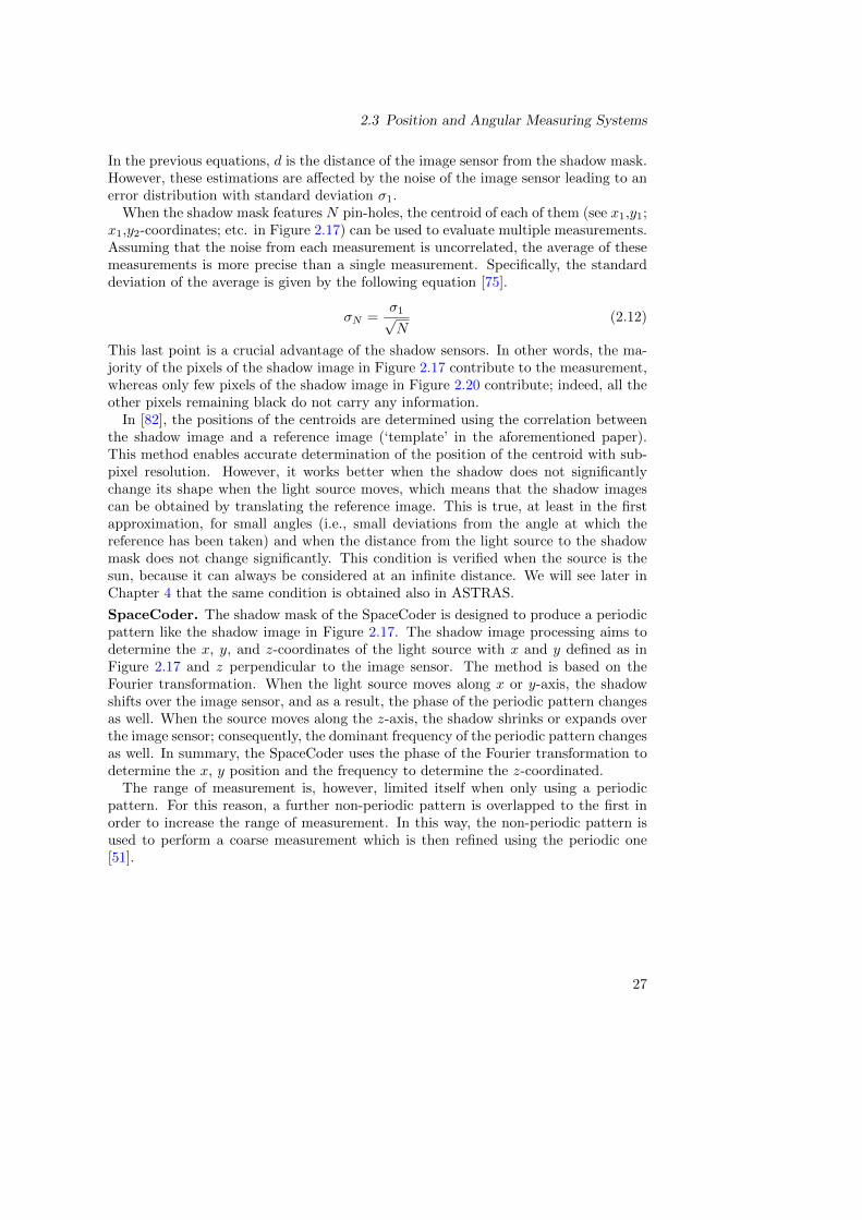
In the previous equations, d is the distance of the image sensor from the shadow mask.However, these estimations are affected by the noise of the image sensor leading to anerror distribution with standard deviation σ1.

When the shadow mask features N pin-holes, the centroid of each of them (see x1,y1;x1,y2-coordinates; etc. in Figure 2.17) can be used to evaluate multiple measurements.Assuming that the noise from each measurement is uncorrelated, the average of thesemeasurements is more precise than a single measurement. Specifically, the standarddeviation of the average is given by the following equation [75].

σN =σ1√N

(2.12)

This last point is a crucial advantage of the shadow sensors. In other words, the ma-jority of the pixels of the shadow image in Figure 2.17 contribute to the measurement,whereas only few pixels of the shadow image in Figure 2.20 contribute; indeed, all theother pixels remaining black do not carry any information.

In [82], the positions of the centroids are determined using the correlation betweenthe shadow image and a reference image (‘template’ in the aforementioned paper).This method enables accurate determination of the position of the centroid with sub-pixel resolution. However, it works better when the shadow does not significantlychange its shape when the light source moves, which means that the shadow imagescan be obtained by translating the reference image. This is true, at least in the firstapproximation, for small angles (i.e., small deviations from the angle at which thereference has been taken) and when the distance from the light source to the shadowmask does not change significantly. This condition is verified when the source is thesun, because it can always be considered at an infinite distance. We will see later inChapter 4 that the same condition is obtained also in ASTRAS.

SpaceCoder. The shadow mask of the SpaceCoder is designed to produce a periodicpattern like the shadow image in Figure 2.17. The shadow image processing aims todetermine the x, y, and z-coordinates of the light source with x and y defined as inFigure 2.17 and z perpendicular to the image sensor. The method is based on theFourier transformation. When the light source moves along x or y-axis, the shadowshifts over the image sensor, and as a result, the phase of the periodic pattern changesas well. When the source moves along the z-axis, the shadow shrinks or expands overthe image sensor; consequently, the dominant frequency of the periodic pattern changesas well. In summary, the SpaceCoder uses the phase of the Fourier transformation todetermine the x, y position and the frequency to determine the z-coordinated.

The range of measurement is, however, limited itself when only using a periodicpattern. For this reason, a further non-periodic pattern is overlapped to the first inorder to increase the range of measurement. In this way, the non-periodic pattern isused to perform a coarse measurement which is then refined using the periodic one[51].

27

3 Apparatus and Method forDetermining the Orientation andPosition of two rigid Bodies

The patent presented in this chapter describes the main concept of ASTRAS and therelated tracking system. The ASTRAS concept is inspired by the shadow sensors.Indeed, it consists of a shadow mask, an image sensor, and a punctual light sourcelike other shadow sensors. The main difference is that ASTRAS further comprisesa mechanical constraint that limits the degrees of freedom, reducing the variables ofthe system. Therefore, it is easier to associate the shadow image to the input anglewith higher accuracy. The patent also describes the new proposed tracking systemconsisting of a multitude of ASTRAS measuring systems embedded in the joints of anarticulated device.

Patent. The following patent was filed on the 16th of December, 2016. Referencenumber: WO2018109218 (A1) (https://worldwide.espacenet.com/)Status. Currently, this patent has been filed and is pending in the following countries:EU, USA, Canada.Note. Despite the inventors being in alphabetical order, I am the main contributorof this patent.

29

3 Apparatus and Method for Determining the Orientation and Position of two rigid Bodies

30


32


34


36


38


40


42


44


46


48


50


52


54


56


58


60

4 Proof of Principle of a NovelAngular Sensor Concept for TrackingSystems

The paper presented in this chapter describes ASTRAS, its measurement model, andits measurement method. It also describes an experimental activity during which thefirst prototype of ASTRAS was built and characterized. Using this prototype, weidentified the most relevant technical details to make ASTRAS accurate.

An experimental characterization showed very promising results. In particular, theprecision of the measuring system was 0.6 arcsec and its sensitivities to temperature(0.4 arcsec/◦C) and to long term drift (0.2 arcsec/day) were negligible .

Publication. The following paper was published on the 19th of August, 2018 inthe journal Sensors and Actuators A: Physical, Elsevier. ©2018 Elsevier. DOI:10.1016/j.sna.2018.08.012

61

Sensors and Actuators A 280 (2018) 390–398

Contents lists available at ScienceDirect

Sensors and Actuators A: Physical

journa l homepage: www.e lsev ier .com/ locate /sna

Proof of principle of a novel angular sensor concept for trackingsystems

Lorenzo Iafolla a,∗, Lilian Witthauer a,∗, Azhar Zam b, Georg Rauter c,Philippe Claude Cattin a

a Center for Medical Image Analysis & Navigation (CIAN), Department of Biomedical Engineering, University of Basel, Gewerbestrasse 14, 4123, Allschwil,Switzerlandb Biomedical Laser and Optics Group (BLOG), Department of Biomedical Engineering, University of Basel, Gewerbestrasse 14, 4123, Allschwil, Switzerlandc Bio-Inspired RObots for MEDicine-Lab (BIROMED), Department of Biomedical Engineering, University of Basel, Gewerbestrasse 14, 4123, Allschwil,Switzerland

a r t i c l e i n f o

Article history:Received 7 February 2018Received in revised form 31 July 2018Accepted 9 August 2018Available online 10 August 2018

Keywords:ASTRASAngular sensorRotary encoderMedical tracking device

a b s t r a c t

Robot-assisted and computer-guided minimally-invasive procedures represent a turning point inMinimally-Invasive Surgery (MIS) because they overcome significant limitations found in current state-of-the-art manual MIS procedures (e.g. imprecise motion, hand tremor, fatigue of the surgeon, limitedworkspace/maneuverability, etc.). Importantly, robotic systems can only reach the required high accu-racy and precision when a tracking system with the corresponding accuracy and precision level for thesurgical tool’s end-effector enables closed-loop feedback control. Herein, we present a tracking systemmeeting the above required high accuracy and precision called ASTRAS (Angular Sensor for TRAcking Sys-tems). In this paper, the working principle and performance of ASTRAS are presented and characterizedrespectively.

ASTRAS is arranged in a way that a tilt of a mirror produces a shift of a shadow cast on an image sensor.Since the mechanical constraints between the light source, mirrors, shadow mask, and image sensorare known, the angle can be derived from the measured shadow shift. The working principle of ASTRASallows the measurement of 2 degrees of freedom at once. Additionally, the commercial availability ofsmall image sensors (∼1 × 1 × 0.5 mm3) allows implementing ASTRAS in the future as a down-scaledversion in surgical tools such endoscopes.

The characterization of ASTRAS was performed with an experimental setup evaluating the angularmeasurement performance in one degree of freedom. The results revealed a precision of ∼3·10−6 rad, athermal stability of 1.9·10-5 rad/◦C, a long term drift 10-5rad/day, and a linearity error of ∼10-4 rad.

Future developments will focus on implementing a miniaturized prototype and making a chain ofsensors to use in articulated devices.

© 2018 Elsevier B.V. All rights reserved.

1. Introduction

In the past years, robot-assisted and computer-guided surgerieshave become more and more important in the medical field. Thesetechnological developments enhance the capabilities of surgeonsin MIS procedures, which is directly beneficial for patients. TheMIRACLE1 project (Minimally Invasive Robot Assisted Computer-guided LaserosteotomE) is devoted to the development of a robotic

∗ Corresponding authors.E-mail addresses: [email protected], [email protected]

(L. Iafolla), [email protected] (L. Witthauer).1 MIRACLE project is funded by the Werner Siemens-Foundation (Zug,

Switzerland).

endoscope able to perform osteotomies (bone cuts) with a laser in aminimally invasive way. Such osteotomies have several advantagescompared to conventional cuts, for example faster healing or thefreedom in cut geometry [1–5]. One fundamental requirement forthe MIRACLE project is to perform minimally invasive accurate lasercuts with a precision of ∼0.2 mm. For this reason, it is required toknow the pose (position and orientation) of the end-effector of therobotic MIRACLE endoscope, or other surgical systems, with highaccuracy and precision in order to close the feedback control loop.In the case of a robotic endoscope with many degrees of freedom,such as it is planned for in the MIRACLE project, it is important notonly to know the pose of the end-effector but also the entire shapeof the endoscope.

General purpose tracking systems (some of which have beenadapted for medical applications) based on different technologies

https://doi.org/10.1016/j.sna.2018.08.0120924-4247/© 2018 Elsevier B.V. All rights reserved.

4 Proof of Principle of a Novel Angular Sensor Concept for Tracking Systems

62

L. Iafolla et al. / Sensors and Actuators A 280 (2018) 390–398 391

are available on the market and the most significant will briefly beoutlined here [6,7]: optical/infrared tracking systems, electromag-netic trackers, IMU (Inertial Measurement Units), FBG (Fiber BraggGrating) shape sensors, rotary encoders, and shadow sensors.

Today, optical trackers (e.g. Polaris/Certus NDI [8] and Axios3D [9]) are the state-of-the-art tracking systems for robotic appli-cations in surgery. Their main components are cameras andretro-reflective markers attached to the device/patient for tracking.Optical trackers are based on the triangulation principle [6–9]. Themost attractive features of optical trackers are their high accuracy(e.g. Polaris NDI [8] ∼0.3 mm (RMS) over ∼4 m3 working volume)and their reliability (they have been developed and commercializedsince the 90 s). However, such optical trackers are strongly limitedby the required line of sight, which precludes applications wherethe instrument is hidden inside the human body (as is the case inendoscopic applications).

EMTS (Electromagnetic tracking systems) are based on the gen-eration of a known electromagnetic field which is then detectedby the target sensors to determine their own positions [6–8].These systems have no line-of-sight requirement and are able totrack instruments such as catheters, endoscopes, and the tip ofneedles within a body. Furthermore, this technology has beendeveloped and commercialized for more than twenty years andhave good accuracy (e.g. AURORA NDI [8] accuracy is ∼0.5 mmand ∼0.3◦ = 5·10−3 rad over 2 m3, ∼40 Hz update frequency andcan track up to eight targets). However, EMTS are limited by theinterference produced by other electromagnetic sources (e.g. therobot itself, ferromagnetic tools, etc.), low update frequency, andthe maximum number of trackable target sensors. In fact, the lattertwo features are essential for the precise determination of the poseand shape of the endoscope.

IMU tracking systems are based on MEMS (Micro Electro-Mechanical Sensors) that combines accelerometers, magnetome-ters and gyroscopes to measure accelerations and angular velocity.As the pose of the tip is determined by integrating these threequantities, small measurement errors accumulate with time, and,therefore, IMUs are not always suitable in medical applications [6].Despite this intrinsic limitation, IMUs can be small (less than 5 mmside) and have no line-of-sight issue, and so further developmentsmay have interesting applications.

FBG sensors are embedded in optical fibers and can measuretheir strain at several points. Three FBGs or more (usually four tocompensate temperature effects) are attached to a bending sup-port (e.g. a tiny flexible tube). Based on the combined measurementof strain at discrete points along all fibers, it is possible to recon-struct the tube’s three-dimensional shape. Though this technologyis very promising because of its miniaturized feature, it still requiresfurther developments to be used in applications requiring highaccuracy [10].

Another tracking technology is given by rotary encoders, whichare suited to measure angles in the joints of articulated devices(e.g. an articulated endoscope). Rotary encoders [11–14] with var-ious working principles exist, whereas Hall Effect Sensors andoptical rotational encoders are the most popular because of theirhigh accuracy and reduced size. However, the accuracy of rotaryencoders depends inverse proportionately to their size: e.g. rotaryencoders from Hengstler with ∼10–6 rad resolution have diame-ters of about 60 mm [13] and others with 8 mm diameter from RLShave an accuracy of 10−2 rad [14]. Medical applications in endo-scopes or instruments would require encoders to be much smallerthan 10 mm with a much higher accuracy than 10−2 rad. Moreover,rotary encoders only work for joints with one degree of freedom(DOF).

The last group of tracking systems outlined here are shadowsensors. These sensors measure the position of a light source or thedirection of the impinging light by detecting a shadow image. All

shadow sensors are composed of the following key elements: animage sensor, a shadow mask, and one or more point-light sources(e.g. LED). The first tracking system based on this concept wasused to measure the direction of light coming from distant lightsources like stars in astronomy [15]. More recently, other sensorshave been implemented to measure not only the position of a pointlight source (e.g. LED) [16,17], but also the position and the orien-tation of a rigid body on which three or more LEDs are mounted[18,19], or the displacement of a concave mirror with respect toa fixed frame [20]. Some sensors have also been adapted to med-ical applications and other fields [21]. The development of thesesensors has been done in the past few years and there is still someroom for improvement. One drawback of the current sensors is thatno profound studies on the characterization of these sensors areavailable to the public. This complicates the interpretation of theirperformance.

This paper proposes an Angular Sensor for TRAcking Systems(ASTRAS) which belongs to the latter described group of shadowsensors. In addition to the key elements of a shadow sensor, ASTRASalso contains a mirror and a mechanical constraint to limit the DOFsof the system.

In contrast to all other described tracking systems, ASTRAS isideally suited to be integrated into articulated devices such as arobotic endoscope because of its technical design and intrinsicproperties. ASTRAS combines the following advantages: immunityto electromagnetic noise, no line-of-sight requirement, poten-tial for miniaturization (image sensors are available as small as1 × 1 × 0.5 mm3 [22] and there are several techniques to miniatur-ize the shadow mask [23,24]), and possibility to track one or twoDOFs.

The technical design and the working principle of ASTRAS is dis-cussed in detail in Section 2. A physical setup, described in Section3, has been developed to characterize the properties of the sen-sor. The experimental validation and characterization of ASTRASare described in Section 4. This characterization quantified the keyparameters of the mechanical implementation, along with the mainsources of error and noise. All parameters and performance mea-surements are used together to validate the working principle andadvantages of ASTRAS over other sensors. Finally, the conclusionsfrom the experimental evaluations are drawn in Section 5.

2. Technical design and working principle

2.1. Technical description of ASTRAS

A technical drawing of ASTRAS is shown in side view in Fig. 1.The purpose of this sensor is to measure the tilt angle betweenplane 1 and plane 2 (2′ when = 0) about the axis x’. In principle,the system can also measure the tilt angle (˛) about y’ as each valueof corresponds to a unique shadow recorded by the image sensor.Though the theoretical extension to two DOFs seems to be straight-forward, the experimental results that are valid for one DOF casecannot be extended directly to two DOFs without any experimentalproof. In this work, only the case with one DOF is studied.

Plane 1 has the following elements: an image sensor, a shadowmask separated from the sensor by a transparent layer (or a simplesupport), and an LED mounted in such a way that it cannot directlyilluminate the sensor. In Fig. 1 the shadow mask is indicated bythree simple bars but can also have a more complicated shape (e.g.in Fig. 2).

Plane 1 is connected to plane 2 by a mechanical constraint (indi-cated in Fig. 1 with a simple arrow). This constraint restricts themovement of the planes to one DOF: plane 1 can only tilt withrespect to plane 2 (by the angle ˇ). A mirror is attached to plane

63

392 L. Iafolla et al. / Sensors and Actuators A 280 (2018) 390–398

Fig. 1. ASTRAS implementation setup. The sensor measures the tilt angle � betweenplane 1 and plane 2 (2’ is the parallel configuration chosen as reference angle � = 0).� is the only DOF of the system since all the others are limited by the mechanicalconstraint (here shown as a simple arrow). In the two DOFs version the secondvariable is �, and the rotation is about the axis indicated with y’.

Fig. 2. Laser cut shadow masks with 10 slits (left, 0.2 mm width) and 5 slits (right,0.4 mm width), made of Molybdenum with a diameter 12 mm and a thickness0.25 mm.

2 in such a way that light from the LED is reflected to the imagesensor through the mask.

To understand the measurement principle, it is easier to con-sider the virtual geometric image of the LED (“virtual LED” or“vLED”) instead of the real one. As changes, the vLED will be mov-ing along a curve, indicated in Fig. 1, causing a shift of the shadowon the sensor, the measurement of which allows the deduction ofthe tilt angle ˇ.

The key feature of ASTRAS is that the directional information ofthe light is spread all over the shadow image; this is very importantbecause it greatly improves the signal-to-noise ratio (SNR).

The environmental light could generate a varying background,complicating the data processing, deteriorating the measurementquality, and even causing fake signals when changing over time.Some solutions based on using a specific wavelength or modulating

the LED intensity and then using a lock-in filter have been proposedby other studies/groups [15–20]. Unfortunately, the first solutiondoes not seem to be effective for high accuracy measurements asthe ambient light may still have some components at that wave-length. The second possibility is a lock-in filter that would limit thesampling frequency (to at least half of the fps of the image sensor).For these reasons, any external light has to be blocked before reach-ing the image sensor (e.g. enclosing ASTRAS with non-transparentscreens).

The possibility that several ASTRAS sensors can be used in a cas-cade broadens its field of application. One potential configuration isshown in Fig. 3, where the sensors are used to measure the anglesat each joint of an articulated device. In general, if the distancesbetween the joints are all known, it is possible to reconstruct theshape of the articulated device and thus the pose of the tip. Sucha system can be miniaturized as a tiny passive chain and incor-porated in the tracked device (such as a continuum robot) or in asimilar way, one ASTRAS can be embedded in each joint of an artic-ulated robot. In particular, the articulated robot can be made of rigidbodies and rotary joints controlled remotely through transmissions(e.g. tendons) by external motors.

ASTRAS measures angles but an estimation of the required accu-racy can be evaluated by the requirement for the position of the tip(2·10−4 m as stated before). As the length of the first endoscope pro-totype is assumed to be 0.3 m, the required accuracy for the angle isthen given by the ratio between the two former quantities ∼(2·10−4

m)/(0.3 m) ∼ 6·10−4 rad. In a tracking device with a cascade of sen-sors, errors will combine (some compensate, others accumulate)but those closer to the tip will contribute less and those which arefurther will contribute most.

2.2. Simplified model of ASTRAS

In contrast to other shadow sensors, the data interpretation ofASTRAS is straightforward. It is easily proven that a variation of thetilt angle will cause a shift of the shadow detected by the sensor.

Theoretically, the two DOFs case is a straightforward extensionof the one DOF case because it can be separated into two indepen-dent parts. A variation of will cause the shadow to translate inone direction while a change in affects the orthogonal directiononly.

A simplified model for ASTRAS, the special case shown in Fig. 4,where the axis of rotation coincides with the surface of the mirror,shall now be considered. An implementation of ASTRAS may havea more complex geometry and this and the following assumptionswould be not valid.

The key property of the sensor is the calibration curve whichencodes the relationship between the shift OT of the shadow on thesensor and the angle ˇ. If the mirror is parallel (ED in Fig. 4) to theimage sensor, the reference value of is zero and the correspondingposition of the virtual LED (vLED) is A. B is the center of the shadowmask and, in the considered simplified model, also the position ofthe real LED. Hence, the shadow of B is projected onto the origin Oof the sensor. Tilting the mirror by an angle (E′D′ in Fig. 4), shiftsvLED to the new position A’, the shadow of the point B will thenshift by a distance OT . It is easy to show that the angle ABA’ and itsopposite are equal to ˇ. Thus, given the distance, d, between thesensor and the shadow mask, OT is given by:

OT = d · tan(ˇ)

� d · (1)

The last approximation produces a linearity error (e.g. for|ˇ|<�/8 the linearity error will be <5%). As a first estimation, this appliesto other points of the shadow mask if is small enough.


64


Fig. 3. Articulated tracking system made of several ASTRAS sensors. Each sensor measures the angle between two consecutive links. Combining the measurements, the shapeof the device (e.g. endoscope) and, the position and the orientation of the tip, can be evaluated.

Fig. 4. Simplified representation of ASTRAS. In this special case the center of rotationC is exactly on the surface of the mirror. � is the angle to be measured, B is the centerof the mask and the location of the LED. A’ and A are the positions of the virtual LEDdepending on the tilt angle � of the mirror. OT is the translation of the center of theshadow caused by tilting.

Eq. (1) describes the calibration curve and the inverse can beused to evaluate by measuring the translation OT:

= atan

(OT

d

)= atan

(n · s

d

)� n · s

d(2)

In which is expressed in radians, n is the shift expressed in pixelsof the image sensor, and s is the side length of the pixel. Eq. (2)is only valid for the trivial case described above. In general, therelation between and n may be a non-linear polynomial withcoefficients Pi:

=∑N

i=0Pi · ni (3)

In linear approximation (P2, P3, etc. = 0) the previous equationsimplifies to:

� P1 · n + P0 (4)

The sensitivity of the sensor is the derivative of the output (shiftmeasured in pixels n) with respect to the input (angle ˇ). Hence,from Eq. (2), one can conclude that:

Sensitivity ≡ ∂n∂ˇ

= d

s(5)

Fig. 5. Shadow image recorded with the ASTRAS prototype using the mask with0.4 mm slits. The white areas are those illuminated by the LED while the dark onesare shadowed by the mask. The black spots are caused by dust on the mirror and onthe sensor, which, in principle, should not affect the measurement. The gray stripsclose to the main brighter ones (e.g. in the up-right region) are the residuals of lightilluminating the sensor directly from the LED.

Eq. (1) can be generalized using Eqs. (4) and (5):

n = Offset + · Sensitivity (6)

in which both Sensitivity( = 1/P1) and Offset(=-P0/P1) are configura-tion characteristics of ASTRAS.

The parameters P1, P0, Sensitivity, and Offset are measured duringthe calibration procedure while the non-linear coefficients (P2, etc.)are found during the linearity tests.

The angular range (ˇR) of ASTRAS can be defined using Eq. (1):

ˇR = arctan(R

d

)∼Rd

(7)

in which R is the maximum shift of the shadow that still allowsto make the measurement. This may be limited by the length Ls ofthe image sensor (R < Ls/2), but it can be extended by encoding thepattern of the shadow mask [17]. However, it is important to noticethat the sensitivity and the range depend on d and are inverselyproportional to each other.

The resolution is defined as the smallest input angle that causesthe minimum detectable variation of the output (as the output isdigital, this is represented by the least significant bit). An overesti-mation of the resolution can be derived from Eq. (2) for n = 1:

ˇr1 � s

d(8)

The shift of the shadow corresponding to n = 1 is one pixel longand will cause a change of the output of all the pixels on the borderbetween the illuminated areas and the shadow; all the other pixelswill not change their outputs (see Fig. 5). The pixels changing theiroutputs are 2·ns·Nc , where ns is the number of slits of the shadowmask and Nc the number of pixels in one column of the image sen-

65


Correlation resultBest fitting parabolaMaximum of the parabola

Fig. 6. Correlation results (Corr(p)) between the reference shadow (Shift = 0 pixel,� = 4.8 mrad) and the input shadow (� = 1.5 mrad). The dashed line is the least-squares best fitting parabola par(t) and its maximum is at tmax = 1.587 pixel. Thiscorresponds to the shift for the best match of the two shadows.

sor. In principle, a very small shift (smaller than one pixel) of theshadow may cause a change in only one single pixel. For this reason,the resolution can be re-estimated as

ˇr2 = ˇr12 · ns · Nc

� s

d · 2 · ns · Nc(9)

Considering also the number of grey levels (NGL) of each pixel, anew estimation of the resolution is given by

ˇr = ˇr2NGL

� s

d · 2 · ns · Nc · NGL(10)

A quantitative estimate of the resolution is in Section 4.4.

2.3. Image analysis

As stated in the previous paragraph, the shift n of the shadow ismeasured in pixel units. For the one DOF case, the system can be setup in a way that the shift will be along the horizontal axis x of theimage and the mask will produce a vertically (along y-axis) stripedshadow (Fig. 5).

The method to measure n is based on the evaluation of the fol-lowing correlation function:

Corr′ (p) =∑

y

∑xI (x, y) · I0 (x + p, y) (11)

in which I is the shadow image recorded during the measurement(e.g. Fig. 5), I0 is the reference shadow (arbitrarily chosen, not nec-essarily corresponding to = 0 but preferably close to the center ofthe angular range in order to avoid the distortions of the biggerangles) recorded during the calibration and p is a discrete vari-able representing the shift along the x-axis also measured in pixelunits. Corr’(p) has a maximum corresponding to the shift n whichis necessary to achieve the best match of I and I0.

Without loss of accuracy, one can use the following function:

Corr (p) =∑

x

(∑yI (x, y) ·

∑yI0 (x + p, y)

)(12)

Analogous to Eq. (11), this equation has a maximum at n too,however, it is computationally less expensive. The discrete func-tions Corr(p) and Corr’(p) can be interpolated with a continuousparabola Par(t) (Fig. 6) with coefficients apar , bpar and cpar:

Par (t) = apar · t2 + bpar · t + cpar (13)

Therefore, the value tmax of the maximum is given by:

tmax = −bpar2 · apar

(14)

This corresponds to the shift n required to evaluate from Eq.(4) or the Sensitivity from Eq. (5) when performing the calibration.

Fig. 7. Photo of the characterization setup. Its volume is 150 × 150 × 165mm3, allother dimensions are given in the schematic picture in Fig. 8.

Fig. 8. Scheme of the characterization setup of ASTRAS setup (all dimensions inmm). The top plane of the rotation stage (goniometer) rotates about the virtualrotation axis.

Using the whole image to calculate the correlation function inEq. (12) greatly improves the signal-to-noise ratio (SNR) and tmaxcan also be estimated with sub-pixel resolution.

3. Characterization setup

A photo and the corresponding technical drawing of the char-acterization setup are shown in Figs. 7 and 8. The key elementsof the setup were: the image sensor (Ximea MU9PC without lens,sensor active area 5.7 × 4.3 mm2, pixel size 2.2 × 2.2 �m2, [25]),


66


the shadow mask (as shown Fig. 2), the LED (SML-P12 SeriesPICOLED, 1 × 0.6 × 0.2 mm3, [26]), and a mirror (aluminum, roundshape 25.4 mm diameter). Excluding the environmental, uncon-trolled and unwanted variables (e.g temperature, pressure, etc.),the input angle is the only variable of ASTRAS and, in this setup, wascontrolled using a rotation stage (Thorlabs GNL10/M, [27]) with anangular resolution of 6.7·10−4 rad. All of the other following chang-ing quantities are parameters of ASTRAS and are not meant to bemodified during the regular functioning.

The camera has a single and a burst capturing mode. In sin-gle mode, the camera captures only one image. In burst mode, thecamera captures several images in a short time (e.g. 100 images in22 s), which was useful to reduce the noise by averaging over theseimages when characterizing the systematic features of ASTRAS(sensitivity, linearity error, etc.). The shadow mask with either 5or 10 slits (the number of slits is a parameter), was fabricated frommolybdenum, 0.25 mm thickness, and was manufactured using alaser cutter (Fig. 2). It was fixed in front of the image sensor withthe help of a threaded ring.

The distance between the sensor and the mask (parameter pre-viously defined as d) was 1.1 mm and was increased by inserting0.2 mm thick glass slides. Due to the limited space, only three con-figurations were used for the current work d = 1.1, 1.3 and 1.5 mm.

The distance between the mirror and the sensor is also a parame-ter (H) and was changed using a vertical stage (Thorlabs MVS005/M,[27]) with a resolution of 0.01 mm. A thermometer (K type ther-mocouple, not shown in the picture) with a resolution of 0.1 ◦C wasplaced on top of the image sensor to measure its temperature.

In order to prevent external light to reach the sensor, the setupwas closed inside a box and/or a cabinet during the measurementphase. To prevent the light from the LED to directly illuminate thecamera, a tiny screen made of black cardboard was glued close tothe LED (not shown in Fig. 8). The remaining direct light from theLED (see Fig. 5) was further compensated for by recording the back-ground after covering the mirror with a black cardboard and waslater subtracted from the images.

4. Characterization measurements and discussion

As can be seen in Eq. (5), the sensitivity of the simplified modeldepends only on the parameter d and the pixel size s of the sensor.As mentioned before, the characterization setup may show a dif-ferent behavior from the simplified model and the sensitivity maydepend also on other parameters of the system. To explain theseeffects a more detailed theoretical model should be used but this isbeyond the scope of this paper. The characterization measurementsare used to analyze the following key parameters: calibration,linearity error, precision, resolution, long term and temperaturestability.

4.1. Calibration and sensitivity

The calibration was performed for several values of the param-eters of ASTRAS (Table 1). Those of the camera were adjusted (e.g.exposure time 9 ms, gain 2 db, 4.61 fps, 1270 × 1693 pixels, 256grey levels) in order to exploit the full dynamic range of the imagesensor and reduce the noise level. Noise reduction was achieved bychoosing the burst mode of the camera and 100 samples were aver-aged to one image. The calibration itself consisted of determiningthe coefficients (Offset and Sensitivity) of Eq. (6). This was done bymeasuring n for several (78) values of equally spaced along thefull range of the goniometer and then fitting (least-squares bestfitting) them with a linear function.

The measure of n cannot be performed before the zero positionof the sensor ( = 0) and the reference image I0 are chosen and,

-0.15

0

Fig. 9. Calibration curve with 5-slits mask, d = 1.1 mm and H = 9 mm. As foreseen bythe simplified model, the calibration curve is, in first approximation, linear with aSensitivity of -489 pixel/rad and Offset of 2.4 pixel.

in principle, these are completely arbitrary. A reasonable choice forboth is the center of the angular range of ASTRAS that, as the sensoris linear, is identified by the mean value of the outputs associatedto the extremes of the range. Another criterion is related to theapplication of the device: for example, in an articulated device, thezero position may be identified by a specific shape of the deviceitself. For the calibration process described here, the zero positionwas defined by the zero position of the goniometer.

Fig. 9 shows the calibration data and the corresponding linearfit for one specific setting (5 slits, d = 1.1 mm, H = 9 mm).

It can be seen that the linear function fits the calibration pointsand the behavior of the sensor is mainly linear as expected. Theevaluation of the non-linearity residuals and further considerationsare described in Section 4.2. It should be noted that the sign of thesensitivity depends only on the sign which was assumed for theinput angle and, as a convention, it was chosen to be positive forthis paper. Also notice that the offset corresponds to the shift of thereference shadow I0 (see Section 2.3) from the one related to = 0.As both the input related to I0 and = 0 are chosen arbitrarily, theoffset has no interesting meaning for the characterization purpose.

Table 1 summarizes the calibration results for several config-urations of the setup parameters. The measured values for thesensitivity are compared to the corresponding sensitivity expectedfrom the simplified model of Section 2.2. As already seen with theconfiguration related to Fig. 9, the sensor was, in a first approxima-tion, linear for all the other configurations. As expected from Eq. (5),Table 1 shows that the sensitivity depends on the distance d (indi-cated in Figs. 4 and 8) between the image sensor and the shadowmask; e.g. only 200 �m difference in d induces a sensitivity changeof ∼12 percent. The simplified model, instead, cannot explain whythe distance H (distance between the image sensor and the mirroras shown in Fig. 8) affects the sensitivity. However, a simple anal-ysis of the results shows that d impacts the sensitivity at least 10times more than H.

Finally, a test with a 10 slits mask was performed to demonstratethat the sensitivity does not significantly depend on the number ofslits. Using the same configuration but with 5 slits, it was indeedshown that the relative difference in sensitivity is about 5 percentand may be due to small errors of the mechanical parameters of thetwo setups.

Deviations from the simplified model may originate from thedifferent and more complex geometry of the characterization setup,the non-negligible thickness of the shadow mask, the refraction oflight at the glass slides used to increase the distance d (see Section3) and, in particular, d might change depending on how tight theshadow mask was fixed to the camera.

67


Table 1The calibration results are divided in three sections based on the changing parameter indicated in bold.

Sensor parameters Calibration results

d [mm] H [mm] Number of slits Sensitivity [pixel/rad] Sensitivity [mm/rad] Expected sensitivity [mm/rad]

1.1 9 5 487 1.07 1.11.3 9 5 545 1.20 1.31.5 9 5 597 1.31 1.51.1 9 5 487 1.07 1.11.1 12 5 559 1.23 1.11.1 15 5 598 1.31 1.11.1 18 5 623 1.37 1.11.1 21 5 640 1.41 1.11.1 9 5 487 1.07 1.11.1 9 10 461 1.01 1.1

-1

-0.5

0

0.5

rad

ASTRASGoniometer

Fig. 10. Linearity error (continuous line) of ASTRAS and linearity error of thegoniometer (dashed line). They both show similar INL and DNL contributions.However, these two results were not obtained simultaneously because of setuplimitations and this explains the slight mismatch.

4.2. Linearity error

The non-linearity (NLshift) or linearity error is the deviation ofthe calibration curve from the ideal (least-squares best fitting) lin-ear behavior described in Eq. (4) with the Sensitivity and the Offsetevaluated during the calibration phase:

NLshift = ncalib(ˇ)

−(

· Sensitivity + Offset), (15)

in which ncalib is the shift measured during the calibration phaseand, as NLshift , is measured in units of pixels. To get an estimate forthe linearity error in radians (NLrad) one can simply use Eq. (4) withP0, P1 evaluated by inverting Eq. (6).

The extracted linearity error for the ASTRAS prototype is shownby a continuous line in Fig. 10 for the same setting as Fig. 9 (5 slits,d = 1.1 mm, H = 9 mm). The values lie within a range of 10−3 radwith a standard deviation of 3·10-4 rad. The plot exhibits two majorcharacteristics: a larger quadratic and a smaller periodic modu-lation referred to as Integral Non-Linearity (INL) and DifferentialNon-Linearity (DNL), according to the terminology of the analog-to-digital converters (ADCs).

The INL can be quantified by using a second degree polynomialfit (Pi = 0 for i≥3 in Eq. (3)), instead of a linear function, to extractthe parameters from the calibration data. For the case shown inFig. 10, the parameter P2 was determined to be 4·10−7 rad/pixel2

instead of zero, which is expected from the ideal linear case and tobe compared to P1 which was ∼2·10-3 rad/pixel. The INL can simplybe compensated by using a second order polynomial fit instead ofa linear one.

Having corrected the INL, the standard deviation of the linear-ity error decreases by a factor of three to 10−4 rad, which can beassigned to the DNL. The DNL must originate from the experimen-tal setup, in particular, from the control screw of the goniometerGNL10/M shown in Figs. 7 and 8. Indeed, tests with the goniometerwere performed by mounting a laser pointer on it and evaluating

-1.50

Fig. 11. Distribution of angular errors. This test has been performed with d = 1.1 mm,H = 9 mm, the 5-slits mask and recording 4.74 frames per second (total 2826 sam-ples). The standard deviation (precision) of the collected samples is 3·10−6 rad.

the angle from the displacement of the spot on a screen mountedfive meters away. These tests (results plotted as dashed curve inFig. 10) have shown similar linearity errors whose periodicity isexactly the same as the one of the screw of the goniometer (1screw turn ≡ 1 period). Both DNL and INL of ASTRAS are similarto the goniometer results showing that the current setup is lim-ited by the goniometer itself. To diminish these errors, a differentcalibration reference is desirable for the future.

4.3. Precision

The precision is the standard deviation of repeated measure-ments and represents the stochastic contributions (e.g. electronicnoise of the camera), worsening the quality of the sensor. Fig. 11shows the distribution of the angular error (difference betweenmeasured angle and input angle) extracted using Eq. (4) for morethan 2800 samples (single measurements). The data were recordedwithout changing the input angle or the measurement setup (5 slits,d = 1.1 mm, H = 9 mm) and keeping the system in a dark environ-ment to reduce the effect of external light variations.

The distribution was approximately Gaussian, which indicatedpure random behavior. The precision was calculated to be 3·10−6

rad.A similar experiment was conducted with a 10 slit mask without

showing significant deviation from the former results.


68


-6

28.5

29

29.5

30

30.5

Angular ErrorTemperature

Fig. 12. Long term record of the angular error (continuous line) in comparison tothe measured temperature (dashed line). This test was performed with d = 1.1 mm,H = 9 mm, the 5-slits mask, and a recording rate of one frame every 10 min.

4.4. Resolution

Eq. (10) provides an estimation of the resolution (d = 1.1 mm,s = 2.2 �m, 5 slits, 1270 pixels per column and 256 grey levels)which is remarkably small:

ˇr � 2.2 · 10−3mm

1.1mm · 2 · 5 · 1270 · 256� 6 · 10−10 rad (16)

Since the precision is 3·10−6 rad, it can be concluded that the res-olution does not limit the performance of ASTRAS and, furthermore,it is not possible to measure it experimentally.

The same can be concluded from Fig. 11 (notice that the bin sizeis not chosen to be representative of the resolution). If the resolu-tion was comparable or larger than the precision, the distributionof the repeated measurements would not be Gaussian but ratherbinomial or constant, meaning that there are other stochastic errorswhich are bigger than the resolution.

4.5. Long term drift and temperature

In order to determine any long term drift and the impact of thetemperature, the acquisition software was programmed to recorda single measurement every 10 min for 5 days without averagingthe measurements or changing the input angle and the configura-tion of the setup. The temperature variations were recorded as wellwith the thermocouple positioned on top of the camera and thenaveraged to have one measurement every 10 min.

In Fig. 12 the angular error versus time is compared to the tem-perature variations. A long term drift of about 5·10−5 rad (10−5

rad/day) and some small oscillations are visible.The long term drift is most likely due to the mechanical relax-

ation of some components of the prototype. Though the majorityof the applications last for a time much shorter than one day, a cal-ibration procedure may be required frequently (e.g. before usage)depending on the desired accuracy.

The small oscillations are correlated with the temperature andcaused by the thermal expansion of the mechanical components ofthe prototype and hence are design and material dependent. Thetemperature change (T-Tcal) produces a fake signal (ˇTemperature),which, by linear approximation, is given by the following equation:

ˇTemperature = cT · (T − TCal) (17)

with Tcal being the temperature during the calibration. Theparameter cT can be found by analyzing the power spectral den-sity of the angular error and the temperature. They both had a peakat 1.16·10−5 Hz (24 h, this is the day-night temperature range) andtheir ratio at this frequency is cT = 1.9·10−5 rad/◦C.

Eq. (17) can be used to compensate the fake signal by simulta-neously measuring the temperature.

5. Conclusion

In this paper the design, working principle, and characteristicsof ASTRAS, a new angular sensor based on shadow imaging, werepresented.

The introduced simplified model was used to understand theresults obtained from measurements with a prototype. The resultsare very promising if compared with the requirement (6·10−4 rad)evaluated for the MIRACLE endoscope. The precision was deter-mined to be 3·10-6 rad, the long term drift was 10-5 rad/day, and thetemperature induced signal was 1.9·10-5 rad/◦C. After removing thequadratic contribution, the standard deviation of the linearity errorwas estimated to be approximately 10−4 rad and seems to be lim-ited more by the characterization setup rather than by the sensoritself. This indicates that there is room for further improvement.

The integration of new mini-cameras with ∼1 × 1 × 0.5 mm3

volume makes ASTRAS suitable for miniaturization and attractivefor application in the medical field for tracking systems as wellas in other fields. A combination of several sensors can be usedin an articulated device (e.g. the robotic endoscope of the projectMIRACLE) to measure its shape, orientation, and position of its tip.

The next development of ASTRAS will address the challengesinvolved in making this technology useful for medical applications(e.g. human body or endoscope tracking). In particular, those ofminiaturization, extension to two DOFs, improvement of the rangeand the acquisition and data processing of multiple sensors througha shared electronic system will be tackled.

References

[1] K.-W. Baek, et al., Clinical applicability of robot-guided contact-free laserosteotomy in cranio-maxillo-facial surgery: in-vitro simulation and in-vivosurgery in minipig mandibles, Br. J. Oral Maxillofac. Surg. 53 (10) (2015)976–981, http://dx.doi.org/10.1016/j.bjoms.2015.07.019, Elsevier.

[2] K.-W. Baek, et al., A comparative investigation of bone surface after cuttingwith mechanical tools and Er:YAG laser, Lasers in Surgey and Medicine, WileyPeriodicals 47 (5) (2015) 426–432, http://dx.doi.org/10.1002/lsm.22352.

[3] A.E. Bruno, H.-F. Zeilhofer, P. Jürgens, Carlo-computer assisted and robotguided laser-osteotome, United States Patents, 2012. Patent US 13/497,520.

[4] M. Eugster, P. Weber, P. Cattin, A. Zam, G. Kosa, G. Rauter, Positioning andStabilisation of a Minimally Invasive Laser Osteotome, Imperial CollegeLondon, 2017.

[5] G. Kosa, G. Aiello, A. Zam, P.C. Cattin, G. Rauter, Automation of a Flexoscopefor Laser Osteotomy, EPiC Series in Health Sciences, 2017.

[6] W. Birkfellner, J. Hummel, E. Wilson, K. Cleary, Tracking devices, in:Image-Guided Interventions, Technology and Applications, Springer Science,2008, ISBN: 978-0-387-73856-7.

[7] P. Gomes, Localization and Tracking Technologies for Medical Robotics, in:Medical Robotics, Minimally Invasive Surgery, Elsevier, 2012, ISBN:978-0-85709-130-7.

[8] Polaris, Certus and Aurora tracking Systems, 2017 www.ndigital.com.[9] AXIOS 3D Tracking Systems, 2017 http://www.axios3d.com.

[10] Chaoyang Shi, et al., Shape sensing techniques for continuum robots inminimally invasive surgery: a survey, IEEE Trans. Biomed. Eng. 64 (8) (2017)1665–1678, http://dx.doi.org/10.1109/TBME.2016.2622361.

[11] Walt Kester, Linear and rotary position and motion sensor, in: SensorTechnology Handbook, Elsevier, 2005, ISBN: 0-7506-7729-5.

[12] Ernest O. Doebelin, Dhanesh N. Manik, Doebelin’s Measurement Systems, 6e,in: Doebelin’s Measurement Systems, 6e, Mc Graw Hill, 2011, ISBN:978-0-07-069968-7.

[13] Rotary Encoder Hengstler Website, 2017 www.hengstler.de.[14] Rotary Encoder RLS Website, 2017 www.rls.si.[15] Douglas B. Leviton, Apparatus and method for a light direction sensor, United

States Patents, 2009. Patent US 7,924,415 B2.[16] P. Masa, E. Edoardo, David Hasler, E. Grenet, Masurement system of a light

source in space, World International Patent Organization, 2012. Patent WO2012/007561.

[17] P. Masa, E. Franzi, C. Urban, Nanometric resolution absolute positionencoders, 13th European Space Mechanisms & (2009).

[18] D. Hasler, Positioning system and method, European Patent Application, 2016.Patent EP 3 045 932 A1.

[19] E. Grenet, et al., SpaceCoder: a Nanometric 3D Position Sensing Device, CSEMScientific and Technical Report, 2011.

[20] P. Masa, Measurement system for optical touch trigger or scanning probe witha concave mirror, European Patent Application, 2013. Patent EP 2 615 425 A1.

[21] A. Chebira, et al., HearRestore: Nanotracking for Image-guided Microsurgery,CSEM Scientific and Technical Report, 2015.

69


[22] AWAIBA Image Sensors, 2017 www.awaiba.com.[23] Micro-milling Machine Tools, 2018 www.pmtnow.com.[24] Lithography Processes, 2018 www.imtag.ch.[25] Ximea Image Sensor, 2017 www.ximea.com.[26] PICOLED Series ROHM, 2017 www.rohm.com.[27] Thorlabs, Motion Control, Manual Stages, 2017 www.thorlabs.com.

Biographies

Lorenzo Iafolla received his master degree in physics with honors from the Univer-sità di Tor Vergata, Rome (Italy) in 2009. After his studies he worked for several yearsfor two of the most important Italian research institutions (National Institute forNuclear Physics and National Institute for Geophysics and Volcanology) and for hisown enterprise which is specialized in scientific instrumentation (high sensitivityaccelerometers). He gained a profound knowledge in precision measurement tech-niques applied to Particle Physics, Geophysics, Oceanography and others scientificfields. Besides that, he expanded his expertise in designing, assembling, and usingmechanical and electronic devices. He has started his Ph.D. in July 2016 in the Plan-ning and Navigation group of the MIRACLE project at the Department of BiomedicalEngineering in Allschwil. During his Ph.D., he will develop new minimally invasivenavigation techniques using an opto-mechanical position sensor (ASTRAS).

Lilian Witthauer received her M.Sc. in Physics from the University of Basel in 2010.For her Ph.D. in the field of experimental nuclear and particle physics, she joinedthe group of Prof. B. Krusche at the Department of Physics of the University of Basel.During several research visits in Mainz and Bonn (Germany), she performed exper-iments at different acceleration facilities and graduated in 2015 with summa cumlaude. She was awarded the Camille- and Henry-Dreyfus grant and the CHIPP Prize2015 for the best Ph.D. student in particle physics in Switzerland. Besides her Ph.D.studies, she completed a Master of Advanced Studies (MAS) in Medical Physics withspecialization in Radiation Therapy at ETH Zürich. Her MAS thesis was devoted tonavigated brachytherapy for liver tumors. Since spring 2016, she is a postdoctoralresearcher in the group of Prof. Ph. Cattin at the Department of Biomedical Engineer-ing of the University of Basel and co-leads the Planning and Navigation Group of theMIRACLE project. Her research is addressed to the development of new minimallyinvasive navigation techniques and the innovative visualization of the progress andthe planning of surgical interventions with the help of augmented reality.

Prof. Azhar Zam, assistant professor for medical laser physics and optics, com-pleted a Bachelor’s degree in medical physics at the University of Indonesia andcontinued his studies in Germany at the Lübeck University of Applied Sciencesand the University of Lübeck, as well as at the Friedrich-Alexander University ofErlangen-Nürnberg, where he finished his PhD in advanced optical technologiesand developed optical tissue differentiation for Laser Surgery Feedback System in2011. In 2012, he developed the first nano sensitive OCT and the first fully integratedMonte Carlo-Photoacoustic wave simulator. In the course of several research visits,he stayed at University of Waterloo (Canada), National University of Ireland, Galway,University of California, Davis (USA) and Ryerson University, Toronto (Canada). Inhis research, Azhar Zam focuses in particular on laser surgery, optical coherencetomography (OCT), laser-tissue interaction, feedback system and monitoring forlaser surgery and therapy, tissue optics and photoacoustic spectroscopy/imaging.

Georg Rauter was born 1980 in Oberndorf bei Salzburg (Austria). He studied mecha-tronics in mechanical engineering at Graz University of Technology (Austria) andmathematical and mechanical modelling at the engineering school MATMECA, Uni-versity Bordeaux 1 (France). In 2006, he developed a prototype for diagnosis inspine pathologies at the enterprise AXS Ingenierie (Merignac, France) before joiningthe SMS-Lab of Prof. Robert Riener (ETH-Zurich, Switzerland). From March 2008 tillOctober 2013, Georg Rauter worked at the SMS Lab as a PhD student in the fieldof robot-assisted human motor learning. During his PhD, he developed a roboticrowing trainer that accelerated motor learning by individualized feedback to thehuman trainee. In 2013, Georg Rauter worked as a postdoc for research in robot-assisted rehabilitation at the Spinal Cord Injury (SCI) Center of Prof. Armin Curt(University Hospital Balgrist, University of Zurich) together with the SMS-Lab (ETHZurich). During his postdoc Georg Rauter also stayed at University of Southern Cal-ifornia (USC), USA with Professors David Z. D’Argenio and Francisco Valero-Cuevasfor half a year. At USC, Georg Rauter developed statistical hierarchical models foranalysis of a clinical multicenter study with the rehabilitation robot ARMin. Since hisPhD, Georg Rauter is a member of the Award Winning Team: 1st price euRoboticsTechnology Transfer Award 2014 for the rehabilitation device THE FLOAT, a Mul-tidirectional Transparent Support System for Over Ground Gait Training. In 2015,he became the CTI-project manager for the FLOAT in a joint project between theSCI Center and the company Lutz Medical Engineering (Rüdlingen, Switzerland).As a result, the first medically certified series version of The FLOAT is available onthe market since June 2016. In May 2016, Georg Rauter was awarded an AssistantProfessorship at the Department of Biomedical Engineering (University of Basel,Switzerland) for the Minimally Invasive Robot Assisted Computerguided Laseros-teotomE (MIRACLE) project. Due to the generous funding of this MIRACLE throughthe Werner von Siemens Foundation (Zug, Switzerland), Georg Rauter could foundthe Bio-Inspired RObots for MEDicine-Lab (BIROMED-Lab). The main focus of theresearch in his BIROMED-Lab is: robotic endoscopes for laser ablation of hard tis-sue, bio-inspired sensor technologies for endoscopic navigation, tele manipulation,automation, kinematics, and control.

Philippe Cattin was born in Switzerland in 1967. He received his B.Sc. degree fromthe University of Applied Science in Brugg/Windisch in 1991. In 1995 he receivedthe M.Sc. degree*in *computer science and in 2003 the Ph.D. degree in robotics fromETH Zurich, Switzerland. From 2003 to 2007 he was a Postdoctoral Fellow with theComputer Vision Laboratory at ETH Zurich. In 2007 he became an Assistant Professorat the University of Basel and was promoted to Associate Professor in 2015. He is thefounder of the Medical Image Analysis Center at the Medical Faculty of the Universityof Basel. He is currently the head of the recently founded Department of BiomedicalEngineering at the University of Basel. His research interests include medical imageanalysis, image-guided therapy and robotics-guided laser osteotomy. As a PrincipalInvestigator he has finished many projects in these areas and published over 100papers, patents and book chapter


70

5 Preliminary Tests of theMiniaturization of a Novel Conceptof Angular Sensors

The proceeding article presented in this chapter describes an experiment where a ver-sion of ASTRAS featuring a miniaturized image sensor (NanEye camera, 1 × 1 ×0.5 mm3) and miniaturized shadow mask (slits width down to 0.08 mm) was tested.This experiment demonstrated that ASTRAS retains its high precision, 6 arcsec, de-spite the use of miniaturized components for the implementation.

Publication. This work was presented in Montreal in October 2019 at the confer-ence IEEE sensors, 2019 and the following proceeding was published on the 13th ofJanuary, 2020 in the journal 2019, IEEE sensors. ©2019 IEEE. DOI: 10.1109/SEN-SORS43011.2019.8956732

71

Preliminary Tests of the Miniaturization of a Novel Concept of Angular Sensors

Lorenzo Iafolla, Lilian Witthauer, Sara Freund, Lorin Fasel, Azhar Zam, Georg Rauter, Philippe C. Cattin Department of Biomedical Engineering, University of Basel, Allschwil, Switzerland

[email protected]

Abstract—This work was done in the framework of the MIRACLE project devoted to the development of a flexible, articulated robotic endoscope to perform laser osteotomies (bone cutting). In order to control this robot with the required accuracy of 0.2 mm at the tip position, a tracking system needs to feed back the pose of the tip and the shape of the endoscope. One of the possible designs of such a robotic endoscope is based on an articulated device that can be tracked by measuring the bending angle at each joint. Recently, we presented (Iafolla et al., 2018) a novel angular sensor called ASTRAS (Angular Sensor for TRAcking Systems), which measures a one degree of freedom rotation by processing a shadow image cast through a shadow mask onto an image sensor. One ASTRAS will be placed at each joint of the articulated robotic endoscope in order to measure their bending angles. The planned diameter of the MIRACLE endoscope is 10 mm and it will contain several components such as the optical fiber for the laser, irrigation and sucking systems, and robot control mechanisms. However, the latest version of ASTRAS covered a volume of 40x40x55 mm3. For this reason, the most demanding requirement for the design of the final ASTRAS sensor is its miniaturization to fit the sensor inside the joint of the endoscope. Consequently, in this contribution, we investigated the possibility of miniaturizing ASTRAS and assess its limitations due to some fundamental aspects. In particular, we built a prototype based on a NanEye camera by AMS (1x1x0.5 mm3) and a micro-milled shadow mask with 0.08 mm wide slits. The tests of this prototype showed encouraging results and will be discussed. In particular, at such small dimensions, there are no unexpected optical effects (e.g. optical diffraction due to the mask) worsening the measurement. Indeed, the precision of 5 arcsec and the linearity error of 23 arcsec RMS are comparable to those of the previous bigger prototype. Further considerations and concepts related to the miniaturization of ASTRAS are also discussed in this paper.

Keywords—ASTRAS; Medical Tracking Systems; Rotary Encoder; Angular Sensor; NanEye Camera

I. INTRODUCTION

In the past decades, various tracking technologies have been developed for medical applications as they are essential in image-guided surgery systems [1]-[3]. In particular, in the case of a robotic system, feedback for its safe and precise control is required. The goal of the MIRACLE project (Minimally Invasive Robot-Assisted Computer-guided LaserosteotomE) is to develop a robotic endoscope able to perform Laser-osteotomies (bone cuts) in minimally invasive surgeries [4]-[7]. The minimally invasive feature requires the endoscope to

be as small as possible (the current design has a 10 mm diameter). In addition, such an endoscope might incorporate several components such as: irrigation and sucking systems to avoid carbonization of the bone and accumulation of liquids and debris [8]; optical/acoustic systems to identify the tissues and to measure the depth of the cut [9],[10]; force sensors to provide feedback to the surgeon [11]; and all the required systems to control the robot (e.g. tendons or motors) [12]-[14]. As a consequence, there will be very limited space for the tracking system. Also, further important constraints and requirements limit the choice of an appropriate sensor e.g.: no line-of-sight for optical trackers as the endoscope will be inside the patient’s body; magnetic interferences, from the operative room or the endoscope itself, would affect magnetic trackers; high end-effector position accuracy (<0.2 mm, to perform accurate cuts and hence promote fast healing) which cannot be reached by small rotary encoders; etc. For all these reasons, we investigated the possibility to implement a novel angular sensor [1] called ASTRAS (Angular Sensor for TRAcking Systems) as basic element of a tracking system. Indeed, this sensor can accurately measure the bending angle of a joint of an articulated endoscope, and it has the potential to be miniaturized. Using one ASTRAS at each joint, the shape of the endoscope and the pose of its tip can be tracked. Also, in

MIRACLE project was funded by the Werner Siemens Foundation.

Fig. 1. Schematic representation of the side view of ASTRAS. The only DOF of the system is represented by the angle β to be measured. When this changes, the position of the virtual image of the LED (Virtual LED) moves along the dashed line and, consequently, the shadow shifts along the image sensor.

978-1-7281-1634-1/19/$31.00 ©2019 IEEE

5 Preliminary Tests of the Miniaturization of a Novel Concept of Angular Sensors

72

case of a continuum robot, several ASTRAS can be used to sample the bending angles at regular intervals.

In [1] we described the first prototype of ASTRAS with dimensions of ~40×40×55 mm3, we defined a simple model, and characterized it (precision ~0.6 arcsec, linearity error ~21 arcsec). Following on from this work, we present here the realization and the characterization of a prototype featuring miniaturized image sensor and shadow mask. Its performances are compared to those of the first prototype and further challenges related to the miniaturization are discussed.

II. WORKING PRINCIPLE OF ASTRAS

ASTRAS belongs to the family of the shadow sensors [15]-[21] and, as shown in Fig. 1, consists of an image sensor, a shadow mask, an LED, and a mirror. These components are mounted on two supports (stator and rotor) connected through a mechanical constraint, in a way that the only degree of freedom (DOF) of the system is the rotation angle β. The light from the LED is reflected by the mirror and then cast onto the image sensor through the shadow mask. The components are arranged so that a variation of β corresponds to a horizontal shift of the shadow image (along the y-axis in Fig. 1). This shift is defined in relation to a reference image captured during the calibration phase. The two images are the shifted versions of each other and to accurately (sub-pixel resolution) measure this shift, their correlation is used.

An important feature for the miniaturized version is the position of the rotation axis of the rotor. In principle, this can be anywhere: e.g. in the first prototype [1], it was passing between the rotor and the stator. However, the mirror has to be dimensioned accordingly in order to always reflect the light of the LED on the stator; otherwise, there would be no signal. As the mirror needs also to be miniaturized, the best choice is to center the rotation axis on the stator (e.g. through the LED as in Fig. 1). In this way, the mirror can be relatively small because it is always facing the stator and reflecting the light onto the image sensor.

III. DESCRIPTION OF THE CHARACTERIZATION PROTOTYPE

The characterization prototype (Fig. 2) features three parts that are miniaturized: the image sensor (NanEye camera without lens, 1 × 1 × 0.5 mm3, [22]), the shadow mask (Fig. 3),

and the LED (PICOLED SML-P12, 1 × 0.6 × 0.2 mm3). The NanEye camera has a resolution of 250 × 250 pixels, with a pixel size of 3 μm, and the images are acquired through a dedicated electronic board (ACQ Camera in Fig. 2). Its sensing surface (0.75 × 0.75 mm2) is covered by a transparent layer of glass (~0.4 mm thick). The camera was fixed inside a little pocket of a 3D-printed camera holder on which the shadow mask was screwed. The shadow mask was in direct contact with the glass of the NanEye so that the distance d (see Fig. 1) between the image sensor and the mask was given by the thickness of the glass. However, as the NanEye is very delicate, small, and has a non-regular shape, it was challenging to accurately fix it in a specific pose. The camera holder also hosted a small PCB with the LED inside a second pocket. We produced several versions of the shadow mask for testing. Fig. 3 depicts one milled from an aluminum sheet (40 × 16 × 2.4 mm3). Its key features were two small slits (width 0.08 mm, thickness 0.12 mm) that make up the miniaturized shadow mask itself. Other features (holes, pockets, etc.) were milled in order to accurately position the slits in front of the camera and let the LED shine over the mirror. The mirror (aluminum, round shape with 25.4 mm diameter) was mounted on a rotational stage (Thorlabs PR01/M) that constituted the mechanical constraint of the system.

The calibration standard used for this prototype, is based on a laser pointer attached to the rotational stage. Measuring the displacement x of its spot over a ruler placed at 10 m, we could evaluate the rotation angle as follows: arctg(x/10 m). The center of the laser spot was identified with an accuracy of ~1 mm. Hence, the accuracy of the calibration standard was ~1 mm/10 m = 10�4 rad ≈ 20 arcsec. However, for large angles, the linearity error should also be evaluated and considered.

IV. EXPERIMENTAL RESULTS AND DISCUSSION

A. Shadow Image Fig. 4 shows two examples of shadow images captured

with the characterization prototype. Even if some residual surface roughness from machining was visible, the image processing was robust enough to tolerate these. Indeed, the reference image was captured with the same shadow mask and the resulting measurement did not deteriorate. Due to the misalignment of the shadow mask and the camera, the shadow image captured at β=0 degree (B in Fig. 4) was shifted to the right. For this reason, an accurate alignment is crucial to have a

Rota onal stage

Camera holder

Mirror

Shadow Mask

ACQ Camera

Laser pointer

Posi on adjustment for the Camera

β

Fig. 2 Characterization prototype of miniaturized ASTRAS.

Fig. 3. Shadow mask (40×16×2.4 mm3) featuring two slits. The width of the slits is 0.08 mm and their thickness is 0.12 mm. The window on the right is for the LED and two round holes on the sides are used to fix the mask to the camera holder.

73

range of measurement centered at β=0 degree. This is even more important when the thickness of the shadow mask is not negligible. Indeed, it is easy to demonstrate that a thick mask will produce thinner shadows, or no shadows, for larger values of |β| (e.g. the stripes of shadow A in Fig. 4 are thinner than in shadow B because |β| was ~ 20 degree and ~0 degree respectively). This means that the captured shadow image was not simply a shifted version of the reference image (see section II) and this might produce undesired results. A thinner shadow mask is then desirable and new techniques to manufacture it should be tested (e.g. glass lithography or coating). Also, to align the system, the mounting operations should be performed using visual feedback of the image sensor, i.e. when the shadow image looks correct, the shadow mask can be blocked (e.g. screwed or glued) to the image sensor.

Finally, a change of the color (green on top and red on the bottom) along the stripes of the shadow images can be seen in Fig. 4. This effect also existed when using masks with wider slits (e.g. 0.12 mm). However, in this implementation of ASTRAS, the color does not play any role and this effect can be neglected. In future developments of ASTRAS (ASTRAS360, [23]-[24]), the color of the shadow will be exploited to extend the range of the measurement and, so, this phenomenon should be further investigated.

B. Calibration, Linearity Error, and Precision The method to characterize ASTRAS is described in more

detail here [1]. The expected calibration curve is a tangent, however, for small angles, a polynomial (or even linear) approximation can be applied. In Fig. 5 (top), the calibration curve is shown. The sensitivity, defined as the absolute value of its first derivative, was ~2.2 pixel/degree (~126 pixel/rad).

This can also be estimated with the simplified model of ASTRAS [1] by calculating the ratio between d (~0.4 mm, see section III) and the length of one pixel of the camera (3 μm) which results ~133 pixel/rad. The discrepancy of ~7% is acceptable considering the simplification of the model and the error in the measurement of d.

The linearity error (deviation of the calibration data from the best fitting straight line) is represented at the bottom of Fig. 5 as a solid line (std. dev. ~335 arcsec). However, as the expected calibration curve is a tangent, it makes sense to fit it with a higher degree polynomial (e.g. 5th). The deviation of the calibration data from the best fitting 5th degree polynomial is plotted as a dashed line (std. dev. ~32 arcsec). These values should be compared with the accuracy of the calibration standard (~20 arcsec, see section III) and the linearity error of the first prototype (~21 arcsec over the range ±8.5 degree, [1]).

Fig. 6 shows the histogram of 504 repeated measurements acquired in ~12 seconds. The standard deviation of this distribution (~5 arcsec) is, by definition, the precision of the system. This should be compared with the precision of the first prototype [1] which was ~0.6 arcsec. It is reasonable to conclude that this discrepancy is due to the smaller amount of pixels of the NanEye (250×250 vs 1693×1270 pixels).

CONCLUSIONS

ASTRAS is still at a very early stage of development but, its characterization, with miniaturized image sensor and shadow mask, is very encouraging. The linearity error (std. dev. ~32 arcsec) is comparable to that of the first prototype and it seems mostly limited by the calibration standard. The precision (~5 arcsec) is still excellent given the small build factor. These results demonstrate the feasibility of a miniaturized version of ASTRAS using a NanEye camera and a shadow mask with 0.08 mm slits.

However, there are still some open challenges for the MIRACLE application such as: the miniaturization of the mechanical constraint; the range extension for larger bending angles of the joints [23]; a real-time acquisition and processing system [24]; and, finally, other techniques of production (e.g. coating or lithography on glass) and assembling (e.g. using directly the visual feedback from the image sensor) of the shadow mask should be deployed for higher quality shadow images.

A B

Fig. 4. Example of two shadow images. The image A was captured with β=20 degree and B with β=0 degree.

Shift

[pix

el]

Line

arity

Err

or [a

rcse

c]

Fig. 5. Top: calibration curve with a sensitivity of 2.2 pixel/degree. Bottom: linearity error with standard deviation of ~335 arcsec. The standard deviation of the polynomial of 5th degree is ~32 arcsec.

-15 -10 -5 0 5 10 15Angular Error [arcsec]

0

10

20

30

40

50

60

Cou

nts

[sam

ples

]

Fig. 6. Histogram of 504 repeated measurements with constant value of the input angle. The standard deviation is ~5 arcsec.

5 Preliminary Tests of the Miniaturization of a Novel Concept of Angular Sensors

74

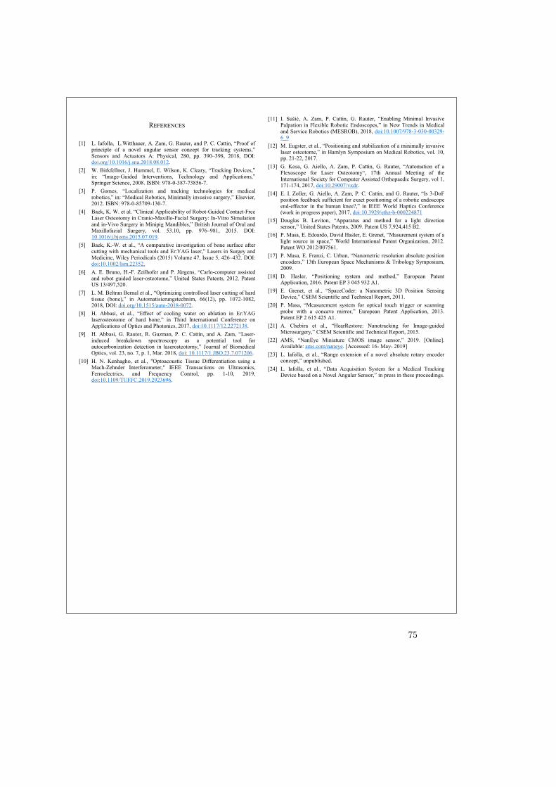
REFERENCES

[1] L. Iafolla, L.Witthauer, A. Zam, G. Rauter, and P. C. Cattin, “Proof of

principle of a novel angular sensor concept for tracking systems,” Sensors and Actuators A: Physical, 280, pp. 390–398, 2018, DOI: doi.org/10.1016/j.sna.2018.08.012.

[2] W. Birkfellner, J. Hummel, E. Wilson, K. Cleary, “Tracking Devices,” in: “Image-Guided Interventions, Technology and Applications,” Springer Science, 2008. ISBN: 978-0-387-73856-7.

[3] P. Gomes, “Localization and tracking technologies for medical robotics,” in: “Medical Robotics, Minimally invasive surgery,” Elsevier, 2012. ISBN: 978-0-85709-130-7.

[4] Baek, K. W. et al. “Clinical Applicability of Robot-Guided Contact-Free Laser Osteotomy in Cranio-Maxillo-Facial Surgery: In-Vitro Simulation and in-Vivo Surgery in Minipig Mandibles,” British Journal of Oral and Maxillofacial Surgery, vol. 53.10, pp. 976–981, 2015. DOI: 10.1016/j.bjoms.2015.07.019.

[5] Baek, K.-W. et al., “A comparative investigation of bone surface after cutting with mechanical tools and Er:YAG laser,” Lasers in Surgey and Medicine, Wiley Periodicals (2015) Volume 47, Issue 5, 426–432. DOI: doi:10.1002/lsm.22352.

[6] A. E. Bruno, H.-F. Zeilhofer and P. Jürgens, “Carlo-computer assisted and robot guided laser-osteotome,” United States Patents, 2012. Patent US 13/497,520.

[7] L. M. Beltran Bernal et al., “Optimizing controlloed laser cutting of hard tissue (bone),” in Automatisierungstechnim, 66(12), pp. 1072-1082, 2018, DOI: doi.org/10.1515/auto-2018-0072.

[8] H. Abbasi, et al., “Effect of cooling water on ablation in Er:YAG laserosteotome of hard bone,” in Third International Conference on Applications of Optics and Photonics, 2017, doi:10.1117/12.2272138.

[9] H. Abbasi, G. Rauter, R. Guzman, P. C. Cattin, and A. Zam, “Laser-induced breakdown spectroscopy as a potential tool for autocarbonization detection in laserosteotomy,” Journal of Biomedical Optics, vol. 23, no. 7, p. 1, Mar. 2018, doi: 10.1117/1.JBO.23.7.071206.

[10] H. N. Kenhagho, et al., "Optoacoustic Tissue Differentiation using a Mach-Zehnder Interferometer," IEEE Transactions on Ultrasonics, Ferroelectrics, and Frequency Control, pp. 1-10, 2019, doi:10.1109/TUFFC.2019.2923696.

[11] I. Sušić, A. Zam, P. Cattin, G. Rauter, “Enabling Minimal Invasive Palpation in Flexible Robotic Endoscopes,” in New Trends in Medical and Service Robotics (MESROB), 2018, doi:10.1007/978-3-030-00329-6_9

[12] M. Eugster, et al., “Positioning and stabilization of a minimally invasive laser osteotome,” in Hamlyn Symposium on Medical Robotics, vol. 10, pp. 21-22, 2017.

[13] G. Kosa, G. Aiello, A. Zam, P. Cattin, G. Rauter, “Automation of a Flexoscope for Laser Osteotomy“, 17th Annual Meeting of the International Society for Computer Assisted Orthopaedic Surgery, vol 1, 171-174, 2017, doi:10.29007/vxdr.

[14] E. I. Zoller, G. Aiello, A. Zam, P. C. Cattin, and G. Rauter, “Is 3-DoF position feedback sufficient for exact positioning of a robotic endoscope end-effector in the human knee?,” in IEEE World Haptics Conference (work in progress paper), 2017, doi:10.3929/ethz-b-000224871

[15] Douglas B. Leviton, “Apparatus and method for a light direction sensor,” United States Patents, 2009. Patent US 7,924,415 B2.

[16] P. Masa, E. Edoardo, David Hasler, E. Grenet, “Masurement system of a light source in space,” World International Patent Organization, 2012. Patent WO 2012/007561.

[17] P. Masa, E. Franzi, C. Urban, “Nanometric resolution absolute position encoders,” 13th European Space Mechanisms & Tribology Symposium, 2009.

[18] D. Hasler, “Positioning system and method,” European Patent Application, 2016. Patent EP 3 045 932 A1.

[19] E. Grenet, et al., “SpaceCoder: a Nanometric 3D Position Sensing Device,” CSEM Scientific and Technical Report, 2011.

[20] P. Masa, “Measurement system for optical touch trigger or scanning probe with a concave mirror,” European Patent Application, 2013. Patent EP 2 615 425 A1.

[21] A. Chebira et al., “HearRestore: Nanotracking for Image-guided Microsurgery,” CSEM Scientific and Technical Report, 2015.

[22] AMS, “NanEye Miniature CMOS image sensor,” 2019. [Online]. Available: ams.com/naneye. [Accessed: 16- May- 2019]

[23] L. Iafolla, et al., “Range extension of a novel absolute rotary encoder concept,” unpublished.

[24] L. Iafolla, et al., “Data Acquisition System for a Medical Tracking Device based on a Novel Angular Sensor,” in press in these proceedings.

75

6 Data Acquisition System for aMedical Tracking Device based on aNovel Angular Sensor

The proceeding article presented in this chapter describes an electronic system able tosimultaneously acquire eight NanEye image sensors and perform the data processingin real-time. This system is based on an FPGA device, a programmable electronicchip that can implement complex embedded systems on a single chip.

Overall, this work introduces the challenges that should be taken in account whendesigning the acquisition system for a tracking system based on ASTRAS.

Publication. This work was presented in Montreal in October 2019 at the confer-ence IEEE sensors, 2019 and the following proceeding was published on the 13th ofJanuary, 2020 in the journal 2019, IEEE sensors. ©2019 IEEE. DOI: 10.1109/SEN-SORS43011.2019.8956777

77

Data Acquisition System for a Medical Tracking Device based on a Novel Angular Sensor How to Acquire and Process Data from the ASTRAS Tracking System

Lorenzo Iafolla, Lilian Witthauer, Sara Freund, Azhar Zam, Georg Rauter, Philippe C. Cattin Department of Biomedical Engineering, University of Basel, Allschwil, Switzerland

[email protected]

Abstract—This research is part of the MIRACLE project (Minimally Invasive Robot-Assisted Computer-guided LaserosteotomE) dedicated to the development of a robotic endoscope to perform minimally invasive laser osteotomies (bone cutting). In this framework, we developed a novel angular sensor called ASTRAS (Angular Sensor for TRAcking Systems) to serve as basic element of a tracking system for articulated devices (e.g. an articulated robotic endoscope). At each joint of the articulated endoscope one ASTRAS sensor is positioned, so that its shape and the pose of its tip can be calculated from the angle measurements. In ASTRAS, the angle is evaluated with high precision by processing the image cast by a shadow mask onto an image sensor. For an articulated endoscope, the acquisition and processing electronics of its tracking system based on ASTRAS has to fulfill the following requirements: 1) acquire and synchronize raw-data from the image sensors; 2) process the images in real-time to compute the angles; 3) provide one channel per endoscope joint; 4) be embedded in a small electronic device (e.g. a single-board computer). In this paper, we propose a solution based on an Field Programmable Gate Array (FPGA) that can acquire raw data from the image sensors, synchronize, and process them. The proposed system has an embedded processor running an operating system (Linux) such that it can easily implement software solutions for both processing and communication. In addition, we also present the results of a preliminary test of the first prototype and show some novel ideas of development.

Keywords—ASTRAS; Medical Tracking Systems; Rotary Encoder; Angular Sensor; NanEye Camera.

I. INTRODUCTION

MIRACLE (Minimally Invasive Robot-Assisted Computer-guided LaserosteotomE) is an ambitious project dedicated to the development of a medical robotic endoscope to perform osteotomies with a laser. In such a robotic system (MIRACLE robot), the shape of the endoscope and the pose of its tip have to be tracked in real-time to control the robot with the required accuracy for a precise cut (~0.2 mm) [1]-[5]. The very demanding requirements (miniaturized, absolute measurement, insensitive to magnetic interferences, no line of sight) of such an accurate tracking system, led us to investigate a new technique based on a novel angular sensor called ASTRAS (Angular Sensor for TRAcking Systems) [6]-[8].

The measurement principle, described in detail in [6] and [8], is based on processing a shadow image (see Fig. 1), cast by a shadow mask, onto an image sensor (e.g. a camera without lens). In particular, the system is arranged in a way that there is a one-to-one correspondence between the angle to be measured and the horizontal position of the shadow on the image sensor. In other words, each recorded image results in one measurement of the angle. In principle, rather than the full image, only few rows of pixels (or even just one row) can be used to perform the measurement, even though, this might worsen the accuracy. Nevertheless, if the image sensor features a rolling shutter, its rows capture the shadow image in sequential moments, which can be exploited to increase the sampling frequency of ASTRAS (up to number of rows × fps of the image sensor): this is for ASTRAS a new acquisition method and we will refer to it as ASTRAS oversampling.

The size of the image sensor has to fulfill the requirement of miniaturization (size of ~1 mm3, [7]). So, it is not surprising that cameras, matching this requirement, often have a quite complicated communication interface. In our first miniaturized prototype [7], we used the NanEye camera by AMS (250×250 pixels, 10 bits per pixel) that has a two wire connection interface. This interface is half-duplex and features an asynchronous LVDS bit serial downstream for data, and an SPI upstream to write the configuration registers [9].

MIRACLE project was funded by the Werner Siemens-Foundation of Zug, Switzerland.

Fig. 1. Example of a shadow image captured by the NanEye camera with a shadow mask featuring slits ~0.1 mm width. Superimposed is the plot of the RGB vectors generated by the NanEye ACQ & pre-processor as described in Section II.C. Changing the angle will result in a horizontal shift of the shadow and of the RGB vectors.

978-1-7281-1634-1/19/$31.00 ©2019 IEEE

6 Data Acquisition System for a Medical Tracking Device based on a Novel Angular Sensor

78

The downloaded bit-stream needs to be pre-processed according to the following steps: synchronize the bits to the system clock; reconstruct the image; separate the rows according to the ASTRAS oversampling technique; separate the RGB channels (required for future developments of ASTRAS that encode the image with colors to increase the measurement range [8]); sum up the columns of each channel to get three vectors (one per RGB channel, see Fig.1); feed these pre-processed data to the algorithm that computes the angle. The key advantage of summing up the image in three vectors is to reduce the amount of data without impacting its information content related to the angle [6]. In the simplest version of ASTRAS, the processing algorithm mainly consisted of: calculating a correlation with some reference vectors; interpolating the correlation with a second degree polynomial to accurately (subpixel resolution) find its maximum; evaluating the angle by computing a polynomial (see [6] and [8] for further details). If the angles are used to close the control-loop of the MIRACLE robot, these computations have to be performed in real-time with minimal lag.

The proposed tracking system calculates the pose and the shape of an articulated device, such as the MIRACLE robot, from the bending angles of its joints measured by several ASTRAS sensors. In this case, the data sourced by the ASTRAS sensors have to be acquired simultaneously, synchronized to each other, and processed in real-time.

The electronic acquisition and processing system (DAQ) of such a medical tracking system is meant to be placed somewhere in the operating room, next to the endoscope, where the space is typically very limited. In addition, communication delays between several devices are unwanted when the output is used as a feedback of a control system. For these reasons, a compact and embedded DAQ is preferable.

Summarizing, the DAQ of the tracking system for endoscopes based on ASTRAS needs to fulfill four key requirements: 1) be able to acquire and synchronize raw data from the image sensors; 2) have the computational resources to process data in real-time; 3) provide one channel for each ASTRAS in the system; 4) be implemented on an embedded/compact device.

In this work, we describe a concept of an acquisition and processing system that fulfills the above requirements. These led us to develop custom electronics based on a prototyping board featuring a Xilinx Zynq XC7Z020 FPGA [10]. We also deployed the interface electronics for the NanEye cameras (Adapter Board) provided by the manufacturer. The main idea is to split the tasks between the programmable logic and the processor embedded in the FPGA. Whereas the first is more suitable and faster to acquire and pre-process data, the latter is easier to program in order to perform the more complex processing algorithms. Some preliminary results are also presented in this contribution.

II. DESCRIPTION OF THE DATA ACQUISITION SYSTEM

A. Electronic DAQ Board The electronic board (Fig. 2) is based on the MicroZed

prototyping board from Avnet featuring a Xilinx Zynq XC7Z020 FPGA and a DDR3 RAM (1 GByte). This FPGA has an embedded dual-core ARM Cortex-A9 MPCore processing system (PS) alongside with the programmable logic (PL). The MicroZed board was mounted on an FMC Carrier board [11] that allowed us to access the connection pins of the FPGA easily. In particular, we deployed the FMC (FPGA Mezzanine Card) connector to interface the FPGA with the Adapter Board [12]. This interface was realized by implementing a connector to connector board (C2C in Fig. 2) on which two Adapter Boards can be connected. As each adapter board can interface four cameras, such a system interfaces the FPGA with up to 8 NanEye cameras.

B. General Scheme of the Acquisition and Processing System Fig. 3 shows the general scheme of the acquisition and

processing system. The PS can be considered as a mini-computer programmed to run an operating system (OS) such as Linux and some of its peripherals are implemented on the PL. In our system, the peripherals on the PL, accessed through the AXI BUS, were: the NanEye ACQ & preprocessor (see next paragraph) and the NanEye Power Control. The NanEye Power Control controls an external DAC, whose output was the power supply of the cameras. As the data rate of the NanEye depends on the supplied voltage, this peripheral is very important for the synchronization of the connected cameras. In the future, a further peripheral, Processing PL, will be implemented to take

Fig. 3. General scheme of the acquisition and processing system implemented on the FPGA. The Processing PL block was not implemented at the moment of the publication.

FPGA

MicroZed Board

FMC Carrier Board

C2C Board

NanEye connectors

NanEye connectors

Adapter Boards

DDR RAM

Fig. 2. ASTRAS electronic DAQ board based on: Avnet MicroZed board, Avnet FMC Carrier Card, and Awaiba (AMS) Adapter Board.

79

over part of the computation from the PS making the execution of the processing algorithm faster. Indeed, this peripheral can exploit the 220 DSP slices embedded in the PL (each of these can perform simple mathematical operations like products, divisions, etc.) and, so, perform several operations in parallel. For example, it can calculate a correlation much faster than the PS. Custom drivers for the OS have been developed to access data, control the peripherals, and manage their interrupts.

The potential development of this data acquisition system are vast. Thanks to the OS, it would be relatively easy to develop processing and communication systems using the peripherals; e.g. the processing PL or an external GPU for data processing and Ethernet, USB, I2C, SPI, or other I/O for communication. Also, within the OS, many programming languages can be employed: C, Python, bash scripting, etc., or a combination of them. Taking benefit of the multitasking capabilities of the OS, it is also possible to program a watchdog to guarantee that the acquisition and processing software are working correctly.

C. NanEye Acquisition and Pre-Processor Fig. 4 shows a simplified scheme of the NanEye acquisition

and pre-processor peripheral. The components represented inside the dashed-box are replicated for each camera (maximum 8 for our electronic DAQ board). Component A is based on a firmware provided by AMS. This expoits a typical technique to synchronize a bit-stream which is based on oversampling: this means that the signal is sampled multiple times in one clock period so that, eventually, it can be reconstructed [13]. This component outputs the reconstructed value of the pixels, the numbers of the current pixel, row, and frame and, also, asserts the validity of the former values.

Component B will use the values of the counters to divide the image in horizontal stripes, whose height is defined by the parameter # of rows to accumulate, while the RGB channels are separated by the Bayer pattern matrix. According to the

ASTRAS oversampling technique, the # of rows to accumulate is inversely proportional to the sampling frequency. The values of the pixels in the same column are accumulated and memorized in specific buffers together with their time-stamps. As the cameras are not synchronized to each other these buffers might be ready at random times. This has to be managed by component C deploying the time-stamps. Finally, the data can be output through a Dual-port RAM to the AXI BUS or, in a future version, directly to the DDR RAM of the PS via DMA (Direct Memory Access).

III. TEST RESULTS

The implemented system was tested with one NanEye camera accumulating the 250 rows of the image with the maximum frame rate of the camera (~50 fps). The three RGB vectors (250 elements × 16 bits, see Fig. 1) generated by the NanEye ACQ & pre-processor were successfully read by the PS using a custom Linux driver through a software interface.

CONCLUSIONS

In this work, we tackled the challenges related to the acquisition and processing of data from a novel medical tracking system consisting of several ASTRAS. The solution we presented is based on an embedded electronic device featuring an FPGA with an integrated processing system running Linux. The system has vast potential for further developments, and a preliminary prototype was successfully tested. However, the full processing of data will require further works (e.g. a specific software for the PS and the Processing PL) and further characterization tests have to be done. Before this activity can be accomplished, the data processing algorithm has to be optimized according to the speed requirements and the new developments of ASTRAS.

Fig. 4. Simplified scheme of the NanEye acquisition and pre-processor peripheral (see Fig. 3). The components in the dashed box are replicated per each connected camera while the DMA to DDR RAM connection has not been implemented yet.

6 Data Acquisition System for a Medical Tracking Device based on a Novel Angular Sensor

80

REFERENCES [1] Baek, K. W. et al. “Clinical Applicability of Robot-Guided Contact-Free

Laser Osteotomy in Cranio-Maxillo-Facial Surgery: In-Vitro Simulation and in-Vivo Surgery in Minipig Mandibles,” British Journal of Oral and Maxillofacial Surgery, vol. 53.10, pp. 976–981, 2015. DOI: 10.1016/j.bjoms.2015.07.019.

[2] Baek, K.-W. et al., “A comparative investigation of bone surface after cutting with mechanical tools and Er:YAG laser,” Lasers in Surgery and Medicine, Wiley Periodicals (2015) Volume 47, Issue 5, 426–432. https://doi.org/10.1002/lsm.22352.

[3] A. E. Bruno, H.-F. Zeilhofer and P. Jürgens, “Carlo-computer assisted and robot guided laser-osteotome,” United States Patents, 2012. Patent US 13/497,520.

[4] L. M. Beltran Bernal et al., “Optimizing controlled laser cutting of hard tissue (bone),” at - Automatisierungstechnik, 66(12), pp. 1072-1082, 2018, DOI: doi.org/10.1515/auto-2018-0072.

[5] L. M. Beltran Bernal et al., “Effect of laser pulse duration on ablation efficiency of hard bone in microseconds regime,” in Third International Conference on Applications of Optics and Photonics, 2017, doi: 10.1117/12.2272253

[6] L. Iafolla, L.Witthauer, A. Zam, G. Rauter, and P. C. Cattin, “Proof of principle of a novel angular sensor concept for tracking systems,” Sensors and Actuators A: Physical, 280, pp. 390–398, 2018, DOI: doi.org/10.1016/j.sna.2018.08.012.

[7] L. Iafolla, et al., “Preliminary tests of the miniaturization of a novel concept of angular sensors,” in press in these proceedings.

[8] L. Iafolla, et al., “Range extension of a novel absolute rotary encoder concept,” unpublished.

[9] AMS, “NanEye Miniature CMOS image sensor,” 2019. [Online]. Available: ams.com/naneye. [Accessed: 16- May- 2019]

[10] Avnet, “MicroZed,” 2019. [Online]. Available: zedboard.org/product/microzed. [Accessed: 16- May- 2019]

[11] Avnet, “MicroZed FMC Carrier,” 2019. [Online]. Available: zedboard.org/product/microzed-fmc-carrier. [Accessed: 16- May- 2019]

[12] AMS, “NanoUSB2 Eval Kit,” 2019. [Online]. Available: ams.com/nanousb2-eval-kit. [Accessed: 16- May- 2019]

[13] N. Sawyer, “Data to clock phase alignment, XApp225,” Xilinx Application Note, Xilinx, February 2009.

81

7 Proof of Concept of a NovelAbsolute Rotary Encoder

The paper presented in this chapter describes ASTRAS360, which is a major exten-sion of ASTRAS. In particular, ASTRAS360 can measure over the full rotation angle,whereas ASTRAS is limited to about 60 degrees. To extend the range, ASTRAS360features several colored mirrors casting a colored shadow onto the image sensor. Be-sides developing its measurement principle, method, and model, the first prototype ofASTRAS360 was implemented and tested. Experimental tests were performed overthe full range of 360 degrees demonstrating the validity of this new concept. As for theprototype of ASTRAS described in Chapter 4, the precision of the presented measuringsystem was 0.6 arcsec.

Publication. The following paper was published on the 30th of May, 2020 in thejournal Sensors and Actuators A: Physical, Elsevier. DOI: 10.1016/j.sna.2020.112100

83

Sensors and Actuators A 312 (2020) 112100


Sensors and Actuators A: Physical

j ourna l h o mepage: www.elsev ier .com/ locate /sna

Proof of concept of a novel absolute rotary encoder�

Lorenzo Iafolla a,∗, Massimiliano Filipozzi a, Sara Freund a, Azhar Zam b, Georg Rauter c,Philippe Claude Cattin a

a Center for medical Image Analysis & Navigation (CIAN), Department of Biomedical Engineering, University of Basel, Gewerbestrasse 14, 4123, Allschwil,Switzerlandb Biomedical Laser and Optics Group (BLOG), Department of Biomedical Engineering, University of Basel, Gewerbestrasse 14, 4123, Allschwil, Switzerlandc Bio-Inspired RObots for MEDicine-Lab (BIROMED), Department of Biomedical Engineering, University of Basel, Gewerbestrasse 14, 4123, Allschwil,Switzerland

a r t i c l e i n f o

Article history:Received 12 December 2019Received in revised form 12 April 2020Accepted 22 May 2020Available online 30 May 2020

Keywords:ASTRASAngular sensorAbsolute rotary encoderMiniaturized rotary encoderMedical tracking device

a b s t r a c t

Rotary encoders are used in many applications that require monitoring or controlling mechanical systemssuch as robots. Typically, small rotary encoders have poor resolution; this is unfortunate for applicationssuch as robotics in medical surgery procedures. For example, in an articulated robotic endoscope, minia-turization is mandatory and, when automation is desired, high accuracy to track the shape and pose ofthe device is required; small (few millimeters) and accurate (few hundred arcsec) rotary encoders arethus needed.

Previously, we introduced a novel concept of a miniaturizable angular sensor, called ASTRAS (AngularSensor for TRAcking System). This was presented as a basic element of a tracking system for articu-lated endoscopes. The principle of measurement of ASTRAS is based on processing a shadow image castby a shadow mask onto an image sensor. The characterization of the first prototype of ASTRAS wasvery promising, however, its angular range of about ±30 degrees was too limiting for many practicalapplications.

In this work, we present an extension of the concept mentioned above to a rotary encoder that canmeasure one full rotation of 360 degrees thus the name is ASTRAS360. Its working principle bases onencoding the shadow image using colored light to distinguish different angular sectors. The identificationof the sector corresponds to a coarse angular measurement, which is afterward refined using the sametechnique as in ASTRAS. We implemented this concept, realizing a prototype and an algorithm to calculatethe angle from the shadow image. The experiments demonstrated the validity of this concept and showedencouraging results with a precision of ∼0.6 arcsec and 6�-resolution of 3.6 arcsec corresponding to19 bits.

© 2020 The Authors. Published by Elsevier B.V. This is an open access article under the CC BY-NC-NDlicense (http://creativecommons.org/licenses/by-nc-nd/4.0/).

1. Introduction

Rotary encoders are used widely in mechanical systems thatrequire monitoring and/or controlling of a moving part. In somefields, such as in medical robotics [1,2], the requirements onsize, accuracy, and reliability (i.e. absolute measurement) are verydemanding, and off-the-shelf rotary encoders are not always ableto address them. For this reason, our objective is to develop an abso-

� This work was part of the MIRACLE project funded by the Werner Siemens-Foundation (Zug, Switzerland).

∗ Corresponding author at: Department of Biomedical Engineering, University ofBasel, Gewerbestrasse 14, 4123, Allschwil, Switzerland.

E-mail addresses: [email protected], [email protected](L. Iafolla).

lute rotary encoder able to outperform the existing ones in terms ofresolution and size. Therefore, this work aims to extend the mea-surement range of a novel concept of a miniaturizable, absolute,high accuracy, angular sensor called ASTRAS (Angular Sensor forTRAcking Systems).

The concept of ASTRAS is described in [3] and it belongs to agroup of sensors called "shadow sensors". They measure the posi-tion of a light source, or the direction of the impinging light, bydetecting a shadow image [4–10]. As described in [3], ASTRASmeasures the angle between a stator and a rotor. Its compo-nents are arranged in such a way that each value of the inputangle ˇ, corresponds to a specific shadow image. The validityof the ASTRAS concept was demonstrated, and its performancescharacterized, resulting in a sensor with absolute encoding, pre-cision of ∼0.6 arcsec, 6�-resolution of ∼3.6 arcsec, linearity error

https://doi.org/10.1016/j.sna.2020.1121000924-4247/© 2020 The Authors. Published by Elsevier B.V. This is an open access article under the CC BY-NC-ND license (http://creativecommons.org/licenses/by-nc-nd/4.0/).

7 Proof of Concept of a Novel Absolute Rotary Encoder

84

2 L. Iafolla, M. Filipozzi, S. Freund et al. / Sensors and Actuators A 312 (2020) 112100

of ∼21 arcsec (rms) over a range of 17 degrees, thermal stability of∼4 arcsec/◦C, and long term drift of ∼2 arcsec/day. The miniaturiza-tion potential of ASTRAS was discussed in [11], and the possibilityof acquiring and processing the data in real-time was investigatedin [12]. Even though these results were promising, the angularrange of ASTRAS was rather small, ±30 degrees thus limiting itsapplicability. Therefore, this work focuses on the method and thecharacterization of a concept, called ASTRAS360, to measure abso-lute angles over one full rotation.

As ASTRAS360 represents a new concept of a rotary encoder(RE), it also has to be compared to other RE concepts. Among themost used RE, there are potentiometers, magnetic encoders, syn-chros, resolvers, optical encoders and inductosyns [13–18]. Here,we focus only on magnetic encoders, optical encoders and induc-tosyns as they belong to the same class of accuracy (better than1 arcmin) that we are targeting for ASTRAS360.

Magnetic encoders detect the rotation of a magnet attached tothe rotor. Often the sensing part, attached to the stator, is a HallEffect device in chip form whose output voltage depends linearlyfrom the rotation angle of the rotor. Though these sensors are quitetolerant to foreign matter, they are typically not chosen for appli-cations in harsh environments or shock conditions [17]. The mainadvantages of the magnetic sensors are absolute encoding, goodrobustness, and their tolerance to liquids. However, they have amodest performance because it is limited by interferences withmagnetic material or with electrical cables in proximity, hysteresiseffects, and temperature variations. An example of a small, off-the-shelf, absolute, magnetic, rotary encoder is the AS5047U by AMS[19]. It has a chip size 5 × 6.4 mm2 (no data related to the rotor arereported) and features a linearity-error down to ∼2900 arcsec andresolution down to 79 arcsec (14 bits).

The optical encoders have an optical sensor head, which actsas the stator, and a grated optical disk or ring which is the rotor.The light, emitted by a source, passes through or is reflected bythe grating and is then detected by the sensing head. The signalgenerated is a sine or square wave whose phase is related to therotation of the disk. Their main advantages are the high resolutionand accuracy (down to 0.01 arcsec) [20–24], and it is a well-knownand developed technology. Typically, these are relative encoders,but absolute encoding is possible at the cost of increased hard-ware complexity by using several gratings with different pitchesor more sophisticated solutions such as a single-track periodicGray code [25]. However, they suffer from multiple limitationsrelated to the alignment (and the displacement) of their sensinghead with the grating, and of the rotation axis with the axis of thedisk (eccentricity) [26]. Several examples of off-the-shelf opticalrotary encoders are available on the market. The MAS10 by CUI Inc.[27], for instance, is a small absolute encoder featuring a diame-ter of 13 mm and a height of 15.5 mm but quite poor resolution(∼5062 arcsec corresponding to 8 bits). Another prototype of thesame class of encoders with a size of 10 × 10 × 10 mm3 and a reso-lution of ∼1266 arcsec (10 bits) has been described in [28]. Finally,the PA2-50 by Faulhaber [29], has been reported to be as small as6 mm in diameter but this comes at the cost of being a relativeencoder and featuring a reduced resolution of 7 degrees).

Inductosyn [30] (and its equivalent Incoder [31]) is a tech-nology that provides very high performance. The measurementof the angular position of the rotor bases on the electrical cou-pling between windings produced by printed-circuit techniques.One winding is printed on the stator and it is excited with alter-nating current; this induces an output current in the windingsprinted on the rotor. The main advantages of the inductosyn areits high accuracy, the possibility for absolute encoding, reliability,and robustness. However, encoders of this type are typically quiteexpensive, and for very high accuracy measurements (down to1 arcsec), they require a fine alignment to reduce eccentricity. The

smallest off-the-shelf absolute Incoders have a diameter of roughly40 mm and a height of 11.2 mm with a resolution of 9.89 arcsec(17 bits) and a systematic error of ∼350 arcsec.

The proposed ASTRAS360 sensor has its pros and cons, but acomparison between the various technologies can only be donein the framework of a specific application. As discussed in [3], anessential property of ASTRAS360 is the possibility of extending thesame concepts and methods to two degrees of freedom (DOF) usingone single sensor, i.e., to measure rotations about two orthogonalaxes simultaneously. This is important, for example, for sensing theshape of a continuum robot that is composed of a sequence of rigidlinks [32,33]. In this case, one ASTRAS360 sensor can measure thetwo tilt angles between two contiguous links.

Furthermore, ASTRAS360 seems to be very promising in termsof resolution. This usually depends on the size of the rotary encoderand is thus an application-specific tradeoff. For applications such asminimally invasive surgical robotics, we believe that the proposedconcept has the potential to outperform the other technologies.Indeed, even using a miniaturized image sensor, such as the Nan-Eye by AMS [34], volume 1 × 1×0.5 mm3 and pixel size 3 × 3 �m2,we could build a prototype of ASTRAS with a systematic errorof 32 arcsec RMS and precision (standard deviation of repeatedmeasurement) down to 5 arcsec [11]. This precision coincides toa 6�-resolution (that is defined as six times the precision [35],)equal to 6 × 5 = 30 arcsec and corresponding to ∼16 bits. Althoughthis was not yet an utterly miniaturized version of ASTRAS (othercomponents, such as the rotary mount, were still big), we expectto achieve the same performance with a miniature version. Onlythe Incoder performs better in terms of resolution. Still, we believethat using the NanEye image sensor and a small ball bearing (diam-eters down to 1.6 mm are available in [36]), ASTRAS360 can bescaled down to a final diameter of 10 mm or even smaller. On theother side, using a slightly larger (5.7 × 4.28 mm2) image sensor butwith smaller pixel size (2.2 × 2.2 �m2), such as the Ximea MU9PCused in [3], we could achieve a 6�-resolution down to 3.6 arcsec.We believe that, in terms of resolution, the intrinsic advantage ofASTRAS360 relies on the small size of the pixels of the image sen-sor that enables measuring tiny differences between the shadowimages.

However, before tackling the challenge of miniaturization orthat of measuring over two DOFs, a good understanding of the con-cept and of the required image processing steps for ASTRAS360 iskey. Focusing on this goal, we implemented the first prototype ofASTRAS360 and evaluated experimentally its working principle.

The working principle and a simplified model of ASTRAS360are discussed in Section 2. As it is a crucial part for the properfunctioning of the sensor. Section 3 described to the requiredimage processing algorithms. To characterize the properties ofASTRAS360, we developed a prototype described in Section 4.Finally, the results of the experiments are discussed in Section 5,providing a validation of the working principle and an estimationof the performance.

2. Working principle and simplified model

Fig. 1 shows a conceptual cross-sectional drawing ofASTRAS360. The mechanical constraint, represented by thered arrows, limits the degrees of freedom in a way that only therotation defined by the angle is possible. The stator, whichis the static part of the system, includes the image sensor, theshadow mask, and the LED. The rotor, which is the moving partof the system, has several (e.g. 8) mirrors with colored surfaces.As shown in Fig. 1, the light emitted by the LED is reflected byone of the mirrors attached to the rotor (mirror H for that specificvalue of ˇ). The reflected light, or in an equivalent formulation, the

85

L. Iafolla, M. Filipozzi, S. Freund et al. / Sensors and Actuators A 312 (2020) 112100 3

Fig. 1. ASTRAS360 conceptual drawing. (For interpretation of the references to colorin the text, the reader is referred to the web version of this article).

light emitted by the virtual image of the LED, then casts a shadowonto the image sensor due to the shadow mask. The position, theshape, and the color of the shadow depends on (see Video 1 and2), that can be therefore evaluated. To define the variables of thesystem and illustrate the geometric relations, we use Fig. 2, whichshows a more detailed view of Fig. 1, with only two mirrors shown.However, it is easy to generalize the definitions for more mirrors.

For each mirror, we can define one interval of ˇ, i.e. � A and � B inFig. 2, and a reference value, i.e. ˇAA and ˇBB. The intervals � A and� B are defined as all the values of in which the correspondingmirror contributes to the shadow image i.e., light is reflected bythis mirror and reaches the image sensor. In this simplified model,ˇAA and ˇBB are defined in a way that the corresponding mirrors Aand B are parallel to the image sensor (for example, when ˇ=ˇAA,the mirror A is parallel to the image sensor). We also define thereference shadow images (or just reference images) RAA and RBBobtained when ˇ=ˇAA and ˇ=ˇBB. Finally, the “shadow A ” is thecontribution of the mirror A to the shadow image and similarly forthe “shadow B” (see the reference shadow images RAA and RBB inFig. 3, which are consistent with Fig. 2).

Considering only one mirror at a time, it is easy to see that, when ∈ � A, an input shadow image can be obtained by shifting the

reference image RAA. According to [3], the following input-outputrelation for mirror A ( ∈ � A) can be used for all mirrors:

shiftA = d · tan(

− ˇAA)

≈ d ·(

− ˇAA)

(1)

Where shiftA is the translation distance of the shadow A withrespect to its reference position in RAA; d is the distance between theshadow mask and the image sensor and it determines, by definition,the sensitivity. As is evident from Eq. (1), ASTRAS360 is a non-linearsensor, but, for small values of ˇ-ˇAA|, a linear approximation ispossible. According to Eq. (1), we can calculate as follow:

= arctan(shiftAd

)+ ˇAA ≈ shiftA

d+ ˇAA (2)

Using a single mirror, the range of measurement [ˇ−;ˇ+] is the-oretically limited between [−90;+90] degrees, as outside of thisrange, the light would no longer be cast onto the image sensor;in a practical case like the one described in [3], the range waseven smaller ([−30;+30] degrees). As demonstrated in [3], the range[ˇ−;ˇ+] for ASTRAS360 is given by:

ˇ±AA = arctan

(±LAAd

)+ ˇAA ≈ ± LAA

d+ ˇAA (3)

Fig. 2. Simplified version of ASTRAS360 featuring only two mirrors. In this state of ASTRAS360, the image sensor would capture a shadow image like RAB in Fig. 3. (Forinterpretation of the references to color in the text, the reader is referred to the web version of this article).


86


Fig. 3. Reference shadow images RAA, RAB, and RBB of sectors �AA, �AB, and �BB (the order of the images is consistent with Fig. 2). Shadow B was generated by mirror Bwhose color filter was pale green. This appeared in both the shadow images RBB and RAB. Similarly, shadow A was generated by mirror A whose color filter was neon blue.It appeared in shadow image RAA and RAB. A drift of the hue in the two-shadow image RAB is visible. In fact, the hue of shadow B drifts from pale green in RBB towards thebrown in RAB. (For interpretation of the references to color in this figure legend, the reader is referred to the web version of this article).

where ±LAA is the range of shiftA that still allows measuring withshadow A. Eventually, the usable range

[ˇ−AA; ˇ+

AA

]also depends

on the image processing algorithm and we can only asses that[ˇ−AA; ˇ+

AA]⊆ � A. Yet, if the system is designed such that the rangeof measurement of each mirror always overlaps with that of thecontiguous mirrors, then the measurement is always possible. Con-sequently, as the name suggests, the range of measurement ofASTRAS360 is 360 degrees.

However, before measuring ˇ, the interval � has to be identi-fied to assign a reference value to in Eq. (2) (e.g. the reference isˇAA when the interval is � A). This can be done because the angularintervals are encoded by the different colors of the mirror filters. Inparticular, each mirror has a specific signature corresponding to aparticular hue of the light (i.e., a particular distribution of values ofthe hue). In other words, identifying � A by measuring the hue, pro-vides ˇAA, which already yields a coarse estimation of ˇ; then, thisestimation is refined by measuring the shiftA using Eq. (2). This newmethod to measure a rotational angle presents several challengesdescribed in the following.

First of all, some transition values of are in the angular intervals� of more contiguous mirrors. For example, in Fig. 2 the interval˝AB identifies the overlap between � A and � B where both mirrors,A and B, contribute to the shadow. These transition angles gener-ate shadow images consisting of the overlap of the light from bothmirrors. For example, the shadow image RAB in Fig. 3 is the overlapof the shadow A generated by the mirror A and the shadow B frommirror B. We will refer to these images as “two-shadow images”to differentiate them from the “single-shadow images” (e.g. RAAand RBB in Fig. 3) that are recorded when only one mirror con-tributes to the appearance of a shadow image. Correspondingly,we define the related intervals of as “two-shadow sectors” and“single-shadow sectors”.

As a consequence of the full 360 ◦ range of ASTRAS360, the two-shadow sectors are unavoidable (this is also visible from Video 1).In principle, also three shadows images are possible but can beavoided using some technical solutions, as explained in Section4. Consequently, we can split the full range of measurement insingle-shadow sectors and two-shadow sectors for a total num-ber of 16 sectors (two per mirror). We associate each sector toa double index identifying the mirror (or mirrors); for exam-ple in Fig. 2, the single-shadow sector associated to the mirrorA is ˝AA whereas the two-shadow sector associated to mirrorsA and B is ˝AB. Correspondingly, we also define the referenceimages RAA (which are identical to those introduced before), RAB,etc. and the reference angles ˇAA (also identical to those intro-duced before), ˇAB, etc. For the two-shadows sector ˝AB, we setˇAB =(ˇAA +ˇBB)/2. We highlight here that the angular intervalsintroduced before (� A, � B, etc.) always overlap with their neigh-

bors, whereas the sectors (˝AA, ˝AB, ˝BB, etc.) never overlap (seeFig. 2).

It should be noticed that within a two-shadow sector, eachshadow shifts according to Eq. (1), where the reference value ˇAAdepends on the mirror generating that specific shadow. For exam-ple, we analyze the two-shadow sector ˝AB between the mirrorsA and B, associated to the reference value ˇAB. The correspondingshifts of each shadow are:

shiftA = d · tan(

− ˇAA)

(4)

shiftB = d · tan(

− ˇBB)

(5)

where shiftA and shiftB are referred to the reference images RAA andRBB, these equations imply that shadows A and B shift differently,and two-shadow images cannot be obtained by merely shiftingRAB. So, in principle, the method explained for the single-shadowsectors, does not work for the two-shadow sectors.

However, using the Taylor expansion of Eqs. (4) and (5) aroundthe reference angle ˇAB of ˝AB, it can be demonstrated that, in afirst approximation, the previous method also applies to the two-shadow sectors. Eqs. (4) and (5) can thus be expanded as follow:

shiftA = d ·(tan

(ˇAB − ˇAA

)+

( − ˇAB

)

cos2(ˇAB − ˇAA

)

+tan

(ˇAB − ˇAA

)·(

− ˇAB)2

cos2(ˇAB − ˇAA

) + · · ·)

(6)

shiftB = d ·(tan

(ˇAB − ˇBB

)+

( − ˇAB

)

cos2(ˇAB − ˇBB

)

+tan

(ˇAB − ˇBB

)·(

− ˇAB)2

cos2(ˇAB − ˇBB

) + · · ·)

(7)

The first terms on the right side of Eqs. (6) and (7) define thepositions of the shadows A and B when ˇ=ˇAB. This can be betterunderstood by comparison with Eq. (1). In other words, they definethe shape of the reference image RAB. The second and the followingterms are the most important ones as they quantify the shifts ofshadows A and B from their positions in RAB. However, from thedefinition of ˇAB, we can write:(ˇAB − ˇAA

)= −

(ˇAB − ˇBB

)(8)

Using this relationship, it is easy to demonstrate that the secondterm on the right of Eqs. (6) and (7) are equal. Therefore, if |ˇ-ˇAB|

87


is small, the following input-output relation can be used for thetwo-shadow sectors:

shiftAB ≈ d

cos2(ˇAB − ˇAA

) ·(

− ˇAB)

(9)

This equation applies to the full shadow image, whereas Eqs. (4)and (5) are specific for the shadows A and B. We also notice thesimilarity with the linear approximation of Eq. (1). However, thesensitivity is slightly bigger in this case. Indeed, the angle ˇAB-ˇAAdepends only on the number of mirrors; with eight mirrors, |ˇAB-ˇAA| = 22.5 degrees and the ratio between the sensitivities is:

SensitivityABSensitivityAA

= d

cos2(ˇAB − ˇAA

) · 1d

= 1cos2 (22.5degrees)

= 1.17.(10)

This means that the sensitivity changes slightly from one sector tothe other, which is not ideal. Indeed, a ratio closer to one wouldbe preferable. This can be achieved using a larger number of mir-rors as |ˇAB-ˇAA| would be smaller; for example, using 10 mirrorswould lead to a ratio of 1.10. But, on the other hand, this wouldalso increase the complexity of the system and might not alwaysbe viable.

Overall, we have demonstrated that the input-output relation ofASTRAS360 is approximately linear only within the specific sectorsand when |ˇ-ˇAA|(or|ˇ-ˇAB|) is small. When the latter is large, andwe consider the transition between sectors, the linearity error isnot negligible. To reduce it, we propose three methods that canbe used at the same time: calibrate each sector separately, usepolynomial best-fitting curves to approximate the experimentalcalibration measurements, and increase the number of mirrors. Thefirst two methods can always be applied and will, therefore, be dis-cussed in the following sections. Increasing the number of mirrorshas important technical implications. For example, it might becomechallenging to find enough color filters that will still allow differ-entiating the sectors (see Section 3); furthermore, the mechanicaldesign becomes very complex. For these reasons, we did not con-sider more than eight mirrors for our characterization prototype.

3. Image processing

3.1. Sector identification and measurement refinement

The image processing algorithm presented herein focuses onthe main steps required to compute the critical information fromthe shadow images, namely the variables ˇAA and shiftAA of Eq. (2).These are obtained by first identifying the sector (coarse measure-ment) followed by fine measuring the shift using the correlationbetween the input image and the reference image, as described in[3].

The main steps of the coarse measurement are depicted in Fig. 4.The image and the plots on the left-hand side of the image referto single-shadow images and those on the right-hand side cor-respond to two-shadow images. The processing of both types ofshadow images, which differ only slightly from one another, will bedescribed in the following. The shadow images shown in Fig. 4 arerepresentatives of all the images that the proposed sensor encoun-ters. The only expected variables are the horizontal shift of theshadow(s), and the change of the hue (see Video 1). Furthermore,the mechanical specifications of the system were defined such thatthe shadows are not shifting out of the field-or-view of the imagesensor.

Assuming that Rjk, Gjk, and, Bjk are the Red, Green, and Blue val-ues of each pixel and the indexes j ∈ [1;J] and k ∈ [1;K] identify therow and the column of the image, we first calculate intensity vector

Ik (or simply I) as follow:

Ik = 100 ×∑J

j=1

(Rjk + Gjk + Bjk

)

maxk′(∑J

j=1

(Rjk′ + Gjk′ + Bjk′

))

= 100 ×∑J

j=1

(Greyjk

)

maxk′(∑J

j=1

(Greyjk′

)) (11)

in which Greyjk is the grey level of the pixel j, k. In Fig. 4, theseare shown in the two plots underneath the corresponding shadowimages (continuous black line). Then, we count the number na ofelements of I whose values are bigger than a threshold tr; these ele-ments are depicted with blue dots in Fig. 4. The number na changesconsistently from single to two-shadow images; this is visible com-paring the number of blue dots in the two intensity plots in Fig. 4.Therefore, when na is smaller than a predefined threshold Tv, theshadow image is identified as a single-shadow image, otherwise, itis recognized as a two-shadow image.

In case of a single-shadow image, the index of the mirror con-tributing to the shadow is identified by analyzing the hue, i.e. color,histogram of the image pixels. The value of the hue is obtained byconverting the color representation from RGB (as recorded by theimage sensor) to HSV (Hue, Saturation, Value), where we use onlythe Hue. It should be noticed that pixels with a low grey level (thosethat are dark in the shadow image) might have a random value ofhue because of the electronic noise of the image sensor. For this rea-son, we plot the histogram of the Hue weighted by the grey levelof the pixels as expressed by the following equation:

Gcounts (H) =∑

{j,k|Hjk=H

}Greyjk (12)

where Hjk is the Hue of the pixels j,k. In this way, pixels with higherintensity will count more and the others will produce a negligibleeffect on the histogram. An example histogram for a single-shadowimage is shown in Fig. 4 (bottom-left side) and, as expected, featuresa single sharp peak. The coordinate of this peak is called hchar, andit is very informative. As we will see in Section 3.2, the color filtersare chosen such that hchar uniquely identifies the single-shadowsector providing a coarse measurement (ˇAA).

For the two-shadow images, the hue-histogram might be morecomplicated, showing multiple not well-defined peaks. For thisreason, we use only the portions of the two-shadow image as iden-tified by the red (L) and blue (R) rectangles in Fig. 4 (top-rightside). These are easy to localize automatically as they correspondto the first and the last elements of I above the threshold tr . In thisway, the expected histograms of the hue of two-shadow imagesto show two peaks at position hL

char and hRchar as shown in Fig. 4

(bottom-right side). As before, the specific combination of their twocoordinates uniquely identifies the two-shadow sectors providingthe coarse measurement. We could use the same method also forsingle-shadow images, but the determination of hchar would beless accurate, leading to unwanted difficulties. Some single-shadowimages show a different hue on the left and the right sides; forthis reason, we decided to use two different methods, as explainedabove.

The shift is measured in the same way for single-shadow sectorsand two-shadow sectors. This is done by calculating the correlationbetween the input shadow image and the reference shadow imageof the identified sector. The shift is defined by the position of thehighest peak of the correlation result.

Finally, as discussed in Section 2, ASTRAS360 shows a non-linearbehavior, and a polynomial relationship could be used for describ-ing the input-output relationship for each sector. Therefore, once


88


Fig. 4. Image processing for the single-shadow image (left side) and two-shadow image (right side). The two plots in the middle represent the intensity vectors I (continuousblack lines). The number of elements above the threshold tr (indicated with blue dots) is na and it is used to distinguish the single-shadow images from the two-shadowones. The last two graphs are the weighted histograms of the hue; the position of the peaks identifies the sector. (For interpretation of the references to color in this figurelegend, the reader is referred to the web version of this article).

the sector is identified (we refer to it as Sector XX), instead of Eq.(2) where we use:

=∑N

i=0Pi,XX · shifti + ˇXX (13)

with ˇXX (similarly to ˇAA) as the reference angle of Sector XX, Pi,XXare the coefficients of the polynomial that best fits the calibrationdata of that sector, and shift is measured in number of pixels.

3.2. Calibration phase

The calibration phase consists of collecting a set of calibrationimages and simultaneously measuring the corresponding angles ˇusing a calibration standard (e.g., the scale of a rotary mount, seeSection 4).

The first step consists of identifying the best value for tr (seeParagraph 3.1 and the plots of the Intensity in Fig. 4). To do so, weuse Otsu’s method [38] over the histogram of the values of vectorsI of all the calibration images together (Fig. 5). In our experiment trwas 48.5.

To define the threshold Tv (see Paragraph 3.1), a histogram of thevalues of na can be computed. The histogram we obtained in ourexperiment is shown in Fig. 6; in this example we can distinguish

Fig. 5. Histogram of the values of all the intensity values of all the calibration images.The threshold tr = 48.5 was calculated with the Otsu’s method.

two main clusters, one around 1750 for the two-shadow images,and one around 910 for the single-shadow images. Tv can be setusing Otsu’s method; e.g., in our experiment, it was 1184.

Once tr and Tv are defined, we can label each calibration imageas either a single-shadow or two-shadows image. As we also knowthe corresponding values of ˇ, we can easily identify the borderangles between the single-shadow sectors and the adjacent two-

89


Fig. 6. Histogram of the values of na of all calibration images. The threshold Tv = 1184was calculated with the Otsu’s method.

shadow sectors (see vertical lines in Fig. 7). In this way, all sectorscan be defined, and their reference angles (ˇAA, ˇAB, etc.) have to beselected close to their central values. In particular, we selected thereference angles among those acquired during the calibration phaseso that we also had the reference images (RAA, RAB, etc.). Fig. 3 showsexamples of reference shadow images for single-shadow sectors(RAA for sector AA and RBB and for sector BB) and for two-shadowsectors (RAB for sector AB).

At this point, the characteristic values of the hue (hchar, hRchar,

hLchar) of all the calibration images can be found and plotted, as

shown in Fig. 7. The single-shadow sectors, such as ˝AA, ˝BB, ˝CC ,etc., feature only one point (black asterisks) per each value of ˇand the two-shadow sectors, such as ˝AB, ˝BC , ˝CD, etc., featuretwo points (blue and red asterisks). From this calibration chart, therules to associate an input image to its own sector can be set usingthe corresponding max and min values of hchar, hR

char and hLchar.

Tables 1 and 2 are the rules related to the calibration chart in Fig. 7.Finally, the coefficients Pi,XX of Eq. (13) are calculated from the

calibration data. This is done for each sector following the sameprocedure as in [3], which consists in finding the best fitting (leastsquare best fit) polynomial for the calibration data.

4. Experimental prototype

The technical drawing of the prototype, photo, and videos of thesetup are shown in Figs. 8 and 9, Video 1, and Video 2. This prototypewas custom designed, and the majority of its components were 3D-printed with a Fortus 250mc by Stratasys using an ABSplus-P430thermoplastic.

The main structure of the rotor was the ASTRAS360-dome thathosted 8 mirrors forming an octagon (diameter of the inscribedcircle is 50 mm). The mirrors were inserted together with the fil-ters inside 8 narrow pockets of the ASTRAS360-dome in a waythat they neatly fit. For the prototype, we used the following fil-ter colors: apple green, salmon, pale blue, pale green, neon blue,deep yellow, peacock, and medium purple. However, this choicewas critical as if the colors were not well separated in the huescale, it would be impossible to distinguish the sectors correctly.Finally, the ASTRAS360-dome could be opened for inspection, butduring the calibration and the measurements, it was always closedto avoid external light to be detected by the image sensor. Therotor was screwed on a rotary mount (OptoSigma KSW-656-M6)as a mechanical constraint. The latter also provided a calibra-tion standard thanks to its scale with a 600 arcsec resolution,and we assumed an accuracy of half a tick, which corresponds to300 arcsec.

The elements of the stator (i.e. image sensor or camera, shadowmask, and LED) were mounted on a 3D-printed support that wasplaced through the center hole of rotation mount. It was designedto slightly tilt the camera in a way that the vertical componentof the light rays intersected the sensor orthogonally. This wasimportant to have a uniform value of the hue over the verticaldirection.

The image sensor (Ximea MU9PC, pixel size 2.2 × 2.2 �m2 [37])was set to acquire RGB images (RGB Bayer mosaic) with an overallresolution of 2592 × 1944 pixels and 12 bits per pixel. The output,obtained by interpolation, consisted of three channels (RGB) with aresolution of 2592 × 1944 pixels and 12 bits per pixel. It was essen-tial to disable the automatic white balance of the image sensor andset the gain of the RGB channels to one. Indeed, the white bal-ance would try to compensate for the color temperature of thelight source by changing the gains of the RGB channels accordingly;this would make the measurement of the hue not repeatable andnot comparable as it depends on the proportion between the RGBvalues.

The shadow mask had five slits (0.4 mm width and 0.8 mm pitch)and was fixed to the image sensor as described in [3] at a distanced of ∼1.1 mm. Finally, the LED (Picoled SML-P12) was mounted ona small PCB and secured in a pocket of the support under the cam-era. This pocket was designed to form two non-transparent screens(beam screens in Fig. 10) next to the LED, which was essential tocreate the shadow images as described in Section 3. In particular,these beam screens prevented that more than two shadows werecast onto the image sensor. In fact, by limiting the angle of the

Fig. 7. Example of calibration chart obtained with tr = 48.5 and TV = 1184. The points associated to the single-shadow sectors (hchar) are in black; those associated to the leftside of a two-shadow sectors (hL

char) are in blue; and those associated to the right (hRchar) are in red. The vertical lines identify the values of � that separate the sectors. (For

interpretation of the references to color in this figure legend, the reader is referred to the web version of this article).


90


Table 1Rules to associate the hue of the single-shadow images (hchar) to the corresponding sector.

Sector � GG HH AA BB CC DD EE FF

Range hchar [104:106] [4:8] [214:242] [44:76] [244:256] [26:43] [146:158] [338:350]

Table 2Rules to associate the hue of the two-shadow images (hL

char and hRchar) to the corresponding sector.

Sector � GH HA AB BC CD DE EF FG

Range hRchar [4:10] [243:326] [344:360]–[0:46] [254:278] [346:360]–[0:28] [22:152] [346:360]–[0:16] [358:360]–[0:92]

Range hLchar [26:106] [4:7] [214:238] [8:68] [245:256] [5:32] [146:160] [340:346]

Fig. 8. Section view of the prototype of ASTRAS360. The stator, highlighted in blue,passes through the hole of the rotary mount. (For interpretation of the references tocolor in this figure legend, the reader is referred to the web version of this article).

Fig. 9. Photo of the characterization prototype featuring a rotary mount. During thetests, the dome was closed in order to prevent the external light to reach the imagesensor. The parts were black painted to avoid unwanted light reflections.

light beam, the mirrors were only illuminated when necessary. Asa beneficial consequence, the maximum angle of incidence of thelight on the camera was also limited, preventing an unwanted driftof the hue (see Sub-section 5.1). Similar beneficial effects couldbe obtained using a collimating lens in front of the LED. How-ever, non-transparent screens are easier to realize and deploy ina miniaturized version of ASTRAS360.

Fig. 10. Beam screens next to the LED limit the light beam so that no more than twomirrors can contribute to shape the shadow image.

5. Experiments and discussion

5.1. Image quality

We verified that all the requirements of the image processingalgorithm (see Section 3) were met along with the 360 degreesrange. This was done in real-time thanks to the acquisitionsoftware (XIMEA CamTool) provided by the manufacturer ofthe camera. Fig. 3 and Video 1 show some representatives ofthe shadow images captured by the camera for three differentsectors.

We observed a drift of the hue when the angle of the incidenceof the light onto the camera was bigger than ∼15 degrees. Thisphenomenon was visible within the two-shadow images as theangle of incidence was bigger. This can be seen in Fig. 3 whereshadow B appears brown in RAB whereas it should be pale greenas in RBB. Most likely, this drift of the hue was due to the differ-ent optical path of the light through the color filters. The effecton the data analysis was that the values hR

char and hLchar had a

big variability as visible in the calibration chart (Fig. 7). Anyway,if the range of values of hchar, hR

char and hLchar are distinguishable

(e.g. like those in Tables 1 and 2), it is always possible to uniquelyidentify the sectors. However, an accurate selection of the colorfilters was required to guarantee the correct identification of thesector.

91


5.2. Calibration and sensitivity

To calibrate the system, we collected 444 shadow images withtheir corresponding angle measured with the rotary mountas ground-truth. We then processed the images as described inSection 3 and obtained the histogram of the na (Fig. 6), the cal-ibration chart (Fig. 7), the corresponding rules to identify thesectors (Tables 1 and 2), the calibration curves per each sec-tor, and the coefficient Pi,XX of Eq. (13) using a third-degreepolynomial.

We evaluated the sensitivity of each sector from the linearterm of Eq. (13). For the two-shadow sectors, the mean sensitiv-ity was 13 ± 1 pixels/degree, while for the single-shadow sectorsit was 12.0 ± 0.1 pixels/degree. The associated error was estimatedas three times the standard deviations of the corresponding set.As predicted by the simplified model (Section 2), the sensitivi-ties of the two-shadow sectors were bigger, and the ratio of themean values was RE=1.10 ± 0.09. We should compare this resultwith the theoretical value of the proportion which was estimatedin Section 2 as RT=1.17; however, as the two-shadow sectors werenot centered between the two corresponding mirrors (i.e. ˇAB -ˇAA /= 22.5 degrees in Eq. (13)), an uncertainty has to be associatedalso to RT . By considering the reference angles chosen for the two-shadow sectors (see the central angles of the sectors identified inFig. 7), we considered an error of (ˇAB - ˇAA) equal to 5 degrees. Con-sequently, propagating this error in Eq. (13), we estimated thatRT=1.17 ± 0.08. Therefore, considering the error intervals, RT andRE were in agreement.

Finally, it is worth noticing that the values of the sensitivity thatwe obtained are consistent with those of ASTRAS [3]. In the caseof ASTRAS, the sensitivity was measured to be 11.2 pixels/degreeinstead of 12.0 pixels/degree as compared to ASTRAS360. Weattribute this slight discrepancy to the fact that the distance Hbetween the mirror and the sensor was slightly larger in ASTRAS360(∼25 mm) as compared to ASTRAS (∼21 mm). In fact, it was mea-sured in [3] that the sensitivity increases with H although thetheoretical model does not predict it.

5.3. Precision, resolution, and systematic error

The precision of ASTRAS360 is the standard deviation ofrepeated measurement. The distribution of 1000 samples was aGaussian, and the standard deviation was 0.6 arcsec. The precisionmainly depends on the noise of the image sensor and on the sensi-tivity (i.e., on d, see Section 2, and on the pixel size, see [3]); thesetwo parameters were the same in the ASTRAS sensor which wasconfirmed by the comparable precision we observed.

The precision limits the resolution of ASTRAS360 and, there-fore, we used the 6�-resolution, defined in [35], to evaluate it as3.6 arcsec, corresponding to 19 bits. It should be noticed that thisvalue can be further improved by selecting an image sensor withlower noise and smaller pixels (see [3]), and by increasing the sen-sitivity, i.e., the distance d between the shadow mask and the imagesensor (see Eq. (1) and Fig. 1).

The systematic error is defined as the deviation of the calibra-tion curve from the best fitting (least square) polynomial line. If thepolynomial is a straight line, this error is called linearity error. AsASTRAS360 is not linear (see Section 2), we used third degree poly-nomials to fit the calibration curves of each sector. The systematicerror versus the input angle is plotted in Fig. 11. The standarddeviation of the error was about 230 arcsec over 360 degrees. Asthis estimation seems limited by the accuracy of the rotary mount(300 arcsec) rather than by ASTRAS360, we believe that this resultshould be interpreted as a proof of the concept rather than a char-acterization measurement.

Fig. 11. Systematic error of ASTRAS360 vs the input angle �. The horizontal linesidentify the standard deviation of the experimental points.

6. Conclusion

In this work, we discussed the development of a novel abso-lute rotary encoder concept called ASTRAS360. In particular, wedescribed an approach to extend the measurement range to360 degrees. We defined a simplified model of the working prin-ciple, thanks to which our experimental results were predicted.We developed and presented the processing algorithm, which is acrucial part of the system. To test the working principle and theperformance of ASTRAS360, we built a prototype for characteriza-tion. The results of these tests were very promising, as the prototypewas able to correctly perform the measurements over the full range,with 0.6 arcsec precision, and 3.6 arcsec 6�-resolution correspond-ing to 19 bits.

In another work [11], it was demonstrated that ASTRAS360 hasthe potential to be miniaturized. However, several challenges arestill remaining: the proper functioning of the processing algorithmis sensitive to the choice of the color filters and should be improved;a miniaturized version of ASTRAS360, based on a NanEye cam-era (1 × 1×0.5 mm3), has to be built and characterized; a real-timeacquisition system has to be implemented in order to acquire andprocess the images from all the sensors of the medical trackingsystem [12]; the systematic error should be characterized with areference encoder with an accuracy better by at least one order ofmagnitude.

Finally, we believe that the concept of ASTRAS360 can beextended to make it usable also for measuring over two degreesof freedom. This new feature would make ASTRAS360 usable inseveral other applications such as the measurement of the anglesbetween two consecutive elements of a continuum robot.

CRediT authorship contribution statement

Lorenzo Iafolla: Conceptualization, Methodology, Software,Validation, Investigation, Writing - original draft, Writing - review& editing, Visualization. Massimiliano Filipozzi: Methodology,Software, Investigation, Writing - review & editing. Sara Freund:Writing - review & editing, Supervision, Project administration.Azhar Zam: Writing - review & editing, Supervision. GeorgRauter: Conceptualization, Writing - review & editing, Supervision.Philippe Claude Cattin: Conceptualization, Methodology, Writing- review & editing, Supervision, Project administration, Fundingacquisition.

Appendix A. Supplementary data

Supplementary material related to this article can be found,in the online version, at doi:https://doi.org/10.1016/j.sna.2020.112100.


92


Declaration of Competing Interest

The authors declare that they have no known competing finan-cial interests or personal relationships that could have appeared toinfluence the work reported in this paper.

References

[1] W. Birkfellner, J. Hummel, E. Wilson, K. Cleary, Tracking devices, in:Image-Guided Interventions, Technology and Applications, Springer Science,2008, ISBN: 978-0-387-73856-73857.

[2] P. Gomes, Localization and tracking technologies for medical robotics, in:Medical Robotics, Minimally Invasive Surgery, Elsevier, 2012, ISBN:978-0-85709-130-137.

[3] L. Iafolla, et al., Proof of principle of a novel angular sensor concept fortracking systems, Sensors and Actuators A: Physical, A 280 (2018) 390–398,http://dx.doi.org/10.1016/j.sna.2018.08.012, Elsevier.

[4] Douglas B. Leviton, Apparatus and method for a light direction sensor, UnitedStates Patents, 2009. Patent US 7,924,415 B2.

[5] P. Masa, E. Edoardo, D. Hasler, E. Grenet, Measurement system of a lightsource in space, World International Patent Organization, 2012. Patent WO2012/007561.

[6] P. Masa, E. Franzi, C. Urban, Nanometric resolution absolute positionencoders, 13th European Space Mechanisms & Tribology Symposium (2009).

[7] D. Hasler, Positioning system and method, European Patent Application, 2016.Patent EP 3 045 932 A1.

[8] E. Grenet, et al., SpaceCoder: a Nanometric 3D Position Sensing Device, CSEMScientific and Technical Report, 2011.

[9] P. Masa, Measurement system for optical touch trigger or scanning probe witha concave mirror, European Patent Application, 2013. Patent EP 2 615 425 A1.

[10] A. Chebira, et al., HearRestore: Nanotracking for Image-guided Microsurgery,CSEM Scientific and Technical Report, 2015.

[11] L. Iafolla, et al., Preliminary Tests of the Miniaturization of a Novel Concept ofAngular Sensors, 2019 IEEE SENSORS, Montreal, QC, Canada, 2019, http://dx.doi.org/10.1109/SENSORS43011.2019.8956732.

[12] L. Iafolla, et al., Data Acquisition System for a Medical Tracking Device Basedon a Novel Angular Sensor, 2019 IEEE SENSORS, Montreal, QC, Canada, 2019,http://dx.doi.org/10.1109/SEN-SORS43011.2019.8956777.

[13] W. Kester, Linear and rotary position and motion sensor, in: SensorTechnology Handbook, Elsevier, 2005, ISBN: 0-7506-7729-5.

[14] E.O. Doebelin, D.N. Manik, Doebelin’s measurement systems, 6e, in: Doebelin’sMeasurement Systems, 6e, Mc Graw Hill, 2011, ISBN: 978-0-07-069968-7.

[15] Rotary Encoder Hengstler Website, 2017 www.hengstler.de.[16] Rotary Encoder RLS Website, 2017 www.rls.si.[17] M. Howard, A Dummy’s Guide to Position Sensors, 2019 https://www.zettlex.

com/articles/.[18] Rotary Encoder Heidenhain Website, 2020 www.heidenhain.com.[19] AMS, AS5047U - High Resolution Rotary Position Sensor, 2019 https://ams.

com/as5047u/.[20] Renishaw, The Accuracy of Angle Encoders, 2019 https://www.renishaw.com/

en/optical-encoders-white-papers–10133.[21] Renishaw, Data Sheet: RESM Rotary Scale, 2019 https://www.renishaw.com/

en/tonic-incremental-encoder-system-with-resm20-rotary-angle-ring–10243.

[22] M. Pisani, M. Astrua, The new INRIM rotating encoder angle comparator(REAC), Meas. Sci. Technol. 28 (4) (2017), http://dx.doi.org/10.1088/1361-6501/aa5af6.

[23] R. Probst, et al., The new PTB angle comparator, Meas. Sci. Technol. 9 (7)(1998), http://dx.doi.org/10.1088/0957-0233/9/7/009.

[24] T. Watanabe, H. Fujimoto, T. Masuda, Self-calibratable rotary encoder, J. Phys.Conf. Ser. 13 (2005) 056, http://dx.doi.org/10.1088/1742-6596/13/1/056.

[25] W. Qiu-Hua, et al., A novel miniature absolute metal rotary encoder based onsingle-track periodic gray code, 2012, Second International Conference onInstrumentation, Measurement, Computer, Communication and Control,Harbin (2012) 399–402, http://dx.doi.org/10.1109/IMCCC.2012.98.

[26] D.H. Breslow, Installation and maintenance of high resolution optical shaftencoders, Proc. SPIE 0134, Photo- and Electro-Optics in RangeInstrumentation (1978), http://dx.doi.org/10.1117/12.956095.

[27] CUI Inc, Absolute, optical Shaft encoder, in: Datasheet of the SeriesMAS10-256G, 2018, Available online: (accessed on 2020 https://www.cuidevices.com.

[28] J. Seybold, et al., Miniaturized optical encoder with Micro structured encoderdisc, Appl. Sci. Basel (Basel) 9 (2019) 452, http://dx.doi.org/10.3390/app9030452.

[29] Faulhaber, Encoders, Optical Encoders, Series PA2-50, 2019 https://www.micromo.com/media/pdfs/PA2-50 MME.pdf.

[30] Farrand Controls, Precision Inductosyn Position Transducer for Industrial,Automation, Aerospace, and Military Applications, 2019 http://www.inductosyn.com/.

[31] Zettlex, Products Datasheet, 2019 https://www.zettlex.com/products/incoder/.

[32] J. Burgner-Kahrs, D.C. Rucker, H. Choset, Continuum robots for medicalapplications: a survey, Ieee Trans. Robot. 31 (December (6)) (2015)1261–1280, http://dx.doi.org/10.1109/TRO.2015.2489500.

[33] C. Shi, et al., Shape sensing techniques for continuum robots in minimallyinvasive surgery: a survey, IEEE Trans. Biomed. Eng. 64 (August (8)) (2017)1665–1678, http://dx.doi.org/10.1109/TBME.2016.2622361.

[34] AMS NanEye, Miniature CMOS Image Sensors, 2019 https://ams.com/miniature-camera-modules/.

[35] Andrew J. Fleming, A review of nanometer resolution position sensors:operation and performance, Sens. Actuators A Phys. 190 (2013), http://dx.doi.org/10.1016/j.sna.2012.10.016.

[36] MPS Micro Precision Systems AG, Economical Bearing SD 1423XZRY, 2020www.mpsag.com.

[37] Ximea Image Sensor, 2019 www.ximea.com.[38] N. Otsu, A threshold selection method from gray-level histograms, IEEE Trans.

Syst. Man Cybern. 9 (January (1)) (1979) 62–66, http://dx.doi.org/10.1109/TSMC.1979.4310076.

Biographies

Lorenzo Iafolla received his master degree in physics with honors from the Univer-sità di Tor Vergata, Rome (Italy) in 2009. After his studies he worked for several yearsfor two of the most important Italian research institutions (National Institute forNuclear Physics and National Institute for Geophysics and Volcanology) and for hisown enterprise which is specialized in scientific instrumentation (high sensitivityaccelerometers). He gained a profound knowledge in precision measurement tech-niques applied to Particle Physics, Geophysics, Oceanography and others scientificfields. Besides that, he expanded his expertise in designing, assembling, and usingmechanical and electronic devices. He has started his Ph.D. in July 2016 in the Plan-ning and Navigation group of the MIRACLE project at the Department of BiomedicalEngineering in Allschwil. During his Ph.D., he will develop new minimally invasivetracking techniques using an opto-mechanical position sensor (ASTRAS).

Massimiliano Filipozzi received his B.Sc. degree in Aerospace engineering in 2016and in 2019 he received the M.Sc. degree Mechatronic engineering from the Politec-nico di Torino, Italy. In 2018, he spent six months of his studies at the UniversidadNacional de Cordoba in Argentina. He started to work for his master thesis at the endof 2018 in the Planning and Navigation group of the MIRACLE project at the Depart-ment of Biomedical Engineering of the University of Basel. His activity focused onan opto-mechanical position sensor (ASTRAS) for medical tracking systems. SinceAugust 2019, he has started his Ph.D. in the same department continuing the inves-tigation and advancement in the sensor tracking system technology for minimallyinvasive surgery.

Sara Freund After a B.Sc. in Applied Physics and Engineering delivered by the Uni-versity of Strasbourg (France) in 2010, Sara Freund received her M.Sc. in Nanosciencefrom the University of Basel (Switzerland) in 2014. She was awarded the best MasterThesis SNI Prize for her work. For her Ph.D. in the field of experimental solid statephysics and surface science, she joined the group of Prof. E. Meyer at the Departmentof Physics of the University of Basel (Switzerland). During her stay in the group ofProf. Meyer, she studied the anchoring of single dye molecules on the surface ofsemiconductors by Atomic Force Microscopy under ultra-high vacuum conditionsand graduated in 2018 with Summa cum Laude. Since March 2019, she is a post-doctoral researcher in the group of Prof. Ph. Cattin at the Department of BiomedicalEngineering of the University of Basel (Switzerland) and co-leads the Planning andNavigation Group of the MIRACLE project, which is dedicated to the developmentof new minimally invasive navigation systems, as well as innovative visualizationof the planning and progress of surgical interventions with the help of virtual andaugmented reality techniques.

Azhar Zam received the B.Sc. degree in medical physics from the University ofIndonesia, Depok, Indonesia, in 2004, the M.Sc. degree in biomedical engineer-ing from the University of Lübeck, Lübeck, Germany, in 2007, and the Ph.D.degree in advanced optical technologies from the Friedrich–Alexander, UniversityErlangen–Nuremberg, Erlangen, Germany, with the focus on optical feedback fortissue-specific laser surgery, in 2011. He held several research positions at theUniversity of Waterloo, Waterloo, ON, Canada, the National University of IrelandGalway, Galway, Ireland, and the University of California at Davis, Davis, CA, USA.He joined the Department of Biomedical Engineering, University of Basel, Allschwil,Switzerland, in 2016, as an Assistant Professor in medical laser and optics, where hefounded and leads the Biomedical Laser and Optics Group (BLOG). He has authoredover 60 peer-reviewed articles, book chapters, books, and patents. His main researchinterests focus on the development of smart devices for medical therapy, diagnos-tics and monitoring using novel optical technologies, including smart laser surgery,optical coherence tomography (OCT), photoacoustics, biomedical spectroscopy (e.g.LIBS and Raman), AI-aided optical diagnostics, optical-based wearable sensors, andminiaturized optical systems.

Georg Rauter was born 1980 in Oberndorf bei Salzburg (Austria). He studied mecha-tronics in mechanical engineering at Graz University of Technology (Austria) andmathematical and mechanical modelling at the engineering school MATMECA, Uni-versity Bordeaux 1 (France). In 2006, he developed a prototype for diagnosis in spinepathologies at the enterprise AXS Ingenierie (Merignac, France) before joining theSMS-Lab of Prof. Robert Riener (ETH-Zurich, Switzerland). From March 2008 tillOctober 2013, Georg Rauter worked at the SMS Lab as a PhD student in the field

93


of robot-assisted human motor learning. During his PhD, he developed a roboticrowing trainer that accelerated motor learning by individualized feedback to thehuman trainee. In 2013, Georg Rauter worked as a postdoc for research in robot-assisted rehabilitation at the Spinal Cord Injury (SCI) Center of Prof. Armin Curt(University Hospital Balgrist, University of Zurich) together with the SMS-Lab (ETHZurich). During his postdoc Georg Rauter also stayed at University of Southern Cal-ifornia (USC), USA with Professors David Z. D’Argenio and Francisco Valero-Cuevasfor half a year. At USC, Georg Rauter developed statistical hierarchical models foranalysis of a clinical multicenter study with the rehabilitation robot ARMin. Since hisPhD, Georg Rauter is a member of the Award Winning Team: 1 st price euRoboticsTechnology Transfer Award 2014 for the rehabilitation device THE FLOAT, a Mul-tidirectional Transparent Support System for Over Ground Gait Training. In 2015,he became the CTI-project manager for the FLOAT in a joint project between theSCI Center and the company Lutz Medical Engineering (Rüdlingen, Switzerland).As a result, the first medically certified series version of The FLOAT is available onthe market since June 2016. In May 2016, Georg Rauter was awarded an AssistantProfessorship at the Department of Biomedical Engineering (University of Basel,Switzerland) for the Minimally Invasive Robot Assisted Computerguided Laseros-teotomE (MIRACLE) project. Due to the generous funding of this MIRACLE throughthe Werner von Siemens Foundation (Zug, Switzerland), Georg Rauter could found

the Bio-Inspired RObots for MEDicine-Lab (BIROMED-Lab). The main focus of theresearch in his BIROMED-Lab is: robotic endoscopes for laser ablation of hard tis-sue, bio-inspired sensor technologies for endoscopic navigation, tele manipulation,automation, kinematics, and control.

Philippe Cattin was born in Switzerland in 1967. He received his B.Sc. degree fromthe University of Applied Science in Brugg/Windisch in 1991. In 1995 he receivedthe M.Sc. degree*in *computer science and in 2003 the Ph.D. degree in robotics fromETH Zurich, Switzerland. From 2003 to 2007 he was a Postdoctoral Fellow with theComputer Vision Laboratory at ETH Zurich. In 2007 he became an Assistant Professorat the University of Basel and was promoted to Associate Professor in 2015. He is thefounder of the Medical Image Analysis Center at the Medical Faculty of the Universityof Basel. He is currently the head of the recently founded Department of BiomedicalEngineering at the University of Basel. His research interests include medical imageanalysis, image-guided therapy and robotics-guided laser osteotomy. As a PrincipalInvestigator he has finished many projects in these areas and published over 100papers, patents and book chapter.


94

8 Machine learning-based method foran absolute rotary encoder

The paper presented in this chapter aimed to demonstrate the potential of machinelearning techniques in the field of measurement technology. Pursuing this aim, AS-TRAS360 was used as a case study for machine learning-based methods to processthe raw data. A system able to automatically collect several thousand labeled datasamples was also designed and implemented.

It was shown that machine learning-based methods can compensate for systematicerrors of ASTRAS360, including non-linearity (down to 10 arcsec) and mechanical de-fects (such as the play of the rotation axis). Within this experiment, it was also demon-strated that its sensitivity to the eccentricity of the rotation axis (425 arcsec/mm) issmall compared to other optical rotary encoders.

Publication. The following paper was published on the 7th of October, 2020 in thejournal Measurement, Elsevier. DOI: 10.1016/j.measurement.2020.108547

95

Measurement 169 (2021) 108547

Available online 7 October 20200263-2241/© 2020 The Author(s). Published by Elsevier Ltd. This is an open access article under the CC BY-NC-ND license(http://creativecommons.org/licenses/by-nc-nd/4.0/).

Machine learning-based method for linearization and error compensation of a novel absolute rotary encoder

Lorenzo Iafolla a,*, Massimiliano Filipozzi a, Sara Freund a, Azhar Zam b, Georg Rauter c, Philippe Claude Cattin a

a Center for Medical Image Analysis & Navigation (CIAN), Department of Biomedical Engineering, University of Basel, Allschwil, Switzerland b Biomedical Laser and Optics Group (BLOG), Department of Biomedical Engineering, University of Basel, Allschwil, Switzerland c Bio-Inspired RObots for MEDicine-Lab (BIROMED), Department of Biomedical Engineering, University of Basel, Allschwil, Switzerland

A R T I C L E I N F O

Keywords: Machine learning Rotary encoder Angular sensor Deep learning Shadow sensors ASTRAS

A B S T R A C T

The main objective of this work is to develop a miniaturized, high accuracy, single-turn absolute, rotary encoder called ASTRAS360. Its measurement principle is based on capturing an image that uniquely identifies the rotation angle. To evaluate this angle, the image first has to be classified into its sector based on its color, and only then can the angle be regressed. Inspired by machine learning, we built a calibration setup, able to generate labeled training data automatically. We used these training data to test, characterize, and compare several machine learning algorithms for the classification and the regression. In an additional experiment, we also characterized the tolerance of our rotary encoder to eccentric mounting. Our findings demonstrate that various algorithms can perform these tasks with high accuracy and reliability; furthermore, providing extra-inputs (e.g. rotation direction) allows the machine learning algorithms to compensate for the mechanical imperfections of the rotary encoder.

1. Introduction

The objective of our research is to develop a high accuracy, minia-turized, single-turn absolute, rotary encoder. Rotary encoders (REs) are used in mechanical systems where rotational angles have to be measured and/or controlled, such as robotics systems. For example, it enables tracking the shape of a robotic hand by placing small REs at each joint of its fingers [1]. Consequently, REs are topic of research and new tech-niques are continuously proposed. For instance, in [2], an angle sensor based on a 2-D color-coded binary scale is presented; in [3], a new high- precision subdivision algorithm for single-track absolute encoder is described; in [4], a graphic decimal shift encoding method for absolute displacement measurement is presented. On the long term, our specific interest is in robotics for minimally-invasive surgery, where miniaturi-zation is crucial. For many surgeries, e.g. laser osteotomy, measurement accuracy (better than 1 arcmin) is critical for achieving the desired treatment performance [5]. Also, absolute measurement is required for safety reasons because relative encoders would need recalibration by referencing, e.g. after a power failure. Although a wide variety of commercial absolute REs exists, their accuracy typically decreases with

size, meaning that small absolute REs are not accurate enough for many applications. For example, among the best performing miniaturized absolute REs, there are the magnetic encoders, such as the AS5047U by AMS (8 mm diameter [6]) that can measure with an accuracy (limited by the systematic error) down to 2700 arcsec and precision (limited by the 14 bits resolution) of approx. 79 arcsec. Therefore, when absolute REs have to be used in small devices and high accuracy is required, there are little solutions available yet.

In previous works, we presented a novel absolute angular measuring system (ASTRAS, Angular Sensor for TRAcking System, [7]) and its measuring interval (measurement range) extension to [0, 360] degrees (ASTRAS360, [8]). This type of measuring system belongs to the family of shadow sensors that measure the position of a light source by pro-cessing a shadow image cast onto an image sensor by a shadow mask [9,10]. ASTRAS consists of a rotor spinning about a stator. The stator hosts an image sensor, a shadow mask, and an LED. The rotor hosts a mirror that reflects the light from the LED through the shadow mask and onto the image sensor. In ASTRAS360 (Fig. 1), the rotor hosts several mirrors (eight in our case) in a way that the measuring interval is extended to 360 degrees. To distinguish the shadows associated with

* Corresponding author. E-mail addresses: [email protected], [email protected] (L. Iafolla).


Measurement

journal homepage: www.elsevier.com/locate/measurement

https://doi.org/10.1016/j.measurement.2020.108547 Received 7 July 2020; Received in revised form 13 August 2020; Accepted 29 September 2020

8 Machine learning-based method for an absolute rotary encoder

96

Measurement 169 (2021) 108547

2

each mirror, color filters are placed in front of them to encode the light. Summarizing, the captured shadow image uniquely identifies the angle β (measurand) between the rotor and the stator (see also Video 1 and 2 of the supplementary material). Compared to other absolute, optical, rotary encoders, ASTRAS360 features no fine grating track deposited on its rotor [11] and its high resolution relies only on the numerous, small- sized pixels of the image sensor.

In [7] and [8], measurement models of ASTRAS and ASTRAS360 were presented, providing an insight of the measuring systems, which is essential to effectively design the image processing algorithm and new implementations (e.g. the miniaturized version). In [12], a prototype of ASTRAS, featuring a miniaturized camera (NanEye by AMS, 1 × 1 × 0.5 mm3, [13]) and a miniaturized shadow mask, was characterized. Its precision was 5 arcsec, corresponding to a 6σ-resolution (defined as six times the precision, [14]) equal to 6 × 5 = 30 arcsec (equivalent to 16 bits) which is a very promising result for future miniaturization of ASTRAS360.

However, some challenges related to image processing are still open. First, our measurement model is not accurate enough to define an ac-curate measurement function. This is particularly challenging for ASTRAS360 where the identification of the sector (i.e. the mirror in front of the stator, see Fig. 2) is not straightforward due to optical ar-tifacts unforeseen by the measurement model (e.g. the change of the color visible in Fig. 3 and Video 1). Second, as demonstrated in [12], a miniaturized version of ASTRAS360 might not provide good quality images, prompting failures of the processing algorithm. Third, image processing must be performed in real-time for many applications (e.g. to close the feedback control loop of a robot), meaning that the algorithm should be, other than accurate, fast (few milliseconds). Fourth, the acquisition and processing system should be implemented preferably in a small embedded device or even on a single chip system (e.g. FPGA, [15]) avoiding bulky computational systems. Furthermore, we are seeking for a processing algorithm able to compensate for the imper-fections of the mechanics (e.g. play of the mechanical constraint) of our measuring system; this will allow us to increase the measurement ac-curacy to otherwise difficult to achieve levels. In particular, this will be beneficial to the manufacturing of a miniaturized version of ASTRAS360. Indeed, a precise alignment of the mechanics would be

more difficult to achieve with small components. For example, a small misalignment of 0.1 mm of the image sensor should be compared to its side length, which is 1 mm in the case of the NanEye.

Consequently, in this work, we wanted to study a set of solutions, based on Machine Learning (ML), to tackle the previous challenges. Compared to conventional (non-ML) measurement model algorithms (i. e. measurement functions), which are entirely defined and implemented by a human operator, ML algorithms make use of training data to automatically learn how to model the behavior of the system [16–18]. The advantage is that this model might be way more exhaustive, accu-rate, robust, and fast to compute than conventional approaches. For example, an ML algorithm can be trained to compensate for the im-perfections of the mechanics of ASTRAS360. ML algorithms, and in

Fig. 1. Section view of ASTRAS360. Each value of the rotation angle β corre-sponds to a unique shadow image captured by the image sensor. (For inter-pretation of the references to color in the text, the reader is referred to the web version of this article).

Fig. 2. Section view of ASTRAS360 (stator is not represented, see Fig. 1) showing the sectors. For the represented value of β, the sector would be HH as indicated by the grey arrow. (For interpretation of the references to color in the text, the reader is referred to the web version of this article).

Fig. 3. Examples of shadow images captured by ASTRAS360 corresponding to different sectors and different values of β (about 45 degrees apart). Should be noticed that the color of the light reflected by the same mirror changes with β; for example, the shadow in DD is yellow but the shadow originating from the same mirror is brownish in CD and DE. (For interpretation of the references to color in the text, the reader is referred to the web version of this article).

L. Iafolla et al.

97

Measurement 169 (2021) 108547

3

particular Artificial Neural Networks (ANN), were already used for linearization and error compensation [19–25]. For instance, an ANN was used to compensate for the systematic error of a low-cost encoder in [19], and an ANN was used to compensate for the environmental in-fluences (e.g. the temperature) of a pressure sensor in [20].

However, there is still a lot that ML algorithms cannot do by them-selves. First, an ML algorithm must be selected according to the task and the requirements (accuracy, training time, inference time, memory, etc.). For example, the ML algorithms must be programmed to do a classification or a regression; in ASTRAS360, both types of tasks will be needed since the identification of the sector is a classification problem whereas the evaluation of β is a regression problem. Moreover, feature engineering must be done to achieve good results. In the ML jargon, a feature is one variable of the input (or a combination thereof); for example, if the input is an image, all its pixels are features. The input can also combine heterogeneous features like the pixels and the direction of rotation of ASTRAS360. The feature engineering consists in pre- processing the data in a way that the inputs will be workable and effective with the selected ML algorithm. Finally, a training dataset is needed to train the ML algorithm and, when the ML algorithm is su-pervised, also the desired outputs (“labels” in ML jargon) are needed.

To train and characterize the ML algorithms for ASTRAS360, we developed a calibration setup able to collect automatically several thousand measurements for different values of β. A commercial highaccuracy optical encoder (calibration standard) measured the value of β simultaneously, providing the desired output. For ML, this calibration setup is an automatic generator of labeled training data. To further test and characterize the ML algorithms and ASTRAS360, we collected data to assess the tolerance to the eccentricity of the rotor.

2. Material and methods for ASTRAS360

2.1. Measurement method of ASTRAS360

Fig. 1 shows the schematic top view of ASTRAS360 and Fig. 4, Videos 1, and 2 show photos, videos, and rendering of the prototype. A me-chanical constraint, not shown in Fig. 1, limits the degrees of freedom to rotation, identified by the angle β, of the rotor about the stator. The angle β is the measurand of ASTRAS360. The stator hosts an image sensor, a shadow mask, and an LED, whereas the rotor hosts several (eight in our case) mirrors with color filters in front. These components are arranged in a way that, one specific color and shape (i.e. a unique shadow image) corresponds to one β angle. This one-to-one correspon-dence is the feature that distinguishes an absolute encoder from a relative one. Examples of shadow images are visible in Video 1, which were recorded by the image sensor of ASTRAS360 while the rotor was rotating, i.e. β was changing.

In Fig. 3, the labels AA, AB, BB, etc. denote the 16 sectors of ASTRAS360 (see also Fig. 2). The shadow images indicated as AA, BB, CC, etc. are called single-shadow images and are generated by a single mirror. Those denoted as AB, BC, CD, etc. are called two-shadow images

and are caused by two consecutive mirrors. The color of the shadow allows us to discriminate between sectors (i.e. involved mirrors). How-ever, notice that the color of the shadow from the same mirror changes with β (see also Video 1).

Whereas identifying the sector provides already a coarse measure-ment of β, its value is refined by comparing the input shadow image with a reference one captured during the calibration of ASTRAS360. Specif-ically, the only expected difference between the input and the reference image is a horizontal shift (see Video 1). This shift, measured in pixel units (i.e. the side length of a pixel), can be accurately determined by identifying the position of the peak of the correlation between the two images (Fig. 5). In [8], it was demonstrated that the following mea-surement function, here defined for the sector AA, applies for all sectors:

β = arctan(

shiftAA

dAA

)

+ βAA (1)

where shiftAA is the shift defined above and in Fig. 5, βAA is the reference angle at which the reference shadow image was captured for sector AA, and dAA defines the sensitivity of the system. It was also demonstrated in [7] and [8] that dAA is, in first approximation, the distance d between the shadow mask and the image sensor (see Fig. 1) although it might slightly change from sector to sector. For this reason, it was also determined during the calibration.

In summary, identifying the sector provides the corresponding values of βAA and dAA previously calculated from the calibration data, while shiftAA can be measured with the correlation method. The angle β can therefore be calculated using Equation (1) or, as it will be discussed in this paper, using better performing regression algorithms based on ML.

Finally, notice from Eq. (1) and Fig. 1 that theoretically, β does not depend on small displacements of the center of rotation (eccentricity). However, we will show experimentally that this is only partially true in a way that ASTRAS360 can still work in presence of eccentricity, but its accuracy is affected.

2.2. Calibration setup

Fig. 6 and Video 1 show the calibration setup. The prototype of ASTRAS360 (see also Fig. 4 and Video 2) was mainly made of parts 3D- printed on a Fortus 250mc by Stratasys using an ABSplus-P430 ther-moplastic. The radius of the rotor (distance between the mirrors and the center of rotation) was about 25 mm. The image sensor was a MU9PC by Ximea featuring 2592 × 1944 pixels with a size of 2.2 × 2.2 μm2 [26]. The shadow mask was made of a layer of molybdenum 0.1 mm thick in which five slits (0.4 mm width and 0.8 mm pitch) were laser cut. The distance between the image sensor and the shadow mask (d in Fig. 1), which mainly defines the sensitivity, was about 1.1 mm. Further details are provided in [8].

In our setup, the rotor of ASTRAS360 was mounted on an interface plate with holes for fixation (eccentric holes in Fig. 6 and Video 2). There are four sets of holes designed in a way that we could change the ec-centricity with respect to those used during the calibration (the rotation center could be displaced by 1, 2, and 4 mm). The interface plate was fixed to the ring of a high accuracy, relative, optical, rotary encoder (Renishaw with Tonic T2011-15A read-head and REST20USA100 ring, [27]) which worked as calibration standard providing measurements of β with resolution of 0.21 arcsec. These measurements are, in terms of ML, the desired outputs (or labels).

The rotor of ASTRAS360, the interface plate, and the ring of the optical rotary encoder were mounted over a rotary mount (Thorlab PR01/M, [28]), which acted as a mechanical constraint and limited the degrees of freedom to the rotation β. We coupled the rotary mount to a stepper-motor Sanyo Denki Sanmotion 103H5 to control the rotation (resolution ~ 0.8 degrees). We highlight here that the accuracy of the control was not crucial for our experiment; only the accurate

Fig. 4. Side view (left) and top view (right) of the prototype of ASTRAS360. During the measurement operations a dome closes the system in order to block the external light.

L. Iafolla et al.


98

Measurement 169 (2021) 108547

4

measurement of the angle β was essential. We took advantage of the inaccuracy of the steps to collect samples at different β. To verify that the samples were approximately equally distributed over the full range of ASTRAS360, we used a histogram such as shown in Fig. 7.

The rotary mount and all the parts above had a through-hole that allowed the stator (visible in Fig. 4) to be fixed and to go through the optical rotary encoder and the rotor of ASTRAS360.

The acquisition of the signal from the optical rotary encoder was made by a microcontroller (Cortex-A9 MPCore processor embedded in a Xilinx Zynq Z7020) that recorded one sample per second and the cor-responding timestamp. The same microcontroller was also driving the

step-motor triggering a step every four seconds during the calibration. The type of optical rotary encoder we used could only measure angles between ‑180 and + 180 degrees. To avoid output errors, we, therefore, programmed the microcontroller to limit the angles to − 178 to 178 degrees. Consequently, we could not collect data for a range of about 4 degrees; however, we consider this acceptable as it represents only about 1% of the full angular range.

Finally, the data acquisition from the image sensor was done with a PC running software by Ximea (CamTool) that, during the calibration, could be programmed to acquire one image every four seconds and save it as a file named with a timestamp. Synchronizing the microcontroller and the PC with about 0.5 s accuracy, we were able to associate each image to the corresponding angle measured by the optical rotary encoder. The system could acquire autonomously several thousand samples working continuously for hours or even a few days.

3. Methods for the machine learning-based data processing

3.1. Features engineering – data pre-processing

In this Section, we define the color intensity vectors (IR, IG, IB), the histogram Lcounts(H), the intensity vector I, the mean intensity, and the direction of rotation which are the features used with the ML algorithms presented in Section 3.2, 3.3, and 3.5.

The feature engineering was done based on the two following as-pects: first, the sector identification requires features containing infor-mation related to the color, whereas the regression to calculate β does not; second, the rows of the shadow image can be averaged to improve the signal-to-noise ratio and to reduce the amount of data [8]. For this reason, rather than using the full images, we can use the color intensity vectors IkR, IkG, IkB (or just IR, IG, IB) where the superscript R, G, and B indicate the color channels (Red, Green and Blue) of the camera and k is an index which identifies the columns of the image (see Fig. 8). For

Fig. 5. Shadow image (a) was the reference image of the sector BB (dBB ~ 12 pixel/degree); below and in plot (c), the corresponding intensity vector (see Paragraph 3) is shown. Shadow image (b) was also captured in sector BB but 12.4 degrees apart from the reference; the corresponding intensity vector is plot below and in (c). The scatter plot (d) shows the correlation between the intensity vectors in (c); the position of its peak (~150 pixels) corresponds to shiftBB in the measurement function (Eq. (1)). We can calculate the position of the peak with sub-pixel resolution by fitting its neighborhood with a parabola [7]. Notice that the sign of the shift corresponds to the rotation direction of the rotor.

Fig. 6. Calibration setup of ASTRAS360. During the measurements the measuring system was sealed with a dome in order to block the external light.

Fig. 7. Distribution of the values of β of our dataset. Bin size is 1degree. Fig. 8. Shadow image (left) and corresponding weighted hue histogram (right).

L. Iafolla et al.

99

Measurement 169 (2021) 108547

5

example, IR is calculated as following from the red channel of the shadow image, and similar equations also apply for the Green and Blue channels:

IRk = 100 ×

∑Jj=1Rjk

maxk’

(∑Jj=1Rjk’

) (2)

where j identifies the rows of the image and Rjk is the value of the pixel in j, k. J is the number of rows we want to average, in our case 1944.

As the sector identification relies on the color of the shadow image, it was useful to work with the HSI (Hue, Saturation, Intensity, [29]) color representation instead of RGB. In particular, we used a weighted his-togram Lcounts(H) (or just L) of the Hue defined as follows (see also Fig. 8):

Lcounts(H) =∑

{k|Hk=H}

(IR

k + IGk + IB

k

)(3)

where Hk is the hue associated to IkR, IkG, IkB. H is defined between 0 and 359, but its value can be discretized to obtain a histogram with a smaller number of bins.

The shift, defined in Section 2.1, was the most effective feature for the regression algorithms. To measure it (see Fig. 5), we used the in-tensity vector Ik (or just I). This was obtained by averaging IR, IG, and IB

as follow:

I = Ik =IR

k + IGk + IB

k

3(4)

Notice that all intensity vectors are normalized to a maximum of 100. A further feature we used was the mean intensity of the image defined as Σk(Ik).

Finally, we also used the direction of rotation (clockwise or counter- clockwise) of ASTRAS360 as a feature. This can be assessed from the previous value of the sector and of the shift. To transform the direction of rotation into a numerical number, as preferred by ML algorithms, we used the classic one-hot encoding [17]. This means that clockwise rotation was represented by ones and counter-clockwise by zeros.

3.2. Data labeling

The calibration setup described in Section 2.2 could automatically associate each shadow image to the corresponding value of β (label). However, as shown in Section 2.1, the data processing also needed to classify the shadow images by sectors; therefore, we needed a further label that was not provided by the calibration setup.

One method, proposed in [8], consisted in distinguishing the two- shadow images from the single-shadow images. To do so, we first computed the intensity vector I (Equation (4)) and then we counted the number of its elements above a predefined threshold; the single-shadow images lay below the threshold and the two-shadow sectors above. Af-terward, we associated each image to the corresponding sector accord-ing to their β.

The method we propose in this work is based on an unsupervised ML algorithm called k-Means [16–18] and we implemented it using the Matlab function kmeans. This algorithm tries to group the input data in k clusters by iteratively searching the centroid of each cluster. We used β and the mean intensity of the shadow images (see Section 3) as features. The parameter k was set to 16 because there were 16 sectors in our eight mirrors version of ASTRAS360 (see Figs. 1 and 3). We could also initialize the position of the centroids because we knew that the center of a single-shadow sector corresponded to the parallel position of the mirror with respect to the image sensor; instead, the center of a two- shadows sector was about 22.5 degrees apart from the centers of the contiguous single-shadow sectors.

It should be noticed that both these methods work only to label the calibration data because they provide the values of β, in other cases β is

unknown.

3.3. Sector classification methods

In Section 2.1, we have shown that the first step of the data pro-cessing consists in identifying the sector; for example, an algorithm should be able to automatically associate each of the shadow images in Fig. 3 to the corresponding sector. This is called classification problem.

In [8], a method based on analyzing the histogram L (see Eq. (3) and Fig. 8) was proposed. In particular, the position of its peak (hchar in Fig. 8), or of its two peaks for two-shadow images, was associated to a specific sector.

Seeking for more robust solutions, we investigated other methods based on ML and present here those that performed better than others which are: Convolutional Neural Network (CNN); k Nearest Neighbours (kNN); decision tree; and Support Vector Machine (SVM).

CNNs are feed-forward Convolutional Neural-Networks with hidden layers between the input and the output layers. A detailed description of the CNNs is provided in [16–18,30,31]. Shortly, the input of a CNNs is typically, but not necessarily, an image, and they can achieve aston-ishing results in classification; for example, they can classify objects, like cats or dogs, in an image. In our case, the inputs were the color intensity vectors, IR, IG, and IB; these can be seen as the three channels of one RGB image with resolution equal to 1 × K (K is the number of pixels in one row of the shadow image, in our case it was 2592). We used the Deep Learning Toolbox of Matlab [31] to implement a CNN. Several hyper- parameters, such as the number of layers, have to be set depending on the task. Unfortunately, there is still not a systematic method to optimize the hyper-parameters; therefore, we just tried to simplify the CNN, e.g. reducing the number of layers, but still achieving the highest possible accuracy (100%). In Table 1, we provide the hyper-parameters of our simplest, best performing, CNN.

kNN, decision trees, and SVM were not capable of classifying directly the color intensity vectors. More successful results were achieved using the histogram L (Eq. (3)) as input. The number of bins of the histogram, that is the number of features, was minimized (see Section 3) to improve the performances of the ML algorithm in terms of speed and memory, but still keeping the expected accuracy. To implement these ML algo-rithms, we used the Classification learner application of Matlab [32].

kNN [18] is one of the oldest and simplest ML algorithm and is based on memorizing the training samples. Once a new sample is presented, it finds the k, which is a predefined integer, nearest neighbor in the space of the features among the training samples. The returning label is then decided by the majority of the k nearest neighbors. We performed tests with k equal to one, ten, and one hundred but we reported only the best performing (see Section 4.1).

A decision tree [18] is a sequential decision process that examines at each node a feature of the sample. Depending on its value, e.g. if it is above a predefined threshold, the algorithm will split and keep exam-ining the sample following one branch after another. Once a leaf (i.e. the end of the branch) is reached, the decision about the class of the input is made. It should be noticed that the same feature can be examined

Table 1 Architecture of the CNN used for the sector classification. For the name of the layers and the parameters, we refer to the documentation of Matlab [31].

Name of the layer Parameters

imageInputLayer [1 2592 3] convolution2dLayer [1 9], 16, ’Padding’, ’same’, ’Stride’, [1 4] batchNormalizationLayer reluLayer maxPooling2dLayer [1 6], ’Stride’, [1 9] dropoutLayer 0.2 fullyConnectedLayer 16 softmaxLayer classificationLayer

L. Iafolla et al.


100

Measurement 169 (2021) 108547

6

several times. Therefore, the number of splits might be bigger than the number of features. In our case, we set the maximum number of splits to 100. Finally, a split criterion had to be chosen for the training; we used Gini’s diversity index [32].

For a long time, SVM has been considered one of the best classifiers [18,32]. It tries to find the best separating hyperplanes in the space of the features: these hyperplanes are the decision boundaries allowing the classification of the samples. It can also incorporate different kernels (linear, quadratic, cubic, Gaussian, etc.) to deal with non-linear data; however, in our case, a linear kernel was sufficient.

3.4. Comparing the classification methods

To assess the accuracy of the algorithms (ratio between correct predictions and the total number of samples, [16]), we analyzed the confusion matrixes of the validation subset, like that in Fig. 9. In the confusion matrix, false predictions next to the diagonal are acceptable as they associate the shadow images to a sector contiguous to the true one. This does not affect the accuracy of the measurement as the corre-sponding Equation (1) still applies correctly to that shadow image. On the other side, when a shadow image is associated to a sector which is not contiguous to the true one, e.g. those three related to the cell (3,15) in Fig. 9, the measurement is corrupted. Therefore, the accuracy has to be computed, accounting for only those three wrong predictions. For example, the accuracy related to the confusion matrix in Fig. 9 is (4196‑3)/4196 = 0.9993≡99.93%, where 4196 are the samples in the validation subset. The significance of this value should be evaluated considering that one single error leads to 99.98% accuracy. More advanced methods could be used to assess the accuracy of our ML al-gorithms with higher precision. For example, we could have used a n‑folds validation method or have divided our data in training, valida-tion, and testing subsets to avoid any bias [16,17]. However, for this work, we believe that our method is sufficient; indeed, more precise estimation of the accuracy would not add much value to the results because the accuracy is already very high.

In Section 3.2, we introduced a method based on the unsupervised k‑Means algorithm to label the data according to their sector. To assess its performance, we used a confusion matrix too, but in this case, the true

sector was obtained with the non-ML method described in Section 2.4. It is not possible to assess the speed of prediction of an algorithm

without having first selected the technology that will execute it. For example, when the ML algorithm can benefit from parallel computing, GPUs and FPGAs can perform better than CPUs. Furthermore, a real- time system should be used to have a deterministic assessment of the computational time. However, for a rough evaluation, we compare the performance by running the ML algorithms on a PC (Intel Xeon W-2133 CPU @ 3.60 GHz) with Matlab and forcing the execution only on the CPU and not on the GPU. Our interest focuses only on the prediction time as this will impact the real-time performances. Therefore, we do not discuss the training time. To assess the prediction time, we analyzed at least one hundred samples measured by the timer of Matlab (function tic).

Finally, to compare the required memory, we used the size of the model stored in Matlab workspace (function whos). This method, as well as that for the speed of prediction, is not the most accurate, however, it provides an initial indication of the differences between the algorithms. For example, it is easy to spot algorithms that memorize all the training data (e.g. kNN) and thus occupy more memory.

3.5. Regression methods

In this section, we will present the regression ML algorithms that worked best for our problem; in particular, these were linear regression (polynomial fit), FFNN, and Gaussian processes.

It has been shown in Section 2.1 and [8] that β can be computed using Eq. (1) once the sector has been identified (i.e. βAA and dAA) and the shiftAA has been measured (see Fig. 5 and [7]). The parameters βAA and dAA can be evaluated from the mechanical specifications or from the calibration data using a model function regression such as the nlinfit function of Matlab. However, as Eq. (1) is the outcome of a simple measurement model of ASTRAS360, it is not surprising that the accuracy is limited by a remaining systematic error (see Fig. 12). For this reason, a method based on polynomial regression was proposed in [8]; in this case, β can be computed, e.g. for sector AA, using the following:

β =∑N

i=0Pi,AA⋅shifti

AA + βAA (5)

where Pi,AA are the coefficients of the polynomial corresponding to sector AA. These coefficients have to be determined for each sector separately using the training data (calibration data) and can be done with the Matlab function polyfit. Polynomial regression is also an ML algorithm belonging to the family of the linear regression. Indeed, by adding some extra virtual features computed from the existing ones, e.g. their power, the linear regression can also fit data with strong non- linearity [18]. Therefore, in our case, the features are the shift and its powers up to the degree chosen according to the desired accuracy. To achieve the most accurate results, we used polynomials with a degree of up to eight for the two-shadow sectors and polynomials with a degree of up to twenty for the single-shadow sectors. This difference might be due to the different length of the sectors; two-shadow sectors span about 10 degrees and single-shadow span over 40 degrees.

We obtained accurate results also using an FFNN for regression (feedforwardnet function of Matlab). A detailed description of an FFNN is out of the scope of this paper, and the reader is referred to [16–18] and [30]. Nevertheless, it is important to know that such a network consists of layers with a certain number of nodes (neurons) that has to be decided by the operator during the calibration procedure. In our case, two- shadow sectors required up to nine neurons, and single-shadows sec-tors required up to eighteen neurons. In general, the number of layers can also vary, but for this specific task we used FFNN with only one hidden layer. The feature used as input was the shift. However, FFNN can be easily adapted to work with additional features; for example, we could improve the accuracy by using the direction of rotation (see Sec-tion 3).

Fig. 9. Confusion matrix obtained using kNN algorithm with k = 100, holdout validation with 25% held out from 16,786 samples. The false discoveries in (3,15) leads to a corrupted measurement of β. Despite this was not one of the best results, it corresponds to 99.9% accuracy.

L. Iafolla et al.

101

Measurement 169 (2021) 108547

7

Gaussian processes [34] (fitrgp function in Matlab with exponential kernel and constant basis, [33]) was another ML algorithm that provided very accurate predictions using, as features, the shift and, optionally, the direction of rotation.

We also used regression methods to compute a coarse estimation of the shift (pre-shift) from the intensity vectors. Using the pre-shift, we could limit the calculation of the correlation in Fig. 5, which is computationally very expensive, to a narrow neighborhood of the peak, improving the speed significantly. For example, we obtained reliable results with the general regression neural network method [35] imple-mented with the newgrnn function of Matlab (spread was set to one) and using I (Eq. (4)) as input feature. As high accuracy is not required for this task, the pre-shift could be also calculated with several other methods not described in this paper.

Finally, it is worth mentioning how to prepare the training data. It is now clear that the dataset has to be split into subsets (one per sector); then, the ML algorithm has to be trained separately per each of them. To achieve the highest accuracy, in particular to reduce the peak-to-peak error, it was beneficial to add to each subset a few neighbor points (we added eight) from the adjacent sectors.

3.6. Comparing the regression methods

To compare the regression algorithms, we used the systematic error, which is the difference between the predicted angle and the input angle (measured by the optical rotary encoder).

We used scatter plots of the systematic error as a function of the input angle β (e.g. Fig. 10) to identify the sectors where the ML algorithm was not able to predict β accurately. To highlight the errors due to variations over the time (e.g. caused by mechanical changes), we plotted the sys-tematic error as a function of time (e.g. top of Fig. 11). The regression fits well the data when the systematic error distributes randomly (e.g. Fig. 12); otherwise, when it follows a specific pattern (e.g. curves like in Fig. 10), it means that there is still space for improvement. To quantify the systematic error, we used its standard deviation and its peak-to-peak values.

Finally, we compared the algorithms in terms of speed and memory with the same approach as for the classification methods (Section 3.4).

3.7. Eccentricity tolerance testing method

To test the eccentricity tolerance of ASTRAS360, we used the eccentric holes described in Section 2.2. In this way, we could acquire four datasets (called Ecc0, Ecc1, Ecc2, and Ecc4) for four values of ec-centricity (0, 1, 2, and 4 mm). We used the dataset Ecc0 for training and all the others for testing. In this way, we could simulate a misplacement of the rotation center with respect to its position during the calibration of ASTRAS360. For the sector classification, we used the CNN described in Table 1 and for the regression, we used the FFNN as described in Section 3.5.

3.8. Training and validation datasets

To train and validate the regression and classification algorithms, we used a dataset of 16786 samples (see the histogram in Fig. 7). To avoid overfitting and wrong assessment of the accuracy, the dataset was divided into subsets as follows.

Fig. 10. Systematic error associated to the model function of Eq. (1). The continuous line (y-axis on the right) represents the sectors and their lengths. Training data are not displayed.

Fig. 11. Systematic error associated to the polynomial regression method (Eq. (5)). The training data are not displayed.

Fig. 12. Systematic error and related histogram obtained using an FFNN. Clockwise and counter-clockwise data were combined; only the test data are shown in the plots.

Table 2 Performance of the classification algorithms.

ML algorithm name

Number of features

Time [ms]

Memory [kB]

Accuracy [%]

CNN 9 layers 3 × 2592 2 100 100.0 CNN 13 layers 3 × 2592 2 60 100.0 CNN 19 layers 3 × 2592 2 450 100.0 kNN (k = 1) 10 11 2100 100.0 Decision tree 23 6 50 100.0 SVM 15 35 760 100.0

Table 3 Performance of the regression algorithms. For the method based on the poly-nomial fitting, we reported in parentheses the sigma and the peak-to-peak error associated to the counter-clockwise dataset.

Algorithm Sigma [arcsec]

Peak-to-peak [arcsec]

Time [μs]

Memory [kB]

Model function regression

187 2700 <1 0.4

Polynomial 11 (157) 136 (200) <1 1.6 Feed-forward neural-

network 8.6 96 60 670

Exp. gaussian process 8.3 267 30 1.2 × 105

L. Iafolla et al.


102

Measurement 169 (2021) 108547

8

To train the classification algorithms (see Table 2), we divided the dataset into a training subset (75%, 12590 samples) and validation subset (25%, 4196 samples).

To train the regression algorithms (see Table 3), it was important to first identify the direction of rotation of the rotor. We called the samples collected with the rotor turning in clockwise direction “clockwise dataset” (they were 50% of the total), and the others “counter-clockwise dataset”. Model function regression and polynomial regression algo-rithms were trained using a training subset (75%) of the clockwise dataset, whereas all the other data were used for validation. FFNN and exponential Gaussian processes were trained using 75% of the whole dataset.

Finally, to perform the eccentricity test, we trained the ML algo-rithms using a subset (9877 samples) of Ecc0, and we tested them using a held-out subset of Ecc0 (1090 samples) and all samples from Ecc1, Ecc2, and Ecc4 (see Table 4).

4. Results

4.1. Unsupervised labeling and classification results

In Section 3.2, we introduced a method based on the k‑Means algo-rithm to label the data according to their sector. As for the classification methods, we used a confusion matrix to assess its accuracy (Section 3.4) that was 100%.

Table 2 provides the characterization results of the best performing classification algorithms. The number of features for the CNN algorithms was defined by the size of the color intensity vectors IR, IG, and IB. The number of features for kNN, decision tree, and SVM corresponds to the number of bins of the histogram L. For these three algorithms, a higher number of features typically corresponded to higher accuracy; therefore, we reported the minimum number required to still achieve the best accuracy. Regardless of the number of bins, to compute the histogram L required 3.5 ms in addition to the prediction time of the ML algorithm under test. For example, the total time for the decision tree was 3.5 +2.5 ms = 6 ms.

4.2. Regression results

Table 3 provides the characterization results of the best performing regression algorithms. As an example of the methods to analyze the results introduced in Section 3.6, we show the plots of the systematic errors in Figs. 10-12.

Fig. 10 shows the systematic error associated to the model function regression (Eq. (1)); in the same plot, we have shown, with a continuous blue line, how β was divided in sectors. Specifically, the red circles are from the clockwise data set and the black crosses are from the counter- clockwise.

Fig. 11 shows the systematic error versus the time (top) and input angle (bottom) associated to the polynomial algorithm (Eq. (5)); in this case, we used eighth degree polynomial for two-shadow sectors and eighteenth degree polynomial for the single-shadow sectors. As before, the red circles are from the clockwise data set and the black crosses are from the counter-clockwise.

Fig. 12 shows the systematic error versus β and its histogram ob-tained using an FFNN. In this case, and for the exponential Gaussian process, the features were the shift and the direction of rotation.

As a final remark, regression algorithms using features different from the shift (e.g. the intensity vectors) provided measurement less accurate or comparable to those of the model function of Eq. (1); consequently the results are not reported here.

4.3. Eccentricity test results

The results of the eccentricity test, described in Section 3.7, are re-ported in Table 4 and in Fig. 13. The classification for Ecc0 dataset was performed with zero errors leading to 100% accuracy. For Ecc1 we got one error, for Ecc2 four errors, and for Ecc3 one error; these lead respectively to accuracy of 99.8%, 99.2%, and 99.8%. In the same table, we reported the standard deviation (sigma) and the peak-to-peak values of the systematic errors plotted in Fig. 13.

5. Discussion

The sector classification method proposed in [8] was based on the analysis of the position hchar of the peak (or the two peaks for the two shadow images) in the histogram L. It was successfully tested over a dataset of 444 samples, however, using the position of the peak deploys only a tiny portion of the information carried by the histogram L. Consequently, for some specific angular intervals, the results were not robust and a tedious fine tuning of the parameters of the algorithm was required. On the other side, the ML algorithms proposed in this work perform the classification using the whole histogram L (kNN, decision tree, and SVM) or directly the intensity vectors IR, IG, IB (CNN). Deploying all the information carried by these inputs, all algorithms were able to classify the sector with high accuracy and reliability. This was further demonstrated with the eccentricity test, where new images were correctly classified despite ASTRAS360 being assembled in slightly different configurations.

Concerning the regression, we noticed that the measurements were affected by the rotation direction (see Fig. 11). Most likely, this is due to play of the rotary mount axis caused by the changing forces applied by the transmission belt of the stepper-motor. We thus expect that the rotation axis of ASTRAS360 shifts slightly when the rotation direction changes or the platform hosting the rotor tilts; this affects differently the measurements of ASTRAS360 and of the calibration standard leading to a systematic error. This is a specific mechanical limitation of our 3D printed prototype and thus subject to change in severity depending on build quality. However, it is reasonable to foresee similar issues with new designs of ASTRAS360. In this regard, when the systematic error depends on a known variable, e.g. the rotation direction, we can use this variable as an additional input of the ML algorithm that will automati-cally compensate for the error. For example, in [20] and [22], the per-formance of a pressure sensor and a gyroscope could be improved using an FFNN with an extra input feature related to the temperature. In our

Table 4 Performance of ASTRAS360 in presence of eccentricity. Sigma and peak-to-peak are referred to the systematic error shown in Fig. 13. The precision of the clas-sification accuracy is 0.2%.

Dataset # of samples

Classification accuracy [%]

Sigma [arcsec]

Peak-to-peak [arcsec]

Ecc0 1090 100.0 10 106 Ecc1 448 99.8 104 510 Ecc2 446 99.2 165 970 Ecc4 447 99.8 338 1800

Fig. 13. Systematic error with eccentricity equal to 0, 1, 2, and 4 mm. For Ecc0 we have plot only the test data.

L. Iafolla et al.

103

Measurement 169 (2021) 108547

9

case, we used the rotation direction as an extra input feature, enhancing the performance of our prototype of ASTRAS360. In general, future designs of ASTRAS360 might include additional sensors (e.g. ther-mometer or pressure sensor) to compensate for errors induced by environmental variables. From this point of view, we believe that the FFNN and Gaussian processes are superior to the polynomial fitting approach, as it is easier to embed an extra input feature. Indeed, using the same additional feature with the linear regression (which is the generalization of the polynomial method, see Section 3.3), we did not achieve results comparable to those of the FFNN. One way could be to define one set of coefficients of the polynomial for each rotation direc-tion by performing two separate calibrations; then, one set or the other would be used depending on the direction of rotation. However, this method would not be optimal for extra input features that change continuously such as the temperature.

Concerning the linearization of the output, the beneficial effect of using artificial neural networks has already been investigated in [19,21,23], and [24]. We concluded that the same should apply for ASTRAS360. However, we also showed that the polynomial method is one of the best performing in terms of accuracy, speed, and memory (see Table 3), although it is not straightforward to integrate extra input features. It is important to remark that using the shift as feature was the key to achieve accurate results in regression. Using different features led to poor results, demonstrating the importance of the feature engineering.

Finally, we have tested the tolerance of ASTRAS360 to eccentricity. This is an important issue for most of the high accuracy REs [36,37]. Indeed, in the worst case, an optical encoder might not work even with eccentricities smaller than one millimeter. From data in Table 4, it is easy to calculate that the peak-to-peak systematic error of ASTRAS360 changes with the eccentricity at a rate of 425 arcsec/mm. In [36], it is shown that the peak-to-peak systematic error of an optical RE with the same radius (25 mm) changes in a range of 8250 arcsec/mm. To correct for this systematic error of optical REs [38] multiple read-heads are used; however, a similar technique could also be used for ASTRAS360 deploying multiple image sensors.

6. Conclusions

The main objective of our research is to develop a new, miniaturized, high accuracy, single-turn absolute, rotary encoder called ASTRAS360.

Pursuing this objective, in this work we presented an experimental calibration setup for ASTRAS360. This setup was able to automatically collect thousands of samples alongside with rotation angle β measured by a commercial RE. From the point of view of ML, we can see this system as an automatic generator of labelled training data. The data processing to calculate β from the raw data included a classification problem and a regression problem. Using the collected dataset, we could demonstrate that several algorithms can reliably classify the data and accurately compute the angle β. The classification accuracy was 100%, and the standard deviation of the systematic error was smaller than 10 arcsec. We also presented the characterization of the best performing algorithms to provide a set of solutions for the future developments of ASTRAS360. For example, we want to develop a miniaturized version, with few millimeters diameter, using a miniaturized image sensor. In particular, the know-how presented in this work will enable the design of new acquisition and processing systems able to fulfill the re-quirements of accuracy, reliability, speed, and usability in embedded systems. Finally, we demonstrated that ASTRAS360 is more tolerant to eccentricity than other optical REs.

New developments of the proposed ML methods will be required for an extension of ASTRAS360 to two degrees of freedom. The latter concept is based on the same measurement principle but the rotor will be able to rotate about a pivot point (two degrees of freedom) rather than a single axis like in ASTRAS360 (one degree of freedom). Further works will also be necessary to implement the proposed methods on a

dedicated device (e.g. an FPGA) and to assess their performance in term of speed, memory, etc. on such devices.

With this work, we also wanted to highlight the relevance of ML in calibration and systematic error compensation of measuring systems. Considering miniaturization trend of microcontrollers, this method will become more and more relevant to the development of future accurate and smart measuring systems.

CRediT authorship contribution statement

Lorenzo Iafolla: Conceptualization, Methodology, Software, Vali-dation, Investigation, Writing - original draft, Writing - review & editing, Visualization. Massimiliano Filipozzi: Conceptualization, Methodol-ogy, Software, Investigation, Visualization. Sara Freund: Writing - re-view & editing, Supervision, Project administration. Azhar Zam: Writing - review & editing, Supervision. Georg Rauter: Writing - review & editing, Supervision. Philippe Claude Cattin: Conceptualization, Methodology, Writing - review & editing, Supervision, Project admin-istration, Funding acquisition.

Declaration of Competing Interest

The authors declare that they have no known competing financial interests or personal relationships that could have appeared to influence the work reported in this paper.

Acknowledgements

This work was part of the MIRACLE project funded by the Werner Siemens-Foundation (Zug, Switzerland).

Appendix A. Supplementary material

Supplementary data to this article can be found online at https://doi. org/10.1016/j.measurement.2020.108547.

References

[1] A. Saudabayev, H.A. Varol, Sensors for Robotic Hands: A Survey of State of the Art, IEEE Access 3 (2015) 1765–1782, https://doi.org/10.1109/ ACCESS.2015.2482543.

[2] J. Kim, J.W. Kim, C. Kang, J.Y. Lee, J.H. Woo, Absolute Planar Position and Full Angle Orientation Sensor Using a 2-D Color-Coded Binary Scale, IEEE Trans. Instrum. Meas. 69 (5) (2020) 2225–2231, https://doi.org/10.1109/ TIM.2019.2922513.

[3] P. Yuan, D. Huang, Z. Lei, An improved high-precision subdivision algorithm for single-track absolute encoder using machine vision techniques, Meas. Control, SAGE Publications Ltd 52 (5–6) (2019) 675–686, https://doi.org/10.1177/ 0020294019834967.

[4] Hailin Shi, Min Fu, Ge Zhu, Fan Chen, Changli Li, Xiaoyu Yu, “An absolute displacement measurement method of simple graphic decimal shift encoding,” in: Proc. SPIE 11439, 2019 Intern. Conf. on Optical Instr. and Tech.: Optoelectronic Meas. Tech. and Syst., 114390U. 2020. https://doi.org/10.1117/12.2543441.

[5] K.-W. Baek, et al., A comparative investigation of bone surface after cutting with mechanical tools and Er:YAG laser, Lasers in Surgey and Medicine, Wiley Periodicals (2015) Volume 47, Issue 5, 426–432, 2015. https://doi.org/10.1002/ lsm.22352.

[6] AMS, AS5047U - High Resolution Rotary Position Sensor, https://ams.com/as 5047u/, 2019.

[7] L. Iafolla, et al., Proof of principle of a novel angular sensor concept for tracking systems, Sens. Actuat. A: Phys., A 280 390-398, Elsevier, 2018. https://doi. org/10.1016/j.sna.2018.08.012.

[8] L. Iafolla, et al., Proof of concept of a novel absolute rotary encoder, Sensors and Actuators A: Physical, issn 0924-4247, Elsevier, 2020. https://doi.org/10.1016/j. sna.2020.112100.

[9] P. Masa, E. Franzi and, C. Urban, Nanometric resolution absolute position encoders, in: 13th European Space Mechanisms & Tribology Symposium, 2009.

[10] E. Grenet, et al., SpaceCoder: a Nanometric 3D Position Sensing Device, CSEM Scient. Tech. Report (2011).

[11] E. O. Doebelin, D. N. Manik, Doebelin’s Measurement Systems, 6e, in: Doebelin’s Measurement Systems, 6e, Mc Graw Hill, 2011. ISBN: 978-0-07-069968-7.

[12] L. Iafolla, et al., Preliminary tests of the miniaturization of a novel concept of angular sensors, 2019 IEEE SENSORS, Montreal, QC, Canada, 2019. https://doi. org/10.1109/SENSORS43011.2019.8956732.

L. Iafolla et al.


104

Measurement 169 (2021) 108547

10

[13] AMS, NanEye, Miniature CMOS image sensors, https://ams.com/miniature-camera -modules/, 2019.

[14] Andrew J. Fleming, A review of nanometer resolution position sensors: Operation and performance, Sens. Actuat. A: Phys., Volume 190, 2013. https://doi. org/10.1016/j.sna.2012.10.016.

[15] L. Iafolla, et al., Data Acquisition System for a Medical Tracking Device based on a Novel Angular Sensor, 2019 IEEE SENSORS, Montreal, QC, Canada, 2019. https://doi.org/10.1109/SENSORS43011.2019.8956777.

[16] A. Burkov, The hundred-page machine learning book, 2019. ISBN 978-1-9995795- 0-0.

[17] O. Theobald, Machine learning for absolute beginners, second edition, 2017. ISBN 9781549617218.

[18] G. Bonaccorso, Machine Learning Algorithms, Packt>, 2017. ISBN 9781785889622.

[19] V. K. Dhar, et al., Artificial neural network-based error compensation procedure for low-cost encoders, Meas. Sci. Technol. Vol. 21, n.1, 2010. Online at stacks.iop.org/ MST/21/015112.

[20] J.C. Patra, G. Chakraborty, P.K. Meher, Neural-Network-Based Robust Linearization and Compensation Technique for Sensors Under Nonlinear Environmental Influences, IEEE Trans. Circ. Syst. I Regul. Pap. 55 (5) (June 2008) 1316–1327, https://doi.org/10.1109/TCSI.2008.916617.

[21] S.A. Khan, D.T. Shahani, A.K. Agarwala, “Sensor calibration and compensation using artificial neural network,” ISA Trans., Volume 42, Issue 3, 2003. https://doi. org/10.1016/S0019-0578(07)60138-4.

[22] R. Fontanella, D. Accardo, R.S.L. Moriello, L. Angrisani, D. De Simone, MEMS gyros temperature calibration through artificial neural networks, Sens. Actuat., A: Phys. 279 (2018), https://doi.org/10.1016/j.sna.2018.04.008.

[23] A.M.M. Almassri, et al., Self-Calibration Algorithm for a Pressure Sensor with a Real-Time Approach Based on an Artificial Neural Network, Sensors (Basel) 18 (8) (2018) 2561, https://doi.org/10.3390/s18082561.

[24] R. Celikel, ANN based angle tracking technique for shaft resolver, Measurement 148 (2019), https://doi.org/10.1016/j.measurement.2019.106910.

[25] T. Islam and S. C. Mukhopadhyay, Linearization of the sensors characteristics: a review, International Journal on Smart Sensing and Intelligent Systems. Vol. 12, Issue 1, ISSN (Online) 1178-5608, April 2019. https://doi.org/10.21307/ijssis-201 9-007.

[26] Ximea, https://www.ximea.com, 2019. [27] Renishaw, https://www.renishaw.com, 2019. [28] Thorlabs, motion control, manual stages, http://www.thorlabs.com, 2019. [29] R.C. Gonzalez, R.E. Woods, Digital Image Processing, Fourth Edition, Pearson,

2017. [30] I. Goodfellow, Y. Bengio, A. Courville, Deep Learning, MIT Press, 2016. [31] M.H. Beale, M.T. Hagan, H.B. Demuth, Deep Learning Toolbox, User’s Guide,

Mathworks, 2019. [32] Mathworks, Statistics and Machine Learning Toolbox, User’s Guide, https://ch.

mathworks.com/products/statistics.html, 2019. [33] Mathworks, Fit a Gaussian process regression (GPR) model (fitrgp), https://ch.

mathworks.com/help/stats/fitrgp.html, 2019. [34] C.E. Rasmussen, C.K.I. Williams, Gaussian Processes for Machine Learning, MIT

Press. Cambridge, Massachusetts, 2006. [35] D.F. Specht, A general regression neural network, IEEE Trans. Neural Networks 2

(6) (Nov. 1991) 568–576, https://doi.org/10.1109/72.97934. [36] Renishaw, The accuracy of angle encoders, https://www.renishaw.com/en/

optical-encoders-white-papers–10133, 2019. [37] D.H. Breslow, Installation and maintenance of high resolution optical shaft

encoders, in: Proc. SPIE 0134, Photo- and electro-optics in range instrumentation, 1978. https://doi.org/10.1117/12.956095.

[38] Tsukasa Watanabe, et al., An angle encoder for super-high resolution and super- high accuracy using SelfA, Meas. Sci. Technol. 25 (2014) 065002, https://doi.org/ 10.1088/0957-0233/25/6/065002.

L. Iafolla et al.

105

9 Discussion, Outlook, and Conclusion

9.1 Discussion

This PhD thesis aimed to develop a new method to track the pose of a surgical tool,specifically a medical robot, for MIS. Tracking is important in all surgical proceduresand is key when high accuracy is required to achieve an optimal patient’s outcome.For example, osteotomy performed with laser light might require position accuracydown to 0.2 mm.

The solution we proposed involves measuring the joints bending angle of an artic-ulated robot using a novel angular measuring system called ASTRAS. Compared tothe state of the art, the ASTRAS tracking principle has the following advantages: (a)there is no need to keep the line-of-sight free to the target like with optical trackers;(b) it is not sensitive to the environment (e.g., to electromagnetic field or temperature)like EMT and FBG-based systems; (c) the evaluation of the robot pose is straightfor-ward and does not need relevant computational efforts like intra-operative image-basedtracking methods.

Tracking a robot by measuring its joints bending angles is a conventional approachusually implemented using REs. However, very strict requirements in MIS do notpermit the use of most of them as they are too big or not absolute. ASTRAS aims tooutperform other REs in terms of requirements such as size and accuracy. Specifically,ASTRAS has the following advantages: (a) it is intrinsically absolute whereas otherencoders have to be specially designed; (b) it has the potential to be miniaturized in avolume much smaller than 10×10×10 mm3 while retaining high resolution (30 arcsec);(c) using the same system and methods, it is possible to develop an angular measuringsystem able to measure over two degrees of freedom; this feature being key for trackingin continuum robots.

9.2 Outlook

Several aspects of ASTRAS can be further improved to increase its application fields.For example, the two degrees of freedom version, which consists of a stator and a rotorable to rotate about a pivot point, has to be developed and tested; this version would beuseful to track the shape of continuum robots. New techniques for fast data samplingmust be explored to use ASTRAS in applications where fast movements have to betracked. For instance, we proposed in Chapter 6 the ASTRAS oversampling technique;alternatively, a profile sensor [37], which pre-processes the data in wired logic, can beused in place of the image sensor. Further works should focus on implementing a veryaccurate version of ASTRAS. This is reached increasing the sensitivity by featuring

107


an image sensor with very small pixels and displacing it at a larger distance from theshadow mask. Such accurate measuring system might find application in other fields,like the electronic industry, where highest accuracy levels are demanded.

Key to the applications in medical robotics, a fully miniaturized version must bemade and tested to integrate it in small devices such as endoscopes. This challengeis matter of study of currently ongoing research projects. However, we will describesome integration concepts within robotic devices in the following subsection.

Integration of ASTRAS in Discrete and Continuum Robots We will consider thetwo types of robot shown in Figure 9.1 and 9.2. Both are made of spacer disks but thefirst type features one-degree of freedom rotational joints, whereas the latter featuresmore complex joints made of a backbone and tendons. Referring to Figure 2.7, the firstcan be modeled as a rigid links architecture and the second as a constant curvaturearchitecture. We highlight here that the two architectures shown in the figures areonly for illustration purpose.

Within the rigid links architecture, a standalone encapsulated version of ASTRAScan be connected to the shaft of each joint. This is how REs are typically integratedin robotic devices. In this case, ASTRAS360 (the RE implementation of ASTRAS, seeChapter 7) can be used if large measuring range is required. Alternatively, ASTRAScan be integrated as shown in Figure 9.3, which is a detail image of Figure 9.1. In thiscase, ASTRAS is embedded in the joints of the robotic system that play as mechanicalconstraints. From the point of view of ASTRAS, the spacer disk on top is the rotorand that on the bottom is the stator. The rotor can rotate only about the rotationaxis because, in this system, the joint has only one degree of freedom. Notice thatASTRAS is mounted on the side of the spacer disk to allow other devices of the roboticsystem (primary backbone, fibers for laser, etc.) to go through the central axis of therobot.

Figure 9.4 shows an example of integration of ASTRAS in a robot, where the jointshave two degrees of freedom like the continuum robot in Figure 9.2. The mechanical

Figure 9.1: Rigid links robot with four 1-DOF joint.

108

9.2 Outlook

Figure 9.2: Constant curvature-continuum robot. Courtesy of Lorin Fasel(BIROMED-Lab of DBE at University of Basel).

Figure 9.3: Example of an integration of ASTRAS in a one-degree of freedom joint.

Figure 9.4: Example of an integration of ASTRAS in a two-degrees of freedom joint.

109


constraint between the stator and the rotor is schematically represented in red. Thelatter can rotate about a pivot point, therefore its position can be determined withtwo angles measurable by ASTRAS. In this case, it is important that the shadowimage allows the measurement of the shift in x and y direction like that in Figure 2.17.Similarly to Figure 2.19, shifts over the x direction are associated to one rotation angle(α), whereas those over the y direction are associated to the other rotation angle (β).Notice that the two degrees of freedom are not required to be purely rotational; whatis important is that a one-to-one correspondence can be identified between the twocoordinates x and y and the two variables that define the position of the rotor.

As a final remark, the integration concepts shown in Figures 9.3 and 9.4 provideus with an estimation of the required volume. In fact, the image sensor, including ashadow mask, can be as small as 1 × 1 × 1 mm3 [2]; off-the-shelf LEDs smaller than0.65 × 0.35 × 0.2 mm3 [46] are available; and a thin metallic mirror coating can bedeposited on the surface of the rotor. However, the space between the stator and therotor should be free or transparent to the light.

9.3 Conclusion

In this thesis, we made major advances in the know-how required to design and imple-ment ASTRAS and its developments. In Chapter 3, inspired by the shadow sensorsconcept, we formulated the measurement principle of ASTRAS. In Chapter 4, we in-vestigated and defined a measurement model providing the theoretical foundation todesign the measuring system. For example, we formulated a measurement functionfrom which the sensitivity of ASTRAS can be deduced using its mechanical param-eters. We also developed a measurement method based on processing the shadowimages from ASTRAS to obtain the angles. Furthermore, to validate this model, webuilt a prototype and performed experiments. In Chapter 5, we implemented a versionof ASTRAS featuring a miniature image sensor (1×1×0.5 mm3) and characterized itsperformance (e.g., the precision is 5 arcsec), proving its potential for miniaturization.In Chapter 6, we started investigating the challenging problem of acquiring and pro-cessing the raw data from an ASTRAS-based tracking system. This challenge includesthe acquisition of several image sensors simultaneously and the real-time processing ofthe data to compute the angles from the images. To tackle this challenge, we proposeda system based on an FPGA device. In Chapter 7, we developed and tested the modeland methods for ASTRAS360, a major extension that can measure over the full ro-tation angle like a RE. Finally, in Chapter 8, using machine learning-based methods,we developed and tested data processing methods able to improve the performance ofASTRAS360. For example, it can compensate for the systematic errors and for themechanical defects of the system, such as the play of the rotation axis.

In conclusion, we developed ASTRAS concept from the ground up, laying down thefoundations and providing the methods to understand its functioning and to developnew versions. Therefore, we are confident that, deploying this know-how, ASTRASwill be used in tracking systems for medical applications where other technologies cannot be used.

110

Bibliography

[1] AMS. As5047u - high resolution rotary position sensor. https://ams.com/

as5047u, 2019.

[2] AMS. Naneye, miniature cmos image sensor. https://ams.com/naneye, 2021.

[3] S. E. Asmai, F. Hennebelle, T. Coorevits, R. Vincent, and J.-F. Fontaine. Propo-sition of a periodic verification test for articulated arm coordinate measuringmachines using a small 3d artefact. Measurement, 154:107472, 2020.

[4] ASME. Methods for performance evaluation of articulated arm coordinate mea-suring machines. https://www.asme.org/codes-standards, 2004.

[5] Atracsys. Fusiontrack 500. www.atracsys-measurement.com/wp-content/

documents/fTk500-datasheet.pdf, 2018.

[6] M. Augello, C. Baetscher, M. Segesser, H.-F. Zeilhofer, P. Cattin, and P. Juergens.Performing partial mandibular resection, fibula free flap reconstruction and mid-facial osteotomies with a cold ablation and robot-guided er:yag laser osteotome(carlo) - a study on applicability and effectiveness in human cadavers. Journal ofCranio-Maxillofacial Surgery, 46(10):1850 – 1855, 2018.

[7] K.-W. Baek, W. Deibel, D. Marinov, M. Griessen, A. Bruno, H.-F. Zeilhofer,Ph. Cattin, and Ph. Juergens. Clinical applicability of robot-guided contact-freelaser osteotomy in cranio-maxillo-facial surgery: in-vitro simulation and in-vivosurgery in minipig mandibles. British Journal of Oral and Maxillofacial Surgery,53(10):976 – 981, 2015.

[8] J. S. Bajic, D. Z. Stupar, B. M. Dakic, M. B. Zivanov, and L. F. Nagy. An absoluterotary position sensor based on cylindrical coordinate color space transformation.Sensors and Actuators A: Physical, 213:27 – 34, 2014.

[9] W. Birkfellner, J. Hummel, E. Wilson, and K. Cleary. Tracking devices. InImage-Guided Interventions: Technology and Applications, pages 23–44. SpringerUS, Boston, MA, 2008.

[10] M. Brandestini. Absolute digital position encoder. https://patentimages.

storage.googleapis.com/50/a6/75/35b9ab72b895f9/EP0635700A1.pdf,1994. EP0635700A1.

[11] J. Burgner-Kahrs, D. C. Rucker, and H. Choset. Continuum robots for medicalapplications: A survey. IEEE Transactions on Robotics, 31(6):1261–1280, Dec2015.

111

https://ams.com/as5047u

https://ams.com/as5047u

https://ams.com/naneye

https://www.asme.org/codes-standards

www.atracsys-measurement.com/wp-content/documents/fTk500-datasheet.pdf

www.atracsys-measurement.com/wp-content/documents/fTk500-datasheet.pdf

https://patentimages.storage.googleapis.com/50/a6/75/35b9ab72b895f9/EP0635700A1.pdf

https://patentimages.storage.googleapis.com/50/a6/75/35b9ab72b895f9/EP0635700A1.pdf

BIBLIOGRAPHY

[12] C. Cao and R. J. Cerfolio. Virtual or augmented reality to enhance surgicaleducation and surgical planning. Thoracic Surgery Clinics, 29(3):329 – 337, 2019.

[13] O. Cartiaux, L. Paul, P. L. Docquier, B. Raucent, E. Dombre, and X. Banse.Computer-assisted and robot-assisted technologies to improve bone-cutting accu-racy when integrated with a freehand process using an oscillating saw. J BoneJoint Surg Am, 92(11):2076–2082, 2010.

[14] A. Chebira. Hearrestore: Nanotracking for image-guided microsurgery. CSEMScientific and Technical Report, 2015.

[15] A.G. Christodoulou, T. Apostolou, A. Ploumis, I. Terzidis, I. Hantzokos, andJ. Pournaras. Pedicle dimensions of the thoracic and lumbar vertebrae in thegreek population. Clinical Anatomy, 18(6):404–408, 2005.

[16] W. Chun and C. Wheelock. Healthcare robotics. surgical robotics, hospital logis-tics robots, rehabilitation robots, robot nurses, telepresence robots, and diagnosticrobots: Global market analysis and forecasts. Tractica, 2016.

[17] K. Cleary and T. M. Peters. Image-guided interventions: Technology review andclinical applications. Annual Review of Biomedical Engineering, 12(1):119–142,2010. PMID: 20415592.

[18] Farrand Controls. Precision inductosyn position transducer for industrial, au-tomation, aerospace, and military applications. http://www.inductosyn.com/,2019.

[19] W. Deibel, A. Schneider, M. Augello, A. E. Bruno, P. Juergens, and P. Cattin.A compact, efficient, and lightweight laser head for CARLO: integration, perfor-mance, and benefits. In Novel Optical Systems Design and Optimization XVIII,volume 9579, pages 8 – 17. International Society for Optics and Photonics, SPIE,2015.

[20] Anthony M. Digioia, David Simon, Branislav Jaramaz, Mike Blackwell,Fredrick M. Morgan, Robert V. O’Toole, Bruce Colgan, and Eric Kischell. Hipnav:Pre-operative planning and intra-operative navigational guidance for acetabularimplant placement in total hip replacement surgery. In Proceedings of ComputerAssisted Orthopaedic Surgery Symposium, 1995.

[21] E. O. Doebelin and D. N. Manik. Doebelin’s Measurement Systems, 6e. Mc GrawHill, 2011.

[22] P. K. Doshi, L. Lemmieux, D. R. Fish, S. D. Shorvon, W. H. Harkness, andD. G. T. Thomas. Frameless stereotaxy and interactiveneurosurgery with the isgviewing wand. In Advances in Stereotactic and Functional Neurosurgery 11, pages49–53, Vienna, 1995. Springer Vienna.

[23] Dynapar. Optical shaft encoders. https://www.dynapar.com/technology/

optical-encoders/, 2020.

112

http://www.inductosyn.com/

https://www.dynapar.com/technology/optical-encoders/

https://www.dynapar.com/technology/optical-encoders/

BIBLIOGRAPHY

[24] Market Research Engine. Surgical robots market by component analysis;by application analysis; by equipment type analysis and by regional analy-sis global forecast by 2018-2025. https://www.marketresearchengine.com/

surgical-robots-market, 2018.

[25] FARO. Faroarm. https://www.faro.com/products/3d-manufacturing/

faroarm, 2020.

[26] Faulhaber. Encoders for faulhaber motors. https://www.faulhaber.com/en/

products/encoders/, 2020.

[27] E. Franzi, E. Grenet, D. Hasler, and P. Masa. Measurement system of a lightsource in space. https://patents.google.com/patent/WO2012007561A3, 2010.WO 2012007561A3.

[28] E. Geist and K. Shimada. Position error reduction in a mechanical trackinglinkage for arthroscopic hip surgery. Int J CARS, 6:693–698, 2011.

[29] N. Glossop. Localization and tracking technologies for medical robotics. In MedicalRobotics, Woodhead Publishing Series in Biomaterials, pages 41 – 58. WoodheadPublishing, 2012.

[30] J. G. Golfinos, B. C. Fitzpatrick, L. R. Smith, and R. F. Spetzler. Clinical useof a frameless stereotactic arm: results of 325 cases. Journal of Neurosurgery,83(2):197 – 205, 1995.

[31] R. C. Gonzalez and R. E. Woods. Digital Image Processing, Fourth Edition.Pearson, 2017.

[32] G. S. Gordon and A. Hillis. Virtual absolute technology. https:

//static1.squarespace.com/static/5b9183b8fcf7fdac4d3a1067/t/

5b93d07e40ec9a30c7421b1b/1536413822865/Virtual_Absolute_Technology.

pdf, 1999.

[33] H. Gray and W. H. Lewis. Anatomy of the human body, 20th ed. Lea and Febiger,1918.

[34] Grayhill. Optical encoders. http://www.grayhill.com/products/

optical-encoders/, 2020.

[35] E. Grenet. Talbot effect increases spacecoder resolution by more than one orderof magnitude. CSEM Scientific and Technical Report, 2019.

[36] M. E. Hagen, H. Stein, and M. J. Curet. Introduction to the Robotic System,pages 9–15. Springer New York, New York, NY, 2014.

[37] Hamamatsu. Profile sensor. https://www.hamamatsu.com/resources/pdf/ssd/s9132_kmpd1075e.pdf, 2014.

113

https://www.marketresearchengine.com/surgical-robots-market

https://www.marketresearchengine.com/surgical-robots-market

https://www.faro.com/products/3d-manufacturing/faroarm

https://www.faro.com/products/3d-manufacturing/faroarm

https://www.faulhaber.com/en/products/encoders/

https://www.faulhaber.com/en/products/encoders/

https://patents.google.com/patent/WO2012007561A3

https://static1.squarespace.com/static/5b9183b8fcf7fdac4d3a1067/t/5b93d07e40ec9a30c7421b1b/1536413822865/Virtual_Absolute_Technology.pdf




http://www.grayhill.com/products/optical-encoders/

http://www.grayhill.com/products/optical-encoders/

https://www.hamamatsu.com/resources/pdf/ssd/s9132_kmpd1075e.pdf

https://www.hamamatsu.com/resources/pdf/ssd/s9132_kmpd1075e.pdf

BIBLIOGRAPHY

[38] D. Hasler. Positioning system and method. https://patents.google.com/

patent/EP3045932A1, 2015. EP3045932A1.

[39] Heidenhain. Rotary encoders. https://www.heidenhain.com/fileadmin/pdb/

media/img/349529-2K_Rotary_Encoders_en.pdf, 2019.

[40] D. Hill, T. Williamson, C. Y. Lai, M. Leary, and M. Brandt. Robots and tools forremodeling bone. IEEE Reviews in Biomedical Engineering, 13:184–198, 2020.

[41] A. P. Hiltgen, K. G. Paterson, and M. Brandestini. Single-track gray codes. IEEETransactions on Information Theory, 42(5):1555–1561, 1996.

[42] P. Horowitz and W. Hill. The art of electronics; 3rd ed. Cambridge UniversityPress, Cambridge, 2015.

[43] Integralife. Stereotaxy precision instruments. https://www.integralife.com/

file/general/1488319726.pdf, 2020.

[44] B. Jaramaz and A. M. DiGioia. CT-Based Navigation Systems, pages 10–16.Springer Berlin Heidelberg, Berlin, Heidelberg, 2004.

[45] F. Khan, A. Pearle, C. Lightcap, P. J. Boland, and J. H. Healey. Haptic robot-assisted surgery improves accuracy of wide resection of bone tumors: a pilot study.Clin. Orthop. Relat. Res., 471(3):851–859, Mar 2013.

[46] Kingbright. Heli-ultraminiature. https://www.kingbrightusa.com/

lobbyHELI-UM.asp, 2021.

[47] Y. S. Kwoh, J. Hou, E. A. Jonckheere, and S. Hayati. A robot with improved ab-solute positioning accuracy for ct guided stereotactic brain surgery. IEEE Trans-actions on Biomedical Engineering, 35(2):153–160, 1988.

[48] D. B. Leviton. Method and system for measurement of road profile. https:

//patents.google.com/patent/US7924415, 2009. US Patents 7924415B2.

[49] S. Chalikonda M. Kroh, editor. Essentials of Robotic Surgery. Springer Interna-tional Publishing, 2015.

[50] P. Markelj, D. Tomazevic, B. Likar, and F. Pernus. A review of 3d/2d registrationmethods for image-guided interventions. Medical Image Analysis, 16(3):642 – 661,2012. Computer Assisted Interventions.

[51] P. Masa. Nanometrics resolution absolute position encoders. ESMATS Sympo-sium, 2009.

[52] P. Masa. Measurement system for optical touch trigger or scanning probe witha concave mirror. https://patents.google.com/patent/EP2615425A1, 2012.EP3045932A1.

114

https://patents.google.com/patent/EP3045932A1


https://www.heidenhain.com/fileadmin/pdb/media/img/349529-2K_Rotary_Encoders_en.pdf

https://www.heidenhain.com/fileadmin/pdb/media/img/349529-2K_Rotary_Encoders_en.pdf

https://www.integralife.com/file/general/1488319726.pdf

https://www.integralife.com/file/general/1488319726.pdf

https://www.kingbrightusa.com/lobbyHELI-UM.asp

https://www.kingbrightusa.com/lobbyHELI-UM.asp

https://patents.google.com/patent/US7924415



BIBLIOGRAPHY

[53] M. W. McDermott and P. H. Gutin. Image-guided surgery for skull base neoplasmsusing the isg viewing wand: Anatomic and technical considerations. NeurosurgeryClinics of North America, 7(2):285 – 295, 1996. Clinical Frontiers of InteractiveImage-Guided Neurosurgery.

[54] M. W. McDermott and S. Wachorst. Application of the isg viewing wand inskull base procedures. In Computer-Assisted Neurosurgery, pages 204–214, Tokyo,1997. Springer Japan.

[55] U. Mezger, C. Jendrewski, and M. Bartels. Navigation in surgery. LangenbecksArch Surg, 398:501–514, 2013.

[56] E. Monahan and K. Shimada. Computer-aided navigation for arthroscopic hipsurgery using encoder linkages for position tracking. The International Journalof Medical Robotics and Computer Assisted Surgery, 2(3):271–278, 2006.

[57] U. Mutilba, G. Kortaberria, A. Olarra, A. Gutierrez, E. Gomez-Acedo, and M. Zu-bieta. Performance calibration of articulated arm coordinate measuring machine.Procedia Engineering, 63:720–727, 2013.

[58] K. G. Nilsson, A. Henricson, B. Norgren, and T. Daln. Uncemented HA-coatedimplant is the optimum fixation for TKA in the young patient. Clin. Orthop.Relat. Res., 448:129–139, Jul 2006.

[59] B. S. Parsley. Robotics in orthopedics: A brave new world. The Journal ofArthroplasty, 33(8):2355 – 2357, 2018.

[60] F. Perna, R. Borghi, F. Pilla, N. Stefanini, A. Mazzotti, and M. Chehrassan.Pedicle screw insertion techniques: an update and review of the literature. Mus-culoskelet Surg., 100:165–169, 2016.

[61] C Plaskos, P Cinquin, S Lavalle, and A J Hodgson. Praxiteles: a miniature bone-mounted robot for minimal access total knee arthroplasty. The InternationalJournal of Medical Robotics and Computer Assisted Surgery, 1(4):67–79, 2005.

[62] W. Qiu-Hua, W. Yuan-Yuan, S. Ying, and Y. Shou-Wang. A novel miniatureabsolute metal rotary encoder based on single-track periodic gray code. In 2012Second International Conference on Instrumentation, Measurement, Computer,Communication and Control, pages 399–402, 2012.

[63] Renishaw. Optical encoders. https://www.renishaw.com/en/

optical-encoders--6433, 2020.

[64] F. Romdhani, F. Hennebelle, M. Ge, P. Juillion, R. Coquet, and J. F.Fontaine. Methodology for the assessment of measuring uncertainties of articu-lated arm coordinate measuring machines. Measurement Science and Technology,25(12):125008, 2014.

115

https://www.renishaw.com/en/optical-encoders--6433

https://www.renishaw.com/en/optical-encoders--6433

BIBLIOGRAPHY

[65] G. Rufino and M. Grassi. Multi-aperture cmos sun sensor for microsatellite atti-tude determination. Sensors, 9(6):4503–4524, 2009.

[66] G. Rufino and M. Grassi. Digital sun sensor multi-spot operation. Sensors,12(12):16451–16465, 2012.

[67] A. Schweikard and F. Ernst. Medical Robotics. Springer International Publishing,2015.

[68] J. Seybold, A. Bulau, K. Fritz, A. Frank, C. Scherjon, J. Burghartz, and A. Zim-mermann. Miniaturized optical encoder with micro structured encoder disc. Ap-plied Sciences, 9(3), 2019.

[69] C. Shi, X. Luo, P. Qi, T. Li, S. Song, Z. Najdovski, T. Fukuda, and H. Ren. Shapesensing techniques for continuum robots in minimally invasive surgery: A survey.IEEE Transactions on Biomedical Engineering, 64(8):1665–1678, 2017.

[70] A. Sorriento, M. B. Porfido, S. Mazzoleni, G. Calvosa, M. Tenucci, G. Ciuti,and P. Dario. Optical and electromagnetic tracking systems for biomedical ap-plications: A critical review on potentialities and limitations. IEEE Reviews inBiomedical Engineering, 13:212–232, 2020.

[71] EL. Steinberg, E. Segev, M. Drexler, T. Ben-Tov, and S. Nimrod. Preoperativeplanning of orthopedic procedures using digitalized software systems. Isr MedAssoc J., 6:354–8, 2018.

[72] S. D. Stulberg. CT-Free-Based-Navigation Systems, pages 24–38. Springer BerlinHeidelberg, Berlin, Heidelberg, 2004.

[73] I. A. Sultan and P. Puthiyaveettil. Calibration of an articulated cmm usingstochastic approximations. The International Journal of Advanced ManufacturingTechnology, 63(1-4):201–207, 2012.

[74] Micro Precision Systems. Economical bearing sd 1423xzry. https://shop.

mps-watch.com/en/economical-bearings/10-sd-1423xzry.html, 2020.

[75] J. Taylor. Introduction to Error Analysis: The Study of Uncertainties in PhysicalMeasurements. Univ Science Books, 1990.

[76] B. Tilly. Mako robotic-arm assisted system: A clinical and economic analy-sis for health plans and providers. https://americanmedicalconcepts.com/

wp-content/uploads/2018/02/MKOSYM_WP_3.pdf.

[77] T. Tomita, T. Fujito, D. Kiyotomo, K. Futai, and K. Sugamoto. CT-Based Navi-gation for Total Knee Arthroplasty, pages 15–26. Springer Singapore, Singapore,2018.

[78] G. H. Tomlinson. Absolute-type shaft encoder using shift register sequences.Electronics Letters, 23(8):398–400, 1987.

116

https://shop.mps-watch.com/en/economical-bearings/10-sd-1423xzry.html

https://shop.mps-watch.com/en/economical-bearings/10-sd-1423xzry.html

https://americanmedicalconcepts.com/wp-content/uploads/2018/02/MKOSYM_WP_3.pdf

https://americanmedicalconcepts.com/wp-content/uploads/2018/02/MKOSYM_WP_3.pdf

BIBLIOGRAPHY

[79] P. Volet. Compact and flexible tracking system for total knee replacement surgery.CSEM Scientific and Technical Report, 2016.

[80] M. Wagner, S. Schafer, C. Strother, and C. Mistretta. 4d interventional devicereconstruction from biplane fluoroscopy. Medical Physics, 43(3):1324–1334, 2016.

[81] S. A. Wingate and G. J. Rust. Single track absolute encoder. https://patents.google.com/patent/US4947166, 1988. US4947166A.

[82] F. Xing, Z. You, G. Zhang, and J. Sun. A novel active pixels sensor (APS) basedsun sensor based on a feature extraction and image correlation (FEIC) technique.Measurement Science and Technology, 19(12):125203, oct 2008.

[83] Z. You, J. Sun, F. Xing, and G.-F. Zhang. A novel multi-aperture based sun sensorbased on a fast multi-point meanshift (fmms) algorithm. Sensors, 11(3):2857–2874, 2011.

[84] Z. Lunwei, Q. Jinwu, S. Linyong, and Z. Yanan. Fbg sensor devices for spatialshape detection of intelligent colonoscope. In IEEE International Conference onRobotics and Automation, 2004. Proceedings. ICRA ’04. 2004, volume 1, pages834–840 Vol.1, 2004.

[85] L. Zamorano, Z. Jiang, and A. Majeed Kadi. Computer-assisted neurosurgery sys-tem: Wayne state university hardware and software configuration. ComputerizedMedical Imaging and Graphics, 18(4):257 – 271, 1994.

[86] Zettlex. Incoder - products datasheet. https://www.zettlex.com/products/

incoder/, 2019.

117



https://www.zettlex.com/products/incoder/

https://www.zettlex.com/products/incoder/

Curriculum Vitae

Name: Lorenzo Iafolla

City: Monte Porzio Catone (RM), Italy

Contact Details: [email protected]

Research Experience

Department of Biomedical Engineering, University of Basel

Dates: 01/07/2016 – 28/05/2021

PhD Student (Basel, Switzerland)

Supervisors: Prof. Dr. Philippe C. Cattin, Prof. Dr. Georg Rauter, Dr. Sara Freund, and Dr. Lilian Witthauer

AGI Assist in Gravitation and Instrumentation

Dates: 16/02/2015 – 15/02/2016

Technologist-Researcher / Employee (Rome, Italy)

Italian National Institute of Geophysics and Volcanology (INGV)

Dates: 16/02/2013 – 15/02/2015

Researcher / Research Fellow (Porto Venere, La Spezia, Italy)

Italian National Institute of Nuclear Physics (INFN)

Dates: 15/09/2010 – 14/09/2012

Technologist-Researcher / Scholarship for newly graduated students (Frascati, Italy)

Education

University of Tor Vergata, Rome (Italy) Graduated in 18/12/2009 with honours

Master Degree (“Laurea Specialistica”): Physics - Electronic and Cybernetic

University of Tor Vergata, Rome (Italy) Graduated in 31/10/2005 with grade 106/110

Bachelor Degree (“Laurea Triennale“): Physics - Mathematics - Experimental methods for Physics

Publications on international journals

F. Serafino, L. Iafolla, E. Fiorenza, C. Carmisciano, Comparison of Sea Wave Measurement Systems based on Ma-

rine Radar and Micro-Seismic Technologies, Geoscience and Remote Sensing Letters, IEEE, 2021. DOI:

10.1109/LGRS.2021.3050815

L. Iafolla, M. Filipozzi, S. Freund, A. Zam, G. Rauter, P. C. Cattin, Machine learning-based method for lineariza-

tion and error compensation of an absolute rotary encoder, Measurements, Elsevier, 2020, DOI:

10.1016/j.measurement.2020.108547

L. Iafolla, M. Filipozzi, S. Freund, A. Zam, G. Rauter, P. C. Cattin, Proof of concept of a novel absolute rotary en-

coder for tracking systems, Sensor and Actuators A, Elsevier, 2020, DOI: 10.1016/j.sna.2020.112100

L. Iafolla, L. Witthauer, A. Zam, G. Rauter, P. C. Cattin, Proof of Principle of a Novel Angular Sensor Concept for

Tracking Systems, Sensor and Actuators A, Elsevier, 2018 DOI: 10.1016/j.sna.2018.08.012

A. Balla, M. M. Beretta, P. Ciambrone, M. Gatta, F. Gonnella, L. Iafolla, M. Mascolo, R. Messi, D. Moricciani, D.

Riondino: The characterization and application of a low resource FPGA-based time to digital converter. Nu-

clear Instruments and Methods in Physics Research Section 03/2014; 739:75–82., Elsevier, 2014 DOI:

10.1016/j.nima.2013.12.033

D. Babusci, et al.: A new limit on the CP violating decay KS -> 3pi0 with the KLOE experiment. Physics Letters B

05/2013; 723(1-3):54., DOI: 10.1016/j.physletb.2013.05.008

D. Babusci, et al.: Precision measurement of and determination of the contribution to the muon anomaly with the

KLOE detector. Physics Letters B 03/2013; 720:336-343., Elsevier, 2013

119

D. Babusci, et al.: Limit on the production of a light vector gauge boson in ϕ meson decays with the KLOE detec-

tor. Physics Letters B 03/2013; 720(1-3):111., Elsevier, 2013

D. Babusci, et al.: Measurement of η meson production in γγ interactions and Γ(η → γγ) with the KLOE detector.

Journal of High Energy Physics 01/2013; 2013(1)., DOI: 10.1007/JHEP01(2013)119.

D. Babusci, et al.: Measurement of eta meson production in gamma\gamma interactions and Gamma( eta to

gamma\gamma) with the KLOE detector. J. of High Energy Physics 01/2013; 2013(1):119

D. Babusci et al.: Measurement of Gamma(eta -> pi^+\pi^-gamma)/Gamma(eta ->pi^+pi^-pi^0) with the KLOE

Detector. Physics Letters B 11/2012; 718(3):910., Elsevier, 2018

F. Archilli, et al.: Search for a vector gauge boson in phi meson decays with the KLOE detector KLOE-2 Collabo-

ration. Physics Letters B 01/2012; 706(4-5-4-5):251-255., Elsevier, 2012

Conference proceedings

L. Iafolla, L. Witthauer, Sara F., Azhar Zam, G. Rauter, P. C. Cattin, Data Acquisition System for a Medical Track-

ing Device based on a Novel Angular Sensor, Sensors, IEEE, October 2019. DOI: 10.1109/SEN-

SORS43011.2019.8956777

L. Iafolla, L. Witthauer, S. Freund, L. Fasel, A. Zam, G. Rauter, P. C. Cattin, Preliminary Tests of the Miniaturiza-

tion of a Novel Concept of Angular Sensors, Sensors, IEEE, October 2019 DOI: 10.1109/SEN-

SORS43011.2019.8956732.

L. Iafolla, E. Fiorenza, V.A. Iafolla, L. Montani, C. Carmisciano, M. Burlando, P. De Gaetano, G. Solari: OS-IS A

new method for the sea waves monitoring. OCEANS 2015 – Genova, IEEE 05/2015

L. Iafolla, C. Carmisciano, E. Fiorenza, V.A. Iafolla, G. Manzella, L. Montani, Bencivenga, M. Burlando, G. So-

lari, P. De Gaetano: OS-IS® Sistema sismico per il monitoraggio e la previsione del moto ondoso. ASITA

2014, ISBN 978-88-903132-9-5; 10/2014, http://atti.asita.it/ASITA2014/Pdf/057.pdf

L. Iafolla, E. Fiorenza, V. Iafolla, Germak A., C. Carmisciano: Seismic Noise Rejection System for a Rise-and-Fall

Absolute Gravimeter. IAG Symposium on Terrestrial Gravimetry: static and mobile measurements (TG-

SMM 2013), Saint Petersburg, Russian Federation; 09/2013

L. Iafolla, A. Balla, M. Beretta, P. Ciambrone, M. Gatta, F. Gonnella, M. Mascolo, R. Messi, D. Moricciani, D.

Riondino: FPGA-based Time to Digital Converter and Data Acquisition system for High Energy Tagger of

KLOE-2 experiment. Nuclear Instruments and Methods in Physics Research Section A, 05/2012; 718., Else-

vier, 2012

L. Iafolla, F. Archilli, D. Babusci, D. Badoni, M. Beretta, F. Gonnella, R. Messi, D. Moricciani: Data acquisition

system for gamma–gamma physics at KLOE2. Nuclear Instruments and Methods in Physics Research Section

A Accelerators Spectrometers Detectors and Associated Equipment 05/2010; 617(1):272-274., Elsevier, 2010

D. Babusci, F. Gonnella, L. Iafolla, M. Iannarelli, M. Mascolo, R. Messi, D. Moricciani, A. Saputi, E. Turri: The

KLOE-2 High Energy Tagger detector. Nuclear Instruments and Methods in Physics Research Section A

06/2012; 718., Elsevier, 2012

F, Archilli, D. Babusci, D. Badoni, M. Beretta, F. Gonnella, L. Iafolla, R. Messi, D. Moricciani, L. Quintieri:

Gamma–gamma tagging system for KLOE2 experiment. Nuclear Instruments and Methods in Physics Re-

search Section A 05/2010; 617(1):266-268., Elsevier, 2010

F. Archilli, F. Gonnella, L. Iafolla, R. Messi, D. Badoni, D. Moricciani, D. Babusci, M. Beretta, L. Quintieri, The

High Energy Tagger for gammagamma physics at KLOE2. Astroparticle, Particle, Space Physics, Radiation

Interaction, Detectors and Medical Physics Applications, World Scientific, 2010

G. Bonino, M. Burlando, C. Carmisciano, P. De Gaetano, L. Iafolla , G. Solari: Sea state monitoring and simula-

tion in the " Wind, Ports, and Sea " Project. IMAM; 09/2015, Towards Green Marine Technology and

Transport, Taylor and Francis Group, 2015

D. Badoni, F. Gonnella, R. Messi, D. Moricciani, F. Archilli, L. Iafolla: A CMOS front-end for SiPM devices aimed

to TOF applications with adjustable threshold and high dynamical range. Nuclear Instruments and Methods

in Physics Research Section A 05/2010; 617(1):310-312., Elsevier, 2010

S. M. Roodsari, L. Witthauer, L. Iafolla, Georg Rauter, Azhar Zam, Philippe C. Cattin: Temperature-compensated

FBG-based 3D shape sensor using single-mode fibers. Bragg Gratings, Photosensitivity and Poling in Glass

Waveguides and Materials; 01/2018, DOI:10.1364/BGPPM.2018.JTu6C.1

Curriculum Vitae

120

P. Branchini et al.: Detector upgrade for the KLOE2 experiment: The calorimeter system, KAON International

Conference (KAON09), Proceedings of Science, 2009

G. Mandaglio, et al.: Precision measurements of the cross section with the KLOE detector. Nuclear Physics B -

Proceedings Supplements 10/2014; 253., DOI:10.1016/j.nuclphysbps.2014.09.028

N. Baccichet, A. Caillat, E. Rakotonimbahy, K. Dohlen, G. Savini, L. Iafolla, V.A. Iafolla: A sparse-aperture,

space-based FIzeau interferometer: results from the payload demonstrator. 4S Symposium, Malta; 05/2016

V.A. Iafolla, E. Fiorenza, L. Iafolla, C. Lefevre, C. Magnafico, F. Santoli, G. Savini: Innovative configuration for a

Far Infrared Space Interferometer. Metrology for Aerospace (MetroAeroSpace), 2016 IEEE; 01/2016

V.A. Iafolla, E. Fiorenza, L. Iafolla, C. Lefevre, C. Magnafico, F. Santoli, L. Spinoglio: FISICA (Far Infrared

Space Interferometer Critical Assessment) metrological problems and system requirements for interferomet-

ric observations from space. Metrology for Aerospace (MetroAeroSpace), 2014 IEEE; 01/2014

Technical reports

C. Carmisciano, et al., Ocean Seismic - Integrated Solutions (OS-IS®): metodo innovativo per il monitoraggio

dello stato del mare, Report number: Numero 355 - ISSN 2039-7941, Affiliation: Rapporti Tecnici INGV,

2016

C. Carmisciano, et al.: Misure idro-oceanografiche e accelerometriche con Nave ‘Palinuro’ nel promontorio del

Gargano. Report number: ISSN 2039-7941 Numero 277, Affiliation: Rapporti Tecnici INGV, 2014

L. Iafolla, P. Ciambrone, G. Felici: Studio di fattibilità di un TDC tollerante alle radiazioni per la camera a deriva

di SuperB. DOI:10.15161/oar.it/1449018317.28, Open Access Repository of INFN, 2012 *Not peer-re-

viewed

L. Iafolla, et al.: Report on the development of the DisOpto board for the HET taggers of KLOE2.

DOI:10.15161/oar.it/1449018317.19, Open Access Repository of INFN, 2012 *Not peer-reviewed

L. Iafolla, et al.: TDC e sistema di acquisizione per il rivelatore HET di KLOE-2: Manuale utente.

DOI:10.15161/oar.it/1449018317.11, Open Access Repository of INFN, 2012 *Not peer-reviewed

A. Balla, L. Iafolla: Test system for the General Interface Boards. DOI:10.15161/oar.it/1449018317.86, Open Ac-

cess Repository of INFN, 2012 *Not peer-reviewed

A. Balla, M. Beretta, P. Ciambrone, G. Felici, M. Gatta, L. Iafolla: Noise lower limit calculation for SuperB DCH

Cluster Counting front-end electronics. DOI:10.15161/oar.it/1449018316.96, Open Access Repository of

INFN, 2012 *Not peer-reviewed

Patents

P. C. Cattin, L. Iafolla, L. Witthauer, WO2018109218 (A1) - Apparatus and Method for Determining the orienta-

tion and position of two rigid bodies, https://worldwide.espacenet.com/ STATUS: European, Canadian and

US patents pending

C. Carmisciano et al., granting n. 0001424040 - Sistema e metodo per la misura del moto ondoso (System and

method to measure the sea waves), http://brevettidb.uibm.gov.it/ (Italian Patent). STATUS: Granted

C. Carmisciano et al., granting n. 0001423649 - Sistema per il monitoraggio di fenomeni di bradisismo e subsid-

enza (System for the monitoring of phenomena of bradyseism and subsidence), http://brevettidb.uibm.gov.it/

(Italian Patent). STATUS: Granted

Books chapters

Co-author in: Vento, Porti e Mare - Il monitoraggio e la previsione delle condizioni meteo-marine per l'accesso in

sicurezza delle aree portuali. Capitolo 2.2. https://issuu.com/gter_srl/docs/ventoportimare_ita-fra

121

Development of an Angular Sensor for Shape Sensing ... - edoc

Documents

Transcript of Development of an Angular Sensor for Shape Sensing ... - edoc