1Tkartwcto[rrtTtcd

h(ciectaiphaom

Cazorla et al. Vol. 25, No. 1 /January 2008 /J. Opt. Soc. Am. A 29

Development of a sky imager for cloud coverassessment

A. Cazorla,1,2 F. J. Olmo,1,2,* and L. Alados-Arboledas1,2

1Grupo de Física de la Atmósfera, Centro Andaluz de Medio Ambiente, Universidad de Granada–Junta deAndalucía, Avenida del Mediterraneo s/n, 18071 Granada, Spain

2Departamento de Física Aplicada, Facultad de Ciencias, Universidad de Granada, Fuentenueva s/n, 18071Granada, Spain

*Corresponding author: fjolmo@ugr.es

Received June 22, 2007; revised October 16, 2007; accepted October 17, 2007;posted October 19, 2007 (Doc. ID 84442); published December 5, 2007

Based on a CCD camera, we have developed an in-house sky imager system for the purpose of cloud coverestimation and characterization. The system captures a multispectral image every 5 min, and the analysis isdone with a method based on an optimized neural network classification procedure and a genetic algorithm.The method discriminates between clear sky and two cloud classes: opaque and thin clouds. It also divides theimage into sectors and finds the percentage of clouds in those different regions. We have validated the classi-fication algorithm on two levels: image level, using the cloud observations included in the METAR registerperformed at the closest meteorological station, and pixel level, determining whether the final classification iscorrect. © 2007 Optical Society of America

OCIS codes: 150.0150, 100.5010, 200.4260, 010.3920, 120.0280, 010.1290.

tg

ssfisuagr

2ATls3li[(amsh

srad

. INTRODUCTIONhe importance of clouds in atmospheric processes is wellnown. They have a decisive role in radiative transfernd climatic processes at the shortwave or IR wavelengthange (e.g., see [1–4]), and we find it especially importanto determine the effect of clouds in the UV, since thisavelength range is important for humans mainly be-

ause of skin cancer [5,6]. Clouds can reflect and scatterhe solar radiation, and they usually reduce the amountf radiation on the Earth’s surface at every wavelength7,8], but in some cases there is an enhancement of localadiation. For example, in the UV this enhancement caneach 30% [9], and knowing the cloud configuration andype is crucial for detecting these special situations [10].hus, in atmospheric radiative processes not only is theotal cloud cover an important parameter, but also theloud configuration, cloud type, and cloud–Sun apparentistance.Traditionally the cloud cover has been determined by

uman observers. The World Meteorological OrganizationWMO) [11] defines the rules for the register of cloudover. Observers estimate the cloud cover in oktas, divid-ng the sky into 8 regions and evaluating the regions cov-red by clouds [12]. Clear skies have 0 oktas, and overcastorresponds to 8 oktas. Advances in CCD cameras providehe opportunity to develop sky imagers that acquire im-ges more frequently than human observers. These skymagers have been designed by several groups and com-anies in the past few years, and numerous algorithmsave been developed to estimate the cloud cover of the im-ges acquired [13–21]. The most used algorithm is basedn threshold of the red/blue ratio image [22], but thisethod has some weakness for cloud classification near

1084-7529/08/010029-11/$15.00 © 2

he horizon, and in near-Sun regions is unable to distin-uish cloud classes.

Taking into account the subjectivity of the human ob-ervers, the need for improving the algorithms used byky cameras, and the cloud coverage information requiredor many radiative and climatic applications, we presentn this paper the design for our sky imager and all theteps required for cloud classification, with a method thatses neural networks for real-time cloud classificationnd cloud cover estimation. Also, we present a genetic al-orithm as an optimization tool in the design of the neu-al network.

. SITE AND INSTRUMENT DESCRIPTION. Site Descriptionhe station of the Atmospheric Physics Group (GFAT) is

ocated at Granada (Spain) on the rooftop of the Andalu-ian Center for Environmental Studies building (CEAMA,7.16°N latitude, 3.6°W longitude, 680 m above seaevel). The station collects meteorological and radiometricnformation. Instruments such as wideband radiometersUV, visible (VIS), and IR], UV spectroradiometerBentham DMc-150) and a photometer (CIMEL CE318)re continuously gathering data. The records are comple-ented with meteorological parameters at ground level

uch as atmospheric pressure, wind, temperature, andumidity.Granada is a nonindustrialized medium-sized city in

outheastern Spain. It is situated in a natural basin sur-ounded by mountains. Continental conditions prevailingt this site are responsible for large seasonal temperatureifferences, with cool Winters and hot Summers. The area

008 Optical Society of America

acmg1cccSs

BTioc

tlsa(rltdrrberd

bcd

afifiidLttel

Apawtptot

crfoSbs

30 J. Opt. Soc. Am. A/Vol. 25, No. 1 /January 2008 Cazorla et al.

lso experiences periods of low humidity. Most rainfall oc-urs during Spring and wintertime. The Summer is nor-ally very dry, with few rainfall events in July and Au-

ust [23]. According to climatology over the period 1961–990 [23], Granada presents an annual base of 31.15% oflear sky days, 46.44% of cloudy days, and 22.4% of over-ast. The region also experiences dust outbreaks thatarry important loads of mineral aerosol coming from theahara desert. These events are especially common inummertime [24].

. All-Sky Imagerhe All-Sky Imager was developed by GFAT to provide

mages of the whole sky dome in daytime for the purposef cloud characterization, and it is used for research asso-iated with radiative transfer in the atmosphere [25].

The All-Sky Imager is a custom adaptation of a scien-ific CCD camera. The principal modifications are theens, the environmental housing, and the solar-shadowystem. The camera body is a color CCD camera by QIm-ging (RETIGA 1300C). It provides full color images1280�1024 pixels) with three channels: one centered ined wavelengths, another centered in the green, and theast one centered in the blue. The camera has 12 bit digi-ization per channel; therefore the final image has 36 bitigitalization and 4096 counts per channel. The nominalesolution is 640�512 in the green and 320�256 in theed and blue, but manufacturer-supplied algorithms com-ine the information to provide full resolution images inach color. These characteristics offer a higher dynamicange than conventional CCD cameras and allow betteriscrimination of details in images with very dark or

Fig. 1. (a) All-Sky Imager and the S

right areas with the same exposure time. A Peltier celloupled to the CCD cools it to 25°C below ambient in or-er to reduce dark noise.The lens is a Fujinon CCTV fish eye lens developed for2/3 in. format megapixel color CCD with C mount. Theeld of view is 185°. This configuration guarantees a 180°eld of view projected onto the CCD, and therefore the

mage captured shows the whole sky dome. The opticalata sheet provided by the manufacturer (FUJINON TVens, Optical Data Reports, FE185C057HA) indicates

hat there is no longitudinal or lateral chromatic aberra-ion and that the angular distortion is less than 0.45% atvery angle between 0 and 180°. Since the distortion is soow, no correction is applied to the images.

An environmental housing built by GFAT protects thell-Sky Imager from the rain, snow, and extreme tem-eratures on the rooftop. The housing has a transparentcrylic dome on the top, and the walls have two layersith polyurethane foam in the middle for thermal isola-

ion. The thermoelectric regulator, a Peltier system by Su-ercool, controls the temperature inside the housing. Theemperature controller configures the Peltier as a coolerr heater as necessary and maintains the same tempera-ure, 25°C, inside the housing under most conditions.

The solar-shadow system must protect the lens, andonsequently the CCD, at every moment from the directadiation of the Sun. The 2AP Sun Tracker/Positionerrom Kipp & Zonen follows the Sun and projects the shadef three spheres onto a tray. The original function of theun Tracker is to shadow three radiometers, but it haseen adapted for the All-Sky Imager. The Sun Trackerhades the All-Sky Imager, which is placed in the middle

acker. (b) Schematic of the housing.

un Tr

otI

CTasehg

etsnwtsiis

ov9rtcT1wchtf

fm

3DIndfiSg

ANtbhanspsstc[

n(ows(eo

wosieo

ftsr

nlnelpsTcpqtpls

Cazorla et al. Vol. 25, No. 1 /January 2008 /J. Opt. Soc. Am. A 31

f the tray. Figure 1 shows the All-Sky Imager placed onhe Sun Tracker and a schematic drawing of the All-Skymager.

. Control Softwarehe All-Sky Imager system includes control software thatutomates the image acquisition. The original controloftware provided by the manufacturer of the CCD cam-ra did not suffice for our needs, and thus new softwareas been developed in the group using an application pro-ram interface (API) supplied by the manufacturer.

The new control software allows setting camera param-ters such as exposure time, gain, and offset. It is possibleo change between 8 and 12 bit digitalization (it is alwayset as 12), and the CCD Peltier cell can be connected orot. The control software has a timer and takes picturesith a specified time interval during daytime only. This

ime interval is set to 5 min as a compromise betweenhort intervals that require large storage space and longntervals where useful information would be lost. All themages with solar zenithal angle less or equal to 80° aretored in the computer.

The data acquisition software changes the format of theriginal image given by the CCD camera. The CCD pro-ides a 1280�1024 pixel image, but we estimated that00�900 pixels cover the useful area. By extracting thisegion, we reduce the size of the images, which is impor-ant because of the massive amount of data stored in theomputer. Then images are saved in the computer inIFF format. This format is selected to enable storage of2 bit images in lossless format. The images represent thehole sky dome, and the useful area of the image is cir-

ular, where the center of the image is the zenith and theorizon is along the border of the circle (spherical projec-ion). Figure 2 shows an example of a sky image extractedrom the All-Sky Imager as described above.

Along with the images, the software stores the settingsor every image as well as an event log (setting changes,alfunctions, etc.).

Fig. 2. Sky image example captured with the All-Sky Imager.

. METHODOLOGY FOR CLOUDETERMINATION

n this section we will describe the development of theeural network method applied to the All-Sky Imager toetermine cloud classification from the raw imagery. Werst used a multilayer perceptron technique discussed inubsection 3.A and then improved the results by using aenetic algorithm discussed in Subsection 3.B.

. Neural Networks for Cloud Classificationeural networks [26–28] are biology-inspired systems

hat emulate the biological conduct of neurons in therain. Basically, a neural network consists of a set ofighly connected neurons that have the ability of learningnd processing in parallel. After the training the neuraletwork learns how to do one of a wide range of tasksuch as classification, pattern recognition, function ap-roximation, and system control. Gutiérrez et al. [29] de-cribe applications of neural networks for atmosphericcience, and our group (GFAT) has some experience inhis field (e.g., see [30]). Nevertheless neural networks forlassification have been used in numerous fields (e.g., see31–35]).

The perceptron [36] is the elementary unit of a neuraletwork and simulates one neuron. It has a set of inputsdendrites in biological neurons), a processing unit (somar nucleus), and an output (axon). The inputs areeighted, and the processing unit calculates the weighted

um of the inputs. The output is a function of that sumthe transference function), and typically it can be a lin-ar function, Gaussian function, sigmoid function, and son.

A set of perceptrons makes a neural network, and theay the perceptrons are connected determines the topol-gy of the network. Each kind of neural network is moreuitable for some tasks than others. The common aspects that all neural networks have a set of inputs (param-ters), the weights, and a learning process and a set ofutputs.

The multilayer perceptron (MLP) [37,38] is widely usedor classification, and the training algorithms have beenested numerous times. Furthermore, the topology is veryimple. We decided to test it for our applications for theseeasons.

The topology of the MLP requires determining theumber of layers and the numbers of perceptrons per

ayer. The first layer is called the input layer, and theumber of perceptrons is determined by the input param-ters and their codification (pattern or prototype). Theast layer is called the output layer, and the number oferceptrons is given by the desired output. In cloud clas-ification it can be, for example, one perceptron per class.he layers between the input and the output layers arealled hidden layers. The number of hidden layers anderceptrons depends on the problem and basically re-uires testing different possibilities. The connections be-ween perceptrons in a MLP are forward. That is, everyerceptron is connected to all the perceptrons in the nextayer except the output layer that directly gives the re-ult.

ttttttwpsltoapTlc

ctbttf

fictepp

s

s

c

pspTc

Vs

nasm

otvtsaacgwTrtgMi

eitt

wcofn

BGTsvatcgTprt

rpsl

tmsnnTt

32 J. Opt. Soc. Am. A/Vol. 25, No. 1 /January 2008 Cazorla et al.

The learning algorithm for MLPs is the backpropaga-ion algorithm [37]. This backpropagation algorithm trieso minimize the mean square error between the output ofhe MLP and the desired output, changing the weights ofhe connections of perceptrons. The algorithm belongs tohe category of supervised learning algorithms. Thereforehe algorithm requires a prototype set of paired inputsith known correct outputs. This set is divided into twoarts: the training set and the test set. The algorithmtarts with random weights, and, in every step, it calcu-ates the mean square error of the output of the MLP forhe training set and changes the weights in the directionf minimizing the mean square error. This is repeated inloop until the MLP learns to classify according to the

roblem (until the mean square error is small enough).he validation of the learning algorithm consists of calcu-

ating the mean square error for the test set and thus cal-ulating the performance of the MLP.

The steps for the design of the MLP for cloud classifi-ation are selection of the input and its codification, selec-ion of the codification of the output, selection of the num-er of hidden layers and the number of perceptrons inhem, selection of the training and test sets, selection ofhe training algorithm, and selection of the transferenceunction for the perceptrons in every layer.

The input of the MLP is a set of parameters extractedrom the pixels of the image, that is, extracted from themage by using 1 and 9 pixel windows. For each pixel weompute some parameters using a 9 pixel window cen-ered on it, that is, using information from the eight pix-ls that surround it (neighbors). The first version of therocedure had a total of 18 parameters extracted from theixels. These parameters are:

• Value of signal in R channel• Value of signal in G channel• Value of signal in B channel• Mean value for the pixel and neighbors in R channel• Mean value for the pixel and neighbors in G channel• Mean value for the pixel and neighbors in B channel• Variance for the pixel and its neighbors in R channel• Variance for the pixel and its neighbors in G channel• Variance for the pixel and its neighbors in B channel• Value of signal in gray scale• Mean value for the pixel and its neighbors in gray

cale• Variance of value for pixel and its neighbors in gray

cale• R/G for pixel• R/B for pixel• G/R for pixel• G/B for pixel• B/R for pixel• B/G for pixel

Consequently, the input layer of the MLP had 18 per-eptrons.

We have established three possible output classes. Theixels are classified as opaque cloud, thin cloud, or clearky. Hence the output layer has three perceptrons. Eacherceptron in this layer evaluates one of the three classes.he outputs of the MLP are in the range �0,1�. Valueslose to 1 indicate that the pixel corresponds to the class.

alues close to 0 indicate that the pixel does not corre-pond to the class.

The MLP has only one hidden layer, as a MLP onlyeeds three layers to create a decision region as complexs required [26], and the number of perceptrons is theame as the input layer, since some testing revealed thatore perceptrons do not increase the performance.The creation of the training and test sets is a delicate

peration. The set has to cover all the possibilities. Forhat reason we examined a set of 50 images with a wideariety of sky conditions and extracted specific regions ofhose images. Those regions are patches of the images,ome of them close to the horizon, the circumsolar area,nd transition between cloud and sky, which are difficultreas to classify, and also areas of clear sky and inside aloud. After this process, we labeled the pixels of those re-ions in one of the three possible classes and made a tableith the input parameters and the corresponding class.his set has a size of about 1000 samples. This set wasandomly divided in two, and one set was selected asraining set and the other as a test set. The training al-orithm was selected by testing several versions of theLP technique. The best performance was reached by us-

ng the resilient backpropagation training algorithm [39].After some testing the best configuration of transfer-

nce functions was found to be a linear function for thenput and the hidden layer and a log-sigmoid function forhe output layer. The maximum in the three outputs de-ermines the class.

The number of parameters used in these initial testsas quite large. There is a procedure of optimization

alled a genetic algorithm that tries to reduce the numberf input parameters while keeping or improving the per-ormance of the MLP. This modification to the MLP tech-ique will be discussed in the next subsection.

. Parameter Optimization with Genetic Algorithmsenetic algorithms [40–43] are also bio-inspired systems.hese are inspired by the theory of evolution by naturalelection developed by Darwin. As a population of indi-iduals evolves through generations, some individualsdapt better to the environment and have more possibili-ies of survival. The evolution occurs owing to two pro-esses, the crossover between individuals (mixing theirenetic information) and the mutation of one individual.he genetic algorithms similarly make use of these tworocesses. The genetic algorithms are used in a wideange of fields such as optimization, robotics, control sys-ems, and classification.

In the case of a neural network using the genetic algo-ithm, the population represents a set of solutions of aroblem. The objective is to evolve the population for apecific problem, trying to produce new generations of so-utions better than their ancestors.

The individuals, or chromosomes, of the population arehe solutions of the problem. The codification of the chro-osome depends on the problem. The codification is like a

tring of genes, and these can be binary numbers, realumbers, letters, intervals of numbers, and so on. The fit-ess function evaluates the individuals in the population.he idea is to determine what individuals (solutions of

he problem) are better adapted to the environment (solve

ttlTsocgvia

camMsb

iau

fwtt

dteMfinafis

ztI

CDtmamoai

tbfttcoicGtls

cgtcitrss

Cazorla et al. Vol. 25, No. 1 /January 2008 /J. Opt. Soc. Am. A 33

he problem better). The operators, crossover, and muta-ion, are applied over a subset of the population. The se-ection procedure chooses the individuals for that subset.he selection depends on the fitness of the individual andome probabilities. Therefore the better individuals, thenes that have better fitness, have a higher probability ofrossing, and their genetic information will continue overenerations. The elitism operator keeps the better indi-idual over generations until another better one replacest. This operator increases the convergence velocity of thelgorithm in optimization.The optimization of the earlier version of the MLP dis-

ussed in Subsection 3.A was done by means of a geneticlgorithm that optimizes the performance of the MLP andinimizes the number of parameters. The number ofLP input parameters has direct repercussions for the

ize and the running time. We try to minimize the num-er of parameters, thus improving the performance.The individuals represent the input parameters to take

nto account in the MLP. They are binary strings. There isgene per input parameter; 1 indicates that the input is

sed, and 0 indicates that the input is not used.The fitness value of the individuals is tested for the per-

ormance of the MLP. The fitness function creates a MLPith the inputs indicated in the individual’s genes, then

rains it and evaluates it. The evaluation is done with theest set calculating the error rate for classification.

Initially, the population of individuals is generated ran-omly, but we also insert the individual with all genes seto 1 in the population so the MLP with 18 parameters isvaluated. Since the fitness is the performance of theLP and the MLP with all the parameters is evaluated

rst, the genetic algorithm evolves to better solutions thatecessarily have fewer parameters. If all the parametersre required, the best performance will be reached in thatrst generation. If not, the next generations create betterolutions with fewer parameters; i.e., there is an optimi-

Fig. 3. (a) Schema of the optimization procedure. (b) Flux di

ation of the original neural network. The use of theseechniques to develop a cloud algorithm for the All-Skymager is discussed in the next Subsection.

. Final Procedure for Detecting Cloudsifferent in-house programs have been designed in order

o develop a final procedure for the cloud cover assess-ent using the techniques discussed in Subsections 3.A

nd 3.B. First, the design of the MLP (creating and opti-izing with a genetic algorithm) was developed and, sec-

nd, the program that classifies the pixels of the sky im-ges and provides the cloud cover assessment of the skymages.

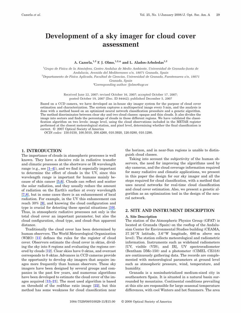
One program, the NN program, enables creating andraining MLPs specifying some parameters, i.e., the num-er of neurons in the different layers, the transferenceunctions, the learning algorithm, and the training andest sets. Another program, the GA program, implementshe genetic algorithm and all the functions required, in-luding the fitness function, i.e., the NN program. Theutputs of the GA program are the best MLP found andts performance. Figure 3(a) shows a schema of this pro-edure, and Figs. 3(b) and 3(c) show flux diagrams of theA program and the subroutine that create and evaluate

he MLP, i.e., the NN program. The performance is calcu-ated from the test set, computing the error rate in thatet.

Finally, another program analyzes the images for cloudlassification using the MLP obtained with the genetic al-orithm. This program first extracts the parameters ofhe image pixels, i.e., the input of the MLP; then the MLPlassifies every pixel; and, finally, a new image, the resultmage, is built representing the opaque clouds as white,he thin clouds as gray, and the sky as blue. The blackepresent the areas not analyzed, which are the solar-hadow system and the building on the horizon. This re-ult image is analyzed to extract information about cloud

for the GA program. (c) Flux diagrams for the NN program.

agram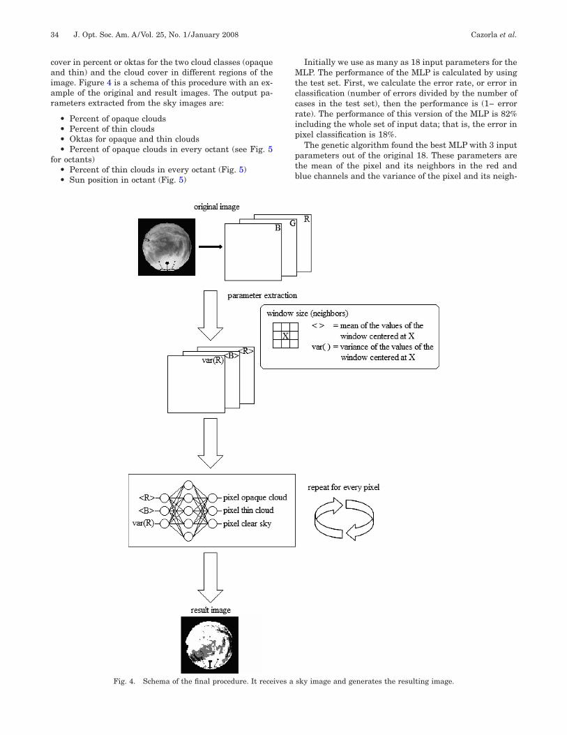

caiar

f

Mtccrip

ptb

34 J. Opt. Soc. Am. A/Vol. 25, No. 1 /January 2008 Cazorla et al.

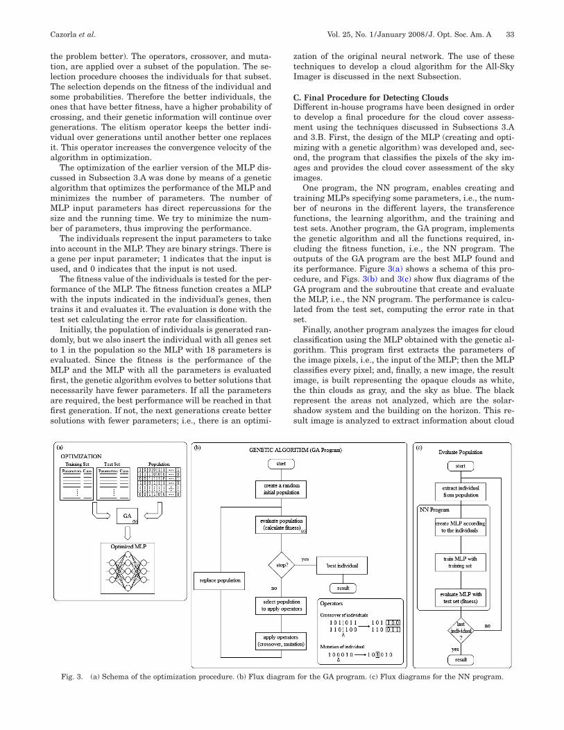
over in percent or oktas for the two cloud classes (opaquend thin) and the cloud cover in different regions of themage. Figure 4 is a schema of this procedure with an ex-mple of the original and result images. The output pa-ameters extracted from the sky images are:

• Percent of opaque clouds• Percent of thin clouds• Oktas for opaque and thin clouds• Percent of opaque clouds in every octant (see Fig. 5

or octants)• Percent of thin clouds in every octant (Fig. 5)• Sun position in octant (Fig. 5)

Initially we use as many as 18 input parameters for theLP. The performance of the MLP is calculated by using

he test set. First, we calculate the error rate, or error inlassification (number of errors divided by the number ofases in the test set), then the performance is (1− errorate). The performance of this version of the MLP is 82%ncluding the whole set of input data; that is, the error inixel classification is 18%.The genetic algorithm found the best MLP with 3 input

arameters out of the original 18. These parameters arehe mean of the pixel and its neighbors in the red andlue channels and the variance of the pixel and its neigh-

Fig. 4. Schema of the final procedure. It receives a sky image and generates the resulting image.

bwtstpattubpiw

4NAAaavtttptttpacspsclgO

tccotfiotbmc

BTmdatdeFmttcotlTigssoc

thco1o

dsMhaef

Fis

P

CTO

Cazorla et al. Vol. 25, No. 1 /January 2008 /J. Opt. Soc. Am. A 35

ors in the red channel (a schema of the neighbors of theindow size can be seen on Fig. 4). The performance of

he optimized MLP is 85%, that is, the error in pixel clas-ification is 15%. More important, with the reduction inhe number of the input parameters, the time used in thearameter extraction procedure is significantly reduced,nd the running time of the whole procedure is reduced,oo. It is also significant to emphasize that the informa-ion is in the red and blue channels; that is, the channelssed in the algorithms are based on threshold of the red/lue ratio image mentioned in Section 1. The use of morearameters or different channels contaminates the learn-ng process of the neural network, worsening performancehen more inputs are used.

. EVALUATION OF THE NEURALETWORK FOR CLOUD CLASSIFICATION. Pixel-Based Evaluations indicated in Section 3, we have selected a set of 50 im-ges with a wide variety of sky conditions, making a set ofbout 1000 samples. This sample test was randomly di-ided in two, one selected as training and the other asest. To evaluate the classification procedure in this sec-ion we have used the set of 500 samples not selected inhe training procedure. Thus, we have used different ap-roaches. In the pixel-based evaluation we have testedhe numbers of successes and failures, discriminating theype of failure. That is, there are three classes, so whenhe MLP fails in the classification of pixels there are twoossibilities: the MLP can fail classifying in one class ornother. Table 1 shows error frequencies for the threelasses. The first row shows the error frequency for clas-ification of the MLP in the three different classes for theixels cataloged as clear sky by a human observer. Theecond row shows the same for pixels cataloged as thinloud by a human observer, and the third row those cata-oged as opaque. The classification of clear skies is quiteood; over 88% of the test pixels are correctly classified.paque clouds are also well classified; more than 84% of

ig. 5. Position of the octants for the output parameters. (Themage is rotated to calculate the percent in regions; hence theouth is always placed at the bottom of the image.)

he test pixels are correctly classified. Over 61% of thinloud pixels are correctly classified, but almost 30% arelassified as clear skies and about 10% are classified aspaque cloud. Human inspection of pixels for classifica-ion is quite complicated in this case. Thin clouds are dif-cult to detect visually in the sky images, so that may bene reason why thin clouds are detected as clear sky. Onhe other hand, the ability of the observer to distinguishetween opaque and thin clouds is a source of errorainly when the pixel is wrongly classified as opaque

loud.

. Image-Based Evaluationhe evaluation of the procedure for cloud cover assess-ent requires a reference to compare the actual sky con-

ition with the cloud cover estimated over the whole im-ge. This can be done by comparing the performance ofhe full classification of our methodology with an indepen-ent record of cloud cover by human observers. The clos-st meteorological office is situated at the Armilla Airorce Base, located 4 km from the station. There are noountains, big buildings, or other obstacles between

hem; so, it is assumed that the cloud cover registered athe meteorological office is similar to the estimation ofloud cover with the All-Sky Imager. The meteorologicalffice archives the METAR reports [44]. METAR meanshe aviation routine weather report, and it is used by pi-ots in partial fulfillment of a preflight weather briefing.hese reports are generated every hour in daytime and

nclude information about cloud cover. The cloud coveriven is not the best, as it is given in ranges of oktas in-tead of oktas per se. That is, there is a category for clearkies (0 oktas), another for few clouds (1–2 oktas), an-ther for scattered clouds (3–4 oktas), another for brokenlouds (5–7 oktas), and the last one for overcast (8 oktas).

The All-Sky Imager provides the percent of clouds andhe number of oktas, so the resolution is different, and weave to assume an uncertainty of at least 1 okta in theomparison. For the METAR categories we use the meanf oktas in the interval, e.g., the “few clouds” category is.5 oktas (±1 okta), “scattered clouds” is 3.5 oktas (±1kta), and so.

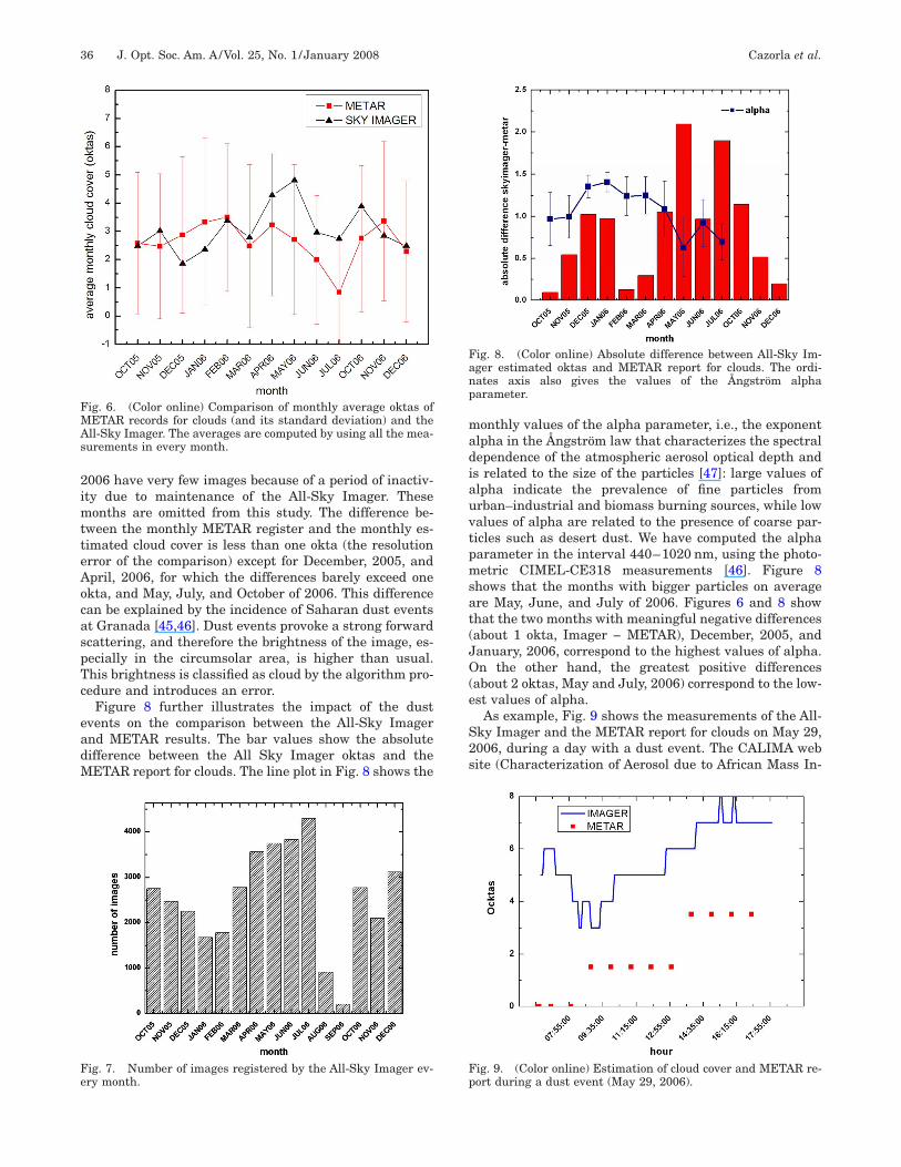
The evaluation has been performed over 15 months ofata (from October, 2005, to December, 2006). Figure 6hows the monthly average oktas registered on theETAR record and by the All-Sky Imager. This average

as been done with an estimation from all the imagesvailable and all the available METAR observations forvery month. Figure 7 shows the number of sky imagesor each month. We can see that August and September of

Table 1. Contingency of the Relative Frequency ofPixel Classificationa

Pixel Estimated as (%)

ixel Observed as Clear Sky Thin Cloud Opaque Cloud

lear sky 88.11 28.44 5.78hin cloud 11.01 61.41 9.45paque cloud 0.88 10.16 84.77

aMaxima are boldface.

2imtteAocaspTc

eadM

madiauvtpmsat(JO(e

S2s

FMAs

Fe

Fanp

Fp

36 J. Opt. Soc. Am. A/Vol. 25, No. 1 /January 2008 Cazorla et al.

006 have very few images because of a period of inactiv-ty due to maintenance of the All-Sky Imager. These

onths are omitted from this study. The difference be-ween the monthly METAR register and the monthly es-imated cloud cover is less than one okta (the resolutionrror of the comparison) except for December, 2005, andpril, 2006, for which the differences barely exceed onekta, and May, July, and October of 2006. This differencean be explained by the incidence of Saharan dust eventst Granada [45,46]. Dust events provoke a strong forwardcattering, and therefore the brightness of the image, es-ecially in the circumsolar area, is higher than usual.his brightness is classified as cloud by the algorithm pro-edure and introduces an error.

Figure 8 further illustrates the impact of the dustvents on the comparison between the All-Sky Imagernd METAR results. The bar values show the absoluteifference between the All Sky Imager oktas and theETAR report for clouds. The line plot in Fig. 8 shows the

ig. 6. (Color online) Comparison of monthly average oktas ofETAR records for clouds (and its standard deviation) and thell-Sky Imager. The averages are computed by using all the mea-urements in every month.

ig. 7. Number of images registered by the All-Sky Imager ev-ry month.

onthly values of the alpha parameter, i.e., the exponentlpha in the Ångström law that characterizes the spectralependence of the atmospheric aerosol optical depth ands related to the size of the particles [47]: large values oflpha indicate the prevalence of fine particles fromrban–industrial and biomass burning sources, while lowalues of alpha are related to the presence of coarse par-icles such as desert dust. We have computed the alphaarameter in the interval 440–1020 nm, using the photo-etric CIMEL-CE318 measurements [46]. Figure 8

hows that the months with bigger particles on averagere May, June, and July of 2006. Figures 6 and 8 showhat the two months with meaningful negative differencesabout 1 okta, Imager − METAR), December, 2005, andanuary, 2006, correspond to the highest values of alpha.n the other hand, the greatest positive differences

about 2 oktas, May and July, 2006) correspond to the low-st values of alpha.

As example, Fig. 9 shows the measurements of the All-ky Imager and the METAR report for clouds on May 29,006, during a day with a dust event. The CALIMA webite (Characterization of Aerosol due to African Mass In-

ig. 8. (Color online) Absolute difference between All-Sky Im-ger estimated oktas and METAR report for clouds. The ordi-ates axis also gives the values of the Ångström alphaarameter.

ig. 9. (Color online) Estimation of cloud cover and METAR re-ort during a dust event (May 29, 2006).

ttSwi

drmlrpisftt

5TaaOidaiitpwpicTbMcnit

itt

eaitbbpcTtet

ohicswritot

etiscw

seUtbbhps

ATCo0RTpeBfaew

Ffcw

Cazorla et al. Vol. 25, No. 1 /January 2008 /J. Opt. Soc. Am. A 37

rusions, www.calima.ws) from the Environmental Minis-ry of Spain recorded that the day was associated with aaharan dust event. Thus, the number of oktas estimatedith the sky images is higher than the values registered

n the METAR reports.Figure 10 shows a relative frequency histogram for the

ifference between All-Sky Imager oktas and the METAReport for cloud cover in temporally coincident measure-ents. More than 60% of the sky images estimates differ

ess than or exactly one okta from the synchronic METAReport. This is the minimum uncertainty that can be ex-ected in the comparison, since METAR data are given inntervals of 2 or 3 oktas. On the other hand, as we haveeen in Fig. 9, dust events explain the cases when the dif-erence between All-Sky Imager and METAR is larger, ashe All-Sky Imager procedure classifies a greater part ofhe sky as cloudy in those cases.

. CONCLUDING REMARKShe use of sky imagery offers better resolution in spacend time than does human observation. The All-Sky Im-ger captures an image every 5 min every day of the year.n the other hand, human observers estimate cloud cover

n oktas, or ranges of oktas as in METAR reports, with aegree of subjectivity. The analysis procedure of the im-ges of the All-Sky Imager, the MLP, includes subjectivityn the election of the training set and the classification oft, i.e., the human interaction in the process. Beyond this,he MLP always acts objectively according to the learningrocess and provides a good way to determine cloud coverith quite good resolution as demonstrated in the com-arison with the METAR records. The apparent complex-ty of the algorithm provides the added value of cloudlassification into two classes (thin and opaque clouds).he results are similar to those obtained with the red/lue ratio threshold method by Long et al. [20], but theLP includes the separation between thin and opaque

louds. Another added value is spatial classification. Theeural algorithm provides as output an ASCII file includ-

ng the spatial classification in oktas, the cloud class, andhe apparent Sun octant position, as well as the processed

ig. 10. (Color online) Relative frequency histogram for the dif-erence between All-Sky Imager oktas and METAR records forloud cover in temporally coincident measurements over thehole data set.

mage. Such results are important for the characteriza-ion of cloud effects on UV radiation, since thin cloudshat nearly obstruct the Sun can enhance UV radiation.

The error rate of the classifier is given in percent of pix-ls, but the final procedure classifies images. The error islways gathered in specific regions. We find from observ-ng the results that the circumsolar area is very difficulto classify. Currently, the MLP always classifies therightness of the Sun as cloud, and this uncertainty isigger in the case of dust events. This also hinders theossibility of detecting solar obstruction by clouds, espe-ially in our location where dust outbreaks are frequent.he ability of the human classifier to distinguish between

hin clouds and sky or opaque clouds is also a source ofrror. Souza-Echer et al. [21] also have problems detectinghin clouds, and the source of error seems to be the same.

The usefulness of the genetic algorithm for parameterptimization is clearly demonstrated. The final prototypeas 1/6 of the original number of required inputs, increas-

ng the speed of the execution of the procedure for cloudover estimation, and the performance of the MLP is alsolightly increased. One of the most important conclusionse can extract from the results of the optimization algo-

ithm is that the information required for cloud detections in the red and blue channels, as in the red/blue ratiohreshold method, and the classification of thin andpaque clouds requires the use of the variance, which is aexture parameter.

The main problems in the design of the MLP are thelection of the training set and its classification. This elec-ion affects the performance of the MLP drastically. It ismportant to select a wide variety of conditions and clas-ify them properly. The use of this technique in other lo-ations might require repeating the training process asell.The main weaknesses of the MLP cloud classification of

ky images are found in the circumsolar area and at clouddges. The circumsolar area is important because of theV enhancement effect, as stated above. The solution of

he circumsolar area problem may be difficult because therightness of that area nearly saturates the pixels andlinds the imager, making it impossible to see what is be-ind the brightness, especially during dust events. Theroblem at cloud edges includes bias by the human ob-erver.

CKNOWLEDGMENTShis work was supported by the Centro de Investigaciónientífica y Tecnológica (CICYT) of the Spanish Ministryf Science and Technology through projects REN2003-3175 and CGL2004-05984-C07-03 and the Andalusianegional Government through project P06-RNM-01503.he Spanish Meteorological Service, INM, kindly sup-lied the METAR reports. We are very grateful to Guill-rmo Ballester, Meteorologist Chief of the Armilla Airase Meteorological Office. Alberto Cazorla has been

unded by the Andalusian Regional Government. We alsore especially thankful to Janet Shields for reading anarlier draft of this manuscript and to Andrew Kowalskiho revised the final manuscript.

R

1

1

1

1

1

1

1

1

1

1

2

2

2

2

2

2

2

2

2

2

3

3

3

3

3

3

3

3

3

3

4

4

38 J. Opt. Soc. Am. A/Vol. 25, No. 1 /January 2008 Cazorla et al.

EFERENCES1. L. Alados-Arboledas, J. Vida, and F. J. Olmo, “The

estimation of thermal radiation under cloudy conditions,”Int. J. Climatol. 15, 107–116 (1995).

2. J. Matthijsen, H. Slaper, H. Reinen, and G. Velders,“Reduction of solar UV by clouds: a comparison betweensatellite-derived cloud effects and ground-based radiationmeasurements,” J. Geophys. Res. 105(D4), 5069–5080(2000).

3. J. Calbó, D. Pages, and J. A. González, “Empirical studiesof cloud effects on UV radiation: a review,” Rev. Geophys.43, 2 (2005).

4. M. Stowaser and K. Hamilton, “Relationship betweenshortwave cloud radiative forcing and local meteorologicalvariables compared in observations and several globalclimate models,” J. Clim. 19, 4344–4359 (2006).

5. J. C. van der Leun and F. R. de Gruijl, “Climate change andskin cancer,” Photochem. Photobiol. Sci. 1, 324–326 (2002).

6. J. C. van der Leun and P. D. Forbes, “Ultraviolet tanningequipment: six questions,” Photodermatol. Photoimmunol.Photomed. 21, 254–259 (2005).

7. L. Alados-Arboledas, I. Alados, I. Foyo-Moreno, A.Alcántara, and F. J. Olmo, “The influence of clouds onsurface UV erythemal irradiance,” Atmos. Res. 66, 273–290(2003).

8. I. Foyo-Moreno, J. Vida, I. Alados, F. J. Olmo, and L.Alados-Arboledas, “The influence of clouds on UV globalirradiance �295–385 nm�,” Agric. Forest Meteorol. 120,101–111 (2003).

9. J. G. Estupiñan, S. Raman, G. H. Crescenti, J. J. Streicher,and W. F. Barnard, “Effects of clouds and haze on UV-Bradiation,” J. Geophys. Res. 101(D11), 16807–16816 (1996).

0. J. M. Sabburg and A. V. Parisi, “Spectral dependency ofcloud enhanced UV irradiance,” Atmos. Res. 81, 206–214(2006).

1. WMO, Guide to Meteorological Practice, Publication No.168 (World Meteorological Organization, 1983).

2. R. R. Rogers and M. K. Yau, A Short Course in CloudPhysics (Pergamon, 1989).

3. J. E. Shields, R. W. Johnson, and T. E. Koehler, “Automatedwhole sky imaging systems for cloud field assessment,”presented at the Fourth Symposium on Global ChangeStudies of the American Meteorological Society, Boston,Massachusetts, January 17–22, 1993.

4. J. E. Shields, M. E. Karr, T. P. Tooman, D. H. Sowle, and S.T. Moore, “The whole sky imager—a year of progress,”presented at the Eighth Atmospheric RadiationMeasurement (ARM) Science Team Meeting, Tucson,Arizona, March 23–27, 1998.

5. J. Sabburg and J. Wong, “Evaluation of a sky camera foruse in radiation measurement,” J. Atmos. Ocean. Technol.16, 752–759 (1999).

6. U. Feister, J. E. Shields, M. E. Karr, R. W. Johnson, K.Dehne, and M. Woldt, “Ground-based cloud images and skyradiances in the visible and near infrared region fromwhole sky imager measurements,” presented at theClimate Monitoring—Satellite Application FacilityTraining Workshop, Dresden, Germany, November 20–22,2000.

7. J. Sabburg, “Quantification of cloud around the sun and itscorrelation with global UV measurement,” Ph.D. thesis(Queensland University of Technology, Brisbane, Australia,2000).

8. J. Sabburg and J. Wong, “Evaluation of a sky/cloud formulafor estimating UV-B irradiance under cloudy conditions,” J.Geophys. Res. 105, 29685–29691 (2000).

9. J. M. Sabburg and C. N. Long, “Improved sky imaging forstudies of enhanced UV irradiance,” Atmos. Chem. Phys.Discuss. 4, 6213–6238 (2004).

0. C. J. Long, J. Sabburg, J. Calbó, and D. Pagès, “Retrievingcloud characteristics from ground-based daytime color all-sky images,” J. Atmos. Ocean. Technol. 23, 633–652 (2006).

1. M. P. Souza-Echer, E. B. Pereira, L. S. Bins, and M. A. R.Andrade, “A simple method for the assessment of the cloudcover state in high-latitude regions by a ground based

digital camera,” J. Atmos. Ocean. Technol. 23, 437–447(2006).

2. J. E. Shields, R. W. Johnson, M. E. Karr, and J. L. Wertz,“Automated day/night whole sky imagers for fieldassessment of cloud cover distributions and radiancedistributions,” presented at the 10th Symposium onMeteorological Observations and Instrumentation of theAmerican Meteorological Society, Boston, Massachusetts,January 11–16, 1998.

3. Anon., Guía Resumida del Clima en España 1961-1990(Resumed guide of Spain Climate 1961-1990) (Ministerio deObras Públicas, Transporte y Medio Ambiente, DirecciónGeneral del Instituto Nacional de Meteorología, 1995).

4. M. Escudero, S. Castillo, X. Querol, A. Avila, M. Alarcón,M. M. Viana, A. Alastuey, E. Cuevas, and S. Rodríguez,“Wet and dry African dust episodes over eastern Spain,” J.Geophys. Res. 110(D18), D18S08 (2005).

5. J. E. Gil, A. Cazorla, F. J. Olmo, and L. Alados-Arboledas,“Experimental set up to study the cloud radiative effects onUVB at Granada (Spain),” in Proceedings of the EuropeanGeosciences Union General Assembly, A. K. Richter, ed.(EGU, 2005) Vol. 1, papers EGU05-A-00320,AS1.08.1WE2P-0059.

6. R. Lippman, “An introduction to computing with neuralnets,” IEEE ASSP Mag. 4(2), 4–22 (1987).

7. T. Khanna, Foundations of Neural Networks (Addison-Wesley, 1990).

8. C. M. Bishop, Neural Networks for Pattern Recognition(Oxford U. Press, 1995).

9. J. M. Gutiérrez, R. Cano, A. S. Cofiño, and C. Sordo, RedesProbabilísticas y Neuronales en las Ciencias Atmosféricas(Probabilistic and Neural Networks on AtmosphericSciences) (Ministerio de Medio Ambiente, DirecciónGeneral del Instituto Nacional de Meteorología, 2004).

0. I. Alados, J. A. Mellado, F. Ramos, and L. Alados-Arboledas, “Estimating UV erythemal irradiance by meansof neural networks,” Photochem. Photobiol. 80, 351–358(2004).

1. S. Greenberg and H. Guterman, “Neural-networkclassifiers for automatic real-world aerial imagerecognition,” Appl. Opt. 35, 4598–4609 (1996).

2. T. A. Dolenko, V. V. Fadeev, I. V. Gerdova, S. A. Dolenko,and R. Reuter, “Fluorescence diagnostics of oil pollution incoastal marine waters by use of artificial neural networks,”Appl. Opt. 41, 5155–5166 (2002).

3. S. A. Marcos, M. Soriano, and C. Saloma, “Classification ofcoral reef images from underwater video using neuralnetworks,” Opt. Express 13, 8766–8771 (2005).

4. M. D. Müller, A. Kaifel, M. Weber, and J. P. Burrows,“Neural network scheme for the retrieval of total ozonefrom Global Ozone Monitoring Experiment data,” Appl.Opt. 41, 5051–5058 (2002).

5. M. Chami and D. Robilliard, “Inversion of oceanicconstituents in case I and II water with geneticprogramming algorithms,” Appl. Opt. 41, 6260–6275(2002).

6. B. Rosenblatt, Principles of Neurodynamics: Perceptronsand the Theory of Brain Mechanisms (Spartan, 1961).

7. D. E. Rumerlhart, G. E. Hilton, and R. J. Williams,“Learning internal representations by errors propagation,”in Parallel Distributed Processing: Exploitations in theMicrostructure of Cognition Foundations, D. E. Rumelhartand J. L. MacClelland, eds. (MIT Press, 1986), Vol. 1, pp.318–362.

8. D. Barber and C. M. Bishop, “Ensemble learning for multi-layer networks,” in Advances in Neural InformationProcessing Systems, M. I. Jordan, M. J. Kearns, and S. A.Solla, eds. (MIT Press, 1997), pp. 395–401.

9. M. Riedmiller and H. Braun, “A direct adaptive method forfaster backpropagation learning: the RPROP algorithm, inProceedings of the IEEE International Conference onNeural Networks (IEEE, 1993), pp. 586–591.

0. J. H. Holland, “Outline for a logical theory of adaptivesystems,” J. Assoc. Comput. Mach. 9, 297–314 (1962).

1. H. J. Bremermann, “Optimization through evolution andrecombination,” in Self Organizing Systems, M. C. Yovits,

4

4

4

4

4

4

Cazorla et al. Vol. 25, No. 1 /January 2008 /J. Opt. Soc. Am. A 39

G. T. Jacobi, and G. D. Goldstein, eds. (Spartan, 1962), pp.93–106.

2. D. E. Goldberg, Genetic Algorithms in Search, Optimizationand Machine Learning (Addison-Wesley, 1989).

3. Z. Michalewicz, Genetic Algorithms + Data Structures =Evolution Programs (Springer-Verlag, 1992).

4. WMO, Manual on Codes, Publication No. 306 (WorldMeteorological Organization, 1995).

5. H. Lyamani, F. J. Olmo, and L. Alados-Arboledas, “Saharan

dust outbreak over southeastern Spain as detected by sunphotometer,” Atmos. Environ. 39, 7276–7284 (2005).

6. H. Lyamani, F. J. Olmo, A. Alcántara, and L. Alados-Arboledas, “Atmospheric aerosols during the 2003 heatwave in southeastern Spain I: spectral optical depth,”Atmos. Environ. 40, 6453–6464 (2006).

7. A. Ångström, “The parameters of atmospheric turbidity,”Tellus 16, 64–75 (1964).