1

Title: Development of a novel computational model for the Balloon Analogue Risk Task: The 1

Exponential-Weight Mean-Variance Model 2

3

Authors: 4

Harhim Park1, Jaeyeong Yang1, Jasmin Vassileva2, 3, and Woo-Young Ahn1 5

6

1Department of Psychology, Seoul National University, Seoul, Korea 7

2Department of Psychiatry, Virginia Commonwealth University, Virginia, United States of America 8

3Institute for Drug and Alcohol Studies, Virginia Commonwealth University, Virginia, United States of 9

America 10

11

Corresponding author: 12

Woo-Young Ahn, Ph.D. 13

Department of Psychology 14

Seoul National University 15

Seoul, Korea 08826 16

Tel: +82-2-880-2538, Fax: +82-2-877-6428. E-mail: wahn55@snu.ac.kr 17

18

Keywords: Balloon Analogue Risk Task, risk-taking, Hierarchical Bayesian Analysis, computational 19

modeling, substance use 20

21

Number of words in the abstract: 150 22

Number of words in the main text (including references): 9,203 23

Number of Figures/Tables in the main text: 7 / 1 24

Number of Figures/Tables in supplemental online material: 14 / 2 25

Number of References: 48 26

27

Conflict of Interest: The authors declare no competing financial interest. 28

29

30

2

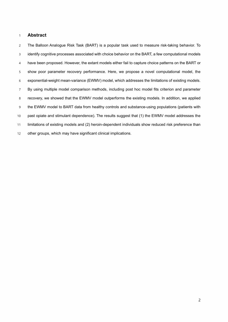
Abstract 1

The Balloon Analogue Risk Task (BART) is a popular task used to measure risk-taking behavior. To 2

identify cognitive processes associated with choice behavior on the BART, a few computational models 3

have been proposed. However, the extant models either fail to capture choice patterns on the BART or 4

show poor parameter recovery performance. Here, we propose a novel computational model, the 5

exponential-weight mean-variance (EWMV) model, which addresses the limitations of existing models. 6

By using multiple model comparison methods, including post hoc model fits criterion and parameter 7

recovery, we showed that the EWMV model outperforms the existing models. In addition, we applied 8

the EWMV model to BART data from healthy controls and substance-using populations (patients with 9

past opiate and stimulant dependence). The results suggest that (1) the EWMV model addresses the 10

limitations of existing models and (2) heroin-dependent individuals show reduced risk preference than 11

other groups, which may have significant clinical implications. 12

3

1. Introduction 1

Computational modeling of cognitive tasks has been widely used to address the limitations of 2

behavioral measures, with which it is often hard to identify underlying cognitive processes (Ahn et al., 3

2014; Daw, Gershman, Seymour, Dayan, & Dolan, 2011; Ratcliff, 1978). For example, research 4

examining a series of models for the Iowa Gambling Task (IGT) has accounted for the various patterns 5

in behavioral data, provided short- and long-term prediction and good parameter recovery (Ahn, 6

Busemeyer, Wagenmakers, & Stout, 2008; Ahn et al., 2014; Busemeyer & Stout, 2002; Haines, 7

Vassileva, & Ahn, 2018; Worthy & Maddox, 2014), and revealed decision-making deficits in several 8

clinical populations that were not detected by traditional performance indices (see Ahn, Dai, Vassileva, 9

Busemeyer, & Stout, 2016 for a review). 10

Like the IGT, the Balloon Analogue Risk Task (BART) (Lejuez et al., 2002) was originally 11

designed for the clinical purpose of measuring risk-taking tendencies and the identification of individuals 12

who are prone to take risks (Lejuez et al., 2002; Lejuez, Simmons, Aklin, Daughters, & Dvir, 2004), but 13

its scope has expanded to other areas of psychology and cognitive science (van Ravenzwaaij, Dutilh, 14

& Wagenmakers, 2011; Wallsten, Pleskac, & Lejuez, 2005). The BART has been shown to identify high 15

risk-taking individuals (Aklin, Lejuez, Zvolensky, Kahler, & Gwadz, 2005; Lejuez et al., 2002; Lejuez et 16

al., 2004) although several previous findings suggested low correlations between the BART 17

performance and risky behavior (Frey, Pedroni, Mata, Rieskamp, & Hertwig, 2017; Hopko et al., 2006). 18

Specifically, the behavioral performance of the BART is significantly correlated with self-report 19

measures of risk-related constructs such as impulsivity and sensation-seeking (Lejuez et al., 2002), 20

and past real-world risky behaviors such as drug use and risky sex (Lejuez et al., 2004). These results 21

presumably reflect at least two features of the BART which make the task similar to real-world situations: 22

First, each trial of the BART includes sequential risk-taking choices and terminates when the participant 23

does not want to take the risk any more or encounters a certain condition that makes it impossible to 24

proceed. Second, the riskiness of the risk-taking choices within a trial increases each time the 25

participant makes a risky choice. Specifically, as the participant makes a risky choice, the loss amount 26

gradually increases, whereas the reward amount remains constant or even decreases. Many actual 27

risky behaviors involve these features. For example, patients with substance use disorders continue to 28

take the drug even in the face of negative consequences until they are satisfied with it or cannot obtain 29

the drug because of external factors such as lack of availability and insufficient money. Also, patients 30

4

often start with smaller amounts of the drug but gradually increase their dosage as their tolerance 1

increases. As their tolerance increases, they must (and are likely to) take more risks to get the same 2

amount of reward. The BART has the distinct advantage of effectively illustrating this kind of real-world 3

situation in a laboratory setting. 4

To quantitatively analyze the underlying cognitive processes on the BART, previous studies 5

have proposed two computational models: a four-parameter model (Wallsten et al., 2005) and a two-6

parameter model (Pleskac, 2008; van Ravenzwaaij et al., 2011). The four-parameter model was 7

proposed as a winning model by comparing several computational models. The parameters of the four-8

parameter model have been shown to correlate with the frequencies of past real-world risky behaviors 9

such as substance use, unprotected sex, and stealing (Wallsten et al., 2005). However, two parameters 10

related to the learning process of the four-parameter model showed poorer parameter recovery and 11

were systematically overestimated (Heathcote, Brown, & Wagenmakers, 2015; van Ravenzwaaij et al., 12

2011). Since good parameter recovery performance is crucial for interpreting results based on the model 13

parameters (van Ravenzwaaij & Oberauer, 2009; Wagenmakers, Van Der Maas, & Grasman, 2007), 14

poor parameter recovery performance is a critical limitation of the four-parameter model. 15

The two-parameter model was proposed to overcome this limitation of the four-parameter model 16

(Pleskac, 2008; van Ravenzwaaij et al., 2011). To develop a model that shows good parameter recovery, 17

the authors simplified the original model by removing parameters that do not exhibit good recovery. The 18

two-parameter model is nested within the four-parameter model, and as a result of simplification, it 19

succeeded in recovering accurate parameter values (van Ravenzwaaij et al., 2011). However, the two-20

parameter model also has a critical limitation; it is based on a strict assumption that participants do not 21

learn during the BART. The assumption is unrealistic unless the researcher tells the participant the 22

actual exploding probability of virtual balloons before starting the experiment. Consistently, Pleskac 23

(2008) showed that the two-parameter model provided a better fit than the four-parameter model when 24

the probability structure was explicitly informed, but a poorer fit than the four-parameter model when 25

the probability structure was uninformed. 26

Furthermore, because this issue is related to the task design, the two-parameter model may not 27

fit the original task design. The original task design has the advantage that it similarly illustrates real-28

world situations, which means if we modify the task design to apply the two-parameter model, we lose 29

the advantage. Thus, there is a need to build a new model, which shows good parameter recovery and 30

5

fits the original task design. 1

Here, we propose a novel BART model, which shows good parameter recovery, fits the original 2

task design, and provides an intuitive interpretation of the learning process. First, we introduce the 3

existing model (the four-parameter model). We also consider a non-learning version of the four-4

parameter model to test the assumption that participants do not learn during the BART is unrealistic. 5

Then, we reparameterize the four-parameter model to improve its parameter recovery. By modifying 6

equations from the reparametrized version of the four-parameter model, we develop candidate models. 7

Finally, we select the best model based on the leave-one-out information criterion (LOOIC) and the 8

parameter recovery. To examine the implication of the new model, we compared the parameters with 9

similar psychological constructs of competing models and applied the new model to BART data from 10

patients with past opiate and stimulant dependence. 11

12

2. Method 13

2.1 Participants 14

The initial sample included 593 individuals who had enrolled for a study of impulsivity in opiate 15

and stimulant users in Sofia, Bulgaria. Then, only those who meet the following criteria were included: 16

age between 18 and 50 years, more than 8 years of formal education, estimated IQ of 80 or above, no 17

history of head injury or loss of consciousness for more than 30 minutes, no history of neurological 18

illness or psychotic disorders, HIV-seronegative status, and not currently on opioid maintenance therapy. 19

All participants had a negative breathalyzer test for alcohol and negative rapid urine toxicology screen 20

for opiates, cannabis, amphetamines, methamphetamines, benzodiazepines, barbiturates, cocaine, 21

MDMA, and methadone. We classified the included participants into three groups: healthy controls, 22

heroin-dependent, and amphetamine-dependent groups. After that, group-specific criteria were applied 23

to make each group include primarily mono-dependent (‘pure’) users. For the healthy control group, 24

participants with any substance dependence or abuse symptom based on DSM-IV criteria were 25

excluded (except for nicotine, caffeine, and past cannabis dependence). For the heroin and the 26

amphetamine-dependent groups, mono-substance-dependent participants who met DSM-IV lifetime 27

criteria for opiate or stimulant dependence with no dependence on any other substances were included. 28

Finally, a total of 226 subjects (135 healthy controls, 47 heroin-dependent, and 44 amphetamine-29

6

dependent individuals) were included in the analysis. For more details about the recruitment and 1

screening procedures, see Ahn and Vassileva (2016). This study was approved by the Institutional 2

Review Boards of the Virginia Commonwealth University and the Medical University in Sofia. All 3

participants provided informed consent. See supplementary material for demographic and clinical 4

characteristics of the participants (Table S1). 5

6

2.2 Task 7

In the BART, a virtual balloon is presented to the participant on each trial. Participants need to 8

decide whether to pump the balloon to accumulate some predefined amount of reward (i.e., pump), or 9

transfer and receive the reward that has been accumulated so far (i.e., transfer). Each trial ends when 10

the participant chooses to transfer the accumulated reward or the balloon explodes. If the balloon 11

explodes, the participant loses all the accumulated reward on that trial. We randomly determined 12

explosion points for each trial; thus, each participant performed the task with a different set of explosion 13

points. Participants are not informed about the probability of the balloon exploding. Typically, the degree 14

of risk-taking on the BART is measured by the adjusted BART score, which is the average number of 15

pumps for unexploded balloons (Lejuez et al., 2002). The adjusted BART score is preferable because 16

it is not directly affected by the explosion probability. To examine group differences in the adjusted BART 17

score between the three groups, we conducted the Bayesian t-test using the R package BEST 18

(Kruschke, 2013; Meredith & Kruschke, 2018). 19

20

2.3 Models 21

2.3.1 The four-parameter model 22

The four-parameter model (Wallsten et al., 2005) is based on two assumptions. First, the 23

participants update the belief about the probability of the balloon exploding after each trial. Second, the 24

participants decide the optimal number of pumps before each trial. 25

From a computational modeling perspective, the first assumption means that 𝑝kburst , the 26

participant’s perceived probability that pumping the balloon on trial 𝑘 will make the balloon explode, is 27

constant during the trial 𝑘. The participant initially has a prior belief about the probability of the balloon 28

exploding and updates the prior belief based on observation on each trial. The updating process is 29

7

described as follows: 1

𝑝𝑘𝑏𝑢𝑟𝑠𝑡 = 1 −

𝛼+∑ 𝑛𝑖𝑠𝑢𝑐𝑐𝑒𝑠𝑠𝑘−1

𝑖=0

𝜇+∑ 𝑛𝑖𝑝𝑢𝑚𝑝𝑠𝑘−1

𝑖=0

𝑤𝑖𝑡ℎ 0 < 𝛼 < 𝜇. (1) 2

In Equation (1), the initial value of 𝑝𝑘𝑏𝑢𝑟𝑠𝑡 is 1 − 𝛼/𝜇 , which reflects the participant’s initial 3

belief that pumping will make the balloon explode. The magnitudes of 𝛼 and 𝜇 indicate the degree of 4

learning from observations; high values indicate that the prior belief is strong and the perceived 5

probability is affected to just a small degree by the observed data. ∑ 𝑛𝑖𝑠𝑢𝑐𝑐𝑒𝑠𝑠𝑘−1

𝑖=0 is the sum of the 6

number of successful pumps up to trial 𝑘 − 1, and ∑ 𝑛𝑖𝑝𝑢𝑚𝑝𝑠𝑘−1

𝑖=0 is the sum of the total number of pumps 7

up to trial 𝑘 − 1. 8

The second assumption that the participant evaluates the optimal number of pumps before 9

each trial is reflected in the equations for calculating the probability that the participant will pump the 10

balloon. Adopting the prospect theory (Kahneman & Tversky, 2013), the expected utility after 𝑙 pumps 11

on trial 𝑘, 𝑈𝑘𝑙, is given by: 12

𝑈𝑘𝑙 = (1 − 𝑝𝑘𝑏𝑢𝑟𝑠𝑡)

𝑙(𝑙𝑟)𝛾. (2) 13

In Equation (2), 𝑟 is the amount of reward per successful pump, and 𝛾 is risk-taking 14

propensity. We can calculate the optimal number of pumps by setting the first derivative of Equation (2) 15

for 𝑙 equals zero. Then, we can easily derive the optimal number of pumps on trial 𝑘, 𝜈𝑘, as follows: 16

𝜈𝑘 =−𝛾

ln (1−𝑝𝑘𝑏𝑢𝑟𝑠𝑡)

𝑤𝑖𝑡ℎ 𝛾 ≥ 0. (3) 17

Based on 𝜈𝑘, we can calculate the probability that the participant will pump the balloon on trial 18

𝑘 for pump 𝑙, 𝑝𝑘𝑙𝑝𝑢𝑚𝑝

: 19

𝑝𝑘𝑙𝑝𝑢𝑚𝑝 =

1

1+𝑒𝜏(𝑙−𝜈𝑘) 𝑤𝑖𝑡ℎ 𝜏 ≥ 0. (4) 20

In this logistic equation, 𝜏 is the inverse temperature parameter. The inverse temperature of 21

the choice rule determines how deterministic or random the choice is; The higher 𝜏 , the more 22

deterministic. If 𝑙 < 𝜈𝑘 , 𝑝𝑘𝑙𝑝𝑢𝑚𝑝

becomes greater than 0.5. Similarly, if 𝑙 > 𝜈𝑘 , 𝑝𝑘𝑙𝑝𝑢𝑚𝑝

becomes less 23

than 0.5. In sum, the four-parameter model has four parameters to be estimated: 𝛼, 𝜇, 𝛾, and 𝜏. 24

We can calculate the likelihood of the data given the parameters by multiplying the probability 25

that the participant will pump on trial 𝑘 for pump 𝑙 , 𝑝𝑘𝑙𝑝𝑢𝑚𝑝

. The probability of the data given the 26

parameters, 𝑝(𝐷|𝛼, 𝜇, 𝛾, 𝜏), is given by: 27

8

𝑝(𝐷|𝛼, 𝜇, 𝛾, 𝜏) = ∏ ∏ 𝑝𝑘𝑙𝑝𝑢𝑚𝑝

(1 − 𝑝𝑘,𝑙𝑘

𝑙𝑎𝑠𝑡+1

𝑝𝑢𝑚𝑝)

𝑑𝑘𝑙𝑘𝑙𝑎𝑠𝑡

𝑙=1𝑘𝑙𝑎𝑠𝑡

𝑘=1 , (5) 1

where 𝑘𝑙𝑎𝑠𝑡 is the last number of trials, 𝑙𝑘𝑙𝑎𝑠𝑡 is the last number of pumping opportunities on trial 𝑘. if 2

the participant transfers the accumulated reward on trial 𝑘 to the virtual bank account, 𝑑𝑘 = 1 and if 3

the balloon explodes on trial 𝑘, 𝑑𝑘 = 0. 4

Although previous researchers have primarily used the four-parameter model, it has been 5

known that 𝛼 and 𝜇 of the four-parameter model are not well recovered. The two-parameter model 6

was proposed to address this problem of the four-parameter model (Pleskac, 2008; van Ravenzwaaij 7

et al., 2011). However, the two-parameter model does not apply to the original BART paradigm because 8

participants are not informed of the probability structure of the task. Therefore, instead of the two-9

parameter model, we considered a non-learning version of the four-parameter model, which is based 10

on an assumption that participants do not learn during the BART. 11

12

2.3.2 Non-learning version (Par3 model) 13

The non-learning version of the four-parameter model is based on the following assumption of 14

the two-parameter model: participants do not learn during the BART. Since participants do not update 15

their belief of the probability of the balloon exploding based on observations and they are not informed 16

of the probability structure of the original BART paradigm, in this model, we assumed participant’s belief 17

of the probability of the balloon exploding as a parameter, 𝜃. Then, similar to Equation (3), we can 18

derive the optimal number of pumps, 𝜈, as follows: 19

𝜈 =−𝛾

ln (1−𝜃) 𝑤𝑖𝑡ℎ 𝛾 ≥ 0. (6) 20

Based on the optimal number of pumps, similar to Equation (4), we can calculate the 21

probability that the participant will pump the balloon for pump 𝑙, 𝑝𝑙𝑝𝑢𝑚𝑝

: 22

𝑝𝑙𝑝𝑢𝑚𝑝 =

1

1+𝑒𝜏(𝑙−𝜈) 𝑤𝑖𝑡ℎ 𝜏 ≥ 0. (7) 23

Notably, the optimal number of pumps, 𝜈, and the probability that the participant will pump the 24

balloon for pump 𝑙, 𝑝𝑙𝑝𝑢𝑚𝑝

, do not depend on the trial number because the participant’s belief of the 25

probability of the balloon exploding is a parameter with a fixed value. In sum, the non-learning version 26

of the four-parameter model includes three free parameters to be estimated: 𝜃, 𝛾, and 𝜏. 27

28

9

2.3.3 Reparametrized version (Par4 model) 1

We suspected that the strong association between 𝛼 and 𝜇 (the ratio reflects the 2

participant’s initial belief and the magnitudes indicate the degree of learning from observations) may be 3

problematic and tested if reparametrizing 𝛼 and 𝜇 would improve the parameter recovery 4

performance of the model. 5

The parameters 𝛼 and 𝜇 are associated with two processes. The ratio of 𝛼 to 𝜇 , 𝛼/𝜇 , 6

refers to the participant’s initial belief that pumping will make the balloon explode, and the magnitudes 7

of both 𝛼 and 𝜇 determine the degree of learning from observations. Thus, we wanted to 8

reparametrize them so that each parameter is uniquely associated with just one process. Also, we 9

wanted to remove the constraint that 𝛼 is less than 𝜇 because the constraint might lead to inefficient 10

sampling for Bayesian parameter estimation (see Section 2.4). 11

For the goal, we reparametrized 𝛼 and 𝜇 into 𝜙 and 𝜂 : 𝜙 = 𝛼/𝜇 and 𝜂 = 1/𝜇 . 12

Substituting these parameters into Equation (1) yields: 13

𝑝𝑘𝑏𝑢𝑟𝑠𝑡 = 1 −

𝜙+𝜂 ∑ 𝑛𝑖𝑠𝑢𝑐𝑐𝑒𝑠𝑠𝑘−1

𝑖=0

1+𝜂 ∑ 𝑛𝑖𝑝𝑢𝑚𝑝𝑠𝑘−1

𝑖=0

𝑤𝑖𝑡ℎ 0 < 𝜙 < 1, 𝜂 > 0. (8) 14

After the reparameterization, the initial value of 𝑝𝑘𝑏𝑢𝑟𝑠𝑡 equals 1 − 𝜙. Thus, 𝜙 indicates the 15

participant’s initial belief that pumping will not make the balloon explode. Also, 𝜂 is an updating 16

coefficient of the participant’s belief by the observed data. If 𝜂 = 0 , 𝑝𝑘𝑏𝑢𝑟𝑠𝑡 is not affected by the 17

observed data. If 𝜂 is very large, 𝑝𝑘𝑏𝑢𝑟𝑠𝑡 rapidly comes close to the observed probability of burst. 18

Equations (3) and (4) remain the same. Note that we included the reparametrized four-parameter 19

version in the hBayesDM package as a function named bart_par4 (Ahn, Haines, & Zhang, 2017). 20

21

2.3.4 The Exponential-Weight model (EW model) 22

The four-parameter model has two critical limitations, even after the reparameterization. First, 23

although the model reflects that the participant updates 𝑝𝑘𝑏𝑢𝑟𝑠𝑡 from the prior belief with the observed 24

data, Equation (8) hardly provides an intuitive interpretation of the learning process. We modified the 25

updating equation in an attempt to show the learning process more clearly. Second, the assumption 26

that the participant determines the optimal number of pumps before each trial may be unjustified. This 27

assumption might be contradictory with the primary goal of the BART, measuring the risk-taking 28

tendency of individuals, because it does not reflect some critical features of risk-taking such as loss 29

10

aversion and impulsive responses. Instead, the participant may decide whether to pump the balloon or 1

not just before each pump. 2

To address the first issue, we defined a parameter, 𝜓 = 1 − 𝜙, which is the initial value of 3

𝑝𝑘𝑏𝑢𝑟𝑠𝑡. Substituting this parameter into Equation (8) yields: 4

𝑝𝑘𝑏𝑢𝑟𝑠𝑡 = 𝜔𝑘−1𝜓 + (1 − 𝜔𝑘−1)𝑃𝑘−1 𝑤𝑖𝑡ℎ 0 < 𝜓 < 1, 𝜂 > 0, (9) 5

where 𝑃𝑘−1 =∑ (𝑛𝑖

𝑝𝑢𝑚𝑝𝑠𝑘−1𝑖=0 −𝑛𝑖

𝑠𝑢𝑐𝑐𝑒𝑠𝑠)

∑ 𝑛𝑖𝑝𝑢𝑚𝑝𝑠𝑘−1

𝑖=0

, which is the observed probability that pumping has made the balloon 6

explode up to trial 𝑘 − 1, and 𝜔𝑘−1 =1

1+𝜂 ∑ 𝑛𝑖𝑝𝑢𝑚𝑝𝑠𝑘−1

𝑖=0

, which is the weight indicating how much weight is 7

given to the prior belief on trial 𝑘 when estimating the probability of the balloon exploding. Each 8

component of Equation (9) has a clear role, which is interpretable as a part of weight updating learning. 9

Specifically, the current value (𝑝𝑘𝑏𝑢𝑟𝑠𝑡) is estimated as a weighted average of the initial value (𝜓) and the 10

observed value (𝑃𝑘−1). As data accumulates, the participant updates the weight (𝜔𝑘−1) and the observed 11

value (𝑃𝑘−1). The weight (𝜔𝑘−1) and the observed value (𝑃𝑘−1) are determined by the total number of 12

the data ( ∑ 𝑛𝑖𝑝𝑢𝑚𝑝𝑠𝑘−1

𝑖=0 ) and the number of the data that meet a certain condition (explosion, 13

∑ (𝑛𝑖𝑝𝑢𝑚𝑝𝑠 − 𝑛𝑖

𝑠𝑢𝑐𝑐𝑒𝑠𝑠)𝑘−1𝑖=0 ). In this framework, 𝜂 indicates how rapidly the participant depends on 14

experience. If 𝜂 → ∞, learning entirely depends on the present outcome. If 𝜂 = 0, no further learning 15

occurs. 16

To improve the model performance within this framework, we modified the functional form of 17

the weight, 𝜔𝑘−1 . If we define 𝑥 as 𝜂 ∑ 𝑛𝑖𝑝𝑢𝑚𝑝𝑠𝑘−1

𝑖=0 , in Equation (9), 𝜔𝑘−1 =1

1+𝑥 , which means the 18

weight is hyperbolic. Other functional forms can be alternatives to the hyperbolic function if they meet 19

two conditions: the participant’s learning starts with the prior belief (if 𝑥 = 0, 𝜔𝑘−1 = 1) and primarily 20

depends on the observed value after observing enough data (if 𝑥 → ∞, 𝜔𝑘−1 → 0). The exponential 21

decay, 𝑒−𝑥, is a reasonable alternative because it meets the two conditions and is commonly used to 22

describe natural phenomena such as the voltage of the resistor-capacitor circuit, the number of remain 23

radioactive atoms, and the concentration of the first-order chemical reaction. Replacing 𝜔𝑘−1 with 𝑒−𝑥 24

in Equation (9) yields: 25

𝑝𝑘𝑏𝑢𝑟𝑠𝑡 = 𝑒−𝜉 ∑ 𝑛𝑖

𝑝𝑢𝑚𝑝𝑠𝑘−1𝑖=0 𝜓 + (1 − 𝑒−𝜉 ∑ 𝑛𝑖

𝑝𝑢𝑚𝑝𝑠𝑘−1𝑖=0 )𝑃𝑘−1 𝑤𝑖𝑡ℎ 0 < 𝜓 < 1, 𝜉 > 0. (10) 26

To avoid confusion, we replaced 𝜂 with 𝜉 and named 𝜉 an updating exponent. 27

For the second issue (the assumption that the participant determines the optimal number of 28

11

pumps before each trial), we tested a new model which assumed that the participant decides whether 1

to pump the balloon or not before each pump instead of each trial. Using the prospect theory 2

(Kahneman & Tversky, 2013), we calculated the subjective utilities for pumping and not-pumping a 3

balloon on trial 𝑘 for pump 𝑙 as follows: 4

𝑈𝑘𝑙𝑝𝑢𝑚𝑝 = (1 − 𝑝𝑘

𝑏𝑢𝑟𝑠𝑡)𝑟𝜌 − 𝑝𝑘𝑏𝑢𝑟𝑠𝑡𝜆{(𝑙 − 1)𝑟}𝜌 𝑤𝑖𝑡ℎ 0 < 𝜌 < 2, 𝜆 > 0, (11) 5

𝑈𝑘𝑙𝑡𝑟𝑎𝑛𝑠𝑓𝑒𝑟

= 0, (12) 6

where 𝑟 is the amount of reward for each successful pump, 𝜌 is risk preference, and 𝜆 is loss 7

aversion. Then, we can calculate the probability that the participant will pump the balloon on trial 𝑘 for 8

pump 𝑙, 𝑝𝑘𝑙𝑝𝑢𝑚𝑝

, by using these subjective utilities. 9

𝑝𝑘𝑙𝑝𝑢𝑚𝑝 =

1

1+𝑒𝜏(𝑈

𝑘𝑙𝑡𝑟𝑎𝑛𝑠𝑓𝑒𝑟

−𝑈𝑘𝑙𝑝𝑢𝑚𝑝

) 𝑤𝑖𝑡ℎ 𝜏 ≥ 0, (13) 10

where 𝜏 is inverse temperature. We noticed that this model (Equations (11), (12), and (13)) is similar 11

to a model (Model1) reported in Wallsten et al. (2005). Although Model1 was not the best-fitting model, 12

its model fit was close to that of the winning model (the four-parameter model). Considering that the 13

EW model has a single parameter for risk preference instead of having separate risk preference 14

parameters for gain and loss like Model1, we also included Model1 in the model comparison to examine 15

its performance compared to other models. In summary, the EW model has five free parameters to be 16

estimated: 𝜓 (prior belief of burst), 𝜉 (updating exponent), 𝜌 (risk preference), 𝜏 (inverse 17

temperature), and 𝜆 (loss aversion). 18

19

2.3.5 Model1 20

In Model1 (Wallsten et al., 2005), the equation calculating the probability of the balloon 21

exploding is the same as the four-parameter model (Equation (1)). Because of the inefficient sampling 22

issue, we utilized the reparametrized version (Equation (4)) instead of Equation (1). 23

Like the EW model, Model1 is based on an assumption that the participant decides whether 24

to pump the balloon or not before each pump based on the subjective utilities for pumping and not-25

pumping. The only difference is that Model1 has separate risk preference parameters for gain and loss. 26

The subjective utilities for pumping and not-pumping a balloon on trial 𝑘 for pump 𝑙 are calculated as 27

follows: 28

𝑈𝑘𝑙𝑝𝑢𝑚𝑝 = (1 − 𝑝𝑘

𝑏𝑢𝑟𝑠𝑡)𝑟𝜌+− 𝑝𝑘

𝑏𝑢𝑟𝑠𝑡𝜆{(𝑙 − 1)𝑟}𝜌− 𝑤𝑖𝑡ℎ 0 < 𝜌+, 𝜌− < 2, 𝜆 > 0, (14) 29

12

𝑈𝑘𝑙𝑡𝑟𝑎𝑛𝑠𝑓𝑒𝑟 = 0, (15) 1

where 𝑟 is the amount of reward for each successful pump, 𝜌+ is risk preference for gain, 𝜌− is risk 2

preference for loss, and 𝜆 is loss aversion. Then, we can calculate the probability that the participant 3

will pump the balloon by using these subjective utilities (Equation (13)). In summary, Model1 includes 4

six free parameters to be estimated: 𝜙 (prior belief of success), 𝜂 (updating coefficient), 𝜌+ (risk 5

preference for gain), 𝜌− (risk preference for loss), 𝜏 (inverse temperature), and 𝜆 (loss aversion). 6

7

2.3.6 The Exponential-Weight Mean-Variance model (EWMV model) 8

The existing models and EW model utilize the prospect theory (Kahneman & Tversky, 2013) 9

to calculate subjective utilities for pumping and not-pumping. Given that previous studies have 10

suggested that the performances of the prospect theory and the mean-variance analysis (Markowitz, 11

1952) are comparable (Boorman & Sallet, 2009; Hens & Mayer, 2014; Levy & Levy, 2004), we tested a 12

model by applying the mean-variance analysis to the EW model. According to the mean-variance 13

analysis, the subjective utility of an option can be formulated by a linear combination of the expected 14

value and the variance of potential outcomes. Applying the mean-variance analysis, we calculated the 15

subjective utilities for pumping and not-pumping a balloon on trial 𝑘 for pump 𝑙 as follows: 16

𝑈𝑘𝑙𝑝𝑢𝑚𝑝

= (1 − 𝑝𝑘𝑏𝑢𝑟𝑠𝑡)𝑟 − 𝑝𝑘

𝑏𝑢𝑟𝑠𝑡 𝜆(𝑙 − 1)𝑟 + 𝜌𝑝𝑘𝑏𝑢𝑟𝑠𝑡(1 − 𝑝𝑘

𝑏𝑢𝑟𝑠𝑡){𝑟 + 𝜆(𝑙 − 1)𝑟}2 𝑤𝑖𝑡ℎ 𝜆 > 0, (16) 17

𝑈𝑘𝑙𝑡𝑟𝑎𝑛𝑠𝑓𝑒𝑟 = 0, (17) 18

where 𝑟 is the amount of reward for each successful pump, 𝜌 is risk preference, and 𝜆 is loss 19

aversion. In Equation (16), the first two terms indicate the expected value of a pump, and the last term 20

indicates the impact of the variance of potential outcomes on the subjective utility. Notably, in the mean-21

variance framework, the risk preference is defined as a coefficient of the variance term, which is a proxy 22

for risk. If 𝜌 < 0, the participant prefers to choose an option with a large variance of potential outcomes. 23

If 𝜌 = 0, the expected value of an option determines the participant's subjective utility. If 𝜌 > 0, the 24

participant prefers to choose an option with a small variance of potential outcomes. Like the EW model, 25

we can calculate the probability of pumping the balloon by using these subjective utilities based on the 26

mean-variance analysis (Equation (13)). In summary, the EWMV model includes five free parameters: 27

𝜓 (prior belief of burst), 𝜉 (updating exponent), 𝜌 (risk preference), 𝜏 (inverse temperature), and 𝜆 28

(loss aversion). 29

13

1

2.4 Hierarchical Bayesian Analysis (HBA) 2

We used hierarchical Bayesian Analysis (HBA) for parameter estimation (Berger, 2013; 3

Gelman, Carlin, Stern, & Rubin, 2004; Lee, 2011). HBA offers several benefits over conventional non-4

hierarchical approaches such as individual-level ordinary least squares and maximum likelihood 5

estimation (MLE) methods. First, HBA estimates parameters as posterior distributions instead of point 6

estimates. Posterior distributions provide us with more information about the parameters than point 7

estimates because distributions show the uncertainty of the estimated values. Second, with HBA, we 8

can systematically characterize similarities and differences across subjects within a Bayesian 9

framework based on the amount of information from each individual. Previous studies suggest that HBA 10

allows us to estimate model parameters more accurately than individual- or group-level MLE methods 11

(Ahn, Krawitz, Kim, Busemeyer, & Brown, 2011). 12

13

We conducted HBA by using Stan (version 2.15.1), a probabilistic programming language for 14

specifying statistical models (Carpenter et al., 2017). Stan uses Hamiltonian Monte Carlo (HMC) for 15

sampling from high-dimensional parameter space. Specifically, we implemented the models in the 16

hBayesDM (Ahn et al., 2017) environment, which uses Stan. For parameter estimation, we used flat or 17

weakly informative priors (Ahn, Haines, & Zhang, 2017; Haines, Vassileva, & Ahn, 2018) to minimize 18

the influence of the priors and the Matt trick (Papaspiliopoulos, Roberts, & Sköld, 2007) to facilitate the 19

sampling process. We will make the Stan codes and precise prior settings publicly available through 20

GitHub. We tested several other types of priors and confirmed that the priors hardly affected the results 21

as long as the priors are approximately uninformative. We used a large enough sample size (4000 22

samples, including 2000 burn-in samples per chain) to assure that parameters converge to the target 23

distributions, with four independent chains to check that the posterior distributions are not dependent 24

on initial starting points. Note that Vehtari, Gelman, Simpson, Carpenter, and Bürkner (2019) 25

recommended running at least four chains by default. The trace plots indicated that chains were well 26

mixed and the �̂� values (Gelman & Rubin, 1992) for all model parameters were lower than 1.1, which 27

indicates that the estimated parameter values converged to their target posterior distributions. Thinning 28

was not applied because thinning of chains is rarely useful for the precision of estimates (Link & Eaton, 29

2012). See supplementary material for detailed information of HBA (Table S2, Figure S3, and Figure 30

14

S4). 1

2

2.5 Model comparison 3

2.5.1 Leave-one-out information criterion (LOOIC) 4

LOOIC is an information criterion calculated from the Leave-one-out cross-validation. Leave-5

one-out cross-validation is a method to estimate out-of-sample prediction accuracy from a fitted 6

Bayesian model based on the log-likelihood evaluated from the posterior distributions (Vehtari, Gelman, 7

& Gabry, 2017). It is well-known that LOOIC has various benefits over simpler estimates such as Akaike 8

Information Criterion (AIC, Akaike, 1998) and Bayesian Information Criterion (BIC, Schwarz, 1978). We 9

used the R package loo (Vehtari et al., 2017) to estimate LOOIC for each model. Because LOOIC is 10

calculated from the log-likelihood, the lower LOOIC is, the better its model fit is. For model selection, 11

LOOIC weights are defined as Akaike weights (Wagenmakers & Farrell, 2004) calculated based on 12

LOOIC values, and the detailed information is provided in the supplementary material (see Model 13

comparison section). 14

15

2.5.2 Parameter recovery 16

We also used parameter recovery to evaluate how accurate a model estimates true parameter 17

values from the simulation data generated from the true parameter values (e.g., Ahn et al., 2011; Ahn 18

et al., 2014; Haines et al., 2018; Wagenmakers et al., 2007). For the comparison, we did parameter 19

recovery analysis for the reparametrized version of the four-parameter model, the EW model, and the 20

EWMV model. For each parameter in each competing model, we randomly sampled true parameter 21

values from the truncated normal distribution with a mean and a standard deviation estimated from data 22

of healthy controls, heroin-dependent, and amphetamine-dependent groups to investigate a broader 23

range of parameter values. For each group, we calculated individual posterior means as individual 24

parameter values for participants and used the mean and standard deviation of the individual parameter 25

values as the mean and standard deviation for the truncated normal distribution. Then, we generated 26

simulation data of 30 trials per subject by using the true parameter values. Lastly, we estimated 27

parameter values from the simulation data. Correlations between the true parameter values and the 28

predicted parameter values and regression coefficients were used to evaluate the model performance. 29

30

15

3. Results 1

3.1 Model comparison 2

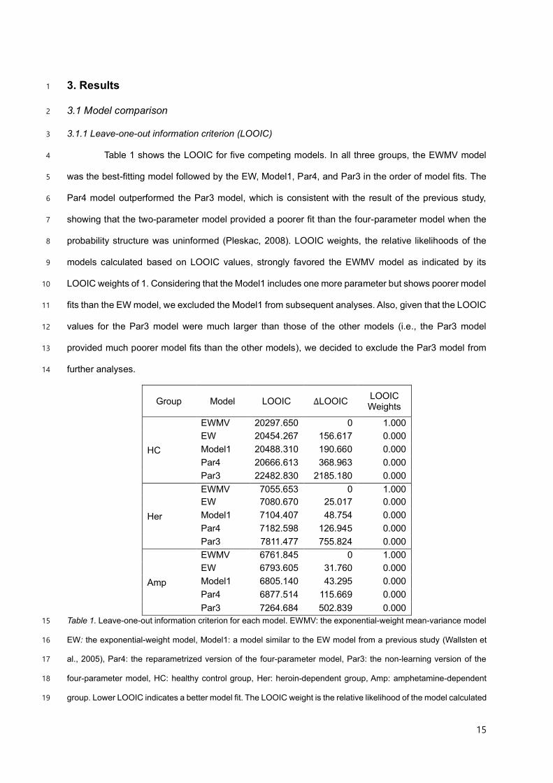
3.1.1 Leave-one-out information criterion (LOOIC) 3

Table 1 shows the LOOIC for five competing models. In all three groups, the EWMV model 4

was the best-fitting model followed by the EW, Model1, Par4, and Par3 in the order of model fits. The 5

Par4 model outperformed the Par3 model, which is consistent with the result of the previous study, 6

showing that the two-parameter model provided a poorer fit than the four-parameter model when the 7

probability structure was uninformed (Pleskac, 2008). LOOIC weights, the relative likelihoods of the 8

models calculated based on LOOIC values, strongly favored the EWMV model as indicated by its 9

LOOIC weights of 1. Considering that the Model1 includes one more parameter but shows poorer model 10

fits than the EW model, we excluded the Model1 from subsequent analyses. Also, given that the LOOIC 11

values for the Par3 model were much larger than those of the other models (i.e., the Par3 model 12

provided much poorer model fits than the other models), we decided to exclude the Par3 model from 13

further analyses. 14

Group Model LOOIC ΔLOOIC LOOIC Weights

HC

EWMV 20297.650 0 1.000

EW 20454.267 156.617 0.000

Model1 20488.310 190.660 0.000

Par4 20666.613 368.963 0.000

Par3 22482.830 2185.180 0.000

Her

EWMV 7055.653 0 1.000

EW 7080.670 25.017 0.000

Model1 7104.407 48.754 0.000

Par4 7182.598 126.945 0.000

Par3 7811.477 755.824 0.000

Amp

EWMV 6761.845 0 1.000

EW 6793.605 31.760 0.000

Model1 6805.140 43.295 0.000

Par4 6877.514 115.669 0.000

Par3 7264.684 502.839 0.000

Table 1. Leave-one-out information criterion for each model. EWMV: the exponential-weight mean-variance model 15

EW: the exponential-weight model, Model1: a model similar to the EW model from a previous study (Wallsten et 16

al., 2005), Par4: the reparametrized version of the four-parameter model, Par3: the non-learning version of the 17

four-parameter model, HC: healthy control group, Her: heroin-dependent group, Amp: amphetamine-dependent 18

group. Lower LOOIC indicates a better model fit. The LOOIC weight is the relative likelihood of the model calculated 19

16

based on its LOOIC. 1

2

3.1.2 Parameter recovery 3

We evaluated the quality of parameter recovery as the correlation between the true and 4

estimated values. Also, we considered the regression coefficients to characterize the degree of 5

associations and biases. In the main text, we report the parameter recovery results from the healthy 6

control group. The parameter recovery results from the heroin- and amphetamine-dependent groups 7

are reported in the supplementary material (Figures S5-S10) and are not qualitatively different from the 8

those from the healthy control group. 9

Figure 1 shows the results of parameter recovery from the healthy control group for the Par4 10

model. As shown in Figure 1, overall all parameters were relatively well recovered in the Par4 model 11

including the prior belief of success (𝝓) and the updating coefficient (𝜼), which were not well recovered 12

and systematically overestimated in the previous studies (Heathcote et al., 2015; van Ravenzwaaij et 13

al., 2011). This suggests that our reparameterization may have improved the parameter recovery 14

performance by separating the roles of the two parameters. To directly compare the parameter recovery 15

of the four-parameter model and the Par4 model, we attempted to recover the parameters of the four-16

parameter model, but the parameters of the original four-parameter model failed to converge even after 17

many (e.g., 4000) burn-in samples. We suggest two possible reasons underlying the failure. First, given 18

that the magnitudes of 𝜶 and 𝝁 commonly indicate the degree of learning from observations, the high 19

correlation between the two parameters might make the sampling process fail to work well even with 20

HMC. Second, the constraint that 𝝁 is always larger than 𝜶 may cause issues in the sampling process. 21

Figure 2 shows the results of parameter recovery from the healthy control group for the EW 22

model. The EW model showed poorer parameter recovery performance than the Par4 model in two 23

aspects. First, the risk preference (𝝆, EW model) exhibited relatively weak recovery compared to the 24

risk-taking propensity (𝜸, Par4 model). Second, for the loss aversion (𝝀, EW model), the estimated 25

values were shrunk towards the mean value. This shrinkage effect indicates that the model parameter 26

might not be accurately estimated from the information the data contain. Figures S7 and S8 show that 27

the loss-aversion ( 𝝀 , EW model) was also not recovered well from the heroin-dependent and 28

amphetamine-dependent groups, which is consistent with the recovery results from the healthy control 29

group. 30

17

Figure 3 shows the results of parameter recovery from the healthy control group for the EWMV 1

model. Most parameters, except for the risk preference (𝜌, EWMV model), showed good parameter 2

recovery, including the loss aversion parameter (𝜆, EWMV model), which was not recovered well for 3

the EW model. For the risk preference (𝜌, EWMV model), the regression line reveals that the estimated 4

values were slightly shrunk towards the mean value. Although the risk preference (𝜌, EWMV model) 5

was not recovered well, considering the EWMV model includes one more parameter than the Par4 6

model (i.e., the EWMV model is more complex than the Par4 model), we decided to scrutinize the 7

parameter recovery more to accurately compare the parameter recovery performances of the EWMV 8

and Par4 models. 9

The parameter recovery results for the prior belief and updating rate provide support for the 10

EWMV model. For the Par4 model, some parameter values of the prior belief of success (𝜙) and the 11

updating coefficient (𝜂) deviated from the diagonal in all three groups (Figures 1, S5, and S6). Notably, 12

the updating coefficient (𝜂) showed poor parameter recovery when we used the mean and standard 13

deviation estimated from the amphetamine-dependent group (Figure S6). In contrast, for the EWMV 14

model, most parameter values of the prior belief of burst (𝜓) and the updating exponent (𝜉) were well 15

recovered (Figures 3, S9, and S10). Considering the LOOIC and parameter recovery results, we 16

selected the EWMV model as the winning model and compared it with the Par4 model in further 17

analyses. 18

19

20

Figure 1. Parameter recovery results for the reparametrized version of the four-parameter model (Par4 model). 21

The red lines denote 𝒚 = 𝒙. The blue lines indicate the regression lines of each graph. Shaded regions indicate 22

95% confidence intervals. The correlation and regression coefficients of each scatter plot is as follows [correlation, 23

slope, intercept]. 𝝓 (prior belief of success): [0.605, 0.896, 0.102], 𝜼 (updating coefficient): [0.702, 0.991, 0.003], 24

𝜸 (risk-taking propensity): [0.918, 0.903, 0.079], 𝝉 (inverse temperature): [0.882, 0.878, 0.034]. The average of 25

the correlation coefficients is 0.777. 26

0.96

0.97

0.98

0.99

1.00

0.96 0.97 0.98 0.99 1.00

ftrue (Prior belief of success)

fp

red (

Pri

or

be

lief

of

su

cce

ss)

0.00

0.02

0.04

0.06

0.08

0.00 0.02 0.04 0.06 0.08

htrue (Updating coefficient)

hpre

d (

Upd

atin

g c

oe

ffic

ien

t)

0.0

0.5

1.0

1.5

2.0

0.0 0.5 1.0 1.5 2.0

gtrue (Risk−taking propensity)

g pre

d (

Ris

k−

takin

g p

rop

ensity)

0.0

0.2

0.4

0.6

0.0 0.2 0.4 0.6

ttrue (Inverse temperature)

t pre

d (

Inve

rse t

em

pe

ratu

re)

18

1

2 Figure 2. Parameter recovery results for the exponential-weight model (EW model). The red lines denote 𝒚 = 𝒙. 3

The blue lines indicate the regression lines of each graph. Shaded regions indicate 95% confidence intervals. The 4

correlation and regression coefficients of each scatter plot is as follows [correlation, slope, intercept]. 𝝍 (prior 5

belief of burst): [0.818, 0.757, 0.003], 𝝃 (updating exponent): [0.764, 0.830, 0.005], 𝝆 (risk preference): [0.666, 6

0.811, 0.138], 𝝉 (inverse temperature): [0.913, 0.973, 0.522], 𝝀 (loss aversion): [0.694, 0.260, 3.350]. The 7

average of the correlation coefficients is 0.771. 8

9

10 Figure 3. Parameter recovery results for the exponential-weight mean-variance model (EWMV model). The red 11

lines denote 𝒚 = 𝒙 . The blue lines indicate the regression lines of each graph. Shaded regions indicate 95% 12

confidence intervals. The correlation and regression coefficients of each scatter plot is as follows [correlation, slope, 13

intercept]. 𝝍 (prior belief of burst): [0.847, 0.810, 0.003], 𝝃 (updating exponent): [0.798, 0.667, 0.005], 𝝆 (risk 14

preference): [0.746, 0.610, 0.000], 𝝉 (inverse temperature): [0.812, 0.870, 1.495], 𝝀 (loss aversion): [0.933, 0.860, 15

0.314]. The average of the correlation coefficients is 0.827. 16

17

3.1.3 Posterior prediction 18

We evaluated the posterior prediction performance of each model as a correlation between 19

the observed and simulated adjusted BART scores. For the goal, we estimated parameters for each 20

model from the observed data and generated simulation data by using the estimated parameters. 21

Then, we calculated the adjusted BART score from the simulation data and compared the simulated 22

score with the observed score for each participant. 23

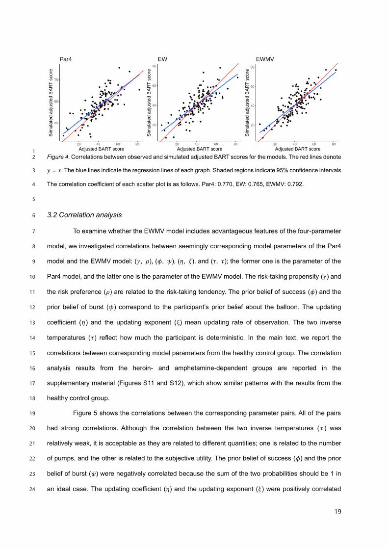
Figure 4 shows the correlations between observed and simulated adjusted BART scores for 24

the Par4, EW, and EWMV models. All models showed good predictive performance, and their 25

predictive performances are comparable. The regression lines display that the simulated values were 26

slightly shrunk towards the mean value. 27

28

0.00

0.01

0.02

0.03

0.00 0.01 0.02 0.03

ytrue (Prior belief of burst)

ypre

d (

Pri

or

belie

f o

f bu

rst)

0.00

0.01

0.02

0.03

0.04

0.05

0.00 0.01 0.02 0.03 0.04 0.05

xtrue (Updating exponent)

xpre

d (

Upd

atin

g e

xp

on

en

t)

0.4

0.6

0.8

1.0

0.4 0.6 0.8 1.0

rtrue (Risk preference)

rpre

d (

Ris

k p

refe

ren

ce

)

5

10

15

20

5 10 15 20

ttrue (Inverse temperature)

t pre

d (

Inve

rse t

em

pe

ratu

re)

2.5

5.0

7.5

10.0

2.5 5.0 7.5 10.0

ltrue (Loss aversion)

lpre

d (

Lo

ss a

ve

rsio

n)

0.00

0.01

0.02

0.03

0.04

0.00 0.01 0.02 0.03 0.04

ytrue (Prior belief of burst)

ypre

d (

Pri

or

belie

f o

f bu

rst)

0.00

0.01

0.02

0.03

0.04

0.00 0.01 0.02 0.03 0.04

xtrue (Updating exponent)

xpre

d (

Upd

atin

g e

xp

on

en

t)

−0.002

0.000

0.002

0.004

−0.002 0.000 0.002 0.004

rtrue (Risk preference)

rpre

d (

Ris

k p

refe

ren

ce

)

5

10

15

5 10 15

ttrue (Inverse temperature)

t pre

d (

Inve

rse t

em

pe

ratu

re)

0

2

4

6

0 2 4 6

ltrue (Loss aversion)

lpre

d (

Lo

ss a

ve

rsio

n)

19

1 Figure 4. Correlations between observed and simulated adjusted BART scores for the models. The red lines denote 2

𝑦 = 𝑥. The blue lines indicate the regression lines of each graph. Shaded regions indicate 95% confidence intervals. 3

The correlation coefficient of each scatter plot is as follows. Par4: 0.770, EW: 0.765, EWMV: 0.792. 4

5

3.2 Correlation analysis 6

To examine whether the EWMV model includes advantageous features of the four-parameter 7

model, we investigated correlations between seemingly corresponding model parameters of the Par4 8

model and the EWMV model: (𝛾, 𝜌), (𝜙, 𝜓), (𝜂, 𝜉), and (𝜏, 𝜏); the former one is the parameter of the 9

Par4 model, and the latter one is the parameter of the EWMV model. The risk-taking propensity (𝛾) and 10

the risk preference (𝜌) are related to the risk-taking tendency. The prior belief of success (𝜙) and the 11

prior belief of burst (𝜓 ) correspond to the participant’s prior belief about the balloon. The updating 12

coefficient (𝜂 ) and the updating exponent (ξ ) mean updating rate of observation. The two inverse 13

temperatures (𝜏 ) reflect how much the participant is deterministic. In the main text, we report the 14

correlations between corresponding model parameters from the healthy control group. The correlation 15

analysis results from the heroin- and amphetamine-dependent groups are reported in the 16

supplementary material (Figures S11 and S12), which show similar patterns with the results from the 17

healthy control group. 18

Figure 5 shows the correlations between the corresponding parameter pairs. All of the pairs 19

had strong correlations. Although the correlation between the two inverse temperatures ( 𝜏 ) was 20

relatively weak, it is acceptable as they are related to different quantities; one is related to the number 21

of pumps, and the other is related to the subjective utility. The prior belief of success (𝜙) and the prior 22

belief of burst (𝜓) were negatively correlated because the sum of the two probabilities should be 1 in 23

an ideal case. The updating coefficient (𝜂) and the updating exponent (𝜉) were positively correlated 24

25

50

75

20 40 60 80

Adjusted BART score

Sim

ula

ted

ad

juste

d B

AR

T s

co

re

Par4

20

40

60

80

20 40 60 80

Adjusted BART scoreS

imula

ted

ad

juste

d B

AR

T s

co

re

EW

20

40

60

80

20 40 60 80

Adjusted BART score

Sim

ula

ted

ad

juste

d B

AR

T s

co

re

EWMV

20

because both of them represent how rapidly the participant updates the belief based on past 1

experiences. Notably, the risk-taking propensity (𝛾) and the risk preference (𝜌) showed a strong positive 2

correlation, which implicates that, like the risk-taking propensity, the risk preference may reflect risk-3

taking tendency and be correlated with the frequencies of the past real-world risky behaviors. 4

5

6

Figure 5. Correlations between the corresponding parameter pairs of the models. The blue lines indicate the 7

regression lines of each graph. Shaded regions indicate 95% confidence intervals. 8

9

3.3 Group difference 10

As a way of evaluating the utility of the EWMV model, we applied the EWMV model to healthy 11

and substance-dependent populations (patients with past heroin or amphetamine dependence). We 12

analyzed the group differences of three groups (healthy control, heroin, and amphetamine-dependent 13

groups; see below for the details) for their behavioral performance and the parameter estimates of the 14

EWMV model (we also tested the Par4 model). 15

16

3.3.1 Behavioral Performance 17

The heroin-dependent group displayed a marginally lower adjusted BART score (95% HDI: [-18

9.73, 0.629], mean= -4.59; 95.9% of the posterior samples were smaller than 0) than the amphetamine-19

dependent group. The result suggests that heroin users might show lower risk-taking than amphetamine 20

users during the BART. See supplementary material for detailed information on the behavioral 21

performance and the group difference in behavioral performance (Figures S1 and S2). 22

23

3.3.2 Model Parameters 24

We estimated parameters of the EWMV model and the Par4 model for each group separately 25

−0.0025

0.0000

0.0025

0.0050

0.0 0.5 1.0 1.5 2.0

g (Risk−taking propensity, Par4)

r (

Ris

k p

refe

ren

ce

, E

WM

V)

r = 0.79(p<0.001)

Pearson's Correlation

5

10

15

20

25

0.0 0.5 1.0 1.5

t (Inverse temperature, Par4)

t (I

nve

rse

tem

pe

ratu

re,

EW

MV

)

r = 0.41(p<0.001)

Pearson's Correlation

0.00

0.02

0.04

0.06

0.96 0.97 0.98 0.99 1.00

f (Prior belief of success, Par4)y

(P

rio

r b

elie

f o

f bu

rst,

EW

MV

)

r = −0.83(p<0.001)

Pearson's Correlation

0.00

0.02

0.04

0.06

0.08

0.00 0.02 0.04 0.06

h (Updating coefficient, Par4)

x (

Upd

atin

g e

xp

on

en

t, E

WM

V)

r = 0.81(p<0.001)

Pearson's Correlation

21

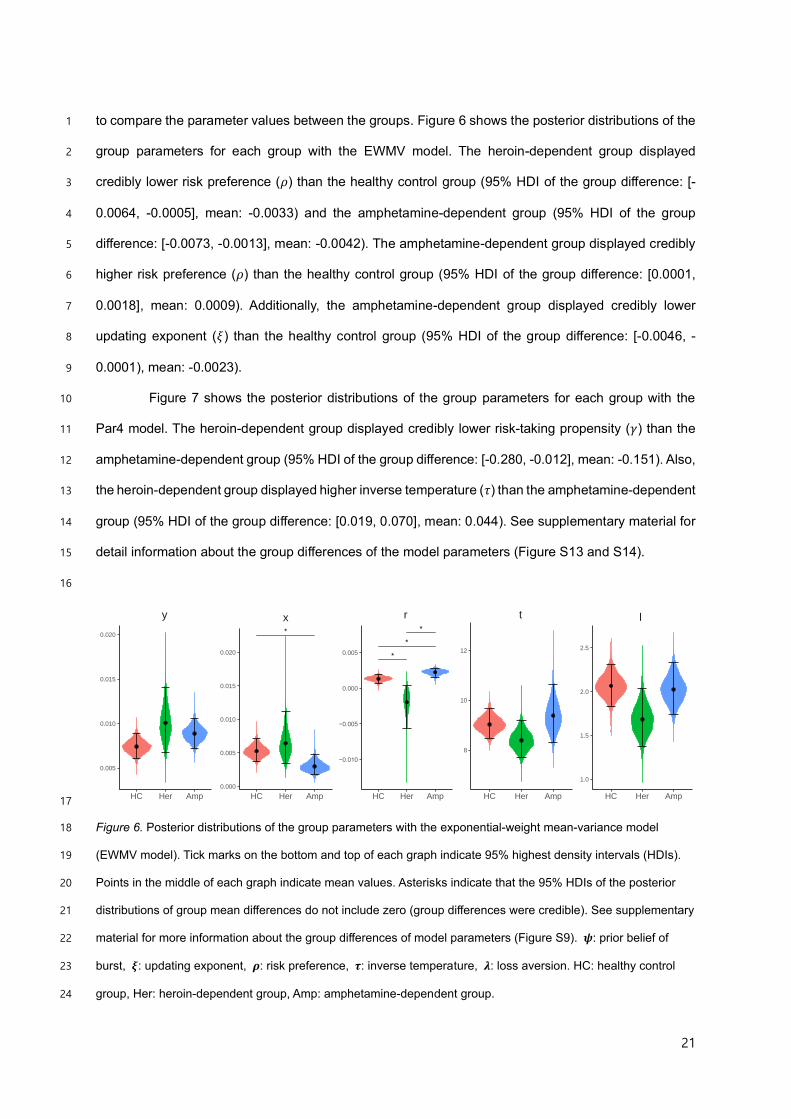
to compare the parameter values between the groups. Figure 6 shows the posterior distributions of the 1

group parameters for each group with the EWMV model. The heroin-dependent group displayed 2

credibly lower risk preference (𝜌) than the healthy control group (95% HDI of the group difference: [-3

0.0064, -0.0005], mean: -0.0033) and the amphetamine-dependent group (95% HDI of the group 4

difference: [-0.0073, -0.0013], mean: -0.0042). The amphetamine-dependent group displayed credibly 5

higher risk preference (𝜌) than the healthy control group (95% HDI of the group difference: [0.0001, 6

0.0018], mean: 0.0009). Additionally, the amphetamine-dependent group displayed credibly lower 7

updating exponent (𝜉) than the healthy control group (95% HDI of the group difference: [-0.0046, -8

0.0001), mean: -0.0023). 9

Figure 7 shows the posterior distributions of the group parameters for each group with the 10

Par4 model. The heroin-dependent group displayed credibly lower risk-taking propensity (𝛾) than the 11

amphetamine-dependent group (95% HDI of the group difference: [-0.280, -0.012], mean: -0.151). Also, 12

the heroin-dependent group displayed higher inverse temperature (𝜏) than the amphetamine-dependent 13

group (95% HDI of the group difference: [0.019, 0.070], mean: 0.044). See supplementary material for 14

detail information about the group differences of the model parameters (Figure S13 and S14). 15

16

17

Figure 6. Posterior distributions of the group parameters with the exponential-weight mean-variance model 18

(EWMV model). Tick marks on the bottom and top of each graph indicate 95% highest density intervals (HDIs). 19

Points in the middle of each graph indicate mean values. Asterisks indicate that the 95% HDIs of the posterior 20

distributions of group mean differences do not include zero (group differences were credible). See supplementary 21

material for more information about the group differences of model parameters (Figure S9). 𝝍: prior belief of 22

burst, 𝝃: updating exponent, 𝝆: risk preference, 𝝉: inverse temperature, 𝝀: loss aversion. HC: healthy control 23

group, Her: heroin-dependent group, Amp: amphetamine-dependent group. 24

y

HC Her Amp

0.005

0.010

0.015

0.020*

x

HC Her Amp

0.000

0.005

0.010

0.015

0.020

*

*

*

r

HC Her Amp

−0.010

−0.005

0.000

0.005

t

HC Her Amp

8

10

12

l

HC Her Amp

1.0

1.5

2.0

2.5

22

1

Figure 7. Posterior distributions of the group parameters with the reparametrized version of the four-parameter 2

model (Par4 model). Tick marks on the bottom and top of each graph indicate 95% highest density intervals (HDIs). 3

Points in the middle of each graph indicate mean values. Asterisks indicate that the 95% HDIs of the posterior 4

distributions of group mean differences do not include zero (group differences were credible). See supplementary 5

material for more information about the group differences of model parameters (Figure S10). 𝜙: prior belief of 6

success, 𝜂: updating coefficient, 𝛾: risk-taking propensity, 𝜏: inverse temperature. HC: healthy control group, Her: 7

heroin-dependent group, Amp: amphetamine-dependent group. 8

9

The results of the behavioral performance and the model parameters are consistent. Among 10

the three groups, the differences between the heroin-dependent and amphetamine-dependent groups 11

were the most noticeable. The heroin-dependent group displayed a marginally lower adjusted BART 12

score, lower risk preference (𝜌), and lower risk-taking propensity (𝛾) compared to the amphetamine-13

dependent group. These results consistently show that heroin users show lower risk-taking than 14

amphetamine users during the BART. 15

16

4. Discussion 17

The main focus of this study is on the development of a novel BART model that addresses the 18

limitations of existing models. We proposed a non-learning version of the four-parameter model (Par3 19

model) and a reparametrized version of the four-parameter model (Par4 model). By modifying equations 20

from the reparametrized version, we developed candidate models and selected the best model (EWMV 21

model) based on the leave-one-out information criterion (LOOIC) and the parameter recovery. The 22

model comparison results suggest that the EWMV model shows better prediction performance across 23

all populations than the other models and good parameter recovery. To examine whether the EWMV 24

f

HC Her Amp

0.9875

0.9900

0.9925

h

HC Her Amp

0.002

0.003

0.004

0.005

0.006

0.007 *

g

HC Her Amp

0.4

0.6

0.8

1.0 *

t

HC Her Amp

0.10

0.15

0.20

23

model includes advantageous features of the four-parameter model, we calculated the correlations 1

between corresponding parameter pairs for the Par4 and EWMV models. All of the corresponding 2

parameter pairs had strong correlations, which implies that the EWMV model may include 3

advantageous features of the four-parameter model. As a way of evaluating the utility of the EWMV 4

model, we analyzed differences among substance-using populations in behavioral performance and 5

model parameters of the Par4 and EWMV models. The group differences in behavioral performance 6

and model parameters of the Par4 and EWMV models were consistent. The results of the group 7

differences show that the EWMV model reveals group differences among the groups more clearly than 8

the behavioral performance and the Par4 model, and provides a measure of an additional core 9

psychological construct of risk-taking behavior. Overall, these results suggest that the EWMV model 10

has distinct merits as a computational model for the original BART paradigm. 11

An important finding of this study is that it suggests a way to improve parameter recovery. We 12

showed that reparametrizing parameters associated with more than one role into parameters with 13

unique roles might help the model recover accurate parameter values. Adequate parameter recovery 14

is a fundamental assumption and necessary for analyzing parameters of a computational model, and it 15

is noteworthy that we can improve parameter recovery by reparameterization alone. At the same time, 16

it is notable that the information criteria such as AIC, BIC, and LOOIC for the reparametrized version 17

and the original model are more or less the same. It suggests that the reparametrized version does not 18

have additional explanatory power compared with the original model. The results demonstrate that 19

parameter recovery and post hoc model fits measured with information criteria reflect different aspects 20

of computational models, and we need to use both methods for comprehensive evaluation. 21

Besides the superior prediction performance and good parameter recovery performance, the 22

EWMV model also has an advantage that it provides a more interpretable learning process: an agent 23

estimates the present value as a weighted average of the initial and observed value and updates the 24

weight and observed value as data accumulates. In addition, all parameters included in the EWMV 25

model have distinct and interpretable roles. Also, the EWMV model might be applicable to a wide range 26

of cognitive tasks other than the BART. The weight updating learning of the EWMV model is analogous 27

to the Kalman filter, an algorithm to track unknown state variables with uncertainty (Welch & Bishop, 28

1995). Because the weight updating learning model might be applicable to all situations that include 29

initial states and sequential observations, it might be an alternative to other well-established models to 30

24

quantify learning situations such as the Rescorla-Wagner model (Rescorla & Wagner, 1972). 1

Utilizing the mean-variance analysis (Markowitz, 1952) is another distinct feature of the EWMV 2

model. Previous studies, which compared the mean-variance analysis and the prospect theory 3

(Kahneman & Tversky, 2013), have suggested that their performances are comparable (Boorman & 4

Sallet, 2009; Hens & Mayer, 2014; Levy & Levy, 2004). However, only a few models (e.g., d'Acremont, 5

Lu, Li, Van der Linden, & Bechara, 2009) directly have utilized the mean-variance analysis to calculate 6

subjective utilities. 7

The group difference results show that the group differences in model parameters of the 8

EWMV model were consistent with the group differences in other indices, including the behavioral 9

performance and model parameters of the Par4 model. One seeming inconsistency is the results of the 10

inverse temperature parameters in the EWMV and Par4 models. For the EWMV model, all groups 11

displayed no credible group differences in the inverse temperature, whereas, for the Par4 model, the 12

heroin-dependent group displayed higher inverse temperature than the amphetamine-dependent group. 13

The reason for this discrepancy may be the two inverse temperatures are related to different quantities. 14

One is related to the subjective utility, whereas the other is related to the number of pumps. 15

Consequently, we did not consider this discrepancy as an inconsistency. The consistent group 16

difference result may indicate that the EWMV model appropriately reflects the participants’ risk-taking 17

tendencies in their behaviors. It is also consistent with the results of previous studies showing that 18

opiates (heroin) and stimulants (amphetamine) addictions are behaviorally and neurobiologically 19

distinct (Badiani, Belin, Epstein, Calu, & Shaham, 2011), related to different dopamine modulation 20

mechanisms (Kreek et al., 2012), and characterized by different personality and neurocognitive profiles 21

(Ahn & Vassileva, 2016). 22

Another key implication from the group difference results is that the model parameters of the 23

EWMV model reveal the group differences more clearly than the adjusted BART score and the model 24

parameters of the Par4 model. It is of note that the group difference results still remain valid after 25

considering the bias in the parameter recovery result of the risk preference for the EWMV model 26

because the similar biased patterns appear in all three groups. Namely, the EWMV model aligns better 27

with the clinical function of the BART, whose original purpose is to identify individuals who are prone to 28

take risks. This implies that the EWMV model may be potentially useful for classifying individuals into 29

several clinical groups and establishing quantitative diagnostic criteria for risk-taking behavior. 30

25

Providing a measure of loss aversion, which is a core psychological construct of risk-taking 1

behavior, is also advantageous to the EWMV model. Previous studies analyzing risk-taking behavior 2

have consistently shown that loss aversion plays a crucial role in risk-taking behavior, and many 3

computational models of experimental paradigms to investigate risk-taking tendency include 4

parameters of loss aversion (Ahn et al., 2008; Ahn et al., 2011; Sokol-Hessner et al., 2009; Worthy, 5

Pang, & Byrne, 2013). This feature makes the EWMV model comparable with the other computational 6

models that include loss aversion. 7

In conclusion, we proposed a novel model for the BART, called the exponential-weight mean-8

variance (EWMV) model, using the weight updating learning and the mean-variance analysis, which 9

addresses the limitations of existing models. The EWMV model outperformed other models in model 10

fits and parameter recovery performance. Also, its distinct merits come with a more interpretable 11

learning process, more salient group differences in model parameters between substance-dependent 12

populations, and the existence of loss aversion parameter. Not limited to the BART, we hope that the 13

weight updating learning model and the mean-variance analysis might apply to other cognitive tasks. 14

15

Declarations of interest: none 16

Acknowledgements 17

We thank the Seoul Science High School (SSHS) students for assistance in data analysis. 18

Also, we would like to thank all volunteers for their participation in this study. We express our gratitude 19

to Georgi Vasilev, Kiril Bozgunov, Elena Psederska, Dimitar Nedelchev, Rada Naslednikova, Ivaylo 20

Raynov, Emiliya Peneva, and Victoria Dobrojalieva for assistance with recruitment and testing of study 21

participants. The research reported in this publication was supported in part by the National Institute on 22

Drug Abuse and Fogarty International Center under award number R01DA021421 to J.V, and the Basic 23

Science Research Program through the National Research Foundation (NRF) of Korea funded by the 24

Ministry of Science, ICT, & Future Planning (NRF-2018R1C1B3007313 and NRF-2018R1A4A1025891) 25

to W.-Y.A., the Institute for Information & Communications Technology Planning & Evaluation (IITP) 26

grant funded by the Korea government (MSIT) (No. 2019-0-01367, BabyMind), and the Creative-27

Pioneering Researchers Program through Seoul National University to W.-Y.A. 28

29

26

References 1

Ahn, W. Y., Busemeyer, J. R., Wagenmakers, E. J., & Stout, J. C. (2008). Comparison of decision learning 2

models using the generalization criterion method. Cognitive science, 32(8), 1376-1402. 3

Ahn, W. Y., Dai, J., Vassileva, J., Busemeyer, J. R., & Stout, J. C. (2016). Computational modeling for 4

addiction medicine: from cognitive models to clinical applications. In Progress in brain 5

research (Vol. 224, pp. 53-65): Elsevier. 6

Ahn, W. Y., Haines, N., & Zhang, L. (2017). Revealing Neurocomputational Mechanisms of 7

Reinforcement Learning and Decision-Making With the hBayesDM Package. Comput 8

Psychiatr, 1, 24-57. doi:10.1162/CPSY_a_00002 9

Ahn, W. Y., Krawitz, A., Kim, W., Busemeyer, J. R., & Brown, J. W. (2011). A model-based fMRI analysis 10

with hierarchical Bayesian parameter estimation. Journal of Neuroscience, Psychology, and 11

Economics, 4(2), 95-110. doi:10.1037/a0020684 12

Ahn, W. Y., Vasilev, G., Lee, S.-H., Busemeyer, J. R., Kruschke, J. K., Bechara, A., & Vassileva, J. (2014). 13

Decision-making in stimulant and opiate addicts in protracted abstinence: evidence from 14

computational modeling with pure users. Frontiers in Psychology, 5, 849. 15

Ahn, W. Y., & Vassileva, J. (2016). Machine-learning identifies substance-specific behavioral markers 16

for opiate and stimulant dependence. Drug alcohol dependence, 161, 247-257. 17

Akaike, H. (1998). Information theory and an extension of the maximum likelihood principle. In 18

Selected papers of hirotugu akaike (pp. 199-213): Springer. 19

Aklin, W. M., Lejuez, C., Zvolensky, M. J., Kahler, C. W., & Gwadz, M. (2005). Evaluation of behavioral 20

measures of risk taking propensity with inner city adolescents. Behaviour research therapy, 21

43(2), 215-228. 22

Badiani, A., Belin, D., Epstein, D., Calu, D., & Shaham, Y. (2011). Opiate versus psychostimulant 23

addiction: the differences do matter. Nature reviews neuroscience, 12(11), 685. 24

Berger, J. O. (2013). Statistical decision theory and Bayesian analysis: Springer Science & Business 25

Media. 26

Boorman, E. D., & Sallet, J. (2009). Mean–variance or prospect theory? The nature of value 27

representations in the human brain. Journal of Neuroscience, 29(25), 7945-7947. 28

Busemeyer, J. R., & Stout, J. C. (2002). A contribution of cognitive decision models to clinical 29

assessment: decomposing performance on the Bechara gambling task. Psychological 30

assessment, 14(3), 253. 31

Carpenter, B., Gelman, A., Hoffman, M. D., Lee, D., Goodrich, B., Betancourt, M., . . . Riddell, A. (2017). 32

Stan: A probabilistic programming language. Journal of statistical software, 76(1). 33

d'Acremont, M., Lu, Z.-L., Li, X., Van der Linden, M., & Bechara, A. (2009). Neural correlates of risk 34

prediction error during reinforcement learning in humans. Neuroimage, 47(4), 1929-1939. 35

Daw, N. D., Gershman, S. J., Seymour, B., Dayan, P., & Dolan, R. J. (2011). Model-based influences on 36

humans' choices and striatal prediction errors. Neuron, 69(6), 1204-1215. 37

Frey, R., Pedroni, A., Mata, R., Rieskamp, J., & Hertwig, R. (2017). Risk preference shares the 38

psychometric structure of major psychological traits. Science advances, 3(10), e1701381. 39

27

Gelman, A., Carlin, J. B., Stern, H. S., & Rubin, D. B. (2004). Bayesian data analysis, 2nd edn. Texts in 1

Statistical Science. In: Boca Raton, London, NewYork, Washington DC: Chapman & Hall, CRC. 2

Gelman, A., & Rubin, D. B. (1992). Inference from iterative simulation using multiple sequences. 3

Statistical science, 7(4), 457-472. 4

Haines, N., Vassileva, J., & Ahn, W. Y. (2018). The Outcome‐Representation Learning Model: A Novel 5

Reinforcement Learning Model of the Iowa Gambling Task. Cognitive science, 42(8), 2534-6

2561. 7

Heathcote, A., Brown, S. D., & Wagenmakers, E.-J. (2015). An introduction to good practices in 8

cognitive modeling. In An introduction to model-based cognitive neuroscience (pp. 25-48): 9

Springer. 10

Hens, T., & Mayer, J. (2014). Cumulative prospect theory and mean variance analysis: a rigorous 11

comparison. Swiss Finance Institute Research Paper(14-23). 12

Hopko, D. R., Lejuez, C., Daughters, S. B., Aklin, W. M., Osborne, A., Simmons, B. L., & Strong, D. R. 13

(2006). Construct validity of the balloon analogue risk task (BART): Relationship with MDMA 14

use by inner-city drug users in residential treatment. Journal of Psychopathology and 15

Behavioral Assessment, 28(2), 95-101. 16

Kahneman, D., & Tversky, A. (2013). Prospect theory: An analysis of decision under risk. In Handbook 17

of the fundamentals of financial decision making: Part I (pp. 99-127): World Scientific. 18

Kreek, M. J., Levran, O., Reed, B., Schlussman, S. D., Zhou, Y., & Butelman, E. R. (2012). Opiate 19

addiction and cocaine addiction: underlying molecular neurobiology and genetics. The 20

Journal of clinical investigation, 122(10), 3387-3393. 21

Kruschke, J. K. (2013). Bayesian estimation supersedes the t test. Journal of Experimental Psychology: 22

General, 142(2), 573. 23

Lee, M. D. (2011). How cognitive modeling can benefit from hierarchical Bayesian models. Journal 24

of Mathematical Psychology, 55(1), 1-7. 25

Lejuez, C. W., Read, J. P., Kahler, C. W., Richards, J. B., Ramsey, S. E., Stuart, G. L., . . . Brown, R. A. 26

(2002). Evaluation of a behavioral measure of risk taking: The Balloon Analogue Risk Task 27

(BART). Journal of Experimental Psychology: Applied, 8(2), 75-84. doi:10.1037/1076-28

898x.8.2.75 29

Lejuez, C. W., Simmons, B. L., Aklin, W. M., Daughters, S. B., & Dvir, S. (2004). Risk-taking propensity 30

and risky sexual behavior of individuals in residential substance use treatment. Addictive 31

behaviors, 29(8), 1643-1647. 32

Levy, H., & Levy, M. (2004). Prospect theory and mean-variance analysis. Review of Financial Studies, 33

17(4), 1015-1041. 34

Link, W. A., & Eaton, M. J. (2012). On thinning of chains in MCMC. Methods in ecology and evolution, 35

3(1), 112-115. 36

Markowitz, H. (1952). Portfolio Selection. The Journal of Finance, 7(1), 77-91. doi:10.2307/2975974 37

Meredith, M., & Kruschke, J. K. (2018). Bayesian Estimation Supersedes the t-Test. 38

Papaspiliopoulos, O., Roberts, G. O., & Sköld, M. (2007). A general framework for the parametrization 39

28

of hierarchical models. Statistical science, 59-73. 1

Pleskac, T. J. (2008). Decision making and learning while taking sequential risks. Journal of 2

Experimental Psychology: Learning, Memory, and Cognition, 34(1), 167. 3

Ratcliff, R. (1978). A theory of memory retrieval. Psychological review, 85(2), 59. 4

Rescorla, R. A., & Wagner, A. R. (1972). A theory of Pavlovian conditioning: Variations in the 5

effectiveness of reinforcement and nonreinforcement. Classical conditioning II: Current 6

research theory, 2, 64-99. 7

Schwarz, G. (1978). Estimating the dimension of a model. The annals of statistics, 6(2), 461-464. 8

Sokol-Hessner, P., Hsu, M., Curley, N. G., Delgado, M. R., Camerer, C. F., & Phelps, E. A. (2009). 9

Thinking like a trader selectively reduces individuals' loss aversion. Proceedings of the 10

National Academy of Sciences, 106(13), 5035-5040. 11

van Ravenzwaaij, D., Dutilh, G., & Wagenmakers, E.-J. (2011). Cognitive model decomposition of the 12

BART: Assessment and application. Journal of Mathematical Psychology, 55(1), 94-105. 13

doi:10.1016/j.jmp.2010.08.010 14

van Ravenzwaaij, D., & Oberauer, K. (2009). How to use the diffusion model: Parameter recovery of 15

three methods: EZ, fast-dm, and DMAT. Journal of Mathematical Psychology, 53(6), 463-473. 16

Vehtari, A., Gelman, A., & Gabry, J. (2017). Practical Bayesian model evaluation using leave-one-out 17

cross-validation and WAIC. Statistics Computing, 27(5), 1413-1432. 18

Vehtari, A., Gelman, A., Simpson, D., Carpenter, B., & Bürkner, P.-C. (2019). Rank-normalization, folding, 19

and localization: An improved $\widehat {R} $ for assessing convergence of MCMC. arXiv 20

preprint arXiv:1903.08008. 21

Wagenmakers, E.-J., & Farrell, S. (2004). AIC model selection using Akaike weights. Psychonomic 22

bulletin & review, 11(1), 192-196. 23

Wagenmakers, E.-J., Van Der Maas, H. L., & Grasman, R. P. (2007). An EZ-diffusion model for response 24

time and accuracy. Psychonomic bulletin review, 14(1), 3-22. 25

Wallsten, T. S., Pleskac, T. J., & Lejuez, C. W. (2005). Modeling behavior in a clinically diagnostic 26

sequential risk-taking task. Psychol Rev, 112(4), 862-880. doi:10.1037/0033-295X.112.4.862 27

Welch, G., & Bishop, G. (1995). An introduction to the Kalman filter. In: Citeseer. 28

Worthy, D. A., & Maddox, W. T. (2014). A comparison model of reinforcement-learning and win-stay-29

lose-shift decision-making processes: A tribute to WK Estes. Journal of Mathematical 30

Psychology, 59, 41-49. 31

Worthy, D. A., Pang, B., & Byrne, K. A. (2013). Decomposing the roles of perseveration and expected 32

value representation in models of the Iowa gambling task. Frontiers in Psychology, 4, 640. 33

34