Development of a Dynamic Data-Driven Model for Effective ...

Take the steps...

Transportation Research

Research...Knowledge...Innovative Solutions!

2009-36

Responding to the Unexpected: Development of a

Dynamic Data-Driven Model for Effective Evacuation

Technical Report Documentation Page 1. Report No. 2. 3. Recipients Accession No. MN/RC 2009-36 4. Title and Subtitle 5. Report Date

Responding to the Unexpected: Development of a Dynamic Data-Driven Model for Effective Evacuation

December 2009 6.

7. Author(s) 8. Performing Organization Report No. Henry X. Liu and Saif Eddin Jabari 9. Performing Organization Name and Address 10. Project/Task/Work Unit No. Department of Civil Engineering University of Minnesota, Twin Cities 500 Pillsbury Drive, S.E. Minneapolis, MN 55455-0116

11. Contract (C) or Grant (G) No.

(c) 89261 (wo) 22

12. Sponsoring Organization Name and Address 13. Type of Report and Period Covered Minnesota Department of Transportation 395 John Ireland Boulevard, Mail Stop 330 Saint Paul, MN 55155-1899

Final Report 14. Sponsoring Agency Code

15. Supplementary Notes http://www.lrrb.org/pdf/200936.pdf 16. Abstract (Limit: 250 words) This research proposes a framework for real-time traffic management under emergency evacuation. A theoretical framework is first proposed for adaptive system control that involves control updating based on real-world traffic data. A heuristic solution framework is then developed to address the computation complexities that come with real-time computations of evacuee routing strategies that aim at minimizing total evacuee exposure time to harm. Further improvements to network traffic throughput are also considered by incorporating officer deployment strategies to critical network intersections. A genetic algorithms based solution scheme is proposed for the combined evacuee routing and officer deployment problem. An evacuation software tool is developed with embedded GIS capabilities that allows users to build evacuation scenarios and run the developed heuristic algorithms. Finally, the quality and efficiency of the developed solution techniques are demonstrated via hypothetical real-world size evacuation scenarios using the software tools.

17. Document Analysis/Descriptors 18. Availability Statement Traffic management, Evacuation, Emergency services, Adaptive Systems, Heuristic solutions, Dynamic system optimum, Police officer deployment

No restrictions. Document available from: National Technical Information Services, Springfield, Virginia 22161

19. Security Class (this report) 20. Security Class (this page) 21. No. of Pages 22. Price Unclassified Unclassified 129

RESPONDING TO THE UNEXPECTED: DEVELOPMENT OF A DYNAMIC DATA-DRIVEN MODEL FOR EFFECTIVE

EVACUATION

Final Report

Prepared by

Henry X. Liu Saif Eddin Jabari

Department of Civil Engineering

University of Minnesota, Twin Cities

December 2009

Published by

Minnesota Department of Transportation Research Services Section

395 John Ireland Boulevard, MS 330 St. Paul, MN 55155

This report represents the results of research conducted by the authors and does not necessarily represent the views or policies of the Minnesota Department of Transportation, the University of Minnesota, or the Department of Civil Engineering. This report does not contain a standard or specified technique. The authors, the Minnesota Department of Transportation, The University of Minnesota, and the Department of Civil Engineering do not endorse products or manufacturers. Trade or manufacturers’ names appear herein solely because they are considered essential to this report.

ACKNOWLEDGMENTS

This work was funded by the Minnesota Department of Transportation. The authors would like to thank Cory Johnson and Ernest Lloyd for their input and support throughout the project. We also wish to thank the members of the technical advisory committee: John Cavanaugh, Gary Fried, Charlie McCarty, and Daryl Taavola, for their valuable input and suggestions.

TABLE OF CONTENTS

CHAPTER 1: INTRODUCTION ................................................................................................... 1 1.1 Introduction and Background ........................................................................................... 1

1.1.1 Adaptive Control and Evacuation ............................................................................. 1

1.1.2 Computation Challenges ........................................................................................... 2

1.2 Problem Scope and Project Objectives ............................................................................ 2

1.2.1 Project Objectives ..................................................................................................... 3

1.2.2 Project Deliverables: ................................................................................................. 3

1.3 Organization of the Report ............................................................................................... 4

CHAPTER 2: ADAPTIVE CONTROL FRAMEWORK FOR EVACUATION .......................... 5 2.1 Introduction ...................................................................................................................... 5

2.2 Components of MRAC..................................................................................................... 6

2.3 The Prescriptive Short-Term Prediction Model ............................................................... 7

2.4 The Descriptive “Real-World” Model ............................................................................. 8

2.5 Model Reference Adaptive Control ................................................................................. 9

2.6 Numerical Example ........................................................................................................ 10

2.7 Concluding Remarks and Future Study ......................................................................... 11

CHAPTER 3: EVACUEE ROUTING: MODEL AND SOLUTION STRATEGY ..................... 13 3.1 Introduction .................................................................................................................... 13

3.2 DSO Model: Background and Description .................................................................... 14

3.3 Heuristic Solution Methodology .................................................................................... 15

3.3.1 Online and Offline Computations ........................................................................... 15

3.3.2 The Length of the Discrete Time Interval and Traffic Fidelity .............................. 16

3.4 Pre-Incident Computations ............................................................................................. 16

3.5 Post-Incident Computations: HASTE ............................................................................ 17


3.7 Concluding Remarks and Future Research .................................................................... 23

CHAPTER 4: THE DOWNTOWN MINNEAPOLIS NETWORK ............................................. 24 4.1 Introduction .................................................................................................................... 24

4.2 The Graph Theoretic Representation ............................................................................. 25

4.3 Downtown Minneapolis Network: Geometric Attributes .............................................. 26

4.4 Downtown Minneapolis Network: Traffic Flow Parameters ......................................... 29

4.5 Downtown Minneapolis Network: Signal Timing Parameters ...................................... 30

4.6 Discrete Representation of the Digraph as Cells ............................................................ 31

CHAPTER 5: SIGNALIZED INTERSECTION MODELING ................................................... 33 5.1 Introduction .................................................................................................................... 33

5.2 Traffic Flow Representation at Signalized Intersections ............................................... 33

5.3 Model and Solution Technique ...................................................................................... 36

5.3.1 Mathematical Model ............................................................................................... 36

5.3.2 Deployment Strategies as Combinations ................................................................ 36

5.3.3 Simple Genetic Algorithms ..................................................................................... 38

5.3.4 Chromosome Fitness and HASTE .......................................................................... 39


5.5 Concluding Remarks ...................................................................................................... 42

CHAPTER 6: SCENARIO TESTING.......................................................................................... 44 6.1 Introduction and Scenario Description ........................................................................... 44

6.2 Scenario Development ................................................................................................... 45

6.3 Evacuee Routing ............................................................................................................ 46

6.3.1 Arrivals to Safety: Solution Quality ....................................................................... 47

6.3.2 Computation Times: Solution Efficiency ............................................................... 48

6.3.3 Fidelity of Traffic Representation: Time Interval Lengths ..................................... 50

6.4 Officer Deployment ........................................................................................................ 52

CHAPTER 7: CONCLUSION AND RECOMMENDATIONS .................................................. 57 REFERENCES ............................................................................................................................. 58 APPENDIX A: HASTE: A HEURISTIC ALGORITHM FOR STAGED TRAFFIC EVACUATION

APPENDIX B: RESPONDING TO THE UNEXPECTED: A MODEL AND SOLUTION STRATEGY FOR COMBINED DYNAMIC EVACUEE ROUTING AND OFFICER DEPLOYMENT

APPENDIX C: EVACUATION SOFTWARE TOOL USER’S GUIDE AND TUTORIAL DATA

LIST OF FIGURES

Figure 1.1 Overall Emergency Evacuation Framework ................................................................. 3 Figure 2.1 Framework for Adaptive Control Based Real-Time Evacuation Traffic Management 5 Figure 2.2 Prescriptive DTA model ................................................................................................ 7 Figure 2.3 MRAC Model for Generating Traffic Control Strategies ............................................. 9 Figure 2.4 The Logan Test Network ............................................................................................. 10 Figure 2.5 Comparison of Total System Travel Time .................................................................. 11 Figure 3.1 Framework for Improving Computational Efficiency ................................................. 13 Figure 3.2 Heuristic Solution Strategies in Evacuation Traffic Assignment ................................ 16 Figure 3.3 Summary of HASTE Procedure .................................................................................. 19 Figure 3.4 Map of Disaster-Impacted Area .................................................................................. 19 Figure 3.5 Skeleton Network ........................................................................................................ 20 Figure 3.6 Original and Efficient Sub-Networks for a Particular Origin ..................................... 20 Figure 3.7 Evacuee Arrival Curves ............................................................................................... 22 Figure 4.1 Graph G = (V, E) ......................................................................................................... 25 Figure 4.2 Digraph D = (V, A) ..................................................................................................... 26 Figure 4.3 Layout of the Network ................................................................................................. 28 Figure 4.4 The Trapezoidal Flow-Density Relationship ............................................................... 29 Figure 4.5 Transforming Arcs into Cells ...................................................................................... 31 Figure 5.1 Graph Theoretic Representation of an Intersection ..................................................... 34 Figure 5.2 The Modified Intersection Representation .................................................................. 35 Figure 5.3 Intersection Gateway Cells .......................................................................................... 35 Figure 5.4 Example of Officer Deployment Combinations .......................................................... 37 Figure 5.5 All Possible Chromosomes for n = 4 and b = 2 ........................................................... 39 Figure 5.6 Layout of the Test Network ......................................................................................... 40 Figure 5.7 Evacuee Arrival Rate to Safety ................................................................................... 42 Figure 6.1 Scenario Area Layout and Demand Locations ............................................................ 44 Figure 6.2 Network Source Vertices ............................................................................................. 45 Figure 6.3 Network Sink Vertices ................................................................................................ 46 Figure 6.4 HASTE vs. AON Assignment ..................................................................................... 47 Figure 6.5 Evacuee Arrivals to Safety .......................................................................................... 48 Figure 6.6 Computation Time Comparison .................................................................................. 49 Figure 6.7 Network Clearance Rates for Different Time Interval Lengths .................................. 50 Figure 6.8 Clearance Time Improvements with Smaller Time Intervals ...................................... 51 Figure 6.9 Computation Time Increase with Smaller Time Intervals .......................................... 52 Figure 6.10 Genetic Algorithm Convergence ............................................................................... 53 Figure 6.11 Intersections Chosen for Officer Deployment ........................................................... 54 Figure 6.12 Network Clearance Times by Officer Budget ........................................................... 54 Figure 6.13 Arrival Rate Curves by Traffic Assignment Scenario ............................................... 55

LIST OF TABLES

Table 2.1 Clearance Times and Victim Vehicles .......................................................................... 11 Table 3.1 Problem Sizes by Traffic Fidelity Level ....................................................................... 21 Table 3.2 Comparing DSO Solutions, HASTE vs. CPLEX ......................................................... 21 Table 6.1 Network Clearance Times for Different Demand Levels ............................................. 48 Table 6.2 Network Clearance Times for Different Time Interval Lengths .................................. 50 Table 6.3 Network Clearance Time Comparisons ........................................................................ 55

EXECUTIVE SUMMARY

E.1 Introduction

Recent natural or man-made disasters around the world have provided compelling evidence that transportation systems play a crucial role in emergency evacuation and have stressed the need for effective evacuation traffic management to maximize the utilization of the transportation system and to minimize fatalities and losses. This research proposes a framework for real-time emergency evacuation management. As a first step, a theoretical framework for adaptive system control is proposed, which involves control updating based on real-world traffic data. Then, computation challenges are addressed by constructing a heuristic framework for real-time computations of evacuee routing strategies and intersection control via officer deployment.

E.2 Model Reference Adaptive Control (MRAC)

In contrast to well-studied evacuation planning practice, real-time traffic management for evacuation aims to dynamically guide (control) traffic flow under evacuation in such a way that a certain system objective (e.g. minimization of fatalities or property losses) could be achieved. The proposed framework is based on both dynamic network modeling techniques and adaptive control theory, by considering traffic networks under evacuation as dynamic systems. First, a prescriptive dynamic traffic assignment model is applied to predict, in a short-term and rolling-horizon manner, the desired traffic states based on a certain system optimal objective. This model will serve as a reference point for the adaptive control. Then, the adaptive control system integrates these desired states and the current prevailing traffic conditions collected via the sensing system to produce real-time traffic control schemes. Finally, these traffic control schemes are implemented in the field to guide the real-world traffic flow toward the desired states. Simulation studies provided in this research (Chapter 2) show that the proposed framework based on MRAC can significantly improve the performance of real-time evacuation traffic management.

E.3 Heuristic Framework for Evacuee Routing Computations

When responding to unanticipated emergency events, time is of the essence. At an operational level, optimal routing may change as traffic dynamics evolve over the course of the evacuation process. The ability to incorporate such changes, in real-time, may have a significant impact on reducing the time required to clear the disaster area and, hence, injury and fatality levels. This introduces time constraints for computation of optimal routing strategies. These computation time constraints are addressed by imposing computation time budgets as external constraints to determine dynamic system optimal routing. A heuristic solution algorithm, HASTE (heuristic algorithm for staged traffic evacuation), is proposed as an on-line (post-incident) computation

procedure along with a pre-incident calculations component. The post-incident component, HASTE, is a dynamic assignment procedure, while the pre-incident component creates efficient sub-networks to simplify the online dynamic shortest path search operations. A hypothetical evacuation scenario using a real-world network demonstrates the applicability of the proposed solution strategy (Chapter 3), which significantly enhances computational efficiency necessary for real-time evacuation management. Under this scenario, the heuristic framework is capable of producing results in less than one minute, compared to traditional solution procedures using LP solvers that required nearly four hours.

E.4 Officer Deployment Strategies

A good evacuee routing strategy is crucial during emergency evacuations. However, under emergency scenarios, signal timing plans optimized for regular traffic conditions could result in excessive delays. To overcome these delays, officers are typically deployed to signalized intersections to improve traffic throughput. But, particularly under a no-notice scenario, the number of officers that can be deployed is limited. To incorporate intersection control, our task consists of (i) determining a traffic flow representation scheme for signalized intersections that captures signal timing changes, (ii) extending the routing model to include officer deployment strategies, and (iii) development of an efficient solution strategy capable of producing high-quality solutions quickly, where a heuristic framework is developed for quick computation. This is of paramount importance under no-notice evacuations. The heuristic scheme uses genetic algorithms to generate officer deployment solutions, while the HASTE is used to approximate solution fitness. A numerical example demonstrates the quality of the heuristic framework compared to a solution using traditional techniques (Chapter 5). Computation times using the heuristic framework are also shown to be significantly smaller than those obtained using traditional methods.

E.5 Scenario Testing

An accurate graph-theoretic representation of a one-mile radius network centered in downtown Minneapolis is developed (Chapter 4) with the necessary traffic flow parameters for evacuation modeling purposes. Signal timing parameters based on the different settings used for different times of day are also integrated in the model. Then, a hypothesized emergency evacuation scenario is designed to test the tools and algorithms developed in this research (Chapter 6). The scenario involves evacuating vehicles in parking lots and parking ramps around the Hubert H. Humphrey Metrodome during the PM peak period. An area of roughly 0.75 square miles surrounding the Metrodome is used. Comparisons with all-or-nothing traffic assignment (all evacuees use the shortest path for their respective origins) are carried out with various officer budgets, illustrating the effectiveness of the proposed algorithms, both in terms of solution quality and solution efficiency (computation times). Additionally, various traffic flow fidelity levels and various demand levels are compared.

E.6 Publications

The work carried out under this project produced one journal article (Liu et. al. 2007), in addition to two research papers that were presented at the Transportation Research Board Annual Meetings in 2007 and 2009: (Liu et. al. 2007) and (Jabari et. al. 2009), respectively. The two papers are also included in Appendices A and B of this report. Additionally, the heuristic framework developed for evacuee routing computations culminated in a Master of Science (M.S.) thesis by Xiaozheng (Sean) He (He 2007).

1

CHAPTER 1: INTRODUCTION

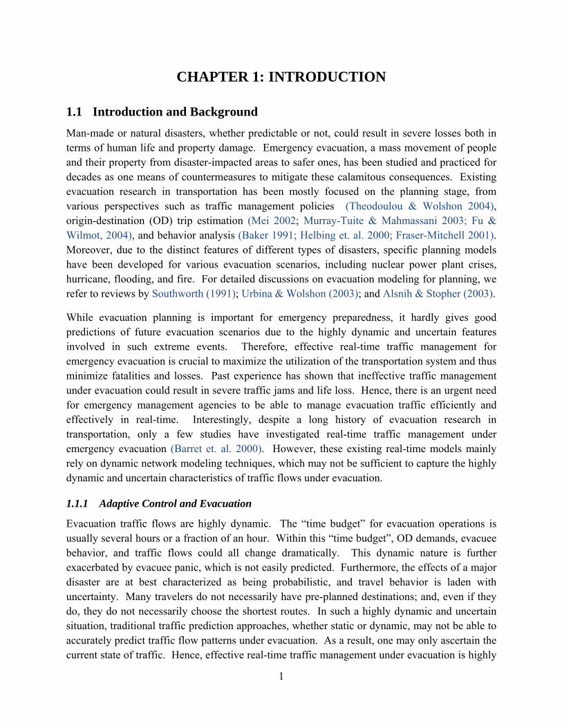
1.1 Introduction and Background Man-made or natural disasters, whether predictable or not, could result in severe losses both in terms of human life and property damage. Emergency evacuation, a mass movement of people and their property from disaster-impacted areas to safer ones, has been studied and practiced for decades as one means of countermeasures to mitigate these calamitous consequences. Existing evacuation research in transportation has been mostly focused on the planning stage, from various perspectives such as traffic management policies (Theodoulou & Wolshon 2004), origin-destination (OD) trip estimation (Mei 2002; Murray-Tuite & Mahmassani 2003; Fu & Wilmot, 2004), and behavior analysis (Baker 1991; Helbing et. al. 2000; Fraser-Mitchell 2001). Moreover, due to the distinct features of different types of disasters, specific planning models have been developed for various evacuation scenarios, including nuclear power plant crises, hurricane, flooding, and fire. For detailed discussions on evacuation modeling for planning, we refer to reviews by Southworth (1991); Urbina & Wolshon (2003); and Alsnih & Stopher (2003).

While evacuation planning is important for emergency preparedness, it hardly gives good predictions of future evacuation scenarios due to the highly dynamic and uncertain features involved in such extreme events. Therefore, effective real-time traffic management for emergency evacuation is crucial to maximize the utilization of the transportation system and thus minimize fatalities and losses. Past experience has shown that ineffective traffic management under evacuation could result in severe traffic jams and life loss. Hence, there is an urgent need for emergency management agencies to be able to manage evacuation traffic efficiently and effectively in real-time. Interestingly, despite a long history of evacuation research in transportation, only a few studies have investigated real-time traffic management under emergency evacuation (Barret et. al. 2000). However, these existing real-time models mainly rely on dynamic network modeling techniques, which may not be sufficient to capture the highly dynamic and uncertain characteristics of traffic flows under evacuation.

1.1.1 Adaptive Control and Evacuation

Evacuation traffic flows are highly dynamic. The “time budget” for evacuation operations is usually several hours or a fraction of an hour. Within this “time budget”, OD demands, evacuee behavior, and traffic flows could all change dramatically. This dynamic nature is further exacerbated by evacuee panic, which is not easily predicted. Furthermore, the effects of a major disaster are at best characterized as being probabilistic, and travel behavior is laden with uncertainty. Many travelers do not necessarily have pre-planned destinations; and, even if they do, they do not necessarily choose the shortest routes. In such a highly dynamic and uncertain situation, traditional traffic prediction approaches, whether static or dynamic, may not be able to accurately predict traffic flow patterns under evacuation. As a result, one may only ascertain the current state of traffic. Hence, effective real-time traffic management under evacuation is highly

2

dependent on the current traffic states and thus must be traffic adaptive. This motivates the application of adaptive control theory (Astrom & Wittermark 1995) to study traffic management under evacuation. The control based approach is actually more desirable since, compared to normal conditions, evacuation is usually a mandatory process and evacuees are more willing to follow guidance from officials (Fu & Wilmot 2004).

1.1.2 Computation Challenges

An efficient prescriptive dynamic traffic assignment model is critical for effective traffic management under emergency evacuation. Although a number of dynamic traffic assignment models have been proposed in previous studies (Li et. al. 1999; Ziliaskopoulos 2000), it is almost impossible to apply them for real-time emergency traffic management due to high computational cost. However, for emergency traffic management, particularly under no-notice evacuation, computational efficiency becomes essential while a reasonably detailed representation of traffic flow dynamics has to be maintained. By assuming that all evacuees have only one destination (the safe area), a prescriptive model may be established as a many-to-one dynamic system optimal problem. Here, a heuristic solution framework that can provide high-quality (near-optimal) solutions quickly is needed. The solution strategy should be able to provide evacuee routing strategies within seconds to only a few minutes for the results to be useful in a real-world evacuation process. It should also be termination-friendly. In other words, intermediate solutions should be useful, in contrast to traditional solution techniques.

1.2 Problem Scope and Project Objectives In this research, the main aim is to strike a balance between the level of fidelity of traffic flow representation in modeling evacuation traffic flows and the computational complexities that come with it. The emergency scenarios in question can be characterized as: (i) scenarios with spatial extents that are relatively small in scale (e.g., a one-mile diameter centered in a critical location, such as a central business district); and (ii) scenarios that are unanticipated in nature (i.e., no-notice emergency evacuations). While pedestrian evacuation strategies could play an important role in such scenarios (Helbing et. al. 2000), this research will focus on vehicular traffic. In particular, two issues will be addresses in the context of minimizing evacuee exposure to harm: (i) evacuee routing to safety in the evacuation road network, and (ii) officer deployment strategies that aim at improving network throughput. The overall framework is illustrated in Figure 1.1 below.

3

Figure 1.1 Overall Emergency Evacuation Framework

The small-scale nature of the evacuation scenarios brings with it little luxury in terms of abstracting traffic flow details; queue build-up, spill-over, and dissipation phenomena cannot be ignored, which brings about computational challenges. This research will, thus, provide efficient solution algorithms that maintain a reasonable level of traffic flow details, which serve as crucial components of the overall framework for real-time emergency evacuation shown in Figure 1.1, enabling rapid on-line computation and updating as the evacuation process proceeds. The following lists the project objectives and deliverables.

1.2.1 Project Objectives

1. To develop a theoretical framework for real-time adaptive evacuation traffic management. 2. To develop a system optimal prescriptive reference model. 3. To construct an efficient solution algorithm for the reference model. 4. To prepare an accurate graph-theoretic representation of the downtown Minneapolis network. 5. To develop an appropriate model-based traffic representation of signalized intersections. 6. To model intersection control optimization via placement of limited numbers of police

officers to guide traffic at critical network locations. 7. To construct a solution technique to obtain officer deployment strategies.

1.2.2 Project Deliverables:

1. A decision support software tool for emergency evacuation traffic management. In Figure 1.1, this tool will constitute: (i) static input: a GIS based traffic network centered in downtown Minneapolis with an approximate diameter of two miles that serves as a prototype system for algorithm testing; (ii) models: a graphical user interface that enables users to

4

interface with the developed models for evacuee routing calculations and officer deployment and officer deployment strategies; and (iii) output: graphical displays in the tool window and file based outputs.

2. A final report detailing the work carried out in this project, scenario testing results, a step-by-step user guide for the software tool, and research papers published and presented at the Transportation Research Board Annual Meetings.

3. Electronic input files for the scenarios tested in Chapter 6.

1.3 Organization of the Report In Chapter 2, a general theoretical framework for adaptive control is presented. The framework consists of three components: (i) a prescriptive short-term prediction model, (ii) a descriptive real-world model, and (iii) a model reference adaptive control component that uses output from the first two components to provide guidance in a real-time fashion. The theoretical framework is tested using microscopic traffic simulation and shown to work well compared to a typical driver route choice scheme.

Chapter 3 presents the evacuee routing model and solution strategy developed. A heuristic framework is proposed to help with real-time computations and a discussion of the fidelity of traffic flow representation in the model is given. Comparisons with traditional solution approaches are also presented.

Chapter 4 resents the graph-theoretic network modeling paradigm adopted for the downtown Minneapolis network along with the main traffic flow attributes needed as input by the model. Chapter 5 develops the necessary components needed to model signalized intersections in the network and presents the officer deployment algorithm along with numerical computations aimed at illustrating the quality and solution efficiency of the proposed algorithms. Finally, Chapter 6 presents scenario tests using the software tools developed in the project and Chapter 7 concludes this report.

Mathematical details of the algorithms are not included in the body of the report. Instead, Appendices A, B, and C include the research papers produced in this work and cover, respectively, the mathematical details of the models presented in Chapters 2, 3, and 5.

5

CHAPTER 2: ADAPTIVE CONTROL FRAMEWORK FOR EVACUATION

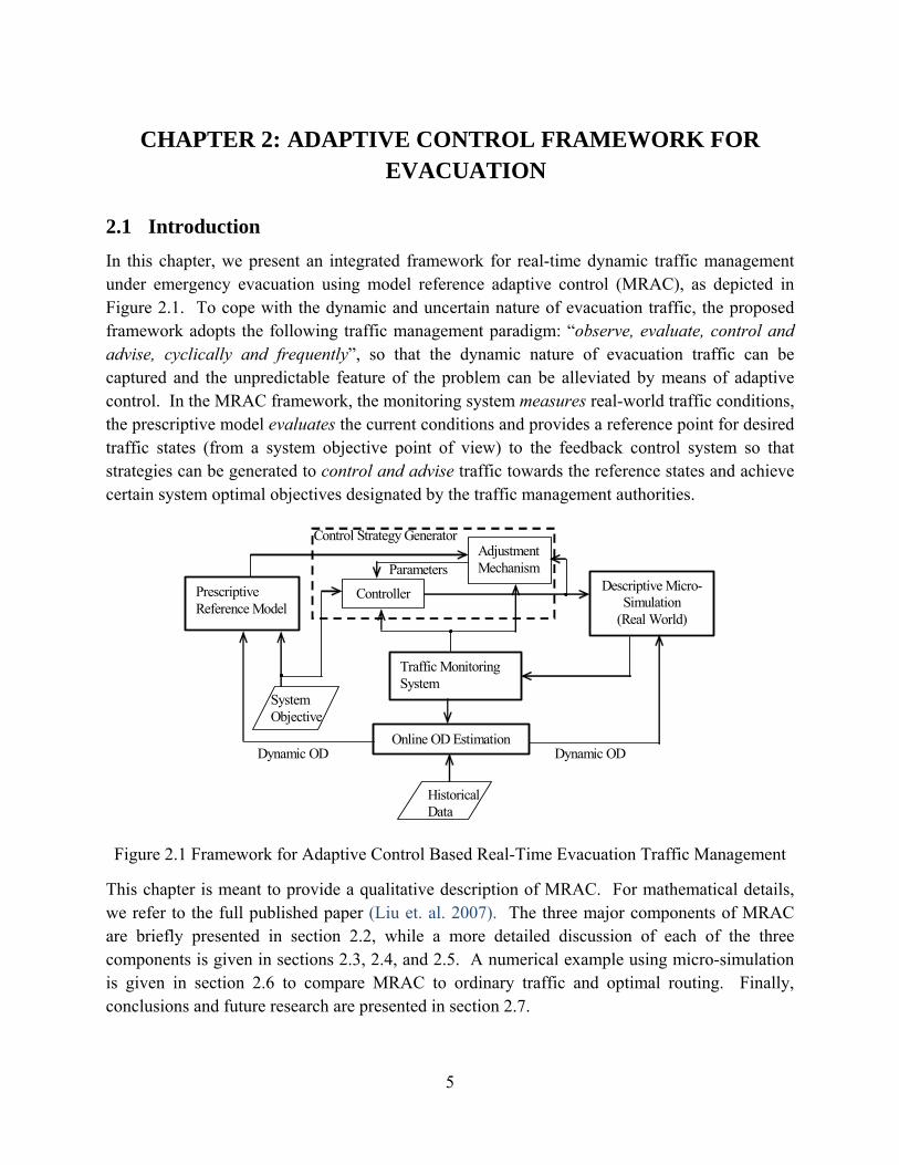
2.1 Introduction In this chapter, we present an integrated framework for real-time dynamic traffic management under emergency evacuation using model reference adaptive control (MRAC), as depicted in Figure 2.1. To cope with the dynamic and uncertain nature of evacuation traffic, the proposed framework adopts the following traffic management paradigm: “observe, evaluate, control and advise, cyclically and frequently”, so that the dynamic nature of evacuation traffic can be captured and the unpredictable feature of the problem can be alleviated by means of adaptive control. In the MRAC framework, the monitoring system measures real-world traffic conditions, the prescriptive model evaluates the current conditions and provides a reference point for desired traffic states (from a system objective point of view) to the feedback control system so that strategies can be generated to control and advise traffic towards the reference states and achieve certain system optimal objectives designated by the traffic management authorities.

Prescriptive Reference Model

Adjustment Mechanism

Controller Descriptive Micro-Simulation

(Real World)

Traffic Monitoring System

Online OD Estimation

Historical Data

Control Strategy Generator

Dynamic OD

System Objective

Parameters

Dynamic OD

Figure 2.1 Framework for Adaptive Control Based Real-Time Evacuation Traffic Management

This chapter is meant to provide a qualitative description of MRAC. For mathematical details, we refer to the full published paper (Liu et. al. 2007). The three major components of MRAC are briefly presented in section 2.2, while a more detailed discussion of each of the three components is given in sections 2.3, 2.4, and 2.5. A numerical example using micro-simulation is given in section 2.6 to compare MRAC to ordinary traffic and optimal routing. Finally, conclusions and future research are presented in section 2.7.

6

2.2 Components of MRAC The proposed adaptive control procedure is carried out cyclically and frequently, in a rolling horizon fashion. This framework is in contrast to traditional evacuation models which only include descriptive traffic assignment or simulation to test fixed evacuation plans (Moeller et. al. 1981; Cova & Johnson 2003; and Yuan & Han 2004). In particular, the MRAC framework comprises:

1. The “prescriptive short-term prediction” model, i.e., reference model, to produce simultaneously the target or desired traffic states and perfect control to achieve such states. This reference model represents the desired response of traffic under evacuation, based on a system objective designated by the traffic management authorities. Since under highly uncertain and panicky driver-behavior, only short-term traffic forecasting is treated as being reliable enough, but that is all that is needed for a closed-loop feedback control approach.

2. The “descriptive real-world” model which will adopt the control strategy (instead of a fixed “plan”) for evacuation; by strategy what is meant is a real-time traffic assignment procedure that provides, cyclically and frequently, a set of routes and traffic control advisories based on feedback of most up-to-date observed traffic states. We propose to use a microscopic traffic simulation model as a representation of “real-world” for the testing and evaluation of this framework.

3. The design of the feedback control system is based on the difference between desired traffic states and the reference model and current prevailing traffic states. For MRAC, the adaptation law searches for parameters such that the response of the plant (real-world traffic flow) under adaptive control matches that of the reference model, i.e., the objective of the adaptation is to get the tracking error to converge to zero.

Although these three models are key components of the MRAC framework, dynamic OD estimation and resource allocation are also important issues. Current state-of-the-art approaches for OD estimation under evacuation heavily depend on historical data and the behavior analysis of evacuees. Usually, the estimation includes two steps (Mei 2002): the total evacuation demand estimation and the dynamic OD matrix generation. The first step uses the so-called “participation rate” which is based on survey data from past evacuations (Wilmot & Mei 2003), while a loading curve is normally applied for the second step to generate dynamic OD data based on behavior analysis of past experience (Tweedie et. al. 1986; Lewis 1985). In this chapter, we will adopt this two step procedure. However, how to update the OD estimates online during the evacuation process based on prevailing traffic states is left for future research.

Here, we will assume that traffic sensing and control devices can cover all locations “perfect sensing and control”. When the number of devices, such as changeable message signs or traffic officers, is limited, then the logistical issues of where and how many devices should be deployed become paramount. In fact, the manner in which these devices are deployed is part of the traffic

7

management strategy utilized, and should be included in the design of the control system. This issue is studied in later chapters.

2.3 The Prescriptive Short-Term Prediction Model In this section, we will depict the prescriptive short term prediction model which generates the desired traffic states, e.g. traffic inflows and splitting rates, based on the system objective given by the traffic management authorities. As shown in Figure 2.2, the prescriptive model is a short-term one and implemented in a rolling horizon manner (Peeta & Mahmassani 1995). At the start of each horizon, the planned control strategies and dynamic OD demands are fixed temporarily using the latest estimated ones. Then the system objective is used to derive the route choice condition from which the dynamic route flows can be computed. These route flows are fed into the traffic flow model and the time-dependent in-link flows are finally generated. During an evacuation, the primary goal is that of moving evacuees to safer areas rather than specific destinations. Therefore, the “super zone” concept can be applied in which all the evacuation destination zones are connected to a single “super destination zone”.

Route Choice Condition

Traffic Flow Model

System Objective

Dynamic OD

Planned Control Strtegies

Converges?

No

Yes

Control Strategy

Generator

Figure 2.2 Prescriptive DTA model

The most distinctive feature of the prescriptive reference model from a network-wide perspective is that arc capacities can no longer be assumed fixed and known exogenously, but become endogenous, as they clearly depend on the amounts of green time assigned to the intersecting streets, and such amounts, in turn, depend on the intensity of the traffic flows using those streets. In the literature, attempts at integrating equilibrium traffic assignment and intersection control into a single modeling framework under the assumption of flow-responsive signal settings have resulted in a class of Combined Traffic Assignment and Control (CTAC) models. The work of (Allsop 1974) is commonly regarded as the pioneering contribution in this area and the reader is referred to (Meneguzzer 1997) for a more recent survey of studies on CTAC.

8

The prescriptive model is a special case of CTAC, but in a dynamic setting. Under emergency evacuation, the prescriptive model aims to produce the target or desired traffic states and to seek the traffic control to achieve such states simultaneously. In an extreme case, we can assume all intersections are controlled by traffic officers, and evacuees will follow their guidance. Then the problem becomes that of finding intersection green time splitting rates that achieve a certain objective (e.g., to minimize the network clearance time), which can be modeled using non-linear programming techniques.

2.4 The Descriptive “Real-World” Model The purpose of the descriptive “real-world” model is to describe, in a short-term fashion, the real-world dynamic traffic flow pattern under evacuation as accurately as possible. Due to the complexity of modeling traffic flows under evacuation, various aspects of evacuation modeling have been proposed and studied such as OD estimation, behavior analysis, contra flow management (Jenkins 2000; Tuydes & Ziliaskopoulos 2006; Lim & Wolshon 2005), and traffic network modeling (Barret et. al. 2000; Chiu et. al. 2005). Here, however, because of the highly unpredictable nature of evacuation traffic, we propose to use a microscopic traffic simulation model to implement the short-term traffic control strategy at the decision vertices based on the splitting rates. In particular, we adopt one of the commercial microscopic simulation models, PARAMICS (PARAllel MICroscopic Simulation), as our evaluation tool. PARAMICS is a scalable and high-performance microscopic traffic simulation package developed in Scotland (Smith et al. 1994). To implement the adaptive control strategies, the capabilities of PARAMICS have to be extended to enable its use. Particularly, a route choice model is developed based on the splitting rate (generated by the controller) at each intersection. This will be accomplished using the PARAMICS Application Programming Interface (API) library through which users could customize and extend many features of the underlying simulation model (Chu et. al. 2002).

Ideally, if traffic officers can be deployed at each intersection to guide the traffic under evacuation, the proposed descriptive model will be straightforward – traffic flows diverge at each intersection according to the designated splitting rate. This is the so-called “rigid control”. Then using the micro-simulation model, the actual traffic states can be represented. However, in reality, two issues invalidate such an ideal scenario. First, besides “rigid” control, there are many other “soft” traffic controls such as traffic advisory radio and changeable message signs, etc. We need to consider the compliance of evacuees towards these control strategies. This is because soft controls cannot strictly divert the traffic (according to the desired splitting rate) and thus a certain compliance rate has to be imposed. Therefore, issues related to driver compliance need to be investigated. The second issue is due to resource limitations: it is possible that control devices can only cover a portion of the network intersections, rather than all of them. This will raise a resource allocation problem (Ibaraki 1988); namely, under resource limitations, which device should be deployed at which intersection? Detailed discussions regarding compliance and resource allocation are left for future research.

9

2.5 Model Reference Adaptive Control The MRAC system produces real-time traffic control strategies (particularly, the splitting rate at each intersection), based on the difference between the desired traffic states from the prescriptive reference model and prevailing traffic states from the descriptive “real-world” model. For MRAC, the desired behavior of the system is specified by a reference model, and the parameters of the controller are adjusted based on the error, which is the difference between the outputs of the closed-loop system and the model. Therefore, the system has an ordinary feedback loop composed of the plant and the controller and another feedback loop that changes the controller parameters (Slotine & Li 1991).

In transportation, feedback control theories have already been applied in dynamic network modeling (Kachroo & Ozbay 1998 and 1999; Papageorgiou 1990; Hawas & Mahmassani 1995; Mammar et. al. 1996; Pavis & Papageorgiou 1999; Wang et. al. 2003). However, due to the fact that traffic flow under evacuation is highly dynamic and uncertain, the parameters for designing the feedback controller may not be determined easily and have to be adjusted accordingly in a timely manner. Therefore, in contrast to all previous studies, we explicitly introduce a prescriptive reference model, which represents the desired behavior of the system, to adjust the controller parameters dynamically and better guide traffic. The objective of the adaptation is to make the tracking error converge to zero.

As depicted in Figure 2.3, the two major components of an MRAC system are shown; namely, the ordinary feedback controller and the adjustment mechanism. The feedback error, which is the difference between the output of the system (i.e. arc inflows or splitting rates from the descriptive “real-world” model) and the output of the reference model (i.e. arc inflows or splitting rates from the prescriptive model), can be used for changing the parameters. The mechanism for adjusting the controller parameters for MRAC can be achieved in two ways: by using a gradient method (used here) or by applying the stability theory.

AdjustmentMechanism

Feedback Controller

Descriptive Model

Prescriptive Model Controller parameter θ

System Objective

Figure 2.3 MRAC Model for Generating Traffic Control Strategies

For details regarding the inner-workings of the MRAC framework, we refer to (Liu et. al. 2007).

10

2.6 Numerical Example To test the performance of the proposed adaptive control based evacuation framework, an example network was built based on a portion of traffic network of the City of Logan, UT, for the purpose of flooding evacuation. The micro-simulator we chose is the Paramics V5. The network shown in Figure 2.4 is a well calibrated network coded in Paramics.

Figure 2.4 The Logan Test Network

The network has 71 vertices and 148 arcs with six origin zones on the right and one super destination zone on the left. We assume the vehicles are safe once they arrive at the destination zone. One-hour demands with a 10 minutes warm-up period are assigned to the network to represent the demand pattern during evacuation.

To obtain the dynamic OD matrix, a two-step procedure is followed. First, the population distribution for the test area is obtained from the City of Logan. Based on this data, the total evacuation demand for each origin zone is estimated. Then, a departure curve is assumed in order to simulate the departure time choice of evacuees.

For comparison purposes, we utilize three performance measures: (i) the total system travel time, (ii) the network clearance time, and (iii) the number of victim vehicles, in our simplified framework implementation. The clearance time is the time for the last evacuee arrives to safety. The number of the victim vehicles represents the number of vehicles that are still present in the network after a certain time budget.

The performances of three scenarios are computed and compared. These scenarios include the dynamic system optimum (DSO), the MRAC control scheme, and stochastic route choice implemented in PARAMICS. The DSO is the best possible performance we can obtain in real-world evacuation. The MRAC scheme is the evacuation scenario resulting from our proposed control strategy, while the stochastic route choice represents the actual evacuation without the

11

proposed MRAC control. Figure 2.5 depicts a comparison of total travel time for the three scenarios. It is obvious from the figure that at the very beginning of the evacuation, the results of the MRAC scheme are far from the DSO. However, as the evacuation proceeds, the controller will guide the real-world evacuation process towards the DSO states; the MRAC and DSO curves get closer as illustrated in the figure. We can also see from the figure that, without adaptive control, the stochastic route choice scenario will be far away from DSO states throughout the entire evacuation process.

Total Travel Time Comparison

0

1000

2000

3000

4000

5000

6000

7000

8000

9000

0 1 2 3 4 5 6 7 8 9 10 11Roll Period

Min

utes

Stoch RoutingMRACDSO

Figure 2.5 Comparison of Total System Travel Time

Table 2.1 further shows the clearance times and number of victim vehicles for each scenario. Note that the time budget for computing the number of victim vehicles is set to 65 minutes, the clearance time of the DSO. It is obvious from this table that the proposed MRAC control scheme can generate shorter clearance times and less victim vehicles than traditional stochastic route choice. These preliminary testing results demonstrate the benefits of applying the MRAC control scheme in actual traffic management under emergency evacuation.

Table 2.1 Clearance Times and Victim Vehicles

DSO MRAC Stochastic Clearance Time (min) 65 84 92

Victim Vehicles 0 630 917

2.7 Concluding Remarks and Future Study In this chapter, a model reference adaptive control (MRAC) framework was proposed for real-time traffic management under emergency evacuation, with a prediction model to generate desired traffic states to achieve optimized system objectives, a real-world traffic model to simulate actual evacuation traffic flows, and an adaptive control model to produce actual traffic

12

control schemes. In contrast to previous planning models, the proposed framework aims to operate in a real-time, dynamic, and feedback based fashion so that current prevailing traffic states can be utilized to more effectively guide traffic under evacuation. Simulation studies showed that the proposed framework can significantly improve the performance of traffic management under evacuation.

For future study, a number of research directions can be identified based on the current framework and our simplified implementation. First, we assumed perfect and rigid control in the simplified framework. However, in reality, soft control devices are widely deployed, e.g. VMS, HAR, etc. The compliance rates of evacuees given these technologies remains a crucial and challenging question, particularly foe complicated traffic conditions under evacuation.

Secondly, this framework assumes that the dynamic OD demand matrix is given and fixed during the entire evacuation process. Due to highly dynamic features of evacuation, dynamic OD demands will very likely change as the evacuation process evolves. With the traffic monitoring and sensing system in place for the proposed MRAC framework, prevailing traffic information, especially real-time traffic volumes, is expected to be available during the evacuation process. Therefore, there is potential for dynamic updating of evacuation OD demands based on real-time traffic data.

Last but not least, the proposed framework is a unified one which can be applied for all evacuation scenarios. However, due to the distinctive characteristics of different types of evacuation, the proposed framework needs to be further tailored to better fit into various evacuation scenarios.

13

CHAPTER 3: EVACUEE ROUTING: MODEL AND SOLUTION STRATEGY

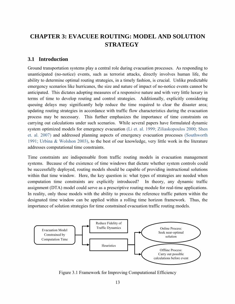
3.1 Introduction Ground transportation systems play a central role during evacuation processes. As responding to unanticipated (no-notice) events, such as terrorist attacks, directly involves human life, the ability to determine optimal routing strategies, in a timely fashion, is crucial. Unlike predictable emergency scenarios like hurricanes, the size and nature of impact of no-notice events cannot be anticipated. This dictates adopting measures of a responsive nature and with very little luxury in terms of time to develop routing and control strategies. Additionally, explicitly considering queuing delays may significantly help reduce the time required to clear the disaster area; updating routing strategies in accordance with traffic flow characteristics during the evacuation process may be necessary. This further emphasizes the importance of time constraints on carrying out calculations under such scenarios. While several papers have formulated dynamic system optimized models for emergency evacuation (Li et. al. 1999; Ziliaskopoulos 2000; Shen et. al. 2007) and addressed planning aspects of emergency evacuation processes (Southworth 1991; Urbina & Wolshon 2003), to the best of our knowledge, very little work in the literature addresses computational time constraints.

Time constraints are indispensable from traffic routing models in evacuation management systems. Because of the existence of time windows that dictate whether system controls could be successfully deployed, routing models should be capable of providing instructional solutions within that time window. Here, the key question is: what types of strategies are needed when computation time constraints are explicitly introduced? In theory, any dynamic traffic assignment (DTA) model could serve as a prescriptive routing module for real-time applications. In reality, only those models with the ability to process the reference traffic pattern within the designated time window can be applied within a rolling time horizon framework. Thus, the importance of solution strategies for time constrained evacuation traffic routing models.

Figure 3.1 Framework for Improving Computational Efficiency

Evacuation Model Constrained by

Computation Time

Reduce Fidelity of Traffic Dynamics

Heuristics

Online Process: Seek near-optimal

solution

Offline Process: Carry out possible

calculations before event

14

Figure 3.1 illustrates two general directions for determining dynamic system optimized (DSO) routing strategies that address time constraints. The first direction considers the tradeoff between computational speed and the fidelity of traffic flow representation. Since accurate traffic flow characteristics need to be captured in evacuation models, excessive fidelity reduction is not recommended. The second direction identifies potential computation time savings by means of improving solution procedures, where heuristics may be adopted in both online and offline processes.

In this chapter, we propose a heuristic approach for determining dynamic system optimized (DSO) routing that addresses time constraints that come with no-notice evacuation scenarios. The heuristic consists of two components, a pre-incident computations component and a post-incident computations component. Pre-incident calculations can serve as an offline process that stores sub-networks for use after the event takes place and reduces shortest path search operations carried out by the post-incident component. The post-incident component serves as an online process and determines routing strategies, which guarantees effective solutions within the time budget and allows for sufficient control deployment time. Another direction that could be employed to improve computation complexity is to reduce the fidelity of traffic flow representation.

The remainder of this chapter is organized as follows: section 3.2 describes the dynamic system optimum routing model used in this study. Section 3.3 introduces the heuristic solution framework used to overcome computation complexities of the DSO; sections 3.4 and 3.5, respectively, discuss in further detail the pre-incident and post-incident computation components of the proposed framework. Computation efficiency, solution quality, and other components of the proposed framework are illustrated by means of a numerical example in section 3.6. We close this chapter with concluding remarks and some potential future research directions in section 3.7.

3.2 DSO Model: Background and Description Because of the dynamic nature of evacuation routing problems and high demand levels on transportation infrastructure during evacuation, hence congestion, dynamic traffic assignment (DTA) models (Peeta & Ziliaskopoulos 2001) have found a niche in evacuation traffic management. The mathematical model adopted in this research is based on formulations proposed in Li et al. (1999) and Ziliaskopoulos (2000) for single destination based DSO, which adopts the cell transmission model (CTM) for traffic flow representation (Daganzo 1994 and 1995). Their linear programming DSO models divide the network into three specific types of cells: ordinary cells with one upstream cell and one downstream cell; diverging cells, which connect one upstream cell with multiple downstream cells; and merging cells having multiple upstream cells and one downstream cell. We refer to Appendix A for a detailed presentation of the mathematical model.

15

In addition to DSO based models, evacuation problems have been formulated using different approaches. For example, Miller-Hooks and Patterson (2004) formulated evacuation traffic as a dynamic earliest arrival flow problem, and Mahmassani and Sbayti (2005) proposed a formulation for dynamic capacity reallocation for evacuation.

Safe zones, to which evacuees are guided under evacuation operations, constitute any part of the network that lies outside of the disaster area. The safe area can, thus, be modeled as a single virtual super destination zone (Chiu et al. 2005), which simplifies the DSO model to a many-to-one problem as in Sheffi and Daganzo (1979). With this simplification, the first-in-first-out (FIFO) discipline is simply dependent on the departure time (or arrival time) as proven by Kuwahara and Akamatsu (1993) and Akamatsu (2000). Time-constrained optimization problems, optimization problems with computation time constraints, although popular in computer science literature (Wall et al. 1992; Mercer et al. 1994; Jones et al. 1996 and 1997; Nieh and Lam, 1997), have not received much attention in transportation literature for evacuation studies.

The objective in the adopted formulation aims to minimize the total system travel time, which was modified to allow for assigning varying weights to different network origins (sources or evacuee concentration locations). The body of the formulation includes flow conservation and flow restriction constraints imposed by the CTM. We also imposed an exogenous computation time budget constraint to allow for incremental results to be provided in online applications.

3.3 Heuristic Solution Methodology

3.3.1 Online and Offline Computations

Due to high computation costs that come with simplex based and interior point method based solutions, commercial LP solvers are undesirable. For this reason, we developed a heuristic approach to approximate a system optimal routing strategy. On one hand, we propose reasonable ways to reduce the problem size arising from the dynamic features of the time-constrained DSO model, so that the problem can be solved within the time budget. On the other hand, noticing that there is infinite computation time available for evacuation planning before the event takes place, heuristics can utilize this unlimited time budget to do preparation calculations that reduce the online process computation burden. Therefore, part of the computational cost in the DSO model can be transferred to some offline processes. This heuristic framework is illustrated in Figure 3.2

16

Figure 3.2 Heuristic Solution Strategies in Evacuation Traffic Assignment

3.3.2 The Length of the Discrete Time Interval and Traffic Fidelity

For a more detailed traffic dynamics representation, a shorter discrete time interval length may be used. This time interval length determines how often the traffic flow pattern is updated, the numbers of cells needed to represent the network flows, and the cell characteristics. In other words, a shorter time interval length provides more detailed traffic information but divides the network into more cells, which in turn results in larger problem sizes.

In addition to increasing the discrete time interval length, fidelity reduction may be achieved by combing multiple small cells into larger ones, i.e. adopting a variable-cell-length based CTM approach (Ziliaskopoulos & Lee 1997; Muñoz et al. 2004; Ishak et al. 2006; Liu et al., 2006).

3.4 Pre-Incident Computations One of the major computational components of the proposed heuristic framework is the shortest path search. Since the temporal dimension of the problem cannot be simplified, one approach to simplify the problem is by reducing the problem size spatially, or in other words to eliminate vertices (intersections) from the network that are not likely to be used by any of the shortest paths. For evacuation scenarios where structures to be evacuated are near the boundary of the safe area, arcs located in remote parts of the evacuation network will most likely not be included in any of the evacuation routes although they will be examined as part of the shortest path search. Hence, eliminating such arcs from the network for those particular sources may have a significant impact on computational efficiency. Here, the concept of an efficient sub-network may be utilized to improve computational efficiency. Structures known to house events that attract large numbers of people, such as sporting stadiums, may be identified as locations where determining sub-networks offline may save computation time should evacuation scenarios arise.

T t Computation

Time Constraint

κ ∞

Eve

nt O

ccur

renc

e T

ime

Pre-incident: Infinite Time Post-incident: Limited Time Budget

Seek routing strategy

(heuristic)

Clearance Time

Evacuation Horizon

Re-run heuristic for

updated routing

strategies

Traffic Fidelity Reduction Pre-Incident Computations

17

An efficient sub-network is defined here as a network that: (i) only includes acyclic paths, (ii) includes vertices that either take flow farther away from the origin or closer to the super-sink, or both. This gives rise to four different types of sub-networks that vary in size: a) origin-efficient sub-networks, which only include arcs that always take flow farther from the sources, but not necessarily closer to the super-sink; b) destination-efficient sub-networks, which only include arcs that bring flow closer to the super-sink, but not necessarily farther from the sources; c) origin-and-destination-efficient sub-networks, which only include arcs that both take flow farther from the sources and closer to the super-sink; and d) origin-or-destination-efficient sub-networks, which include arcs that either take flow farther away from the origin or closer to the super-destination.

The important distinction between these different types of sub-networks is their size; while origin-efficient and destination-efficient may result in equivalent sub-network sizes, origin-and-destination-efficient sub-networks are much more restrictive in terms of arcs included; and origin-or-destination-efficient sub-networks are much less restrictive resulting in larger sub-networks. As traffic flow situations evolve in the network during the evacuation process, arcs that were considered inefficient may become efficient, resulting in new paths that could be used. This means that effective sub-networks, determined offline, may require updating online during the evacuation process. Larger sub-networks require less online updating, if any, than smaller ones; here, a tradeoff arises between the type of sub-network used and computation complexity that may vary dramatically depending on network topology, demand levels, evacuation type, and so on. Nonetheless, reducing the spatial dimension of the network may still have a significant impact on computation time.

Determining the sub-network is a static procedure carried out using a simplified version of Dial’s assignment algorithm (Dial 1971; Sheffi 1985), where instead of computing “arc likelihoods” and probabilistic flows, we employ an arc flagging process. At the end of the algorithm, arcs with flags = 0 are eliminated in the sub-network and arcs with flags = 1 are included. We refer to Appendix A for algorithm details.

3.5 Post-Incident Computations: HASTE To reduce system travel time, the basic idea is that through departure rate control, travelers will use the same facilities at different times to avoid delay. We, thus, refer to this procedure as a heuristic algorithm for staged traffic evacuation (HASTE). HASTE fully utilizes available arc capacity on shortest paths but attempts not to exceed it. Therefore, arc capacities along dynamic shortest paths are updated for different evacuee groups at different times.

To achieve near-system optimal states, HASTE employs the concept of store-and-forward proposed by Gazis (1974) and D’Ans & Gazis, (1976), to mimic the traffic dynamics under evacuation. Maximizing the number of people evacuated at each time step has a close relationship with the dynamic maximum flow problem. Liu et al. (2006) provided a rigorous

18

proof that shows that the CTM-based DSO problem formulation is equivalent to a dynamic maximum flow problem. Because of this close relationship, the evacuation traffic assignment problem may be seen as one with the ultimate goal of fully utilizing available network capacities at each time interval represented by the store-and-forward movements. When the evacuation traffic fully utilizes network bottleneck capacity, no available capacity for management can further improve traffic performance, based on current network topology. Possible further improvement may only rely on the capacity expansion, e.g. contra-flow implementation (Theodoulou & Wolshon 2004; Tuydes & Ziliaskopoulos 2006). However, in dynamic evacuation traffic assignment, network bottlenecks change with time and are very difficult to capture. One possible way to apply this idea is to consider the capacities of the arcs on the disaster-impacted area boundary, instead of the arcs of the network bottleneck. Thus, HASTE may be classified as a greedy algorithm, which attempts to maximize capacity usage on the boundary arcs. Each step, groups of evacuees that can utilize network bottleneck capacities are assigned. Since the evacuation objective is to minimize the clearance time or minimize total system travel time, the evacuee groups need to be assigned to time-dependent shortest paths, such that they arrive at the destination (or the boundary arcs) as soon as possible. Also, because we wish to maximize capacity usage on the boundary arcs, we may first assign evacuees closer to the boundary of the disaster-impacted area. A similar approach, but with static capacity constraints, i.e. static bottlenecks, was proposed by Lu et al. (2005).

Finally, due to the fact that traffic assignment is based on the CTM, HASTE needs to consider arc capacities and flow propagation dynamics. Therefore, determining the numbers of evacuees assigned to dynamic shortest paths should satisfy flow conservation and flow restriction constraints. The number of evacuees, departing as a group, represents the bottleneck of the dynamic shortest path, and part of the network bottleneck capacity as well. This is done so that HASTE can mimic the system objective of maximizing the traffic throughput in the evacuation network.

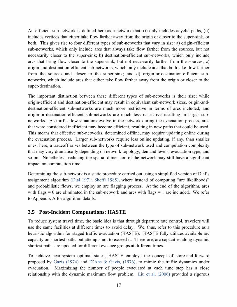
In summary, HASTE utilizes a greedy algorithm concept, considers the bottleneck flows on dynamic shortest paths, and assigns the evacuees in an order that depends on their distances from the boundary (or depending on demand level), to achieve the system objective of maximizing the number of evacuees arriving at each time interval. If better arrival rates at the boundary arcs cannot be obtained at each time interval, the dynamic traffic assignment solution is optimal. Figure 3.3 summarizes HASTE. A more detailed flow chart is provided in Appendix A.

19

Figure 3.3 Summary of HASTE Procedure

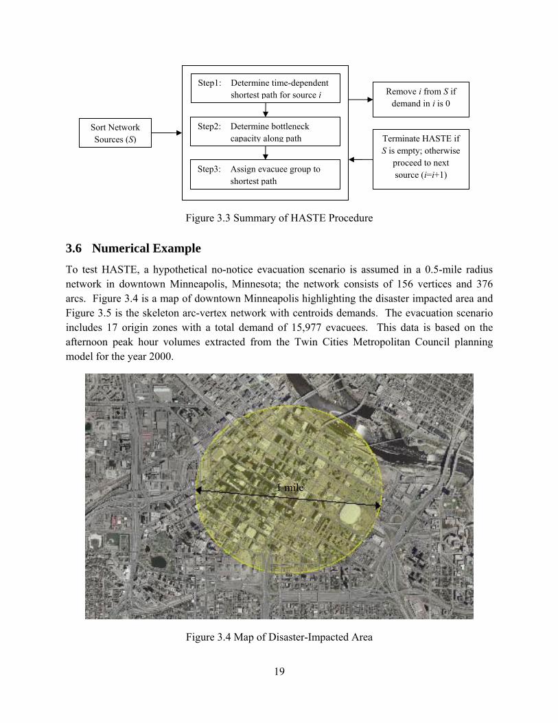
3.6 Numerical Example To test HASTE, a hypothetical no-notice evacuation scenario is assumed in a 0.5-mile radius network in downtown Minneapolis, Minnesota; the network consists of 156 vertices and 376 arcs. Figure 3.4 is a map of downtown Minneapolis highlighting the disaster impacted area and Figure 3.5 is the skeleton arc-vertex network with centroids demands. The evacuation scenario includes 17 origin zones with a total demand of 15,977 evacuees. This data is based on the afternoon peak hour volumes extracted from the Twin Cities Metropolitan Council planning model for the year 2000.

Figure 3.4 Map of Disaster-Impacted Area

Remove i from S if demand in i is 0

Terminate HASTE if S is empty; otherwise

proceed to next source (i=i+1)

Step1: Determine time-dependent shortest path for source i

Step2: Determine bottleneck capacity along path

Step3: Assign evacuee group to shortest path

Sort Network Sources (S)

1 mile

20

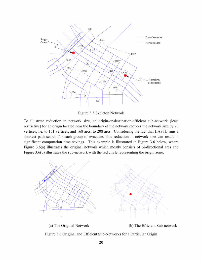
Figure 3.5 Skeleton Network

To illustrate reduction in network size, an origin-or-destination-efficient sub-network (least restrictive) for an origin located near the boundary of the network reduces the network size by 20 vertices, i.e. to 151 vertices, and 168 arcs, to 208 arcs. Considering the fact that HASTE runs a shortest path search for each group of evacuees, this reduction in network size can result in significant computation time savings. This example is illustrated in Figure 3.6 below, where Figure 3.6(a) illustrates the original network which mostly consists of bi-directional arcs and Figure 3.6(b) illustrates the sub-network with the red circle representing the origin zone.

(a) The Original Network (b) The Efficient Sub-network

Figure 3.6 Original and Efficient Sub-Networks for a Particular Origin

21

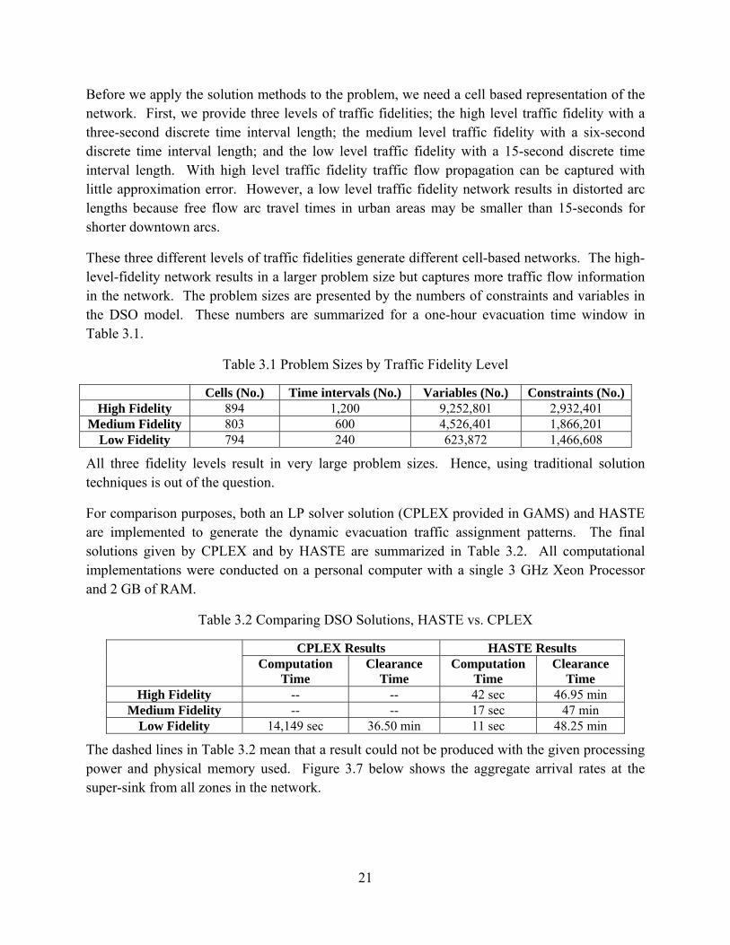
Before we apply the solution methods to the problem, we need a cell based representation of the network. First, we provide three levels of traffic fidelities; the high level traffic fidelity with a three-second discrete time interval length; the medium level traffic fidelity with a six-second discrete time interval length; and the low level traffic fidelity with a 15-second discrete time interval length. With high level traffic fidelity traffic flow propagation can be captured with little approximation error. However, a low level traffic fidelity network results in distorted arc lengths because free flow arc travel times in urban areas may be smaller than 15-seconds for shorter downtown arcs.

These three different levels of traffic fidelities generate different cell-based networks. The high-level-fidelity network results in a larger problem size but captures more traffic flow information in the network. The problem sizes are presented by the numbers of constraints and variables in the DSO model. These numbers are summarized for a one-hour evacuation time window in Table 3.1.

Table 3.1 Problem Sizes by Traffic Fidelity Level

Cells (No.) Time intervals (No.) Variables (No.) Constraints (No.)High Fidelity 894 1,200 9,252,801 2,932,401

Medium Fidelity 803 600 4,526,401 1,866,201 Low Fidelity 794 240 623,872 1,466,608

All three fidelity levels result in very large problem sizes. Hence, using traditional solution techniques is out of the question.

For comparison purposes, both an LP solver solution (CPLEX provided in GAMS) and HASTE are implemented to generate the dynamic evacuation traffic assignment patterns. The final solutions given by CPLEX and by HASTE are summarized in Table 3.2. All computational implementations were conducted on a personal computer with a single 3 GHz Xeon Processor and 2 GB of RAM.

Table 3.2 Comparing DSO Solutions, HASTE vs. CPLEX

CPLEX Results HASTE Results Computation

Time Clearance

Time Computation

Time Clearance

Time High Fidelity -- -- 42 sec 46.95 min

Medium Fidelity -- -- 17 sec 47 min Low Fidelity 14,149 sec 36.50 min 11 sec 48.25 min

The dashed lines in Table 3.2 mean that a result could not be produced with the given processing power and physical memory used. Figure 3.7 below shows the aggregate arrival rates at the super-sink from all zones in the network.

22

0 5 10 15 20 25 30 35 40 45 50 55 600

2000

4000

6000

8000

10000

12000

14000

16000

CPLEX Result

HASTE: Low Fidelity

HASTE: Medium Fidelity

HASTE: High Fidelity

Heuristic'sClearance Time

Solver'sClearance Time

Agg

rega

ted

Num

ber o

f Eva

cuee

s

Time (min)

32%

Figure 3.7 Evacuee Arrival Curves

When examining the CPLEX result in Figure 3.7, we see that, for the most part, it maintains a consistent arrival rate. This can be explained by the fact that there exists a network bottleneck capacity, as discussed above, and a system optimized solution fully utilizes this capacity so as to minimize the clearance time (or maximize the network throughput). We also see that the heuristic solutions, despite different discrete time interval lengths, results in similar arrival rates over the evacuation process. The figure also shows that HASTE also provides very close matches to the optimal solution for the majority of the evacuation process, but taper off towards the end. The reason for this is that the greedy nature of the procedure does not consider marginal costs, but rather assigns all groups to dynamic shortest paths. Despite the 32% difference between the heuristics and the optimal solution in total network clearance time, the computation time savings shown in Table 3.2 make HASTE an attractive alternative. It takes nearly four hours for an LP solver solution for an evacuation time window of less than one hour, as opposed to less than one-minute for various network fidelity levels using HASTE.

23

3.7 Concluding Remarks and Future Research This chapter proposes solution strategies for solving time-constrained optimal routing problems for real-time no-notice emergency evacuation operations. A time-constrained DSO model using a cell-based network representation was adopted. The nature of no-notice evacuation scenarios dictates external computation time constraints that may have a significant impact on evacuation operations in real-world settings. Due to the large size of the DSO linear program, commercial linear programming solvers do not serve as good because (1) LP solvers generally are not efficient for solving DSO problems, (2) they cannot provide reasonable results if they are arbitrarily terminated, and (3) LP solver solutions only provide arc/cell volumes, but not routes, which means that additional processing would yet be required in order to obtain results that are meaningful to decision makers.

The proposed solution procedure consists of pre-incident and post-incident heuristics. Pre-incident computations include efficient sub-network determination to help reduce the size of the problem spatially. This is particularly useful for real-world no-notice scenarios that include sizable evacuation networks. The post-incident computations help determine evacuee departure rates, time schedules, and dynamic shortest paths that evacuees should use. Although the proposed heuristic approach only provides close-to-optimum solutions to the DSO model, its high computational efficiency and termination-friendly feature make it outperform any commercial LP solver solutions. Numerical examples validate this statement.

The quality of the solutions produced by HASTE in this study was demonstrated by means of example. A thorough study of the quality of solutions produced by HASTE, in terms of bounds and deviation from optimality as a function of problem dimensions, is left as future research. HASTE is primarily a routing algorithm; intersection control strategies using HASTE are developed in subsequent chapters, while signal timing optimization is left for future research.

24

CHAPTER 4: THE DOWNTOWN MINNEAPOLIS NETWORK

4.1 Introduction For evacuation purposes, specifically no-notice evacuations over relatively small radii, it is crucial that the graph theoretic representation of the transportation network be accurate. Transportation network studies typically rely on readily-available representations used for metro-wide planning purposes. Metro-wide demand planning models employ a great deal of simplification, since a great deal of accuracy is not needed for static four-step planning procedures. In this study, an accurate graph theoretic representation is developed for purposes of dynamic evacuation planning and operations analysis.

Network geometric parameters were determined using the Lawrence Group (TLG) database, maintained by MetroGIS, a GIS database of the Twin Cities roadway network. The Twin Cities Metropolitan Council planning demand model and the Highway Capacity Manual (HCM) were used as the primary data sources for aggregate level traffic flow parameters such as capacities, free-flow speeds, and jam densities. The proposed models for vehicle evacuation rely on a mesoscopic level dynamic representation of traffic flow, which routes groups of vehicles as packets through the network over discrete time slices. This level of representation allows for direct use of the traffic flow parameters, as opposed to a microscopic level representation (individual vehicles), which would require a thorough calibration procedure to reproduce the aggregate level traffic flow parameters. Additionally, typical day-to-day demand and traffic volume patterns are not representative under emergency evacuation scenarios, and due to the adopted definition of safety in the network as being any part of the network outside of a particular radius, a thorough origin-destination matrix estimation process is not needed. Furthermore, in this project, it is desirable to allow for flexibility in the demand levels and locations in order to model varying emergency evacuation scenarios; for this purpose, the developed network model will allow for any point in the network to be defined as an origin or evacuee concentration point.

This chapter highlights the development of a one-mile radius network model for downtown Minneapolis, its attributes, traffic flow parameters, signal timing parameters, and the conversion process to a cell transmission model based network for mesoscopic traffic flow representation. Section 4.2 of this report provides a brief introduction to graph theoretic representations of road networks defining the relevant concepts to this research. Section 4.3 presents the detailed geometric attributes of the elements of the model and the data sources used to develop the model. Section 4.4 discusses the traffic flow parameters of the model and section 4.5 briefly discusses the signal timing parameters. Section 4.6 presents the transformation of the graph theoretic model into a discrete cell transmission based network.

25

4.2 The Graph Theoretic Representation A graph G = (V, E) is a structure that is defined by two elements, a set of vertices V and a set of edges E, where vertices can be thought of as the corners of the graph, while edges are objects that connect pairs of nodes; see Figure 4.1 below for an example. Note that the order in which a pair of vertices appears, to represent an edge, is not important; i.e., [v1, v2] and [v2, v1] refer to the same edge. Graphs are used to model pair-wise relations between the different objects in the graph; e.g. the number of edges emanating from a particular vertex, the distance between two adjacent vertices (represented as the length of the connecting edge), and the shortest path from one vertex to another.

The degree of a vertex v of graph G is the number of edges connected to v. For example, in Figure 4.1, the degree of vertex v1 is 2, and the degree of vertex v2 is 3.

Figure 4.1 Graph G = (V, E)

A directed graph, or digraph, D = (V, A) is a graph with directions attached to its edges. Directed edges are typically referred to as arcs; here, the set of arcs is denoted by A. An arc is represented by an ordered pair of vertices; i.e. (v1, v3) and (v3, v1) do not refer to the same arc. An example of a digraph is shown in Figure 4.2 below. It is worth noting that vertices are sometimes referred to as nodes and arcs as links; the terminology is interchangeable in many references. In a digraph, there are two types of degrees of a vertex v, in-degree and out-degree, which correspond to the number of arcs terminating in v and the number of arcs that emanate from v, respectively. For example, the in-degree of vertex v1 in Figure 4.2 is 1 and its out-degree is 2; the in-degree of v4 is 2 and the out-degree is 0.

e5

e4 e2

e1

e2

v1 v2

v3 v4

V = {v1, v2, v3, v4} E = { [v1, v2], [v1, v3], [v2, v3], [v2, v4], [v3, v4] }

26

Figure 4.2 Digraph D = (V, A)

In a graph, a sequence of vertices connected by edges is a path. The same applies to paths in digraphs, but with the arc directions considered. Two examples of paths connecting vertex v1 to vertex v4 in the digraph in Figure 4.2 are (v1, v3, v4) and (v1, v2, v4); note that the order of the vertices (representing the direction of the arcs) is important in defining the paths. Paths are important graph theoretic objects in transportation applications in general, and in vehicle evacuation in specific, where determining the shortest paths in the network is a crucial component of evacuee routing strategies.

Transportation networks are amongst the most intuitive objects to represent as digraphs; the vertices typically represent the network junctions (e.g., traffic signals, unsignalized intersections, and ramp junctions), while the arcs represent the roads in the network. Digraph representations are typically preferred to regular graph representations to account for combinations of one-way and two-way streets. As discussed, paths in the graph theoretic representation are used to refer to routes in a transportation network. In a transportation network, vertices with in-degree 0 are called sources and vertices with out-degree 0 are called sinks. Sources represent the network origins, which hold the network demands, i.e., the evacuee concentrations in the network; in this project, this requirement is relaxed in the sense that any vertex may be converted to a source, regardless of its in-degree. The sinks represent the network destinations, which constitute safety in the evacuation model. For further information on network flow modeling and graph theoretical basics, see Ahuja, Magnanti, & Orlin (1993).

4.3 Downtown Minneapolis Network: Geometric Attributes This section describes the one-mile radius network model centered in downtown Minneapolis, its attributes, and the source of information used to construct the model. The geographic extent of the road network includes areas that cover half-mile radii centered in three important structures in downtown Minneapolis, the Hubert H. Humphrey Metrodome, the Minneapolis Convention Center, and the Target Center. The three half-mile radii are encompassed within the one-mile downtown Minneapolis network.

v1 v2

v3 v4

V = {v1, v2, v3, v4} E = { (v1, v2), (v1, v3), (v2, v4), (v3, v1), (v3, v2), (v3, v4) }

27

For an accurate representation of the network, a collection of 754 vertices and 1,565 directed arcs are used. The geographic attributes of the vertices and the arcs of the network constitute a skeleton of the road network with additional data attached to them. These attributes were primarily obtained using the Lawrence Group (TLG) database, maintained by MetroGIS, a GIS database of the Twin Cities roadway network. The vertices represent all road junctions in the network, which include traffic signals, unsignalized intersections, and freeway junctions such as off-ramp entrances and on-ramp merge points. The following is a description of the vertex attributes:

ID: The vertex ID is simply a unique identifier (a number) that was established for each vertex in the network.

2) DEMAND: This is an attribute that can be edited by users to create different evacuation scenarios. If the demand is not zero, the vertex will be treated as a source in the network. In setting up different scenarios, this will be one of the important model attributes to be edited.

3) STR1, STR2, STR3, and STR4: These four attributes are names of the cross streets or freeways and ramps that intersect at the vertex. Four cross street names were used because this was found to be the largest number of distinct street names meeting at a specific junction. Where there are fewer cross street names, the last attributes are not used; e.g., with only two distinct cross street names, only STR1 and STR2 are used and a “-“ is used for both STR3 and STR4.

4) X and Y: These are the vertex coordinates (in meters) according to the Universal Transverse Mercator (UTM) coordinate system, zone 15 for the Twin Cities.

5) DESC: This attribute describes the vertex junction type by use of the following symbols; ‘S’ = signalized intersection, ‘U’ = unsignalized intersection, ‘O’ = ordinary vertex with out-degree 1 and in-degree 0 or 1, ‘F’ = freeway vertex, ‘OFF’ = off-ramp entrance, and ‘ON’ = freeway/on-ramp merge point.

6) Signal Attributes: These will be discussed in Chapter 5 of this report.

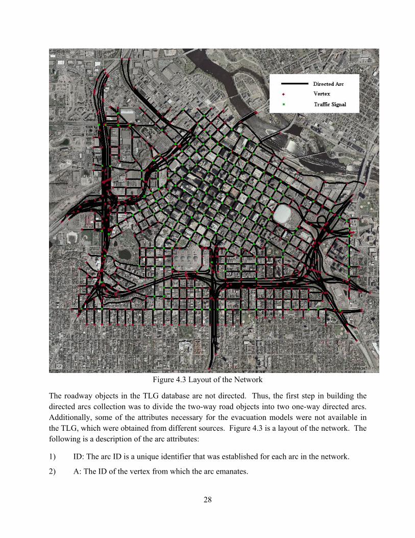
28

Figure 4.3 Layout of the Network

The roadway objects in the TLG database are not directed. Thus, the first step in building the directed arcs collection was to divide the two-way road objects into two one-way directed arcs. Additionally, some of the attributes necessary for the evacuation models were not available in the TLG, which were obtained from different sources. Figure 4.3 is a layout of the network. The following is a description of the arc attributes:

1) ID: The arc ID is a unique identifier that was established for each arc in the network.

2) A: The ID of the vertex from which the arc emanates.

29

3) B: The ID of the vertex in which the arc terminates.

4) LANES: The number of lanes, which was obtained from Google Street View for each arc in the model.

5) LENGTH: The length of the arc (in meters).

6) NAME: The street name.

7) SPEED_LIM: The posted speed limit for the arc.

4.4 Downtown Minneapolis Network: Traffic Flow Parameters The traffic flow parameters of the model are primary arc attributes used to determine flow restriction characteristics for each of the arcs in the network. The cell transmission model (CTM) is used for traffic flow representation in the evacuation models, which uses the trapezoidal flow-density relationship depicted in Figure 4.4. The CTM, developed by Professor Carlos Daganzo in (Daganzo 1994 and 1995) is a discrete time approximation scheme of the hydrodynamic traffic flow equations due to Lighthill & Whitham (1955) and Richards (1956), which are commonly referred to as the LWR equations.

Density

Flow

w−

Jk

maxq

wv

kJ

11+

v

Figure 4.4 The Trapezoidal Flow-Density Relationship

The trapezoidal flow density relationship divides flow patterns on a roadway into three regimes represented by the three regions of the flow-density diagram. The first region represents under-saturated traffic flow conditions (free-flow and constant speed v); the second region represents saturation conditions (capacity qmax); and the third region represents over-saturated conditions that result in backward shockwaves with constant speed w (deterioration in flow rates due to congestion).

Traffic flow characteristics for any arc in the network are determined by their flow-density relationships. Due to the simplicity (linear nature) of the trapezoidal flow-density relationship,

30

knowledge of a few parameters determines the shape of the curve. These arc-level traffic flow parameters are described as follows:

1) FREE FLOW SPEED: The arc free flow speeds used in the model are the posted speed limits in miles per hour plus five miles per hour. Given the free flow speed of the arc, the first region of the flow-density curve is simply a straight line from the origin with slope v, representing the free flow speed.

2) LANE CAPACITY: Lane capacities vary by facility type. Freeway arc lane capacities

were obtained from the Twin Cities Metropolitan Council planning model (in vehicles per hour per lane). Downtown arc lane capacities in the Metropolitan Council model are averaged over multiple signal timing cycles, an unnecessary simplification for the purposes of this project, since the underlying models are dynamic. This means that traffic flow characteristics vary depending on the signal indication. For this reason, the Metropolitan Council planning model arterial arc lane capacities were not used. Instead, typical values for lane capacities based on Highway Capacity Manual (HCM) guidelines were used. Arc capacity is simply the lane capacity of the arc multiplied by the number of lanes. Once the arc capacity qmax is known, the second region of the flow-density curve is constructed by simply drawing a horizontal line that intersects the flow axis at qmax.

3) JAM DENSITY: Two typical values were used for jam density in the model, one for

freeway arcs (210 vehicles per mile per lane), and the other for arterial arcs (260 vehicles per mile per lane). The arc jam density is simply the lane jam density multiplied by the number of lanes. Given the jam density of the arc, the third region of the free-flow curve is constructed by drawing a line from the jam density point on the density axis with –w slope (a typical value of w = ½v was used) that intersects with the horizontal capacity line, or the free-flow speed line for cases of high free flow speed, resulting in a triangular flow-density curve.

4.5 Downtown Minneapolis Network: Signal Timing Parameters The signal timing parameters were obtained from the city of Minneapolis for 217 traffic signals in the model. The data was first geo-coded into the one-mile radius downtown Minneapolis model to properly associate the timing plans provided by the city of Minneapolis with the network vertices. The next step was to determine the phasing plan based on the movements at each of the intersections and associate each turning movement in the model with an appropriate NEMA phase.

The signalized intersections in the model all use fixed timing logic with splitting rates that vary by time of day. Three splitting schemes are provided in the dataset, a morning peak period timing plan, and off-peak timing plan, and an afternoon peak period timing plan. For each of the

31

timing plans, the cycle length and the splitting percentages are provided. Traffic signal representation and traffic flow at signalized intersections for evacuation purposes will be discussed in Chapter 5.

4.6 Discrete Representation of the Digraph as Cells The CTM can be thought of as a scheme in which network arcs are divided into cells. Capacities and densities are then defined at the cell level in units of numbers of vehicles and not rates as in the flow-density relationships for the arcs. As such, the capacity of cell i, Qi may be interpreted as the maximum number of vehicles that can flow into or out of a cell over a predefined discrete time interval length ∆t and cell density (maximum occupancy) Ni may be interpreted as the maximum number of vehicles that can be stored in the cell. The length of cell i, li is the portion of the arc that can be traversed at free-flow speed; thus:

li = ∆t × v (1)

Qi = ∆t × qmax (2)

Ni = li × kj (3)

Note that the cell-level parameters are the same for all cells that comprise a single arc. The number of cells that an arc is divided into is equal to the length of the arc divided by the lengths of the cells that comprise it. This transformation scheme is illustrated in Figure 4.5 below.

Figure 4.5 Transforming Arcs into Cells

arc

L = arc length qmax = arc capacity kj = jam density v = free-flow speed

1 2 3

∆t = discrete time interval length (e.g. 5 seconds) Number of cells = L ÷ li

cells

li = cell length = ∆t × v Qi = cell capacity = ∆t × qmax Ni = cell max density = li × kj

32

It is worth noting that the discrete transformation scheme discussed here applies to within arc traffic flows. Traffic flows in between arcs and particularly at traffic signal will be discussed in Chapter 5.

33

CHAPTER 5: SIGNALIZED INTERSECTION MODELING

5.1 Introduction When faced with unanticipated emergency events, authorities need to make critical decisions to minimize evacuee exposure to harm. Two such decisions involve: (i) evacuee routing strategies and (ii) intersection controls that involve, for example, officer deployment, signal timing, and/or road closure. Evacuee routing was studied in Chapter 3 and fast computation was achieved by developing the heuristic algorithm for staged traffic evacuation (HASTE). As central business districts are typically heavily controlled by traffic signals, intersection control and signal timing is a crucial component of rapid vehicle evacuation. In this task, intersection control considerations are incorporated into the existing evacuation framework. In addition to evacuee routing schedules, the evacuation model is extended to include determination of critical intersections to which officers may be deployed to improve throughput through the intersections, given a limited number of police officers (a resource budget).

Additionally, responding to no-notice events is reactive in nature; thus, every minute counts, both in terms of network clearance times and computation times for evacuation strategies. Evacuee routing and officer deployment to critical network locations are two intertwined components of vehicle evacuation in the sense that, at optimality, different deployment strategies may be associated with different routing strategies. Hence, the two components need to be solved for simultaneously and not sequentially. Also, given the size of real-world no-notice evacuation problems, this work will emphasize computation techniques used to produce such strategies.

Section 5.2 of this report presents the traffic flow representation strategy using the cell transmission model for signalized intersections. Section 4.3 briefly discusses the mathematical model developed for combined vehicle routing and officer deployment to critical intersections. It also presents the solution technique employed for computing these strategies. Finally, Section 5.4 presents a numerical example and compares the proposed solution strategy to analytical solution strategies in terms of solution quality and computation times. Finally, concluding remarks and potential future research directions are discussed in section 5.5.

5.2 Traffic Flow Representation at Signalized Intersections In Chapter 4 of this report, the graph theoretic representation of a road network was presented in addition to the cell transmission model (CTM), which was used to represent traffic flow within network arcs. A similar scheme for representing traffic flow at traffic signals is presented in this section of the report. Figure 5.1 illustrates the graph theoretic representation of a single intersection in a network.

34

It is clear from the figure that the graph theoretic representation would need to be extended to account for varying signal timing plans and phasing schemes. The first step in this modification is to extend the vertex/arc representation to include all possible movements at the intersection. This is done as follows:

1) Divide the intersection vertex into multiple vertices, one separate end vertex for each inbound arc and one separate start vertex for each outbound arc. For the example in Figure 5.2, the vertex would be divided into four vertices, two for the inbound arcs and two for the outbound arcs.

2) Create new arcs connecting the new vertices. These new arcs are short arcs that represent each of the movements at the intersection. In Figure 5.1, there are four movements at the intersection. A new arc for each movement is created.

Figure 5.1 Graph Theoretic Representation of an Intersection

This modification is illustrated in Figure 5.2 below, for the intersection in Figure 5.1.

Intersection Movements Vertex/Arcs Representation

35

Figure 5.2 The Modified Intersection Representation

The new arcs at the intersection are short arcs in the sense that they are each represented by a single cell in the CTM network. The cells that are used to represent the short arcs will be referred to as gateway cells. Figure 5.3 illustrates the CTM representation, including the gateway cells, for the intersection in Figures 5.1 and 5.2.

Figure 5.3 Intersection Gateway Cells

Gateway cells differ from other cells in the network in that they represent the turning movements at the intersection and their capacities change over time to capture signal indication changes at the intersection. Determining their parameters involves minor changes to the computations used for other network cells. Since a short arc is always translated into a single gateway cell, the length of the corresponding gateway cell i is not important. The maximum occupancy of the cell Ni is determined from the arc from which it departs. For the example in Figure 5.1, the eastbound left-turn movement uses a single lane; thus, Ni for the corresponding gateway cell is

Regular Cell

Gateway Cell

Cell Connector

Vertex/Arcs Representation Modified Representation

New vertex

New arc

36

simply the jam density (in vehicles per mile per lane) of the inbound arc multiplied by the length of its cells (l × ½ kj). The gateway cell capacity, during a green indication, qi is computed as qi = ∆t × sm, where sm is the saturation flow rate for the subject movement (typically 1,200 vehicles per hour per lane). The gateway cell capacity during a red indication is 0 since no vehicles can flow through the cell during red. Thus, the gateway cell capacity is a quantity that fluctuates between 0 and qi; with the signal timing plans known, the gateway cell capacity Qi

t ε {0, qi} is known over the evacuation time horizon (the superscript t denotes the discrete time interval in question).

5.3 Model and Solution Technique

5.3.1 Mathematical Model

The mathematical formulation for combined vehicle routing and officer deployment for emergency evacuation is essentially an extension to the original mathematical formulation for dynamic system optimal traffic assignment presented in Chapter 3 and detailed in Appendix A. It considers improvements to the traffic flow by means of determining a predetermined number of critical network intersections b (for budget) to which police officers may be deployed to override the signal control and improve traffic throughput for effective vehicle evacuation. For further details of the mathematical formulation, we refer to Appendix B.

5.3.2 Deployment Strategies as Combinations

Signalized intersections within a predetermined disaster impact area are the candidate intersections considered for officer deployment; the number of candidate intersections is denoted by n and the number of police officers available for deployment is denoted by b. When b ≥ n (there are enough officers to deploy to each candidate intersection), the problem collapses to a simple routing problem and can be solved using HASTE as in Chapter 3. The more difficult (and more likely) scenario is when b < n; i.e., not all candidate intersections can be covered by the available number of police officers. In this case, the officer deployment strategy can be treated as one of many different combinations of b (or less) officers deployed to n candidate intersections; it is, thus, a combinatorial problem where the number of different possible combinations grows disproportionately as b and n get larger. For example, if the number of candidate intersections is 4 (n = 4) and the number of officers available for deployment is 2 (b = 2), then the number of possible combinations is 10. The combinations are shown in Figure 5.4 below.

37

Figure 5.4 Example of Officer Deployment Combinations

The boxes in Figure 4 are the candidate intersections numbered 1 through 4; the symbol X indicates that an officer is deployed to that intersection. Note that combinations with only one officer are also considered, since solutions that may involve the use of fewer officers than what is available should also be considered. The total number of such combinations is then computed as the sum of the different combinations; e.g. the number of two-officer combinations + the number of one-officer combinations. In general, the number of combinations can be computed as nCb (read “n choose b”) = n! ÷ (b!×(n – b)!). For the two-officer combination in the above example, this is (4×3×2×1) ÷ ((2×2)×(2×2)) = 6; for the one-officer combinations, this is (4×3×2×1) ÷ ((1)×(3×2×1)) = 4, bringing the total number of combinations to 6 + 4 = 10. More generally, this is computed as:

∑∑== −

=b

i

b

ii

n

bnbnC

11 )!(!!

(1)

It is clear that the number of combinations grows very quickly as n and b get larger. To see this, take an example that is slightly larger with n = 10 and b = 4; the number of combinations grows to 1,080; a more realistic problem size would be n = 20 and b = 10, for which the number of combinations grows to 2,771,330.

The officer deployment problem can be stated as the problem of finding the best combination. The best combination is essentially the one, when coupled with its best corresponding evacuee routing strategy, results in the smallest disaster area clearance time. Enumerating all possible combinations to determine the best cannot be done in a feasible amount of time. In fact, intelligent search techniques that can guarantee finding the best combination without full

1 2 3 4

X X

1 2 3 4

X X

1 2 3 4

X X

1 2 3 4

X X

2 3 4

X X

1 2 3 4

X X

1

1 2 3 4

X

1 2 3 4

X

2 3 4

X

1 2 3 4

X

1Tw

o-O

ffic

er C

ombi

natio

ns

Sing

le-O

ffic

er C

ombi

natio

ns

38

enumeration remain unknown. However, meta-heuristic techniques are known to produce good solutions relatively fast, but without any guarantees of these solutions being the best of all possible combinations. One of the more popular techniques is called Genetic Algorithms (GA), which is adopted in this work as a search technique for finding good officer deployment strategies.

5.3.3 Simple Genetic Algorithms

Genetic algorithms (GA) are heuristic search approaches that mimic survival of the fittest in natural systems. In simple GA's, three operations are used for this purpose: (i) reproduction, (ii) crossover, and (iii) mutation. First, a population of combinations (referred to as chromosomes) is generated, typically, at random. The fitness (or quality) of these chromosomes is then assessed and the chromosomes are ranked. A new population is then reproduced, at random, and depending on chromosome fitness. The higher the fitness, the more likely the chromosome will be reproduced; the lower the fitness, the more likely the chromosome will not be reproduced. Thus, the fittest survive (and possibly multiply), while the least fit do not. The reproduced chromosomes then mate by interchanging (crossing over) parts of two parent chromosomes to produce two new offspring chromosomes (a new population). Mutation is a rare operation that ensures that the GA searches do not lock into local optima, where individual genes in a chromosome may change value, at random.

To represent officer deployment strategies, chromosomes of length b are generated, where each gene assumes a value between 1 and n. In other words, the value of the gene indicates a location that is to be chosen for officer deployment. This is in contrast to a binary chromosome scheme with n genes each representing a candidate location as shown in Figure 5.4. Under the latter scheme, chromosome crossover and/or mutation are likely to produce infeasible chromosomes; the number of X's in this scheme must adhere to the budget b. The former scheme, on the other hand, does not suffer this limitation. This chromosome (combination) set-up is illustrated in Figure 5.5 for the same combinations in Figure 5.4, where the boxes (referred to as genes) represent the officers rather than the intersections and the numbers inside the boxes (gene values) refer to the intersections to which the officers are to be deployed.

Two things in Figure 5.5 are worth noting:

1) The number of combinations is larger than that for the binary scheme. This may seem as a drawback, but in fact makes the search faster. In this case the total number of combinations is computed as nb (e.g., 42 = 16).

2) The single-officer combinations are not be interpreted as both officers are deployed to the same intersection, but as a duplicate.

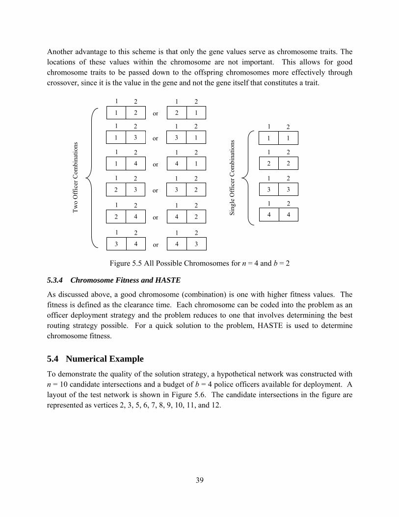
39

Another advantage to this scheme is that only the gene values serve as chromosome traits. The locations of these values within the chromosome are not important. This allows for good chromosome traits to be passed down to the offspring chromosomes more effectively through crossover, since it is the value in the gene and not the gene itself that constitutes a trait.

Figure 5.5 All Possible Chromosomes for n = 4 and b = 2

5.3.4 Chromosome Fitness and HASTE

As discussed above, a good chromosome (combination) is one with higher fitness values. The fitness is defined as the clearance time. Each chromosome can be coded into the problem as an officer deployment strategy and the problem reduces to one that involves determining the best routing strategy possible. For a quick solution to the problem, HASTE is used to determine chromosome fitness.

5.4 Numerical Example To demonstrate the quality of the solution strategy, a hypothetical network was constructed with n = 10 candidate intersections and a budget of b = 4 police officers available for deployment. A layout of the test network is shown in Figure 5.6. The candidate intersections in the figure are represented as vertices 2, 3, 5, 6, 7, 8, 9, 10, 11, and 12.

2 1 2

1 2 2 1

1

1 2

3 3

1 2

4 4

2

1 1

1 2

2 2

1

Two

Off

icer

Com

bina

tions

Sing

le O

ffic

er C

ombi

natio

ns

or

2 1 2

1 3 3 1

1

or

2 1 2

1 4 4 1

1

or

2 1 2

2 3 3 2

1

or

2 1 2

2 4 4 2

1

or

2 1 2

3 4 4 3

1

or

40

Figure 5.6 Layout of the Test Network

41

The length of the discrete time interval (∆t) is three seconds. The saturation flow rates used are 1,200 vphpl (cell capacities = 2 veh/cell), jam density used is 235 veh/mi (cell occupancies = 8 veh/cell and 4 veh/cell for gateway cells). The signal timing plans used are based on 60 second cycle lengths (30 seconds for each approach). The signal timing settings allow for smooth progression at free-flow along both the north-south and east-west directions. Total demand D is 2,700 evacuees distributed amongst the network sources.

The problem was first solved analytically using the GAMS/CPLEX mathematical program solver. The time horizon selected to solve the problem was 55 minutes or 1,100 three-second discrete time intervals. Prior to solving the problem, the evacuation time horizon is not known. Selection of a proper time horizon is important, as selection of too short a horizon would result in an infeasible solution and selection of too long a time horizon would result in increased problem size. For this hypothetical problem, the number of continuous variables is 304,977 and the number of binary variables is 10. The total number of constraints (not including variable type constraints) in the problem is 662,951.

This is a relatively large problem, which will most likely be the case for real-world no-notice evacuation problems. The problem was solved using the GAMS/CPLEX solver. The time required to produce a feasible solution analytically was 1,104 minutes (18 hours and 24 minutes) within 1.07% of the lower bound relaxation; i.e., GAMS/CPLEX could not produce an optimal solution. The clearance time provided by the analytical solution was 31 minutes and 15 seconds (or 625 three-second time intervals).

The problem was then solved using the heuristic framework presented in section 5.3. An evacuation time horizon is not required a priori. An 80% crossover rate and a mutation rate of 1% were employed; this means that, on average, 80% of the population will mate to produce offspring after reproduction and, on average, 1% of the genes in the new population will randomly change their value. A population size of 20 chromosomes was used and 20 generations were produced. The CPU time required was five minutes and seven seconds, which is much smaller than the computation time required to solve the model analytically. The clearance time provided by the heuristic solution was 33 minutes and 30 seconds (or 670 three-second time intervals). The difference in clearance time is only two minutes and 15 seconds. Figure 5.7 compares the cumulative arrivals at the super-sink over the evacuation time horizon for the analytical and the heuristic solutions.

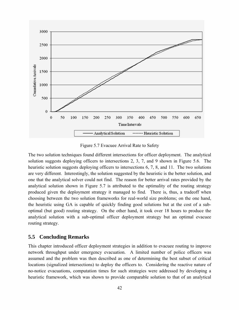
42

Figure 5.7 Evacuee Arrival Rate to Safety

The two solution techniques found different intersections for officer deployment. The analytical solution suggests deploying officers to intersections 2, 3, 7, and 9 shown in Figure 5.6. The heuristic solution suggests deploying officers to intersections 6, 7, 8, and 11. The two solutions are very different. Interestingly, the solution suggested by the heuristic is the better solution, and one that the analytical solver could not find. The reason for better arrival rates provided by the analytical solution shown in Figure 5.7 is attributed to the optimality of the routing strategy produced given the deployment strategy it managed to find. There is, thus, a tradeoff when choosing between the two solution frameworks for real-world size problems; on the one hand, the heuristic using GA is capable of quickly finding good solutions but at the cost of a sub-optimal (but good) routing strategy. On the other hand, it took over 18 hours to produce the analytical solution with a sub-optimal officer deployment strategy but an optimal evacuee routing strategy.

5.5 Concluding Remarks This chapter introduced officer deployment strategies in addition to evacuee routing to improve network throughput under emergency evacuation. A limited number of police officers was assumed and the problem was then described as one of determining the best subset of critical locations (signalized intersections) to deploy the officers to. Considering the reactive nature of no-notice evacuations, computation times for such strategies were addressed by developing a heuristic framework, which was shown to provide comparable solution to that of an analytical

43

model, but considerably faster. For officer deployment strategies, a genetic algorithm (GA) based approach was adopted and the heuristic algorithm for staged traffic evacuation (HASTE) was used to assess the fitness of the GA solutions.

The effectiveness of GA in exploring the possible officer deployment strategies primarily stems from the simplicity of the discrete component of the analytical model being approximated. The number of binary variables was kept at a minimum. The computation speed of the heuristic framework is primarily due to the use of HASTE for solution fitness approximation. Our future work will consider improvements to the meta-heuristics component GA, while also exploring the possibility of using other meta-heuristics such as ant colony optimization, which have been shown to be effective in network design problem contexts.

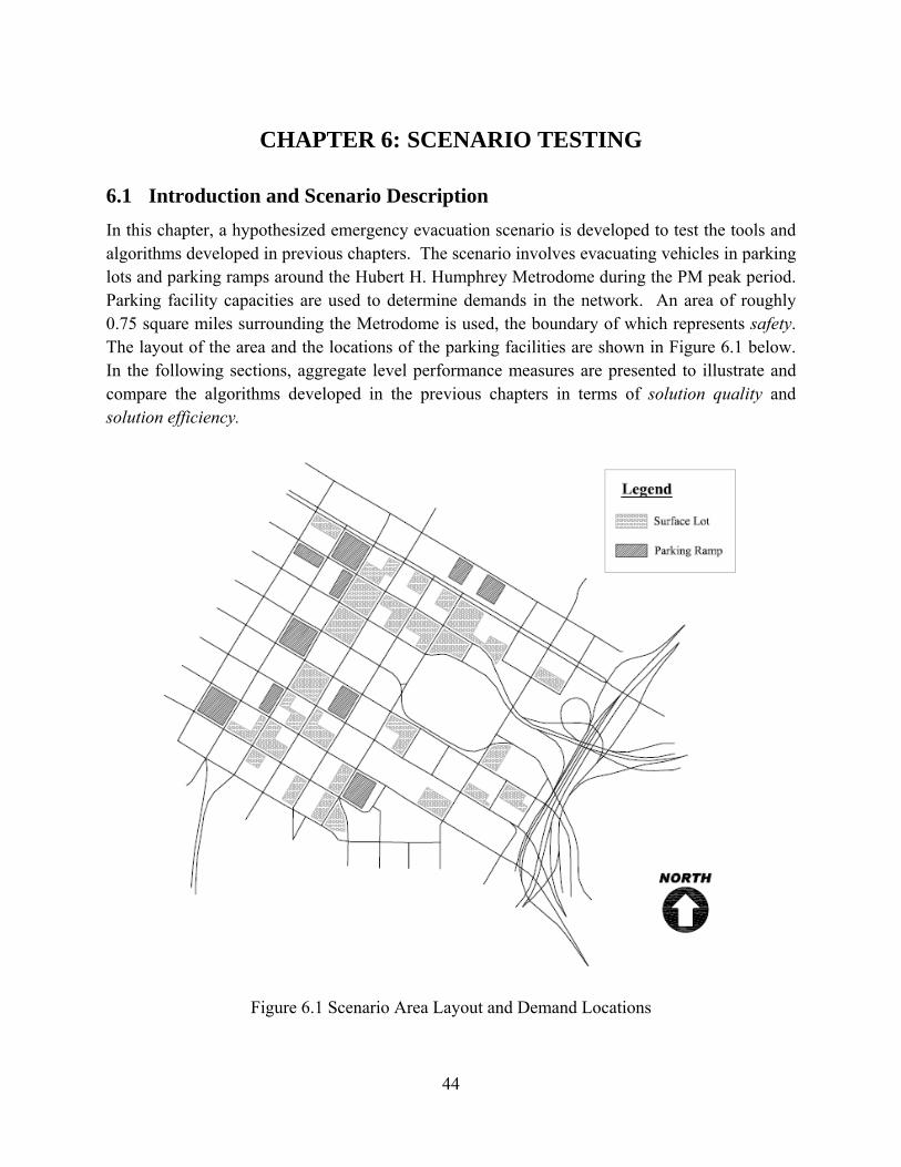
44

CHAPTER 6: SCENARIO TESTING

6.1 Introduction and Scenario Description In this chapter, a hypothesized emergency evacuation scenario is developed to test the tools and algorithms developed in previous chapters. The scenario involves evacuating vehicles in parking lots and parking ramps around the Hubert H. Humphrey Metrodome during the PM peak period. Parking facility capacities are used to determine demands in the network. An area of roughly 0.75 square miles surrounding the Metrodome is used, the boundary of which represents safety. The layout of the area and the locations of the parking facilities are shown in Figure 6.1 below. In the following sections, aggregate level performance measures are presented to illustrate and compare the algorithms developed in the previous chapters in terms of solution quality and solution efficiency.

Figure 6.1 Scenario Area Layout and Demand Locations

45

The area of the study network was chosen to be large enough to accommodate the large vehicular demands that would typically arise during a sporting event. The capacities of the surface lots, shown in light gray in Figure 6.1, were obtained by counting the total number of available spots in each of the lots from aerial photographs in Google Maps. The total lot capacities were either obtained directly from the City of Minneapolis Parking Services website, or approximated based on number of levels and typical parking facility layout by floor area. The remainder of this chapter is organized as follows: section 6.2 briefly presents scenario development using the software tool. Evacuee routing strategies are discussed in section 6.3, while officer deployment strategies for the scenarios are presented in section 6.4. Finally, conclusions and software usage recommendations are presented in section 6.5.

6.2 Scenario Development Developing evacuation scenarios using the evacuation software tool is a three-step process: (i) area selection from the base-map; (ii) scenario network editing (e.g. removal of arcs and vertices and arc capacity adjustments); and (iii) source and sink definition by entering demands and selecting sink vertices, respectively. Details of the process are included in Appendix C. Figures 6.2 and 6.3 below show the scenario network layout using the developed software tool highlighting the network sources and sinks, respectively.

Figure 6.2 Network Source Vertices

46

Figure 6.3 Network Sink Vertices

The 61 demand vertices in the network (shown in Figure 6.2) were selected based on proximity to parking facility exits. To test the routing algorithm, HASTE, under various demand levels, ten copies of the scenario network were made with demands as percentages of the parking facility capacities, i.e., ranging from 10% of the capacities to 100% of the capacities with total capacity at 15,425 vehicles. For testing purposes, 110% and 120% of capacity demand scenarios were also developed. We note that the distribution of demands in the network is crucial in terms of accuracy of the algorithm, the realism of the scenario, and the computation times. Concentrating very large demands in one vertex will result in excessively high computation times, due to limitations in the capacities of the outgoing arcs both in the model and in reality.

6.3 Evacuee Routing In this section the routing algorithm, HASTE, is tested in terms of network clearance times (solution quality) and computation time (solution efficiency) for different demand levels and different discrete time interval lengths. As discussed in Chapter 3, shorter discrete time interval lengths provide a more accurate traffic flow representation, but at the cost of higher computation times, which is a crucial consideration for no-notice evacuation computations.

47

6.3.1 Arrivals to Safety: Solution Quality

The numbers of evacuees that arrive to safety over the course of the evacuation process (network clearance rates) is an important performance measure of the quality of routing solutions. To illustrates the quality of a solution computed using HASTE, we fist compare the network clearance rates using HASTE to an all-or-nothing (AON) traffic assignment, i.e., where all evacuees use the shortest path to safety for each source. This is shown in Figure 6.4 below for the 100% of capacity demand scenario.

Figure 6.4 HASTE vs. AON Assignment

Clearly, HASTE outperforms an AON assignment both in terms of evacuee arrival rates to safety and total network clearance time. We note that the use of AON assignment as a basis for comparison was inspired by observed route choices made by evacuees in Texas and Louisiana during hurricanes Rita and Katrina. It seems that evacuees have the tendency to all choose the shortest route away from the disaster area, which may result in high congestion levels and, consequently, lower network clearance times.

Figure 6.5 shows the arrival rates of the evacuees to safety for different demand levels and Table 6.1 lists the network clearance times. It can be seen that HASTE tends to perform well during the congested parts of the evacuation process, where the steeper curves indicate larger arrival rates to safety.

48

The figure also illustrates the flattening of the arrival rate curves towards the end of the evacuation process, which is more pronounced for the lower demand cases. This is due to the heuristic nature of HASTE, which approximates system optimal traffic assignment by means of utilizing available network capacity to the best degree possible; an efficient approach for high demands as illustrated by the steepness of the arrival rate curves for the higher demand scenarios. The drop in the arrival curves takes place after the majority of the evacuees have arrived to safety.

Figure 6.5 Evacuee Arrivals to Safety

Table 6.1 Network Clearance Times for Different Demand Levels

Demand Level (% of Capacity) Network Clearance Time 40% 52 min 15 sec 60% 56 min 0 sec 80% 71 min 30 sec

100% 98 min 0 sec 120% 102 min 15 sec

6.3.2 Computation Times: Solution Efficiency

The graph theoretic representation of the study network consists of 717 vertices and 1,072 directed arcs, which are converted to 1,176 cells for 15 second discrete time interval lengths. This includes all turning movement vertices, arcs and cells in the network. When including the

49

time dimension, the size of the problem becomes extremely large. For instance, 285 time intervals were needed to clear the network for the 80% of capacity scenario. This means that roughly 700,000 variables are needed to model the scenario and the ability to produce optimal routing strategies using standard techniques is not possible, at least within minutes. The computation times of HASTE are shown in Figure 6.6. All computations were carried out using a personal computer with a single 3.0 GHz Intel Xeon CPU and 2 GB of RAM. Note that the computation times presented here only include algorithm running time. The time required in converting the network from a GIS format to a graph theoretic data structure and a cellular network are not included in these figures.

Figure 6.6 Computation Time Comparison

It can be seen in Figure 6.6 that the computation times grow linearly with demand (all else held constant). The average increase in computation time per 10% increase in demand (i.e., 1,543 evacuees) was 1,496.17 milliseconds. In other words, an average of less than one millisecond of additional computation time was needed per each additional evacuee. The R2 value of 98.46% illustrates a strong linear trend in the computation time increase with demand. It is also notable that the maximum computation time was less than 18 seconds, which is crucial for computing no-notice evacuation routing strategies.

50

6.3.3 Fidelity of Traffic Representation: Time Interval Lengths

Different discrete time interval lengths result in different network sizes. To illustrate the impact of different time interval lengths on solution quality and efficiency, the 100% of capacity scenario was computed using different time interval lengths. Figure 6.7 below shows the network clearance rates produced using 2, 3, 5, 6, 10, and 15 second time interval lengths for the same evacuation scenario and Table 6.2 lists the network clearance times.

Figure 6.7 Network Clearance Rates for Different Time Interval Lengths

Table 6.2 Network Clearance Times for Different Time Interval Lengths

Discrete Time Interval Length Network Clearance Time 2 sec 56 min 0 sec 3 sec 57 min 18 sec 5 sec 60 min 35 sec 6 sec 69 min 24 sec

10 sec 77 min 40 sec 15 sec 98 min 0 sec

While the network clearance times in Table 6.2 may suggest substantial differences between the shorter time interval lengths, (e.g., two and three second interval lengths) and the longer time interval lengths, (e.g. 10 and 15 second interval lengths), the clearance curves in Figure 6.7 illustrate meager differences. These differences may be directly attributed to the higher flattening in the arrival curves towards the end of the evacuation process when using longer time

51

interval lengths, i.e., the arrival of the last evacuees in the network to safety. This, in turn, could be attributed to the more granular representation of traffic flow with longer discrete time interval lengths. Additionally, Figure 6.8 below illustrates that the gains in clearance time drop following a quadratic trend (R2 = 99.08%); it can thus be expected that using yet smaller discrete time interval lengths would bring about negligible improvement, if any, in network clearance times.

Figure 6.8 Clearance Time Improvements with Smaller Time Intervals

The discussion above focused mainly on comparing the effect of smaller discrete time interval lengths on solutions quality. We now turn to the computation times required for the different discrete time interval lengths, which are shown in Figure 6.9 below.

52

Figure 6.9 Computation Time Increase with Smaller Time Intervals

It can be seen in Figure 6.9 that computation times increase at an exponential rate with network size (as a result of decreasing the discrete time interval length). This is in contrast to the linear increase in computation time that was observed with demand increases for the same network. Because HASTE iteratively computes shortest paths for evacuee routing, the increase in network size brings with it exponentially larger computation times. However, despite this exponential trend, we see that the computation times remain reasonable, even for the 2 second case, which took less than two minutes to compute.

6.4 Officer Deployment To determine the best locations (signalized intersections) for officer deployment, the proposed technique uses a genetic algorithm (GA) combined with HASTE for routing. As such, these computations are not meant to be online computations, but rather offline, or for planning purposes.

To put this into perspective, for GA choice of 10 generations and 10 chromosomes, HASTE would run 100 times; if a single run requires 20 seconds to complete, then the entire algorithm would require 2000 seconds to complete (33 minutes and 20 seconds). However, officer deployment strategies determined offline may be used as input during online routing computations. The routing strategies computed in the previous section all assume that no officers are deployed at any of the signalized intersections in the network and drivers are assumed to adhere to traffic control rules (i.e., they stop at red lights). As evacuation traffic

53

patterns significantly differ from regular traffic patterns, signal timing parameters that are set in accordance with regular traffic become ineffective. While the tools developed do not aim to compute optimal signal timing parameters under evacuation traffic conditions, the best locations to deploy police officers are computed. The underlying assumption is that police officers will do the best job possible. The purpose of this section is to illustrate the improvement in network clearance times when officers are deployed to network intersections.

Figure 6.10 below illustrates convergence of the GA procedure over 40 generations (iterations) with 10 chromosomes for the 80% of capacity demand level, at time interval length of 15 seconds, and a budget of 20 officers. Figure 6.11 illustrates graphically the locations determined by the algorithm.

There are two things to note in Figure 6.10 below: (i) it took less than 10 generations (seven generations) to find an officer deployment strategy that could not be improved throughout the remaining generations; and (ii) the algorithm managed to find a strategy that results in a significant drop in network clearance time, from 71.5 minutes to 42 minutes. Additionally, while a budget of 20 officers was provided, the best deployment strategy only requires 17 officers (one officer per intersection).

Figure 6.10 Genetic Algorithm Convergence

54

Figure 6.11 Intersections Chosen for Officer Deployment

To investigate the improvement in network clearance times by number of officers available for deployment, the 100% of capacity demand level scenario is used with 15 second time interval lengths. The improvement in network clearance times is shown in Figure 6.12.

Figure 6.12 Network Clearance Times by Officer Budget

55

In Figure 6.12, it can be seen that the savings in network clearance times deteriorate following an exponential trend as the number of officers deployed is increased approaching a full deployment (63 officers). This may be attributed to the fact that major routes in the network provide most of the benefit in terms of clearance time, while other routes provide small incremental improvement.

Finally, Table 6.3 below provides a comparison between AON assignment, a routing solution that involves no officer deployment, a solution with a 10-officer budget, and a solution with a 20-officer budget. All computations were carried out using 15 second time interval lengths and the 120% of capacity demand scenario.

Table 6.3 Network Clearance Time Comparisons

Traffic Assignment Scenario Network Clearance Time AON Assignment 248 minutes and 15 seconds

HASTE (No Officers) 102 minutes and 15 seconds GA Optimized with 10 Officers 76 minutes and 30 seconds GA Optimized with 20 Officers 68 minutes and 0 seconds

Note that under the 10-officer budget case only 9 officers are actually used; likewise only 18 officers are used in the 20-officer budget case. Figure 6.13 shows the network clearance rates for the above traffic assignment scenarios.

Figure 6.13 Arrival Rate Curves by Traffic Assignment Scenario

56

While meager differences are observed in Figure 6.13 between the no-officer assignment case and the 10-officer case (mostly at the very end of the evacuation process), we see an improvement with a 20-officer budget. When compared to the AON assignment scenario, the 10- and 20-officer budget cases and HASTE illustrate a substantial improvement.

57

CHAPTER 7: CONCLUSION AND RECOMMENDATIONS

In this chapter, a real-world evacuation scenario was constructed and the algorithms developed in previous chapters were tested using the evacuation software tool. It was illustrated that HASTE evacuee routing solutions provide substantial improvements in network clearance times when compared to AON assignment. It was also shown that solution quality using HASTE improves as network congestion increases due to higher demands. Computation times using HASTE were shown to increase gracefully with demand increases, following a linear trend, an important feature when considering online computation under no-notice evacuation. Additionally, all routing computations were completed within two minutes, illustrating the efficiency of HASTE. Using GA, effective officer deployment strategies were found within less than 10 generations, allowing for offline scenario testing. Based on the analysis presented in this chapter, we provide the following recommendations:

• The distribution of network demands should be as close to reality as possible; placing excessively high demands at a single vertex will result in unrealistic solutions.

• All boundary vertices in the network should be specified as sinks. • It is recommended that evacuation networks be designed and prepared offline and used

online when necessary, although on-line scenario development could easily be carried out using the software tool within minutes.

• When using shorter discrete time interval lengths for higher traffic flow fidelity, higher computation and memory costs are incurred. For example, the two-second scenario required approximately 1.5 GB of memory alone (under the 100% of capacity demand scenario).

• The recommended GA parameters for officer deployment computations are 10 generations, 10 chromosomes, 80% crossover rate, and 1% mutation rate (software defaults) for off-line computations. For smaller networks, on-line officer deployment strategy computations can also be completed within minutes. Smaller numbers of generations, e.g. five generations instead of 10, are also capable of producing high-quality solutions for on-line computations.

• It is recommended that officer deployment strategies be computed off-line for larger networks (half mile radii and greater); changing the demand levels has very small impact on the quality of the officer deployment solutions. Note, however, that demand locations may have an impact on the officer deployment solutions.

• When computing officer deployment strategies, it is recommended that 15-second discrete time interval lengths be used. For higher fidelity routing, the results (i.e., best deployment strategy) may be read from the results and then used as input for higher fidelity routing computations.

58

REFERENCES

Ahuja, R., Magnanti, T., & Orlin, J. (1993). Network Flows: Theory, Algorithms, and Applications. Upper Saddle River, NJ: Prentice-Hall, Inc.

Akamatsu, T. (2000). "A Dynamic Traffic Equilibrium Assignment Paradox". Transportation Research B, Vol. 34B, No. 6 , 515-531.

Allsop, R. (1974). "Some Possibilities for Using Traffic Control to Influence Trip Distribution and Route Choice". Proceedings of the 6th International Symposium on Transportation and Traffic Theory, D.J. Buckley ed. (pp. 345-373). New York, N.Y.: Elsevier.

Alsnih, R., & Stopher, P. (2003). "A Review of the Procedures Associated with Devising Emergency Evacuation Plans". Proceedings of the 82nd Annual Meeting of the Transportation Research Board (CD-ROM). Washington, D.C.

Astrom, K., & Wittermark, B. (1995). Adaptive Control, 2nd Edition. New York, N.Y.: Addison-Wesley.

Baker, E. (1991). "Hurricane Evacuation Behavior". International Journal of Mass Emergencies and Disasters 9(2) , 287-310.

Barret, B., Ran, B., & Pillai, R. (2000). "Developing a Dynamic Traffic Management Modeling Framework for Hurricane Evacuation". Transportation Research Record: Journal of the Transportation Research Board 1773 , 115-121.

Chiu, Y., Koraka, P., & Mirchandani, P. (2005). "Dynamic Traffic Management for Evacuation". 84th TRB Annual Meeting CD-ROM. Washington, D.C.: Transportation Research Board.

Chu, L., Liu, H., & Recker, W. (2002). Development of the Capability-Enhanced PARAMICS Simulation Environment (UCI-ITS-TS-WP-02-12). Irvine, CA.: Center for Traffic Simulation Studies, University of California, Irvine.

Cova, T., & Johnson, J. (2003). "A Network Flow Model for Lane-Based Evacuation Routing". Transportation Research 37A , 579-604.

D’Ans, G., & Gazis, D. (1976). "Optimal Control of Store-and-Forward Transportation Networks". Transportation Science, Vol. 10 , 1–19.

Daganzo, C. (1995). "The Cell Transmission Model, Part II: Network Traffic". Transportation Research, 29B(2) , 79-93.

Daganzo, C. (1994). "The Cell Transmission Model: A Dynamic Representation of Highway Traffic Consistent with the Hydrodynamic Theory". Transportation Research, 28B(4) , 269-287.

59

Dial, R. (1971). "A Probabilistic Multipath Traffic Assignment Algorithm Which Obviates Path Enumeration". Transportation Research, Vol. 5, No. 2 , 83-111.

Fraser-Mitchell, J. (2001). "Simulated Evacuations of an Airport Terminal Building, using the CRISP Model". 2nd International Symposium in Human Behavior in Fire, (pp. 89-100). Boston, MA.

Fu, H., & Wilmot, C. (2004). "A Sequential Logit Dynamic Travel Demand Model for Hurricane Evacuation". Proceedings of 83rd Annual Meeting of the Transportation Research Board (CD-ROM). Washington, D.C.

Gazis, D. (1974). "Modeling and Optimal Control of Congested Transportation Systems". Networks, Vol. 4 , 113–124.

Hawas, Y., & Mahmassani, H. (1995). "A Decentralized Scheme for Real-time Route Guidance in Vehicular Traffic Networks". Proceedings of the Second World Congress on Intelligent Transport Systems, Vol. 4, (pp. 1956-1963). Yokohama, Japan.

He, X. (2007). "A Time-Constrained Heuristic Solution Algorithm for Dynamic System Optimal Routing under Emergency Evacuation". Master's Thesis, University of Minnesota .

Helbing, D., Farkas, I., & Vicsek, T. (2000). "Simulating Dynamical Features of Escape Panic". Nature, Vol. 487 , 487-490.

Ibaraki, T. (1988). Resource Allocation Problems: Algorithmic Approaches. Cambridge, MA.: MIT Press.

Ishak, S., Alecsandru, C., & Seedah, D. (2006). "Improvement and Evaluation of Cell-Transmission Model for Operational Analysis of Traffic Networks". transportation Research Record, Vol. 165 , 171-182.

Jabari, S., He, X., & Liu, H. (2009). "Responding to the Unexpected: A Model and Solution Strategy for Combined Dynamic Evacuee Routing and Officer Deployment". Proceedings of the 88th Annual Meeting of the Transportation Research Board (CD-ROM). Washington, D.C.

Jenkins, R. (2000). "Lessons Learned About Transportation Operations During Major Evacuations – South Carolina". Technical Presentation to the FHWA Transportation Operations during Major Evacuations: Hurricane Workshop. Atlanta, GA.

Jones, M., Barrera, J., Forin, A., Leach, P., Rosu, D., & Rosu, M. (1996). "An Overview of the Rialto Real-Time Architecture". Seventh ACM SIGOPS European Workshop, (pp. 249–256). Connemara, Ireland.

60

Jones, M., Rosu, D., & Rosu, M. (1997). "CPU Reservations and Time Constraints: Efficient, Predictable Scheduling of Independent Activities". 16th ACM Symposium on Operating System Principles, (pp. 198–211). St-Molo, France.

Kachroo, P., & Ozbay, K. (1998). "Solution to The User Equilibrium Dynamic Traffic Routing Problem using Feedback Linearization". Transportation Research 32B (5), 343-360.

Kachroo, P., & Ozbay, K. (1999). Feedback Control Theory for Dynamic Traffic Assignment. New York, N.Y.: Springer-Verlag.

Kuwahara, M., & Akamatsu, T. (1993). "Dynamic Equilibrium Assignment with Queues for a One-to-Many OD Pattern". Transportation and Traffic Theory, 12 , 185-204.

Lewis, D. (1985). "Transportation Planning for Hurricane Evacuations". ITE Journal, 31-35.

Li, Y., Ziliaskopoulos, A., & Waller, S. (1999). "Linear Programming Formulations for System Optimum Dynamic Traffic Assignment with Arrival Time-Based Demands". Transportation Research Record: Journal of the Transportation Research Board, 1667 , 52-59.

Lighthill, M., & Whitham, G. (1955). "On Kinematic Waves II: A Theory of Traffic Flow on Long Crowded Roads". Proceedings of the Royal Society of London. Series A, Mathematical and Physical Sciences, Vol. 229, No. 1178 , 317-345.

Lim, E., & Wolshon, B. (2005). "Modeling and Performance Assessment of Contraflow Evacuation Termination Points". Proceedings of the 84th Annual Meeting of the Transportation Research Board (CD-ROM). Washington, D.C.

Liu, H., Ban, J., Ma, W., & Mirchandani, P. (2007). "Model Reference Adaptive Control Framework for Real-Time Traffic Management under Emergency Evacuation". Journal of Urban Planning and Development, Vol. 133, Issue 1 , 43-50.

Liu, H., He, X., & Ban, X. (2007). "A Cell-Based Many-to-One Dynamic System Optimal Model and Its Heuristic Solution Method for Emergency Evacuation". Proceedings of the 86th Annual Meeting of the Transportation Research Board (CD-ROM). Washington, D.C.

Liu, Y., Lai, X., & Chang, G. (2006). "Two-Level Integrated Optimization System for Planning of Emergency Evacuation". Journal of Transportation Engineering, 132(10) , 800-807.

Lu, Q., George, B., & Shekhar, S. (2005). "Capacity Constrained Routing Algorithms for Evacuation Planning: A Summary of Results". Advances in Spatial and Temporal Databases, Proceeding of 9th International Symposium on Spatial and Temporal Databases (SSTD'05), Angra dos Reis, Brazil (pp. 291-307). Berlin: Springer-Verlag.

Mahmassani, H., & Sbayti, H. (2005). "Optimal Scheduling of Contraflow Operations for Network Evacuation Planning". INFORMS Annual Meeting. San Fransisco, CA.

61

Mammar, S., Messmer, A., Jensen, P., Papageorgiou, M., Haj-Salem, H., & Jensen, L. (1996). "Automatic Control of Variable Message Signs in Aalborg". Transportation Research 4C (3) , 131-150.

Mei, B. (2002). "Development of Trip Generation Models for Hurricane Evacuation". Master's Thesis, Louisiana State University, Baton Rouge, Louisiana .

Meneguzzer, C. (1997). "Review of Models Combining Traffic Assignment and Signal Control". Journal of Transportation Engineering, Vol. 123 , 148-155.

Mercer, C., Savage, S., & Tokuda, H. (1994). "Processor Capacity Reserves: Operating System Support for Multimedia Applications". IEEE International Conference on Multimedia Computing and Systems.

Miller-Hooks, E., & Patterson, S. (2004). "On Solving Quickest Time Problems in Time Dependent, Dynamic Networks". Journal of Mathematical Modeling and Algorithms, Vol. 3, Issue 1 , 39-71.

Moeller, M., Urbanik, T., & Desrosiers, A. (1981). "CLEAR (Calculated Logical Evacuation and Response): A Generic Transportation Network Model for the Calculation of Evacuation Time Estimates". Prepared for the Nuclear Regulatory Commission by Pacific Northwest Laboratory (NUREG/CR-2504), Washington, D.C.

Muñoz, L., Sun, X., Sun, D., Gomes, G., & Horowitz, R. (2004). "Methodological Calibration of the Cell Transmission Model". The 2004 American Control Conference, (pp. 798-803). Boston, MA.

Murray-Tuite, P., & Mahmassani, H. (2003). "Model of Household Trip Chain Sequencing in an Emergency Evacuation". Transportation Research Record: Journal of the Transportation Research Board 1831 , 21-29.

Nieh, J., & Lam, M. (1997). "The Design, Implementation and Evaluation of SMART: A Scheduler for Multimedia Applications". 16th ACM Symposium on Operating Systems Principles. Saint-Malo, France.

Papageorgiou, M. (1990). "Dynamic Modeling, Assignment, and Route Guidance in Traffic Networks". Transportation Research 24B (6) , 471-495.

Pavis, Y., & Papageorgiou, M. (1999). "Simple Decentralized Feedback Strategies for Route Guidance in Traffic Networks". Transportation Science 33(3) , 264-278.

Peeta, S., & Mahmassani, H. (1995). "Multiple User Classes Real-Time Traffic Assignment for Online Operations: A Rolling Horizon Solution Framework". Transportation Research 3C , 83-98.

62

Peeta, S., & Ziliaskopoulos, A. (2001). "Foundations of Dynamic Traffic Assignmnet: The Past, the Present, and the Future". Networks and Spatial Economics, 1 , 233-265.

Richards, P. (1956). "Shockwaves on the Highway". Operations Research, Vol. 4 , 42-51.

City of Minneapolis Parking Services. Retrieved 12 2, 2009, from http://www.ci.minneapolis.mn.us/parking/

Sheffi, Y. (1985). "Stochastic Network Models". In Y. Sheffi, Urban Transportation Networks: Equilibrium Analysis with Mathematical Programming Methods (pp. 287-308, Chapter 11). Englewood Cliffs, NJ: Prentice-Hall.

Sheffi, Y., & Daganzo, C. (1979). "Hypernetworks and Supply/Demand Equilibrium Obtained with Disaggregate Demand Models". Transportation Research Record, Vol. 673 , 113-120.

Shen, W., Nie, Y., & Zhang, H. (2007). "Dynamic Network Simplex Method for Designing Emergency Evacuation Plans". Transportation Research Record: Journal of the Transportation Research Board, 2022 , 83-93.

Slotine, J., & Li, W. (1991). Applied Nonlinear Control. Englewood Cliffs, N.J.: Prentice Hall.

Smith, M., Druitt, S., Cameron, G., & MacArthur, D. (1994). Paramics Final Report, Technical Rep. EPCC-PARAMICS-FINAL. Scotland, U.K.: University of Edinburgh.

Southworth, F. (1991). Regional Evacuation Modeling: A State of the Art Review. Oak Ridge, TN: Center for Transportation Analysis, Oak Ridge National Laboratory.

Theodoulou, G., & Wolshon, B. (2004). "Modeling and Analyses of Freeway Contraflow to Improve Future Evacuations". Proceedings of the 83rd Annual Meeting of the Transportation Research Board (CD-ROM). Washington, D.C.: Transportation Research Board.

Tuydes, H., & Ziliaskopoulos, A. (2006). "Tabu-based Heuristic Approach for Optimization of Network Evacuation Contraflow". Transportation Research Record, Vol. 1964 , 157–168.

Tweedie, S., Rowland, J., Walsh, S., & Rhoten, R. (1986). "A Methodology for Estimating Emergency Evacuation Time". The Social Science Journal, 23(2) , 189-204.

Urbina, E., & Wolshon, B. (2003). "National Review of Hurricane Evacuation Plans and Policies: A Comparison and Contrast of State Practices". Transportation Research, 37A(3) , 257-275.

Wall, G., Hanko, J., & Northcutt, J. (1992). "Bus Bandwidth Management in a High Resolution Video Workstation". Third International Workshop on Network and Operating System Support for Digital Audio and Video (pp. 236-250). San Diego, CA: IEEE Computer Society.

63

Wang, Y., Papageorgiou, M., & Messer, A. (2003). "A Predictive Feedback Routing Control Strategy for Freeway Network Traffic". Proceedings of the 82nd Annual Meeting of the Transportation Research Board (CD-ROM). Washington, D.C.

Wilmot, C., & Mei, B. (2003). "Comparison of Alternative Trip Generation Models for Hurricane Evacuation". Proceedings of the 82nd Annual Meeting of the Transportation Research Board (CD-ROM). Washington, D.C.

Yuan, F., & Han, L. (2004). "Evacuation Modeling and Operations using Dynamic Traffic Assignment and Most Desirable Destination Approaches". Proceedings of the 83rd Annual Meeting of the Transportation Research Board (CD-ROM). Washington, D.C.

Ziliaskopoulos, A. (2000). "A Linear Programming Model for the Single Destination System Optimum Dynamic Traffic Assignment Problem". Transportation Science, 34(1) , 37-49.

Ziliaskopoulos, A., & Lee, S. (1997). "A Cell Transmission based Assignment-Simulation Model for Integrated Freeway/Surface Street Systems". Transportation Research Record, Vol. 1701 , 12-23.

APPENDIX A: HASTE: A HEURISTIC ALGORITHM FOR STAGED TRAFFIC EVACUATION

A-1

ABSTRACT

When responding to unanticipated emergency events, time is of the essence. At an operational level, optimal routing may change as traffic dynamics evolve over the course of the evacuation process. The ability to incorporate such changes, in a time-dependent manner, may have a significant impact on reducing the time required to clear disaster areas and, hence, injury and fatality levels. Considering the reactive nature of no-notice emergency response operations, computational time of routing strategies is paramount. This paper proposes a divide-and-conquer based solution strategy, HASTE (heuristic algorithm for staged traffic evacuation), which employs a time-dependent traffic assignment procedure for computation of close-to-optimal routing strategies based on the minimization of total system travel time. In this paper, computation efficiency and solution quality are demonstrated for real-world problems and compared to traditional dynamic system optimal traffic assignment.

Key Words: Emergency evacuation, heuristic solutions, computation complexity, dynamic system optimal assignment.

1. INTRODUCTION

Ground transportation systems play a central role during evacuation processes. As responding to unanticipated (no-notice) events directly involves human life, the ability to determine optimal routing strategies in a timely fashion is crucial. Unlike predictable emergency scenarios, the size and nature of impact of no-notice events cannot be anticipated. This dictates adopting measures of a responsive nature and with very little luxury in terms of time to compute routing strategies. Additionally, updating routing strategies in accordance with traffic flow characteristics during the evacuation process may be necessary. This illustrates (i) the need to treat routing under emergency evacuation as a dynamic process and (ii) the importance of computation time.

No-notice events, particularly man-made disasters such as terrorist attacks, chemical spills, and unanticipated structural failures, are small-scale in nature, in the sense that they tend to cover relatively smaller geographic areas compared to hurricane, which may cover an entire region. The latter tend to be more planning oriented; see Southworth (1991) and Urbina and Wolshon (2003). The former are more operational in nature as traffic queue formation and dissipation phenomena play a large role in the time it takes to clear the disaster areas. Such evacuation problems have been formulated as dynamic system optimal (DSO) models to consider time dependent traffic flow dynamics. Most notable of these models are the linear programs (LPs) proposed by Li et al (1999), Ziliaskopoulos (2000), and Chiu et al (2007), which adopt the cell transmission model (CTM) for traffic flow representation (see Daganzo (1994) and (1995)). Another distinctive feature of these models is that they use a single “super-sink” to represent safe

A-2

zone, which simplifies the problem dimensions to a many-to-one assignment problem and removes first-in-first-out restrictions.

The DSO models are reasonable in the level of traffic flow realism they provide. However, despite their simplicity (linearity and many-to-one assignment), computational time of such models is still prohibitively high with realistically sized small-scale emergency scenarios. This is a severe restriction when dealing with no-notice events. Additionally, optimal solutions to the DSO models produce time-dependent link/cell assignments that are difficult to translate into routing strategies that can be implemented by emergency response authorities. It is noteworthy that very little work in the literature addresses these problems. Lu et al (2005) develop a solution procedure that considers network capacity constraints, but not queue formation and propagation. While a routing strategy is provided by their solution, traffic flow realism becomes questionable when considering small-scale evacuations.

In this paper, a heuristic solution framework is developed to address these problems. The proposed framework is named HASTE for heuristic algorithm for staged traffic evacuation, which aims to generate close-to-optimal solutions to the DSO model with significantly reduced computation times. The heuristic consists of two components: (i) a pre-incident (offline) component that stores sub-networks to reduce shortest-path search processes that are carried out on-line; and (ii) a post-incident component that employs a divide-and-conquer strategy to generate evacuee routing plans. The post-incident component divides the evacuee population into a series of smaller groups and then solves the associated series of easier problems related to optimally routing the individual groups. It is a heuristic approach in the sense that it attempts to approximate a CTM based DSO solution and is tailored to evacuation problems. Another attractive feature of HASTE is that each step of the algorithm possesses a clear interpretation and intermediate termination of the algorithm still provides optimal or near-optimal routing strategies for a portion of the evacuee population.

The remainder of this paper is organized as follows. Section 2 briefly presents the DSO model adopted. Section 3 presents the post-incident (online) component of HASTE and the computational complexity of the online component is presented in Section 4. Section 5 presents the pre-incident (offline) component of HASTE. In Section 6, solution quality and computation efficiency of HASTE are demonstrated by means of a hypothetical evacuation example for a real-world size problem. Conclusions and future research are presented in Section 7.

A-3

2. LINEAR PROGRAMMING MODEL

Because of the dynamic nature of evacuation routing problems and high demand levels on transportation infrastructure during evacuation, and hence, congestion, dynamic traffic assignment (DTA) models have found a niche in evacuation traffic management (for a review of DTA, we refer to Peeta & Ziliaskopoulos (2001)). The mathematical model used in this framework was formulated as a linear program by Li et al. (1999) and Ziliaskopoulos (2000) for single destination based DSO, which adopts the cell transmission model (CTM) for traffic flow representation (for details on the CTM, see Daganzo (1994) and (1995)). We include a brief formulation herein for completeness and refer to the original research articles for more details

The terminology and notation used in this study is consistent with that used by Ziliaskopoulos (2000), where the term cell “connector” is used instead of the term “link” originally used by Daganzo. The term “link” is used here to refer to a directed network arc typically connecting two intersections (or nodes). According to the CTM, a link-node network can be transformed into a cell-connector network, denoted by G(C, E), with cell set C and connector set E. There are three types of cells in the cell-connector network: ordinary cells with one predecessor and one successor, diverging cells with one predecessor and multiple successors, and merging cells with multiple predecessors and one successor. The maximum number of vehicles Ni

t that cell i can hold at time t is determined by cell length, number of lanes, and jam density. The maximum number of vehicles that can flow into or out of cell i during interval t is denoted by Qi

t, which is determined by link capacity at time interval t. We denote by xi

t the number of vehicles in cell i at time t, and by yij

t the number of vehicles moving from cell i to cell j during time interval t.

Base on Ziliaskopoulos (2000), the single destination DSO has the formulation:

min Tt CCi

tii

s

x\

(1)

s.t. 1

1 1 1 0,t t t ti i ki ij

j ik i

x x y y

,i C t T (2)

max , min , ,t t t t t t tij i i j j i jy x Q Q N x , ,i j E t T

(3)

tij i

j t

y d Ri C (4)

0i ix i C (5)

0, 0t ti ijx y , , ,i C i j E t T (6)

The objective function represents the total system evacuation time of all vehicles; βi in the objective function assigns a waiting cost weight factor for cell i. Because the time interval length is constant, it can be omitted from the objective function; minimizing the objective (1) is equivalent to minimizing the total evacuation cost for all cells over the evacuation time horizon T. Note that (1) represents the total waiting cost over the evacuation process weighted according to

A-4

cell importance. The weights βi can be set based on the importance of different locations or numbers of evacuees at the origins. For example, the weights could be higher for the origin zones close to the disaster location. Constraints (2) represent the flow conservation constraints. Constraints (3) represent flow restriction, and Ziliaskopoulos (2000) provides detailed representation of flow restriction for different types of cells. Constraint (4) represents source demands, where the summation of outflows over the evacuation time horizon T for origin cell i is equal to the total evacuation demand di, which is assumed to be known a priori. Constraint (5) initializes the network and constraint (6) represents non-negativity conditions.

3. HASTE: POST-INCIDENT COMPUTATIONS

To reduce system travel time, the basic idea in HASTE is that through departure rate control, travelers will use the same facilities at different times to avoid delay. HASTE fully utilizes available link capacity on shortest paths but attempts not to exceed it. Therefore, link capacities along dynamic shortest paths are updated for different evacuee groups at different times. Maximizing the number of people evacuated at each time step has a close relationship with the dynamic maximum flow problem; see Liu et al (2006). Because of this close relationship, the evacuation traffic assignment problem may be seen as one with the ultimate goal of fully utilizing available network capacities at each time interval. The required input for HASTE and output from HASTE is summarized in Figure 1 below.

Input: (1): ),( ECG : a graph G with a set of cells C and a set of cell connectors E

Each cell Ci at time Tt has three properties:

Maximum_Cell_Occupancy, tiN : non-negative

Maximum_Cell_Capacity, tiQ : non-negative

Current_Cell_Occupancy, tix : non-negative

Each cell connector Eji ),( at time Tt has three properties:

Upstream_Cell_Index, i : non-negative

Downstream_Cell_Index, j : non-negative

Current_Flow, tijy : non-negative

(2): R : set of origins, CCR

(3): S : destination (“super sink”), CCS

(4): id : set of demands on each origin cell RCi

Output: Evacuation plan

(1): t

rF : vector of evacuee group sizes for origin r at time interval t

(2): t

rP : vector of paths to which groups t

rF are assigned

Figure 1 HASTE Input and Output

A-5

Figure 2 summarizes the initialization step in HASTE. Step (0.1) is a sorting procedure implemented to determine the order in which origins are processed; the ordered origin set is denoted by . Sorting criteria may vary from proximity to the boundary of the disaster zone, to origin demand, to proximity to the location of the disaster, or any combination of these criteria. The order may be maintained throughout the algorithm iterates or periodically changed. The sorting strategy generally imposes different priority levels for different groups. On the one hand, this allows for some flexibility in choosing which groups have higher priority to available network capacity; for example, evacuees departing from nodes where the disaster hit may be given higher priority. On the other hand, the sorting strategy is somewhat arbitrary and is one reason why HASTE may produce sub-optimal results when compared to an optimal DSO assignment in terms of total system clearance time. Step (0.2) in the algorithm simply initializes the network demands, available cell occupancies, and connector capacities.

Initialization: (0)

Sort origins as set R̂ according to pre-determined criteria; (0.1)

Initial demands and connector capacities: (0.2)

assign initial cell occupancies Cix ii ,0 ;

set Available_Cell_Occupancy tiNti ),( ;

set Available_Connector_Capacity ),min(),,( tj

ti QQtji ;

Figure 2 HASTE Initialization

The traffic assignment steps in HASTE are illustrated in Figure 3. For each origin zone in the network with non-zero demand, the first step is a dynamic shortest path search to the super sink, denoted p. Since only one origin is considered at a time and FIFO conditions are not restrictive in the many-to-one case, a simple generalization of Dijkstra’s algorithm (1959) with the same complexity can be used to solve the time dependent shortest path problem, as reported by Dreyfus (1969) and mentioned by Chabini (1998). The number of evacuees using path p, denoted by fp, departing as a group is next computed as the bottleneck capacity (or minimum cell capacity) of the dynamic shortest path. This is done so that the algorithm can mimic the system objective of maximizing the traffic throughput in the evacuation network. The capacities along path p are then reserved by this group of evacuees and the demand at the origin is reduced by fp. The available capacity on each connector is restricted by the remaining occupancy of the downstream cells during the preceding time interval. When all evacuees are assigned their departure times and evacuation routes, the algorithm terminates. The evacuation time horizon T is self-determined in HASTE. This is in contrast to a priori required time horizons to solve the DSO using LP techniques. Furthermore, it is clear that only capacity and cell occupancy constraints restrict traffic from flowing into downstream cells; i.e., traffic holding is not allowed in HASTE.

A-6

Assignment Method (Evacuee Group Routing):

while evacuees are still present in any origin, in an order of R̂ , do { (1)

if demand 0id , do {

find the time-dependent shortest path niiip ...,,,: 10 with: (2)

time schedule nttt ...,,, 10 , such that

Available_Cell_Occupancy: ),( kk tioccu >0 and

Available_Connector_Capacity: ),,( 1 kkk tiicapa >0;

determine evacuee group size fp

Bottleneck flow v = min( ),( kk tioccu , ),,( 1 kkk tiicapa , nk ,...1,0 ); (3)

group size = flow on path p, fp = min( id ,v); (4)

perform time dependent network loading

for 1:0 nk do { (5)

Available_Cell_Occupancy: ),( kk tioccu = ),( kk tioccu - fp; (6)

Available_Connector_Capacity: ),,( 1 kkk tiicapa = ),,( 1 kkk tiicapa - fp; (7)

pti

ti fxx k

k

k

k ; (8)

pt

iit

ii fyy k

kk

k

kk

11; (9)

}

demand pii fdd ; (10)

}

}

Figure 3 HASTE Network Updating and Assignment Procedure

Under situations where the computation time, denoted in Figure 4 below, meets or exceeds an available budget κ, i.e. for small time budgets and/or larger problems, routing strategies determined by the algorithm at time κ can be extracted, which do not necessarily cover the entire evacuation population, but can be effectively used for current evacuation operations and the solution procedure may proceed to produce routing schedules for the remainder of the evacuee population. This is in contrast to an intermediate analytical LP solution, which may differ substantially from the optimal solution. A flow chart illustration of HASTE is shown in Figure 4 without updating the sorted origin set.

A-7

Figure 4 HASTE Flow-Chart

Start

Sort origins as set

=Φ?

Find dynamic shortest path p

for origins Oi

Find bottleneck vp along p

Flow fp = min( vp, di )

Capacity cp = cp - fp

D: di = di – fp = 0?

= \ {Oi}

All Oi done?

i = i + 1

End

Yes

No

No

Yes

No

Yes

Output: dynamic shortest paths and

corresponding flows τc κ ?

No

Yes

Output: dynamic shortest paths and

corresponding flows Input: new conditions

A-8

4. POST-INCIDENT COMPUTATIONS: COMPLEXITY ANALYSIS

In HASTE, the number of shortest path search operations in HASTE is the same as the number of evacuee groups, Ng, using the same shortest path and departing at the same time. Each path carries at least one evacuee; in the worst case, each group only contains one evacuee and as a result, the number of iterations has an upper bound equal to the number of evacuees. In other words, if we let M denote the total number of evacuees, then Ng = O(M) in the worst case.

The computation costs for a single HASTE iteration consist of three main parts: (i) the time-dependent shortest path search p (ii) a time dependent walk through p to determine evacuee group size, and (iii) a second time dependent walk to carry the evacuee group through p and update cell capacities and occupancies along p (assignment). The time-dependent shortest path search is applied to the original link-based network G(N, L) instead of the cell based network G(C, E) as a computation simplification method, where cell capacities and occupancies determine link costs.

Let k = |N|×|T| represent the number of nodes in a time expanded network, e = |L|×|T| the number of links in the time expanded network, and l = |C|×|T| represent the total number of cells in the time expanded network. The computation cost of Dijkstra’s shortest path algorithm is ·log as shown by Barbehenn (1998). Evacuees are assigned to the cell-based network G(C, E); hence, the computational complexity of each of the two time dependent walks is O(l). The computational complexity of a single iteration becomes · log 2 and the overall complexity of HASTE is · log 2 in the worst case. On the other hand, solving the DSO problem, as presented in Section 2, generally takes much longer time. The popular algorithms used in commercial software to solve linear program are the Simplex method, the interior-point method, and the trust-region method. The average complexity of the Simplex method is O((n-m)mn2) as reported by Dantzig and Thappa (1997). However, for the worst case, the computational complexity of simplex method is known to be exponential. To the best of our knowledge, the LP solution algorithm with the best polynomial computational complexity was proposed by Anstreicher (1999); it has a worst case complexity of O((n3/log n)L).

As we will demonstrate in Section 6, the linear program can easily give rise to millions of variables and constraints due to its time-dependent nature. Without considering the special structure of the evacuation problem, existing solution algorithms to the LP take a long time to manipulate the huge coefficient matrices typical to realistic problems. Shen et. al. (2007) introduced a network simplex method for solving DSO evacuation problems. With an implicit network representation inside the solution algorithm, their method outperforms standard LP algorithms. However, the network simplex method requires the predetermined evacuation horizon T and a time-expanded network. An arbitrary initial assignment in the network simplex method will result in a longer evacuation horizon T than necessary, and thus a huge problem size. Further, the network simplex method, as other standard LP algorithms, is not able to generate routing plans in its solutions. In contrast, HASTE keeps the problem size relatively small, and results in faster computation. It is able to provide routing plans even when it is interrupted due

A-9

to operational time budget, although the solution is an approximation of the optimum. Additionally, the post-incident (online) computation cost of HASTE can be further reduced by including a pre-incident (offline) processor, as introduced in the next section.

5. HASTE: PRE-INCIDENT COMPUTATIONS

Since one of the major computational components of heuristic is the shortest path search, and since the temporal dimension of the problem cannot be simplified, one approach to simplify the problem is by reducing the problem size spatially, or in other words to eliminate nodes from the network that are not likely to be used by any of the shortest paths. For evacuation scenarios where structures to be evacuated are near the boundary of the safe area, links located in remote parts of the evacuation network will most likely not be included in any of the evacuation routes although they will be examined as part of the shortest path search. Hence, eliminating such links from the network for those particular origin zones may have a significant impact on computational efficiency. Therefore, the concept of an efficient sub-network is utilized to improve computational efficiency.

An efficient sub-network is defined here as a network that: (i) only includes acyclic paths, (ii) includes nodes that either take flow farther away from the origin or closer to the super destination, or both. This gives rise to four different types of sub-networks that vary in size: (a) origin-efficient sub-networks, which only include links that always take flow farther from the origin, but not necessarily closer to the super-destination; (b) destination-efficient sub-network, which only include links that bring flow closer to the super-destination, but not necessarily farther from the origin; (c) origin-and-destination-efficient sub-networks, which only include links that both take flow farther from the origin and closer to the super destination; and (d) origin-or-destination-efficient sub-networks, which include links that either take flow farther away from the origin or closer to the super-destination.

The important distinction between these different types of sub-networks is their size; while origin-efficient and destination-efficient may result in equivalent sub-network sizes, origin-and-destination-efficient sub-networks are much more restrictive in terms of links included; and origin-or-destination-efficient sub-networks are much less restrictive resulting in larger sub-networks. As traffic flow situations evolve in the network during the evacuation process, links that were considered inefficient may become efficient, resulting in new paths that could be used. This means that effective sub-networks, determined offline, may require updating online during the evacuation process. Larger sub-networks require less online updating, if any, than smaller ones; here, a tradeoff arises between the type of sub-network used and computation complexity that may vary dramatically depending on network topology, demand levels, evacuation type, and

A-10

so on. Nonetheless, reducing the spatial dimension of the network may still have a significant impact on computation time.

Determining the sub-network is a static procedure carried out using a simplified version of Dial’s assignment algorithm (Dial (1971); Sheffi (1985)), where instead of computing “link likelihoods” and probabilistic flows, we employ a link flagging process. At the end of the algorithm, links with flags = 0 are eliminated in the sub-network and links with flags = 1 are included.

Step 0: Initialization

For each node in the network, let:

i. r(i) denote the shortest path distance from the origin node to node i

ii. s(i) denote the shortest path distance from node i to the super destination node

iii. Ii denote the set of outbound links from node i

iv. Fi denote the set of inbound links to node i

Step 1: Preliminary Link Flags

For each link connecting nodes i → j, determine the link flag A(i → j), where:

For an origin-efficient sub-network, only the first condition ( r(i) < r(j) ) applies; only the second ( s(i) > s(j) ) applies for a destination-efficient sub-network; using both conditions results in an origin-and-destination-efficient sub-network; and using either results in an origin-or-destination-efficient sub-network.

Step 2: Forward Pass

After the initial link elimination process, certain links in the sub-network become isolated due to either elimination of all predecessor links or all successor links. In this step, links in the sub-network that do not have incoming links, i.e., cannot be traced back to the origin, are also eliminated. For all nodes in the network in ascending order of r(i):

A(i → j) =

A(i → j) if i = origin node

1 if A(i → j) ∑ A(l → i) > 0 for all A(l → i) Fi

0 otherwise

A(i → j) = 1 if r(i) < r(j) either/and/or s(i) > s(j)

0 otherwise

A-11

Step 3: Backward Pass

In this step, links in the sub-network that do not have successor links, i.e., cannot reach the super destination, are also eliminated. For all nodes in the network in ascending order of s(i):

Figure 5 below illustrates the reduction in network size for a small hypothetical grid-network with origin node 1, destination node 9, and using origin-efficient paths.


Figure 5 Origin-Efficient Sub-Network Example

6. COMPUTATIONAL EXPERIMENTS

To test HASTE, a hypothetical no-notice evacuation scenario is assumed in a 0.5-mile radius network in downtown Minneapolis, Minnesota; the network consists of 156 nodes and 376 links. Figure 6(a) is a map of downtown Minneapolis highlighting the disaster impacted area and Figure 6(b) is the skeleton link-node network with centroids demands. The evacuation scenario includes 17 origin zones with a total demand of 15,977 evacuees. This data is based on the afternoon peak hour volumes extracted from the Twin Cities Metropolitan Council planning model for the year 2000.

A(i → j) =

A(i → j) if i = super destination node

1 if A(i → j) ∑ A(j → m) > 0 for all A(j → m) Ii

0 otherwise

A-12

(a)

(b)

Figure 6 Hypothetical Disaster Impacted Area: (a) Map of Impact Area, (b) Skeleton Network

To illustrate reduction in network size, an origin-or-destination-efficient sub-network (least restrictive) for an origin located near the boundary of the network reduces the network size by 20 nodes, i.e. to 151 nodes, and 168 links, to 208 links. Considering the fact that HASTE runs a shortest path search for each group of evacuees, this reduction in network size can result in significant computation time savings. This example is illustrated in Figure 7 below, where

1 mile

A-13

Figure 7(a) illustrates the original network which mostly consists of bi-directional links and Figure 7(b) illustrates the sub-network with the red circle representing the origin zone.


Figure 7 Efficient Sub-Network for a Real-World Example

Before we apply the DSO model and solution methods to the problem, we need a cell based representation of the network. First, we provide three levels of traffic fidelities; the high level traffic fidelity uses 3-second as a discrete time interval; the medium level traffic fidelity adopts 6-second as a discrete time interval; and the low level traffic fidelity employs 15-second as a discrete time interval. With high level traffic fidelity traffic flow propagation can be captured with little approximation error. However, a low level traffic fidelity network results in distorted link lengths because free flow link travel times in urban areas may be smaller than 15-seconds for shorter downtown links.

These three different levels of traffic fidelities generate different cell-based networks. The high-level-fidelity network results in a larger problem size but captures more traffic flow information in the network. The problem sizes are presented by the numbers of constraints and variables in the DSO model (1)-(6). These numbers are summarized for a 1-hour evacuation time window in Table 1.

Table 1 Problem Size Indices

Cells (#) Time Intervals (#) Variables (#) Constraints (#) High Fidelity 894 1,200 9,252,801 2,932,401

Medium Fidelity 803 600 4,526,401 1,866,201 Low Fidelity 794 240 623,872 1,466,608

A-14

Table 1 illustrates the difficulty of solving this evacuation problem. All three fidelity levels result in problem sizes with millions of variables and constraints. Hence, using LP solvers will most likely result in excessively high computation times. This also exemplifies the importance of heuristics, such as HASTE, to overcome computational burdens. For the purpose of this example, origin-or-destination-efficient sub-networks were determined for all 17 origin zones in the network.

For comparison purposes, both an LP solver solution (CPLEX provided in GAMS) and HASTE are implemented, to generate the dynamic evacuation traffic assignment patterns. The final solutions given by CPLEX and by HASTE are summarized in Table 2. All computational implementations were conducted on a personal computer with a single 3 GHz Xeon Processor and 2 GB of RAM.

Table 2 Dynamic System Optimal Solutions Given by CPLEX and HASTE

Methods CPLEX Results HASTE Results

Results Computation

Time Clearance

Time Objective

Value Computation

Time Clearance

Time Objective

Value

High Fidelity -- -- -- 42 sec 46.95 min 16,936,371

Medium Fidelity -- -- -- 17 sec 47 min 17,791,134

Low Fidelity 14,149 sec 35.5 min 16,530,915 7.72 sec 48 min 18,751,817

The dashed lines in Table 2 denote that a result could not be produced with the given processing power and physical memory used. The objective values in this table represent the total system travel times. It is worth noting that larger problems (e.g., higher demands, larger radii, and high fidelity) couldn’t be solved using the same desktop computer for the optimal DSO solution. HASTE, on the other hand was tested on laptop computers with less processing power and only 512MB of memory, but still managed to produce the same solutions shown above within similar time frames. Figure 8 below shows the aggregate arrival rates at the super-destination zone from all zones in the network.

A-15

0 5 10 15 20 25 30 35 40 45 50 55 600

2000

4000

6000

8000

10000

12000

14000

16000

DSO SolutionHASTE: Low FidelityHASTE: High FidelityHASTE: Medium Fidelity

Eva

cuee

Arr

ival

at S

uper

-Sin

k

Time (minutes)

35%

DSO AssignmentClearance Time:

35min 30sec

HASTE: ClearanceTime: 48min

Figure 8 Aggregated Arriving Rates Results

When examining the CPLEX results in Figure 8, we see that, for the most part, it maintains a consistent arrival rate. This can be explained by the fact that there exists a network bottleneck capacity, as discussed above, and a system optimized solution fully utilizes this capacity so as to minimize the clearance time (or maximize the network throughput). We also see that the heuristic solutions, despite different discrete time interval lengths, results in similar arrival rates over the evacuation process. The figure also shows that HASTE also provides very close matches to the optimal solution for the majority of the evacuation process, but taper off towards the end. The reason for this is that the greedy nature of the procedure does not consider marginal costs, but rather assigns all groups to dynamic shortest paths. Despite the 35% difference between the heuristics and the optimal solution in total network clearance time, the computation time savings shown in Table 2 make HASTE an attractive alternative. It takes nearly 4-hours for an LP solver solution for an evacuation time window of less than 1-hour, as opposed to less than 1-minute for various network fidelity levels using HASTE.

The assignment order , shown in Figure 4, impacts the solution quality of HASTE. We mentioned two types of sorting strategies in Section 3: static sorting and dynamic sorting. Static

A-16

sorting strategy maintains a fixed order of origins throughout the algorithm iterates, while dynamic sorting strategy periodically changes the order of origins. In previous tests, the static sorting strategy was applied. For a comparison, we also applied a dynamic sorting strategy in HASTE, to solve the low fidelity evacuation problem. The dynamic sorting strategy applied here incrementally selects the origin with highest demand after each assignment step. Solution qualities of HASTE using the two strategies are illustrated by Table 3 and Figure 9.

Table 3 Performance Comparison between Different Sorting Strategies

GAMS/CPLEX

Solution HASTE: Sorting

Strategy 1 (Static) HASTE: Sorting

Strategy 2 (Dynamic)

Computation (CPU) Time 15,362 sec 7.72 sec 4.81 sec

Network Clearance Time 35.5 min 48 min 39.75 min

Objective Value (Veh*Sec) 16,530,915 18,751,817 17,360,174

0 5 10 15 20 25 30 35 40 45 50 55 600

2000

4000

6000

8000

10000

12000

14000

16000

DSO SolutionHASTE: Static Sorting StrategyHASTE: Dynamic Sorting Strategy

DSO AssignmentClearance Time:

35min 30sec

HASTE: StaticSorting Clearance

Time: 48min

HASTE: DynamicSorting Clearance

Time: 39min 45sec

35%

Eva

cuee

Arr

ival

at S

uper

-Sin

k

Time (minutes)

12%

Figure 9 Evacuee Arrival Rates for Differing Sorting Strategies

A-17

As demonstrated by Table 3, the second (dynamic) sorting strategy produced a solution that is within 5.0% of the optimal solution in terms of objective value (total system travel time) with a network clearance time that is only 4.75 minutes longer (or 13% higher). The second sorting strategy also outperforms the first sorting strategy in terms of both solution quality and computation time. The main reason for the difference in computation time is that the time horizon is smaller with the second solution strategy; thus fewer algorithm steps were required.

7. CONCLUSIONS AND FUTURE RESEARCH

This paper proposes solution strategies for solving time-constrained optimal routing problems for real-time no-notice emergency evacuation operations. A time-constrained DSO model using a cell-based network representation is adopted. The nature of no-notice evacuation scenarios dictates external computation time constraints that may have a significant impact on evacuation operation in real-world settings. Due to the large size of the DSO linear program, commercial linear programming solvers do not serve as good alternatives for such scenarios because (1) LP solvers generally are not efficient for solving DSO problems, and (2) they cannot provide reasonable results if they are arbitrarily terminated.

The proposed solution procedure, HASTE, consists of pre-incident and post-incident heuristics. Pre-incident computations include efficient sub-network determination to help reduce the size of the problem spatially. This is particularly useful for real-world no-notice scenarios that include evacuation networks with a sizeable number of links and nodes. The post-incident computations help determine evacuee departure rates, time schedules, and dynamic shortest paths that evacuees should use. Although the proposed heuristic approach only provides close-to-optimum solutions to the DSO model, its high computational efficiency and termination-friendly feature make it outperform any commercial LP solver solutions and are more attractive to practical evacuation operations. Numerical examples validate this statement.

The quality of the solutions produced by HASTE in this study was demonstrated by means of example. One aspect that impacts HASTE performance is the sorting strategy. As demonstrated by the example, a good sorting strategy may improve the solution quality of HASTE without adding computation burden. A thorough study of the quality of solutions produced by HASTE, in terms of bounds and deviation from optimality as a function of problem dimensions, is left as future research. HASTE is primarily a routing algorithm with the underlying assumption that all signalized intersections and ramp meters are under full control and the best is being done in terms of signal timing settings. As future research, the authors intend to extend the DSO to the case where only a subset of signalized intersections can be controlled.

A-18

REFERENCES

Antstreicher, K. (1999). Linear Programming in O((n^3/log n)/L) Operations. SIAM Journal of Optimization, 9 , 803-812.

Barbehenn, M. (1998). A Note on the Complexity of Dijkstra's Algorithm for Graphs with Weighted Vertices. IEEE Transactions on Computers, 47(2) , 263.

Chabini, I. (1998). Discrete Dynamic Shortest Path Problems in Transportation Applications: Complexity and Algorithms with Optimal Run Time. Transportation Research Record: Journal of the Transportation Research Board, 1645 , 170-175.

Chiu, Y.-C., Zheng, H., Villalobos, J., & Gautam, B. (2007). Modeling No-Notice Mass Evacuation using a Dynamic Traffic Flow Optimization Model. IEE Transactions, 39(1) , 83-94.

Daganzo, C. (1995). The Cell Transmission Model, Part II: Network Traffic. Transportation Research, 29B(2) , 79-93.

Daganzo, C. (1994). The Cell Transmission Model: A Dynamic Representation of Highway Traffic Consistent with the Hydrodynamic Theory. Transportation Research, 28B(4) , 269-287.

Dantzig, G., & Thapa, M. (1997). Linear Programming 1: Introduction; 2: Theory and Extensions. New York City, NY: Springer.

Dial, R. (1971). A Probabilistic Multipath Traffic Assignment Algorithm Which Obviates Path Enumeration. Transportation Research, Vol. 5, No. 2 , 83-111.

Dijkstra, E. (1959). A Note on Two Problems in Connexion with Graphs. Numerische Mathematik, 1 , 269-271.

Dreyfus, S. (1969). An Appraisal of Some Shortest Path Algorithms. Operations Research, 17 , 395-412.

Li, Y., Ziliaskopoulos, A., & Waller, S. (1999). Linear Programming Formulations for System Optimum Dynamic Traffic Assignment with Arrival Time-Based Demands. Transportation Research Record: Journal of the Transportation Research Board, 1667 , 52-59.

Liu, Y., Lai, X., & Chang, G. (2006). Two-Level Integrated Optimization System for Planning of Emergency Evacuation. Journal of Transportation Engineering, 132(10) , 800-807.

Lu, Q., George, B., & Shekhar, S. (2005). Capacity Constrained Routing Algorithms for Evacuation Planning: A Summary of Results. Advances in Spatial and Temporal Databases, Proceeding of 9th International Symposium on Spatial and Temporal Databases (SSTD'05), Angra dos Reis, Brazil (pp. 291-307). Berlin: Springer-Verlag.

A-19

Peeta, S., & Ziliaskopoulos, A. (2001). Foundations of Dynamic Traffic Assignmnet: The Past, the Present, and the Future. Networks and Spatial Economics, 1 , 233-265.

Sheffi, Y. (1985). Stochastic Network Models. In Y. Sheffi, Urban Transportation Networks: Equilibrium Analysis with Mathematical Programming Methods (pp. 287-308, Chapter 11). Englewood Cliffs, NJ: Prentice-Hall.

Shen, W., Nie, Y., & Zhang, H. (2007). Dynamic Network Simplex Method for Designing Emergency Evacuation Plans. Transportation Research Record: Journal of the Transportation Research Board, 2022 , 83-93.

Southworth, F. (1991). Regional Evacuation Modeling: A State of the Art Review. Oak Ridge, TN: Center for Transportation Analysis, Oak Ridge National Laboratory.

Urbina, E., & Wolshon, B. (2003). National Review of Hurricane Evacuation Plans and Policies: A Comparison and Contrast of State Practices. Transportation Research, 37A(3) , 257-275.

Ziliaskopoulos, A. (2000). A Linear Programming Model for the Single Destination System Optimum Dynamic Traffic Assignment Problem. Transportation Science, 34(1) , 37-49.

A-20

APPENDIX: DSO FORMULATION

The notation used in the DSO formulation:

C : all network cells : SRMDO CCCCC

OC : ordinary cells (cells with one predecessor and one successor)

DC : diverging cells (cells with one predecessor and multiple successors)

MC : merging cells (cells with multiple predecessors and one successor)

RC : source cells (cells without predecessors)

SC : sink cell (super sink)

E : cell connectors : SRMDO EEEEE

OE : ordinary cell connectors (connecting ordinary cells)

DE : diverging cell connectors (with a diverging cell head)

ME : merging cell connectors (with a merging cell tail)

RE : source connectors (connecting source cell)

SE : sink connectors (connecting sink cell)

T : set of discrete time intervals tix : number of vehicles in cell i during time interval t tijy : number of vehicles moving from cell i to cell j during time interval t

tiN : maximum number of vehicles that can be held in cell i during time interval t tiQ : maximum number of vehicles that can flow into or out of cell i during interval t

id : total demand flow out of source cell i tid : demand flow out of source cell i during time interval t ti : the ratio of w/v for cell i during time interval t

i : set of successor cells to cell i

i1 : set of predecessor cells to cell i

i : initial number of vehicles present in cell i at time 0

A-21

The problem formulation:

min Tt CCi

ti

s

x\

(1)

s.t.

,0111

1

ij

tij

ik

tki

ti

ti yyxx TtCCCi SR ,,\ (2)

,,,,0 tj

tj

tj

tj

tij

tj

tij

ti

tij

ti

tij NxyQyQyxy TtEEji RO ,),( (3)

,,0 ti

tij

ti

tij Qyxy TtEji S ,),( (4)

,, tj

tj

tj

tj

tij

tj

tij NxyQy TtEji D ,),( (5)

,,0 ti

ij

tij

ti

ij

tij Qyxy

TtCi D , (6)

,,0 ti

tij

ti

tij Qyxy TtEji M ,),( (7)

,,11

tj

tj

tj

tj

ji

tij

tj

ji

tij NxyQy

TtCj M , (8)

,011 ti

tij

ti

ti dyxx TtCi R , (9)

,0 Tt

tii dd RCi (10)

,000 ii dx RCi (11)

,0iix SR CCCi ,\ (12)

,00 ijy Eji ),( (13)

,0tix TtCi , (14)

,0tijy TtEji ,),( (15)

APPENDIX B: RESPONDING TO THE UNEXPECTED: A MODEL AND SOLUTION STRATEGY FOR COMBINED

DYNAMIC EVACUEE ROUTING AND OFFICER DEPLOYMENT

B-1

Responding to the Unexpected: A Model and Solution Strategy for

Combined Dynamic Evacuee Routing and Officer Deployment

Saif Eddin Jabari a , Xiaozheng He

a , Henry Liu

a,

aUniversity of Minnesota Twin Cities, Department of Civil Engineering, 500 Pillsbury Drive S.E., Minneapolis, MN

55455

Abstract

This study proposes a mixed 0-1 integer programming extension to the cell transmission model (CTM) based dynamic system optimal (DSO) problem to identify critical network locations under no-notice evacuation. The formulation developed serves as a baseline analytical model for combined dynamic evacuee routing and improved network throughput through deployment of a limited number of police officers at the critical locations. A heuristic framework is then developed for quick computation, which is of paramount importance under no-notice evacuations. The heuristic scheme uses genetic algorithms to generate officer deployment solutions, while the heuristic algorithm for staged traffic evacuation (HASTE) is used to approximate solution fitness. A numerical example demonstrates the quality of the heuristic framework compared to a solution to the analytical model. Computation times using the heuristic framework are also shown to be significantly smaller than that obtained analytically.

Key words: Dynamic system optimal assignment, Police officer deployment, Emergency evacuation, Limited resources, The cell transmission model

Word Count: 4,177 (Body), 4×250 (Figures), 5,177 (Total)

Corresponding author. Email addresses: [email protected] (Saif Eddin Jabari), [email protected] (Xiaozheng He),

[email protected] (Henry Liu).

B-2

1. Introduction

Ground transportation systems play a central role during evacuation processes. When faced with unanticipated emergency events, authorities need to make critical decisions to minimize evacuee exposure to harm. Two such decisions involve: (i) evacuee routing strategies and (ii) officer deployment to critical network locations. These decisions are made under conditions where limited resources are immediately available.

Responding to no-notice events is reactive in nature; thus, every minute counts, both in terms of network clearance times and computation times for evacuation strategies. Evacuee routing and officer deployment to critical network locations are two intertwined components of vehicle evacuation in the sense that, at optimality, different deployment strategies may be associated with different routing strategies. Hence, the two components need to be solved for simultaneously and not sequentially.

This research considers real-world no-notice evacuation problem sizes while emphasizing the importance of computation times to produce such strategies, as they are unanticipated in nature. To describe the problem, the cell transmission model (CTM) based dynamic system optimal (DSO) assignment model, developed by Ziliaskopoulos (2000), is extended to include critical location determination and optimized departure rates rather than a-priori known departure rates. A simplified representation of network intersections is adopted to reduce problem complexity and only fixed signal timing plans are considered. A heuristic solution approach for simultaneously determining dynamic routing solutions coupled with static officer deployment strategies is then developed, which is capable of producing high quality solutions.

This paper is organized as follows. In section 2, the CTM-based traffic flow representation scheme is summarized. Section 3 re-iterates the relaxation scheme adopted in Ziliaskopoulos (2000), and problem initial conditions and treatment of network demands are introduced. The officer deployment constraints are then developed as an extension to the DSO in section 4. The heuristic solution strategy is presented in section 5. A numerical example highlighting the quality of the heuristic solution strategy is provided in section 6. Finally, a summary and conclusion is presented in section 7.

2. Traffic Flow Representation

The cell transmission model (CTM), developed by Professor Carlos Daganzo in Daganzo (1994; 1995), is a discrete time approximation of the hydrodynamic traffic flow equations due to Lighthill and Whitham (1955) and Richards (1956) (commonly referred to as the LWR equations). The CTM has received a great deal of attention in the literature and practice due to its simplicity and yet rich level of traffic flow repre-sentation.

The CTM can be thought of as a scheme in which network arcs are divided into cells. Capacities and occupancies are then defined at the cell level in units of numbers of vehicles and not rates. As such, cell capacity may be interpreted as the maximum number of vehicles that can flow into or out of the cell and occupancy as the maximum number of vehicles that can be stored in the cell.

The primary contribution of the CTM to the model is in representing flow conservation at the cell level

and flow restrictions between cells. The terminology and mathematical notation used in this paper is adopted from Ziliaskopoulos (2000) as described below.

We use Qit, Ni

t, and xit to denote the capacity, maximum occupancy, and number of vehicles present in

B-3

cell i during time interval t, respectively. The set of network cells C = CO CD CM CR CS is the union of the mutually exclusive and exhaustive sets of ordinary, diverging, merging, source, and sink cells, respectively; while Γ

−(i), Γ(i)

+ C are sets of cells immediately upstream and downstream cell i.

The set CS only contains the single super-sink cell; we will use the subscript s to denote the super-sink, which represents safety. The evacuation time horizon is the set of all discrete time intervals in the problem and is denoted by T.

The flow between two adjacent cells i and j during time interval t T, also interpreted as the flow on connector (i, j), is represented as yij

t. The set of network connectors E = EO ED EM ER ES is the union of the mutually exclusive and exhaustive sets of ordinary, diverging, merging, source, and sink connectors, respectively. An ordinary connector links two ordinary cells; a diverging connector links a diverging cell to an ordinary cell in the downstream; a merging connector links an ordinary cell to a merging cell downstream; a source connector links a source cell to an ordinary cell; a sink connector links an ordinary cell to the super sink cell.

2.1. Flow Conservation

For conservation of flow in cells, the difference between the number of vehicles present in cell i for two consecutive time intervals must be equal to the difference between the number of vehicles that entered cell i and the number of vehicles that left cell i during the earlier time interval. For k Γ

−(i) and j Γ

+(i),

this is written as:

(1a)

(1b)

(1c)

Equation (1a) applies to all intermediate cells in the network, while inflow and outflow do not apply to source and sink cells, as shown in equations (1b) and (1c), respectively.

2.2. Flow Restriction

Flow propagation in the CTM is restricted by the three regions of the underlying triangular flow-density relationship (see Daganzo (1994) and Daganzo (1995)). The first region represents under-saturated traffic flow conditions (free-flow), the second saturated conditions (capacity), and the third over-saturated conditions (deterioration in flow due to congestion). Under free-flow conditions, flow from cell i into cell j is restricted by the number of vehicles present in cell i during the time interval under consideration. Under saturated conditions, flow between cells i and j is restricted by their capacities. For oversaturated conditions, the number of vehicles that can flow into cell j is restricted by the available occupancy of cell j expressed by the difference Nj

t - xjt multiplied by the backward wave propagation

speed to free-flow speed ratio w/v denoted by δjt. The flow restriction conditions are written as:

B-4

(2a)

(2b)

(2c)

(2d)

Programs (2) serve two purposes: (i) they state the CTM flow restriction conditions, and (ii) they

ensure maximum throughput through network cells without traffic holding. (2a) and (2b) define flow restriction conditions for ordinary, source, and sink connectors, while programs (2c) and (2d) define flow restrictions without traffic holding in diverging and merging connectors, respectively.

3. Adopted DSO Formulation

3.1. Relaxation of Flow Restriction Conditions

Flow restriction programs (2) are non-smooth. Here, we adopt the linear relaxation of the flow restriction programs shown in Ziliaskopoulos (2000) to simplify the model. The cost of this relaxation is that traffic holding will be allowed in the formulation. For an alternative re-formulation that explicitly ensures no traffic holding, we refer to Lo (1999a). The flow restriction conditions are restated as: (3a)

(3b)

(3c)

(3d)

(3e)

(3f)

(3g)

B-5

(3h)

The flow restriction constraints do not include any explicit treatment of signal timing or prioritization at

intersections. A solution to the DSO problem, with flow restriction stated as in constraints (3), may be interpreted as one with full control over the network; i.e., the best time-dependent prioritization scheme is implemented at all network intersections.

3.2. Initial Conditions, Network Demands, and Variable Type Constraints

The formulation in this paper does not assume knowledge of the time dependent departure rates from the origin cells; they are rather optimized in accordance with the system objective. For each source cell i

CR, the initial demand is denoted by . The total demand in the network is represented by . This assumes that network demands only consist of source cell demands and intermediate

cells in the network are all empty at time 0. This is not very restrictive as additional source cells may be added to the network and intermediate cell occupancies may be transferred to these new sources. Thus, for all i CR, we have ; and for all i C\CR, we have and no initial flow, for all (i, j) E. For all time intervals t T, all cell occupancies are non-negative; i.e., , for all i C. Likewise, for all t T, connector flows are all non-negative: , for all (i, j) E. Total flow into the super-sink over the entire evacuation horizon is D; this is stated as: .

3.3. System Objective

As presented in Ziliaskopoulos (2000), minimizing the system travel time can be represented by the sum of vehicles stored in all network cells excluding the super-sink over all time periods

, since the length of individual time intervals is constant and may be omitted. We modify the objective by adding higher weights to vehicles stored in the source cells to penalize any holding in the origin cells. We denote these weights by βi, where i CR. The weights are scalars greater than 1.0 that are provided a-priori and may be allowed to vary from one source to the next. The system objective becomes , which is to be minimized.

B-6

4. Officer Deployment

In this section, we extend the DSO formulation above to include officer deployment strategies. Candidate officer locations considered are network intersections with conflicting movements. Here, we assume that officers will route vehicles through the intersection in the best manner possible. The primary question at hand is: under a DSO scheme and limited resources, which intersections should be chosen for officer deployment? To answer this question, we first describe the problem as one with n candidate intersections and a budget of b denoting the number of intersections that can be controlled, where b<n. We also treat this as a static deployment problem. In other words, officers are deployed to locations that they remain in throughout the evacuation process. This is not much of a drawback considering the short time horizons over which no-notice evacuation operations typically take place.

The cellular representation of an intersection used here is determined by discretizing an arc-node

representation in which every movement at the intersection is represented by a separate arc. This is illustrated in Figure 1, where movement arc lengths used are small enough to be represented by a single cell. The cells used to represent intersection movements are referred to as gateway cells. For a more detailed representation of intersection movements using the cell transmission model, we refer to Lee (1996).

Figure 1: Gateway Cells

To capture existing signal timing at the intersection, we allow capacities of gateway cells to fluctuate

between 0, when the movement has a red indication, and an upper value denoted by qi when the movement has a green indication, where qi may be interpreted as saturation flow rate for the movement as in Lo (1999b); thus, for gateway cell i, the capacity is Qi

t {0,qi}. Gateway cell maximum occupancies depend on intersection layouts.

It is easy to see that various phasing schemes may be accommodated by modifying the time dependent capacities. While this gating approach only applies to protected movements, it may be generalized to permitted movements by allowing qi to also be time-dependent. However, to keep the formulation simple, we do not consider this case. We also assume fixed timing plans and ignore cycle lost times and yellow indications to simplify the formulation.

We now have two sets of ordinary cells: gateway cells and non-gateway cells. We will simply treat

gateway cells as a subset of ordinary cells. We denote the set of gateway cells by . We will also use the superscript l =1, ..., n to denote the candidate intersection to which cell i belongs. Thus, the set may be partitioned into the disjoint sets { } such that , where each set belongs to a candidate intersection. We now introduce n binary variables and l =1, ..., n, where if

B-7

candidate intersection l is to be controlled, and otherwise. Flow restriction for gateway cells will be treated in a different manner than for other ordinary cells. This will be reflected in the relaxed constraints (3b) and (3c). These constraints will now be modified to refer to non-gateway cells only:

(4a)

(4b)

For gateway cells, we first note that the set of intersections chosen for control is not time-dependent; i.e., the best set of intersections will be chosen for control throughout the entire evacuation process. Intersections not under full control should have capacities that fluctuate according to their ’s. Intersections that are under full control, on the other hand, have fixed capacities at the gateway cells equivalent to movement saturation flow rates (or their fixed qi’s). This is written as:

(5a)

(5b)

To ensure that the budget b is not exceeded, we have:

(6)

Constraint (5a) restricts flow leaving gateway cells and (5b) restricts flow entering gateway cells. By setting to 1 for some intersection l, capacities for all gateway cells belonging to intersection l are set to their upper values: and for , existing signal timing restricts the flow:

. This allows for splitting rates at the intersections to follow a system optimizes assignment only; i.e., delays incurred at intersections are only due to downstream capacity or flow restriction in general.

We point out that this scheme is not intended to provide optimal signal timing plans, but only the locations of critical intersections. Situations where conflicting movements merge into a downstream cell during the same time interval are not explicitly prevented; we allow for this in order to maintain a simple program. This simplicity is most obvious when examining the total number of binary variables in the problem which is equivalent to the number of candidate intersections n, keeping the number of complicating variables to a minimum. This is in contrast to DSO approaches that aim to provide for signal timing plans, where the number of discrete variables is proportional to the number of intersections multiplied by the number of discrete time intervals in the problem. In a no-notice evacuation scenario, solving problems with such sizes becomes preventative. For a CTM-based simultaneous signal timing optimization and system optimized assignment model, we refer to Lo (2001) and to Lo et al. (2001) for the solution strategy. Other models were proposed by Lin and Wang (2004) and Beard and Ziliaskopoulos (2006).

B-8

5. Heuristic Solution Strategy

The small number of binary variables in the problem allows for effective use of known meta-heuristic methods. In this paper, we adopt a simple genetic algorithm to search for officer deployment strategies. With a given officer deployment strategy, the ’s become constant and the problem is reduced to a linear program. Nonetheless, for real world problem sizes, solutions to these linear programs are computationally burdensome. Thus, for solution quality (or fitness), the heuristic algorithm for staged traffic evacuation (HASTE), developed by the authors, is used.

5.1. The Simple Genetic Algorithm

Genetic algorithms (GA) are heuristic search approaches that mimic survival of the fittest in natural systems. In simple GA’s, three operations are used for this purpose: (i) reproduction, (ii) crossover, and (iii) mutation. First, a population of solutions (chromosomes) is generated, typically, at random. The fitness of these chromosomes is then assessed and the chromosomes are ranked. A new population is then reproduced, at random, and depending on chromosome fitness. The higher the fitness, the more likely the chromosome will be reproduced; the lower the fitness, the more likely the chromosome will not be reproduced. Thus, the fittest survive (and possibly multiply), while the least fit do not. The reproduced chromosomes then mate by interchanging (crossing over) parts of two parent chromosomes to produce two new offspring chromosomes. Mutation is a rare operation that ensures that the GA searches do not lock into local optima, where individual genes in a chromosome may change value, at random. For a detailed presentation of GAs, we refer to Goldberg (1989).

To represent officer deployment strategies, chromosomes of length b are generated, where each gene

assumes a value between 1 and n (or 0 and n − 1). In other words, the value of the gene indicates a location that is to be chosen for officer deployment. This is in contrast to a binary chromosome scheme with n genes each representing a candidate location, where the genes assume vales of either 0 or 1. Under the latter scheme, chromosome crossover and/or mutation are likely to produce infeasible chromosomes; the number of 1’s in this scheme must adhere to the budget b. The former scheme, on the other hand, does not suffer this limitation. Solutions that involve a deployment strategy with a chosen number of locations smaller than b are also allowed. Such a situation may be represented by duplicate gene values. Another advantage to this scheme is that only the gene values serve as chromosome traits. The locations of these values within the chromosome are not important. This allows for good chromosome traits to be passed down to the offspring chromosomes more effectively through crossover, since it is the value in the gene and not the gene itself that constitutes a trait. 5.2. HASTE

HASTE (see He (2007) for details) is a fast solution technique used to approximate a CTM-based DSO assignment. Several numerical experiments with both hypothetical and real-world size problems were carried out by the authors, and revealed that HASTE is capable of producing high quality assignment solutions (compared to the DSO) in a matter of seconds or less. It is noteworthy that solutions produced by HASTE contain no vehicle holding and routing schedules are directly produced by the algorithm. Figure 2 is a flow chart of the HASTE solution process. The first step in the algorithm is a sorting scheme. On the one hand, this gives users flexibility in selecting which origins (or sources) are to be prioritized. On the other hand, the sorting scheme is typically arbitrary and may lead solutions produced by HASTE towards non-optimality in the DSO sense.

B-9

Figure 2: Flowchart of HASTE

After sorting the sources in HASTE, each origin is processed according the chosen order. For each

origin, three procedures are invoked: (i) a dynamic shortest path search, p. (ii) Computation of bottleneck flow along the shortest path v(p), which is done by carrying out a time dependent walk through the path and determining the minimum available capacity or available occupancy; the smallest of these values and the remaining demand in the origin is then used as the flow to be assigned, f(p), representing the evacuee group size. (iii) A time-dependent assignment of f(p) along p. When demand at a source is depleted, it is removed from the sorted set, and HASTE is terminated when the sorted set becomes empty.

B-10

6. Numerical Example

To demonstrate the quality of the heuristic solution strategy, a hypothetical network was constructed with n = 10 candidate intersections and a budget of b = 4 police officers available for deployment. A layout of the test network is shown in Figure 3. The length of the discrete time interval is 3 seconds. The saturation flow rates used are 1,200 vphpl (cell capacities = 2 veh/cell), Jam density used is 235 veh/mi (cell occupancies = 8 veh/cell and 4 veh/cell for gateway cells). The signal timing plans used are based on 60 second cycle lengths (30 seconds for each approach). The signal timing settings allow for smooth progression at free-flow along both the north-south and east-west directions. Total demand D is 2,700 evacuees distributed amongst the network sources. The source weights βi used are 10 for all source cells. The 10 candidate intersections considered for officer deployment are illustrated with gateway cells in Figure 3.

Figure 3: Network Layout

B-11

We first solve the problem using classical techniques. The time horizon |T| selected to solve the

problem was 55 minutes or 1,100 3-second discrete time intervals. Prior to solving the problem, we have no knowledge of the evacuation time horizon. Selection of a proper time horizon is important, as selection of too short a horizon would result in an infeasible solution and selection of too long a time horizon would result in increased problem size. For this hypothetical problem, the number of continuous variables is 304,977 and the number of binary variables is 10. The total number of constraints (not including variable type constraints) in the problem is 662,951. This is a relatively large problem, which will most likely be the case for real-world no-notice evacuation problems. The problem was solved using the GAMS/CPLEX solver. The time required to produce a feasible solution analytically was 1,104 minutes (18 hours and 24 minutes) within 1.07% of the lower bound relaxation. The clearance time provided by the analytical solution was 31 minutes and 15 seconds (or 625 3-second time intervals).

We then solve the problem using the heuristic framework. An evacuation time horizon is not required

a-priori. An 80% crossover rate and a mutation rate of 1% were employed. One point cross-over was used. A population size of 20 chromosomes was used and 20 generations were produced. The CPU time required was 5 minutes and 7 seconds, which is much smaller than the computation time required to solve the problem using GAMS/CLPEX. The clearance time provided by the heuristic solution was 33 minutes and 30 seconds (or 670 3-second time intervals). The difference in clearance time is only 2 minutes and 15 seconds. Figure 4 compares the cumulative arrivals at the super-sink over the evacuation time horizon for the GAMS/CPLEX and the heuristic solutions.

Figure 4: Arrival Rate at Super-sink

B-12

7. Concluding Remarks

This paper considered two types of decisions that authorities are faced with when responding to no-notice emergency events; evacuee routing, and improving network throughput by deploying a limited number of police officers to critical network locations. A 0-1 mixed integer extension to the CTM-based DSO model was developed as a baseline model to solve for optimal routing and optimal officer deployment strategies. Considering the reactive nature of no-notice evacuations, computation times for such strategies were addressed by developing a heuristic solution framework, which was shown to provide a comparable solution to that of the analytical model, but considerably faster. For officer deployment strategies, a genetic algorithm (GA) based approach was adopted and the heuristic algorithm for staged traffic evacuation (HASTE) was used to assess the fitness of the GA solutions.

The effectiveness of GA in exploring the possible officer deployment strategies primarily stems from

the simplicity of the discrete component of the analytical model. The number of binary variables was kept at a minimum. The computation speed of the heuristic framework is primarily due to the use of HASTE for solution fitness approximation. Our future work will consider improvements to the meta-heuristic component GA, while also exploring the possibility of using other meta-heuristics such as ant colony optimization, which have shown to be effective in network design problem contexts.

References

Beard, C., Ziliaskopoulos, A., 2006. System Optimal Signal Optimization Formulation. Transportation Research Record: Journal of the Transportation Research Board 1978, 102–112.

Daganzo, C., 1994. The Cell Transmission Model. Part I: A Simple Dynamic Representation of Highway Traffic. Transportation Research B 28, 269–287.

Daganzo, C., 1995. The Cell Transmission Model, Part II: Network Traffic. Transportation Research Part B 29 (2), 79–93.

Goldberg, D., 1989. Genetic Algorithms in Search, Optimization and Machine Learning. Addison-Wesley Longman Publishing Co., Inc. Boston, MA, USA.

He, X., 2007. A Time-Constrained Heuristic Solution Algorithm for Dynamic System Optimal Routing under Emergency Evacuation. Master’s thesis, University of Minnesota.

Lee, S., 1996. A Cell Transmission Based Assignment-Simulation Model for Integrated Freeway/Surface Street Systems. Master’s thesis, Ohio State University.

Lighthill, M., Whitham, G., 1955. On Kinematic Waves. II. A Theory of Traffic Flow on Long Crowded Roads. Proceedings of the Royal Society of London. Series A, Mathematical and Physical Sciences (1934-1990) 229 (1178), 317–345.

Lin, W., Wang, C., 2004. An enhanced 0-1 Mixed-Integer LP Formulation for Traffic Signal Control. Intelligent Transportation Systems, IEEE Transactions on 5 (4), 238–245.

Lo, H., 1999a. A Dynamic Traffic Assignment Formulation that Encapsulates the Cell-Transmission Model. Transportation and Traffic Theory, 327–350.

Lo, H., 1999b. A novel traffic signal control formulation. Transportation Research Part A 33 (6), 433–

448.

B-13

Lo, H., 2001. A Cell-Based Traffic Control Formulation: Strategies and Benefits of Dynamic Timing Plans. Transportation Science 35 (2), 148–164.

Lo, H., Chang, E., Chan, Y., 2001. Dynamic network traffic control. Transportation Research Part A 35 (8), 721–744.

Richards, P., 1956. Shock waves on the highway. Operations Research 4 (1), 42–51.

Ziliaskopoulos, A., 2000. A Linear Programming Model for the Single Destination System Optimum Dynamic Traffic Assignment Problem. Transportation Science 34 (1), 37–49.

APPENDIX C: EVACUATION SOFTWARE TOOL USER’S GUIDE AND TUTORIAL DATA

C-1

1 Introduction This guide is meant to serve as a user’s manual for the evacuation software tool. The organization of the guide reflects the step-by-step process that a user would follow from software installation, to producing an evacuation scenario, to viewing the results. We also refer to Chapter 6 of the final project report for a more technical discussion of the software features.

2 Installation 1. Double-click “setup.exe”. 2. Click “Next” on the welcome screen (see Figure 1)

Figure 1 Installation Welcome Screen

3. Select the installation directory by clicking the “Browse” button (see Figure 2). The default Directory is: “C:\Program Files\University of Minnesota\No-notice Evacuation Tool\”. In this guide, it will be assumed that the user selected the default directory.

Figure 2 Installation Folder Screen

C-2

4. Click “Next” in the installation confirmation screen (Figure 3) to begin installation. The installation screen will appear, showing installation progress (Figure 4).

Figure 3 Confirm Installation Screen

Figure 4 Installation Screen

5. Click “Close” on the installation complete screen (Figure 5). The installation process is complete. The installation will place a short-cut named “Evacuation” on the user’s desktop and in the start menu under programs.

C-3

Figure 5 Installation Complete Screen

The installation program also installs two GIS data layers in the installation directory in the “BackgroundMap” folder: (1) a “Links” layer that includes all road attributes in the downtown Minneapolis network and (2) a “Nodes” layer that includes all junction attributes including signal timing attributes for the AM peak period, the PM peak period, and the off-peak period. The folder also includes an intersection turning movements file, “Mvmnts.csv”. These files include all of the necessary data for designing evacuation scenarios in downtown Minneapolis. These files should be left intact; scenario-specific modifications should only be made to scenario files (discussed later).

Opening the Downtown Minneapolis Background Map

1. Start the evacuation tool by either: (i) double-clicking the short-cut on the desktop, (ii) clicking the short-cut in the start menu, or (iii) double-clicking the executable in the installation directory. The main window of the tool should appear.

2. To open the background map, click “File” then “Open” (or use the short-cut in the toolbar). In the “Browse For Folder” dialog box, scroll to the installation directory (“C:\Program Files\University of Minnesota\No-notice Evacuation Tool” by default), select the “BackgroundMap” folder, and click “OK”. This pulls up the downtown Minneapolis background map, shown in Figure 6.

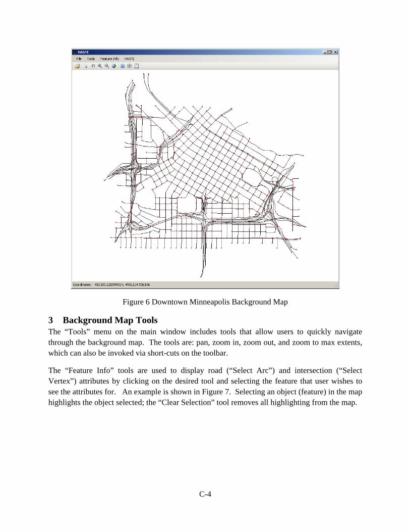
C-4

Figure 6 Downtown Minneapolis Background Map

3 Background Map Tools The “Tools” menu on the main window includes tools that allow users to quickly navigate through the background map. The tools are: pan, zoom in, zoom out, and zoom to max extents, which can also be invoked via short-cuts on the toolbar.

The “Feature Info” tools are used to display road (“Select Arc”) and intersection (“Select Vertex”) attributes by clicking on the desired tool and selecting the feature that user wishes to see the attributes for. An example is shown in Figure 7. Selecting an object (feature) in the map highlights the object selected; the “Clear Selection” tool removes all highlighting from the map.

C-5

Figure 7 Feature Selection

4 Scenario Development 1. Under the “HASTE” menu item, click “Select Area”. The radius input box shown in Figure

8 will appear.

Figure 8 Selection of Disaster Area Radius

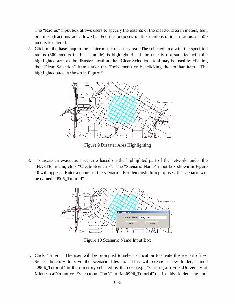
C-6

The “Radius” input box allows users to specify the extents of the disaster area in meters, feet, or miles (fractions are allowed). For the purposes of this demonstration a radius of 500 meters is entered.

2. Click on the base map in the center of the disaster area. The selected area with the specified radius (500 meters in this example) is highlighted. If the user is not satisfied with the highlighted area as the disaster location, the “Clear Selection” tool may be used by clicking the “Clear Selection” item under the Tools menu or by clicking the toolbar item. The highlighted area is shown in Figure 9.

Figure 9 Disaster Area Highlighting

3. To create an evacuation scenario based on the highlighted part of the network, under the

“HASTE” menu, click “Create Scenario”. The “Scenario Name” input box shown in Figure 10 will appear. Enter a name for the scenario. For demonstration purposes, the scenario will be named “0906_Tutorial”.

Figure 10 Scenario Name Input Box

4. Click “Enter”. The user will be prompted to select a location to create the scenario files.

Select directory to save the scenario files to. This will create a new folder, named “0906_Tutorial” in the directory selected by the user (e.g., “C:\Program Files\University of Minnesota\No-notice Evacuation Tool\Tutorial\0906_Tutorial”). In this folder, the tool

C-7

creates two GIS layers, a links layer and a nodes layer with their names prefixed by the scenario name (i.e., 0906_Tutorial_Links and 0906_Tutorial_Nodes). The two layers are displayed in the scenario set-up window, which appears after the files are created.

5 Scenario Set-up Scenario set-up can be summarized by the following four steps:

1. Trimming the network by deleting arcs and vertices. 2. Modification of arc capacities and jam densities, if necessary. 3. Entering demands (i.e., defining the network sources). 4. Defining the network sinks.

5.1 Delete Arc To delete a network arc from the scenario network, select “Delete Arc” under the “Edit Network” menu and select the arc to delete. The same process is carried out for each arc to be deleted, where after each arc is deleted the user is asked to confirm deletion as shown in Figure 11.

Figure 11 Deleting an Arc

After deleting some of the network arcs, vertices that are no longer attached to the remaining network (see Figure 12) should also be deleted. This is done the same way it was done when deleting arcs using the “Delete Vertex” tool under the “Edit Network” menu.

Figure 12 Unconnected Vertices

C-8

Note that upon confirming deletion of either an arc or a vertex, changes are immediately saved in the GIS link and node files for the scenario.

5.2 Modifying Arc Attributes The tool also allows users to modify arc attributes to represent changes in the physical network; this is useful when dealing with partial link closures (e.g., lane drops) and to minimize the utilization of certain roads in the network as part of the evacuation strategy when full road closures represented by deleting an arc is not desired. To modify arc attributes, click “Select Arc” under the “Feature Info” menu or click the grid icon on the toolbar. The two arc attributes that can be modified for this purpose are the capacity and jam density of the arc (see Figure 13).

Figure 13 Modifying Arc Attributes

5.3 Entering Demands Network demands are the most crucial input in scenario set-up process. Vertices with non-zero demands are considered evacuee concentration points in the network. The distribution of demands in the network is crucial in terms of accuracy of the algorithms, the realism of the scenario, and the computation times. Concentrating very large demands in one vertex will result in excessively high computation times, due to limitations in the capacities of the outgoing arcs both in the model and in reality.

To enter demands, select the “Select Vertex” tool under the “Feature Info” menu or click the “Select Single Vertex” button on the toolbar. Then click on the vertex on the map to view the vertex attributes and enter/modify demands. For purposes of this demonstration, two vertices are selected and 500 vehicles are entered as demands. This is illustrated in Figure 14.

C-9

Figure 14 Entering Demands

5.4 Defining Network Sinks To define the network sinks, click “Select Sinks” under the “Edit Network” menu. The tool will assume sink selection mode (Figure 15), which does not allow the user to use any of the network modification tools. It is crucial that all boundary vertices are selected in order to have an accurate representation. It is also crucial that only boundary vertices are selected. Upon selecting each of the vertices, the vertex attributes box will appear which can be closed by clicking the close button (or the spacebar) and resuming selection. Upon completing selection, the “Stop Adding Sinks” button (red X) can be clicked.

Figure 15 Sink Selection Mode

C-10

To view the selected sinks, click on “Edit Network” -> “Sink List” -> “Highlight Sinks”. The result is shown in Figure 16.

Figure 16 Highlighting Selected Sinks

Highlighting the selected sinks allows the user to check is whether enough sinks have been selected. To add more sinks to the selection, simply click “Select Sinks” to go back to sink selection mode. To modify the selection (i.e. remove sinks from the selection), click “Edit Network” -> “Sink List” -> “Clear List” and redo the selection.

This concludes scenario set-up. The scenario files are ready for the algorithms.

6 Running the Evacuation Algorithms

6.1 Creating the Evacuation Network 1. Under the “HASTE” menu, select the “Create Evacuation Network” tool. 2. The “Signal Timing Period” input box appears, prompting the user to select a signal timing

period since different times of the day are associated with different signal timing plans. For purposes of this demonstration, “PM Peak” option will be selected (Figure 17).

3. Click OK in the “Signal Timing Period” input box after selecting the analysis period. 4. Allow a few seconds for processing the user input. The “Delta T” input box appears

prompting the user to select an appropriate discrete time interval length for the algorithms (Figure 18). For purposes of this demonstration, 10 seconds will be selected. Click “OK”.

C-11

5. Allow a few seconds for processing. When done a message box displaying the message “Done Converting Network” will appear (Figure 19). Click “OK” to close the message.

Figure 17 Signal Timing Period Input Box

Figure 18 Discrete Time Interval Length “Delta T”

Figure 19 Done Converting Network Message

This completes the scenario set-up procedure. After completing the scenario set-up procedure, the next step is to run the algorithms. First, under the “HASTE” menu, click “Run HASTE”. This brings up the “Dynamic Assignment” window shown in Figure 20.

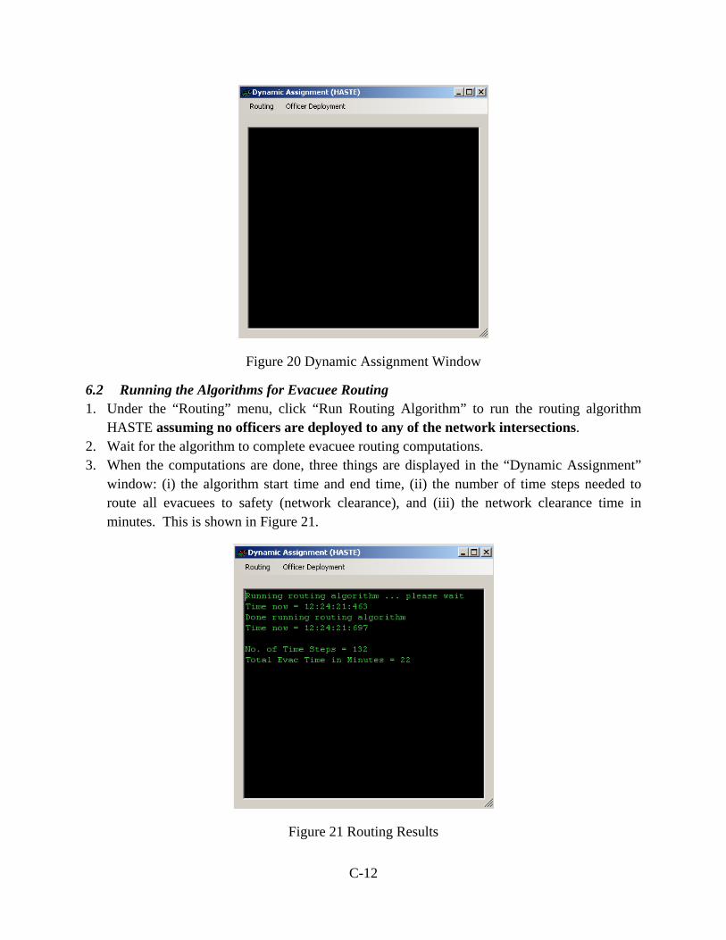
C-12

Figure 20 Dynamic Assignment Window

6.2 Running the Algorithms for Evacuee Routing 1. Under the “Routing” menu, click “Run Routing Algorithm” to run the routing algorithm

HASTE assuming no officers are deployed to any of the network intersections. 2. Wait for the algorithm to complete evacuee routing computations. 3. When the computations are done, three things are displayed in the “Dynamic Assignment”

window: (i) the algorithm start time and end time, (ii) the number of time steps needed to route all evacuees to safety (network clearance), and (iii) the network clearance time in minutes. This is shown in Figure 21.

Figure 21 Routing Results

C-13

Note that the start and end times displayed in the “Dynamic Assignment” window are the start and end times of the algorithm only. There are additional preparatory computations that take place before running the algorithm, where the graph theoretic network structure is transformed into a network of cells.

In addition to network clearance times, the tool also produces evacuee departure plans as text files in the scenario directory. Text based results and graphical displays of results are discussed later.

6.3 Manual Selection of Officer Deployment Locations The software tool also allows analysts to test their own officer deployment strategies. For demonstration purposes, we will arbitrarily assign 5 officers to 5 randomly selected intersections in the network, as follows:

1. Under the “Routing” menu, click “Select Intersections and Route”. This will bring up the “Signal Selection” input box shown in Figure 22.

2. Check the boxes in the “Signal Selection” input box to select the desired intersections.

Figure 22 Signal Selection

3. After selecting the desired intersections for officer deployment, click “Run Routing

Algorithm”. The clearance time results are displayed in the “Dynamic Assignment” (Figure 23).

There are two things to note in the routing examples:

• The routing algorithm required less than 300 milliseconds to compute routing strategies in both cases (with and without officers).

• The clearance time is slightly better with the 5 officers deployed randomly to five signalized intersections (22 minutes vs. 20.5 minutes in Figure 21 and Figure 23, respectively).

C-14

Figure 23 Routing Results with Five Officers

6.4 Optimized Officer Deployment Strategies In the example above, five officers were deployed manually to five randomly selected locations in the network. We will now turn to finding optimized officer deployment strategies using the evacuation software tool.

1. In the “Dynamic Assignment” window, under the “Officer Deployment” menu, click “GA Parameters”. This brings up the deployment algorithm parameter input box shown in Figure 24.

2. For officer deployment budget, enter 5 and use the defaults for all other parameters.

Figure 24 Genetic Algorithm Parameters

3. Click “Enter Parameters”.

C-15

4. Under the “Officer Deployment” menu, click “Run Algorithm”. The “Dynamic Assignment” window goes to waiting mode while carrying out the calculations (Figure 25).

Figure 25 Waiting Mode

After calculations are completed, the algorithm start and end times and the best network clearance time are shown in the “Dynamic Assignment” window (Figure 26).

Figure 26 Optimized Officer Deployment Strategy Results

Note that to compute the officer deployment strategy more time was required. However, the algorithm run time is still less than 30 seconds for this small scenario. Also note the improvement in the network clearance time (14 minutes).

C-16

7 Results

7.1 Graphical Display All routing and officer deployment results are saved in text files in the scenario directory. Some of the results can be displayed graphically in the scenario window.

1. Close the “Dynamic Assignment” window. 2. On the scenario window, under the “Results” menu, click “View Selected Intersections”.

The signalized intersection selected for officer deployment are highlighted on the map and a list of all network signalized intersections with the “CHOSEN” and “NOT CHOSEN” appear in the “List of Selected Intersections” window (Figure 27).

Figure 27 List of Selected Intersections

3. Close the “List of Selected Intersections” window. 4. Click “Clear Selection” under the “Feature Info” window to clear the highlighting. 5. Click “Route Sets” under the “Results” menu to graphically display the routes suggested by

the routing algorithm for each network source. The “Route Sets” window shown in Figure 28 can now be used to view routes in the scenario window by selecting a route and clicking

C-17

“View Route”. The “Route Sets” window displays the route sets under each of the network sources and displays the total number of evacuees assigned to each of the routes.

6. Expand one of the routes by clicking on the + icon next to it. This will list all roads comprising the route, numbered by their object identifiers in the links shapefile.

Figure 28 Route Sets

7.2 Text Files All routing an officer deployment results are also save in the “HASTE” folder in the scenario directory (“C:\Program Files\University of Minnesota\No-notice Evacuation Tool\Tutorial\0906_Tutorial\HASTE”). This includes:

• “Log.txt”: the results displayed in the “Dynamic Assignment” window. • “ShapesChosen.csv”: the shape id’s of the vertices chosen for officer deployment in the

nodes shapefile. • “IntersectonsChosen.txt”: a list of signalized intersections in the scenario network indicating

which intersections are chosen for officer deployment. • “Assignment.csv”: a time-space table listing all cell occupancies over the course of the

evacuation process. • The “Routing” folder includes one sub-folder for each source in the scenario network with

two files inside of each folder: “FlowList.csv”: a departure schedule with the route index in the first column and the

number of evacuees assigned to the routes in the second column.

C-18

“Paths.csv”: a list of paths used by the source (one path per row). The first column is the total number of evacuees assigned to the path and the other columns hold the shape id’s of the arcs that constitute the path.

Development of a Dynamic Data-Driven Model for Effective ...

Documents

Transcript of Development of a Dynamic Data-Driven Model for Effective ...