applied sciences

Article

Dynamic Plan Control: An Effective Tool to Manage DemandConsidering Mobile Internet Network Congestion

Xiaoyu Ma 1, Jihong Zhang 1, Yuan Cao 2, Zhou He 3,4,* and Jonas Nebel 5

�����������������

Citation: Ma, X.; Zhang, J.; Cao, Y.;

He, Z.; Nebel, J. Dynamic Plan Control:

An Effective Tool to Manage Demand

Considering Mobile Internet Network

Congestion. Appl. Sci. 2021, 11, 91.

https://dx.doi.org/10.3390/

app11010091

Received: 1 December 2020

Accepted: 18 December 2020

Published: 24 December 2020

Publisher’s Note: MDPI stays neu-

tral with regard to jurisdictional claims

in published maps and institutional

affiliations.

Copyright: © 2020 by the authors. Li-

censee MDPI, Basel, Switzerland. This

article is an open access article distributed

under the terms and conditions of the

Creative Commons Attribution (CC BY)

license (https://creativecommons.org/

licenses/by/4.0/).

1 International Business School, Beijing Foreign Studies University, Beijing 100089, China;maxiaoyu@bfsu.edu.cn (X.M.); zhangjihong@bfsu.edu.cn (J.Z.)

2 Antai College of Economics and Management, Shanghai Jiao Tong University, Shanghai 200030, China;caoyuan0406@sjtu.edu.cn

3 School of Economics and Management, University of Chinese Academy of Sciences, Beijing 100049, China4 Key Laboratory of Big Data Mining and Knowledge Management, Chinese Academy of Sciences,

Beijing 100049, China5 Department of Industrial Engineering, Tsinghua University, Beijing 100084, China;

jonasfriedrich.nebel@gmail.com* Correspondence: hezhou@ucas.ac.cn

Abstract: Rapidly increasing mobile data traffic have placed a significant burden on mobile Internetnetworks. Due to limited network capacity, a mobile network is congested when it handles too muchdata traffic simultaneously. In turn, some customers leave the network, which induces a revenue lossfor the mobile service provider. To manage demand and maximize revenue, we propose a dynamicplan control method for the mobile service providers under connection-speed-restriction pricing.This method allows the mobile service provider to dynamically set the data plans’ availability forpotential customers’ new subscriptions. With dynamic plan control, the service provider can adjustdata network utilization and achieve high customer satisfaction and a low churn rate, which reflecthigh service supply chain performance. To find the optimal control policy, we transform the high-dimensional dynamic programming problem into an equivalent mixed integer linear programmingproblem. We find that dynamic plan control is an effective tool for managing demand and increasingrevenue in the long term. Numerical evaluation with a large European mobile service provider furthersupports our conclusion. Furthermore, when network capacity or potential customers’ willingness tojoin the network changes, the dynamic plan control method generates robust revenue for the serviceprovider.

Keywords: demand management; dynamic plan control; mobile Internet network congestion;connection-speed-restriction pricing

1. Introduction

Mobile data traffic have exploded with the wide popularity of mobile Internet serviceand the exponential growth of mobile applications. According to the Cisco Visual Net-working Index released in February 2019 [1], global mobile data traffic have grown 17-foldfrom 2012 to 2017 and will continue growing at a compound annual growth rate (CAGR)of 46% from 2017 to 2022, reaching 77.5 exabytes per month by 2022. To handle rapidlyincreasing data traffic, new technology for wireless communications is needed. However,it takes a long time to promote technology. For example, the second-generation of wirelesstelecommunications technology (2G) appeared ten years before the third-generation (3G),followed by the fourth-generation (4G) eight years later. The fifth-generation of wirelesstelecommunications was developed fast, but it still took six years to finally launch 5G [2].According to the technology characteristics, the capacity of the mobile network is fixedduring the same generation of wireless telecommunications.

Customers use ever-increasing mobile Internet data while the mobile network capacityis fixed during several years of the same generation. As a consequence, limited mobile

Appl. Sci. 2021, 11, 91. https://dx.doi.org/10.3390/app11010091 https://www.mdpi.com/journal/applsci

Appl. Sci. 2021, 11, 91 2 of 23

network capacity is threatened by immense data traffic. Specifically, when a mobilenetwork handles too much data traffic simultaneously, network congestion occurs [3,4].Network congestion leads to customer dissatisfaction in this wireless service supply chain.For example, Internet web pages cannot be displayed quickly, and videos cannot be playedsmoothly. In turn, customer dissatisfaction drives a number of customers to leave thewireless network and then influences the service provider’s revenue and the wirelessservice supply chain’s performance. Therefore, mobile service providers should take thepotential network congestion into consideration while maximizing revenue [5]. To this end,several demand management methods considering congestion have been proposed andstudied, such as time-of-day pricing [6] and Wi-Fi offloading [7]. A detailed discussion ofthese demand management methods is included in the literature review.

It is worth noting that the pricing scheme, where demand management methodsapply, has evolved with the progression of wireless telecommunications technology. In the1980s, the first-generation of wireless telecommunications technology (1G) was launched.Its connection speed was only 2.4 Kb/s (1 Gb = 1024 Mb; 1 Mb = 1024 Kb) , and users couldonly make voice calls. At this time, flat-rate pricing dominated, which charges each user afixed fee per session independently of the user’s data usage. As wireless telecommunica-tions technology upgraded to the second-generation (2G) and third-generation (3G), theconnection speed could reach up to 10 Mb/s. Multimedia services emerged, such as theglobal positioning system (GPS) and video conferencing [8]. In the era of 2G and 3G, peopleused mobile Internet for different purposes, which made data usage vary greatly from oneuser to another. In 2011, the top 1% of mobile Internet users generated approximately 35%of the traffic over the world [9]. To better match a customer’s cost with her/his data usage,many service providers moved away from the simple flat-rate pricing to metered pricing,which charges a user in proportion to her/his data usage. In contrast to flat-rate pricing,metered pricing is concerned about not only whether a customer uses the data service, butalso how much data she/he consumes.

Since the fourth-generation of wireless telecommunications technology (4G) waslaunched around 2009, connection speed has been greatly improved to 100 Mb/s. MobileInternet service is fast becoming an integral part of people’s daily life and is used throughvarious kinds of applications, including mobile videos, file transferring, social networkservices, etc. Most people already consider mobile Internet service as a necessity. In contrastto spending too much for mere access to mobile networks, people are more willing to pay fora high connection speed. This is where connection-speed-restriction pricing comes into play.Under connection-speed-restriction pricing, data usage is unlimited for users. However,when a user’s data usage exceeds a threshold in a billing period, her/his connection speedwill be decreased. Throughout the rest of the current billing period, she/he can continueusing mobile Internet, but at the restricted speed. To re-obtain full-speed mobile Internetservice, the user needs to buy the supplementary data package or wait until the beginningof the next billing period. In contrast to flat-rate pricing and metered pricing, connection-speed-restriction pricing considers the connection speed, which is the focus for customerexperience.

In practice, connection-speed-restriction pricing plays an increasingly important rolein mobile Internet pricing. A study conducted on North American mobile service providersshowed that the percentage of data plans offered under connection-speed-restriction pricinghad grown from 39% in September 2016 to 66% in August 2018 [1]. In the arriving era of5G, connection speed can reach up to 1 Gb/s, which is much faster than the speed of the4G network. Hence, mobile service providers will have a strong motivation to employconnection-speed-restriction pricing in the 5G era.

Technically, the restriction of a user’s connection speed is achieved by shifting her/hisdata connection from a high-generation network to a low-generation network. For example,if a service provider uses a 5G network to provide full-speed data service, the restrictionof a user’s connection speed can be achieved by shifting his/her data connection from a5G network to a 3G network or even a 2G network. Most importantly, a 5G connection

Appl. Sci. 2021, 11, 91 3 of 23

provides much higher connection speed than a 3G connection. According to Qualcomm’sexperiment, a 5G connection provides over 100 times faster speed on average than a 3Gconnection. This fact provides valuable insight into demand management while consider-ing network congestion. On the one hand, if too many customers buy the supplementarydata package to use full-speed data service in the high-generation network, then the mobilenetwork is highly prone to congestion. On the other hand, if too many customers do notbuy the supplementary data package, then the service provider wastes the network capac-ity and loses potential revenue. Therefore, how can a wireless service provider managedemand and maximize revenue under connection-speed-restriction pricing? We explorethis issue in our paper.

Based on connection-speed-restriction pricing, we propose a dynamic plan controlmethod. With this method, a wireless service provider can dynamically control which dataplans are open and which data plans are closed for new customers at the beginning of eachperiod. Here, each period refers to one month, one quarter, or another time dimensionaccording to the service provider’s state of operation. In each period, new customerscan only subscribe to one of the open data plans. The close of a plan only prevents newcustomers from subscribing to it during a certain period, while old customers of this plancan still use and pay for it during this period. Therefore, the service provider can take thelimited network capacity into consideration and maximize revenue in the long term bythis dynamic plan control method. At the same time, customer experience is ensured, andsupply chain performance is enhanced.

Our study has three contributions. First, we take the limited network capacity intoconsideration and build a dynamic plan control model. The traditional dynamic pricingof mobile data plans focuses on finding the optimal pricing parameters by assuming thatnetwork capacity is unlimited. However, with the rapid growth of data traffic, networkcapacity has become a bottleneck that affects how service providers can address customers’demand. This research attempts to offer new insights into managing demand when networkcapacity is limited. Compared with the all plans always open method, which is currentlyimplemented by most mobile service providers, our dynamic plan control method candynamically open a subset of data plans for new customers at the beginning of each period.This dynamic control allows the service provider to adjust data network utilization andachieve high customer satisfaction and a low churn rate, which reflect high service supplychain performance.

Second, we provide a framework to model the behaviors of service providers andcustomers under connection-speed-restriction pricing. Despite the growing popularity ofconnection-speed-restriction pricing, little research has been devoted to demand manage-ment under this pricing scheme. Our study addresses this issue and models the behaviorsof both service providers and customers under connection-speed-restriction pricing.

Third, the service provider’s optimization problem is a dynamic programming prob-lem. Due to the high-dimensional property of the problem, it is difficult to implementbackward induction. To solve the problem efficiently, we propose an equivalent mixed inte-ger linear programming (MILP) formulation. Through numerical evaluation, the efficiencyof the solution method is further validated.

The remainder of this paper is organized as follows. We conduct a brief review of therelevant literature in Section 2. In Section 3, we describe the models of the service providerand customers. Section 4 provides the solution approach, and Section 5 examines theeffect of our model with numerical experiments. Finally, Section 6 offers some concludingremarks and future research directions.

2. Literature Review

Our research relates to two topics in the literature: the pricing scheme used for mobiledata service and the demand management methods considering congestion used by mobileservice providers. In this section, we review the relevant works on these two topics.

Appl. Sci. 2021, 11, 91 4 of 23

2.1. Pricing Scheme

The pricing scheme used for mobile data service has evolved in the past two decades.Because flat-rate pricing is easy to implement and quite effective in stimulating datademand [10], it was popular when the total market demand for data service was low.As data demand grew, mobile service providers moved to metered pricing, where acustomer is charged a fixed fee first and then a per-unit fee. In contrast to flat-rate pricing,metered pricing allows mobile service providers to facilitate price discrimination andthereby increase their revenue [11,12]. In practice, there are two versions of meteredpricing: two part pricing and three part pricing. The difference is that three part pricingbundles some allotted data into the fixed fee, but two part pricing does not (see Figure 1a,b).Danaher [13] studied two part pricing and found the optimal fixed fee and per-unit fee forthe revenue-maximizing strategy. In addition, they showed that the fixed fee and per-unitfee have different relative effects on the demand and retention of users.

A similar investigation analyzed three part pricing. Reference [14] assumed thateach consumer has a predetermined demand. He showed that for consumers who arenot overconfident, the firm’s optimal strategy is a high fixed fee and thus takes all ofthe consumers’ surplus. Furthermore, the firm’s profit increases if the consumers areoverconfident. Later, Reference [15] characterized the optimal three part pricing planunder more general conditions. Based on a global bound for the service provider’s profit,they employed a methodology that was different from the standard first-order conditionsapproach and showed that this bound is attained using the optimal plan. In addition,some researchers compared two part pricing and three part pricing and tried to find whichone was better for service providers. Reference [12] concluded that a relatively small menuof three part pricing can be more profitable than a menu of two part pricing of any size.In contrast, Reference [16] showed that the optimal three part pricing outcomes are identical tothe optimal two part pricing outcomes when the market demand follows an increasing priceelasticity or when the consumer distribution approximately follows an increasing hazard rate.

Data usage

Fixed

fee

Price

(a) Two-part Pricing

Data usage

Price

(b) Three-part Pricing

Allotted data

Fixed

fee

Data usage

Price

(c) Connection-speed-restriction Pricing

Two options

for customers

Pay the premium

Not pay the premium

Threshold

Fixed

fee

Figure 1. Two part pricing, three part pricing, and connection-speed-restriction pricing.

Since we entered the era of 4G, connection-speed-restriction pricing has rapidly be-come a popular pricing scheme used by the industry. Figure 1 shows the differencesamong two part pricing, three part pricing, and connection-speed-restriction pricing. In anoverview of smart data pricing, Sen et al. [17] addressed connection-speed-restrictionpricing as a new trend of data pricing. However, to the best of our knowledge, few studieshave been devoted to connection-speed-restriction pricing. Our study aims to fill this gap.

2.2. Demand Management Considering Congestion

Another relevant stream of the literature is demand management methods consideringcongestion in mobile Internet networks. As the demand for data service grew dramatically,demand management has become a new challenge for service providers. Research ondemand management is conducted mainly considering two concepts, time-dependentpricing and the traffic offloading mechanism, which aim to relieve network congestion by

Appl. Sci. 2021, 11, 91 5 of 23

giving users incentives to shift their mobile data demand to less-congested time periods orto supplementary networks (such as Wi-Fi) [18].

Time-dependent pricing has many variants. The most basic version is time-of-daypricing, which charges users a higher price for data usage during certain “peak” hours ofthe day than at other times of the day, so that network congestion in these time periodscan be relieved [19–21]. In contrast to time-of-day pricing, day-ahead pricing computesnew prices for different times of the next day in advance, based on predicted congestionlevels. Reference [22] showed that day-ahead pricing benefits both service providers andcustomers, flattening the temporal fluctuation of data demand while allowing users tosave money by choosing the time and volume of their usage. Besides, day-ahead pricing isalso used in the electricity pricing context. Reference [23] considered a model for a singlesmart home and for a community (multiple homes) with different priorities. The prioritywas assigned to each appliance by electricity consumers. In their scheme, day-ahead realtime pricing (DA-RTP) and critical peak pricing (CPP) were utilized to calculate electricitycost. Time-dependent pricing typically requires information about user demand [24,25].To obtain a reliable forecast of user demand, Reference [26] built a multiple equationtime-series model. For day-ahead forecasting, the mean absolute percentage error (MAPE)returned by the model over a period of 11 years was an impressive 1.36%, which is superiorto all benchmarks that the authors chose.

In addition to time-dependent pricing, service providers can manage demand byencouraging users to shift some of their data traffic to supplementary networks such asWi-Fi [27]. Reference [28] noted that the success of such a “traffic offloading” strategylargely relies on the economic incentives provided to users. Reference [29] proposed a novelcongestion-optimal Wi-Fi offloading (COWO) algorithm based on the subgradient method,which aims to obtain the optimal offloading ratio for each access point to maximize thethroughput and minimize network congestion. Reference [30] proposed a downloadingmechanism in different vehicular networks that comprises an ad hoc network and a cellularnetwork. In this mechanism, roadside units act as traffic managers to collect data fromthe Internet and then distribute them to vehicles in an approximately optimal manner.Reference [31] constructed an intelligent offloading method for vehicular networks. Theyjointly utilized licensed cellular spectrum and unlicensed channels and used the real dataof the traces of taxies to illustrate the effectiveness of the solution. In general, Reference [18]stated that the realizations of time-dependent pricing and traffic offloading can help createa financial win-win solution for service providers and their users.

Although time-dependent pricing and traffic offloading mechanisms have been provento be helpful in demand management, they have some drawbacks and limitations [18,32].Time-dependent pricing makes the price change too frequently, which leads to extra costs,including operational costs and costs to help consumers in understanding and making aselection from a complex menu of choices [33]. Traffic offloading seems to be the directionin which many service providers are going today, but it requires investment in expandingwired and wireless network capacities.

To meet these challenges, we propose another demand management tool, the dynamicplan control method, which can dynamically control open and closed plans for potentialcustomers in each period to relieve mobile network congestion. Moreover, we innovativelyapply it in the framework of connection-speed-restriction pricing, which is increasinglypopular now that 4G and 5G are available.

3. The Model

A mobile service provider (SP) employs connection-speed-restriction pricing andoffers m different data plans. The information about the data plans is pre-announced to thecustomers. We consider a market composed of a large number of customers. The customerpopulation, denoted by N, is deterministic.

All data plans give customers unlimited data. The differences between the data plansare their prices and allotted volumes of full-speed data. We denote bi as the price per period

Appl. Sci. 2021, 11, 91 6 of 23

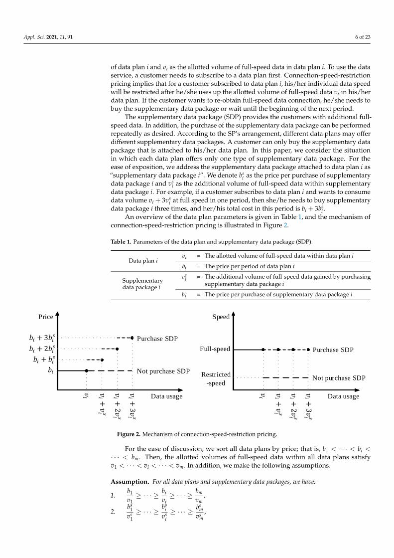
of data plan i and vi as the allotted volume of full-speed data in data plan i. To use the dataservice, a customer needs to subscribe to a data plan first. Connection-speed-restrictionpricing implies that for a customer subscribed to data plan i, his/her individual data speedwill be restricted after he/she uses up the allotted volume of full-speed data vi in his/herdata plan. If the customer wants to re-obtain full-speed data connection, he/she needs tobuy the supplementary data package or wait until the beginning of the next period.

The supplementary data package (SDP) provides the customers with additional full-speed data. In addition, the purchase of the supplementary data package can be performedrepeatedly as desired. According to the SP’s arrangement, different data plans may offerdifferent supplementary data packages. A customer can only buy the supplementary datapackage that is attached to his/her data plan. In this paper, we consider the situationin which each data plan offers only one type of supplementary data package. For theease of exposition, we address the supplementary data package attached to data plan i as“supplementary data package i”. We denote bs

i as the price per purchase of supplementarydata package i and vs

i as the additional volume of full-speed data within supplementarydata package i. For example, if a customer subscribes to data plan i and wants to consumedata volume vi + 3vs

i at full speed in one period, then she/he needs to buy supplementarydata package i three times, and her/his total cost in this period is bi + 3bs

i .An overview of the data plan parameters is given in Table 1, and the mechanism of

connection-speed-restriction pricing is illustrated in Figure 2.

Table 1. Parameters of the data plan and supplementary data package (SDP).

Data plan ivi = The allotted volume of full-speed data within data plan i

bi = The price per period of data plan i

Supplementarydata package i

vsi = The additional volume of full-speed data gained by purchasing

supplementary data package i

bsi = The price per purchase of supplementary data package i

Data usage

Price

Purchase SDP

Not purchase SDP𝑏𝑖

𝑣𝑖

𝑏𝑖 + 𝑏𝑖𝑠

Data usage

Full-speed

Speed

Restricted

-speed

Purchase SDP

Not purchase SDP

𝑏𝑖 + 2𝑏𝑖𝑠

𝑏𝑖 + 3𝑏𝑖𝑠

𝑣𝑖+𝑣𝑖 𝑠

𝑣𝑖+2𝑣𝑖 𝑠

𝑣𝑖+3𝑣𝑖 𝑠

𝑣𝑖

𝑣𝑖+𝑣𝑖 𝑠

𝑣𝑖+2𝑣𝑖 𝑠

𝑣𝑖+3𝑣𝑖 𝑠

Figure 2. Mechanism of connection-speed-restriction pricing.

For the ease of discussion, we sort all data plans by price; that is, b1 < · · · < bi <· · · < bm. Then, the allotted volumes of full-speed data within all data plans satisfyv1 < · · · < vi < · · · < vm. In addition, we make the following assumptions.

Assumption. For all data plans and supplementary data packages, we have:

1.b1

v1≥ · · · ≥ bi

vi≥ · · · ≥ bm

vm,

2.bs

1vs

1≥ · · · ≥

bsi

vsi≥ · · · ≥ bs

mvs

m,

Appl. Sci. 2021, 11, 91 7 of 23

3. bi+1 < bi +

⌈vi+1 − vi

vsi

⌉· bs

i , ∀i = 1, 2, · · · , m− 1.

These three assumptions are mild and easily satisfied in real practice. Assumptions 1and 2 are straightforward: a high-priced data plan (and its corresponding supplementarydata package) means a low unit price of full-speed data. Assumption 3 implies that when acustomer’s full-speed data usage is larger than a critical value, a higher price data plan isalways preferred by the customer over a lower price data plan.

Because the network capacity is fixed, network congestion occurs when the overalldata traffic in the network exceeds a threshold. Network congestion influences the customerexperience, resulting in a number of customers leaving the network. To manage networkcongestion, the service provider can use the dynamic plan control method. With thismethod, the service provider opens a subset of data plans in each period, and potentialcustomers can subscribe to only the open data plans. Let Ci,t be a binary variable indicatingthe open/closed status of the data plan i in period t. Ci,t = 1 if the data plan i is open inperiod t, and Ci,t = 0 otherwise. In the following, we model the behaviors of the serviceprovider and customers and then give the service provider’s revenue function.

3.1. Decisions of Potential Customers

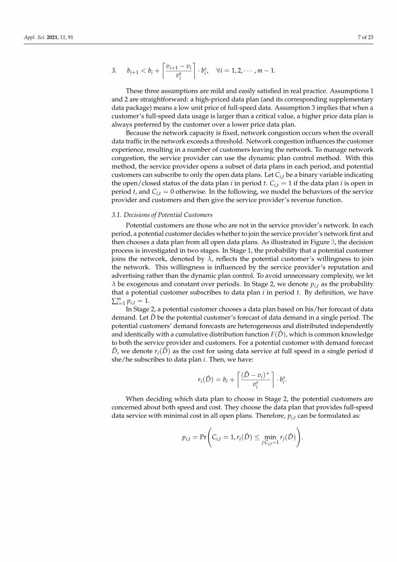
Potential customers are those who are not in the service provider’s network. In eachperiod, a potential customer decides whether to join the service provider’s network first andthen chooses a data plan from all open data plans. As illustrated in Figure 3, the decisionprocess is investigated in two stages. In Stage 1, the probability that a potential customerjoins the network, denoted by λ, reflects the potential customer’s willingness to jointhe network. This willingness is influenced by the service provider’s reputation andadvertising rather than the dynamic plan control. To avoid unnecessary complexity, we letλ be exogenous and constant over periods. In Stage 2, we denote pi,t as the probabilitythat a potential customer subscribes to data plan i in period t. By definition, we have∑m

i=1 pi,t = 1.In Stage 2, a potential customer chooses a data plan based on his/her forecast of data

demand. Let D be the potential customer’s forecast of data demand in a single period. Thepotential customers’ demand forecasts are heterogeneous and distributed independentlyand identically with a cumulative distribution function F(D), which is common knowledgeto both the service provider and customers. For a potential customer with demand forecastD, we denote ri(D) as the cost for using data service at full speed in a single period ifshe/he subscribes to data plan i. Then, we have:

ri(D) = bi +

⌈(D− vi)

+

vsi

⌉· bs

i .

When deciding which data plan to choose in Stage 2, the potential customers areconcerned about both speed and cost. They choose the data plan that provides full-speeddata service with minimal cost in all open plans. Therefore, pi,t can be formulated as:

pi,t = Pr

(Ci,t = 1, ri(D) ≤ min

j:Cj,t=1rj(D)

).

Appl. Sci. 2021, 11, 91 8 of 23

A potential

customer

Not join the network

Join the network

Subscribe to data plan 1

Subscribe to data plan 2

Subscribe to data plan m

Subscribe to data plan i

w.p. 𝜆

w.p. 1− 𝜆

w.p. λ𝑝1,𝑡

w.p. 𝜆𝑝2,𝑡

w.p. 𝜆𝑝𝑖,𝑡

w.p. 𝜆𝑝𝑚 ,𝑡

Figure 3. Decisions of the potential customers.

3.2. Characteristics of the Subscribed Customers

For a customer subscribed to data plan i, we introduce a vector (Ui, U fi ), where Ui

is his/her total data usage (including full-speed data usage and restricted-speed datausage) in a period and U f

i is his/her full-speed data usage in a period. In each period, thesubscribed customer consumes data continuously throughout the entire period. Therefore,the vector (Ui, U f

i ) is random at the beginning of the period and realized at the end ofthe period.

We model two key characteristics of the subscribed customers’ behavior. First, a cus-tomer’s total data usage does not necessarily equal her/his data demand forecast, despitethe fact that the customer chooses the data plan based on her/his data demand forecast.Generally, the customer’s total data usage fluctuates around the volume of full-speeddata in her/his data plan. This is reasonable because if the customer’s total data usageis far below vi, then she/he should have subscribed to a “low-priced” data plan. If thecustomer’s total data usage is far beyond vi, then she/he should have subscribed to a “high-priced” data plan. Therefore, we assume that the expected volume of the customer’s totaldata usage equals the volume of full-speed data in her/his data plan; that is, E[Ui] = vi.In addition, we assume that the total data usage of all customers subscribed to plan i aredistributed independently and identically with a cumulative distribution function Fi(Ui).Moreover, Fi(Ui) is homogeneous over periods.

Second, if a subscribed customer wants to consume more full-speed data than theallotted volume within his/her data plan, he/she purchases the supplementary datapackage repeatedly to maintain full speed throughout the entire period. This assumptionis reasonable because the marginal price for any supplementary data package is constant.

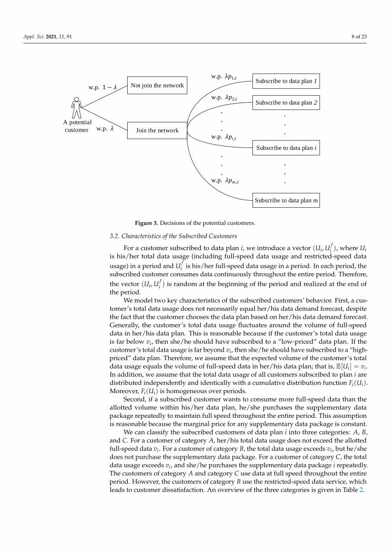
We can classify the subscribed customers of data plan i into three categories: A, B,and C. For a customer of category A, her/his total data usage does not exceed the allottedfull-speed data vi. For a customer of category B, the total data usage exceeds vi, but he/shedoes not purchase the supplementary data package. For a customer of category C, the totaldata usage exceeds vi, and she/he purchases the supplementary data package i repeatedly.The customers of category A and category C use data at full speed throughout the entireperiod. However, the customers of category B use the restricted-speed data service, whichleads to customer dissatisfaction. An overview of the three categories is given in Table 2.

Appl. Sci. 2021, 11, 91 9 of 23

Table 2. Three categories of subscribed customers.

Total Data UsageUi

Willing to BuySDP

Full-Speed DataUsage U f

i

Price to Pay inOne Period

CustomerSatisfaction

Category A ≤ vi Not necessary = Ui = bi YesCategory B > vi No = vi = bi NoCategory C > vi Yes = Ui = bi + k · bs

i Yes

Let Si,t be the number of customers subscribed to data plan i at the beginning ofperiod t. Let SA

i,t, SBi,t, and SC

i,t be the number of customers in the A, B, and C categories,respectively. By definition, we have Si,t = SA

i,t + SBi,t + SC

i,t. In addition, we define wi =

SCi,t/(S

Bi,t + SC

i,t), which reflects the customers’ willingness to purchase supplementary datapackages. We assume that wi is constant over periods.

In period t, the customers of both A and B categories pay bi. The service provider’srevenue generated from the customers of category A and category B is:

m

∑i=1

(SAi,t + SB

i,t) · bi.

To formulate the revenue generated from the customers of category C, we need tofurther differentiate the data usage. We define k (k ∈ N+) as an integer that satisfiesvi + (k − 1) · vs

i < Ui ≤ vi + k · vsi , where k denotes the number of supplementary data

packages a category C customer with data usage Ui purchases in a single period. Let SC,ki,t

be the number of subscribed customers of data plan i who purchase k supplementary datapackages in period t. Then, the service provider’s revenue generated from the customersof category C in period t is:

m

∑i=1

k∗t

∑k=1

SC,ki,t · (bi + k · bs

i ),

where k∗t denotes the largest k in period t.

3.3. Network Congestion and Plan-Leaving Characteristics

Network congestion occurs when total full-speed data usage exceeds a threshold. LetGt be a binary variable indicating whether network congestion occurs in period t. Gt = 1 ifnetwork congestion occurs in periods t, and Gt = 0 if not.

For a subscribed customer of data plan i, the expected volume of full-speed data usagein a single period is E[U f

i ]. By definition, we have:

E[U fi ] =

∫ vi

0Ui · fi(Ui) dUi + vi · [1− Fi(vi)] · (1− wi) +

∫ ∞

vi

Ui · fi(Ui) · wi dUi.

When the subscribed customers feel unsatisfied with the service, they may quit theservice. There are multiple reasons that lead to customer dissatisfaction, but we modelonly the two most important reasons, namely network congestion (NC) and individualspeed restriction (ISR). Let qP

i,t be the probability that a customer quits the service whenNC happens but ISR does not and qE

i,t be the probability that a customer quits the servicewhen ISR happens, but NC does not.

Let qi,t be the probability that a subscribed customer quits the service. Because networkcongestion and individual speed restriction are two independent events, we have:

Appl. Sci. 2021, 11, 91 10 of 23

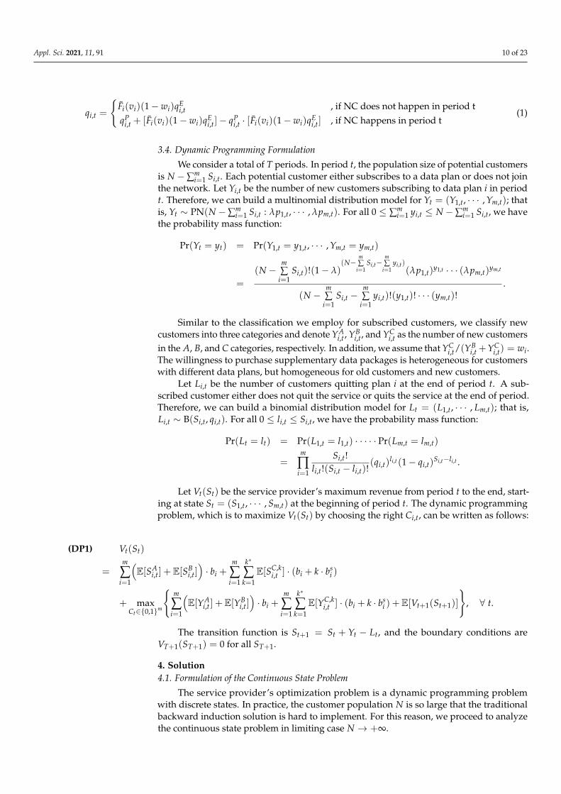
qi,t =

{Fi(vi)(1− wi)qE

i,t , if NC does not happen in period tqP

i,t + [Fi(vi)(1− wi)qEi,t]− qP

i,t · [Fi(vi)(1− wi)qEi,t] , if NC happens in period t

(1)

3.4. Dynamic Programming Formulation

We consider a total of T periods. In period t, the population size of potential customersis N −∑m

i=1 Si,t. Each potential customer either subscribes to a data plan or does not jointhe network. Let Yi,t be the number of new customers subscribing to data plan i in periodt. Therefore, we can build a multinomial distribution model for Yt = (Y1,t, · · · , Ym,t); thatis, Yt ∼ PN(N −∑m

i=1 Si,t : λp1,t, · · · , λpm,t). For all 0 ≤ ∑mi=1 yi,t ≤ N −∑m

i=1 Si,t, we havethe probability mass function:

Pr(Yt = yt) = Pr(Y1,t = y1,t, · · · , Ym,t = ym,t)

=

(N −m∑

i=1Si,t)!(1− λ)

(N−m∑

i=1Si,t−

m∑

i=1yi,t)

(λp1,t)y1,t · · · (λpm,t)ym,t

(N −m∑

i=1Si,t −

m∑

i=1yi,t)!(y1,t)! · · · (ym,t)!

.

Similar to the classification we employ for subscribed customers, we classify newcustomers into three categories and denote YA

i,t , YBi,t, and YC

i,t as the number of new customersin the A, B, and C categories, respectively. In addition, we assume that YC

i,t/(YBi,t +YC

i,t) = wi.The willingness to purchase supplementary data packages is heterogeneous for customerswith different data plans, but homogeneous for old customers and new customers.

Let Li,t be the number of customers quitting plan i at the end of period t. A sub-scribed customer either does not quit the service or quits the service at the end of period.Therefore, we can build a binomial distribution model for Lt = (L1,t, · · · , Lm,t); that is,Li,t ∼ B(Si,t, qi,t). For all 0 ≤ li,t ≤ Si,t, we have the probability mass function:

Pr(Lt = lt) = Pr(L1,t = l1,t) · · · · · Pr(Lm,t = lm,t)

=m

∏i=1

Si,t!li,t!(Si,t − li,t)!

(qi,t)li,t(1− qi,t)

Si,t−li,t .

Let Vt(St) be the service provider’s maximum revenue from period t to the end, start-ing at state St = (S1,t, · · · , Sm,t) at the beginning of period t. The dynamic programmingproblem, which is to maximize Vt(St) by choosing the right Ci,t, can be written as follows:

(DP1) Vt(St)

=m

∑i=1

(E[SA

i,t] +E[SBi,t])· bi +

m

∑i=1

k∗

∑k=1

E[SC,ki,t ] · (bi + k · bs

i )

+ maxCt∈{0,1}m

{m

∑i=1

(E[YA

i,t ] +E[YBi,t])· bi +

m

∑i=1

k∗

∑k=1

E[YC,ki,t ] · (bi + k · bs

i ) +E[Vt+1(St+1)]

}, ∀ t.

The transition function is St+1 = St + Yt − Lt, and the boundary conditions areVT+1(ST+1) = 0 for all ST+1.

4. Solution4.1. Formulation of the Continuous State Problem

The service provider’s optimization problem is a dynamic programming problemwith discrete states. In practice, the customer population N is so large that the traditionalbackward induction solution is hard to implement. For this reason, we proceed to analyzethe continuous state problem in limiting case N → +∞.

Appl. Sci. 2021, 11, 91 11 of 23

To characterize the percentage of customers already in data plan i at the begin-ning of period t, we define θi,t = lim

N→+∞Si,t/N. For convenience, we define θ0,t =

limN→+∞

(N −∑mi=1 Si,t)/N. Moreover, we let Vt(θt) be the service provider’s maximum aver-

age revenue per customer from period t to the end, starting at state θt = (θ0,t, θ1,t, · · · , θm,t).To simplify the expression, we let:

ρi =k∗t

∑k=1

[Fi(vi + kvsi )− Fi(vi + (k− 1)vs

i )] · (1 + k ·bs

ibi),

where ρi can be interpreted as the expectation that a customer of category C has to paymore than customers of category A or B.

The dynamic programming problem (DP2) can be written as follows:

(DP2) Vt(θt)

=m

∑i=1

θi,t · [Fi(vi) + Fi(vi) · (1− wi) + ρi · wi] · bi

+ maxCt∈{0,1}m

{θ0,t ·

m

∑i=1

λpi,t · [Fi(vi) + Fi(vi) · (1− wi) + ρi · wi] · bi +E[Vt+1(At(θt, It) · θt)

]}, ∀ t.

The boundary conditions are VT+1(θT+1) = 0 for all θT+1. The transition matrixAt(θt, Ct) can be formulated as:

At(θt, Ct) =

[A1 A2A3 A4

],

where A1 ∈ R, A2 ∈ R1×m, A3 ∈ Rm×1, and A4 ∈ Rm×m with:

A1 = 1−m

∑i=1

λ · pi,t,

{A2}i = λ · pi,t, ∀ i,

{A3}i = qi,t, ∀ i,

{A4}ii =

{1− qi,t, if i = i, ∀ i, i,0, if i 6= i, ∀ i, i.

According to the definition of θi,t, we have:

∑mi=1 θi,t · [Fi(vi) + Fi(vi)(1− wi) + ρi · wi] · bi

= ∑mi=1 lim

N→∞

Si,tN · [Fi(vi) + Fi(vi)(1− wi) + ρi · wi] · bi

= limN→∞

1N {∑

mi=1[Si,tFi(vi) + Si,t Fi(vi)(1− wi)] · bi

+ ∑mi=1 Si,t ·∑

k∗tk=1

[Fi(vi + kvs

i)− Fi

(vi + (k− 1)vs

i)]· (bi + k · bs

i )}

= limN→∞

1N

{∑m

i=1

(E[SA

i,t] +E[SBi,t])· bi + ∑m

i=1 ∑k∗tk=1 E[S

C,ki,t ] · (bi + k · bs

i )}

, ∀ t. (2)

Analogously, we can derive:

maxCt∈{0,1}m

{θ0,t ∑m

i=1 λ · pi,t · [Fi(vi) + Fi(vi)(1− wi) + ρi · wi] · bi}

= limN→∞

1N max

Ct∈{0,1}m

{∑m

i=1

(E[YA

i,t ] +E[YBi,t])· bi + ∑m

i=1 ∑k∗tk=1 E[Y

C,ki,t ] ·

(bi + k · bs

i)}

, ∀ t. (3)

Appl. Sci. 2021, 11, 91 12 of 23

Summing (2) and (3) over t and plugging them into the formulation of Data Plan 2(DP2), we obtain:

Vt(θt) = limN→∞

Vt(St)

N, ∀ t.

Due to the strong law of large numbers, we can reformulate θi,t+1 and θ0,t+1 as follows.

θi,t+1 = limN→∞

Si,t+1

N

= limN→∞

Si,t + Yi,t − Li,t

N= θ0,t · λpi,t + θi,t · (1− qi,t), ∀ i, t. (4)

θ0,t+1 = 1−m

∑i=1

θi,t+1

= 1−m

∑i=1{θ0,t · λpi,t + θi,t · (1− qi,t)}

= θ0,t · (1−m

∑i=1

λpi,t) +m

∑i=1

θi,t · qi,t, ∀ t. (5)

Combining (4) and (5), we have the transition function θt+1 = At(θt, Ct) · θt.The arguments above can be summarized in the following theorem.

Theorem 1. The optimal objective value in (DP2) equals the optimal objective value in (DP1):V1(θ1) = lim

N→∞V1(S1)/N.

Theorem 1 suggests that when the customer population becomes large enough (whichis easily satisfied in real applications), we can approximately solve the SP’s dynamicprogramming problem with discrete states by solving a related problem with a continu-ous state.

4.2. Formulation of Mixed Integer Linear Programming

In this subsection, an equivalent mixed integer linear programming (MILP) formula-tion is proposed. With this MILP formulation, we can solve the dynamic programmingproblem with a continuous state much more efficiently.

4.2.1. System state transitions

Define αi,t = θ0,t · λpi,t and βi,t = θi,t · qi,t, where αi,t denotes the percentage of newcustomers who join plan i in period t and βi,t denotes the percentage of customers quittingplan i in period t. Then, we have the following state transition functions:

θi,t+1 = θi,t + αi,t − βi,t, ∀ i, t,

θ0,t+1 = θ0,t −m

∑i=1

αi,t +m

∑i=1

βi,t, ∀ t,

m

∑i=0

θi,t = 1.

(6)

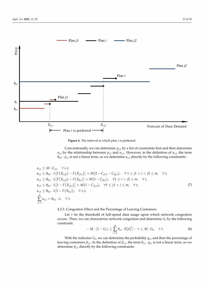
4.2.2. Percentage of New Customers

Figure 4 shows how we determine the probability pi,t. For all open data plans i, j1,and j2 that satisfy 1 ≤ j1 < i < j2 ≤ m, a potential customer chooses a data plan i ifher/his data demand forecast falls into the interval (Xj1,i, Xi,j2], where:

Xj1,i = vj1 +

⌊bi − bj1

bsj1

⌋· vs

j1, Xi,j2 = vi +

⌊ bj2 − bi

bsi

⌋· vs

i .

Appl. Sci. 2021, 11, 91 13 of 23

Forecast of Data Demand

Pri

ce

Xj1,i Xi,j2

Plan i is preferred

Plan i

Plan j1

Plan j2

Plan j1 Plan i Plan j2

bi

bj1

bj2

Figure 4. The interval in which plan i is preferred.

Conventionally, we can determine pi,t by a list of constraints first and then determineαi,t by the relationship between pi,t and αi,t. However, in the definition of αi,t, the termθ0,t · pi,t is not a linear term, so we determine αi,t directly by the following constraints:

αi,t ≤ M · Ci,t, ∀ i, t,

αi,t ≤ θ0,t · λ[F(Xi,j2

)− F

(Xj1,i

)]+ M

(2− Cj1,t − Cj2,t

), ∀ 1 ≤ j1 < i < j2 ≤ m, ∀ t,

αi,t ≤ θ0,t · λ[F(Xi,j2

)− F(X0,i)

]+ M

(1− Cj2,t

), ∀1 ≤ i < j2 ≤ m, ∀ t,

αi,t ≤ θ0,t · λ[1− F

(Xj1,i

)]+ M

(1− Cj1,t

), ∀1 ≤ j1 < i ≤ m, ∀ t,

αi,t ≤ θ0,t · λ[1− F(X0,i)], ∀ i, t,m

∑i=1

αi,t = θ0,t · λ, ∀ t.

(7)

4.2.3. Congestion Effect and the Percentage of Leaving Customers

Let τ be the threshold of full-speed data usage upon which network congestionoccurs. Then, we can characterize network congestion and determine Gt by the followingconstraint:

−M · (1− Gt) ≤m

∑i=1

θi,t ·E[Ufi ]− τ ≤ M · Gt, ∀ t. (8)

With the indicator Gt, we can determine the probability qi,t and then the percentage ofleaving customers βi,t. In the definition of βi,t, the term θi,t · qi,t is not a linear term, so wedetermine βi,t directly by the following constraints:

Appl. Sci. 2021, 11, 91 14 of 23

βi,t ≥ θi,t · Fi(vi)(1− wi)qEi,t −M · Gt, ∀ i, t

βi,t ≤ θi,t · Fi(vi)(1− wi)qEi,t + M · Gt, ∀ i, t

βi,t ≥ θi,t ·{

qPi,t + [Fi(vi)(1− wi)qE

i,t]− qPi,t · [Fi(vi)(1− wi)qE

i,t]}−M · (1− Gt), ∀ i, t

βi,t ≤ θi,t ·{

qPi,t + [Fi(vi)(1− wi)qE

i,t]− qPi,t · [Fi(vi)(1− wi)qE

i,t]}+ M · (1− Gt), ∀ i, t

(9)

4.2.4. Final Formulation

Let Z(θ1) be the SP’s maximum average revenue per customer from Period 1 to theend, starting at the initial state θ1. Then, the equivalent mixed integer linear programmingproblem can be proposed as follows:

(MILP) Z(θ1) = maxCt∈{0,1}m

T

∑t=1

m

∑i=1

(θi,t + αi,t) · [Fi(vi) + Fi(vi) · (1− wi) + ρi · wi] · bi,

s.t. (A),(B),(C),(D),

Ci,t ∈ {0, 1}, ∀ i, t

Gt ∈ {0, 1}, ∀ t

θ0,t ≥ 0, ∀ t

θi,t ≥ 0, ∀ i, t

α0,t ≥ 0, ∀ t

αi,t ≥ 0, ∀ i, t

βi,t ≥ 0, ∀ i, t

Theorem 2. The optimal solution to (MILP) is the same as the optimal solution to (DP2), and theoptimal objective values Z(θ1) = V1(θ1).

Proof. See Appendix A.

Theorem 2 suggests that we transform the SP’s dynamic programming problem intoan equivalent mixed integer linear programming problem. The new problem’s dimensionis significantly reduced, and it can be solved efficiently by many commercial softwareprograms, such as CPLEX and Gurobi.

5. Numerical Evaluation

To evaluate the dynamic plan control method, we apply our model to a large mobileservice provider in Europe. The service provider employs connection-speed-restrictionpricing and offers five data plans. It is worth noting that the five supplementary datapackages attached to the five data plans are identical in this case, which is a special situationthat satisfies our assumptions. The relevant attributes are shown in Table 3.

Appl. Sci. 2021, 11, 91 15 of 23

Table 3. Overview of the five data plans and supplementary data packages.

DP a 1 DP 2 DP 3 DP 4 DP 5

The allotted volume of full-speed data 1 GB b 3 GB 6 GB 8 GB 10 GBThe price per period e 34.45 e 43.95 e 67.75 e 83.65 e 98.15

SDP c 1 SDP 2 SDP 3 SDP 4 SDP 5

The additional volume of full-speed data 250 MB 250 MB 250 MB 250 MB 250 MBThe price per purchase e 4.95 e 4.95 e 4.95 e 4.95 e 4.95

a DP: data plan; b 1 GB ≈ 1000 MB; c SDP: supplementary data package.

To construct a base case, we make the following estimate based on the real situation:

1. The service provider has a high initial market share (=45%).2. λ is empirically set to be 8%.3. The threshold τ is set empirically to be 2.2 GB per customer.

We list all plan-related parameters for the base case in Table 4. The total number ofperiods considered in the base case is seven.

Table 4. Base case: parameters related to the data plans and supplementary data packages.

Plan 1 Plan 2 Plan 3 Plan 4 Plan 5

Initial percentage subscribed, θi,1 11.0% 12.1% 10.4% 6.3% 5.2%Churn rate qP

i 60% 60% 60% 70% 70%Churn rate qE

i 15% 18% 21% 24% 27%Willingness to buy SDP, wi 50% 50% 50% 60% 60%

5.1. Results of the Base Case

The optimization problem of the service provider’s revenue is solved, and the optimalcontrol policy is shown in Table 5. In addition, we compare the optimal revenue under twomethods. One method is the dynamic plan control (DPC) proposed in our study, and theother method is to keep all plans always open (APAO). The results of this comparison arelisted in Table 5.

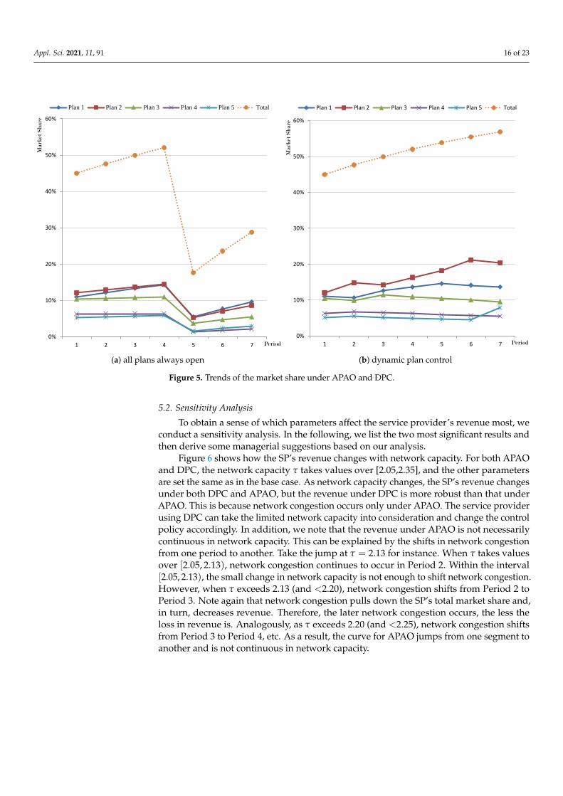
Figure 5 shows the trends of market share across periods under two methods. As il-lustrated in Figure 5, if the SP uses APAO, network congestion occurs in Period 4. Whennetwork congestion occurs, many customers leave the network, and the total market shareof the five data plans drops dramatically. With DPC, the service provider opens data plansin a more reasonable way. Network congestion is avoided, and the total market share neverdecreases. A detailed analysis shows that before Period 4, the SP’s revenue is 1.02% less ifusing DPC rather than APAO. However, the revenue of SP using DPC is 31.44% higherthan APAO after a total of seven periods. Note again that DPC enables the SP to balancethe benefit of earning more revenue in the short term and the cost of network congestiondue to too much data traffic. Within the limited network capacity, DPC helps the SP reacha more reasonable allocation of resources.

Table 5. Results of the base case. APAO, all plans always open; DPC, dynamic plan control.

Optimal Dynamic Plan Control Policy Maximum Average Revenue Per Customer

1 2 3 4 5 6 7 APAO: DPC:

Plan 1 0 1 1 1 0 0 0 e 170.253 e 226.404Plan 2 1 0 1 1 1 0 0 Revenue incrementPlan 3 0 1 0 0 0 0 0 e 54.151Plan 4 1 0 0 0 0 0 0 Increased percentagePlan 5 1 0 0 0 0 1 1 31.44%

Appl. Sci. 2021, 11, 91 16 of 23

0%

10%

20%

30%

40%

50%

60%

1 2 3 4 5 6 7

Mark

et S

hare

Period

Plan 1 Plan 2 Plan 3 Plan 4 Plan 5 Total

(a) all plans always open

0%

10%

20%

30%

40%

50%

60%

1 2 3 4 5 6 7

Mark

et S

hare

Period

Plan 1 Plan 2 Plan 3 Plan 4 Plan 5 Total

(b) dynamic plan control

Figure 5. Trends of the market share under APAO and DPC.

5.2. Sensitivity Analysis

To obtain a sense of which parameters affect the service provider’s revenue most, weconduct a sensitivity analysis. In the following, we list the two most significant results andthen derive some managerial suggestions based on our analysis.

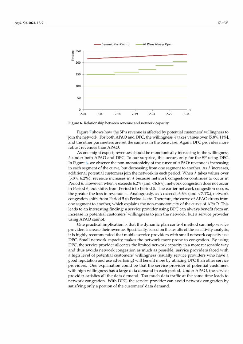
Figure 6 shows how the SP’s revenue changes with network capacity. For both APAOand DPC, the network capacity τ takes values over [2.05,2.35], and the other parametersare set the same as in the base case. As network capacity changes, the SP’s revenue changesunder both DPC and APAO, but the revenue under DPC is more robust than that underAPAO. This is because network congestion occurs only under APAO. The service providerusing DPC can take the limited network capacity into consideration and change the controlpolicy accordingly. In addition, we note that the revenue under APAO is not necessarilycontinuous in network capacity. This can be explained by the shifts in network congestionfrom one period to another. Take the jump at τ = 2.13 for instance. When τ takes valuesover [2.05, 2.13), network congestion continues to occur in Period 2. Within the interval[2.05, 2.13), the small change in network capacity is not enough to shift network congestion.However, when τ exceeds 2.13 (and <2.20), network congestion shifts from Period 2 toPeriod 3. Note again that network congestion pulls down the SP’s total market share and,in turn, decreases revenue. Therefore, the later network congestion occurs, the less theloss in revenue is. Analogously, as τ exceeds 2.20 (and <2.25), network congestion shiftsfrom Period 3 to Period 4, etc. As a result, the curve for APAO jumps from one segment toanother and is not continuous in network capacity.

Appl. Sci. 2021, 11, 91 17 of 23

0

50

100

150

200

250

2.04 2.09 2.14 2.19 2.24 2.29 2.34

Rev

enu

e

τ

Dynamic Plan Control All Plans Always Open

Figure 6. Relationship between revenue and network capacity.

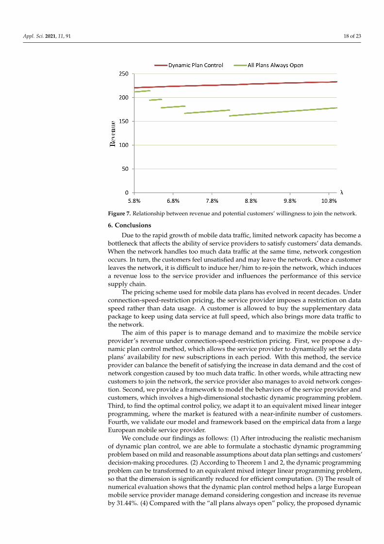
Figure 7 shows how the SP’s revenue is affected by potential customers’ willingness tojoin the network. For both APAO and DPC, the willingness λ takes values over [5.8%,11%],and the other parameters are set the same as in the base case. Again, DPC provides morerobust revenues than APAO.

As one might expect, revenues should be monotonically increasing in the willingnessλ under both APAO and DPC. To our surprise, this occurs only for the SP using DPC.In Figure 6, we observe the non-monotonicity of the curve of APAO: revenue is increasingin each segment of the curve, but decreasing from one segment to another. As λ increases,additional potential customers join the network in each period. When λ takes values over[5.8%, 6.2%), revenue increases in λ because network congestion continues to occur inPeriod 6. However, when λ exceeds 6.2% (and <6.6%), network congestion does not occurin Period 6, but shifts from Period 6 to Period 5. The earlier network congestion occurs,the greater the loss in revenue is. Analogously, as λ exceeds 6.6% (and <7.1%), networkcongestion shifts from Period 5 to Period 4, etc. Therefore, the curve of APAO drops fromone segment to another, which explains the non-monotonicity of the curve of APAO. Thisleads to an interesting finding: a service provider using DPC can always benefit from anincrease in potential customers’ willingness to join the network, but a service providerusing APAO cannot.

One practical implication is that the dynamic plan control method can help serviceproviders increase their revenue. Specifically, based on the results of the sensitivity analysis,it is highly recommended that mobile service providers with small network capacity useDPC. Small network capacity makes the network more prone to congestion. By usingDPC, the service provider allocates the limited network capacity in a more reasonable wayand thus avoids network congestion as much as possible. service providers faced witha high level of potential customers’ willingness (usually service providers who have agood reputation and use advertising) will benefit more by utilizing DPC than other serviceproviders. One explanation could be that the service provider of potential customerswith high willingness has a large data demand in each period. Under APAO, the serviceprovider satisfies all the data demand. Too much data traffic at the same time leads tonetwork congestion. With DPC, the service provider can avoid network congestion bysatisfying only a portion of the customers’ data demand.

Appl. Sci. 2021, 11, 91 18 of 23

Figure 7. Relationship between revenue and potential customers’ willingness to join the network.

6. Conclusions

Due to the rapid growth of mobile data traffic, limited network capacity has become abottleneck that affects the ability of service providers to satisfy customers’ data demands.When the network handles too much data traffic at the same time, network congestionoccurs. In turn, the customers feel unsatisfied and may leave the network. Once a customerleaves the network, it is difficult to induce her/him to re-join the network, which inducesa revenue loss to the service provider and influences the performance of this servicesupply chain.

The pricing scheme used for mobile data plans has evolved in recent decades. Underconnection-speed-restriction pricing, the service provider imposes a restriction on dataspeed rather than data usage. A customer is allowed to buy the supplementary datapackage to keep using data service at full speed, which also brings more data traffic tothe network.

The aim of this paper is to manage demand and to maximize the mobile serviceprovider’s revenue under connection-speed-restriction pricing. First, we propose a dy-namic plan control method, which allows the service provider to dynamically set the dataplans’ availability for new subscriptions in each period. With this method, the serviceprovider can balance the benefit of satisfying the increase in data demand and the cost ofnetwork congestion caused by too much data traffic. In other words, while attracting newcustomers to join the network, the service provider also manages to avoid network conges-tion. Second, we provide a framework to model the behaviors of the service provider andcustomers, which involves a high-dimensional stochastic dynamic programming problem.Third, to find the optimal control policy, we adapt it to an equivalent mixed linear integerprogramming, where the market is featured with a near-infinite number of customers.Fourth, we validate our model and framework based on the empirical data from a largeEuropean mobile service provider.

We conclude our findings as follows: (1) After introducing the realistic mechanismof dynamic plan control, we are able to formulate a stochastic dynamic programmingproblem based on mild and reasonable assumptions about data plan settings and customers’decision-making procedures. (2) According to Theorem 1 and 2, the dynamic programmingproblem can be transformed to an equivalent mixed integer linear programming problem,so that the dimension is significantly reduced for efficient computation. (3) The result ofnumerical evaluation shows that the dynamic plan control method helps a large Europeanmobile service provider manage demand considering congestion and increase its revenueby 31.44%. (4) Compared with the “all plans always open” policy, the proposed dynamic

Appl. Sci. 2021, 11, 91 19 of 23

plan control method is able to provide more robust revenue for the service provider whennetwork capacity or the potential customers’ willingness to join the network changes. If amobile service provider has a small network capacity or its potential customers have ahigh level of willingness, then it can benefit more from the dynamic plan control method.

Although we summarized three important contributions of this study in Section 1,we suggest the following directions for future research based on current limitations. First,this paper only assumes the connection-speed-restriction pricing scheme, so it would beinteresting to implement the dynamic plan control under other types of pricing schemes.Second, our model considers only one mobile service provider. Based on our research,a model with competing mobile service providers would be an interesting extension,especially if these service providers employ different pricing schemes. Finally, since ourapproach succeeds in the context of wireless telecommunication management, we considerexploring its applications in other similar systems.

Author Contributions: Formal analysis, X.M., J.Z. and Z.H.; investigation, J.N.; data curation, Y.C.;All authors have read and agreed to the published version of the manuscript.

Funding: This research was funded by the National Natural Science Foundation of China, grantnumber 71602011, 71371032, 71901202, and 71932002; and by the Fundamental Research Funds forthe Central Universities, grant number 2021JZ001.

Institutional Review Board Statement: Not applicable.

Informed Consent Statement: Not applicable.

Data Availability Statement: Restrictions apply to the availability of these data. Data was obtainedfrom a large European mobile service provider and are available from the authors with the permissionof the mobile service provider.

Acknowledgments: We would like to thank the anonymous reviewers for constructive commentsand suggestions.

Conflicts of Interest: The authors declare no conflict of interest.

Appendix A

Proof of Theorem 2This proof consists of four steps: the first two steps show that Z(θ1) ≥ V1(θ1), and

the last two steps show that Z(θ1) ≤ V1(θ1).Step 1:

Given the optimal solution (θ∗, C∗) to (DP2), we show that there exists a feasiblesolution (θ∗, C∗, G∗, α∗, β∗) to (MILP).

As the optimal solution to (DP2), (θ∗, C∗) satisfies the following constraints.

θ∗t+1 = At(θ∗t , C∗t ) · θ∗t , ∀ t, (A1)

θ∗i,t ≥ 0, ∀ i, t (A2)

θ∗1 = θ1 (A3)

Recall the definitions αi,t = θ0,t · λpi,t and βi,t = θi,t · qi,t; then, (DP2) can be reformu-lated as:

θ∗i,t+1 = θ∗i,t + α∗i,t − β∗i,t, ∀ i, t

Next, we prove that α∗i,t satisfies the constraint (6) in (MILP).

αi,t ≤ M · Ci,t, ∀ i, t, (A4)

αi,t ≤ θ0,t · λ[F(Xi,j2

)− F

(Xj1,i

)]+ M

(2− Cj1,t − Cj2,t

), ∀ 1 ≤ j1 < i < j2 ≤ m, ∀ t, (A5)

αi,t ≤ θ0,t · λ[F(Xi,j2

)− F(X0,i)

]+ M

(1− Cj2,t

), ∀1 ≤ i < j2 ≤ m, ∀ t, (A6)

αi,t ≤ θ0,t · λ[1− F

(Xj1,i

)]+ M

(1− Cj1,t

), ∀1 ≤ j1 < i ≤ m, ∀ t, (A7)

αi,t ≤ θ0,t · λ[1− F(X0,i)], ∀ i, t, (A8)m

∑i=1

αi,t = θ0,t · λ, ∀ t. (A9)

Appl. Sci. 2021, 11, 91 20 of 23

Equation (A4) is verified by the fact that α∗i,t = 0 if C∗i,t = 0 and α∗i,t ≥ 0 if C∗i,t = 1.

To verify (A5), recall the definition pi,t = Pr

(Ci,t = 1, ri(D) ≤ min

j:Cj,t=1rj(D)

). When

Ci,t = 1 and there exists j1 and j2 satisfying 1 ≤ j1 < i < j2 ≤ m and Ij1,t = 1, Ij2,t = 1,we have:

pi,t

= Pr

(ri(D) ≤ min

i:Cj,t=1rj(D)

)

≤ Pr

(bi +

⌈(D− vi)

+

vsi

⌉bs

i ≤ bj1 +

⌈(D− vj1)

+

vsj1

⌉bs

j1, bi +

⌈(D− vi)

+

vsi

⌉bs

i ≤ bj2 +

⌈(D− vj2)

+

vsj2

⌉bs

j2

)= Pr

(Xi1,j ≤ D ≤ Xj,i2

)= F

(Xi,j2

)− F

(Xj1,i

),

and αi,t = θ0,t · λpi,t ≤ θ0,t · λ[F(Xi,j2

)− F

(Xj1,i

)]. Hence, (A5) is verified.

Equations (A6)–(A8) can be verified in a similar manner.Then, we proceed to the constraint (8),

−M · (1− Gt) ≤m

∑i=1

θi,t ·E[Ufi ]− τ ≤ M · Gt, ∀ t, (A10)

and the constraint (9),

βi,t ≥ θi,t · Fi(vi)(1− wi)qEi,t −M · Gt, ∀ i, t, (A11)

βi,t ≤ θi,t · Fi(vi)(1− wi)qEi,t + M · Gt, ∀ i, t, (A12)

βi,t ≥ θi,t ·{

qPi,t + [Fi(vi)(1− wi)qE

i,t]− qPi,t · [Fi(vi)(1− wi)qE

i,t]}−M · (1− Gt), ∀ i, t, (A13)

βi,t ≤ θi,t ·{

qPi,t + [Fi(vi)(1− wi)qE

i,t]− qPi,t · [Fi(vi)(1− wi)qE

i,t]}+ M · (1− Gt), ∀ i, t. (A14)

Equation (A10) ensures that Gt = 1 if network congestion, i.e., ∑mi=1 θi,t · E[U

fi ] > τ,

occurs in period t and Gt = 0 if not.Recall Equation (1) in Section 3.3. We can reformulate (1) with Gt as:

qi,t ≥ Fi(vi)(1− wi)qEi,t −M · Gt, ∀ i, t, (A15)

qi,t ≤ Fi(vi)(1− wi)qEi,t + M · Gt, ∀ i, t, (A16)

qi,t ≥ qPi,t + [Fi(vi)(1− wi)qE

i,t]− qPi,t · [Fi(vi)(1− wi)qE

i,t]−M · (1− Gt), ∀ i, t, (A17)

qi,t ≤ qPi,t + [Fi(vi)(1− wi)qE

i,t]− qPi,t · [Fi(vi)(1− wi)qE

i,t] + M · (1− Gt), ∀ i, t. (A18)

With the definition βi,t = θi,t · qi,t, (A11)–(A14) can be easily derived from (A15)–(A18).In sum, (θ∗, C∗, G∗, α∗, β∗) satisfies all the constraints of the (MILP) problem. We

conclude that (θ∗, C∗, G∗, α∗, β∗) is a feasible solution to the (MILP) problem.Step 2, Z(θ1) ≥ V1(θ1):

Appl. Sci. 2021, 11, 91 21 of 23

Because (θ∗, C∗) is the optimal solution to (DP2),

V1(θ1)

=m

∑i=1

θ∗i,1 · [Fi(vi) + Fi(vi) · (1− wi) + ρi · wi] · bi

+ (1−m

∑i=1

θ∗i,1) ·m

∑i=1

λpi,1(C∗1 ) · [Fi(vi) + Fi(vi) · (1− wi) + ρi · wi] · bi + V2(θ∗2 )

=T

∑t=1

m

∑i=1

θ∗i,t · [Fi(vi) + Fi(vi) · (1− wi) + ρi · wi] · bi

+T

∑t=1

(1−m

∑i=1

θ∗i,t) ·m

∑i=1

λpi,t(C∗t ) · [Fi(vi) + Fi(vi) · (1− wi) + ρi · wi] · bi

=T

∑t=1

m

∑i=1

(θ∗i,t + α∗i,t) · [Fi(vi) + Fi(vi) · (1− wi) + ρi · wi] · bi.

The second equal sign holds by recursion, and the third equal sign holds with the definitionof αi,t.

Because (θ∗, α∗) is a feasible solution to (MILP), we have:

Z(θ1) ≥T

∑t=1

m

∑i=1

(θ∗i,t + α∗i,t) · [Fi(vi) + Fi(vi) · (1− wi) + ρi · wi] · bi

= V1(θ1).

Step 3: Given the optimal solution (θ∗, C∗, G∗, α∗, β∗) to (MILP), we show that there existsa feasible solution (θ∗, C∗) to (DP2).

As the optimal solution to (MILP), (θ∗, C∗, α∗) satisfies the constraint (6).

αi,t ≤ M · Ci,t, ∀ i, t, (A19)

αi,t ≤ θ0,t · λ[F(Xi,j2

)− F

(Xj1,i

)]+ M

(2− Cj1,t − Cj2,t

), ∀ 1 ≤ j1 < i < j2 ≤ m, ∀ t, (A20)

αi,t ≤ θ0,t · λ[F(Xi,j2

)− F(X0,i)

]+ M

(1− Cj2,t

), ∀1 ≤ i < j2 ≤ m, ∀ t, (A21)

αi,t ≤ θ0,t · λ[1− F

(Xj1,i

)]+ M

(1− Cj1,t

), ∀1 ≤ j1 < i ≤ m, ∀ t, (A22)

αi,t ≤ θ0,t · λ[1− F(X0,i)], ∀ i, t, (A23)m

∑i=1

αi,t = θ0,t · λ, ∀ t. (A24)

Equations (A20)–(A23) imply that:

αi,t ≤ Ci,t · θ0,t · λ · min{j1, j2 :

Ij1,t = 1,Ij2,t = 1}

{F(Xi,j2

)− F

(Xj1,i

), F(Xi,j2

)− F(X0,i), 1− F

(Xj1,i

), 1− F(X0,i)

}(A25)

For any Ct, we have:

pi,t = Pr

(Ci,t = 1, ri(D) ≤ min

j:Cj,t=1rj(D)

)= Ci,t · min

{j1, j2 :Ij1,t = 1,Ij2,t = 1}

{F(Xi,j2

)− F

(Xj1,i

), F(Xi,j2

)− F(X0,i), 1− F

(Xj1,i

), 1− F(X0,i)

}(A26)

Combining (A25) and (A26), we have αi,t ≤ θ0,t · λ · pi,t. Then, with (A24) and theproperty that ∑m

i=1 pi,t = 1, we have:

yαi,t = θ0,t · λ · pi,t, ∀ i, t. (A27)

Appl. Sci. 2021, 11, 91 22 of 23

With an analogous proof for the constraints (8) and (9) in Step 1, we can show thatif ∑m

i=1 θi,t · E[Ufi ] > τ, then Gt = 1, and if ∑m

i=1 θi,t · E[Ufi ] ≤ τ, then Gt = 0. No

matter whether network congestion occurs or not in period t, the equation βi,t = θi,t · qi,talways holds.

Then,θ∗i,t+1 = θ∗i,t + α∗i,t − β∗i,t, ∀ i, t,

can be reformulated as:θ∗t+1 = At(θ

∗t , C∗t ) · θ∗t .

We conclude that given the optimal solution (θ∗, C∗, G∗, α∗, β∗) to (MILP), there existsa feasible solution (θ∗, C∗) to (DP2).Step 4, Z(θ1) ≤ V1(θ1):

Because (θ∗, α∗) is the optimal solution to (MILP),

Z(θ1)

=T

∑t=1

m

∑i=1

(θ∗i,t + α∗i,t) · [Fi(vi) + Fi(vi) · (1− wi) + ρi · wi] · bi

=T

∑t=1

m

∑i=1

θ∗i,t · [Fi(vi) + Fi(vi) · (1− wi) + ρi · wi] · bi

+T

∑t=1

(1−m

∑i=1

θ∗i,t) ·m

∑i=1

λpi,t(C∗t ) · [Fi(vi) + Fi(vi) · (1− wi) + ρi · wi] · bi

=m

∑i=1

θ∗i,1 · [Fi(vi) + Fi(vi) · (1− wi) + ρi · wi] · bi

+ (1−m

∑i=1

θ∗i,1) ·m

∑i=1

λpi,1(C∗1 ) · [Fi(vi) + Fi(vi) · (1− wi) + ρi · wi] · bi + V2(θ∗2 )

Because (θ∗, C∗) is a feasible solution to (DP2), we have:

V1(θ1) =m

∑i=1

θ∗i,1 · [Fi(vi) + Fi(vi) · (1− wi) + ρi · wi] · bi

+ (1−m

∑i=1

θ∗i,1) ·m

∑i=1

λpi,1(C∗1 ) · [Fi(vi) + Fi(vi) · (1− wi) + ρi · wi] · bi + V2(θ∗2 )

= Z(θ1).

In conclusion, we have Z(θ1) = V1(θ1). Theorem 2 holds.

References1. Cisco. Cisco Visual Networking Index: Global Mobile Data Traffic Forecast Update, 2017–2022 White Paper; White Paper; Cisco: San Jose,

CA, USA, 2019.2. Hwang, R.H.; Peng, M.C.; Cheng, K.C. QoS-guaranteed radio resource management in LTE-A co-channel networks with dual

connectivity. Appl. Sci. 2019, 9, 3018. [CrossRef]3. Ma, X.; Deng, T.; Xue, M.; Shen, Z.J.M.; Lan, B. Optimal dynamic pricing of mobile data plans in wireless communications. Omega

2017, 66, 91–105. [CrossRef]4. Perez-Murueta, P.; Gómez-Espinosa, A.; Cardenas, C.; Gonzalez-Mendoza, M. Deep Learning System for Vehicular Re-Routing

and Congestion Avoidance. Appl. Sci. 2019, 9, 2717. [CrossRef]5. Deng, T.; Shen, Z.J.M.; Shanthikumar, J.G. Statistical Learning of Service-Dependent Demand in a Multiperiod Newsvendor

Setting. Oper. Res. 2014, 62, 1064–1076. [CrossRef]6. Loiseau, P.; Schwartz, G.; Musacchio, J.; Amin, S. Incentive schemes for Internet congestion management: Raffles versus

time-of-day pricing. In Proceedings of the 2011 49th Annual Allerton Conference on Communication, Control, and Computing(Allerton), Monticello, IL, USA, 28–30 September 2011; pp. 103–110. [CrossRef]

Appl. Sci. 2021, 11, 91 23 of 23

7. Lee, J.; Yi, Y.; Chong, S.; Jin, Y. Economics of WiFi offloading: Trading delay for cellular capacity. In Proceedings of the 2013IEEE Conference on Computer Communications Workshops (INFOCOM WKSHPS), Turin, Italy, 14–19 April 2013; pp. 357–362.[CrossRef]

8. Cheng, H.K.; Bose, I. Performance models of a proxy cache server: The impact of multimedia traffic. Eur. J. Oper. Res. 2004,154, 218–229. [CrossRef]

9. Cisco. Cisco Visual Networking Index: Global Mobile Data Traffic Forecast Update, 2011–2016; White Paper; Cisco: San Jose, CA, USA,2012.

10. Odlyzko, A. Internet pricing and the history of communications. Comput. Netw. 2001, 36, 493–517. [CrossRef]11. Gizelis, C.A.; Vergados, D.D. A Survey of Pricing Schemes in Wireless Networks. IEEE Commun. Surv. Tutor. 2011, 13, 126–145.

[CrossRef]12. Bagh, A.; Bhargava, H.K. How to Price Discriminate When Tariff Size Matters. Mark. Sci. 2012, 32, 111–126. [CrossRef]13. Danaher, P.J. Optimal Pricing of New Subscription Services: Analysis of a Market Experiment. Mark. Sci. 2002, 21, 119–138.

[CrossRef]14. Grubb, M.D. Selling to Overconfident Consumers. Am. Econ. Rev. 2009, 99, 1770–1807. [CrossRef]15. Fibich, G.; Klein, R.; Koenigsberg, O.; Muller, E. Optimal Three-Part Tariff Plans. Oper. Res. 2017, 65, 1177–1189. [CrossRef]16. Bhargava, H.K.; Gangwar, M. On the Optimality of Three-Part Tariff Plans: When Does Free Allowance Matter? Oper. Res. 2018,

66, 1517–1532. [CrossRef]17. Sen, S.; Joe-Wong, C.; Ha, S.; Chiang, M. A survey of smart data pricing: Past proposals, current plans, and future trends. ACM

Comput. Surv. 2013, 46, 1–37. [CrossRef]18. Sen, S.; Joe-Wong, C.; Ha, S.; Chiang, M. Smart data pricing: Using economics to manage network congestion. Commun. ACM

2015, 58, 86–93. [CrossRef]19. Jiang, L.; Parekh, S.; Walrand, J. Time-Dependent Network Pricing and Bandwidth Trading. In Proceedings of the NOMS

Workshops 2008—IEEE Network Operations and Management Symposium Workshops, Salvador da Bahia, Brazil, 7–11 April2008; pp. 193–200. [CrossRef]

20. Joe-Wong, C.; Ha, S.; Chiang, M. Time-Dependent Broadband Pricing: Feasibility and Benefits. In Proceedings of the 2011 31stInternational Conference on Distributed Computing Systems, Minneapolis, MN, USA, 20–24 June 2011; pp. 288–298. [CrossRef]

21. Batur, D.; Ryan, J.K.; Zhao, Z.; Vuran, M.C. Dynamic Pricing of Wireless Internet Based on Usage and Stochastically ChangingCapacity. Manuf. Serv. Oper. Manag. 2019. [CrossRef]

22. Ha, S.; Sen, S.; Joe-Wong, C.; Im, Y.; Chiang, M. TUBE: Time-dependent pricing for mobile data. Acm Sigcomm Comput. Commun.Rev. 2012, 42, 247–258. [CrossRef]

23. Javaid, N.; Ahmed, A.; Iqbal, S.; Ashraf, M. Day ahead real time pricing and critical peak pricing based power scheduling forsmart homes with different duty cycles. Energies 2018, 11, 1464. [CrossRef]

24. Loiseau, P.; Schwartz, G.; Musacchio, J.; Amin, S.; Sastry, S.S. Incentive Mechanisms for Internet Congestion Management:Fixed-Budget Rebate Versus Time-of-Day Pricing. IEEE/ACM Trans. Netw. 2014, 22, 647–661. [CrossRef]

25. Ma, X.; Deng, T.; Lan, B. Demand estimation and assortment planning in wireless communications. J. Syst. Sci. Syst. Eng. 2016,25, 1–26. [CrossRef]

26. Clements, A.E.; Hurn, A.S.; Li, Z. Forecasting day-ahead electricity load using a multiple equation time series approach. Eur. J.Oper. Res. 2016, 251, 522–530. [CrossRef]

27. Abbas, N.; Yu, F.; Fan, Y. Intelligent video surveillance platform for wireless multimedia sensor networks. Appl. Sci. 2018, 8, 348.[CrossRef]

28. Lee, J.; Yi, Y.; Chong, S.; Jin, Y. Economics of WiFi Offloading: Trading Delay for Cellular Capacity. IEEE Trans. Wirel. Commun.2014, 13, 1540–1554. [CrossRef]

29. Liu, B.; Zhu, Q.; Tan, W.; Zhu, H. Congestion-Optimal WiFi Offloading with User Mobility Management in Smart Communications.Wirel. Commun. Mob. Comput. 2018, 2018, 9297536. [CrossRef]

30. Sun, Y.; Xu, L.; Tang, Y.; Zhuang, W. Traffic offloading for online video service in vehicular networks: A cooperative approach.IEEE Trans. Veh. Technol. 2018, 67, 7630–7642. [CrossRef]

31. Ning, Z.; Dong, P.; Wang, X.; Obaidat, M.S.; Hu, X.; Guo, L.; Guo, Y.; Huang, J.; Hu, B.; Li, Y. When deep reinforcement learningmeets 5G-enabled vehicular networks: A distributed offloading framework for traffic big data. IEEE Trans. Ind. Inform. 2019,16, 1352–1361. [CrossRef]

32. Sen, S.; Joe-Wong, C.; Ha, S.; Chiang, M. Time-Dependent Pricing for Multimedia Data Traffic: Analysis, Systems, and Trials.IEEE J. Sel. Areas Commun. 2019, 37, 1504–1517. [CrossRef]

33. Schlereth, C.; Skiera, B.; Schulz, F. Why do consumers prefer static instead of dynamic pricing plans? An empirical study for abetter understanding of the low preferences for time-variant pricing plans. Eur. J. Oper. Res. 2018, 269, 1165–1179. [CrossRef]